Embed Size (px)
Citation preview
Dipartimento di Matematica “Guido Castelnuovo”Dottorato di Ricerca in Matematica XXI ciclo
Eigenvalues and homogenization ofsome fully nonlinear partial
differential equations
Thesis submitted to obtain the degree ofDoctor of Philosophy (“Dottore di Ricerca”) in Mathematics
October 2009
by
Stefania Patrizi
Thesis Advisors CommitteeIsabeau Birindelli Martino Bardi
Italo Capuzzo Dolcetta Regis MonneauAntonio Siconolfi

ii
Contents
Introduction vI.1 An overview of the literature . . . . . . . . . . . . . . . . . . . . . . viI.2 Outline of the results of Chapters 1, 2 and 3 . . . . . . . . . . . . . . ixI.3 The Peierls-Nabarro model for dislocation dynamics . . . . . . . . . xvI.4 Local Hamilton-Jacobi equations . . . . . . . . . . . . . . . . . . . . xxiii
I Neumann generalized principal eigenvalues 1
1 Fully nonlinear singular operators 31.1 Lipschitz continuity of viscosity solutions . . . . . . . . . . . . . . . 51.2 The Maximum Principle and the principal eigenvalues . . . . . . . . 11
1.2.1 The case c(x) ≤ 0 . . . . . . . . . . . . . . . . . . . . . . . . 111.2.2 The threshold for the Maximum Principle . . . . . . . . . . . 141.2.3 The Maximum Principle for c(x) changing sign: an example. 22
1.3 Some existence results . . . . . . . . . . . . . . . . . . . . . . . . . . 27
2 Isaacs operators 332.1 Assumptions . . . . . . . . . . . . . . . . . . . . . . . . . . . . . . . 342.2 The Strong Comparison Principle . . . . . . . . . . . . . . . . . . . . 372.3 The Maximum Principle and the principal eigenvalues . . . . . . . . 41
2.3.1 The case F proper . . . . . . . . . . . . . . . . . . . . . . . . 412.3.2 The Maximum Principle for λ < λ . . . . . . . . . . . . . . . 422.3.3 An example . . . . . . . . . . . . . . . . . . . . . . . . . . . . 44
2.4 Lipschitz regularity . . . . . . . . . . . . . . . . . . . . . . . . . . . . 452.5 Existence results . . . . . . . . . . . . . . . . . . . . . . . . . . . . . 502.6 Properties of the principal eigenvalues . . . . . . . . . . . . . . . . . 532.7 The Pucci’s operators . . . . . . . . . . . . . . . . . . . . . . . . . . 55
3 The infinity-Laplacian 573.1 Assumptions and definitions . . . . . . . . . . . . . . . . . . . . . . . 583.2 Lipschitz continuity of viscosity solutions . . . . . . . . . . . . . . . 603.3 The Maximum Principle and the principal eigenvalues . . . . . . . . 65
3.3.1 The case c(x) ≤ 0 . . . . . . . . . . . . . . . . . . . . . . . . 663.3.2 The threshold for the Maximum Principle . . . . . . . . . . . 683.3.3 The Maximum Principle for c(x) changing sign: an example. 75
3.4 Some existence results . . . . . . . . . . . . . . . . . . . . . . . . . . 76
iii
3.5 A decay estimate for solutions of the evolution problem . . . . . . . 80
II Homogenization of first order Hamilton-Jacobi equations 85
4 The Peierls-Nabarro model for dislocation dynamics 874.1 Main results . . . . . . . . . . . . . . . . . . . . . . . . . . . . . . . . 884.2 Results about viscosity solutions for non-local equations . . . . . . . 89
4.2.1 Definition of viscosity solution . . . . . . . . . . . . . . . . . 894.2.2 Comparison principle and existence results . . . . . . . . . . 894.2.3 Hölder regularity . . . . . . . . . . . . . . . . . . . . . . . . . 91
4.3 The proof of convergence . . . . . . . . . . . . . . . . . . . . . . . . 944.3.1 Proof of Theorem 4.1.2 . . . . . . . . . . . . . . . . . . . . . 96
4.4 Building of Lipschitz sub and supercorrectors . . . . . . . . . . . . . 1024.4.1 Comparison principle . . . . . . . . . . . . . . . . . . . . . . 1034.4.2 Lipschitz regularity . . . . . . . . . . . . . . . . . . . . . . . . 1054.4.3 Ergodicity . . . . . . . . . . . . . . . . . . . . . . . . . . . . . 1074.4.4 Proof of Theorem 4.1.1 . . . . . . . . . . . . . . . . . . . . . 1104.4.5 Proof of Proposition 4.4.1 . . . . . . . . . . . . . . . . . . . . 1104.4.6 Proof of Proposition 4.3.3 . . . . . . . . . . . . . . . . . . . . 111
4.5 Smooth approximate correctors . . . . . . . . . . . . . . . . . . . . . 1124.5.1 Proof of Proposition 4.3.4 . . . . . . . . . . . . . . . . . . . . 113
4.6 The Orowan’s law . . . . . . . . . . . . . . . . . . . . . . . . . . . . 1144.6.1 Proof of Proposition 4.6.2. . . . . . . . . . . . . . . . . . . . . 1174.6.2 Proof of Lemma 4.6.4. . . . . . . . . . . . . . . . . . . . . . . 1264.6.3 Proof of Lemma 4.6.5. . . . . . . . . . . . . . . . . . . . . . . 127
5 Rate of convergence in homogenization of local Hamilton-Jacobiequations 1315.1 An estimate on the rate of convergence when ε→ 0 . . . . . . . . . . 132
5.1.1 The main result . . . . . . . . . . . . . . . . . . . . . . . . . 1325.1.2 Preliminary results . . . . . . . . . . . . . . . . . . . . . . . . 1325.1.3 Proof of the main result . . . . . . . . . . . . . . . . . . . . . 135
5.2 Approximation of the effective Hamiltonian by Eulerian schemes . . 1425.2.1 Long time approximation . . . . . . . . . . . . . . . . . . . . 1525.2.2 Approximation of the homogenized problem . . . . . . . . . . 153
5.3 Numerical Tests . . . . . . . . . . . . . . . . . . . . . . . . . . . . . . 1545.3.1 Results . . . . . . . . . . . . . . . . . . . . . . . . . . . . . . 154
5.4 Appendix . . . . . . . . . . . . . . . . . . . . . . . . . . . . . . . . . 158
A Notation list 163
Bibliography 164
iv
Introduction
This thesis is a contribution to the theory of viscosity solutions of fully nonlinearequations of first and second order. It is divided in two parts. The first one, whichcollects the results contained in [97], [96] and [98], studies the generalized principaleigenvalues associated to nonlinear elliptic operators of second order with Neumannboundary conditions. Three different classes of operators are considered respectivelyin Chapters 1, 2 and 3.
The second part is dedicated to homogenization problems for first order localand non-local Hamilton-Jacobi equations. In Chapter 4 we presents the results of[92], where we study the time-dependent Peierls-Nabarro model which is a phasefield model for dislocation dynamics. This model leads to a non-local parabolic PDEwith a first order Lévy operator. After a proper rescaling, a macroscopic modeldescribing the evolution of a density of dislocations is obtained. In Chapter 5 westudy the rate of convergence in homogenization of local parabolic Hamilton-Jacobiequations, the results of this chapter are contained in [2].
We recall that viscosity solutions were introduced by M. G. Crandall and P. L.Lions [41] in 1981 for first order Hamilton-Jacobi equations. Successively, manyauthors have contributed to the theory of viscosity solutions which was extendedto a large class of first and second order partial differential equations. For a gooddescription of viscosity solutions we refer to Crandall, Ishii and Lions [40], to theCIME course [14] and to the books: Fleming and Soner [54] for applications to thestochastic control theory; Barles [17], Bardi and Capuzzo Dolcetta [13] for first orderequations and applications to the deterministic control; Cabré and Caffarelli [32] forthe regularity of solutions of uniformly elliptic equations.
Motivated by applications to finance but also by an increasing number of othermathematical models (physical sciences, mechanics, biological models etc.), thetheory of viscosity solutions has been extended to the context of partial integro-differential equations, i.e. partial equations involving non-local operators such as theLévy ones. To the best of our knowledge the first paper devoted to this extension wasthe one by Soner [107] in the context of stochastic control of jump diffusion processes.Following Soner’s work, a quite general class of integro-differential equations nonlinearwith respect the non-local operators was developed by Awatif, [12]. Successively,many results were extended to equations involving also second order derivatives, seefor instance [84] and [22].
In the framework of viscosity solutions, the homogenization problem for firstorder Hamilton-Jacobi equations has been extensively studied. First of all, LionsPapanicolaou and Varadhan [88] completely solved the problem in the case of
v
time-independent periodic and coercive Hamiltonians. After this seminal paper,homogenization of Hamilton-Jacobi equations for coercive Hamiltonians has beentreated for a wider class of periodic situations, c.f. Ishii [72], for problems set onbounded domains, c.f. Alvarez [3], Horie and Ishii [64], for equations with differentstructures, c.f. Alvarez and Ishii [8], for deterministic control problems in L∞, c.f.Alvarez and Barron [6], for almost periodic Hamiltonians, c.f. Ishii [70], and forHamiltonians with stochastic dependence, c.f. Souganidis [108].
For different structures assumptions, non-local operators and further results onhomogenization we refer the reader to e.g. [49], [50], [53], [24], [18], [67], [68], [5],[4], [35] and references therein.
PART I
I.1 An overview of the literature
The eigenvalue problem for linear elliptic operators has a very long history and goesback to Fourier. Here we limit to recall some classical results.
Let L be a general uniformly elliptic linear operator of second order defined in abounded domain Ω ⊂ RN , of the form
Lu = −aij(x)∂iju+ bi(x)∂iu+ c(x)u, in Ω (I.1.1)
that is uniformly elliptic, i.e.,
a|ξ|2 ≤ aij(x)ξiξj ≤ A|ξ|2 for any x ∈ Ω, ξ ∈ RN ,
with a and A positive constants. Let B be the boundary operator defined by
Bu = γ(x)u+ δ∂u
∂−→non ∂Ω,
where −→n (x) is the exterior normal to Ω at x ∈ ∂Ω, and either δ = 0 and γ ≡ 1 (i.e.B is the Dirichlet boundary operator) or δ = 1 and γ ≥ 0 (i.e. B is the Neumann oroblique derivative boundary operator).
It is well known that when ∂Ω and the coefficients of L and B are sufficientlyregular, there is a real number λ1, called first or principal eigenvalue for L withassociated the boundary operator B, such that
a) (λ1 is an eigenvalue) there exists a positive function φ, called principal eigen-function, solution of
Lφ = λ1φ in ΩBφ = 0 on ∂Ω; (I.1.2)
b) (λ1 is the smallest real eigenvalue) for any eigenvalue λ 6= λ1 of L with boundaryoperator B then
Reλ > λ1.
vi
The existence of such a pair (λ1, φ) follows from the Krein Rutman Theorem, seefor example [9]. Other properties of the principal eigenvalue are the following: λ1 issimple, i.e. any solution of (I.1.2) is a multiple of φ; if ψ is a positive eigenfunctionwith eigenvalue λ, then λ = λ1; λ1 is an isolated eigenvalue.
When L associated to the boundary operator B is self-adjoint (with respect toL2(Ω)), i.e. L has the form
Lu = −∂i(aij(x)∂ju) + c(x)u,
δ = 0 and γ ≡ 1, the first eigenvalue can be characterized as the minimum of the socalled Rayleigh quotient:
λ1 = minu∈C∞0 (Ω)\0
∫Ω(aij(x)∂iu∂ju+ c(x)u2)dx∫
Ω u2dx
, (I.1.3)
see e.g. [61]. A variational formulation for the principal eigenvalue of a generallinear second-order operator with Dirichlet boundary conditions and with maximumprinciple was given by Donsker and Varadhan in [45] and [46].
More recently, Berestycki, Nirenberg and Varadhan [26] gave a characterizationof the first eigenvalue of a linear uniformly elliptic operator of second order throughthe maximum principle. They consider the operator (I.1.1) defined in a boundeddomain Ω and with associated Dirichlet boundary conditions. In addition to theuniform ellipticity condition, they assume on the coefficients of L:
aij ∈ C(Ω), bi, c ∈ L∞(Ω) for any i, j.
One of the main feature of the paper is that no regularity is required on ∂Ω. In thisthesis we will not deal with the question of the regularity of the domain and willalways assume ∂Ω smooth.
Berestycki, Nirenberg and Varadhan define
λ1 := supλ ∈ R | ∃ v > 0 in Ω supersolution of Lv = λv in Ω. (I.1.4)
Here a solution (resp. sub, supersolution) of Lu = f in Ω is a function u ∈W 2,ploc (Ω)
for all finite p > N , satisfying Lu = f (resp. ≤, ≥) for a.e. x ∈ Ω.In [26], the authors show that λ1 defined as in (I.1.4) is the principal eigenvalue
of L, i.e. there exists a positive function φ such that the pair (λ1, φ) have properties(a) and (b) with Bu = u. They also prove that the maximum principle for L holdstrue if and only if λ1 > 0. Indeed, they show that if λ1 > 0, u is a subsolution ofLu = 0 in Ω and u ≤ 0 on ∂Ω, then u ≤ 0 in Ω (i.e. the maximum principle holds).On the other hand, if λ ≥ λ1 then φ is a counterexample to the maximum principle.
Several other properties of the first eigenvalue, such as simplicity and stability,are established in [26].
In view of its relation with the maximum and the comparison principles, theconcept of principal eigenvalue has been extended to nonlinear operators to studythe associated boundary value problems.
A classical example of nonlinear eigenvalue problem is the one associated to thep-Laplacian defined for 1 < p <∞ by:
∆pu = div(|Du|p−2Du).
vii
The natural way to define the principal eigenvalue for the p-Laplacian is by genera-lizing definition (I.1.3) to the nonlinear case. Indeed, if λ1 is the minimum of theassociated Rayleigh quotient ∫
Ω |Du|pdx∫Ω |u|pdx
among all the functions belonging to W 1,p0 (Ω) \ 0, then any minimizing function φ
is a weak solution of the corresponding Euler-Lagrange equation−∆pφ = λ1|φ|p−2φ in Ωφ = 0 on ∂Ω. (I.1.5)
Moreover any solution of (I.1.5) does not change sign in Ω and (I.1.5) does notadmit non-trivial solutions if we replace λ1 by λ < λ1, see e.g. [90]. Because ofthese properties, the minimum λ1 of the Rayleigh quotient is called the principaleigenvalue of −∆p and the solutions of (I.1.5) are called principal eigenfunctions.
Remark that the operator ∆pu+ λ1|u|p−2u is homogeneous of degree p− 1. Thisimplies that if φ is solution of (I.1.5) then tφ is solution of the same problem for anyt ∈ R. On the other hand, it is possible to prove that if φ and ψ are two principaleigenfunctions, then there exists t ∈ R \ 0 such that φ = tψ. This property of λ1is called simplicity and was proved indipendently by Anane [10] and by Otani andTeshima [95]. The principle eigenvalue of the p-Laplacian has almost all the typicalproperties of the first eigenvalue of a linear operator, see [90].
The method of the minimization of the Rayleigh quotient uses heavily thevariational structure of the operator and cannot be applied to operators which havenot this property. An important step in the study of the eigenvalue problem fornonlinear operators in non-divergence form was made by Lions in [87]. In thatpaper, using probabilistic and analytic methods, he showed the existence of principaleigenvalues for the uniformly elliptic Bellman operator and obtained results for therelated Dirichlet problems. Very recently, many authors, inspired by [26], have deve-loped an eigenvalue theory for fully nonlinear operators which are non-variational.The Pucci’s extremal operatorsMa,A(D2u) have been treated by Quaas [103] andBusca, Esteban and Quaas [31]. Related results have been obtained by Birindelli andDemengel in [28] for singular or degenerate elliptic operators, like |Du|αMa,A(D2u),α > −1, the p-Laplacian and some of its non-variational generalizations. In [104]Quaas and Sirakov have studied the eigenvalue problem for fully nonlinear ellipticoperators which are convex and positively homogenous, like the Hamilton-Jacobi-Bellman one. In that paper many properties of the principal eigenvalues, includingthe fact that they are simple and isolated, have been established. Similar results havebeen obtained by Ishii and Yoshimura [76] for non-convex operators. The existenceof a principal eigenvalue defined as in [26] for the ∞-Laplacian has been proved byJuutinen in [80] together with many other results. A different approach to investigatethe eigenvalue problem for∞-Laplacian consists in studying the asymptotic behavior,as p → ∞, of the p-Laplacian eigenvalue equation, see [82] and [59]. This secondmethod uses the variational formulation of the approximate problems and leads to adifferent limit eigenvalue problem, see [80].
All the mentioned papers treat Dirichlet boundary conditions.
viii
I.2 Outline of the results of Chapters 1, 2 and 3In the first part of this thesis we study the eigenvalue problem for some classes offully nonlinear homogenous operators G(x, u,Du,D2u) with Neumann boundaryconditions. We are thus concerned with the fully nonlinear elliptic problem
G(x, u,Du,D2u) = g(x) in ΩB(x, u,Du) = 0 on ∂Ω, (I.2.6)
where Ω is a bounded domain of class C2 and B(x, u,Du) is a first order boundaryoperator. The problem we consider may have weak solutions which are not smoothenough to satisfy the differential equations involved in the classical sense. We adoptthe notion of viscosity solution as the weak solution of (I.2.6).
Let us recall the definition of viscosity solution of (I.2.6), for F : Ω× R× RN ×S(N)→ R and B : ∂Ω× R× RN → R continuous functions.
Definition I.2.1. A function u ∈ USC(Ω) (resp. u ∈ LSC(Ω)) is called viscositysubsolution (resp. supersolution) of (I.2.6) if the following conditions hold
(i) For every x0 ∈ Ω, for all ϕ ∈ C2(Ω), such that u − ϕ has a local maximum(resp. minimum) at x0, one has
G(x0, u(x0), Dϕ(x0), D2ϕ(x0)) ≤ (resp. ≥ ) g(x0).
(ii) For every x0 ∈ ∂Ω, for all ϕ ∈ C2(Ω), such that u− ϕ has a local maximum(resp. minimum) at x0, one has
(G(x0, u(x0), Dϕ(x0), D2ϕ(x0))− g(x0)) ∧B(x0, u(x0), Dϕ(x0)) ≤ 0
(resp.
(G(x0, u(x0), Dϕ(x0), D2ϕ(x0))− g(x0)) ∨B(x0, u(x0), Dϕ(x0)) ≥ 0).
A viscosity solution is a continuous function which is both a subsolution and asupersolution.
In Chapters 1 and 3 we consider operators G of the form
G(x, u,Du,D2u) = −F (x,Du,D2u) + b(x) ·Du|Du|α + c(x)|u|αu, (I.2.7)
with α > −1 and b, c, g continuous functions on Ω. F is a fully nonlinear operatorthat may be singular or degenerate where the gradient vanishes. Since we cannot testwhen the test function has zero gradient, we have to modify the previous definitionof solution of the Neumann problem associated to these operators. We adopt thenotion of viscosity solution given by Birindelli and Demengel in [28] adapted to ourcase.
Definition I.2.2. Any function u ∈ USC(Ω) (resp. u ∈ LSC(Ω)) is called viscositysubsolution (resp. supersolution) of (I.2.6) with G defined as in (I.2.7), if thefollowing conditions hold
ix
(i) For every x0 ∈ Ω, for all ϕ ∈ C2(Ω), such that u − ϕ has a local maximum(resp. minimum) at x0 and Dϕ(x0) 6= 0, one has
G(x0, u(x0), Dϕ(x0), D2ϕ(x0)) ≤ (resp. ≥ ) g(x0).
If u ≡ k =const. in a neighborhood of x0, then
c(x0)|k|αk ≤ (resp. ≥ ) g(x0).
(ii) For every x0 ∈ ∂Ω, for all ϕ ∈ C2(Ω), such that u− ϕ has a local maximum(resp. minimum) at x0 and Dϕ(x0) 6= 0, one has
(G(x0, u(x0), Dϕ(x0), D2ϕ(x0))− g(x0)) ∧B(x0, u(x0), Dϕ(x0)) ≤ 0
(resp.
(G(x0, u(x0), Dϕ(x0), D2ϕ(x0))− g(x0)) ∨B(x0, u(x0), Dϕ(x0)) ≥ 0).
If u ≡ k =const. in a neighborhood of x0 in Ω, then
(c(x0)|k|αk − g(x0)) ∧B(x0, k, 0) ≤ 0
(resp.(c(x0)|k|αk − g(x0)) ∨B(x0, k, 0) ≥ 0).
A viscosity solution is a continuous function which is both a subsolution and asupersolution.
This is a new definition of viscosity solution when α = 0 and F (x,Du,D2u) isthe ∞-Laplacian, studied in Chapter 3, which is equivalent to the standard one.
Singular fully nonlinear operators
In Chapter 1 we present the results contained in [97]. We study the maximumprinciple, principal eigenvalues, regularity and existence for viscosity solutions ofthe problem (I.2.6) where G is defined as in (I.2.7) and
B(x, u,Du) = B(Du) = ∂u
∂−→n
is the pure Neumann boundary operator. Here and in what follows −→n (x) is theexterior normal to the domain Ω at x ∈ ∂Ω. The fully nonlinear and singularoperator F satisfies the following homogeneity and ellipticity conditions
(F1) For all t ∈ R∗, µ ≥ 0, (x, p,X) ∈ Ω× RN \ 0 × S(N)
F (x, tp, µX) = |t|αµF (x, p,X).
(F2) There exist a,A > 0 such that for x ∈ Ω, p ∈ RN \ 0,M,N ∈ S(N), N ≥ 0
a|p|αtrN ≤ F (x, p,M +N)− F (x, p,M) ≤ A|p|αtrN.
x
In addition, we will assume on F some Hölder’s continuity hypothesis that will bemade precise in Chapter 1. Remark that G is positively homogenous of degree α+ 1:
G(x, tu, tDu, tD2u) = tα+1G(x, u,Du,D2u) for any t > 0.
In this class of operators one can consider for example
F (Du,D2u) = |Du|αM+−a,A(D2u),
α > −1, whereM+−a,A(D2u) are the Pucci’s operators defined for X ∈ S(N) by
M+a,A(X) = A
∑ei>0
ei + a∑ei<0
ei,
M−a,A(X) = a∑ei>0
ei +A∑ei<0
ei,
where e1, ..., eN are the eigenvalues of X (see e.g. [32]).Other examples for F are given by the p-Laplacian with α = p − 2, and non-
variational generalizations of the p-Laplacian, depending explicitly on x, like theoperator
F (x,Du,D2u) = |Du|q−2tr(B1(x)D2u) + c0|Du|q−4〈D2uB2(x)Du,B2(x)Du〉,
with α = q− 2, where q > 1, B1 and B2 are θ-Hölderian functions with θ > 12 , which
send Ω into S(N), aI ≤ B1 ≤ AI, −√aI ≤ B2 ≤
√AI and c0 > −1.
These operators were introduced by Birindelli and Demengel in [28] (see also[27]), where the Dirichlet eigenvalue problem is studied. They assume slightly lessgeneral structure conditions on F , but on the other hand, some of their results canbe applied to degenerate elliptic equations.
Following the ideas of [26], we define
λ := supλ ∈ R | ∃ v > 0 bounded viscosity supersolution of
G(x, v,Dv,D2v) = λvα+1 in Ω, ∂v∂−→n
= 0 on ∂Ω.
We prove that λ is a generalized principal eigenvalue of G with the Neumannboundary condition. Indeed, we show the existence of a positive and Lipschitzcontinuous function φ+ that is a viscosity solution of
G(x, φ+, Dφ+, D2φ+) = λ(φ+)α+1 in Ω∂φ+
∂−→n = 0 on ∂Ω.
Moreover, as in the linear case, the maximum principle for G with the Neumanncondition holds true if and only if λ > 0. This means that if λ > 0, whenever u is aviscosity subsolution of
G(x, u,Du,D2u) = 0 in Ω∂u∂−→n = 0 on ∂Ω,
(I.2.8)
xi
then u ≤ 0 in Ω. On the other hand, if λ ≤ 0 then the principal eigenfunction φ+ isa counterexample to the maximum principle. In particular, λ is the smallest realnumber λ such that there exists a positive solution of
G(x, v,Dv,D2v) = λ|v|αv in Ω∂v∂−→n = 0 on ∂Ω.
(I.2.9)
Indeed, by the maximum principle if λ < λ any subsolution of (I.2.9) must benon-positive.
It is not hard to prove that a sufficient condition to the maximum principle tohold is that the function c(x) in (I.2.7) satisfies: c ≥ 0 in Ω and c 6≡ 0. On theother hand, if c(x) ≤ 0 the maximum principle fails, since the positive constantsare subsolution of (I.2.8). It is natural to wonder if the condition λ > 0 is weakerthan the non-negativity of c(x). We give a positive answer to this question, byconstructing an explicit example of a bounded positive viscosity supersolution ofG(x, v,Dv,D2v) = λvα+1 in Ω, ∂v
∂−→n = 0 on ∂Ω, with λ > 0, for some c(x) changingsign in Ω. The existence of such v implies, by definition, λ > 0.
For fully nonlinear operators it is possible to define another principal eigenvalueλ := supλ ∈ R | ∃u < 0 bounded viscosity subsolution of
G(x, u,Du,D2u) = λ|u|αu in Ω, ∂u∂−→n
= 0 on ∂Ω.
If F (x, p,X) = −F (x, p,−X) then λ = λ, otherwise λ may be different from λ.Symmetrical results can be proved for λ: there exists a negative and Lipschitz
continuous eigenfunction φ− associated to λ. Moreover, the minimum principle for Gwith the Neumann condition is valid if and only if λ > 0. We say that the minimumprinciple holds true if whenever u is a supersolution of (I.2.8) then u ≥ 0 in Ω.
The minimum principle implies that λ is the smallest real number λ such thatthere exists a negative solution of (I.2.9).
We conclude Chapter 1, by applying the results about the principal eigenvaluesto solve the Neumann problem (I.2.6) for (I.2.7). We prove that if λ > 0 and g ≥ 0,g 6≡ 0, (I.2.6) admits a positive solution which is unique if g > 0. Symmetrically,if λ > 0 and g ≤ 0, g 6≡ 0, then there exists a negative solution of (I.2.6) which isunique if g < 0. Finally, if both the eigenvalues are positive, the Neumann problem(I.2.6) is solvable for any right-hand side g.
The Isaacs operators
In Chapter 2 we present the results obtained in [96]. We consider uniformly ellipticoperators, G(x, u,Du,D2u), which are positively homogenous of order 1 and withsome additional assumptions that will be made precise in Chapter 2. This classincludes the uniformly elliptic Hamilton-Jacobi-Bellman operator
G(x, u,Du,D2u) = supα∈A−tr(Aα(x)D2u) + bα(x) ·Du+ cα(x)u, (I.2.10)
which arises in stochastic optimal control, see [13] and [54], or more in general theIsaacs operator
G(x, u,Du,D2u) = supα∈A
infβ∈B−tr(Aα,β(x)D2u) + bα,β(x) ·Du+ cα,β(x)u, (I.2.11)
xii
which arises in stochastic differential games, see [54].To G we associate the following boundary condition
B(x, u,Du) = f(x, u) + ∂u
∂−→n= 0 x ∈ ∂Ω. (I.2.12)
Typically f will bef(x, u) = γ(x)u,
with γ(x) continuous and non-negative on ∂Ω.The main result of Chapter 2 is the strong comparison principle between sub and
supersolutions: we show that if u and v are respectively a sub and a supersolution of(I.2.6) for the considered operators G and B, and u ≤ v, then either u ≡ v or u < von Ω. This result can be applied to develop an eigenvalue theory for the uniformlyelliptic homogenous operators we are studying. Again as in [26], we define
λ := supλ ∈ R | ∃ v > 0 on Ω bounded viscosity supersolution ofG(x, v,Dv,D2v) = λv in Ω, B(x, v,Dv) = 0 on ∂Ω,
λ := supλ ∈ R | ∃u < 0 on Ω bounded viscosity subsolution ofG(x, u,Du,D2u) = λu in Ω, B(x, u,Du) = 0 on ∂Ω.
With the aid of the strong comparison principle we are able to show that λ andλ are principal eigenvalues, i.e., that there exist a positive and a negative function,φ+ and φ− that are respectively viscosity solutions of
G(x, φ+, Dφ+, D2φ+) = λφ+ in ΩB(x, φ+, Dφ+) = 0 on ∂Ω,
(I.2.13)
G(x, φ−, Dφ−, D2φ−) = λφ− in ΩB(x, φ−, Dφ−) = 0 on ∂Ω.
(I.2.14)
Moreover, the maximum principle (resp. the minimum principle) for G withboundary condition (I.2.12) holds true if and only if λ (resp. λ) is positive.
The strong comparison principle implies some of the basic properties of principaleigenvalues. The first one is simplicity: if u is a solution of (I.2.13) (resp. solutionof (I.2.14)) and u is positive (resp. negative) at some point, then there exists t > 0such that u ≡ tφ+ (resp. u ≡ tφ−). If, in addition, F is convex or concave, thesame statement holds true for some t ∈ R, without conditions on the sign of u. TheHamilton-Jacobi-Bellmann operator (I.2.11) is an example of convex operator.
We also prove that the principal eigenvalues are isolated and they are the onlyeigenvalues to which there correspond eigenfunctions that do not change sign in Ω.
A comparison between the principal eigenvalues for G corresponding to Dirichletand Neumann boundary conditions is also possible. If we denote by λ = λN , λ = λNand λD, λD respectively the principal eigenvalues corresponding to the Neumannand the Dirichlet problems, then we have: λN < λD and λN < λD.
The strong comparison principle is not known for the singular operators thatwe study in Chapter 1. This is the main reason why some questions about theproperties of principal eigenvalues are still open problems, both in the Neumann and
xiii
Dirichlet cases. Recently, Birindelli and Demengel [29] have proved simplicity in theDirichlet case for any smooth bounded domain Ω of RN when ∂Ω has one connectedcomponents and when N = 2 and ∂Ω has at most two connected components.
We have already remarked that for nonlinear operators the two principal eigen-values may not coincide. We exhibit an example in which this eventuality alwaysoccurs. Indeed, we show that when
G(x, u,Du,D2u) = −M(D2u) + b(x) ·Du+ c(x)u,
where M(D2u) is one of the Pucci’s operators and c(x) is not constant, then wehave λ 6= λ.
Finally, we apply our results to the study of the Neumann problem (I.2.6). Itis well known that for the operators considered in Chapter 2 (I.2.6) is uniquelysolvable if there exists σ > 0 such that for any (x, p,X) ∈ Ω × RN × S(N) thefunction r → G(x, r, p,X)− σr is non-decreasing on R, see e.g [40]. For the Isaacsoperator (I.2.10) this condition is equivalent to cα,β(x) ≥ c0 > 0 for all x ∈ Ωand (α, β) ∈ A × B. Without requiring this assumption, we prove that if λ > 0and g ≥ 0 (resp. λ > 0 and g ≤ 0), g 6≡ 0, then (I.2.6) admits a positive (resp.negative) Lipschitz continuous solution which is unique if g > 0 (resp. g < 0). Theboundary value problem (I.2.6) is solvable for any right-hand side if both the twoeigenvalues are positive. It is easy to see that the non-decreasing monotonicity ofr → G(x, r, p,X)− σr implies λ, λ > 0.
The ∞-Laplacian
In Chapter 3 we extend the results obtained for the singular operators considered inChapter 1 to the operator:
G(x, u,Du,D2u) = −∆∞u+ b(x) ·Du+ c(x)u (I.2.15)
where∆∞u = 〈D2u
Du
|Du|,Du
|Du|〉,
is the 1-homogeneous version of the∞-Laplacian. The results presented are containedin [98].
Because of its strong degeneracy, the∞-Laplacian does not satisfy the assumption(F2) of Chapter 1, so it is not covered by [28] or [97].
The ∞-Laplacian, which arises from the optimal Lipschitz extension problem,see [11], appears also in the Monge-Kantorovich mass transfer problem, see [51], andrecently, some authors have introduced a game theoretic interpretation of it, see[100].
Since the operator (I.2.15) is 1-homogenous, we define the principal eigenvalueas follows
λ := supλ ∈ R | ∃ v > 0 on Ω bounded viscosity supersolution of
G(x, v,Dv,D2v) = λv in Ω, ∂v∂−→n
= 0 on ∂Ω.
xiv
Remark that since ∆∞(−u) = −∆∞u, if we define λ in the usual way, then λ = λ.We show that all the results presented in Chapter 1 such as the existence of
eigenfunctions and the solvability of the associated Neumann problem are true forthe operator (I.2.15).
The question of simplicity of the principal eigenvalue is still open in both theDirichlet and the Neumann cases. The main difficulty comes from the fact that thestrong comparison principle for ∞-Laplacian is not valid as shown in [83].
A further application of the eigenvalue theory is the decay estimate for solutionsof the following Neumann evolution problem:
ht = ∆∞h+ c(x)h in (0,+∞)× Ω∂h
∂−→n= 0 on [0,+∞)× ∂Ω
h(0, x) = h0(x) for x ∈ Ω.
(I.2.16)
We show that if h is a solution of (I.2.16) and the principal eigenvalue of the stationaryoperator associated to (I.2.16) is positive, then h decays to zero exponentially andthat the rate of the decay depends on it. Precisely, if λ and v are respectively theprincipal eigenvalue and a principal eigenfunction, then
supΩ×[0,+∞)
h(t, x)eλtv(x) ≤ sup
Ω
h+0 (x)v(x) ,
where h+0 = maxh0, 0 denotes the positive part of h0.
PART II
I.3 The Peierls-Nabarro model for dislocation dynamics
Dislocations are defect lines in crystalline solids whose motion is directly responsiblefor the plastic deformation of these materials. Their typical length is of order of10−6m with thickness of order of 10−9m.
The theoretical study of dislocations, started in the 30’s, had a considerabledevelopment in the 90’s thanks to the increasing power of computers which madepossible to simulate the 3D behavior of dislocations.
Recently, a new approach has emerged: the so called phase field model ofdislocations, where dislocations are described by variations of continuous fields(see for instance [105], [43] and [57]). This approach has the advantage that thepossible topological changes during dislocation movement are automatically takeninto account and that the interactions of dislocations movement with other defectsor phases can be easily incorporated in the model.
A brief presentation of the theory of dislocations
We are going to present some basic facts of the theory of dislocations in crystals.For a complete presentation of the theory we refer the reader to the book by Hirth,Lothe [63].
xv
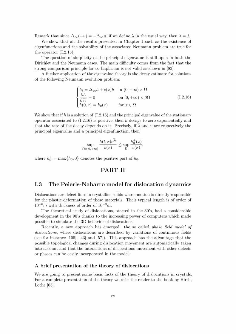
Let us start with the geometrical description of a dislocation. Consider a perfectcrystal cube, acted on a shear stress as shown in Figure I.3.16-(a). The edgedislocation in Figure I.3.16-(b) is producing by slicing the cube from the left to rightnormal to z and displacing the cube to comply with the stress. The dislocation isthe line representing the boundary of the slipped region.
Figure I.3.16. Geometry of an edge dislocation.
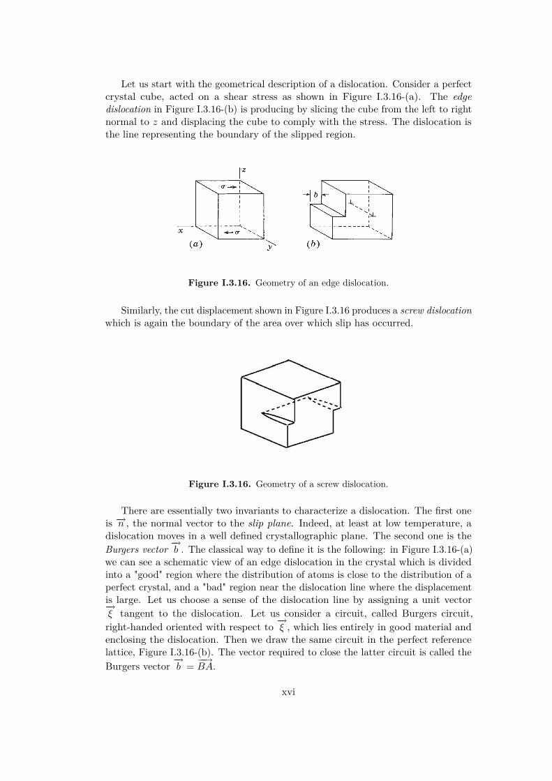
Similarly, the cut displacement shown in Figure I.3.16 produces a screw dislocationwhich is again the boundary of the area over which slip has occurred.
Figure I.3.16. Geometry of a screw dislocation.
There are essentially two invariants to characterize a dislocation. The first oneis −→n , the normal vector to the slip plane. Indeed, at least at low temperature, adislocation moves in a well defined crystallographic plane. The second one is theBurgers vector
−→b . The classical way to define it is the following: in Figure I.3.16-(a)
we can see a schematic view of an edge dislocation in the crystal which is dividedinto a "good" region where the distribution of atoms is close to the distribution of aperfect crystal, and a "bad" region near the dislocation line where the displacementis large. Let us choose a sense of the dislocation line by assigning a unit vector−→ξ tangent to the dislocation. Let us consider a circuit, called Burgers circuit,right-handed oriented with respect to −→ξ , which lies entirely in good material andenclosing the dislocation. Then we draw the same circuit in the perfect referencelattice, Figure I.3.16-(b). The vector required to close the latter circuit is called theBurgers vector −→b = −−→BA.
xvi
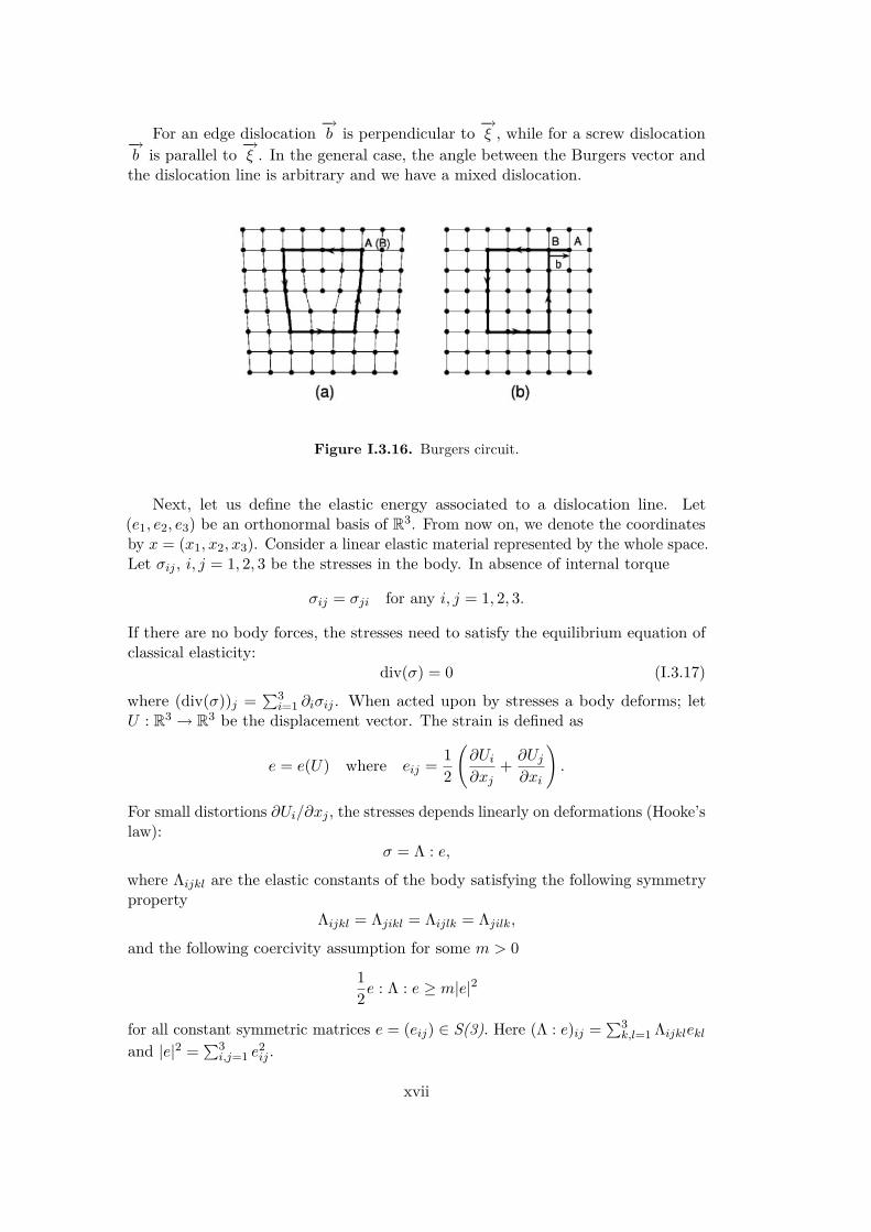
For an edge dislocation −→b is perpendicular to −→ξ , while for a screw dislocation−→b is parallel to −→ξ . In the general case, the angle between the Burgers vector andthe dislocation line is arbitrary and we have a mixed dislocation.
Figure I.3.16. Burgers circuit.
Next, let us define the elastic energy associated to a dislocation line. Let(e1, e2, e3) be an orthonormal basis of R3. From now on, we denote the coordinatesby x = (x1, x2, x3). Consider a linear elastic material represented by the whole space.Let σij , i, j = 1, 2, 3 be the stresses in the body. In absence of internal torque
σij = σji for any i, j = 1, 2, 3.
If there are no body forces, the stresses need to satisfy the equilibrium equation ofclassical elasticity:
div(σ) = 0 (I.3.17)
where (div(σ))j = ∑3i=1 ∂iσij . When acted upon by stresses a body deforms; let
U : R3 → R3 be the displacement vector. The strain is defined as
e = e(U) where eij = 12
(∂Ui∂xj
+ ∂Uj∂xi
).
For small distortions ∂Ui/∂xj , the stresses depends linearly on deformations (Hooke’slaw):
σ = Λ : e,
where Λijkl are the elastic constants of the body satisfying the following symmetryproperty
Λijkl = Λjikl = Λijlk = Λjilk,
and the following coercivity assumption for some m > 0
12e : Λ : e ≥ m|e|2
for all constant symmetric matrices e = (eij) ∈ S(3). Here (Λ : e)ij = ∑3k,l=1 Λijklekl
and |e|2 = ∑3i,j=1 e
2ij .
xvii
The equation of linear elasticity (I.3.17) is the Euler-Lagrange equation (mini-mizing with respect to U) associated to the elastic energy
Eel = 12
∫R3e : Λ : edx. (I.3.18)
If the medium is elastically isotropic, i.e. the elastic properties are independentof direction, only two independent elastic constants are required: the Lamé constantλ and the shear modulus µ, with µ > 0 and 3λ + 2µ > 0. In this case the elasticenergy has the form
Eel =∫
R3µ|e(U)|2 + λ
2 |tre(U)|2dx. (I.3.19)
Now, let us assume that there is a dislocation line in the material, representedby the boundary Γ of a smooth domain Ω0 contained in the plane x3 = 0 (slipplane). In this case we have to consider a plastic deformation epl in addition to theelastic one eel:
e(U) = eel + epl,
whereepl = e0ρδ0(x3), with e0 = 1
2(−→b ⊗−→n +−→n ⊗−→b
).
Here δ0(x3) is the Dirac mass only in the x3 component, −→n = e3 and ρ is thecharacteristic function of Ω0. The classical theory of dislocations asserts that thedislocation line creates a distortion in the strain e such that
div(Λ : e(U)) = div(ρδ0(x3)Λ : e0)
in the sense of distributions. The dislocation line is surrounded by a region, knownas the dislocation core, where the atomic positions cannot be described by a smallhomogenous deformation of the reference crystal. To take into consideration thenonlinear atomic interaction across the slip plane, in many models a tension lineenergy is added to the elastic energy, see for instance [30] and [25]. The energy isthus formally given by
E = 12
∫R3eel : Λ : eeldx+
∫ΓW (−→n )dS,
where W is an energy of tension line. In the dislocation core the linear continuumelastic theory is not longer valid, in other words, the elastic energy may be infiniteclose to the dislocation line. A simple way to overcome this difficulty has beenproposed by Alvarez, Hoch, Le Bouar and Monneau [7] and consists in introducing aregularizing core tensor χ and replacing eel by eelχ = χ?eel, where ? is the convolutionoperation. We refer to [7] for more details.
Description of the Peierls-Nabarro model
The Peierls-Nabarro model is a phase field model incorporating atomic features intocontinuum framework.
We briefly review the model for a straight dislocation, see [63] for a detailedpresentation. As an example, consider an edge dislocation in a crystal with simple
xviii
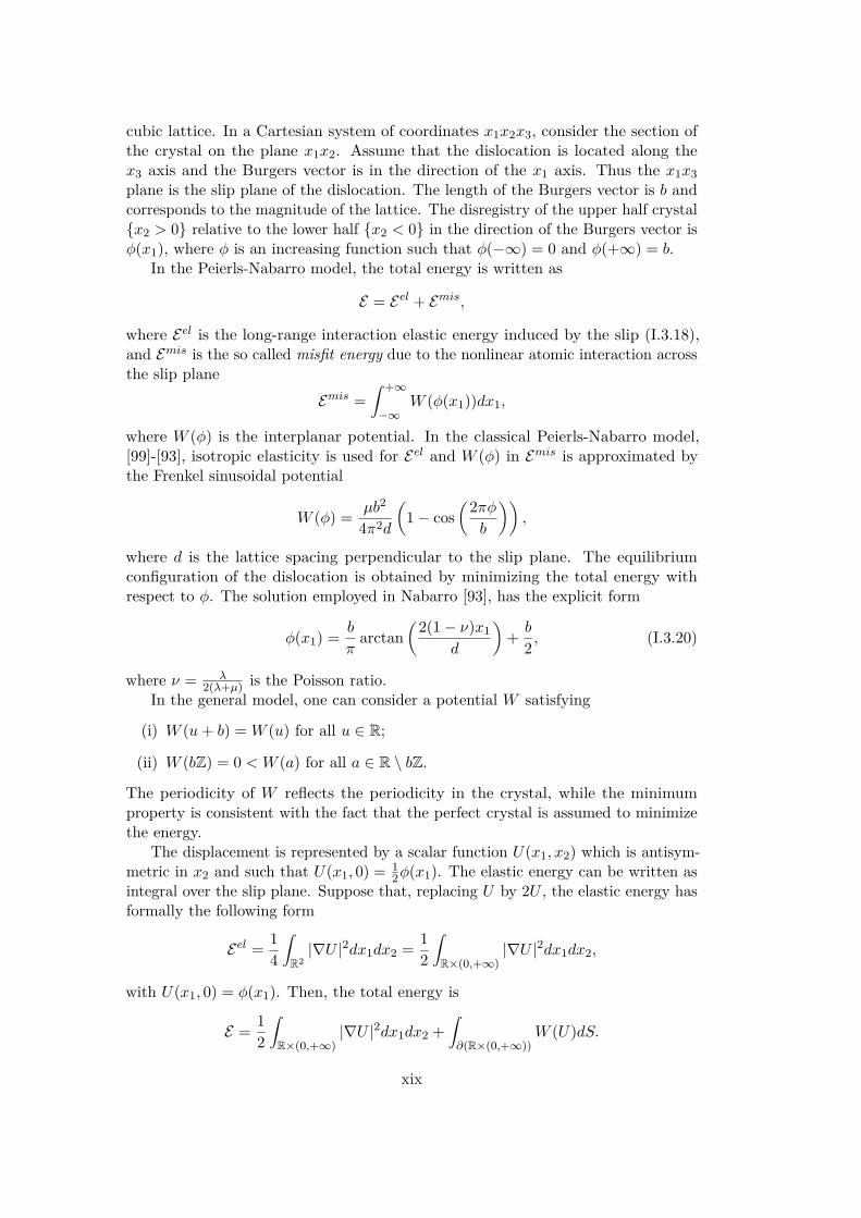
cubic lattice. In a Cartesian system of coordinates x1x2x3, consider the section ofthe crystal on the plane x1x2. Assume that the dislocation is located along thex3 axis and the Burgers vector is in the direction of the x1 axis. Thus the x1x3plane is the slip plane of the dislocation. The length of the Burgers vector is b andcorresponds to the magnitude of the lattice. The disregistry of the upper half crystalx2 > 0 relative to the lower half x2 < 0 in the direction of the Burgers vector isφ(x1), where φ is an increasing function such that φ(−∞) = 0 and φ(+∞) = b.
In the Peierls-Nabarro model, the total energy is written as
E = Eel + Emis,
where Eel is the long-range interaction elastic energy induced by the slip (I.3.18),and Emis is the so called misfit energy due to the nonlinear atomic interaction acrossthe slip plane
Emis =∫ +∞
−∞W (φ(x1))dx1,
where W (φ) is the interplanar potential. In the classical Peierls-Nabarro model,[99]-[93], isotropic elasticity is used for Eel and W (φ) in Emis is approximated bythe Frenkel sinusoidal potential
W (φ) = µb2
4π2d
(1− cos
(2πφb
)),
where d is the lattice spacing perpendicular to the slip plane. The equilibriumconfiguration of the dislocation is obtained by minimizing the total energy withrespect to φ. The solution employed in Nabarro [93], has the explicit form
φ(x1) = b
πarctan
(2(1− ν)x1d
)+ b
2 , (I.3.20)
where ν = λ2(λ+µ) is the Poisson ratio.
In the general model, one can consider a potential W satisfying
(i) W (u+ b) = W (u) for all u ∈ R;
(ii) W (bZ) = 0 < W (a) for all a ∈ R \ bZ.
The periodicity of W reflects the periodicity in the crystal, while the minimumproperty is consistent with the fact that the perfect crystal is assumed to minimizethe energy.
The displacement is represented by a scalar function U(x1, x2) which is antisym-metric in x2 and such that U(x1, 0) = 1
2φ(x1). The elastic energy can be written asintegral over the slip plane. Suppose that, replacing U by 2U , the elastic energy hasformally the following form
Eel = 14
∫R2|∇U |2dx1dx2 = 1
2
∫R×(0,+∞)
|∇U |2dx1dx2,
with U(x1, 0) = φ(x1). Then, the total energy is
E = 12
∫R×(0,+∞)
|∇U |2dx1dx2 +∫∂(R×(0,+∞))
W (U)dS.
xix
A local minimizer of the energy is a solution of∆U = 0, in Ω∂U∂−→n = −W ′(U), on ∂Ω (I.3.21)
where Ω = (x1, x2) |x2 > 0 and ∂U∂−→n = − ∂U
∂x2is the exterior normal derivative of U ,
see Cabré and Solà-Morales [33]. It is well known that if V is a smooth function onRN×[0,+∞) which is harmonic in RN×(0,+∞) and V (x1, ..., xN , 0) = v(x1, ..., xN ),then ∂V
∂xN+1(x1, ..., xN , 0) = −(−∆) 1
2 v(x1, ..., xN ), where the half-Laplacian (−∆) 12
is the fractional operator defined on the Schwartz class S(RN ) by
(−∆)12 v = F−1(| · |F(v)),
see [86]. Here F is the Fourier transform. For a bounded real smooth function vdefined on RN , the linear operator −(−∆) 1
2 is given by the Lévy-Khintchine formula(see Theorem 1 in [66]):
− (−∆)12 v(y) = CN
∫RN
(v(y + z)− v(y)−∇v(y) · z1|z|≤1)dz
|z|N+1 (I.3.22)
where CN is a constant depending on the dimension N and 1|z|≤1 is the characte-ristic function of the set |z| ≤ 1. Hence, for smooth solutions, system (I.3.21) canbe rewritten for φ(x1) = U(x1, 0) as
−(−∆)12φ = W ′(φ) on R,
where −(−∆) 12 is the non-local operator defined by (I.3.22) with N = 1. In [33] the
authors show that for smooth potentials W satisfying assumptions (i) and (ii) above,there exists a function φ solution of
−(−∆) 12φ = W ′(φ), on R
φ′ > 0, and φ(−∞) = 0 φ(+∞) = b.(I.3.23)
The function φ is called layer solution. If in addition W satisfies
(iii) W ′′(bZ) > 0,
then the layer solution is unique up to translations. When the elastic energy has thegeneral form (I.3.18), then the phase transition φ is a solution of
I1[φ] = W ′(φ) on R, (I.3.24)
where I1 is the anisotropic Lévy operator of order 1, defined on bounded C2-functions by
I1[v](x) =∫
R(v(x+ z)− v(x)− zv′(y)1|z|≤1)
1|z|2
g
(z
|z|
)dz
with g positive and even function. See [7] for the characterization of g. In the specialcase of isotropic elasticity, we have g(z) = µ
2π(1−ν) and the function (I.3.20) is a layersolution of (I.3.24).
xx
Outline of the results of Chapter 4
In the face cubic structured (FCC) observed in many metals and alloys, dislocationsmove at low temperature on the slip plane at a velocity of order 10ms−1. To takeinto consideration the dynamics effects in motion of dislocations, in Chapter 4 westudy the evolutive version in dimension N of the Peierls-Nabarro model (I.3.24)introduced in the previous section. The results presented are contained in [92].Precisely, we consider the non-local parabolic equation
∂tu = I1[u(t, ·)]−W ′ (u) + σ (t, x) in R+ × RN (I.3.25)
where I1 is the anisotropic Lévy operator of order 1, defined on bounded C2-functions U : RN → R for r > 0 by
I1[U ](x) =∫|z|≤r
(U(x+ z)− U(x)−∇U(x) · z) 1|z|N+1 g
(z
|z|
)dz
+∫|z|>r
(U(x+ z)− U(x)) 1|z|N+1 g
(z
|z|
)dz.
Here g is a positive and even continuous function andW and σ are periodic functions.See Chapter 4 for the precise assumptions on g, σ and W . In the model σ has beenintroduced to take into account the possible external applied shear stress on thematerial.
We suppose that at initial time t = 0 u satisfies
u(0, x) = 1εu0(εx) on RN , (I.3.26)
where u0 is a regular bounded function and ε is a small positive parameter.Problem (I.3.25)-(I.3.26) for N = 1 models the dynamics of a collection of parallel
straight edge dislocation lines with the same Burgers vector, all contained in thesame slip plane and moving in a landscape with periodic obstacles. The parameter εtakes into account the fact that the number of dislocations is increasing of order 1/ε.
We want to identify at large scale an evolution model for the dynamics of adensity of dislocations and we do this by a periodic homogenization approach. Weconsider the following rescaling
uε(t, x) = εu
(t
ε,x
ε
),
the functions uε are solutions of∂tuε = I1[uε(t, ·)]−W ′(uε
ε
)+ σ
(tε ,xε
)in R+ × RN
uε(0, x) = u0(x) on RN .(I.3.27)
A good notion of solution for system (I.3.27) is the notion of viscosity solution fornon-local equations given for instance in [12]. See also [34], [22] and [65].
We prove that the limit u0 of uε as ε → 0 exists and is the unique solution ofthe homogenized problem
∂tu = H(∇u, I1[u(t, ·)]) in R+ × RN
u(0, x) = u0(x) on RN ,(I.3.28)
xxi
for some continuous function H usually called effective Hamiltonian. As usual inperiodic homogenization, the limit equation is determined by a cell problem. In ourcase, such a problem is for any p ∈ RN and L ∈ R the following:
λ+ ∂tv = I1[v(τ, ·)] + L−W ′(v + λt+ p · x) + σ(t, x) in R+ × RN
v(0, x) = 0 on RN .(I.3.29)
We show that there is a unique number λ = λ(p, L) for which there exists a solutionof (I.3.29) which is bounded on R+ × RN . The effective Hamiltonian of (I.3.28) isthus defined as follows: H(p, L) := λ(p, L). The function H(p, L) is continuous onRN × R and non-decreasing in L.
A specific technical difficulty in this problem is to deal with the case λ = p = 0.In order to overcome it, following [67] and [68], we consider cell problems in a higherdimensional space. The lack of smooth solutions for these problems, has inducedus to construct regular approximated sub and supercorrectors, i.e. regular suband supersolutions of approximate N + 1-dimensional cell problems, and this isenough to conclude. Let us also point out that, differently from the case of equationsindependent of uε/ε, correctors here are not periodic with respect to the spacevariable in general. Moreover, correctors are necessarily time dependent.
The homogenized equation (I.3.28) can be interpreted as the plastic flow rule ina model for macroscopic crystal plasticity, i.e. a relationship between the plasticstrain velocity and the stress. In the homogenized equation (I.3.28):
• u0 is the plastic strain;
• ∂tu0 is the plastic strain velocity;
• ∇u0 is the dislocation density;
• I1[u0] is the internal stress created by the density of dislocations contained ina slip plane.
In dimension N = 1, when I1 is the half-Laplacian and the periodic stress σ is equalto 0, we get
H(p, L) ∼ 12γ|p|L (I.3.30)
for small p and L, where γ = 2(∫R(φ′)2)−1 is the inverse of the so called damping
factor and φ is a layer solution, i.e. a solution of (I.3.23). This characterization ofthe effective Hamiltonian is known in physics as Orowan’s law.
Remark I.3.1. Fractional reaction-diffusion equations of the form
∂tu = I1[u] + f(u) in R+ × RN (I.3.31)
where N ≥ 2 and f is a bistable nonlinearity have been studied by Imbert andSouganidis [69]. In this paper the authors show that solutions of (I.3.31), afterproperly rescaling them, exhibit a moving interface. Analogous results have beenobtained by González and Monneau [62] for the evolutive Peierls-Nabarro model indimension N = 1. In the one dimensional space, the moving interface are points.The dynamics of these particles corresponds to the classical discrete dislocation
xxii
dynamics, in the particular case of of parallel straight edge dislocation lines in thesame slip plane with the same Burgers vector. Considering the motion of theseparticles they identify at large scale an evolution model for the dynamics of a densityof dislocations that corresponds to (I.3.28).
Finally, let us mention that in [57] and [58] Garroni and Muller study a variationalmodel for dislocations that is the variational formulation of the stationary Peierls-Nabarro equation.
I.4 Local Hamilton-Jacobi equations
In Chapter 5 we present the results of [2]. We consider homogenization problems forfirst order local Hamilton-Jacobi equations with uε/ε periodic dependence, namely
uεt +H(tε ,xε ,
uε
ε , Duε)
= 0, (t, x) ∈ (0,+∞)× RN ,
uε(0, x) = u0(x), x ∈ RN(I.4.32)
with the following assumptions on the Hamiltonian H:
(H1) Periodicity: for any (t, x, u, p) ∈ R× RN × R× RN
H(t+ 1, x+ k, u+ 1, p) = H(t, x, u, p) for any k ∈ ZN ;
(H2) Regularity: H : R×RN ×R×RN → R is Lipschitz continuous and there existsa constant C1 > 0 such that, for almost every (t, x, u, p) ∈ R× RN × R× RN
|D(t,x)H(t, x, u, p)| ≤ C1(1+|p|), |DuH(t, x, u, p)| ≤ C1, |DpH(t, x, u, p)| ≤ C1;
(H3) H(t, x, u, p)→ +∞ as |p| → +∞ uniformly for (t, x, u) ∈ R× RN × R;
(H4) There exists a constant C such that for almost every (t, x, u, p) ∈ R× RN ×R× RN
|DpH(t, x, u, p) · p−H(t, x, u, p)| ≤ C.
Problem (I.4.32) with H independent of t was introduced by Imbert and Monneau[67] as a simplified model for dislocation dynamics in material science. The completemodel is introduced in [68] and leads to non-local first order equations of the type
uεt +(c
(x
ε
)+M ε
(uε
ε
))|Duε|+H
(uε
ε,Duε
)= 0
where M ε is a non-local jump operator and c is a periodic velocity. In the lattermodel, the level sets of the solution uε describe dislocations.
Going back to (I.4.32), it was proved in [67] that, with H independent of t,
• under assumptions (H1) and (H2), there exists a unique bounded continuousviscosity solution of (I.4.32);
xxiii
• under assumptions (H1)-(H3), the limit u0 of uε as ε→ 0 exists and it is theunique bounded continuous solution of the homogenized problem
u0t +H(Du0) = 0, (t, x) ∈ (0,+∞)× RN ,u0(0, x) = u0(x), x ∈ RN ,
(I.4.33)
where the effective Hamiltonian H is uniquely defined by the long time behaviorof the solution of
λ = vt +H(x,−λt+ p · x+ v, p+Dv), (t, x) ∈ (0,+∞)× RN ,v(0, x) = 0, x ∈ RN .
(I.4.34)
More precisely, we have the following theorem
Theorem I.4.1 (Imbert-Monneau, [67]). Let H be independent of t. Assume (H1)-(H3) and u0 ∈ W 1,∞(RN ). Then, as ε → 0, the sequence uε converges locallyuniformly in (0,+∞) × RN to the solution u0 of (I.4.33), where, for any p ∈ RN
H(p) is defined as the unique number λ for which there exists a bounded continuousviscosity solution of (I.4.34). Moreover H : RN → R is continuous and satisfies thecoercivity property
H(p)→ +∞ as |p| → +∞.
The proof in [67] is rather involved: it uses a twisted perturbed test function fora higher dimensional problem posed in R× RN × R.Under the additional assumption (H4), an easier proof of Theorem I.4.1 was given byBarles, [18], as a byproduct of a general result on the homogenization of Hamilton-Jacobi equations with non-coercive Hamiltonians.
Remark I.4.2. The hypothesis (H4) which was not used in [67] guarantees theexistence of a function H∞ such that
H∞(t, x, u, p) = lims→0+
sH(t, x, u, s−1p).
Moreover H∞ satisfies (H1)-(H3).
In [18], thanks to assumption (H4), the equation for uε is interpreted as anequation for the motion of a graph: indeed, following [18], for t ∈ R, (x, y) ∈ RN+1,(px, py) ∈ RN+1, let us introduce the non-coercive Hamiltonian F defined by
F (t, x, y, px, py) =|py|H(t, x, y, |py|−1px), if py 6= 0,H∞(t, x, y, px), otherwise.
The function U ε(t, x, y) := uε(t, x)− y satisfiesU εt + F
(tε ,xε ,
Uε+yε , DxU
ε, DyUε)
= 0, (t, x, y) ∈ (0,+∞)× RN+1,
U ε(0, x, y) = u0(x)− y, (x, y) ∈ RN+1.(I.4.35)
In [18] Barles proves that the sequence U ε converges to the solution U0 of thefollowing problem
U0t + F (DxU
0, DyU0) = 0, (t, x, y) ∈ (0,+∞)× RN+1,
U0(0, x, y) = u0(x)− y, (x, y) ∈ RN+1,(I.4.36)
xxiv
where for (px, py) ∈ RN+1, F (px, py) is the unique number λ for which the cellproblem
Vt + F (t, x, y, px +DxV, py +DyV ) = λ in R× RN+1. (I.4.37)
admits bounded sub and supersolutions. This result makes it possible to solve thehomogenization problem for (I.4.32):
Theorem I.4.3 (Barles, [18]). Assume (H1)-(H4). Then the sequence uε convergeslocally uniformly in (0,+∞) × RN to the solution u0 of (I.4.33). The functionH(p) in (I.4.33) can be characterized as follows: H(p) = F (p,−1), where, for any(px, py) ∈ RN+1, F (px, py) is the unique number λ for which the equation (I.4.37)admits bounded sub and supersolutions in R× RN+1.
An important step in the proof of Theorem I.4.3 consists of homogenizing thenon-coercive level-set equation satisfied by 11Uε≥0.
Outline of the results of Chapter 5
In Chapter 5, we tackle two questions:
• Is it possible to estimate the rate of convergence of uε to u0 when ε→ 0?
• Is is possible to approximate numerically the effective Hamiltonian?
The first question was answered by Capuzzo Dolcetta and Ishii, [36] for a moreclassical homogenization problem: the estimate ‖uε − u0‖∞ ≤ Cε
13 was obtained for
Hamilton-Jacobi equations of the type
uε +H
(x,x
ε, uε)
= 0,
where (x, y, p)→ H(x, y, p) is a coercive Hamiltonian, uniformly Lipschitz continuousfor |p| bounded and periodic with respect to y; moreover, if H(x, y, p) does notdepend on x, then the convergence is linear in ε.
We show that in the present case, it is possible to obtain the same rates ofconvergence as ε→ 0 by adapting the proof in [36] using the arguments containedin [18]. The main idea is to approximate U ε (with an error smaller than ε) by adiscontinuous function U ε which takes integer values where U ε has noninteger valuesand which is a discontinuous viscosity solution of
U εt + F
(t
ε,x
ε,y
ε,DxU
ε, DyUε)
= 0, (t, x, y) ∈ (0,+∞)× RN+1.
The latter equation has to be compared with (I.4.35). This approximation U ε isobtained as the limit as δ → 0 of φδ(U ε) where (φδ)δ is a sequence of increasingfunctions. The method of Capuzzo Dolcetta and Ishii [36] can then be applied to U ε.The second question was studied in [1] for equation
uε +H
(x
ε, uε)
= 0,
xxv
where (y, p) → H(y, p) is a coercive Hamiltonian, uniformly Lipschitz continuousfor |p| bounded and periodic with respect to y; in this article, a complete numericalmethod for solving the homogenized problem was studied, including as a main stepthe approximation of the effective Hamiltonian by solving discrete cell problems.Error estimates were proved. Here, we study the approximation of the cell problem(I.4.37) by Eulerian schemes in the discrete torus. We have preferred to study theapproximation of the noncoercive N + 2 dimensional problem (I.4.37) rather thanthat of the coercive N+1 dimensional problem (I.4.34) because the solution of (I.4.34)may not be periodic. We prove the discrete analogue of the ergodicity Theorems in[18], i.e. that there exists a unique real number λ∆t
h such that the discrete analogueof (I.4.37) has a solution. The arguments in the proof are the discrete counterpartsof those in [18]. We also show that the discrete effective Hamiltonian converges tothe effective Hamiltonian when the grid step of the discrete cell problem tends tozero.
xxvi

Part I
Neumann generalized principaleigenvalues
1

Chapter 1
Fully nonlinear singularoperators
In this chapter we study the maximum principle, principal eigenvalues, regularityand existence for viscosity solutions of the Neumann boundary value problem
F (x,Du,D2u) + b(x) ·Du|Du|α + (c(x) + λ)|u|αu = g(x) in Ω〈Du,−→n (x)〉 = 0 on ∂Ω,
(1.0.1)
where Ω is a bounded domain of class C2, −→n (x) is the exterior normal to the domainΩ at x, α > −1, λ ∈ R and b, c, g are continuous functions on Ω. F is a fullynonlinear operator that may be singular at the points where the gradient vanishes.F : Ω× RN \ 0 × S(N)→ R satisfies the following conditions
(F1) For all t ∈ R∗, µ ≥ 0, (x, p,X) ∈ Ω× RN \ 0 × S(N)
F (x, tp, µX) = |t|αµF (x, p,X).
(F2) There exist a,A > 0 such that for x ∈ Ω, p ∈ RN \ 0,M,N ∈ S(N), N ≥ 0
a|p|αtrN ≤ F (x, p,M +N)− F (x, p,M) ≤ A|p|αtrN.
(F3) There exist C1 > 0 and θ ∈ (12 , 1] such that for all x, y ∈ Ω, p ∈ RN \ 0, X ∈
S(N)|F (x, p,X)− F (y, p,X)| ≤ C1|x− y|θ|p|α‖X‖.
(F4) There exist C2 > 0 and ν ∈ (12 , 1] such that for all x ∈ Ω, p ∈ RN \ 0,
p0 ∈ RN , |p0| ≤ |p|2 , X ∈ S(N)
|F (x, p+ p0, X)− F (x, p,X)| ≤ C2|p|α−ν |p0|ν‖X‖.
The domain Ω is supposed to be bounded and of class C2. In particular, it satisfiesthe interior sphere condition and the uniform exterior sphere condition, i.e.,
(Ω1) For each x ∈ ∂Ω there exist R > 0 and y ∈ Ω for which |x − y| = R andB(y,R) ⊂ Ω.
3
4 1. Fully nonlinear singular operators
(Ω2) There exists r > 0 such that B(x+ r−→n (x), r) ∩ Ω = ∅ for any x ∈ ∂Ω.
From the property (Ω2) it follows that
〈y − x,−→n (x)〉 ≤ 12r |y − x|
2 for x ∈ ∂Ω and y ∈ Ω. (1.0.2)
Moreover, the C2-regularity of Ω implies the existence of a neighborhood of ∂Ω in Ωon which the distance from the boundary
d(x) := inf|x− y|, y ∈ ∂Ω, x ∈ Ω
is of class C2. We still denote by d a C2 extension of the distance function to thewhole Ω. Without loss of generality we can assume that |Dd(x)| ≤ 1 in Ω.
Here we adopt the notion of viscosity solution given in Definition I.2.2. We callstrong viscosity subsolutions (resp., supersolutions) the viscosity subsolutions (resp.,supersolutions) that satisfy B(x, u,Du) ≤ (resp., ≥) 0 in the viscosity sense for allx ∈ ∂Ω. If λ→ B(x, r, p−λ−→n ) is non-increasing in λ ≥ 0, then classical subsolutions(resp., supersolutions) are strong viscosity subsolutions (resp., supersolutions), see[40] Proposition 7.2.
In the definition of viscosity solution the test functions can be substituted bythe elements of the semijets J2,+
u(x0) when u is a subsolution and J2,−u(x0) when
u is a supersolution, see [40].For simplicity of notation we denote
G(x, u,Du,D2u) := F (x,Du,D2u) + b(x) ·Du|Du|α + c(x)|u|αu.
Remark that the function b, c and g correspond respectively to −b,−c and −g of(I.2.7).
Following the ideas of [26], we define the principal eigenvalue as
λ := supλ ∈ R | ∃ v > 0 bounded viscosity supersolution ofG(x, v,Dv,D2v) + λvα+1 = 0 in Ω, 〈Dv,−→n 〉 = 0 on ∂Ω.
(1.0.3)
λ is well defined since the above set is not empty; indeed, −|c|∞ belongs to it, beingv(x) ≡ 1 a corresponding supersolution. Furthermore it is an interval because if λbelongs to it then so does any λ′ < λ.
We will prove that λ is an "eigenvalue" for −G which admits a positive "eigen-function", in the sense that there exists φ > 0 solution of
G(x, φ,Dφ,D2φ) + λφα+1 = 0 in Ω〈Dφ,−→n (x)〉 = 0 on ∂Ω.
Moreover, λ can be characterized as the supremum of those λ for which the opera-tor G(x, u,Du,D2u) + λ|u|αu with the Neumann boundary condition satisfies themaximum principle. As a consequence λ is the least "eigenvalue" to which therecorrespond "eigenfunctions" positive somewhere. These results are applied to obtainexistence and uniqueness for the boundary value problem (1.0.1).
1.1 Lipschitz continuity of viscosity solutions 5
For fully nonlinear operators it is possible to define another principal eigenvalue
λ := supλ ∈ R | ∃u < 0 bounded viscosity subsolution ofG(x, u,Du,D2u) + λ|u|αu = 0 in Ω, 〈Du,−→n 〉 = 0 on ∂Ω.
If F (x, p,X) = −F (x, p,−X) then λ = λ, otherwise λ may be different from λ.Symmetrical results can be obtained for λ.
The classical assumption which guarantees the solvability of the Neumann pro-blem (1.0.1) with λ = 0 is c < 0 in Ω. We show that the right hypothesis for anyright-hand side is the positivity of the two principal eigenvalues.
In the next we establish a Lipschitz regularity result for viscosity solutions of(1.0.1). Section 1.2 is devoted to the study of the maximum principle for subsolutionsof (1.0.1). In Section 1.2.1 we show that it holds (even for more general boundaryconditions) for G(x, u,Du,D2u) if c(x) ≤ 0 and c 6≡ 0, see Theorem 1.2.5. One of themain result of this chapter is that the maximum principle holds for G(x, u,Du,D2u)+λ|u|αu for any λ < λ, as we show in Theorem 1.2.9 of Section 1.2.2. In particular itholds for G(x, u,Du,D2u) if λ > 0. It is natural to wonder if the result of Theorem1.2.9 is stronger than that of Theorem 1.2.5; indeed if c ≡ 0, one has λ = 0. Apositive answer is given in Section 1.2.3, where we construct an explicit exampleof a bounded positive viscosity supersolution of G(x, v,Dv,D2v) + λvα+1 = 0 in Ω,〈Dv,−→n 〉 = 0 on ∂Ω, λ > 0, with c(x) changing sign. The existence of such v implies,by definition, λ > 0. Finally, in Section 1.3 we show some existence and comparisontheorems.
1.1 Lipschitz continuity of viscosity solutions
Theorem 1.1.1. Let Ω be a bounded domain of class C2. Suppose that F satisfies(F2)-(F4) and that b, c, g are bounded in Ω. If u ∈ C(Ω) is a viscosity solution of
F (x,Du,D2u) + b(x) ·Du|Du|α + c(x)|u|αu = g(x) in Ω〈Du,−→n (x)〉 = 0 on ∂Ω,
then|u(x)− u(y)| ≤ C0|x− y| ∀x, y ∈ Ω,
where C0 depends on Ω, N, α, a, A, θ, ν, C1, C2, |b|∞, |c|∞, |g|∞, and |u|∞.
The Theorem is an immediate consequence of the next lemma. To prove thelemma we adopt the technique used in Proposition III.1 of [75] for Dirichlet problems,that we modify taking test functions which depend on d(x).
The lemma plays a key role also in the proof of Theorem 1.2.9 in the next section.
Lemma 1.1.2. Assume the hypothesis of Theorem 1.1.1 and suppose that g and hare bounded functions. Let u ∈ USC(Ω) be a viscosity subsolution of
F (x,Du,D2u) + b(x) ·Du|Du|α + c(x)|u|αu = g(x) in Ω〈Du,−→n (x)〉 = 0 on ∂Ω,
6 1. Fully nonlinear singular operators
and v ∈ LSC(Ω) a viscosity supersolution ofF (x,Dv,D2v) + b(x) ·Dv|Dv|α + c(x)|v|αv = h(x) in Ω〈Dv,−→n (x)〉 = 0 on ∂Ω,
with u and v bounded, or v ≥ 0 and bounded. If m = maxΩ(u− v) ≥ 0, then thereexists C0 > 0 such that
u(x)− v(y) ≤ m+ C0|x− y| ∀x, y ∈ Ω, (1.1.4)
where C0 depends on Ω, N, α, a, A, θ, ν, C1, C2, |b|∞, |c|∞, |g|∞, |h|∞, |v|∞, m and|u|∞ or supΩ u.
Proof. We setΦ(x) = MK|x| −M(K|x|)2,
andϕ(x, y) = m+ e−L(d(x)+d(y))Φ(x− y),
where L is a fixed number greater than 2/(3r) with r the radius in the condition(Ω2) and K and M are two positive constants to be chosen later. If K|x| ≤ 1
4 , then
Φ(x) ≥ 34MK|x|. (1.1.5)
We define∆K :=
(x, y) ∈ RN × RN : |x− y| ≤ 1
4K
.
We fix M such that
maxΩ 2
(u(x)− v(y)) ≤ m+ e−2Ld0M
8 , (1.1.6)
where d0 = maxx∈Ω d(x), and we claim that taking K large enough, one has
u(x)− v(y)− ϕ(x, y) ≤ 0 for (x, y) ∈ ∆K ∩ Ω2.
In this case (1.1.4) is proven. To show the last inequality we suppose by contradictionthat for some (x, y) ∈ ∆K ∩ Ω2
u(x)− v(y)− ϕ(x, y) = max∆K∩Ω 2
(u(x)− v(y)− ϕ(x, y)) > 0.
Here we have dropped the dependence of x, y on K for simplicity of notations.Observe that if v ≥ 0, since from (1.1.5) Φ(x − y) is non-negative in ∆K and
m ≥ 0, one has u(x) > 0.Clearly x 6= y. Moreover the point (x, y) belongs to int(∆K) ∩ Ω2. Indeed, if
|x− y| = 14K , by (1.1.6) and (1.1.5) we have
u(x)− v(y) ≤ m+ e−2Ld0M
8 ≤ m+ e−L(d(x)+d(y)) 12MK|x− y| ≤ ϕ(x, y).
1.1 Lipschitz continuity of viscosity solutions 7
Since x 6= y we can compute the derivatives of ϕ in (x, y) obtaining
Dxϕ(x, y) = e−L(d(x)+d(y))MK− L|x− y|(1−K|x− y|)Dd(x)
+ (1− 2K|x− y|)(x− y)|x− y|
,
Dyϕ(x, y) = e−L(d(x)+d(y))MK− L|x− y|(1−K|x− y|)Dd(y)
− (1− 2K|x− y|)(x− y)|x− y|
.
Observe that for large K
e−2Ld0MK
4 ≤ e−L(d(x)+d(y))MK
(12 − L|x− y|
)≤ |Dxϕ(x, y)|, |Dyϕ(x, y)|
≤ 2MK.
(1.1.7)
Using (1.0.2), if x ∈ ∂Ω we have
〈Dxϕ(x, y),−→n (x)〉
= e−Ld(y)MKL|x− y|(1−K|x− y|) + (1− 2K|x− y|)〈(x− y)
|x− y|,−→n (x)〉
≥ e−Ld(y)MK
34L|x− y| − (1− 2K|x− y|) |x− y|2r
≥ 1
2e−Ld(y)MK|x− y|
(32L−
1r
)> 0,
since x 6= y and L > 2/(3r). Similarly, if y ∈ ∂Ω
〈−Dyϕ(x, y),−→n (y)〉 ≤ 12e−Ld(x)MK|x− y|
(−3
2L+ 1r
)< 0.
In view of definition of sub and supersolution, we conclude that
G(x, u(x), Dxϕ(x, y), X) ≥ g(x) if (Dxϕ(x, y), X) ∈ J2,+u(x),
G(y, v(y),−Dyϕ(x, y), Y ) ≤ h(y) if (−Dyϕ(x, y), Y ) ∈ J2,−v(y).
Since (x, y) ∈ int∆K ∩ Ω2, it is a local maximum point of u(x)− v(y)− ϕ(x, y)in Ω2. Then applying Theorem 3.2 in [40], for every ε > 0 there exist X,Y ∈ S(N)such that (Dxϕ(x, y), X) ∈ J 2,+u(x), (−Dyϕ(x, y), Y ) ∈ J 2,−v(y) and(
X 00 −Y
)≤ D2(ϕ(x, y)) + ε(D2(ϕ(x, y)))2. (1.1.8)
Now we want to estimate the matrix on the right-hand side of the last inequality.
D2ϕ(x, y) = Φ(x− y)D2(e−L(d(x)+d(y))) +D(e−L(d(x)+d(y)))⊗D(Φ(x− y))+D(Φ(x− y))⊗D(e−L(d(x)+d(y))) + e−L(d(x)+d(y))D2(Φ(x− y)).
8 1. Fully nonlinear singular operators
We setA1 := Φ(x− y)D2(e−L(d(x)+d(y))),
A2 := D(e−L(d(x)+d(y)))⊗D(Φ(x− y)) +D(Φ(x− y))⊗D(e−L(d(x)+d(y))),A3 := e−L(d(x)+d(y))D2(Φ(x− y)).
Observe thatA1 ≤ CK|x− y|
(I 00 I
). (1.1.9)
Here and henceforth C denotes various positive constants independent of K.For A2 we have the following estimate
A2 ≤ CK(I 00 I
)+ CK
(I −I−I I
). (1.1.10)
Indeed for ξ, η ∈ RN we compute
〈A2(ξ, η), (ξ, η)〉 = 2Le−L(d(x)+d(y))〈Dd(x)⊗DΦ(x− y)(η − ξ), ξ〉+ 〈Dd(y)⊗DΦ(x− y)(η − ξ), η〉 ≤ CK(|ξ|+ |η|)|η − ξ|≤ CK(|ξ|2 + |η|2) + CK|η − ξ|2.
Now we consider A3. The matrix D2(Φ(x− y)) has the form
D2(Φ(x− y)) =(
D2Φ(x− y) −D2Φ(x− y)−D2Φ(x− y) D2Φ(x− y)
),
and the Hessian matrix of Φ(x) is
D2Φ(x) = MK
|x|
(I − x⊗ x
|x|2)− 2MK2I. (1.1.11)
If we chooseε = |x− y|
2MKe−L(d(x)+d(y)) ,
then we have the following estimates
εA21 ≤ CK|x− y|3I2N , εA2
2 ≤ CK|x− y|I2N ,
ε(A1A2 +A2A1) ≤ CK|x− y|2I2N , (1.1.12)
ε(A1A3 +A3A1) ≤ CK|x− y|I2N , ε(A2A3 +A3A2) ≤ CKI2N ,
where I2N :=(I 00 I
). Then using (??), (1.1.10), (1.1.12) and observing that
(D2(Φ(x− y)))2 =(
2(D2Φ(x− y))2 −2(D2Φ(x− y))2
−2(D2Φ(x− y))2 2(D2Φ(x− y))2
),
from (1.1.8) we conclude that(X 00 −Y
)≤ O(K)
(I 00 I
)+(
B −B−B B
),
1.1 Lipschitz continuity of viscosity solutions 9
where
B = CKI + e−L(d(x)+d(y))[D2Φ(x− y) + |x− y|
MK(D2Φ(x− y))2
].
The last inequality can be rewritten as follows(X 00 −Y
)≤(
B −B−B B
),
with X = X −O(K)I and Y = Y +O(K)I.Now we want to get a good estimate for tr(X − Y ), as in [75]. For that aim let
0 ≤ P := (x− y)⊗ (x− y)|x− y|2
≤ I.
Since X − Y ≤ 0 and X − Y ≤ 4B, we have
tr(X − Y ) ≤ tr(P (X − Y )) ≤ 4tr(PB).
We have to compute tr(PB). From (1.1.11), observing that the matrix (1/|x|2)x⊗xis idempotent, i.e., [(1/|x|2)x⊗ x]2 = (1/|x|2)x⊗ x, we compute
(D2Φ(x))2 = M2K2
|x|2(1− 4K|x|)
(I − x⊗ x
|x|2)
+ 4M2K4I.
Then, since trP = 1 and 4K|x− y| ≤ 1, we have
tr(PB) = CK + e−L(d(x)+d(y))(−2MK2 + 4MK3|x− y|)≤ CK − e−L(d(x)+d(y))MK2 < 0,
for large K. This gives
|tr(X − Y )| = −tr(X − Y ) ≥ 4e−L(d(x)+d(y))MK2 − 4CK ≥ CK2,
for large K. Since ‖B‖ ≤ CK|x−y| , we have
‖B‖12 |tr(X − Y )|
12 ≤
(CK
|x− y|
) 12|tr(X − Y )|
12 ≤ C
K12 |x− y|
12|tr(X − Y )|.
The Lemma III.I in [75] ensures the existence of a universal constant C dependingonly on N such that
‖X‖, ‖Y ‖ ≤ C|tr(X − Y )|+ ‖B‖12 |tr(X − Y )|
12 .
Thanks to the above estimates we can conclude that
‖X‖, ‖Y ‖ ≤ C|tr(X − Y )|(
1 + 1K
12 |x− y|
12
). (1.1.13)
10 1. Fully nonlinear singular operators
Now, using the assumptions (F2), (F3) and (F4) concerning F , the definitionof X and Y and the fact that u and v are respectively sub and supersolution wecompute
g(x)− c(x)|u(x)|αu(x) ≤ F (x,Dxϕ,X) + b(x) ·Dxϕ|Dxϕ|α
≤ F (x,Dxϕ, X) + |Dxϕ|αO(K) + b(x) ·Dxϕ|Dxϕ|α
≤ F (y,−Dyϕ, Y ) + C1|x− y|θ|Dxϕ|α‖X‖+ CKν |x− y|ν |Dxϕ|α−ν‖X‖+ a|Dyϕ|αtr(X − Y )+ |Dxϕ|αO(K) + b(x) ·Dxϕ|Dxϕ|α
≤ b(y) ·Dyϕ|Dyϕ|α − c(y)|v(y)|αv(y) + h(y)+ C1|x− y|θ|Dxϕ|α‖X‖+ CKν |x− y|ν |Dxϕ|α−ν‖X‖+ a|Dyϕ|αtr(X − Y ) + |Dyϕ|α ∨ |Dxϕ|αO(K)+ b(x) ·Dxϕ|Dxϕ|α.
From this inequalities, using (1.1.7), (1.1.13) and the fact that θ, ν > 12 we get
g(x)− h(y)− c(x)|u(x)|αu(x) + c(y)|v(y)|αv(y) ≤ |Dyϕ|α ∨ |Dxϕ|α[atr(X − Y )+ C1|x− y|θ‖X‖+ C|x− y|ν‖X‖+O(K)] ≤ CKα[atr(X − Y ) + o(|tr(X − Y )|)].
If both u and v are bounded, then the first member in the last inequalities isbounded from below by −|g|∞ − |h|∞ − |c|∞(|u|α+1
∞ + |v|α+1∞ ). Otherwise, if v
is non-negative and bounded, then u(x) ≥ 0 and that quantity is greater than−|g|∞ − |h|∞ − |c|∞(supu)α+1 − |c|∞|v|α+1
∞ . On the other hand, the last membergoes to −∞ as K → +∞, hence taking K large enough we obtain a contradictionand this concludes the proof. 2
Remark 1.1.3. If F satisfies (F2) and (F3), u is a subsolution of G(x, u,Du,D2u) =g, v is a supersolution of G(x, v,Dv,D2v) = h in Ω, u ≤ v on ∂Ω and m > 0then the estimate (1.1.4) still holds for any x, y ∈ Ω. To prove this define ϕ =m+MK|x| −M(K|x|)2 and follow the proof of Lemma 1.1.2.
Since the Lipschitz estimate depends only on the bounds of the solution, of gand on the structural constants, an immediate consequence of Theorem 1.1.1 is thefollowing compactness criterion that will be useful in the last section.
Corollary 1.1.4. Assume the hypothesis of Theorem 1.1.1 on Ω, F and b. Supposethat (gn)n is a sequence of continuous and uniformly bounded functions and (un)n isa sequence of uniformly bounded viscosity solutions of
F (x,Dun, D2un) + b(x) ·Dun|Dun|α = gn(x) in Ω〈Dun,−→n (x)〉 = 0 on ∂Ω.
Then the sequence (un)n is relatively compact in C(Ω).
1.2 The Maximum Principle and the principal eigenvalues 11
1.2 The Maximum Principle and the principal eigenval-ues
We say that the operator G(x, u,Du,D2u) with the Neumann boundary conditionsatisfies the maximum principle if whenever u ∈ USC(Ω) is a viscosity subsolutionof
G(x, u,Du,D2u) = 0 in Ω〈Du,−→n (x)〉 = 0 on ∂Ω,
then u ≤ 0 in Ω.We first prove that the maximum principle holds under the classical assumption
c ≤ 0, also for domain which are not of class C2 and with more general boundaryconditions. Then we show that the operator G(x, u,Du,D2u) + λ|u|αu with theNeumann boundary condition satisfies the maximum principle for any λ < λ. Thisis the best result that one can expect, indeed, as we will see in the last section, λadmits a positive eigenfunction which provides a counterexample to the maximumprinciple for λ ≥ λ.
Finally, we give an example of c(x) which changes sign in Ω and such that theassociated principal eigenvalue λ is positive.
1.2.1 The case c(x) ≤ 0
In this subsection we assume that Ω is of class C1 and satisfies the interior spherecondition (Ω1). We need the comparison principle between sub and supersolutions ofthe Dirichlet problem when c < 0 in Ω. This result is proven in [28] under differentassumptions on F and b; thanks to the estimate (1.1.4), see Remark 1.1.3, we canshow it using the same strategy of [28], if F satisfies the conditions (F2) and (F3)and b is continuous and bounded on Ω.
Theorem 1.2.1. Let Ω be bounded. Assume that (F2) and (F3) hold, that b, c and gare continuous and bounded on Ω and c < 0 in Ω. If u ∈ USC(Ω) and v ∈ LSC(Ω)are respectively sub and supersolution of
F (x,Du,D2u) + b(x) ·Du|Du|α + c(x)|u|αu = g(x) in Ω,
and u ≤ v on ∂Ω then u ≤ v in Ω.
For convenience of the reader we postpone the proof of the theorem to the nextsubsection.
The previous comparison result allows us to establish the strong minimum andmaximum principles, for sub and supersolutions of the Neumann problem even withthe following more general boundary condition
f(x, u) + 〈Du,−→n (x)〉 = 0 x ∈ ∂Ω,
for some f : ∂Ω× R→ R. We do not assume any regularity on f .
12 1. Fully nonlinear singular operators
Proposition 1.2.2. Let Ω be a C1 domain satisfying (Ω1). Assume that (F1)-(F3)hold, that b and c are bounded and continuous on Ω and that f(x, 0) ≤ 0 for allx ∈ ∂Ω. If v ∈ LSC(Ω) is a non-negative viscosity supersolution of
F (x,Dv,D2v) + b(x) ·Dv|Dv|α + c(x)|v|αv = 0 in Ωf(x, v) + 〈Dv,−→n (x)〉 = 0 on ∂Ω,
(1.2.14)
then either v ≡ 0 or v > 0 in Ω.
Proof. The assumption (F2) and the fact that F (x, p, 0) = 0 imply that
F (x, p,M) ≥ |p|αM−a,AM = |p|α(atr(M+)−Atr(M−)) =: H(p,M),
where M = M+−M− is the minimal decomposition of M into positive and negativesymmetric matrices. It follows, since v is non-negative, that it suffices to prove theproposition when v is a supersolution of the Neumann problem for the equation
H(Dv,D2v) + b(x) ·Dv|Dv|α − |c|∞v1+α = 0 in Ω. (1.2.15)
Moreover we can assume |c|∞ > 0. Following the proof of Theorem 2 in [28] it can beshowed that v > 0 in Ω. We prove that v cannot vanish on the boundary of Ω. Wesuppose by contradiction that x0 is some point in ∂Ω on which v(x0) = 0. For theinterior sphere condition (Ω1) there exist R > 0 and y ∈ Ω such that the ball centeredin y and of radius R, B(y,R), is contained in Ω and x0 ∈ ∂B(y,R). Fixed 0 < ρ < R,let us construct a subsolution of (1.2.15) in the annulus ρ < |x− y| = r < R. Letus consider the function φ(x) = e−kr − e−kR, where k is a positive constant to bedetermined. If we compute the derivatives of φ we get
Dφ(x) = −ke−kr (x− y)r
, D2φ(x) =(k2e−kr + k
re−kr
) (x− y)⊗ (x− y)r2 −k
re−krI.
The eigenvalues of D2φ(x) are k2e−kr of multiplicity 1 and −ke−kr/r of multiplicityN − 1. Then
H(Dφ,D2φ) + b(x) ·Dφ|Dφ|α − |c|∞φ1+α
≥ e−(α+1)kr(akα+2 −
(AN − 1ρ
+ |b|∞)kα+1 − |c|∞
).
Take k such that
akα+2 −(AN − 1ρ
+ |b|∞)kα+1 − |c|∞ > ε,
for some ε > 0, then φ is a strict subsolution of the equation (1.2.15). Now choosem > 0 such that
m(e−kρ − e−kR) = v1 := inf|x−y|=ρv(x) > 0,
and define w(x) = m(e−kr − e−kR). By homogeneity w is still a subsolution of(1.2.15) in the annulus ρ < |x − y| < R, moreover w = v1 ≤ v if |x − y| = ρ and
1.2 The Maximum Principle and the principal eigenvalues 13
w = 0 ≤ v if |x− y| = R. Then by the comparison principle, Theorem 1.2.1, w ≤ vin the entire annulus.
Now let δ be a positive number smaller than R− ρ. In B(x0, δ) ∩ Ω it is againw ≤ v, in fact where |x− y| > R it is w < 0 ≤ v; moreover w(x0) = v(x0) = 0. Thenw is a test function for v at x0. But
H(Dw(x0), D2w(x0)) + b(x0) ·Dw(x0)|Dw(x0)|α − |c|∞w1+α(x0) > 0,
and
f(x0, w(x0)) + 〈Dw(x0),−→n (x0)〉 = f(x0, 0) + ∂w
∂−→n(x0) ≤ −kme−kR < 0.
This contradicts the definition of v. Finally v cannot be zero in Ω. 2
Remark 1.2.3. By Proposition 1.2.2 the supersolutions in the definition (1.0.3) arepositive in the whole Ω.
Proposition 1.2.4. Let Ω be a C1 domain satisfying (Ω1). Assume that (F1)-(F3)hold, that b and c are bounded and continuous on Ω and that f(x, 0) ≥ 0 for allx ∈ ∂Ω. If u ∈ USC(Ω) is a non-positive viscosity subsolution of (1.2.14) theneither u ≡ 0 or u < 0 in Ω.
Proof. The proof is similar to the proof of Proposition 1.2.2, observing that (F1)and the fact that F (x, p, 0) = 0 imply that
F (x, p,M) ≤ |p|α(Atr(M+)− atr(M−)).
2
For x ∈ ∂Ω, let us introduce S(x), the symmetric operator corresponding to thesecond fundamental form of ∂Ω in x oriented with the exterior normal to Ω.
Theorem 1.2.5 (Maximum Principle for c ≤ 0). Assume the hypothesis of Propo-sition 1.2.4. In addition suppose that Ω is bounded, c ≤ 0, c 6≡ 0 and r → f(x, r)is non-decreasing on R. If u ∈ USC(Ω) is a viscosity subsolution of (1.2.14) thenu ≤ 0 in Ω. The same conclusion holds also if c ≡ 0 in the following two cases
(i) Ω is a C2 domain and there exists x ∈ ∂Ω such that S(x) ≤ 0, 〈b(x),−→n (x)〉 > 0and f(x, r) > 0 for any r > 0;
(ii) There exists x ∈ ∂Ω such that f(x, r) > 0 for any r > 0 and u is a strongsubsolution.
Proof. Let u be a subsolution of (1.2.14) and c 6≡ 0. First let us suppose u ≡k =const. By definition
c(x)|k|αk ≥ 0 in Ω,
which implies k ≤ 0.Now we assume that u is not a constant. We argue by contradiction; suppose
that maxΩ u = u(x0) > 0, for some x0 ∈ Ω. Define u(x) := u(x) − u(x0). Sincec ≤ 0 and f is non-decreasing, u is a non-positive subsolution of (1.2.14). Then,
14 1. Fully nonlinear singular operators
from Proposition 1.2.4, either u ≡ u(x0) or u < u(x0) in Ω. In both cases we get acontradiction.
Let us turn to the case c ≡ 0. Suppose that Ω is a C2 domain, S(x) ≤ 0,〈b(x),−→n (x)〉 > 0 and f(x, r) > 0 for any r > 0 and some point x ∈ ∂Ω. Wehave to prove that u cannot be a positive constant. Suppose by contradictionthat u ≡ k. In general, if φ is a C2 function, x ∈ ∂Ω and S(x) ≤ 0, then(Dφ(x) − λ−→n (x), D2φ(x)) ∈ J2,+φ(x), for λ ≥ 0 (see [40] Remark 2.7). Hence(−λ−→n (x), 0) ∈ J2,+u(x). But
f(x, k)− λ〈−→n (x),−→n (x)〉 = f(x, k)− λ > 0,
for λ > 0 small enough, and
G(x, k,−λ−→n (x), 0) = −λα+1〈b(x),−→n (x)〉 < 0.
This contradicts the definition of u.Finally, if u is a strong subsolution, f(x, r) > 0 for r > 0 and some x ∈ ∂Ω,
u ≡ k > 0, then the boundary condition is not satisfied at x for p = 0. 2
Remark 1.2.6. Under the same assumptions of Theorem 1.2.5, but now with fsatisfying f(x, 0) ≤ 0 for all x ∈ ∂Ω and with f(x, r) < 0 for any r < 0 and somex ∈ ∂Ω in (i) and (ii), using Proposition 1.2.2 we can prove the minimum principle,i.e., if u ∈ LSC(Ω) is a viscosity supersolution of (1.2.14) then u ≥ 0 in Ω.
Remark 1.2.7. C2 convex sets satisfy the condition S ≤ 0 in every point of theboundary.
Remark 1.2.8. If c ≡ 0 and f ≡ 0 a counterexample to the maximum principle isgiven by the positive constants.
1.2.2 The threshold for the Maximum Principle
In this subsection and in the rest of the paper we always assume that Ω is boundedand of class C2, that F satisfies (F1)-(F4), that b and c are continuous on Ω.
Theorem 1.2.9 (Maximum Principle for λ < λ). Let λ < λ and let u ∈ USC(Ω)be a viscosity subsolution of
G(x, u,Du,D2u) + λ|u|αu = 0 in Ω〈Du,−→n (x)〉 = 0 on ∂Ω,
(1.2.16)
then u ≤ 0 in Ω.
Remark 1.2.10. Similarly it is possible to prove that if λ < λ and v is a supersolu-tion of (1.2.16) then v ≥ 0 in Ω.
Corollary 1.2.11. The quantities λ and λ are finite.
1.2 The Maximum Principle and the principal eigenvalues 15
Proof. It suffices to observe that λ, λ ≤ |c|∞, since when the zero order coefficientis c(x) + |c|∞ the maximum and the minimum principles do not hold. The theoremsfail respectively for the positive and negative constants. 2
In the proof of Theorem 1.2.9 the Lemma 1.1.2 is one of the main ingredient.Furthermore, we need the following two results. The first one is an adaptation ofLemma 1 of [28] for supersolutions of the Neumann boundary value problem; thesecond one is a lemma due to Barles and Ramaswamy, [23].
Lemma 1.2.12. Let v ∈ LSC(Ω) be a viscosity supersolution ofF (x,Dv,D2v) + b(x) ·Dv|Dv|α − β(v(x)) = g(x) in Ω〈Dv,−→n (x)〉 = 0 on ∂Ω,
for some functions g, β ∈ USC(Ω). Suppose that x ∈ Ω is a strict local minimumof v(x) + C|x− x|qe−kd(x), k > q
2r , where r is the radius in the condition (Ω2) andq > max2, α+2
α+1. Moreover suppose that v is not locally constant around x. Then
−β(v(x)) ≤ g(x).
Remark 1.2.13. Similarly, if β, g ∈ LSC(Ω), u ∈ USC(Ω) is a supersolution, x isa strict local maximum of u(x)− C|x− x|qe−kd(x), k > q
2r , q > max2, α+2α+1 and u
is not locally constant around x, it can be proved that
−β(u(x)) ≥ g(x).
Lemma 1.2.14. If X,Y ∈ S(N) satisfy
−ζ(I 00 I
)≤(X 00 −Y
)≤ ζ
(I −I−I I
)
then we have
X − Y ≤ − 12ζ (tX + (1− t)Y )2 for all t ∈ [0, 1].
Proof of Theorem 1.2.9. Let τ ∈]λ, λ[, then by definition there exists v > 0 in Ωbounded viscosity supersolution of
G(x, v,Dv,D2v) + τvα+1 = 0 in Ω〈Dv,−→n (x)〉 = 0 on ∂Ω.
(1.2.17)
We argue by contradiction that u has a positive maximum in Ω. As in [28],we define γ′ := supΩ(u/v) > 0 and w = γv, with γ ∈ (0, γ′) to be determined.By homogeneity, w is still a supersolution of (1.2.17). Let y ∈ Ω be such thatu(y)/v(y) = γ′. Since u(y) − w(y) = (γ′ − γ)v(y) > 0, the supremum of u − w isstrictly positive, then by upper semicontinuity there exists x ∈ Ω such that
u(x)− w(x) = maxΩ
(u− w) = m > 0.
16 1. Fully nonlinear singular operators
Clearly u(x) > w(x) > 0, moreover u(x) ≤ γ′v(x) = γ′
γ w(x), from which
w(x) ≥ γ
γ′u(x). (1.2.18)
Fix q > max2, α+2α+1 and k > q/(2r), where r is the radius in the condition (Ω2),
and define for j ∈ N the functions φ ∈ C2(Ω× Ω) and ψ ∈ USC(Ω× Ω) by
φ(x, y) = j
q|x− y|qe−k(d(x)+d(y)), ψ(x, y) = u(x)− w(y)− φ(x, y).
Let (xj , yj) ∈ Ω×Ω be a maximum point of ψ, then m = ψ(x, x) ≤ u(xj)−w(yj)−φ(xj , yj), from which
j
q|xj − yj |q ≤ (u(xj)− w(yj)−m)ek(d(xj)+d(yj)) ≤ C, (1.2.19)
where C is independent of j. The last relation implies that, up to subsequence, xjand yj converge to some z ∈ Ω as j → +∞. Classical arguments show that
limj→+∞
j
q|xj − yj |q = 0, lim
j→+∞u(xj) = u(z), lim
j→+∞w(yj) = w(z),
andu(z)− w(z) = m.
Claim 1 For j large enough, there exist xj and yj such that (xj , yj) is a maximumpoint of ψ and xj 6= yj.
Indeed if xj = yj we have
ψ(xj , x) = u(xj)− w(x)− j
q|x− xj |qe−k(d(xj)+d(x)) ≤ ψ(xj , xj) = u(xj)− w(xj),
and
ψ(x, xj) = u(x)− w(xj)−j
q|x− xj |qe−k(d(x)+d(xj)) ≤ ψ(xj , xj) = u(xj)− w(xj).
Then xj is a minimum point for
W (x) := w(x) + j
qe−kd(xj)|x− xj |qe−kd(x),
and a maximum point for
U(x) := u(x)− j
qe−kd(xj)|x− xj |qe−kd(x).
We first exclude that xj is both a strict local minimum and a strict local maximum.Indeed in that case, if u and w are not locally constant around xj , by Lemma 1.2.12
(c(xj) + τ)w(xj)α+1 ≤ (c(xj) + λ)u(xj)α+1.
The same result holds if u or w are locally constant by definition of sub andsupersolution. The last inequality leads to a contradiction, as we will see at the end
1.2 The Maximum Principle and the principal eigenvalues 17
of the proof. Hence xj cannot be both a strict local minimum and a strict localmaximum. In the first case there exist δ > 0 and R > δ such that
w(xj) = minδ≤|x−xj |≤R
x∈Ω
(w(x) + j
q|x− xj |qe−k(d(xj)+d(x))
)
= w(yj) + j
q|yj − xj |qe−k(d(xj)+d(yj)),
for some yj 6= xj , so that (xj , yj) is still a maximum point for ψ. In the other case,similarly, one can replace xj by a point yj 6= xj such that (yj , xj) is a maximum forψ. This concludes the Claim 1.
Now computing the derivatives of φ we get
Dxφ(x, y) = j|x− y|q−2e−k(d(x)+d(y))(x− y)− k jq|x− y|qe−k(d(x)+d(y))Dd(x),
and
Dyφ(x, y) = −j|x− y|q−2e−k(d(x)+d(y))(x− y)− k jq|x− y|qe−k(d(x)+d(y))Dd(y).
Denote pj := Dxφ(xj , yj) and rj := −Dyφ(xj , yj). Since xj 6= yj , pj and rj aredifferent from 0 for j large enough. Indeed
|pj |, |rj | ≥ j|xj − yj |q−1e−k(d(xj)+d(yj))(
1− k
q|xj − yj |
)≥ j
2 |xj − yj |q−1e−2kd0 ,
where d0 = maxΩ d(x). Using (1.0.2), if xj ∈ ∂Ω then
〈pj ,−→n (xj)〉 ≥ j|xj − yj |qe−kd(yj)(− 1
2r + k
q
)> 0,
and if yj ∈ ∂Ω then
〈rj ,−→n (yj)〉 ≤ j|xj − yj |qe−kd(xj)( 1
2r −k
q
)< 0,
since k > q/(2r) and xj 6= yj . In view of definition of sub and supersolution weconclude that
G(xj , u(xj), pj , X) + λu(xj)α+1 ≥ 0 if (pj , X) ∈ J2,+u(xj),
G(yj , w(yj), rj , Y ) + τw(yj)α+1 ≤ 0 if (rj , Y ) ∈ J2,−w(yj).
Then the previous relations hold for (xj , yj) ∈ Ω2, provided j is large.Now, applying Theorem 3.2 of [40] for any ε > 0 there exist Xj , Yj ∈ S(N) such
that (pj , Xj) ∈ J2,+u(xj), (rj , Yj) ∈ J
2,−w(yj) and
−(1ε
+ ‖D2φ(xj , yj)‖)(
I 00 I
)≤(Xj 00 −Yj
)≤ D2φ(xj , yj)+ε(D2φ(xj , yj))2.
(1.2.20)
18 1. Fully nonlinear singular operators
Claim 2 Xj and Yj satisfy
− ζj
(I 00 I
)≤(Xj − Xj 0
0 −Yj + Yj
)≤ ζj
(I −I−I I
), (1.2.21)
where ζj = Cj|xj − yj |q−2, for some positive constant C independent of j and somematrices Xj , Yj = O(j|xj − yj |q).
To prove the claim we need to estimate D2φ(xj , yj).
D2φ(xj , yj) = j
q|xj − yj |qD2(e−k(d(xj)+d(yj))) +D(e−k(d(xj)+d(yj)))⊗ j
qD(|xj − yj |q)
+ j
qD(|xj − yj |q)⊗D(e−k(d(xj)+d(yj))) + e−k(d(xj)+d(yj)) j
qD2(|xj − yj |q).
We denoteA1 := j
q|xj − yj |qD2(e−k(d(xj)+d(yj))),
A2 := De−k(d(xj)+d(yj)) ⊗ j
qD(|xj − yj |q) + j
qD(|xj − yj |q)⊗D(e−k(d(xj)+d(yj))),
A3 := e−k(d(xj)+d(yj)) j
qD2(|xj − yj |q).
For A1 and A3 we have
A1 ≤ Cj|xj − yj |q(I 00 I
),
A3 ≤ (q − 1)j|xj − yj |q−2(
I −I−I I
).
Here and henceforth, as usual, the letter C denotes various constants independentof j. Now we consider the quantity 〈A2(ξ, η), (ξ, η)〉 for ξ, η ∈ RN . We have
〈A2(ξ, η), (ξ, η)〉 = 2kj|xj − yj |q−2e−k(d(xj)+d(yj))[〈Dd(xj)⊗ (xj − yj)(η − ξ), ξ〉+ 〈Dd(yj)⊗ (xj − yj)(η − ξ), η〉]≤ Cj|xj − yj |q−1|ξ − η|(|ξ|+ |η|)
≤ Cj|xj − yj |q−1(|ξ − η|2
|xj − yj |+ (|ξ|+ |η|)2
4 |xj − yj |)
≤ C[j|xj − yj |q−2|ξ − η|2 + j|xj − yj |q(|ξ|2 + |η|2)
].
The last inequality can be rewritten equivalently in this way
A2 ≤ Cj|xj − yj |q−2(
I −I−I I
)+ Cj|xj − yj |q
(I 00 I
).
Finally if we chooseε = 1
j|xj − yj |q−2 ,
1.2 The Maximum Principle and the principal eigenvalues 19
we get the same estimates for the matrix ε(D2φ(xj , yj))2. In conclusion we have
D2φ(xj , yj) + ε(D2φ(xj , yj))2 ≤ Cj|xj − yj |q−2(
I −I−I I
)
+ Cj|xj − yj |q(I 00 I
).
Hence, since ‖D2φ(xj , yj)‖ ≤ Cj|xj−yj |q−2, (1.2.20) implies (1.2.21) and the Claim2 is proved.
Claim 3 F (xj , pj , Xj − Xj)−F (yj , rj , Yj − Yj) ≤ oj, where oj → 0 as j → +∞.First we need to know that the quantity j|xj − yj |q−1 is bounded uniformly in j.
This is a simple consequence of Lemma 1.1.2. Indeed, since m > 0 and w is positiveand bounded, the estimate (1.1.4) holds for u and w; then using it in (1.2.19) anddividing by |xj − yj | 6= 0 we obtain
j
q|xj − yj |q−1 ≤ C0e
k(d(xj)+d(yj)) ≤ C.
Consequently, there exists R > 0 such that for large j
Cζj |xj − yj | ≤j
2 |xj − yj |q−1e−k(d(xj)+d(yj)) ≤ |pj |, |rj | ≤ 2j|xj − yj |q−1 ≤ R.
(1.2.22)Denote for simplicity Zj := Xj − Xj and Wj := Yj − Yj . By (1.2.21) and Lemma1.2.14 with t = 0, we have
Zj −Wj ≤ −1
2ζjW 2j .
As in the appendix of [21] we use the previous relation, the Cauchy-Schwarz’sinequality and the properties of F to get the estimate of the claim
F (xj , pj , Zj)− F (yj , rj ,Wj) = F (xj , pj , Zj)− F (xj , pj ,Wj) + F (xj , pj ,Wj)− F (yj , pj ,Wj) + F (yj , pj ,Wj)− F (yj , rj ,Wj)
≤ − a
2ζj|pj |αtrW 2
j + C1|xj − yj |θ|pj |α‖Wj‖
+ C2|pj |α−ν |pj − rj |ν‖Wj‖ ≤ −a
2ζj|pj |αtrW 2
j
+ a
4ζj|pj |αtrW 2
j + C21 |xj − yj |2θ|pj |2αζj
a|pj |α
+ a
4ζj|pj |αtrW 2
j + C22 |pj |2(α−ν)|pj − rj |2νζj
a|pj |α
= Cζj |xj − yj |2θ|pj |α + Cζj |pj |α−2ν |pj − rj |2ν .
Now consider the first term of the last quantity. Using (1.2.22) we have
Cζj |xj − yj |2θ|pj |α ≤Cζj |xj − yj |2θ|pj |α+1
ζj |xj − yj |≤ CRα+1|xj − yj |2θ−1,
20 1. Fully nonlinear singular operators
and the last term goes to 0 as j → +∞ since θ > 12 . It remains to estimate
Cζj |pj |α−2ν |pj − rj |2ν . Observe that
|pj − rj | ≤ 2k jq|xj − yj |q = Cζj |xj − yj |2,
then we have
Cζj |pj |α−2ν |pj − rj |2ν = C|pj |α+1 ζj|pj ||pj − rj |2ν
|pj |2ν≤ CRα+1
|xj − yj ||xj − yj |2ν
= CRα+1|xj − yj |2ν−1.
Also the last quantity goes to 0 as j → +∞ since ν > 12 and this concludes the
Claim 3.Now using the properties of F and the fact that u and w are respectively sub
and supersolution we compute
−(λ+ c(xj))u(xj)α+1 ≤ F (xj , pj , Xj) + b(xj) · pj |pj |α
≤ F (xj , pj , Xj − Xj) + b(xj) · pj |pj |α + |pj |αO (j|xj − yj |q)≤ F (yj , rj , Yj − Yj) + b(xj) · pj |pj |α + |pj |αO (j|xj − yj |q) + oj
≤ −(τ + c(yj))w(yj)α+1 + b(xj) · pj |pj |α − b(yj) · rj |rj |α
+ (|pj |α ∨ |rj |α)O (j|xj − yj |q) + oj .
Sending j → +∞ we obtain
− (λ+ c(z))u(z)α+1 ≤ −(τ + c(z))w(z)α+1. (1.2.23)
Indeed oj → 0 as j → +∞ and
(|pj |α ∨ |rj |α)O (j|xj − yj |q) ≤ C(j|xj − yj |q−1)α+1|xj − yj | ≤ CRα+1|xj − yj | → 0
as j → +∞. Moreover, up to subsequence pj , rj → p0 ∈ RN . If p0 6= 0 then
b(xj) · pj |pj |α, b(yj) · rj |rj |α → b(z) · p0|p0|α
and so the difference goes to 0, otherwise
|b(xj) · pj ||pj |α ≤ |b(xj)||pj |α+1 → 0 as j → +∞.
The same result holds for b(yj) · rj |rj |α.If τ + c(z) > 0, from (1.2.18) and (1.2.23) we have
−(λ+ c(z))u(z)α+1 ≤ −(τ + c(z))(γ
γ′
)α+1u(z)α+1,
and taking γ sufficiently close to γ′ in order thatτ
(γγ′
)α+1−λ
1−(γγ′
)α+1 > |c|∞, we get a
contradiction. Finally if τ + c(z) ≤ 0 we obtain
−(λ+ c(z))u(z)α+1 ≤ −(τ + c(z))w(z)α+1 ≤ −(τ + c(z))u(z)α+1,
1.2 The Maximum Principle and the principal eigenvalues 21
once more a contradiction since λ < τ . 2
Proof of Lemma 1.2.12. Without loss of generality we can assume that x = 0.Since the minimum is strict there exists a small δ > 0 such that
v(0) < v(x) + C|x|qe−kd(x) for any x ∈ Ω, 0 < |x| ≤ δ.
Since v is not locally constant and q > 1, for any n > δ−1 there exists (tn, zn) ∈B(0, 1
n)2 ∩ Ω2 such that
v(tn) > v(zn) + C|zn − tn|qe−kd(zn).
Consequently, for n > δ−1 the minimum of the function v(x) + C|x− tn|qe−kd(x) inB(0, δ) ∩ Ω is not achieved on tn. Indeed
min|x|≤δ, x∈Ω
(v(x) + C|x− tn|qe−kd(x)) ≤ v(zn) + C|zn − tn|qe−kd(zn) < v(tn).
Let yn 6= tn be some point in B(0, δ)∩Ω on which the minimum is achieved. Passingto the limit as n goes to infinity, tn goes to 0 and, up to subsequence, yn convergesto some y ∈ B(0, δ) ∩ Ω. By the lower semicontinuity of v and the fact that 0 is alocal minimum of v(x) + C|x|qe−kd(x) we have
v(0) ≤ v(y) + C|y|qe−kd(y) ≤ lim infn→+∞
(v(yn) + C|yn|qe−kd(yn)),
and using that v(0) + C|tn|qe−kd(0) ≥ v(yn) + C|yn − tn|qe−kd(yn), one has
v(0) ≥ lim supn→+∞
(v(yn) + C|yn|qe−kd(yn)).
Thenv(0) = v(y) + C|y|qe−kd(y) = lim
n→+∞(v(yn) + C|yn|qe−kd(yn)).
Since 0 is a strict local minimum of v(x) + C|x|qe−kd(x), the last equalities implythat y = 0 and v(yn) goes to v(0) as n→ +∞. Then for large n, yn is an interiorpoint of B(0, δ) so that the function
ϕ(x) = v(yn) + C|yn − tn|qe−kd(yn) − C|x− tn|qe−kd(x)
is a test function for v at yn. Moreover, the gradient of ϕ
Dϕ(x) = −Cq|x− tn|q−2e−kd(x)(x− tn) + kC|x− tn|qe−kd(x)Dd(x)
is different from 0 at x = yn for small δ, indeed
|Dϕ(yn)| ≥ C|yn−tn|q−1e−kd(yn)(q−k|yn−tn|) ≥ C|yn−tn|q−1e−kd(yn)(q−2kδ) > 0.
Using (1.0.2), if yn ∈ ∂Ω we have
〈Dϕ(yn),−→n (yn)〉 ≤ C|yn − tn|q(q
2r − k)< 0,
22 1. Fully nonlinear singular operators
since k > q/(2r). Then we conclude that
F (yn, Dϕ(yn), D2ϕ(yn)) + b(yn) ·Dϕ(yn)|Dϕ(yn)|α − β(v(yn)) ≤ g(yn).
This inequality together with the condition (F2) implies that
−|Dϕ(yn)|αAtr(D2ϕ(yn))−+b(yn)·Dϕ(yn)|Dϕ(yn)|α−β(v(yn)) ≤ g(yn). (1.2.24)
Observe that D2ϕ(yn) = |yn − tn|q−2M, where M is a matrix such that trM+ andtrM− are bounded by a constant independent of δ and n. Hence, from (1.2.24) weget
C0|yn − tn|α(q−1)+q−2 − β(v(yn)) ≤ g(yn),
for some constant C0, where the exponent α(q− 1) + q− 2 = q(α+ 1)− (α+ 2) > 0.Passing to the limit, since β and g are upper semicontinuous we get
−β(v(0)) ≤ g(0),
which is the desired conclusion. 2
We conclude sketching the proof of Theorem 1.2.1.Proof of Theorem 1.2.1. Suppose by contradiction that maxΩ(u− v) = m > 0.Since u ≤ v on the boundary, the supremum is achieved inside Ω. Let us define forj ∈ N and some q > max2, α+2
α+1
ψ(x, y) = u(x)− v(y)− j
q|x− y|q.
Suppose that (xj , yj) is a maximum point for ψ in Ω2. Then |xj−yj | → 0 as j → +∞and up to subsequence xj , yj → x, u(xj)→ u(x), v(yj)→ v(x) and j|xj − yj |q → 0as j → +∞. Moreover, x is such that u(x)− v(x) = m and we can choose xj 6= yj .Recalling by Remark 1.1.3 that the estimate (1.1.4) holds in Ω, we can proceed asin the proof of Theorem 1.2.9 to get
−c(x)|u(x)|αu(x) ≤ −c(x)|v(x)|αv(x).
This is a contradiction since c(x) < 0. 2
1.2.3 The Maximum Principle for c(x) changing sign: an example.
In the previous subsections we have proved that G(x, u,Du,D2u) with the Neumannboundary condition satisfies the maximum principle if c(x) ≤ 0 or without conditionon the sign of c(x) provided λ > 0. In this subsection we want to prove that thesetwo cases do not coincide, i.e., that there exists some c(x) which changes sign inΩ such that the associated principal eigenvalue λ is positive. To prove this, bydefinition of λ, it suffices to find a function c(x) changing sign for which there existsa bounded positive supersolution of
F (x,Dv,D2v) + b(x) ·Dv|Dv|α + c(x)|v|αv = −m in Ω〈Dv,−→n (x)〉 = 0 on ∂Ω,
(1.2.25)
1.2 The Maximum Principle and the principal eigenvalues 23
where m > 0.In the rest of this subsection we will construct an explicit example of such
function. For simplicity, let us suppose that b ≡ 0 and Ω is the ball of center 0 andradius R. We will look for c such that:
c(x) < 0 if R− ε < |x| ≤ Rc(x) ≤ −β1 if ρ < |x| ≤ R− εc(x) ≤ β2 if |x| ≤ ρ,
(1.2.26)
where 0 < ρ < R − ε and ε, β1, β2 are positive constants which satisfy a suitableinequality. Remark that in the ball of radius ρ, c(x) may assume positive values.
In order to construct a supersolution, we define the function
v(x) :=
D if R− ε < |x| ≤ RE|x|2 − E(R+ ρ− ε)|x|+D + Eρ(R− ε) if ρ < |x| ≤ R− εD + 1− ek(|x|−ρ) if |x| ≤ ρ,
(1.2.27)
where D, E, k are positive constants to be chosen later.
Lemma 1.2.15. The function v defined in (1.2.27) has the following properties
(i) v is continuous on B(0, R) and of class C2 in the sets B(0, ρ) \ 0, B(0, R−ε) \B(0, ρ), B(0, R) \B(0, R− ε);
(ii) v is positive provided D > E4 (R− ρ− ε)2;
(iii) J2,−v(x) = ∅ if x = 0, |x| = R− ε and if |x| = ρ provided E(R− ρ− ε) > k.
Proof. The proof of (i) is a very simple calculation.For (ii) we observe that v is positive if R−ε ≤ |x| ≤ R and |x| ≤ ρ since D, k > 0.
In the region ρ ≤ |x| ≤ R− ε v is positive on the boundary where takes the valueD, while in the interior Dv(x) = 2Ex− E(R + ρ− ε) x
|x| = 0 if |x| = R+ρ−ε2 . In such
points v(x) = −E4 (R− ρ− ε)2 +D, then they are global minimums where v takes
positive value if D > E4 (R− ρ− ε)2.
Now we turn to (iii). Let x ∈ Ω be such that |x| = ρ and let (p,X) ∈ J2,−v(x),then by definition of semi-jet
v(x) ≥ v(x) + 〈p, x− x〉+ 12〈X(x− x), x− x〉+ o(|x− x|2), (1.2.28)
as x → x. If we take x = x + t−→n (x), for t > 0, where −→n (x) = x|x| is the exterior
normal to the sphere of radius ρ at x, then |x| > ρ and dividing (1.2.28) by t wehave
v(x+ t−→n (x))− v(x)t
≥ pn +O(t),
where pn = p · −→n (x). Letting t→ 0+ we get
pn ≤ 〈2Ex− E(R+ ρ− ε) x|x|,x
|x|〉 = −E(R− ρ− ε).
24 1. Fully nonlinear singular operators
On the other hand, if we take x = x− t−→n (x), t > 0, in (1.2.28) and divide by −t,letting t→ 0+ we get
pn ≥ 〈−kek(|x|−ρ) x
|x|,x
|x|〉 = −k.
In conclusionE(R− ρ− ε) ≤ −pn ≤ k.
Assuming the hypothesis in (iii) the previous condition cannot never be satisfied,then J2,−v(x) = ∅.
In the same way it can be proved that if x ∈ Ω is such that |x| = R − ρ and(p,X) ∈ J2,−v(x) then
E(R− ρ− ε) ≤ pn ≤ 0,and clearly also this condition cannot be satisfied, consequently J2,−v(x) = ∅.
Finally it is easy to see that J2,−v(0) = ∅. 2
Proposition 1.2.16. There exist ε, β1, β2 > 0 such that for any c(x) satisfying(1.2.26) the function v defined in (1.2.27) is a positive continuous viscosity solutionof (1.2.25).
Proof. Clearly v satisfies the boundary condition. Since the semi-jet J2,−v(x) isempty if |x| = ρ, |x| = R− ε and x = 0, in such points we have nothing to test. InB(0, ρ) \ 0, B(0, R − ε) \ B(0, ρ), B(0, R) \ B(0, R − ε) v is of class C2, then itsuffices to prove that v is a classical supersolution of (1.2.25) in these open sets.Case I: R− ε < |x| < R.
Since c < 0 and continuous on R− ε ≤ |x| ≤ R, we have
c(x)vα+1 = c(x)Dα+1 ≤ −m1 < 0. (1.2.29)
Hence, by definition v is supersolution.Case II: ρ < |x| < R− ε.
In this set
Dv(x) = E[2|x| − (R+ ρ− ε)] x|x|, D2v(x) = 2EI −E(R+ ρ− ε) 1
|x|
(I − x⊗ x
|x|2).
Since −(R− ρ− ε) ≤ 2|x| − (R+ ρ− ε) ≤ R− ρ− ε, using (F2) we compute
F (x,Dv,D2v) ≤ Eα+1(R− ρ− ε)α[2AN(R− ε)− a(R+ ρ− ε)N + a(R+ ρ− ε)
R− ε
]= Eα+1 (R− ρ− ε)α
R− εN [(A− a)(R− ε) +A(R− ε)− aρ] + a(R+ ρ− ε).
Observe that all the factors in the last member are positive. Using the last compu-tation, the fact that in the minimum points v takes the value D − E
4 (R − ρ − ε)2
(see the proof of Lemma 1.2.15) and that c ≤ −β1, we have
F (x,Dv,D2v) + c(x)vα+1 ≤ Eα+1 (R− ρ− ε)αR− ε
N [(A− a)(R− ε) +A(R− ε)− aρ]
+ a(R+ ρ− ε) − β1
[D − E
4 (R− ρ− ε)2]α+1
=: −m2.
(1.2.30)
1.2 The Maximum Principle and the principal eigenvalues 25
The above quantity is negative if
D >E
4 (R− ρ− ε)2 + EC, (1.2.31)
where
C := (R− ρ− ε)αα+1
β1
α+11 (R− ε)
1α+1
N [(A− a)(R− ε) +A(R− ε)− aρ] + a(R+ ρ− ε)1
α+1 > 0.
Case III: 0 < |x| < ρ.Here we have
Dv(x) = −kek(|x|−ρ) x
|x|, D2v(x) = −k2ek(|x|−ρ)x⊗ x
|x|2−kek(|x|−ρ) 1
|x|
(I − x⊗ x
|x|2).
Then
F (x,Dv,D2v) + c(x)vα+1 ≤ −kα+1e(α+1)k(|x|−ρ)a
(k + N − 1
|x|
)+ β2(D + 1
− ek(|x|−ρ))α+1 ≤ −kα+1e−(α+1)kρa
(k + N − 1
ρ
)+ β2(D + 1− e−kρ)α+1 =: −m3.
(1.2.32)
The last quantity is negative if
β2 <kα+1e−(α+1)kρa
(k + N−1
ρ
)(D + 1− e−kρ)α+1 . (1.2.33)
Since E must satisfy the condition in (iii) of Lemma 1.2.15, we choose
E := k
R− ρ− ε′, (1.2.34)
for ε < ε′ < R− ρ. Furthermore we take
D := E
4 (R− ρ− ε)2 + EC + ε = k(R− ρ− ε)2
4(R− ρ− ε′) + kC
R− ρ− ε′+ ε. (1.2.35)
With this choice of D, (1.2.31) is satisfied and v is positive by (ii) of Lemma 1.2.15.Observe that
D → k
R− ρ4 +[2NAR− (N − 1)a(R+ ρ)
β1R(R− ρ)
] 1α+1
as ε, ε′ → 0+.
Finally we can write the relation between β1 and β2:
β2 <kα+1e−(α+1)kρa
(k + N−1
ρ
)(k
R−ρ
4 +[
2NAR−(N−1)a(R+ρ)β1R(R−ρ)
] 1α+1
+ 1− e−kρ)α+1 . (1.2.36)
26 1. Fully nonlinear singular operators
Suppose that (1.2.36) holds for some k > 0, then we can choose ε′ > ε > 0 so smallthat
β2 <kα+1e−(α+1)kρa
(k + N−1
ρ
)(D + 1− e−kρ)α+1 ,
where D is defined by (1.2.35). Define E as in (1.2.34), then v is a positive supersolu-tion of (1.2.25) with m the minimum between the quantity m1,m2 and m3 definedrespectively in (1.2.29), (1.2.30) and (1.2.32). Observe that the size of ε is given by(1.2.36). 2
Remark 1.2.17. If we call UB(β2) the upper bound of β2 in (1.2.36), we can seethat if we choose k = 1
ρ then UB(β2) goes to +∞ as ρ→ 0+, that is, if the set wherec is positive becomes smaller then the values of c in this set can be very large. Onthe contrary, for any value of k, if ρ→ R− then UB(β2) goes to 0. Finally, for anyk, if β1 → 0+ then again UB(β2) goes to 0. So there is a sort of balance betweenβ1 and β2. This behavior can be explained by the following example: consider theequation ∆v + c(x)v = 0 which is a subcase of our equation and suppose that v > 0in Ω is a classical solution of ∆v + c(x)v ≤ 0 in Ω, ∂v
∂−→n ≥ 0 on ∂Ω. Then dividing byv and integrating by part we get∫
Ωc(x)dx ≤ −
∫Ω
|Dv|2
v2 dx−∫∂Ω
1v
∂v
∂−→ndS ≤ 0, (1.2.37)
the first inequality being strict if ∆v+c(x)v 6≡ 0. If the supersolution is C2 piecewisewith J2,−v = ∅ in the non-regular points, as the one constructed before, then wecan repeat this computation in any set where v is C2 getting again∫
Ωc(x)dx < 0.
Remark 1.2.18. The construction above can be repeated for any C2 domain. Theassumptions on c and the supersolution v can be rewritten respectively as follows
c(x) < 0 if d(x) < ε
c(x) ≤ −β1 if ε ≤ d(x) < δ
c(x) ≤ β2 if d(x) ≥ δ,
v(x) :=
D if d(x) < ε
E(δ + ε− d(x))2 + E(δ + ε)(d(x)− ε− δ) +D + Eεδ if ε ≤ d(x) < δ
D + 1− ek(δ−d(x)) if d(x) ≥ δ,
where 0 < ε < δ and d(x) is precisely the distance function, not one of its C2
extensions. We recall some properties of the distance function:
• There exists µ > 0 such that d is of class C2 in Ωµ := x ∈ Ω| d(x) < µ andthe eigenvalues of the hessian matrix of d at x are 0 and ki
1+d(x)ki , i = 1, ..., N−1,where ki are the principal curvatures of ∂Ω corresponding to the directionsorthogonal to −→n at the point y = x− d(x)Dd(x);
1.3 Some existence results 27
• d is semi-concave in Ω, i.e., there exists s0 > 0 such that d(x) − s02 |x|
2 isconcave;
• If J2,−d(x) 6= ∅, d is differentiable at x and |Dd(x)| = 1.
We choose δ so small that in Ωδ+δ′ d is of class C2 for some small δ′ > 0. Then, asin previous example, where δ was R− ρ, it can be proved that v is continuous on Ω,positive if D > E
4 (δ− ε)2 and of class C2 on Ωε, Ωδ \Ωε. Furthermore, J2,−v(x) = ∅if d(x) = ε and if d(x) = δ provided E(δ − ε) > k.
Let K be such that |ki(x)| ≤ K for all i and all x ∈ ∂Ω. Then, if ε < d(x) < δwe have the following estimate
F (x,Dv,D2v) + c(x)vα+1 ≤ Eα+1(δ − ε)α
2A+ [Aδ + (A− 2a)ε](N − 1)K
+ [(2A− a)δ − aε] (N − 1)K1− δK
− β1
[D − E
4 (δ − ε)2]α+1
.
Now suppose d(x) > δ, then v(x) = D + 1 − ek(δ−d(x)). Let x ∈ Ω be such thatd(x) > δ and let ψ be a C2 function such that (v − ψ)(x) ≥ (v − ψ)(x) = 0 for all xin a small neighborhood of x. Then the function φ defined as
φ(x) := −1k
log(D + 1− ψ(x)) + δ
is a C2 function in a neighborhood of x, such that (d− φ)(x) ≥ (d− φ)(x) = 0. Thisimplies that J2,−d(x) 6= ∅. According to some of the properties of d recalled before,on such point d is differentiable, Dφ(x) = Dd(x) and D2φ(x) ≤ s0I. Then it easyto check that for k > s0AN
a
F (x,Dψ(x), D2ψ(x)) + c(x)vα+1 ≤ kα+1e−(α+1)k(R−δ)(s0AN − ka)+ β2(D + 1− e−k(R−δ))α+1,
where R := maxΩ d(x).We can repeat the argument used before to conclude that v is a positive superso-
lution of (1.2.25) if ε is small enough and β1 and β2 satisfy the following inequalityfor some k > s0AN
a
β2 <kα+1e−(α+1)k(R−δ)(ka− s0AN)
k
[δ4 +
[2A+(N−1)δK[A+(2A−a)(1−δK)−1]
β1δ
] 1α+1]
+ 1− e−k(R−δ)α+1 .
Of course the relation between β1 and β2 can be bettered if we have moreinformations about the domain Ω.
1.3 Some existence resultsThis section is devoted to the problem of the existence of a solution of
F (x,Du,D2u) + b(x) ·Du|Du|α + (c(x) + λ)|u|αu = g(x) in Ω〈Du,−→n (x)〉 = 0 on ∂Ω.
(1.3.38)
28 1. Fully nonlinear singular operators
The first existence result for (1.3.38) is obtained when λ = 0 and c < 0, via Perron’smethod. Using it, we will prove the existence of a positive solution of (1.3.38) when gis non-positive and λ < λ, without condition on the sign of c. Then we will show theexistence of a positive principal eigenfunction corresponding to λ, that is a solutionof (1.3.38) when g ≡ 0 and λ = λ. For the last two results we will follow the proofgiven in [28] for the analogous theorems with the Dirichlet boundary condition.
Symmetrical results can be obtained for the eigenvalue λ.Finally, we will prove that the Neumann problem (1.3.38) is solvable for any
right-hand side if λ < minλ, λ.Comparison results guarantee for (1.3.38) the uniqueness of the solution when
c < 0, of the positive solution when λ < λ and g < 0 and of the negative solutionwhen λ < λ and g > 0.
Theorem 1.3.1. Suppose that c < 0 and g is continuous on Ω. If u ∈ USC(Ω) andv ∈ LSC(Ω) are respectively viscosity sub and supersolution of
F (x,Du,D2u) + b(x) ·Du|Du|α + c(x)|u|αu = g(x) in Ω〈Du,−→n (x)〉 = 0 on ∂Ω,
(1.3.39)
with u and v bounded or v ≥ 0 and bounded, then u ≤ v in Ω. Moreover (1.3.39)has a unique viscosity solution.
Proof. We suppose by contradiction that maxΩ(u − v) = m > 0. Repeating theproof of Theorem 1.2.9 taking v as w, we arrive to the following inequality
−c(z)|u(z)|αu(z) ≤ −c(z)|v(z)|αv(z),
where z ∈ Ω is such that u(z)− v(z) = m > 0. This is a contradiction since c(z) < 0.The existence of a solution follows from Perron’s method of Ishii [73] and the
comparison result just proved, provided there is a bounded subsolution and abounded supersolution of (1.3.39). Since c is negative and continuous on Ω, thereexists c0 > 0 such that c(x) ≤ −c0 for every x ∈ Ω. Then
u1 := −( |g|∞c0
) 1α+1
, u2 :=( |g|∞c0
) 1α+1
are respectively a bounded sub and supersolution of (1.3.39).Put
u(x) := supϕ(x)|u1 ≤ ϕ ≤ u2 and ϕ is a subsolution of (1.3.39) ,
then u is a solution of (1.3.39). We first show that the upper semicontinuous envelopeof u defined as
u∗(x) := limρ↓0
supu(y) : y ∈ Ω and |y − x| ≤ ρ
is a subsolution of (1.3.39). Indeed if (p,X) ∈ J2,+u(x0) and p 6= 0 then by thestandard arguments of the Perron’s method it can be proved thatG(x0, u(x0), p,X) ≥g(x0) if x0 ∈ Ω and (−G(x0, u(x0), p,X) + g(x0)) ∧ 〈p,−→n (x0)〉 ≤ 0 if x0 ∈ ∂Ω.
1.3 Some existence results 29
Now suppose u∗ ≡ k in a neighborhood of x0 ∈ Ω. If x0 ∈ ∂Ω clearly u∗ issubsolution in x0. Assume that x0 is an interior point of Ω. We may choose asequence of subsolutions (ϕn)n and a sequence of points (xn)n in Ω such that xn → x0and ϕn(xn)→ k. Suppose that |xn − x0| < an with an decreasing to 0 as n→ +∞.If, up to subsequence, ϕn is constant in B(x0, an) for any n, then passing to the limitin the relation c(xn)|ϕn(xn)|αϕn(xn) ≥ g(xn) we get c(x0)|k|αk ≥ g(x0) as desired.Otherwise, suppose that for any n ϕn is not constant in B(x0, an). Repeating theargument of Lemma 1.2.12 we find a sequence (tn, yn)n∈N ⊂ Ω2 and a small δ > 0such that |tn−x0| < an, |yn−x0| ≤ δ, tn 6= yn, ϕn(x)−|x−tn|q ≤ ϕn(yn)−|yn−tn|qfor any x ∈ B(x0, δ), with q > max2, α+2
α+1 and u∗ ≡ k in B(x0, δ). Up tosubsequence yn → y ∈ B(x0, δ) as n→ +∞. We have
k = limn→+∞
(ϕn(xn)− |xn − tn|q) ≤ lim infn→+∞
(ϕn(yn)− |yn − tn|q)
≤ lim supn→+∞
(ϕn(yn)− |yn − tn|q) ≤ k − |y − x0|q.
The last inequalities imply that y = x0 and ϕn(yn) → k. Then for large n, ynis an interior point of B(x0, δ) and φn(x) := ϕn(yn) − |yn − tn|q + |x − tn|q isa test function for ϕn at yn. Passing to the limit as n → +∞ in the relationG(yn, ϕn(yn), Dφn(yn), D2φn(yn)) ≥ g(yn), we get again c(x0)|k|αk ≥ g(x0). Inconclusion u∗ is a subsolution of (1.3.39). Since u1 ≤ u∗ ≤ u2, it follows from thedefinition of u that u = u∗.
Finally the lower semicontinuous envelope of u defined as
u∗(x) := limρ↓0
infu(y) : y ∈ Ω and |y − x| ≤ ρ
is a supersolution. Indeed, if it is not, the Perron’s method provides a viscositysubsolution of (1.3.39) greater than u, contradicting the definition of u. If u∗ ≡ kin a neighborhood of x0 ∈ Ω and c(x0)|k|αk > g(x0) then for small δ and ρ, thesubsolution is
uδ,ρ(x) :=
maxu(x), k + δρ2
8 − δ|x− x0|2 if |x− x0| < ρ,
u(x) otherwise.
Hence u∗ is a supersolution of (1.3.39) and then, by comparison, u∗ = u ≤ u∗,showing that u is continuous and is a solution.
The uniqueness of the solution is an immediate consequence of the comparisonprinciple just proved. 2
Theorem 1.3.2. Suppose g ∈ LSC(Ω), h ∈ USC(Ω), h ≤ 0, h ≤ g and g(x) > 0 ifh(x) = 0. Let u ∈ USC(Ω) be a viscosity subsolution of (1.3.38) and v ∈ LSC(Ω)be a bounded positive viscosity supersolution of (1.3.38) with g replaced by h. Thenu ≤ v in Ω.
Remark 1.3.3. The existence of a such v implies λ ≤ λ.
Proof. It suffices to prove the theorem for h < g. Indeed, for l > 1 the functiondefined by vl := lv is a supersolution of (1.3.38) with right-hand side lα+1h(x). By
30 1. Fully nonlinear singular operators
the assumptions on h and g, lα+1h < g. If u ≤ lv for any l > 1, passing to the limitas l→ 1+, one obtains u ≤ v as desired.
Hence we can assume h < g. By upper semicontinuity maxΩ(h− g) = −M < 0.Suppose by contradiction that u > v somewhere in Ω. Then there exists y ∈ Ω suchthat
γ′ := u(y)v(y) = max
x∈Ω
u(x)v(x) > 1.
Define w = γv for some 1 ≤ γ < γ′. Since h ≤ 0 and γ ≥ 1, γα+1h ≤ h andthen w is still a supersolution of (1.3.38) with right-hand side h. The supremumof u− w is strictly positive then, by upper semicontinuity, there exists x ∈ Ω suchthat u(x) − w(x) = maxΩ(u − w) > 0. We have u(x) > w(x) and w(x) ≥ γ
γ′u(x).Repeating the proof of Theorem 1.2.9, we get
g(z)− (λ+ c(z))u(z)α+1 ≤ h(z)− (λ+ c(z))w(z)α+1,
where z is some point in Ω where the maximum of u−w is attained. If λ+ c(z) ≤ 0,then
−(λ+ c(z))u(z)α+1 ≤ h(z)− g(z)− (λ+ c(z))w(z)α+1 < −(λ+ c(z))u(z)α+1,
which is a contradiction. If λ+ c(z) > 0, then
−(λ+ c(z))u(z)α+1 ≤ h(z)− g(z)− (λ+ c(z))(γ
γ′
)α+1u(z)α+1.
If we choose γ sufficiently close to γ′ in order that
|λ+ c|∞
[(γ
γ′
)α+1− 1
](max
Ωu)α+1 ≥ −M2 ,
we get once more a contradiction. 2
Theorem 1.3.4. Suppose that λ < λ, g ≤ 0, g 6≡ 0 and g is continuous on Ω, thenthere exists a positive viscosity solution of (1.3.38). If g < 0, the positive solution isunique.
Proof. If λ < −|c|∞ then the existence of the solution is guaranteed by Theorem1.3.1. Let us suppose λ ≥ −|c|∞ and define by induction the sequence (un)n byu1 = 0 and un+1 as the solution of
F (x,Dun+1, D2un+1) + b(x) ·Dun+1|Dun+1|α
+(c(x)− |c|∞ − 1)|un+1|αun+1 = g − (λ+ |c|∞ + 1)|un|αun in Ω〈Dun+1,
−→n (x)〉 = 0 on ∂Ω,
which exists by Theorem 1.3.1. By the comparison principle, since g ≤ 0 and g 6≡ 0the sequence is positive and increasing. We use the argument of Theorem 7 of [28] toprove that (un)n is also bounded. Suppose that it is not, then dividing by |un+1|α+1
∞and defining vn := un
|un|∞ one gets that vn+1 is a solution ofF (x,Dvn+1, D
2vn+1) + b(x) ·Dvn+1|Dvn+1|α
+(c(x)− |c|∞ − 1)vα+1n+1 = g
|un+1|α+1∞− (λ+ |c|∞ + 1) uα+1
n
|un+1|α+1∞
in Ω〈Dvn+1,
−→n (x)〉 = 0 on ∂Ω.
1.3 Some existence results 31
By Corollary 1.1.4, (vn)n converges to a positive function v with |v|∞ = 1 whichsatisfies
F (x,Dv,D2v) + b(x) ·Dv|Dv|α + (c(x) + λ)vα+1
= (λ+ |c|∞ + 1)(1− k)vα+1 ≥ 0 in Ω〈Dv,−→n (x)〉 = 0 on ∂Ω,
where k := limn→+∞|un|α+1
∞|un+1|α+1
∞≤ 1. This contradicts the maximum principle, Theo-
rem 1.2.9.Then (un)n is bounded and letting n go to infinity, by the compactness result,
the sequence converges to a function u which is a solution. Moreover, the solution ispositive in Ω by the strong minimum principle, Proposition 1.2.2.
If g < 0, the uniqueness of the positive solution follows from Theorem 1.3.2.2
Theorem 1.3.5 (Existence of principal eigenfunctions). There exists φ > 0 in Ωviscosity solution of
F (x,Dφ,D2φ) + b(x) ·Dφ|Dφ|α + (c(x) + λ)φα+1 = 0 in Ω〈Dφ,−→n (x)〉 = 0 on ∂Ω.
Moreover φ is Lipschitz continuous on Ω.
Proof. Let λn be an increasing sequence which converges to λ. Let un be thepositive solution of (1.3.38) with λ = λn and g ≡ −1. By Theorem 1.3.4 thesequence (un)n is well defined. Following the argument of the proof of Theorem8 of [28], we can prove that it is unbounded, otherwise one would contradict thedefinition of λ. Then, up to subsequence |un|∞ → +∞ as n → +∞ and definingvn := un
|un|∞ one gets that vn satisfies (1.3.38) with λ = λn and g ≡ − 1|un|α+1
∞. By
Corollary 1.1.4, we can extract a subsequence converging to a positive function φwith |φ|∞ = 1 which is the desired solution. By Theorem 1.1.1 the solution is alsoLipschitz continuous on Ω. 2
Remark 1.3.6. With the same arguments used in the proofs of Theorems 1.3.2,1.3.4 and 1.3.5 one can prove: the comparison result between u ∈ USC(Ω) boundedand negative viscosity subsolution of (1.3.38) and v ∈ LSC(Ω) supersolution of(1.3.38) with g replaced by h, provided g ≥ 0, h ≤ g and h(x) < 0 if g(x) = 0; theexistence of a negative viscosity solution of (1.3.38), for λ < λ and g ≥ 0, g 6≡ 0;the existence of a negative Lipschitz first eigenfunction corresponding to λ, i.e., asolution of (1.3.38) with λ = λ and g ≡ 0.
Theorem 1.3.7. Suppose that λ < minλ, λ and g is continuous on Ω, then thereexists a viscosity solution of (1.3.38).
Proof. If g ≡ 0, by the maximum and minimum principles the only solution isu ≡ 0. Let us suppose g 6≡ 0. Since λ < minλ, λ by Theorem 1.3.4 and Remark1.3.6 there exist v0 positive viscosity solution of (1.3.38) with right-hand side −|g|∞and u0 negative viscosity solution of (1.3.38) with right-hand side |g|∞.
32 1. Fully nonlinear singular operators
Let us suppose λ+ |c|∞ ≥ 0. Let (un)n be the sequence defined in the proof ofTheorem 1.3.4 with u1 = u0, then by comparison Theorem 1.3.1 we have u0 = u1 ≤u2 ≤ ... ≤ v0. Hence, by the compactness Corollary 1.1.4 the sequence converges toa continuous function which is the desired solution. 2
Chapter 2
Isaacs operators
In this chapter we want to develop an eigenvalue theory for a class of fully nonlinearoperators with Neumann boundary conditions in a bounded C2 domain Ω. Precisely,we consider a uniformly elliptic operator which is positively homogenous of order 1
F [u](x) = F (x, u,Du,D2u), (2.0.1)
for any u ∈ C2(Ω), with some additional assumptions that will be made precise inthe next section. This class includes the non-convex Isaacs operator I.2.10.
To (2.0.1) we associate the following boundary condition
B(x, u,Du) = f(x, u) + ∂u
∂−→n= 0 x ∈ ∂Ω, (2.0.2)
where −→n (x) is the exterior normal to the domain Ω at x.Following the ideas of [26], we define the principal eigenvalues as
λ := supλ ∈ R | ∃ v > 0 on Ω bounded viscosity supersolution ofF (x, v,Dv,D2v) = λv in Ω, B(x, v,Dv) = 0 on ∂Ω,
λ := supλ ∈ R | ∃u < 0 on Ω bounded viscosity subsolution ofF (x, u,Du,D2u) = λu in Ω, B(x, u,Du) = 0 on ∂Ω.
We will prove that λ and λ are "eigenvalues" for F which admit respectively apositive and a negative "eigenfunction". Moreover, we show that λ (resp., λ) canbe characterized as the supremum of those λ for which the operator F − λI withboundary condition (2.0.2) satisfies the maximum (resp., minimum) principle. Asa consequence, λ (resp., λ) is the least "eigenvalue" to which there correspond"eigenfunctions" positive (resp., negative) somewhere.
Other properties of the principal eigenvalues are established: we show thatthey are simple, isolated and the only "eigenvalues" to which there correspond"eigenfunctions" which do not change sign in Ω. Finally, we obtain Lipschitz regularity,uniqueness and existence results for viscosity solutions of
F (x, u,Du,D2u) = g(x) in ΩB(x, u,Du) = 0 on ∂Ω.
(2.0.3)
33
34 2. Isaacs operators
In particular, we prove that (2.0.3) is solvable for any continuous right-hand side ifthe two principal eigenvalues are positive.
In the next section we give assumptions. In Section 2.2 we prove the strongcomparison principle between sub and supersolutions of (2.0.3). This allows usto prove the maximum principle for subsolutions of the Neumann boundary valueproblem. We first show it under the classical assumption that F be proper, seeTheorem 2.3.1; then we prove in Theorem 2.3.5 that the operator F − λI withboundary condition (2.0.2) satisfies the maximum principle for any λ < λ. Using theexample given in [97] we show that the result of Theorem 2.3.5 is stronger than thatof Theorem 2.3.1, i.e., that there exist non-proper operators which have positiveprincipal eigenvalue λ, and then for which the maximum principle holds.
In Section 2.4 we establish a Lipschitz regularity result for viscosity solutions of(2.0.3). In Section 2.5 we show some existence and comparison theorems. In Section2.6 we establish some of the basic properties of the principal eigenvalues. Finally, inSection 2.7 we show, through an example, that λ and λ may be different.
2.1 AssumptionsWe recall thatM+
a,A,M−a,A : S(N)→ R are the Pucci’s extremal operators defined
byM+
a,A(X) = A∑ei>0
ei + a∑ei<0
ei,
M−a,A(X) = a∑ei>0
ei +A∑ei<0
ei,
where e1, ..., eN are the eigenvalues of X (see e.g. [32]).The operator F is supposed to be continuous on Ω× R× RN × S(N), moreover
we shall make the following assumptions:
(F1) For all (x, r, p,X) ∈ Ω× R× RN × S(N) and t ≥ 0
F (x, tr, tp, tX) = tF (x, r, p,X).
(F2) There exist b, c > 0 such that for x ∈ Ω, r, s ∈ R, p, q ∈ RN , X, Y ∈ S(N)
M−a,A(Y −X)− b|p− q| − c|r − s| ≤ F (x, r, p,X)− F (x, s, q, Y )≤M+
a,A(Y −X) + b|p− q|+ c|r − s|.
(F3) For each T > 0 there exists a continuous function ωT with ωT (0) = 0, suchthat if X,Y ∈ S(N) and ζ > 0 satisfy
−3ζ(I 00 I
)≤(X 00 −Y
)≤ 3ζ
(I −I−I I
)
and I is the identity matrix in RN , then for all x, y ∈ Ω, r ∈ [−T, T ], p ∈ RN
F (y, r, p, Y )− F (x, r, p,X) ≤ ωT (ζ|x− y|2 + |x− y|(|p|+ 1)).
2.1 Assumptions 35
(F4) There exists C1 > 0 such that for all x, y ∈ Ω and X ∈ S(N)
|F (x, 0, 0, X)− F (y, 0, 0, X)| ≤ C1|x− y|12 ‖X‖.
Remark that (F1) implies that F (x, 0, 0, 0) ≡ 0.The Isaacs operator (I.2.10) is continuous and satisfies (F1) and (F2) if aI ≤
Aα,β(x) ≤ AI for any x ∈ Ω, (α, β) ∈ A × B and the functions Aα,β, bα,β, cα,β arecontinuous on Ω uniformly in α and β, where A and B are arbitrary index sets. Ifthe matrices Aα,β are equi-Hölderian of exponent 1
2 , i.e., for some constant C > 0
‖Aα,β(x)−Aα,β(y)‖ ≤ C|x− y|12 for all x, y ∈ Ω and (α, β) ∈ A× B,
then F satisfies (F4). Finally, (F3) is satisfied by F if, in addition to the uniformelliptic condition Aα,β(x) ≥ aI and the equi-continuity of cα,β, the functions Aα,βand bα,β are equi-Lipschitz continuous, i.e., there exists L > 0 such that for allx, y ∈ Ω and (α, β) ∈ A× B
‖Aα,β(x)−Aα,β(y)‖ ≤ L|x− y|, |bα,β(x)− bα,β(y)| ≤ L|x− y|.
We assume throughout the paper that Ω is a bounded domain of RN of classC2. In particular it satisfies the interior sphere condition and the uniform exteriorsphere condition, i.e.,
(Ω1) For each x ∈ ∂Ω there exist R > 0 and y ∈ Ω for which |x − y| = R andB(y,R) ⊂ Ω.
(Ω2) There exists r > 0 such that B(x+ r−→n (x), r) ∩ Ω = ∅ for any x ∈ ∂Ω.
From property (Ω2) it follows that
〈−→n (x), y − x〉 ≤ 12r |y − x|
2 for x ∈ ∂Ω and y ∈ Ω. (2.1.4)
Moreover, the C2-regularity of Ω implies the existence of a neighborhood of ∂Ω in Ωon which the distance from the boundary
d(x) := inf|x− y|, y ∈ ∂Ω, x ∈ Ω
is of class C2. We still denote by d a C2 extension of the distance function to thewhole Ω. Without loss of generality we can assume that |Dd(x)| ≤ 1 on Ω.
On the function f in (2.0.2) we shall suppose
(f1) f : ∂Ω× R→ R is continuous.
(f2) For all (x, r) ∈ ∂Ω× R and t ≥ 0
f(x, tr) = tf(x, r).
For the existence results we will assume in addition
(f3) For all x ∈ ∂Ω r → f(x, r) is non-decreasing on R.
36 2. Isaacs operators
Clearly, f(x, u) = γ(x)u with γ(x) ≥ 0 and continuous on ∂Ω, satisfies all the threehypothesis.
In this chapter, for (2.0.3) we adopt the classical notion of viscosity solutionDefinition I.2.1 given in the Introduction. In the definition the test functions can besubstituted by the elements of the semi-jets J2,+
u(x0) when u is a subsolution andJ
2,−u(x0) when u is a supersolution, see [40].One of the motivation for the relaxed boundary conditions required in Definition
I.2.1 is the stability under uniform convergence. Actually, if the operator F satisfies(F2) and the domain Ω the exterior sphere condition, viscosity subsolutions (resp.,supersolutions) satisfy in the viscosity sense B(x, u(x), Du(x)) ≤ (resp. ≥ ) 0 forany x ∈ ∂Ω, as shown in the following proposition due to Hitoshi Ishii, [74], whoseproof is given for the reader’s convenience.
Proposition 2.1.1. Suppose that Ω satisfies the exterior sphere condition. If thereexists b > 0 such that for x ∈ Ω, r ∈ R, p, q ∈ RN , X, Y ∈ S(N)
F (x, r, p,X)− F (x, r, q, Y ) ≥M−a,A(Y −X)− b|p− q|,
and u is a viscosity subsolution of (2.0.3) then u satisfies in the viscosity sense
B(x0, u(x0), Du(x0)) ≤ 0,
for any x0 ∈ ∂Ω. If
F (x, r, p,X)− F (x, r, q, Y ) ≤M+a,A(Y −X) + b|p− q|,
and u is a viscosity supersolution of (2.0.3) then u satisfies in the viscosity sense
B(x0, u(x0), Du(x0)) ≥ 0,
for any x0 ∈ ∂Ω.
Proof. We show the proposition for subsolutions. Set
g(t) = −Kt2 + εt ∀t ∈ R,
where K 1 and 0 < ε 1. Observe that g(0) = 0, g′(0) = ε, g′′(0) = −2K, and
0 < t <ε
K=⇒ g(t) > 0.
Let ϕ ∈ C2(Ω) and x0 ∈ ∂Ω. Assume that u−ϕ attains a maximum at x0. We needto prove that f(x0, u(x0)) + 〈−→n (x0), Dϕ(x0)〉 ≤ 0.
Let y0 ∈ RN and R > 0 satisfy
B(y0, R) ∩ Ω = x0.
We may assume by translation that y0 = 0. We set
ψ(x) = g(|x| −R) ∀x ∈ RN .
2.2 The Strong Comparison Principle 37
Note that ψ(x0) = g(0) = 0,
Dψ(x0) = g′(0) x0|x0|
= εe0, where e0 = x0|x0|
,
−→n (x0) ·Dψ(x0) = −e0 · εe0 = −ε,
D2ψ(x0) = g′′(0)e0 ⊗ e0 + g′(0)|x0|
(I − e0 ⊗ e0)
= −2Ke0 ⊗ e0 + ε
R(I − e0 ⊗ e0),
M−a,A(−D2ψ(x0)) = −ε(N − 1)AR
+ 2Ka,
R < |x| < R+ ε
K=⇒ ψ(x) > 0.
Moreover we observe that u− ϕ− ψ attains a local maximum at x0. Remark that
F (x0, u(x0), Dϕ(x0) +Dψ(x0), D2ϕ(x0) +D2ψ(x0))≥ F (x0, u(x0), Dϕ(x0), D2ϕ(x0))− b|Dψ(x0)|+M−a,A(−D2ψ(x0))
≥ F (x0, u(x0), Dϕ(x0), D2ϕ(x0))− bε− ε(N − 1)AR
+ 2Ka.
We fix K 1 so that for any 0 < ε < 1
F (x0, u(x0), Dϕ(x0), D2ϕ(x0))− bε− ε(N − 1)AR
+ 2Ka > g(x0).
Then, by definition of subsolution we get that
0 ≥ f(x0, u(x0)) +−→n (x0) · (Dϕ(x0) +Dψ(x0)) = f(x0, u(x0)) +−→n (x0) ·Dϕ(x0)− ε,
from which we obtain
f(x0, u(x0)) +−→n (x0) ·Dϕ(x0) ≤ 0,
as desired. 2
2.2 The Strong Comparison Principle
The strong comparison principle is the key ingredient in the development of ourtheory.
Theorem 2.2.1. Assume that (F2), (F3), (f1) hold and that g is continuous on Ω.Let u ∈ USC(Ω) and v ∈ LSC(Ω) be respectively a sub and a supersolution of
F (x, u,Du,D2u) = g(x) in ΩB(x, u,Du) = 0 on ∂Ω.
If u ≤ v on Ω then either u < v on Ω or u ≡ v on Ω.
38 2. Isaacs operators
Let us recall that for the sub and the supersolutions of the Dirichlet problem thefollowing theorem holds, see [76].
Theorem 2.2.2. Assume that (F2), (F3) hold and that g is continuous on Ω. Letu ∈ USC(Ω) and v ∈ LSC(Ω) be respectively a sub and a supersolution of
F (x, u,Du,D2u) = g(x).
If u ≤ v in Ω then either u < v in Ω or u ≡ v in Ω.
Proof of Theorem 2.2.1. Assume u 6≡ v, then by Theorem 2.2.2 u < v in Ω.Suppose by contradiction that there exists a point x0 ∈ ∂Ω on which u(x0) = v(x0).
The interior sphere condition (Ω1) implies that there exist R > 0 and y0 ∈ Ωsuch that the ball centered in y0 and of radius R, B1, is contained in Ω and x0 ∈ ∂B1.Let for k > 2/R2 and x ∈ Ω
w(x) := e−kR2 − e−k|x−y0|2 .
This function has the following properties
w(x) < 0 in B1,
w(x) = 0 on ∂B1,
w(x) > 0 outside B1.
Let B2 be the ball of center y0 and radius R2 and −m := maxB2
(u− v) < 0. Chooseσ > 0 so small that
σ infB2w ≥ −m2 . (2.2.5)
Let us define for j ∈ N the functions
φ(x, y) := j
2 |x− y|2 + σ
2 (w(x) + w(y))− f(x0, u(x0))〈−→n (x0), x− y〉,
andψ(x, y) := u(x)− v(y)− φ(x, y).
Let (xj , yj) ∈ Ω2 be a maximum point of ψ in Ω2. We have
0 = u(x0)− v(x0)− σw(x0) ≤ u(xj)− v(yj)−j
2 |xj − yj |2 − σ
2 (w(xj) + w(yj))
+ f(x0, u(x0))〈−→n (x0), xj − yj〉,(2.2.6)
from which we can see that |xj − yj | → 0 as j → +∞. Up to subsequence, xj andyj converge to some z ∈ Ω. Standard arguments show that
limj→+∞
j
2 |xj − yj |2 = 0, lim
j→+∞u(xj)→ u(z) and lim
j→+∞v(yj)→ v(z).
Passing to the limit in (2.2.6) we get
σw(z) ≤ u(z)− v(z) ≤ 0, (2.2.7)
2.2 The Strong Comparison Principle 39
which implies that the limit point z belongs to B1. Furthermore, since u(z)− v(z)−σw(z) ≥ 0, it cannot belong to B2, indeed by (2.2.5) we have u(x)− v(x)−σw(x) ≤−m
2 < 0, for any x ∈ B2. In conclusion
R
2 < |z − y0| ≤ R.
Computing the derivatives of φ we get
Dxφ(x, y) = j(x− y) + σke−k|x−y0|2(x− y0)− f(x0, u(x0))−→n (x0),
Dyφ(x, y) = −j(x− y) + σke−k|y−y0|2(y − y0) + f(x0, u(x0))−→n (x0).
If xj ∈ ∂Ω then z = x0 and using (2.1.4) we have
B(xj , u(xj), Dxφ(xj , yj)) ≥ f(xj , u(xj))− f(x0, u(x0))〈−→n (x0),−→n (xj)〉
− j
2r |xj − yj |2 + σke−k|xj−y0|2〈xj − y0,
−→n (xj)〉 > 0
for large j, since the last term goes to σke−kR2R as j → +∞, being −→n (x0) = x0−y0
R .Similarly if yj ∈ ∂Ω then z = x0 and u(x0) = v(x0) so that
B(yj , v(yj),−Dyφ(xj , yj)) ≤ f(yj , v(yj))− f(x0, u(x0))〈−→n (x0),−→n (yj)〉
+ j
2r |xj − yj |2 − σke−k|yj−y0|2〈yj − y0,
−→n (yj)〉 < 0
for large j. Then xj and yj are internal points and
F (xj , u(xj), Dxφ(xj , yj), X) ≤ g(xj) if (Dxφ(xj , yj), X) ∈ J2,+u(xj),
F (yj , v(yj),−Dyφ(xj , yj), Y ) ≥ g(yj) if (−Dyφ(xj , yj), Y ) ∈ J2,−v(yj).
Then the previous relations hold for (xj , yj) ∈ Ω2, provided j is large.Since (xj , yj) is a local maximum point of ψ(x, y) = (u(x) − σ
2w(x)) − (v(y) +σ2w(y))− j
2 |x− y|2 + f(x0, u(x0))〈−→n (x0), x− y〉 in Ω2, applying Theorem 3.2 of [40]
there existXj , Yj ∈S(N) such that (Dxφ(xj , yj), Xj) ∈ J2,+u(xj), (−Dyφ(xj , yj), Yj) ∈
J2,−v(yj) and
−3j(I 00 I
)≤(Xj − σ
2D2w(xj) 0
0 −(Yj + σ2D
2w(yj))
)≤ 3j
(I −I−I I
).
The hessian matrix of w(x) is
D2w(x) = 2ke−k|x−y0|2I − 4k2e−k|x−y0|2(x− y0)⊗ (x− y0).
Its eigenvalues are 2ke−k|x−y0|2 with multiplicityN−1 and 2ke−k|x−y0|2(1−2k|x−y0|2)with multiplicity 1. In the annulus B1 \B2 we have 2ke−k|x−y0|2(1− 2k|x− y0|2) ≤2ke−k|x−y0|2
(1− kR2
2
)< 0 since k > 2
R2 .
40 2. Isaacs operators
Using the fact that u and v are respectively sub and supersolution and theproperties of the operator F we have
g(yj) ≤ F (yj , v(yj),−Dyφ, Yj)
≤ F (yj , v(yj),−Dyφ, Yj + σ
2D2w(yj)) + σ
2M+a,A(D2w(yj))
≤ F (xj , v(yj),−Dyφ,Xj −σ
2D2w(xj)) + ωT (oj) + σ
2M+a,A(D2w(yj))
≤ F (xj , u(xj), Dxφ,Xj) + ωT (oj) + σ
2M+a,A(D2w(xj)) + σ
2M+a,A(D2w(yj))
+ bσ
2 |Dw(xj)|+ bσ
2 |Dw(yj)|+ c|u(xj)− v(yj)|
≤ g(xj) + ωT (oj) + σ
2M+a,A(D2w(xj)) + σ
2M+a,A(D2w(yj)) + b
σ
2 |Dw(xj)|
+ bσ
2 |Dw(yj)|+ c|u(xj)− v(yj)|,
where oj = j|xj − yj |2 + |xj − yj |(|Dyφ|+ 1)→ 0 as j → +∞. Then
g(yj) ≤ g(xj) +A(N − 1)σke−k|xj−y0|2 + aσke−k|xj−y0|2(1− 2k|xj − y0|2)+A(N − 1)σke−k|yj−y0|2 + aσke−k|yj−y0|2(1− 2k|yj − y0|2)+ kσe−k|xj−y0|2b|xj − y0|+ kσe−k|yj−y0|2b|yj − y0|+ c|u(xj)− v(yj)|+ ωT (oj).
Passing to the limit as j → +∞ we get
2σe−k|z−y0|2−2ak2|z − y0|2 + [A(N − 1) + a+ b|z − y0|]k+ c|u(z)− v(z)| ≥ 0.
Using (2.2.7) and the fact that R2 < |z − y0| ≤ R, we have
0 ≤ 2σe−k|z−y0|2−2ak2|z − y0|2 + [A(N − 1) + a+ b|z − y0|]k+ c|u(z)− v(z)|
≤ 2σe−k|z−y0|2−ak2R
2
2 + [A(N − 1) + a+ bR]k
+ σc(e−k|z−y0|2 − e−kR2)
≤ σe−k|z−y0|2−ak2R2 + 2[A(N − 1) + a+ bR]k + c.
If we fix k > 2/R2 so large that
−ak2R2 + 2[A(N − 1) + a+ bR]k + c < 0,
we obtain a contradiction, then u < v on Ω. 2
Remark 2.2.3. In Theorem 2.2.1 the domain Ω may be unbounded. In that case,in the proof of the theorem it suffices to maximize ψ(x, y) on the compact set(B(y0, 2R) ∩ Ω)2, instead of the whole Ω.
A consequence of Theorem 2.2.1 are the following strong maximum and minimumprinciples.
Corollary 2.2.4. Assume the hypothesis of Theorem 2.2.1. If f(x, 0) ≤ 0 for anyx ∈ ∂Ω and v ∈ LSC(Ω) is a non-negative viscosity supersolution of
F (x, v,Dv,D2v) = 0 in ΩB(x, v,Dv) = 0 on ∂Ω,
(2.2.8)
2.3 The Maximum Principle and the principal eigenvalues 41
then either v ≡ 0 or v > 0 on Ω. If f(x, 0) ≥ 0 for any x ∈ ∂Ω and u ∈ USC(Ω) isa non-positive viscosity subsolution of (2.2.8) then either u ≡ 0 or u < 0 on Ω.
Proof. If f(x, 0) ≤ 0 for any x ∈ ∂Ω then u ≡ 0 is a subsolution of (2.2.8). Thethesis follows applying Theorem 2.2.1. 2
2.3 The Maximum Principle and the principal eigenval-ues
We say that F with boundary condition (2.0.2) satisfies the maximum principle, ifwhenever u ∈ USC(Ω) is a viscosity subsolution of
F (x, u,Du,D2u) = 0 in ΩB(x, u,Du) = 0 on ∂Ω,
then u ≤ 0 on Ω. We first prove that the maximum principle holds if F is proper,i.e., if r → F (x, r, p,M) is non-decreasing. Observe that we do not require thestronger condition F (x, r, p,X)− σr non-decreasing in r for some σ > 0, in whichcase the comparison principle holds (see [40] Theorem 7.5) and implies the maximumprinciple if u ≡ 0 is a supersolution.
Successively, we show that the operator F − λI with boundary condition (2.0.2)satisfies the maximum principle for any λ < λ. To prove that the two results donot coincide, we construct a class of operators which are not proper but that havepositive principal eigenvalue λ, hence for which the maximum principle holds.
2.3.1 The case F proper
Theorem 2.3.1. Assume that (F2), (F3), (f1) and (f3) hold, that r → F (x, r, p,M)is non-decreasing on R for all (x, p,M) ∈ Ω× RN × S(N), F (x, 0, 0, 0) ≥ 0 for allx ∈ Ω, f(x, 0) ≥ 0 for all x ∈ ∂Ω and
maxx∈∂Ω
f(x, r) ∨maxx∈Ω
F (x, r, 0, 0) > 0 for any r > 0. (2.3.9)
If u ∈ USC(Ω) is a viscosity subsolution ofF (x, u,Du,D2u) = 0 in ΩB(x, u,Du) = 0 on ∂Ω,
(2.3.10)
then u ≤ 0 on Ω.
Proof. Let u be a subsolution of (2.3.10). First let us suppose u ≡ k =const. Bydefinition of subsolution and Proposition 2.1.1
F (x, k, 0, 0) ≤ 0, for any x ∈ Ω
andB(x, k, 0) = f(x, k) ≤ 0 for any x ∈ ∂Ω.
42 2. Isaacs operators
Then the hypothesis (2.3.9) implies k ≤ 0.Now we assume that u is not a constant. We argue by contradiction; suppose
that maxΩ u = u(x0) > 0, for some x0 ∈ Ω. Define u(x) := u(x) − u(x0). Sincer → F (x, r, p,M) and r → f(x, r) are non-decreasing, u is a non-positive subsolutionof (2.3.10). The properties F (x, 0, 0, 0) ≥ 0 and f(x, 0) ≥ 0 imply that v ≡ 0 is asupersolution of (2.3.10). Then it follows from Theorem 2.2.1 that either u ≡ u(x0)or u < u(x0) on Ω. In both cases we get a contradiction.
2
Remark 2.3.2. Under the assumptions of Theorem 2.3.1, but now with F (x, 0, 0, 0) ≤0 for all x ∈ Ω, f(x, 0) ≤ 0 for all x ∈ ∂Ω and minx∈∂Ω f(x, r)∨minx∈Ω F (x, r, 0, 0) <0 for any r < 0, we can prove the minimum principle, i.e., if u ∈ LSC(Ω) is a viscositysupersolution of (2.3.10) then u ≥ 0 on Ω.Remark 2.3.3. If F does not depend on r and f ≡ 0 a counterexample to thevalidity of the maximum principle is given by the positive constants.
2.3.2 The Maximum Principle for λ < λ
We setE := λ ∈ R | ∃ v > 0 on Ω bounded viscosity supersolution of
F (x, v,Dv,D2v) = λv in Ω, B(x, v,Dv) = 0 on ∂Ω,
E := λ ∈ R | ∃u < 0 on Ω bounded viscosity subsolution ofF (x, u,Du,D2u) = λu in Ω, B(x, u,Du) = 0 on ∂Ω.
The set E is not empty, indeed the function v(x) = e−|f(·,1)|∞d(x) satisfies
F (x, v,Dv,D2v)− λv ≥ e−|f(·,1)|∞d(x)−M+a,A
(|f(·, 1)|2∞Dd(x)⊗Dd(x)
− |f(·, 1)|∞D2d(x))− b|f(·, 1)|∞ − c− λ
≥ 0,
in Ω, for λ small enough, and
B(x, v,Dv) = f(x, 1) + |f(x, 1)|∞ ≥ 0,
on ∂Ω. As a consequence λ = supE is well defined. Similarly we can prove that Eis not empty. We shall show that λ and λ are finite.
We want to remark that since in the sequel we will assume (f2), which impliesf(x, 0) = 0 for any x ∈ ∂Ω, by Corollary 2.2.4 any non-negative supersolution (resp.,non-positive subsolution) of F (x, v,Dv,D2v) = 0 in Ω, B(x, v,Dv) = 0 on ∂Ω whichis non-zero will be positive (resp., negative) in all Ω.Theorem 2.3.4. Assume that (F1)-(F3), (f1) and (f2) hold. Let u ∈ USC(Ω) andv ∈ LSC(Ω) be respectively sub and supersolution of
F (x, u,Du,D2u) = 0 in ΩB(x, u,Du) = 0 on ∂Ω.
If v is bounded, v > 0 on Ω and u(x0) > 0 for some x0 ∈ Ω, then there exists t > 0such that v ≡ tu. The same conclusion holds if u is bounded, u < 0 on Ω andv(x0) < 0.
2.3 The Maximum Principle and the principal eigenvalues 43
Proof. Suppose that v > 0 on Ω and u(x0) > 0. We prove the theorem trough atypical argument which is used in [26] for the linear case and Dirichlet boundarycondition. Set wt = u− tv. If t is large enough wt < 0 on Ω. We define
τ = inft |wt < 0 on Ω.
Clearly wτ ≤ 0. If maxΩwτ = m < 0, then for any x ∈ Ω
wτ−ε(x) = u(x)− (τ − ε)v(x) ≤ m+ ε|v|∞ < 0,
for ε small enough. This contradicts the definition of τ . Then wτ vanishes somewhereon Ω and τ > 0 since u(x0) > 0. In conclusion u ≤ τv and u(x) = τv(x) for somex ∈ Ω. Since τv is again a supersolution, by Theorem 2.2.1 we have u ≡ τv.
If the inequalities satisfied by u and v are reversed, that is u < 0 and v(x0) < 0,we consider the function wt = tu− v and use the same argument. 2
Theorem 2.3.5 (Maximum Principle for λ < λ). Assume that (F1)-(F3), (f1) and(f2) hold and λ < λ. Let u ∈ USC(Ω) be a viscosity subsolution of
F (x, u,Du,D2u) = λu in ΩB(x, u,Du) = 0 on ∂Ω,
(2.3.11)
then u ≤ 0 on Ω.
Proof. Let τ ∈]λ, λ[, then by definition there exists v > 0 on Ω bounded viscositysupersolution of
F (x, v,Dv,D2v) = τv in ΩB(x, v,Dv) = 0 on ∂Ω.
Then v satisfies F (x, v,Dv,D2v)− λv ≥ (τ − λ)v > 0 in ΩB(x, v,Dv) ≥ 0 on ∂Ω,
(2.3.12)
in the viscosity sense. Suppose by contradiction that u(x0) > 0 for some x0 ∈ Ω.Applying Theorem 2.3.4 to the operator F − λI, there exists t > 0 such that u ≡ tv.Then u is positive on Ω and by homogeneity satisfies (2.3.12) in the viscosity sense.Since in addition u is a viscosity subsolution of (2.3.11), using Lemma 7.3 of [76] weget
(τ − λ)u ≤ 0 in Ω,
which is a contradiction. 2
Remark 2.3.6. Similarly, we can prove the minimum principle for λ < λ, i.e., ifu ∈ LSC(Ω) is a viscosity supersolution of (2.3.11) and λ < λ then u ≥ 0 on Ω.
Corollary 2.3.7. Under the assumptions of Theorem 2.3.5, the quantities λ and λare finite.
44 2. Isaacs operators
Proof. By Theorem 2.3.5 it suffices to find λ ∈ R and a function w which is apositive subsolution of
F (x,w,Dw,D2w) = λw in ΩB(x,w,Dw) = 0 on ∂Ω.
For
λ ≥ −M−a,A(|f(·, 1)|2∞Dd(x)⊗Dd(x) + |f(·, 1)|∞D2d(x)
)+ b|f(·, 1)|∞ + c,
a subsolution is w(x) = e|f(·,1)|∞d(x). 2
2.3.3 An example
We want to show there exist some operators which are not proper but whose firsteigenvalue λ is positive.
For simplicity, let us suppose that F is independent of the gradient variableand that Ω is the ball of center 0 and radius R. We assume in addition that for all(x,X) ∈ Ω× S(N) and any r > 0
F (x, r,X) ≥ −M+a,A(X) + c0(x)r, (2.3.13)
for some functions c0(x). The Isaacs operator (I.2.10) satisfies (2.3.13) if
cα,β(x) ≥ c0(x) for all x ∈ Ω and (α, β) ∈ A× B.
In this case the operator is proper if c0(x) ≥ 0. Since we are interested in non-properF , we are looking for functions c0(x) in (2.3.13) that may be negative somewhere.We suppose that
c0(x) > 0 if R− ε < |x| ≤ Rc0(x) ≥ β1 if ρ < |x| ≤ R− εc0(x) ≥ −β2 if |x| ≤ ρ,
where 0 < ρ < R, ε > 0 is small enough and β1, β2 > 0. Remark that in the ball ofradius ρ, c0(x) may assume negative values. To prove that λ > 0 it suffices to findv > 0 bounded supersolution of
−M+a,A(D2v) + c0(x)v = λv in Ω
B(x, v,Dv) = 0 on ∂Ω,
for some λ > 0. Assume f(x, r) ≥ 0 for any x ∈ ∂Ω and r ≥ 0, then, as shown in[97], such supersolution v exists if β1 and β2 satisfy the following inequality for somek > 0
β2 <ke−kρa
(k + N−1
ρ
)kR−ρ4 + k 2NAR−(N−1)a(R+ρ)
β1R(R−ρ) + 1− e−kρ.
As observed in [97], from the last relation we can see that choosing k = 1ρ the term
on the right-hand side goes to +∞ as ρ → 0+, that is, if the set where c0(x) is
2.4 Lipschitz regularity 45
negative becomes smaller then the values of c0(x) in this set can be very negative.On the contrary, for any value of k, if ρ→ R− then β2 goes to 0. Finally, for any k,if β1 → 0+ then again β2 goes to 0. So there is a sort of balance between β1 andβ2. In [97] we present an example to explain this behavior. For operators whichsatisfy (2.3.13), the property λ > 0 can be proved in any C2 domain, under similarassumptions on c0(x), see [97].
2.4 Lipschitz regularityIn this section we shall prove that viscosity solutions are Lipschitz continuous on Ω.We want to mention the works of Barles and Da Lio [20] and Milakis and Silvestre[91] about Hölder estimates of viscosity solutions of fully nonlinear elliptic equationsassociated to Neumann type boundary conditions.
Theorem 2.4.1. Assume that (F1), (F2), (F4), (f1) and (f2) hold. Let g be abounded function and u ∈ C(Ω) be a viscosity solution of
F (x, u,Du,D2u) = g(x) in ΩB(x, u,Du) = 0 on ∂Ω,
then there exists C0 > 0 such that
|u(x)− u(y)| ≤ C0|x− y| ∀x, y ∈ Ω, (2.4.14)
where C0 depends on N, a, A, b, c, C1, Ω and |f(·, u(·))|∞.
Proof. We follow the proof of Proposition III.1 of [75], that we modify takingtest functions which depend on the distance function and that are suitable for theNeumann boundary conditions.
We setΦ(x) = MK|x| −M(K|x|)2,
andϕ(x, y) = e−L(d(x)+d(y))Φ(x− y),
where L is a fixed number greater than 23r with r the radius in the condition (Ω2)
and K and M are two positive constants to be chosen later. If K|x| ≤ 14 , then
Φ(x) ≥ 34MK|x|. (2.4.15)
We define∆K :=
(x, y) ∈ RN × RN : |x− y| ≤ 1
4K
.
We fix M such thatmaxΩ 2|u(x)− u(y)| ≤ e−2Ld0M
8 , (2.4.16)
where d0 = maxx∈Ω d(x), and we claim that taking δ small enough and K largeenough, one has
δ(u(x)− u(y))− ϕ(x, y) ≤ 0 for (x, y) ∈ ∆K ∩ Ω2. (2.4.17)
46 2. Isaacs operators
In this case (2.4.14) is proven. To show (2.4.17) we suppose by contradiction thatfor some (x, y) ∈ ∆K ∩ Ω2
δu(x)− δu(y)− ϕ(x, y) = max∆K∩Ω 2
(δu(x)− δu(y)− ϕ(x, y)) > 0. (2.4.18)
Observe that δu is again a solution since both F and B are positively homogeneous.Here we have dropped the dependence of x, y on K and δ for simplicity of notations.
Clearly x 6= y. Moreover the point (x, y) belongs to int(∆K) ∩ Ω2. Indeed, if|x− y| = 1
4K , by (2.4.16) and (2.4.15) for δ ≤ 1 we have
δu(x)− δu(y) ≤ |u(x)− u(y)| ≤ e−2Ld0M
8 ≤ e−L(d(x)+d(y)) 1
2MK|x− y| ≤ ϕ(x, y).
Since x 6= y we can compute the derivatives of ϕ in (x, y) obtaining
Dxϕ(x, y) =− Le−L(d(x)+d(y))MK|x− y|(1−K|x− y|)Dd(x)
+ e−L(d(x)+d(y))MK(1− 2K|x− y|)(x− y)|x− y|
,
Dyϕ(x, y) =− Le−L(d(x)+d(y))MK|x− y|(1−K|x− y|)Dd(y)
− e−L(d(x)+d(y))MK(1− 2K|x− y|)(x− y)|x− y|
.
Observe that for K ≥ L4
|Dxϕ(x, y)|, |Dyϕ(x, y)| ≤ 2MK. (2.4.19)
Using (2.1.4), if x ∈ ∂Ω we have
B(x, δu(x), Dxϕ(x, y)) = f(x, δu(x)) + Le−Ld(y)MK|x− y|(1−K|x− y|)
+ e−Ld(y)MK(1− 2K|x− y|)〈−→n (x), (x− y)|x− y|
〉
≥ 12e−Ld(y)MK|x− y|
(32L−
1r
)− δ|f(·, u(·))|∞ > 0,
(2.4.20)
since x 6= y, L > 23r , for δ small enough. Similarly, if y ∈ ∂Ω then
B(y, δu(y),−Dyϕ(x, y)) ≤ 12e−Ld(x)MK|x− y|
(−3
2L+ 1r
)+ δ|f(·, u(·))|∞ < 0.
Then x, y ∈ Ω and
F (x, δu(x), Dxϕ(x, y), X) ≤ δg(x), if (Dxϕ(x, y), X) ∈ J2,+δu(x),
F (y, δu(y),−Dyϕ(x, y), Y ) ≥ δg(y) if (−Dyϕ(x, y), Y ) ∈ J2,−δu(y).
Since (x, y) ∈ int∆K ∩ Ω 2, it is a local maximum point of δu(x)− δu(y)− ϕ(x, y)in Ω 2. Then applying Theorem 3.2 in [40], for every ε > 0 there exist X,Y ∈ S(N)such that (Dxϕ(x, y), X) ∈ J 2,+δu(x), (−Dyϕ(x, y), Y ) ∈ J 2,−δu(y) and(
X 00 −Y
)≤ D2(ϕ(x, y)) + ε(D2(ϕ(x, y)))2. (2.4.21)
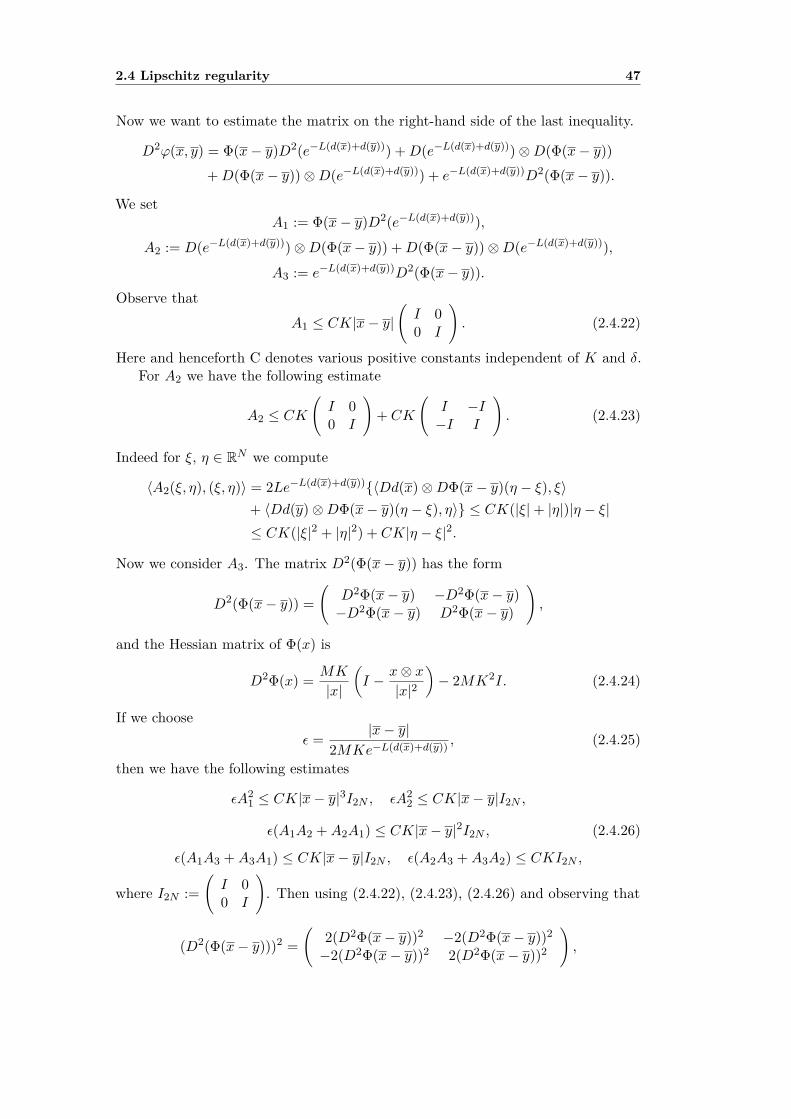
2.4 Lipschitz regularity 47
Now we want to estimate the matrix on the right-hand side of the last inequality.
D2ϕ(x, y) = Φ(x− y)D2(e−L(d(x)+d(y))) +D(e−L(d(x)+d(y)))⊗D(Φ(x− y))+D(Φ(x− y))⊗D(e−L(d(x)+d(y))) + e−L(d(x)+d(y))D2(Φ(x− y)).
We setA1 := Φ(x− y)D2(e−L(d(x)+d(y))),
A2 := D(e−L(d(x)+d(y)))⊗D(Φ(x− y)) +D(Φ(x− y))⊗D(e−L(d(x)+d(y))),A3 := e−L(d(x)+d(y))D2(Φ(x− y)).
Observe thatA1 ≤ CK|x− y|
(I 00 I
). (2.4.22)
Here and henceforth C denotes various positive constants independent of K and δ.For A2 we have the following estimate
A2 ≤ CK(I 00 I
)+ CK
(I −I−I I
). (2.4.23)
Indeed for ξ, η ∈ RN we compute
〈A2(ξ, η), (ξ, η)〉 = 2Le−L(d(x)+d(y))〈Dd(x)⊗DΦ(x− y)(η − ξ), ξ〉+ 〈Dd(y)⊗DΦ(x− y)(η − ξ), η〉 ≤ CK(|ξ|+ |η|)|η − ξ|≤ CK(|ξ|2 + |η|2) + CK|η − ξ|2.
Now we consider A3. The matrix D2(Φ(x− y)) has the form
D2(Φ(x− y)) =(
D2Φ(x− y) −D2Φ(x− y)−D2Φ(x− y) D2Φ(x− y)
),
and the Hessian matrix of Φ(x) is
D2Φ(x) = MK
|x|
(I − x⊗ x
|x|2)− 2MK2I. (2.4.24)
If we chooseε = |x− y|
2MKe−L(d(x)+d(y)) , (2.4.25)
then we have the following estimates
εA21 ≤ CK|x− y|3I2N , εA2
2 ≤ CK|x− y|I2N ,
ε(A1A2 +A2A1) ≤ CK|x− y|2I2N , (2.4.26)
ε(A1A3 +A3A1) ≤ CK|x− y|I2N , ε(A2A3 +A3A2) ≤ CKI2N ,
where I2N :=(I 00 I
). Then using (2.4.22), (2.4.23), (2.4.26) and observing that
(D2(Φ(x− y)))2 =(
2(D2Φ(x− y))2 −2(D2Φ(x− y))2
−2(D2Φ(x− y))2 2(D2Φ(x− y))2
),
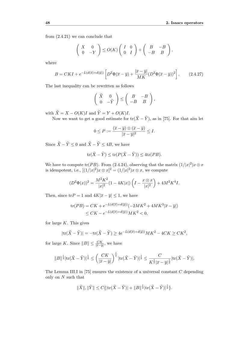
48 2. Isaacs operators
from (2.4.21) we can conclude that(X 00 −Y
)≤ O(K)
(I 00 I
)+(
B −B−B B
),
where
B = CKI + e−L(d(x)+d(y))[D2Φ(x− y) + |x− y|
MK(D2Φ(x− y))2
]. (2.4.27)
The last inequality can be rewritten as follows(X 00 −Y
)≤(
B −B−B B
),
with X = X −O(K)I and Y = Y +O(K)I.Now we want to get a good estimate for tr(X − Y ), as in [75]. For that aim let
0 ≤ P := (x− y)⊗ (x− y)|x− y|2
≤ I.
Since X − Y ≤ 0 and X − Y ≤ 4B, we have
tr(X − Y ) ≤ tr(P (X − Y )) ≤ 4tr(PB).
We have to compute tr(PB). From (2.4.24), observing that the matrix (1/|x|2)x⊗xis idempotent, i.e., [(1/|x|2)x⊗ x]2 = (1/|x|2)x⊗ x, we compute
(D2Φ(x))2 = M2K2
|x|2(1− 4K|x|)
(I − x⊗ x
|x|2)
+ 4M2K4I.
Then, since trP = 1 and 4K|x− y| ≤ 1, we have
tr(PB) = CK + e−L(d(x)+d(y))(−2MK2 + 4MK3|x− y|)≤ CK − e−L(d(x)+d(y))MK2 < 0,
for large K. This gives
|tr(X − Y )| = −tr(X − Y ) ≥ 4e−L(d(x)+d(y))MK2 − 4CK ≥ CK2,
for large K. Since ‖B‖ ≤ CK|x−y| , we have
‖B‖12 |tr(X − Y )|
12 ≤
(CK
|x− y|
) 12|tr(X − Y )|
12 ≤ C
K12 |x− y|
12|tr(X − Y )|.
The Lemma III.I in [75] ensures the existence of a universal constant C dependingonly on N such that
‖X‖, ‖Y ‖ ≤ C|tr(X − Y )|+ ‖B‖12 |tr(X − Y )|
12 .
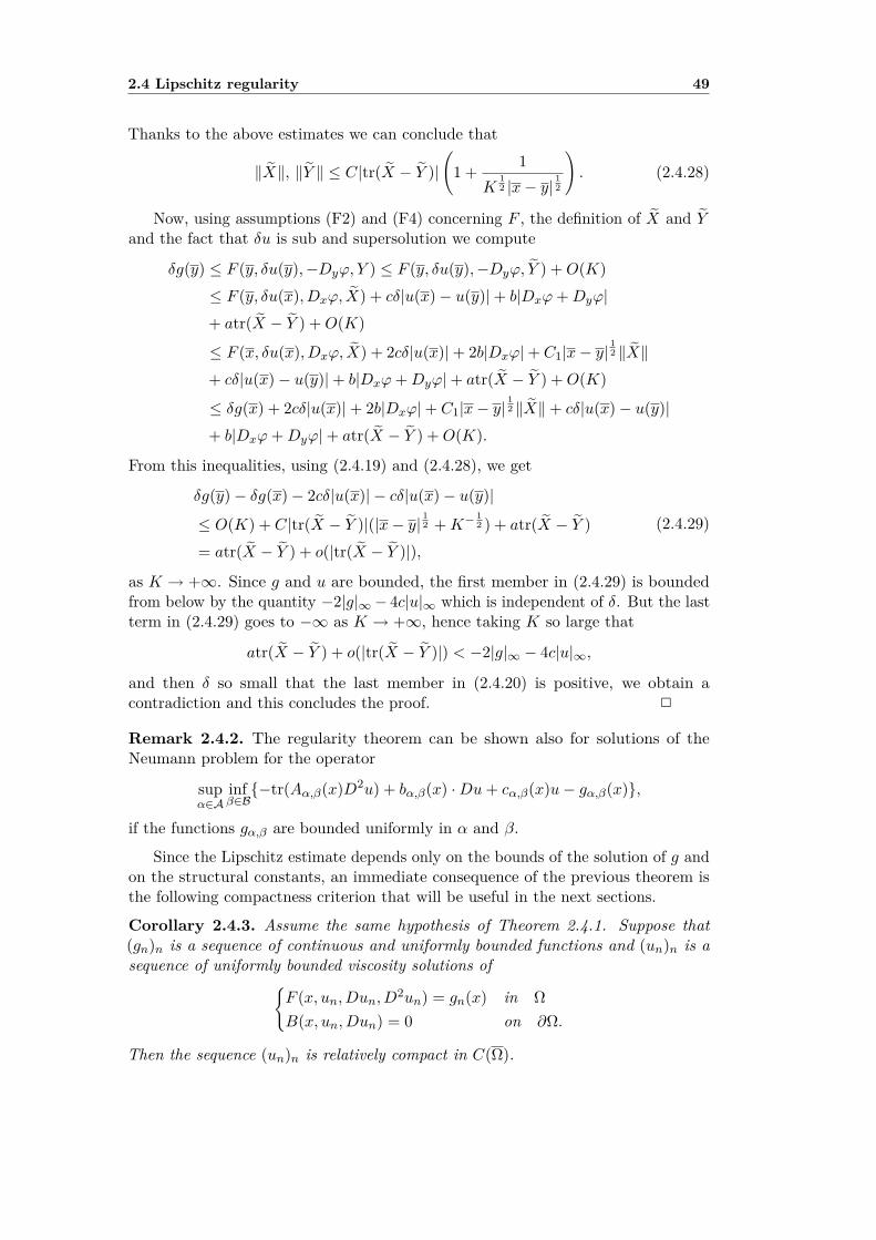
2.4 Lipschitz regularity 49
Thanks to the above estimates we can conclude that
‖X‖, ‖Y ‖ ≤ C|tr(X − Y )|(
1 + 1K
12 |x− y|
12
). (2.4.28)
Now, using assumptions (F2) and (F4) concerning F , the definition of X and Yand the fact that δu is sub and supersolution we compute
δg(y) ≤ F (y, δu(y),−Dyϕ, Y ) ≤ F (y, δu(y),−Dyϕ, Y ) +O(K)≤ F (y, δu(x), Dxϕ, X) + cδ|u(x)− u(y)|+ b|Dxϕ+Dyϕ|+ atr(X − Y ) +O(K)
≤ F (x, δu(x), Dxϕ, X) + 2cδ|u(x)|+ 2b|Dxϕ|+ C1|x− y|12 ‖X‖
+ cδ|u(x)− u(y)|+ b|Dxϕ+Dyϕ|+ atr(X − Y ) +O(K)
≤ δg(x) + 2cδ|u(x)|+ 2b|Dxϕ|+ C1|x− y|12 ‖X‖+ cδ|u(x)− u(y)|
+ b|Dxϕ+Dyϕ|+ atr(X − Y ) +O(K).
From this inequalities, using (2.4.19) and (2.4.28), we get
δg(y)− δg(x)− 2cδ|u(x)| − cδ|u(x)− u(y)|
≤ O(K) + C|tr(X − Y )|(|x− y|12 +K−
12 ) + atr(X − Y )
= atr(X − Y ) + o(|tr(X − Y )|),(2.4.29)
as K → +∞. Since g and u are bounded, the first member in (2.4.29) is boundedfrom below by the quantity −2|g|∞− 4c|u|∞ which is independent of δ. But the lastterm in (2.4.29) goes to −∞ as K → +∞, hence taking K so large that
atr(X − Y ) + o(|tr(X − Y )|) < −2|g|∞ − 4c|u|∞,
and then δ so small that the last member in (2.4.20) is positive, we obtain acontradiction and this concludes the proof. 2
Remark 2.4.2. The regularity theorem can be shown also for solutions of theNeumann problem for the operator
supα∈A
infβ∈B−tr(Aα,β(x)D2u) + bα,β(x) ·Du+ cα,β(x)u− gα,β(x),
if the functions gα,β are bounded uniformly in α and β.
Since the Lipschitz estimate depends only on the bounds of the solution of g andon the structural constants, an immediate consequence of the previous theorem isthe following compactness criterion that will be useful in the next sections.
Corollary 2.4.3. Assume the same hypothesis of Theorem 2.4.1. Suppose that(gn)n is a sequence of continuous and uniformly bounded functions and (un)n is asequence of uniformly bounded viscosity solutions of
F (x, un, Dun, D2un) = gn(x) in ΩB(x, un, Dun) = 0 on ∂Ω.
Then the sequence (un)n is relatively compact in C(Ω).
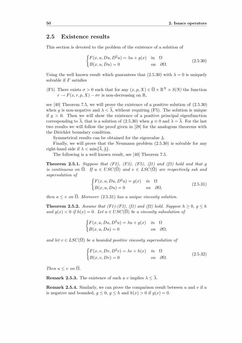
50 2. Isaacs operators
2.5 Existence results
This section is devoted to the problem of the existence of a solution ofF (x, u,Du,D2u) = λu+ g(x) in ΩB(x, u,Du) = 0 on ∂Ω.
(2.5.30)
Using the well known result which guarantees that (2.5.30) with λ = 0 is uniquelysolvable if F satisfies
(F5) There exists σ > 0 such that for any (x, p,X) ∈ Ω× RN × S(N) the functionr → F (x, r, p,X)− σr is non-decreasing on R,
see [40] Theorem 7.5, we will prove the existence of a positive solution of (2.5.30)when g is non-negative and λ < λ, without requiring (F5). The solution is uniqueif g > 0. Then we will show the existence of a positive principal eigenfunctioncorresponding to λ, that is a solution of (2.5.30) when g ≡ 0 and λ = λ. For the lasttwo results we will follow the proof given in [28] for the analogous theorems withthe Dirichlet boundary condition.
Symmetrical results can be obtained for the eigenvalue λ.Finally, we will prove that the Neumann problem (2.5.30) is solvable for any
right-hand side if λ < minλ, λ.The following is a well known result, see [40] Theorem 7.5.
Theorem 2.5.1. Suppose that (F2), (F3), (F5), (f1) and (f3) hold and that gis continuous on Ω. If u ∈ USC(Ω) and v ∈ LSC(Ω) are respectively sub andsupersolution of
F (x, u,Du,D2u) = g(x) in ΩB(x, u,Du) = 0 on ∂Ω,
(2.5.31)
then u ≤ v on Ω. Moreover (2.5.31) has a unique viscosity solution.
Theorem 2.5.2. Assume that (F1)-(F3), (f1) and (f2) hold. Suppose h ≥ 0, g ≤ hand g(x) < 0 if h(x) = 0. Let u ∈ USC(Ω) be a viscosity subsolution of
F (x, u,Du,D2u) = λu+ g(x) in ΩB(x, u,Du) = 0 on ∂Ω,
and let v ∈ LSC(Ω) be a bounded positive viscosity supersolution ofF (x, v,Dv,D2v) = λv + h(x) in ΩB(x, v,Dv) = 0 on ∂Ω.
(2.5.32)
Then u ≤ v on Ω.
Remark 2.5.3. The existence of such a v implies λ ≤ λ.
Remark 2.5.4. Similarly, we can prove the comparison result between u and v if uis negative and bounded, g ≤ 0, g ≤ h and h(x) > 0 if g(x) = 0.
2.5 Existence results 51
Proof. Suppose by contradiction that maxΩ(u − v) = u(x) − v(x) > 0 for somex ∈ Ω. Set wt = u− tv. If t is large enough wt < 0 on Ω. We define
τ = inft |wt < 0 on Ω.
As in the proof of Theorem 2.3.4, wτ ≤ 0 and vanishes in some point, i.e., u ≤ τvand u(x) = τv(x) for some x ∈ Ω. Moreover, since u(x) > v(x) we know that τ > 1,which implies that h ≤ τh, being h non-negative. Then τv is still a supersolution of(2.5.32) and u ≡ τv by Theorem 2.2.1. Hence, applying Lemma 7.3 of [76] we get
τh ≤ g,
which contradicts the assumptions on g and h. 2
Theorem 2.5.5. Suppose that (F1)-(F4), (f1)-(f3) hold, that λ < λ, g ≥ 0, g 6≡ 0and g is continuous on Ω, then there exists a positive viscosity solution of (2.5.30).The positive solution is unique if g > 0.
Proof. The condition (F2) implies that r → F (x, r, p,X) + cr is non-decreasing.Hence the operator F +(2c+ |λ|)I satisfies (F5) with σ = c+ |λ|, so that by Theorem2.5.1 the sequence (un)n defined by u1 = 0 and un+1 as the solution of
F (x, un+1, Dun+1, D2un+1) + (2c+ |λ|)un+1 = g + (2c+ |λ|+ λ)un in Ω
B(x, un+1, Dun+1) = 0 on ∂Ω,
is well defined. By the comparison Theorems 2.5.1 and 2.2.1, since g ≥ 0 and g 6≡ 0the sequence is positive and increasing.
We use the argument of Theorem 7 of [28] to prove that (un)n is also bounded.Suppose that it is not, then dividing by |un+1|∞ and defining vn := un
|un|∞ one getsthat vn+1 is a solution of
F (x, vn+1, Dvn+1, D2vn+1) + (2c+ |λ|)vn+1
= g|un+1|∞ + (2c+ |λ|+ λ) un
|un+1|∞ in ΩB(x, vn+1, Dvn+1) = 0 on ∂Ω.
By Corollary 2.4.3, (vn)n converges along a subsequence to a positive function vwhich satisfies
F (x, v,Dv,D2v)− λv = (2c+ |λ|+ λ)(k − 1)v ≤ 0 in ΩB(x, v,Dv) = 0 on ∂Ω,
where k := lim supn→+∞|un|∞|un+1|∞ ≤ 1. This contradicts the maximum principle, Theo-
rem 2.3.5. Then (un)n is bounded and letting n go to infinity, by the compactnessresult, the sequence converges uniformly to a function u which is a solution. Moreoverthe solution is positive on Ω by Corollary 2.2.4.
The uniqueness of the positive solution follows from Theorem 2.5.2. 2
52 2. Isaacs operators
Theorem 2.5.6 (Existence of principal eigenfunctions). Suppose that (F1)-(F4),(f1)-(f3) hold. Then there exists φ > 0 on Ω viscosity solution of
F (x, φ,Dφ,D2φ) = λφ in ΩB(x, φ,Dφ) = 0 on ∂Ω.
(2.5.33)
Moreover φ is Lipschitz continuous on Ω.
Proof. Let λn be an increasing sequence which converges to λ. Let un be a positivesolution of
F (x, un, Dun, D2un) = λnun + 1 in ΩB(x, un, Dun) = 0 on ∂Ω.
By Theorem 2.5.5 the sequence (un)n is well defined. Following the argument of theproof of Theorem 8 of [28] we can prove that it is unbounded, otherwise one wouldcontradict the definition of λ. Then, up to subsequence, |un|∞ → +∞ as n→ +∞and defining vn := un
|un|∞ one gets that vn satisfies
F (x, vn, Dvn, D2vn) = λnvn + 1|un|∞ in Ω
B(x, vn, Dvn) = 0 on ∂Ω.
Then, by Corollary 2.4.3, we can extract a subsequence converging to a function φwith |φ|∞ = 1 which is positive on Ω by Corollary 2.2.4 and is the desired solution.By Theorem 2.4.1 the solution is also Lipschitz continuous on Ω. 2
Remark 2.5.7. With the same arguments used in the proofs of Theorems 2.5.5and 2.5.6 one can prove: the existence of a negative viscosity solution of (2.5.30),for λ < λ and g ≤ 0, g 6≡ 0, which is unique if g < 0 by Remark 2.5.4; the existenceof a negative Lipschitz principal eigenfunction corresponding to λ, i.e., a solution of
F (x, φ,Dφ,D2φ) = λφ in ΩB(x, φ,Dφ) = 0 on ∂Ω.
(2.5.34)
Theorem 2.5.8. Suppose that (F1)-(F4), (f1)-(f3) hold. Suppose that λ < minλ, λand g is continuous on Ω, then there exists a viscosity solution of (2.5.30).
Proof. If g ≡ 0, by the maximum and minimum principles the only solution isu ≡ 0. Let us suppose g 6≡ 0. Since λ < minλ, λ by Theorem 2.5.5 and Remark2.5.7 there exist v0 ∈ C(Ω) positive viscosity solution of (2.5.30) with right-handside |g|∞ and u0 ∈ C(Ω) negative viscosity solution of (2.5.30) with right-hand side−|g|∞.
Let (un)n be the sequence defined in the proof of Theorem 2.5.5 with u1 = u0.By comparison Theorem 2.5.1 we have u0 = u1 ≤ u2 ≤ ... ≤ v0. Hence, by thecompactness Corollary 2.4.3 the sequence converges to a continuous function whichis the desired solution. 2
2.6 Properties of the principal eigenvalues 53
Remark 2.5.9. The existence results can be shown also for the operator
supα∈A
infβ∈B−tr(Aα,β(x)D2u) + bα,β(x) ·Du+ cα,β(x)u− gα,β(x),
if the functions gα,β are continuous uniformly in α and β. In particular, in that case,if λ and λ are positive there exists a viscosity solution of
supα∈A infβ∈B−tr(Aα,β(x)D2u) + bα,β(x) ·Du+ cα,β(x)u− gα,β(x) = 0 in ΩB(x, u,Du) = 0 on ∂Ω.
2.6 Properties of the principal eigenvaluesIn this section we establish some of the basic properties of the principal eigenvalues.We denote by φ+ a positive eigenfunction corresponding to λ and by φ− a negativeeigenfunction corresponding to λ. Throughout this section we assume (F1)-(F4) and(f1)-(f3).
The next result states that the principal eigenfunctions are simple, in the sensethat they are equal up to a multiplicative constant.
Proposition 2.6.1. If u ∈ USC(Ω) is a viscosity subsolution ofF (x, u,Du,D2u) = λu in ΩB(x, u,Du) = 0 on ∂Ω,
(2.6.35)
and u(x0) > 0 for some x0 ∈ Ω then there exists t > 0 such that u ≡ tφ+. Ifu ∈ LSC(Ω) is a viscosity supersolution of (2.6.35) with λ replaced by λ andu(x0) < 0, then there exists t > 0 such that u ≡ tφ−.
Assume in addition
− F (x,−r,−p,−X) ≤ F (x, r, p,X) for any (x, r, p,X) ∈ Ω× R× RN × S(N)(2.6.36)
and− f(x,−r) ≤ f(x, r) for any (x, r) ∈ ∂Ω× R. (2.6.37)
If u ∈ C(Ω), u 6≡ 0, is a viscosity subsolution of (2.6.35) then there exists t ∈ Rsuch that u ≡ tφ+. If u ∈ C(Ω), u 6≡ 0 is a viscosity solution of (2.6.35) with λreplaced by λ, there exists t ∈ R such that u ≡ tφ−.
Proof. If u is a subsolution (resp., supersolution) of (2.6.35) (resp., of (2.6.35) withλ instead of λ) and u(x0) > 0 (resp., u(x0) < 0), then by Theorem 2.3.4 we haveu ≡ tφ+ (resp., u ≡ tφ−) for some t > 0.
Now assume (2.6.36)-(2.6.37) and let u 6≡ 0 be a subsolution of (2.6.35). If uis positive somewhere we are in the previous case. If u is negative on Ω then thefunction w := −u is a positive continuous supersolution of
F (x,w,Dw,D2w)− λw ≥ −F (x,−w,−Dw,−D2w) + λ(−w) ≥ 0 in ΩB(x,w,Dw) ≥ −B(x,−w,−Dw) ≥ 0 on ∂Ω.
Hence, again from Theorem 2.3.4 it follows that u ≡ tφ+, for some t < 0.
54 2. Isaacs operators
Finally, let u 6≡ 0 be a solution of (2.6.35) with λ instead of λ. Remark thatconditions (2.6.36)-(2.6.37) imply λ ≤ λ. If λ < λ, then by the maximum principle,Theorem 2.3.5, u < 0 on Ω and we are in the first case. If λ = λ, by the simplicityof λ just proved, u ≡ tφ− for some t < 0. 2
Remark 2.6.2. If F and f satisfy
−F (x,−r,−p,−X) ≥ F (x, r, p,X) for any (x, r, p,X) ∈ Ω× R× RN × S(N)
and−f(x,−r) ≥ f(x, r) for any (x, r) ∈ ∂Ω× R,
then, applying Proposition 2.6.1 to the operator G(x, r, p,X) = −F (x,−r,−p,−X)with B(x, r, p) = f(x, r) + 〈p,−→n (x)〉, where f(x, r) = −f(x,−r), we get againsimplicity of principal eigenvalues.
Remark 2.6.3. Convex and 1-homogeneous operators satisfy the assumption(2.6.36).
Proposition 2.6.4. λ (resp., λ) is the only eigenvalue corresponding to a positive(resp., negative) eigenfunction.
Proof. Let u be a positive eigenfunction corresponding to µ. By the definition ofλ, we have µ ≤ λ. If µ < λ, we must have u ≤ 0 by Theorem 2.3.5, which is acontradiction. Thus µ = λ. 2
The following proposition states that the principal eigenvalues are isolated.
Proposition 2.6.5. There exists ε > 0 such that the problemF (x, u,Du,D2u) = λu in ΩB(x, u,Du) = 0 on ∂Ω,
(2.6.38)
has no solutions u 6≡ 0, for λ ∈ (−∞,maxλ, λ+ ε) \ λ, λ.
Proof. We may suppose without loss of generality that λ ≤ λ. If λ < λ ≤ λ then itfollows from the maximum and minimum principles that u ≡ 0 is the only solutionof (2.6.38).
If λ < λ and u 6≡ 0 is a solution of (2.6.38), by the minimum principle we haveu > 0 on Ω. Then Proposition 2.6.4 implies λ = λ.
Finally suppose that there exists a sequence λn ↓ λ such that the problem(2.6.38) with λ = λn has a solution φn 6≡ 0. We can assume that |φn|∞ = 1 for anyn. Then by the compactness criterion, Corollary 2.4.3, the sequence (φn)n convergesuniformly on Ω to a function φ 6≡ 0 which is a solution of (2.6.38) with λ = λ. ByProposition 2.6.4 the functions φn change sign in Ω while by Proposition 2.6.1 andTheorem 2.2.1 either φ > 0 or φ < 0 on Ω. This contradicts the uniform convergenceof (φn)n to φ. 2
We want to conclude this section with the following comparison, suggested byHitoshi Ishii [74], between λ = λN and λD respectively the principal eigenvaluescorresponding to the Neumann and the Dirichlet problems.
2.7 The Pucci’s operators 55
Proposition 2.6.6. λN < λD.
Proof. Let v and w be respectively the eigenfunctions corresponding to λN and λD.That is
F (x, v,Dv,D2v) = λNv in Ω, B(x, v,Dv) = 0 on ∂Ω, v > 0 on Ω,
F (x,w,Dw,D2w) = λDw in Ω, w = 0 on ∂Ω, w > 0 in Ω.Since f(x, 0) = 0, we see that w satisfies
F (x,w,Dw,D2w) = λDw in Ω, B(x,w,Dw) ≤ 0 on ∂Ω.
Let us suppose λN ≥ λD. Then
F (x,w,Dw,D2w) ≤ λNw in Ω, B(x,w,Dw) ≤ 0 on ∂Ω.
Replacing w by its constant multiple tw with t > 0, we may assume that w ≤ v onΩ and w(x0) = v(x0) for some x0 ∈ Ω. Note that w(x) = 0 < v(x) for all x ∈ ∂Ω.By Theorem 2.2.2 we must have w ≡ v or w < v on Ω. This is a contradiction.
2
2.7 The Pucci’s operatorsIn this section we want to show that the two principal eigenvalues of the followingoperator
F (x, u,Du,D2u) = −M+a,A(D2u) + b(x) ·Du+ c(x)u,
with the pure Neumann boundary condition may be different. Suppose b ∈ C0,1(Ω),c ∈ C0,β(Ω) for some β > 0 and Ω of class C2,β.
If c(x) ≡ c0 is constant then it is easy to see that λ = λ = c0 and by Proposition2.6.1 the only eigenfunctions are the constants. Nevertheless, if c(x) is not constantthe two principal eigenvalues never coincide, unlessM+
a,A is the Laplacian. To provethis we need the following lemma, whose proof is given for the sake of completness.
Lemma 2.7.1. Suppose that Ω is a C2,β domain, b ∈ C0,β(Ω) and c ∈ C0,β(Ω), forsome 0 < β ≤ 1. Then the viscosity solutions of
−∆u+ b(x) ·Du+ c(x)u = 0 in Ω〈Du,−→n (x)〉 = 0 on ∂Ω,
(2.7.39)
are in C2(Ω).
Proof. Consider the problem−∆v + b(x) ·Dv + v = f(x) in Ω〈Dv,−→n (x)〉 = 0 on ∂Ω,
(2.7.40)
where f(x) = (1 − c(x))u(x). By Theorem 2.4.1, u is Lipschitz continuous on Ωand then the function f is Hölder continuous on Ω. Moreover, it is clear that u is asolution of (2.7.40). The classical theory says that (2.7.40) has a solution v ∈ C2(Ω).By uniqueness of viscosity solutions of (2.7.40), we find that u = v. 2
56 2. Isaacs operators
Proposition 2.7.2. Assume the hypothesis of Lemma 2.7.1 and let b ∈ C0,1(Ω). IfA 6= a and λ = λ then c(x) is constant.
Proof. Let φ be a positive eigenfunction of λ, i.e.−M+
a,A(D2φ) + b(x) ·Dφ+ (c(x)− λ)φ = 0 in Ω〈Dφ,−→n (x)〉 = 0 on ∂Ω,
(2.7.41)
and let −ψ be a negative eigenfunction corresponding to λ. SinceM+a,A(−D2ψ) =
−M−a,A(D2ψ), ψ satisfies−M−a,A(D2ψ) + b(x) ·Dψ + (c(x)− λ)ψ = 0 in Ω〈Dψ,−→n (x)〉 = 0 on ∂Ω.
(2.7.42)
If λ = λ then by Proposition 2.6.1 ψ = tφ for some t > 0. We can assume ψ = φ. Bysumming the first equations in (2.7.41) and (2.7.42), we can see that φ is a positiveviscosity solution of
−(A+ a)∆φ+ 2b(x) ·Dφ+ 2(c(x)− λ)φ = 0 in Ω〈Dφ,−→n (x)〉 = 0 on ∂Ω.
Then by Lemma 2.7.1, φ ∈ C2(Ω). Subtracting the first equations in (2.7.41) and(2.7.42), we can see that φ is a classical solution of
(A− a)N∑i=1|ei(x)| = 0 in Ω,
where e1(x), ..., eN (x) are the eigenvalues of D2φ(x). Since A 6= a, the last equationimplies that ei(x) = 0 in Ω for any i = 1...N . In particular, taking into considerationthe boundary condition, φ is a classical solution of
∆φ = 0 in Ω〈Dφ,−→n (x)〉 = 0 on ∂Ω,
and then has to be constant. This implies
c(x)− λ = 0 in Ω,
i.e., c ≡ λ is constant. 2
Chapter 3
The infinity-Laplacian
In this chapter we study the maximum principle, the principal eigenvalue, regularity,existence and uniqueness for viscosity solutions of the Neumann boundary valueproblem
∆∞u+ b(x) ·Du+ (c(x) + λ)u = g(x) in Ω∂u∂−→n = 0 on ∂Ω,
(3.0.1)
where Ω is a bounded smooth domain, −→n (x) is the exterior normal to the domain Ωat x, b, c and g are continuous functions on Ω, λ ∈ R and
∆∞u = 〈D2uDu
|Du|,Du
|Du|〉, (3.0.2)
for u ∈ C2(Ω), is the 1-homogeneous version of the ∞-Laplacian.We define and investigate the properties of the principal eigenvalue of the operator
−(∆∞ + b(x) ·D + c(x)),
with the Neumann boundary condition and as an application, we get existence anduniqueness results for (3.0.1) and a decay estimate for the solution of the associatedevolution problem.
Following the ideas of [26], we define the principal eigenvalue as
λ := supλ ∈ R | ∃ v > 0 on Ω bounded viscosity supersolution of
∆∞v + b(x) ·Dv + (c(x) + λ)v = 0 in Ω, ∂v∂−→n
= 0 on ∂Ω.(3.0.3)
The quantity λ is well defined since the above set is not empty; indeed, −|c|∞belongs to it, being v(x) ≡ 1 a corresponding supersolution. Furthermore it is aninterval because if λ belongs to it then so does any λ′ < λ.
We will prove that λ is an "eigenvalue" for −(∆∞ + b(x) · D + c(x)) whichadmits a positive "eigenfunction". As in the linear case it can be characterized asthe supremum of those λ for which ∆∞ + b(x) ·D + c(x) + λ with the Neumannboundary condition satisfies the maximum principle. As a consequence, λ is the
57
58 3. The infinity-Laplacian
least "eigenvalue", i.e., the least number λ for which there exists a non-zero solutionof
∆∞u+ b(x) ·Du+ (c(x) + λ)u = 0 in Ω∂u∂−→n = 0 on ∂Ω.
These results are applied to obtain existence and uniqueness for the boundary valueproblem (3.0.1).
Remark that since ∆∞(−u) = −∆∞u, λ can be defined also in the following way
λ = supλ ∈ R | ∃u < 0 on Ω bounded viscosity subsolution of
∆∞u+ b(x) ·Du+ (c(x) + λ)u = 0 in Ω, ∂u∂−→n
= 0 on ∂Ω.(3.0.4)
For a fully nonlinear operator, λ defined as in (3.0.3) may be different from thequantity defined as in (3.0.4), see Chapter 2.
In the next section we give assumptions. In Section 3.2 we establish a Lipschitzregularity result for viscosity solutions of (3.0.1). Section 3.3 is devoted to themaximum principle for subsolutions of (3.0.1). In Section 3.3.1 we show that it holds(even for more general boundary conditions) for ∆∞ + b(x) ·D + c(x) if c(x) ≤ 0and c 6≡ 0, see Theorem 3.3.4. One of the main result of this chapter is that themaximum principle holds for ∆∞ + b(x) ·D + c(x) + λ for any λ < λ, as we showin Theorem 3.3.8 of Section 3.3.2. In particular it holds for ∆∞ + b(x) ·D + c(x)if λ > 0. Following the example given in [97] we show that the result of Theorem3.3.8 is stronger than that of Theorem 3.3.4, i.e., that there exist some functionsc(x) changing sign in Ω for which the principal eigenvalue of ∆∞ + b(x) ·D+ c(x) ispositive and then for which the maximum principle holds.
In Section 3.4 we show some existence and comparison theorems. In particular,we prove that the Neumann problem (3.0.1) is solvable for any right-hand side ifλ < λ.
Finally, in Section 3.5 we prove a decay estimate for solutions of the Neumannevolution problem.
3.1 Assumptions and definitionsLet σ : RN → S(N) be the function defined by
σ(p) := p⊗ p|p|2
.
The ∞-Laplacian can be written as
∆∞u = tr(σ(Du)D2u),
for any u ∈ C2(Ω).It easy to check that σ has the following properties:
• σ(p) is homogeneous of order 0, i.e., for any α ∈ R and p ∈ RN
σ(αp) = σ(p);
3.1 Assumptions and definitions 59
• For all p ∈ RN
0 ≤ σ(p) ≤ I,
where I is the identity matrix in RN ;
• σ(p) is idempotent, i.e.,(σ(p))2 = σ(p);
• For any p ∈ RN \ 0 and p0 ∈ Rn with |p0| ≤ |p|2
tr[(σ(p+ p0)− σ(p))2
]≤ 8 |p0|2
|p|2. (3.1.5)
The domain Ω is supposed to be bounded and of class C2. In particular, itsatisfies the interior sphere condition and the uniform exterior sphere condition, i.e.
(Ω1) For each x ∈ ∂Ω there exist R > 0 and y ∈ Ω for which |x − y| = R andB(y,R) ⊂ Ω.
(Ω2) There exists r > 0 such that B(x+ r−→n (x), r) ∩ Ω = ∅ for any x ∈ ∂Ω.
From the property (Ω2) it follows that
〈y − x,−→n (x)〉 ≤ 12r |y − x|
2 for x ∈ ∂Ω and y ∈ Ω. (3.1.6)
Moreover, the C2-regularity of Ω implies the existence of a neighborhood of ∂Ω in Ωon which the distance from the boundary
d(x) := inf|x− y|, y ∈ ∂Ω, x ∈ Ω
is of class C2. We still denote by d a C2 extension of the distance function to thewhole Ω. Without loss of generality we can assume that |Dd(x)| ≤ 1 on Ω.
For (3.0.1) we adopt the notion of viscosity solution Definition I.2.2 given in theIntroduction.
It is possible to define sub and supersolutions of the ∞-Laplace equation alsousing the semicontinous extensions of the function (p,X)→ tr(σ(p)X) as done in[80] and [81]. In Definition I.2.2 it is remarkable that nothing is required in the caseDϕ(x0) = 0 if u is not constant.
We call strong viscosity subsolutions (resp., supersolutions) the viscosity subsolu-tions (resp., supersolutions) that satisfy B(x, u,Du) ≤ (resp., ≥) 0 in the viscositysense for all x ∈ ∂Ω. If λ → B(x, r, p − λ−→n ) is non-increasing in λ ≥ 0, thenclassical subsolutions (resp., supersolutions) are strong viscosity subsolutions (resp.,supersolutions), see [40] Proposition 7.2.
In the definitions the test functions can be substituted by the elements of thesemijets J2,+
u(x0) when u is a subsolution and J2,−u(x0) when u is a supersolution,
see [40].
60 3. The infinity-Laplacian
3.2 Lipschitz continuity of viscosity solutionsIt is known that the ∞-harmonic functions, i.e., the solution of ∆∞u = 0 are locallyLipschitz continuous, see e.g. [11]. We now show the Lipschitz regularity in thewhole Ω of the solutions of the Neumann problem associated to the ∞-Laplacianplus lower order terms.
Theorem 3.2.1. Assume that Ω is a bounded domain of class C2 and that b, c, gare bounded in Ω. If u ∈ C(Ω) is a viscosity solution of
∆∞u+ b(x) ·Du+ c(x)u = g(x) in Ω∂u∂−→n = 0 on ∂Ω,
then|u(x)− u(y)| ≤ C0|x− y| ∀x, y ∈ Ω,
where C0 depends on Ω, N, |b|∞, |c|∞, |g|∞, and |u|∞.
The Theorem is an immediate consequence of the next lemma, the proof of which,though following the line of Proposition III.1 of [75], introduces new test functionsthat, in particular, depend on the distance function d(x).
The lemma will be used also in the proof of Theorem 3.3.8 in the next section.
Lemma 3.2.2. Assume the hypothesis of Theorem 3.2.1 and suppose that g and hare bounded functions. Let u ∈ USC(Ω) be a viscosity subsolution of
∆∞u+ b(x) ·Du+ c(x)u = g(x) in Ω∂u∂−→n = 0 on ∂Ω,
and v ∈ LSC(Ω) a viscosity supersolution of∆∞v + b(x) ·Dv + c(x)v = h(x) in Ω∂v∂−→n = 0 on ∂Ω,
with u and v bounded, or v ≥ 0 and bounded. If m = maxΩ(u− v) ≥ 0, then thereexists C0 > 0 such that
u(x)− v(y) ≤ m+ C0|x− y| ∀x, y ∈ Ω, (3.2.7)
where C0 depends on Ω, N, |b|∞, |c|∞, |g|∞, |h|∞, |v|∞, m and |u|∞ or supΩ u.
Proof. We setΦ(x) = MK|x| −M(K|x|)2,
andϕ(x, y) = m+ e−L(d(x)+d(y))Φ(x− y),
where L is a fixed number greater than 2/(3r) with r the radius in the condition(Ω2) and where K and M are two positive constants to be chosen later. If K|x| ≤ 1
4 ,then
Φ(x) ≥ 34MK|x|. (3.2.8)
3.2 Lipschitz continuity of viscosity solutions 61
We define∆K :=
(x, y) ∈ RN × RN | |x− y| ≤ 1
4K
.
We fix M such that
maxΩ 2
(u(x)− v(y)) ≤ m+ e−2Ld0M
8 , (3.2.9)
where d0 = maxx∈Ω d(x). To prove (3.2.7) it is enough to show that taking K largeenough, one has
u(x)− v(y)− ϕ(x, y) ≤ 0 for (x, y) ∈ ∆K ∩ Ω2.
Suppose by contradiction that for each K there is some point (x, y) ∈ ∆K ∩Ω2 suchthat
u(x)− v(y)− ϕ(x, y) = max∆K∩Ω 2
(u(x)− v(y)− ϕ(x, y)) > 0.
Here we have dropped the dependence of x, y on K for simplicity of notations.Observe that if v ≥ 0, since from (3.2.8) Φ(x − y) is non-negative in ∆K and
m ≥ 0, one has u(x) > 0.Clearly x 6= y. Moreover the point (x, y) belongs to int(∆K) ∩ Ω2. Indeed, if
|x− y| = 14K , by (3.2.9) and (3.2.8) we have
u(x)− v(y) ≤ m+ e−2Ld0M
8 ≤ m+ e−L(d(x)+d(y)) 12MK|x− y| ≤ ϕ(x, y).
Since x 6= y we can compute the derivatives of ϕ at (x, y) obtaining
Dxϕ(x, y) = e−L(d(x)+d(y))MK− L|x− y|(1−K|x− y|)Dd(x)
+ (1− 2K|x− y|)(x− y)|x− y|
,
Dyϕ(x, y) = e−L(d(x)+d(y))MK− L|x− y|(1−K|x− y|)Dd(y)
− (1− 2K|x− y|)(x− y)|x− y|
.
Observe that for large K
0 < e−L(d(x)+d(y))MK
(12 − L|x− y|
)≤ |Dxϕ(x, y)|, |Dyϕ(x, y)| ≤ 2MK.
(3.2.10)Using (3.1.6), if x ∈ ∂Ω we have
〈Dxϕ(x, y),−→n (x)〉
= e−Ld(y)MKL|x− y|(1−K|x− y|) + (1− 2K|x− y|)〈(x− y)
|x− y|,−→n (x)〉
≥ e−Ld(y)MK
34L|x− y| − (1− 2K|x− y|) |x− y|2r
≥ 1
2e−Ld(y)MK|x− y|
(32L−
1r
)> 0,
62 3. The infinity-Laplacian
since x 6= y and L > 2/(3r). Similarly, if y ∈ ∂Ω
〈−Dyϕ(x, y),−→n (y)〉 ≤ 12e−Ld(x)MK|x− y|
(−3
2L+ 1r
)< 0.
In view of definition of sub and supersolution, we conclude that
tr(σ(Dxϕ(x, y))X)+b(x)·Dxϕ(x, y)+c(x)u(x) ≥ g(x) if (Dxϕ(x, y), X) ∈ J2,+u(x),
tr(σ(Dyϕ(x, y))Y )−b(y)·Dyϕ(x, y)+c(y)v(y) ≤ h(y) if (−Dyϕ(x, y), Y ) ∈ J2,−v(y).
Then the previous inequalities holds for any maximum point (x, y) ∈ ∆K ∩ Ω 2,provided K is large enough.
Since (x, y) ∈ int∆K ∩Ω 2, it is a local maximum of u(x)− v(y)− ϕ(x, y) in Ω 2.Applying Theorem 3.2 in [40], for every ε > 0 there exist X,Y ∈ S(N) such that(Dxϕ(x, y), X) ∈ J 2,+u(x), (−Dyϕ(x, y), Y ) ∈ J 2,−v(y) and(
X 00 −Y
)≤ D2(ϕ(x, y)) + ε(D2(ϕ(x, y)))2. (3.2.11)
Now we want to estimate the matrix on the right-hand side of the last inequality.
D2ϕ(x, y) = Φ(x− y)D2(e−L(d(x)+d(y))) +D(e−L(d(x)+d(y)))⊗D(Φ(x− y))+D(Φ(x− y))⊗D(e−L(d(x)+d(y))) + e−L(d(x)+d(y))D2(Φ(x− y)).
We setA1 := Φ(x− y)D2(e−L(d(x)+d(y))),
A2 := D(e−L(d(x)+d(y)))⊗D(Φ(x− y)) +D(Φ(x− y))⊗D(e−L(d(x)+d(y))),
A3 := e−L(d(x)+d(y))D2(Φ(x− y)).
Observe thatA1 ≤ CK|x− y|
(I 00 I
). (3.2.12)
Here and henceforth C denotes various positive constants independent of K.For A2 we have the following estimate
A2 ≤ CK(I 00 I
)+ CK
(I −I−I I
). (3.2.13)
Indeed for ξ, η ∈ RN we compute
〈A2(ξ, η), (ξ, η)〉 = 2Le−L(d(x)+d(y))〈Dd(x)⊗DΦ(x− y)(η − ξ), ξ〉+ 〈Dd(y)⊗DΦ(x− y)(η − ξ), η〉 ≤ CK(|ξ|+ |η|)|η − ξ|≤ CK(|ξ|2 + |η|2) + CK|η − ξ|2.
Now we consider A3. The matrix D2(Φ(x− y)) has the form
D2(Φ(x− y)) =(
D2Φ(x− y) −D2Φ(x− y)−D2Φ(x− y) D2Φ(x− y)
),
3.2 Lipschitz continuity of viscosity solutions 63
and the Hessian matrix of Φ(x) is
D2Φ(x) = MK
|x|
(I − x⊗ x
|x|2)− 2MK2I. (3.2.14)
If we chooseε = |x− y|
2MKe−L(d(x)+d(y)) , (3.2.15)
then we have the following estimates
εA21 ≤ CK|x− y|3I2N , εA2
2 ≤ CK|x− y|I2N ,
ε(A1A2 +A2A1) ≤ CK|x− y|2I2N , (3.2.16)
ε(A1A3 +A3A1) ≤ CK|x− y|I2N , ε(A2A3 +A3A2) ≤ CKI2N ,
where I2N :=(I 00 I
). Then using (??), (3.2.13), (3.2.16) and observing that
(D2(Φ(x− y)))2 =(
2(D2Φ(x− y))2 −2(D2Φ(x− y))2
−2(D2Φ(x− y))2 2(D2Φ(x− y))2
),
from (??) we conclude that(X 00 −Y
)≤ O(K)
(I 00 I
)+(
B −B−B B
),
where
B = CKI + e−L(d(x)+d(y))[D2Φ(x− y) + |x− y|
MK(D2Φ(x− y))2
].
The last inequality can be rewritten as follows(X 00 −Y
)≤(
B −B−B B
),
with X = X − O(K)I and Y = Y + O(K)I. Multiplying on the left the previousinequality by the non-negative symmetric matrix(
σ(Dxϕ(x, y)) 00 σ(Dyϕ(x, y))
),
and taking traces we get
tr(σ(Dxϕ(x, y))X)− tr(σ(Dyϕ(x, y))Y ) ≤ tr(σ(Dxϕ(x, y))B) + tr(σ(Dyϕ(x, y))B).(3.2.17)
We want to get a good estimate for the matrix on the right-hand side above. Forthat aim let
0 ≤ P := (x− y)⊗ (x− y)|x− y|2
≤ I,
64 3. The infinity-Laplacian
and let us compute tr(PB). From (3.2.14), since the matrix (1/|x|2)x⊗ x is idem-potent, we get
(D2Φ(x))2 = M2K2
|x|2(1− 4K|x|)
(I − x⊗ x
|x|2)
+ 4M2K4I.
Then, using that trP = 1 and 4K|x− y| ≤ 1, we have
tr(PB) = CK + e−L(d(x)+d(y))(−2MK2 + 4MK3|x− y|)≤ CK − e−L(d(x)+d(y))MK2 ≤ −CK2,
for large K. The vector Dxϕ(x, y) can be written in the following way
Dxϕ(x, y) = e−L(d(x)+d(y))MK(v1 + v2),
where
v1 = −L|x− y|(1−K|x− y|)Dd(x), v2 = (1− 2K|x− y|)(x− y)|x− y|
,
and soσ(Dxϕ(x, y)) = v1 ⊗ v1
|v1 + v2|2+ v1 ⊗ v2 + v2 ⊗ v1
|v1 + v2|2+ v2 ⊗ v2|v1 + v2|2
.
Since K|x− y| ≤ 14 , for large K we have
14 = 1
2 −14 ≤ |v2| − |v1| ≤ |v1 + v2| ≤ |v1|+ |v2| ≤ 2,
and‖B‖ ≤ CK
|x− y|.
Then ∣∣∣∣tr( v1 ⊗ v1|v1 + v2|2
B
)∣∣∣∣ ≤ C|x− y|2‖B‖ ≤ CK|x− y|,∣∣∣∣tr(v1 ⊗ v2 + v2 ⊗ v1|v1 + v2|2
B
)∣∣∣∣ ≤ C|x− y|‖B‖ ≤ CKand
tr(v2 ⊗ v2|v1 + v2|2
B
)= 1|v1 + v2|2
tr(PB) ≤ −CK2.
In conclusiontr(σ(Dxϕ(x, y)B)) ≤ O(K)− CK2.
The same estimate holds for tr(σ(Dyϕ(x, y))B). Hence, from (3.2.17) we concludethat
tr(σ(Dxϕ(x, y)X)− tr(σ(Dyϕ(x, y)Y ) ≤ O(K)− CK2.
Now, using the previous estimate, the definition of X and Y and the fact that u andv are respectively sub and supersolution we compute
g(x)− c(x)u(x) ≤ tr(σ(Dxϕ)X) + b(x) ·Dxϕ
≤ tr(σ(Dxϕ)X) +O(K) + b(x) ·Dxϕ
≤ tr(σ(Dyϕ)Y ) +O(K)− CK2 + b(x) ·Dxϕ
≤ b(y) ·Dyϕ− c(y)v(y) + h(y) +O(K)− CK2 + b(x) ·Dxϕ.
3.3 The Maximum Principle and the principal eigenvalues 65
From this inequalities, using (3.2.10) we get
g(x)− h(y)− c(x)u(x) + c(y)v(y) ≤ O(K)− CK2.
If both u and v are bounded, then the member on the left-hand side of the lastinequality is bounded from below by −|g|∞ − |h|∞ − |c|∞(|u|∞ + |v|∞). Otherwise,if v is non-negative and bounded, then u(x) ≥ 0 and that quantity is greater than−|g|∞−|h|∞−|c|∞(supu+ |v|∞). On the other hand, the member on the right-handside goes to −∞ asK → +∞, hence takingK large enough we obtain a contradictionand this concludes the proof. 2
Remark 3.2.3. If u is a subsolution of ∆∞u + b(x) · Du + c(x)u = g, v is asupersolution of ∆∞v + b(x) · Dv + c(x)v = h in Ω, u ≤ v on ∂Ω and m > 0then the estimate (3.2.7) still holds for any x, y ∈ Ω. To prove this define ϕ =m+MK|x| −M(K|x|)2 and follow the proof of Lemma 3.2.2.
Since the Lipschitz estimate depends only on the bounds of the solution of gand on the structural constants, an immediate consequence of Theorem 3.2.1 is thefollowing compactness criterion that will be useful in the next sections.
Corollary 3.2.4. Assume the hypothesis of Theorem 3.2.1 on Ω, F and b. Supposethat (gn)n is a sequence of continuous and uniformly bounded functions and (un)n isa sequence of uniformly bounded viscosity solutions of
∆∞un + b(x) ·Dun = gn(x) in Ω∂un∂−→n = 0 on ∂Ω.
Then the sequence (un)n is relatively compact in C(Ω).
3.3 The Maximum Principle and the principal eigenval-ues
We say that the operator ∆∞+b(x) ·D+c(x) with the Neumann boundary conditionsatisfies the maximum principle if whenever u ∈ USC(Ω) is a viscosity subsolutionof
∆∞u+ b(x) ·Du+ c(x)u = 0 in Ω∂u∂−→n = 0 on ∂Ω,
then u ≤ 0 on Ω.We first prove that the maximum principle holds under the classical assumption
c ≤ 0, also for domain which are not of class C2 and with more general boundaryconditions. Then we show that the operator ∆∞ + b(x) · D + c(x) + λ with theNeumann boundary condition satisfies the maximum principle for any λ < λ. Thisis the best result that one can expect, indeed, as we will see, λ admits a positiveeigenfunction which provides a counterexample to the maximum principle for λ ≥ λ.
Finally, we give an example of class of functions c(x) which change sign in Ω andsuch that the associated principal eigenvalue λ is positive.
66 3. The infinity-Laplacian
3.3.1 The case c(x) ≤ 0In this subsection we assume that Ω is of class C1 and satisfies the interior spherecondition (Ω1). We need the comparison principle between sub and supersolutionsof the Dirichlet problem when c < 0 in Ω. This result is known for the operator∆∞u+ b(x) ·Du+ c(x)u when b is Lipschitz continuous or b satisfies 〈b(x)− b(y), x−y〉 ≤ 0, see e.g. [40]. Actually, we can remove these conditions.
Theorem 3.3.1. Let Ω be bounded. Assume that b, c and g are continuous andbounded in Ω and c < 0 on Ω. If u ∈ USC(Ω) and v ∈ LSC(Ω) are respectively suband supersolution of
∆∞u+ b(x) ·Du+ c(x)u = g(x) in Ω,
and u ≤ v on ∂Ω then u ≤ v in Ω.
For convenience of the reader the proof of the theorem will be sketched at theend of the next subsection.
The previous comparison result allows us to establish the strong minimum andmaximum principles, for sub and supersolutions of the Neumann problem even withthe following more general boundary condition
f(x, u) + ∂u
∂−→n= 0 x ∈ ∂Ω,
for some f : ∂Ω× R→ R.
Proposition 3.3.2. Let Ω be a C1 domain satisfying (Ω1). Suppose that b and care bounded and continuous in Ω and that f(x, 0) ≤ 0 for all x ∈ ∂Ω. If v ∈ LSC(Ω)is a non-negative viscosity supersolution of
∆∞v + b(x) ·Dv + c(x)v = 0 in Ωf(x, v) + ∂v
∂−→n = 0 on ∂Ω,(3.3.18)
then either v ≡ 0 or v > 0 on Ω.
Proof. Since v is non-negative, it is supersolution in Ω of the equation
∆∞v + b(x) ·Dv − |c|∞v = 0. (3.3.19)
Without loss of generality we can assume |c|∞ > 0. Suppose by contradiction thatv 6≡ 0 vanishes somewhere in Ω. Then we can find x1, x0 ∈ Ω and R > 0 such thatB(x1,
32R) ⊂ Ω, v > 0 in B(x1, R), |x1 − x0| = R and v(x0) = 0. Let us construct a
subsolution of (3.3.19) in the annulus R2 < |x− x1| = r < 3
2R.Let us consider the function φ(x) = e−kr−e−kR, where k is a positive constant to
be determined. It easy to see that for radial functions g(x) = ϕ(r), ∆∞g(x) = ϕ′′(r).
Then
∆∞φ+ b(x) ·Dφ− |c|∞φ = k2e−kr − ke−krb(x) · (x− y)r
− |c|∞(e−kr − e−kR)
≥ e−kr(k2 − |b|∞k − |c|∞
).
3.3 The Maximum Principle and the principal eigenvalues 67
Take k such thatk2 − |b|∞k − |c|∞ > 0,
then φ is a strict subsolution of the equation (3.3.19). Now choose m > 0 such that
m(e−kR2 − e−kR) = v1 := inf|x−x1|=R
2v(x) > 0,
and define w(x) = m(e−kr − e−kR). By homogeneity w is still a subsolution of(3.3.19) in the annulus R
2 < |x − x1| < 32R, moreover w = v1 ≤ v if |x − x1| = R
2and w < 0 ≤ v if |x− x1| = 3
2R. Then by the comparison principle, Theorem 3.3.1,w ≤ v in the entire annulus.
Since v(x0) = w(x0) = 0, w is a test function for v at x0 with Dw(x0) 6= 0. But
∆∞w(x0) + b(x0) ·Dw(x0)− |c|∞v(x0) > 0,
and this contradicts the definition of v. Then v > 0 in Ω.Now suppose by contradiction that x0 is some point in ∂Ω on which v(x0) = 0.
The interior sphere condition (Ω1) implies that there exist R > 0 and y ∈ Ωsuch that the ball centered in y and of radius R, B(y,R), is contained in Ω andx0 ∈ ∂B(y,R). Fixed 0 < ρ < R, as before the function w(x) = m(e−kr − e−kR) isa strict subsolution of (3.3.19) in the annulus ρ < |x− y| = r < R, where m is suchthat m(e−kρ − e−kR) = v1 := inf|x−y|=ρv(x) > 0. Since w ≤ v on the boundary ofthe annulus then again by the comparison principle, Theorem 3.3.1, w ≤ v in theentire annulus.
Now let δ be a positive number smaller than R− ρ. In B(x0, δ) ∩ Ω still w ≤ v,since for |x − y| > R, w < 0 ≤ v; moreover w(x0) = v(x0) = 0. Then w is a testfunction for v at x0. But
∆∞w(x0) + b(x0) ·Dw(x0)− |c|∞v(x0) > 0,
andf(x0, v(x0)) + ∂w
∂−→n(x0) = f(x0, 0)− kme−kR < 0.
This contradicts the definition of v. Finally v cannot be zero on Ω. 2
Similarly we can prove
Proposition 3.3.3. Let Ω be a C1 domain satisfying (Ω1). Assume that b and c arebounded and continuous in Ω and that f(x, 0) ≥ 0 for all x ∈ ∂Ω. If u ∈ USC(Ω) isa non-positive viscosity subsolution of (3.3.18) then either u ≡ 0 or u < 0 on Ω.
For x ∈ ∂Ω, let us introduce S(x), the symmetric operator corresponding to thesecond fundamental form of ∂Ω in x oriented with the exterior normal to Ω.
Theorem 3.3.4 (Maximum Principle for c ≤ 0). Assume the hypothesis of Propo-sition 3.3.3. In addition suppose that Ω is bounded, c ≤ 0, c 6≡ 0 and r → f(x, r)is non-decreasing on R. If u ∈ USC(Ω) is a viscosity subsolution of (3.3.18) thenu ≤ 0 on Ω. The same conclusion holds also if c ≡ 0 in the following two cases
(i) Ω is a C2 domain and for any r > 0 there exists x ∈ ∂Ω such that f(x, r) > 0,S(x) ≤ 0 and 〈b(x),−→n (x)〉 > 0;
68 3. The infinity-Laplacian
(ii) maxx∈∂Ω f(x, r) > 0 for any r > 0 and u is a strong subsolution.
Proof. Let u be a subsolution of (3.3.18) and c 6≡ 0. First let us suppose u ≡k =const. By definition
c(x)k ≥ 0 in Ω,which implies k ≤ 0.
Now we assume that u is not a constant. We argue by contradiction; supposethat maxΩ u = u(x0) > 0, for some x0 ∈ Ω. Define u(x) := u(x) − u(x0). Sincec ≤ 0 and f is non-decreasing, u is a non-positive subsolution of (3.3.18). Then,from Proposition 3.3.3, either u ≡ u(x0) or u < u(x0) on Ω. In both cases we get acontradiction.
Let us turn to the case c ≡ 0. We have to prove that u cannot be a positiveconstant. Suppose by contradiction that u ≡ k. Suppose that Ω is a C2 domain andlet x ∈ ∂Ω be such that S(x) ≤ 0, 〈b(x),−→n (x)〉 > 0 and f(x, k) > 0. In general, if φis a C2 function, x ∈ ∂Ω and S(x) ≤ 0, then (Dφ(x)− λ−→n (x), D2φ(x)) ∈ J2,+φ(x),for λ ≥ 0 (see [40] Remark 2.7). Hence (−λ−→n (x), 0) ∈ J2,+u(x). But
f(x, k)− λ〈−→n (x),−→n (x)〉 = f(x, k)− λ > 0,
for λ > 0 small enough, and
−λ〈b(x),−→n (x)〉 < 0.
This contradicts the definition of u.Finally if u is a strong subsolution, u ≡ k > 0 and f(x, k) > 0 for some x ∈ ∂Ω,
then the boundary condition is not satisfied at x for p = 0. 2
Remark 3.3.5. Under the same assumptions of Theorem 3.3.4, but now with fsatisfying f(x, 0) ≤ 0 for all x ∈ ∂Ω and with f(x, r) < 0 for r < 0 in (i) andminx∈∂Ω f(x, r) < 0 for r < 0 in (ii), using Proposition 3.3.2 we can prove theminimum principle, i.e., if u ∈ LSC(Ω) is a viscosity supersolution of (3.3.18) thenu ≥ 0 on Ω.
Remark 3.3.6. C2 convex sets satisfy the condition S ≤ 0 in every point of theboundary.
Remark 3.3.7. If c ≡ 0 and f ≡ 0 a counterexample to the maximum principle isgiven by the positive constants.
3.3.2 The threshold for the Maximum Principle
In this subsection and in the rest of the paper we always assume that Ω is boundedand of class C2 and that b and c are continuous on Ω.
Theorem 3.3.8 (Maximum Principle for λ < λ). Let λ < λ and let u ∈ USC(Ω)be a viscosity subsolution of∆∞u+ b(x) ·Du+ (c(x) + λ)u = 0 in Ω
∂u
∂−→n= 0 on ∂Ω,
(3.3.20)
then u ≤ 0 on Ω.
3.3 The Maximum Principle and the principal eigenvalues 69
Corollary 3.3.9. The quantity λ is finite.
Proof. It suffices to observe that λ ≤ |c|∞, since when the zero order coefficient isc(x) + |c|∞ the maximum principle does not hold. A counterexample is given by thepositive constants. 2
In the proof of Theorem 3.3.8 we need the following result which is an adaptationof Lemma 1 of [28] for supersolutions of the Neumann boundary value problem.
Lemma 3.3.10. Let v ∈ LSC(Ω) be a viscosity supersolution of∆∞v + b(x) ·Dv − β(v(x)) = g(x) in Ω∂v
∂−→n= 0 on ∂Ω,
for some functions g, β ∈ USC(Ω). Suppose that x ∈ Ω is a strict local minimumof v(x) + C|x− x|qe−kd(x), k > q
2r , where r is the radius in the condition (Ω2) andq > 2. Moreover suppose that v is not locally constant around x. Then
−β(v(x)) ≤ g(x).
Remark 3.3.11. Similarly, if β, g ∈ LSC(Ω), u ∈ USC(Ω) is a supersolution, x isa strict local maximum of u(x)−C|x−x|qe−kd(x), k > q
2r , q > 2 and u is not locallyconstant around x, it can be proved that
−β(u(x)) ≥ g(x).
Proof of Theorem 3.3.8. Let τ ∈]λ, λ[, then by definition there exists v > 0 onΩ bounded viscosity supersolution of∆∞v + b(x) ·Dv + (c(x) + τ)v = 0 in Ω
∂v
∂−→n= 0 on ∂Ω.
(3.3.21)
We argue by contradiction and suppose that u has a positive maximum in Ω. Asin [28], we define γ′ := supΩ(u/v) > 0 and w = γv, with γ ∈ (0, γ′) to be determined.By homogeneity, w is still a supersolution of (3.3.21). Let y ∈ Ω be such thatu(y)/v(y) = γ′. Since u(y) − w(y) = (γ′ − γ)v(y) > 0, the supremum of u − w isstrictly positive, then by upper semicontinuity there exists x ∈ Ω such that
u(x)− w(x) = maxΩ
(u− w) = m > 0.
Clearly u(x) > w(x) > 0, moreover u(x) ≤ γ′v(x) = γ′
γ w(x), from which
w(x) ≥ γ
γ′u(x). (3.3.22)
Fix q > 2 and k > q/(2r), where r is the radius in the condition (Ω2), and definefor j ∈ N the functions φ ∈ C2(Ω× Ω) and ψ ∈ USC(Ω× Ω) by
φ(x, y) = j
q|x− y|qe−k(d(x)+d(y)), ψ(x, y) = u(x)− w(y)− φ(x, y).
70 3. The infinity-Laplacian
Let (xj , yj) ∈ Ω×Ω be a maximum point of ψ, then m = ψ(x, x) ≤ u(xj)−w(yj)−φ(xj , yj), from which
j
q|xj − yj |q ≤ (u(xj)− w(yj)−m)ek(d(xj)+d(yj)) ≤ C, (3.3.23)
where C is independent of j. The last relation implies that, up to subsequence, xjand yj converge to some z ∈ Ω as j → +∞. Classical arguments show that
limj→+∞
j
q|xj − yj |q = 0, lim
j→+∞u(xj) = u(z), lim
j→+∞w(yj) = w(z),
andu(z)− w(z) = m.
Claim 1 For j large enough, there exist xj and yj such that (xj , yj) is a maximumpoint of ψ and xj 6= yj.
Indeed if xj = yj we have
ψ(xj , x) = u(xj)− w(x)− j
q|x− xj |qe−k(d(xj)+d(x)) ≤ ψ(xj , xj) = u(xj)− w(xj),
and
ψ(x, xj) = u(x)− w(xj)−j
q|x− xj |qe−k(d(x)+d(xj)) ≤ ψ(xj , xj) = u(xj)− w(xj).
Then xj is a minimum point for
W (x) := w(x) + j
qe−kd(xj)|x− xj |qe−kd(x),
and a maximum point for
U(x) := u(x)− j
qe−kd(xj)|x− xj |qe−kd(x).
We first exclude that xj is both a strict local minimum and a strict local maximum.Indeed in that case, if u and w are not locally constant around xj , by Lemma 3.3.10
(c(xj) + τ)w(xj) ≤ (c(xj) + λ)u(xj).
The same result holds if u or w are locally constant by definition of sub andsupersolution. The last inequality leads to a contradiction, as we will see at the endof the proof. Hence xj cannot be both a strict local minimum and a strict localmaximum. In the first case there exist δ > 0 and R > δ such that
w(xj) = minδ≤|x−xj |≤R
x∈Ω
(w(x) + j
q|x− xj |qe−k(d(xj)+d(x))
)
= w(yj) + j
q|yj − xj |qe−k(d(xj)+d(yj)),
for some yj 6= xj , so that (xj , yj) is still a maximum point for ψ. In the other case,similarly, one can replace xj by a point yj 6= xj such that (yj , xj) is a maximum forψ. This concludes the Claim 1.
3.3 The Maximum Principle and the principal eigenvalues 71
Now computing the derivatives of φ we get
Dxφ(x, y) = j|x− y|q−2e−k(d(x)+d(y))(x− y)− k jq|x− y|qe−k(d(x)+d(y))Dd(x),
and
Dyφ(x, y) = −j|x− y|q−2e−k(d(x)+d(y))(x− y)− k jq|x− y|qe−k(d(x)+d(y))Dd(y).
Denote pj := Dxφ(xj , yj) and rj := −Dyφ(xj , yj). Since xj 6= yj , pj and rj aredifferent from 0 for j large enough. Indeed
0 < j
2 |xj − yj |q−1e−2kd0 ≤ |pj |, |rj | ≤ 2j|xj − yj |q−1, (3.3.24)
for large j, where d0 = maxΩ d(x). Using (3.1.6), if xj ∈ ∂Ω then
〈pj ,−→n (xj)〉 ≥ j|xj − yj |qe−kd(yj)(− 1
2r + k
q
)> 0,
and if yj ∈ ∂Ω then
〈rj ,−→n (yj)〉 ≤ j|xj − yj |qe−kd(xj)( 1
2r −k
q
)< 0,
since k > q/(2r) and xj 6= yj . In view of definition of sub and supersolution weconclude that
tr(σ(pj)X) + b(xj) · pj + (c(xj) + λ)u(xj) ≥ 0 if (pj , X) ∈ J2,+u(xj),
tr(σ(rj)Y ) + b(yj) · rj + (c(yj) + τ)w(yj) ≤ 0 if (rj , Y ) ∈ J2,−w(yj).
Applying Theorem 3.2 of [40] for any ε > 0 there exist Xj , Yj ∈ S(N) such that(pj , Xj) ∈ J
2,+u(xj), (rj , Yj) ∈ J
2,−w(yj) and
−(1ε
+ ‖D2φ(xj , yj)‖)(
I 00 I
)≤(Xj 00 −Yj
)≤ D2φ(xj , yj)+ε(D2φ(xj , yj))2.
(3.3.25)Claim 2 Xj and Yj satisfy(
Xj − Xj 00 −Yj + Yj
)≤ ζj
(I −I−I I
), (3.3.26)
where ζj = Cj|xj − yj |q−2, for some positive constant C independent of j and somematrices Xj , Yj = O(j|xj − yj |q).
To prove the claim we need to estimate D2φ(xj , yj).
D2φ(xj , yj) = j
q|xj − yj |qD2(e−k(d(xj)+d(yj))) +D(e−k(d(xj)+d(yj)))⊗ j
qD(|xj − yj |q)
+ j
qD(|xj − yj |q)⊗D(e−k(d(xj)+d(yj))) + e−k(d(xj)+d(yj)) j
qD2(|xj − yj |q).
72 3. The infinity-Laplacian
We denoteA1 := j
q|xj − yj |qD2(e−k(d(xj)+d(yj))),
A2 := De−k(d(xj)+d(yj)) ⊗ j
qD(|xj − yj |q) + j
qD(|xj − yj |q)⊗D(e−k(d(xj)+d(yj))),
A3 := e−k(d(xj)+d(yj)) j
qD2(|xj − yj |q).
For A1 and A3 we have
A1 ≤ Cj|xj − yj |q(I 00 I
),
A3 ≤ (q − 1)j|xj − yj |q−2(
I −I−I I
).
Here and henceforth, as usual, the letter C denotes various constants independentof j. Now we consider the quantity 〈A2(ξ, η), (ξ, η)〉 for ξ, η ∈ RN . We have
〈A2(ξ, η), (ξ, η)〉 = 2kj|xj − yj |q−2e−k(d(xj)+d(yj))[〈Dd(xj)⊗ (xj − yj)(η − ξ), ξ〉+ 〈Dd(yj)⊗ (xj − yj)(η − ξ), η〉]≤ Cj|xj − yj |q−1|ξ − η|(|ξ|+ |η|)
≤ Cj|xj − yj |q−1(|ξ − η|2
|xj − yj |+ (|ξ|+ |η|)2
4 |xj − yj |)
≤ C[j|xj − yj |q−2|ξ − η|2 + j|xj − yj |q(|ξ|2 + |η|2)
].
The last inequality can be rewritten equivalently in this way
A2 ≤ Cj|xj − yj |q−2(
I −I−I I
)+ Cj|xj − yj |q
(I 00 I
).
Finally if we chooseε = 1
j|xj − yj |q−2 ,
we get the same estimates for the matrix ε(D2φ(xj , yj))2. In conclusion we have
D2φ(xj , yj) + ε(D2φ(xj , yj))2 ≤ Cj|xj − yj |q−2(
I −I−I I
)
+ Cj|xj − yj |q(I 00 I
),
and (3.3.25) implies (3.3.26). The Claim 2 is proved.Now, multiplying the inequality (3.3.26) on the left for the non-negative sym-
metric matrix(σ(pj)σ(pj) σ(pj)σ(rj)σ(rj)σ(pj) σ(rj)σ(rj)
)=(
σ(pj) σ(pj)σ(rj)σ(rj)σ(pj) σ(rj)
),
3.3 The Maximum Principle and the principal eigenvalues 73
taking traces and using (3.1.5) and (3.3.24), we get
tr(σ(pj)(Xj − Xj))− tr(σ(rj)(Yj − Yj)) ≤ ζjtr[(σ(pj)− σ(rj))2] ≤ 8ζj|pj |2
|pj − rj |2
≤ C j|xj − yj |q−2j2|xj − yj |2q
j2|xj − yj |2(q−1)
= Cj|xj − yj |q.
Now using that u and w are respectively sub and supersolution we compute
−(λ+ c(xj))u(xj) ≤ tr(σ(pj)Xj) + b(xj) · pj≤ tr(σ(pj)(Xj − Xj)) + b(xj) · pj +O (j|xj − yj |q)≤ tr(σ(rj)(Yj − Yj)) + b(xj) · pj +O (j|xj − yj |q)≤ −(τ + c(yj))w(yj) + b(xj) · pj − b(yj) · rj +O (j|xj − yj |q) .
The quantity b(xj) · pj − b(yj) · rj goes to 0 as j → +∞. Indeed, since m > 0 andw is positive and bounded, the estimate (3.2.7) of Lemma 3.2.2 holds for u and w;using it in (3.3.23) and dividing by |xj − yj | 6= 0 we obtain
j
q|xj − yj |q−1 ≤ C0e
k(d(xj)+d(yj)) ≤ C.
Then by (3.3.24) we conclude that the sequences pj and rj are bounded, sothat, since in addition |pj − rj | ≤ Cj|xj − yj |q → 0 as j → +∞, up to subsequencepj , rj → p0 as j → +∞.
Hence, sending j → +∞ we obtain
−(λ+ c(z))u(z) ≤ −(τ + c(z))w(z).
If τ + c(z) > 0, using (3.3.22) we get
−(λ+ c(z))u(z) ≤ −(τ + c(z)) γγ′u(z),
and taking γ sufficiently close to γ′ in order thatτ γγ′−λ
1− γγ′
> |c|∞, we obtain acontradiction. Finally if τ + c(z) ≤ 0 we have
−(λ+ c(z))u(z) ≤ −(τ + c(z))w(z) ≤ −(τ + c(z))u(z),
once more a contradiction since λ < τ . 2
Proof of Lemma 3.3.10. Without loss of generality we can assume that x = 0.Since the minimum is strict there exists a small δ > 0 such that
v(0) < v(x) + C|x|qe−kd(x) for any x ∈ Ω, 0 < |x| ≤ δ.
Since v is not locally constant and q > 1 for any n > δ−1 there exists (tn, zn) ∈B(0, 1
n)2 ∩ Ω2 such that
v(tn) > v(zn) + C|zn − tn|qe−kd(zn).
74 3. The infinity-Laplacian
Consequently, for n > δ−1 the minimum of the function v(x) + C|x− tn|qe−kd(x) inB(0, δ) ∩ Ω is not achieved on tn. Indeed
min|x|≤δ, x∈Ω
(v(x) + C|x− tn|qe−kd(x)) ≤ v(zn) + C|zn − tn|qe−kd(zn) < v(tn).
Let yn 6= tn be some point in B(0, δ)∩Ω on which the minimum is achieved. Passingto the limit as n goes to infinity, tn goes to 0 and, up to subsequence, yn convergesto some y ∈ B(0, δ) ∩ Ω. By the lower semicontinuity of v and the fact that 0 is alocal minimum of v(x) + C|x|qe−kd(x) we have
v(0) ≤ v(y) + C|y|qe−kd(y) ≤ lim infn→+∞
(v(yn) + C|yn|qe−kd(yn)),
and using that v(0) + C|tn|qe−kd(0) ≥ v(yn) + C|yn − tn|qe−kd(yn), one has
v(0) ≥ lim supn→+∞
(v(yn) + C|yn|qe−kd(yn)).
Thenv(0) = v(y) + C|y|qe−kd(y) = lim
n→+∞(v(yn) + C|yn|qe−kd(yn)).
Since 0 is a strict local minimum of v(x) + C|x|qe−kd(x), the last equalities implythat y = 0 and v(yn) goes to v(0) as n→ +∞. Then for large n, yn is an interiorpoint of B(0, δ) so that the function
ϕ(x) = v(yn) + C|yn − tn|qe−kd(yn) − C|x− tn|qe−kd(x)
is a test function for v at yn. Moreover, the gradient of ϕ
Dϕ(x) = −Cq|x− tn|q−2e−kd(x)(x− tn) + kC|x− tn|qe−kd(x)Dd(x)
is different from 0 at x = yn for small δ, indeed
|Dϕ(yn)| ≥ C|yn−tn|q−1e−kd(yn)(q−k|yn−tn|) ≥ C|yn−tn|q−1e−kd(yn)(q−2kδ) > 0.
Using (3.1.6), if yn ∈ ∂Ω we have
〈Dϕ(yn),−→n (yn)〉 ≤ C|yn − tn|q(q
2r − k)< 0,
since k > q/(2r). Then we conclude that
tr(σ(Dϕ(yn))D2ϕ(yn)
)+ b(yn) ·Dϕ(yn)− β(v(yn)) ≤ g(yn).
Observe that D2ϕ(yn) = |yn− tn|q−2M, where M is a bounded matrix. Hence, fromthe last inequality we get
C0|yn − tn|q−2 − β(v(yn)) ≤ g(yn),
for some constant C0. Passing to the limit, since β and g are upper semicontinuouswe obtain
−β(v(0)) ≤ g(0),
3.3 The Maximum Principle and the principal eigenvalues 75
which is the desired conclusion. 2
We conclude sketching the proof of Theorem 3.3.1.Proof of Theorem 3.3.1. Suppose by contradiction that maxΩ(u− v) = m > 0.Since u ≤ v on the boundary, the supremum is achieved inside Ω. Let us define forj ∈ N and some q > 2
ψ(x, y) = u(x)− v(y)− j
q|x− y|q.
Suppose that (xj , yj) is a maximum point for ψ in Ω2. Then |xj−yj | → 0 as j → +∞and up to subsequence xj , yj → x, u(xj)→ u(x), v(yj)→ v(x) and j|xj − yj |q → 0as j → +∞. Moreover, x is such that u(x)− v(x) = m and we can choose xj 6= yj .Recalling by Remark 3.2.3 that the estimate (3.2.7) holds in Ω, we can proceed asin the proof of Theorem 3.3.8 to get
−c(x)u(x) ≤ −c(x)v(x).This is a contradiction since c(x) < 0. 2
3.3.3 The Maximum Principle for c(x) changing sign: an example.
In the previous subsections we have proved that ∆∞ + b(x) · D + c(x) with theNeumann boundary condition satisfies the maximum principle if c(x) ≤ 0 or withoutcondition on the sign of c(x) provided λ > 0. In this subsection we want to showthat these two cases do not coincide, i.e., that there exists some c(x) which changessign in Ω such that the associated principal eigenvalue λ is positive. To prove this,by definition of λ, it suffices to find a function c(x) changing sign for which thereexists a bounded positive supersolution of∆∞v + b(x) ·Dv + (c(x) + λ)v = 0 in Ω
∂v
∂−→n= 0 on ∂Ω,
(3.3.27)
for some λ > 0. For simplicity, let us suppose that b ≡ 0 and Ω is the ball of center0 and radius R. We will look for c such that:
c(x) < 0 if R− ε < |x| ≤ Rc(x) ≤ −β1 if ρ < |x| ≤ R− εc(x) ≤ β2 if |x| ≤ ρ,
(3.3.28)
where 0 < ρ < R− ε and ε, β1, β2 are positive constants. Remark that in the ball ofradius ρ, c(x) may assume positive values. Following [97], it is possible to constructa supersolution of (3.3.27) if ε is small enough and
β2 <k2e−kρ
k4 (R− ρ) + 2k
β1(R−ρ) + 1− e−kρ,
for some k > 0. From the last relation we can see that choosing k = 1ρ the term
on the right-hand side goes to +∞ as ρ → 0+, that is, if the set where c0(x) ispositive becomes smaller then the values of c0(x) in this set can be very large. Onthe contrary, for any value of k, if ρ→ R− then β2 goes to 0. Finally for any k ifβ1 → 0+, then again β2 goes to 0.
76 3. The infinity-Laplacian
3.4 Some existence results
This section is devoted to the problem of the existence of a solution of∆∞u+ b(x) ·Du+ (c(x) + λ)u = g(x) in Ω∂u
∂−→n= 0 on ∂Ω.
(3.4.29)
The first existence result for (3.4.29) is obtained when λ = 0 and c < 0, via Perron’smethod. Then, we will prove the existence of a positive solution of (3.4.29) when gis non-positive and λ < λ (without condition on the sign of c). These two results willallow us to prove that the Neumann problem (3.4.29) is solvable for any right-handside if λ < λ. Finally, we will prove the existence of a positive principal eigenfunctioncorresponding to λ, that is a solution of (3.4.29) when g ≡ 0 and λ = λ.
Comparison results guarantee for (3.4.29) the uniqueness of the solution whenc < 0 and when λ < λ and g < 0 or g > 0.
Theorem 3.4.1. Suppose that c < 0 and g is continuous on Ω. If u ∈ USC(Ω) andv ∈ LSC(Ω) are respectively viscosity sub and supersolution of∆∞u+ b(x) ·Du+ c(x)u = g(x) in Ω
∂u
∂−→n= 0 on ∂Ω,
(3.4.30)
with u and v bounded or v ≥ 0 and bounded, then u ≤ v on Ω. Moreover (3.4.30)has a unique viscosity solution.
Proof. We suppose by contradiction that maxΩ(u − v) = m > 0. Repeating theproof of Theorem 3.3.8 taking v as w, we arrive to the following inequality
−c(z)u(z) ≤ −c(z)v(z),
where z ∈ Ω is such that u(z)− v(z) = m > 0. This is a contradiction since c(z) < 0.The existence of a solution follows from Perron’s method of Ishii, see e.g. [40],
and the comparison result just proved, provided there is a bounded subsolution anda bounded supersolution of (3.4.30). Since c is negative and continuous on Ω, thereexists c0 > 0 such that c(x) ≤ −c0 for every x ∈ Ω. Then
u1 := −|g|∞c0
, u2 := |g|∞c0
are respectively a bounded sub and supersolution of (3.4.30).Define
u(x) := supϕ(x)|u1 ≤ ϕ ≤ u2 and ϕ is a subsolution of (3.4.30) ,
we claim that u is a solution of (3.4.30). We first show that the upper semicontinuousenvelope of u defined as
u∗(x) := limρ↓0
supu(y) : y ∈ Ω and |y − x| ≤ ρ
3.4 Some existence results 77
is a subsolution of (3.4.30). Indeed if (p,X) ∈ J2,+u(x0) and p 6= 0 then by thestandard arguments of the Perron’s method it can be proved that tr(σ(p)X) + b(x0) ·p+ c(x0)u(x0) ≥ g(x0) if x0 ∈ Ω and (−tr(σ(p)X)− b(x0) · p− c(x0)u(x0) + g(x0))∧〈p,−→n (x0)〉 ≤ 0 if x0 ∈ ∂Ω.
Now suppose u∗ ≡ k in a neighborhood of x0 ∈ Ω. If x0 ∈ ∂Ω clearly u∗ issubsolution at x0. Assume that x0 is an interior point of Ω. We may choose asequence of subsolutions (ϕn)n and a sequence of points (xn)n in Ω such that xn → x0and ϕn(xn)→ k. Suppose that |xn − x0| < an with an decreasing to 0 as n→ +∞.If, up to subsequence, ϕn is constant in B(x0, an) for any n, then passing to the limitin the relation c(xn)ϕn(xn) ≥ g(xn) we get c(x0)k ≥ g(x0) as desired. Otherwise,suppose that for any n ϕn is not constant in B(x0, an). Repeating the argumentof Lemma 3.3.10 we find a sequence (tn, yn)n∈N ⊂ Ω2 and a small δ > 0 suchthat |tn − x0| < an, |yn − x0| ≤ δ, tn 6= yn, ϕn(x)− |x− tn|q ≤ ϕn(yn)− |yn − tn|qfor any x ∈ B(x0, δ), with q > 2 and u∗ ≡ k in B(x0, δ). Up to subsequenceyn → y ∈ B(x0, δ) as n→ +∞. We have
k = limn→+∞
(ϕn(xn)− |xn − tn|q) ≤ lim infn→+∞
(ϕn(yn)− |yn − tn|q)
≤ lim supn→+∞
(ϕn(yn)− |yn − tn|q) ≤ k − |y − x0|q.
The last inequalities imply that y = x0 and ϕn(yn) → k. Then, for large n, ynis an interior point of B(x0, δ) and φn(x) := ϕn(yn) − |yn − tn|q + |x − tn|q isa test function for ϕn at yn. Passing to the limit as n → +∞ in the relation∆∞φn(yn) + b(yn) ·Dφn(yn) + c(yn)ϕn(yn)) ≥ g(yn), we get again c(x0)k ≥ g(x0).In conclusion u∗ is a subsolution of (3.4.30). Since u∗ ≤ u2, it follows from thedefinition of u that u = u∗.
Finally the lower semicontinuous envelope of u defined as
u∗(x) := limρ↓0
infu(y) : y ∈ Ω and |y − x| ≤ ρ
is a supersolution. Indeed, if it is not, the Perron’s method provides a viscositysubsolution of (3.4.30) greater than u, contradicting the definition of u. If u∗ ≡ k ina neighborhood of x0 ∈ Ω and c(x0)k > g(x0) then for small δ and ρ, the subsolutionis
uδ,ρ(x) :=
maxu(x), k + δρ2
8 − δ|x− x0|2 if |x− x0| < ρ,
u(x) otherwise.
Hence u∗ is a supersolution of (3.4.30) and then, by comparison, u∗ = u ≤ u∗,showing that u is continuous and is a solution.
The uniqueness of the solution is an immediate consequence of the comparisonprinciple just proved. 2
Theorem 3.4.2. Suppose g ∈ LSC(Ω), h ∈ USC(Ω), h ≤ 0, h ≤ g and g(x) > 0 ifh(x) = 0. Let u ∈ USC(Ω) be a viscosity subsolution of (3.4.29) and v ∈ LSC(Ω)be a bounded positive viscosity supersolution of (3.4.29) with g replaced by h. Thenu ≤ v on Ω.
Remark 3.4.3. The existence of a such v implies λ ≤ λ.
78 3. The infinity-Laplacian
Proof. It suffices to prove the theorem for h < g. Indeed, for l > 1 the function lvis a supersolution of (3.4.29) with right-hand side lh(x) and by the assumptions onh and g, lh < g. If u ≤ lv for any l > 1, passing to the limit as l→ 1+, one obtainsu ≤ v as desired.
Hence we can assume h < g. By upper semicontinuity maxΩ(h− g) = −M < 0.Suppose by contradiction that u > v somewhere in Ω. Then there exists y ∈ Ω suchthat
γ′ := u(y)v(y) = max
x∈Ω
u(x)v(x) > 1.
Define w = γv for some 1 ≤ γ < γ′. Since h ≤ 0 and γ ≥ 1, γh ≤ h and thenw is still a supersolution of (3.4.29) with right-hand side h. The supremum ofu − w is strictly positive then, by upper semicontinuity, there exists x ∈ Ω suchthat u(x) − w(x) = maxΩ(u − w) > 0. We have u(x) > w(x) and w(x) ≥ γ
γ′u(x).Repeating the proof of Theorem 3.3.8, we get
g(z)− (λ+ c(z))u(z) ≤ h(z)− (λ+ c(z))w(z),
where z is some point in Ω where the maximum of u−w is attained. If λ+ c(z) ≤ 0,then
−(λ+ c(z))u(z) ≤ h(z)− g(z)− (λ+ c(z))w(z) < −(λ+ c(z))u(z),
which is a contradiction. If λ+ c(z) > 0, then
−(λ+ c(z))u(z) ≤ h(z)− g(z)− (λ+ c(z)) γγ′u(z).
If we choose γ sufficiently close to γ′ in order that
|λ+ c|∞(γ
γ′− 1
)max
Ωu ≥ −M2 ,
we get once more a contradiction. 2
Theorem 3.4.4. Suppose that λ < λ, g ≤ 0, g 6≡ 0 and g is continuous on Ω, thenthere exists a positive viscosity solution of (3.4.29). If g < 0, the solution is unique.
Proof. We follow the proof of Theorem 7 of [28].If λ < −|c|∞ then the existence of the solution is guaranteed by Theorem 3.4.1.
Let us suppose λ ≥ −|c|∞ and define by induction the sequence (un)n by u1 = 0and un+1 as the solution of∆∞un+1 + b(x) ·Dun+1 + (c(x)− |c|∞ − 1)un+1 = g − (λ+ |c|∞ + 1)un in Ω∂un+1∂−→n
= 0 on ∂Ω,
which exists by Theorem 3.4.1. By the comparison principle, since g ≤ 0 and g 6≡ 0the sequence is positive and increasing.
3.4 Some existence results 79
We claim that (un)n is also bounded. Suppose that it is not, then dividing by|un+1|∞ and defining vn := un
|un|∞ one gets that vn+1 is a solution of
∆∞vn+1 + b(x) ·Dvn+1 + (c(x)− |c|∞ − 1)vn+1
= g|un+1|∞ − (λ+ |c|∞ + 1) un
|un+1|∞ in Ω∂vn+1∂−→n
= 0 on ∂Ω.
By Corollary 3.2.4, (vn)n converges to a positive function v with |v|∞ = 1, whichsatisfies
∆∞v + b(x) ·Dv + (c(x) + λ)v= (λ+ |c|∞ + 1)(1− k)v ≥ 0 in Ω
∂vn+1∂−→n
= 0 on ∂Ω,
where k := limn→+∞|un|∞|un+1|∞ ≤ 1. This contradicts the maximum principle, Theorem
3.3.8.Then (un)n is bounded and letting n go to infinity, by the compactness result,
the sequence converges to a function u which is a solution. Moreover, the solution ispositive on Ω by the strong minimum principle, Proposition 3.3.2.
If g < 0, the uniqueness of the solution follows from Theorem 3.4.2. 2
Remark 3.4.5. Clearly, since the operator ∆∞ is odd, by Theorem 3.4.4, thereexists a negative solution of (3.4.29) for λ < λ and g ≥ 0, g 6≡ 0, which is unique ifg > 0.
Theorem 3.4.6. Suppose that λ < λ and g is continuous on Ω, then there exists aviscosity solution of (3.4.29).
Proof. If g ≡ 0, by the maximum principle the only solution is u ≡ 0. Let ussuppose g 6≡ 0. Since λ < λ by Theorem 3.4.4 there exist v0 positive viscositysolution of (3.4.29) with right-hand side −|g|∞ and u0 negative viscosity solution of(3.4.29) with right-hand side |g|∞.
Let us suppose λ+ |c|∞ ≥ 0. Let (un)n be the sequence defined in the proof ofTheorem 3.4.4 with u1 = u0, then by comparison Theorem 3.4.1 we have u0 = u1 ≤u2 ≤ ... ≤ v0. Hence, by the compactness Corollary 3.2.4 the sequence converges toa continuous function which is the desired solution. 2
Theorem 3.4.7 (Existence of principal eigenfunctions). There exists φ > 0 on Ωviscosity solution of∆∞φ+ b(x) ·Dφ+ (c(x) + λ)φ = 0 in Ω
∂φ
∂−→n= 0 on ∂Ω.
Moreover φ is Lipschitz continuous on Ω.
Proof. Let λn be an increasing sequence which converges to λ. Let un be thepositive solution of (3.4.29) with λ = λn and g ≡ −1. By Theorem 3.4.4 the
80 3. The infinity-Laplacian
sequence (un)n is well defined. Following the argument of the proof of Theorem8 of [28], it can proved that it is unbounded, otherwise one would contradict thedefinition of λ. Then, up to subsequence |un|∞ → +∞ as n → +∞ and definingvn := un
|un|∞ one gets that vn satisfies (3.4.29) with λ = λn and g ≡ − 1|un|∞ . Then
by Corollary 3.2.4, we can extract a subsequence converging to a positive function φwith |φ|∞ = 1 which is the desired solution. By Theorem 3.2.1 the solution is alsoLipschitz continuous on Ω. 2
3.5 A decay estimate for solutions of the evolution prob-lem
In this section we want to study the asymptotic behavior as t→ +∞ of the solutionh(t, x) of the evolution problem
ht = ∆∞h+ c(x)h in (0,+∞)× Ω∂h
∂−→n= 0 on [0,+∞)× ∂Ω
h(0, x) = h0(x) for x ∈ Ω,
(3.5.31)
where h0 is a continuous function on Ω. As in [80] and in [81] we use the semi-continuous extensions of the function (p,X) → tr(σ(p)X) to define the viscositysolutions of (3.5.31). For X ∈ S(N), let us denote its smaller and larger eigenvaluerespectively by m(X) and M(X), that is
m(X) := min|ξ|=1〈Xξ, ξ〉,
M(X) := max|ξ|=1〈Xξ, ξ〉.
Definition 3.5.1. Any function u ∈ USC([0,+∞)×Ω) (resp., u ∈ LSC([0,+∞)×Ω)) is called viscosity subsolution (resp., supersolution) of (3.5.31) if for any x ∈ Ω,u(0, x) ≤ h0(x) (resp., u(0, x) ≥ h0(x)) and if the following conditions hold
(i) For every (t0, x0) ∈ (0,+∞)×Ω, for all ϕ ∈ C2([0,+∞)×Ω), such that u−ϕhas a local maximum (resp., minimum) at (t0, x0), one hasϕt(t0, x0) ≤ ∆∞ϕ(t0, x0) + c(x0)u(t0, x0) (resp., ≥) if Dϕ(t0, x0) 6= 0,ϕt(t0, x0) ≤M(D2ϕ(t0, x0)) + c(x0)u(t0, x0) if Dϕ(t0, x0) = 0(resp., ϕt(t0, x0) ≥ m(D2ϕ(t0, x0)) + c(x0)u(t0, x0)).
(ii) For every (t0, x0) ∈ (0,+∞) × ∂Ω, for all ϕ ∈ C2([0,+∞) × Ω), such thatu− ϕ has a local maximum (resp., minimum) at (t0, x0) and Dϕ(t0, x0) 6= 0,one has
(ϕt(t0, x0)−∆∞ϕ(t0, x0)− c(x0)u(t0, x0)) ∧ 〈Dϕ(t0, x0),−→n (x0)〉 ≤ 0.
(resp.,
(ϕt(t0, x0)−∆∞ϕ(t0, x0)− c(x0)u(t0, x0)) ∨ 〈Dϕ(t0, x0),−→n (x0)〉 ≥ 0.)
3.5 A decay estimate for solutions of the evolution problem 81
Remark that if (t0, x0) ∈ (0,+∞)× ∂Ω and Dϕ(t0, x0) = 0, then the boundarycondition is satisfied.
We will show that if the principal eigenvalue of the stationary operator associatedto (3.5.31) is positive, then h decays to zero exponentially and that the rate of thedecay depends on it. Let λ and v be respectively the principal eigenvalue and aprincipal eigenfunction, i.e., v is a positive solution of∆∞v + (c(x) + λ)v = 0 in Ω
∂v
∂−→n= 0 on ∂Ω.
Proposition 3.5.1. Let h ∈ C(Ω× [0,+∞)) be a solution of (3.5.31) then
supΩ×[0,+∞)
h(t, x)eλtv(x) ≤ sup
Ω
h+0 (x)v(x) , (3.5.32)
where h+0 = maxh0, 0 denotes the positive part of h0.
Proof. It suffices to prove that, fixed λ < λ
sup[0,T )×Ω
h(t, x)eλtv(x) ≤ sup
Ω
h+0 (x)v(x) ,
for any T > 0. This implies that
sup[0,T )×Ω
h(t, x)eλtv(x) ≤ sup
Ω
h+0 (x)v(x) ,
for any T > 0 and consequently (3.5.32). Let us denote H(t, x) = h(t, x)eλt, it iseasy to see that H(t, x) satisfies
Ht = ∆∞H + (c(x) + λ)H in [0,+∞)× Ω∂H
∂−→n= 0 on [0,+∞)× ∂Ω
H(0, x) = h0(x) for x ∈ Ω.
(3.5.33)
Suppose by contradiction that there exists T > 0 such that
γ′ := sup[0,T )×Ω
h(t, x)eλtv(x) > sup
Ω
h+0 (x)v(x) =: h ≥ 0. (3.5.34)
Let us denote w = γv, whereh < γ < γ′
and γ is sufficiently close to γ′ in order that
λ γγ′ − λ
1− γγ′
> |c|∞. (3.5.35)
Since γ < γ′, the function H − w has a positive maximum on [0, T ]× Ω.
82 3. The infinity-Laplacian
Fix q > 2, k > q2r and ε > 0 small, for j ∈ N we define the function
φ(t, x, s, y) =(j
q|x− y|q + j
2 |t− s|2)e−k(d(x)+d(y)) + ε
T − t,
and we consider the supremum of
H(t, x)− w(y)− φ(t, x, s, y)
over ([0, T )×Ω)2. Let (tj , xj , sj , yj) be a point in (Ω× [0, T ))2 where the maximumis attained. From
H(tj , xj)− w(yj)− φ(tj , xj , tj , yj) ≤ H(tj , xj)− w(yj)− φ(tj , xj , sj , yj)
we deduce thattj = sj .
Let (t, x) ∈ [0, T [×Ω be such that H(t, x)− w(x) = l > 0, then for ε small enoughwe have
l
2 ≤ H(t, x)−w(x)− ε
T − t≤ H(tj , xj)−w(yj)−
ε
T − tj− jq|xj−yj |qe−k(d(xj)+d(yj)).
Since εT−t → +∞ as t ↑ T , the previous inequality implies that, up to subsequence
(tj , xj , yj)→ (t, x, x) as j → +∞ with t < T and that
H(t, x)− w(x) > 0. (3.5.36)
Moreoverlim
j→+∞
j
q|xj − yj |q = 0,
and from (3.5.34) we deduce that
w(x) ≥ γ
γ′H(t, x). (3.5.37)
Finally, since γ > h, it is t > 0. Hence for j large enough, 0 < tj < T .As in Theorem 3.3.8 the following holds true.Claim For j large enough, we can choose xj 6= yj .Indeed, suppose that xj = yj , then (tj , xj) is a maximum point for
U(t, x) := H(t, x)− ε
T − t− e−kd(xj)
(j
q|x− xj |q + j
2 |t− tj |2)e−kd(x),
and a minimum point for
W (t, x) := w(x) + e−kd(xj)(j
q|x− xj |q + j
2 |t− tj |2)e−kd(x).
We prove that (tj , xj) is not both a strict local maximum and a strict localminimum. Indeed, in that case, if H(t, x) − ε
T−t is not locally constant around
3.5 A decay estimate for solutions of the evolution problem 83
(tj , xj), following the proof of Lemma 3.3.10, we can construct sequences (tn, xn)n,(sn, yn)n converging to (tj , xj) as n→ +∞, such that (tn, xn) 6= (sn, yn) and
ϕ(t, x) := C
(|x− xn|q
q+ |t− tn|
2
2
)e−kd(x) + ε
T − t+H(sn, yn)
− ε
T − sn− C
(|yn − xn|q
q+ |sn − tn|
2
2
)e−kd(yn)
is a test function for H(t, x) at (sn, yn), where C = je−kd(xj). If yn ∈ ∂Ω, then
〈Dϕ(sn, yn),−→n (yn)〉 ≥ C[(k
q− 1
2r
)|xn − yn|q + k
2 |sn − tn|2]> 0.
Then Dϕ(sn, yn) 6= 0 and by definition of subsolutionε
(T − sn)2 + Ce−kd(yn)(sn − tn) ≤ ∆∞(ϕ(sn, yn)) + (c(yn) + λ)H(sn, yn).
If yn is an interior point and Dϕ(sn, yn) 6= 0, then again the previous inequalityholds true, otherwise if Dϕ(sn, yn) = 0, we have
ε
(T − sn)2 + Ce−kd(yn)(sn − tn) ≤M(D2ϕ(sn, yn)) + (c(yn) + λ)H(sn, yn).
Passing to the limit as n→ +∞, from both the previous relations we getε
(T − tj)2 ≤ (c(xj) + λ)H(tj , xj).
By definition of subsolution, we get the same inequality if H(t, x)− εT−t is locally
constant around (tj , xj).Proceeding in the same way, if either w is locally constant around xj or not,
since (tj , xj) is a strict local minimum of W (t, x), we get(c(xj) + λ)w(xj) ≤ 0.
Then, passing to the limit as j → +∞, we finally obtain
(c(x) + λ)w(x) < ε
(T − t)2 ≤ (c(x) + λ)H(t, x), (3.5.38)
which contradicts (3.5.35), (3.5.36) and (3.5.37).Hence (tj , xj) cannot be both a strict local maximum and a strict local minimum.
In the first case, there exists (sj , yj) 6= (tj , xj) such that
H(sj , yj)− w(xj)−ε
T − sj−(j
q|xj − yj |q + j
2 |tj − sj |2)e−k(d(xj)+d(yj))
= H(tj , xj)− w(xj)−ε
T − tj= sup
([0,T )×Ω)2(H(t, x)− w(y)− φ(t, x, s, y)).
As before we get that sj = tj , then xj 6= yj and this concludes the claim.From the claim we deduce that Dxφ(tj , xj , tj , yj) and Dyφ(tj , xj , tj , yj) are
different from 0. Moreover there exist Xj , Yj ∈ S(N) satisfying (3.3.26) suchthat
(ε
(T−tj)2 , Dxφ(tj , xj , tj , yj), Xj
)∈ P2,+H(tj , xj) and (−Dyφ(tj , xj , tj , yj), Yj) ∈
J2,−w(yj). Now we can proceed as in the proof of Theorem 3.3.8 to obtain (3.5.38)and hence to reach a contradiction.
2

Part II
Homogenization of first orderHamilton-Jacobi equations
85

Chapter 4
The Peierls-Nabarro model fordislocation dynamics
In this chapter we are concerned with a non-local Hamilton-Jacobi equation describingdislocation dynamics. We investigate the limit as ε→ 0 of the solution uε of:∂tuε = I1[uε(t, ·)]−W ′
(uε
ε
)+ σ
(tε ,xε
)in R+ × RN
uε(0, x) = u0(x) on RN ,(4.0.1)
where I1 is an anisotropic Lévy operator of order 1, defined on bounded C2- functionsfor r > 0 by
I1[U ](x) =∫|z|≤r
(U(x+ z)− U(x)−∇U(x) · z) 1|z|N+1 g
(z
|z|
)dz
+∫|z|>r
(U(x+ z)− U(x)) 1|z|N+1 g
(z
|z|
)dz,
where the function g satisfies
(H1) g ∈ C(SN−1), g > 0;
(H2) ∃r0 > 0 such that
c0 := infe∈[0,1)N
∫|z|>r0∩|z+e|>r0
min 1|z|N+1 g
(z
|z|
),
1|z + e|N+1 g
(z + e
|z + e|
)dz > 0.
On the functions W , σ and u0 we assume:
(H3) W ∈ C1,1(R) and W (v + 1) = W (v) for any v ∈ R;
(H4) σ ∈ C0,1(R+ × RN ) and σ(t + 1, x) = σ(t, x), σ(t, x + k) = σ(t, x) for anyk ∈ ZN and (t, x) ∈ R+ × RN ;
(H5) u0 ∈W 2,∞(RN ).
We prove that the limit u0 of uε as ε→ 0 exists and is the unique solution of thehomogenized problem
∂tu = H(∇xu, I1[u(t, ·)]) in R+ × RN
u(0, x) = u0(x) on RN ,(4.0.2)
87
88 4. The Peierls-Nabarro model for dislocation dynamics
for some continuous function H usually called effective Hamiltonian.
Notation.It is convenient to introduce the singular measure defined on RN \ 0 by
µ(dz) = 1|z|N+1 g
(z
|z|
)dz = µ0(z)dz,
and to denote
I1,r1 [U, x] =
∫|z|≤r
(U(x+ z)− U(x)−∇U(x) · z)µ(dz),
I2,r1 [U, x] =
∫|z|>r
(U(x+ z)− U(x))µ(dz),
I1[U, x] = I1,r1 [U, x] + I2,r
1 [U, x].
Sometimes when r = 1 we will omit r and we will write simply I11 and I2
1 .See the Appendix for further notations used in this chapter.
4.1 Main resultsAs usual in periodic homogenization, the limit equation is determined by a cellproblem. In our case, such a problem is for any p ∈ RN and L ∈ R the following:
λ+ ∂τv = I1[v(τ, ·)] + L−W ′(v + λτ + p · y) + σ(τ, y) in R+ × RN
v(0, y) = 0 on RN ,(4.1.3)
where λ = λ(p, L) is the unique number for which there exists a solution of (4.1.3)which is bounded on R+ × RN . In order to solve (4.1.3), we show for any p ∈ RN
and L ∈ R the existence of a unique solution of∂τw = I1[w(τ, ·)] + L−W ′(w + p · y) + σ(τ, y) in R+ × RN
w(0, y) = 0 on RN ,(4.1.4)
and we look for some λ ∈ R for which w − λτ is bounded. Precisely we have:
Theorem 4.1.1 (Ergodicity). Assume (H1)-(H5). For L ∈ R and p ∈ RN , thereexists a unique viscosity solution w ∈ Cb(R+ × RN ) of (4.1.4) and there exists aunique λ ∈ R such that w satisfies: w(τ,y)
τ converges towards λ as τ → +∞, locallyuniformly in y. The real number λ is denoted by H(p, L). The function H(p, L) iscontinuous on RN × R and non-decreasing in L.
With the aid of the bounded solution of (4.1.3), usually called corrector, weprove the convergence of the sequence uε to the solution of (4.0.2).
Theorem 4.1.2 (Convergence). Assume (H1)-(H5). The solution uε of (4.0.1)converges towards the solution u0 of (4.0.2) locally uniformly in (t, x), where H isdefined in Theorem 4.1.1.
4.2 Results about viscosity solutions for non-local equations 89
4.2 Results about viscosity solutions for non-local equa-tions
The classical notion of viscosity solution can be adapted for Hamilton-Jacobi equa-tions involving non-local operators, see for instance [12]. In this section we statecomparison principles, existence and regularity results for viscosity solutions of(4.0.1) and (4.0.2), that will be used later in the proofs.
4.2.1 Definition of viscosity solution
We first recall the definition of viscosity solution for a general first order non-localequation with associated an initial condition:
ut = F (t, x, u,Du, I1[u]) in R+ × RN
u(0, x) = u0(x) on RN ,(4.2.5)
where F (t, x, u, p, L) is continuous and non-decreasing in L.
Definition 4.2.1 (r-viscosity solution). A function u ∈ USCb(R+ × RN ) (resp.,u ∈ LSCb(R+ × RN )) is a r-viscosity subsolution (resp., supersolution) of (4.2.5) ifu(0, x) ≤ (u0)∗(x) (resp., u(0, x) ≥ (u0)∗(x)) and for any (t0, x0) ∈ R+ × RN , anyτ ∈ (0, t0) and any test function φ ∈ C2(R+ × RN ) such that u− φ attains a localmaximum (resp., minimum) at the point (t0, x0) on Q(τ,r)(t0, x0), then we have
∂tφ(t0, x0)− F (t0, x0, u(t0, x0),∇xφ(t0, x0), I1,r1 [φ(t0, ·), x0] + I2,r
1 [u(t0, ·), x0]) ≤ 0(resp., ≥ 0).
A function u ∈ Cb(R+ × RN ) is a r-viscosity solution of (4.2.5) if it is a r-viscositysub and supersolution of (4.2.5).
It is classical that the maximum in the above definition can be supposed to beglobal and this will be used later. We have also the following property, see e.g. [12]:
Proposition 4.2.1 (Equivalence of the definitions). Assume F (t, x, u, p, L) continu-ous and non-decreasing in L. Let r > 0 and r′ > 0. A function u ∈ USCb(R+×RN )(resp., u ∈ LSCb(R+ × RN )) is a r-viscosity subsolution (resp., supersolution) of(4.2.5) if and only if it is a r′-viscosity subsolution (resp., supersolution) of (4.2.5).
Because of this proposition, if we do not need to emphasize r, we will omit itwhen calling viscosity sub and supersolutions.
4.2.2 Comparison principle and existence results
In this subsection, we successively give comparison principles and existence resultsfor (4.0.1) and (4.0.2). The following comparison theorem is shown in [81] for moregeneral parabolic integro-PDEs.
Proposition 4.2.2 (Comparison Principle for (4.0.1)). Consider u ∈ USCb(R+ ×RN ) subsolution and v ∈ LSCb(R+ × RN ) supersolution of (4.0.1), then u ≤ v onR+ × RN .
90 4. The Peierls-Nabarro model for dislocation dynamics
Following [81] it can also be proved the comparison principle for (4.0.1) inbounded domains. Since we deal with a non-local equation, we need to compare thesub and the supersolution everywhere outside the domain.
Proposition 4.2.3 (Comparison Principle on bounded domains for (4.0.1)). Let Ω bea bounded domain of R+×RN and let u ∈ USCb(R+×RN ) and v ∈ LSCb(R+×RN )be respectively a sub and a supersolution of
∂τuε = I1[uε(t, ·)]−W ′
(uε
ε
)+ σ
(t
ε,x
ε
)in Ω. If u ≤ v outside Ω, then u ≤ v in Ω.
Proposition 4.2.4 (Existence for (4.0.1)). For ε > 0 there exists uε ∈ Cb(R+×RN )(unique) viscosity solution of (4.0.1). Moreover, there exists a constant C > 0independent of ε such that
|uε(t, x)− u0(x)| ≤ Ct. (4.2.6)
Proof. Adapting the argument of [65], we can construct a solution by Perron’smethod if we construct sub and supersolutions of (4.0.1). Since u0 ∈W 2,∞, the twofunctions u
+− (t, x) := u0(x)+
−Ct are respectively a super and a subsolution of (4.0.1)for any ε > 0, if
C ≥ DN‖u0‖2,∞ + ‖W ′‖∞ + ‖σ‖∞,
with DN depending on the dimension N . By comparison we also get the estimate(4.2.6). 2
We next recall the comparison and the existence results for (4.0.2).
Proposition 4.2.5 ([68], Proposition 3). Let H : RN × R → R be continuouswith H(p, ·) non-decreasing on R for any p ∈ RN . If u ∈ USCb(R+ × RN ) andv ∈ LSCb(R+×RN ) are respectively a sub and a supersolution of (4.0.2), then u ≤ von R+ × RN . Moreover there exists a (unique) viscosity solution of (4.0.2).
In the next sections, we will embed the problem in the higher dimensional spaceR+ × RN+1 by adding a new variable xN+1 in the equations. We will need thefollowing proposition showing that sub and supersolutions of the higher dimensionalproblem are also sub and supersolutions of the lower dimensional one. This inparticular implies that the comparison principle between sub and supersolutionsremains true increasing the dimension.
Proposition 4.2.6. Assume F (t, x, xN+1, U, p, L) continuous and non-decreasingin L. Suppose that U ∈ LSCb(R+ × RN+1) (resp., U ∈ USCb(R+ × RN+1) is aviscosity supersolution (resp., subsolution) of
Ut = F (t, x, xN+1, U,DxU, I1[U(t, ·, xN+1)]) in R+ × RN+1,
then, for any xN+1 ∈ R U is a viscosity supersolution (resp., subsolution) of
Ut = F (t, x, xN+1, U,DxU, I1[U(t, ·, xN+1)]) in R+ × RN .
4.2 Results about viscosity solutions for non-local equations 91
Proof. We show the result for supersolutions. Fix x0N+1 ∈ R. Let us consider a
point (t0, x0) ∈ R+ × RN and a smooth function ϕ : R+ × RN → R such that
U(t, x, x0N+1)− ϕ(t, x) ≥ U(t0, x0, x
0N+1)− ϕ(t0, x0) = 0 for (t, x) ∈ Qτ,r(t0, x0).
We have to show that
∂tϕ(t0, x0) ≥ F (t0, x0, x0N+1, U(t0, x0, x
0N+1), Dxϕ(t0, x0), I1
1 [ϕ(t0, ·), x0]+ I2
1 [U(t0, ·, x0N+1), x0]).
Without loss of generality, we can assume that the minimum is strict. For ε > 0 letϕε : R+ × RN+1 → R be defined by
ϕε(t, x, xN+1) = ϕ(t, x)− 1ε|xN+1 − x0
N+1|2.
Let (tε, xε, xεN+1) be a minimum point of U − ϕε in Qτ,r(t0, x0, x0N+1). Stan-
dard arguments show that (tε, xε, xεN+1) → (t0, x0, x0N+1) as ε → 0 and that
limε→0 U(tε, xε, xεN+1) = U(t0, x0, x0N+1). In particular, (tε, xε, xεN+1) is internal
to Qτ,r(t0, x0, x0N+1) for ε small enough, then we get
∂tϕ(tε, xε) ≥ F (tε, xε, U(tε, xε, xεN+1), Dxϕ(tε, xε), I11 [ϕ(tε, ·), xε]+I2
1 [U(tε, ·, xεN+1), xε]).(4.2.7)
By the Dominate Convergence Theorem limε→0 I11 [ϕ(tε, ·), xε] = I1
1 [ϕ(t0, ·), x0]; bythe Fatou’s Lemma and the convergence of U(tε, xε, xεN+1) to U(t0, x0, x
0N+1), we
deduce that
I21 [U(t0, ·, x0
N+1), x0] ≤ lim infε→0
I21 [U(tε, ·, xεN+1), xε].
Then, passing to the limit in (4.2.7) and using the continuity and monotonicity ofF , we get the desired inequality. 2
4.2.3 Hölder regularity
In this subsection we state and prove a regularity result for sub and supersolutionsof semilinear non-local equations.
Proposition 4.2.7 (Hölder regularity). Assume (H1) and let g1, g2 : R+×RN×R→R be bounded functions. Suppose that u ∈ C(R+ ×RN ) and bounded on R+ ×RN isa viscosity subsolution of
∂tu = I1[u(t, ·)] + g1(t, x, u) in R+ × RN
u(0, x) = 0 on RN ,
and a viscosity supersolution of∂tu = I1[u(t, ·)] + g2(t, x, u) in R+ × RN
u(0, x) = 0 on RN .
Then, for any 0 < α < 1, u ∈ Cαx (R+ × RN ) with < u >αx≤ C, where C depends on‖u‖∞, ‖g1‖∞ and ‖g2‖∞.
92 4. The Peierls-Nabarro model for dislocation dynamics
Proof.Suppose by contradiction that u does not belong to Cαx (R+ ×RN ). Let uε,ε′ and
uε,ε′ be respectively the double-parameters sup and inf convolution of u in R+×RN ,i.e.
uε,ε′(t, x) = sup
(s,y)∈R+×RN
(u(s, y)− 1
2ε |x− y|2 − 1
2ε′ (t− s)2),
uε,ε′(t, x) = inf(s,y)∈R+×RN
(u(s, y) + 1
2ε |x− y|2 + 1
2ε′ (t− s)2).
Then uε,ε′ is semiconvex and is a subsolution of
∂tuε,ε′ = I1[uε,ε′(t, ·)] + gε,ε
′
1 (t, x) in (tε′ ,+∞)× RN
and uε,ε′ is semiconcave and is a supersolution of
∂tuε,ε′ = I1[uε,ε′(t, ·)] + gε,ε′
2 (t, x) in (tε′ ,+∞)× RN ,
where tε′ → 0 as ε′ → 0 and gε,ε′
1 and gε,ε′
2 are bounded functions such that gε,ε′
i (t, x)→gi(t, x, u(t, x)) as ε, ε′ → 0, ‖gε,ε
′
i ‖∞ = ‖gi‖∞, i = 1, 2, see e.g. [12]. Let us considersmooth functions ψ1(t) and ψ2(x) with bounded first and second derivatives suchthat ψ1(t)→ +∞ as t→ +∞, ψ2(x)→ +∞ as |x| → +∞ and there exists K0 > 0such that |ψ2(x)| ≤ K0(1 +
√x). Then, for any K > 0 and ε′ and β small enough,
the supremum of the function uε,ε′(t, x1) − uε,ε′(t, x2) − φ(t, x1, x2) on R+ × R2N ,
where φ(t, x1, x2) = K|x1 − x2|α + βψ1(t) + βψ2(x1), is positive and is attained atsome point (t, x1, x2) ∈ (tε′ ,+∞)× R2N , with x1 6= x2. Remark that
|x1 − x2| ≤(
2 sup(t,x)∈R+×RN |u(t, x)|K
) 1α
.
In order to apply the Jensen’s Lemma, see e.g. Lemma A.3 of [40], we have totransform (t, x1, x2) into a strict maximum point. To do so, we consider a smoothbounded function h : R+ → R, with bounded derivatives, such that h(0) = 0 andh(s) > 0 for s > 0 and we set θ(t, x1, x2) = h((t− t)2) +h(|x1−x1|2) +h(|x2−x2|2).Next we consider a smooth function χ : RN → R such that χ(x) = 1 if |x| ≤ 1/4and χ(x) = 0 for |x| ≥ 1/2. Clearly (t, x1, x2) is a strict maximum point ofuε,ε
′(t, x1)− uε,ε′(t, x2)− φ(t, x1, x2)− θ(t, x1, x2) and by Jensen’s Lemma, for everysmall and positive δ there exist tδ ∈ R, qδ1, qδ2 ∈ RN with |tδ|, |qδ1|, |qδ2| ≤ δ such thatthe function
uε,ε′(t, x1)− uε,ε′(t, x2)−K|x1 − x2|α − ϕ1(t, x1)− ϕ2(x2), (4.2.8)
where
ϕ1(t, x1) = βψ1(t) + βψ2(x1) + h((t− t)2) + h(|x1 − x1|2) + tδt+ χ(x1 − x1)qδ1 · x1,
ϕ2(x2) = h(|x2 − x2|2) + χ(x2 − x2)qδ2 · x2,
has a maximum at (tδ, xδ1, xδ2) with |tδ − t|, |xδ1 − x1|, |xδ2 − x2| ≤ δ and uε,ε′(t, x1)−uε,ε′(t, x2) twice differentiable at (tδ, xδ1, xδ2). In particular uε,ε′ is twice differentiable
4.2 Results about viscosity solutions for non-local equations 93
w.r.t. x1 at (tδ, xδ1) and uε,ε′ is twice differentiable with respect to x2 at (tδ, xδ2).Moreover, the fact that (tδ, xδ1, xδ2) is a maximum point implies that
∇x1uε,ε′(tδ, xδ1) = ∇x2uε,ε′(tδ, xδ2) +∇x1ϕ1(tδ, xδ1) +∇x2ϕ2(xδ2),
and for any z ∈ RN
uε,ε′(tδ, xδ1 + z)− uε,ε′(tδ, xδ1)−∇x1u
ε,ε′(tδ, xδ1) · z1B(z)≤ uε,ε′(tδ, xδ2 + z)− uε,ε′(tδ, xδ2)−∇x2uε,ε′(tδ, xδ2) · z1B(z)+ ϕ1(tδ, xδ1 + z)− ϕ1(tδ, xδ1)−∇x1ϕ1(tδ, xδ1) · z1B(z)+ ϕ2(xδ2 + z)− ϕ2(xδ2)−∇x2ϕ2(xδ2) · z1B(z),
(4.2.9)
where we denote by B the unit ball of RN and by 1B(z) the indicator function of B.The last inequality, in particular implies that
I21 [uε,ε′(tδ, ·), xδ1] ≤ I2
1 [uε,ε′(tδ, ·), xδ2] + I21 [ϕ1(tδ, ·), xδ1] + I2
1 [ϕ2, xδ2].
By doubling the variables and passing to the limit, we can obtain the followingviscosity inequalities
a ≤ I1[uε,ε′(tδ, ·), xδ1] + gε,ε′
1 (tδ, xδ1),
b ≥ I1[uε,ε′(tδ, ·), xδ2] + gε,ε′
2 (tδ, xδ2),with a− b = ∂tϕ1(tδ, xδ1). Then, using (4.2.9), we get
a ≤ I1[uε,ε′(tδ, ·), xδ1] + gε,ε′
1 (tδ, xδ1)
≤ I1[uε,ε′(tδ, ·), xδ2] + gε,ε′
2 (tδ, xδ2) + ‖g1‖∞ + ‖g2‖∞+ I2
1 [ϕ1(tδ, ·), xδ1] + I21 [ϕ2, x
δ2] + (I1
1 [uε,ε′(tδ, ·), xδ1]− I11 [uε,ε′(tδ, ·), xδ2])
≤ b+ ‖g1‖∞ + ‖g2‖∞ + I21 [ϕ1(tδ, ·), xδ1] + I2
1 [ϕ2, xδ2]
+ (I11 [uε,ε′(tδ, ·), xδ1]− I1
1 [uε,ε′(tδ, ·), xδ2]).
(4.2.10)
Now, let us estimate the term I11 [uε,ε′(tδ, ·), xδ1]− I1
1 [uε,ε′(tδ, ·), xδ2]. For δ smallenough, we can assume xδ1 6= xδ2. Since (tδ, xδ1, xδ2) is a maximum point for thefunction (4.2.8) we have (
X 00 Y
)≤(
B −B−B B
)where
X = D2x1x1u
ε,ε′(tδ, xδ1)−D2x1x1ϕ1(tδ, xδ1), Y = −D2
x2x2uε,ε′(tδ, xδ2)−D2
x2x2ϕ(xδ2),
B = αK|xδ1 − xδ2|α−2(I + (α− 2)P ) and P = (xδ1 − xδ2)⊗ (xδ1 − xδ2)|xδ1 − xδ2|2
,
where ⊗ is the tensor product of matrices. This implies that X + Y ≤ 0 andX + Y ≤ 4B. We need a more precise estimate as in [75]. Since 0 ≤ P ≤ I, usingthe properties of symmetric matrices one has
X + Y ≤ (X + Y )P ≤ 4PB,
94 4. The Peierls-Nabarro model for dislocation dynamics
that is
D2x1x1u
ε,ε′(tδ, xδ1)−D2x2x2uε,ε′(t
δ, xδ2) ≤ 4PB +D2x1x1ϕ1(tδ, xδ1) +D2
x2x2ϕ(xδ2).(4.2.11)
Now, we are ready to estimate I11 [uε,ε′(tδ, ·), xδ1]− I1
1 [uε,ε′(tδ, ·), xδ2]. We first remarkthat from (4.2.9) we have
I11 [uε,ε′(tδ, ·), xδ1]− I1
1 [uε,ε′(tδ, ·), xδ2] = 12
∫|z|≤1
zt[D2x1x1u
ε,ε′(tδ, xδ1)−D2x2x2uε,ε′(t
δ, xδ2)]z
+ oε,ε′,δ(|z|2)µ(dz) ≤ Cwhere C is independent of the parameters. Moreover, by semiconvexity we have
12
∫|z|≤1
zt[D2x1x1u
ε,ε′(tδ, xδ1)−D2x2x2uε,ε′(t
δ, xδ2)]zµ(dz) ≥ −1
ε
∫|z|≤1
|z|2µ(dz).
The two previous inequalities imply that the quantity∫|z|≤1 oε,ε′,δ(|z|2)µ(dz) is
bounded from above by C + 1ε
∫|z|≤1 |z|2µ(dz). Using this estimate, (4.2.11) and that
P is idempotent, i.e., P 2 = P , we get
I11 [uε,ε′(tδ, ·), xδ1]− I1
1 [uε,ε′(tδ, ·), xδ2] ≤ 2∫|z|≤1
ztBPzµ(dz) + C + 1ε
∫|z|≤1
|z|2µ(dz)
= −2αK|xδ1 − xδ2|α−2(1− α)∫|z|≤1
ztPzµ(dz) + C + 1ε
∫|z|≤1
|z|2µ(dz).
(4.2.12)
Remark that by (H1) ∫|z|≤1
ztPzµ(dz) = CN > 0.
Finally, from (4.2.10) and (4.2.12), we obtain
2αK|xδ1 − xδ2|α−2(1− α)CN ≤ C + CNε− ∂tϕ1(tδ, xδ1) + ‖g1‖∞ + ‖g2‖∞
+ I21 [ϕ1(tδ, ·), xδ1] + I2
1 [ϕ2, xδ2]
≤ C + CNε
+ β‖ψ′1‖∞ + ‖h′‖∞ + Cδ + ‖g1‖∞ + ‖g2‖∞
+ CβK0 + C‖h‖∞,
which is a contradiction for K large enough and fixed ε. Hence u ∈ Cαx (R+ × RN ).2
4.3 The proof of convergenceThis section is dedicated to the proof of Theorem 4.1.2. Before presenting it, we firstimbed the problem in a higher dimensional one. Precisely, we consider U ε solution of∂tU ε = I1[U ε(t, ·, xN+1)]−W ′
(Uε
ε
)+ σ
(tε ,xε
)in R+ × RN+1
U ε(0, x, xN+1) = u0(x) + xN+1 on RN+1.(4.3.13)
By Proposition 4.2.6 and Proposition 4.2.2, the comparison principle holds true for(4.3.13). Then, as in the proof of Proposition 4.2.4, by Perron’s method we have:
4.3 The proof of convergence 95
Proposition 4.3.1 (Existence for (4.3.13)). For ε > 0 there exists U ε ∈ Cb(R+ ×RN+1) (unique) viscosity solution of (4.3.13). Moreover, there exists a constantC > 0 independent of ε such that
|U ε(t, x, xN+1)− u0(x)− xN+1| ≤ Ct. (4.3.14)
Let us exhibit the link between the problem in RN and the problem in RN+1.
Lemma 4.3.2 (Link between the problems on RN and on RN+1). If uε and U εdenote respectively the solution of (4.0.1) and (4.3.13), then we have∣∣∣∣U ε(t, x, xN+1)− uε(t, x)− ε
⌊xN+1ε
⌋∣∣∣∣ ≤ ε,U ε(t, x, xN+1 + ε
⌊a
ε
⌋)= U ε(t, x, xN+1) + ε
⌊a
ε
⌋for any a ∈ R. (4.3.15)
This lemma is a consequence of comparison principle for (4.3.13) and of invarianceby ε-translations w.r.t. xN+1.
We need to make more precise the dependence of the real number λ given byTheorem 4.1.1 on its variables. The following properties will be shown in the nextsection.
Proposition 4.3.3 (Properties of the effective Hamiltonian). Let p ∈ RN andL ∈ R. Let H(p, L) be the constant defined by Theorem 4.1.1, then H : RN ×R→ Ris a continuous function with the following properties:
(i) H(p, L)→ +−∞ as L→ +
−∞ for any p ∈ RN ;
(ii) H(p, ·) is non-decreasing on R for any p ∈ RN ;
(iii) If σ(τ, y) = σ(τ,−y) then
H(p, L) = H(−p, L);
(iv) If W ′(−s) = −W ′(s) and σ(τ,−y) = −σ(τ, y) then
H(p,−L) = −H(p, L).
In the proof of convergence, we will use smooth approximate sub and super-correctors on R+ × RN+1. More precisely, we consider for P = (p, 1) ∈ RN+1 andL ∈ R:
λ+ ∂τV = L+ I1[U(τ, ·, yN+1)]−W ′(V + P · Y + λτ) + σ(τ, y) in R+ × RN+1
V (0, Y ) = 0 on RN+1.
(4.3.16)Here and in what follows, we denote Y = (y, yN+1). We will use also the notationX = (x, xN+1).
Then, we have the following proposition.
96 4. The Peierls-Nabarro model for dislocation dynamics
Proposition 4.3.4 (Smooth approximate correctors). Let λ be the constant definedby Theorem 4.1.1. For any fixed p ∈ RN , P = (p, 1), L ∈ R and η > 0 small enough,there exist real numbers λ+
η (p, L), λ−η (p, L), a constant C > 0 (independent of η, pand L) and bounded super and subcorrectors V +
η , V−η i.e. respectively a super and a
subsolution ofλ
+−η + ∂τV
+−η = L+ I1[V
+−η (τ, ·, yN+1)]
−W ′(V+−η + P · Y + λ
+−η τ) + σ(τ, y)−+oη(1) in R+ × RN+1
V+−η (0, Y ) = 0 on RN+1,
(4.3.17)where 0 ≤ oη(1)→ 0 as η → 0+, such that
limη→0+
λ+η (p, L) = lim
η→0+λ−η (p, L) = λ(p, L), (4.3.18)
λ+−η satisfy (i) and (ii) of Proposition 4.3.3 and for any (τ, Y ) ∈ R+ × RN+1
|V+−η (τ, Y )| ≤ C. (4.3.19)
Moreover V+−η are of class C2 w.r.t. yN+1, and for any 0 < α < 1
− 1 ≤ ∂yN+1V+−η ≤
‖W ′′‖∞η
, (4.3.20)
< ∂yN+1V+−η >αy , ‖∂2
yN+1yN+1V+−η ‖∞ ≤ Cη. (4.3.21)
4.3.1 Proof of Theorem 4.1.2
By (4.3.14), we know that the family of functions U εε>0 is locally bounded,then U+ := lim sup∗ε→0 U
ε is everywhere finite. Classically we prove that U+ is asubsolution of
∂tU = H(∇xU, I1[U(t, ·, xN+1)]) in R+ × RN+1
U(0, x, xN+1) = u0(x) + xN+1 on RN+1.(4.3.22)
Similarly, we can prove that U− = lim inf∗ε→0Uε is a supersolution of (4.3.22). More-
over U+(0, x, xN+1) = U−(0, x, xN+1) = u0(x) + xN+1. The comparison principlefor (4.3.22), which is an immediate consequence of Propositions 4.2.5 and 4.2.6, thenimplies that U+ ≤ U−. Since the reverse inequality U− ≤ U+ always holds true, weconclude that the two functions coincide with U0, the unique viscosity solution of(4.3.22).
The link between problems (4.0.2) and (4.3.22) is given by the following lemma.
Lemma 4.3.5. Let u0 and U0 be respectively the solutions of (4.0.2) and (4.3.22).Then, we have
U0(t, x, xN+1) = u0(t, x) + xN+1,
U0(t, x, xN+1 + a) = U0(t, x, xN+1) + a.
4.3 The proof of convergence 97
Lemma 4.3.5 is a consequence of comparison principle for (4.3.22) and theinvariance by translations w.r.t. yN+1.
By Lemmata 4.3.2 and 4.3.5, the convergence of U ε to U0 proves in particularthat uε converges towards u0 viscosity solution of (4.0.2).
We argue by contradiction. We consider a test function φ such that U+ − φattains a strict global zero maximum at (t0, X0) with t0 > 0 and X0 = (x0, x
0N+1),
and we suppose that there exists θ > 0 such that
∂tφ(t0, X0) = H(∇xφ(t0, X0), L0) + θ,
where
L0 =∫|x|≤1
(φ(t0, x0 + x, x0N+1)− φ(t0, X0)−∇xφ(t0, X0) · x)µ(dx)
+∫|x|>1
(U+(t0, x0 + x, x0N+1)− U+(t0, X0))µ(dx).
(4.3.23)
By Proposition 4.3.3, we know that there exists L1 > 0 such that
H(∇xφ(t0, X0), L0) + θ = H(∇xφ(t0, X0), L0 + L1).
By Proposition 4.3.4, we can consider a sequence Lη → L1 as η → 0+, such thatλ+η (∇xφ(t0, X0), L0 + Lη) = λ(∇xφ(t0, X0), L0 + L1). We choose η so small thatLη − oη(1) ≥ L1/2 > 0, where oη(1) is defined in Proposition 4.3.4. Let V +
η be theapproximate supercorrector given by Proposition 4.3.4 with
p = ∇xφ(t0, X0), L = L0 + Lη
andλ+η = λ+
η (p, L0 + Lη) = ∂tφ(t0, X0).
For simplicity of notations, in the following we denote V = V +η . We consider the
function F (t,X) = φ(t,X) − p · x − λt, and as in [67] and [68] we introduce the"xN+1-twisted perturbed test function" φε defined by:
φε(t,X) :=
φ(t,X) + εV(tε ,xε ,
F (t,X)ε
)+ εkε in ( t02 , 2t0)×B 1
2(X0)
U ε(t,X) outside,(4.3.24)
where kε ∈ Z will be chosen later. We are going to prove that φε is a supersolution of(4.3.13) in Qr,r(t0, X0) for some r < 1
2 properly chosen and such that Qr,r(t0, X0) ⊂( t02 , 2t0) × B 1
2(X0). First, remark that since U+ − φ attains a strict maximum at
(t0, X0) and V is bounded, we can ensure that there exists ε0 = ε0(r) > 0 such thatfor ε ≤ ε0
U ε(t,X) ≤ φ(t,X) + εV
(t
ε,x
ε,F (t,X)
ε
)−γr, in
(t03 , 3t0
)×B1(x0)\Qr,r(t0, x0)
(4.3.25)for some γr = or(1) > 0. Hence choosing kε = d−γrε e we get U ε ≤ φε outsideQr,r(t0, X0).
98 4. The Peierls-Nabarro model for dislocation dynamics
Let us next study the equation. From (4.3.15), we deduce that U+(t, x, xN+1 +a) = U+(t, x, xN+1) + a for any a ∈ R, from which we derive that ∂xN+1F (t0, X0) =∂xN+1φ(t0, X0) = 1. Then, there exists r0 > 0 such that the map
Id× F : Qr0,r0(t0, X0) −→ Ur0(t, x, xN+1) 7−→ (t, x, F (t, x, xN+1))
is a C1-diffeomorphism from Qr0,r0(t0, X0) onto its range Ur0 . Let G : Ur0 → R bethe map such that
Id×G : Ur0 −→ Qr0,r0(t0, X0)(t, x, ξN+1) 7−→ (t, x,G(t, x, ξN+1))
is the inverse of Id× F . Let us introduce the variables τ = t/ε, Y = (y, yN+1) withy = x/ε and yN+1 = F (t,X)/ε. Let us consider a test function ψ such that φε − ψattains a global zero minimum at (t,X) ∈ Qr0,r0(t0, X0) and define
Γε(τ, Y ) = 1ε
[ψ(ετ, εy,G(ετ, εy, εyN+1))− φ(ετ, εy,G(ετ, εy, εyN+1))]− kε.
Then
Γε(τ , Y ) = V (τ , Y ) and Γε(τ, Y ) ≤ V (τ, Y ) for all (ετ, εY ) ∈ Qr0,r0(t0, X0),(4.3.26)
where τ = t/ε, y = x/ε, yN+1 = F (t,X)/ε, Y = (y, yN+1). From Proposition 4.3.4,we know that V is Lipschitz continuous w.r.t. yN+1 with Lipschitz constant Lηdepending on η. This implies that
|∂yN+1Γε(τ , Y )| ≤ Lη. (4.3.27)
Simple computations yield with P = (p, 1) ∈ RN+1:λ+η + ∂τΓε(τ , Y ) = ∂tψ(t,X) +
(1− ∂yN+1Γε(τ , Y )
)(∂tφ(t0, X0)− ∂tφ(t,X)),
p+∇yΓε(τ , Y ) = ∇xψ(t,X) +(1− ∂yN+1Γε(τ , Y )
)(∇xφ(t0, X0)−∇xφ(t,X)),
λ+η τ + P · Y + V (τ , Y ) = φε(t,X)
ε − kε.(4.3.28)
Using (4.3.28) and (4.3.27), Equation (4.3.17) yields for any ρ > 0
∂tψ(t,X) + or(1) ≥ L0 + Lη + I1,ρ1 [Γε(τ , ·, yN+1), y] + I2,ρ
1 [V (τ , ·, yN+1), y]
−W ′(φε(t,X)
ε
)+ σ
(t
ε,x
ε
)− oη(1).
(4.3.29)
We now use the following lemma whose proof is postponed:
Lemma 4.3.6. For ε ≤ ε0(r) < r ≤ r0, we have
∂tψ(t,X) ≥ I1,11 [ψ(t, ·, xN+1), x] + I2,1
1 [φε(t, ·, xN+1), x]
−W ′(φε(t,X)
ε
)+ σ
(t
ε,x
ε
)− oη(1) + or(1) + Lη.
4.3 The proof of convergence 99
Let r ≤ r0 be so small that or(1) ≥ −L1/4. Then, recalling that Lη − oη(1) ≥L1/2, for ε ≤ ε0(r) we have
∂tψ(t,X) ≥ I1,11 [ψ(t, ·, xN+1), x] + I2,1
1 [φε(t, ·, xN+1), x]−W ′(φε(t,X)
ε
)
+ σ
(t
ε,x
ε
)+ L1
4 ,
and therefore φε is a supersolution of (4.3.13) in Qr,r(t0, X0). Since U ε ≤ φε out-side Qr,r(t0, X0), by the comparison principle, Proposition 4.2.3, we conclude thatU ε(t,X) ≤ φ(t,X)+ εV
(tε ,xε ,
F (t,X)ε
)+ εkε in Qr,r(t0, X0) and we obtain the desired
contradiction by passing to the upper limit as ε→ 0 at (t0, X0) using the fact thatU+(t0, X0) = φ(t0, X0): 0 ≤ −γr.
Proof of Lemma 4.3.6. We call
L10 =
∫|x|≤1
(φ(t0, x0 + x, x0N+1)− φ(t0, X0)−∇φ(t0, X0) · x)µ(dx),
L20 =
∫|x|>1
(U+(t0, x0 + x, x0N+1)− U+(t0, X0))µ(dx).
Then
L0 = L10 + L2
0. (4.3.30)
Keep in mind that yN = F (t,X)ε . Since ψ(t,X) = φ(t,X) + εΓε
(tε ,xε ,
F (t,X)ε
)+ εkε,
we have
I1,11 [ψε(t, ·, xN+1), x] = I1 + I2, (4.3.31)
where
I1 =∫|x|≤1
ε
(Γε(t
ε,x+ x
ε,F (t, x+ x, xN+1)
ε
)− Γε(τ , Y )−∇yΓε(τ , Y ) · x
ε
−∂yN+1Γε(τ , Y )∇xF (t,X) · xε
)µ(dx),
I2 =∫|x|≤1
(φ(t, x+ x, xN+1)− φ(t,X)−∇φ(t,X) · x
)µ(dx).
To show the result, we proceed in several steps. In what follows, we denote by Cvarious positive constants independent of ε.Step 1: We can choose ε0 so small that for any ε ≤ ε0 and any ρ > 0 small enough
I1 ≤ I1,ρ1 [Γε(τ , ·, yN+1), y] + I2,ρ
1 [V (τ , ·, yN+1), y] + or(1) + Cερ.
Take ρ > 0, δ > ρ small and R > 0 large and such that εR < 1. Since g is even,we can write
100 4. The Peierls-Nabarro model for dislocation dynamics
I1 = I01 + I1
1 + I21 + I3
1 ,
where
I01 =
∫|x|≤ερ
ε
(Γε(t
ε,x+ x
ε,F (t, x+ x, xN+1)
ε
)− Γε(τ , Y )−∇yΓε(τ , Y ) · x
ε
−∂yN+1Γε(τ , Y )∇xF (t,X) · xε
)µ(dx),
I11 =
∫ερ≤|x|≤εδ
ε
(Γε(t
ε,x+ x
ε,F (t, x+ x, xN+1)
ε
)− Γε(τ , Y )
)µ(dx),
I21 =
∫εδ≤|x|≤εR
ε
(Γε(t
ε,x+ x
ε,F (t, x+ x, xN+1)
ε
)− Γε(τ , Y )
)µ(dx),
I31 =
∫εR≤|x|≤1
ε
(Γε(t
ε,x+ x
ε,F (t, x+ x, xN+1)
ε
)− Γε(τ , Y )
)µ(dx),
andI2,ρ
1 [V (τ , ·, yN+1), y] = J1 + J2 + J3,
where
J1 =∫ρ<|z|≤δ
(V (τ , y + z, yN+1)− V (τ , Y ))µ(dz),
J1 =∫δ<|z|≤R
(V (τ , y + z, yN+1)− V (τ , Y ))µ(dz),
J3 =∫|z|>R
(V (τ , y + z, yN+1)− V (τ , Y ))µ(dz).
STEP 1.1: Estimate of I01 and I1,ρ
1 [Γε(τ , ·, yN+1), y].Since Γε is of class C2, we have
|I01 |, |I
1,ρ1 [Γε(τ , ·, yN+1), y]| ≤ Cερ, (4.3.32)
where Cε depends on the second derivatives of Γε.STEP 1.2 Estimate of I1
1 − J1. Using (4.3.26) and the fact that g is even, we canestimate I1
1 − J1 as follows
I11 − J1 ≤
∫ρ<|z|≤δ
[V
(τ , y + z,
F (t, x+ εz, xN+1)ε
)− V
(τ , y + z,
F (t, x)ε
)]µ(dz)
=∫ρ<|z|≤δ
[V
(τ , y + z,
F (t, x+ εz, xN+1)ε
)− V
(τ , y + z,
F (t, x)ε
)
−∂yN+1V
(τ , y + z,
F (t,X)ε
)∇xF (t,X) · z
]+[∂yN+1V (τ , y + z, yN+1)− ∂yN+1V (τ , Y )
]∇xF (t,X) · z
µ(dz).
4.3 The proof of convergence 101
Next, using (4.3.20) and (4.3.21), we get
I11 − J1 ≤ C
∫|z|≤δ
(|z|2 + |z|1+α)µ(dz) ≤ Cδα. (4.3.33)
STEP 1.3 Estimate of I21 − J2. If Lη is the Lipschitz constant of V w.r.t. yN+1,
then
I21 − J2 ≤
∫δ<|z|≤R
(V
(τ , y + z,
F (t, x+ εz, xN+1)ε
)− V
(τ , y + z,
F (t,X)ε
))µ(dz)
≤ Lη∫δ<|z|≤R
∣∣∣∣∣F (t, x+ εz, xN+1)ε
− F (t,X)ε
∣∣∣∣∣µ(dz)
≤ Lη∫δ<|z|≤R
sup|z|≤R
|∇xF (t, x+ εz, xN+1)||z|µ(dz).
ThenI2
1 − J2 ≤ C sup|z|≤R
|∇xF (t, x+ εz, xN+1)| log(R/δ) (4.3.34)
STEP 1.4: Estimate of I31 and J3. Since V is uniformly bounded on R+ × RN+1,
we have
I31 ≤
∫R<|z|≤ 1
ε
(V
(τ , y + z,
F (t, x+ εz, xN+1)ε
)− V (τ , Y )
)µ(dz)
≤∫|z|>R
2‖v‖∞µ(dz) ≤ C
R.
(4.3.35)
SimilarlyJ3 ≤
C
R. (4.3.36)
Now, from (4.3.32), (4.3.33), (4.3.34), (4.3.35) and (4.3.36), we infer that
I1 ≤ I1,ρ1 [Γε(τ , ·, yN+1), y] + I2,ρ
1 [V (τ , ·, yN+1), y] + 2Cερ+ Cδα
+ C sup|z|≤R
|∇xF (t, x+ εz, xN+1)| log(R
δ
)+ C
R.
We choose R = R(r) such R→ +∞ as r → 0+, ε0 = ε0(r) such that Rε0(r) ≤ rand δ = δ(r) > 0 such that δ → 0 as r → 0+ and r log(R/δ)→ 0 as r → 0+. Withthis choice, for any ε ≤ ε0 and any ρ < δ
Cδα + C sup|z|≤R
|∇xF (t, x+ εz, xN+1)| log(R
δ
)+ C
R= or(1) as r → 0+,
and Step 1 is proved.Step 2: I2 ≤ L1
0 + or(1).For 0 < ν < 1 we can split I2 and L1
0 as follows
I2 =∫|x|≤ν
(φ(t, x+ x, xN+1)− φ(t,X)−∇φ(t,X) · x)µ(dx)
+∫ν≤|x|≤1
(φ(t, x+ x, xN+1)− φ(t,X))µ(dx) = I12 + I2
2 ,
102 4. The Peierls-Nabarro model for dislocation dynamics
L10 =
∫|x|≤ν
(φ(t0, x0 + x, x0N+1)− φ(t0, X0)−∇φ(t0, X0) · x)µ(dx)
+∫ν≤|x|≤1
(φ(t0, x0 + x, x0N+1)− φ(t0, X0))µ(dx) = T1 + T2.
Since φ is of class C2 we haveI1
2 , T1 ≤ Cν.
Using the Lipschitz continuity of φ we get
I22 − T2 =
∫ν<|x|≤1
Crµ(dx) ≤ C rν.
Hence, Step 2 follows choosing ν = ν(r) such that ν → 0 and r/ν → 0 as r → 0+.Step 3: I2,1
1 [φε(t, ·, xN+1), x] ≤ L20 + or(1).
Remark that
U ε(t, x+x, xN+1)−φ(t,X)−εV (τ , Y ) ≤ U+(t0, x0+x, x0N+1)−φ(t0, X0)+oε(1)+or(1).
Then, recalling that φ(t0, X0) = U+(t0, X0), for ε ≤ ε0 we get
I2,11 [φε(t, ·, xN+1), x]− L2
0 ≤ or(1)
and Step 3 is proved.Finally (4.3.30), (4.3.31), Steps 1, 2 and 3 give
I1,11 [ψ(t, ·, xN+1), x] + I2,1
1 [φε(t, ·, xN+1), x] ≤ I1,ρ1 [Γε(τ , ·, yN+1), y] + I2,ρ
1 [V (τ , ·, yN+1), y]+ L0 + or(1) + Cερ.
from which, using inequality (4.3.29) and letting ρ→ 0+, we get for ε ≤ ε0
∂tψ(t,X) ≥ I1,11 [ψ(t, ·, xN+1), x] + I2,1
1 [φε(t, ·, xN+1), x]−W ′(φε(t,X)
ε
)+ σ
(t
ε,x
ε
)− oη(1) + or(1) + Lη
and this concludes the proof of the lemma. 2
4.4 Building of Lipschitz sub and supercorrectors
In this section we construct sub and supersolutions of (4.3.16) that are Lipschitzw.r.t. yN+1. As a byproduct, we will prove Theorem 4.1.1 and Proposition 4.3.3.
Proposition 4.4.1 (Lipschitz continuous sub and supercorrectors). Let λ be thequantity defined by Theorem 4.1.1. Then, for any fixed p ∈ RN , P = (p, 1), L ∈ Rand η > 0 small enough, there exist real numbers λ+
η (p, L), λ−η (p, L), a constantC > 0 (independent of η, p and L) and bounded super and subcorrectors W+
η ,W−η
i.e. respectively a super and a subsolution of (4.3.16) such that
limη→0+
λ+η (p, L) = lim
η→0+λ−η (p, L) = λ(p, L),
4.4 Building of Lipschitz sub and supercorrectors 103
λ+−η satisfy (i) and (ii) of Proposition 4.3.3 and for any (τ, Y ) ∈ R+ × RN+1
|W+−η (τ, Y )| ≤ C. (4.4.37)
Moreover W+−η are Lipschitz continuous w.r.t. yN+1 and α-Hölder continuous w.r.t.
y for any 0 < α < 1, with
− 1 ≤ ∂yN+1W+−η ≤
‖W ′′‖∞η
, (4.4.38)
< W+−η >αy≤ Cη. (4.4.39)
In order to prove the proposition, for η ≥ 0, L ∈ R, p ∈ RN and P = (p, 1), weintroduce the problem
∂τU = L+ I1[U(τ, ·, yN+1)]−W ′(U + P · Y ) + σ(τ, y)+η[a0 + infY ′ U(τ, Y ′)− U(τ, Y )]|∂yN+1U + 1| in R+ × RN+1
U(0, Y ) = 0 on RN+1.(4.4.40)
4.4.1 Comparison principle
Proposition 4.4.2 (Comparison principle for (4.4.40)). Let U1 ∈ USCb(R+×RN+1)and U2 ∈ LSCb(R+×RN+1) be respectively a viscosity subsolution and supersolutionof (4.4.40), then U1 ≤ U2 on R+ × RN+1.
Proof. Let us define the functions V1(τ, Y ) := e−kτU1(τ, Y ) and V2(τ, Y ) :=e−kτU2(τ, Y ), where k := ‖W ′′‖∞+1. It is easy to see that V1 and V2 are respectivelysub and supersolution of
∂τV = Le−kτ + I1[V (τ, ·, yN+1)] + g(τ, Y, V )+η[a0 + ekτ (infY ′ V (τ, Y ′)− V (τ, Y ))]|∂yN+1V + e−kτ | in R+ × RN+1
V (0, Y ) = 0 on RN+1,(4.4.41)
where g(τ, Y, V ) = −e−kτW ′(ekτV + P · Y ) − kV + e−kτσ(τ, y). Remark that,by the choice of k,
g(τ, Y, V1)− g(τ, Z, V2) ≤ −(V1− V2) + e−kτ (‖W ′′‖∞|P |+ ‖σ′‖∞)|Y −Z|. (4.4.42)
To prove the comparison between U1 and U2, it suffices to show that V1(τ, Y ) ≤V2(τ, Y ) for all (τ, Y ) ∈ (0, T )× RN+1 and for any T > 0.
Suppose by contradiction that M = sup(τ,Y )∈(0,T )×RN+1(V1(τ, Y )−V2(τ, Y )) > 0for some T > 0. Define for small ν1, ν2, β, δ > 0 the function φ ∈ C2((R+ ×RN+1)2)by
φ(τ, Y, s, Z) = 12ν1|τ − s|2 + 1
2ν2|Y − Z|2 + βψ(Y ) + δ
T − τ,
where ψ is defined as the function ψ2 in the proof of Proposition 4.2.7. Thesupremum of V1(τ, Y )−V2(s, Z)−φ(τ, Y, s, Z) is attained at some point (τ , Y , s, Z) ∈((0, T )× RN+1)2. Standard arguments show that
(τ , Y , s, Z)→ (τ , τ , Y , Z) as ν1 → 0,
104 4. The Peierls-Nabarro model for dislocation dynamics
V1(τ , Y )→ V1(τ , Y ), V2(s, Z)→ V2(τ , Z) as ν1 → 0,
where (τ , Y , Z) is a maximum point of V1(τ, Y )−V2(τ, Z)− 12ν2|Y −Z|2−βψ(Y )− η
T−τ .Moreover, it is easy to see that
lim supν1→0
infY ′V1(τ , Y ′) ≤ inf
Y ′V1(τ , Y ′), lim inf
ν1→0infY ′V2(s, Y ′) ≥ inf
Y ′V2(τ , Y ′).
Since V1 and V2 are respectively sub and supersolution of (4.4.41), for any r > 0we have
δ
(T − τ)2 + τ − sν1
≤ Le−kτ + CNr
ν2+ βI1,r
1 [ψ(·, yN+1), y] + I2,r1 [V1(τ , ·, yN+1), y] + g(τ , Y , V1(τ , Y ))
+ η[a0 + ekτ (infY ′V1(τ , Y ′)− V1(τ , Y ))]
∣∣∣∣yN+1 − zN+1ν2
+ β∂yN+1ψ(Y ) + e−kτ∣∣∣∣(4.4.43)
andτ − sν1≥ Le−ks − CNr
ν2+ I2,r
1 [V2(s, ·, zN+1), z] + g(s, Z, V2(s, Z))
+ η[a0 + eks(infY ′V2(s, Y ′)− V2(s, Z))]
∣∣∣∣yN+1 − zN+1ν2
+ e−ks∣∣∣∣ , (4.4.44)
where CN is a constant depending on the dimension N . Since (τ , Y , s, Z) is amaximum point, we have
V1(τ , y + x, yN+1)− V1(τ , Y ) ≤ V2(s, z + x, zN+1)− V2(s, Z) + β[ψ(y + x, yN+1)− ψ(Y )],
for any x ∈ RN , which implies that for any r > 0
I2,r1 [V1(τ , ·, yN+1), y] ≤ I2,r
1 [V2(s, ·, zN+1), z] + βI2,r1 [ψ(·, yN+1), y].
Then, subtracting (4.4.43) with (4.4.44) and letting r → 0+, we get
δ
(T − τ)2 ≤ L(e−kτ − e−ks) + βI1[ψ(·, yN+1), y] + g(τ , Y , V1(τ , Y ))− g(s, Z, V2(s, Z))
+ η[a0 + ekτ (infY ′V1(τ , Y ′)− V1(τ , Y ))]
∣∣∣∣yN+1 − zN+1ν2
+ β∂yN+1ψ(Y ) + e−kτ∣∣∣∣
− η[a0 + eks(infY ′V2(s, Y ′)− V2(s, Z))]
∣∣∣∣yN+1 − zN+1ν2
+ e−ks∣∣∣∣ .
Next, letting ν1 → 0 and using (4.4.42), we obtain
δ
(T − τ)2
≤ βI1[ψ(·, yN+1), y]− (V1(τ , Y )− V2(τ , Z)) + e−kτ (‖W ′′‖∞|P |+ ‖σ′‖∞)|Y − Z|+ Cβ
+ ηekτ [infY ′V1(τ , Y ′)− inf
Y ′V2(τ , Y ′)− (V1(τ , Y )− V2(τ , Z))]
∣∣∣∣ yN+1 − zN+1ν2
+ e−kτ∣∣∣∣ .
(4.4.45)
4.4 Building of Lipschitz sub and supercorrectors 105
It is easy to prove that
lim sup(β,δ)→(0,0)
(V1(τ , Y )− V2(τ , Z)) ≥M (4.4.46)
and|Y − Z|2
ν2≤ C,
where C is independent of β and δ. Up to subsequence, τ → τ0 ∈ [0, T ] as(β, δ)→ (0, 0) and by (4.4.46), we have
lim sup(β,δ)→(0,0)
infY ′V1(τ , Y ′)− inf
Y ′V2(τ , Y ′)− (V1(τ , Y )− V2(τ , Z))
≤ infY ′V (τ0, Y
′)− infY ′V2(τ0, Y
′)− supY ′
(V1(τ0, Y′)− V2(τ0, Y
′))
≤ 0.
Then, passing to the limit first as (β, δ)→ (0, 0) and then as ν2 → 0 in (4.4.45)we finally get the contradiction:
M ≤ 0,
and this concludes the proof of the comparison theorem. 2
4.4.2 Lipschitz regularity
Proposition 4.4.3 (Lipschitz continuity in yN+1). Suppose η > 0. Let Uη ∈Cb(R+×RN+1) be the viscosity solution of (4.4.40). Then Uη is Lipschitz continuousw.r.t. yN+1 and for almost every (τ, Y ) ∈ R+ × RN+1
− 1 ≤ ∂yN+1Uη(τ, Y ) ≤ ‖W′′‖∞η
. (4.4.47)
Proof. Let us define U(τ, Y ) = U(τ, Y ) + yN+1, then U satisfies∂τ U = L+ I1[U(τ, ·, yN+1)]−W ′(U + p · y) + σ(τ, y)
+η[a0 + infY ′(U(τ, Y ′)− y′N+1)− (U(τ, Y )− yN+1)]|∂yN+1U | in R+ × RN+1
U(0, Y ) = yN+1 on RN+1.(4.4.48)
We are going to prove that U is Lipschitz continuous w.r.t. yN+1 with
0 ≤ ∂yN+1U(τ, Y ) ≤ 1 + ‖W′′‖∞η
.
By comparison, U(t, y, yN+1) ≤ U(t, y, yN+1 + h) for h ≥ 0, from which immediatelyfollows that ∂yN+1U ≥ 0. In particular we can replace |∂yN+1U | by ∂yN+1U in(4.4.48).
Let us now show that ∂yN+1U ≤ 1 + ‖W ′′‖∞η . We argue by contradiction by
assuming that for some T > 0 the supremum of the function U(τ, y, yN+1) −
106 4. The Peierls-Nabarro model for dislocation dynamics
U(τ, y, zN+1) − K|yN+1 − zN+1| on [0, T ] × RN+1 is strictly positive as soon asK > 1 + ‖W ′′‖∞
η . Then for δ, β > 0 small enough, M defined by
M = max(τ,y)∈[0,T ]×RNyN+1,zN+1∈R
(U(τ, y, yN+1)− U(τ, y, zN+1)−K|yN+1 − zN+1| − βψ(Y )− δ
T − τ
),
where ψ is defined as the function ψ2 in the proof of Proposition 4.2.7, is positive.For j > 0 let
Mj = maxτ,s∈[0,T ],y,z∈RNyN+1,zN+1∈R
(U(τ, y, yN+1)− U(s, z, zN+1)−K|yN+1 − zN+1| − βψ(Y )
− δ
T − τ− j|τ − s|2 − j|y − z|2
),
and let (τ j , yj , yjN+1, sj , zj , zjN+1) ∈ ([0, T ] × RN+1)2 be a point where Mj is at-
tained. Classical arguments show that Mj → M , (τ j , yj , yjN+1, sj , zj , zjN+1) →
(τ , y, yN+1, τ , y, zN+1) as j → +∞, where (τ , y, yN+1, zN+1) is a point where M isattained.
Remark that 0 < τ < T , moreover, since U(τ , y, yN+1) > U(τ , y, zN+1) and U isnondecreasing in yN+1, it is
yN+1 > zN+1. (4.4.49)
In particular yjN+1 6= zjN+1 and 0 < sj , τj < T for j large enough. Hence, for r > 0,we obtain the following viscosity inequalities
δ
(T − τj)2 + j(tj − sj)
≤ L0 + CN jr + βI1,r1 [ψ(·, yjN+1), yj ] + I2,r
1 [U(τ j , ·, yjN+1), yj ]−W ′(U(τ j , yj , yjN+1) + p · yj) + σ(τ j , yj) + η[a0 + inf
Y ′(U(τj , Y ′)− y′N+1)
− (U(τ j , yj , yjN+1)− yjN+1)](K
yjN+1 − zjN+1
|yjN+1 − zjN+1|
+ β∂yN+1ψ(yj , yjN+1)),
(4.4.50)
and
j(tj − sj)≥ L0 − CNjr + I2,r
1 [U(sj , ·, zjN+1), zj ]−W ′(U(sj , zj , zjN+1) + p · zj) + σ(sj , zj)
+ η[a0 + infY ′
(U(sj , Y ′)− y′N+1)− (U(sj , zj , zjN+1)− zjN+1)]KyjN+1 − z
jN+1
|yjN+1 − zjN+1|
,
(4.4.51)
where CN is a constant depending on N . Since (τ j , yj , yjN+1, sj , zj , zjN+1) is a
maximum point, we have
U(τ j , yj + x, yjN+1)− U(τ j , yj , yjN+1) ≤ U(sj , zj + x, zjN+1)− U(sj , zj , zjN+1)+ β[ψ(yj + x, yjN+1)− ψ(yj , yjN+1)]
4.4 Building of Lipschitz sub and supercorrectors 107
for any x ∈ RN , which implies that for any r > 0
I2,r1 [U(τ j , ·, yjN+1), yj ] ≤ I2,r
1 [U(sj , ·, zjN+1), zj ] + βI2,r1 [ψ(·, yjN+1), yj ].
Hence, subtracting (4.4.50) with (4.4.51), sending r → 0+ and then j → +∞, weget
δ
(T − τ)2 ≤ βI1[ψ(·, yN+1), y] +W ′(U(τ , y, zN+1) + p · y)−W ′(U(τ , y, yN+1) + p · y)
− η[U(τ , y, yN+1)− U(τ , y, zN+1)− (yN+1 − zN+1)]K yN+1 − zN+1|yN+1 − zN+1|
+ β∂yN+1ψ(y, yN+1)η[a0 + infY ′
(U(τ , Y ′)− y′N+1)− (U(τ , y, yN+1)− yN+1)]
≤ ‖W ′′‖∞|U(τ , y, yN+1)− U(τ , y, zN+1)| − η[U(τ , y, yN+1)− U(τ , y, zN+1)
− (yN+1 − zN+1)]K yN+1 − zN+1|yN+1 − zN+1|
+ βC.
Then, using (4.4.49) and that K|yN+1 − zN+1| < U(τ , y, yN+1)− U(τ , y, zN+1), forβ small enough, we finally obtain
(‖W ′′‖∞ + η − ηK)(U(τ , y, yN+1)− U(τ , y, zN+1)) ≥ 0,
which is a contradiction for K > 1 + ‖W ′′‖∞η . 2
4.4.3 Ergodicity
Proposition 4.4.4 (Ergodic properties). There exists a unique λη = λη(p, L) suchthat the viscosity solution Uη ∈ Cb(R+ × RN+1) of (4.4.40) satisfies:
|Uη(τ, Y )− λητ | ≤ C3 for all τ > 0, Y ∈ RN+1, (4.4.52)
where
C3 = 5dC1e+ 1 + 2‖W ′‖∞ + 2‖σ‖∞, C1 =2‖W ′‖∞ + 2‖σ‖∞ + 2‖µ0‖L1(RN\Br0 )
c0,
and c0 is defined as in (H2). Moreover
L− ‖W ′‖∞ − ‖σ‖∞ + ηa0 ≤ λη ≤ L+ ‖W ′‖∞ + ‖σ‖∞ + ηa0. (4.4.53)
Proof. For simplicity of notations, in what follows we denote U = Uη and λ = λη.To prove the proposition we follow the proof of the analogue result in [68]. We
proceed in three steps.
Step 1: existence The functions W+(τ, Y ) = C+τ and W−(τ, Y ) = C−τ , where
C+− = L
+−‖W ′‖∞
+−‖σ‖∞ + ηa0,
are respectively sub and supersolution of (4.4.1). Then the existence of a uniquesolution of (4.4.1) follows from Perron’s method.
108 4. The Peierls-Nabarro model for dislocation dynamics
Step 2: control of the oscillations w.r.t. space.We want to prove that there exists C1 > 0 such that
|U(τ, Y )− U(τ, Z)| ≤ C1 for all τ ≥ 0, Y, Z ∈ RN+1. (4.4.54)
STEP 2.1. For a given k ∈ ZN+1, we set P ·k = l+α, with l ∈ Z and α ∈ [0, 1). Thefunction U(τ, Y ) = U(τ, Y + k) + α is still a solution of (4.4.40), with U(0, Y ) = αMoreover
U(0, Y ) = 0 ≤ U(0, Y ) = α ≤ 1 = U(0, Y ) + 1.
Then from the comparison principle for (4.4.40) and invariance by integer translationswe deduce for all τ ≥ 0:
|U(τ, Y + k)− U(τ, Y )| ≤ 1. (4.4.55)
STEP 2.2. We proceed as in [68] by considering the functions
M(τ) := supY ∈RN+1
U(τ, Y ), m(τ) := infY ∈RN+1
U(τ, Y ),
q(τ) := M(τ)−m(τ) = osc U(τ, ·).
Let us assume that the extrema defining these functions are attained: M(τ) =U(τ, Y τ ), m(τ) = U(τ, Zτ ). If this is not the case, consider an ε-supremum and anε-infimum and use a variational principle, such as Stegal’s one for instance (see [38]).
It is easy ti see that M(τ) and m(τ) satisfy in the viscosity sense
∂τM ≤ L+I2,r1 [U(τ, ·, yτN+1), yτ ]−W ′(M+P ·Y τ )+σ(τ, yτ )+η[a0 +m(τ)−M(τ)],
∂τm ≥ L+ I2,r1 [U(τ, ·, zτN+1), zτ ]−W ′(m+ P · Zτ ) + σ(τ, zτ ) + ηa0,
for any r > 0.Choose r = r0, where r0 is as in (H2). Then q satisfies in the viscosity sense
∂τq ≤ I2,r01 [U(τ, ·, yτN+1), yτ ]− I2,r0
1 [U(τ, ·, zτN+1), zτ ]−W ′(M + P · Y τ )+W ′(m+ P · Zτ ) + σ(τ, yτ )− σ(τ, zτ )≤ I2,r0
1 [U(τ, ·, yτN+1), yτ ]− I2,r01 [U(τ, ·, zτN+1), zτ ] + 2‖W ′‖∞ + 2‖σ‖∞.
Let us estimate the quantity L(τ) := I2,r01 [U(τ, ·, yτN+1), yτ ]− I2,r0
1 [U(τ, ·, zτN+1), zτ ]from above by a function of q. Let us define kτ ∈ ZN+1 such that Y τ − (Zτ + kτ ) ∈[0, 1)N+1 and let Zτ := Zτ + kτ . Using successively (4.4.55) and the first inequalityin (4.4.47), we obtain:
L(τ) ≤∫|z|>r0
(U(τ, yτ + z, yτN+1)− U(τ, Y τ ))µ(dz)
−∫|z|>r0
(U(τ, zτ + z, zτN+1)− U(τ, Zτ ))µ(dz) + µ
≤∫|z|>r0
(U(τ, yτ + z, yτN+1)− U(τ, Y τ ))µ(dz)
−∫|z|>r0
(U(τ, zτ + z, yτN+1)− U(τ, Zτ ))µ(dz) + 2µ,
4.4 Building of Lipschitz sub and supercorrectors 109
where µ = ‖µ0‖L1(RN\Br0 (0)). Now, let us introduce cτ = yτ+zτ2 and δτ = yτ−zτ
2 ∈[0, 1
2)N so that yτ = cτ + δτ and zτ = cτ − δτ . Hence
L(τ) ≤ 2µ+∫|z|>r0
(U(τ, cτ + z + δτ , yτN+1)− U(τ, Y τ ))µ(dz)
−∫|z|>r0
(U(τ, cτ + z − δτ , yτN+1)− U(τ, Zτ ))µ(dz)
≤ 2µ+∫|z−δτ |>r0
(U(τ, cτ + z, yτN+1)− U(τ, Y τ ))µ0(z − δτ )dz
−∫|z+δτ |>r0
(U(τ, cτ + z, yτN+1)− U(τ, Zτ ))µ0(z + δτ )dz
≤ 2µ−∫|z−δτ |>r0∩|z+δτ |>r0
(U(τ, Y τ )− U(τ, Zτ )) minµ0(z − δτ ), µ0(z + δτ )dz
≤ 2µ− c0q(τ)
where c0 is defined as in (H2). We conclude that q satisfies in the viscosity sense
∂τq(τ) ≤ 2‖W ′‖∞ + 2‖σ‖∞ + 2µ− c0q(τ),
with q(0) = 0, from which we obtain (4.4.54).
Step 3: control of the oscillations in time. We follow [68] by introducingthe two quantities:
λ+(T ) := supτ≥0
U(τ + T, 0)− U(τ, 0)T
and λ−(T ) := infτ≥0
U(τ + T, 0)− U(τ, 0)T
,
and proving that they have a common limit as T → +∞. First let us estimateλ+(T ) from above. The function U+(t, Y ) := U(τ, 0) +C1 +C+t, is a supersolutionof (4.4.40) if C+ = L+ ‖W ′‖∞ + ‖σ‖∞ + ηa0. Since U+(0, Y ) ≥ U(τ, Y ) if C1 is asin (4.4.54), by the comparison principle for (4.4.40) in the time interval [τ, τ + τ0],for any τ0 > 0 and t ∈ [0, τ0] we get
U(τ + t, Y ) ≤ U(τ, 0) + C1 + C+t. (4.4.56)
SimilarlyU(τ + t, Y ) ≥ U(τ, 0)− C1 + C−t, (4.4.57)
where C− = L− ‖W ′‖∞ − ‖σ‖∞ + ηa0. We then obtain for τ0 = t = T and y = 0:
L−‖W ′‖∞−‖σ‖∞+ηa0−C1T≤ λ−(T ) ≤ λ+(T ) ≤ L+‖W ′‖∞+‖σ‖∞+ηa0 + C1
T.
(4.4.58)By definition of λ
+− (T ), for any δ > 0, there exist τ
+− ≥ 0 such that∣∣∣∣∣∣λ+
− (T )− U(τ+− + T, 0)− U(τ
+− , 0)
T
∣∣∣∣∣∣ ≤ δ.
110 4. The Peierls-Nabarro model for dislocation dynamics
Let us consider α, β ∈ [0, 1) such that τ+− τ−− β = k ∈ Z, and U(τ+, 0)−U(τ+−k, 0) + α ∈ Z. From (4.4.54) we have
U(τ+, Y ) ≤ U(τ+, 0) + C1 ≤ U(τ+ − k, Y ) + 2C1 + (U(τ+, 0)− U(τ+ − k, 0))≤ U(τ+ − k, Y ) + 2dC1e+ (U(τ+, 0)− U(τ+ − k, 0) + α).
Since σ(·, y) and W ′(·) are Z-periodic, the comparison principle for (4.4.40) on thetime interval [τ+, τ+ + T ] implies that:
U(τ+ + T, Y ) ≤ U(τ+ − k + T, Y ) + 2dC1e+ U(τ+, 0)− U(τ+ − k, 0) + 1.
Choosing Y = 0 in the previous inequality we get
U(τ+ + T, 0)− U(τ+, 0) ≤ U(τ+ − k + T, 0)− U(τ+ − k, 0) + 2dC1e+ 1= U(τ− + β + T, 0)− U(τ− + β, 0) + 2dC1e+ 1,
and setting t = β and τ = τ− + T in (4.4.56) and τ = τ− in (4.4.57) we finallyobtain:
Tλ+(T ) ≤ Tλ−(T ) + 4dC1e+ 1 + 2‖W ′‖∞ + 2‖σ‖∞ + 2δT.
Since this is true for any δ > 0, we conclude that:
|λ+(T )− λ−(T )| ≤ 4dC1e+ 1 + 2‖W ′‖∞ + 2‖σ‖∞T
.
Now arguing as in [67] and [68], we conclude that there exist limT→+∞ λ+− (T ) =: λ
and|λ
+− (T )− λ| ≤ 4dC1e+ 1 + 2‖W ′‖∞ + 2‖σ‖∞
T,
which implies that
|U(T, 0)− λT | ≤ 4dC1e+ 1 + 2‖W ′‖∞ + 2‖σ‖∞,
and then, using (4.4.54) we get (4.4.52). The uniqueness of λ follows from (4.4.52).Finally, (4.4.53) is obtained from (4.4.58) as T → +∞. 2
4.4.4 Proof of Theorem 4.1.1
Let us consider the viscosity solution of (4.4.40) for η = 0. By Proposition 4.4.4we know that there exists a unique λ such that U(τ, Y )/τ converges to λ as τ goesto +∞ for any Y ∈ RN+1. Moreover, by Proposition 4.2.6, U(τ, y, 0) is viscositysolution of (4.1.4). Hence, the theorem follows immediately from the uniqueness ofthe viscosity solution of (4.1.4).
4.4.5 Proof of Proposition 4.4.1
Let us denote by U+η the solution of (4.4.40) with a0 = C1, where C1 is defined as in
(4.4.54), and by U−η the solution of (4.4.40) with a0 = 0. Let λ+η = limτ→+∞
U+η (τ,Y )τ
and λ−η = limτ→+∞U−η (τ,Y )
τ ; the existence of λ+η and λ−η is guaranteed by Proposition
4.4 Building of Lipschitz sub and supercorrectors 111
4.4.4. By stability (see e.g. [22]), for η → 0+ the sequence (U+η )η converges to U
solution of (4.4.40) with η = 0. Moreover by (4.4.53) the sequence (λ+η )η is bounded.
Take a subsequence ηn → 0 as n→ +∞ such that λ+ηn → λ∞ as n→ +∞. We want
to show that λ∞ = λ, where λ = limτ→+∞U(τ,Y )τ . By the proof of Theorem 4.1.1,
we know that λ is the same quantity defined in Theorem 4.1.1. Using (4.4.52), weget
|λ− λ∞| ≤∣∣∣∣λ− U(τ, 0)
τ
∣∣∣∣+∣∣∣∣∣U(τ, 0)
τ−U+ηn(τ, 0)τ
∣∣∣∣∣+∣∣∣∣∣U+
ηn(τ, 0)τ
− λ+ηn
∣∣∣∣∣+ |λ+ηn − λ∞|
≤∣∣∣∣λ− U(τ, 0)
τ
∣∣∣∣+∣∣∣∣∣U(τ, 0)
τ−U+ηn(τ, 0)τ
∣∣∣∣∣+ C3τ
+ |λ+ηn − λ∞|
where C3 does not depend on n. Then, passing to the limit first as n→ +∞ andthen as τ → +∞, we obtain that λ = λ∞. This implies that λ+
η → λ as η → 0.The same argument shows that λ−η → λ as η → 0.Now, we set
W+η (τ, Y ) := U+
η (τ, Y )− λ+η τ
andW−η (τ, Y ) := U−η (τ, Y )− λ−η τ.
Then, W+η and W−η are respectively the desired super and subsolution.
Indeed, since by (4.4.54), C0 + infY ′ U+η (τ, Y ′)−U+
η (τ, Y ) ≥ 0, W+η is supersolu-
tion of (4.3.16) with λ = λ+η . Moreover, by (4.4.52), W+
η is bounded on R+ ×RN+1
uniformly w.r.t. η: |W+η (τ, Y )| ≤ C3 for all (τ, Y ) ∈ R+ × RN+1.
By (4.4.47), W+η is Lipschitz continuous w.r.t. yN+1 and −1 ≤ ∂yN+1W
+η ≤
‖W ′′‖∞η . This implies that W+
η is also a viscosity subsolution of
λ+η + ∂τV = L+ I1[V (τ, ·, yN+1)]−W ′(V + λ+
η τ + P · Y ) + σ(τ, y)+C1(‖W ′′‖∞ + η) in R+ × RN+1
V (0, Y ) = 0 on RN+1.(4.4.59)
By Proposition 4.2.6, W+η is supersolution of (4.3.16) and subsolution of (4.4.59)
in R+ × RN for any yN+1 ∈ R. Then by Proposition 4.2.7, W+η is of class Cα w.r.t.
y uniformly in yN+1 and η, for any 0 < α < 1.Similar arguments show that W−η is subsolution of (4.3.16) with λ = λ−η , is
bounded on R+ × RN+1, Lipschitz continuous w.r.t. yN+1 with −1 ≤ ∂yN+1W+η ≤
‖W ′′‖∞η and Hölder continuous w.r.t. y. This concludes the proof of Proposition
4.4.1.
4.4.6 Proof of Proposition 4.3.3
The continuity of H(p, L) follows from stability of viscosity solutions of (4.1.4) (seee.g. [22]) and from (4.4.52). Indeed, let (pn, Ln) be a sequence converging to (p0, L0)as n→ +∞ and set λn = λ(pn, Ln), n ≥ 0. By (4.4.52), we have for any τ > 0∣∣∣∣λn − wn(τ, y)
τ
∣∣∣∣ ≤ C3τ.
112 4. The Peierls-Nabarro model for dislocation dynamics
Stability of viscosity solutions of (4.1.4) implies that wn converges locally uniformlyin (τ, y) to a function w0 which is a solution of (4.1.4) with (p, L) = (p0, L0). Thisimplies that lim supn→+∞ |λn − λ0| ≤ 2C3
τ for any τ > 0. Hence, we conclude thatlimn→+∞ λn = λ0.
Property (i) is an immediate consequence of (4.4.53).The monotonicity in L of H(p, L) comes from the comparison principle.Let us show (iii). Let v be the solution of (4.1.3) and λ = λ(p, L). Set v(τ, y) :=
v(τ,−y). Remark that I1[v(τ, ·), y] = I1[v(τ, ·),−y]. If σ(τ, ·) is even then v satisfiesλ+ ∂τ v = I1[v(τ, ·), y] + L−W ′(v + λt− p · y) + σ(τ, y) in R+ × RN
v(0, y) = 0 on RN .
By the uniqueness of λ we deduce that λ(L, p) = λ(L,−p), i.e. (iii).Finally let us turn to (iv). Define v(τ, y) := −v(τ,−y). If W ′(·) and σ(τ, ·) are
odd functions, v satisfies−λ+ ∂τ v = I1[v(τ, ·), y]− L−W ′(v − λt+ p · y) + σ(τ, y) in R+ × RN
v(0, y) = 0 on RN .
As before, we conclude that λ(−L, p) = −λ(L, p), i.e. (iv).
4.5 Smooth approximate correctorsIn this section, we prove the existence of approximate correctors that are smoothw.r.t. yN+1, namely Proposition 4.3.4. We first need the following lemma:Lemma 4.5.1. Let u1, u2 ∈ Cb(R+ × RN ) be viscosity subsolutions (resp. super-solutions) of (4.3.16) in R+ × RN , then u1 + u2 is viscosity subsolution (resp.,supersolution) of
λ+ ∂τv = L+ I1[v]−W ′(u1 + P · Y + λτ)−W ′(u2 + P · Y + λτ) + σ(τ, y) in R+ × RN
v(0, y) = 0 on RN .
For the proof see Lemma 5.8 in [34].Next, let us consider a positive smooth function ρ : R → R, with support in
B1(0) and mass 1. We define a sequence of mollifiers (ρδ)δ by ρδ(s) = 1δρ(sδ
), s ∈ R.
Let W+η (resp. W−η ) be the Lipschitz supersolution (resp. subsolution) of (4.3.16)
with λ = λ+η (resp. λ = λ−η ), whose existence is guaranteed by Proposition 4.4.1.
We define
V+−η,δ(t, y, yN+1) := W
+−η (t, y, ·) ? ρδ(·) =
∫RW
+−η (t, y, z)ρδ(yN+1 − z)dz. (4.5.60)
Lemma 4.5.2. The functions V +η,δ and V −η,δ are respectively super and subsolution
ofλ
+−η + ∂τV
+−η,δ = L+ I1[V
+−η,δ(τ, ·, yN+1)] + σ(τ, y)
−∫RW
′(W+−η (τ, y, z) + p · y + z + λ
+−η τ)ρδ(yN+1 − z)dz in R+ × RN+1
V+−η (0, Y ) = 0 on RN+1.
(4.5.61)
4.5 Smooth approximate correctors 113
Proof. We prove the lemma for supersolutions. Let Qeh = e+[−h/2, h/2), ρδ(e, h) =∫Qehρδ(y)dy and
Ih(τ, y, yN+1) =∑e∈hZ
W+η (τ, y, yN+1 − e)ρδ(e, h).
The function Ih is a discretization of the convolution integral and by classical results,converges uniformly to V +
η,δ as h → 0. By Proposition 4.2.6, W+η is a viscosity
supersolution of (4.3.16) also in R+×RN . Then, by Lemma 4.5.1, for any yN+1 ∈ R,Ih(τ, y, yN+1) is a supersolution of
λ+η + ∂τV = L+ I1[V (τ, ·, yN+1)] + σ(τ, y)∑e∈hZ ρδ(e, h)
−∑e∈hZW
′(W+η (τ, y, yN+1 − e)
+p · y + (yN+1 − e) + λ+η τ)ρδ(e, h) in R+ × RN
V (0, y) = 0 on RN .
Using the stability result for viscosity solution of non-local equations, see [22],we conclude that V +
η,δ is supersolution of (4.5.61) in R+ × RN and hence also inR+ × RN+1. 2
4.5.1 Proof of Proposition 4.3.4
We first show that the functions V +η,δ and V
−η,δ, defined in (4.5.60), are respectively
super and subsolution ofλ
+−η + ∂τV
+−η,δ = L+ I1[V
+−η,δ(τ, ·, yN+1)]−W ′(V
+−η,δ + P · Y + λ
+−η τ)
+σ(τ, y)−+Cη,δ in R+ × RN+1
V+−η (0, Y ) = 0 on RN+1,
(4.5.62)where Cη,δ = ‖W ′′‖∞(2δ‖W ′′‖∞/η + δ). Using (4.4.38) and the properties of themollifiers, we get∣∣∣∣W ′(V +
−η,δ(τ, y, yN+1) + p · y + yN+1 + λ
+−η τ)−
∫RW ′(W
+−η (τ, y, z) + p · y + z + λ
+−η τ)ρδ(yN+1 − z)dz
∣∣∣∣≤∫
R
∣∣∣∣W ′(V +−η,δ(τ, y, yN+1) + p · y + yN+1 + λ
+−η τ)−W ′(W
+−η (τ, y, z) + p · y + z + λ
+−η τ)
∣∣∣∣ ρδ(yN+1 − z)dz
≤ ‖W ′′‖∞∫
R
[∣∣∣∣V +−η,δ(τ, y, yN+1)−W
+−η (τ, y, z)
∣∣∣∣+ |yN+1 − z|]ρδ(yN+1 − z)dz
≤ ‖W ′′‖∞∫
R
[∫R
∣∣∣∣W +−η (τ, y, r)−W
+−η (τ, y, z)
∣∣∣∣ ρδ(yN+1 − r)dr + |yN+1 − z|]ρδ(yN+1 − z)dz
≤ ‖W ′′‖∞∫
R
[∫|yN+1−r|≤δ
‖W ′′‖∞η
|r − z|ρδ(yN+1 − r)dr + |yN+1 − z|]ρδ(yN+1 − z)dz
≤ ‖W ′′‖∞∫|yN+1−z|≤δ
[‖W ′′‖∞η
(|yN+1 − z|+ δ) + |yN+1 − z|]ρδ(yN+1 − z)dz
≤ ‖W ′′‖∞(
2δ‖W′′‖∞η
+ δ
)
114 4. The Peierls-Nabarro model for dislocation dynamics
From this estimate and Lemma 4.5.2, we deduce that V +η,δ and V −η,δ are respec-
tively super and subsolution of (4.5.62). Now, we choose δ = δ(η) such that‖W ′′‖∞(2δ‖W ′′‖∞/η + δ) = oη(1) as η → 0 and define
V+−η (τ, Y ) := V
+−η,δ(η)(τ, Y ).
Then the functions V+−η are the desired super and subcorrectors. Indeed, we have
already shown that they are super and subsolution of (4.3.17) with λ+η and λ−η
satisfying (4.3.18). Properties (i) and (ii) of Proposition 4.3.3 can be shown as inthe proof of the proposition. Finally, (4.3.19), (4.3.20) and (4.3.21) easily followfrom (4.4.37), (4.4.38), (4.4.39) and the properties of the mollifiers. 2
4.6 The Orowan’s lawIn this section we study the behavior of the effective Hamiltonian H(p, L) close tothe origin, in dimension N = 1, when I1 is the half-Laplacian and σ ≡ 0. We wantto prove that H(p, L) ∼ c0|p|L when p and L are very small, where c0 is a positiveconstant to be made precise. This property is known in physics as the Orowan’s law.In order to prove it, let us introduce a new corrector h, usually called hull function.For the precise definition of such a function we refer to [56] and references therein.For p 6= 0 and L ∈ R, let w be the solution of (4.1.4) and let u(τ, y) = w(τ, y) + py.Let us define the function h(z) such that u(τ, y) = h(λτ + py). We see that h isformally a solution of
λh′ = |p|I1[h]−W ′(h) + L in R. (4.6.63)
Moreover, by the ergodicity property of w, |h(z)− z| ≤ C3 for any z ∈ R. Let us fixp0 ∈ R \ 0, L0 ∈ R and let p = δp0 and L = δL0, where δ is a small parameter.The main idea to prove the result is to approximate h, for such p and L, by thefollowing ansatz
h(x) = L0δ
α+
+∞∑i=−∞
[φ
(x− iδ|p0|
)− 1
2
]+ δ
+∞∑i=−∞
ψ
(x− iδ|p0|
), (4.6.64)
where α = W ′′(0) > 0 (see later) and the functions φ and ψ are respectively thesolutions of the following problems
I1[φ] = W ′(φ) in Rlimx→−∞ φ(x) = 0, limx→+∞ φ(x) = 1, φ(0) = 1
2φ′ > 0 in R,
(4.6.65)
and I1[ψ] = W ′′(φ)ψ + L
W ′′(0)(W ′′(φ)−W ′′(0)) + cφ′ in Rlimx→+
−∞ψ(x) = 0
c = L∫R(φ′)2 ,
(4.6.66)
4.6 The Orowan’s law 115
with L = L0. Here and in what follows, I1 denote the half-Laplacian in dimension 1,i.e., µ(dy) = dy/|y|2. On the function W we assume the following hypothesis:
W ∈ C4,β(R) for some 0 < β < 1W (v + 1) = W (v) for any v ∈ RW = 0 on ZW > 0 on R \ Zα = W ′′(0) > 0.
(4.6.67)
If (4.6.67) holds true, there exists a unique solution of (4.6.65) which is of classC4,β, as shown by Cabré and Solà-Morales in [33]. Under (4.6.67), the existence ofa solution of class C3,β of the problem (4.6.66) is proved by Gonzáles and Monneauin [62] .
We will show that the function (4.6.64) satisfies, up to small errors, the equation(4.6.63) with λ = c0|δp0|δL0, where c0 = (
∫R(φ′)2)−1. This implies, by comparison,
that H(δp0, δL0) ∼ c0|δp0|δL0 as δ → 0+. Precisely we have:
Proposition 4.6.1. Assume (4.6.67) and let p0, L0 ∈ R. Then
H(δp0, δL0)δ2 → c0|p0|L0 as δ → 0+. (4.6.68)
Proof. Suppose p0 6= 0. For L ∈ R, δ > 0 and n ∈ N we define the sequencesLδ,n(x)n by
sLδ,n(x) = Lδ
α+
n∑i=−n
φ
(x− iδ|p0|
)+ δ
n∑i=−n
ψ
(x− iδ|p0|
)− n
where φ is a solution of (4.6.65) and ψ is a solution of (4.6.66). We consider thedifferential operator NLλ
LδL , defined on smooth functions as follows
NLλLδL [h] = λ
Lδ h′ − δ|p0|I1[h] +W ′(h)− δL,
whereλLδ = δ2c0|p0|L.
Then we have
Proposition 4.6.2. Assume (4.6.67). For any x ∈ R there exists finite the limit
hLδ (x) = limn→+∞
sLδ,n(x).
Moreover hLδ has the following properties:
(i) hLδ ∈ C2(R) and satisfies
NLλLδL [hLδ ](x) = o(δ),
where limδ→0o(δ)δ = 0 uniformly for x ∈ R;
116 4. The Peierls-Nabarro model for dislocation dynamics
(ii) There exists a constant C > 0 such that |h(x)− x| ≤ C for any x ∈ R.The proof of Proposition 4.6.2 is postponed.
Remark 4.6.3. From (ii) of Proposition 4.6.2, we see that the function hLδ (x) goes toinfinity like the power x. Then the integral I2
1 [hLδ , x] =∫|y|>1(hLδ (x+ y)− hLδ (x)) dy|y|2 ,
is not well defined in the sense of the Lesbegue integration. By I21 [hLδ , x], we mean
I21 [hLδ , x] = lim
a→+∞
∫1<|y|<a
(hLδ (x+ y)− hLδ (x)) dy|y|2
.
This definition coincides with the standard Lesbegue integral for integrable functions.In what follows we will consider the function w(τ, y) = hLδ (δp0y+λ
Lδ τ)− δp0y which
belongs to Cb(R+ × R) and then for which I21 is well defined and
I21 [w(τ, ·), y] = lim
a→+∞
∫1<|z|<a
(w(τ, y + z)− w(τ, y)) dz|z|2
= δp0I21 [hLδ , δp0y + λ
Lδ τ ].
Fix η > 0 and let L = L0 − η. By (i) of Proposition 4.6.2, there exists δ0 =δ0(η) > 0 such that for any δ ∈ (0, δ0) we have
NLλLδL0
[hLδ ] = NLλLδL [hLδ ]− δη < 0 in R. (4.6.69)
Define the function w(τ, y) by
w(τ, y) = hLδ (δp0y + λLδ τ)− δp0y.
Then w ∈ Cb(R+ × R), since by (ii) of Proposition 4.6.2
|w(τ, y)− λLδ τ | ≤ dCe. (4.6.70)Moreover, by (4.6.69) and (4.6.70) w satisfies
wτ ≤ I1[w]−W ′(w + δp0y) + δL0 in R+ × Rw(0, y) ≤ dCe on R.
Let w(τ, y) be the solution of (4.1.4) with N = 1, p = δp0, L = δL0 and σ ≡ 0,whose existence is ensured by Theorem 4.1.1, then from the comparison principleand the periodicity of W , we deduce that
w(τ, y) ≤ w(τ, y) + dCe.By the previous inequality and (4.6.70), we get
λLδ τ ≤ w(τ, y) + 2dCe,
and dividing by τ and letting τ go to +∞, we finally obtain
δ2c0|p0|(L0 − η) = λLδ ≤ H(δp0, δL0).
Similarly, it is possible to show thatH(δp0, δL0) ≤ δ2c0|p0|(L0 + η).
We have proved that for any η > 0 there exists δ0 = δ0(η) > 0 such that for anyδ ∈ (0, δ0) we have ∣∣∣∣∣H(δp0, δL0)
δ2 − c0|p0|L0
∣∣∣∣∣ ≤ c0|p0|η,
i.e. (4.6.68), as desired. 2
4.6 The Orowan’s law 117
4.6.1 Proof of Proposition 4.6.2.
To prove the proposition we need the following two lemmas about the behavior ofthe functions φ and ψ at infinity. We denote by H(x) the heaveside function definedby
H(x) =
1 for x ≥ 00 for x < 0.
Then we have
Lemma 4.6.4. Assume (4.6.67). Let φ be the solution of (4.6.65), then there existconstants K0,K1 > 0 such that∣∣∣∣φ(x)−H(x) + 1
απx
∣∣∣∣ ≤ K1x2 , for |x| ≥ 1, (4.6.71)
and for any x ∈ R0 < K0
1 + x2 ≤ φ′(x) ≤ K1
1 + x2 , (4.6.72)
− K11 + x2 ≤ φ
′′(x) ≤ K11 + x2 , (4.6.73)
− K11 + x2 ≤ φ
′′′(x) ≤ K11 + x2 . (4.6.74)
Lemma 4.6.5. Assume (4.6.67). Let ψ be the solution of (4.6.66), then for anyL ∈ R there exist constants K2 and K3, with K3 > 0, depending on L such that∣∣∣∣ψ(x)− K2
x
∣∣∣∣ ≤ K3x2 , for |x| ≥ 1, (4.6.75)
and for any x ∈ R− K3
1 + x2 ≤ ψ′(x) ≤ K3
1 + x2 , (4.6.76)
− K31 + x2 ≤ ψ
′′(x) ≤ K31 + x2 . (4.6.77)
We postpone the proof of the two lemmas to the end of the section.For simplicity of notation we denote
xi = x− iδ|p0|
, φ(z) = φ(z)−H(z).
We proceed by proving several claims.Claim 1: Let x = i0 + γ, with i0 ∈ Z and γ ∈
(−1
2 ,12
], then
n∑i=−ni6=i0
1x− i
→ −2γ+∞∑i=1
1i2 − γ2 as n→ +∞,
i0−1∑i=−n
1(x− i)2 →
+∞∑i=1
1(i+ γ)2 as n→ +∞,
118 4. The Peierls-Nabarro model for dislocation dynamics
n∑i=i0+1
1(x− i)2 →
+∞∑i=1
1(i− γ)2 as n→ +∞.
We have
n∑i=−ni 6=i0
1x− i
=i0−1∑i=−n
1i0 + γ − i
+n∑
i=i0+1
1i0 + γ − i
=n+i0∑i=1
1i+ γ
−n−i0∑i=1
1i− γ
=
∑ni=1
−2γi2−γ2 , if i0 = 0∑n−i0
i=1−2γi2−γ2 +∑n+i0
i=n−i0+11i+γ , if i0 > 0∑n+i0
i=1−2γi2−γ2 −
∑n−i0i=n+i0+1
1i−γ , if i0 < 0
→ −2γ+∞∑i=1
1i2 − γ2 as n→ +∞.
Let us prove the second limit of the claim.
i0−1∑i=−n
1(x− i)2 =
n+i0∑i=1
1(i+ γ)2 →
+∞∑i=1
1(i+ γ)2 as n→ +∞.
Finally
n∑i=i0+1
1(x− i)2 =
n−i0∑i=1
1(i− γ)2 →
+∞∑i=1
1(i− γ)2 as n→ +∞,
and the claim is proved.By Claim 1 ∑n
i=−ni 6=i0
1x−i ,
∑i0−1i=−n
1(x−i)2 and ∑n
i=i0+11
(x−i)2 are Cauchy sequencesand then for k > m > |i0| we have
−m−1∑i=−k
1x− i
+k∑
i=m+1
1x− i
→ 0 as m, k → +∞, (4.6.78)
−m−1∑i=−k
1(x− i)2 → 0 as m, k → +∞, (4.6.79)
andk∑
i=m+1
1(x− i)2 → 0 as m, k → +∞. (4.6.80)
Claim 2: For any x ∈ R the sequence sLδ,n(x)n converges as n→ +∞.We show that sLδ,n(x)n is a Cauchy sequence. Fix x ∈ R and let i0 ∈ Z be theclosest integer to x, then x = i0 + γ with γ ∈
(−1
2 ,12
]and |x − i| ≥ 1
2 for i 6= i0.Let δ be so small that 1
δ|p0| ≥ 2, then |x−i|δ|p0| ≥ 1 for i 6= i0. Let k > m > |i0|, using
4.6 The Orowan’s law 119
(4.6.71) and (4.6.75) we get
sLδ,k(x)− sLδ,m(x) =−m−1∑i=−k
[φ(xi) + δψ(xi)] +k∑
i=m+1[φ(xi) + δψ(xi)]− (k −m)
=−m−1∑i=−k
[(φ(xi)− 1) + δψ(xi)] +k∑
i=m+1[φ(xi) + δψ(xi)]
≤ −( 1απ− δK2
)δ|p0|
−m−1∑i=−k
1x− i
+ (K1 + δK3)δ2|p0|2−m−1∑i=−k
1(x− i)2
−( 1απ− δK2
)δ|p0|
k∑i=m+1
1x− i
+ (K1 + δK3)δ2|p0|2k∑
i=m+1
1(x− i)2 ,
and
sLδ,k(x)− sLδ,m(x) ≥ −( 1απ− δK2
)δ|p0|
−m−1∑i=−k
1x− i
+k∑
i=m+1
1x− i
− (K1 + δK3)δ2|p0|2
−m−1∑i=−k
1(x− i)2 +
k∑i=m+1
1(x− i)2
.Then from (4.6.78), (4.6.79), (4.6.80), we conclude that
|sLδ,k(x)− sLδ,m(x)| → 0 as m, k → +∞,
as desired.Claim 3: The sequence (sLδ,n)′n converges on R as n → +∞, uniformly oncompact sets.To prove the uniform convergence, it suffices to show that (sLδ,n)′(x)n is a Cauchysequence uniformly on compact sets. Let us consider a bounded interval [a, b] and letx ∈ [a, b]. For 1
δ|p0| ≥ 2 and k > m > max|a|, |b|, by (4.6.72) and (4.6.76) we have
(sLδ,k)′(x)− (sLδ,m)′(x) = 1δ|p0|
−m−1∑i=−k
[φ′(xi) + δψ′(xi)
]+ 1δ|p0|
k∑i=m+1
[φ′(xi) + δψ′(xi)
]
≤ (K1 + δK3)δ|p0|
−m−1∑i=−k
1(x− i)2 +
k∑i=m+1
1(x− i)2
≤ (K1 + δK3)δ|p0|
−m−1∑i=−k
1(a− i)2 +
k∑i=m+1
1(b− i)2
,and
(sLδ,k)′(x)− (sLδ,m)′(x) ≥ −K3δ2|p0|
−m−1∑i=−k
1(b− i)2 +
k∑i=m+1
1(a− i)2
.Then by (4.6.79) and (4.6.80)
supx∈[a,b]
|(sLδ,k)′(x)− (sLδ,m)′(x)| → 0 as k,m→ +∞,
120 4. The Peierls-Nabarro model for dislocation dynamics
and Claim 3 is proved.Claim 4: The sequence (sLδ,n)′′n converges on R as n → +∞, uniformly oncompact sets.Claim 4 can be proved like Claim 3. Indeed
(sLδ,n)′′(x) = 1δ2|p0|2
n∑i=−n
[φ′′(xi) + δψ′′(xi)
]and using (4.6.73) and (4.6.77), it is easy to show that (sLδ,n)′′n is a Cauchysequence uniformly on compact sets.Claim 5: For any x ∈ R the sequences
∑ni=−n I1[φ, xi] and
∑ni=−n I1[ψ, xi] converge
as n→ +∞.We have
I1[φ] = W ′(φ) = W ′(φ) = W ′′(0)φ+O(φ)2.
Let x = i0 + γ with γ ∈(−1
2 ,12
], and k > m > |i0|. From (4.6.71), (4.6.78), (4.6.79)
and (4.6.80) we get
k∑i=−k
I1[φ, xi]−m∑
i=−mI1[φ, xi] =
−m−1∑i=−k
[αφ(xi) +O(φ(xi))2] +k∑
i=m+1[αφ(xi) +O(φ(xi))2]
≤ −δ|p0|π
−m−1∑i=−k
1x− i
+k∑
i=m+1
1x− i
+ C−m−1∑i=−k
1(x− i)2 + C
k∑i=m+1
1(x− i)2 → 0,
as m, k → +∞, for some constant C > 0, and
k∑i=−k
I1[φ, xi]−m∑
i=−mI1[φ, xi]
≥ −δ|p0|π
−m−1∑i=−k
1x− i
+k∑
i=m+1
1x− i
− C −m−1∑i=−k
1(x− i)2 − C
k∑i=m+1
1(x− i)2 → 0,
as m, k → +∞. Then ∑ni=−n I1[φ, xi] is a Cauchy sequence, i.e. it converges.
Let us consider now ∑ni=−n I1[ψ, xi]. We have
I1[ψ] = W ′′(φ)ψ+ L
α(W ′′(φ)−W ′′(0)) + cφ′ = W ′′(φ)ψ+ L
αW ′′′(0)φ+O(φ)2 + cφ′.
Let R > 0 be such that 0 < α2 ≤ W ′′(φ(z)) ≤ 2α for |z| ≥ R and let δ be so small
that |x−i|δ|p0| > R for i 6= i0, then 0 < α2 ≤W
′′(φ(xi)) ≤ 2α for i 6= i0 and by (4.6.71),(4.6.72) and (4.6.75) we get
k∑i=−k
I1[ψ, xi]−m∑
i=−mI1[ψ, xi]
≤ C
−m−1∑i=−k
1x− i
+k∑
i=m+1
1x− i
+ C−m−1∑i=−k
1(x− i)2 + C
k∑i=m+1
1(x− i)2 ,
4.6 The Orowan’s law 121
andk∑
i=−kI1[ψ, xi]−
m∑i=−m
I1[ψ, xi]
≥ C
−m−1∑i=−k
1x− i
+k∑
i=m+1
1x− i
− C −m−1∑i=−k
1(x− i)2 − C
k∑i=m+1
1(x− i)2 ,
for some C ∈ R and C > 0, which ensures the convergence of ∑ni=−n I1[ψ, xi].
Claim 6: −Cδ2 ≤ limn→+∞NLλLδL [sLδ,n](x) ≤ Cδ2, where C is independent of x.
Fix x ∈ R, let i0 ∈ Z and γ ∈(−1
2 ,12
]be such that x = i0 + γ, let 1
δ|p0| ≥ 2 andn > |i0|. Then we have
NLλLδL [sLδ,n](x)
= λLδ
δ|p0|
n∑i=−n
[φ′(xi) + δψ′(xi)
]−
n∑i=−n
[I1[φ, xi] + δI1[ψ, xi]]
+W ′
Lδα
+n∑
i=−n[φ(xi) + δψ(xi)]
− δL= λ
Lδ
δ|p0|
φ′(xi0) + δψ′(xi0) +n∑
i=−ni6=i0
[φ′(xi) + δψ′(xi)
]−n∑
i=−ni6=i0
W ′(φ(xi))− δI1[ψ, xi0 ]
− δn∑
i=−ni6=i0
I1[ψ, xi] +W ′
Lδα
+n∑
i=−n
[φ(xi) + δψ(xi)
]−W ′(φ(xi0))− δL
= δcoL
φ′(xi0) + δψ′(xi0) +n∑
i=−ni6=i0
[φ′(xi) + δψ′(xi)
]−W ′′(0)n∑
i=−ni 6=i0
φ(xi)− δI1[ψ, xi0 ]
− δn∑
i=−ni6=i0
I1[ψ, xi] +W ′′(φ(xi0))
Lδα
+ δψ(xi0) +n∑
i=−ni 6=i0
[φ(xi) + δψ(xi)
]
+n∑
i=−ni 6=i0
O(φ(xi))2 +O
Lδα
+ δψ(xi0) +n∑
i=−ni 6=i0
[φ(xi) + δψ(xi)
]2
− δL
= δcoL
δψ′(xi0) +n∑
i=−ni6=i0
[φ′(xi) + δψ′(xi)
]−W ′′(0)n∑
i=−ni6=i0
φ(xi)− δn∑
i=−ni 6=i0
I1[ψ, xi]
+W ′′(φ(xi0))
n∑i=−ni6=i0
[φ(xi) + δψ(xi)
]+ δ(− I1[ψ, xi0 ] +W ′′(φ(xi0))ψ(xi0)
+ L
αW ′′(φ(xi0))− L+ cφ′(xi0)
)+
n∑i=−ni 6=i0
O(φ(xi))2
122 4. The Peierls-Nabarro model for dislocation dynamics
+O
Lδα
+ δψ(xi0) +n∑
i=−ni6=i0
[φ(xi) + δψ(xi)
]2
= δc0L
δψ′(xi0) +n∑
i=−ni 6=i0
[φ′(xi) + δψ′(xi)
]+ (W ′′(φ(xi0))−W ′′(0))n∑
i=−ni6=i0
φ(xi)
− δn∑
i=−ni6=i0
I1[ψ, xi] +W ′′(φ(xi0))δn∑
i=−ni6=i0
ψ(xi) +n∑
i=−ni6=i0
O(φ(xi))2
+O
Lδα
+ δψ(xi0) +n∑
i=−ni6=i0
[φ(xi) + δψ(xi)
]2
Let us bound the second member of the last equality, uniformly in x. From (4.6.72)and (4.6.76) it follows that
−δ3|p0|2K3
n∑i=−ni 6=i0
1(x− i)2 ≤
n∑i=−ni6=i0
[φ′(xi) + δψ′(xi)
]≤ δ2|p0|2(K1+δK3)
n∑i=−ni6=i0
1(x− i)2 ,
and then by Claim 1 we get
− Cδ3 ≤ limn→+∞
n∑i=−ni 6=i0
[φ′(xi) + δψ′(xi)
]≤ Cδ2. (4.6.81)
Here and henceforth, C denotes various positive constants independent of x.Now, let us prove that
− Cδ2 ≤ limn→+∞
(W ′′(φ(xi0))−W ′′(0))n∑
i=−ni 6=i0
φ(xi) ≤ Cδ2. (4.6.82)
By (4.6.71) we have∣∣∣∣∣∣∣n∑
i=−ni 6=i0
φ(xi) + δ|p0|απ
n∑i=−ni6=i0
1x− i
∣∣∣∣∣∣∣ ≤ K1δ2|p0|2
n∑i=−ni 6=i0
1(x− i)2 . (4.6.83)
If |γ| ≥ δ|p0|, then again from (4.6.71), |φ(xi0) + δ|p0|απγ | ≤ K1
δ2|p0|2γ2 which implies
that
|W ′′(φ(xi0))−W ′′(0)| ≤ |W ′′′(0)φ(xi0)|+O(φ(xi0))2 ≤ C δ
|γ|+ C
δ2
γ2 .
By the previous inequality, (4.6.83) and Claim 1 we deduce that∣∣∣∣∣∣∣ limn→+∞
(W ′′(φ(xi0))−W ′′(0))n∑
i=−ni 6=i0
φ(xi)
∣∣∣∣∣∣∣ ≤ C(δ
|γ|+ δ2
γ2
)(δ|γ|+ δ2) ≤ Cδ2,
4.6 The Orowan’s law 123
where C is independent of γ.Finally, if |γ| < δ|p0|, from (4.6.83) and Claim 1 we conclude that
∣∣∣∣∣∣∣ limn→+∞
(W ′′(φ(xi0))−W ′′(0))n∑
i=−ni6=i0
φ(xi)
∣∣∣∣∣∣∣ ≤ Cδ|γ|+ Cδ2 ≤ Cδ2,
and (4.6.82) is proved.Now, let us consider δ∑n
i=−ni 6=i0I1[ψ, xi]. Let δ be so small that α2 ≤W ′′(φ(xi)) ≤ α
for i 6= i0. Then, since ψ satisfies (4.6.66), we have
I1[ψ, xi] = W ′′(φ(xi))ψ(xi) + L
αW ′′′(0)φ(xi) +O(φ(xi))2 + cφ′2(xi) ≤ C
δ
x− i+ C
δ2
(x− i)2 ,
and
I1[ψ, xi] ≥ cδ
x− i− C δ2
(x− i)2 ,
for some constants c, C ∈ R, C > 0. Then, from Claim 1 we deduce that∣∣∣∣∣∣∣ limn→+∞
δn∑
i=−ni 6=i0
I1[ψ, xi]
∣∣∣∣∣∣∣ ≤ Cδ2. (4.6.84)
Similar computations show that∣∣∣∣∣∣∣ limn→+∞
W ′′(φ(xi0))δn∑
i=−ni 6=i0
ψ(xi)
∣∣∣∣∣∣∣ ≤ Cδ2. (4.6.85)
Finally, still from (4.6.71), (4.6.75), and Claim 1 it follows that
∣∣∣∣∣∣∣ limn→+∞
n∑i=−ni 6=i0
(φ(xi))2 +O
Lδα
+ δψ(xi0) +n∑
i=−ni 6=i0
[φ(xi) + δψ(xi)
]2∣∣∣∣∣∣∣ ≤ Cδ2.
(4.6.86)Therefore, from (4.6.81), (4.6.82), (4.6.84), (4.6.85) and (4.6.86) we conclude that
−Cδ2 ≤ limn→+∞
NLλLδL [sLδ,n] ≤ Cδ2
with C independent of x and Claim 6 is proved.Claim 7: |hLδ (x)− x| ≤ C for any x ∈ R.Let x = i0 + γ with i0 ∈ Z and γ ∈
(−1
2 ,12
]. Let n > i0, then by (4.6.71) and
124 4. The Peierls-Nabarro model for dislocation dynamics
(4.6.75) we get
sLδ,n(x)− x = Lδ
α+ φ(xi0) + δψ(xi0) +
n∑i=−ni 6=i0
[φ(xi) + δψ(xi)]− n− i0 − γ
= Lδ
α+ φ(xi0) + δψ(xi0) +
n∑i=−ni 6=i0
[φ(xi) + δψ(xi)]− γ
≤ Lδ
α+ 1 + δ‖ψ‖∞ +
n∑i=−ni 6=i0
[−( 1απ− δK2
)δ|p0|x− i
+ (K1 + δK3) δ2|p0|2
(x− i)2
]+ 1
2 .
Then, by Claim 1hLδ (x)− x = lim
n→+∞sLδ,n(x)− x ≤ C.
Similarly we can prove thathLδ (x)− x ≥ −C,
which concludes the claim.Now, let us show (i).The function hLδ (x) = limn→+∞ s
Lδ,n(x) is well defined for any x ∈ R by Claim 2.
Moreover, by Claim 3 and 4 and classical analysis results, it is of class C2 on R with
(hLδ )′(x) = limn→+∞
(sLδ,n)′(x) = limn→+∞
1δ|p0|
n∑i=−n
[φ′(x− iδ|p0|
)+ δψ′
(x− iδ|p0|
)],
(hLδ )′′(x) = limn→+∞
(sLδ,n)′′(x) = limn→+∞
1δ2|p0|2
n∑i=−n
[φ′′(x− iδ|p0|
)+ δψ′′
(x− iδ|p0|
)],
and the convergence of sLδ,nn, (sLδ,n)′n and (sLδ,n)′′n is uniform on compact sets.Let us show that for any x ∈ R
I1[hLδ , x] = limn→+∞
I1[sLδ,n, x]. (4.6.87)
First, we prove thatI1
1 [hLδ , x] = limn→+∞
I11 [sLδ,n, x]. (4.6.88)
Fix x ∈ R, we know that for any y ∈ [−1, 1], y 6= 0
sLδ,n(x+ y)− sLδ,n(x)− (sLδ,n)′(x)y|y|2
→ hLδ (x+ y)− hLδ (x)− (hLδ )′(x)y|y|2
as n→ +∞.
By the uniform convergence of the sequence (sLδ,n)′′n we have
|sLδ,n(x+ y)− sLδ,n(x)− (sLδ,n)′(x)y||y|2
≤ supz∈[x−1,x+1]
(sLδ,n)′′(z) ≤ C,
where C is indipendent of n, and (4.6.88) follows from the dominate convergenceTheorem.
4.6 The Orowan’s law 125
Then, to prove (4.6.87) it suffices to show that
I21 [hLδ , x] = lim
n→+∞I2
1 [sLδ,n, x].
From Claim 5 and (4.6.88), we know that for any x ∈ R there exists limn→+∞ I21 [sLδ,n, x].
For a > 1, we have
I21 [sLδ,n, x] =
∫1≤|y|≤a
[sLδ,n(x+ y)− sLδ,n(x)] dy|y|2
+∫|y|≥a
[sLδ,n(x+ y)− sLδ,n(x)] dy|y|2
.
By the uniform convergence of sLδ,nn on compact sets
limn→+∞
∫1≤|y|≤a
[sLδ,n(x+ y)− sLδ,n(x)] dy|y|2
=∫
1≤|y|≤a[hLδ (x+ y)− hLδ (x)] dy
|y|2,
then there exists the limit
limn→+∞
∫|y|≥a
[sLδ,n(x+ y)− sLδ,n(x)] dy|y|2
.
Using (4.6.71) and (4.6.75) is not hard to prove that
lima→+∞
limn→+∞
∫|y|≥a
[sLδ,n(x+ y)− sLδ,n(x)] dy|y|2
= 0.
Then, we finally we get
limn→+∞
I21 [sLδ,n, x] = lim
a→+∞lim
n→+∞I2
1 [sLδ,n, x]
= lima→+∞
limn→+∞
∫1≤|y|≤a
[sLδ,n(x+ y)− sLδ,n(x)] dy|y|2
+ lima→+∞
limn→+∞
∫|y|>a
[sLδ,n(x+ y)− sLδ,n(x)] dy|y|2
= lima→+∞
∫1≤|y|≤a
[hLδ (x+ y)− hLδ (x)] dy|y|2
= I21 [hLδ , x],
as desired.Now we can conclude the proof of (i). Indeed, by Claim 2, Claim 3 and (4.6.87),
for any x ∈ R
NLλLδL [hLδ , x] = lim
n→+∞NL
λLδL [sLδ,n, x],
and Claim 6 implies that
NLλLδL [hLδ , x] = o(δ), as δ → 0,
where limδ→0o(δ)δ = 0, uniformly for x ∈ R. 2
126 4. The Peierls-Nabarro model for dislocation dynamics
4.6.2 Proof of Lemma 4.6.4.
Properties (4.6.71) and (4.6.72) are proved in [62].Let us show (4.6.73).For a > 0, we denote by φ′a(x) = φ′
(xa
). Remark that φ′a is a solution of
I1[φ′a] = 1aW ′′(φa)φ′a in R.
Since φ′′ is bounded and of class C2,β, I1[φ′′] is well defined and by derivingtwice the equation in (4.6.65) we see that φ′′ is a solution of
I1[φ′′] = W ′′(φ)φ′′ +W ′′′(φ)(φ′)2.
Let φ = φ′′ − Cφ′a, with C > 0, then φ satisfies
I1[φ]−W ′′(φ)φ = Cφ′a
(W ′′(φ)− 1
aW ′′(φa)
)+W ′′′(φ)(φ′)2
= Cφ′a
(W ′′(φ)− 1
aW ′′(φa)
)+ o
( 11 + x2
),
as |x| → +∞, by (4.6.72). Fix a > 0 and R > 0 such thatW ′′(φ)− 1
aW′′(φa) > 0 on R \ [−R,R];
W ′′(φ) > 0, on R \ [−R,R]. (4.6.89)
Then from (4.6.72), for C large enough we getI1[φ]−W ′′(φ)φ ≥ 0 on R \ [−R,R].
Choosing C such that moreoverφ < 0 on [−R,R],
we can ensure that φ ≤ 0 on R. Indeed, assume by contradiction that there existsx0 ∈ R \ [−R,R] such that
φ(x0) = supRφ > 0.
Then I1[φ, x0] ≤ 0;I1[φ, x0]−W ′′(φ(x0))φ(x0) ≥ 0;W ′′(φ(x0)) > 0,
from whichφ(x0) ≤ 0,
a contradiction. Therefore φ ≤ 0 on R and then, by renaming the constants, from(4.6.72) we get φ′′ ≤ K1
1+x2 .To prove that φ′′ ≥ − K1
1+x2 , we look at the infimum of the function φ′′ + Cφ′a toget similarly that φ′′ + Cφ′a ≥ 0 on R.
To show (4.6.74) we proceed as in the proof of (4.6.73). Indeed, the function φ′′′which is bounded and of class C1,β, satisfies
I1[φ′′′] = W ′′(φ)φ′′′ + 3W ′′′(φ)φ′φ′′ +W IV (φ)(φ′)3 = W ′′(φ)φ′′′ + o
( 11 + x2
),
as |x| → +∞, by (4.6.72) and (4.6.73). Then, as before, for C and a large enoughφ′′′ − Cφ′a ≤ 0 and φ′′′ + Cφ′a ≥ 0 on R, which implies (4.6.74). 2
4.6 The Orowan’s law 127
4.6.3 Proof of Lemma 4.6.5.
Let us prove (4.6.75).For a > 0 we denote by φa(x) = φ
(xa
), which is solution of
I1[φa] = 1aW ′(φa) in R.
Let a and b be positive numbers, then making a Taylor expansion of the derivativesof W , we get
I1[ψ − (φa − φb)] = W ′′(φ)ψ + L
α(W ′′(φ)−W ′′(0)) + cφ′ +
(1bW ′(φb)−
1aW ′(φa)
)= W ′′(φ)(ψ − (φa − φb)) +W ′′(φ)(φa − φb) + L
α(W ′′(φ)−W ′′(0))
+ cφ′ +(1bW ′(φb)−
1aW ′(φa)
)= W ′′(φ)(ψ − (φa − φb)) +W ′′(0)(φa − φb) + L
αW ′′′(0)φ+ cφ′
+W ′′(0)(1bφb −
1aφa
)+ (φa − φb)O(φ) +O(φ)2 +O(φa)2 +O(φb)2,
and then the function ψ = ψ − (φa − φb) satisfies
I1[ψ]−W ′′(φ)ψ = α(φa − φb) + L
αW ′′′(0)φ+ cφ′ + α
(1bφb −
1aφa
)+ (φa − φb)O(φ) +O(φ)2 +O(φa)2 +O(φb)2.
We want to estimate the right-hand side of the last equality. By Lemma 4.6.4, for|x| ≥ max1, |a|, |b| we have
α(φa−φb)+L
αW ′′′(0)φ ≥ − 1
πx
[(a− b) + L
α2W′′′(0)
]−K1α
x2
(a2 + b2 + |L|
α2 |W′′′(0)|
).
Choose a, b > 0 such that (a− b) + Lα2W
′′′(0) = 0, then
α(φa − φb) + L
αW ′′′(0)φ ≥ − C
x2 ,
for |x| ≥ max1, |a|, |b|. Here and in what follows, as usual C denotes variouspositive constants. From Lemma 4.6.4 we also derive that
α
(1bφb −
1aφa
)≥ − C
x2 ,
cφ′ ≥ − C
1 + x2 ,
and(φa − φb)O(φ) +O(φ)2 +O(φa)2 +O(φb)2 ≥ − C
1 + x2 ,
for |x| ≥ max1, |a|, |b|. Then we conclude that there exists R > 0 such that for|x| ≥ R we have
I1[ψ]−W ′′(φ)ψ ≥ − C
1 + x2 .
128 4. The Peierls-Nabarro model for dislocation dynamics
Now, let us consider the function φ′d(x) = φ′(xd
), d > 0, which is solution of
I1[φ′d] = 1dW ′′(φd)φ′d in R,
and denoteψ = ψ − Cφ′d,
with C > 0. Then, for |x| ≥ R we have
I1[ψ] ≥W ′′(φ)ψ− CdW ′′(φd)φ′d−
C
1 + x2 = W ′′(φ)ψ+Cφ′d(W ′′(φ)− 1
dW ′′(φd)
)− C
1 + x2 .
Let us choose d > 0 and R2 > R such thatW ′′(φ)− 1
dW′′(φd) > 0 on R \ [−R2, R2];
W ′′(φ) > 0 on R \ [−R2, R2],
then from (4.6.72), for C large enough we get
I1[ψ]−W ′′(φ)ψ ≥ 0 on R \ [−R2, R2],
andψ < 0 on [−R2, R2].
As in the proof of Lemma 4.6.4, we deduce that ψ ≤ 0 on R and then
ψ ≤ K2x
+ K3x2 for |x| ≥ 1,
for some K2 ∈ R and K3 > 0.Looking at the function ψ − (φa − φb) + Cφ′d, we conclude similarly that
ψ ≥ K2x− K3x2 for |x| ≥ 1,
and (4.6.75) is proved.Now let us turn to (4.6.76). By deriving the first equation in (4.6.66), we see
that the function ψ′ which is bounded and of class C2,β, is a solution of
I1[ψ′] = W ′′(φ)ψ′ +W ′′′(φ)φ′ψ + L
αW ′′′(φ)φ′ + cφ′′ in R.
Then the function ψ′ = ψ′ − Cφ′a, satisfies
I1[ψ′]−W ′′(φ)ψ′ = Cφ′a
(W ′′(φ)− 1
aW ′′(φa)
)+W ′′′(φ)φ′ψ + L
αW ′′′(φ)φ′ + cφ′′
= Cφ′a
(W ′′(φ)− 1
aW ′′(φa)
)+O
( 11 + x2
),
by (4.6.72), (4.6.73) and (4.6.75), and as in the proof of Lemma 4.6.4, we deducethat for C and a large enough ψ
′ ≤ 0 on R, which implies that ψ′ ≤ K31+x2 . The
inequality ψ′ ≥ − K31+x2 is obtained similarly by proving that ψ′ + Cφ′a ≥ 0 on R.
4.6 The Orowan’s law 129
Finally, with the same proof as before, using (4.6.72)-(4.6.76), we can prove theestimate (4.6.77) for the function ψ′′ which is a bounded C1,β solution of
I1[ψ′′] = W ′′(φ)ψ′′ + 2W ′′′(φ)φ′ψ′ +W IV (φ)(φ′)2ψ +W ′′′(φ)φ′′ψ + L
αW ′′′(φ)φ′′
+ L
αW IV (φ)(φ′)2 + cφ′′′
= W ′′(φ)ψ′′ +O
( 11 + x2
).
2

Chapter 5
Rate of convergence inhomogenization of localHamilton-Jacobi equations
We consider homogenization problems for first order Hamilton-Jacobi equations withuε/ε periodic dependence, namely
uεt +H(tε ,xε ,
uε
ε , Duε)
= 0, (t, x) ∈ (0,+∞)× RN ,
uε(0, x) = u0(x), x ∈ RN(5.0.1)
with the following assumptions on the Hamiltonian H:
(H1) Periodicity: for any (t, x, u, p) ∈ R× RN × R× RN
H(t+ 1, x+ k, u+ 1, p) = H(t, x, u, p) for any k ∈ ZN ;
(H2) Regularity: H : R×RN ×R×RN → R is Lipschitz continuous and there existsa constant C1 > 0 such that, for almost every (t, x, u, p) ∈ R× RN × R× RN
|D(t,x)H(t, x, u, p)| ≤ C1(1+|p|), |DuH(t, x, u, p)| ≤ C1, |DpH(t, x, u, p)| ≤ C1;
(H3) H(t, x, u, p)→ +∞ as |p| → +∞ uniformly for (t, x, u) ∈ R× RN × R;
(H4) There exists a constant C such that for almost every (t, x, u, p) ∈ R× RN ×R× RN
|DpH(t, x, u, p) · p−H(t, x, u, p)| ≤ C.
Let us introduce the non-coercive Hamiltonian F defined by
F (t, x, y, px, py) =|py|H(t, x, y, |py|−1px), if py 6= 0,H∞(t, x, y, px), otherwise, (5.0.2)
whereH∞(t, x, u, p) = lims→0+ sH(t, x, u, s−1p). The function U ε(t, x, y) := uε(t, x)−y satisfies
U εt + F(tε ,xε ,
Uε+yε , DxU
ε, DyUε)
= 0, (t, x, y) ∈ (0,+∞)× RN+1,
U ε(0, x, y) = u0(x)− y, (x, y) ∈ RN+1.(5.0.3)
131
1325. Rate of convergence in homogenization of local Hamilton-Jacobi equations
We recall that in [18] Barles proves that under assumptions (H1)-(H4), the sequenceU ε converges to the solution U0 of the following problem
U0t + F (DxU
0, DyU0) = 0, (t, x, y) ∈ (0,+∞)× RN+1,
U0(0, x, y) = u0(x)− y, (x, y) ∈ RN+1,(5.0.4)
where for (px, py) ∈ RN+1, F (px, py) is the unique number λ for which the cellproblem
Vt + F (t, x, y, px +DxV, py +DyV ) = λ in R× RN+1. (5.0.5)
admits bounded sub and supersolutions. This implies that the functions uε convergeas ε→ 0 to the solution u0 of
u0t +H(Du0) = 0, (t, x) ∈ (0,+∞)× RN ,u0(0, x) = u0(x), x ∈ RN ,
(5.0.6)
where H(p) = F (p,−1).The chapter is organized as follows: Section 5.1 is devoted to finding estimates
on the rate of convergence as ε → 0. Section 5.2 is devoted to the numericalapproximation of the effective Hamiltonian by Eulerian schemes. Finally, we presentsome numerical tests in Section 5.3.
5.1 An estimate on the rate of convergence when ε→ 0
This section is devoted to the estimate of the rate of the uniform convergence of thesolutions of (5.0.1) to the solution of the equation (5.0.6) in term of ε.
5.1.1 The main result
Theorem 5.1.1. Assume (H1)-(H4) and u0 ∈W 1,∞(RN ). Let uε and u0 be respec-tively the viscosity solutions of (5.0.1) and (5.0.6). Then there exists a constant C,independent of ε ∈ (0, 1), such that for any T > 0
sup[0,T ]×RN
|uε(t, x)− u0(t, x)| ≤ CeT ε13 . (5.1.7)
If u0 is affine thensup
R+×RN|uε(t, x)− u0(t, x)| ≤ Cε. (5.1.8)
5.1.2 Preliminary results
In this section we recall some results that will be used later to obtain error estimates.The assumptions (H1)-(H4) on H guarantee that F satisfies
(F1) Periodicity: for any (t, x, y, px, py) ∈ R× RN+1 × RN+1
F (t+ 1, x+ k, y + 1, px, py) = F (t, x, y, px, py) for any k ∈ ZN ;
5.1 An estimate on the rate of convergence when ε→ 0 133
(F2) Regularity: F : R×RN+1×RN+1 → R is Lipschitz continuous and there existsa constant C1 > 0 such that, for almost every (t, x, y, px, py) ∈ R×RN+1×RN+1
|D(t,x)F (t, x, y, px, py)| ≤ C1(|px|+ |py|), |DyF (t, x, y, px, py)| ≤ C1|py|,
|D(px,py)F (t, x, y, px, py)| ≤ C1;
(F3) Coercivity: F (t, x, y, px, py) → +∞ as |px| → +∞ uniformly for (t, x, y) ∈R× RN+1, |py| ≤ R, for any R > 0;
Remark that F (t, x, y, 0, 0) = 0. This and (F2) imply that for every (t, x, y, px, py) ∈R× RN+1 × RN+1
|F (t, x, y, px, py)| ≤ C1(|px|+ |py|). (5.1.9)
Moreover, by construction, F satisfies the "geometrical" assumption
(F4) For any (t, x, y, px, py) ∈ R× RN+1 × RN+1 and any λ > 0,
F (t, x, y, λpx, λpy) = λF (t, x, y, px, py).
Assumption (F4) guarantees that (5.0.3) is invariant by any nondecreasing changeU → ϕ(U), see [37] and [52], i.e., any function V = ϕ(U ε), with ϕ nondecreasing issolution of
Vt + F(tε ,xε ,
Uε+yε , DxV,DyV
)= 0, (t, x, y) ∈ (0,+∞)× RN+1,
V (0, x, y) = ϕ(u0(x)− y), (x, y) ∈ RN+1.
Finally, note that (F3) and (F4) imply the existence of a positive constant C2 suchthat
F (t, x, y, px, 0) ≥ C2|px| for all (t, x, y, px) ∈ R× RN+1 × RN . (5.1.10)
In [18], in order to construct sub and supersolutions of (5.0.5), Barles introducesfor α > 0 the auxiliary equation
Wαt +F (t, x, y, px+DxW
α, py+DyWα)+αWα = 0, (t, x, y) ∈ R×RN+1, (5.1.11)
with F defined by (5.0.2), and shows that if (H1)-(H4) hold true, then (5.1.11)admits a unique continuous periodic viscosity solution. Moreover the limit ofαWα(t, x, y) as α→ 0+ does not depend on (t, x, y) and the half-relaxed limits ofWα−minWα provide a bounded subsolution and a bounded supersolution of (5.0.5),with λ = − limα→0+ αWα(t, x, y). We use the notation P = (px, py) ∈ RN+1 andWα(x, y, P ) for the unique solution of (5.1.11). We have the following proposition:
Proposition 5.1.2 (Barles, [18]). For any (t, x, y, P ) ∈ R × RN+1 × RN+1, P =(px, py), the following estimates hold
(i) min(t,x,y)∈R×RN+1 −F (t, x, y, P ) ≤ αWα(t, x, y, P ) ≤ max(t,x,y)∈R×RN+1 −F (t, x, y, P );
(ii) There exists a constant K1 > 0 depending on ‖F (t, x, y, px, py)‖∞ and C2 suchthat
maxR×RN+1
Wα − minR×RN+1
Wα ≤ K1.
1345. Rate of convergence in homogenization of local Hamilton-Jacobi equations
Further properties of Wα(x, y, P ) are given in the following lemma:
Lemma 5.1.3. For any (t, x, y, P ) ∈ R×RN+1×RN+1 the following estimates hold
(i) α|DPWα(t, x, y, P )| ≤ C1, where C1 is introduced in (F2);
(ii) |αWα(t, x, y, P ) + F (P )| ≤ αK1, where K1 is introduced in Proposition 5.1.2;
(iii) Wα(t, x, y, 0) ≡ 0;
(iv) ‖DF‖∞ ≤ C1.
Proof. Let us fix Q ∈ RN+1. The Lipschitz continuity of F , i.e. (F2), implies thatthe function W (t, x, y) = Wα(t, x, y, P +Q) satisfies
Wt + F (t, x, y, P +DW ) + αW ≤ C1|Q|
and then, by comparison
αW (t, x, y) ≤ αWα(t, x, y, P ) + C1|Q|.
A similar argument shows that αW (t, x, y) ≥ αWα(t, x, y, P )−C1|Q|. It then follows
α|Wα(t, x, y, P +Q)−Wα(t, x, y, P )| ≤ C1|Q|,
which proves (i).Let us turn out to (ii). We claim that
µ := α maxR×RN+1
Wα ≥ −F (P ).
Indeed, Wα(t, x, y, P ) is a supersolution of
Wαt + F (t, x, y, P +DWα) = −µ.
Let V be a bounded subsolution of (5.0.5), then by comparison between Wα + µtand V − F (P )t, we have
V (t, x, y)−Wα(t, x, y) ≤ V (0, x, y)−Wα(0, x, y) + t(F (P ) + µ).
Since V and Wα are bounded, dividing by t > 0 and letting t tend to +∞, we obtainµ ≥ −F (P ). Then from (ii) of Proposition 5.1.2, for (t, x, y) ∈ R× RN+1,
αWα(t, x, y, P ) ≥ α minR×RN+1
Wα ≥ α maxR×RN+1
Wα − αK1 ≥ −F (P )− αK1.
A similar argument shows that
αWα(t, x, y, P ) + F (P ) ≤ αK1;
this concludes the proof of (ii).Property (iii) follows from F (t, x, y, 0, 0) = 0 and the uniqueness of the periodic
solution of (5.1.11).Finally, (iv) is an immediate consequence of
F (P )− F (Q) ≤ 2αK1 + α‖DPWα‖∞|P −Q|
and of (i). 2
We conclude this section by recalling some properties of the solutions u0 and uε.
5.1 An estimate on the rate of convergence when ε→ 0 135
Proposition 5.1.4. There exist constants CT , L > 0 such that for any (t, x), (s, y) ∈[0, T ]× RN
|uε(t, x)|, |u0(t, x)| ≤ CT , (5.1.12)
|u0(t, x)− u0(s, y)| ≤ L(|t− s|+ |x− y|). (5.1.13)
Moreover, for any t ∈ [0, T ], the Lipschitz constant of u0(t, ·) is the Lipschitz constantof the initial datum u0.
Proof. By comparison|uε(t, x)− u0(x)| ≤ C0t
where C0 = maxx,y,|p|≤|u0|1,∞ |H(x, y, p)|. This implies (5.1.12) for uε. Similarly canbe showed the same estimate for u0.
The Lipschitz continuity of u0 follows from the comparison principle for (5.0.6),see [13], Theorem III.3.7 and Remark III.3.8. 2
5.1.3 Proof of the main result
This section is devoted to the proof of Theorem 5.1.1. We are going to show thatfor any T > 0
sup[0,T ]×RN+1
|U ε(t, x, y)− U0(t, x, y)| ≤ CeT ε13 ,
where C does not depend on T . Since U ε(t, x, y) = uε(t, x) − y and U0(t, x, y) =u0(t, x)− y, this estimate automatically gives (5.1.7).
Let us consider a function φ : R→ R with the following propertiesφ′(s) > 0, for any s ∈ R,
lims→+∞
φ(s) = 1, lims→−∞
φ(s) = 0,|φ(s)− χ(s)|, |φ′(s)| ≤ K2
1+s2 , for any s ∈ R,(5.1.14)
where we have denoted by χ(s) the heaviside function defined by
χ(s) =
1, for s ≥ 0,0, for s < 0.
For n ∈ N, ε, δ > 0, let us define the function
ϕn,δε (s) :=n∑
i=−nεφ
(s− iεδ
)− ε(n+ 1).
Then we have:
Lemma 5.1.5. Assume (5.1.14). Then for any s ∈ R, the limit limn→+∞ ϕn,δε (s)
exists and the function ϕδε :
ϕδε(s) := limn→+∞
ϕn,δε (s)
is of class C1 with (ϕδε)′(s) > 0 for any s ∈ R. Moreover
limδ→0+
ϕδε(s) =
(i− 1)ε+ φ(0)ε, if s = iε,iε, if iε < s < (i+ 1)ε. (5.1.15)
1365. Rate of convergence in homogenization of local Hamilton-Jacobi equations
See the Appendix of this chapter for the proof of the lemma.Let us define
U ε,δ(t, x, y) := ϕδε(U ε(t, x, y)).
Since F satisfies the "geometrical" assumption (F4), the function U ε,δ is solution ofU ε,δt + F
(tε ,xε ,
Uε+yε , DxU
ε,δ, DyUε,δ)
= 0, (t, x, y) ∈ (0, T )× RN+1,
U ε,δ(0, x, y) = ϕδε(u0(x)− y), (x, y) ∈ RN+1.(5.1.16)
By stability of viscosity solutions, see e.g. [40], the limit U ε(t, x, y) of U ε,δ(t, x, y) asδ → 0+ is a discontinuous viscosity solution of (5.1.16) with initial datum ϕε(u0(x)−y), where ϕε(s) = limδ→0+ ϕδε(s). This means that (U ε)∗ = lim sup∗δ→0+ U ε,δ (resp.(U ε)∗ = lim inf∗ δ→0+ U ε,δ) is a viscosity subsolution (resp. supersolution) of (5.1.16),and (U ε)∗(0, x, y) ≤ (ϕε)∗(u0(x) − y) (resp. (U ε)∗(0, x, y) ≥ (ϕε)∗(u0(x) − y)).Moreover, by (5.1.15)
U ε(t, x, y) =
iε, if iε < U ε(t, x, y) < (i+ 1)ε,(i− 1)ε+ φ(0)ε, if (t, x, y) ∈ IntU ε = iε.
At the points (t, x, y) ∈ ∂U ε = iε, the value of U ε depends on the lower semi-continuous or the upper semi-continuous envelope that we consider in the definitionof discontinuous viscosity solution. In particular, since U ε is continuous, U ε has thefollowing properties
|(U ε)∗(t, x, y)−U ε(t, x, y)|, |(U ε)∗(t, x, y)−U ε(t, x, y)| ≤ ε for any (t, x, y) ∈ [0, T ]×RN+1
(5.1.17)and
DU ε(t, x, y) = 0 if U ε(t, x, y) 6= iε, i ∈ Z. (5.1.18)
Condition (5.1.18) implies that U ε is actually a solution ofU εt + F
(tε ,xε ,
yε , DxU
ε, DyUε)
= 0, (t, x, y) ∈ (0, T )× RN+1,
U ε(0, x, y) = ϕε(u0(x)− y), (x, y) ∈ RN+1.
Indeed, when iε < U ε(t, x, y) < (i + 1)ε, for some i ∈ Z, the function U ε isconstant in a neighborhood of (t, x, y). Then the result follows from the factthat F (t, x, y, 0) = 0. On the other hand, when U ε(t, x, y) = iε, by periodicity,F(tε ,xε ,
Uε+yε , P
)= F
(tε ,xε ,
yε , P
).
In order to estimate |U ε − U0| it is convenient to estimate |U ε − U0|; indeed, Uεεdoes not any longer appear in the equation satisfied by U ε.
Let us define V ε(t, x, y) = e−tU ε(t, x, y) and V 0(t, x, y) = e−tU0(t, x, y). Thefunctions V ε and V 0 are respectively solutions of
V εt + V ε + F
(tε ,xε ,
yε , DxV
ε, DyVε)
= 0, (t, x, y) ∈ (0, T )× RN+1,V ε(0, x, y) = ϕε(u0(x)− y), (x, y) ∈ RN+1,
(5.1.19)
and
5.1 An estimate on the rate of convergence when ε→ 0 137
V 0t + V 0 + F (DxV
0, DyV0) = 0, (t, x, y) ∈ (0, T )× RN+1,
V 0(0, x, y) = u0(x)− y, (x, y) ∈ RN+1.(5.1.20)
For alleviating the notations, let us denote a vector of RN+1 by X = (x, xN+1),where x ∈ RN and xN+1 ∈ R. We first estimate from above the difference (V ε)∗−V 0:for this, let us introduce the auxiliary function
Φ(t,X, s, Y ) = (V ε)∗(t,X)− V 0(s, Y )− εWα(t
ε,X
ε,X − Yεβ
)− |X − Y |
2
2εβ − |t− s|2
2σ − r
2 |X|2 − η
T − t,
(5.1.21)
where α = εθ, θ, β, σ, r, η ∈ (0, 1) will be fix later on and β and θ satisfy
0 < θ < 1− β. (5.1.22)
In view of (5.1.12), (5.1.17), (i) of Proposition 5.1.2 and (5.1.9),
Φ(t,X, s, Y ) ≤ 2CT + ε+ |xN+1 − yN+1|+ε
αC1|X − Y |εβ
− |X − Y |2
2εβ − r
2 |X|2
for all (t,X), (s, Y ) ∈ [0, T ]× RN+1. Hence, Φ attains a global maximum at somepoint (t,X, σ, Y ) ∈ ([0, T ]× RN+1)2. Standard arguments show that t, σ < T for σsmall enough.
Claim 1: There exists a constant M1 > 0 independent of ε such that |t−σ|σ ≤M1(1 + |yN+1|).The inequality Φ(t,X, t, Y ) ≤ Φ(t,X, σ, Y ) and Proposition (5.1.4) imply
|t− σ|2
2σ ≤ V 0(t, Y )− V 0(σ, Y ) ≤ |e−t − e−σ||U0(t, Y )|+ e−σ|U0(t, Y )− U0(σ, Y )|
≤ |t− σ|(CT + |yN+1|) + L|t− σ|
from which Claim 1 follows.
Claim 2: There exists a constant M2 > 0 independent of ε and T , such that|X−Y |εβ≤M2.
The inequality Φ(t,X, σ,X) ≤ Φ(t,X, σ, Y ) implies
|X − Y |2
εβ≤ V 0(σ,X)− V 0(σ, Y ) + εWα
(t
ε,X
ε, 0)− εWα
(t
ε,X
ε,X − Yεβ
).
Using (5.1.13),(i) of Lemma 5.1.3 and (5.1.22) we then infer
|X − Y |2
εβ≤ (L+ 1)|X − Y |+ ε
αC1|X − Y |εβ
= (L+ 1)|X − Y |+ ε1−θ−βC1|X − Y |
≤M2|X − Y |.
1385. Rate of convergence in homogenization of local Hamilton-Jacobi equations
This concludes the proof of Claim 2.
Claim 3: There exists a constantM3 > 0 independent of ε such that r|X|2 ≤M3.The inequality Φ(t, 0, σ, 0) ≤ Φ(t,X, σ, Y ) implies
r
2 |X|2 ≤ (V ε)∗(t,X)− V 0(σ, Y ) + V 0(σ, 0)− (V ε)∗(t, 0) + εWα
(t
ε, 0, 0
)
− εWα
(t
ε,X
ε,X − Yεβ
).
Then, using (5.1.12), (5.1.17), Claims 1 and 2, (iii) of Lemma 5.1.3, (i) of Proposition5.1.2 and (5.1.9), we deduce
r
2 |X|2 ≤ e−t[U ε(t,X)− U0(σ, Y )] + |e−t − e−σ||U0(σ, Y )|+ ε
+ V 0(σ, 0)− (V ε)∗(t, 0)− εWα
(t
ε,X
ε,X − Yεβ
)
≤ 4CT +M2εβ + |t− σ|(CT + |yN+1|) + 2ε+ ε
αC1|X − Y |εβ
≤ C + 2σM1|yN+1|2 ≤ C + 2σM1|X|2,
and Claim 3 follows by choosing σ < r8M1
.
Now, suppose first that t = 0, then
(V ε)∗(t,X)− V 0(t,X)− εWα(t
ε,X
ε, 0)− η
T − t− r
2 |X|2
≤ (ϕε)∗(u0(x)− xN+1)− V 0(σ, Y )− εWα
(0, X
ε,X − Yεβ
)
for any (t,X) ∈ [0, T ] × RN+1, from which, using (i) of Proposition 5.1.2, (iii) ofLemma 5.1.3, (5.1.9) and Claim 2, we deduce
(V ε)∗(t,X)− V 0(t,X) ≤ (ϕε)∗(u0(x)− xN+1)− V 0(σ, Y ) + η
T − t+ r
2 |X|2 + ε1−θC1M2.
Letting σ, η and r go to 0+ and using (5.1.17) and Claim 2 we obtain
(V ε)∗(t,X)− V 0(t,X) ≤ (ϕε)∗(u0(x)− xN+1)− (u0(y)− yN+1) + Cε1−θ
≤ (ϕε)∗(u0(x)− xN+1)− (u0(x)− xN+1) + (L+ 1)|X − Y |+ Cε1−θ
≤ C(εβ + ε1−θ) + ε,
which impliesU ε(t,X)− U0(t,X) ≤ Cet(εβ + ε1−θ). (5.1.23)
The same estimate can be showed if σ = 0.Next, let us consider the case t, σ > 0.Claim 4: There exists a constant C > 0 independent of ε and T such that
t− σσ
+ η
(T − t)2 + (V ε)∗(t,X) + F
(X − Yεβ
)≤ C(ε1−θ−β + εθ).
5.1 An estimate on the rate of convergence when ε→ 0 139
The function
(t,X)→ (V ε)∗(t,X)− εWα
(t
ε,X
ε,X − Yεβ
)− |X − Y |
2
2εβ − r
2 |X|2 − |t− σ|
2
2σ − η
T − t(5.1.24)
has a maximum at (t,X). By adding to Φ a smooth function vanishing with its firstderivative at (t,X), we may assume the maximum is strict.
Next, for j > 0, let us introduce the function
Ψj(t, s,X, Y, Z) : = (V ε)∗(t,X)− εWα
(s, Y,
Z − Yεβ
)− |X − Y |
2
2εβ − r
2 |X|2 − |t− σ|
2
2σ
− η
T − t− j
2(|t− εs|2 + |X − Z|2 + |X − εY |2).
Let Pj = (tj , sj , Xj , Yj , Zj) be a maximum point of Ψj on the set
A := B(t, 1)×B(t
ε, 1)×B(X, 1)×B
(X
ε, 1)×B(X, 1).
Since (t,X) is a strict maximum point of (5.1.24), tj → t, sj → tε , Xj , Zj → X
and Yj → Xε as j → +∞. Then, for j large enough, Pj lies in the interior of A.
Moreover, standard arguments show that
j|tj − εsj |2, j|Xj − Zj |2, j|Xj − εYj |2 → 0 as j → +∞. (5.1.25)
Remark that this implies in addition that
2j|tj − εsj ||Xj − εYj | ≤ j|tj − εsj |2 + j|Xj − εYj |2 → 0 as j → +∞. (5.1.26)
Since (V ε)∗ and Wα are respectively viscosity subsolutions of (5.1.19) and superso-lution of (5.1.11), we obtain
tj − σσ
+ η
(T − tj)2 + j(tj − εsj) + (V ε)∗(tj , Xj)
+ F
(tjε,Xj
ε,Xj − Yεβ
+ rXj + j(Xj − Zj) + j(Xj − εYj))≤ 0
(5.1.27)
and
j(tj − εsj) + αWα
(sj , Yj ,
Zj − Yεβ
)+ F
(sj , Yj ,
Zj − Yεβ
+ j(Xj − εYj))≥ 0.
(5.1.28)Subtracting (5.1.27) and (5.1.28) and using the Lipschitz continuity of F , assumption(F2), we get
tj − σσ
+ η
(T − tj)2 + (V ε)∗(tj , Xj)− αWα
(sj , Yj ,
Zj − Yεβ
)
≤ C1ε
(|tj − εsj |+ |Xj − εYj |)(|Zj − Y |
εβ+ j|Xj − εYj |
)
+ C1
( |Xj − Zj |εβ
+ r|Xj |+ j|Xj − Zj |).
(5.1.29)
1405. Rate of convergence in homogenization of local Hamilton-Jacobi equations
Let us estimate j|Xj−Zj |. From the inequality Ψj(tj , sj , Xj , Yj , Xj) ≤ Ψj(tj , sj , Xj , Yj , Zj)we deduce that
j
2 |Xj − Zj |2 ≤ εWα
(sj , Yj ,
Xj − Yεβ
)− εWα
(sj , Yj ,
Zj − Yεβ
),
and using (i) of Lemma 5.1.3 we get
j
2 |Xj − Zj |2 ≤ C1ε
α
|Xj − Zj |εβ
= C1ε1−θ−β|Xj − Zj |.
Thenj|Xj − Zj | ≤ 2C1ε
1−θ−β. (5.1.30)
Then, passing to the limsup as j → +∞ in (5.1.29) and taking into account Claim2, (5.1.25) and (5.1.26), we obtain
t− σσ
+ η
(T − t)2 +(V ε)∗(t,X)−αWα
(t
ε,X
ε,X − Yε
)≤ C(ε1−θ−β+r|X|). (5.1.31)
By Claim 3, r|X| ≤ r12M
12
3 , hence choosing r > 0 such that r 12M
12
3 ≤ ε1−θ−β, wehave r|X| ≤ ε1−θ−β.
Finally, Claim 4 easily follows from (5.1.31), Claim 2 and the following inequality
−αWα
(t
ε,X
ε,X − Yεβ
)≥ F
(X − Yεβ
)− αK1 ≥ F
(X − Yεβ
)−K1ε
θ
which comes from (ii) of Lemma 5.1.3 .
Claim 5: There exists a constant C > 0 independent of ε and T such that
t− σσ
+ V 0(σ, Y ) + F
(X − Yεβ
)≥ −Cε1−θ−β.
The function
(s, Y )→ φ(s, Y ) := V 0(s, Y ) + εWα
(t
ε,X
ε,X − Yεβ
)+ |X − Y |
2
2εβ + |t− s|2
2σ
has a minimum at (σ, Y ), consequently (0, 0) ∈ D−φ(σ, Y ). If we set
V (s, Y ) := V 0(s, Y ) + |X − Y |2
2εβ + |t− s|2
2σ , W (Y ) := εWα
(t
ε,X
ε,X − Yεβ
),
by properties of semijets of Lipschitz functions, see e.g. Lemma 2.4 in [36], thereexists Q ∈ RN+1 such that
(0, Q) ∈ D−V (σ, Y ) = D−V 0(σ, Y )−(t− σσ
,X − Yεβ
)−Q ∈ D−W (Y ).
5.1 An estimate on the rate of convergence when ε→ 0 141
Since V 0 is a supersolution of (5.1.20), we have
t− σσ
+ V 0(σ, Y ) + F
(X − Yεβ
+Q
)≥ 0. (5.1.32)
By (i) of Lemma 5.1.3,∣∣∣∣∣εWα
(t
ε,X
ε,X − Yεβ
)− εWα
(t
ε,X
ε,X − Zεβ
)∣∣∣∣∣ ≤ ε
αC1|Y − Z|εβ
= C1ε1−θ−β|Y −Z|,
from which we get the following estimate of Q:
|Q| ≤ C1ε1−θ−β. (5.1.33)
Then, Claim 5 follows from (5.1.32) using estimate (5.1.33) and the Lipschitz conti-nuity of F assured by (iv) of Lemma 5.1.3.
Claims 4 and 5 imply
(V ε)∗(t,X)− V 0(σ, Y ) ≤ C(ε1−θ−β + εθ),
for some constant C independent of ε and T . Since (t,X, σ, Y ) is a maximum pointof Φ, we have
(V ε)∗(t,X)− V 0(t,X) ≤ Φ(t,X, σ, Y ) + εWα(t
ε,X
ε, 0)
+ r
2 |X|2 + η
T − t,
for all (t,X) ∈ [0, T ]× RN+1. Then, by (iii) of Lemma 5.1.3
(V ε)∗(t,X)− V 0(t,X) ≤ (V ε)∗(t,X)− V 0(σ, Y )− εWα
(t
ε,X
ε,X − Yεβ
)+ r
2 |X|2 + η
T − t
≤ C(ε1−θ−β + εθ) + ε
αC1|X − Y |εβ
+ r
2 |X|2 + η
T − t≤ C(ε1−θ−β + εθ) + r
2 |X|2 + η
T − t,
for some positive constant C. Hence, sending r, η,→ 0+ and taking into account(5.1.17), we get
U ε(t,X)− U0(t,X) ≤ Cet(ε1−θ−β + εθ).Then, from the previous estimate and (5.1.23), we can conclude that for all β, θ ∈(0, 1) satisfying (5.1.22) we have
U ε(t,X)− U0(t,X) ≤ Cet(ε1−θ−β + εθ + εβ),
for all (t,X) ∈ [0, T ]× RN+1. The optimal choice of the parameters is θ = β = 13 ,
which givessup
[0,T ]×RN+1(U ε(t,X)− U0(t,X)) ≤ Cε
13 .
The opposite inequality follows by similar arguments, replacing (V ε)∗ with V 0 andV 0 with (V ε)∗ in (5.1.21), and the proof of Theorem 5.1.1 in the general case iscomplete.
1425. Rate of convergence in homogenization of local Hamilton-Jacobi equations
Now, let us consider the case when u0 is affine. Let us suppose that u0(x) =p · x + c0 for some p ∈ RN and c0 ∈ R. In this case, the solution of (5.0.6) isu0(t, x) = p · x+ c0 −H(p)t. Let V be a bounded viscosity supersolution of (5.0.5)with px = p and py = −1. Let us define
V ε(t,X) = U0(t,X) + εV
(t
ε,X
ε
).
Since u0(x)− y ≥ ϕε(u0(x)− y)− ε then V ε(0, X) ≥ ϕε(u0(x)− y)− (M + 1)ε whereM = ‖V ‖∞. Hence, it is easy to check that V ε is a supersolution of
V εt + F
(tε ,Xε , DXV
ε)
= 0, (t,X) ∈ (0, T )× RN+1,
V ε(0, X) = ϕε(u0(x)− y)− (M + 1)ε, (x, y) ∈ RN+1.
By comparison we get V ε(t,X) ≥ (U ε)∗(t,X) − (M + 1)ε and this implies thatU0(t,X)−U ε(t,X) ≥ −Cε. A similar argument shows that U0(t,X)−U ε(t,X) ≤ Cεand this concludes the proof of the theorem. 2
5.2 Approximation of the effective Hamiltonian by Eu-lerian schemes
In this section we give an approximation of the effective Hamiltonian F (P ). Tothis end, we introduce an approximation scheme for the equation (5.1.11) and forsimplicity we only discuss the case N = 2. Given NX and Nt positive integers, weintroduce ∆t = 1/Nt, h = 1/NX and
R2h := Xi,j = (xi, yj) |xi = ih, yj = jh, i, j ∈ Z,
R∆t := tn = n∆t |n ∈ Z.
An anisotropic mesh with steps h1 and h2 is possible too; we take h1 = h2 onlyfor simplicity. We denote by Wn,P,α
i,j our numerical approximation of WP,α at(tn, xi, yj) ∈ R∆t × R2
h. For (5.1.11) we consider the implicit Eulerian scheme of theform
Wn+1,P,αi,j −Wn,P,α
i,j
∆t + αWn+1,P,αi,j + S(tn, xi, yj , h, [Wn+1,P,α]i,j) = 0, (5.2.34)
where
S(tn, xi, yj , h, [W ]i,j)= g(tn, xi, yj , (∆+
1 W )i,j + px, (∆+1 W )i−1,j + px, (∆+
2 W )i,j + py, (∆+2 W )i,j−1 + py)
(5.2.35)
and(∆+
1 W )i,j = Wi+1,j −Wi,j
h, (∆+
2 W )i,j = Wi,j+1 −Wi,j
h.
We make the following assumptions on g:
5.2 Approximation of the effective Hamiltonian by Eulerian schemes 143
(g1) Monotonicity: g is nonincreasing with respect to its fourth and sixth arguments,and nondecreasing with respect to its fifth and seventh arguments;
(g2) Consistency: for any t ∈ R, (x, y) ∈ R2 and (qx, qy) ∈ R2
g(t, x, y, qx, qx, qy, qy) = F (t, x, y, qx, qy).
(g3) Periodicity: for any t ∈ R, (x, y) ∈ R2 and Q ∈ R4
g(t+ 1, x+ 1, y + 1, Q) = g(t, x, y,Q);
(g4) Regularity: g is locally Lipschitz continuous and there exists C1 > 0 such thatfor any t ∈ R, (x, y) ∈ R2 and Q ∈ R4
|DQg(t, x, y,Q)| ≤ C1;
(g5) Coercivity: there exist C2, C3 > 0 such that for any t ∈ R, (x, y) ∈ R2,(q1, q2) ∈ R2
g(t, x, y, q1, q2, 0, 0) ≥ C2(|q−1 |2 + |q+2 |
2)12 − C3;
(g6) For any t ∈ R, (x, y1), (x, y2) ∈ R2, q1, q2 ∈ R
g(t, x, y1, q1, q2, 0, 0) = g(t, x, y2, q1, q2, 0, 0).
The points (g1)-(g4) are standard assumptions in the study of numerical schemesfor Hamilton-Jacobi equations. The coercivity hypothesis (g5) can be substitutedby the weaker condition
limq+1 +q−2 →+∞
g(x, y, q1, q2, q3, q4) = +∞
if g (and hence F ) does not depend on time. If g is homogeneous of degree 1 w.r.t.Q, then the two coercivity conditions are equivalent.
As an example, we suppose that the Hamiltonian F is of the form F (t, x, y, px, py) =a(t, x)|px|+ b(t, x, y)|py|, with a and b Lipschitz continuous functions and a(t, x) ≥C2 > 0; we consider a generalization of the Godunov scheme proposed in [94]:
g(t, x, y, q1, q2, q3, q4)
= a(t, x)[(q−1 )2 + (q+2 )2]
12 + b+(t, x, y)[(q−3 )2 + (q+
4 )2]12 − b−(t, x, y)[(q+
3 )2 + (q−4 )2]12 .
where q+ = max(q, 0) and q− = (−q)+. Then hypothesis (g1)-(g6) are satisfied.The following theorem is the discrete version of the analogous result in [18] for
the exact solution WP,α of (5.1.11).
Theorem 5.2.1. Assume (g1)-(g6). Then we have
(i) For any P = (px, py) ∈ R2, α, h, ∆t > 0 there exists a unique (Wn,P,αi,j )
periodic solution of (5.2.34);
1445. Rate of convergence in homogenization of local Hamilton-Jacobi equations
(ii) There exists a constant K1 depending on ‖F (·, ·, ·, P )‖∞, C1 in (g4), C2, C3in (g5), px and py, but independent of α, h and ∆t such that
maxi,j,n
Wn,P,αi,j −min
i,j,nWn,P,αi,j ≤ K1;
(iii) There exists a constant F∆th (P ) such that
limα→0+
αWn,P,αi,j = −F∆t
h (P ) ∀i, j, n; (5.2.36)
(iv) F∆th (P ) is the unique number λ∆t
h ∈ R such that the equation
Wn+1,Pi,j −Wn,P
i,j
∆t + S(tn, xi, yj , h, [Wn+1,P ]i,j) = λ∆th (5.2.37)
admits a bounded solution.
Proof. A proof of the existence of a solution of (5.2.34) in the uniform grid on thetorus with step h is given in [39].
Let us prove (ii). First, remark that by comparison with constants we have
maxi,j,n|αWn,P,α
i,j | ≤ C0, (5.2.38)
where C0 := ‖F (·, ·, ·, P )‖∞. Next, let us define
Wni := max
jWn,P,αi,j .
We claim that Wni satisfies
Wn+1i −Wn
i
∆t + αWn+1i + S(tn, xi, h, [W
n+1]i) ≤ 0,
where
S(tn, xi, h, [W ]i) := minjg(tn, xi, yj , (∆+
1 W )i + px, (∆+1 W )i−1 + px, py, py).
Indeed, for any i and n, denote by j(i,n) the index j such that Wni = maxjWn,P,α
i,j =Wn,P,α
i,j(i,n), then
Wn+1,P,αi,j(i,n+1)
−Wn,P,α
i,j(i,n+1)
∆t ≥Wn+1,P,αi,j(i,n+1)
−Wn,P,α
i,j(i,n)
∆t = Wn+1i −Wn
i
∆t ,
(∆+1 W
n+1,P,α)i,j(i,n+1)=Wn+1,P,αi+1,j(i,n+1)
−Wn+1,P,αi,j(i,n+1)
h≤Wn+1,P,αi+1,ji+1,n+1
−Wn+1,P,αi,j(i,n+1)
h
= (∆+1 W
n+1)i,
5.2 Approximation of the effective Hamiltonian by Eulerian schemes 145
(∆+1 W
n+1,P,α)i−1,j(i,n+1)=Wn+1,P,αi,j(i,n+1)
−Wn+1,P,αi−1,j(i,n+1)
h≥Wn+1,P,αi,j(i,n+1)
−Wn+1,P,αi−1,j(i−1,n+1)
h
= (∆+1 W
n+1)i−1,
and
(∆+2 W
n+1,P,α)i,j(i,n+1)=Wn+1,P,αi,j(i,n+1)+1 −W
n+1,P,αi,j(i,n+1)
h≤ 0,
(∆+2 W
n+1,P,α)i,j(i,n+1)−1 =Wn+1,P,αi,j(i,n+1)
−Wn+1,P,αi,j(i,n+1)−1
h≥ 0.
Since (Wn,P,αi,j ) satisfies (5.2.34), using the monotonicity assumption (g1), we get
Wn+1i −Wn
i
∆t + αWn+1i + S(tn, xi, h, [W
n+1]i)
≤ Wn+1i −Wn
i
∆t + αWn+1,P,αi,j(i,n+1)
+ g(tn, xi, yj(i,n+1), (∆+
1 Wn+1)i + px, (∆+
1 Wn+1)i−1 + px, py, py)
≤Wn+1,P,αi,j(i,n+1)
−Wn,P,α
i,j(i,n+1)
∆t + αWn+1,P,αi,j(i,n+1)
+ g(tn, xi, yj(i,n+1), (∆+
1 Wn+1,P,α)i,j(i,n+1)
+ px, (∆+1 W
n+1,P,α)i−1,j(i,n+1)+ px,
(∆+2 W
n+1,P,α)i,j(i,n+1)+ py, (∆+
2 Wn+1,P,α)i,j(i,n+1)−1 + py)
≤ 0,
as desired. Then, by (g4), (g5) and (5.2.38), we see that Wni satisfies
Wn+1i −Wn
i
∆t + C2(|[(∆+
1 Wn+1)i + px]−|2 + |[(∆+
1 Wn+1)i−1 + px]+|2
) 12 − ≤ 0,
where K1 = C0 + C3 + 2C1|py|. In particular we infer that
Wn+1i −Wn
i ≤ K1∆t,
which implies that if n ≥ m then
Wni −W
mi ≤ K1(n−m)∆t = K1(tn − tm). (5.2.39)
Next, let us considerW i = max
nW
ni .
Similar arguments as before show that W i satisfies
C2(|[(∆+
1 W )i + px]−|2 + |[(∆+1 W )i−1 + px]+|2
) 12 ≤ K1,
1465. Rate of convergence in homogenization of local Hamilton-Jacobi equations
which implies the existence of a constant K2 > 0 depending on C0, C1, C2, C3, pxand py such that
maxi|(∆+
1 W )i| ≤ K2. (5.2.40)
Now, let (i1, n1) and (i2, n2) be such that maxi,nWni = W
n1i1 and mini,nW
ni =
Wn2i2 , and let ni2 be such that W i2 = maxnW
ni2 = W
ni2i2
. By periodicity, we maytake |xi1 − xi2 | ≤ 1 and 0 ≤ tni2 − tn2 ≤ 1. Then using (5.2.40) and (5.2.39), we get
Wn1i1 = W i1
≤W i2 +K2|xi1 − xi2 |≤Wni2
i2+K2
≤Wn2i2 +K1(tni2 − tn2) +K2
≤Wn2i2 +K0.
Then we have proved that
maxi,n
Wni −min
i,nW
ni ≤ K0, (5.2.41)
where K0 depends only on C0, C1, C2, C3, px and py.Next, we consider the behavior of Wn,P,α
i,j in j. We claim that
Wn,P,αi,j1
+ pyyj1 ≤Wn,P,αi,j2
+ pyyj2 if j1 ≥ j2 and py < 0,
Wn,P,αi,j1
= Wn,P,αi,j2
for any j1, j2 if py = 0, (5.2.42)
Wn,P,αi,j1
+ pyyj1 ≥Wn,P,αi,j2
+ pyyj2 if j1 ≥ j2 and py > 0.
Let us consider the case py < 0. Suppose by contradiction that
M := maxi,n,j1≥j2
(Wn,P,αi,j1
−Wn,P,αi,j2
+py(yj1−yj2)) = Wn,P,α
i,j1−Wn,P,α
i,j2+py(yj1−yj2) > 0.
Then j1 ≥ j2 + 1. We have the following estimate
(∆+1 W
n,P,α)i,j1 − (∆+1 W
n,P,α)i,j2 =Wn,P,α
i+1,j1−Wn,P,α
i,j1
h−Wn,P,α
i+1,j2−Wn,P,α
i,j2
h
=Wn,P,α
i+1,j1−Wn,P,α
i+1,j2h
−Wn,P,α
i,j1−Wn,P,α
i,j2
h≤ 0.
Similarly(∆+
1 Wn,P,α)i−1,j1
≥ (∆+1 W
n,P,α)i−1,j2,
andWn,P,α
i,j1−Wn−1,P,α
i,j1
∆t ≥Wn,P,α
i,j2−Wn−1,P,α
i,j2
∆t .
5.2 Approximation of the effective Hamiltonian by Eulerian schemes 147
Moreover, we have
(∆+2 W
n,P,α)i,j1 + py =Wn,P,α
i,j1+1 −WnP,α
i,j1
h+ py
=Wn,P,α
i,j1+1 −Wn,P,α
i,j2
h+ py
yj1+1 − yj2h
−Wn,P,α
i,j1−Wn,P,α
i,j2
h− py
yj1− yj2h
≤ 0,
similarly
(∆+2 W
n,P,α)i,j1−1 +py ≥ 0, (∆+2 W
n,P,α)i,j2 +py ≥ 0, (∆+2 W
n,P,α)i,j2−1 +py ≤ 0.
Then, since Wn,P,αi,j satisfies (5.2.34), using assumptions (g1) and (g6), we get
α(Wn,P,α
i,j1−Wn,P,α
i,j2) ≤ −g(tn, xi, yj1 , (∆
+1 W
n,P,α)i,j1 + px, (∆+1 W
n,P,α)i−1,j1+ px, 0, 0)
+ g(tn, xi, yj2 , (∆+1 W
n,P,α)i,j1 + px, (∆+1 W
n,P,α)i−1,j1+ px, 0, 0) = 0.
This implies that
0 < αM = α(Wn,P,α
i,j1−Wn,P,α
i,j2+ py(yj1 − yj2)) ≤ αpy(yj1 − yj2) < 0,
which is a contradiction and this concludes the proof of (5.2.42) for py < 0. Thecase py ≥ 0 can be treated in an analogous way.
Now, to prove (ii), we use the properties (5.2.41) and (5.2.42) of Wn,P,αi,j and
again we only consider the case py < 0. Let (i1, j1, n1) and (i2, j2, n2) be suchthat Wn1,P,α
i1,j1= maxi,j,nWn,P,α
i,j and Wn2,P,αi2,j2
= mini,j,nWn,P,αi,j . Let j be such that
Wn2i2 = Wn2,P,α
i2,j. By periodicity, we can take 0 ≤ yj − yj2 ≤ 1 and |xi1 − xi2 | ≤ 1.
Then
Wn1,P,αi1,j1
= Wn1i1
≤Wn2i2 +K0
= Wn2,P,α
i2,j+K0
≤Wn2,P,αi2,j2
+ py(yj2 − yj) +K0
≤Wn2,P,αi2,j2
− py +K0,
and this concludes the proof of (ii).The property (iii) easily follows from (ii) and (5.2.38). Indeed, from (5.2.38),
up to subsequence, αmini,j,nWn,P,αi,j converges to a constant −F∆t
h (P ) as α→ 0+.Then from (ii), for any i, j, n, we get
|αWn,P,αi,j + F
∆th (P )| ≤ |αmin
i,j,nWn,P,αi,j + F
∆th (P )|+ α|Wn,P,α
i,j −mini,j,n
Wn,P,αi,j |
≤ |αmini,j,n
Wn,P,αi,j + F
∆th |+ αK1 → 0 as α→ 0+,
and (iii) is proved.
1485. Rate of convergence in homogenization of local Hamilton-Jacobi equations
Let us turn to (iv). Let us define Zn,P,αi,j = Wn,P,αi,j −mini,j,nWn,P,α
i,j . By (ii), upto subsequence, (Zn,P,αi,j ) converges to a grid function (Zn,Pi,j ) as α→ 0+. The gridfunction (Zn,P,αi,j ) satisfies
Zn+1,P,αi,j − Zn,P,αi,j
∆t + αZn+1,P,αi,j + S(tn, xi, yj , h, [Zn+1,P,α]i,j) = −αmin
i,j,nWn,P,αi,j .
Letting α → 0+, since by (ii) (Zn,P,αi,j ) is bounded and αmini,j,nWn,P,αi,j → −F∆t
h ,we see that (Zn,Pi,j ) is a solution of (5.2.37) with λ∆t
h = F∆th .
To prove the uniqueness of a solution (λ∆th , (Wn,P
i,j )) of (5.2.37), we show thatif there exists a subsolution (Un,Pi,j ) of (5.2.37) with λ∆t
h = λ1 and a supersolution(V n,Pi,j ) of (5.2.37) with λ∆t
h = λ2, then λ2 ≤ λ1.Let M = maxi,j,n(Un,Pi,j − V
n,Pi,j ) = Un0,P
i0,j0− V n0,P
i0,j0. Then
Un0,Pi0,j0
− Un0−1,Pi0,j0
∆t ≥V n0,Pi0,j0
− V n0−1,Pi0,j0
∆t ,
(∆+1 U
n0,P )i0,j0 ≤ (∆+1 V
n0,P )i0,j0 , (∆+1 U
n0,P )i0−1,j0 ≥ (∆+1 V
n0,P )i0−1,j0 ,
(∆+2 U
n0,P )i0,j0 ≤ (∆+2 V
n0,P )i0,j0 , (∆+2 U
n0,P )i0,j0−1 ≥ (∆+2 V
n0,P )i0,j0−1.
From the monotonicity of g,
λ1 ≥Un0,Pi0,j0
− Un0−1,Pi0,j0
∆t + g(tn0 , xi0 , yj0 , (∆+
1 Un0,P )i0,j0 + px, (∆+
1 Un0,P )i0−1,j0 + px,
(∆+2 U
n0,P )i0,j0 + py, (∆+2 U
n0,P )i0,j0−1 + py)
≥V n0,Pi0,j0
− V n0−1,Pi0,j0
∆t + g(tn0 , xi0 , yj0 , (∆+
1 Vn0,P )i0,j0 + px, (∆+
1 Vn0,P )i0−1,j0 + px,
(∆+2 V
n0,P )i0,j0 + py, (∆+2 V
n0,P )i0,j0−1 + py)
≥ λ2.
This concludes the proof of (iv). 2
We need a more precise estimate on the rate of convergence of αWn,α,Pi,j to
F∆th (P ):
Proposition 5.2.2. Assume (g1)-(g6). Then for any i, j, n
|αWn,α,Pi,j + F
∆th (P )| ≤ K1α,
where K1 = K1(P ) is the constant in (ii) of Theorem 5.2.1.
Proof. As in the proof of (ii) of Lemma 5.1.3, the result follows from the comparisonprinciple for (5.2.34) and (ii) of Theorem 5.2.1. 2
Now, we are ready to show that the function F∆th is actually an approximation
of the effective Hamiltonian F .
5.2 Approximation of the effective Hamiltonian by Eulerian schemes 149
Proposition 5.2.3. Assume (g1)-(g6). Let F∆th be defined by (5.2.36) and let F be
the effective Hamiltonian. Then, for any P ∈ R2
lim(∆t,h)→(0,0)
F∆th (P ) = F (P )
uniformly on compact sets of R2.
Proof. To show the result we estimate WP,α(tn, xi, yj) − Wn,P,αi,j . To this end,
following the same proof as in [42] and [1], we assume that
supi,j,n|αWP,α(tn, xi, yj)− αWn,P,α
i,j | = supi,j,n
(αWP,α(tn, xi, yj)− αWn,P,αi,j ) = m ≥ 0.
The case when supi,j,n |αWP,α(tn, xi, yj)−αWn,P,αi,j | = supi,j,n(αWn,P,α
i,j −αWP,α(tn, xi, yj))is handled in a similar manner.
For simplicity of notations we omit the index P . Let us denote Wαh,∆t(tn, Xi,j) :=
Wn,αi,j , (tn, Xi,j) ∈ R∆t × R2
h. For (X,Y ) ∈ R2 × R2h and (t, s) ∈ R× R∆t, consider
the function
Ψ(t,X, s, Y ) = αWα(t,X)− αWαh,∆t(s, Y ) +
(5C0 + m
2
)βε(t− s,X − Y ),
where, as before, C0 = ‖F (·, ·, ·, P )‖∞ and βε = β(tε ,Xε
)with β a non-negative
smooth function such thatβ(t,X) = 1− |X|2 − |t|2 , if |X|2 + |t|2 ≤ 1
2 ,
β ≤ 12 , if 1
2 ≤ |X|2 + |t|2 ≤ 1,
β = 0, if |X|2 + |t|2 > 1.
We have the following lemma:
Lemma 5.2.4. The function Ψ attains its maximum at a point (t0, X0, s0, Y0) suchthat
(i) Ψ(t0, X0, s0, Y0) ≥ 5C0 + 32m;
(ii) βε(t0 − s0, X0 − Y0) ≥ 35 .
For the proof, see Lemma 4.1 in [42].Lemma 5.2.4 (ii) implies that
βε(t0 − s0, X0 − Y0) = 1−∣∣∣∣X0 − Y0
ε
∣∣∣∣2 − ∣∣∣∣ t0 − s0ε
∣∣∣∣2 .Then, from the inequality Ψ(s0, Y0, s0, Y0) ≤ Ψ(t0, X0, s0, Y0) we deduce that
(5C0 + m
2
)(∣∣∣∣X0 − Y0ε
∣∣∣∣2 +∣∣∣∣ t0 − s0
ε
∣∣∣∣2)≤ αWα(t0, X0)− αWα(s0, Y0) ≤ 2C0.
(5.2.43)
1505. Rate of convergence in homogenization of local Hamilton-Jacobi equations
This implies that |t0 − s0| → 0 and |X0 − Y0| → 0 as ε → 0. Moreover, since Wα
and Wαh,∆t are periodic, we can assume that (t0, X0, s0, Y0) lies in a compact set of
(R× R2)2. Hence, from (5.2.43) and the continuity of Wα we get that∣∣∣∣X0 − Y0ε
∣∣∣∣2 +∣∣∣∣ t0 − s0
ε
∣∣∣∣2 → 0 as ε→ 0. (5.2.44)
Since (t0, X0) is a maximum point of (t,X) → αWα(t,X) +(5C0 + m
2)βε(t −
s0, X − Y0), we have
−5C0 + m
2α
∂tβε(t0 − s0, X0 − Y0) + αWα(t0, X0)
+ F
(t0, X0,−
5C0 +m/2α
DXβε(t0 − s0, X0 − Y0) + P
)≤ 0.
(5.2.45)
Let i0, j0 and n0 be such that Xi0,j0 = Y0 and s0 = tn0 . Since (s0, Y0) is aminimum point of (s, Y ) → αWα
h,∆t(s, Y ) − (5C0 +m/2)βε(t0 − s,X0 − Y ), weobtain
Wn0,αi0+1,j0 −W
n0,αi0,j0
≥ 5C0 +m/2α
[βε(t0 − s0, X0 − Y0 − he1)− βε(t0 − s0, X0 − Y0)],
where e1 = (1, 0)T . From the monotonicity of g,
Wn0,αi0,j0−Wn0−1,α
i0,j0
∆t + αWn0,αi0,j0
+ g
(s0, Y0,
5C0 +m/2α
(∆+1 βε(t0 − s0, X0 − ·))i0,j0 + px,
(∆+1 W
n0,α)i0−1,j0 + px, (∆+2 W
n0,α)i0,j0 + py, (∆+2 W
n0,α)i0,j0−1 + py)≥ 0.
(5.2.46)
But
|(∆+1 βε(t0−s0, X0−·))i0,j0−e1·DY βε(t0−s0, X0−Y0)| = h
2 |eT1 D
2Y Y βε(t0−s0, X0−Y )e1|,
for some Y belonging to the segment (Y0, Y0 + he1). Assuming h small enough, sothat Lemma 5.2.4 (ii) implies that |t0 − s0|2 + |X0 − Y0|2 + h2 ≤ ε2
2 , we obtain thatD2Y Y βε(t0 − s0, X0 − Y ) = 2
ε2 I, then
|(∆+1 βε(t0 − s0, X0 − ·))i0,j0 − e1 ·DY βε(t0 − s0, X0 − Y0)| = h
ε2. (5.2.47)
Now, (5.2.46), (5.2.47) and the monotonicity of g yield
Wn0,αi0,j0−Wn0−1,α
i0,j0
∆t + αWn0,αi0,j0
+ g
(s0, Y0,
5C0 +m/2α
e1 ·DY βε(t0 − s0, X0 − Y0) + px,
(∆+1 W
n0,α)i0−1,j0 + px, (∆+2 W
n0,α)i0,j0 + py, (∆+2 W
n0,α)i0,j0−1 + py)
+ C1h5C0 +m/2
ε2α≥ 0.
Repeating similar estimates for the other arguments in g and for the derivative withrespect to time, we finally find that
5C0 +m/2α
∂sβε(t0 − s0, X0 − Y0) + αWn0,αi0,j0
+
F
(s0, Y0,
5C0 +m/2α
DY βε(t0 − s0, X0 − Y0) + P
)+ C
h+ ∆tε2α
≥ 0,(5.2.48)
5.2 Approximation of the effective Hamiltonian by Eulerian schemes 151
where C is independent of h,∆t, ε and α.Subtracting (5.2.45) and (5.2.48) and using (F2) we get
αWα(t0, X0)−αWαh,∆t(s0, Y0) ≤ Ch+ ∆t
ε2α+C
α
∣∣∣∣X0 − Y0ε
∣∣∣∣2 +C
α
∣∣∣∣ t0 − s0ε
∣∣∣∣2 , (5.2.49)where C is independent of h,∆t, ε and α.
Choose ε = ε(∆t, h) such that ε → 0 as (∆t, h) → (0, 0) and h+∆tε2 → 0 as
(∆t, h)→ (0, 0). From (i) of Lemma 5.2.4
supi,j,n|αWP,α(tn, xi, yj)− αWn,P,α
i,j | = m ≤ sup Ψ−(
5C0 + m
2
)βε(t0 − s0, X0 − Y0)
= αWα(t0, X0)− αWαh,∆t(s0, Y0).
Then from (5.2.49) and (5.2.44), we obtain
supi,j,n|αWP,α(tn, xi, yj)− αWn,P,α
i,j | ≤ C
αo(1) as (∆t, h)→ (0, 0).
From the previous estimate, (ii) of Lemma 5.1.3 and Proposition 5.2.2 we finallyobtain
|F (P )− F∆th (P )| ≤ K1α+K1α+ C
αo(1),
and letting (h,∆t)→ (0, 0), we find that
lim sup(∆t,h)→(0,0)
|F (P )− F∆th (P )| ≤ K1α+K1α,
for any fixed α > 0. This implies that lim(∆t,h)→(0,0) F∆th (P ) = F (P ). Since
K1 = K1(P ) and K1 = K1(P ) are bounded for P lying on compact subsets of R2,the convergence is uniform on compact sets. 2
Remark 5.2.5. If F is coercive, then we can get an estimate of the rate of conver-gence of F∆t
h to F . Indeed, we have:
|F∆th − F | ≤ (h+ ∆t)
12 ,
see Proposition A.3 in [1].
We conclude this subsection by recalling the principal properties of F∆th .
Proposition 5.2.6. Assume (g1)-(g6), (H1)-(H4). Then the approximate effectiveHamiltonian F∆t
h is Lipschitz continuous with a Lipschitz constant independent of hand ∆t and for any px ∈ R
F∆th (px, 0) ≥ C2|px|.
1525. Rate of convergence in homogenization of local Hamilton-Jacobi equations
Proof. For the proof of the Lipschitz continuity of F , see the proof of PropositionA.2 in [1].
Let us show the coercivity property. Let (Wn,P,αi,j ) be a solution of (5.2.37) for
P = (px, 0). Let (i0, j0, n0) be a maximum point of (Wn,P,αi,j ), then
Wn0,P,αi0,j0
−Wn0−1,P,αi0,j0
∆t ≥ 0, (∆+1 W
n0,P,α)i0,j0 ≤ 0, (∆+1 W
n0,P,α)i0−1,j0 ≥ 0,
(∆+2 W
n0,P,α)i0,j0 ≤ 0, (∆+2 W
n0,P,α)i0,j0−1 ≥ 0.
By the monotonicity assumption (g1) and (5.1.10), we have
F∆th (px, 0) ≥ g(tn0 , xi0 , yi0 , px, px, 0, 0) = F (tn0 , xi0 , yi0 , px, 0) ≥ C2|px|.
2
5.2.1 Long time approximation
A different way to approximate the effective Hamiltonian is given by the evolutiveHamilton-Jacobi equation
Vt + F (t, x, y, px +DxV, py +DyV ) = 0, (t, x, y) ∈ (0,+∞)× RN+1,V (0, x, y) = V0(x, y), (x, y) ∈ RN+1,
(5.2.50)where V0 is bounded and uniformly continuous on RN+1. Indeed, it is proved in [18]that (5.2.50) admits a unique solution V which is bounded and uniformly continuouson [0, T ]× RN+1 for any T > 0, and satisfies
limt→+∞
V (t, x, y)t
= −F (P ).
We approximate (5.2.50) by the implicit Eulerian scheme
V n+1,Pi,j −V n,Pi,j
∆t + S(tn, xi, yj , h, [V n+1,P ]i,j) = 0V 0,Pi,j = V0(xi, yj),
(5.2.51)
where S is defined as in (5.2.35). A proof of the existence of a solution V = (V n,Pi,j )
of (5.2.51) is given in [39] under assumptions (g1)-(g5).Let W = (Wn,P,α
i,j ) be a solution of (5.2.37), then by comparison, there existconstants c and c such that
c+Wn,P,αi,j − nF∆t
h (P )∆t ≤ V n,Pi,j ≤ c+Wn,P,α
i,j − nF∆th (P )∆t.
Since W is bounded, this proves that
limn→+∞
V n,Pi,j
n∆t = −F∆th (P ).
5.2 Approximation of the effective Hamiltonian by Eulerian schemes 153
5.2.2 Approximation of the homogenized problem
We now come back to the N -dimensional homogenized problem (5.0.6). FromTheorem I.4.3 we know that if H is the effective Hamiltonian in (5.0.6), thenH(p) = F (p,−1) for any p ∈ RN . Hence, from Proposition 5.2.3, the discreteHamiltonian
H∆th (p) := F
∆th (p,−1),
is an approximation of H(p) for any p ∈ RN .As in [1], we approximate (5.0.6) by the problem
∂tu∆t,h +H∆th (Du∆t,h) = 0, (t, x) ∈ (0,+∞)× RN ,
u∆t,h(0, x) = u0(x), x ∈ RN ,(5.2.52)
where h and ∆t are fixed, and u0 is the same initial datum as in (5.0.6).By Proposition 5.2.6 H∆t
h is Lipschitz continuous and coercive, so (5.2.52) hasa unique viscosity solution u∆t,h which is an approximation of the solution u0 of(5.0.6):
Proposition 5.2.7. Let u0 and u∆t,h be respectively the viscosity solutions of (5.0.6)and (5.2.52). Then for any T > 0
sup[0,T ]×RN
|u∆t,h − u0| → 0 as (∆t, h)→ (0, 0). (5.2.53)
Proof. If L is the Lipschitz constant of the initial datum u0, then, by Proposition5.1.4, the functions u0(t, x) and u∆t,h(t, x) are Lipschitz continuous with respect to xwith same Lipschitz constant L, By Proposition 5.2.3 the approximate HamiltonianH
∆th converges to H uniformly for |p| ≤ L. Hence (5.2.53) follows by the following
proposition, which is a standard estimate in the regular perturbation theory ofHamilton-Jacobi equations (see Theorem VI.22.1 in [13])
Proposition 5.2.8. If there exists η > 0 such that if Hi, i = 1, 2, satisfy (H1)-(H3)with
‖H1 −H2‖∞ ≤ η,
and if ui, i = 1, 2, are viscosity solutions ofut +Hi(Du) = 0, (t, x) ∈ (0, T )× RN
u(0, x) = u0(x), x ∈ RN ,
where u0 is bounded and uniformly continuous on RN , then, for some constant C,
‖u1 − u2‖∞ ≤ Cη.2
Remark 5.2.9. In order to compute numerically the approximation of u0, we needfurther discretizations. Indeed, we have approximated H(p) by H∆t
h (p) for any fixedp ∈ RN . Since it is not possible to compute H∆t
h (p) for any p, one possibility is tointroduce a triangulation of a bounded region of RN and compute H∆t
h (pi), where
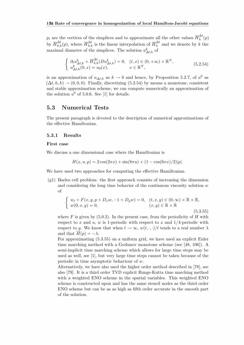
1545. Rate of convergence in homogenization of local Hamilton-Jacobi equations
pi are the vertices of the simplices and to approximate all the other values H∆th (p)
by H∆th,k(p), where H
∆th,k is the linear interpolation of H∆t
h and we denote by k themaximal diameter of the simplices. The solution uk∆t,h of
∂tuk∆t,h +H
∆th,k(Duk∆t,h) = 0, (t, x) ∈ (0,+∞)× RN ,
uk∆t,h(0, x) = u0(x), x ∈ RN ,(5.2.54)
is an approximation of u∆t,h as k → 0 and hence, by Proposition 5.2.7, of u0 as(∆t, h, k)→ (0, 0, 0). Finally, discretizing (5.2.54) by means a monotone, consistentand stable approximation scheme, we can compute numerically an approximation ofthe solution u0 of 5.0.6. See [1] for details.
5.3 Numerical TestsThe present paragraph is devoted to the description of numerical approximations ofthe effective Hamiltonian.
5.3.1 Results
First case
We discuss a one dimensional case where the Hamiltonian is
H(x, u, p) = 2 cos(2πx) + sin(8πu) + (1− cos(6πx)/2)|p|.
We have used two approaches for computing the effective Hamiltonian.
(g1) Barles cell problem: the first approach consists of increasing the dimensionand considering the long time behavior of the continuous viscosity solution wof
wt + F (x, y, p+Dxw,−1 +Dyw) = 0, (t, x, y) ∈ (0,∞)× R× R,w(0, x, y) = 0, (x, y) ∈ R× R
(5.3.55)where F is given by (5.0.2). In the present case, from the periodicity of H withrespect to x and u, w is 1-periodic with respect to x and 1/4-periodic withrespect to y. We know that when t→∞, w(t, ·, ·)/t tends to a real number λand that H(p) = −λ.For approximating (5.3.55) on a uniform grid, we have used an explicit Eulertime marching method with a Godunov monotone scheme (see [48, 106]). Asemi-implicit time marching scheme which allows for large time steps may beused as well, see [1], but very large time steps cannot be taken because of theperiodic in time asymptotic behaviour of w.Alternatively, we have also used the higher order method described in [78], seealso [79]. It is a third order TVD explicit Runge-Kutta time marching methodwith a weighted ENO scheme in the spatial variables. This weighted ENOscheme is constructed upon and has the same stencil nodes as the third orderENO scheme but can be as as high as fifth order accurate in the smooth partof the solution.
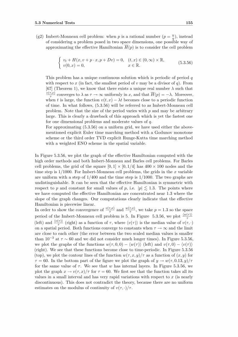
5.3 Numerical Tests 155
(g2) Imbert-Monneau cell problem: when p is a rational number (p = nq ), instead
of considering a problem posed in two space dimensions, one possible way ofapproximating the effective Hamiltonian H(p) is to consider the cell problem
vt +H(x, v + p · x, p+Dv) = 0, (t, x) ∈ (0,∞)× R,v(0, x) = 0, x ∈ R. (5.3.56)
This problem has a unique continuous solution which is periodic of period qwith respect to x (in fact, the smallest period of v may be a divisor of q). From[67] (Theorem 1), we know that there exists a unique real number λ such thatv(τ,x)τ converges to λ as τ →∞ uniformly in x, and that H(p) = −λ. Moreover,
when t is large, the function v(t, x)− λt becomes close to a periodic functionof time. In what follows, (5.3.56) will be referred to as Imbert-Monneau cellproblem. Note that the size of the period varies with p and may be arbitrarylarge. This is clearly a drawback of this approach which is yet the fastest onefor one dimensional problems and moderate values of q.For approximating (5.3.56) on a uniform grid, we have used either the above-mentioned explicit Euler time marching method with a Godunov monotonescheme or the third order TVD explicit Runge-Kutta time marching methodwith a weighted ENO scheme in the spatial variable.
In Figure 5.3.56, we plot the graph of the effective Hamiltonian computed with thehigh order methods and both Imbert-Monneau and Barles cell problems. For Barlescell problems, the grid of the square [0, 1] × [0, 1/4] has 400 × 100 nodes and thetime step is 1/1000. For Imbert-Monneau cell problems, the grids in the x variableare uniform with a step of 1/400 and the time step is 1/1000. The two graphs areundistinguishable. It can be seen that the effective Hamiltonian is symmetric withrespect to p and constant for small values of p, i.e. |p| . 1.3. The points wherewe have computed the effective Hamiltonian are concentrated near 1.3 where theslope of the graph changes. Our computations clearly indicate that the effectiveHamiltonian is piecewise linear.In order to show the convergence of v(τ,x)
τ and w(τ,x)τ , we take p = 1.3 so the space
period of the Imbert-Monneau cell problem is 5. In Figure 5.3.56, we plot 〈w(τ)〉τ
(left) and 〈v(τ)〉τ (right) as a function of τ , where 〈v(τ)〉 is the median value of v(τ, ·)
on a spatial period. Both functions converge to constants when τ →∞ and the limitare close to each other (the error between the two scaled median values is smallerthan 10−3 at τ ∼ 60 and we did not consider much longer times). In Figure 5.3.56,we plot the graphs of the functions w(τ, 0, 0) − 〈w(τ)〉 (left) and v(τ, 0) − 〈v(τ)〉(right). We see that these functions become close to time-periodic. In Figure 5.3.56(top), we plot the contour lines of the function w(τ, x, y)/τ as a function of (x, y) forτ = 60. In the bottom part of the figure we plot the graph of y → w(τ, 0.13, y)/τfor the same value of τ . We see that w has internal layers. In Figure 5.3.56, weplot the graph x→ v(τ, x)/τ for τ = 60. We first see that the function takes all itsvalues in a small interval and has very rapid variations with respect to x (is nearlydiscontinuous). This does not contradict the theory, because there are no uniformestimates on the modulus of continuity of v(τ, ·)/τ .
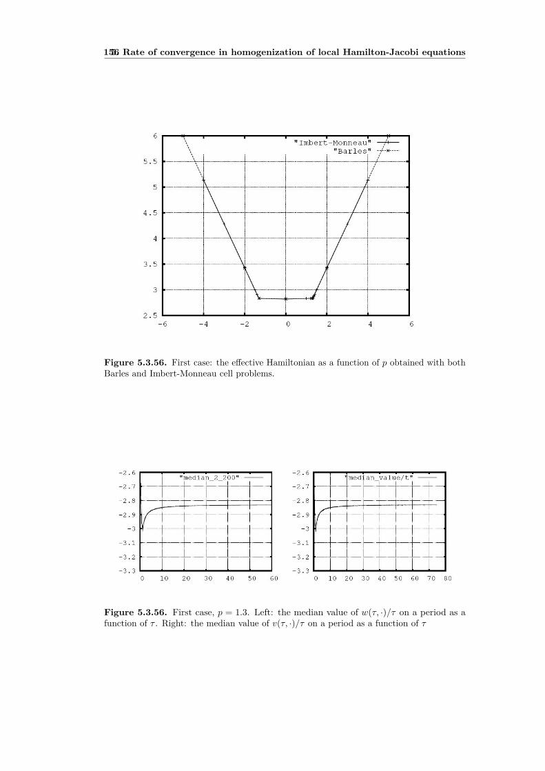
1565. Rate of convergence in homogenization of local Hamilton-Jacobi equations
Figure 5.3.56. First case: the effective Hamiltonian as a function of p obtained with bothBarles and Imbert-Monneau cell problems.
Figure 5.3.56. First case, p = 1.3. Left: the median value of w(τ, ·)/τ on a period as afunction of τ . Right: the median value of v(τ, ·)/τ on a period as a function of τ
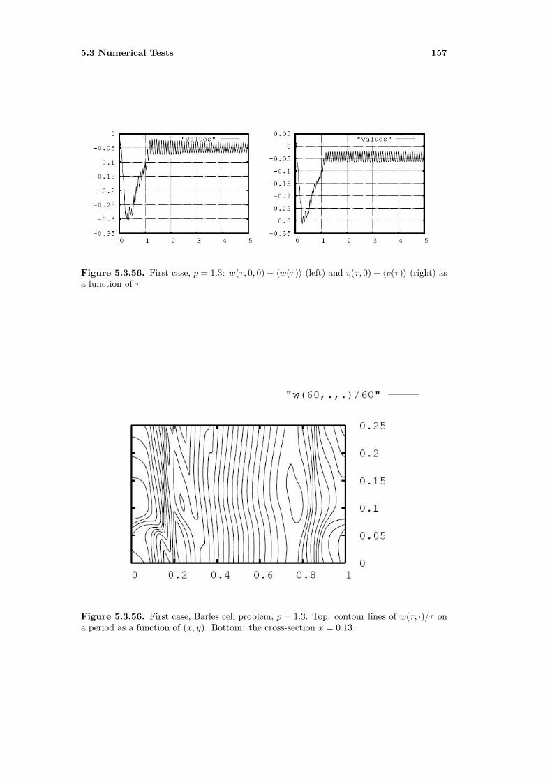
5.3 Numerical Tests 157
Figure 5.3.56. First case, p = 1.3: w(τ, 0, 0)− 〈w(τ)〉 (left) and v(τ, 0)− 〈v(τ)〉 (right) asa function of τ
Figure 5.3.56. First case, Barles cell problem, p = 1.3. Top: contour lines of w(τ, ·)/τ ona period as a function of (x, y). Bottom: the cross-section x = 0.13.
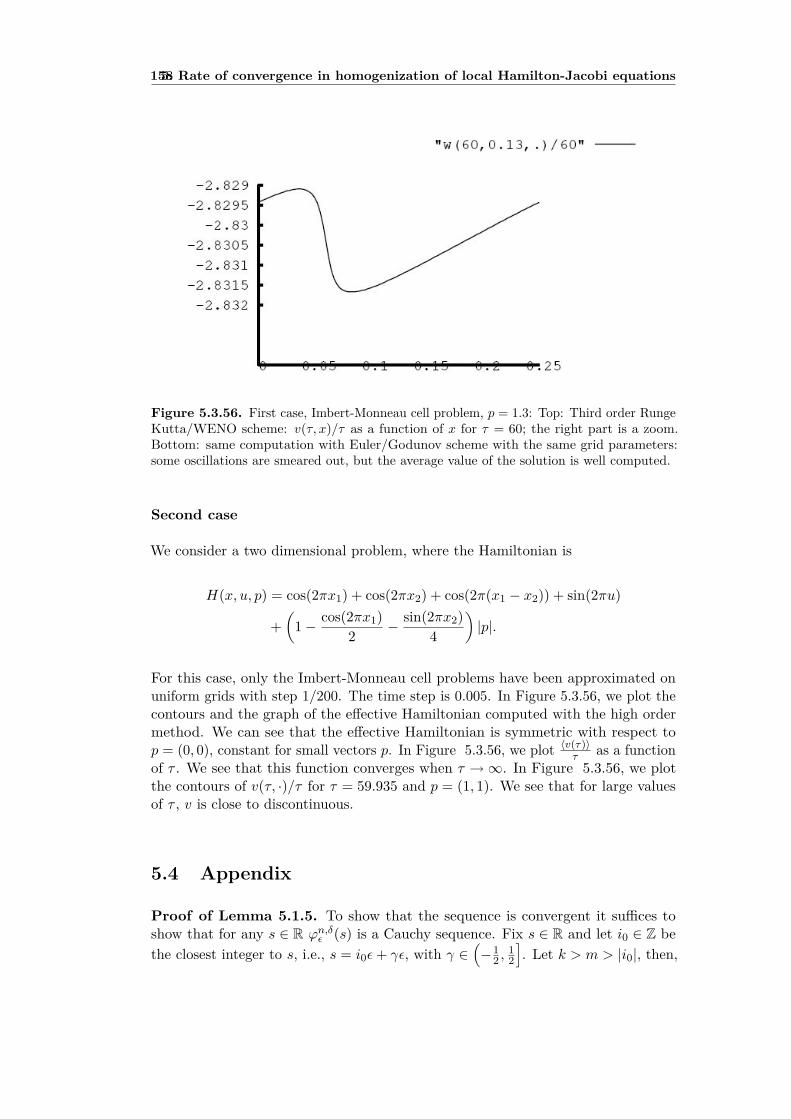
1585. Rate of convergence in homogenization of local Hamilton-Jacobi equations
Figure 5.3.56. First case, Imbert-Monneau cell problem, p = 1.3: Top: Third order RungeKutta/WENO scheme: v(τ, x)/τ as a function of x for τ = 60; the right part is a zoom.Bottom: same computation with Euler/Godunov scheme with the same grid parameters:some oscillations are smeared out, but the average value of the solution is well computed.
Second case
We consider a two dimensional problem, where the Hamiltonian is
H(x, u, p) = cos(2πx1) + cos(2πx2) + cos(2π(x1 − x2)) + sin(2πu)
+(
1− cos(2πx1)2 − sin(2πx2)
4
)|p|.
For this case, only the Imbert-Monneau cell problems have been approximated onuniform grids with step 1/200. The time step is 0.005. In Figure 5.3.56, we plot thecontours and the graph of the effective Hamiltonian computed with the high ordermethod. We can see that the effective Hamiltonian is symmetric with respect top = (0, 0), constant for small vectors p. In Figure 5.3.56, we plot 〈v(τ)〉
τ as a functionof τ . We see that this function converges when τ →∞. In Figure 5.3.56, we plotthe contours of v(τ, ·)/τ for τ = 59.935 and p = (1, 1). We see that for large valuesof τ , v is close to discontinuous.
5.4 Appendix
Proof of Lemma 5.1.5. To show that the sequence is convergent it suffices toshow that for any s ∈ R ϕn,δε (s) is a Cauchy sequence. Fix s ∈ R and let i0 ∈ Z bethe closest integer to s, i.e., s = i0ε+ γε, with γ ∈
(−1
2 ,12
]. Let k > m > |i0|, then,
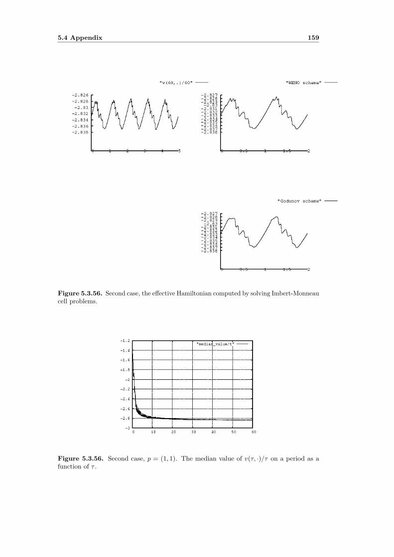
5.4 Appendix 159
Figure 5.3.56. Second case, the effective Hamiltonian computed by solving Imbert-Monneaucell problems.
Figure 5.3.56. Second case, p = (1, 1). The median value of v(τ, ·)/τ on a period as afunction of τ .
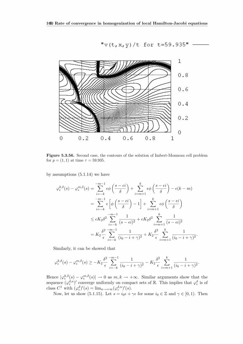
1605. Rate of convergence in homogenization of local Hamilton-Jacobi equations
Figure 5.3.56. Second case, the contours of the solution of Imbert-Monneau cell problemfor p = (1, 1) at time τ = 59.935.
by assumptions (5.1.14) we have
ϕk,δε (s)− ϕm,δε (s) =−m−1∑i=−k
εφ
(s− εiδ
)+
k∑i=m+1
εφ
(s− εiδ
)− ε(k −m)
=−m−1∑i=−k
ε
[φ
(s− εiδ
)− 1
]+
k∑i=m+1
εφ
(s− εiδ
)
≤ εK2δ2−m−1∑i=−k
1(s− εi)2 + εK2δ
2k∑
i=m+1
1(s− εi)2
= K2δ2
ε
−m−1∑i=−k
1(i0 − i+ γ)2 +K2
δ2
ε
k∑i=m+1
1(i0 − i+ γ)2 .
Similarly, it can be showed that
ϕk,δε (s)− ϕm,δε (s) ≥ −K2δ2
ε
−m−1∑i=−k
1(i0 − i+ γ)2 −K2
δ2
ε
k∑i=m+1
1(i0 − i+ γ)2 .
Hence |ϕk,δε (s) − ϕm,δε (s)| → 0 as m, k → +∞. Similar arguments show that thesequence (ϕδ,nε )′ converge uniformly on compact sets of R. This implies that ϕδε is ofclass C1 with (ϕδε)′(s) = limn→+∞(ϕδ,nε )′(s).
Now, let us show (5.1.15). Let s = i0ε+ γε for some i0 ∈ Z and γ ∈ [0, 1). Then
5.4 Appendix 161
ϕn,δε (s)− i0ε = ε
[φ
(γε
δ
)− 1
]+
i0−1∑i=−n
ε
[φ
(i0ε+ γε− εi
δ
)− 1
]+
n∑i=i0+1
εφ
(i0ε+ γε− εi
δ
)
≤ ε[φ
(γε
δ
)− 1
]ε+ δ2
εK2
i0−1∑i=−n
1(i0 − i+ γ)2 + δ2
εK2
n∑i=i0+1
1(i− i0 − γ)2
= ε
[φ
(γε
δ
)− 1
]+ δ2
εK2
n+i0∑i=1
1(i+ γ)2 + δ2
εK2
n−i0∑i=1
1(i− γ)2 .
Similarly
ϕn,δε (s)− i0ε ≥ ε[φ
(γε
δ
)− 1
]− δ2
εK2
n+i0∑i=1
1(i+ γ)2 −
δ2
εK2
n−i0∑i=1
1(i− γ)2 .
Letting n→ +∞, we get∣∣∣∣ϕδε(s)− i0ε− ε [φ(γεδ)− 1
]∣∣∣∣ ≤ δ2
εK2
+∞∑i=1
1(i+ γ)2 + δ2
εK2
+∞∑i=1
1(i− γ)2 .
If γ > 0 then φ(γεδ
)− 1→ 0 as δ → 0+ and ϕδε(s)→ i0ε if δ → 0+. If γ = 0, then
ϕδε(s)→ (i0 − 1)ε+ φ(0)ε if δ → 0+ and (5.1.15) is proved. 2

Appendix A
Notation list
Br(x) ball of radius r centered at x
C(Ω) set of continuous functions on Ω
Cb(R+ × RN ) set of continuous functions on R+ × RN which are bounded on(0, T )× RN for any T > 0
Cαx ((0, T ) × RN ) space of continuous functions defined on (0, T ) × RN that arebounded and with bounded seminorm < u >αx
d(x) distance function
LSC(Ω) set of lower semicontinuous functions on Ω
LSCb(R+ × RN ) set of lower semicontinuous functions on R+ × RN which arebounded on (0, T )× RN for any T > 0
For u : A→ R and x ∈ A, J2,+u(x), J2,−u(x) are the second-order semi-jets definedby
J2,+u(x) =(p,X) ∈ RN × S(N) |u(y) ≤ u(x) + 〈p, y − x〉+ 12〈X(y − x), y − x〉
+ o(|y − x|2) as y → x, y ∈ A
J2,−u(x) =(p,X) ∈ RN × S(N) |u(y) ≥ u(x) + 〈p, y − x〉+ 12〈X(y − x), y − x〉
+ o(|y − x|2) as y → x, y ∈ A
For u : A→ R and x ∈ A
J2,+u(x) =(p,X) ∈ RN × S(N) | ∃(xn, pn, Xn) ∈ A× RN × S(N)
(pn, Xn) ∈ J2,+u(xn) and (xn, u(xn), pn, Xn)→ (x, u(x), p,X)
J2,−u(x) =(p,X) ∈ RN × S(N) | ∃(xn, pn, Xn) ∈ A× RN × S(N)
(pn, Xn) ∈ J2,−u(xn) and (xn, u(xn), pn, Xn)→ (x, u(x), p,X)
M+−a,A(D2u) Pucci’s operators
163
164 A. Notation list
Qτ,r(t, x) = (t− τ, t+ τ)×Br(x)
S(N) space of real symmetric matrices N ×N
SN−1 unit sphere of RN
USC(Ω) set of upper semicontinuous functions on Ω
USCb(R+ × RN ) set of upper semicontinuous functions on R+ × RN which arebounded on (0, T )× RN for any T > 0
For u : (0, T )× RN → R, 0 < T ≤ +∞, for 0 < α < 1
< u >αx := sup(t,x), (t,x′)∈(0,T )×RN
x 6=x′
|u(t, x)− u(t, x′)||x− x′|α
ForX ∈ S(N), ‖X‖ = sup|Xξ| | ξ ∈ RN , |ξ| ≤ 1 = sup|λ| : λ is an eigenvalue of X
For X ∈ S(N) tr(X) denotes the trace of X
For ξ, η ∈ RN , ξ ⊗ η denotes the matrix (ξiηj)ij
bxc floor integer part of x
dxe ceil integer part of x
a ∨ b = max(a, b), a ∧ b = min(a, b)
Bibliography
[1] Y. Achdou, F. Camilli and I. Capuzzo Dolcetta, Homogenization ofHamilton-Jacobi equations: Numerical Methods. Math. Models Methods Appl.Sci., 18 (2008), 1115-1143.
[2] Y. Achdou and S. Patrizi, Homogenization of first order equations withu/ε-periodic Hamiltonian: Rate of convergence as ε→ 0 and numerical approx-imation of the effective Hamiltonian, submitted.
[3] O. Alvarez, Homogenization of Hamilton-Jacobi equations in perforated sets,J. Differential Equations, 159 (1999), no. 2, 543-577.
[4] O. Alvarez and M. Bardi, Singular perturbations of nonlinear degenerateparabolic PDEs: a general convergence result, Arch. Ration. Mech. Anal., 170(2003), no. 1, 17-61.
[5] O. Alvarez and M. Bardi, Viscosity solutions methods for singular pertur-bations in deterministic and stochatic control, SIAM J. Control Optim., 40(2001/02), no. 4, 1159-1188 (electronic).
[6] O. Alvarez and E. N. Barron, Homogenization in L∞, J. DifferentialEquations, 183 (2001), no. 1, 132-164.
[7] O. Alvarez, P. Hoch, Y. Le Bouar and R. Monneau, Dislocation dy-namics described by non-local Hamilton-Jacobi equations, Materials Scienceand Engineering: A, 400-401 (2005), 162-165.
[8] O. Alvarez and H. Ishii, Hamilton-Jacobi equations with partial gradientand application to homogenization, Comm. Part. Differential Equations, 26(2001), no. 5-6, 983-1002.
[9] H. Amann, Fixed point equations and nonlinear eigenvalue problems in orderedBanach spaces, SIAM Rev., 18 (1976), 620-709.
[10] A. Anane, Simplicité et isolation de la première valeur propre du p-Laplacienavec poids. (French) [Simplicity and isolation of the first eigenvalue of thep-Laplacian with weight] C. R. Acad. Sci. Paris Sr I Math., 305 (1987), no. 16,752-728.
[11] G. Aronsson, M. G. Crandall and P. Juutinen, A tour of the theory ofabsolutely minimizing functions, Bull. Amer. Math. Soc. (N. S.), 41 (2004), no.4, 439-505.
165
166 Bibliography
[12] S. Awatif, Équations d’Hamilton-Jacobi du premier ordre avec termes intégro-différentiels. I. Unicité des solutions de viscosité. II. Existence de solutions deviscosité,Comm. Partial Differential Equations, 16 (1991), no. 6-7, 1057-1093.
[13] M. Bardi and I. Capuzzo Dolcetta, Optimal control and viscosity solutionsof Hamilton-Jacobi-Bellmann equations, Birkhauser, 1997.
[14] M. Bardi, M. G. Crandall, L. C. Evans, H. M. Soner and P. E.Souganidis, Viscosity solutions and applications, I. Capuzzo Dolcetta and P.L. Lions eds, Lectures Notes in Mathematics 1660, Springer, Berlin, 1997.
[15] G. Barles, Fully nonlinear Neumann type boundary conditions for second-order elliptic and parabolic equations, J. Differential Equations, 106 (1993),no. 1, 90-106.
[16] G. Barles, Nonlinear Neumann boundary conditions for quasilinear degenerateelliptic equations and applications, J. Differential Equations, 154 (1999), 191-224.
[17] G. Barles, Solution de Viscosité des équations de Hamilton-Jacobi, Spronger-Verlag, Paris, 1994.
[18] G. Barles, Some homogenization results for non-coercive Hamilton-Jacobiequations. Calculus of Variations and Partial Differential Equations, 30 (2007),no. 4, 449-466.
[19] G. Barles, E. Chasseigne and C. Imbert, Hölder continuity of solutionsof second-order non-linear elliptic integro-differential equations, to appear inJornal of the European Mathematical Society.
[20] G. Barles and F. Da Lio, Local C0,α estimates for viscosity solutions ofNeumann-type boundary value problems, J. Differential Equations, 225 (2006),no. 1, 202-241.
[21] G. Barles and F. Da Lio, On the boundary ergodic problem for fullynonlinear equations in bounded domains with general nonlinear Neumannboundary conditions, Ann. I. H. Poincaré, 22 (2005), 501-541.
[22] G. Barles and C. Imbert Second-order elliptic integro-differential equations:viscosity solution’s theory revisited, Annales de l’IHP, 25 (2008), no. 3, 567-585.
[23] G. Barles and M. Ramaswamy, Sufficient structure conditions for uniquenessof viscosity solutions of semilinear and quasilinear equations, NoDEA, 12 (2006),no. 4, 503-523.
[24] G. Barles and P. E. Souganidis, On the large time behavior of solutions ofHamilton-Jacobi equations, SIAM J. Math. Anal., 31 (2000), no. 4, 925-939(electronic).
[25] D. M. Barnett and S. D. Gavazza, The self-force on a planar dislocationloop in an anisotropic linear-elastic medium, Phy. Stat. Sol. (a), 38 (1976), p.637.

Bibliography 167
[26] H. Berestycki, L. Nirenberg and S.R.S. Varadhan, The principal eigen-value and maximum principle for second order elliptic operators in generaldomain, Comm. Pure Appl. Math., 47 (1994), no. 1, 47-92.
[27] I. Birindelli and F. Demengel, Comparison principle and Liouville typeresults for singular fully nonlinear operators, Ann. Fac. Sci. Toulouse Math. 13(2004), no. 2, 261-287.
[28] I. Birindelli and F. Demengel, Eigenvalue, maximum principle and regu-larity for fully nonlinear homogeneous operators, Comm. Pure Appl. Anal., 6(2007), no. 2, 335-366.
[29] I. Birindelli and F. Demengel, Regularity and uniqueness of the firsteigenfunction for singular fully nonlinear operators, preprint.
[30] L. Brown, The self-stress of dislocations and the shape of extended nodes,Phil. Mag., 10 (1964), p. 441.
[31] J. Busca, M. J. Esteban, A. Quaas, Nonlinear eigenvalues and bifurcationproblems for Pucci’s operators, Ann. Inst. H. Poincaré Anal. Non Linéaire, 22(2005), no. 2, 187-206.
[32] X. Cabré and L. Caffarelli Fully nonlinear equations Colloquium Publica-tions 43, American Mathematical Society, Providence, RI, 1995.
[33] X. Cabré and J. Solà-Morales, Layer solutions in a half-space for boundaryreactions, Comm. Pure Appl. Math., 58 (2005) no. 12, 1678-1732.
[34] L. Caffarelli and L. Silvestre Regularity theory for fully nonlinear integro-differential equations, Comm. Pure Appl. Math., 62 (2009), no. 5, 597-638.
[35] L. Caffarelli, P. E. Souganidis and L. Wang, Homogenization of fullynonlinear, uniformly elliptic and parabolic partial differential equations instationary ergodic media, Comm. Pure Appl. Math., 58 (2005), no. 3, 319-361.
[36] I. Capuzzo Dolcetta and H. Ishii, On the rate of convergence in homog-enization of Hamilton-Jacobi equations. Indiana Univ. Math. J., 50 (2001),1113-1129.
[37] Y. G. Chen, Y. Giga and S. Goto, Uniqueness and existence of viscositysolutions of generalized mean curvature flow equations. J. Differential Geom.,33 (1991), 749-786.
[38] F. H. Clarke, Yu. S. Ledyaev, R. J. Stern and P. R. Wolenski, Nons-mooth Analysis and Control Theory, vol. 178 of Graduate Texts in Mathematics.Springer, 1997.
[39] B. Cockburn and J. Qian, Continuous dependence results for Hamilton-Jacobi equations, Collected lectures on the preservation of stability underdiscretization (Fort Collins, CO, 2001) SIAM, 67-90.
168 Bibliography
[40] M. C. Crandall, H. Ishii and P. L. Lions, User’s guide to viscosity solutionsof second order partial differential equations, Bull. Amer. Math. Soc. (N.S.),27 (1992), no. 1, 1-67.
[41] M. C. Crandall and P. L. Lions, Viscosity solutions of Hamilton-JacobiEquations, Trans. Amer. Math. Soc., 277 (1983), 1-67.
[42] M. C. Crandall and P. L. Lions, Two approximations of solutions ofHamilton-Jacobi equations, Mathematics of Computations, 43 (1984), 1-19.
[43] A. M. Cuitino, M. Koslowski and M. Ortiz, A phase-field theory ofdislocation dinamics, strain hardening and hysteresis in ductile single crystal, J.Mech. Phys. Solids, 50 (2002), 2597-2635.
[44] F. Da Lio, N. Forcadel and R. Monneau, Convergence of a non-localeikonal equation to anisotropic mean curvature motion. Application to disloca-tions dynamics, Journal of the European Mathematical Society 10 (2008), no. 4,1061-1104.
[45] M. D. Donsker and S. R. S. Varadhan, On a variational formula for theprincipal eigenvalue for operators with maximum principle, Proc. Nat. Acad.Sci. USA, 72 (1975), 780-783.
[46] M. D. Donsker and S. R. S. Varadhan, On the principal eigenvalue ofsecond-order elliptic differential operators, Comm. Pure Appl. Math., 29 (1976),595-621.
[47] A. El Hajj, H. Ibrahim and R. Monneau, Dislocation dynamics: frommicroscopic models to macroscopic crystal plasticity, Continuum Mechanicsand Thermodynamics, 21 (2009), no. 2, 109-123.
[48] B. Engquist and S. Osher, One-sided difference approximations for nonlinearconservation laws, Math. Comp., 36-154 (1981), 321–351.
[49] L. C. Evans, Periodic homogenisation of certain fully nonlinear partial dif-ferential equations, Proc. Roy. Soc. Edinburgh Sect. A, 120 (1992), no. 3-4,245-265.
[50] L. C. Evans, The perturbed test function method for viscosity solutions ofnonlinear PDE, Proc. Roy. Soc. Edinburgh Sect. A, 111 (1989), no. 3-4, 359-375.
[51] L. C. Evans and W. Gangbo, Differential equations methods for the Monge-Kantorovich mass tranfer problem, Mem. Amer. Math. Soc., 137 (1999), no.653.
[52] L. C. Evans and J. Spruck, Motion of level sets by mean curvature. J.Differential Geom., 33 (1991), 635-681.
[53] A. Fathi, Sur la convergence du semi-group de Lax-Oleinik, C. R. Acad. Sci.Paris Sér. I Math., 327 (1998) no. 3, 267-270.
Bibliography 169
[54] W. H. Fleming and H. M. Soner, Controlled Markov processes and viscositysolutions. Applications of Mathematics (New York), 25. Springer-Verlag, NewYork, 1993.
[55] N. Forcadel, C. Imbert and R. Monneau, Homogenization of dislocationdynamics and some particle systems with two-body interactions, Discrete andContinuous Dynamical Systems - A, 23 (2009), no.3, 785 - 826.
[56] N. Forcadel, C. Imbert and R. Monneau, Homogenization of fully over-damped Frenkel-Kontorova models, Journal of Differential Equations, 246(2009), no. 1, 1057-1097.
[57] A. Garroni and S. Müller, Γ-limit of a phase-field model of dislocationsSIAM J. Math. Anal., 36 (2005), no. 6, 1943-1964.
[58] A. Garroni and S. Müller, A variational model for dislocations in the linetension limit, Arch. Ration. Mech. Anal., 181 (2006), 535-578.
[59] J. Garcia-Azorero, J. J. Manfredi, I. Peral and J. D. Rossi, Stekloveigenvalues for the ∞-Laplacian, Rend. Lincei Mat. Appl., 17 (2006), no. 3,199-210.
[60] Y. Giga and M. Ohnuma On strong comparison principle for semicontinuousviscosity solutions of some nonlinear elliptic equations, preprint.
[61] D. Gilbarg and N.S. Trudinger, Elliptic partial differential equations ofsecond order. Reprint of the 1998 edition. Classics in Mathematics. Springer-Verlag, Berlin, 2001.
[62] M. González and R. Monneau, work in progres.
[63] J. R. Hirth and L. Lothe, Theory of dislocations, Second Edition. Malabar,Florida: Krieger, 1992.
[64] K. Horie and H. Ishii, Homogenization of Hamilton-Jacobi equations ondomains with small scale periodic structure, Indiana Univ. Math. J., 47 (1998),no. 3, 1011-1058.
[65] C. Imbert, A non-local regularization of first order Hamilton-Jacobi equations.Journal of Differential Equations, 211 (2005), no. 1, 214-246.
[66] C. Imbert and J. Droniou, Fractal first order partial differential equations,Archive for Rational Mechanics and Analysis, 182 (2006), no. 2, 299-331.
[67] C. Imbert and R. Monneau, Homogenization of first order equations with u/ε-periodic Hamiltonians. Part I: local equations, Archive for Rational Mechanicsand Analysis, 187 (2008), no. 1, 49-89.
[68] C. Imbert, R. Monneau and E. Rouy, Homogenization of first orderequations with u/ε-periodic Hamiltonians. Part II: application to dislocationsdynamics, Communications in Partial Differential Equations, 33 (2008), no.1-3, 479-516.
170 Bibliography
[69] C. Imbert and P. E. Souganidis, Phasefield theory for fractional diffusion-reaction equations and applications, preprint.
[70] H. Ishii, Almost periodic homogenization of Hamilton-Jacobi equations, Inter-national Conference in Differential Equations, Vol. 1, 2, Berlin (1999), 600-605,World Sci. Publishing, River Edge, NJ, 2000.
[71] H. Ishii, Fully nonlinear oblique derivative problems for Nonlinear Second-OrderElliptic PDE’s, Duke Math. J., 62 (1991), no. 3, 633-661.
[72] H. Ishii, Homogenization of the Cauchy problem for Hamilton-Jacobi equations,Stochastic analysis, control, optimization and applications, System ControlFound. Appl., 305-324, Birkhäuser Boston, Boston, MA, 1999.
[73] H. Ishii, Perron’s method for Hamilton-Jacobi Equations, Duke Math. J., 55(1987), 369-384.
[74] H. Ishii, Personal Communication.
[75] H. Ishii and P.L. Lions, Viscosity Solutions of Fully Nonlinear Second-OrderElliptic Partial Differential Equations, J. Differential Equations, 83 (1990), no.1, 26-78.
[76] H. Ishii and Y. Yoshimura, Demi-eigenvalues for uniformly elliptic Isaacsoperators, preprint.
[77] R. Jensen, Uniqueness of Lipschitz extensions: minimizing the sup norm ofthe gradient, Arch. Rational. Mech. Anal., 123, (1993) no.1, 51-74.
[78] G.-S. Jiang and D. Peng, Weighted ENO schemes for Hamilton-Jacobiequations. SIAM J. Sci. Comput.,21(6) (2000), 2126–2143.
[79] G.-S. Jiang and C.-W. Shu, Efficient implementation of weighted ENOschemes. J. Comput. Phys., 126(1) (1996),202–228.
[80] P. Juutinen, Principal eigenvalue of a very badly degenerate operator andapplications, J. Differential Equations, 236 (2007), no. 2, 532-550.
[81] P. Juutinen and B. Kawohl, On the evolution governed by the infinityLaplacian, Math. Ann., 335 (2006), 819-851.
[82] P. Juutinen, P. Lindqvist and J. J. Manfredi, The∞-eigenvalue problem,Arch. Ration. Mech. Anal., 148 (1999), no. 2, 89-105.
[83] P. Juutinen, P. Lindqvist and J. J. Manfredi, The infinity Laplacian:examples and observations, Papers on analysis, 207-217, Rep. Univ. JyväskyläDep. Math. Stat., 83, Univ. Jyväskylä, Jyväskylä, 2001.
[84] E. R. Jakobsen and K. H. Karlsen, Continuous dependence estimatesfor viscosity solutions of integro-PDEs. J. Differential Equations, 212 (2005),278-318.
Bibliography 171
[85] O. A. Ladyzhenskaya, V. A. Solonnikov and N. N. Ural’tseva, Linearand Quasi-linear Equations of Parabolic Type, "Nauka" Moscov, 1967; Englishtransl, Am. Math. Soc., Providence, RI, 1968.
[86] N.S. Landkof, Foundations of Modern Potential Theory, Springer-Verlag,1972.
[87] P. L. Lions, Bifurcation and optimal stochastic control, Nonlinear Anal., 7(1983), no. 2, 177-207.
[88] P. L. Lions, G. C. Papanicolaou and S. R. S. Varadhan, Homogenizationof Hamilton-Jacobi equations, unpublished, 1986.
[89] P. Lindqvist, Notes on the p-Laplace equation, Report. University of JyväskyläDepartment of Mathematics and Statistics, 102. University of Jyväskylä,Jyväskylä, (2006). ii+80 pp.
[90] P. Lindqvist, On a nonlinear eigenvalue problem, Fall. School in Analysis(Jyväskylä, 1994), 33-54. Report, 68, Univ. Jyväskylä, Jyväskylä, 1995.
[91] E. Milakis and L. E. Silvestre, Regularity for fully nonlinear ellipticequations with Neumann boundary data, Comm. Partial Differential Equations,31 (2006), no. 7-9, 1227-1252.
[92] R. Monneau and S. Patrizi, work in progress.
[93] F. R. N. Nabarro, Dislocations in a simple cubic lattice, Proc. Phys. Soc.,59 (1947), 256-272.
[94] S. Osher and J. A. Sethian, Fronts propagation with curvature-dependentspeed: Algorithms based on Hamilton-Jacobi formulations. J. Comput. Phys.,79 (1988), no. 1, 12-49.
[95] M. Otani and T. Teshima, On the first eigenvalue of some quasi linear ellipticequations, Proc. Japan. Acad. Ser. A. Math. Sci., 64 (1988), no. 1, 8-10.
[96] S. Patrizi, Principal eigenvalues for Isaacs operators with Neumann boundaryconditions, NoDEA, 16 (2009), no. 1, 79-107.
[97] S. Patrizi, The Neumann problem for singular fully nonlinear operators,Journal de Mathématiques Pure et Appliquées, 90 (2008), no. 3, 286-311.
[98] S. Patrizi The principal eigenvalue of the infinity-Laplacian with the Neumannboundary condition, to appear in ESAIM: Control, Optimisation and Calculusof Variations.
[99] R. Peierls, The size of a dislocation, Proc. Phys. Soc., 52(1940), 34-37.
[100] Y. Peres, O. Schramm, S. Sheffield and D. Wilson, Tug-of-war andthe infinity Laplacian, J. Amer. Math. Soc., 22 (2009), 167-210.
[101] M.H. Protter and H.F. Weinberger, Maximum principles in differentialequations. Prentice-Hall, Inc., Englewood Cliffs, N.J. 1967.
172 Bibliography
[102] M.H. Protter and H.F. Weinberger, On the spectrum of general secondorder operators, Bull. AMS, 72 (1966), 251-255.
[103] A. Quaas, Existence of positive solutions to a "semilinear" equation involvingthe Pucci’s operators in a convex domain, Differential Integral Equations, 17(2004), no. 5-6, 481-494.
[104] A. Quaas and B. Sirakov, On the principal eigenvalues and the Dirichletproblem for fully nonlinear operators, C. R. Math. Acad. Sci. Paris, 342 (2006),no. 2, 115-118.
[105] D. Rodney, Y. Le Bouar and A. Finel, Phase field methods and disloca-tions, Acta Mater., 51 (2003), 17-30.
[106] J. A. Sethian, Level set methods and fast marching methods, volume 3of Cambridge Monographs on Applied and Computational Mathematics. Cam-bridge University Press, Cambridge, second edition, 1999. Evolving interfacesin computational geometry, fluid mechanics, computer vision, and materialsscience.
[107] H. M. Soner, Optimal control with state-space constraint, II, SIAM J.Control Optim., 24 (1986), no. 6, 1110-1122.
[108] , P. E. Souganidis, Stochastic homogenization of Hamilton-Jacobi equationsand some applications, Asymptot. Anal., 20 (1999), no. 1, 1-11.


![Master Thesis Nguyen Tien Thinh - This problem was introduced in [5] by P.L. Lions, G. Papanicolaou and S.R.S. Varadhan in 1986. ... Lions in 1983 regarding the Hamilton-Jacobi equation](https://img.pdfslide.us/doc/110x75/5ae5fc347f8b9a6d4f8c0cd7/master-thesis-nguyen-tien-thinh-problem-was-introduced-in-5-by-pl-lions-g.jpg)
![u i(x)-h - Princeton Universityweinan/s/homogenization.pdf · has already been studied by Lions, Papanicolaou, and Varadhan in [10]. Naturally, in (1.2), we assume that H(y,p) is](https://img.pdfslide.us/doc/110x75/5ae5fc347f8b9a6d4f8c0ca0/u-ix-h-princeton-university-weinanshomogenizationpdfhas-already-been-studied.jpg)
![AUBRY-MATHER MEASURES IN THE NON CONVEX … · to Lions, Papanicolaou and Varadhan. Theorem 1.2 (See [LPV88]). Let H: Tn ×Rn → R be smooth such that lim ... AUBRY-MATHER MEASURES](https://img.pdfslide.us/doc/110x75/5ae5fc347f8b9a6d4f8c0cc8/aubry-mather-measures-in-the-non-convex-lions-papanicolaou-and-varadhan-theorem.jpg)


![Some Inverse Problems in Periodic Homogenization of ... · It was proved by Lions, Papanicolaou and Varadhan [16] that u](https://img.pdfslide.us/doc/110x75/5ae5fc347f8b9a6d4f8c0cc4/some-inverse-problems-in-periodic-homogenization-of-was-proved-by-lions-papanicolaou.jpg)