Embed Size (px)
Citation preview
ARTICLE IN PRESS YJDEQ:5340JID:YJDEQ AID:5340 /FLA [m1+; v 1.73; Prn:10/07/2007; 12:43] P.1 (1-39)
J. Differential Equations ••• (••••) •••–•••www.elsevier.com/locate/jde
Multiscale problems and homogenizationfor second-order Hamilton–Jacobi equations
Olivier Alvarez a, Martino Bardi b,∗, Claudio Marchi c
a UMR 60-85, Université de Rouen, 76821 Mont-Saint Aignan cedex, Franceb Dipartimento di Matematica Pura ed Applicata, Università di Padova, via Trieste 63, 35121 Padova, Italy
c Dipartimento di Matematica, Università della Calabria, Ponte Bucci 30B, 87036 Rende (CS), Italy
Received 22 May 2007
Dedicated to Arrigo Cellina for his 65th birthday
Abstract
We prove a general convergence result for singular perturbations with an arbitrary number of scales offully nonlinear degenerate parabolic PDEs. As a special case we cover the iterated homogenization for suchequations with oscillating initial data. Explicit examples, among others, are the two-scale homogenization ofquasilinear equations driven by a general hypoelliptic operator and the n-scale homogenization of uniformlyparabolic fully nonlinear PDEs.© 2007 Elsevier Inc. All rights reserved.
Keywords: Singular perturbations; Viscosity solutions; Nonlinear parabolic equations; Hamilton–Jacobi equations;Bellman–Isaacs equations; Ergodicity; Stabilization; Homogenization; Iterated homogenization; Multiscaleproblem; Oscillating initial data; Hypoelliptic operators
0. Introduction
This paper is devoted to singular perturbation problems with an arbitrary finite number ofscales for fully nonlinear degenerate parabolic PDEs, and to the iterated homogenization of suchPDEs with oscillating initial data, in the framework of viscosity solutions. Some new results on
* Corresponding author.E-mail addresses: [email protected] (O. Alvarez), [email protected] (M. Bardi),
[email protected] (C. Marchi).
Please cite this article in press as: O. Alvarez et al., Multiscale problems and homogenization for second-orderHamilton–Jacobi equations, J. Differential Equations (2007), doi:10.1016/j.jde.2007.05.027
0022-0396/$ – see front matter © 2007 Elsevier Inc. All rights reserved.doi:10.1016/j.jde.2007.05.027
ARTICLE IN PRESS YJDEQ:5340JID:YJDEQ AID:5340 /FLA [m1+; v 1.73; Prn:10/07/2007; 12:43] P.2 (1-39)
2 O. Alvarez et al. / J. Differential Equations ••• (••••) •••–•••
the case of two scales are given for their own interest and because they are needed in the proofof the general n-scale case.
The theory of homogenization of fully nonlinear PDEs by viscosity methods started with theseminal paper by P.-L. Lions, Papanicolaou, and Varadhan [46] on first-order Hamilton–Jacobiequations
∂tvε + G
(x,
x
ε,Dxv
ε
)= 0 in (0, T ) × R
n, vε(0, x) = h(x), (1)
and with the work of L.C. Evans [31,32], who introduced the perturbed test function methodfor first-order and second-order elliptic equations. It was continued by many authors to cover anumber of different issues, such as problems without equicontinuity estimates [15], perforateddomains [3,9,36], nonperiodic homogenization [10,20,38,47], elliptic and parabolic equationsin divergence form [28,35], Neumann boundary conditions [16]. A recent important addition tothe theory is the stochastic homogenization of PDEs in stationary ergodic media [29,48,52,54].The main motivation of all this theory is understanding the macroscopic properties of modelswith high oscillations at a microscopic scale, as in the classical homogenization of variationalproblems, see, e.g., the monographs [19,25,41,56].
Some related asymptotic problems are the singular perturbations of degenerate parabolicequations of the form
∂tuε + H
(x, y,Dxu
ε,1
εDyu
ε,D2xxu
ε,1
εD2
yyuε,
1√εD2
xyuε
)= 0 in (0, T ) × R
n × Rm,
uε(0, x, y) = h(x, y) on Rn × R
m, (2)
where one seeks a limit u(t, x) of uε(t, x, y) independent of y and solving a suitable Cauchyproblem in (0, T ) × R
n. They arise in the optimal control of deterministic or stochastic systemswhose state variables evolve on two different time-scales, namely,
dxs = f (xs, ys, as) ds + σ(xs, ys, as) dWs, 0 < s < t, x0 = x ∈ Rn,
ε dys = g(xs, ys, as) ds + √ετ(xs, ys, as) dWs, y0 = y ∈ R
m,
where Ws is a multidimensional Brownian motion and as an admissible control function. If oneminimizes an integral cost functional plus a terminal cost h(xt , yt ), the corresponding valuefunction uε(t, x, y) solves (2) with a Hamilton–Jacobi–Bellman Hamiltonian H (i.e., the supof a family of linear degenerate elliptic operators parametrized by a). Here the macroscopicvariable x in (2) has the meaning of the slow variable in the dynamical system, whereas themicroscopic variable y corresponds to the fast variable of the control system. Passing to the limitas ε → 0+ in this problem amounts to reducing the dimension of a large system by decouplingthe behavior of the fast and the slow variables. These problems have a large literature, see thebooks [13,17,42,44] and the references therein. A viscosity solutions approach to these problemswas developed by the first two authors of the present paper [4,5,7], using some of the ideas ofthe homogenization theory quoted above.
In fact, many homogenization problems can be seen as special cases of singular perturbations.For instance, the PDE in (1) is transformed into
Please cite this article in press as: O. Alvarez et al., Multiscale problems and homogenization for second-orderHamilton–Jacobi equations, J. Differential Equations (2007), doi:10.1016/j.jde.2007.05.027
ARTICLE IN PRESS YJDEQ:5340JID:YJDEQ AID:5340 /FLA [m1+; v 1.73; Prn:10/07/2007; 12:43] P.3 (1-39)
O. Alvarez et al. / J. Differential Equations ••• (••••) •••–••• 3
∂tuε + G
(x, y,Dxu
ε + Dyuε
ε
)= 0 in (0, T ) × R
n × Rn,
by setting vε(t, x) = uε(t, x, xε) and y = x
ε. In the same way the second-order equation
∂tvε + F
(x,
x
ε,Dxv
ε,D2xxv
ε
)= 0 in (0, T ) × R
n (3)
becomes
uεt + F
(x, y,Dxu
ε + Dyuε
ε,D2
xxuε + D2
yyuε
ε2+ D2
xyuε
ε+ (D2
xyuε)T
ε
)= 0
in (0, T ) × Rn × R
n.
After replacing ε with√
ε, this is also of the form (2) in the case F is independent of thefirst-order terms. The general homogenization problem with first and second-order terms canbe written as an equation of the form (2) if H is replaced by a suitable Hε with
Hε → H as ε → 0 uniformly on the compact sets.
With this motivation, and as a tool for the asymptotic problems with more than two scales,we first prove a convergence theorem for regular perturbations of the singular perturbation prob-lem, that is, for (2) with H is replaced by Hε and h replaced by hε , hε → h uniformly. Theassumptions are only on the unperturbed Hamiltonian H and are the same as in [5], namely, theproperties of ergodicity and stabilization to a constant that we recall in the next sections. Theseassumptions allow to define the effective PDE and initial data that should be satisfied by thelimit of uε as ε → 0. The local uniform convergence of uε to the unique solution of the effec-tive Cauchy problem is desired. However, this strong convergence does not hold in general, asshown by the example in Section 11 of [7]. Our result then states the weak convergence of uε , inthe sense that the relaxed upper (respectively lower) semi-limit is a viscosity sub- (respectivelysuper-) solution of the limit equation. Strong convergence will be shown under suitable additionalassumptions on the Hamiltonian that guarantee that the limit equation satisfies the ComparisonPrinciple. We give several examples and refer to [5] and [7] for more details.
This theorem embeds homogenization theory into singular perturbations, at least forHamilton–Jacobi–Bellman–Isaacs equations. It allows an approach to homogenization that isa fully nonlinear counterpart of the two-scale convergence by Allaire and Nguetseng [1] forvariational problems. An immediate consequence is a new general treatment of the degenerateparabolic equations (3) with oscillating initial data, that is, under the initial condition
vε(0, x) = h
(x,
x
ε
).
Of course there is a boundary layer at t = 0 and one must find the effective initial condition h sothat vε converges as ε → 0 to the solution of
∂tv + F(x,Dxv,D2
xxv) = 0, v(0, x) = h(x),
Please cite this article in press as: O. Alvarez et al., Multiscale problems and homogenization for second-orderHamilton–Jacobi equations, J. Differential Equations (2007), doi:10.1016/j.jde.2007.05.027
ARTICLE IN PRESS YJDEQ:5340JID:YJDEQ AID:5340 /FLA [m1+; v 1.73; Prn:10/07/2007; 12:43] P.4 (1-39)
4 O. Alvarez et al. / J. Differential Equations ••• (••••) •••–•••
where F is the effective Hamiltonian associated to F . The definitions are recalled in the nextsections and some methods for determining h and F can be found in [5,7,12,32].
We give three examples: the first is the case of uniformly elliptic F , for which we improve theexisting theory. The second is a very degenerate case where F satisfies a nonresonance conditionintroduced by Arisawa and Lions [12]. The third concerns the equation
∂tvε − tr
(σσT
2
(x
ε
)D2
xxvε
)+ G
(x,
x
ε,Dxv
ε
)= 0, vε(0, x) = h
(x,
x
ε
),
where tr denotes the trace, under a full rank bracket generating condition on the columns ofthe matrix σ . We prove the uniform convergence of vε over compact sets to the solution of theeffective limit problem
∂tu −∫
(0,1)n
[tr
(σσT
2(y)D2
xxu
)− G(x,y,Dxu)
]dμ(y) = 0, u(0, x) =
∫(0,1)n
h(x, y) dμ(y),
where dμ(y) = ϕ(y)dy is the invariant measure associated to the diffusion process generated byσ and ϕ ∈ C∞(Rn). Although the PDE is quasilinear with a hypoelliptic principal part, this resultseems to be completely new; indeed, all the results we know involving subelliptic operators treatonly variational and stationary equations on the Heisenberg group and use completely differentmethods, see Biroli, Mosco and Tchou [21,22] as well as [23,34] and the references therein.
The second and main part of the paper is devoted to singular perturbations with more than twoscales. The simplest situation is the three-scale problem
∂tuε + Hε
(x, y, z,Dxu
ε,Dyu
ε
ε,Dzu
ε
ε2,D2
xxuε,
D2yyu
ε
ε,D2
zzuε
ε2,D2
xyuε
ε1/2,D2
xzuε
ε,D2
yzuε
ε3/2
)= 0,
uε(0, x, y, z) = hε(x, y, z),
still with Hε → H and hε → h locally uniformly. It arises, in the special case Hε = H , inthe study via Dynamic Programming of the value function in optimal control and differentialgames for multiscale stochastic systems of the form
dxs = f ds + σ dWs,
ε dys = g ds + √ε τ dWs,
ε2 dzs = ϕ ds + ε υ dWs,
where the drift vectors f,g,ϕ and the dispersion matrices σ, τ,υ depend on the state variablesxs, ys, zs and on the control functions of one or two controllers, and Ws is a multidimensionalBrownian motion. It applies also, for a suitable choice of Hε → H locally uniformly, to theiterated homogenization problem
∂tvε + F
(x,
x,
x
2,Dxv
ε,D2xxv
ε
)= 0, vε(0, x) = h
(x,
x,
x
2
),
Please cite this article in press as: O. Alvarez et al., Multiscale problems and homogenization for second-orderHamilton–Jacobi equations, J. Differential Equations (2007), doi:10.1016/j.jde.2007.05.027
ε ε ε ε
ARTICLE IN PRESS YJDEQ:5340JID:YJDEQ AID:5340 /FLA [m1+; v 1.73; Prn:10/07/2007; 12:43] P.5 (1-39)
O. Alvarez et al. / J. Differential Equations ••• (••••) •••–••• 5
if uε(t, x, xε, x
ε2 ) = vε(t, x). Here we work out in detail the case of uniformly elliptic F . Theapplications to first-order equations are made in our paper [8].
Our methods are general and allow to attack singular perturbation and homogenization prob-lems with an arbitrary number of scales. As far as we know, this is the first paper treatingproblems with more than two scales for fully nonlinear equations. Up to now iterated homog-enization was addressed only in the variational setting, starting with the pioneering work ofBensoussan, J.-L. Lions and Papanicolaou [19] for linear equations and, afterwards, for semi-linear equations, using the Γ -convergence approach, see [25,49] and the references therein, orG-convergence techniques [2,14,45].
The plan of the paper is as follows. The standing assumptions are listed in Section 1. Section 2recalls the notions of ergodicity and stabilization for a Hamiltonian. In Section 3, we improvethe convergence result of [5] by considering the regular perturbation of a singular perturbationproblem. Applications to problems with a noncritical scale factor and to homogenization aregiven in Section 4. In Section 5, we present the regular–singular perturbation result for threescales, then apply it to iterated homogenization, and finally extend it to an arbitrary number ofscales.
1. Standing assumptions
In order to avoid a long list of assumptions on the Hamiltonian and the initial data that mayseem technical to the reader nonexpert in viscosity solutions, we shall specialize to the case ofHamilton–Jacobi–Bellman–Isaacs (HJBI) operators. This is an expedient to get easily existenceand the Comparison Principle (which implies uniqueness) for a few ancillary problems. We leaveit to the reader to extend our results to Hamiltonians in the general form (as in [5]). We thereforeassume that the Hamiltonian is given by
H(x,y,px,py,Xxx,Xyy,Xxy) := minβ∈B
maxα∈A
Lα,β(x, y,px,py,Xxx,Xyy,Xxy),
for the family of linear operators
Lα,β(x, y,px,py,Xxx,Xyy,Xxy) := − tr(Xxxa(x, y,α,β)
) − tr(Xyyb(x, y,α,β)
)− 2 tr
(Xxyc(x, y,α,β)
) − px · f (x, y,α,β)
− py · g(x, y,α,β) − �(x, y,α,β)
with
a := σ σT /2, b := τ τT /2, c := τ σT /2,
where tr(M) denotes the trace of the matrix M . HJBI operators arise in the dynamic program-ming approach to stochastic optimal control problems and stochastic differential games (seeSection 4.2). But it actually concerns far more general situations, as a wide class of elliptic oper-ators can be represented as HJBI operators [43].
The following standing assumptions are very classical, apart perhaps for the last one, whichwill be discussed below. They will hold throughout this paper.
– The control sets A and B are compact metric spaces.
Please cite this article in press as: O. Alvarez et al., Multiscale problems and homogenization for second-orderHamilton–Jacobi equations, J. Differential Equations (2007), doi:10.1016/j.jde.2007.05.027
ARTICLE IN PRESS YJDEQ:5340JID:YJDEQ AID:5340 /FLA [m1+; v 1.73; Prn:10/07/2007; 12:43] P.6 (1-39)
6 O. Alvarez et al. / J. Differential Equations ••• (••••) •••–•••
– The functions f , g, σ , τ , and � are bounded continuous functions in Rn × R
m ×A×B withvalues, respectively, in R
n, Rm, M
n,r (the set of the n × r real matrices), Mm,r , and R.
– The drift vectors f and g and the dispersion matrices σ and τ are Lipschitz continuous in(x, y), uniformly in (α,β).
– The running cost � is uniformly continuous in (x, y), uniformly in (α,β).– The initial data h is a bounded continuous function in R
n × Rm with values in R.
– The functions f , g, σ , τ , � and h are Zm-periodic in the fast variable y.
Periodicity in the fast variable y is a simplification that permits to ignore boundary conditionsor conditions at infinity since y will remain in a compact manifold without boundary (the torus).Most of the results we prove here extend to the case of a fast variable y living in a compact setwith appropriate boundary conditions, such as Neumann conditions or the boundary conditionsarising in problems with state constraints (see Section 1 in [4]). The adaptations require suitableassumptions on g and τ near the boundary.
Given the above Hamiltonian H , we associate its recession function, or homogeneous part, inthe fast derivatives (py,Xyy) given by
H ′(x, y,py,Xyy) := minβ∈B
maxα∈A
{− tr(Xyy b(x, y,α,β)
) − py · g(x, y,α,β)}.
We note that H ′ is positively 1-homogeneous in (py,Xyy), i.e.
H ′(x, y,λpy,λXyy) = λH ′(x, y,py,Xyy), λ > 0,
and that, for every x ∈ Rn, px ∈ R
n, Xxx ∈ Sn (the set of the n × n symmetric matrices), there is
a constant C so that
∣∣H(x,y,px,py,Xxx,Xyy,0) − H ′(x, y,py,Xyy)∣∣ � C
∀(y,py,Xyy) ∈ Rm × R
m × Sm, (4)
for every (x,px,Xxx) in a neighborhood of (x,px,Xxx).
2. Ergodicity and stabilization
2.1. Ergodicity and the effective Hamiltonian
In this subsection we briefly recall the definition of ergodicity of the operator H from [5].We refer to [6,7] for a discussion of the notion with numerous examples arising from stochasticoptimal control and differential games.
We fix a slow variable (x,px,Xxx). By the standard viscosity solution theory, under the cur-rent assumptions, the cell δ-problem with discounting parameter δ > 0
δwδ + H(x, y,px,Dywδ,Xxx,D
2yywδ,0
) = 0 in Rm, wδ periodic, (CPδ)
Please cite this article in press as: O. Alvarez et al., Multiscale problems and homogenization for second-orderHamilton–Jacobi equations, J. Differential Equations (2007), doi:10.1016/j.jde.2007.05.027
ARTICLE IN PRESS YJDEQ:5340JID:YJDEQ AID:5340 /FLA [m1+; v 1.73; Prn:10/07/2007; 12:43] P.7 (1-39)
O. Alvarez et al. / J. Differential Equations ••• (••••) •••–••• 7
has a unique viscosity solution. We denote the solution by wδ(y;x,px,Xxx) so as to display itsdependence on the frozen slow variables. We say that the Hamiltonian is (uniquely) ergodic inthe fast variable at (x,px,Xxx) if
δwδ(y;x,px,Xxx) → const as δ → 0, uniformly in y.
We say that the Hamiltonian is ergodic if it is ergodic at every (x,px,Xxx). When the operatoris ergodic at (x,px,Xxx), we put
H(x,px,Xxx) = − limδ→0
δwδ(y;x,px,Xxx).
The function H is called the effective operator, or effective Hamiltonian.In general, there is no explicit formula for the effective Hamiltonian, but it can be proved
that it inherits several properties from the Hamiltonian H [5]. In particular, H is automaticallycontinuous in R
n × Rn × S
n and degenerate elliptic, that is,
H(x,px,Xxx) � H(x,px,X
′xx
)if Xxx � X′
xx.
A more natural definition of effective Hamiltonian, following the classical homogenizationtheory for Hamilton–Jacobi equation [32,46], is in terms of the true cell problem
H(x, y,px,Dyχ,Xxx,D
2yyχ,0
) = λ in Rm, χ periodic. (5)
There is at most one λ ∈ R such that (5) has a continuous solution χ . When it exists, λ is calledthe effective Hamiltonian and χ a corrector. This definition is less general than ours. If the truecell problem has a solution, then the Hamiltonian is ergodic with effective Hamiltonian λ, but inthe current generality the converse is false, i.e. there may be no corrector associated to a givenergodic Hamiltonian, see [12] and [7] for a simple example with a linear Hamiltonian. In fact,the solution of (CPδ) can be used to construct approximate correctors, an idea used also by otherauthors, such as Arisawa [10] and Ishii [38].
There are many papers on sufficient conditions for ergodicity, see [6,7,12] and the referencestherein; [7] gives also a characterization of ergodicity in terms of the validity of the Strong Maxi-mum Principle. The two most classical examples are the following. The first is the nondegeneracyof the fast diffusion
for some ν > 0, b(x, y,α,β) � νIm for all (x, y,α,β). (6)
It entails the uniform ellipticity of the Hamiltonian in Xyy . The second is the existence of A′ ⊆ A
such that
B(0, ν) ⊂ conv{g(x, y,α,β)
∣∣ α ∈ A′}, τ (x, y,α,β) = 0 for all x, y,β and α ∈ A′, (7)
where B(0, ν) ⊂ Rm denotes the open ball of radius ν centered at the origin. It means the ex-
istence of a deterministic fast subsystem with a strong property of small-time controllability bythe player acting on α. It implies that the Hamiltonian is of first-order with respect to the fastvariable (i.e. it is independent of Xyy and Xxy ) and that it is coercive with respect to the fastgradient py .
Please cite this article in press as: O. Alvarez et al., Multiscale problems and homogenization for second-orderHamilton–Jacobi equations, J. Differential Equations (2007), doi:10.1016/j.jde.2007.05.027
ARTICLE IN PRESS YJDEQ:5340JID:YJDEQ AID:5340 /FLA [m1+; v 1.73; Prn:10/07/2007; 12:43] P.8 (1-39)
8 O. Alvarez et al. / J. Differential Equations ••• (••••) •••–•••
We close this subsection with a technical lemma on ergodicity that will be used later. It statesthat the uniform limit of ergodic Hamiltonians is ergodic. We emphasize that the result is global.Indeed, ergodicity is not preserved by local uniform convergence (any Hamiltonian, whetherergodic or not, is locally uniformly the limit of uniformly elliptic Hamiltonians, all of which areergodic). We shall write ‖f ‖∞ for the uniform norm of the function f .
Lemma 1. Let Hk(y,py,Xyy) be a sequence of ergodic Hamiltonians with effective Hamil-tonian Hk . Then, for every k and k′, we have the inequality
|Hk − Hk′ | � ‖Hk − Hk′ ‖∞.
In particular, if Hk converges uniformly to H , then H is ergodic with effective HamiltonianH = limHk .
Proof. Let wδ,k be the solution of (CPδ) with Hamiltonian Hk . By the Comparison Principle,we immediately get that
‖δwδ,k − δwδ,k′ ‖∞ � ‖Hk − Hk′ ‖∞.
Sending δ → 0, we obtain the inequality stated in the lemma.If Hk uniformly converges to H , the inequality implies that Hk must converge to some con-
stant L. The inequality above applied to Hk and H gives that
‖δwδ,k − δwδ‖∞ � ‖Hk − H‖∞.
Hence,
‖δwδ − L‖∞ � ‖Hk − H‖∞ + ‖δwδ,k − Hk‖∞ + |Hk − L|.
By choosing k large enough we see that δwδ converges to L uniformly as δ → 0 . Hence, H isergodic with effective Hamiltonian L. �Technical remark. In the study of multiscale problems in Section 5 we need the ergodicityof some intermediate effective Hamiltonian that in general is merely continuous. Therefore thecell problem (CPδ) for this Hamiltonian may not satisfy the Comparison Principle. As it is wellknown, this implies that (CPδ) may have several viscosity solutions, possibly discontinuous (ex-istence follows from Perron’s method). We say that such a Hamiltonian is ergodic if, for everycollection of solutions (wδ)δ>0 of (CPδ), δwδ converges uniformly as δ → 0 to a constant that isindependent of the collection. This extended definition allows us to prove the weak convergencefor n-scale problems under minimal assumptions. In the applications presented here, however,we shall mainly deal with cases for which all the effective Hamiltonians satisfy the ComparisonPrinciple and therefore we will get strong convergence results. For these examples the standarddefinition of ergodicity would be enough.
Please cite this article in press as: O. Alvarez et al., Multiscale problems and homogenization for second-orderHamilton–Jacobi equations, J. Differential Equations (2007), doi:10.1016/j.jde.2007.05.027
ARTICLE IN PRESS YJDEQ:5340JID:YJDEQ AID:5340 /FLA [m1+; v 1.73; Prn:10/07/2007; 12:43] P.9 (1-39)
O. Alvarez et al. / J. Differential Equations ••• (••••) •••–••• 9
2.2. Stabilization and the effective initial data
The notion of stabilization to a constant for degenerate equations was introduced in [5]. For x
fixed, the cell Cauchy problem for the homogeneous Hamiltonian H ′
∂tw + H ′(x, y,Dyw,D2yyw
) = 0 in (0,+∞) × Rm, w(0, y) = h(x, y), w periodic,
(CP′)
has a unique bounded viscosity solution w(t, y;x). Using the Comparison Principle and the factthat the constants are solutions of the equation by virtue of the positive homogeneity of H ′, wehave the uniform bound ‖w(t, ·)‖∞ � ‖h(x, ·)‖∞ for all t � 0.
We say that the pair (H,h) is stabilizing (to a constant) at x if
w(t, y;x) → const as t → +∞, uniformly in y. (8)
In this case, we set
h(x) := limt→+∞w(t, y;x). (9)
We say that the Hamiltonian is stabilizing if it is stabilizing at every x ∈ Rn and for every con-
tinuous h. The function h is called the effective initial data. It can be proved that h is continuousand bounded [5].
Sufficient conditions for stabilization are, for instance, uniform ellipticity (6) or coercivity (7)[7,12]; [7] gives other examples and a characterization of stabilization via the parabolic StrongMaximum Principle.
Technical remark. As for ergodicity, we need to define stabilization under the assumption thatthe Hamiltonian H ′ is merely continuous. This will imply that (CP′) has discontinuous solu-tions, and they can be nonunique. By stabilization, we mean here that, for every discontinuousviscosity solution w of (CP′) , w(t, ·) converges as t → +∞ uniformly in y to a constant that isindependent of the solution. This remark will only apply on Section 5.
3. Regular perturbation of singular perturbation problems
In this section, we prove a general convergence result for the regular perturbation of a singularperturbation problem
∂tuε + Hε
(x, y,Dxu
ε,1
εDyu
ε,D2xxu
ε,1
εD2
yyuε,
1√εD2
xyuε
)= 0 in (0, T ) × R
n × Rm,
uε(0, x, y) = hε(x, y) on Rn × R
m. (HJε)
By regular perturbation, we mean that
Hε → H and hε → h as ε → 0 uniformly on all compact sets.
We assume that H , h and every Hε , hε satisfy the standard assumptions of Section 1. For ex-ample, the Hamiltonian Hε will be a regular perturbation of H if the control sets A and B are
Please cite this article in press as: O. Alvarez et al., Multiscale problems and homogenization for second-orderHamilton–Jacobi equations, J. Differential Equations (2007), doi:10.1016/j.jde.2007.05.027
ARTICLE IN PRESS YJDEQ:5340JID:YJDEQ AID:5340 /FLA [m1+; v 1.73; Prn:10/07/2007; 12:43] P.10 (1-39)
10 O. Alvarez et al. / J. Differential Equations ••• (••••) •••–•••
independent of ε and if the functions f ε , gε , σε , τ ε and �ε converge uniformly on the compactsets to f , g, σ , τ and �. Under these assumptions on the Hamiltonian, and because the scalinggenerates a Hamiltonian of the same form (with fast drift ε−1gε and fast diffusion ε−1/2τ ε), theequation (HJε) has a unique bounded viscosity solution.
We suppose also that
∣∣hε(x, y)∣∣ � C for all (x, y), (10)
and
∣∣Hε(x, y,0, . . . ,0)∣∣ � C for all (x, y), (11)
for some constant C independent of ε small. These assumptions are satisfied for instance if theinitial costs hε and running costs �ε are equibounded.
We finally assume that condition (4) holds uniformly in ε, in the following sense. For everyε > 0, there is a function Hε,′(x, y,py,Xyy) that is positively 1-homogeneous in (py,Xyy),which fulfills the following property: for every (x,px,Xxx), there is a constant C so that
∣∣Hε(x, y,px,py,Xxx,Xyy,0) − Hε,′(x, y,py,Xyy)∣∣ � C for every (y,py,Xyy), (12)
for every (x,px,Xxx) in a neighborhood of (x,px,Xxx) and every ε. This is satisfied for in-stance if the functions f ε , σε and �ε are bounded uniformly in ε. The uniformity of the conditionin ε implies of course that the recession function H ′ of H is the uniform limit on the compactsets of Hε,′ as ε → 0.
The convergence result we prove extends the result of [5] which corresponds to the case whenHε = H . It says roughly that whenever the limit Hamiltonian H is ergodic and stabilizing in thefast variable, uε will converge to the solution of the effective equation
∂tu + H(x,Dxu,D2
xxu) = 0 in (0, T ) × R
n, u(0, x) = h(x) on Rn, (HJ)
where H and h are the effective Hamiltonian and data associated to H and h by the ergodicityand stabilization assumptions.
In most cases the convergence is locally uniform. This happens when the limit equation sat-isfies the Comparison Principle. However, this is not true in the current generality, see [7] for acounterexample. Therefore we state the main result in terms of relaxed semi-limits.
The family {uε} is equibounded under (10) and (11) for ε small. Indeed, the ComparisonPrinciple gives the a priori bound
∥∥uε(t, ·)∥∥∞ � supε
∥∥hε∥∥∞ + Ct.
We can therefore define the upper semi-limit u of uε as follows
u(t, x) := lim supε→0, (t ′,x′)→(t,x)
supy
uε(t ′, x′, y) if t > 0,
u(0, x) := lim sup′ ′ ′
u(t ′, x′) if t = 0.
Please cite this article in press as: O. Alvarez et al., Multiscale problems and homogenization for second-orderHamilton–Jacobi equations, J. Differential Equations (2007), doi:10.1016/j.jde.2007.05.027
(t ,x )→(0,x), t >0
ARTICLE IN PRESS YJDEQ:5340JID:YJDEQ AID:5340 /FLA [m1+; v 1.73; Prn:10/07/2007; 12:43] P.11 (1-39)
O. Alvarez et al. / J. Differential Equations ••• (••••) •••–••• 11
It is a bounded u.s.c. function. We define analogously the lower semi-limit u by replacing lim supwith lim inf and sup with inf. The two-steps definition of the semi-limit for t = 0 is necessary tosweep away an expected initial layer.
Theorem 1. Assume that Hε and hε converge, respectively, to H and to h uniformly on thecompact sets. Assume the equiboundedness conditions (10), (11), and (12). Assume also that thelimit Hamiltonian H is ergodic and stabilizing. Then, the semi-limits u and u are, respectively,a subsolution and a supersolution of the effective Cauchy problem (HJ).
Before giving the proof, let us stress that from the weak convergence stated by this theoremit is easy to deduce the strong convergence of uε if the Comparison Principle holds for the limitequation (HJ), i.e.
if u is a bounded u.s.c. subsolution of (HJ) and v is a bounded l.s.c. supersolution,
then u � v on [0, T ) × Rn. (13)
This will imply indeed that u � u. Since the reverse inequality is always true by definition, wededuce that u = u. This implies that uε converges locally uniformly to the function u = u whichis the unique continuous viscosity solution of (HJ). We thus have the following corollary.
Corollary 1. Besides the hypotheses of Theorem 1, assume also that the effective Hamiltonian H
satisfies the Comparison Principle (13). Then, uε converges uniformly on the compact subsets of(0, T ) × R
n × Rm to the unique viscosity solution of (HJ).
In general, however, (HJ) does not satisfy the Comparison Principle without further assump-tions on the data. In Section 11 of [7] it is shown that uε may have a discontinuous limit underthe mere assumptions of Theorem 1. In the next section we give explicit conditions that implythe Comparison Principle, and therefore the uniform convergence, for homogenization problems,see Corollaries 2, 3, 4, and 5. We give next two simple examples that do not come from homog-enization and extend the pioneering work of Jensen and P.-L. Lions [40] motivated by stochasticcontrol theory. We refer the reader to the papers [4,5,7] for other singular perturbation problems.
Examples. Consider first the problem
∂tuε + Fε
(x, y,Dxu
ε,D2xxu
ε) − 1
εΔyyu
ε = 0, uε(0, x, y) = hε(x, y),
with Fε → F , hε → h locally uniformly and Fε , F satisfying the structural conditions for theComparison Principle [30]. Then the Hamiltonian H := F(x, y,px,Xxx) − trXyy is ergodicbecause it is uniformly elliptic in the fast variables and the effective Cauchy problem is
∂tu +∫
(0,1)m
F(x, y,Dxu,D2
xxu)dy = 0, u(0, x) =
∫(0,1)m
h(x, y) dy,
see [5,7]. The explicit formula for H allows to check easily that it verifies the structural condi-tions for the Comparison Principle, and then uε → u locally uniformly on (0, T ) × R
n × Rm.
Please cite this article in press as: O. Alvarez et al., Multiscale problems and homogenization for second-orderHamilton–Jacobi equations, J. Differential Equations (2007), doi:10.1016/j.jde.2007.05.027
ARTICLE IN PRESS YJDEQ:5340JID:YJDEQ AID:5340 /FLA [m1+; v 1.73; Prn:10/07/2007; 12:43] P.12 (1-39)
12 O. Alvarez et al. / J. Differential Equations ••• (••••) •••–•••
The second example is
∂tuε + Fε
(x, y,Dxu
ε,D2xxu
ε) + 1
ε
∣∣Dyuε∣∣ = 0, uε(0, x, y) = hε(x, y),
with the same assumptions on Fε and hε . Then the Hamiltonian H := F(x, y,px,Xxx) + |py |is ergodic because it is coercive with respect to the gradient of the fast variables and the effectiveCauchy problem is
∂tu + maxy∈[0,1]m
F(x, y,Dxu,D2
xxu) = 0, u(0, x) = min
y∈[0,1]m h(x, y),
see [5,7]. The structural conditions for the Comparison Principle are again easy to check anduε → u locally uniformly on (0, T ) × R
n × Rm.
Remark. In the case when the initial data h are independent of y, one easily adapts the above con-vergence results to show that convergence is uniform on the compact subsets of [0, T )×R
n×Rm.
This follows from a simple change in the definition of the semi-limits (see [5, Remark 3]).
Proof of Theorem 1. The proof of the convergence result is close to the main result in [5,Theorem 1]. However, since the ideas will be used later for the multiscale problem, we prefer togive the complete proof instead of referring to the steps that are common with [5, Theorem 1].A key observation in the proof is that we do not require the correctors to be smooth.
We begin by proving that the upper semi-limit u is a subsolution of (HJ) in (0, T ) × Rn by
contradiction. We therefore assume that there are a point (t, x) ∈ (0, T ) × Rn and a smooth test
function ϕ such that: u(t, x) = ϕ(t, x), (t, x) is a strict maximum point of u − ϕ and there holds
∂tϕ(t, x) + H(x,Dxϕ(t, x),D2
xxϕ(t, x))� 3η
for some η > 0. For every r > 0, we define
Hεr (y,py,Xyy) := min
{Hε
(x, y,Dxϕ(t, x),py,D
2xxϕ(t, x),Xyy,0
) ∣∣ |t − t | � r, |x − x| � r}.
We put H := H(x,px,Xxx) with px = Dxϕ(t, x) and Xxx = D2xxϕ(t, x) and we fix r0 > 0 so
that
∣∣∂tϕ(t, x) − ∂tϕ(t, x)∣∣ � η as |t − t | < r0, |x − x| � r0.
We claim that, for every r > 0 small enough, there is a parameter ε′ > 0 and an equiboundedfamily of functions {χε | 0 < ε < ε′} so that
Hεr
(y,Dyχ
ε,D2yyχ
ε)� H − 2η in R
m. (14)
The function χε will be referred to as a corrector (by analogy with the true cell problem (5)).To construct the corrector, we first fix a small parameter δ > 0 so that
‖δwδ + H‖∞ � η,
Please cite this article in press as: O. Alvarez et al., Multiscale problems and homogenization for second-orderHamilton–Jacobi equations, J. Differential Equations (2007), doi:10.1016/j.jde.2007.05.027
ARTICLE IN PRESS YJDEQ:5340JID:YJDEQ AID:5340 /FLA [m1+; v 1.73; Prn:10/07/2007; 12:43] P.13 (1-39)
O. Alvarez et al. / J. Differential Equations ••• (••••) •••–••• 13
where wδ is the solution of the cell δ-problem (CPδ). This is possible by virtue of the ergodicityof H . Then, as
Hεr (y,py,Xyy) → H(x,y,px,py,Xxx,Xyy,0) as (ε, r) → (0,0)
uniformly on the compact sets, we deduce from the stability properties of viscosity solutions thatthe solution wε
δ,r of
δwεδ,r + Hε
r
(y,Dyw
εδ,r ,D
2yyw
εδ,r
) = 0 in Rm, wε
δ,r periodic,
converges uniformly to wδ as (ε, r) → (0,0). Thus, for ε′ > 0 and 0 < r ′ < min{r0, t}, we shallhave ∥∥δwε
δ,r + H∥∥∞ � 2η when 0 < ε < ε′ and 0 < r < r ′.
The function χε = wεδ,r is clearly a supersolution of (14). Moreover, by the Comparison Princi-
ple, the family {χε} is equibounded with the bound∥∥χε∥∥∞ � δ−1 sup
{∣∣Hεr (y,0,0)
∣∣ ∣∣ y ∈ Rm, 0 < ε < ε′}.
Once the corrector is constructed, the rest of the proof is like the one of [5, Theorem 1]. Weconsider the perturbed test function
ψε(t, x, y) = ϕ(t, x) + εχε(y).
In the cylinder Qr = ]t − r, t + r[ × Br(x) × Rm, the function ψε is a supersolution of
∂tψε(t, x, y) + Hε
(x, y,Dxψ
ε, ε−1Dyψε,D2
xxψε, ε−1D2
yyψε, ε−1/2D2
xyψε)
= ∂tϕ(t, x) + Hε(x, y,Dxϕ(t, x),Dyχ
ε(y),D2xxϕ(t, x),D2
yyχε(y),0
)� ∂tϕ(t, x) + Hε
r
(y,Dyχ
ε(y),D2yyχ
ε(y))
� ∂tϕ(t, x) + H − 2η
� ∂tϕ(t, x) + H − 3η
� 0.
This formal computation was derived as if the corrector were differentiable and the inequalitieshold pointwise. Actually, in full generality, the corrector may be nonsmooth; in this case, theabove computation is justified by the argument given in [5]. For the sake of completeness, weshall provide the rigorous computation at the end of the proof.
Since {ψε} converges uniformly to ϕ on Qr because of the equiboundedness of {χε}, we have
lim supε→0, t ′→t, x′→x
supy
(uε − ψε
)(t ′, x′, y) = u(t, x) − ϕ(t, x).
But (t, x) is a strict maximum point of u−ϕ, so the above relaxed upper limit is < 0 on ∂Qr . Bycompactness, one can find η′ > 0 so that uε − ψε � −η′ on ∂Qr for ε small, i.e., ψε � uε + η′
Please cite this article in press as: O. Alvarez et al., Multiscale problems and homogenization for second-orderHamilton–Jacobi equations, J. Differential Equations (2007), doi:10.1016/j.jde.2007.05.027
ARTICLE IN PRESS YJDEQ:5340JID:YJDEQ AID:5340 /FLA [m1+; v 1.73; Prn:10/07/2007; 12:43] P.14 (1-39)
14 O. Alvarez et al. / J. Differential Equations ••• (••••) •••–•••
on ∂Qr . Since ψε is a supersolution in Qr , we deduce from the Comparison Principle that ψε �uε +η′ in Qr for ε small. Taking the upper semi-limit, we get ϕ � u+η′ in (t −r, t +r)×B(x, r).This is impossible, for ϕ(t, x) = u(t, x). Thus, we have reached the desired contradiction.
One can show similarly that u is a supersolution of (HJ) in (0, T ) × Rn.
We now verify the initial condition. We define the homogeneous Hamiltonian in the fast deriv-atives (py,Xyy)
Hε,′r (y,py,Xyy) = min
{Hε,′(x, y,py,Xyy)
∣∣ |x − x| � r}
as well as the initial data
hεr (y) = max
{hε(x, y)
∣∣ |x − x| � r}.
Let wεr be the unique solution of the following Cauchy problem
∂twεr + Hε,′
r
(y,Dyw
εr ,D
2yyw
εr
) = 0 in (0,+∞) × Rm, wε
r (0, y) = hεr (y), wε
r periodic in y.
Since Hε,′r → H ′(x, ·) and hε
r → h(x, ·) as (ε, r) → (0,0) uniformly on the compact sets, wecan show that
lim supr→0, ε→0, t→∞
supy
∣∣wεr (t, y) − h(x)
∣∣ = 0. (15)
Indeed, let w′ be the solution of the Cauchy problem
∂tw + H ′(x, y,Dyw,D2yyw
) = 0 in (0,+∞) × Rm,
w(0, y) = h(x, y) on Rm, w periodic.
Fix η > 0. By the definition of h(x), we can find some time T > 0 so that∥∥w(T , ·) − h(x)∥∥∞ � η.
By the stability properties of viscosity solutions, we know that wεr → w′ uniformly on the com-
pact sets as (ε, r) → (0,0). Therefore there are ε′ and r ′ so that∥∥wεr (T , ·) − h(x)
∥∥∞ � 2η for all 0 < ε < ε′, 0 < r < r ′.
Noting that Hε,′r (·,0,0) ≡ 0 by positive homogeneity, we deduce from the Comparison Principle
that ∥∥wεr (t, ·) − h(x)
∥∥∞ � 2η for all t � T , 0 < ε < ε′, 0 < r < r ′.
This gives (15).The rest of the proof is similar to that of [5, Theorem 1]. We fix η > 0 arbitrarily and then
r > 0, ε′ > 0, T > 0 so that
sup′sup sup
y
∣∣wεr (t, y) − h(x)
∣∣ � η.
Please cite this article in press as: O. Alvarez et al., Multiscale problems and homogenization for second-orderHamilton–Jacobi equations, J. Differential Equations (2007), doi:10.1016/j.jde.2007.05.027
0<ε<ε t�T
ARTICLE IN PRESS YJDEQ:5340JID:YJDEQ AID:5340 /FLA [m1+; v 1.73; Prn:10/07/2007; 12:43] P.15 (1-39)
O. Alvarez et al. / J. Differential Equations ••• (••••) •••–••• 15
We put Q+r (x) = (0, r) × Br(x) × R
m and we fix M so that M � ‖uε‖L∞(Q+r (x)) for all ε < ε′.
Then, we construct a bump function ψ0 that is nonnegative, smooth, with ψ0(x) = 0 and ψ0 �2M on ∂Br(x). Finally, we choose the constant C > 0 given by (12) so that
∣∣Hε(x, y,Dxψ0(x),py,D
2xxψ0(x),Xyy,0
) − Hε,′(x, y,py,Xyy)∣∣ � C
for every (y,py,Xyy), x ∈ Br(x), 0 < ε < ε′. The function
ψε(t, x, y) = wεr
(t
ε, y
)+ ψ0(x) + Ct
is a supersolution of
∂tψε + Hε
(x, y,Dxψ
ε, ε−1Dyψε,D2
xxψε, ε−1D2
yyψε, ε−1/2D2
xyψε) = 0 in Q+
r (x),
ψε = hε on {0} × Br(x) × Rm, ψε = M on [0, r) × ∂Br(x) × R
m.
Indeed, the initial and boundary conditions are clearly satisfied by the definition of wεr and by
the construction of M (note in particular that ‖wεr ‖∞ � ‖hε‖∞ � M). Moreover, in Q+
r (x), wehave that
∂tψε + Hε
(x, y,Dxψ
ε, ε−1Dyψε,D2
xxψε, ε−1D2
yyψε, ε−1/2D2
xyψε)
= ε−1∂twεr + C + Hε
(x, y,Dxψ0, ε
−1Dywεr ,D
2xxψ0, ε
−1D2yyw
εr ,0
)� ε−1(∂tw
εr + Hε,′(x, y,Dyw
εr ,D
2yyw
εr
))� ε−1(∂tw
εr + Hε,′
r
(y,Dyw
εr ,D
2yyw
εr
))= 0.
By the Comparison Principle, we deduce that
uε(t, x, y) � ψε(t, x, y) = wεr
(t
ε, y
)+ ψ0(x) + Ct in Q+
r (x).
Taking the supremum over y and sending ε → 0, we obtain the inequality
u(t, x) � h(x) + η + ψ0(x) + Ct for all t > 0, x ∈ Br(x).
Sending t → 0+, x → x, we get u(0, x) � h(x)+η. The arbitrariness of η yields u(0, x) � h(x).One shows similarly that u(0, x) � h(x).Finally, let us provide the rigorous argument of [5] for showing that ψε is a viscosity super-
solution to (HJε) in Qr . We denote by J−ψε(t, x, y) and by J−ψε(t, x, y), respectively, theparabolic subdifferential of ψε in (t, x, y) and its closure (see the User’s guide [30] for the pre-cise definitions); in particular, a vector (π,p, q,Θ) ∈ R × R
n × Rm × S
n+m, with Θ := (X Z
ZT Y
)(where S
i is the set of i × i symmetric real matrices) belongs to J−ψε(t, x, y) if the Taylorinequality
Please cite this article in press as: O. Alvarez et al., Multiscale problems and homogenization for second-orderHamilton–Jacobi equations, J. Differential Equations (2007), doi:10.1016/j.jde.2007.05.027
ARTICLE IN PRESS YJDEQ:5340JID:YJDEQ AID:5340 /FLA [m1+; v 1.73; Prn:10/07/2007; 12:43] P.16 (1-39)
16 O. Alvarez et al. / J. Differential Equations ••• (••••) •••–•••
ψε(t + ht , x + hx, y + hy) � ψε(t, x, y) + πht + (p,hx) + (q,hy) + 1
2(Xhx,hx)
+ 1
2(Yhy,hy) + (Zhy,hx) − o
(|ht | + |hx |2 + |hy |2)
is fulfilled for every ht , hx and hy sufficiently small.Our aim is to show that, for every (t, x, y) ∈ Qr and (π,p, q,Θ) ∈ J−ψε(t, x, y) there holds
π + Hε(x, y,p, ε−1q,X, ε−1Y, ε−1/2Z
)� 0. (16)
We apply [30, Theorem 8.3] on the characterization of the subdifferential of the sum of twofunctions with independent variables: for every δ > 0, there are X ∈ S
n and Y ∈ Sm so that
(π,p, X) ∈ J−ϕ(t, x) and (q, Y ) ∈ εJ−χε(y) with(
X 00 Y
)� Θ − δΘ2. We set Θ2 =: ( X′ Z′
(Z′)T Y ′).
Since it is regular, the function ϕ satisfies:
π = ϕt (t, x), p = Dxϕ(t, x) and X � D2xxϕ(t, x).
By the properties of X and Y and by the degenerate ellipticity of Hε , we infer
π + Hε(x, y,p, ε−1q,X − δX′, ε−1(Y − δY ′), ε−1/2(Z − δZ′)
)� π + Hε
(x, y,p, ε−1q, X, ε−1Y ′,0
)� ϕt (t, x) + Hε
(x, y,Dxϕ(t, x), ε−1q,D2
xxϕ(t, x), ε−1Y ′,0)
� ϕt (t, x) + Hεr
(y, ε−1q, ε−1Y ′)
(where, in the last inequality, the definition of Hεr has been used). Since χε is a solution to (14)
and (q, Y ) ∈ εJ−χε(y), we deduce
Hεr
(y, ε−1q, ε−1Y
)� H − 2η.
By the last two inequalities, we conclude
π + Hε(x, y,p, ε−1q,X − δX′, ε−1(Y − δY ′), ε−1/2(Z − δZ′)
)� ϕt (t, x) + H − 2η � ϕ(t, x) + H − 3η � 0.
Letting δ → 0, we accomplish the proof of our claim (16). �4. Applications: Noncritical scalings and homogenization
4.1. Singular perturbations with noncritical scalings
Most applications we have in mind for regular perturbations of the Hamiltonian correspondto a singular perturbation problem depending on a scale factor γ > 0,
∂tuε + H
(x, y,Dxu
ε,1
εDyu
ε,D2xxu
ε,1
ε2γD2
yyuε,
1
εγD2
xyuε
)= 0 in (0, T ) × R
n × Rm,
uε(0, x, y) = h(x, y) on Rn × R
m, (HJεγ )
Please cite this article in press as: O. Alvarez et al., Multiscale problems and homogenization for second-orderHamilton–Jacobi equations, J. Differential Equations (2007), doi:10.1016/j.jde.2007.05.027
ARTICLE IN PRESS YJDEQ:5340JID:YJDEQ AID:5340 /FLA [m1+; v 1.73; Prn:10/07/2007; 12:43] P.17 (1-39)
O. Alvarez et al. / J. Differential Equations ••• (••••) •••–••• 17
where the Hamiltonian H fulfills the assumptions of Section 1. To simplify the writing, we takethe initial data independent of ε. The purpose of this subsection is to explain what the limit willbe according to the values of γ .
The critical value is γ = 1/2 because the derivatives Dy and Dyy are multiplied by the samepower of ε so they both appear in the cell problem. This corresponds to the situation studied in[5]. It is the natural scaling in most singular perturbations problems arising in optimal stochasticcontrol theory [4,17,44]. But, noncritical values for the scale factor, i.e. γ = 1/2, are also impor-tant for the applications. In this case, the first-order term and the second-order term will not havethe same power. One of them will therefore dominate the other and will determine the cell prob-lem. The case 0 < γ < 1/2 appears in optimal control and corresponds to weak diffusion; in thelimit, the stochastic fast variable will behave like a deterministic process. This will be consideredin Section 4.2. On the contrary, when γ > 1/2, the fast process will behave like a pure diffusion,with no drift. The case γ = 1 is most important as it arises in periodic homogenization and inproblems in very thin domains. This will be explained in Sections 4.4 and 4.3.
Let us now state precise results. When 0 < γ < 1/2, the leading term in the operator is thefirst-order term in the fast variable. Therefore we expect the situation be the same as if we hadstarted with the Hamiltonian
Hf (x, y,px,py,Xxx) := H(x,y,px,py,Xxx,0,0).
Note that Hf is first-order with respect to the fast variable, and the subscript f recalls this fact.The proof is obtained by applying Theorem 1 to
Hε(x, y,px,py,Xxx,Xyy,Xxy) := H(x, y,px,py,Xxx, ε
1−2γ Xyy, ε1/2−γ Xxy
).
Indeed, Hε satisfies the standing assumptions together with (11) and (12) with recession func-tion Hε,′ = H ′(x, y,py, ε
1−2γ Xyy), and Hε converges uniformly on the compact sets to Hf .We therefore have the following result.
Proposition 1. Assume 0 < γ < 1/2. Assume that the Hamiltonian Hf is ergodic and stabilizingand denote with Hf and hf the corresponding effective Hamiltonian and initial data. Then thesemi-limits u and u of the solutions uε of (HJε
γ ) are, respectively, a subsolution and a supersolu-tion of the effective Cauchy problem
∂tu + Hf
(x,Dxu,D2
xxu) = 0 in (0, T ) × R
n, u(0, x) = hf (x) on Rn. (HJ1)
When γ > 1/2, the leading term in the operator is the second-order term in the fast variable.The situation is now expected to be the same as if we had started with the Hamiltonian
Hs(x, y,px,Xxx,Xyy,Xxy) := H(x,y,px,0,Xxx,Xyy,Xxy).
Note that Hs only involves second-order derivatives with respect to the fast variable. To provethe claim, we put
Hε(x, y,px,py,Xxx,Xyy,Xxy) := H(x, y,px, ε
1−1/(2γ )py,Xxx,Xyy,Xxy
).
We note that Hε satisfies the standing assumptions as well as (11) and (12) with recession func-tion Hε,′ = H ′(x, y, ε1−1/(2γ )py,Xyy) and that Hε converges uniformly on the compact sets
Please cite this article in press as: O. Alvarez et al., Multiscale problems and homogenization for second-orderHamilton–Jacobi equations, J. Differential Equations (2007), doi:10.1016/j.jde.2007.05.027
ARTICLE IN PRESS YJDEQ:5340JID:YJDEQ AID:5340 /FLA [m1+; v 1.73; Prn:10/07/2007; 12:43] P.18 (1-39)
18 O. Alvarez et al. / J. Differential Equations ••• (••••) •••–•••
to Hs . We denote by uε the solution of (HJεγ ) and vε the solution of (HJε) with hε = h. An im-
mediate computation reveals that v(ε2γ ) solves (HJεγ ). By uniqueness, we deduce that uε = v(ε2γ ).
Theorem 1 thus gives the following:
Proposition 2. Assume γ > 1/2. Assume that the Hamiltonian Hs is ergodic and stabilizing anddenote with Hs and hs the corresponding effective Hamiltonian and initial data. Then the semi-limits u and u of the solutions uε of (HJε
γ ) are, respectively, a subsolution and a supersolution ofthe effective Cauchy problem
∂tu + Hs
(x,Dxu,D2
xxu) = 0 in (0, T ) × R
n, u(0, x) = hs(x) on Rn. (HJ2)
4.2. Example: Systems with weak or strong diffusion in the fast dynamics
In this subsection we provide an interpretation of the preceding results in the context of sto-chastic control problems and differential games. Consider the controlled stochastic differentialequation
dxs = f (xs, ys, αs, βs) ds + σ(xs, ys, αs, βs) dWs, x0 = x,
dys = 1
εg(xs, ys, αs, βs) ds + 1
εγτ (xs, ys, αs, βs) dWs, y0 = y,
for s � 0, where Ws is a r-dimensional Brownian motion. The admissible controls αs and βs
take values, respectively, in the sets A and B . We also define a payoff functional on each timeinterval [0, t] of the form
J ε(t, x, y,α,β) := E(x,y)
[ t∫0
�(xs, ys, αs, βs) ds + h(xt , yt )
],
where E(x,y) denotes the expectation, � represents a running cost for the players and h is theterminal payoff depending of the position of the system at the final time t . The first player wantsto minimize the criterion by acting on α while the second player wants to maximize it by actingon β . There are two value functions, whose definition depends on the information available toeach player. The lower value is
uε(t, x, y) := infα∈Γ (t)
supβ∈B(t)
J ε(t, x, y,α[β], β)
,
where B(t) denotes the set of admissible controls of the second player in the interval [0, t]and Γ (t) denotes the set of admissible strategies of the first player in the same interval (i.e.,nonanticipating maps from B(t) into the admissible controls of the first player), see Fleming andSouganidis [33] or Swiech [55] for the precise definitions. Symmetrically, one can define theupper value function by switching the information pattern and allowing the second player to usestrategies, instead of the first. Under the assumptions of Section 1 the lower value is the uniqueviscosity solution of the Hamilton–Jacobi–Bellman–Isaacs equation (HJε
γ ) [33,55], whereas theupper value solves the same equation with min and max switched in the definition of H .
Please cite this article in press as: O. Alvarez et al., Multiscale problems and homogenization for second-orderHamilton–Jacobi equations, J. Differential Equations (2007), doi:10.1016/j.jde.2007.05.027
ARTICLE IN PRESS YJDEQ:5340JID:YJDEQ AID:5340 /FLA [m1+; v 1.73; Prn:10/07/2007; 12:43] P.19 (1-39)
O. Alvarez et al. / J. Differential Equations ••• (••••) •••–••• 19
As mentioned above, the classical scaling is the critical value γ = 1/2. It is treated in [4] for asingle player. Theorem 1 extends that result to two players, initial data depending also on y, andregular perturbations of the vector fields and the running cost.
If 0 < γ < 1/2, we say that the diffusion in the fast dynamic is weak. Problems of this typewere studied for instance by Kabanov and Pergamenshchikov [42] without periodicity assump-tions, see also the references therein. Proposition 1 states that the singular perturbation convergesif there is ergodicity and stabilization of the corrected Hamiltonian
Hf (x, y,px,py,Xxx)
= minβ∈B
maxα∈A
{−tr(Xxxa(x, y,α,β)
) − px · f (x, y,α,β) − py · g(x, y,α,β) − �(x, y,α,β)}.
Since Hf does not depend on Xyy , the needed assumptions are only on the drift g of the fastvariables and correspond to setting τ ≡ 0. In other words, we must look at the ergodic propertiesof the controlled deterministic system
dys = g(x, ys, αs, βs) ds
for each slow variable x fixed. As recalled in Section 2, a simple sufficient condition for Hf
to be ergodic and stabilizing is its coercivity in py , which corresponds to the assumption (7)on the dynamical system. We refer to [7] for weaker assumptions that guarantee ergodicity andstabilization for Hf . Whenever Hf is ergodic, it admits a representation formula as the lowervalue of an ergodic differential game for the preceding deterministic system, see [4,6,7].
If γ > 1/2, we say that the diffusion is strong. Though less studied in the context of singularperturbations, this case is natural in homogenization. In this case we have to consider the ergod-icity and stabilization properties of the Hamiltonian Hs , i.e. the ergodic properties of the purelystochastic control system
dys = τ(x, ys, αs, βs) dWs.
As recalled in Section 2, a sufficient condition for ergodicity and stabilization for Hs is theuniform nondegeneracy of τ (6). Finally, when Hs is ergodic it can be represented as the lowervalue of an ergodic stochastic differential game for the preceding controlled diffusion process[4,6,7].
4.3. Example: Thin domains
Proposition 2 applies also to HJBI equations in a very thin domain. In the case of homoge-neous Neumann boundary conditions, the problem was studied by Arisawa and Giga [11] foroperators modeling the propagation of fronts. In the periodic setting, the problem is a slightvariant of homogenization. The equation now has the form
∂tuε + F
(x,
z
ε,Dxu
ε,Dzuε,D2
xxuε,D2
zzuε,D2
xzuε
)= 0 in (0, T ) × R
n × Rm,
uε(0, x) = h
(x,
z)
on (x, z) ∈ Rn × R
m.
Please cite this article in press as: O. Alvarez et al., Multiscale problems and homogenization for second-orderHamilton–Jacobi equations, J. Differential Equations (2007), doi:10.1016/j.jde.2007.05.027
ε
ARTICLE IN PRESS YJDEQ:5340JID:YJDEQ AID:5340 /FLA [m1+; v 1.73; Prn:10/07/2007; 12:43] P.20 (1-39)
20 O. Alvarez et al. / J. Differential Equations ••• (••••) •••–•••
The functions F and h are periodic in the variable y = z/ε. By uniqueness, the solu-tion uε(t, x, z) is periodic in z with period ε. This models the situation where the state variable(x, z) lies in a very thin strip with width ε (namely R
n × (0, ε)m) and it can be extended peri-odically in the z direction so as to live in R
n × Rm. Then, vε(t, x, y) = uε(t, x, εy) is a solution
of (HJεγ ) with scale factor γ = 1. Proposition 2 applies in a trivial manner.
4.4. Periodic homogenization for uniformly parabolic equations
In this subsection, we specialize to the case γ = 1 and explain how it covers homogenizationproblems. We are given the Cauchy problem
∂tuε + F
(x,
x
ε,Dxu
ε,D2xxu
ε
)= 0 in (0, T ) × R
n, uε(0, x) = h
(x,
x
ε
)on R
n, (17)
where the functions F and h are periodic in the y = x/ε variable. We assume that F is a HJBIoperator
F(x, y,px,Xxx) := minβ∈B
maxα∈A
{−tr(Xxxa(x, y,α,β)
) − px · f (x, y,α,β) − �(x, y,α,β)}
where a = σσT /2 and the coefficients σ , f , �, and the initial datum h satisfy the assumptions ofSection 1. The recession function needed for the cell Cauchy problem is defined as
F ′(x, y,Xxx) := minβ∈B
maxα∈A
{−tr(Xxxa(x, y,α,β)
)}.
(It is independent of the gradient because we are in the case γ > 1/2.)The relationship between homogenization and singular perturbations is the following. In ho-
mogenization for differential games, the dynamical system is
dxs = f
(xs,
xs
ε,αs, βs
)ds + σ
(xs,
xs
ε,αs, βs
)dWs, x0 = x. (18)
Introducing the shadow variable y = x/ε, we see, by uniqueness, that the system can be writtenas
dxs = f (xs, ys, αs, βs) ds + σ(xs, ys, αs, βs) dWs, x0 = x,
dys = 1
εf (xs, ys, αs, βs) ds + 1
εσ (xs, ys, αs, βs) dWs, y0 = y,
for the initial data y = x/ε.Let us interpret this observation in terms of the HJBI equation and explain how Proposition 2
applies. Consider the solution vε of (HJεγ ) with scale factor γ = 1 and Hamiltonian
H(x,y,px,py,Xxx,Xyy,Xxy) = F(x, y,px + py,Xxx + Xyy + Xxy + XT
xy
).
It clearly satisfies the assumptions of Section 1. By uniqueness, one sees immediately that
uε(t, x) = vε(t, x, x/ε).
Please cite this article in press as: O. Alvarez et al., Multiscale problems and homogenization for second-orderHamilton–Jacobi equations, J. Differential Equations (2007), doi:10.1016/j.jde.2007.05.027
ARTICLE IN PRESS YJDEQ:5340JID:YJDEQ AID:5340 /FLA [m1+; v 1.73; Prn:10/07/2007; 12:43] P.21 (1-39)
O. Alvarez et al. / J. Differential Equations ••• (••••) •••–••• 21
Now define the relaxed semi-limits of vε , that is, for t > 0,
v(t, x) := lim supε→0, (t ′,x′)→(t,x)
supy
vε(t ′, x′, y), v(t, x) := lim infε→0, (t ′,x′)→(t,x)
infy
vε(t ′, x′, y),
extended for t = 0 by taking their u.s.c. and l.s.c. envelopes, respectively, and call them two-scalesemi-limits associated to the homogenization problem (17). Their connection with the relaxedsemi-limits of the solution uε to (17), namely u(t, x) := lim supε→0, (t ′,x′)→(t,x) u
ε(t ′, x′) andthe symmetric definition for u, is given by the inequalities v � u � u � v. Consequently, ifProposition 2 applies and the effective Hamiltonian Hs satisfies the Comparison Principle, weshall deduce that v = v and conclude that uε converges uniformly on the compact sets.
Let us give some explicit conditions on the operator F that allow to apply Proposition 2 toperiodic homogenization. We need the ergodicity and stabilization of the Hamiltonian
Hs(x, y,px,Xxx,Xyy,0) = F(x, y,px,Xxx + Xyy).
The effective Hamiltonian for F is defined by F(x,px,Xxx) := Hs(x,px,Xxx). More explicitly,
F(x,px,Xxx) = − limδ→0+ δwδ(y;x,px,Xxx), (19)
where, for the fixed parameters x,px,Xxx , wδ solves
δwδ + minβ∈B
maxα∈A
{−tr(D2
yywδa(x, y,α,β)) − L(y,α,β)
} = 0 in Rn, wδ periodic,
and
L(y,α,β) = L(y,α,β;x,px,Xxx) := tr(Xxxa(x, y,α,β)
) + px · f (x, y,α,β) + �(x, y,α,β).
Since Hs does not depend on py , a natural sufficient condition for ergodicity is the uniformellipticity
for some ν > 0, a(x, y,α,β) � νIn for all (x, y,α,β) (20)
(this is (6) of course, since σ = τ here).The effective initial condition is
hs(x) := limt→∞w(t, y;x), (21)
where w solves
∂tw − maxβ∈B
minα∈A
tr(D2
yyw a(x, y,α,β)) = 0 in (0,+∞) × R
n, w(0, y) = h(x, y).
In order to guarantee that the Comparison Principle holds for the limit Cauchy problem
∂tu + F(x,Dxu,D2
xxu) = 0 in (0, T ) × R
n, u(0, x) = hs(x) on Rn, (22)
Please cite this article in press as: O. Alvarez et al., Multiscale problems and homogenization for second-orderHamilton–Jacobi equations, J. Differential Equations (2007), doi:10.1016/j.jde.2007.05.027
ARTICLE IN PRESS YJDEQ:5340JID:YJDEQ AID:5340 /FLA [m1+; v 1.73; Prn:10/07/2007; 12:43] P.22 (1-39)
22 O. Alvarez et al. / J. Differential Equations ••• (••••) •••–•••
we can make one of the following assumptions. Either F is concave in Xxx and Hölder continu-ous in y, i.e.
a ≡ a(x, y,β), � is Hölder continuous in y, uniformly in (x, y,α,β), (23)
or F is uniformly continuous in x, uniformly in Xxx (see (25) below), i.e., in terms of the dy-namics,
a ≡ a(y,α,β). (24)
We therefore obtain the following result.
Corollary 2. If F is uniformly elliptic (20), then the two-scale semi-limits v and v are, respec-tively, a supersolution and a subsolution of the effective Cauchy problem (22) with F and hs
given by (19) and (21).If, in addition, F satisfies either (23) or (24), then the solution uε of the homogenization
problem (17) converges uniformly on the compact subsets of (0, T ) × Rn as ε → 0 to the unique
solution of (22).
Proof. The first part of the corollary follows from the ergodicity and stabilization of Hs un-der (20) and from Proposition 2.
By Corollary 1 we prove the second part once we show that the effective Hamiltonian F isregular enough to ensure the Comparison Principle for the effective equation (22). It is classicalto check that F is uniformly elliptic. Under (23), the regularity of F follows from the resultsof [7]. Under (24), this follows from the inequality
∣∣F(x′,px,Xxx) − F(x,px,Xxx)∣∣ � C|x′ − x|(1 + |px |
) + ω(|x′ − x|).
This is a simple consequence of the inequality∣∣F(x′, y,px,Xxx) − F(x, y,px,Xxx)∣∣ � C|x′ − x|(1 + |px |
) + ω(|x′ − x|)
for all x, x′, y,px,Xxx. (25)
(See e.g. the argument of [4, Proposition 12] for a proof of this implication.) These regularityproperties for F imply the Comparison Principle for (22), see, e.g., [39]. �Remark. A different characterization of the effective data F and hs can be given in terms ofdifferential games. By the results of Swiech [55], wδ is the lower value function of the stochasticgame for the system
dys = σ(x, ys, αs, βs) dWs, y0 = y,
with infinite horizon cost functional
Ey
[ +∞∫L(ys,αs, βs)e
−δs ds
].
Please cite this article in press as: O. Alvarez et al., Multiscale problems and homogenization for second-orderHamilton–Jacobi equations, J. Differential Equations (2007), doi:10.1016/j.jde.2007.05.027
0
ARTICLE IN PRESS YJDEQ:5340JID:YJDEQ AID:5340 /FLA [m1+; v 1.73; Prn:10/07/2007; 12:43] P.23 (1-39)
O. Alvarez et al. / J. Differential Equations ••• (••••) •••–••• 23
Therefore F is the lower value of an ergodic game, see [6]. Similarly, w is the lower value func-tion of the stochastic game for the same system with finite horizon cost functional Ey[h(x, yt )],so we can write a representation formula for hs .
Remark. Under the assumption (20) it is possible to prove that also the semi-limits u and u area sub- and a supersolution to the effective Cauchy problem.
4.5. Periodic homogenization under a nonresonance condition
In this subsection we give a homogenization theorem where uniform ellipticity is replaced bya nonresonance condition (introduced by Arisawa, Lions [12] for optimal control problems). Itconcerns the HJB equation
∂tuε + max
α∈A
{−tr
(σσT
2(x,α)D2
xxuε
)− Dxu
ε · f(
x,x
ε,α
)− �
(x,
x
ε,α
)}= 0
in (0, T ) × Rn,
uε(0, x) = h
(x,
x
ε
)on R
n. (26)
The nonresonance condition is, for each fixed x,
for every k ∈ Zn \ {0}, there is α ∈ A such that σT (x,α)k = 0. (27)
It is the natural counterpart for controlled diffusions of the classical nonresonance conditionfor the ergodicity of the translations on the torus. It allows for very degenerate diffusions. Forinstance, if ξ is a vector with rationally independent coordinates and if the diffusion matrix is ofthe form a(α) = ξ ⊗ ξ , then the nonresonance condition is satisfied (and the matrix has rank 1).We refer to Arisawa, Lions [12] for a complete discussion of this hypothesis and for a proof ofthe ergodicity of the associated Hamiltonian Hs , and to [5,7] for the proofs that Hs is stabilizingand the Comparison Principle holds for F if σ is independent of x.
Corollary 3. Assume (27) for all x ∈ Rn. Then there exist a continuous degenerate elliptic F and
a continuous hs such that the two-scale semi-limits v and v associated to (26) are, respectively,a supersolution and a subsolution of the effective Cauchy problem (22).
If, in addition, σ = σ(α) is independent of x, then the solution uε of the homogenizationproblem (26) converges uniformly on the compact subsets of (0, T ) × R
n as ε → 0 to the uniquesolution of (22).
Remark. The same statement holds if we replace the PDE in (26) with
∂tuε − min
α∈Atr
(σσT
2(x,α)D2
xxuε
)+ G
(x,
x
ε,Dxu
ε
)= 0
with
G : Rn × R
n × Rn → R Lipschitz continuous and Z
n periodic in y. (28)
Please cite this article in press as: O. Alvarez et al., Multiscale problems and homogenization for second-orderHamilton–Jacobi equations, J. Differential Equations (2007), doi:10.1016/j.jde.2007.05.027
ARTICLE IN PRESS YJDEQ:5340JID:YJDEQ AID:5340 /FLA [m1+; v 1.73; Prn:10/07/2007; 12:43] P.24 (1-39)
24 O. Alvarez et al. / J. Differential Equations ••• (••••) •••–•••
No convexity in the px variables is needed. Therefore it applies to stochastic differential gamesfor the system (18) if the dispersion matrix σ depends at most on x and on one of the players,and it satisfies the nonresonance condition.
A more precise result can be obtained if σ in independent of the controls. Then we have aquasilinear equation of the form
∂tuε − tr
(σσT
2(x)D2
xxuε
)+ G
(x,
x
ε,Dxu
ε
)= 0
and the nonresonance condition reads
σT (x)k = 0 for every k ∈ Zn \ {0}. (29)
For quasilinear equations the effective data are obtained by averaging with respect to the invari-ant measure associated to the diffusion process, and it was shown in [5] that the unique invariantprobability measure of a nonresonant diffusion is the Lebesgue measure. This leads to the fol-lowing.
Corollary 4. Assume that in (26) σ = σ(x) and (29) holds for all x ∈ Rn. Then the solution uε
converges uniformly on the compact subsets of (0, T ) × Rn as ε → 0 to the unique solution of
∂tu − tr
(σσT
2(x)D2
xxu
)+
∫(0,1)n
G(x, y,Dxu)dy = 0 in (0, T ) × Rn,
u(0, x) =∫
(0,1)n
h(x, y) dy on Rn.
4.6. Periodic homogenization under a hypoellipticity condition
In this subsection we give a homogenization theorem for a quasilinear equation where uniformellipticity is replaced by a hypoellipticity assumption. We consider the problem
∂tuε − tr
(σσT
2
(x,
x
ε
)D2
xxuε
)+ G
(x,
x
ε,Dxu
ε
)= 0 in (0, T ) × R
n,
uε(0, x) = h
(x,
x
ε
)on R
n, (30)
where G is Lipschitz continuous and periodic in y, and the principal part of the operator ishypoelliptic in the oscillating variables, which means the following. Denote with σ i the ithcolumn of the matrix σ . For each frozen x, consider the operator Xi := σ i(x, y) · ∇y associatedto the vector field σ i(x, ·), i = 1, . . . , r . We assume these vector fields are C∞ and, for all x ∈ R
n,
⎧⎨⎩
X1, . . . ,Xr and their commutators
up to a certain fixed order r
n n
(31)
Please cite this article in press as: O. Alvarez et al., Multiscale problems and homogenization for second-orderHamilton–Jacobi equations, J. Differential Equations (2007), doi:10.1016/j.jde.2007.05.027
span R at each point of R .
ARTICLE IN PRESS YJDEQ:5340JID:YJDEQ AID:5340 /FLA [m1+; v 1.73; Prn:10/07/2007; 12:43] P.25 (1-39)
O. Alvarez et al. / J. Differential Equations ••• (••••) •••–••• 25
Under this Hörmander-type condition it is known that there is a unique probability measure μx
invariant for the diffusion process dys = σ(x, ys) dWs, see [37] for a probabilistic proof and [7]for an analytic one. Moreover μx is the unique solution in the sense of distributions of
∑i,j,k
∂2
∂yi∂yj
(σik(x, y)σjk(x, y)μx
) = 0 in Rn, μx periodic,
∫(0,1)n
dμx(y) = 1,
and μx has a density ϕ(x, ·) ∈ C∞(Rn), dμx(y) = ϕ(x, y) dy. Therefore the Hamiltonian Hs
associated to our homogenization problem is ergodic and stabilizing and the effective data areobtained by averaging with respect to μx [7].
Corollary 5. Assume (28), σ(x, ·) is C∞ and satisfies (31) for all x ∈ Rn. Then the two-scale
semi-limits v and v associated to (30) are, respectively, a supersolution and a subsolution of theeffective Cauchy problem
∂tu −∫
(0,1)n
[tr
(σσT
2(x, y)D2
xxu
)− G(x,y,Dxu)
]ϕ(x, y) dy = 0 in (0, T ) × R
n,
u(0, x) =∫
(0,1)n
h(x, y)ϕ(x, y) dy on Rn.
If, in addition, σ = σ(xε) is independent of x, then ϕ = ϕ(y) is independent of x and the
solution uε of the homogenization problem (30) converges uniformly on the compact subsetsof (0, T ) × R
n as ε → 0 to the unique solution of the effective Cauchy problem.
4.7. Bibliographical remarks on periodic homogenization
We outline here the main differences of our results from the literature on periodic homoge-nization for nonlinear nonvariational elliptic or parabolic equations. Our main improvement isthe general treatment of oscillating initial data. To our knowledge they were considered beforeus only in the linear case [24,41]. Our related papers [5,50] anticipate some special nonlinearcases (and the third author [50] treats also operators oscillating in t).
The first papers for HJB equations [15,18,31], deal with the Dirichlet problem for quasilin-ear uniformly elliptic equations in bounded domains. Evans’ seminal paper [32] for the fullynonlinear case considers uniformly elliptic equations under structural assumptions on F morerestrictive than ours for Bellman–Isaacs operators. Our methods apply to the Dirichlet problemfor uniformly elliptic equations, at least for boundary data depending only on x, as soon as ateach point of the boundary there exist barriers uniform in ε. So the results of [18,31,32] canbe extended to operators satisfying the milder conditions of this paper, at least in the uniformlyelliptic case.
The paper [4] by the first two authors contains the results of Sections 4.4 and 4.5 in thecontext of optimal control problems with nonoscillating initial data, h = h(x). The articles byPardoux [51] and Buckdahn et al. [26,27] concern probabilistic methods for the homogenizationof nonlinear parabolic equations. Finally, the recent paper of Lions and Souganidis [47] studiesdegenerate elliptic equations with coefficients of the second derivatives vanishing at the samerate as the space oscillations in almost periodic environment.
Please cite this article in press as: O. Alvarez et al., Multiscale problems and homogenization for second-orderHamilton–Jacobi equations, J. Differential Equations (2007), doi:10.1016/j.jde.2007.05.027
ARTICLE IN PRESS YJDEQ:5340JID:YJDEQ AID:5340 /FLA [m1+; v 1.73; Prn:10/07/2007; 12:43] P.26 (1-39)
26 O. Alvarez et al. / J. Differential Equations ••• (••••) •••–•••
5. Singular perturbations with multiple scales
5.1. The three-scale problem
In this subsection, we consider the three-scale Cauchy problem
∂tuε + Hε
(x, y, z,Dxu
ε,Dyu
ε
ε,Dzu
ε
ε2,D2
xxuε,
D2yyu
ε
ε,D2
zzuε
ε2,D2
xyuε
ε1/2,D2
xzuε
ε,D2
yzuε
ε3/2
)= 0
(32)
in (0, T ) × Rn × R
m × Rp , with the initial condition
uε(0, x, y, z) = hε(x, y, z) on Rn × R
m × Rp.
The problem is assumed to be 1-periodic in y and z. Each variable corresponds to a certain scaleof the problem. To avoid any confusion in the name of the variables, we prefer the space scaleinterpretation to the time scale interpretation. We shall therefore call x the macroscopic variable(or the slow variable), y is the mesoscopic variable (or the not so fast variable) and z is themicroscopic variable (or the fast variable).
Let us briefly explain the idea of how we take the limit in (32). In a first approximation theproblem can be viewed as a singular perturbation problem in the microscopic variable z, becausethe power of ε in front of the derivatives with respect to z dominates. Under suitable ergodicityand stabilization assumptions in the microscopic variable giving rise to a mesoscopic effectiveHamiltonian H1 and initial data h1, this suggests that the solution uε(t, x, y, z) of (32) should beclose to the solution vε(t, x, y) of the mesoscopic problem
∂tvε + H1
(x, y,Dxv
ε,Dyv
ε
ε,D2
xxvε,
D2yyv
ε
ε,D2
xyvε
ε1/2
)= 0 in (0, T ) × R
n × Rm,
vε(0, x, y) = h1(x, y) on Rn × R
m. (33)
But this singular perturbation problem falls within the theory of [5]. If the mesoscopic Hamil-tonian H1 is ergodic and stabilizing and if we call H and h the effective macroscopic Hamiltonianand initial data, we know that vε will converge to the solution u of the limit problem (HJ). Inconclusion, we expect that uε(t, x, y, z) will converge to u(t, x) where the effective quantitiesare defined iteratively. This viewpoint that consists in regarding the three-scale problem (32) asthe singular perturbation of a two-scale problem is the key idea in our proof of convergence.
Let us list the precise assumptions of the subsection. As before, we assume that
Hε → H and hε → h as ε → 0 uniformly on the compact sets.
We also suppose that H , h and every Hε , hε satisfy the standard assumptions of Section 1, i.e.they are 1-periodic in (y, z) and Hε , H are HJBI operators with the regularity in the coefficientssuitably extended to the additional variable z. In order to keep the notations reasonable, we shallnot write down the explicit form of the HJBI operator for the three-scale problem in terms of theunderlying differential game problem. This will be done however for iterated homogenization inthe next subsection.
Please cite this article in press as: O. Alvarez et al., Multiscale problems and homogenization for second-orderHamilton–Jacobi equations, J. Differential Equations (2007), doi:10.1016/j.jde.2007.05.027
ARTICLE IN PRESS YJDEQ:5340JID:YJDEQ AID:5340 /FLA [m1+; v 1.73; Prn:10/07/2007; 12:43] P.27 (1-39)
O. Alvarez et al. / J. Differential Equations ••• (••••) •••–••• 27
We also assume that the functions Hε and hε are equibounded in the sense of (10)and (11). We finally suppose that there is a recession function with respect to the variables(y, z), i.e. a function Hε,′ = Hε,′(x, y, z,py,pz,Xyy,Xzz,Xyz) positively 1-homogeneous in(py,pz,Xyy,Xzz,Xyz), which satisfies for some constant C∣∣Hε(x, y, z,px,py,pz,Xxx,Xyy,Xzz,0,0,Xyz) − Hε,′(x, y, z,py,pz,Xyy,Xzz,Xyz)
∣∣ � C
(34)
for every (y, z,py,pz,Xyy,Xzz,Xyz) ∈ Rm × R
p × Rm × R
p × Sm × S
p × Mm,p , for every
(x,px,Xxx) in a neighborhood of (x,px,Xxx) and for every ε. Let us recall that this unifor-mity in ε implies that H has a recession function H ′ and that this is the uniform limit on thecompact sets of Hε,′ as ε → 0. As mentioned in Section 3, a sufficient condition for (34) is theequiboundedness in ε of the data of the differential game.
These assumptions guarantee that the problem (32) admits a unique bounded viscosity so-lution uε ∈ C([0, T ] × R
n × Rm × R
p), that it is periodic in (y, z) and that the family {uε} isequibounded. We can therefore define the upper and lower semi-limit u and u. For instance, weshall have
u(t, x) := lim supε→0, (t ′,x′)→(t,x)
supy,z
uε(t ′, x′, y, z) if t > 0.
The second set of assumptions is necessary to define the effective Hamiltonian. They requirethe ergodicity of suitable problems.
– Microscopic ergodicity. The Hamiltonian H is ergodic with respect to the microscopicvariable z. Namely, for every macro- and mesoscopic variables (x, y,px,py,Xxx,Xyy), theunique periodic viscosity solution of the microscopic cell problem
δwδ,2 + H(x, y, z,px,py,Dzwδ,2,Xxx,Xyy,D
2zzwδ,2,0,0,0
) = 0
is such that δwδ,2 converges uniformly to a constant as δ → 0. The constant is denoted by−H1(x, y,px,py,Xxx,Xyy) and the function H1 is called the effective mesoscopic Hamil-tonian.
– Mesoscopic ergodicity of the effective mesoscopic Hamiltonian. The Hamiltonian H1 isergodic with respect to the mesoscopic variable y. Namely, for every macroscopic variables(x,px,Xxx), all periodic viscosity solutions of the mesoscopic cell problem
δwδ,1 + H1(x, y,px,Dywδ,1,Xxx,D
2yywδ,1
) = 0 (35)
are such that δwδ,1 converges uniformly to a constant as δ → 0. The constant is denoted by−H(x,px,Xxx) and the function H is called the effective (macroscopic) Hamiltonian.
We recall that the Comparison Principle may not hold for the mesoscopic cell problem, becausein general H1 is merely continuous. This is the reason why we extended the definition of ergod-icity to all discontinuous viscosity solutions, as explained in the Technical Remark of Section 2.An alternative way would be to keep the classical assumption of ergodicity and suppose that theComparison Principle holds for the mesoscopic problem. This would give a less general result,though suitable for most applications.
Please cite this article in press as: O. Alvarez et al., Multiscale problems and homogenization for second-orderHamilton–Jacobi equations, J. Differential Equations (2007), doi:10.1016/j.jde.2007.05.027
ARTICLE IN PRESS YJDEQ:5340JID:YJDEQ AID:5340 /FLA [m1+; v 1.73; Prn:10/07/2007; 12:43] P.28 (1-39)
28 O. Alvarez et al. / J. Differential Equations ••• (••••) •••–•••
In order to define the effective initial condition, we have to construct the recession functionsof suitable Hamiltonians. We first note that
H ′′(x, y, z,pz,Xzz) = H ′(x, y, z,0,pz,0,Xzz,0)
is the recession function of H with respect to the microscopic variable for frozen macro- andmesoscopic variables. It is indeed positively homogeneous in (pz,Xzz) and, because H is anHJBI operator with bounded coefficients, we have that: for every (x, y,px,py,Xxx,Xyy), thereis a constant C so that∣∣H(x,y, z,px,py,pz,Xxx,Xyy,Xzz,0,0,0) − H ′′(x, y, z,pz,Xzz)
∣∣ � C
for every (z,pz,Xzz), (36)
for every (x, y,px,py,Xxx,Xyy) in a neighborhood of (x, y,px,py,Xxx,Xyy).We shall also need the recession function of the effective mesoscopic Hamiltonian H1. Its
existence is guaranteed by the following lemma.
Lemma 2. Assume that the Hamiltonian H is ergodic with respect to the microscopic variable z.Then, so is the recession Hamiltonian H ′. Moreover, the associated effective Hamiltonian H ′
1 isthe recession function of the mesoscopic effective Hamiltonian H1.
Proof. We first show that the recession Hamiltonian H ′ is ergodic in z. For every λ > 0, define
Hλ(x, y, z,py,pz,Xyy,Xzz,Xyz) = λ−1H(x,y, z,0, λpy,λpz,0, λXyy,λXzz,0,0, λXyz).
One deduces easily from the ergodicity of H in the microscopic variable that Hλ is ergodic witheffective Hamiltonian
Hλ(x, y,py,Xyy) = λ−1H1(x, y,0, λpy,0, λXyy).
On the other hand, by assumption (34) written for H and H ′, we have that, for every x boundedand every (py,pz,Xyy,Xzz,Xyz),∣∣Hλ(x, y, z,py,pz,Xyy,Xzz,Xyz) − H ′(x, y, z,py,pz,Xyy,Xzz,Xyz)
∣∣ � C/λ. (37)
Thus, Hλ converges to H ′ uniformly (for x bounded) as λ → +∞. We deduce easily fromLemma 1 that H ′ is ergodic with effective Hamiltonian H ′
1 = limλ→0 Hλ.It remains to show that H ′
1 is the recession function of H1. The positive homogeneity of H ′1
in (py,Xyy) is inherited from that of H ′ by a standard argument. Since estimate (34) for H andH ′ is uniform in the microscopic variable, we deduce from Lemma 1 that, for every (x,px,Xxx)
bounded and every (py,Xyy),∣∣H1(x, y,px,py,Xxx,Xyy) − H ′1(x, y,py,Xyy)
∣∣ � C.
Hence, H ′1 is the recession function of H1 in the mesoscopic variable y. �
We are now in a position to state the assumptions for micro and mesoscopic stabilization.
Please cite this article in press as: O. Alvarez et al., Multiscale problems and homogenization for second-orderHamilton–Jacobi equations, J. Differential Equations (2007), doi:10.1016/j.jde.2007.05.027
ARTICLE IN PRESS YJDEQ:5340JID:YJDEQ AID:5340 /FLA [m1+; v 1.73; Prn:10/07/2007; 12:43] P.29 (1-39)
O. Alvarez et al. / J. Differential Equations ••• (••••) •••–••• 29
– Microscopic stabilization. The pair (H ′′, h) is stabilizing for the microscopic variable z
at each point (x, y). Namely, for every macro- and mesoscopic variables (x, y), the uniqueperiodic viscosity solution of the microscopic Cauchy cell problem
∂tw2 + H ′′(x, y, z,Dzw2,D2zzw2
) = 0 in (0,+∞) × Rp,
w2(0, z) = h(x, y, z), w2 periodic,
is such that w2(t, ·) converges uniformly to a constant as t → +∞. The constant is denotedby h1(x, y) and is called the effective mesoscopic initial data.
– Mesoscopic stabilization. The pair (H ′1, h1) is stabilizing for the mesoscopic variable y at
each point x. Namely, all periodic viscosity solutions of the mesoscopic Cauchy cell problem
∂tw1 + H ′1
(x, y,Dyw1,D
2yyw1
) = 0 in (0,+∞) × Rm,
w1(0, y) = h1(x, y), w1 periodic, (38)
are such that w1(t, ·) converges uniformly to a constant as t → +∞ (and the constant isindependent of the solution). The constant is denoted by h(x) and is called the effective(macroscopic) initial data.
We recall that, since the Comparison Principle may not hold for the mesoscopic Cauchy cellproblem, stabilization has to be defined for all discontinuous viscosity solutions.
Examples and references about sufficient conditions for micro- and mesoscopic ergodicityand stabilization are in Section 2. As an example, in the next subsection on three-scale homoge-nization we will assume the uniform ellipticity of the operator.
Convergence for the three-scale singular perturbation problem is given in the following result.
Theorem 2. Under the above assumptions, the semi-limits u and u are, respectively, a subso-lution and a supersolution of the effective Cauchy problem (HJ). Moreover, if H satisfies theComparison Principle, then uε converges uniformly on the compact subsets to the viscosity so-lution of (HJ).
Proof. The proof adapts the arguments of Theorem 1 in Section 3. Consequently, we shall onlystress the main differences.
Let us first show that u is a subsolution to the effective equation. Fix a point (t, x) with t > 0.Let ϕ be a smooth test function such that: u(t, x) = ϕ(t, x), (t, x) is a strict maximum point ofu − ϕ and
∂tϕ(t, x) + H(x,Dxϕ(t, x),D2
xxϕ(t, x))� 3η. (39)
From now on, we put px = Dxϕ(t, x), Xxx = D2xxϕ(t, x) and H := H(x,px,Xxx). We claim
that, for every r > 0 small enough, there is a parameter ε′ > 0 and an equibounded family ofcontinuous correctors {χε | 0 < ε < ε′} so that
Hε
(x, y, z,Dxϕ(t, x),Dyχ
ε,Dzχ
ε
,D2xxϕ(t, x),D2
yyχε,
D2zzχ
ε
,0,0,D2
yzχε
1/2
)� H − 2η
Please cite this article in press as: O. Alvarez et al., Multiscale problems and homogenization for second-orderHamilton–Jacobi equations, J. Differential Equations (2007), doi:10.1016/j.jde.2007.05.027
ε ε ε
ARTICLE IN PRESS YJDEQ:5340JID:YJDEQ AID:5340 /FLA [m1+; v 1.73; Prn:10/07/2007; 12:43] P.30 (1-39)
30 O. Alvarez et al. / J. Differential Equations ••• (••••) •••–•••
in Qr(t, x) = (t − r, t + r) × Br(x) × Rm × R
p for all ε < ε′. This will imply that the perturbedtest function
ψε(t, x, y, z) = ϕ(t, x) + εχε(y, z)
is a supersolution of (32) in Qr(t, x) for all ε < ε′. Since {ψε} uniformly converges to ϕ on Qr ,we obtain the desired contradiction by the Comparison Principle, as in the proof of Theorem 1.
To construct the family of the equibounded correctors χε , we first consider the solution wδ(y)
of the mesoscopic cell problem
δwδ + H1(x, y,px,Dywδ,Xxx,D
2yywδ
) = 0. (40)
It has a maximal u.s.c. subsolution wδ,+ and a minimal l.s.c. supersolution wδ,−. By Perron’smethod, they are actually discontinuous viscosity solutions given by
wδ,+ = sup{w
∣∣ w is a periodic subsolution of (40)}
and a symmetric formula for wδ,−. By the ergodicity of H1, there exists a parameter δ > 0sufficiently small such that
‖δwδ,− + H‖∞ � η, ‖δwδ,+ + H‖∞ � η. (41)
For every ε > 0 and r > 0, we introduce the perturbed Hamiltonian
Hεr (y, z,py,pz,Xyy,Xzz,Xyz)
:= min(t,x)∈(t−r,t+r)×Br(x)
Hε(x, y, z,Dxϕ(t, x),py,pz,D
2xxϕ(t, x),Xyy,Xzz,0,0,Xyz
).
We note that
Hεr (y, z,py,pz,Xyy,Xzz,Xyz) → H(x,y, z,px,py,pz,Xxx,Xyy,Xzz,0,0,Xyz)
uniformly on the compact sets as (ε, r) → (0,0). Moreover, by the continuity of Hεr , the singular
perturbation problem
δwεδ,r + Hε
r
(y, z,Dyw
εδ,r ,
Dzwεδ,r
ε,D2
yywεδ,r ,
D2zzw
εδ,r
ε,D2
yzwεδ,r
ε1/2
)= 0
has a unique viscosity solution wεδ,r that is periodic both in y and in z. By assumption, the limit
Hamiltonian H is ergodic in the microscopic variable z and its effective Hamiltonian is H1.Hence, arguing as in Theorem 1, we deduce that the semi-limits
wδ(y) = lim infε→0, r→0, y′→y
infz
wεδ,r (y
′, z), wδ(y) = lim supε→0, r→0, y′→y
supz
wεδ,r (y
′, z)
are, respectively, a supersolution and a subsolution of (40). In particular,
wδ,− � wδ � wδ � wδ,+.
Please cite this article in press as: O. Alvarez et al., Multiscale problems and homogenization for second-orderHamilton–Jacobi equations, J. Differential Equations (2007), doi:10.1016/j.jde.2007.05.027
ARTICLE IN PRESS YJDEQ:5340JID:YJDEQ AID:5340 /FLA [m1+; v 1.73; Prn:10/07/2007; 12:43] P.31 (1-39)
O. Alvarez et al. / J. Differential Equations ••• (••••) •••–••• 31
By compactness and (41), we deduce that there are small ε′ and r ′ so that
∥∥δwεδ,r + H
∥∥∞ � 2η for all 0 < ε < ε′, 0 < r < r ′.
For every 0 < r < r ′ fixed, we define the corrector
χε(y, z) = wεδ,r (y, z).
Clearly, the correctors are equibounded with the bound
∥∥χε∥∥∞ � δ−1 sup
{∣∣Hεr (y, z,0, . . . ,0)
∣∣ ∣∣ y, z, ε}
(this follows from testing χε against constants). Moreover, using the above mentioned propertiesof wε
δ,r , we get that
Hεr
(y, z,Dyχ
ε,Dzχ
ε
ε,D2
yyχε,
D2zzχ
ε
ε,D2
yzχε
ε1/2
)= −δwε
δ,r � H − 2η.
The definition of Hεr yields
Hε
(x, y, z,Dxϕ(t, x),Dyχ
ε,Dzχ
ε
ε,D2
xxϕ(t, x),D2yyχ
ε,D2
zzχε
ε,0,0,
D2yzχ
ε
ε1/2
)� H − 2η
in Qr(t, x) for all ε < ε′. Therefore, we have constructed a family of correctors with the de-sired properties. This completes the proof that u is a subsolution of the effective equation in(0, T ) × R
n.Now, let us turn to the proof that u is a subsolution to the effective initial condition. We
introduce the following notations:
Hε,′r (y, z,py,pz,Xyy,Xzz,Xyz) := min|x−x|�r
Hε,′(x, y, z,py,pz,Xyy,Xzz,Xyz),
hεr (y, z) := max
|x−x|�rhε(x, y, z).
It can be easily checked that, as (ε, r) → (0,0), Hε,′r and hε
r converge locally uniformly, respec-tively, to H ′(x, ·) and to h(x, ·). Let wε
r be the unique solution of the Cauchy problem
∂twεr + Hε,′
r
(y, z,Dyw
εr ,
Dzwεr
ε,D2
yywεr ,
D2zzw
εr
ε,D2
yzwεr
ε1/2
)= 0 in (0,+∞) × R
m × Rp,
wεr (0, y, z) = hε
r (y, z), on Rm × R
p, wεr periodic in y and in z.
By assumptions and by Lemma 2, the limit Hamiltonian H ′(x, ·) is ergodic and stabilizingwith respect to the microscopic variable z. We infer from Theorem 1 that the semi-limits w andw of wε
r as (ε, r) → (0,0) are, respectively, a subsolution and a supersolution of the effectiveproblem
Please cite this article in press as: O. Alvarez et al., Multiscale problems and homogenization for second-orderHamilton–Jacobi equations, J. Differential Equations (2007), doi:10.1016/j.jde.2007.05.027
ARTICLE IN PRESS YJDEQ:5340JID:YJDEQ AID:5340 /FLA [m1+; v 1.73; Prn:10/07/2007; 12:43] P.32 (1-39)
32 O. Alvarez et al. / J. Differential Equations ••• (••••) •••–•••
∂tw + H ′1
(x, y,Dyw,D2
yyw) = 0 in (0,+∞) × R
m,
w(0, y) = h1(x, y) on Rm, w periodic in y.
We denote by w+ and w− the maximal u.s.c. subsolution and minimal l.s.c. supersolution of thecell problem (38). We therefore have that
w− � w � w � w+.
Since w+ and w− are discontinuous solutions and since H ′1 is stabilizing, we know that for every
η > 0, there exists T > 0 such that∥∥w−(T , ·) − h(x)∥∥∞,
∥∥w+(T , ·) − h(x)∥∥∞ � η/2.
By compactness, the previous two relations entail that, for every η > 0 and for T sufficientlylarge, there exist (ε′, r ′) so small that∥∥wε
r (T , ·,·) − h(x)∥∥∞ � η for every ε � ε′, r � r ′.
Therefore, by the Comparison Principle, we obtain:∥∥wεr (t, ·,·) − h(x)
∥∥∞ � η for every ε � ε′, r � r ′, t � T
(here, the relation Hε,′r (y, z,0,0,0,0,0) = 0 has been used). In other words,
wεr (t, ·,·) → h(x) uniformly as (t, ε, r) → (+∞,0,0).
The rest of the proof is similar to the proof of Theorem 1. For each η > 0, we consider (ε′, r ′)and T so that
sup0<ε<ε′,0<r<r ′
supt�T
supy,z
∣∣wεr (t, y, z) − h(x)
∣∣ � η.
Then, we construct the function ψ0 as in the proof of Theorem 1 and choose the constant C > 0so that
∣∣Hε(x, y, z,Dψ0(x),py,pz,D
2xxψ0(x),Xyy,Xzz,0,0,Xyz
)− Hε,′(x, y, z,py,pz,Xyy,Xzz,Xyz)
∣∣ � C
for every (y, z,py,pz,Xyy,Xzz,Xyz), x ∈ Br(x), 0 < ε < ε′. The function
ψε(t, x, y, z) := wεr
(t
ε, y, z
)+ ψ0(x) + Ct
is readily seen to be a supersolution of (32) in (0, r) × Br(x) × Rm × R
p , with boundary condi-tion ψε � uε on (0, r) × ∂Br(x) × R
m × Rp . By the Comparison Principle, we conclude that
uε(t, x, y, z) � ψε(t, x, y, z) in (0, r) × Br(x) × Rm × R
p.
Please cite this article in press as: O. Alvarez et al., Multiscale problems and homogenization for second-orderHamilton–Jacobi equations, J. Differential Equations (2007), doi:10.1016/j.jde.2007.05.027
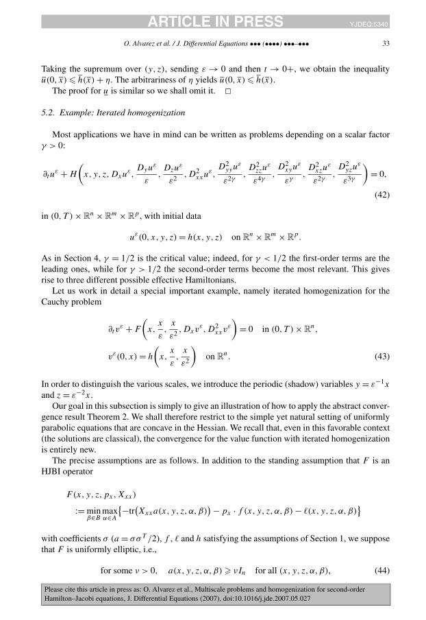
ARTICLE IN PRESS YJDEQ:5340JID:YJDEQ AID:5340 /FLA [m1+; v 1.73; Prn:10/07/2007; 12:43] P.33 (1-39)
O. Alvarez et al. / J. Differential Equations ••• (••••) •••–••• 33
Taking the supremum over (y, z), sending ε → 0 and then t → 0+, we obtain the inequalityu(0, x) � h(x) + η. The arbitrariness of η yields u(0, x) � h(x).
The proof for u is similar so we shall omit it. �5.2. Example: Iterated homogenization
Most applications we have in mind can be written as problems depending on a scalar factorγ > 0:
∂tuε + H
(x, y, z,Dxu
ε,Dyu
ε
ε,Dzu
ε
ε2,D2
xxuε,
D2yyu
ε
ε2γ,D2
zzuε
ε4γ,D2
xyuε
εγ,D2
xzuε
ε2γ,D2
yzuε
ε3γ
)= 0,
(42)
in (0, T ) × Rn × R
m × Rp , with initial data
uε(0, x, y, z) = h(x, y, z) on Rn × R
m × Rp.
As in Section 4, γ = 1/2 is the critical value; indeed, for γ < 1/2 the first-order terms are theleading ones, while for γ > 1/2 the second-order terms become the most relevant. This givesrise to three different possible effective Hamiltonians.
Let us work in detail a special important example, namely iterated homogenization for theCauchy problem
∂tvε + F
(x,
x
ε,
x
ε2,Dxv
ε,D2xxv
ε
)= 0 in (0, T ) × R
n,
vε(0, x) = h
(x,
x
ε,
x
ε2
)on R
n. (43)
In order to distinguish the various scales, we introduce the periodic (shadow) variables y = ε−1x
and z = ε−2x.Our goal in this subsection is simply to give an illustration of how to apply the abstract conver-
gence result Theorem 2. We shall therefore restrict to the simple yet natural setting of uniformlyparabolic equations that are concave in the Hessian. We recall that, even in this favorable context(the solutions are classical), the convergence for the value function with iterated homogenizationis entirely new.
The precise assumptions are as follows. In addition to the standing assumption that F is anHJBI operator
F(x, y, z,px,Xxx)
:= minβ∈B
maxα∈A
{−tr(Xxxa(x, y, z,α,β)
) − px · f (x, y, z,α,β) − �(x, y, z,α,β)}
with coefficients σ (a = σσT /2), f , � and h satisfying the assumptions of Section 1, we supposethat F is uniformly elliptic, i.e.,
for some ν > 0, a(x, y, z,α,β) � νIn for all (x, y, z,α,β), (44)
Please cite this article in press as: O. Alvarez et al., Multiscale problems and homogenization for second-orderHamilton–Jacobi equations, J. Differential Equations (2007), doi:10.1016/j.jde.2007.05.027
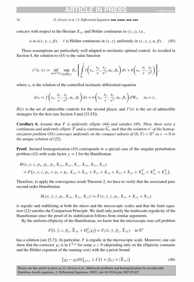
ARTICLE IN PRESS YJDEQ:5340JID:YJDEQ AID:5340 /FLA [m1+; v 1.73; Prn:10/07/2007; 12:43] P.34 (1-39)
34 O. Alvarez et al. / J. Differential Equations ••• (••••) •••–•••
concave with respect to the Hessian Xxx and Hölder continuous in (y, z), i.e.,
a ≡ a(x, y, z,β), � is Hölder continuous in (y, z), uniformly in (x, y, z,α,β). (45)
These assumptions are particularly well adapted to stochastic optimal control. As recalled inSection 4, the solution to (43) is the value function
vε(t, x) := infα∈Γ (t)
supβ∈B(t)
Ex
{ t∫0
�
(xs,
xs
ε,xs
ε2, αs, βs
)ds + h
(xt ,
xt
ε,xt
ε2
)},
where xs is the solution of the controlled stochastic differential equation
dxs = f
(xs,
xs
ε,xs
ε2, αs, βs
)ds + σ
(xs,
xs
ε,xs
ε2, αs, βs
)dWs, x0 = x,
B(t) is the set of admissible controls for the second player, and Γ (t) is the set of admissiblestrategies for the first (see Section 4 and [33,55]).
Corollary 6. Assume that F is uniformly elliptic (44) and satisfies (45). Then, there exist acontinuous and uniformly elliptic F and a continuous hs , such that the solution vε of the homog-enization problem (43) converges uniformly on the compact subsets of (0, T ) × R
n as ε → 0 tothe unique solution of (22).
Proof. Iterated homogenization (43) corresponds to a special case of the singular perturbationproblem (42) with scale factor γ = 1 for the Hamiltonian
H(x,y, z,px,py,pz,Xxx,Xyy,Xzz,Xxy,Xxz,Xyz)
= F(x, y, z,px + py + pz,Xxx + Xyy + Xzz + Xxy + Xxz + Xyz + XT
xy + XTxz + XT
yz
).
Therefore, to apply the convergence result Theorem 2, we have to verify that the associated puresecond-order Hamiltonian
Hs(x, y, z,px,Xxx,Xyy,Xzz) := F(x, y, z,px,Xxx + Xyy + Xzz)
is ergodic and stabilizing at both the micro and the mesoscopic scales and that the limit equa-tion (22) satisfies the Comparison Principle. We shall only justify the multiscale ergodicity of theHamiltonian since the proof of its stabilization follows from similar arguments.
By the uniform ellipticity of the Hamiltonian, we know that the microscopic true cell problem
F(x,y, z,px,Xxx + D2
zzχ2) = F1(x, y,px,Xxx) in R
n
has a solution (see [5,7]). In particular, F is ergodic at the microscopic scale. Moreover, one canshow that the corrector χ2 is in C2,ρ for some ρ > 0 (depending only on the ellipticity constantsand the Hölder exponent of the running cost) with the a priori bound∥∥χ2 − χ2(0)
∥∥2,ρ � C
(1 + |px | + |Xxx |
)(46)
Please cite this article in press as: O. Alvarez et al., Multiscale problems and homogenization for second-orderHamilton–Jacobi equations, J. Differential Equations (2007), doi:10.1016/j.jde.2007.05.027
C
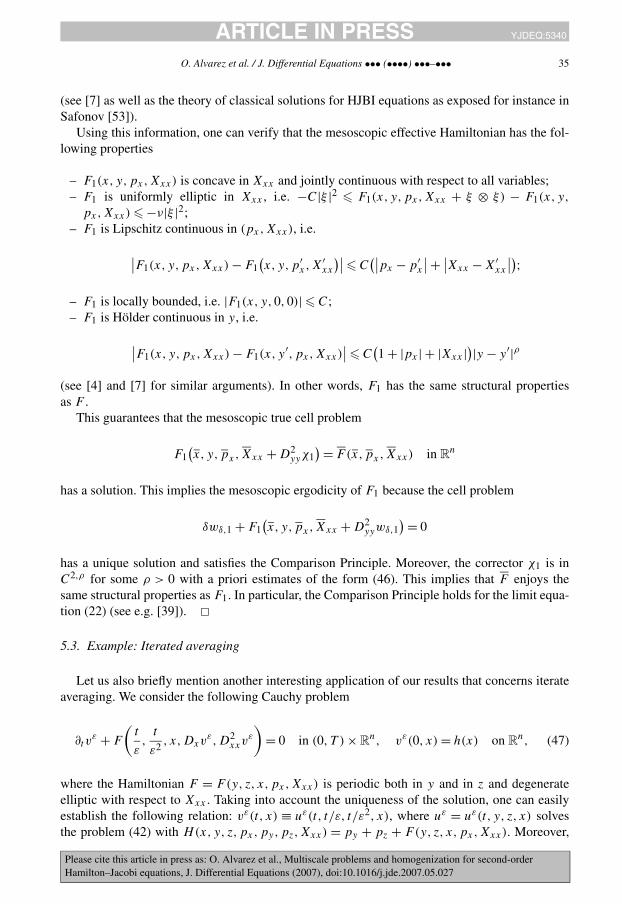
ARTICLE IN PRESS YJDEQ:5340JID:YJDEQ AID:5340 /FLA [m1+; v 1.73; Prn:10/07/2007; 12:43] P.35 (1-39)
O. Alvarez et al. / J. Differential Equations ••• (••••) •••–••• 35
(see [7] as well as the theory of classical solutions for HJBI equations as exposed for instance inSafonov [53]).
Using this information, one can verify that the mesoscopic effective Hamiltonian has the fol-lowing properties
– F1(x, y,px,Xxx) is concave in Xxx and jointly continuous with respect to all variables;– F1 is uniformly elliptic in Xxx , i.e. −C|ξ |2 � F1(x, y,px,Xxx + ξ ⊗ ξ) − F1(x, y,
px,Xxx) � −ν|ξ |2;– F1 is Lipschitz continuous in (px,Xxx), i.e.
∣∣F1(x, y,px,Xxx) − F1(x, y,p′
x,X′xx
)∣∣ � C(∣∣px − p′
x
∣∣ + ∣∣Xxx − X′xx
∣∣);– F1 is locally bounded, i.e. |F1(x, y,0,0)| � C;– F1 is Hölder continuous in y, i.e.
∣∣F1(x, y,px,Xxx) − F1(x, y′,px,Xxx)∣∣ � C
(1 + |px | + |Xxx |
)|y − y′|ρ
(see [4] and [7] for similar arguments). In other words, F1 has the same structural propertiesas F .
This guarantees that the mesoscopic true cell problem
F1(x, y,px,Xxx + D2
yyχ1) = F(x,px,Xxx) in R
n
has a solution. This implies the mesoscopic ergodicity of F1 because the cell problem
δwδ,1 + F1(x, y,px,Xxx + D2
yywδ,1) = 0
has a unique solution and satisfies the Comparison Principle. Moreover, the corrector χ1 is inC2,ρ for some ρ > 0 with a priori estimates of the form (46). This implies that F enjoys thesame structural properties as F1. In particular, the Comparison Principle holds for the limit equa-tion (22) (see e.g. [39]). �5.3. Example: Iterated averaging
Let us also briefly mention another interesting application of our results that concerns iterateaveraging. We consider the following Cauchy problem
∂tvε + F
(t
ε,
t
ε2, x,Dxv
ε,D2xxv
ε
)= 0 in (0, T ) × R
n, vε(0, x) = h(x) on Rn, (47)
where the Hamiltonian F = F(y, z, x,px,Xxx) is periodic both in y and in z and degenerateelliptic with respect to Xxx . Taking into account the uniqueness of the solution, one can easilyestablish the following relation: vε(t, x) ≡ uε(t, t/ε, t/ε2, x), where uε = uε(t, y, z, x) solvesthe problem (42) with H(x,y, z,px,py,pz,Xxx) = py + pz + F(y, z, x,px,Xxx). Moreover,
Please cite this article in press as: O. Alvarez et al., Multiscale problems and homogenization for second-orderHamilton–Jacobi equations, J. Differential Equations (2007), doi:10.1016/j.jde.2007.05.027
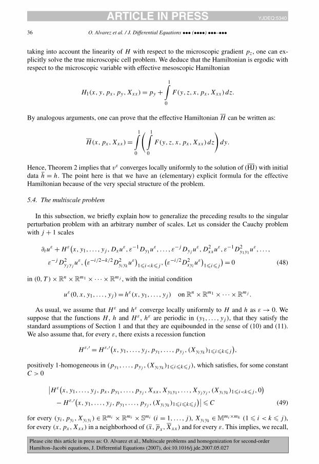
ARTICLE IN PRESS YJDEQ:5340JID:YJDEQ AID:5340 /FLA [m1+; v 1.73; Prn:10/07/2007; 12:43] P.36 (1-39)
36 O. Alvarez et al. / J. Differential Equations ••• (••••) •••–•••
taking into account the linearity of H with respect to the microscopic gradient pz, one can ex-plicitly solve the true microscopic cell problem. We deduce that the Hamiltonian is ergodic withrespect to the microscopic variable with effective mesoscopic Hamiltonian
H1(x, y,px,py,Xxx) = py +1∫
0
F(y, z, x,px,Xxx) dz.
By analogous arguments, one can prove that the effective Hamiltonian H can be written as:
H(x,px,Xxx) =1∫
0
( 1∫0
F(y, z, x,px,Xxx) dz
)dy.
Hence, Theorem 2 implies that vε converges locally uniformly to the solution of (HJ) with initialdata h = h. The point here is that we have an (elementary) explicit formula for the effectiveHamiltonian because of the very special structure of the problem.
5.4. The multiscale problem
In this subsection, we briefly explain how to generalize the preceding results to the singularperturbation problem with an arbitrary number of scales. Let us consider the Cauchy problemwith j + 1 scales
∂tuε + Hε
(x, y1, . . . , yj ,Dxu
ε, ε−1Dy1uε, . . . , ε−jDyj
uε,D2xxu
ε, ε−1D2y1y1
uε, . . . ,
ε−jD2yj yj
uε,(ε−i/2−k/2D2
yiykuε
)1�i<k�j
,(ε−i/2D2
xyiuε
)1�i�j
) = 0 (48)
in (0, T ) × Rn × R
m1 × · · · × Rmj , with the initial condition
uε(0, x, y1, . . . , yj ) = hε(x, y1, . . . , yj ) on Rn × R
m1 × · · · × Rmj .
As usual, we assume that Hε and hε converge locally uniformly to H and h as ε → 0. Wesuppose that the functions H , h and Hε , hε are periodic in (y1, . . . , yj ), that they satisfy thestandard assumptions of Section 1 and that they are equibounded in the sense of (10) and (11).We also assume that, for every ε, there exists a recession function
Hε,′ = Hε,′(x, y1, . . . , yj ,py1 , . . . , pyj, (Xyiyk
)1�i�k�j
),
positively 1-homogeneous in (py1 , . . . , pyj, (Xyiyk
)1�i�k�j ), which satisfies, for some constantC > 0
∣∣Hε(x, y1, . . . , yj ,px,py1 , . . . , pyj
,Xxx,Xy1y1 , . . . ,Xyj yj, (Xyiyk
)1�i<k�j ,0)
− Hε,′(x, y1, . . . , yj ,py1, . . . , pyj, (Xyiyk
)1�i�k�j
)∣∣ � C (49)
for every (yi,pyi,Xyiyi
) ∈ Rmi × R
mi × Smi (i = 1, . . . , j ), Xyiyk
∈ Mmi×mk (1 � i < k � j ),
for every (x,px,Xxx) in a neighborhood of (x,px,Xxx) and for every ε. This implies, we recall,
Please cite this article in press as: O. Alvarez et al., Multiscale problems and homogenization for second-orderHamilton–Jacobi equations, J. Differential Equations (2007), doi:10.1016/j.jde.2007.05.027
ARTICLE IN PRESS YJDEQ:5340JID:YJDEQ AID:5340 /FLA [m1+; v 1.73; Prn:10/07/2007; 12:43] P.37 (1-39)
O. Alvarez et al. / J. Differential Equations ••• (••••) •••–••• 37
that the Hamiltonian H has a recession function H ′ which is the uniform limit on the compactsets of Hε,′ as ε → 0.
Our ergodicity and stabilization assumptions are defined by induction. We set Hj = H andhj = h.
– Iterated ergodicity. For every i = j , . . . , 1, Hi is ergodic with respect to yi . We denote byHi−1 its effective Hamiltonian and we put H = H0.
Arguing as for the three-scale problem (Lemma 2), one can deduce from (49) that every ef-fective Hamiltonian Hi has a recession function H ′
i , that every H ′i is ergodic and that its effective
Hamiltonian is H ′i−1.
– Iterated stabilization. For every i = j , . . . , 1, we set
H ′′i := H ′
i (x, y1, . . . , yi,0, . . . ,0,pi,0, . . . ,0,Xyiyi,0).
The pair (H ′′i , hi) is stabilizing with respect to yi at each point (x, y1, . . . , yi−1). We denote
by hi−1 its effective initial data and we put h = h0.
As usual, the Cauchy problem (48) has exactly one continuous solution uε and the family {uε}is equibounded; so the weak semi-limits u and u are well defined.
Theorem 3. Under the above assumptions, the semi-limits u and u are, respectively, a subso-lution and a supersolution to problem (HJ). Furthermore, uε converges locally uniformly to thesolution of (HJ) provided that the effective Hamiltonian H satisfies the Comparison Principle.
The proof of the Theorem follows simply by induction and by using the arguments introducedfor the three-scale problem (Theorem 2). Since the modifications are only routine, we leave thedetailed proof to the reader.
Remark. The convergence result can be immediately extended to nonpower-like scales
∂tuε + Hε
(x, y1, . . . , yj ,Dxu
ε, ε−11 Dy1u
ε, . . . , ε−1j Dyj
uε,D2xxu
ε, ε−11 D2
y1y1uε, . . . ,
ε−1j D2
yj yjuε,
(ε−1/2i ε
−1/2k D2
yiykuε
)1�i<k�j
,(ε−1/2i D2
xyiuε
)1�i�j
) = 0.
The assumption is that ε := (ε1, . . . , εj ) tends to 0 in the sense that ε1 → 0 and εi/εi−1 → 0(i = 2, . . . , j ). Equation (48) is a particular case of the above equation, choosing εi = εi .
Acknowledgments
Olivier Alvarez was partially supported by the research project ACI-JC 1025 “Dislocationdynamics” of the French Ministry of Education.
Martino Bardi was partially supported by the research project “Viscosity, metric, and controltheoretic methods for nonlinear partial differential equations” of the Italian M.I.U.R.
Claudio Marchi was partially supported by the University of Padova (in particular by the‘Progetto Giovani ricercatori’ CPDG034579 “Homogenization in periodic (and nonperiodic)
Please cite this article in press as: O. Alvarez et al., Multiscale problems and homogenization for second-orderHamilton–Jacobi equations, J. Differential Equations (2007), doi:10.1016/j.jde.2007.05.027
ARTICLE IN PRESS YJDEQ:5340JID:YJDEQ AID:5340 /FLA [m1+; v 1.73; Prn:10/07/2007; 12:43] P.38 (1-39)
38 O. Alvarez et al. / J. Differential Equations ••• (••••) •••–•••
medium of fully nonlinear partial differential equations and applications to the stabilizationof singularly perturbed dynamical systems”) and by the RTN-Program “Fronts-Singularities”HPRN-CT-2002-00274 of the EU.
References
[1] G. Allaire, Homogenization and two-scale convergence, SIAM J. Math. Anal. 23 (1992) 1482–1518.[2] G. Allaire, M. Briane, Multiscale convergence and reiterated homogenisation, Proc. Roy. Soc. Edinburgh
Sect. A 126 (1996) 297–342.[3] O. Alvarez, Homogenization of Hamilton–Jacobi equations in perforated sets, J. Differential Equations 159 (1999)
543–577.[4] O. Alvarez, M. Bardi, Viscosity solutions methods for singular perturbations in deterministic and stochastic control,
SIAM J. Control Optim. 40 (2001) 1159–1188.[5] O. Alvarez, M. Bardi, Singular perturbations of nonlinear degenerate parabolic PDEs: A general convergence result,
Arch. Ration. Mech. Anal. 170 (2003) 17–61.[6] O. Alvarez, M. Bardi, Ergodic problems in differential games, in: S. Jorgensen, M. Quincampoix, T.L. Vincent
(Eds.), Advances in Dynamic Game Theory, in: Ann. Internat. Soc. Dynam. Games, vol. 9, Birkhäuser, Boston,2007, pp. 131–152.
[7] O. Alvarez, M. Bardi, Ergodicity, stabilization and singular perturbations for Bellman–Isaacs equations, Tech. re-port, University of Padova, 2007, available at http://cpde.iac.rm.cnr.it/ricerca.php.
[8] O. Alvarez, M. Bardi, C. Marchi, Multiscale singular perturbations and homogenization of optimal control prob-lems, in: F. Ancona, A. Bressan, P. Cannarsa, F.H. Clarke, P.R. Wolenski (Eds.), Geometric Control and NonsmoothAnalysis, in: Ser. Adv. Math. Appl. Sci., World Scientific Publishing, in press.
[9] O. Alvarez, H. Ishii, Hamilton–Jacobi equations with partial gradient and application to homogenization, Comm.Partial Differential Equations 26 (2001) 983–1002.
[10] M. Arisawa, Quasi-periodic homogenizations for second-order Hamilton–Jacobi–Bellman equations, Adv. Math.Sci. Appl. 11 (2001) 465–480.
[11] M. Arisawa, Y. Giga, Anisotropic curvature flow in a very thin domain, Indiana Univ. Math. J. 52 (2003) 257–281.[12] M. Arisawa, P.-L. Lions, On ergodic stochastic control, Comm. Partial Differential Equations 23 (1998) 2187–2217.[13] Z. Artstein, V. Gaitsgory, The value function of singularly perturbed control systems, Appl. Math. Optim. 41 (2000)
425–445.[14] M. Avellaneda, Iterated homogenization, differential effective medium theory and applications, Comm. Pure Appl.
Math. 40 (1987) 527–554.[15] M. Bardi, Homogenization of quasilinear elliptic equations with possibly superquadratic growth, in: A. Marino,
M.K.V. Murthy (Eds.), Nonlinear Variational Problems and Partial Differential Equations, Isola d’Elba, 1990, in:Pitman Res. Notes Math., vol. 320, Longman, Harlow, 1995, pp. 44–56.
[16] G. Barles, F. Da Lio, P.-L. Lions, P.E. Souganidis, Ergodic problems and periodic homogenization for fully nonlinearequations in half-space type domains with Neumann boundary conditions, preprint.
[17] A. Bensoussan, Perturbation Methods in Optimal Control, Wiley/Gauthiers–Villars, Chichester, 1988.[18] A. Bensoussan, L. Boccardo, F. Murat, Homogenization of elliptic equations with principal part not in divergence
form and Hamiltonian with quadratic growth, Comm. Pure Appl. Math. 39 (1986) 769–805.[19] A. Bensoussan, J.-L. Lions, G. Papanicolaou, Asymptotic Analysis for Periodic Structures, North-Holland, Ams-
terdam, 1978.[20] I. Birindelli, J. Wigniolle, Homogenization of Hamilton–Jacobi equations in the Heisenberg group, Comm. Pure
Appl. Anal. 2 (2003) 461–479.[21] M. Biroli, U. Mosco, N. Tchou, Homogenization for degenerate operators with periodical coefficients with respect
to the Heisenberg group, C. R. Acad. Sci. Paris Sér. I Math. 322 (1996) 439–444.[22] M. Biroli, U. Mosco, N. Tchou, Homogenization by the Heisenberg group, Adv. Math. Sci. Appl. 7 (1997) 809–831.[23] M. Biroli, C. Picard, N. Tchou, Homogenization of the p-Laplacian associated with the Heisenberg group, Rend.
Accad. Naz. Sci. XL Mem. Mat. Appl. 22 (1998) 23–42.[24] S. Brahim-Otsmane, G.A. Francfort, F. Murat, Correctors for the homogenization of the wave and heat equations,
J. Math. Pures Appl. 71 (1992) 197–231.[25] A. Braides, A. Defranceschi, Homogenizations of Multiple Integrals, Clarendon Press, Oxford, 1998.[26] R. Buckdahn, Y. Hu, S. Peng, Probabilistic approach to homogenization of viscosity solutions of parabolic PDEs,
NoDEA Nonlinear Differential Equations Appl. 6 (1999) 395–411.
Please cite this article in press as: O. Alvarez et al., Multiscale problems and homogenization for second-orderHamilton–Jacobi equations, J. Differential Equations (2007), doi:10.1016/j.jde.2007.05.027
ARTICLE IN PRESS YJDEQ:5340JID:YJDEQ AID:5340 /FLA [m1+; v 1.73; Prn:10/07/2007; 12:43] P.39 (1-39)
O. Alvarez et al. / J. Differential Equations ••• (••••) •••–••• 39
[27] R. Buckdahn, N. Ichihara, Limit theorems for controlled backward SDEs and homogenization of Hamilton–Jacobi–Bellman equations, Appl. Math. Optim. 51 (2005) 1–33.
[28] L.A. Caffarelli, A note on nonlinear homogenization, Comm. Pure Appl. Math. 52 (1999) 829–838.[29] L.A. Caffarelli, P.E. Souganidis, L. Wang, Homogenization of fully nonlinear, uniformly elliptic and parabolic
partial differential equations in stationary ergodic media, Comm. Pure Appl. Math. 58 (2005) 319–361.[30] M.G. Crandall, H. Ishii, P.-L. Lions, User’s guide to viscosity solutions of second order partial differential equations,
Bull. Amer. Math. Soc. (N.S.) 27 (1992) 1–67.[31] L. Evans, The perturbed test function method for viscosity solutions of nonlinear P.D.E., Proc. Roy. Soc. Edinburgh
Sect. A 111 (1989) 359–375.[32] L. Evans, Periodic homogenisation of certain fully nonlinear partial differential equations, Proc. Roy. Soc. Edin-
burgh Sect. A 120 (1992) 245–265.[33] W.H. Fleming, P.E. Souganidis, On the existence of value functions of two-players, zero-sum stochastic differential
games, Indiana Univ. Math. J. 38 (1989) 293–314.[34] B. Franchi, M.C. Tesi, Two-scale homogenization in the Heisenberg group, J. Math. Pures Appl. 81 (2002) 495–532.[35] J. García-Azorero, C.E. Gutiérrez, I. Peral, Homogenization of quasilinear parabolic equations in periodic media,
Comm. Partial Differential Equations 28 (2003) 1887–1910.[36] K. Horie, H. Ishii, Homogenization of Hamilton–Jacobi equations on domains with small scale periodic structure,
Indiana Univ. Math. J. 47 (1998) 1011–1058.[37] K. Ichihara, H. Kunita, A classification of the second order degenerate elliptic operators and its probabilistic char-
acterization, Z. Wahrsch. Verw. Geb. 30 (1974) 235–254.[38] H. Ishii, Almost periodic homogenization of Hamilton–Jacobi equations, in: B. Fiedler (Ed.), International Confer-
ence on Differential Equations, Proceedings of the Conference, vol. 1, Equadiff ’99, Singapore, World Scientific,2000, pp. 600–605.
[39] H. Ishii, P.-L. Lions, Viscosity solutions of fully nonlinear second-order elliptic partial differential equations, J. Dif-ferential Equations 83 (1990) 26–78.
[40] R. Jensen, P.-L. Lions, Some asymptotic problems in fully nonlinear elliptic equations and stochastic control, Ann.Scuola Norm. Sup. Pisa Cl. Sci. (4) 11 (1984) 129–176.
[41] V.V. Jikov, S.M. Kozlov, O.A. Oleinik, Homogenization of Differential Operators and Integral Functionals,Springer-Verlag, Berlin, 1994.
[42] Y. Kabanov, S. Pergamenshchikov, Two-Scale Stochastic Systems. Asymptotic Analysis and Control, Springer-Verlag, Berlin, 2003.
[43] M.A. Katsoulakis, A representation formula and regularizing properties for viscosity solutions of second-order fullynonlinear degenerate parabolic equations, Nonlinear Anal. 24 (1995) 147–158.
[44] H.J. Kushner, Weak Convergence Methods and Singularly Perturbed Stochastic Control and Filtering Problems,Birkhäuser, Boston, 1990.
[45] J.-L. Lions, D. Lukkassen, L.E. Persson, P. Wall, Reiterated homogenization of nonlinear monotone operators,Chinese Ann. Math. Ser. B 22 (2001) 1–12.
[46] P.-L. Lions, G. Papanicolaou, S.R.S. Varadhan, Homogenization of Hamilton–Jacobi equations, unpublished, 1986.[47] P.-L. Lions, P.E. Souganidis, Homogenization of degenerate second-order PDE in periodic and almost periodic
environments and applications, Ann. Inst. H. Poincaré Anal. Non Linéaire 22 (2005) 667–677.[48] P.-L. Lions, P.E. Souganidis, Homogenization of “viscous” Hamilton–Jacobi equations in stationary ergodic media,
Comm. Partial Differential Equations 30 (2005) 335–375.[49] D. Lukkassen, Reiterated homogenization of nonstandard Lagrangians, C. R. Acad. Sci. Paris Sér. I Math. 332
(2001) 999–1004.[50] C. Marchi, Homogenization for fully nonlinear parabolic equations, Nonlinear Anal. 60 (2005) 411–428.[51] E. Pardoux, Homogenization of linear and semi-linear second order parabolic PDEs with periodic coefficients:
A probabilistic approach, J. Funct. Anal. 167 (1999) 498–520.[52] F. Rezakhanlou, J.E. Tarver, Homogenization for stochastic Hamilton–Jacobi equations, Arch. Ration. Mech.
Anal. 151 (2000) 277–309.[53] M.V. Safonov, On the classical solution of nonlinear elliptic equations of second-order, Math. USSR Izv. 33 (1989)
597–612; Engl. transl.: Izv. Akad. Nauk SSSR Ser. Mat. 52 (1988).[54] P.E. Souganidis, Stochastic homogenization of Hamilton–Jacobi equations and some applications, Asymptot.
Anal. 20 (1999) 1–11.[55] A. Swiech, Another approach to the existence of value functions of stochastic differential games, J. Math. Anal.
Appl. 204 (1996) 884–897.[56] L. Tartar, An introduction to the homogenization method in optimal design, in: Optimal Shape Design, Tróia, 1998,
Springer-Verlag, Berlin, 2000, pp. 47–156.
Please cite this article in press as: O. Alvarez et al., Multiscale problems and homogenization for second-orderHamilton–Jacobi equations, J. Differential Equations (2007), doi:10.1016/j.jde.2007.05.027
![u i(x)-h - Princeton Universityweinan/s/homogenization.pdf · has already been studied by Lions, Papanicolaou, and Varadhan in [10]. Naturally, in (1.2), we assume that H(y,p) is](https://img.pdfslide.us/doc/110x75/5ae5fc347f8b9a6d4f8c0ca0/u-ix-h-princeton-university-weinanshomogenizationpdfhas-already-been-studied.jpg)
![Master Thesis Nguyen Tien Thinh - This problem was introduced in [5] by P.L. Lions, G. Papanicolaou and S.R.S. Varadhan in 1986. ... Lions in 1983 regarding the Hamilton-Jacobi equation](https://img.pdfslide.us/doc/110x75/5ae5fc347f8b9a6d4f8c0cd7/master-thesis-nguyen-tien-thinh-problem-was-introduced-in-5-by-pl-lions-g.jpg)


![AUBRY-MATHER MEASURES IN THE NON CONVEX … · to Lions, Papanicolaou and Varadhan. Theorem 1.2 (See [LPV88]). Let H: Tn ×Rn → R be smooth such that lim ... AUBRY-MATHER MEASURES](https://img.pdfslide.us/doc/110x75/5ae5fc347f8b9a6d4f8c0cc8/aubry-mather-measures-in-the-non-convex-lions-papanicolaou-and-varadhan-theorem.jpg)


![Some Inverse Problems in Periodic Homogenization of ... · It was proved by Lions, Papanicolaou and Varadhan [16] that u](https://img.pdfslide.us/doc/110x75/5ae5fc347f8b9a6d4f8c0cc4/some-inverse-problems-in-periodic-homogenization-of-was-proved-by-lions-papanicolaou.jpg)


![Andrew Papanicolaou arXiv:1504.05309v1 [q-fin.MF] 21 Apr 2015](https://img.pdfslide.us/doc/110x75/6181f75658c0cf0e30341b85/andrew-papanicolaou-arxiv150405309v1-q-finmf-21-apr-2015.jpg)
