Eigenvalue filtering in VAR models with application to the Czech

WORKING PAPER SER IESNO. 549 / NOVEMBER 2005

EIGENVALUE FILTERING IN VAR MODELS WITH APPLICATION TO THE CZECH BUSINESS CYCLE

by Jaromír Benešand David Vávra

In 2005 all ECB publications will feature

a motif taken from the

€50 banknote.

WORK ING PAPER S ER I E SNO. 549 / NOVEMBER 2005

This paper can be downloaded without charge from http://www.ecb.int or from the Social Science Research Network

electronic library at http://ssrn.com/abstract_id=839231.

EIGENVALUE FILTERING IN VAR MODELS WITH APPLICATION TO THE

CZECH BUSINESS CYCLE

by Jaromír Beneš 1

and David Vávra 2

1 Czech National Bank, Monetary and Statistics Department, e-mail: [email protected] Czech National Bank, Monetary and Statistics Department, e-mail: [email protected]

© European Central Bank, 2005

AddressKaiserstrasse 2960311 Frankfurt am Main, Germany

Postal addressPostfach 16 03 1960066 Frankfurt am Main, Germany

Telephone+49 69 1344 0

Internethttp://www.ecb.int

Fax+49 69 1344 6000

Telex411 144 ecb d

All rights reserved.

Any reproduction, publication andreprint in the form of a differentpublication, whether printed orproduced electronically, in whole or inpart, is permitted only with the explicitwritten authorisation of the ECB or theauthor(s).

The views expressed in this paper do notnecessarily reflect those of the EuropeanCentral Bank.

The statement of purpose for the ECBWorking Paper Series is available fromthe ECB website, http://www.ecb.int.

ISSN 1561-0810 (print)ISSN 1725-2806 (online)

3ECB

Working Paper Series No. 549November 2005

CONTENTS

Abstract 4

Non-technical summary 5

1 Introduction 7

2 Canonical state-space representationof VAR models 9

3 Eigenvalue filtering 11

4 Structural identification 14

5 Application to the Czech business cycle 16

6 Estimation and simulation results 17

7 Concluding remarks 20

References 21

Tables and figures 23

European Central Bank working paper series 31

Abstract

We propose the method of eigenvalue filtering as a new tool to extract time series subcom-ponents (such as business-cycle or irregular) defined by properties of the underlying eigen-values. We logically extend the Beveridge-Nelson decomposition of the VAR time-seriesmodels focusing on the transient component. We introduce the canonical state-space repre-sentation of the VAR models to facilitate this type of analysis. We illustrate the eigenvaluefiltering by examining a stylized model of inflation determination estimated on the Czechdata. We characterize the estimated components of CPI, WPI and import inflations, togetherwith the real production wage and real output, survey their basic properties, and impose anidentification scheme to calculate the structural innovations. We test the results in a sim-ple bootstrap simulation experiment. We find two major areas for further research: first,verifying and improving the robustness of the method, and second, exploring the method’spotential for empirical validation of structural economic models.

Key words: business cycle, inflation, eigenvalues, filtering, Beveridge-Nelsondecomposition, time series analysisJEL Classification: C32, E32

4ECBWorking Paper Series No. 549November 2005

This working paper develops a methodology for time series decomposition based onthe Beveridge and Nelson (BN) framework, and applies it to the Czech data. It addsto the existing empirical filtering literature that has so far, especially as concerns theCzech experience, seemed to prefer the unobserved components (UC) methodology.The BN decompositions have the advantage of imposing less economic and iden-tification restrictions on the underlying series; the uncovered cycles and trends aretherefore more driven by the data themselves. This methodology then appears a use-ful complement to the UC techniques based usually on an a priori theoretical model.Cross-checking the results from the two types of methods can lead to a more robustassessment of the cyclical position of the economy to the benefit of monetary pol-icy making. In addition, the application of the BN methodology can give additionalinsight into the workings of the economy at specific moments of its history. As a fur-ther extension of this research, the BN methodology can be more useful in empiricalvalidation of DSGE models than more often used UC based approaches.

The standard BN methodology decomposes time series (or vectors of them) intotheir trend and transient components by identifying permanent and temporary effectsof random innovations (shocks). The transient components may, however, contain(apart from the business cycle) also irregular or highly volatile fluctuations. In or-der to facilitate the economic interpretation, we therefore further decompose thesetransient elements into their business-cycle and irregular parts by imposing certaineigenvalue restrictions corresponding to some definition of the business cycle. Themethod can be easily generalized to define and extract any other desired types of timeseries components.

We apply the multivariate eigenvalue filtering to extract the trend, business-cycleand irregular components from a set of measures of Czech inflation and real eco-nomic activity in order to investigate the workings of the economy typified by stylizedPhillips curve mechanics. For that purpose we combine net CPI inflation, industrialWPI inflation, import price inflation, the real production wage in the business sector,and real gross domestic product. The last two measures should capture movementsin the real marginal cost of domestic value added. The robustness of the results ischecked in a bootstrap simulation experiment.

Our empirical analysis yields several important conclusions. Overall, we find evi-dence favoring the hypothesis of a) faster import price and exchange rate pass-throughinto domestic producer prices than directly into those of domestic consumers, b) ofthe nominal wage being more sticky than the nominal price, as real wage changes areinduced by movements in the underlying price indices. This is especially illuminatingin the period of 2000 and 2001, when import prices were rapidly changing. The expe-

5ECB


Non-technical Summary

rience from this period hints at substantial technology or labor supply (intratemporalpreference) shocks. Importantly, a Phillips curve type of relationship is detected, asthe behavior of the permanent components fails to exhibit strong signs of super neu-trality, with disinflation having negative effects on real variables. However, the realmarginal cost concept hypothesized in the Phillips curve in our working paper yieldscounterintuitive results, namely an inverse effect of real output on the one hand andthe real wage on the other hand into the CPI and WPI, and needs to be further refined.

Last, the overall statistical properties of the eigenvalue filtering need to be subjectof further research, especially the robustness checks, as they tend to display a signifi-cant skewness.


1 Introduction

In this paper we develop the eigenvalue filtering methodology for decomposition ofthe VAR time-series models, and apply the method to the Czech data. By develop-ing and applying this technique based on the original multivariate Beveridge-Nelson(BN) framework 1 we add to the existing empirical filtering literature that has so farpreferred in the monetary policy context the unobserved component (UC) methodol-ogy (and especially so in applications on the Czech economy). As the BN decomposi-tions are less restrictive and more driven by the data themselves, they appear a usefulcomplement to the UC techniques based usually on an a priori theoretical model. 2

Cross-checking results from the two types of methods can lead to a more robust as-sessment of the cyclical position of the economy to the benefit of monetary policymaking. In addition, the application of the BN methodology can give additional in-sight into the workings of the economy at specific moments of its history and, inturn, can be useful for empirical validation of dynamic stochastic general equilibriummodels (DSGE), as claimed in Section 3.

Extracting the cyclical and trend components from observed time series has be-come an increasingly important activity at central banks in the last decade, especiallyas many of them have moved towards more or less explicit inflation targeting regimes.The medium-term focus of this type of monetary policy in particular raises demandsfor a good understanding of business cycle mechanisms and for robust knowledge ofthe current business cycle position of the economy, especially as regards the cycli-cal fluctuations and interactions between inflation and real economic activity. Cor-respondingly, many central bank researchers have recently been preoccupied withmultivariate techniques that explore these economic relationships, but are simultane-ously more immune to the common (e.g. end-point) problems of many mechanicalfilters. As a product, a suite of structural multivariate UC models have been createdat many of these banks to support forecasting and policy analysis systems, particu-larly focused on identifying the cycles in real output, the real exchange rate, the realinterest rate, and the real marginal costs of producers.

The relative neglect of the BN approaches is in this regard rather unfortunate, giventhe extra insight that can be learnt from comparing the two approaches noted above.Moreover, we argue here, this neglect is bound to change, as many of the centralbanks increasingly experiment with using DSGE models in their forecasting systems.

1 See Beveridge and Nelson (1981) and Engle and Granger (1987).2 Morley, Nelson, and Zivot (2003) show that the usually encountered differences in theresults of the BN and UC decompositions mainly arise not because of some principal incon-sistency of the two methods but rather because of substantial differences in the additionalunderlying identification assumptions.

7ECB


Applying these models to data requires a very good distinction between real (supply)and nominal (demand) shocks. It is here where the flexibility of the BN techniquesin describing the co-movements between trend and cyclical components is helpful.Whereas real shocks will in general be associated with their negative correlation (aslong-run productivity fundamentals improve, the actual output catches up only grad-ually), no correlation should be expected for nominal shocks (that raise, say, outputtemporarily above the long-run trend). In this paper we further develop this flexibilityby removing irregular or erratic fluctuations from the observed data, thereby focusingthe decomposition only on the frequencies that are subject of the DSGE modeling.The recovered cycle and trend properties of data can then be used for empirical vali-dation of these models.

In this paper we develop and apply a BN-based multivariate eigenvalue filteringmethod to extract the trend, business-cycle and irregular components from a set ofmeasures of Czech inflation and real economic activity in order to investigate theworkings of the economy typified by stylized Phillips curve mechanics in a smallopen economy. We thus illustrate the potential of the BN approach in understandingthe nature of economic business cycle, both in theory and in application to the Czechdata.

This approach is intended to complement the existing vast stock of experience inusing UC filtering techniques in research and monetary policy inference in the CzechNational Bank, which is documented inter alia by Coats, Laxton, and Rose (2003)and Benes and N’Diaye (2004). Transition towards using more BN based techniquesis taking place against the backdrop of introducing a DSGE model as the new coreforecasting tool of the Bank. Given the same theoretical foundations of the two tech-niques, such a transition should be viewed as a smooth learning process, rather thana discontinuous new practice.

The paper is organized as follows. In Section 2 we review the Beveridge-Nelsonpermanent-transient decomposition in the vector moving-average and common-trendsframeworks, and introduce the canonical state-space representation as a convenientdevice to deal with the VAR models. We extend the Beveridge-Nelson concept in Sec-tion 3 focusing on the filtering of the transient component based on the propertiesof the underlying eigenvalues. In Section 4 we discuss the structural identification inthe canonical state-space framework based on long-run recursiveness. We apply theeigenvalue filtering method and the proposed structural identification scheme to anempirical model of the Czech business cycle with a set of measures of Czech infla-tion and real economic activity, examine their economic and stochastic properties,and verify the method in a simple bootstrap simulation experiment in Sections 5 and6. Section 7 concludes.


2 Canonical state-space representation of VAR models

The subject of our interest is finite-order autoregressive models for vector processes(VAR models) in which the deterministic part has been removed prior to the analysis,

A(L)yt = εt , A(L) = In−∑pi=1 Ak Li, (1)

where yt is an n-dimensional random vector, εt is an i.i.d. a vector of the linear forecasterror with mean of zero and covariance matrix Ω, L is the lag operator, and 0 < p < ∞.We furthermore restrict ourselves to vector processes whose elements are integratedof order 0 or 1 or cointegrated of order (1,1) as defined by Johansen (1995). Finally,we only allow for the zero-frequency unit roots excluding hence the seasonal integra-tion and cointegration for ease of the exposition. We therefore impose the followingconditions adopted from Johansen (1995) and extended to cover the two limit cases[i.e. I(0) models, or I(1) models without cointegration]:

(i) rankA(1) = r where 0≤ r ≤ n,(ii) the inverse characteristic equation |In λ p−∑p

k=1 Ak λ p−k| = 0 has n− r rootsequal to 1 and all other roots inside the unit circle, |λ |< 1.

We use the term VAR to refer to such processes (1) that satisfy Conditions (i) and (ii)throughout the paper.

Our primary objective is to extend the concept of the Beveridge-Nelson decompo-sition 3 focusing on the properties of the transient component. More specifically, theVAR process has the Wold, or vector moving-average (VMA), representation,

∆yt = C(L)εt ,

which can be further re-written as

yt = C(1)∑∞i=0 εt−i +C?(L)εt , (2)

to establish the multivariate Beveridge-Nelson permanent-transient decomposition,see e.g. Engle and Granger (1987), where C(1), the “factor loading” matrix, has rankk = n− r corresponding to the number of independent stochastic trends that underliepermanent movements in yt , whereas C?(L) = ∑∞

i=0C?i Li is an absolutely summable

generating function, ∑∞i=0 |C?

i | < ∞, which produces transient stationary fluctuationsof the process around these trends. However, a more convenient representation tocompare our work with is the common trends (CT) form introduced by Stock andWatson (1988), or alternatively by King, Plosser, Stock, and Watson (1987),

yt = Fyt + yt such that (1−L)yt = Gηt , yt = D(L)ηt , (3)

3 See Beveridge and Nelson (1981) for the treatment of univariate models.

9ECB


where yt is an k-dimensional vector of common trends, yt is an n-dimensional vec-tor of transient components, F is an n× k matrix of rank k, D(L) is again an ab-solutely summable generating function, and some structural identification scheme isimposed on the reduced-form innovations such that ηt = Ω−1/2εt , Eηtη ′t = In, withΩ1/2 Ω1/2′ = Ω. The structural identification is discussed in detail in a separate sec-tion.

In our analysis, we convert the VAR model to its state-space representation basedon the Jordan canonical factorization of the system transition matrix, and term this asthe canonical state-space (CSS) form. We show that within the VAR models the CSS

representation is useful as a starting point for calculating the two other ones above andconvenient for further examination and decomposition of the process, yt , that we latercall the eigenvalue filtering. Note that when adopting the state-space representationwe deal with the process in levels following therefore the approach of Casals, Jerez,and Sotoca (2002) rather than Proietti (1997). We start from the first-order companionform

yt = H Yt , Yt = T Yt−1 +H ′εt , (4)

with the vector of stacked observations Yt = [y′t . . . y′t−p+1]′, the selection matrix

H = [In 0n . . . 0n], and the system transition matrix

T =

A1 . . .Ap

Im 0m×n

,

where m = n(p−1), by calculating T = P−1ΛP, where P is a matrix whose columnsare T ’s eigenvectors, and Λ is a diagonal matrix of T ’s eigenvalues. 4 We then obtainthe CSS representation for (1),

yt = P1xt , xt = Λxt−1 +P1εt , (5)

with Pxt = Yt , P1 = HP, and P1 = P−1H ′, which partitions P and P−1 conformablywith H as P = [P1

′ P2′]′ and P−1 = [P1 P2] so that P1 and P1 are respectively n×np

and np×n blocks.Assuming without loss of generality that the eigenvalues in Λ occur in descending

order by their moduli, partitioning Λ so that the leading k× k block is an identitymatrix, Λ = Ik, whereas the remaining diagonal block, denoted by Λ, contains theother eigenvalues, and partitioning furthermore P1 and P1 conformably with these

4 The eigenvalues associated with T are obviously identical to the roots of the inverse char-acteristic equation in Condition (ii), see e.g. Lutkepohl (1993) for a proof.


blocks so that P1 = [P1 P1] and P1 = [P1′ P1′]′, we may easily calculate both the VMA

representation (2),

C(1) = P1 P1, C?(L) = P1(Inp−k− ΛL)−1 P1,

where the existence of the inverse in the latter term is guaranteed by construction, andthe CT representation (3),

F = P1, G = P1 Ω1/2, D(L) = P1(Inp−k− ΛL)−1 P1 Ω1/2.

based again on a particular identification scheme Ω1/2.Finally, we examine the implications of the existence of cointegrating and/or serial-

correlation cofeature vectors for the CSS representation. First note that the definitionsof cointegration and common features relate to truly I(1) models, in other words tothose where at least one element of yt is I(1). 5 We therefore impose such a restrictionin the remainder of this section.

Following inter alia Vahid and Engle (1993), a vector β is called a cointegratingvector if β ′yt is I(0); similarly, a vector γ is called a serial-correlation cofeature vectorif γ ′∆yt is orthogonal to all observed information prior to t (random walk). The latteris in fact only the strong-form reduced-rank structure as recognized by Hecq, Palm,and Urbain (2000), but we skip the weak form here. Clearly, β must lie in the left-null space of P1P1, whereas γ in the overlap of the left-null spaces of the individualmatrices defining the generating function C?(L) = P1(Inp−k − ΛL)−1 P1. However,noting that γ must be therefore necessarily orthogonal to C?(0) = P1P1, and that byconstruction P1P1 + P1P1 = In, we conclude that beacuse γ ′P1P1 = In, γ lies in thespace spanned by the eigenvectors associated with the unit eigenvalues of P1P1.

3 Eigenvalue filtering

In the light of the CSS representation the Beveridge-Nelson decomposition can beindeed viewed as extraction of components that are defined by the eigenvalues, or bycertain properties of the eigenvalues, that carry these components. More specifically,the permanent-transient decomposition in the VAR models is given by the following

5 See Definitions 3.1–3.2 in Johansen (1995).

11ECB


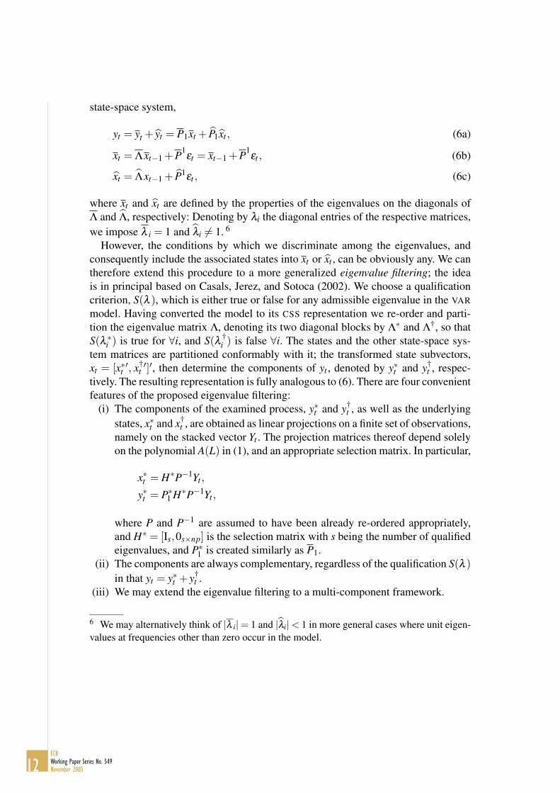
state-space system,

yt = yt + yt = P1xt + P1xt , (6a)

xt = Λxt−1 +P1εt = xt−1 +P1εt , (6b)

xt = Λxt−1 + P1εt , (6c)

where xt and xt are defined by the properties of the eigenvalues on the diagonals ofΛ and Λ, respectively: Denoting by λi the diagonal entries of the respective matrices,we impose λ i = 1 and λi 6= 1. 6

However, the conditions by which we discriminate among the eigenvalues, andconsequently include the associated states into xt or xt , can be obviously any. We cantherefore extend this procedure to a more generalized eigenvalue filtering; the ideais in principal based on Casals, Jerez, and Sotoca (2002). We choose a qualificationcriterion, S(λ ), which is either true or false for any admissible eigenvalue in the VAR

model. Having converted the model to its CSS representation we re-order and parti-tion the eigenvalue matrix Λ, denoting its two diagonal blocks by Λ∗ and Λ†, so thatS(λ ∗i ) is true for ∀i, and S(λ †

i ) is false ∀i. The states and the other state-space sys-tem matrices are partitioned conformably with it; the transformed state subvectors,xt = [x∗t ′, x†

t′]′, then determine the components of yt , denoted by y∗t and y†

t , respec-tively. The resulting representation is fully analogous to (6). There are four convenientfeatures of the proposed eigenvalue filtering:

(i) The components of the examined process, y∗t and y†t , as well as the underlying

states, x∗t and x†t , are obtained as linear projections on a finite set of observations,

namely on the stacked vector Yt . The projection matrices thereof depend solelyon the polynomial A(L) in (1), and an appropriate selection matrix. In particular,

x∗t = H∗P−1Yt ,

y∗t = P∗1 H∗P−1Yt ,

where P and P−1 are assumed to have been already re-ordered appropriately,and H∗ = [Is,0s×np] is the selection matrix with s being the number of qualifiedeigenvalues, and P∗1 is created similarly as P1.

(ii) The components are always complementary, regardless of the qualification S(λ )in that yt = y∗t + y†

t .(iii) We may extend the eigenvalue filtering to a multi-component framework.

6 We may alternatively think of |λ i|= 1 and |λi|< 1 in more general cases where unit eigen-values at frequencies other than zero occur in the model.


(iv) Since the filtering is described by a state-space system we may easily drawinferences about the stochastic properties of the filtered components in both thetime and frequency domains.

The eigenvalue qualification can have a potentially strong economic interpretation.The most striking example is a further filtering of the classical Beveridge-Nelsontransient component aimed at extracting some more systematic, business-cycle, fluc-tuations from yt that are net of irregular or erratic noise. As there is no unique agreeddefinition of the business cycle (or, equivalently, of the irregular noise) we use thetraditional one dating back to Burns and Mitchell (1946) and ascribe to the businesscycle only those fluctuations that last between 6 and 32 quarters. In terms of theeigenvalue qualification we propose the following two criteria:

(i) [Magnitude qualification] The business-cycle eigenvalue induces an impulse re-sponse of which not less than 10 % survives in the 6th quarter and not more than90 % in the 32nd quarter.

(ii) [Phase angle qualification] The business-cycle eigenvalue induces an impulseresponse with periodicity of 6 or more quarters. 7

These two conditions need to hold simultaneously for an eigenvalue to qualify asa business-cycle one. The former one leads to a range of approximately [0.68, 0.93]for the moduli of a quarterly model’s eigenvalues while the latter to a range of [−π

3 , π3 ]

for their phase angles. The qualification region within the unit circle is depicted as ashadow area in Figure 1. 8

We find the eigenvalue filtering framework potentially appealing especially in thearea of empirical validation of structural, say DSGE, models. These models usuallyclaim to explain only certain dimensions of the observed data, 9 or even their popula-tion moments. To this end, the eigenvalue filtering may provide an econometricallyrelevant empirical counterpart to the examined model properties, net of those fac-tors in the data generating process that are clearly beyond the model’s scope, such ashighly volatile or erratic—say non-fundamental—fluctuations in prices or financial

7 There is no upper bound imposed on the periodicity because we want the real, appropriatelyscaled, eigenvalues to qualify as the business-cycle ones too.8 Note, however, that the properties of the business-cycle components obtained from theeigenvalue filtering differ essentially from those computed by the the band-pass, or frequency-selective, filters proposed recently in the macroeconomics literature by Baxter and King(1999) or Christiano and Fitzgerald (2003). An ideal band-pass filter would entirely cut offthe higher and lower frequencies in the spectrum of the desired business-cycle componentwhereas the eigenvalue-filter business-cycle components will always display continuous non-zero spectra over the whole range [0, π].

13ECB


markets indicators.

4 Structural identification

With an estimated VAR converted to its CSS form we need to impose additional restric-tions to identify the structural innovations, denoted by ηt , from the forecast errors, εt ,and hence to make inferences about the impulse responses of yt or its eigenvalue-filtered components, and about the corresponding variance decomposition. For futurereference we denote by Ψη the matrix of the permanent effect of ηt on yt , which isΨη = P1P1S, where Sηt = εt . 10

Our scheme to identify S is similar to the one used by King, Plosser, Stock, andWatson (1991), 11 in that we make the following identifying assumptions:

(i) the structural innovations are mutually uncorrelated and have unit variances:Eηtηt

′ = In,(ii) the structural innovations lie in the space spanned by the current and lagged

observations: Sηt = εt where S is nonsingular,(iii) the number of the structural innovations with a permanent effect on yt equals the

number of underlying stochastic trends, and their effect has a recursive struc-ture: Ψη = [Ψη

1 0n×(n−k)] where Ψη is an n× k lower triangular matrix.Note that Assumptions (i) to (iii) properly identify only the permanent structural in-novations. The transient innovations can be, however, identified using the otherwisestandard results from the VAR literature, i.e. by assuming certain recursiveness of theirinstantaneous effect on yt . This can be performed as an extra step in the proceduresuggested herein.

Our calculation of S and ηt involves the QR factorizations; this has been origi-nally proposed by Hoffmann (2001) for the vector error-correction representations.Accordingly we proceed in three steps:1. We arbitrarily pre-orthonormalize the forecast errors, e.g. by the Cholesky factor

of their covariance matrix, denoting these newly created innovations by ξ t ,

Kξ t = εt , K K ′ = Ω,

which produces Eξ tξ t′ = In. In the subsequent steps we only rotate the innovations

by unitary matrices, and preserve thus the covariance matrix In: EMξ tξ t′M ′ =

9 In this regard, Geweke (1999) provides formal definitions of the so-called weak and mini-mal econometric interpretations of the DSGE models.10 The permanent effect is of course transmitted through na instantaneous effect of ηt on xt asthe latter are random walks.11 Cf. Appendix therein.


M In M ′ = In for any M M ′ = In.2. We separate the permanent and transient innovations. Recall that an innovation is

permanent if and only if it immediately affects xt , and is transient if and only ifit fails to do so. Clearly, the instantaneous multipliers for the entire state vector xtwith respect to ξ t are given by the matrix Φξ = P1K. We may now partition thisas

Φξ =

Φξ

1

Φξ2

, conformably with the number of stochastic trends k so that the upper block Φξ1 is

k×n, and find the QR factors of its transpose,

Φξ1 = R ′Q ′,

where Q is an n× n matrix such that QQ ′ = In and R is an n× k matrix suchthat R′ is lower triangular with zeros in its last n− k columns. The matrix Q isnow a suitable basis for a transformation which gives rise to two subvectors ofinnovations, permanent and transient. Letting Qν t = ξ t we compute the effect ofν t on xt , denoted by Φν , as follows:

Φν = Φξ Q =

R ′Q ′

Φξ2

Q =

R ′

Φξ2 Q

,

so that the first k elements of xt , i.e. the subvector xt , are only affected by the firstk elements of ν t , denoted hence by ν t . In other words, ν t are permanent whilethe remainder of ν t is only transient with respect to their respective impacts on yt .Consequently,

Ψν = P1R ′ =[Ψν

, 0n×(n−k)

].

Note that whenever the VAR model is not cointegrated, k = n, we simply skip Step2 since permanent are all innovations by Assumption (iii).

3. Finally, we find the desired structural innovations, ηt , to achieve a recursive struc-ture of their permanent effect. This is accomplished by another QR factorizationof the transpose of Ψν = U ′Z ′ which yields a unitary k× k matrix Z, and a k×nmatrix U such that U ′ is lower triangular. We define η by a diagonal matrix com-

15ECB


posed of Z and an identity In−k,

Z ηt = νt , Z =

Z 0k×(n−k)

0(n−k)×k In−k

,

whose permanent effect is

Ψη = Ψν Z =[U ′Z ′, 0n×(n−k)

] Z 0k×(n−k)

0(n−k)×k In−k

=

[U ′, 0n×(n−k)

].

The resulting transformation,

K QZ ηt = εt ,

is nonsingular by its construction, and can be therefore used to calculate ηt directlyfrom the forecast errors εt .

5 Application to the Czech business cycle

We apply the proposed eigenvalue filtering to extract the trend, business-cycle andirregular components from a set of measures of Czech inflation and real economicactivity, and to make conclusions about their economic and stochastic properties.The primary economic motivation for the particular model adopted here comes froma stylized Phillips curve based on the staggered price-setting theory where the optimalproducers’ or distributors’ price decisions are mainly determined by the fluctuationsof the real marginal costs around their hypothetical flexible-price level. More back-ground theory is found, inter alia, in Gali and Gertler (1999) or Christiano, Eichen-baum, and Evans (2005).

We use the following seasonally adjusted time series to set up a VAR model:• One-quarter net CPI inflation, i.e. CPI net of administered prices,• One-quarter WPI inflation in manufacturing,• One-quarter import price inflation in domestic-currency units,• the real production wage in the profit sector, i.e. nominal wage divided by the WPI• Real GDP in chained 1995 CZK.The last two variables on the list are to capture movements in the real marginal cost ofdomestic value added 12 , whereas the effect of import price inflation is twofold: first,

12 Fluctuations in the real marginal cost are generally determined by movements in the factorprices and in the level of production.


a direct impact on the CPI via directly consumed imports, and second, an indirectimpact via material and intermediate imports passed through to producer prices andconsecutively consumer prices.

Next, we make the following assumptions:• all the examined time series are assumed I(1),• CPI inflation, WPI inflation, and import price inflation are assumed to share one

common stochastic trend; this restriction is imposed by the following basis of thecointegrating space: [1,−1,0]′ and [0,1,−1]′.

We regard the imposed first-order integration of inflation series as a useful shortcutfor reduced-form within-sample modeling of the disinflation episode of the Czecheconomy in the 1990s. However, it is evidently inconsistent with the existence of aninflation-targeting monetary authority in itself and hence utterly inappropriate for anyout-of-sample conclusions. With these I(1) inflation processes, the respective pricelevels themselves follow I(2) but cointegration of them makes the relative prices I(1)again; in other words, we allow for stochastic trends in relative prices, and thesemight be thought of as results of e.g. Balassa-Samuelson effects (in the case of therelative import price) or systematic changes in producers’ markups due to changes inthe market structure (in the case of the relative consumer-producer price).

Regarding the identification of structural innovations, recall that our set of five I(1)variables with a two-dimensional cointegrating space is underlain by three stochastictrends. According to our identification scheme set forth in Section 4 we obtain threeinnovations with permanent effect and two other with only transient effect. Further-more, keeping the ordering as described in this section the matrix of permanent effect,Ψη , has necessarily its 3×4 top-right block filled with zeros (since the permanent ef-fect of any structural innovation must be identical for all inflation processes).

To impose conveniently the desired cointegrating space we estimate the model as asecond-order VEC, using the multivariate LS on a quarterly sample 1995:1—2003:4,and convert it to its VAR and CSS representations, (1) and (5), respectively. We thencompute the individual components and their stochastic properties. This is discussedin the subsequent section. Finally, we examine the robustness and small-sample prop-erties of the estimator in a simple bootstrap experiment whose design is also describedin the subsequent section.

6 Estimation and Simulation Results

In this section we review the estimation results and accompany them with a list ofissues that remain open or unclear.

As illustrated in Figure 1, only 4 out of the 12 stable eigenvalues of the estimatedVAR qualify as contributors to the business-cycle fluctuations. When interpreting

17ECB


these business-cycle fluctuations and the corresponding trend components, extractedby eigenvalue filtering and plotted in Figures 2 and 3, we must always read a cyclicalpeak as an indicator of an innovation or accumulation of innovations that cause anultimate decline in the respective variable over the long-run horizon. In other words,a positive transitory deviation means that the observed variable will be pushed down-wards over the long run, if not hit by other shocks. Figure 2 also provides a simpleeyeballmetric for the inspection of the relative signal-to-noise ratio in the examinedseries. In line with our intuition both of the real variables (output and wage) togetherwith CPI inflation are considerably less noisy then import price inflation or WPI in-flation. This may be viewed as a basis for our selection of robust measures of thebusiness-cycle position of the economy in our future research.

Considering the identification across wider economic evidence, we find an inter-esting period in late 2000 and early 2001. A sudden drop in inflation trends wasaccompanied by a simultaneous decline in real domestic output and a rise in the realwage. The underlying hypothesis is that a fall in the relative import price also oc-curred about this time [since the relative price trends themselves are considered I(1)]and intratemporal goods substitution took place, cutting the demand for domesticgoods. This is confirmed by the bottom-right panel in Figure 3. As WPI inflation al-most immediately followed the new trend we may furthermore hypothesize a sharperor faster development in material and intermediate imports rather than those for fi-nal consumption; the CPI then reacted fully only in 2002. On the production side,substitution occurred between domestic value added (mainly labor) and imports, po-tentially pushing the marginal product of labor up. The fundamental source for thesemovements may lie in a shift of households’ marginal rate of substitution betweenconsumption and leisure, or as an observational equivalent, in institutional or bar-gaining changes in the labor market.

The overall business-cycle autocorrelations are reported in Table 1. First, we cancheck that there is a faster pass-through of import inflation to WPI inflation than CPIinflation. This may indicate either a high content of material or intermediate importsin gross domestic production and a relatively high elasticity of substitution betweenthese imports and domestic value added, i.e. real output (which is also indirectlysupported by a rather large negative correlation of real output and current-dated andlagged import prices) or a fundamentally different nature of price contracts in thewholesale and retail sectors. 13 Next, the reported overall correlation patterns failto support the sketched Phillips curve in the preceding section as a systematic tieof inflation and real economic activity. Opposite signs on the correlations betweenWPI inflation and the real wage versus real output over the whole reported range oflags leave room for future refinements of the current concept of measuring the real

13 For instance, a significantly shorter average duration of typical wholesale contracts.


marginal cost. Finally, Table 1 gives strong evidence in favor of countercyclical be-havior of real wages, which is congruent with the traditional Keynesian interpretationof the business cycle conditioned upon nominal wage stickiness: however we canonly discover a higher degree of stickiness in the nominal wage relative to the CPIfrom the negative correlations between the real wage and CPI inflation, not relativeto the WPI.

The impulse responses to structural innovations computed as subject to the long-run recursive property are summarized in Table 2 and Figures 4 and 5. Dependingon the sign of the long-run effect of permanent innovations on our model’s variables,Table 2, we may attempt to attach a more or less structural interpretation to them. Thefirst permanent innovation is clearly (dis-)inflationary, simultaneously affecting alsoreal output (negatively) and the real production wage (positively). This is a break-down of monetary super neutrality, simply because we have not imposed it in themodel at all, and arises evidently as a consequence of the disinflation being run atreal costs in the 1990s. The second permanent innovation influences solely the realvariables, namely in the same direction, whereas the third one does the same with anopposite effect on each variable. They are thus candidates for, respectively, technol-ogy (productivity) and intratemporal preference innovations.

The response profiles are then depicted in the subsequent Figures 4 and 5. As notedin the preceding paragraph the disinflationary innovation incurs permanent real cost,although primarily the drop in CPI inflation is led by faster and more pronouncedchanges in import inflation—obviously in the nominal exchange rate indeed—and indomestic WPI inflation, with both of them jumping below or to the new steady-statelevel instantaneously. In all the reported shocks we can again find evidence favoringthe hypothesis of the nominal wage being more sticky than the nominal price, asthe real wage changes are markedly induced by movements in the underlying priceindices. This is especially the case with the second permanent shock (compare theimmediate profile of WPI inflation and the real wage).

It remains to verify the sampling variability of our results, in particular that of theestimates of the business-cycle components. We use an algorithm based on resam-pling from the observed data known as the non-parametric Cholesky factor bootstrap;the method has been described by Diebold, Ohanian, and Berkowitz (1998). We draw1,000 samples of time-series data, re-estimate the underlying VAR models, re-filterthe time-series components and construct the confidence bands as the 0.10 and 0.90percentiles.

To summarize the exercise, the point estimates of the business-cycle componenttend to be rather indicators for the upper (if positive) or lower (if negative) bandsof the empirical distribution. The simulated distributions are asymmetric and skewedtowards zero (evidently seen particularly with import inflation). Moreover, we also

19ECB


detect bimodal distributions peaking at zero and near to the point estimate. This isdocumented by the 0.10 and 0.90 percentiles attached to the actual estimates of thebusiness-cycle component in Figure 6, and by selected profiles of empirical distri-butions plotted at the points of maximum deviations of the respective variables fromzero, as in Figure 7. The sources of these distortions are subject of further research:they may be attributed to the small sample bias, together with the discrete nature ofthe eigenvalue qualification, in that there are only two discrete states: an eigenvalueeither qualifies or fails to qualify. For this, a certain sort of fuzziness in the qualifica-tion conditions might improve the robustness and overall properties of the estimator.

7 Concluding Remarks

In this working paper we extend the multivariate Beveridge-Nelson decomposition oftime series focusing particularly on the transient component. We introduce the canon-ical state-space form as a convenient representation of VAR models permitting furtherintuitive decomposition of the Beveridge-Nelson transient component and defininge.g. business-cycle and irregular fluctuations in time series on the basis of the proper-ties of the underlying eigenvalues.

We use this concept to examine a simple empirical model of the inflation determi-nation based on a stylized composite indicator of the real marginal cost in a smallopen economy using the Czech data. We characterize the estimated components ofinflation in the CPI, WPI and import prices, together with real output and the realproduction wage, surveying their basic stochastic properties and identifying long-run recursive structural innovations. We investigate the impulse responses, and testthe sampling variability of the results in a bootstrap simulation. The conclusions wemake on this basis regard the speed of import price and exchange rate pass-through,the basic pro- or counter-cyclicality with implications for the degree of stickiness inprices and wages, and the relevance of the real marginal cost measure used in themodel.

Finally, we find that major room for further research lies in two areas. First, in fur-ther investigation of the robustness of the method, particularly in documenting andexplaining the towards-zero skewness of the component estimator which may ariseprobably also because of the discrete (true–false) nature of the eigenvalue qualifi-cation. Second, in exploring the method’s potential for empirical validation of trulystructural, e.g. dynamic stochastic general equilibrium, models in which only certaindimensions of the data properties, such as the correlation patterns pertaining to thefluctuations at business-cycle frequencies, are addressed.


References

Baxter, M., and R. G. King (1999). “Measuring Business Cycles: Approximate Band-Pass Filters for Economic Times Series,” Review of Economics and Statistics,81(4), 575–593.

Benes, J., and P. N’Diaye (2004). “A Multivariate Filter for Measuring Potential Out-put and the NAIRU: Application to the Czech Republic,” IMF Working Paper Se-ries, 45.

Beveridge, S., and C. R. Nelson (1981). “A New Approach to Decomposition of Eco-nomic Time Series into Permanent and Transitory Components with Particular At-tention to Measurement of the Business Cycle,” Journal of Monetary Economics,7(2), 151–174.

Burns, A. F., and W. C. Mitchell (1946). Measuring Business Cycles. National Bureauof Economic Research, New York.

Casals, J., M. Jerez, and S. Sotoca (2002). “An exact multivariate model-based struc-tural decomposition,” Journal of the American Statistical Association, 97(458),553–564.

Christiano, L. J., M. Eichenbaum, and C. L. Evans (2005). “Nominal Rigidities andthe Dynamic Effects of a Shock to Monetary Policy,” Journal of Political Economy,118(1), 1–45.

Christiano, L. J., and T. J. Fitzgerald (2003). “The Band Pass Filter,” InternationalEconomic Review, 44(2), 435–465.

Coats, W., D. M. Laxton, and D. Rose (2003). The Czech National Bank’s Forecastingand Policy Analysis System. Czech National Bank, Praha.

Diebold, F. X., L. E. Ohanian, and J. Berkowitz (1998). “Dynamic EquilibriumEconomies: A Framework for Comparing Models and Data,” Review of EconomicStudies, 65, 433–451.

Engle, R. F., and C. Granger (1987). “Cointegration and Error Correction: Represen-tation, Estimation, and Testing,” Econometrica, 55(2), 251–276.

Gali, J., and M. Gertler (1999). “Inflation Dynamics: A Structural Econometric Anal-ysis,” Journal of Monetary Economics, 44(2), 195–222.

Geweke, J. F. (1999). “Computational Experiments and Reality,” Computing in Eco-nomics and Finance, 410.

Hecq, A., F. C. Palm, and J.-P. Urbain (2000). “Permanent-Transitory Decomposi-tion in VAR Models with Cointegration and Commen Cycles,” Oxford Bulletin ofEconomics and Statistics, 62(4), 511–532.

Hoffmann, M. (2001). “Long-run recursive VAR models and QR decompositions,”Economic Letters, 73, 15–20.

Johansen, S. (1995). Likelihood-Based Inference in Cointegrated Vector Autoregres-

21ECB


sive Models. Oxford University Press, Oxford.

King, R. G., C. I. Plosser, J. H. Stock, and M. W. Watson (1987). “Stochastic Trendsand Economic Fluctuations,” NBER Working Paper Series, 2229.

(1991). “Stochastic Trends and Economic Fluctuations,” American Eco-nomic Review, 81(4), 819–840.

Lutkepohl, H. (1993). Introduction to Multiple Time Series Analysis. Springer-Verlag.Morley, J. C., C. R. Nelson, and E. Zivot (2003). “Why Are the Beveridge-Nelson

and Unobserved-Components Decompositions of GDP So Different?,” Review ofEconomics and Statistics, 85(2), 235–243.

Proietti, T. (1997). “Short-run Dynamics in Cointegrated Systems,” Oxford Bulletinof Economics and Statistics, 59(3), 4055–422.

Stock, J. H., and M. W. Watson (1988). “Testing for common trends,” Journal of theAmerican Statistical Association, 83, 1097–1107.

Vahid, F., and R. F. Engle (1993). “Common Trends and and Common Cycles,” Jour-nal of Applied Econometrics, 8(4), 341–360.


Table 1.Estimates of autocorrelations of business-cycle components

Cross-correlations

Net CPI inflation 1.00 0.56 -0.21 -0.49 0.43

WPI inflation 0.56 1.00 0.43 0.25 -0.26

Import inflation -0.21 0.43 1.00 0.65 -0.55

Real wage -0.49 0.25 0.65 1.00 -0.23

Real output 0.43 -0.26 -0.55 -0.23 1.00

Serial first-order cross-correlations

Net CPI inflation 0.66 0.57 0.32 -0.10 0.09

WPI inflation 0.24 0.79 0.74 0.54 -0.32

Import inflation -0.66 0.08 0.83 0.78 -0.63

Real wage -0.51 -0.11 0.37 0.68 -0.04

Real output 0.46 -0.25 -0.36 -0.38 0.78

Table 2.Asymptotic effects of permanent structural innovations

#1 #2 #3

Net CPI inflation -1.07 0.00 0.00

WPI inflation -1.07 0.00 0.00

Import inflation -1.07 0.00 0.00

Real wage 0.55 -0.23 -0.98

Real output -0.35 -0.87 0.10

23ECB


Figure 1.Business-cycle qualification of eigenvalues

−1 −0.5 0 0.5 1 −1 i

−0.5 i

0 i

0.5 i

1 i


Figure 2.Business-cycle [—] and irregular components [– –]

Net CPI inflation WPI inflation

1994 1996 1998 2000 2002 2004−4

−2

0

2

4

6

1994 1996 1998 2000 2002 2004−4

−2

0

2

4

Import inflation Real wage

1994 1996 1998 2000 2002 2004−15

−10

−5

0

5

10

15

1994 1996 1998 2000 2002 2004−3

−2

−1

0

1

2

3

Real output

1994 1996 1998 2000 2002 2004−3

−2

−1

0

1

2

25ECB


Figure 3.Data [—] and trend components [– –]

Net CPI inflation WPI inflation

1994 1996 1998 2000 2002 2004−5

0

5

10

1994 1996 1998 2000 2002 2004−5

0

5

10

15


1994 1996 1998 2000 2002 2004−15

−10

−5

0

5

10

15

1994 1996 1998 2000 2002 2004450

460

470

480

490

500

510

Real output Relative import price

1994 1996 1998 2000 2002 2004580

585

590

595

600

1994 1996 1998 2000 2002 2004−100

−80

−60

−40

−20

0

20


Figure 4.Impulse responses of business-cycle + trend components

Perm

anen

t #1

Perm

anen

t #2

Perm

anen

t #3

Tem

pora

ry#1

Tem

pora

ry#3

CPIinflation

05

1015

−2

−1.

5

−1

−0.

50

05

1015

−0.

2

−0.

10

0.1

0.2

05

1015

−0.

50

0.5

05

1015

−1012

05

1015

−0.

50

0.5

WPIinflation

05

1015

−2

−1.

5

−1

−0.

50

05

1015

−0.

50

0.5

05

1015

−0.

50

0.5

05

1015

−0.

50

0.5

05

1015

−1

−0.

50

0.5

Importinflation

05

1015

−505

05

1015

−1

−0.

50

0.5

05

1015

−1012

05

1015

−2

−101

05

1015

−1012

Realwage

05

1015

0

0.51

05

1015

−0.

50

0.5

05

1015

−1.

5

−1

−0.

50

05

1015

−0.

2

−0.

10

0.1

0.2

05

1015

−0.

2

−0.

10

0.1

0.2

Realoutput

05

1015

−0.

4

−0.

3

−0.

2

−0.

10

05

1015

−1

−0.

50

05

1015

−0.

50

0.5

05

1015

−0.

50

0.5

05

1015

−0.

1

−0.

050

0.050.1

27ECB


Figure 5.Impulse responses of irregular high-frequency components

Perm

anen

t #1

Perm

anen

t #2

Perm

anen

t #3

Tem

pora

ry#1

Tem

pora

ry#3

CPIinflation

05

1015

−0.

50

0.5

05

1015

−0.

50

0.5

05

1015

−0.

50

0.5

05

1015

−1012

05

1015

−0.

50

0.5

WPIinflation

05

1015

−2

−101

05

1015

−0.

50

0.5

05

1015

−0.

50

0.5

05

1015

−0.

50

0.5

05

1015

−1

−0.

50

0.5

Importinflation

05

1015

−505

05

1015

−1

−0.

50

0.51

05

1015

−1012

05

1015

−0.

50

0.51

05

1015

−1012

Realwage

05

1015

−0.

1

−0.

050

0.050.1

05

1015

−0.

1

−0.

050

0.050.1

05

1015

−0.

50

0.5

05

1015

−0.

1

−0.

050

0.050.1

05

1015

−0.

2

−0.

10

0.1

0.2

Realoutput

05

1015

−0.

050

0.05

05

1015

−1

−0.

50

0.5

05

1015

−0.

1

−0.

050

0.050.1

05

1015

−0.

1

−0.

050

0.050.1

05

1015

−0.

1

−0.

050

0.050.1


Figure 6.Business-cycle components [0.10 and 0.90 bootstrapped percentiles]

CPI inflation WPI inflation

1994 1996 1998 2000 2002 2004−6

−4

−2

0

2

4

6

1994 1996 1998 2000 2002 2004−5

0

5


1994 1996 1998 2000 2002 2004−15

−10

−5

0

5

10

15

1994 1996 1998 2000 2002 2004−5

0

5

Real output

1994 1996 1998 2000 2002 2004−4

−2

0

2

4

29ECB


Figure 7.Empirical bootstrapped distributions of business-cycle components

CPI inflation [2001:1] WPI inflation [1996:1]

−5 0 5 10 15 200

50

100

150

200

−20 −10 0 10 200

50

100

150

200

250

300

Import inflation [1999:4] Real wage [1997:1]

−10 0 10 20 300

50

100

150

−10 −5 0 5 10 150

50

100

150

200

250

300

Real output [2000:2]

−15 −10 −5 0 5 100

50

100

150

200

250

300

Profiles at the point of a maximum deviation from zero, vertical linesdenote point estimates.


31ECB


European Central Bank working paper series

For a complete list of Working Papers published by the ECB, please visit the ECB’s website(http://www.ecb.int)

509 “Productivity shocks, budget deficits and the current account” by M. Bussière, M. Fratzscherand G. J. Müller, August 2005.

510 “Factor analysis in a New-Keynesian model” by A. Beyer, R. E. A. Farmer, J. Henryand M. Marcellino, August 2005.

511 “Time or state dependent price setting rules? Evidence from Portuguese micro data”by D. A. Dias, C. R. Marques and J. M. C. Santos Silva, August 2005.

512 “Counterfeiting and inflation” by C. Monnet, August 2005.

513 “Does government spending crowd in private consumption? Theory and empirical evidence forthe euro area” by G. Coenen and R. Straub, August 2005.

514 “Gains from international monetary policy coordination: does it pay to be different?”by Z. Liu and E. Pappa, August 2005.

515 “An international analysis of earnings, stock prices and bond yields”by A. Durré and P. Giot, August 2005.

516 “The European Monetary Union as a commitment device for new EU Member States”by F. Ravenna, August 2005.

517 “Credit ratings and the standardised approach to credit risk in Basel II” by P. Van Roy,August 2005.

518 “Term structure and the sluggishness of retail bank interest rates in euro area countries”by G. de Bondt, B. Mojon and N. Valla, September 2005.

519 “Non-Keynesian effects of fiscal contraction in new Member States” by A. Rzońca andP. Ciz· kowicz, September 2005.

520 “Delegated portfolio management: a survey of the theoretical literature” by L. Stracca,September 2005.

521 “Inflation persistence in structural macroeconomic models (RG10)” by R.-P. Berben,R. Mestre, T. Mitrakos, J. Morgan and N. G. Zonzilos, September 2005.

522 “Price setting behaviour in Spain: evidence from micro PPI data” by L. J. Álvarez, P. Burrieland I. Hernando, September 2005.

523 “How frequently do consumer prices change in Austria? Evidence from micro CPI data”by J. Baumgartner, E. Glatzer, F. Rumler and A. Stiglbauer, September 2005.

524 “Price setting in the euro area: some stylized facts from individual consumer price data”by E. Dhyne, L. J. Álvarez, H. Le Bihan, G. Veronese, D. Dias, J. Hoffmann, N. Jonker,P. Lünnemann, F. Rumler and J. Vilmunen, September 2005.


525 “Distilling co-movements from persistent macro and financial series” by K. Abadir andG. Talmain, September 2005.

526 “On some fiscal effects on mortgage debt growth in the EU” by G. Wolswijk, September 2005.

527 “Banking system stability: a cross-Atlantic perspective” by P. Hartmann, S. Straetmans andC. de Vries, September 2005.

528 “How successful are exchange rate communication and interventions? Evidence from time-seriesand event-study approaches” by M. Fratzscher, September 2005.

529 “Explaining exchange rate dynamics: the uncovered equity return parity condition”by L. Cappiello and R. A. De Santis, September 2005.

530 “Cross-dynamics of volatility term structures implied by foreign exchange options”by E. Krylova, J. Nikkinen and S. Vähämaa, September 2005.

531 “Market power, innovative activity and exchange rate pass-through in the euro area”by S. N. Brissimis and T. S. Kosma, October 2005.

532 “Intra- and extra-euro area import demand for manufactures” by R. Anderton, B. H. Baltagi,F. Skudelny and N. Sousa, October 2005.

533October 2005.

534 “Time-dependent or state-dependent price setting? Micro-evidence from German metal-workingindustries” by H. Stahl, October 2005.

535 “The pricing behaviour of firms in the euro area: new survey evidence” by S. Fabiani, M. Druant,I. Hernando, C. Kwapil, B. Landau, C. Loupias, F. Martins, T. Y. Mathä, R. Sabbatini, H. Stahl andA. C. J. Stokman, October 2005.

536 “Heterogeneity in consumer price stickiness: a microeconometric investigation” by D. Fougère,H. Le Bihan and P. Sevestre, October 2005.

537 “Global inflation” by M. Ciccarelli and B. Mojon, October 2005.

538 “The price setting behaviour of Spanish firms: evidence from survey data” by L. J. Álvarez andI. Hernando, October 2005.

539 “Inflation persistence and monetary policy design: an overview” by A. T. Levin, and R. Moessner,November 2005.

540 “Optimal discretionary policy and uncertainty about inflation persistence” by R. Moessner,November 2005.

541 “Consumer price behaviour in Luxembourg: evidence from micro CPI data” by P. Lünnemannand T. Y. Mathä, November 2005.

542November 2005.

“Discretionary policy, multiple equilibria, and monetary instruments” by A. Schabert,

“Liquidity and real equilibrium interest rates: a framework of analysis” by L. Stracca,

33ECB


543by M. Brzoza-Brzezina, November 2005.

544VAR approach” by E. Mönch, November 2005.

545 “Trade integration of Central and Eastern European countries: lessons from a gravity model”by M. Bussière, J. Fidrmuc and B. Schnatz, November 2005.

546by J. Garnier and B.-R. Wilhelmsen, November 2005.

547 “Bank finance versus bond finance: what explains the differences between US and Europe?”by F. de Fiore and H. Uhlig, November 2005.

548 “The link between interest rates and exchange rates: do contractionary depreciations make adifference?” by M. Sánchez, November 2005.

549 “Eigenvalue filtering in VAR models with application to the Czech business cycle”by J. Beneš and D. Vávra, November 2005.

“Lending booms in the new EU Member States: will euro adoption matter?”

“Forecasting the yield curve in a data-rich environment: a no-arbitrage factor-augmented

“The natural real interest rate and the output gap in the euro area: a joint estimation”

Documents

Eigenvalue filtering in VAR models with application to the Czech