Efﬁcient source and mask optimization with augmented ...nom.mse.hust.edu.cn/__local/A/C8/2C/E4D007402F24CA... · Abstract: Source mask optimization (SMO) is a powerful and effective

Efficient source and mask optimizationwith augmented Lagrangian methods in

optical lithography

Jia Li,1 Shiyuan Liu,2 and Edmund Y. Lam1,∗1Imaging Systems Laboratory, Department of Electrical and Electronic Engineering,

The University of Hong Kong, Pokfulam Road, Hong Kong, China2State Key Laboratory of Digital Manufacturing Equipment and Technology,

Huazhong University of Science and Technology, Wuhan, China∗[email protected]

Abstract: Source mask optimization (SMO) is a powerful and effectivetechnique to obtain sufficient process stability in optical lithography, partic-ularly in view of the challenges associated with 22nm process technologyand beyond. However, SMO algorithms generally involve computation-intensive nonlinear optimization. In this work, a fast algorithm based onaugmented Lagrangian methods (ALMs) is developed for solving SMO.We first convert the optimization to an equivalent problem with constraintsusing variable splitting, and then apply an alternating minimization methodwhich gives a straightforward implementation of the algorithm. We alsouse the quasi-Newton method to tackle the sub-problem so as to accelerateconvergence, and a tentative penalty parameter schedule for adjustment andcontrol. Simulation results demonstrate that the proposed method leads tofaster convergence and better pattern fidelity.

© 2013 Optical Society of AmericaOCIS codes: (110.3960) Microlithography; (110.5220) Photolithography; (110.1758) Compu-tational imaging.

References and links1. B. Kuchler, A. Shamsuarov, T. Mulders, U. Klostermann, S.-H. Yang, S. Moon, V. Domnenko, and S.-W. Park,

“Computational process optimization of array edges,” in Optical Microlithography XXV, W. Conley, ed. (2012),vol. 8326 of Proc. SPIE, p. 83260H.

2. X. Ma and G. R. Arce, “Pixel-based simultaneous source and mask optimization for resolution enhancement inoptical lithography,” Opt. Express 17, 5783–5793 (2009).

3. M. Fakhry, Y. Granik, K. Adam, and K. Lai, “Total source mask optimization: high-capacity, resist modeling,and production-ready mask solution,” in Photomask Technology 2011, W. Maurer and F. E. Abboud, eds. (2011),vol. 8166 of Proc. SPIE, p. 81663M.

4. N. Jia and E. Y. Lam, “Pixelated source mask optimization for process robustness in optical lithography,” Opt.Express 19, 19384–19398 (2011).

5. S. K. Choy, N. Jia, C. S. Tong, M. L. Tang, and E. Y. Lam, “A robust computational algorithm for inversephotomask synthesis in optical projection lithography,” SIAM J. Imaging Sciences 5, 625–651 (2012).

6. Y. Peng, J. Zhang, Y. Wang, and Z. Yu, “Gradient-based source and mask optimization in optical lithography,”IEEE Trans. Image Process. 20, 2856–2864 (2011).

7. Y. Deng, Y. Zou, K. Yoshimoto, Y. Ma, C. E. Tabery, J. Kye, L. Capodieci, and H. J. Levinson, “Considerations insource-mask optimization for logic applications,” in Optical Microlithography XXIII, M. V. Dusa and W. Conley,eds. (2010), vol. 7640 of Proc. SPIE, p. 7640J.

8. D. Zhang, G. Chua, Y. Foong, Y. Zou, S. Hsu, S. Baron, M. Feng, H.-Y. Liu, Z. Li, S. Jessy, T. Yun, C. Bab-cock, C. B. IL, R. Stefan, A. Navarra, T. Fischer, A. Leschok, X. Liu, W. Shi, J. Qiu, and R. Dover, “Sourcemask optimization methodology (SMO) and application to real full chip optical proximity correction,” in OpticalMicrolithography XXV, W. Conley, ed. (2012), vol. 8326 of Proc. SPIE, p. 83261V.

#184602 - $15.00 USD Received 31 Jan 2013; accepted 8 Mar 2013; published 27 Mar 2013(C) 2013 OSA 8 April 2013 / Vol. 21, No. 7 / OPTICS EXPRESS 8076

9. K. Iwase, P. D. Bisschop, B. Laenens, Z. Li, K. Gronlund, P. V. Adrichem, and S. Hsu, “A new source optimizationapproach for 2X node logic,” in Photomask Technology 2011, W. Maurer and F. E. Abboud, eds. (2011), vol. 8166of Proc. SPIE, p. 81662A.

10. J.-C. Yu, P. Yu, and H.-Y. Chao, “Fast source optimization involving quadratic line-contour objectives for theresist image,” Opt. Express 20, 8161–8174 (2012).

11. J. Li, Y. Shen, and E. Y. Lam, “Hotspot-aware fast source and mask optimization,” Opt. Express 20, 21792–21804(2012).

12. Y. Shen, N. Wong, and E. Y. Lam, “Level-set-based inverse lithography for photomask synthesis,” Opt. Express17, 23690–23701 (2009).

13. L. Pang, G. Xiao, V. Tolani, P. Hu, T. Cecil, T. Dam, K.-H. Baik, and B. Gleason, “Considering MEEF in inverselithography technology (ILT) and source mask optimization (SMO),” in Photomask Technology, H. Kawahiraand L. S. Zurbrick, eds. (2008), vol. 7122 of Proc. SPIE, p. 71221W.

14. Y. Shen, N. Jia, N. Wong, and E. Y. Lam, “Robust level-set-based inverse lithography,” Opt. Express 19, 5511–5521 (2011).

15. J.-C. Yu and P. Yu, “Gradient-based fast source mask optimization (SMO),” in Optical Microlithography XXIV,M. V. Dusa, ed. (2011), vol. 7973 of Proc. SPIE, p. 797320.

16. N. Jia and E. Y. Lam, “Machine learning for inverse lithography: using stochastic gradient descent for robustphotomask synthesis,” J. Opt. 12, 045601 (2010).

17. S. H. Chan, A. K. Wong, and E. Y. Lam, “Initialization for robust inverse synthesis of phase-shifting masks inoptical projection lithography,” Opt. Express 16, 14746–14760 (2008).

18. S. H. Chan and E. Y. Lam, “Inverse image problem of designing phase shifting masks in optical lithography,” inIEEE International Conference on Image Processing, (2008), p. 1832–1835.

19. E. Y. Lam and A. K. Wong, “Computation lithography: Virtual reality and virtual virtuality,” Opt. Express 17,12259–12268 (2009).

20. E. Y. Lam and A. K. Wong, “Nebulous hotspot and algorithm variability in computation lithography,” J. Mi-cro/Nanolith., MEMS, MOEMS 9, 033002 (2010).

21. J. Nocedal and S. J. Wright, Numerical Optimization, 2nd ed. (Springer, 2006).22. M. R. Hestenes, “Multiplier and gradient methods,” J. Optimiz. Theory App. 4, 303–320 (1969).23. M. Powell, “A method for nonlinear constraints in minimization problems,” in Optimization, R. Fletcher, ed.

(1969), Academic, p. 283–298.24. M. V. Afonso, J. M. Bioucas-Dias, and M. A. T. Figueiredo, “An augmented Lagrangian approach to the

constrained optimization formulation of imaging inverse problems,” IEEE Trans. Image Process. 20, 681–695(2011).

25. S. Ramani and J. A. Fessler, “Parallel MR image reconstruction using augmented Lagrangian methods,” IEEETrans. Image Process. 30, 694–706 (2011).

26. S. Boyd, N. Parikh, E. Chu, B. Peleato, and J. Eckstein, “Distributed optimization and statistical learning via thealternating direction method of multipliers,” Found. Trends Mach. Learn. 3, 1–124 (2011).

27. R. T. Rockafellar, “Augmented Lagrange multiplier functions and duality in nonconvex programming,” SIAM J.Control 12, 268–285 (1974).

28. N. B. Cobb, “Fast optical and process proximity correction algorithms for integrated circuit manufacturing,”Ph.D. thesis, Univ. of California at Berkeley, Berkeley, California (1998).

29. A. K. Wong, Optical Imaging in Projection Microlithography (SPIE, 2005).30. A. Poonawala and P. Milanfar, “Mask design for optical microlithography— an inverse imaging problem,” IEEE

Trans. Image Process. 16, 774–788 (2007).31. T. Goldstein and S. Osher, “The split Bregman algorithm for l1 regularized problems,” SIAM J. Imaging Sciences

2, 323–343 (2009).32. M. V. Afonso, J. M. Bioucas-Dias, and M. A. T. Figueiredo, “Fast image recovery using variable splitting and

constrained optimization,” IEEE Trans. Image Process. 19, 2345–2356 (2010).33. J. L. Morales and J. Nocedal, “Remark on ‘algorithm 778: L-BFGS-B: Fortran subroutines for large-scale bound

constrained optimization’,” ACM Trans. Math Software 23, 550–560 (2011).34. S. H. Chan, R. Khoshabeh, K. B. Gibson, P. E. Gill, and T. Q. Nguyen, “An augmented Lagrangian method for

total variation video restoration,” IEEE Trans. Image Process. 20, 14746–14760 (2011).35. D. Noll, “Local convergence of an augmented Lagrangian method for matrix inequality constrained program-

ming,” Optim. Method Softw. 22, 777–802 (2007).36. D. K. Bertsekas, Constrained Optimization and Lagrange Multiplier Method (Academic, 1982).

1. Introduction

The limitation in resolution capacity of physical lithography tools and the ever growing integra-tion density of semiconductor devices lead to reduced pattern fidelity and smaller process win-dow (PW) in optical lithography [1], particularly for the 22nm feature generation and beyond.


As an integral part of advanced computational lithography techniques, source mask optimiza-tion (SMO) has been considered a promising candidate to tackle these challenges and enablethe continuation of current immersion lithography [2, 3].

The main goal of the SMO approach is to achieve a pair of optimal source and mask, whichtogether ensure that a higher image fidelity and improved performance on aberration stabilityare obtained. The cost function of SMO typically measures the image fidelity in terms of edgeplacement errors (EPEs) or the deviation of the printed image from the desired one [4, 5],and evaluates the process robustness by depth of focus (DoF) [6], process window or otherfactors as deemed appropriate [7]. This objective function can also strike a moderate balancebetween the conflicting optimization performances, such as the small mask error enhancementfactor (MEEF) and large DoF [8]. Moreover, source optimization during SMO provides moreflexibility regarding both the source profile and its intensity [9, 10], improving the processmargin on the wafer. Besides these desirable features, the SMO process can also focus on thecritical patterns and obtain a sufficiently large process window for these hotspot regions [11].Most existing SMO algorithms pose the mask synthesis and source design as an inverse problemsolved by iterative methods [12], including level-set method [13, 14] and different gradient-based approaches, like steepest descent algorithm [15, 16] and conjugate gradient method [4,17, 18].

Unfortunately, although these methods have been applied to tackle the constrained optimiza-tion problem within the inverse imaging calculations, they are normally computationally in-tensive, resulting in slow convergence and limiting the wide adoption of SMO for practicalfull-chip circuits patterns simulations [19, 20]. Additionally, the computed free-form sourceand pixelated mask design can be too complex to fulfill manufacturing constraints. To addressthese two issues, in this paper we propose an efficient SMO algorithm based on augmentedLagrangian methods (ALMs). ALMs are a certain class of algorithms for solving constrainedoptimization problems, which replace the original optimization problem with a series of uncon-strained problems, reducing the possibility of a widely changing objective function by intro-ducing the Lagrange multiplier into the augmented Lagrangian function [21]. The study ofALMs dates back to as early as the late 1960s [22, 23], yet recent developments that incorpo-rate sparse matrix techniques and the use of partial updates have rekindled a lot of interest inthis approach [24–26]. This is especially true in solving constrained optimization problems,due to its flexible problem formulation, desirable convergence property and avoidance of theill-conditional behavior, and its global convergence for non-convex optimization problems [27].ALMs can be implemented by general-purpose software packages (e.g., LANCELOT and MI-NOS) or tailored for specific purposes.

This paper focuses on a fast SMO algorithm using inverse synthesis based on ALMs, andthe major contributions are threefold. First, in terms of image quality, we demonstrate a betteralgorithmic performance with fewer pattern errors, better normalized image log slopes (NILS)and larger process window sizes, based on simulation results with gate and poly patterns. Sec-ond, in terms of processing time, we achieve a higher speed compared to other commonly-usedmethods. This results from the use of the quasi-Newton method and an updated scheme of thepenalty parameter, which are iteratively computed to find solutions to two sub-problems. Ourmethod can improve the convergence rate, thereby shortening the overall execution time. Third,in terms of manufacturability, our algorithm is able to generate low-complexity source andmask patterns. This is fulfilled by constructing an augmented Lagrangian function, where weincorporate the complexity penalty as an equality constraint, resulting in a bound-constrainednonlinear optimization problem that can be solved by minimizing alternatively with respect toone auxiliary variable at a time.


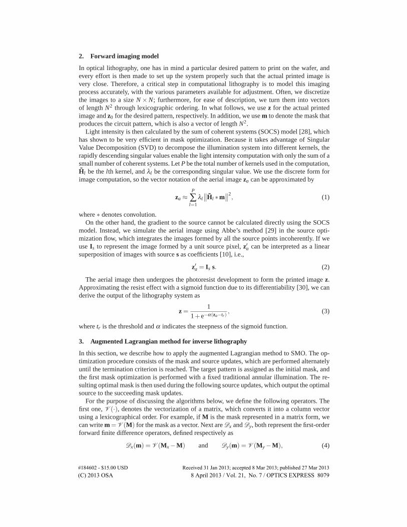
2. Forward imaging model

In optical lithography, one has in mind a particular desired pattern to print on the wafer, andevery effort is then made to set up the system properly such that the actual printed image isvery close. Therefore, a critical step in computational lithography is to model this imagingprocess accurately, with the various parameters available for adjustment. Often, we discretizethe images to a size N ×N; furthermore, for ease of description, we turn them into vectorsof length N2 through lexicographic ordering. In what follows, we use z for the actual printedimage and z0 for the desired pattern, respectively. In addition, we use m to denote the mask thatproduces the circuit pattern, which is also a vector of length N2.

Light intensity is then calculated by the sum of coherent systems (SOCS) model [28], whichhas shown to be very efficient in mask optimization. Because it takes advantage of SingularValue Decomposition (SVD) to decompose the illumination system into different kernels, therapidly descending singular values enable the light intensity computation with only the sum of asmall number of coherent systems. Let P be the total number of kernels used in the computation,Hl be the lth kernel, and λl be the corresponding singular value. We use the discrete form forimage computation, so the vector notation of the aerial image za can be approximated by

za ≈P

∑l=1

λl∥∥Hl ∗m

∥∥2, (1)

where ∗ denotes convolution.On the other hand, the gradient to the source cannot be calculated directly using the SOCS

model. Instead, we simulate the aerial image using Abbe’s method [29] in the source opti-mization flow, which integrates the images formed by all the source points incoherently. If weuse Is to represent the image formed by a unit source pixel, z′a can be interpreted as a linearsuperposition of images with source s as coefficients [10], i.e.,

z′a = Is s. (2)

The aerial image then undergoes the photoresist development to form the printed image z.Approximating the resist effect with a sigmoid function due to its differentiability [30], we canderive the output of the lithography system as

z =1

1+ e−α(za−tr), (3)

where tr is the threshold and α indicates the steepness of the sigmoid function.

3. Augmented Lagrangian method for inverse lithography

In this section, we describe how to apply the augmented Lagrangian method to SMO. The op-timization procedure consists of the mask and source updates, which are performed alternatelyuntil the termination criterion is reached. The target pattern is assigned as the initial mask, andthe first mask optimization is performed with a fixed traditional annular illumination. The re-sulting optimal mask is then used during the following source updates, which output the optimalsource to the succeeding mask updates.

For the purpose of discussing the algorithms below, we define the following operators. Thefirst one, V (·), denotes the vectorization of a matrix, which converts it into a column vectorusing a lexicographical order. For example, if M is the mask represented in a matrix form, wecan write m=V (M) for the mask as a vector. Next are Dx and Dy, both represent the first-orderforward finite difference operators, defined respectively as

Dx(m) = V (Mx−M) and Dy(m) = V (My−M), (4)


where Mx and My means shifting M along the horizontal and vertical directions by one pixel,respectively. To write the equations as compact as possible, we also define

D =

[Dx

Dy

]

. (5)

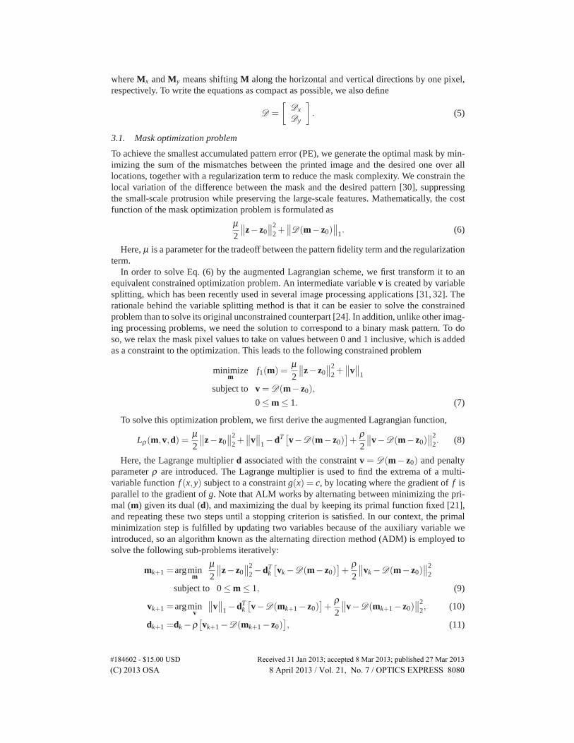
3.1. Mask optimization problem

To achieve the smallest accumulated pattern error (PE), we generate the optimal mask by min-imizing the sum of the mismatches between the printed image and the desired one over alllocations, together with a regularization term to reduce the mask complexity. We constrain thelocal variation of the difference between the mask and the desired pattern [30], suppressingthe small-scale protrusion while preserving the large-scale features. Mathematically, the costfunction of the mask optimization problem is formulated as

μ2

∥∥z− z0

∥∥2

2 +∥∥D(m− z0)

∥∥

1. (6)

Here, μ is a parameter for the tradeoff between the pattern fidelity term and the regularizationterm.

In order to solve Eq. (6) by the augmented Lagrangian scheme, we first transform it to anequivalent constrained optimization problem. An intermediate variable v is created by variablesplitting, which has been recently used in several image processing applications [31, 32]. Therationale behind the variable splitting method is that it can be easier to solve the constrainedproblem than to solve its original unconstrained counterpart [24]. In addition, unlike other imag-ing processing problems, we need the solution to correspond to a binary mask pattern. To doso, we relax the mask pixel values to take on values between 0 and 1 inclusive, which is addedas a constraint to the optimization. This leads to the following constrained problem

minimizem

f1(m) =μ2

∥∥z− z0

∥∥2

2 +∥∥v

∥∥

1

subject to v = D(m− z0),

0≤m≤ 1. (7)

To solve this optimization problem, we first derive the augmented Lagrangian function,

Lρ(m,v,d) =μ2

∥∥z− z0

∥∥2

2 +∥∥v

∥∥

1−dT [v−D(m− z0)]

+ρ2

∥∥v−D(m− z0)

∥∥2

2. (8)

Here, the Lagrange multiplier d associated with the constraint v = D(m− z0) and penaltyparameter ρ are introduced. The Lagrange multiplier is used to find the extrema of a multi-variable function f (x,y) subject to a constraint g(x) = c, by locating where the gradient of f isparallel to the gradient of g. Note that ALM works by alternating between minimizing the pri-mal (m) given its dual (d), and maximizing the dual by keeping its primal function fixed [21],and repeating these two steps until a stopping criterion is satisfied. In our context, the primalminimization step is fulfilled by updating two variables because of the auxiliary variable weintroduced, so an algorithm known as the alternating direction method (ADM) is employed tosolve the following sub-problems iteratively:

mk+1 =argminm

μ2

∥∥z− z0

∥∥2

2−dTk

[

vk−D(m− z0)]

+ρ2

∥∥vk−D(m− z0)

∥∥2

2

subject to 0≤m≤ 1, (9)

vk+1 =argminv

∥∥v

∥∥

1−dTk

[

v−D(mk+1− z0)]

+ρ2

∥∥v−D(mk+1− z0)

∥∥2

2, (10)

dk+1 =dk−ρ[

vk+1−D(mk+1− z0)]

, (11)


in which the subscript k denotes the kth iteration.We now investigate these sub-problems in the following subsections.

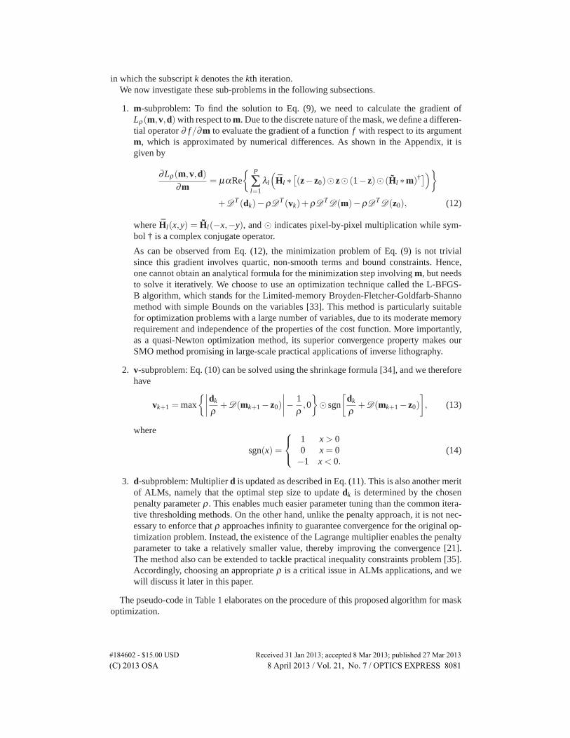
1. m-subproblem: To find the solution to Eq. (9), we need to calculate the gradient ofLρ(m,v,d)with respect to m. Due to the discrete nature of the mask, we define a differen-tial operator ∂ f/∂m to evaluate the gradient of a function f with respect to its argumentm, which is approximated by numerical differences. As shown in the Appendix, it isgiven by

∂Lρ(m,v,d)∂m

= μαRe

{ P

∑l=1

λl

(

Hl ∗[

(z− z0)� z� (1− z)� (Hl ∗m)†])}

+DT (dk)−ρDT (vk)+ρDT D(m)−ρDT D(z0), (12)

where Hl(x,y) = Hl(−x,−y), and � indicates pixel-by-pixel multiplication while sym-bol † is a complex conjugate operator.

As can be observed from Eq. (12), the minimization problem of Eq. (9) is not trivialsince this gradient involves quartic, non-smooth terms and bound constraints. Hence,one cannot obtain an analytical formula for the minimization step involving m, but needsto solve it iteratively. We choose to use an optimization technique called the L-BFGS-B algorithm, which stands for the Limited-memory Broyden-Fletcher-Goldfarb-Shannomethod with simple Bounds on the variables [33]. This method is particularly suitablefor optimization problems with a large number of variables, due to its moderate memoryrequirement and independence of the properties of the cost function. More importantly,as a quasi-Newton optimization method, its superior convergence property makes ourSMO method promising in large-scale practical applications of inverse lithography.

2. v-subproblem: Eq. (10) can be solved using the shrinkage formula [34], and we thereforehave

vk+1 = max

{∣∣∣∣

dk

ρ+D(mk+1− z0)

∣∣∣∣− 1

ρ,0

}

� sgn

[dk

ρ+D(mk+1− z0)

]

, (13)

where

sgn(x) =

⎧

⎨

⎩

1 x > 00 x = 0−1 x < 0.

(14)

3. d-subproblem: Multiplier d is updated as described in Eq. (11). This is also another meritof ALMs, namely that the optimal step size to update dk is determined by the chosenpenalty parameter ρ . This enables much easier parameter tuning than the common itera-tive thresholding methods. On the other hand, unlike the penalty approach, it is not nec-essary to enforce that ρ approaches infinity to guarantee convergence for the original op-timization problem. Instead, the existence of the Lagrange multiplier enables the penaltyparameter to take a relatively smaller value, thereby improving the convergence [21].The method also can be extended to tackle practical inequality constraints problem [35].Accordingly, choosing an appropriate ρ is a critical issue in ALMs applications, and wewill discuss it later in this paper.

The pseudo-code in Table 1 elaborates on the procedure of this proposed algorithm for maskoptimization.


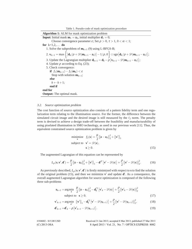
Table 1. Pseudo-code of mask optimization procedure

Algorithm 1: ALM for mask optimization problemInput: Initial mask m1 = z0, initial multiplier d1 = 0;

Choose convergence parameter ε; Set ρ > 0, τ > 1, 0 < α < 1;for k=1,2,. . . do

1. Solve the subproblem of mk+1 (9) using L-BFGS-B;

2. vk+1 = max

{∣∣dk/ρ +D(mk+1− z0)

∣∣−1/ρ ,0

}

� sgn[

dk/ρ +D(mk+1− z0)]

;

3. Update the Lagrangian multiplier dk+1 = dk−ρ[

vk+1−D(mk+1− z0)]

;4. Update ρ according to Eq. (23);5. Check convergence:

if f1(mk+1)− f1(mk)< εStop with solution mk+1;

elsek← k+1;

end ifend forOutput: The optimal mask.

3.2. Source optimization problem

The cost function of source optimization also consists of a pattern fidelity term and one regu-larization term relating to the illumination source. For the former, the difference between thesimulated circuit image and the desired image is still measured by the �2 norm. The penaltyterm is devised to achieve a design trade-off between the feasibility and manufacturability ofusing pixelated illumination in SMO technology, as used in our previous work [11]. Thus, theequivalent constrained source optimization problem is given by

minimizes

f2(s) =μ2

∥∥z− z0

∥∥2

2 +∥∥v′

∥∥

1

subject to v′ = D(s),

s≥ 0. (15)

The augmented Lagrangian of this equation can be represented by

Lρ(s,v′,d′) =μ2

∥∥z− z0

∥∥2

2 +∥∥v′

∥∥

1−d′T[

v′ −D(s)]

+ρ2

∥∥v′ −D(s)

∥∥2

2. (16)

As previously described, Lρ(s,v′,d′) is firstly minimized with respect to s to find the solutionof the original problem (15), and then we minimize v′ and update d′. As a consequence, theoverall augmented Lagrangian algorithm for source optimization is composed of the followingthree sub-problems

sk+1 =argmins

μ2

∥∥z− z0

∥∥2

2−d′Tk

[

v′k−D(s)]

+ρ2

∥∥v′k−D(s)

∥∥2

2

subject to s≥ 0, (17)

v′k+1 =argminv′

∥∥v′

∥∥

1−d′Tk

[

v′ −D(sk+1)]

+ρ2

∥∥v′ −D(sk+1)

∥∥2

2, (18)

d′k+1 =d′k−ρ[

v′k+1−D(sk+1)]

. (19)


As with ALM for mask optimization, using L-BFGS-B requires the first derivative ofLρ(s,v′,d′) with respect to the source. Note that the upper bound of the source can be setto infinity. Thus, the gradient we need is

∂Lρ(s,v′,d′)∂ s

= μαITs

[

(z− z0)� z� (1− z)]

+DT (d′k)−ρDT (v′k)+ρDT D(s). (20)

The derivation is detailed in the Appendix. The solution of v′ is similar to that of maskoptimization, i.e.,

v′k+1 = max

{∣∣∣∣

d′kρ

+D(sk+1)

∣∣∣∣− 1

ρ,0

}

� sgn

(d′kρ

+D(sk+1)

)

. (21)

Algorithm 2 lists the pseudo-code of the ALM for source optimization.

Table 2. Pseudo-code of source optimization procedure

Algorithm 2: ALM for source optimization problemInput: Assign multiplier d′1 = 0 and the starting source s1;

Choose convergence parameter ε; Set ρ > 0, τ > 1, 0 < α < 1;for k=1,2,. . . do

1. Solve the subproblem of sk+1 (17) using L-BFGS-B;

2. v′k+1 = max

{∣∣d′k/ρ +D(sk+1)

∣∣−1/ρ ,0

}

� sgn(

d′k/ρ +D(sk+1))

;

3. Update the Lagrangian multiplier d′k+1 = d′k−ρ[

v′k+1−D(sk+1)]

;4. Update ρ according to Eq. (23);5. Check convergence:

if f2(sk+1)− f2(sk)< εStop with solution sk+1;

elsek← k+1;

end ifend forOutput: The optimal source.

On the basis of above description, we now generalize the conversion of the cost function insource optimization to an equivalent constrained one. Assuming the source optimization prob-lem in which the cost function is the sum of the pattern fidelity term f (s) and the regularizationterm r(s), then the constrained problem is given by

minimizes

f (s)+ rg(u)

subject to u = g(s),

s≥ 0. (22)

Then ALM can be used to address Eq. (22). rg(u) is derived from r(s). The �2 norm and totalvariation in this paper are specific conditions of f (s) and r(s), respectively. The generalizedformulation for mask optimization is similar.

3.3. Parameters analysis

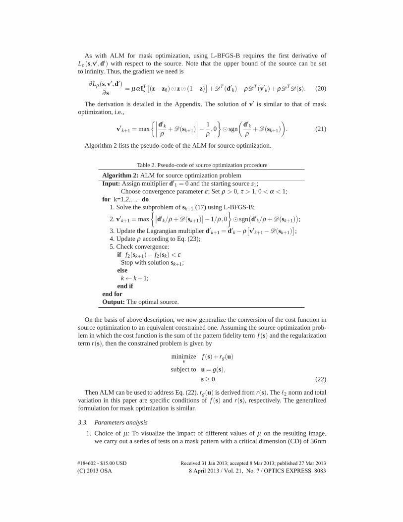
1. Choice of μ: To visualize the impact of different values of μ on the resulting image,we carry out a series of tests on a mask pattern with a critical dimension (CD) of 36nm


−300 −200 −100 0 100 200 300

300

200

100

0

−100

−200

−300

(a) Test pattern

(b) μ = 80 (c) μ = 472 (d) μ = 1000 (e) μ = 13650

(f) PE = 123 (g) PE = 131 (h) PE = 71 (i) PE = 66

Fig. 1. Simulation results of the test pattern with different choices of μ . Top row is thetarget image, and middle row presents the optimized masks and the corresponding outputswith pattern error (PE) are in the third row. The units of PE are in pixels.

(size 151× 151, pixel resolution 4nm) by fixing the annular source (0.7/0.9 annulus).As illustrated in Fig. 1, large μ tends to deliver a pattern closer to the design, but smallvalues yield relatively simpler masks. In our experiments, μ is set to 1000 for both maskand source optimization problems.

2. Choice of ρ: Rather than treating ρ as a fixed constant, we adopt the following updatescheme

ρ =

{ρ , if

∥∥vk+1−D(mk+1− z0)

∥∥

2 ≤ ητρ, otherwise,

(23)

where τ is the multiplication factor for updating ρ to be found empirically, and η is aconstant to specify whether the current value of the penalty parameter is producing an ac-ceptable level of constraint violation. This enables a faster rate of convergence as derivedin [23]. Ideally, the condition ρ

2

∥∥vk−D(mk− z0)

∥∥2

2 should decrease as k increases [34].However, if not, it can be forced to reduce by increasing its relative weight in the objectivefunction. Hence, the update scheme of τρ guarantees the convergence of the proposedalgorithm, and when the steady state is reached as k approaches infinity, ρ becomes aconstant [36]. The update for ρ in source optimization follows a similar approach.


0 30 60 90 120 150 180

5000

10000

15000

Iteration

Pat

tern

Err

or

τ=10τ=5τ=2τ=1

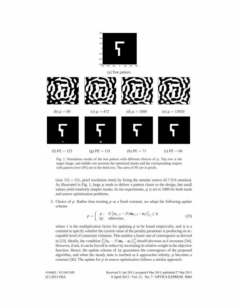
Fig. 2. Convergence profile of the proposed algorithm using different values of τ .

Empirically, a reasonable initial value of ρ typically lies in the range [0.01,10]. Too largea value (in the order of 100) may miss the solution to the original problem, while too smalla ρ will neglect the effect of the complexity penalty condition

∥∥vk−D(mk− z0)

∥∥2

2. Thefour colored curves in Fig. 2 show the convergence rate using different values of τ withFig. 1(a) as the input pattern. We find that ρ = 0.5 and τ = 2 are robust to most maskpatterns.

4. Results

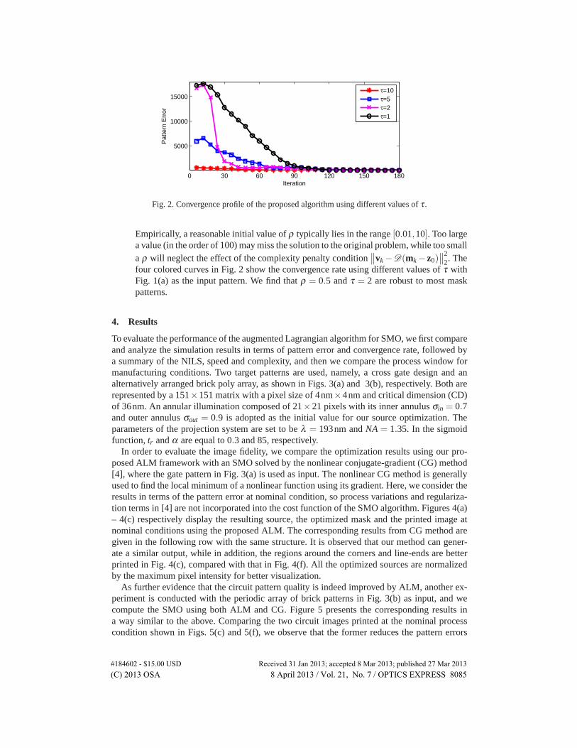
To evaluate the performance of the augmented Lagrangian algorithm for SMO, we first compareand analyze the simulation results in terms of pattern error and convergence rate, followed bya summary of the NILS, speed and complexity, and then we compare the process window formanufacturing conditions. Two target patterns are used, namely, a cross gate design and analternatively arranged brick poly array, as shown in Figs. 3(a) and 3(b), respectively. Both arerepresented by a 151×151 matrix with a pixel size of 4nm×4nm and critical dimension (CD)of 36nm. An annular illumination composed of 21×21 pixels with its inner annulus σin = 0.7and outer annulus σout = 0.9 is adopted as the initial value for our source optimization. Theparameters of the projection system are set to be λ = 193nm and NA = 1.35. In the sigmoidfunction, tr and α are equal to 0.3 and 85, respectively.

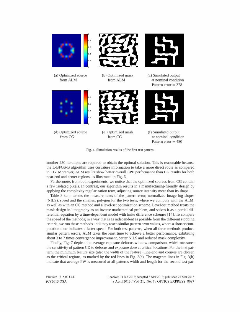
In order to evaluate the image fidelity, we compare the optimization results using our pro-posed ALM framework with an SMO solved by the nonlinear conjugate-gradient (CG) method[4], where the gate pattern in Fig. 3(a) is used as input. The nonlinear CG method is generallyused to find the local minimum of a nonlinear function using its gradient. Here, we consider theresults in terms of the pattern error at nominal condition, so process variations and regulariza-tion terms in [4] are not incorporated into the cost function of the SMO algorithm. Figures 4(a)– 4(c) respectively display the resulting source, the optimized mask and the printed image atnominal conditions using the proposed ALM. The corresponding results from CG method aregiven in the following row with the same structure. It is observed that our method can gener-ate a similar output, while in addition, the regions around the corners and line-ends are betterprinted in Fig. 4(c), compared with that in Fig. 4(f). All the optimized sources are normalizedby the maximum pixel intensity for better visualization.

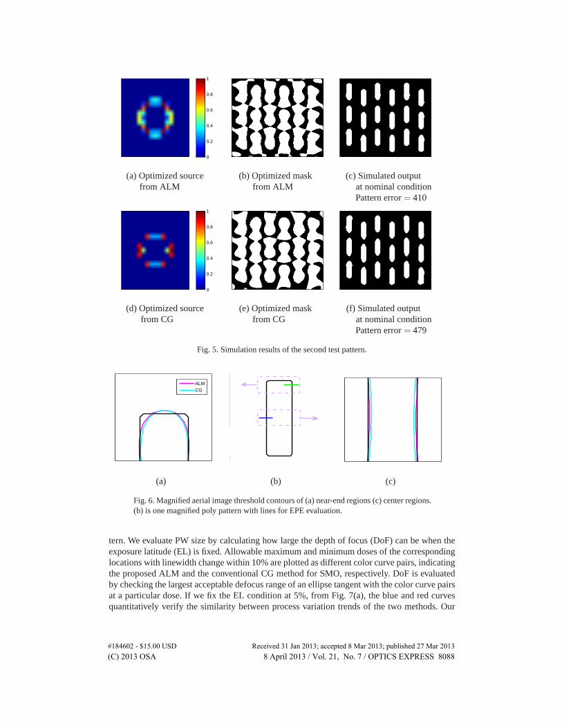
As further evidence that the circuit pattern quality is indeed improved by ALM, another ex-periment is conducted with the periodic array of brick patterns in Fig. 3(b) as input, and wecompute the SMO using both ALM and CG. Figure 5 presents the corresponding results ina way similar to the above. Comparing the two circuit images printed at the nominal processcondition shown in Figs. 5(c) and 5(f), we observe that the former reduces the pattern errors


−300 −200 −100 0 100 200 300

300

200

100

0

−100

−200

−300−300 −200 −100 0 100 200 300

300

200

100

0

−100

−200

−300

(a) (b)

Fig. 3. Two test patterns used in experiments: (a) cross gate design and (b) brick poly array.Red and magenta lines mark the critical locations for measuring the process window of thetwo patterns, respectively.

by 15% more than that of the latter. It is worth noting that the end regions of the poly array inFig. 5(f) have more distortions, which signifies that our method has a better resolution enhance-ment capacity over such regions.

It should also be noted that SMO with the CG method is not capable of acquiring the bestpattern fidelity in terms of the pattern error achieved by ALM even if it continues the iteration.Simulations conducted by ALM in Fig. 4(c) and Fig. 5(c), showing pattern error results of 378and 410 under best focus for two test patterns respectively, are far better than the results inFig. 4(f) and Fig. 5(f) (with pattern errors of 480 and 479, respectively). This is consistent withour observation in the corner areas of Figs. 4(c) and 4(f), as well as Figs. 5(c) and 5(f). Thisresult is related to the fact that the CG method is only applicable to certain types of equations,where the Hessian matrix is positive definite. If it is not for a particular optimization problem,the CG method fails to work properly and the algorithm does not converge to the minimum. Inother words, ALM can explore a larger solution space of the inverse problems than CG. Theabove two simulation results also affirm that the proposed ALM is suitable for printing bothgate pattern and periodic array.

After evaluating the image quality of different algorithms, we can now assess the impact ofthe proposed augmented Lagrangian algorithm in terms of the convergence rate represented bythe edge-placement error (EPE) versus the iteration number. EPE evaluates aerial image qualityby measuring the difference between the ideal profile and the simulated edge placement. In thefollowing analysis, one can see that the optimal source and mask in ALM can be found withless time than that with the CG method.

With the brick poly array as input, the blue and green lines in Fig. 6(b) are the center andnear-end edges where we calculate EPE. We magnify these two regions in Figs. 6(a) and 6(c),where the cyan and magenta curves are the threshold contours of the aerial image after SMOcalculation by using CG and ALM, respectively. The black curve is the target pattern contour.EPE evaluates the pattern fidelity by computing the distance between the output pattern contourand the desired pattern. During the optimization process, we observe that the EPE rapidly con-verges in the ALM for both the center and near-end lines. ALM reaches the optimal solutionafter 160 iterations, with a near 0nm EPE for the middle regions. Meanwhile for CG, after un-dergoing the same time, it prints the edge marked by a magenta line with an EPE of 4.9nm, and


0

0.2

0.4

0.6

0.8

1

(a) Optimized source (b) Optimized mask (c) Simulated outputfrom ALM from ALM at nominal condition

Pattern error = 378

0

0.2

0.4

0.6

0.8

1

(d) Optimized source (e) Optimized mask (f) Simulated outputfrom CG from CG at nominal condition

Pattern error = 480

Fig. 4. Simulation results of the first test pattern.

another 250 iterations are required to obtain the optimal solution. This is reasonable becausethe L-BFGS-B algorithm uses curvature information to take a more direct route as comparedto CG. Moreover, ALM results show better overall EPE performance than CG results for bothnear-end and center regions, as illustrated in Fig. 6.

Furthermore, from both experiments, we notice that the optimized sources from CG containa few isolated pixels. In contrast, our algorithm results in a manufacturing-friendly design byapplying the complexity regularization term, adjusting source intensity more than its shape.

Table 3 summarizes the measurements of the pattern error, normalized image log slopes(NILS), speed and the smallest polygon for the two tests, where we compute with the ALM,as well as with an CG method and a level-set optimization scheme. Level-set method treats themask design in lithography as an inverse mathematical problem, and solves it as a partial dif-ferential equation by a time-dependent model with finite difference schemes [14]. To comparethe speed of the methods, in a way that is as independent as possible from the different stoppingcriteria, we run these methods until they reach similar pattern error values, where a shorter com-putation time indicates a faster speed. For both test patterns, when all three methods producesimilar pattern errors, ALM takes the least time to achieve a better performance, exhibitingabout 3 to 7 times convergence improvement, better NILS and reduced mask complexity.

Finally, Fig. 7 depicts the average exposure-defocus window comparison, which measuresthe sensitivity of pattern CD to defocus and exposure dose at critical locations. For the first pat-tern, the minimum feature size (also the width of the feature), line-end and corners are chosenas the critical regions, as marked by the red lines in Fig. 3(a). The magenta lines in Fig. 3(b)indicate that average PW is measured at all patterns width and length for the second test pat-


0

0.2

0.4

0.6

0.8

1

(a) Optimized source (b) Optimized mask (c) Simulated outputfrom ALM from ALM at nominal condition

Pattern error = 410

0

0.2

0.4

0.6

0.8

1

(d) Optimized source (e) Optimized mask (f) Simulated outputfrom CG from CG at nominal condition

Pattern error = 479

Fig. 5. Simulation results of the second test pattern.

ALMCG

(a) (b) (c)

Fig. 6. Magnified aerial image threshold contours of (a) near-end regions (c) center regions.(b) is one magnified poly pattern with lines for EPE evaluation.

tern. We evaluate PW size by calculating how large the depth of focus (DoF) can be when theexposure latitude (EL) is fixed. Allowable maximum and minimum doses of the correspondinglocations with linewidth change within 10% are plotted as different color curve pairs, indicatingthe proposed ALM and the conventional CG method for SMO, respectively. DoF is evaluatedby checking the largest acceptable defocus range of an ellipse tangent with the color curve pairsat a particular dose. If we fix the EL condition at 5%, from Fig. 7(a), the blue and red curvesquantitatively verify the similarity between process variation trends of the two methods. Our


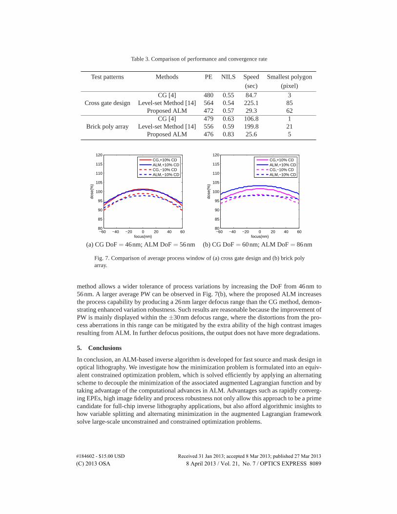
Table 3. Comparison of performance and convergence rate

Test patterns Methods PE NILS Speed Smallest polygon

(sec) (pixel)

CG [4] 480 0.55 84.7 3Cross gate design Level-set Method [14] 564 0.54 225.1 85

Proposed ALM 472 0.57 29.3 62CG [4] 479 0.63 106.8 1

Brick poly array Level-set Method [14] 556 0.59 199.8 21Proposed ALM 476 0.83 25.6 5

−60 −40 −20 0 20 40 6080

85

90

95

100

105

110

115

120

focus(nm)

dose

(%)

CG,+10% CDALM,+10% CDCG,−10% CDALM,−10% CD

−60 −40 −20 0 20 40 6080

85

90

95

100

105

110

115

120

focus(nm)

dose

(%)

CG,+10% CDALM,+10% CDCG,−10% CDALM,−10% CD

(a) CG DoF = 46nm; ALM DoF = 56nm (b) CG DoF = 60nm; ALM DoF = 86nm

Fig. 7. Comparison of average process window of (a) cross gate design and (b) brick polyarray.

method allows a wider tolerance of process variations by increasing the DoF from 46nm to56nm. A larger average PW can be observed in Fig. 7(b), where the proposed ALM increasesthe process capability by producing a 26nm larger defocus range than the CG method, demon-strating enhanced variation robustness. Such results are reasonable because the improvement ofPW is mainly displayed within the ±30nm defocus range, where the distortions from the pro-cess aberrations in this range can be mitigated by the extra ability of the high contrast imagesresulting from ALM. In further defocus positions, the output does not have more degradations.

5. Conclusions

In conclusion, an ALM-based inverse algorithm is developed for fast source and mask design inoptical lithography. We investigate how the minimization problem is formulated into an equiv-alent constrained optimization problem, which is solved efficiently by applying an alternatingscheme to decouple the minimization of the associated augmented Lagrangian function and bytaking advantage of the computational advances in ALM. Advantages such as rapidly converg-ing EPEs, high image fidelity and process robustness not only allow this approach to be a primecandidate for full-chip inverse lithography applications, but also afford algorithmic insights tohow variable splitting and alternating minimization in the augmented Lagrangian frameworksolve large-scale unconstrained and constrained optimization problems.


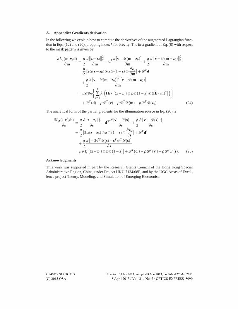
A. Appendix: Gradients derivation

In the following we explain how to compute the derivatives of the augmented Lagrangian func-tion in Eqs. (12) and (20), dropping index k for brevity. The first gradient of Eq. (8) with respectto the mask pattern is given by

∂Lρ(m,v,d)∂m

=μ2

∂∥∥z− z0

∥∥2

2

∂m−dT ∂

[

v−D(m− z0)]

∂m+

ρ2

∂∥∥v−D(m− z0)

∥∥2

2

∂m

=μ2

[

2α(z− z0)� z� (1− z)� ∂za

∂m

]

+DT d

+ρ2

∂[

v−D(m− z0)]T [v−D(m− z0)

]

∂m

= μαRe

{ P

∑l=1

λl

(

Hl ∗[

(z− z0)� z� (1− z)� (Hl ∗m)†])}

+DT (d)−ρDT (v)+ρDT D(m)−ρDT D(z0). (24)

The analytical form of the partial gradients for the illumination source in Eq. (20) is

∂Lρ(s,v′,d′)∂ s

=μ2

∂‖z− z0‖22∂ s

−d′T ∂

[

v′ −D(s)]

∂ s+

ρ2

∂‖v′ −D(s)‖22∂ s

=μ2

[

2α(z− z0)� z� (1− z)� ∂z′a∂ s

]

+DT d′

+ρ2

∂[−2v

′T D(s)+ sT DT D(s)]

∂ s= μαIT

s

[

(z− z0)� z� (1− z)]

+DT (d′)−ρDT (v′)+ρDT D(s). (25)

Acknowledgments

This work was supported in part by the Research Grants Council of the Hong Kong SpecialAdministrative Region, China, under Project HKU 7134/08E, and by the UGC Areas of Excel-lence project Theory, Modeling, and Simulation of Emerging Electronics.


Documents

Efﬁcient source and mask optimization with augmented ...nom.mse.hust.edu.cn/__local/A/C8/2C/E4D007402F24CA... · Abstract: Source mask optimization (SMO) is a powerful and effective