Embed Size (px)
Citation preview
Efficient Models for Timetable Informationin Public Transportation Systems
EVANGELIA PYRGA
Max-Planck-Institut fur Informatik
FRANK SCHULZ and DOROTHEA WAGNER
University of Karlsruhe
and
CHRISTOS ZAROLIAGIS
CTI and University of Patras
We consider two approaches that model timetable information in public transportation systemsas shortest-path problems in weighted graphs. In the time-expanded approach, every event ata station, e.g., the departure of a train, is modeled as a node in the graph, while in the time-dependent approach the graph contains only one node per station. Both approaches have beenrecently considered for (a simplified version of) the earliest arrival problem, but little is knownabout their relative performance. Thus far, there are only theoretical arguments in favor of thetime-dependent approach. In this paper, we provide the first extensive experimental comparison ofthe two approaches. Using several real-world data sets, we evaluate the performance of the basicmodels and of several new extensions towards realistic modeling. Furthermore, new insights onsolving bicriteria optimization problems in both models are presented. The time-expanded approachturns out to be more robust for modeling more complex scenarios, whereas the time-dependentapproach shows a clearly better performance.
This work was partially supported by the Human Potential Programme of EC under contractno. HPRN-CT-1999-00104 (AMORE), by the Future and Emerging Technologies Unit of EC (ISTpriority – 6th FP), under contracts no. IST-2002-001907 (DELIS) and no. FP6-021235-2 (ARRIVAL),and by the DFG under grant WA 654/1-12. Part of this work has been done while the first authorwas with the University of Patras, the second and the third authors were with the University ofKonstanz, and while the last author was visiting the University of Karlsruhe.Authors’ addresses: Evangelia Pyrga, Max-Planck-Institut fur Informatik, Stuhlsatzenhausweg 85,66123 Saarbrucken, Germany; email: [email protected]. Frank Schulz, Department of Com-puter Science, University of Karlsruhe, 76128 Karlsruhe, Germany; email: [email protected] Wagner, Department of Computer Science, University of Karlsruhe, 76128 Karlsruhe,Germany; email: [email protected]. Christos Zaroliagis, R.A. Computer Technology Institute,N. Kazantzaki Str, Patras University Campus, 26500 Patras, Greece, and Department of Com-puter Engineering and Informatics, University of Patras, 26500 Patras, Greece; email: [email protected] to make digital or hard copies of part or all of this work for personal or classroom use isgranted without fee provided that copies are not made or distributed for profit or direct commercialadvantage and that copies show this notice on the first page or initial screen of a display alongwith the full citation. Copyrights for components of this work owned by others than ACM must behonored. Abstracting with credit is permitted. To copy otherwise, to republish, to post on servers,to redistribute to lists, or to use any component of this work in other works requires prior specificpermission and/or a fee. Permissions may be requested from Publications Dept., ACM, Inc., 2 PennPlaza, Suite 701, New York, NY 10121-0701 USA, fax +1 (212) 869-0481, or [email protected]© 2007 ACM 1084-6654/2007/ART2.4 $5.00 DOI 10.1145/1227161.1227166 http://doi.acm.org10.1145/1227161.1227166
ACM Journal of Experimental Algorithmics, Vol. 12, Article No. 2.4, Publication June: 2008.
2.4
2 • E. Pyrga et al.
Categories and Subject Descriptors: G.2.1 [Combinatorics]: Combinatorial algorithms; G.2.2[Graph Theory]: Graph algorithms, Network problems, Path and circuit problems; G.2.3 [Ap-plications]: Traffic information systems; G.4 [Mathematical Software]: Algorithm design andanalysis; D.2.8 [Metrics]: Performance Measures; E.1 [Data Structures]: Graphs and Networks
General Terms: Algorithms, Design, Experimentation, Measurement, Performance
Additional Key Words and Phrases: Shortest path, timetable information, public transportationsystem, itinerary query
ACM Reference Format:Pyrga, E., Schulz, F., Wagner, D., and Zaroliagis, C. 2007. Efficient models for timetable informa-tion in public transportation systems. ACM J. Exp. Algor. 12, Article 2.4 (2007), 39 pages DOI10.1145/1227161.1227166 http://doi.acm.org 10.1145/ 1227161.1227166
1. INTRODUCTION
An important problem in public transportation systems is to model timetableinformation so that subsequent queries asking for optimal itineraries can beefficiently answered. The main target that underlies the modeling (and whichapplies not only to public transportation systems, but also to other systemsas well, like route planning for car traffic, database queries, web searching,etc.) is to process a vast number of on-line queries as fast as possible. Inthis paper, we are concerned with a specific, query-intensive scenario aris-ing in public railway transport, where a central server is directly accessibleto any customer, either through terminals in train stations or through a webinterface and has to answer a potentially infinite number of queries.1 Themain goal in such an application is to reduce the average response time for aquery.
Two main approaches have been proposed for modeling timetable informa-tion: the time-expanded [Muller-Hannemann and Weihe 2001; Pallottino andScutella 1998; Schulz et al. 2000, 2002], and the time-dependent approach[Brodal and Jacob 2004; Nachtigal 1995; Orda and Rom 1990, 1991]. The com-mon characteristic of both approaches is that a query is answered by apply-ing some shortest-path algorithm to a suitably constructed digraph. The time-expanded approach [Schulz et al. 2000] constructs the time-expanded digraphin which every node corresponds to a specific time event (departure or arrival)at a station and edges between nodes represent either elementary connectionsbetween the two events (i.e., served by a train that does not stop in-between)or waiting within a station. Depending on the problem that we want to solve(see below), the construction assigns specific fixed costs to the edges. This nat-urally results in the construction of a very large (but usually sparse) graph.The time-dependent approach [Brodal and Jacob 2004] constructs the time-dependent digraph in which every node represents a station and two nodes areconnected by an edge if the corresponding stations are connected by an elemen-tary connection. The costs on the edges are assigned “on-the-fly,” i.e., the costof an edge depends on the time in which the particular edge will be used by theshortest-path algorithm to answer the query.
1For example, the server of the German railways receives about 100 queries per second.
ACM Journal of Experimental Algorithmics, Vol. 12, Article No. 2.4, Publication June: 2008.
Efficient Models for Timetable Information in Public Transportation Systems • 3
The two most frequently encountered timetable problems are the earliestarrival and the minimum number of transfers problems. In the earliest-arrivalproblem, the goal is to find a train connection from a departure station A to anarrival station B that departs from A later than a given departure time andarrives at B as early as possible. There are two variants of the problem, depend-ing on whether train transfers within a station are assumed to take negligibletime (simplified version) or not. In the minimum number of transfers problem,the goal is to find a connection that minimizes the number of train transferswhen considering an itinerary from A to B. We also consider combinations ofthe above problems as bicriteria optimization problems.
Techniques for solving general multicriteria optimization problems havebeen discussed in Mohring [1999] and Muller-Hannemann and Weihe [2001],where the discussion in the former is focused on a distributed approach fortimetable information problems. Space consumption aspects of modeling morecomplex real-world scenarios is considered in Muller-Hannemann et al. [2002].For the time-expanded model, the simplified version of the earliest-arrival prob-lem has been extensively studied [Schulz et al. 2000, 2002], and an extension ofthe model able to solve the minimum number of transfers problem, but withouttransfer times, is discussed in Muller-Hannemann and Weihe [2001]. Compar-ing the time-expanded and time-dependent approach, it is argued theoreticallyin Brodal and Jacob [2004] that the time-dependent approach is better than thetime-expanded one when the simplified version of the earliest-arrival problemis considered.
In this paper, we provide the first experimental comparison of the time-expanded and the time-dependent approaches with respect to their performancein the specific, query-intensive scenario mentioned earlier. For the simplifiedearliest-arrival problem, we show that the time-dependent approach is clearlysuperior to the time-expanded approach.
In order to cope with more realistic requirements, we present new extensionsof both approaches. In particular, the proposed extensions can handle cases nottackled by most previous studies for the sake of simplification. These new casesare: (a) the waiving of the assumption that transfer of trains within a stationtakes negligible time; (b) the consideration of the minimum number of transfersproblem; (c) the involvement of traffic days; and (d) the consideration of bicri-teria optimization problems combining the earliest-arrival and the minimumnumber of transfers problems.
We also conducted extensive experiments comparing the extended ap-proaches. This comparison is important, since the described extensions aremandatory for real-world applications, and (to the best of our knowledge)nothing is known about the relative behavior of realistic versions of the twoapproaches.
The rest of this paper is organized as follows. In Section 2, the variants ofitinerary problems that are considered in this paper are defined. The modelingof the simplified version of the earliest-arrival problem is considered in Sec-tion 3, where the basic ideas of the original time-expanded and time-dependentmodels are briefly reviewed. In Section 4 the new extensions to these approachesare presented in order to cope with the realistic version of the earliest-arrival
ACM Journal of Experimental Algorithmics, Vol. 12, Article No. 2.4, Publication June: 2008.

4 • E. Pyrga et al.
problem. Section 5 discusses the incorporation of different traffic days in theoriginal or in the extended models. Sections 6 and 7 discuss how the mini-mum number of transfers problem and the bicriteria optimization problems,respectively, can be solved in either of the extended models. Heuristics thatspeedup the proposed algorithmic solutions are discussed in Section 8. The ex-perimental comparison of the two approaches based on real-world data fromthe German and French railways is presented in Section 9. We first considerhow the original versions of the two approaches compare and, subsequently,investigate the comparison of the extended models on the realistic versionof the earliest-arrival problem, the minimum number of transfers problem,and the bicriteria optimization problems. Section 10 summarizes our insightson the advantages and disadvantages of the approaches under comparison.Preliminary parts of this work appeared in Pyrga et al. [2004a, 2004b].
2. ITINERARY PROBLEMS
In this section, we provide definitions of the timetable problems that we willconsider. Problem definitions, as well as models and algorithms that will bepresented throughout the paper for their efficient solution, refer to timetableinformation in a railway system, but the modeling and the algorithms canbe applied to any other public transportation system provided that its timetablesatisfies the same characteristics.
A timetable consists of data concerning: stations (or bus stops, ports, etc),trains (or busses, ferries, etc), connecting stations, departure and arrival timesof trains at stations, and traffic days. More formally, we are given a set of trainsZ, a set of stationsB, and a set of elementary connections C, whose elements c are5-tuples of the form c = (Z , S1, S2, td , ta). Such a tuple (elementary connection)is interpreted as train Z leaves station S1 at time td and the immediately nextstop of train Z is station S2 at time ta. If x denotes a tuple’s field, then thenotation x(c) specifies the value of x in the elementary connection c.
The departure and arrival times td (c) and ta(c) of an elementary connec-tion c ∈ C within a day are integers in the interval [0, 1439] representingtime in minutes after midnight. Given two time values t and t ′, t ≤ t ′, thecycle difference(t, t ′) is the smallest nonnegative integer l such that l ≡ t ′ − t(mod 1440). The length of an elementary connection c, denoted by length(c), iscycle difference(td (c), ta(c)). A timetable is valid for a number of N traffic days,and every train is assigned a bit-field of N bits determining on which trafficdays the train operates (for overnight trains the departure of the first elemen-tary connection counts). We will generally assume that trains operate daily; inSection 5 we will discuss how different traffic days can be incorporated in themodels.
At a station S ∈ B it is possible to transfer from one train to another. Sucha transfer is only possible if the time between the arrival and the departureat that station S is larger than or equal to a given, station-specific, minimumtransfer time, denoted by transfer(S).
Let P = (c1, . . . , ck) be a sequence of elementary connections togetherwith departure times depi(P ) and arrival times arri(P ) for each elementary
ACM Journal of Experimental Algorithmics, Vol. 12, Article No. 2.4, Publication June: 2008.
Efficient Models for Timetable Information in Public Transportation Systems • 5
connection ci, 1 ≤ i ≤ k. We assume that the times depi(P ) and arri(P ) includedata regarding also the departure/arrival day by counting time in minutes fromthe first day of the timetable. Such a time t is of the form t = a 1440 + b,where a ∈ [0, N − 1] and b ∈ [0, 1439]. Hence, the actual time within a day is t(mod 1440) and the actual day is �t/1440�. Such a sequence P is called a consis-tent connection from station A = S1(c1) to station B = S2(ck) if it fulfills someconsistency conditions: (a) the departure station of ci+1 is the arrival station ofci; (b) the time values depi(P ) and arri(P ) correspond to the time values td andta, resp., of the elementary connections (modulo 1440) and respect the transfertimes at stations. More formally, P is a consistent connection if the followingconditions are satisfied:
ci is valid on day �depi(P )/1440�S2(ci) = S1(ci+1)
depi(P ) ≡ td (ci) (mod 1440)
arri(P ) = length(ci) + depi(P )
depi+1(P ) − arri(P ) ≥{
0 if Z (ci+1) = Z (ci)
transfer(S2(ci)) otherwise
For the timetable-information problems defined below, we are, in addition,given a large, on-line sequence of queries. A query defines a set of valid connec-tions and an optimization criterion (or criteria) on that set of connections. Theproblem is to find the optimal connection (or a set of optimal connections) withrespect to the specific criterion or criteria.
In this work, we are concerned with two of the most important criteria,namely, the earliest arrival (EA) and the minimum number of transfers (MNT),and, consequently, investigate two single-criterion and a few bicriteria opti-mization problems, which are defined next.
2.1 Earliest-Arrival Problem (EAP)
A query (A, B, t0) consists of a departure station A, an arrival station B, and adeparture time t0 (including the departure day). Connections are valid if theydepart at least at the given departure time t0, and the optimization criterionis to minimize the difference between the arrival time and the given departuretime. We distinguish between two different variants of the problem: (a) Thesimplified version, where train transfers take negligible time and, hence, theinput is restricted to transfer(S) = 0 for all stations S. (b) The realistic version,where train transfers require arbitrary nonnegative minimum transfer timestransfer(S). We discuss efficient solutions to these problems in Sections 3 and
4. A special case of the earliest-arrival problem is the latest-departure problem:among all connections with earliest-arrival time at the arrival station, maxi-mize the actual departure time at the departure station. Efficient solutions tothis problem are discussed in Section 10.
ACM Journal of Experimental Algorithmics, Vol. 12, Article No. 2.4, Publication June: 2008.
6 • E. Pyrga et al.
2.2 Minimum Number of Transfers Problem (MNTP)
A query consists only of a departure station A and an arrival station B. Trainsare assumed to operate daily, and there is no restriction on the number of daysa timetable is valid.2 All connections from A to B are valid and the optimizationcriterion is to minimize the number of train transfers. In particular, let P =(c1, . . . , ck) be a connection from A to B and let transi(P ) ∈ {0, 1} be a variabledenoting whether a transfer is needed from elementary connection ci to ci+1,1 ≤ i < k. Then, transi(P ) = 1, if Z (ci+1) = Z (ci), and transi(P ) = 0, otherwise.Consequently, the objective of MNTP is to minimize, among all P , the quantity∑k−1
i=1 transi(P ). We will discuss this problem in Section 6.
2.3 Bicriteria Optimization Problems
We consider also bicriteria or Pareto-optimal problems with the earliest arrival(EA) and the minimum number of transfers (MNT) as the two criteria. Weare interested in three problem variants: (1) finding the so-called Pareto-curve,which is the set of all undominated Pareto-optimal paths (the set of feasiblesolutions where the attribute vector of one solution is not dominated by theattribute vector of another solution); (2) finding the solution that minimizesone criterion while retaining the second below a given threshold; (3) finding thelexicographically first Pareto-optimal solution (e.g., find among all connectionsthat minimize EA the one with the minimum number of transfers). We willdiscuss these problems in Section 7.
3. EARLIEST-ARRIVAL PROBLEM—SIMPLIFIED VERSION
In this section, we review the modeling of the simplified version of EAP, in boththe time-expanded and the time-dependent approach. Recall that, in this case,transfer time between trains at a station is negligible.
3.1 Time-Expanded Model
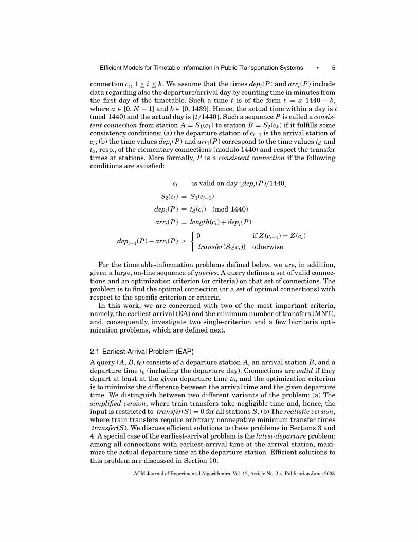
The time-expanded model [Schulz et al. 2000] is based on the time-expandeddigraph, which is constructed as follows. There is a node for every time event(departure or arrival) at a station and there are two types of edges. For everyelementary connection (Z , S1, S2, td , ta) in the timetable, there is a train edgein the graph connecting a departure node belonging to station S1 and associ-ated with time td , to an arrival node belonging to station S2 and associatedwith time ta. In other words, the endpoints of the train edges induce the setof nodes of the graph. For each station S, all nodes belonging to S are or-dered according to their time values. Let v1, . . . , vk be the nodes of S in thatorder. Then, there is a set of stay edges (vi, vi+1), 1 ≤ i ≤ k − 1, and (vk , v1),connecting the time events within a station and representing waiting withinthat station. The cost of an edge (p, q) is cycle difference(tp, tq), where tp andtq are the time values associated with nodes p and q, respectively. Figure 1
2This assumption can be safely made since time is not minimized in MNTP and, thus, in a MNT-optimal connection, one can wait arbitrarily long at a station for some connection that is valid onlyon certain days.
ACM Journal of Experimental Algorithmics, Vol. 12, Article No. 2.4, Publication June: 2008.

Efficient Models for Timetable Information in Public Transportation Systems • 7
Fig. 1. The time-expanded (left) and the time-dependent digraph (right) of a timetable with threestations A, B, C. There are three trains that connect A with B (elementary connections α, β, γ ), onetrain from C via B to A (δ, ε), and one train from C to B (ζ ).
illustrates this definition. The following theorem states that an appropriateshortest-path computation on the above graph solves the simplified versionof EAP.
THEOREM 1. A shortest path in the time-expanded digraph from the firstdeparture node s at the departure station A with departure time later than orequal to the given start time t0 to one of the arrival nodes of the destinationstation B constitutes a solution to the simplified version of EAP in the time-expanded model. The actual path can be found by Dijkstra’s algorithm in timeO(meo + neo log neo ), where neo (resp. meo ) is the number of nodes (resp. edges) ofthe time-expanded digraph.
PROOF. An optimal connection never stays more than a day at a station,because otherwise there would be a 1 day faster connection, since every train isassumed to operate daily.3 Let � be a path in the time-expanded digraph from
3When traffic days are modeled, this is not necessarily true anymore; see Section 5.
ACM Journal of Experimental Algorithmics, Vol. 12, Article No. 2.4, Publication June: 2008.
8 • E. Pyrga et al.
node s of station A to some arrival node of station B. To prove correctness, itsuffices to show that there is a one-to-one correspondence between path � and avalid and consistent A–B connection P , such that the cost of path � equals theduration of P . Clearly, such a one-to-one correspondence applies between theshortest among those paths � and the minimum in duration among all thosevalid and consistent connections P .
We will first show that path � corresponds to a valid and consistent A–Bconnection P in the EAP setting. Define P to be the sequence of all elementaryconnections corresponding to the train edges that occur in the path �. Further,define the time value depi(P ) to be the cost of the subpath from s to the tail ofthe ith train edge plus the time associated with s. Similarly, set arri(P ) to bethe cost of the subpath from s to the the head of the ith train edge plus the timeassociated with s. It can be easily verified that P is a valid and consistent A–Bconnection, whose duration equals the cost of path �.
Conversely, let P ′ be a valid and consistent A–B connection that never staysmore than a day at a station, departing from A at t0 or at the earliest possibletime after t0, and let the corresponding departure node in the time-expandeddigraph be s. We will show that P ′ corresponds to a path �′ starting from node sof station A and ending at some arrival node of B in the time-expanded digraph.Path �′ is constructed as follows. It contains all train edges corresponding tothe elementary connections in P ′. Path �′ starts at s, which is connected by asimple path of stay edges with the tail of the first train edge. The head of thefirst train edge is connected by a path of stay edges to the tail of the secondtrain edge, and so on, until the tail of the last train edge is reached. Clearly, thehead of the last train edge is an arrival node of B. It can be easily verified thatthe cost of path �′ is equal to the difference of the arrival and the departuretime of P ′.
Since edge costs are nonnegative, the actual path can be found by usingDijkstra’s algorithm [Dijkstra 1959] and abort the main loop when a node atthe destination station is reached.
3.2 Time-Dependent Model
The time-dependent model [Brodal and Jacob 2004] is also based on a digraph,called time-dependent graph. In this graph there is only one node per station,and there is an edge e from station A –B if there is an elementary connectionfrom A to B. The set of elementary connections from A to B is denoted by C(e).The definition is illustrated in Figure 1. The cost of an edge e = (A, B) dependson the time at which this particular edge will be used by an algorithm that solvesEAP. In other words, if T is a set denoting time, then the cost of an edge (A, B)is given by f (A,B)(t) − t, where t is the departure time at v, f (A,B) : T → T is afunction such that f (A,B)(t) = t ′, and t ′ ≥ t is the earliest possible arrival timeat B. The time-dependent model is based on the assumption that overtaking oftrains on an edge is not allowed.
ASSUMPTION 1. For any two given stations A and B, there are no two trainsleaving A and arriving to B such that the train that leaves A second arrives firstat B.
ACM Journal of Experimental Algorithmics, Vol. 12, Article No. 2.4, Publication June: 2008.

Efficient Models for Timetable Information in Public Transportation Systems • 9
A modification of Dijkstra’s algorithm can be used to solve the earliest arrivalproblem in the time-dependent model [Brodal and Jacob 2004]. Let D denotethe departure station, t0 the earliest departure time, and δ : V → R the distancelabels maintained by Dijkstra’s algorithm. The differences, w.r.t. Dijkstra’s algo-rithm, are: set the distance label δ(D) of the starting node corresponding to thedeparture station D to t0 (and not to 0), and calculate the edge costs on-the-fly.The edge costs (and, implicitly, the time-dependent function f ) are calculatedas follows. Since Dijkstra’s algorithm is a label-setting shortest-path algorithm,whenever an edge e = (A, B) is considered, the distance label δ(A) of node A isoptimal. In the time-dependent model, δ(A) denotes the earliest-arrival time atstation A. In other words, we, indeed, know the earliest-arrival time at stationA whenever the edge e = (A, B) is considered, and, therefore, we know at thatstage of the algorithm (by Assumption 1) which train has to be taken to reachstation B via A as early as possible: the first train that departs later than orequal to the earliest-arrival time at A. Let t = δ(A) and let c∗ ∈ C(e) be theconnection minimizing {cycle difference(t, td (c)) | c ∈ C(e)}. The particular con-nection c∗ can be easily found by binary search if the elementary connectionsC(e) are maintained in a sorted array. The edge cost of e, e(t), is then definedas e(t) = cycle difference(t, td (c∗)) + length(c∗). Consequently, fe(t) = t + e(t).
The following theorem is proved in Brodal and Jacob [2004]. Its correctnessis based on the fact that f has nonnegative delay (∀t, f (t) ≥ t), and is non-decreasing (t ≤ t ′ ⇒ f (t) ≤ f (t ′)), which follows directly from Assumption 1.Because of the nature of the investigated application, we can safely assumethat all functions defined throughout the paper have nonnegative delay.
THEOREM 2. The above modified Dijkstra’s algorithm solves the simplifiedversion of EAP in the time-dependent model, provided that Assumption 1 holds,in time O(mdo log Wo + ndo log ndo ), where ndo (resp. mdo ) is the number of nodes(resp. edges) of the time-dependent digraph, and Wo is the maximum number ofelementary connections associated with an edge.
4. EARLIEST-ARRIVAL PROBLEM—REALISTIC VERSION
In this section, we describe how both models of Section 3 can be extended tosolve the realistic version of EAP, where transfer time between trains at astation is non-zero.
4.1 Time-Expanded Model
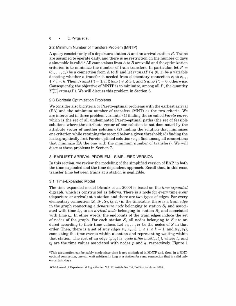
To solve the realistic version of EAP, in this case, we extend the time-expandedmodel by constructing the realistic time-expanded digraph as follows. Based onthe time-expanded digraph, we keep, for each station, a copy of all departure andarrival nodes in the station, which we call transfer nodes; see Figure 2. The stayedges are now introduced between the transfer nodes. For every arrival nodethere is now one edge to the first transfer node with time value greater than orequal to the time of the arrival node plus the minimum time needed to changetrains at the corresponding station, and a second edge from the arrival nodeto the departure node of the same train, if it departs from the correspondingstation (otherwise there is no second edge). The edge costs are defined as in
ACM Journal of Experimental Algorithmics, Vol. 12, Article No. 2.4, Publication June: 2008.
10 • E. Pyrga et al.
Fig. 2. Modeling train transfers in the time-expanded model for a sample station. The realistictime-expanded digraph has three types of nodes: arrival, transfer and departure nodes.
the definition of the original model (see Section 3.1). The correctness of themodeling is established by the following theorem.
THEOREM 3. A shortest path in the realistic time-expanded digraph from thefirst departure node at the departure station A with departure time later thanor equal to the given start time t0 to one of the arrival nodes of the destinationstation B, constitutes a solution to the realistic version of EAP in the extendedtime-expanded model. The actual path can be found by Dijkstra’s algorithm intime O(me + ne log ne), where ne (resp. me) is the number of nodes (resp. edges)of the realistic time-expanded digraph.
PROOF. The proof of Theorem 1 that allows construction of paths from con-nections (and vice versa) can be analogously adapted to establish an one-to-onecorrespondence between paths and valid and consistent connections in the re-alistic version of EAP.
4.2 Time-Dependent Model
To model non-zero train transfers, we extend the original time-dependent modelusing information on the routes that trains may follow. We examine both thecases of constant and variable transfer times (a somehow similar idea for theconstant transfer time case was very briefly mentioned in Brodal and Jacob[2004], but without providing the details). In the following, we describe theconstruction of a digraph G = (V , E) that models these two cases. We shallrefer to G as the train-route digraph.
Since now there is no one-to-one correspondence between nodes and stations,we denote nodes of the train-route digraph with small latin letters u, v, . . . . LetS be a set of nodes representing stations (i.e., for each station in the input there
ACM Journal of Experimental Algorithmics, Vol. 12, Article No. 2.4, Publication June: 2008.
Efficient Models for Timetable Information in Public Transportation Systems • 11
is a node in S that corresponds to that station, and each u ∈ S corresponds to adifferent station). For u ∈ S, we denote by station(u) the actual station, whichu represents (station(·) is a function mapping a node of S to its correspondingstation).
We divide the set of trains Z into so-called train routes: A train route rconsists of a maximal subset of the set of trains Z, such that each train of rfollows the exact same route, i.e., passes through the exact same stations, at theexact same order, possibly at different times throughout the day. In other words,two trains are equivalent concerning their route if the sequence of stations thetrains pass is the same. The train routes are the equivalence classes of thisrelation.
For each different route r, let kr > 0 be the number of stations, not allof them necessarily distinct, that r stops at (including the first station of theroute). Denote by S1, S2, . . . , Skr the stations that r visits, in this order. (It canbe Si = Sj for i = j , in the general case that r, at some point, forms a loop.) Letv1, . . . vkr ∈ S be the nodes for which station(vi) = Si, 1 ≤ i ≤ kr , and define setsPvi as follows: for each i, 1 ≤ i ≤ kr , insert a new route node to Pvi modelingthe fact that r passes through station(vi). Thus, for each u ∈ S, a node set Pu
is constructed by repeating this procedure for all train routes.Also, let Pu = |Pu|, and P = ⋃
u∈S Pu. Then, the node set V of G is defined asV = S ⋃P. For u ∈ S, we denote by pu
i , 0 ≤ i < Pu, the Pu nodes contained inPu, in some arbitrary order.
We distinguish four types of edges for the train-route digraph: edges I froma route node to a station node, edges D from a station node to a route node,edges D between route nodes of the same station, and route edges R betweenroute nodes of the same route. More formally, the edge set E = I
⋃D
⋃D
⋃R
of G is defined as follows.
� I = ⋃u∈S Iu, where Iu = ⋃
0≤i<Pu{(pu
i , u)}.� D = ⋃
u∈S Du, where Du = ⋃0≤i<Pu
{(u, pui )}.
� D = ⋃u∈S Du, where Du = ∅, if the time needed for a transfer is the same for
all trains that stop to station(u); Du = ⋃0≤i, j<Pu,i = j {(pu
i , puj )}, otherwise.
� R = ⋃u,v∈S,0≤i<Pu,0≤ j<Pv
{(pui , pv
j ) : station(u) and station(v) are visited suc-cessively by the same train route and pu
i , pvj are the corresponding route
nodes that belong to Pu and Pv, respectively}.An edge e is called a route or timetable edge if e ∈ R, and it is called a transfer
edge if e ∈ I⋃
D⋃
D. The modeling with train routes is based on two additionalassumptions.
ASSUMPTION 2. Let u, v be any two nodes in S and pui ∈ Pu, pv
j ∈ Pv such that(pu
i , pvj ) ∈ R. If d1, d2 are departure times from pu
i and a1, a2 are the respectivearrival times to pv
j , then d1 ≤ d2 ⇒ a1 ≤ a2.
This assumption states that there cannot be two trains that belong to thesame train route, such that the first of them leaving a station is a slow train,while the following one is a fast train and it arrives to the next station beforethe first. When this assumption is violated, we can enforce it by separating
ACM Journal of Experimental Algorithmics, Vol. 12, Article No. 2.4, Publication June: 2008.
12 • E. Pyrga et al.
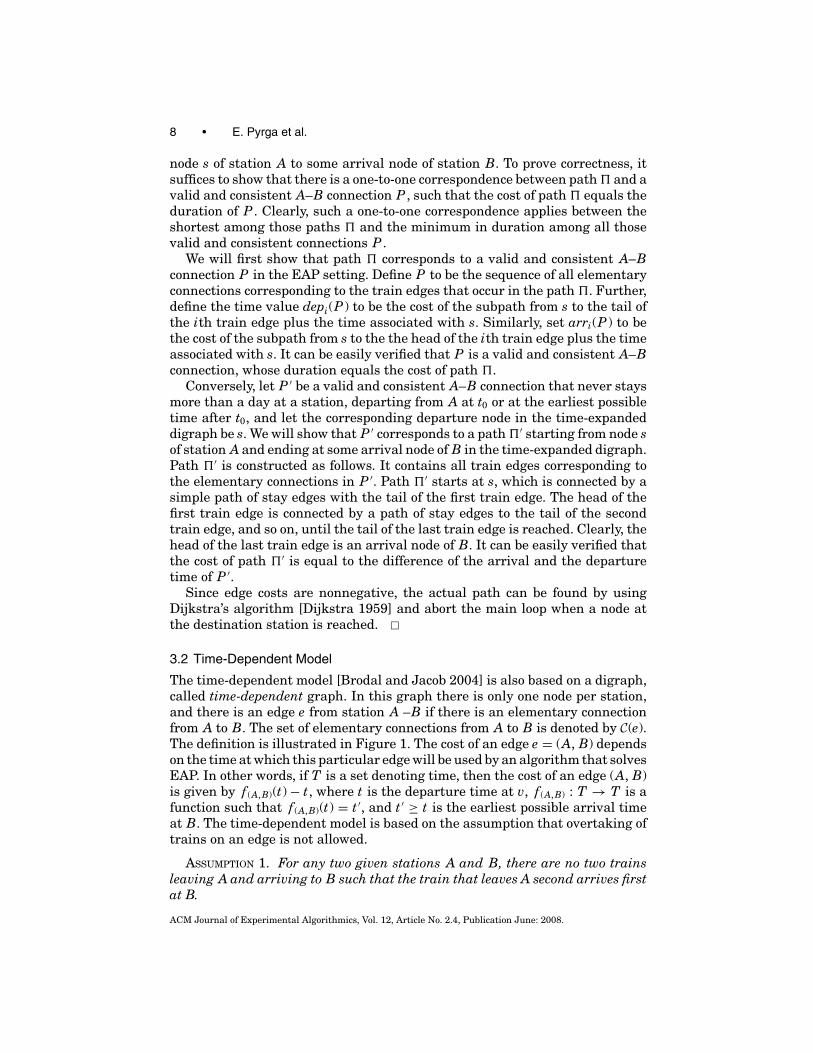
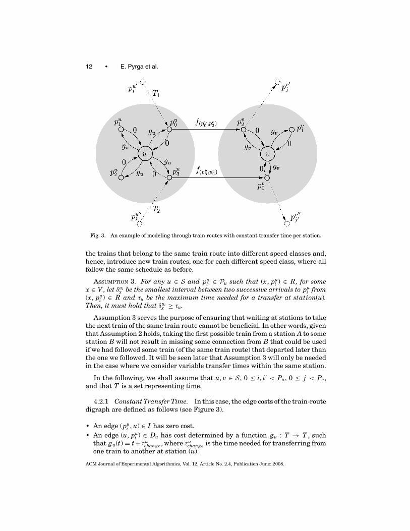
Fig. 3. An example of modeling through train routes with constant transfer time per station.
the trains that belong to the same train route into different speed classes and,hence, introduce new train routes, one for each different speed class, where allfollow the same schedule as before.
ASSUMPTION 3. For any u ∈ S and pui ∈ Pu such that (x, pu
i ) ∈ R, for somex ∈ V , let δui
x be the smallest interval between two successive arrivals to pui from
(x, pui ) ∈ R and τu be the maximum time needed for a transfer at station(u).
Then, it must hold that δuix ≥ τu.
Assumption 3 serves the purpose of ensuring that waiting at stations to takethe next train of the same train route cannot be beneficial. In other words, giventhat Assumption 2 holds, taking the first possible train from a station A to somestation B will not result in missing some connection from B that could be usedif we had followed some train (of the same train route) that departed later thanthe one we followed. It will be seen later that Assumption 3 will only be neededin the case where we consider variable transfer times within the same station.
In the following, we shall assume that u, v ∈ S, 0 ≤ i, i′ < Pu, 0 ≤ j < Pv,and that T is a set representing time.
4.2.1 Constant Transfer Time. In this case, the edge costs of the train-routedigraph are defined as follows (see Figure 3).
� An edge (pui , u) ∈ I has zero cost.
� An edge (u, pui ) ∈ Du has cost determined by a function gu : T → T , such
that gu(t) = t +τuchange, where τu
change is the time needed for transferring fromone train to another at station (u).
ACM Journal of Experimental Algorithmics, Vol. 12, Article No. 2.4, Publication June: 2008.

Efficient Models for Timetable Information in Public Transportation Systems • 13
� An edge (pui , pv
j ) ∈ R has cost determined by a function f (pui , pv
j ) : T → T suchthat f (pu
i , pvj )(t) is the time at which pv
j will be reached using the edge (pui , pv
j ),given that pu
i was reached at time t.
To solve the realistic version of EAP for a given query (A, B, t0), we need tofind a shortest path from station A to B using the modified Dijkstra’s algorithm(cf. Section 3.2), where for each edge we use its associated cost function asdescribed above. We actually need to find the shortest path in the graph G =(V , EA,B) from sA ∈ S to sB ∈ S starting at time t0, where station(sA) = A,station(sB) = B, and EA,B ≡ I
⋃D
⋃R (see Figure 3). Note that all edges
e ∈ DsA must have zero cost.
THEOREM 4. The above algorithm solves the realistic version of EAP withconstant transfer times at stations in the extended time-dependent model, pro-vided that Assumption 2 holds, in time O(md log W + nd log nd ), where nd
(resp. md ) is the number of nodes (resp. edges) of the train-route digraph, andW is the maximum number of elementary connections associated with an edge.
PROOF. In view of the discussion in Section 3.2, regarding the correctness ofTheorem 2, the correctness of the above algorithm for solving the realistic ver-sion of EAP, when the transfer time in each station is constant, follows from thenonnegative delay assumptions of functions f and g , and by the fact that bothfunctions are nondecreasing ( f by Assumption 2 and g by construction).
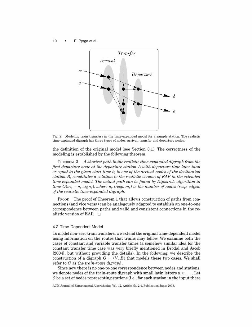
4.2.2 Variable Transfer Time. The edge costs of the train-route digraph inthis case are defined as follows (see also Figure 4).
� An edge (pui , u) ∈ I has zero cost.
� An edge (u, pui ) ∈ Du has zero cost. An edge (pu
i , pui′ ) ∈ Du has cost deter-
mined by a function f (pui , pu
i′ ) : T → T such that f (pui , pu
i′ )(t) represents the timerequired by a passenger who reached station(u) at time t with a train of thetrain route pu
i , to be transferred to the first possible train of route pui′ . In par-
ticular, f (pui , pu
i′ )(t) = t + τuchange(i,i′)(t), where τu
change(i,i′)(t) is the function that,for each arriving time, returns the corresponding transfer time.
� An edge (pui , pv
j ) ∈ R has cost determined by a function f (pui , pv
j ) : T → T suchthat f (pu
i , pvj )(t) is the time at which pv
j will be reached using the edge (pui , pv
j ),given that pu
i was reached at time t.
As before, given a query (A, B, t0), all we need is to find a shortest path fromstation A–B in the above graph, where for each edge we use its associatedcost function as described above. This is again accomplished by the modifiedDijkstra’s algorithm (Section 3.2). We actually need to find a shortest path inthe graph G = (V , EA,B) from sA to sB starting at time t0, but now EA,B ≡DsA
⋃IsB
⋃D
⋃R. Note that all edges e ∈ DsA must have zero cost.
Let nodes pui , pu
j ∈ Pu, 0 ≤ i, j < Pu, i = j , such that (pui , pu
j ) ∈ D. Inaddition, let node pv
i′ ∈ Pv, 0 ≤ i′ < Pv, such that (pvi′ , pu
i ) ∈ R. In orderto be able to apply the above algorithm and solve EAP in this case, we haveto ensure that the functions are nondecreasing. Assumption 2 ensures thatf (pv
i′ , pui )(t) is nondecreasing. What we need to prove is that f (pu
i , puj )(t) is also
ACM Journal of Experimental Algorithmics, Vol. 12, Article No. 2.4, Publication June: 2008.
14 • E. Pyrga et al.
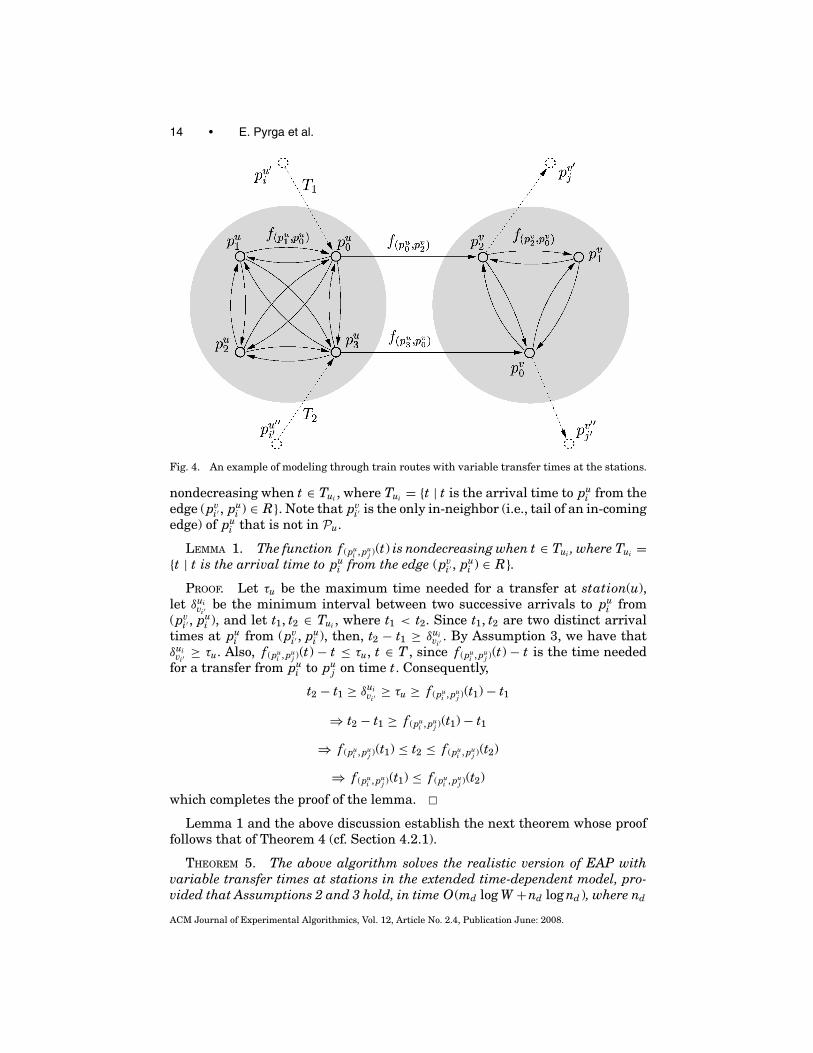
Fig. 4. An example of modeling through train routes with variable transfer times at the stations.
nondecreasing when t ∈ Tui , where Tui = {t | t is the arrival time to pui from the
edge (pvi′ , pu
i ) ∈ R}. Note that pvi′ is the only in-neighbor (i.e., tail of an in-coming
edge) of pui that is not in Pu.
LEMMA 1. The function f (pui , pu
j )(t) is nondecreasing when t ∈ Tui , where Tui ={t | t is the arrival time to pu
i from the edge (pvi′ , pu
i ) ∈ R}.PROOF. Let τu be the maximum time needed for a transfer at station(u),
let δuivi′ be the minimum interval between two successive arrivals to pu
i from(pv
i′ , pui ), and let t1, t2 ∈ Tui , where t1 < t2. Since t1, t2 are two distinct arrival
times at pui from (pv
i′ , pui ), then, t2 − t1 ≥ δui
vi′ . By Assumption 3, we have thatδui
vi′ ≥ τu. Also, f (pui , pu
j )(t) − t ≤ τu, t ∈ T , since f (pui , pu
j )(t) − t is the time neededfor a transfer from pu
i to puj on time t. Consequently,
t2 − t1 ≥ δuivi′ ≥ τu ≥ f (pu
i , puj )(t1) − t1
⇒ t2 − t1 ≥ f (pui , pu
j )(t1) − t1
⇒ f (pui , pu
j )(t1) ≤ t2 ≤ f (pui , pu
j )(t2)
⇒ f (pui , pu
j )(t1) ≤ f (pui , pu
j )(t2)
which completes the proof of the lemma.
Lemma 1 and the above discussion establish the next theorem whose prooffollows that of Theorem 4 (cf. Section 4.2.1).
THEOREM 5. The above algorithm solves the realistic version of EAP withvariable transfer times at stations in the extended time-dependent model, pro-vided that Assumptions 2 and 3 hold, in time O(md log W +nd log nd ), where nd
ACM Journal of Experimental Algorithmics, Vol. 12, Article No. 2.4, Publication June: 2008.
Efficient Models for Timetable Information in Public Transportation Systems • 15
(resp. md ) is the number of nodes (resp. edges) of the train-route digraph, andW is the maximum number of elementary connections associated with an edge.
5. INCORPORATING TRAFFIC DAYS
For all models described so far we have assumed that every train operates daily,i.e., the timetable is identical every day. In this section, we discuss how differenttraffic days can be integrated in the models. For each elementary connectionwe are given the information on which day of the timetable it is valid.
5.1 Time-Expanded Model
When traffic days are used, an optimal connection may stay for more than aday at an intermediate station (e.g., assume on a holiday no trains are operatedat all at that station). Such connections do not correspond to simple paths inthe previous time-expanded digraph, and the problem cannot be solved directlyusing that graph. Therefore, we introduce the fully time-expanded digraph totackle the problem in the time-expanded approach. As we will see below, we donot have to explicitly maintain this graph. The execution of an algorithm onthe fully time-expanded digraph can be simulated on the original (Section 3.1)or on the realistic time-expanded digraph (Section 4.1).
If the timetable is valid for N days, the fully time-expanded digraph is basedon N copies of the (original or realistic) time-expanded digraph. Wheneverthere is an overnight edge in the ith copy, the edge is redirected to the corre-sponding node in the i + 1th copy, if i < N ; in the N th copy, overnight edgesare deleted. Furthermore, in the ith copy all train edges that correspond toelementary connections that are not valid on day i are deleted from the graph.In the following, we assume that each node in the fully-expanded digraph isnot only assigned the time of the day td in the interval [0, 1439], but also theabsolute time in the timetable, i.e., a node in the copy corresponding to day i isassigned time t = td + i 1440. In contrast to the previous (original or extended)time-expanded models, there is an obvious one-to-one correspondence between(valid and consistent) connections and paths in the fully time-expanded di-graph, which immediately yields the following.
LEMMA 2. A shortest path in the original (resp. realistic) fully time-expandeddigraph constitutes a solution to the simplified (resp. realistic) version of EAPwhen elementary connections are valid on specific traffic days only.
Since the size of the fully time-expanded digraph is huge (N times the size ofthe time-expanded digraph), we consider now how we can avoid to maintain thishuge graph explicitly. By construction, all edge costs in the fully time-expandeddigraph are less than a day. Assume an application of Dijkstra’s algorithm tothe fully time-expanded digraph, and let t be the time associated with thefirst node in the priority queue. All other nodes in the priority queue have anassociated time larger than or equal to t and less than t+1440. This observationallows the simulation of Dijkstra’s algorithm on the time-expanded digraph: thetime-expanded digraph reflects the subgraph of the fully time-expanded graphinduced by the nodes with associated time in the interval [t, t + 1440], and
ACM Journal of Experimental Algorithmics, Vol. 12, Article No. 2.4, Publication June: 2008.
16 • E. Pyrga et al.
by ignoring all train edges that correspond to trains, which do not operate onthe considered day. The simulation works as follows. Whenever a departurenode v gets settled, we consider the day specified by the label of that node (i.e.,by dividing its time label by 1440). If its corresponding elementary connection(departure) is not valid on that day, then the outgoing, edge of v is ignored.However, since v is settled, although it corresponds to a nonvalid connection,we consider v as untouched again by setting its distance label to infinity andreinserting it in the priority queue, because from that point on it is consideredto be the copy of the node in the next day.
We can actually avoid resetting the distance labels of the settled nodes toinfinity, by inserting in the priority queue only those nodes that correspond tovalid connections for the specific day. To achieve this, the algorithm is modifiedas follows.
Call a transfer node valid if its corresponding departure is an elementaryconnection that is valid at the day specified by the label of the transfer node.Suppose that instead of using the first transfer node that has a departuretime greater than or equal to the given starting time, we start Dijkstra’s al-gorithm from the first such node that also corresponds to a valid elementaryconnection.
Let v0, v1, v2, . . . , vk be the different transfer nodes of the same station, suchthat they are connected with each other through the edges (vi, v(i+1)modk), 0 ≤i ≤ k. Let wt(e) be the cost of edge e. Node vi has two outgoing edges, (vi, dvi )and (vi, v(i+1)modk), where dvi is the corresponding departure node. When vi getssettled, we know that the train connection of dvi is valid for the day that isspecified by the label of vi. Thus, (vi, dvi ) is relaxed. Now, instead of relaxingthe edge (vi, v(i+1)modk), so as to perform an update to the label of v(i+1)modk ,we do the following. Starting from node v(i+1)modk , we check the following twoconditions: (a) whether its corresponding elementary connection is valid for theday that is specified by the label l(i+1)modk = l (vi) + wt(vi, v(i+1)modk), and (b)whether v(i+1)modk has not already been settled. If both the above conditionshold for v(i+1)modk , then we check whether the current label of v(i+1)modk needsto be updated by l(i+1)modk . If any of the above conditions does not hold, then weproceed with v(i+2)modk , setting l(i+2)modk = l(i+1)modk +wt(v(i+1)modk , v(i+2)modk) =l (vi) + wt(vi, v(i+1)modk) + wt(v(i+1)modk , v(i+2)modk) and so on, until we either finda node vj , 0 ≤ j ≤ k, j = i, that satisfies the above conditions (in whichcase we check whether the label of vj needs to be updated by l j ), or we reachagain vi. In the latter case, no suitable transfer node has been found and sono other update takes place. The above procedure guarantees that the transfernodes and departure nodes in the priority queue will only correspond to validconnections.
Now, if a is an arrival node and there exists an edge (a, vi), where vi is atransfer node, then when a gets settled with label la, instead of trying to updatethe label of the corresponding transfer node vi, we perform again the previousprocedure for the transfer nodes, starting with label li = la + wt(a, vi) for thenode vi. Node a has also an outgoing edge leading to a departure node. Thisedge will be relaxed only if the conditions mentioned above for a transfer nodeare also satisfied by that departure node.
ACM Journal of Experimental Algorithmics, Vol. 12, Article No. 2.4, Publication June: 2008.
Efficient Models for Timetable Information in Public Transportation Systems • 17
Let us now discuss the correctness of the aforementioned approach. Giventhe fact that we start from a valid transfer node and that we can only inserta transfer node in the priority queue if it is valid, we ensure that all transfernodes that get settled are valid. This means that the corresponding outgoingedge that leads to a departure node is relaxed only if that departure is valid atthe specific day.
Exactly for these reasons, there is no longer the need to reset the label ofa node to infinity. The next time this node will be considered, the potentialdistance label that could be given to it will be greater than (or equal to) thelabel that it had when it was settled, and since it was valid for that label, thenthe new label cannot correspond to a better path.
5.2 Time-Dependent Model
The model as defined in Section 3.2 or in Section 4.2 is inherently able to handletraffic days. For route edges, the cost is determined by the first elementaryconnection on that edge leaving later than the arrival time. Now, the cost isdetermined by the first edge leaving later than the arrival time that is valid onthe day under consideration (the day is computed by dividing the arrival timeby 1440).
6. THE MINIMUM NUMBER OF TRANSFERS PROBLEM
The graphs defined for the realistic version of the earliest arrival problem inboth the time-expanded (Section 4.1) and the time-dependent (Section 4.2) ap-proach can be used to solve the minimum number of transfers (MNT) problemwith a similar method: edges that model transfers are assigned a cost of one,and all the other edges are assigned cost zero. In the time-expanded case, allincoming edges of transfer nodes have cost one, whereas in the time-dependentcase the edges in the set D or D (depending on whether there are constant orvariable transfer times at the station), except those belonging to the departurestation, are assigned cost one, and all other edges have cost zero. Note that theedge costs in the time-dependent digraph are all static in this problem. Thecorrectness of this modeling for finding MNT-optimal connections as shortestpaths can be easily verified as in the proof of Theorem 1. This establishes thefollowing.
THEOREM 6. A shortest path in the realistic time expanded (resp. train route)digraph, with the edge costs given above, from a node belonging to (resp. rep-resenting) the departure station to a node belonging to (resp. representing) thearrival station is a solution to the MNTP.
7. BICRITERIA OPTIMIZATION PROBLEMS
We consider bicriteria optimization problems with the earliest arrival (EA)and the minimum number of transfers (MNT) as the two criteria. We inves-tigate three problem variants: (1) finding all Pareto-optimal solutions (thePareto-curve); (2) finding the solution that minimizes one criterion while retain-ing the second below a given threshold; (3) finding the lexicographically first
ACM Journal of Experimental Algorithmics, Vol. 12, Article No. 2.4, Publication June: 2008.

18 • E. Pyrga et al.
Pareto-optimal solution (e.g., find among all connections that minimize EA theone with minimum number of transfers). Variant (2) is investigated only in thetime-dependent model, since it is used as an intermediate step to solve variant(1). In the following, we parameterize the bicriterion problem we consider by(X,Y), where X (resp. Y) is the first (resp. second) criterion we want to optimizeand X,Y ∈ {EA,MNT}.
7.1 Time-Expanded Model
We use the realistic time-expanded digraph (Section 4.1) to find the lexicograph-ically first Pareto-optimum as well as all Pareto-optimal solutions.
7.1.1 Lexicographically First Pareto-optima. We first consider the(EA,MNT) case. Every edge e of the realistic time-expanded digraph is nowassociated with a pair of costs (a, b) = (E A(e), M N T (e)), where E A(e) is thecost of e when solving the realistic version of EAP (Section 4.1) and M N T (e) isthe cost of e when solving MNTP (Section 6). Define on these cost pairs (a, b) thecanonical addition, i.e., (a, b) + (a′, b′) = (a + a′, b + b′), and the lexicographiccomparison, i.e., (a, b) < (a′, b′) ⇔ (a < a′) or (a = a′ and b < b′). To findthe lexicographically first (EA,MNT) Pareto-optimal solution, it then sufficesto run Dijkstra’s algorithm by maintaining distance labels as pairs of integersand by initializing the distance label of the start-node s to (0, 0). The optimalsolution is found when a node at the destination station is settled for the firsttime during the execution of the algorithm. The (MNT,EA) case is symmetricto the above and can be similarly solved. The proof of Theorem 1 can be easilyadopted to establish the following.
THEOREM 7. A shortest path in the realistic time-expanded digraph usingcost pairs associated with its edges as defined above constitutes a solution to theproblem of finding the lexicographically first Pareto-optimal connection (amongall connections that minimize the first criterion, the one with minimum value inthe second criterion). The actual path can be found by Dijkstra’s algorithm intime O(me + ne log ne), where ne (resp. me) is the number of nodes (resp. edges)of the realistic time-expanded digraph.
7.1.2 All Pareto-optima. Finding all Pareto-optimal solutions is generallya hard problem, since there can be an exponential number of them. However,if we consider the realistic fully time-expanded digraph used in Section 5, thenevery node in the time-expanded graph can have only one Pareto-optimum.Hence, we can compute for each node of the destination station the shortestpath according to the cost pairs (a, b) = (E A(e), M N T (e)) with the canoni-cal addition and the lexicographic comparison. This is done as follows. Whenthe first node of the destination station is settled, we have found the first(EA,MNT)–Pareto-optimal connection. We then let Dijkstra’s algorithm con-tinue; whenever a node of the destination station is settled with a smallernumber of transfers than in any of the already found Pareto-optimal solutions,a new Pareto-optimal connection (which corresponds to the shortest path to thatnode) is found. The algorithm can be stopped when the Pareto-optimal solution
ACM Journal of Experimental Algorithmics, Vol. 12, Article No. 2.4, Publication June: 2008.
Efficient Models for Timetable Information in Public Transportation Systems • 19
with the lowest possible number of transfers (i.e., the solution of MNTP) isfound.
THEOREM 8. All Pareto-optimal solutions for the two criteria EA and MNTcan be enumerated during one run of Dijkstra’s algorithm in the realistic fullytime-expanded digraph using cost pairs associated with its edges as definedabove in time O(N (me + ne log(Nne))), where ne (resp. me) is the number ofnodes (resp. edges) of the realistic time-expanded digraph and N is the numberof traffic days a timetable is valid.
PROOF. It suffices to prove that each node of the destination station inthe fully time-expanded digraph has only one Pareto-optimal solution. In thatgraph, every node v is associated with an absolute time value t(v) (not only thetime of the day). Thus, every v1-v2 path has cost l = t(v2) − t(v1) according tothe EA criterion, and, if k is the minimum number of transfers from v1 to v2,then (l , k) is the only Pareto-optimal solution for v2, since all other solutionshave the same EA cost l and an equal or larger than k number of transfers. Thetime bound follows by the fact that the realistic fully time-expanded digraph isN times the size of the realistic time-expanded digraph.
Now, similarly to Section 5.1, the realistic fully time-expanded digraph doesnot need to be maintained explicitly. The above algorithm can again be sim-ulated on the realistic time-expanded digraph. The simulation is identical tothat described in Section 5.1, with the exception of the procedure that pre-vents insertion in the priority queue of any node that corresponds to a nonvalidelementary connection. This procedure needs a slight modification, which isdescribed next.
Let the label of a node v that is settled be (tv, τv), where tv is the time attributeand τv is the number of transfers performed, and let (u, v) be an incoming edge ofv. Assume that at some subsequent point of the algorithm node u is settled, and,consequently, (u, v) is relaxed resulting on a new possible label (t ′
v, τ ′v) for v. We
know that t ′v ≥ tv. If τ ′
v < τv, then we reinsert node v in the priority queue withlabel (t ′
v, τ ′v) and continue the algorithm, as if the node has not been settled (and
storing label (tv, τv) as Pareto-optimum if v belongs to the destination station).This implies that the conditions mentioned in Section 5.1, regarding when toupdate the label of a transfer or departure node v with a new label (t ′
v, τ ′v), has
to change as follows: (a) v is valid for the day specified by t ′v; and (b) v is not
settled or v has been settled but with a number of transfers greater than τ ′v.
Again, we terminate the algorithm when a solution with transfer value equalto the solution of MNTP is found.
Note that the simulation changes the time for enumerating all Pareto-optimal solutions to O(Mme + M Qne + Mne log(Mne)), where M is the maxi-mum number of transfers achieved by the solution of EAP and Q is the max-imum number of transfer nodes within a station. This is because every nodewill be inserted in the priority queue, at most, M + 1 times, every edge willbe relaxed, at most, M + 1 times, and because of the procedure, which pre-vents insertion in the priority queue of any node that corresponds to a nonvalidelementary connection, at most, Q stay edges may have to be examined, for
ACM Journal of Experimental Algorithmics, Vol. 12, Article No. 2.4, Publication June: 2008.

20 • E. Pyrga et al.
every node deleted from the priority queue, until the next valid transfer node isfound.
7.2 Time-Dependent Model
We use the train-route digraph that models the realistic version of EAP(Section 4.2) to solve the three variants of the bicriteria optimization problems.
7.2.1 Lexicographically First Pareto-optima. We present an approach sim-ilar to that described for the time-expanded case, but which finds only the lex-icographically first (MNT,EA) Pareto-optimal solution. Later, we will explainwhy it fails to do the same for the (EA,MNT) case.
A solution to the lexicographically first (MNT,EA) Pareto-optimum problemcan be easily achieved, if instead of using a single value for the cost of an edge,we use a pair (a, b) of values, and define the canonical addition and lexico-graphic comparison to these pairs (exactly as in Section 7.1.1). The attributevalues a, b of the pairs are updated separately. For the (MNT,EA) case, a is theMNT cost defined on IN (nonnegative integers), and b is the EA cost definedon T (set representing time). An edge e ∈ E has cost determined by a functionhe : (IN , T ) → (IN , T ), such that each attribute value is determined by thecorresponding edge function.
THEOREM 9. A shortest path in the train-route digraph using cost pairs as-sociated with its edges, as defined above, constitutes a solution to the problemof finding the lexicographically first (MNT,EA) Pareto-optimal connection. Theactual path can be found in time O(md log W + nd log nd ), where nd (resp. md )is the number of nodes (resp. edges) of the train-route digraph, and W is themaximum number of elementary connections associated with an edge.
PROOF. To prove the correctness, it suffices to show that the new edge costfunction he is nondecreasing and with nonnegative delay. Consider the modelingof the constant transfer cost case, and let τ, τ1, τ2 ∈ IN and t, t1, t2 ∈ T .� If e ∈ I , then he(τ, t) = (τ, t). If (τ1, t1) ≤ (τ2, t2), then he(τ1, t1) ≤ he(τ2, t2).� If e ∈ D, then he(τ, t) = (τ + 1, t + x) ≥ (τ, t), where x ≥ 0 ∈ T is the transfer
time at the station that e belongs to. If (τ1, t1) ≤ (τ2, t2), then he(τ1, t1) =(τ1 + 1, t1 + x) ≤ (τ2 + 1, t2 + x) = he(τ2, t2).
� If e ∈ R, then he(τ, t) = (τ, fe(t)) ≥ (τ, t), since fe has nonnegative delay. If(τ1, t1) ≤ (τ2, t2), then—if τ1 < τ2, then he(τ1, t1) = (τ1, fe(t1)) < (τ2, fe(t2)) = he(τ2, t2), and—if τ1 = τ2 = τ and t1 ≤ t2, then he(τ1, t1) = (τ, fe(t1)) ≤ (τ, fe(t2)) =
he(τ2, t2).
The case with variable transfer cost can be similarly proved. The time boundfollows by that of Theorems 4 and 5.
In contrast to the time-expanded case, the symmetric problem of finding alexicographically first (EA,MNT) Pareto-optimal solution cannot be solved byjust using appropriate edge cost pairs on the train-route digraph, as in Sec-tion 7.1.1. To show that such an approach may fail, consider the train-route
ACM Journal of Experimental Algorithmics, Vol. 12, Article No. 2.4, Publication June: 2008.
Efficient Models for Timetable Information in Public Transportation Systems • 21
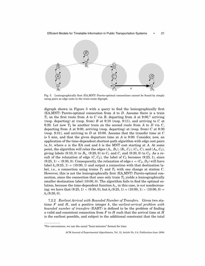
Fig. 5. Lexicographically first (EA,MNT) Pareto-optimal connections cannot be found by simplyusing pairs as edge costs in the train-route digraph.
digraph shown in Figure 5 with a query to find the lexicographically first(EA,MNT) Pareto-optimal connection from A to D. Assume there is a trainT1 on the first route from A to C via B, departing from A at 9:00,4 arriving(resp. departing) at (resp. from) B at 9:10 (resp. 9:11), and arriving to C at9:20. Let now T2 be another train on the second route from A to D via C,departing from A at 9:00, arriving (resp. departing) at (resp. from) C at 9:30(resp. 9:31), and arriving to D at 10:00. Assume that the transfer time at Cis 5 min, and that the given departure time at A is 9:00. Consider, now, anapplication of the time-dependent shortest-path algorithm with edge cost pairs(a, b), where a is the EA cost and b is the MNT cost starting at A. At somepoint, the algorithm will relax the edges (A1, B1), (B1, C1), (C1, C), and (A2, C2),giving labels (9:10, 0) to B1, (9:20, 0) to C1 and C, and (9:30, 0) to C2. As a re-sult of the relaxation of edge (C, C2), the label of C2 becomes (9:25, 1), since(9:25, 1) < (9:30, 0). Consequently, the relaxation of edge e = (C2, D2) will havelabel he(9:25, 1) = (10:00, 1) and output a connection with that destination la-bel, i.e., a connection using trains T1 and T2 with one change at station C.However, this is not the lexicographically first (EA,MNT) Pareto-optimal con-nection, since the connection that uses only train T2 yields a lexicographicallysmaller destination label (10:00, 0). The algorithm fails to find the optimal so-lution, because the time-dependent function he, in this case, is not nondecreas-ing: we have that (9:25, 1) < (9:30, 0), but he(9:25, 1) = (10:00, 1) > (10:00, 0) =he(9:30, 0).
7.2.2 Earliest Arrival with Bounded Number of Transfers. Given two sta-tions F and H, and a positive integer k, the earliest-arrival problem withbounded number of transfers (EABT) is defined to be the problem of findinga valid and consistent connection from F to H such that the arrival time at His the earliest possible, and subject to the additional constraint that the total
4For convenience, we use the usual “hour:minutes” format for time.
ACM Journal of Experimental Algorithmics, Vol. 12, Article No. 2.4, Publication June: 2008.
22 • E. Pyrga et al.
number of transfers performed in the path is not greater than k. Since EAPreduces to a shortest-path problem, EABT is clearly a resource-constrainedshortest-path problem.
In this section, we describe two algorithms for solving the EABT problem.The first one is an adaptation of the graph-copying method proposed in Bro-dal and Jacob [2004] to our realistic time-dependent model (train-route di-graph). The second one is an adaptation of the labeling approach (see e.g.,[Ziegelmann 2001]) for solving resource-constraint shortest paths to our real-istic time-dependent model.
The idea of Brodal and Jacob [2004] adapted to our realistic time-dependentmodel is as follows. We construct a new digraph G ′ = (V ′, E ′) consisting of k +1levels. Each level contains a copy of the train-route digraph G = (V , E), whereE = I
⋃D
⋃D
⋃R) (cf. Section 4.2). For node u ∈ V , we denote its ith copy,
placed at the ith level, by ui, 0 ≤ i ≤ k. For each edge (u, v) ∈ I⋃
R, we placein E ′ the edges (ui, vi), ∀0 ≤ i ≤ k. For each edge (u, v) ∈ D
⋃D, we place
in E ′ the edges (ui, vi+1), ∀0 ≤ i ≤ k. These edges, which connect consecutivelevels, indicate transfers. With the above construction, it is easy to verify thata path from some node s0 (copy of s at the 0th level) to a node xl (copy of x atthe lth level) represents a path from station(s) to station(x) with l transfers.In other words, the EABT problem can be solved by performing a shortest-pathcomputation in G ′ aiming to find a shortest path from a node ps
0 at level 0, whereF = station(s), to the first possible ui at level i, 0 ≤ i ≤ k, where u is the node ofthe train-route graph such that H = station(u). Let nd = |V |, md = |E|, and letW be the maximum number of elementary connections associated with an edgee ∈ E. Since G ′ consists of k + 1 copies of G and since during the shortest-pathcomputation in G ′ a binary search has to be performed when an edge is relaxedto determine its cost, it follows that an application of Dijkstra’s algorithm onG ′ for solving EABT takes O(md k log W + nd k log(nd k)) time.
The adaptation of the labeling approach to our train-route digraph G =(V , E) is as follows. We use the modified Dijkstra’s algorithm (cf. Section 4.2),where we now maintain k + 1 (instead of one) labels, and which requires someadditional operations to take place as nodes are extracted from the priorityqueue. Each label is of the form (tl , l )u, 0 ≤ l ≤ k, representing the currentlybest time tl to reach node u by performing exactly l transfers.
Let s be the node for which F = station(s). The algorithm works as follows.Initially, we insert to the priority queue the label (t, 0)s. The priority queue isordered according to time, aiming at computing the earliest arrival path. Whenwe extract a label (tl , l )u, we relax the outgoing edges of u considering that u isreached on time tl and with l transfers. In addition, if (tl ′ , l ′) was the last labelof u that has been extracted, we then delete from the priority queue all labelsof the form (tr , r)u for l < r < l ′, setting l ′ = k in the case where (tl , l )u wasthe first of the labels of u to have been extracted. In this way, we discard thedominated—by (tl , l )u—labels from the priority queue, since for all such (tr , r)u
it holds that tl ≤ tr (as (tl , l )u was extracted before (tr , r)u) and l < r. Clearly,such labels are no longer useful as (tl , l )u corresponds to an s–u path at leastas fast as the one suggested by (tr , r)u, and with less transfers than the latter.Exactly for the same reasons, when we relax an edge (u, v) ∈ E having found a
ACM Journal of Experimental Algorithmics, Vol. 12, Article No. 2.4, Publication June: 2008.
Efficient Models for Timetable Information in Public Transportation Systems • 23
new label (tl1 , l1)v for v, we will actually update the label of v only if there hasbeen so far no label of v extracted from the priority queue, or if the last label ofv that was extracted had a number of transfers greater than l1.
Concerning now the complexity of the labeling algorithm, we need to seethat for each node the total number of labels that is scanned in order to findthose that that are in the priority queue and can be safely deleted is O(k),while the total number of deletions is O(nd k), where nd = |V |. This is becauseof the fact that we only check the labels from the current number of trans-fers (given by the ultimate delete-min operation) until its previous value (givenby the penultimate delete-min operation). In this way, each label is checked,at most, once throughout the execution of the algorithm. Since each edge willbe relaxed, at most, k + 1 times, the total number of relaxations is O(md k),resulting in a total time of O(md k log W ) for relaxations, where md = |E|and W is the maximum number of elementary connections associated withan edge e ∈ E. We can also see that the total number of labels that is in thepriority queue is, at most, O(nd k). Because of this, the time for a delete-minor a delete operation is O(log(nd k)). This means that the total time neededfor the algorithm is O(md k log W + nd k · log(nd k)), which is asymptoticallythe same as the previous one. The discussion in this section establishes thefollowing.
THEOREM 10. The earliest-arrival with bounded number of transfers prob-lem can be solved in the extended time-dependent model in time O(md k log W +nd k log(nd k)), where nd (resp. md ) is the number of nodes (resp. edges) of thetrain-route digraph, W is the maximum number of elementary connections as-sociated with an edge, and k is the bound in the number of transfers.
7.2.3 All Pareto-optima. The solution to EABT can be used to generate allPareto-optimal solutions in the time-dependent model. In particular, the follow-ing approach finds all Pareto-optima. First, solve EAP and count the numberof transfers found, say M . Then, run the labeling algorithm of Section 7.2.2for solving EABT for all values M − 1, M − 2, . . . , 0 of transfers. Note that thelabeling algorithm can actually be used to speedup the process of solving MEABT problems. Recall that the algorithm maintains for each node M + 1 la-bels, where label 0 ≤ i ≤ M stores the best EA solution performing exactly itransfers (provided that such a solution exists), and discards dominated paths.Hence, instead of stopping the algorithm when the optimal solution with, atmost, M − 1 transfers at the destination is found and repeat with the nexttransfer bound of M − 2, we can just continue with the execution of the algo-rithm to produce the next solution with, at most, M − 2 transfers, consideringthe bound k being equal to M−2, and so on, until no new path can be found. Notethat during the above process, we can discard previously found paths, whichare dominated by subsequent solutions. The above discussion is summarizedas follows.
THEOREM 11. The modified labeling algorithm can enumerate all Pareto-optimal solutions for the two criteria EA and MNT in the extended time-dependent model in O(md M log W + nd M log(nd M )) time, where nd (resp. md )
ACM Journal of Experimental Algorithmics, Vol. 12, Article No. 2.4, Publication June: 2008.

24 • E. Pyrga et al.
is the number of nodes (resp. edges) of the train-route digraph, W is the maxi-mum number of elementary connections associated with an edge, and M is themaximum number of transfers achieved by the solution of EAP.
8. HEURISTICS FOR SPEEDING-UP QUERY TIME
Previous experimental studies with the time-expanded model [Schulz et al.2000, 2002; Wagner et al. 2006] have shown that heuristic improvements canconsiderably speedup performance. These techniques allow for generation ofadditional data during preprocessing that can be used in the on-line phase tospeedup the algorithm. Since one of our goals is to investigate the practical per-formance of the time-dependent model and its extensions, and, in particular, incomparison to the time-expanded model, we have considered several heuristicsfor both models. We focus on a general heuristic (goal-directed search) that canbe applied to both models and also to model specific speedup heuristics. Someof the heuristics have been introduced elsewhere, while some others are new.Since all of them are considered in our experimental study, in the rest of thesection we briefly review the former, while we present the latter in more detail.
8.1 Time-Expanded Model
8.1.1 Goal-Directed Search. The most natural heuristic to consider is thegoal-directed search or the method of potentials (see e.g., [Lengauer 1990]), inorder to exploit the geometric information associated with the nodes (coordi-nates of stations). In this heuristic the cost of every edge is modified in a waythat if the edge points toward the destination its new cost gets smaller, while ifthe edge points away from the destination node, then its new cost gets larger.More precisely, for an edge (u, v) with cost wt(u, v), its new cost wt ′(u, v) becomeswt ′(u, v) = wt(u, v) − p[u] + p[v], where p[·] is a potential function associatedwith the nodes of the graph. The crucial fact is that p[·] must be chosen in sucha way so that wt ′(u, v) is nonnegative.
This heuristic was considered in Schulz et al. [2000] for the time-expandedmodel: if d (u, t) denotes the Euclidean distance of a node u to the destinationstation t of the query and vmax is the maximum speed of the timetable,5 the po-tential function in the time-expanded model is defined as p[u] = d (u, t)/vmax.This scaling of Euclidean distances is necessary to guarantee valid (i.e., non-negative) potentials.
8.1.2 Omitting Nodes. There is a simple way to reduce the size of thegraphs in the time-expanded model, based on the fact that there are a lot ofnodes with out-degree one. Any path through such a node must continue to thehead of the single outgoing edge. Thus, we can safely delete such nodes fromthe graph and redirect the incoming edges to the head of the single outgoingedge. The cost of a redirected edge is the sum of the incoming edge plus the costof the outgoing edge.
5The speed of an elementary connection is the Euclidean distance of the two stations involveddivided by the travel time. The maximum speed vmax of the timetable is the maximum over allspeeds of elementary connections.
ACM Journal of Experimental Algorithmics, Vol. 12, Article No. 2.4, Publication June: 2008.
Efficient Models for Timetable Information in Public Transportation Systems • 25
In the original time-expanded digraph, we omit arrival nodes except forthose in the destination station. Since the latter are only known when a queryis issued, omitting nodes is accomplished as follows. We deactivate (mark asdeleted) all arrival nodes in the graph. When, during the execution of the al-gorithm for answering the query, an edge leading to a node in the destinationstation is relaxed, the corresponding arrival node is activated. In the realis-tic time-expanded digraph we omit departure nodes, and, hence, no particulartreatment is required at query time.
For the original time-expanded digraph, this technique yields a graph ofroughly one-half the original size, since all arrival nodes have out-degree one.In the realistic time-expanded digraph, every departure node has out-degreeone and, hence, this graph is reduced by about one-third.
8.2 Time-Dependent Model
8.2.1 Goal-Directed Search. The goal-directed search heuristic describedin Section 8.1.1 can be also applied in the time-dependent model. However, pre-liminary experiments with exactly the same technique showed no improvementof the running time in the time-dependent model. Therefore, we had to inventsome new variant of the goal-directed search method to improve the runningtime. Our new variant uses: (1) a different potential function, which depends onthe destination station; (2) Manhattan, besides Euclidean, distances betweenstations; and (3) integral potentials to avoid expensive floating-point operations.The details are as follows.
As in Section 8.1.1, for an edge (u, v) ∈ E with cost function wt(u, v, τ ),where τ is the arrival time at u, the new cost function wt ′(u, v, τ ) is defined aswt ′(u, v, τ ) = wt(u, v, τ ) − p[u] + p[v], where p[·] is the potential function. Lett be the destination node. Then, define
p[u] = d (u, t)λt , u ∈ V , λt ≥ 0
where d (u, t) is the Euclidean or Manhattan distance between nodes u and t,based on the coordinates of (the stations corresponding to) u and t. The param-eter λt is called the scaling factor and is a nonnegative number (which can bedifferent for each destination node t) that is used to scale the distances so thatwt ′(u, v, τ ) is nonnegative. The scaling factor is defined as
λt = min(u,v)∈E,d (u,t)−d (v,t)>0
minτ wt(u, v, τ )d (u, t) − d (v, t)
Note that λt corresponds to the inverse of the maximum speed considered inSection 8.1.1; however, in Section 8.1.1 the maximum speed is the same for alldestinations t, while λt depends on t. Potentials p[·], as defined above, are validas the next lemma shows.
LEMMA 3. The function p[·] is a valid potential function for the goal-directedsearch, i.e., wt ′(u, v) is nonnegative for each edge (u, v).
PROOF. Let (α, β) ∈ E be the edge with the above property and wt(α, β, τ0) =minτ wt(α, β, τ ). Note that there has to be an edge (α, β) ∈ E such that d (α, t) −d (β, t) > 0, since otherwise there would be no way reaching t – the distance to
ACM Journal of Experimental Algorithmics, Vol. 12, Article No. 2.4, Publication June: 2008.

26 • E. Pyrga et al.
get there from any node u ∈ V could never be reduced. Then, for every edge(u, v) ∈ E with d (u, t) > d (v, t), we have
minτ wt(u, v, τ )d (u, t) − d (v, t)
≥ wt(α, β, τ0)d (α, t) − d (β, t)
(1)
wt ′(u, v, τ ′) = wt(u, v, τ ′) − p[u] + p[v], τ ′ ≥ 0 (2)
From Eq. (2) we get
wt ′(u, v, τ ′) ≥ minτ wt(u, v, τ ) − wt(α, β, τ0)d (u, t) − d (v, t)d (α, t) − d (β, t)
and from Eq. (1) we obtain that
minτ
wt(u, v, τ ) ≥ wt(α, β, τ0)d (u, t) − d (v, t)d (α, t) − d (β, t)
which, consequently, implies that
wt ′(u, v) ≥ 0
Now, if d (u, t) − d (v, t) ≤ 0, then −[d (u, t) − d (v, t)] ≥ 0 and −λt[d (u, t) −d (v, t)] ≥ 0, which means that wt ′(u, v) = wt(u, v) − λt[d (u, t) − d (v, t)] ≥wt(u, v) ≥ 0.
Even if all edge cost are integers, the use of the Euclidean or Manhattan dis-tances as potentials forces us to use floating-point numbers in the priorityqueue, and this may result in an additional time overhead. In order to avoid this,we can transform the floating-point potentials to integers without invalidatingthe potentials, as the following lemma shows.
LEMMA 4. If, for the nonnegative numbers w ∈ IN, a, b ∈ IR+, it holds thatw − a + b ≥ 0, then it will also hold that w − �a� + �b� ≥ 0.
PROOF. If a = b, the proposition holds trivially. Let f r(a) = a − �a� andfr(b) = b − �b�. Consider first the case a < b. Then, a − b < 0 ⇒ �a� − �b� <
fr(b) − fr(a). Assume that w − �a� + �b� < 0. Since w ≥ 0, we must have that�a�−�b� > 0, and, hence, 0 < �a�−�b� < fr(b)− fr(a). However, fr(b)− fr(a) < 1and �a� − �b� is an integer, a contradiction.
We turn now to the case a > b. Assume again that w − �a� + �b� < 0. Then,w < �a�−�b�. We also have �a�−�b� ≤ w+ fr(b)− fr(a). Combining the last twoinequalities and the fact that fr(b)−fr(a) < 1, we get that w < �a�−�b� < w+1,which is again a contradiction.
Consideration of the integral parts of the floating-point potentials turned outto be rather beneficial in certain cases, as our experiments show.
8.2.2 Avoiding Binary Search. For the original time-dependent model, wealso considered the heuristic that avoids the binary search as described inBrodal and Jacob [2004]. This speedup technique assumes that there existsa single timetable with no exception in which day a train operates. The ideais as follows. Let k be the out-degree of a node v in the time-dependent di-graph and let (v, u1), . . . , (v, uk) be its outgoing edges. Construct a table Dv
ACM Journal of Experimental Algorithmics, Vol. 12, Article No. 2.4, Publication June: 2008.
Efficient Models for Timetable Information in Public Transportation Systems • 27
by sorting all events of v’s outgoing edges w.r.t. their departure time. Placethe first k such events in the first k entries (primary segment) of Dv, leavethe next k entries empty (secondary segment), place the next k events in thenext k entries of Dv, and so on. Let t0 be the last event in Dv before somesecondary segment. For every (v, ui), 1 ≤ i ≤ k, find the first event with de-parture time t ≥ t0 and put it into the ith entry of the next secondary seg-ment. For an edge (w, v), let t1 be the arrival time of a primary event Pw ∈ Dw
(event belonging to some primary segment of Dw). Create a pointer from Pw
to the immediately next primary event Pv ∈ Dv with timestamp t2 ≥ t1. Theabove construction avoids binary search, because when node v is extractedfrom the priority queue, we simply follow the pointer of the event Pw thatcaused v’s extraction from the priority queue, and which leads to a primaryentry Pv ∈ Dv. Hence, to find the next outgoing event of node v, it sufficesto scan the rest of the primary segment containing Pv and its next secondarysegment.
8.2.3 Further Speedup When Modeling with Train Routes. In order toquickly find the most suited connection for each edge, we need to store theinformation efficiently. In this section, we elaborate on implementation issuesregarding the efficient storage and retrieval of information concerning the com-putation of edge costs.
From the input we know that every edge (x, y) ∈ E is associated witha timetable. The entries of the timetable are stored lexicographically, i.e., if(d1, a1), (d2, a2) are two such entries, then (d1, a1) < (d2, a2) iff d1 < d2, ord1 = d2 and a1 < a2. Recall that for each edge (x, y) ∈ E, there is a functionf ′
(x, y) : T → T , which determines the cost of the edge. In this way, before relax-ing the outgoing edges of a node, we need to call the corresponding function f ′
to compute the cost of the edge at the specified time.Consider the case of variable transfer costs within the same station. Note
that the different time needed for each transfer at some station between thesame train routes is caused by the fact that the trains that perform the sameroute do not stop every time at the same platform of the station. The inputregarding the time for the transfers takes into consideration the platforms atwhich the trains stop. This means that for every event e there must be someinformation about the first train of every other train route that can be followed.As a result, for the case of variable transfer costs, each edge (pu
i , pui′ ) ∈ Du, u ∈ S,
has a timetable with one entry for each possible arrival time to pui . Because of
this, all edge functions f ′ must perform a search in order to find the most suit-able entry in the edge’s timetable. To avoid the search, we can store additionalinformation at the edges (x, y) ∈ R, instead of storing a timetable at each edge(x, y) ∈ D.
Let (pvj , pu
i ), (pui , pw
l ) ∈ R be two edges which belong to the same route and letT(pv
j , pui ), T(pu
i , pwl ) be their corresponding timetables. Also, let s be the station that
pui belongs to. For each event (entry) e ∈ T(pv
j , pui ) we store a pointer same traine
to the event e′ of T(pui , pw
l ) such that e, e′ are performed successively by the sametrain. (We assume that the first train that leaves pu
i after the arrival time of eis the same train that e belongs to.) In this way when we need to relax the only
ACM Journal of Experimental Algorithmics, Vol. 12, Article No. 2.4, Publication June: 2008.
28 • E. Pyrga et al.
outgoing edge of pui that belongs to R (no transfer is performed), we just need
to follow the same traine of the event e that brought us to that node.Now, we consider the case where we need to relax an outgoing edge (pu
i , pui′ ) ∈
D of pui . Let (pu
i′ , pw′l ′ ), for pw′
l ′ ∈ V , be the outgoing edge of pui′ that belongs to R,
and T(pui′ , pw′
l ′ ) its respective timetable. Instead of storing a timetable for (pui , pu
i′ ),we store for each e ∈ T(pv
j , pui ) a pointer ver y nexte,i′ , to the event e′ of T(pu
i′ , pw′l ′ )
such that e′ is the first event of (pui′ , pw′
l ′ ) that can be followed given that pui
was reached by use of e. Having one such pointer ver y nexte,i′ for all pui′ , we
can relax at once the outgoing edges of all nodes of station s belonging to R,and thus avoid the relaxation of all other edges (not in R) among those nodes.This means that we no longer need to store any other information regardingthese latter edges. Note also that the same traine pointer is ver y nexte,i sosame train pointers need not be stored explicitly either.
For the case of constant transfer time at each station, we can avoid someof the binary searches when solving one of the problems by expanding, if nec-essary, the graph a little more. Suppose that when the trains are separatedinto train routes at the construction of the graph, we impose the additionalconstraint that for each train route the events that belong to the same trainof the route are always indexed by the same number at the (sorted) timeta-bles of the (timetable) edges of the corresponding route. Suppose, also, that ateach route node u, an index next departureu is maintained. If during the ex-ecution of the algorithm u is reached by its incoming (if any) route edge, thennext departureu is set to the index of the event that was used on the incom-ing edge. If, on the other hand, u was reached through a transfer edge, thennext departureu is set to −1. In this way, when u is extracted from the priorityqueue, if next departureu is nonnegative, the corresponding event can be usedto relax its outgoing route edge, without the need to perform a binary search. Ifnot, a binary search must be performed. Moreover, a negative next departureu
value means that the shortest path from the source node to u passes throughthe central node of u’s station. Thus, the outgoing (transfer) edge of u that leadsto the central node does not need to be relaxed.
9. EXPERIMENTS
The main goal of our experimental study is to compare, in practice, the perfor-mance of the time-expanded and the time-dependent approach, both in theiroriginal and in their extended versions.
Given two different implementations and a timetable, we define the relativeperformance or speedup with respect to a measured performance parameteras the ratio of the value obtained by the first implementation and the valueobtained by the second one. When one time-expanded and one time-dependentimplementation is compared, we always divide the time-expanded value by thetime-dependent value, i.e., we consider the speedup achieved when the time-dependent approach is used instead of the time-expanded approach.
All of our code is written in C++ and compiled with the GNU C++ com-piler version 3.2. The experiments were run on a PC with AMD Athlon XP1500+ processor at 1.3 GHz and 512 MB of memory running Linux (kernel
ACM Journal of Experimental Algorithmics, Vol. 12, Article No. 2.4, Publication June: 2008.
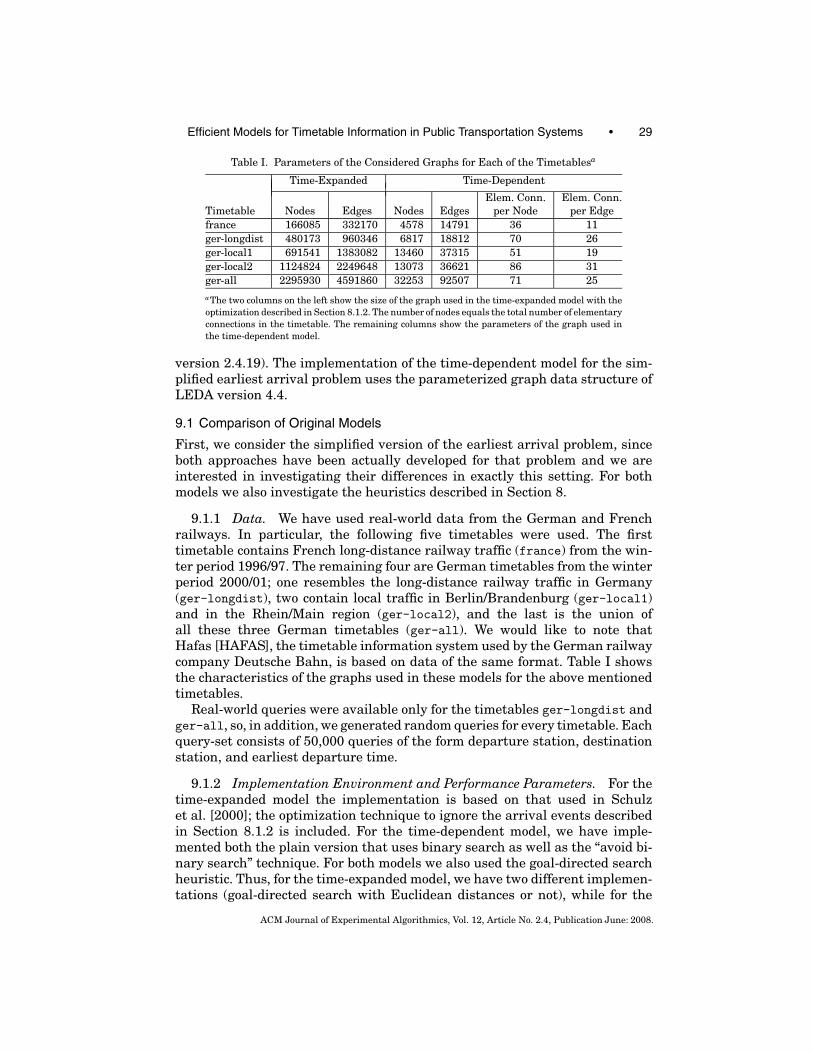
Efficient Models for Timetable Information in Public Transportation Systems • 29
Table I. Parameters of the Considered Graphs for Each of the Timetablesa
Time-Expanded Time-Dependent
Elem. Conn. Elem. Conn.Timetable Nodes Edges Nodes Edges per Node per Edgefrance 166085 332170 4578 14791 36 11ger-longdist 480173 960346 6817 18812 70 26ger-local1 691541 1383082 13460 37315 51 19ger-local2 1124824 2249648 13073 36621 86 31ger-all 2295930 4591860 32253 92507 71 25aThe two columns on the left show the size of the graph used in the time-expanded model with theoptimization described in Section 8.1.2. The number of nodes equals the total number of elementaryconnections in the timetable. The remaining columns show the parameters of the graph used inthe time-dependent model.
version 2.4.19). The implementation of the time-dependent model for the sim-plified earliest arrival problem uses the parameterized graph data structure ofLEDA version 4.4.
9.1 Comparison of Original Models
First, we consider the simplified version of the earliest arrival problem, sinceboth approaches have been actually developed for that problem and we areinterested in investigating their differences in exactly this setting. For bothmodels we also investigate the heuristics described in Section 8.
9.1.1 Data. We have used real-world data from the German and Frenchrailways. In particular, the following five timetables were used. The firsttimetable contains French long-distance railway traffic (france) from the win-ter period 1996/97. The remaining four are German timetables from the winterperiod 2000/01; one resembles the long-distance railway traffic in Germany(ger-longdist), two contain local traffic in Berlin/Brandenburg (ger-local1)and in the Rhein/Main region (ger-local2), and the last is the union ofall these three German timetables (ger-all). We would like to note thatHafas [HAFAS], the timetable information system used by the German railwaycompany Deutsche Bahn, is based on data of the same format. Table I showsthe characteristics of the graphs used in these models for the above mentionedtimetables.
Real-world queries were available only for the timetables ger-longdist andger-all, so, in addition, we generated random queries for every timetable. Eachquery-set consists of 50,000 queries of the form departure station, destinationstation, and earliest departure time.
9.1.2 Implementation Environment and Performance Parameters. For thetime-expanded model the implementation is based on that used in Schulzet al. [2000]; the optimization technique to ignore the arrival events describedin Section 8.1.2 is included. For the time-dependent model, we have imple-mented both the plain version that uses binary search as well as the “avoid bi-nary search” technique. For both models we also used the goal-directed searchheuristic. Thus, for the time-expanded model, we have two different implemen-tations (goal-directed search with Euclidean distances or not), while for the
ACM Journal of Experimental Algorithmics, Vol. 12, Article No. 2.4, Publication June: 2008.

30 • E. Pyrga et al.
time-dependent model we have several implementations depending on the useof: binary search or the “avoid binary search” version, the goal-directed searchheuristic with Euclidean or Manhattan distances, and whether floating-pointor integral potentials are used.
For each possible combination of timetable and implementation variant,we performed the corresponding set of random queries (for ger-longdist andger-all we, in addition, performed the corresponding real-world queries) andmeasured the following performance parameters as average values over theset of performed queries: CPU time in milliseconds, number of nodes, numberof edges, and number of elementary connections touched by the algorithm. Forthe time-expanded model, the number of elementary connections touched is thenumber of train edges touched by the algorithm, while for the time-dependentmodel it is the total number of elementary connections that have been used bybinary search for calculating the edge costs.
9.1.3 Results and Discussion. Our experimental results are reported inFigure 6 and Tables II, III, and IV. The reported results clearly show that thetime-dependent model solves the simplified earliest-arrival problem consider-ably faster than the time-expanded model, for every considered data set. Re-garding CPU time, the speedup ranges between 12 (france) and 40 (ger-local2)when the basic implementations are used (see Figure 6 and Table II), and be-tween 17 (france) and 57 (ger-local2) when comparison concerns the bestimplementations (including heuristics) in both models (see Tables III and IV).
Concerning the time-dependent model, we observe that is is better to use the“avoid binary search” technique (see Tables III and IV). Compared to the binarysearch implementation, the speedup was between 1.39 (ger-local1) and 1.86(ger-all with real-world queries). The goal-directed search technique alwaysreduces the search space of Dijkstra’s algorithm, i.e., the number of touchednodes and edges. However, this reduction payed off only in a few cases in thesense that it could not also decrease the CPU time. In most cases, the CPU timewas increased because of the additional computations required to calculate theedge costs and this is the main reason why this technique appears slower inthe results. Another reason is that in the timetables used in our experimentsthe maximum speed over all elementary connections is high. A high maximumspeed yields small potential functions,6 and thus bad performance of the goal-directed search technique.
9.2 Comparison of Realistic Models
In this section, we investigate how the time-expanded and the time-dependentapproaches compare when the realistic versions of the problems and modelsare considered. As input data, we used a modification of the ger-longdisttimetable, which we refer to as ger-longdist1. Since train changes are consid-ered here, we only used the trains of the timetable that operate on one specific
6In both models, the potentials are inversely proportional to the maximum speed; for the time-expanded case this is clear by definition; for the time-dependent case, see the definition of thefactor λt .
ACM Journal of Experimental Algorithmics, Vol. 12, Article No. 2.4, Publication June: 2008.
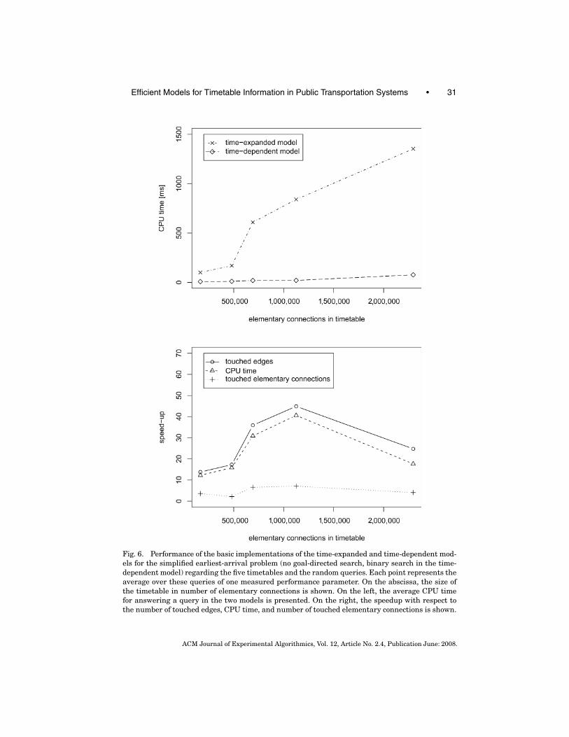
Efficient Models for Timetable Information in Public Transportation Systems • 31
Fig. 6. Performance of the basic implementations of the time-expanded and time-dependent mod-els for the simplified earliest-arrival problem (no goal-directed search, binary search in the time-dependent model) regarding the five timetables and the random queries. Each point represents theaverage over these queries of one measured performance parameter. On the abscissa, the size ofthe timetable in number of elementary connections is shown. On the left, the average CPU timefor answering a query in the two models is presented. On the right, the speedup with respect tothe number of touched edges, CPU time, and number of touched elementary connections is shown.
ACM Journal of Experimental Algorithmics, Vol. 12, Article No. 2.4, Publication June: 2008.

32 • E. Pyrga et al.
Table II. Average CPU Time and Operation Counts for Solving a Single Query forthe Time-Expanded (Upper Part) and the Time-Dependent Model (Lower Part)a
Timetable Real Time [ms] El. Conn. Nodes EdgesExpanded france 100.4 30824 33391 61649
ger-longdist 169.6 44334 48094 88668ger-local1 608.7 176720 182717 353443ger-local2 840.1 226027 232511 452056ger-all 1352.8 326186 342917 652378ger-longdist × 66.7 18891 20853 37783ger-all × 392.1 96943 104369 193888
Dependent france 8.2 8539 2269 4463ger-longdist 10.7 20066 3396 5129ger-local1 19.7 26792 6535 9835ger-local2 20.7 31698 6524 10075ger-all 76.6 79981 16145 26333ger-longdist × 5.5 11173 1711 2682ger-all × 37.3 40808 6926 11647
aThe arrival nodes are omitted in the time-expanded model (see Section 8.1.2), and in the time-dependent model binary search was used. Goal-directed search was not applied in both cases.The column Real indicates whether real-world or random queries have been used.
day, whereas in the simplified case discussed before, we assumed that all trainsoperate daily. We used the modeling with constant transfer times at stations,since only the maximum possible transfer time for each station was available inthe input data. We also used the real-world and random queries as described inSection 9.1.1. Table V shows the parameters of the graphs used in the realisticmodels compared to the original models.
9.2.1 Implementation Environment. For both approaches we implementedthe described solutions for the realistic earliest-arrival (EA-realistic) problem(Section 4), the minimum number of transfers (MNT) problem (Section 6), theall Pareto-optima (All Pareto-Opt) problem involving EA and MNT as the twocriteria (Section 7), the lexicographically first (MNT,EA) Pareto-optimum (Lex-F(MNT,EA), and the lexicographically first (EA,MNT) Pareto-optimum (Lex-F(EA,MNT))—the latter only for the time-expanded model see Section 7.2.1).Moreover, for the time-dependent model, we have also considered the two algo-rithms for solving the earliest arrival with bounded number of transfers prob-lem (Section 7.2.2): the one based on the graph-copying approach (EABT-BJ)and the one based on the labeling approach (EABT-L).
In the time-expanded implementations we again reduced the node set byomitting the departure nodes in the realistic time-expanded graph (see Sec-tion 8.1.2). In the realistic time-dependent implementations, we also appliedthe heuristic described in Section 8.2.3.
9.2.2 Results. Table V (lower part) shows the comparison between theproblems solved in both realistic versions of the time and the time-dependentapproaches. The key parameters—number of touched nodes, edges, and av-erage running time—are displayed for the real-world queries. More details,as well as results on random queries and other problems, are shown inTable VI.
ACM Journal of Experimental Algorithmics, Vol. 12, Article No. 2.4, Publication June: 2008.

Efficient Models for Timetable Information in Public Transportation Systems • 33
Table III. Comparison of the Time-Dependent Implementations that Use BinarySearch and Four Different Versions of Goal-Directed Search: Euclidean Distance with
Integer and Float Potentials and Manhattan Distance with Integer and FloatPotentialsa
Time-dependent Model, Binary SearchTimetable Real Time [ms] El. conn. Nodes Edges
Goal Eucl. int france 9.4 7072 1593 3415ger-longdist 13.5 16597 2737 4217ger-local1 28.6 26008 6257 9434ger-local2 30.4 31196 6398 9895ger-all 100.3 74525 14568 24030ger-longdist × 6.3 8349 1238 1991ger-all × 43.1 33676 5551 9420
Goal Eucl. float france 9.4 7062 1590 3410ger-longdist 13.6 16560 2730 4208ger-local1 28.9 25975 6249 9422ger-local2 30.7 31152 6389 9882ger-all 103.6 74394 14538 23983ger-longdist × 6.4 8318 1233 1984ger-all × 44.5 33565 5532 9388
Goal Manh. int france 7.9 7225 1647 3511ger-longdist 11.2 16975 2807 4316ger-local1 23.2 26086 6284 9473ger-local2 24.7 31235 6407 9908ger-all 86.4 74822 14639 24138ger-longdist × 5.3 8555 1272 2041ger-all × 38.0 33994 5615 9524
Goal Manh. float france 7.7 7214 1644 3505ger-longdist 11.1 16938 2800 4306ger-local1 23.1 26053 6276 9461ger-local2 24.6 31189 6398 9894ger-all 88.9 74689 14608 24091ger-longdist × 5.2 8524 1267 2034ger-all × 39.0 33880 5594 9491
aColumns are as in Table II.
Concerning CPU time, the results show that the time-dependent approachstill performs better than the time-expanded approach in all cases considered.However, the gap for the realistic EAP is not as large as it was for the simpli-fied EAP; in fact, for real-world queries the speedup is now only 1.5. Moreover,if one considers the total number of touched edges, for real-world queries thespeedup is smaller than 1 (i.e., the time-expanded approach is better). However,this does not affect the running time, since less than one-half of the total touchededges require extra operations for computing their costs (timetable edgestouched; see Table VI, lower part) and the rest has a fixed cost (transfer edgestouched).
For the other problems considered, the time speedup ranges from 1.5 to 3.3,while the touched-edges speedup is 1.6, in all cases. In particular, for the MNTproblem, the extended time-dependent model (train-route digraph) is clearlysuperior to the extended time-expanded model (realistic time-expanded di-graph); the speedup with respect to CPU time is 3.3 for real-world queries and4.5 for random queries. A similar observation holds for the lexicographically
ACM Journal of Experimental Algorithmics, Vol. 12, Article No. 2.4, Publication June: 2008.
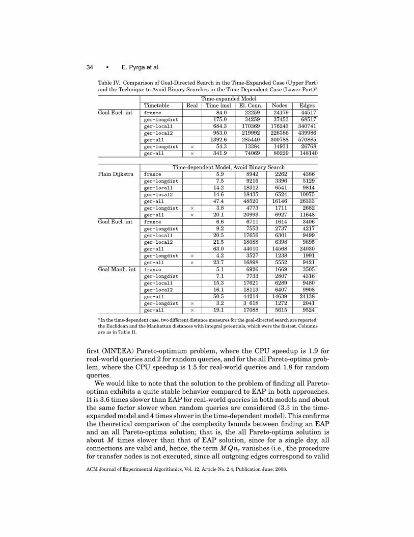
34 • E. Pyrga et al.
Table IV. Comparison of Goal-Directed Search in the Time-Expanded Case (Upper Part)and the Technique to Avoid Binary Searches in the Time-Dependent Case (Lower Part)a
Time-expanded ModelTimetable Real Time [ms] El. Conn. Nodes Edges
Goal Eucl. int france 84.0 22259 24179 44517ger-longdist 175.0 34259 37453 68517ger-local1 684.3 170369 176243 340741ger-local2 953.0 219992 226386 439986ger-all 1392.6 285440 300788 570885ger-longdist × 54.3 13384 14931 26768ger-all × 341.9 74069 80229 148140
Time-dependent Model, Avoid Binary SearchPlain Dijkstra france 5.9 8942 2262 4386
ger-longdist 7.5 9216 3396 5129ger-local1 14.2 18312 6541 9814ger-local2 14.6 18435 6524 10075ger-all 47.4 48520 16146 26333ger-longdist × 3.8 4773 1711 2682ger-all × 20.1 20993 6927 11648
Goal Eucl. int france 6.6 6711 1614 3406ger-longdist 9.2 7553 2737 4217ger-local1 20.5 17656 6301 9499ger-local2 21.5 18088 6398 9895ger-all 63.0 44010 14568 24030ger-longdist × 4.2 3527 1238 1991ger-all × 23.7 16898 5552 9421
Goal Manh. int france 5.1 6926 1669 3505ger-longdist 7.1 7733 2807 4316ger-local1 15.3 17621 6289 9480ger-local2 16.1 18113 6407 9908ger-all 50.5 44214 14639 24138ger-longdist × 3.2 3 618 1272 2041ger-all × 19.1 17088 5615 9524
aIn the time-dependent case, two different distance measures for the goal-directed search are reported:the Euclidean and the Manhattan distances with integral potentials, which were the fastest. Columnsare as in Table II.
first (MNT,EA) Pareto-optimum problem, where the CPU speedup is 1.9 forreal-world queries and 2 for random queries, and for the all Pareto-optima prob-lem, where the CPU speedup is 1.5 for real-world queries and 1.8 for randomqueries.
We would like to note that the solution to the problem of finding all Pareto-optima exhibits a quite stable behavior compared to EAP in both approaches.It is 3.6 times slower than EAP for real-world queries in both models and aboutthe same factor slower when random queries are considered (3.3 in the time-expanded model and 4 times slower in the time-dependent model). This confirmsthe theoretical comparison of the complexity bounds between finding an EAPand an all Pareto-optima solution; that is, the all Pareto-optima solution isabout M times slower than that of EAP solution, since for a single day, allconnections are valid and, hence, the term M Qne vanishes (i.e., the procedurefor transfer nodes is not executed, since all outgoing edges correspond to valid
ACM Journal of Experimental Algorithmics, Vol. 12, Article No. 2.4, Publication June: 2008.

Efficient Models for Timetable Information in Public Transportation Systems • 35
Table V. Graph Parameters and Main Results for Realistic Models, Applied to theSame Input Timetable ger-longdist1a
Time-expanded Time-dependentStation Route Timetable Transfer
Graph Nodes Edges Nodes Nodes Edges EdgesSimplified 289432 578864 6685 — 17577 —Realistic 578864 1131164 6685 79784 72779 159568
Time-expanded Time-dependentProblem Nodes Edges Time [ms] Nodes Edges Time [ms]EA-realistic 40624 73104 78 44731 83662 50MNT 101731 138417 125 26680 83173 38Lex-F(MNT,EA) 99061 137075 161 28272 83363 83All Pareto-Opt 123943 236887 287 78412 145444 181
aThe upper part shows the number of nodes and edges of the graphs compared to the simplified, origi-nal models. The lower part contains the average values over all real-world queries of the performanceparameters for the different problems solved.
connections). A closer look at our data reveals that the average M over all valuesof M is 3.62 for real-world queries and 4 for random queries (the value of M foreach query is the number of transfers achieved by the solution of EAP for thatquery).
Further observations regarding each model separately are as follows.
9.2.2.1 Time-Expanded Model. The graph used in the realistic EAP (Ta-ble VI) has less than twice as many nodes and edges as the graph used inthe simplified EAP and is of very similar structure. Thus, it needs only slightlymore time to solve the realistic EAP than to solve the simplified EAP (11% moretime using real-world queries and 16% more using random queries). The lexico-graphically first (EA,MNT) Pareto-optimal problem is solved in a very similarway as the realistic EAP. It is interesting to observe that the CPU time, as wellas the average number of nodes and edges touched, are almost identical. Incontrast, the MNT, the lexicographically first (MNT,EA) Pareto-optimum, andthe all Pareto-optima problems require more CPU time than the realistic EAP,since a much bigger part of the graph has to be explored.
9.2.2.2 Time-Dependent Model. Although the train-route digraph has ap-proximately 13 times more nodes and edges than the digraph of the originaltime-dependent model (see Table V), the experimental results reported in Ta-ble VI show that the time required for solving the realistic EAP is only fivetimes slower than that of the simplified EAP. This is because of the fact thatthe structure of the two graphs is quite different. While the original time-dependent digraph has only timetable edges, almost 70% of the train-route di-graph edges have constant cost and the timetables of the other edges have muchfewer events than their corresponding edges in the original time-dependentdigraph.
The MNT problem is solved faster than the realistic EAP, since, in this case,all edge costs in the train-route digraph are static and, hence, no binary searchis needed.
ACM Journal of Experimental Algorithmics, Vol. 12, Article No. 2.4, Publication June: 2008.
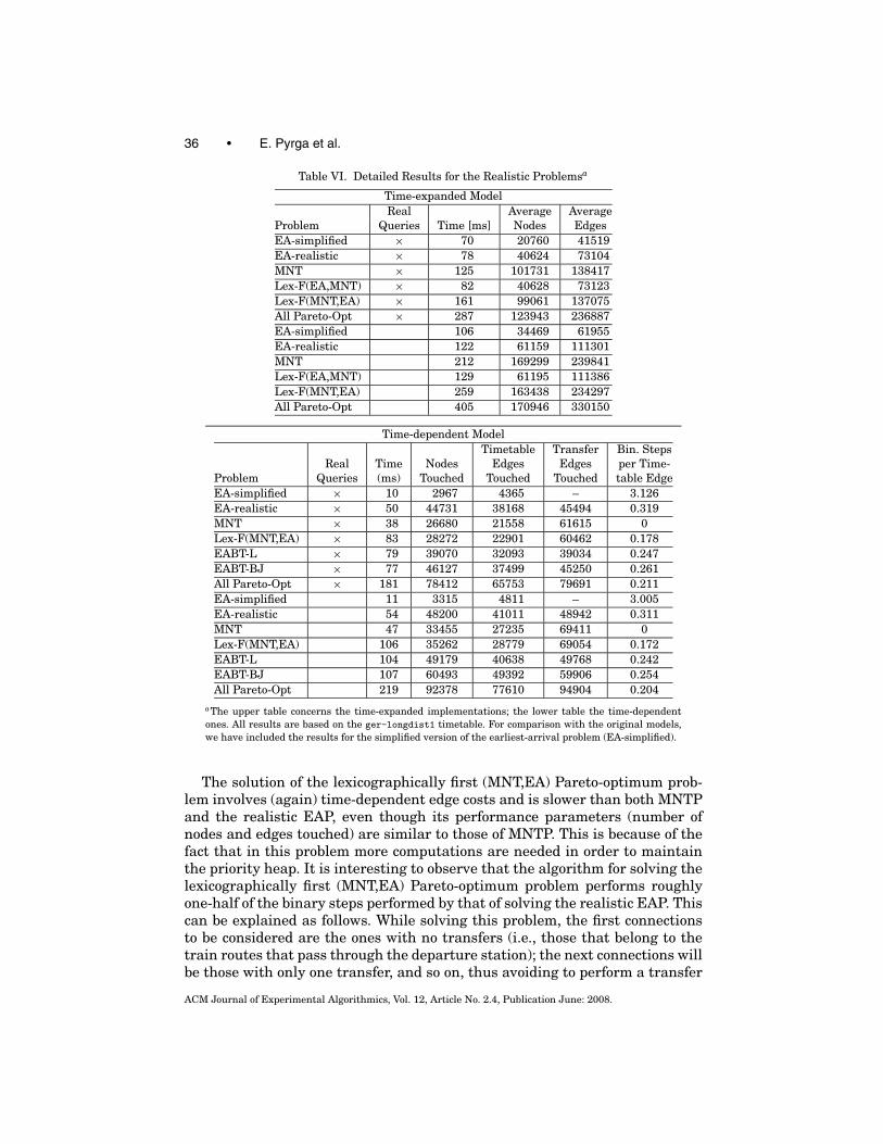
36 • E. Pyrga et al.
Table VI. Detailed Results for the Realistic Problemsa
Time-expanded ModelReal Average Average
Problem Queries Time [ms] Nodes EdgesEA-simplified × 70 20760 41519EA-realistic × 78 40624 73104MNT × 125 101731 138417Lex-F(EA,MNT) × 82 40628 73123Lex-F(MNT,EA) × 161 99061 137075All Pareto-Opt × 287 123943 236887EA-simplified 106 34469 61955EA-realistic 122 61159 111301MNT 212 169299 239841Lex-F(EA,MNT) 129 61195 111386Lex-F(MNT,EA) 259 163438 234297All Pareto-Opt 405 170946 330150
Time-dependent ModelTimetable Transfer Bin. Steps
Real Time Nodes Edges Edges per Time-Problem Queries (ms) Touched Touched Touched table EdgeEA-simplified × 10 2967 4365 – 3.126EA-realistic × 50 44731 38168 45494 0.319MNT × 38 26680 21558 61615 0Lex-F(MNT,EA) × 83 28272 22901 60462 0.178EABT-L × 79 39070 32093 39034 0.247EABT-BJ × 77 46127 37499 45250 0.261All Pareto-Opt × 181 78412 65753 79691 0.211EA-simplified 11 3315 4811 – 3.005EA-realistic 54 48200 41011 48942 0.311MNT 47 33455 27235 69411 0Lex-F(MNT,EA) 106 35262 28779 69054 0.172EABT-L 104 49179 40638 49768 0.242EABT-BJ 107 60493 49392 59906 0.254All Pareto-Opt 219 92378 77610 94904 0.204
aThe upper table concerns the time-expanded implementations; the lower table the time-dependentones. All results are based on the ger-longdist1 timetable. For comparison with the original models,we have included the results for the simplified version of the earliest-arrival problem (EA-simplified).
The solution of the lexicographically first (MNT,EA) Pareto-optimum prob-lem involves (again) time-dependent edge costs and is slower than both MNTPand the realistic EAP, even though its performance parameters (number ofnodes and edges touched) are similar to those of MNTP. This is because of thefact that in this problem more computations are needed in order to maintainthe priority heap. It is interesting to observe that the algorithm for solving thelexicographically first (MNT,EA) Pareto-optimum problem performs roughlyone-half of the binary steps performed by that of solving the realistic EAP. Thiscan be explained as follows. While solving this problem, the first connectionsto be considered are the ones with no transfers (i.e., those that belong to thetrain routes that pass through the departure station); the next connections willbe those with only one transfer, and so on, thus avoiding to perform a transfer
ACM Journal of Experimental Algorithmics, Vol. 12, Article No. 2.4, Publication June: 2008.
Efficient Models for Timetable Information in Public Transportation Systems • 37
as long as possible. Now, the implementation does not use binary search at atimetable edge, unless the source of the edge has been reached through a trans-fer edge of the same station. In addition, the time of this problem is greater thanthe time of EAP, since, in this case, the comparison of two labels may demandcomparisons between two pairs of values instead of just two values.
Concerning the EABT problem, we can see that even though the labeling ap-proach (EABT-L) touches much fewer nodes and edges than the graph-copyingapproach (EABT-BJ), both algorithms require practically the same time. Thiscan be explained as follows. The labeling approach requires some additionalinformation in order to efficiently manage the k labels at each node and easilyperform the deletion of the labels that have become obsolete. The space neededfor this information is linear in the number of nodes. On the other hand, thegraph-copying approach uses storage space linear in the product of k and thesize of the graph (since it produces k + 1 copies of the graph), while both ap-proaches require the same space for storing the priority queue. This meansthat when k becomes quite large, the graph-copying approach will need muchmore storage and time than the labeling approach. In the experiments con-ducted, the average k over all values of k was rather small, with a value of2.66 for real-world queries and 2.99 for random queries (we took as the valueof k for each query the average of the minimum and maximum number oftransfers required for the query). Consequently, the running times of the twoapproaches are similar. If the value of k was larger, then the running timeof the labeling approach would be smaller than the one of the graph-copyingapproach.
The algorithm for enumerating all Pareto-optimal solutions uses the com-putation of the EABT problem as a subprocedure. We observe that it needs,at most, double the time it is required for the solution of EABT. This can beagain explained by comparing the values of k and M . Since M is, at most,twice the value of k, we expect (from the worst-case bounds of EABT and allPareto-optima problems) a similar behavior in the actual running times.
10. CONCLUSIONS AND FURTHER DISCUSSION
We have discussed time-expanded and time-dependent models for several kindsof single-criteria and bicriteria optimization problems on timetable informationsystems. In the time-expanded case, extensions that model more realistic re-quirements (like modeling train transfers) could be integrated in a more-or-lessstraightforward way and the central characteristic of the approach is that a so-lution to a given optimization problem could be provided by solving a shortest-path problem in a static graph, even for finding all Pareto-optimal solutionsin the considered bicriteria optimization problems. In the time-dependent case,the central characteristic of having one node per station had to be violated whenmore realistic requirements (like the integration of minimum transfer times atstations) were considered and more sophisticated techniques in the bicriteriaoptimization problems had to be used for their effective solution. Neverthe-less, all the problems under consideration could be efficiently modeled in anextension of the time-dependent model introduced here. Moreover, it turned
ACM Journal of Experimental Algorithmics, Vol. 12, Article No. 2.4, Publication June: 2008.
38 • E. Pyrga et al.
out that such modeling was more compact than its counterpart in the extendedtime-expanded model, thus resulting in better performance in practice.
Our experimental study showed that the time-dependent approach is clearlysuperior with respect to performance when the original version of the modelsis considered and speedup factors in the range from 12 to 57 were observed.When considering extensions of the models for the solution of realistic ver-sions of optimization problems, the time-dependent approach still performsbetter, but with a much smaller difference (the speedup is now reduced in therange of 1.5 to 3.3). The time-expanded approach benefits, in this case, fromthe straightforward modeling that allows more direct extensions and effectivesolutions.
Finally, we would like to comment on the solution of the latest departureproblem. In the time-expanded model, it can be solved in the same way as thelexicographically first Pareto-optimum problem (Section 7.1.1) by minimizingthe difference between arrival time and actual departure time as second crite-rion. In the time-dependent model, this approach does not work, since the useof the EA cost as the first criterion may again result in not nondecreasing func-tions (as in the case of the lexicographically first (EA,MNT) Pareto-optimumproblem; see Section 7.2.1). The latest departure problem can be solved by com-puting two paths in the EAP setting. In particular, we first compute a shortest(EA) path from the source station A to the destination station B (starting notearlier than a given time tA). Let tB be the arrival time of this path at B. Wethen compute a maximum cost path from B (departing at time tB) to A in thereverse digraph G ′ of the time-dependent (or train-route) digraph G, where thedirections of all edges have been reversed and the edge costs have become non-positive. More precisely, if (u, v) is an edge of G with constant cost c, then thecost of (v, u) in G ′ will be −c. If (u, v) is an edge of G with a timetable (i.e., associ-ated with several elementary connections), then to compute the cost of (v, u) inG ′ we do the following. Let tv be the time at which node v is reached during thecomputation of a maximum cost path in G ′. To find the time (label) that shouldbe associated with u, we find the event e = (de, ae) of (u, v) that has the latestpossible arrival time, subject to the constraint that tv ≥ ae (mod 1440). Thecost of the edge (v, u) will then be equal to −(cycle difference(ae, tv) + length (e)).The edge relaxations are performed in the same way as in Dijkstra’s algorithm,taking into consideration that we are now looking for a maximum cost path.It can be easily verified that the computed path in G ′ is the earliest-arrivalconnection to B with the latest departure from A.
REFERENCES
BRODAL, G. S. AND JACOB, R. 2004. Time-dependent networks as models to achieve fast exacttime-table queries. In Proc. 3rd Workshop on Algorithmic Methods and Models for Optimizationof Railways (ATMOS 2003). Electronic Notes in Theoretical Computer Science, vol. 92. Elsevier.
DIJKSTRA, E. W. 1959. A note on two problems in connexion with graphs. Numerische Mathe-matik 1, 269–271.
HAFAS. A timetable information system by HaCon Ingenieurgesellschaft mbH, Hannover,Germany. http://www.hacon.de/hafas/.
LENGAUER, T. 1990. Combinatorial Algorithms for Integrated Circuit Layout. Wiley, New York.
ACM Journal of Experimental Algorithmics, Vol. 12, Article No. 2.4, Publication June: 2008.

Efficient Models for Timetable Information in Public Transportation Systems • 39
MOHRING, R. 1999. Angewandte Mathematik—insbesondere Informatik. Vieweg, Wiesbaden,Germany. 192–220.
MULLER-HANNEMANN, M. AND WEIHE, K. 2001. Pareto shortest paths is often feasible in practice.In Algorithm Engineering—WAE 2001. Lecture Notes in Computer Science, vol. 2141. Springer,New York. 185–198.
MULLER-HANNEMANN, M., SCHNEE, M., AND WEIHE, K. 2002. Getting train timetables into the mainstorage. In Proc. 2nd Workshop on Algorithmic Methods and Models for Optimization of Railways(ATMOS 2002). Electronic Notes in Theoretical Computer Science, vol. 66. Elsevier, New York.
NACHTIGAL, K. 1995. Time depending shortest-path problems with applications to railway net-works. European Journal of Operations Research 83, 154–166.
ORDA, A. AND ROM, R. 1990. Shortest-path and minimum-delay algorithms in networks withtime-dependent edge-length. Journal of the ACM 37, 3.
ORDA, A. AND ROM, R. 1991. Minimum weight paths in time-dependent networks. Networks 21.PALLOTTINO, S. AND SCUTELLA, M. G. 1998. Equilibrium and Advanced Transportation Modelling.
Kluwer Academic Publ. Boston, MA. Chapter 11.PYRGA, E., SCHULZ, F., WAGNER, D., AND ZAROLIAGIS, C. 2004a. Experimental comparison of short-
est path approaches for timetable information. In Algorithm Engineering and Experiments—ALENEX 2004. SIAM, 88–99.
PYRGA, E., SCHULZ, F., WAGNER, D., AND ZAROLIAGIS, C. 2004b. Towards realistic modeling of time-table information through the time-dependent approach. In Proc. 3rd Workshop on AlgorithmicMethods and Models for Optimization of Railways (ATMOS 2003). Electronic Notes in TheoreticalComputer Science, vol. 92. Elsevier, New York. 85–103.
SCHULZ, F., WAGNER, D., AND WEIHE, K. 2000. Dijkstra’s algorithm on-line: An empirical case studyfrom public railroad transport. ACM Journal of Experimental Algorithmics 5, 12.
SCHULZ, F., WAGNER, D., AND ZAROLIAGIS, C. 2002. Using multi-level graphs for timetable informa-tion in railway systems. In Algorithm Engineering and Experiments—ALENEX 2002. LectureNotes in Computer Science, vol. 2409. Springer, New York. 43–59.
WAGNER, D., WILLHALM, T., AND ZAROLIAGIS, C. 2006. Geometric containers for efficient shortestpath computation. ACM Journal of Experimental Algorithmics 10, 1.3, 1–30.
ZIEGELMANN, M. 2001. Constrained shortest paths and related problems. Ph.D. thesis,Naturwissenschaftlich-Technischen Fakultat der Universitat des Saarlandes.
Received April 2004; revised June 2006; accepted December 2006
ACM Journal of Experimental Algorithmics, Vol. 12, Article No. 2.4, Publication June: 2008.