EFFICIENT SCALABLE ALGORITHMS FOR SOLVING DENSE LINEAR SYSTEMS

SIAM J. SCI. COMPUT. c© 2013 Society for Industrial and Applied MathematicsVol. 35, No. 6, pp. C519–C544

EFFICIENT SCALABLE ALGORITHMS FOR SOLVING DENSELINEAR SYSTEMS WITH HIERARCHICALLY SEMISEPARABLE

STRUCTURES∗

SHEN WANG† , XIAOYE S. LI‡ , JIANLIN XIA† , YINGCHONG SITU§ , AND

MAARTEN V. DE HOOP†

Abstract. Hierarchically semiseparable (HSS) matrix techniques are emerging in constructingsuperfast direct solvers for both dense and sparse linear systems. Here, we develop a set of novelparallel algorithms for key HSS operations that are used for solving large linear systems. Theseare parallel rank-revealing QR factorization, HSS constructions with hierarchical compression, ULVHSS factorization, and HSS solutions. The HSS tree-based parallelism is fully exploited at thecoarse level. The BLACS and ScaLAPACK libraries are used to facilitate the parallel dense kerneloperations at the fine-grained level. We appply our new solvers for discretized Helmholtz equationsfor multifrequency seismic imaging and iteratively solve time-harmonic seismic inverse boundaryvalue problems. In particular, we use the HSS algorithms to solve the dense Schur complementsystems associated with the root separator of the separator tree obtained from nested dissectionof the graph of discretized Helmholtz equations. We demonstrate that the new approach is muchfaster and uses much less memory than the LU factorization algorithm for both two-dimensional andthree-dimensional problems, using up to 8912 processing cores. This is the first work in parallelizingHSS algorithms and conducting detailed performance analysis on a large parallel machine. This alsolays a good foundation for developing scalable sparse structured factorization algorithms for generalsparse linear systems.

Key words. HSS matrix, parallel HSS algorithm, low-rank property, compression, HSS con-struction, direct solver

AMS subject classifications. 15A23, 65F05, 65F30, 65F50

DOI. 10.1137/110848062

1. Introduction. In recent years, rank structured matrices have attracted muchattention and have been widely used in the fast solutions of various partial differentialequations, integral equations, and eigenvalue problems. Several useful rank structuredmatrix representations have been developed, such as H-matrices [17, 15, 14], H2-matrices [4, 5, 16], quasi-separable matrices [1, 9], and semiseparable matrices [6, 23].

Here, we focus on a type of semiseparable structures, called hierarchically semisep-arable (HSS) forms. Key applications of the HSS algorithms, coupled with sparse ma-trix techniques such as multifrontal solvers [28], have been shown very useful in solvingcertain large-scale discretized PDEs and computational inverse problems. For exam-ple, they can be built into parallel structured direct solvers for Helmholtz equations

∗Submitted to the journal’s Software and High-Performance Computing section September 15,2011; accepted for publication (in revised form) October 15, 2013; published electronically December11, 2013. This research used resources of the National Energy Research Scientific Computing Center,which is supported by the Office of Science of the U.S. Department of Energy under contract DE-AC02-05CH11231.

http://www.siam.org/journals/sisc/35-6/84806.html†Department of Mathematics, Purdue University, West Lafayette, IN 47907 (wang273@math.

purdue.edu, [email protected], [email protected]). The research of the third authorwas supported in part by NSF grants DMS-1115572 and CHE-0957024.

‡Lawrence Berkeley National Laboratory, Berkeley, CA 94720 ([email protected]). The research of thisauthor was supported in part by the director of the Office of Science, Office of Advanced ScientificComputing Research of the U.S. Department of Energy under contract DE-AC02-05CH11231.

§Department of Computer Science, Purdue University, West Lafayette, IN 47907 ([email protected]).

C519

C520 WANG, LI, XIA, SITU, AND DE HOOP

arising from time-harmonic wave equation modeling prevailing in the energy indus-try [24, 25]. Direct solvers are particularly important in the time-harmonic formulationof the seismic inverse boundary value problem. Following the iterative reconstructionapproach, one has to solve the Helmholtz equation for many right-hand sides on alarge domain for a selected set of frequencies. The computational accuracy can becontrolled, namely, in concert with the accuracy of the data.

An HSS representation has a binary tree structure, called the HSS tree, and theHSS operations can be generally conducted following the traversal of this tree in aparallel fashion. However, the existing studies of the HSS structures focus only ontheir mathematical aspects, and the current HSS methods are only implemented insequential computations. Similar limitations also exist for some other rank structuredmethods.

Here, we present new parallel and efficient HSS algorithms and study their scal-ability. We concentrate on the three most significant HSS algorithms: the parallelconstruction of an HSS representation or approximation for a dense matrix using aparallel block compression scheme, the parallel ULV-type factorization [7] of such amatrix, and the parallel solution. The operation complexities of the HSS construction,factorization, and solution algorithms are O(rn2), O(r2n), and O(rn), respectively,where r is the maximum numerical rank and n is the size of the dense matrix [7, 29].(The numerical rank of a matrix is the number of its singular values greater than agiven tolerance.) We further analyze the communication complexity of our parallelalgorithms and demonstrate parallel performance on a real machine.

Our parallel HSS construction consists of three phases: parallel block compressionbased on a modified Gram–Schmidt method with column pivoting, parallel row com-pression, and parallel column compression. The parallel HSS factorization involvesthe use of two children’s contexts for a given parent context. The communicationpatterns are composed of intracontext and intercontext ones. Similar strategies arealso applied to the HSS solution. Some tree techniques for symmetric positive defi-nite HSS matrices in [30] are generalized in order to efficiently handle nonsymmetricmatrices in parallel. We present analyses of the communication costs in the differentprocedures. For example, in the HSS construction, the number of messages and thenumber of words transferred are O(r log2 P +logP ) and O(rn log P + r2 log2 P + rn),respectively, where P is the number of processes. In our numerical experiments, weconfirm the accuracy and the weak scaling of the methods when they are used as ker-nels for solving large (two-dimensional) and (three-dimensional) Helmholtz problems.We show that our new parallel HSS solution methods are superior to the traditionaldense LU factorization kernels in all the performance metrics.

Our main contributions are summarized as follows. We are the first to developthe scalable algorithms as well as the parallel code for the HSS algorithms used in thesolution of dense linear systems. We performed detailed complexity analysis of ourparallel HSS algorthms, taking into account communication latency and bandwidth.We demonstrated our code performance on an actual parallel computational platformwith input matrices associated with the Schur complement systems from an importantapplication area—the Helmholtz equations in seismic inversion. This parallelizationeffort has paved the way for a wide spectrum of research of employing HSS structuretechniques in the solution methods for solving many large-scale PDE problems onextreme scale parallel machines.

The outline of the paper is as follows. In section 2, we present an overview of HSSstructures. The fundamental parallelization strategy and the performance model areintroduced in section 3, where we also briefly discuss our use of BLACS and ScaLAPACK

PARALLEL HSS ALGORITHMS C521

to implement the high-performance kernels. In section 4, we present our parallel HSSconstruction framework. The parallel HSS factorization is described in section 5. Insection 6, we discuss the parallel solution strategy. Some computational experimentsare given in section 7.

2. Overview of HSS structures. We briefly summarize the key concepts ofHSS structures following the definitions and notation in [32, 29]. Let A be a generaln× n real or complex matrix and I = {1, 2, . . . , n} be the set of all row and columnindices. Suppose T is a full binary tree with 2k−1 nodes labeled as i = 1, 2, . . . , 2k−1,such that the root node is 2k − 1 and the number of leaf nodes is k. Let T also be apostordered tree. That is, for each nonleaf node i of T , its left child c1 and right childc2 satisfy c1 < c2 < i. Let ti ⊂ I be an index subset associated with each node i ofT . We use A|ti×tj to denote the submatrix of A with row index subset ti and columnindex subset tj .

HSS matrices are designed to take advantage of the low-rank property. In particu-lar, when the off-diagonal blocks of a matrix (with hierarchical partitioning) have small(numerical) ranks, they are represented or approximated hierarchically by compactforms. These compact forms at different hierarchical levels are also related throughnested basis forms. This can be seen from the definition of an HSS form.

Definition 2.1. We say that A is in a postordered HSS form with the corre-sponding HSS tree T if the following conditions are satisfied:

• tc1 ∩ tc2 = ∅, tc1 ∪ tc2 = ti for each nonleaf node i of T with children c1 andc2, and t2k−1 = I.

• There exist matrices Di, Ui, Ri, Bi,Wi, Vi (called HSS generators) associatedwith each node i of T such that

D2k−1 = A,

Di = A|ti×ti =

(Dc1 Uc1Bc1V

Hc2

Uc2Bc2VHc1 Dc2

),(2.1)

Ui =

(Uc1Rc1

Uc2Rc2

), Vi =

(Vc1Wc1

Vc2Wc2

),

where the superscript H denotes the Hermitian transpose, and U2k−1, V2k−1,R2k−1, B2k−1 are not needed.

The HSS generators define the HSS form of A. The use of a postordered HSS treeenables us to use a single subscript (corresponding to the label of a node of T ) for eachHSS generator [29] instead of up to three subscripts as in [7]. Thus, we also call theHSS form a postordered one. Figure 2.1 illustrates a block 8 × 8 HSS representationA. As a special example, its leading block 4× 4 part looks like

A|t7×t7 =

⎛⎜⎜⎝(

D1 U1B1VH2

U2B2VH1 D2

) (U1R1

U2R2

)B3

(WH

4 V H4 WH

5 V H5

)(U4R4

U5R5

)B6

(WH

1 V H1 WH

2 V H2

) (D4 U4B4V

H5

U5B5VH4 D5

)⎞⎟⎟⎠ .

For each diagonal block Di = A|ti×ti associated with each node i of T , we define

A−i = A|ti×(I\ti) to be the HSS block row and A

|i = A|(I\ti)×ti to be the HSS block

column. They are both called HSS blocks. The maximum rank r (or numerical rankr for a given tolerance) of all HSS blocks is called the HSS rank of A. If r is small ascompared with the matrix size, we say that A has a low-rank property.


Fig. 2.1. Pictorial illustrations of a block 8× 8 HSS form and the corresponding HSS tree T .

Given a general dense matrix A with the low-rank property, we seek to constructan HSS representation in parallel or an HSS approximation when compression with agiven tolerance is used. Our HSS factorization and solution will be conducted on theHSS forms.

3. Parallelization strategy. For ease of exposition, we assume that all the di-agonal blocks associated with the leaf nodes have the same block size m. We choosem first, which is related to the HSS rank, and then choose the HSS tree and thenumber of processes P ≈ n/m. For simplicity, assume P is a power of two. Someexisting serial HSS algorithms traverse the HSS tree in a postorder [29, 32]. For theHSS construction, the postordered traversal allows us to take advantage of previouslycompressed forms in later compression steps. However, the postordered HSS con-struction is serial in nature and involves global access of the matrix entries [29] andis not suitable for parallel computation.

To fully exploit parallelism, we reorganize the algorithms so that the HSS treesare traversed level by level. We use the HSS tree T as the primary tool to guidethe matrix distribution and parallel matrix operations. Associated with each treenode i, various matrix operations are performed on the HSS generators of node i:Di, Ui, Ri, Bi,Wi, Vi. We arrange the parallel framework in such a way that all theoperations are performed in either an upward sweep or a downward sweep along theHSS tree. We refer to the leaf/bottom level of the tree as level 1, the next level up aslevel 2, and so on. We use the example in Figure 2.1 to illustrate the organization of thealgorithms. The matrix is partitioned into eight block rows (Figure 3.1). We use eightprocesses {0, 1, 2, 3, 4, 5, 6, 7} for the parallel operations. Each process individuallyworks on one leaf node at level 1 of T . At the second level, each group of twoprocesses cooperates at a level-2 node. At the third level, each group of four processescooperates at a level-3 node, and so on.

3.1. Using ScaLAPACK and BLACS for dense operations. Most of the HSSalgorithms consist of dense matrix kernels; although the matrix sizes are relativelysmall, the ScaLAPACK library [21] and the BLACS library [3] were used as much aspossible. This way, we can fully benefit from the state-of-the-art high-performancedense linear algebra kernels and speed up the code development. The governingdistribution scheme in ScaLAPACK is a 2D block cyclic matrix layout, in which the userspecifies the block size of a submatrix and the shape of the 2D process grid. The blocksof matrices are then cyclically mapped to the process grid in both row and columndimensions. Furthermore, the processes can be divided into subgroups (called context


Fig. 3.1. A block partition of a dense matrix A before the construction of the HSS form inFigure 2.1, where the labels inside the matrix and beside the nodes show the processes assigned tothe nodes of the HSS tree in Figure 2.1.

in BLACS terms) to work on independent parts of the calculations. Each subgroup issimilar to the subcommunicator concept in MPI [20]. All our algorithms start witha global context created from the entire communicator, e.g., MPI COMM WORLD. Whenwe move up the HSS tree, we define the other contexts encompassing the processsubgroups.

For example, in Figures 2.1 and 3.1, the eight processes can be arranged as eightcontexts for the leaf nodes in T . At the second level, a group of two processes formsa context and is mapped to one node of T . We use the notation {0, 1} ↔ node 3 toindicate that the set of processes {0, 1} forms a context and is mapped to node 3.Hence, four contexts are defined at the second level:

{0, 1} ↔ node 3, {2, 3} ↔ node 6, {4, 5} ↔ node 10, and {6, 7} ↔ node 13.

Two contexts are defined at the third level:

{0, 1; 2, 3} ↔ node 7, {4, 5; 6, 7} ↔ node 14,

where the notation {0, 1; 2, 3}means that processes 0 and 1 are stacked atop processes2 and 3. Finally, one context is defined:

[0, 1, 4, 5; 2, 3, 6, 7] ↔ node 15.

We always arrange the process grid as square as possible, i.e., P ≈√P ×

√P , and

we can conveniently use√P to refer to the number of processes in the row or column

dimension. Figure 3.2 depicts a process tree associated with an HSS tree with 16nodes. This illustrates how the 16 processes are arranged as subgroups while goingup the tree.

When the algorithms move up the HSS tree, we need to perform redistribution tomerge the submatrices in the two children’s process contexts to a submatrix in the par-ent’s context. Since the two children’s contexts have the same size and shape and theparent context doubles each child’s context, the parent context can always be arrangedto combine the two children’s contexts either side by side or one on top of the other, asshown in Figure 3.2. With this arrangement, the redistribution pattern involves onlypairwise exchanges, that is, only the pair of processes at the same coordinate in the twochildren’s contexts exchange data. For example, the redistribution from {0, 1; 2, 3}


Fig. 3.2. Illustration of the 16 processes which form various process subgroups/contexts alongan HSS tree.

and {4, 5; 6, 7} to {0, 1, 4, 5; 2, 3, 6, 7} is achieved by the following pairwise exchanges:0 ↔ 4, 1 ↔ 5, 2 ↔ 6, and 3 ↔ 7. The redistribution from {0, 1, 4, 5; 2, 3, 6, 7} and{8, 9, 12, 13; 10, 11, 14, 15} to {0, 1, 4, 5; 2, 3, 6, 7; 8, 9, 12, 13; 10, 11, 14, 15} is achievedby the following pairwise exchanges: 0 ↔ 8, 1 ↔ 9, 4 ↔ 12, 5 ↔ 13, 2 ↔ 10, 3 ↔ 11.6 ↔ 14, and 7 ↔ 15.

3.2. Parallel runtime model. We will use the following notation in the anal-ysis of the computational cost of our parallel algorithms:

• r is the HSS rank of A.• The pair [#messages, #words] is used to count the number of messages andthe number of words transferred. The parallel runtime can be modeled as thefollowing (ignoring the overlap of communication with computation):

Time = #flops · γ + #messages · α+ #words · β,

where γ, α, and β are the time taken for each flop, each message (latency),and each word transferred (reciprocal bandwidth), respectively. This modelis realistic for our parallel algorithms, since our algorithms are mostly blocksynchronous, composed of sequences of communication phases followed bycomputation phases. There is very little overlap between communication andcomputation.

• The cost of broadcasting a message ofW words among P processes is modeledas [logP, W logP ], assuming that a tree-based or hypercube-based broadcastalgorithm is used [22]. The same cost is incurred for a reduction operation ofW words.

The floating point operation counts were analyzed previously in [29, 32], whichare O(rn2) for HSS construction, O(r2n) for ULV factorization, and O(rn) for solu-tion, respectively. The flop counts between our levelwise HSS construction and thepostordered one in [29, 32] are roughly the same. In fact, the flop count with thelevelwise traversal is slightly higher by O(rn log n), while the leading terms O(rn2)in the counts are the same, or the asymptotic behavior is the same [32].

In the following sections, we will focus on analyzing the communication cost ofour new parallel algorithms.


4. Parallel HSS construction. In this section we discuss the construction ofan HSS representation (or approximation) for A in parallel. The construction iscomposed of a row compression step (section 4.2) followed by a column compressionstep (section 4.3). The column compression step is applied to the intermediate matrixthat is already row compressed. That is, the column compression is applied to apotentially much smaller matrix. The key kernel is a parallel compression algorithmwhich we discuss first.

4.1. Parallel block compression. The key step in the HSS construction is tocompress the HSS blocks of A. For example, consider an HSS block F . TruncatedSVD is one option to realize such compression. That is, we drop those singular valuesbelow a prescribed threshold of all the singular values of F . SVD is generally veryexpensive. An efficient alternative is to use QR factorization with column pivotingand truncation, which is often sufficient. We now describe our parallel compressionalgorithm.

The input matrix is F of size M × N and is distributed in the process contextP ≈

√P ×

√P . That is, the local dimension of F is M√

P× N√

P. The second input

is a prescribed tolerance τ to be used as a threshold to terminate the rank-revealingprocess when some |Tii| is relatively smaller than τ .

The following Algorithm 1, based on a modified Gram–Schmidt strategy whichis revised from a QR factorization scheme in [12, 13], computes block compression

in parallel: F ≈ QT , where Q = (q1, q2, . . . , qr) and TH = (t1, t2, . . . , tr). Assumingthat the HSS rank is r, each rank-revealing process takes no more than r steps, andit exits the loop when the stopping criterion is satisfied; see line 3 of Algorithm 1.Note that step 2 is used for clarity of explanation and is not done in the actual code.Step 3 is done quickly by the norm update strategy as in [12].

Algorithm 1. Parallel compression of F with a relative tolerance τ .subroutine [Q, T, r] = compr(F, τ), such that F ≈ QTfor i = 1 :min(M,N)1. In parallel, find the column fj = F (:, j) with the maximum norm2. Interchange fi and fj3. Set tii = ‖fi‖2, and if tii/t11 ≤ τ , then EXIT with r := i4. Normalize fi: qi = fi/‖fi‖25. Broadcast qi rowwise within the context in which F resides6. PBLAS2: tHi = qHi (fi+1, fi+2, . . . , fN)7. Compute rank-1 update: (fi+1, fi+2, . . . , fN)=(fi+1, fi+2, . . . , fN )−qit

Hi

end

Communications occur in steps 1 and 5. The other steps only involve local com-putations. In step 1, the processes in each column group perform one reduction of sizeN√P

to compute the column norms, with communication cost [log√P, N√

Plog

√P ].

This is followed by another reduction among the processes in the row group to find themaximum norm among all the columns, with communication cost [log

√P , log

√P ].

In step 5, the processes among each row group broadcast qi of size M√P, costing

[log√P , M√

Plog

√P ].

Summing the leading terms for (at most) r steps, we obtain the following com-munication cost:


(4.1) Commcompr =

[log

√P ,

M +N√P

log√P

]· r .

To achieve higher performance, a block strategy can be adopted similarly, likethe serial LAPACK subroutine xGEQP3 [19]. The parallel blocked algorithm remains ourfuture work.

4.2. Parallel row compression stage. Algorithm 2 gives an overview of themain steps of parallel row compression stage [29]:

• At the leaf level, compute the compression of the HSS block rows with aQR factorization with column pivoting. Then ignore the resulting orthogonalbasis (which are the U generators).

• At an upper level, merge the remaining factors from the child compression,and form a block to compress. The compression yields the R generators,which are ignored in upper level compression.

(The remaining blocks participate in the column compression later, which has asimilar framework.)

We use the block 8 × 8 matrix in Figures 2.1 and 3.1 to illustrate the algorithmstep by step.

Algorithm 2. Parallel row compression of A with P processes.Let L = logP be the number of leaves of the HSS tree T and L+ 1 be thenumber of levels of T .1.At level-1 leaf nodes,(1.1) In parallel, each process i performs local compression on node i:

Fi ≈ UiFi, where, Fi ≡ A−i = A|ti×(I\ti).

(1.2) Redistribution to prepare for level-2 compression:For i = 0 . . . L/2, pairs of processes {2i} ↔ {2i+ 1} do pairwise exchange,

2r × n matrix [F2i; F2i+1] is distributed in new process subgroup {2i, 2i+ 1}.2.For levels l = 2 . . . L+ 1 in T ,

(2.1) Each 2D process subgroup 2�l2 �−1 × 2�

l2 � performs parallel compression

on node i, with c1 and c2 being two children of i:

Fi ≡(

Fc1

Fc2

)≈(

Rc1

Rc2

)Fi

(2.2) (If l �= L+ 1) Redistribution to prepare for level l + 1 compression:For i = 0 . . . L/2, pairs of processes {2i} ↔ {2i+ 2l} do pairwise exchange,

2r × n matrix [F2i; F2i+1] is distributed in new process subgroup

2�l+12 �−1 × 2�

l+12 �.

Endfor

4.2.1. Row compression—level 1. In the first step, all the leaves 1, 2, 4, 5,8, 9, 11, and 12 of T have their own processes {0}, {1}, {2}, {3}, {4}, {5}, {6}, and{7}, respectively. Each process owns a block row of the global matrix A, given byDi = A|ti×ti and A−

i = A|ti×(I\ti), as illustrated in Figure 3.1. The off-diagonal

block to be compressed is Fi ≡ A−i . Each process performs a sequential operation of

compression on Fi:

Fi ≈ UiFi.


For notational convenience, we write Fi ≡ A|ti×(I\ti), which can be understood as Fi

is stored in the space of Fi or in A with row index set ti. That is, we can write theabove factorization as1

(4.2) A|ti×(I\ti) ≈ UiA|ti×(I\ti).

No communication is involved in this step. One of the HSS generators Ui is obtainedhere.

We now prepare for the compression at the upper level, level 2 of T . The upperlevel compression must be carried out among a pair of processes in each context.For this purpose, we need a redistribution phase prior to the compression. That is,we perform pairwise exchange of data: {0} ↔ {1}, {2} ↔ {3}, {4} ↔ {5}, and{6} ↔ {7}. The level-2 nodes on T are 3, 6, 10, and 13, whose contexts are {0, 1},{2, 3}, {4, 5}, and {6, 7}, respectively. For each node i at level 2 with children c1 andc2, we have

A|tc1×tc2≈ Uc1A|tc1×tc2

, A|tc2×tc1≈ Uc2A|tc2×tc1

, A−i ≈

(Uc1A|tc1×(I\ti)Uc2A|tc2×(I\ti)

).

Ignoring the basis matrices Uc1 and Uc2 , the block to be compressed in the next stepis

(4.3) Fi ≡(

A|tc1×(I\ti)A|tc2×(I\ti)

).

This procedure is illustrated in Figure 4.1(a). Two communication steps are usedduring redistribution. First, exchange A|tc1×tc2

and A|tc2×tc1between c1’s and c2’s

contexts. This prepares for the column compression in the future (section 4.3). Next,redistribute the newly merged off-diagonal block Fi, i = 3, 6, 10, 13, into the processgrid contexts {0, 1}, {2, 3}, {4, 5}, and {6, 7} corresponding to nodes 3, 6, 10, and13, respectively. Here we use a ScaLAPACK subroutine PxGEMR2D to realize the dataexchange and redistribution steps.

During the redistribution phase, the number of messages is 2, and the number ofwords exchanged is rn

2 · 2. The communication cost is [2, rn2 · 2]. We recall that n is

the number of columns of Fi and each compressed block row is assumed to have thesame rank r.

4.2.2. Row compression—level 2. At level 2 of T , within the context foreach node i = 3, 6, 10, 13, we perform parallel compression for Fi in (4.3):

(4.4) Fi ≈(

Rc1

Rc2

)A|ti×(I\ti),

where A|ti×(I\ti) is defined similar to the one in (4.2). The R generators associatedwith the child level are then obtained. Since the size of each Fi is bounded by 2r× nand two processes are used for the compression, we obtain the communication cost[log

√2, 2r+n√

2log

√2] · r using (4.1).

To prepare for the compression at level 3 of T , again, we need a redistributionphase, performing the following pairwise data exchange: {0, 1} ↔ {2, 3} and {4, 5} ↔

1This is only a way to simplify notation in the presentation and is not the actual storage usedin our implementation.


Fig. 4.1. Illustration of data distribution in the row and column compressions, where the labelsinside the matrix mean processes, and those outside mean the nodes of T .

{6, 7}. In this notation, the exchanges 0 ↔ 2 and 1 ↔ 3 occur simultaneously. There isno need for data exchanges between processes 0 and 3, nor 1 and 2. The level-3 nodesare 7 and 14 with the process contexts {0, 1; 2, 3} and {4, 5; 6, 7}, respectively. Thereare also communications similar to the procedure for forming (4.3) in the previousstep, so that each of the two off-diagonal blocks Fi, i = 7, 14, is formed and distributedonto the respective process context. This is illustrated in Figure 4.1(b).


During the redistribution phase, the number of messages is 2, and the number ofwords exchanged is rn

22 · 2. Thus the communication cost is [2, rn22 · 2].

4.2.3. Row compression—level 3. At level 3, we perform the parallel com-pression within each context for each Fi, i = 7, 14, similar to (4.4). The R generatorsassociated with the child level are also obtained here. The communication cost of thecompression is given by [log

√4, 2r+n√

4log

√4] · r.

Since the upper level node has only one node, the root node 15 of T , thereis no off-diagonal block associated with it. Thus, to prepare for the column HSSconstructions, only one pairwise exchange step is needed between the two contexts:{0, 1; 2, 3} ↔ {4, 5; 6, 7}, meaning 0 ↔ 4, 1 ↔ 5, 2 ↔ 6, and 3 ↔ 7. This is similar to(4.3) except that there is no merging step to form F15. The procedure is illustrated inFigure 4.1(c). The communication cost in the redistribution phase is [2, rn

23 · 2].

4.2.4. Communication costs in row compression. In general, the compres-sion and communication for an HSS matrix with more blocks can be similarly shown,following Algorithm 2. Here, we sum the messages and number of words communi-cated at all the levels of the tree in this row compression stage. For simplicity, assumethere are P leaves and about L ≈ logP levels in T . Then the total communicationcost is summed up by the following:2

(1) Redistributions:

#messages =L∑

i=1

2 ≈ 2 logP,

#words =

L∑i=1

(rn2i

2)= O(2rn).

(2) RRQR compression (Algorithm 1):

#messages =

L∑i=1

(log√2i) · r = r log 2

L∑i=1

i

2= O(r log2 P ),

#words =

L∑i=1

(2r + n√

2ilog

√2i)· r

= r

(2r + n

2

)log 2

L∑i=1

i

2i/2= O(rn logP ).

The total flop count of all the row compression is

L∑i=1

O(r

n

2L−i

(n− n

2i

))= O(rn2),

where we assume the bottom level diagonal blocks have sizes O(r), as commonly done[32].

2In most situations in which we are interested, we can assume n � r.


4.3. Parallel column compression stage. After the row compression, theblocks A|tj×(I\tj) that remain to be compressed in the column compression stage are

much smaller. In addition, in this stage, pieces of the blocks A|tj×(I\tj) for nodes jat different levels may be compressed together to get a V generator. For example, fornode 11 in Figure 4.1(c), to form the block to be compressed, we need to stack theoff-diagonal pieces (marked with process 6) resulting from row compression at threedifferent levels:

GH11 =

⎛⎝ A|t12×t11A|t10×t11A|t7×t11

⎞⎠.

Clearly, A|t7×t11and A|t10×t11

are pieces associated with nodes 7 and 10, respectively,which are previously visited.

To systematically keep track of the nodes which are previously visited and needto be considered in a column compress step, we use the following definition, whichgeneralizes the concept of visited sets in [30] for symmetric positive definite matricesto nonsymmetric ones. (Please see [30] for a related illustration.)

Definition 4.1. The left visited set associated with a node i of a postorderedfull binary tree T is

Vi = {j | j is a left node and sib(j) ∈ ances(i)},

where sib(j) is the sibling of j in T and ances(i) is the set of ancestors of node iincluding i. Similarly, the right visited set associated with i is

Wi = {j | j is a right node and sib(j) ∈ ances(i)}.

Vi and Wi are essentially the stacks before the visit of i in the postordered andreverse-postordered traversals of T , respectively.

We now describe how the column compression works. We use the same 8 × 8block matrix example after the row compression for illustration.

4.3.1. Column compression—level 1. After the row compression, the up-dated off-diagonal blocks Fj ≡ A|tj×(I\tj), j = 1, 2, . . . , 14, are stored in the indi-

vidual contexts, at different levels of the HSS tree. For example, F1 is stored inthe context {0}, F3 is stored in the context {0, 1}, and F7 is stored in the context{0, 1; 2, 3}. Similar to the row compression phase, the column compression proceedsupward along T level by level. The difference is that, here, associated with each treenode is a block column of the matrix, and it was already compressed during the rowcompression stage. To prepare for the compression associated with the leaf nodes, wefirst need a redistribution phase to transfer the A|tj×sib(j) blocks for nodes j at thehigher levels to the bottom leaf level. This is achieved in logP steps of communicationin a top-down fashion. In each step, we redistribute A|tj×sib(j) in the context of jto the contexts of the leaf nodes. These j indices of the row blocks that need to beredistributed downward are precisely those in the visited sets in Definition 4.1. Forinstance, the block column associated with leaf node 2 needs the pieces correspond-ing to the nodes V2 ∪ W2 = {1} ∪ {6, 14}. For all the leaf nodes, the redistributionprocedure achieves the following blocks which need to be compressed in this stage:


(4.5)

GH1 =

⎛⎝ A|t2×t1A|t6×t1A|t14×t1

⎞⎠ , GH2 =

⎛⎝ A|t1×t2A|t6×t2A|t14×t2

⎞⎠ , GH4 =

⎛⎝ A|t3×t4A|t5×t4A|t14×t4

⎞⎠ , GH5 =

⎛⎝ A|t4×t5A|t3×t5A|t14×t5

⎞⎠ ,

GH8 =

⎛⎝ A|t9×t8A|t13×t8A|t7×t8

⎞⎠ , GH9 =

⎛⎝ A|t8×t9A|t13×t9A|t7×t9

⎞⎠ , GH11 =

⎛⎝A|t12×t11A|t10×t11A|t7×t11

⎞⎠ , GH12 =

⎛⎝A|t11×t12A|t10×t12A|t7×t12

⎞⎠ .

We can use Vi and Wi to simplify the notation. For example, we write

t1 = t2 ∪ t6 ∪ t14, GH1 = A|t1×t1 .

We still use the ScaLAPACK subroutine PxGEMR2D to perform these intercontextcommunications. In this redistribution phase, the number of messages sent is logP ,and the number of words is r n√

PlogP . Thus the communication cost is [logP, rn√

PlogP ].

After the redistribution, the layout of the off-diagonal blocks is illustrated byFigure 4.1(c), which initiates the parallel column construction. At the bottom level,the contexts {0}, {1}, {2}, {3}, {4}, {5}, {6}, and {7} are associated with the leafnodes 1, 2, 4, 5, 8, 9, 11, and 12, respectively. GH

i for all leaves i are indicated by theshaded areas in Figure 4.1(c). We carry out parallel compression on Gi:

Gi ≈ ViGi.

This can be denoted as

Gi ≈ A|ti×tiVHi ,

where ti is a subset of ti and we can understand that Gi =(A|ti×ti

)Hcan be stored

in the space of Gi. (This is solely for notational convenience. See the remark for(4.2).) We note that this step is done locally within each process. The V generatorsare obtained here. See Figure 4.1(c)–(d).

To prepare for the upper level column compression, communications occur pair-wise: {0} ↔ {1}, {2} ↔ {3}, {4} ↔ {5}, {6} ↔ {7}. The upper level blocksGi, i = 3, 6, 10, 13, for compression are formed by ignoring the V basis matrices andmerging parts of A|tc1×tc1

and A|tc2×tc2. That is, we set

(4.6) Gi =(

A|ti×tc1, A|ti×tc2

), Bc1 = A|tc1×tc2

, Bc2 = A|tc2×tc1.

This procedure is illustrated in Figure 4.1(d). Two communication steps are needed.In the first step Bc1 and Bc2 are generated by exchanging A|tc2×tc1

and A|tc1×tc2pairwise between c1’s and c2’s contexts. We note that some B generators are obtainedhere. The second step is to redistribute the newly merged off-diagonal block Gi ontothe process grid associated with the contexts for nodes i = 3, 6, 10, 13.

We note that during the column compression stage, the number of nodes in Vi∪Wi

needed to form Gi is the same as the number of levels in the HSS tree, which islog( n

m ) ≈ logP . See, e.g., (4.6). Therefore, the row dimension of Gi is boundedby r log( n

m ), which is much smaller than the column dimension n during the rowcompression stage. Similar to the level-1 row compression, during this redistribution

phase, the number of messages is 2 and the number of words exchanged is r2 logP2 · 2.

The communication cost is then [2, r2 logP2 · 2].


4.3.2. Column compression—level 2. At level 2, the contexts {0, 1}, {2, 3},{4, 5}, and {6, 7} are associated with the nodes 3, 6, 10, and 13, respectively. Each off-diagonal block Gi, i = 3, 6, 10, 13, has already been distributed onto the respectiveprocess context, as illustrated in Figure 4.1(d). That is, Gi is formed by mergingappropriate blocks associated with the children c1 and c2:

Gi =

((A|ti×tc1

)H

(A|ti×tc2)H

).

Then we perform parallel compression on each Gi:

(4.7) Gi =

(Wc1

Wc2

)Gi, Gi ≡

(A|ti×ti

)H.

See Figure 4.1(d)–(e). Some W generators are obtained. Since each Gi is boundedby the size r logP × 2r and two processes are used for its compression, using (4.1),we obtain the communication cost [log

√2, 2r+r log P√

2log

√2] · r.

To enable the upper level column HSS construction, communication occurs pair-wise: {0, 1} ↔ {2, 3} and {4, 5} ↔ {6, 7}. The procedure is illustrated by Fig-ure 4.1(e). Similar to (4.6), two communication steps are needed. During the dis-tribution phase, the number of messages is 2, and the number of words exchanged isr2 log P

4 · 2. The communication cost is [2, r2 logP4 · 2].

4.3.3. Column compression—level 3. At level 3, the two contexts {0, 1; 2, 3}and {4, 5; 6, 7} are associated with the nodes 7 and 14, respectively. Each off-diagonalblock Fi, i = 7, 14, has already been distributed onto the respective process con-texts, as shown in Figure 4.1(e). Then we perform the compression similarly to(4.7). See Figure 4.1(e)–(f). The communication cost of the compression is given by[log

√4, 2r+r logP√

4log

√4] · r.

Since the level-4 node is the root node 15 of T , there is no off-diagonal block F15

associated with it. Thus, the entire parallel HSS construction is finalized at this step.There is only one stage of communications occurring: {0, 1; 2, 3} ↔ {4, 5; 6, 7}, whichis similar to (4.6) except there is no merging step. Figure 4.1(f) indicates that afterthis final communication, all the HSS generators are obtained. The communication

cost is [2, r2 logP8 · 2].

4.3.4. Communication costs in column compression. We now sum all themessages and words communicated at all the levels of the tree during the columncompression and obtain the total communication costs as follows, where L ≈ logP :


#messages = logP +

L∑i=1

2 ≈ 3 logP,

#words =rn√P

logP +

L∑i=1

(r2 logP

2i2

)= O(rn).


(2) RRQR compression (Algorithm 1):

#messages =

L∑i=1

log√2i · r = r log 2

L∑i=1

i

2= O(r log2 P ),

#words =

L∑i=1

(2r + r logP√

2ilog

√2i)· r

= r · 2r + r logP

2log 2

L∑i=1

i

2i/2= O(r2 log2 P ).

The flop count of all the column compression is less straightforward. Just like in[32], with the aid of visited sets (see Definition 4.1), it can be shown that the cost isO(rn log n).

4.4. Total communication cost in parallel HSS construction. After thetwo stages of compression, all the HSS generators Di, Ui, Ri, Bi,Wi, Vi are obtained.The following formulas summarize the total communication costs for the entire parallelHSS construction, including both the row construction and the column construction:


#messages = O(logP ),(4.8)

#words = O(rn).(4.9)

(2) RRQR compression:

#messages = O(r log2 P ),(4.10)

#words = O(rn logP + r2 log2 P ).(4.11)

Comparing (4.8)–(4.11), we see that the compression dominates the communica-tion costs both in message count and in message volume.

Remarks. Putting this in perspective, we compare the communication complexityto the flop count. It was analyzed in [29] that the total #flops of the sequential HSSconstruction algorithm is O(rn2). Then, assuming a perfect load balance, the flop

count per process is O( rn2

P ). Taking (4.11) to be the dominant communication partfor large problems, the flop-to-byte ratio is roughly n

P logP , which is very small. Thisindicates that our parallel algorithm is very much communication bound, and itsparallel performance is more sensitive to the network speed than the CPU speed.

When the HSS-based method is used to solve a linear system, the construction costdominates those of the ULV factorization (section 5) and solution (section 6). There-fore, we can now compare this complexity to that of Gaussian elimination commonlyused for solving a dense linear system. We recall that the parallel LU factorization

implemented in ScaLAPACK needs O(n3) flops and [O(n logP ),O(n2 logP√

P)] communi-

cation cost [2]. They are both higher than the HSS counterparts. For the ScaLAPACKLU algorithm, the flop-to-byte ratio is O( n√

P logP). Therefore, the new HSS algorithm

has a lower flop-to-byte ratio than the classical dense LU algorithm, indicating lesspotential for data reuse and more communication bound.

If a (relative) tolerance τ is used in the HSS construction, the Frobenius-normrelative approximation error is O(τ

√r logn) [33]. In practice, the errors are often

much smaller.


From our experiences with seismic applications using the Helmholtz equations [27,26], the HSS ranks r are usually on the order of 10 s for 2D problems and 100 s∼ 1000 sfor 3D problems. The typical values of n/r are about 100 s for 2D problems and 10 sfor 3D problems (see Figure 7.1 in section 7). This corroborates the prior analysisthat for 2D problems, r is about O(logn) [10], and for 3D, it is about O(

√n) [31].

Thus, n/r is larger in 2D than in 3D. Therefore, from the #flops viewpoint, HSS hasgreater advantage over LU in 2D than in 3D.

5. Parallel ULV HSS factorization. After the HSS approximation to A isconstructed, we are ready to factorize it via the generators. In these two sections, wediscuss a type of factorization and solution strategies, called ULV HSS factorizationand solution [7, 29]. That is, the factorization on an HSS matrix generates a sequenceof orthogonal (U, V) and triangular (L) local matrices. These local matrices are alsoobtained during the traversal of the HSS tree and are also associated with the nodes.The ULV HSS factorization generally involves these steps:

• Introduce zeros into off-diagonal block rows using the U generators.• Partially factorize and eliminate the diagonal blocks.• Merge the remaining blocks and repeat.

(A framework for the ULV solution can be similarly outlined.)Here, we present our parallel strategy in terms of a block 2× 2 HSS form which

is a submatrix of the HSS matrix and corresponds to two leaves in the HSS tree(Figure 5.1(a)):

(5.1)

(Dc1 Uc1Bc1V

Hc2

Uc2Bc2VHc1 Dc2

),

where c1 and c2 are children of a node i and are leaves of the HSS tree T , and thegenerators associated with c1 and c2 are distributed on the process grids correspondingto the contexts of c1 and c2, respectively. The context of i is the union of the contextsof c1 and c2. We assume that the sizes of Uc1 and Uc2 are m× r.

We start with the QL factorization of Uc1 and Uc2 :

(5.2) Uc1 = Qc1

(0

Uc1

), Uc2 = Qc2

(0

Uc2

),

where Uc1 and Uc2 are lower triangular matrices of size r × r, respectively. (In fact,since Uc1 and Uc2 have orthonormal columns in our HSS construction, we can directly

derive orthogonal matrices so that Uc1 and Uc2 become identity matrices.) We notethat there is no intercontext communication at this stage. We multiply QH

c1 and QHc2

to the block rows independently within each context and obtain

(QH

c1 00 QH

c2

)(Dc1 Uc1Bc1V

Hc2

Uc2Bc2VHc1 Dc2

)=

⎛⎜⎜⎝ Dc1

(0

Uc1

)Bc1V

Hc2(

0

Uc2

)Bc2V

Hc1 Dc2

⎞⎟⎟⎠ ,

where

Dc1 = QHc1Dc1 , Dc2 = QH

c2Dc2 .

This is illustrated by Figure 5.1(b).


Fig. 5.1. (a) The ULV factorization of a block 2 × 2 HSS form and the illustration of theintercontext communication to form (5.4).

Next, we partition the diagonal blocks conformably as

Dc1 =

(Dc1;1,1 Dc1;1,2

Dc1;2,1 Dc1;2,2

), Dc2 =

(Dc2;1,1 Dc2;1,2

Dc2;2,1 Dc2;2,2

),

where Dc1;2,2 and Dc2;2,2 are of size r× r and correspond to the rows of Uc1 and Uc2 ,respectively. Compute an LQ factorization independently within each context:(

Dc1;1,1 Dc1;1,2

)=(

Dc1;1,1 0)Pc1 ,(

Dc2;1,1 Dc2;1,2

)=(

Dc2;1,1 0)Pc2 .

We multiply Pc1 and Pc2 to the block columns independently within each context andobtain (

QHc1 00 QH

c2

)(Dc1 Uc1Bc1V

Hc2

Uc2Bc2VHc1 Dc2

)(PHc1 00 PH

c2

)

=

⎛⎜⎜⎜⎜⎝(

Dc1;1,1 0

Dc1;2,1 Dc1;2,2

) (0

Uc1Bc1

(V Hc2;1 V H

c2;2

) )(0

Uc2Bc2

(V Hc1;1 V H

c1;2

) ) (Dc2;1,1 0

Dc2;2,1 Dc2;2,2

)⎞⎟⎟⎟⎟⎠ ,(5.3)

where the blocks are partitioned conformably. See Figure 5.1(c). We note that thereis still no intercontext communication up to this stage.


After this, we can assign new generators to the parent node i of c1 and c2:(5.4)

Di =

(Dc1;2,2 Uc1Bc1 V

Hc2;2

Uc2Bc2 VHc1;2 Dc2;2,2

), Ui =

(Uc1Rc1

Uc2Rc2

), Vi =

(Vc1;2Wc1

Vc2;2Wc2

).

These generators are formed via intercontext communications. See Figure 5.1(d).Equation (5.4) maintains the form of the recursive definition (2.1) of the HSS gener-ators, except that the size has been reduced due to the HSS compression introducedin section 4. Then we remove c1 and c2 from T (the related processes are finished),so that i becomes a leaf and we can repeat the above steps on i.

Such a step is then performed recursively. When the root node is reached, an LUfactorization with partial pivoting is performed on Di.

We now examine the communication cost in the HSS factorization. In the first stepcorresponding to the leaf level, each process performs local QL and LQ factorizationswith Ui of size bounded by m× r. No communication is involved. In the subsequenthigher levels, the sizes of all the matrices are bounded by 2r× 2r, as in Figure 5.1(d)and (5.4). The ScaLAPACK QL/LQ factorization and matrix multiplication routines

all have the communication cost [O(2rb ), O( (2r)2

√Pi

)] [2], where b is the block size used

in ScaLAPACK, and Pi is the number of processes used for node i of T . Summing overall the levels, the total cost is bounded by

[O(r

blogP ), O(r2 logP )].

Since r � n, this cost is much smaller than that incurred during the HSS compressionphase (see (4.10)–(4.11)).

Clearly, there are O(r3) operations associated with each node of the HSS tree.Thus, the total cost for the factorization is [29]

O(n

r

)×O(r3) = O(r2n).

Note that in the HSS ULV factorization, the two major operations (introducingzeros into the off-diagonal blocks and partially factorizing the diagonal blocks) areboth done by QR factorizations. Thus, the overall ULV algorithm can be consideredas a generalized QR algorithm, and generally no pivoting is necessary. This can alsobe understood as follows. If a local diagonal block is ill-conditioned, the intermediateQR factorizations pass the ill-conditioning all the way up along the tree, until the rootnode is reached, where the final reduced matrix [31] has the same condition numberas the original HSS matrix, but is small and can be factorized accurately. In fact, itis shown in [33] that the stability of the ULV factorization is significantly better thanstandard LU factorizations with partial pivoting.

6. Parallel HSS solution. We solve the linear system of equations Ax = bafter obtaining an HSS approximation to A in section 4 and the ULV factorization insection 5. We continue the discussion for the block 2 × 2 HSS form in section 5, andthe HSS system looks like

(6.1)

(Dc1 Uc1Bc1V

Hc2

Uc2Bc2VHc1 Dc2

)(xc1

xc2

)=

(bc1bc2

).


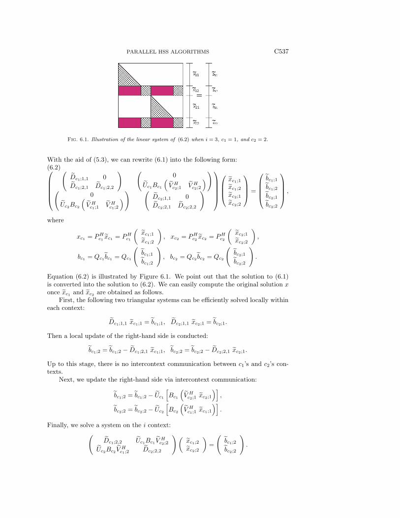
Fig. 6.1. Illustration of the linear system of (6.2) when i = 3, c1 = 1, and c2 = 2.

With the aid of (5.3), we can rewrite (6.1) into the following form:(6.2)⎛⎜⎜⎜⎜⎝

(Dc1;1,1 0

Dc1;2,1 Dc1;2,2

) (0

Uc1Bc1

(V Hc2;1 V H

c2;2

))(0

Uc2Bc2

(V Hc1;1 V H

c1;2

)) (Dc2;1,1 0

Dc2;2,1 Dc2;2,2

)⎞⎟⎟⎟⎟⎠⎛⎜⎜⎝

xc1;1

xc1;2

xc2;1

xc2;2

⎞⎟⎟⎠ =

⎛⎜⎜⎜⎝bc1;1bc1;2bc2;1bc2;2

⎞⎟⎟⎟⎠ ,

where

xc1 = PHc1 xc1 = PH

c1

(xc1;1

xc1;2

), xc2 = PH

c2 xc2 = PHc2

(xc2;1

xc2;2

),

bc1 = Qc1 bc1 = Qc1

(bc1;1bc1;2

), bc2 = Qc2 bc2 = Qc2

(bc2;1bc2;2

).

Equation (6.2) is illustrated by Figure 6.1. We point out that the solution to (6.1)is converted into the solution to (6.2). We can easily compute the original solution xonce xc1 and xc2 are obtained as follows.

First, the following two triangular systems can be efficiently solved locally withineach context:

Dc1;1,1 xc1;1 = bc1;1, Dc2;1,1 xc2;1 = bc2;1.

Then a local update of the right-hand side is conducted:

bc1;2 = bc1;2 − Dc1;2,1 xc1;1, bc2;2 = bc2;2 − Dc2;2,1 xc2;1.

Up to this stage, there is no intercontext communication between c1’s and c2’s con-texts.

Next, we update the right-hand side via intercontext communication:

bc1;2 = bc1;2 − Uc1

[Bc1

(V Hc2;1 xc2;1

)],

bc2;2 = bc2;2 − Uc2

[Bc2

(V Hc1;1 xc1;1

)].

Finally, we solve a system on the i context:(Dc1;2,2 Uc1Bc1 V

Hc2;2

Uc2Bc2 VHc1;2 Dc2;2,2

)(xc1;2

xc2;2

)=

(bc1;2bc2;2

).


This can be done by two triangular solutions after the LU factorization of the coeffi-cient matrix.

For the general case, the above idea is applied recursively. Clearly, there areO(r2) operations associated with each node of the HSS tree. Thus, the total cost forthe solution is [29]

O(nr

)×O(r2) = O(rn).

7. Performance tests and numerical results. In this section, we presentthe performance results of our parallel HSS solver when applied to some matricesarising from real applications. We carry out the experiments on the cluster Cray XE6(hopper.nersc.gov) at the National Energy Research Scientific Computing Center.Each node has two 12-core AMD MagnyCours 2.1-GHz processors with 24 cores intotal on a node. Each node has 32 GB memory.

Our primary application testbed is the modeling of time-harmonic seismic waves,for which we need to solve the Helmholtz equation of the form

(7.1)

(−Δ− ω2

v(x)2

)u(x, ω) = s(x, ω),

where Δ is the Laplacian, ω is the angular frequency, v(x) is the wavespeed (possiblycomplex), and u(x, ω) is called the time-harmonic wavefield solution to the forcingterm s(x, ω). Helmholtz equations arise frequently in real applications such as seismicimaging. The discretization of the Helmholtz operator commonly leads to very largesparse matrices A which are indefinite and ill-conditioned. The matrices are complexand unsymmetric. It has been observed that in the direct factorization of A the denseintermediate matrices are highly compressible [10, 24].

Previously, we developed a parallel multifrontal factorization method for sparsematrix A based on the multifrontal method [8] with nested dissection reordering [11].Some performance results of the multifrontal solver for this application were presentedin [25]. Now, we apply our parallel HSS construction/ULV factorization/solutionalgorithms to the dense Schur complement matrix corresponding to the root of theseparator tree in the nested dissection partitioning. In the following experiments, weappy nested dissection to either a 2D k × k mesh or a 3D k × k × k mesh, where themesh is recursively partitioned into submeshes by the separators. The dimension ofthe last Schur complement matrix A is n = k in two dimensions and n = k2 in threedimensions. The frequency ω = 5Hz is used to obtain A, and A is obtained afterpartial elimination of all the variables prior to the top level separator.

For these seismic applications, often the initial data has low accuracy (one to twodigits) in approximating the actual problems. Thus, two to three digits are usuallysufficient for compression accuracy. In our tests, we use τ = 10−3 in the compressionalgorithm (Algorithm 1), and single precision is used in the code. Detailed errorand stability analysis is performed in [33], which indicates that we can usually getnice accuracy as desired. To validate the accuracy, we present the normwise relative

residual, ‖Ax−b‖∞‖A‖∞‖x‖∞+‖b‖∞ , in the last row of Tables 7.1 and 7.2, when we solve Ax = b

using the HSS compression and ULV factorization of A. Recall that ε ≈ 5.96× 10−8

in single precision.In this paper, for convenience, we assume the dense matrix is stored first. In

practice, for problems such as solving Toeplitz problems with HSS methods in Fourierspace [33], there is no need to store the dense matrix in advance, and the blocks canbe formed dynamically based on some analytical representations. Even if we need to


Table 7.1

Parallel runtime, gigaflops rate, and memory usage of the HSS algorithms applied to the largestdense frontal matrices A from the exact multifrontal factorization of 2D discretized Helmholtz oper-ators in (7.1). n is the order of A, P is the number of processes, and the relative tolerance in HSSconstruction is τ = 10−3. Each addition (multiplication) of two complex numbers is counted as two(six) regular flops.

k (mesh: k × k; n = k) 5,000 10,000 20,000 40,000 80,000

P 16 64 256 1, 024 4, 096

LU factorization (s) 1.96 4.27 9.35 22.47 63.06Gflops/s 170.3 625.1 2280.4 7596.4 21649.9

Dense LU Triangular solve (s) 0.01 0.03 0.05 0.10 0.30Gflops/s 27.7 63.1 133.5 265.8 336.7

Total memory (GB) 0.2 0.8 3.2 12.8 51.2

HSS rank r 9 9 11 12 17Total (s) 0.24 0.31 0.49 0.97 2.31

Constr. RRQR (s) 0.16 0.19 0.23 0.34 0.41HSS Redist. (s) 0.06 0.05 0.10 0.19 0.32

Gflops/s 12.3 44.1 120.4 260.8 462.8ULV factorization (s) 0.11 0.09 0.11 0.21 0.45

Gflops/s 95.6 243.5 402.3 427.4 399.4Solution (s) 0.01 0.02 0.12 0.53 2.76

Gflops/s 1.9 2.1 0.8 0.4 0.1Total memory (GB) 0.05 0.05 0.11 0.21 0.43Relative residual 5.2e-4 8.1e-4 2.5e-3 4.7e-3 5.5e-3

Table 7.2

Parallel runtime and gigaflops rate of the HSS algorithms applied to the largest dense frontalmatrices A from the exact multifrontal factorization of 3D discretized Helmholtz operators in (7.1),where n2 is the size of A, P is the number of processes, and the relative tolerance in HSS constructionis τ = 10−3. Each addition (multiplication) of two complex numbers is counted as two (six) regularflops.

k (mesh: k × k × k; n = k2) 100 200 300 400 500

P 64 256 1,024 4,096 8,192

LU factorization (s) 4.21 57.62 175.85 312.87 540.28Gflops/s 633.3 2961.8 11054.6 34911.6 77120.2

Dense Triangular solve (s) 0.02 0.12 0.30 0.80 1.34LU Gflops/s 65.6 215.2 434.6 511.3 748.4

Total memory (GB) 0.8 12.8 64.8 204.8 500

HSS rank r 335 618 894 1226 1497Total (s) 8.30 51.49 193.40 207.72 259.46

Constr. RRQR (s) 7.94 50.09 189.86 203.94 251.56HSS Redist. (s) 0.24 1.05 2.21 2.11 3.22

Gflops/s 100.8 382.2 595.5 2041.5 4050.1ULV factorization (s) 0.40 1.42 1.76 2.46 4.16

Gflops/s 166.3 495.3 1286.5 2863.8 2513.7Solution (s) 0.04 0.20 0.55 2.29 9.52

Gflops/s 1.1 1.6 1.5 0.9 0.3Total memory (GB) 0.12 0.76 1.96 4.55 6.84Relative residual 9.7e-3 1.1e-2 1.7e-2 1.5e-2 1.7e-2


form the dense matrix first, we may work by panels on part of the matrix, and thepanel storage can be reused by the panels at different times. In the results presentedbelow, the memory we consider is the memory for the HSS factors, as compared withthe dense LU factors.

Example 7.1. The 2D Helmholtz equations are discretized on k× k mesh. Weapply the parallel HSS algortihms to the last Schur complement A corresponding tothe top level separator in the nested dissection ordering.

For the weak scaling test, we increase the number of cores by a factor of four upondoubling the mesh size k. Table 7.1 shows the various performance statistics of theparallel HSS methods for k ranging from 5,000 to 80,000. As a comparison, we includethe results of parallel dense LU factorization and triangular solution from the routinesPCGETRF and PCGETRS in ScaLAPACK [21]. Recall that the HSS rank r is defined asthe maximum rank of all the HSS blocks. Here, for the 2D problems, the HSS ranksare more or less constant (less than 20) and are independent of the problem size. Wesplit the total HSS compression time into an RRQR factorization (Algorithm 1) partand a data redistribution part. As predicted, the HSS factorization and solution arefaster than the HSS compression. Inside the compression phase, the redistributionpart takes less time than the RRQR factorization. This validates our earlier analysison communication complexity; see section 4.4.

Figure 7.1(a) visually compares the weak scaling performance of the new HSS ap-proach to the LU approach. Here we focus only on the HSS construction algorithm,because it dominates the ULV factorization and solution. For each performance met-ric, time, storage, #flops, and gigaflop rate, we plot the ratio of the LU algorithmover the HSS construction algorithm. In all these metrics, the HSS method is alwaysbetter than the LU approach and scales better in parallel runtime, memory usage,and #flops. For the largest mesh size 80,000 using 4096 cores, the HSS algorithm isabout 30 times faster than the LU algorithm and memory usage is reduced by 100-fold. The #flops increases faster for the LU than for the HSS. For the largest problem,the LU #flops is about 1000 times more than the HSS flops. On the other hand, theLU Gflops/s rate is much higher than the HSS Gflops/s rate, as much as 40 timeshigher. This is because the HSS algorithm involves operations with much smaller ma-trices and spends a larger fraction of the time in memory access and communication,as analyzed in section 4. (See remarks on the flop-to-byte ratio in section 4.4.) There-fore, the flop count alone is not a very good predictive metric about parallel runtimefor this class of algorithms.

Example 7.2. The 3D Helmholtz equations discretized on k× k× k mesh. Weapply the parallel HSS algortihms to the last Schur complement A corresponding tothe top level separator in a nested dissection ordering.

We now repeat the same experiments for the 3D problems. We increase thenumber of cores used while increasing the mesh size k. Table 7.2 shows the variousperformance statistics of the parallel HSS methods for k ranging from 100 to 500(i.e., n ranging from 10,000 to 250,000. As a comparison, we include the results ofparallel dense LU factorization and triangular solution from the routines PCGETRF andPCGETRS in ScaLAPACK.

In contrast to the 2D case, now the HSS ranks increase with the problem size.The growth is linear with respect to one side of the mesh (i.e., k), which seems tocorroborate the theory predicted in [10]. The larger HSS ranks give less advantage forthe HSS method over the LU method than the 2D case. Figure 7.1(b) compares theweak scaling performance of the HSS construction to the LU factorization. The HSS


time is faster than that of LU for large problems. For the largest mesh size 5003 using8192 cores, the HSS algorithm is over 2 times faster and memory usage is reducedby 70-fold. The #flops increases faster for the LU than for the HSS. For the largestproblem, the LU #flops is about 40 times more than the HSS flops. On the otherhand, the LU Gflops/s rate is 18 times higher than the HSS Gflops/s rate.

Notice that for the 3D case, the RRQR compression time much more dominatesthe entire HSS construction time. One reason is that the HSS rank r is much largernow, which represents a larger factor to both the computation cost (O(rn2)) andthe communication cost associated with the RRQR compression algorithm (see (4.8)to (4.11)). Another reason is that the ranks of different HSS blocks (i.e., differentbranches of the HSS tree) are not of similar values. We observed over 2 times thedifference between the ranks of some branches. With our current data distributionscheme (see Figure 3.2), this causes significant load imbalance among the processors

Fig. 7.1. Performance ratio of LU over HSS.


on the two branches of the tree. Overall, the RRQR time for the slowest processorcan be 2 to 3 times larger than that of the fastest processor. We will address this loadimbalance issue in our future work.

7.1. Communication cost. Finally, we examine the communication overheadfor the same 2D and 3D matrices. The communication statistics are collected usingthe IPM (integrated performance monitoring) performance profiling tool [18].

Figure 7.2 compares the time spent in communication for the HSS constructionand for the LU factorization. In the 2D case, Figure 7.2(a), the fraction of time incommunication increases with the increasing matrix size and the number of process-ing cores used. Furthermore, the LU algorithm spends a larger fraction of time incommunication than the HSS algorithm. In the 3D case, Figure 7.2(b), the fraction

Fig. 7.2. Percentage time spent in MPI communication.


of time in communication also increases with the increasing matrix size and numberof cores. But now, both the LU algorithm and the HSS algorithm spend a similarfraction of time in communication. This is because the HSS ranks in the 3D case aremuch larger, which contributes to a larger amount of communication (see (4.10) and(4.11)).

8. Conclusions. We have designed and implemented novel parallel algorithmsfor the HSS structured matrix algorithms in parallel computation. We are able toconduct classical structured compression, factorizations, and solutions in parallel. Weperformed a detailed analysis of the communication costs of the parallel algorithmsand found that the algorithms are more communication bound than the other al-gorithms without using the rank structures. This is mainly because the amount offloating point operations is drastically reduced by exploiting the low rankness, butthe reduction in communication is moderate. The future challenge is to design novelcommunication-avoiding algorithms for this class of rank structured methods.

Our implementations are portable by using the two well-established librariesBLACS and ScaLAPACK. The computational results for weak scaling, strong scal-ing, and accuracy demonstrate the high efficiency and scalability of our algorithms.The algorithms are very useful in solving large dense and sparse linear systems thatarise in real-world applications. For example, we have applied our new parallel HSS-embedded multifrontal solver to the Helmholtz equation for time-harmonic seismicinverse boundary value problems, and we were able to solve a linear system with 6.4billion unknowns using 4096 processors in about 20 minutes. The classical multi-frontal solver simply failed due to high demand for memory. Our techniques can alsobenefit the development of fast parallel methods using the other rank structures.

Acknowledgments. We thank Francois-Henry Rouet for insightful discussionsabout the parallel performance bottleneck of the code and for providing the code forcomputing the residual. We thank the members of the Geo-Mathematical ImagingGroup at Purdue University, BGP, ConocoPhillips, ExxonMobil, PGS, Statoil, andTotal for partial financial support.

REFERENCES

[1] T. Bella, Y. Eidelman, V. Gohberg, and I. Olshevsky, Computations with quasiseparablepolynomials and matrices, Theoret. Comput. Sci., 409 (2008), pp. 158–179.

[2] L. S. Blackford, J. Choi, E. D’Azevedo, J. Demmel, I. Dhillon, J. Dongarra, S. Ham-

marling, G. Henry, A. Petitet, K. Stanley, D. Walker, and R. C. Whaley,ScaLAPACK Users’ Guide, Software Environ. Tools, SIAM, Philadelphia, 1997.

[3] BLACS. http://www.netlib.org/blacs.[4] S. Borm, L. Grasedyck, and W. Hackbusch, Introduction to hierarchical matrices with

applications, Eng. Anal. Bound. Elem, 27 (2003), pp. 405–422.[5] S. Borm and W. Hackbusch, Data-Sparse Approximation by Adaptive H2-Matrices, Technical

report, Max Planck Institute for Mathematics, Leipzig, Germany, 2001.[6] S. Chandrasekaran, P. Dewilde, M. Gu, T. Pals, X. Sun, A.-J. van der Veen, and

D. White, Some fast algorithms for sequentially semiseparable representations, SIAM J.Matrix Anal. Appl., 27 (2005), pp. 341–364.

[7] S. Chandrasekaran, M. Gu, and T. Pals, A fast ULV decomposition solver for hierarchicallysemiseparable representations, SIAM J. Matrix Anal. Appl., 28 (2006), pp. 603–622.

[8] I. S. Duff and J. K. Reid, The multifrontal solution of indefinite sparse symmetric linearequations, ACM Trans. Math. Softw., 9 (1983), pp. 302–325.

[9] Y. Eidelman and I. Gohberg, On a new class of structured matrices, Integral EquationsOperator Theory, 34 (1999), pp. 293–324.

[10] B. Engquist and L. Ying, Sweeping preconditioner for the Helmholtz equation: Hierarchicalmatrix representation, Comm. Pure Appl. Math., 64 (2011), pp. 697–735.


[11] J. A. George, Nested dissection of a regular finite element mesh, SIAM J. Numer. Anal., 10(1973), pp. 345–363.

[12] G. H. Golub and C. V. Loan, Matrix Computations, 3rd ed., Johns Hopkins University Press,Baltimore, MD, 1996.

[13] M. Gu and S. C. Eisenstat, Efficient algorithms for computing a strong rank-revealing qrfactorization, SIAM J. Sci. Comput., 17 (1996), pp. 848–869.

[14] W. Hackbusch, L. Grasedyck, and S. Borm, An introduction to hierarchical matrices, Math.Bohem., 127 (2002), pp. 229–241.

[15] W. Hackbusch and B. N. Khoromskij, A sparse H-matrix arithmetic. Part II: Applicationto multi-dimensional problems, Computing, 64 (2000), pp. 21–47.

[16] W. Hackbusch, B. Khoromskij, and S. A. Sauter, On H2-Matrices, Lectures on Appl.Math., Springer, Berlin, 2000, pp. 9–29.

[17] W. Hackbusch, A sparse matrix arithmetic based on H-matrices. Part I: Introduction toH-matrices, Computing, 62 (1999), pp. 89–108.

[18] Integrated Performance Monitoring: IPM, http://ipm-hpc.sourceforge.net.[19] LAPACK—Linear Algebra PACKage, http://www.netlib.org/lapack.[20] Message Passing Interface Forum, http://www.mpi-forum.org.[21] ScaLAPACK—Scalable Linear Algebra PACKage, http://www.netlib.org/scalapack.[22] R. Thakur, R. Rabenseifner, and W. Gropp, Optimization of collective communication

operations in MPICH, Int. J. High Performance Comput. Appl., 19 (2005), pp. 49–66.[23] R. Vandebril, M. Van Barel, G. Golub, and N. Mastronardi, A bibliography on semisep-

arable matrices, Calcolo, 42 (2005), pp. 249–270.[24] S. Wang, M. V. de Hoop, and J. Xia, Seismic inverse scattering via Helmholtz operator

factorization and optimization, J. Comput. Phys., 229 (2010), pp. 8445–8462.[25] S. Wang, M. V. de Hoop, and J. Xia, On 3D modeling of seismic wave propagation via a

structured massively parallel multifrontal direct Helmholtz solver, Geophys. Prospect., 59(2011), pp. 857–873.

[26] S. Wang, M. V. de Hoop, J. Xia, and X. S. Li, Massively parallel structured multifrontalsolver for time-harmonic elastic waves in 3D anisotropic media, Geophys. J. Int., 91(2012), pp. 346–366.

[27] S. Wang, J. Xia, M. V. de Hoop, and X. S. Li, Massively parallel structured direct solverfor equations describing time-harmonic qP-polarized waves in TTI media, Geophysics, 77(2012), pp. T69–T82.

[28] J. Xia, S. Chandrasekaran, M. Gu, and X. S. Li, Superfast multifrontal method for largestructured linear systems of equations, SIAM J. Matrix Anal. Appl., 31 (2009), pp. 1382–1411.

[29] J. Xia, S. Chandrasekaran, M. Gu, and X. S. Li, Fast algorithms for hierarchically semisep-arable matrices, Numer. Linear Algebra Appl., 2010 (2010), pp. 953–976.

[30] J. Xia and M. Gu, Robust approximate cholesky factorization of rank-structured symmetricpositive definite matrices, SIAM J. Matrix Anal. Appl., 31 (2010), pp. 2899–2920.

[31] J. Xia, Efficient structured multifrontal factorization for general large sparse matrices, SIAMJ. Sci. Comput., 35 (2012), pp. A832–A860.

[32] J. Xia, On the complexity of some hierarchical structured matrix algorithms, SIAM J. MatrixAnal. Appl., 33 (2012), pp. 388–410.

[33] Y. Xi, J. Xia, S. Cauley, and V. Balakrishnan, Superfast and stable structured solvers forToeplitz least squares via randomized sampling, SIAM J. Matrix Anal. Appl., submitted.

Documents

EFFICIENT SCALABLE ALGORITHMS FOR SOLVING DENSE LINEAR SYSTEMS