Embed Size (px)
Citation preview
Towards Dense and Scalable Soil Sensing ThroughLow-Cost WiFi Sensing Networks
Steven M. Hernandez, Deniz Erdag and Eyuphan BulutDepartment of Computer Science, Virginia Commonwealth University
401 West Main St. Richmond, VA 23284, USA{hernandezsm, erdagd, ebulut}@vcu.edu
Abstract—Precision agriculture uses precise sensor data col-lected throughout farmland to give farmers better insight intotheir land, allowing for greater crop yields and reduced resourceusage. However, existing solutions require high hardware coststhus limiting large scale deployments. To address that, we proposea low-cost and scalable solution for sensing physical attributesof soil using IoT based WiFi sensing devices. By understandingvariations in WiFi radio signals with channel state information(CSI) and machine learning models, we evaluate the proposed soilsensing system through experiments on physical soil traits suchas soil moisture content, soil texture and position. Moreover, wealso demonstrate how a mesh network of WiFi sensing devicesallows us to predict the physical traits of the soil in the areabetween each pair of sensors, allowing for an increase in sensingarea coverage as nodes are added.
Index Terms—WiFi sensing, sensor networks, soil sensing, soilmoisture, precision agriculture.
I. INTRODUCTION
Growing global population paired with environmentalchanges requires the development of innovative solutions toensure sufficient future food production. Projections proposethat by 2050, agricultural food production will need to increaseupwards of 70% [1]. Precision agriculture aims to increasecommercial farmland yields while using available resources(e.g., water) efficiently through sensor data collection andadvanced prediction models [2]–[4]. One group of importantmetrics for farmland sensing are the physical soil attributessuch as the moisture content and texture, where the latteris usually described by the mixture of silt, clay, sand, andstones. While the soil texture is generally static over time,some attributes of the soil are time variant. For example, soilmoisture content will vary depending on the time since the lastrain fall or last manual irrigation. Additionally, these attributeswill vary based on unique soil texture properties and based onthe time of day as moisture evaporates from the soil.
A key issue in data collection for precision agriculture is thesparseness of sensor deployment. Direct methods for measur-ing soil moisture are considered the most accurate option [5]because they directly measure water content, while indirectmethods measure some related property such as resistance orcapacitance. Even so, direct methods such as the gravimetricmethod require soil samples to be physically removed fromthe environment resulting in destructive and non-continuoussensing of the moisture level. Furthermore, this method re-quires a 24 hour oven drying time for every measurement.
Alternatively, there are some sensors that can sense the soilmoisture continuously and provide measurements over time.However, they can only sense data in the immediate regionwhere the sensor is placed. Moreover, such sensors are mostlyexpensive (e.g., Tensiometers ranging from $100 to upwardsof $1, 000 [6] per sensor) thus their dense deployment acrosslarge farmlands is not affordable by most farmers. Whilesome low-cost sensors exist for sensing soil moisture, theyare mostly unreliable and do not provide commercial-gradeaccurate measurements, thus are only used by hobbyist.
Radio frequency-based sensing methods have appeared asalternatives for tracking soil attributes such as moisture con-tent [7]. However, most of the signal-based systems (e.g.,ground penetrating radar (GPR) [7], [8]) require high costtransmitting and receiving equipment. A more recent workaddresses this by considering commodity WiFi devices [9] asa lower cost solution for wireless soil sensing. Even so, thecost and size of the required hardware is still quite significantand as such, only a single receiver device was deployedwithin the soil. With our recently developed ESP32 CSIToolkit [10], we can collect channel state information (CSI)of WiFi signals from a very low-cost (< $5), standalone IoTmicrocontroller. This allows for wider deployments of WiFisensing devices enabling soil sensing within a network of thesedevices. Soil properties can then be tracked between each pairof WiFi sensing transceiver devices. Furthermore, the WiFinetwork can be used to communicate this sensed data withoutrequiring additional hardware to a centrally located databasefor further processing and analysis thus further reducing thecosts associated with deploying our proposed system.
In this work, we explore the use of our proposed WiFi sens-ing system for tracking soil attributes using machine learning.We evaluate the use of CSI for predicting soil properties suchas soil moisture levels, soil texture and positioning. Finally, weevaluate how our proposed sensing system architecture shownin Fig. 1c can distinguish soil properties with greater coveragecompared to standard sensor-based approaches through the useof a mesh WiFi sensing network.
The rest of the paper is organized as follows. In Section II,we discuss background information about precision agricultureand WiFi sensing. In Section III, we discuss our proposedsystem including details about the hardware and machinelearning architectures as well as information about our ex-perimental methods using this system. We continue with the
accepted to appear in Proceedings of the 46th IEEE Conference on Local Computer Networks (LCN), October 4-7, 2021.
analysis and evaluation of the experiments in Section IV. Thenwe show how IoT WiFi soil sensing nodes can be used todevelop a mesh network with exponentially growing coveragein Section V. Lastly, we conclude this work with our finalremarks in Section VI.
II. BACKGROUND
Precision agriculture (PA) aims to gather large amounts ofanalytical data about farmland through the use of IoT sensingdevices distributed throughout the farmland. After processingthis data, the goal is to give farmers more insight into temporalcharacteristics of their farms as well as spatially localizedsuggestions such as in precision irrigation decision making [2].PA covers all aspects of farmland management through sensorsand advanced information technology techniques such as fieldtracking through UAVs [4] as well as modeling spatial andtemporal crop yield predictions through machine learning [11].Wireless sensor networks (WSN) are typically deployed [3] toaggregate the data from the distributed sensors to a singlecentral location such as a cloud storage for further processingusing cloud computation platforms.
WiFi sensing uses the signal data collected from WiFidevices such as laptops, phones and routers to understandphysical attributes of the environment through signal variationscaused by Line-of-Sight (LoS) obstructions, Non-LOS multi-path interference as well as phase shifts caused by timedelay. Using WiFi for soil sensing in PA is useful becauseit can reduce the hardware cost while also increasing sensingcoverage because the area between each pair of transceiverdevices is sensed. Furthermore, WiFi can be used for dualpurposes, first for wireless sensing of soil traits and secondas a communication method in a WSN. One common metricused for WiFi sensing is channel state information (CSI) [10].CSI is used in orthogonal frequency division multiplexing(OFDM) systems to estimate signal propagation informationdetails over multiple subcarrier frequencies. CSI (H) is givenas an M × N matrix where M is the number of antennasand N is the number of subcarriers. To identify the valuefor H, we consider the equation y = Hx + η where x isthe transmitted signal, y is the received signal and η is somenoise from the environment. Given the real component (hr)and imaginary component (him) for each subcarrier i withinH , we can calculate the amplitude (A) and phase (φ) by:
A =
√(hr)
2+ (him)
2, (1)
φ = atan2 (him, hr) . (2)
For our experiments, we use a single antenna for both thetransmitter and receiver using standard 2.4GHz channels witha bandwidth of 20MHz which allows us to collect values for64 subcarriers where 52 are non-null. Signal propagation forfrequency f at a distance d can be modeled as
E(f, d) = Ae−(α+jβ)d, (3)
where α is an attenuation coefficient due to the physical en-vironment between the transmitter and receiver resulting from
(a)
(b)
Raw CSI
Preprocessing
Moisture Sensing Texture Sensing Positioning
ML Models
Precision Mapping
(c)
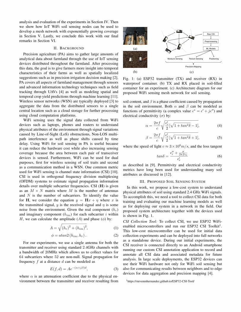
Fig. 1: (a) ESP32 transmitter (TX) and receiver (RX) inwaterproof container. (b) TX and RX placed in soil-filledcontainer for an experiment. (c) Architecture diagram for ourproposed WiFi sensing mesh network for soil sensing.
soil content, and β is a phase coefficient caused by propagationin the soil environment. Both α and β can be modeled asfunctions of permittivity (a complex value ε∗ = ε′ + jε′′) andelectrical conductivity (σ) by:
α =2πf
c
√ε′r2
[√
1 + tan2δ − 1], (4)
β =2πf
c
√ε′r2
[√
1 + tan2δ + 1], (5)
where the speed of light c ≈ 3×10⁸m/s, and the loss tangent
tanδ =ε′′r + σ
2πfε0
ε′r(6)
as described in [9]. Permittivity and electrical conductivitymetrics have long been used for understanding many soilattributes as discussed in [12].
III. PROPOSED SOIL SENSING SYSTEM
In this work, we propose a low-cost system to understandphysical attributes of soil using standard 2.4 GHz WiFi signals.To accomplish this, we need a tool to collect CSI data for bothtraining and evaluating our machine learning models as wellas for deploying our system in a network in the field. Ourproposed system architecture together with the devices usedis shown in Fig. 1.CSI Collection Tool: To collect CSI, we use ESP32 WiFi-enabled microcontrollers and run our ESP32 CSI Toolkit1.This low-cost microcontroller can be used for initial datacollection experiments and can be deployed into full networksas a standalone device. During our initial experiments, theCSI receiver is connected directly to an Android smartphonerunning our custom CSI annotation application to record andannotate all CSI data and associated metadata for futureanalysis. In large scale deployments, the ESP32 devices canuse their WiFi hardware not only for WiFi soil sensing butalso for communicating results between neighbors and to edgedevices for data aggregation and precision mapping [4].
1https://stevenmhernandez.github.io/ESP32-CSI-Tool/
Machine Learning Architecture: To make our predictions, weselect a Dense Neural Network (DNN) classifier architecturewith two hidden dense layers with identical number of hiddenneurons, each followed by a dropout layer used to preventoverfitting by setting the output of neurons randomly to 0 witha probability of Pdropout = 0.2. We use a softmax activationfunction and Stochastic Gradient Descent (SGD) to optimizeour loss function
L(x, y) =1
N
N∑i=1
(F(xi)− yi)2, (7)
where F is the model, xi is the i-th input sample for themodel and yi is the label for the i-th sample. We use learningrate η ∈ {0.001, 0.01, 0.1} to control the speed at which themodel converges during training. As input to the classifierwe give a matrix of size w × n, where w is a window ofCSI measurements and n = 64 is the number of subcarriers.Our preprocessing and machine learning steps are written inPython using the Keras [13] deep learning library. Hyper-parameter optimization was used to balance model accuracywith computation time. For reproducibility in our experiments,we use the Sacred experiment database Python library [14]to capture results for each experiment along with the chosenhyperparameter values.Experiment Process: To evaluate the proposed system for soilsensing tasks, we use our ESP32 toolkit to collect and annotateCSI to predict the following physical soil traits: depth in soil,distance in soil between the transmitter (TX) and receiver(RX), soil moisture level, and soil texture. For each experi-ment, we use two ESP32s, one TX and one RX which are bothhoused inside waterproof enclosures as shown in Fig. 1a. Forsoil depth and TX/RX distance experiments, the enclosures areplaced directly in the soil for each position as shown in Fig. 1b.For soil texture and soil moisture experiments, we constructeda jig to hold the ESP32s stationary across multiple repetitions.We collect CSI for each state in an experiment using a timerto ensure a similar number of samples are collected per class.Annotated data for each experiment is split such that the first50% of samples per class are used for training and the final50% of samples are used for testing.
IV. EXPERIMENTAL RESULTS
To explore the use of WiFi for soil sensing, we evaluateour CSI collection system and machine learning predictionmodels for the following tasks. First, we identify if the modelis able to recognize different depths and distances betweentransmitter and receiver in different soil types in Section IV-A.This first set of experiments is useful to ensure that the modelis able to detect the physical location even when devices areplaced underground. Next, we look at how well our modelis able to distinguish moisture levels in Section IV-B. Soilmoisture is a dynamic metric which changes over time andmust be maintained through precision irrigation to ensureproper crop growth. Following this, we also look at how soiltexture can be detected with our model in Section IV-C. Soiltexture is defined by the distribution of clay, sand and silt
10 cm
20 cm
30 cm
Predicted Class
10 cm
20 cm
30 cmTru
e C
lass
0
0
0.1
0.1
0
0.1
99.9
99.9
99.9
0
50
100
(a) Silt
10 cm
20 cm
30 cm
Predicted Class
10 cm
20 cm
30 cmTru
e C
lass
0.2
0.6
0.1
0
0.4
0
99.5
99.8
99.4
0
50
100
(b) Sand10 cm (s
and)
10 cm (soil)
20 cm (sand)
20 cm (soil)
30 cm (sand)
30 cm (soil)
Predicted Class
10 cm (sand)
10 cm (soil)
20 cm (sand)
20 cm (soil)
30 cm (sand)
30 cm (soil)
Tru
e C
lass 0.1
0.7
0
0.2
0
0
0
1.8
0.1
0
0.3
0
0
0.1
0
0
1.5
0
0
0
0
0
0.1
0.2
0.1
0.1
0
0
0
0
99.6
98.4
99.2
98.1
99.6
99.90
20
40
60
80
100
(c) Silt and Sand
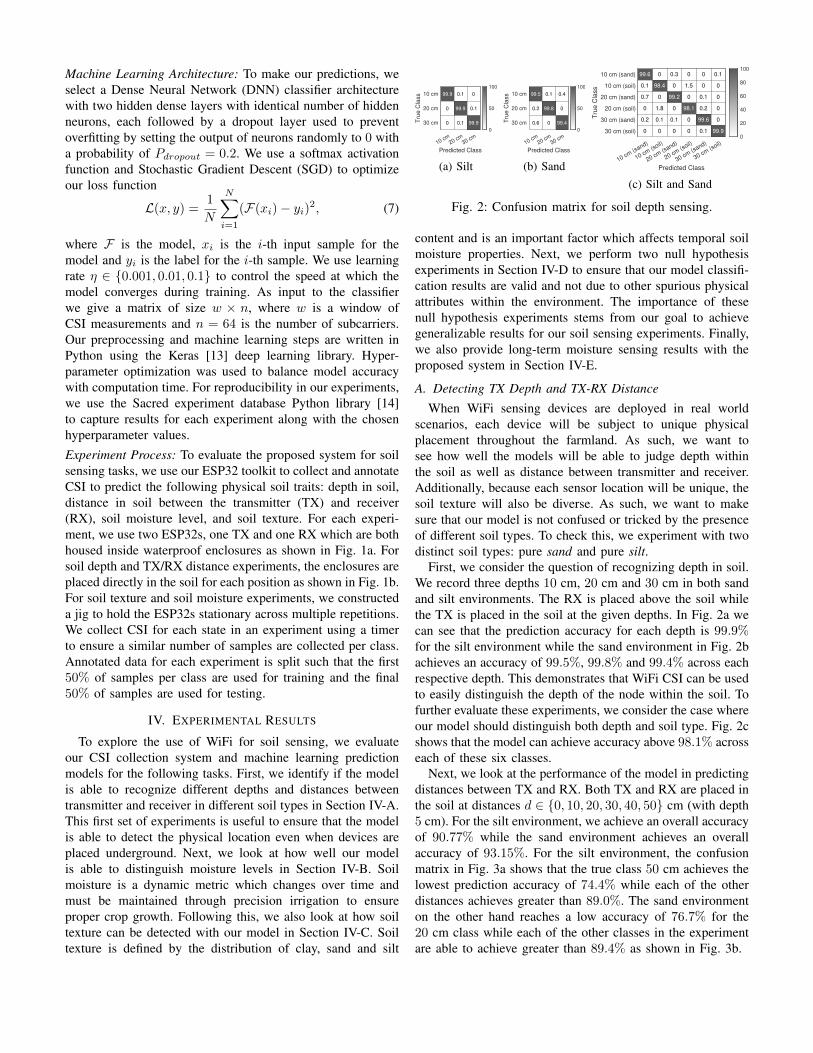
Fig. 2: Confusion matrix for soil depth sensing.
content and is an important factor which affects temporal soilmoisture properties. Next, we perform two null hypothesisexperiments in Section IV-D to ensure that our model classifi-cation results are valid and not due to other spurious physicalattributes within the environment. The importance of thesenull hypothesis experiments stems from our goal to achievegeneralizable results for our soil sensing experiments. Finally,we also provide long-term moisture sensing results with theproposed system in Section IV-E.
A. Detecting TX Depth and TX-RX Distance
When WiFi sensing devices are deployed in real worldscenarios, each device will be subject to unique physicalplacement throughout the farmland. As such, we want tosee how well the models will be able to judge depth withinthe soil as well as distance between transmitter and receiver.Additionally, because each sensor location will be unique, thesoil texture will also be diverse. As such, we want to makesure that our model is not confused or tricked by the presenceof different soil types. To check this, we experiment with twodistinct soil types: pure sand and pure silt.
First, we consider the question of recognizing depth in soil.We record three depths 10 cm, 20 cm and 30 cm in both sandand silt environments. The RX is placed above the soil whilethe TX is placed in the soil at the given depths. In Fig. 2a wecan see that the prediction accuracy for each depth is 99.9%for the silt environment while the sand environment in Fig. 2bachieves an accuracy of 99.5%, 99.8% and 99.4% across eachrespective depth. This demonstrates that WiFi CSI can be usedto easily distinguish the depth of the node within the soil. Tofurther evaluate these experiments, we consider the case whereour model should distinguish both depth and soil type. Fig. 2cshows that the model can achieve accuracy above 98.1% acrosseach of these six classes.
Next, we look at the performance of the model in predictingdistances between TX and RX. Both TX and RX are placed inthe soil at distances d ∈ {0, 10, 20, 30, 40, 50} cm (with depth5 cm). For the silt environment, we achieve an overall accuracyof 90.77% while the sand environment achieves an overallaccuracy of 93.15%. For the silt environment, the confusionmatrix in Fig. 3a shows that the true class 50 cm achieves thelowest prediction accuracy of 74.4% while each of the otherdistances achieves greater than 89.0%. The sand environmenton the other hand reaches a low accuracy of 76.7% for the20 cm class while each of the other classes in the experimentare able to achieve greater than 89.4% as shown in Fig. 3b.
0 cm
10 cm
20 cm
30 cm
40 cm
50 cm
Predicted Class
0 cm
10 cm
20 cm
30 cm
40 cm
50 cm
Tru
e C
lass
0
0
0
0
0
1.6
0
1
0
0
0
7.8
0
0
21.1
0
0
0
11
1.4
0
0
0
8.2
3
0
0
0
0
0
74.4
98.4
92.2
100
90.7
89
0
20
40
60
80
100
(a) Silt
0 cm
10 cm
20 cm
30 cm
40 cm
50 cm
Predicted Class
0 cm
10 cm
20 cm
30 cm
40 cm
50 cm
Tru
e C
lass
0.8
0.5
0.2
0
0
1.7
1.4
2.9
0
0
0
1.4
6.5
0
0
0
3.1
21.4
0
0
0
0
0
1
0.1
0
0
0
0
0
98.3
94.7
76.7
89.4
99.9
99.9
0
20
40
60
80
100
(b) Sand
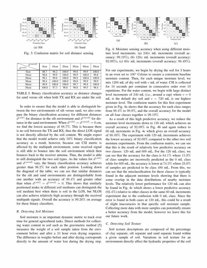
Fig. 3: Confusion matrix for soil distance sensing.
d(silt)d(sand)
0cm 10cm 20cm 30cm 40cm 50cm
0cm 88.7 96.2 100.0 99.8 99.9 100.010cm 98.6 99.9 100.0 99.9 100.0 99.820cm 99.1 99.8 100.0 99.9 100.0 100.030cm 99.4 100.0 100.0 99.8 99.9 99.940cm 99.9 100.0 100.0 99.7 99.4 100.050cm 100.0 97.3 98.8 99.8 99.5 98.4
TABLE I: Binary classification accuracy as distance changesfor sand versus silt when both TX and RX are under the soil.
In order to ensure that the model is able to distinguish be-tween the two environments of silt versus sand, we also com-pare the binary classification accuracy for different distancesd(silt) for distance in the silt environment and d(sand) for dis-tance in the sand environment. When d(silt) = d(sand) = 0 cm,we find the lowest accuracy of 88.7%. This is because thereis no soil between the TX and RX, thus the direct LOS signalis not directly affected by the soil content. We might expectthat the model would achieve only 50% binary classificationaccuracy as a result, however, because our CSI metric isaffected by the multipath environment, some received signalis still able to bounce into the soil environment which thenbounces back to the receiver antenna. Thus, the model is ableto still distinguish the two soil types. As the values for d(silt)
and d(sand) vary, the binary classification accuracy achievesgreater than 96.2% for each other position. Looking downthe diagonal of the table, we can see that similar distancesfor the silt and sand environments are distinguishable fromone another with an accuracy of 98.4% and greater otherthan when d(silt) = d(sand) = 0. This shows that similarlypositioned nodes in different soil mediums can distinguish thesoil medium best when there is soil in the LOS, but NLOScan also achieve relatively high accuracy through the receivedmultipath signals. Overall the accuracy is 99.26% on averagefor these binary classifiers.
B. Detecting Soil Moisture
Soil moisture is an important dynamic metric to track overtime for general agricultural tasks. Direct methods for collect-ing water content in soil such as the gravimetric method [5]measures the weight of a soil sample taken from the envi-ronment before and after a 24 hour oven drying sequence.The difference in weights before and after drying correspondsdirectly to the amount of water lost during the drying step.
0 240 480 720
Predicted Class
0
240
480
720
Tru
e C
lass
0
0
0
0
0.1
0
0
1.6
1.2
0.3
0
0
99.7
98.4
99.9
98.8
0
20
40
60
80
100
(a)0 120 240 360 480 600
Predicted Class
0
120
240
360
480
600
Tru
e C
lass
15.9
0
0
0
0.2
0.7
0
0
0
0
0
0
0.3
0
0.6
0
0
0.9
0
1.7
0
0
0
0
23
0
0
0
1.2
3
74.5
99.3
84.1
99.1
98.6
97
0
20
40
60
80
100
(b)
0 60 120 180 240 320
Predicted Class
0
60
120
180
240
320
Tru
e C
lass
0
7.6
0
0
0
0
0
0
0
0
1.3
0
0
0.1
0
0.1
0
0
0
0
0
0
0
0
0
0
0
0
0
0
98.6
100
92.4
100
99.9
100
0
20
40
60
80
100
(c)
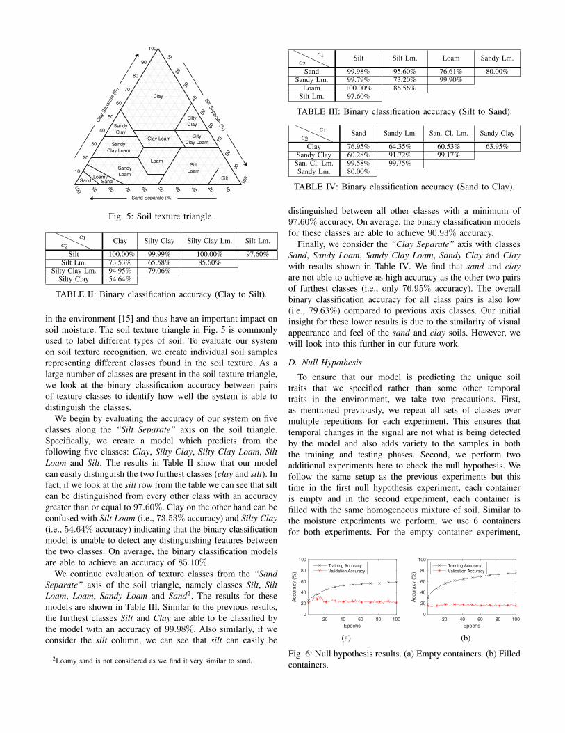
Fig. 4: Moisture sensing accuracy when using different mois-ture level increments. (a) 240x mL increments (overall ac-curacy: 99.19%), (b) 120x mL increments (overall accuracy:92.09%), (c) 60x mL increments (overall accuracy: 98.49%).
For our experiments, we begin by drying the soil for 3 hoursin an oven set to 100° Celsius to ensure a consistent baselinemoisture content. Then, for each unique moisture level, wemix 1200 mL of dry soil with v mL of water. CSI is collectedfor 10 seconds per container in consecutive order over 10repetitions. For the water content, we begin with large distinctlevel increments of 240 mL (i.e., around a cup) where v = 0mL is the default dry soil and v = 720 mL is our highestmoisture level. The confusion matrix for this first experimentgiven in Fig. 4a shows that the accuracy for each class rangesfrom 98.4% to 99.9%, and the overall accuracy for the modelon all four classes together is 99.19%.
As a result of this high predictive accuracy, we reduce themoisture level increments down to 120 mL which achieves anoverall accuracy of 92.09% in Fig. 4b and again reduce to60 mL increments in Fig. 4c which gives an overall accuracyof 98.49%. The experiment with 120 mL increments achievesthe lowest accuracy of 92.09% compared to the other two soilmoisture experiments. From the confusion matrix, we can seethat this is the result of relatively low predictive accuracy ontwo classes: 120 mL and 600 mL. For the 120 mL class, wecan see that the accuracy for the class is 84.1% where 15.9%of class samples are incorrectly predicted as the 0 mL classwhile for 600 mL, the accuracy is lower at 74.5% where 23.0%of samples are predicted to be class 480 mL. From this, wecan see that the misclassification for these classes is typicallyfound in the adjacent moisture levels showing that there issome overlap in the data distributions of nearby moisturelevels. The relatively lower performance for 120 mL can alsobe found in Fig. 4c which shows a lower predictive accuracy(92.4%) relative to other classes in the same 60 mL incrementsexperiment due to the confusion with 0 mL class. Since theerror is found in both cases at 120 mL, this could be a resultof slight inaccuracies in that specific soil moisture sample.Collecting more data with more samples can potentially ensurea better accuracy from the model, however we leave this forour future work.
C. Detecting Soil Texture
Soil texture descriptions are composed of the percentageof clay separate, silt separate and sand separate found withina given sample of soil. Variations in soil texture for anenvironment directly affect the hydraulic properties of the soil
Sand Separate (%)
10
20
30
40
50
60
70
80
90
100
Cla
y S
epara
te (%
)
10
20
30
40
50
60
70
80
90
100
Silt S
epara
te (%
)
10
20
30
40
50
60
70
80
90
100Silt
Silt
Loam
Loam
Sandy
LoamLoamy
SandSand
Sandy
Clay Loam
Sandy
Clay
Clay LoamSilty
Clay Loam
Silty
Clay
Clay
Fig. 5: Soil texture triangle.
c2
c1 Clay Silty Clay Silty Clay Lm. Silt Lm.
Silt 100.00% 99.99% 100.00% 97.60%Silt Lm. 73.53% 65.58% 85.60%
Silty Clay Lm. 94.95% 79.06%Silty Clay 54.64%
TABLE II: Binary classification accuracy (Clay to Silt).
in the environment [15] and thus have an important impact onsoil moisture. The soil texture triangle in Fig. 5 is commonlyused to label different types of soil. To evaluate our systemon soil texture recognition, we create individual soil samplesrepresenting different classes found in the soil texture. As alarge number of classes are present in the soil texture triangle,we look at the binary classification accuracy between pairsof texture classes to identify how well the system is able todistinguish the classes.
We begin by evaluating the accuracy of our system on fiveclasses along the “Silt Separate” axis on the soil triangle.Specifically, we create a model which predicts from thefollowing five classes: Clay, Silty Clay, Silty Clay Loam, SiltLoam and Silt. The results in Table II show that our modelcan easily distinguish the two furthest classes (clay and silt). Infact, if we look at the silt row from the table we can see that siltcan be distinguished from every other class with an accuracygreater than or equal to 97.60%. Clay on the other hand can beconfused with Silt Loam (i.e., 73.53% accuracy) and Silty Clay(i.e., 54.64% accuracy) indicating that the binary classificationmodel is unable to detect any distinguishing features betweenthe two classes. On average, the binary classification modelsare able to achieve an accuracy of 85.10%.
We continue evaluation of texture classes from the “SandSeparate” axis of the soil triangle, namely classes Silt, SiltLoam, Loam, Sandy Loam and Sand2. The results for thesemodels are shown in Table III. Similar to the previous results,the furthest classes Silt and Clay are able to be classified bythe model with an accuracy of 99.98%. Also similarly, if weconsider the silt column, we can see that silt can easily be
2Loamy sand is not considered as we find it very similar to sand.
c2
c1 Silt Silt Lm. Loam Sandy Lm.
Sand 99.98% 95.60% 76.61% 80.00%Sandy Lm. 99.79% 73.20% 99.90%
Loam 100.00% 86.56%Silt Lm. 97.60%
TABLE III: Binary classification accuracy (Silt to Sand).
c2
c1 Sand Sandy Lm. San. Cl. Lm. Sandy Clay
Clay 76.95% 64.35% 60.53% 63.95%Sandy Clay 60.28% 91.72% 99.17%
San. Cl. Lm. 99.58% 99.75%Sandy Lm. 80.00%
TABLE IV: Binary classification accuracy (Sand to Clay).
distinguished between all other classes with a minimum of97.60% accuracy. On average, the binary classification modelsfor these classes are able to achieve 90.93% accuracy.
Finally, we consider the “Clay Separate” axis with classesSand, Sandy Loam, Sandy Clay Loam, Sandy Clay and Claywith results shown in Table IV. We find that sand and clayare not able to achieve as high accuracy as the other two pairsof furthest classes (i.e., only 76.95% accuracy). The overallbinary classification accuracy for all class pairs is also low(i.e., 79.63%) compared to previous axis classes. Our initialinsight for these lower results is due to the similarity of visualappearance and feel of the sand and clay soils. However, wewill look into this further in our future work.
D. Null Hypothesis
To ensure that our model is predicting the unique soiltraits that we specified rather than some other temporaltraits in the environment, we take two precautions. First,as mentioned previously, we repeat all sets of classes overmultiple repetitions for each experiment. This ensures thattemporal changes in the signal are not what is being detectedby the model and also adds variety to the samples in boththe training and testing phases. Second, we perform twoadditional experiments here to check the null hypothesis. Wefollow the same setup as the previous experiments but thistime in the first null hypothesis experiment, each containeris empty and in the second experiment, each container isfilled with the same homogeneous mixture of soil. Similar tothe moisture experiments we perform, we use 6 containersfor both experiments. For the empty container experiment,
20 40 60 80 100
Epochs
0
20
40
60
80
100
Accu
racy (
%)
Training Accuracy
Validation Accuracy
(a)
20 40 60 80 100
Epochs
0
20
40
60
80
100
Accu
racy (
%)
Training Accuracy
Validation Accuracy
(b)
Fig. 6: Null hypothesis results. (a) Empty containers. (b) Filledcontainers.
TX RXSensors
PiArduino
(a)
0 5 10 15 200
5
10
15
20
25
PD
F (
%)
1 hour
2 hours
6 hours
12 hours
(b)
0 200 400 600 800 1000
Epochs
50
60
70
80
90
100
Accura
cy (
%)
(c)
0 2 4 6 8 1070
80
90
100
CD
F (
%)
Training Accuracy
Validation Accuracy
(d)
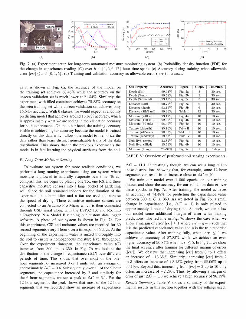
Fig. 7: (a) Experiment setup for long-term automated moisture monitoring system. (b) Probability density function (PDF) forthe change in capacitance reading (C) over h ∈ {1, 2, 6, 12} hour time-spans. (c) Accuracy during training when allowableerror |err| ≤ e ∈ {0, 1, 5}. (d) Training and validation accuracy as allowable error (|err|) increases.
as it is shown in Fig. 6a, the accuracy of the model onthe training set achieves 58.46% while the accuracy on theunseen validation set is much lower at 21.54%. Similarly, theexperiment with filled containers achieves 75.83% accuracy onthe seen training set while unseen validation set achieves only15.54% accuracy. With 6 classes, we would expect a randomlypredicting model that achieves around 16.67% accuracy, whichis approximately what we are seeing in the validation accuracyfor both experiments. On the other hand, the training accuracyis able to achieve higher accuracy because the model is traineddirectly on this data which allows the model to memorize thedata rather than learn distinct generalizable traits of the datadistribution. This shows that in the previous experiments themodel is in fact learning the physical attributes from the soil.
E. Long-Term Moisture Sensing
To evaluate our system for more realistic conditions, weperform a long running experiment using our system wheremoisture is allowed to naturally evaporate over time. To ac-complish this, we begin by placing one TX, one RX and threecapacitive moisture sensors into a large bucket of gardeningsoil. Since the soil remained indoors for the duration of theexperiment, a dehumidifier and a fan are used to increasethe speed of drying. Three capacitive moisture sensors areconnected to an Arduino Pro Micro which is then connectedthrough USB serial along with the ESP32 TX and RX intoa Raspberry Pi 4 Model B running our custom data loggersoftware. A photo of our system is shown in Fig. 7a. Forthis experiment, CSI and moisture values are recorded for 30second segments every 1 hour over a timespan of 5 days. At thebeginning of the experiment, water is mixed thoroughly intothe soil to ensure a homogeneous moisture level throughout.Over the experiment timespan, the capacitance value (C)increases from 300 up to 350. In Fig. 7b we look at thedistribution of the change in capacitance (∆C) over differentperiods of time. This shows that over most of the one-hour segments, C increased 0 or 1 units with an average ofapproximately ∆C = 0.6. Subsequently, over all of the 2 hoursegments, the capacitance increased by 2 and similarly forthe 6 hour segments, we see a peak at ∆C = 6.1. For the12 hour segments, the peak shows that most of the 12 hoursegments that we recorded show an increase of capacitance
Soil Property Accuracy Figure #Reps. Time/Rep.Depth (Silt) 99.91% Fig. 2a 3 30 sec.Depth (Sand) 99.58% Fig. 2b 3 30 sec.Depth (Silt/Sand) 99.13% Fig. 2c 3 30 sec.Distance (Silt) 90.77% Fig. 3a 6 30 sec.Distance (Sand) 93.15% Fig. 3b 6 30 sec.Distance (Silt/Sand) 99.26% Table I 12 30 sec.Moisture (240 mL) 99.19% Fig. 4a 10 10 sec.Moisture (120 mL) 92.09% Fig. 4b 10 10 sec.Moisture (60 mL) 98.49% Fig. 4c 10 10 sec.Texture (clay/silt) 85.10% Table II 10 10 sec.Texture (silt/sand) 90.03% Table III 10 10 sec.Texture (sand/clay) 79.63% Table IV 10 10 sec.Null Hyp. (empty) 23.82% Fig. 6a 10 10 sec.Null Hyp. (filled) 15.54% Fig. 6b 10 10 sec.Moisture (Long) 74–97% Fig. 7c 1 5 days
TABLE V: Overview of performed soil sensing experiments.
∆C = 11.1. Interestingly though, we can see a long tail tothese distributions showing that, for example, some 12 hoursegments can result in an increase close to ∆C = 20.
We train our model over 1, 000 epochs on our trainingdataset and show the accuracy for our validation dataset overthese epochs in Fig. 7c. After training, the model achievesan accuracy of 74.48% for predicting the capacitance valuebetween 300 ≤ C ≤ 350. As we noted in Fig. 7b, a smallchange in capacitance (i.e., ∆C = 1) is only related toapproximately 1 hour of drying time. As such, we can allowour model some additional margin of error when makingpredictions. The red line in Fig. 7c shows the case when weallow a margin of error |err| ≤ 1 where err = y− y such thaty is the predicted capacitance value and y is the true recordedcapacitance value. After training fully, when |err| ≤ 1 weachieve an accuracy of 87.83% while we achieve an evenhigher accuracy of 96.84% when |err| ≤ 5. In Fig.7d, we showthe final accuracy after training for different margin of errors(|err|). We observe that increasing |err| from 0 to 1 offersan increase of +13.35%. Similarly, increasing |err| from 2to 3 offers an increase of +8.13% going from 88.06% up to96.19%. Beyond this, increasing from |err| = 3 up to 10 onlyoffers an increase of +2.29%. Thus, by allowing a margin oferror of just ∆C = ±3 we achieve a high accuracy of 96.19%.
Results Summary. Table V shows a summary of the experi-mental results in this section together with the settings used.
V. SCALABLE MESH NETWORK
Thanks to the low cost of the ESP32 microcontrollers usedin our proposed system, a large number of devices can bedeployed to cover large areas of farmland. Through a meshnetwork, sensed data can be routed to an aggregation locationfor further processing without requiring each device to bedirectly connected to a router. This is important because inlarge farmland deployments, it is not expected that WiFisignals of standard routers will cover the entire area. Instead,each ESP32 can perform both WiFi sensing and WiFi routingto share information. Moreover, each ESP32 can also act asboth transmitter and CSI receivers. As a result of this, eachESP32 can then capture raw CSI from multiple neighboringtransmitters. Preprocessing this raw CSI and inputting it intopretrained machine learning models allows us to performmoisture sensing, texture sensing and positioning tasks whichcan then be used together to calculate precision mapping [4].
A. Communication within SoilWhen radios are placed into soil, signal attenuation in-
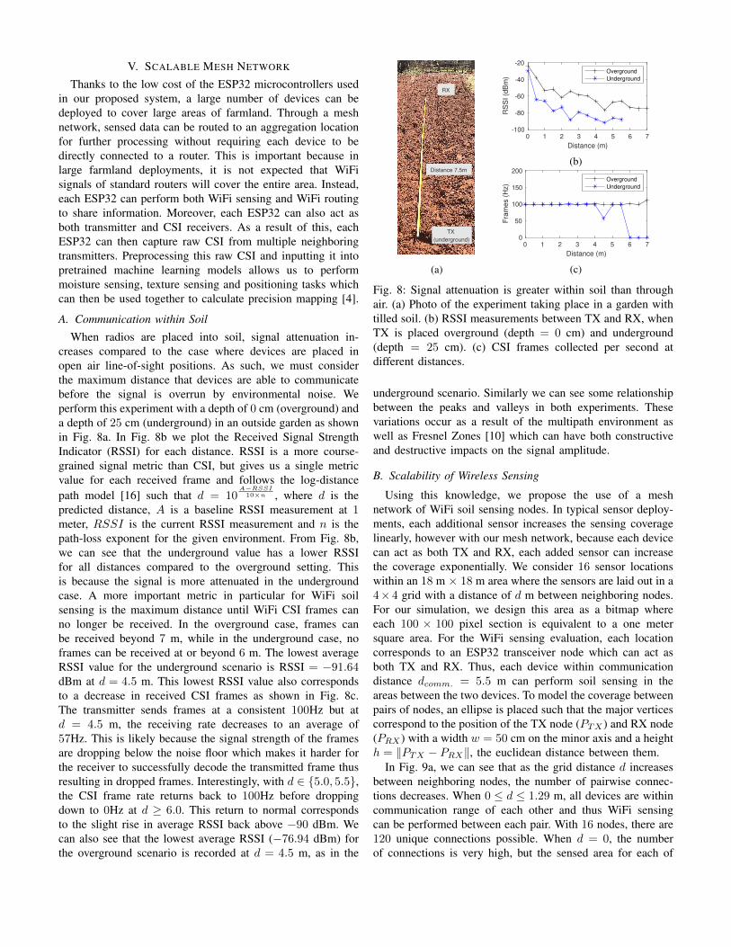
creases compared to the case where devices are placed inopen air line-of-sight positions. As such, we must considerthe maximum distance that devices are able to communicatebefore the signal is overrun by environmental noise. Weperform this experiment with a depth of 0 cm (overground) anda depth of 25 cm (underground) in an outside garden as shownin Fig. 8a. In Fig. 8b we plot the Received Signal StrengthIndicator (RSSI) for each distance. RSSI is a more course-grained signal metric than CSI, but gives us a single metricvalue for each received frame and follows the log-distancepath model [16] such that d = 10
A−RSSI10×n , where d is the
predicted distance, A is a baseline RSSI measurement at 1meter, RSSI is the current RSSI measurement and n is thepath-loss exponent for the given environment. From Fig. 8b,we can see that the underground value has a lower RSSIfor all distances compared to the overground setting. Thisis because the signal is more attenuated in the undergroundcase. A more important metric in particular for WiFi soilsensing is the maximum distance until WiFi CSI frames canno longer be received. In the overground case, frames canbe received beyond 7 m, while in the underground case, noframes can be received at or beyond 6 m. The lowest averageRSSI value for the underground scenario is RSSI = −91.64dBm at d = 4.5 m. This lowest RSSI value also correspondsto a decrease in received CSI frames as shown in Fig. 8c.The transmitter sends frames at a consistent 100Hz but atd = 4.5 m, the receiving rate decreases to an average of57Hz. This is likely because the signal strength of the framesare dropping below the noise floor which makes it harder forthe receiver to successfully decode the transmitted frame thusresulting in dropped frames. Interestingly, with d ∈ {5.0, 5.5},the CSI frame rate returns back to 100Hz before droppingdown to 0Hz at d ≥ 6.0. This return to normal correspondsto the slight rise in average RSSI back above −90 dBm. Wecan also see that the lowest average RSSI (−76.94 dBm) forthe overground scenario is recorded at d = 4.5 m, as in the
TX (underground)
Distance 7.5m
RX
(a)
0 1 2 3 4 5 6 7
Distance (m)
-100
-80
-60
-40
-20
RS
SI
(dB
m)
Overground
Underground
(b)
0 1 2 3 4 5 6 7
Distance (m)
0
50
100
150
200
Fra
me
s (
Hz)
Overground
Underground
(c)
Fig. 8: Signal attenuation is greater within soil than throughair. (a) Photo of the experiment taking place in a garden withtilled soil. (b) RSSI measurements between TX and RX, whenTX is placed overground (depth = 0 cm) and underground(depth = 25 cm). (c) CSI frames collected per second atdifferent distances.
underground scenario. Similarly we can see some relationshipbetween the peaks and valleys in both experiments. Thesevariations occur as a result of the multipath environment aswell as Fresnel Zones [10] which can have both constructiveand destructive impacts on the signal amplitude.
B. Scalability of Wireless Sensing
Using this knowledge, we propose the use of a meshnetwork of WiFi soil sensing nodes. In typical sensor deploy-ments, each additional sensor increases the sensing coveragelinearly, however with our mesh network, because each devicecan act as both TX and RX, each added sensor can increasethe coverage exponentially. We consider 16 sensor locationswithin an 18 m × 18 m area where the sensors are laid out in a4× 4 grid with a distance of d m between neighboring nodes.For our simulation, we design this area as a bitmap whereeach 100 × 100 pixel section is equivalent to a one metersquare area. For the WiFi sensing evaluation, each locationcorresponds to an ESP32 transceiver node which can act asboth TX and RX. Thus, each device within communicationdistance dcomm. = 5.5 m can perform soil sensing in theareas between the two devices. To model the coverage betweenpairs of nodes, an ellipse is placed such that the major verticescorrespond to the position of the TX node (PTX ) and RX node(PRX ) with a width w = 50 cm on the minor axis and a heighth = ‖PTX − PRX‖, the euclidean distance between them.
In Fig. 9a, we can see that as the grid distance d increasesbetween neighboring nodes, the number of pairwise connec-tions decreases. When 0 ≤ d ≤ 1.29 m, all devices are withincommunication range of each other and thus WiFi sensingcan be performed between each pair. With 16 nodes, there are120 unique connections possible. When d = 0, the numberof connections is very high, but the sensed area for each of
0 1 2 3 4 5 6
Distance (m)
0
50
100
150# C
onnection
(a)
0 1 2 3 4 5 6
Distance (m)
0
10
20
30
Covera
ge (
%)
WiFi Sensor
(b)
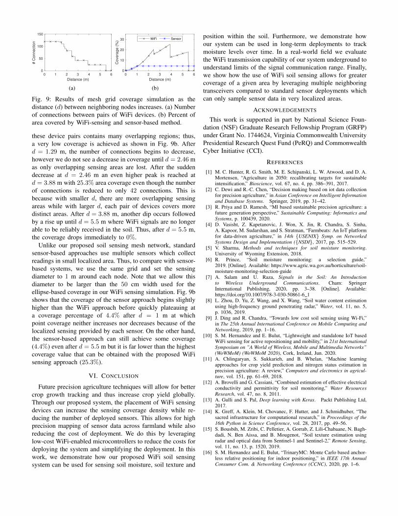
Fig. 9: Results of mesh grid coverage simulation as thedistance (d) between neighboring nodes increases. (a) Numberof connections between pairs of WiFi devices. (b) Percent ofarea covered by WiFi-sensing and sensor-based method.
these device pairs contains many overlapping regions; thus,a very low coverage is achieved as shown in Fig. 9b. Afterd = 1.29 m, the number of connections begins to decrease,however we do not see a decrease in coverage until d = 2.46 mas only overlapping sensing areas are lost. After the suddendecrease at d = 2.46 m an even higher peak is reached atd = 3.88 m with 25.3% area coverage even though the numberof connections is reduced to only 42 connections. This isbecause with smaller d, there are more overlapping sensingareas while with larger d, each pair of devices covers moredistinct areas. After d = 3.88 m, another dip occurs followedby a rise up until d = 5.5 m where WiFi signals are no longerable to be reliably received in the soil. Thus, after d = 5.5 m,the coverage drops immediately to 0%.
Unlike our proposed soil sensing mesh network, standardsensor-based approaches use multiple sensors which collectreadings in small localized area. Thus, to compare with sensor-based systems, we use the same grid and set the sensingdiameter to 1 m around each node. Note that we allow thisdiameter to be larger than the 50 cm width used for theellipse-based coverage in our WiFi sensing simulation. Fig. 9bshows that the coverage of the sensor approach begins slightlyhigher than the WiFi approach before quickly plateauing ata coverage percentage of 4.4% after d = 1 m at whichpoint coverage neither increases nor decreases because of thelocalized sensing provided by each sensor. On the other hand,the sensor-based approach can still achieve some coverage(4.4%) even after d = 5.5 m but it is far lower than the highestcoverage value that can be obtained with the proposed WiFisensing approach (25.3%).
VI. CONCLUSION
Future precision agriculture techniques will allow for bettercrop growth tracking and thus increase crop yield globally.Through our proposed system, the placement of WiFi sensingdevices can increase the sensing coverage density while re-ducing the number of deployed sensors. This allows for highprecision mapping of sensor data across farmland while alsoreducing the cost of deployment. We do this by leveraginglow-cost WiFi-enabled microcontrollers to reduce the costs fordeploying the system and simplifying the deployment. In thiswork, we demonstrate how our proposed WiFi soil sensingsystem can be used for sensing soil moisture, soil texture and
position within the soil. Furthermore, we demonstrate howour system can be used in long-term deployments to trackmoisture levels over time. In a real-world field we evaluatethe WiFi transmission capability of our system underground tounderstand limits of the signal communication range. Finally,we show how the use of WiFi soil sensing allows for greatercoverage of a given area by leveraging multiple neighboringtransceivers compared to standard sensor deployments whichcan only sample sensor data in very localized areas.
ACKNOWLEDGEMENTS
This work is supported in part by National Science Foun-dation (NSF) Graduate Research Fellowship Program (GRFP)under Grant No. 1744624, Virginia Commonwealth UniversityPresidential Research Quest Fund (PeRQ) and CommonwealthCyber Initiative (CCI).
REFERENCES
[1] M. C. Hunter, R. G. Smith, M. E. Schipanski, L. W. Atwood, and D. A.Mortensen, “Agriculture in 2050: recalibrating targets for sustainableintensification,” Bioscience, vol. 67, no. 4, pp. 386–391, 2017.
[2] C. Dewi and R.-C. Chen, “Decision making based on iot data collectionfor precision agriculture,” in Asian Conference on Intelligent Informationand Database Systems. Springer, 2019, pp. 31–42.
[3] R. Priya and D. Ramesh, “Ml based sustainable precision agriculture: afuture generation perspective,” Sustainable Computing: Informatics andSystems, p. 100439, 2020.
[4] D. Vasisht, Z. Kapetanovic, J. Won, X. Jin, R. Chandra, S. Sinha,A. Kapoor, M. Sudarshan, and S. Stratman, “Farmbeats: An IoT platformfor data-driven agriculture,” in 14th {USENIX} Symp. on NetworkedSystems Design and Implementation ({NSDI}, 2017, pp. 515–529.
[5] V. Sharma, Methods and techniques for soil moisture monitoring.University of Wyoming Extension, 2018.
[6] R. Prince, “Soil moisture monitoring: a selection guide,”2019. [Online]. Available: https://www.agric.wa.gov.au/horticulture/soil-moisture-monitoring-selection-guide
[7] A. Salam and U. Raza, Signals in the Soil: An Introductionto Wireless Underground Communications. Cham: SpringerInternational Publishing, 2020, pp. 3–38. [Online]. Available:https://doi.org/10.1007/978-3-030-50861-6 1
[8] L. Zhou, D. Yu, Z. Wang, and X. Wang, “Soil water content estimationusing high-frequency ground penetrating radar,” Water, vol. 11, no. 5,p. 1036, 2019.
[9] J. Ding and R. Chandra, “Towards low cost soil sensing using Wi-Fi,”in The 25th Annual International Conference on Mobile Computing andNetworking, 2019, pp. 1–16.
[10] S. M. Hernandez and E. Bulut, “Lightweight and standalone IoT basedWiFi sensing for active repositioning and mobility,” in 21st InternationalSymposium on ”A World of Wireless, Mobile and Multimedia Networks”(WoWMoM) (WoWMoM 2020), Cork, Ireland, Jun. 2020.
[11] A. Chlingaryan, S. Sukkarieh, and B. Whelan, “Machine learningapproaches for crop yield prediction and nitrogen status estimation inprecision agriculture: A review,” Computers and electronics in agricul-ture, vol. 151, pp. 61–69, 2018.
[12] A. Brovelli and G. Cassiani, “Combined estimation of effective electricalconductivity and permittivity for soil monitoring,” Water ResourcesResearch, vol. 47, no. 8, 2011.
[13] A. Gulli and S. Pal, Deep learning with Keras. Packt Publishing Ltd,2017.
[14] K. Greff, A. Klein, M. Chovanec, F. Hutter, and J. Schmidhuber, “Thesacred infrastructure for computational research,” in Proceedings of the16th Python in Science Conference, vol. 28, 2017, pp. 49–56.
[15] S. Bousbih, M. Zribi, C. Pelletier, A. Gorrab, Z. Lili-Chabaane, N. Bagh-dadi, N. Ben Aissa, and B. Mougenot, “Soil texture estimation usingradar and optical data from Sentinel-1 and Sentinel-2,” Remote Sensing,vol. 11, no. 13, p. 1520, 2019.
[16] S. M. Hernandez and E. Bulut, “TrinaryMC: Monte Carlo based anchor-less relative positioning for indoor positioning,” in IEEE 17th AnnualConsumer Com. & Networking Conference (CCNC), 2020, pp. 1–6.