Efficient Protocols for Accurate Radiochromic Film Calibration and Dosimetry

I. INTRODUCTION

Accurate and reproducible film dosimetry is the goal of every user. Consistent success

in this endeavor is assured by adopting and sticking to a specific, well-defined set of

procedures. The protocol described in this article stems from extensive and detailed

work to understand the factors impacting the measurement uncertainties surrounding

the use radiochromic film and particularly those involving measurements using a film

scanner. The basis for these recommendation is contained in several publications in

Medical Physics1-5.

The process begins with adopting FilmQAPro software to execute triple-channel

dosimetry1 with GAFChromic radiochromic film. This provides the ability to compare

dose measurement results from three color channels with the key advantage of

establishing the consistency of these dose values. A poor correspondence of the values

(>4%) equates to substantial dose uncertainty and points towards faulty application of

the protocol, whereas high consistency of the dose values builds confidence in the

measurement results. Dose consistency of better than 2% between the color channels

should be routinely achievable and frequently the results should be better than 1%.

Follow the simple instructions closely and you will find you can rely on radiochromic film

to provide absolute dose measurement that is consistent and dependable.

The detailed instructions define the procedure for establishing a calibration curve for a

specific lot of radiochromic film using FilmQAPro and for using the software to obtain

dose measurements from the exposure of an application film from the same production

lot. The procedures described have been thoroughly validated and are in widespread

use in the medical physics community providing dose measurement uncertainty well

below 2%.

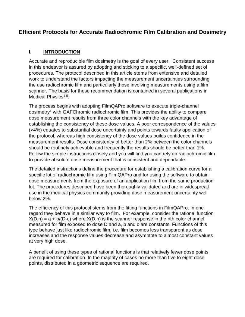
The efficiency of this protocol stems from the fitting functions in FilmQAPro. In one regard they behave in a similar way to film. For example, consider the rational function X(D,n) = a + b/(D-c) where X(D,n) is the scanner response in the nth color channel measured for film exposed to dose D and a, b and c are constants. Functions of this type behave just like radiochromic film, i.e. film becomes less transparent as dose increases and the response values decrease and asymptote to almost constant values at very high dose. A benefit of using these types of rational functions is that relatively fewer dose points are required for calibration. In the majority of cases no more than five to eight dose points, distributed in a geometric sequence are required.

Figure 1

II. EQUIPMENT AND MATERIALS

GAFChromic, EBT3, EBT-XD, MD-V3, HD-V2 or the single-sided version of

EBT3 radiochromic film.

Scissors or paper cutter

Adhesive tape

Calibrated exposure source

48-bit rgb flatbed scanner, preferably Epson model 10000XL or 11000XL with transparency adapter

Epson Scan software and Twain driver

FilmQAPro Pro software application

Solid water or suitable phantom material for exposing the radiochromic films

Glass compression plate – 3-4 mm thick and same size as window of scanner (31.5 x 45 cm2 for Epson 10000XL and 11000XL)

III. FILM HANDLINGWith the exception of HD-V2 and the single-sided version of EBT3 the films are relatively sturdy with the active layer protected on both sides by clear polyester film substrates. This allows the films to be immersed in water for short periods and to be handled with clean, bare hands. Try to handle film by the edges. While a few fingerprints and smudges are usually not problematic they can be easily removed with an alcohol swab. Film can be marked with a felt-tip pen, but if these marks would subsequently interfere with measurement an alcohol swab will remove them. In HD-V2 film and the single-sided version of EBT3 the active layer is exposed to damage and should be handled more carefully and certainly not with wet or damp hands. It should not be immersed in water. Handle the film by the edges to avoid lots of finger prints. In most cases, a small smudge or two won’t be problematic. If you wish to remove any fingerprints or debris from the films, either a wet paper towel or an alcohol wipe will

work, but in general this is not usually necessary. The active layer of the film is sandwiched between two polyester layers, so it is protected.

Note: When a film is not being used the best practice is to keep it in the box or a black envelope. While films are relatively insensitive to indoor ambient light a long exposure will cause darkening. Do not expose film to sunlight, even through a window, as the UV component will quickly darken the film.

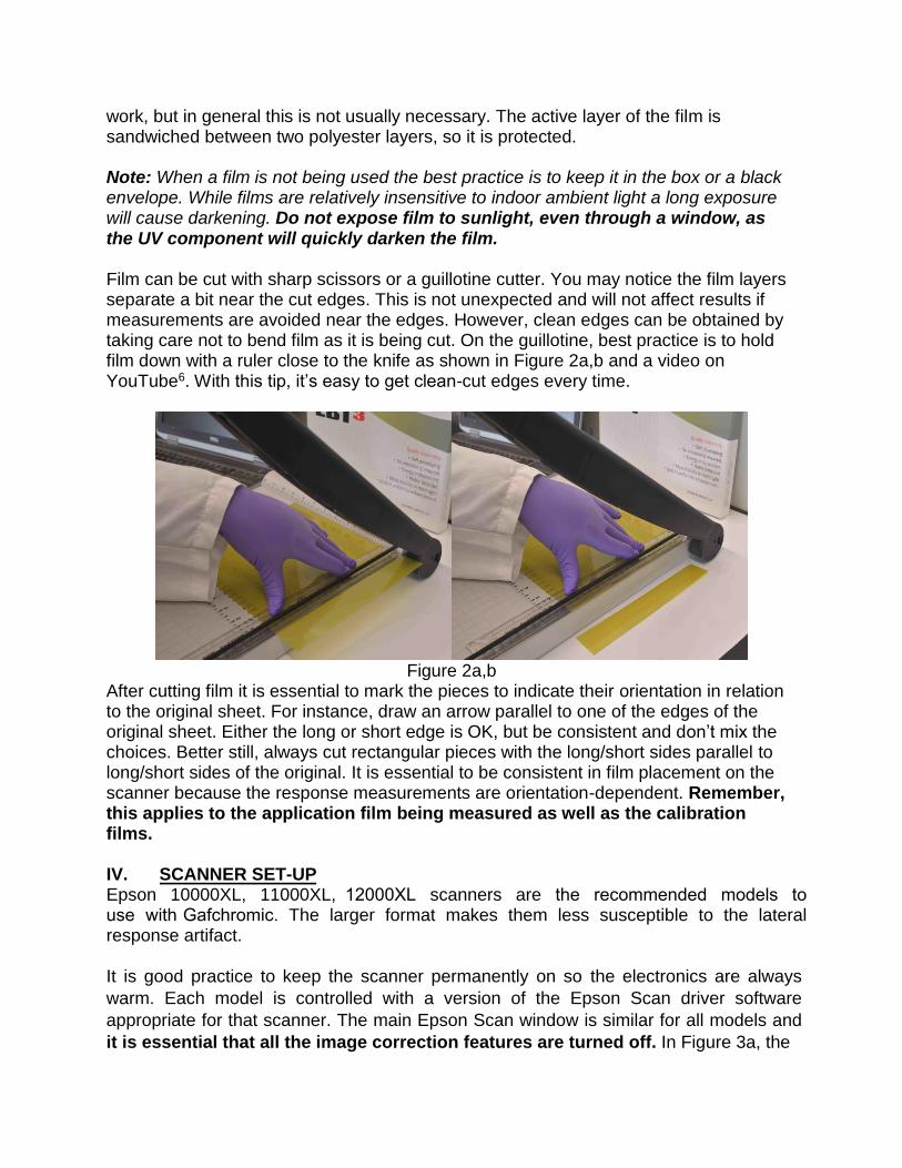
Film can be cut with sharp scissors or a guillotine cutter. You may notice the film layers separate a bit near the cut edges. This is not unexpected and will not affect results if measurements are avoided near the edges. However, clean edges can be obtained by taking care not to bend film as it is being cut. On the guillotine, best practice is to hold film down with a ruler close to the knife as shown in Figure 2a,b and a video on YouTube6. With this tip, it’s easy to get clean-cut edges every time.

Figure 2a,b After cutting film it is essential to mark the pieces to indicate their orientation in relation to the original sheet. For instance, draw an arrow parallel to one of the edges of the original sheet. Either the long or short edge is OK, but be consistent and don’t mix the choices. Better still, always cut rectangular pieces with the long/short sides parallel to long/short sides of the original. It is essential to be consistent in film placement on the scanner because the response measurements are orientation-dependent. Remember, this applies to the application film being measured as well as the calibration films.

IV. SCANNER SET-UPEpson 10000XL, 11000XL, 12000XL scanners are the recommended models to use with Gafchromic. The larger format makes them less susceptible to the lateral response artifact.

It is good practice to keep the scanner permanently on so the electronics are always

warm. Each model is controlled with a version of the Epson Scan driver software

appropriate for that scanner. The main Epson Scan window is similar for all models and

it is essential that all the image correction features are turned off. In Figure 3a, the

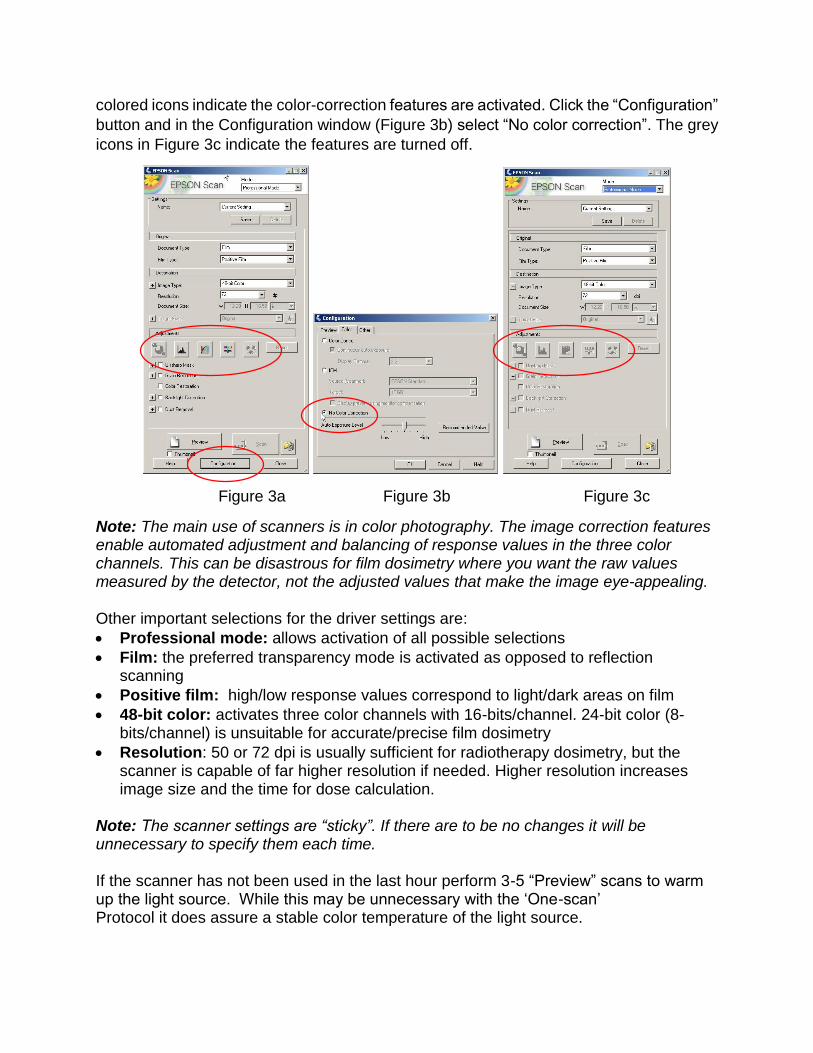
colored icons indicate the color-correction features are activated. Click the “Configuration”

button and in the Configuration window (Figure 3b) select “No color correction”. The grey

icons in Figure 3c indicate the features are turned off.

Figure 3a Figure 3b Figure 3c

Note: The main use of scanners is in color photography. The image correction features enable automated adjustment and balancing of response values in the three color channels. This can be disastrous for film dosimetry where you want the raw values measured by the detector, not the adjusted values that make the image eye-appealing.

Other important selections for the driver settings are:

Professional mode: allows activation of all possible selections

Film: the preferred transparency mode is activated as opposed to reflectionscanning

Positive film: high/low response values correspond to light/dark areas on film

48-bit color: activates three color channels with 16-bits/channel. 24-bit color (8-bits/channel) is unsuitable for accurate/precise film dosimetry

Resolution: 50 or 72 dpi is usually sufficient for radiotherapy dosimetry, but thescanner is capable of far higher resolution if needed. Higher resolution increasesimage size and the time for dose calculation.

Note: The scanner settings are “sticky”. If there are to be no changes it will be unnecessary to specify them each time.

If the scanner has not been used in the last hour perform 3-5 “Preview” scans to warm up the light source. While this may be unnecessary with the ‘One-scan’ Protocol it does assure a stable color temperature of the light source.

IVa. Glass Compression Plate

After film is placed for scanning use a glass compression plate to ensure film is flat on the scanner window. This is a sheet of clear glass, 3-4 mm thick and the same size as the glass window of the scanner. In addition to the film, the compression plate should cover the 1-2 cm wide calibration area of the window situated where the scan begins. If film is not flat to the window response values increase about 1.2% for every millimeter the film is closer to the light source4.

V. CALIBRATION PROCEDURE

Cut an 8”x10” sheet of film into 1.25”x8” strips. The size/shape of the strips leaves no

doubt as to their orientation relative to the original sheet. Six to eight strips and dose

points (including zero dose) are usually sufficient for calibration. Any strips remaining can

be used as reference films (see Section VI) when making dose measurements. Although

the calibration will be valid for doses up to the highest dose used, it is preferable if two of

the calibration doses are equal or greater than the highest dose to be measured. By their

nature the asymptotic fitting functions used for calibration in the FilmQAPro software work

well when the doses (except for zero) are in geometric progression, i.e. X, nX, n2X, n3X,

etc., rather than arithmetic progression.

The calibration will be valid for other films from the same production lot as the calibration

films. While the following procedure assumes the film strips will be exposed separately,

an alternate method could utilize a linear accelerator to expose stripes to known doses

across the 8” width of a film sheet.

Step 1: Position a film strip in the phantom (Figure V-1) at the center of the exposure field

and perpendicular to the beam.

Figure V-1

Step 2: Expose the strip to one of the required calibration doses to create a large area of

uniform exposure on the film. A 10 cm x 10 cm2 field works well. Note the time of the

exposure and store film in the dark.

Figure V-2

Step 3: Repeat Step 1 as needed using additional film strips. As explained in Step 6, the

time window during which the calibration films are exposed is related to how soon the

scanning can be started.

Step 4: Connect the scanner to a computer. Open FilmQAPro Pro and from the drop-

down menu under “Case Object Management” select ‘Film Calibration (ordinary)’.

Figure V-3

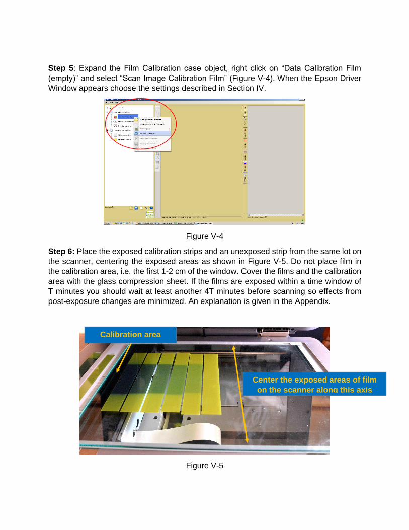
Step 5: Expand the Film Calibration case object, right click on “Data Calibration Film

(empty)” and select “Scan Image Calibration Film” (Figure V-4). When the Epson Driver

Window appears choose the settings described in Section IV.

Figure V-4

Step 6: Place the exposed calibration strips and an unexposed strip from the same lot on

the scanner, centering the exposed areas as shown in Figure V-5. Do not place film in

the calibration area, i.e. the first 1-2 cm of the window. Cover the films and the calibration

area with the glass compression sheet. If the films are exposed within a time window of

T minutes you should wait at least another 4T minutes before scanning so effects from

post-exposure changes are minimized. An explanation is given in the Appendix.

Figure V-5

Center the exposed areas of film

on the scanner along this axis

Calibration area

Step 7: Scan the films. Then use the Frame Tool in FilmQAPro to mark areas of interest

at the center of each calibration strip (Figure V-6).

Figure V-6

Step 8: Click the “123” icon (bottom right corner in Figure V-7). Select the “Color

reciprocal linear vs. dose” fitting function and type in the dose values into the first

column of the calibration table.

Select fitting function

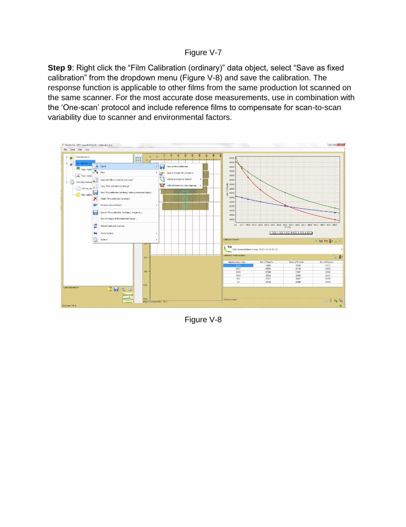
Figure V-7

Step 9: Right click the “Film Calibration (ordinary)” data object, select “Save as fixed

calibration” from the dropdown menu (Figure V-8) and save the calibration. The

response function is applicable to other films from the same production lot scanned on

the same scanner. For the most accurate dose measurements, use in combination with

the ‘One-scan’ protocol and include reference films to compensate for scan-to-scan

variability due to scanner and environmental factors.

Figure V-8

V1. DOSIMETRY PROCEDURE

The procedure follows the ‘One-scan’ protocol2. In addition to the application film it

employs two reference films – one is unexposed and the second is exposed to a known

dose immediately before or after the application film. When scanned with the application

film, the reference films are used to re-scale the calibration function to fit the responses

of that specific scan. This compensates for scan-to-scan variability from any source4,

enabling reliable absolute dosimetry. When a reference film is exposed within a few

minutes of the application film the ‘One-scan’ protocol allows scanning to be done and

measurements made almost immediately after exposure without having to wait for post-

exposure changes to stabilize2.

The reference films are preferably 1.25” x 8” strips cut from 8”x10” sheets from the same

production lot as the application film. The application film for dose measurements may be

an 8”x10” sheet, or a piece cut to smaller size as required. In any event, it is essential to

track the orientation of each film so that all are scanned in the same orientation as the

calibration films.

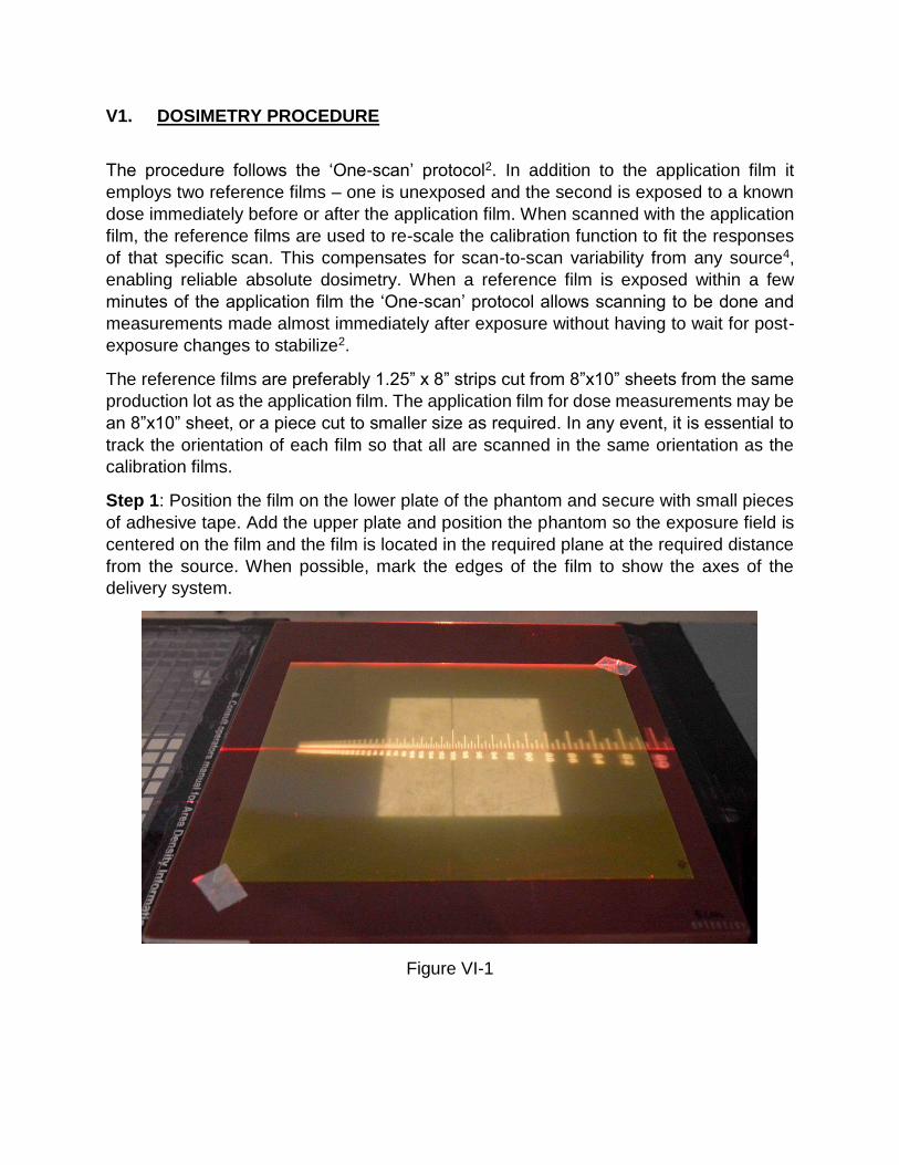
Step 1: Position the film on the lower plate of the phantom and secure with small pieces

of adhesive tape. Add the upper plate and position the phantom so the exposure field is

centered on the film and the film is located in the required plane at the required distance

from the source. When possible, mark the edges of the film to show the axes of the

delivery system.

Figure VI-1

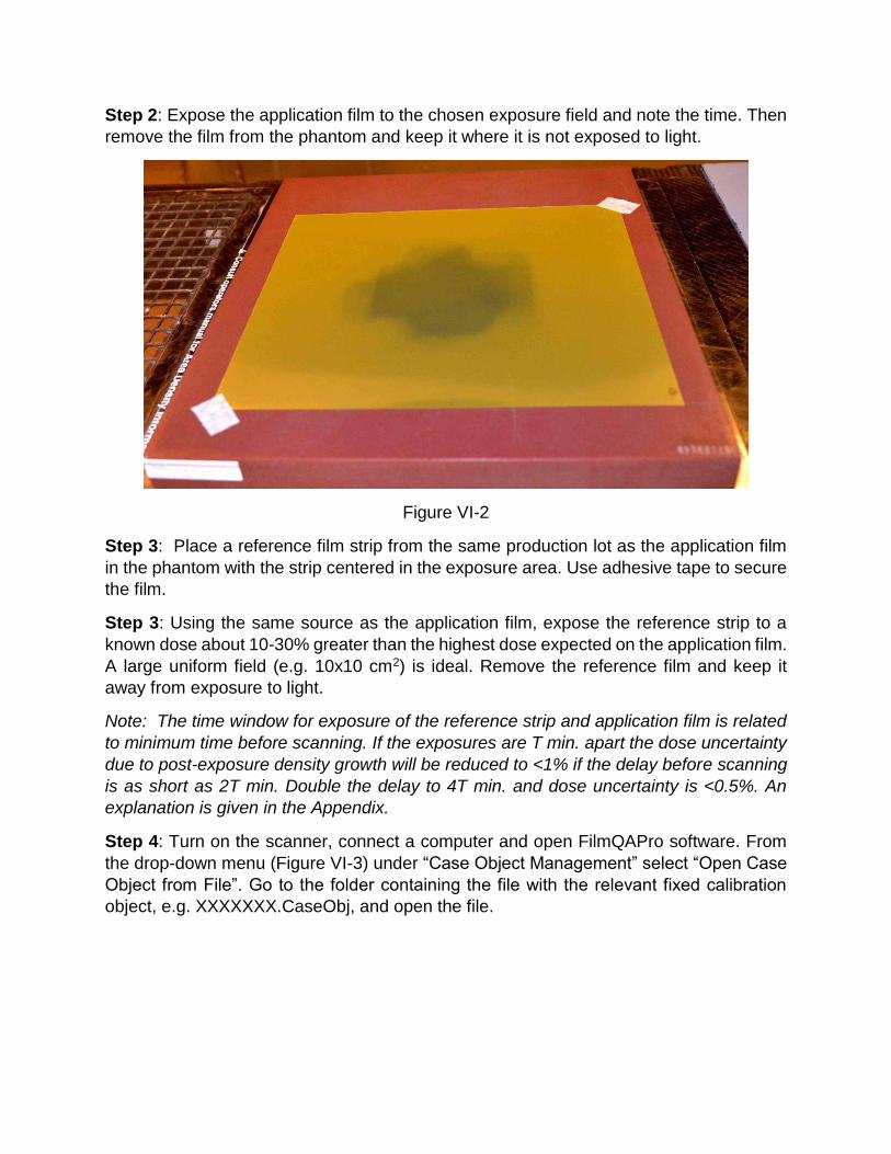
Step 2: Expose the application film to the chosen exposure field and note the time. Then

remove the film from the phantom and keep it where it is not exposed to light.

Figure VI-2

Step 3: Place a reference film strip from the same production lot as the application film

in the phantom with the strip centered in the exposure area. Use adhesive tape to secure

the film.

Step 3: Using the same source as the application film, expose the reference strip to a

known dose about 10-30% greater than the highest dose expected on the application film.

A large uniform field (e.g. 10x10 cm2) is ideal. Remove the reference film and keep it

away from exposure to light.

Note: The time window for exposure of the reference strip and application film is related

to minimum time before scanning. If the exposures are T min. apart the dose uncertainty

due to post-exposure density growth will be reduced to <1% if the delay before scanning

is as short as 2T min. Double the delay to 4T min. and dose uncertainty is <0.5%. An

explanation is given in the Appendix.

Step 4: Turn on the scanner, connect a computer and open FilmQAPro software. From

the drop-down menu (Figure VI-3) under “Case Object Management” select “Open Case

Object from File”. Go to the folder containing the file with the relevant fixed calibration

object, e.g. XXXXXXX.CaseObj, and open the file.

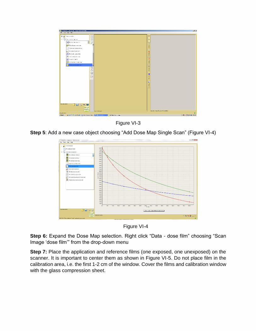
Figure VI-3

Step 5: Add a new case object choosing “Add Dose Map Single Scan” (Figure VI-4)

Figure VI-4

Step 6: Expand the Dose Map selection. Right click “Data - dose film” choosing “Scan

Image ‘dose film’” from the drop-down menu

Step 7: Place the application and reference films (one exposed, one unexposed) on the

scanner. It is important to center them as shown in Figure VI-5. Do not place film in the

calibration area, i.e. the first 1-2 cm of the window. Cover the films and calibration window

with the glass compression sheet.

Figure VI-5

Note: The time window for exposure of the reference strip and application film is related

to minimum time before scanning. If the exposures are T min. apart the dose uncertainty

due to post-exposure density growth will be reduced to <1% if the delay before scanning

is as short as 2T min. Double the delay to 4T min. and dose uncertainty is <0.5%. An

explanation is given in the Appendix.

Step 8: Use the Frame Tool to select areas of interest in the centers of the reference

strips. Right click the areas of interest (Figure VI-6a) to name the region types as

“Calibration Region”. Then right click the regions, select “Calibration Value” (Figure VI-

6b), type in the dose (Figure VI-7), hit enter and OK

.

Figure VI-6a Figure VI-6b

Calibration area

Center the exposed areas of films

on the scanner along this axis

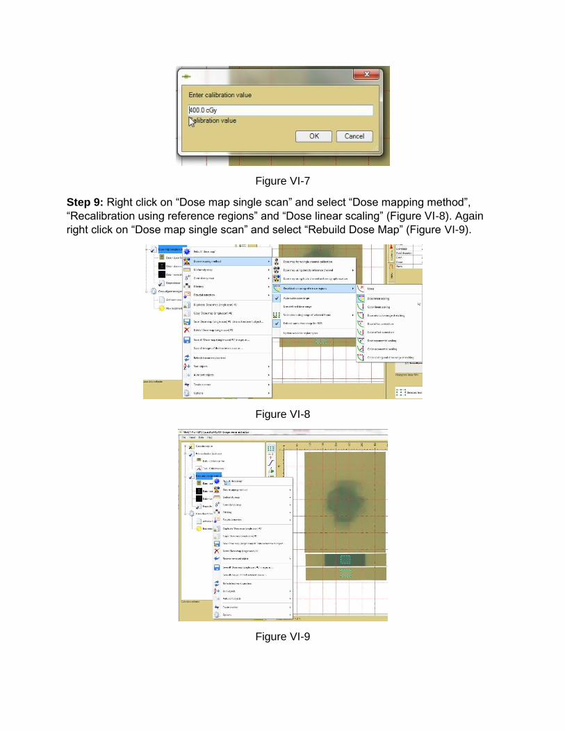
Figure VI-7

Step 9: Right click on “Dose map single scan” and select “Dose mapping method”,

“Recalibration using reference regions” and “Dose linear scaling” (Figure VI-8). Again

right click on “Dose map single scan” and select “Rebuild Dose Map” (Figure VI-9).

Figure VI-8

Figure VI-9

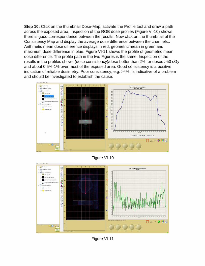
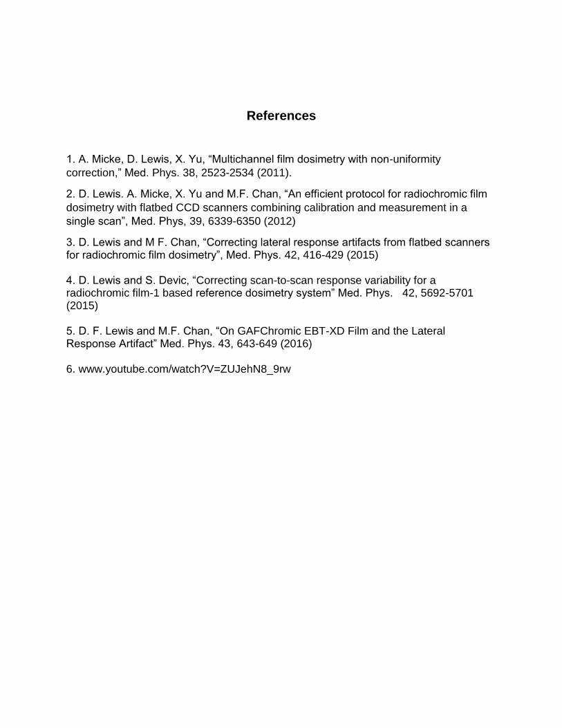
Step 10: Click on the thumbnail Dose-Map, activate the Profile tool and draw a path

across the exposed area. Inspection of the RGB dose profiles (Figure VI-10) shows

there is good correspondence between the results. Now click on the thumbnail of the

Consistency Map and display the average dose difference between the channels..

Arithmetic mean dose difference displays in red, geometric mean in green and

maximum dose difference in blue. Figure VI-11 shows the profile of geometric mean

dose difference. The profile path in the two Figures is the same. Inspection of the

results in the profiles shows (dose consistency)/dose better than 2% for doses >50 cGy

and about 0.5%-1% over most of the exposed area. Good consistency is a positive

indication of reliable dosimetry. Poor consistency, e.g. >4%, is indicative of a problem

and should be investigated to establish the cause.

Figure VI-10

Figure VI-11

References

1. A. Micke, D. Lewis, X. Yu, “Multichannel film dosimetry with non-uniformity

correction,” Med. Phys. 38, 2523-2534 (2011).

2. D. Lewis. A. Micke, X. Yu and M.F. Chan, “An efficient protocol for radiochromic film

dosimetry with flatbed CCD scanners combining calibration and measurement in a

single scan”, Med. Phys, 39, 6339-6350 (2012)

3. D. Lewis and M F. Chan, “Correcting lateral response artifacts from flatbed scannersfor radiochromic film dosimetry”, Med. Phys. 42, 416-429 (2015)

4. D. Lewis and S. Devic, “Correcting scan-to-scan response variability for aradiochromic film-1 based reference dosimetry system” Med. Phys. 42, 5692-5701(2015)

5. D. F. Lewis and M.F. Chan, “On GAFChromic EBT-XD Film and the LateralResponse Artifact” Med. Phys. 43, 643-649 (2016)

6. www.youtube.com/watch?V=ZUJehN8_9rw

Appendix

Post-Exposure Change and the Efficient Radiochromic Film Dosimetry Protocol

Exposure of radiochromic film to ionizing radiation starts a solid-state polymerization in

crystals of the active component. Polymer grows within the crystal matrix of the

monomer. Interatomic distances in the polymer are shorter than in the monomer

causing the gap between the end of the growing polymer chain and the next monomer

molecule to increase as polymerization progresses. Consequently the rate of

polymerization decreases with time. Based on measurement, the response is linear with

log(time-after-exposure) as shown in Figure A-1. This means that if dose-response

calibration is established by scanning calibration films at a given time-after-exposure an

error in dose will results if the application film is scanned at a different time-after-

exposure. However, the error diminishes rapidly as the ratio of the timing error to the

time-after-exposure decreases.

Figure A-1

0.0

0.1

0.2

0.3

0.4

0.5

0.6

0.0 0.5 1.0 1.5 2.0 2.5 3.0 3.5

Op

tica

l d

en

sit

y

Log10(time, minutes)

GAFCHROMIC EBT2: Post-Exposure Changes

0.5Gy

1Gy

1.5Gy

2.5Gy

From Figure A-1, it is calculated that at time-after-exposure of 30 min. a 5-minutes

timing error results in a dose error of about 0.3%, while a 10 minute timing error results

in a dose error about 0.6%. If the time-after-exposure increases to 60 min. the dose

error for a given timing error decreases by a factor of two. The One-Scan protocol

employs a single scan to make dose measurements of application film and calibration

film exposed at different times. To keep dose errors small (<0.5%) film scanning should

be delayed for a time period a minimum about 4X longer than the interval between the

exposure of the application film and the calibration film. For example, if the exposures of

the films were 5 min. apart the films could be scanned 20 min. later or any time

thereafter.