Embed Size (px)
Citation preview

Efficient Measurement Techniques in
Reverberation Chamber
by
Zhihao Tian
Submitted in accordance with the requirements for the award of the
degree of Doctor of Philosophy of the University of Liverpool
September 2017

P a g e | i
Copyright
Copyright © 2017 Zhihao Tian. All rights reserved.
The copyright of this thesis rests with the author. Copies (by any means) either in full
or of extracts may not be made without prior written consent from the author.

P a g e | ii
To my family: Thank you for all of your efforts and for your support.

P a g e | iii
Table of Contents
Copyright ...................................................................................................................... i
Table of Contents ........................................................................................................ iii
Acronyms and Abbreviations ..................................................................................... vii
Acknowledgements ...................................................................................................... ix
List of Publications ...................................................................................................... x
Abstract ..................................................................................................................... xiv
Chapter 1: Introduction ............................................................................................ 1
1.1 Background .................................................................................................... 1
1.1.1 Anechoic Chamber .................................................................................... 1
1.1.2 TEM Cells ................................................................................................. 2
1.1.3 Reverberation Chamber ............................................................................ 4
1.2 Motivation and Objective ............................................................................... 6
1.3 Organisation of the Thesis ............................................................................. 7
1.4 References ...................................................................................................... 9
Chapter 2: Theories of Reverberation Chamber .................................................. 12
2.1 Introduction .................................................................................................. 12
2.2 Deterministic Theory ................................................................................... 13
2.2.1 Resonant Modes ...................................................................................... 13

P a g e | iv
2.2.2 Modes inside a Lossy Cavity .................................................................. 20
2.2.3 Lowest Usable Frequency ....................................................................... 22
2.2.4 Number of Cavity Modes ........................................................................ 23
2.2.5 Green’s Function ..................................................................................... 26
2.3 Stirring Techniques ...................................................................................... 29
2.3.1 Mechanical Stirring ................................................................................. 30
2.3.2 Frequency Stirring ................................................................................... 31
2.3.3 Source Stirring ........................................................................................ 32
2.4 Statistical Theory ......................................................................................... 33
2.4.1 Plane-wave Integration Model ................................................................ 33
2.4.2 Statistical Properties of Fields ................................................................. 36
2.4.3 Probability Density Functions for the Fields .......................................... 38
2.4.4 Loss Mechanism and Q Factor ................................................................ 41
2.4.5 Chamber Decay Time ............................................................................. 43
2.4.6 Stirred and Unstirred Power .................................................................... 45
2.4.7 Enhanced Backscatter Effect................................................................... 51
2.5 Summary ...................................................................................................... 54
2.6 References .................................................................................................... 54
Chapter 3: Efficient Averaged Absorption Cross Section Measurement ........... 61
3.1 Introduction .................................................................................................. 61
3.2 Theory .......................................................................................................... 62

P a g e | v
3.2.1 Frequency Domain .................................................................................. 63
3.2.2 Time Domain .......................................................................................... 65
3.3 Measurement ................................................................................................ 66
3.4 Convergence Property .................................................................................. 74
3.5 ACS Measurement without Calibration ....................................................... 78
3.6 Discussions and Conclusion ......................................................................... 83
3.7 References .................................................................................................... 85
Chapter 4: Volume Measurement Using Averaged Absorption Cross Section.. 90
4.1 Introduction .................................................................................................. 90
4.2 Theory .......................................................................................................... 91
4.3 Measurement ................................................................................................ 92
4.4 Discussions and Conclusion ....................................................................... 105
4.5 References .................................................................................................. 105
Chapter 5: Simplified Shielding Effectiveness Measurement of Small Cavity 109
5.1 Introduction ................................................................................................ 109
5.2 Theory ........................................................................................................ 110
5.2.1 Frequency Domain ................................................................................ 110
5.2.2 Time Domain ........................................................................................ 112
5.3 Measurement .............................................................................................. 114
5.4 Convergence Behaviour ............................................................................. 122
5.5 Discussions and Conclusion ....................................................................... 128
P a g e | vi
5.6 References .................................................................................................. 129
Chapter 6: Antenna Array Efficiency Measurement ......................................... 133
6.1 Introduction ................................................................................................ 133
6.2 The Problem ............................................................................................... 134
6.2.1 Single Antenna Case ............................................................................. 134
6.2.2 Antenna Array Case .............................................................................. 141
6.3 Improved Method ....................................................................................... 142
6.4 Measurement Uncertainty .......................................................................... 150
6.5 Discussions and Conclusion ....................................................................... 153
6.6 References .................................................................................................. 154
Chapter 7: Conclusions and Future Work .......................................................... 157
References ............................................................................................................ 160
Appendix A. Vector and Dyadic Analysis ............................................................... 162
Appendix B. Probability Density Function .............................................................. 165
References ............................................................................................................ 166

P a g e | vii
Acronyms and Abbreviations
AC Anechoic Chamber
ACS Absorption Cross Section
AUT Antenna under Test
CST Computer Simulation Technology
DC Direct Current
EM Electromagnetic
EMC Electromagnetic Compatibility
EUT Equipment under Test
FD Frequency Domain
IEEE Institute of Electrical and Electronics Engineers
IFT Inverse Fourier Transform
IFFT Inverse Fast Fourier Transform
LoS Line-of-Sight
LPDA Log Periodic Dipole Antenna
LUF Lowest Usable Frequency
NLoS Non-Line-of-Sight
OUT Object under Test
1D One Dimensional
PDF Probability Density Function
PDP Power Delay Profile

P a g e | viii
PEC Perfect Electrical Conductor
RAM Radio Absorbing Material
RC Reverberation Chamber
RMS Root Mean Square
RMSE Root Mean Square Error
SAR Specific Absorption Rate
SE Shielding Effectiveness
SI International System of Units
3D Three Dimensional
TD Time Domain
TE Transverse Electric
TEM Transverse Electromagnetic
TM Transverse Magnetic
VNA Vector Network Analyser
VSWR Voltage Standing Wave Ratio

P a g e | ix
Acknowledgements
First and foremost, I would like to express my sincere gratitude to my supervisors
Professor Yi Huang and Professor Yaochun Shen. I thank you both for your
invaluable guidance and persistent support for my research. Without your help, this
dissertation would not have been possible. I would also like to thank Dr. Qian Xu. I
learned a lot from him during our many discussions about reverberation chamber
measurement and analysis techniques. I feel lucky to be working in a research group
that stimulates original ideas and insightful thoughts. I really enjoy the intellectual
delight in our group. The beneficial discussions and selfless help from my colleagues
are much appreciated.
This work would not be completed without the financial support of CSC (China
Scholarship Council). I would like to acknowledge the important role of them.
Finally, I would like to thank my research lab colleagues and my friends: Prof.
Chenjiang Guo, Dr. Stephen Boyes, Dr. Shufeng Sun, Dr. Saqer Alja’afreh, Dr.
Gaosheng Li, Dr. Neda Khiabani, Dr. Lei Xing, Alieldin Ahmed, Dr. Ping Cao, Dr.
Jingwei Zhang, Saidatul Izyanie, Dr. Sheng Yuan, Chaoyun Song, Manoj Stanley,
Zhouxiang Fei, Dr. Muayad Kod, Dr. Rula Alrawashdeh, Muaad Hussein, Aznida
Abu Bakar Sajak, Dr. Amir Kotb, Abed Pour Sohrab, Anqi Chen, Yuan Zhuang,
Umniyyah Ulfa, Yukun Zhao, Shuang Li, Bahaa Al-Juboori, Chen Xu, Wenzhang
Zhang, Sumi Joseph, Tianyuan Jia, Dr. Tian-Hong Loh, and Dr. Chong Li. I have
enjoyed working with you all and I appreciate the help and support that you gave me.
P a g e | x
List of Publications
Journal Publications
[1] Z. Tian, Y. Huang, Q. Xu, and G. Li, “A Rapid Method for Measuring the
Volume of a Large Cavity Using Averaged Absorption Cross Section,” IEEE
Access, 2017, DOI: 10.1109/ACCESS.2017.2745698.
[2] Z. Tian, Y. Huang, and Q. Xu, “Efficient Methods of Measuring Shielding
Effectiveness of Electrically Large Enclosures Using Nested Reverberation
Chambers with Only Two Antennas,” IEEE Transactions on Electromagnetic
Compatibility, vol. 59, no. 6, pp. 1872-1879, December 2017.
[3] Z. Tian, Y. Huang, and Q. Xu, “An Improved Method for Efficiency
Measurement of All-Excited Antenna Array in Reverberation Chamber Using
Power Divider,” IEEE Transactions on Antennas and Propagation, vol. 65,
no. 6, pp. 3005-3013, June 2017.
[4] Z. Tian, Y. Huang, Y. Shen, and Q. Xu, “Efficient and Accurate
Measurement of Absorption Cross Section of a Lossy Object in
Reverberation Chamber Using Two One-Antenna Methods,” IEEE
Transactions on Electromagnetic Compatibility, vol. 58, no. 3, pp. 686-693,
June 2016.
[5] M. Stanley, Y, Huang, H. Wang, Z. Hai, Z. Tian, and Q. Xu, “A Novel
Reconfigurable Metal Rim Integrated Open Slot Antenna for Octa-band
Smartphone Applications”, IEEE Transactions on Antennas and
Propagation, vol. 65, no. 7, pp. 3352-3363, July 2017.
[6] C. Li, T. H. Loh, Z. Tian, Q. Xu, and Y. Huang, “Evaluation of Chamber
Effects on Antenna Efficiency Measurements Using Non-reference Antenna
Methods in Two Reverberation Chambers,” IET Microwaves, Antennas &
Propagation, June 2017, DOI: 10.1049/iet-map.2015.0838.

P a g e | xi
[7] Q. Xu, Y. Huang, L. Xing, C. Song, Z. Tian, S. Alja'afreh, and M. Stanley,
“3D Antenna Radiation Pattern Reconstruction in a Reverberation Chamber
Using Spherical Wave Decomposition,” IEEE Transactions on Antennas and
Propagation, vol. 65, no. 4, pp. 1728-1739, April 2017.
[8] Q. Xu, Y. Huang, L. Xing, Z. Tian, J. Zhou, A. Chen, and Y. Zhuang,
“Average Absorption Coefficient Measurement of Arbitrarily Shaped
Electrically Large Objects in a Reverberation Chamber,” IEEE Transactions
on Electromagnetic Compatibility, vol. 58, no. 6, pp. 1776-1779, December
2016.
[9] Q. Xu, Y. Huang, L. Xing, Z. Tian, M. Stanley, and S. Yuan, “B-scan in a
reverberation chamber,” IEEE Transactions on Antennas and Propagation,
vol. 64, no. 5, pp. 1740-1750, May 2016.
[10] Q. Xu, Y. Huang, L. Xing, Z. Tian, C. Song, and M. Stanley, “The Limit of
the Total Scattering Cross Section of Electrically Large Stirrers in a
Reverberation Chamber,” IEEE Transactions on Electromagnetic
Compatibility, vol. 58, no. 2, pp. 623-626, April 2016.
[11] Q. Xu, Y. Huang, L. Xing, and Z. Tian, “Extract the Decay Constant of a
Reverberation Chamber Without Satisfying Nyquist Criterion,” IEEE
Microwave and Wireless Components Letters, vol. 26, no. 3, pp. 153-155,
March 2016.
[12] Q. Xu, Y. Huang, S. Yuan, L. Xing, and Z. Tian, “Two alternative methods
to measure the radiated emission in a reverberation chamber,” International
Journal of Antennas and Propagation, vol. 2016, Article ID: 5291072, 7
pages, February 2016.
[13] Q. Xu, Y. Huang, X. Zhu, L. Xing, Z. Tian, and C. Song, “A Modified Two-
Antenna Method to Measure the Radiation Efficiency of Antennas in a
Reverberation Chamber,” IEEE Antennas and Wireless Propagation Letters,
vol. 15, pp. 336-339, February 2016.

P a g e | xii
[14] Q. Xu, Y. Huang, X. Zhu, L. Xing, Z. Tian, and C. Song, “Shielding
effectiveness measurement of an electrically large enclosure using one
antenna,” IEEE Transactions on Electromagnetic Compatibility, vol. 57, no.
6, pp. 1466-1471, December 2015.
[15] Q. Xu, Y. Huang, L. Xing, Z. Tian, Z. Fei, and L. Zheng, “A fast method to
measure the volume of a large cavity,” IEEE Access, vol. 3, pp. 1555-1561,
September 2015.
[16] Q. Xu, Y. Huang, X. Zhu, S. Alja’afreh, L. Xing, and Z. Tian, “Diversity
gain measurement in a reverberation chamber without extra antennas,” IEEE
Antennas and Wireless Propagation Letters, vol. 14, pp. 1666-1669, August
2015.
Conference Publications
[1] Z. Tian, Y. Huang, and Q. Xu, “Efficient Measurement Techniques on OTA
Test in Reverberation Chamber”, 2017 IEEE AP-S Symposium on Antennas
and Propagation and USNC-URSI Radio Science Meeting, San Diego, U.S.,
2017.
[2] Z. Tian, Y. Huang, and Q. Xu, “Enhanced Backscatter Coefficient
Measurement at High Frequencies in Reverberation Chamber”, International
Workshop on Electromagnetics (iWEM), London, U.K., 2017.
[3] Z. Tian, Y. Huang, and Q. Xu, “Measurement of Absorption Cross Section
of a Lossy Object in Reverberation Chamber without the Need for
Calibration”, Loughborough Antennas and Propagation Conference (LAPC),
Loughborough, U.K., 2016.
[4] Z. Tian, Y. Huang, and Q. Xu, “Stirring effectiveness characterization based
on Doppler spread in a reverberation chamber,” European Conference on
Antennas and Propagation (EuCAP), Davos, Switzerland, 2016.

P a g e | xiii
[5] Z. Tian, Y. Huang, and Q. Xu, “A further investigation of the source stirred
chamber method for antenna efficiency measurements,” 8th UK, Europe,
China Conference on Millimetre Waves and Terahertz Technologies
(UCMMT), Cardiff, U.K., 2015.
[6] Z. Tian, Y. Huang, Y. Shen, and Q. Xu, “An electrical stirring method for a
reverberation chamber,” Antennas and Propagation Conference (LAPC),
U.K., Loughborough, 2014.
[7] Q. Xu, Y. Huang, Y. Zhao, L. Xing, Z. Tian, and T. H. Loh, “Investigation
of Bandpass Filters in the Time Domain Signal Analysis of Reverberation
Chamber”, 2017 URSI General Assembly and Scientific Symposium
(GASS), Montreal, Canada, 2017.
[8] C. Li, T. Loh, Z. Tian, Q. Xu, and Y. Huang, “A comparison of antenna
efficiency measurements performed in two reverberation chambers using
non-reference antenna methods,” Loughborough Antennas and Propagation
Conference (LAPC), Loughborough, U.K., 2015. (Best Non-student Paper
Award)
[9] Q. Xu, Y. Huang, X. Zhu, L. Xing, and Z. Tian, “Antenna radiation
efficiency measurement in a reverberation chamber without the need for
calibration,” IEEE AP-S Symposium on Antennas and Propagation (APS),
Vancouver, Canada, 2015.
[10] Q. Xu, Y. Huang, X. Zhu, L. Xing, and Z. Tian, “Permittivity measurement
of spherical objects using a reverberation chamber,” Loughborough Antennas
and Propagation Conference (LAPC), Loughborough, U.K., 2014. (Best
Student Paper Award)

P a g e | xiv
Abstract
The rapid expansion of electronic industry calls for effective and efficient
electromagnetic (EM) measurements, including the characterization of devices under
test (DUT), such as antennas or wireless devices, and the electromagnetic
compatibility (EMC) testing.
In the real world, EM measurements can be influenced by a number of
uncontrollable factors which will afflict the measurements. These factors make the
measurements very difficult especially when the measurements require high
precision and/or low power relative to the background noise. To conduct EM
measurements accurately, many different facilities/environments have been
developed, including anechoic chambers (ACs), transverse electromagnetic (TEM)
Cells, and reverberation chambers (RCs). These three environments have different
characteristics.
Over the past several decades, RCs have been enjoying growing popularity as a
promising facility for the characterization of wireless devices and for the EMC
testing. The RC measurement method exhibits much competitive superiority over the
AC method and TEM Cell method, such as low cost, enhanced test repeatability, a
more realistic test environment, and easily achieved high-field environment. The
application of the RC for performing EMC testing was first proposed by H. A.
Mendes in 1968. In the recent IEC 61000-4-21 standard, the importance of EMC
testing using RCs as an alternative measurement technique has been recognized.
To make the RC well stirred, a large number of independent samples (stirrer
positions) are required. Consequently, the measurement time is usually long
(typically several hours), which has greatly restricted the engineering applications of
the RC measurement techniques.
The purpose of this thesis is to present our studies on improving the measurement
efficiency of RCs in recent years, including the efficient measurement of the
averaged absorption cross section (ACS) with only one antenna, the rapid volume
measurement method using the averaged ACS, the simplified shielding effectiveness

P a g e | xv
(SE) measurement using the nested RC with two antennas, and the improved antenna
array efficiency measurement in an RC.
For ACS measurement, the proposed one-antenna methods in both the frequency
domain and the time domain are presented. The measurement setup is greatly
simplified and the measurement time is significantly shortened. The efficient
measurement of the ACS can be used to obtain the volume of a chamber, which leads
to the rapid volume measurement method. For the SE measurement of electrically
large enclosures using a nested RC, four improved measurement methods are
proposed. Both the frequency-domain and time-domain methods are studied. The
proposed methods require only two antennas and provide efficient measurement of
SE without losing the accuracy. Finally, the accurate array efficiency measurement
method in an RC using a power divider is presented. A power divider is used to
excite the feeding ports of the array elements simultaneously. Thus, the efficiency
measurement of the entire array can be effectively treated in a manner similar to a
single port antenna, which would simplify the measurement procedure and reduce
the overall measurement time. By introducing proper attenuators between the array
elements and the power divider to alleviate the effect of the reflected power from the
array to the insertion loss of the power divider, the array efficiency can be measured
accurately even when the elements of the array are not well-matched with the power
divider. The proposed method is advantageous especially for wideband antenna
arrays where good impedance matching of array elements is difficult to maintain.
In this thesis, it is shown that our proposed methods have greatly improved the RC
measurement efficiency and simplified the measurement setup at the same time.
These contributions could promote the industrial application of RCs.

Chapter 1: Introduction P a g e | 1
Chapter 1: Introduction
1.1 Background
With the blooming electronic industry, electromagnetic (EM) measurements are becoming
more and more important, including the characterization of devices under test (DUT), such as
antennas or wireless devices, and the electromagnetic compatibility (EMC) testing. Real
world EM measurements can be easily affected by the surroundings where a number of
uncontrollable factors exist. The surroundings will afflict the measurements. Consequently,
field experiments can be difficult to perform, especially if the measurements require high
precision and/or low power relative to the background noise [1]. Nevertheless, for the EM
characterization of a DUT, to determine if the DUT can operate correctly in the environment
it is intended for, field experiments are essential. In practice, these tests are performed after
the DUT has been fully characterized under idealized environments which are close to
analytic or numerical models. For EMC testing, its purpose is to keep all electronic products
not disturbing the proper operation of the other products and inversely withstanding EM
radiation emitted from surrounding devices [1] – [2]. An important aspect of a successful
electronic product development is therefore the efficient and effective EMC testing [1].
Over the past decades, to conduct EM measurements accurately, many different facilities
have been developed, including anechoic chambers (ACs), transverse electromagnetic (TEM)
Cells, and reverberation chambers (RCs). Each of these three facilities creates an idealized
environment that allows measurements to be compared with various analytic or numerical
models.
1.1.1 Anechoic Chamber
An AC is a room lined with radio absorbing materials (RAMs) on the walls, floor, and ceiling
– non-reflecting boundaries are created [3] – [4]. EM waves are allowed to propagate away
from the source as if they were in free space. Thus, all outdoor EM measurements can be
conducted inside an indoor environment which is not subject to any interference [4]. As such,

Chapter 1: Introduction P a g e | 2
ACs are very suitable for characterizing quantities as a function of angles, such as antennas
and wireless devices radiation patterns. In addition, measurements in ACs can be directly
compared with models assuming no boundary reflections, as is typically done for antennas
[5]. The 3D model of an AC is shown in Figure 1.1(a) and a typical AC measurement is
shown in Figure 1.1(b). However, the expensive RAMs are often prohibitive for potential
users [4]. In addition, during the measurement, the DUT needs to be mounted on a positioner
to be reoriented which limits the size and the form factor of the test objects [5].
(a) (b)
Figure 1.1 Anechoic chamber (a) 3D model [6], (b) flight test in the anechoic chamber [7].
1.1.2 TEM Cells
TEM Cells are essentially large transmission lines used for establishing standard EM fields in
a shielded environment. The cell consists of a section of rectangular coaxial transmission line
tapered at each end to adapt to standard coaxial connectors [8]. A diagram and a picture of a
TEM Cell are shown in Figure 1.2(a) and (b), respectively. The waves traveling through the
cell are similar to plane waves in the test area [9], thus providing a close approximation to a
far-field plane propagating in free space. A TEM cell operates from DC (0 Hz) up to a cut-off
frequency, determined by the dimensions of the cell. A DUT is subjected to a well-
characterized (ideally uniform) field in TEM Cells, or conversely, the radiation from the
DUT can couple into the TEM mode of the cell. TEM Cells can be used for emission testing
of small equipment, for calibration of radio frequency (RF) probes, and for biomedical

Chapter 1: Introduction P a g e | 3
experiments. TEM Cells are far less expensive than ACs. However, the cell also has
limitations, among which is that the upper useful frequency is bound by its physical
dimensions which, in turn, constrain the size of a DUT that can be tested with the cell [5].
Additionally, larger TEM Cells have lower cut-off frequencies for the higher order modes.
This makes large objects test be very difficult at higher frequencies in TEM Cells.
(a)
(b)
Figure 1.2 TEM Cell: (a) TEM Cell diagram [10], (b) photograph of the prototype of the
open TEM Cell [11].

Chapter 1: Introduction P a g e | 4
1.1.3 Reverberation Chamber
An RC is an electrically large, highly conductive cavity or chamber, furnished with a
mechanism for altering/stirring its modes, to perform EM measurements on electronic
equipment [12]. A diagram of a typical RC is shown in Figure 1.3. A photograph of a
measurement setup in the RC at the University of Liverpool is shown in Figure 1.4. The RC
is designed to work in an “over-mode” condition. Generally, the dimensions of an RC should
be large with respect to the wavelength at the lowest usable frequency (LUF). And also, it
should be large enough to accommodate the DUT, the stirrers, and the antennas used in the
measurement. The RC is normally equipped with mechanical stirrers whose dimensions are
Figure 1.3 A typical RC facility [12].

Chapter 1: Introduction P a g e | 5
significant fractions of the RC dimensions and of the wavelength at the LUF [12]. The
mechanical stirrers can be rotated stepwise by a drive motor to different positions and thus
the multi-mode EM environment can be stirred. After averaging over a sufficient number of
stirrer positions, the resulting field is statistically uniform, isotropic (i.e., energy coming from
all aspect angles), and randomly polarised (i.e., waves having all possible polarisation
directions) [12].
To stir the RC well, many samples that are used to perform the statistical analysis should be
collected. An effective stirring process will produce highly independent samples (low
correlation). If enough statistically independent samples can be obtained, then the average of
the power measured at any location within the working volume of the RC will be constant
(within some standard deviation) and the RC is said to be spatially uniform [13]. Therefore,
the RC measurements can be compared to models of a DUT subjected to incident EM fields
from all directions and all polarization angles. Conversely, the total radiating field of a source
can be measured without moving the source itself. In the RC, the mode density increases with
Figure 1.4 Photograph of a typical measurement setup in the RC at the University of
Liverpool.

Chapter 1: Introduction P a g e | 6
frequency, consequently, large-form-factor DUTs can be measured at high frequencies as
long as they are relatively small compared with the RC. Although the DUT size is a factor
that needs to be considered when selecting the size of the RC, generally it is the lowest
operating frequency that determines how large the RC needs to be for a particular test [12].
Low-frequency measurements require big size RCs. For tens-of-MHz measurements, the
dimensions of the RC should be at least several meters. However, above 1.0 GHz, an RC can
be small enough to fit on a lab table [5]. RCs are generally more expensive than TEM Cells
but they are much less expensive than ACs. And also, RCs have many advantages over ACs
and TEM Cells, such as enhanced test repeatability, a more realistic test environment, and
easily achieved high-field environment [1], [5], [12]. Therefore, RCs have been enjoying
growing popularity as a promising facility for EM measurements in the past decades.
1.2 Motivation and Objective
The selection of a measurement environment is an important consideration when performing
EM measurements. While ACs, TEM Cells, and RCs are often used to conduct the same
types of measurements, they have different properties from one another. Because of the
aforementioned competitive superiorities of RCs over ACs and TEM Cells, RCs are
becoming more prevalent for EM measurements. However, a large number of stirring
positions are required to well stir an RC. Therefore, the measurement in an RC is normally
time-consuming (typically several hours), which has greatly restricted the industrial
applications of the RC measurement techniques.
Although much research has been performed on RCs over the past decades, the research on
improving the measurement efficiency is relatively lacking. The aim of this thesis is to
improve the measurement efficiency of RCs, including the efficient measurement of the
averaged absorption cross section with only one antenna [14], the rapid volume measurement
method using the averaged absorption cross section [15], the simplified shielding
effectiveness measurement using the nested RC with two antennas [16], and the improved
antenna array efficiency measurement in an RC [17].

Chapter 1: Introduction P a g e | 7
In this thesis, it is shown that our proposed methods have greatly improved the RC
measurement efficiency and simplified the measurement setup at the same time. These
contributions could promote the industrial application of RCs.
1.3 Organisation of the Thesis
The contents of this thesis are organized in the following manner.
Chapter 2 is to review and discuss the theories of the RC. Relevant concepts and the
theoretical foundations are established in this chapter.
In Chapter 3, one-antenna methods are presented for determining the averaged absorption
cross section of a lossy object in both the frequency domain and the time domain. The
commonly used RC technique for determining the averaged absorption cross section of a
lossy object requires two antennas and the radiation efficiency of the two antennas should be
known. In this chapter, the one-antenna method in the frequency domain is first presented
which requires only one antenna (with known efficiency) by making use of enhanced
backscatter effect. Thus, the measurement setup is simplified. Then, the one-antenna method
in the time domain is presented which needs no knowledge of the efficiency of the antenna.
The experimental setup is illustrated and measurement results are presented. It seems that the
measured averaged absorption cross sections by the three methods (the conventional two-
antenna method, the proposed frequency-domain one-antenna method, and the proposed
time-domain one-antenna method) are in good agreement. Furthermore, the robustness of the
chamber decay time and the convergence speed of the three methods are investigated. It is
found that the time-domain method converges much faster than the frequency-domain
methods. A rapid and accurate measurement can be achieved in the time domain based on
this finding by using source stirring technique. Moreover, in the time-domain approach, the
RC can be replaced by a suitable electrically large conducting cavity, which will greatly
reduce the hardware requirement. It is demonstrated that the time-domain method is much
more efficient and its hardware requirement is much lower than the frequency-domain
method.

Chapter 1: Introduction P a g e | 8
Chapter 4 concerns a rapid and accurate measurement method for estimating the volume of a
large cavity using the averaged absorption cross section. A piece of RAM with a known
averaged absorption cross section is selected to aid the measurement. Using this method the
cavity volume can be obtained by measuring its decay time constants with and without the
RAM. The proposed method has been validated with both theory and measurement studies. It
is found that the measurement can be completed rapidly with a simple measurement setup
using this method, which makes it an attractive way for the cavity volume measurement.
Furthermore, by using acoustic waves, the proposed method can be generalized and the
cavity under test does not have to be of conducting material.
In Chapter 5, the nested RC measurement is considered. The two-antenna methods for the
shielding effectiveness measurement using the nested RC in both the frequency domain and
the time domain have been presented. These two-antenna methods have simplified the
measurement setup and improved the measurement efficiency. It is demonstrated that the
measured shielding effectiveness using the proposed two-antenna methods and the
conventional three-antenna method agrees well. The time-domain method goes to
convergence much faster than the frequency-domain methods. Consequently, in the time
domain, fast and accurate measurement can be realized by using the source stirring technique,
which will result in fast shielding effectiveness measurement in reality. Furthermore, in the
time-domain approach, by replacing the RC with a suitable conducting cavity (electrically
large) and using the source stirring technique, the hardware requirement will be greatly
reduced. It is found that the time-domain method outperforms the frequency-domain method
with much higher measurement efficiency and much lower hardware requirement.
Chapter 6 concerns the characterization of antenna arrays using an RC. An improved
measurement-based method to obtain the efficiency of an all-excited antenna array in an RC
is proposed. When measuring the efficiency of an antenna array in an RC, to make the array
work in an “all-excited” manner, a power divider is normally employed to excite the feeding
ports of the array elements simultaneously, that is, all the array elements are excited through
a series of power dividers by merely a single excitation source. Thus, the efficiency
measurement of the entire array can be effectively treated in a manner similar to a single port
antenna, which would simplify the measurement procedure and reduce the overall
measurement time. However, the introduction of the power divider will inevitably bring in

Chapter 1: Introduction P a g e | 9
insertion loss which needs to be quantified and calibrated out. The previous method is correct
if each element of the antenna array is well matched. However, if some elements of the array
antenna are not well matched, a considerable error may occur. In this chapter, the power
dissipated on the isolation resistance of the power divider has been minimized by introducing
10-dB attenuators between array elements and power divider ports. The attenuators would
alleviate the reflection from the array antenna to the power divider and thus reduce the
dissipated power on the power divider. Moreover, because the attenuation of the attenuator is
known, thus we can calibrate it out accurately. It is shown that this method is effective to
measure the efficiency of an antenna array especially for an antenna array that some elements
of it are not well matched. It is advantageous especially for wideband antenna arrays where
good impedance matching of array elements is difficult to maintain.
In Chapter 7, all the work in this thesis is summarized, the key contributions and potential
problems are identified, and the future work is discussed.
1.4 References
[1] Christian Bruns, “Three-dimensional Simulation and Experimental Verification of a
Reverberation Chamber,” Ph.D. dissertation, Swiss Federal Institute of Technology
Zurich, Zurich, Switzerland, 2005.
[2] P. A. Chatterton, and M. A. Houlden, EMC: Electromagnetic Theory to Practical
Design, West Sussex, UK: Wiley, 1992.
[3] W. H. Emerson, “Electromagnetic wave absorbers and anechoic chamber through the
years,” IEEE Trans. Antennas Propag., vol. 21, no. 4, pp. 484-490, Jul. 1973.
[4] Q. Xu, “Anechoic and Reverberation Chamber Design and Measurements,” Ph.D.
dissertation, Dept. of Elect. Eng. and Electr., Univ. of Liverpool, Liverpool, UK,
2015.

Chapter 1: Introduction P a g e | 10
[5] C. R. Dunlap, “Reverberation chamber characterization using enhanced backscatter
coefficient measurements,” Ph.D. dissertation, Dept. of Elect., Comput. and Eng.,
Univ. of Colorado, Boulder, USA, 2013.
[6] [Online]. Available: https://www.comsol.jp/blogs/how-to-adapt-the-real-world-for-
electromagnetics-simulations/. [Accessed: 18-Apr-2017].
[7] [Online]. Available: https://www.flickr.com/photos/usairforce/15710179866/.
[Accessed: 18-Apr-2017].
[8] M. L. Crawford, “Generation of Standard EM Fields Using TEM Transmission Cells,”
IEEE Trans. Electromagn. Compat., vol. EMC-16, no. 4, pp. 189-195, Nov. 1974.
[9] M. L. Crawford, J. L. Workman, and C. L. Thomas, “Generation of EM Susceptibility
Test Fields Using a Large Absorber-Loaded TEM Cell,” IEEE Trans. Instrum. Meas.,
vol. 26, no. 3, pp. 225-230, Sept. 1977.
[10] M. T. Ma, M. Kanda, M. L. Crawford, and E. B. Larsen, “A review of
electromagnetic compatibility/interference measurement methodologies,” Proc. IEEE,
vol. 73, no. 3, pp. 388-411, Mar. 1985.
[11] [Online]. Available: http://www.montena.com/fileadmin/technology_tests/documents
/data_sheets/Data_sheet_TEM_cell_open.pdf. [Accessed: 18-Apr-2017].
[12] Electromagnetic Compatibility (EMC) part 4–21: Testing and measurement
techniques-Reverberation chamber test methods, IEC 61000-4-21, 2003.
[13] D. A. Hill, Electromagnetic Fields in Cavities: Deterministic and Statistical Theories.
New York, NY, USA: Wiley-IEEE Press, 2009.
[14] Z. Tian, Y. Huang, Y. Shen, and Q. Xu, “Efficient and Accurate Measurement of
Absorption Cross Section of a Lossy Object in Reverberation Chamber Using Two
One-Antenna Methods,” IEEE Trans. Electromagn. Compat., vol. 58, no. 3, pp. 686-
693, Jun. 2016.

Chapter 1: Introduction P a g e | 11
[15] Z. Tian, Y. Huang, Q. Xu, and G. Li, “A Rapid Method for Measuring the Volume of
a Large Cavity Using Averaged Absorption Cross Section,” IEEE ACCESS, in
revision.
[16] Z. Tian, Y. Huang, and Q. Xu, “Efficient Methods of Measuring Shielding
Effectiveness of Electrically Large Enclosures Using Nested Reverberation Chambers
with Only Two Antennas,” IEEE Trans. Electromagn. Compat., doi:
10.1109/TEMC.2017.2696743.
[17] Z. Tian, Y. Huang, and Q. Xu, “An Improved Method for Efficiency Measurement of
All-Excited Antenna Array in Reverberation Chamber Using Power Divider,” IEEE
Trans. Antennas Propag., doi: 10.1109/TAP.2017.2684133.

Chapter 2: Theories of Reverberation Chamber P a g e | 12
Chapter 2: Theories of Reverberation Chamber
2.1 Introduction
This chapter is intended to review the concepts and introduce the theories that will later be
referred to and relied upon in the following chapters, including the deterministic theory and
the statistical theory.
First of all, the deterministic theory is presented in Section 2.2. The cavity discussed in
Section 2.2 consists of a rectangular region (because most of the RCs are of rectangular shape)
bounded by conducting walls and filled with a uniform dielectric (usually free space). After a
brief discussion of fundamentals of EM theory, the general properties of cavity modes will be
given. Subsequently, the detailed expressions for the modal resonant frequencies, modes
number/density, and Dyadic Green’s Function are given.
The deterministic theory is convenient for regularly designed cavities. The cavity details,
such as shape, dimensions, and fill contents are well known. The cavity is generally of a
simple/separable geometry. However, for electrically large, complex cavities those are not
regularly designed, the details of the cavity geometry and loading objects are not expected to
be precisely known [1]. In such cases, the deterministic mode theory is not appropriate for
predicting the field properties while the statistical theory is [2] – [6]. An RC is a complex
cavity and many stirrer positions are employed in RC measurements [7], therefore a statistical
model is required to determine the statistics of the fields and DUT response. In this thesis, the
well-known plane-wave integral representation for the electric and magnetic fields is selected
[1], [8] – [9]. This model is consistent with Maxwell’s equations and also includes the
statistical properties expected for a well-stirred field. The statistical nature of the fields is
introduced through the plane-wave coefficients that are taken to be random variables with
fairly simple statistical properties [1], [9]. Because the theory uses only propagating plane
waves, it is fairly easy to use to calculate the responses of DUTs.
The International System of Units (SI) is used throughout the thesis.

Chapter 2: Theories of Reverberation Chamber P a g e | 13
2.2 Deterministic Theory
An RC is a metallic room with stirrers installed inside. To better understand its basic
operating principles, the RC is first abstracted to an empty, rectangular cavity resonator with
walls made of perfect electrical conductor (PEC).
2.2.1 Resonant Modes
As it is well known, a cavity resonator can be formed by closing the separated ends of a
rectangular waveguide [10] – [11]. If the geometrical dimensions of this resonator reach
certain lengths, at a given frequency an EM field within this resonator forms a standing wave
pattern – resonant modes [12]. The geometry of a typical rectangular cavity is shown in
Figure 2.1.
Generally, in order to construct the resonant modes in a rectangular cavity, the modes that are
transverse electric (TE) or transverse magnetic (TM) to one of the three axes need to be
derived [10]. In our thesis, the z axis is chosen to keep with standard waveguide notation. The
TE modes are normally called magnetic modes because the Ez component is zero. Similarly,
the TM modes are normally called electric modes because the Hz component is zero [1], [10].
This standing wave pattern can be mathematically described by solving Maxwell’s equations.
The general form of time-varying Maxwell’s equations can be written in the differential form
as [10]
The quantities in these equations represent time-varying vector fields and are real functions

Chapter 2: Theories of Reverberation Chamber P a g e | 14
of spatial coordinates x, y, z, and the time variable t. These quantities are defined as follows
[10]
is the electric field, in volts per meter (V/m).
is the magnetic field, in amperes per meter (A/m).
is the electric flux density, in coulombs per meter squared (C/m2).
is the magnetic flux density, in webers per meter squared (Wb/m2).
is the electric current density, in amperes per meter squared (A/m2).
is the electric charge density, in coulombs per meter cubed (C/m3).
The sources of the EM fields are the electric current and the electric charge density ρ. In
order to derive the numerical formulation valid inside an ideal cavity, it is assumed that there
are no sources inside the computational volume V, i.e. ρ = 0 and . Furthermore the
properties of the materials in which EM fields exist are taken to be linear, homogeneous, and
Figure 2.1 Geometry of a rectangular cavity.

Chapter 2: Theories of Reverberation Chamber P a g e | 15
isotropic so that the constitutive equations will be [10] – [12],
Herein ε denotes the dielectric permittivity and μ the magnetic permeability. In free space, the
corresponding permittivity ɛ0 = 8.854×10⁻¹²
farad/m, and the corresponding permeability µ0 =
4π×10-7
henry/m [10]. In a dielectric, ε = ɛrɛ0 and μ = µrµ0, where ɛr and µr are the relative
permittivity and permeability of the material inside the cavity, respectively. For time-
harmonic fields with an ejωt
-dependence, utilizing the material equations (2.5) – (2.6), (2.1) –
(2.4) can be simplified to
Applying the vector identity in Appendix A
( ) ( )
to (2.7) and (2.8), the electrical and magnetic wave equations can be derived as
which can be used to describe the fields within a cavity. c denotes the propagation speed of
the EM wave in the medium and is given by
√

Chapter 2: Theories of Reverberation Chamber P a g e | 16
with c0 = 3×10⁸ m/s being the speed of an EM wave in vacuum. The partial differential
equations (2.12) and (2.13) can be solved by the method of separation of variables [10] using
boundary conditions. The boundary conditions can be derived for both the tangential
components and normal components. For the tangential components of the electric and the
magnetic field, respectively, it can be derived
(
)
(
)
wherein is the electric surface current density that may exist on the interface. The vector
represents a normal vector pointing from dielectric 1 into dielectric 2.
For the normal components of the electric and magnetic field, the boundary conditions are
enforced by
(
)
(
)
where ρs is the surface charge density on the interface. For an interface between two
dielectric materials (normally no charge or surface current densities will exist), equations
(2.15) – (2.18) state that the normal components of and are continuous across the
interface, and the tangential components of and are continuous across the interface [10].
For an ideal cavity, from (2.15) and (2.18), it can obtained
which is valid on the PEC wall surface of the cavity for the tangential components of the
electrical field and the normal component of the magnetic field . Applying (2.19) and
(2.20) to the rectangular cavity shown in Figure 2.1 yields
and

Chapter 2: Theories of Reverberation Chamber P a g e | 17
and
and
Using the boundary conditions (2.21) – (2.23), the wave equations (2.12) and (2.13) can be
solved and the certain EM field standing wave patterns (cavity modes) can be obtained.
These cavity modes can be classified into two main categories: the TE modes with Ez = 0 and
the TM modes with Hz = 0. As a result, for the field components of TMmnp modes in an ideal
rectangular cavity, it can be derived
(
) (
) (
) (
) (
)
(
) (
) (
) (
) (
)
(
) (
) (
)
(
) (
) (
) (
)
(
) (
) (
) (
)
with the integer numbers m, n = 1, 2, 3, ∙∙∙ and p = 0, 1, 2, ∙∙∙. The indices m, n, and p denote
the number of half wavelengths in x-, y-, and z-direction, respectively. E0 is a constant with a
unit of V/m. Similarly, for TEmnp modes, the following equations can be derived
(
) (
) (
) (
)
(
) (
) (
) (
)

Chapter 2: Theories of Reverberation Chamber P a g e | 18
(
) (
) (
) (
) (
)
(
) (
) (
) (
) (
)
(
) (
) (
)
with m, n = 0, 1, 2, 3, ∙∙∙ and p = 1, 2, 3, ∙∙∙, with the only exception that m = n = 0 is not
allowed. H0 is a constant with a unit of A/m. The wave number ⁄ , λ is the
wavelength. The constant kmn utilized as an abbreviation in (2.24) – (2.29) and (2.30) – (2.35)
is given as
√(
)
(
)
The angular frequency ω as employed in (2.24) – (2.35) can be calculated from
√(
)
(
)
(
)
with c as given by (2.14) and f as the frequency. In an ideal cavity, i.e., a lossless cavity, the
cut-off frequencies of the individual modes are described by
√(
)
(
)
(
)
The modes with the lowest cut-off frequencies can be TM110, TE011, or TE101 mode depending
on the actual dimensions of a cavity, i.e. the relation between w, h, and l. Assuming w ˂ h ˂ l,
the lowest resonant frequency occurs for TE011 mode. It is important to note that there can be
several modes having the same cut-off frequency. If several modes exhibit the same cut-off
frequency they are called “degenerate modes”. For the RC at the University of Liverpool, its
dimension is l = 5.8 m, w = 3.6 m, and h = 4.0 m. The first five resonant modes that can exist
are shown in Table 2.1. The theoretical mode distribution as a function of frequency for our
RC in 40 – 200 MHz is shown in Figure 2.2. Each mode represents a unique spatial field

Chapter 2: Theories of Reverberation Chamber P a g e | 19
variation or modal structure. It can be seen that at the lower frequencies, the modal
population of the RC is sparse and it is with frequency gaps of different size. With the
increase of the frequency, the mode structure becomes finer. The lowest resonant frequency
(the first resonance) of our RC occurs at 45.55 MHz corresponding to the TE011 mode in
Table 2.1.
Table 2.1: The first five resonant modes in the RC at the University of Liverpool
Figure 2.2 Theoretical modal structures for the RC at the University of Liverpool.
Mode number m n p Resonant frequency (MHz)
1 0 1 1 45.55
2 1 0 1 49.04
3 1 1 0 56.06
4 1 1 1 61.73
5 0 1 2 63.89

Chapter 2: Theories of Reverberation Chamber P a g e | 20
2.2.2 Modes inside a Lossy Cavity
For an ideal, lossless cavity the mode spectrum is discrete. Theoretically, a resonance only
occurs at the frequency f0 corresponding to the exact frequency of the resonant mode [13] –
[14]. However, in a finitely conducting cavity, modes over a certain “modal bandwidth” Δf
exist. The modal bandwidth can be defined as “The bandwidth over which the excited power
in a particular cavity mode with resonance frequency f0 is larger than half the excited power
at f0” [15]. For simplicity it is assumed that the modes can only be excited within the range:
⁄ ⁄
wherein fres is the resonant frequency, therefore the mode spectrum is not fully discrete
anymore. Outside of its modal bandwidth, the contribution of a mode to the overall field
distribution can be neglected [12]. From a certain frequency on, the modal bandwidths for
different resonant frequencies start to overlap and consequently, multiple modes can be
excited at a single frequency. The number of modes that can be excited simultaneously at a
given frequency varies depending on the quality factor Q of the lossy cavity. At this point, the
cavity turns into multi-mode operation regime. The field distribution obtained within the
cavity for multi-mode operation is the superposition of the individual modes [7]. In practice,
the modal bandwidth can be formulated by
⁄
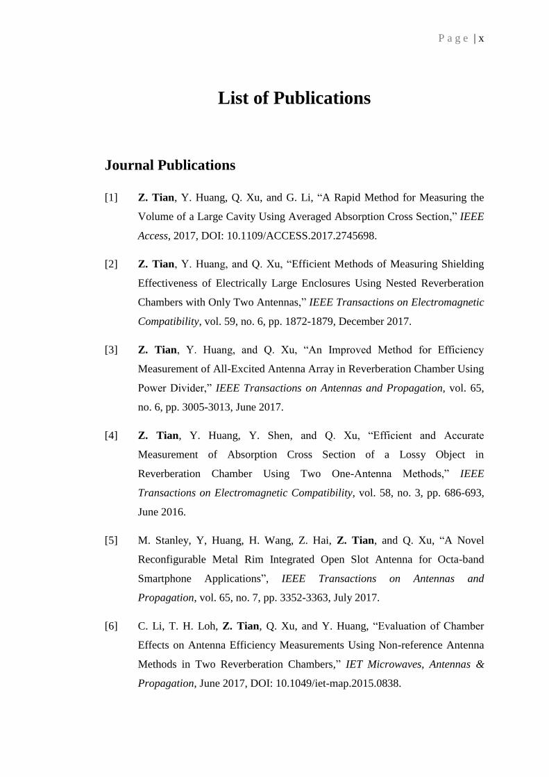
The modal bandwidth is measured in our RC. Both the “unloaded” scenario and the “loaded”
scenario are studied. In both scenarios, the transmitting antenna (antenna 1) is a log periodic
antenna (LPDA), and the receiving antenna (antenna 2) is a folded diploe antenna. The
efficiency of the two antennas is with known efficiency values. In the “loaded” configuration,
the RC has been loaded with two pieces of RAMs placed in the two corners of the chamber to
illustrate the loading effect on the average mode bandwidth. The measurement setup can be
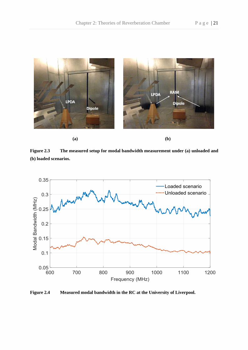
seen from Figure 2.3(a) and (b). The measurement results are depicted in Figure 2.4. It can be
seen that the modal bandwidth is slightly decreasing for increasing frequency, which means
the window in which subsequent modes can be excited grows smaller at higher frequencies.
However, at higher frequencies the mode density is higher, meaning that many modes can
still be excited.
Chapter 2: Theories of Reverberation Chamber P a g e | 21
(a) (b)
Figure 2.3 The measured setup for modal bandwidth measurement under (a) unloaded and
(b) loaded scenarios.
Figure 2.4 Measured modal bandwidth in the RC at the University of Liverpool.

Chapter 2: Theories of Reverberation Chamber P a g e | 22
Figure 2.5 Modal Structure with small and high Q superimposed at 602 MHz in the RC at
the University of Liverpool.
The effect of decreasing the Q of the RC is shown in Figure 2.5. In this case, additional
modes can be excited when the cavity is driven at the frequency of about 602 MHz because
of the broader modal overlap due to lower Q. The effective modal structure is the vector sum
of the excited modes with different weighting factors of amplitudes. The spatial field
variation will now be different from that obtained with the higher Q RC. Thus, varying the Q
of the RC can change the “effective” modal structure. It should be noted that if the frequency
were increased, more modes would be available within a given modal bandwidth, giving rise
to a finer structure of the field. Again, the effective modal structure would be the vector sum
of the modes.
2.2.3 Lowest Usable Frequency
The lowest usable frequency (LUF) fLUF is commonly defined as the frequency from which

Chapter 2: Theories of Reverberation Chamber P a g e | 23
the RC meets the operational requirements [7], [16]. There are several definitions for the LUF:
• The LUF is three times the cut-off frequency fc of the fundamental mode of a cavity
with the same dimensions as the RC, i.e., fLUF = 3fc [7].
• The LUF is defined as the frequency at which 60 ∙∙∙ 100 modes within an ideal cavity
of the same dimensions as the RC are above cut-off frequency and at least 1.5
modes/MHz are present [7], [17].
• The LUF is defined as the lowest frequency at which specified field uniformity can be
achieved over a volume constrained by eight corner locations [7].
It is worth mentioning that the first two definitions are relatively qualitative criteria which
offer only a rough overview on whether an RC begins to meet the operational requirements
from a certain frequency. The third definition is much more stringent because it involves
measurements within the RC and also considers the desired measurement uncertainties and
confidence intervals to be obtained for a given number of stirrer positions. The LUF can be
determined by the RC size, shape, quality factor, and the effectiveness of the stirrers [7].
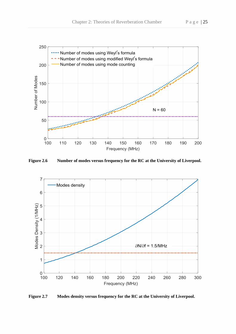
2.2.4 Number of Cavity Modes
In order to evaluate from which frequency fLUF on an RC begins to satisfy the operational
requirements, the cumulated number of modes and the mode density must be known. Again,
computation of these parameters assumes an empty RC without any stirrers, i.e., a rectangular
cavity resonator.
There are three common methods to assess the number of modes that are present in a given
cavity. The first method is termed as “mode counting” which can be performed by the
repeated solution of (2.38) for both TE and TM modes [13]. And then the total number of
modes present with eigenvalues less than or equal to kmnp will be counted. Theoretically, N as
a function of kmnp is discrete, but people have derived a smooth approximation referred to as
“Weyl’s formula” [1], which is valid for cavities of general shape and can be written as

Chapter 2: Theories of Reverberation Chamber P a g e | 24
where N(f) is the cumulated number of modes. The third method is a modified version of
Weyl’s formula specific to rectangular cavities [1] and is stated in (2.42).
It can be seen that the RC volume has the major impact on the cumulated number of modes,
as shown by the first part of (2.42). The second part of (2.42) represents the contribution of
the combined edge length of an RC. A comparison of the modal numbers presented in the RC
at the University of Liverpool by mode counting, Weyl’s formula, and modified Weyl’s
formula is shown in Figure 2.6. It can be seen that the extra terms in (2.42) improve the
agreement obtained with the mode counting method as opposed to using the original Weyl’s
formula in (2.41). With the increase of frequency, it can be seen that the number of modes
increases with respect to the cavity volume and the third power of frequency. As noted above,
for a proper operation of an RC usually at least 60 modes above the cut-off frequency are
required. As noted from Figure 2.6, the LUF for our RC is about 140 MHz.
The mode density ∂N/∂f (number of modes per frequency interval) can be calculated from
(2.43) to be
The
dependence in (2.43) indicates that the mode density also increases rapidly for high
frequencies [1]. To achieve sufficient statistical field uniformity and isotropy, a common RC
specification is to have at least ∂N/∂f = 1.5 modes/MHz above cut-off frequencies [18]. A
plot of the mode density can be seen in Figure 2.7. It can be seen that the chamber has a mode
density of at least 1.5 modes per megahertz from about 140 MHz upwards, i.e., the
corresponding LUF is about 140 MHz, which agrees well with the prediction from Figure 2.6.
A low mode density in any given chamber means that chamber would not have adequate
performance, as the mode density is too small to obtain spatial field uniformity [7].
Chapter 2: Theories of Reverberation Chamber P a g e | 25
Figure 2.6 Number of modes versus frequency for the RC at the University of Liverpool.
Figure 2.7 Modes density versus frequency for the RC at the University of Liverpool.

Chapter 2: Theories of Reverberation Chamber P a g e | 26
2.2.5 Green’s Function
The Dyadic Green’s function is a bridge to link the excitation source and its generated
electric and magnetic fields [19] – [20]. Different from the prior field equations in (2.24) to
(2.35), it is advantageous to visualise these fields in a “non-empty” cavity, i.e., with a
realistic excitation involved [13]. The EM fields inside a rectangular cavity outside of the
source area are purely the superposition of all TE and TM modes generated within it. In the
source area, special treatment is required [1], [13], [19] – [20], but the Dyadic Green’s
functions are still useful there. Modes inside the cavity can be controlled by choosing the
polarisation and location of the excitation source [19] – [20].
Figure 2.8 A volume current density confined to a volume in a rectangular
cavity.
In [20], a computationally efficient series of equations based on Dyadic Green’s functions
was derived in order to study the resultant electric field inside shielded enclosures (the
magnetic field can also be derived similarly). Consider a volume current density
confined to a volume in a rectangular cavity, as shown in Figure 2.8. The resulting electric
field was deduced using (2.44), (2.45) and (2.46).

Chapter 2: Theories of Reverberation Chamber P a g e | 27
∫
where is the Dyadic Green’s function. The double arrow above the Green’s functions
indicates a three by three dyadic. It can be expressed as
∑ ∑
[
[
[
∑ ∑
[
( ) [
[
∑ ∑
[
[
[
where ⁄ , ⁄ , ⁄ , √
, √
,
√
, and
.

Chapter 2: Theories of Reverberation Chamber P a g e | 28
Assuming the current source used to generate the field inside the RC is a y polarised unit
element, the resultant electric field on an xz plane can be obtained using (2.46) [13] [19] – [20]
∑ ∑
[
( ) [
[
The Ey electric field distribution at 200 MHz, 600 MHz, and 1200 MHz on the xz plane in the
RC at the University of Liverpool is plotted in Figure 2.9(a), (b), and (c), respectively. The
observation plane in all the depicted plots is y = l/2 (the mid-point in length of the RC). The
current source is located at x1 = 0.4 m, x2 = 0.5 m, y1 = 1.35 m, y2 = 1.4 m and z0 = 0.5 m,
which is corresponding to the corner of the RC [13]. It can be seen from Figures 2.9, the
electric fields inside the RC are formed as a result of standing waves that have a sine and
cosine dependence. With the increase of frequency, the fields begin to vary in a more
complex manner. The magnitudes of the fields have significantly different values from point
to point.
(a)

Chapter 2: Theories of Reverberation Chamber P a g e | 29
(b)
(c)
Figure 2.9 Normalised Ey field distribution in the RC at the University of Liverpool at (a)
200 MHz, (b) 600 MHz, and (c) 1200 MHz.
2.3 Stirring Techniques
The statistical nature of the fields in the RC is realized by employing stirring techniques. The
purpose of these techniques is to make the fields statistically uniform and isotropic on
average. In practice, the analysis of the measured data in RCs is always based on some
limited number of stirring samples (stirring positions). In this section, these frequently used
stirring techniques will be introduced and how they are implemented is explained.

Chapter 2: Theories of Reverberation Chamber P a g e | 30
2.3.1 Mechanical Stirring
The mechanical stirring technique, also called mode stirring technique, is the most common
technique employed to stir the fields inside an RC. This stirring technique is realized by
rotating the electrically large stirrers. By “electrically large”, it means the size of the stirrer is
at least comparable with respect to the wavelength of operation. When this is not the case, the
stirrers’ performance in significantly changing the field distribution will diminish. The
stirrers are designed to be non-symmetric and arbitrarily shaped to generate more
independent samples. An example of mechanical stirrer design in the University of Liverpool
RC can be viewed in Figure. 1.4.
Figure 2.10 The effect of using the mechanical stirring technique to obtain statistical values
of S11.
The stirrers can be rotated in a stepwise or continuous manner and thus the boundary
conditions for the EM field inside the RC vary [7]. The effect of changing the boundary
conditions for the field means that the high and low field magnitudes, called hot and cold
spots, throughout the RC will change as a function of location. This means that the field
distribution can be rendered statistically homogeneous and isotropic on average from many
stirrer positions. Wu and Chang [21] pointed out that the rotating stirrers continuously change

Chapter 2: Theories of Reverberation Chamber P a g e | 31
the resonant frequencies of the RC modes and that mechanical stirring has some equivalence
to the frequency modulation of the source. The mechanical stirring technique can be quite
effective [22], but it is fairly slow. Figure 2.10 shows the effect of using the mechanical
stirring technique to obtain statistical values of S-parameters (S11 here). As can be seen with
the increase of the number of samples, S11 becomes smoother because the effect caused by
stochastic factors is averaged.
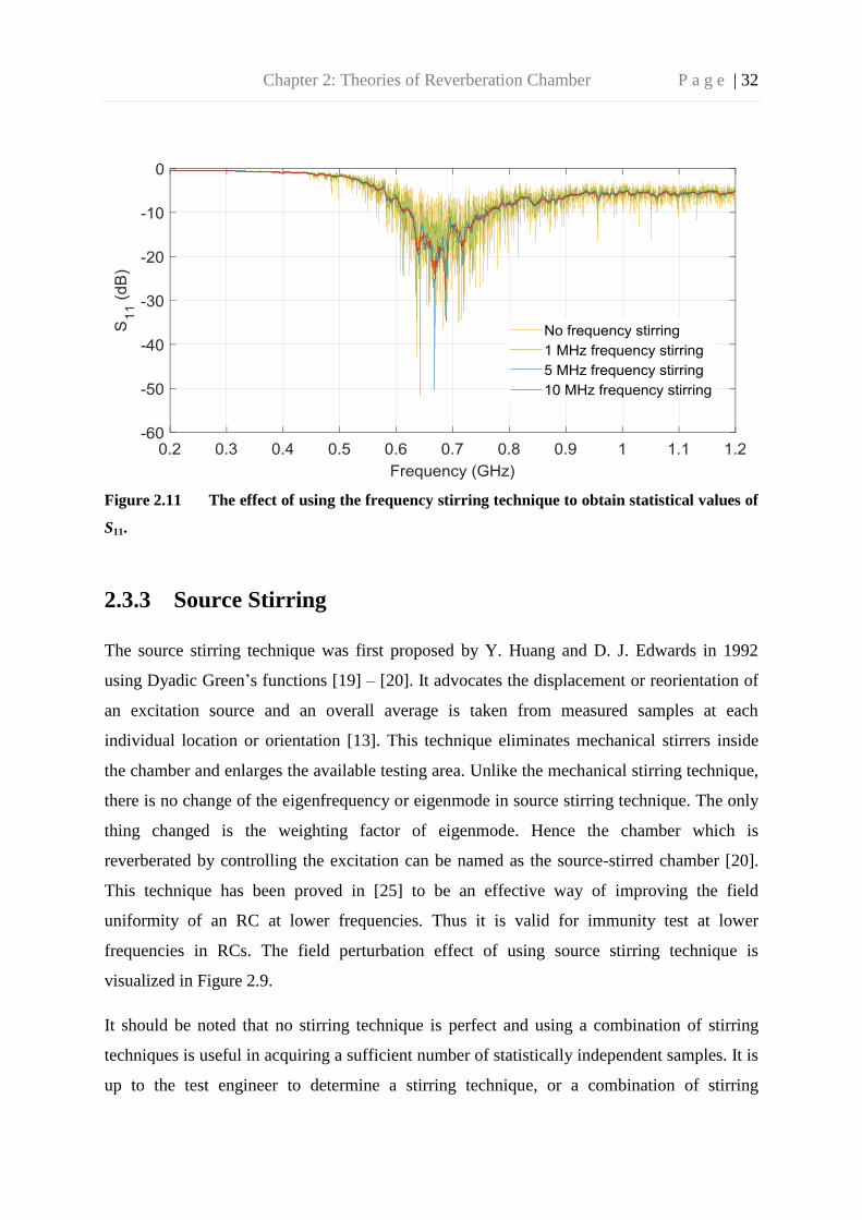
2.3.2 Frequency Stirring
Frequency stirring technique or electronic stirring technique is used to achieve the spatially
uniform field by sweeping the source frequency over some narrow bandwidth of frequencies
[23]. As the centre frequency is changed the hot spots and cold spots spatially move around
the chamber. The power measured at the various discrete frequency points within a window
of frequencies is averaged. The average computed from the window of frequencies is then
attributed to the centre frequency in the window [24]. By sliding the same bandwidth window,
measurements over the full frequency span are accomplished. It should be careful about the
window bandwidth when performing frequency stirring. If too large smoothing bandwidth is
taken, the loss of frequency resolution in any measured data will occur. Frequency stirring is
similar to smoothing the data over frequency, but frequency stirring must be applied to the
raw measured data (typically complex data), while smoothing is generally applied to the final
computation of the desired quantity [13], [24]. For example, S-parameters measurements
collected with a vector network analyzer (VNA) can be frequency stirred in order to obtain
the average reflection coefficient, as shown in Figure 2.11. Frequency stirring with different
certain bandwidth is adopted. As can be seen, S11 is averaged just as mechanical stirred data
is averaged over all measured stirrer positions. Theoretically, if the RC is spatially uniform,
the frequency stirring and mechanical stirring techniques should give the same average result.
In addition, when smoothing the raw data a rectangular window must be used because the
frequency stirring technique is meant to be an un-weighted average just as other stirring
techniques are [24].
Chapter 2: Theories of Reverberation Chamber P a g e | 32
Figure 2.11 The effect of using the frequency stirring technique to obtain statistical values of
S11.
2.3.3 Source Stirring
The source stirring technique was first proposed by Y. Huang and D. J. Edwards in 1992
using Dyadic Green’s functions [19] – [20]. It advocates the displacement or reorientation of
an excitation source and an overall average is taken from measured samples at each
individual location or orientation [13]. This technique eliminates mechanical stirrers inside
the chamber and enlarges the available testing area. Unlike the mechanical stirring technique,
there is no change of the eigenfrequency or eigenmode in source stirring technique. The only
thing changed is the weighting factor of eigenmode. Hence the chamber which is
reverberated by controlling the excitation can be named as the source-stirred chamber [20].
This technique has been proved in [25] to be an effective way of improving the field
uniformity of an RC at lower frequencies. Thus it is valid for immunity test at lower
frequencies in RCs. The field perturbation effect of using source stirring technique is
visualized in Figure 2.9.
It should be noted that no stirring technique is perfect and using a combination of stirring
techniques is useful in acquiring a sufficient number of statistically independent samples. It is
up to the test engineer to determine a stirring technique, or a combination of stirring

Chapter 2: Theories of Reverberation Chamber P a g e | 33
techniques, in order to minimise the statistical error and reinforce the confidence attributed to
the statistically determined field values [24].
2.4 Statistical Theory
For carefully designed cavities, the cavity details such as shape, dimensions, and materials
are precisely known, and the cavity is generally of a simple/separable geometry. In such cases,
deterministic theories are appropriate. However, in practice, the details of the cavity
geometry and loading objects, such as cable bundles, scatterers, and absorbers are not
expected to be well known [1]. Consequently, for many applications in EMC and wireless
communications, people have to deal with problems where only a partial knowledge of the
cavity geometry and its interior loading are known. Over the past two decades, techniques in
statistical electromagnetics have been developed to deal with such a kind of problems [2], [3],
[26] – [27]. The RC is a good example of a cavity with a complex interior. Clearly, all the
information (scatters, loading object characteristics, and apertures, etc.) will not be known in
detail. Statistical models for angle of arrival have been found useful for characterizing EM
propagation in RCs [28].
2.4.1 Plane-wave Integration Model
As discussed above, it is not convenient to predict the field properties in electrically large,
complex cavities using deterministic theories. Since many samples (stirrer positions) are
employed in RC measurements, a statistical method [26] – [28] is required to determine the
statistics of the fields and test object response. Moreover, the associated EM theory must be
consistent with Maxwell’s equations. The well-known plane-wave integration model for the
EM fields has been found to be successful [1], [8]. This model satisfies Maxwell’s equations
and at the same time includes the statistical properties expected for a well-stirred field [8].
The plane-wave coefficients in the model are random variables with fairly simple statistical
properties, thus, the fields are of statistical nature. Because the theory uses only propagating
plane waves, it is fairly easy to calculate the responses of test objects or reference antennas
using this model [1].

Chapter 2: Theories of Reverberation Chamber P a g e | 34
In a source-free, finite volume, the electric field at location can be represented by
integrating plane waves from all directions
∬ ( )
where Ω is the solid angle and dΩ = sinθdθdφ. θ and φ the elevation and azimuth angles,
respectively. The geometry of a plane-wave component is shown in Figure 2.12. The vector
wavenumber is
Figure 2.12 Plane-wave integration model.
So (2.47) can be re-written as
∫ ∫

Chapter 2: Theories of Reverberation Chamber P a g e | 35
The angular spectrum can be written more explicitly in two polarisations
where and are unit vectors that are orthogonal to each other and to . Both Fθ and Fφ are
complex and can be written in terms of their real and imaginary parts (to represent the phase)
and
The angular spectrum is taken to be a random variable in RCs. It depends on stirrer
positions, i.e., is different for each stirrer position. The statistical properties of the
angular spectrum are defined as follows
⟨ ⟩ ⟨ ⟩
⟨ ⟩ ⟨ ⟩
⟨ ⟩ ⟨ ⟩
⟨ ⟩ ⟨ ⟩
⟨ ⟩ ⟨ ⟩
⟨ ⟩ ⟨ ⟩
where ⟨ ⟩ represents an ensemble average over all samples, δ is the Dirac delta function [29].
CE is a constant with units of (V/m)2 and it is proportional to the square of the electric field
strength, as shown in the following section. It is useful to interpret the physical meaning of
(2.52) – (2.54). (2.52) indicates the mean value of the angular spectrum is zero because the
rays from all directions are with random phases. (2.53) means angular spectrum components
with orthogonal polarizations or quadrature phase is uncorrelated. (2.54) indicates angular
spectrum components arriving from different directions are uncorrelated because they have
taken very different multiple scattering paths.
From (2.53) and (2.54), the following useful relationships can also be obtained

Chapter 2: Theories of Reverberation Chamber P a g e | 36
⟨ ⟩
⟨ ⟩ ⟨
⟩
where * denotes complex conjugate.
2.4.2 Statistical Properties of Fields
In this section, some useful field properties will be derived using (2.47) and (2.52) – (2.56).
First of all, the mean value of the electric field ⟨ ⟩ can be derived as
⟨ ⟩ ∬⟨ ⟩ ( )
This result is expected in a well-stirred RC where the field is the sum of many multipath rays
with random phases.
From (2.47), the square of the absolute value of the electric field can be written as
| | ∬∬
( ( ) )
By applying (2.55) and (2.56), the mean-square value of the electric field can be obtained [1]
⟨| | ⟩ ∬
From (2.59), it can be seen that ⟨| | ⟩ is independent of position. This is the spatial
uniformity property of an ideal RC.
Similarly, the mean-square values of the rectangular components of the electric field can be
derived as
⟨| | ⟩ ⟨| |
⟩ ⟨| |
⟩
This indicates the isotropy property of an ideal RC.
Chapter 2: Theories of Reverberation Chamber P a g e | 37
The magnetic field has the similar statistical properties and the results are listed as follows
⟨ ⟩
⟨| | ⟩
⟨| | ⟩ ⟨| |
⟩ ⟨| |
⟩
where η is the characteristic impedance of the free space.
The energy density W can be written as [10] – [11]
[ | |
| |
]
⟨ ⟩
[ ⟨| |
⟩ ⟨| |
⟩]
It can be seen that the average value of the energy density is also independent of position.
The power density or Poynting vector can be written as
The mean value of is
⟨ ⟩
A physical interpretation of (2.67) is that each plane wave carries equal power in any
direction so that the vector sum over the whole space is zero [1]. The result shows that is
not the proper quantity to characterize the field strength in an RC while ⟨ ⟩ is an
appropriate quantity.
Similar to the plane wave in free space, a scalar power density can be defined as
⟨ ⟩

Chapter 2: Theories of Reverberation Chamber P a g e | 38
2.4.3 Probability Density Functions for the Fields
The knowledge of the probability density functions (PDF) of the filed quantities can be very
useful for analysis of measured data in an RC because the measured data in an RC is always
based on a limited number of samples. The rectangular components can be written in terms of
their real and imaginary parts as
, ,
where Exr / Eyr / Ezr and Exi / Eyi / Ezi are the real and imaginary part of Ex / Ey / Ez. From
(2.52) – (2.54), it can be derived that the mean values of all the real and imaginary parts in
(2.69) are zero
⟨ ⟩ ⟨ ⟩ ⟨ ⟩ ⟨ ⟩ ⟨ ⟩ ⟨ ⟩
and the variances of the real and imaginary parts are half the result for the complex
components in (2.60)
⟨ ⟩ ⟨
⟩ ⟨ ⟩ ⟨
⟩ ⟨ ⟩ ⟨
⟩
If the mean and variance are specified for a PDF over the range from - ∞ to ∞, then the
maximum entropy theorem [30] or central limit theorem [31] predicts a Gaussian PDF. So the
PDF of Exr is
√ [
]
where σ is defined in (2.71). The other real and imaginary parts of the electric components
have the same PDF.
It has also been proved that the real and imaginary parts of the electric field components are
uncorrelated, i.e.,
⟨ ⟩

Chapter 2: Theories of Reverberation Chamber P a g e | 39
For now, it has been known that the real and imaginary parts of the rectangular components
of the electric field are independent, normally distributed with zero mean and equal variances.
Therefore, the following conclusions can be deduced
| | | |
[
| |
]
That is the magnitude of Ex has a Rayleigh distribution [31]. The comparison of (2.74) with
measured data at 2.0 GHz in the University of Liverpool RC is shown in Figure 2.13. The
two stirrers are stepwise rotated simultaneously. The total number of samples is 120. As can
be seen, good agreement between measured data and theoretical prediction is obtained.
Figure 2.13 Comparison of the measured PDF of |Ex| with theoretical Rayleigh distribution.
The squared magnitude of Ex is chi-square distributed with two degrees of freedom
(exponential distribution) [31]
| |
[
| |
]

Chapter 2: Theories of Reverberation Chamber P a g e | 40
The comparison of (2.75) with measured data at 2.0 GHz in the University of Liverpool RC is
shown in Figure 2.14. (2.74) and (2.75) also hold for Ey and Ez.
The total electric field magnitude is chi distributed with six degrees of freedom [31]
(| |) | |
[
| |
]
The squared magnitude of the total electric field is chi-square distributed with six degrees of
freedom [31]
(| | )
| |
[
| |
]
The dual PDFs for the magnetic field can be obtained by the aforementioned procedure. And
the dual of the results in (2.74) – (2.77) can be obtained by replacing E by H and σ by σH [1].
Figure 2.14 Comparison of the measured PDF of |Ex|2 with theoretical exponential
distribution.
Chapter 2: Theories of Reverberation Chamber P a g e | 41
2.4.4 Loss Mechanism and Q Factor
The Q factor describes the rate at which an RC loses energy due to the overall losses inside [3]
[32]. Generally, there are four loss terms in an RC: the RC wall loss (Q1), the loss due to
aperture leakage (Q2), the loss of lossy objects (Q3), and the antenna loss (Q4).
The total Q factor can be defined as [1], [3] [33].
⁄
where ω is the angular frequency, Us is the steady state energy and Pd is the power dissipated.
where V is the volume of the RC and W is the energy density as defined before.
where ε0 is the permittivity of the medium in the RC (free space) and E is the RMS (root-
mean-square) electric field. The power density Sc in the RC can be expressed as
where √ ⁄ is the intrinsic impedance of the medium in the RC.
To calculate the Q factor of the RC, all losses should be accounted for. Thus, it can be
derived
where Pd1 is the power dissipated in the cavity walls, Pd2 is the power absorbed by lossy
objects within the cavity, Pd3 is the power leaked through apertures, and Pd4 is the power
dissipated on receiving antennas [3]. By substituting (2.82) into (2.78) the following
expression can be written for the inverse of Q
where

Chapter 2: Theories of Reverberation Chamber P a g e | 42
⁄ , ⁄ ⁄ ⁄
The separate loss terms Q1 to Q4 can analysed as follows
where √ ⁄ , ⁄ . µw and σw are the permeability and conductivity of
the wall material, respectively. µwr is the relative permeability of the wall material. δ is the
skin depth and Sa is the RC surface area.
⟨ ⟩
where ⟨ ⟩ is the averaged absorption cross section of the lossy objects loading the chamber
and λ is the wavelength. A measurement procedure to deduce this term can be found in [33] –
[37].
⟨ ⟩
where ⟨ ⟩ is the average transmission cross section of any apertures.
where m is the impedance mismatch factor (m = 1 for a matched load).
Under steady-state conditions, the power transmitted into the chamber (Pt) is equal to the
power dissipated by the overall loss, i.e.,
By substituting (2.78), (2.79), (2.81) into (2.89), the power density in the RC can be rewritten
as

Chapter 2: Theories of Reverberation Chamber P a g e | 43
If an impedance matched antenna is used, then the received power (Pr) is a product of the
effective area ⁄ [38] – [39] and the received power can be expressed as
Solving (2.91) in terms of Q yields the chamber Q factor in terms of the measured power
ratio (Pr/Pt). Thus (2.92) represents a commonly used frequency-domain approach to measure
the chamber Q factor [40] – [41]. The equation assumes well matched and lossless antennas.
where
⟨| |
⟩
|⟨ ⟩| |⟨ ⟩|
where S11 and S22 are the reflection coefficients of antenna 1 and antenna 2, respectively and
S21 is the transmission coefficient of the two antennas. It should be noted that if the antennas
are not ideal, the antenna loss (including ohmic loss and mismatch loss) should be calibrated
out when using (2.92) and (2.93).
2.4.5 Chamber Decay Time
Up to this point, only the frequency-domain response of the RC has been considered. In the
following part, the time-domain response will be considered which is of interest for transient
applications. The case of field decay where the excitation source is instantaneously turned off
is first considered. The following differential equation can be obtained
where dU is the energy change in the RC over a time increment dt. Use (2.78) to replace Pd in
(2.94)
⁄

Chapter 2: Theories of Reverberation Chamber P a g e | 44
where the chamber decay time (or chamber time constant) ⁄ . Using the initial
condition U = Us at t = 0, (2.95) can be solved as
⁄
The chamber decay time τ has been measured by fitting the decay curve in (2.96) to
experimental data [40] – [44]. Once τ has been determined, the frequency-dependent Q is
determined from
⟨ ⟩
where ⟨ ⟩ signifies the ensemble average. Equation (2.97) offers a time-domain method to
measure Q. The comparison of the measured Q with the frequency-domain method and time-
domain method is shown in Figures 2.15. A good agreement between the time-domain Q and
the frequency-domain Q is shown when the antenna loss is removed. When the antenna loss
is included, the frequency-domain Q is lower than the time-domain Q. Actually, for this case,
the ratio of the frequency-domain Q and the time-domain Q contains the information of the
antenna efficiency. Three antenna efficiency measurement techniques based on this fact is
discussed in detail in [40].
Figure 2.15 Comparison of the frequency-domain Q and the time-domain Q.

Chapter 2: Theories of Reverberation Chamber P a g e | 45
2.4.6 Stirred and Unstirred Power
As stated above, the magnitude of any of the electric field components is statistically
Rayleigh distributed in theory. However, if any line-of-sight (LoS) path exists in an RC, the
stirred power and the unstirred power together will manifest itself as being Rician distributed
[13]. The unstirred power is the power that is coupled directly from the transmitting antenna
to the receiving antenna without interaction with any mode stirrers. The stirred power results
from the power radiating from a transmitting antenna that fully interacts with the mode
stirrers before being captured by the receiving antenna [13], [45] – [46]. In practice, the RC
could be used to emulate a Rician environment if desired [45]. However, for most of the
measurements in an RC, any unstirred power is supposed to be minimised and a Rayleigh
environment is desired.
The unstirred multipath propagation in the RC can be characterized by the Rician K-factor. A
brief derivation of this quantity is summarised as follows.
Any transmission measurement in an RC essentially comprises of the chamber’s physical and
statistical properties [13]. This measured complex transmission coefficient S21 consists of two
parts: the unstirred part (S21,u) and the stirred part (S21,s).
The unstirred components and
are constants with zero variance for a given
measurement configuration, and the stirred components and
are supposed to be
independent Gaussian random variables with zero mean and identical variance σ2 under ideal
RC conditions, i.e., pure non-line-of-sight (NLoS) environment. That is
⟨ ⟩
and
where ⟨ ⟩ signifies the ensemble average. Then it can be derived

Chapter 2: Theories of Reverberation Chamber P a g e | 46
(
) and (
)
From the above distribution analysis, the stirred and unstirred power can be express as
stirred power ⟨| ⟨ ⟩| ⟩
unstirred power |⟨ ⟩|
This is seen visually by referring to the scattering plots in Figure 2.16(a) and (b). d is the
distance of the centroid (green dot) of the clutter from the origin (red dot). As can be seen
from Figure 2.16(b), the bias of the cluster of data from the origin is very small, which
represents the case where very weak direct antenna coupling is present. This is desired for a
well-stirred RC.
(a)

Chapter 2: Theories of Reverberation Chamber P a g e | 47
(b)
Figure 2.16 Scatter plot of measured S21 at 4.0 GHz: (a) normal view, and (b) zoom in.
The Rician K-factor defined as the ratio of the unstirred power to the stirred power can be
expressed as [46] – [48]
|⟨ ⟩|
⟨| ⟨ ⟩| ⟩
It is an important characteristic parameter for a wireless fading channel since it is a measure
of the distribution of the components of the received signal resulting from various
interactions with the surrounding environment. Here, the K-factor for an RC setup exhibiting
good field uniformity is estimated, i.e., for a chamber with lower values of K-factor. [49]. A

Chapter 2: Theories of Reverberation Chamber P a g e | 48
well-stirred RC should typically have a Rician K-factor value below 0.1 [49]. RC setups with
such low K-factors enable low measurement uncertainty for over-the-air tests [50].
Figure 2.17(a) and (b) depict the measurement setup and the measured Rician K-factor as a
function of frequency in the RC at the University of Liverpool, respectively. During the
measurement, antenna 1 directed to one corner of the RC and antenna 2 directed to the
vertical stirrer to avoid LoS illumination. It can be seen that the stirred power in the RC is
dominant as the measured K-factor value is below 0.1. That means any LoS path is very small
and as a result, the statistical form of the magnitudes will tend towards a Rayleigh
distribution as opposed to a Rician distribution (ideal Rayleigh distribution: K → 0).
(a)

Chapter 2: Theories of Reverberation Chamber P a g e | 49
(b)
Figure 2.17 Rician K-factor from 2.0 to 3.0 GHz: (a) measurement setup, (b) measured
results.
Similar to the transmission coefficient, the reflection coefficient measured in the RC also
comprises of the stirred part (S11,s) and the unstirred part (S11,u)
The unstirred part S11,u includes the contribution of the antenna mismatch (free space
response) and the unstirred energy in the RC. If the RC is ideally stirred [44], i.e., the RC
environment in a pure Rayleigh environment, the stirred part S11,s is of Gaussian distribution
with zero mean. Thus, the following relationship can be derived
⟨ ⟩ ⟨ ⟩
where S11,fs is the free-space antenna reflection coefficient. The S11,fs is measured in the RC
and in the AC, respectively, as shown in Figure 2.18(a) and (b). An LPDA was selected as
the antenna under test (AUT). The complex S-parameters measured in the RC were averaged
over 360 stirrer positions. 10,001 points were sampled in the frequency range of 0 to 10 GHz.
A comparison of measured results in both amplitude and phase is depicted in Figure 2.19(a)

Chapter 2: Theories of Reverberation Chamber P a g e | 50
and (b), respectively. In Figure 2.19(b), only 0 – 2 GHz is selected for the clearer show. It can
be seen that the measured results in the RC and the AC agree very well. At the lower
frequency band (from 200 – 600 MHz), the RC is not very well stirred, and therefore some
small difference shows. From 0 – 200 MHz, the two curves also agree well, but it is because
of the antenna mismatch (radiation is low) while not the well-stirred field.
(a) (b)
Figure 2.18 Free-space antenna reflection coefficient measurement setups: (a) in the RC, and
(b) in the AC, respectively.
(a)

Chapter 2: Theories of Reverberation Chamber P a g e | 51
(b)
Figure 2.19 Comparison of measured free-space antenna reflection coefficient in RC and AC
in both (a) amplitude and (b) phase.
2.4.7 Enhanced Backscatter Effect
The enhanced backscatter effect was first observed by John M. Ladbury and David A. Hill in
the year of 2007 [51] and subsequently used to characterize the performance of RCs [52] and
measure the radiation efficiency of antennas [40], [53] – [54]. It states that the power
received by the source antenna is higher than that at any other random location in the RC [52].
Using the infinite plane wave integration model it is found that
⟨ ⟩ ⟨ ⟩
where Prx is the power incident at the receiving antenna, Prf is the power reflected back to the
transmitting antenna, is defined as the enhanced backscatter coefficient, and ⟨ ⟩, as before,
indicates the ensemble average. For idealized antennas (well-matched, lossless)
That is, in an ideally stirred RC the average power received by the transmitter is twice as the

Chapter 2: Theories of Reverberation Chamber P a g e | 52
power received by the receiver [1], [52]. This phenomenon is observed in other disciplines as
well, such as scattering from the rough surface in optics [55], and reverberant acoustical
fields [56] – [57].
Under the assumption that the field can be described as an infinite sum of plane waves and
the antennas used are perfectly matched and lossless, can be related to the S-parameters by
⟨| | ⟩ ⟨| |
⟩
However, for real antennas of non-ideal characteristics, (2.111) needs to be modified. The
final result is obtained by
⟨| |
⟩
⟨| | ⟩
where
⟨ ⟩, and ⟨ ⟩
An experimental verification of (2.111) in the University of Liverpool RC is shown in Figure
2.20. As can be seen, the agreement with the factor of 2 is good above 200 MHz where the
mode density of the RC is sufficiently high. The number of samples at each frequency is 120.
For now, it is known that the enhanced backscatter factor is 2 for an ideally stirred RC, but
what is the size of the region over which the enhanced backscatter occurs? It has been proved
that the enhanced backscatter constant varies as a function of distance r [1]
where r is the distance between the source and the random location in the RC. Considering
two extreme cases r = 0 and r → ∞. It is easy to conclude that when r = 0, , which is
consistent with the uniform-field result in (2.110). And when r → ∞, , i.e., no
enhanced backscatter effect occurs. (2.114) is plotted in Figure 2.21. It can be seen that when
r > λ/4, is close to 1. The region of enhanced backscatter can be defined as the distance
from which . Hence, the region of enhanced backscatter is a fairly small (especially for
high frequency) sphere of radius λ/4 [1].

Chapter 2: Theories of Reverberation Chamber P a g e | 53
Figure 2.20 Enhanced backscatter coefficient from 100 MHz to 500 MHz.
Figure 2.21 Enhanced backscatter coefficient as a function of distance r.
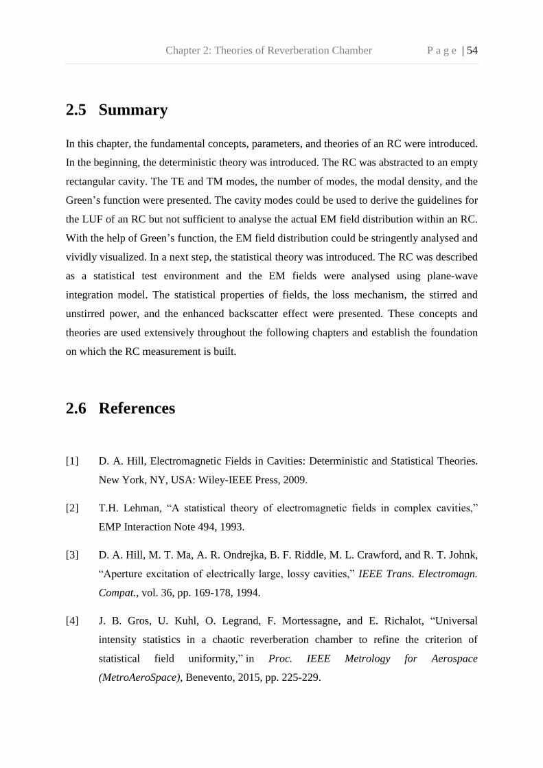
Chapter 2: Theories of Reverberation Chamber P a g e | 54
2.5 Summary
In this chapter, the fundamental concepts, parameters, and theories of an RC were introduced.
In the beginning, the deterministic theory was introduced. The RC was abstracted to an empty
rectangular cavity. The TE and TM modes, the number of modes, the modal density, and the
Green’s function were presented. The cavity modes could be used to derive the guidelines for
the LUF of an RC but not sufficient to analyse the actual EM field distribution within an RC.
With the help of Green’s function, the EM field distribution could be stringently analysed and
vividly visualized. In a next step, the statistical theory was introduced. The RC was described
as a statistical test environment and the EM fields were analysed using plane-wave
integration model. The statistical properties of fields, the loss mechanism, the stirred and
unstirred power, and the enhanced backscatter effect were presented. These concepts and
theories are used extensively throughout the following chapters and establish the foundation
on which the RC measurement is built.
2.6 References
[1] D. A. Hill, Electromagnetic Fields in Cavities: Deterministic and Statistical Theories.
New York, NY, USA: Wiley-IEEE Press, 2009.
[2] T.H. Lehman, “A statistical theory of electromagnetic fields in complex cavities,”
EMP Interaction Note 494, 1993.
[3] D. A. Hill, M. T. Ma, A. R. Ondrejka, B. F. Riddle, M. L. Crawford, and R. T. Johnk,
“Aperture excitation of electrically large, lossy cavities,” IEEE Trans. Electromagn.
Compat., vol. 36, pp. 169-178, 1994.
[4] J. B. Gros, U. Kuhl, O. Legrand, F. Mortessagne, and E. Richalot, “Universal
intensity statistics in a chaotic reverberation chamber to refine the criterion of
statistical field uniformity,” in Proc. IEEE Metrology for Aerospace
(MetroAeroSpace), Benevento, 2015, pp. 225-229.

Chapter 2: Theories of Reverberation Chamber P a g e | 55
[5] X. Chen, “Generalized Statistics of Antenna Efficiency Measurement in a
Reverberation Chamber,” IEEE Trans. Antenna Propag., vol. 62, no. 3, pp. 1504-
1507, Mar. 2014.
[6] A. Cozza, “A statistics-based definition of the overmoded condition for reverberation
chambers,” 2011 URSI General Assembly and Scientific Symposium, Istanbul, 2011,
pp. 1-4.
[7] Electromagnetic Compatibility (EMC) part 4-21: Testing and measurement
techniques-Reverberation chamber test methods, IEC 61000-4-21, 2003.
[8] D. A. Hill, “Plane wave integral representation for fields in reverberation chambers,”
IEEE Trans. Electromagn. Compat., vol. 40, pp. 209-217, 1998.
[9] D. A. Hill, “Electromagnetic Theory of Reverberation Chambers,” NIST Technical
Note 1506, Dec. 1998.
[10] David M. Pozar, Microwave Engineering. Singapore: Wiley, 4th ed., 2011.
[11] R. E. Collin, Foundations for Microwave Engineering. New York, NY: McGraw-Hill,
1966.
[12] Christian Bruns, “Three-dimensional Simulation and Experimental Verification of a
Reverberation Chamber,” Ph.D. dissertation, Swiss Federal Institute of Technology
Zurich, Zurich, Switzerland, 2005.
[13] S. J. Boyes, and Yi Huang, Reverberation Chambers: Theories and Applications to
EMC and Antenna Measurements, West Sussex, WS, UK: Wiley, 2016.
[14] K. Rosengren, and P. S. Kildal, “Study of distributions of modes and plane waves in
reverberation chambers for the characterization of antennas in a multipath
environment,” Microw. Opt. Technol. Lett., vol. 30, pp. 386-391, 2001.
[15] P. S. Kildal, X. Chen, C. Orlenius, M. Franzen, and C. S. L. Patane, “Characterization
of Reverberation Chambers for OTA Measurements of Wireless Devices: Physical
Formulations of Channel Matrix and New Uncertainty Formula,” IEEE Trans.
Antennas Propag., vol. 60, pp. 3875-3891, 2012.

Chapter 2: Theories of Reverberation Chamber P a g e | 56
[16] L. R. Arnaut, “Operation of electromagnetic reverberation chambers with wave
diffractors at relatively low frequencies,” IEEE Trans. Electromagn. Compat., vol. 43,
no. 4, pp. 637-653, Nov. 2001.
[17] Requirement for the Control of Electromagnetic Interference Characteristics of
Subsystems and Equipment, MIL-STD-461E, 1999.
[18] B. H. Liu, D. C. Chang, and M. T. Ma, “Eigenmodes and the composite quality factor
of a reverberating chamber,” National Bureau of Standards (NBS), Tech. Rep., 1983.
[19] Y. Huang, and D. J. Edwards, “A novel reverberating chamber: the source-stirred
chamber,” in Proc. 8th Int. Conf. Electromagn. Compat., Edinburgh, U.K., Sept.
1992, pp. 120-124.
[20] Y. Huang, “The investigation of chamber for electromagnetic systems,” Ph.D.
dissertation, Dept. of Eng. Sci., Univ. of Oxford, Oxford, U.K., 1993.
[21] D. I. Wu, and D. C. Chang, “The effect of an electrically large stirrer in a mode-
stirred chamber,” IEEE Trans. Electromagn. Compat., vol. 31, no. 2, pp. 164-169,
May 1989.
[22] M. L. Crawford, and G. H. Koepke, “Design, Evaluation, and Use of a Reverberation
Chamber for Performing Electromagnetic Susceptibility/Vulnerability Measurements,”
NBS Technical Note 1092, Apr. 1986.
[23] D. A. Hill, “Electronic mode stirring for reverberation chambers,” IEEE Trans.
Electromagn. Compat., vol. 36, no. 4, pp. 294-299, Nov. 1994.
[24] C. R. Dunlap, “Reverberation chamber characterization using enhanced backscatter
coefficient measurements,” Ph.D. dissertation, Dept. of Elect., Comput. and Eng.,
Univ. of Colorado, Boulder, USA, 2013.
[25] A. De Leo, V. M. Primiani, P. Russo, and G. Cerri, “Low-Frequency Theoretical
Analysis of a Source-Stirred Reverberation Chamber,” IEEE Trans. Electromagn.
Compat., vol. 59, no. 2, pp. 315-324, Apr. 2017.

Chapter 2: Theories of Reverberation Chamber P a g e | 57
[26] R. H. Price, H. T. Davis, and E. P. Wenaas, “Determination of the statistical
distribution of electromagnetic-field amplitudes in complex cavities,” Phys. Rev. E,
vol. 48, pp. 4716-4729, 1993.
[27] R. Holland, and R. St. John, Statistical Electromagnetics. Philadelphia: Taylor &
Francis, 1999.
[28] W. Spencer, M. Rice, B. Jeffs, and M. Jensen, “A statistical model for angle of arrival
in indoor multipath propagation,” Proc. VTC’97, pp. 1415-1419, 1997.
[29] G. B. Arfken, H. J. Weber, and F. E. Harris, Mathematical Methods for Physicists
(7th Edition), Academic Press, Boston, USA, 2013.
[30] J. N. Kapur, and H. K. Kesavan, Entropy Optimization Principles with Applications.
Boston: Academic Press, 1992.
[31] A. Papoulis, Probability, Random Variables, and Stochastic Processes. New York:
McGraw-Hill Book Co., 1965.
[32] C. L. Holloway, D. A. Hill, J. M. Ladbury, and G. Koepke, “Requirements for an
effective reverberation chamber: unloaded or loaded,” IEEE Trans. Electromagn.
Compat., vol. 48, no. 1, pp. 187-194, Feb. 2006.
[33] U. Carlberg, P. S. Kildal, A. Wolfgang, O. Sotoudeh, and C. Orlenius, “Calculated
and measured absorption cross sections of lossy objects in reverberation chamber,”
IEEE Trans. Electromagn. Compat., vol. 46, no. 2, pp. 146-154, May 2004.
[34] G. C. R. Melia, M. P. Robinson, I. D. Flintoft, A. C. Marvin, and J. F. Dawson,
“Broadband Measurement of Absorption Cross Section of the Human Body in a
Reverberation Chamber,” IEEE Trans. Electromagn. Compat., vol. 55, no. 6, pp.
1043-1050, Dec. 2013.
[35] I. D. Flintoft, G. C. R. Melia, M. P. Robinson, J. F. Dawson, and A. C. Marvin.
“Rapid and accurate broadband absorption cross-section measurement of human
bodies in a reverberation chamber,” Meas. Sci. Technol., vol. 26, no. 6, pp. 65701-
65709, Jun. 2015.

Chapter 2: Theories of Reverberation Chamber P a g e | 58
[36] P. Hallbjorner, U. Carlberg, K. Madsen, and J. Andersson, “Extracting electrical
material parameters of electrically large dielectric objects from reverberation chamber
measurements of absorption cross section,” IEEE Trans. Electromagn. Compat., vol.
47, no. 2, pp. 291-303, May 2005.
[37] Z. Tian, Y. Huang, Y. Shen, and Q. Xu, “Efficient and Accurate Measurement of
Absorption Cross Section of a Lossy Object in Reverberation Chamber Using Two
One-Antenna Methods,” IEEE Trans. Electromagn. Compat., vol. 58, no. 3, pp. 686-
693, Jun. 2016.
[38] C. T. Tai, “On the definition of effective aperture of antennas,” IEEE Trans. Antennas
Propagat., vol. AP-9, pp. 224-225, 1961.
[39] Yi Huang, and Kevin Boyle, Antennas: from Theory to Practice. West Sussex, UK:
Wiley, 2008.
[40] C. L. Holloway, H. A. Shah, R. J. Pirkl, W. F. Young, D. A. Hill, and J. Ladbury,
“Reverberation chamber techniques for determining the radiation and total efficiency
of antennas,” IEEE Trans. Antennas Propag., vol. 60, no. 4, pp. 1758-1770, Apr.
2012.
[41] C. L. Holloway, H. A. Shah, R. J. Pirkl, K. A. Remley, D. A. Hill, and J. Ladbury,
“Early Time Behavior in Reverberation Chambers and Its Effect on the Relationships
Between Coherence Bandwidth, Chamber Decay Time, RMS Delay Spread, and the
Chamber Buildup Time,” IEEE Trans. Electromagn. Compat., vol. 54, no. 4, pp. 714-
725, Aug. 2012.
[42] Q. Xu, Y. Huang, L. Xing, and Z. Tian, “Extract the Decay Constant of a
Reverberation Chamber Without Satisfying Nyquist Criterion,” IEEE Microwave and
Wireless Components Letters, vol. 26, no. 3, pp. 153-155, Mar. 2016.
[43] Q. Xu, Y. Huang, X. Zhu, L. Xing, Z. Tian, and C. Song, “Shielding effectiveness
measurement of an electrically large enclosure using one antenna,” IEEE
Transactions on Electromagnetic Compatibility, vol. 57, no. 6, pp. 1466-1471, Dec.
2015.

Chapter 2: Theories of Reverberation Chamber P a g e | 59
[44] Q. Xu, Y. Huang, L. Xing, Z. Tian, M. Stanley, and S. Yuan, “B-scan in a
reverberation chamber,” IEEE Transactions on Antennas and Propagation, vol. 64,
no. 5, pp. 1740-1750, May 2016.
[45] C. L. Holloway, D. A. Hill, J. M. Ladbury, P. F. Wilson, G. Koepke, and J. Coder,
“On the Use of Reverberation Chambers to Simulate a Rician Radio Environment for
the Testing of Wireless Devices,” IEEE Trans. Antennas Propag., vol. 54, no. 11, pp.
3167-3177, Nov. 2006.
[46] P. S. Kildal, X. Chen, C. Orlenius, M. Franzen, and C. S. L. Patane, “Characterization
of Reverberation Chambers for OTA Measurements of Wireless Devices: Physical
Formulations of Channel Matrix and New Uncertainty Formula,” IEEE Trans.
Antennas Propag., vol. 60, no. 8, pp. 3875-3891, Aug. 2012.
[47] C. Lemoine, E. Amador, P. Besnier, J. M. Floc'h, and A. Laisné, “Antenna Directivity
Measurement in Reverberation Chamber From Rician K-Factor Estimation,” IEEE
Trans. Antennas Propag., vol. 61, no. 10, pp. 5307-5310, Oct. 2013.
[48] X. Chen, P. S. Kildal, and S. H. Lai, “Estimation of Average Rician K-Factor and
Average Mode Bandwidth in Loaded Reverberation Chamber,” IEEE Antennas
Wireless Propag. Lett., vol. 10, pp. 1437-1440, 2011.
[49] C. M. J. Wang, et al., “Parameter Estimation and Uncertainty Evaluation in a Low
Rician K-Factor Reverberation-Chamber Environment,” IEEE Trans. Electromagn.
Compat., vol. 56, no. 5, pp. 1002-1012, Oct. 2014.
[50] X. Chen, P. S. Kildal, and J. Carlsson, “Verification of the Rician K-factor-based
uncertainty model for measurements in reverberation chambers,” IET Sci. Meas.
Techn., vol. 9, no. 5, pp. 534-539, Aug. 2015.
[51] J. M. Ladbury, and D. A. Hill, “Enhanced Backscatter in a Reverberation Chamber:
Inside Every Complex Problem is a Simple Solution Struggling to Get Out,” in Proc.
IEEE Int. Symp. on Electromagn. Compat., Jul. 2007, pp. 1-5.

Chapter 2: Theories of Reverberation Chamber P a g e | 60
[52] C. R. Dunlap, “Reverberation chamber characterization using enhanced backscatter
coefficient measurements,” Ph.D. dissertation, Dept. of Elect., Comput. and Eng.,
Univ. of Colorado, Boulder, USA, 2013.
[53] C. L. Holloway et al., “Validation of a two-antenna reverberation-chamber technique
for estimating the total and radiation efficiency of antennas,” in Proc. IEEE Int. Symp.
on Electromagn. Compat., Rome, IT, 2012, pp. 1-6.
[54] C. L. Holloway et al., “Validation of a one-antenna reverberation-chamber technique
for estimating the total and radiation efficiency of an antenna,” in Proc. IEEE Int.
Symp. on Electromagn. Compat., Pittsburgh, PA, 2012, pp. 205-209.
[55] M. T. Ma, M. Kanda, M. L. Krawford, and E. B. Larsen. “A Review of
Electromagnetic Compatibility/Interference Measurement Methodologies,” Proc
IEEE, vol. 73, no. 3, pp. 388-412, Mar. 1985.
[56] F. Jacobsen, and A. R. Molares. “Sound Power Emitted by a Pure-Tone Source in a
Reverberation Room,” Journal of the Acoustical Society of America, vol. 126, no. 2,
pp. 676-684, Aug. 2009.
[57] F. Jacobsen, and A. R. Molares, “The Ensemble Variance of Pure-Tone
Measurements in Reverberation Rooms,” Journal of the Acoustical Society of
America, vo. 127, no. 1, pp. 233-237, Jan. 2010.

Chapter 3: Efficient Averaged Absorption Cross Section Measurement P a g e | 61
Chapter 3: Efficient Averaged Absorption Cross
Section Measurement
3.1 Introduction
RCs have been widely used for radiated power measurement [1] – [9]. Recently, it has been
shown that the RC can also be used to measure the averaged absorption cross section (ACS)
of a lossy object, which is averaged over all angles of incidence and polarization [10] – [11].
The measurement of the ACS of a lossy object is required for many applications including
the characterization of the effect of lossy objects in multipath environments such as interiors
of mass transit vehicles or aircraft loaded with cargoes or passengers [12], biometrics EM
exposure studies such as human’s specific absorption rate (SAR) [13].
The ACS of a lossy object is defined as the ratio of the power dissipated in the object to the
power density of the incident plane wave. The averaged statistic power transfer function of an
RC is proportional to its quality factor. The ACS contribution to the quality factor was
derived mathematically in [14], which offers an opportunity to measure the averaged ACS of
an object from the quality factor of the RC.
For ACS measurement, the common approach is to place a transmitting antenna inside a
chamber along with a generic receiving antenna and extract the power transfer function by
measuring the transmission coefficient S21, and reflection coefficients S11 and S22. The
problem with this approach is that it requires two antennas with known efficiency – this could
be a problem in reality. An alternative technique given in [15] is to use the coherence
bandwidth which is estimated from the complex correlation function of the loaded and
unloaded chambers, but it has its own approximations and limitations because of the
ambiguity introduced by selecting the threshold for determining the bandwidth of the modes.
In this chapter, both the frequency-domain and the time-domain information is proposed to be
used to obtain ACS. Our method requires only one antenna and provides an accurate
measurement of ACS without the above-mentioned limitations and approximations.

Chapter 3: Efficient Averaged Absorption Cross Section Measurement P a g e | 62
3.2 Theory
The quality factor Q of an RC is a key quantity in calculating the ACS of a lossy object.
Generally, as mentioned in Section 2.4.4, in an electrically large cavity, Q is defined as
⁄
When the cavity is unloaded, i.e., there are no lossy objects within the chamber, the
dissipated power can be written as the summation of three items [14]
where Pdu is the total power dissipated under the unloaded scenario, Pd1, Pd3, and Pd4 are as
defined in (2.82).
By substituting (3.2) to (3.1), the following equation can be written for the inverse of Q
where Qu is the chamber quality factor under the unloaded scenario. Q1, Q3, and Q4 are as
defined in (2.83).
When the cavity is loaded with lossy objects, the total dissipated power can be rewritten as
where Pdl is the total power dissipated under the loaded scenario, Pd2 is the power absorbed
by lossy objects as mentioned in Section 2.4.4.
The corresponding inverse of Q becomes
Q2 is the contribution of the ACS to the cavity Q and can be expressed as
⟨ ⟩⁄

Chapter 3: Efficient Averaged Absorption Cross Section Measurement P a g e | 63
where V is the RC volume and λ is the wavelength.
The averaged ACS ⟨ ⟩ of a lossy object can determine it from its contribution to chamber Q
from (3.6)
⟨ ⟩
where ⟨ ⟩ indicates average with respect to the incidence angle and polarization.
From (3.3), (3.5) and (3.7), the averaged ACS can be rewritten in terms of the measured
loaded and unloaded chamber Q factors Ql and Qu
⟨ ⟩
Thus two pieces of information are still needed, Ql and Qu, in order to determine ⟨ ⟩.
Basically, the chamber Q factor can be measured either in the frequency domain or in the
time domain. In the frequency domain, the chamber Q can be evaluated from the averaged
net power transfer function T by using Hill’s formulas in [14]. In the time domain, the
chamber Q can be obtained from the chamber decay time τ [2], [16] – [18]. Both the averaged
net power transfer function and the chamber decay time can be extracted using only one
antenna [2]. In the following part of this section, the formulas required for the one-antenna
method to determine the ACS of lossy objects within an RC will be derived in both the
frequency domain and the time domain.
3.2.1 Frequency Domain
In the frequency domain, the averaged statistic power transfer function of an RC is
proportional to its quality factor QFD [14]. The subscript “FD” is used to emphasize that it is
measured in the frequency domain.
⟨ ⟩

Chapter 3: Efficient Averaged Absorption Cross Section Measurement P a g e | 64
where ⟨ ⟩ is the average received power, Pt is the power transmitted into the chamber, and
⟨ ⟩ means average over all stirrer positions. The second item on the right-hand side of (3.9) is
related to the S-parameters measured using a VNA as
⟨ ⟩
⟨| |
⟩
A simple measurement of this S-parameter would account for contributions from dissipative
and mismatch loss of antennas. The contributions from the stirred (energy that interacts with
the stirrers) and unstirred energy (energy that does not interact with the stirrers) in the
chamber are included as well. Thus, ⟨| | ⟩ can be regarded as the uncalibrated chamber
transfer function. By calibrating out the dissipative and mismatch loss of antennas the
unstirred contributions of S-parameters can be removed. The net power transfer function T
can be extracted as [19]
⟨| |
⟩
|⟨ ⟩| |⟨ ⟩|
where S21,s is the stirred part of S21 which can be obtained by the vector average subtraction
[20]
⟨ ⟩
⟨ ⟩ means the averaged value of the S-parameters, as defined earlier, but here it is linked to
the stirring method (mode stirring, frequency stirring, source stirring, etc.), and
are
the radiation efficiency of antenna 1 and antenna 2 that are used in the measurement,
respectively.
Substituting (3.9) – (3.12) into (3.8), the averaged ACS ⟨ ⟩ can be determined from the net
power transfer function with and without the lossy objects (Tl, Tu)
⟨ ⟩
Typically, the net power transfer function is measured with two low-loss antennas using
(3.11). The radiation efficiency of the two antennas ( ,
) should be known in advance,

Chapter 3: Efficient Averaged Absorption Cross Section Measurement P a g e | 65
or, for a rough measurement, the efficiency could be assumed to be unity, which will
actually introduce systematic errors.
For a well performed RC, the enhanced backscatter coefficient [2] – [21]
√⟨| | ⟩ ⟨| |
⟩ ⟨| |
⟩⁄
Assuming two identical antennas are used in the measurement, it can be derived ⟨| | ⟩
⟨| | ⟩ ⟨| |
⟩. Now, equation (3.11) can be expressed as
⟨| |
⟩
|⟨ ⟩|
Thus, only one antenna is needed to complete this measurement, and the radiation efficiency
of only one antenna needs to be known, which will greatly simplify the measurement.
3.2.2 Time Domain
The time-domain method is realized by performing the measurement in the frequency domain
and then transforming the results to the time domain. In the time domain, the loaded and
unloaded chamber Q can be determined from the chamber decay time. [2], [22] have shown
. Similarly, the subscript “TD” is used to emphasize that the measurement is
conducted in the time domain. ω is the angular frequency and τ is the chamber decay time.
The loaded and unloaded Q can be written as
⟨ ⟩ and ⟨ ⟩
where ⟨ ⟩ is the average loaded chamber decay time and ⟨ ⟩ is the average unloaded
chamber decay time. Substituting (3.16) into (3.8), the ACS can also be obtained in the
following form [22]
⟨ ⟩
⟨ ⟩
⟨ ⟩

Chapter 3: Efficient Averaged Absorption Cross Section Measurement P a g e | 66
where c is the speed of light in the chamber (equal to c0). This technique requires the
knowledge of the chamber decay time τ. It is worth mentioning that τ can be measured in the
time domain directly or in the frequency domain. In this thesis, the frequency-domain
measurement is adopted because it normally gives a larger dynamic range than the time-
domain measurement. The time-domain response is obtained from the inverse Fourier
transform (IFT) of the measured frequency-domain response. Here, to obtain τ, the power
delay profile (PDP) of the RC is first needs to be obtained from the IFT of S11. Because the
time-domain power in the RC decays exponentially, thus τ can be obtained from the slope of
ln(power) in the time domain. The details for extracting τ from the S-parameters can be found
in [16]. Compared with the frequency-domain method, the time-domain method is simpler
and more accurate because the knowledge of the antenna efficiency is not required and the
systematic error caused by antenna efficiency estimation can be avoided.
3.3 Measurement
To validate the proposed methods, measurements were performed from 4.0 – 5.0 GHz in the
University of Liverpool RC which has a size of 3.6 m × 4 m × 5.8 m. It has two mode-stir
paddles: the vertical one is mounted in a corner while the horizontal one is set close to the
ceiling. Two double-ridged waveguide horn antennas were used as antenna 1 (SATIMO® SH
2000) and antenna 2 (Rohde & Schwarz® HF 906). Antenna 1 was mounted on a turn-table
platform to introduce source stirring positions and connected to port 1 of a VNA via a cable
running through the bulkhead of the chamber, and antenna 2 was connected to port 2 of the
VNA via another cable through the bulkhead of the chamber. During the measurement, the
turn-table platform was moved stepwise to 3 source stirring positions (20 degrees for each
step). At each source stirring position the two paddles were moved simultaneously and
stepwise to 100 positions (3.6 degrees for each step). At each mode stirring position and for
each source stirring position, a full frequency sweep was performed by the VNA and the S-
parameters were collected. Thus, for each frequency, 300 stirring positions are obtained (3
source stirring positions, and 100 mode stirring positions for each source stirring position). A
piece of RAM was selected as an object under test (OUT). The measurement setups without

Chapter 3: Efficient Averaged Absorption Cross Section Measurement P a g e | 67
and with the OUT are shown in Figure 3.1(a) and (b), respectively. The whole measurement
system is shown in Figure 3.1(c).
(a)
(b)

Chapter 3: Efficient Averaged Absorption Cross Section Measurement P a g e | 68
(c)
Figure 3.1 ACS measurement setup in the RC: (a) unloaded scenario, (b) loaded scenario,
(c) measurement system.
The measurement procedure is given as follows.
Step 1: Calibrate the VNA including the cables according to the standard calibration
procedure.
Step 2: Place the two antennas, the turn-table platform and the support (excluding the
OUT) inside the RC.
Step 3: Connect antenna 1 to port 1 of the VNA and antenna 2 to port 2 of the VNA,
and collect the full S-parameters for each stirring position.
Step 4: Keep the previous measurement setup unchanged and place the OUT on the
support, and repeat Step 3.
In this measurement, 10,001 points were sampled in the frequency range from 3.8 to 5.2 GHz.
The ACS of the OUT was calculated using the conventional two-antenna method (ACSFD, 2),

Chapter 3: Efficient Averaged Absorption Cross Section Measurement P a g e | 69
the one-antenna method in the frequency domain (ACSFD, 1) and the one-antenna method in
the time domain (ACSTD, 2), respectively. The first subscript “FD” or “TD” is used to indicate
that the measurement is conducted in the frequency domain or in the time domain,
respectively, and the second subscript “1” or “ ” is used to indicate that one antenna or two
antennas were used in the measurement. In the frequency domain, the enhanced backscatter
coefficients ( ) under the loaded and unloaded scenarios are obtained and shown in Figure
3.2. It can be seen that they are very close to 2, which means the RC is well stirred and
measurement setup is reasonable [23].
Figure 3.2 under the loaded and unloaded scenarios.
The chamber transfer functions using one antenna method (TFD,1) and two-antenna method
(TFD,2) under loaded and unloaded scenarios are shown in Figure 3.3. As can be seen, the
chamber transfer function is reduced when the chamber is loaded because of the increase of
the power loss. TFD,1 is very close to TFD,2 for both loaded and unloaded scenarios, which
manifests the effectiveness of the one-antenna method in the frequency domain.
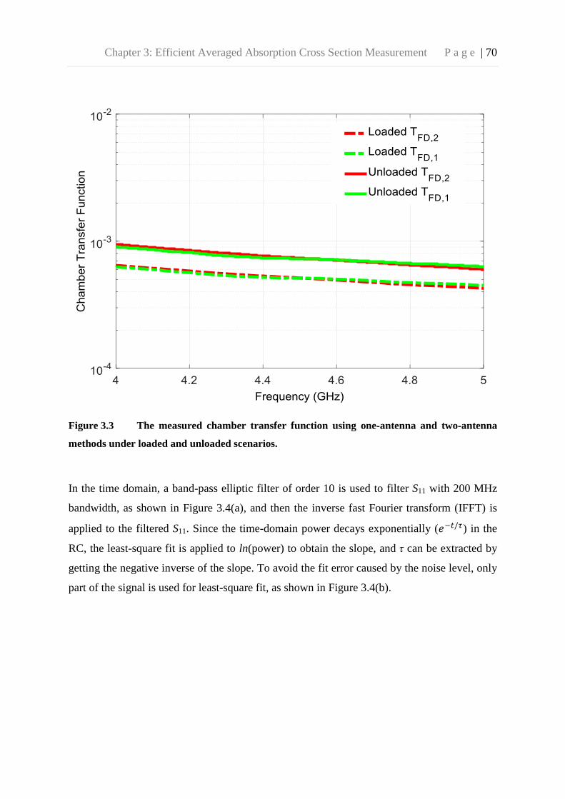
Chapter 3: Efficient Averaged Absorption Cross Section Measurement P a g e | 70
Figure 3.3 The measured chamber transfer function using one-antenna and two-antenna
methods under loaded and unloaded scenarios.
In the time domain, a band-pass elliptic filter of order 10 is used to filter S11 with 200 MHz
bandwidth, as shown in Figure 3.4(a), and then the inverse fast Fourier transform (IFFT) is
applied to the filtered S11. Since the time-domain power decays exponentially ( ) in the
RC, the least-square fit is applied to ln(power) to obtain the slope, and τ can be extracted by
getting the negative inverse of the slope. To avoid the fit error caused by the noise level, only
part of the signal is used for least-square fit, as shown in Figure 3.4(b).

Chapter 3: Efficient Averaged Absorption Cross Section Measurement P a g e | 71
(a)
(b)
Figure 3.4 Extracting τ from S11: (a) measured S11 and filtered S11, (b) time-domain
response: ln([IFFT(S11)]2) and least-square fit.

Chapter 3: Efficient Averaged Absorption Cross Section Measurement P a g e | 72
By sweeping the centre frequency of the filter, τ at different centre frequencies is obtained.
The measured chamber decay time using one-antenna method under loaded and unloaded
scenarios are depicted in Figure 3.5.
Figure 3.5 The measured chamber decay time using one-antenna method under loaded and
unloaded scenarios.
The thin cyan curves are the measured τ for different stirring samples and the thick dash
curves are the averaged τ for all samples. As expected, the chamber decay time is reduced
when the chamber is loaded. Another thing to be noted is that τ is very robust in the full
frequency span, i.e., τ does not vary much for different stirring samples. The reason can be
explained as follows: the chamber decay time τ is determined by the chamber loss. For a
given frequency, the chamber loss will vary due to the change of the paddle positions and the
change of the chamber modes. When the number of resonant modes is massive (1,657,518
modes in 4.0 GHz in our RC according to Weyl’s formula [22]), the positions of the peaks
and troughs of the resonant mode will not change much for different boundary conditions,

Chapter 3: Efficient Averaged Absorption Cross Section Measurement P a g e | 73
and the loss variation is relatively small for different paddle positions. Hence, the chamber
decay time is very robust. As shown in Figure 3.5, under the unloaded scenario, the variation
between the τ for one sample and the averaged τ is within about ±10%. And under the loaded
scenario, the variation is within about ±5%. It is easy to understand when the RC is loaded,
the majority of the power is consumed by the lossy objects, the power loss is not sensitive to
the boundary condition of the RC, and hence the loaded τ is more robust than the unloaded τ.
The robustness of the chamber decay time actually offers an opportunity to extract τ by
merely a few stirring samples, thus the ACS can be measured rapidly and accurately, which
will be detailed later.
The ACS measurement results are shown in Figure 3.6. In the frequency domain, 200 MHz
frequency stirring is adopted. The efficiency of antenna 1 and antenna 2 in 4.0 – 5.0 GHz are
78% and 95%, respectively. It can be seen clearly that the measured ACSs using the three
methods are all around 0.1 m2 and the maximum variation is within 10%.
Figure 3.6 The measured ACS of the OUT.

Chapter 3: Efficient Averaged Absorption Cross Section Measurement P a g e | 74
3.4 Convergence Property
The convergence properties of the three methods are also studied. The root-mean-square-
error (RMSE) of the measured ACS from 4.0 – 5.0 GHz with different numbers of stirring
positions to the ACS measured with 300 stirring positions is adopted to evaluate the
convergence, and the algorithm is expressed as
√∑ ( )
where i is the number of stirring positions, M is the maximum number of stirring positions, j
is the frequency sampling point number, N is the number of frequency sampling points in 4.0
– 5.0 GHz. In our case, M = 300 and N = 7143. The calculated results are shown in Figure 3.7.
Figure 3.7 The RMSE with the increase of the number of stirring positions for different
methods.

Chapter 3: Efficient Averaged Absorption Cross Section Measurement P a g e | 75
As can be seen, the convergence speeds of the one-antenna method and the two-antenna
method in the frequency domain are close but the time-domain method converges faster than
the frequency-domain methods. This is because the chamber decay time τ is not sensitive to
the boundary conditions and only depends on the overall loss of the RC. While the chamber
transfer function and depend on how well the RC is stirred. Thus, ACSTD, 1 converges
faster than ACSFD, 1 and ACSFD, 2. It is worth mentioning that, in the time domain, the RMSE
is always below 10% (compared with the averaged ACS in the full frequency span, about 0.1
m2 from Figure 3.6) and drops below 3% after 15 stirring positions. However, in the
frequency domain, the one-antenna method and the two-antenna method have similar
convergence behaviour, the RMSEs are always above 10% before the first 10 stirring
positions and drop down slowly afterwards. They are below 3% after 100 stirring positions.
As implied in (3.14) and (3.15), the one-antenna method in the frequency domain requires
. Inaccurate results may be obtained if deviates from 2. To show the influence of
the deviation of from 2 to the validity of the measurement in the frequency domain based
on one-antenna approach, the convergence behaviour of the measured (under both loaded
and unloaded scenarios) and ACSFD, 1 at 4.5 GHz has been checked, as shown in Figure 3.8.
The level and ACSFD, 1 0.1 m level are marked out with dash lines. As can be seen,
at the first dozens of stirs, the deviation of from 2 fluctuates drastically, the measured ACS
is unreliable. However, with the increase of the number of stir, converges to 2 gradually.
The convergence behaviour of ACSFD, 1 is very similar to . After about 150 stirs, the
variation of from 2 becomes small (within 10% variation) and the measured ACSFD, 1
becomes stable (it converges to 0.1 m2). That means the accuracy of the frequency-domain
one-antenna approach depends on , i.e., how well the chamber is stirred.
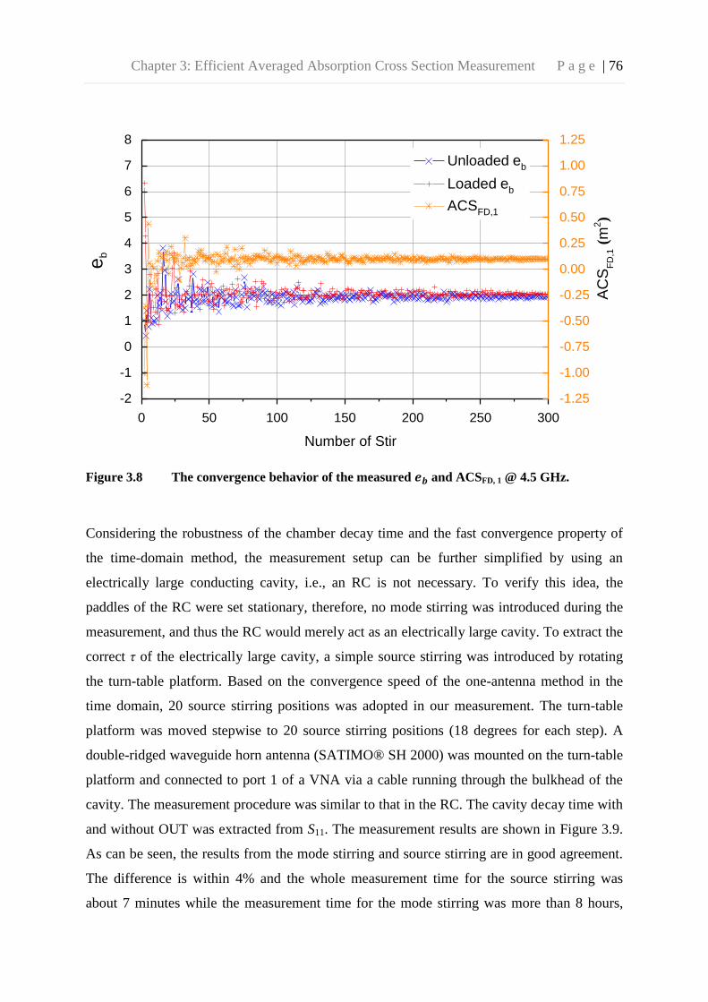
Chapter 3: Efficient Averaged Absorption Cross Section Measurement P a g e | 76
Figure 3.8 The convergence behavior of the measured and ACSFD, 1 @ 4.5 GHz.
Considering the robustness of the chamber decay time and the fast convergence property of
the time-domain method, the measurement setup can be further simplified by using an
electrically large conducting cavity, i.e., an RC is not necessary. To verify this idea, the
paddles of the RC were set stationary, therefore, no mode stirring was introduced during the
measurement, and thus the RC would merely act as an electrically large cavity. To extract the
correct τ of the electrically large cavity, a simple source stirring was introduced by rotating
the turn-table platform. Based on the convergence speed of the one-antenna method in the
time domain, 20 source stirring positions was adopted in our measurement. The turn-table
platform was moved stepwise to 20 source stirring positions (18 degrees for each step). A
double-ridged waveguide horn antenna (SATIMO® SH 2000) was mounted on the turn-table
platform and connected to port 1 of a VNA via a cable running through the bulkhead of the
cavity. The measurement procedure was similar to that in the RC. The cavity decay time with
and without OUT was extracted from S11. The measurement results are shown in Figure 3.9.
As can be seen, the results from the mode stirring and source stirring are in good agreement.
The difference is within 4% and the whole measurement time for the source stirring was
about 7 minutes while the measurement time for the mode stirring was more than 8 hours,
0 50 100 150 200 250 300
-2
-1
0
1
2
3
4
5
6
7
8
Unloaded eb
Loaded eb
ACSFD,1
Number of Stir
eb
-1.25
-1.00
-0.75
-0.50
-0.25
0.00
0.25
0.50
0.75
1.00
1.25
AC
SF
D,1 (
m2)

Chapter 3: Efficient Averaged Absorption Cross Section Measurement P a g e | 77
which means that the ACS can be measured in the time domain rapidly and accurately. The
major contribution to the measurement time is the damping time of the turn-table platform
between the steps and the time of transferring data from the VNA to the computer. The
measurement time of this method is comparable with that of the rapid method proposed in
[24] and therefore, it is quite suitable for applications requiring discriminations between
subjects due to its high accuracy and short measurement time. It should be pointed out that
the cavity should be large enough to support sufficient cavity modes to ensure enough
independent samples to be obtained at the lowest frequency of the measurement, or the OUT
could not fully “submerge” into the field-uniform area and the measurement result could be
wrong. This is the main consideration for the selection of the size of the conducting cavity in
the measurement.
Figure 3.9 The comparison of the measured ACS in the time domain with 20 source stirring
positions and 360 mode stirring positions.

Chapter 3: Efficient Averaged Absorption Cross Section Measurement P a g e | 78
3.5 ACS Measurement without Calibration
In this section, it is shown that the ACS can be measured accurately without calibration. This
is realized by making use of the fact that the chamber decay time is independent of the
insertion loss of cables in the measurement. Measurements have been done to verify the
proposed procedure. It has been shown that the measurement process is simplified and the
measurement time is shortened at the same time.
As mentioned in Section 3.3, in order to extract the chamber decay time, a full two-port (for
two-antenna methods) or one-port (for one-antenna method) calibration must be carried out
before collecting the S-parameters of the antennas. In such measurements, the reference
planes are calibrated at the end of the cables, as shown in Figure 3.10(a) with dot lines.
However, the calibration process is tedious and time-consuming. Nowadays, some VNAs are
pre-calibrated with the reference planes at the output connectors of the VNAs, when the VNA
is pre-set the reference planes are restored [25]. This offers an opportunity to perform the
measurement without the need for calibration. The antennas and the cables after the reference
planes can be regarded as integrated antennas. Since the chamber decay time does not depend
on the insertion loss of cables used in the measurement and it is only determined by the
diffused loss in the RC. The ACS can be measured accurately without calibration, which will
simplify the measurement process and shorten the measurement time.
To validate the proposed method, measurements were performed from 4.0 – 5.0 GHz in our
RC. The two-antenna method was adopted. Antenna 1 (SATIMO® SH 2000) was connected
to port 1 of a VNA and antenna 2 (Rohde & Schwarz® HF 906) was connected to port 2 of
the VNA as in Section 3.3. During the measurement, the two stirrers were moved
simultaneously and stepwise to 120 positions (3 degrees for each step). At each mode stirring
position, a full frequency sweep was performed by the VNA and the full S-parameters were
collected. A piece of RAM was selected as an OUT. The measurement setup is shown in
Figure 3.10(a). The measurement setups without and with the OUT are shown in Figure
3.10(b) and (c), respectively.
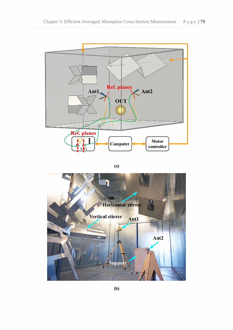
Chapter 3: Efficient Averaged Absorption Cross Section Measurement P a g e | 79
(a)
(b)

Chapter 3: Efficient Averaged Absorption Cross Section Measurement P a g e | 80
(c)
Figure 3.10 ACS measurement setup in the RC: (a) measurement system, (b) unloaded
scenario, (c) loaded scenario.
The measurement procedure is given as follows.
Step 1: Calibrate the VNA including the cables according to the standard calibration
procedure.
Step 2: Place the two antennas and the support (excluding the OUT) inside the RC.
Step 3: Connect antenna 1 to port 1 of the VNA and antenna 2 to port 2 of the VNA,
and collect the full S-parameters for each stirring position.
Step 4: Keep the previous measurement setup unchanged and place the OUT on the
support, and repeat Step 3.
Step 5: Preset the VNA to shift the reference planes, and repeat Step 3 without
calibration. Move the OUT out of the RC, and repeat Step 3 without
calibration.

Chapter 3: Efficient Averaged Absorption Cross Section Measurement P a g e | 81
Figure 3.11 Time-domain response with calibration: ln([IFFT(S21)]2) and least-square fit
under loaded and unloaded scenarios.
Figure 3.12 Time-domain response with no calibration and the close-up of the early-time
behavior.

Chapter 3: Efficient Averaged Absorption Cross Section Measurement P a g e | 82
In this measurement, 10,001 points were sampled in the frequency range from 3.8 to 5.2 GHz.
The ACS of the OUT was calculated using (3.17). A band-pass elliptic filter of order 10 is
used to filter S21 with 200 MHz bandwidth, and then the IFFT is applied to the filtered S21.
The chamber decay time τ can be extracted by the same procedure as described in Section 3.3,
as shown in Figure 3.11. The average chamber decay time ⟨ ⟩ is then obtained from the
ensemble average of the τ for different stirring positions. The early time behaviour is depicted
in detail in Figure 3.12. As can be seen, in the first 83.65 ns, the chamber is not charged, this
is the time that the wave travels in the cables. In our case, the total length of the two cables is
about 16 m and the travelling speed of the wave inside the cables is about 2 × 10⁸ m/s [26].
Thus, the 83.65 ns corresponds to 16.73 m which agrees well with the total length of our
cables used in the measurement (our VNA is pre-calibrated with the reference planes at the
output connectors of the VNA, when the VNA is pre-set the reference planes are restored).
By sweeping the centre frequency of the filter, τ at different centre frequencies is obtained.
The measured chamber decay time with and without calibration under loaded and unloaded
scenarios is shown in Figure 3.13.
Figure 3.13 The comparison of the average chamber decay time with and without calibration
under loaded and unloaded scenarios.

Chapter 3: Efficient Averaged Absorption Cross Section Measurement P a g e | 83
As expected, the chamber decay time is reduced when the chamber is loaded. The chamber
decay time with calibration and that without calibration agree well, i.e., the chamber decay
time can be measured accurately without calibration. The measured ACSs with and without
calibration are depicted in Figure 3.14. As can be seen, they agree well and the maximum
difference is within 2%, which manifests the effectiveness of the proposed method.
Figure 3.14 The comparison of the measured ACS with and without calibration.
3.6 Discussions and Conclusion
In this chapter, one-antenna methods for determining the ACS of the OUT in the frequency
domain and in the time domain were presented at the beginning. The commonly used RC
technique for determining the ACS of the OUT requires two antennas and the radiation
efficiency of the two antennas should be known. In this chapter, the one-antenna method in
the frequency domain was first presented which requires only one antenna (with known
efficiency) by making use of enhanced backscatter effect. Thus, the measurement setup was

Chapter 3: Efficient Averaged Absorption Cross Section Measurement P a g e | 84
simplified. Then, the one-antenna method in the time domain was presented which needs no
knowledge of the efficiency of the antenna. The experimental setup was illustrated and
measurement results were presented. It seems that the measured ACSs by the three methods
are in good agreement. The robustness of the chamber decay time and the convergence speed
of the three methods were investigated. It is found that the time domain method converges
much faster than the frequency domain methods. A rapid and accurate measurement can be
achieved in the time domain based on this finding by using source stirring technique, which
makes it quite suitable for human absorption and exposure measurement. Furthermore, in the
time domain approach, the RC can be replaced by a suitable electrically large conducting
cavity, which will greatly reduce the hardware requirement. The method was validated in the
RC by setting the paddles stationary and the results agree well with that measured in the RC
using mode stirring. The comparison of the measurement methods mentioned above is shown
in Table 3.1. It is demonstrated that the time domain method is much more efficient and its
hardware requirement is much lower than the frequency domain method.
Table 3.1: Comparison of Different Measurement Methods
Following the previous work, a reliable and simple no-calibration method was proposed for
the measurement of the averaged ACS of a lossy object based on the time-domain
measurement in an RC. By making use of the fact that the chamber decay time is independent
of the insertion loss in the system, the ACS can be measured accurately without calibration,
which will simplify the measurement process and shorten the measurement time at the same
time. Measurement has been done to validate the proposed method. The results show that the
Measurement methods Number of antennas Time Facility
FD two-antenna method 2 approx. 8 hrs RC
FD one-antenna method 1 approx. 8 hrs RC
TD one-antenna method
(mode stirring) 1 approx. 7 mins RC
TD one-antenna method
(source stirring) 1 approx. 7 mins electrically large cavity

Chapter 3: Efficient Averaged Absorption Cross Section Measurement P a g e | 85
averaged ACS of the OUT can be accurately measured using the proposed method with no
calibration process.
There are some points that need to be emphasized. Firstly, the proposed methods presented in
this chapter assume that the RC was well stirred. When the RC is not well stirred, the OUT
could not fully “submerge” in the field-uniform area. The measured chamber transfer
function and chamber decay time will be inaccurate, hence the measured ACS will be of
considerable errors. Secondly, the antennas used in the measurement should be of high
efficiency in the time domain method, i.e., the losses in the RC are dominated by the chamber
wall loss and OUT loss rather than by the losses of the antennas used in the measurement.
Otherwise, the power will not decay exponentially and chamber decay time cannot be
extracted correctly. However, in the frequency domain, the antennas used do not have to be
of high efficiency because the antenna efficiency has been calibrated out in the net power
transfer function. Thirdly, during the measurement, the OUT should be set far away (more
than 10λ is recommended) from the antennas to avoid the proximity effect [27]. Last but not
least, the calculation of the ACS requires the difference in the net power transfer function (in
the frequency domain) or the chamber decay time (in the time domain) with and without the
OUT, as seen in (3.13) and (3.17). If the loss of the OUT is too small compared with that of
the chamber itself, it will be very difficult for the chamber to distinguish the difference of the
loss (i.e., the difference of the Q factors between loaded and unloaded scenarios), which will
result in the inaccuracy of the measurement. However, for most of the applications, like the
measurement of the human body absorption cross section, the loss of the OUT is normally
large enough for the chamber to see and thus the ACS can be accurately calculated.
3.7 References
[1] Electromagnetic Compatibility (EMC) part 4-21: Testing and measurement
techniques-Reverberation chamber test methods, IEC 61000-4-21, 2003.
[2] C. L. Holloway, H. A. Shah, R. J. Pirkl, W. F. Young, D. A. Hill, and J. Ladbury,
“Reverberation chamber techniques for determining the radiation and total efficiency

Chapter 3: Efficient Averaged Absorption Cross Section Measurement P a g e | 86
of antennas,” IEEE Trans. Antennas Propag., vol. 60, no. 4, pp. 1758-1770, Apr.
2012.
[3] C. L. Holloway, R. Smith, C. Dunlap, R. Pirkl, J. Ladbury, W. Young, B. Hansell, M.
Shadish, and K. Sullivan, “Validation of a one-antenna reverberation-chamber
technique for estimating the total and radiation efficiency of an antenna,” in Proc.
IEEE Int. Symp. on Electromagn. Compat., Aug. 2012, pp. 205-209.
[4] H. G. Krauthauser, and M. Herbrig, “Yet another antenna efficiency measurement
method in reverberation chambers,” in Proc. IEEE Int. Symp. on Electromagn.
Compat., Jul. 2010, pp. 536-540.
[5] IEEE Standard Method for Measuring the Effectiveness of Electromagnetic Shielding
Enclosures, IEEE Standard 299, 2006.
[6] C. L. Holloway, D. A. Hill, M. Sandroni, J. M. Ladbury, J. Coder, G. Koepke, A. C.
Marvin, and Yuhui He, “Use of Reverberation Chambers to Determine the Shielding
Effectiveness of Physically Small, Electrically Large Enclosures and Cavities,” IEEE
Trans. Electromagn. Compat., vol.50, no.4, pp. 770-782, Nov. 2008.
[7] D. Fedeli, G. Gradoni, V. M. Primiani, and F. Moglie, “Accurate analysis of
reverberation field penetration into an equipment-level enclosure,” IEEE Trans.
Electromagn. Compat., vol. 51, no. 2, pp. 170-180, May 2009.
[8] G. B. Tait, C. Hager, M. B. Slocum, and M. O. Hatfield, “On Measuring Shielding
Effectiveness of Sparsely-Moded Enclosures in a Reverberation Chamber,” IEEE
Trans. Electromagn. Compat., vol. 55, no. 2, pp. 231-240, Apr. 2013.
[9] H. G. Krauthäuser, “On the measurement of total radiated power in uncalibrated
reverberation chambers,” IEEE Trans. Electromagn. Compat., vol. 49, no. 2, pp. 270-
279, 2007.
[10] U. Carlberg, P.-S. Kildal, A. Wolfgang, O. Sotoudeh, and C. Orlenius, “Calculated
and measured absorption cross sections of lossy objects in reverberation chamber,”
IEEE Trans. Electromagn. Compat., vol. 46, no. 2, pp. 146-154, May 2004.

Chapter 3: Efficient Averaged Absorption Cross Section Measurement P a g e | 87
[11] E. Amador, M. Andries, C. Lemoine, and P. Besnier, “Absorbing material
characterization in a reverberation chamber,” in Proc. IEEE Int. Symp. on
Electromagn. Compat., Sept. 2011, pp. 117-122.
[12] G. C. R. Melia, M. P. Robinson, I. D. Flintoft, A. C. Marvin, and J. F. Dawson,
“Broadband Measurement of Absorption Cross Section of the Human Body in a
Reverberation Chamber,” IEEE Trans. Electromagn. Compat., vol. 55, no. 6, pp.
1043-1050, Dec. 2013.
[13] A. Bamba, D. P. Gaillot, E. Tanghe, G. Vermeeren, W. Joseph, M. Lienard, and L.
Martens, “Assessing Whole-Body Absorption Cross Section For Diffuse Exposure
From Reverberation Chamber Measurements,” IEEE Trans. Electromagn. Compat.,
vol. 57, no. 1, pp. 27-34, Feb. 2015.
[14] D. A. Hill, M. T. Ma, A. R. Ondrejka, B. F. Riddle, M. L. Crawford, and R. T. Johnk,
“Aperture excitation of electrically large, lossy cavities,” IEEE Trans. Electromagn.
Compat., vol. 36, no. 3, pp. 169-178, Aug. 1994.
[15] M. I. Andries, P. Besnier, and C. Lemoine, “On the prediction of the average
absorbing cross section of materials from coherence bandwidth measurements in
reverberation chamber,” in Proc. IEEE Int. Symp. on Electromagn. Compat., Sept.
2012, pp. 1-6.
[16] C. L. Holloway, H. A. Shah, R. J. Pirkl, K. A. Remley, D. A. Hill, and J. Ladbury,
“Early Time Behavior in Reverberation Chambers and Its Effect on the Relationships
Between Coherence Bandwidth, Chamber Decay Time, RMS Delay Spread, and the
Chamber Buildup Time,” IEEE Trans. Electromagn. Compat., vol. 54, no. 4, pp. 714-
725, Aug. 2012.
[17] D. L. Green, V. Rajamani, C. F. Bunting, B. Archambeault, and S. Connor, “One-port
time domain measurement technique for quality factor of loaded and unloaded
cavities,” in Proc. IEEE Int. Symp. on Electromagn. Compat., Aug. 2013, pp. 747-
750.

Chapter 3: Efficient Averaged Absorption Cross Section Measurement P a g e | 88
[18] C. Vyhlidal, V. Rajamani, C. F. Bunting, P. Damacharla, and V. Devabhaktuni,
“Estimation of absorber performance using reverberation techniques and artificial
neural network models,” in Proc. IEEE Int. Symp. on Electromagn. Compat., Aug.
2015, pp. 897-901.
[19] S. J. Boyes, P. J. Soh, Y. Huang, G. A. E. Vandenbosch, and N. Khiabani,
“Measurement and Performance of Textile Antenna Efficiency on a Human Body in a
Reverberation Chamber,” IEEE Trans. Antennas Propag., vol.61, no.2, pp. 871-881,
Feb. 2013.
[20] C. L. Holloway, D. A. Hill, J. M. Ladbury, P. F. Wilson, G. Koepke, and J. Coder,
“On the Use of Reverberation Chambers to Simulate a Rician Radio Environment for
the Testing of Wireless Devices,” IEEE Trans. Antennas Propag., vol.54, no.11, pp.
3167-3177, Nov. 2006.
[21] J. M. Ladbury, and D. A. Hill, “Enhanced Backscatter in a Reverberation Chamber:
Inside Every Complex Problem is a Simple Solution Struggling to Get Out,” in Proc.
IEEE Int. Symp. on Electromagn. Compat., Jul. 2007, pp. 1-5.
[22] D. A. Hill, Electromagnetic Fields in Cavities: Deterministic and Statistical Theories.
New York, NY, USA: Wiley-IEEE Press, 2009.
[23] C. R. Dunlap, “Reverberation chamber characterization using enhanced backscatter
coefficient measurements,” Ph.D. dissertation, Dept. of Elect., Comput. and Eng.,
Univ. of Colorado, Boulder, USA, 2013.
[24] I. D. Flintoft, G. C. R. Melia, M. P. Robinson, J. F. Dawson, and A. C. Marvin.
“Rapid and accurate broadband absorption cross-section measurement of human
bodies in a reverberation chamber,” Meas. Sci. Technol., vol. 26, no. 6, pp. 65701-
65709, Jun. 2015.
[25] Q. Xu, Y. Huang, X. Zhu, L. Xing, and Z. Tian, “Measure the radiation efficiency of
antennas in a reverberation chamber without calibration,” in Proc. IEEE int. Symp. on
Antennas Propag., Vancouver, BC, 2015, pp. 1178-1179.

Chapter 3: Efficient Averaged Absorption Cross Section Measurement P a g e | 89
[26] [Online] Available:
http://web.physics.ucsb.edu/~lecturedemonstrations/Composer/Pages/76.18.html.
[Accessed: 18-Apr-2017]
[27] W. T. C. Burger, K. A. Remley, C. L. Holloway, and J. M. Ladbury, “Proximity and
antenna orientation effects for large-form-factor devices in a reverberation chamber,”
in Proc. IEEE Int. Symp. on Electromagn. Compat., Aug. 5-9, 2013, pp. 671-676.

Chapter 4: Volume Measurement Using Averaged Absorption Cross Section P a g e | 90
Chapter 4: Volume Measurement Using Averaged
Absorption Cross Section
4.1 Introduction
In last chapter, the ACS measurement methods in an RC have been discussed. In this chapter,
an interesting practical application of the ACS measurement methods will be introduced –
cavity volume measurement.
The measurement of the volume of a large cavity is required especially in shipping and
aircraft industry. In practice, to optimize the capacity of the cargo compartment of a ship or
an aircraft, it is necessary to get the knowledge of its volume. An example is shown in Figure.
4.1. However, the volume of such a cavity is not easy to obtain because of its irregular shape
and the complex inner environment. Normally, a 3D laser scanner can be employed [2]. The
laser scanner first scans the whole profile of the cavity under test and builds its 3D model.
Subsequently, the volume of the cavity can be calculated from the 3D model. However, this
method is time-consuming and costly. It may not be available for some companies or
institutes. And also, before scanning the profile of the cavity, the contents that may block the
laser beam in the cavity should be removed, which could be tedious or sometimes impossible
in reality. Since such a cavity is normally made of metal, an alternative method based on the
statistical theory of EM waves was proposed in [3]. In this method, the volume of a cavity is
extracted by comparing the cavity quality factors in the frequency domain and in the time
domain [4] – [7]. This method is economical, but it is not efficient enough because many
stirring positions are required during the measurement. A more efficient method is in demand
for practical purpose.
In this chapter, a new rapid method to measure the volume of a large cavity is presented. This
method is based on the measurement of the cavity decay time constants with and without a
lossy object. A lossy object with a known averaged ACS [8] – [14] is required for the
measurement. It is found that only one antenna is required in this method. Hence, the
hardware requirement is very simple, which makes the method very economical. Also, this

Chapter 4: Volume Measurement Using Averaged Absorption Cross Section P a g e | 91
method is very efficient because only a few stirring positions are needed to complete the
measurement. Consequently, the measurement time can be greatly shortened. Furthermore,
by using acoustic waves instead of EM waves, this method can be generalized and the cavity
under test does not have to be metallic.
Figure 4.1 The cargo compartment of an aircraft and the demand of measuring its volume
[1].
4.2 Theory
Before studying how to measure the cavity volume using the ACS, it is useful to first
introduce how the ACS is measured in an electrically large cavity using an electromagnetic
method. It has been detailed in Chapter 3 that the averaged ACS ⟨ ⟩ can be measured in the
time domain [9], [15] as
⟨ ⟩
⟨ ⟩
⟨ ⟩

Chapter 4: Volume Measurement Using Averaged Absorption Cross Section P a g e | 92
The definitions of V, c, ⟨ ⟩, and ⟨ ⟩ can be found in Section 3.2.
It can be clearly seen from (4.1), the cavity volume V is required to calculate the ACS. (4.1)
can be transformed to the form
⟨ ⟩
⟨ ⟩ ⟨ ⟩
It can be seen that if the averaged ACS of an OUT is known or pre-calibrated, (4.2) provides
a method to obtain the cavity volume. The quantities that needs to be measured is τl and τu. In
this method, only one antenna is required since τ can be obtained from S11. Furthermore,
because τ is very robust [9], only a very few stirring positions are needed to extract it
accurately. Thus, this method can be very efficient.
4.3 Measurement
To verify the proposed method, measurements were conducted in the frequency range of 2.8
to 4.2 GHz in the RC at the University of Liverpool. The volume of the RC is 3.6 m × 4.0 m
× 5.8 m = 83.52 m3. A double-ridged waveguide horn antenna (SATIMO® SH 2000) was
used in the measurement. The antenna was mounted on a turn-table platform to introduce
source stirring positions [16] – [17]. It was connected to port 1 of the VNA via a cable
running through the bulkhead of the RC. A piece of RAM was selected as the OUT which
was placed on the support (a carton box). In the measurement, the turn-table platform was
rotated stepwise to 18 different positions (10 degrees for each step). At each source stirring
position, the VNA swept the S-parameters over the full frequency span. It should be noted
that the antenna should direct away from the OUT to avoid LoS illumination (to provide a
random environment). Therefore, a directional antenna was used and the turn-table platform
was rotated 180° instead of 360°. During the measurement, the two stirrers of the RC were
not used because in practice it may not have a stirring system in a cavity. A general
measurement setup is shown in Figure 4.2(a). The measurement setups without and with the
OUT are shown in Figure 4.2(b) and (c), respectively.

Chapter 4: Volume Measurement Using Averaged Absorption Cross Section P a g e | 93
(a)
(b)

Chapter 4: Volume Measurement Using Averaged Absorption Cross Section P a g e | 94
(c)
Figure 4.2 Measurement setup in the RC: (a) global measurement system, (b) without ACS,
(c) with ACS.
The measurement was conducted with the following five steps.
Step 1: Calibrate the VNA including the cables.
Step 2: Place the antenna, the turn-table platform and the support inside the RC,
excluding the OUT.
Step 3: Connect the antenna to the cable connected to VNA port 1 and record the S-
parameters S11 at each source stirring position.
Step 4: Keep the measurement setup unchanged, place the OUT on the support and
repeat Step 3.
Step 5: Extract the cavity decay time constants with and without the OUT and
calculate the volume of the RC using (4.2).

Chapter 4: Volume Measurement Using Averaged Absorption Cross Section P a g e | 95
In our measurement, 10,001 points were sampled in the frequency range of 2.8 – 4.2 GHz. S11
in this frequency span at each source stirring position was collected. The cavity decay time
constant was extracted with the same procedure detailed in Section 3.3. The results are shown
in Figure 4.3.
Figure 4.3 Measured cavity decay time constants τ under loaded and unloaded scenarios.
The thin curves are the measured τ for each source stirring position and the thick curves are
the averaged τ for all the 18 source stirring positions. The averaged τ was used to calculate
the cavity volume. The robustness of τ can be observed in Figure 4.3. As can be seen, under
the unloaded scenario (without OUT), the variation between the τ for one stirring position and
the averaged τ is within about ± 10% and under the loaded scenario (with OUT), it is within
about ± 5%. This is because τ is determined by the diffuse loss of the RC which is not
sensitive to the source stirring positions [9].
To measure the volume of the RC, the ACS of the OUT was first calibrated in the frequency
range of interest, as shown in Figure 4.4. It can be seen that the ACS of the OUT is 0.1078 m2
in the frequency band of 3.0 – 4.0 GHz. And also, the ACS seems frequency independent.

Chapter 4: Volume Measurement Using Averaged Absorption Cross Section P a g e | 96
The reason is, when the OUT is electrically large, the ACS only determined by its surface
area which does not depend on the frequency [8]. Actually, this provides a faster method to
obtain the ACS of a RAM and consequently, a faster and simpler method to measure the
cavity volume with ACS. This point will be discussed later.
Figure 4.4 The averaged ACS of the OUT in 3.0 – 4.0 GHz.
In practice, a cavity is hardly vacant or well shielded. It may be loaded with cargoes or have
apertures (such as windows or ventilation openings). To verify the validity of the proposed
method in a practical environment, the volume of the RC in three different scenarios were
measured: the well-shielded scenario, the open-door scenario, and the cargo-loaded scenario,
as shown in Figure 4.5(a), (b) and (c), respectively. In the following part, the measurement
results under these three different scenarios using the proposed method are detailed.

Chapter 4: Volume Measurement Using Averaged Absorption Cross Section P a g e | 97
(a)
(b)
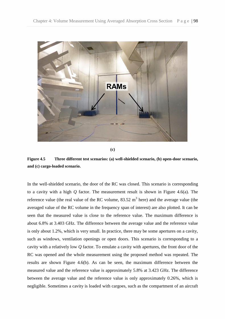
Chapter 4: Volume Measurement Using Averaged Absorption Cross Section P a g e | 98
(c)
Figure 4.5 Three different test scenarios: (a) well-shielded scenario, (b) open-door scenario,
and (c) cargo-loaded scenario.
In the well-shielded scenario, the door of the RC was closed. This scenario is corresponding
to a cavity with a high Q factor. The measurement result is shown in Figure 4.6(a). The
reference value (the real value of the RC volume, 83.52 m3 here) and the average value (the
averaged value of the RC volume in the frequency span of interest) are also plotted. It can be
seen that the measured value is close to the reference value. The maximum difference is
about 6.8% at 3.403 GHz. The difference between the average value and the reference value
is only about 1.2%, which is very small. In practice, there may be some apertures on a cavity,
such as windows, ventilation openings or open doors. This scenario is corresponding to a
cavity with a relatively low Q factor. To emulate a cavity with apertures, the front door of the
RC was opened and the whole measurement using the proposed method was repeated. The
results are shown Figure 4.6(b). As can be seen, the maximum difference between the
measured value and the reference value is approximately 5.8% at 3.423 GHz. The difference
between the average value and the reference value is only approximately 0.26%, which is
negligible. Sometimes a cavity is loaded with cargoes, such as the compartment of an aircraft

Chapter 4: Volume Measurement Using Averaged Absorption Cross Section P a g e | 99
or the refrigerated warehouse of a supermarket. When a cavity is loaded with cargoes, its Q
factor will decrease. To emulate a cavity loaded with cargoes, two pieces of RAM were
placed at the corners of the RC to decrease its Q factor. The measurement result is depicted in
Figure 4.6(c). As can be seen, the maximum difference between the measured value and the
reference value is around 5% at 3.182 GHz. The difference between the average value and
the reference value is around 0.5%, which can be neglected.
(a)
(b)
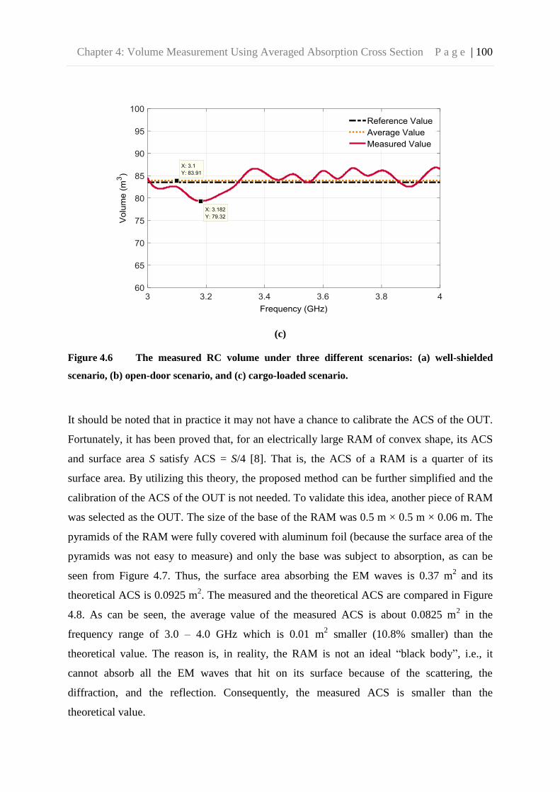
Chapter 4: Volume Measurement Using Averaged Absorption Cross Section P a g e | 100
(c)
Figure 4.6 The measured RC volume under three different scenarios: (a) well-shielded
scenario, (b) open-door scenario, and (c) cargo-loaded scenario.
It should be noted that in practice it may not have a chance to calibrate the ACS of the OUT.
Fortunately, it has been proved that, for an electrically large RAM of convex shape, its ACS
and surface area S satisfy ACS = S/4 [8]. That is, the ACS of a RAM is a quarter of its
surface area. By utilizing this theory, the proposed method can be further simplified and the
calibration of the ACS of the OUT is not needed. To validate this idea, another piece of RAM
was selected as the OUT. The size of the base of the RAM was 0.5 m × 0.5 m × 0.06 m. The
pyramids of the RAM were fully covered with aluminum foil (because the surface area of the
pyramids was not easy to measure) and only the base was subject to absorption, as can be
seen from Figure 4.7. Thus, the surface area absorbing the EM waves is 0.37 m2 and its
theoretical ACS is 0.0925 m2. The measured and the theoretical ACS are compared in Figure
4.8. As can be seen, the average value of the measured ACS is about 0.0825 m2 in the
frequency range of 3.0 – 4.0 GHz which is 0.01 m2 smaller (10.8% smaller) than the
theoretical value. The reason is, in reality, the RAM is not an ideal “black body”, i.e., it
cannot absorb all the EM waves that hit on its surface because of the scattering, the
diffraction, and the reflection. Consequently, the measured ACS is smaller than the
theoretical value.

Chapter 4: Volume Measurement Using Averaged Absorption Cross Section P a g e | 101
Figure 4.7 The RAM with its pyramids covered by aluminum foil. The size of its base is
marked.
Figure 4.8 The measured ACS of the OUT. Its theoretical value and average value are
marked out as well.
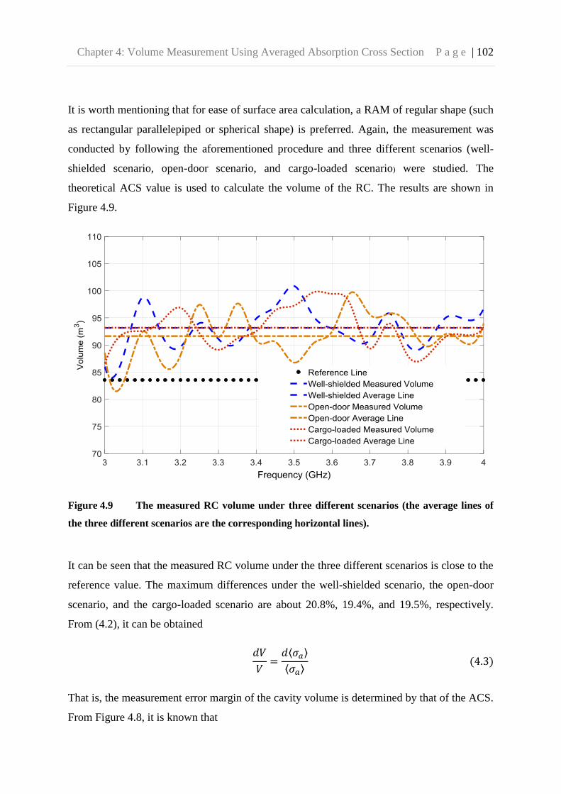
Chapter 4: Volume Measurement Using Averaged Absorption Cross Section P a g e | 102
It is worth mentioning that for ease of surface area calculation, a RAM of regular shape (such
as rectangular parallelepiped or spherical shape) is preferred. Again, the measurement was
conducted by following the aforementioned procedure and three different scenarios (well-
shielded scenario, open-door scenario, and cargo-loaded scenario) were studied. The
theoretical ACS value is used to calculate the volume of the RC. The results are shown in
Figure 4.9.
Figure 4.9 The measured RC volume under three different scenarios (the average lines of
the three different scenarios are the corresponding horizontal lines).
It can be seen that the measured RC volume under the three different scenarios is close to the
reference value. The maximum differences under the well-shielded scenario, the open-door
scenario, and the cargo-loaded scenario are about 20.8%, 19.4%, and 19.5%, respectively.
From (4.2), it can be obtained
⟨ ⟩
⟨ ⟩
That is, the measurement error margin of the cavity volume is determined by that of the ACS.
From Figure 4.8, it is known that

Chapter 4: Volume Measurement Using Averaged Absorption Cross Section P a g e | 103
⟨ ⟩
⟨ ⟩
Therefore, the difference of cavity volume between the measured average value and the
reference value should be around 12%. As shown in Figure 4.9, the differences between the
average value and the reference value under the well-shielded scenario, the open-door
scenario, and the cargo-loaded scenario are about 11.5%, 11.6%, and 9.7%, respectively,
which agree well with the theoretical prediction in (4.4).
The measurement results are summarized in Table 4.1. A comparison between this proposed
method and the method proposed in [3] is made. It can be seen that the proposed one-antenna
method using source stirring and calibrated ACS can finish the measurement with minimum
errors in the shortest time. The proposed one-antenna method using source stirring and
theoretical ACS has the merit of short measurement time as well, but its measurement errors
are relatively bigger.
It should be pointed out that the method of using EM waves is only valid for conducting
cavities and the OUT should absorb radio waves. If the cavity is made of non-conducting
materials such as concrete or bricks, acoustic waves should be used to detect the volume of
the cavity. In acoustics, it can be derived [18]
⟨ ⟩
where ⟨ ⟩ represents the average over different microphone positions. ⟨ ⟩ is the averaged
ACS of the OUT (acoustic wave absorbers), V is the volume of the cavity and is the sound
speed in the air. and are the reverberation time (the decay time for a 60 dB sound
pressure level decrease) of the cavity with and without the OUT inside, respectively. (4.5)
can be converted to
⟨ ⟩
and can be extracted from the PDPs of the cavity with and without the OUT inside.
Thus, the feasibility of the proposed method is generalized. It is not only limited to
conducting cavities.

Chapter 4: Volume Measurement Using Averaged Absorption Cross Section P a g e | 104

Chapter 4: Volume Measurement Using Averaged Absorption Cross Section P a g e | 105
4.4 Discussions and Conclusion
In this chapter, a rapid and accurate measurement method has been developed to measure the
volume of a large cavity. A RAM with a known averaged ACS is selected as an OUT to aid
the measurement. Using this method, the cavity volume can be obtained by measuring its
decay time constants with and without the OUT. The proposed method has been validated
with both theory and measurement studies. It is found that the measurement can be completed
rapidly with a simple measurement setup using this method, which makes it an ideal way of
measuring the cavity volume. Furthermore, by using acoustic waves, the proposed method
can be generalized and the cavity under test does not have to be conducting.
The preconditions of the proposed method should be pointed out. First, the environment
inside the cavity under test should be reverberant, i.e., the Q factor of the cavity should not be
too low. If its Q is very low, i.e., the cavity is very lossy, it will be very difficult to realize a
statistically uniform field inside the cavity. Second, the loss of the OUT should not be too
small. As can be seen from (4.2), the calculation of the cavity volume requires the difference
of the cavity decay time constants with and without the OUT. If the OUT loss is too small
compared with the cavity loss, it may not be possible for the cavity to perceive the difference
of the loss (i.e., the difference of the Q factors with and without OUT), which will result in an
inaccurate measurement. Third, during the measurement, the LoS illumination of the antenna
to the OUT should be avoided. Or the inaccurate measurement of τl could occur because most
of the power from the antenna will be captured and absorbed by the OUT before being
reverberated by the cavity. Last but not least, the proposed method is valid for a single cavity
while not for coupled cavities because for coupled cavities, the loss mechanism is different
[19] – [21] and (4.1) is no longer hold.
4.5 References
[1] [Online]. Available: https://www.airtransport.cc. [Accessed: 03-Mar-2017].

Chapter 4: Volume Measurement Using Averaged Absorption Cross Section P a g e | 106
[2] S. S. Bhat, and D. J. Smith, “Laser and sound scanner for non-contact 3D volume
measurement and surface texture analysis,” Physiological Meas., vol. 15, no. 1, pp.
7988, 1994.
[3] Q. Xu, Y. Huang, L. Xing, Z. Tian, Z. Fei, and L. Zheng, “A Fast Method to Measure
the Volume of a Large Cavity,” IEEE Access, vol. 3, pp. 1555-1561, 2015.
[4] C. L. Holloway, H. A. Shah, R. J. Pirkl, W. F. Young, D. A. Hill, and J. Ladbury,
“Reverberation chamber techniques for determining the radiation and total efficiency
of antennas,” IEEE Trans. Antennas Propag., vol. 60, no. 4, pp. 1758-1770, Apr.
2012.
[5] J. M. Ladbury, and D. A. Hill, “Enhanced backscatter in a reverberation chamber:
Inside every complex problem is a simple solution struggling to get out,” in Proc.
IEEE Int. Symp. Electromagn. Compat., pp. 1-5, Jul. 2007.
[6] E. Amador, C. Lemoine, P. Besnier, and A. Laisné, “Reverberation chamber
modeling based on image theory: Investigation in the pulse regime,” IEEE Trans.
Electromagn. Compat., vol. 52, no. 4, pp. 778-789, Nov. 2010.
[7] E. Genender, C. L. Holloway, K. A. Remley, J. M. Ladbury, G. Koepke, and H.
Garbe, “Simulating the multipath channel with a reverberation chamber: Application
to bit error rate measurements,” IEEE Trans. Electromagn. Compat., vol. 52, no. 4,
pp. 766-777, Nov. 2010.
[8] U. Carlberg, P. S. Kildal, A. Wolfgang, O. Sotoudeh, and C. Orlenius, “Calculated
and measured absorption cross sections of lossy objects in reverberation chamber,”
IEEE Trans. Electromagn. Compat., vol. 46, no. 2, pp. 146-154, May 2004.
[9] Z. Tian, Y. Huang, Y. Shen, and Q. Xu, “Efficient and Accurate Measurement of
Absorption Cross Section of a Lossy Object in Reverberation Chamber Using Two
One-Antenna Methods,” IEEE Trans. Electromagn. Compat., vol. 58, no. 3, pp. 686-
693, Jun. 2016.

Chapter 4: Volume Measurement Using Averaged Absorption Cross Section P a g e | 107
[10] E. Amador, M. Andries, C. Lemoine, and P. Besnier, “Absorbing material
characterization in a reverberation chamber,” in Proc. IEEE Int. Symp. on
Electromagn. Compat., Sept. 2011, pp. 117-122.
[11] G. C. R. Melia, M. P. Robinson, I. D. Flintoft, A. C. Marvin, and J. F. Dawson,
“Broadband Measurement of Absorption Cross Section of the Human Body in a
Reverberation Chamber,” IEEE Trans. Electromagn. Compat., vol. 55, no. 6, pp.
1043-1050, Dec. 2013.
[12] A. Bamba, D. P. Gaillot, E. Tanghe, G. Vermeeren, W. Joseph, M. Lienard, and L.
Martens, “Assessing Whole-Body Absorption Cross Section For Diffuse Exposure
From Reverberation Chamber Measurements,” IEEE Trans. Electromagn. Compat.,
vol. 57, no. 1, pp. 27-34, Feb. 2015.
[13] D. A. Hill, M. T. Ma, A. R. Ondrejka, B. F. Riddle, M. L. Crawford, and R. T. Johnk,
“Aperture excitation of electrically large, lossy cavities,” IEEE Trans. Electromagn.
Compat., vol. 36, no. 3, pp. 169-178, Aug. 1994.
[14] M. I. Andries, P. Besnier, and C. Lemoine, “On the prediction of the average
absorbing cross section of materials from coherence bandwidth measurements in
reverberation chamber,” in Proc. IEEE Int. Symp. on Electromagn. Compat., Sept.
2012, pp. 1-6.
[15] D. A. Hill, Electromagnetic Fields in Cavities: Deterministic and Statistical Theories.
New York, NY, USA: Wiley-IEEE Press, 2009.
[16] Y. Huang, and D. J. Edwards, “A novel reverberating chamber: the source-stirred
chamber,” in Proc. 8th Int. Conf. Electromagn. Compat., Edinburgh, U.K., Sept.
1992, pp. 120-124.
[17] Y. Huang, “The investigation of chamber for electromagnetic systems,” Ph.D.
dissertation, Dept. of Eng. Sci., Univ. of Oxford, Oxford, U.K., 1993.
[18] M. Kleiner,,and J. Tichy, Acoustics of Small Rooms. Boca Raton, FL, USA: CRC
Press, 2014 [Online]. Available: https://www.airtransport.cc. [Accessed: 03-Mar-
2017].

Chapter 4: Volume Measurement Using Averaged Absorption Cross Section P a g e | 108
[19] G. B. Tait, R. E. Richardson, M. B. Slocum, and M. O. Hatfield, “Time-Dependent
Model of RF Energy Propagation in Coupled Reverberant Cavities,” IEEE Trans.
Electromagn. Compat., vol. 53, no. 3, pp. 846-849, Aug. 2011.
[20] G. B. Tait, R. E. Richardson, M. B. Slocum, M. O. Hatfield, and M. J. Rodriguez,
“Reverberant Microwave Propagation in Coupled Complex Cavities,” IEEE Trans.
Electromagn. Compat., vol. 53, no. 1, pp. 229-232, Feb. 2011.
[21] R.Richardson, “Reverberant microwave propagation,” Naval Surface Warfare Center,
Dahlgren Division, Dahlgren, VA, Tech. Rep. NSWCDD/TR-08/127, Oct. 2008.

Chapter 5: Simplified Shielding Effectiveness Measurement of Small Cavity P a g e | 109
Chapter 5: Simplified Shielding Effectiveness
Measurement of Small Cavity
5.1 Introduction
Chapter 3 and Chapter 4 have considered measurements in a single cavity (i.e., RC only).
However, in practice, the nested-cavity or cascade-connected-cavity method is required for
some measurements, e.g., the EM shielding of enclosures or materials. In this chapter, the
measurement of the EM shielding of physically small but electrically large enclosures using
nested RC will be considered.
EM shielding has become a significant issue due to the proliferation of electronic devices in
the world. Shielding enclosures are used to either protect or control immunity and/or
emission of electronic devices for many applications. The shielding effectiveness (SE) is an
important figure of merit to characterize the EM isolation performance of enclosures.
Generally, an IEEE standard can be followed for measuring the SE of EM shielding
enclosures [1] in an AC. The idea is to illuminate the equipment under test (EUT) with a
plane wave, and consequently, the results are only valid for specific incidence directions and
polarizations tested in practice. However, in real-life, equipment is seldom exposed to a
single plane wave; a more realistic scenario would be waves coming from different
directions. Recently, the RC technique is becoming prevalent for the SE measurement [2] –
[9]. The use of RCs for determining the SE has the advantage over other techniques in that
the RC offers a more realistic environment. That is, in an RC, the fields are incident on the
EUT with various polarizations and angles of incidence [10].
Conventionally, to measure the SE of an electrically large enclosure in an RC, it is required to
set a transmitting antenna (Tx) along with a receiving antenna in the large RC (Rxo) and a
receiving antenna inside the nested small enclosure (Rxi). By comparing the power transfer
functions between Tx – Rxo and between Tx – Rxi in the frequency domain, the SE of the small
enclosure can be extracted. However, this approach requires three antennas with known

Chapter 5: Simplified Shielding Effectiveness Measurement of Small Cavity P a g e | 110
efficiency of the two receiving antennas, which could be problematic sometimes in practice.
An optional time-domain method proposed in [5] is to use the decay time of the enclosure to
extract SE. But it needs to cover and uncover the aperture of the enclosure which may not be
applicable for some equipment with complex structures. And also, when the EUT is well
shielded, the measurement uncertainty increases very quickly.
5.2 Theory
It has been shown that for a well-stirred electrically large enclosure, the SE of the enclosure
is defined as follows
⟨ ⟩
⟨ ⟩
or
⟨ ⟩
⟨ ⟩
where Pin and Pout are the power levels inside and outside the enclosure, Sin and Sout are the
power density levels inside and outside the enclosure, respectively. ⟨ ⟩ denotes an ensemble
average for all stirring sequences.
5.2.1 Frequency Domain
In the frequency domain, the existing measurement method of determining the SE is to
compare the power transfer functions between Tx – Rxo and between Tx – Rxi. As stated in
Section 3.2.1, the power transfer function can be obtained from the S-parameter as [11]
⟨ ⟩
⟨| |
⟩
⟨| | ⟩ is an uncalibrated power transfer function including the ohmic loss of antennas, the
antennas mismatch, and also, both the stirred and unstirred power. The net power transfer

Chapter 5: Simplified Shielding Effectiveness Measurement of Small Cavity P a g e | 111
function T can be obtained by removing the ohmic loss and mismatch of antennas and the
unstirred power as [3], [11] – [13]
⟨| |
⟩
|⟨ ⟩| |⟨ ⟩|
where S21,s represents the stirred power contribution of S21. and
are the efficiency
of the transmitting and the receiving antennas, respectively.
In the following analysis, the transmitting antenna in the RC is denoted by antenna 1, the
receiving antenna in the RC is denoted by antenna 2 and the receiving antenna in the EUT is
denoted by antenna 3, as can be seen from Figure 5.1(a). Then, the net power transfer
function in the RC (To) can be extracted as
⟨| |
⟩
|⟨ ⟩| |⟨ ⟩|
The net power transfer function between the RC and the EUT (Ti) can be given as
⟨| |
⟩
|⟨ ⟩| |⟨ ⟩|
where are the efficiency of antenna 3.
Substituting (5.3), (5.5) and (5.6) into (5.1), the SE can be determined from ratio of the net
power transfer functions Ti and To
(
) (
⟨| | ⟩
⟨| | ⟩ |⟨ ⟩|
|⟨ ⟩|
)
As can be seen from (5.7), three antennas are needed in the measurement. Typically, the net
power transfer functions are measured with two high-efficiency antennas using (5.5) and
(5.6) with the knowledge of their efficiency ( ,
). And also, for the measurement
using a two-port VNA, two measurements are required (connecting receiving port to antenna
2 and antenna 3, respectively), which is really time consuming.
If an RC is ideally performing, the enhanced backscatter constant [11], [16], [17]

Chapter 5: Simplified Shielding Effectiveness Measurement of Small Cavity P a g e | 112
√⟨| | ⟩ ⟨| |
⟩ ⟨| |
⟩⁄
Assuming antenna 1 and antenna 2 are identical, it can be obtained ⟨| | ⟩ ⟨| |
⟩
⟨| | ⟩. Now, equation (5.5) can be converted to the form [11]
⟨| |
⟩
|⟨ ⟩|
Substituting (5.9) into (5.7), the SE can be rewritten as
( ⟨| |
⟩
⟨| | ⟩ |⟨ ⟩|
|⟨ ⟩|
)
Thus, only two antennas are needed (one transmitting antenna in the RC and one receiving
antenna in the EUT) and the measurement can be completed once, which will greatly
simplify the measurement. The precondition for this method is . The impact of to
the validity of this method will be discussed in Section 5.4. If the transmitting antenna in the
RC and the receiving antenna in the EUT are identical, (5.10) can be further simplified as
( ⟨| |
⟩
⟨| | ⟩)
It is interesting to note that the efficiency is eliminated in (5.11) and the knowledge of the
efficiency of any antenna used in the measurement is not needed – the condition is both
antennas are identical.
5.2.2 Time Domain
In the time domain, the reverberant diffuse fields in each cavity, denoted by subscript i = 1, 2,
are analysed based on the time-dependent full exchange of radiated EM power between
coupled spaces [8], [18] – [20]. The spatially averaged power density is modeled from
conservation of energy consideration when the excitation source is in cavity 1
⟨ ⟩ ⟨ ⟩ ⟨ ⟩

Chapter 5: Simplified Shielding Effectiveness Measurement of Small Cavity P a g e | 113
⟨ ⟩ ⟨ ⟩ ⟨ ⟩
where ⟨ ⟩ is the averaged power density in cavity i, ⟨ ⟩ signifies the time rate of change
of the averaged power density of cavity i. Vi is the volume of cavity i and δ(t) is an impulse of
EM power fed to the cavity at time t = 0. Λi and Λt are the energy loss rate coefficients for
cavity i and for coupling between the two cavities, respectively [20].
The analytical solutions to (5.12) and (5.13) are provided in [21] and [22] as
⟨ ⟩
[
( )
]
⟨ ⟩
where the coefficients α and β are defined according to the relationships shown in (5.16) and
(5.17)
√
√
and U0 is the total power injected into cavity 1 by the impulse excitation at time t = 0.
(5.14) and (5.15) can be rewritten as
⟨ ⟩
[
]
⟨ ⟩
where ⟨ ⟩ and ⟨ ⟩ are the averaged total power in cavity 1 and cavity 2, respectively.
(5.18) and (5.19) describe the dynamics of power level inside the RC (cavity 1) and the EUT
(cavity 2) when a short pulse is injected into the RC. As can be seen, the time-domain
response of the RC and the EUT is of double-exponential behaviour [23]. The transient
response of ⟨ ⟩ and ⟨ ⟩ can be obtained by fitting the PDPs of the RC and the EUT,

Chapter 5: Simplified Shielding Effectiveness Measurement of Small Cavity P a g e | 114
respectively. This fitting process can be realized through a least-square-fit optimization
routine that minimizes the sum of the squares of the error between overlaid modelled and
measured curves. The SE of the EUT can then be obtained by the difference of the fitted PDP
(in dB format) of the RC (PDPRC) and that of the EUT (PDPEUT) [20]
The PDPRC and PDPEUT are obtained from S21 data and S31 data, respectively. For an ideally
stirred RC, it has been proved that in the time domain [16]
√
where ,
and (in linear format) are the PDPs (excluding the early-
time part) of the RC from the S11, S22 and S21 data, respectively. Likewise, assuming antenna
1 and antenna 2 are identical, (5.21) then becomes
Or in dB format,
And (5.20) can be rewritten as
Thus, antenna 2 is eliminated in (5.24) and the formula for the two-antenna method in the
time domain is mathematically derived.
5.3 Measurement
Measurements were conducted from 2.8 to 4.2 GHz in our RC to verify the proposed
methods. Three antennas were used: two double-ridged waveguide horn antennas were used
as antenna 1 (Rohde & Schwarz® HF 906) and antenna 3 (SATIMO® SH 2000),

Chapter 5: Simplified Shielding Effectiveness Measurement of Small Cavity P a g e | 115
respectively, one planar monopole antenna was used as antenna 2. Antenna 1 was connected
to VNA port 1 and antenna 2 (or antenna 3) was connected to VNA port 2. The step-by-step
rotation of the two stirrers was synchronized. 360 positions were obtained (1 degree per step).
For each mode stirring position, the VNA swept over the full frequency span and recorded
the S-parameters. A metallic enclosure with an open-air aperture is employed as the EUT.
The EUT has a size of 1.0 m × 1.0 m × 1.1 m (about 10 λ × 10 λ × 11 λ at 3.0 GHz). The size
of the aperture is about 1.0 m × 0.1 m. According to Weyl’s formula [3], [24], the mode
number is around 9,185 inside the EUT at 3.0 GHz, which is large enough for the RC to
perform well. The whole measurement system is depicted in Figure 5.1(a). Figure 5.1(b) and
(c) illustrate the measurement setup and the detail of the aperture is shown in Figure5.1 (d).
(a)

Chapter 5: Simplified Shielding Effectiveness Measurement of Small Cavity P a g e | 116
(b)
(c)

Chapter 5: Simplified Shielding Effectiveness Measurement of Small Cavity P a g e | 117
(d)
Figure 5.1 SE measurement setup in the RC: (a) measurement system, (b) measurement
setup in the experiment, (c) antenna 3 (SATIMO® horn antenna) in the EUT, (d) the aperture
of the EUT.
The measurement was performed according to the following procedure.
Step 1: Do standard calibration process of the VNA including the cables.
Step 2: Place antenna 1 and antenna 2 inside the RC and place antenna 3 inside the
EUT. Place all the antenna supports along with the antennas inside the RC to
keep the chamber loss constant.
Step 3: Connect antenna 1 to port 1 of the VNA and antenna 2 to port 2 of the VNA,
load antenna 3 with a 50 Ω termination and collect the full S-parameters for
each stirring position.
Step 4: Repeat Step 3 with antenna 3 connected to port 2 of the VNA and antenna 2
loaded with a 50 Ω termination.
In practice, it may not have a chance to introduce mode stirring or source stirring in the EUT,
thus only frequency stirring is used here. In the measurement, 10,001 points were sampled in
the frequency span of 2.8 to 4.2 GHz. The conventional three-antenna method (SEFD, 3), the
two-antenna method in the frequency domain (SEFD, 2) and the two-antenna method in the
time domain (SETD, 2) were adopted respectively to calculate the SE of the EUT. To make the
abbreviation clear, the first subscript “FD” or “TD” is used to indicate that the measurement

Chapter 5: Simplified Shielding Effectiveness Measurement of Small Cavity P a g e | 118
is conducted in the frequency domain or in the time domain, respectively. “ ” or “3” is
assigned to the second subscript to signify that two or three antennas were used in the
measurement. In the frequency domain, the enhanced backscatter constant ( ) is calculated
and plotted in Figure 5.2. As can be seen, it is close to 2. This means the RC was well
performing and the experiment equipment was reasonably set up [11], [16].
Figure 5.2 The measured in the RC.
The power transfer functions of the RC measured using antenna 1 ( ) and using antenna 1
and antenna 2 ( ) are shown in Figure 5.3. The power transfer function from the RC to the
EUT ( ) measured using antenna 1 and antenna 3 is plotted in Figure 5.3 as well. Again, to
make the abbreviation clear, “o” or “i” is assigned to the first subscript to signify that the
measurement was done when the receiving antenna was outside or inside the EUT. “1” or “2”
in the second subscript means one or two antennas were required in the measurement. As can
be seen, is smaller than and because of the shielding of the EUT. agrees well
with , which manifests that the two-antenna method for SE measurement in the frequency
domain is effective.

Chapter 5: Simplified Shielding Effectiveness Measurement of Small Cavity P a g e | 119
Figure 5.3 The measured power transfer functions in the RC and between the RC and the
EUT.
Figure 5.4 Measured S31 and filtered S31.

Chapter 5: Simplified Shielding Effectiveness Measurement of Small Cavity P a g e | 120
Since the data was measured in the frequency domain, the time-domain method was attained
by applying the IFT on the measured data. In the time domain, a 10-order band-pass elliptic
filter was used to filter S11 and S31 with a 200 MHz bandwidth [11], as can be seen from
Figure 5.4. Since the transient responses of the power in the RC and in the EUT are of double
exponential behaviour, the least-square-fit optimization is applied to the PDPs and the
modeled decay behaviour can be obtained, as shown in Figure 5.5(a). The dynamics of power
transfer between the RC and the EUT are of particular interest. As can be seen from Figure
5.5(b), the early-time behaviour is observed because of the unstirred reflections from the
antenna itself and from the walls of the RC [20]. For P2(t), at the first 200 ns, it rises slowly
and the energy in the RC must leak into the EUT gradually through the leakage aperture
described by Λt. After the EUT is fully filled, P2(t) ultimately decreases along with P1(t). It
can be noticed, at the first 20 ns, no rise appears for P2(t) because the power emitting from
the Tx antenna takes certain time to reach the Rx antenna. The 20 ns correspond to about 6
meters for EM wave travelling in free space, which agrees well with the distance between
antenna 1 and antenna 3 in the experiment. The difference between P1(t) and P2(t) at the late
time gives us the information of SE of the EUT. It is worth noting that, to avoid the influence
of the early-time behaviour, only part of the PDPs (the late-time part) should be used to
evaluate the SE.
The results are illustrated in Figure 5.6. 200 MHz frequency stirring is used in the frequency
domain. The average efficiency of antenna 1, antenna 2 and antenna 3 in 3.0 – 4.0 GHz is
95%, 80%, and 82%, respectively. When conducting the measurement using the two-
identical-antenna method, antenna 1 was replaced with another SATIMO® SH 2000 horn
antenna. It can be seen clearly from Figure 5.6 that the measured SEs using the four methods
agree well and the maximum difference is within 0.5 dB.

Chapter 5: Simplified Shielding Effectiveness Measurement of Small Cavity P a g e | 121
(a)
(b)
Figure 5.5 Transient responses of the PDPs in the RC and in the EUT for the impulse
excitation injected into the RC: (a) PDPs from S11 and from S31, respectively, (b) early-time
responses of PDPs.

Chapter 5: Simplified Shielding Effectiveness Measurement of Small Cavity P a g e | 122
Figure 5.6 The SEs of the EUT measured with different methods.
5.4 Convergence Behaviour
The convergence behaviour of the proposed two-antenna methods in the frequency domain
and in the time domain is studied.
As indicated in (5.8) and (5.9), the two-antenna method in the frequency domain requires
. A basic question is “what is the impact of to the validity of the frequency domain
measurement method?” That is, if deviates from 2, what kind of results should be
expected? In fact, intuition and experience say that if deviates from 2 a lot, the measured
SE should be unreliable because the field in the RC is not well stirred, i.e., the field is not
statistically uniform. To investigate this issue, the variation of the measured SEFD, along
with at 3.5 GHz was checked where the SE is 8 dB, as shown in Figure 5.7. It can be seen
clearly that the deviation of from 2 fluctuates intensely at about the first 50 stirring
positions. Consequently, the measured SE is inaccurate as expected. The maximum
difference can reach about 90%. However, begins to converge to 2 gradually with the
stirring positions number increasing. For SEFD, 2, its convergence behaviour is coincident with

Chapter 5: Simplified Shielding Effectiveness Measurement of Small Cavity P a g e | 123
. The measured SEFD, 2 becomes stable (it converges to 8 dB) after about 250 stirring
positions when the variation of from 2 becomes very small (within 10% variation). From
the above analysis, it is known that the accuracy of the frequency domain two-antenna
method relies on . That is to say, the frequency-domain measurement is sensitive to
the deviation of the chamber field from the ideally over-moded case.
Figure 5.7 The convergence properties of and SEFD, 2 at 3.5 GHz.
The convergence behaviour of the proposed two-antenna methods in the time domain is
studied by comparing it with the convergence behaviour in the frequency domain. The root-
mean-square-error (RMSE) of the measured SE from 3.0 – 4.0 GHz with different numbers
of stirring positions was evaluated [11]. The reference used is the SE measured with 360
stirring positions. The algorithm is expressed as
√∑ ( )
In (5.25), i represents the number of stirring positions and M is the maxima of i. j signifies the
frequency sampling point number and N is the maximal value of j. In our measurement, M =
0 50 100 150 200 250 300 350 4000
1
2
3
4
eb
SEFD,2
Nubmer of stir
eb
0
4
8
12
16
SE
(d
B)

Chapter 5: Simplified Shielding Effectiveness Measurement of Small Cavity P a g e | 124
360 and N = 7144. The comparison of RMSEs of different methods is depicted in Figure 5.8.
As can be seen, the convergence speeds of the two-antenna method and the three-antenna
method in the frequency domain are close but the time-domain method converges faster than
the frequency domain methods. This is because the power transfer function and are very
sensitive to deviations of the chamber field from the ideally over-mode case (i.e., how well
the RC is stirred). But, the modelled PDP is not susceptible to the boundary conditions. It is
mainly determined by the diffuse loss of the RC. That means the PDP is very robust. In other
words, the time-domain measurement is far less sensitive to the non-ideal chamber field and
appears to yield an average of the PDP. As a result, SETD, 2 converges faster than SEFD, 2 and
SEFD, 3. To be more specific, in the time domain, the RMSE remains less than 10% (in
comparison with the averaged SE in the frequency span of interest, about 8 dB from Figure
5.6) and drops below 5% after about 10 stirring positions. However, in the frequency domain,
the RMSEs of the two-antenna method and the three-antenna method drop below 5% after
about 100 stirring positions. And also, the RMSEs keep exceeding 10% for the first 40
stirring positions and then decline gradually afterwards.
Figure 5.8 The comparison of RMSEs of different methods.
100
101
102
103
10-2
10-1
100
101
102
RM
SE
(d
B)
Nubmer of Stir
SEFD,3
Convergence
SEFD,2
Convergence
SETD,2
Convergence
5% threshold

Chapter 5: Simplified Shielding Effectiveness Measurement of Small Cavity P a g e | 125
From above analysis, it is known that the PDP is robust and the time-domain method
converges fast. Actually, these properties offer us a way to obtain SE with a small number of
stirring positions and subsequently result in an efficient measurement method of SE.
Basically, for a small number of stirring positions case, source stirring technique can be
adopted, which will avoid rotating the stirrers. In practice, the measurement can be completed
in an electrically large conducting cavity, i.e., no mode-stirred RC is required. By doing this,
the measurement simplification can go a step further. To validate this idea, another set of
measurement was performed. In this measurement, the RC stirrers were kept fixed (no mode
stirring introduced). Consequently, the RC would just serve as an electrically large enclosure.
In order to recover the true PDP, a turn-table platform was rotated on which the transmitting
antenna was mounted (thus the source was rotated). Considering the convergence speed of
SETD, 2, 10 source stirring positions were chosen. The turn-table platform was rotated
stepwise to 10 positions (36 degrees for each step). Antenna 1 (Rohde & Schwarz® HF 906)
was mounted on the turn-table platform and connected to VNA port 1. Antenna 2
(SATIMO® SH 2000) was placed inside the EUT and connected to VNA port 2. The PDPs
of the outer cavity (i.e., the RC with stirrers being fixed) and between the outer cavity and the
EUT were extracted from S11 and S21, respectively. The measured SEs are plotted in Figure
5.9.
It can be seen that the SEs measured using 360 mode stirring positions and 10 source stirring
positions agree well and the maximal variation is less than 10%. Also, the entire time
consumed by the source-stir measurement was only approximately 10 minutes. It signifies
that the SE can be measured in the time domain instantly and precisely. The consumed time
of this method is comparable with the one proposed in [5]. But it is more advisable for EUTs
with complex structures because it is no need to cover and uncover the apertures. And
therefore, it is quite general and efficient for SE measurement of electrically large enclosures.
The aforementioned measurement methods are compared and summarized in Table 5.1.
Because the measurement accuracy relies on the number of independent samples in
measurement sequences, a sufficient number of independent samples should be obtained at
the lowest frequency of the measurement. This makes a request for the size of the outer
cavity – it should be suitably large to accommodate sufficient cavity modes. When selecting
the outer cavity for the measurement, its size should be carefully considered.
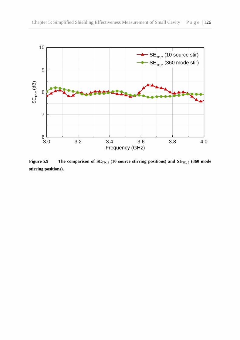
Chapter 5: Simplified Shielding Effectiveness Measurement of Small Cavity P a g e | 126
Figure 5.9 The comparison of SETD, 2 (10 source stirring positions) and SETD, 2 (360 mode
stirring positions).
3.0 3.2 3.4 3.6 3.8 4.06
7
8
9
10
SE
TD
,2 (
dB
)
Frequency (GHz)
SETD,2
(10 source stir)
SETD,2
(360 mode stir)

Chapter 5: Simplified Shielding Effectiveness Measurement of Small Cavity P a g e | 127

Chapter 5: Simplified Shielding Effectiveness Measurement of Small Cavity P a g e | 128
5.5 Discussions and Conclusion
In this chapter, the two-antenna methods for the SE measurement using the nested RC in both
the frequency domain and the time domain have been presented. These two-antenna methods
have simplified the measurement setup and improved the measurement efficiency. It is
demonstrated that the measured SEs using the proposed two-antenna methods and the
conventional three-antenna method agree well. The time-domain method goes to convergence
much faster than the frequency-domain methods. Consequently, in the time domain, fast and
accurate measurement can be realized by using the source stirring technique, which will
result in fast SE measurement in reality. Furthermore, in the time-domain approach, by
replacing the RC with a suitable conducting cavity (electrically large) and using the source
stirring technique, the hardware requirement will be greatly reduced. The aforementioned
measurement methods are compared. It is found that the time-domain method outperforms
the frequency-domain method with much higher measurement efficiency and much lower
hardware requirement.
Note that the proposed methods are based on the assumption that both the RC and the EUT
are well stirred, if not, the measured power transfer function and PDP will be of considerable
errors. Hence, the measured SE will be inaccurate. Another point that should be noted is that
high-efficiency antennas should be used for the time-domain method, i.e., the loss of the
antennas used in the measurement should be negligible. Otherwise, the measured PDP will be
influenced by the loss of the antennas and (5.20) is no longer valid. However, in the
frequency domain, as can be seen from (5.4), (5.5) and (5.6), the antenna efficiency has been
calibrated out in the net power transfer function. Thus, it is not necessary for the antennas to
be of high efficiency. Moreover, the proposed methods are general for SE measurement no
matter the SE is low or high. The measurement uncertainty is only determined by the
dynamic range of the VNA. When the EUT is well shielded, the power coupled from the RC
into the EUT will be very small. Consequently, S31 will be very small. Under this
circumstance, The VNA used in the measurement should have a large dynamic range to
measure the small S31 accurately. Or, the measured SE could be of big error. Finally, during
the measurement, the antennas (especially the one in the EUT) should be placed away from

Chapter 5: Simplified Shielding Effectiveness Measurement of Small Cavity P a g e | 129
the conducting walls of the cavities (at least quarter-wavelength distance from the nearest
walls for the lowest frequency) to avoid the boundary effect [25], [26].
5.6 References
[1] IEEE Standard Method for Measuring the Effectiveness of Electromagnetic Shielding
Enclosures, IEEE Standard 299, 2006.
[2] D. A. Hill, M. T. Ma, A. R. Ondrejka, B. F. Riddle, M. L. Crawford, and R. T. Johnk,
“Aperture excitation of electrically large, lossy cavities,” IEEE Trans. Electromagn.
Compat., vol. 36, no. 3, pp. 169-178, Aug. 1994.
[3] D. A. Hill, Electromagnetic Fields in Cavities: Deterministic and Statistical Theories.
New York, NY, USA: Wiley-IEEE Press, 2009.
[4] C. L. Holloway, D. A. Hill, M. Sandroni, J. M. Ladbury, J. Coder, G. Koepke, A. C.
Marvin, and Y. He, “Use of Reverberation Chambers to Determine the Shielding
Effectiveness of Physically Small, Electrically Large Enclosures and Cavities,” IEEE
Trans. Electromagn. Compat., vol. 50, no. 4, pp. 770-782, Nov. 2008.
[5] Q. Xu, Y. Huang, X. Zhu, L. Xing, Z. Tian, and C. Song, “Shielding Effectiveness
Measurement of an Electrically Large Enclosure Using One Antenna,” IEEE Trans.
Electromagn. Compat., vol. 57, no. 6, pp. 1466-1471, Dec. 2015.
[6] C. L. Holloway, D. A. Hill, J. Ladbury, G. Koepke, and R. Garzia, “Shielding
effectiveness measurements of materials using nested reverberation chambers,” IEEE
Trans. Electromagn. Compat., vol. 45, no. 2, pp. 350-356, May 2003.
[7] J. Carlsson, K. Karlsson, and A. Johansson, “Validation of shielding effectiveness
measurement method using nested reverberation chambers by comparison with
aperture theory,” in Proc. IEEE Int. Symp. Electromagn. Compat., Sept. 2012, pp. 1-6.

Chapter 5: Simplified Shielding Effectiveness Measurement of Small Cavity P a g e | 130
[8] G. B. Tait, R. E. Richardson, M. B. Slocum, and M. O. Hatfield, “Time-Dependent
Model of RF Energy Propagation in Coupled Reverberant Cavities,” IEEE Trans.
Electromagn. Compat., vol. 53, no. 3, pp. 846-849, Aug. 2011.
[9] S. Greco, and M. S. Sarto, “Hybrid Mode-Stirring Technique for Shielding
Effectiveness Measurement of Enclosures Using Reverberation Chambers,” in Proc.
IEEE Int. Symp. on Electromagn. Compat., Jul. 2007, pp. 1-6.
[10] Electromagnetic Compatibility (EMC) Part 4-21: Testing and Measurement
Techniques-Reverberation Chamber Test Methods, IEC 61000-4-21, 2003.
[11] Z. Tian, Y. Huang, Y. Shen, and Q. Xu, “Efficient and Accurate Measurement of
Absorption Cross Section of a Lossy Object in Reverberation Chamber Using Two
One-Antenna Methods,” IEEE Trans. Electromagn. Compat., vol. 58, no. 3, pp. 686-
693, Jun. 2016.
[12] C. L. Holloway, H. A. Shah, R. J. Pirkl, W. F. Young, D. A. Hill, and J. Ladbury,
“Reverberation Chamber Techniques for Determining the Radiation and Total
Efficiency of Antennas,” IEEE Trans. Antennas Propag., vol. 60, no. 4, pp. 1758-
1770, Apr. 2012.
[13] P. S. Kildal, X. Chen, C. Orlenius, M. Franzen, and C. S. L. Patane, “Characterization
of Reverberation Chambers for OTA Measurements of Wireless Devices: Physical
Formulations of Channel Matrix and New Uncertainty Formula,” IEEE Trans.
Antennas Propag., vol. 60, no. 8, pp. 3875-3891, Aug. 2012.
[14] Y. Huang, and D. J. Edwards, “A novel reverberating chamber: the source-stirred
chamber,” 8th Int. Conf. Electromagn. Compat., Edinburgh, 1992, pp. 120-124.
[15] D. A. Hill, “Electronic mode stirring for reverberation chambers,” IEEE Trans.
Electromagn. Compat., vol. 36, no. 4, pp. 294-299, Nov. 1994.
[16] C. R. Dunlap, “Reverberation chamber characterization using enhanced backscatter
coefficient measurements,” Ph.D. dissertation, Dept. of Elect. Comput. and Eng.,
Univ. of Colorado, Boulder, USA, 2013.

Chapter 5: Simplified Shielding Effectiveness Measurement of Small Cavity P a g e | 131
[17] C. R. Dunlap, C. L. Holloway, R. Pirkl, J. Ladbury, E. F. Kuester, D. A. Hill, and S.
van de Beek, “Characterizing reverberation chambers by measurements of the
enhanced backscatter coefficient,” in Proc. IEEE Int. Symp. on Electromagn.
Compat., Aug. 2012, pp. 210-215.
[18] G. B. Tait, R. E. Richardson, M. B. Slocum, M. O. Hatfield, and M. J. Rodriguez,
“Reverberant Microwave Propagation in Coupled Complex Cavities,” IEEE Trans.
Electromagn. Compat., vol. 53, no. 1, pp. 229-232, Feb. 2011.
[19] J. S. Giuseppe, C. Hager, and G. B. Tait, “Wireless RF Energy Propagation in
Multiply-Connected Reverberant Spaces,” IEEE Antennas Wireless Propag. Lett.,
vol. 10, pp. 1251-1254, 2011.
[20] R.Richardson, “Reverberant microwave propagation,” Naval Surface Warfare Center,
Dahlgren Division, Dahlgren, VA, Tech. Rep. NSWCDD/TR-08/127, Oct. 2008.
[21] A. H. Davis, “Reverberation equations for two adjacent rooms connected by an
incompletely soundproof partition,” Philos. Mag., vol. 50, no. 295, pp. 75–80, Jul.
1925.
[22] A. D. Pierce, Acoustics: An Introduction to Its Physical Principles and Applications.
New York: McGraw-Hill, 1981, ch. 6.
[23] C. L. Holloway, H. A. Shah, R. J. Pirkl, K. A. Remley, D. A. Hill, and J. Ladbury,
“Early Time Behavior in Reverberation Chambers and Its Effect on the Relationships
Between Coherence Bandwidth, Chamber Decay Time, RMS Delay Spread, and the
Chamber Buildup Time,” IEEE Trans. Electromagn. Compat., vol. 54, no. 4, pp. 714-
725, Aug. 2012.
[24] S. J. Boyes, “Reverberation Chambers and the Measurement of Antenna
Characteristics,” Ph.D. dissertation, Dept. of Elect. Eng. and Electron., Univ. of
Liverpool, Liverpool, U.K., 2013.
[25] D. A. Hill, “Boundary fields in reverberation chambers,” IEEE Trans. Electromagn.
Compat., vol. 47, no. 2, pp. 281-290, May 2005.

Chapter 5: Simplified Shielding Effectiveness Measurement of Small Cavity P a g e | 132
[26] A. Somani, S. Gorla, M. Magdowski, and R. Vick, “Measurement of boundary fields
in a reverberation chamber,” in Proc. IEEE Int. Symp. on Electromagn. Compat., Sept.
2011, pp. 123-127, IEEE Standard Method for Measuring the Effectiveness of
Electromagnetic Shielding Enclosures, IEEE Standard 299, 2006.

Chapter 6: Antenna Array Efficiency Measurement P a g e | 133
Chapter 6: Antenna Array Efficiency Measurement
6.1 Introduction
As mentioned in Chapter 1, RCs can be used for the characterization of DUTs, such as
antennas or wireless devices, and for the EMC testing. Chapter 3 to Chapter 5 have
considered the EMC testing/measurement in RCs. In this chapter, the characterization of
DUTs using RCs will be considered – antenna array efficiency measurement.
The efficiency of an antenna array is an important indicative measure of the merits of a given
design. Conventionally, the efficiency measurement of an antenna array is conducted in an
AC with the pattern integration method [1]. However, the measurement setup of this method
is complicated and the measurement uncertainty is usually high (>10%) [1]. Over the past
few years, the RC is becoming a prevalent alternative facility for performing radiated power
measurements of either an antenna or a DUT [2] – [7]. It is very applicable to determine the
efficiency of antennas.
In [8], the efficiency of an antenna array was measured with the reference antenna method in
an RC. In this approach, to make the array work in an “all-excited” manner, a power divider
is used to excite the feeding ports of the array elements simultaneously, that is, all the array
elements are excited through a power divider by merely a single excitation source. Thus, the
efficiency measurement of the entire array can be effectively treated in a manner similar to a
single port antenna, which would simplify the measurement procedure and reduce the overall
measurement time. Because of the introduction of the power divider that is external to the
array under test, the consequent insertion loss has to be calibrated out. In [8], to measure the
insertion loss of the power divider, all outputs except the one were terminated in impedance-
matched loads and the transmission coefficient between the input and the one output was
measured. Then the measurement proceeded in turn for each output (the insertion loss was
measured in the condition of 50 Ohm loads). It is correct for the antenna array that each
element is well-matched but it could be a problem when some elements are not well-matched
because the reflection from the array elements could contribute to the insertion loss of the
power divider, which will result in an inaccurate evaluation of the array efficiency.

Chapter 6: Antenna Array Efficiency Measurement P a g e | 134
In this chapter, it is shown that the array efficiency can be obtained accurately using a power
divider even when the elements of the array are not well-matched with the power divider.
This is realized by introducing proper attenuators between the array elements and the power
divider to alleviate the effect of the reflected power from the array to the insertion loss of the
power divider. The theoretical investigation is detailed. Simulations and measurements are
conducted to validate the effectiveness of the proposed method.
6.2 The Problem
As mentioned above, there is a problem with the existing method [8] for the efficiency
measurement of an antenna array which is hard to reveal it directly and clearly. However, it
can be much easier and clearer to start the analysis from a single antenna and then extend it to
an antenna array. Thus, the progressive steps in the problem-solving process will be made
explicit.
6.2.1 Single Antenna Case
In the single antenna case, a sleeve dipole antenna was selected as an AUT. A 5-dB RF
attenuator was connected to the AUT to introduce specific insertion loss, as shown in Figure
6.1(a). Measurements were performed from 2.6 to 2.8 GHz in the RC at the University of
Liverpool. In this measurement, the reference antenna method was adopted to obtain the
radiation efficiency and the total efficiency of the AUT. Two double-ridged waveguide horn
antennas were used as the transmitting antenna (SATIMO® SH 2000) and the reference
antenna (Rohde & Schwarz® HF 906), respectively. The antennas were connected to a VNA
via cables running through the bulkheads of the chamber. During the measurement, the two
stirrers were moved simultaneously and stepwise to 360 positions (1 degree for each step). At
each mode stirring position, a full frequency sweep was performed using the VNA and the S-
parameters were collected. In this measurement, 10,001 points were sampled in the measured
frequency range. The measurement setup is shown in Figure 6.1(b).
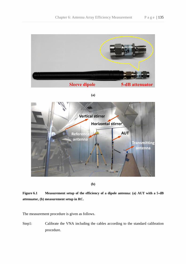
Chapter 6: Antenna Array Efficiency Measurement P a g e | 135
(a)
(b)
Figure 6.1 Measurement setup of the efficiency of a dipole antenna: (a) AUT with a 5-dB
attenuator, (b) measurement setup in RC.
The measurement procedure is given as follows.
Step1: Calibrate the VNA including the cables according to the standard calibration
procedure.

Chapter 6: Antenna Array Efficiency Measurement P a g e | 136
Step2: Place the AUT, the reference antenna, the transmitting antenna and the
supports inside the RC to keep the chamber loss constant.
Step3: Connect the AUT to port 1 of the VNA and the transmitting antenna to port 2
of the VNA, terminate the reference antenna with a 50 Ω load and record the
full S-parameters for each stirring position.
Step4: Disconnect the AUT from port 1 of the VNA and terminate it with a 50 Ω load.
Connect the reference antenna to port 1 of the VNA and the transmitting
antenna is kept connecting to port 2 of the VNA. Record the full S-parameters
for each stirring position.
The radiation efficiency of the AUT ( ) is then calculated using the reference antenna
method [9] – [11]
[
⟨| |
⟩
⟨|
| ⟩
|⟨ ⟩|
|⟨ ⟩|
]
where is the radiation efficiency of the reference antenna. The quantities ⟨|
| ⟩ and
⟨|
| ⟩ represent the stirred energy contributions of
and
, respectively [4].
and
are the transmission coefficients when the VNA port 1 is connecting to the AUT
and the reference antenna, respectively. and
are the reflection coefficients of the
AUT and the reference antenna, respectively. IL is the insertion loss introduced by the
attenuator (5 dB here). The measurement results are shown in Figure 6.2. As can be seen,
when the AUT is matched very well (S11 is approximately below -15 dB in this case), the
measured radiation efficiency agrees well with the real radiation efficiency (the real
radiation/total efficiency was measured with the conventional reference antenna method
without the attenuator which should be accurate), shown as the shaded band. However, when
the AUT is not well matched, considerable errors may occur (the maximum error is
approximately 25% in this case). The reason can be explained as follows: when the AUT is
very well matched, and |⟨
⟩| , which means is not easily
influenced by . The contribution of
to is negligible. However, when the AUT
is not well matched, the contribution of to
cannot be neglected. Actually, the
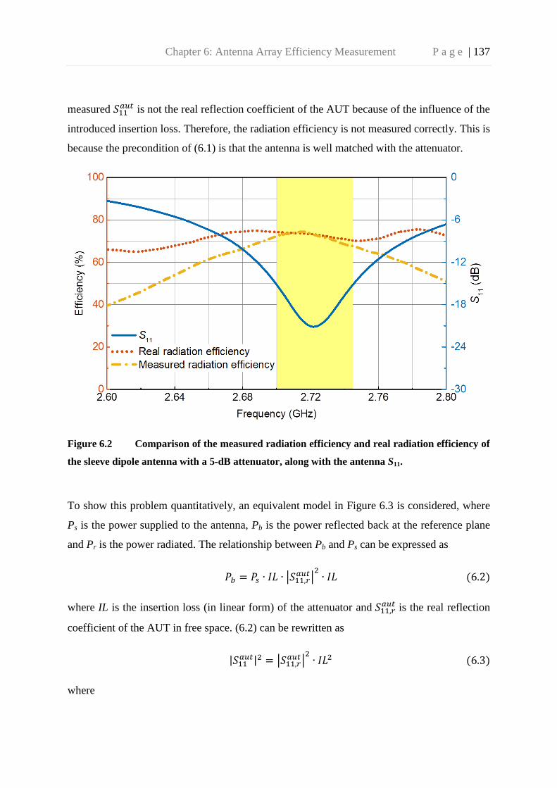
Chapter 6: Antenna Array Efficiency Measurement P a g e | 137
measured is not the real reflection coefficient of the AUT because of the influence of the
introduced insertion loss. Therefore, the radiation efficiency is not measured correctly. This is
because the precondition of (6.1) is that the antenna is well matched with the attenuator.
Figure 6.2 Comparison of the measured radiation efficiency and real radiation efficiency of
the sleeve dipole antenna with a 5-dB attenuator, along with the antenna S11.
To show this problem quantitatively, an equivalent model in Figure 6.3 is considered, where
Ps is the power supplied to the antenna, Pb is the power reflected back at the reference plane
and Pr is the power radiated. The relationship between Pb and Ps can be expressed as
| |
where IL is the insertion loss (in linear form) of the attenuator and is the real reflection
coefficient of the AUT in free space. (6.2) can be rewritten as
| | |
|
where

Chapter 6: Antenna Array Efficiency Measurement P a g e | 138
| | ⁄
is the measured reflection coefficient at the reference plane.
Figure 6.3 The equivalent model.
The radiated power Pr is linked to the supplied power Ps by
| |
where is the real radiation efficiency of the antenna. The corresponding transformation
of (6.5) is
| |
where
⁄
is the measured total efficiency at the reference plane.
For the reference antenna method, it can be derived
⁄ ⟨| |
⟩ ⟨|
| ⟩⁄
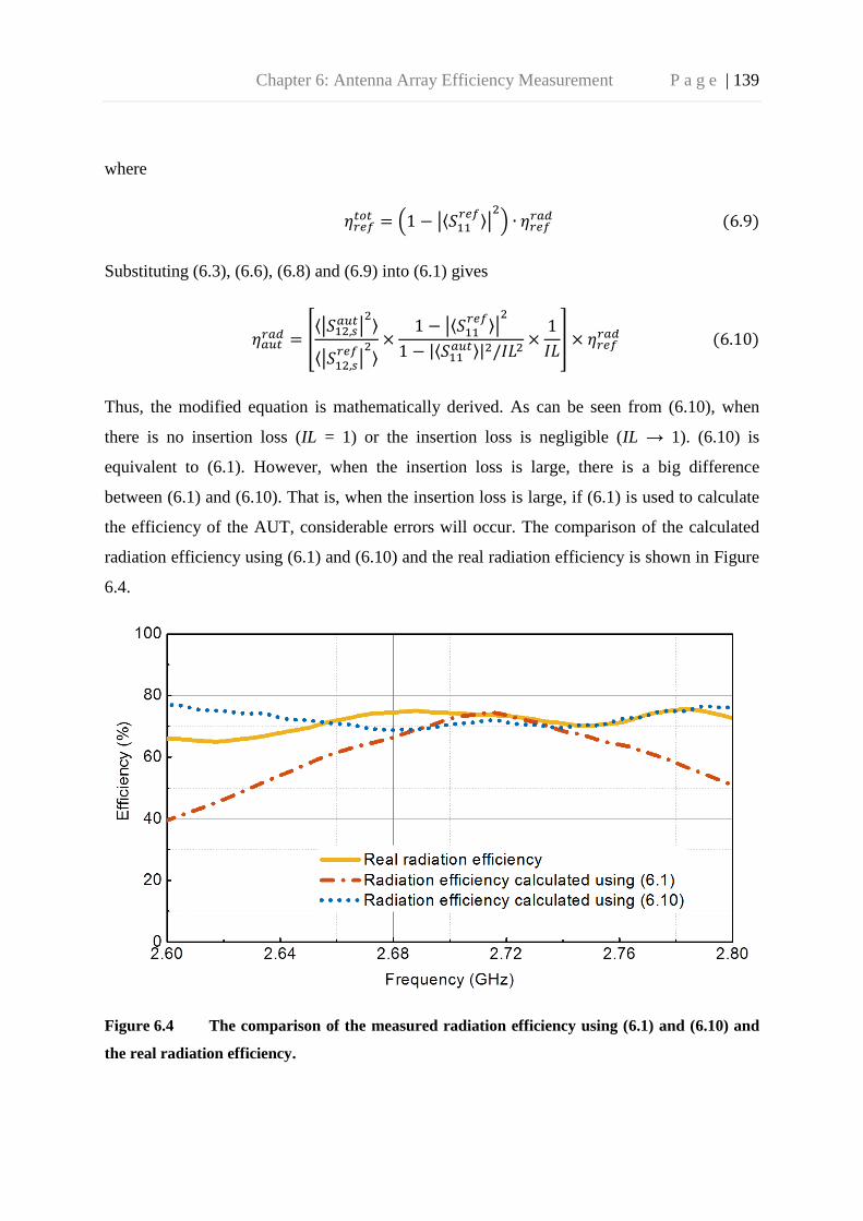
Chapter 6: Antenna Array Efficiency Measurement P a g e | 139
where
( |⟨
⟩| )
Substituting (6.3), (6.6), (6.8) and (6.9) into (6.1) gives
[
⟨| |
⟩
⟨|
| ⟩
|⟨ ⟩|
|⟨ ⟩|
]
Thus, the modified equation is mathematically derived. As can be seen from (6.10), when
there is no insertion loss (IL = 1) or the insertion loss is negligible (IL → 1). (6.10) is
equivalent to (6.1). However, when the insertion loss is large, there is a big difference
between (6.1) and (6.10). That is, when the insertion loss is large, if (6.1) is used to calculate
the efficiency of the AUT, considerable errors will occur. The comparison of the calculated
radiation efficiency using (6.1) and (6.10) and the real radiation efficiency is shown in Figure
6.4.
Figure 6.4 The comparison of the measured radiation efficiency using (6.1) and (6.10) and
the real radiation efficiency.

Chapter 6: Antenna Array Efficiency Measurement P a g e | 140
Figure 6.5 Comparison of the real total efficiency and the measured total efficiency.
It can be seen that the radiation efficiency calculated using (6.10) seems closer to the real
radiation efficiency in most of the frequency span than that calculated using (6.1). But it does
not agree well with the real radiation efficiency as expected. At some frequency bands, say,
2.60 – 2.64 GHz, there is still significant error between the measured radiation efficiency and
the real radiation efficiency. This error is caused by the imperfection of the transition section
between the antenna and the attenuator or the attenuator and the cable. To be more specific,
when the AUT is connected with the attenuator, the reflection coefficient measured at the
reference plane is very small. Thus, it is easily affected by the mismatch caused by the
imperfection of the transition section. A small mismatch of the transition section may cause a
big variation of the reflection coefficient measured at the reference plane. Therefore, it would
be very difficult to calibrate the influence of the insertion loss to S11 of the AUT in practice.
Thus, in reality, the radiation efficiency is hard to be measured accurately when there is
insertion loss between the AUT and the feeding port. However, S12 is not easily affected by
the small mismatch of the transition section because this mismatch is negligible compared
with the insertion loss caused by the attenuator. Therefore, the total efficiency can be
measured correctly because the total efficiency depends only on
while not on ,

Chapter 6: Antenna Array Efficiency Measurement P a g e | 141
as indicated in (6.11). The comparison of the real total efficiency and the measured total
efficiency are shown in Figure 6.5. It can be seen that the results are in reasonable agreement.
[
⟨| |
⟩
⟨|
| ⟩ |⟨
⟩|
]
6.2.2 Antenna Array Case
When measuring the efficiency of an antenna array, to make the array work in an “all-
excited” manner, a power divider is normally adopted to excite the feeding ports of the array
elements simultaneously [8], [12], i.e., all the array elements are excited through a series of
power dividers by merely a single excitation source. Thus, the efficiency measurement of the
entire array can be effectively treated in a manner similar to a single port antenna. The power
divider is such a network with the property of appearing lossless when the output ports are
matched and only the reflected power from the output ports is dissipated [13]. The reflected
power will be consumed by the isolation resistance (Riso) in the power divider, as can be seen
in Figure 6.6.
Figure 6.6 A typical 2-way Wilkinson power divider in microstrip line format.

Chapter 6: Antenna Array Efficiency Measurement P a g e | 142
Therefore, the insertion loss of the power divider depends on the impedance of the external
device. When the elements of the antenna array are well matched, very small amount of
power will be reflected from each element and the insertion loss of the power divider can be
neglected. However, when the elements are not well matched, a large amount of power will
be reflected from each element and then dissipated on the Riso, thus the insertion loss can be
very large. Even worse, unlike the single antenna case, the insertion loss of the power divider
caused by the reflection from the antenna array cannot be quantified because it is not possible
to know how much power has been dissipated on Riso. Therefore, the measurement problem
caused by the insertion loss will become more complicated. Neither the radiation efficiency
nor the total efficiency can be measured accurately when the elements of the antenna array
are not well matched.
6.3 Improved Method
From the above analysis, it is known that it is difficult to quantify the insertion loss of the
power divider when the external device is not well matched. In this case, it is useful to try to
minimise the dissipated power on Riso of the power divider, i.e., minimise the reflected power
from the antenna array. In this section, we propose to introduce an attenuator of a proper
value between each array element and each power divider port. Actually, by introducing an
attenuator, the effects of mismatch between the array elements and the power divider ports
could be minimized. Thus, the use of the attenuator allows transferring the power that should
have been dissipated on Riso to the attenuator. To validate this idea, field-circuit co-simulation
is employed in CST (Computer Simulation Technology) Microwave Studio in the frequency
range of 2.0 – 3.5 GHz. A two-dipole array is adopted as an antenna under simulation, as can
be seen in Figure 6.7. In the two-dipole array, one element is 53.4 mm long and the other is
46.5 mm long. The spacing between these two elements is set to be 25.4 mm. The material
for making the array is PEC. The reflection coefficients, the phase of the reflection
coefficients and the transmission coefficients of the array are shown in Figure 6.8. As can be
seen, S11 and S22 are interlaced (both in amplitude and phase), which ensures that there will be
power loss on the Riso. Another thing that should be noted is that S21 and S12 are very small

Chapter 6: Antenna Array Efficiency Measurement P a g e | 143
(below -15 dB), which means the mutual coupling between the two dipole elements is
negligible.
Figure 6.7 The two-dipole array used for simulation in CST.
Figure 6.8 The simulated S-parameters of the two-dipole array.

Chapter 6: Antenna Array Efficiency Measurement P a g e | 144
In practice, the mutual coupling between elements is an importance issue that needs to be
carefully considered in an antenna array. In this section, the impact of the mutual coupling to
the validity of the proposed method is studied as well and will be discussed later. The
schematic of the field-circuit co-simulation model is given in Figure 6.9. To obtain the power
loss on the Riso, a current probe P1 is introduced to monitor the current on the Riso. The
feeding power from port 1 is 1 W. The attenuation of the attenuators is tuned stepwise from 0
dB to 10 dB (2 dB per step). The power consumed on the Riso is shown in Figure 6.10. Two
things can be identified from this figure. First, because of the mismatch of the array elements,
there exists power loss on Riso (when the attenuation is zero, the power consumed is not zero).
Second, with the increase of the attenuation, the power consumed on Riso will decrease as
expected. When the attenuation is 10 dB, the power consumed on the Riso will be always
below 0.002 W, that is, only less than 0.2% power will be consumed by Riso.
Figure 6.9 Schematic of the circuit.

Chapter 6: Antenna Array Efficiency Measurement P a g e | 145
Figure 6.10 Simulated power consumed on the isolation resistance of the power divider for 1
W input power with different attenuators.
From the above simulation analysis, it can be seen that the attenuator can help to reduce the
power loss on the Riso. Because the attenuation value is exactly known, the insertion loss
caused by the attenuator can be calibrated out for the total efficiency measurement. However,
the radiation efficiency measurement is still a problem because the effect of the imperfection
of the transition section between the antenna and the attenuator or the attenuator and the cable
is hard to remove, as discussed in Section 6.2. In the following part, it will demonstrate that
the radiation efficiency can be measured accurately using the proposed method.
To demonstrate the effectiveness of the proposed method, a measurement was performed in
our RC. A 2-way 0° power divider (Mini-Circuits® ZAPD-4-S+) with a voltage standing
wave ratio (VSWR) < 1.33:1 from 2.0 – 4.2 GHz was employed in this study. The spacing of
the two output ports is 25.4 mm. The AUT in this study is a two-dipole array consisting of
two parallel dipole elements with the spacing of 25.4 mm. The S-parameters of the two dipole
elements are shown in Figure 6.11. The power divider is connected to the AUT to feed the
two dipole elements with equal weights, as can be seen from Figure 6.12.

Chapter 6: Antenna Array Efficiency Measurement P a g e | 146
Figure 6.11 Comparison of the measured total efficiency of the two-dipole array with the
conventional method and with the proposed method.
Figure 6.12 The two-dipole array connected with the 2-way power divider.

Chapter 6: Antenna Array Efficiency Measurement P a g e | 147
The measurement was conducted in the frequency range of 2.0 – 3.5 GHz. The reference
antenna method is adopted in this measurement. The measurement setup and measurement
procedure are the same as detailed in Section 6.2.1. The comparison of the measured total
efficiency of the two-dipole array with the conventional method and with the proposed
method is shown in Figure 6.11. It can be seen that, in the frequency range of 2.0 – 2.6 GHz
and 3.1 – 3.5 GHz, there is not much difference of the amplitude and phase between S11 and
S22. Therefore, very little power will be consumed on the Riso. Thus, the total efficiency
measured with the conventional method and with the proposed method agrees well. However,
in the frequency range of 2.6 – 3.1 GHz, there is a significant difference of the amplitude or
phase between S11 and S22, i.e., a considerable amount of power will be consumed by Riso. In
this case, the IL in (6.11) cannot be accurately obtained. The IL of the power divider
measured (using the method in [8]) is not correct because it is accurate only when the power
divider ports are terminated with impedance-matched loads, i.e., no reflection occurs. Thus,
considerable errors could occur if the conventional method is adopted for the not-well-
matched case. Conversely, for the proposed method, the IL is dominated by the attenuators
and the contribution of the power divider to the IL can be neglected. Besides, the reflected
power from the array elements will be attenuated by the attenuators as well. Hence, the IL of
the power divider including the reflection effect will have little influence on IL in (6.11). As
can be seen in Figure 6.11, the total efficiency measured using the conventional method has
obvious errors compared with that measured using the proposed method in the frequency
range of 2.6 – 3.1 GHz where the amount of the power consumed on Riso is big. The
maximum error can reach 15% at about 2.76 GHz, which cannot be neglected in practice.
One thing to be noted is that there is always some uncertainty on the attenuation value of the
attenuator. That is, the actual attenuation value is not always exactly the same as the nominal
value. The attenuator used in the experiment has about ± 0.5 dB deviation in the frequency
range of DC to 3.0 GHz [14]. To show the impact of the deviation of the attenuation value on
the efficiency of the antenna array, the field-circuit co-simulation was conducted in the
above-mentioned two-dipole array model in CST. The total efficiency of the two-dipole array
was calculated with the attenuation value of 9.5 dB, 10 dB, and 10.5 dB, respectively. The
results are shown in Figure 6.13.

Chapter 6: Antenna Array Efficiency Measurement P a g e | 148
Figure 6.13 The total efficiency of the two-dipole array in CST with different attenuation
values.
As can be seen, only a very small difference can be observed for the total efficiency of the
array calculated with different attenuation values in the full frequency span. The maximum
difference is only about 4% which is small. Thus, the impact of the uncertainty from the
attenuation value of the attenuator can be neglected. Another point that may be concerned is
the impact of the mutual coupling between antenna elements on the validity of the proposed
method. To investigate this issue, a simulation is done using CST. In this simulation, the
spacing between the two elements of the dipole array (as shown in Figure 6.7) is set to be 5.0
mm, which results in significant increase in the mutual coupling of the two dipole elements.
Thus, a new dipole array with higher mutual coupling is created. As can be seen from Figure
6.14, the mutual coupling of the new dipole array exceeds -10 dB from 2.5 GHz to 3.45 GHz
and can reach about -3 dB at 2.9 GHz. The array total efficiency predicted by CST (used as a
benchmark here) and that obtained from the field-circuit model using our proposed method
are plotted and compared in Figure 6.14. The total efficiency of the array with a low mutual

Chapter 6: Antenna Array Efficiency Measurement P a g e | 149
coupling (the array shown in Figure 6.7 and Figure 6.8) is also plotted for reference here. It
can be seen that no matter the mutual coupling is high or low, the efficiency obtained from
our proposed method does not have a big difference from the benchmark. The maximum
difference is only about 3% for both high coupling and low coupling scenarios, which is very
small. That is, the mutual coupling does not influence the validity of the proposed method.
The proposed method is general for the efficiency measurement of antenna arrays regardless
of the mutual coupling.
Figure 6.14 The two-dipole array total efficiency predicted by CST and that obtained from
the field-circuit model using our proposed method with low and high mutual coupling.
Once the total efficiency has been known, the radiation efficiency can be calculated by
excluding the impedance mismatch effect of the antenna elements. The radiation efficiency
can then be expressed as
| | | |

Chapter 6: Antenna Array Efficiency Measurement P a g e | 150
The array radiation efficiency, the array total efficiency and the mutual coupling S21 of the
two dipole elements are shown in Figure 6.15. As can be seen, the radiation efficiency is
reasonable and the mutual coupling between array elements is negligible.
Generally, for an antenna array with N elements, the total efficiency can be obtained using
(6.11) and the radiation efficiency will become
∑ | |
where i is the element number.
Figure 6.15 The comparison of the radiation efficiency and the total efficiency of the two-
dipole array and the mutual coupling S21 of the two dipole elements.
6.4 Measurement Uncertainty
To quantify the measurement uncertainty, the method proposed in [15] has been adopted. As
demonstrated in [15], the direct coupling can be a major source of uncertainty inherent during
over-the-air measurements in an RC. Therefore, the direct coupling (normally expressed as

Chapter 6: Antenna Array Efficiency Measurement P a g e | 151
the Rician K-factor) should be as small as possible. Furthermore, the uncertainty model
presented in [15] combines the random NLoS process and the random LoS process, and the
combined standard deviation can be written as
√
√
where √ ⁄ , √ ⁄ and K = average Rician K-factor,
comprising the samples obtained from mechanical stirring, source stirring and polarization
stirring. and are the NLoS independent samples and LoS independent
samples, respectively. The Rician K-factor is calculated as follows
|⟨
⟩|
⟨| ⟨
⟩| ⟩
The standard σ is presented in dB scale by averaging the dB values of ( ) and ( ),
i.e.,
(
)
is computed by applying the standardized circular autocorrelation to a 1D (one
dimensional) array written using the received power samples during one rotation cycle [16].
The critical value r suggested by the standard [7] is applied.
(
)
where n is the number of the checked samples (120 in our case). The autocorrelation
coefficient of the received power samples at the lowest frequency 2.0 GHz is shown in Figure
6.16. As can be seen, it is always below the critical value for the lag number from 1 to 199,
which means the 120 samples are independent. can be calculated via
where is the number of antenna positions, and is the number of independent
antennas used in the chamber. In our case, . The measured Rician K-

Chapter 6: Antenna Array Efficiency Measurement P a g e | 152
factor and standard deviation in decibel format are shown in Figure 6.17. It can be seen that
any contribution toward the uncertainty from LoS coupling is small and the overall
uncertainty inherent in the measurements is acceptably low.
Figure 6.16 The autocorrelation coefficient of the received power samples and the lag at
which the correlation is lost (@ 2.0 GHz).
Figure 6.17 Rician K-factor and standard deviation.

Chapter 6: Antenna Array Efficiency Measurement P a g e | 153
6.5 Discussions and Conclusion
In this chapter, an improved measurement-based method to obtain the efficiency of an all-
excited antenna array in an RC has been presented. When measuring the efficiency of an
antenna array in an RC, to make the array work in an “all-excited” manner, a power divider is
normally employed to excite the feeding ports of the array elements simultaneously, that is,
all the array elements are excited through a series of power dividers by merely a single
excitation source. Thus, the efficiency measurement of the entire array can be effectively
treated in a manner similar to a single port antenna, which would simplify the measurement
procedure and reduce the overall measurement time. However, the introduction of the power
divider will inevitably bring in insertion loss which needs to be quantified and calibrated out.
In our previous work, the calibration of the insertion loss of the power divider was
implemented by terminating all outputs in impedance-matched loads and measured the
transmission coefficient between the input and the output port. By repeating this procedure
for each output port, the S-parameters from the input to all output ports can be obtained. The
total insertion loss is calculated by summating the measured transmission coefficient of each
port. It is correct if each element of the antenna array is well matched. However, if some
elements of the array antenna are not well matched, a considerable error may occur. The
reason is, when the element is not well matched, a non-ignorable amount of the power fed to
the element will be reflected back to the power divider and then dissipated on the Riso. The
power dissipated on the Riso is very difficult to quantify. Therefore, the insertion loss of the
power divider cannot be exactly known.
In this study, the power dissipated on the Riso of the power divider has been minimized by
introducing 10-dB attenuators between array elements and power divider ports. The
attenuators would alleviate the reflection from the array antenna to the power divider and thus
reduce the dissipated power on the attenuator. Moreover, because the attenuation of the
attenuator is known, thus it can be calibrated out accurately. Simulations and measurements
have been done to validate the proposed method. The results show that this method is
effective to measure the efficiency of an antenna array especially for an antenna array that
some elements of it are not well matched. It is advantageous especially for wideband antenna
arrays where good impedance matching of array elements is difficult to maintain.

Chapter 6: Antenna Array Efficiency Measurement P a g e | 154
There are some points that need to be emphasized. Firstly, the attenuation of the attenuators
used in the measurement should be large enough. Otherwise, when the attenuator is loaded
with the mismatched antenna, the attenuation value will be changed [13]. In our case, a 10-dB
attenuator is suitable. Theoretically, the bigger the attenuation, the less sensitive the
attenuation to the impedance of the mismatched antenna, and consequently, the more accurate
the measured results will be. However, considering the dynamic range of the VNA, the
attenuation cannot be too large to ensure the accurate measurement of the S-parameters.
Therefore, the attenuation value should be carefully selected before the measurement.
Secondly, the proposed method is time-saving as the whole array is treated in a manner
similar to a single port antenna, and also it is no need to calibrate the insertion loss of power
divider. This is advantageous especially for arrays of a large number of elements. However,
no verification of this method has been performed for such arrays, and it is left as a topic for
future work.
6.6 References
[1] Y. Huang, “Radiation efficiency measurements of small antennas,” in Handbook of
Antenna Technologies, ed by Z. Chen, Singapore: Springer, 2015.
[2] D. A. Hill, Electromagnetic Fields in Cavities: Deterministic and Statistical Theories.
New York, NY, USA: Wiley-IEEE Press, 2009.
[3] C. L. Holloway, H. A. Shah, R. J. Pirkl, W. F. Young, D. A. Hill, and J. Ladbury,
“Reverberation chamber techniques for determining the radiation and total efficiency
of antennas,” IEEE Trans. Antennas Propag., vol. 60, no. 4, pp. 1758-1770, Apr.
2012.
[4] C. L. Holloway, D. A. Hill, J. M. Ladbury, P. F. Wilson, G. Koepke, and J. Coder,
“On the Use of Reverberation Chambers to Simulate a Rician Radio Environment for
the Testing of Wireless Devices,” IEEE Trans. Antennas Propag., Special Issue on
Wireless Communications, vol. 54, no. 11, pp. 3167-3177, Nov. 2006.

Chapter 6: Antenna Array Efficiency Measurement P a g e | 155
[5] H. G. Krauthäuser, and M. Herbrig, “Yet another antenna efficiency measurement
method in reverberation chambers,” in Proc. IEEE Int. Symp. Electromagn.
Compat.,Jul. 25-30, 2010, pp. 536-540.
[6] P.-S. Kildal, and K. Rosengren, “Correlation and capacity of MIMO systems and
mutual coupling, radiation efficiency, and diversity gain of their antennas: simulations
and measurements in a reverberation chamber,” IEEE Commun. Mag., vol. 42, no. 12,
pp. 104-112, Dec. 2004.
[7] Electromagnetic Compatibility (EMC) part 4-21: Testing and measurement
techniques-Reverberation chamber test methods, IEC 61000-4-21, 2003.
[8] S. J. Boyes, Y. Zhang, A. K. Brown, and Y. Huang, “A Method to De-Embed
External Power Dividers in Efficiency Measurements of All-Excited Antenna Arrays
in Reverberation Chamber,” IEEE Antennas Wireless Propag. Lett., vol. 11, pp. 1418-
1421, 2012.
[9] K. Rosengren, and P.-S. Kildal, “Radiation efficiency, correlation, diversity gain and
capacity of a six-monopole antenna array for a MIMO system: Theory, simulation and
measurement in reverberation chamber,” IEE Proc. Microw. Antennas Propag., vol.
152, pp. 7-16, 2005.
[10] G. le Fur, C. Lemoine, P. Besnier, and A. Sharaiha, “Performances of UWB wheeler
cap and reverberation chamber to carry out efficiency measurements of narrowband
antennas,” IEEE Antennas Wireless Propag. Lett., vol. 8, pp. 332-335, 2009.
[11] S. J. Boyes, P. J. Soh, Y. Huang, G. A. E. Vandenbosch, and N. Khiabani,
“Measurement and Performance of Textile Antenna Efficiency on a Human Body in a
Reverberation Chamber,” IEEE Trans. Antennas Propag., vol.61, no.2, pp. 871-881,
Feb. 2013.
[12] M. V. Ivashina, M. N. M. Kehn, P.-S. Kildal, and R. Maaskant, “Decoupling
efficiency of a wideband Vivaldi focal plane array feeding a reflector antenna,” IEEE
Trans. Antennas Propag., vol. 57, no. 2, pp. 373-382, 2009.

Chapter 6: Antenna Array Efficiency Measurement P a g e | 156
[13] David M. Pozar, “Power dividers and directional couplers,” in Microwave
Engineering, 4th ed., 2011, Singapore: Wiley, pp. 317-379.
[14] [Online]. Available: http://uk.rs-online.com/web/p/products/2859551/?tpr=3.
[Accessed: 04-Nov-2016].
[15] P. S. Kildal, X. Chen, C. Orlenius, M. Franzen, and C. S. L. Patane, “Characterization
of Reverberation Chambers for OTA Measurements of Wireless Devices: Physical
Formulations of Channel Matrix and New Uncertainty Formula,” IEEE Trans.
Antennas Propag., vol. 60, no. 8, pp. 3875-3891, Aug. 2012.
[16] F. Moglie, and V. M. Primiani, “Analysis of the Independent Positions of
Reverberation Chamber Stirrers as a Function of Their Operating Conditions,” IEEE
Trans. Electromagn. Compat., vol. 53, no. 2, pp. 288-295, May 2011.

Chapter 7: Conclusions and Future Work P a g e | 157
Chapter 7: Conclusions and Future Work
In this thesis, efficient measurement techniques in an RC have been discussed, including the
efficient measurement of the averaged ACS with only one antenna, the rapid volume
measurement method using the averaged ACS, the simplified SE measurement using the
nested RC with two antennas, and the improved antenna array efficiency measurement in an
RC. The efficient measurement is realized by using the enhanced backscatter effect or the
robustness of the chamber decay time for averaged ACS, cavity volume, and SE
measurement. And for the antenna array efficiency measurement, it has been pointed out the
RC method is much more efficient than the conventional AC method. Our contribution is to
make the measurement more accurate.
To be more specific, the key contributions in each chapter are summarized as follows:
Chapter 3: Averaged ACS measurement
The commonly used RC technique for determining the averaged ACS of a lossy object
requires two antennas and the radiation efficiency of the two antennas should be known. In
this chapter, the one-antenna method in both the frequency domain and the time domain was
presented [1]. The measurement setup is greatly simplified and moreover, in the time domain,
the knowledge of the antenna efficiency is not required. From the experimental results, it is
found that the measured averaged ACSs by the three methods the conventional two-antenna
method, the proposed frequency-domain one-antenna method, and the proposed time-domain
one-antenna method are in good agreement. It is found that the time-domain method
converges much faster than the frequency-domain methods because of the robustness of the
chamber decay time (which is only determined by the diffuse loss of the chamber). A rapid
and accurate measurement can be achieved in the time domain based on this finding by using
source stirring technique. Furthermore, in the time-domain approach, the RC can be replaced
by a suitable electrically large conducting cavity, which will further reduce the hardware
requirement. The method was validated in the RC by setting the paddles stationary and the
results agree well with that measured in the RC using mechanical stirring. It is demonstrated

Chapter 7: Conclusions and Future Work P a g e | 158
that the time-domain method is much more efficient and its hardware requirement is much
lower than the frequency-domain method.
Chapter 4: Cavity volume measurement using statistical EM theory
In this chapter, an efficient and effective method for measuring the volume of a large cavity
is proposed [2]. A piece of RAM with a known averaged ACS is selected to aid the
measurement. The cavity volume can be obtained by measuring its decay time constants with
and without the RAM. Both the theory and measurement studies are conducted. It is found
that the measurement can be completed rapidly with a simple measurement setup using the
proposed method, which makes it an attractive method for the cavity volume measurement.
Moreover, by using acoustic waves, the proposed method can be generalized and the cavity
under test does not have to be metallic.
Chapter 5: SE measurement using nested RC
The conventional method for SE measurement of a physically small but electrically large
cavity in an RC requires three antennas. And the efficiency of the two receiving antennas
should be known. In this chapter, two-antenna methods for the SE measurement using the
nested RC were proposed in both the frequency domain and the time domain [3]. The
measurement setup is simplified and the measurement efficiency is improved. It is
demonstrated that the measured SE using the proposed two-antenna methods and the
conventional three-antenna method agrees well. The time-domain method converges much
faster than the frequency-domain methods. Consequently, in the time domain, fast and
accurate measurement can be realized by using the source stirring technique, which will
result in fast SE measurement in reality. Furthermore, in the time-domain approach, by
replacing the RC with a suitable conducting cavity (electrically large) and using the source-
stir technique, the hardware requirement will be greatly reduced. The aforementioned
measurement methods are compared. It is found that the time-domain method outperforms
the frequency-domain method with much higher measurement efficiency and much lower
hardware requirement.
Chapter 6: All-excited antenna array efficiency measurement

Chapter 7: Conclusions and Future Work P a g e | 159
Chapter 6 proposes an improved measurement-based method to obtain the efficiency of an
all-excited antenna array in an RC [4]. When measuring the efficiency of an antenna array in
an RC, to make the array work in an “all-excited” manner, a power divider is normally
employed to excite the feeding ports of the array elements simultaneously, that is, all the
array elements are excited through a series of power dividers by merely a single excitation
source. Thus, the efficiency measurement of the entire array can be effectively treated in a
manner similar to a single port antenna, which would simplify the measurement procedure
and reduce the overall measurement time. However, the introduction of the power divider
will inevitably bring in insertion loss which needs to be quantified and calibrated out. The
previous calibration method is correct when each element of the antenna array is well
matched but not if some elements of the array antenna are mismatched. In this chapter, a new
method to remove the insertion loss effect of the power divider by introducing attenuators
between array elements and power divider ports was proposed. The attenuators would
alleviate the reflection from the array antenna to the power divider and thus reduce the
dissipated power on the power divider. Simulations and measurements have been done to
validate the proposed method. The results show that this method is effective to measure the
efficiency of an antenna array especially for an antenna array that some elements of it are not
well matched. It is advantageous especially for wideband antenna arrays where good
impedance matching of array elements is difficult to maintain.
There are also some possible future works related to this thesis:
Based on the conclusions drawn from above and taking into account the limitations of the
work present in each chapter, future work can be carried out in the following area.
From Chapter 3, the calculation of the ACS requires the difference in the net power transfer
function (in the frequency domain) or the chamber decay time (in the time domain) with and
without the OUT. If the loss of the OUT is too small compared with that of the chamber itself,
it will be very difficult for the chamber to distinguish the difference of the loss, which will
result in the inaccuracy of the measurement. How to measure the ACS of a small OUT in a
big RC is still a problem. Is there any method to improve the “sensitivity” of the RC? This
work is still under investigation. Another possible future work may include the real

Chapter 7: Conclusions and Future Work P a g e | 160
application of the proposed one-antenna method for, e.g., the measurement of the ACS of
human bodies in the RC [5].
In Chapter 4, the condition of the proposed method is that the environment inside the cavity
under test should be reverberant, i.e., the cavity should not be too lossy. How to realize a
statistically uniform field inside a relatively lossy cavity is still a problem. Another issue is if
the cavity is partially filled with liquid or dielectric materials either absorb or reflect waves
completely (inhomogeneous cavity), the wave velocity is changed which could increase the
measurement error [6]. How the inhomogeneous materials affect the results is still unknown.
Finally, another possible extension of this work would be on-site measurement practice.
From Chapter 5, the assumption of the proposed method is that the EM field inside both the
RC and the EUT is statistically uniform. What if the EUT is very lossy? When the EUT is
very lossy, it is very difficult to stir the field inside the EUT well. Hence, the measured SE
will be inaccurate. Another problem is when the EUT is shielded very well the power coupled
from the RC into the EUT will be very small, even out of the VNA dynamic range sometimes.
Under this circumstance, a power amplifier is probably required to measure the SE accurately.
In this chapter, only a two-coupled-cavities scenario was considered. What will the results be
for a multiple-couple-cavities scenario (i.e., three or more cavities coupled)? The relevant
theory has been established in [7], but more practical investigations or applications are
needed. The industrial applications of the proposed simplified methods for real reverberant
environments such as the below-deck compartments in ships and aircraft cabins and bays are
also possible future work [8].
In Chapter 6, the time-saving merit of the proposed method is advantageous especially for
arrays of a large number of elements. For now, no verification of this method has been
performed for such arrays, and it is left as a topic for future work.
References

Chapter 7: Conclusions and Future Work P a g e | 161
[1] Z. Tian, Y. Huang, Y. Shen, and Q. Xu, “Efficient and Accurate Measurement of
Absorption Cross Section of a Lossy Object in Reverberation Chamber Using Two
One-Antenna Methods,” IEEE Trans. Electromagn. Compat., vol. 58, no. 3, pp. 686-
693, Jun. 2016.
[2] Z. Tian, Y. Huang, Q. Xu, and Gaosheng Li, “A Rapid Method for Measuring the
Volume of a Large Cavity Using Averaged Absorption Cross Section,” IEEE Access,
in revision.
[3] Z. Tian, Y. Huang, and Q. Xu, “Efficient Methods of Measuring Shielding
Effectiveness of Electrically Large Enclosures Using Nested Reverberation Chambers
with Only Two Antennas,” IEEE Trans. Electromagn. Compat., DOI:
10.1109/TEMC.2017.2696743.
[4] Z. Tian, Y. Huang, and Q. Xu, “An Improved Method for Efficiency Measurement of
All-Excited Antenna Array in Reverberation Chamber Using Power Divider,” IEEE
Trans. Antennas Propag., vol. 65, no. 6, pp. 3005-3013, Jun. 2017.
[5] I. D. Flintoft, G. C. R. Melia, M. P. Robinson, J. F. Dawson, and A. C. Marvin.
“Rapid and accurate broadband absorption cross-section measurement of human
bodies in a reverberation chamber,” Meas. Sci. Technol., vol. 26, no. 6, pp. 65701-
65709, Jun. 2015.
[6] Q. Xu, Y. Huang, L. Xing, Z. Tian, Z. Fei, and L. Zheng, “A Fast Method to Measure
the Volume of a Large Cavity,” IEEE Access, vol. 3, pp. 1555-1561, 2015.
[7] G. B. Tait, R. E. Richardson, M. B. Slocum, M. O. Hatfield, and M. J. Rodriguez,
“Reverberant Microwave Propagation in Coupled Complex Cavities,” IEEE Trans.
Electromagn. Compat., vol. 53, no. 1, pp. 229-232, Feb. 2011.
[8] G. B. Tait, and M. B. Slocum, “Electromagnetic environment characterization of
below-deck spaces in ships,” in Proc IEEE Int. Symp. on Electromagn. Compat.,
Detroit, MI, 2008, pp. 1-6.

Appendix A P a g e | 162
Appendix A. Vector and Dyadic Analysis
In a rectangular coordinate, a general vector can be written as
where ( ) denotes the unit vector for the rectangular coordinate system.
Vector addition is defined as
Scalar multiplication or dot product is defined as
Vector multiplication or cross product is defined as
|
|
The frequently used differential operators are the gradient ( ), divergence ( ), curl
( ), and Laplacian ( ). In a rectangular coordinate, the vector operator del ( ) is
and the differential operations are written as [1]
||
||
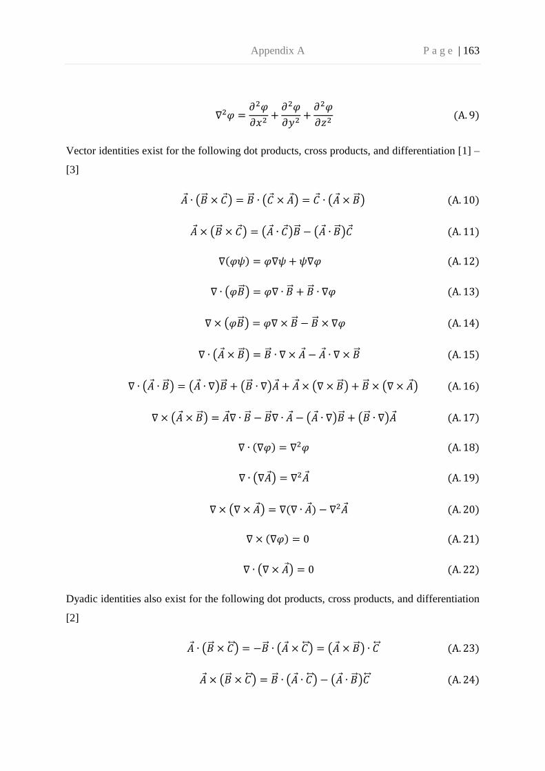
Appendix A P a g e | 163
Vector identities exist for the following dot products, cross products, and differentiation [1] –
[3]
( ) ( ) ( )
( ) ( ) ( )
( )
( )
( )
( ) ( ) ( ) ( ) ( )
( ) ( ) ( )
( )
( )
( )
Dyadic identities also exist for the following dot products, cross products, and differentiation
[2]
( ) ( ) ( )
( ) ( ) ( )

Appendix A P a g e | 164
( )
( )
( ) ( )
( )

Appendix B P a g e | 165
Appendix B. Probability Density Function
For a random variable g, the probability that g lies within a small range between g and g + dg
can be written as f(g)dg. The function f(g) is called the probability density function (PDF).
Since probabilities cannot be negative, all PDFs must be positive or zero
f(g) ≥ 0, for all g (B.1)
PDFs do not have to be continuous or even finite. However, since the random variable g must
lie between -∞ and +∞, the following integral relationship must hold [4]
∫
The mean value or ensemble average (normally designated µ) of g is ⟨ ⟩ which can be
determined from the following integral using the PDF
⟨ ⟩ ∫
The variance (frequently designated as σ2) of g is defined as ⟨ ⟩. It can also be
determined from the PDF as
⟨ ⟩ ∫
The standard deviation σ is the square root of the variance.

Appendix B P a g e | 166
References
[1] R. F. Harrington, Time-Harmonic Electromagnetic Fields, 2nd Edition. New York:
Wiley-IEEE Press, 2001.
[2] C. T. Tai, Dyadic Green Functions in Electromagnetic Theory. New York: IEEE Press,
1997.
[3] D. L. Sengupta, and V. V. Liepa, Applied Electromagnetics and Electromagnetic
Compatibility. Hoboken, NJ: Wiley, 2006.
[4] D. A. Hill, Electromagnetic Fields in Cavities: Deterministic and Statistical Theories.
New York, NY, USA: Wiley-IEEE Press, 2009.