Efficient Generation of

Hyperpolarized Molecules

Utilizing the Scalar Order of

Parahydrogen

 

 

 

Thesis by

Valerie Ann Norton  

 

In Partial Fulfillment of the Requirements for the Degree of

Doctor of Philosophy  

 

 

 

CALIFORNIA INSTITUTE OF TECHNOLOGY

Pasadena, California

2010

(Defended 11 May 2010)

 

 

 

 

 

 

 

 

 

 

 

 

 

 

 

 

 

 

 

 

© 2010 Valerie Ann Norton

All Rights Reserved

ii 

 

Acknowledgements

I  would  like  to  thank  my  thesis  advisor,  Dan  Weitekamp,  for  his  invaluable 

support which has allowed me to work on interesting and diverse projects in my time at 

Caltech.  He has given me a truly unique opportunity to work on both experimental and 

theoretical  aspects  of  these  projects.   His  keen  insights  have  provided  the means  to 

surmount the obstacles along the way. 

I would also  like  to acknowledge Pratip Bhattacharya whose drive and passion 

brought PASADENA back to Pasadena.  Without him, my part on the project would not 

have  been  possible.    He  and  his  colleagues  at  HMRI  have  been  instrumental  in  all 

aspects of the experimental work.  Eduard Chekmenev has brought a practicality to the 

process.    Jan  Hövener  was  a  great  help  in  making  the  wavelet  phase  experiments 

happen.    All  three,  as well  as  Kent Harris  and  Raymond Weitekamp,  have  had  their 

hands in building the polarizers and keeping them in working shape. 

I would also like to thank Jim Kempf, Gary Leskowitz, and Lou Madsen for being 

so welcoming when I first joined the group.  I would like to thank Bruce Lambert, Ramez 

Elgammal, and Mark Butler  for all  their  support during much of my  time here.   And  I 

would  like  to  thank  Jessica Pfeilsticker who has been making  the  final  few years here 

most  interesting and hopeful,  for  it  is her  task  to continue  the effort  to hyperpolarize 

ever more molecules. 

iii 

 

Abstract

This dissertation describes methods that polarize the spin of a specific nucleus in 

molecules synthesized by molecular addition of parahydrogen to a precursor molecule.  

Nuclear magnetic resonance  (NMR) pulse sequences are designed to perform efficient 

transfer  of  spin  order  by way  of  the  scalar  spin  couplings  between  the  two  nascent 

protons  and  a heteronuclear  spin  label  target.    The  result  is  an  increase  in  the NMR 

signal from that nucleus by several orders of magnitude, approaching unity polarization.  

Algorithms  are  presented  to  effect  the  desired  unitary  evolution  of  this  three‐spin 

system over the range of couplings  found  in diverse molecules and  in the presence of 

interfering spins.  These methods are explored theoretically and comparisons are made 

to select the most advantageous method given a specific problem. 

Issues  concerning  the  choice  of  target  molecule,  portable  equipment,  and 

automation are discussed.  Some design choices made for convenience in one aspect of 

the execution of  the methods  raise difficulties  in other aspects.   These difficulties are 

elucidated and methods of mitigation are discussed.   

Pulse  design  issues  are  elucidated with  numerical  calculations which  confirm 

analytical  results  for  the  time  dependence  obtained  in  the  multiply  rotating  frame 

approximation.    Failures  of  this  approximation  at  low  frequencies  are  explored 

numerically leading to novel pulse sequence design rules which ameliorate undesirable 

phenomena  peculiar  to  low  field  NMR,  enabling  its  employment  for  this  and  other 

iv 

 

applications  requiring precise  control of  the  spin degrees of  freedom.      Experimental 

results, primarily aimed at biomedical applications, are reviewed. 

v 

 

Table of Contents

Acknowledgements ..................................................................................................ii 

Abstract ................................................................................................................... iii 

Table of Contents ..................................................................................................... v 

Table of Figures ....................................................................................................... ix 

Nomenclature ....................................................................................................... xiii 

I.  History and Introduction ................................................................................. 1 

A.  Increasing polarization ................................................................................ 3 

B.  Hyperpolarization ....................................................................................... 4 

C.  Recent advances ......................................................................................... 8 

D.  Overview of thesis sections ...................................................................... 11 

II.  Background ................................................................................................... 13 

A.  Parahydrogen ............................................................................................ 13 

B.  PASADENA ................................................................................................. 15 

C.  Order Preservation ................................................................................... 18 

D.  Three Spin System ..................................................................................... 20 

III.  Pulse sequence algorithms ........................................................................... 24 

A.  Medium range pulse sequence algorithm ................................................ 24 

1.  Algorithm for  4θ π=  .......................................................................... 25 

2.  Modifications for a larger range ........................................................... 30 

vi 

 

3.  Operation in real systems ..................................................................... 32 

4.  Behavior under experimental error ...................................................... 36 

i.  Scalar coupling errors ....................................................................... 36 

ii.  Magnetic field strength and pulse power ......................................... 41 

B.  Small range pulse sequence algorithm ..................................................... 43 

1.  Algorithm for the limit  0θ →  .............................................................. 43 

2.  Modifications for a larger range ........................................................... 46 

3.  Operation in real systems ..................................................................... 47 

4.  Behavior under experimental error ...................................................... 48 

i.  Scalar coupling errors ....................................................................... 48 

C.  Large range pulse sequence algorithm ..................................................... 51 

1.  Algorithm for the limit  2θ π→  .......................................................... 51 

2.  Modifications for more consistent polarization ................................... 54 

3.  Operation in real systems ..................................................................... 56 

4.  Behavior under experimental error ...................................................... 57 

i.  Scalar coupling errors ....................................................................... 57 

D.  Comparison of sequence algorithms ........................................................ 60 

1.  For the range  4θ π≤  .......................................................................... 61 

2.  For the range  4π θ<  .......................................................................... 62 

IV.  Instrumentation and execution .................................................................... 65 

vii 

 

A.  Instrument hardware ................................................................................ 66 

B.  Computer program ................................................................................... 71 

C.  Field calibration......................................................................................... 77 

D.  Pulse calibration ........................................................................................ 79 

E.  Polarization ............................................................................................... 80 

F.  Polarization verification ............................................................................ 81 

G.  Molecule selection and characterization .................................................. 86 

1.  Measurement of   ............................................................................... 86 1T

2.  Measurement of coupling constants .................................................... 88 

3.  Molecular variations ............................................................................. 88 

V.  Low field effects ............................................................................................ 90 

A.  Lab frame introduction ............................................................................. 90 

B.  Using GAMMA for lab frame calculations ................................................ 93 

C.  Pulse length at low field ............................................................................ 95 

D.  Unintended nutation of other isotopes .................................................... 98 

E.  Bloch‐Siegert effects ............................................................................... 100 

F.  Wavelet phase dependence ................................................................... 101 

VI.  Solutions for wavelet phase dependence................................................... 108 

A.  Increase pulse time ................................................................................. 108 

B.  Only allow certain wavelet phases ......................................................... 109 

C.  Composite pulses .................................................................................... 110 

viii 

 

D.  Shaped pulses ......................................................................................... 112 

VII.  Further Considerations ........................................................................... 118 

A.  Refocused INEPT ..................................................................................... 118 

B.  Generation of singlet order .................................................................... 122 

C.  Conclusions ............................................................................................. 124 

VIII.  References .............................................................................................. 129 

 

ix 

 

Table of Figures

Figure 1. Energy levels of protons in a magnetic field ..................................................... 2 

Figure 2. Example PASADENA experiment ...................................................................... 6 

Figure 3. Maximum polarization using a single pulse ...................................................... 7 

Figure 4. Mole fraction of parahydrogen vs. temperature ............................................ 15 

Figure 5. Three‐spin system ........................................................................................... 20 

Figure 6. Medium θ  pulse sequence algorithm schematic........................................... 26 

Figure 7. Coordinate reference for describing evolution under the intrinsic 

Hamiltonian ..................................................................................................... 27 

Figure 8. Evolution of the system during the first two wait periods for Goldman’s 

algorithm ......................................................................................................... 29 

Figure 9. Maximum polarization using the medium θ  pulse sequence algorithm ....... 32 

Figure 10. 2,2,3,3‐tetrafluoropropyl 1‐13C‐propionate‐d3 ............................................... 33 

Figure 11. Utility of reoptimization of pulse sequence parameters for mitigating 

adverse effects of spectator spins .................................................................. 35 

Figure 12. Utility of longer pulses for mitigating the adverse effects of spectator spins 

of isotopes with similar frequencies ............................................................... 35 

Figure 13. Routes of succinate hydrogenation for selecting J‐coupling constants ......... 37 

Figure 14. Medium θ  pulse sequence algorithm sensitivity to errors in the J‐coupling 

constants near the high end of the range ...................................................... 39 

x 

 

Figure 15. 1‐phenylethylphenylphosphinic acid generation scheme .............................. 40 

Figure 16. Medium θ  pulse sequence algorithm sensitivity to errors in the J‐coupling 

constants near the low end of the range ....................................................... 41 

Figure 17. Echo pulse phase cycling to improve against  1B  offset problems ................. 42 

Figure 18. Small θ  pulse sequence algorithm schematic ............................................... 44 

Figure 19. Maximum polarization using the small θ  pulse sequence algorithm ............ 47 

Figure 20. Small θ  pulse sequence algorithm sensitivity to errors in the J‐coupling 

constants near the high end of the range ...................................................... 49 

Figure 21. Small θ  pulse sequence algorithm sensitivity to errors in the J‐coupling 

constants near the low end of the range ....................................................... 50 

Figure 22. Large θ  pulse sequence algorithm schematic ............................................... 53 

Figure 23. Total time required for large θ  sequence algorithm execution .................... 55 

Figure 24. Maximum polarization using the large θ  pulse sequence algorithm ............ 56 

Figure 25. Large θ  pulse sequence algorithm sensitivity to errors in the J‐coupling 

constants near the low end of the range ....................................................... 58 

Figure 26. Large θ  pulse sequence algorithm sensitivity to errors in the J‐coupling 

constants higher in the range ......................................................................... 59 

Figure 27. Comparison of the total time required for execution of the small and 

medium θ  pulse sequence algorithms .......................................................... 62 

Figure 28. Comparison of the total time required for the execution of the medium 

and large θ  pulse sequence algorithms ......................................................... 64 

xi 

 

Figure 29. Parahydrogen reactor ..................................................................................... 67 

Figure 30. Measured polarizer pulse shapes ................................................................... 68 

Figure 31. Experimental timeline ..................................................................................... 69 

Figure 32. Pulse programmer flow chart ......................................................................... 76 

Figure 33. Static field calibration curve ........................................................................... 78 

Figure 34. Pulse amplitude calibration curve .................................................................. 79 

Figure 35. Coupled protons used for measurement of the absolute polarization of a 

heteronucleus ................................................................................................. 84 

Figure 36. Coupled protons used for measurement of the absolute polarization of a 

heteronucleus in more complicated systems ................................................. 85 

Figure 37. Comparison of the lab frame and rotating frame .......................................... 91 

Figure 38. Optimization for determining good square π  pulse length .......................... 96 

Figure 39. Nutation path for square π  pulses ................................................................ 97 

Figure 40. Nutation of heteronuclei when using square pulses ...................................... 99 

Figure 41. Wavelet phase illustration ............................................................................ 103 

Figure 42. Schematic of wavelet phase effect experiment design philosophy ............. 104 

Figure 43. Experiment demonstrating wavelet phase effects ....................................... 105 

Figure 44. Optimal field and pulse strength for square π  pulses ................................. 106 

Figure 45. Nutation angle of square π  pulses .............................................................. 107 

Figure 46. Nutation angle of two simple composite π  pulses ...................................... 111 

Figure 47. Nutation of heteronuclei when using half‐sine pulses ................................. 114 

xii 

 

Figure 48. Optimal field and pulse strength for half‐sine π  pulses .............................. 115 

Figure 49. Nutation angle of half‐sine π  pulses ............................................................ 115 

Figure 50. Optimization for determining good half‐sine π  pulse length ...................... 117 

Figure 51. Average proton polarization on succinate after refocused INEPT ............... 121 

Figure 52. Example applications of these algorithms .................................................... 127 

 

 

xiii 

 

Nomenclature

AWG  arbitrary waveform generator 

DAQ  data acquisition card 

HEP  2‐hydroxy‐ethylpropionate 

INEPT  insensitive nuclear enhancement by polarization transfer 

MLEV  Malcolm Levitt’s decoupling sequence 

MRI  magnetic resonance imaging 

NMR  nuclear magnetic resonance 

NOE  nuclear Overhauser effect 

PASADENA  parahydrogen  and  synthesis  allow  dramatically  enhanced  nuclear 

alignment 

TFPP  2,2,3,3‐tetrafluoropropyl 1‐13C‐propionate‐d3 

Constants and parameters 

0B   static magnetic field magnitude 

1B   oscillating magnetic field magnitude 

f   quality factor for scalar spin order 

I   spin quantum number 

iI   the  nuclear  spin  angular momentum  operators  on  the  i th  proton with 

Cartesian components  ixI ,  iyI ,  izI ,  1,2i =  

xiv 

 

12J   J‐coupling between protons in radians per second 

1SJ ,  2SJ   heteronuclear J‐coupling in radians per second 

ijJ   J‐coupling constants in Hz 

k   Boltzmann’s constant 

P   polarization 

S   the nuclear spin angular momentum operators on the target nucleus with 

Cartesian components of  xS ,  ,   yS zS

T   temperature 

1T   time constant for longitudinal nuclear spin relaxation 

Hγ   gyromagnetic ratio of hydrogen 

Sγ   gyromagnetic ratio of the target nucleus 

φ   pulse carrier phase 

wφ   pulse wavelet phase 

θ   angular parameter classifying the 3‐spin system and the pulse sequences 

derived from the J‐coupling constants 

ρ   density operator of the spin system 

1lτ , 2lτ , 3lτ   duration of the three sections of the large θ  pulse sequence algorithm 

1mτ , 2mτ , 3mτ   duration  of  the  three  sections  of  the  medium  θ  pulse  sequence 

algorithm 

xv 

 

1sτ , 2sτ , 3sτ   duration of the three sections of the small θ  pulse sequence algorithm 

ω   reference angular frequency defining the rotating frame 

1 

 

I. History and Introduction

The  technique  of Nuclear Magnetic  Resonance  (NMR)  has  its  origins  in  Rabi’s 

molecular beam experiments  (1) measuring  the  intrinsic magnetic moment of  atomic 

nuclei  predicted  to  exist  by  quantum mechanics.   Guided  by  these  experiments  and 

Gorter’s attempt (2,3), Purcell (4) and Bloch (5) showed the same measurements could 

be  performed  on  hydrogen  in  solid  and  liquid  samples,  respectively,  using  inductive 

detection similar to that utilized today. 

The  presence  of  other  nuclear  and  electron  magnetic  moments  near  the 

measured  nuclear magnetic moment would  be  expected  to  affect  the measurement.  

One  way  this  effect  manifests  is  in  the  dependence  of  line  positions  on  sample 

orientation in single crystal solids shown by Purcell (6).  This single effect was enough to 

begin the use of NMR to probe chemical properties.   The power of the technique was 

first demonstrated by Pake  (7)  to measure  the hydrogen spacing  in CaSO4∙2H2O using 

both a single crystal and a powdered sample.

Other more  subtle effects were expected  (8), but were beyond  the abilities of 

the  equipment.    Refinement  in  equipment  and  an  ever  increasing  library  of  tested 

samples led quickly to new discoveries.  In metals, Knight found resonances that were at 

higher  frequencies  than  had  been  observed  for  salts  of  those metals  (9)  giving  the 

Knight  shift  due  to  coupling  to  rapidly  relaxing  electron  paramagnetism.    In 

simultaneous discoveries, it was found that the resonances of 14N (10) and 19F (11) were 

2 

 

dependent upon the chemical compound in which they were found giving the chemical 

shift.  Scalar couplings were found in NaSbF6 (12) although it was not correctly explained 

for another year (13). 

These  and  other  discoveries  have  formed  the  basis  by  which  the  nucleus 

becomes a sensitive probe of  the  local molecular environment.   Using  them,  it  is now 

possible  to  find  the  structure  of molecules  in  solution,  even  aqueous  proteins  (14).  

Kinetic studies (15‐17) are routinely done, including on systems at chemical equilibrium, 

for which NMR is uniquely capable of probing rates of reaction and diffusion. 

0 5 10 15 20−2

−1

0

1

2x 10

−4

magnetic field B0 (T)

ener

gy/k

T

 

Figure 1.  The separation of energy levels between states of protons with their magnetic moment 

aligned with  the  field and against  the  field  is dependent upon  the magnitude of  the  field.   This energy 

separation is small compared to  kT  at room temperature even in high field magnets. 

As  powerful  as  NMR  is  as  a  sensitive  probe  of  the molecular  structure  and 

dynamics,  it  is  highly  insensitive  as  well.    NMR  is  fundamentally  a  spectroscopic 

technique  studying  differences  in  energy  levels  that  are  small  compared  to   at 

ambient conditions (Fig. 

kT

1).  As a result, the system is highly disordered and the excess 

3 

 

population of  the  lower energy  level  is only  a  few parts per million even  in  the high 

fields, up to about 20 T, in use today.  It is possible to increase the equilibrium order at 

low temperatures, but relaxation times in the solid state can grow impractically long at 

low  temperatures and  the spectra desired  for chemical and biological applications are 

often required to be in the liquid state. 

A. Increasing polarization

The signal in NMR is proportional to the polarization of the nucleus that is being 

detected.  The fractional polarization of a nucleus is given by  

 N NPN N

+ −

+ −

−=

+  (1) 

where   is the number of spins aligned with the magnetic field and   is the number 

of spins aligned against  the  field.   A  few  techniques have been developed  in order  to 

combat  this  problem  of  low  signal  by manipulating  the  populations  of  energy  levels.  

Some  enhance  certain  population  differences  at  the  expense  of  others  that  are  less 

important or more rapidly refreshed.  For example, an increase in the polarization of an 

insensitive nucleus may be generated at the expense of proton polarization where the 

gain  factor  includes  the  ratio  of  the  gyromagnetic  ratios.    Saturation  of  hydrogen 

transitions  in  heteronuclear  systems  leads  to  small  enhancements  by  the  nuclear 

Overhauser effect (NOE), an example of cross relaxation between spins (18).  Somewhat 

larger  enhancements  can  be  achieved  by  using  resolved  scalar  couplings  between 

N+ N−

4 

 

isotopes  in  a  more  sophisticated  pulse  technique  such  as  insensitive  nuclear 

enhancement by polarization transfer (INEPT) (19).  While these techniques do increase 

the  polarization  available  for  detection  of  these  heteronuclei,  it  is  by  factors  on  the 

order of the ratio of the gyromagnetic ratios.  This is at most an order of magnitude for 

typical  isotopes.    Although  these  are  important  improvements  over  the  equilibrium 

values,  the  actual population difference  remains  the  same order of magnitude as  for 

protons at equilibrium. 

B. Hyperpolarization

Substantially  greater  order  can  be  imposed  on  the  system  by  using  some 

external perturbation in a few select nonequilibrium situations.  One example of this is 

chemically  induced dynamic nuclear polarization (20), where ultraviolet  light  is used to 

break apart a molecule and the following geminate radical recombination is directed in 

part by the nuclear state.  When the products have different resonant frequencies, large 

absorption and emission  lines can be seen from each of the products due to the order 

imposed by sorting of nuclear spin  in  the recombination process.   Another example  is 

optical  pumping  with  circularly  polarized  light  of  systems  where  unpaired  electrons 

interact with the nucleus.   The optical pumping orders the unpaired electron which  in 

turn helps to order the nucleus.    In gases, this has been used to polarize 3He  (21) and 

129Xe (22) mixed with Rb as high as 70%. 

The  technique  of  PASADENA  (parahydrogen  and  synthesis  allow  dramatically 

5 

 

enhanced nuclear alignment) (23‐25) (Fig. 2) applies the idea of chemically combining an 

easily generated, highly ordered, component with a disordered component as the initial 

step of  the  experiment.    The  system  generated  from  chemical  reaction of  these  two 

materials has a source of order  that may be manipulated  in an effort  to generate  the 

spin  order  desired  by  the  experimenter.    The  disordered  element  is  a  precursor 

molecule that will become the desired molecule after molecular addition of hydrogen.  

The ordered element is hydrogen in the para state, which is easily generated by passing 

molecular  hydrogen  over  a  catalyst  that  speeds  equilibration  of  spin  isomers  at 

sufficiently low temperature.  Removed from such catalytic particles, parahydrogen may 

be  stored  at  room  temperature  for  days without  significant  equilibration  of  the  spin 

state.  The signal gain possible from the technique is dependent upon the purity of the 

spin  state  of  the  reactant  hydrogen.    The  figure  of  merit  for  this  purity  is 

( )4 1pf χ= − 3  where  pχ  is the mole fraction of parahydrogen. 

6 

 

10 ms

π/4 pulse

π/4 pulse

10 ms

H2

H2

a)

b)

DBr

HBr

H

D

H

Br

H

H

H

Br

 

Figure 2.  Simulated PASADENA spectrum 10 ms after reaction for a) the reaction of 1‐bromo‐2‐

deutero‐ethylyne  with  parahydrogen  to  form  1‐bromo‐2‐deutero‐ethylene  and  b)  the  reaction  of 

bromoethylyne with parahydrogen to form bromoethylene. 

In the original proposal (23) and experimental demonstration (24,26), the newly 

introduced proton pair evolves under the new molecular Hamiltonian for a short time, 

on  the order of  seconds, while  the hydrogen product  accumulates.   Radiation of  the 

system with  a  4π  pulse  shows  strong  antiphase  peaks  (Fig.  2)  from  these  coupled, 

inequivalent protons.   As well as enhancing the signals from specific protons that were 

derived  from  a  chemical  reaction with  parahydrogen,  those  initial  papers  presented 

methods by which neighboring protons could be highly polarized as well.   The unitary 

evolution under  the chemical shift differences and scalar couplings can  ideally  lead  to 

 on  a  particular  site  (23).    In  order  to  reach  this  limit  experimentally,  it  is 

necessary to retard evolution out of the singlet state during the reaction, for instance by 

P f=

7 

 

coherently averaging the chemical shift difference of the protons to zero with a train of 

π  pulses  (27,28).    In practice,  any method of  sufficiently  strong proton decoupling  is 

suitable for this (29). 

Later  experiments  observed  enhanced  antiphase  multiplets  upon  a  spin  ½ 

heteronucleus  coupled  to  the  nascent  protons  from  parahydrogen  in  response  to  a 

single pulse (30).  This was quantified (31) using the same idea as for the homonuclear 

case: the scalar order of parahydrogen is projected onto the eigenstates of the product 

molecule  to  give  the  spin density operator  at  the beginning of  the NMR experiment.  

While  this  one‐pulse  experiment  is  inefficient,  it  ideally  has  the  capacity  to  generate 

polarization  of  nearly  3f  for  spin  systems  with  advantageous  coupling  constants 

(Fig. 3), a significant increase compared to equilibrium. 

0 0.5 1 1.50

50

100

P (

%)

θ (rad)  

Figure 3.   Maximum polarization on  the heteronucleus using a single pulse  technique  is  found 

using the formula  2cos sinP f θ θ= .  The value of θ  is dependent upon the scalar coupling constants of 

the system as defined in Eq. (17). 

8 

 

C. Recent advances

Proposals in the context of other experiments utilizing parahydrogen (27,28) as a 

source  of  scalar  order  demonstrate  the  use  of  a  decoupling  scheme  to  arrest  the 

evolution of  spin  states  in  the product molecule.   This  serves  to “suspend  time”  such 

that all molecules are in the same initial state when the decoupling stops.  In addition to 

the work utilizing parahydrogen  as  a  source of  spin order, other  experimenters have 

shown  that  equivalent  scalar  or  “singlet”  spin  order  can  be  prepared  from  Zeeman 

polarization  and  is  long‐lived  in  systems  with  inequivalent  hydrogen  sites  under 

sufficiently strong proton decoupling (32,33).  

The use of proton decoupling during  the chemical  reaction  for preservation of 

the  singlet  state  and  increased  lifetime  has  lead  to  the  development  of  a  more 

complicated  but  efficient  three  pulse  sequence  for  the  transfer  of  spin  order  to  a 

heteronucleus  (34,35), which  is discussed  in section  III.A.   This sequence  is capable of 

the  theoretical maximum  polarization P f=  for  advantageous  spin  systems.    In  this 

way, the nuclei can be made to be nearly fully aligned with the applied magnetic field 

increasing the signal by several orders of magnitude.   In practice, absolute polarization 

levels of 15‐20% have been achieved (36). 

Efforts are now being made  to expand  the number of molecules which can be 

hyperpolarized  subsequent  to  formation  from parahydrogen  and  also  to  increase  the 

spectroscopic environments in which externally generated molecules, hyperpolarized by 

9 

 

any method, may be used, particularly  in biological applications.   Hyperpolarized 129Xe 

has long been used for magnetic resonance imaging (MRI) of lung where sparse proton 

density and drastic magnetic susceptibility gradients make traditional methods difficult 

(37).  Also showing potential medical relevance, subsecond angiography was performed 

by real time imaging of a hyperpolarized tracer molecule, revealing flow in major blood 

vessels  in  rats  and  lung  vasculature  in  pigs  (38).    This  was  quickly  followed  by 

angiography utilizing more biologically relevant solutions (39). 

These  hyperpolarized  MRI  methods  are  intrinsically  transient  in  nature,  but 

utilize pulse  sequences usually  associated with  the unrelated method of  steady  state 

free  precession  (SSFP).    These  sequences  consist  of  hundreds  of  gradient  echo 

experiments  repeated  at  intervals  of  several ms  to  create  2D  and  3D  images.    For 

hyperpolarized studies, they are repurposed to gather unique data as quickly as possible 

where averaging is not required due to the high signal level (38).  This repurposing was 

improved by utilizing methods that refocus the magnetization at the end of each data 

collection window  instead of discarding  it with spoiling gradients, enabling 3D  imaging 

with a single hyperpolarized sample (40,41). 

Once  injected hyperpolarized molecules are moving  in the vascular system,  it  is 

of interest to study interactions of the molecules with some aspect of that system, such 

as their transport, binding, and metabolism.  To that end, an amphiphilic probe 2,2,3,3‐

tetrafluoropropyl  1‐13C‐propionate‐d3  (TFPP)  that  binds  with  lipid  bilayers  was 

developed (42).  When a binding event occurs, the chemical shift of this probe changes 

10 

 

sufficiently to be distinct from that of the molecule  in solution, enabling chemical shift 

imaging (CSI) in vivo (43).  With a similar method, tissue pH has been studied in vivo (44) 

by measuring  the  relative concentration of H13CO3‐ and  13CO2 which have a significant 

chemical shift difference. 

In  addition  to  these  simple  interactions, molecules  that  are  expected  to  react 

and  form new molecules  in  the accessible  time period can be  introduced  to a system 

and monitored. This application of CSI is used for metabolic imaging with pyruvate (45) 

and with succinate (46).  When the injected molecule reacts to form daughter molecules 

that  are  also  hyperpolarized,  those  new  molecules  are  initially  at  much  lower 

concentration than the  initial molecule, so have much  lower signal.    It  is useful to use 

large angle pulses  in order to see the product molecules, but  large angle pulses on the 

initial molecule drastically reduces the time  large polarizations are available.   Also, the 

signal  from  the  initial molecule may  overwhelm  signal  from  the  lower  concentration 

products.      In order  to mitigate dissipation of  spin order by observation of  the  initial 

species, shaped pulses have been developed that excite the products selectively while 

leaving the initial reactant largely unperturbed (47). 

The Faraday‐law signal level from a heteronucleus is not as large as that from an 

equally polarized proton by a factor of  ( )2S Hγ γ .  When the heteronucleus is being used 

in an MRI application,  larger gradients by a  factor of  H Sγ γ  must be used  in order  to 

acquire  the  same  spatial  resolution  as  with  protons.    On  the  other  hand,  protons 

11 

 

generally have much  shorter  lifetimes  than heteronuclei,  allowing  the polarization  to 

decay away before the molecule can be placed in a useful molecular environment.  With 

these limitations in mind, it has been shown that the long‐lived nucleus can be used for 

storing the polarization while a molecule is transported to the location where it reacts.  

When the experiment  is ready to be performed, the polarization can be moved to the 

more sensitive protons (48).  Further work has been done to improve this method in the 

complicated spin systems of  interest here using selective recoupling of a subset of the 

scalar couplings to direct the polarization as desired (49). 

D. Overview of thesis sections

Section  II  is  used  to  set  up  some  of  the  mathematical  tools  required  to 

understand the later sections.  First, parahydrogen is described in detail illustrating the 

scalar  order  it  contains  and  its  origin  in  rotational  energy  splittings.   Next,  the  early 

PASADENA experiments are briefly  reviewed, demonstrating  the quantification of  this 

spin  order  with  spin  density  operator  methods.    After  that,  a  “time  suspension” 

prescription for preserving the order during chemical reaction is described.  Finally, the 

theoretical methods needed  for the specific problem at hand, polarizing a third target 

heteronucleus, are introduced. 

Section III describes the methods for efficiently using parahydrogen as a source 

of order to generate very  large polarizations that are referred to as hyperpolarization.  

The prior art method of efficient order transfer from parahydrogen to a target nucleus 

12 

 

that results in theoretical polarization  1P =  for a small class of molecules is described in 

detail and  its effective range of applicability to molecules  is  increased by modifications 

to the algorithm for choosing pulse timing.  Then two further methods are developed to 

address molecules  that  are not well  addressed by  the existing method.    These entail 

novel uses of  coherent averaging  to effectively  change  the average  spin Hamiltonian.  

Finally, a comparison is made of the various algorithms. 

Section  IV  describes  the  hardware  and  software  used  to  implement  these 

methods.  Calibration procedures are illustrated.  Drawbacks to this particular hardware 

are  shown,  particularly  difficulties  using  pulsed  techniques  in  a  low  field, where  the 

usual  multiply  rotating  frame  approximation  fails.    Solutions  that  address  these 

problems are discussed. 

Theoretical calculations are used  throughout  in order  to  support and  illustrate 

the points made.  These calculations are performed with GAMMA (50), a library of NMR 

functions written  in C++  to  facilitate modeling of NMR  systems  to  varying degrees of 

exactness.   The calculations performed here are either  ideal or  lab  frame calculations.  

Ideal  calculations  make  use  of  certain  simplifications  such  as  the  rotating  frame 

approximation and ideal pulses.  Lab frame calculations more closely model the systems 

in question using audio frequency pulses with real shapes and this work introduces such 

exact  techniques  to  the  GAMMA  environment.    Relaxation  effects  are  discussed 

qualitatively to motivate experimental design. 

13 

 

II. Background

A. Parahydrogen

Molecular  hydrogen  is  a  diatomic  gas  at  standard  temperature  and  pressure.  

Hydrogen  is  found  in two stable  isotopes of which 1H  is vastly more common.   The 1H 

nucleus  is a spin ½ particle, so the symmetrization postulate demands that the overall 

wavefunction must be antisymmetric with respect to interchange of particle labels.  This 

nuclear  wavefunction  is  a  product  of  translational,  vibrational,  rotational,  and  spin 

functions. 

  ( ) ( ) ( ) ( ), , , ,t v rr r sψ θ φ ψ ψ ψ θ φ ψ=R R   (2) 

The translational portion of the function depends only on the location   of the center 

of mass,  so  is  unchanged  by  exchange  of  particles  and  is  necessarily  symmetric  in 

nature.    The  vibrational  portion may  be  approximated  by  the  eigenfunctions  of  the 

linear harmonic oscillator  for  sufficiently  small  vibrations.    These  are only dependent 

upon  the  change  of  the  magnitude  of  ,  the  distance  between  the  nuclei,  so  are 

likewise unchanged by the exchange of particles.   Since these are both symmetric, the 

antisymmetric nature of the overall wavefunction must come from either the rotational 

or spin functions. 

R

r

The  rotational  portion  of  the  wavefunction  is  characterized  by  the 

eigenfunctions of the rigid rotor.  These are given by the spherical harmonics 

14 

 

  ( ) ( ), cmimr le Pφ osψ θ φ θ∝   (3) 

where   and   are  the  quantum  numbers  corresponding  to  the  total  angular 

momentum  and  its  projection  along  an  axis  defined  by 

l m

0θ =  and 

( ) ( ) ( )2u1mmm

l lm

dP u P udu

= −  where  ( )lP u  are  the  Legendre  polynomials.    The 

exchange  of  particle  indices  is  equivalent  to  changing  ( )θ π θ→ −  and  ( )φ φ π→ + .  

Under  this  change,  all  rψ  with  even   are  symmetric  and  all l rψ  with  odd   are 

antisymmetric with respect to exchange. 

l

The spin portion of the wavefunction  is made up of  linear combinations of the 

direct product basis states. The required  linear combinations are eigenfunctions of the 

total  angular momentum  I  of  the  system which  can  be  1  or  0.    There  are 2 1I 3+ =  

states  for  1I =  which  comprise a  triplet  that  is  symmetric with exchange and 1  state 

with  , a singlet that is antisymmetric with exchange: 0I =

 ( )

( )

12

12

s T

s S

αα

ψ αβ βα

ββ

ψ αβ βα

⎧⎪⎪= +⎨⎪⎪⎩

= −

.  (4) 

To achieve the overall antisymmetry of the system, physical states with odd   must be 

in any one of the triplet states while states with even  l  only exist in the singlet state. 

l

The  lowest energy state of the system  is the one where   and the system  is 

in the spin singlet state.   This correlation of rotational and spin states allows a method 

0l =

15 

 

of generating a sample of hydrogen in a pure spin state by bringing it to equilibrium at a 

sufficiently  low  temperature.    In practice, a catalyst  is  required  to allow mixing of  the 

spin states sufficiently  to bring a sample  to equilibrium  in a reasonable  time.   For our 

experiments, hydrogen  gas was  flowed over  an  iron oxide  catalyst  at  roughly 18 K  in 

order  to  get  97%  or  better  purity.    This would  be  sufficient  to  generate  nearly  pure 

parahydrogen  if  it was brought  fully  to equilibrium at  this  temperature  (Fig. 4).   Once 

the  gas  is  removed  from  the  catalyst,  it may  be warmed  to  room  temperature  and 

stored for up to a week while maintaining high spin purity. 

0 50 100 150 200 250 300 3500

0.2

0.4

0.6

0.8

1

mol

e fr

actio

n of

par

ahyd

roge

n

temperature (K)  

Figure 4.  The mole fraction of parahydrogen in a hydrogen sample as a function of temperature. 

B. PASADENA

The  technique  of  PASADENA  utilizes  the  spin  order  found  in  parahydrogen  to 

generate  strong NMR  signals  from  specific magnetic  spins  in  the molecule.   By  itself, 

16 

 

parahydrogen  is  invisible to NMR since the overall spin of the system  is 0.    In order to 

generate signal  from  this system,  the symmetry must be broken  in some way.   This  is 

achieved by chemical  synthesis of a molecule of  interest by adding  the parahydrogen 

molecule across a double or triple bond in a manner that preserves the spin state of the 

two protons. 

It has been found (24,38,40) that Wilkinson’s catalyst (51) and similar cationic Rh 

complexes  that add hydrogen molecularly  such  that both nascent protons are on  the 

same side of a double or triple bonds also preserves the spin order of the protons.  This 

need  for  a molecular  addition hydrogenation  reaction mechanism  sets  a  limit on  the 

particular molecules that may be studied by the method. 

The  initial  condition  of  the  product  spin  system  is  given,  using  the  sudden 

approximation, as the state of the reactant system.   For the spins that come from the 

hydrogen molecule, this initial state is given by the density operator  

  ( ) 1 2 1 21 1 14 14 3 4H P fρ χ= − − ⋅ = −I I I I⋅   (5) 

where  Pχ  is the mole fraction of parahydrogen and   is the total spin operator for spin 

.    This  state has been  variously described  interchangeably  as  symmetrization order, 

scalar order, or singlet order.  It is fully characterized by 

iI

i

f  (Eq. (5)), which has the range 

1 3 1f− ≤ ≤ , the extremes exemplified by pure orthohydrogen and pure parahydrogen, 

respectively. 

The spins that are initially on the precursor molecule are at thermal equilibrium 

17 

 

with the environment so the density operator of spins 3  through  is given by  N

  ,

3

ˆexp

Ni z i

Xi

IHkT kT

ωρ

=

⎛ ⎞= − ≈ −⎜ ⎟

⎝ ⎠∑1   (6) 

where  iω  is  the  frequency of  the  spin  in  the  applied magnetic  field,   is Boltzmann’s 

constant,  and T  is  temperature.    The  total  density  operator  is  the  tensor  product  of 

these two operators. 

k

  H Xρ ρ ρ= ⊗   (7) 

Once  the  hydrogen  is  incorporated  into  a  molecule  where  the  symmetry  is 

broken,  the  singlet  state  is no  longer an eigenstate of  the  system but mixes with  the 

triplet state that has   projection along the  ‐axis.   For a fluid system of only the two 

protons from hydrogen, the Hamiltonian is  

0 z

  1 1 2 2 12 1 2ˆ

z zH I I Jω ω= + + ⋅I I   (8) 

where  12 122J Jπ=  is the scalar coupling between the protons in radians per second, and 

the eigenstates are given by 

 ( ) ( )( ) ( )2 2

2 2

1

2 cos sin

3 sin cos

4

κ κ

κ κ

αα

αβ βα

αβ β

ββ

=

= +

= − +

=

α  (9) 

where  ( )12 1 2tan Jκ ω= −ω .    In  the  above eigenbasis of  the Hamiltonian,  the density 

operator  Hρ  has the matrix representation  

18 

 

 

14

1 cos4 2 2

1cos2 4 2

14

0 00 sin0 s0 0 0

f

f f

f f

00

in 0f

κ

κ

κρ

κ

−

+

+

−

⎡ ⎤⎢ ⎥−⎢ ⎥=⎢ ⎥+⎢ ⎥⎢ ⎥⎣ ⎦

.  (10) 

The off‐diagonal coherences are lost if the spread of reaction times is long compared to 

the period of the coherence unless a method to suspend evolution  is used.   When this 

system is subjected to the pulse sequence  4wπτ − , a signal with antiphase doublet peaks 

separated by  12J  is seen at each chemical shift. 

This  signal  has  been  used  directly  as  a  sensitive  probe  of  protons  in  low 

population and short lived species such as in catalytic systems (24,25,52,53). 

C. Order Preservation

Each molecule  is  formed  in a coherent  superposition of  the eigenstates of  the 

spin Hamiltonian, and so  is evolving  in time starting from the creation of the molecule 

from precursor and parahydrogen.   The  spread of  reaction  times necessarily averages 

the  ensemble  density  operator  over  time,  however,  dissipating  that  part  of  the 

ensemble spin order which corresponds to these time dependent terms  in the density 

operator.    In order  to  fully utilize  this order,  it would be necessary  that  the  reaction 

happen  in  a  time  scale  short  compared  to  the  coherence  period,  which  is 

( )2212 1 22 Jπ ω ω+ −  (23,25).  For typical values of these spin Hamiltonian parameters, 

this  requires  that  the  reaction  be  completed  in  a  small  fraction  of  a  second.    This 

19 

 

requirement is impractically severe for known reactions. 

In the proposal of a related parahydrogen experiment, in which optical detection 

of  f  substitutes  for NMR detection of   (27,28),  it was pointed out  that a train of P π  

pulses  delivered  during  reactions,  in  this  case  during  an  initial  adsorption  or 

hydrogenation and a final desorption or dehydrogenation, would serve to preserve the 

spin order during those periods.   For the two spin case (23), this “time suspension” of 

the  spins, while  the  chemical  reaction  product  accumulates,  increases  the  attainable 

polarization   by a factor of two, enabling P P f= , ideally.  Although the protons are on 

the catalyst for a much shorter time than on the molecule, this “time suspension” is also 

important at these times to prevent mixing on the catalyst. 

Carravetta et al. (29,32) have demonstrated in a separate experiment that when 

the  scalar  order,  created  in  this  case  from  ordinary  polarization,  is  preserved  by 

decoupling,  such  as  a π  train,  the  lifetime of  that  state  is under  some  circumstances 

greatly  extended  beyond  the  lattice  relaxation  time  ,  typically  thought  of  as  the 

longest  time  constant  for  NMR  processes.    The  singlet  character  of  the  effective 

eigenstate protects  the population  from  relaxation due  to  fluctuations of  interactions 

that are symmetric with respect to exchange of the two hydrogen spin labels.  Notably, 

this  includes the  intrapair dipolar coupling, which  is time dependent  in solution due to 

molecular tumbling and frequently an important source of spin relaxation. 

1T

Taken  together,  the  time  suspension  aspect  and  the  decreased  spin‐lattice 

20 

 

relaxation  allow  for  reaction  times  of  some  seconds while  preserving  the  scalar  spin 

order.   Evolution under  the Hamiltonian  in Eq.  (8)  then  starts at  the  cessation of  the 

proton  decoupling  instead  of  the  moment  of  product  formation.  Thus,  decoupling 

allows  all  of  the  order  from  the  parahydrogen  to  be  accessible  to  the  experimenter 

within a new molecule. 

D. Three Spin System

The  system  of  interest  (Fig.  5)  for  heteronuclear  PASADENA  consists  of  three 

spins:  the  protons  derived  from  addition  of  parahydrogen   and  ,  which  are  the 

source of spin order in the system, and a relatively insensitive spin ½ nucleus S  which is 

the  target  for  spin order.   Transferring  spin order  to  the S  spin has many advantages 

that  include  its  longer  spin  lattice  relaxation  time,  lower  background  signal  from 

unpolarized molecules  in  a mixture,  and  the  greater  chemical  specificity  of  the NMR 

spectrum.   For the  initial discussion, other spins  in the molecule will be assumed to be 

noninteracting. 

1I 2I

R

O

H

D13C

O

D

DH

J1S

J2S

J12

 

Figure 5.  The 3‐spin system with the homonuclear and heteronuclear coupling constants defined 

on a representative molecule. 

21 

 

Immediately  following  the  addition  of  parahydrogen  to  a  precursor molecule, 

the spin state of the nascent protons is unchanged, therefore the initial condition is 

  ( )1 28 1fi H Xρ ρ ρ= ⊗ ≈ − ⋅I I   (11) 

and the rotating frame Hamiltonian for this fluid system in a static field is 

  1 1 2 2 12 1 2 1 1 2 2ˆ

S z z z S SH S I I J J Jω ω ω= + + + ⋅ + ⋅ + ⋅I I I S I S   (12) 

where  ijJ  are  the  scalar  coupling  constants  between  spins  in  rad/s.    The  desired 

evolution of the system is entirely mediated by the scalar coupling in the system so can 

be made  nearly  invariant  to  the  applied  static  field  so  long  as  it  is  high  enough  to 

separate Larmor frequencies allowing selective excitation of the different isotopes.  The 

field used in experiments is 1.8 mT, corresponding to a proton frequency of 75 kHz and 

carbon frequency of 19 kHz, which  is sufficiently  low that the chemical shift difference 

of the protons may be neglected but high enough to neglect the flip‐flop coupling terms 

between  heteronuclei.    Thus  the  Hamiltonian  in  the  doubly  rotating  frame may  be 

simplified to 

  12 1 2 1 1 2 2ˆ

S z z S z zH J J I S J I S= ⋅ + +I I .  (13) 

  For  the  discussion,  it  is  useful  to  represent  the  protons  with  the  pseudo‐spin  , 

defined as  

K

 

( )

1 2 1 2

1 2 1 2

11 22

x x x y y

y y x x

z z z

K I I I I

K I I I I

K I Iy

= +

= −

= −

  (14) 

22 

 

where  ( )1 2-S SJ J JΔ = 2 . This pseudo‐spin has the commutation relations of an angular 

momentum  spin  operator.    In  this  system,  the  initial  condition, with  f  set  to 1,  and 

Hamiltonian may be written as  

  ( )11 28 1 4 4i xK I Iρ = − − z z   (15) 

  ( )12 1 2 12 1 2ˆ 2x z z z z z z zH J K J K S J I I S J I IΔ += + + + +   (16) 

where  ( )1 2 2S SJ J J+ = + .   Of the three terms  in the  initial state, only the second term 

evolves under this Hamiltonian.  Of the four terms in the Hamiltonian, only the first two 

lead to  important evolution.   The third and  fourth terms  in the Hamiltonian commute 

with the other terms and with the initial density operator so are not considered further. 

The spin order that is important for evolution under this Hamiltonian is in the off 

diagonal elements represented by  xK .    It  is therefore  important that some method of 

order  preservation  be  applied  to  this  system.   Unlike  the Hamiltonian  in  Eq.  (8),  the 

symmetry breaking element is scalar coupling to a third nucleus rather than a difference 

in chemical shift.  Time suspension pulses, operationally the same as proton decoupling, 

suffice  during  the  reaction  period  in  order  to  preserve  the  product molecules  in  the 

singlet state so that all product molecules start evolving under the Hamiltonian at the 

same time. 

This  time suspension additionally has  the  fortuitous side effect  that  the singlet 

spin state on the protons has a much longer lifetime than that associated with ordinary 

Zeeman magnetization (32).  The polarization on protons typically decays on time scales 

23 

 

on the order of a second while the order of the singlet state may decay on time scales 

on the order of tens of seconds.  This allows for longer reaction times without significant 

loss of order. 

The individual molecular systems are well categorized based upon the value of  

  112tan J Jθ −

Δ=   (17) 

which  ranges on  the  interval 0 2θ π< < .   An algorithm  for  systems with  4θ π=  has 

been developed by Goldman et al.  (34,35).   This algorithm will be discussed  in detail.  

Then a method of extending  the effectiveness of  the algorithm will be discussed and 

two  new  algorithms will  be  added  so  that  there  is  an  appropriate  algorithm  for  the 

hyperpolarization of a heteronucleus in any molecular system made up of the requisite 

three spins with spectrally resolved J‐couplings. 

24 

 

III. Pulse sequence algorithms

The goal is to find pulse sequences by which the spin system can be manipulated 

from singlet order into Zeeman polarization in a time short compared to the irreversible 

dephasing.   Qualitatively, one might expect  that  if  the  three  scalar couplings are well 

resolved this might be practical.  The effective strategy turns out to depend nontrivially 

on  the  ratio of  coupling  through  the parameter θ  (Eq.  (17)).   An established method 

exists  for  systems where  4θ π≈ ,  the medium  range.   As θ  nears  the extremes of 0  

and  2π , this evolution under the initial Hamiltonian is no longer advantageous leading 

to inefficiencies ( ) or pulse sequences that are too long.  To better address these 

cases,  new  algorithms  are  introduced  that  use  pulses  on  the  system  to  effectively 

change  the  average  Hamiltonian  by  turning  off  parts  of  the  Hamiltonian  in  Eq. 

P f

(16) 

during one or more evolution periods are developed.   These new  algorithms  share  a 

basic  structure  with  the  original  algorithm  and  understanding  it  is  helpful  to 

understanding them, so the existing algorithm will be described in detail as well. 

A. Medium range pulse sequence algorithm

The  medium  range  is  characterized  by  4θ π≈ .    Goldman  et  al.  (34,35) 

developed an efficient pulse  sequence algorithm designed  specifically  for  the  4θ π=  

case.  This sequence is less effective as θ  diverges from that value.  Extra pulses, either 

before or after the algorithm, increase the efficiency so that, in principle, any molecule 

25 

 

may  be  polarized  to  near  unity with  this  algorithm.    However,  the  pulse  sequences 

become very  long, so as a practical matter,  those molecules  that diverge greatly  from 

the optimal value of θ  are not effectively addressed. 

1. Algorithm for 4θ π=

The algorithm, based on the pulse sequence shown in Fig. 6, utilizes the relevant 

intrinsic Hamiltonian, which is given by  

  12ˆ 2x z zH J K J K SΔ= +   (18) 

 after removing those pieces of Eq. (16) that are not important as described previously, 

throughout the generated sequence to efficiently develop Zeeman polarization from the 

initial singlet order.   Under this Hamiltonian, the evolution of the pseudo‐spin   is to 

precess  in  the  operator  space  defined  by 

K

( ), 2 , 2x y z z zK K S K S  around  a  field  in  the 

direction  12 ˆ ˆJ Jζ = x zΔ+  with characteristic angular frequency  212KJ J JΔ= + 2  (Fig. 7).  

The evolving portion of the initial state,  2i xKρ = − , evolves under the intrinsic 

Hamiltonian as  

 ( )

( )( ) ( ) ( )

2 2sin cos cos

cos sin 2 sin cos 1- cos 2

x K x

K y z K z z

K J t K

J t K S J t K S

θ θ

θ θ θ

⎡ ⎤→ +⎣ ⎦⎡ ⎤+ + ⎣ ⎦

.  (19) 

Application  of  a  2yπ  pulse  on   generates  antiphase  transverse  order  on  the 

heteronucleus.    Specifically,  the  new  states   and   are  created  while 

anything  left  in 

S

2 z xK S 2 y xK S

xK  will  continue  as  before.    Under  the  intrinsic  Hamiltonian,  the 

26 

 

evolution of each of these two new states is described by  

 ( ) ( )( ) ( ) ( )( )

11 22

2 2

2 sin cos 1 cos 4

cos sin cos 2 sin sin 2

y x K y z z y

K y x K z x

K S J t S I I S

J t K S J t K S

θ θ

θ θ θ

⎡ ⎤→ − −⎣ ⎦⎡ ⎤+ + +⎣ ⎦

  (20) 

 ( )( ) ( )( )

( )( )

11 222 cos sin 4 sin sin 2

cos 2z x K y z z y K y x

K z x

K S J t S I I S J t K S

J t K S

θ θ→ − −

+.  (21) 

H:

τ1m

S:

y x

τ3mτ2m  

Figure  6.    Schematic  of  the  medium θ  pulse  sequence  algorithm.    The  main  pulses  of  the 

algorithm are shown  in black and recommended echo pulses are shown  in grey.  Solid pulses are π  and 

open pulses are  2π .  The echo pulses occur at 1 4  and  3 4  on the time of each wait period. 

27 

 

ζ

ξ

θ

α

x

z

O

JK

η

α

θ

 

Figure  7.    Coordinates  for  graphically  describing  the  evolution  of  xK  under  the  intrinsic 

Hamiltonian. 

When  4θ π≥ , the most advantageous evolution is from the state   which 

takes  advantage  of  relation 

2 y xK S

(20)  to  generate  Zeeman  order  on  .    The  algorithm  is 

designed to pass the system through this exact state. Briefly, hydrogen decoupling  for 

time suspension during  the  reaction  is  followed by 

S

( ) ( )1 2 3- - - 2 - - 2m m my xτ π τ π τ π  on 

.   The  first two wait periods S 1mτ  and  2mτ  of the algorithm are optimized to place the 

system  entirely  into  the   state.    The  final  wait  period 2 y zK S 3mτ  allows  transverse 

polarization to develop which is finally stored along  . z

However, when  3θ π> , the  first two periods are no  longer sufficient to reach 

the  state  .    Further  wait  periods 2 y zK S pre KJτ π=  followed  by π  pulses  executed 

before  the  sequence,  referred  to as prepulses, allow efficient conversion  to  this  state 

28 

 

(34,35).  The number of prepulses   required is given by n

  ( )2 1n θ π θ⎡ ⎤= − −⎢ ⎥ .  (22) 

Under the experimentalist’s discretion, “pump” pulses may be applied after the 

completion of the basic sequence in order to increase the final order.  These are further 

wait periods  pump KJτ π=  followed by pulses of varying angles (34,35).  The wait allows 

more  of  the  state  (11 22 4y z )yS I I− zS  to  form  from  the  leftover multi‐quantum  order.  

Once  this  forms,  the  overall  polarization S  is  no  longer  in  the  z  direction,  so  an 

appropriate  small  angle  pulse  is  used  to  put  it  there.    The  maximum  polarization 

obtainable by  this  sequence  algorithm  as described,  including  any  required prepulses 

but no pump pulses, is  ( )sin 2θ . 

29 

 

η

x

z

ξ

ζ

x

z

τ 1

x

z

π pulse

τ 2

a) b)

c) d)

y

ζ

η

ξ

η

ξ

ζ

ξ 

Figure 8.   Evolution of the system during the first two wait times.    In the space defined by the 

operators  ( ), 2 , 2x y z z zK K S K S ,  ρ  (grey  arrow)  starts  out  along  x  (a)  and  precesses  around ζ .   When 

the projection of  ρ  onto the  xz  plane  is along η  (b), a π  pulse  is given which causes the projection of 

ρ  onto  the  xz  plane  to be  along ξ  (c),  that  is  ρ  is  in  the  yξ  plane which  is  perpendicular  to ζ .   A 

second wait brings  ρ  along   (d).  The next pulse moves the system into a different operator space. y

The  timing  required  to  achieve  this was  described  in  terms  of  the  geometric 

model (Fig 8).   The state of  ρ  is first allowed to precess until  its projection  in the Ox  

plane makes  the  angle 

z

θ  with  .    At  this  point,  the  pulse will  place Ox ρ  in  a  plane 

30 

 

perpendicular to the fictitious field about which it precesses.  It is allowed to continue to 

precess until  it  comes parallel with  , which  corresponds with being entirely  in  the 

desired state.  This recipe yields the times  

Oy

( ) ( )

( ) ( )( ) ( )

1

2 2 2

3

arccos cot 2

an

τ θ tan

csc 2 tanarct

1 cot 2 tan

m K

m K

m K

J

J

J

α

α

α

θ φ

θ θ φτ π

θ θ φ

τ π

⎡ ⎤= −⎣ ⎦⎧ ⎫⎡ ⎤−⎪ ⎪⎢ ⎥= −⎨ ⎬

⎢ ⎥− −⎪ ⎪⎣ ⎦⎩ ⎭=

    (23) 

where  ( )2nαφ π θ= − . 

These first two steps are efficient for placing the system entirely into the 2  

state.  The final step is only efficient for 

y zK S

4θ π= .  All other cases lead to losses of order 

into undesired states.    If these  losses can be removed over some range, the algorithm 

will be more effective. 

2. Modifications for a larger range

The cases  in which  4θ π=  are very  few.   Most  likely,  the actual value will be 

larger or smaller than this ideal value.  Looking again at relations (20) and (21), it can be 

seen  that  in  the  cases when  4θ π< ,  the most  advantageous  evolution during  3mτ  is 

from a linear combination of the two states present during  1mτ  and  2mτ  rather than one 

or  the  other.    The  optimal  linear  combination  for  ρ  after  the  second  pulse  in  the 

algorithm that leads to perfect conversion is 

  ( ) ( )2tan 2 1 tan 2y x z xK S K Sρ θ θ= + − .  (24) 

31 

 

Variation  of  the  timing  of  the  sequence  from  that  first  prescribed  by  the  algorithm 

above  suffices  to  allow  the  creation  of  this  state  and  leads  to  theoretically  perfect 

conversion of the singlet spin order to Zeeman polarization for a much  larger range of 

molecules.    For  the  region where  ( )arctan 1 2 4θ π< < ,  the optimal wait  times  are 

given by  

 

( ) ( )( )

( )

( ) ( )( ) ( )

( ) ( )

52

52

1 211 4

21

2

1 23

arc csc sec 2 cos 2 sin sin 3

2cos 2 2cos 2 csccsc secarc 1 cos 2 cos 48 cos 2 csc

cos 6 8cos 2 sin

arc tan

m K

m K

m K

J

J

J

τ θ θ θ θ θ

θ θ θθ θτ θ θ

θ θθ θ θ

τ θ

−

−

−

⎡ ⎤= − +⎢ ⎥⎣ ⎦⎡ ⎤⎛ ⎞+ +⎢ ⎥⎜ ⎟⎢ ⎥⎜ ⎟= ⎛ ⎞+ + +⎢ ⎥⎜ ⎟− ⎜ ⎟−⎢ ⎥⎜ ⎟⎜ ⎟+⎝ ⎠⎢ ⎥⎝ ⎠⎣ ⎦⎡ ⎤= −⎣ ⎦

  (25) 

and on the region where  ( )arctan 1 2θ ≤ , the optimal times are given by  

 

( ) ( )( )

( )

( )( ) ( )

( ) ( )

52

52

1 211 4

2 2

12 3 2

1 23

arc csc sec 2 cos 2 sin sin 3

2 2cos 2 csc sec 2 tancscarc 1 cos 2 cos 4

8 cos 2 csc tancos 6 8cos 2 sin

arc tan .

m K

m K

m K

J

J

J

τ θ θ θ θ θ

θ θ θ θθτ θ θθ θ θ

θ θ θ

τ θ

−

−

−

⎡ ⎤= − − +⎢ ⎥⎣ ⎦⎡ ⎤⎛ ⎞− − +⎢ ⎥⎜ ⎟⎢ ⎥⎜ ⎟= ⎛ ⎞+ + +⎢ ⎥⎜ ⎟⎜ ⎟−⎢ ⎥⎜ ⎟⎜ ⎟−⎝ ⎠⎢ ⎥⎝ ⎠⎣ ⎦⎡ ⎤= −⎣ ⎦

  (26) 

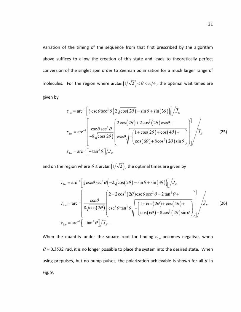
When  the  quantity  under  the  square  root  for  finding  2mτ  becomes  negative,  when 

0.3532θ ≈  rad, it is no longer possible to place the system into the desired state.  When 

using prepulses, but no pump pulses,  the polarization achievable  is shown  for all θ  in 

Fig. 9. 

32 

 

0 0.5 1 1.50

50

100

P (

%)

θ (rad)  

Figure 9.   The resultant polarization achieved by the medium θ  sequence algorithm (solid  line) 

and  original  algorithm  by Goldman  et  al.  (dashed  line)  over  the  range  of  possible θ .    This  uses  ideal 

calculations. 

3. Operation in real systems

It  is often not possible  to  completely  isolate  the  spin  system of a molecule of 

interest  from  all  other  spins.    Such  common  atoms  as  hydrogen  have  no  isotopes 

without  spin  and  others  would  be  prohibitively  expensive  to  replace  with  a  spin  0 

isotope.   Rather  than completely  isolate  the desired  three spin system, steps must be 

taken  to mitigate  the effects of spectator spins  in  the system.   All hydrogen  that may 

couple  to  the  system of  interest on  the precursor molecule needs  to be  replaced by 

deuterium.  When spectator protons are replaced with deuterons, the coupling between 

the spins is weakened by a factor of approximately six and, more importantly, pulses can 

be  applied  to  these  spins  separately  from  protons.    This  allows  decoupling  of  these 

undesirable  spins  from  the  system  by  echo  pulses  on  protons  or  heteronuclear 

decoupling.  Spins with the same isotopic identity as the target isotope that couple with 

the desired system must also be replaced. 

33 

 

The  interference  from  spectator  spins  is  likely  to  still  be  too  great  in  most 

systems  where  it  is  needed  even  with  the  reduction  in  coupling  strength  by  using 

deuterons  for  protons.    To  further  reduce  the  effects  of  these  spectator  spins,  echo 

pulses  need  to  be  added  to  the  sequence  in  such  a  way  that  the  overall  average 

Hamiltonian remains unchanged from that of the three spin system.  This is done simply 

by  applying  the π  pulses  to  both  protons  and  target  nuclei.    Even without  spectator 

spins, one set is useful to refocus the chemical shift terms.  With the spectator spins, a 

symmetric  set  is much more  effective  for  refocusing  of  the  effects  of  heteronuclear 

scalar couplings to the spectator spins, as described by Goldman et al. (34,35).  Thus, in 

order to mitigate the effects of these spins reasonably well, each wait period τ  in the 

sequence must have π  pulses on both the protons and the target nucleus at times given 

by  4τ  and 3 4τ  during the period.  Having two pulses also allows phase cycling, which 

can help reduce problems due to misset pulses. 

13C

H2

HD

F

HHH

D D

DD

D

13CFF

FFFF

F O O

OO 

Figure 10.   The molecule 2,2,3,3‐tetrafluoropropyl 1‐13C‐propionate‐d3    is derived  from 2,2,3,3‐

tetrafluoropropyl 1‐13C‐acrylate‐d3.    It  is vital to deuterate the acrylate portion of the molecule and may 

be  important  to deuterate  the  closer protons on  the  tetrafluoropropyl portion which have  some  small 

coupling with the labeled carbon. 

34 

 

 coupling is strong. 

Since the sequences are performed in a low field, some care must be taken when 

using  molecules  with  spectator  isotopes  that  have  Larmor  frequencies  sufficiently 

similar to that of the protons or the target spin.   As an example, the molecule TFPP  in 

Fig. 10 was found to have some small coupling between the target 13C and the protons 

across  the ether oxygen when  refocused  INEPT was performed on  the hyperpolarized 

molecule (48).  In this molecule, the proton spectrum showed significant polarization on 

both  added  protons  as well  as  the  two  nearest  protons  from  the  precursor.    For  a 

molecule  with  the  parameters  of  the  three  spin  system  of  TFPP,  the  polarization 

obtained  on  13C  is  reduced when  there  is  coupling  to  two  extra  protons  as  seen  in 

Fig.  11.    This  reduction  can  be  mitigated  by  optimization  of  the  sequence  timing, 

numerically  taking  into  account  the  entire  spin  system,  but  it  cannot  be  completely 

recovered  in  this  way  (Fig  11).    The  molecule  was  chosen  to  have  a  fluorinated 

hydrocarbon moiety which is known to bind to lipids, so a first approach to reducing the 

problem might be to replace these two protons with fluorine.   This helps, but since 1H 

and 19F frequencies are so close in the low field, it also requires much longer pulses than 

would ordinarily be used, as seen in Fig. 12, where the longest pulses, 187 μs when the 

proton frequency is 75 kHz, are required when

35 

 

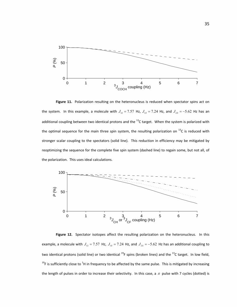
0 1 2 3 4 5 6 70

50

100

3JCOCH

coupling (Hz)

P (

%)

 

Figure 11.   Polarization  resulting on  the heteronucleus  is reduced when spectator spins act on 

the  system.    In  this example, a molecule with  12 7.57J =  Hz,  1 7.24SJ =  Hz, and   Hz has an 

additional coupling between two identical protons and the 13C target.  When the system is polarized with 

the optimal  sequence  for  the main  three spin  system,  the  resulting polarization on  13C  is  reduced with 

stronger scalar coupling  to  the spectators  (solid  line).   This  reduction  in efficiency may be mitigated by 

reoptimizing the sequence for the complete five spin system (dashed line) to regain some, but not all, of 

the polarization.  This uses ideal calculations. 

2 5.62SJ = −

0 1 2 3 4 5 6 70

50

100

3JCH

or 3JCF

coupling (Hz)

P (

%)

 

Figure  12.    Spectator  isotopes  affect  the  resulting  polarization  on  the  heteronucleus.    In  this 

example, a molecule with   Hz, 12 7.57J = 1 7.24SJ =  Hz, and  2 5.62SJ = −  Hz has an additional coupling to 

two identical protons (solid line) or two identical 19F spins (broken lines) and the 13C target.  In low field, 

19F is sufficiently close to 1H in frequency to be affected by the same pulse.  This is mitigated by increasing 

the length of pulses in order to increase their selectivity.  In this case, a π  pulse with 7 cycles (dotted) is 

36 

 

not  as good  as  a π  pulse with 10  cycles  (dash‐dot), which  is not  as  good  as  a π  pulse with 14  cycles 

(dashed).  They are all improvements over protons with pulses of any of these lengths (14 cycles is shown 

but all follow the same curve).  This uses lab frame calculations. 

4. Behavior under experimental error

In order  to estimate how well  this pulse  sequence algorithm will perform  in a 

given  situation,  it  is  useful  to  know  how well  it  continues  to  perform  in  the  face  of 

common  experimental  errors.    Errors may  arise  from  inaccurate  adjustments  of  the 

static field strength or its variation due to the movement of objects near the equipment.  

Other errors include the strength of pulses at the  I  or S  Larmor frequencies and errors 

in determining the scalar couplings in the system. 

i. Scalar coupling errors 

The pulse  sequences derived  from  the medium θ  algorithm are  specific  to  the 

coupling  constants  of  the  given molecule.    Experimental  error  in  determining  these 

scalar  coupling  constants  is  in  principle  avoidable,  but  is  common  as  the  first  order 

theory typically used is often insufficient in systems with multiple coupling constants of 

similar magnitude.  Additionally, these couplings are sometimes dependent upon other 

factors such as solution pH and temperature.    In some situations, the proton coupling 

depends upon the configuration of the precursor molecule. 

An  example  of  a molecule  that  displays many  of  these  complications  is  1‐13C 

succinic acid.  Both homonuclear and heteronuclear scalar coupling constants of succinic 

37 

 

acid  vary  very  strongly  with  pH  near  neutral  due  to  the  changing  probabilities  of 

conformations as  the protonation  state of  the molecule changes.   Two proton‐proton 

coupling  constants are  found at each pH  (36,54)  in  the undeuterated  system.    In  this 

case, the coupling constants can be made fairly certain by performing the experiment in 

basic  or  acidic  solution  where  there  is  no  strong  dependence.    That  we  find  two 

different coupling constants between the methylene groups shows that final coupling of 

the parahydrogen derived protons on C2 and C3 will depend on  the  choice of maleic 

acid or  fumaric acid as  the deuterated alkene precursor molecule since  these  isomers 

lead to different succinate isomers after hydrogenation (Fig. 13). 

H2

D O

H

H2

DO

H H

H

O

O

OO

OO O-

O-O-O-

O-O-

O-O-

D

D

DD

D D

*

* *

*

 

Figure  13.    The  geometry  of  the  precursor  selects which  of  the  two  proton‐proton  coupling 

constants available  in succinate  is active after hydrogenation.    In conditions where the acid groups stay 

primarily  in  the  trans position,  the  fumarate precursor  (left)  is expected    to have  the  smaller  coupling 

constant associated with the gauche geometry while the maleate precursor (right) is expected to have the 

larger coupling constant associated with the trans geometry.  The location of the 13C is marked with a star. 

Once the appropriate scalar coupling constants have been found to some degree 

38 

 

of  certainty,  the  pulse  sequence  can  be  generated.    The  expectation  of  how well  a 

certain  sequence will perform varies over  the  range of θ  over which  the algorithm  is 

expected  to  be  useful.    An  example  of  a molecule with θ  near  the  high  end  of  the 

medium  range  is  1‐13C‐succinic  acid  at  pH 4.31=  with  the  smaller  coupling  constant.  

This molecule has   Hz, 12 6.07J = 1SJ 6.80= −  Hz, and  2 5.47J S =  Hz  (36) yielding timing 

constants  of  1m 26.08τ =  ms,  2m 45.32τ =  ms,  and  3 54.14mτ =  ms.    Should  the  actual 

coupling  constants  vary  from  those  used  to  generate  the  sequence,  the  resulting 

polarization will not be as high as shown in Fig. 14. 

39 

 10

2030

40

40

40

50

50

50

50

60

60

60

60

60

70

70

70

70

70

70

80

80

80

80

80

80

9090

90

90

90

actual J12

(Hz)

actu

al J

Δ (H

z)

4 4.5 5 5.5 6 6.5 7 7.5 8 8.5

4

4.5

5

5.5

6

6.5

7

7.5

8

8.5

 

Figure 14.  Contour plot of the percent of polarization on the target 13C nucleus generated by the 

pulse sequence derived  for 1‐13C‐succinic acid at  pH 4.31=  over a wide range of similar scalar coupling 

constants.   The major  contours are marked  for every 10% and  the minor  contours are every 2%.   The 

pulse  sequence  generates 100% polarization when  the  coupling  constants are  correct.   This uses  ideal 

calculations. 

An example of a molecule with θ  near the small end of the medium range is 1‐

phenylethylphenylphosphinic  acid  (Fig. 15) where  the  target  is  the phosphorus  atom.  

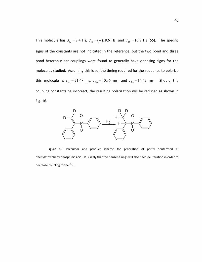
40 

 

This molecule has   Hz, 12 7.4J = ( )1 18.6SJ = −  Hz,  and  2 16.8SJ =  Hz  (55).    The  specific 

signs of the constants are not  indicated  in the reference, but the two bond and three 

bond  heteronuclear  couplings  were  found  to  generally  have  opposing  signs  for  the 

molecules studied.  Assuming this is so, the timing required for the sequence to polarize 

this  molecule  is  1 21.68mτ =  ms,  2 10.35mτ =  ms,  and  3 14.49mτ =  ms.    Should  the 

coupling constants be  incorrect, the resulting polarization will be reduced as shown  in 

Fig. 16.  

H2

D O

P

DDD

O

O

O

PH

H

 

Figure  15.  Precursor  and  product  scheme  for  generation  of  partly  deuterated  1‐

phenylethylphenylphosphinic acid.  It is likely that the benzene rings will also need deuteration in order to 

decrease coupling to the 31P. 

41 

 

50

60

60

60

60

70

70

70

70 70

70

7070

80

80

80

80

8080

80

90

90

90

90

90

actual J12

(Hz)

actu

al J

Δ (H

z)

4 5 6 7 8 9 10 11

12

14

16

18

20

22

24

 

Figure 16. Contour plot of the percent of polarization on the target 31P nucleus generated by the 

pulse  sequence  derived  for  1‐phenylethylphenylphosphinic  acid  over  a  wide  range  of  similar  scalar 

coupling constants.  The major contours are marked for every 10% and the minor contours are every 2%.  

The pulse sequence generates 100% polarization when the coupling constants are correct.  This uses ideal 

calculations. 

ii. Magnetic field strength and pulse power 

The  interactions that generate polarization via these pulse sequence algorithms 

42 

 

are not dependent upon  the magnetic  field strength, however  the pulses delivered  to 

the system are  tuned  to a specific magnetic  field.   When  the strength of  the static or 

oscillating fields is incorrectly set, the pulse sequence is adversely affected reducing the 

final polarization.  The extent of the harm from these effects is highly dependent upon 

features of the pulse sequence that do not figure in the outcome unless the pulses are 

not generated correctly.   Phase cycling the echo pulses by applying the second around 

the negative axis of the first for each set of echoes significantly improves the resilience 

against  these  sorts  of  incorrect  settings  (Fig.  17).    The main  pulses  in  the  sequence 

cannot be cycled, but pulse shaping, which  is useful for other reasons and simple with 

the  hardware  used,  is  generally  useful  to  decrease  the  dependence  of  the  nutation 

angle on these factors as well.  This is discussed in section VI.D. 

50 60 70 80 90 100 110 120 130 140 1500

50

100

P (

%)

B1 for 1H pulse (% of correct value)

a)

50 60 70 80 90 100 110 120 130 140 1500

50

100

P (

%)

B1 for 13C pulse (% of correct value)

b)

 

Figure 17.  Using simple phase cycling (solid line) with the echo pulses improves the behavior of 

43 

 

the pulse sequences over not doing so (dashed line) with respect to incorrect setting of the pulse power 

for  both  a)  proton  pulses  and  b)  pulses  on  the  target  nucleus.    This  example  is  a  lab  frame GAMMA 

calculation that uses the succinate molecule described in Fig. 14 and the pulse sequence described in the 

text for that molecule. 

B. Small range pulse sequence algorithm

The  small  range  is  characterized  by  0.3532θ d ,  generally  due  to  a  large 

difference  in  the heteronuclear scalar coupling.   Below  the  lower  limit of  the medium 

range  algorithm,  the  effectiveness  falls  off  sharply  (Fig.  9).    Pump  pulses  allow  the 

experimentalist  to  increase  the  polarization  by  increasing  the  time  required  by  the 

sequence, but cannot perfectly polarize the target.  A different algorithm is needed for 

this range.  Molecules with strong two‐bond and three‐bond heteronuclear coupling to 

protons,  for  example  those with  a  31P  target  spin,  and molecules where  the  added 

protons are attached directly to the target have will often fall into this range. 

1. Algorithm for the limit 0θ →

The  spin  order  transfer  requires  a  nonzero  value  of  both  12J  and  JΔ ,  but 

becomes challenging when either one dominates.  Looking at relations (20) and (21), it is 

clear  that  the most  effective  evolution  for  the  system  during  3sτ  in  the  limit  0θ →  

comes from relation (21).    In order to take advantage of this, an algorithm that places 

the system into the intermediate state   at time 2 z xK S 1 2s sτ τ+  must be found.  One way 

to more easily control the evolution of the states is to be able to turn off one part of the 

44 

 

other of the intrinsic Hamiltonian in Eq. (18).  One method to do this is using decoupling 

applied to the target isotope, which is used for this algorithm.  In effect, this temporarily 

switches the effective Hamiltonian to that of the limit  2θ π→  for the period  2sτ .  This 

degree of freedom modifies the strategy.  The form of the novel small θ  pulse sequence 

algorithm is shown in Fig. 18. 

H:

S:

y x

τ1s τ2s τ3s

decouple

 

Figure 18.  Schematic of the small θ  range pulse sequence.  The main pulses of the algorithm are 

dark and recommended echo pulses are light.  Solid pulses are π , open pulses are  2π , and decoupling 

uses a typical cyclic method that returns the polarization to the starting point, such as MLEV‐16. 

Briefly, the initial proton decoupling during the reaction is followed by a wait of 

1sτ , then decoupling is applied to the target for a second wait  2sτ  until the system is in 

the desired  intermediate  state.   A  ( )2y

π  mixing pulse on  the  target after decoupling 

starts the evolution that develops polarization during the third wait  3sτ .  A final  ( )2x

π  

pulse stores the magnetization along  .  The recommended echo scheme (grey pulses) 

to mitigate the effects of spectator spins is largely unchanged. 

z

In detail, first the system is allowed to evolve from the initial condition under the 

45 

 

intrinsic Hamiltonian until  the maximum amount of 2  and   has developed.  

This  leaves  the  system  in  a  linear  combination  of  the  two  states  that  is  generally 

different from the desired state with no order left in the 

y zK S 2 z zK S

xK  state.  Second, the system 

is subjected to coherent decoupling on the insensitive target nucleus until the system is 

in  the desired  intermediate  state.   Decoupling effectively  changes  the Hamiltonian of 

the  system during  this period  such  that  the heteronuclear  coupling does not operate 

leading  to a new  type of evolution.   During  this  time,  the average Hamiltonian  in  the 

rotating frame is given by   

  12ˆdec xH J K= .  (27) 

Under  this  Hamiltonian,  xK  does  not  evolve  but  the  two  states  it  evolves  into 

interconvert such that 

  ( )( ) ( )( )12 122 cos 2 sin 2y z y z z zK S J t K S J t K S→ +   (28) 

  ( )( ) ( )( )12 122 sin 2 cos 2z z y z z zK S J t K S J t K S→ + .  (29) 

This decoupling  is  left on until  the system evolves entirely  into  the   state. After 

this evolution, a 

2 z zK S

( )2y

π  pulse on S  is applied to produce the desired intermediate state 

.  Finally, the system is again allowed to evolve under the intrinsic Hamiltonian so 

that  ‐like  polarization  develops  according  to  relation 

2 z xK S

yS (21).    A  2xπ  pulse  on S  is 

applied to store the polarization as Zeeman order when the transverse order is greatest.  

To follow this recipe exactly, the times are given by 

46 

 

  2

1

3

2

2

arccos tan

arct cot 1 taa nn

2s

s K

s

K

J

J

J

θ θ

θ

τ

τ

τ

π

⎡ ⎤=

⎡ ⎤−⎣ ⎦=

−⎣ ⎦

= 12   (30) 

which  yields  a  maximum  polarization  of  cosθ  for  4θ π≤  and  22sin cosθ θ  for 

4θ π>  when using the real part of the times. 

2. Modifications for a larger range

In order  to make  this algorithm effective  for  real  systems,  it  is again useful  to 

observe  that  the optimal  intermediate  state  for 0 4θ π< ≤  is  the  linear  combination 

given in Eq. (24).  This sequence is easily modified to generate the correct intermediate 

state  by  simply  shortening  the  second wait.    The  third wait  also  needs  correction  to 

generate the optimal sequence. 

The  optimal  sequence  for  the  range  of θ  then  is  to  allow  evolution  from  the 

initial state, after  the  time suspension,  to  the state with  the minimum amount of  xK .  

Next, turn on cyclic decoupling on the target nucleus until the state is the optimal state 

indicated  by  Eq.  (24).    Then  a  ( )2y

π  mixing  pulse  triggers  evolution  generating 

transverse spin order on the target which  is finally stored  in   by a final z ( )2x

π  pulse.  

This sequence is generated using times given by  

 ( )

( ) ( )

21 3

22

122 tan t

arccos tan

arccos 1 an

s s K

s

J

J

τ τ θ

τ θ

⎡ ⎤= = −⎣ ⎦

= ⎡ ⎤⎣ ⎦− θ

  (31) 

47 

 

and yields the polarization of 1 for the range 0 4θ π< ≤  (Fig. 19). 

0 0.5 1 1.50

50

100

P (

%)

θ (rad)  

Figure  19.    The  theoretical  polarization  possible  by  application  of  the  small  θ  sequence 

algorithm in with the most optimal times (solid) and as it was originally designed (dashed).  This uses ideal 

calculations. 

3. Operation in real systems

Similarly  to  the medium θ  case,  the  spin  system must  not  contain  any  other 

isotopes with  the  same  identity  as  the  target  or  protons  for  the  pulse  sequence  to 

operate correctly.  This is generally a matter of deuterating the precursor molecule to be 

used in reaction. 

As well, echo pulses are  required during  the wait periods of  the  small θ  pulse 

sequence algorithm to refocus what little chemical shift or resonance offset there is and 

to mitigate  the effects of  spectator  isotopes.    For  the  first  and  last wait periods,  the 

same  approach  using  two  symmetric  echoes  on  both  protons  and  target  is  most 

effective.    For  the  second wait  period,  the  problem  is  simplified  by  the  decoupling 

applied to the target  isotope.    In this case, symmetric echoes are only required on the 

protons. 

48 

 

4. Behavior under experimental error

Just as with the medium θ  range sequence algorithm, the required parameters 

will only be known within some experimental error and magnetic fields are not perfect.  

It is useful to know how the sequence acts when these common problems occur. 

i. Scalar coupling errors 

To demonstrate the degree of difficulty poorly known scalar couplings cause for 

the generation of hyperpolarization using the small θ  range pulse sequence algorithm, 

two molecules  are  selected  as  examples  of  the  extremes  of  the  range  in which  the 

algorithm would  be  applied.   At  the  large  end  of  the  range,  an  example molecule  is 

ethylphosphonyl  dichloride where  the  target  is  31P.    This molecule  has   Hz, 

 Hz,  and   Hz with  the  relative  sign  of  the  heteronuclear  coupling 

constants noted as being opposite (55).  Taking 

12 6 8J = −

1 30.0SJ = 2 14.2SJ =

12J 7=  Hz, the sequence generated has 

1 3s s 11.47τ τ= =  ms and  2s 21.06τ =  ms.   If the system has parameters similar to these, 

then this sequence is applied the resulting polarization on 31P can be found in Fig. 20. 

49 

 40

5060

60

60

60

60

70

70

70

70

70

70

80

80

80

8080

80

80

90

90

9090

90

actual J12

(Hz)

actu

al J

Δ (H

z)

4 5 6 7 8 9 10 11

16

18

20

22

24

26

28

 

Figure  20.    The  polarization  expected  on  31P  of  ethylphosphonyl  dichloride  when  the  pulse 

sequence derived  from  the  literature scalar coupling constants  is delivered  to  the molecule considering 

that the actual scalar coupling constants may differ  from the  literature values.   The major contours are 

marked  for  every  10%  and  the minor  contours  are  every  2%.    The  pulse  sequence  generates  100% 

polarization when the coupling constants are correct.  This uses ideal calculations. 

An example molecule  representing  the  low end of  the  small θ  range  is diethyl 

mercury where 199Hg is the target nucleus.  This molecule has   Hz, 12J = 7.5 1 91SJ =  Hz, 

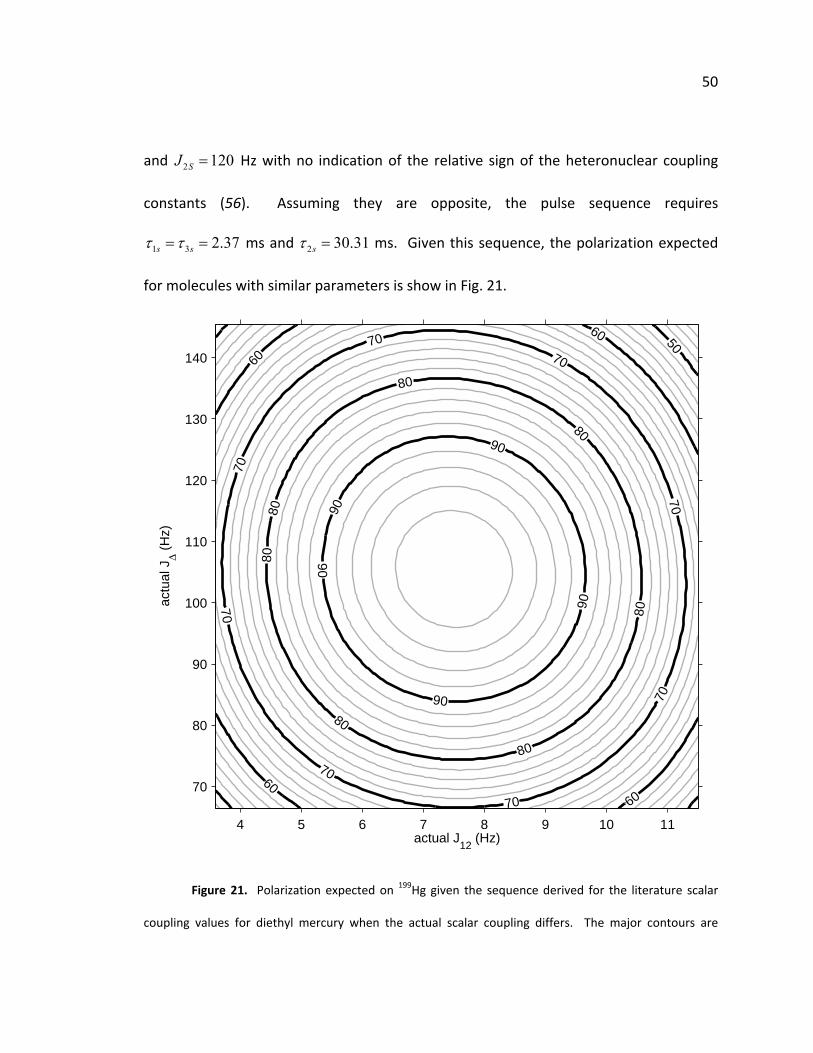
50 

 

and   Hz with no  indication of  the  relative sign of  the heteronuclear coupling 

constants  (56).    Assuming  they  are  opposite,  the  pulse  sequence  requires 

2 120SJ =

1 3 2.37s sτ τ= =  ms and  2 30.31sτ =  ms.   Given this sequence, the polarization expected 

for molecules with similar parameters is show in Fig. 21. 

50

60

60

60

60

70

70

70

70

70

70

70

80

90

90

70

80

80

80

80

80

80

90

90

90

actual J12

(Hz)

actu

al J

Δ (H

z)

5 64 7 8 9 10 11

70

80

90

100

110

120

130

140

 

Figure 21.   Polarization expected on  199Hg given  the  sequence derived  for  the  literature  scalar 

coupling  values  for  diethyl mercury when  the  actual  scalar  coupling  differs.    The major  contours  are 

51 

 

marked  for  every  10%  and  the minor  contours  are  every  2%.    The  pulse  sequence  generates  100% 

polarization when the coupling constants are correct.  This uses ideal calculations. 

C. Large range pulse sequence algorithm

The  large  range  is  characterized  very  roughly  by  1θ t ,  generally  due  to weak 

scalar  coupling  to  the  target  nucleus.    Both  small  and  medium  range  sequence 

algorithms  are  ineffective  over  this  range.    Pump  pulses  after  either  sequence  allow 

increases to the polarization, but are increasingly fruitless when they are most required 

and expand the sequence time beyond acceptable  limits.   Still another novel algorithm 

is needed for this range.   Molecules with  low γ , weakly coupling heteronuclei such as 

15N which promise particularly  long lifetimes for the generated polarization tend to fall 

into this range. 

1. Algorithm for the limit 2θ π→

In  the  case where  12J  comes  to  dominate  JΔ ,  neither  of  the  relations  (20)  or 

(21)  generates  useful  evolution  for  this  system.    In  order  to  generate  the  desired 

polarization at the end of the sequence, the intrinsic Hamiltonian needs to be changed 

during this period.  Specifically, some method of homonuclear decoupling by which the 

12 xJ K  piece in the Hamiltonian is effectively removed while the heteronuclear coupling 

remains, would generate useful evolution for this range.  Unlike the case of decoupling 

heteronuclei, no general strategy is known for decoupling homonuclear scalar couplings. 

52 

 

The innovation here is to show that a J‐synchronized train of π  pulses on the S  

spins  is able to generate the desired Hamiltonian.   This synchronous train  is a series of 

π  pulses given  twice over each period of  122res Jτ π=  at  4resτ  and 3 res 4τ .   Average 

Hamiltonian  theory  is used  to  show  analytically how  this  affects  the evolution of  the 

system.   Starting with  the Hamiltonian  in Eq.  (18),  then  transforming away  the pulses 

and  the  homonuclear  coupling  yields  a  time  dependent  Hamiltonian  in  the  toggling 

frame given by  

 ( ) ( ) ( )

( ) ( ) ( )

12 12

12 12

3ˆ 2 cos 2 sin , ,4 4

3ˆ 2 cos 2 sin ,4 4

res resT z z y z

res resT z z y z

H t J K S J t J K S J t t t

H t J K S J t J K S J t t

τ τ

τ τ

Δ Δ

Δ Δ

= + <

= − − < <

<.  (32) 

Integrating this Hamiltonian over the interval  resτ  then gives  

  ( )2 2 z zH J K Sπ Δ= .  (33) 

Thus, the homonuclear coupling has indeed been removed leaving only a heteronuclear 

coupling  scaled down by 2 π  in  its place.    The  relevant evolution of  the  spin  system 

under this Hamiltonian is given by  

  ( ) ( )( )2 2cos sin 2x x yK J t K J t Kπ πΔ Δ→ + zS   (34) 

  ( )( ) ( )( )1 2 21 222 sin 4 cos 2z x y z z y z xK S J t S I I S J t K Sπ πΔ→ − + Δ .  (35) 

The evolution in relation (35) is advantageous for generating the desired polarized state 

that can be stored in   with a final pulse. z

53 

 

τ1l τ3lτ2l

H:

S:

y xdecouple

X:

J synchronous π train

 

Figure  22.    Schematic  of  the  large θ  range  pulse  sequence.    The  number  of  pulses  in  the  J‐

synchronized π  train should be set to the number required by the algorithm; three is used as an example.  

The main  pulses  of  the  algorithm  are  dark  and  recommended  echoes  on  proton  and  decoupling  on 

spectator  isotopes X are  light.    Solid pulses  are π , open pulses  are  2π , and decoupling uses  a  cyclic 

method that returns the polarization to the starting point, such as MLEV‐16. 

In  order  to  best  utilize  this  evolution,  the  system must  be  placed  in  a  state 

without any  xK  in it.  The evolution of the system under the intrinsic Hamiltonian is not 

useful  for bringing  the  system  into  such a  state,  so  the  J‐synchronized π  train  is also 

useful for the first part of the sequence, utilizing the evolution in relation (34). 

An  algorithm  for  the  large  range,  starting  when  time  suspension  during  the 

precursor reaction  is completed, would then utilize a J‐synchronized π  train for a time 

1lτ  to  fully  convert  the  xK

2l

 spin  order  to  .    Cyclic  decoupling  is  applied  to  the 

target isotope for a time 

2 y zK S

τ  until the system is in the state  .  A 2 z zK S 2 yπ  mixing pulse 

is  applied  to  the  target  isotope  and  second  J‐synchronized π  train  is  applied  to  the 

54 

 

system  for a time  3lτ  until the transverse polarization has built up.   A  final  2xπ  pulse 

stores  this  as  longitudinal  polarization  for  future  use.    This  algorithm  is  illustrated  in 

Fig. 22, including a scheme for compensating for the effects of spectator isotopes.   The 

timing required for this algorithm is given by  

 2

1 3

2 12

42

l l

l

JJ

τ τ π

τ πΔ= =

=.  (36) 

While  formally  the average Hamiltonian  theory used  requires a cycle of pulses 

that brings the system back to its original state, in practice the homonuclear decoupling 

operates over an odd number of pulses as well.  Since the first and third waits are during 

J‐synchronized π  trains, their timing cannot freely be set to any value but must be set 

to an integer multiple of  2resτ .  Therefore, the value of  1l 3lτ τ=  must be coerced to the 

integer or half integer multiple of  resτ  that is nearest to the prescribed time given by Eq. 

(36). 

2. Modifications for more consistent polarization

While the time desired for the waits  1l 3lτ τ=  is very close to an integer multiple 

of  2resτ  when θ  nears the upper limit of its range, the difference between the optimal 

time and an allowed time can become quite dramatic as θ  nears  4π  where the other 

algorithms  start  to  fall  off  in  effectiveness.    This  mismatch  reduces  the  resulting 

polarization of the algorithm.  This problem is particularly apparent near  1.09θ =  where 

the effectiveness of the large range sequence actually drops below that of the medium 

55 

 

range sequence. 

Numerical optimization of the sequence holding the number of π  pulses steady 

but  allowing  the  times  to  vary  increases  the  polarization  of  the  sequence  without 

requiring  large  changes  in  the  time  needed  (Fig.  23).    By  allowing  this  variation,  the 

polarization increases to unity over an extensive range (Fig. 24). 

0.8 0.9 1 1.1 1.2 1.3 1.4 1.5

101

102

tota

l tim

e (t

d )

θ (rad)  

Figure  23.  The wait  times  required  by  the  large θ  sequence  algorithm  generally  need  to  be 

optimized  in order  to achieve unity polarization.   The  total  time  for  the sequence as calculated  (line)  is 

compared to the total of the numerically optimized times (dots) and found to be similar.  This uses ideal 

calculations. 

56 

 

0 0.5 1 1.50

50

100

P (

%)

θ (rad)  

Figure  24.    The  theoretical  polarization  achievable  using  the  large θ  sequence  algorithm  as 

described with calculated times (solid) and after numerical optimization (dashed).  The minimum number 

of π  pulses in each synchronous period is 1.  This uses ideal calculations. 

3. Operation in real systems

Similar  to  the  medium  and  small  range θ  cases,  the  spin  system  must  not 

contain  interfering spins of the same  isotope as the target nor any  interfering protons 

for the pulse sequence to operate correctly.  This generally requires deuteration of the 

precursor molecule to be used in the reaction. 

As well, a means of refocusing the chemical shift of the target and mitigating the 

effects  of  spectator  isotopes  is  required.   Over  the  second wait  period,  this  requires 

symmetric echoes on the protons.  Over the J‐synchronized π  train, this is more difficult 

to apply.  The target chemical shift is already refocused by the pulses, but pulses on the 

protons to lessen the effects of deuterium will interfere with the J‐synchronized π  train.  

Over these periods,  it  is possible to apply decoupling to those  isotopes other than the 

target and protons that are known to be part of the spin system.  A second method is to 

treat each  segment  in  the  J‐synchronized π  train  as  a  separate period  and  apply  the 

57 

 

symmetric echoes to target and protons during each one. 

4. Behavior under experimental error

To understand how well the sequence is likely to perform in a real experiment, it 

is useful to look at how it fails when common experimental errors occur.  These are the 

same as for the small and medium θ  range sequence algorithms. 

i. Scalar coupling errors 

To see how uncertain scalar coupling affects  the outcome of a particular pulse 

sequence,  it  is useful  to examine  it at different points  in  the  range.   An example of a 

molecule at  the  low end of  the  large θ  range  is 1‐13C‐succinate at   with  the 

larger of the two proton‐proton coupling constants.   This molecule has scalar coupling 

constants of   Hz, 

pH 13.3=

12 8.51J = 1 6.32SJ = −  Hz, and  2 4.13SJ =  Hz  (36).   The  timing  for  this 

pulse  sequence,  after  optimization,  is  1 3 70.02l lτ τ= =  ms  with  1 π  pulse  in  the  J‐

synchronized π  train and  2 21.29lτ =  ms.  This sequence performs as seen in Fig. 25. 

58 

 

−30

−15

−15

−15

0

0

0

0015

15

15 15

15

15

30

30

30 30

30

30

45

45

45

45

45

45

60

60

60

6060

60

75

75

75

75

75

90

90

90

actual J12

(Hz)

actu

al J

Δ (H

z)

6.5 7 7.5 8 8.5 9 9.5 10 10.5 11

3

3.5

4

4.5

5

5.5

6

6.5

7

7.5

 

Figure  25.    Pulse  sequence performance  for  the  sequence  derived  for  1‐13C‐succinate  in  very 

basic solution when the scalar coupling constants diverge from those given  in the  literature.   The major 

contours are marked for every 15% and the minor contours are every 3%.  The pulse sequence generates 

100% polarization when the coupling constants are correct.  This uses ideal calculations. 

An example of a molecule with somewhat larger θ  is 15N‐choline.  This molecule 

has   Hz  or   Hz  and 12 3.15J = 12 7.00J = 1 3.68SJ =  Hz  with  only  one  heteronuclear 

59 

 

coupling corresponding to the three bond coupling observed (57).  The pulse sequence 

for this molecule with the  larger   value requires that 12J 1 3 214.16l lτ τ= =  ms with 3 π  

pulses and  2 38.68lτ =  ms.  This sequence performs as seen in Fig. 26. 

−80

−80

−80

−80

−60

−60

−60

−60

−60 −60

−40

−40

−40

−40

−40

−40

−40

−20

−20

−20

−20

−20

−20

−20

−20

−20

0

0

0

0

0

0

0

0

20

20

20

20

20

20

20

20

40

40

40

40

40

60

60

60

80

80

80

actual J12

(Hz)

actu

al J

Δ (H

z)

5 5.5 6 6.5 7 7.5 8 8.5 9

−0.5

0

0.5

1

1.5

2

2.5

3

3.5

4

 

Figure 26.  Expected performance of the pulse sequence derived for 15N‐choline should the scalar 

coupling values differ from those found  in the  literature. The major contours are marked for every 20% 

and  the minor  contours  are  every  4%.    The  pulse  sequence  generates  100%  polarization  when  the 

coupling constants are correct.  This uses ideal calculations. 

60 

 

Comparing Figs. 25 and 26 shows the  increasing  importance of having accurate 

scalar coupling values, particularly for  , as the value of 12J θ  increases. 

D. Comparison of sequence algorithms

There  is  great  overlap  in  the  regions  in  which  this  set  of  pulse  sequence 

algorithms is capable of generating unity polarization.  In order to select between them, 

it is useful to examine the time requirements of each algorithm.  Over the entire range, 

there are multiple regions that are best handled in different ways.  These regions will be 

examined starting with the highest where  4θ π≤  and proceeding to lower values of θ , 

then  examine  the  regions where  4θ π> .    To  give  a better  idea of  the  general  time 

requirement of the pulse sequences, they are compared using the dimensionless time 

12dt J τ= .  This is a useful comparison since the formulae generate times that depend on 

the values of various scalar couplings.  For a given a value of θ , the value of one scalar 

coupling  determines  the  rest,  so  the  dimensionless  product  of  one  coupling  and  the 

total  time  is  a  quality  factor  by which  sequences may  be  compared,  for which   is 

preferred.    The magnitude of 

dt

12 2J π  changes over  a  relatively  small  range,  generally 

being between 3 1  Hz.  Values of 2− 2J πΔ  as small as  Hz are likely practical before 

dephasing effects dominate, but it and 

0.5

2KJ π  can easily range up to   Hz.  Using this 

dimensionless time will show the time behavior of the sequences over the range of 

120

θ  

with  the  least amount of distortion due  to  the general correlation of  the other  scalar 

61 

 

couplings with θ . 

1. For the range 4θ π≤

This is a region over which any one of the three algorithms given may operate on 

the  system  to  generate  unity  polarization.    Considerations  like  the  time  required  to 

deliver the sequence, ease of implementation, and behavior due to common errors are 

also important in considering which sequence to use. 

The  large θ  range  sequence  was  not  designed  for  this  region  and  does  not 

generate  sequences  with  good  time  requirements  over  this  region.    The  sequences 

contain one π  pulse for the J‐synchronized π  train regions when  4θ π< , so the time 

to  complete  the  calculated  sequence  is  12 2.5Jτ π= .    The  optimization  generally 

increases this time slightly.  This is significantly greater than the other two sequences.  If 

the  sequence  is  allowed  to  have  0 π  pulses  when θ  becomes  small  enough,  the 

sequence  reduces  to  the  small θ  range  case and  is no  longer  interesting  as  a unique 

procedure. 

The  small and medium θ  ranges have  complicated dependencies  (Fig. 27), but 

show three distinctive regions.  The first to note is when  ( )arctan 1 2 4θ π< ≤ .  Over 

this  region,  the  medium  range  sequence  is  the  clear  winner  generating  the  faster 

sequence.    At  (arctan 1 )= 2θ ,  the  two  sequences  are  equivalent  as  2 2 0s mτ τ= = .  

Just  above  this,  2sτ  reaches  the  maximum  value  before  the  systems  start  sampling 

62 

 

states equivalent to those sampled at earlier times, causing the sudden jump to smaller 

times.   Second, when  ( )0.3532 arctan 1 2θ< ≤ , both algorithms generate  sequences 

that perform in a comparable manner with only slight time advantage found in using the 

small  range  sequence.    Third, when  0.3532θ <  rad,  the medium  sequence  no  longer 

achieves  unity  polarization,  so  although  it  does  eventually  gain  better  time 

performance,  it  is  not  the  preferred  algorithm.    At  the θ  where  the  time  for  the 

sequences is equivalent, the polarization has only dropped to about   but is rapidly 

decreasing.    In  this  range,  the  gains  in  time  are not worth  the  losses  in polarization, 

generally, but quantifying the tradeoff would require consideration of dephasing effects. 

94%

0 0.1 0.2

1

0.3 0.4 0.5 0.6 0.7

0.5

0

tota

l tim

e (t

d )

θ (rad)  

Figure  27.    The  time  performance  of  the  small  (solid)  and  medium  (dotted)  range  pulse 

sequences over  the  range  in which one or both of  them  generates unity polarization.   This uses  ideal 

calculations. 

2. For the range 4π θ<

The  large  range  is  characterized by weaker heteronuclear  coupling  and  longer 

pulse  sequences.    As  such,  the  choice  between  pulse  sequences  is  often  a  tradeoff 

63 

 

between one that performs faster but does not give very good polarization and one that 

does give good polarization on the target, but does not perform as quickly as desired. 

The large θ  pulse sequence algorithm will always deliver a fully polarized target 

nucleus  when  relaxation  is  not  taken  into  account.    The medium θ  pulse  sequence 

algorithm  is  expected  to  give  increasingly  poor  polarization  that  can  be  arbitrarily 

increased by  the use of pump pulses after  the main  sequence  is  completed.   After n  

such pump pulses, the polarization on the target is expected to be  

  ( ) ( )2 11 cos 2nnP θ+= −   (37) 

when  relaxation  is  not  taken  into  account  (34).    This  process  requires  an  increasing 

number of pulses each with a unique angle that has been determined in the absence of 

relaxation but is changed when the relaxation constants are unequal. 

By rearranging Eq. (37),  it  is possible to estimate the  length of time that would 

be  required  to  gain  a  minimum  desired  polarization  using  the  edium m θ  pulse 

sequence algorithm.   This value can be compared to th   large e θ  pulse sequence and a 

choice made about which sequence to use based on whether the time savings, if there is 

any,  justifies  the  loss  of  polarization.    A  few  comparisons  of  this  type  are  shown  in 

Fig. 28 for examples where the  edium m θ  sequence achieves 99%, 90%, 75%, and  just 

50% polarization, all of which eventually require more time than the  large θ  sequence 

requires for unity polarization. 

64 

 

0.8 0.9 1 1.1 1.2 1.3 1.4 1.5

101

102

tota

l tim

e (t

d )

θ (rad)

optimized large θmedium θ to 99%medium θ to 90%medium θ to 75%medium θ to 50%

 

Figure 28.  The time performance of the optimized large pulse sequence algorithm, compared to 

that of various versions of  the medium pulse  sequence algorithm which are able  to deliver 99%, 90%, 

75%, or 50% polarization to the target nucleus.   The number of pump pulses has not been forced to an 

integer value, so the times represent a minimum estimate.  This uses ideal calculations. 

65 

 

IV. Instrumentation and execution

The  instrumentation  initially  used  at  CIT  and  Huntington  Medical  Research 

Institutes  (40)  to  carry  out  the  hydrogenation  reaction  and  low  field  order  transfer 

experiment  to  13C  on  was  obtained  from  Amersham  (now  part  of  G.E.)  in  Malmo, 

Sweden  on  temporary  loan.    An  improved  homebuilt  instrument  was  subsequently 

developed  and  is  described  here.   A  principal  goal was  to miniaturize  the  reactor  to 

produce  smaller  samples of only 2 mL  rather  than approximately 12 mL,  sufficient  for 

studies  on  rodents,  thus  minimizing  the  costs  of  reagents.    Faster,  cheaper,  more 

competent digital components were used, which also required fundamental changes to 

the computer program which controls the equipment.  I designed the computer related 

architecture of the device and performed the significant programming of the software, 

including changes to handle the new controlling hardware and the computer program 

that automated the several functions.  This section will describe the components in the 

system which holds  reagents, delivers  them  to  the  reactor  volume, which  is  also  the 

locus for the  low field NMR which generates the hyperpolarized molecules. It will then 

describe the procedure  for generating hyperpolarized molecules.   More details can be 

found  in  previously  published  (58,59)  papers  concerning  an  earlier  version  of  the 

instrument, also based on my hardware choices and software. 

66 

 

A. Instrument hardware

The  hardware  for  the  system  includes  the  reactor  system  and  controlling 

hardware that  interfaces with the computer.   The reactor system  is the hardware that 

holds  reactants,  performs  product  forming  reactions,  and  executes  the  spin  order 

transfer sequence.  Hyperpolarized molecules are then ejected to atmospheric pressure 

for use in high field NMR or MRI for experiments.  The heart of this system is the reactor 

itself.  This reactor is a container consisting of a polymer cylinder that is threaded at the 

top and bottom.   A threaded disk screws  into the top and contains separate  inputs at 

the top for parahydrogen gas and an aqueous solution of the precursor molecule and a 

hydrogenation  catalyst.    A  second  threaded  disk  screws  into  the  bottom  and  has  a 

conical  indentation  leading  to an outlet  that allows  the product  to be removed at  the 

end of hyperpolarization.  The piecewise structure allows for easy cleaning of the inside 

of the reactor.  It was produced in house. 

67 

 

H2input

N2input

aqueousreagent

input

reactor

saddlecoil

solenoid

outlet

valves

holdingchamber

reactionchamber

 

Figure 29.   Schematic of the reactor system.   The aqueous mixture of precursor and catalyst  is 

placed  in  the holding  chamber and  solenoid providing   is powered  to prepare  for hyperpolarization.  

The  reaction chamber  is  filled with parahydrogen, proton decoupling  initiated with  the saddle coil, and 

precursor  solution  pushed  into  the  reaction  chamber  under  nitrogen  pressure.    After  the  spin  order 

transfer sequence pulsing finishes, the product is removed through the outlet valve at reduced pressure. 

0B

68 

 

The  reactor  is  surrounded by  a  solenoid  electromagnet  that provides  a  stable 

magnetic  field  0B  in  the  z  direction along  the axis of  the reactor.   An untuned saddle 

coil set between the solenoid and the reactor is used to deliver the audio frequency  1B  

fields perpendicular to the static field.   All pulses for all nuclei are generated using this 

coil.  These were also built in house.  Although the pulse coil is untuned, it does have a 

variable  response  to  different  frequencies  due  to  its  inductive  reactance.    This  is 

manifest  in  that  the  voltage  levels  required  in  the  definition  of  one  pulse  cannot  be 

directly calculated based on another nucleus  that has already been calibrated.    It also 

causes changes  in  the  shapes of pulses, particularly  short pulses  (Fig 30).    In order  to 

accurately calculate how well these pulses work for the system, it is necessary to collect 

data on the current passing through the coils as a result of the programmed pulses. 

0 100 200 300time (μs)

b)

0 50 100 150 200time (μs)

a)

0 200 400 600time (μs)

d)

0 100 200 300time (μs)

c)

 

Figure 30.  Actual pulse shapes (lines) measured by measuring the voltage drop across a 0.1Ω spy 

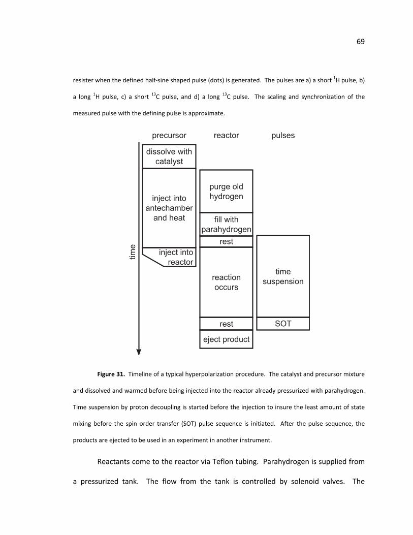
69 

 

resister when the defined half‐sine shaped pulse (dots) is generated.  The pulses are a) a short 1H pulse, b) 

a  long  1H pulse,  c)  a  short  13C pulse,  and d)  a  long  13C pulse.    The  scaling  and  synchronization of  the 

measured pulse with the defining pulse is approximate. 

dissolve withcatalyst

precursor reactor pulses

timesuspension

rest

rest

eject product

inject intoantechamber

and heat

inject intoreactor

purge oldhydrogen

fill withparahydrogen

SOT

reactionoccurs

time

 

Figure 31.  Timeline of a typical hyperpolarization procedure.  The catalyst and precursor mixture 

and dissolved and warmed before being injected into the reactor already pressurized with parahydrogen.  

Time suspension by proton decoupling is started before the injection to insure the least amount of state 

mixing before  the  spin order  transfer  (SOT) pulse  sequence  is  initiated.   After  the pulse  sequence,  the 

products are ejected to be used in an experiment in another instrument. 

Reactants come to the reactor via Teflon tubing.  Parahydrogen is supplied from 

a  pressurized  tank.    The  flow  from  the  tank  is  controlled  by  solenoid  valves.    The 

70 

 

precursor  and  catalyst mixture  is  loaded  into  a  holding  chamber  at  the  start  of  an 

experiment.   This mixture  is pushed  from the holding chamber to the reactor through 

Teflon tubing using pressure supplied by a tank of nitrogen.  This flow is also controlled 

by solenoid valves.   The pressure of nitrogen (12 bar) and parahydrogen (10 bar)  is set 

by  regulators on  the gas  tanks.   During an experiment,  the  reactants are sprayed  into 

the reactor already filled with parahydrogen.   An example of the order of the steps of 

the experiment is illustrated in Fig. 31. 

The plumbing, holding chamber, and reactor are all housed  in an  insulated box 

so  that  the  experiment  may  be  heated  to  improve  reaction  time.    During  normal 

experiments, this system is kept at 60°C. 

The  reactor  system  is  computer  controlled  via  a  National  Instruments  (NI) 

multifunction DAQ  card model NI PXI‐6251  in a model NI PXI‐1042  chassis  interfaced 

with a desktop computer using a model NI PXI‐PCI8331  controller.   Outputs  from  the 

card are made accessible using a model NI SCB‐68 screw terminal connector block.  The 

card has digital outputs that control the opening and closing of the solenoid valves via a 

connected  NI  ER‐16  electromechanical  relay  for  timed  control  of  the movement  of 

reactants and products through the system.   The card also has analog outputs, one of 

which  is the  input to the amplifier that powers the  1B  saddle coil for generation of the 

pulses  used  to  deliver  the  pulse  sequence  for  hyperpolarization  of  the  product 

molecules in the reactor. 

71 

 

B. Computer program

The computer program is written in NI LabVIEW 8.5 (60) and a basic flow chart of 

its operation  is provided  in Fig. 32.    It dictates when valves open and close and when 

and how  1B  pulses are delivered.  The program has two main components visible on the 

primary  user  interface.   One  component  allows  a  sequence  of  events  to  be  run  in  a 

prescribed  order with  set  timing.    These  sequences,  generally  referred  to  as  “pulse 

programs”, can be saved and recalled for use in automatically generating hyperpolarized 

product with the equipment.  The second component allows real time manual control of 

the valves during times when a pulse program is not being run. 

The pulse program steps are defined by an array of clusters.  The clusters contain 

elements  that  define  the  state  of  the  system  during  each  step  of  the  array.    The 

elements in this cluster are as follows:  

1) Type.  This element defines what sort of step is being performed.  The type may 

be “timed”  (the program preserves  the state  for a set  time), “start pulse”  (the 

program initiates the programmed pulse sequence), “finish pulse” (the program 

waits  for  the end of  the programmed pulse sequence), or “wait”  (the program 

waits for the user to click “okay” on a dialog box before continuing to the next 

step). 

2) Time.  This element defines the time that a timed step will last. 

3) Valves.    This  is  a  cluster  of  Boolean  buttons  representing  the  valves  in  the 

72 

 

system.  They are set to “off” to keep the valves closed and to “on” to open the 

valves. 

In order to generate a pulse program, the user sets the elements in the cluster to 

depict the state the system should be in at a given moment.  That is, the user turns the 

valves that are desired to be open to “on”, sets the type of step and, if needed, the time 

the step will  last.    If a “start pulse” step  is used, those parameters also need to be set 

separately and a “finish pulse” step will need to follow at some point afterward in order 

to  leave the DAQ card ready  for another pulse.   Only one type of “pulse” step can be 

used during a particular run of a pulse program.  More steps are produced by stepping 

the  array  forward  and  setting  the  elements  appropriately.    The  program  is  run  by 

pressing a start button after which it steps through the defined steps sequentially until 

the last one is reached. 

A secondary pulse setup program panel allows setting and  testing  the  1B  pulse 

sequence that will be delivered during a pulse program or single pulse that can be used 

directly for calibration purposes.  Pulses are defined by an array of voltage values output 

from  the analog out  to  the amplifier at a user defined  frequency.   The user may also 

select an offset  from zero and a scaling  factor  for  the pulses.   A set of MATLAB®  (61) 

functions has been created to easily generate the data file used to define the series of 

voltage values that represent a pulse.   All pulse settings are kept as global variables to 

simplify the data flow. 

The separate MATLAB® functions contain programs to generate specific pulses of 

73 

 

various shapes,  link these pulses together  in specific desirable ways, and a  few helper 

functions.   A  few variables considered  to be “spectrometer settings”  (that a user of a 

pulse programmer would not  frequently alter) are  set as global variables.   These are: 

“omega”, which denotes the frequency of protons in Hz; “cardfreq”, which  is the word 

rate at which the arbitrary waveform generator (AWG) (part of the multifunctional DAQ 

card) outputs the voltage data points when generating a pulse; and “now”, which keeps 

track of the cumulative time, in seconds, that has passed during all the previous pulses 

and delays that have been created. 

To use  them,  a user  first declares  these  three  variables  to be  global  and  sets 

them  to  the  desired  values.    Usually  “now”  is  initialized  to 0  or  to  half  the  time 

represented by one point.  Then the pulses and delays that are needed are generated in 

order and concatenated  into a single vector.   When the pulse  is ready, the real part  is 

saved with the “save_pulse” helper function which writes  it  in the form needed by the 

LabVIEW program.   This program has additional  functionality  to  save  the pulse  in  the 

form  needed  by  GAMMA  programs  to  facilitate  theoretical  modeling  of  the  pulse 

results. 

The  pulse  generating  functions  all  take  three  required  variables  and  return  a 

vector of voltage values representing the desired pulse.  The first is a variable containing 

information about  the  isotope  to be pulsed,  the second  is  the nutation angle desired, 

and  the  third  is  the pulse phase φ .   Some pulses, such as Gaussian pulses, have extra 

parameters that can be optionally supplied after these required variables.  These are set 

74 

 

to default values  if not provided.   The variable containing  isotope  information can be 

generated by hand or by use of a helper  function  that  takes a string with  the  isotope 

name as input and returns the required variable with standard values derived from the 

value of “omega”.   This variable contains the type of  isotope, the carrier  frequency of 

the  isotope  at  the  given  static  field,  the  amplitude  (which  needs  to  be  set  from 

calibration),  and  the  2π  times  for  various  pulse  types.    The  2π  times  can  be 

customized by supplying a second variable  representing  the number of periods of  the 

carrier frequency that such a pulse should last. 

In addition to the pulses, a delay function is provided.  The delay function takes 

the number of seconds to wait as the only parameter and returns zeros that will cause a 

pause for the requested amount of time at the specified data rate.  At the end of both 

pulse and delay functions, the amount of time represented by the number of points  in 

the  vector  returned  is added  to  the  value of  “now”  so  that  the next pulse  along will 

generate  the  correctly  phased  carrier.    Since multiple  isotopes  are  being  pulsed,  the 

carrier frequency  is not always the same and the pulse sequence cannot be formed by 

concatenating envelopes for the pulses together and mixing them with the carrier as a 

final step. 

Some  preprogrammed  pulse  sequences  exist  in  order  to  simplify  their 

generation.   One program  is supplied for decoupling with MLEV‐16 (62) which requires 

an  isotope variable (as previously described), a time  in seconds, and the type of pulses 

that  are  desired.    At  the  end  of  the  initial  decoupling  for  time  suspension  prior  to 

75 

 

generating sequences  for heteronuclear PASADENA order transfer, the value of “now” 

may  be  reset  to  the  initial  value  if  desired,  since  phase  coherence  between  these 

periods is immaterial.  Distinct programs were written for the small, medium, and large 

θ  pulse  sequence  algorithms  including  phase  cycled  echoes.    These  take  the  timing 

parameters needed by the sequence, and  isotope variables  for the protons and target 

spins as parameters. 

76 

 

star

t

load

last

setti

ngs

end

save

last

setti

ngsst

op

done

star

t

puls

ese

tting

sm

anua

lco

ntro

lpr

ogra

mch

ange

set v

alve

son

or o

ff as

indi

cate

d

adju

st, d

elet

e,or

add

ste

p; o

rlo

ad o

r sav

epr

ogra

m

set v

alve

sfo

r the

ste

pre

adty

petim

ed

star

tpu

lse

finis

hpu

lse

wai

t

mor

e st

eps

to d

o wai

t set

time

incr

amen

tst

ep

set u

p an

alog

outp

ut ta

sktri

gger

task

sta

rt

wai

t for

pul

seen

ded

sign

alse

t ana

log

outp

ut to

0

wai

t for

user

clic

k

open

pul

sese

tup

prog

ram

retu

rn

load

puls

e

test

puls

ech

ange

setti

ng

DA

Qse

tting

set u

p an

alog

outp

ut ta

sktri

gger

task

sta

rtset n

ewse

tting

set

varia

bles

wai

t for

pul

seen

ded

sign

al

puls

ese

tting

plot

puls

e

set a

nalo

gou

tput

to 0

wai

t for

mou

secl

ick

wai

t for

mou

secl

ick

choo

sepu

lse

file

 

Figure  32.    Flow  chart  of  the  pulse  program  described  in  the  text  including  manual  and 

77 

 

programmatic control of all aspects of the polarizer.   Some lesser functions and checking procedures are 

not shown. 

C. Field calibration

The secondary panel of the user interface, used for setting up and testing pulse 

sequences, is also used for calibration of the  0B  and  1B  fields.  The low‐field instrument 

is not set up to collect a signal from a precessing nucleus, complicating the procedure of 

testing  the  pulses  delivered  at  a  particular  amplitude.  Thus,  this  procedure  relies  on 

manually  transporting  a  sample  from  a  high  field  to  the  polarizer  field,  delivering  a 

pulse, and  transporting  the  sample back  to high  field  for observation of  the  surviving 

magnetization. 

Initially, the pulse power is set to a value that is expected to give a large nutation 

angle somewhat less than what is required to fully invert the magnetization.  If too large 

an  amplitude  is  used,  the  curve will  flatten  or  show  a  local maximum  at  the  center 

where the global minimum should be (Fig. 33).  It is expected that the pulse power will 

shift the resonance frequency somewhat due to Bloch‐Siegert effects (63) so that there 

are  interactions between  the values of    0B  and  1B  of a  type  that are not significant  in 

high  field NMR.    If  a  pulse  that  is  too  small  is  used  for  the  calibration,  an  incorrect 

resonance will be found due to insufficiently accounting for these interactions. 

For each test, the standard sample  is allowed to come to equilibrium  in a high 

field NMR spectrometer to provide initial polarization.  The sample is then carried to the 

78 

 

polarizer and placed within  the  reactor volume.   The  test pulse  is  triggered,  then  the 

sample  is moved  back  to  the  high  field  instrument.   During  this  second  passage,  all 

transverse polarization generated by the test pulse  is  lost, but  longitudinal polarization 

remains.    The  sample  is  given  a  2π  pulse  in  the  high  field  spectrometer  and  the 

amplitude of the signal  indicates the size of the  longitudinal polarization after the test 

pulse.  Relaxation during each passage causes some slight distortion, but does not affect 

the calibration so long as the timing is carefully kept the same for each passage. 

1.8 1.85 1.9 1.95 2 2.05 2.1 2.15−1.8

−1.6

−1.4

−1.2

−1

−0.8

−0.6

−0.4

−0.2

0

static field (mT)

ampl

itude

left

in z

 

Figure 33.  Experimental data points showing an example of a calibration curve for determining 

the static field using a 13C pulse applied to deuterated and 1‐13C labeled acetate.  The line is intended only 

as an aid for the eye. 

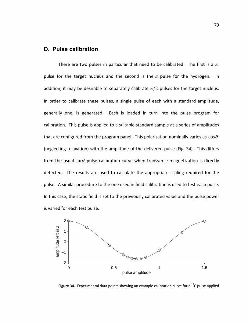
79 

 

D. Pulse calibration

There are  two pulses  in particular  that need  to be calibrated.   The  first  is a π  

pulse  for  the  target  nucleus  and  the  second  is  the π  pulse  for  the  hydrogen.    In 

addition,  it may be desirable to separately calibrate  2π  pulses  for the target nucleus.  

In  order  to  calibrate  these  pulses,  a  single  pulse  of  each with  a  standard  amplitude, 

generally  one,  is  generated.    Each  is  loaded  in  turn  into  the  pulse  program  for 

calibration.  This pulse is applied to a suitable standard sample at a series of amplitudes 

that are configured from the program panel.  This polarization nominally varies as cosθ  

(neglecting relaxation) with the amplitude of the delivered pulse (Fig. 34).   This differs 

from  the usual  sinθ  pulse calibration curve when  transverse magnetization  is directly 

detected.    The  results  are  used  to  calculate  the  appropriate  scaling  required  for  the 

pulse.  A similar procedure to the one used in field calibration is used to test each pulse.  

In this case, the static field is set to the previously calibrated value and the pulse power 

is varied for each test pulse. 

0 0.5 1 1.5−2

−1

0

1

2

pulse amplitude

ampl

itude

left

in z

 

Figure 34.  Experimental data points showing an example calibration curve for a 13C pulse applied 

80 

 

to deuterated and 13C labeled acetate.  The sample is first polarized at 4.7 T for at least 240 s, then moved 

to the low field polarizer for each of the series of pulses, then moved back to sample the amplitude of the 

remaining polarization.  The line is the least squares fit of the experimental data points to the functional 

form  ( )3 1cosc x cπ + 2c  where   are the fitting parameters.  The desired pulse amplitude from this fit is 

. 

ic

1c

E. Polarization

Once  the  pulse  amplitudes  have  been  calibrated,  the  pulse  sequence  for  the 

molecule  to be polarized  is generated.   This pulse contains an  initial  segment of  time 

suspension proton decoupling, which defines the effective time allowed for formation of 

those products that will contribute to the hyperpolarized signal.  This time, generally 4 s, 

is followed by the polarization transfer sequence.  It is loaded into the pulse parameters 

in  the LabVIEW software.   A pulse program  is  loaded  into  the software  to control  the 

experiment.   The mixture of precursor and catalyst  is  loaded  into the holding chamber 

and the pressurized gasses are connected to their  inlets.   The system  is closed up and 

allowed to come to equilibrium at the controlled temperature. 

When  everything  is  physically  set  up  and  the  experimentalist  is  ready  to 

generate  the hyperpolarized product,  the  start button  is pressed  to  initiate  the pulse 

program.    This  program  is  usually  set  up  to  purge  the  reactor  volume  of  any  old 

parahydrogen  and  then  fill  it  with  fresh  parahydrogen  from  a  holding  tank.  

Parahydrogen is given 2‐4 s to pressurize the reactor volume, then the time suspension 

81 

 

is initiated directly before the precursor and catalyst mixture is pushed into the reactor 

volume by nitrogen at higher pressure than the hydrogen already in the reactor.  At the 

end of the pulse, the product  is expelled.   The hyperpolarized product  is then taken to 

the high field  instrument for use.   The simplest high field experiment simply supplies a 

pulse to check how much polarization  is achieved.   In some cases, the transport of the 

sample  to  the high  field  instrument was done pneumatically.   For animal  studies,  the 

hyperpolarized product was ejected  into a  syringe which was  carried  to  the prepared 

injection apparatus. 

After the molecule  is hyperpolarized, the system  is flushed by running nitrogen 

gas  through  the  plumbing.    This  is  intended  to  remove  any  residual  fluid  from  the 

previous to a new run. 

F. Polarization verification

Many techniques exist to verify the level of polarization that has been obtained, 

each with strengths and weaknesses.   The one commonly  in use for MRI compares the 

signal  from  the  relatively dilute hyperpolarized product  (10  to 100 mM)  to  the  signal 

from a highly concentrated sample of 13C labeled acetic acid or pure natural abundance 

ethanol that is also in the NMR coil.  These signals are easily separated by location in the 

reconstructed image.  Using the known concentrations of the sample and standard, the 

signal  from  the hyperpolarized  sample  is  easily  compared  to  the  thermal  equilibrium 

polarization  at  the  particular  field  of  the  instrument.    This  gives  a  field  dependent 

82 

 

enhancement value which can be converted  to an absolute enhancement by knowing 

the  thermal equilibrium polarization of  the  standard.    Implicit  in  the  interpretation of 

the  hyperpolarization   from  such  a  calibration  is  the  assumption  that  the  original 

reaction went to completion by the time the spin order transfer sequence began.    If  it 

did  not,  then  the  fraction 

P

χ  of  the molecules  that  were  formed  sufficiently  quickly 

actually carry  the higher polarization  P χ .   Comparisons of polarization based on  the 

concentration of the sample and the standard are also biased to smaller values due to 

the  inclusion  of  small  gas  bubbles  in  the  sample  that  change  the  observed 

concentration. 

Another common method of determining  the polarization compares  the  signal 

from the hyperpolarized sample to  itself after the polarization has decayed to thermal 

equilibrium  in the high  field magnet.   This again gives a field dependent enhancement 

value  that  can  be  converted  to  an  absolute  polarization  knowing  the  equilibrium 

polarization at  that  field.   Since  the catalyst  is not  removed after  the set  time  for  the 

time suspension, the completeness of the reaction, as measured by ordinary NMR many 

minutes later, may be partly attributable to reactions that occurred after the time frame 

of  the  time  suspension.  Currently,  there  is  no method  to  stop  the  reaction  on  the 

second time scale, which would allow the course of the reaction to be studied by more 

direct means,  independent  of  the  transient  hyperpolarized  signal.    This  technique  is 

complicated by the many orders of magnitude difference between the signal from the 

hyperpolarized  molecule  and  that  from  the  molecule  at  equilibrium.    Higher  gain 

83 

 

settings  and,  generally,  extensive  averaging  are  required  to  collect  signal  from  the 

sample at thermal equilibrium. 

An  alternative  method,  that  determines  the  absolute  polarization  directly, 

measures the signal not from the hyperpolarized nucleus, but from the protons that are 

coupled to the hyperpolarized nucleus.  Since the coupling to the spin ½ heteronucleus 

causes  the proton peaks  to  split  into  two with each peak  associated with  a different 

state  of  the  neighboring  heteronucleus,  this  doublet  signal  gives  the  absolute 

polarization,  if  resolved.    The  simplest  example  is  a  molecule  with  a  polarized  13C 

coupled  to a  single proton.   Figure 35 demonstrates  the peak differences  seen  in  this 

case  for both positive and negative polarizations of  the carbon nucleus.   Determining 

the polarization of this system is a matter of determining the area under each peak and 

fitting it to Eq. (1) where   and N+ N−  are these areas.  This technique is complicated by 

the extra scalar couplings in the case of the three spin system needed for heteronuclear 

PASADENA.  In these cases, more elaborate data fitting is required, but the systems do 

generate  distinctive  patterns when  there  is  sufficient  resolution  as  demonstrated  in 

Fig. 36. 

84 

 

−200 −100 0 100 200frequency (Hz)

−100%

−200 −100 0 100 200frequency (Hz)

100%

−80%80%

−60%60%

−40%40%

−20%20%

0%

 

Figure 35.   When a nucleus couples to a proton, the polarization of that nucleus  is apparent  in 

the peak heights of the proton spectrum, obtained from the fid subsequent to a  2π  pulse.  These plots 

compare the relative peak heights in the proton spectrum of a single proton coupled to a 13C nucleus with 

the indicated polarization.  The coupling constant is  110CHJ =  Hz and all plots are on the same y‐scale. 

85 

 

−100 −50 0 50 100frequency (Hz)

−100%

−100 −50 0 50 100frequency (Hz)

100%

−80%80%

−60%60%

−40%40%

−20%20%

0%

 

Figure 36.   When a nucleus couples to two coupled protons, the polarization of that nucleus  is 

apparent  in  the  peak  pattern  of  the  protons.    These  plots  compare  the  relative  peak  patterns  in  the 

proton spectrum of two protons coupled to a  13C nucleus with the  indicated polarization.   The coupling 

constants  are  is   Hz, 12 8.51J = 1 6.32SJ = −  Hz,  and  2 4.13SJ =  Hz,  the  protons  are  split  by  0.2δ =  at 

500 MHz,  and  all  plots  are  on  the  same  ‐scale.    The  spectra  are  simulated  for  the  case  of  an  FID 

subsequent to a 

y

2π  pulse. 

In  any  case  in  which  sample  transport  is  needed  prior  to  detection,  the 

polarization of  the sample at  the end of  the pulse sequence  is not what  is measured.  

86 

 

The  travel  time  between  instruments  (about  10 s)  allows  relaxation  from  the 

hyperpolarized  state.    In  order  to  estimate  the  hyperpolarization  achieved,  the 

measured polarization is corrected for the theoretical relaxation loss. 

G. Molecule selection and characterization

The molecule to be hyperpolarized must be one that is obtainable by molecular 

addition of hydrogen across an accessible double or triple bond of a precursor molecule.  

A target nucleus near the addition point must have resolvable scalar coupling with these 

added  hydrogen.    It  is  possible  to  generate  saturated  molecules  with  specific 

stereochemistry with the aqueous hydrogenation catalyst that has been used for these 

reactions  (64,65).    Some  example  molecules  that  have  been  hyperpolarized  are  2‐

hydroxy‐ethylpropionate  (HEP)  (40,66),  maleate  (67),  succinate  (36,67),  and  the 

amphiphile TFPP (48). 

1. Measurement of 1T

In general, the molecule cannot be generated in the “location” in which it will be 

used.    Therefore,  in  order  to  reap  the  greatest  benefit  from  the  hyperpolarization 

process, the target nucleus on the molecule should have a  long  longitudinal relaxation 

time constant   allowing  the polarization  to be stored  for  the greatest  length of  time 

while the molecule travels to the required location. 

1T

The  typical method  of   measurement  (68)  involves  inverting  the  equilibrium 1T

87 

 

magnetization and allowing it to recover for some time before measuring the amplitude 

of  the  longitudinal magnetization with a  2π  pulse.   This  is  repeated  for a number of 

inversions and  fit  to an exponential dependent upon  time.   After each measurement, 

the system must be allowed to relax for some multiple of the expected time constant; 

 is usually considered to be enough.   Since these are meant to be molecules with a 

long  relaxation  time,  this  measurement  can  become  quite  lengthy.    One  method 

commonly  employed  to  measure  this  somewhat  more  quickly  is  to  saturate  the 

magnetization and then measure the rate at which it recovers from zero instead of from 

a negative value.  This removes the requirement of any wait between experiments and 

eliminates  the prospect of needing  to  repeat a measurement because  the value of   

has been underestimated too greatly. 

15T

1T

In  some  cases,  NOE  or  some  other  nonequilibrium  method  can  be  used  to 

establish the  initial polarization on the target nucleus  (69).   When this  is possible, this 

strategy can be used to help measure the relaxation time quickly as well.  In order to do 

this, the relaxation from the inversion of the enhanced state to equilibrium is subtracted 

from the relaxation from the enhanced state to equilibrium resulting in decay to zero. 

It  is  important that   be measured on the product molecule with the  intended 

isotopic  composition  since  deuteration will  affect  this  value.    There  are  two ways  in 

which  deuterium  affects  the  relaxation  of  the  nearby  proton,  one  that  increases  the 

relaxation and one  that decreases  the  relaxation  in  comparison  to proton.    Since  the 

1T

88 

 

deuterium gyromagnetic ratio is about one sixth that of proton, the two frequencies are 

significantly  different  and  relaxation  effects  do  not  couple  effectively between  them.  

However, since deuterium  is a spin 1 nucleus,  it relaxes far more quickly than protons, 

generating a polarization sink that quickly relaxes anything that does couple with  it to 

equilibrium. 

2. Measurement of coupling constants

Once a molecule  is selected,  the coupling constants need  to be determined  to 

appropriate  accuracy,  especially  when  applying  the  large θ  range  pulse  sequence 

algorithm.  This is aided by undecoupled spectra of the heteronucleus.  Another method 

is  to  simply perform  the original PASADENA experiment on  the molecule  in question.  

This both tests that the catalytic addition of parahydrogen  is working as expected and 

measures  the  required  scalar  coupling  constants  without  ambiguity  even  when 

geometric considerations such as those shown in Fig. 13 are active. 

3. Molecular variations

In  some  cases,  the  desired molecule may  not  have  particularly  advantageous 

parameters  for  the  polarization method.    One  such molecule  is  15N  labeled  choline 

which has very weak coupling between the protons and the nitrogen target leading to a 

somewhat long polarization sequence.  In this case it may help to vary the molecule by 

adding an  intermediary nucleus for polarization which  is then transferred to the target 

nitrogen  label by  some more  traditional means  such  as  INEPT.    Specifically,  a  carbon 

89 

 

directly  connected  to  the  nitrogen  and  one  of  the  added  protons  could  be  a  13C 

intermediary.    This  transforms  the  molecule  from  the  large θ  range,  which  often 

requires  long  sequences,  to  the  small θ  range  which  generally  requires  quite  short 

sequences. 

90 

 

V. Low field effects

The equipment constructed for generation of hyperpolarized reagents has been 

built with a relatively small magnetic field so that the equipment is mobile enough to be 

brought to where it is needed and does not cause problems with other equipment that 

is sensitive to magnetic fields.  Using the low field also allows for the use of cheaper and 

more general equipment for pulse generation since the frequencies involved are in the 

kHz  range.    This  low  field  is  possible  since  the  sequences  rely  upon  internal  scalar 

coupling to generate the necessary evolution that results in hyperpolarization. 

Thus,  while  the  use  of  low  field  has  advantages,  it  also  generates  some 

problems.  These problems and their solutions are to be discussed in this section. 

A. Lab frame introduction

Generally, NMR calculations are conducted in the rotating frame.  This is covered 

in the elementary texts on the subject such as that by Levitt (70) or Goldman (71).    In 

NMR,  the  signal of  interest  contains  small deviations  from  some  large  frequency.    In 

order to be more sensitive to these small deviations, the system  is transformed  into a 

reference frame that is spinning at some reference frequency Ω .  Then everything that 

is  precessing  at  the  reference  frequency  appears  to  be  stationary  and  the  small 

deviations are low frequency effects that can be easily tracked, as can be seen in Fig. 37.  

This leads to both conceptual and numerical simplifications. 

91 

 

a) b)

 

Figure 37.  Comparison of the lab frame and rotating frame.  The two plots follow the rotation of 

a unit vector of magnetization acted on by a four cycle linear square inversion pulse in (a) the lab frame 

and (b) the rotating frame.  In the rotating frame, the deviations of the path of the magnetization from a 

smooth arc are clearly visible while  in the  lab  frame these deviations are hidden by the  larger effect of 

precession. 

Pulses  are  described  with  the  carrier  at  the  reference  frequency.    The  time 

dependence  is piecewise‐constant variations  in amplitude and phase of this carrier.   In 

typical NMR applications as well as  this particular application, pulses are delivered by 

coils  that  create  a  1B  field  that  is  constant  in  direction,  i.e.  they  generate  linearly 

polarized  pulses.    A  linearly  polarized  pulse  at  frequency Ω  and  phase  offset φ  is 

equivalent to a circularly polarized pulse at the desired frequency and a counterrotating 

circularly polarized pulse of equal amplitude.  

  ( ) ( ) ( )12cos i t i tt e eφ φφ Ω + − Ω +⎡ ⎤Ω + = +⎣ ⎦   (38) 

This can be transformed into the rotating frame by multiplication by  . i te− Ω

  ( ) ( )212cos 1 ii te t e φφ − Ω+− Ω ⎡ ⎤Ω + = +⎣ ⎦   (39) 

This gives a stationary piece and a time dependent piece varying at a high frequency.  In 

92 

 

order  to  simplify  this,  the  rotating  frame  approximation  is  taken  by  tossing  out  the 

rapidly varying piece.   This  simplifies  the  calculations when  the  counterrotating piece 

can be neglected. 

When there are multiple nuclei  in a spin system, a multiply rotating coordinate 

system is used with one reference frequency for each nucleus.  In this case, those pieces 

of  the  Hamiltonian  that  depend  on  the  relative  frequency  between  the  nuclei  are 

neglected.  This includes the effects of pulses on the nuclei other than the one they are 

meant for and the transverse pieces of heteronuclear scalar coupling. 

In high  field NMR these simplifications are reasonable.   At sufficiently  low  field 

NMR, they ignore effects as large as the ones they examine such that calculations using 

them are uninformative.   The  0B  field of a  few mT used here  lies  in a middle  regime 

where  rotating  frame calculations can be  informative but  they are  inadequate  for  the 

complete model of the system.  In order to help understand and solve the difficulties of 

low  field NMR, calculations  in  fully non‐rotating  frames are needed.   This approach  is 

straightforward  in  that  the  full  time dependence  is  treated by breaking up  the pulse 

sequences  into  intervals  that  are  short  compared  to  the  period  of  the  carrier 

frequencies  and  concatenating  the  evolution  due  to  this  piecewise‐constant 

approximation of the Hamiltonian. 

In order to more fully understand the implications of using low field, calculations 

in  the  lab  frame are performed.   These calculations make use of GAMMA  (50), a C++ 

library  of  NMR  related  functions.    This  library  has  been  created  specifically  to  take 

93 

 

advantage of  the simplifications brought about by using a multiply  rotating  frame but 

has many  readymade  functions  that are  readily adaptable  to  the  inertial  frame of  the 

lab.   As such,  it offers a handy framework for modeling NMR experiments  in the usual 

multiply rotating frame and in the lab frame for comparison. 

B. Using GAMMA for lab frame calculations

Programs written in GAMMA are able to read in the parameters of a spin system, 

generate  the  initial condition density matrix, and evolve  this density matrix under  the 

effects of Hamiltonians that are static or include pulses, either ideal, square, or shaped.  

In order  to perform calculations  that model  the system of  interest,  functions must be 

made that cast the problem as a sufficiently accurate piecewise constant Hamiltonian.  

Specifically, the initial condition and the Hamiltonians that are in effect at various times 

during the application of a pulse sequence need to be generated. 

The  initial condition of  interest uses the tensor product construction  in Eq.  (7).  

The  first  two  spins  in  a  system  are  assumed  to  be  the  protons  added  from 

parahydrogen,  while  all  other  spins  are  at  thermal  equilibrium  which  uses  room 

temperature as the default.  This method restricts the form in which the file holding the 

spin system must be written in that the choice of the identity of the first two spins is not 

free, but does not restrict the calculation. 

The  GAMMA  library  already  contains  functions  to  generate  the  appropriate 

intrinsic Hamiltonian  in  the  lab  frame, but  a new  function  for  the Hamiltonian when 

94 

 

pulses  are  in  operation  must  be  generated.    For  the  purpose  of  programming  the 

instrument, these pulses are defined by a  list of voltage  levels that are each held for a 

set time.  This form is smoothed and changed by the filtering effects of real electronics, 

but  unless  otherwise  stated  serves  as  the  approximation  of  the  pulse  as  a  series  of 

piecewise  constant  segments.    The  time  step  is  typically   μs  in  the  arbitrary 

waveform  generator  and  typically  this  or 1 μs  in  the  lab  frame  calculations.    Shaped 

pulses  in the multiply rotating frame version of GAMMA are defined as a similar series 

of  piecewise  constant  segments  in  the  rotating  frame  appropriate  to  the  Larmor 

frequencies of each nucleus.  The value of each segment is 

3.3

1Bγ  in Hz while the value of 

the  segments  defined  for  the  polarizer  are  the  voltage  values  input  to  the  amplifier.  

These  values  need  to  be  multiplied  by  some  arbitrary  conversion  factor  to  be 

appropriate as inputs to a GAMMA program.  This factor can be found by calibrating a π  

lse described in the same piecewise manner. pu

The existing shaped pulse function is used as a prototype for a lab frame function 

that  calculates  the  effects  of  linear  pulses  delivered  to multinuclear  systems.    This 

function only  accounts  for  the effects of  the pulse on one  isotope  since  the  rotating 

frame  approximation  assumes  that  all  other  isotopes  are  sufficiently  separated  in 

frequency to be unaffected by the pulse.  The new function must account for the effects 

on all nuclei  in  the  system.    In order  to do  this  for a pulse meant  for  isotope  ,  the 

interaction of the pulse must be applied to all nuclei of the same isotope with the given 

Rabi frequency as well as to the other isotopes at their appropriate Rabi frequency.  For 

a

95 

 

instance, all nuclei of  isotope b  will need  the value of  1aBγ  scaled by  b aγ γ  and  then 

applied to account for the effect of the different gyromagnetic ratios. 

In order to  input the  long vectors that define the pulses, existing functions that 

read  in MATLAB® files were used.   By doing this, the same functions that generate the 

pulse sequence for the polarizer can also be used for input to GAMMA programs simply 

by  saving  the  file  in  a  different way.   Due  to  differences  in  the  amplification  of  the 

different frequencies for hydrogen and carbon  in the polarizer, the relative magnitude 

of pulses for each of the isotopes used must also be changed. 

C. Pulse length at low field

A  few  considerations  must  be  made  about  pulses  at  low  field  that  are  not 

needed at high  field.   Two considerations have  to do with  the  length of  the pulse.    In 

high field, pulse lengths, often about 10μs, are many cycles of the carrier frequency.  In 

a field of only 1.8mT, the proton Larmor frequency is 75 kHz and a 10 μs pulse would be 

less than one cycle of the carrier frequency long.  Such a pulse would have large effects 

on all isotopes in the system and those effects would be highly dependent on the phase 

of the pulse.  In order to render the effects of the pulse largely selective to one isotope, 

the pulse must be lengthened.  The length needed is dependent upon the shape of the 

pulse, but typically must be at  least a few cycles of the carrier frequency.   For reasons 

that will be demonstrated, it is also advantageous that the length be chosen among the 

discrete values of  time  that make  the pulse an  integer or half  integer multiple of  the 

96 

 

carrier wave period. 

74

74.5

75

75.5

γ 1H B

0 (kH

z)

a)

3.6 3.7 3.8 3.9 4 4.1 4.2 4.3 4.4 4.516

18

20

22

γ 1H B

1 (kH

z)

pulse length (carrier periods)

b)

0 radπ/3 rad2π/3 rad

 

Figure 38.  The optimal static field and pulse strength to give near perfect inversion with square 

pulses that are near four cycles of the carrier frequency long at a few example wavelet phases as shown in 

the legend. 

Making  the  length  such  a multiple  of  the  carrier  period  helps  insure  that  the 

effect of  the pulse  is not dependent on  the phase of  the  carrier  (Fig. 38b)  for purely 

geometric reasons.  From the viewpoint of the rotating frame with the counterrotating 

wave discarded, the strength of  1B  for a square pulse  is constant throughout the pulse 

so  the  Rabi  frequency,  the  frequency  at which  the magnetization  nutates  about  the 

pulse axis, is constant as well.  If the pulse is started a little earlier or later, but lasts the 

same time, the pulse will turn the magnetization by the same amount.  However, from 

the  lab  frame  viewpoint,  the  strength  of  1B  rises  and  falls  and  the  instantaneous 

97 

 

frequency  rises  and  falls with  it  (Fig.  39).    If  the  length  is  not  carefully  chosen,  then 

changes  in  when  the  pulse  happens  also  change  the  overall  rotation  of  the 

magnetization due to the pulse.  Careful pulse construction where the magnitude of  1B  

is  dependent  upon  the  wavelet  phase  could  be  used  to  help  lift  this  pulse  length 

restriction in applications where the wavelet phase is known before the pulse is given. 

0 5 10 15 20 25 30 35 40 45 500

50

100

150

time (μs)

angl

e to

z−

axis

 

Figure  39.    In  the  rotating  frame,  the  linearly  polarized  square  pulse  is  approximated  as  a 

circularly polarized pulse with half the amplitude.  In the lab frame, the circularly polarized pulse (dotted) 

shows consistent Rabi frequency but the linear pulse (solid) does not and requires careful selection of the 

pulse length.  These pulses are both π  pulses that are four carrier wave periods long. 

The choice of the overall length of the pulse among the lengths that are allowed 

is  far  more  complicated.    Shorter  pulses  are  desirable  for  better  time  resolution, 

particularly  in very short pulse sequences.   Longer pulses are desirable  for  fewer non‐

ideal effects such as causing significant nutation on other isotopes, Bloch‐Siegert effects, 

and wavelet phase dependence.  These effects are both length and shape dependent, so 

require further discussion to fully understand. 

It  is worth noting that the non‐geometric effects that control the optimal static 

98 

 

field of the pulse (Fig. 38a) imply that a pulse that is a quarter period longer or shorter 

than an  integer multiple of the carrier period would be the best choice.   Pulses of this 

length have not been explored due to the numerous other drawbacks that square pulses 

have  in ways  that are not expected  to be affected by  small adjustments  in  the pulse 

length. 

D. Unintended nutation of other isotopes

The separation in frequency of isotopes is linearly dependent upon the strength 

of  the  static  field  0B .    At  1.8 mT,  some  isotopes  that may  be  encountered  are  only 

separated by a  few kHz.   This situation requires that the pulses have sufficiently small 

bandwidth so as not to cause nutation on isotopes that is not intended.  The bandwidth 

is generally dependent upon  the  inverse of  the  time of  the pulse.   At  first glance,  the 

fact that pulses that are quite long compared to high field practice seem to be good in 

this respect, but in the relative sense of the number of carrier wave periods they persist 

for,  the pulses are much  shorter  than  in  conventional  systems.    It  turns out  that  this 

relative sense gives the better picture of the situation.  These pulses cover a much larger 

bandwidth in terms of their ability to rotate nearby isotopes (Fig. 40), complicating the 

pulse sequence design. 

99 

 

0 10 20 30 40 50 60 70 80 90 1000

20

40

60

80

100

120

140

160

180

Larmor frequency (kHz)

angl

e to

z-a

xis

1H

19F

31P

13C

2H15N

14N

 

Figure  40.    Pulses  intended  for  one  isotope  have  significant  affect  on  other  isotopes  in  the 

sample.  Here are π  pulses for two common isotopes, 1H (thick) and 13C (thin).  These are square pulses 

that are six carrier wave periods of the target nucleus long.  The locations of the reference frequencies for 

these isotopes and other common or useful isotopes are indicated by arrows. 

The unintended nutation effects are worse for pulses intended for isotopes with 

a smaller gyromagnetic ratio.  This is due to the relative sensitivity of the nuclei and the 

consequences of this sensitivity.  Isotopes with a lower gyromagnetic ratio require larger 

amounts of power in order to achieve the same Rabi frequency as a direct consequence 

of the smaller magnetic moment.   Also as a direct consequence, those  isotopes with a 

larger moment are more sensitive to the power being applied.  This effect can be seen in 

Fig. 40 in the increased size of the lobes on the higher frequency side of each pulse. 

100 

 

E. Bloch-Siegert effects

In the absence of any field in the transverse plane, the resonance frequency of a 

particular isotope is dependent only on the static field.  However, when a magnetic field 

is  turned on  in  the  transverse place,  this  causes  the  size and direction of  the  field  to 

change which  in  turn  causes  the  resonance  frequency  to  shift.   When  this  transverse 

field is also static, the problem is uninteresting in that a change of axes will show it to be 

equivalent to the situation without the transverse field on, but with a slightly different 

resonance frequency.  When the field becomes time dependent, the problem becomes 

much more interesting. 

Even before  the  first NMR experiments were performed on stationary samples 

instead of molecular beams, Siegert and Bloch (63) contemplated the effect of the time 

dependent  transverse  field  1B  in  the  larger  static  field  0B .   They  studied  the  situation 

for the general problem of two  independent, orthogonal fields  in the transverse plane 

and explored the consequences for a circularly and linearly polarized field.  They found 

that  the  linearly  polarized  case  shifts  the  resonance  of  the  sample  by  a  factor  of 

( )21 02B B ,  to  first  order,  and  estimated  that  it  was  a  negligible  effect  in  the 

experiments of the time. 

In the current experiments, π  pulses as short as four carrier wave periods have 

been used, giving  1 0 1 8B B = .   This gives a  first order estimate of the offset as nearly 

300 Hz while the actual offset due to other considerations can be as much as 1 kHz.  The 

101 

 

first  order  estimate  of  the  Bloch‐Siegert  shift  is  increasingly  inaccurate  as  this  ratio 

becomes large so it is insufficient to use the estimate for this situation.  In practice the 

response is calculated numerically without recourse to an expansion in  1 0B B . 

In the case of on resonance circular polarization, there  is no Bloch‐Siegert shift.  

As  such,  it would  be  reasonable  to  construct  an  instrument  capable  of  delivering  a 

circularly polarized pulse  in order  to  remove some of  the difficulties  inherent  in using 

low field.  However, circular polarization only helps with the on resonance isotope; the 

effects  of  each  pulse  on  other  isotopes  continue  to  be  a  problem  and  this  problem 

selectivity even increases in some cases. 

F. Wavelet phase dependence

One unexpected result found in the course of performing lab frame calculations 

was  a dependence of  the pulse  results on  the wavelet phase.    In  the  context of  the 

rotating frame, this possibility does not arise.  Such an effect implies that there is some 

universal time  , seemingly violating a basic  law of physics.   However, without the 

approximations  of  the  rotating  frame,  pulses  with  different  wavelet  phase  are 

distinguishable and no physical laws are violated. 

0t =

The wavelet phase  is  the phase  that  the  carrier wave happens  to have  at  the 

start  of  a  pulse.   NMR  pulses  can  be  thought  of  as  a  carrier wave multiplied  by  an 

envelope.    The  carrier  is  a  function  ( )exp i tω φ⎡ ⎤+⎣ ⎦  which  oscillates  at  the  angular 

frequency ω  near the Larmor frequency of the spin the pulse is intended to affect.  The 

102 

 

phase φ  is relative  to  the reference wave defining  the rotating  frame and  is  the usual 

notation  of  phase  in  high  field  NMR.    The  envelope  is  the  shape  of  the  pulse,  for 

instance, for a square pulse, the envelope is a constant.  In order to generate a pulse at 

time  t , the carrier with the desired phase is multiplied by the desired envelope.  The 

wavelet phase 

pulse

wφ  is the quantity  mod 2pulsetω π  in radians. 

In the rotating frame, a π  pulse delivered to a system at equilibrium at  0pulset =  

or one delivered after a short wait should give exactly the same result because they are 

indistinguishable except for the time that has passed since the arbitrarily chosen  initial 

time.    In the  lab  frame, the pulse given by coils on a single axis  is the real part of the 

function  ( t )cos ω φ+  which does change according to the arbitrarily chosen initial time.  

As it turns out, these changes are important (Fig. 41). 

103 

 

-1

0

1a)

-1

0

1b)

0 10 20 30 40 50 60 70 80-1

0

1

time (ms)

c)

170°

180°

175°

 

Figure 41.  Examples of pulses with a square envelope with pulse phase  0φ =  and wavelet phase 

(a)  3 2wφ π= ,  (b)  0wφ = ,  and  (c)  3wφ π= .    When  applied  with  the  same  amplitude  to  a  system 

resonating at 75 kHz,  the  resulting nutation axis and angle depends on  the wavelet phase,  to a degree 

which is significant for the frequencies and pulse widths of interest here, but is typically negligible in high 

field NMR. 

The wavelet phase effects can be shown experimentally when the pulse wavelet 

phase  can  be  measured  or  controlled.    With  the  equipment  currently  in  use  for 

heteronuclear  PASADENA  experiments,  it  is  the  case  that  the wavelet  phase  can  be 

controlled and an experiment has been performed to demonstrate the effect.   For the 

demonstration, two pulses were made using six π  pulses followed by a  2π  pulse.  The 

first used the phases  xxxxxxy , where the letters denote the axis about which the pulse 

104 

 

operates  and  the  over  bar  denotes  the  negative  axis.    This  sequence  is  predicted  to 

show extreme variation over the tested phases, while the second, with phases  xxxxxxy , 

should show very little variation.  The design concept of this experiment is illustrated in 

Fig. 42 and the results of this experiment are shown in Fig. 43 with a fit calculated using 

GAMMA  on  the  same  pulse  shapes with  the  values  of  0B ,  1B ,  and  an  amplitude  as 

fitting  parameters.    This  amplitude  parameter was  required  because  the  divergence 

found in the experiment was more than is expected from these pulses.  This difference 

may be due to distortions  in the pulse shape by the polarizer electronics such that the 

pulse delivered is not exactly as designed. 

a) b) c)z

x

zz

xx

 

Figure 42.   Schematic of  the expected nutation of various series of six π  pulses  followed by a 

2π  pulse.  For a pulse with the phases  xxxxxxy  (a and b), the magnetization that starts along the  ‐axis 

at the empty triangle and nutates with ever  increasing error dependent upon the wavelet phase until  it 

finishes at  the  large dot.   At one extreme  (a),  this error results  in a  large, negative magnitude along   

after the 

z

z

2π  pulse, while at the other extreme (b), this error results in a large, positive magnitude along 

 after the z 2π  pulse.  For a pulse with the phases  xxxxxxy  (c), the magnetization that starts along the  

‐axis at the empty triangle and nutates with increasing error until the end of the third inversion (at the z

105 

 

diamond) after which the path is retraced back to the start so that all wavelet phases give approximately 

no magnetization along   after the z 2π  pulse. 

0 0.5 1 1.5 2 2.5 3−0.8

−0.6

−0.4

−0.2

0

0.2

0.4

0.6

0.8

wavelet phase (rad)

ampl

itude

left

in z

 

Figure  43.    Experimental  demonstration  of  wavelet  phase  effects.    Six π  pulses  are  applied 

successively  followed by a  ( )2y

π pulse.   These π  pulses were applied with  the phases  xxxxxx  (circles 

with solid line fit), thus increasing the divergence from the rotating frame expectation with each pulse, or 

with the phases  xxxxxx  (points with dashed  line fit), thus  increasing the divergence over the first three 

pulses and then decreasing  it over the second three pulses.   The data are normalized by dividing by the 

signal obtained with no pulses. 

Given  a  pulse  with  a  certain  carrier  frequency,  there  is  an  optimal  Larmor 

106 

 

frequency  0Bγ  and Rabi  frequency  1Bγ  at which  that pulse gives perfect  inversion  for 

any particular wavelet phase (Fig. 44).  However, in a real experiment it is impractical to 

change the value of the static field as part of the pulse sequence.  When both fields are 

set  to  particular  values,  only  a  few  values  of  the  wavelet  phase  will  give  perfect 

inversion while the others give poor inversion, sometimes substantially so (Fig. 45).  This 

is not markedly improved when the value of  1Bγ  is optimized for each wavelet phase. 

74

74.5

75

75.5

γ HB

0 (kH

z)

0 1 2 3 4 5 618.8

19

19.2

wavelet phase (rad)

γ HB

1 (kH

z)

 

Figure 44.   The optimal values  for  0Bγ  and  1Bγ  for a π  proton pulse with a  square envelope, 

0φ = ,  and  a  carrier  frequency of 75 kHz  that  lasts  four  cycles of  the  carrier  for  the  range of possible 

wavelet phase values.   When the pulse  is used with these  field strengths,  it gives a perfect  inversion at 

each wavelet phase. 

107 

 

0 1 2 3 4 5 6165

170

175

180

wavelet phase (rad)

angl

e to

z−

axis

 

Figure 45.   Variation of the nutation angle with wavelet phase after a nominal π  proton pulse 

with a square envelope,  0φ = , and a carrier frequency of 75 kHz that lasts four cycles of the carrier.  The 

solid line is a pulse that has been optimized for  0 75H Bγ =  kHz which requires that  1 19.12H Bγ =  kHz and 

gives  perfect  inversion  at  0.4398wφ =  rad.    The  dashed  line  is  a  pulse  that  has  been  optimized  for 

4wφ π=  rad which requires that  0H B 74.58γ =  kHz and  1 19.04BHγ =  kHz. 

A pulse might not be capable of generating a full inversion for all wavelet phases 

either because the axis of rotation  is outside of the  xy ‐plane or because the required 

Rabi  frequency changes with wavelet phase.   While both of  these effects are  seen  to 

some extent,  the great majority of  the problem  comes  from  the  first.   The particular 

effect is actually seen in Haeberlen’s (72) analytical treatment of continuous wave (CW) 

decoupling by average Hamiltonian theory. 

108 

 

VI. Solutions for wavelet phase dependence

Some  level  of  wavelet  phase  dependence  is  expected  for  any  low  field 

experiment.  The key to performing a successful pulsed experiment in the low field is to 

find a method that reduces these effects to an acceptable  level without causing other 

problems  that are unacceptable  for  the particular experiment.   A number of different 

solutions exist with differing levels of complexity. 

A. Increase pulse time

The dependence of the nutation angle on the happenstance phase of the carrier 

is reduced by increasing the length of the pulses.  This is a reasonable solution in some 

cases, but may not be desirable  in all cases, particularly with  low γ  nuclei.    Increasing 

the  pulse  time  by  a multiple  of  four  to  give  sixteen  cycles  of  the  carrier  frequency 

produces a pulse that is capable of placing the magnetization within 3° of inversion for 

the on  resonance  case.    For  1H,  this would  increase  the pulse  time  from  53.33 μs  to 

213.33 μs but for 15N it increases the time from 525.88 μs to 2103.94 μs.  A pulse of over 

2 ms may adversely affect the pulse sequence due to the difficulty of correctly placing 

the  long  pulses  and  the  other  pulses  that  are meant  to  occur  simultaneously  in  the 

sequences. 

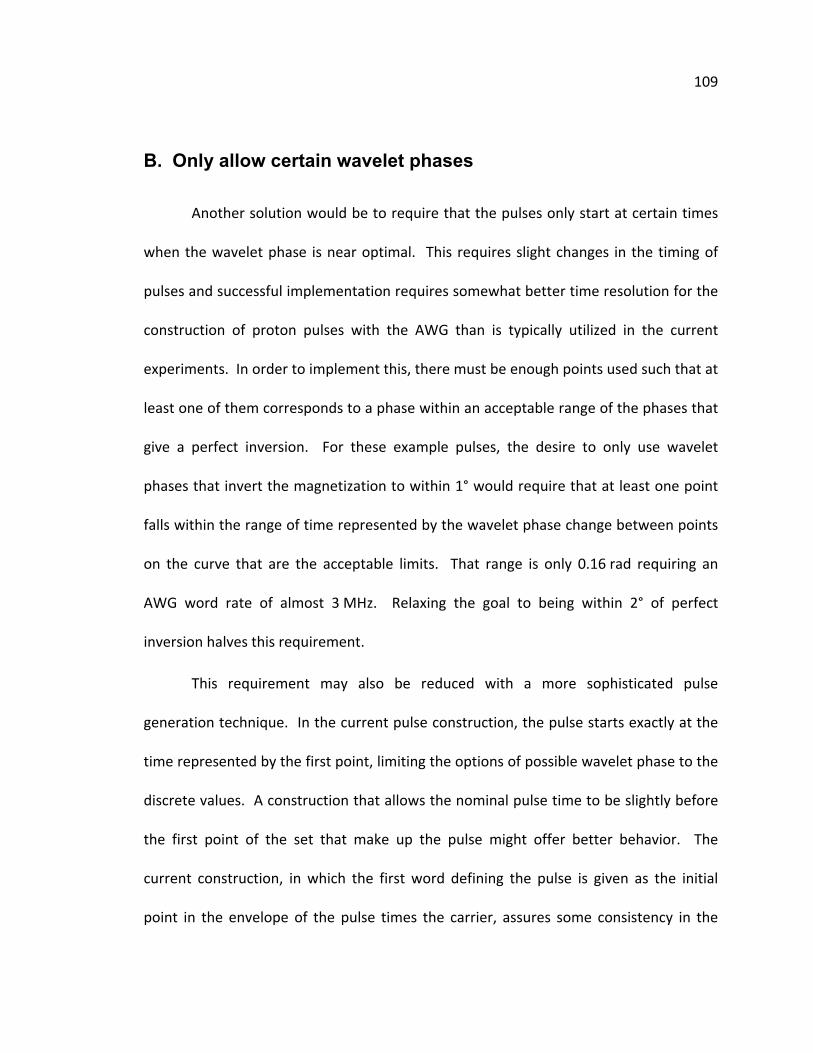
109 

 

B. Only allow certain wavelet phases

Another solution would be to require that the pulses only start at certain times 

when the wavelet phase  is near optimal.   This requires slight changes  in the timing of 

pulses and successful implementation requires somewhat better time resolution for the 

construction  of  proton  pulses with  the  AWG  than  is  typically  utilized  in  the  current 

experiments.  In order to implement this, there must be enough points used such that at 

least one of them corresponds to a phase within an acceptable range of the phases that 

give  a  perfect  inversion.    For  these  example  pulses,  the  desire  to  only  use wavelet 

phases that invert the magnetization to within 1° would require that at least one point 

falls within the range of time represented by the wavelet phase change between points 

on  the  curve  that  are  the  acceptable  limits.   That  range  is only 0.16 rad  requiring  an 

AWG  word  rate  of  almost  3 MHz.    Relaxing  the  goal  to  being  within  2°  of  perfect 

inversion halves this requirement. 

This  requirement  may  also  be  reduced  with  a  more  sophisticated  pulse 

generation technique.  In the current pulse construction, the pulse starts exactly at the 

time represented by the first point, limiting the options of possible wavelet phase to the 

discrete values.  A construction that allows the nominal pulse time to be slightly before 

the  first  point  of  the  set  that make  up  the  pulse might  offer  better  behavior.    The 

current  construction,  in which  the  first word defining  the pulse  is  given  as  the  initial 

point  in  the envelope of  the pulse  times  the  carrier, assures  some  consistency  in  the 

110 

 

pulse  construction  that may  also  be  important  to  generating  pulses with  consistent 

nutation. 

C. Composite pulses

A  third  solution  would  be  composite  pulses.    These  require  careful  pulse 

construction  so  that  rounding errors do not alter  the  relative wavelet phase between 

constituent  pulses  from  what  is  expected.    A  great  variety  of  composite  pulses,  all 

designed  within  the  rotating  frame  approximation,  are  used  to  compensate  for 

uncertainty in  0B  or  1B  or the variation of these fields over the sample.  Two examples 

will be examined numerically  to  illustrate  the possibility of using a  similar  strategy  to 

compensate for wavelet phase effects at low field. 

One of the first and most common composite pulses (73)  is the  inversion pulse 

( ) ( )2 y 2x x

π π π .  This composite pulse is designed to compensate for incorrect settings 

of the Rabi frequency.  Starting from longitudinal magnetization, it nominally places the 

magnetization on the  ‐axis, then rotates  it about that axis before finally finishing the 

inversion.  In this way, pulses that don’t quite make it to the 

y

y ‐axis are moved closer to 

the  ‐axis by the second pulse so that the third pulse, just like the first, can finish the 

inversion.   Pulses that go too far during the first pulse are moved further away so that 

the last pulse needs to take it a little further. 

z−

The  second  inversion  pulse  considered  here  is  a  variation  of  the  first, 

111 

 

( ) ( ) ( )2 2 2x y

π π πx.   This variation  is non‐obvious, based purely on  the basis of  the 

way it operates in low field. 

0 1 2 3 4 5 6

170

175

180

wavelet phase (rad)

angl

e to

z−

axis

 

Figure 46.   A well  constructed  composite pulse  can  reduce  the wavelet phase dependence or 

simply  change  it.   The well known  ( ) ( )2 y 2x x

π π π  pulse  (dotted  line)  shows as much variation  in  the 

resultant nutation angle as  is  seen with  single pulses.   The alternative  composite  ( ) ( ) ( )2 2 2x y x

π π π   

(solid line) shows very little wavelet phase dependence at the price of incomplete inversion for all.  These 

are proton pulses with a square envelope.  The carrier frequency and  0H Bγ  are set to 75 kHz and  1H Bγ  is 

set so that perfect inversion is possible at some wavelet phase for the first pulse and set to give the best 

inversion overall for the second pulse. 

Composite pulses arguably do not have a single wavelet phase since each of the 

substituent pulses has its own wavelet phase, but it is valid to examine them based on 

the wavelet  phase  of  the  first  pulse  since  the  others  have  a  definite  relative  phase 

compared to this first pulse so long there are no rounding errors.  When this is done for 

the  two  composite  inversion  pulses, we  find  the  dependence  shown  in  Fig.  46.    The 

( ) ( )2 y 2x x

π π π  pulse has the same wavelet phase dependence of the single π  pulse, 

but shifted in phase, so is not useful.  The  ( ) ( ) ( )2 2 2x y

π π πx pulse succeeds in having 

112 

 

very little wavelet phase dependence, but at the cost of never generating a particularly 

accurate inversion.  Both come at the cost of longer pulse time. 

In the current pulse construction, when a desired pulse time does not match an 

integer  number  of words,  then  the  length  is  rounded,  changing  the  time  at which  a 

pulse will occur and thus changing its relative wavelet phase slightly.  When rounding is 

required,  the  pulse  will  be  made  with  consistent  relative  wavelet  phases  in  the 

composite pulse, but they may not be the desired phases.  The examples of Fig. 46 use a 

word rate which is a multiple of the carrier frequency of the protons so that no rounding 

is required.  It is generally not possible to choose such a frequency when pulses for two 

isotopes  are  needed,  reducing  the  utility  of  this  technique  with  the  current 

programming. 

D. Shaped pulses

Another solution is shaping the pulse envelope.  Just as with composite pulses, a 

great variety of  shaped pulses have been useful  in high  field NMR and new ones are 

easy to generate.   A common motivation for shaping pulse envelopes  is to narrow the 

range of  resonance  frequencies over which  they are effective.   This motivation  is also 

relevant here in that the design process is greatly simplified if a given pulse acts on only 

one isotope.   A bonus is that this strategy also mitigates the undesired dependence on 

wavelet  phase.    A  few  simple  envelope  shapes  (74)  were  evaluated  by  numerical 

calculations  including Hanning, Hamming, Gaussian  (75),  sinc  (76),  and  half‐sine.   Of 

113 

 

these, the half‐sine pulses seemed to perform the best  in  initial tests.   Gaussian pulses 

also performed quite well, but would require an additional parameter, a cutoff point for 

the otherwise infinite pulse shape. 

In  another  effort  to  improve  the  pulse  shapes,  they were  filtered  to  remove 

undesirable  effects.    In  order  to  do  this,  they were  Fourier  transformed  to  give  the 

frequency  response  and  undesirable  frequencies were  set  to  zero.    They were  then 

inverse Fourier transformed back into the time domain for a new pulse.  This procedure 

returned  pulses  very  similar  to  half‐sine  pulses  in  all  cases,  so  half‐sine  pulses were 

chosen to be the pulse shape. 

The half‐sine pulse uses the first lobe of a sine, from the node at 0  to the node 

at π , inclusive of those nodes, to define the shape of the envelope.  They were found to 

cause  less nutation on distant  isotopes at the expense of  inducing greater nutation on 

nearby isotopes (Fig. 47).   For most systems under consideration for hyperpolarization, 

this  is  a  substantial  improvement  in  selectivity.    As with  the  square  pulses,  there  is 

always  a  value  of  0Bγ  and  1Bγ  that  allows  perfect  inversion  of  the  pulsed  isotope  at 

every wavelet  phase  (Fig.  48).    The  optimal  value  of  0Bγ  varies much  less  than  for 

square pulses, but  is never  equivalent  to  the  carrier  frequency  as  the  example  given 

here  that  is  four cycles of  the carrier wave period  long shows.   When used at a  fixed 

value of  0Bγ , they demonstrate less wavelet phase dependence for pulses of the same 

length (Fig. 49). 

114 

 

0 10 20 30 40 50 60 70 80 90 1000

20

40

60

80

100

120

140

160

180

Larmor frequency (kHz)

angl

e to

z-a

xis

1H

19F

31P

13C

2H15N

14N

 

Figure  47.   Pulses  intended  for one  isotope have  a  significant  effect on other  isotopes  in  the 

sample.  Here are inversion pulses for two common isotopes, 1H (thick) and 13C (thin).  These are half‐sine 

pulses  that  are  six  carrier  wave  periods  of  the  target  nucleus  long.    The  locations  of  the  reference 

frequencies for these isotopes and other common or useful isotopes are indicated by arrows. 

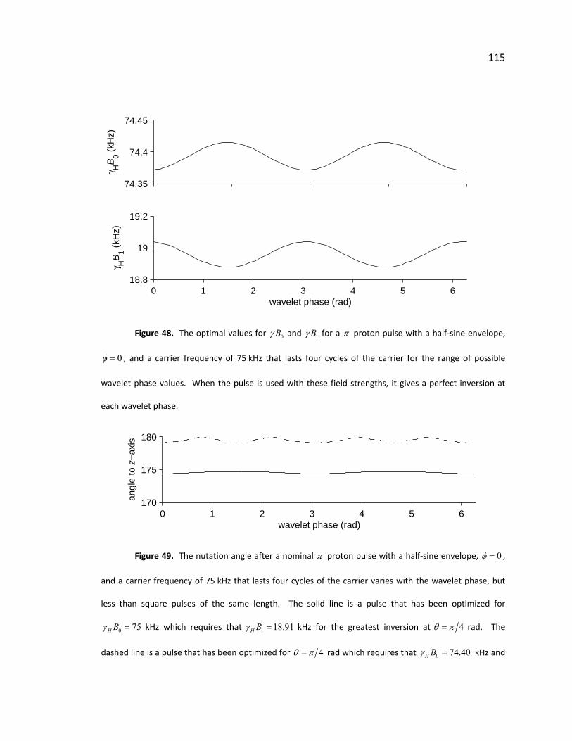
115 

 

74.35

74.4

74.45γ H

B0 (

kHz)

0 1 2 3 4 5 618.8

19

19.2

wavelet phase (rad)

γ HB

1 (kH

z)

 

Figure 48.  The optimal values for  0Bγ  and  1Bγ  for a π  proton pulse with a half‐sine envelope, 

0φ = ,  and  a  carrier  frequency of 75 kHz  that  lasts  four  cycles of  the  carrier  for  the  range of possible 

wavelet phase values.   When the pulse  is used with these  field strengths,  it gives a perfect  inversion at 

each wavelet phase. 

0 1 2 3 4 5 6170

175

180

wavelet phase (rad)

angl

e to

z−

axis

 

Figure 49.  The nutation angle after a nominal π  proton pulse with a half‐sine envelope,  0φ = , 

and a carrier frequency of 75 kHz that  lasts four cycles of the carrier varies with the wavelet phase, but 

less  than  square  pulses  of  the  same  length.    The  solid  line  is  a  pulse  that  has  been  optimized  for 

0 75H Bγ =  kHz  which  requires  that  1 18.91H Bγ =  kHz  for  the  greatest  inversion  at  4θ π=  rad.    The 

dashed line is a pulse that has been optimized for  4θ π=  rad which requires that  0 74.40H Bγ =  kHz and 

116 

 

1 18.94H Bγ =  kHz. 

It might be expected that pulse shaping would change or lift the restriction that 

pulses be a  length  that  is an  integer or half  integer multiple of  the carrier  frequency.  

This restriction is related to the specification that  1B  should not be dependent upon the 

wavelet phase.  When pulses of this type with varying lengths are optimized for the best 

inversion by allowing  0B  and  1B  to vary, there is a length where  1B  does not vary and it 

is moved substantially from the previous length restriction (Fig. 50b).  The shaping also 

reduces  this dependence of 1  B  on wavelet phase  for any  length pulse.   Notably, near 

the previous length restriction, there is a position about 0.04 of the carrier period longer 

than  the  integer  or  half  integer  multiple  of  the  carrier  period  where  0B  is  not 

dependent upon  the wavelet  phase  (Fig.  50a).    This  value  does  not  vary when  using 

different data  rates  to define  the pulses, which makes  it a good  length  restriction  for 

these pulses. 

117 

 

74.2

74.4

74.6

74.8γ 1H

B0 (

kHz)

a)

3.6 3.7 3.8 3.9 4 4.1 4.2 4.3 4.4 4.516

18

20

22

γ 1H B

1 (kH

z)

pulse length (carrier periods)

b)

0 radπ/3 rad2π/3 rad

 

Figure 50.  The optimal static field and pulse strength to give near perfect inversion with half‐sine 

shaped pulses  that are near  four cycles of  the carrier  frequency  long at a  few example wavelet phases 

shown in the legend. 

118 

 

VII. Further Considerations

Hyperpolarization  experiments  are  fundamentally  different  from  those  done 

with equilibrium polarization.  In the case of ordinary polarization, multiple experiments 

can be conducted in order to gain further pieces of information about an experiment.  In 

the case of hyperpolarization, once the polarization is lost it cannot be regained simply 

by waiting long enough.  New methods are needed to utilize the available signal to the 

greatest  advantage  and  extract  information  from  the  system  as  quickly  as  possible 

(40,41).    Refocused  INEPT  sequences  offer  one  route  to  the  extraction  of  greater 

information. 

Although  the  well  known  Zeeman  polarization  is  generally  the  spin  order  of 

choice  in  an  NMR  experiment,  other  spin  order  types  have  been  utilized.    New 

experiments are currently being developed that utilize singlet spin order in varied ways 

so  there  is  interest  in  being  able  to  produce  this  spin  order  in many  types  of  spin 

systems.    Application  of  the  spin  order  transfer  algorithms  described  in  the  reverse 

sense would allow generation of singlet spin order when starting from Zeeman order. 

A. Refocused INEPT

Detection  on  protons  is  desirable  for  better  sensitivity  and  higher  spatial 

resolution in MRI experiments.  For inductively detected NMR and MRI, the sensitivity is 

proportional to the value of  2γ  at a particular polarization.  One factor comes from the 

119 

 

magnitude of  the  gyromagnetic  ratio.    The other  comes  from  the  Faraday  law which 

states that the voltage signal is proportional to the rate of change of the magnetic field 

so the higher precession of the  larger gyromagnetic ratio gives a  larger signal.   For 13C, 

the sensitivity gain is approximately 16 and for 15N, the gain is approximately 100. 

In MRI, the spatial resolution is proportional to the value of γ .  This resolution is 

dependent upon the changes  in frequency across a sample when a gradient  is applied.  

In any application,  the size of  the gradient  is  limited by  the physical  limitations of  the 

system.  In the medical applications typical to MRI use, the gradient magnitude and rate 

of change are limited by safety considerations.   

The  protons  added  initially  by  molecular  addition  in  order  to  reach  a  high 

polarization on the heteronucleus are ripe for use by INEPT (19).  Refocusing is desirable 

to bring  the antiphase peaks  into phase  for maximum effect  in  the MRI environment 

where  field homogeneity within biological  tissue  is difficult  to achieve.    Ideally,  INEPT 

performed  by  transferring  polarization  from  a  single  nucleus  to  a  single  nucleus will 

perfectly  transfer  the  polarization.    The  efficiency  when  performed  from  one 

heteronucleus to multiple equivalent nuclei of another isotope is readily calculated (49), 

and with optimization can lead to a similar overall gain. 

Since  the  protons  added  in  heteronuclear  PASADENA  are  inequivalent  and 

couple together, the problem is more complicated than has been treated analytically.  In 

general  these  two  effects  will  lessen  the  utility  of  the  technique,  but  it  will  still 

demonstrate  advantage  over  heteronuclear  detection  in  most  cases.    Since  every 

120 

 

molecule is unique, mapping the expected result with different wait times is helpful as a 

guide  to  determine  the  appropriate  wait  times.    For  example,  succinate  in  basic 

conditions  ( ) with  the  coupling  constants pH 13.3= 12 6.68J =  Hz,   Hz,  and 

 Hz  (36) would be  expected  to have  average enhancement on  the protons 

shown  in Fig. 

1 6.32SJ = −

2 4.13SJ =

51 as a percentage of the starting polarization on the 13C heteronucleus.  

In this example, an advantageous initial wait (transfer time) would be about 60 ms and 

the second wait (refocusing time) would be about 70 ms to give an average polarization 

on the protons of about 25%.  This is roughly half what is expected in the ideal case of 

equivalent protons reducing the sensitivity advantage of detecting on protons instead of 

carbon from 16 to 8, still an appreciable advantage.  Experimentally, such a method has 

been shown to increase the overall sensitivity by 6.5 (48). 

121 

 

−20

−20

−20

−10

−10

−10

−10

−10

−10−10

−10

−10

0 0 0 0 0

0

0

0

0

0

0

0

0

0

0

0

00

00

0

0

0

10

10

10

10

10 10

10 20

20

first wait (ms)

seco

nd w

ait (

ms)

0 20 40 60 80 100 120 140 160 180 2000

20

40

60

80

100

120

140

160

180

200

 

Figure  51.    Expected  average  polarization  on  the  two  protons  of  succinate  from  molecular 

addition of hydrogen to a deuterated precursor in base as a percentage of the starting polarization on the 

heteronucleus  for  guiding  the  choice  of  timing  constants  in  a  refocused  INEPT  experiment.    Major 

contours are spaced every 10% and minor contours are spaced every 2%.  This is an ideal calculation that 

assumes the  1 24 z z zS I I  order has relaxed to Zeeman polarization. 

In cases where the chemical shift of the protons is sufficient, selective pulses can 

be used to restrict the transferred Zeeman spin order to one of the protons when the 

122 

 

molecule has been transferred to a high field for the experiment.  This cannot be done 

for succinate, where the chemical shift difference  is slight and only due to a secondary 

isotope effect from the single carbon label, but is useful for a number of demonstrated 

and proposed molecules.   For TFPP, which has been demonstrated with an unselective 

refocused  INEPT  sequence  (48),  any  of  the  three  distinct  protonated  sites  to which 

polarization transfer was observed could be chosen for selective transfer, since they are 

all separated by over 1 PPM.   For choline  labeled with  15N, which  is also an attractive 

molecule  for  biological  applications,  nonselective  refocused  INEPT  has  been 

demonstrated with molecules hyperpolarized by DNP (77) and it is reasonable to expect 

that  any  of  the  protons  that  couple with  the  15N  could  also  be  selectively  polarized.  

Selective  polarization  transfer  has  been  demonstrated  to  the  nine  equivalent methyl 

protons  by  incorporating  a  single  selective  π  pulse  within  the  refocused  INEPT 

sequence (49). 

B. Generation of singlet order

For applications where very  long  lived spin states are desirable,  the  lifetime of 

Zeeman order on a nucleus that is slow to relax can often be surpassed by the lifetime 

of  a  singlet  state  shared between  two nuclei  (29,32,33).    Long  lived  spin  states have 

been  used  as  a method  of  spin  labeling molecules  for  experiments  that  track  their 

disposition  through  rate  processes  such  as  slow  diffusion  (78)  or  chemical  exchange 

(79).    These  studies  have  been  extended  to  utilizing  the  long  lived  singlet  state  on 

123 

 

protons  (80)  and  heteronuclei,  for  example,  the  singlet  state  of  15N2O  which  has  a 

lifetime of over 25 min (81). 

The  pulse  sequence  algorithms  presented  here  performed  in  reverse  would 

generate  singlet  order  from  Zeeman  polarization.    This  would  be  possible  from  a 

heteronucleus to a set of protons or from a proton or isotopically distinct heteronucleus 

to  a  pair  of  heteronuclei,  so  long  as  the  nuclei  involved  are  all  spin  ½.    Previous 

techniques for this purpose rely on chemical shift difference, which is not required here.  

The present  sequence  algorithms,  using only  the  J‐couplings, would have  advantages 

wherever  the  chemical  shift was  small,  such  as  in  low  fields  or  in molecules where 

approximate magnetic equivalence is found either by symmetry or by chance. 

In  performing  the  backwards  sequence,  the  part  of  the  initial  condition  of 

interest is   rather than zS (11 22 4z z z zS S I I− )  which is found immediately after performing 

the  sequence  in  the  forward direction.   This  initial condition  for  the  reverse direction 

can be thought of as  

  ( ) ( )1 2 1 21 14 42 2r z z z z z z zS I I S S I I Sρ = − + + z .  (40) 

The first piece will lead to singlet order.  After the sequence is executed, heteronuclear 

decoupling on the system tuned to the isotope  in the singlet state preserves the scalar 

spin order. 

124 

 

C. Conclusions

The  pulse  sequence  algorithms  presented  here  are  capable  of  efficiently 

converting  singlet  spin  order  into  Zeeman  polarization.    These  algorithms  generate 

polarization   in  the  ideal  case where  100% parahydrogen  is used  and  relaxation 

during  the sequence  is negligible.   Previously,  this polarization could only be obtained 

for  the  specific  case  that 

1P =

4θ π≈  and  could  be  asymptotically  approached  for  other 

values  of θ  with  an  increasing  number  of  pulses  of  successively  smaller  angle  as   θ  

becomes  bigger  or  smaller  than  4π  (34,35).    Relaxation  ultimately  will  limit  the 

efficiency with which spin order transfer can be achieved.  Additionally, when transverse 

and longitudinal relaxation constants are not the same, the previous procedure must be 

compensated for this difference but it does not affect the new algorithms. 

The first increase in the range of molecules to which the algorithms apply comes 

from  introducing  a  more  efficient  use  of  the  prior  art  medium θ  pulse  sequence 

algorithm.    This  extends  the  range  of θ  values  over which  1P =  in  the  ideal  case  to 

0.3532 4θ π≤d .    Outside  of  this  range,  the  previous  procedure  could  be  used  to 

increase  polarization  with  modifications  in  the  case  of  smaller θ  values,  but  with 

compromises between achieved polarization and  the duration of  the pulse  sequence.  

This  fact motivates  the  introduction of  two new pulse  sequences, which make use of 

selective  averaging  of  the  terms  in  the  spin  Hamiltonian,  effectively making θ  time 

dependent within the sequence. 

125 

 

The second increase of range of molecules comes from a new pulse sequence for 

the small values of θ .  This pulse sequence replaces the π  pulse at the end of the first 

wait period with  the onset of  cyclic heteronuclear decoupling.   This has  the effect of 

removing  the heteronuclear coupling  terms  from  the Hamiltonian  in operation on  the 

system, effectively increasing the value of θ  for a time so that it is large enough for the 

sequence to operate without  losses.   This small θ  pulse sequence algorithm  is capable 

of generating   in the ideal case for 1P = 0 4θ π< ≤ .  In practical terms,   needs to be 

small enough that the calculated delay times for the sequence are not vanishingly small. 

JΔ

The  last  increase  of  range  of  molecules  comes  from  a  second  new  pulse 

sequence  for  large  values  of θ .    This  sequence modifies  the  first  new  sequence  by 

applying  a  J‐synchronized π  pulse  train  during  the  first  and  third  delays  in  order  to 

change the Hamiltonian in operation during those times in the average sense.  This train 

of  pulses  causes  homonuclear  decoupling  while  keeping  the  heteronuclear  coupling 

terms,  effectively  decreasing  the  value  of θ  for  a  time  such  that  the  algorithm  can 

operate without  losses.   The use of the J‐synchronized π  pulse train restricts the total 

time of  the  first and  last wait  to  integer multiples of  the  synchronization period  such 

that the  ideal delay suggested by coherent averaging theory cannot be picked  in many 

cases.    Nevertheless,  when  this  is  so,  numerical  optimizations  show  that  the 

synchronization  time  and  heteronuclear  decoupling  time  may  be  varied  to  yield  a 

sequence that can be executed without  losses over the range  4 2π θ π≤ <  as well as 

lower values where other  sequences are equally effective and are  faster.    In practical 

126 

 

terms,   needs to be  large enough that the delays do not become  long compared to 

the relevant relaxation.  This is the large 

JΔ

θ  pulse sequence algorithm. 

In  order  to  choose which  pulse  sequence  algorithm  is  best  given  a  particular 

molecule with  a  particular  value  of θ ,  the  length  of  time  required  to  generate  the 

desired  polarization  is  examined.    This  examination  indicates  that  the  small θ  pulse 

sequence algorithm should be used  in the range  ( )0 arctan 1θ< ≤ 2  and the medium 

θ  pulse  sequence  algorithm  should  be  used  in  the  range  ( )arctan 1 2 4θ π< ≤ .  

Above this range,  it  is more difficult to determine which algorithm  is best because the 

large  θ  pulse  sequence  algorithm  generally  requires  longer  times,  so  relaxation 

processes may remove the advantage of the algorithm.   Taking a requirement that the 

medium θ  algorithm  should  be  able  to  achieve  polarization  of  at  least  90%,  that 

algorithm  requires  a  shorter  time  for  1θ d  while  the  large θ  algorithm  requires  a 

shorter time above this to give 100% polarization. 

With  these  algorithms  in  hand,  the  challenge  becomes  to  find  the  correct 

precursors for desirable molecules.  A few example molecules that may be desirable are 

plotted in Fig. 52, showing a sampling of the array of molecular constants that may now 

be addressed with the new pulse sequence algorithms in reasonable time. 

127 

 

2 3 4 5 6 7 8 9 1010

0

101

102

1−13C−succinic acid, 115ms: 99%

1−13C−succinic acid, 110ms: 100%

1−13C−β−glucose, 236ms: 100%

15N−choline, 440ms: 100%

13C−choline, 38ms: 100%

31P ethylphosphonyl dichloride, 44ms: 100%

15N−phosphoryl choline, 449ms: 100%

31P phosphoryl choline, 192ms: 100%

31P AMP, 210ms: 100%

31P UMP, 203ms: 100%

J Δ (H

z)

J12

(Hz) 

Figure 52. A selection of molecules  to which  the pulse sequence algorithms presented may be 

applied with  the  time required and  the resulting polarization.   The sequences utilized are generated by 

the small ( ), medium ( ), and large ( ) θ  pulse sequence algorithms. 

An  instrument has been built  to perform  the pulse  sequences generated  from 

these algorithms on real molecules for applications in vitro and in vivo.  This was used to 

hyperpolarize  a  number  of  molecules,  including  succinate  (36,48,67),  the  first 

metabolite  to  be  hyperpolarized  with  heteronuclear  PASADENA.    This molecule  has 

potential  for  imaging metabolic  processes  (46).    An  amphiphilic molecule,  TFPP,  has 

been developed that is sufficiently soluble for delivery and binds with lipids (48).  When 

bound,  the  chemical  shift of  the hyperpolarized  spin  shifts  so  that  the bound  form  is 

128 

 

discernible  from  that  in  solution,  allowing  a method  to  potentially  characterize  the 

amount of or placement of vulnerable plaques in the cardiovascular system (43). 

In  some  cases,  it  is  not  attractive  to  detect  signal  on  the  heteronucleus.  

Sensitivity gains are seen in using protons for detection instead.  In MRI, the resolution 

of the image is improved by using protons.  In order to take advantage of this, refocused 

INEPT methods are being developed for application to complicated spin systems (49,77). 

129 

 

VIII. References

(1)  Rabi, I. I.; Millman, S.; Kusch, P.; Zacharias, J. R. The Molecular Beam Resonance Method for Measuring Nuclear Magnetic Moments. The Magnetic Moments of 3Li

6, 3Li7 

and 9F19. Phys. Rev. 1939, 55, 526‐535. 

(2)  Gorter, C.  J. Negative Result of an Attempt  to Detect Nuclear Magnetic  Spins. Physica 1936, 3, 995‐998. (3)  Gorter, C.  J.; Broer,  L.  J.  F. Negative Result of  an Attempt  to Observe Nuclear Magnetic Resonance in Solids. Physica 1942, 9, 591‐596. (4)  Purcell,  E. M.;  Torrey,  H.  C.;  Pound,  R.  V.  Resonance  Absorption  by  Nuclear Magnetic Moments in a Solid. Phys. Rev. 1946, 69, 37‐38. (5)  Bloch,  F.; Hansen, W. W.; Packard, M. Nuclear  Induction. Phys. Rev. 1946, 69, 127. (6)  Purcell, E. M.; Bloembergen, N.; Pound, R. V. Resonance Absorption by Nuclear Magnetic Moments in a Single Crystal of CaF2. Phys. Rev. 1946, 70, 988. (7)  Pake, G. E. Nuclear Resonance Absorption in Hydrated Crystals: Fine Structure of the Proton Line. J. Chem. Phys. 1948, 16, 327‐336. (8)  Lamb, W. E. Internal Diamagnetic Fields. Phys. Rev. 1941, 60, 817‐819. (9)  Knight, W. D. Nuclear Magnetic Resonance Shift  in Metals. Phys. Rev. 1949, 76, 1259‐1260. (10)  Proctor, W.  G.;  Yu,  F.  C.  The  Dependence  of  a  Nuclear Magnetic  Resonance Frequency upon Chemical Compound. Phys. Rev. 1950, 77, 717. (11)  Dickinson, W. C. Dependence of the F19 Nuclear Resonance Position on Chemical Compound. Phys. Rev. 1950, 77, 736‐737. (12)  Proctor, W. G.;  Yu,  F. C. On  the Nuclear Magnetic Moments of  Several  Stable Isotopes. Phys. Rev. 1951, 81, 20‐30. (13)  Gutowsky, H. S.; McCall, D. W.; Slichter, C. P. Coupling Among Nuclear Magnetic Dipoles in Molecules. Phys. Rev. 1951, 84, 589‐590. (14)  Williamson, M. P.; Havel, T. F.; Wuthrich, K. Solution Conformation of Proteinase Inhibitor‐IIA from Bull Seminal Plasma by 1H Nuclear Magnetic Resonance and Distance Geometry. J. Mol. Biol. 1985, 182, 295‐315. (15)  Gutowsky, H.  S.; Holm, C. H. Rate Processes and Nuclear Magnetic Resonance Spectra .2. Hindered Internal Rotation of Amides. J. Chem. Phys. 1956, 25, 1228‐1234. (16)  Alger, J. R.; Shulman, R. G. NMR Studies of Enzymatic Rates in vitro and in vivo by Magnetization Transfer. Qu. Rev. Biophys. 1984, 17, 83‐124. (17)  Perrin,  C.  L.;  Dwyer,  T.  J.  Application  of  2‐Dimensional  NMR  to  Kinetics  of Chemical Exchange. Chem. Rev. 1990, 90, 935‐967. (18)  Kuhlmann,  K.  F.;  Grant,  D. M.  The  Nuclear  Overhauser  Enhancement  of  the Carbon‐13 Magnetic Resonance Spectrum of Formic Acid.  J. Am. Chem. Soc. 1968, 90, 

130 

 

7355‐7357. (19)  Morris, G. A.; Freeman, R. Enhancement of Nuclear Magnetic Resonance Signals by Polarization Transfer. J. Am. Chem. Soc. 1979, 101, 760‐762. (20)  Kaptein, R.; Oosterhoff, J. L. Chemically Induced Dynamic Nuclear Polarization II ‐ (Relation with Anomalous ESR spectra). Chem. Phys. Lett. 1969, 4, 195‐197. (21)  Bouchiat, M. A.;  Carver,  T.  R.; Varnum,  C. M. Nuclear  Polarization  in He3 Gas Induced by Optical Pumping and Dipolar Exchange. Phys. Rev. Lett. 1960, 5, 373‐375. (22)  Grover, B. C. Noble‐Gas NMR Detection Through Noble‐Gas‐Rubidium Hyperfine Contact Interaction. Phys. Rev. Lett. 1978, 40, 391‐392. (23)  Bowers,  C.  R.; Weitekamp,  D.  P.  Transformation  of  Symmetrization  Order  to Nuclear‐Spin  Magnetization  by  Chemical‐Reaction  and  Nuclear‐Magnetic‐Resonance. Phys. Rev. Lett. 1986, 57, 2645‐2648. (24)  Bowers, C. R.; Weitekamp, D. P. Parahydrogen and Synthesis Allow Dramatically Enhanced Nuclear Alignment. J. Am. Chem. Soc. 1987, 109, 5541‐5542. (25)  Bowers, C. R. Parahydrogen and Synthesis Allow Dramatically Enhanced Nuclear Alignment. Ph.D. Dissertation, California  Institute of Technology, Pasadena, California, 1991. (26)  Eisenschmid, T. C.; Kirss, R. U.; Deutsch, P. P.; Hommeltoft, S.  I.; Eisenberg, R.; Bargon,  J.;  Lawler,  R.  G.;  Balch,  A.  L.  Para  Hydrogen  Induced  Polarization  in Hydrogenation Reactions. J. Am. Chem. Soc. 1987, 109, 8089‐8091. (27)  Bowers,  C.  R.;  Jones,  D.  H.;  Kurur,  N.  D.;  Labinger,  J.  A.;  Pravica,  M.  G.; Weitekamp,  D.  P.  Symmetrization  Postulate  and  Nuclear  Magnetic  Resonance  of Reacting Systems. Adv. Magn. Reson. 1990, 14, 269‐291. (28)  Bowers,  C.  R.; Weitekamp,  D.  P.  Nuclear Magnetic  Resonance  by Measuring Reaction Yield of Spin Symmetry Species. Solid State Nucl. Magn. Reson. 1998, 11, 123‐128. (29)  Carravetta, M.; Levitt, M. H. Long‐lived Nuclear Spin States in High‐field Solution NMR. J. Am. Chem. Soc. 2004, 126, 6228‐6229. (30)  Eisenschmid, T. C.; McDonald, J.; Eisenberg, R.; Lawler, R. G. INEPT in a Chemical Way. Polarization Transfer From Para Hydrogen to 31P by Oxidative Addition and Dipolar Relaxation. J. Am. Chem. Soc. 1989, 111, 7267‐7269. (31)  Natterer, J.; Schedletzky, O.; Barkemeyer, J.; Bargon, J.; Glaser, S. J. Investigating Catalytic Processes with Parahydrogen: Evolution of Zero‐quantum Coherence in AA ' X Spin Systems. J. Magn. Reson. 1998, 133, 92‐97. (32)  Carravetta, M.;  Johannessen, O. G.;  Levitt, M. H. Beyond  the T‐1  Limit: Singlet Nuclear Spin States in Low Magnetic Fields. Phys. Rev. Lett. 2004, 92, 153003. (33)  Carravetta, M.; Levitt, M. H. Theory of Long‐lived Nuclear Spin States in Solution Nuclear Magnetic  Resonance.  I.  Singlet  States  in  Low Magnetic  Field.  J.  Chem.  Phys. 2005, 122, 214505. (34)  Goldman, M.;  Johannesson, H. Conversion of a Proton Pair Para Order  into  13C Polarization by RF Irradiation, for Use in MRI. C. R. Phys. 2005, 6, 575‐581. 

131 

 

(35)  Goldman,  M.;  Johannesson,  H.;  Axelsson,  O.;  Karlsson,  M.  Design  and Implementation of  13C Hyper Polarization  from Para‐hydrogen, For New MRI Contrast Agents. C. R. Chimie 2006, 9, 357‐363. (36)  Chekmenev,  E.  Y.;  Hovener,  J.‐B.;  Norton,  V.  A.;  Harris,  K.;  Batchelder,  L.  S.; Bhattacharya, P.; Ross, B. D.; Weitekamp, D. P. PASADENA Hyperpolarization of Succinic Acid for MRI and NMR Spectroscopy. J. Am. Chem. Soc. 2008, 130, 4212‐4213. (37)  Albert, M.  S.; Cates, G. D.; Driehuys, B.; Happer, W.;  Saam, B.;  Springer, C.  S.; Wishnia, A. Biological Magnetic Resonance  Imaging Using Laser Polarized 129Xe. Nature 1994, 370, 199‐201. (38)  Golman, K.; Axelsson, O.; Johannesson, H.; Mansson, S.; Olofsson, C.; Petersson, J. S. Parahydrogen‐induced Polarization  in  Imaging: Subsecond 13C Angiography. Magn. Reson. Med. 2001, 46, 1‐5. (39)  Golman, K.; Ardenkjaer‐Larsen,  J. H.; Petersson,  J. S.; Mansson, S.; Leunbach,  I. Molecular  Imaging with  Endogenous  Substances.  Proc. Natl. Acad.  Sci. U.  S. A.  2003, 100, 10435‐10439. (40)  Bhattacharya, P.; Harris, K.; Lin, A. P.; Mansson, M.; Norton, V. A.; Perman, W. H.; Weitekamp, D. P.; Ross, B. D. Ultra‐fast Three Dimensional  Imaging of Hyperpolarized 13C in vivo. Magn. Reson. Mat. Phys. Biol. Med. 2005, 18, 245‐256. (41)  Perman, W. H.; Bhattacharya, P.; Leupold, J.; Lin, A. P.; Harris, K. C.; Norton, V. A.; Hövener,  J.‐B.;  Ross,  B.  D.  Fast  Volumetric  Spatial‐Spectral  MR  Imaging  of Hyperpolarized  13C‐Labeled Compounds Using Multiple  Echo  3D bSSFP. Magn. Reson. Imag. 2010, 28, 459‐465. (42)  Chekmenev,  E.  Y.;  Chow,  S.  K.;  Tofan,  D.;  Weitekamp,  D.  P.;  Ross,  B.  D.; Bhattacharya,  P.  Fluorine‐19  NMR  Chemical  Shift  Probes Molecular  Binding  to  Lipid Membranes. J. Phys. Chem. B 2008, 112, 6285‐6287. (43)  Chekmenev,  E.  Y.;  Reynolds, W.  F.;  Chow,  S.‐K.; Hövener,  J.  B.; Norton, V. A.; Tran, T. T.; Chan, H. C.; Wagner, S. R.; Perman, W. H.; Weitekamp, D. P.; Ross, B. D.; Bhattacharya, P. In Experimental NMR Conference Asilomar, California, 2009. (44)  Gallagher, F. A.; Kettunen, M. I.; Day, S. E.; Hu, D. E.; Ardenkjaer‐Larsen, J. H.; in't Zandt, R.; Jensen, P. R.; Karlsson, M.; Golman, K.; Lerche, M. H.; Brindle, K. M. Magnetic Resonance Imaging of pH in vivo Using Hyperpolarized 13C‐labelled Bicarbonate. Nature 2008, 453, 940‐943. (45)  Golman,  K.;  in't  Zandt,  R.;  Lerche,  M.;  Pehrson,  R.;  Ardenkjaer‐Larsen,  J.  H. Metabolic Imaging by Hyperpolarized 13C Magnetic Resonance Imaging for in vivo Tumor Diagnosis. Can. Res. 2006, 66, 10855‐10860. (46)  Ross, B. D.; Bhattacharya, P.; Wagner, S.; Tran, T.; Sailasuta, N. Hyperpolarized MR Imaging: Neurologic Applications of Hyperpolarized Metabolism. Am. J. Neuroradiol. 2010, 31, 24‐33. (47)  Larson,  P.  E.  Z.;  Kerr,  A.  B.;  Chen,  A.  P.;  Lustig, M.  S.;  Zierhut, M.  L.;  Hu,  S.; Cunningham, C. H.; Pauly,  J. M.; Kurhanewicz,  J.; Vigneron, D. B. Multiband Excitation Pulses  for Hyperpolarized  13C Dynamic Chemical‐shift  Imaging.  J. Magn. Reson.  2008, 

132 

 

194, 121‐127. (48)  Chekmenev,  E.  Y.;  Norton,  V.  A.;  Weitekamp,  D.  P.;  Bhattacharya,  P. Hyperpolarized 1H NMR Employing Low Gamma Nucleus for Spin Polarization Storage. J. Am. Chem. Soc. 2009, 131, 3164‐3165. (49)  Pfeilsticker, J. A.; Ollerenshaw, J. E.; Norton, V. A.; Weitekamp, D. P. A Selective 15N‐to‐1H Polarization Transfer Sequence for More Sensitive Detection of 15N‐Choline. J. Magn. Reson. 2010, In Press. (50)  Smith,  S. A.;  Levante, T. O.; Meier, B. H.; Ernst, R. R. Computer‐Simulations  in Magnetic‐Resonance ‐ an Object‐Oriented Programming Approach. J. Magn. Reson. Ser. A 1994, 106, 75‐105. (51)  Osborn,  J.  A.;  Jardine,  F.  H.;  Young,  J.  F.; Wilkinson,  G.  The  Preparation  and Properties of Tris(triphenylphosphine)halogenorhodium(I) and Some Reactions Thereof Including  Catalytic Homogeneous Hydrogenation  of Olefins  and Acetylenes  and  Their Derivatives. J. Chem. Soc. A 1966, 1711‐1732. (52)  Eisenberg, R.; Eisenschmid, T. C.; Chinn, M. S.; Kirss, R. U. Parahydrogen Induced Polarization  and  Polarization  Transfer  in  Hydrogenation  and  Oxidative  Addition Reactions ‐ A Mechanistic Probe. Adv. Chem. Ser. 1992, 47‐74. (53)  Duckett,  S.  B.;  Sleigh,  C.  J.  Applications  of  the  Parahydrogen  Phenomenon:  A Chemical Perspective. Prog. Nuc. Magn. Reson. Spec. 1999, 34, 71‐92. (54)  Lit,  E.  S.; Mallon,  F.  K.;  Tsai,  H.  Y.;  Roberts,  J.  D.  Conformational  Changes  of Butanedioic Acid as a Function of pH as Determined From Changes  in Vicinal Proton‐proton NMR Couplings. J. Am. Chem. Soc. 1993, 115, 9563‐9567. (55)  Siddall, T. H.; Prohaska, C. A. Conformation of Organophosphorus Compounds. I. Proton  Magnetic  Resonance  Studies  of  Some  Phosphinates,  Phosphinic  Acids, Phosphinyl  Chlorides  and  Phosphonyl Dichlorides.  J.  Am.  Chem.  Soc.  1962,  84,  2502‐2506. (56)  Dessy, R. E.; Flautt, T. J.; Jaffe, H. H.; Reynolds, G. F. Nuclear Magnetic Resonance Spectra of Some Dialkylmercury Compounds. J. Chem. Phys. 1959, 30, 1422‐1425. (57)  Govindaraju,  V.;  Young,  K.; Maudsley,  A.  A.  Proton  NMR  Chemical  Shifts  and Coupling Constants for Brain Metabolites. NMR Biomed. 2000, 13, 129‐153. (58)  Hovener, J. B.; Chekmenev, E. Y.; Harris, K. C.; Perman, W. H.; Robertson, L. W.; Ross,  B.  D.;  Bhattacharya,  P.  PASADENA  Hyperpolarization  of  13C  Biomolecules: Equipment Design and  Installation. Magn. Reson. Mat. Phys. Biol. Med. 2009, 22, 111‐121. (59)  Hovener, J. B.; Chekmenev, E. Y.; Harris, K. C.; Perman, W. H.; Tran, T. T.; Ross, B. D.;  Bhattacharya,  P.  Quality  Assurance  of  PASADENA  Hyperpolarization  for  13C Biomolecules. Magn. Reson. Mat. Phys. Biol. Med. 2009, 22, 123‐134. (60)  LabVIEW™, version 8.5; National Instruments: Austin, Texas, 2007. (61)  MATLAB®,  version R2008a; The Mathworks,  Inc.: Natick, Massachusetts, 1984‐2008. (62)  Levitt, M. H.; Freeman, R.; Frenkiel, T. Broad‐band Heteronuclear Decoupling. J. 

133 

 

Magn. Reson. 1982, 47, 328‐330. (63)  Bloch, F.; Siegert, A. Magnetic Resonance for Nonrotating Fields. Phys. Rev. 1940, 57, 522‐527. (64)  Gridnev,  I. D.; Higashi, N.; Asakura, K.;  Imamoto, T. Mechanism of Asymmetric Hydrogenation  Catalyzed  by  a  Rhodium  Complex  of  (S,S)‐1,2‐bis(tert‐butylmethylphosphino)ethane. Dihydride Mechanism of Asymmetric Hydrogenation.  J. Am. Chem. Soc. 2000, 122, 7183‐7194. (65)  Gridnev, I. D.; Imamoto, T. On the Mechanism of Stereoselection in Rh‐catalyzed Asymmetric  Hydrogenation:  A  General  Approach  for  Predicting  the  Sense  of Enantioselectivity. Accounts Chem. Res. 2004, 37, 633‐644. (66)  Golman, K.; Axelsson, O.; Johannesson, H.; Mansson, S.; Olofsson, C.; Petersson, J. S. Parahydrogen‐induced polarization in imaging: Subsecond C‐13 angiography. Magn. Reson. Med. 2001, 46, 1‐5. (67)  Bhattacharya,  P.;  Chekmenev,  E.  Y.;  Perman, W.  H.;  Harris,  K.  C.;  Lin,  A.  P.; Norton,  V.  A.;  Tan,  C.  T.;  Ross,  B. D.; Weitekamp, D.  P.  Towards Hyperpolarized  13C‐Succinate Imaging of Brain Cancer. 2007, 186, 150‐155. (68)  Vold,  R.  L.;  Waugh,  J.  S.;  Klein,  M.  P.;  Phelps,  D.  E.  Measurement  of  Spin Relaxation in Complex Systems. J. Chem. Phys. 1968, 48, 3831‐3832. (69)  Torchia,  D.  A. Measurement  of  Proton‐enhanced  13C  T1  Values  by  a Method Which Supresses Artifacts. J. Magn. Reson. 1978, 30, 613‐616. (70)  Levitt, M. H. Spin Dynamics: Basics of Nuclear Magnetic Resonance; John Wiley & Sons Ltd.: Chichester, 2001. (71)  Goldman, M. Quantum Description  of High‐Resolution NMR  in  Liquids; Oxford University Press, Inc.: Oxford, 1988. (72)  Haeberlen,  U.  High  Resolution  NMR  in  Solids:  Selective  Averaging;  Academic Press: New York, 1976. (73)  Levitt, M. H.; Freeman, R. NMR Population‐Inversion Using a Composite Pulse. J. Magn. Reson. 1979, 33, 473‐476. (74)  Borgnat,  P.;  Lesage,  A.;  Caldarelli,  S.;  Emsley,  L.  Narrowband  Linear  Selective Pulses for NMR. J. Magn. Reson. A 1996, 119, 289‐294. (75)  Bauer,  C.;  Freeman,  R.;  Frenkiel,  T.;  Keeler,  J.;  Shaka, A.  J. Gaussian  Pulses.  J. Magn. Reson. 1984, 58, 442‐457. (76)  Temps, A. J.; Brewer, C. F. Synthesis of Arbitrary Frequency Domain Transmitting Pulses Applicable to Pulsed NMR Instruments. J. Magn. Reson. 1984, 56, 355‐372. (77)  Sarkar, R.; Comment, A.; Vasos, P. R.; Jannin, S.; Gruetter, R.; Bodenhausen, G.; Hall, H.  l. n.; Kirik, D.; Denisov, V. P. Proton NMR of 15N‐Choline Metabolites Enhanced by Dynamic Nuclear Polarization. J. Am. Chem. Soc. 2009, 131, 16014‐16015. (78)  Ferrage, F.; Zoonens, M.; Warschawski, D. E.; Popot, J.‐L.; Bodenhausen, G. Slow Diffusion of Macromolecular Assemblies by a New Pulsed Field Gradient NMR Method. J. Am. Chem. Soc. 2003, 125, 2541‐2545. (79)  Wenter, P.; Bodenhausen, G.; Dittmer, J.; Pitsch, S. Kinetics of RNA Refolding  in 

134 

 

Dynamic Equilibrium by 1H‐Detected 15N Exchange NMR Spectroscopy. J. Am. Chem. Soc. 2006, 128, 7579‐7587. (80)  Cavadini,  S.;  Dittmer,  J.;  Antonijevic,  S.;  Bodenhausen,  G.  Slow  Diffusion  By Singlet State NMR Spectroscopy. J. Am. Chem. Soc. 2005, 127, 15744‐15748. (81)  Pileio, G.; Carravetta, M.; Hughes, E.; Levitt, M. H. The Long‐Lived Nuclear Singlet State of 15N‐Nitrous Oxide in Solution. J. Am. Chem. Soc. 2008, 130, 12582‐12583.