METHODS ARTICLEpublished: 29 October 2013

doi: 10.3389/fncom.2013.00129

Efficient calculation of the quasi-static electrical potentialon a tetrahedral mesh and its implementation in STEPSIain Hepburn1,2, Robert Cannon3 and Erik De Schutter1,2*

1 Computational Neuroscience Unit, Okinawa Institute of Science and Technology, Onna-son, Japan2 Theoretical Neurobiology, University of Antwerp, Antwerp, Belgium3 Textensor Limited, Edinburgh, UK

Edited by:

Terrence J. Sejnowski, The SalkInstitute for Biological Studies, USA

Reviewed by:

Upinder S. Bhalla, National Centerfor Biological Sciences, IndiaChristian Leibold, LudwigMaximilians University, Germany

*Correspondence:

Erik De Schutter, ComputationalNeuroscience Unit, OkinawaInstitute of Science and Technology,1919-1 Tancha, Onna-son, Okinawa904-0495, Japane-mail: erik@oist.jp

We describe a novel method for calculating the quasi-static electrical potential ontetrahedral meshes, which we call E-Field. The E-Field method is implemented in STEPS,which performs stochastic spatial reaction-diffusion computations in tetrahedral-basedcellular geometry reconstructions. This provides a level of integration between electricalexcitability and spatial molecular dynamics in realistic cellular morphology not previouslyachievable. Deterministic solutions are also possible. By performing the Rallpack tests wedemonstrate the accuracy of the E-Field method. Efficient node ordering is an importantpractical consideration, and we find that a breadth-first search provides the best solutions,although principal axis ordering suffices for some geometries. We discuss potentialapplications and possible future directions, and predict that the E-Field implementationin STEPS will play an important role in the future of multiscale neural simulations.

Keywords: 3D electrical potential, tetrahedral meshes, membrane potential, complex morphology, spatial

stochastic simulation, multiscale simulation, efficient node ordering

1. INTRODUCTIONIn computational neuroscience, up until now studies of the elec-trical behavior of cells and networks have not often includeddetailed biochemical signaling network components. Vice-versa,studies of molecular systems have usually not taken into accountthe electrical excitablity of the cellular membranes that surroundthem. While many important advances in our understanding ofneural systems have been made by this approach, future studiesare expected to focus more and more on the interaction acrossdifferent spatial and temporal scales exploring the impact thatdifferent systems have on each other, an approach often termedmultiscale modeling. Although adding a new level of complex-ity to simulations, multiscale modeling is expected to play a vitalrole in the future of computational neuroscience (Djurfeldt et al.,2010; Bhalla, 2011; Anwar et al., 2013).

Developing tools that can perform seamless integration acrossdifferent spatial and temporal scales is a challenging task. Incellular simulations this amounts to connecting the electricalexcitability of the cell with reaction-diffusion models of biochem-ical networks. Furthermore, computations must be as efficientas possible so that no component forms a bottleneck, yet mustnot over-simplify any component so as to ensure no significantloss of accuracy. An increasing number of simulators have beenmaking strides toward this goal, including MOOSE (Ray andBhalla, 2008) and GENESIS 3 (Cornelis et al., 2012). Presentapproaches often involve integrating two or more simulators:for example, one to perform the whole-cell electrical calcula-tions and another carrying out reaction-diffusion calculations(Brandi et al., 2011), which already open up a wealth of potentialapplications. However, many simulators offer only limited mor-phological resolution often based on connected cylinders. Theremay be occasions where accurate morphological representation of

complex cellular geometry below the μm scale is necessary along-side a tighter integration between the electrical and molecularsystems, which is the motivation for this work. One clear examplewhere such simulations are potentially advantageous is where amolecular species carrying a significant current across the mem-brane also acts as an important signaling molecule, of which oneimportant example is calcium. When such signals are highly local-ized [which can often be the case (Fakler and Adelman, 2008)]and are strongly influenced by morphology (Santamaria et al.,2006; Anwar et al., 2013) a detailed spatial description of thecomponents that are important within both the electrical and themolecular scales, namely voltage-dependent channels and signal-ing ions, may be vital. Furthermore, ionic channel currents areoften better described by the GHK equation (Goldman, 1943;Hodgkin and Katz, 1949), and may be best modeled also as astochastic process (Mak and Webb, 1997). These considerationstogether point to the need for software capable of accurate com-putation of electrical potential in realistic morphologies tightlycoupled with a detailed spatial description of voltage-dependentchannels, their transported ions and other important signalingmolecules, with a full stochastic account of the interactions.

We describe a novel method we term E-Field, which performselectrical potential calculation in complex 3D morphologies rep-resented by tetrahedral meshes, which are far more suitable fordescribing complex morphology than cubic meshes (Hepburnet al., 2012). E-Field is integrated in STEPS (Hepburn et al.,2012) alongside complementary components such as voltage-dependent transitions and channel currents, and tightly inte-grated with spatial reaction-diffusion computations based onGillespie’s SSA (Gillespie, 1977). We demonstrate accuracy andoptimization efforts, describe potential applications and discussfuture expansions on this groundwork.

Frontiers in Computational Neuroscience www.frontiersin.org October 2013 | Volume 7 | Article 129 | 1

COMPUTATIONAL NEUROSCIENCE

Hepburn et al. E-Field in STEPS

2. MATERIALS AND METHODS2.1. E-FIELD: THE TETRAHEDRAL MESH POTENTIAL CALCULATION IN

STEPSThe evolution of the electric field on the tetrahedral mesh issolved as a set of simultaneous difference equations for internalpoints and differential equations for capacitative surface ele-ments. Each edge in the mesh gives rise to one equation and asparse matrix method is used to compute the changes in poten-tial over a timestep. We first show how the difference equationson the mesh are derived from the quasi-static Maxwell equationsand then briefly describe the matrix method used to solve them.

2.1.1. Reduction of Maxwell’s equations for neural tissueFor fixed and moving charges as are present in small sections ofa neuron, the evolution of the electric and magnetic field is gov-erned by the Maxwell equations. However, on the timescales ofinterest here, where the frequency of changes is well below theMHz range, the coupling of the magnetic field to the electricalfield, which gives rise to electromagnetic waves, can be neglected(Plonsey, 1969; Nunez and Srinivasan, 2006).

Under these conditions, the system is governed by the quasi-static Maxwell equations which can be written as:

∇ · J + ∂ρ

∂t= 0 (1)

∇ · D = ρ (2)

where J is the current density, ρ is the charge density, t is time andD is the electrical displacement. Experimentally, for most materi-als the quantities J and D are related to the electric field by theconstitutive relations:

J = σE (3)

and

D = εE (4)

where σ is the conductivity, and ε is the permittivity.The combination of Equations (1) and (3) expresses the con-

servation of charge, and Equations (2) and (4) form Gauss’ lawwhich implies that the electric field can be expressed as thegradient of the electrical potential, �:

E = ∇�. (5)

From an electrical perspective, neural tissue is composed of twomain materials: the cytoplasm which contains many freely mov-ing charges and hence a relatively high conductivity, σ, and themembrane which is effectively an insulator with a very low con-ductivity. The cytoplasmic conductivity prevents the build-up ofstatic charge, so, from Equations (1), (3), and (5), the potentialthere satisfies

∇2� = 0. (6)

In principle, Equations (1) to (5) could also be used to computethe field within the membrane in terms of ε, σ and the membrane

dimensions. In practice, this is not a useful approach because thequantities required are not well-determined. These equations do,however, give the form of the equation that governs the mem-brane through the standard analysis of a thin plate capacitor. Thisintroduces a new quantity, Cspec, the specific capacitance, suchthat � satisfies

CspecA∂�

∂t+ I = 0 (7)

where I is the current flowing perpendicular to a section of mem-brane of area A. Experiments yield a value of Cspec ≈ 1μFcm−2.

Assuming that the segment of neurite under study is locatedin an earthed bath, we can take � = 0 outside the structure. Thegoverning equations for the system are then Equation (6) insidethe structure and (7) on the surface.

2.1.2. Formulation of difference equations on a tetrahedral meshIn order to compute the electric field numerically, the structureunder study can be represented by a mesh with the potential, �, tobe determined at the vertices of the mesh. Assuming that � varieslinearly within each tetrahedron, the value at any point inside canbe determined by linear interpolation. The first step is to divideeach tetrahedron up and associate the charge inside it with one ofits vertices. In effect, this creates a new set of elements centeredaround a vertex which will form the set of solution volumes witha one-to-one correspondence to the vertices. Equal areas of a tri-angle can be obtained by cuts joining the center of mass to themidpoint of each side and a similar result holds for splitting up atetrahedron. The charge associated with a vertex is then the inte-gral of the charge density over the associated volume. Followingfrom (2), by Gauss’ law this integral can be replaced by the integralof the normal component of the gradient of the charge density, E,over the surface of the volume:

∫element

ρdV =∫

surface

E · ndS (8)

where n is the unit vector perpendicular to the surface S.Consider a point p in the mesh surrounded by tetrahedra and

one such tetrahedron with corners at p, a, b, and c where a, b andc form a right-handed set. Let a, b, and c be the vectors from p toa, b, and c, respectively.

The potential at a point (x, y, z) within the tetrahedron can bewritten as

� = �p + (α, β, γ)

⎛⎝x

yz

⎞⎠ (9)

for unknowns α, β, and γ. By coordinate transformation, thepotentials at the vertices, �a, �b, and �c satisfy:

⎛⎝�a

�b

�c

⎞⎠ = (α, β, γ)

⎡⎣ax bx cx

ay by cy

az bz cz

⎤⎦ (10)

Frontiers in Computational Neuroscience www.frontiersin.org October 2013 | Volume 7 | Article 129 | 2

Hepburn et al. E-Field in STEPS

where ax etc are the components of the vectors a etc.This can be written as a matrix equation:

⎛⎝�a

�b

�c

⎞⎠ = M

⎛⎝α

β

γ

⎞⎠

where M is the transpose of the matrix in Equation (10). Theinverse of M then gives α, β, and γ in terms of the potentials:

⎛⎝α

β

γ

⎞⎠ = M−1

⎛⎝�a

�b

�c

⎞⎠ . (11)

The combination of Equations (9) and (11) now gives the poten-tial anywhere in the tetrahedron in terms of the geometricalconstants and the potentials at the vertices.

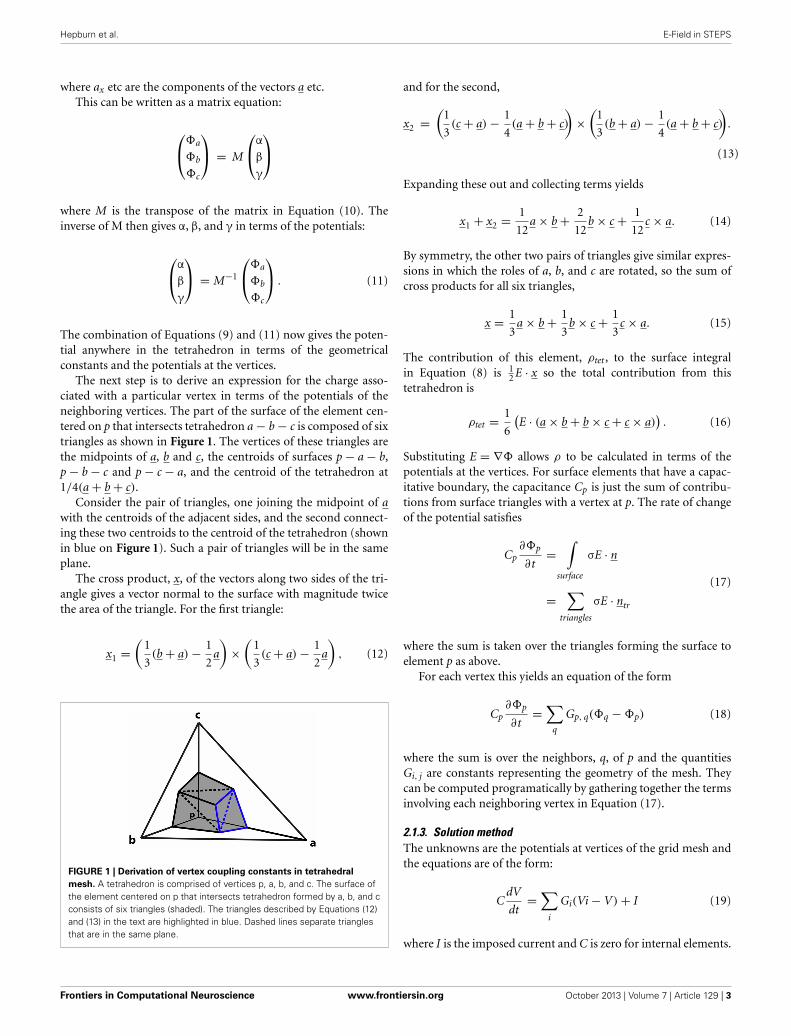
The next step is to derive an expression for the charge asso-ciated with a particular vertex in terms of the potentials of theneighboring vertices. The part of the surface of the element cen-tered on p that intersects tetrahedron a − b − c is composed of sixtriangles as shown in Figure 1. The vertices of these triangles arethe midpoints of a, b and c, the centroids of surfaces p − a − b,p − b − c and p − c − a, and the centroid of the tetrahedron at1/4(a + b + c).

Consider the pair of triangles, one joining the midpoint of awith the centroids of the adjacent sides, and the second connect-ing these two centroids to the centroid of the tetrahedron (shownin blue on Figure 1). Such a pair of triangles will be in the sameplane.

The cross product, x, of the vectors along two sides of the tri-angle gives a vector normal to the surface with magnitude twicethe area of the triangle. For the first triangle:

x1 =(

1

3(b + a) − 1

2a

)×

(1

3(c + a) − 1

2a

), (12)

FIGURE 1 | Derivation of vertex coupling constants in tetrahedral

mesh. A tetrahedron is comprised of vertices p, a, b, and c. The surface ofthe element centered on p that intersects tetrahedron formed by a, b, and cconsists of six triangles (shaded). The triangles described by Equations (12)and (13) in the text are highlighted in blue. Dashed lines separate trianglesthat are in the same plane.

and for the second,

x2 =(

1

3(c + a) − 1

4(a + b + c)

)×

(1

3(b + a) − 1

4(a + b + c)

).

(13)

Expanding these out and collecting terms yields

x1 + x2 = 1

12a × b + 2

12b × c + 1

12c × a. (14)

By symmetry, the other two pairs of triangles give similar expres-sions in which the roles of a, b, and c are rotated, so the sum ofcross products for all six triangles,

x = 1

3a × b + 1

3b × c + 1

3c × a. (15)

The contribution of this element, ρtet , to the surface integralin Equation (8) is 1

2 E · x so the total contribution from thistetrahedron is

ρtet = 1

6

(E · (a × b + b × c + c × a)

). (16)

Substituting E = ∇� allows ρ to be calculated in terms of thepotentials at the vertices. For surface elements that have a capac-itative boundary, the capacitance Cp is just the sum of contribu-tions from surface triangles with a vertex at p. The rate of changeof the potential satisfies

Cp∂�p

∂t=

∫surface

σE · n

=∑

triangles

σE · ntr

(17)

where the sum is taken over the triangles forming the surface toelement p as above.

For each vertex this yields an equation of the form

Cp∂�p

∂t=

∑q

Gp, q(�q − �p) (18)

where the sum is over the neighbors, q, of p and the quantitiesGi, j are constants representing the geometry of the mesh. Theycan be computed programatically by gathering together the termsinvolving each neighboring vertex in Equation (17).

2.1.3. Solution methodThe unknowns are the potentials at vertices of the grid mesh andthe equations are of the form:

CdV

dt=

∑i

Gi(Vi − V) + I (19)

where I is the imposed current and C is zero for internal elements.

Frontiers in Computational Neuroscience www.frontiersin.org October 2013 | Volume 7 | Article 129 | 3

Hepburn et al. E-Field in STEPS

Over a time interval δt during which dV/dt can be treated asconstant, this gives algebraic equations connecting the potentialat time t + 1 with the potentials at time t:

C(Vt + 1 − Vt) =∑

i

Gi(Vi, t + 1 − Vt + 1) + Iδt. (20)

Collecting the time terms together:

(C + δt

∑Gi

)Vt + 1 − δt

∑i

Vi, t + 1 = CVt + Iδt. (21)

Equation (21) is of the form

∑j

Mi, jVj, t + 1 = Ri

in which the matrix M is constant over a timestep and the righthand side contains terms from any applied currents.

At each step, the solution process involves iterating over themesh to populate M and R, and then solving the matrix equa-tion to compute the potentials. The matrix element mi, j of Mis only non-zero if the vertices i and j are neighbors. However,although the matrix is initially sparse, direct solution methodssuch as Gauss–Jordan elimination involve populating more ele-ments that were originally zero. The extent to which this occursdepends how the elements are ordered. For a computationallyefficient solution it is therefore important to find an orderingof the mesh points that minimizes infill during the matrix solu-tion. In the present study two approaches have been explored.In the first, the mesh points are ordered according to their posi-tion along the principal axis of the structure being modeled. Aslong as the structure has one axis which is significantly longerthan the other, this keeps the non-zero elements of M close tothe diagonal (see Results). An upper bound can be placed onthe number of elements each side of the diagonal that must bestored thereby reducing total memory requirements comparedto a full matrix solution. For more complex shapes a breadth-first tree iteration over the mesh visiting each point only once,with a search for the best starting point included, gives betterresults in terms of memory bounds and total operation count(see Results).

2.2. INTEGRATION WITH STOCHASTIC REACTION-DIFFUSIONSIMULATION IN STEPS

An E-Field implementation is included in STEPS 2 and integratedwith spatial reaction-diffusion simulations on unstructured tetra-hedral meshes that accurately represent cellular morphology. Amodel that is built in STEPS, in which tetrahedral subvolumes arelinked with diffusive molecular flux, may be simulated stochas-tically, or converted to a set of ordinary differential equationsthat are then solved deterministically in CVODE (Cohen andHindmarsh, 1996). The addition of the E-Field object bringswith it several new components to STEPS models. These objectsallow simulation of effects that occur in excitable membranes,such as voltage-dependent channel transitions and ligand bind-ing, along with channel currents. The objects that have been

added in version 2 of STEPS since version 1.3 (Hepburn et al.,2012) are:

• Membrane (class steps.geom.Memb): Represents the mem-brane across which the electrical potential will be solved. It iscomprised of a collection of triangles specified by one or morepatches (class steps.geom.TmPatch), which must form a singlesurface that can, however, be open (i.e. it may contain holes) orclosed. The support of closed loops and therefore torus topolo-gies is relevant for many cell biological cases. The Membranecan be on the surface of the tetrahedral mesh, or may be aninternal surface so as to allow outer compartments. Currentlyonly one Membrane may exist in a STEPS simulation (thoughsee Future improvements to simulation realism).

• Channel (class steps.model.Chan): Used to represent a specifictype of chemical species: one that can undergo conforma-tional changes, which may be voltage-dependent. In practice,in STEPS models a Channel object exists only to group a set ofChannel States.

• Channel State (class steps.model.ChanState): Used to modelone specific configuration of a Channel. Channel States aresimilar to Species objects in STEPS in that they may diffusein volumes, or be bound to surfaces, but with the impor-tant difference that a Channel State may be defined as aconducting state with the mapping of currents (presentlyof class steps.model.GHKcurr or steps.model.OhmicCurr)to that state. A Channel State may only undergo voltage-dependent transitions and conduct currents when embed-ded in a Membrane and not when diffusing in a volume(though they may undergo ordinary reactions when in anylocation). Channel States are used as the basis of Markov-schemes in STEPS, and may interact with surrounding intra-and extra-cellular compartments, allowing for features such asphosphorylation-dependent modulation of channel conduc-tance.

• GHK Current (class steps.model.GHKcurr): Describes a cur-rent passing through a given Channel State which is approx-imated by the Goldman-Hodgkin-Katz flux solution to elec-trodiffusion (Goldman, 1943; Hodgkin and Katz, 1949). TheGHK equation has been shown to be an accurate approxima-tion to full electrodiffusion under a wide range of physiologicalconditions, only breaking down when channel pore occupa-tion saturates or competition occurs between different ionicspecies [see Hille (2001a) for further detail on the simplify-ing assumptions and discussion of the accuracy of the GHKequation]. Fluctuations in ionic concentrations both aroundand within a channel pore can result in significant noise insingle-channel current (Mak and Webb, 1997), indicating theneed for stochastic currents and sampling of local concen-trations around each individual channel. The ionic flux inSTEPS is calculated stochastically and discretely within thereaction-diffusion computations, with a rate derived from localconcentrations around each channel, and this flux (optionally)results in transport of ions between compartments (see GHKCurrent calculation). This is particularly useful when comput-ing the flux of important signaling ions, such as calcium, to agood degree of accuracy.

Frontiers in Computational Neuroscience www.frontiersin.org October 2013 | Volume 7 | Article 129 | 4

Hepburn et al. E-Field in STEPS

• Ohmic Current (class steps.model.OhmicCurr): Represent achannel current as an Ohmic current, and are therefore definedby a single-channel conductance and reversal potential. Thiscurrent does not relate to a transport of ions between com-partments in a STEPS simulation. Ohmic Current objects areincluded due to their prevalence in many models (for examplein Hodgkin–Huxley models) and for considerations of effi-ciency, but for many channels the GHK Current should givea more accurate representation of the true biophysical current(see GHK flux as a more accurate representation of single-channel currents compared to the Ohmic approximation).

• Voltage-Dependent Surface Reaction (classsteps.model.VDepSreac): Used to model processes thattake place on a Membrane where the reaction propensitydepends on the local potential across that surface. Suchprocesses are used for modeling channels that undergovoltage-dependent conformational changes [e.g., sodium andpotassium channels in Hodgkin-Huxley models, calcium-activated potassium channels (Anwar et al., 2013)] and/orvoltage-dependent ligand binding [e.g., models of NMDAreceptor voltage-dependent channel block by magnesium(Vargas-Caballero and Robinson, 2004)]. A channel may ofcourse undergo both voltage-dependent interactions as well asnon-voltage-dependent ones such as in Vargas-Caballero andRobinson (2004) and the mslo/BK-type channel in Anwar et al.(2013), which undergoes voltage-dependent conformationalchanges and non-voltage-dependent calcium-activation.

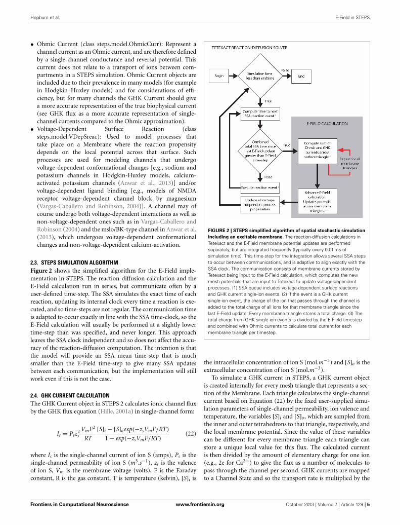
2.3. STEPS SIMULATION ALGORITHMFigure 2 shows the simplified algorithm for the E-Field imple-mentation in STEPS. The reaction-diffusion calculation and theE-Field calculation run in series, but communicate often by auser-defined time-step. The SSA simulates the exact time of eachreaction, updating its internal clock every time a reaction is exe-cuted, and so time-steps are not regular. The communication timeis adapted to occur exactly in line with the SSA time-clock, so theE-Field calculation will usually be performed at a slightly lowertime-step than was specified, and never longer. This approachleaves the SSA clock independent and so does not affect the accu-racy of the reaction-diffusion computation. The intention is thatthe model will provide an SSA mean time-step that is muchsmaller than the E-Field time-step to give many SSA updatesbetween each communication, but the implementation will stillwork even if this is not the case.

2.4. GHK CURRENT CALCULATIONThe GHK Current object in STEPS 2 calculates ionic channel fluxby the GHK flux equation (Hille, 2001a) in single-channel form:

Is = Psz2s

VmF2

RT

[S]i − [S]oexp(−zsVmF/RT)

1 − exp(−zsVmF/RT)(22)

where Is is the single-channel current of ion S (amps), Ps is thesingle-channel permeability of ion S (m3.s−1), zs is the valenceof ion S, Vm is the membrane voltage (volts), F is the Faradayconstant, R is the gas constant, T is temperature (kelvin), [S]i is

FIGURE 2 | STEPS simplified algorithm of spatial stochastic simulation

including an excitable membrane. The reaction-diffusion calculations inTetexact and the E-Field membrane potential updates are performedseparately, but are integrated frequently (typically every 0.01 ms ofsimulation time). This time-step for the integration allows several SSA stepsto occur between communications, and is adaptive to align exactly with theSSA clock. The communication consists of membrane currents stored byTetexact being input to the E-Field calculation, which computes the newmesh potentials that are input to Tetexact to update voltage-dependentprocesses. (1) SSA queue includes voltage-dependent surface reactionsand GHK current single-ion events. (2) If the event is a GHK currentsingle-ion event, the charge of the ion that passes through the channel isadded to the total charge of all ions for that membrane triangle since thelast E-Field update. Every membrane triangle stores a total charge. (3) Thetotal charge from GHK single-ion events is divided by the E-Field timestepand combined with Ohmic currents to calculate total current for eachmembrane triangle per timestep.

the intracellular concentration of ion S (mol.m−3) and [S]o is theextracellular concentration of ion S (mol.m−3).

To simulate a GHK current in STEPS, a GHK current objectis created internally for every mesh triangle that represents a sec-tion of the Membrane. Each triangle calculates the single-channelcurrent based on Equation (22) by the fixed user-supplied simu-lation parameters of single-channel permeability, ion valence andtemperature, the variables [S]i and [S]o, which are sampled fromthe inner and outer tetrahedrons to that triangle, respectively, andthe local membrane potential. Since the value of these variablescan be different for every membrane triangle each triangle canstore a unique local value for this flux. The calculated currentis then divided by the amount of elementary charge for one ion(e.g., 2e for Ca2+) to give the flux as a number of molecules topass through the channel per second. GHK currents are mappedto a Channel State and so the transport rate is multiplied by the

Frontiers in Computational Neuroscience www.frontiersin.org October 2013 | Volume 7 | Article 129 | 5

Hepburn et al. E-Field in STEPS

population of the Channel State to give a total rate for this “reac-tion.” This is then treated as an ordinary “reaction rate” in STEPSand is solved within the SSA for one reaction-diffusion time-step(Figure 2). When this “reaction” executes it results in transport ofions between compartments (e.g., from an extracellular tetrahe-dron to an intracellular tetrahedron or vice-versa) and the rate isre-calculated due to the changes in concentration around the localmembrane surface. A simplified GHK current object is also avail-able, which is a pure current that does not model ion transport.Per reaction-diffusion time-step STEPS stores, triangle by trian-gle, the total charge that crossed the membrane triangle. At theend of a time-step these numbers are converted to currents, addedto any other GHK currents and Ohmic currents, and passed tothe E-Field object to update potential. Single-channel currents arethen recalculated with the new V, transported charges reset to zeroand the process begins again.

3. RESULTS3.1. VALIDATIONSTo demonstrate the accuracy of the E-Field method, we per-formed the Rallpack tests (Bhalla and Bower, 1992) using tetra-hedral meshes to represent the cable compartments. The Rallpacktests are a set of benchmarks that were designed to evaluatethe accuracy of neuronal simulators. Although the Rallpacks arebased on somewhat larger compartments than those to whichthe E-Field method was intended to be applied, these compart-ments can be supported in tetrahedral meshes and are useful foraccuracy studies.

3.1.1. Rallpack1: Uniform unbranched passive cableA mesh of 220,615 tetrahedrons was generated to represent acylinder of length 1 mm and diameter 1 μm. The mesh was con-trolled to give an almost perfect match in volume to a truecylinder, but contained an unavoidable error of 1.0% in surfacearea. Membrane resistance and capacitance were controlled tomatch the values for cylindrical geometry perfectly.

The current of 0.1nA was injected over the nodes at oneend of the cylinder, and potential recorded at both ends (0 and1000 μm). The E-Field calculation was performed every 0.01 msup to total simulated time of 0.25 s.

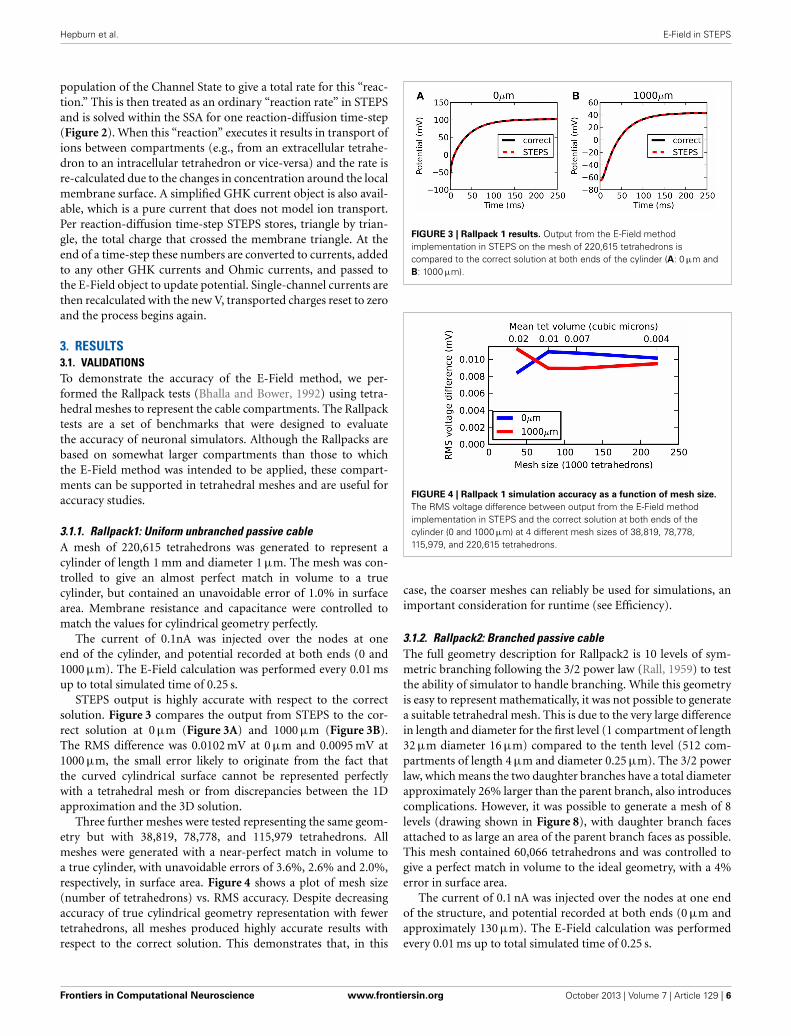
STEPS output is highly accurate with respect to the correctsolution. Figure 3 compares the output from STEPS to the cor-rect solution at 0 μm (Figure 3A) and 1000 μm (Figure 3B).The RMS difference was 0.0102 mV at 0 μm and 0.0095 mV at1000 μm, the small error likely to originate from the fact thatthe curved cylindrical surface cannot be represented perfectlywith a tetrahedral mesh or from discrepancies between the 1Dapproximation and the 3D solution.

Three further meshes were tested representing the same geom-etry but with 38,819, 78,778, and 115,979 tetrahedrons. Allmeshes were generated with a near-perfect match in volume toa true cylinder, with unavoidable errors of 3.6%, 2.6% and 2.0%,respectively, in surface area. Figure 4 shows a plot of mesh size(number of tetrahedrons) vs. RMS accuracy. Despite decreasingaccuracy of true cylindrical geometry representation with fewertetrahedrons, all meshes produced highly accurate results withrespect to the correct solution. This demonstrates that, in this

FIGURE 3 | Rallpack 1 results. Output from the E-Field methodimplementation in STEPS on the mesh of 220,615 tetrahedrons iscompared to the correct solution at both ends of the cylinder (A: 0 μm andB: 1000 μm).

FIGURE 4 | Rallpack 1 simulation accuracy as a function of mesh size.

The RMS voltage difference between output from the E-Field methodimplementation in STEPS and the correct solution at both ends of thecylinder (0 and 1000 μm) at 4 different mesh sizes of 38,819, 78,778,115,979, and 220,615 tetrahedrons.

case, the coarser meshes can reliably be used for simulations, animportant consideration for runtime (see Efficiency).

3.1.2. Rallpack2: Branched passive cableThe full geometry description for Rallpack2 is 10 levels of sym-metric branching following the 3/2 power law (Rall, 1959) to testthe ability of simulator to handle branching. While this geometryis easy to represent mathematically, it was not possible to generatea suitable tetrahedral mesh. This is due to the very large differencein length and diameter for the first level (1 compartment of length32 μm diameter 16 μm) compared to the tenth level (512 com-partments of length 4 μm and diameter 0.25 μm). The 3/2 powerlaw, which means the two daughter branches have a total diameterapproximately 26% larger than the parent branch, also introducescomplications. However, it was possible to generate a mesh of 8levels (drawing shown in Figure 8), with daughter branch facesattached to as large an area of the parent branch faces as possible.This mesh contained 60,066 tetrahedrons and was controlled togive a perfect match in volume to the ideal geometry, with a 4%error in surface area.

The current of 0.1 nA was injected over the nodes at one endof the structure, and potential recorded at both ends (0 μm andapproximately 130 μm). The E-Field calculation was performedevery 0.01 ms up to total simulated time of 0.25 s.

Frontiers in Computational Neuroscience www.frontiersin.org October 2013 | Volume 7 | Article 129 | 6

Hepburn et al. E-Field in STEPS

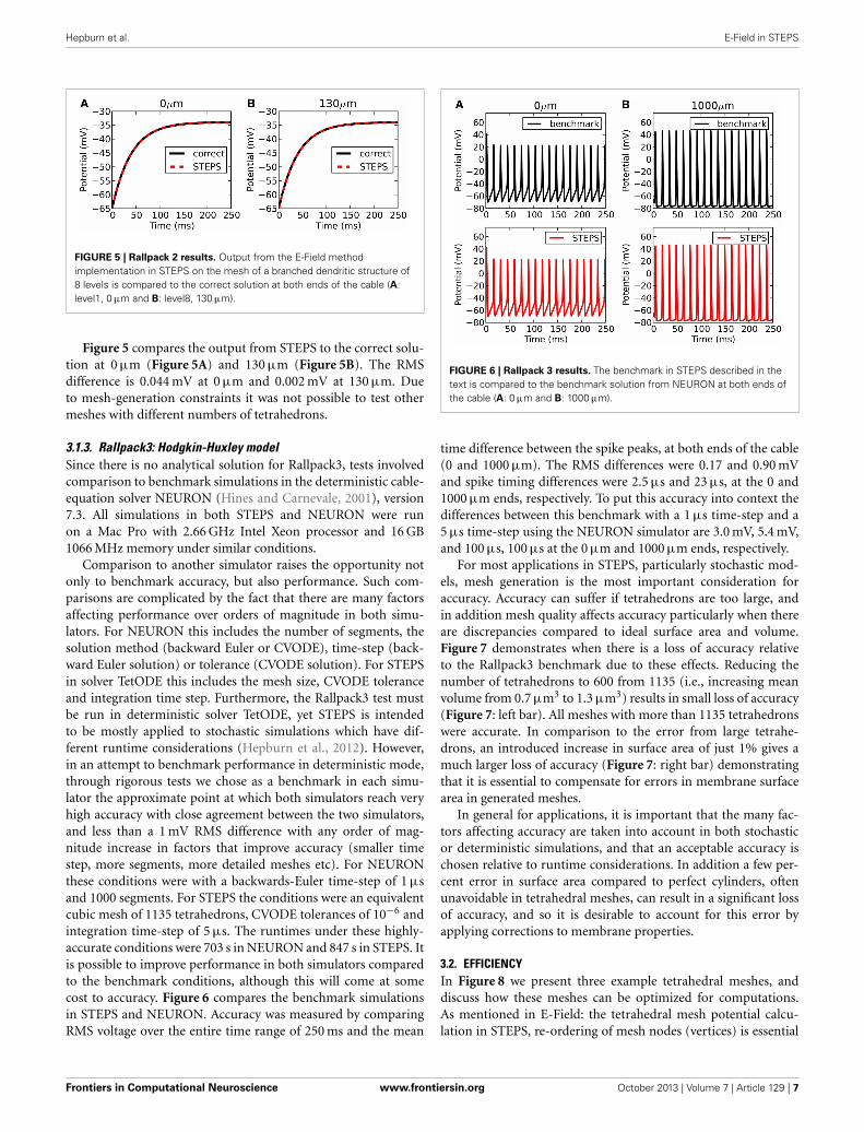
FIGURE 5 | Rallpack 2 results. Output from the E-Field methodimplementation in STEPS on the mesh of a branched dendritic structure of8 levels is compared to the correct solution at both ends of the cable (A:level1, 0 μm and B: level8, 130 μm).

Figure 5 compares the output from STEPS to the correct solu-tion at 0 μm (Figure 5A) and 130 μm (Figure 5B). The RMSdifference is 0.044 mV at 0 μm and 0.002 mV at 130 μm. Dueto mesh-generation constraints it was not possible to test othermeshes with different numbers of tetrahedrons.

3.1.3. Rallpack3: Hodgkin-Huxley modelSince there is no analytical solution for Rallpack3, tests involvedcomparison to benchmark simulations in the deterministic cable-equation solver NEURON (Hines and Carnevale, 2001), version7.3. All simulations in both STEPS and NEURON were runon a Mac Pro with 2.66 GHz Intel Xeon processor and 16 GB1066 MHz memory under similar conditions.

Comparison to another simulator raises the opportunity notonly to benchmark accuracy, but also performance. Such com-parisons are complicated by the fact that there are many factorsaffecting performance over orders of magnitude in both simu-lators. For NEURON this includes the number of segments, thesolution method (backward Euler or CVODE), time-step (back-ward Euler solution) or tolerance (CVODE solution). For STEPSin solver TetODE this includes the mesh size, CVODE toleranceand integration time step. Furthermore, the Rallpack3 test mustbe run in deterministic solver TetODE, yet STEPS is intendedto be mostly applied to stochastic simulations which have dif-ferent runtime considerations (Hepburn et al., 2012). However,in an attempt to benchmark performance in deterministic mode,through rigorous tests we chose as a benchmark in each simu-lator the approximate point at which both simulators reach veryhigh accuracy with close agreement between the two simulators,and less than a 1 mV RMS difference with any order of mag-nitude increase in factors that improve accuracy (smaller timestep, more segments, more detailed meshes etc). For NEURONthese conditions were with a backwards-Euler time-step of 1 μsand 1000 segments. For STEPS the conditions were an equivalentcubic mesh of 1135 tetrahedrons, CVODE tolerances of 10−6 andintegration time-step of 5 μs. The runtimes under these highly-accurate conditions were 703 s in NEURON and 847 s in STEPS. Itis possible to improve performance in both simulators comparedto the benchmark conditions, although this will come at somecost to accuracy. Figure 6 compares the benchmark simulationsin STEPS and NEURON. Accuracy was measured by comparingRMS voltage over the entire time range of 250 ms and the mean

FIGURE 6 | Rallpack 3 results. The benchmark in STEPS described in thetext is compared to the benchmark solution from NEURON at both ends ofthe cable (A: 0 μm and B: 1000 μm).

time difference between the spike peaks, at both ends of the cable(0 and 1000 μm). The RMS differences were 0.17 and 0.90 mVand spike timing differences were 2.5 μs and 23 μs, at the 0 and1000 μm ends, respectively. To put this accuracy into context thedifferences between this benchmark with a 1 μs time-step and a5 μs time-step using the NEURON simulator are 3.0 mV, 5.4 mV,and 100 μs, 100 μs at the 0 μm and 1000 μm ends, respectively.

For most applications in STEPS, particularly stochastic mod-els, mesh generation is the most important consideration foraccuracy. Accuracy can suffer if tetrahedrons are too large, andin addition mesh quality affects accuracy particularly when thereare discrepancies compared to ideal surface area and volume.Figure 7 demonstrates when there is a loss of accuracy relativeto the Rallpack3 benchmark due to these effects. Reducing thenumber of tetrahedrons to 600 from 1135 (i.e., increasing meanvolume from 0.7 μm3 to 1.3 μm3) results in small loss of accuracy(Figure 7: left bar). All meshes with more than 1135 tetrahedronswere accurate. In comparison to the error from large tetrahe-drons, an introduced increase in surface area of just 1% gives amuch larger loss of accuracy (Figure 7: right bar) demonstratingthat it is essential to compensate for errors in membrane surfacearea in generated meshes.

In general for applications, it is important that the many fac-tors affecting accuracy are taken into account in both stochasticor deterministic simulations, and that an acceptable accuracy ischosen relative to runtime considerations. In addition a few per-cent error in surface area compared to perfect cylinders, oftenunavoidable in tetrahedral meshes, can result in a significant lossof accuracy, and so it is desirable to account for this error byapplying corrections to membrane properties.

3.2. EFFICIENCYIn Figure 8 we present three example tetrahedral meshes, anddiscuss how these meshes can be optimized for computations.As mentioned in E-Field: the tetrahedral mesh potential calcu-lation in STEPS, re-ordering of mesh nodes (vertices) is essential

Frontiers in Computational Neuroscience www.frontiersin.org October 2013 | Volume 7 | Article 129 | 7

Hepburn et al. E-Field in STEPS

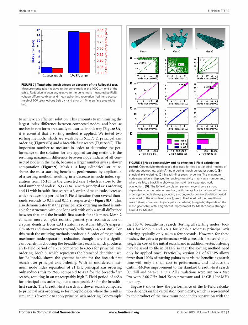
FIGURE 7 | Tetrahedral mesh effects on accuracy of the Rallpack3 test.

Measurements taken relative to the benchmark at the 1000 μm end of thecable. Reduction in accuracy relative to the benchmark measured by RMSvoltage difference (blue) and mean spike-time resolution (red) for a coarsemesh of 600 tetrahedrons (left bar) and error of 1% in surface area (rightbar).

to achieve an efficient solution. This amounts to minimizing thelargest index difference between connected nodes, and becausemeshes in raw form are usually not sorted in this way (Figure 8A)it is essential that a sorting method is applied. We tested twosorting methods, which are available in STEPS 2: principal axisordering (Figure 8B) and a breadth-first search (Figure 8C). Theimportant number to measure in order to determine the per-formance of the solution for any applied sorting method is theresulting maximum difference between node indices of all con-nected nodes in the mesh, because a larger number gives a slowercomputation (Figure 9). Mesh 1, a long cylindrical structure,shows the most startling benefit to performance by applicationof a sorting method, resulting in a decrease in node index sep-aration from 16,105 in the unsorted case (which is close to thetotal number of nodes: 16,177) to 14 with principal axis orderingand 11 with breadth-first search, a 3-order of magnitude decrease,which reduces the period for E-Field iteration from several thou-sands seconds to 0.14 and 0.11 s, respectively (Figure 8D). Thisalso demonstrates that the principal axis ordering method is suit-able for structures with one long axis with only a small differencebetween that and the breadth-first search for this mesh. Mesh 2contains more complex realistic geometry: a reconstruction ofa spiny dendrite from CA1 stratum radiatum (http://synapses.clm.utexas.edu/anatomy/ca1pyrmd/radiatum/k24/k24.stm). Forthis mesh the ordering methods produce a 2-order of magnitudemaximum node separation reduction, though there is a signifi-cant benefit in choosing the breadth-first search, which producesan E-Field period of 1.76 s compared to 6.65 s for principal axisordering. Mesh 3, which represents the branched dendrite usedfor Rallpack2, shows the greatest benefit for the breadth-firstsearch over principal axis ordering. With an unordered maxi-mum node index separation of 21,151, principal axis orderingonly reduces this to 2688 compared to 423 for the breadth-firstsearch, resulting in an unacceptably high E-Field period of 465 sfor principal axis ordering, but a manageable 8 s for the breadth-first search. The breadth-first search is a slower search comparedto principal axis ordering, so for morphologies where the result issimilar it is favorable to apply principal axis ordering. For example

FIGURE 8 | Node connectivity and its effect on E-Field calculation

period. Connectivity matrices are displayed for three tetrahedral meshes ofdifferent geometries, with (A): no ordering (mesh generator output), (B):principal axis ordering, (C): breadth-first search ordering. The maximumnode separation is displayed for each connectivity matrix as a number and,where visible, a black line showing the maximally separated nodeconnection. (D): The E-Field calculation performance shows a strongdependency on the ordering method, with the application of one of the twoordering methods always producing a strong reduction in calculation periodcompared to the unordered case (green). The benefit of the breadth-firstsearch (blue) compared to principal axis ordering (magenta) depends on themesh geometry, with a significant improvement for Mesh 2 and a strongerbenefit for Mesh 3.

the 100 % breadth-first search (testing all starting nodes) took146 s for Mesh 2 and 736 s for Mesh 3 whereas principal axisordering typically only takes a few seconds. However, for thesemeshes, the gains to performance with a breadth-first search out-weigh the cost of the initial search, and in addition vertex orderingmay be saved to file in STEPS so that the sorting method needonly be applied once. Practically, version 2.1 of STEPS allowsfewer than 100% of starting points to be visited benefitting searchtime with only a small cost to performance, and includes theCuthill-McKee improvement to the standard breadth-first search(Cuthill and McKee, 1969). All simulations were run on a MacPro with 2.66 GHz Intel Xeon processor and 16 GB 1066 MHzmemory.

Figure 9 shows how the performance of the E-Field calcula-tion depends on the calculation complexity, which is representedby the product of the maximum node index separation with the

Frontiers in Computational Neuroscience www.frontiersin.org October 2013 | Volume 7 | Article 129 | 8

Hepburn et al. E-Field in STEPS

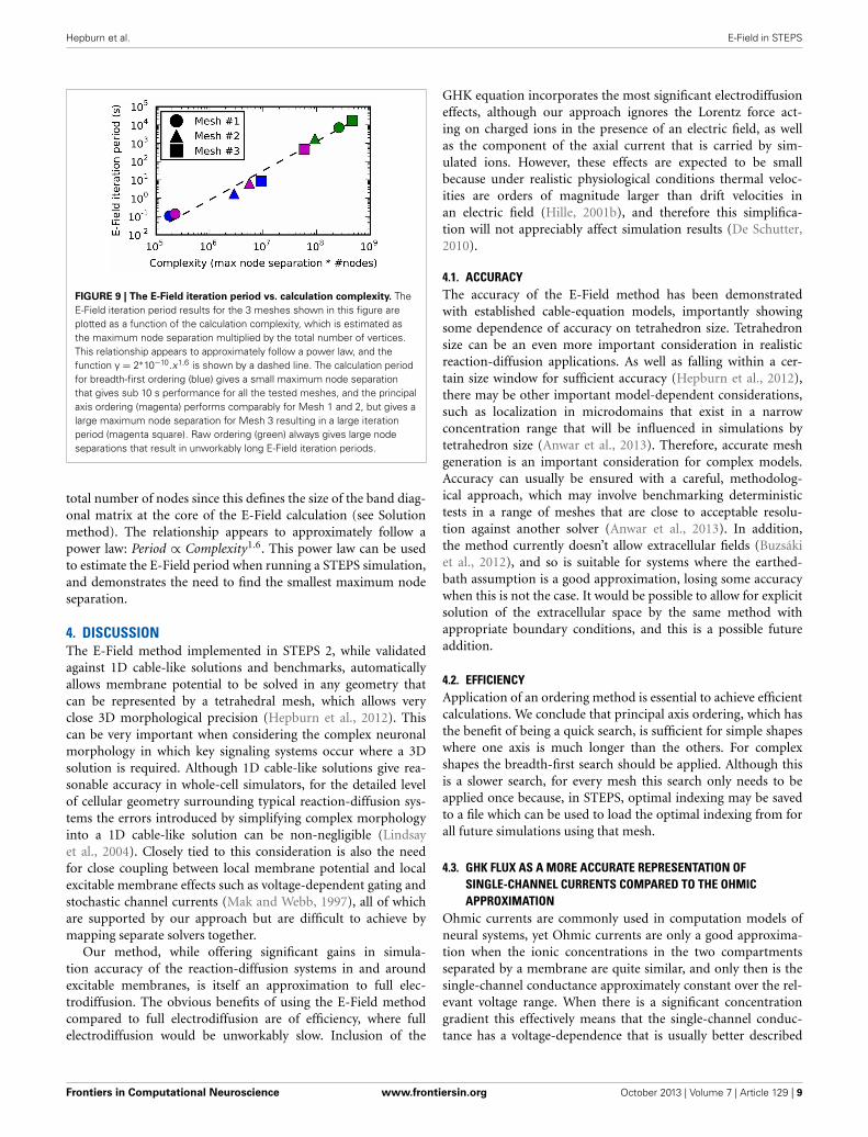
FIGURE 9 | The E-Field iteration period vs. calculation complexity. TheE-Field iteration period results for the 3 meshes shown in this figure areplotted as a function of the calculation complexity, which is estimated asthe maximum node separation multiplied by the total number of vertices.This relationship appears to approximately follow a power law, and thefunction y = 2∗10−10.x1.6 is shown by a dashed line. The calculation periodfor breadth-first ordering (blue) gives a small maximum node separationthat gives sub 10 s performance for all the tested meshes, and the principalaxis ordering (magenta) performs comparably for Mesh 1 and 2, but gives alarge maximum node separation for Mesh 3 resulting in a large iterationperiod (magenta square). Raw ordering (green) always gives large nodeseparations that result in unworkably long E-Field iteration periods.

total number of nodes since this defines the size of the band diag-onal matrix at the core of the E-Field calculation (see Solutionmethod). The relationship appears to approximately follow apower law: Period ∝ Complexity1.6. This power law can be usedto estimate the E-Field period when running a STEPS simulation,and demonstrates the need to find the smallest maximum nodeseparation.

4. DISCUSSIONThe E-Field method implemented in STEPS 2, while validatedagainst 1D cable-like solutions and benchmarks, automaticallyallows membrane potential to be solved in any geometry thatcan be represented by a tetrahedral mesh, which allows veryclose 3D morphological precision (Hepburn et al., 2012). Thiscan be very important when considering the complex neuronalmorphology in which key signaling systems occur where a 3Dsolution is required. Although 1D cable-like solutions give rea-sonable accuracy in whole-cell simulators, for the detailed levelof cellular geometry surrounding typical reaction-diffusion sys-tems the errors introduced by simplifying complex morphologyinto a 1D cable-like solution can be non-negligible (Lindsayet al., 2004). Closely tied to this consideration is also the needfor close coupling between local membrane potential and localexcitable membrane effects such as voltage-dependent gating andstochastic channel currents (Mak and Webb, 1997), all of whichare supported by our approach but are difficult to achieve bymapping separate solvers together.

Our method, while offering significant gains in simula-tion accuracy of the reaction-diffusion systems in and aroundexcitable membranes, is itself an approximation to full elec-trodiffusion. The obvious benefits of using the E-Field methodcompared to full electrodiffusion are of efficiency, where fullelectrodiffusion would be unworkably slow. Inclusion of the

GHK equation incorporates the most significant electrodiffusioneffects, although our approach ignores the Lorentz force act-ing on charged ions in the presence of an electric field, as wellas the component of the axial current that is carried by sim-ulated ions. However, these effects are expected to be smallbecause under realistic physiological conditions thermal veloc-ities are orders of magnitude larger than drift velocities inan electric field (Hille, 2001b), and therefore this simplifica-tion will not appreciably affect simulation results (De Schutter,2010).

4.1. ACCURACYThe accuracy of the E-Field method has been demonstratedwith established cable-equation models, importantly showingsome dependence of accuracy on tetrahedron size. Tetrahedronsize can be an even more important consideration in realisticreaction-diffusion applications. As well as falling within a cer-tain size window for sufficient accuracy (Hepburn et al., 2012),there may be other important model-dependent considerations,such as localization in microdomains that exist in a narrowconcentration range that will be influenced in simulations bytetrahedron size (Anwar et al., 2013). Therefore, accurate meshgeneration is an important consideration for complex models.Accuracy can usually be ensured with a careful, methodolog-ical approach, which may involve benchmarking deterministictests in a range of meshes that are close to acceptable resolu-tion against another solver (Anwar et al., 2013). In addition,the method currently doesn’t allow extracellular fields (Buzsákiet al., 2012), and so is suitable for systems where the earthed-bath assumption is a good approximation, losing some accuracywhen this is not the case. It would be possible to allow for explicitsolution of the extracellular space by the same method withappropriate boundary conditions, and this is a possible futureaddition.

4.2. EFFICIENCYApplication of an ordering method is essential to achieve efficientcalculations. We conclude that principal axis ordering, which hasthe benefit of being a quick search, is sufficient for simple shapeswhere one axis is much longer than the others. For complexshapes the breadth-first search should be applied. Although thisis a slower search, for every mesh this search only needs to beapplied once because, in STEPS, optimal indexing may be savedto a file which can be used to load the optimal indexing from forall future simulations using that mesh.

4.3. GHK FLUX AS A MORE ACCURATE REPRESENTATION OFSINGLE-CHANNEL CURRENTS COMPARED TO THE OHMICAPPROXIMATION

Ohmic currents are commonly used in computation models ofneural systems, yet Ohmic currents are only a good approxima-tion when the ionic concentrations in the two compartmentsseparated by a membrane are quite similar, and only then is thesingle-channel conductance approximately constant over the rel-evant voltage range. When there is a significant concentrationgradient this effectively means that the single-channel conduc-tance has a voltage-dependence that is usually better described

Frontiers in Computational Neuroscience www.frontiersin.org October 2013 | Volume 7 | Article 129 | 9

Hepburn et al. E-Field in STEPS

by the GHK flux equation (Hille, 2001a; Clay, 2009). There areoccasions when an Ohmic current is a good approximation evenwhen a significant concentration gradient exists, which is causedby some external effect, such as the squid giant axon sodiumcurrent which is linearized in the physiological range by partialblock of the current by calcium and magnesium ions (Vandenbergand Bezanilla, 1991). However, the GHK equation is usually themore accurate representation, and this accuracy is particularlyimportant when calculating the flux of ions that then undergoimportant intracellular processes, such as calcium (De Schutter,2010).

4.4. FUTURE INTEGRATION WITH WHOLE-CELL SOLVERSThe E-Field implementation in STEPS was developed with theintention of being applied to the complex morphologies sur-rounding micrometer cellular signaling regions. Although it iscapable of solving membrane potential in anything that can berepresented by a tetrahedral mesh and therefore could, in theory,be used in whole-cell models, often such a level of detail is notnecessary and would introduce runtime concerns at such scales,and the whole-cell calculations would be much better solvedby cable-theory based simulators such as PSICS (http://www.

psics.org), NEURON (http://www.neuron.yale.edu) or GENESIS(http://www.genesis-sim.org). Therefore, important future workwill involve integrating STEPS with one or more whole-celland network simulators, where STEPS simulates a section ofthe morphology completely and the rest of the cell is solvedby a whole-cell simulator, with coupling consisting ideally ofa single axial current. This could be achieved in a numberof ways. For example, the tools are already in place to forma connection through Python of STEPS to other simulatorswith a Python interface, which are many. However, this wouldmost likely be the least efficient approach. More efficient cou-pling could be achieved through software designed for this goal,such as MUSIC (Djurfeldt et al., 2010), or through a moredirect approach. With successful integration between simula-tors achieved many more applications will open up in whichSTEPS could potentially form a component in full multi-scalemodels.

4.5. FUTURE IMPROVEMENTS TO SIMULATION REALISMWhile the introduction of accurate calculation of the time-varying electrical potential in complex 3D geometries is animportant advance in multiscale simulation by making it pos-sible to tightly integrate local membrane potential and currentswith reaction-diffusion calculations, there is the possibility forfurther additions to this in the future. Small deviations fromthe GHK flux are possible in some biological channel currents;for example competition may exist in the pore which results insome weak voltage and/or concentration dependence to perme-ability (Jatzke et al., 2002). Improvements to calculation accuracyfor such channel currents could be possible by simulating thecurrent through pores as particles “hopping over” energy barri-ers (Hille, 2001a), though this could come at a significant costto simulation runtime. In addition, the present implementationis restricted to simulating the potential across only one cellularmembrane for which the outer potential is assumed fixed, yet cellscan contain internal membranes (such as the endoplasmic reticu-lum) that are capable of charge separation and therefore containa potential across them (Shemer et al., 2008), and can themselvescontain channels and pumps that transport ions from intracel-lular stores (Szewczyk, 1998; Hille, 2001c) by processes that canalso be voltage-dependent (Sepehri et al., 2007). Therefore, therecould be many useful applications of an extension that allows sim-ulation of the potential across such internal membranes, whichwill involve a modification to the present implementation to allowa varying outer compartment potential.

AVAILABILITYSTEPS is available at: http://steps.sourceforge.net

ACKNOWLEDGMENTSWe thank Stefan Wils for his initial work on implementingthe E-Field method in STEPS. CUBIT was used under rightsand license from Sandia National Laboratories: Sandia LicenseNumber 09-N06832.

FUNDINGThis work was supported by OISTPC and OISTSC.

REFERENCESAnwar, H., Hepburn, I., Nedelescu,

H., Chen, W., and De Schutter,E. (2013). Stochastic calciummechanisms cause dendriticcalcium spike variability. J.Neurosci. 33, 15848–15867. doi:10.1523/JNEUROSCI.1722-13.2013

Bhalla, U. S. (2011). Multiscale inter-actions between chemical andelectric signaling in LTP induc-tion, LTP reversal and dendriticexcitability. Neural Netw. 24,943–949. doi: 10.1016/j.neunet.2011.05.001

Bhalla, U. S., Bilitch, D. H., andBower, J. M. (1992). Rallpacks: aset of benchmarks for neuronalsimulators. Trends Neurosci. 15,453–458. doi: 10.1016/0166-2236(92)90009-W

Brandi, M., Brocke, E., Talukdar, H.,Hanke, M., Bhalla, U. S., Kotaleski,J., et al. (2011). ConnectingMOOSE and NeuroRD throughMUSIC: towards a communicationframework for multi-scale mod-eling. BMC Neurosci. 12(Suppl1):P77. doi: 10.1186/1471-2202-12-S1-P77.

Buzsáki, G., Anastassiou, C. A., andKoch, C. (2012). The origin ofextracellular fields and currents –EEG, ECoG, LFP and spikes. Nat.Rev. Neurosci. 13, 407–420. doi:10.1038/nrn3241

Clay, J. R. (2009). Determining K+channel activation curves from K+channel currents often requires theGoldman-Hodgkin-Katz equation.Front Cell. Neurosci. 3:20. doi:10.3389/neuro.03.020.2009.

Cohen, S. D., and Hindmarsh, A.C. (1996). CVODE, a stiff/nonstiffODE solver in C. Comput. Phys. 10,138–143.

Cornelis, H., Rodriguez, A. L., Coop,A. D., and Bower, J. M. (2012).Python as a federation tool forGENESIS 3.0. PLoS ONE 7:e29018.doi: 10.1371/journal.pone.0029018.

Cuthill, E., and McKee, J. (1969).“Reducing the bandwidth ofsparse symmetric matrices,” inACM Proceedings of the 1969 24thnational conference, (New York,NY), 157–172.

De Schutter, E. (2010). “Modelingintracellular calcium dynamics,” inComputational Modeling Methodsfor Neuroscientists, ed E. De Schutter(Cambridge, MA: The MIT Press),93–105.

Djurfeldt, M., Hjorth, J., Eppler,J. M., Dudani, N., Helias, M.,Potjans, T. C., et al. (2010). Run-time interoperability betweenneuronal network simulatorsbased on the MUSIC framework.Neuroinformatics 8, 43–60. doi:10.1007/s12021-010-9064-z.

Fakler, B., and Adelman, J. P.(2008). Control of K(Ca)channels by calcium nano/microdomains. Neuron 59,873–881. doi: 10.1016/j.neuron.2008.09.001

Gillespie, D. T. (1977). Exact stochasticsimulation of coupled chem-ical reactions. J. Phys. Chem.81, 2340–2361. doi: 10.1021/j100540a008

Goldman, D. E. (1943). Potential,impedance, and rectification in

Frontiers in Computational Neuroscience www.frontiersin.org October 2013 | Volume 7 | Article 129 | 10

Hepburn et al. E-Field in STEPS

membranes. J. Gen. Physiol. 27,37–60. doi: 10.1085/jgp.27.1.37

Hepburn, I., Chen, W., Wils, S., and DeSchutter, E. (2012). STEPS: efficientsimulation of stochastic reaction–diffusion models in realistic mor-phologies. BMC Syst. Biol. 6:36. doi:10.1186/1752-0509-6-36

Hille, B. (2001a). Ion Channels ofExcitable Membranes. Sunderland,MA: Sinauer Associates.

Hille, B. (2001b). “Elementary prop-erties of ions in solution,” in IonChannels of Excitable Membranes, edB. Hille (Sunderland, MA: SinauerAssociates), 309–345.

Hille, B. (2001c). “Calcium dynamics,epithelial transport, and intercel-lular coupling,” in Ion Channelsof Excitable Membranes, ed B.Hille (Sunderland, MA: SinauerAssociates), 269–306.

Hines, M. L., and Carnevale, N. T.(2001). NEURON: a tool for neuro-scientists. Neuroscientist 7, 123–135.doi: 10.1177/107385840100700207.

Hodgkin, A. L., and Katz, B. (1949).The effect of sodium ions onthe electrical activity of the giantaxon of the squid. J. Physiol. 108,37–77.

Jatzke, C., Watanabe, J., and Wollmuth,L. P. (2002). Voltage and con-centration dependence of Ca(2+)permeability in recombinantglutamate receptor subtypes.

J. Physiol. 538, 25–39. doi:10.1113/jphysiol.2001.012897

Lindsay, K. A., Rosenberg, J. R.,and Tucker, G. (2004). FromMaxwell’s equations to the cableequation and beyond. Progr.Biophys. Mol. Biol. 85, 71–116. doi:10.1016/j.pbiomolbio.2003.08.001.

Mak, D. O., and Webb, W. W. (1997).Conductivity noise in transmem-brane ion channels due to ion con-centration fluctuations via diffu-sion. Biophys. J. 72, 1153–1164. doi:10.1016/S0006-3495(97)78764-2.

Nunez, P. L., and Srinivasan, R.(2006). Electric Fields of the Brain:The Neurophysics of EEG. NewYork, NY: Oxford UniversityPress. doi: 10.1093/acprof:oso/9780195050387.001.0001

Plonsey, R. (1969). BioelectricPhenomena. New York, NY:McGraw Hill.

Rall, W. (1959). Branching dendritictrees and motoneuron membraneresistivity. Exp. Neurol. 1, 491–527.doi: 10.1016/0014-4886(59)90046-9

Ray, S., and Bhalla, U. S. (2008).PyMOOSE: interoperable script-ing in python for MOOSE.Front. Neuroinformatics 2:6. doi:10.3389/neuro.11.006.2008

Santamaria, F., Wils, S., De Schutter,E., and Augustine, G. J. (2006).Anomolous diffusion in purk-inje cell dendrites caused by

spines. Neuron 52, 635–648. doi:10.1016/j.neuron.2006.10.025.

Sepehri, H., Eliassi, A., Sauvé, R.,Ashrafpour, M., and Saghiri, R.(2007). Evidence for a large conduc-tance voltage gated cationic chan-nel in rough endoplasmic retic-ulum of rat hepatocytes. Arch.Biochem. Biophys. 457, 35–40. doi:10.1016/j.abb.2006.10.012

Shemer, I., Brinne, B., Tegnér, J.,and Grillner, S. (2008). Electrotonicsignals along intracellular mem-branes may interconnect dendriticspines and nucleus. PLOS Comput.Biol. 4:e1000036. doi: 10.1371/jour-nal.pcbi.1000036

Szewczyk, A. (1998). The intracel-lular potassium and chloridechannels: properties, pharma-cology and function (Review).Mol. Membr. Biol. 15, 49–58. doi:10.3109/09687689809027518

Vandenberg, C. A., and Bezanilla,F. (1991). Single-channel, macro-scopic, and gating currents fromsodium channels in the squid giantaxon. Biophys. J. 60, 1499–1510. doi:10.1016/S0006-3495(91)82185-3

Vargas-Caballero, M., and Robinson,H. P. C. (2004). Fast and slowvoltage-dependent dynamicsof magnesium block in theNMDA receptor: the asym-metric trapping block model.J. Neurosci. 24, 6171–6180.

doi: 10.1523/JNEUROSCI.1380-04.2004

Conflict of Interest Statement: Theauthors declare that the researchwas conducted in the absence of anycommercial or financial relationshipsthat could be construed as a potentialconflict of interest.

Received: 20 May 2013; accepted: 09September 2013; published online: 29October 2013.Citation: Hepburn I, Cannon R and DeSchutter E (2013) Efficient calculationof the quasi-static electrical potential ona tetrahedral mesh and its implementa-tion in STEPS. Front. Comput. Neurosci.7:129. doi: 10.3389/fncom.2013.00129This article was submitted to thejournal Frontiers in ComputationalNeuroscience.Copyright © 2013 Hepburn, Cannonand De Schutter. This is an open-accessarticle distributed under the terms ofthe Creative Commons AttributionLicense (CC BY). The use, distribu-tion or reproduction in other forumsis permitted, provided the originalauthor(s) or licensor are credited andthat the original publication in thisjournal is cited, in accordance withaccepted academic practice. No use,distribution or reproduction is permit-ted which does not comply with theseterms.

Frontiers in Computational Neuroscience www.frontiersin.org October 2013 | Volume 7 | Article 129 | 11