Efficacy of diffeomorphic surface matching and 3D

HAL Id: hal-02059270https://hal.archives-ouvertes.fr/hal-02059270

Submitted on 25 Feb 2021

HAL is a multi-disciplinary open accessarchive for the deposit and dissemination of sci-entific research documents, whether they are pub-lished or not. The documents may come fromteaching and research institutions in France orabroad, or from public or private research centers.

L’archive ouverte pluridisciplinaire HAL, estdestinée au dépôt et à la diffusion de documentsscientifiques de niveau recherche, publiés ou non,émanant des établissements d’enseignement et derecherche français ou étrangers, des laboratoirespublics ou privés.

Efficacy of diffeomorphic surface matching and 3Dgeometric morphometrics for taxonomic discrimination

of Early Pleistocene hominin mandibular molarsJosé Braga, Veronika Zimmer, Jean Dumoncel, Chafik Samir, Frikkie de Beer,

Clément Zanolli, Deborah Pinto, F. James Rohlf, Frederick Grine

To cite this version:José Braga, Veronika Zimmer, Jean Dumoncel, Chafik Samir, Frikkie de Beer, et al.. Efficacy ofdiffeomorphic surface matching and 3D geometric morphometrics for taxonomic discrimination ofEarly Pleistocene hominin mandibular molars. Journal of Human Evolution, Elsevier, 2019, 130,pp.21-35. �10.1016/j.jhevol.2019.01.009�. �hal-02059270�

https://hal.archives-ouvertes.fr/hal-02059270

https://hal.archives-ouvertes.fr

1

Efficacy of diffeomorphic surface matching and 3D geometric morphometrics

for taxonomic discrimination of Early Pleistocene hominin mandibular

molars.

José Braga a, b*, Veronika Zimmer c, d, Jean Dumoncel a, Chafik Samir e, Frikkie

de Beer f, Clément Zanolli a, Deborah Pinto a, F. James Rohlf g, Frederick E. Grine

g, h

a Computer-assisted Palaeoanthropology Team, UMR 5288 CNRS-Université de Toulouse (Paul Sabatier), 37 Allées Jules Guesde, 31000 Toulouse, France. ([email protected]) ([email protected]) ([email protected]) ([email protected]) b Evolutionary Studies Institute, University of the Witwatersrand, Johannesburg, 2050, South Africa. c Department of Anatomy, Faculty of Health Sciences, University of Pretoria, Pretoria 0001, South Africa. ([email protected]) d Department of Biomedical Engineering, King’s College London, London, UK e LIMOS, UMR 6158 CNRS-Université Clermont Auvergne, 63173 Aubière, France ([email protected]) f South African Nuclear Energy Corporation (Necsa), Pelindaba, North West Province,

South Africa. ([email protected]) g Department of Anthropology, Stony Brook University, Stony Brook, NY 11794, USA ([email protected]; [email protected]) h Department of Anatomical Sciences, Stony Brook University, Stony Brook, NY 11794 USA * Corresponding author. E-mail address: [email protected] Telephone: + 33 (0)5 61 55 80 65 (J. Braga) Keywords:

2

Sterkfontein; Swartkrans; Australopithecus africanus; Paranthropus robustus; Homo

ABSTRACT

Morphometric assessments of the dentition have played significant roles in hypotheses relating to

taxonomic diversity among extinct hominins. In this regard, emphasis has been placed on the

statistical appraisal of intraspecific variation to identify morphological criteria that convey

maximum discriminatory power. Three-dimensional geometric morphometric (3D GM)

approaches that utilize landmarks and semi-landmarks to quantify shape variation have enjoyed

increasingly popular use over the past twenty-five years in assessments of the outer enamel

surface (OES) and enamel-dentine junction (EDJ) of fossil molars. Recently developed

diffeomorphic surface matching (DSM) methods that model the deformation between shapes

have drastically reduced if not altogether eliminated potential methodological inconsistencies

associated with the a priori identification of landmarks and delineation of semi-landmarks. As

such, DSM has the potential to better capture the geometric details that describe tooth shape by

accounting for both homologous and non-homologous (i.e., discrete) features, and permitting the

statistical determination of geometric correspondence. We compare the discriminatory power of

3D GM and DSM in the evaluation of the OES and EDJ of mandibular permanent molars

attributed to Australopithecus africanus, Paranthropus robustus and early Homo sp. from the

sites of Sterkfontein and Swartkrans. For all three molars, classification and clustering scores

demonstrate that DSM performs better at separating the A. africanus and P. robustus samples

than does 3D GM. The EDJ provided the best results. Paranthropus robustus evinces greater

morphological variability than A. africanus. The DSM assessment of the early Homo molar from

Swartkrans reveals its distinctiveness from either australopith sample, and the “unknown”

specimen from Sterkfontein (Stw 151) is notably more similar to Homo than to A. africanus.

3

1. Introduction

The sizes and shapes of teeth have been widely used to generate hypotheses relating to early

hominin taxonomy and phylogeny. Traditionally, these studies have relied on linear

morphometric variables, such as the mesiodistal and buccolingual diameters of tooth crowns, the

planimetric areas occupied by molar cusps, and the subjective assessment of morphological

features that manifest at the outer enamel surface (OES) of a tooth (e.g., Robinson, 1956;

Coppens, 1980; Wood and Abbott, 1983; Grine, 1984, 1985, 1988; 1993; Wood and

Uytterschaut, 1987; Wood and Engleman, 1988; Suwa, 1988, 1996; Suwa et al., 1996; Irish and

Guatelli-Steinberg, 2003; Moggi-Cecchi, 2003; Prat et al., 2005; Moggi-Cecchi et al., 2006,

2010; Moggi-Cecchi and Boccone, 2007; Martinón-Torres et al., 2008, 2012; Grine et al., 2009,

2013; Irish et al., 2013; Kaifu et al., 2015; Villmoare et al., 2015).

Over the past twenty-five years, such classic methods have been extended and

supplemented by three-dimensional geometric morphometric (3D GM) approaches that utilize

landmark and semi-landmark as well as landmark-free data to quantify shape variation (e.g.,

Bookstein, 1991; Rohlf and Marcus, 1993; O’Higgins, 2000; Adams et al., 2004, 2013; Slice,

2005, 2007; Mitteroecker and Gunz, 2009; Gunz and Mitteroecker, 2013). Landmark-based

approaches entail the statistical analysis of shape variation and its covariation with other

variables through the “Procrustes paradigm” where landmarks are superimposed to a common

coordinate system. This approach has been widely applied in studies of the OES and enamel-

dentine junction (EDJ) topographies of extant and fossil hominid dental samples (e.g., Martinón -

Torres et al., 2006; Gómez-Robles et al., 2007, 2008, 2015; Skinner et al., 2008a, 2009a, 2009b;

Braga et al., 2010; Zanolli et al., 2012; Pan et al., 2016) and, owing to its relative success, has

come to represent the current mainstream 3D approach to dental paleoanthropology.

4

Although 3D GM represents a powerful tool by which to assess morphological variation,

assessments are based on correspondences between geometric features (anatomical landmarks)

that have been specified a priori on the basis of observer expertise. As discussed below (see

Methods), the main limitations of GM pertain to (i) the representation of shape by sets of

homologous points, (ii) the use of a linear transformation for the matching procedure, and (iii)

the definition and statistical analysis of shape differences that are based on the relative positions

of individual landmark (and semi-landmark) points. A direct consequence is that 3D GM does

not permit comparisons of differences that are related to local, non-homologous morphological

features (e.g., presence versus absence of discrete trait such as a protostylid). Because non-

homologous dental traits cannot be accounted for by 3D GM, they are commonly assessed

separately using scoring systems such as the ASU dental reference plaques of Turner et al.

(1991) (e.g., Skinner et al., 2008b, 2009c). The separate treatment of homologous and non-

homologous features greatly hinders evaluation of their respective contributions to taxonomic

discrimination within a single statistical framework. Indeed, it is not always obvious whether

such categorical or quantitative data necessarily represent the best means by which to identify all

relevant morphological information that can be extracted from either the OES or the EDJ of a

tooth. Differing reliance on these data feeds the active debate over early hominin taxonomic

diversity (e.g., Haile-Selassie et al., 2004; 2010; Clarke, 2013; Grine et al., 2013; Fornai et al.,

2015).

As observed by MacLeod et al. (2010), the need to more fully automate morphological

studies to determine geometric correspondence between shapes is a critical step that will enhance

taxonomic studies. In their words, this might serve to “transform alpha taxonomy from a cottage

industry dependent on the expertise of a few individuals to a testable and verifiable science

5

accessible to anyone needing to recognize objects” (MacLeod et al., 2010: 154). Recent progress

in 3D mathematical modeling and the development of surface matching methods (Boyer et al.,

2011; Durrleman et al. 2012; Koehl and Hass, 2015) have permitted “the documentation of

anatomical variation and quantitative traits with previously unmatched comprehensiveness and

objectivity” (Boyer et al., 2011: 18226). In large measure, this has been through the elimination

of inconsistencies in the prior choices of categorical features and landmarks. Diffeomorphisms is

one of the surface matching methods that can capture 3D geometric details related to the cusps,

basins, grooves, accessory cusps and ridges that define the shapes of teeth.

Surface matching using diffeomorphisms was first applied in evolutionary anthropology

by Durrleman et al. (2012), who provided detail descriptions of the most important differences

between diffeomorphic surface matching (DSM) and landmark-based 3D GM approaches. In

comparison to 3D GM, diffeomorphic surface matching (DSM) models deformations between

shapes that are represented as continuous surfaces rather than the positions of a relatively

confined number of homologous points, and the matching process is based on anatomically

“plausible” (i.e., smooth without tearing or folding), non-linear deformations (diffeomorphisms).

While both 3D GM and DSM entail geometric approaches to morphometry, DSM utilizes

geodesic distances, where the length of the geodesic provides a metric that measures the amount

of diffeomorphic deformation. With DSM, shape differences are both defined by and statistically

analyzed as deformations rather than by point positions, and this approach has been employed in

several anthropological investigations (e.g., Koehl and Hass, 2015; Beaudet et al., 2016a, 2016b;

Braga et al., 2016). In the present study, we utilize the DSM method of Durrleman et al. (2012,

2014) to investigate mandibular molar shape differences among South African Early Pleistocene

hominins.

6

In order to assess the potential for DSM to recover novel data from early hominin teeth,

we compare the results of analyses of dental shape obtained using both 3D GM and DSM

methods. We also employ DSM to integrate homologous and non-homologous features in a

single statistical framework so as to evaluate their respective contributions to intraspecific

variation and taxonomic discrimination. Towards this end, we examine samples of lower

permanent molars of Australopithecus africanus and Paranthropus robustus at both the OES and

the EDJ. We further utilize these two methods to investigate the phenetic relationships of one

specimen each from the sites of Swartkrans (SKX 257/258) and Sterkfontein (Stw 151) that have

either been attributed or likened to early Homo sp. (Grine, 1989; Moggi-Cecchi et al., 1998).

2. Materials

The present study is based on micro-focal X-ray computed-tomography (micro-CT) data

obtained for the three permanent lower molars (M1, M2 and M3) of specimens attributed to

Paranthropus robustus from the site of Swartkrans and to Australopithecus africanus from the

site of Sterkfontein (Table 1). Unworn molars or those that exhibit minimal occlusal wear were

chosen for study to maximize the number for which both the OES and EDJ could be modeled.

The P. robustus sample consists of 21 specimens, the majority of which derive from the

Member 1 “Hanging Remnant” deposit. While most are represented at only a single tooth

position, seven are represented by more than one molar. The attribution of the specimens to P.

robustus by Robinson (1956), Grine (1988, 1989) and Grine and Daegling (1993) has enjoyed

nearly universal acceptance by subsequent workers (e.g., Skinner et al., 2008; Pan et al., 2016)

with the sole exception of Schwartz and Tattersall (2003), who assigned SK 843 and SKX 4446

to Homo (“Morph 1”). However, Grine (2005) has demonstrated that the dimensions and shape

7

of the mandibular corpus and the sizes of the P4 and M1 of SKX 4446 and the M1 of SK 843 are

consistent with their attribution to Paranthropus and unlike homologues of early Homo.

The Swartkrans sample also includes a single specimen from Member 2 (the SKX

257/258 M1 antimeres) that has been attributed to Homo sp. by Grine (1989: 447) based on their

relative BL narrowness, the presence of a moderate postmetaconulid (i.e., incipient tuberculum

intermedium) and the absence of a tuberculum sextum. Grine’s (1989) identification of SKX

257/258 has been accepted by all subsequent workers except Schwartz and Tattersall (2003),

who misidentified the molars as deciduous rather than permanent (see Grine, 2005).

The A. africanus sample comprises 11 specimens from the Sterkfontein Member 4

deposit, and four of these are represented at more than one molar position. The attribution of

these fossils to A. africanus by Robinson (1956) and Moggi-Cecchi et al. (2006) has seemingly

enjoyed universal acceptance by subsequent workers. While Clarke (1988, 1994, 2008) has

attributed a number of dental specimens from Sterkfontein to a second australopith species, A.

prometheus, none of the fossils included in the current study have been so designated by him.

Rather, Clarke (1988, 1994) has specifically referred two of the fossils in the current sample (Sts

52 and Stw 404) to A. africanus.

The Sterkfontein sample also includes one specimen (Stw 151) that comprises the

associated teeth and skull fragments of a juvenile individual that likely derives from the same

Member 5A deposit that yielded the Stw 53 Homo cranium. The Stw 151 composite was

described by Moggi-Cecchi et al. (1998) as being more derived towards the early Homo

condition than the rest of the A. africanus sample. Although Quam et al. (2013) attributed the

specimen to A. africanus without explanation, Dean and Liversidge (2015; Dean, 2016) have

8

adduced evidence pertaining to dental development that is more consistent with its assignation to

Homo than Australopithecus.

A total of 24 teeth in the current sample (7 M1s, 8 M2s and 9 M3s) exhibit no or minimal

wear and revealed sufficient contrast between dentine and enamel to be used for morphometric

analyses at both the OES and EDJ. Another 24 molars (10 M1s, 7 M2s and 7 M3s) were restricted

to analysis of the EDJ because occlusal wear has obscured the pristine OES morphology.

3. Methods

All micro-CT (µCT) scans were performed using either the X-Tek XT H225L system

(Metris) at the South African Nuclear Energy Corporation, Pelindaba (NECSA,

www.necsa.co.za), or the XTH 225/320 LC dual source system (Nikon) at the Palaeosciences

Centre, University of the Witwatersrand, Johannesburg. Isometric voxel dimensions ranged from

7.2 to 41 µm.

The µCT data were first imported into Avizo v7.0 (www.vsg3d.com/avizo) for

segmentation and the reconstruction of the surface models (via triangulated “meshes” simplified

to 100,000 faces) of either the EDJ or the OES (Figure 1). In those instances where antimeres

were present, the better-preserved crown was employed. In most cases, molars from the right

side were used; in those instances where only the left molar was available, it was mirrored for

subsequent computations using either 3D GM or DSM.

3.1 The 3D GM (landmark-based) approach

As noted above, 3D GM encodes shapes as represented by discrete, relatively small

numbers of homologous landmarks and semi-landmarks configured either as Procrustes residuals

9

or a matrix of partial warp scores. Although GM methodology currently represents the main 3D

approach to study of dental morphology, there are several limitations associated with it. These

relate specifically to 1) its restricted representation of shape, 2) the ability of its model to capture

large deformations when partial warp scores are used to project the landmark data into Kendall’s

tangent space, and 3) its ability to define variability in shape when one or more surfaces

comprise local non-homologous features. Each of these is briefly discussed below.

1) Shape representation GM represents shapes by means of a relatively limited set of

homologous landmarks, and therefore it “cannot find changes within particular regions unless

[there are] dense landmarks within them” (Zelditch et al. 2004: 28). In other words, because GM

cannot capture morphology that is not encoded by the landmarks and semi-landmarks that have

been selected in advance, its ability to analyze overall shape is limited.

2) Deformation model GM compares shapes by examining residuals after rigid

matching (translation, rotation) and size scaling. These linear transformations, which are,

orthogonal transformations in a 3D Euclidean space, are global in nature. Therefore, even if GM

is performed in a point-wise manner over entire surfaces that have been densely sampled (and no

such study of this nature on teeth has been published to date), the performance of the rigid

matching decreases in the face of non-homologous features. In other words, when shapes

undergo large non-rigid deformations due to the occurrence of non-homologous features, rigid

superimposition will necessarily lead to a poor fit and more often to a distortion of the surface.

Furthermore, the measure of shape differences at any non-homologous region depends on the

pattern of variation at its neighboring homologous areas. This limitation has been emphasized in

a number of studies (e.g., Walker, 2000; Zelditch et al., 2004; von Cramon-Taubadel et al., 2007;

Márquez et al 2012) and is due to computing the residuals based on a quadratic measure of fit.

10

Accordingly, differences that would lead to large residuals are reduced because a squared large

residual will dominate the fitting process. In other words, least squares superimposition

distributes local shape differences among 3D surfaces evenly across all landmarks. This is

particularly evident when most of the shape differences occur at few landmark positions.

The point of note here is that GM requires homology in the sense that there must be

correspondence between points that are considered to represent the same morphological

manifestation.

3) Definition of shape variability The establishment of correspondences among

definable homologous landmarks (as defined in Bookstein, 1991) is a prerequisite in GM. This

means that any landmark that is identified on a particular form must be associated with its

corresponding landmark on all the other geometric forms in the data set. Therefore, GM cannot

properly compare two surfaces if one or both present local non-homologous (i.e., non-

corresponding) features. This represents a potentially serious limitation in studies of the dentition,

since any number of accessory grooves, pits, crests, crenulations and/or cusps that define surface

shape may not necessarily be homologous between the surfaces being compared. Such variable

features have been amply documented as being of taxonomic relevance among early hominin

dentitions (e.g., Robinson, 1956; Coppens, 1980; Wood and Abbott, 1983; Grine, 1984, 1985,

1988; 1993; Wood and Uytterschaut, 1987; Wood and Engleman, 1988; Suwa, 1988; Suwa,

1996; Suwa et al., 1996; Irish and Guatelli-Steinberg, 2003; Moggi-Cecchi, 2003; Prat et al.,

2005; Moggi-Cecchi et al., 2006, 2010; Moggi-Cecchi and Boccone, 2007; Skinner et al., 2008b;

Martinón-Torres et al., 2008, 2012; Grine et al., 2009, 2013; Irish et al., 2013; Kaifu et al., 2015;

Villmoare et al., 2015). Of course, information conveyed by some of these variable (non-

homologous) structures may be of limited taxonomic and/or phylogenetic utility, but this same

11

caveat applies equally to features defined by homologous sets of landmarks and/or semi-

landmarks.

In the current study, we utilized 3D GM only in comparisons of the EDJ because it was

not possible to reliably locate landmarks and semi-landmarks on the OES. With reference to the

EDJ, two sets of landmarks and semi-landmarks were defined following the convention

established by previous studies (e.g., Skinner et al., 2008a; 2009a; Braga et al., 2010). The first

set included the dentine horn tips of the five principal cusps - protoconid, metaconid, entoconid,

hypoconid and hypoconulid - as well as semi-landmarks located along the marginal ridges

between these horn tips (Figure 1). The second set comprised 30 semi-landmarks that delineated

the cervical margin of the crown, beginning below the protoconid dentine horn (Figure 1). In

order to assess the influence of the template on the results, two separate GM analyses were

conducted. In the first (“GM1”), only the first set of landmarks and semi-landmarks was

employed. In the second (“GM2”), the two sets of landmarks and semi-landmarks were

combined. Three incompletely developed molars (SK 64 M1, SK 63 M2, SK 6 M3) were

excluded from the GM2 analysis because the cervical margin had not yet been finalized at the

time of death. The pattern of relationships in the landmark and semi-landmark configurations

among the teeth were studied using principal component analysis (PCA).

___________________________________________________________

Figure 1 About Here

PRINT FULL PAGE WIDTH

____________________________________________________________

3.2 The DSM (mesh-based) approach

The DSM approach establishes correspondences between surfaces by aligning them using

12

local as well as global geometric features, and the difference between surfaces is interpreted as

the amount of deformation needed to align them by using diffeomorphic shape matching

(Durrleman et al., 2012). One of the main advantages of this method is its invariance to the

extent to which non-homologous features are present in observed shapes. Furthermore, it is

symmetric such that the deformation aligning shape A to shape B is the inverse of the

deformation aligning shape B to shape A. This inverse relationship exists because the

deformations are modelled as diffeomorphisms. As above, we present a discussion of the same

three parameters as they relate to the application of DSM, namely 1) its representation of shape,

2) the ability of its model to capture deformations, and 3) its ability to define variability in shape

when one or more surfaces comprise local non-homologous features.

1) Shape representation In DSM, shape is represented as a continuous surface. Each

shape consists of an unordered set of points (vertices), edges (connections between two vertices)

and faces (closed sets of edges) that jointly represent the surface in an explicit manner.

Correspondences between surfaces are established through a kernel metric that considers all

points on the surface without assuming any point-to-point correspondence (Durrleman, 2010).

Importantly, this kernel metric represents the surface as vector fields and can be made insensitive

to very small-scale surface variations that may occur due to segmentation errors or differing

segmentation methods and that are not reproducible across individuals. Moreover, it does not

depend on how the 3D meshes are sampled (numerically) and/or simplified by using different

(larger or smaller) numbers of faces (Vaillant and Glaunès, 2005; Vaillant et al., 2007). This

approach, which is widely applied in the field of “computational anatomy” (Vaillant and Glaunès,

2005; Qiu et al., 2007; Vaillant et al., 2007; Li et al., 2010, Durrleman et al., 2012), has the

13

advantage of enabling direct computations of continuous and smooth deformations between two

(or more) teeth that evince distinct morphologies even if the local features are not homologous.

2) Deformation model The deformations between two shapes are mathematically

modeled as smooth and invertible functions referred to as diffeomorphisms. By using such

functions, the topologies of the surfaces are preserved such that any deformation between them is

anatomically “plausible” (i.e., smooth). The alignment of two surfaces using diffeomorphisms is

obtained by optimizing an energy function. This procedure consists of maximizing the

superimposition of the source surface onto the target surface as measured using the metric of

currents, while constraining the deformation to be diffeomorphic. The consequence of the

minimal energy principle and the topology-preserving constraint is that points belonging to the

surface do not necessarily follow straight lines during deformation but may instead follow non-

linear trajectories. The resulting diffeomorphisms rely on all data points represented on the

continuous 3D surface without utilizing explicit point correspondences.

3) Definition of shape variability Analyses of the correspondence between two surfaces

are based on the deformations (diffeomorphisms) between shapes rather than the correspondence

between predetermined positions of points as it is the case with 3D GM. Vaillant et al. (2007)

have demonstrated that DSM significantly improves matching in comparison to landmarks with

regard to the measures of distances between surfaces in MRI scans. As such, DSM increases “the

power of statistical testing of shape” (Vaillant et al., 2007: 17).

3.3 Statistical Analyses

From the sample at each molar position (i.e., M1, M2 and M3), a reference specimen was

chosen at random, and all other specimens were rigidly aligned to its surface in position, rotation

14

and scale. This was done by minimizing the root mean square distance between the points of

each specimen to corresponding points on the reference surface using an iterative closest point

algorithm. The Deformetrica software (www.deformetrica.org) (Durrleman et al., 2014) was then

used to compute the diffeomorphisms separately for the EDJ and OES of the M1, M2 and M3.

The resulting diffeomorphisms were represented as vector fields describing the deformation at

uniformly spaced control points. We then employed two distinct statistical approaches to

analyzing the resultant differences among surfaces: 1) a pairwise approach combined with

multidimensional scaling (MDS), and 2) a statistical atlas approach. Both of these are described

below.

1) Pairwise approach In the pairwise approach, all the possible pairwise OES and EDJ

diffeomorphisms were computed separately for the samples of the M1, M2 and M3. Those

diffeomorphisms are modelled as displacements of control-points to deform the underlying 3D

space. A (symmetric) distance matrix was computed, where the pairwise deformation between

any two specimens is computed from the average of the control-point displacements between

them.

We employed a nonmetric, non-classical multidimensional scaling (MDS) (Cox and Cox,

2001), with a dimension of 3 and a stress normalized by the sum of the squares of the

dissimilarities using Matlab in order to display the information contained in the pairwise distance

matrices obtained for diffeomorphisms on the EDJ (Figure 2; SOM1) and the OES (Figure 3;

SOM 2). Indeed, the goal of MDS is to reduce the dimensionality of a dataset (which consists of

the relevant surfaces of all specimens) while preserving its intrinsic structure. New, low

dimensional coordinates for each sample are based on a monotonic transformation of the

pairwise distance matrix. In this regard, the aim of MDS is to optimize the location of each

15

specimen in n-dimensional space where the dimensions (typically n=2 or n=3 for purposes of

visualization) are specified a priori. The MDS then results in a new set of coordinates for each

specimen. The proximity of specimens to one another in this low-dimensional space reflects how

(dis)similar they are to one another in the original space of dense (high-dimensional) surfaces. In

other words, the distances between pairs of specimens have the strongest possible relation to the

dissimilarities among the pairs of 3D models that are compared using diffeomorphisms.

We present the PCA (for GM) and the MDS (for DSM) data using the first three

dimensions (or modes) because this results in a better statistical fit than when two dimensions are

employed. In order to evaluate and compare the GM and DSM approaches for morphological

analysis of the EDJ, we analyze the low-dimensional spaces obtained by PCA and MDS (Figure

2 and SOM 1). Ideally, such low-dimensional space should preserve distance structures between

specimens. This means that similar shapes should map close together in the low-dimensional

space and dissimilar shapes should map farther apart. All of the minimized stress values are

below 15%, which indicates that the MDS data obtained using the first three dimensions conform

well to the original distance matrices.

For a comparison of the discriminatory powers of DSM and GM, we performed

clustering and classification experiments both in the high-dimensional shape spaces and in the

low-dimensional embeddings. In the case of GM, the shape space consists of the landmark

residuals after Procrustes alignment. Using the pairwise DSM approach, an explicit

representation in shape space is not available and the symmetric distance matrix obtained by the

mean deformation was used instead. We performed a hierarchical clustering and evaluated the

homogeneity and completeness of the clusters with respect to taxonomic attributions using the

V-measure (Rosenberg and Hirschberg, 2007). The V-measure registers values between 0 (poor

16

clustering) and 1 (good quality clustering). In addition, we performed a k-nearest neighbor

classification in the low-dimensional spaces to evaluate how well the class membership (i.e., the

output in k-NN classification) distinguished the specimens according to their a priori taxonomic

affiliation (i.e., either A. africanus or P. robustus). This was done using a leave-one-out cross-

validation with k=3, and evaluated with the balanced accuracy to account for class imbalance.

___________________________________________________________

Figure 1 About Here


____________________________________________________________

__________________________________________________________

Figure 2 About Here


____________________________________________________________

The MDS (for DSM) data of the OES for the three molars types of P. robustus and A.

africanus are displayed graphically in Figure 3.

___________________________________________________________

Figure 3 About Here

PRINT COLUMN WIDTH

____________________________________________________________

2) Statistical atlas approach The concept of a statistical atlas was introduced in medical

imaging as a means by which to provide information on normative (multidimensional)

morphological geometry and its variation in the description of shape (e.g., Chen, 1999; Chen et

al., 1999; Däuber et al., 2002; Wu et al., 2009; Davatzikos and Verma, 2010; Fonseca et al.,

2011). The statistical atlas represents a smooth probability map of the morphology of a given

anatomical structure in a population, where that structure is modelled statistically using the

17

sample of 3D meshes that represent it. The atlas enables the images from different individuals to

be integrated in the same coordinate frame in a way that permits the norm and its variation to be

visualized (Davatzikos and Verma, 2010). As such, it provides unique insight into the location(s)

of the deviations from the morphological average.

A statistical atlas is constructed by aligning the 3D meshes into a reference, common

coordinate system by iteratively applying diffeomorphisms. This establishes a function that is

equivalent to numerical homology (Jardine and Jardine, 1967; Gao et al., 2018), which is

equivalent to and has the same logical limitations as elliptical Fourier analysis of outline shapes

(Rohlf and Archie, 1984; Rohlf, 1992). The geometrical variability within the sample of 3D

meshes is estimated by first computing a mean surface (the “template”). When this mean shape is

deformed onto each surface, the point distribution of the locations of the mesh vertices can be

analyzed statistically. A statistical atlas encodes the geometrical variation within a sample by

computing a 3D mesh that represents the mean shape and its principal “modes” of variation

using the equivalent of principal component analysis (PCA) (Vaillant and Glaunès, 2005). In

other words, a statistical atlas maps geometrical data from several individuals into one

anatomical reference (i.e., a mean shape) so that the statistics of normal variability and

deviations from it (i.e., the modes of variation) can be computed.

The construction of statistical atlases for the A. africanus or P. robustus samples followed

this approach. In the first instance, mean shapes were computed for the A. africanus and P.

robustus samples at each of the three molar positions (Figure 4).

___________________________________________________________

Figure 4 About Here


____________________________________________________________

18

The clustering and classification results of the GM1/2 and DSM analyses were

subsequently employed to ascertain whether the samples that were used to compute the statistical

atlases were appropriate.

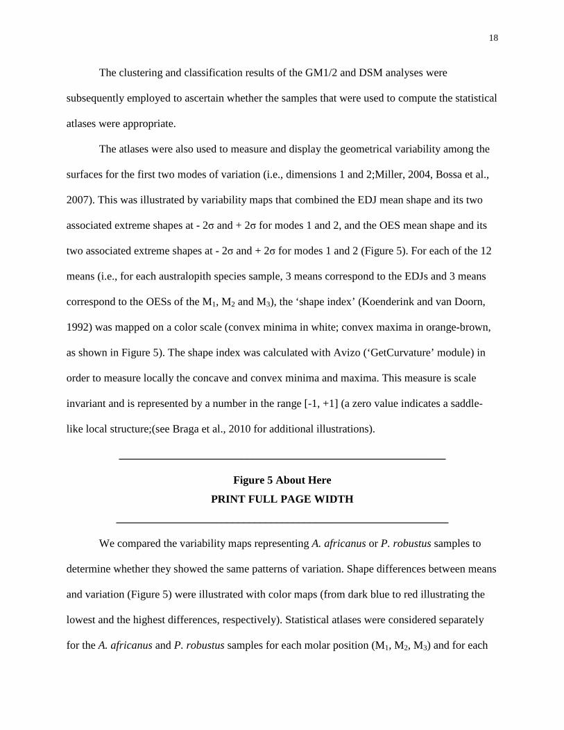
The atlases were also used to measure and display the geometrical variability among the

surfaces for the first two modes of variation (i.e., dimensions 1 and 2;Miller, 2004, Bossa et al.,

2007). This was illustrated by variability maps that combined the EDJ mean shape and its two

associated extreme shapes at - 2σ and + 2σ for modes 1 and 2, and the OES mean shape and its

two associated extreme shapes at - 2σ and + 2σ for modes 1 and 2 (Figure 5). For each of the 12

means (i.e., for each australopith species sample, 3 means correspond to the EDJs and 3 means

correspond to the OESs of the M1, M2 and M3), the ‘shape index’ (Koenderink and van Doorn,

1992) was mapped on a color scale (convex minima in white; convex maxima in orange-brown,

as shown in Figure 5). The shape index was calculated with Avizo (‘GetCurvature’ module) in

order to measure locally the concave and convex minima and maxima. This measure is scale

invariant and is represented by a number in the range [-1, +1] (a zero value indicates a saddle-

like local structure;(see Braga et al., 2010 for additional illustrations).

___________________________________________________________

Figure 5 About Here


____________________________________________________________

We compared the variability maps representing A. africanus or P. robustus samples to

determine whether they showed the same patterns of variation. Shape differences between means

and variation (Figure 5) were illustrated with color maps (from dark blue to red illustrating the

lowest and the highest differences, respectively). Statistical atlases were considered separately

for the A. africanus and P. robustus samples for each molar position (M1, M2, M3) and for each

19

surface (EDJ or OES) in order to better visualize (i) the most distinctive morphological features

between the two taxa (Figure 4), and (ii) the most variable areas within each (Figure 5).

4. Results

The degree to which the molars of A. africanus or P. robustus can be differentiated, and

the degree to which the Swartkrans Homo (SKX 257/258) and Sterkfontein cf. Homo (Stw 151)

specimens appear to differ from either are considered in relation to the performances of the 3D

GM and DSM methods.

4.1 3D GM (landmark-based) versus DSM (mesh-based) Approaches

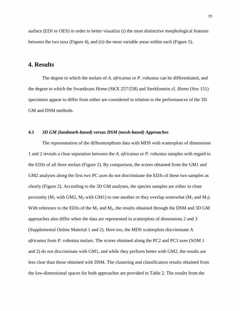
The representation of the diffeomorphism data with MDS with scatterplots of dimensions

1 and 2 reveals a clear separation between the A. africanus or P. robustus samples with regard to

the EDJs of all three molars (Figure 2). By comparison, the scores obtained from the GM1 and

GM2 analyses along the first two PC axes do not discriminate the EDJs of these two samples as

clearly (Figure 2). According to the 3D GM analyses, the species samples are either in close

proximity (M1 with GM2, M2 with GM1) to one another or they overlap somewhat (M1 and M3).

With reference to the EDJs of the M1 and M2, the results obtained through the DSM and 3D GM

approaches also differ when the data are represented in scatterplots of dimensions 2 and 3

(Supplemental Online Material 1 and 2). Here too, the MDS scatterplots discriminate A.

africanus from P. robustus molars. The scores obtained along the PC2 and PC3 axes (SOM 1

and 2) do not discriminate with GM1, and while they perform better with GM2, the results are

less clear than those obtained with DSM. The clustering and classification results obtained from

the low-dimensional spaces for both approaches are provided in Table 2. The results from the

20

low- and high-dimensional spaces are very similar for all methods, which indicates that PCA and

MDS capture the most discriminatory information of shape spaces in only 3 dimensions. Below,

we report the results obtained from the high-dimensional shape space, but similar conclusions are

achieved with the low-dimensional space results.

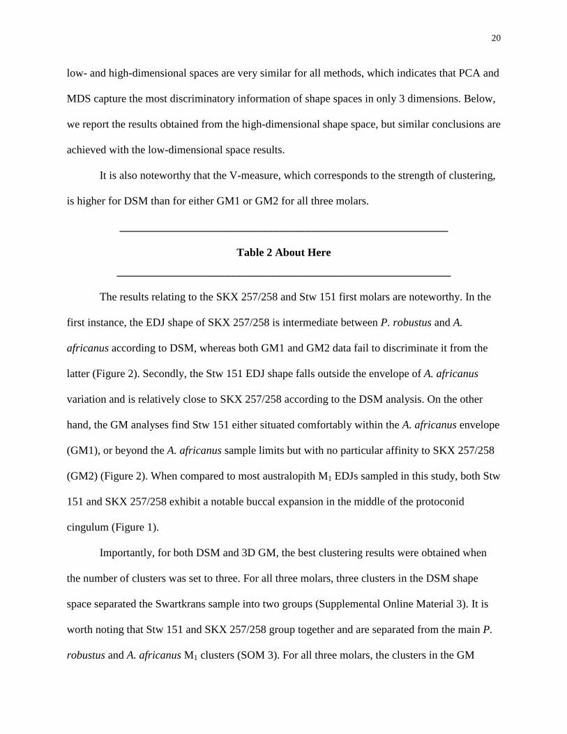
It is also noteworthy that the V-measure, which corresponds to the strength of clustering,

is higher for DSM than for either GM1 or GM2 for all three molars.

___________________________________________________________

Table 2 About Here

____________________________________________________________

The results relating to the SKX 257/258 and Stw 151 first molars are noteworthy. In the

first instance, the EDJ shape of SKX 257/258 is intermediate between P. robustus and A.

africanus according to DSM, whereas both GM1 and GM2 data fail to discriminate it from the

latter (Figure 2). Secondly, the Stw 151 EDJ shape falls outside the envelope of A. africanus

variation and is relatively close to SKX 257/258 according to the DSM analysis. On the other

hand, the GM analyses find Stw 151 either situated comfortably within the A. africanus envelope

(GM1), or beyond the A. africanus sample limits but with no particular affinity to SKX 257/258

(GM2) (Figure 2). When compared to most australopith M1 EDJs sampled in this study, both Stw

151 and SKX 257/258 exhibit a notable buccal expansion in the middle of the protoconid

cingulum (Figure 1).

Importantly, for both DSM and 3D GM, the best clustering results were obtained when

the number of clusters was set to three. For all three molars, three clusters in the DSM shape

space separated the Swartkrans sample into two groups (Supplemental Online Material 3). It is

worth noting that Stw 151 and SKX 257/258 group together and are separated from the main P.

robustus and A. africanus M1 clusters (SOM 3). For all three molars, the clusters in the GM

21

shape space were more heterogeneous (Table 2). The classification results also indicate a better

separation between A. africanus and P. robustus when using DSM compared to either GM1 or

GM2. In the GM2 analysis, the Stw 151 and SKX 257/258 M1s group together but, in contrast to

the DSM space, there is not a clear separation of the A. africanus and P. robustus samples. The

low-dimensional DSM space separated the specimens more accurately (Table 2). In this instance,

a relatively low accuracy for M1 EDJ classification was obtained using either GM (0.29 for GM1,

0.31 for GM2) or DSM (0.45) because Stw 151 and SKX 257/258 were considered to belong to

neither A. africanus nor P. robustus. When Stw 151 and SKX 257/258 are excluded from

comparison, accuracy increased for both methods (0.5 for GM1, 0.63 for GM2 and 0.88 for DSM

(Table 2).

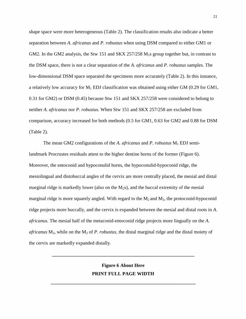
The mean GM2 configurations of the A. africanus and P. robustus M1 EDJ semi-

landmark Procrustes residuals attest to the higher dentine horns of the former (Figure 6).

Moreover, the entoconid and hypoconulid horns, the hypoconulid-hypoconid ridge, the

mesiolingual and distobuccal angles of the cervix are more centrally placed, the mesial and distal

marginal ridge is markedly lower (also on the M2s), and the buccal extremity of the mesial

marginal ridge is more squarely angled. With regard to the M2 and M3, the protoconid-hypoconid

ridge projects more buccally, and the cervix is expanded between the mesial and distal roots in A.

africanus. The mesial half of the metaconid-entoconid ridge projects more lingually on the A.

africanus M3, while on the M3 of P. robustus, the distal marginal ridge and the distal moiety of

the cervix are markedly expanded distally.

___________________________________________________________

Figure 6 About Here


____________________________________________________________

22

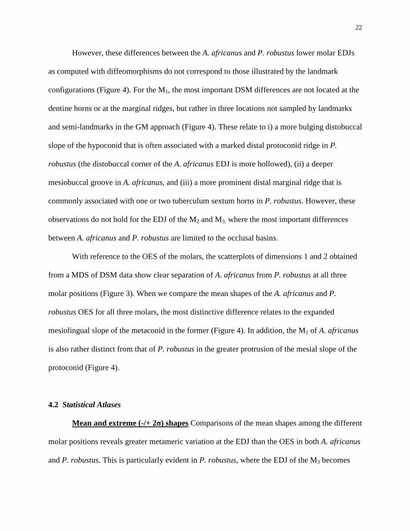
However, these differences between the A. africanus and P. robustus lower molar EDJs

as computed with diffeomorphisms do not correspond to those illustrated by the landmark

configurations (Figure 4). For the M1, the most important DSM differences are not located at the

dentine horns or at the marginal ridges, but rather in three locations not sampled by landmarks

and semi-landmarks in the GM approach (Figure 4). These relate to i) a more bulging distobuccal

slope of the hypoconid that is often associated with a marked distal protoconid ridge in P.

robustus (the distobuccal corner of the A. africanus EDJ is more hollowed), (ii) a deeper

mesiobuccal groove in A. africanus, and (iii) a more prominent distal marginal ridge that is

commonly associated with one or two tuberculum sextum horns in P. robustus. However, these

observations do not hold for the EDJ of the M2 and M3, where the most important differences

between A. africanus and P. robustus are limited to the occlusal basins.

With reference to the OES of the molars, the scatterplots of dimensions 1 and 2 obtained

from a MDS of DSM data show clear separation of A. africanus from P. robustus at all three

molar positions (Figure 3). When we compare the mean shapes of the A. africanus and P.

robustus OES for all three molars, the most distinctive difference relates to the expanded

mesiolingual slope of the metaconid in the former (Figure 4). In addition, the M1 of A. africanus

is also rather distinct from that of P. robustus in the greater protrusion of the mesial slope of the

protoconid (Figure 4).

4.2 Statistical Atlases

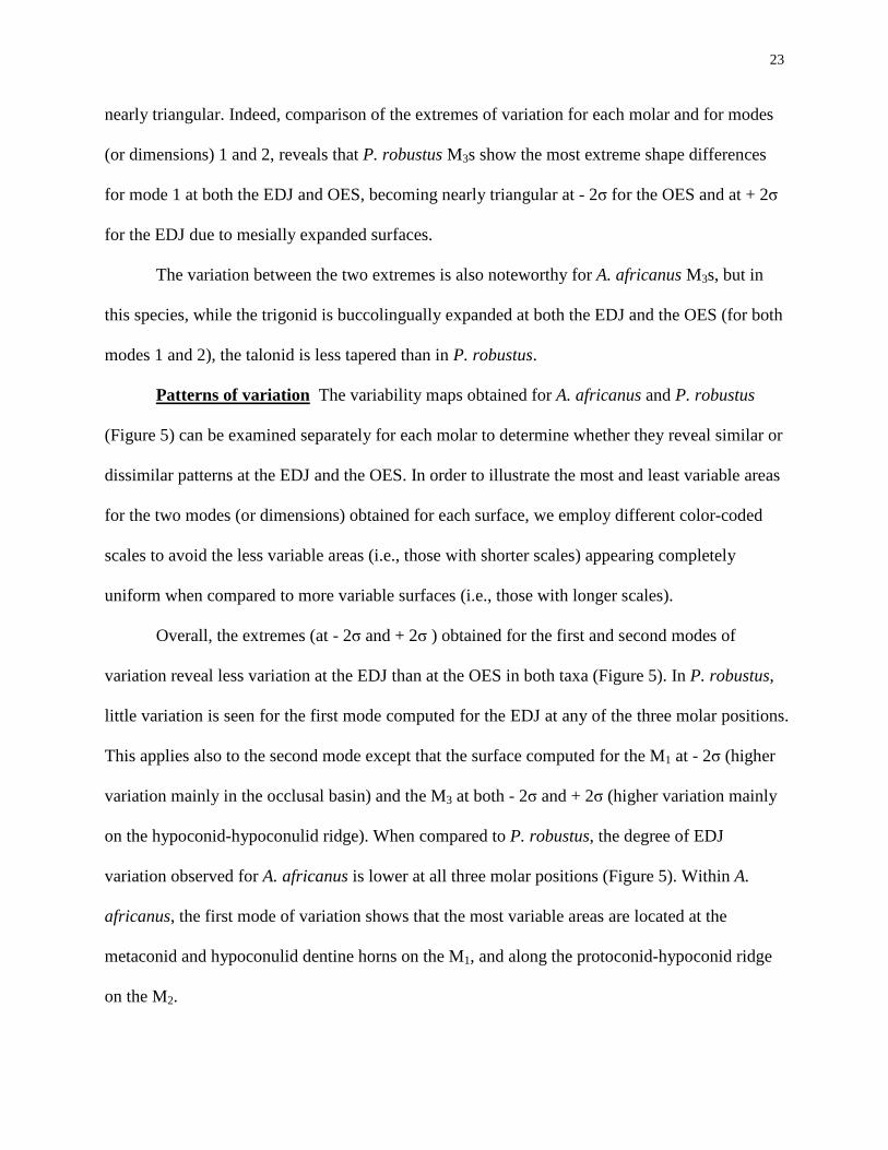
Mean and extreme (-/+ 2σ) shapes Comparisons of the mean shapes among the different

molar positions reveals greater metameric variation at the EDJ than the OES in both A. africanus

and P. robustus. This is particularly evident in P. robustus, where the EDJ of the M3 becomes

23

nearly triangular. Indeed, comparison of the extremes of variation for each molar and for modes

(or dimensions) 1 and 2, reveals that P. robustus M3s show the most extreme shape differences

for mode 1 at both the EDJ and OES, becoming nearly triangular at - 2σ for the OES and at + 2σ

for the EDJ due to mesially expanded surfaces.

The variation between the two extremes is also noteworthy for A. africanus M3s, but in

this species, while the trigonid is buccolingually expanded at both the EDJ and the OES (for both

modes 1 and 2), the talonid is less tapered than in P. robustus.

Patterns of variation The variability maps obtained for A. africanus and P. robustus

(Figure 5) can be examined separately for each molar to determine whether they reveal similar or

dissimilar patterns at the EDJ and the OES. In order to illustrate the most and least variable areas

for the two modes (or dimensions) obtained for each surface, we employ different color-coded

scales to avoid the less variable areas (i.e., those with shorter scales) appearing completely

uniform when compared to more variable surfaces (i.e., those with longer scales).

Overall, the extremes (at - 2σ and + 2σ ) obtained for the first and second modes of

variation reveal less variation at the EDJ than at the OES in both taxa (Figure 5). In P. robustus,

little variation is seen for the first mode computed for the EDJ at any of the three molar positions.

This applies also to the second mode except that the surface computed for the M1 at - 2σ (higher

variation mainly in the occlusal basin) and the M3 at both - 2σ and + 2σ (higher variation mainly

on the hypoconid-hypoconulid ridge). When compared to P. robustus, the degree of EDJ

variation observed for A. africanus is lower at all three molar positions (Figure 5). Within A.

africanus, the first mode of variation shows that the most variable areas are located at the

metaconid and hypoconulid dentine horns on the M1, and along the protoconid-hypoconid ridge

on the M2.

24

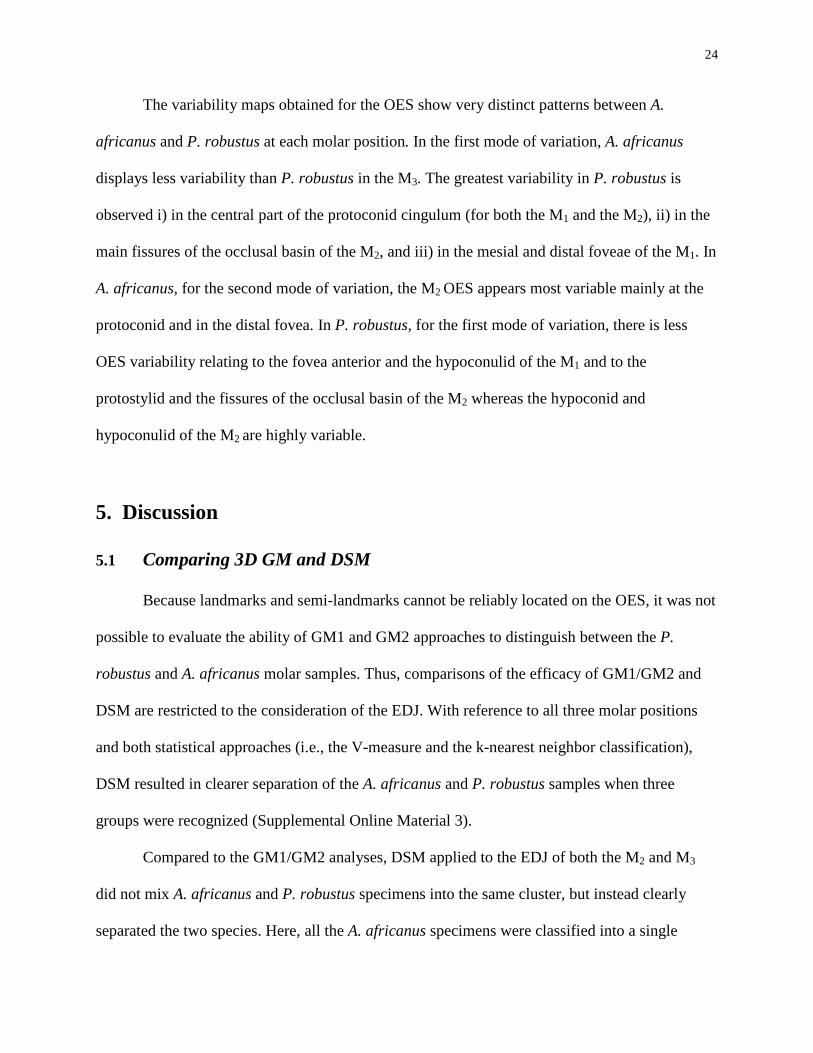
The variability maps obtained for the OES show very distinct patterns between A.

africanus and P. robustus at each molar position. In the first mode of variation, A. africanus

displays less variability than P. robustus in the M3. The greatest variability in P. robustus is

observed i) in the central part of the protoconid cingulum (for both the M1 and the M2), ii) in the

main fissures of the occlusal basin of the M2, and iii) in the mesial and distal foveae of the M1. In

A. africanus, for the second mode of variation, the M2 OES appears most variable mainly at the

protoconid and in the distal fovea. In P. robustus, for the first mode of variation, there is less

OES variability relating to the fovea anterior and the hypoconulid of the M1 and to the

protostylid and the fissures of the occlusal basin of the M2 whereas the hypoconid and

hypoconulid of the M2 are highly variable.

5. Discussion

5.1 Comparing 3D GM and DSM

Because landmarks and semi-landmarks cannot be reliably located on the OES, it was not

possible to evaluate the ability of GM1 and GM2 approaches to distinguish between the P.

robustus and A. africanus molar samples. Thus, comparisons of the efficacy of GM1/GM2 and

DSM are restricted to the consideration of the EDJ. With reference to all three molar positions

and both statistical approaches (i.e., the V-measure and the k-nearest neighbor classification),

DSM resulted in clearer separation of the A. africanus and P. robustus samples when three

groups were recognized (Supplemental Online Material 3).

Compared to the GM1/GM2 analyses, DSM applied to the EDJ of both the M2 and M3

did not mix A. africanus and P. robustus specimens into the same cluster, but instead clearly

separated the two species. Here, all the A. africanus specimens were classified into a single

25

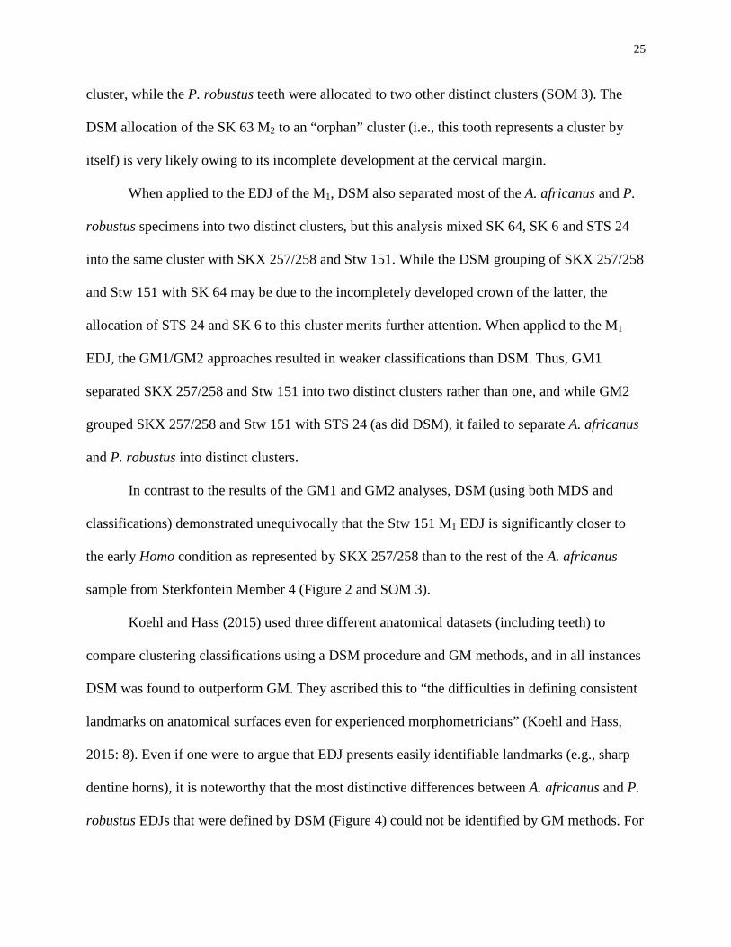
cluster, while the P. robustus teeth were allocated to two other distinct clusters (SOM 3). The

DSM allocation of the SK 63 M2 to an “orphan” cluster (i.e., this tooth represents a cluster by

itself) is very likely owing to its incomplete development at the cervical margin.

When applied to the EDJ of the M1, DSM also separated most of the A. africanus and P.

robustus specimens into two distinct clusters, but this analysis mixed SK 64, SK 6 and STS 24

into the same cluster with SKX 257/258 and Stw 151. While the DSM grouping of SKX 257/258

and Stw 151 with SK 64 may be due to the incompletely developed crown of the latter, the

allocation of STS 24 and SK 6 to this cluster merits further attention. When applied to the M1

EDJ, the GM1/GM2 approaches resulted in weaker classifications than DSM. Thus, GM1

separated SKX 257/258 and Stw 151 into two distinct clusters rather than one, and while GM2

grouped SKX 257/258 and Stw 151 with STS 24 (as did DSM), it failed to separate A. africanus

and P. robustus into distinct clusters.

In contrast to the results of the GM1 and GM2 analyses, DSM (using both MDS and

classifications) demonstrated unequivocally that the Stw 151 M1 EDJ is significantly closer to

the early Homo condition as represented by SKX 257/258 than to the rest of the A. africanus

sample from Sterkfontein Member 4 (Figure 2 and SOM 3).

Koehl and Hass (2015) used three different anatomical datasets (including teeth) to

compare clustering classifications using a DSM procedure and GM methods, and in all instances

DSM was found to outperform GM. They ascribed this to “the difficulties in defining consistent

landmarks on anatomical surfaces even for experienced morphometricians” (Koehl and Hass,

2015: 8). Even if one were to argue that EDJ presents easily identifiable landmarks (e.g., sharp

dentine horns), it is noteworthy that the most distinctive differences between A. africanus and P.

robustus EDJs that were defined by DSM (Figure 4) could not be identified by GM methods. For

26

example, the expansion of the distobuccal face of the in P. robustus M1s contributes significantly

to the high statistical accuracy of their distinction from A. africanus homologues. Another

important difference between GM and DSM lies in the latter’s visualization of morphological

variability within a sample, and the ability to compute statistical atlases using DSM. Importantly,

the MDS and the classifications obtained in this study confirmed the a priori taxonomic

attributions (Table 1).

5.2 Incorporating Categorical Features into 3D Shape Analyses

In addition to the degree to which the distobuccal surface of the hypoconid of the P.

robustus M1 EDJ is expanded, two other regions of this tooth are distinctive between A. africanus

and P. robustus, and both correspond to what have been described as “discrete” features. The

first relates to the greater prominence of the distal marginal ridge on the P. robustus M1, which

corresponds to the (variably-sized) tuberculum sextum that is manifest at the OES in much

higher frequencies in this species than in A. africanus (Wood and Abbott 1983; Irish and

Guatelli-Steinberg, 2003; Grine et al., 2012; Irish et al., 2013). The second relates to the

shallower mesiobuccal groove on the EDJ in P. robustus, and this corresponds to differences in

the expression of the protostylid between it and A. africanus at both OES and EDJ (Robinson,

1956; Sperber, 1974; Hlusko, 2004; Skinner et al., 2009).

Qualitative analyses of discrete dental features among early hominins have sometimes

resulted in different interpretations owing to differing definitions and scoring methods, and to

questions of homology. This study has demonstrated that DSM enables the 3D quantification of

such discrete, possibly non-homologous entities that provide teeth with their individuality. As

27

such, DSM may help to overcome the difficulties associated with the subjective scoring of

discrete features.

5.3 Future Perspectives

The differences between the A. africanus and the P. robustus samples described in this

study, together with the clear and separate clustering of Stw 151 with the SK 257/258 early

Homo M1 represent encouraging developments for the employment of DSM in taxonomic and

morphologic assessment. However, the samples that were employed here must be augmented

with other specimens that have been attributed to these taxa to more fully assess the potential of

DSM to address taxonomic issues. Thus, for example, the present study did not entail

investigation of possible differences among Sterkfontein and Makapansgat specimens with

reference to suggestions that they attest to the presence of more than one species of

Australopithecus (cf.., Clarke, 1988, 1994, 2008; Moggi-Cecchi 2003; Moggi-Cecchi and

Boccone 2007; Fornai et al., 2015; Grine, 2013; Grine et al. 2013). Similarly, this study did not

include the important fossils from the sites of Kromdraai, Drimolen and Gondolin that are

attributed to P. robustus, but for which there have been suggestions of some morphological

differences (e.g., Howell, 1978; Grine, 1985, 1988, 1993; Kaszycka, 2002; Braga et al., 2013,

2017).

The confirmation of the distinctiveness of Stw 151 from the A. africanus sample (Moggi-

Cecchi et al., 1998) and its attribution to Homo through the application of DSM techniques has

important implications for the analysis of other Early Pleistocene specimens that have been

purported to be members of our genus. In particular, DSM could be applied fruitfully to

28

questions relating to the attribution of fossils to Homo habilis and H. rudolfensis and to the

taxonomic relationships of the South African Homo specimens (Grine et al., 2019).

Finally, a more comprehensive DSM examination of the South African australopith

samples, together with the inclusion of additional fossils that have been attributed (or at least

likened) to early Homo from these and Pleistocene sites in South Africa may help clarify

questions that have been raised concerning the affinities of recently described forms such as

Australopithecus sediba (e.g., Berger et al., 2010; Wood and Harrison, 2011; Berger, 2013; Been

and Rak, 2014; Rak and Been, 2014; Ritzman et al., 2016; Kimbel and Rak, 2017) and Homo

naledi (Berger et al., 2015, 2017; Hawks et al., 2017; Neves et al., 2017; Schroeder et al., 2017).

Acknowledgements

This work was supported by the Erasmus Mundus “AESOP+” programme of the European

Union, the French Ministry of Foreign Affairs, the French Embassy in South Africa through the

Cultural and Cooperation Services, the Centre National de la Recherche Scientifique and the

HPC resources of the CALMIP supercomputing centre. FEG and FJR were additionally

supported by the College of Arts and Sciences, Stony Brook University. We thank Stephany

Potze, Ditsong Museum, Pretoria, and Bernhard Zipfel and the Fossil Access Committee of the

University of the Witwatersrand, Johannesburg, for access to specimens. We are also grateful to

Jakobus Hoffman and Jakata Kudakwashe for their help with scanning at the South African

Nuclear Energy Corporation, Pelindaba (NECSA) and the Palaeosciences Centre Microfocus X-

ray Computed Tomography (CT) Facility at the University of the Witwatersrand. We thank Mike

Plavcan, the associate editor and two anonymous reviewers for their helpful comments that

improved the manuscript.

29

References

Adams, D.C., Rohlf, F.J., Slice, D.E. 2004. Geometric morphometrics: ten years of progress

following the “revolution”. Italian Journal of Zoology 71, 5-16.

Adams, D.C., Rohlf, F.J., Slice, D.E., 2013. A field comes of age: geometric morphometrics in

the 21st Century. Hystrix 24, 7-14.

Beaudet, A., Dumoncel, J., Thackeray, J.F., Bruxelles, L., Duployer, B., Tenailleau, C., Bam, L.,

Hoffman, J., de Beer, F., Braga, J., 2016a. Upper third molar inner structural organization

and semicircular canal morphology in Plio-Pleistocene South-African cercopithecoids.

Journal of Human Evolution 95, 104-120.

Beaudet, A., Dumoncel, J., de Beer, F., Duployer, B., Durrleman, S., Gilissen, E., Hoffman, J.,

Tenailleau, C., Thackeray, J.F., Braga, J., 2016b. Morphoarchitectural variation in

South African fossil cercopithecoid endocasts. Journal of Human Evolution 101, 65-78.

Bookstein F.L., 1991. Morphometric tools for landmark data: Geometry and Biology. Cambridge

University Press, Cambridge.

Bossa, M., Hernandez. M., Olmos, S. 2007. Contributions to 3D diffeomorphic atlas estimation:

application to brain images. Medical Image Computing and Computer-Assisted

Intervention. MICCAI. Volume 4791 of the Series Lecture Notes in Computer Science,

pp. 667-674.

Boyer, D.M., Lipman, Y., St Clair, E., Puente, J., Patel, B.A., Funkhouser, T., Jernvall, J.,

Daubechies, I., 2011 Algorithms to automatically quantify the geometric similarity of

anatomical surface. Proceedings of the National Academy of Sciences of the United

States of America 108, 18221-18226.

30

Braga, J., Thackeray, J.F., Subsol, G., Kahn, J.-L., Maret, D., Treil, J., Beck, A., 2010. The

enamel–dentine junction in the postcanine dentition of Australopithecus africanus:

intra-individual metameric and antimeric variation. Journal of Anatomy 216, 62-79.

Braga, J., Thackeray, J.F., Dumoncel, J., Descouens, D., Bruxelles, L., Loubes, J.-M., Kahn,

J.L., Stampanoni, M., Bam, L., Hoffman, J., de Beer, F., Spoor, F., 2013. A new partial

temporal bone of a juvenile hominin from the site of Kromdraai B (South Africa). Journal

of Human Evolution 65, 447-456.

Braga, J., Dumoncel, J., Duployer, B., Tenailleau, C., de Beer, F., Thackeray, J.F., 2016. The

Kromdraai hominins revisited with an updated portrayal of differences between

Australopithecus africanus and Paranthropus robustus. In: Braga, J., Thackeray, J.F.

(Eds.), Kromdraai, a Birthplace of Paranthropus in the Cradle of Humankind.

Johannesburg, Sun Media Metro, pp. 49-68.

Braga, J., Thackeray, J.F., Bruxelles, L., Dumoncel, J., Fourvel, J.-B., 2017. Stretching the time

span of hominin evolution at Kromdraai (Gauteng, South Africa): recent discoveries.

Comptes Rendus Palevol 16, 58-70.

Bromage, T.G., Schrenk, F., Zonneveld, F.W., 1995. Paleoanthropology of the Malawi Rift: an

early hominid mandible from the Chiwondo Beds, northern Malawi. Journal of Human

Evolution 28, 71-108.

Bronstein, A.M., Bronstein, M.M., Kimmel, R., 2006. Generalized multidimensional scaling: a

framework for isometry-invariant partial surface matching. Proceedings of the National

Academy of Sciences of the USA 103, 1168–1172.

Broom, R., 1949. Another new type of fossil ape-man. Nature 163, 57.

31

Chen, M., 1999. 3-D deformable registration using a statistical atlas with applications in

medicine. PhD Dissertation, Carnegie Mellon University.

Chen, M., Kanade, T., Pomerleau, D., Schneider, J., 1999. 3-D deformable registration of

medical images using a statistical atlas. In: Taylor, C., Colchester A. (Eds), Medical

Image Computing and Computer-Assisted Intervention - MICCAI 1999. Springer,

Berlin, pp. 621-630.

Clarke, R.J., 1988. A new Australopithecus cranium from Sterkfontein and its bearing on the

ancestry of Paranthropus. In: Grine, F.E. (Ed.), Evolutionary History of the "Robust"

Australopithecines. New York: Aldine de Gruyter, pp. 285-292.

Clarke, R.J., 1994. Advances in understanding the craniofacial anatomy of South African

early hominids. In: Corruccini, R.S., Ciochon, R.L. (Eds), Integrative Paths to the Past.

Paleoanthropological Advances in Honor of F. Clark Howell. Englewood Cliffs, NJ:

Prentice Hall, pp. 205-222.

Clarke, R.J., 2008. Latest information on Sterkfontein’s Australopithecus skeleton and a new

look at Australopithecus. South African Journal of Science 104, 443-449.

Clarke, R.J., 2013. Australopithecus from Sterkfontein caves, South Africa. In: Reed, K.E.,

Fleagle, J.G., Leakey, R.E. (Eds), The Paleobiology of Australopithecus. Springer,

New York, pp. 105-123.

Coppens, Y., 1980. The differences between Australopithecus and Homo: preliminary

conclusions from the Omo Research Expedition’s studies. In: Königsson, L.K. (Ed.),

Current Argument on Early Man, pp. 207-225. Oxford: Pergamon.

Cox, T.F., Cox, M.A.A. 2001. Multidimensional Scaling. Boca Raton, Chapman and Hall/CRC

Monographs on Statistics & Applied Probability.

32

Däuber, S., Krempien, R., Krätz, M., Welzel, T., Wörn, H., 2002. Creating a statistical atlas of

the cranium. Studies in Health Technology and Informatics 85, 116-120.

Davatzikos, C., Verma, R., 2010. Statistical Atlases. In: Bryan, N. (Ed.), Introduction to the

Science of Medical Imaging. Cambridge University Press, Cambridge, pp. 240-249.

Dean, M.C., Liversidge, H.M., 2015. Age estimation in fossil hominins: comparing dental

development in early Homo with modern humans. Annals of Human Biology 42, 415-429.

Dean, M.C., 2016. Measures of maturation in early fossil hominins: events at the first

transition from australopiths to early Homo. Philosophical Transactions of the Royal

Society B, Biolological Sciences 371, 20150234.

Durrleman, S., 2010. Statistical models of currents for measuring the variability of anatomical

curves, surfaces and their evolution. Thesis, University of Nice - Sophia Antipolis.

Durrleman, S., Pennec, X., Trouvé, A., Ayache, N., Braga, J., 2012. Comparison of the

endocranial ontogenies between chimpanzees and bonobos via temporal regression

and spatiotemporal registration. Journal of Human Evolution 62, 74-88.

Durrleman, S., Prastawa, M., Charon, N., Korenberg, J.R., Joshi, S., Gerig, G., Trouvé, A., 2014.

Morphometry of anatomical shape complexes with dense deformations and sparse

parameters. NeuroImage 101, 35-49.

Fonseca, C.G., Backhaus, M., Bluemke, D.A., Britten, R.D., Chung, J.D., Cowan, B.R., Dinov,

I.D., Finn, J.P., Hunter, P.J., Kadish, A.H., 2011. The Cardiac Atlas Project - an imaging

database for computational modeling and statistical atlases of the heart. Bioinformatics 27,

2288-2295.

Fornai, C., Bookstein, F.L., Weber, G.W., 2015. Variability of Australopithecus second

maxillary molars from Sterkfontein Member 4. Journal of Human Evolution 85, 181-192.

33

Gao, T.R., Yapuncich, G.S., Daubechies, I., Mukherjee, S., Boyer, D.M., 2018. Development

and assessment of fully automated and globally transitive geometric morphometric

methods, with application to a biological comparative dataset with high interspecific

variation. Anatomical Record 301, 636-658.

Gómez-Robles, A., Martinón-Torres, M., Bermúdez de Castro, J.M., Margvelashvili, A., Bastir,

M., Arsuaga, J.L., Pérez-Pérez, A., Estebaranz, F., Martínez, L.M., 2007. A geometric

morphometric analysis of hominin upper first molar shape. Journal of Human Evolution

53, 272-285.

Gómez-Robles, A., Martinón -Torres, M., Bermúdez de Castro, J.M., Prado, S., Sarmiento, S.,

Arsuaga, J.L., 2008. Geometric morphometric analysis of the crown morphology of the

lower first premolar of hominins, with special attention to Pleistocene Homo. Journal of

Human Evolution 55, 627-638.

Gómez‐Robles, A., Bermúdez de Castro, J.M., Martinón‐Torres, M., Prado‐Simón, L., Arsuaga,

J.L., 2015. A geometric morphometric analysis of hominin lower molars: evolutionary

implications and overview of postcanine dental variation. Journal of Human Evolution 82,

34-50.

Grine, F.E., 1985. Australopithecine evolution: the deciduous dental evidence. In: Delson, E.

(Ed), Ancestors: the Hard Evidence. New York, Alan R. Liss, pp. 153-167.

Grine, F.E., 1988. New craniodental fossils of Paranthropus from the Swartkrans formation and

their significance in ‘robust’ australopithecine evolution. In: Grine, F.E. (Ed),

Evolutionary History of the ‘Robust’ Australopithecines. New York, Aldine de Gruyter,

pp. 223-243.

34

Grine, F.E., 1989. New hominid fossils from the Swartkrans Formation (1979-1986

excavations): craniodental specimens. American Journal of Physical Anthropology 79,

409-449.

Grine, F.E., 1993. Description and preliminary analysis of new hominid craniodental fossils

from the Swartkrans Formation. In: Brain, C.K. (Ed), Swartkrans. A Cave’s Chronicle

of Early Man. Pretoria, Transvaal Museum, pp. 75-116.

Grine, F.E., 2013. The alpha taxonomy of Australopithecus africanus. In: Reed, K.E., Fleagle,

J.G., Leakey, R.E., (Eds), The Paleobiology of Australopithecus. Dordrecht: Springer,

pp. 73-104.

Grine, F.E., Daegling, D.J., 1993. New mandible of Paranthropus robustus from Member 1,

Swartkrans Formation, South Africa. Journal of Human Evolution 24, 319-333.

Grine, F.E., Smith, H.F., Heesy, C.P., Smith, E.J., 2009. Phenetic affinities of Plio-Pleistocene

Homo fossils from South Africa: molar cusp proportions. In: Grine, F.E., Fleagle, J.G.,

Leakey, R.E. (Eds), The First Humans. Origin and Early Evolution of the Genus Homo.

Springer, New York, pp. 49-62.

Grine, F.E., Jacobs, R.L., Reed, K.E., Plavcan, J.M., 2012. The enigmatic molar from Gondolin,

South Africa: implications for Paranthropus paleobiology. Journal of Human Evolution

63, 597-609.

Grine, F.E., Delanty, M.M., Wood, B.A., 2013. Variation in mandibular postcanine dental

morphology and hominin species representation in Member 4, Sterkfontein, South Africa.

In: Reed, K.E., Fleagle, J.G., Leakey, R.E. (Eds), The Paleobiology of Australopithecus.

Springer, New York, pp. 125-146.

35

Grine, F.E., Leakey, M.G., Gathago, P.N., Brown, F.H., Mongle, C.S., Yang, D., Jungers, W.L.,

Leakey, L.N., 2019. Complete permanent mandibular dentition of early Homo from the

upper Burgi Member of the Koobi Fora Formation, Ileret, Kenya. Journal of Human

Evolution (IN PRESS).

Gunz, P., Mitteroecker, P., 2013. Semilandmarks: a method for quantifying curves and surfaces.

Hystrix 24, 103-109.

Haile-Selassie, Y., Suwa, G., White, T.D., 2004. Late Miocene teeth from Middle Awash,

Ethiopia, and early hominid dental evolution. Science 303, 1503-1505.

Haile-Selassie, Y., Saylor, B.Z., Deino, A., Alene, M., Latimer, B.M., 2010. New hominid

fossils from Woranso-Mille (Central Afar, Ethiopia) and taxonomy of early

Australopithecus. American Journal of Physical Anthropology 141, 406-417.

Hlusko, L.J., 2004. Protostylid variation in Australopithecus. Journal of Human Evolution 46,

579-594.

Howell, F.C., 1978. Hominidae. In: Maglio, V.J., Cooke, H.B.S. (Eds.), Evolution of African

Mammals. Cambridge, Harvard University Press, pp. 154-248.

Irish, J.D., Guatelli-Steinberg, D., 2003. Ancient teeth and modern human origins: an expanded

comparison of African Plio-Pleistocene and recent world dental samples. Journal of

Human Evolution 45, 113-144.

Irish, J.D., Guatelli-Steinberg, D., Legge, S.S., de Ruiter, D.J., Berger, L.R., 2013. Dental

morphology and the phylogenetic “place” of Australopithecus sediba. Science 340,

1233062-1-4.

Jardine, N., Jardine, C.J. (1967). Numerical homology. Nature 216, 301-302.

36

Kaifu, Y., Kono, R.T., Sutikna, T., Saptomo, E.W., Jatmiko, D.A.R, 2015. Unique dental

morphology of Homo floresiensis and its evolutionary implications. PLoS ONE 10(11):

e0141614.

Kaszycka, K.A., 2002. Status of Kromdraai: Cranial, Mandibular and Dental Morphology,

Systematic Relationships, and Significance of the Kromdraai Hominids. Editions du

Cahiers de Paléoanthropologie, CNRS, Paris.

Koehl, P., Hass, J., 2015. Landmark-free geometric methods in biological shape analysis.

Journal of the Royal Society Interface 12, 20150795.

Koenderink, J.J., van Doorn, A.J., 1992. Surface perception in pictures. Perceptions and

Psychophysics 52, 487-296.

MacLeod, N., Benfield, M., Culverhouse, P., 2010. Time to automate identification. Nature 467,

154-155.

Marquez, E.J., Cabeen, R., Woods, R.P., Houle, D., 2012. The measurement of local variation in

shape. Evolutionary Biology 39, 419–439.

Martinón-Torres, M., Bastir, M., Bermúdez de Castro, J.M., Gómez, A., Sarmiento, S., Muela,

A., Arsuaga, J.L., 2006. Hominin lower second premolar morphology: evolutionary

inferences through geometric morphometric analysis. Journal of Human Evolution 50,

523-533.

Martinón-Torres, M., Bermúdez de Castro, J., Gómez-Robles, A., Margvelashvili, A., Prado, L.,

Lordkipanidze, D., Vekua, A., 2008. Dental remains from Dmanisi (Republic of

Georgia): morphological analysis and comparative study. Journal of Human Evolution 55,

249-273.

37

Martinón-Torres, M., de Castro, J.M.B., Gómez-Robles, A., Prado-Simon, L., Arsuaga, J.L.,

2012. Morphological description and comparison of the dental remains from

Atapuerca-Sima de los Huesos site (Spain). Journal of Human Evolution 62, 7-58.

Miller, M, 2004. Computational anatomy: shape, growth, and atrophy comparison via

diffeomorphisms. NeuroImage 23, S19-S33.

Mitteroecker P., Gunz P., 2009. Advances in geometric morphometrics. Evolutionary Biology

36, 235-247.

Moggi-Cecchi, J., Boccone, S. 2007. Maxillary molars cusp morphology of South African

australopithecines. In: Bailey, S.E., Hublin, J.J. (Eds), Dental Perspectives on Human

Evolution: State-of-the-Art Research in Dental Paleoanthropology. Dordrecht: Springer,

pp. 53-64.

Moggi-Cecchi, J., Tobias, P.V., Beynon, A.D., 1998. The mixed dentition and associated skull

fragments of a juvenile fossil hominid from Sterkfontein, South Africa. American Journal

of Physical Anthropology 106, 425-465.

Moggi-Cecchi, J., Grine, F.E., Tobias, P.V., 2006. Early hominid dental remains from Members

4 and 5 of the Sterkfontein Formation (1966-1996 excavations): catalogue, individual

associations, morphological descriptions and initial metrical analysis. Journal of Human


Moggi-Cecchi, J., Menter, C.G., Boccone, S., Keyser, A.W., 2010. Early hominin dental remains

from the Plio-Pleistocene site of Drimolen, South Africa. Journal of Human Evolution 58,

374-405.

O’Higgins P., 2000. The study of morphological variation in the hominid fossil record: biology,

landmarks and geometry. Journal of Anatomy 197, 103-120.

38

Pan, L., Dumoncel, J., de Beer, F., Hoffman, J., Thackeray, J.F., Duployer, B., Tenailleau, C.,

Braga, J., 2016. Further morphological evidence on South African earliest Homo lower

postcanine dentition: enamel thickness and enamel dentine junction. Journal of Human


Prat, S., Brugal, J.P., Tiercelin, J.J., Barrat, J.A., Bohn, M., Delagnes, A., Harmand, S., Kimeu,

K., Kibunjia, M., Texier, P.J., Roche, H., 2005. First occurrence of early Homo in the

Nachukui Formation (West Turkana, Kenya) at 2.3 - 2.4 Myr. Journal of Human


Qiu, A., Younes, L., Wang, L., Ratnanather, J.T., Gillepsie, S.K., Kaplan, G., Csernansky, J.,

Miller, M., 2007. Combining anatomical manifold information via diffeomorphic metric

mappings for studying cortical thinning of the cingulate gyrus in schizophrenia.

Neuroimage, 37, 821-833.

Quam, R.M., de Ruiter, D.J., Masali, M., Arsuaga, J.-L., Martínez, I., Moggi-Cecchi, J., 2013.

Early hominin auditory ossicles from South Africa. Proceedings of the National Academy

of Sciences of the United States of America 110, 8847-8851.

Robinson J.T., 1956. The Dentition of the Australopithecinae. Transvaal Museum Memoir 9.

Transvaal Museum, Pretoria.

Rohlf F.J., 1992. The analysis of shape variation using ordinations of fitted functions. In:

Sorensen J.T. (Ed.). Ordinations in the Study of Morphology, Evolution and Systematics

of Insects: Applications and Quantitative Genetic Rationales. Elsevier, Amsterdam,

pp. 95-122.

Rohlf, F.J., Archie, J.W., 1984. A comparison of Fourier methods for the description of wing

shape in mosquitoes (Diptera: Culicidae). Systematic Zoology 33, 302-317.

39

Rohlf, F.J., Marcus, L.F., 1993. A revolution in morphometrics. Trends in Ecology and


Rosenberg, A., Hirschberg, J., 2007. V-Measure: a conditional entropy-based external cluster

evaluation measure. Proceedings of Joint Conference on Empirical Methods in Natural

Language Processing and Computational Natural Language Learning. pp. 410–420.

Schwartz, J.H., Tattersall I., 2003. The Human Fossil Record. Vol. 2. Craniodental

Morphology of Genus Homo (Africa and Asia). Wiley-Liss, NewYork, pp. 409–449.

Shen, D., Davatzikos, C., 2002. HAMMER: hierarchical attribute matching mechanism for

elastic registration. IEEE Transactions on Medical Imaging 21, 1421-1439.

Skinner, M.M, Gunz, P., Wood, B.A., Hublin, J.J., 2008a. Enamel-dentine junction (EDJ)

morphology distinguishes the lower molars of Australopithecus africanus and

Paranthropus robustus. Journal of Human Evolution 55, 979-988.

Skinner, M.M., Wood, B., Boesch, C., Olejniczak, A.J., Rosas. A., Smith, T.M., Hublin, J.J.,

2008b. Dental trait expression at the enamel-dentine junction of lower molars in extant

and fossil hominoids. Journal of Human Evolution 54, 173-186.

Skinner, M.M., Gunz, P., Wood, B., Boesch, C., Hublin, J.J., 2009a. Discrimination of extant

Pan species and subspecies using the enamel-dentine junction morphology of lower

molars. American Journal of Physical Anthropology 140, 234-243.

Skinner, M.M., Gunz, P., Wood, B.A., Hublin, J.J., 2009b. How many landmarks? Assessing

the classification accuracy of Pan lower molars using a geometric morphometric

analysis of the occlusal basin as seen at the enamel-dentine junction. Frontiers of Oral

Biology 13, 23-29.

40

Skinner, M.M., Wood, B.A., Hublin, J.J., 2009c. Protostylid expression at the enamel-dentine

junction and enamel surface of mandibular molars of Paranthropus robustus and

Australopithecus africanus. Journal of Human Evolution 56, 76-85.

Slice D.E., 2005. Modern morphometrics. In: Slice D.E. (Ed.). Modern Morphometrics in

Physical Anthropology. Klewer Press, New York, pp. 1–45.

Slice D.E., 2007. Geometric morphometrics. Annual Review of Anthropology 36, 261–281.

Sperber, G.H., 1974. Morphology of the cheek teeth of early South African hominids. Ph.D.

Dissertation, University of the Witwatersrand.

Suwa, G., 1988. Evolution of the “robust” australopithecines in the Omo succession: evidence

from mandibular premolar morphology. In: Grine, F.E. (Ed), Evolutionary History of the

‘Robust’ Australopithecines. New York, Aldine de Gruyter, pp. 199-222.

Suwa, G., 1996. Serial allocations of isolated mandibular molars of unknown taxonomic

affinities from the Shungura and Usno formations, Ethiopia, a combined method

approach. Human Evolution 11, 269–282.

Suwa, G., White, T.D., Howell, F.C., 1996. Mandibular postcanine dentition from the Shungura

Formation, Ethiopia: crown morphology, taxonomic allocations, and Plio-Pleistocene

hominid evolution. American Journal of Physical Anthropology 101, 247–282.

Turner, C.G., Nichol, C.R., Scott, G.R., 1991. Scoring procedures for key morphological traits

of the permanent dentition: the Arizona State University dental anthropology system. In:

Kelley, M.A., Larsen, C.S. (Eds), Advances in Dental Anthropology. New York: Wiley-

Liss, pp. 13–32.

Vaillant, M., Glaunès, J., 2005. Surface matching via currents. Information Processing in

Medical Imaging 3565, 381-392.

41

Vaillant, M., Qiu, A., Glaunès, J., Miller, M.I., 2007. Diffeomorphic metric surface mapping

in superior temporal gyrus. Neuroimage 34, 1149-1159.

Villmoare, B., Kimbel, W.H., Seyoum, C., Campisano, C.J., DiMaggio, E.N., Rowan, J., Braun,

D.R., Arrowsmith, J.R., Reed, K.E., 2015. Early Homo at 2.8 Ma from Ledi-Geraru, Afar,

Ethiopia. Science 347, 1352-1355.

von Cramon-Taubadel, N., Frazier, B.C., Lahr, M.M., 2007. The problem of assessing landmark

error in geometric morphometrics: theory, methods, and modifications. American Journal

of Physical Anthropology 134, 24-35

Walker, J.A., 2000. Ability of geometric morphometric methods to estimate a known

covariance matrix. Systematic Biology 49, 686-696.

Wood, B.A., Abbott, S.A., 1983. Analysis of the dental morphology of Plio-Pleistocene

hominids. I. Mandibular molars: crown area measurements and morphological traits.

Journal of Anatomy 136, 197-219.

Wood, B.A., Engleman, C.A., 1988. Analysis of the dental morphology of Plio-Pleistocene

hominids. V. Maxillary postcanine tooth morphology. Journal of Anatomy 161, 1-35.

Wood, B.A., Uytterschaut, H.T., 1987. Analysis of the dental morphology of Plio-Pleistocene

hominids. III. Mandibular premolar crowns. Journal of Anatomy 154, 121-156.

Wood, B.A., Abbott, S.A., Graham, S.H., 1983. Analysis of the dental morphology of Plio-

Pleistocene hominids. II. Mandibular molars-study of cusp areas, fissure pattern and

cross sectional shape of the crown. Journal of Anatomy 137, 287-314.

Wu, C., Murtha, P.E., Jaramaz, B. 2009. Femur statistical atlas construction based on two-level

3D non-rigid registration. Computer Aided Surgery 14, 83-99.

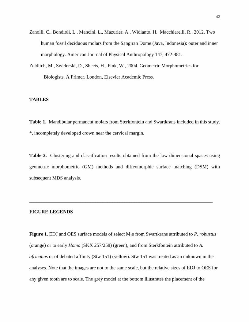
42

Zanolli, C., Bondioli, L., Mancini, L., Mazurier, A., Widianto, H., Macchiarelli, R., 2012. Two

human fossil deciduous molars from the Sangiran Dome (Java, Indonesia): outer and inner

morphology. American Journal of Physical Anthropology 147, 472-481.

Zelditch, M., Swiderski, D., Sheets, H., Fink, W., 2004. Geometric Morphometrics for

Biologists. A Primer. London, Elsevier Academic Press.

TABLES

Table 1. Mandibular permanent molars from Sterkfontein and Swartkrans included in this study.

*, incompletely developed crown near the cervical margin.

Table 2. Clustering and classification results obtained from the low-dimensional spaces using

geometric morphometric (GM) methods and diffeomorphic surface matching (DSM) with

subsequent MDS analysis.

___________________________________________________________________________

FIGURE LEGENDS

Figure 1. EDJ and OES surface models of select M1s from Swartkrans attributed to P. robustus

(orange) or to early Homo (SKX 257/258) (green), and from Sterkfontein attributed to A.

africanus or of debated affinity (Stw 151) (yellow). Stw 151 was treated as an unknown in the

analyses. Note that the images are not to the same scale, but the relative sizes of EDJ to OES for

any given tooth are to scale. The grey model at the bottom illustrates the placement of the

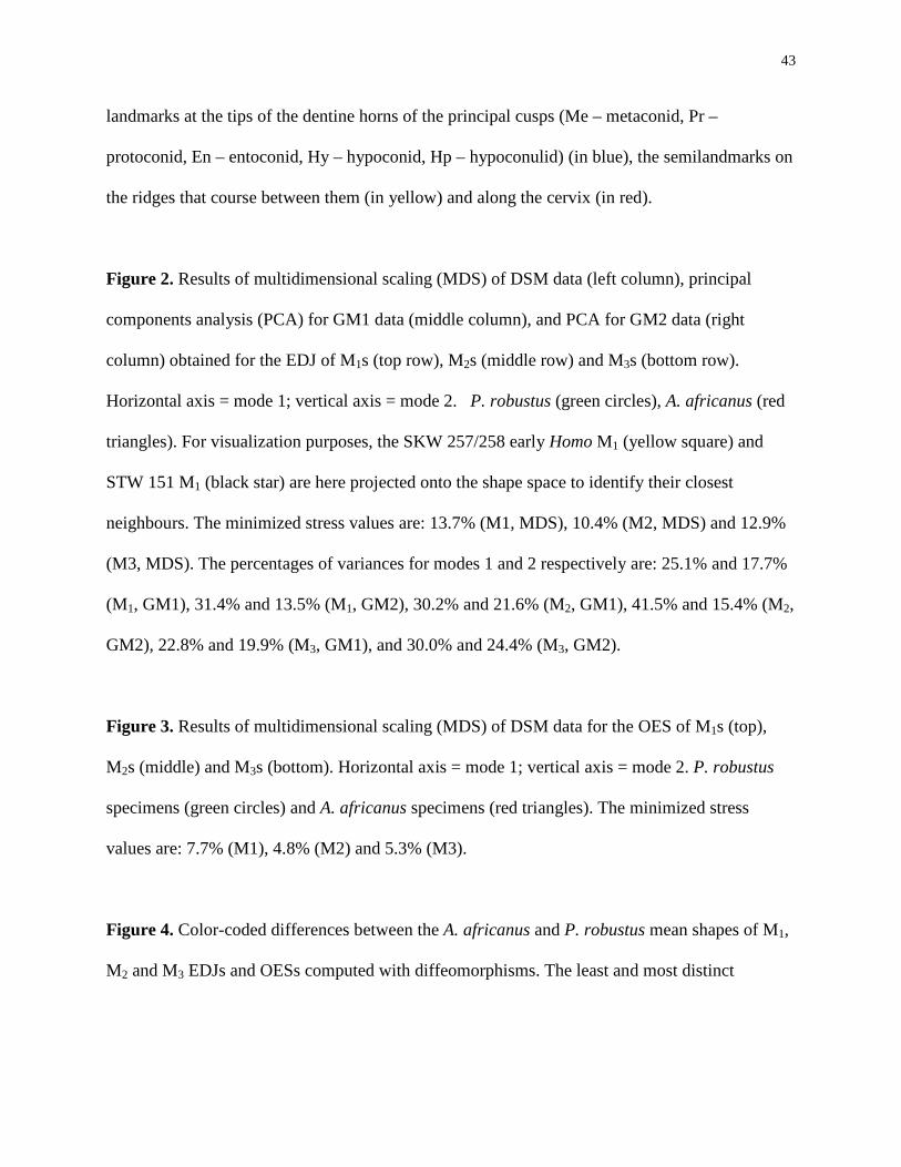
43

landmarks at the tips of the dentine horns of the principal cusps (Me – metaconid, Pr –

protoconid, En – entoconid, Hy – hypoconid, Hp – hypoconulid) (in blue), the semilandmarks on

the ridges that course between them (in yellow) and along the cervix (in red).

Figure 2. Results of multidimensional scaling (MDS) of DSM data (left column), principal

components analysis (PCA) for GM1 data (middle column), and PCA for GM2 data (right

column) obtained for the EDJ of M1s (top row), M2s (middle row) and M3s (bottom row).

Horizontal axis = mode 1; vertical axis = mode 2. P. robustus (green circles), A. africanus (red

triangles). For visualization purposes, the SKW 257/258 early Homo M1 (yellow square) and

STW 151 M1 (black star) are here projected onto the shape space to identify their closest

neighbours. The minimized stress values are: 13.7% (M1, MDS), 10.4% (M2, MDS) and 12.9%

(M3, MDS). The percentages of variances for modes 1 and 2 respectively are: 25.1% and 17.7%

(M1, GM1), 31.4% and 13.5% (M1, GM2), 30.2% and 21.6% (M2, GM1), 41.5% and 15.4% (M2,

GM2), 22.8% and 19.9% (M3, GM1), and 30.0% and 24.4% (M3, GM2).

Figure 3. Results of multidimensional scaling (MDS) of DSM data for the OES of M1s (top),

M2s (middle) and M3s (bottom). Horizontal axis = mode 1; vertical axis = mode 2. P. robustus

specimens (green circles) and A. africanus specimens (red triangles). The minimized stress

values are: 7.7% (M1), 4.8% (M2) and 5.3% (M3).

Figure 4. Color-coded differences between the A. africanus and P. robustus mean shapes of M1,

M2 and M3 EDJs and OESs computed with diffeomorphisms. The least and most distinct

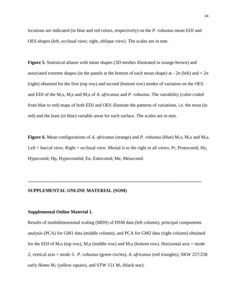
44

locations are indicated (in blue and red colors, respectively) on the P. robustus mean EDJ and

OES shapes (left, occlusal view; right, oblique view). The scales are in mm.

Figure 5. Statistical atlases with mean shapes (3D meshes illustrated in orange-brown) and

associated extreme shapes (in the panels at the bottom of each mean shape) at - 2σ (left) and + 2σ

(right) obtained for the first (top row) and second (bottom row) modes of variation on the OES

and EDJ of the M1s, M2s and M3s of A. africanus and P. robustus. The variability (color-coded

from blue to red) maps of both EDJ and OES illustrate the patterns of variations, i.e. the most (in

red) and the least (in blue) variable areas for each surface. The scales are in mm.

Figure 6. Mean configurations of A. africanus (orange) and P. robustus (blue) M1s, M2s and M3s.

Left = buccal view; Right = occlusal view. Mesial is to the right in all views. Pr, Protoconid; Hy,

Hypoconid; Hp, Hypoconulid; En, Entoconid; Me, Metaconid.

___________________________________________________________________________

SUPPLEMENTAL ONLINE MATERIAL (SOM)

Supplemental Online Material 1.

Results of multidimensional scaling (MDS) of DSM data (left column), principal components

analysis (PCA) for GM1 data (middle column), and PCA for GM2 data (right column) obtained

for the EDJ of M1s (top row), M2s (middle row) and M3s (bottom row). Horizontal axis = mode

2; vertical axis = mode 3. P. robustus (green circles), A. africanus (red triangles), SKW 257/258

early Homo M1 (yellow square), and STW 151 M1 (black star).

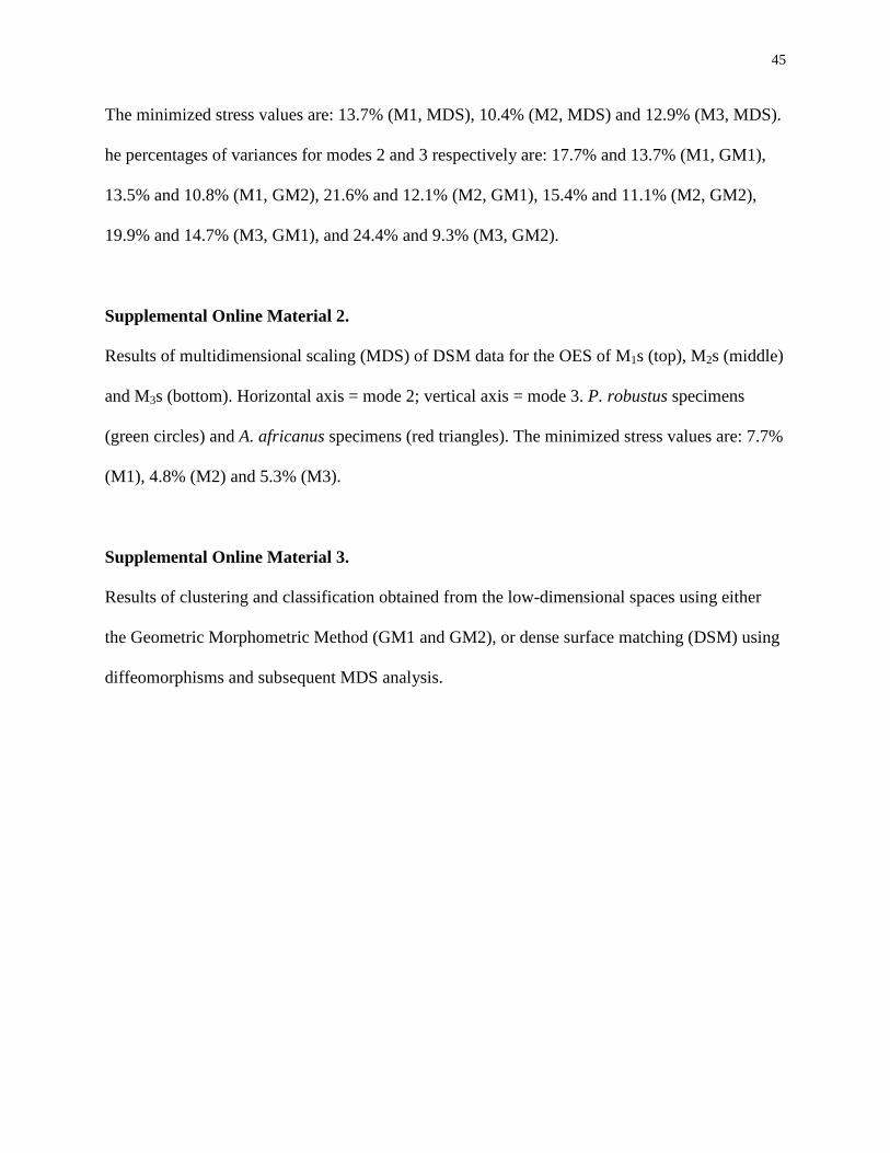
45

The minimized stress values are: 13.7% (M1, MDS), 10.4% (M2, MDS) and 12.9% (M3, MDS).

he percentages of variances for modes 2 and 3 respectively are: 17.7% and 13.7% (M1, GM1),

13.5% and 10.8% (M1, GM2), 21.6% and 12.1% (M2, GM1), 15.4% and 11.1% (M2, GM2),

19.9% and 14.7% (M3, GM1), and 24.4% and 9.3% (M3, GM2).


Results of multidimensional scaling (MDS) of DSM data for the OES of M1s (top), M2s (middle)

and M3s (bottom). Horizontal axis = mode 2; vertical axis = mode 3. P. robustus specimens

(green circles) and A. africanus specimens (red triangles). The minimized stress values are: 7.7%

(M1), 4.8% (M2) and 5.3% (M3).


Results of clustering and classification obtained from the low-dimensional spaces using either

the Geometric Morphometric Method (GM1 and GM2), or dense surface matching (DSM) using

diffeomorphisms and subsequent MDS analysis.

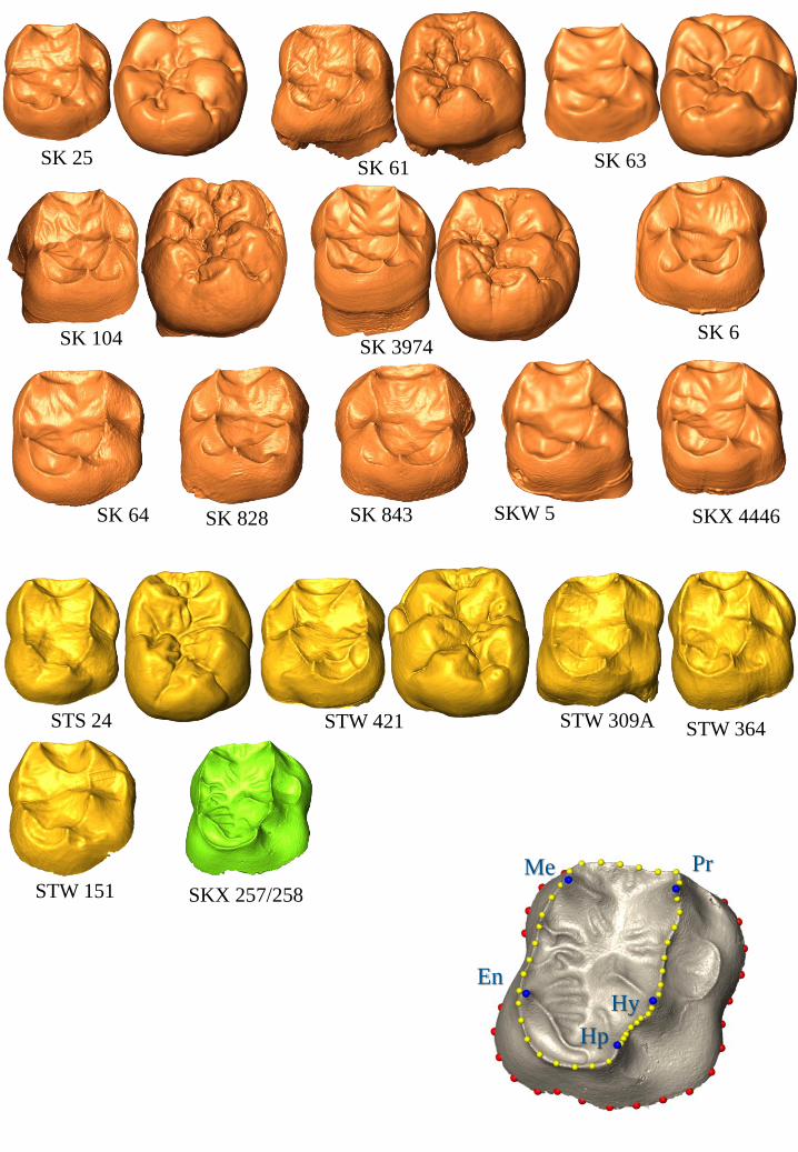
SK 25SK 61 SK 63

SK 104 SK 3974SK 6

SK 64 SK 828 SK 843 SKW 5 SKX 4446

STS 24 STW 421 STW 309A STW 364

STW 151 SKX 257/258

Pr

Hy

Hp

En

Me

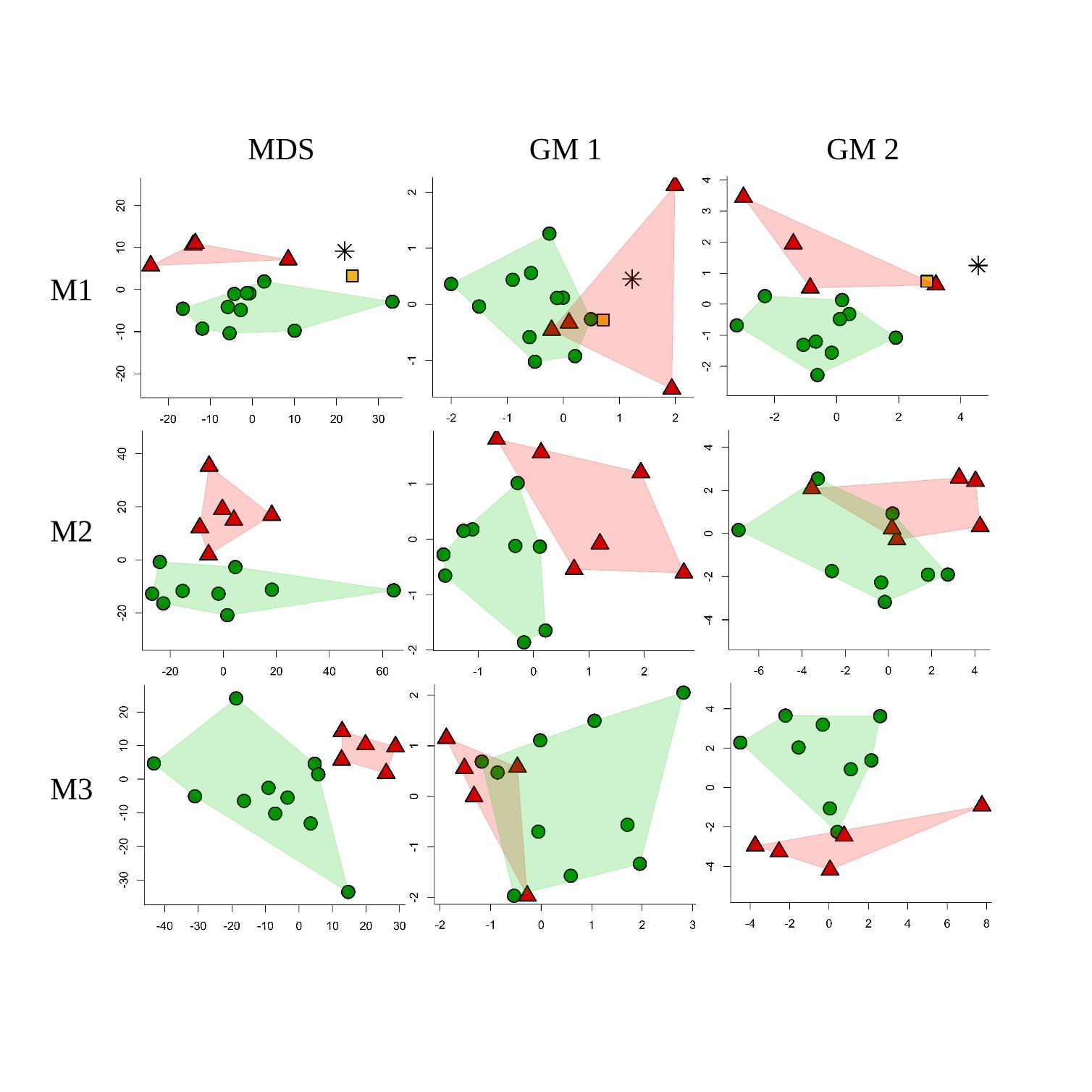
MDS GM 1 GM 2

M1

M2

M3

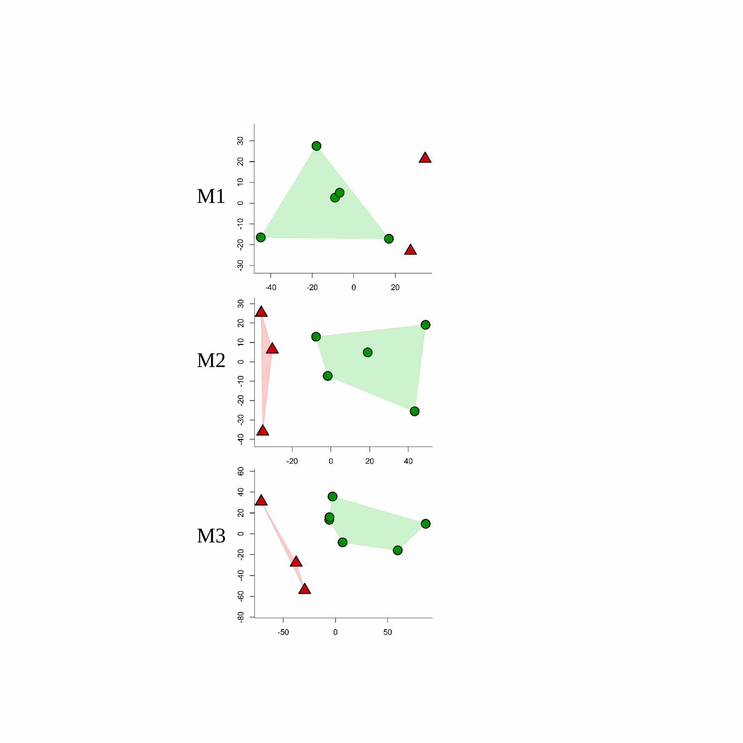
M1

M2

M3

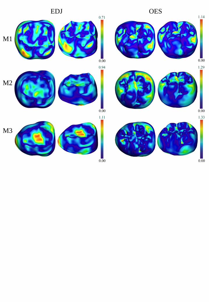
M1

M2

M3

OESEDJ

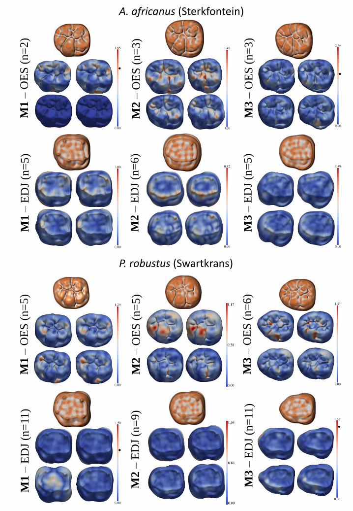
A. africanus (Sterkfontein)M

1 –

OE

S (

n=

2)

P. robustus (Swartkrans)

M1 –

ED

J (n

=5)

M1 –

OE

S (

n=

5)

M1 –

ED

J (n

=11)

M2 –

OE

S (

n=

3)

M2 –

ED

J (n

=6)

M2 –

OE

S (

n=

5)

M2 –

ED

J (n

=9)

M3 –

OE

S (

n=

3)

M3 –

ED

J (n

=5)

M3 –

OE

S (

n=

6)

M3 –

ED

J (n

=11)

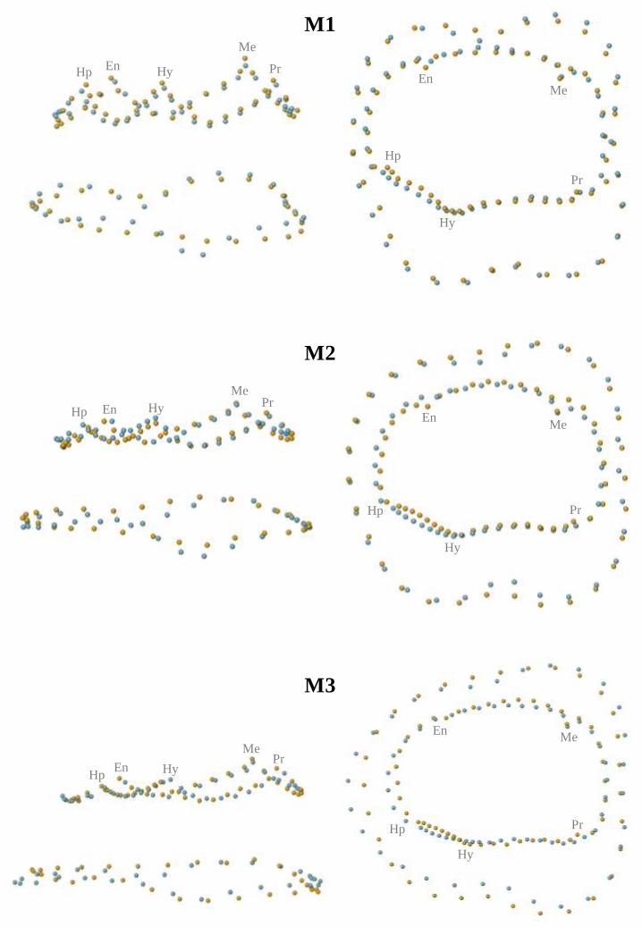
M1

M2

M3

Me

EnHp Hy Pr

MeEn

Hp

Hy

Pr

Me

EnHp Hy Pr

MeEn

Hp

Hy

Pr

Me

EnHp

HyPr

MeEn

Hp

Hy

Pr

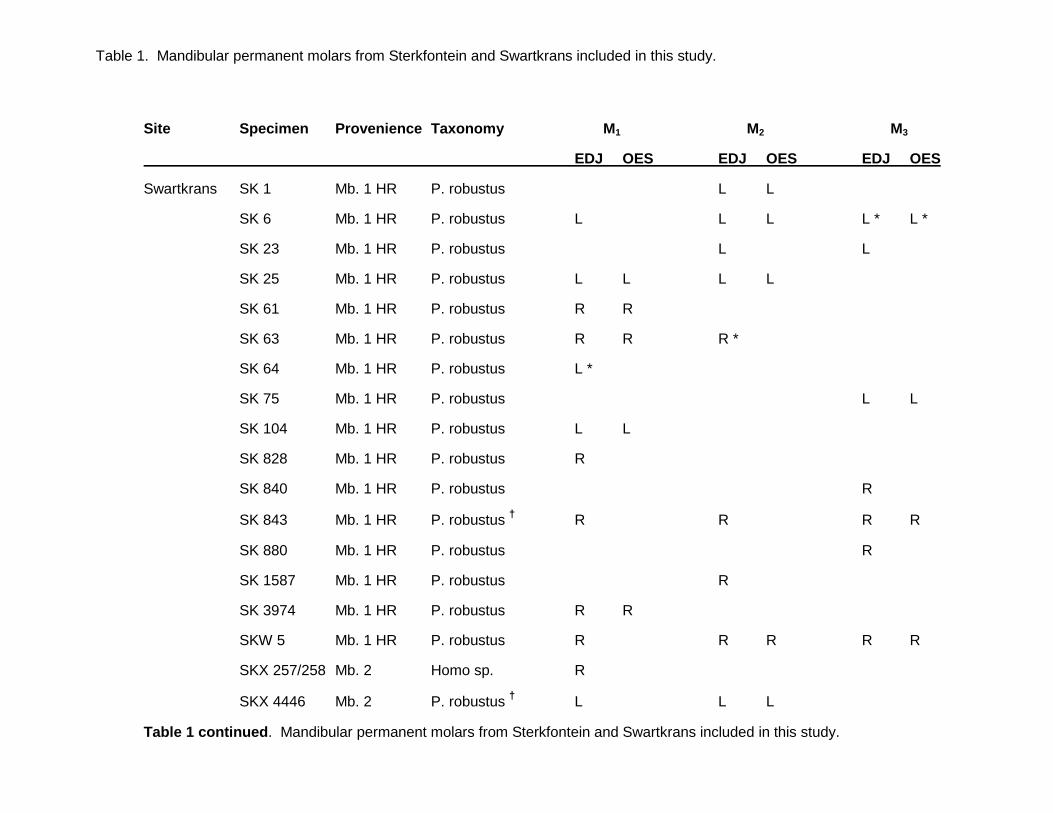
Table 1. Mandibular permanent molars from Sterkfontein and Swartkrans included in this study.

Site Specimen Provenience Taxonomy M 1 M2 M3

EDJ OES EDJ OES EDJ OES

Swartkrans SK 1 Mb. 1 HR P. robustus L L

SK 6 Mb. 1 HR P. robustus L L L L * L *

SK 23 Mb. 1 HR P. robustus L L

SK 25 Mb. 1 HR P. robustus L L L L

SK 61 Mb. 1 HR P. robustus R R

SK 63 Mb. 1 HR P. robustus R R R *

SK 64 Mb. 1 HR P. robustus L *



SK 828 Mb. 1 HR P. robustus R


SK 843 Mb. 1 HR P. robustus † R R R R



SK 3974 Mb. 1 HR P. robustus R R

SKW 5 Mb. 1 HR P. robustus R R R R R

SKX 257/258 Mb. 2 Homo sp. R

SKX 4446 Mb. 2 P. robustus † L L L

Table 1 continued . Mandibular permanent molars from Sterkfontein and Swartkrans included in this study.

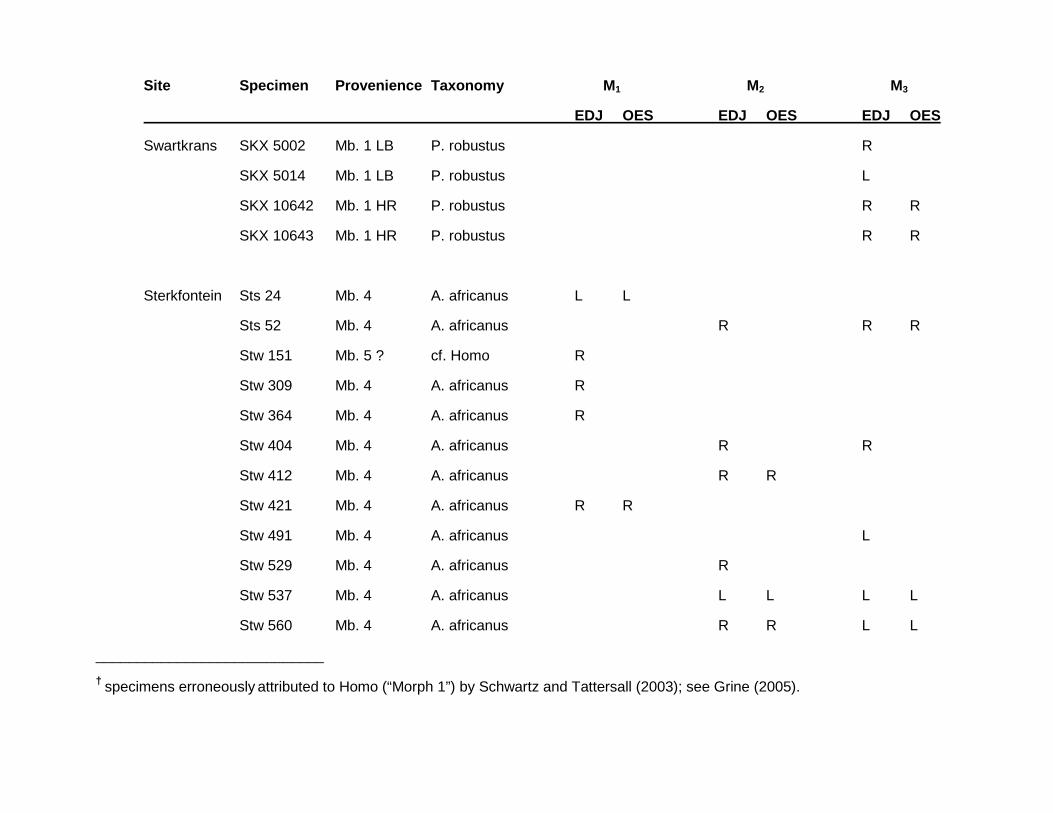
Site Specimen Provenience Taxonomy M 1 M2 M3

EDJ OES EDJ OES EDJ OES

Swartkrans SKX 5002 Mb. 1 LB P. robustus R

SKX 5014 Mb. 1 LB P. robustus L

SKX 10642 Mb. 1 HR P. robustus R R

SKX 10643 Mb. 1 HR P. robustus R R

Sterkfontein Sts 24 Mb. 4 A. africanus L L

Sts 52 Mb. 4 A. africanus R R R

Stw 151 Mb. 5 ? cf. Homo R

Stw 309 Mb. 4 A. africanus R


Stw 404 Mb. 4 A. africanus R R



Stw 491 Mb. 4 A. africanus L


Stw 537 Mb. 4 A. africanus L L L L

Stw 560 Mb. 4 A. africanus R R L L

____________________________

† specimens erroneously attributed to Homo (“Morph 1”) by Schwartz and Tattersall (2003); see Grine (2005).

*, incompletely developed crown near the cervical margin.

Abbreviations: P. = Paranthropus; A. = Australopithecus; Mb = member; EDJ = enamel dentin junction; OES = outer enamel surface;

R = right; L = left.

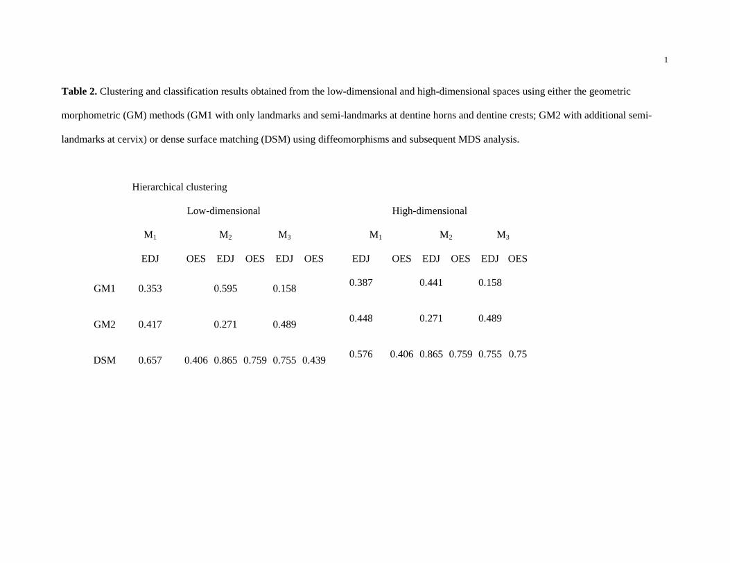
1

Table 2. Clustering and classification results obtained from the low-dimensional and high-dimensional spaces using either the geometric

morphometric (GM) methods (GM1 with only landmarks and semi-landmarks at dentine horns and dentine crests; GM2 with additional semi-

landmarks at cervix) or dense surface matching (DSM) using diffeomorphisms and subsequent MDS analysis.

Hierarchical clustering

Low-dimensional High-dimensional

M1

M2

M3

M1 M2 M3

EDJ OES EDJ OES EDJ OES EDJ OES EDJ OES EDJ OES

GM1 0.353

0.595

0.158

0.387 0.441

0.158

GM2 0.417 0.271 0.489 0.448

0.271

0.489

DSM 0.657 0.406 0.865 0.759 0.755 0.439 0.576

0.406

0.865

0.759

0.755

0.75

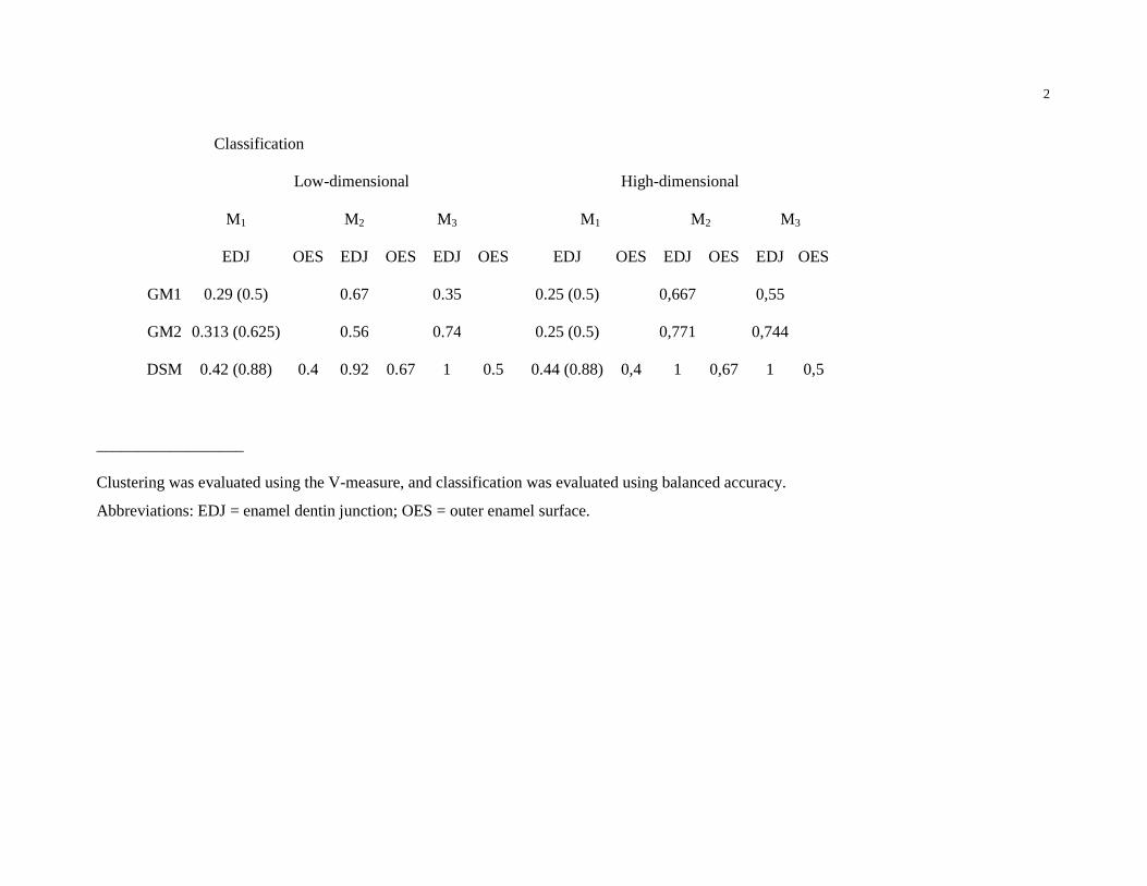
2

Classification

Low-dimensional High-dimensional

M1

M2

M3

M1 M2 M3

EDJ OES EDJ OES EDJ OES EDJ OES EDJ OES EDJ OES

GM1 0.29 (0.5)

0.67

0.35

0.25 (0.5) 0,667 0,55

GM2 0.313 (0.625) 0.56 0.74 0.25 (0.5) 0,771 0,744

DSM 0.42 (0.88) 0.4 0.92 0.67 1 0.5 0.44 (0.88) 0,4 1 0,67 1 0,5

__________________

Clustering was evaluated using the V-measure, and classification was evaluated using balanced accuracy.

Abbreviations: EDJ = enamel dentin junction; OES = outer enamel surface.

Documents

Efficacy of diffeomorphic surface matching and 3D