Embed Size (px)
Citation preview
DEMAND
Effects of the Built Environment on Transportation: Energy Use, Greenhouse Gas Emissions, and Other Factors

TRANSPORTATION ENERGY FUTURES SERIES: Effects of the Built Environment on Transportation:
Energy Use, Greenhouse Gas Emissions, and Other Factors
A Study Sponsored by
U.S. Department of Energy Office of Energy Efficiency and Renewable Energy
March 2013
Prepared by
CAMBRIDGE SYSTEMATICS Cambridge, MA 02140
under subcontract DGJ-1-11857-01
Technical monitoring performed by NATIONAL RENEWABLE ENERGY LABORATORY
Golden, Colorado 80401-3305 managed by
Alliance for Sustainable Energy, LLC for the
U.S. DEPARTMENT OF ENERGY Under contract DC-A36-08GO28308
This report was prepared as an account of work sponsored by an agency of the United States Government. Neither the United States Government nor any agency thereof, nor any of their employees, makes any warranty, expressed or implied, or assumes any legal liability or responsibility for the accuracy, completeness, or usefulness of any information, apparatus, product, or process disclosed, or represents that its use would not infringe privately owned rights. Reference herein to any specific commercial product, process, or service by trade name, trademark, manufacturer, or otherwise, does not necessarily constitute or imply its endorsement, recommendation, or favoring by the United States Government or any agency thereof. The views and opinions of authors expressed herein do not necessarily state or reflect those of the United States Government or any agency thereof.

iv
ABOUT THE TRANSPORTATION ENERGY FUTURES PROJECT
This is one of a series of reports produced as a result of the Transportation Energy Futures (TEF) project, a U.S. Department of Energy (DOE)-sponsored multi-agency project initiated to identify underexplored strategies for abating greenhouse gases and reducing petroleum dependence related to transportation. The project was designed to consolidate existing transportation energy knowledge, advance analytic capacity-building, and uncover opportunities for sound strategic action.
Transportation currently accounts for 71% of total U.S. petroleum use and 33% of the nation’s total carbon emissions. The TEF project explores how combining multiple strategies could reduce GHG emissions and petroleum use by 80%. Researchers examined four key areas – light-duty vehicles, non-light-duty vehicles, fuels, and transportation demand – in the context of the marketplace, consumer behavior, industry capabilities, technology and the energy and transportation infrastructure. The TEF reports support DOE long-term planning. The reports provide analysis to inform decisions about transportation energy research investments, as well as the role of advanced transportation energy technologies and systems in the development of new physical, strategic, and policy alternatives.
In addition to the DOE and its Office of Energy Efficiency and Renewable Energy, TEF benefitted from the collaboration of experts from the National Renewable Energy Laboratory and Argonne National Laboratory, along with steering committee members from the Environmental Protection Agency, the Department of Transportation, academic institutions and industry associations. More detail on the project, as well as the full series of reports, can be found at http://www.eere.energy.gov/analysis/transportationenergyfutures.
Contract Nos. DC-A36-08GO28308 and DE-AC02-06CH11357

v
AVAILABILITY This report is available electronically at http://www.osti.gov/bridge Available for a processing fee to U.S. Department of Energy and its contractors, in paper form, from: U.S. Department of Energy Office of Scientific and Technical Information P.O. Box 62 Oak Ridge, TN 37831-0062 phone: 865.576.8401 fax: 865.576.5728 email: [email protected]
Available for sale to the public, in paper form, from: U.S. Department of Commerce National Technical Information Service 5285 Port Royal Road Springfield, VA 22161 phone: 800.553.6847 fax: 703.605.6900 email: [email protected] online ordering: http://www.ntis.gov/help/ordermethods.aspx
CITATION Please cite as follows: Porter, C.D.; Brown, A.; Dunphy, R.T.; Vimmerstedt, L. (March 2013). Effects of the Built Environment on Transportation: Energy Use, Greenhouse Gas Emissions, and Other Factors. Transportation Energy Futures Series. Prepared by the National Renewable Energy Laboratory (Golden, CO) and Cambridge Systematics, Inc. (Cambridge, MA), for the U.S. Department of Energy, Washington, DC. DOE/GO-102013-3703. 91 pp.

vi
REPORT CONTRIBUTORS AND ROLES National Renewable Energy Laboratory Austin Brown Co-lead Laura Vimmerstedt Co-lead
Cambridge Systematics Christopher D. Porter Primary author
Consultant Robert T. Dunphy Contributing author
vii
ACKNOWLEDGMENTS We are grateful to colleagues who reviewed portions or the entirety of this report in draft form, including:
Lee Cook, Group Manager, Transportation and Regional Program Division, U.S. Environmental Protection Agency (EPA)
John Davies, Environmental Protection Specialist, Sustainable Transport and Climate Change Team, Office of Planning, Environment, and Realty, Federal Highway Administration, U.S. Department of Transportation (U.S. DOT)
Elizabeth Deakin, Professor of City, Regional Planning and Urban Design, University of California, Berkeley
Art Rypinski, Economist, Office of the Secretary, U.S. DOT
Mark Simons, Office of Transportation and Air Quality, EPA John Thomas, Director, Community Assistance and Research Division Office of Sustainable Communities, EPA
Diane Turchetta, Transportation Specialist, Sustainable Transport and Climate Change Team, Office of Planning, Environment, and Realty, Federal Highway Administration, U.S. DOT
Participants in an initial Transportation Energy Futures scoping meeting in June 2010 – representing the U.S. Department of Energy and national laboratories – assisted by formulating innovative and timely ideas to consider for the project. Steering Committee members and observers offered their thoughtful perspective on transportation analytic research needs as well as insightful comments on an initial Transportation Energy Futures work plan in a December 2010 meeting, and periodic teleconferences through the project.
Many analysts and managers at the U.S. Department of Energy played important roles in sponsoring this work and providing valuable guidance. From the Office of Energy Efficiency and Renewable Energy, Sam Baldwin and Carla Frisch provided leadership in conceptualizing the project, and Seth Federspiel provided technical review. A core team of analysts collaborated closely with the national lab team throughout implementation of the project. These included:
Jacob Ward and Philip Patterson (now retired), Vehicle Technologies Office
Tien Nguyen and Fred Joseck, Fuel Cell Technologies Office
Zia Haq, Kristen Johnson, and Alicia Lindauer-Thompson, Bioenergy Technologies Office
The national lab project management team consisted of Austin Brown, Project Lead, and Laura Vimmerstedt, Project Manager (from the National Renewable Energy Laboratory); and Tom Stephens, Argonne Lead (from Argonne National Laboratory). Data analysts, life cycle assessment analysts, managers, contract administrators, administrative staff, and editors at both labs offered their dedication and support to this effort.


ix
TABLE OF CONTENTS List of Figures ........................................................................................................................... x List of Tables ............................................................................................................................. x Acronyms ................................................................................................................................. xi Executive Summary .................................................................................................................. 1 1. Introduction ......................................................................................................................... 5 2. Characterizing Urban Form and the Built Environment ................................................... 7
2.1. Local/Neighborhood-Level Characterization .............................................................. 7 2.2. Regional-Level Characterization ................................................................................ 8
3. Impacts of Urban Form and the Built Environment ........................................................ 12 3.1. Travel, Energy Use, and Greenhouse Gas Emissions ............................................. 12 3.2. Economic Impacts ................................................................................................... 21 3.3. Other Factors ........................................................................................................... 22
4. Analysis Methods .............................................................................................................. 28 4.1. “Four-Step” and Other Travel Demand Models ........................................................ 29 4.2. Transportation Land-Use Models ............................................................................. 31 4.3. 4-D Methods ............................................................................................................ 32 4.4. Land-Use Scenario Planning Tools .......................................................................... 33 4.5. Municipal Transportation and Greenhouse Gas (MUNTAG) Model .......................... 34 4.6. Moving Cooler Method Based on CUTR VMT Forecasting Model ............................ 35 4.7. Housing and Transportation Affordability Index ........................................................ 36 4.8. Analysis of the National Household Travel Survey ................................................... 36 4.9. Structural Equations Modeling ................................................................................. 37 4.10. Discrete and Discrete-Continuous Choice Models ................................................... 38 4.11. Life-Cycle Assessment (LCA) Methods .................................................................... 39
5. Factors That Influence Urban Form ................................................................................. 41 5.1. Demographic, Social, Economic, Technological, and Policy Drivers ........................ 41 5.2. Decision-Making Processes ..................................................................................... 44 5.3. Historical Examples of Energy and GHG Goals and Programs for Urban Planning .. 45 5.4. Smart Growth Opportunities .................................................................................... 49
6. Federal Actions That Might Influence Urban Form ......................................................... 51 6.1. Historical Influences ................................................................................................. 51 6.2. Current Federal Actions ........................................................................................... 54 6.3. Potential Federal Opportunities................................................................................ 56
7. Additional Analysis ........................................................................................................... 62 7.1. Technical Issues ...................................................................................................... 62 7.2. Modeling and Assessment Tools ............................................................................. 63 7.3. Effects of Federal Policy on Urban Form ................................................................. 64
8. Conclusions....................................................................................................................... 65 Appendix. Literature Review .................................................................................................. 69 References .............................................................................................................................. 82

x
LIST OF FIGURES Figure 3.1. Private VKT per capita versus urban density ........................................................... 18 Figure 3.2. Car ownership versus urban density ....................................................................... 18 Figure 3.3. Vehicle trips per capita versus income .................................................................... 19 Figure 3.4. Comparison of CO2 emission rates for transient versus smooth driving .................. 20
LIST OF TABLES Table ES.1. Comparison of Studies on Land Use and GHG Reduction ....................................... 3 Table ES.2. Opportunity Matrix for Built Environment Strategies ................................................. 4 Table 2.1. Sprawl Indicators ........................................................................................................ 9 Table 3.1. VMT Forecasts by Census Tract Density ................................................................. 12 Table 3.2. Comparison of Studies on Land Use and GHG Reduction ....................................... 14 Table 3.3. Mode Share by Census Tract Density, All Trips ....................................................... 16 Table 3.4. VMT Elasticities with Respect to Built Environment Variables .................................. 16 Table 3.5. Water and Sewer Costs per New Dwelling Unit ........................................................ 22 Table 3.6. Local Road Costs per Person ................................................................................... 23 Table 3.7. Unit Residential Infrastructure Costs by Density Group ............................................ 23 Table 4.1. Summary of Tools and Methods for Assessing Travel, Energy, and GHG Impacts
of Urban Form ......................................................................................................... 28 Table 5.1. Projected Housing Demand and Density in 2025 versus 2003 ................................. 44 Table 6.1. The Top 10 Influences on the American Metropolis of the Past 50 Years ................. 51 Table 6.2. Examples of Existing Federal Actions ....................................................................... 57 Table 6.3. Strategy Assessment for Federal Policy and Program Options ................................. 58 Table 6.4. Opportunity Matrix for Built Environment Strategies ................................................. 61

xi
ACRONYMS 3 Ds density, diversity, and design CNT Center for Neighborhood Technology CO2 carbon dioxide CO2e carbon dioxide equivalent CTOD Center for Transit-Oriented Development CUTR Center for Urban Transportation Research DOE U.S. Department of Energy DOT department of transportation (state or regional) EPA U.S. Environmental Protection Agency FHWA Federal Highway Administration FTA Federal Transit Administration GHG greenhouse gas GMA Growth Management Act (state) HUD U.S. Department of Housing and Urban Development LCA life-cycle assessment mpg miles per gallon MPO metropolitan planning organization MSA metropolitan and micropolitan statistical area NCHRP National Cooperative Highway Research Program NHTS National Household Travel Survey OECD Organisation for Economic Co-operation and Development ORNL Oak Ridge National Laboratory ppsm persons per square mile RCLCO Robert Charles Lesser & Co. SAFETEA-LU Safe, Accountable, Flexible, and Efficient Transportation Equity Act: A Legacy for
Users of 2005 TAZ traffic analysis zone TCRP Transit Cooperative Research Program TEF Transportation Energy Futures TIGER Census files: topologically integrated geographic encoding and referencing TIGER U.S. DOT’s Transportation Investment Generating Economic Recovery program TOD transit-oriented development TRB Transportation Research Board of the National Academies U.S. DOT U.S. Department of Transportation UA urbanized area UC urban cluster VKT vehicle-kilometers of travel VMT vehicle-miles of travel VTPI Victoria Transport Policy Institute


EXECUTIVE SUMMARY
Designing the Built Environment to Reduce Energy Use and Emissions
Urban form has evolved in response to a variety of demographic, social, economic, technological, and policy drivers. While direct authority over land use resides primarily at the local level, the federal government’s transportation and housing policies have indirectly influenced the built environment. These policies accelerated mid- and late-20th century trends of decentralization and declines in population density that were driven by increasing automotive mobility and the post-World War II baby boom. Suburbanization now shows some signs of slowing or reversing in response to demographic, economic, and cultural changes, renewing interest in smaller homes in urban settings. Local governments are increasingly implementing smart growth policies in attempts to manage growth and land use change, and constrain sprawl, with governments at higher levels supporting initiatives through funding, technical assistance, and incentives. This study examines the energy implications of the built environment, and the role the federal government could play.
This report reviews and summarizes literature on the relationships between the built environment and transportation-related energy use and greenhouse gas (GHG) emissions, along with implications for factors such as economic growth and quality of life. This report is one of a series of reports and tools, several of which address transportation demand, developed as part of the U.S. Department of Energy (DOE) Transportation Energy Futures (TEF) project, under the leadership of the National Renewable Energy Laboratory and Argonne National Laboratory. This report was developed under a National Renewable Energy Laboratory subcontract with Cambridge Systematics, which provided subject matter expertise. In addition to findings from the published literature, the report contains unpublished perspectives that are based on Cambridge Systematics’ experience.
The primary objectives of this report are to inform national policy experts and decision-makers about how changes to land use and the built environment could reduce transportation energy use, and the feasibility and possible impacts of potential federal actions (including DOE actions) to affect the built environment. In recent years, a substantial body of literature has examined the relationship between the built environment, travel, and energy use. Planning initiatives in many regions and communities throughout the country have been directed at changing land use in order to reduce transportation energy use, decrease emissions, and achieve related benefits. This report reviews the state of knowledge on the potential of such initiatives, and identifies possible federal actions to help shape the built environment.
Key Findings
• Higher densities, a mix of uses, and walkable neighborhoods contribute to lower vehicle travel and energy use.
• Changes to the built environment could result in a reduction in U.S. transportation energy and GHG emissions from less than 1% to as high as 10% by 2050, the high end corresponding to a reduction of up to 16%–18% in the urban light-duty vehicle travel subsector.
• Expansion of federal efforts to influence development through funding incentives and other voluntary initiatives could support more effective land use planning and reduce transportation energy use.
• The relationships among built environment metrics, transportation systems, and travel are nonlinear and interactive. Network-based models are best suited to assess these relationships.
1

Built Environment TRANSPORTATION ENERGY FUTURES SERIES
2
The report’s findings have also supported the development of a tool to allow the National Renewable Energy Laboratory and DOE to evaluate the transportation energy and GHG impacts of urban form scenarios at a national level through 2050. The report has been reviewed by subject matter experts from other federal agencies including the U.S. Department of Transportation (U.S. DOT) and the U.S. Environmental Protection Agency (EPA), as well as researchers in the field.
Factors with the Greatest Impact
While many different factors can be used to characterize the built environment, this report focuses on four of the most important factors identified by the literature review, often referred to as the four Ds:
• Density – population or jobs per square mile
• Diversity – the number of different land uses in a given area and the degree to which they are represented
• Design – how friendly the local environment is to nonmotorized travel
• Destination accessibility – ease of access to trip attractions.
These factors may be measured, to varying degrees, on both a local and a regional scale. All of these factors – as well as automobile ownership, trip frequency, trip lengths, and modal shares – interact in sometimes complex ways to affect travel.
Tools for Measuring the Impacts of the Built Environment
We identified roughly a dozen individual tools or classes of tools that are currently used to assess relationships between transportation and land use. None of the tools are ideally suited for measuring all aspects of the built environment’s effects on travel. The best are probably the more well-developed regional travel demand models that incorporate transit and nonmotorized mode choice, as well as factors that reflect built environment variables such as the quality of the pedestrian environment and mix of uses.
Ranges of Potential Improvement
This study confirms the built environment’s important effect on travel, with higher densities, a mix of uses, and walkable neighborhoods contributing to lessened vehicle travel and energy use. Examination of density, diversity, design, and destination accessibility revealed ranges of potential improvement in each of these areas.
Density Higher densities contribute to shorter trip lengths and make transit and nonmotorized modes more viable. Gross neighborhood densities in the range 4,000–10,000 persons per square mile seem to act as the threshold for the most meaningful reductions in automobile travel. Residents of compact, walkable neighborhoods have about 20% to 40% fewer vehicle-miles of travel (VMT) per capita, on average, than residents of less-dense neighborhoods.
The effects of density, however, are difficult to capture through simple metrics such as average neighborhood or regional density. For example, the Los Angeles urbanized area has a higher average population density than the New York metropolitan area, yet has higher VMT per capita and much higher automobile mode shares. This is because the New York region contains a high-density core with a large fraction of population and employment that can be readily served by transit and walking, whereas Los Angeles is more uniformly distributed at moderate densities best served by the automobile.
Density’s effects can also be indirect, with high densities leading to greater traffic congestion and higher parking costs, which make alternatives modes of transportation more attractive.

TRANSPORTATION ENERGY FUTURES SERIES Built Environment
3
Diversity, Design, and Destination Accessibility The effects of diversity and design on transportation patterns are modest—doubling diversity and design metrics typically results in a VMT change in the range of 5% to 10% or less. Although these are meaningful contributing factors at higher densities, at lower densities no design can make travel by transit or walking competitive. Especially at the neighborhood level, accessibility of residents closer to the center of a region versus that of those who live in outlying areas may lead the effects of density to be overstated. People who live closer to the center of a region tend to travel shorter distances than those who live in outlying areas, even if neighborhood design and composition are similar.
Despite numerous studies of the built environment’s effects on travel, researchers still disagree on the extent to which the built environment itself accounts for differences in travel behavior versus other factors such as income, demographic, and personal preferences.
Overall Potential A number of recent studies have estimated the potential for land-use changes to reduce U.S. transportation GHG emissions from 0.6% to as high as 10% by 2050 (Table ES.1). The high-end 10% reduction corresponds to a reduction of up to 16%–18% in urban light-duty vehicle travel, a subsector of GHG-generating transportation activity. The higher end of the range is based on very optimistic assumptions (e.g., 75% to 90% of new development between now and 2050 being located in compact, walkable neighborhoods) that may be unlikely to be achievable without aggressive policy action and supportive market forces.
Table ES.1. Comparison of Studies on Land Use and GHG Reduction
Transportation Research Board
(TRB 2011) Rodier
(Rodier 2009)
Cambridge Systematics, Inc.
(EPA 2003) Ewing (Ewing
et al. 2007)
Urban light-duty vehicle VMT reduction in 2050
1%–11% Median 16% (range 3%–28%)
1.7%–12.6% 12%–18%
U.S. transportation GHG reduction below 2050 baseline (baselines vary)
0.6%–6.5% N/A 2.0%–3.4% 7%–10%
As vehicles meet increasingly more stringent fuel economy standards, the absolute energy benefits of land-use change will decline, since the total baseline energy and emissions from automobiles will decrease.
Other Outcomes We also reviewed literature related to the effects of the built environment on a variety of other outcomes. Compact development and smart growth deliver municipal infrastructure cost and environmental impact benefits, especially in the preservation of agricultural and forest land and natural habitats. Limited evidence suggests that traffic safety, public health, and equity benefits can result from land-use patterns that reduce traffic speeds and encourage travel by transit and nonmotorized modes. Findings on economic, housing affordability, and consumer welfare benefits are limited and inconclusive.
Federal Policy Options
Federal agencies including the U.S. DOT, the EPA, and the U.S. Department of Housing and Urban Development (HUD) are currently engaged in a number of funding, technical assistance, and incentive programs promoting coordinated land use, transportation planning and smart growth. Federal actions, including expansion of existing federal initiatives, could help drive the changes to the built environment that are identified above.

Built Environment TRANSPORTATION ENERGY FUTURES SERIES
4
Table ES.2 is an opportunity matrix showing federal authority versus potential transportation energy reduction payoff for strategies designed to affect the built environment. Expansion of existing activities (e.g., tax credits, planning and technical assistance) tends to have higher feasibility but low to moderate potential payoff. Actions such as eliminating the home mortgage interest deduction or implementing planning requirements, which would likely have a greater impact on urban form, would be harder to implement.
Table ES.2. Opportunity Matrix for Built Environment Strategies
Federal Authority
Potential Payoff
Low Medium High
High Marketing and outreach Funding for brownfields cleanup and public housing renewal Tax credits for brownfield, transit-oriented development
Funding for planning Technical assistance Funding for transit infrastructure (without planning requirements) Location-related criteria for federally funded programs
Eliminate home mortgage interest deduction Funding for transit infrastructure (with planning requirements)
Medium Location-efficient mortgages Requirements for regional integrated planning
Low Requirements for local comprehensive planning and zoning Direct federal planning
While few strategies to affect the built environment currently fall under the DOE’s jurisdiction, the DOE can and does have influence, primarily through departmental funding into planning and technical assistance programs, which may further support activities already undertaken by the EPA, HUD, and the U.S. DOT.
The Potential for Significant Impact
Although researchers still disagree on the extent to which land use accounts for differences in travel behavior among neighborhoods and regions, the evidence suggests that changes to the built environment, such as higher densities and mixed-use, walkable communities, have significant potential to impact transportation energy and GHG emissions significantly over the long term. Additional research and the refinement of analysis tools to better understand the relationships between built environment and income, demographics, personal preferences, commerce, marketplace factors and other transportation strategies could support further implementation of built environment strategies to reduce energy use, GHG emissions, and petroleum dependence.

TRANSPORTATION ENERGY FUTURES SERIES Built Environment
5
1. INTRODUCTION
Planning initiatives in many regions and communities throughout the country have been directed at changing land use in order to reduce transportation energy use, decrease greenhouse gas (GHG) emissions, and achieve other economic, social, and environmental benefits. Research has suggested that a shift towards more compact and walkable development patterns could reduce the nation’s transportation energy use and GHG emissions by up to 10% by 2050, playing an important role to complement other technology improvements and travel reduction measures.
While land use planning in the United States is primarily a matter of local (municipal) authority, an increasing number of regional and state initiatives are directed at better coordinating transportation and land use planning. Previous federal government policies have also indirectly influenced land use (e.g., the Interstate Highway System, model subdivision regulations), and in some cases played a direct role, such as through urban renewal programs. In recent years, federal emphasis has shifted towards supporting voluntary and collaborative planning initiatives.
This report reviews the state of knowledge on the potential of such initiatives to reduce energy and GHG emissions and deliver other benefits, based on published literature, as well as on Cambridge Systematics’ expertise. The report draws on a range of evidence, including empirically verifiable statements of fact and quantitative findings from published studies, as well as interpretations and judgments. The report also identifies possible federal actions to help shape the built environment. The primary objectives of this report are to provide information about how changes to land use and the built environment could reduce transportation energy use, and the feasibility and impacts of potential federal actions [including U.S. Department of Energy (DOE) actions] to affect the built environment. The report is not intended to propose or promote such actions.
The report addresses the following questions:
• How have the built environment and urban form been characterized in travel behavior research? (Section 2)
• How does the built environment affect travel, as well as transportation-related energy use and GHG emissions? (Section 3)
• How does the built environment affect other factors, including economic growth, infrastructure and housing costs, the environment, social welfare, and equity? (Section 3)
• What tools and methods are available for analyzing the impacts of changes in the built environment on travel, energy, and GHG emissions? (Section 4)
• What are the primary factors that influence urban form−including demographic, social, economic, technological, and policy drivers−and decision-making processes? (Section 5)
• What has been the past role of the federal government in influencing urban form, either directly or indirectly? What current federal policies and programs are directed at influencing urban form? (Section 6)
• What actions could the federal government potentially take in the future to influence urban form? (Section 6)
• What additional analysis is needed to better understand the effects of changes in urban form on travel and energy? What is needed to better understand the potential effects of federal actions on urban form? (Section 7)
An annotated outline of the literature reviewed is provided in the appendix, focusing on key sources that summarize research findings. This report was developed with input from subject matter experts from

Built Environment TRANSPORTATION ENERGY FUTURES SERIES
6
other federal agencies, including the U.S. Department of Transportation (U.S. DOT) and the U.S. Environmental Protection Agency (EPA), as well as researchers in the field.
This report also provides background for the development of a sketch-level tool, the Built Environment Energy Analysis Tool. The tool makes it possible to evaluate the transportation energy and GHG impacts of urban form scenarios at a national level through 2050. Information from the literature reviewed for this report informed the choice of datasets, variables, and analytical methods to develop this tool. This tool can be accessed through the TEF website: http://www.nrel.gov/analysis/transportation_futures.

TRANSPORTATION ENERGY FUTURES SERIES Built Environment
7
2. CHARACTERIZING URBAN FORM AND THE BUILT ENVIRONMENT
This section provides background on how urban form and the built environment are characterized in ways that relate to energy use and GHG emissions, based on published literature and Cambridge Systematics’ interpretations. Such metrics have primarily been developed at two levels: 1) the local or neighborhood level, and 2) the regional level.
2.1. Local/Neighborhood-Level Characterization Local-level studies have examined relationships between travel measured at the individual or neighborhood level, and local (neighborhood-scale) land-use characteristics at home, work, and sometimes other destinations. The “Ds” are frequently used to characterize local-scale land-use characteristics. Cervero and Kockelman (1997) first coined the “3 Ds” – density, diversity, and design – as measures of the built environment that influence travel. Researchers soon followed with two more “Ds” – destination accessibility and distance to transit (Ewing and Cervero 2001). The “Ds” are frequently applied at the micro-scale level in travel behavior research; density applies regionally as well. They can be defined as follows (Ewing and Cervero 2010):
Density is a variable of interest per unit of area. Population is the most frequently used variable of interest, but studies have used household, employment, and development density (number of dwelling units or square footage). Activity density is a more general concept that describes the number of trip-ends (i.e., trips originating or ending) in a given area. Higher densities should lead to shorter trip lengths (destinations are closer together) and make transit more competitive as compared to automobile travel, which can easily serve low-density, dispersed destinations. Density also affects travel behavior indirectly. For example, parking charges are more likely to be levied in high-density areas where land is at a premium. Higher density will also lead to higher levels of traffic congestion due to a greater concentration of trip-ends. Both of these factors make alternatives to automobile travel more competitive.
Diversity indicates the number of different land uses in a given area and the degree to which they are represented. Measures of diversity include entropy1 as well as jobs-housing or jobs-population ratios. Along with density, diversity can affect trip lengths and therefore mode shares, as locating destinations closer together provides the ability to use slower modes of travel.
Design characterizes how friendly the local environment is to nonmotorized travel. Design includes street network characteristics such as average block size and connectivity; pedestrian and bicycle network factors (e.g., sidewalk coverage, pedestrian crossings); pedestrian and bicycle amenities (e.g., street trees, parking); and site design metrics such as building setbacks and placement of parking.
Destination accessibility measures ease of access to trip attractions. It reflects the characteristics of a place relative to the broader subregion or region, using metrics such as number of jobs or shopping opportunities within a given travel time, or distance from the central business district. It has been used as a way of introducing regional characteristics into studies that have focused largely on local/neighborhood-scale characteristics.
Distance to transit measures access to transit, using specific metrics such as average distance between residences or workplaces and the nearest rail station or bus stop, transit route density, or percent of population within one-quarter mile of a transit stop.
1 A quantitative measure that increases when the number of types of land use increases and obtains maximum value when all types are equally represented.

Built Environment TRANSPORTATION ENERGY FUTURES SERIES
8
2.2. Regional-Level Characterization Regional-level studies have examined relationships between metropolitan or regional-level descriptors of urban form and aggregate travel patterns as measured at this level. To understand regional-level characterizations, it is helpful to have an understanding of U.S. Census Bureau definitions that relate to metropolitan and urbanized areas.
• The term “Core-Based Statistical Area” is a collective term for both metropolitan and micropolitan statistical areas (MSAs). A metropolitan area contains a core urban area of 50,000 or more population, and a micropolitan area (a concept first introduced in the 2000 census) contains an urban core of at least 10,000 but fewer than 50,000 population. Each metropolitan or micropolitan area consists of one or more counties and includes the counties containing the core urban area as well as any adjacent counties that have a high degree of social and economic integration (as measured by commuting to work) with the urban core (U.S. Census Bureau 2011).
• Urbanized areas (UAs) and urban clusters (UCs), both defined using the same criteria, represent densely developed territory, encompassing residential, commercial, and other nonresidential urban land uses. In general, this territory consists of areas of high population density and urban land use resulting in a representation of the urban footprint. A UA consists of densely developed territory that contains 50,000 or more people, while a UC consists of densely developed territory that has at least 2,500 people but fewer than 50,000 people (this concept was first introduced in the 2000 census). Areas that are not UAs or UCs are classified as rural (Braslow 1999).
• UAs and UCs are defined based on census tract and block group geography rather than counties. It is important to note that UAs and UCs have different boundaries and are often smaller than their corresponding MSA. MSAs may include significant amounts of land in counties within the metropolitan area that is not urban in character. The most extreme example is San Bernardino County in California, which encompasses much of Death Valley and the Mojave Desert as well as the City of San Bernardino and environs.
2.2.1. Measures of Concentration and Sprawl
The simplest, and most widely used, macro-level urban form descriptor is “average population density” [persons per square mile (ppsm) or persons per hectare]. Average population density can be computed for a MSA or for a UA. Particularly for metropolitan areas in the western United States, the use of urbanized densities is preferable to metropolitan area densities. Metropolitan densities may be misleading if there are large amounts of rural land, water, or other undeveloped or undevelopable land within the metropolitan boundary. On the other hand, the use of the county-based MSA boundaries can be preferable for examining changes in a fixed, consistent geographic area over time.
In addition to a simple snapshot of density, growth trends have been measured by comparing the amount of land added per new person in a region, essentially a measure of the density of new population, which can be compared with the density of existing population. Using data from the Natural Resources Inventory, which is conducted at five-year intervals, to compare 1997 versus 1982, Fulton et al. (2001) find that most metropolitan areas in the United States were adding urbanized land at a much faster rate than they were adding population, but with significant differences among regions – new growth in the West was much more dense than new growth in the South.
Average population density has been used in a number of studies, including international studies that compare travel metrics [such as vehicle-miles of travel (VMT) per capita or transit mode share] against factors, including urban form and infrastructure supply. Perhaps the best known studies are those by Kenworthy and colleagues (Kenworthy et al. 1999), who collected data on land-use transport indicators from cities throughout the world in the late 1990s and early 2000s. Using the average population density has a number of limitations, however, that have led researchers to develop more sophisticated measures of

TRANSPORTATION ENERGY FUTURES SERIES Built Environment
9
urban form. Eidlin (2010) points out that the distribution of density is much more important than the average density, and notes that the Los Angeles metro area actually has a higher average density than the New York metro area, yet is much more automobile-dependent. He cites alternative measures, including:
• The Gini coefficient, a measure of deviation from uniformity
• Perceived density (the average of small-area densities weighted by population)
• A density gradient index, the ratio of perceived density to standard density.
New York, Boston, and Philadelphia, which have very dense cores but low-density suburbs, have high density gradients, while Los Angeles, Phoenix, and Miami have much more uniform, moderate densities. Eidlin cites data from Bradford (2008) showing that density gradient is highly correlated with public transit and walking commute mode, in contrast with average density, which shows almost no correlation.
The distribution of employment can be used to indicate the degree of centralization of a region. For example, Glaeser and Kahn (2004) measure urban sprawl based on the share of employment within a certain radius of the central business district.
Ewing, Pendall, and Chen (2002) go beyond density and concentration as the measures of urban form, and develop a more general index of sprawl based on 22 variables grouped into four factors:
1. Residential density
2. Neighborhood mix of homes, jobs, and services
3. Strength of activity centers and downtowns
4. Accessibility of the street network.
They define and assemble data on these factors for 83 metropolitan areas and combine the data into an overall “sprawl index” for each area in the year 2000. The specific variables, data sources, and relative contribution of each variable to the four factors are shown in Table 2.1. The data are taken from a variety of sources, including the census, U.S. Department of Agriculture Natural Resource Inventory, ZIP Code Business Patterns, and the American Housing Survey. The authors find clear relationships between this index and daily VMT per person, vehicle ownership, and reduced levels of transit and walking, but do not find a relationship with traffic delays.
Table 2.1. Sprawl Indicators
Factora Variable Source Variable Loadingb
Density 0.57 Gross population density (persons per square
mile) U.S. Census (1990 and 2000) 0.89
Percentage of population living at densities less than 1,500 ppsm
-0.69
Percentage of population living at densities greater than 12,500 ppsm
0.94
Estimated density at the center of the metro area derived from a negative exponential density function
0.90
Gross population density of urban lands U.S. Department of Agriculture Natural Resources Inventory (1987-1997)
0.94
Density (continued)
Weighted average lot size (square feet) for single-family dwellings
American Housing Survey (1989-1999)
-0.30
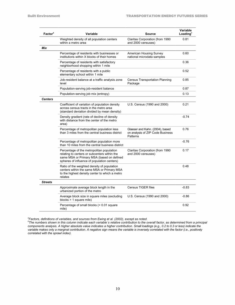
Built Environment TRANSPORTATION ENERGY FUTURES SERIES
10
Factora Variable Source Variable Loadingb
Weighted density of all population centers within a metro area
Claritas Corporation (from 1990 and 2000 censuses)
0.81
Mix Percentage of residents with businesses or
institutions within X blocks of their homes American Housing Survey national microdata samples
0.60
Percentage of residents with satisfactory neighborhood shopping within 1 mile
0.36
Percentage of residents with a public elementary school within 1 mile
0.52
Job-resident balance at a traffic analysis zone level
Census Transportation Planning Package
0.85
Population-serving job-resident balance 0.87
Population-serving job mix (entropy) 0.13
Centers Coefficient of variation of population density
across census tracts in the metro area (standard deviation divided by mean density)
U.S. Census (1990 and 2000) 0.21
Density gradient (rate of decline of density with distance from the center of the metro area)
-0.74
Percentage of metropolitan population less than 3 miles from the central business district
Glaeser and Kahn. (2004), based on analysis of ZIP Code Business Patterns
0.76
Percentage of metropolitan population more than 10 miles from the central business district
-0.76
Percentage of the metropolitan population relating to centers or subcenters within the same MSA or Primary MSA (based on defined spheres of influence of population centers)
Claritas Corporation (from 1990 and 2000 censuses)
0.17
Ratio of the weighted density of population centers within the same MSA or Primary MSA to the highest density center to which a metro relates
0.48
Streets Approximate average block length in the
urbanized portion of the metro Census TIGER files -0.83
Average block size in square miles (excluding blocks > 1 square mile)
U.S. Census (1990 and 2000) -0.86
Percentage of small blocks (< 0.01 square mile)
0.92
aFactors, definitions of variables, and sources from Ewing et al. (2002), except as noted. bThe numbers shown in this column indicate each variable’s relative contribution to the overall factor, as determined from a principal components analysis. A higher absolute value indicates a higher contribution. Small loadings (e.g., 0.2 to 0.3 or less) indicate the variable makes only a marginal contribution. A negative sign means the variable is inversely correlated with the factor (i.e., positively correlated with the sprawl index).

TRANSPORTATION ENERGY FUTURES SERIES Built Environment
11
The variables shown in Table 2.1 provide ideas for metropolitan-level variables that can be used in the Built Environment Energy Analysis Tool developed through this project to analyze national development scenarios in 2030 and 2050. Not all of the variables shown here may be suitable for this work, however. Some are from data sources that are no longer updated (e.g., American Housing Survey) or were developed from a one-time analysis (Glaeser and Kahn 2004). Others might require data processing that is beyond the scope of this project. Variables that can be both intuitively understood and readily forecasted are also desirable so that future scenarios can be developed using these variables. In developing the Built Environment Energy Analysis Tool, basic variables were used that describe the above factors and can be readily constructed from available data. Future enhancements could include investigation of additional variables and the extent to which they add explanatory power to the tool or expand the range of scenarios that can be tested.

Built Environment TRANSPORTATION ENERGY FUTURES SERIES
12
3. IMPACTS OF URBAN FORM AND THE BUILT ENVIRONMENT
This section describes how urban form and the built environment affect travel patterns, energy use, GHG emissions, and other factors, based on published literature as well as Cambridge Systematics’ expertise.
3.1. Travel, Energy Use, and Greenhouse Gas Emissions The impact of urban form on travel has been widely studied. Many studies within the past two to three decades have used empirical data to relate travel patterns to land-use and urban design factors, by examining the behavior of individual households, or the aggregate characteristics of travelers at a neighborhood (e.g., census tract or traffic analysis zone) or metropolitan level. Some studies have used regional-scale data (e.g., average population density) while others have used local-scale land-use descriptors, as described above. The “Ds” have become widely accepted as an organizing framework for conducting research on travel and the built environment, as documented in Ewing and Cervero (2010), who conducted a meta-analysis of more than 50 studies drawn from over 200 empirical studies conducted on land use and travel.
In addition to empirical studies, travel demand models have been used to predict the potential effect of alternative land-use and transportation scenarios on travel at a subregional or regional level. The best studies of this type have used models that are informed by the empirical research described above. Other studies have used state of practice travel demand models that do not incorporate data specifically on micro-scale design characteristics, but are still capable of reflecting the network/system-levels impacts of the spatial arrangement of a region. The research described below—selected and interpreted based on Cambridge Systematics’ experience—reflects a synthesis of empirical and modeling research from various sources.
3.1.1. Overall Impacts on Vehicle-Travel, Energy, and GHG
The impacts of land-use patterns on energy and GHG (U.S. DOT 2010) at a site or neighborhood level can be significant. A recent review of the literature concluded that vehicle travel is typically 20% to 40% lower for residents of compact neighborhoods compared to residents of sprawl neighborhoods (Ewing et al. 2007). Infill sites have been shown to reduce VMT by 15% to 50% compared to greenfields (previously undeveloped locations) (Kooshian and Winkelman 2011). Data from a VMT forecasting model developed by Polzin and Chu of the Center for Urban Transportation Research (CUTR) (2007) and based on the 2001 National Household Travel Survey (NHTS) suggests that households in the highest-density neighborhoods (over 10,000 ppsm) produce less than half the annual carbon dioxide (CO2) emissions produced by households in the lowest-density neighborhoods (under 500 ppsm). Table 3.1 shows VMT per capita estimates and forecasts for 2005 and 2035 by neighborhood (census tract) density. VMT per capita is forecast to increase in the future due primarily to income growth.
Table 3.1. VMT Forecasts by Census Tract Density Annual VMT per Capita
Persons per Square Mile (ppsm)
Approximate Dwelling Units
per Acre 2005 VMT VMT Compared to < 500 ppsm 2035 VMT
VMT Compared to < 500 ppsm
0-499 < 0.6 11,422 0.0% 13,798 0.0%
500-1,999 0.6-2.5 10,083 -11.7% 12,196 -11.6%
2,000-3,999 2.5-5 9,345 -18.2% 11,345 -17.8%
4,000-9,999 5-12 7,986 -30.1% 9,782 -29.1%
10,000+ > 12 4,437 -61.2% 5,651 -59.0%
[Source: CUTR VMT forecasting model (Polzin and Chu 2007) as applied by Cambridge Systematics (Urban Land Institute 2009)] Dwelling units per acre conversions are gross densities estimated at roughly 50% residential land per tract.

TRANSPORTATION ENERGY FUTURES SERIES Built Environment
13
Empirical examinations of the relationship between density and VMT may be somewhat confounded by the effects of other variables, including household income, household size, and regional accessibility (e.g., proximity to the central business district or other major job centers). However, much of the literature suggests there are relationships with density even after controlling for other variables. The CUTR model controls for some demographic variables, although not income by tract. A model developed for this study using 2009 NHTS survey data (NHTS 2010) finds local density significant even with income included. Furthermore, an analysis of tract-level median income and population density from the American Community Survey shows only a small inverse correlation between the two variables (-0.10 for density at urban densities greater than 700 ppsm), suggesting that income differences introduce little bias in relationships based on national-level data. A contrasting viewpoint is provided by Barnes (2001), who finds that local and regional density variables show very little relationship with travel behavior, especially once the effects of other variables (such as regional access) are considered.2
The net benefits of actions to change urban form and the built environment are tempered by the long-term nature of land-use changes. Land-use change can occur as population in a region grows, and as obsolete building stock is replaced. [Nelson (2006) cites residential and commercial turnover rates of about 6% and 20% per decade, respectively.] VMT and GHG reduction benefits reported in recent efforts to quantify the potential benefits of land-use changes at a national scale are discussed below.
Growing Cooler. The Growing Cooler study (Ewing et al. 2007) estimated that changes in land-use patterns to focus most new development into compact, walkable, transit-accessible communities could reduce total U.S. GHG from transportation sources by 7% to 10% from forecast levels by 2050, or urban VMT by 12% to 18%. The Growing Cooler estimates were based on very aggressive land-use changes, with a range of 60% to 90% of new development between the time of the study and 2050 located in compact neighborhoods where vehicle travel is reduced by 20% to 40% (with an average of 30%) compared to conventional development. This assessment is based on considering a range of studies that may have controlled for confounding effects to varying degrees.
Moving Cooler. The Moving Cooler study (Urban Land Institute 2009) found potential reductions in urban light-duty VMT ranging from 2% (for a scenario based on a very conservative assumption of 43% of development in compact areas3), to nearly 13% for assumptions regarding compact development that were similar to the most aggressive assumptions in Growing Cooler, specifically, that 90% of new development would occur in compact, walkable neighborhoods with gross densities of at least 4,000 ppsm (2009). The assumptions regarding per-capita VMT by local density are based on the CUTR model (Ewing et al. 2007).
TRB Special Report 298. The Transportation Research Board’s (TRB) Special Report 298 found results in the same range (TRB 2009). Special Report 298 estimated that the reduction in VMT, energy use, and CO2 emissions resulting from more compact, mixed-use development would be in the range of less than 1% to 11% by 2050. The estimated GHG reduction range in Special Report 298 is based on 25% to 75% of new residential development taking place at double the average density of new acres developed between 1987 and 1997. Development between 1987 and 1997 was significantly less dense than existing development. As such, under the low-end scenario, average densities would continue to decline. Under the most aggressive scenario, average densities would increase from current levels to densities on the ground in the early 1990s. Committee members for the TRB report disagreed about whether the changes
2 If all of the effect is due to regional accessibility, rather than local density, the conclusion is that two neighborhoods directly adjacent to each other will have similar travel characteristics, even if one is high density and one is low density. This is largely expected since most trips occur outside the neighborhood. However, the effects of local density on travel cannot be discounted. The aggregation of local densities creates a regional pattern that affects longer trips. An agglomeration of low-density neighborhoods will lead to a low-density region, which will require longer trip lengths and greater reliance on automobile travel compared to an agglomeration of high-density neighborhoods that creates a high-density region. 3 This is based on the development that was compact in the year 2000, which was lower than more recent development.

Built Environment TRANSPORTATION ENERGY FUTURES SERIES
14
in development patterns and public policies necessary to achieve the high end of these estimates are possible.
Regional scenario planning studies. Scenario planning studies using travel forecasting models have estimated that land-use changes in U.S. metropolitan areas, combined with supportive transit investments, could reduce metropolitan VMT by a median of 16% below forecast levels over a 40-year time horizon (Rodier 2009), which is in the same range as the Growing Cooler results. Because land-use change occurs slowly over time, the impact over a shorter timeframe will be proportionately less; the Rodier study found a median VMT reduction of 8% over a 20-year time horizon. The potential benefits depend on the projected growth in the region, aggressiveness of assumed land-use and transit changes, as well as the forecasting model’s capabilities and specific methodological assumptions. In general, the modeled scenarios were postulated land-use changes rather than changes that had been determined to be politically or market-feasible. Forty-year VMT reductions in the Rodier review ranged from a low of 3% to a high of 28% across all studies. Outputs of the Built Environment Energy Analysis Tool could potentially be compared against regional modeling results from these studies as a validity check on the magnitude of results, although the specific assumptions within each study vary widely.
U.S. DOT Report to Congress. This report synthesized previous research, relying on the Growing Cooler, Moving Cooler, TRB Report 298, and Rodier results reported above. The report concluded that land-use strategies could reduce U.S. GHG emissions by 28 to 84 million metric tons carbon dioxide equivalent (CO2e), or 2.5% to 7.8% of light-duty vehicle emissions, in the year 2030. Benefits would grow over time to possibly double that amount annually in 2050 (U.S. DOT 2010).
A comparison of three source studies that each took a similar approach to macro-level description of land-use scenario benefits is shown in Table 3.2. The absolute reduction in CO2e assumes the adoption of model year 2012–2016 federal fuel economy standards, but not 2017–2025 standards proposed in November 2011 (Federal Register 2010b, 2010a). Adoption of these new standards would reduce the magnitude of CO2e benefits but would have little impact on the percentage benefit (reduction expressed as a percentage of light-duty vehicle emissions).
Table 3.2. Comparison of Studies on Land Use and GHG Reduction
Transportation Research Board
(TRB 2011) Moving Cooler Ewing (Ewing et al.
2007)
Of the total land area that is developed in 2050, percent that will be developed or redeveloped between present and 2050
41%–55% 64% 67% (Population growth plus 6% housing stock and 20% nonresidential redeveloped per decade)
Percent of new development assumed to be compacta
25%–75% 43%–90% 60%–90%
Definition of “compact” 1.98 dwelling units per acre (roughly 4 units per residential acre)
> 4,000 ppsm (roughly > 5 units per residential acre)
Density, diversity, design, destination accessibility, and distance to transit
VMT in compact development
5%–25% lower 23% lower 30% lower
Other key assumptions New development will more likely be on urban fringe, VMT adjusted upward. VMT of those who live in existing housing will remain the same.
VMT of those who live in existing housing will continue to grow.
GHG reduction discounted by 10% to account for increased cold starts and reduced vehicle speeds with compact development.
Overall urban light-duty vehicle VMT reduction
1%–11% 1.7%–12.6% 12%–18%

TRANSPORTATION ENERGY FUTURES SERIES Built Environment
15
Transportation Research Board
(TRB 2011) Moving Cooler Ewing (Ewing et al.
2007)
Overall U.S. transportation GHG reduction below 2050 baseline (baselines vary)
0.6%–6.5% (1%–11% reduction in light-duty GHGs)
2.0%–3.4% 7%–10%
The GHG reduction estimates presented in this table represent savings from reduced personal vehicle travel; they do not assume any offsetting increase from transit service emissions (Source: U.S. DOT 2010). aLower ranges were considered by the authors of each study to be more likely or feasible, while upper ranges were considered as maximum that might occur with more aggressive policy and/or market changes.
3.1.2. How Impacts Are Manifested
While overall VMT is the primary measure of interest from an energy and GHG perspective, it is also worth considering how urban development patterns affect different aspects of travel. Kuzmyak et al. (2003) identify how land-use and site design characteristics affect different aspects of traveler response. The authors identify specific categories of response, including:
Auto ownership – Most researchers have found a small causal relationship between higher densities and lower auto ownership after controlling for income.
Person trip generation – Considering household trips by all modes, there is at most only a minor variation (15%) in trip rates (trips per person per day) across densities. Some studies have found higher trip rates in areas with high population and employment densities and a mix of uses, particularly in the form of additional walk trips and/or trip chaining.
Vehicle trip generation – This has been found to be negatively related to density and to some extent quality of the pedestrian environment, although the relationships are modest under most conditions.
Trip length – The authors cite evidence that trip lengths are shorter in areas of good jobs-housing balance, and to some extent in areas of mixed-use and traditional neighborhood design. Analysis of 2001 NHTS data shows that car trip lengths are about 12% longer than average in low-density areas (100 to 500 ppsm, but about 15% shorter than average for population densities over 4,000 ppsm. There was very little difference in car trip lengths at higher densities, suggesting that most VMT reductions above this threshold come from mode shifting (FHWA 2001).
Non-auto mode share – Transit mode shares are highly related to density, in part because higher densities are required to support transit service, leading to higher levels of service provision. Nonmotorized mode shares are also related to pedestrian and bicycle infrastructure and amenities.
While there are clearly relationships between density and travel behavior, the relationships are not necessarily linear. There is some evidence of threshold effects—changes up to a certain point are modest. For example, increasing neighborhood density [measured at a tract or traffic analysis zone (TAZ) level] at levels up to roughly 10,000 ppsm seems to lead to somewhat less vehicle travel (see Table 3.1), but does not support significant reductions in auto ownership or increases in transit and nonmotorized travel. Below this threshold, lower levels of VMT per capita appear to result primarily from shorter trip lengths due to destinations being in closer proximity. Only as densities increase above 10,000 ppsm do the effects of travel alternatives become more substantial. This can be illustrated with data on mode shares from the 2001 NHTS shown in Table 3.3. Walk trips and utilitarian bike trips exhibit only a modest increase across the first four density ranges but a substantial jump in the highest density range. The effects of density also reflect diversity or mix of uses, since at higher densities, there are enough destinations in close proximity to make walk and bike trips feasible in many situations. Personal vehicle trips exhibit nearly no difference across the first three density ranges (89% to 90%), dropping only slightly to 86% in the fourth range, but then dropping very dramatically to 63% in the highest density range. (Transit would account for most of

Built Environment TRANSPORTATION ENERGY FUTURES SERIES
16
the trips not shown in this table.) The 2009 NHTS will include an additional density range of at least 25,000 ppsm.
Table 3.3. Mode Share by Census Tract Density, All Trips
Persons per Square Mile (ppsm) Personal Vehicle Walk Bike
Bike (except Social/Recreational Trips)
0-499 90.2% 5.8% 0.8% 0.3%
500-1,999 89.8% 6.1% 0.9% 0.4%
2,000-3,999 88.7% 7.8% 0.7% 0.3%
4,000-9,999 85.7% 9.8% 0.8% 0.4%
10,000+ 63.3% 22.7% 1.0% 0.8%
Population-weighted average
86.4% 8.7% 0.8% 0.4%
[Source: 2001 National Household Travel Survey (FHWA 2001), analyzed by Cambridge Systematics, Inc., using On-Line Query Tool.]
Researchers have also attempted to disentangle the contributions to travel of different land-use/urban design variables, but with mixed success. These efforts are summarized here, based on Cambridge Systematics’ interpretations of published and unpublished insights. Factors that support travel alternatives and shorter trips are often highly correlated, e.g., higher-density neighborhoods have better pedestrian infrastructure, and often are located in older urban cores built on grid street systems, closer to the center of the region. On the whole, though, density seems necessary to support travel alternatives. Destinations must be close enough together to walk to, and transit and nonmotorized alternatives must be reasonably competitive with driving from a travel time and cost standpoint. High densities are also related to higher levels of traffic congestion and parking costs, which are important incentives for reducing vehicle travel. Once sufficient density exists, design factors are also important in encouraging the use of alternative modes. On the other hand, policy interventions, such as improving pedestrian facilities in low-density environments, are not likely to have a meaningful effect on VMT, energy, or GHG emissions.
Table 3.4 shows elasticities of VMT with respect to the “5 Ds” as identified by Ewing and Cervero (Ewing and Cervero 2010) in a meta-analysis of the literature. Elasticities can indicate the general magnitude of relationships, although they fail to reflect nonlinearities (i.e., the elasticities may differ across different ranges of the indicator variable, but such differences are usually not analyzed or reported). The elasticities also suggest that relationships between any one variable and VMT are modest; for example, a doubling of local density leads to a 4% reduction in VMT. The largest individual effects are for destination accessibility, which reflects regional context more than local/neighborhood characteristics.
Table 3.4. VMT Elasticities with Respect to Built Environment Variables
“D” Variable Specific Indicator Weighted Average Elasticity of VMT
Density Household/population density - 0.04
Job density 0.00
Diversity Land-use mix (entropy index) - 0.09
Jobs-housing balance - 0.02
Design Intersection/street density - 0.12
Percent four-way intersections - 0.12
Destination accessibility Job accessibility by auto - 0.20
Job accessibility by transit - 0.05

TRANSPORTATION ENERGY FUTURES SERIES Built Environment
17
“D” Variable Specific Indicator Weighted Average Elasticity of VMT
Destination accessibility (cont.)
Distance to downtown - 0.22a
Distance to transit Distance to nearest transit stop - 0.05a
(Source: Ewing and Cervero 2010) a The authors reversed the signs on these variables so that a shorter distance corresponds to a lower VMT.
3.1.3. International Comparison
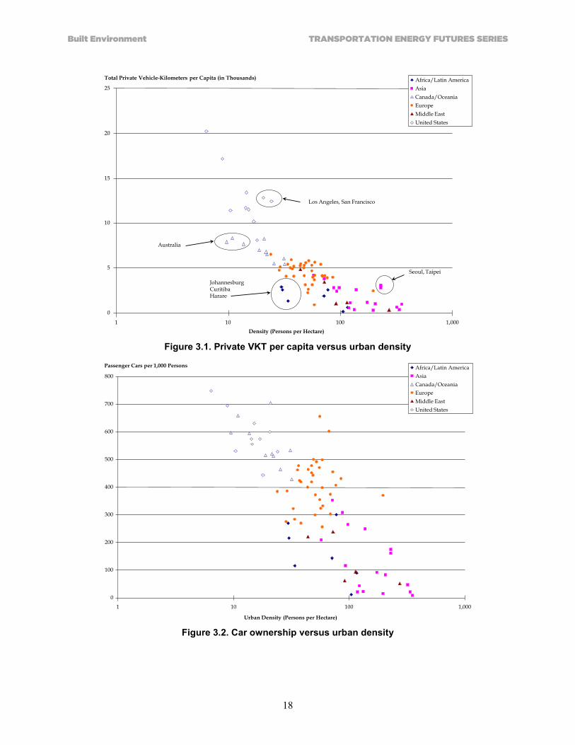
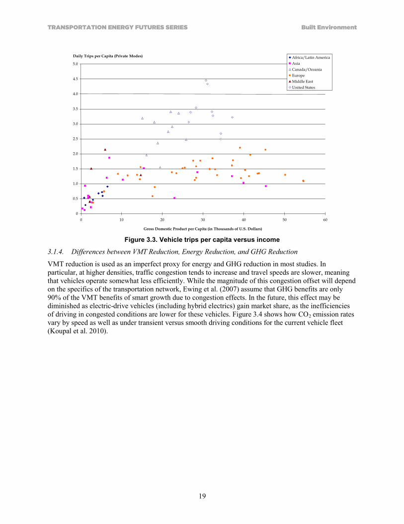
Cambridge Systematics, Inc. (EPA 2003) used data from the Millennium Cities Database to compare travel patterns, including vehicle-kilometers of travel (VKT) per capita, vehicle-trips per capita, and mode shares, against metropolitan-level variables including population density, income, and road supply (miles per capita).4 Figures 3.1 to 3.3 show a sample of these data, including private VKT per capita versus density (Figure 3.1), car ownership versus density (Figure 3.2), and daily private vehicle trips per capita versus income (Figure 3.3). As is evident from Figure 3.1, densities are strongly correlated with private vehicle travel. The United States, Canada, and Australia have the lowest densities and also the highest rates of private vehicle travel. Figure 3.2 illustrates a similar relationship between density and car ownership, although there are a number of European cities with car ownership rates approaching those of U.S. cities. Differences in auto ownership and VKT per capita are not just a function of income; Figure 3.3 illustrates that private vehicle trip rates are about twice as high in the United States as they are in European cities with similar incomes. The regression models developed for this research predicted different elasticities of VKT with respect to density, depending on the density (persons per hectare), infrastructure supply (freeway-kilometers per capita), and user cost (gross domestic product per-capita per car-kilometer). VKT was more sensitive to high densities, high user costs, and low freeway supply.
4 The Millennium Cities Database, assembled by Australian researchers Jeff Kenworthy and Felix Laube, contains aggregate (metropolitan-level) data on urban structure, the economy, transportation infrastructure, and travel characteristics in cities around the world. The database includes up to 200 indicators for each of 100 cities. The data are generally from the late 1990s (Kenworthy et al. 1999; UITP 2001).
Built Environment TRANSPORTATION ENERGY FUTURES SERIES
18
Total Private Vehicle-Kilometers per Capita (in Thousands)
Density (Persons per Hectare)
0
5
10
15
20
25
1 10 100 1,000
Australia
Los Angeles, San Francisco
JohannesburgCuritibaHarare
Seoul, Taipei
Africa/Latin AmericaAsiaCanada/OceaniaEuropeMiddle EastUnited States
Figure 3.1. Private VKT per capita versus urban density
0
100
200
300
400
500
600
700
800
1 10 100 1,000
Passenger Cars per 1,000 Persons
Urban Density (Persons per Hectare)
Africa/Latin AmericaAsiaCanada/OceaniaEuropeMiddle EastUnited States
Figure 3.2. Car ownership versus urban density
TRANSPORTATION ENERGY FUTURES SERIES Built Environment
19
0
0.5
1.0
1.5
2.0
2.5
3.0
3.5
4.0
4.5
5.0
0 10 20 30 40 50 60
Daily Trips per Capita (Private Modes)
Gross Domestic Product per Capita (in Thousands of U.S. Dollars)
Africa/Latin AmericaAsiaCanada/OceaniaEuropeMiddle EastUnited States
Figure 3.3. Vehicle trips per capita versus income
3.1.4. Differences between VMT Reduction, Energy Reduction, and GHG Reduction
VMT reduction is used as an imperfect proxy for energy and GHG reduction in most studies. In particular, at higher densities, traffic congestion tends to increase and travel speeds are slower, meaning that vehicles operate somewhat less efficiently. While the magnitude of this congestion offset will depend on the specifics of the transportation network, Ewing et al. (2007) assume that GHG benefits are only 90% of the VMT benefits of smart growth due to congestion effects. In the future, this effect may be diminished as electric-drive vehicles (including hybrid electrics) gain market share, as the inefficiencies of driving in congested conditions are lower for these vehicles. Figure 3.4 shows how CO2 emission rates vary by speed as well as under transient versus smooth driving conditions for the current vehicle fleet (Koupal et al. 2010).

Built Environment TRANSPORTATION ENERGY FUTURES SERIES
20
C02 (g/mile)700
650
600
550
500
450
400
350
300
250
2000 10 20 30 40 50 60 70 80
Average Speed Bin (mph)
Transient Driving Smooth Driving
Figure 3.4. Comparison of CO2 emission rates for transient versus smooth driving (Source: Koupal et al. 2010)
3.1.5. Effects of Alternative Fuel Sources and Federal Fuel Economy Standards on the Estimates Presented in This Report
In May 2010, the EPA and the National Highway Traffic Safety Administration adopted a set of new light-duty vehicle GHG emissions and fuel economy standards through 2016 consistent with California GHG emissions standards. In November 2011, the agencies proposed more stringent light-duty standards for the 2017 through 2025 model years, with equivalent miles per gallon (mpg) for the light-duty fleet (including passenger cars and light trucks) increasing from 36.6 in 2017 to 54.5 in 2025. In addition, the Federal Renewable Fuel Standard-2, the part of the Energy Independence and Security Act of 2007 that sets minimum production requirements for particular types of biofuels through the year 2022, aims to affect the mix of fuels used.
Energy use and GHG emissions are linked in a nearly one-to-one relationship assuming that continued use of existing petroleum-based fuel sources dominates the transportation sector. However, a switch to different fuel sources over time will change the relative petroleum savings or GHG benefit of a given unit of energy reduction. For example, the use of alternative fuels (such as biofuels, electricity, natural gas, and hydrogen) will lead to a corresponding decrease in petroleum use per unit of energy consumed (less any petroleum inputs used to produce the fuel). Alternative fuels will also have different GHG emissions per unit of energy consumed, with the specific effect depending on the characteristics of each fuel source and production pathway – usually (but not always) resulting in a decrease in GHG emissions per unit of energy.
The introduction of these new standards will have little effect on the relative impacts of built environment strategies on light-duty vehicle energy use and GHG emissions (i.e., on the percent change in energy and emissions from the strategies versus a projected baseline). However, they will have the effect of decreasing the benefits as expressed in absolute terms (gallons of gasoline, tons of CO2, etc.). For example, the nearly 50% increase in fuel efficiency over the 2017–2025 time period would, in the long term (roughly 2040 and beyond, after most of the fleet has turned over), reduce the absolute energy and GHG benefits of built environment strategies by about one-third, compared to estimates that were

TRANSPORTATION ENERGY FUTURES SERIES Built Environment
21
developed based on the 2012–2016 standard. Another way of looking at this is that energy and GHG reductions realized from built environment strategies would reduce the absolute benefits of fuel economy standards in proportion to the reduction in baseline emissions from built environment strategies.
3.2. Economic Impacts While there is an extensive body of literature on agglomeration effects and associated concepts of optimal city size, there has been very little research relating economic outcomes (such as growth, productivity, and wages) to measures of urban form. The Organisation for Economic Co-operation and Development (OECD) (2007) provides an overview of the expected effects on productivity of city size, density, and transportation costs. It notes that while there is general agreement on the phenomenon of economies of agglomeration (proximity to a greater number of workers, suppliers, customers, etc., that increases productivity), there is some disagreement as to whether city size or density is the primary driver of agglomeration economies and the resulting productivity improvements. They also note that it may depend on the measure, citing findings by Glaeser and Kahn (Glaeser and Kahn 2004) that aggregate density at the metropolitan area-level does impact variations in per capita income across cities, but the degree to which jobs are centralized in a central business district seems to be irrelevant.
A few U.S. studies link employment density and economic activity. Using county-level data on employment density and state-level data on productivity, Ciccone and Hall (1996) found that workers in the 10 densest states produced $38,782 of value annually, while those in the 10 least dense states produced only $31,578 in output—about 25% less—and attribute more than half the variance to employment density. Cervero (2000) found that compact, accessible cities with efficient transportation links were more productive than areas with more dispersed populations. Carlino (2001) links denser local economies to increased patenting activity, finding that patenting was significantly greater during the 1990s in regions with higher employment density (Muro and Puentes 2004).
A recent report by Kooshian and Winkelman (2011) and various reports by Litman synthesize a combination of research studies and more anecdotal evidence on the relationship between smart growth and economic development (Rodrique 2011). However, these reports are written from advocates’ perspectives and therefore provide a somewhat selective view on the topic. Kooshian and Winkelman cite evidence suggesting that smart growth neighborhoods have held property values much better than conventional sprawl development. For example, Cortright (CEOs for Cities 2009) finds a positive impact between walkability and home values in 13 of 15 U.S. markets studied. Similarly, access to transit has been shown to have a positive effect on property values in a number of cities. However, researchers have not linked smart growth or transit-oriented development to broader economic outcomes such as overall productivity or wealth creation, and property value impacts may reflect primarily a redistribution of value rather than a net increase.
From a theoretical standpoint, the effects of land-use patterns on the overall economy are unclear. These effects will depend on three factors:
1. Accessibility benefits – in particular, business access to workers, suppliers, and customers within a given travel time and the implications for business costs and productivity
2. Land costs, which affect the cost of doing business 3. Net infrastructure and transportation costs.
Under compact land use scenarios, land costs are likely to be higher, but infrastructure and transportation costs lower (as discussed below). The implications of compact land use for accessibility are not clear as there are two offsetting effects: greater proximity (which will increase accessibility) and greater congestion and lower travel speeds (which will decrease it). Overall the balance of these factors has not been well documented.

Built Environment TRANSPORTATION ENERGY FUTURES SERIES
22
3.3. Other Factors Energy is only one consideration in the potential impacts of built environment strategies. Many other factors are also influenced, and must be taken into account in assessing the costs, benefits, and viability of a built environment approach to energy and GHG savings.
3.3.1. Infrastructure and Other Municipal Costs
Urban form may affect infrastructure costs by affecting the amount of road, utility, and other public or private infrastructure needed. In some cases, it may also shift the balance of services provided between the private and public sectors. For example, some smart growth neighborhood designs provide greater amounts of public space (parks, play areas, etc.) at the expense of private yards.
There is good evidence that more compact development can lead to significant savings in infrastructure costs through reductions in the length of local roads and utility connections that must be provided (per dwelling unit). Burchell (2005) finds a potential 11% nationwide reduction in local road and water/sewer costs from a future scenario emphasizing compact development over sprawl, or $126 billion over the 2000–2025 timeframe. Table 3.5 shows Burchell’s estimated costs for water and sewer per new dwelling unit by type and location of unit. Attached and multifamily units are estimated to have costs 23% to 41% lower than detached units, and urban units to have costs 12% to 23% lower than suburban units. Table 3.6 shows local road costs by population density, as estimated from Burchell et al.’s (2002) 2000 cost functions. Costs at high urban densities (12,000 ppsm) are around one-third to two-thirds lower than costs at suburban densities in the range of 1,000 to 3,000 ppsm, with cost differences in the range of $600 to $2,000 per person.5
Table 3.5. Water and Sewer Costs per New Dwelling Unit
Percent Difference versus SF Detached
Location Single-Family
Detached Single-Family
Attached Multifamily Single-Family
Attached Multifamily
Rural (septic) $9,600
Suburban (package) $8,500 $5,755 -32%
Urban (public) $6,540 $5,050 $3,860 -23% -41%
Urban versus Suburban -23% -12%
(Source: Burchell 2005)
Finally, Burchell (2005) combines the local road and water/sewer costs with estimates of reduced land costs due to higher population densities. They conclude that total per unit housing development costs would average $154,000 under a compact growth scenario compared to $167,000 under a sprawl growth scenario, a difference of $13,000 per unit or 7.8%.6 The cost difference would increase to $16,000 in the 30 largest metropolitan areas. Nonresidential development costs would be only modestly impacted—about $900 lower under the compact scenario, or 1.1% on a base cost of about $75,000, as lower land and utility costs are outweighed by higher development costs.
5 Local road costs were calculated based on population density rather than dwelling unit type and cannot be presented in a format comparable to the water and sewer costs. 6 The authors imply that part of this cost difference would be due to smaller units, but do not explicitly show the contribution of this factor in their estimates. Their assumption for the price of a new home, while based on 2000 data, is similar to current conditions – about $170,000 in 2011 (National Association of Realtors, 2011).

TRANSPORTATION ENERGY FUTURES SERIES Built Environment
23
Table 3.6. Local Road Costs per Person
Population Density Range (ppsm)
Population Density (ppsm)
Approximate Units per
Residential Acre Developed
Areas Undeveloped
Areas
500-1,999 1,250 0.6-2.5 $2,619 $3,034
2,000-3,999 3,000 2.5-5.0 $1,592 $1,782
4,000-9,999 7,000 5.0-12.5 $1,229 $1,335
10,000 or more 12,000 > 12.5 $905 $962
(Source: Cambridge Systematics, Inc.) Calculations based on data on road costs as a function of population density as presented in Burchell et al. (2002). Units per residential acre (shown for comparison purposes only) are converted from ppsm based on 2.5 persons per unit and approximately 50% of land in residential use.
Scenario planning studies in locations such as Sacramento, Salt Lake City, and Charlottesville, Virginia, have also shown a significant reduction in regional road investment needs because of reduced traffic associated with compact development, although these savings are partially offset by the need for increased transit investment. For example, Envision Utah (FHWA 2000) found that a regional “quality growth” scenario would add $1.5 billion over 20 years in transit costs, but save $2.6 billion in regional road costs, for a net savings of $1.2 billion. Additional subregional infrastructure cost savings—including roads, water, and other utilities—would total $3.3 billion or 26%. These figures compare with a total regional and subregional infrastructure cost of about $26.5 billion under the baseline scenario, yielding a net savings of $4.5 billion or 17%. Table 3.7 compares subregional unit infrastructure costs by development density and type of development. The cost differences for infill or reuse versus raw development are in the same range as Burchell et al.’s (2002) compact-versus-sprawl ratio estimates for densities of 8 to 16 units per acre, although the disparity is somewhat larger with lower density developments. The proportion of single-family homes would decrease from 73% to 67% under the “quality growth strategy” (FHWA 2000), average single-family lot size would fall from 0.35 to 0.29 acres, and new developed area would fall by over half – from 325 to 154 square miles between 1998 and 2020.
Table 3.7. Unit Residential Infrastructure Costs by Density Group
Density (Dwelling Units per Acre)
Development Type
Raw Infill Reuse
4 $43,145 $25,101 $23,766
8 $19,015 $11,177 $12,226
16 $12,872 $8,864 $8,496
[Source: Envision Utah (FHWA 2000)]
The savings would accrue to local, state, and regional governments, as well as developers and consumers. However, some public-sector costs would increase—notably investment in transit and nonmotorized infrastructure. The overall impact on public infrastructure costs would depend on the specific program of investments in a given metropolitan area.
Achieving the benefits of infill development may in some cases involve the cleanup and reuse of “brownfields” sites (contaminated) or “greyfields” sites (subject to prior use). Greater short-term costs may be incurred by the public and/or private sectors for brownfields infill development, compared to a unit of “greenfields” development. Median brownfields cleanup costs run about $57,000 per acre according to a Center for Urban Economic Development study cited in Paull (2008). Land assembly, demolition of existing structures, and more involved permitting processes can also increase the costs of

Built Environment TRANSPORTATION ENERGY FUTURES SERIES
24
infill versus greenfields development. Cost differentials may require subsidies or tax incentives by government agencies to stimulate private investment in particular areas. For example, the City of Portland, Oregon, provides a residential tax exemption for qualifying new construction in transit station areas.
Research has found only very weak evidence of a connection between urban form and non-infrastructure fiscal costs, such as budgets for schools, trash collection, emergency services, etc. For example, Burchell (2005) estimated a reduction in municipal services costs of 3% nationwide for a compact growth versus sprawl scenario in 2025. There seem to be both economies and diseconomies in municipal services provision associated with density, and the variation in service costs due to other factors can overwhelm the small differences due to urban form when analyzed in the aggregate.
3.3.2. Housing Affordability
Housing affordability has been an issue of interest specifically in relationship to growth management policies, which may attempt to direct urban form by containing urban development within a set boundary. To the extent that such policies constrain the supply of land, consumers and businesses may experience higher land costs and therefore higher home prices and rental rates. Growth management policies have been most strongly implemented in Oregon, which has required metropolitan areas to adopt and enforce urban growth boundaries for over three decades.
Some have argued that growth management laws have had significant impacts on affordability. For example, Staley and Gilroy (2001) conclude that Florida’s Growth Management Act (GMA) may have contributed to a 15% decline in affordability between 1994 and 2000, and that Washington State’s GMA may have added about 0.7 percentage point to the housing inflation rate for each year that a county had a comprehensive plan in place. Other studies, however, have found that growth management effects are minor after controlling for other factors. For example, an analysis of the urban growth boundary in Portland, Oregon, found that the boundary has created upward pressure on housing prices, but the effect is relatively small in magnitude, contributing no more than $10,000 compared to an overall cost appreciation of $144,000 over their study period (Phillips and Goodstein 2000). A broader literature review concluded that market factors, including increased housing demand, increased employment, and rising incomes are much more significant influences; and furthermore, that policy changes to allow increased densities and smaller units have mitigated any affordability impacts by allowing housing supply to be increased within the growth boundary (Nelson, Pendall, and Dawkins 2002).
3.3.3. Combined Housing and Transportation Costs
The Housing and Transportation Affordability Index, developed by the Center for Transit-Oriented Development (CTOD) and the Center for Neighborhood Technology (CNT), provides information on how the combined cost of housing and transportation varies among different neighborhoods. The index considers vehicle ownership, vehicle operating, and transit fare costs. Costs per household are modeled based on seven local built environment variables (households per residence and acre, average block size, transit connectivity, distance to employment centers, job density, and service job density) and two household variables (income and size). VMT and auto ownership are modeled as a function of these variables using Census and NHTS data, and costs associated per vehicle and per mile (CTOD 2006). A limitation of the index is that it does not take into account public sector costs for the provision of transit service, which are paid broadly by individuals through taxes.
CNT notes that places with access to services, walkable destinations, extensive and frequent transit, access to jobs, and density have lower household transportation costs. An example from the Washington, D.C., region is illustrative. A central-city neighborhood (Logan Circle) has higher housing costs than outlying neighborhoods in Prince George’s and Loudon County, with housing costs representing 32.4% versus 29.6% and 28.8%, respectively, of area median income. However, household transportation costs are much lower in Logan Circle – 10.9% versus 18.7% or 20.8% of area median income, respectively, a

TRANSPORTATION ENERGY FUTURES SERIES Built Environment
25
savings of $5,000 to $6,000 per year. The net effect is a cost savings in the central city of over 6% of area median income (CTOD 2008).7
3.3.4. Traffic Safety
Some researchers have identified safety benefits from compact growth patterns. Land-use patterns affect traffic safety in three primary ways: 1) overall traffic speeds (which affect the severity of crashes); 2) street network design (which affects the opportunities for traffic conflicts which may lead to crashes); and 3) the amount of travel by different modes (which affects exposure to risk of a crash). More densely populated areas are often more congested, leading to lower traffic speeds and therefore fewer severe crashes. They also can result in lower VMT and hence lower motorized crash risk. On the other hand, they often have more interconnected street networks (creating more opportunities for conflict) and may have higher rates of walking and bicycling, which are higher-risk travel modes.
Transportation engineering practice in the latter half of the 20th century was to reduce the number of four-way intersections and channel traffic out of subdivisions, shopping areas, etc., onto main roads via a very limited number of access points. This was expected to reduce crashes by reducing the number of conflict opportunities, as well as congestion. However, this was done in conjunction with the establishment of higher-speed, higher-capacity arterial roadways, which are also unfriendly to nonmotorized travel. Recent research, however, has increasingly questioned the benefits of conventional (post-World War II) traffic design practices. For example, Ewing, Pendall, and Chen (2002) find that U.S. metropolitan areas with high levels of sprawl have higher traffic fatality rates than nonsprawling regions. Kim and Yamashita (2002), examining data from Hawaii, find that higher population densities are associated with lower crash rates. Dumbaugh and Rae (2009), using data from San Antonio, find that neighborhoods with traditional design features (higher densities, pedestrian-oriented retail uses, interconnected streets) have fewer serious crashes than suburban neighborhoods. Marshall and Garrick (2011), using data from 24 California cities, conclude that denser street networks with higher intersection counts per area are associated with fewer crashes across all severity levels. However, increased street connectivity (as well as additional travel lanes along the major streets) correlated with more crashes.
3.3.5. Public Health
In addition to traffic safety, other public health benefits may be realized from due to higher levels of physical activity from walking, bicycling, and mass transit use. Researchers that have studied the link between urban design and nonmotorized or active travel have made an additional linkage with health benefits. Transportation Research Board and Institute of Medicine (2005) find that the built environment can facilitate or constrain physical activity, although the relationship is complex, with many other mediating factors (such as safety and security, and personal characteristics). Frumkin, Frank, and Jackson (2004) note higher neighborhood densities, mixed uses, and pedestrian-friendly environments as factors that can encourage physical activity. In a study of the Atlanta region, Goldberg et al. (2007) find that people who live in neighborhoods with the lowest walkability drive an average of 30% more than those who live in areas with the highest walkability. Residents of the most walkable areas of the region are 2.4 times more likely to get the level of activity necessary to maintain health. People who live in neighborhoods with a mix of shops and businesses within easy walking distance are 7% less likely to be obese than those living in a mix level equal to the lower regional average. Benefits are realized from transit use as well as purely nonmotorized trips; for example, Morency, Trépanier, and Demers (2011) find that on average, a round-trip via transit in Montreal involves 2,500 steps, which account for 25% of the recommended volume of physical activity per day.
Access to recreational opportunities, such as trails and parks, also affects engagement in physical activity. For example, a statewide survey in Georgia found that people who lived within 10 minutes’ walk of a
7 Median income is based on the area covering Washington, D.C., Maryland, Virginia, and West Virginia.

Built Environment TRANSPORTATION ENERGY FUTURES SERIES
26
park had a 52% probability of meeting physical activity recommendations, compared to 37% for people without such access (Powell, Martin, and Chowdhury 2003).
A potential negative public health effect of increased density is greater exposure to air pollution. Even if overall air pollutant emissions decrease because of VMT reductions, concentrated land use has the effect of concentrating air and water emissions in areas of potentially greater population exposure. While this issue has not been widely studied, an analysis in the Salt Lake City region found that a “quality growth strategy” reduced mobile source emissions by 7.3% and total emissions by 3.5% in 2020, yet showed a small negative impact on indices of the concentration of emissions and their distribution with respect to population (FHWA 2009). Hankey, Marshall, and Brauer (2012) examined the impacts of both physical activity and air pollution on the incidence of heart disease in southern California neighborhoods with different levels of walkability. The impacts of the two factors were both modest and roughly offsetting, with residents of high-walkability neighborhoods showing seven fewer deaths per 100,000 per year due to higher physical activity, nine more deaths per 100,000 per year due to higher levels of particulate matter, and three fewer deaths per 100,000 per year due to lower levels of ozone.
3.3.6. Environmental Benefits
Regional scenario modeling has found reductions in air pollutant emissions generally consistent with the VMT reductions from alternative growth strategies. Compact growth patterns also should reduce land conversion for urban uses, helping preserve agricultural land, forests, open space, wetlands, and species habitat. For example, the Seattle region’s VISION 2020, adopted in 1990, was forecast to reduce loss of open space from 750 square miles under trend conditions to 400 square miles under a preferred alternative focusing growth in centers and within an urban boundary (Puget Sound Council of Governments 1990). Regional planning studies in other areas have found similar land preservation benefits from compact development scenarios.
3.3.7. Consumer Welfare
A variety of other social benefits and ills have been assigned to sprawl versus compact land-use patterns (Burchell et al. 2002). For example, some have argued that land-use controls could reduce consumer welfare by constraining consumer choice (e.g., requiring smaller dwelling units and/or yards). To the extent that land-use policy changes simply accommodate latent market trends for more compact development, this should not be a concern. However, more aggressive policy changes that restrict where people live could potentially lead to welfare losses. Others have postulated that social benefits, including increased social capital, can result from traditional neighborhood design and walkable communities (Rogers et al. 2011). The factors that influence residential and neighborhood quality are complex, and there is not a consensus on the extent to which compact land use may increase or decrease overall social welfare.
A study by Rodier et al. (2010) is one of the few studies of the overall welfare impacts of urban growth scenarios. The study uses an integrated transportation and land-use model to evaluate the equity impacts (travel time and cost effects across income groups) of a business-as-usual versus “Blueprint” compact growth scenario in the Sacramento region. The study finds an overall 10% decrease in the percent of income dedicated to transportation under the Blueprint scenario, as well as a decline in average rents due to a greater supply of multifamily housing. The cost of living also decreases, but net wages decrease as well.
3.3.8. Equity and Environmental Justice
To the extent that urban growth patterns support transit access and reduce vehicle trip lengths and vehicle ownership and use costs, low-income populations would benefit through greater access to jobs and services and lower transportation costs. On the other hand, low-income populations may be negatively impacted if housing costs are higher in more compact regions (see discussion above) or if they are priced out of the most accessible locations.

TRANSPORTATION ENERGY FUTURES SERIES Built Environment
27
Rodier’s evaluation of the Sacramento growth scenarios also examines the distribution of impacts among income groups. The study finds that the Blueprint scenario leads to a net increase in consumer surplus except for higher-income groups, who are less willing to switch to higher-density dwellings, are more likely to own their own homes, and more affected by wage decreases.

Built Environment TRANSPORTATION ENERGY FUTURES SERIES
28
4. ANALYSIS METHODS
This section reviews 11 analysis methods and ways to assess relationships between transportation and land use. The scope of this section was selected based on authors’ judgment and in consultation with stakeholders on methods of greatest potential interest, and may not be comprehensive of all potentially relevant methods. Assessment of methods relies upon Cambridge Systematics’ judgment and unpublished knowledge, as well as published literature. Most of these analysis methods are directed at measuring the impact of land use and the built environment on travel. One particular category (transportation–land-use models) is directed at measuring the impacts of transportation and land use, or capturing feedback relationships. While few of the methods measure energy impacts directly, travel outputs can be easily combined with energy and emissions models or factors to develop energy and GHG estimates. The extent of use of these tools and methods is summarized in Table 4.1. Each method is then described in detail, including:
• Developer/owner
• Examples of specific models
• Intellectual property and transparency
• Contact person
• Major inputs
• Major outputs
• Overview of methodology
• Scope (geographic, temporal, modal, vehicle, and fuel type)
• Strengths and weaknesses for energy scenario analysis
• Additional resources.
Table 4.1. Summary of Tools and Methods for Assessing Travel, Energy, and GHG Impacts of Urban Form
Tool or Method Description Best Uses Extent of Use
“Four-Step” and Other Travel Demand Models
Regional-scale network models used to forecast flows based on socioeconomic projections and alternative transportation networks
Testing impact of regional or subregional reallocation of growth and major transportation network changes on travel Providing baseline travel data for a particular area
In use by nearly all metropolitan planning organizations (MPOs) and some state departments of transportation (DOTs)
Transportation–Land-Use Models
Regional-scale models used to predict land development in a region over time, based on socioeconomic forecasts, transportation networks and accessibility, and other factors
Forecasting general effects of land-use policies and transportation investments on land-use patterns, and resulting travel impacts, at a regional scale
Developed and applied by a few state and regional transportation agencies and academics
4-D Methods Application of “4-D” elasticities to model changes in travel as a function of changes in land-use variables
Sketch-level assessment of travel impacts of neighborhood-level built environment changes (often used in conjunction with four-step models or scenario planning tools)
Applied by a few MPOs to enhance four-step models

TRANSPORTATION ENERGY FUTURES SERIES Built Environment
29
Tool or Method Description Best Uses Extent of Use
Land-Use Scenario Planning Tools
GIS-based tools primarily designed to assist planners and stakeholders with development and analysis of alternative land-use scenarios at a site, community, or regional level
Sketch-level assessment of travel impacts of neighborhood-level built environment changes Creating inputs (land-use changes) to a regional travel demand model
Sometimes used by MPOs; more often applied at local level for community planning
Municipal Transportation and Greenhouse Gas (MUNTAG) Model
Web-based tool, based on aggregate data (e.g., urban density and infrastructure provision), intended to help Canadian municipalities estimate their current transportation emissions, set future targets, and run forecasting scenarios
Useful as a screening tool for strategy analysis at a municipal level
Unknown if applied in United States
Moving Cooler Method Based on CUTR VMT Forecasting Model
Model for assessing urban form impacts on VMT based on population distribution in different density classes
Sketch-level assessment of impacts of population growth at different densities on overall travel
Used for a few research studies
Housing and Transportation Affordability Index
Calculator of average household-level travel based on multidimensional regression analysis of household and built environment variables
Currently available via web interface to examine average estimated household transportation costs, VMT, and GHG by census tract
Unknown
NHTS Last conducted in 2009, a nationwide survey that provides comprehensive data on travel and transportation patterns at the aggregate and household levels
Data source for disaggregate analysis of travel and vehicle ownership patterns in relationship to personal, household, and location characteristics
Widely used for travel analysis
Structural Equations Modeling
Statistical technique for testing and estimating causal relations using a combination of statistical data and qualitative causal assumptions
Can be used to examine causal effects/linkages among aggregate-level built environment, transportation, and other variables
Sometimes used for travel analysis
Discrete and Discrete-Continuous Choice Models
Statistical technique for modeling choices (vehicle ownership, mode choice, destination choice, etc.) at an individual or household level
Analysis technique that can be applied to model individual and household-level choices from disaggregate datasets
Widely used for travel analysis, especially mode choice
Life-Cycle Assessment Methods
Technique to assess environmental impacts associated with all the stages of a product or system’s life
Concept that allows expansion of benefits examined beyond transportation operating emissions and to include construction, maintenance, buildings, etc.
Sometimes used for transportation analysis
4.1. “Four-Step” and Other Travel Demand Models Overview: These models are used in regional and project-level planning to forecast transportation network flows and traffic conditions based on socioeconomic projections (population, households, jobs by type) and alternative transportation networks and facility characteristics.
Developer/Owner: Typically developed and applied by state and regional departments of transportation (DOTs) and metropolitan planning organizations (MPOs) using commercially available software. All MPOs are required to maintain travel demand forecasting models for use in transportation planning and, if needed, air quality analysis.

Built Environment TRANSPORTATION ENERGY FUTURES SERIES
30
Examples of Specific Models: TransCAD, TP+, CUBE, EMME/2 (software platforms).
Intellectual Property Rights and Transparency: Software platform is typically licensed for use by public agency. Input data and methods are documented in the public domain.
Contact Person: Typically state DOT and MPO travel forecasting staff, sometimes consultants.
Major Inputs: Highway and transit networks, socioeconomic and demographic projections by TAZ, various behavioral parameters (e.g., trip generation rates by household type, mode choice coefficients).
Major Outputs: Traffic volumes and speeds by network link (which can be summarized at a subarea- or regional-level); trips, VMT, and passenger-miles of travel by mode. VMT and speed outputs can be used in conjunction with emission factor models or fuel consumption rates to estimate energy and GHG.
Overview of Calculations: “Four-step” models are commonly used: 1) trip generation (number of trips by time period by TAZ); 2) trip distribution (trip flows between TAZs); 3) mode choice; and 4) traffic assignment (assign flows to routes on network). More sophisticated models may have feedback between various steps, additional steps such as auto ownership, etc.
Scope:
• Temporal – Typically run for a base year and one or more future years up to 20 to 25 years out for long-range planning purposes.
• Geographic – Typically metropolitan or statewide. May be used at a smaller scale (e.g., corridor).
• Modal, Vehicle, Fuel – Always highway, sometimes transit, occasionally bike/pedestrian. Multimodal models are more common in larger metro areas. Vehicle and fuel choices are not modeled.
Strengths and Weaknesses for Energy Scenario Analysis:
• Strengths – These models are the accepted state of practice for regional transportation modeling at a network level. Their greatest value for land-use/urban form analysis is to test changes in regional land-use patterns (e.g., focus on infill, transit corridors, or activity centers), by changing the distribution of future population and employment amongst TAZs. Such changes can be analyzed in combination with alternative transportation networks.
• Weaknesses – The capability of most models to test local-scale urban form characteristics (mix of uses, pedestrian design, etc.) is very limited and often nonexistent. Some models include nonmotorized mode choice but only a few have been enhanced to be sensitive to the effects of nonmotorized infrastructure improvements. However, techniques such as “4-D” postprocessors can be used in conjunction with travel model output to estimate the travel and resulting emissions impacts of changes to the various land use-related “D” metrics (e.g., density, diversity, design, destination accessibility). Not all models fully incorporate feedback relationships (e.g., how changes in transportation conditions may affect land-use patterns which then further affect transportation).

TRANSPORTATION ENERGY FUTURES SERIES Built Environment
31
Resource Notes:
California Department of Transportation (2007). Assessment of Local Models and Tools for Analyzing Smart-Growth Strategies provides a discussion of travel demand model strengths, limitations, and enhancements specifically with respect to smart growth and nonmotorized travel. Prepared for California Department of Transportation by DKS Associates, University of California at Irvine et al.
4.2. Transportation Land-Use Models Overview: These models are used to predict land development in a region over time, based on socioeconomic forecasts, transportation networks and accessibility, and other factors. They are typically integrated with travel demand models to allow feedback between land-use changes and travel demand.
Developer/Owner: Developed and applied by a few state and regional transportation agencies (DOTs and MPOs) using commercially available software; applied in some areas by academics for research purposes.
Examples of Specific Models: PECAS, UrbanSim, TRANUS.
Intellectual Property Rights and Transparency: Software platform is typically licensed for use by public agency. Input data and methods are documented in the public domain. Some software is open-source (e.g., UrbanSim).
Contact Person: State DOT and MPO travel forecasting staff, consultants, or academic (model developers).
Major Inputs: Highway and transit networks, socioeconomic and demographic projections by TAZ; various land-use parameters (e.g., land values, land-use types, existing zoning, built densities); various behavioral parameters (e.g., trip generation rates by household and industry type, mode choice coefficients, developer choice, location choice).
Major Outputs: Future year land-use (type and intensity) by parcel or subarea; traffic volumes and speeds by network link; trips, VMT, and passenger-miles of travel by mode.
Overview of Calculations: Different models have been developed that operate in different ways, with the most significant distinction being aggregate versus disaggregate (individual-level) modeling of locational and development decisions. The trend is towards disaggregate modeling with very detailed land-use data (e.g., parcel or grid-cell). The models may have a built-in transportation network that is typically at a coarser level than the regional travel demand model, or they may be used in conjunction with the regional model.
Scope:
• Temporal – Typically run for a base year and one or more future years up to 20 to 25 years out for long-range planning purposes. Feedback often performed in 5-year increments.
• Geographic – Typically metropolitan or statewide. Outputs have not been found to be reasonably calibrated at less than a county level.
• Modal, Vehicle, Fuel – Highway and transit. Vehicle and fuel choices are not modeled.
Strengths and Weaknesses for Energy Scenario Analysis:
• Strengths – The most sophisticated tools in existence for analyzing the impacts of transportation choices, as well as other policy factors such as zoning or prices, on land development patterns and resulting feedback to transportation conditions and impacts.
• Weaknesses – Resource-intensive to develop and apply. Only a few areas have developed integrated transportation and land-use forecasting models that are highly sensitive to transportation

Built Environment TRANSPORTATION ENERGY FUTURES SERIES
32
improvements as well as to a variety of land-use policies, and even these models are not fully developed in most cases.
Resource Notes:
Forecasting Indirect Land Use Effects of Transportation Projects, which was prepared for American Association of State Highway and Transportation Officials, supplements National Cooperative Highway Research Program Report 466 by providing additional and updated guidance on the use of land-use forecasting methods (Avin et al. 2007).
Land-use models to evaluate the feasibility of urban plans are being developed based on insights into the tradeoffs between size, shape, and functionality of urban environments. Understanding the impacts of climate change, managing sprawl, as well as other economic and sociological problems can be informed by the science of a city’s size, shape, and networks, and the effect of each of these on the underlying functionality of the city (Batty 2008).
A report by Iacono et al. summarizes the history and practice of modeling the relationships between transportation and land-use change, with a focus on land-use models that capture the effects of transportation networks as well as other factors (Iacono, Levinson, and El-Geneidy 2008).
A core practitioners’ guidance document, prepared by Louis Berger and Associates for the National Cooperative Highway Research Program, provides information and guidance on the various methods available for land-use forecasting (National Cooperative Highway Research Program 2002).
4.3. 4-D Methods Overview: This method applies “4-D” elasticities (travel elasticities with respect to land-use density, diversity, design, and destination accessibility) to model changes in travel (VMT, vehicle-trips, or mode shares) as a function of changes in land-use variables. Sometimes used to post-process travel demand model data which provides baseline information on VMT and vehicle-trips by subarea.
Developer/Owner: Reid Ewing; Fehr & Peers Associates; others.
Examples of Specific Models: An early version (using 3 Ds) was operationalized in EPA’s Smart Growth INDEX model. Fehr & Peers has developed a spreadsheet tool to adjust trip generation and VMT estimates from local or national sources to account for smart growth and sustainable development practices using the 4 Ds.
Intellectual Property Rights and Transparency: The approach is based on publicly available data and is documented.
Major Inputs: Baseline trip rates and VMT; percent changes in land-use density, diversity, design, and destination accessibility at a neighborhood level (census tract, TAZ, etc.) under hypothetical scenarios.
Major Outputs: Changes in trip rates and VMT as a result of changes in land-use characteristics.
Overview of Calculations: Simple application of elasticities to baseline values and percent changes input variables.
Scope:
• Temporal – Can be applied for any current or hypothetical future year for which baseline travel and land-use changes can be provided.
• Geographic – Intended for application at small-area level (neighborhood, tract, TAZ for use with travel demand models); results can be aggregated across areas.
• Modal, Vehicle, Fuel – Usually focused on VMT and vehicle-trips, but could be applied to predict transit and nonmotorized trips as well.

TRANSPORTATION ENERGY FUTURES SERIES Built Environment
33
Strengths and Weaknesses for Energy Scenario Analysis:
• Strengths – Simple procedure to estimate impacts of micro-scale urban design features that are not captured well in regional travel demand models.
• Weaknesses – Elasticities assume that a given percent change in one variable (land use) always leads to the same percent change in another variable (travel). Does not account for regional structure, travel costs, or other contextual factors that may influence how much a local land-use change affects travel. The 4-D metrics (e.g., design index) can vary and the data underlying the elasticities is not always robust.
Resources Notes:
A presentation by Fehr & Peers et al. compares 4-D spreadsheet adjustments with other tools including scenario planning tools and travel demand models as described elsewhere in this review (Washington State Department of Commerce 2009).
Ewing and Cervero review estimates of the 4-D elasticities from the literature (Ewing and Cervero 2010).
4.4. Land-Use Scenario Planning Tools Overview: These geographic information systems -based tools are primarily design to assist planners and stakeholders with the development and analysis of alternative land-use scenarios at a site, community, or regional level.
Models and Developers/Owners: Smart Growth INDEX is freely available from the EPA. PLACE3S is available from the California Energy Commission. Other models can be licensed from private developers: INDEX (including Paint the Region and Plan Builder) from Criterion Planners, CommunityViz from Placeways, CorPlan from Renaissance Planning Group, Envision Tomorrow from Fregonese Associates, and MetroQuest from Envision Sustainability Tools Inc.
Intellectual Property Rights and Transparency: Most of these models are maintained, licensed, and customized by private developers for use by public agencies. Assumptions and methods are generally documented, although ease of obtaining documentation may vary.
Major Inputs: Typically detailed land-use and transportation data such as existing and planned land use by parcel, street and sidewalk networks, locations of transit stops, etc.
Major Outputs: A wide variety of community indicators related to transportation, land use, the environment, and other issues. These may include VMT per capita or household, fuel consumption, and GHG emissions, along with other factors such as population density, percent population within one-quarter mile of transit, impermeable surface area, economic indicators such as rate of return on a parcel, etc.
Overview of Calculations: The models typically estimate changes in VMT based on elasticities, or relationships between factors such as population density, land-use mix, and pedestrian design and vehicle-travel, calculated at a small-area/neighborhood level.
Scope:
• Temporal – May be run for any base or future year for which land-use inputs are provided.
• Geographic – Often used at a site or neighborhood level; sometimes applied at a regional scale.
• Modal, Vehicle, Fuel – Produces changes in vehicle-trips and VMT; transit and pedestrian indicators (but not ridership forecasts). Vehicle and fuel choices are not modeled.

Built Environment TRANSPORTATION ENERGY FUTURES SERIES
34
Strengths and Weaknesses for Energy Scenario Analysis:
• Strengths – These tools can be of value in creating inputs (i.e., in the form of land-use changes) to a regional travel demand model that can be used for GHG emissions analysis purposes. Some can also estimate energy use and GHG emissions from buildings as well as transportation sources, taking into consideration factors such as building density, orientation, floor space, and mix of housing types.
• Weaknesses – They are relatively data-intensive to set up, in particular, requiring detailed land-use data, and (except for EPA’s Smart Growth INDEX) are not intended for evaluating transportation network changes. Estimates of VMT, transportation energy, and GHG produced within the model tend to be relatively simplistic because they usually do not account for the regional context of the development, which tends to have a greater impact on vehicle-travel and GHG emissions than the characteristics of an individual development.
Resource Notes:
The publication Urban Planning Tools for Climate Change Mitigation (Policy Focus Report) provides an overview of land-use scenario planning tools along with some case studies of their application relevant to GHG reduction (Condon, Cavens, and Miller 2009).
The FHWA web site includes several case studies and examples of scenario planning and visioning projects using these and other geographic information system-based tools (Energy Information Administration 2010).
4.5. Municipal Transportation and Greenhouse Gas (MUNTAG) Model Overview: This model is intended to help municipalities estimate their current transportation emissions, set future targets, and run forecasting scenarios.
Developer/Owner: MUNTAG was developed by the Sustainable Infrastructure Group at the University of Toronto, Canada.
Intellectual Property Rights and Transparency: Web-based “black box” tool available for use by Canadian municipalities. Model is documented by Derrible et al. (Derrible et al. 2010).
Major Inputs: Gross domestic product, population density, number of vehicles, transit miles, bicycle lanes, financial policies including gasoline/parking prices, tolls, and taxes.
Major Outputs: Per capita travel measures and total GHG emissions from the movement of people in an urban municipality. The primary output is passenger-kilometers traveled (per capita), which is transformed into VKT (per capita) and subsequently GHG emissions.
Overview of Calculations: The model is divided into five strategies, which are examined separately and then integrated to provide total GHG emissions from transportation with and without financial policies such as tolls or taxes. Per capita passenger-kilometer traveled in various modes is calculated. Potential impacts of financial policies are then calculated. Vehicle technology change can then be modeled by changing the emissions factors of vehicles and the results can be compared to the base case.
Scope:
• Temporal – Can be used to address current GHG emissions and future scenarios. A Toronto-based case study examined a current metro system and 15- and 25-year plans.
• Geographic – An urban municipality.
• Modal, Vehicle, Fuel – Private automobiles, transit, and bike travel. Vehicle and fuel characteristics can be adapted to account for technological change.

TRANSPORTATION ENERGY FUTURES SERIES Built Environment
35
Strengths and Weaknesses for Energy Scenario Analysis:
• Strengths – Useful as a screening tool or for strategic analysis. Low input requirements and ease of use make it accessible to a wide range of municipalities, including small municipalities that do not have the data to use other methods.
• Weaknesses – Aggregation bias and need for standardization among municipalities. Only available for Canadian municipalities.
Resource Notes:
The “Macroscopic Model of Greenhouse Gas Emissions for Municipalities” article provides an overview of the scope and methodology of the MUNTAG model, as well as an application to the City of Toronto (Derrible et al. 2010).
The Carbon Neutral City Planner Web Tool (2011) is available for building and assessing carbon mitigation strategies.
4.6. Moving Cooler Method Based on CUTR VMT Forecasting Model Overview: This is a sketch-level model for assessing urban form impacts on VMT at an aggregate (regional) level, based on population distribution in different density classes.
Developer/Owner: C. Porter, Cambridge Systematics, Inc., using data from the CUTR VMT Forecasting Model (Polzin and Chu 2007).
Intellectual Property Rights and Transparency: Public data sources and documentation.
Major Inputs: Existing population and percent population growth by five density classes (census tract persons per square mile) consistent with density classes used in reporting NHTS survey results for 2001 (U.S. DOT 2009).
Major Outputs: VMT per capita.
Overview of Calculations: VMT is calculated based on VMT per capita by population size in five population density classes.
Scope:
• Temporal – Through 2050; operationalized for 2020, 2030, and 2050 time horizons.
• Geographic – Applied at the national, state, and regional levels using census tract-level population distributions.
• Modal, Vehicle, Fuel – On-road passenger travel only, does not address vehicle/fuel issues.
Strengths and Weaknesses for Energy Scenario Analysis:
• Strengths – Easy to use, sketch-level method; accounts for different growth rates among regions, as well as redevelopment.
• Weaknesses – Population density distributions are the only urban form variable affecting VMT – assumes that density serves as a proxy for other factors such as walkability, transit access, worksite accessibility, mix of uses, etc.
Resource Notes:
Porter, in a report presented at the 2009 Air Quality Conference in Denver, presents an overview of the modeling approach and compares results for the United States (from the Moving Cooler study), three states, and the southern Maine region (Porter 2009).

Built Environment TRANSPORTATION ENERGY FUTURES SERIES
36
4.7. Housing and Transportation Affordability Index Overview: The model calculates travel on the household level based on a multidimensional regression analysis of household and built environment variables. This model is then used to calculate a variety of statistics, including per acre and per household levels of GHG emissions based on household auto use. Users can compare region-specific versus national data on typical or moderate households using a visual interface tool on the CNT web site CTOD (2006).
Developer/Owner: The Housing and Transportation Affordability Index was developed by the CNT and its collaborative partner, the CTOD, as a project of the Brookings Institution’s Urban Markets Initiative.
Intellectual Property Rights and Transparency: U.S. Census, NHTS, and other publicly available data sets. Details of the models on which the interface is built are publicly available.
Major Inputs: Census block-level data on household variables such as income and size; information on vehicle ownership and use; and built environment variables including gross density, residential density, average block size, transit connectivity, and employment access.
Major Outputs: The major output of the model is the cost of transportation, but other outputs include GHG emissions from transportation.
Overview of Calculations: The household transportation model is based on a multidimensional regression analysis, in which a formula describes the relationship between three dependent variables (auto ownership, auto use, and transit use) and nine main independent household and local environment variables. The output is transferred to a map-based graphical interface that can be used to compare between output measures.
Scope:
• Temporal – Provides a snapshot of current conditions (currently 2000 census data and 2001 NHTS data).
• Geographic – Region-specific, within and surrounding major U.S. population centers.
• Modal, Vehicle, Fuel – indicates transit and auto trips, but does not disaggregate within these categories.
Strengths and Weaknesses for Energy Scenario Analysis:
• Strengths – Comparison at the census block level of different factors, including factors based on density and factors based on household characteristics. The visual interface allows for modeling both dependent and output variables of the model.
• Weaknesses – Not available for predictive modeling, or for comparison between regions.
Resource Notes:
Haas et al. (2008) documents at a high level the process of developing the H+T affordability index, but is noted by the CNT to be out of date.
4.8. Analysis of the National Household Travel Survey Overview: The NHTS provides comprehensive data on travel and transportation patterns at the aggregate and household levels. Information from the survey can be transferred to a specific geographic area (census tract or traffic analysis zone level) using the Oak Ridge National Laboratory (ORNL) NHTS Transferability tool. The dataset can be used to calculate and make predictions about VMT and CO2 emissions for an area of interest.

TRANSPORTATION ENERGY FUTURES SERIES Built Environment
37
Developer/Owner: U.S. DOT and ORNL; analysis is typically done by consultants and academics, often in conjunction with public agencies.
Examples of Specific Models: The ORNL model to transfer region-specific data is publicly available on the NHTS web site (U.S. DOT 2009). A specific model to calculate VMT and GHG emissions at the household and neighborhood level was developed by Nancy McGuckin for the Pasadena DOT (McGuckin 2011).
Intellectual Property Rights and Transparency: NHTS and ORNL transferability data are publicly available, and many analysis methods are publicly documented.
Major Inputs: NHTS data at the municipality or regional level. Inputs related to the built environment include residential density (tract level), city size, and perceived access to transit.
Major Outputs: VMT and GHG emissions at the per capita, household, neighborhood, or municipality level.
Overview of Calculations: NHTS data is separated into region-specific data using the ORNL transferability tool and analyzed in order to calculate disaggregate VMT and GHG emissions. “What if” scenarios can be developed to analyze the impacts of policy change on the output measures.
Scope:
• Temporal – Can be used to assess current impacts. 2009 NHTS data available, but currently only 2001 NHTS data currently are available with the ORNL tool.
• Geographic – Can be applied to any U.S. region.
• Modal, Vehicle, Fuel – All modes and vehicle choices included in the NHTS survey can be analyzed. Effects of technology change or vehicle choice can be estimated using “what if” scenarios.
Strengths and Weaknesses for Energy Scenario Analysis:
• Strengths – Publicly available, comprehensive data can provide information on current trends and VMT or emission levels at a municipality or regional level. Data has some flexibility to be combined with regional- or vehicle-specific emissions levels.
• Weaknesses – ORNL transferability tool currently only available for 2001 data. Difficult to model changes over time, or in changes to the built environment (i.e., transit-oriented development).
Resource Notes:
The “Transferring 2001 National Household Travel Survey” document contains information about the transferability tool and the process through which this tool was developed for use with NHTS data (Hu, Reuscher, and Schmoyer 2007).
4.9. Structural Equations Modeling Overview: Structural equations modeling is a statistical technique for testing and estimating causal relations using a combination of statistical data and qualitative causal assumptions. It was used in the Growing Cooler study to examine macro-level relationships between urban form, transportation infrastructure, and travel, and implications for GHG emissions. Differences between municipalities/regions and changes to a municipality/region over time are modeled with this technique.
Developer/Owner: Structural equations modeling is a commonly used statistical method. The Growing Cooler study was published by the Urban Land Institute, and authored by Reid Ewing, National Center for Smart Growth Research and Education, University of Maryland and others (Ewing et al. 2007).

Built Environment TRANSPORTATION ENERGY FUTURES SERIES
38
Intellectual Property Rights and Transparency: Model and methods are documented by the author. Inputs are documented in the public domain, produced by the Texas Transportation Institute.
Major Inputs: The Growing Cooler study uses four policy inputs – land use, transit service levels, highway capacity, and road pricing – along with VMT and socioeconomic data. Data are used from the Texas Transportation Institute’s Urban Mobility Report.
Major Outputs: VMT, as well as elasticity of and causal relationships between VMT and other variables.
Overview of Calculations: Both cross sectional and longitudinal variables are used in structural equations models. A set of equations that focus on the different correlation in the data is solved. Results include both elasticity of and causal relationships between variables.
Scope:
• Temporal – A longitudinal version of the model captures changes in VMT based on changes in parameters.
• Geographic – Multicity, and focuses on the relationships between different parameters.
• Modal, Vehicle, Fuel – Output is based on total VMT. Transit and rail use are considered as inputs.
Strengths and Weaknesses for Energy Scenario Analysis:
• Strengths – This model indicates the relative impact of different variables (such as population growth) on VMT, and thus emissions. Indirect effects of each variable on the final output are also measurable, such as population growth’s effect on vehicle lane-miles, which thus has an effect on VMT.
• Weaknesses – Sole focus is on VMT. Does not account for other modes of transportation, technology shift, or emissions from nonvehicle sources. Assumes that key relationships can be captured through aggregate metropolitan-area data (e.g., metropolitan density, road supply).
4.10. Discrete and Discrete-Continuous Choice Models Overview: Discrete and discrete-continuous household-level models of vehicle choice have been developed as a function of neighborhood characteristics and other factors. Discrete choice models have also been used to predict residential and employer location decisions (Bhat and Sen 2006).
Developer/Owner: An example of a vehicle choice model is provided by S. Sen and C. Bhat, at the University of Texas - Austin.
Examples of Specific Models: Combined multiple discrete-continuous extreme value (MDCEV) and multinomial logit model.
Intellectual Property Rights and Transparency: Publicly available travel survey data can be used in conjunction with publicly available demographic data and methodologies.
Major Inputs: Travel survey data [Bay Area Transit Survey data used in Bhat and Sen (2006)], specific vehicle characteristics and purchase price, data on fuel cost and emissions factors, and census demographic data.
Major Outputs: The outputs of the model include the characteristics of households, vehicle specifications, and the built environment that have an effect on vehicle choice, which in turn effects fuel consumption and emissions.

TRANSPORTATION ENERGY FUTURES SERIES Built Environment
39
Overview of Calculations: Multinomial logit model is used in conjunction with a MDCEV formulation to analyze vehicle choice. Impacts of land-use and fuel cost changes on vehicle holdings and usage are predicted.
Scope:
• Temporal – Snapshot model that can be used to inform future policy.
• Geographic – Can be applied at the municipality or regional level if data are available.
• Modal, Vehicle, Fuel – High level of disaggregation within the automobile mode, with the ability to adjust fuel and vehicle factors on an individual basis.
Strengths and Weaknesses for Energy Scenario Analysis:
• Strengths – An in-depth method for assessing the impacts and potential impacts of parameters related to vehicle choice, including the built environment, on emissions and potential future emissions.
• Weaknesses – The specificity of the model is also a weakness, in that it only indirectly assesses effects of parameters or parameter change on emissions through the issue of vehicle choice. Resource-intensive to develop models using this approach.
4.11. Life-Cycle Assessment (LCA) Methods Overview: LCA is a technique to assess environmental impacts associated with all the stages of a product or system’s life. These models are used to assess the environmental impacts of a variety of systems, including structures, vehicles, and policy decisions. Models can use project-specific data, aggregate economic data, or a combination of both.
Developer/Owner: Various agencies, academics, and consultants. An on-line tool is available from the Green Design Institute at Carnegie Mellon (http://www.eiolca.net).
Examples of Specific Models: LCA has been used to compare the GHG effects of residential density (Norman, MacLean, and Kennedy 2006) and transportation vehicles (Chester and Horvath 2009). Models that contain both high-level aggregate data, and region-specific project-level data are being developed by many researchers, including Croft McKenzie & Durango-Cohen, (2010).
Intellectual Property Rights and Transparency: LCA is a part of ISO 14000 environmental management standards. Many models use publicly available data. Supplementary, region-specific data can be added if desired. A web-based tool for LCA using aggregate economic data is found at http://www.eiolca.net.
Major Inputs: Direct requirements, i.e., a bill of materials for construction or manufacturing, raw material and supply chain data (if available), Department of Commerce data, environmental impact factors from the EPA, other agencies, or proprietary sources.
Major Outputs: Environmental impacts including GHG emissions and energy use.
Overview of Calculations: Information on the requirements necessary in construction and use of structures or system, such as raw materials, fuel use, energy use, etc., is used to construct a model of the product or system’s life, including inputs and discharges into the environment. Environmental repercussions over the life cycle are then calculated based on these inputs and discharges.

Built Environment TRANSPORTATION ENERGY FUTURES SERIES
40
Scope:
• Temporal – Can be used to assess current or future impacts. Changes can be modeled by comparing LCAs of current and proposed systems.
• Geographic – Can be directed at a single piece of infrastructure, or type of development (i.e., high-density versus low-density residential housing) at the regional level.
• Modal, Vehicle, Fuel – Models can be adapted to account for changes in vehicle specifications and modes.
Strengths and Weaknesses for Energy Scenario Analysis:
• Strengths – Useful for targeting effects of a specific structure, system, or policy. Future impacts or change in impacts can be easily assessed. Flexibility in temporal, geographic, and input parameters. Specific or aggregate data can be used as inputs. Can be used in conjunction with broader planning models. A technique that is particularly appropriate for examining energy use from buildings as well as transportation.
• Weaknesses – Model is best suited for targeted application, not a broad evaluation of GHG emissions, so may be most useful in conjunction with other planning models. Comparison between studies may not be possible when data is not standardized.
Resource Notes:
The Norman study assesses the energy use and GHG emissions associated with different types of residential development by evaluating the effects of infrastructure construction, building operation, and transportation activity (Norman, MacLean, and Kennedy 2006).
The Chester and Horvath (2009) article details the GHG impacts of transportation modes and vehicles in the United States.
The Croft McKenzie and Durango-Cohen study (2010) outlines the use of LCA models in a decision-making context to inform the choice between materials or policy to minimize GHG impacts.
The Economic Input-Output Life-Cycle Assessment Calculator includes an on-line tool for life-cycle assessment, as well as links to current research in the methodology and application of LCA (http://www.eiolca.net).
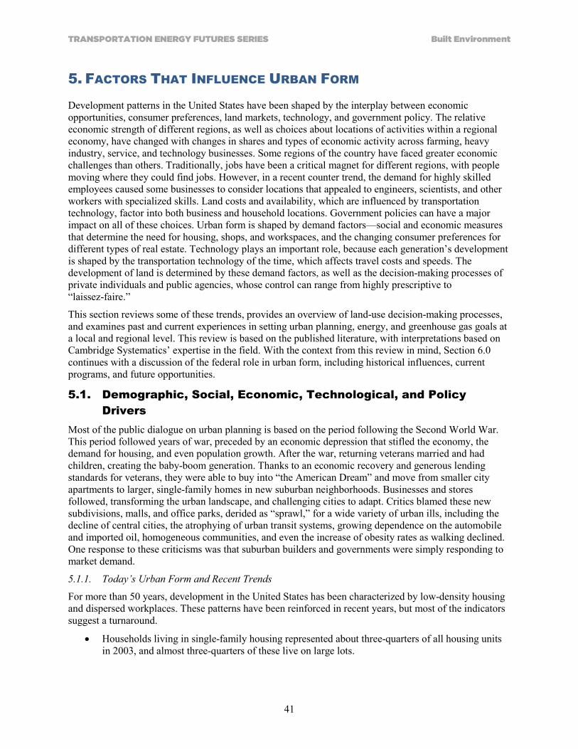
TRANSPORTATION ENERGY FUTURES SERIES Built Environment
41
5. FACTORS THAT INFLUENCE URBAN FORM
Development patterns in the United States have been shaped by the interplay between economic opportunities, consumer preferences, land markets, technology, and government policy. The relative economic strength of different regions, as well as choices about locations of activities within a regional economy, have changed with changes in shares and types of economic activity across farming, heavy industry, service, and technology businesses. Some regions of the country have faced greater economic challenges than others. Traditionally, jobs have been a critical magnet for different regions, with people moving where they could find jobs. However, in a recent counter trend, the demand for highly skilled employees caused some businesses to consider locations that appealed to engineers, scientists, and other workers with specialized skills. Land costs and availability, which are influenced by transportation technology, factor into both business and household locations. Government policies can have a major impact on all of these choices. Urban form is shaped by demand factors—social and economic measures that determine the need for housing, shops, and workspaces, and the changing consumer preferences for different types of real estate. Technology plays an important role, because each generation’s development is shaped by the transportation technology of the time, which affects travel costs and speeds. The development of land is determined by these demand factors, as well as the decision-making processes of private individuals and public agencies, whose control can range from highly prescriptive to “laissez-faire.”
This section reviews some of these trends, provides an overview of land-use decision-making processes, and examines past and current experiences in setting urban planning, energy, and greenhouse gas goals at a local and regional level. This review is based on the published literature, with interpretations based on Cambridge Systematics’ expertise in the field. With the context from this review in mind, Section 6.0 continues with a discussion of the federal role in urban form, including historical influences, current programs, and future opportunities.
5.1. Demographic, Social, Economic, Technological, and Policy Drivers
Most of the public dialogue on urban planning is based on the period following the Second World War. This period followed years of war, preceded by an economic depression that stifled the economy, the demand for housing, and even population growth. After the war, returning veterans married and had children, creating the baby-boom generation. Thanks to an economic recovery and generous lending standards for veterans, they were able to buy into “the American Dream” and move from smaller city apartments to larger, single-family homes in new suburban neighborhoods. Businesses and stores followed, transforming the urban landscape, and challenging cities to adapt. Critics blamed these new subdivisions, malls, and office parks, derided as “sprawl,” for a wide variety of urban ills, including the decline of central cities, the atrophying of urban transit systems, growing dependence on the automobile and imported oil, homogeneous communities, and even the increase of obesity rates as walking declined. One response to these criticisms was that suburban builders and governments were simply responding to market demand.
5.1.1. Today’s Urban Form and Recent Trends
For more than 50 years, development in the United States has been characterized by low-density housing and dispersed workplaces. These patterns have been reinforced in recent years, but most of the indicators suggest a turnaround.
• Households living in single-family housing represented about three-quarters of all housing units in 2003, and almost three-quarters of these live on large lots.

Built Environment TRANSPORTATION ENERGY FUTURES SERIES
42
• In 2000, one-third of households contained children, the primary market for detached homes, but this category is expected to account for only one out of eight new households in the next 25 years.
• When preferences for different types of housing, as estimated by industry preference surveys, are applied to the growth in household types, Nelson (Nelson 2006) estimates that about half of the demand for new housing through 2025 will be for attached units, with the remainder for small-lot homes. He also estimates a slight decline in demand for large-lot homes compared to current supply.
• A review of recent housing construction data shows similar trends. Between 2001 and 2008, the share of detached single-family homes declined from 73% of the national total to 59%, with comparable gains in townhouses, condos, and multifamily units. The geography of development has followed along. In 26 regions, the share of new housing in central cities has doubled or tripled since 2000 (EPA 2010b).
5.1.2. A Market for Smart Growth as Well as Sprawl
Recent trends have seen a significant change in the types of development, a response to shifting demographics, consumer tastes, and growing expertise in smart growth among developers and planning officials. The American public is largely split over preferences for smart growth versus sprawl, with many desiring attributes of both. A survey of potential home buyers in 2011 showed changes in attitudes and circumstances since a similar survey in 2004 (Davis, Diegel, and Boundy 2011).
• When asked about preferences when selecting a community, nearly half of the public (47%) would prefer to live in a city (19%) or a suburban neighborhood with a mix of houses, shops, and businesses (28%). This is slightly lower than the 50% reporting that they live in cities or mixed-use suburbs today. Another four in 10 (40%) would prefer a rural area or a small town, higher than the 30% currently reporting that they live in such communities. Only about one in 10 (12%) say they would prefer a suburban neighborhood with houses only, substantially below the 19% who currently reside there. These results contradict the conventional wisdom that most home buyers want a standalone suburban home, but also demonstrate an enduring demand for suburbs and smaller communities.
• When offered choices between smart growth communities and sprawling suburbs, smart growth won out by a 56% to 43% margin. Among those voting for sprawl—the interview did not use that term, which could sound pejorative, but instead provided detailed descriptions—the qualities respondents liked were the single-family homes on large lots (71%), proximity to services within a short drive (16%), and ample parking (9%). Those who picked smart growth—a more neutral description was offered—liked the proximity of services within an easy walk (60%), the mix of housing types (16%), sidewalks, and public transportation (11% each). (The sprawl community did not have these characteristics, and services were a short drive rather than a short walk.) When asked what they liked about the smart growth community, those who opted for sprawl were much less inclined toward walkable destinations (40% versus 60%), but actually mentioned sidewalks and public transportation more frequently than those who opted for smart growth.
• The survey found a variety of responses for different demographic groups. Younger unmarried people preferred the convenience of smart growth, walkable communities, while subdivision-type communities appeal more to middle-aged married couples. Those who live in housing-only suburbs, small towns, and rural areas preferred more spread out, less walkable communities.
5.1.3. Fewer Families, Fewer Detached Homes
The most fundamental factor in housing choice is the composition of the household. Families with children prefer, and need, larger homes, typically on larger lots, while singles and couples without children gravitate toward apartments and condos. For households in between these extremes, larger
TRANSPORTATION ENERGY FUTURES SERIES Built Environment
43
households and those with children tend more toward single-family homes. The composition of the American family has changed dramatically since new suburbs grew seemingly overnight in the 1940s, filled with new parents of baby-boomers. Since 1980, 85% of household growth has consisted of households without children, and these trends are expected to continue. This dramatic change in the American family has important implications for housing needs. RCLCO, a leading real estate consultant, points out that between 2010 and 2020, population growth is expected among groups aged 25 to 39 and 55 to 80, with declines expected for the in-between group aged 40 to 55 (Underwood 2009). Traditionally, the younger group represents the entry-level housing market, those between 40 and 55 represent the traditional established suburban homes, and the older group is looking to downsize. The consultants suggest:
• The young cohort, in Generation Y, is expected to be looking for apartments and condos, townhouses, and starter (entry-level) detached homes.
• Those between 40 and 55 years old are expected to be looking for townhomes and condos; single-family homes on clustered, smaller lots; and traditional single-family homes.
• The 70 and older group provides some market for senior housing (Ducker 2010).
These changing demographics will require major shifts in housing patterns to meet a changing market, which could simultaneously move toward more sustainable development patterns with lower environmental impacts. They also present a significant challenge for the housing market, since many builders lack experience with nontraditional housing products. In addition, population losses in the prime home-owning category suggest a shrinking market for conventional detached suburban homes, with some analysts predicting a glut of detached suburban homes in the future. While an extreme surplus is unlikely, the key point is that there has been a mismatch in the past between sustainable development supply and demand. Brookings fellow Christopher Leinberger pointed out in an Atlantic article that while only 5% to 10% of households live in walkable urban places, possibly one in three households would prefer such a development (Leinberger 2008).
5.1.4. What Will Generation Y Do?
The biggest question in housing demand in coming years is the housing behavior of those born between 1979 and 1998, known as the Millennial generation, or Generation Y, a cohort even larger than the baby-boom generation. A 2010 survey of members of this generation out of high school, aged 18 to 32, found that while 26% still relied on parents or schools for housing, a surprisingly high 36% already were home owners, equaling the 36% who were renters. When asked to rank the importance of eight different housing features in selecting a rental or ownership unit, cost ranked number one, but interior space and design were important as well (Lachman and Brett 2011). According to market research consultants RCLCO, many in Generation Y will be moving to walkable urban and “urban lite” locations, and they appear to be willing to eschew the single-family, large-lot homes of their parents in favor of smaller homes and higher densities in mixed-use locations. Baby-boomers, in contrast, appear to prefer urban amenities in suburban locations. While the market appears to be moving strongly toward smart growth and sustainability, the consultants suggest one concern is whether the market will be able to provide such development in adequate scale, since so many developers build primarily single-family tract homes on large suburban lots (Ducker 2010).
Table 5.1 shows Underwood’s projections for Generation Y housing demand (2009) compared with Nelson’s (2006) projections for demand by housing type (as previously discussed). Both sources show a significant shift towards attached and small-lot detached homes compared to current supply.

Built Environment TRANSPORTATION ENERGY FUTURES SERIES
44
Table 5.1. Projected Housing Demand and Density in 2025 versus 2003
Type Density (Units per net Acre)
2003 Units (Percent) Preferences
2025 Demand (Percent)
Generation Y Demand
Attached 20 25% 38% 31% 34%
Small-lot detached 7 21% 37% 29% 35%
Large-lot detached 2 54% 25% 40% 31%
[Source: Nelson (2006) and Underwood (2009)] “Small lots” are less than one-sixth acre. 2003 units from Nelson. “Preferences” are Nelson’s interpretation of surveys conducted between ~1997 and 2003. “2025 demand” is Nelson’s forecast for total housing demand. “Generation Y demand” is Underwood’s forecast for Generation Y demand consistent with Nelson’s housing types.
5.2. Decision-Making Processes The critical actions that shape urban form are largely private decisions made by end users—consumers, businesses, and institutions—financed by private lenders and executed by real estate developers. These are framed and bounded within government regulations and planning policies. Understanding the real estate development process is important to those wishing to successfully influence urban form, especially in a way to make it more sustainable. Sustainable development generally comes down to a strategy of promoting development in established areas with a range of travel options and a diversity of nearby destinations, so that driving and energy consumption is substantially lower than in sprawling suburbs, where distances are longer and alternatives to driving are few. To switch development patterns, developers would need incentives to build infill development and disincentives for conventional suburban development. Current incentives work just the opposite way, with great burdens for building in town—financial, environmental, and political—and few if any impediments to building subdivisions on cheap land on the urban fringe. In addition, for development patterns to change, the long-term benefits from compactness, quality communal places, and open space would need to be communicated to and valued by buyers, builders, and officials; a shorter-term focus on low costs is now common (Porter 2002).
The dramatic changes in demographics discussed above are moving the housing market toward much smaller, more affordable products in more central locations. If governments and other stakeholders wish to reinforce these trends, the challenge will be to assure that local plans respond and that other impediments are overcome, especially in lower-income neighborhoods. There is strong built-in resistance to change, especially in the suburbs, so a case needs to be made to existing residents about the importance of crafting new plans that present change as an asset to the community and a move toward a better future.
5.2.1. Local Land-Use Regulation – Protected Provincialism
According to the U.S. Census Bureau, there are nearly 21,400 municipalities in the United States, including over 3,000 counties and over 18,000 cities, towns, and villages. Many, but not all, of these municipalities have comprehensive plans and zoning codes that regulate development (requirements vary by state). Most urban municipalities have such plans and codes, with some notable exceptions, such as the City of Houston, Texas.
Zoning is a responsibility generally reserved by local governments. State agencies pressured to assess the potential community development impacts of their programs, such as road and transit extensions, agricultural policies, and business assistance, often reply, “We do not do land use.” However, the responsibility to regulate land use is a relatively recent one, and there is no guarantee that it will remain exclusively a local government activity. In fact, broad land-use issues not addressed by localities have resulted in some states curtailing some local authority, and broader environmental concerns, including climate change, have led some states to see their involvement as even more important.

TRANSPORTATION ENERGY FUTURES SERIES Built Environment
45
To planning outsiders, the term “zoning” is shorthand for all of the various policies involved in the regulation of land use. The first comprehensive zoning ordinance was adopted in 1916 in New York City, although Los Angeles and Boston implemented somewhat more rudimentary zoning earlier. The New York law divided the city into zones according to permitted uses of land, minimum lot size, and maximum building heights. A challenge to the segregation of single-family homes from commerce in Village of Euclid v. Ambler Realty Co. was upheld by the U.S. Supreme Court in 1926, clearing the way for zoning codes already proliferating throughout major cities, and introducing the name “Euclidean zoning” (characterized by the segregation of land uses into specified districts) to the lexicon.
In the 1920s, the U.S. Department of Commerce drafted a model Standard State Zoning Enabling Act, which granted cities the power to restrict building size and height, the size of yards and other open spaces, the density of population, and the location and use of buildings (Lamer 2003). While courts upheld the legitimate practice of zoning, they also protected property rights by drawing a limit on how many restrictions localities might impose. The U.S. Supreme Court in Pennsylvania Coal Co. v. Mahon (1922) stated that land-use regulation, if too onerous, constituted a taking of property without compensation, contrary to the Fifth Amendment to the Constitution.
Widespread zoning practices such as segregation of uses, minimum lot sizes, low density limits, large building setbacks, and high minimum parking capacities—established to protect neighborhoods from traffic, noise, large buildings, and other real or perceived detriments to property values—have been a major contributing factor to inefficient development patterns in the decades since the 1930s. Perhaps as important as zoning itself have been subdivision regulations, which include drawings of a parcel showing its division into individual lots, which facilitated the process of buying and selling land. Subdivision ordinances also established design standards, such as street widths, building setbacks, and location of public facilities. These ordinances prevent higher-density, mixed-use development which could serve a growing market demand and address sustainability goals calling for alternatives to the private automobile.
Just as states have the authority to delegate zoning powers to municipalities, they can also revoke such authority, and a number of states did so in the 1960s and 1970s. Some of the key reasons were a perception that local governments revert to parochial concerns even on issues that require a bigger picture: crises created when critical natural resources are vulnerable to development proposals; and the threatened imposition of federal land-use controls.
5.3. Historical Examples of Energy and GHG Goals and Programs for Urban Planning
Urban planning in the United States has evolved in response to the problems of each era. The first modern planning regulations emerged in the 1920s and 1930s partly as a reaction to the poor housing and environmental conditions of the industrialized cities. Zoning, housing, and subdivision codes were established by states and localities to prevent overcrowding, protect against contaminated water and air, and improve access to open spaces. The American suburbs as we know them were created through a confluence of public policies and demographic and market forces: federal government involvement during the New Deal of the 1930s to expand subdivision regulations and provide mortgage insurance to improve the often poor conditions of housing; establishment of the Interstate Highway System in the 1950s; and the demographic push for expanded home ownership as returning veterans married and had children. Increasing automobile travel contributed to the rise of air pollution as a national concern, resulting in the Clean Air Act of 1963, which set the stage for automobile pollution control standards and area air quality designations beginning with the Clean Air Act amendments of 1970, and later the broader requirement for transportation control measures (including such things as ridesharing, transit improvements, bicycle facilities, and auto-restricted zones) in the amendments of 1977 and 1990.
Suburban centers became major job and retail hubs in the 1980s, as the Interstate Highway System was built out, and growing traffic congestion led to new growth management initiatives. These attempted to

Built Environment TRANSPORTATION ENERGY FUTURES SERIES
46
place some limits on sprawl, and sought to assign responsibility to developers for mitigating traffic. By the 1990s, the smart growth movement was born out of contentious battles between development and no-growth advocates. Even critics of growth recognized that growth was inevitable, and that a wiser response than no-growth was to shape development to minimize negative impacts on traffic and the environment, while possibly enriching the surrounding community (TRB 2009).
This brief review has shown that the goals for urban planning, while changing with the issues of the day, have remained remarkably focused on protecting health and wellbeing, initially from substandard housing and adjacent nuisances, and potentially extending to broader regional and even global concerns. The federal government has explicitly left land use planning in local hands, with the singular exception of urban renewal, deferring land-use planning authority to states and localities. In contrast to local concerns such as traffic and land development, however, energy security and GHG mitigation involve the federal government.
5.3.1. The On-and-Off (and On) Energy Crisis
While affordable energy, particularly transportation fuel, was central to the development of the suburbs and the exponential growth of car ownership and driving, addressing the nation’s dependence on oil did not become a national goal until the Arab oil embargo of the early 1970s. This crisis resulted in the establishment of the Corporate Average Fuel Economy standards, created by Congress in 1975, which established fuel efficiency standards for car manufacturers. The federal approach to reducing energy consumption has been largely to focus on improved efficiency, including appliances that use less electricity, greater insulation of buildings to reduce heating and air conditioning; and increased fuel efficiency of cars and trucks. Programs to decrease transportation demand, such as ridesharing and transit programs implemented through the Urban Mass Transit Administration’s Service and Methods Demonstration Program, were also implemented in the 1970s. In contrast to energy and emissions requirements, however, these programs were mostly voluntary and incentive-based. Also, they largely disappeared in the 1980s as oil prices fell and political leadership changed. Some research was conducted on the effects of urban form on travel in the 1970s, but the federal government did not undertake major policy initiatives focused on land use as an energy conservation measure.
Since the 1970s, the political will to cut dependence on oil has risen with each spike in the price of oil, at least until prices fell again. However, new concerns about the threats of imported oil to the nation’s political and economic security have created a renewed emphasis on energy policy. The volatility of oil prices—crude oil prices have soared as high as $140 and dropped as low as $20 per barrel over the last dozen years—has contributed to these concerns. The Bipartisan Policy Center, a Washington think tank that promotes policy to bridge political divides, warned in a 2011 open letter that, “without question, our economy – in fact our way of life – is highly dependent on access to stable, affordable supplies of energy” (Bipartisan Policy Center 2011). The federal response has focused primarily on more efficient transportation and buildings, rather than addressing the connection between transportation, urban development patterns, and energy use.
5.3.2. GHG as an Emerging Concern
The current administration called for a national cap-and-trade program to reduce GHG emissions in the President’s first address to a joint session of Congress on February 24, 2009. Related legislation has not moved forward, in the midst of contentious budget battles. Meanwhile, policies to address climate change have been proposed and implemented in states and localities, building on their own powers, and in some cases relying on additional federal assistance.
Some states have also sought to establish their own energy and GHG performance standards. However, only California has been granted authority under the federal Clean Air Act to establish its own emissions performance standards for automobiles, although to do so it must obtain a waiver from EPA. Other states can adopt standards if they are identical to California’s. California has long established air pollution

TRANSPORTATION ENERGY FUTURES SERIES Built Environment
47
control standards that are stricter than federal standards (with perhaps a dozen other West Coast and northeast states also adopting the California standards), and in 2009 was granted authority by EPA to establish its own GHG emissions standards. Any potential differences between federal and state-level fuel economy and GHG standards were preempted by the recent adoption of new federal Corporate Average Fuel Economy standards that match California standards for model years 2012 through 2016 (Federal Register 2010b), and proposed standards for light-duty vehicles that would extend through model year 2025 (Federal Register 2010a).
Emissions from vehicles and electricity for buildings are only part of the GHG equation, however. Numerous studies, many discussed in this report, show that the structure of communities also affects how people travel and the corresponding energy use and emissions from transportation sources.
5.3.3. Urban Planning – Local, Regional, and State Initiatives
Planning for compact communities requires more widespread use of policies and practices similar to those of smart growth and green development. As discussed above, this new generation of planning is being practiced in some communities throughout the United States. Local governments are adopting smart growth and variants such as transit-oriented development (TOD), form-based zoning, and the supporting codes. In addition to code reform, local governments have also undertaken other actions to help level the playing field between infill and greenfield development, such as:
• Streamlining the development permitting process or giving preferential treatment for projects meeting smart growth criteria
• Creating land banks to assist with land assembly, helping to overcome the problem of small, dispersed parcels in existing urban neighborhoods
• Financing the reconstruction of aging infrastructure (streets, sidewalks, water, sewer, and other utilities) in targeted redevelopment areas
• Funding catalyst projects, such as public or nonprofit facilities to create a core of new development around which private developers will follow.
While planning is still a closely guarded local function, other levels of government are also involved, often with competitive funding programs to provide incentives for certain characteristics in local plans. Within the past one to two decades, many regional agencies—including MPOs and councils of governments—have become increasingly concerned about the disconnect between transportation and land use in planning practice in the United States. Transportation planning authority often exists at the regional level, but land-use planning authority only exists at the local level.8 These agencies have increasingly led voluntary initiatives to promote integrated transportation and land-use planning in the region. Such regional initiatives commonly include the following elements:
• Formation of a regional coalition, including agency heads, local elected officials, business leaders, advocacy groups, foundations, and others, who agree that a coordinated approach to regional development is important.
• Undertaking a process with extensive public and stakeholder involvement, along with supporting technical analysis, to develop a vision for the region, create alternative development scenarios, and analyze the effects of those scenarios on various factors (e.g., mobility, infrastructure costs, land consumption, energy, emissions, economic vitality).
8 MPOs are the federally designated transportation planning agencies for metropolitan areas of at least 50,000 population. Councils of governments are associations of local governments formed to work on issues of regional interest. Councils of governments, where they exist, often (but not always) take on the function of the MPO. In some states, nonmetropolitan communities are also grouped into regions with a regional planning agency.

Built Environment TRANSPORTATION ENERGY FUTURES SERIES
48
• Development of an implementation plan and action steps to implement a preferred scenario. This will include preferred transportation system concepts (which can be incorporated in the long-range transportation plan), land-use planning principles (growth centers, preservation areas, design guidelines, etc.), and other factors.
• Ongoing work with stakeholders, especially local governments and the development community, to implement the vision. For example, the MPO can direct transportation funding to support local planning activities as well as revise transportation project selection criteria. Implementation activities are by necessity voluntary, and this stage requires sustained action by coalition partners to create change at the decision-making level.
A few of the more acclaimed examples of this type of regional initiative include Envision Utah in the Salt Lake City region, Sacramento Blueprint, myregion.org in Central Florida (Orlando), Metro Vision 2020 (now 2035) in Denver, and the Eastern Planning Initiative in Charlottesville, Virginia. A 2005 report for FHWA identified 80 scenario planning initiatives completed or in progress in 50 metropolitan areas (Bartholomew 2005). The Atlanta Regional Council, the region’s MPO, has created an award-winning Livable Centers Initiative, which has provided over $10 million in over 10 years for planning activities and $500 million for funding transportation projects to support such developments. Similar programs exist in San Francisco, Minneapolis-St. Paul, and the Washington, D.C., regions, among others.
A few states have engaged in growth management and smart growth initiatives. The best known example is Oregon, which established planning and growth management requirements as early as the 1960s. State action in the 1970s required urban areas to set growth boundaries and gave regional agencies the authority to develop and enforce land-use plans. Washington’s 1990 GMA represents a milder version of Oregon’s approach, with fewer powers for state and regional enforcement. Florida, Maryland, and New Jersey have also worked for over two decades to develop and implement growth management programs, although the states have found it an ongoing struggle to effectively enforce their programs. Wisconsin’s 1999 Comprehensive Planning Law required local plans and provided incentives for smart growth and cross-jurisdictional coordination. Other states have adopted planning requirements, although generally without performance standards specifically directed at smart growth (National Cooperative Highway Research Program 2004).
Some states have adopted planning requirements for GHG reduction purposes. Most notably, California’s Senate Bill 375 calls on regional transportation planning agencies and local governments to develop strategies for reducing GHG emissions from passenger vehicles by reducing per capita VMT (Bedsworth, Hanak, and Kolko 2011). Oregon has followed with similar legislation. California’s approach, the California’s Blueprint process is a state-led initiative that provides grants and other resources to support regional scenario planning throughout the state.
Another emerging trend is planning at the “megaregion” level, defined by one source as “clustered networks of metropolitan areas that exceed 10 million total residents.” (Lang and Dhavale 2005). Such planning can involve multiple sectors or issues including transportation, land use and housing, energy, environment, water, finance, and others (U.S. DOT 2012). Examples of megaregion planning initiatives include the Regional Plan Association’s work in New York, New Jersey, and Connecticut (2012) and the Alternative Transportation Futures Project in Oregon’s Willamette Valley (Willamette Valley Livability Forum 2012). These efforts have been entirely voluntary and cooperative efforts of states, MPOs, and other entities, given that there are no federally or state mandated institutional structures at these levels. However, the integration of transportation and land use at the megaregion scale introduces issues such as intercity travel (both passengers and freight) and transit-oriented development for both high-speed rail and urban transit.
Although government actions have some influence, the private market remains a driving force in development patterns. Zoning codes can shape how developers build, but cannot direct them to build at

TRANSPORTATION ENERGY FUTURES SERIES Built Environment
49
certain densities or in specific locations. Even Portland, Oregon’s, longstanding, enforceable urban growth boundary has been criticized for still allowing auto-oriented (if somewhat more dense) patterns of development within the city boundary (Song and Knaap 2004). Changes to local ordinances can clearly pave the way for smart growth development where a market exists, but cannot create a market where it does not exist. Short of a move towards highly centralized (i.e., European-style) land-use planning, the extent of change that may be achieved through plan and code revision alone, or even through coordinated regional actions, may be limited, although as discussed in Section 5.1, still significant, in light of changing market trends. For that reason, it is important to engage the private sector, understand their motivations, and craft policies and education to gain their leadership toward consensus development goals. Most recent exercises to establish regional vision plans have involved the private sector, and in some cases have been led by business and real estate leaders. For example, the Urban Land Institute conducted seven reality checks in the form of one-day, participatory, regional visioning exercises to engage leaders in a regional dialogue on growth issues between 2005 and 2009.
5.4. Smart Growth Opportunities There are three significant target areas for new development: infill housing in older neighborhoods, redevelopment of suburban centers, and growth on suburban greenfields. This section considers trends and research that may inform how development in these areas can serve future community needs. A review of these opportunities is preceded by a brief review of local zoning and development regulation.
5.4.1. Urban Infill and TOD
Older neighborhoods have many of the qualities admired by smart growth advocates: higher densities, grid streets, high-quality transit, and sidewalks. In fact, many such neighborhoods are at the forefront of an urban renaissance in Chicago, San Francisco, Houston, Washington, D.C., and other cities. With market support, new development can work. Planners in such cases need to address regulations and focus on complete communities while preserving housing affordability. A review of housing potential near transit in Denver, for example, estimated that the amount of housing in rail transit station areas could triple, but that “there is considerable risk that virtually all new development near transit in the region will be unaffordable to moderate-income households, those most likely to be transit users” (Belzer et al. 2007). The other challenge for planning in strong markets is to balance market cycles for different types of land uses with a long-term vision of a community with a full range of services, a comprehensive view that does not build simply what the market seems to desire at any given time, but promotes a longer-term view with improved retail services, community facilities, and opportunities for new jobs.
While planning for infill development in strong markets (where there is greater economic growth and demand for housing) is complex, the challenge in weak market communities is even greater, and there are many such areas where development must be accommodated to meet broader TOD and sustainability goals. Even in the San Francisco Bay area, whose central cities and core suburbs doubled their share of residential building since the early 1990s (from 28% to 57% of new residential permits), financing for infill and TOD projects desired to meet regional goals is difficult (EPA 2010b). A study of financing in the Bay Area found that TOD and infill projects are more expensive because of infrastructure upgrades, high land costs, and complicated construction. While strong markets are able to absorb such costs “in most places around the region, the market is often not quite capable of covering the increased costs associated with infill development and TOD” (Metropolitan Transportation Commission 2008). A good example of such a weak market is the City Heights neighborhood in San Diego, an inner-city community not served by the popular San Diego Trolley, divided by an urban freeway and once ravaged by crime and drugs. A redevelopment plan has gradually added community and retail services, including a new police substation, a library, and a grocery store, with housing rehabilitation and development planned, as well as a bus rapid transit connection to enhance transit. This redevelopment project has required strong planning as well as financial support from government and nonprofits.
Built Environment TRANSPORTATION ENERGY FUTURES SERIES
50
5.4.2. Redeveloping Suburban Centers
Many suburbs, especially the oldest, or “first ring” suburbs around central cities which grew up as “street car suburbs,” have excellent transit connections and compact pedestrian patterns, and are ideal targets for regional smart growth development. Some of this is happening through normal market forces, such as in the Bay Area, described above. Sensitive planning is needed to allay local concerns about development and change. An especially complex issue is what to do about suburban centers developed around freeways, divided by main roads, not served by transit, clustered into malls and office parks, and cut off from pedestrian access to the housing in surrounding neighborhoods. From a compact growth perspective that seeks alternatives to automobile travel, such segregated uses are held up as the worst transgressions to wise planning, but they are also pervasive. Some communities now seek to address this enormous planning challenge, requiring virtually a complete do-over in some cases, to change these factors, by adding:
• A grid system to improve connectivity, replacing divisive superblocks • Expanded housing to create street life and support local merchants • Integrated retail, office, and housing • Attractive central amenities and pleasant pedestrian corridors rather than mall-style retail • Extensive transit choices • Parks and civic institutions to add to the sense of community • Shared, fee-based, smaller-scale parking.
There are a growing number of examples of these retrofits, typically in upscale neighborhoods. One of these, the Kendall area south of Miami, the community surrounding the Dadeland Mall, had long been considered a quintessential piecemeal suburban development, economically successful, but low-density and car-dependent, despite having two stations on Miami’s Metro system. A plan adopted in 1999 called for creating a street grid, higher densities, more housing, a mix of uses, enhanced architectural style, and pedestrian improvements. The plan shaped development in the early 2000s, until the housing bubble burst. The expectation is that eventually Kendall will be transformed into a mixed-use, pedestrian-friendly TOD.
5.4.3. Better Greenfield Development
To critics, conventional greenfield developments in fringe neighborhoods are the embodiment of sprawl, while developers of large-scale master-planned communities claim they actually include many positive environmental and planning features, at an affordable price. The momentum may be changing, at least for now, with experts in the Urban Land Institute’s latest survey of development outlook finding that “the overall residential tide is moving from fringe suburbs to urbanizing suburban nodes, and 24-hour downtown cores gain momentum. You can live more efficiently with less environmental impact in infill areas” (Miller 2012). However, there is still a market for suburban homes on large lots, so for those markets the primary challenge is how to create better suburban greenfield developments. This may include paying special attention to environmental protection and preservation, beginning with the importance of natural surroundings and features, as well as historic structures and elements. Such a broad approach protects places that should not be developed, and helps head off growth/no-growth battles early, rather than triggering a contest over each development proposal. In addition to making the environment a central focus, it also creates a diversity of housing, a mix of uses, and a range of densities. Such planning also paves the way for future transit opportunities, by creating transit-ready communities with the mix of uses and densities appropriate to future transit corridors, and assurance that growth patterns will create support for future transit extensions (Corrigan et al. 2007).

TRANSPORTATION ENERGY FUTURES SERIES Built Environment
51
6. FEDERAL ACTIONS THAT MIGHT INFLUENCE URBAN FORM
This section summarizes the history of federal actions that have influenced urban form, reviews current actions, and describes additional actions that could be undertaken if the federal government seeks greater influence on urban form to reduce energy use and GHG emissions. This report does not advocate for or discourage such federal involvement. This section includes information from the literature, as well as assessments and information that are based on Cambridge Systematics’ judgment and unpublished knowledge of the field. It is focused on potential actions directed at transportation, land use, and community development, rather than on broader economy-wide actions such as energy or carbon pricing, or on indirect influences, such as those resulting from technological changes to vehicles and fuels.
6.1. Historical Influences The most significant federal influences on urban form have been largely indirect rather than direct. For example, the Interstate Highway System is widely regarded as one of America’s greatest achievements, not only by construction and engineering groups, but by the wider public. In 1999, to commemorate the turn of the century, U.S. News and World Report (1999) included the Interstate system among “25 Shapers of the Modern Era.” That same year, a survey by the Fannie Mae Foundation listed the Interstate Highway System, along with the dominance of the automobile, as the number one influence on the American metropolis over the last 50 years (Fishman 2000). Also on the list of top influences were federal housing mortgages and subdivision regulation (number 2), and urban renewal originated by the 1949 Federal Housing Act (number 4) (see Table 6.1) (Weingroff 2000).
Table 6.1. The Top 10 Influences on the American Metropolis of the Past 50 Years
1. The 1956 Interstate Highway Act and the dominance of the automobile 2. Federal Housing Administration mortgage financing and subdivision regulation 3. De-industrialization of central cities 4. Urban renewal – downtown redevelopment and public housing (1949 Housing Act) 5. Levittown (planned communities and the mass-produced suburban tract housing) 6. Racial segregation and job discrimination in cities and suburbs 7. Enclosed shopping malls 8. Sunbelt-style sprawl 9. Air conditioning 10. Urban riots of the 1960s
[Source: Weingroff (2000)]
These three programs combined to provide urban renewal, mortgages for suburban housing, and a new system of superhighways to connect them all, a comprehensive approach to linking urban development and transportation. All three were conceived during the Great Depression, and their political history illustrates how transportation and land-use planning have played a role in the longstanding national debate about the appropriate role of the federal government.
6.1.1. Prospects for National Planning
Fishman (Fishman 2004) reviews two bold examples of national planning that changed the direction of the country, one in 1808, and another a century later. The 1808 Gallatin Plan, according to Fishman, “embodied perhaps the most revolutionary vision of any national plan: the creation of a truly democratic society through the planned settlement of a whole continent.” The sale of federal lands would be organized to produce a society dominated by independent farmers, and this new continent of citizen-farmers would be connected to thriving cities and their worldwide markets by a federally financed network of roads and canals to form the world’s most productive economy. The Report on Roads and

Built Environment TRANSPORTATION ENERGY FUTURES SERIES
52
Canals by Albert Gallatin, Secretary of the Treasury under Jefferson, had two main components: plans for a set of roads and canals to improve transportation along the Atlantic coastline, and the plans for more difficult, expensive, but vitally necessary canal and road systems over the Alleghenies. This vision dominated land and transportation policy of the 19th century, reaching its climax during the Civil War years, when Lincoln definitively linked the Jeffersonian ideal of the citizen-farmer to the new technology of the railroad. The fulfillment of Jefferson’s idea came in the form of the Homestead Act of 1862 that awarded 160 free acres of federal land to any family that would claim and farm it. Jefferson’s goal of creating a society of citizen farmers had been united with Washington’s need to link the new territories with the original 13 colonies. Moreover, Lincoln tied this new settlement to federal support for a new transportation technology, the railroad.
By the end of the 19th century, however, this original vision had been lost. The railroads controlled the land grants and exploited resources, consuming whole forests, damaging prairies, and polluting rivers. A 1908 Preliminary Report of the Inland Waterways Commission given by the President to the Senate of the 60th Congress set the stage for a new vision for the 20th century (U.S. Inland Waterways Commission 1908). This report emphasized river navigation, power, irrigation, and conservation. Dams would protect downstream communities, ensure safe navigation, and generate cheap power, as well as provide irrigation for millions of arid acres. Watersheds and upland forests would be protected by an early form of regional planning, that promoted sustainable farming and prevented soil erosion in the agricultural plains, and improved sewage treatment for the industrial cities. Rivers would also serve as transportation corridors, which offered alternatives to the railroads with their monopoly rates. This report served as a key resource for a White House “Conference of the Governors of the United States” convened by President Theodore Roosevelt. Implementation of the plan was thwarted for the next quarter century, however, by battles over the balance between private and public enterprise. Implementing Roosevelt’s National Conservation plan fell to Franklin Delano Roosevelt, spurred by Great Depression workforce needs and the environmental crisis of the Dustbowl. The Tennessee Valley Authority made coordinated conservation/development planning a keynote of New Deal policy, the model for a national effort of forest and farmland preservation and rivershed planning.
By the 1930s, the alternative to a transportation system dominated by railroad monopolies was touted as “superhighway” system, a national highway plan, first published in 1939 under the title “Toll Roads and Free Roads” (U.S. Public Roads Administration 1938). The Interstate Highway System adopted under Eisenhower became a major framework for federal transportation and land use influence, similar to the transcontinental railway plans and land grants of the Lincoln years.
6.1.2. Command, Control, Collaboration?
This brief look back helps reinforce the notion that bold national land use and transportation strategies are not new to the United States. Even the Interstate Highway System, blamed by critics for a single-minded focus on road building that often cut through urban communities, was originally part of a broader program to revitalize cities. A collaboration was envisioned in which the highway program would quickly eliminate “thousands of substandard houses,” while the Public Building Administration, the federal government’s housing agency, would redevelop civic centers in many cities, and the Bureau of Community Facilities, another Federal Works subagency, would loan funds for additional public buildings. New express highways were viewed as “the framework of the redeveloped city” (Weingroff 2000).
There is certainly strong precedent for a coordinated federal program that links transportation investments and growth in support of a broader national agenda, but what are the possible roles for today’s federal government? Federal government involvement raises concerns if it is perceived to encroach on local or state prerogatives. However, there is ample historical precedent for a collaborative federal role. During the canal era, the emphasis was on supporting private companies to build the canals, a model followed with the transcontinental railroad. Even in the case of the Interstate Highway System, the model most

TRANSPORTATION ENERGY FUTURES SERIES Built Environment
53
recognized by a generation of transportation engineers and drivers, primary responsibility for building and operating routes fell to the states. By picking up a very generous share of the costs, the federal program was able to engage states to carry out the plan. Creating such collaboration through federal spending, however, may raise concerns about federal budget growth. If those concerns can be addressed, federal directions consistent with this approach might include:
• Reinforce existing investment and communities. Maintaining a good state of infrastructure is a prudent, fiscally conservative concept that reinforces existing communities in efforts to initiate new sustainable development. A considerable level of transportation investment will be required to maintain the Interstate Highway System, and to address ongoing transit system rehabilitation needs. Such investments could be used to reinforce sustainable development.
• Support sustainable regional visions. There are a growing number of initiatives to address growth, environmental, and even economic development needs of the nation’s major regions. Such visioning exercises use tools ranging from simple to sophisticated, but they engage a much wider range of local civic, business, and government leaders. As indicated above, there is existing U.S. DOT funding for these visioning exercises, as well as examples of direct involvement of the federal government. The Interagency Transportation, Land Use, and Climate Change Pilot Project is a collaboration among 13 federal agencies and state and local governments to develop a multi-agency transportation and land-use strategy for Cape Cod, Massachusetts, focused on GHG emissions and sea level rise (Rasmussen et al. 2011).
• Recognize that land resource decisions shape regional development. Environmental, natural resource, and infrastructure agencies can have a powerful impact on local development, especially in the West, where federal lands are so extensive. Sensitivity to local authority over land-use regulation leads federal agencies to limit their involvement in land-use policy issues. Infrastructure investments can change property values and land acquisitions to remove property from private use are significant land-use actions. Enhanced federal collaboration on smart growth would emphasize the importance of such decisions, reinforcing local and state smart growth policies. Officials can recognize that “if you are in the infrastructure business, you are in the land-use business.” The Federal Transit Administration’s (FTA’s) New Starts program has integrated land-use considerations, but similar considerations do not exist with respect to highway funding, which is allocated to states to use at their discretion.
• Link infrastructure expansion to sustainable development. Past decisions on infrastructure have often contributed to sprawl by creating opportunities for more for development. Expanded roads and transit lines in greenfield locations should be clearly linked to the locations and patterns of desired future growth, ideally through a regional vision defining corridors for growth and areas for preservation. New developments would include plans for a mix of housing, jobs, and retail, and a mix of densities to support affordable housing and future transit.
• Leverage real estate revenues to support transportation. Localities have become increasingly dependent on real estate exactions to pay for local infrastructure growth, but neither states nor federal agencies have taken advantage of this opportunity, perhaps due to limited jurisdiction. A good case can be made that major extensions of road and transit systems should be financed by the development they serve. Costs could be assessed on property owners or developers if a regional vision can fairly allocate such costs to planned corridors. Funding facilities in this manner also helps assure that effective projects will be built, because developers are both the beneficiaries and have a stake in the costs.
• Focus federal assistance. A collaboration between the U.S. Department of Housing and Urban Development (HUD), U.S. DOT, and EPA has expanded to a wide group of agencies with similar interest, and now includes the Centers for Disease Control and Prevention, U.S. Department of

Built Environment TRANSPORTATION ENERGY FUTURES SERIES
54
Agriculture, the Department of Defense, the Department of Education, DOE, the Department of Health and Human Services, the Economic Development Administration, the Federal Emergency Management Agency, the General Services Administration, the National Endowment for the Arts, and the National Oceanic and Atmospheric Administration. This growing federal collaboration has the potential to create a focus on capital investments and federal assistance in support of better development patterns.
6.2. Current Federal Actions Federal policies to assist urban development during the last two decades have included direct funding for projects, technical assistance, awards, and comprehensive planning requirements. The rise and fall of planning requirements reflect the ebb and flow of federal involvement in land use. The Intermodal Surface Transportation Efficiency Act of 1991 required MPOs to consider 15 interrelated factors in the development of metropolitan transportation plans, one of which was the consistency with land-use and development plans. Just having the MPOs involved in local land-use plans was considered controversial and the Transportation Equity Act for the 21st Century of 1998 (U.S. DOT 1998) reduced the number of planning factors to nine and dropped land use. It reappears in the fifth planning factor in the Safe, Accountable, Flexible, and Efficient Transportation Equity Act: A Legacy for Users (SAFETEA-LU) of 2005, which reads in full, “Protect and enhance the environment, promote energy conservation, improve the quality of life, and promote consistency between transportation improvements and state and local planned growth and economic development patterns.” SAFETEA-LU also requires that transportation agencies consult with land-use agencies when developing statewide and metropolitan transportation plans.
Federal agencies play a direct role in the use of land as owners and regulators, including agriculture, national parks and other federally-owned properties, but their role in an urban context is relatively limited. Agencies that have support for better urban planning as part of their mission include: EPA; U.S. DOT, including FHWA and FTA; and HUD. Existing programs by these agencies include:
EPA Brownfields Program. This program assists states, communities, and other stakeholders in cleaning up and reusing brownfields (properties contaminated by hazardous substances or pollutants). Such properties are often located in disadvantaged communities of major cities that present opportunities for promoting more sustainable development. However, the stigma of contamination has often prevented such sites from redevelopment even when the contaminants had been successfully remediated. Federal grants are provided for assessment, cleanup, workforce development, job training, technical assistance, and revolving loan funds. In 2010, the new Areawide Planning Pilot Program provided about $4 million in grant funding and direct assistance to 23 communities to plan, assess, clean up, and reuse brownfield properties and promote areawide revitalization (EPA 2010a, Brownfields Areawide Planning Pilot Program).9 As of November 2011, the Brownfields Program had prepared more than 25,000 acres on 672 sites for reuse, with more than $900 million in EPA program funds leveraging $17.6 billion in additional public and private cleanup funding (EPA 1995, Brownfields Program Benefits.).10
EPA Smart Growth Program (EPA Smart Growth 2010)11. This program was established in 1996 and funds a network of smart growth organizations, a sustainable development awards program, and direct technical assistance to communities to help overcome barriers. The program currently is operated through EPA’s Office of Sustainable Communities. In addition to promoting smart growth, EPA has established the following funding and recognition programs:
• The Smart Growth Implementation Assistance Program is an annual, competitive solicitation open to state, local, regional, and tribal governments (and nonprofits that have partnered with a
9 $4 million estimate based on $175,000 per recipient. 10 Estimate of program funds is based on $17.6 billion leveraged and $18.29 leveraged per EPA dollar spent. 11 Funding levels for this program could not be identified but are probably on the order of a few million a year.

TRANSPORTATION ENERGY FUTURES SERIES Built Environment
55
governmental entity) that want to incorporate complex or cutting-edge smart growth techniques in future development. EPA typically helps three to five communities each year through the Smart Growth Implementation Assistance program and about two dozen projects have been completed since 2005.
• Building Blocks for Sustainable Communities provides quick, targeted technical assistance to communities using a variety of tools that have demonstrated results and widespread application. In spring 2011, EPA selected 32 communities from two sources to receive Building Blocks assistance.
• Through the National Award for Smart Growth Achievement, EPA recognizes and supports communities that use innovative development policies and strategies to strengthen their economies, provide housing and transportation choices, bring benefits to a wide range of residents, and protect the environment. This program has provided annual awards since 2002.
FTA New Starts Program. This program provides funding for major transit capital investments. Among other criteria, project sponsors applying for funds are evaluated based on transit-supportive existing land use and policies. The program has been funded at a level of about $1.65 billion per year under SAFETEA-LU.
FHWA/FTA Transportation Capacity Building Program. Created in 2001 with a focus on the MPO planning process, the Transportation Capacity Building Program provides information, training, and technical assistance to metropolitan transportation planning professionals and officials. Transportation Capacity Building Program activities are funded through a variety of sources, including the Surface Transportation Environment and Planning cooperative research program, FTA Section 5314-Research, and FTA Section 5327-Oversight (U.S. DOT 2008).
FHWA Transportation and Community and System Preservation Program. This program, initiated in 1998, supports innovative strategies that use transportation to build livable communities by improving efficiency, environmental performance and accessibility, while “examining development patterns and identifying strategies to encourage private-sector development patterns that achieve these goals.” A number of projects focusing on transportation and land-use planning integration were funded in the first two to three years of the program, but Congressional earmarking soon tilted the balance of projects to focused capital investments such as bicycle and pedestrian improvements. The Transportation and Community and System Preservation program was authorized at a level of $61.5 million per year in 2006 and beyond under SAFETEA-LU.
HUD HOPE VI Program. This program was developed to help eradicate severely distressed public housing. The program provided a total of $6.7 billion from FY 1993 through FY 2010 (an average of $372 million per year), for revitalization, planning, demolition, and grants for smaller communities to develop affordable housing (HUD HOPE VI undated).
HUD Choice Neighborhoods Program. This is a new program that awards grants to transform distressed neighborhoods and public and assisted projects into viable and sustainable mixed-income neighborhoods by linking housing improvements with services, schools, public assets, transportation, and access to jobs. Five cities were awarded a total of $122 million in FY 2011. The program is a centerpiece of the current Administration’s interagency Neighborhood Revitalization Initiative – a collaboration between the Departments of Housing and Urban Development, Education, Justice, Treasury, and Health and Human Services in support of local public- and private-sector leaders in attracting the investments needed to transform distressed neighborhoods into sustainable, mixed-income neighborhoods with affordable housing, safe streets and good schools (HUD Choice Neighborhoods undated).
Partnership for Sustainable Communities. This joint effort of the U.S. DOT, HUD, and EPA was initiated in 2009. The partnership has adopted joint livability principles, and its member agencies are working to coordinate investments to support communities that want to improve housing, transportation, and

Built Environment TRANSPORTATION ENERGY FUTURES SERIES
56
business opportunities. In its first year, the program awarded transportation planning and integrated planning grants; revised policies to simplify development of Federal Housing Administration-insured multifamily housing on former brownfield sites; provided guidance on state water grants that discourage expanding infrastructure to accommodate growth; developed a guide to help planners implement mixed-income, transit-oriented development; and selected participants for a pilot program with five communities to clean up and reuse contaminated and vacant properties. In October 2010, the Partnership announced the award of $100 million of HUD funding to 45 regions through the Sustainable Communities Regional Planning Grant program; $40 million of HUD funding in Sustainable Community Challenge Grants for local planning; and $28 million in U.S. DOT Transportation Investment Generating Economic Recovery (TIGER) II Planning Grants to implement localized plans. Funding was not provided in FY 2012 and future funding is uncertain.
To put the scale of the program funding levels in context, the entire federal aid highway program is about $38 billion per year (authorized at $193 billion between FY 2005 and 2009 under SAFETEA-LU and continued at a similar level under extensions to the bill). This includes federal funds for transportation system planning, construction, and maintenance. Some of the funding categories under this program may be used for purposes other than highways, including bicycle, pedestrian, and transit projects, at the discretion of states and MPOs to which the funding is distributed.
6.3. Potential Federal Opportunities This section discusses and evaluates some specific actions that the federal government could potentially take to promote more energy-efficient transportation, land use, and development. This report does not propose or promote such actions. These actions may take a variety of forms, including:
• Technical and planning assistance to states, regional planning agencies, and local communities, e.g., through the publication of resource documents, tool kits, case studies and models, or conducting peer exchanges
• Marketing and outreach – provision of information directly to the general public
• Funding directly targeted at efficient growth, including funding for integrated planning; transportation infrastructure to shape growth patterns in desired ways, and other projects and activities, awarded based on criteria related to the effect on growth patterns
• Tax policy that may influence land development
• Regulations that apply to federal agencies, states, and/or local communities.
Table 6.2 reviews examples of existing federal actions that fall within each category. Many of these programs are funding programs that are described in more detail in Section 6.2. Additional actions listed in this table include:
• The Brownfields Tax Incentive encourages the cleanup and reuse of brownfields. Under the Brownfields Tax Incentive, environmental cleanup costs are fully deductible in the year incurred, rather than capitalized and spread over time.
• Federal land development and disposal policies – The federal government is a major landowner in certain regions of the country, especially the Rocky Mountain and intermountain west. Bureau of Land Management, U.S. Forest Service, and Department of Defense policies towards land development and disposal can have a significant impact on urban growth in some western cities. For example, Bureau of Land Management land surrounding Las Vegas, Nevada, may be a contributing factor to relatively compact (high-density) development patterns in this city. Military base realignment and closure and redevelopment of other major federal facilities represent

TRANSPORTATION ENERGY FUTURES SERIES Built Environment
57
opportunities in other parts of the country, and some ongoing or completed redevelopment projects (such as the Lowry Air Force Base in Denver) already reflect smart growth principles.
Table 6.2. Examples of Existing Federal Actions
Type of Action Examples
Technical and planning assistance
EPA Smart Growth Implementation Assistance FHWA/FTA Transportation Capacity Building Program – e.g., peer exchanges and other resources on scenario planning
Marketing and outreach EPA Smart Growth Achievement Awards EPA Smart Growth program information and resources
Funding and funding criteria for:
• Planning HUD/EPA/DOT Sustainable Communities Planning and Challenge Grants EPA Brownfields Areawide Planning Pilot Program
• Transportation infrastructure FTA New Starts Program FHWA Transportation and Community and System Preservation Program
• Development EPA Brownfields Program HUD HOPE VI and Choice Neighborhoods
Tax policy Brownfields Tax Incentive
Regulation Federal land development and disposal policies (e.g., Bureau of Land Management, U.S. Forest Service, Department of Defense/Base Realignment and Closure)
Table 6.3 lists additional strategies that could be employed by the federal government to encourage more efficient development patterns. These strategies are described in more detail following Table 6.3. Some of these represent expansions of existing programs, and therefore have clear federal authority and precedent, but expansion would require a Congressional funding decision. Others represent new initiatives, or revocation of existing programs, that would in most cases need to be authorized by Congress.
Table 6.3 assesses the following factors:
Potential Payoff – The extent to which the action will encourage more efficient development patterns or overcome barriers to such patterns. Available data do not allow us to directly quantify the effects of specific federal policies on urban form patterns or provide an evidence-based quantitative assessment of payoff. The following definitions are provided for benchmarking purposes, and categorization is based on judgment of the authors within these benchmarks:
• High – The strategy could potentially influence or shape at least 20% of new development.
• Medium – The strategy could potentially shape in the range of 5% to 20% of new development.
• Low – The strategy could potentially shape less than 5% of new development.

Built Environment TRANSPORTATION ENERGY FUTURES SERIES
58
Table 6.3. Strategy Assessment for Federal Policy and Program Options
Strategy Type Federal Policy and Program Options Potential Payoff
Factors Affecting Potential Payoff
Federal Implementation Authority
Technical assistance Expanded Smart Growth or other federal technical assistance programs Model planning ordinances and zoning codes
Low-Medium High
Marketing and outreach Promote cost calculator/comparisons (such as Housing and Transportation Affordability Index) to potential homebuyers
Low High
Information to advise developers on the financial performance of low-income housing projects near transit
Low High
Funding for:
• Planning Increased funding for regional and community-level integrated planning
Medium Amount of funding High
• Transportation infrastructure
Increased funding for urban road and transit to facilitate development in urban locations
Medium-High Amount of funding; whether linked with funding for land-use planning
High
Increased funding for high-speed rail Low-Medium Amount of funding; whether land-use planning criteria or funding also attached
High
• Other implementation Increased funding for brownfields cleanup and public housing renewal
Low Amount of funding High
Tax and lending policy Eliminate home mortgage deduction High High
Location-efficient mortgages Low Medium
Tax credits for brownfields, TOD, other infill/redevelopment
Low Amount of credits and criteria for application
High
Regulation Location-related funding criteria for federally funded programs
Low-Medium Specific criteria and extent of application High
Requirements for regions to conduct integrated planning Medium Incentives or disincentives to enforce requirements
Medium
Requirements for local comprehensive planning and zoning
Low-High Extent to which requirements are performance-based
Low
Regulations related to value capture, e.g., TOD

TRANSPORTATION ENERGY FUTURES SERIES Built Environment
59
Factors Affecting the Potential Payoff – Payoff can vary depending on how the strategy is implemented
Federal Implementation Authority
• High – Clear authority exists.
• Medium – The extent of federal authority is unclear or limited.
• Low – Authority may not currently exist.
A brief discussion of each of the strategies shown in Table 6.3 follows, including how the strategy is intended to affect urban form.
Expanded federal funding and technical assistance programs directed at regional and community integrated planning for smart growth. Many communities would like to adopt smart growth practices (e.g., overhauling zoning codes), but do not have the in-house know-how or the financial resources to hire an expert consultant. At a regional scale, institutional structures and funding mechanisms to support integrated planning may be tapped out by responding to required activities, such as developing transportation and air quality plans. Increased funding can help communities at all scales move beyond required planning activities. Technical assistance is especially useful for helping smaller communities that may not have planners on staff. Undertaking planning activities or zoning reforms does not guarantee more efficient future development patterns, but it is an important step in laying the framework and clarifying options for elected officials and for the public.
Model planning ordinances and zoning codes. The Federal Housing Administration’s model subdivision ordinance, created in the 1930s, has contributed to suburban sprawl and disconnected transportation networks. Recently, the EPA Smart Growth and HUD sustainable communities programs have attempted to provide alternatives to this approach by offering resources for smart growth plans and zoning. Small towns and rural communities have a particular need for technical assistance to help manage the interface with urban areas.
Marketing and outreach. Federal lending agencies (Fannie Mae and Freddie Mac) could take a more proactive role in helping buyers understand total occupancy costs, including housing and transportation. In addition, HUD could provide better data on costs, activity, absorption, and outcomes of affordable housing near transit, to assist investors and lenders who may perceive such projects as risky.12
Increased funding for urban transit and/or high-speed rail. Shifting national infrastructure funding priorities towards transit would not directly create more efficient urban patterns, but would support a movement in this direction. The risk is that transit alone may not be a significant factor shaping growth patterns in many areas. Infrastructure investment will be most effective if implemented via criteria that reward land-use planning (such as FTA’s New Starts criteria), or if the provision of planning funds is coordinated with infrastructure investment.
Increased funding for brownfields cleanup and public housing renewal. While the geographic scope of these programs is limited, they can act as catalysts, overcoming fiscal and social barriers to make neighborhoods attractive for infill and provide more alternatives to greenfield development.
Eliminate home mortgage deduction. The existing home interest mortgage deduction is an example of a current federal program that may contribute to inefficient urban form. This tax deduction, which provides a financial advantage to ownership versus renting, encourages the financing of single-family homes. As was seen in the recent housing boom and subsequent bust, other home mortgage lending policies may also affect the ability to finance and construct new single-family housing. Development of new single-family homes, especially large homes on large lots in greenfield areas, contributes to urban sprawl.
12 For example, a recent report notes that the Qualified Census Tracts and Difficult Development Areas designations by HUD are generally not supportive of locating affordable housing near transit (HUD, 2010, Policy Paper 2, Financing Tools and Strategies).

Built Environment TRANSPORTATION ENERGY FUTURES SERIES
60
Location-efficient mortgages. The idea behind the location-efficient mortgage is that homeowners can afford a higher mortgage payment in transportation-efficient locations where household transportation costs are less (for example, as measured through the Housing and Transportation Affordability Index). While location-efficient mortgages were implemented on a pilot basis in a number of cities, they have had little impact and have not gained widespread appeal among lenders or buyers. In part this may be due to adding complexity to the already complicated home buying and mortgage approval process. Federal lending agencies can support location-efficient mortgages but need the cooperation of private mortgage providers. In addition to providing information on housing and transportation costs, HUD could begin to develop studies of differences in foreclosure rates between areas with different housing and transportation costs, and incorporate these into mortgage qualifications if a significant difference is found.
Tax credits for brownfields, TOD, other infill/redevelopment. Tax credits currently are available for brownfields redevelopment. These credits could, in theory, be expanded to support other forms of smart growth, such as development near a transit station. The goal of such credits is to help make developments feasible by overcoming cost differentials, so they primarily assist development of properties that deliver marginal return on investment. Decisions about the extent of crediting would balance program benefits against the potentially significant revenue losses.
Requirements for regions to conduct integrated planning. The federal government could require regions to develop integrated transportation and land-use plans as a condition of transportation (or other) funding. Such a requirement would not be popular, however, and would run the risk that plans would be developed simply to fulfill the requirement, and not implemented effectively due to lack of local buy-in. The effectiveness would also depend on penalties for noncompliance and performance standards.
Requirements and support for local comprehensive planning and zoning. Similarly, the government could require and/or support municipalities to develop local comprehensive plans and zoning codes. Currently, this issue is left to the states, and the federal government may not have the constitutional authority to intervene. However, a collaborative federal role could support dissemination of effective methods. Whether such a requirement would lead to more efficient development practices would also depend on the extent to which performance-based standards are applied (e.g., minimum zoning densities) and compliance with adopted regulations is actually enforced. Any federal action perceived as intrusion into local planning authority would most likely encounter resistance. A variation on this strategy would be to empower regional agencies to conduct land-use planning with authority to approve or reject plans, as well as to monitor and enforce compliance.
Location-related funding criteria for federally funded programs. The federal government funds many transportation, housing, economic development, environmental cleanup, schools, and public facility programs. Funding could be contingent on meeting siting criteria, such as siting schools in locations with a minimum population within walking distance, or prioritizing transportation projects serving existing communities. This has been done on through the new HUD/U.S. DOT/EPA partnership (e.g., TIGER funding criteria that relate to livability criteria), and could be expanded. If expanded to encompass the majority of federal funding, it would likely encounter strong political resistance from communities whose proposals do not meet siting criteria.
Direct federal planning. The federal government could take a direct role in conducting land-use planning. Within the existing legal and regulatory framework, this is only feasible for land under federal ownership, which represents only a small fraction of land in or adjacent to most urban areas. However, the government could still establish more specific criteria related to transportation and energy-efficient growth and redevelopment principles for these areas.
Table 6.4 presents the strategies listed in Table 6.3 in the form of an opportunity matrix. Strategies are arrayed according to the level of federal authority versus potential payoff. Those with higher levels of both authority and payoff represent the greatest potential opportunity areas. This table does not reflect the political feasibility of the strategies, which may change over a short timeframe.

TRANSPORTATION ENERGY FUTURES SERIES Built Environment
61
Table 6.4. Opportunity Matrix for Built Environment Strategies
Federal Authority
Potential Payoff
Low Medium High
High Marketing and outreach Funding for brownfields cleanup and public housing renewal Tax credits for brownfield, TOD
Funding for planning Technical assistance Funding for transit infrastructure (without planning requirements) Location-related criteria for federally funded programs
Eliminate home mortgage interest deduction Funding for transit infrastructure (with planning requirements)
Medium Location-efficient mortgages Requirements for regional integrated planning
Low Requirements for local comprehensive planning and zoning Direct federal planning
It is clear from the discussions in Section 2.0 and 3.0 that the built environment can have a significant effect on transportation energy use (as well as other social and environmental outcomes), and therefore may be of interest to the DOE. Few of the strategies listed in Tables 6.3 and 6.4, however, appear to currently fall under DOE’s jurisdiction. One option for DOE involvement would be to direct departmental funding into planning and technical assistance programs, further supporting the activities already undertaken by EPA, HUD, and U.S. DOT. This would logically be done by working as part of the Partnership for Sustainable Communities. Another role for DOE could be to support applied research and the development and improvement of analysis tools to help inform decision-making regarding the built environment. Needs and opportunities for research and development in this area are discussed in the next section.

Built Environment TRANSPORTATION ENERGY FUTURES SERIES
62
7. ADDITIONAL ANALYSIS
This section describes additional analysis that would help improve understanding of the effects of changes in urban form and potential federal actions on energy use and greenhouse gas emissions. It includes research on technical issues in an effort to understand the interactions between built environment and travel; modeling and assessment tool improvements; and the potential effects of federal action. Selection of these topics for additional analysis is based on consultation with stakeholders and Cambridge Systematics’ expertise. This report does not advocate for or against filling these research gaps, but intends only to identify them.
7.1. Technical Issues Many issues about the interactions between the built environment and travel are not well understood. Key technical issues that may warrant further research include:
Interactions between urban form and other transportation strategies, including pricing, transit investment, nonmotorized travel, and travel demand management. Many transportation GHG-reduction assessments have taken individual strategies and calculated the cumulative benefits, with no or limited consideration of synergistic or antagonistic effects. Regional modeling studies have accounted for interactions among land use, transit, and sometimes pricing and nonmotorized travel. However, in most cases the scenarios have not been constructed in a way that can demonstrate (or refute) the existence of synergistic effects, and the few that have done so have produced mixed results. Evidence on the extent of interactive effects and the potential implications for long-term VMT and GHG reduction remains limited.
Impacts of urban form on accessibility, productivity, agglomeration, income, and economic growth. Key questions include: 1) For a given metro area population, how do different combinations of urban form and transportation networks affect accessibility, with resulting business/economic and consumer/traveler benefits? 2) To what extent do TOD, higher densities, etc., lead to agglomeration benefits? and 3) How does urban form affect land prices, affordability, and consumer and producer welfare (including equity/benefits across income levels)?
Impacts of land use/urban form on goods movement and travel by service trucks. To what extent does smart growth reduce truck travel by reducing trip distances? Can local and regional land-use strategies make goods movement more efficient, either by locating freight destinations in closer proximity or facilitating mode-shift through rail-oriented development? (Note: The TRB Committee on Land Development is developing a research needs statement on this topic.)
Can we reduce travel while also maintaining personal automotive mobility? New developments—especially in the high-growth south and west—are increasingly adopting traditional design practices that include a mix of uses and a pedestrian-friendly environment. However, these communities are often isolated and interconnected by wide high-speed arterial streets, limiting the potential for mode shift and vehicle trip reduction. How do the benefits of smart growth vary across different implementation scales and contexts?
Benefits of retrofitting suburbia. Much of the United States already is developed in auto-oriented patterns of segregated, low-density uses. Various retrofit strategies have been proposed, such as infill and redevelopment of shopping malls and office parks, and creation of interconnected pedestrian and bicycle links. What is the potential extent of such retrofit strategies (both technically and politically), where are the potential markets, and what transportation impacts might result?
Current and future market for smart growth development in different regions of the country. The current land-use planning framework and political climate in the United States generally allows for changes to policy and regulations to facilitate higher-density development (and even require certain design features), but unless strict growth controls (such as Oregon’s urban growth boundaries) are widely implemented or

TRANSPORTATION ENERGY FUTURES SERIES Built Environment
63
minimum density requirements are established (unlikely in most areas), developers cannot be required to build at high densities. Policy actions to reform land-use regulations will therefore only result in changes that the market supports. This in turn will depend on regional demographics and constraints on land values. Especially in smaller and lower-density urban areas, what is the potential market for smart growth development that can reduce travel significantly, and how might this change as demographics, energy prices, or other factors shift in the future?
7.2. Modeling and Assessment Tools Opportunities also exist for improving the ability of modeling tools to assess energy impacts. For example:
• There is limited understanding within the transportation and land-use planning community of how urban form affects nontransportation energy use, and how to model the nontransportation energy effects of alternative growth scenarios. Some sketch planning tools (such as PLACE3S, developed by the California Energy Commission) do include built environment energy factors. Sketch tools, however, include only rudimentary transportation relationships (e.g., elasticities of VMT with respect to the 3 Ds). A set of factors and methods that could be integrated with transportation and land-use models and scenario planning tools would be useful.
• A more comprehensive assessment of energy use as it relates to both buildings and transportation could also be used to improve environmental rating systems, such as the Leadership in Energy and Environmental Design (LEED) – Neighborhood Development. EPA has funded research to incorporate transportation into this index, but more information would be helpful.
• There are many needs for improving travel demand modeling, and integrated transportation-land-use modeling, which are critical to accurately assessing transportation energy use from future scenarios. For example, most modeling systems in use today do not fully incorporate feedback between transportation investments and growth patterns, meaning that induced demand effects of investments are not fully captured. This is an area of ongoing activity through the U.S. DOT’s Travel Model Improvement Program (in partnership with EPA), but it is possible that DOE could contribute resources to this effort. A major challenge is that advances in modeling techniques have outpaced the ability of resource-constrained metropolitan planning organizations to implement them.
• Emissions modeling tools, including EPA’s MOVES model and the California Air Resources Board’s EMFAC model, have very limited ability to account for alternative fuel vehicles. DOE’s GREET model is useful for developing energy and emission factors for a wide range of vehicle/fuel types, but does not provide output consistent with MOVES or EMFAC (e.g., energy and emissions in GREET are not speed-based and are provided for only three classes of light-duty vehicles). This is perhaps an area where DOE could collaborate with EPA to better integrate future versions of these models, given the rising interest in alternative fuel vehicles. This issue is not specific to modeling urban form, but does affect the ability to accurately model the effects of urban form strategies.
• There is a lack of sketch-level tools that can be applied to analyze the impacts of future land-use/urban form scenarios, when resources do not permit the use of a full-scale model. Methods are generally developed ad hoc, but assumptions vary widely. This was demonstrated in the recent development of Climate Action Plans for a number of states, where land-use strategies were estimated to have widely varying, and in some cases quite unrealistic, effects on GHG reduction over the next 10 to 15 years. The Built Environment Energy Analysis Tool being developed for the current project represents an important step in filling this need.

Built Environment TRANSPORTATION ENERGY FUTURES SERIES
64
7.3. Effects of Federal Policy on Urban Form It is somewhat more difficult to identify key uncertainties regarding the effects of federal policy on urban form. The challenge is that the federal government has historically chosen to play a hands-off role in land use and urban development, ceding authority to the states (with the exception of the urban renewal programs of the mid-20th century). Without a major shift in federal policy, to what extent can federal steps such as planning and implementation grants, technical assistance, etc., affect local and regional land-use planning? As discussed in Section 4.0, the federal government’s existing authority is primarily through transportation funding, environmental regulatory authority under the Clean Air Act, housing programs, and economic development initiatives. The extent of impact on planning practice will be related to the size of the financial incentive or disincentive offered. What is not known is the extent to which actual development will be affected; this will vary locally depending on whether a market exists for such development (see Section 5.1).
The federal government could clearly take much stronger action in determining urban form, requiring growth boundaries and smart growth zoning, or making transportation funding contingent on land-use policy actions and outcomes. European national and regional governments take a much more active role in planning. Without a major shift, however, it appears unlikely that the U.S. government would begin to play a much more active role in land use, and the question of the potential impacts of a far more active federal role on land use outcomes may not be relevant.

TRANSPORTATION ENERGY FUTURES SERIES Built Environment
65
8. CONCLUSIONS
Policy Leading to Potential Energy and GHG Benefits
A number of recent studies have attempted to use modeling approaches to estimate the nationwide VMT, energy, and GHG emissions reductions possible through land-use changes through the year 2050. The built environment has an important effect on travel, with higher densities, a mix of uses, and walkable neighborhoods contributing to lower vehicle travel and energy use. Urban form has evolved in response to a variety of demographic, social, economic, technological, and policy drivers. Although most authority for regulating land resides with local governments, federal policy has indirectly had a major influence on urban form, through transportation investment (especially the Interstate Highway System) and housing and urban development policy (e.g., mortgage financing and subdivision regulation).
Through most of the 20th century, local land use and zoning policy has favored segregating different uses and developing at low-density. Recently, suburbanization has shown signs of slowing or reversing, as demographic, economic, and cultural changes create renewed interest in smaller homes in urban settings. The American public is largely split over preferences for smart growth versus sprawl, with many desiring attributes of both.
Local governments are increasingly implementing smart growth policies in attempts to constrain sprawl through overhauls to zoning codes and permitting processes, and through redevelopment initiatives focusing on infill and revitalization of existing neighborhoods. State and federal governments can support such initiatives through funding, technical assistance, transportation policy, and other voluntary means. In formulating these policies, it is crucial for government agencies to weigh the key factors of density, diversity, design, and accessibility.
Impacts of Urban Form
Density has important effects on travel. Higher densities contribute to shorter trip lengths (since origins and destinations are closer together), and make transit and nonmotorized modes more viable. Gross neighborhood densities in the range of at least 4,000, and more significantly at 7,000 to 10,000 persons per square mile, seem to represent a threshold over which the largest reductions in automobile travel may occur. One widely cited study concluded, based on a review of literature, that residents of compact, walkable neighborhoods have about 20% to 40% lower VMT per capita, on average, than residents of sprawl neighborhoods (Ewing et al. 2007).
The effects of density, however, are difficult to capture through simple metrics such as average neighborhood or regional density. For example, the Los Angeles urbanized area has a higher average population density than the New York metropolitan area, yet has higher VMT per capita and much higher automobile mode shares. This is because the New York region contains a high-density core with a large fraction of population and employment that can be readily served by transit and walking, whereas Los Angeles is more uniformly distributed at moderate densities best served by the automobile. Los Angeles does have significantly lower trip lengths and VMT per capita, however, than large cities with much lower regional average densities, such as Atlanta.
In other instances, the effects of the density of the built environment on travel are indirect. For example, high densities lead to greater traffic congestion, as well as higher parking costs due to competition for land – both factors which discourage automobile travel and make alternatives more attractive.
Effects of Diversity, Design, and Accessibility
While the effects of diversity and design are modest (a doubling of various metrics typically results in a VMT change in the range of 5% to 10% or less), they are still important complements to density, at least at higher densities. At lower densities, even bicycle- and pedestrian-friendly design will be insufficient to
Built Environment TRANSPORTATION ENERGY FUTURES SERIES
66
make travel by transit or walking competitive. Regional accessibility is an important factor. For example, people who live closer to the center of a region tend to travel shorter distances than those who live in outlying areas, even if neighborhood design and composition are similar.
Despite numerous studies of the built environment’s effects on travel, researchers still disagree on the extent to which the built environment itself, versus other factors such as income, demographics, and preferences, accounts for differences in travel behavior among neighborhoods and regions.
Impacts of the Built Environment on Other Outcomes
Economic growth – Very little research has related economic outcomes to measures of urban form. While there is general agreement on the phenomenon of economies of agglomeration (greater proximity to workers, suppliers, customers, etc., that increases productivity), there is some disagreement as to whether city size or density is the primary driver.
Infrastructure and other municipal costs – Evidence suggests that compact development can lead to savings in infrastructure costs through reductions in the length of local roads and utility connections.
Housing affordability – There are limited data on this factor, and opinions differ on whether growth management results in higher housing costs. Some authors have suggested that even if housing costs are higher in higher-density neighborhoods, these prices are offset by lower transportation costs.
Traffic safety – Smart growth development exhibits characteristics that may both support improved traffic safety (such as lower traffic speeds and VMT) and not support it (such as more four-way intersections). The net effect is challenging to estimate, but one study found that U.S. metropolitan areas with high levels of “sprawl” have higher traffic fatality rates than “nonsprawling” regions.
Public health – Limited evidence suggests that physical activity benefits related to an increase in walking and bicycling in smart growth neighborhoods are at least comparable to, and may outweigh, health costs from increased air pollution exposure and safety risks.
Environmental benefits – Compact growth patterns have been demonstrated to reduce land conversion for urban uses, supporting preservation of agricultural land, forests, open space, wetlands, and wildlife habitats.
Consumer welfare – A variety of other social benefits and ills have been assigned to sprawling versus compact land-use patterns. However, there has been little quantitative analysis of such outcomes.
Equity and environmental justice – Compact development can benefit low-income populations by supporting transit access and reducing vehicle costs. On the other hand, such populations may be negatively impacted if housing costs are higher, or if they are priced out of the most accessible locations.
Tools for Measuring the Impacts of the Built Environment
Most tools used to assess relationships between transportation and land use, ranging from simple spreadsheet-based sketch methods to complex network-based travel demand and integrated land-use models, are not ideally suited for measuring all aspects of the built environment’s effects on travel. The best for this purpose are probably the more well-developed regional travel demand models that incorporate transit and nonmotorized mode choices, as well as factors that reflect built environment variables, such as the quality of the pedestrian environment and mix of uses. While travel demand models are used for metropolitan transportation planning throughout the United States, they are resource intensive to apply, and few have benefited from the enhancements required to adequately model built environment factors. Sketch-level tools are more widely used, but primarily account for neighborhood-level factors rather than regional patterns of accessibility. New and enhanced tools are needed to accurately and comprehensively model these complicated relationships.

TRANSPORTATION ENERGY FUTURES SERIES Built Environment
67
These new tools might include:
• Incorporating nontransportation energy use into transportation scenario planning tools
• Improving the state of practice in travel demand modeling and integrated transportation land-use modeling to better incorporate built environment factors. Developing improved sketch-level tools that can be applied to analyze the impacts of future land-use/urban form scenarios when resources do not permit the use of a full-scale model.
Federal Policy Options
Changes to the built environment could result in U.S. transportation energy and GHG emission reductions of 1% to 10% by 2050, the equivalent of a reduction of up to 16% to 18% in the urban light-duty-vehicle travel subsector. However, the higher end of the range is based on very optimistic assumptions (e.g., the location of 75% to 90% of new development between now and 2050 in compact, walkable neighborhoods) that are unlikely without aggressive policy action and supportive market forces.
Federal actions that could drive such changes can take a variety of forms, including:
Technical and planning assistance to states, regional planning agencies, and local communities, (e.g., through the publication of resource documents, tool kits, case studies and models, or the hosting of peer exchanges)
Marketing and outreach campaigns providing information directly to the general public
Funding directly targeted at efficient growth, including monies for integrated planning, transportation infrastructure, and other projects and activities, awarded based on criteria intended to shape growth patterns in desired ways
Tax policy that may influence land development
Regulations that apply to federal agencies, states, and/or local communities, such as requirements to consider land use effects in transportation funding decisions
Few strategies that directly affect the built environment currently fall under the DOE’s jurisdiction. One direct action the DOE could consider would be directing departmental funding into planning and technical assistance programs, further supporting the activities already undertaken by the EPA, HUD, and the U.S. DOT.
Additional Research Opportunities
Much is still not understood about the interactions between the built environment and travel. Key technical issues that may warrant further research include:
• Interactions between urban form and other transportation strategies
• Impacts of urban form on accessibility, productivity, agglomeration, income, and economic growth
• Impacts of land use/urban form on goods movement and travel by service trucks
• Benefits of retrofits to establish more smart growth features in suburban locations
• Current and future market demand for smart growth development in different regions of the country.

Built Environment TRANSPORTATION ENERGY FUTURES SERIES
68
The Potential for Significant Impact
Changes to the built environment, such as higher densities and mixed-use, walkable communities, have the potential to impact transportation energy and GHG emissions significantly over the long term, reducing total national transportation energy use by up to 10 % by 2050, and complementing the results of other travel reduction and energy efficiency strategies. Although estimates of potential impacts vary widely depending on the context of the changes and the aggressiveness of implementation, DOE actions could help better understand these relationships and inform decision making, leading to implementation of built environment strategies that more dramatically reduce energy use, GHG emissions, and petroleum dependence.

TRANSPORTATION ENERGY FUTURES SERIES Built Environment
69
APPENDIX. LITERATURE REVIEW This annotated literature review is organized according to the topics covered in the remaining sections of this report. There have been numerous studies of some of the topics covered in the review (such as the influence of the built environment on travel). This review focuses on key studies that summarize the weight of evidence or otherwise represent landmarks on the topics covered, based on Cambridge Systematics’ knowledge of the field. Resources on tools and methods are listed separately in Section 4.0 for each tool or method discussed.
A.1. Measuring Urban Form
Cervero and Kockelman (1997). Travel Demand and the 3 Ds: Density, Diversity, and Design. Transportation Research D, 2(3), 199–219.
This study introduced the concept of the “3 Ds” as metrics of urban form and examined the link between these metrics and travel behavior.
Eidlin (2010). What Density Doesn’t Tell Us About Sprawl. Access Magazine, 37, pages 2–9.
Sprawl is generally measured by either VMT or population density metrics, but cities with high average density can also have high levels of VMT. This report finds that urban areas with relatively high population density evenly distributed over a wide area can experience the negative effects of both urbanism and sprawl. For example, Los Angeles has many characteristics associated with sprawl (including low rates of walking, bicycling, and transit ridership) yet has the highest average density of any metropolitan area at 59 persons per acre. Measures of weighted density or a density gradient have a much stronger association with use of non-auto modes. Location of density and arrangements of the built environment and perception of density may be more helpful to policy-makers attempting to reduce auto dependence and sprawl.
Ewing, Pendall, and Chen (2002). Measuring Sprawl and Its Impact. Smart Growth America.
This report creates a sprawl index based on four factors that can be measured and analyzed: residential density; neighborhood mix of homes, jobs, and services; strength of activity centers and downtowns; and accessibility of the street network. It then compares 83 U.S. metropolitan areas on various measures of performance, including driving rates, vehicle ownership, ozone pollution, fatal accidents, rates of walking and alternative transport use, and congestion delays.
Galster et al. (2001). Wrestling Sprawl to the Ground: Defining and Measuring an Elusive Concept. Housing Policy Debate, Volume 12, No. 4.
This article presents a conceptual definition of sprawl based on eight dimensions: density, continuity, concentration, clustering, centrality, nuclearity, mixed uses, and proximity. Each dimension is operationally defined and tested in 13 urban areas. The approach is found to be useful to developing objective measures of sprawl for different urban areas. Measurement was performed based on aggregation of census data for one-half-mile and one-mile grid cells.
Karathodorou and Graham (2011). The Measurement of Land Use Mixing, Presented at 2011 meeting of Transportation Research Board.
This report finds that few studies have looked at the measurement of land-use mix per se, and reviews the land-use mix measures that have been used in the literature and uses simulations to illustrate that the use of alternative measures seldom produce equivalent results.

Built Environment TRANSPORTATION ENERGY FUTURES SERIES
70
Kirk et al. (2010). Design of a Framework for Measuring Sustainable Regional Development. University of Minnesota Center for Transportation Studies.
The proposed framework includes a set of sustainability principles, indicators, measures, and accompanying data sources. The study team built on the livability principles established by the EPA, HUD, and the U.S. DOT. Using input from a focus group event, the research team assessed the quality, reliability, validity, scale, and availability of the identified data sources and proposed an analysis plan for future development of baseline measures.
Pidot and Sommer (1974). Modal Cities. U.S. Environmental Protection Agency, EPA-600/5-74-027.
This report used principal components analysis to categorize 224 standard metropolitan statistical areas according to 48 variables representing demographic housing, income, labor force, and business characteristics. Variables related to urban form included population per square mile, percent urban population, and percent single-family housing units. The analysis yielded 14 principal components, of which seven explained 67% of the variance. The groupings had a distinct regional character.
U.S. Environmental Protection Agency (2011). Guide to Sustainable Transportation Performance Measures. EPA 231-K-10-004 (EPA, 2011).
This document describes opportunities to incorporate environmental, economic, and social sustainability into transportation decision-making through the use of performance measures. Measures directly describing urban form include transit accessibility, mixed land uses, and land consumption. Other measures may be related to urban form (e.g., bicycle and pedestrian mode share, VMT per capita, carbon intensity, transit productivity).
Other references relevant to this topic: Ewing and Cervero (2010).
A.2. Travel, Energy, and GHG Impacts
U.S. Studies
Arrington and Cervero (2008). Effects of Transit-Oriented Development on Housing, Parking, and Travel. TCRP 128, Transportation Research Board.
Results of this research show that TOD housing results in fewer trips than conventional development in the four urbanized areas that were studied, roughly half the rate estimated by typical Institute of Transportation Engineers trip generation rates. Parking ratios for residential TODs may be overstated by the same order of magnitude. (Note: Part of this effect is likely due to the smaller average dwelling unit sizes in the TOD housing samples versus traditional housing, reflecting the different demographics of TOD.)
Barnes (2001). Population and Employment Density and Travel Behavior in Large U.S. Cities. Center for Transportation Studies, University of Minnesota.
This report sought to determine whether high population density or some other aggregate land-use characteristic can be used to create beneficial effects on travel behavior for urbanized areas. The research also looked at variations in travel behavior across large U.S. cities. A variety of urbanized area-level land-use measures were tested, including average population density, perceived population density from residential locations (i.e., zonal density weighted by residents), perceived job density from work locations, and residential and job concentration. The study found that while VMT per capita showed a variation of about 25% across most cities, even large differences in the land-use metrics—spanning across the range of cities in the United States—had very little impact on travel behavior as measured by VMT and travel time per capita, mode shares, or travel speeds. One exception was that transit use was primarily explained by job perceived density and residential concentration. The authors also note that regressions

TRANSPORTATION ENERGY FUTURES SERIES Built Environment
71
on density alone overlook effects of access, and that in the Twin Cities, the effect of local density disappeared entirely when access to jobs was accounted for.
Bartholomew (2005). Integrating Land Use Issues into Transportation Planning: Scenario Planning. University of Utah; Prepared for FHWA.
This report reviews over 80 regional transportation and land-use scenario planning efforts, comparing lead agencies, archetypal forms, analysis tools, and performance metrics. Evaluation results show a median reduction in VMT for alternative versus trend scenarios of 2.3% over a 20-year timeframe, ranging from an increase of 7% to a decrease of 17% across 31 projects.
Urban Land Institute (2009). Moving Cooler: An Analysis of Transportation Strategies for Reducing Greenhouse Gas Emissions. Urban Land Institute, Washington, D.C.
This report presents an analysis of the nationwide GHG reduction benefits and costs of system efficiency and travel behavior/VMT reduction strategies, including land use. Cumulative benefits and costs over the 2010-2050 time period are estimated for each strategy and snapshot results are provided for 2020, 2030, and 2050. Three levels of implementation aggressiveness are evaluated. The study found that U.S. transportation GHGs could be reduced by 2% to 3.4% below baseline in 2050 if 43% to 90% of new urban development occurred in areas of 4,000 persons per square mile or more. GHG reductions are based on the differences in VMT by density from the 2001 NHTS, and modeled by CUTR. Costs and equity implications are also assessed.
Ewing et al. (2007). Growing Cooler: The Evidence on Urban Development and Climate Change, report to the Urban Land Institute.
This report summarizes the evidence on the impacts of smart growth on vehicle travel and makes some sketch-level calculations of the potential nationwide impacts of focusing urban growth in compact neighborhoods as contrasted with sprawl trends. The study estimated that changes in land-use patterns to focus most new development into compact, walkable, transit-accessible communities could reduce total U.S. GHGs from transportation sources by 7% to 10% from forecast levels by 2050, or urban VMT by 12% to 18%. The estimates were based on the assumption of 60% to 90% of new development being located in compact neighborhoods, along with findings from a literature review and structural equations modeling suggesting that compact development can reduce VMT per capita by about 20% to 40% relative sprawl, with an average reduction of 30%.
Ewing and Cervero (2010). “Travel and the Built Environment,” Journal of the American Planning Association Volume 76, No. 3, Summer 2010.
This article is a meta-analysis of the built environment-travel literature existing at the end of 2009. It summarizes and synthesizes elasticities of travel (VMT, walking, transit use) with respect to built environment variables such as density, diversity, and design.
Guo et al. (2011). The Intersection of Urban Form and Mileage Fees: Findings from the Oregon Road User Fee Pilot Program. Mineta Transportation Institute.
This report analyzes data from the 2006-2007 Oregon Road User Fee Pilot Program to assess if and how urban form variables correlate with travel behavior changes that participants made in response to the mileage fee program. The study tested the impact of two fee structures, a variable charge and a flat rate, on seven types of VMT, and finds that charging a noticeably higher fee for driving in congested conditions can successfully motivate households to reduce their VMT. It also finds that a mileage fee program that charges a high rate during the peak hour is likely to strengthen the underlying influence of urban form on travel behavior, making land use matter more to transportation planning. This finding about the link between land-use patterns and travel behavior in response to a mileage fee suggests that program designers will need to carefully consider both current and future land-use patterns when

Built Environment TRANSPORTATION ENERGY FUTURES SERIES
72
estimating the likely revenues collected from mileage fees and also the impact the fees could have on congestion levels.
Hankey and Marshall (2010). “Impacts of Urban Form on Future U.S. Passenger-Vehicle Greenhouse Gas Emissions.” Energy Policy, doi:10.1016/j.enpol.2009.07.005.
This study uses Monte Carlo simulation to develop future scenarios of urban form in the United States, as measured through distributions of population density and linear population density (persons in a one-meter linear transect of the area), for two groups of cities by size. Future VKT is predicted based on historical relationships with density. The study estimated the following annual VKT growth rates for different scenarios for the 2000-2020 period: complete infill: -0.22%; constant density: 0.05%; three scenarios from the Monte Carlo simulation: 0.12% to 1.02%; “suburban nation”: 1.59%. Annual emissions in 2020 ranged from 0.66 gigatons CO2e under the complete infill scenario to 0.94 gigatons under the suburban nation scenario, meaning that the infill scenario would reduce CO2e by about 30% compared to suburban nation. The authors also examined the impacts of urban form combined with different vehicle and fuel technology scenarios. An interesting aspect of the research may be the approach to generating future density distributions.
Kuzmyak et al. (2003). Land Use and Site Design: Traveler Response to Transportation System Changes. Transit Cooperative Research Program Report 95 Chapter 15.
This report is an at-the-time comprehensive summary of the state of knowledge of the impacts of land-use patterns and urban design on travel behavior. The report summarizes research information in a way that can be used by practitioners to understand the impacts of various factors such as density, land-use mix, and site design characteristics.
Litman (2011b). Land Use Impacts on Transport: How Land Use Factors Affect Travel Behavior. Victoria Transport Policy Institute, Victoria, British Columbia.
This report examines how land-use factors such as density, regional accessibility, roadway design, and smart growth programs effect transportation. Land-use factors have cumulative effects on outcome measures such as vehicle trips and use of nonmotorized transportation. Understanding the individual and cumulative effects of these factors is important in evaluating land-use policies targeted at reducing fuel consumption or emissions reductions.
Mees (2009). “The Density Delusion? Urban Form and Sustainable Transport in Australian, Canadian, and U.S. Cities.” World Transport Policy and Practice Volume 15, No. 2.
This report reexamines the relationship between population density and transport mode choice, taking another look at the ideas that have come to be known as the “compact city.” It begins by reviewing the origins of the view that density determines mode choice, and that viable public transport cannot be provided below a density threshold variously estimated at 30 to 100 persons per hectare. The claim has been widely made, but an examination of its basis reveals multiple layers of citation ultimately deriving from a single source, the Chicago Area Transportation Study (1956). The author asserts that the Chicago Area Transportation Study analysis erroneously attributed poor suburban public transport to low densities, when the real causes were failures of planning and policy. The report then reviews the more recent data provided by Newman and Kenworthy, who found a similar relationship to that reported in the Chicago Area Transportation Study. According to the author, use of the most recent census data from Australia, Canada, and the United States suggests the existence of errors and inconsistencies in the estimation of urban densities. When these are corrected, the results reveal only a very weak correlation between density and public transport use, and no correlation at all with walking and cycling. The report concludes that the “compact city” notion is not substantiated by evidence.

TRANSPORTATION ENERGY FUTURES SERIES Built Environment
73
Melia, Parkhurst, and Barton (2011). “The Paradox of Intensification.” Transport Policy, 18(2011), pages 46-52.
This article examines the problem of traffic generation caused by urban intensification by reviewing the evidence from recent studies. Increasing density is usually accompanied by a reduction in car use, benefiting the overall environment, but evidence suggests the effect is less than proportional. “Smart growth” is possible if measures to combat traffic increases are combined with increases in density of the built environment.
Litman (2011a). Critique of the National Association of Home Builders’ Research on Land Use Emission Reduction Impacts. National Association of Home Builders.
This report summarizes the findings of five background studies conducted for National Association of Home Builders as, “[f]indings indicate that the assumption that higher density equals fewer GHG emissions is not based in fact. Instead, multiple factors involving density, vehicle miles traveled, market forces, and demographics are what determine the overall impact of land use on climate change.” Litman offers a critique of this study, claiming that the summary understates the effects of land use on travel.
Norman, MacLean, and Kennedy (2006). Comparing High and Low Residential Density: Life-Cycle Analysis of Energy Use and Greenhouse Gas Emissions. Journal of Urban Planning and Development, March 2006.
This study provides an empirical assessment of energy use and GHG emissions associated with high and low residential development. It is unique in that three major elements of urban development are considered: construction materials for infrastructure (residential dwellings, utilities, and roads); building operations; and transportation (private automobiles and public transit). The results show that low-density suburban development is more energy and GHG intensive (by a factor of 2.0 to 2.5) than high-density urban core development on a per capita basis, although the differences decrease to a factor of 1.0 to 1.5 per unit of living space. The Toronto study relied on Canadian travel survey data to estimate differences in vehicle-travel for people living in high-density core urban areas (6 vehicle-kilometers per person per day) versus low-density suburban areas (22 vehicle-kilometers per person per day, or 3.7 times higher). Emissions from transit were also considered but only accounted for 2% to 5% of transportation energy use. Transportation accounted for 40% to 60% of life-cycle energy and emissions in residential development.
Polzin (2004). The Relationship between Land Use, Urban Form and Vehicle Miles of Travel: The State of Knowledge and Implications for Transportation Planning. Prepared for the Florida Department of Transportation, Report No. BC 353: RPWO: 46.
This white paper provides a review of the literature and a synthesis of findings regarding the relationship between land use and urban form and personal VMT. The report discusses drivers of VMT growth, presents a summary of knowledge about land use, urban form, and VMT, and identifies policy implications. Conclusions are presented qualitatively rather than quantitatively.
Rodier et al. (2010). Equity Analysis of Land Use and Transportation Plans Using an Integrated Spatial Model. Report presented at the 2010 Transportation Research Board Annual Meeting.
The researchers use the PECAS activity allocation module to evaluate the equity impacts (travel time and cost effects across income groups) of a “business as usual” versus “Blueprint” compact growth scenario in Sacramento. The authors find an overall ~10% decrease in the percent of income dedicated to transportation under the Blueprint scenario, as well as a decline in average rents due to greater supply of multifamily housing. The cost of living also decreases, along with net wages. There is a net increase in consumer surplus except for higher-income groups, which are less willing to switch to higher-density dwellings, are more likely to own their own home, and are more affected by wage decreases.

Built Environment TRANSPORTATION ENERGY FUTURES SERIES
74
Safirova, Houde, and Harrington (2007). Spatial Development and Energy Consumption. Resources for the Future, Washington, D.C.
This report discusses the potential effectiveness of urban policies in improving energy efficiency. Several abstract scenarios are analyzed to see whether making a previously dispersed city more compact would result in improved energy efficiency. Then “realistic” transportation and land-use policies – a “live near your work” program, inclusionary zoning, and a VMT tax of 10 cents per mile – are modeled for the Washington, D.C. region. Land-use policies are also modeled in conjunction with pricing policies. The analysis includes transportation-related and building heating/cooling-related effects, and also measures welfare changes. The authors conclude that land-use changes would result in only small changes in VMT and vehicular and residential energy use (less than 1%), and that VMT pricing would be much more effective at reducing travel.
Transportation Research Board (2009). Driving and the Built Environment: The Effects of Compact Development on Motorized Travel, Energy Use, and CO2 Emissions. TRB Special Report 298, National Academy Press, Washington, D.C. (TRB 2009).
This report assesses the link between development patterns, VMT, and energy and GHG emissions. The report illustrates the potential effects of conservative and aggressive changes in land-use patterns, as measured by the fraction of new and redeveloped housing occurring in “compact communities” in 2030 and 2050. The report estimated that the reduction in VMT, energy use, and CO2 emissions resulting from more compact, mixed-use development would be in the range of less than 1% to 11% by 2050. This is based on 25% to 75% of new residential development taking place at double the average density of new acres developed between 1987 and 1997.
Transportation Research Board (2011). Policy Options for Reducing Energy Use and Greenhouse Gas Emissions from U.S. Transportation. Transportation Research Board Special Report 307, National Academies Press, Washington, D.C. (TRB 2011).
While this report contains only a brief summary (see pages 115–116) of the effects of land use/urban form on travel, primarily citing TRB Special Report 298, it does contain a useful discussion of factors driving modal energy use and emissions, including VMT growth (Chapter 4).
U.S. Department of Transportation (2010). Transportation’s Role in Reducing U.S. Greenhouse Gas Emissions. Report to Congress (U.S. DOT 2010).
This report presents a comprehensive summary of existing literature, and some original analysis, on the GHG impacts and cost-effectiveness of a full range of transportation strategies for all transportation modes. The chapter on reduction in carbon-intensive travel activity includes a section on land-use strategies. Some individual study results are presented, and summary ranges (low-high) of nationwide effectiveness (expressed in million metric tonnes CO2e in 2030) and cost-effectiveness (dollars per tonne) are presented for each strategy. The report also discusses co-benefits of each strategy as well as issues affecting feasibility.
Weisel and Schofer (1980). The Effects of Nucleated Urban Growth Patterns on Transportation Energy Consumption. Research and Special Programs Administration, U.S. Department of Transportation.
This report continues the exploration of energy consumption on urban passenger travel, land use, and transportation system characteristics begun in a first volume by Peskin and Schofer. Findings are based on 88 policy experiments using an integrated land-use model incorporating mode choice determination, network flow equilibrium and generalized cost as the travel impedance measure. The effects of decentralized nucleated growth nodes, in the form of residential, retail, basic employment, and integrated land-use clusters, were tested in detail. Results suggest that centralized growth is more energy efficient than decentralized development; off-center basic employment nodes were least efficient; similarly located population and retail clusters were more efficient than off-center employment, but not as efficient as

TRANSPORTATION ENERGY FUTURES SERIES Built Environment
75
centralized development. Edge-clusters are inclined to encourage sprawl. Guidelines for encouraging more energy-efficient land-use patterns are presented, and likely obstacles associated with these guidelines are discussed.
Other references relevant to this topic: Burchell et al. (2002).
A.3. International Studies
EPA (2003). Simplified Travel Demand Forecasting for Developing Countries, Phase I Findings. Prepared for U.S. Environmental Protection Agency by Cambridge Systematics, Inc.
This report includes an analysis of the Millennium Cities Database (compiled by Newman, Kenworthy and colleagues), which contains data on metropolitan population, density, highway and transit infrastructure supply and costs, and travel patterns from cities throughout the world. Simple correlations are performed and regression models developed to evaluate relationships among the various factors.
Mindali, Raveh, and Salomon (2004). “Urban Density and Energy Consumption: A New Look at Old Statistics.” Transportation Research Part A: Policy and Practice, Volume 38 No. 2.
This study uses an innovative multivariate statistical technique called Co-Plot to crystallize some of the relationships between urban density and energy consumption in cities in developed countries. The method is applied on Newman and Kenworthy’s (1989) data, leading to the conclusion that there is no direct impact of total urban density. However, there are correlations between energy consumption and several aspects of density. For example, inner area and central business district levels of employment density appear to have the potential to reduce energy consumption. This relationship, as well as the strong negative correlation between energy consumption and the level of use of public transportation, emphasizes the relative advantages of radial transit trips mainly for work purposes.
Kenworthy et al. (1999). An International Sourcebook of Automobile Dependence in Cities 1960-1990. University Press of Colorado.
This book represents an update and extension of the data and analyses component of Cities and Automobile Dependence: An International Sourcebook by Peter Newman and Jeffrey Kenworthy. That original book contained an extensive set of land use, transportation, and energy data on 32 major cities in North America, Australia, Europe, and the more developed part of Asia for the years 1960, 1970, and 1980. It provides a basic set of data that gives an insight into the extent of commitment to the car within many cities, and the associated land-use patterns. The present book updates all the data for the original cities to a 1990 or 1991 base year (depending on the year of the national census in each country), and extends the coverage of cities to 46 major global metropolitan areas.
Rodier (2009). “A Review of the International Modeling Literature: Transit, Land Use, and Auto Pricing Strategies to Reduce Vehicle Miles Traveled and Greenhouse Gas Emissions.” Transportation Research Record 2132.
This report reviews and summarizes the findings of regional scenario modeling studies that compare the VMT and/or GHG impacts of alternative long-term regional growth scenarios. Models suggest that land-use changes, combined with supportive transit investments, could reduce metropolitan VMT by a median of 8% below forecast levels over a 20-year horizon or 16% over a 40-year time horizon.
van de Coevering and Schwanen (2006). “Reevaluating the Impact of Urban Form on Travel Patterns in Europe and North America.” Transport Policy Volume 13, No. 3.
The work by Newman, Kenworthy and colleagues on the link between land use, transportation systems, travel patterns, and energy use has been received enthusiastically but also criticized strongly. In this report, concerns are expressed about the role accorded to individual travelers and the wider space-time context of cities in the empirical-analytical work by Kenworthy and colleagues. To investigate the seriousness of these concerns, the data collected by Kenworthy and colleagues for European, Canadian,

Built Environment TRANSPORTATION ENERGY FUTURES SERIES
76
and U.S. cities in 1990 have been augmented with information on housing, urban development history, and the sociodemographic situation. Regression models are described in which the role of urban form is investigated while account is taken of other relevant factors. The empirical analysis suggests that the space-time context of cities should be taken into account in aggregate-level comparisons of the relations between urban form and transport. Policy recommendations based on the original data may be reconsidered and tailored to the space-time context and population characteristics of cities.
A.4. Other Social, Economic, and Environmental Outcomes
Burchell et al. (2002). The Costs of Sprawl – 2000. Transit Cooperative Research Program Report 74, National Academy Press, Washington, D.C.
This extensive research project defines sprawl; addresses sprawl and its historical context in the United States; presents analysis results regarding the incidence of sprawl and the potential for its control through a controlled-growth scenario; models land conversion, water and sewer infrastructure, local road infrastructure, local public-service costs, and real estate development costs; and examines the personal costs of sprawl, including its impact on individual travel costs (for both privately operated vehicles and transit), quality of life, and the livability of cities. The costs of sprawl are calculated from 25-year growth projections where resulting impacts are recorded in each of 3,100 counties nationwide.
Burchell (2005). Sprawl Costs: Economic Impacts of Unchecked Development. Island Press.
This book summarizes research presented in Burchell et al. (2002) in a format oriented towards the lay reader. The study concluded that the cost of required future water/sewer and local road infrastructure in the United States under a sprawling growth scenario would be about $21,000 per unit, compared to $18,750 per unit under a compact growth scenario, a savings of $126 billion or almost 11% for growth between 2000 and 2025. The compact scenario is based on a redirection of growth to more urban counties at somewhat higher densities, shifting where a total of 4.4 million people would live.
Kahn (2006). “The Quality of Life in Sprawled versus Compact Cities.” Tufts University.
This report does not refute findings of earlier work addressing the travel and energy impacts of sprawl but rather discusses some of the benefits of sprawl. By merging American Housing Survey data with the sprawl indices developed by Ewing, Pendall, and Chen (2003), the author finds that home ownership rates are 8.5 percentage points higher in the most sprawled cities relative to the most compact cities, and houses and lots are larger. Despite having commutes that are 1.8 miles longer, the journey to work is 4.3 minutes shorter in sprawl cities. Access to cheap retail and lower local government service costs are also postulated as benefits, although not substantiated with data.
Kooshian and Winkelman (2011). Growing Wealthier: Smart Growth, Climate Change and Prosperity. Center for Clean Air Policy.
This report summarizes theory and evidence from the literature on the economic benefits of smart growth, as evaluated against 10 smart growth principles. While written with a particular agenda in mind, it provides some useful references ranging from anecdotal examples to rigorous academic studies.
Nelson, Pendall, and Dawkins (2002). The Link between Growth Management and Housing Affordability: The Academic Evidence. Discussion Report prepared for The Brookings Institution Center on Urban and Metropolitan Policy.
This literature review evaluated the impact of growth management policies on housing and land prices. The authors concluded that market factors, including increased housing demand, increased employment, and rising incomes are much more significant influences than growth management policies; and furthermore, looking at the Portland, Oregon region in particular, that policy changes to allow increased densities and smaller units have mitigated any affordability impacts by allowing housing supply to be increased within the growth boundary.

TRANSPORTATION ENERGY FUTURES SERIES Built Environment
77
Organisation for Economic Co-operation and Development (2007). Conclusions of Round Table 137: Transport, Urban Form, and Economic Growth. European Conference of Ministers of Transport (OECD 2007).
Round Table participants discussed effects of sprawl on commuting, productivity, growth, and social and environmental costs. The discussion identified two main benefits to be drawn from current trends towards suburbanization (an increase in city size, and a decreasing housing and population density in urban areas): lower commuting times and lower land rents, resulting in higher rates of home ownership and land consumption, particularly benefiting low-income households. On the other hand, to the extent that the ease of interaction between individuals who transmit or jointly produce knowledge depends on density, urban sprawl might negatively affect growth. Other economic costs of sprawl include loss of prime farmland, higher infrastructure costs, and worsened air pollution.
Phillips and Goodstein (2000). “Growth Management and Housing Prices: The Case of Portland, Oregon.” Contemporary Economic Policy, Volume 18, No. 3, July 2000.
The authors conduct an econometric analysis of housing prices, designed to separate the effects of the Portland, Oregon, urban growth boundary from other impacts including a bull market in housing. The authors find that the boundary has created upward pressure on prices, but the effect is relatively small in magnitude, contributing no more than $10,000 compared to an overall cost appreciation of $144,000 over their study period.
Staley and Gilroy (2001). Smart Growth and Housing Affordability: Evidence from Statewide Planning. Reason Foundation, Policy Study 287.
The authors examine the impact of statewide comprehensive planning policies on housing affordability. They conclude that Florida’s GMA may have contributed to a 15% decline in affordability between 1994 and 2000, and that Washington State’s GMA may have added about 0.7 percentage points to the housing inflation rate for each year the county had a comprehensive plan in place.
Other references relevant to this topic: U.S. DOT (2010).
A.5. Factors That Influence Urban Form
Historical Technology and Policy Forces
Fishman (2004). “The American Metropolis at Century’s End.” In Shrinking Cities: Complete Works 1, Büro Philipp Oswalt, Eisenacher Straße 74, D-10823 Berlin.
This chapter reports on a survey that asked scholars to rank the key influences shaping the past and future American metropolis. Among past influences, three of the top four were federal policies; the 1956 Interstate Highway Act (as well as the dominance of the automobile), Federal Housing Administration mortgage financing and subdivision regulation, and urban renewal. Among the 10 most likely influences in the future, the only one in the top 10 related to the federal government was the expectation of “expanded outer beltways to serve new edge cities,” which presumably would be supported by federal funding.
Fishman (2007). 1808-1908-2008: National Planning for America, America 2050, Regional Plan Association, New York City.
This article discusses the two great “campaigns” of national planning that have profoundly shaped this country: the 1808 “Gallatin Plan” of roads and canals whose themes guided long-term federal policy through the 19th century, and Theodore Roosevelt’s 1908 set of conservation and transportation initiatives that guided the 20th century. The author’s intent is not merely to challenge the idea that national planning in this country is “un-American,” but also to explore elements in our tradition of national planning that

Built Environment TRANSPORTATION ENERGY FUTURES SERIES
78
are still valuable and powerful, and that a new national vision could build on the achievements of 1808 and 1908 to reshape the nation over the next century.
Hall (1988). Cities of Tomorrow. Blackwell, Oxford, UK and Cambridge, Massachusetts.
This book reviews the planning and evolution of cities since the late 1800s. It examines successive eras in planning and development, including mass transit suburbs, garden cities, the birth of regional planning, the City Beautiful movement, the automobile city, and other developments. The book covers the influences of technology, policy, and social factors.
Recent Demographic, Economic, and Cultural Trends
Baldassare (2004). PPIC Statewide Survey: Special Survey on Californians and Their Housing.
This report was based on a survey of Californians’ views on housing, at a time of skyrocketing cost increases. Californians expressed grave concerns about the cost of housing and saw little upside to the run-up in housing prices, with about one in four saying the cost of housing in their region was forcing them to consider moving elsewhere in the state or away from California altogether. There were questions on satisfaction with commuting – three out of four were satisfied – and tradeoffs between housing and commuting. Over half (53%) said they would choose to live in a small home with a small backyard if it meant a shorter commute to work.
National Association of Realtors (2011). The 2011 Community Preference Survey: What Americans Are Looking for When Deciding Where to Live. Prepared for National Association of Realtors by Beldon Russonello & Stewart.
This report presents the findings of a survey on Americans’ preferences regarding the communities in which they live. When selecting a community, nearly half of the public (47%) would prefer to live in a city (19%) or a suburban neighborhood with a mix of houses, shops, and businesses (28%). Another 4 in 10 (40%) would prefer a rural area (22%) or a small town (18%). Only about 1 in 10 (12%) say they would prefer a suburban neighborhood with houses only. After hearing detailed descriptions of two different types of communities, 56% of Americans select the smart growth community and 43% select the sprawl community. While walkability is seen as a desirable attribute by most, majorities of Americans are willing to live in communities where they have to drive most places if it means they would have larger lots with more distance from neighbors, and 8 in 10 (80%) would prefer to live in single-family, detached houses over other types of housing such as townhouses, condominiums, or apartments. Younger people who are unmarried tend to prefer the convenience of smart growth and walkable communities. Subdivision-type communities appeal more to middle-aged, married couples.
Center for Transit-Oriented Development (2004). Hidden in Plain Sight: Capturing the Demand for Housing Near Transit (2006), and Preserving and Promoting Diverse Transit-Oriented Neighborhoods (CTOD 2004, 2006)
These reports examine the existing and potential future demand (through 2030) for housing near transit, based on demographic characteristics compatible with TOD. They provide a look at demographic trends affecting the market for different types of urban development. The 2004 study finds there is likely to be significant demand for housing within a half-mile radius of fixed guideway transit stations – areas called “transit zones” for the purposes of this study – over the next 25 years. A market assessment shows that at least a quarter of all new households – 14.6 million households – could be looking for housing in these transit zones, compared to 6 million households currently living within a half-mile of transit stations. While most of the demand will occur in the five metro regions that have mature and extensive transit systems – New York, Chicago, the San Francisco Bay Area, Boston, and Philadelphia – and in Los Angeles, regions that are expanding their systems have the potential for high rates of growth in demand,

TRANSPORTATION ENERGY FUTURES SERIES Built Environment
79
especially regions like Denver, Salt Lake City, and Seattle. The reports also include policy recommendations.
Hewlett (2010). Demographic Drivers and Consumer Preferences: Shaping the Future of Housing. Future of Housing Symposium, Washington, D.C.
This is a presentation of key factors in housing demand including the estimate that 85% of net household growth between now and 2025 is projected to consist of households without children. Generation X and Generation Y are compared in terms of housing preferences, especially the potential for mixed-income housing in walkable communities.
Karash et al. (2008). Understanding How Individuals Make Travel and Location Decisions: Implications for Public Transportation. TCRP Report 123, Transportation Research Board.
This report explores the broader social context for individual decision-making related to residential location and travel behavior. Because residential location and travel behavior have a large effect on society’s consumption of energy, on levels of pollution, and on health, better understanding of consumer choices can inform better policy on creating compact neighborhoods to serve the demand. The research provides additional evidence for the debate on whether encouraging people to locate in compact neighborhoods with transit service would actually result in their using transit more and driving less. It also suggests that automobile availability and orientation may play a larger role than either values or urban design.
Lachman and Brett (2011). Generation Y: America’s New Housing Wave. Urban Land Institute, 2011.
This report studies the likely housing choices for Generation Y, aged 15 to 32 years old, which at nearly 78 million is now the largest generation in the United States. It includes survey research showing that Generation Y holds a high view of the American Dream, with the majority of respondents expecting to own homes within five years. Their choices will have enormous influence on the development patterns in the United States, the real estate industry, and the economy in general. The report features the results of a nationwide survey, conducted during the summer of 2010.
Litman (2011c). Where We Want to Be – Home Location Preferences and Their Implications for Smart Growth. Victoria, BC: Victoria Transport Policy Institute.
This report surveys the literature on consumer housing location preferences and their relationship to smart growth. It demonstrates the support for accessible locations, land-use mix, and diverse transport options. The role of demographic and economic trends in supporting such housing, and shifting away from conventional large-lot suburban development is explored. Estimates of a shortage of such housing by 2025 are presented.
Nelson (2006). “Leadership in a New Era.” Journal of the American Planning Association, Volume 72, No. 4.
The study examines the potential to reshape development, considering both demand and supply factors. More than half of the built environment of the United States we will see in 2025 did not exist in 2000, giving planners an unprecedented opportunity to reshape the landscape. Current demand for development that could be compact in nature (attached and small-lot detached) is estimated at 46% of the market and could increase to 60% in 2025. The report also presents a concise summary of the history of federal activities influencing urban development.
Robert Charles Lesser & Co. (RCLCO). (2008). Generation Y. Presented to Urban Land Institute Young Leaders’ Panel.
This presentation compares the views of Generation Y with Generation X, on a variety of attitudes on housing, including their support for mixed-use, compact, neighborhoods, which are a central element of smart growth policies to encourage more transit and walking and less driving. While the vast majority of
Built Environment TRANSPORTATION ENERGY FUTURES SERIES
80
Generation Y are renting, they will increasingly become homebuyers after 2012. Desired areas are in-town areas, close to work, and in mixed-use environments. Although 66% prefer single-family homes, 70% do not believe they have to move to the suburbs once they have kids, and most prefer a smaller lot if that means they can live in a walkable community.
Underwood (2009). Generation Y in the Marketplace. Presentation Robert Charles Lesser & Co.
This presentation includes information similar to that contained in RCLCO (2008) and also includes projections of housing demand by type for Generation Y people, consistent with Nelson’s (2006) housing type categories and projections.
U.S. Environmental Protection Agency (2010). Residential Construction Trends in America’s Metropolitan Regions: 2010 Edition. (EPA 2010b).
This working report reviews U.S. Census residential building permit data for the 50 largest metropolitan regions over a 19-year period and compares trends in permits for central cities with core suburban, suburban, and exurban communities.
Metropolitan Transportation Commission (2010). Choosing Where We Live: Attracting Residents to Transit-Oriented Neighborhoods in the San Francisco Bay Area.
This “briefing book” summarizes the results of a study that examined what attracts home-seekers to TOD in the San Francisco Bay Area, and how to improve TODs to better attract these groups. A survey of recent movers was conducted to determine their interest in living in high-quality transit communities and regional centers as opposed to the convenience of driving. Case studies of neighborhoods were then examined in terms of how well they related to the transit preferring characteristics and potential strategies to improve their attractiveness to the key target group.
Federal Policy Options
Bedsworth, Hanak, and Kolko (2011). Driving Change: Reducing Vehicle Miles Traveled in California. Public Policy Institute of California.
This report assesses how well California’s local and regional governments are positioned to meet the targets set under Senate Bill 375, the 2008 law that aims to reduce passenger vehicle use. SB 375 calls for the State’s major metropolitan areas to reduce per capita emissions from driving about 7% by 2020 and about 15% by 2035. The Public Policy Institute of California analysis draws on a survey of local governments, interviews with land-use and transportation planners, and other data sources. It reveals reasons for optimism that the State can achieve its goals – but also warning signs, especially resistance to the use of pricing tools, like higher fuel taxes and road use charges, to discourage solo driving.
Brown, Southworth, and Sarzynski (2008). Shrinking the Carbon Footprint of Metropolitan America. Brookings Institution.
This report quantifies transportation and residential carbon emissions for the 100 largest U.S. metropolitan areas, showing that metro area residents have smaller carbon footprints than the U.S. average, although metro footprints vary widely. It identifies the limits of existing federal policy and suggests areas in which federal policy could play a powerful role in helping metropolitan areas shrink their carbon footprint further. These include promoting more transportation choices to expand transit and compact development options; introducing more energy-efficient freight operations with regional freight planning; requiring home energy cost disclosure when selling and “on-bill” financing to stimulate energy-efficient retrofitting of residential housing; and using federal housing policy to create incentives for energy- and location-efficient decisions.
Dawkins and Buehler (2010). Promoting Affordable Housing Near Public Transit: The Role of Planning. U.S. Department of Housing and Urban Development.

TRANSPORTATION ENERGY FUTURES SERIES Built Environment
81
This report discusses the role of federal, state, and local strategies in the preservation and expansion of affordable housing opportunities near transit. The role of local and regional plans, local inclusionary zoning regulations, and financing streams tied to specific planning requirements is discussed, as well as how the different actors involved in TOD planning coordinate their efforts. Three case studies (Washington, D.C., Denver, and San Francisco) are included. While federal requirements do not explicitly require the integration of planning for affordable housing and TOD, possibilities for indirect links between planning for transportation and affordable housing are identified.
Federal Highway Administration (Energy Information Administration 2010).
This tool kit provides a web-based source of methods, strategies, and procedures for integrating land-use and transportation planning, decision-making, and project implementation, directed especially at state and regional transportation agencies. The tool kit includes examples of planning activities, public involvement methods, analysis methods, project funding, and design guidelines to integrate transportation and land use.
Lubell and Salomon (2010). How Transportation Reform Could Increase the Availability of Housing Affordable to Families with a Mix of Incomes Near Public Transit, Job Centers, and Other Essential Destinations. Center for Housing Policy and Metropolitan Planning Council.
This report argues that to make substantial progress in addressing these difficult challenges of affordable housing and affordable transportation, the housing community needs to look beyond the normal housing policy levers to seek reform of the federal transportation funding system. It suggests that transportation funding be allocated to provide strong financial incentives for states, metropolitan areas, and local communities to increase the compactness of residential development; expand the availability of mixed-income housing near public transit; and better coordinate affordable housing, transportation, and workforce policies.
McIlwain and Gupta (2007). “Urban Place Remaking: Point of View.” Multifamily Trends, May/June 2007, Urban Land Institute.
This article offers a brief review of attempts at urban revitalization, beginning with federally supported urban renewal and the adaptation of urban neighborhoods to new roads and auto-oriented development. Recent successes are seen as more holistic, back-to-basics approaches targeted on basic strengths of cities; a kinder, gentler, and more equitable urban revitalization tool kit – in most cases locally driven without federal support.
Roerty, S.Z., H. Carapella, and M. Plotz (2010). Increasing Physical Activity through Community Design: A Guide for Public Health Practitioners and Livable Community Advocates. National Center for Bicycling and Walking.
This report is a guide intended for health care professionals and local advocates on creating and funding complete streets and off-street trails as part of a program to increase walking and exercise.
Other references relevant to this topic: Bartholomew (2005); CTOD (2006, 2004); Nelson (2006); U.S. DOT (2010).

Built Environment TRANSPORTATION ENERGY FUTURES SERIES
82
REFERENCES Arrington, G.B., Robert Cervero. 2008. Effects of TOD on Housing, Parking, and Travel. TCRP Report 128. Washington, DC: Transportation Research Board. http://onlinepubs.trb.org/onlinepubs/tcrp/tcrp_rpt_128.pdf
Avin, Uri, Robert Cervero, Terry Moore, Christopher Dorney. 2007. Forecasting Indirect Land Use Effects of Transportation Projects. Washington, DC: American Association of State Highway and Transportation Officials. http://onlinepubs.trb.org/onlinepubs/archive/NotesDocs/25-25%2822%29_FR.pdf
Baldassare, Mark. 2004. PPIC Statewide Survey: Special Survey on Californians and Their Housing. San Francisco, CA: Public Policy Institute of California. http://www.ppic.org/content/pubs/survey/S_1104MBS.pdf
Barnes, Gary. 2001. Population and Employment Density and Travel Behavior in Large U.S. Cities. MN/RC – 2001-24. St. Paul, Minnesota: Minnesota Department of Transportation. http://www.cts.umn.edu/Publications/ResearchReports/reportdetail.html?id=627
Bartholomew, Keith. 2005. Integrating Land Use Issues into Transportation Planning: Scenario Planning. Washington, DC: Federal Highway Administration. http://faculty.arch.utah.edu/bartholomew/SP_SummaryRpt_Web.pdf and http://faculty.arch.utah.edu/bartholomew/Bibliography.pdf
Batty, Michael. 2008. “The Size, Scale, and Shape of Cities.” Science no. 319 (5864):769–771. http://dx.doi.org/10.1126/science.1151419
Bedsworth, Louise, Ellen Hanak, Jed Kolko. 2011. Driving Change: Reducing Vehicle Miles Traveled in California. San Francisco, CA.: Public Policy Institute of California. http://www.ppic.org/content/pubs/report/R_211LBR.pdf
Belzer, Dena, Robert Hickey, Wells Lawson, Shelley Poticha, Jeff Wood. 2007. The Case for Mixed-Income Transit-Oriented Development in the Denver Region. Denver, CO: Enterprise Community Partners. http://www.reconnectingamerica.org/assets/Uploads/enterprise.pdf
Bhat, Chandra R., Sudeshna Sen. 2006. “Household Vehicle Type Holdings and Usage: An Application of the Multiple Discrete-Continuous Extreme Value (MDCEV) Model.” Transportation Research Part B: Methodological no. 40 (1):35-53. http://dx.doi.org/10.1016/j.trb.2005.01.003
Bipartisan Policy Center. 2011. An Open Letter to the American People and America’s Leaders: A New Era for U.S. Energy Security. Washington, DC: Bipartisan Policy Center. http://bipartisanpolicy.org/sites/default/files/Open%20Letter.pdf
Bradford, Chris. 2008. “Density Calculations for U.S. Urbanized Areas, Weighted by Census Tract.” In Austin Contrarian.
Braslow, Albert L. 1999. A History of Suction-Type Laminar-Flow Control with Emphasis on Flight Research. Washington DC: NASA History Division. http://www.nasa.gov/centers/dryden/pdf/88792main_Laminar.pdf
Brown, Marilyn A., Frank Southworth, Andrea Sarzynski. 2008. Shrinking the Carbon Footprint of Metropolitan America. Washington, DC: Brookings Institution. http://www.brookings.edu/~/media/Files/rc/reports/2008/05_carbon_footprint_sarzynski/carbonfootprint_report.pdf
Burchell, Robert W. 2005. Sprawl Costs: Economic Impacts of Unchecked Development. Washington, DC: Island Press.
TRANSPORTATION ENERGY FUTURES SERIES Built Environment
83
Burchell, Robert W., George Lowenstein, William R. Dolphin, Catherine C. Galley, Anthony Downs, Samuel Seskin, Katherine Gray Still, Terry Moore. 2002. Costs of Sprawl-2000. TCRP Report 74. Washington, DC: Transportation Research Board of the National Academies. http://www.trb.org/Main/Blurbs/160966.aspx
California Department of Transportation. 2007. Assessment of Local Models and Tools for Analyzing Smart-Growth Strategies Final Report. Sacramento, CA: California Department of Transportation. http://www.dot.ca.gov/hq/research/researchreports/reports/2007/local_models_tools.pdf
Carbon Neutral City Planner Web Tool. 2011. http://carboncityplanner.com
Carlino, Jerry. 2001. “Knowledge Spillovers: Cities’ Role in the New Economy.” Business Review no. Q4:17–26. http://www.phil.frb.org/research-and-data/publications/business-review/2001/q4/brq401gc.pdf
Center for Transit-Oriented Development. 2004. Hidden in Plain Sight: Capturing the Demand for Housing Near Transit. Reconnecting America’s Center for Transit-Oriented Development. http://www.reconnectingamerica.org/assets/Uploads/2004Ctodreport.pdf
———. 2006. The Affordability Index: A New Tool for Measuring the True Affordability of a Housing Choice. Washington, DC: The Brookings Institution, Center for Transit-Oriented Development and Center for Neighborhood Technology. http://www.brookings.edu/~/media/Files/rc/reports/2006/01_affordability_index/20060127_affindex.pdf
CEOs for Cities. 2009. Walking the Walk: How Walkability Raises Home Values in U.S. Cities. Chicago, IL: CEOs for Cities. http://www.ceosforcities.org/files/WalkingTheWalk_CEOsforCities.pdf
Cervero, Robert. 2000. Efficient Urbanization: Economic Performance and the Shape of the Metropolis. Cambridge, MA: Lincoln Institute of Land Policy. https://www.lincolninst.edu/pubs/dl/88_CERVEWEB.pdf
Cervero, Robert, Kara Kockelman. 1997. “Travel Demand and the 3Ds: Density, Diversity, and Design.” Transportation Research Part D: Transport and Environment no. 2 (3):199–219. http://dx.doi.org/10.1016/S1361-9209(97)00009-6
Chester, M. V., A. Horvath. 2009. “Environmental Assessment of Passenger Transportation Should Include Infrastructure and Supply Chains.” Environmental Research Letters no. 4 (2):8. http://dx.doi.org/10.1088/1748-9326/4/2/024008
Ciccone, Antonio, Robert E. Hall. 1996. “Productivity and the Density of Economic Activity.” The American Economic Review no. 86 (1):54–70. http://www.stanford.edu/~rehall/Productivity-AER-March-1996.pdf
Condon, Patrick M., Duncan Cavens, Nicole Miller. 2009. Urban Planning Tools for Climate Change Mitigation. Cambridge, MA: Lincoln Institute of Land Policy. http://www.dcs.sala.ubc.ca/docs/lincoln_tools%20_for_climate%20change%20final_sec.pdf
Corrigan, Mary Beth, Robert T. Dunphy, Nicholas M. Gabel, Rachelle L. Levitt, Edward T. McMahon, Michael Pawlukiewicz. 2007. Ten Principles for Smart Growth on the Suburban Fringe. Washington, DC: Urban Land Institute. http://www.uli.org/wp-content/uploads/2012/07/TP_SuburbanFringe.ashx_.pdf
Croft McKenzie, Elaine, Pablo Durango-Cohen. 2010. “An Input-Output Approach for the Efficient Design of Sustainable Goods and Services.” The International Journal of Life Cycle Assessment no. 15 (9):946–961. http://dx.doi.org/10.1007/s11367-010-0227-9
Davis, Stacy C., Susan W. Diegel, Robert G. Boundy. 2011. Transportation Energy Data Book: Edition 30. Oak Ridge, TN: Oak Ridge National Laboratory. http://cta.ornl.gov/data/download30.shtml

Built Environment TRANSPORTATION ENERGY FUTURES SERIES
84
Dawkins, Casey J., Ralph Buehler. 2010. Promoting Affordable Housing Near Public Transit: The Role of Planning. Policy Paper #3. Washington, DC: U.S. Department of Housing and Urban Development. http://www.newportpartnersllc.com/PDFs/NewportPublications/Paper3_PromotingAffordableHousingNearPublicTransit.pdf
Derrible, Sybil, Sheyda Saneinejad, Lorraine Sugar, Christopher Kennedy. 2010. “Macroscopic Model of Greenhouse Gas Emissions for Municipalities.” Transportation Research Record: Journal of the Transportation Research Board no. 2191:174–181. http://dx.doi.org/10.3141/2191-22
Ducker, Adam. 2010. “Market Forces Shaping Smart Growth.” In Smart Growth Seres: National Building Museum.
Dumbaugh, Eric, Robert Rae. 2009. “Safe Urban Form: Revisiting the Relationship Between Community Design and Traffic Safety.” Journal of the American Planning Association no. 75 (3):309–329. http://dx.doi.org/10.1080/01944360902950349
Eidlin, Eric. 2010. “What Density Doesn’t Tell Us About Sprawl.” Access. Fall (37):2-9. http://www.uctc.net/access/37/access37sprawl.pdf
Energy Information Administration. 2010. Annual Energy Review 2010. Washington DC: Energy Information Administration, U.S. Dept. of Energy. http://www.eia.gov/totalenergy/data/annual/
Environmental Protection Agency. Undated. Smart Growth. http://epa.gov/dced/
———. 1995. EPA Brownfields Program Benefits. U.S. Environmental Protection Agency, February 22, 2012, cited February 28, 2012. http://epa.gov/brownfields
———. 2003. Simplified Travel Demand Forecasting for Developing Countries: Phase 1 Findings. Washington, DC: U.S. Environmental Protection Agency.
———. 2010a. Brownfields Area-Wide Planning Pilot Program. U.S. Environmental Protection Agency, February 16, 2012, cited February 28, 2012. http://epa.gov/brownfields/areawide_grants.htm.
———. 2010b. Residential Construction Trends in America’s Metropolitan Regions: 2010 Edition. Washington, DC: U.S. Environmental Protection Agency. http://www.epa.gov/smartgrowth/pdf/metro_res_const_trends_10.pdf
———. 2011. Guide to Sustainable Transportation Performance Measures. EPA 231-K-10-004. Washington, DC: U.S. Environmental Protection Agency. http://www.epa.gov/smartgrowth/pdf/Sustainable_Transpo_Performance.pdf
Ewing, Reid, Keith Bartholomew, Steve Winkelman, Jerry Walters, Don Chen, Barbara McCann, David Goldberg. 2007. Growing Cooler: The Evidence on Urban Development and Climate Change. Washington, DC: ULI-The Urban Land Institute. http://postcarboncities.net/files/SGA_GrowingCooler9-18-07small.pdf
Ewing, Reid, Robert Cervero. 2001. “Travel and the Built Environment: A Synthesis.” Transportation Research Record: Journal of the Transportation Research Board no. 1780:87–114. http://dx.doi.org/10.3141/1780-10
———. 2010. “Travel and the Built Environment.” Journal of the American Planning Association no. 76 (3):265–294. http://dx.doi.org/10.1080/01944361003766766
Ewing, Reid, Rolf Pendall, Don Chen. 2002. Measuring Sprawl and Its Impacts. Washington, DC: Smart Growth America. http://www.smartgrowthamerica.org/documents/MeasuringSprawl.PDF

TRANSPORTATION ENERGY FUTURES SERIES Built Environment
85
Federal Highway Administration (FHWA). Toolbox for Regional Policy Analysis Report (2000). Case Study: Envision Utah (Table 5. Quality Growth Strategy Impacts). U.S. Department of Transportation, Federal Highway Administration, May 22, 2012. http://www.fhwa.dot.gov/planning/processes/tools/toolbox/utah/utah_table5.cfm .
———. 2009. National Household Travel Survey (NHTS). U.S. Department of Transportation, Federal Highway Administration, cited March 13, 2012. http://nhts.ornl.gov/index.shtml .
Federal Register. 2010a. 2017 and Later Model Year Light-Duty Vehicle Greenhouse Gas Emissions and Corporate Average Fuel Economy Standards. Washington, DC: U.S. Government Printing Office.
———. 2010b. Light-Duty Vehicle Greenhouse Gas Emission Standards and Corporate Average Fuel Economy Standards; Final Rule. Washington, DC: U.S. Government Printing Office.
Fishman, Robert. 2000. “The American Metropolis at Century’s End: Past and Future Influences.” Housing Policy Debate no. 11 (1):199-213. http://www.knowledgeplex.org/kp/text_document_summary/scholarly_article/relfiles/hpd_1101_fishman.pdf
———. 2004. “The American Metropolis at Century’s End.” In Shrinking Cities: Complete Works 1, edited by Philipp Oswalt, 18–27. Berlin, Germany: ARCH+ Verlag GmbH.
———. 2007. 1808-1908-2008: National Planning for America. New York, NY: America 2050. http://www.america2050.org/2007/06/1808-1908-2008-national-planni.html
Frumkin, Howard, Lawrence Frank, Richard Joseph Jackson. 2004. Urban Sprawl and Public Health: Designing, Planning, and Building for Healthy Communities. Washington, DC: Island Press.
Fulton, William, Rolf Pendall, Mai Nguyen, Alicia Harrison. 2001. Who Sprawls Most? How Growth Patterns Differ Across the U.S. Washington, DC: The Brookings Institution. http://www.brookings.edu/es/urban/publications/fulton.pdf
Galster, George, Royce Hanson, Michael R. Ratcliffe, Harold Wolman, Stephen Coleman, Jason Freihage. 2001. “Wrestling Sprawl to the Ground: Defining and measuring an elusive concept.” Housing Policy Debate no. 12 (4):681-717. http://dx.doi.org/10.1080/10511482.2001.9521426
Glaeser, Edward L., Matthew E. Kahn. 2004. “Sprawl and Urban Growth.” In Handbook of Regional and Urban Economics, edited by J.V. Henderson and J.F. Thisse, 2482–2527. New York, NY: Elsevier.
Goldberg, David, Lawrence Frank, Barbara McCann, Jim Chapman, Sarah Kavage. 2007. New Data for a New Era: A Summary of the SMARTRAQ Findings. Vancouver, BC, Canada: The University of British Columbia, Health & Comm. http://health-design.spph.ubc.ca/files/2011/06/smartraq_summary.pdf
Guo, Zhan, Asha Weinstein Agrawal, Jennifer Dill, Megan Quirk, Melissa Reese. 2011. The Intersection of Urban Form and Mileage Fees: Findings from the Oregon Road User Fee Pilot Program. CA-MTI-10-2909. Sacramento, CA: California Department of Transportation. http://transweb.sjsu.edu/PDFs/research/2909_10-04.pdf
Haas, Peter, Carrie Makarewicz, Albert Benedict, Scott Bernstein. 2008. “Estimating Transportation Costs by Characteristics of Neighborhood and Household.” Transportation Research Record: Journal of the Transportation Research Board no. 2077:62-70. http://dx.doi.org/10.3141/2077-09
Hall, Peter. 1988. Cities of Tomorrow. Malden, MA: Blackwell Publishing.
Hankey, Steve, Julian D. Marshall. 2010. “Impacts of Urban Form on Future US Passenger-Vehicle Greenhouse Gas Emissions.” Energy Policy no. 38 (9):4880-4887. http://dx.doi.org/10.1016/j.enpol.2009.07.005

Built Environment TRANSPORTATION ENERGY FUTURES SERIES
86
Hankey, Steve, Julian D. Marshall, Michael Brauer. 2012. “Health Impacts of the Built Environment: Within-Urban Variability in Physical Inactivity, Air Pollution, and Ischemic Heart Disease Mortality.” Environmental Health Perspectives no. 120 (2):247–253. http://www.ncbi.nlm.nih.gov/pmc/articles/PMC3279444/pdf/ehp.1103806.pdf
Hewlett, Charles. 2010. Demographic Drivers and Consumer Preferences Shaping the Future of Housing. In Future of Housing Symposium. Washington, DC.
Housing and Urban Development. Undated. “About HOPE VI.” U.S. Department of Housing and Urban Development. http://portal.hud.gov/hudportal/HUD?src=/program_offices/public_indian_housing/programs/ph/hope6/about#2
Housing and Urban Development. Undated. “Choice Neighborhoods.” U.S. Department of Housing and Urban Development. http://portal.hud.gov/hudportal/HUD?src=/program_offices/public_indian_housing/programs/ph/cn
Housing and Urban Development. 2010. Transportation II-Strategies for Expanding Affordable Housing Near Transit. Washington, DC: U.S. Department of Housing and Urban Development. http://www.newportpartnersllc.com/PDFs/NewportPublications/strategiestoexpand_financing.pdf
Hu, Patricia S., Timothy Reuscher, Richard L. Schmoyer. 2007. Transferring 2001 National Household Travel Survey. ORNL/TM-2007/013. Washington, DC: U.S. Department of Transportation, Federal Highway Administration. http://nhts.ornl.gov/tx/TransferabilityReport.pdf
Iacono, Michael, David Levinson, Ahmed El-Geneidy. 2008. “Models of Transportation and Land Use Change: A Guide to the Territory.” Journal of Planning Literature no. 22 (4):323–340. http://dx.doi.org/10.1177/0885412207314010
Kahn, Matthew E. 2006. The Quality of Life in Sprawled versus Compact Cities. Environmental and Urban Economics.
Karash, Karla H., Matthew A. Coogan, Thomas Adler, Chris Cluett, Susan A. Shaheen, Icek Aizen, Monica Simon. 2008. Understanding How Individuals Make Travel and Location Decisions: Implications for Public Transport. TCRP Report 123. Washington, DC: Transportation Research Board of the National Academies. http://onlinepubs.trb.org/onlinepubs/tcrp/tcrp_rpt_123.pdf
Karathodorou, Niovi, Daniel J. Graham. 2011. “The Measurement of Land Use Mixing.” Paper read at Transportation Research Board 90th Annual Meeting, at Washington DC.
Kenworthy, Jeffrey R., Felix B. Laube, Peter Newman, Paul Barter, Tamim Raad, Chamlong Poboon, Benedicto Guia. 1999. An International Sourcebook of Automobile Dependence in Cities: 1960-1990. Boulder, CO.: University Press of Colorado.
Kim, Karl, Eric Yamashita. 2002. “Motor Vehicle Crashes and Land Use: Empirical Analysis from Hawaii.” Transportation Research Record: Journal of the Transportation Research Board no. 1784:73–79. http://dx.doi.org/10.3141/1784-10
Kirk, Kaydee, Jody Tablepoerter, Andrew Senn, Jennifer Day, Jason Cao, Yingling Fan, Carissa Schively Slotterback, Edward Goetz, Laurie McGinnis. 2010. Framework for Measuring Sustainable Regional Development for the Twin Cities Region. CTS 10-04. Minneapolis, MN: University of Minnesota, Center for Urban & Regional Affairs. http://www.cts.umn.edu/Publications/ResearchReports/reportdetail.html?id=1886
Kooshian, C., Steve Winkelman. 2011. Growing Wealthier: Smart Growth, Climate Change and Prosperity. Washington, DC: Center for Clean Air Policy. http://www.growingwealthier.info/index.aspx

Built Environment TRANSPORTATION ENERGY FUTURES SERIES
87
Koupal, J., J. Beardsley, D. Brzezinski, J. Warila, W. Faler. 2010. U.S. EPA’s MOVES2010 Vehicle Emission Model: Overview and Considerations for International Application. Ann Arbor, MI: U.S. Environmental Protection Agency, Office of Transportation and Air Quality. http://www.epa.gov/oms/models/moves/MOVES2010a/paper137-tap2010.pdf
Kuzmyak, J. Richard, Richard H. Pratt, G. Bruce Douglas, Frank Spielberg. 2003. Traveler Response to Transportation System Changes Chapter 15-Land Use and Site Design. TCRP Report 95. Washington, DC: Transportation Research Board of the National Academies. http://onlinepubs.trb.org/onlinepubs/tcrp/tcrp_rpt_95c15.pdf
Lachman, M. Leanne, Deborah L. Brett. 2011. Generation Y: America’s New Housing Wave. Washington, DC: Urban Land Institute. http://www.prea.org/research/20110510-GenY-Report_Final.pdf
Lamer, Chad. 2003. “Why Government Policies Encourage Urban Sprawl and the Alternatives Offered by New Urbanism.” Kansas Journal of Law & Public Policy no. 13 (3):391–411.
Lang, Robert E., Dawn Dhavale. 2005. Beyond Megalopolis: Exploring America’s New “Megapolitan” Geography. Alexandria, VA: Metropolitan Institute at Virginia Tech. http://america2050.org/pdf/beyondmegalopolislang.pdf
Leinberger, Christopher B. 2008. “The Next Slum?” The Atlantic.
Litman, Todd. 2011a. Critique of the National Association of Home Builders’ Research on Land Use Emission Reduction Impacts. Victoria, BC, Canada: Victoria Transport Policy Institute. http://www.vtpi.org/NHBAcritique.pdf
———. 2011b. Land Use Impacts on Transport: How Land Use Factors Affect Travel Bahavior. Victoria, BC, Canada: Victoria Transport Policy Institute. http://www.vtpi.org/landtravel.pdf
———. 2011c. Where We Want to Be: Home Location Preferences and Their Implications foe Smart Growth. Victoria, BC, Canada: Victoria Transport Institute. http://www.vtpi.org/sgcp.pdf
Lubell, Jeffrey, Emily Salomon. 2010. How Transportation Reform Could Increase the Availability of Housing Affordable to Families with a Mix of Incomes Near Public Transit, Job Centers, and Other Essential Destinations. Center for Housing Policy (Washington, DC) and Metropolitan Planning Council (Chicago, IL). http://www.nhc.org/media/documents/Surdna_Transportation_Reform_020810.pdf
Marshall, Wesley Earl, Norman W. Garrick. 2011. “Does Street Network Design Affect Traffic Safety?” Accident Analysis & Prevention no. 43 (3):769-781. http://dx.doi.org/10.1016/j.aap.2010.10.024
McGuckin, Nancy. 2011. “Sustainable Community Performance Measures: An Example.” In Travel Data Users Forum.
McIlwain, John, Prema Katari Gupta. 2007. “Urban Place Remaking.” Multifamily Trends, May/June 2007, 24–29.
Mees, Paul. 2009. “Density Delusion? Urban Form and Sustainable Transport in Australian, Canadian and US Cities.” World Transport Policy & Practice no. 15 (2):29–42. http://www.eco-logica.co.uk/pdf/wtpp15.2.pdf
Melia, Steve, Graham Parkhurst, Hugh Barton. 2011. “The Paradox of Intensification.” Transport Policy no. 18 (1):46-52. http://dx.doi.org/10.1016/j.tranpol.2010.05.007
Metropolitan Transportation Commission. 2008. Financing Transit-Oriented Development in the San Francisco Bay Area: Policy Options and Strategies. Oakland, CA.: Metropolitan Transportation Commission. http://www.mtc.ca.gov/planning/smart_growth/tod/Financing_TOD_in_SFBA.pdf
———. 2010. Choosing Where We Live: Attracting Residents to Transit-Oriented Neighborhoods in the San Francisco Bay Area. Oakland, CA.: Metropolitan Transportation

TRANSPORTATION ENERGY FUTURES SERIES Built Environment
88
Commission. http://www.mtc.ca.gov/planning/smart_growth/tod/5-10/Briefing_Book-Choosing_Where_We_Live.pdf
Miller, Jonathan D. 2012. Emerging Trends in Real Estate 2012. Washington, DC: Urban Land Institute. http://www.uli.org/wp-content/uploads/ULI-Documents/ET_US2012.pdf
Mindali, Orit, Adi Raveh, Ilan Salomon. 2004. “Urban Density and Energy Consumption: A New Look at Old Statistics.” Transportation Research Part A: Policy and Practice no. 38 (2):143–162. http://dx.doi.org/10.1016/j.tra.2003.10.004
Morency, Catherine, Martin Trépanier, Marie Demers. 2011. “Walking to transit: An unexpected source of physical activity.” Transport Policy no. 18 (6):800–806. http://dx.doi.org/10.1016/j.tranpol.2011.03.010
Muro, Mark, Robert Puentes. 2004. Investing in a Better Future: A Review of the Fiscal and Competitive Advantages of Smarter Growth Development Patterns. Washington, DC: The Brookings Institution. http://www.brookings.edu/~/media/Files/rc/reports/2004/03metropolitanpolicy_muro/200403_smartgrowth.pdf
National Association of Realtors. 2011. The 2011 Community Preference Survey: What Americans Are Looking for When Deciding Where to Live. Washington, DC: National Association of Realtors. http://www.realtor.org/wps/wcm/connect/a0806b00465fb7babfd0bfce195c5fb4/smart_growth_comm_survey_results_2011.pdf?MOD=AJPERES
National Center for Bicycling & Walking. 2010. Increasing Physical Activity Through Community Design: A Guide for Public Health Practitioners and Livable Community Advocates. Washington, DC: National Center for Bicycling & Walking. http://www.bikewalk.org/pdfs/2010/IPA_full.pdf
National Cooperative Highway Research Program. 2002. Desk Reference for Estimating the Indirect Effects of Proposed Transportation Projects. NCHRP Report 466. Washington, DC: Transportation Research Board. http://onlinepubs.trb.org/onlinepubs/nchrp/nchrp_rpt_466.pdf
———. 2004. Transportation Impacts of Smart Growth and Comprehensive Planning Initiatives. NCHRP 25-25 Task 02. Washington, DC: Transportation Research Board of the National Academies, National Cooperative Highway Research Program. http://onlinepubs.trb.org/onlinepubs/archive/NotesDocs/25-25%282%29_FR.pdf
Nelson, Arthur C. 2006. “Leadership in a New Era: Comment on ‘Planning Leadership in a New Era‘.” Journal of the American Planning Association no. 72 (4):393–409. http://dx.doi.org/10.1080/01944360608976762
Nelson, Arthur C., Rolf Pendall, Casey J. Dawkins. 2002. The Link Between Growth Management and Housing Affordability: The Academic Evidence. Washington, DC: Brookings Institution. http://www.brookings.edu/~/media/Files/rc/reports/2002/02metropolitanpolicy_arthur%20c%20%20nelson%20%20rolf%20pendall%20%20casey%20j%20%20dawkins%20%20and%20gerrit%20j%20%20knaap/growthmang.pdf
Norman, J., H. L. MacLean, C. A. Kennedy. 2006. “Comparing high and low residential density: Life-Cycle Analysis of Energy Use and Greenhouse Gas Emissions.” Journal of Urban Planning and Development-Asce no. 132 (1):10-21. http://dx.doi.org/10.1061/(asce)0733-9488(2006)132:1(10)
Organisation for Economic Co-operation and Development. 2007. Report of the 137th Round Table on Transport Economics: Transport, Urban Form and Economic Growth. Paris, France: International Transport Forum. http://internationaltransportforum.org/pub/pdf/07rt137.pdf
Paull, Evans. 2008. The Environmental and Economic Impacts of Brownfields Redevelopment. Washington, DC: Northeast Midwest Institute. http://www.nemw.org/images/stories/documents/EnvironEconImpactsBFRedev.pdf

Built Environment TRANSPORTATION ENERGY FUTURES SERIES
89
Phillips, J., E. Goodstein. 2000. “Growth Management and Housing Prices: The Case of Portland, Oregon.” Contemporary Economic Policy no. 18 (3):334–344. http://dx.doi.org/10.1111/j.1465-7287.2000.tb00030.x
Pidot, George B., John W. Sommer. 1974. Modal Cities. EPA-600-5-74-027; EPA-R-801226. Washington, DC: U.S. Environmental Protection Agency.
Polzin, Steven E. 2004. The Relationship Between Land Use, Urban Form and Vehicle Miles of Travel: The State of Knowledge and Implications for Transportation Planning. BC 353; RPWO 46. Tallahassee, FL: Florida Department of Transportation. http://www.cutr.usf.edu/pubs/Trans-LU%20White%20Paper%20Final.pdf
Polzin, Steven E., Xuehao Chu. 2007. Exploring Long-Range U.S. Travel Demand: A Model for Forecasting State Level Person Miles and Vehicle Miles of Travel for 2035 and 2055. Tampa, FL: Center for Urban Transportation Research, University of South Florida.
Porter, Christopher. 2009. “Greenhouse Gas Benefits of Land Use Strategies.” Paper read at Transportation, Land Use, Planning, and Air Quality, Denver, Colorado. http://dx.doi.org/10.1061/41059(347)13
Porter, Douglas A. 2002. Making Smart Growth Work. Washington, DC: Urban Land Institute.
Powell, Kenneth E., Linda M. Martin, Pranesh P. Chowdhury. 2003. “Places to Walk: Convenience and Regular Physical Activity.” American Journal of Public Health no. 93 (9):1519–1521. http://www.ncbi.nlm.nih.gov/pmc/articles/PMC1448003/pdf/0931519.pdf
Puget Sound Council of Governments. 1990. Vision 2020: Growth Strategy and Transportation Plan for the Central Puget Sound Region: Final Environmental Impact Statement. Seattle, WA: Puget Sound Council of Governments.
Rasmussen, B., L. Morse, D. Perlman, G. Filosa, C. Poe. 2011. A Framework for Considering Climate Change in Transportation and Land Use Scenario Planning: Final Report; Lessons Learned from an Interagency Pilot Project on Cape Cod. Washington, DC: Federal Highway Administration and U.S. Fish and Wildlife Service. http://www.volpe.dot.gov/coi/ppoa/publiclands/projects/docs/cape_cod_pilot_finalreport.pdf
Regional Plan Association. 2012. Presentation by Chris Jones of the Regional Plan Association at the New England Smart Growth Leadership Forum, December 2, 2011, Boston, MA. (unpublished) http://www.rpa.org/
Robert Charles Lesser & Co. (2008). Generation Y. Presented to Urban Land Institute Young Leaders’ Panel.
Rodier, Caroline. 2009. “Review of International Modeling Literature.” Transportation Research Record: Journal of the Transportation Research Board no. 2132:1–12. http://dx.doi.org/10.3141/2132-01
Rodier, Caroline J., John E. Abraham, Brenda Dix, John Douglas Hunt. 2010. “Equity Analysis of Land Use and Transportation Plans Using an Integrated Spatial Model.” Paper read at Transportation Research Board 89th Annual Meeting, at Washington, DC. http://www.climateplan.org/wp-content/uploads/2011/05/FINAL_PECAS_EJ_TRB10.pdf
Rodrique, J P. 2011. “ Chapter 5, The Geography of Transport Systems.” In Globalization and International Trade. Hofstra University Department of Global Studies and Geography.
Rogers, Shannon, John Halstead, Kevin Gardner, Cynthia Carlson. 2011. “Examining Walkability and Social Capital as Indicators of Quality of Life at the Municipal and Neighborhood Scales.” Applied Research in Quality of Life no. 6 (2):201-213. http://dx.doi.org/10.1007/s11482-010-9132-4

TRANSPORTATION ENERGY FUTURES SERIES Built Environment
90
Safirova, Elena, Sebastien Houde, Winston Harrington. 2007. Spatial Development and Energy Consumption. RFF DP 07-51. Washington, DC: Resources for the Future. http://www.rff.org/RFF/Documents/RFF-DP-07-51.pdf
Song, Yan, Gerrit-Jan Knaap. 2004. “Measuring Urban Form: Is Portland Winning the War on Sprawl?” Journal of the American Planning Association no. 70 (2):210-225. http://dx.doi.org/10.1080/01944360408976371
Staley, Samuel R., Leonard C. Gilroy. 2001. Smart Growth and Housing Affordability: Evidence from Statewide Planning Laws. Los Angeles, CA: Reason Public Policy Institute. http://reason.org/files/8c953681f2d45e198d94a2c7eceea370.pdf
Transportation Research Board. 2009. Driving and the Built Environment: The Effects of Compact Development on Motorized Travel, Energy Use, and CO2 Emissions. Special Report 298. Washington, DC: Transportation Research Board of the National Academies. http://onlinepubs.trb.org/Onlinepubs/sr/sr298.pdf
———. 2011. Policy Options for Reducing Energy Use and Greenhouse Gas Emissions from U.S. Transportation. Special Report 307. Washington, DC: Transportation Research Board. http://onlinepubs.trb.org/onlinepubs/sr/sr307.pdf
Transportation Research Board and Institute of Medicine. 2005. Does the Built Environment Influence Physical Activity?Examining the Evidence. Special Report 282: The National Academies Press.
U.S. Census Bureau. 1990 Census. U.S. Census Bureau, May 31, 2012, cited June 28, 2012. http://www.census.gov/main/www/cen1990.html
———. American Housing Survey (AHS). U.S. Census Bureau. cited June 28, 2012. http://www.census.gov/housing/ahs/
———. 2011. Geographic Terms and Concepts-Core Based Statistical Areas and Related Statistical Areas. U.S. Census Bureau, Geography Division February 18, 2011 cited June 28, 2012. http://www.census.gov/geo/www/2010census/gtc/gtc_cbsa.html
———. TIGER Products. U.S. Census Bureau. cited June 29, 2012. http://www.census.gov/geo/www/tiger/
U.S. Department of Agriculture. National Resources Inventory. U.S. Department of Agriculture, June 18, 2012. cited June 28, 2012. http://www.nrcs.usda.gov/wps/portal/nrcs/detailfull/national/technical/nra/nri/results/?&cid=nrcs143_014196
U.S. Department of Transportation. 1998. Transportation Equity Act for the 21st Century (TEA-21). U.S. Department of Transportation Federal Highway Administration. cited October 17, 2012. http://www.fhwa.dot.gov/tea21/legis.htm
———. Transportation Planning Capacity Building Program: A Five-Year Review Fiscal Years 2004-2008. U.S. Department of Transportation, Federal Highway Administration/Federal Transit Administration, 2008 cited February 29, 2012. http://www.planning.dot.gov/documents/annualreport/annualreport_04-08.asp
———. 2009. National Household Travel Survey 2001 (NHTS). U.S. Department of Transportation, Federal Highway Administration, cited March 13, 2012. http://nhts.ornl.gov/publications.shtml .
———. 2010. Transportation’s Role in Reducing U.S. Greenhouse Gas Emissions. Washington, DC: U.S. Department of Transportation. http://ntl.bts.gov/lib/32000/32700/32779/DOT_Climate_Change_Report_-_April_2010_-_Volume_1_and_2.pdf

Built Environment TRANSPORTATION ENERGY FUTURES SERIES
91
———. 2012. Megaregions Planning for MPOs and Partners: A TPCB Peer Exchange. http://www.planning.dot.gov/documents/MAG_Megaregions_Planning_for_MPOs_TPCB_Peer_Report_May%202012.pdf
U.S. Inland Waterways Commission.1908. Preliminary Report of the Inland Waterways Commission transmitted by the President to the Senate of the 60th Congress. Washington DC: GPO.
U.S. News and World Report. 1999. “25 Shapers of the Modern Era.” Vol. 127. Issue 25, December 27, 1999. pg 48.
U.S. Public Roads Administration. 1938. Toll Roads and Free Roads: Part I. The Feasibility of a System of Transcontinental Toll Roads, Part II. A Master Plan for Free Highway Development.
UITP. 2001. Millennium Cities Database for Sustainable Transport. UITP.
Underwood, Terrye. 2009. “Generation Y in the Marketplace.” Presentation to PCBC. http://www.rclco.com/generalpdf/general_Sep2320101200_PCBC-Gen-Y_in_the_marketplace_-_Underwood-6-17-09_[Compatibility_Mode].pdf
Urban Land Institute. 2009. Moving Cooler: An Analysis of Transportation Strategies for Reducing Greenhouse Gas Emissions. Washington, DC: Urban Land Institute.
van de Coevering, Paul, Tim Schwanen. 2006. “Re-evaluating the Impact of Urban Form on travel Patterns in Europe and North-America.” Transport Policy no. 13 (3):229-239. http://dx.doi.org/10.1016/j.tranpol.2005.10.001
Washington State Department of Commerce. 2009. Assessment of Greenhouse Gas Analysis Tools. Olympia, WA: Washington State Department of Commerce. http://www.commerce.wa.gov/DesktopModules/CTEDPublications/CTEDPublicationsView.aspx?tabID=0&ItemID=7797&MId=944&wversion=Staging
Weingroff, Richard F. 2000. “The Genie in the Bottle: The Interstate System and Urban Problems, 1939-1957.” Public Roads no. 64 (2). http://www.fhwa.dot.gov/publications/publicroads/00septoct/urban.cfm
Weisel, William M., Joseph L. Schofer. 1980. The Effects of Nucleated Urban Growth Patterns on Transportation Energy Consumption. Washington, D.C.: U.S. Department of Transportation. http://ntl.bts.gov/DOCS/371NUG.html
Willamette Valley Livability Forum. 2001. “Alternative Transportation Futures.” http://docs.lcog.org/wvlf/atf.html


DOE/GO-102013-3703 • March 2013 eere.energy.gov/analysis/transportationenergyfutures