Effects of n-Propylbenzene Addition on Soot Formation in an n-Dodecane Laminar Coflow Diffusion Flame

by

Liyun Zhao

A thesis submitted in conformity with the requirements for the degree of Masters of Applied Science

Graduate Department of Mechanical and Industrial Engineering University of Toronto

© Copyright by Liyun Zhao 2016

ii

Abstract

Effects of n-Propylbenzene Addition on Soot Formation in an n-

Dodecane Laminar Coflow Diffusion Flame

Liyun Zhao

Masters of Applied Science

Graduate Department of Mechanical and Industrial Engineering

University of Toronto

2016

The first part of this thesis addresses the validation of combined laser extinction and two-angle

elastic laser scattering diagnostics for soot characterization. The results from three measurement

heights (30, 40, 50 mm) of a non-smoking ethylene-air laminar coflow diffusion flame were found

to agree well with those from the literatures.

The second part of this thesis applies the optical diagnostics mentioned above to investigate the

effects of n-propylbenzene addition on soot formation in an n-dodecane laminar coflow diffusion

flame. All of the tested flames had similar temperature profiles. Soot volume fraction was found

to increase at all flame heights as the mole fraction of n-propylbenzene increases. Along the

centerline, the increase of the soot formation was mainly caused by the combined effect of higher

soot inception rate and surface growth rate, while along the wing, the higher soot formation was

mainly because of the higher surface growth rate.

iii

Acknowledgments

Firstly, I would like to express my sincere thanks to my supervisor Professor Murray J. Thomson

for his constant supports and motivation. His guidance and patience helped me in all the time of

my studies and research.

Besides my supervisor, I would like to thank my laboratory colleagues for the stimulating

discussions and the warm research environment. Special thanks to Tongfeng Zhang, who

collaborated with me to make experimental measurements, gave me insightful comments and

encouragement. Also, I would like to thank Jason Weingarten, Anton Sediako who helped me with

the temperature measurements.

Many thanks to the staff in the Machine shop and Purchasing Office of Mechanical & Industrial

Engineering at University of Toronto. Their help was important in the development of the research

facilities for my thesis.

I am also grateful to my great family for supporting me spiritually throughout my last two years.

The accomplishment could not be possible without the people mentioned above.

iv

Table of Contents

Abstract .......................................................................................................................................... ii

Acknowledgments ........................................................................................................................ iii

Table of Contents ......................................................................................................................... iv

List of Tables ............................................................................................................................... vii

List of Figures ............................................................................................................................. viii

Chapter 1 ....................................................................................................................................... 1

Introduction ................................................................................................................................... 1

1.1 Motivation ........................................................................................................................ 1

1.2 Objectives ......................................................................................................................... 4

Chapter 2 ....................................................................................................................................... 5

Literature Review ......................................................................................................................... 5

2.1 Soot Evolution Mechanism .............................................................................................. 5

2.1.1 Soot Formation .......................................................................................................... 5

2.1.1.1 Fuel Pyrolysis .................................................................................................... 5

2.1.1.2 Polycyclic Aromatic Hydrocarbon (PAH) Formation ....................................... 5

2.1.1.3 PAH Growth ...................................................................................................... 6

2.1.1.4 Particle Inception ............................................................................................... 7

2.1.2 Soot Growth .............................................................................................................. 7

2.1.3 Soot Coagulation and Agglomeration ....................................................................... 8

2.1.4 Soot Oxidation .......................................................................................................... 9

2.2 The Combustion of Aromatics ......................................................................................... 9

2.3 Jet Fuels and Surrogates ................................................................................................. 14

2.3.1 Jet Fuels .................................................................................................................. 14

2.3.2 Surrogates Formulation ........................................................................................... 16

2.3.3 Surrogates for Real Fuels ........................................................................................ 18

Chapter 3 ..................................................................................................................................... 20

Experimental Methodology ........................................................................................................ 20

3.1 Coflow Burner ................................................................................................................ 20

v

3.2 Fuel and Oxidizer Delivery System ............................................................................... 21

3.2.1 Oxidizer Delivery System ....................................................................................... 21

3.2.2 Gaseous Fuel Delivery System ............................................................................... 22

3.2.3 Liquid Fuel Delivery System .................................................................................. 22

3.3 Soot Optical Diagnostics ................................................................................................ 24

3.3.1 Laser Extinction Technique .................................................................................... 25

3.3.2 Elastic Laser Scattering Technique ......................................................................... 26

3.4 Optical Configuration ..................................................................................................... 29

3.5 Detection and Data Acquisition Equipment ................................................................... 30

3.6 Constants ........................................................................................................................ 31

3.6.1 Refractive Index ...................................................................................................... 32

3.6.2 Fractal Dimension and Fractal Prefactor ................................................................ 34

3.7 Temperature Measurements ........................................................................................... 37

3.8 Optics Alignment ........................................................................................................... 39

3.9 Scattering Calibration ..................................................................................................... 40

3.10 Test Conditions .............................................................................................................. 41

3.11 Uncertainty Analysis ...................................................................................................... 41

Chapter 4 ..................................................................................................................................... 44

Results and Discussion ................................................................................................................ 44

4.1 Validation of Experimental Apparatus ........................................................................... 44

4.1.1 Validation of Laser Extinction Apparatus .............................................................. 44

4.1.2 Validation of Two-angle Elastic Laser Scattering Apparatus ................................. 46

4.2 Investigation of the Effects of n-Propylbenzene Addition on Soot Formation in an n-

Dodecane Laminar Coflow Diffusion Flame ................................................................. 49

4.2.1 Flame Descriptions ................................................................................................. 50

4.2.2 Soot Volume Fraction Profiles ................................................................................ 50

4.2.3 Primary Particle Diameter and Number Density Profiles ....................................... 53

4.2.4 Temperature Profiles ............................................................................................... 56

4.2.4.1 Comparison Among Different Liquid Fuel Mixtures ...................................... 56

vi

4.2.4.2 Comparison Between Different Techniques .................................................... 58

Chapter 5 ..................................................................................................................................... 60

Conclusions and Recommendations .......................................................................................... 60

5.1 Conclusions .................................................................................................................... 60

5.2 Recommendations .......................................................................................................... 61

Attributions ................................................................................................................................. 62

Bibliography ................................................................................................................................ 63

Appendices ................................................................................................................................... 78

Appendix A MATLAB Code .................................................................................................... 78

A.1 MATLAB Code for Soot Volume Fraction .................................................................... 78

A.2 MATLAB Code for Temperature ................................................................................... 81

Appendix B Procedure of Calculating Soot Properties ............................................................. 85

Appendix C Optics Alignment .................................................................................................. 86

Appendix D Soot Volume Fraction Profiles ............................................................................. 89

D.1 Pure n-Dodecane ............................................................................................................. 89

D.2 Pure n-Dodecane Doped with 15 mol. % n-Propylbenzene ........................................... 90

D.3 Pure n-Dodecane Doped with 30 mol. % n-Propylbenzene ........................................... 91

D.4 Pure n-Dodecane Doped with 45 mol. % n-Propylbenzene ........................................... 92

Appendix E Temperature Profiles ............................................................................................. 93

E.1 Pure n-Dodecane ............................................................................................................. 93

E.2 Pure n-Dodecane Doped with 15 mol. % n-Propylbenzene ............................................ 94

E.3 Pure n-Dodecane Doped with 30 mol. % n-Propylbenzene ............................................ 95

E.4 Pure n-Dodecane Doped with 45 mol. % n-Propylbenzene ............................................ 96

vii

List of Tables

Table 2. 1: Properties of common jet fuels. .................................................................................. 15

Table 2. 2: Proposed components for jet fuels, formulas and molecular structures. .................... 18

Table 3. 1: Gas pressures used in the measurements. ................................................................... 24

Table 3. 2: Complex refractive index of soot used or determined by various researchers. .......... 34

Table 3. 3: Fractal dimension and fractal prefactor of soot used or determined by various

researchers. .................................................................................................................. 36

Table 3. 4: Experimental test conditions. ...................................................................................... 41

Table 3. 5: Values and errors of each component of soot volume fraction. ................................. 43

Table 3. 6: Sources and values of errors for temperature measurements. .................................... 43

Table 4. 1: Ratios of dp3 from HAB = 50 mm to HAB = 70 mm on the flame centerline. .......... 55

Table 4. 2: Ratios of dp3 from HAB = 30 mm to HAB = 50 mm on the flame wing. .................. 55

Table 4. 3: Ratios of Np from HAB = 50 mm to HAB = 70 mm on the flame centerline. ........... 55

Table 4. 4: Ratios of Np from HAB = 30 mm to HAB = 50 mm on the flame wing. ................... 55

viii

List of Figures

Figure 2. 1: HACA mechanisms of PAH growth. .......................................................................... 6

Figure 2. 2: Schematic picture displaying three possible consumption pathways of benzene in

flames. Pathways (1) and (2) can occur with or without oxygen and pathway (3) can

only occur with oxygen. BZ: benzene, C5H5: cyclopentadienyl radical, C6H5: phenyl

radical, C6H5O: phenoxy radical, C8H6: phenylacetylene, C10H8: naphthalene. Arrow

do not represent elementary reactions. ....................................................................... 10

Figure 2. 3: Oxidation pathways of n-propylbenzene in a JSR at 1 atm (1200 K). ...................... 14

Figure 2. 4: Compositions of a sample jet-A fuel. ........................................................................ 15

Figure 2. 5: C-C bond and C-H bond dissociation energies (kcal/mol) of the n-propylbenzene

side chain. The red bold italicized numbers represent the C-C bond energies. Plain

numbers denote C-H bond energies. .......................................................................... 19

Figure 3. 1: Air supply apparatus. ................................................................................................. 21

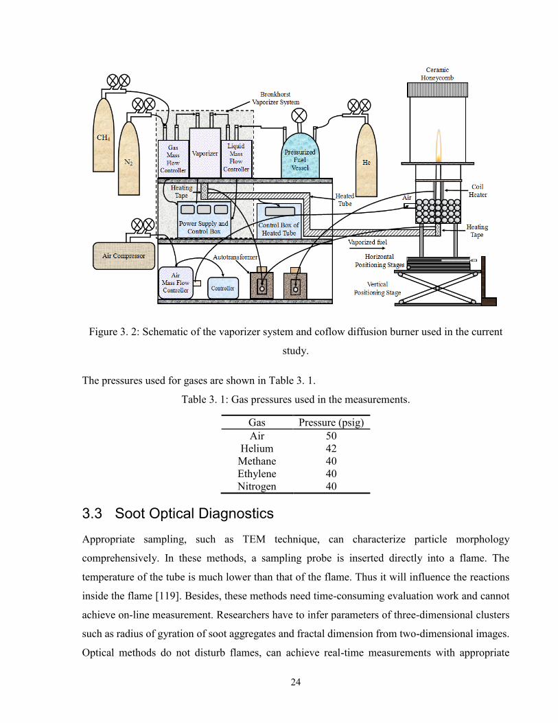
Figure 3. 2: Schematic of the vaporizer system and coflow diffusion burner used in the current

study. .......................................................................................................................... 24

Figure 3. 3: Layout of combined laser extinction and two-angle elastic laser scattering apparatus.

.................................................................................................................................... 30

Figure 3. 4: Experimental apparatus of the rapid thermocouple insertion method. ...................... 37

Figure 3. 5: Thermocouple readings at soot free regions and soot containing regions inside

flames. ........................................................................................................................ 38

Figure 4. 1: Transmittance profiles at different heights above burner (HAB) compared with those

from Santoro et al. ...................................................................................................... 45

Figure 4. 2: Soot volume fraction values of different heights above burner (HAB) at the

centerline of ethylene-air diffusion flame compared with those from Santoro et al. . 46

Figure 4. 3: Scattering cross section (30° and 150°) profiles at different heights above burner

(HAB) compared with those from Santoro et al. ....................................................... 47

Figure 4. 4: Values of primary particle diameter, primary particle number density, aggregate

number density, average number of primary particles per aggregate of different

heights above burner (HAB) at the centerline of ethylene-air diffusion flame

compared with those from literatures. ........................................................................ 49

Figure 4. 5: Visible flame images for the four levels of n-propylbenzene addition. .................... 50

ix

Figure 4. 6: Soot volume fraction profiles at different flame heights (HAB) of the four flames

studied. ....................................................................................................................... 51

Figure 4. 7: Soot volume fraction profiles along the centerline and the locations of peak soot

concentration of the four flames studied. ................................................................... 52

Figure 4. 8: Primary particle diameter and number density profiles along the centerline and the

locations of peak soot concentration of the four flames studied. ............................... 54

Figure 4. 9: Temperature profiles at different flame heights of the four flames studied. ............. 57

Figure 4. 10: Comparisons of temperature profiles of pure n-dodecane laminar coflow diffusion

flame at HAB = 50 mm, 60 mm obtained by rapid thermocouple insertion

technique and by soot spectral emission (SSE) technique. ..................................... 58

Figure 4. 11: Thermocouple readings at the centerline position and peak value position for HAB

= 50 mm of pure n-dodecane laminar coflow diffusion flame. ............................... 59

Figure B. 1: Procedure of calculating soot properties for combined laser extinction and two angle

elastic laser scattering experiments. ......................................................................... 85

Figure C. 1: Schematic of optics alignment for two-angle elastic laser scattering part. ............... 88

Figure D. 1: Soot volume fraction profiles with error bars for pure n-dodecane. ........................ 89

Figure D. 2: Soot volume fraction profiles with error bars for pure n-dodecane doped with 15

mol. % n-propylbenzene. ......................................................................................... 90

Figure D. 3: Soot volume fraction profiles with error bars for pure n-dodecane doped with 30

mol. % n-propylbenzene. ......................................................................................... 91

Figure D. 4: Soot volume fraction profiles with error bars for pure n-dodecane doped with 45

mol. % n-propylbenzene. ......................................................................................... 92

Figure E. 1: Temperature profiles with error bars for pure n-dodecane. ...................................... 93

Figure E. 2: Temperature profiles with error bars for pure n-dodecane doped with 15 mol. % n-

propylbenzene. ......................................................................................................... 94

Figure E. 3: Temperature profiles with error bars for pure n-dodecane doped with 30 mol. % n-

propylbenzene. ......................................................................................................... 95

Figure E. 4: Temperature profiles with error bars for pure n-dodecane doped with 45 mol. % n-

propylbenzene. ......................................................................................................... 96

1

Chapter 1

Introduction

1.1 Motivation

Soot refers to carbonaceous solid particulates which may contain varying quantities of oxygen and

hydrogen, and is formed by the combustion of hydrocarbon fuels under fuel rich conditions where

oxygen is not enough to completely convert the fuel into carbon dioxide (CO2) and water (H2O)

[1]. The presence of soot in flames can be observed by the characteristic yellow luminosity under

various operating conditions [2]. Soot primarily comes from furnaces, gas turbines, diesel engines,

and other combustion appliances that burn liquid fuels. The hydrocarbon fuels typically contain

alkanes, alkenes, cycloalkanes, and aromatics, whose carbon atoms vary from 5 to 20 [3].

It was found that the first stage of soot formation is characterized by the formation of particles

with diameters of 5-10 nm by the coagulation of polycyclic aromatic hydrocarbons (PAHs) [4].

Later stages include surface growth, coalescence, and coagulation resulting in the increase of

particle size. “Soot nuclei” whose structure has more condensed aromatic rings and more compact

shape is formed by simultaneously rearranging soot precursor particles [5]. Then surface reactions

and coagulation of these nuclei generate aggregates. From transmission electron microscopy (TEM)

observation, soot particles consist of approximately spherical, randomly arranged primary particles

with a certain degree of overlap [6], which depends on combustion conditions [7].

In practical combustion appliances, soot would reduce the device efficiency and influence the

maintenance of the device due to its deposition on the exhaust systems and the generation of dark

exhaust plumes [8], thus soot emission implies poor combustion conditions [9]. Besides, radiative

heat transfer from soot to engines walls contributes significantly to the total heat loss in diesel

engines and lower flame temperature influences NOx formation pathways [10]. In addition, soot

would increase the emission of CO because of the competition with CO for OH in flames [11].

It has been found that many PAHs are tumorigenic or mutagenic [12-17]. Soot emission often

associates with PAHs thus it is harmful to human health [9], and can cause lung cancer and

cardiopulmonary disease [18]. The death caused by the toxicity of fine particles per year can reach

up to 60,000 in the United States [19], which is much more than that caused by homicide or traffic

2

accidents (around 15,000 and 40,000 per year, respectively) [20]. The size and the number

concentration of particles affect health effects more than their mass concentration [21]. Fine

particles (PM2.5: diameter smaller than or equal to 2.5 μm) and ultra-fine particles (PM0.1:

diameter smaller than 0.1 μm) [22] are more toxic than larger particles and can penetrate more

deeply into human lungs, thus they have a greater risk to human health [23]. Many regulations

have been proposed to limit the number concentration of particle emission instead of mass

concentration of particle emission [21]. The United States Environmental Protection Agency has

set the upper limit of the concentration of fine particulates [24].

Besides the influence on practical combustion appliances and human health, soot also affects

atmospheric visibility as a major contributor to anthropogenic aerosols [25]. In addition, since

soot can absorb light, it increases the melting of polar ice by depositing on it. It has been studied

that soot may result in as much as 94% of Arctic warming [26] and the warming of atmosphere

caused by carbon black is 0.5-0.8 W/m2 [27, 28], while that caused by the most important

greenhouse gas (carbon dioxide) is 1.46 W/m2, and that caused by the second most important

greenhouse gas (CH4) is 0.48 W/m2 [ 29 ]. Furthermore, soot is one of the causes of the

photochemical smog formation due to its dispersion into atmosphere [30] and soot particles in the

upper atmosphere deplete the ozone layer significantly [31].

Several soot formation processes are still not well understood such as the detailed process about

the formation and growth of aromatic species, particle inception, surface growth, coagulation and

oxidation. Quantitative and qualitative understanding about these processes are important to design

the operating conditions and modify technology to reduce aerosols emission [21]. Besides, better

understanding of soot formation can assist in increasing the performance of combustion devices

[2] and reducing the air pollution. To accurately determine the properties of soot, reliable values

of soot refractive index, soot structure and soot dimensions are required [32, 33], which can be

obtained using laser diagnostics. With the application of elastic laser scattering technique, more

properties of soot can be investigated such as primary particle diameter and primary particle

number density.

Aromatics are toxic hydrocarbons that contain benzenoid ring structures [3]. Aromatics contribute

20-40% (30-35% average) in the commercial US diesel fuels [34]. Aromatics are mainly 1-ring

structures, for example, alkyl-benzenes (15%), with 5% substituted 2-ring structures. The

3

concentrations of 3-ring cyclo-paraffins and naphtha-aromatics are relatively small and are

probable to decrease in the future [35].

The formation of small aromatic hydrocarbon is one of the essential steps towards soot generation

[3]. If the fuel is non-aromatic, the aromatic ring will be produced by the precursors cyclization

[36]. The reaction of the first ring formation from small aliphatics is a rate-controlling step [37]

and is much more sensitive to the molecular structure of fuel than growth process [3]. For aromatic

fuel, it is the addition of additional benzenoid rings to the initial structures that forms larger

aromatics, not the decomposition reaction of the initial structures to non-aromatic structures and

the generation of new rings [3]. Small aromatics (≤3 benzenoid ring) are produced by adding the

first new benzenoid ring to the single-ring, and two-ring hydrocarbons which make up the bulk of

fuels, while large aromatics (>3 benzenoid ring) are produced by subsequent soot growth process

[3].

Although the formation of small aromatics only accounts for a small part in the whole soot

formation process, it strongly affects soot concentration in flames [3]. The molecular structures of

hydrocarbons significantly affect soot formation in flames [38]. Particularly, aromatic components

in hydrocarbon fuels greatly influence soot formation process in flames [38]. Variations in the rate

of benzene formation lead to the corresponding difference in the rate of soot formation [3]. Soot

generated in flames of aromatic hydrocarbon fuels is much more than that generated in flames of

non-aromatic hydrocarbon fuels [3]. Aromatic fuels soot heavily because the relatively slow step

of creating the initial ring is evited [3]. Fuel pyrolysis and the formation of one-ring to two-ring

aromatic structures are essential steps in soot formation. Each aromatic structure has several

generation pathways [3]. The detailed fuel pyrolysis and formation pathways of aromatics are not

understood completely [3].

Since turbulent fluctuations in turbulent flames make the study of aromatic formation much more

complicated, most of the research on aromatics formation is conducted in laminar flames [3].

Besides, the advantage of using coflow flames to study fuel decomposition and aromatic formation

is that these processes occur throughout the fuel-rich core of the flame, whose dimensions are

comparable to the flame height and tube-diameter or slot-width [3]. The spatial resolution

accessible with probe samples is always smaller than these dimensions, thus the spatial behaviour

of hydrocarbon fuels can be easily detected [3].

4

1.2 Objectives

The first objective of this work is to validate the experimental apparatus for combined laser

extinction (LE) and two-angle elastic laser scattering (ELS) diagnostics to study soot formation in

laminar coflow diffusion flames. The validation was performed by comparing the results of the

current apparatus with those of the literatures for a non-smoking ethylene-air laminar coflow

diffusion flame. The results include experimental raw data from laser extinction and laser

scattering measurements, as well as the information about soot properties, such as soot volume

fractions, primary particle diameters and primary particle number densities.

The second objective of this work is to understand the underlying mechanisms of the effects of n-

propylbenzene addition on soot formation in an n-dodecane laminar coflow diffusion flame. To

achieve this, methane was used as carrier gas, n-dodecane was selected to establish the base flame

environment and n-propylbenzene was mixed into n-dodecane with mole fractions from 0 mole. %

to 45 mol. %. The total inlet carbon flow rate was held constant for all of the flames. The combined

laser extinction and two-angle elastic laser scattering diagnostics was applied to obtain information

about soot volume fraction, primary particle diameter, and primary particle number density. Rapid

thermocouple insertion method was used to obtain the temperature profiles.

5

Chapter 2

Literature Review

2.1 Soot Evolution Mechanism

2.1.1 Soot Formation

2.1.1.1 Fuel Pyrolysis

Soot precursors are formed by fuel pyrolysis, which is controlled by a gas-phase chemical kinetic

mechanism. In this process, large hydrocarbon structures decompose into smaller components,

such as acetylene, polyacetylenes, unsaturated hydrocarbons and polycyclic aromatic

hydrocarbons [39] at high enough temperature. Temperature as well as molecule concentration

strongly affects the decomposition rate [39].

Fuel pyrolysis process generates initial precursors to form soot. Important precursors (gaseous)

may involve polyacetylenes [40], ionic species [41] (a carbon vapor formed from dehydrogenation

of initial hydrocarbon molecules), or polycyclic aromatic hydrocarbons (PAHs) [9]. Currently, the

majority of opinions support the conclusion that carbon nuclei is formed from PAHs [37].

2.1.1.2 Polycyclic Aromatic Hydrocarbon (PAH) Formation

PAH formation was debated among combustion researchers until Bittner and Howard [42] found

that unsaturated aliphatic species are produced from the thermal decomposition of the fuel and

then PAH is formed via reactions between acetylenic species and aromatics using a molecular

beam mass spectrometer system.

Soot formation and the chemistry of primary combustion zone are connected by the formation and

growth of aromatic species [37]. The formation of the initial aromatic ring is limited by rate [37]

and is slower than the growth process to larger aromatic ring structures [43]. Thus the rate of soot

formation is controlled by the formation of initial aromatic ring. Miller and Melius [44] proposed

that it is the reactions of two propargyl radicals that form the first ring.

C3H3 + C3H3 → benzene or phenyl + H (2. 1)

6

The assumption that aromatics are formed via propargyl has long been adopted [45, 46]. The

reaction of CH3 with C5H5 [47] and the recombination and rearrangement of two C5H5 radicals

[48] are other pathways suggested to form benzene:

C5H5 + CH3 → benzene + H + H (2. 2)

C5H5 + C5H5 → naphthalene + H + H (2. 3)

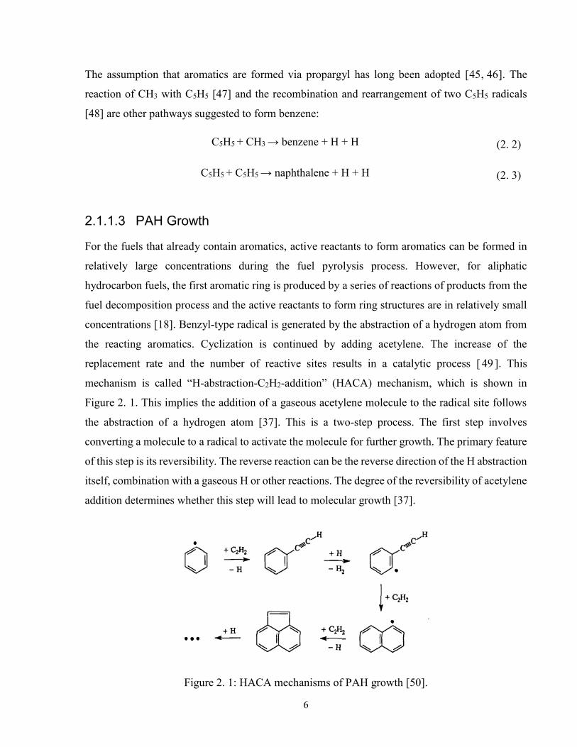
2.1.1.3 PAH Growth

For the fuels that already contain aromatics, active reactants to form aromatics can be formed in

relatively large concentrations during the fuel pyrolysis process. However, for aliphatic

hydrocarbon fuels, the first aromatic ring is produced by a series of reactions of products from the

fuel decomposition process and the active reactants to form ring structures are in relatively small

concentrations [18]. Benzyl-type radical is generated by the abstraction of a hydrogen atom from

the reacting aromatics. Cyclization is continued by adding acetylene. The increase of the

replacement rate and the number of reactive sites results in a catalytic process [ 49 ]. This

mechanism is called “H-abstraction-C2H2-addition” (HACA) mechanism, which is shown in

Figure 2. 1. This implies the addition of a gaseous acetylene molecule to the radical site follows

the abstraction of a hydrogen atom [37]. This is a two-step process. The first step involves

converting a molecule to a radical to activate the molecule for further growth. The primary feature

of this step is its reversibility. The reverse reaction can be the reverse direction of the H abstraction

itself, combination with a gaseous H or other reactions. The degree of the reversibility of acetylene

addition determines whether this step will lead to molecular growth [37].

Figure 2. 1: HACA mechanisms of PAH growth [50].

7

Kinetic models for the multi-ring molecules formation have been studied and the mechanisms of

three-dimensional networks needs more attention [49]. The local composition, burning conditions

and the temperature of the combustion system determine whether a group of soot precursors

become soot [49].

2.1.1.4 Particle Inception

Currently the particle inception process (Nucleation) is the most poorly understood part in the

whole soot formation process [37]. Some researchers [51, 52] proposed that the appearance of

nascent soot particles results from the continued growth of PAH groups involving physical and

chemical coalescence. PAH species at some size start to stick to each other via collisions producing

PAH dimers. Then these dimers continue colliding with PAH molecules generating PAH trimers

or with other PAH dimers generating PAH tetramers and so on. During the collision of PAH

species, the sizes of individual PAH species keep increasing through reactions of molecular

chemical growth. In this mechanism, clusters of PAH evolve into solid particles.

2.1.2 Soot Growth

Although soot particle inception is an important part in soot formation process, it only contributes

to 10% of the soot mass produced. The other 90% is from the surface growth process [49]. While

the number of nascent particles and the evolution of the particle number density are determined by

the nucleation kinetics and coagulation process, the carbon mass accumulated on soot is mainly

controlled by surface reaction, growth and oxidation [53].

The surface growth process occurs under conditions with high amount of acetylene [37]. In the

soot surface growth process, H reacts with soot surface and then the hydrogen atom is abstracted

from the carbon-hydrogen bond, leading to the formation of an active site on soot surface. If

acetylene exists, the active site will react with acetylene, and thus the carbon amount of particles

are increased. This process is similar to the HACA mechanism [37], as is discussed in section 2.1.

1.3. In this process, surface migration of H atom is found to be rapid enough to dominate the

formation of final product from initial adduct [54, 55]. The collision and condensation of PAH

species on the soot surface is another path of soot growth, which is called PAH-soot surface

condensation [55, 56].

8

Surface growth appears to occur both on the individual particle and on the aggregates. In the soot

growth process, the mass of the soot particle increases while the number of soot particles remain

constant [39]. The majority of soot mass is accumulated in the soot growth process. Since smaller

particles have more reactive radical sites, the rate of soot growth for smaller particles is higher

than that for larger particles [57].

2.1.3 Soot Coagulation and Agglomeration

A great number of particles collide due to the Brownian motion and then generate larger spherical

particles. This process is called coagulation, which produces fractal-like primary particles [58]. It

is different from the soot surface growth process, because the kinetics for the coagulation is

physical in nature while surface growth is driven by chemical mechanisms [59]. Coagulation

decreases soot number density, and changes size distribution and soot morphology while leaving

the total soot mass unchanged [58].

The fast restructuring of small and young particles is called coalescence [60]. In this process, the

two small particles coalesce into each other completely resulting a larger particle. As for the larger

particles, the restructuring is relatively slow and the colliding particles just merge into each other

partially resulting a transition region connecting them together. In this case, soot particles become

larger aggregates. The collision and sticking of two aggregates which consist of several primary

particles will lead to the formation of a larger aggregate. This process is called agglomeration or

aggregation [59]. The mechanisms of restructuring depend on particle size, particle material

property and local temperature. An important issue regarding coagulation is its efficiency.

Traditionally, it was assumed that every collision results in a successful coagulation. However,

some studies showed that the coagulation cannot always be successful. Under some flame

conditions, the collision of particles cannot result in sticking particles, which is called thermal

rebound effect [31, 61]. No matter what kinds of conditions are, the ultimate number density of

agglomerates is similar around 1016 /m3 [62]. It has been found that soot coagulation process takes

place almost immediately after the soot formation process, or when particles are relatively young

or small [6]. However, soot agglomeration usually occurs relatively later when there is no

coagulation [63].

9

2.1.4 Soot Oxidation

Soot oxidation and soot formation process may occur simultaneously, as in well-mixed combustors

or premixed flames, soot oxidation may occur after soot formation process as in staged combustors

or diffusion flames [18]. In the soot oxidation process, soot particles react with oxidizer back into

gaseous states, and the carbon accumulated on the soot particles is depleted [6]. The oxidation of

soot or soot precursors always competes against the production of soot or soot precursors [49].

The net amount of soot from soot formation and oxidation process determines the final particulate

emission from combustion devices [59].

Both mass transport and chemical mechanisms with heat transfer are involved in the oxidation

process. Surface intermediates are formed by the absorption of gaseous oxidizer on the surface.

Then the intermediates rearrange and desorb into gaseous products [8]. Soot can be oxidized either

by O2 or OH. The efficiency of the collision between OH and soot is relatively high. The reaction

usually occurs in the fuel-rich region. For O2, the efficiency is much lower. And O2 is a major

contributor in fuel-lean region [64]. Under some conditions, species such as O, CO2, H2O may act

as important oxidizers in soot oxidation process [65].

2.2 The Combustion of Aromatics

Aromatic hydrocarbons have a high tendency to generate soot in both diffusion flames [66] and

premixed flames [67]. Aromatics normally constitute 5 to 60% of the hydrocarbons in unleaded

gasolines, jet fuels and diesel fuels [68, 69] and generate more PAH and soot compared with non-

aromatic fuels [70], presumably because the aromatic ring can stay intact and avoid the slow

process of the first ring formation [71]. This behaviour shifts the rate-limiting step to the formation

of the second ring (naphthalene) and arouses interests in which pathways are more important for

the naphthalene formation from fuels containing monoaromatic hydrocarbons [72].

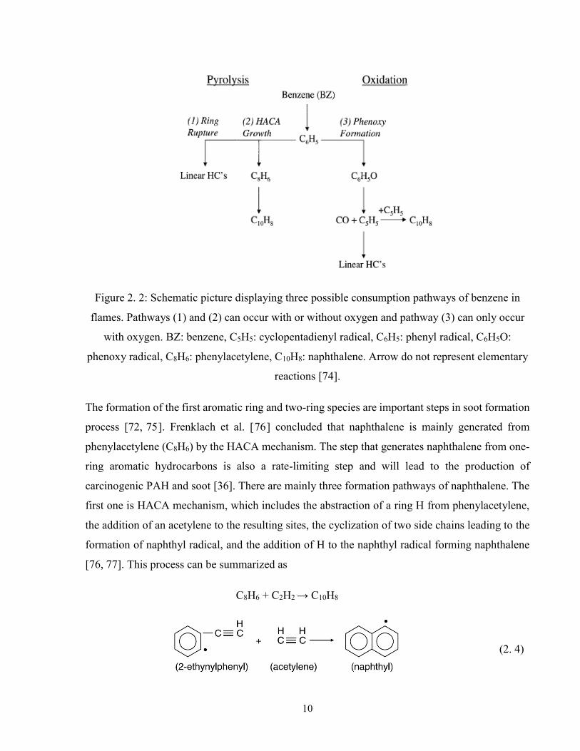
The oxidative pyrolysis mechanism of aromatic hydrocarbons is very different from pure pyrolysis

mechanism [68, 73]: pyrolysis of aromatic hydrocarbons leads to the destruction of six-membered

ring through ring rupture reactions and the formation of C4 and C2 hydrocarbons, as is shown in

pathway (1) of Figure 2. 2; phenoxy radical (C6H5O) is produced by oxidation process and then

goes through the ring contraction to generate cyclopentadienyl radical (C5H5) and CO, as is shown

in pathway (3) of Figure 2. 2.

10

Figure 2. 2: Schematic picture displaying three possible consumption pathways of benzene in

flames. Pathways (1) and (2) can occur with or without oxygen and pathway (3) can only occur

with oxygen. BZ: benzene, C5H5: cyclopentadienyl radical, C6H5: phenyl radical, C6H5O:

phenoxy radical, C8H6: phenylacetylene, C10H8: naphthalene. Arrow do not represent elementary

reactions [74].

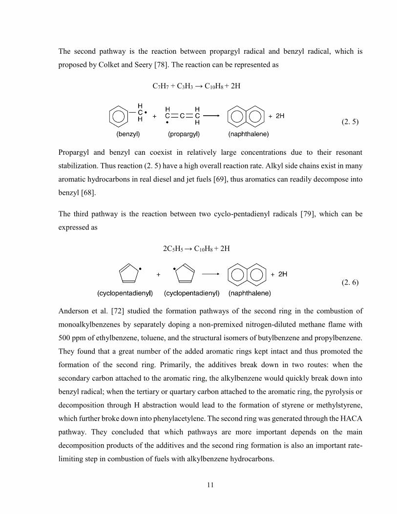
The formation of the first aromatic ring and two-ring species are important steps in soot formation

process [72, 75]. Frenklach et al. [76] concluded that naphthalene is mainly generated from

phenylacetylene (C8H6) by the HACA mechanism. The step that generates naphthalene from one-

ring aromatic hydrocarbons is also a rate-limiting step and will lead to the production of

carcinogenic PAH and soot [36]. There are mainly three formation pathways of naphthalene. The

first one is HACA mechanism, which includes the abstraction of a ring H from phenylacetylene,

the addition of an acetylene to the resulting sites, the cyclization of two side chains leading to the

formation of naphthyl radical, and the addition of H to the naphthyl radical forming naphthalene

[76, 77]. This process can be summarized as

C8H6 + C2H2 → C10H8

(2. 4)

11

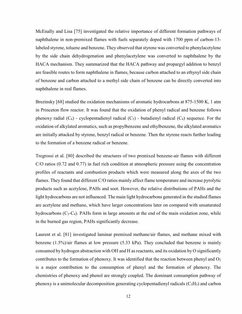
The second pathway is the reaction between propargyl radical and benzyl radical, which is

proposed by Colket and Seery [78]. The reaction can be represented as

C7H7 + C3H3 → C10H8 + 2H

(2. 5)

Propargyl and benzyl can coexist in relatively large concentrations due to their resonant

stabilization. Thus reaction (2. 5) have a high overall reaction rate. Alkyl side chains exist in many

aromatic hydrocarbons in real diesel and jet fuels [69], thus aromatics can readily decompose into

benzyl [68].

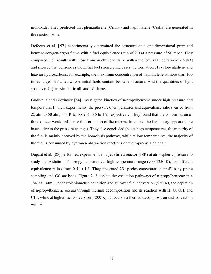
The third pathway is the reaction between two cyclo-pentadienyl radicals [79], which can be

expressed as

2C5H5 → C10H8 + 2H

(2. 6)

Anderson et al. [72] studied the formation pathways of the second ring in the combustion of

monoalkylbenzenes by separately doping a non-premixed nitrogen-diluted methane flame with

500 ppm of ethylbenzene, toluene, and the structural isomers of butylbenzene and propylbenzene.

They found that a great number of the added aromatic rings kept intact and thus promoted the

formation of the second ring. Primarily, the additives break down in two routes: when the

secondary carbon attached to the aromatic ring, the alkylbenzene would quickly break down into

benzyl radical; when the tertiary or quartary carbon attached to the aromatic ring, the pyrolysis or

decomposition through H abstraction would lead to the formation of styrene or methylstyrene,

which further broke down into phenylacetylene. The second ring was generated through the HACA

pathway. They concluded that which pathways are more important depends on the main

decomposition products of the additives and the second ring formation is also an important rate-

limiting step in combustion of fuels with alkylbenzene hydrocarbons.

12

McEnally and Lisa [75] investigated the relative importance of different formation pathways of

naphthalene in non-premixed flames with fuels separately doped with 1700 ppm of carbon-13-

labeled styrene, toluene and benzene. They observed that styrene was converted to phenylacetylene

by the side chain dehydrogenation and phenylacetylene was converted to naphthalene by the

HACA mechanism. They summarized that the HACA pathway and propargyl addition to benzyl

are feasible routes to form naphthalene in flames, because carbon attached to an ethynyl side chain

of benzene and carbon attached to a methyl side chain of benzene can be directly converted into

naphthalene in real flames.

Brezinsky [68] studied the oxidation mechanisms of aromatic hydrocarbons at 875-1500 K, 1 atm

in Princeton flow reactor. It was found that the oxidation of phenyl radical and benzene follows

phenoxy radial (C6) - cyclopentadienyl radical (C5) - butadienyl radical (C4) sequence. For the

oxidation of alkylated aromatics, such as propylbenzene and ethylbenzene, the alkylated aromatics

are initially attacked by styrene, benzyl radical or benzene. Then the styrene reacts further leading

to the formation of a benzene radical or benzene.

Tregrossi et al. [80] described the structures of two premixed benzene-air flames with different

C/O ratios (0.72 and 0.77) in fuel rich condition at atmospheric pressure using the concentration

profiles of reactants and combustion products which were measured along the axes of the two

flames. They found that different C/O ratios mainly affect flame temperature and increase pyrolytic

products such as acetylene, PAHs and soot. However, the relative distributions of PAHs and the

light hydrocarbons are not influenced. The main light hydrocarbons generated in the studied flames

are acetylene and methane, which have larger concentrations later on compared with unsaturated

hydrocarbons (C3-C4). PAHs form in large amounts at the end of the main oxidation zone, while

in the burned gas region, PAHs significantly decrease.

Laurent et al. [81] investigated laminar premixed methane/air flames, and methane mixed with

benzene (1.5%)/air flames at low pressure (5.33 kPa). They concluded that benzene is mainly

consumed by hydrogen abstraction with OH and H as reactants, and its oxidation by O significantly

contributes to the formation of phenoxy. It was identified that the reaction between phenyl and O2

is a major contribution to the consumption of phenyl and the formation of phenoxy. The

chemistries of phenoxy and phenol are strongly coupled. The dominant consumption pathway of

phenoxy is a unimolecular decomposition generating cyclopentadienyl radicals (C5H5) and carbon

13

monoxide. They predicted that phenanthrene (C14H10) and naphthalene (C10H8) are generated in

the reaction zone.

Defoeux et al. [82] experimentally determined the structure of a one-dimensional premixed

benzene-oxygen-argon flame with a fuel equivalence ratio of 2.0 at a pressure of 50 mbar. They

compared their results with those from an ethylene flame with a fuel equivalence ratio of 2.5 [83]

and showed that benzene as the initial fuel strongly increases the formation of cyclopentadiene and

heavier hydrocarbons, for example, the maximum concentration of naphthalene is more than 100

times larger in flames whose initial fuels contain benzene structure. And the quantities of light

species (<C3) are similar in all studied flames.

Gudiyella and Brezinsky [84] investigated kinetics of n-propylbenzene under high pressure and

temperature. In their experiments, the pressures, temperatures and equivalence ratios varied from

25 atm to 50 atm, 838 K to 1669 K, 0.5 to 1.9, respectively. They found that the concentration of

the oxidizer would influence the formation of the intermediates and the fuel decay appears to be

insensitive to the pressure changes. They also concluded that at high temperatures, the majority of

the fuel is mainly decayed by the homolysis pathway, while at low temperatures, the majority of

the fuel is consumed by hydrogen abstraction reactions on the n-propyl side chain.

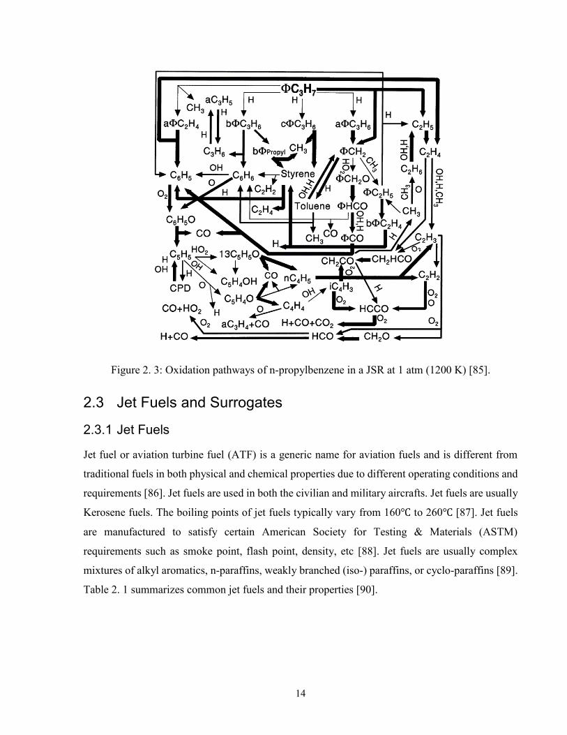
Dagaut et al. [85] performed experiments in a jet-stirred reactor (JSR) at atmospheric pressure to

study the oxidation of n-propylbenzene over high temperature range (900-1250 K), for different

equivalence ratios from 0.5 to 1.5. They presented 23 species concentration profiles by probe

sampling and GC analyses. Figure 2. 3 depicts the oxidation pathways of n-propylbenzene in a

JSR at 1 atm. Under stoichiometric condition and at lower fuel conversion (950 K), the depletion

of n-propylbenzene occurs through thermal decomposition and its reaction with H, O, OH, and

CH3, while at higher fuel conversion (1200 K), it occurs via thermal decomposition and its reaction

with H.

14

Figure 2. 3: Oxidation pathways of n-propylbenzene in a JSR at 1 atm (1200 K) [85].

2.3 Jet Fuels and Surrogates

2.3.1 Jet Fuels

Jet fuel or aviation turbine fuel (ATF) is a generic name for aviation fuels and is different from

traditional fuels in both physical and chemical properties due to different operating conditions and

requirements [86]. Jet fuels are used in both the civilian and military aircrafts. Jet fuels are usually

Kerosene fuels. The boiling points of jet fuels typically vary from 160 to 260 [87]. Jet fuels

are manufactured to satisfy certain American Society for Testing & Materials (ASTM)

requirements such as smoke point, flash point, density, etc [88]. Jet fuels are usually complex

mixtures of alkyl aromatics, n-paraffins, weakly branched (iso-) paraffins, or cyclo-paraffins [89].

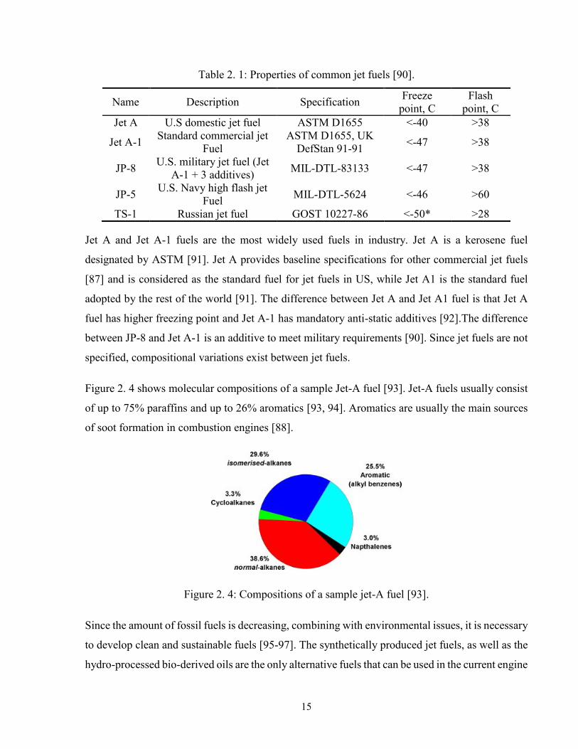
Table 2. 1 summarizes common jet fuels and their properties [90].

15

Table 2. 1: Properties of common jet fuels [90].

Name Description Specification Freeze

point, C

Flash

point, C

Jet A U.S domestic jet fuel ASTM D1655 <-40 >38

Jet A-1 Standard commercial jet

Fuel

ASTM D1655, UK

DefStan 91-91 <-47 >38

JP-8 U.S. military jet fuel (Jet

A-1 + 3 additives) MIL-DTL-83133 <-47 >38

JP-5 U.S. Navy high flash jet

Fuel MIL-DTL-5624 <-46 >60

TS-1 Russian jet fuel GOST 10227-86 <-50* >28

Jet A and Jet A-1 fuels are the most widely used fuels in industry. Jet A is a kerosene fuel

designated by ASTM [91]. Jet A provides baseline specifications for other commercial jet fuels

[87] and is considered as the standard fuel for jet fuels in US, while Jet A1 is the standard fuel

adopted by the rest of the world [91]. The difference between Jet A and Jet A1 fuel is that Jet A

fuel has higher freezing point and Jet A-1 has mandatory anti-static additives [92].The difference

between JP-8 and Jet A-1 is an additive to meet military requirements [90]. Since jet fuels are not

specified, compositional variations exist between jet fuels.

Figure 2. 4 shows molecular compositions of a sample Jet-A fuel [93]. Jet-A fuels usually consist

of up to 75% paraffins and up to 26% aromatics [93, 94]. Aromatics are usually the main sources

of soot formation in combustion engines [88].

Figure 2. 4: Compositions of a sample jet-A fuel [93].

Since the amount of fossil fuels is decreasing, combining with environmental issues, it is necessary

to develop clean and sustainable fuels [95-97]. The synthetically produced jet fuels, as well as the

hydro-processed bio-derived oils are the only alternative fuels that can be used in the current engine

16

design. Synthetic jet fuels can be produced from coal, biomass or natural gas by the Fischer-

Tropsch (FT) process [98].

2.3.2 Surrogates Formulation

Since real fuels are usually mixed with hundreds of components in detail and the components of

different fuels are significantly different, thus enormous computational resources are required to

model them. It is out of reach to numerically simulate and describe the combustion of all the

components. In addition, data is limited on the chemical reaction pathways, thermodynamic

parameters and kinetic rate constants of a number of components [93]. Using a surrogate fuel

mixture which can emulate both the physical and chemical properties of the real target fuel is a

prevalent method adopted by combustion research [93].

The compositions of real fuel are usually complex and variable [93]. Most aviation fuels are mixed

with a great number of hydrocarbons, usually from four hydrocarbon classes-nomal paraffins, iso-

paraffins, cyclo-paraffins, and aromatics [90, 99, 100]. Surrogate formulation should be flexible

enough to study a wide range of real fuels. A surrogate fuel usually contains one to ten pure

hydrocarbon components from these representative hydrocarbon classes found in real fuels. These

components are chosen to replicate the same combustion properties in real conditions, sometimes

physical properties as well [90, 101-105]. Surrogate compositions have large variations due to the

wide variety of jet fuel applications and the composition sensitivity to these applications [90]. One

component would be enough for estimating simple properties such as combustion efficiency.

However, for applications which depend on chemistry such as radiation loading, soot formation

and emission, more complex surrogates are required [90]. Physical properties of fuels such as

distillation characteristics can also be simulated if suitable number of components are selected [90].

The combustion community has been working on searching the surrogate fuels which can replicate

the performance and emissions of real jet fuels for decades [90]. Before formulating surrogates for

real target fuels, detailed chemical kinetic mechanism of each component must first be studied.

Many researchers tested these components in flow reactors, shock tubes, and rapid compression

machines to develop kinetics models of these components. Then comparisons can be made

between surrogates and real fuels in the mentioned devices [88]. Combustion kinetics are

principally driven by the ability of fuel components to generate important radical species which

17

influence both chain branching reactions of radicals and primary heat production and release in the

combustion process [93]. The formation properties and various chemical properties of individual

radical species make up the phenomena of combustion kinetics [93]. Thus the main target of

formulating surrogate is to reproduce those radicals. To formulate surrogates for real fuel, several

combustion property targets are considered to specify the identity and fraction of each component

[106, 107]. These combustion property targets include average fuel molecular weight (MW),

hydrogen/carbon molar ratio (H/C), threshold sooting index (TSI), derived cetane number (DCN).

MW strongly influences the diffusive properties of gas phase [108]. Therefore, similar average

molecular weight is required to emulate the diffusive properties of real fuels in gas phase [93]. For

real jet fuels, the average carbon number is approximately 12 [89].

H/C molar ratio determines the ratio of CO2 to H2O formed in combustion process and influences

reaction enthalpy. Besides, the ratio of hydrogen/carbon also describes the diversity of molecule

structure which determines the air fuel stoichiometry. In addition, hydrogen/carbon ratio also

strongly affects total radical population [93].

TSI is proposed by Calcote and Manos [109] for describing sooting tendency which considers

molecular weight. It is defined as:

𝑇𝑆𝐼 = 𝑎 (𝑀𝑜𝑙𝑒𝑐𝑢𝑙𝑎𝑟 𝑤𝑒𝑖𝑔ℎ𝑡

𝑆𝑚𝑜𝑘𝑒 𝑝𝑜𝑖𝑛𝑡) + 𝑏 (2. 7)

Where smoke point is the maximum diffusion flame height (mm) when there is no soot breaking

through the flame [110], molecular weight is in g/mol, a is in mol mm/g and b is a dimensionless

experimental constant. The constant a and constant b were determined so that different studies can

fall on a single scale [88]. It was found that TSI strongly depends on aromatic component fractions

[38]. A reference database has been developed for the TSI values of common surrogate

components [111].

DCN was selected to replicate the auto-ignition property of real fuels [88].

The hydrocarbons shown in Table 2. 2 are usually used as surrogate components of jet fuels [106,

112].

18

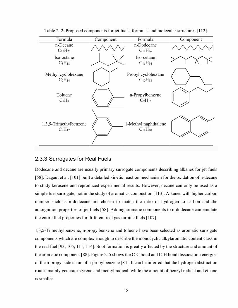
Table 2. 2: Proposed components for jet fuels, formulas and molecular structures [112].

Formula Component Formula Component

n-Decane

C10H22 n-Dodecane

C12H26

Iso-octane

C8H18

Iso-cetane

C16H34

Methyl cyclohexane

C7H14

Propyl cyclohexane

C10H18

Toluene

C7H8

n-Propylbenzene

C9H12

1,3,5-Trimethylbenzene

C9H12

1-Methyl naphthalene

C11H10

2.3.3 Surrogates for Real Fuels

Dodecane and decane are usually primary surrogate components describing alkanes for jet fuels

[58]. Dagaut et al. [101] built a detailed kinetic reaction mechanism for the oxidation of n-decane

to study kerosene and reproduced experimental results. However, decane can only be used as a

simple fuel surrogate, not in the study of aromatics combustion [113]. Alkanes with higher carbon

number such as n-dodecane are chosen to match the ratio of hydrogen to carbon and the

autoignition properties of jet fuels [58]. Adding aromatic components to n-dodecane can emulate

the entire fuel properties for different real gas turbine fuels [107].

1,3,5-Trimethylbenzene, n-propylbenzene and toluene have been selected as aromatic surrogate

components which are complex enough to describe the monocyclic alkylaromatic content class in

the real fuel [93, 105, 111, 114]. Soot formation is greatly affected by the structure and amount of

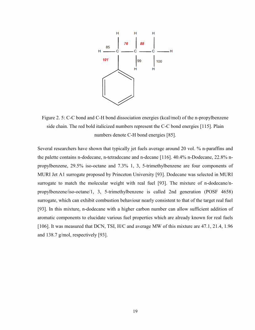
the aromatic component [88]. Figure 2. 5 shows the C-C bond and C-H bond dissociation energies

of the n-propyl side chain of n-propylbenzene [84]. It can be inferred that the hydrogen abstraction

routes mainly generate styrene and methyl radical, while the amount of benzyl radical and ethane

is smaller.

19

Figure 2. 5: C-C bond and C-H bond dissociation energies (kcal/mol) of the n-propylbenzene

side chain. The red bold italicized numbers represent the C-C bond energies [115]. Plain

numbers denote C-H bond energies [85].

Several researchers have shown that typically jet fuels average around 20 vol. % n-paraffins and

the palette contains n-dodecane, n-tetradecane and n-decane [116]. 40.4% n-Dodecane, 22.8% n-

propylbenzene, 29.5% iso-octane and 7.3% 1, 3, 5-trimethylbenzene are four components of

MURI Jet A1 surrogate proposed by Princeton University [93]. Dodecane was selected in MURI

surrogate to match the molecular weight with real fuel [93]. The mixture of n-dodecane/n-

propylbenzene/iso-octane/1, 3, 5-trimethylbenzene is called 2nd generation (POSF 4658)

surrogate, which can exhibit combustion behaviour nearly consistent to that of the target real fuel

[93]. In this mixture, n-dodecane with a higher carbon number can allow sufficient addition of

aromatic components to elucidate various fuel properties which are already known for real fuels

[106]. It was measured that DCN, TSI, H/C and average MW of this mixture are 47.1, 21.4, 1.96

and 138.7 g/mol, respectively [93].

20

Chapter 3

Experimental Methodology

3.1 Coflow Burner

The laminar coflow diffusion flame in this work was generated by a coflow diffusion burner, which

was designed for a stable and axisymmetric diffusion flame. Fuels passed through the inner

stainless steel fuel tube with an inner diameter of 10.90 mm. Oxidizer flowed through the

concentric annulus with an inner diameter of 90 mm. The fuel tube is long enough to ensure a fully

developed velocity profile of the fuel stream when it reaches the exit. The lower part of the annulus

is filled with 5 mm spherical glass beads enclosed by a porous metal disk. The beads and the porous

disk can unify laminar flow velocity profiles and stabilize flames. In the combustion research lab

at University of Toronto, a ceramic honeycomb with the size of 150×150×100 mm was used to

straighten the flow from the exit of the fuel tube and prevent air circulation down the side walls,

thus it can help obtain a stable flame. The flame was shielded from the outside lab air currents by

an optically clear acrylic tube with a 304.8 mm length, 3.175 mm wall thickness, and 152.4 mm

outside diameter. Different ports were machined on the tube for the laser extinction and scattering

experiments. Because the signal of scattering is relatively low and the influence of the tube

reflections on scattering signal is relatively large, we covered black aluminum foil tape both inside

and outside of the tube. This tape is flame-retardant, non-reflective and can be exposed to a 20 W

laser beam for 10 seconds [117].

To make experimental measurements at different positions inside flames, it is more convenient to

move the position of the burner instead of the LE and ELS system. Two linear translation stages

(Newport Model No. M-436) with low-profile crossed-roller bearing and a lab jack (Newport

Model No. M-EL120) were used to make the burner move horizontally and vertically. The travel

range of the two stages is 50.8 mm and the load capacity is 556 N. The lab jack has a travel length

of 120 mm and a load capacity of 500 N. Different from the stages, the lab jack cannot provide

direct position readings. To determine different flame heights, an absolute digimatic scale unit

(Mitutoyo Model No. 572-571) with a range of 152.4 mm and an accuracy of 0.0254 mm was

mounted to the lab jack.

21

3.2 Fuel and Oxidizer Delivery System

3.2.1 Oxidizer Delivery System

Several devices were used in the oxidizer gas line to obtain repeatable, accurate stream pressures

and flow rates.

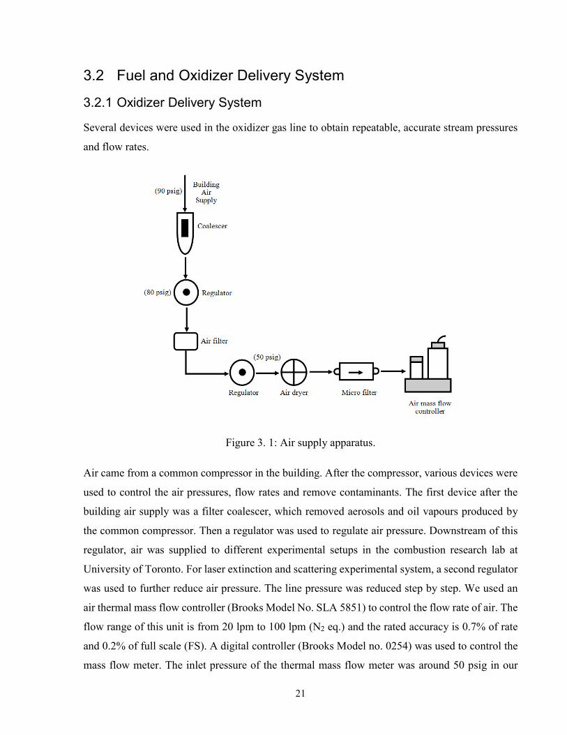
Figure 3. 1: Air supply apparatus.

Air came from a common compressor in the building. After the compressor, various devices were

used to control the air pressures, flow rates and remove contaminants. The first device after the

building air supply was a filter coalescer, which removed aerosols and oil vapours produced by

the common compressor. Then a regulator was used to regulate air pressure. Downstream of this

regulator, air was supplied to different experimental setups in the combustion research lab at

University of Toronto. For laser extinction and scattering experimental system, a second regulator

was used to further reduce air pressure. The line pressure was reduced step by step. We used an

air thermal mass flow controller (Brooks Model No. SLA 5851) to control the flow rate of air. The

flow range of this unit is from 20 lpm to 100 lpm (N2 eq.) and the rated accuracy is 0.7% of rate

and 0.2% of full scale (FS). A digital controller (Brooks Model no. 0254) was used to control the

mass flow meter. The inlet pressure of the thermal mass flow meter was around 50 psig in our

22

system. There were two filters in the air gas line. The first one was placed downstream of the

coalescer and could remove larger contaminants down to 5 μm. Very fine particles with size of 1-

2 μm cannot be captured by this step. As a result, another micron filter (Swagelok Model No. SS-

SCF3-VR4-P-225) was placed upstream of a digital mass flow controller. The particle removal

rating of this filter is greater than 99.9999999% at 0.003 μm at maximum flow rate. Besides the

filters, a chemical resistant air dryer was used to remove moisture, oil and oil vapor. The

arrangement of the devices is shown in Figure 3. 1.

3.2.2 Gaseous Fuel Delivery System

For the validation of experimental apparatus, the ethylene-air diffusion flame data from Santoro et

al. [118] was used as a benchmark to evaluate our laser extinction and scattering system.

Ethylene used in this study was supplied from a compressed cylinder with a purity of 99.5%. A

regulator was used to reduce the high pressure of the cylinder to the operating pressure of around

40 psig. A high-accuracy rotameter (Matheson Gas Model No. FM1050) was used to measure the

fuel flow rates. A needle valve was attached to the rotameter to set the desired flow rates. A small

glass ball in the glass tube displayed the fuel flow rate. When the ball suspended in the glass tube,

the drag force from the flow was equal to the weight of the ball. The scale on the rotameter is linear.

The accuracy of the rotameter does not fluctuate a lot with day-by-day use under the experimental

conditions. As the rotameter itself cannot indicate the accurate fuel flow rate, another flow

measurement device was used to calibrate it. The rotameter was calibrated by a primary gas flow

calibrator-BIOS piston prover (Mesalabs Model No. Definer 220). The BIOS calibrator can

measure flow rates from 0.005 liters to 30 liters and can work as a primary flow standard with an

accuracy of ±1% of readings standardized for temperature and pressure, and 0.75 ± 0.75% of

volumetric flow.

3.2.3 Liquid Fuel Delivery System

Most research on soot formation use gas fuels, such as methane, ethylene, and acetylene, instead

of liquid fuels. From an experimental point of view, studying liquid fuels requires a vaporizer

system to vaporize the fuel and liquid fuels generate heavy soot, which makes experiments much

more complicated. However, these gas fuels lack most of the molecular structures that characterize

liquid fuels: allylic bonds, alkyl rings, alkyl carbon-carbon bonds, and benzenoid rings. Thus

23

studying flames of liquid fuels can provide a more complete picture of fuel decomposition and

aromatics formation chemistry [3].

In the investigation of n-propylbenzene addition on soot formation in an n-dodecane laminar

coflow diffusion flame, liquid fuel was vaporized by a Bronkhorst® Controlled-Evaporator-Mixer

(CEM) unit, including a gas mass flow controller (EL-Flow Model No. F-201-CV-5K0-AAD-

22V), a liquid mass flow controller (LIQUI-FLOW Model No. L13-AAD-22K-10S), and a 3-way

mixing evaporator (CEM Model No. W-102A-222-K). Methane with a purity of 99.99% was

selected as carrier gas. The quantities of soot produced by methane itself is very small. The peak

soot volume fraction value of pure methane flame was about 0.33 ppm with a flow rate of 0.33

L/min. This peak value was less than 25% of that of pure n-dodecane flame. The adiabatic flame

temperature of pure methane under stoichiometric condition was 2321 K, which was 150 K higher

than that of 5 mol.% n-dodecane in nitrogen. Pure methane which produces very small amount of

soot made the flame temperatures more representative of that in practical conditions compared to

nitrogen used as carrier gas. Nitrogen with a purity of 99.998% was used to flush and cool the

vaporizer system and the burner after each measurement was finished. The temperature of the

vaporizer and mass flow rates were controlled by a digital readout (Bronkhorst Model No. E-7120).

Liquid fuel was supplied using a dispensing pressure vessel (Millipore Model No. XX6700P01),

which was pressurized by helium with a purity of 99.999%. It was assumed that the solubility of

helium in liquid fuel can be neglected at the temperatures and pressures used in this study.

A heated tube from Unique Heated Products INC was used to deliver the vaporized gas mixtures

to the coflow diffusion burner. The heated tube was wrapped with heating tapes (Omegalux

Catalog No. SWH171 - 020) at the outlet of the vaporizer and inlet of the burner. The fuel tube of

the burner was also heated using coil heaters (O.E.M. Heaters Model No. K460182). All of these

heaters were used to prevent fuel condensation. The temperatures of vaporizer, heated tube, and

coil heaters were set to around 460 K, 550 K, and 590 K, respectively. A schematic of the vaporizer

and burner apparatus is illustrated in Figure 3. 2.

24

Figure 3. 2: Schematic of the vaporizer system and coflow diffusion burner used in the current

study.

The pressures used for gases are shown in Table 3. 1.

Table 3. 1: Gas pressures used in the measurements.

Gas Pressure (psig)

Air 50

Helium 42

Methane 40

Ethylene 40

Nitrogen 40

3.3 Soot Optical Diagnostics

Appropriate sampling, such as TEM technique, can characterize particle morphology

comprehensively. In these methods, a sampling probe is inserted directly into a flame. The

temperature of the tube is much lower than that of the flame. Thus it will influence the reactions

inside the flame [119]. Besides, these methods need time-consuming evaluation work and cannot

achieve on-line measurement. Researchers have to infer parameters of three-dimensional clusters

such as radius of gyration of soot aggregates and fractal dimension from two-dimensional images.

Optical methods do not disturb flames, can achieve real-time measurements with appropriate

25

sensitivity, and can remotely sense even in hostile environments [119]. Therefore, optical methods

are developed to improve the field of combustion research.

Optical techniques used for combustion research include laser extinction (LE) technique, soot

spectral emission (SSE) technique, laser-induced Incandescence (LII) technique, and elastic laser

scattering (ELS) technique. Optical methods are conducted in an in situ, non-intrusive way. The

energy they add to the flame field is considered as negligible [120]. Thus they can provide

information without disturbing the flame. Optical methods are highly sensitive and have high

spatial resolution. LE method can be used to obtain information of soot volume fraction. SSE

method can be used to study soot temperature and soot volume fraction in flames. LII method can

be used to determine soot volume fraction and reduced primary particle diameter. ELS method can

provide information about primary particle diameter and primary particle number density. LE and

ELS methods are used in this work.

3.3.1 Laser Extinction Technique

LE technique measures the extinction of a collimated laser beam after it passes through a field

containing particles by optical detectors. The loss of light intensity from the light source to the

detector is caused by both the absorption and scattering by the particles along the light path.

Extinction = Absorption + Scattering (3. 1)

The extinction of laser beam is related to the length of laser path and the extinction coefficient of

particles, which can be described by Beer-Lambert law：

𝐼𝜆 = 𝐼𝜆0𝑒𝑥𝑝 (− ∫ 𝐾𝑒,𝜆

𝐿

0

𝑑𝑥) (3. 2)

Where λ is laser wavelength, Ke,λ is local extinction coefficient, Iλ,0 is the laser beam intensity

before passing through the flame chord, Iλ is the laser beam intensity after passing through the

flame chord, L is the length of the flame chord that laser passes through.

Soot volume fraction can be calculated as formula (3. 3) with the assumption that soot particles

are almost spherical [121]:

𝑓𝑣 =𝜆

𝐾𝑒𝐾𝑒,𝜆 (3. 3)

26

Where Ke is dimensionless optical extinction coefficient, which can be presented as:

𝐾𝑒 = 6𝜋(1 + 𝜌𝑠,𝑎)𝐸() (3. 4)

Where ps,a is the ratio of scattering to absorption. E is a function of the soot refractive index ,

which can be calculated as:

𝐸(𝑚) = −𝐼𝑚 [𝑚2 − 1

𝑚2 + 2] (3. 5)

According to equation (3. 3) and (3. 4), soot volume fraction can be expressed as:

𝑓𝑣 =𝐾𝑒,𝜆𝜆

6𝜋(1 + 𝜌𝑠,𝑎)𝐸() (3. 6)

The transmittance Iλ/Iλ0 is equal to the integrated value of local extinction coefficient along the

chord of flame that laser beam passes through. Thus the local extinction coefficient can be

calculated by inverting the measured transmittance, which is called tomographic reconstruction

technique. In this method, the flame was assumed symmetric. Saffaripour et al. [122] has used the

three-point Abel inversion method to obtain local extinction coefficient. LE method is flexible and

simple to conduct. However, it cannot be applied to asymmetric and non-steady flame due to

tomographic reconstruction technique and line-of-sight approach.

3.3.2 Elastic Laser Scattering Technique

Previous study from Dobbins [123] showed that the ratio of scattering to absorption can reach to

40% under a population of polydisperse aggregates. Zhu et al. [124] measured the ratios of

scattering to extinction cross-section at different light wavelength (543.6 nm, 632.8 nm, and 856

nm). The average values are 24.5%, 19.5%, and 19.5% for ethane and 31.1%, 22.8%, and 23.7%

for acetylene, respectively. It has been found that soot usually contains aggregates which consists

of a number of monomers or spherules [123]. In this case, light scattering should be considered in

the total extinction [123].

It has been observed that the light intensity absorbed by a soot particle is proportional to its volume,

and the light intensity scattered by a soot particle is proportional to the square of its diameter. Thus

the particle diameter can be obtained by calculating the ratio of absorption to scattering. This

theory has been the foundation of many research efforts in the recent past [123, 125-132]. More

detailed work is discussed below.

27

Most of previous studies use Rayleigh theory to study soot scattering. This method is suitable when

the particle size is smaller than the wavelength of incident laser beam. And Mie theory is suitable

when the size of particles is comparable to the wavelength of the light source. However, primary

soot particles usually stick together to form aggregates instead of existing separately. The size of

aggregates may be larger than the wavelength of laser light, because the number of primary

particles in an aggregate varies from 10 to 104 [133]. Thus it is inaccurate to use Rayleigh theory

and Mie theory to study soot in flames. The classical Rayleigh-Debye-Gans scattering theory has

been generalized for fractal aggregates by using fractal ideas along with certain assumptions about

multiple scattering and primary particle properties in aggregates. There are analytical expressions

in the formulation which directly relate optical cross sections to aggregate size, particle size and

morphology [134]. For elastic light scattering, Rayleigh theory and Mie theory has substantial

disadvantages in accurately determining the aggregates scattering cross sections [135]. On the

contrary, Rayleigh-Debye-Gans Fractal Aggregate (RDG/FA) theory [136] is more reliable to

analyze soot aggregate properties because it considers the optical cross sections of particulate

aggregates and aggregate polydispersity. In the current work, we used an improved data analysis

[137] approach to relate the various measured optical cross sections to soot aggregate properties

based on the RDG-FA theory. In this approach, we assumed that the soot primary particles are

spherical scatterers that only make point contact with each other. The full calculation procedure is

shown in appendix B.

Puri et al. [128] analyzed a coannular ethane diffusion flame using laser extinction technique and

laser scattering technique at multiple angles (45°, 90°, 135°) combined with additional information

from TEM measurements. It was shown in this study that the data reduction is quite different

between those based on aggregate cross sections and those using Rayleigh or Mie theory. Based

on Mie and Rayleigh theory, the volume mean diameter increases much more modestly in the

growth region and decreases quite moderately in the oxidation region. It was found that the particle

number concentration shows a slight increase in the growth region in the Rayleigh sphere data

reduction and is constant along most streamline in Mie data reduction using scattering/extinction

cross sections, which indicates cluster-cluster aggregation (CCA) is absent or CCA is offset by the

increase of aggregate population through inception. Besides, Mie theory with dissymmetry

measurements yields a much lower number concentration, which is unreasonable due to the

generation of more than twice theoretical aggregation rate. For peak soot volume fraction, the

28

result obtained from Rayleigh theory is around 30% higher and that from Mie theory is 15% lower

at the intermediate flame heights. Mie theory overestimates the contribution of scattering to

extinction, while Rayleigh theory ignores the contribution of scattering compared to RDG/FA

theory.

Link et al. [135] studied the ability of multi-angle scattering measurements to determine soot

aggregate properties including the fractal dimension and the size distribution. The range of angles

spans from 10° to 160°. They found that it is difficult to unambiguously determine the size

distribution parameters using multi-angle scatter intensities and the measured part of the overall

structure factor is significantly limited by the corresponding range of scattering wave vector. It

was shown that relative multi-angle (10° to 160°) scattering experiments with laser wavelength in

the visible region can only obtain possible combinations of the size distribution of soot aggregates

and fractal dimension instead of determining their values simultaneously.

Iuliis et al. [138] compared the results of three angle laser scattering and laser extinction technique

with those from TEM analysis. The primary particle diameter and radius of gyration with the

presence of mature soot agree well with each other. However, in the relatively lower region of the

flame, difference was found due to different structures from mature soot. There are substantial

limitations to both optical and TEM methods at these regions due to different optical properties

and the splashing of the liquid-like structure respectively. For young soot, more structural and

optical information are required.

Teng et al. [139] suggested two optimum scattering angles (30° and 150°) by considering both the

sensitivity analysis and the spatial resolution. From sensitivity analysis aspect, the further the two

scattering angles are separate, the more accurate the aggregate size inversion is; from spatial

resolution aspect, since the scattering volume detected by the detector increases with 1/sin θ (θ:

scattering angle), too small or too large scattering angles will result in a poor spatial resolution.

Besides, the scattering length and volume detected by the detector are determined by the pinhole

in front of the photomultiplier. On one hand, to ensure enough scattered light is collected, the size

of pinhole should be large enough; on the other hand, to ensure the solid angle is not too large, the

size of pinhole should be small enough. A scattering angle of more than 150° or less than 30°

would possibly make the radial distance that the signal averages exceeds the desirable limit of

spatial resolution. Thus 30° and 150° were selected for the optical arrangement of scattering

29

experiments. They evaluated the measurements using exact scattering computations on fractal-like

aggregates with convenient form of structure factor. The aggregate gyration radius inferred from

computations of dissymmetry ratios of 30° and 150° agrees well with the initially prescribed values

and the spherule diameters also agree well with the simulation values, except for relatively small

aggregates, since the dissymmetry ratio of them is close to unity. Their computational results

showed that inverse analysis of laser scattering at only two angles can provide information about

spherule and aggregate sizes with minor errors. In the current work, two scattering angles (30° and

150°) were selected to study soot formation in laminar coflow diffusion flames. The two scattering

angles combined with the improved data analysis approach [137] allow us to remove the

assumption made about the regime in which the scattering measurements are made.

3.4 Optical Configuration

The optical apparatus for LE and ELS measurement is shown in Figure 3. 3. It consists of a

Coherent CW high-power optically pumped semiconductor laser with a wavelength of 639 nm.

The incident laser power was set to 150 mW for LE measurements and 1000 mW for ELS

measurements. Laser beam was modulated by a mechanical chopper at 1015 Hz. The modulated

beam was then enlarged using a plano-concave lens with a focal length of 25 mm and a plano-

convex lens with a focal length of 150 mm. Then the enlarged beam passed through a polarizer

with an extinction ratio of 100,000:1 to ensure the light was polarized in the vertical direction. A

beam splitter with a split ratio of 90:10 was used to partially transmit the polarized beam to a

photodiode to monitor the power fluctuations of laser. This measurement was used to correct the

detected signals in laser power. The direction of the other portion of the laser beam passing through

beam splitter was changed by a mirror and then focused to the center of the coflow burner by a

750 mm focal length lens. After the beam passed through the flame, a 100 mm plano-convex lens

was used to collimate the beam. Then the collimated beam was focused into an integrating sphere

by a plano-convex lens with the same focal length. This integrating sphere was used to uniformly

distribute the incoming light by multiple reflections inside the sphere. After that, the uniform

distributed laser beam was collected by a photodiode. For the scattering part, the scattered light

was first collimated using a 200 mm focal plano-convex lens. Then the collimated light passed

through a Glan-Laser Calcite polarizer to make sure that only vertically polarized light was

transmitted. Then a plano-convex lens with the same focal length focused the beam into a 500 μm

pinhole located in front of the photomultiplier tubes (PMTs). The pinhole was used to define the

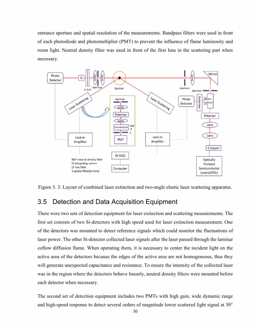
30

entrance aperture and spatial resolution of the measurements. Bandpass filters were used in front

of each photodiode and photomultiplier (PMT) to prevent the influence of flame luminosity and

room light. Neutral density filter was used in front of the first lens in the scattering part when

necessary.

Figure 3. 3: Layout of combined laser extinction and two-angle elastic laser scattering apparatus.

3.5 Detection and Data Acquisition Equipment

There were two sets of detection equipment for laser extinction and scattering measurements. The

first set consists of two Si-detectors with high speed used for laser extinction measurement. One

of the detectors was mounted to detect reference signals which could monitor the fluctuations of

laser power. The other Si-detector collected laser signals after the laser passed through the laminar

coflow diffusion flame. When operating them, it is necessary to center the incident light on the

active area of the detectors because the edges of the active area are not homogeneous, thus they

will generate unexpected capacitance and resistance. To ensure the intensity of the collected laser

was in the region where the detectors behave linearly, neutral density filters were mounted before

each detector when necessary.

The second set of detection equipment includes two PMTs with high gain, wide dynamic range

and high-speed response to detect several orders of magnitude lower scattered light signal at 30°

31

and 150° to the incident beam. In the scattering part, the first element was an aperture with a

diameter range from 0.8 mm to 12 mm, which was used to define the solid angle for collecting

scattered light. A plano-convex lens with a focal length of 200 mm was mounted at a distance of

200 mm from the center of the fuel tube to collimate the scattered light. The aperture, lens,

polarizer, pinhole and band pass filter were all mounted inside a tube to prevent unwanted light

from entering the PMT.

There were four data channels in total in the current LE and two-angle ELS setup. Two of them

were for LE measurements from two Si-detectors, the other two were for ELS measurements from

two PMTs. BNC terminators were used to convert the current signals to voltage signals. Then the

signals were transmitted to the lock-in amplifiers (Stanford Research Systems, Model No. SR-830).

The measured signals had both the alternating current (AC) component and the direct current (DC)

component. The AC signal was from the scattered light or the transmitted light and the DC signal

was from extraneous light, such as flame radiation. The incident light was modulated at a specified

frequency (1015 Hz) by a chopper. Lock-in amplifiers were capable to select these AC signals and

recover the signals that were mixed with other signals. The time constant used in the lock-in

amplifier was 1s.

In the current study, data acquisition system includes the LabVIEW software installed in a

ThinkPad computer and National instruments (NI) data acquisition (DAQ) system. All of the above

mentioned data channels-two for scattering measurements from PMTs and two for extinction

measurements from Si-detectors were transmitted into a National Instruments (NI) model. This

module has 4 analog input channels (Al) with a sampling rate of from 1 S/s up to 102.4 kS/s and

1 analog output channel (A0) with an update rate of 96 kS/s. All of the Al channels were sampled

simultaneously [140]. All the data was saved to an Excel file by the LabVIEW code.

3.6 Constants

In the current study, soot aggregate properties were determined using the measured volumetric

extinction coefficients and scattering coefficients through the Rayleigh-Debye-Gans Fractal

Aggregate (RDG/FA) theory. This calculation requires the values of soot refractive index (m),

fractal dimension (Df) and fractal prefactor (kf). Many researchers have attempted to determine the

values of complex refractive index, fractal dimension and fractal prefactor. Some of these studies

are discussed below.

32

3.6.1 Refractive Index

Erickson et al. [141] measured the concentrations and sizes of soot particles in a premixed laminar

benzene-air flame using laser scattering technique and compared the experimental results with

theoretical calculated parameters. They found that the best fit between experimental value and

theoretically calculated value for monodisperse spheres occurs when refractive index m = 1.40-

1.00i at x = 1.05 (x = particle perimeter/wavelength, πd/λ) was selected to calculate the properties

of soot particles. However, this only demonstrated that it is possible to match the results of

experiments and theoretical calculations for monodisperse spheres, but it did not mean the values

for m and x are correct.

Lee and Tien [142] developed a dispersion model to analyze the optical constants of soot based on

a more rigorous consideration of the dispersion constants and the electronic band structures. They

concluded that soot optical properties are not sensitive to increasing temperatures and are relatively

independent of the fuel hydrogen/carbon ratio.

Bockhorn et al. [143] investigated soot concentrations and particle sizes in a propane-oxygen flame

with additives of hydrogen and ammonia at atmospheric pressure by laser scattering and probe

measurements. They evaluated the measurement results of light scattering by nonlinear regression

analysis. It was found that the regression can be improved if the real part and imaginary part of the

refractive index are not assumed constant. They obtained refractive index m = 1.1-0.37i for

propane-oxygen flame, m = 1.3-0.74i for propane-oxygen flame with additive of hydrogen, m =

1.3-0.94i for propane-oxygen flame with additive of ammonia at the height of 25 mm above the

burner.

Charalampopoulos and Felske [144] studied a fuel-rich premixed methane-oxygen flame and

inferred complex refractive index of Rayleigh size soot particles from extinction and classical

scattering data. The particle size distribution was separately determined from the refractive index

and particle concentration. For monodisperse, the real parts of the refractive index they obtained

are between 1.37 and 1.79 and the imaginary parts of the refractive index are between 0.41 and

0.74; for polydisperse, the real parts of the refractive index they obtained are between 1.38 and

1.86, the imaginary parts of the refractive index are between 0.42 and 0.78.

33

Mullins and Williams [145] measured refractive index of soot in flames of four fuels: n-heptane,

propane, methane and toluene (methyl benzene) at two laser wavelengths, 450 nm and 633 nm,

using two techniques, light attenuation and light reflectance. They found that the contribution of

light scattering to light attenuation is approximately 5%. By comparing their experimental results

with the theoretical values calculated by Lee and Tien [142], they concluded that Mie scattering

theory, which is usually applied to describe light attenuation by small spherical particles, can

successfully determine the complex refractive index of soot when the density and mean particle

size are provided. They also found that soot collected from four different flames through means of

impingement on a plate has similar optical properties at 300 K by using light attenuation technique,

which are consistent with the theoretical values of the complex index at 300 K. However, the light

reflectance technique resulted in higher values of the imaginary part of the complex refractive

index compared to the light attenuation technique. They proposed that this difference occurs

because light reflectance technique is sensitive to the surface roughness degree. In their results,

the real part of refractive index varies between 1.88 and 1.93 in both methods, the imaginary part

of refractive index varies between -0.78 and -0.51 in the light reflectance method, and between -

0.46 and -0.39 in light attenuation method.

Vaglieco et al. [146] evaluated the optical property dispersion of absorbing submicronic aerosols

in premixed flames at atmospheric pressure by simultaneously measuring scattering and extinction

coefficients in the near UV and visible spectrum. They used non-aromatic fuels such as CH4, C2H2,

and C2H4 at different flow rates and C/O ratios. They assumed the particles are not agglomerated

and not considered as Rayleigh scatterers, and the contribution of molecules is negligible when

determining the spectral properties of the real and imaginary parts of the complex refractive index

of soot. Their method required that the optical properties at a reference wavelength, the average

size and number density of the soot particles are known independently, laser scattering and

extinction are primarily caused by solid submicronic particles, and fluorescence and absorption

from aromatic gaseous compounds are negligible. They found that the real part of the complex

refractive index displays a strong dispersion in the visible region and decreases from the visible

region to the UV region while the imaginary part decreases when wavelengths are shorter than 300

nm and remains constant in the visible region.

Smyth and Shaddix [147] indicated that refractive index m = 1.57-0.56i is still by far the most

often cited value in the visible wavelengths by combustion community. They found that the value

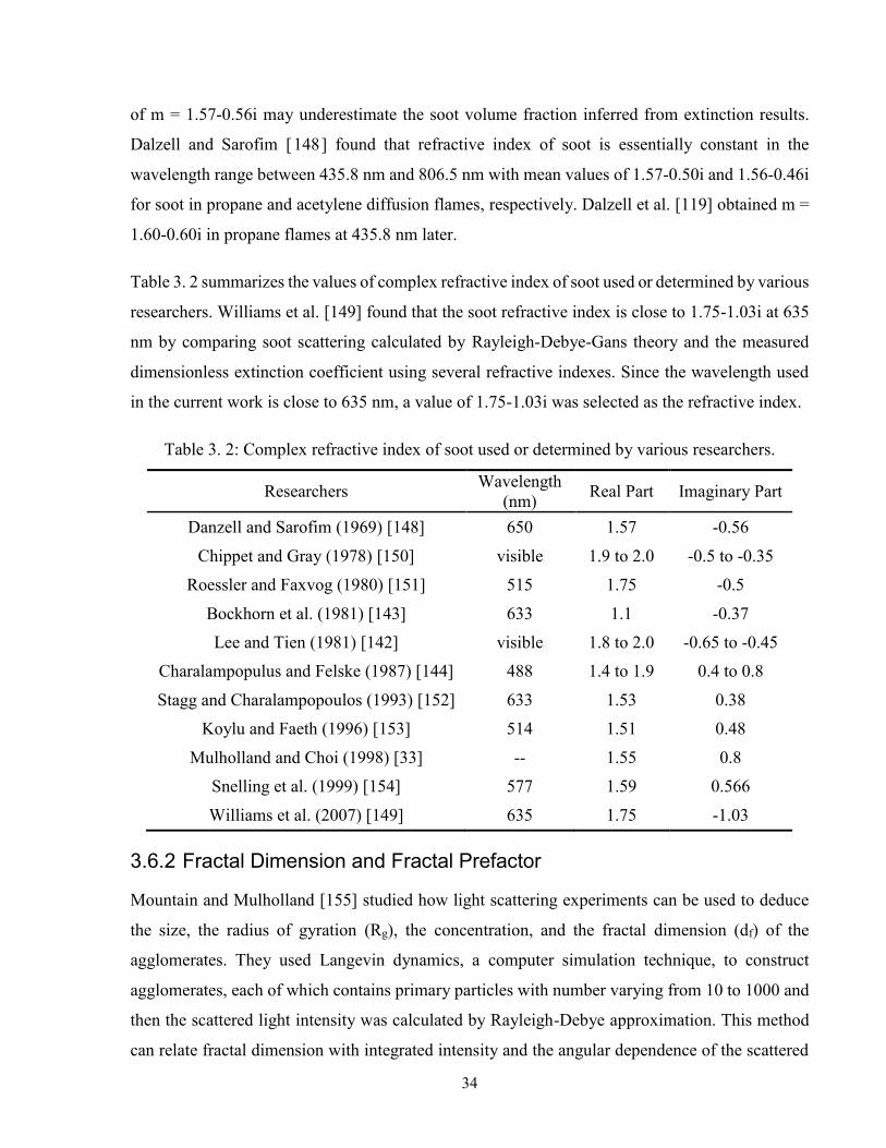
34

of m = 1.57-0.56i may underestimate the soot volume fraction inferred from extinction results.

Dalzell and Sarofim [148] found that refractive index of soot is essentially constant in the

wavelength range between 435.8 nm and 806.5 nm with mean values of 1.57-0.50i and 1.56-0.46i

for soot in propane and acetylene diffusion flames, respectively. Dalzell et al. [119] obtained m =

1.60-0.60i in propane flames at 435.8 nm later.

Table 3. 2 summarizes the values of complex refractive index of soot used or determined by various

researchers. Williams et al. [149] found that the soot refractive index is close to 1.75-1.03i at 635

nm by comparing soot scattering calculated by Rayleigh-Debye-Gans theory and the measured

dimensionless extinction coefficient using several refractive indexes. Since the wavelength used

in the current work is close to 635 nm, a value of 1.75-1.03i was selected as the refractive index.

Table 3. 2: Complex refractive index of soot used or determined by various researchers.

Researchers Wavelength

(nm) Real Part Imaginary Part

Danzell and Sarofim (1969) [148] 650 1.57 -0.56

Chippet and Gray (1978) [150] visible 1.9 to 2.0 -0.5 to -0.35

Roessler and Faxvog (1980) [151] 515 1.75 -0.5

Bockhorn et al. (1981) [143] 633 1.1 -0.37

Lee and Tien (1981) [142] visible 1.8 to 2.0 -0.65 to -0.45

Charalampopulus and Felske (1987) [144] 488 1.4 to 1.9 0.4 to 0.8

Stagg and Charalampopoulos (1993) [152] 633 1.53 0.38

Koylu and Faeth (1996) [153] 514 1.51 0.48

Mulholland and Choi (1998) [33] -- 1.55 0.8

Snelling et al. (1999) [154] 577 1.59 0.566

Williams et al. (2007) [149] 635 1.75 -1.03

3.6.2 Fractal Dimension and Fractal Prefactor

Mountain and Mulholland [155] studied how light scattering experiments can be used to deduce

the size, the radius of gyration (Rg), the concentration, and the fractal dimension (df) of the

agglomerates. They used Langevin dynamics, a computer simulation technique, to construct

agglomerates, each of which contains primary particles with number varying from 10 to 1000 and

then the scattered light intensity was calculated by Rayleigh-Debye approximation. This method

can relate fractal dimension with integrated intensity and the angular dependence of the scattered

35

light. They found that the fractal dimension lies in the interval between 1.7 and 1.9. They showed

that the radius of gyration (Rg) is a function of the number (N) of primary particles as N =

5.8(Rg/σ)1.9 when selecting fractal dimension as 1.9 and fractal prefactor as 5.8. The value 5.8 for

fractal prefactor was empirically determined.

Meakin [156] simulated diffusion-limited aggregation (DLA) process and indicated that the fractal

dimensions may vary from 1.35 to 1.85. Jullien [157] simulated cluster-cluster aggregation. In

their model, all clusters stuck at their first contact resulting in diffusing and growth. This model

can be used to describe the aggregation of aerosols or colloids. The experimentally estimated value

of fractal dimension (D = 1.49 ± 0.05) agrees well with their calculation value. They also found

that the value of fractal dimension is between 1.44 and 1.78.

Dobbins and Megaridis [158] investigated the absorption, scattering and differential scattering

cross sections for polydisperse aggregates with prescribed fractal dimension. The value they used

for fractal dimension varies from 1.7 to 1.9 for aggregated materials generated by cluster-cluster

aggregation and the value used for fractal prefactor is constant to be 5.8. Dobbins et al. [123] also

proposed that the value of fractal dimension is in the range from 1.7 to 1.9 when aggregates grow

through the processes of cluster-cluster collision.

Puri [128] determined the fractal dimension of aggregates as 1.74 in a coannular ethane diffusion

flame using laser extinction and laser scattering measurements at multiple angles and the value 9.0

of fractal prefactor was obtained approximately by a regression analysis. Koylu [132] inferred

fractal dimension in the fuel-rich region of laminar ethylene flame and the post-flame region of

turbulent ethylene flame as 1.73 and 1.83 respectively based on RDG/PFA scattering theory with

prefactor as 8.5 and refractive index as 1.54 + 0.48i.

Koylu and Faeth [129] investigated soot structure in the overfire (fuel-lean) region of buoyant

turbulent diffusion flames using transmission electron technique. They concluded that fractal

dimensions of aggregates are less dependent on fuel type and vary between 1.70 and 1.79 with the

assumed value of prefactor as 5.8.

It can be found from the above literatures that generally the value of fractal prefactor was assumed

by researchers while the value of fractal dimension can be deduced by combining experimental

data and computer simulations. Table 3. 3 summarizes the values of fractal dimension and fractal

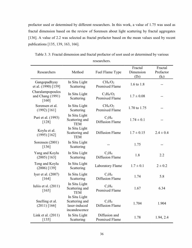
36

prefactor used or determined by different researchers. In this work, a value of 1.75 was used as

fractal dimension based on the review of Sorensen about light scattering by fractal aggregates

[136]. A value of 2.2 was selected as fractal prefactor based on the mean values used by recent

publications [135, 139, 163, 166].

Table 3. 3: Fractal dimension and fractal prefactor of soot used or determined by various

researchers.

Researchers Method Fuel Flame Type

Fractal

Dimension

(Df)

Fractal

Prefactor

(kf)

Gangopadhyay

et al. (1990) [159]

In Situ Light

Scattering

CH4/O2

Premixed Flame 1.6 to 1.8 --

Charalampopoulos

and Chang (1991)

[160]

In Situ Light

Scattering

C3H8/O2

Premixed Flame 1.7 ± 0.08 --

Sorensen et al.

(1992) [161]

In Situ Light

Scattering

CH4/O2

Premixed Flame 1.70 to 1.75 --

Puri et al. (1993)

[128]

In Situ Light

Scattering and

TEM

C2H4

Diffusion Flame 1.74 ± 0.1 --

Koylu et al.

(1995) [162]

In Situ Light

Scattering and

TEM

Diffusion Flame 1.7 ± 0.15 2.4 ± 0.4

Sorensen (2001)

[136]

In Situ Light

Scattering -- 1.75 --

Yang and Koylu

(2005) [163]

In Situ Light

Scattering

C2H4

Diffusion Flame 1.8 2.2

Teng and Koylu

(2006) [139]

In Situ Light

Scattering Laboratory Flame 1.7 ± 0.1 2 ± 0.2

Iyer et al. (2007)

[164]

In Situ Light

Scattering

C2H4

Diffusion Flame 1.74 5.8

Iuliis et sl. (2011)

[165]

In Situ Light

Scattering and

TEM

C2H4

Premixed Flame 1.67 6.34

Snelling et al.

(2011) [166]

In Situ Light

Scattering and

laser-induced

incandescence

C2H4

Diffusion Flame 1.704 1.904

Link et al. (2011)

[135]

In Situ Light

Scattering

Diffusion and

Premixed Flame 1.78 1.94, 2.4

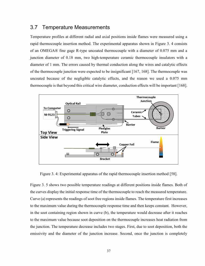
37

3.7 Temperature Measurements

Temperature profiles at different radial and axial positions inside flames were measured using a

rapid thermocouple insertion method. The experimental apparatus shown in Figure 3. 4 consists

of an OMEGA® fine gage R-type uncoated thermocouple with a diameter of 0.075 mm and a

junction diameter of 0.18 mm, two high-temperature ceramic thermocouple insulators with a

diameter of 1 mm. The errors caused by thermal conduction along the wires and catalytic effects

of the thermocouple junction were expected to be insignificant [167, 168]. The thermocouple was

uncoated because of the negligible catalytic effects, and the reason we used a 0.075 mm

thermocouple is that beyond this critical wire diameter, conduction effects will be important [168].

Figure 3. 4: Experimental apparatus of the rapid thermocouple insertion method [58].

Figure 3. 5 shows two possible temperature readings at different positions inside flames. Both of

the curves display the initial response time of the thermocouple to reach the measured temperature.

Curve (a) represents the readings of soot free regions inside flames. The temperature first increases

to the maximum value during the thermocouple response time and then keeps constant. However,

in the soot containing region shown in curve (b), the temperature would decrease after it reaches

to the maximum value because soot deposition on the thermocouple increases heat radiation from

the junction. The temperature decrease includes two stages. First, due to soot deposition, both the

emissivity and the diameter of the junction increase. Second, once the junction is completely

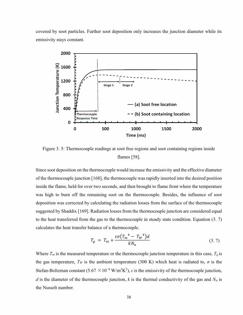
38

covered by soot particles. Further soot deposition only increases the junction diameter while its

emissivity stays constant.

Figure 3. 5: Thermocouple readings at soot free regions and soot containing regions inside

flames [58].

Since soot deposition on the thermocouple would increase the emissivity and the effective diameter

of the thermocouple junction [168], the thermocouple was rapidly inserted into the desired position

inside the flame, held for over two seconds, and then brought to flame front where the temperature

was high to burn off the remaining soot on the thermocouple. Besides, the influence of soot

deposition was corrected by calculating the radiation losses from the surface of the thermocouple

suggested by Shaddix [169]. Radiation losses from the thermocouple junction are considered equal

to the heat transferred from the gas to the thermocouple in steady state condition. Equation (3. 7)

calculates the heat transfer balance of a thermocouple.

𝑇𝑔 = 𝑇𝑚 +휀𝜎(𝑇𝑚

4 − 𝑇𝑊4)𝑑

𝑘𝑁𝑢 (3. 7)

Where Tm is the measured temperature or the thermocouple junction temperature in this case, Tg is

the gas temperature, TW is the ambient temperature (300 K) which heat is radiated to, σ is the

Stefan-Boltzman constant (5.67 ×10−8 W/m2K2), ε is the emissivity of the thermocouple junction,

d is the diameter of the thermocouple junction, k is the thermal conductivity of the gas and Nu is

the Nusselt number.

39

The diameter of the thermocouple junction, the emissivity of the thermocouple junction and the

Nusselt number are three main factors that influence radiation losses. The effect of junction

diameter was minimized by using a thin 0.075 mm thermocouple. The emissivity value of uncoated

thermocouple at different temperatures was obtained from Bradley and Entwistle [170]. The

estimated value 2 was used for the Nusselt number based on the correlation suggested by Shaddix

[169].

3.8 Optics Alignment

Proper optics alignment is one of the main factors that affect the accuracy of data sets. Since it is

difficult for the researcher to distinguish if the deviations of profiles from the expected trends are

caused by improper optics alignment or some other experimental errors, a careful effort should be

made to make sure all of the optics and the coflow diffusion burner are appropriately positioned.

Two factors should be considered when aligning optics: efficiency and position. Efficiency means

that we should consider if the transmitting efficiency meets expectation after laser passes through

each element in an optical system. Position means that we should consider if the laser passes

through the center of a symmetrical system and if the position of focal point satisfies the design

requirement.

Before performing optics alignment, the adjusters of each mount should be checked if they are in

the middle position, which is the balance position. This step is to leave enough allowance to align

the optics. The basic principles for optics alignment are described as following:

1. Sequence principle: Usually, an optical system consists of fixing element and adjustable

element. Fixed elements should be handled first, then determine the alignment sequence of

adjustable elements. For our experimental system, we fixed the position of semiconductor

laser. Our optical system consists of laser extinction part and laser scattering part. We first

aligned the laser extinction part and determined the center position of flames, and then

aligned the laser scattering part.

2. Middle principle: When performing optics alignment, enough space and allowance should

be left. The deviation of the laser beam from the center of all the optics should be as small

as possible.

40

3. Safety principle: To ensure both personal safety and instrumental safety, when aligning

optics, the output power of laser should be set as low as possible to prevent harm to eyes,

as well as the damage to system elements due to improper behaviours.

The detailed optics alignment procedure is described in Appendix C.

3.9 Scattering Calibration

The intensity of scattered light which is measured by PMT is related to the number density of

scatterers (np), the incident laser power (I0), and the size and the shape of the scatterers which are

soot particles in the probe volume for the current study. The output of PMT is a function of the

solid angle (∆Ω), the size of the probe volume (∆V), the quantum efficiency of the PMT (ηpmt), the

efficiency of the optics (ηopt), and the above mentioned parameters.

𝑉𝑠 = 𝐼0𝜂𝑝𝑚𝑡𝜂𝑜𝑝𝑡𝑛𝑝𝐶𝑣𝑣(𝜃)∆𝑉∆Ω (3. 8)

Here, Vs is the measured signal, Cvv(θ) is the differential cross section of a single scatterer in the

direction 𝜃. In equation (3. 8), I0, ηpmt, ηopt, ∆V, and ∆Ω are unknown, these constants are combined

into a single constant C. Through the scattering calibration procedure, C can be determined by

using a scatter whose cross section is already known, such as ethylene and propane. Thus, the

scattering cross section can be determined without obtaining the value of each constant separately.

Equation (3. 8) can be written as:

𝑉𝑠 = 𝐶𝑛𝑝𝐶𝑣𝑣(𝜃) (3. 9)

In this study, we used ethylene and propane as calibration gases, the number density of each gas

can be calculated by the ideal gas equation. Scattering calibration was conducted at room

temperature and pressure. We flowed the ethylene and propane in the fuel tube of the burner. To

ensure that we only detected the light scattered by the calibration gas and the light scattered by the

lip of the burner did not enter the solid angle, the calibration was carried out at the height of 7 mm

above the centerline of the burner. Then we compared the ratio of the signal obtained from propane

to that from ethylene with theoretical value. If the error was within 5%, then the scattering

alignment was considered to be accurate enough [133].

41

3.10 Test Conditions

For the ethylene-air diffusion flame, the air flow rate was set to 42.7 L/min, while the fuel flow

rate was set to 0.231 L/min at 293.15 K, 101.3 kPa.

For the flame of n-dodecane doped with n-propylbenzene, the tested experimental conditions are

shown in Table 3. 4. The flow rates of methane, air and total carbon at inlet were held constant for

all of the four flames. The mole fraction of n-dodecane in fuel stream at inlet was 3% for the base

flame. The mole fractions of added n-propylbenzene in the liquid fuel mixtures varied from 0% to

45%. The main purpose was to distinguish the effects of n-propylbenzene addition on soot

formation pathways under nearly unchanged thermodynamic and chemical environments. The

variations of soot refractive index with soot maturity in flames and the influences of PAH

absorption on extinction measurements were not considered in the current study. These

experimental uncertainties should be similar for the four flames.

Table 3. 4: Experimental test conditions.

Liquid fuel Molecular fraction CH4 flow

rate (L/min)a

Air flow

rate (L/min)a

Liquid fuel

flow rate (g/h) n-C9H12 n-C12H26

Pure n-dodecane 0% 100% 0.32 60 4

15 mol. % n-propylbenzene 15% 85% 0.32 60 3.97

30 mol. % n-propylbenzene 30% 70% 0.32 60 3.94

45 mol. % n-propylbenzene 45% 55% 0.32 60 3.91 a 293.15 K, 101.3 kPa.

3.11 Uncertainty Analysis

The uncertainty in this work was calculated based on the Root-Sum-Squares (RSS) method,

combining with the error propagation equation [171]. In the RSS method, the uncertainty of a

result is affected by the interaction of each individual error with the other errors. This method

assumes that the square of an uncertainty is a measure of the variance assigned to an error. And

these variances propagate to produce a probable estimate of the final result uncertainty. The final

uncertainty is reported to be at 95% probability level. If the measured variable Y is in a relationship

with several dependent variables (X1, X2, …, Xn), represented in equation (3. 10), and each

individual error is stated as 𝛿n, where n = 1, 2, …, n, then the total uncertainty of Y can be

represented in equation (3. 11).

Y = f (X1, X2, …, Xn) (3. 10)

42

𝛿𝑌 = √𝛿12 + 𝛿2

2+. . . +𝛿𝑛2 (3. 11)

In the error propagation method, if a result Y is determined by one variable X, then the uncertainty

of Y is related to the uncertainty of X by

𝛿𝑌 = (𝑑𝑌

𝑑𝑋)

𝑋 =

𝛿𝑋 (3. 12)

Extend this idea to a result which is effected by several variables. The uncertainty propagation

from the variables to the final result can be represented by

𝛿𝑌 = ∑ (𝜕𝑌

𝜕𝑋𝑖𝛿𝑋𝑖

)2𝑛

𝑖 = 1

1/2

(3. 13)

As a result, the estimate of the true value Y would be as:

Y = 𝑌 ± 𝛿𝑌 (3. 14)

where is the value determined using the measured values (𝑋1 , 𝑋2 , …, 𝑋𝑛 ) according to equation

(3. 10). In this study, we used the RSS method for the uncertainty analysis.

Take error calculation of soot volume fraction for example, soot volume fraction was calculated

using the following equation:

𝑓𝑣 =𝐾𝑒,𝜆𝜆

6𝜋(1 + 𝜌𝑠,𝑎)𝐸() (3. 15)

Where Ke,λ is the local extinction coefficient, ρs,a is the ratio of scattering to absorption, λ is the

laser wavelength, and E() is a function of the soot complex refractive index . The uncertainty

of soot volume fraction was analyzed based on the uncertainty of the local extinction coefficient,

the ratio of scattering to absorption, the laser wavelength and the function of soot complex

refractive index. Thus, the uncertainty for soot volume fraction can be calculated by

𝛿𝑓𝑣= (

𝜕𝑓𝑣

𝜕𝐾𝑒𝑥𝑡𝛿𝐾𝑒𝑥𝑡

)2

+ (𝜕𝑓𝑣

𝜕𝜆𝛿𝜆)

2

+ (𝜕𝑓𝑣

𝜕𝜌𝑠𝑎𝛿𝜌𝑠𝑎

)2

+ (𝜕𝑓𝑣

𝜕𝐸(𝑚)𝛿𝐸(𝑚))

2

1/2

(3. 16)

43

= (𝜆

6𝜋(1 + 𝜌𝑠𝑎)𝐸(𝑚)𝛿𝐾𝑒𝑥𝑡

)2

+ (𝐾𝑒𝑥𝑡

6𝜋(1 + 𝜌𝑠𝑎)𝐸(𝑚)𝛿𝜆)

2

+ (−6𝜋𝐾𝑒𝑥𝑡𝜆𝐸(𝑚)

(6𝜋(1 + 𝜌𝑠𝑎)𝐸(𝑚))2𝛿𝜌𝑠𝑎

)2

+ (−𝐾𝑒𝑥𝑡𝜆

6𝜋(1 + 𝜌𝑠𝑎)𝐸(𝑚)2𝛿𝐸(𝑚))

2

1/2

The uncertainty for the laser wavelength was ±3 nm. The average ratio of scattering to extinction

was 10% calculated based on the Rayleigh-Gans-Debye scattering theory with an error of 20%.

16% uncertainty was considered for extinction coefficient. The variation of refractive index, which

comes from different soot properties in the soot formation process, was considered in the current

error calculation as it affects the accuracy of experimental measurements [172]. An error of 15%

was chosen for the function of the refractive index. Table 3. 5 shows the values and errors for each

component.

Table 3. 5: Values and errors of each component of soot volume fraction.

Component λ Ke,λ ρs,a E(m)

Value 639 nm - 10% 0.373

Error 3 nm 16% 20% 15%

The errors for temperature, primary particle diameter and primary particle number density are also

estimated based on the RSS method. For temperature measurements, the sources of errors and their

corresponding values are listed in Table 3. 6. An error of ±50 K is added for the impact of the

radiative heat transfer between the thermocouple junction and the luminous flame zone [173]. The

coating on the thermocouple junction increases the diameter, emissivity, and the response time of

the junction [174, 175], and catalytic effects are found to be minimal when making temperature

measurements, however, ±30 K is considered for the error caused by the catalytic effects in the

current study based on [167]. The effect of soot deposition on the junction is evaluated as ±10 K

[176]. By comparing the results of a 0.075 mm thermocouple and a more thinner but fragile 0.050

mm thermocouple, ±10 K is obtained for the conductive heat transfer effect along the 0.075 mm

thermocouple [168].

Table 3. 6: Sources and values of errors for temperature measurements.

Component Radiation

Correction

Catalytic

Effects

Soot

Deposition

Conductive

Heat Transfer Precision

Error ±50 K ±30 K ±10 K ±10 K ±5%

44

Chapter 4

Results and Discussion

4.1 Validation of Experimental Apparatus

We used a non-smoking ethylene-air laminar coflow diffusion flame to validate the experimental

apparatus. The LE and two-angle ELS measurements were conducted at three different heights

above burner (HAB): HAB = 30, 40, and 50 mm. The flow rates of air and ethylene were set to the

same values used by Santoro et al. [118]. The radial profiles for both laser extinction and scattering

tests were obtained from R = -4 mm to R = +4 mm. Results were compared with the profiles from

Santoro et al. [118]. This reference was selected because they presented complete and reliable

results, including raw data, for both laser extinction and scattering measurements. The flame was

found to be steady and repeatable between multiple tests on different days.

4.1.1 Validation of Laser Extinction Apparatus

Since the measured transmittance (Iλ,/Iλ,0) is not influenced by the assumed parameters in the post

processing code, such as soot refractive index, transmittance profiles were used to validate the

experimental apparatus of laser extinction technique. Figure 4. 1 shows the measured transmittance

profiles as a function of radius for ethylene-air diffusion flame compared with those of Santoro et

al. [118]. The radial position refers to the distance from the centerline of the flame to the chord

that laser beam passes through. Measured transmittance is the integrated value of the local

extinction coefficient along the optical path through the flame. These integrated values were then

inverted to the local values to calculate the extinction coefficient by three-point Abel inversion

technique [177]. It is promising that both data sets display a similar trend. For both trends,

transmittance is much higher at HAB = 30 mm compared to HAB = 40 mm, 50 mm. Our results

appear to be larger than those of Santoro et al. This is probably due to systematic errors, for

example, the laser, the burner and the optical system we used are different from those used by

Santoro et al. [118]. The higher laser wavelength (639 nm) we used compared with the one (514.5

nm) used by Santoro et al. [118] is the main factor causing the differences. According to equation

(3. 6), if the laser wavelength is higher, the local extinction coefficient will be lower when the

same flame region is studied. According to equation (3. 2), a lower local extinction coefficient will

be accompanied by a higher transmittance for the same flame length that laser passes through.

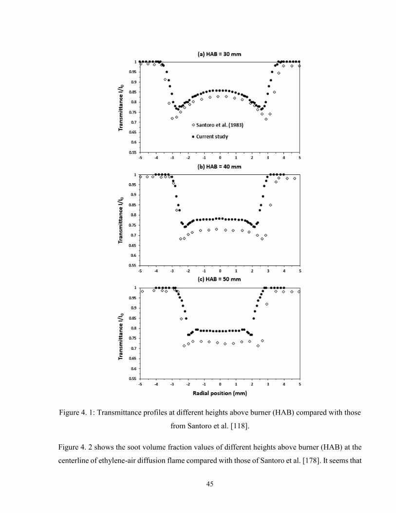
45

Figure 4. 1: Transmittance profiles at different heights above burner (HAB) compared with those

from Santoro et al. [118].

Figure 4. 2 shows the soot volume fraction values of different heights above burner (HAB) at the

centerline of ethylene-air diffusion flame compared with those of Santoro et al. [178]. It seems that

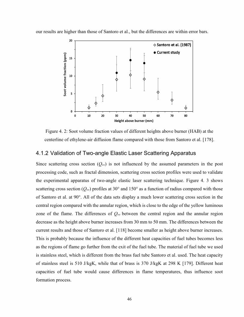
46

our results are higher than those of Santoro et al., but the differences are within error bars.

Figure 4. 2: Soot volume fraction values of different heights above burner (HAB) at the

centerline of ethylene-air diffusion flame compared with those from Santoro et al. [178].

4.1.2 Validation of Two-angle Elastic Laser Scattering Apparatus

Since scattering cross section (Qvv) is not influenced by the assumed parameters in the post

processing code, such as fractal dimension, scattering cross section profiles were used to validate

the experimental apparatus of two-angle elastic laser scattering technique. Figure 4. 3 shows

scattering cross section (Qvv) profiles at 30° and 150° as a function of radius compared with those

of Santoro et al. at 90°. All of the data sets display a much lower scattering cross section in the

central region compared with the annular region, which is close to the edge of the yellow luminous

zone of the flame. The differences of Qvv between the central region and the annular region

decrease as the height above burner increases from 30 mm to 50 mm. The differences between the

current results and those of Santoro et al. [118] become smaller as height above burner increases.

This is probably because the influence of the different heat capacities of fuel tubes becomes less

as the regions of flame go further from the exit of the fuel tube. The material of fuel tube we used

is stainless steel, which is different from the brass fuel tube Santoro et al. used. The heat capacity

of stainless steel is 510 J/kgK, while that of brass is 370 J/kgK at 298 K [179]. Different heat

capacities of fuel tube would cause differences in flame temperatures, thus influence soot

formation process.

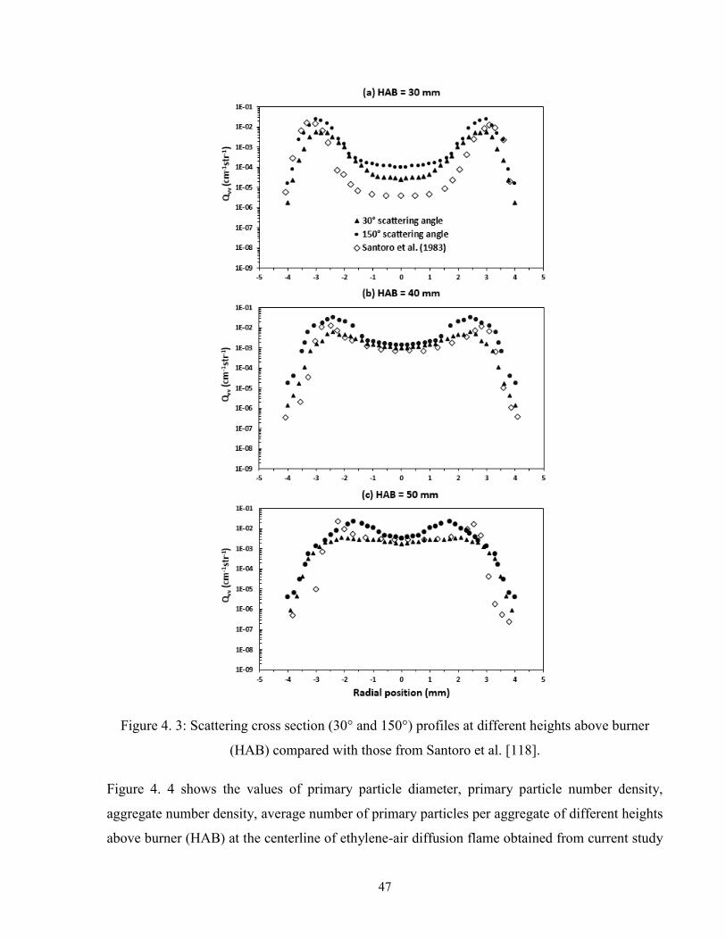
47

Figure 4. 3: Scattering cross section (30° and 150°) profiles at different heights above burner

(HAB) compared with those from Santoro et al. [118].

Figure 4. 4 shows the values of primary particle diameter, primary particle number density,

aggregate number density, average number of primary particles per aggregate of different heights

above burner (HAB) at the centerline of ethylene-air diffusion flame obtained from current study

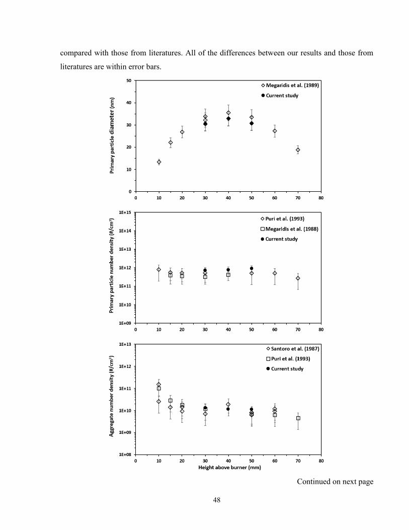
48

compared with those from literatures. All of the differences between our results and those from

literatures are within error bars.

Continued on next page

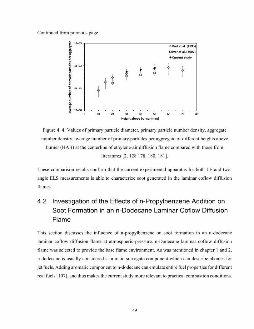
49

Continued from previous page

Figure 4. 4: Values of primary particle diameter, primary particle number density, aggregate

number density, average number of primary particles per aggregate of different heights above

burner (HAB) at the centerline of ethylene-air diffusion flame compared with those from

literatures [2, 128 178, 180, 181].

These comparison results confirm that the current experimental apparatus for both LE and two-

angle ELS measurements is able to characterize soot generated in the laminar coflow diffusion

flames.

4.2 Investigation of the Effects of n-Propylbenzene Addition on

Soot Formation in an n-Dodecane Laminar Coflow Diffusion

Flame

This section discusses the influence of n-propylbenzene on soot formation in an n-dodecane

laminar coflow diffusion flame at atmospheric-pressure. n-Dodecane laminar coflow diffusion

flame was selected to provide the base flame environment. As was mentioned in chapter 1 and 2,

n-dodecane is usually considered as a main surrogate component which can describe alkanes for

jet fuels. Adding aromatic component to n-dodecane can emulate entire fuel properties for different

real fuels [107], and thus makes the current study more relevant to practical combustion conditions.

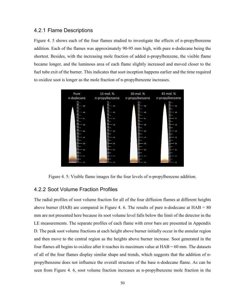
50

4.2.1 Flame Descriptions

Figure 4. 5 shows each of the four flames studied to investigate the effects of n-propylbenzene

addition. Each of the flames was approximately 90-95 mm high, with pure n-dodecane being the

shortest. Besides, with the increasing mole fraction of added n-propylbenzene, the visible flame

became longer, and the luminous area of each flame slightly increased and moved closer to the

fuel tube exit of the burner. This indicates that soot inception happens earlier and the time required

to oxidize soot is longer as the mole fraction of n-propylbenzene increases.

Figure 4. 5: Visible flame images for the four levels of n-propylbenzene addition.

4.2.2 Soot Volume Fraction Profiles

The radial profiles of soot volume fraction for all of the four diffusion flames at different heights

above burner (HAB) are compared in Figure 4. 6. The results of pure n-dodecane at HAB = 80

mm are not presented here because its soot volume level falls below the limit of the detector in the

LE measurements. The separate profiles of each flame with error bars are presented in Appendix

D. The peak soot volume fractions at each height above burner initially occur in the annular region

and then move to the central region as the heights above burner increase. Soot generated in the

four flames all begins to oxidize after it reaches its maximum value at HAB = 60 mm. The datasets

of all of the four flames display similar shape and trends, which suggests that the addition of n-

propylbenzene does not influence the overall structure of the base n-dodecane flame. As can be

seen from Figure 4. 6, soot volume fraction increases as n-propylbenzene mole fraction in the

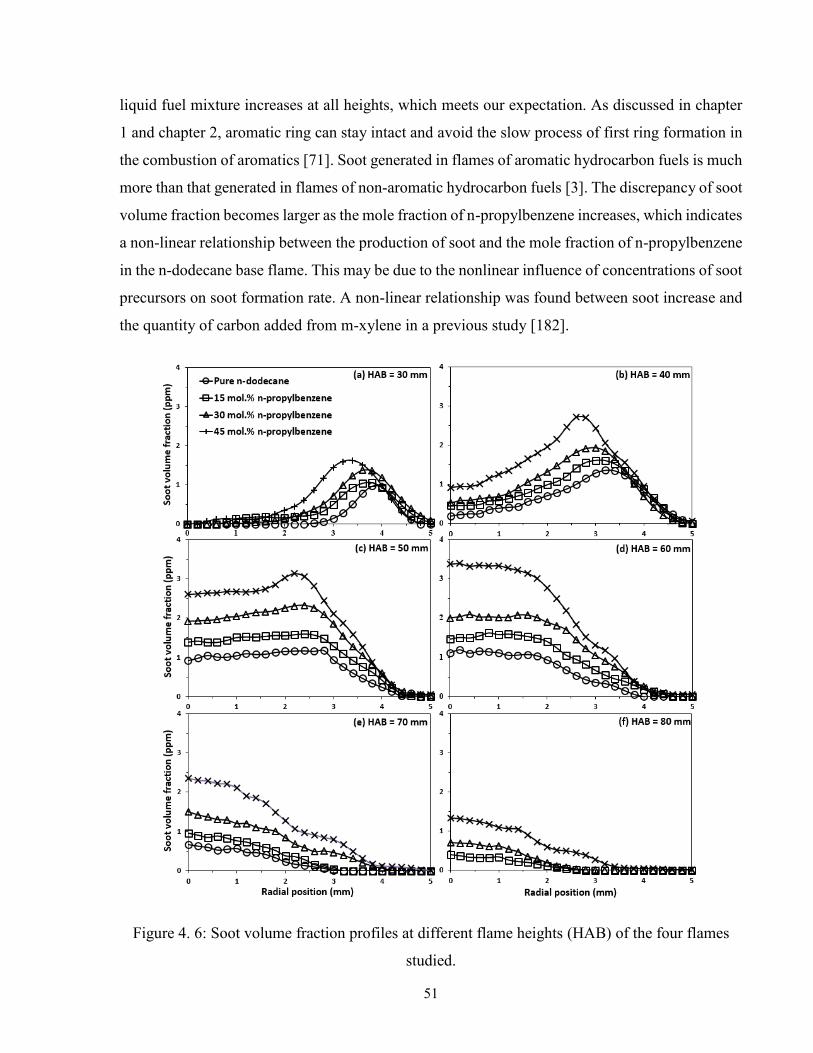
51

liquid fuel mixture increases at all heights, which meets our expectation. As discussed in chapter

1 and chapter 2, aromatic ring can stay intact and avoid the slow process of first ring formation in

the combustion of aromatics [71]. Soot generated in flames of aromatic hydrocarbon fuels is much

more than that generated in flames of non-aromatic hydrocarbon fuels [3]. The discrepancy of soot

volume fraction becomes larger as the mole fraction of n-propylbenzene increases, which indicates

a non-linear relationship between the production of soot and the mole fraction of n-propylbenzene

in the n-dodecane base flame. This may be due to the nonlinear influence of concentrations of soot

precursors on soot formation rate. A non-linear relationship was found between soot increase and

the quantity of carbon added from m-xylene in a previous study [182].

Figure 4. 6: Soot volume fraction profiles at different flame heights (HAB) of the four flames

studied.

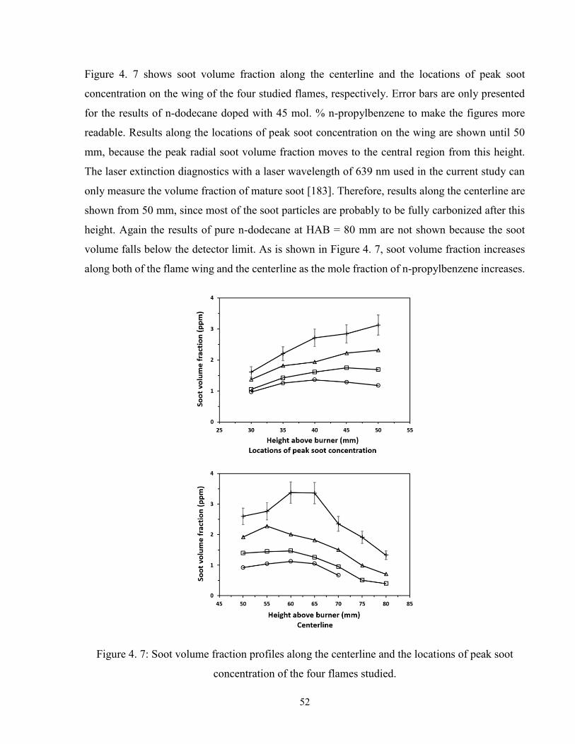
52

Figure 4. 7 shows soot volume fraction along the centerline and the locations of peak soot

concentration on the wing of the four studied flames, respectively. Error bars are only presented

for the results of n-dodecane doped with 45 mol. % n-propylbenzene to make the figures more

readable. Results along the locations of peak soot concentration on the wing are shown until 50

mm, because the peak radial soot volume fraction moves to the central region from this height.

The laser extinction diagnostics with a laser wavelength of 639 nm used in the current study can

only measure the volume fraction of mature soot [183]. Therefore, results along the centerline are

shown from 50 mm, since most of the soot particles are probably to be fully carbonized after this

height. Again the results of pure n-dodecane at HAB = 80 mm are not shown because the soot

volume falls below the detector limit. As is shown in Figure 4. 7, soot volume fraction increases

along both of the flame wing and the centerline as the mole fraction of n-propylbenzene increases.

Figure 4. 7: Soot volume fraction profiles along the centerline and the locations of peak soot

concentration of the four flames studied.

53

4.2.3 Primary Particle Diameter and Number Density Profiles

Figure 4. 8 displays the comparison profiles of primary particle diameter and primary particle

number density along the centerline and the locations of peak soot concentration on the wing of

the four studied flames, respectively. The primary particle diameter here refers to an equivalent

optical diameter, which considers a primary particle as an equivalent sphere having the same

optical properties. Due to the same reason mentioned in the previous section, error bars are only

included for the results of n-dodecane doped with 45 mol. % n-propylbenzene, results along the

wing of flames are shown until 50 mm and results along the centerline of flames are shown from

50 mm.

As is shown in Figure 4. 8 (a1) and (a2), as the n-propylbenzene mole fraction increases, the

primary particle diameter increases while the primary particle number density does not display any

significant change, implying that it is primarily the higher surface growth rate that results in the

higher soot formation along the wing. From Figure 4. 8 (b1) and (b2), along the centerline, both

of the primary particle diameter and number density display obvious increase as the mole fraction

of n-propylbenzene increases, which indicates that the increase in soot formation along the

centerline was caused by the combined effect of increase in soot inception and surface growth rate.

Besides, the central region of flames is typically a low temperature fuel rich region [184] and along

the centerline, with small addition of aromatics, the concentration of naphthalene increases while

the concentration of acetylene almost keeps unaltered [185], thus it can be inferred that the

structure of n-propylbenzene can be maintained instead of decomposing into smaller hydrocarbons

along the centerline of the studied flames. These maintained aromatic structure will increase the

amount of soot precursors.

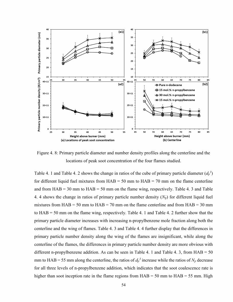
54

Figure 4. 8: Primary particle diameter and number density profiles along the centerline and the

locations of peak soot concentration of the four flames studied.

Table 4. 1 and Table 4. 2 shows the change in ratios of the cube of primary particle diameter (dp3)

for different liquid fuel mixtures from HAB = 50 mm to HAB = 70 mm on the flame centerline

and from HAB = 30 mm to HAB = 50 mm on the flame wing, respectively. Table 4. 3 and Table

4. 4 shows the change in ratios of primary particle number density (Np) for different liquid fuel

mixtures from HAB = 50 mm to HAB = 70 mm on the flame centerline and from HAB = 30 mm

to HAB = 50 mm on the flame wing, respectively. Table 4. 1 and Table 4. 2 further show that the

primary particle diameter increases with increasing n-propylbenzene mole fraction along both the

centerline and the wing of flames. Table 4. 3 and Table 4. 4 further display that the differences in

primary particle number density along the wing of the flames are insignificant, while along the

centerline of the flames, the differences in primary particle number density are more obvious with

different n-propylbenzene addition. As can be seen in Table 4. 1 and Table 4. 3, from HAB = 50

mm to HAB = 55 mm along the centerline, the ratios of dp3 increase while the ratios of Np decrease

for all three levels of n-propylbenzene addition, which indicates that the soot coalescence rate is

higher than soot inception rate in the flame regions from HAB = 50 mm to HAB = 55 mm. High

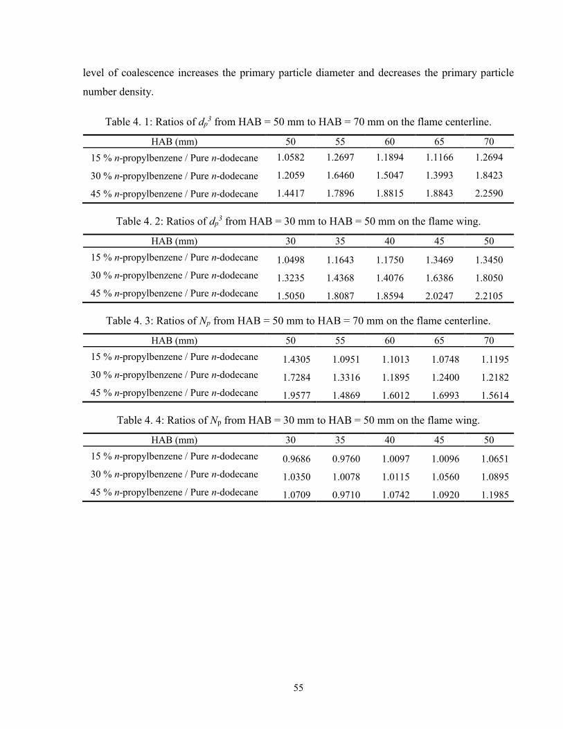
55

level of coalescence increases the primary particle diameter and decreases the primary particle

number density.

Table 4. 1: Ratios of dp3 from HAB = 50 mm to HAB = 70 mm on the flame centerline.

HAB (mm) 50 55 60 65 70

15 % n-propylbenzene / Pure n-dodecane 1.0582 1.2697 1.1894 1.1166 1.2694

30 % n-propylbenzene / Pure n-dodecane 1.2059 1.6460 1.5047 1.3993 1.8423

45 % n-propylbenzene / Pure n-dodecane 1.4417 1.7896 1.8815 1.8843 2.2590

Table 4. 2: Ratios of dp3 from HAB = 30 mm to HAB = 50 mm on the flame wing.

HAB (mm) 30 35 40 45 50

15 % n-propylbenzene / Pure n-dodecane 1.0498 1.1643 1.1750 1.3469 1.3450

30 % n-propylbenzene / Pure n-dodecane 1.3235 1.4368 1.4076 1.6386 1.8050

45 % n-propylbenzene / Pure n-dodecane 1.5050 1.8087 1.8594 2.0247 2.2105

Table 4. 3: Ratios of Np from HAB = 50 mm to HAB = 70 mm on the flame centerline.

HAB (mm) 50 55 60 65 70

15 % n-propylbenzene / Pure n-dodecane 1.4305 1.0951 1.1013 1.0748 1.1195

30 % n-propylbenzene / Pure n-dodecane 1.7284 1.3316 1.1895 1.2400 1.2182

45 % n-propylbenzene / Pure n-dodecane 1.9577 1.4869 1.6012 1.6993 1.5614

Table 4. 4: Ratios of Np from HAB = 30 mm to HAB = 50 mm on the flame wing.

HAB (mm) 30 35 40 45 50

15 % n-propylbenzene / Pure n-dodecane 0.9686 0.9760 1.0097 1.0096 1.0651

30 % n-propylbenzene / Pure n-dodecane 1.0350 1.0078 1.0115 1.0560 1.0895

45 % n-propylbenzene / Pure n-dodecane 1.0709 0.9710 1.0742 1.0920 1.1985

56

4.2.4 Temperature Profiles

4.2.4.1 Comparison Among Different Liquid Fuel Mixtures

Temperature has a strong influence on soot formation process. To determine temperature effects

on sooting tendency of the four different fuels studied, temperature measurements were performed

at different radial and axial positions inside flames.

Figure 4. 9 shows comparison of temperature profiles of the four studied diffusion flames at

different heights above burner (HAB). The separate profiles of each flame with errors are shown

in Appendix E. As can be seen, there is no significant difference among the four temperature

profiles at each height above burner (HAB). The peak temperatures of all the four profiles move

from the annular regions of flames to the central regions of flames as the flame heights increase

and first increase to the maximum value with increasing flame heights until approximately HAB

= 40 - 50 mm and then decrease as flame heights further increase. The temperature profiles of pure

n-dodecane flame are the highest, which can be explained by the radiation effect of soot and the

relatively less soot in the pure n-dodecane flame compared with the other three flames with n-

propylbenzene addition. The differences in the radial positions of peak temperatures among the

four profiles can be attributed to the positioning errors (±0.4 mm) [58]. The temperature

uncertainties can reach to ±130 K in the current study by considering radiation effects, catalytic

effects, soot deposition, conductive heat transfer effects and the experimental precision. Generally,

all of the temperature profiles display similar trends, which indicates that temperature effects on

soot formation in different flames can be neglected and the differences in soot volume fraction

profiles, soot particle diameter profiles and number density profiles are caused by different fuel

compositions.

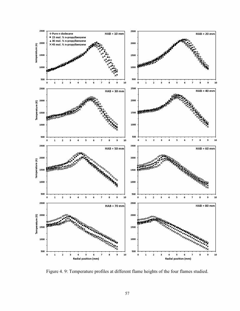
57

Figure 4. 9: Temperature profiles at different flame heights of the four flames studied.

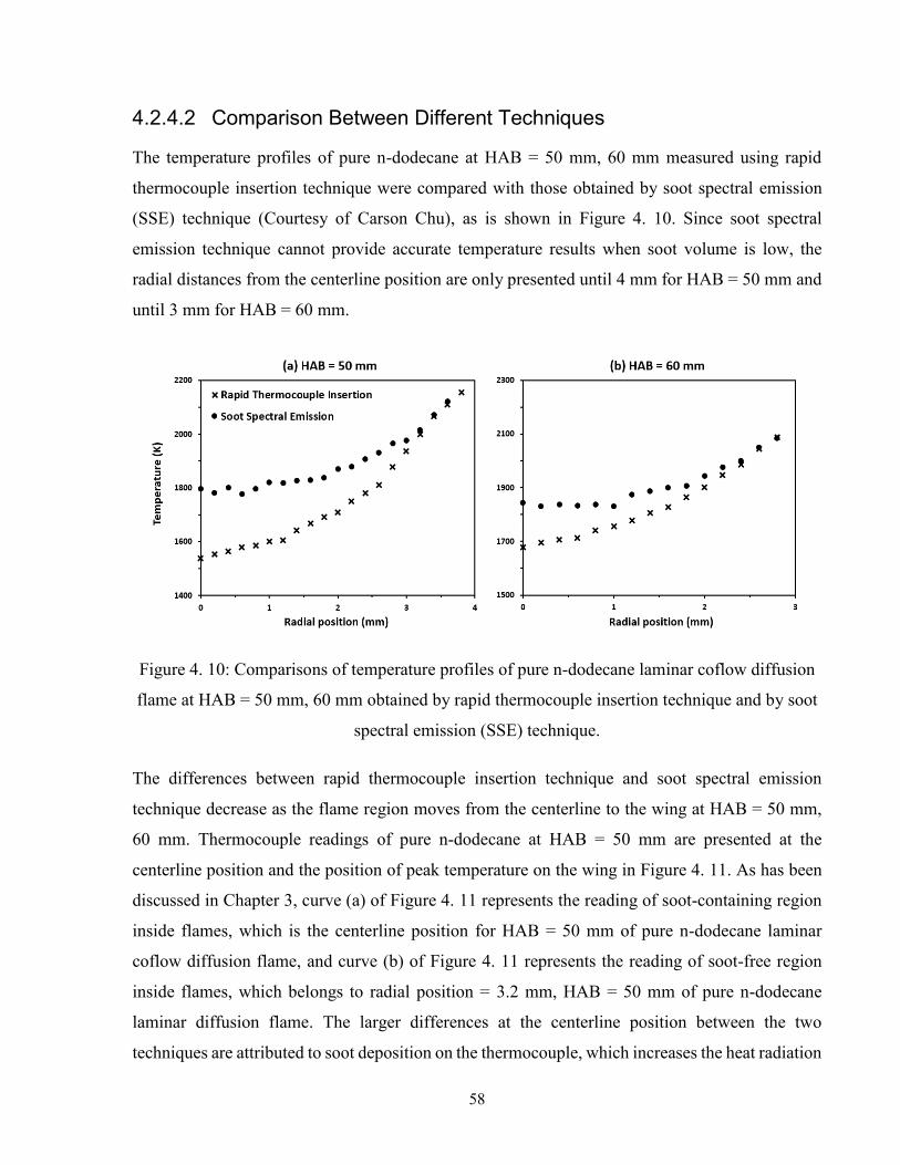
58

4.2.4.2 Comparison Between Different Techniques

The temperature profiles of pure n-dodecane at HAB = 50 mm, 60 mm measured using rapid

thermocouple insertion technique were compared with those obtained by soot spectral emission

(SSE) technique (Courtesy of Carson Chu), as is shown in Figure 4. 10. Since soot spectral

emission technique cannot provide accurate temperature results when soot volume is low, the

radial distances from the centerline position are only presented until 4 mm for HAB = 50 mm and

until 3 mm for HAB = 60 mm.

Figure 4. 10: Comparisons of temperature profiles of pure n-dodecane laminar coflow diffusion

flame at HAB = 50 mm, 60 mm obtained by rapid thermocouple insertion technique and by soot

spectral emission (SSE) technique.

The differences between rapid thermocouple insertion technique and soot spectral emission

technique decrease as the flame region moves from the centerline to the wing at HAB = 50 mm,

60 mm. Thermocouple readings of pure n-dodecane at HAB = 50 mm are presented at the

centerline position and the position of peak temperature on the wing in Figure 4. 11. As has been

discussed in Chapter 3, curve (a) of Figure 4. 11 represents the reading of soot-containing region

inside flames, which is the centerline position for HAB = 50 mm of pure n-dodecane laminar

coflow diffusion flame, and curve (b) of Figure 4. 11 represents the reading of soot-free region

inside flames, which belongs to radial position = 3.2 mm, HAB = 50 mm of pure n-dodecane

laminar diffusion flame. The larger differences at the centerline position between the two

techniques are attributed to soot deposition on the thermocouple, which increases the heat radiation

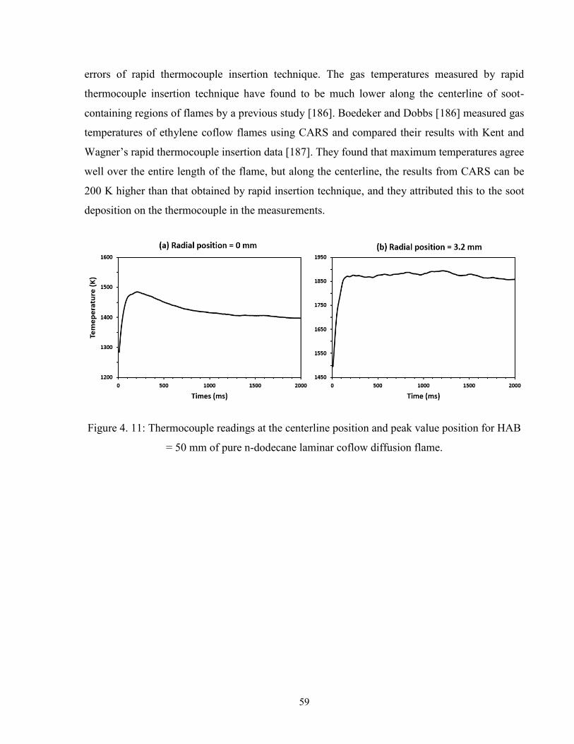
59

errors of rapid thermocouple insertion technique. The gas temperatures measured by rapid

thermocouple insertion technique have found to be much lower along the centerline of soot-

containing regions of flames by a previous study [186]. Boedeker and Dobbs [186] measured gas

temperatures of ethylene coflow flames using CARS and compared their results with Kent and

Wagner’s rapid thermocouple insertion data [187]. They found that maximum temperatures agree

well over the entire length of the flame, but along the centerline, the results from CARS can be

200 K higher than that obtained by rapid insertion technique, and they attributed this to the soot

deposition on the thermocouple in the measurements.

Figure 4. 11: Thermocouple readings at the centerline position and peak value position for HAB

= 50 mm of pure n-dodecane laminar coflow diffusion flame.

60

Chapter 5

Conclusions and Recommendations

5.1 Conclusions

The current study validated the experimental apparatus for combined LE and two-angle ELS

diagnostics to study soot formation in laminar coflow diffusion flames. Multiple radial

measurements were made at three heights above burner, HAB = 30, 40, and 50 mm of a non-

smoking ethylene air laminar coflow diffusion flame. Both the results of LE measurements and

the results of two-angle ELS display similar trends and shape with those from the literatures and

the differences are within error bars. The comparison profiles prove that the current experimental

apparatus is capable to characterize soot formation in laminar coflow diffusion flames.

The effects of n-propylbenzene addition in an n-dodecane laminar diffusion flame were

investigated by measuring soot volume fractions, primary particle diameters, primary particle

number densities using the validated experimental apparatus, and measuring temperatures using

the rapid thermocouple insertion method. To distinguish the effects of n-propylbenzene, n-

dodecane laminar coflow diffusion flame established the base flame environment with different

addition of n-propylbenzene from 0 mol.% to 45 mol.% in the liquid fuel mixtures. The total inlet

carbon flow rate was kept constant.

Generally, the soot volume fraction profiles, primary particle diameter profiles, primary particle

number density profiles, and flame temperature profiles are all very similar for all of the four

flames, which confirms that the overall flame structure is not affected by the different additions of

n-propylbenzene. Because of the similar flame temperature profiles, we can consider the

differences in soot volume fraction profiles, primary particle diameter profiles, primary particle

number density profiles are caused by different fuel compositions instead of different flame

temperatures.

The sooting tendency increases at all measured flame heights as mole fraction of n-propylbenzene

in the liquid fuel mixtures increases. The differences of sooting tendency become larger with

increasing mole fraction of n-propylbenzene, indicating a non-linear relationship between the

increase of soot formation and the increase of mole fractions of n-propylbenzene in the fuel mixture.

61

By comparing the profiles of primary particle diameters and primary particle number densities, we

found out that along the wing of flames, the increase of sooting tendency is primarily caused by a

higher surface growth rate, while along the centerline of flames, it is the combined effect of the

higher soot inception and soot surface growth rates that results in the higher sooting tendency.

5.2 Recommendations

The current section proposes several recommendations for the future experiments.

1. The current laser with a wavelength of 639 nm can only be used to measure the soot volume

fraction of mature soot particles, which limits the ability to detect soot at low flame heights

and leads to the lower soot volume fraction results compared to the practical conditions. A

UV laser which can detect the transparent soot particles as well as PAHs can be combined

with the current laser to improve the accuracy of our results.

2. For some optical mounts used in the current study such as mirror mounts, the adjusters

cannot be locked once the optics are aligned. Thus the desired position can be changed.

Since the laser scattering signal is several orders of magnitude lower than the laser

extinction signal, even a slight move of the adjusters would result in a big difference in the

scattering signal. In the future, it is recommended by the author to replace the current

mounts to the ones on which the adjusters can be locked.

3. A shorter heated tube to transfer the vaporized fuel would improve the flame stability due

to a lower chance of flame flicker.

4. In the current work, the Three-Point Abel Inversion method was used to calculate the local

extinction coefficient from the measured signals. The results obtained by this method

display large errors in the central region of flames. Using the Tikhonov regularization

method to process the data can provide more accurate results [188].

62

Attributions

The experimental apparatus of combined laser extinction and two-angle elastic laser scattering

diagnostics was validated by the author and Tongfeng Zhang together. The laser extinction

measurements, two-angle elastic laser scattering measurements, and temperature measurements

were conducted by the author and Tongfeng Zhang together. The author designed the fuel and

oxidizer delivery system and upgraded the setup of rapid thermocouple insertion technique.

Tongfeng Zhang designed the optical system and developed the improved data analysis to calculate

soot aggregate properties based on Rayleigh-Debye-Gans Fractal Aggregate (RDG/FA) theory.

Jason Weingarten developed the LabVIEW code to collect data.

63

Bibliography

[1] Sunderland, P. B., and G. M. Faeth. "Soot formation in hydrocarbon/air laminar jet

diffusion flames." Combustion and flame 105.1 (1996): 132-146.

[2] Megaridis, C. M., and R. A. Dobbins. "Soot aerosol dynamics in a laminar ethylene

diffusion flame." Symposium (International) on Combustion. Vol. 22. No. 1. Elsevier,

1989.

[3] McEnally, Charles S., et al. "Studies of aromatic hydrocarbon formation mechanisms in

flames: Progress towards closing the fuel gap." Progress in Energy and Combustion

Science 32.3 (2006): 247-294.

[4] Onischuk, A. A., et al. "Evolution of structure and charge of soot aggregates during and

after formation in a propane/air diffusion flame." Journal of aerosol science 34.4 (2003):

383-403.

[5] D’Anna, Andrea, Antonio D’Alessio, and Patrizia Minutolo. "Spectroscopic and chemical

characterization of soot inception processes in premixed laminar flames at atmospheric

pressure." Soot formation in combustion. Springer Berlin Heidelberg, 1994. 83-103.

[6] Xi, Jun, and B‐J. Zhong. "Soot in diesel combustion systems." Chemical engineering &

technology 29.6 (2006): 665-673.

[7] Balthasar, Michael, and Michael Frenklach. "Detailed kinetic modeling of soot aggregate

formation in laminar premixed flames." Combustion and Flame 140.1 (2005): 130-145.

[8] Stanmore, Brian R., Jean-Francois Brilhac, and Patrick Gilot. "The oxidation of soot: a

review of experiments, mechanisms and models." Carbon 39.15 (2001): 2247-2268.

[9] Haynes, Brian S., and H. Gg Wagner. "Soot formation." Progress in Energy and

Combustion Science 7.4 (1981): 229-273.

[10] Alder, B. J., et al. "Short Communication Effects of Partial Premixing on NOx Emission

Indices of Soot-Containing Flames." Combustion science and technology 152.1 (2000):

167-178.

[11] Puri, Rahul, Robert J. Santoro, and Kermit C. Smyth. "The oxidation of soot and carbon

monoxide in hydrocarbon diffusion flames." Combustion and Flame 97.2 (1994): 125-144.

[12] Kaden, Debra A., Ronald A. Hites, and William G. Thilly. "Mutagenicity of soot and

associated polycyclic aromatic hydrocarbons to Salmonella typhimurium." Cancer

Research 39.10 (1979): 4152-4159.

64

[13] Wood, Alexander W., et al. "Mutagenicity and tumor-initiating activity of cyclopenta (c, d)

pyrene and structurally related compounds." Cancer research 40.3 (1980): 642-649.

[14] Fu, Peter P., Frederick A. Beland, and Shen K. Yang. "Cyclopenta-polycyclic aromatic

hydrocarbons: potential carcinogens and mutagens." Carcinogenesis 1.8 (1980): 725-727.

[15] Busby, William F., et al. "Dose—response relationships of the tumorigenicity of

cyclopenta [cd] pyrene, benzo [a] pyrene and 6-nitrochrysene in a newborn mouse lung

adenoma bioassay." Carcinogenesis 9.5 (1988): 741-746.

[16] Lafleur, Arthur L., et al. "Chemical characterization and bacterial mutagenicity testing of

ethylene combustion products from a jet-stirred/plug-flow reactor." Energy & Fuels 4.3

(1990): 307-319.

[17] Durant, John L., et al. "Human cell mutagenicity of oxygenated, nitrated and unsubstituted

polycyclic aromatic hydrocarbons associated with urban aerosols." Mutation

Research/Genetic Toxicology 371.3 (1996): 123-157.

[18] Richter, Henning, and Jack B. Howard. "Formation of polycyclic aromatic hydrocarbons

and their growth to soot—a review of chemical reaction pathways." Progress in Energy and

Combustion science 26.4 (2000): 565-608.

[19] Kaiser, Jocelyn. "Showdown over clean air science." Science 277.5325 (1997): 466-469.

[20] Statistical abstract of the United States. Washington, DC: US Census Bureau; 2004–

5, http://www.census.gov/prod/www/statistical-abstract-04.html.

[21] D'ANNA∗, A., J. H. Kent, and R. J. Santoro. "Investigation of species concentration and

soot formation in a co-flowing diffusion flame of ethylene." Combustion science and

technology 179.1-2 (2007): 355-369.

[22] Schwartz, Joel. "Air pollution and daily mortality: a review and meta analysis."

Environmental research 64.1 (1994): 36-52.

[23] Miller, Frederick J., et al. "Size considerations for establishing a standard for inhalable

particles." Journal of the Air Pollution Control Association 29.6 (1979): 610-615.

[24] Avakian, Maureen D., et al. "The origin, fate, and health effects of combustion by-

products: a research framework." Environmental health perspectives 110.11 (2002): 1155.

[25] Horvath, H. "Atmospheric light absorption—A review." Atmospheric Environment. Part

A. General Topics 27.3 (1993): 293-317.

65

[26] McConnell, Joseph R., et al. "20th-century industrial black carbon emissions altered arctic

climate forcing." Science 317.5843 (2007): 1381-1384.

[27] Jacobson, Mark Z. "Strong radiative heating due to the mixing state of black carbon in

atmospheric aerosols." Nature 409.6821 (2001): 695-697.

[28] Hansen, James, and Larissa Nazarenko. "Soot climate forcing via snow and ice

albedos." Proceedings of the National Academy of Sciences of the United States of

America 101.2 (2004): 423-428.

[29] Ramaswamy, V., et al. "Radiative forcing of climate." Climate change (2001): 349-416.

[30] Dickerson, R. R., et al. "The impact of aerosols on solar ultraviolet radiation and

photochemical smog." Science 278.5339 (1997): 827-830.

[31] Kellerer, H., R. Koch, and S. Wittig. "Measurements of the growth and coagulation of soot

particles in a high-pressure shock tube." Combustion and Flame 120.1 (2000): 188-199.

[32] Choi, M. Y., et al. "Comparisons of the soot volume fraction using gravimetric and light

extinction techniques." Combustion and Flame 102.1 (1995): 161-169.

[33] Mulholland, George W., and Mun Y. Choi. "Measurement of the mass specific extinction

coefficient for acetylene and ethene smoke using the large agglomerate optics

facility." Symposium (international) on combustion. Vol. 27. No. 1. Elsevier, 1998.

[34] Grumman, Northrop. "Diesel Fuel Oils, 2003." Report NGMS-232 PPS (2004).

[35] Farrell, J. T., et al. "Development of an experimental database and kinetic models for

surrogate diesel fuels." SAE technical paper 2007-01 (2007): 0201.

[36] Glassman, Irvin. "Soot formation in combustion processes." Symposium (international) on

combustion. Vol. 22. No. 1. Elsevier, 1989.

[37] Frenklach, Michael. "Reaction mechanism of soot formation in flames." Physical

Chemistry Chemical Physics 4.11 (2002): 2028-2037.

[38] Yang, Yi, André L. Boehman, and Robert J. Santoro. "A study of jet fuel sooting tendency

using the threshold sooting index (TSI) model."Combustion and Flame 149.1 (2007): 191-

205.

[39] Tree, Dale R., and Kenth I. Svensson. "Soot processes in compression ignition

engines." Progress in Energy and Combustion Science 33.3 (2007): 272-309.

[40] Homann, Klaus H., and H. Gg Wagner. "Some new aspects of the mechanism of carbon

formation in premixed flames." Symposium (International) on Combustion. Vol. 11. No. 1.

Elsevier, 1967.

66

[41] Calcote, Hartwell F. "Mechanisms of soot nucleation in flames—a critical review.”

Combustion and Flame 42 (1981): 215-242.

[42] Bittner, J. D., and J. B. Howard. "Composition profiles and reaction mechanisms in a near-

sooting premixed benzene/oxygen/argon flame." Symposium (International) on

Combustion. Vol. 18. No. 1. Elsevier, 1981.

[43] Irvin, Glassman, and Yetter Richard. "Combustion." (2008).

[44] Miller, James A., and Carl F. Melius. "Kinetic and thermodynamic issues in the formation

of aromatic compounds in flames of aliphatic fuels." Combustion and Flame 91.1 (1992):

21-39.

[45] Frenklach, M., T. Yuan, and M. K. Ramachandra. "Soot formation in binary hydrocarbon

mixtures." Energy & fuels 2.4 (1988): 462-480.

[46] Frenklach, M., et al. "Soot formation in shock-tube pyrolysis of acetylene, allene, and 1, 3-

butadiene." Combustion and Flame 54.1 (1983): 81-101.

[47] Moskaleva, L. V., A. M. Mebel, and M. C. Lin. "The CH3+ C5H5 reaction: A potential

source of benzene at high temperatures." Symposium (International) on Combustion. Vol.

26. No. 1. Elsevier, 1996.

[48] Melius, Carl F., et al. "Reaction mechanisms in aromatic hydrocarbon formation involving

the C 5 H 5 cyclopentadienyl moiety." Symposium (International) on Combustion. Vol. 26.

No. 1. Elsevier, 1996.

[49] Lahaye, J. "Mechanisms of soot formation." Polymer Degradation and Stability 30.1

(1990): 111-121.

[50] Frenklach, Michael, and Hai Wang. "Aromatics growth beyond the first ring and the

nucleation of soot particles." Prepr. Pap. Am. Chem. Soc. Div. Fuel Chem 36 (1991): 1509.

[51] Frenklach, Michael, and Hai Wang. "Detailed modeling of soot particle nucleation and

growth." Symposium (International) on Combustion. Vol. 23. No. 1. Elsevier, 1991.

[52] Frenklach, Michael, and Hai Wang. "Detailed mechanism and modeling of soot particle

formation." Soot formation in combustion. Springer Berlin Heidelberg, 1994. 165-192.

[53] Haynes, B. S., and H. Gg Wagner. "The surface growth phenomenon in soot

formation." Zeitschrift für Physikalische Chemie 133.2 (1982): 201-213.

[54] Frenklach, Michael, Nigel W. Moriarty, and Nancy J. Brown. "Hydrogen migration in

polyaromatic growth." Symposium (International) on Combustion. Vol. 27. No. 2.

Elsevier, 1998.

67

[55] Appel, Jörg, Henning Bockhorn, and Michael Frenklach. "Kinetic modeling of soot

formation with detailed chemistry and physics: laminar premixed flames of C2

hydrocarbons." Combustion and Flame 121.1 (2000): 122-136.

[56] Kronholm, David F., and Jack B. Howard. "Analysis of soot surface growth pathways

using published plug-flow reactor data with new particle size distribution measurements

and published premixed flame data." Proceedings of the Combustion Institute 28.2 (2000):

2555-2561.

[57] Bartok, William, and Adel F. Sarofim. "Fossil fuel combustion: a source book." (1991).

[58] Kholghy, Mohammad Reza. The evolution of soot morphology in laminar co-flow

diffusion flames of the surrogates for jet A-1 and a synthetic kerosene. Diss. University of

Toronto, 2012.

[59] Borshanpour, Babak. Development and Validation of an Experimental Apparatus for the

Characterization of Soot in a Laminar Co-Flow Diffusion Flame Using Laser-Induced

Incandescence. Diss. 2013.

[60] Dobbins, R. A., R. A. Fletcher, and W. Lu. "Laser microprobe analysis of soot precursor

particles and carbonaceous soot." Combustion and flame100.1 (1995): 301-309.

[61] D’Alessio, A., et al. "Surface deposition and coagulation efficiency of combustion

generated nanoparticles in the size range from 1 to 10nm." Proceedings of the Combustion

Institute 30.2 (2005): 2595-2603.

[62] Lahaye, J. "Particulate carbon from the gas phase." Carbon 30.3 (1992): 309-314.

[63] Warnatz, J., U. Maas, and R. W. Dibble. "Combustion: physical and chemical

fundamentals, modeling and simulation, experiments, pollutant formation. 2006." 73-81.

[64] Fenimore, Charles P., and George Wallace Jones. "Oxidation of soot by hydroxyl

radicals." The Journal of Physical Chemistry 71.3 (1967): 593-597.

[65] Kennedy, Ian M. "Models of soot formation and oxidation." Progress in Energy and

Combustion Science 23.2 (1997): 95-132.

[66] Schalla, Rose L., and GLEN E. McDONALD. "Mechanism of smoke formation in

diffusion flames." Symposium (International) on Combustion. Vol. 5. No. 1. Elsevier,

1955.

[67] Takahashi, F., and I. Glassman. "Sooting correlations for premixed flames." Combustion

Science and Technology 37.1-2 (1984): 1-19.

68

[68] Brezinsky, Kenneth. "The high-temperature oxidation of aromatic hydrocarbons." Progress

in Energy and Combustion Science 12.1 (1986): 1-24.

[69] Lindstedt, Peter. "Modeling of the chemical complexities of flames." Symposium

(International) on Combustion. Vol. 27. No. 1. Elsevier, 1998.

[70] Glassman, Irvin, Richard A. Yetter, and Nick G. Glumac. Combustion. Academic press,

2014.

[71] Gomez, A., G. Sidebotham, and I. Glassman. "Sooting behavior in temperature-controlled

laminar diffusion flames." Combustion and flame 58.1 (1984): 45-57.

[72] Anderson, Henrik, Charles S. McEnally, and Lisa D. Pfefferle. "Experimental study of

naphthalene formation pathways in non-premixed methane flames doped with

alkylbenzenes." Proceedings of the Combustion Institute 28.2 (2000): 2577-2583.

[73] Sidebotham, G. W., K. Saito, and I. Glassman. "Pyrolysis Zone Structure of Allene, 1, 3

Butadiene and Benzene Smoke Point Diffusion Flames*."Combustion science and

technology 85.1-6 (1992): 283-296.

[74] McEnally, Charles S., and Lisa D. Pfefferle. "The effects of slight premixing on fuel

decomposition and hydrocarbon growth in benzene-doped methane nonpremixed

flames." Combustion and flame 129.3 (2002): 305-323.

[75] McEnally, Charles S., and Lisa D. Pfefferle. "The use of carbon-13-labeled fuel dopants

for identifying naphthalene formation pathways in non-premixed flames." Proceedings of

the Combustion Institute 28.2 (2000): 2569-2576.

[76] Frenklach, Michael, et al. "Detailed kinetic modeling of soot formation in shock-tube

pyrolysis of acetylene." Symposium (International) on Combustion. Vol. 20. No. 1.

Elsevier, 1985.

[77] Wang, Hai, and Michael Frenklach. "A detailed kinetic modeling study of aromatics

formation in laminar premixed acetylene and ethylene flames." Combustion and

flame 110.1 (1997): 173-221.

[78] Colket, M. B., and D. J. Seery. "Reaction mechanisms for toluene pyrolysis." Symposium

(International) on Combustion. Vol. 25. No. 1. Elsevier, 1994.

[79] Marinov, N. M., et al. "Modeling of aromatic and polycyclic aromatic hydrocarbon

formation in premixed methane and ethane flames." Combustion Science and

Technology 116.1-6 (1996): 211-287.

69

[80] Tregrossi, A., A. Ciajolo, and R. Barbella. "The combustion of benzene in rich premixed

flames at atmospheric pressure." Combustion and flame 117.3 (1999): 553-561.

[81] Dupont, Laurent, et al. "Investigation of stoichiometric methane/air/benzene (1.5%) and

methane/air low pressure flames." Combustion and flame 135.1 (2003): 171-183.

[82] Defoeux, François, et al. "Experimental investigation of the structure of a sooting premixed

benzene/oxygen/argon flame burning at low pressure." Proceedings of the Combustion

Institute 30.1 (2005): 1407-1415.

[83] Renard, Charles, P. J. Van Tiggelen, and Jacques Vandooren. "Effect of

dimethoxymethane addition on the experimental structure of a rich ethylene/oxygen/argon

flame." Proceedings of the Combustion Institute 29.1 (2002): 1277-1284.

[84] Gudiyella, Soumya, and Kenneth Brezinsky. "High pressure study of n-propylbenzene

oxidation." Combustion and Flame 159.3 (2012): 940-958.

[85] Dagaut, P., et al. "Experimental and kinetic modeling study of the oxidation of n-

propylbenzene." Fuel 81.2 (2002): 173-184.

[86] Kallio, Pauli, et al. "Renewable jet fuel." Current opinion in biotechnology 26 (2014): 50-

55.

[87] Coordinating Research Council. Handbook of aviation fuel properties. No. 530. The

Council, 1983.

[88] Iyer, Venkatesh R. Effect of Aromatic Components in Surrogate Fuels on Soot in Co-Flow

Flames and a Model Gas Turbine Combustor. Diss. The Pennsylvania State University,

2012.

[89] Defense Energy Support Centre, Petroleum Quality Information Systems 2008 Annual

Report, (PQIS2008), https://www.desc.dla.mil/DCM/Files/2004PQISreportsmall.pdf.

[90] Colket, Meredith, et al. "Development of an experimental database and kinetic models for

surrogate jet fuels." 45th AIAA Aerospace Sciences Meeting and Exhibit. 2007.

[91] Maurice, Lourdes Q., et al. "Advanced aviation fuels: a look ahead via a historical

perspective." Fuel 80.5 (2001): 747-756.

[92] Shell Web Page, "World-wide Civil Jet Fuel Grades." - Australia. Web. 29 Feb. 2016.

<http://www.shell.com.au/products-services/solutions-for

businesses/aviation/products/fuels/jet-a1.html>.

70

[93] Dooley, Stephen, et al. "The experimental evaluation of a methodology for surrogate fuel

formulation to emulate gas phase combustion kinetic phenomena." Combustion and

Flame 159.4 (2012): 1444-1466.

[94] Widegren, Jason A., and Thomas J. Bruno. "Thermal decomposition kinetics of the

aviation turbine fuel Jet A." Industrial & Engineering Chemistry Research 47.13 (2008):

4342-4348.

[95] Lee, David S., et al. "Aviation and global climate change in the 21st century." Atmospheric

Environment 43.22 (2009): 3520-3537.

[96] Mayor, Karen, and Richard SJ Tol. "The impact of European climate change regulations

on international tourist markets." Transportation Research Part D: Transport and

Environment 15.1 (2010): 26-36.

[97] Pejovic, Tamara, et al. "Estimates of UK CO2 emissions from aviation using air traffic

data." Climatic change 88.3-4 (2008): 367-384.

[98] Boyle, Karleen. "Evaluating particulate emissions from jet engines: analysis of chemical

and physical characteristics and potential impacts on coastal environments and human

health." Transportation Research Record: Journal of the Transportation Research

Board 1517 (1996): 1-9.

[99] Edwards, Tim, Bill Harrison, and Lourdes Maurice. "Properties and usage of Air Force

fuel- JP-8." AIAA, Aerospace Sciences Meeting and Exhibit, 39th, Reno, NV. 2001.

[100] Dean, A. J., et al. "Autoignition of surrogate fuels at elevated temperatures and

pressures." Proceedings of the Combustion Institute 31.2 (2007): 2481-2488.

[101] Dagaut, Philippe, et al. "Kerosene combustion at pressures up to 40 atm: Experimental

study and detailed chemical kinetic modeling." Symposium (International) on Combustion.

Vol. 25. No. 1. Elsevier, 1994.

[102] Violi, A., et al. "Experimental formulation and kinetic model for JP-8 surrogate

mixtures." Combustion Science and Technology 174.11-12 (2002): 399-417.

[103] Cooke, James A., et al. "Computational and experimental study of JP-8, a surrogate, and its

components in counterflow diffusion flames." Proceedings of the Combustion

Institute 30.1 (2005): 439-446.

[104] Eddings, Eric G., et al. "Formulation of a surrogate for the simulation of jet fuel pool

fires." Combust. Sci. and Tech. 177.4 (2005): 715-739.

71

[105] Pitz, William J., and Charles J. Mueller. "Recent progress in the development of diesel

surrogate fuels." Progress in Energy and Combustion Science 37.3 (2011): 330-350.

[106] Dooley, Stephen, et al. "A jet fuel surrogate formulated by real fuel properties."

Combustion and Flame 157.12 (2010): 2333-2339.

[107] Xu, H., et al. "JANNAF 42nd Combustion Joint Sub-committee Meeting Modeling and

Data for Combustion Simulation." Boston Marriott Newton, Hanscom AF Base, Newton,

MA (2008).

[108] Holley, A. T., et al. "Sensitivity of propagation and extinction of large hydrocarbon flames

to fuel diffusion." Proceedings of the Combustion Institute 32.1 (2009): 1157-1163.

[109] Calcote, H. F., and D. M. Manos. "Effect of molecular structure on incipient soot

formation." Combustion and Flame 49.1 (1983): 289-304.

[110] Olson, D. B., J. C. Pickens, and R. J. Gill. "The effects of molecular structure on soot

formation II. Diffusion flames." Combustion and Flame 62.1 (1985): 43-60.

[111] Mensch, Amy, et al. "Sooting characteristics of surrogates for jet fuels." Combustion and

Flame 157.6 (2010): 1097-1105.

[112] Colket, Meredith, et al. "Identification of target validation data for development of

surrogate jet fuels." 46th AIAA, Aerospace Sciences Meeting and Exhibit, Reno, NV,

Paper No. AIAA. Vol. 972. 2008.

[113] Dagaut, Philippe. "On the kinetics of hydrocarbons oxidation from natural gas to kerosene

and diesel fuel." Physical Chemistry Chemical Physics 4.11 (2002): 2079-2094.

[114] Dagaut, Philippe, and Michel Cathonnet. "The ignition, oxidation, and combustion of

kerosene: A review of experimental and kinetic modeling." Progress in energy and

combustion science 32.1 (2006): 48-92.

[115] Litzinger, T. A., K. Brezinsky, and I. Glassman. "Reactions of n-propylbenzene during gas

phase oxidation." Combustion science and technology 50.1-3 (1986): 117-133.

[116] Edwards, T. "USAF supercritical hydrocarbon fuels interests." AIAA paper93 (1993).

[117] Thorlabs Inc. Web Page, "Summary." Blackout Materials. Web. 29 Feb. 2016.

<https://www.thorlabs.com/newgrouppage9.cfm?objectgroup_id=190>.

[118] Santoro, R. J., H. G. Semerjian, and R. A. Dobbins. "Soot particle measurements in

diffusion flames." Combustion and Flame 51 (1983): 203-218.

72

[119] Dalzell, W. H., G. C. Williams, and H. C. Hottel. "A light-scattering method for soot

concentration measurements." Combustion and Flame 14.2 (1970): 161-169.

[120] Hofeldt, David L. Real-time soot concentration measurement technique for engine exhaust

streams. No. 930079. SAE Technical Paper, 1993.

[121] Di Sante, R. "Laser extinction technique for measurements of carbon particles

concentration during combustion." Optics and Lasers in Engineering51.6 (2013): 783-789.

[122] Saffaripour, M., et al. "A numerical and experimental study of a laminar sooting coflow

Jet-A1 diffusion flame." Proceedings of the Combustion Institute 33.1 (2011): 601-608.

[123] Dobbins, R. A., R. J. Santoro, and H. G. Semerjian. "Analysis of light scattering from soot

using optical cross sections for aggregates." Symposium (International) on Combustion.

Vol. 23. No. 1. Elsevier, 1991.

[124] Zhu, Jinyu, et al. "Soot scattering measurements in the visible and near-infrared

spectrum." Proceedings of the Combustion Institute 28.1 (2000): 439-446.

[125] Dobbins, Richard A., and Constantine M. Megaridis. "Absorption and scattering of light

by polydisperse aggregates." Applied Optics 30.33 (1991): 4747-4754.

[126] Dobbins, R. A., R. J. Santoro, and H. G. Semerjian. "Interpretation of optical

measurements of soot in flames." Progress in Astronautics and Aeronautics92 (1984): 208-

237.

[127] Wersborg, Benno L., Jack Benny Howard, and Glenn Carber Williams. "Physical

mechanisms in carbon formation in flames." Symposium (International) on Combustion.

Vol. 14. No. 1. Elsevier, 1973.

[128] Puri, R. T. F. R. J. R. A., et al. "Aerosol dynamic processes of soot aggregates in a laminar

ethene diffusion flame." Combustion and Flame 92.3 (1993): 320-333.

[129] Köylü, Ümit Özgür, and Gerard M. Faeth. "Structure of overfire soot in buoyant turbulent

diffusion flames at long residence times." Combustion and Flame 89.2 (1992): 140-156.

[130] Koylu, U O, and G. M. Faeth. "Radiative properties of flame-generated soot." Journal of

heat transfer 115.2 (1993): 409-417.

[131] Koylu, U O, and G. M. Faeth. "Optical properties of soot in buoyant laminar diffusion

flames." Journal of heat transfer 116.4 (1994): 971-979.

73

[132] Köylü, Ümit Özgür. "Quantitative analysis of in situ optical diagnostics for inferring

particle/aggregate parameters in flames: Implications for soot surface growth and total

emissivity." Combustion and flame 109.3 (1997): 488-500.

[133] Suresh Iyer. Enhanced optical methods of soot characterization for application to diesel

emission measurements. Diss. Pennsylvania State University. 2005.

[134] Farias, Tiago L., Ümit Özgür Köylü, and Maria da Gracia Carvalho. "Range of validity of

the Rayleigh–Debye–Gans theory for optics of fractal aggregates." Applied Optics 35.33

(1996): 6560-6567.

[135] Link, O., et al. "Development of absolute intensity multi-angle light scattering for the

determination of polydisperse soot aggregate properties." Proceedings of the Combustion

Institute 33.1 (2011): 847-854.

[136] Sorensen, C. M. "Light scattering by fractal aggregates: a review." Aerosol Science &

Technology 35.2 (2001): 648-687.

[137] Zhang, Tongfeng, and Murray J. Thomson. "Development of an improved data analysis

approach for combined laser extinction and two-angle elastic light scattering diagnostics of

soot aggregates." Applied optics 55.4 (2016): 920-928.

[138] De Iuliis, S., et al. "Three-angle scattering/extinction versus TEM measurements on soot in

premixed ethylene/air flame." Applied Physics B102.4 (2011): 891-903.

[139] Teng, Yingwu, and Umit O. Koylu. "Optical sizing of aggregated combustion particles:

computational development of a two-angle laser scattering technique." Applied

optics 45.18 (2006): 4396-4403.

[140] National Instruments Web Page, "NI USB-4431 24-Bit Analog I/O, 102.4 KS/s, ±10

V." NI USB-4431. Web. 29 Feb. 2016.

<http://sine.ni.com/nips/cds/view/p/lang/en/nid/206676>.

[141] Erickson, W. D., G. C. Williams, and H. C. Hottel. "Light scattering measurements on soot

in a benzene-air flame." Combustion and Flame 8.2 (1964): 127-132.

[142] Lee, S. C., and C. L. Tien. "Optical constants of soot in hydrocarbon flames." Symposium

(international) on combustion. Vol. 18. No. 1. Elsevier, 1981.

[143] Bockhorn, H., et al. "Measurement of the soot concentration and soot particle sizes in

propane oxygen flames." Symposium (International) on Combustion. Vol. 18. No. 1.

Elsevier, 1981.

74

[144] Charalampopoulos, T. T., and J. D. Felske. "Refractive indices of soot particles deduced

from in-situ laser light scattering measurements." Combustion and flame 68.3 (1987): 283-

294.

[145] Mullins, Jeremy, and Alan Williams. "The optical properties of soot: a comparison

between experimental and theoretical values." Fuel 66.2 (1987): 277-280.

[146] Vaglieco, B. M., F. Beretta, and A. d'Alessio. "In situ evaluation of the soot refractive

index in the UV-visible from the measurement of the scattering and extinction coefficients

in rich flames." Combustion and flame 79.3 (1990): 259-271.

[147] Smyth, Kermit C., and Christopher R. Shaddix. "The elusive history of = 1.57–0.56i for

the refractive index of soot." Combustion and Flame 107.3 (1996): 314-320.

[148] Dalzell, W. H., and A. F. Sarofim. "Optical constants of soot and their application to heat-

flux calculations." Journal of Heat Transfer 91.1 (1969): 100-104.

[149] Williams, Timothy C., et al. "Measurement of the dimensionless extinction coefficient of

soot within laminar diffusion flames." International Journal of Heat and Mass

Transfer 50.7 (2007): 1616-1630.

[150] Chippett, S., and W. A. Gray. "The size and optical properties of soot particles.”

Combustion and Flame 31 (1978): 149-159.

[151] Roessler, D. M., and F. R. Faxvog. "Optical properties of agglomerated acetylene smoke

particles at 0.5145-µm and 10.6-µm wavelengths." JOSA70.2 (1980): 230-235.

[152] Stagg, B. J., and T. T. Charalampopoulos. "Refractive indices of pyrolytic graphite,

amorphous carbon, and flame soot in the temperature range 25 to 600 C." Combustion and

flame 94.4 (1993): 381-396.

[153] Koylu, U O, and G. M. Faeth. "Spectral extinction coefficients of soot aggregates from

turbulent diffusion flames." Journal of Heat Transfer 118.2 (1996): 415-421.

[154] Snelling, David R., et al. "Two-dimensional imaging of soot volume fraction in laminar

diffusion flames." Applied Optics 38.12 (1999): 2478-2485.

[155] Mountain, Raymond D., and G. W. Mulholland. "Light scattering from simulated smoke

agglomerates." Langmuir 4.6 (1988): 1321-1326.

[156] Meakin, Paul. "Computer simulations of diffusion-limited aggregation processes." Faraday

Discussions of the Chemical Society 83 (1987): 113-124.

75

[157] Jullien, R. R. P. M., R. Botet, and P. M. Mors. "Computer simulations of cluster–cluster

aggregation." Faraday Discussions of the Chemical Society83 (1987): 125-137.

[158] Dobbins, Richard A., and Constantine M. Megaridis. "Absorption and scattering of light by

polydisperse aggregates." Applied Optics 30.33 (1991): 4747-4754.

[159] Gangopadhyay, S. I. C. M., I. Elminyawi, and Christopher M. Sorensen. "Optical structure

factor measurements of soot particles in a premixed flame." Applied optics 30.33 (1991):

4859-4864.

[160] Charalampopoulos, T. T., and H. Chang. "Agglomerate parameters and fractal dimension

of soot using light scattering—effects on surface growth." Combustion and flame 87.1

(1991): 89-99.

[161] Sorensen, C. M., J. Cai, and N. Lu. "Test of static structure factors for describing light

scattering from fractal soot aggregates." Langmuir 8.8 (1992): 2064-2069.

[162] Umit O. Koylu, Yangchuan Xing, and Daniel E. Rosner. "Fractal morphology analysis of

combustion-generated aggregates using angular light scattering and electron microscope

images." Langmuir 11.12 (1995): 4848-4854.

[163] Yang, Bo, and Umit O. Koylu. "Detailed soot field in a turbulent non-premixed

ethylene/air flame from laser scattering and extinction experiments." Combustion and

Flame 141.1 (2005): 55-65.

[164] Iyer, Suresh S., et al. "Determination of soot scattering coefficient from extinction and

three-angle scattering in a laminar diffusion flame."Combustion and flame 149.1 (2007):

206-216.

[165] De Iuliis, S., et al. "Three-angle scattering/extinction versus TEM measurements on soot in

premixed ethylene/air flame." Applied Physics B102.4 (2011): 891-903.

[166] Snelling, D. R., et al. "Measurement of soot morphology by integrated LII and elastic light

scattering." Applied Physics B 104.2 (2011): 385-397.

[167] Heitor, M. V., A. M. K. P. Taylor, and J. H. Whitelaw. "The interaction of turbulence and

pressure gradients in a baffle-stabilized premixed flame." Journal of Fluid mechanics 181

(1987): 387-413.

[168] McEnally, Charles S., et al. "Soot volume fraction and temperature measurements in

laminar nonpremixed flames using thermocouples." Combustion and Flame 109.4 (1997):

701-720.

76

[169] Shaddix, Christopher R. Correcting thermocouple measurements for radiation loss: a

critical review. No. CONF-990805--. Sandia National Labs., Livermore, CA (US), 1999.

[170] Bradley, D., and A. G. Entwistle. "Determination of the emissivity, for total radiation, of

small diameter platinum-10% rhodium wires in the temperature range 600-1450 C." British

Journal of Applied Physics 12.12 (1961): 708

[171] Figliola, Richard S., and Donald Beasley. Theory and design for mechanical

measurements. John Wiley & Sons, 2015.

[172] Henriksen, Tara, et al. "Determination of soot refractive index as a function of height in an

inverse diffusion flame." 5th US Combustion Meeting, University of California at San

Diego. 2007.

[173] Aksit, I. M., and J. B. Moss. "Model fuels to reproduce the sooting behaviour of aviation

kerosene." Fuel 84.2 (2005): 239-245.

[174] Heitor, M. V., and A. L. N. Moreira. "Thermocouples and sample probes for combustion

studies." Progress in energy and combustion science 19.3 (1993): 259-278.

[175] Heitor, M. V., A. M. K. P. Taylor, and J. H. Whitelaw. "Simultaneous velocity and

temperature measurements in a premixed flame." Experiments in Fluids3.6 (1985): 323-

339.

[176] Saffaripour, Meghdad, et al. "Experimental investigation and detailed modeling of soot

aggregate formation and size distribution in laminar coflow diffusion flames of Jet A-1, a

synthetic kerosene, and n-decane."Combustion and Flame 161.3 (2014): 848-863.

[177] Dasch, Cameron J. "One-dimensional tomography: a comparison of Abel, onion-peeling,

and filtered back projection methods." Applied optics 31.8 (1992): 1146-1152.

[178] Santoro, R. J., et al. "The transport and growth of soot particles in laminar diffusion

flames." Combustion Science and Technology 53.2-3 (1987): 89-115.

[179] DiracDelta.co.uk." Specific Heat Capacity. Web. 29 Feb. 2016.

<http://www.diracdelta.co.uk/science/source/s/p/specific heat

capacity/source.html#.VqkKrhUrK70.>.

[180] Constantine, M. Megaridis, and A. Dobbins Richard. "Comparison of Soot Growth and

Oxidation in Smoking and Non–Smoking Ethylene Diffusion Flames." Combustion

Science and Technology 66.1-3 (1989): 1-16.

77

[181] Iyer, Suresh S., et al. "Determination of soot scattering coefficient from extinction and

three-angle scattering in a laminar diffusion flame." Combustion and flame 149.1 (2007):

206-216.

[182] Mouis, Anne Geraldine, et al. "Effects of a JP-8 surrogate and its components on soot in

laminar, N 2-diluted ethylene co-flow diffusion flames from 1 to 5atm." Combustion and

Flame 162.5 (2015): 1987-1995.

[183] D’Anna, A., et al. "Nano-organic carbon and soot particle measurements in a laminar

ethylene diffusion flame." Proceedings of the Combustion Institute30.1 (2005): 1449-1456.

[184] Kholghy, Mohammadreza, et al. "The evolution of soot morphology in a laminar coflow

diffusion flame of a surrogate for Jet A-1." Combustion and Flame 160.10 (2013): 2119-

2130.

[185] McEnally, Charles S., and Lisa D. Pfefferle. "Experimental assessment of naphthalene

formation mechanisms in non-premixed flames." Combustion science and

technology 128.1-6 (1997): 257-278.

[186] Boedeker, Laurence R., and Gregory M. Dobbs. "Soot distribution and cars temperature

measurements in axisymmetric laminar diffusion flames with several fuels." Symposium

(International) on Combustion. Vol. 21. No. 1. Elsevier, 1988.

[187] Kent, John H., and H. Gg Wagner. "Who do diffusion flames emit smoke." Combustion

science and technology 41.5-6 (1984): 245-269.

[188] Daun, Kyle J., et al. "Deconvolution of axisymmetric flame properties using Tikhonov

regularization." Applied optics 45.19 (2006): 4638-4646.

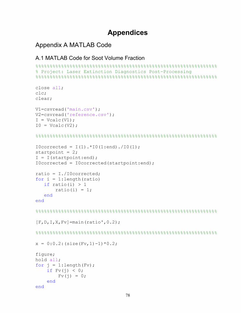
78

Appendices

Appendix A MATLAB Code

A.1 MATLAB Code for Soot Volume Fraction

%%%%%%%%%%%%%%%%%%%%%%%%%%%%%%%%%%%%%%%%%%%%%%%%%%%%%%%%%%%%%%%%

% Project: Laser Extinction Diagnostics Post-Processing

%%%%%%%%%%%%%%%%%%%%%%%%%%%%%%%%%%%%%%%%%%%%%%%%%%%%%%%%%%%%%%%%

close all;

clc;

clear;

V1=csvread('main.csv');

V2=csvread('reference.csv');

I = Vcalc(V1);

I0 = Vcalc(V2);

%%%%%%%%%%%%%%%%%%%%%%%%%%%%%%%%%%%%%%%%%%%%%%%%%%%%%%%%%%%%%%%%

I0corrected = I(1).*I0(1:end)./I0(1);

startpoint = 2;

I = I(startpoint:end);

I0corrected = I0corrected(startpoint:end);

ratio = I./I0corrected;

for i = 1:length(ratio)

if ratio(i) > 1

ratio(i) = 1;

end

end

%%%%%%%%%%%%%%%%%%%%%%%%%%%%%%%%%%%%%%%%%%%%%%%%%%%%%%%%%%%%%%%%

[F,D,I,X,Fv]=main(ratio',0.2);

%%%%%%%%%%%%%%%%%%%%%%%%%%%%%%%%%%%%%%%%%%%%%%%%%%%%%%%%%%%%%%%%

x = 0:0.2:(size(Fv,1)-1)*0.2;

figure;

hold all;

for j = 1:length(Fv);

if Fv(j) < 0;

Fv(j) = 0;

end

end

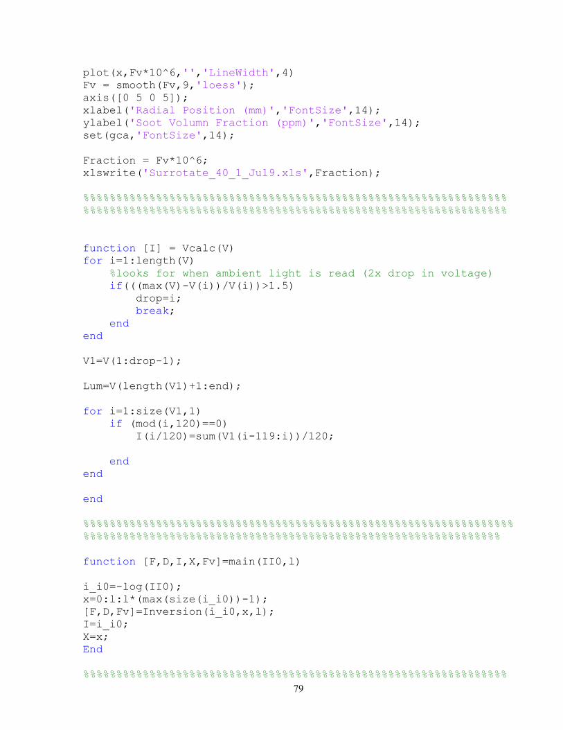
79

plot(x,Fv*10^6,'','LineWidth',4)

Fv = smooth(Fv,9,'loess');

axis([0 5 0 5]);

xlabel('Radial Position (mm)','FontSize',14);

ylabel('Soot Volumn Fraction (ppm)','FontSize',14);

set(gca,'FontSize',14);

Fraction = Fv*10^6;

xlswrite('Surrotate_40_1_Jul9.xls',Fraction);

%%%%%%%%%%%%%%%%%%%%%%%%%%%%%%%%%%%%%%%%%%%%%%%%%%%%%%%%%%%%%%%%

%%%%%%%%%%%%%%%%%%%%%%%%%%%%%%%%%%%%%%%%%%%%%%%%%%%%%%%%%%%%%%%%

function [I] = Vcalc(V)

for i=1:length(V)

%looks for when ambient light is read (2x drop in voltage)

if(((max(V)-V(i))/V(i))>1.5)

drop=i;

break;

end

end

V1=V(1:drop-1);

Lum=V(length(V1)+1:end);

for i=1:size(V1,1)

if (mod(i,120)==0)

I(i/120)=sum(V1(i-119:i))/120;

end

end

end

%%%%%%%%%%%%%%%%%%%%%%%%%%%%%%%%%%%%%%%%%%%%%%%%%%%%%%%%%%%%%%%%%

%%%%%%%%%%%%%%%%%%%%%%%%%%%%%%%%%%%%%%%%%%%%%%%%%%%%%%%%%%%%%%%

function [F,D,I,X,Fv]=main(II0,l)

i_i0=-log(II0);

x=0:l:l*(max(size(i_i0))-1);

[F,D,Fv]=Inversion(i_i0,x,l);

I=i_i0;

X=x;

End

%%%%%%%%%%%%%%%%%%%%%%%%%%%%%%%%%%%%%%%%%%%%%%%%%%%%%%%%%%%%%%%%

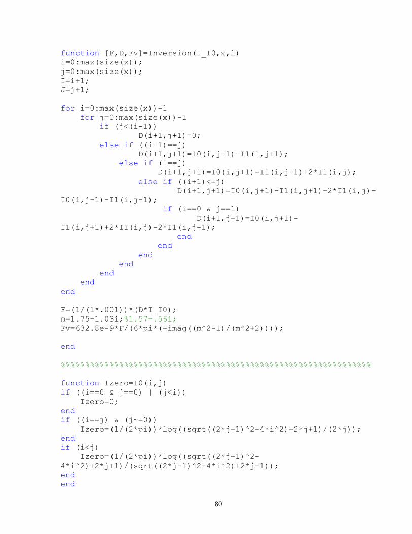
80

function [F,D,Fv]=Inversion(I_I0,x,l)

i=0:max(size(x));

j=0:max(size(x));

I=i+1;

J=j+1;

for i=0:max(size(x))-1

for j=0:max(size(x))-1

if (j<(i-1))

D(i+1,j+1)=0;

else if ((i-1)==j)

D(i+1,j+1)=I0(i,j+1)-I1(i,j+1);

else if (i==j)

D(i+1,j+1)=I0(i,j+1)-I1(i,j+1)+2*I1(i,j);

else if ((i+1)<=j)

D(i+1,j+1)=I0(i,j+1)-I1(i,j+1)+2*I1(i,j)-

I0(i,j-1)-I1(i,j-1);

if (i==0 & j==1)

D(i+1,j+1)=I0(i,j+1)-

I1(i,j+1)+2*I1(i,j)-2*I1(i,j-1);

end

end

end

end

end

end

end

F=(1/(l*.001))*(D*I_I0);

m=1.75-1.03i;%1.57-.56i;

Fv=632.8e-9*F/(6*pi*(-imag((m^2-1)/(m^2+2))));

end

%%%%%%%%%%%%%%%%%%%%%%%%%%%%%%%%%%%%%%%%%%%%%%%%%%%%%%%%%%%%%%%%

function Izero=I0(i,j)

if ((i==0 & j==0) | (j<i))

Izero=0;

end

if ((i==j) & (j~=0))

Izero=(1/(2*pi))*log((sqrt((2*j+1)^2-4*i^2)+2*j+1)/(2*j));

end

if (i<j)

Izero=(1/(2*pi))*log((sqrt((2*j+1)^2-

4*i^2)+2*j+1)/(sqrt((2*j-1)^2-4*i^2)+2*j-1));

end

end

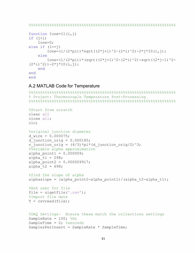
81

%%%%%%%%%%%%%%%%%%%%%%%%%%%%%%%%%%%%%%%%%%%%%%%%%%%%%%%%%%%%%%%%

function Ione=I1(i,j)

if (j<i)

Ione=0;

else if (i==j)

Ione=(1/(2*pi))*sqrt((2*j+1)^2-(2*i)^2)-2*j*I0(i,j);

else

Ione=(1/(2*pi))*(sqrt((2*j+1)^2-(2*i)^2)-sqrt((2*j-1)^2-

(2*i)^2))-2*j*I0(i,j);

end

end

end

A.2 MATLAB Code for Temperature

%%%%%%%%%%%%%%%%%%%%%%%%%%%%%%%%%%%%%%%%%%%%%%%%%%%%%%%%%%%%%%%%

% Project: Thermocouple Temperature Post-Processing

%%%%%%%%%%%%%%%%%%%%%%%%%%%%%%%%%%%%%%%%%%%%%%%%%%%%%%%%%%%%%%%%

%Start from scratch

clear all

close all;

clc;

%original junction diameter

d_wire = 0.000075;

d_junction_orig = 0.000185;

v_junction_orig = (4/3)*pi*(d_junction_orig/2)^3;

%Variable alpha approximation

alpha_point1 = 0.000009;

alpha_t1 = 298;

alpha_point2 = 0.000009917;

alpha_t2 = 698;

%find the slope of alpha

alphaslope = (alpha_point2-alpha_point1)/(alpha_t2-alpha_t1);

%Ask user for file

file = uigetfile('.csv');

%Import file data

T = csvread(file);

%DAQ Settings- Ensure these match the collections settings

SampleRate = 100; %Hz

SampleTime = 2; %seconds

SamplesPerInsert = SampleRate * SampleTime;

82

j=1; %Counter

i=0; %Sample Counter

n=1; %Counter in array k

x=2; %Position in flame, starting position from centerline

NumAve = 26; %Number of points used in the average calculation

%%%%%%%%%%%%%%%%%%%%%%%%%%%%%%%%%%%%%%%%%%%%%%%%%%%%%%%%%%%%%%%%

Devfwd = 20;

Devbk = 5;

extra = 0;

%%%%%%%%%%%%%%%%%%%%%%%%%%%%%%%%%%%%%%%%%%%%%%%%%%%%%%%%%%%%%%%%

%Creates an array that stores all the T array positions for the

%maximum temp values

MaxPosition = zeros((size(T,1))/200);

Tj = zeros((size(T,1))/200);

Tmax = zeros((size(T,1))/200);

displacement = 0.2; % the dist the stage was programmed to move

each time

CtoK = 273.15; %Convert degC to degK

%%%%%%%%%%%%%%%%%%%%%%%%%%%%%%%%%%%%%%%%%%%%%%%%%%%%%%%%%%%%%%%%

Te=[900

1000

1100

1200

1300

1400

1450

];

%%%%%%%%%%%%%%%%%%%%%%%%%%%%%%%%%%%%%%%%%%%%%%%%%%%%%%%%%%%%%%%%

emis=[0.1723

0.1837

0.1937

0.2032

0.2122

0.2206

0.2243

];

%%%%%%%%%%%%%%%%%%%%%%%%%%%%%%%%%%%%%%%%%%%%%%%%%%%%%%%%%%%%%%%%

83

Tk=[800

900

1000

];

%%%%%%%%%%%%%%%%%%%%%%%%%%%%%%%%%%%%%%%%%%%%%%%%%%%%%%%%%%%%%%%%

k=[57.25

62.54

67.68

];

%%%%%%%%%%%%%%%%%%%%%%%%%%%%%%%%%%%%%%%%%%%%%%%%%%%%%%%%%%%%%%%%

E=polyfit(Te,emis,1);% fits a linear curve to emis data

K=polyfit(Tk,k,1);% fits a linear curve to k data

%%%%%%%%%%%%%%%%%%%%%%%%%%%%%%%%%%%%%%%%%%%%%%%%%%%%%%%%%%%%%%%%

% Calculates the size of the whole data file and loops through it

for i=1:SamplesPerInsert:size(T,1)

Tmax(j)=max(T(i:i+SamplesPerInsert-1))+CtoK;

for m = i:(i + SamplesPerInsert)

if floor(T(m,1))== floor((Tmax(j)-CtoK))

MaxPosition(n) = m;

break

end

end

if i < SamplesPerInsert

if Devbk > MaxPosition(n)

extra = Devbk - MaxPosition(n) + 1;

end

Tj(j) = ((sum(T(((MaxPosition(n))-

Devbk+extra):((MaxPosition(n))+Devfwd+extra)))) / NumAve) + CtoK;

else

if Devbk > (MaxPosition(n) - i)

extra = Devfwd - MaxPosition(n) - i + 1;

end

Tj(j) = ((sum(T(((MaxPosition(n))-

Devbk+extra):((MaxPosition(n))+Devfwd+extra)))) / NumAve) + CtoK;

end

84

%Correction

alpha(j) = alpha_point1 + alphaslope*(Tj(j)-

alpha_t1); %Find local alpha

deltaV(j) = 3*alpha(j)*v_junction_orig*(Tj(j)-

298); %Find delta volume

V_2 (j) =

v_junction_orig+deltaV(j); %Find new volume

d_junction(j) =

2*(((3/4)*V_2(j)/pi)^(1/3)); %Find new bead diameter

%now run correction with updated diameter

Tg1(j)=Tj(j)+polyval(E,Tj(j))*0.0000000567*d_junction(j)*(Tj(j)^4

-296^4)/(.001*2*polyval(K,Tj(j)));

Tg(j)=Tj(j)+polyval(E,Tj(j))*0.0000000567*d_junction(j)*(Tj(j)^4-

296^4)/(.001*2*polyval(K,Tg1(j)));

%Increments n to store next max temp in MaxPosition

n = n + 1;

j = j + 1;

end

%%%%%%%%%%%%%%%%%%%%%%%%%%%%%%%%%%%%%%%%%%%%%%%%%%%%%%%%%%%%%%%%

x=0 : displacement : displacement*(size(Tg,2)-1);

%%%%%%%%%%%%%%%%%%%%%%%%%%%%%%%%%%%%%%%%%%%%%%%%%%%%%%%%%%%%%%%%

hold all

plot(x,Tg,'LineWidth',2)

axis([0 10 0 3000])

xlabel('R (mm)')

ylabel('T (K)')

Data_to_file = transpose(Tg);

%%%%%%%%%%%%%%%%%%%%%%%%%%%%%%%%%%%%%%%%%%%%%%%%%%%%%%%%%%%%%%%%

xlsFileName = input('Enter the name for the xls file: ', 's');

xlswrite(xlsFileName,Data_to_file);

%%%%%%%%%%%%%%%%%%%%%%%%%%%%%%%%%%%%%%%%%%%%%%%%%%%%%%%%%%%%%%%%

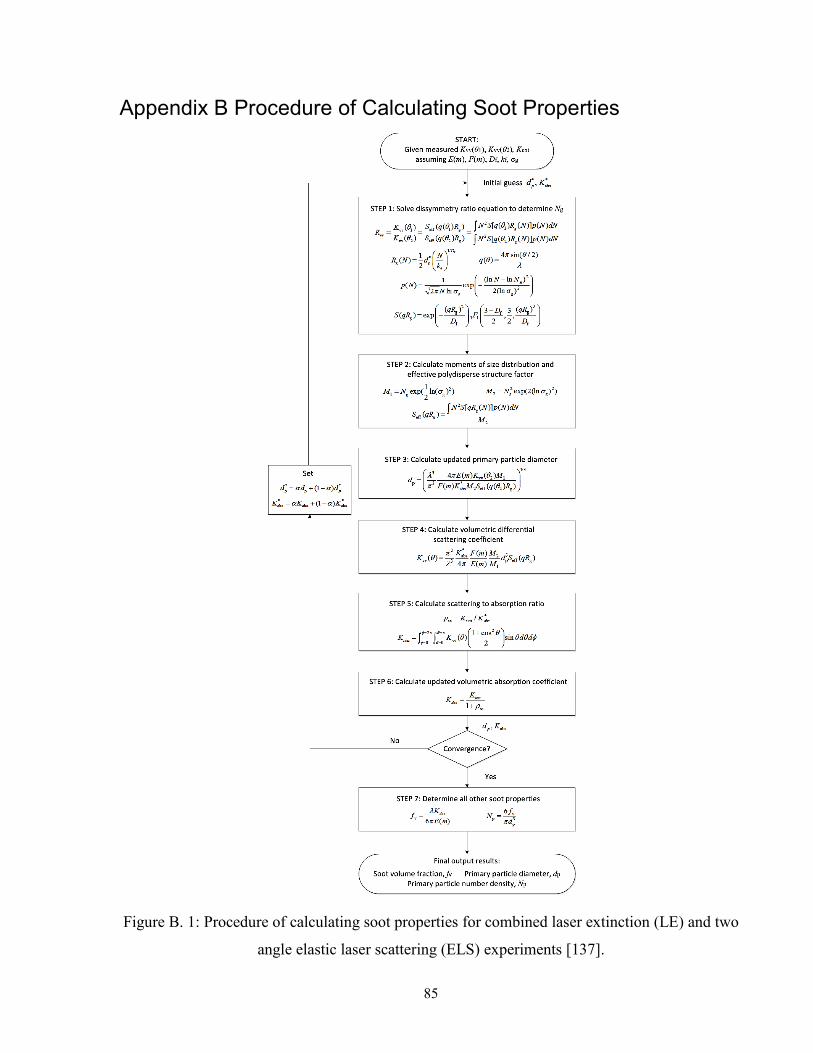
85

Appendix B Procedure of Calculating Soot Properties

Figure B. 1: Procedure of calculating soot properties for combined laser extinction (LE) and two

angle elastic laser scattering (ELS) experiments [137].

86

Appendix C Optics Alignment

The optics used in our setup are listed below (in sequence starting from the first optics after the

semiconductor laser):

1. Periscope;

2. Mirror-1;

3. Lens-1;

4. Lens-2;

5. Polarizer;

6. Beamsplitter;

7. Aperture-1;

8. Mirror-2;

9. Lens-3;

10. Aperture-2;

11. Lens-4;

12. Aperture-3;

13. Lens-5;

14. Integrating sphere;

15. Photodetector;

Optics alignment in our setup started from periscope. The steps for optics alignment of laser

extinction part are as following:

1. Place the periscope at the right position according to the exit position of laser to make sure

laser arrived at the center of the lower mirror. At the same time, rotate the upper and lower

housing to make sure the direction of laser light was changed as desired.

2. Position lens-1and lens-2 according to the requirement of focal length. According to the

design requirement, the laser comes out of lens-2 should be a collimated beam with larger

beam diameter compared to the laser beam that comes into lens-1. Lens-1 is concave lens

and lens-2 is convex lens. These two lenses constitute laser beam expanders. The lens

mounts were adjusted so that laser passed through the center of the lenses.

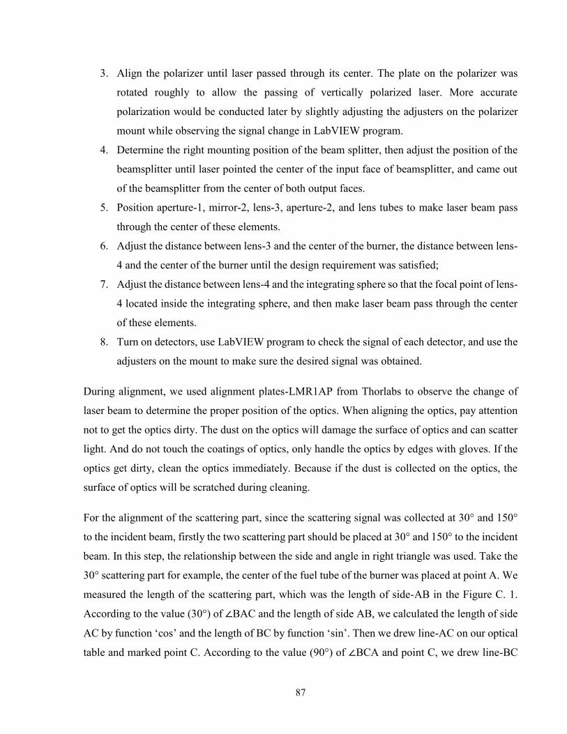
87

3. Align the polarizer until laser passed through its center. The plate on the polarizer was

rotated roughly to allow the passing of vertically polarized laser. More accurate

polarization would be conducted later by slightly adjusting the adjusters on the polarizer

mount while observing the signal change in LabVIEW program.

4. Determine the right mounting position of the beam splitter, then adjust the position of the

beamsplitter until laser pointed the center of the input face of beamsplitter, and came out

of the beamsplitter from the center of both output faces.

5. Position aperture-1, mirror-2, lens-3, aperture-2, and lens tubes to make laser beam pass

through the center of these elements.

6. Adjust the distance between lens-3 and the center of the burner, the distance between lens-

4 and the center of the burner until the design requirement was satisfied;

7. Adjust the distance between lens-4 and the integrating sphere so that the focal point of lens-

4 located inside the integrating sphere, and then make laser beam pass through the center

of these elements.

8. Turn on detectors, use LabVIEW program to check the signal of each detector, and use the

adjusters on the mount to make sure the desired signal was obtained.

During alignment, we used alignment plates-LMR1AP from Thorlabs to observe the change of

laser beam to determine the proper position of the optics. When aligning the optics, pay attention

not to get the optics dirty. The dust on the optics will damage the surface of optics and can scatter

light. And do not touch the coatings of optics, only handle the optics by edges with gloves. If the

optics get dirty, clean the optics immediately. Because if the dust is collected on the optics, the

surface of optics will be scratched during cleaning.

For the alignment of the scattering part, since the scattering signal was collected at 30° and 150°

to the incident beam, firstly the two scattering part should be placed at 30° and 150° to the incident

beam. In this step, the relationship between the side and angle in right triangle was used. Take the

30° scattering part for example, the center of the fuel tube of the burner was placed at point A. We

measured the length of the scattering part, which was the length of side-AB in the Figure C. 1.

According to the value (30°) of ∠BAC and the length of side AB, we calculated the length of side

AC by function ‘cos’ and the length of BC by function ‘sin’. Then we drew line-AC on our optical

table and marked point C. According to the value (90°) of ∠BCA and point C, we drew line-BC

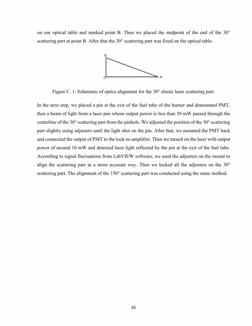
88

on our optical table and marked point B. Then we placed the midpoint of the end of the 30°

scattering part at point B. After that the 30° scattering part was fixed on the optical table.

Figure C. 1: Schematic of optics alignment for the 30° elastic laser scattering part.

In the next step, we placed a pin at the exit of the fuel tube of the burner and demounted PMT,

then a beam of light from a laser pen whose output power is less than 50 mW passed through the

centerline of the 30° scattering part from the pinhole. We adjusted the position of the 30° scattering

part slightly using adjusters until the light shot on the pin. After that, we mounted the PMT back

and connected the output of PMT to the lock-in-amplifier. Then we turned on the laser with output

power of around 10 mW and detected laser light reflected by the pin at the exit of the fuel tube.

According to signal fluctuations from LabVIEW software, we used the adjusters on the mount to

align the scattering part in a more accurate way. Then we locked all the adjusters on the 30°

scattering part. The alignment of the 150° scattering part was conducted using the same method.

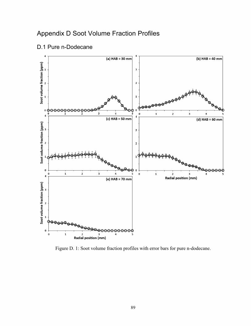
89

Appendix D Soot Volume Fraction Profiles

D.1 Pure n-Dodecane

Figure D. 1: Soot volume fraction profiles with error bars for pure n-dodecane.

90

D.2 Pure n-Dodecane Doped with 15 mol. % n-Propylbenzene

Figure D. 2: Soot volume fraction profiles with error bars for pure n-dodecane doped with 15

mol. % n-propylbenzene.

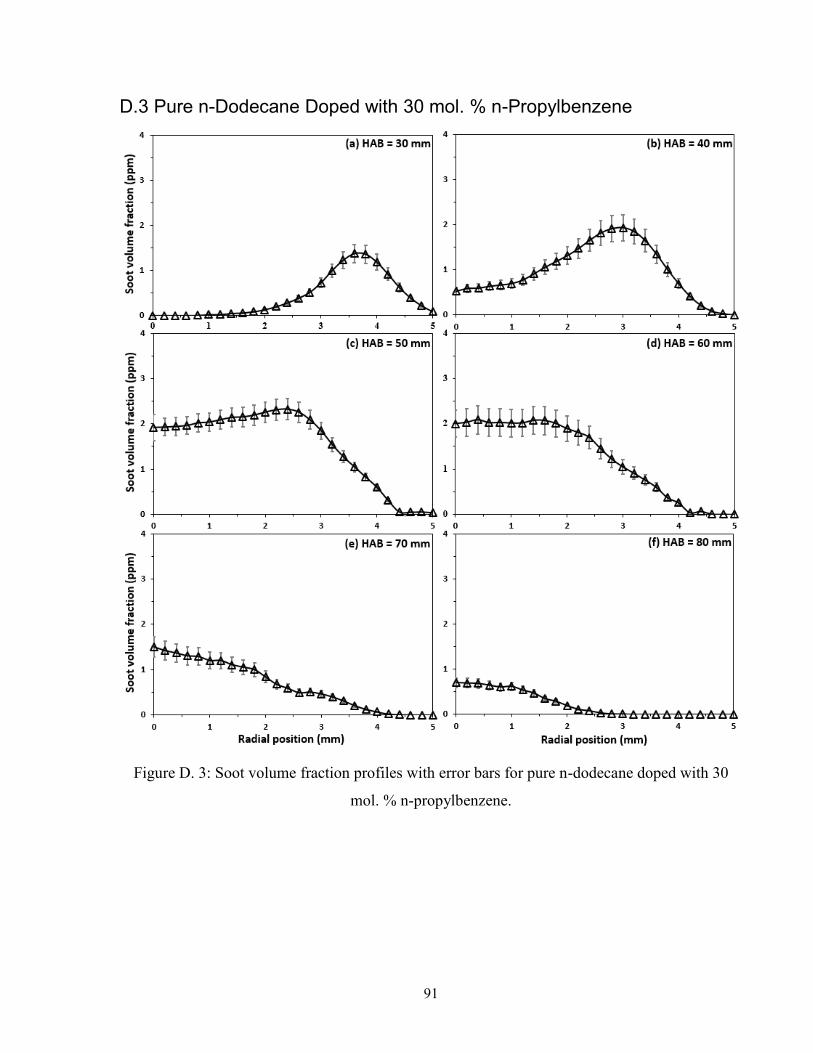
91

D.3 Pure n-Dodecane Doped with 30 mol. % n-Propylbenzene

Figure D. 3: Soot volume fraction profiles with error bars for pure n-dodecane doped with 30

mol. % n-propylbenzene.

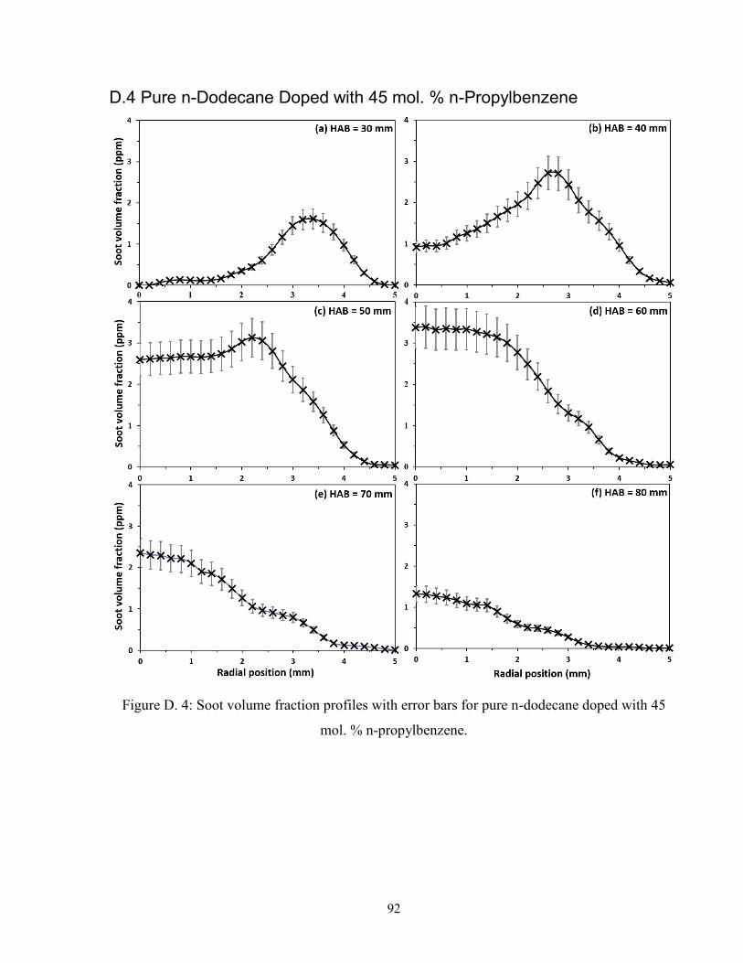
92

D.4 Pure n-Dodecane Doped with 45 mol. % n-Propylbenzene

Figure D. 4: Soot volume fraction profiles with error bars for pure n-dodecane doped with 45

mol. % n-propylbenzene.

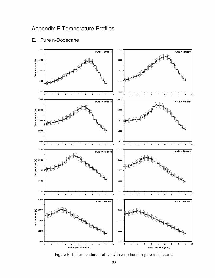
93

Appendix E Temperature Profiles

E.1 Pure n-Dodecane

Figure E. 1: Temperature profiles with error bars for pure n-dodecane.

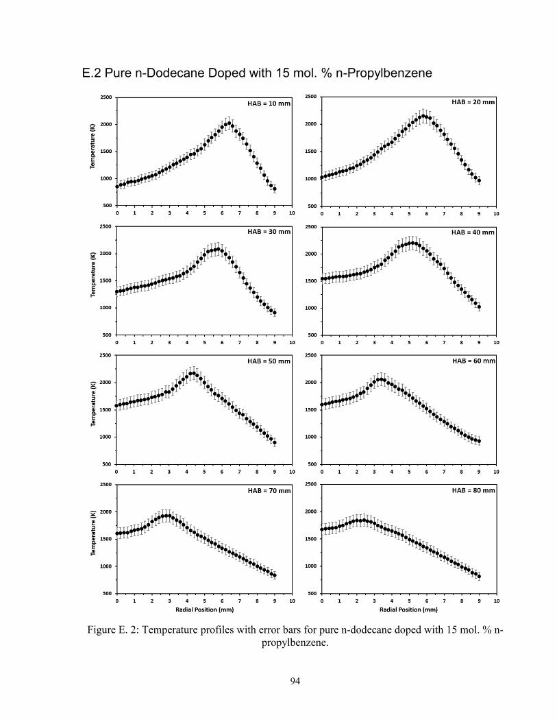
94

E.2 Pure n-Dodecane Doped with 15 mol. % n-Propylbenzene

Figure E. 2: Temperature profiles with error bars for pure n-dodecane doped with 15 mol. % n-

propylbenzene.

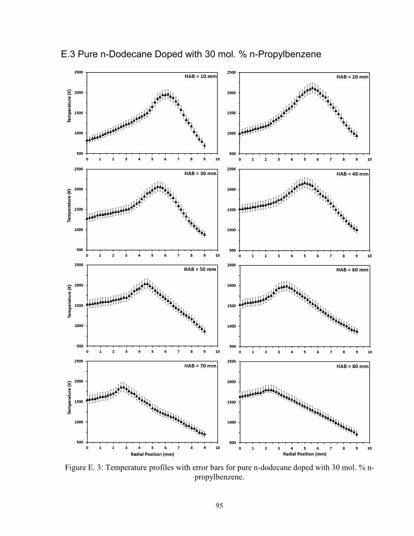
95

E.3 Pure n-Dodecane Doped with 30 mol. % n-Propylbenzene

Figure E. 3: Temperature profiles with error bars for pure n-dodecane doped with 30 mol. % n-

propylbenzene.

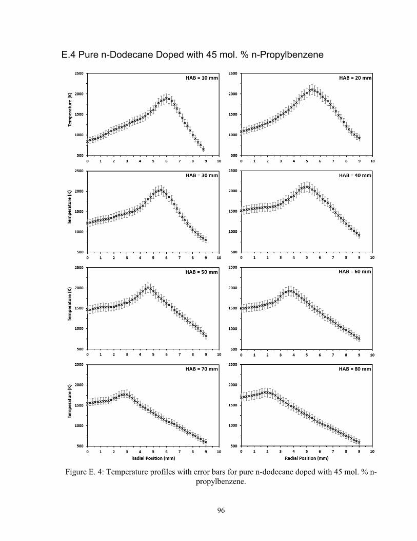
96

E.4 Pure n-Dodecane Doped with 45 mol. % n-Propylbenzene

Figure E. 4: Temperature profiles with error bars for pure n-dodecane doped with 45 mol. % n-

propylbenzene.