Effects of Frother Type on Single

Bubble Rise Velocity

Amir Arash Rafiei Mehrabadi

Department of Mining, Metals and Materials Engineering

McGill University

Montreal, Canada

June 2009

A thesis submitted to McGill University in partial fulfillment of

the requirements for the degree of Master of Engineering

© Amir Arash Rafiei Mehrabadi, 2009

ii

Abstract The addition of frother in flotation has two main functions, to help reduce bubble size and help produce a stable froth. A role of frother on bubble behavior in pulp zone is usually not considered. A previous study showed that as frother type was changed the same gas holdup was given by different size bubbles. This implies that bubble rise velocity depends on the nature of the surfactant (frother type). A study using bubble swarms appears to support the frother type effect but bubble interactions are a possible confounding factor. This study resolved the question by measuring terminal rise velocity profile of single bubbles (ca. 1 to 2 mm) as a function of frother type. It is shown that at the concentrations of interest in flotation, 1-pentanol hardly alters the velocity compared to water alone while F150 (a polyglycol) reduces the velocity by up to 50%. The results become in 1-pentanol bubble did not reach terminal velocity. For high concentration of 1-pentanol (>130ppm) the rise velocity is reduced comparable to F150. To investigate, experiments were performed using aliphatic alcohols from 1-butanol (C4) to 1-octanol (C8). It was found there is a minimum concentration for the frother to give terminal velocity close to the Clift et al. contaminated eater result. The concentration decreases as molecular weight (chain length) of alcohol increases. Larger bubbles (1.8 vs. 1.5mm) require higher minimum concentration. To study the influence of molecular structure, three 6-C alcohols, 1-hexanol, MIBC and 2-hexanol, were used. The results show that molecular structure influences rise velocity through the position of OH group, and whether the alcohol is straight chained or branched. The observation can make a useful link frother to chemistry for understanding frother influence on bubble rise and possibly its function in flotation. The influence of three industrial frother, MIBC, F150 and DF250, was studied and it was observed that over the practical concentration range all reduce rise velocity similar to contaminated water and their critical concentration are very low compared to the aliphatic alcohols. In addition, the influence of a salt, NaCl, on bubble rise velocity was compared to MIBC and confirms a previous observation that reported the similar capability of NaCl to act like MIBC.

iii

Résumé Deux raisons principales commandent à l´ajout de la mousse dans le processus de flottation, à savoir, la réduction de la bulle et la production d´une mousse stable. L´effet de la mousse sur le comportement de la bulle en zone pulpaire n´est pas pris en compte. Un travail antérieur a démontré que pour la même fraction d´air transporté par les bulles, le type de mousse a de l´influence sur la taille des bulles. Cela implique que la vélocité de la bulle dépend de la nature du surfactant (type de mousse). Une étude basée sur l´usage de plusieurs bulles semble s´accorder avec l´hypothèse relative au type de mousse, néanmoins les interactions des bulles rendent le problème complexe. La présente étude a résolu cette question en mesurant la vélocité d´une bulle dont les dimensions sont presque égales à 1 ou 2 mm, suivant le type de mousse. Il en est résulté que dans l´intervalle des concentrations d´importance en flottation, le pentanol peine à influencer la vélocité, alors que l´eau toute seule en serait capable. En revanche, le F150 (un polyglycol) réduit la vélocité de 50%. Pour les concentrations élevées de pentanol (>100 ppm), la vélocité décroit et devient comparable à celle engendrée par la présence du F150. Il va de soi que l´observation antérieure est confirmée dans l´intervalle pratique des concentrations. En guise d´investigations, des expériences au cours desquelles les alcools aliphatiques allant du butanol (C4) à l´octanol (C8), ont été réalisées. Il a été démontré que l´effet du type de mousse sur la vélocité dépend de la concentration. Il existe une concentration minimale de la mousse en dessous de laquelle, la bulle monte comme dans le modèle de l´eau contaminée de Clift et al. La concentration minimale critique dépend de la dimension de la bulle et du déplacement mesuré à partir du point terminal du tube capillaire. L´on rapporte que les bulles les plus larges et les mousses de petite masse moléculaire nécessitent une concentration élevée pour épouser le comportement de l´eau contaminée. Au dessus de cette concentration, la vélocité de la bulle est indépendante du type de mousse et de la concentration. Afin d´étudier la possible influence de la structure moléculaire, trois alcools (C6) dont 1-hexanol, MIBC et 2-hexanol ont été utilisés. Les résultats ont montré que la structure moléculaire influence la vélocité via la position du groupe OH, selon qu´elle est linéaire ou ramifiée. Cette observation fait clairement un lien avec la chimie et permet de mieux comprendre la relation entre la mousse et la vélocité de la bulle et possiblement sa fonction. L´influence de 3 mousses industrielles dont le MIBC, le F150 et le DF250, a été étudiée. L´on a observé qu´au - delà de l´intervalle pratique de concentrations, ces mousses réduisent la vélocité de la même manière que l´eau contaminée. Leurs concentrations critiques sont de beaucoup inferieures à celles des alcools aliphatiques. En plus, l´influence du sel (NaCl) sur la vélocité a été comparée à celle du MIBC. Cette expérience a confirmé que le NaCl peut se comporter comme le MIBC.

iv

Acknowledgements I wish to express my sincerest appreciation and utmost gratitude to my supervisor, Professor James A. Finch, for his guidance, support, patience, continuous encouragement, trust, discussions, valuable technical assistance, very high teaching skills and especially his brilliant vision about the current research. During all precious days of my work at McGill his integrity, discipline, well-organized planning, timing and attitude gave me very important experiences and ideas to be more successful in my future life. Briefly, as a very important key of success that I have learned, he is one of the people who really enjoys from his work life. I would like to thank Dr. Ram Rao who helped me to understand some problems in organic chemistry. Also I want to thank Dr Cesar O. Gomez for all his efforts in preparing the column for running experiments and his brilliant engineering ideas in re-designing the column for providing better performance. Thanks must go to my colleagues for providing support and very good collaboration, especially Dr. Mitra Mirnezami for her advice and help. I would like to gratitude the organizations and companies that provided sufficient financial support for doing my work. The last but the most gratitude must go to my family and especially my mother who means every thing to me.

v

Table of Contents 1. INTRODUCTION 1

1.1. Single bubble rise velocity 1 1.2. Velocity profile and terminal velocity of a single bubble 2 1.3. Objectives of the study 4 1.4. Structure of the thesis 5

2. BACKGROUND 6 2.1. Bubble formation in gas-liquid systems 6 2.2. Theoretical aspects 6

2.2.1. Forces 6 2.2.1.1. Surface tension 7 2.2.1.2. Buoyancy 7 2.2.1.3. Drag 8

2.2.2. Force ratio 8 2.2.3. Wake phenomenon 10

2.3. Surfactants and their influence at air/water interface 11 2.3.1. Surfactant and frother 11 2.3.2. Surfactant adsorption mechanism 12 2.3.3. Surfactant distribution 13 2.3.4. Some consequences of presence of surfactant at air/water interface 15

2.3.4.1. Marangoni effect 15 2.3.4.2. Interaction between surfactant and water molecules 17 2.3.4.3. Effect on bubble internal circulation 17

2.4. Bubble behavior 18 2.4.1. Bubble size 20 2.4.2. Bubble shape 21 2.4.3. Bubble rise path 24 2.4.4. Bubble rise velocity 25

2.4.4.1. Factors affecting the rise velocity 26 2.4.5. Formulation for rise velocity correlation 30

2.5. Contaminants and rise velocity 30 2.5.1. Surfactant 30

2.5.1.1. Newtonian liquids 30 2.5.1.2. Non-Newtonian liquids 32 2.5.1.3. High viscosity liquids 32 2.5.1.4. Simulation and numerical analysis 32

2.5.2. Frothers 33 2.5.3. Salts 36

3. EXPERIMENTAL SETUP 39 3.1. Equipment 39

3.1.1. Column setup 39 3.1.2. Air line 39 3.1.3. Camera moving device 39 3.1.4. Capillaries 41

3.2. Requirements 41

vi

3.2.1. Temperature control 41 3.2.2. Bubbling frequency 41 3.2.3. Water saturation 41

3.3. Procedures 41 3.3.1. Bubble velocity profile 41 3.3.2. Data Processing 42

3.4. Reagents 43 3.5. Measurement techniques 45

3.5.1. Bubble position 45 3.5.2. Local velocity 45 3.5.3. Bubble size 46 3.5.4. Reagents and choice of reagent concentration 47

4.RESULTS AND DISCUSSION 49 4.1. Reliability 49

4.1.1. Bubble generation 49 4.1.2. Terminal velocity 51 4.1.3. Bubble size 53

4.2. Velocity profile analysis 54 4.2.1. Examples 54 4.2.2. Maximum velocity 56

4.3. Reagent type: pentanol vs. F150 57 4.3.1. Velocity profile 57 4.3.2. Comparison of terminal/apparent terminal velocities 58

4.4. Aliphatic alcohols 59 4.4.1. Concentration effect 62 4.4.2. The influence of molecular structure: C-6 alcohols 69

4.4. Comparison of MIBC and NaCl 72 4.6. Comparison of frothers 74 4.7. The dependency of terminal velocity on frother properties 76

5. CONCLUSIONS AND RECOMMENDATIONS 80 5.1. Conclusions 80

5.1.1. Bubble generation 80 5.1.2. Velocity profile analysis 80 5.1.3. Hypothesis based on observation of Azgomi et al. (2007) 80 5.1.4. Aliphatic alcohols 81 5.1.5. The comparison of MIBC and NaCl 81 5.1.6. Commercial frothers 82 5.1.7. Dependency of terminal velocity on frother properties 82

5.2. Recommendations for future works 82 Refferences 84 Appendix 99

vii

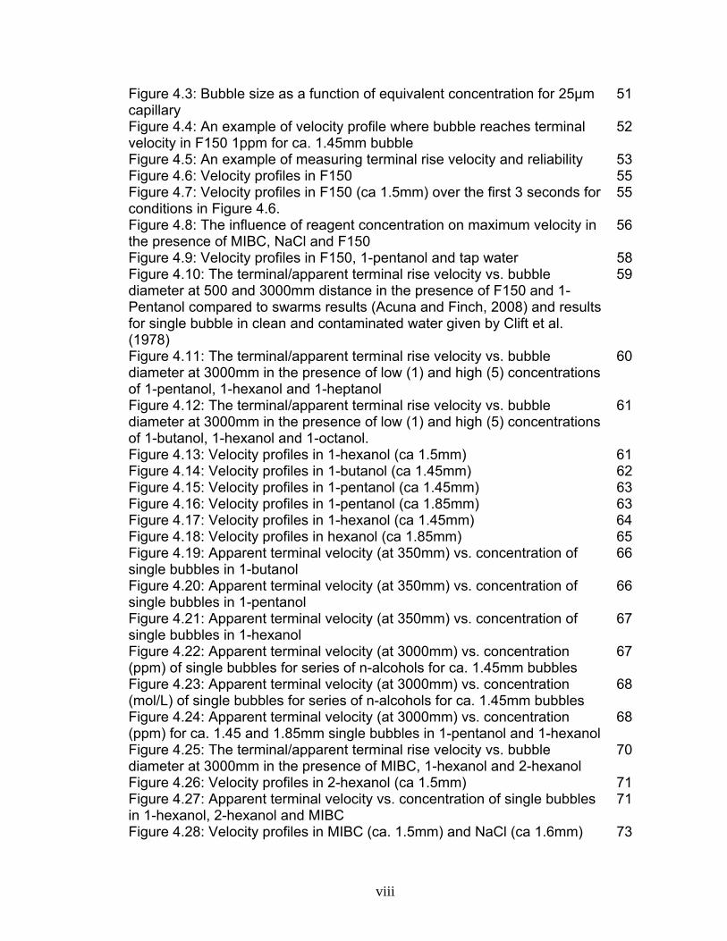
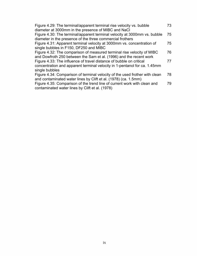
List of Figures Figure 1.1: The stages of a typical velocity profile 3 Figure 1.2: Typical trend for terminal rise velocity in clean and contaminated water

4

Figure 2.1: Circulation region (wake) behind a sphere at various Reynolds numbers

11

Figure 2.2: Accumulation of surfactant at air/water interface 14 Figure 2.3: Surfactant and velocity distribution on bubble surface for the two extremes

15

Figure 2.4: The distribution of adsorbed surface active solute on the surface of a rising bubble

16

Figure 2.5: The internal circulation of moving fluid showing the direction of relative flow: (a) complete circulation, (b) part circulation, (c) stagnant

18

Figure 2.6: The relationships between identified factors that affect bubble behavior

20

Figure 2.7: Illustration of dynamic pressure causing bubble deformation in water only case (a), and the force created by surface tension gradient that occurs in presence of surfactant that resists deformation (b) (Finch et al., 2008).

22

Figure 2.8: Bubble shape regime 23 Figure 2.9: Typical trends in rise velocity with bubble size for pure and contaminated liquids

27

Figure 2.10: Effect of initial bubble deformation on terminal velocity in distilled water

27

Figure 2.11: a. Velocity profiles for 2.2mm bubbles in MIBC, b. Terminal velocity vs. bubble size in the presence of some frothers

34

Figure 2.12: Bubble size measurement at same gas holdup (8%) for F150 and Pentanol

35

Figure 2.13: Comparison between influences of F150 and Pentanol on terminal rise velocity of bubbles in swarms

36

Figure 2.14: Suggested explanation for action of high concentration salts which act like frother

37

Figure 2.15: Influence of potassium chloride concentration on terminal rise velocity

37

Figure 3.1: The experimental column setup 40 Figure 3.2: The data processing flowchart 43 Figure 3.3: The required information for measuring bubble height during rise on one image

45

Figure 3.4: The applied technique for measuring local velocity 46 Figure 3.5: The technique applied for measuring bubble size 47 Figure 3.6: The description of technique that applied to determine equivalent concentrations of F150 and 1-Pentanol

47

Figure 4.1: Variation of single bubble size vs. bubble frequency for reagents using 25μm capillary.

50

Figure 4.2: The variation of single bubble size vs. bubble frequency for the three applied capillaries

50

viii

Figure 4.3: Bubble size as a function of equivalent concentration for 25μm capillary

51

Figure 4.4: An example of velocity profile where bubble reaches terminal velocity in F150 1ppm for ca. 1.45mm bubble

52

Figure 4.5: An example of measuring terminal rise velocity and reliability 53 Figure 4.6: Velocity profiles in F150 55 Figure 4.7: Velocity profiles in F150 (ca 1.5mm) over the first 3 seconds for conditions in Figure 4.6.

55

Figure 4.8: The influence of reagent concentration on maximum velocity in the presence of MIBC, NaCl and F150

56

Figure 4.9: Velocity profiles in F150, 1-pentanol and tap water 58 Figure 4.10: The terminal/apparent terminal rise velocity vs. bubble diameter at 500 and 3000mm distance in the presence of F150 and 1-Pentanol compared to swarms results (Acuna and Finch, 2008) and results for single bubble in clean and contaminated water given by Clift et al. (1978)

59

Figure 4.11: The terminal/apparent terminal rise velocity vs. bubble diameter at 3000mm in the presence of low (1) and high (5) concentrations of 1-pentanol, 1-hexanol and 1-heptanol

60

Figure 4.12: The terminal/apparent terminal rise velocity vs. bubble diameter at 3000mm in the presence of low (1) and high (5) concentrations of 1-butanol, 1-hexanol and 1-octanol.

61

Figure 4.13: Velocity profiles in 1-hexanol (ca 1.5mm) 61 Figure 4.14: Velocity profiles in 1-butanol (ca 1.45mm) 62 Figure 4.15: Velocity profiles in 1-pentanol (ca 1.45mm) 63 Figure 4.16: Velocity profiles in 1-pentanol (ca 1.85mm) 63 Figure 4.17: Velocity profiles in 1-hexanol (ca 1.45mm) 64 Figure 4.18: Velocity profiles in hexanol (ca 1.85mm) 65 Figure 4.19: Apparent terminal velocity (at 350mm) vs. concentration of single bubbles in 1-butanol

66

Figure 4.20: Apparent terminal velocity (at 350mm) vs. concentration of single bubbles in 1-pentanol

66

Figure 4.21: Apparent terminal velocity (at 350mm) vs. concentration of single bubbles in 1-hexanol

67

Figure 4.22: Apparent terminal velocity (at 3000mm) vs. concentration (ppm) of single bubbles for series of n-alcohols for ca. 1.45mm bubbles

67

Figure 4.23: Apparent terminal velocity (at 3000mm) vs. concentration (mol/L) of single bubbles for series of n-alcohols for ca. 1.45mm bubbles

68

Figure 4.24: Apparent terminal velocity (at 3000mm) vs. concentration (ppm) for ca. 1.45 and 1.85mm single bubbles in 1-pentanol and 1-hexanol

68

Figure 4.25: The terminal/apparent terminal rise velocity vs. bubble diameter at 3000mm in the presence of MIBC, 1-hexanol and 2-hexanol

70

Figure 4.26: Velocity profiles in 2-hexanol (ca 1.5mm) 71 Figure 4.27: Apparent terminal velocity vs. concentration of single bubbles in 1-hexanol, 2-hexanol and MIBC

71

Figure 4.28: Velocity profiles in MIBC (ca. 1.5mm) and NaCl (ca 1.6mm) 73

ix

Figure 4.29: The terminal/apparent terminal rise velocity vs. bubble diameter at 3000mm in the presence of MIBC and NaCl

73

Figure 4.30: The terminal/apparent terminal velocity at 3000mm vs. bubble diameter in the presence of the three commercial frothers

75

Figure 4.31: Apparent terminal velocity at 3000mm vs. concentration of single bubbles in F150, DF250 and MIBC

75

Figure 4.32: The comparison of measured terminal rise velocity of MIBC and Dowfroth 250 between the Sam et al. (1996) and the recent work

76

Figure 4.33: The influence of travel distance of bubble on critical concentration and apparent terminal velocity in 1-pentanol for ca. 1.45mm single bubbles

77

Figure 4.34: Comparison of terminal velocity of the used frother with clean and contaminated water lines by Clift et al. (1978) (ca. 1.5mm)

78

Figure 4.35: Comparison of the trend line of current work with clean and contaminated water lines by Clift et al. (1978)

79

x

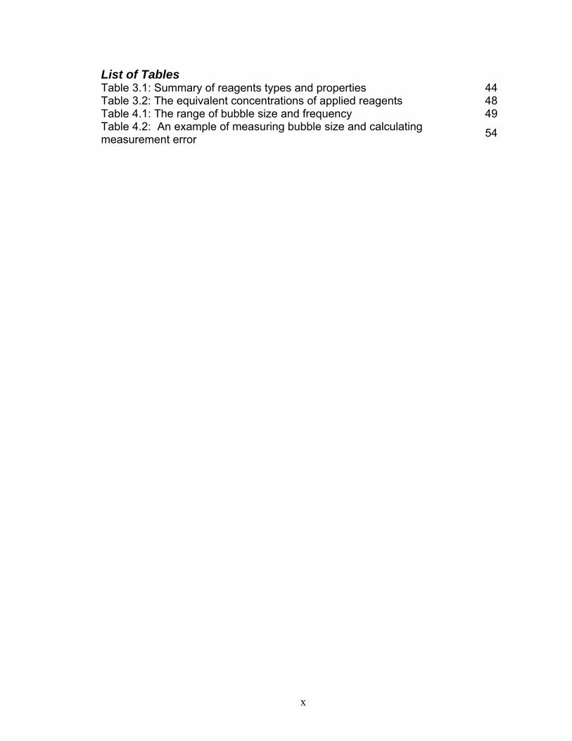
List of Tables Table 3.1: Summary of reagents types and properties 44 Table 3.2: The equivalent concentrations of applied reagents 48 Table 4.1: The range of bubble size and frequency 49 Table 4.2: An example of measuring bubble size and calculating measurement error 54

xi

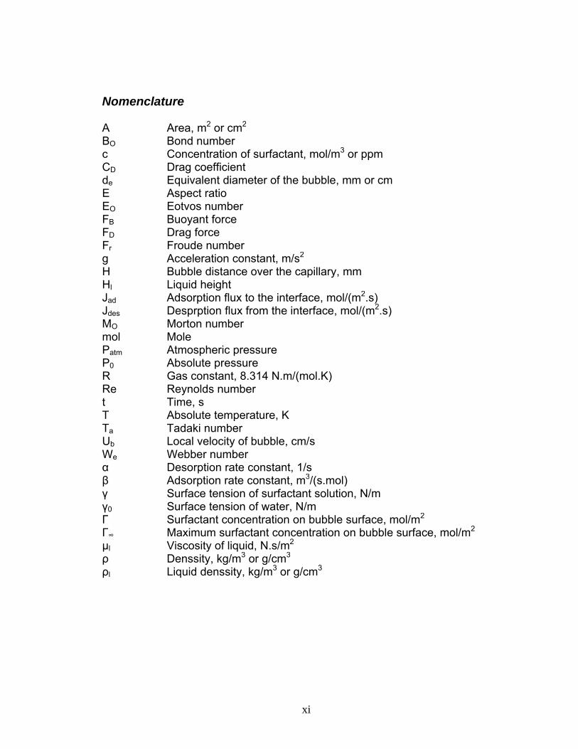
Nomenclature A Area, m2 or cm2 BO Bond number c Concentration of surfactant, mol/m3 or ppm CD Drag coefficient de Equivalent diameter of the bubble, mm or cm E Aspect ratio EO Eotvos number FB Buoyant force FD Drag force Fr Froude number g Acceleration constant, m/s2 H Bubble distance over the capillary, mm Hl Liquid height Jad Adsorption flux to the interface, mol/(m2.s) Jdes Desprption flux from the interface, mol/(m2.s) MO Morton number mol Mole Patm Atmospheric pressure P0 Absolute pressure R Gas constant, 8.314 N.m/(mol.K) Re Reynolds number t Time, s T Absolute temperature, K Ta Tadaki number Ub Local velocity of bubble, cm/s We Webber number α Desorption rate constant, 1/s β Adsorption rate constant, m3/(s.mol) γ Surface tension of surfactant solution, N/m γ0 Surface tension of water, N/m Γ Surfactant concentration on bubble surface, mol/m2 Γ∞ Maximum surfactant concentration on bubble surface, mol/m2 μl Viscosity of liquid, N.s/m2 ρ Denssity, kg/m3 or g/cm3 ρl Liquid denssity, kg/m3 or g/cm3

xii

1

CHAPTER ONE: INTRODUCTION

Particulate systems can be categorized on the basis of the phases involved: solid

particle, liquid and gas bubble. There are many wide industrial processes based

on two or three phase systems. It is important to understand the interactions to

optimize these processes. The complex nature of water requires special attention

to understand water-based two and three phase systems.

Bubble rise in liquids under different conditions is one of the oldest of scientific

investigations. It is of interest as the characteristics of a rising bubble (e.g. size,

shape, velocity and trajectory) give insight into the dynamics of a system. Rise

velocity is one of the most important characteristics of a rising bubble.

1.1. Single bubble rise velocity

Numerous studies have been performed on the motion of single bubbles. Clift et

al. (1978) reviewed the research prior to 1978. Kulkarani and Joshi (2005)

provide the most recent review on bubble formation and bubble rise velocity in

gas-liquid systems. There remain problems with some of the previous works

because of restrictions imposed by the experimental set-up and differences in

understanding the nature of bubble velocity especially in surfactant solutions.

The measurement of terminal velocity is a case in point: it is important to clarify

what velocity is being determined experimentally. Most studies report the

terminal velocity as an average velocity of a bubble over a given distance. Others

use the velocity at a fixed distance above the point of bubble release. Both

measures overlook a possible time-dependence of the velocity. This has led to

confusion over interpreting the impact of surfactant type and concentration.

Sam (1995) was one of the pioneers who applied an adjustable speed moving

video camera system to measure the velocity of a rising bubble as a function of

time or height, referring to this as the “velocity profile” (Sam et al., 1996). This

setup has opened a new approach to the fundamental study of the bubble motion

2

mechanism, as recognized by Dewsburry et al. (1999) and Kulkarani and Joshi

(2005).

In the presence of surfactant, depending on type and concentration, the velocity

profile (time-history) revealed three stages: acceleration, deceleration and

constant (terminal) velocity.

The common interpretation is that surfactants adsorb on the bubble and retard

the mobility of surface resulting in increased drag (Frumkin and Levich, 1947).

As the bubble rise and surfactant accumulates the corresponding increase in

drag can account for the three stages (Sam et al., 1996). Theoretically, the

velocity of a single bubble rising in surfactant solution can be solved by a

combination of the Navier-Stokes equation, mass transfer and the Marangoni

effect. These govern the fluid flow around the bubble, the amount of surfactant

on the bubble, and the extent of surface retardation and distribution of surfactant

on the surface, respectively. The surface retardation can be simulated by uniform

and stagnant cap models that determine rise velocity according to rate and

extent of accumulation of surfactant molecules on the bubble surface (Zhang et

al.., 2001; Zhang and Finch, 2002).

1.2. Velocity profile and terminal velocity of a single bubble

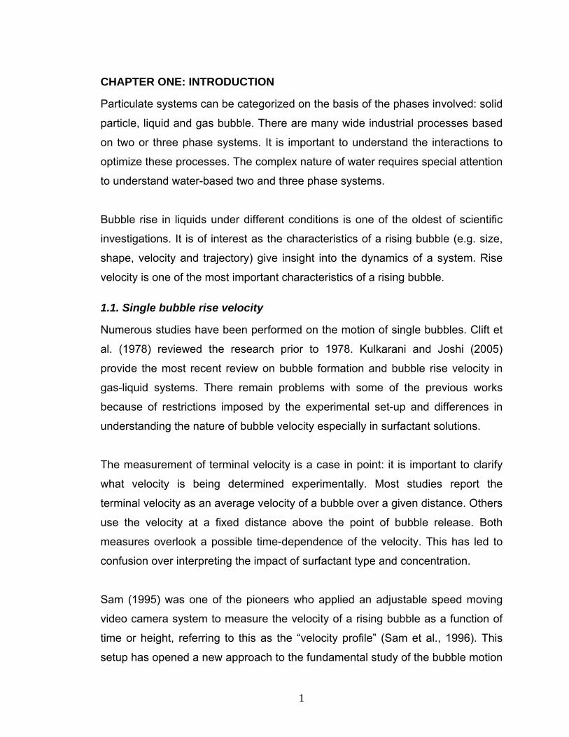
Sam et al. (1996) characterized the single bubble velocity profile by suggesting

three stages (Figure 1.1): first, a rapid increase to a maximum value

(acceleration); second, a decrease (deceleration); and third, a constant (terminal)

velocity stage. They observed the profile was strongly dependent on surfactant

type and concentration.

3

Figure1.1: The stages of a typical velocity profile.

The different stages in the profile reflect different amount of adsorbed surfactant.

Initially the bubble surface is almost free of surfactant and the bubble accelerates

towards the velocity in a surfactant-free system. As surfactant molecules

accumulate drag increases and the bubble slows and eventually decelerates.

When adsorption reaches equilibrium (a steady state between adsorption at the

forward part of the bubble from where surfactant is swept by the flowing liquid

and desorption from the rear of the bubble to where the surfactants are swept)

the velocity of the bubble becomes constant considered as the terminal velocity.

According to Newton’s second law the terminal velocity of a body is the velocity

at which the body moves under a zero-acceleration condition. In the case of

terminal velocity of a bubble this indicates a balance between upward buoyancy

and downward drag forces.

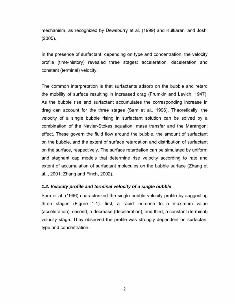
Sam et al. (1996) reported that terminal velocity of a single bubble appeared to

depend on surfactant type but not surfactant concentration, only the time to reach

terminal velocity is affected. According to that conclusion, analysis of single

bubble terminal velocity vs. bubble size should reveal the influence of surfactant

4

type. Figure 1.2 presents the terminal velocity extremes, the trend for “clean” and

“contaminated” water (Clift et al., 2005).

Figure 1.2: Typical trend for terminal rise velocity in clean and contaminated water

(reproduced with permission from Clift et al. 2005).

While terminal velocity is an important property, the velocity profile can provide

further insight into surfactant action on bubble motion. This thesis will examine

velocity profile and terminal velocity of single bubbles in systems of interest in

mineral flotation.

1.3. Objectives of the study

The general objective is to use local rise velocity vs. distance (time) of single

bubbles (i.e., the velocity profile) to characterize systems of interest in flotation.

Some specific objectives include:

• Measure the velocity profile of some selected frothers, alcohols and salts

over a range of concentration and bubble size of interest to flotation (0.5-

2.5mm);

• Compare velocity vs. bubble size in 1-Pentanol (as a simple alcohol) and

F150 (as a polyglycol) to test the claim of frother type effect on velocity

presented by Azgomi et al. (2006);

5

• Compare velocity vs. bubble size between MIBC (as a weak frother) and

NaCl (as a salt) to verify their common effect, according to the

observation of Quinn et al. (2007);

• Compare velocity vs. bubble size among some alcohols (C4-C8) to track

the effect of chain length;

• Compare single bubble results with recent swarms results (Acuna and

Finch, 2008).

1.4. Structure of the thesis

Chapter 1. Introduction: The gas/liquid system and parameters of bubble rise in

water are introduced followed by introduction to concept of velocity profile and

terminal rise velocity. The chapter ends by introducing objectives of the study

and structure of the thesis.

Chapter 2. Background and Literature Review: Required background

concerning forces acting and surfactant properties are presented. The literature

review begins with an introduction to bubble behavior and ends with more

detailed discussion on the impact of contaminants on bubble rise velocity.

Chapter 3. Experimental Setup: Here the experimental setup, methods,

measurement techniques and software are described.

Chapter 4. Results and Discussion: The results achieved toward each

objective are presented. Data are analyzed and compared with published works.

Chapter 5. Conclusions and Recommendations: The conclusions are

summarized and recommendations for future work entertained.

6

CHAPTER TWO: BACKGROUND

2.1. Bubble formation in gas-liquid systems

Some of the earliest studies on the formation of single bubbles were by Tate

(1864) and Bashforth and Adams (1883). A significant body of work on bubble

formation over a wide range of design and operational parameters has appeared

in the literature over the last few decades (Davidson and Schuler (1960), Tsuge

and co-workers, (1983, 1986, 1992, 1993, 1997, and 1999), Kumar et al.(1969),

Marmur et al. (1973, 1976), Vogelophl and co-workers (1982, 1986), Tan and co-

workers (2000, 2003).

A model of bubble formation from submerged orifice was proposed by Kumar et

al. (1969). Tsuge (1986) reviewed the hydrodynamics of bubble formation and

discussed various models. Rabiger and Vogelpohl (1986) discussed the various

factors affecting bubble formation. There have been several recent developments

in both numerical and experimental methods (Kulkarani and Joshi, 2005).

Bubble formation at a single submerged orifice can be classified according to the

following modes: low frequency bubbling, chain bubbling, wobbling and jetting.

These modes are dependent on the orifice configuration, the gas velocity, and

gas/liquid system properties.

2.2. Theoretical aspects

2.2.1. Forces

Particle (defined generally to include solid, liquid (droplet) or gas (bubble)) motion

in a liquid is controlled by forces that act on the particle. The fundamental

aspects are based on Newton’s second law illustrated by the momentum “Navier-

Stokes” equation.

7

The motion of a bubble in a liquid is subjected to buoyancy and drag forces and,

because there is a different cohesive force between water and air molecules, an

interfacial force also appears, surface tension. The forces are briefly described.

2.2.1.1. Surface tension

The Navier-Stokes equation can be considered as a general force balance for a

fluid in motion. When an interface is involved (e.g., bubble/water interface), an

interfacial (or surface) tension force is present. The interface behaves like a thin

stressed membrane under tension (Eskinazi, 1968).

Surfactant and salts affect the surface tension of the air/water interface, the

former reducing surface tension the later often increasing surface tension. The

surface tension may be a function of time called dynamic surface tension (Defay

and Prigozine, 1960). That feature is recognized to have a role in some flotation

systems (Defay and Prigozine, 1960; Finch and Smith, 1972; Kulkarani and

Somasundaran, 1975; Leja, 1982; Comley et al. 2002). The equilibrium surface

tension of an air/water interface depends on the quantity of adsorbed molecules

of surfactant. Above a certain concentration of surfactant, the surface tension

becomes constant and any surfactant forms colloidal aggregates within the bulk

solution known as micelles where CMC stands for critical micelle concentration.

2.2.1.2. Buoyancy

According to Archimedes’ principle a particle whose average density is less than

that of the liquid floats on that liquid. The direction of the buoyancy force for both

falling (object has higher density than water) and rising (object has lower density

than water) motion in water is upward. For a sphere the buoyancy force FB, is

determined by:

6

3 gdF leB

ρπ= (2-1)

where, de and ρl, are particle equivalent diameter and liquid density, respectively.

8

In bubble motion analysis, it is usually assumed that because the density of air is

very small the gravitational force is negligible.

2.2.1.3. Drag

Drag force is defined as the resultant of the forces acting to resist motion of a

particle in a liquid; on a bubble rising through a liquid the direction of this force is

downward. For a bubble in motion relative to liquid, a skin (viscous or shear) drag

will exist between the bubble surface and the fluid. The drag comes from the

friction of the fluid on the bubble surface and demonstrates itself as the viscous

force in the Navier-Stokes equation even if viscosity is very low (Binder, 1973).

During motion of a bubble the liquid passes over the bubble and the flow

separates at some point on the rear half of the bubble. Thus a pressure

difference occurs between the separated and non-separated flow regions. By

considering a pressure difference on a projected area of a bubble, a drag force

called pressure or shape drag is derived.

The drag coefficient (CD) is a dimensionless quantity which is used to describe

the drag force. The total drag force can then be expressed as:

AUCF blDD 2

2ρ= (2-2)

where, ρl, Ub and A are liquid density, bubble local rise velocity and area,

respectively.

According to the dependency of the drag force on the bubble shape and

Reynolds number, it is normally presented as a plot of Reynolds number vs.

particle shape (Massey, 1983).

2.2.2. Force ratio

Dimensionless analysis is a tool for checking equations and units, determining a

convenient arrangement of physical variables and planning systematic

experiments (Binder, 1973). Since physical laws express natural phenomena,

9

they are independent of the units of the dimensions used; thus it is possible to

express the laws in dimensionless form.

Dimensionless groups arise from dynamic similarity (Massey, 1983). If two

systems are dynamically similar then the magnitude of forces at similarly located

points in each system are in a fixed ratio. Consequently, when the ratio of forces

acting on a fluid particle in one case is the same as the ratio of those forces at a

corresponding point in another case, then mechanical similarity is realized

(Binder, 1973). In general, the similarity of flow depends not only on one ratio of

forces, but on two or possibly three ratios.

The dimensionless groups which have usually been considered in bubble motion

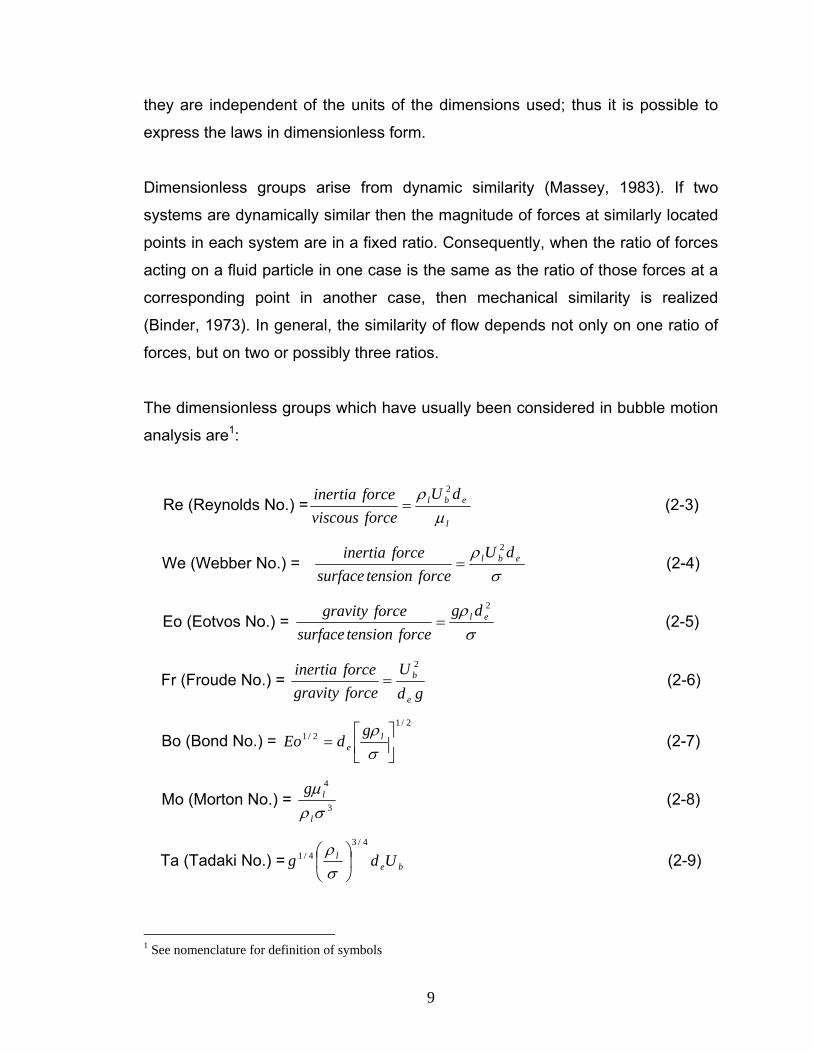
analysis are1:

Re (Reynolds No.) =l

ebl dUforceviscousforceinertia

μρ 2

= (2-3)

We (Webber No.) = σ

ρ ebl dUforcetensionsurface

forceinertia 2

= (2-4)

Eo (Eotvos No.) = σρ 2

el dgforcetensionsurface

forcegravity= (2-5)

Fr (Froude No.) = gd

Uforcegravityforceinertia

e

b2

= (2-6)

Bo (Bond No.) = 2/1

2/1⎥⎦

⎤⎢⎣

⎡=

σρ l

eg

dEo (2-7)

Mo (Morton No.) = 3

4

σρμ

l

lg (2-8)

Ta (Tadaki No.) = bel Udg

4/34/1 ⎟

⎠

⎞⎜⎝

⎛σρ

(2-9)

1 See nomenclature for definition of symbols

10

2.2.3. Wake phenomenon

It is known that the rise characteristics of bubbles in liquid, such as shape, rise

velocity and oscillations are closely related to the bubble wake behavior

(Tsuchiya and Fan, 1988). The wake structure is dependent upon several

factors including: particle geometry, size and nature of the particle surface;

relative motion between the particle and surrounding medium; and the physical

properties of particle and liquid.

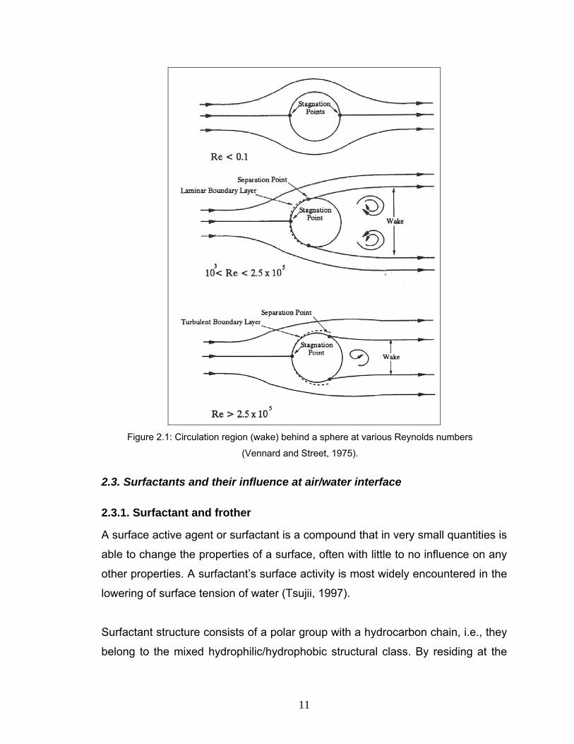
Vannard and Street (1975) characterized wake phenomenon as a function of

Reynolds number (Figure 2.1). At Re<1 there is no wake. As Re increases at a

certain Re (about Re ≈ 20), the flow starts to separate from the particle surface.

This critical Re is dependent on particle shape, particle surface nature and the

turbulence intensity in the surrounding media. As the Reynolds number increases

from the critical value, the separated streamlines branch off from the particle

contour. This creates a closed region behind the particle called the “wake or

circulation region” (Figure 2.1).

The wake structure for bubbles is known to differ from that for solid particles, due

to bubble oscillation or rocking under the influence of asymmetric vortex

shedding at least for bubbles ≥1.5mm. Bhaga (1976), Clift et al. (1978), Bhaga

and Weber (1980, 81), Weber and Bhaga (1982), Tsuchiya and Fan (1988),

Kreischer et al. (1990) and Fan and Tsuchiya (1990) among others have

investigated bubble wake phenomena. They discussed the bubble wake

structure and geometry, circulation flow pattern in the bubble wake and bubble

wake instability for different bubble sizes and shapes or, generally, for different

Reynolds numbers.

The wake volume is a function of Reynolds number and the ratio of the wake

volume to the bubble volume increases with increasing Reynolds number (Bhaga

and Weber, 1981). George et al. (2006) report an empirical correlation for

volume.

11

Figure 2.1: Circulation region (wake) behind a sphere at various Reynolds numbers

(Vennard and Street, 1975).

2.3. Surfactants and their influence at air/water interface

2.3.1. Surfactant and frother

A surface active agent or surfactant is a compound that in very small quantities is

able to change the properties of a surface, often with little to no influence on any

other properties. A surfactant’s surface activity is most widely encountered in the

lowering of surface tension of water (Tsujii, 1997).

Surfactant structure consists of a polar group with a hydrocarbon chain, i.e., they

belong to the mixed hydrophilic/hydrophobic structural class. By residing at the

12

interface with the polar part in the water and the hydrocarbon chain in air both the

hydrophilic and hydrophobic properties are satisfied simultaneously.

Consequently, surfactant accumulates at the interface.

Frothers, the reagents added in most flotation systems to control bubble related

properties, are surfactants. Most frothers are based on alcohols and polyglycols.

Their main tasks are to reduce bubble size and promote froth stability

2.3.2. Surfactant adsorption mechanism

The exchange rate of surfactant between the bulk solution and interface is a

function of surfactant concentration and surface activity. Two mechanisms,

diffusional transport and non-diffusional adsorption, govern the exchange rate.

For highly surface active (or strong) surfactants, i.e., those for which rate of

surface tension decrease with concentration is high, the exchange rate is

controlled by diffusional transport if the concentration is low. For weak

surfactants and comparatively high concentrations of strong surfactants, non-

diffusional adsorption kinetics govern (Bleys and Loos, 1985; Fainerman, 1985).

The Langmuir adsorption model is one of the first and most important models.

Here, the adsorption rate is described as a balance of surfactant adsorption flux

to the interface (Jad) and desorption flux from the interface (Jdes):

desad JJdtd

−=Γ (2-10)

The Langmuir model can be presented as:

( ) Γ−Γ−Γ=Γ

∞ αβ ),0( tcdtd (2-11)

For most surfactants non-diffusional adsorption kinetics can be expected if the

Langmuir-Von Szyskowski constant (a = α/β) is larger than 1 mol.m-3 (Fainerman

et al., 1998).

13

When equilibrium is reached the Gibbs adsorption isotherm relates the surfactant

excess concentration on the interface to the surface tension:

cdd

RT ln1 γ

−=Γ (2-12)

Combining with the Langmuir adsorption isotherm gives:

)1ln(0∞

∞ ΓΓ

−Γ−=− RTγγ (2-13)

where γ0 is the surface tension of water. If the surfactant concentration is very

low, ∞ΓΓ would be close to zero and the Langmuir isotherm can be simplified to:

Γ=− RTγγ 0 (2-14)

In the other words in this situation there is a linear dependency between surface

tension and surface concentration (or adsorption density). Frumkin (1925)

introduced additional interaction forces between adsorbed molecules into the

Langmuir adsorption isotherm.

2.3.3. Surfactant distribution

Dukhin et al. (1995) reviewed developments in the theory, and experimental

aspects of surfactant adsorption at a liquid interface. One of the models of

surfactant distribution between interface and bulk solution is shown schematically

in Figure 2.2.

According to Figure 2.2 the air/water interface is divided into three regions: the

interface, where the surfactant molecules accumulate; the sublayer that is

adjacent to the interface and is in equilibrium with the interface at all times; and

the bulk solution that has a uniform concentration of surfactant. Here the

transport of surfactant from bulk solution to the interface occurs by migration of

surfactant from the bulk to the sublayer, followed by its adsorption at the

interface.

14

Figure 2.2: Accumulation of surfactant at air/water interface (after Dukhin et al., 1995).

The distribution of surfactant over the bubble surface is governed by the

adsorption kinetics and transport properties of the surfactant. The nature of the

adsorbed layer at the interface can be characterized by two extremes: soluble

and non-soluble. If the surfactant flux from the bulk is extremely slow compared

to surface convection, the adsorbed surfactant behaves as an insoluble

monolayer. At this extreme the interface can be divided into two zones, the

leading zone, which is mobile and swept free of surfactant, and the trailing zone

which has a high surfactant concentration and is considered stagnated (Cuenot

et aI., 1997). The size of this stagnant region is specified by a cap angle (θ)

measured from the trailing pole to the edge of the stagnated zone. At the

opposite extreme, when the surfactant flux from the bulk is only slightly less than

the surface convective flux, a smoothly changing concentration gradient develops

over the entire surface. The bubble surface can then be classified into four cases

according to the surface velocity: the unretarded surface; the uniformly retarded

surface; the partly stagnated surface; and the completely stagnant interface.

Figure 2.3 shows the distribution of surfactant and surface velocity (US) on the

bubble for the two extremes of the adsorption layer.

15

Figure 2.3: Surfactant and velocity distribution on bubble surface for the two

extremes (Cuenot et al., 1997).

The uniformly retarded surface model has been considered by many researchers

(Levich, 1962; Schechter and Fairley, 1963; Newman, 1967; Harper, 1972; He et

al., 1991). However, stagnant cap model is considered appropriate in most

cases (Savic, 1953; Garner and Skelland, 1955; Elzinga and Banchero, 1961;

Griffith, 1962; Horton el aI., 1965; Huang and Kintner, 1969; Beitel and

Heidegger, 1971; Yamamoto and Ishii, 1987).

2.3.4. Some consequences of presence of surfactant at air/water interface

2.3.4.1. Marangoni effect

Natural convection due to density differences and Marangoni convection due to

an interfacial tension gradient at the free interface of the fluid (Marangoni effect)

can occur spontaneously (Okano et al., 1989; Bergman and Webb, 1990;

Gaskell, 1992; Lan and Kou, 1992).

In an isothermal system the Marangoni effect can be explained as follows. After

releasing a bubble into water that contains surfactant, the surfactant adsorbs at

16

the air/water interface. But the motion of the bubble sweeps the adsorbed

surfactant molecules from the front of the bubble to the rear; i.e., provides a non-

uniform distribution of surfactant (Figure 2.4). Therefore, the concentration of

surfactant at the rear is larger than that at the front. This non-uniformity induces a

surface tension gradient toward the front of the bubble which subsequently

generates a tangential shear stress that retards the surface velocity and

increases the drag coefficient. This phenomenon is called the Marangoni effect

(Frumkin and Levich, 1947; Levich 1962).

Figure 2.4: The distribution of adsorbed surface active solute on the surface of a

rising bubble (Linton, 1957).

One consequence is a reduced bubble rise velocity because of the increase in

drag coefficient. Another consequence is the bubble attains a more spherical

shape, the shear stress opposing the force resulting from the pressure drop

across the bubble which causes it to flatten. The bubble is said to become more

“rigid”.

In a non isothermal system the convection direction is from the hot to the cold

region. Density and surface tension are lower on the hot side and, consequently

Marangoni convection again occurs.

17

2.3.4.2. Interaction between surfactant and water molecules

In addition to surface tension gradient driven phenomena the interaction between

the polar group and water molecules via H-bonding can also be a factor

controlling bubble motion. Water molecules can be seen as traveling with the

bubble and retarding the bubble rise through an increase in surface viscosity. It is

the combination of interaction with water molecules and the surface tension

gradient effect that increases the drag on the bubble according to some

(Fuerstenau and Wayman, 1958; Leja, 1982; King, 1982; Crozier, 1992; Urry,

1995). In a similar vein Malysa et al. (1988) reported that long chain polymers

could reduce the settling velocity of colloidal particles significantly, which was

attributed to interaction with water molecules.

By introducing this chemical aspect an effect of surfactant type as well as

concentration is anticipated which is not so readily associated with the physical

properties due to surface tension phenomena.

2.3.4.3. Effect on bubble internal circulation

There are a few studies on bubble internal circulation (Hadamard and

Rybczynski, 1911; Garner and Hammerton, 1954; Linton and Sutherland, 1957;

Griffith, 1962; Lochiel, 1965; Clift et al., 1978). As the internal circulation depends

on the mobility of the surface, the properties of the interface and the effect of

surfactants play a significant role.

For a moving bubble any part of the surface experiences a tangential force

proportional to the viscosity of the external medium. The circulation pattern is

dependent on the fluid properties, and size and shape of the bubble (Linton and

Sutherland, 1957).

Schechter and Farley (1963) considered the circulation as resulting from the air

inside the bubble near the interface being swept from the leading end to the rear

by the action of the flowing liquid inducing stress on the interface. At the rear of

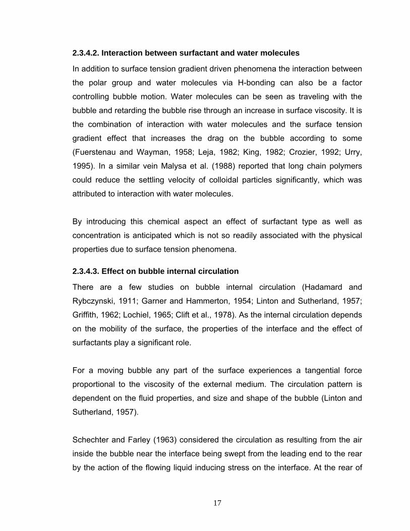
18

the bubble air flowing along the interface is then forced into the interior of the

bubble and the circulation pattern is established.

If due to presence of surfactant the surface becomes sufficiently rigid the internal

circulation decreases. In the other words, an opposing force to circulation is

introduced if the interfacial tension varies over the surface. If the adsorption-

desorption process of surfactant is fast the surface tension will be almost

constant over the surface and the resultant surface tension gradient would be

small. Oppositely, if the adsorption-desorption process is slow higher surface

tension gradients would be produced. The modes of internal circulation are:

complete circulation, part circulation, and stagnant (Figure 2.5).

Figure 2.5: The internal circulation of moving fluid showing the direction of relative flow: (a)

complete circulation, (b) part circulation, (c) stagnant (Linton, 1957).

According to Figure 2.5 complete circulation occurs in pure liquids and fully

stagnant mode can be achieved as a result of a large enough surface tension

gradient. In general, the internal circulation is governed by the velocity, pressure

drop across the bubble and time dependent surface tension gradient in the

bubble surface. One consequence is that larger bubbles experience more

internal circulation.

19

2.3. Bubble behavior

Bubble rise in liquids has been investigated over many decades. In the early

work it was assumed that the fluid surrounding the bubble has zero viscosity, and

there is no slip at the boundary (Lamb, 1954). But for real fluids the situation is

more complex because the gas bubble does experience slip and viscous and

inertial forces are present.

The regimes of bubble motion in liquid can be classified as Stokes regime,

Hadamard regime, Levich regime, and Taylor regime (Astarita and Apuzzo,

1965). The characteristics of a rising bubble (i.e., its size, rise velocity, trajectory,

etc.), differ from system to system, making it difficult to develop generalized

correlations. To understand bubble behavior fundamental analyses have been

performed from different points of view (Auton, 1987; Eames & Hunt, 1997;

Magnaudet & Eames, 2000; Mei and Klausner, 1992). However, the most usual

approach is through the force balance.

Many investigators (Astarita, 1996; Davis and Acrivos, 1996; Haque et al., 1987;

Clift et al., 1978; Abou-ElHassan, 1983; Chhabra, 1993; Gummalam, 1987;

Rodrigue, 2001, 2002) have worked extensively in various gas-liquid systems

and developed correlations for a specific range of conditions. It seems the recent

attempts by Nguyen (1998) and Rodrigue and co-workers (1996, 2001, 2002,

2004) to develop a generalized correlation can be considered applicable over a

wide range; still, important deviations remain to be incorporated.

Single bubble rise characteristics depend on the bubble generation system and

the force acting. Figure 2.6 describes the connections among various factors.

Examination of these parameters can provide an indirect understanding of the

forces acting and their consequences.

20

Figure 2.6: The relationships between identified factors that affect bubble behavior.

2.31. Bubble size

The surface mobility of a bubble provides for variable shape during its rise in a

liquid. It is then convenient to define an equivalent diameter (de), namely:

( ) 3/1.. zyxde = (2-15)

where, x, y and z are diameters in the X, Y, Z directions.

Gas/Liquid system: -Gas: type, temperature, saturation, solubility, density -Liquid: density, temperature, type, purity, surface tension, viscosity -Orifice: Type, size, direction, material -Column: size -Surfactant: type, concentration, surface tension -Bubble Generation: gas rate, frequency, system geometry

Forces: -buoyancy -drag -surface tension

Consequences: -surface mobility -wake -internal circulation -Marangoni effect -surface tension gradients

Bubble Behavior: -size -velocity -shape -path

21

For a spherical bubble these diameters will be similar and for a flattened bubble

(oblate spheroid), Δy, for instance, will be less than Δx. Aspect ratio (E) is the

ratio of minor to major axis. If aspect ratio is close to 1 (0.9>E>1) the object can

considered as spherical (Clift et al., 1978).

Bubble size is changed by hydrostatic pressure. In a static fluid, shear and

tensile forces are absent, and the only force involved is a compressive one.

According to Pascal’s law the pressure in a static fluid is the same in all

directions. The absolute pressure (P0) is given by equation:

latm ghPP ρ+=0 (2-16)

where Patm is atmospheric pressure and hl is the height of liquid over the bubble.

As a bubble rises through a column the height of liquid above and therefore

pressure on the bubble decreases. Assuming the ideal gas law and an

isothermal system the bubble size increase during rise in a liquid can be

calculated.

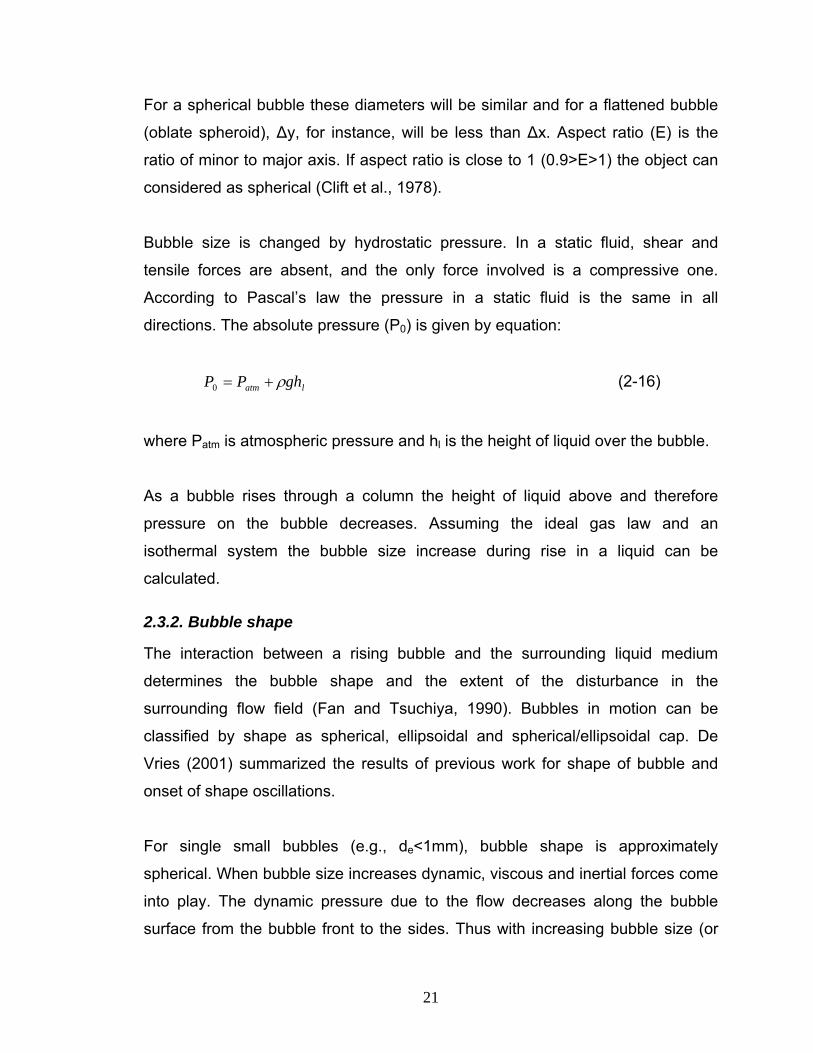
2.3.2. Bubble shape

The interaction between a rising bubble and the surrounding liquid medium

determines the bubble shape and the extent of the disturbance in the

surrounding flow field (Fan and Tsuchiya, 1990). Bubbles in motion can be

classified by shape as spherical, ellipsoidal and spherical/ellipsoidal cap. De

Vries (2001) summarized the results of previous work for shape of bubble and

onset of shape oscillations.

For single small bubbles (e.g., de<1mm), bubble shape is approximately

spherical. When bubble size increases dynamic, viscous and inertial forces come

into play. The dynamic pressure due to the flow decreases along the bubble

surface from the bubble front to the sides. Thus with increasing bubble size (or

22

Re), the dynamic pressure between the bubble front and bubble side increases

which explains why the bubble flattens (ellipsoid oblate shape) in the direction of

the bubble motion. Addition of surfactant by introducing surface viscosity and

surface tension effects can reduce the effect of dynamic pressure difference on

flattening; i.e., increases the aspect ratio of the bubble (Figure 2.7).

Figure 2.7: Illustration of dynamic pressure causing bubble deformation in water only case

(a), and the force created by surface tension gradient that occurs in presence of surfactant

that resists deformation (b) (Finch et al., 2008).

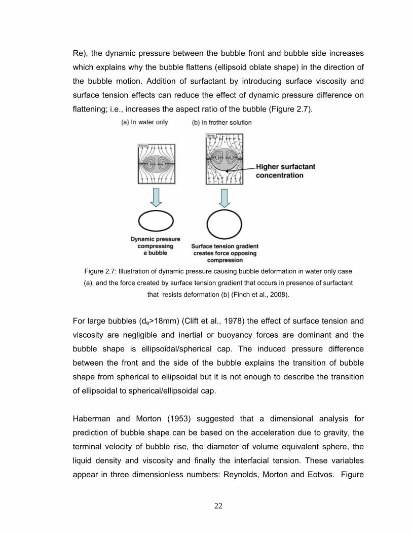
For large bubbles (de>18mm) (Clift et al., 1978) the effect of surface tension and

viscosity are negligible and inertial or buoyancy forces are dominant and the

bubble shape is ellipsoidal/spherical cap. The induced pressure difference

between the front and the side of the bubble explains the transition of bubble

shape from spherical to ellipsoidal but it is not enough to describe the transition

of ellipsoidal to spherical/ellipsoidal cap.

Haberman and Morton (1953) suggested that a dimensional analysis for

prediction of bubble shape can be based on the acceleration due to gravity, the

terminal velocity of bubble rise, the diameter of volume equivalent sphere, the

liquid density and viscosity and finally the interfacial tension. These variables

appear in three dimensionless numbers: Reynolds, Morton and Eotvos. Figure

23

2.8 shows the shape regimes and bubble shape transition boundaries for

bubbles in motion through liquids (Clift et al., 1978).

Generally, for a given size of bubble it becomes less flattened when the liquid

surface tension is large (low We or Eo) and the liquid viscosity is large (low Re).

But when the system is contaminated, by surfactant molecules that collect at the

liquid-bubble interface the bubble shape cannot be determined by liquid

properties alone. In other words, the bubble shape is strongly influenced by the

conditions at the gas/liquid interface (Griffith, 1962; Grace et al., 1976). By

adsorption of surfactant at the interface, the viscous drag increases (Boussinesq,

1913; Sciven, 1959; Agrawal and Wasa, 1979; Fan and Tsuchiya, 1990).

Figure 2.8: Bubble shape regime (reproduced with permission from Clift et al., 1978).

24

2.3.3. Bubble rise path

The bubble rise path can be defined by the trajectory of the bubble centre. Fan

and Tsuchiya (1990) note that the bubble rise path and change in orientation

(defined as the angle between the bubble major axis and the vertical axis of the

system) are strongly dependent on the bubble shape. De Vries (2001)

summarized the path instability modes and the regimes observed.

Single bubbles rise in a straight line (rectilinear) when they are spherical. On

increasing bubble size the bubble starts to deform into an ellipsoidal shape and

the bubble starts to exhibit zigzag or spiral motion. Bubble orientation is also

affected by shape deformation (Tsuge and Hibino, 1977; Fan and Tsuchiya,

1990). As the bubble changes from ellipsoidal to spherical/ellipsoidal cap (at Re

≈ 5000 (Miyahara, 1988)), the radius of the spiral or the amplitude of the zigzag

decreases and the motion becomes rectilinear, but with rocking.

The bubble rise path and fluctuations in the orientation of the bubble can be

characterized by the frequency or period of cycle of the motion according to

Tsuge and Hibino (1971). In general, both the amplitude and frequency of bubble

oscillation are related to the bubble size, shape and presence/absence of

surfactants.

Detailed experiments were discussed by De Vries et al. (2002), who investigated

the motion of gas bubbles in highly purified water. For bubble size <2mm, the

bubbles rise axisymmetrically. Shape oscillation for bubble size >2mm was

observed at a certain height depending on the conditions and especially bubble

size. In this situation bubbles establish an approximately ellipsoidal shape.

Typically, the dynamics of bubble rise is nonlinear and the extent of nonlinearity

increases with bubbles size. Observations have shown that bubble trajectories

have a primary and secondary structure (Yoshida and Manasseh, 1997). For

high viscosity Newtonian and non-Newtonian liquids, irrespective of the size of

25

the bubble the trajectories are rectilinear, mainly because of the large viscous

drag.

Lunde and Perkins (1997) clarified the relationship between the wake structure

and trajectory of clean bubbles (helical or zigzag). They suggested that there

may be a correspondence between the wake structure and the bubble trajectory.

2.3.4. Bubble rise velocity

After the detachment of a bubble from an orifice under a liquid, the buoyant force

causes it to rise. The dynamics associated with the rise are mainly due to

temporal variation in bubble characteristics.

Measurement of bubble rise velocity is important in order to understand, for

example bubble dispersion in a liquid and the adsorption mechanism at a

gas/liquid interface. Rise velocity is fundamental to the performance of bubble

reactors.

To discuss rise velocity of a bubble two terms are introduced: local and terminal

velocity. Local velocity is the velocity of a rising bubble at a certain time or

distance after release. Terminal velocity is the velocity of a bubble when

according to the Newton’s second law acceleration is zero. In other words, it

represents the constant velocity of the rising bubble when time no longer

influences local velocity significantly. Figure 1.1 showed the terminal velocity as

the third stage of the velocity profile (Sam et al., 1996). (In reality the bubble will

increase in size as it rises due to decreasing hydrostatic pressure and velocity

will change in a predictable manner (e.g. see Zhang et al. (2003)).

The rise of a bubble in a liquid can be considered as a function of several

parameters including: bubble characteristics (size and shape); properties of the

gas-liquid system (density, viscosity, surface tension, concentration of solute,

density difference between gas and liquid); liquid motion (direction); and

26

operating conditions (temperature and pressure). Some of these will be

described with regard to their importance as established in many studies.

2.3.4.1. Factors affecting the rise velocity

a- Type and purity of liquid

The rise velocity in each pure liquid would be different. However, the same trend

may be observed. Kulkarani and Joshi (2005) presented bubble rise velocity for

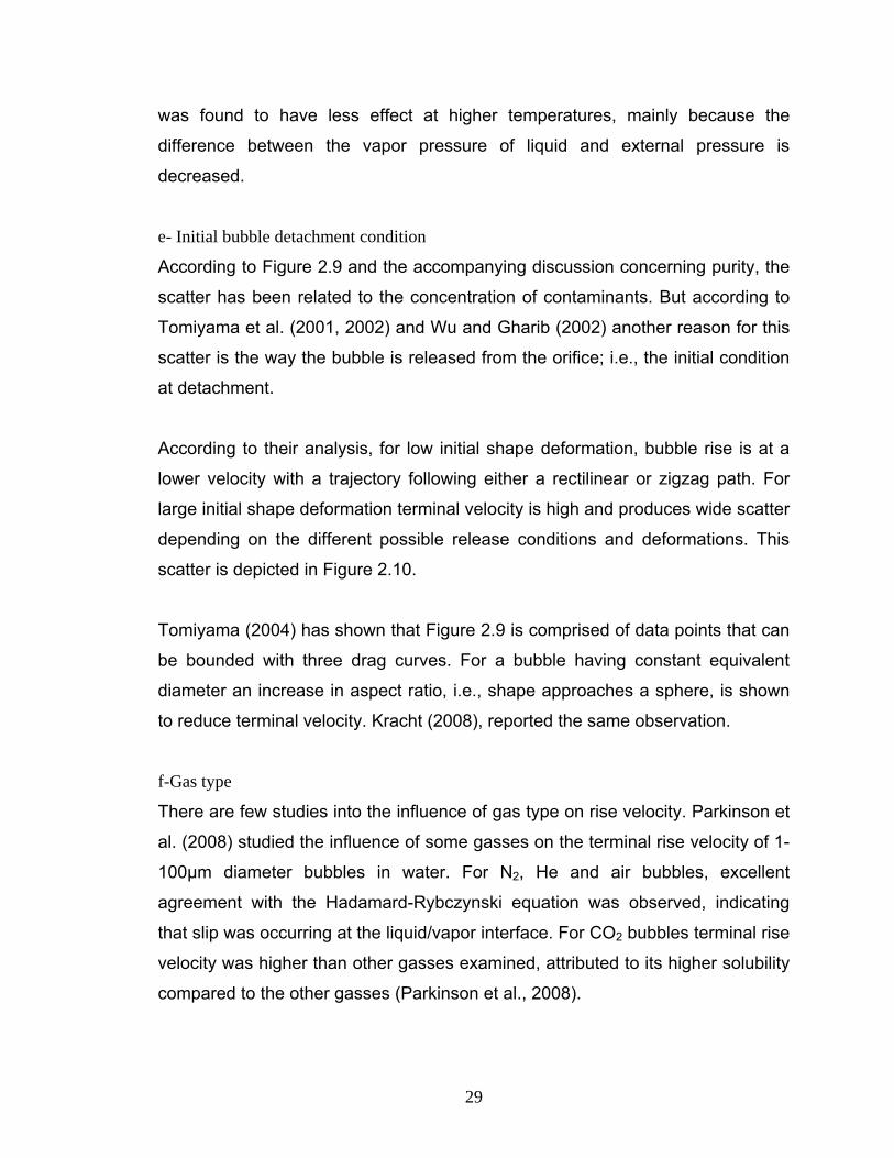
some pure and contaminated liquids.

In Figure 2.9, bubble terminal rise velocity vs. size is shown for an inviscid water.

Here the upper bound of the terminal velocity data is considered to correspond to

bubbles in pure water while in the presence of surfactant, the drag force

increases and consequently causes a reduction in velocity leading to the scatter

in the data (Clift et al., 1978; Fan and Tsuchiya, 1990). The influence of

surfactants on bubble rise velocity will form a large part of this review. The results

for fully contaminated water give the lower part of the data envelope.

b- Liquid viscosity

The modes of bubble rise show distinct behavior in viscous Newtonian fluids

compared to inviscid and non-Newtonian liquids (Gonzaleztello et al., 1992).

Rodrigue et al. (1996) reported an almost linear relationship between rise velocity

and the bubble volume dependent on the liquid viscosity.

For the case of different non-Newtonian liquids, viscosity influences the

relationship between the bubble size and rise velocity. For instance, terminal rise

velocity may exhibit a discontinuity at a certain critical bubble size in some

liquids, while no discontinuity is observed for some others. Leal et al. (1971),

Astarita and Apuzzo (1965), Acharya et aI. (1978), and Rodrigue (1998) have

investigated this phenomenon in detail.

27

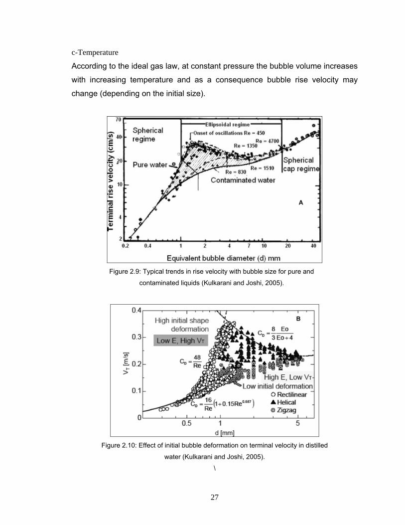
c-Temperature

According to the ideal gas law, at constant pressure the bubble volume increases

with increasing temperature and as a consequence bubble rise velocity may

change (depending on the initial size).

Figure 2.9: Typical trends in rise velocity with bubble size for pure and

contaminated liquids (Kulkarani and Joshi, 2005).

Figure 2.10: Effect of initial bubble deformation on terminal velocity in distilled

water (Kulkarani and Joshi, 2005).

\

28

In addition liquid density is inversely proportional to the temperature variation,

which influences buoyancy and thus rise velocity. However, this effect is not

significant when compared to other physical properties of the liquid that affect the

bubble rise velocity.

There are few studies on the effect of temperature on rise velocity of a bubble. At

ambient conditions, the rise velocity follows a certain trend with bubble size. Here

two different cases may be considered: rise of a gas bubble that is insoluble in

the liquid and rise of vapor bubble in liquid at relatively low temperature. Both

cases are common, while only the second case has been studied systematically.

In the first case the heat transfer across the interface causes an increase in

bubble volume. Also, at higher temperature the density difference between the

two fluids decreases. Hence the buoyancy decreases and this reduces the rise

velocity. The counteracting effects are dominant in different ranges of

temperature and in a certain temperature range rise velocity is a strong function

of size.

Zhang (2000) and Zhang et al. (2003) reported a temperature effect on single

bubble velocity profile in water and surfactant solution. The profiles indicated that

the time to reach constant velocity tended to decrease as temperature increased.

d- External pressure

Although most laboratory scale investigations of bubble dynamics are carried out

at ambient conditions, the operating conditions in industrial systems are often

significantly different (e.g. at elevated pressure). As a result of the outside

pressure, bubbles are formed only after a minimum gas velocity is reached

(which is higher than under ambient conditions), while the bubble sizes are

smaller (subsequently reducing rise velocity). Letzel (1998) systematically

analyzed the effect of gas density on the rise velocity of large bubbles. In a

similar attempt, under the assumption of homogeneous nature of the suspension,

Luo et al. (1997) studied the effect of external pressure on bubble rise velocity in

a gas-liquid-solid fluidized bed (Newtonian viscous system). Increased pressure

29

was found to have less effect at higher temperatures, mainly because the

difference between the vapor pressure of liquid and external pressure is

decreased.

e- Initial bubble detachment condition

According to Figure 2.9 and the accompanying discussion concerning purity, the

scatter has been related to the concentration of contaminants. But according to

Tomiyama et al. (2001, 2002) and Wu and Gharib (2002) another reason for this

scatter is the way the bubble is released from the orifice; i.e., the initial condition

at detachment.

According to their analysis, for low initial shape deformation, bubble rise is at a

lower velocity with a trajectory following either a rectilinear or zigzag path. For

large initial shape deformation terminal velocity is high and produces wide scatter

depending on the different possible release conditions and deformations. This

scatter is depicted in Figure 2.10.

Tomiyama (2004) has shown that Figure 2.9 is comprised of data points that can

be bounded with three drag curves. For a bubble having constant equivalent

diameter an increase in aspect ratio, i.e., shape approaches a sphere, is shown

to reduce terminal velocity. Kracht (2008), reported the same observation.

f-Gas type

There are few studies into the influence of gas type on rise velocity. Parkinson et

al. (2008) studied the influence of some gasses on the terminal rise velocity of 1-

100μm diameter bubbles in water. For N2, He and air bubbles, excellent

agreement with the Hadamard-Rybczynski equation was observed, indicating

that slip was occurring at the liquid/vapor interface. For CO2 bubbles terminal rise

velocity was higher than other gasses examined, attributed to its higher solubility

compared to the other gasses (Parkinson et al., 2008).

30

Zhang (2000) examined the influence of gas saturation (humidity) on terminal

velocity. In general, air (as a gas) is able to absorb a certain amount of moisture.

In that study the air was first fed through a water container to become saturated

by water. The saturated air was fed to a column to generate bubbles. The results

indicated that there was no significant difference between fresh and moisture

saturated air bubbles.

2.3.5. Formulation for rise velocity correlation

Several investigators have developed empirical, semi-empirical and theoretical

simulations for bubble rise velocity. Most apply only for a narrow range of

governing parameters. In the review by Kulkarani and Joshi (2005) some rise

velocity models were based on the following: force balance, dimensional

analysis, and wave analogy. They listed many formulae for rise velocity in

Newtonian and non-Newtonian liquids.

2.4. Contaminants and rise velocity

As the main purpose of this research is focused on the effect of frother

(surfactant) on single bubble rise velocity, this will naturally occupy a significant

part of the review. In addition to the effects of frother, the role of salts is included

as, for some functions, frother and some salts are interchangeable.

2.4.1. Surfactant

According to Figure 2.9 at ambient conditions the velocity increases with size and

passes through a maximum at ca 1.3mm (diameter) followed by a decrease in

velocity over a restricted size range after which it attains a weakly positive

dependence on bubble size. Depending upon the type and concentration of

contaminant, the rise velocity characteristics of a bubble change significantly.

The impact of surfactants on bubble rise velocity is reviewed according to liquid

rheological class.

31

2.4.1.1. Newtonian liquids

In a Newtonian liquid the non-uniformly distributed adsorbed surfactant

generates a surface tension gradient. Since the surface tension gradient must be

balanced by a jump in the shear stress across the interface (Marangoni effect), a

shear-free boundary condition can no longer be imposed on the liquid at the gas-

liquid interface. So this leads to an increase in the drag force (stagnant cap

hypothesis). As a result of formation of a rigid interface and enhancement in

drag, internal circulation is reduced and the rise velocity is lower than in the clean

(surfactant-free) liquid. The stagnant cap hypothesis has been used successfully

for the estimation of bubble rise velocity and has also been used for the

prediction of drag coefficient with respect to extent of surface contamination.

Frumkin & Levich (1947) and Levich (1962) developed a so-called adsorption

theory to explain the reduction in rise velocity. Savic (1953) reported the

existence of a cap (surface immobilization) on the rear part of a moving liquid

drop, while the rest was tangentially stress free (mobile). Griffith (1962) studied

the effect of surfactant on the terminal velocity of drops and bubbles. Kopf-Sill

and Homsey (1988) applied the Hele-Shaw cell model to analyze the effect of

surfactants. Fdilha and Duineveld (1995) investigated the effect of surfactant on

the rise of a spherical bubble at high Reynolds and Peclet numbers. They found

that the rapid slowdown of the bubble occurs when nearly half of the bubble

surface is covered by the surfactant layer. De Kee et al. (1990) reported that a

reduction in surface tension resulted in a decrease of bubble rise velocity of small

bubbles without any discontinuity. However Rodrigue et al.(1996) reporting the

same phenomenon, found no influence on bubble rise velocity over a certain

concentration of surfactant. Cuenot et al. (1997) discussed how retardation of the

bubble surface fluidity is dependent on the amount of adsorbed surfactant. Sam

et al. (1996) studied axial velocity profiles of single bubbles in water/frother

solutions and among other findings concluded there was no concentration effect

on terminal velocity only on the time to reach terminal velocity. Zhang and Finch

(2000) confirmed that terminal rise velocity was independent of concentration on

32

concentration for the surfactants tested. Krzan et al. (2004) studied the influence

of the surfactant polar group on the local and terminal velocities of bubbles. Here

the minimum adsorption coverage required to immobilize the bubble surface was

estimated for some surfactants. They concluded that mainly surfactant

adsorption kinetics governed the mobility of rising bubble interfaces. Recently,

Acuna et al. (2008) reported that the frother type could affect the terminal

velocities of same size bubbles in swarms, even for diameters below 1mm.

2.4.1.2. Non-Newtonian liquids

Rheological behavior of non-Newtonian liquids is complex and the motion of

bubbles in these liquids has different characteristics to those observed in

Newtonian liquids. For the case of power-law non-Newtonian liquids, Tzounakos

et al. (2004) studied the effects of surfactants based on analysis of the drag

curve. Ybert and Di Meglio (1998) measured bubble rise velocity as a function of

distance traveled. After the initial stage of acceleration from rest, the

instantaneous rise velocity of a given bubble depended only on the total amount

of surfactant adsorbed on the bubble surface. It was also shown that the

surfactants are not only absorbed onto the bubble surface, but may also desorb,

which increases the bubble rise velocity.

2.4.1.3. High viscosity liquids

The few studies (Barnett et al.,1966; Haque et al., 1988; Margaritis et al.,1999;

Miyahara and Yamanaka, 1993 and De Kee et al., 1986) have shown that for

high viscosity Newtonian liquids, the rise velocity is a weak function of the bubble

volume, while for non-Newtonian liquids, it has a linear dependence but the

velocities in the former case are much higher than in the latter.

2.4.1.4. Simulation and numerical analysis

There are several published simulations and numerical analyses of bubble rise

velocity in the presence of surfactant. Some that directly discuss terminal velocity

are: Harper (1973 and 1987), Fdhila and Duineveld (1995), McLaughlin (1996),

Nguyen (1998), Rodrigue et al. (1999), Liao and McLaughilin (2000), Bozzano

33

and Dente (2001), Zhang et al. (2001), Alves et al. (2005), Liao et al. (2004) and

Takemura (2005).

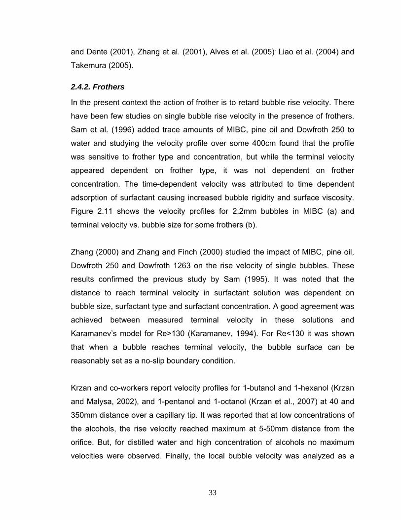
2.4.2. Frothers

In the present context the action of frother is to retard bubble rise velocity. There

have been few studies on single bubble rise velocity in the presence of frothers.

Sam et al. (1996) added trace amounts of MIBC, pine oil and Dowfroth 250 to

water and studying the velocity profile over some 400cm found that the profile

was sensitive to frother type and concentration, but while the terminal velocity

appeared dependent on frother type, it was not dependent on frother

concentration. The time-dependent velocity was attributed to time dependent

adsorption of surfactant causing increased bubble rigidity and surface viscosity.

Figure 2.11 shows the velocity profiles for 2.2mm bubbles in MIBC (a) and

terminal velocity vs. bubble size for some frothers (b).

Zhang (2000) and Zhang and Finch (2000) studied the impact of MIBC, pine oil,

Dowfroth 250 and Dowfroth 1263 on the rise velocity of single bubbles. These

results confirmed the previous study by Sam (1995). It was noted that the

distance to reach terminal velocity in surfactant solution was dependent on

bubble size, surfactant type and surfactant concentration. A good agreement was

achieved between measured terminal velocity in these solutions and

Karamanev’s model for Re>130 (Karamanev, 1994). For Re<130 it was shown

that when a bubble reaches terminal velocity, the bubble surface can be

reasonably set as a no-slip boundary condition.

Krzan and co-workers report velocity profiles for 1-butanol and 1-hexanol (Krzan

and Malysa, 2002), and 1-pentanol and 1-octanol (Krzan et al., 2007) at 40 and

350mm distance over a capillary tip. It was reported that at low concentrations of

the alcohols, the rise velocity reached maximum at 5-50mm distance from the

orifice. But, for distilled water and high concentration of alcohols no maximum

velocities were observed. Finally, the local bubble velocity was analyzed as a

34

function of the adsorption coverage of surfactant on the bubble surface.

Figure 2 11: a. Velocity profiles for 2.2mm bubbles in MIBC, b. Terminal velocity vs. bubble size

in the presence of some frothers (Sam, 1995).

a

b

35

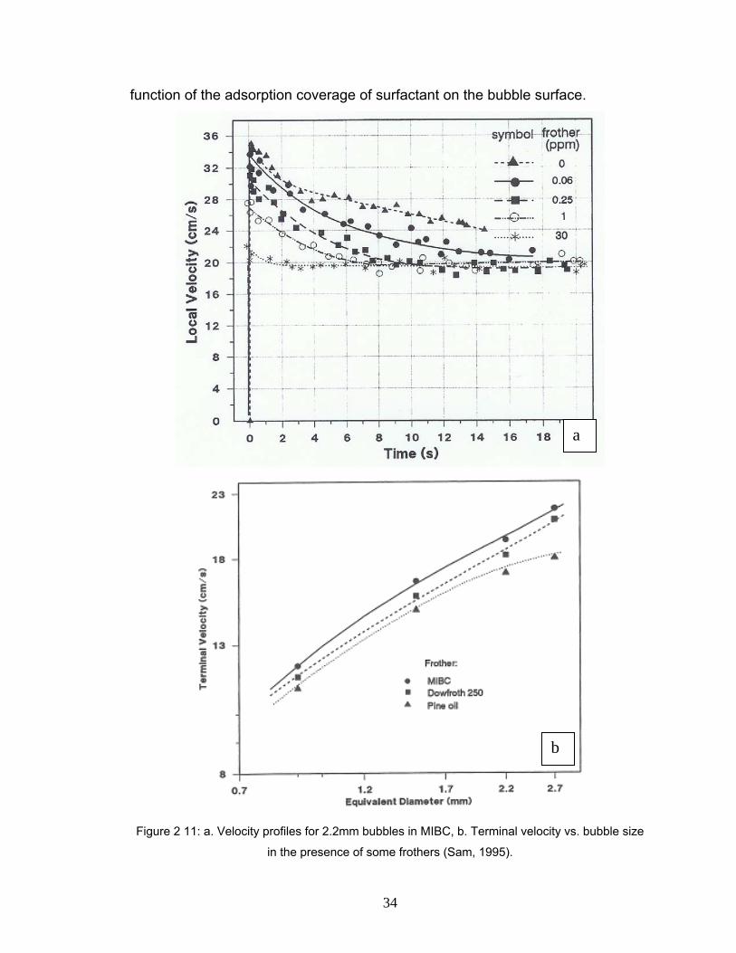
Azgomi et al. (2007), trying to characterize frothers, reported that for the same

gas holdup and gas rate, the bubble size depended markedly on frother type

(Figure 2.12). This observation gave rise to the hypothesis explored in this thesis

namely that frother type can affect bubble rise velocity.

Figure 2.12: Bubble size measurement at same gas holdup (8%) for F150 and

Pentanol (Azgomi et al., 2007).

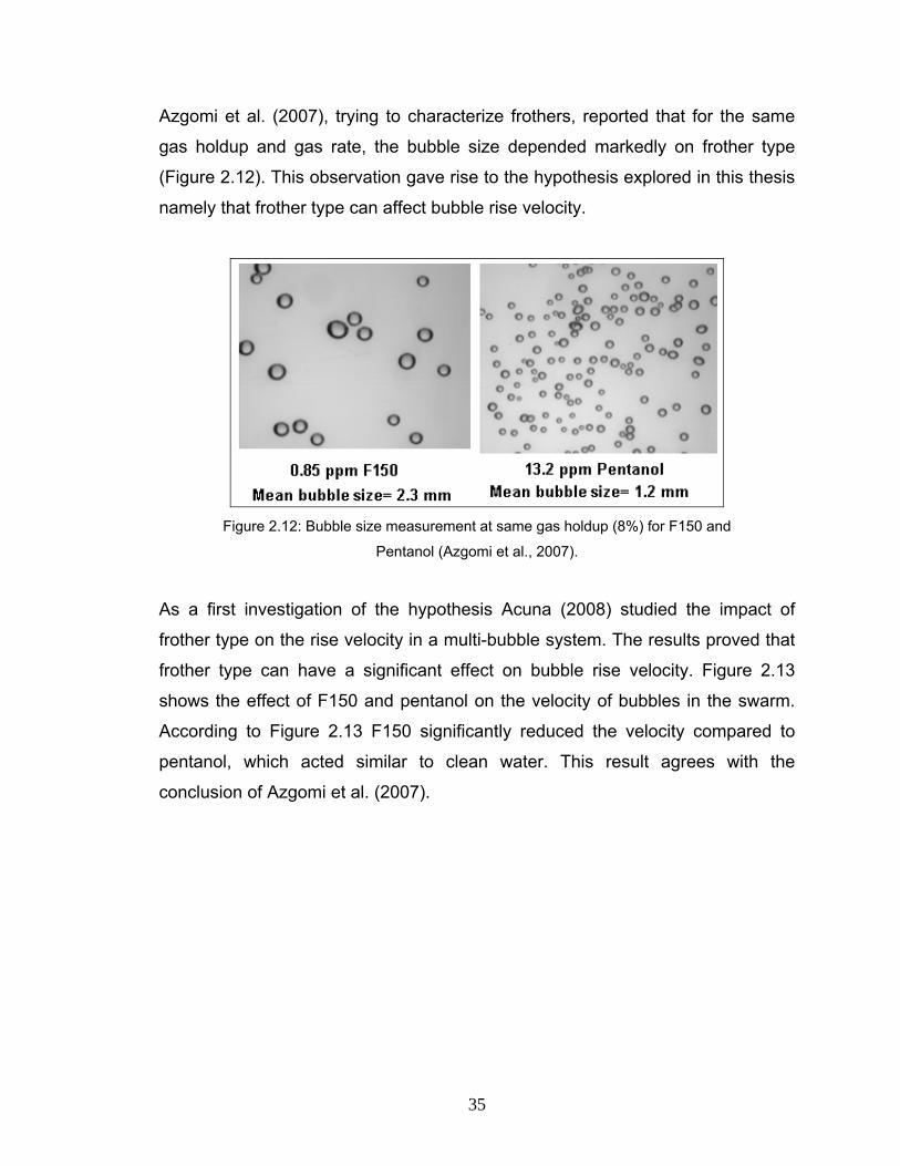
As a first investigation of the hypothesis Acuna (2008) studied the impact of

frother type on the rise velocity in a multi-bubble system. The results proved that

frother type can have a significant effect on bubble rise velocity. Figure 2.13

shows the effect of F150 and pentanol on the velocity of bubbles in the swarm.

According to Figure 2.13 F150 significantly reduced the velocity compared to

pentanol, which acted similar to clean water. This result agrees with the

conclusion of Azgomi et al. (2007).

36

Figure 2.13: Comparison between influences of F150 and Pentanol on terminal

rise velocity of bubbles in swarms (Acuna, 2008).

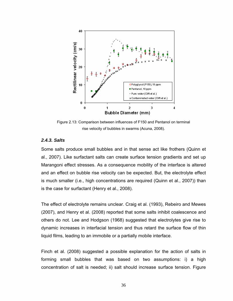
2.4.3. Salts

Some salts produce small bubbles and in that sense act like frothers (Quinn et

al., 2007). Like surfactant salts can create surface tension gradients and set up

Marangoni effect stresses. As a consequence mobility of the interface is altered

and an effect on bubble rise velocity can be expected. But, the electrolyte effect

is much smaller (i.e., high concentrations are required (Quinn et al., 2007)) than

is the case for surfactant (Henry et al., 2008).

The effect of electrolyte remains unclear. Craig et al. (1993), Rebeiro and Mewes

(2007), and Henry et al. (2008) reported that some salts inhibit coalescence and

others do not. Lee and Hodgson (1968) suggested that electrolytes give rise to

dynamic increases in interfacial tension and thus retard the surface flow of thin

liquid films, leading to an immobile or a partially mobile interface.

Finch et al. (2008) suggested a possible explanation for the action of salts in

forming small bubbles that was based on two assumptions: i) a high

concentration of salt is needed; ii) salt should increase surface tension. Figure

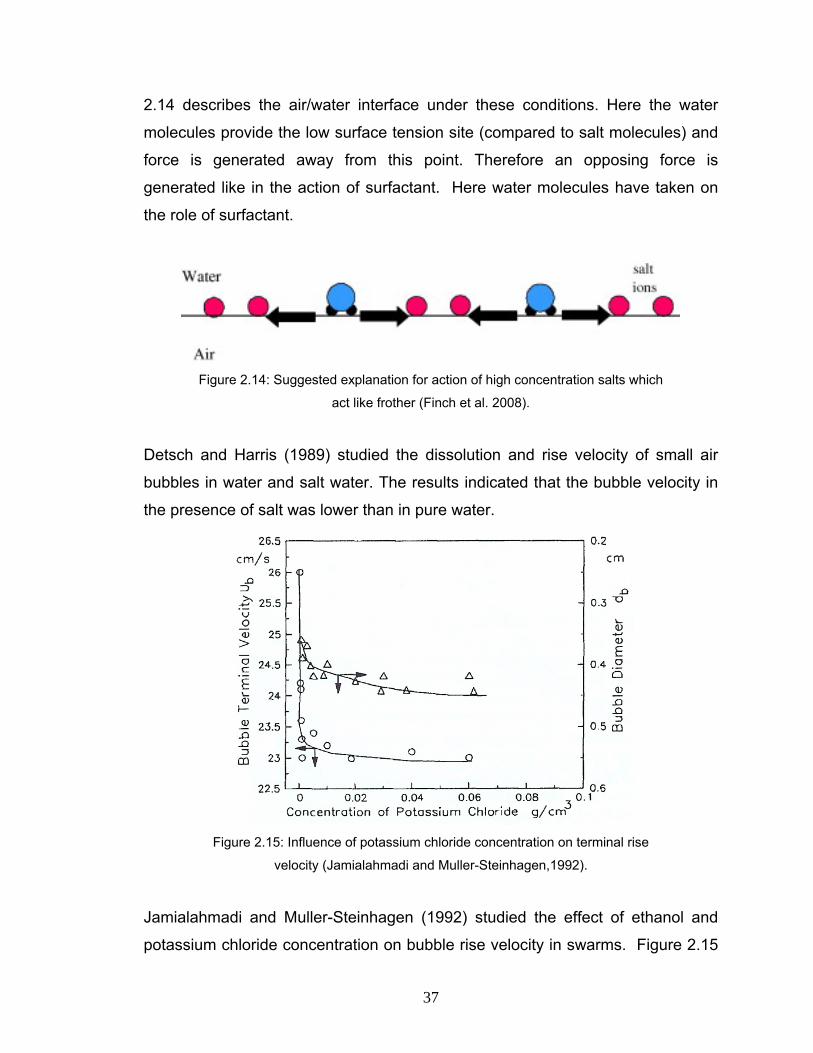
37

2.14 describes the air/water interface under these conditions. Here the water

molecules provide the low surface tension site (compared to salt molecules) and

force is generated away from this point. Therefore an opposing force is

generated like in the action of surfactant. Here water molecules have taken on

the role of surfactant.

Figure 2.14: Suggested explanation for action of high concentration salts which

act like frother (Finch et al. 2008).

Detsch and Harris (1989) studied the dissolution and rise velocity of small air

bubbles in water and salt water. The results indicated that the bubble velocity in

the presence of salt was lower than in pure water.

Figure 2.15: Influence of potassium chloride concentration on terminal rise

velocity (Jamialahmadi and Muller-Steinhagen,1992).

Jamialahmadi and Muller-Steinhagen (1992) studied the effect of ethanol and

potassium chloride concentration on bubble rise velocity in swarms. Figure 2.15

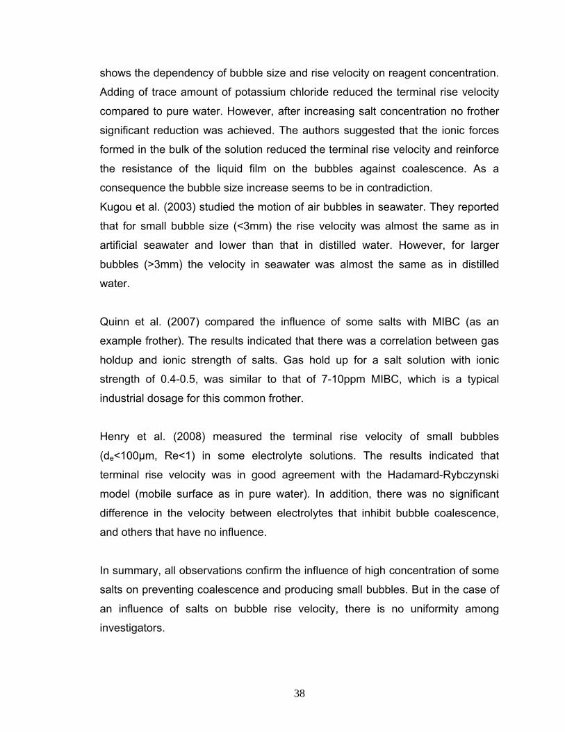
38

shows the dependency of bubble size and rise velocity on reagent concentration.

Adding of trace amount of potassium chloride reduced the terminal rise velocity

compared to pure water. However, after increasing salt concentration no frother

significant reduction was achieved. The authors suggested that the ionic forces

formed in the bulk of the solution reduced the terminal rise velocity and reinforce

the resistance of the liquid film on the bubbles against coalescence. As a

consequence the bubble size increase seems to be in contradiction.

Kugou et al. (2003) studied the motion of air bubbles in seawater. They reported

that for small bubble size (<3mm) the rise velocity was almost the same as in

artificial seawater and lower than that in distilled water. However, for larger

bubbles (>3mm) the velocity in seawater was almost the same as in distilled

water.

Quinn et al. (2007) compared the influence of some salts with MIBC (as an

example frother). The results indicated that there was a correlation between gas

holdup and ionic strength of salts. Gas hold up for a salt solution with ionic

strength of 0.4-0.5, was similar to that of 7-10ppm MIBC, which is a typical

industrial dosage for this common frother.

Henry et al. (2008) measured the terminal rise velocity of small bubbles

(de<100μm, Re<1) in some electrolyte solutions. The results indicated that

terminal rise velocity was in good agreement with the Hadamard-Rybczynski

model (mobile surface as in pure water). In addition, there was no significant

difference in the velocity between electrolytes that inhibit bubble coalescence,

and others that have no influence.

In summary, all observations confirm the influence of high concentration of some

salts on preventing coalescence and producing small bubbles. But in the case of

an influence of salts on bubble rise velocity, there is no uniformity among

investigators.

39

CHAPTER THREE: EXPERIMENTAL SETUP

The methods for measurement of bubble rise velocity can be classified as either

intrusive or non-intrusive. A non-intrusive measurement method is desirable and

photography is considered the most practical (Kulkarani and Joshi, 2005).

Chapter three describes the photographic technique used.

3.1. Equipment

3.1.1. Column setup

A circular Plexiglas column 6.35cm diameter by 350cm high was used

surrounded by a square Plexiglas water jacket (8 x 8 x 330 cm) (Figure 3.1). A

measuring tape was placed along the central axis of the column to measure the

size and local velocity of the bubbles. The column diameter was large enough to

avoid wall effects for bubbles < 3 mm (Grace, 1973; Narayanan et al., 1974;

Bhaga, 1976; Clift et al., 1978). To control a uniform temperature along the

column water was circulated through the jacket; the square column also avoided

optical distortion associated with a curved surface.

3.1.2. Air line

Air was provided from a controllable compressed air system with flow rate

adjusted by an online monitoring system. Plastic tubes and connectors were

used to transfer air from the source to the glass capillary at the bottom of the

column. The air was from the university compressor and was dry.

3.1.3. Camera moving device

A mobile digital video camera was used to track a single bubble during its rise.

To follow the bubble it is necessary to have a variable speed motor, in this case

driving a chain belt over a pulley (Figure 3.1). Limit switches were placed at the

bottom and top of the column to arrest the movement. The movement of the

camera was controlled manually through the variable speed controller over a

range from zero to 50 cm/s, the experimenter adjusting the speed to keep the

bubble in view (on a monitor) during its rise.

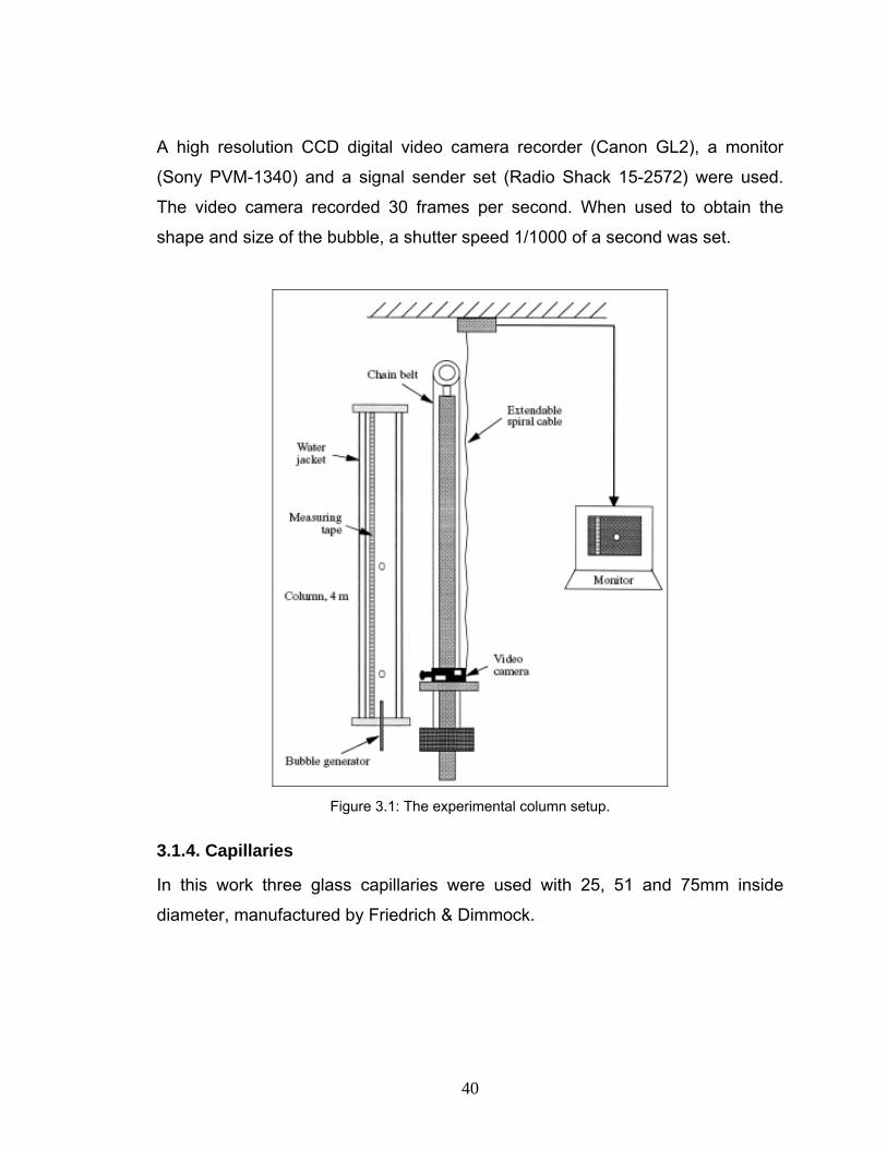
40

A high resolution CCD digital video camera recorder (Canon GL2), a monitor

(Sony PVM-1340) and a signal sender set (Radio Shack 15-2572) were used.

The video camera recorded 30 frames per second. When used to obtain the

shape and size of the bubble, a shutter speed 1/1000 of a second was set.

Figure 3.1: The experimental column setup.

3.1.4. Capillaries

In this work three glass capillaries were used with 25, 51 and 75mm inside

diameter, manufactured by Friedrich & Dimmock.

41

3.2. Requirements

3.2.1. Temperature control

Any temperature variation along the column would affect bubble motion;

consequently the temperature was kept uniform at room temperature by

circulating water. To achieve room temperature, Montreal tap water was held in a

large container (55 L, sufficient for both preparation of test solution as well as

circulating water) for over 10 hours prior to a test. The temperature remained in

the range 24 to 26˚C.

3.2.2. Bubbling frequency

Bubble frequency up to 80 bubbles per minute has been shown to have no effect

on velocity (Sam et al., 1996). As a consequence, bubble frequency was

adjusted to less than 80 per minute for all current tests.

3.2.3. Water saturation

It was suspected that the humidity of the air might affect the bubble rise velocity.

Zhang (2000) reported no obvious difference between “dry” and “water-

saturated” bubbles in either tap water or contaminated water. Based on this no

special precautions regarding humidity were taken.

3.3. Procedures

3.3.1. Bubble velocity profile

To set up, the column was filled with tap water and appropriate concentration of

reagent. Tap water was circulated inside the water-jacket layer to keep the

temperature uniform at room temperature. Single bubbles were generated at a

stable frequency regime (less than 80 bubbles per minute). The experiment was

initiated by activating the mobile video camera at the moment a bubble was

released from the orifice. The images captured by the tracking camera were

displayed on a monitor and the experimenter adjusted the speed to maintain the

single bubble at approximately the center of the field of view. Images were

42

recorded on digital tape and were later transferred to a computer for data

processing.

3.3.2. Data Processing

To process the data several steps were executed (Figure 3.2). The captured

images contained the data required to determine velocity profile and bubble size

(and to check frequency). The information was transferred from digital tape to a

computer using Windows Movie Maker software and was converted to a video

file. The video file was cut into parts using the software and put in different

folders according to the type of information sought. The video files were

processed to measure bubble size and obtain velocity profile and terminal

velocity.

All results were entered into a database. The results were checked and if errors

(such as low level of reliability, abnormal data, etc.) were detected the

measurement was repeated. The database was developed using Microsoft Excel

and consisted of four layers: data entry, data summary, calculations and results.

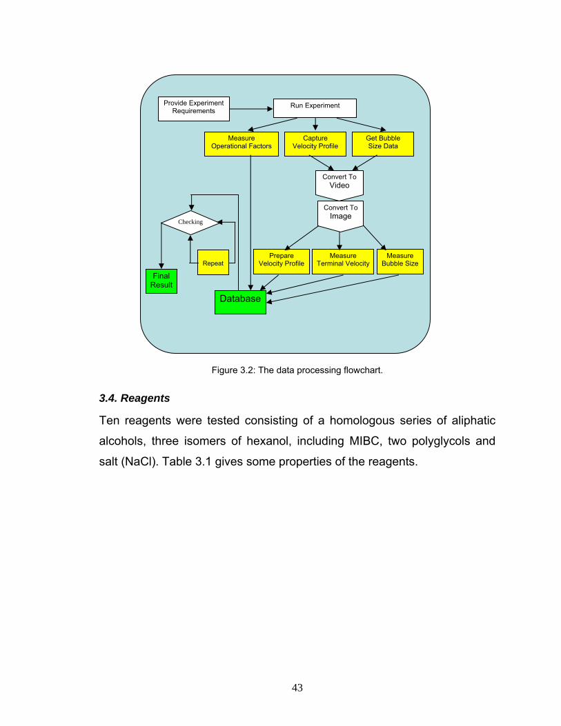
43

Provide Experiment Requirements

Run Experiment

Measure Operational Factors

Capture Velocity Profile

Get Bubble Size Data

Measure Bubble Size

Measure Terminal Velocity

Prepare Velocity Profile

Convert To Video

Convert To Image

Database

Checking

Final Result

Repeat

Figure 3.2: The data processing flowchart.

3.4. Reagents

Ten reagents were tested consisting of a homologous series of aliphatic

alcohols, three isomers of hexanol, including MIBC, two polyglycols and

salt (NaCl). Table 3.1 gives some properties of the reagents.

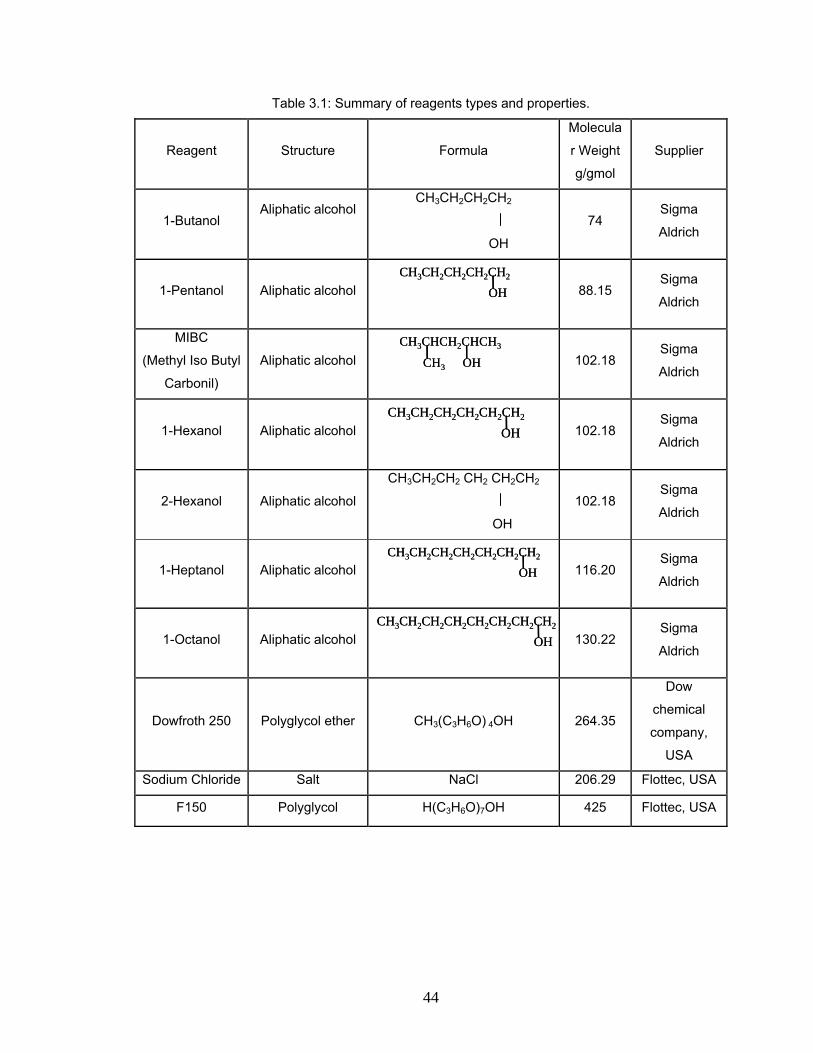
44

Table 3.1: Summary of reagents types and properties.

Reagent Structure Formula

Molecula

r Weight

g/gmol

Supplier

1-Butanol Aliphatic alcohol

CH3CH2CH2CH2

OH

74 Sigma

Aldrich

1-Pentanol Aliphatic alcohol

88.15 Sigma

Aldrich

MIBC

(Methyl Iso Butyl

Carbonil)

Aliphatic alcohol

102.18 Sigma

Aldrich

1-Hexanol Aliphatic alcohol

102.18 Sigma

Aldrich

2-Hexanol Aliphatic alcohol

CH3CH2CH2 CH2 CH2CH2

OH

102.18 Sigma

Aldrich

1-Heptanol Aliphatic alcohol

116.20 Sigma

Aldrich

1-Octanol Aliphatic alcohol

130.22 Sigma

Aldrich

Dowfroth 250 Polyglycol ether CH3(C3H6O) 4OH 264.35

Dow

chemical

company,

USA

Sodium Chloride Salt NaCl 206.29 Flottec, USA

F150 Polyglycol H(C3H6O)7OH 425 Flottec, USA

CH3CH2CH2CH2CH2

OHCH3CH2CH2CH2CH2

OH

CH3CHCH2CHCH3

CH3 OH

CH3CHCH2CHCH3

CH3 OH

CH3CH2CH2CH2CH2CH2

OHCH3CH2CH2CH2CH2CH2

OH

CH3CH2CH2CH2CH2CH2CH2CH2

OHCH3CH2CH2CH2CH2CH2CH2CH2

OH

CH3CH2CH2CH2CH2CH2CH2

OHCH3CH2CH2CH2CH2CH2CH2

OH

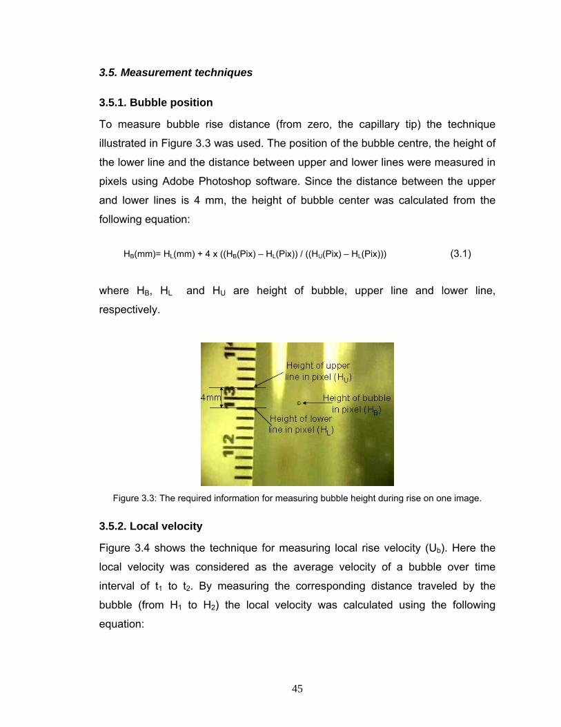
45

3.5. Measurement techniques

3.5.1. Bubble position

To measure bubble rise distance (from zero, the capillary tip) the technique

illustrated in Figure 3.3 was used. The position of the bubble centre, the height of

the lower line and the distance between upper and lower lines were measured in

pixels using Adobe Photoshop software. Since the distance between the upper

and lower lines is 4 mm, the height of bubble center was calculated from the

following equation:

HB(mm)= HL(mm) + 4 x ((HB(Pix) – HL(Pix)) / ((HU(Pix) – HL(Pix))) (3.1)

where HB, HL and HU are height of bubble, upper line and lower line,

respectively.

Figure 3.3: The required information for measuring bubble height during rise on one image.

3.5.2. Local velocity

Figure 3.4 shows the technique for measuring local rise velocity (Ub). Here the

local velocity was considered as the average velocity of a bubble over time

interval of t1 to t2. By measuring the corresponding distance traveled by the

bubble (from H1 to H2) the local velocity was calculated using the following

equation:

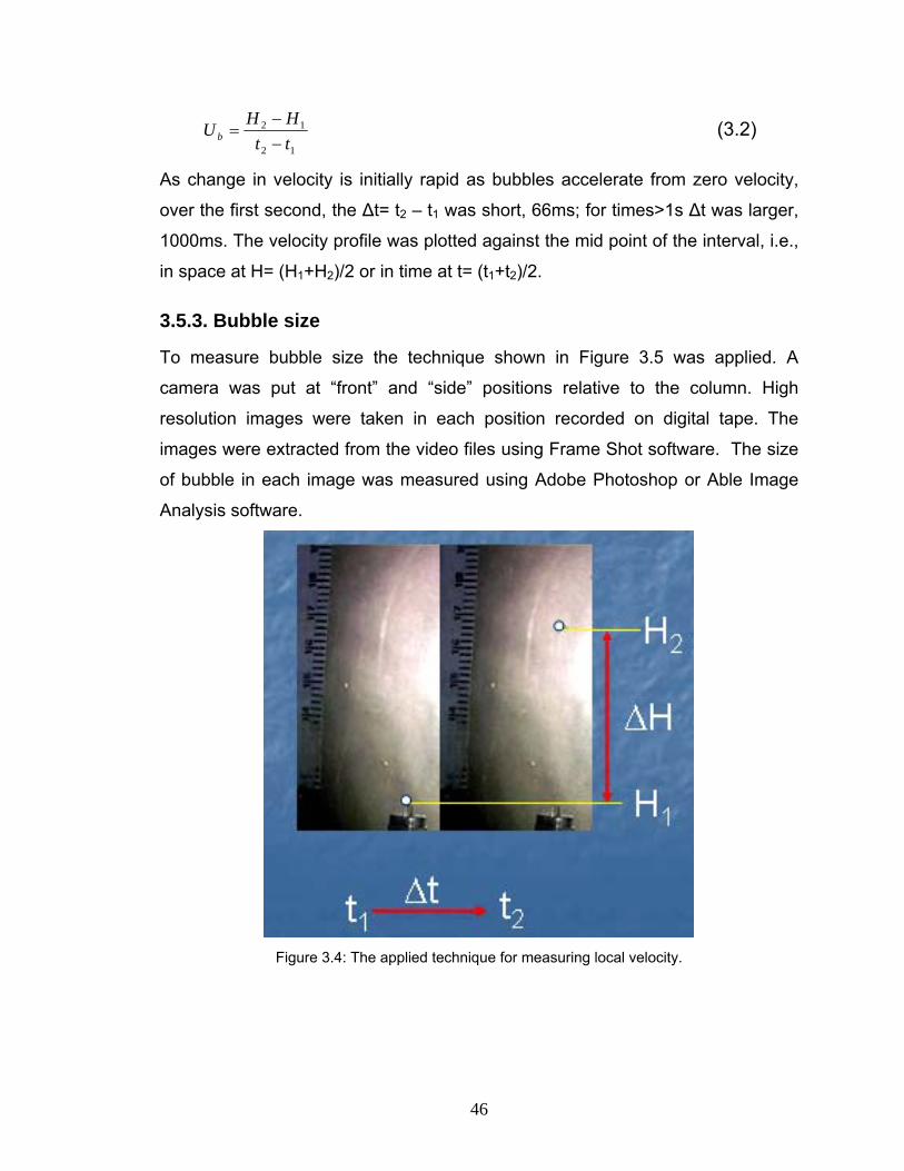
46

12

12

ttHH

U b −−

= (3.2)

As change in velocity is initially rapid as bubbles accelerate from zero velocity,

over the first second, the Δt= t2 – t1 was short, 66ms; for times>1s Δt was larger,

1000ms. The velocity profile was plotted against the mid point of the interval, i.e.,

in space at H= (H1+H2)/2 or in time at t= (t1+t2)/2.

3.5.3. Bubble size

To measure bubble size the technique shown in Figure 3.5 was applied. A

camera was put at “front” and “side” positions relative to the column. High

resolution images were taken in each position recorded on digital tape. The

images were extracted from the video files using Frame Shot software. The size

of bubble in each image was measured using Adobe Photoshop or Able Image

Analysis software.

Figure 3.4: The applied technique for measuring local velocity.

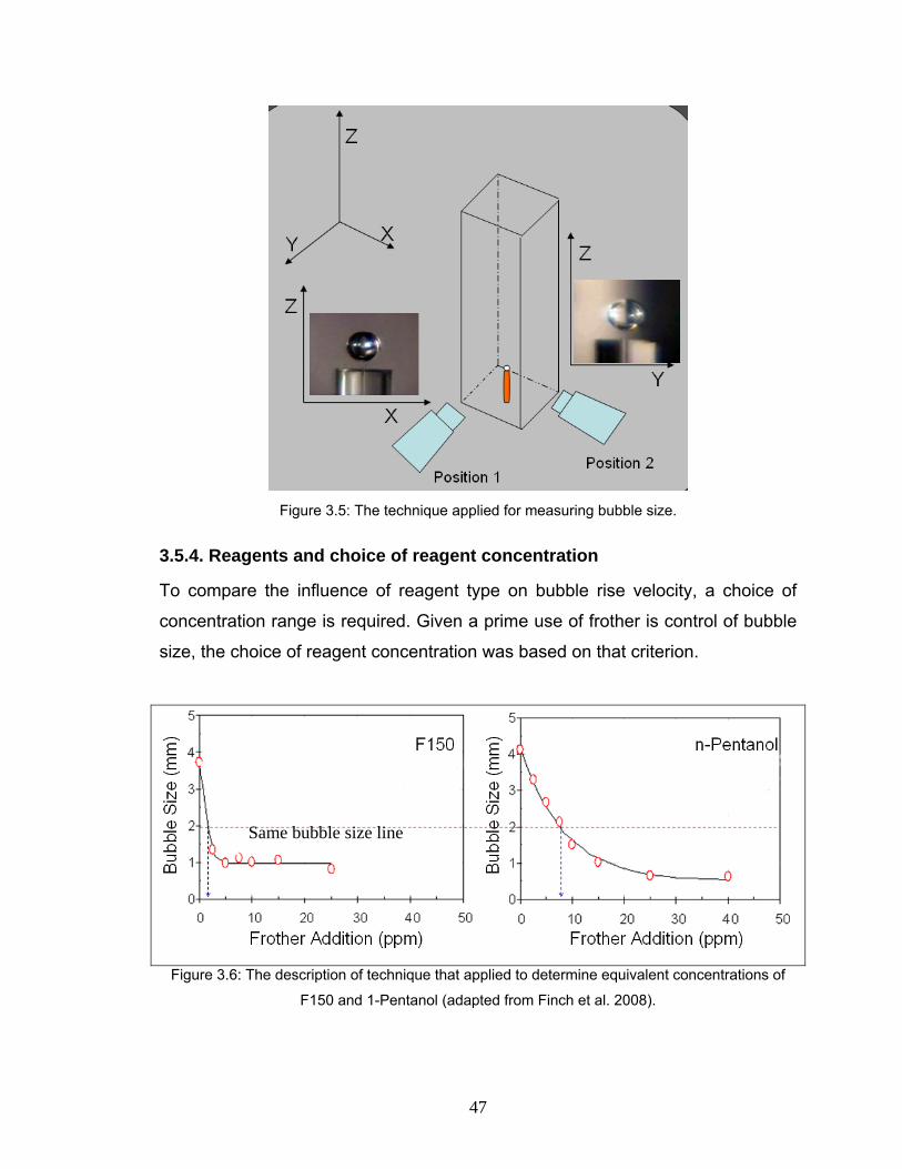
47

Figure 3.5: The technique applied for measuring bubble size.

3.5.4. Reagents and choice of reagent concentration

To compare the influence of reagent type on bubble rise velocity, a choice of

concentration range is required. Given a prime use of frother is control of bubble

size, the choice of reagent concentration was based on that criterion.

Figure 3.6: The description of technique that applied to determine equivalent concentrations of

F150 and 1-Pentanol (adapted from Finch et al. 2008).

Same bubble size line

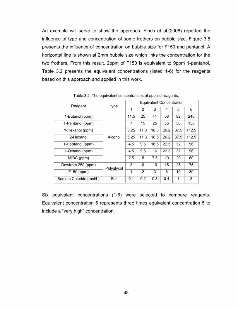
48

An example will serve to show the approach. Finch et al.(2008) reported the

influence of type and concentration of some frothers on bubble size. Figure 3.6

presents the influence of concentration on bubble size for F150 and pentanol. A

horizontal line is shown at 2mm bubble size which links the concentration for the

two frothers. From this result, 2ppm of F150 is equivalent to 9ppm 1-pentanol.

Table 3.2 presents the equivalent concentrations (listed 1-6) for the reagents

based on this approach and applied in this work.

Table 3.2: The equivalent concentrations of applied reagents.

Reagent type Equivalent Concentration

1 2 3 4 5 6

1-Butanol (ppm)

Alcohol

11.5 25 41 58 82 246

1-Pentanol (ppm) 7 15 25 35 50 150

1-Hexanol (ppm) 5.25 11.3 18.5 26.2 37.5 112.5

2-Hexanol 5.25 11.3 18.5 26.2 37.5 112.5

1-Heptanol (ppm) 4.5 9.6 16.5 22.5 32 96

1-Octanol (ppm) 4.5 9.5 16 22.3 32 96

MIBC (ppm) 2.5 5 7.5 10 20 60

Dowfroth 250 (ppm) Polyglycol

3 6 10 15 25 75

F150 (ppm) 1 2 3 5 10 30

Sodium Chloride (mol/L) Salt 0.1 0.2 0.3 0.4 1 3

Six equivalent concentrations (1-6) were selected to compare reagents.

Equivalent concentration 6 represents three times equivalent concentration 5 to

include a “very high” concentration.

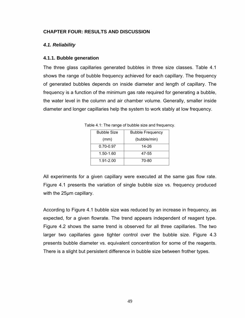
49

CHAPTER FOUR: RESULTS AND DISCUSSION

4.1. Reliability

4.1.1. Bubble generation

The three glass capillaries generated bubbles in three size classes. Table 4.1

shows the range of bubble frequency achieved for each capillary. The frequency

of generated bubbles depends on inside diameter and length of capillary. The

frequency is a function of the minimum gas rate required for generating a bubble,

the water level in the column and air chamber volume. Generally, smaller inside

diameter and longer capillaries help the system to work stably at low frequency.

Table 4.1: The range of bubble size and frequency.

Bubble Size

(mm)

Bubble Frequency

(bubble/min)

0.70-0.97 14-26

1.50-1.60 47-55

1.91-2.00 70-80

All experiments for a given capillary were executed at the same gas flow rate.

Figure 4.1 presents the variation of single bubble size vs. frequency produced

with the 25μm capillary.

According to Figure 4.1 bubble size was reduced by an increase in frequency, as

expected, for a given flowrate. The trend appears independent of reagent type.

Figure 4.2 shows the same trend is observed for all three capillaries. The two

larger two capillaries gave tighter control over the bubble size. Figure 4.3

presents bubble diameter vs. equivalent concentration for some of the reagents.

There is a slight but persistent difference in bubble size between frother types.

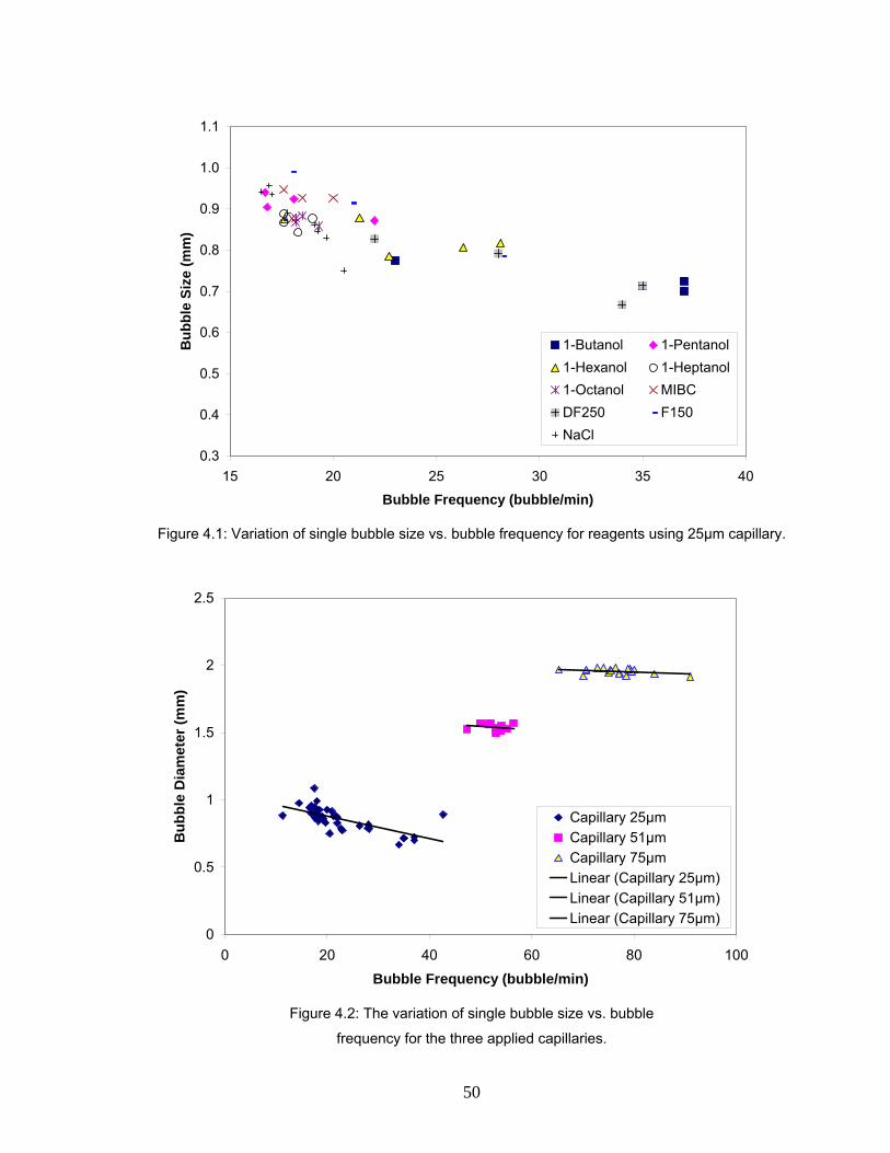
50

0.3

0.4

0.5

0.6

0.7

0.8

0.9

1.0

1.1

15 20 25 30 35 40

Bubble Frequency (bubble/min)

Bub

ble

Size

(mm

)

1-Butanol 1-Pentanol1-Hexanol 1-Heptanol1-Octanol MIBCDF250 F150NaCl

Figure 4.1: Variation of single bubble size vs. bubble frequency for reagents using 25μm capillary.

0

0.5

1

1.5

2

2.5

0 20 40 60 80 100Bubble Frequency (bubble/min)

Bub

ble

Dia

met

er (m

m)

Capillary 25μmCapillary 51μmCapillary 75μmLinear (Capillary 25μm)Linear (Capillary 51μm)Linear (Capillary 75μm)

Figure 4.2: The variation of single bubble size vs. bubble

frequency for the three applied capillaries.

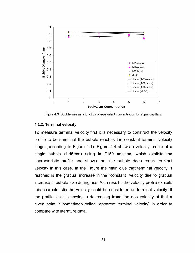
51

0

0.1

0.2

0.3

0.4

0.5

0.6

0.7

0.8

0.9

1

0 1 2 3 4 5 6 7Equivalent Concentration

Bub

ble

Dia

met

er (m

m)

1-Pentanol1-Heptanol1-OctanolMIBCLinear (1-Pentanol)Linear (1-Octanol)Linear (1-Octanol)Linear (MIBC)

Figure 4.3: Bubble size as a function of equivalent concentration for 25μm capillary.

4.1.2. Terminal velocity

To measure terminal velocity first it is necessary to construct the velocity

profile to be sure that the bubble reaches the constant terminal velocity

stage (according to Figure 1.1). Figure 4.4 shows a velocity profile of a

single bubble (1.45mm) rising in F150 solution, which exhibits the

characteristic profile and shows that the bubble does reach terminal

velocity in this case. In the Figure the main clue that terminal velocity is

reached is the gradual increase in the “constant” velocity due to gradual

increase in bubble size during rise. As a result if the velocity profile exhibits

this characteristic the velocity could be considered as terminal velocity. If

the profile is still showing a decreasing trend the rise velocity at that a

given point is sometimes called “apparent terminal velocity” in order to

compare with literature data.

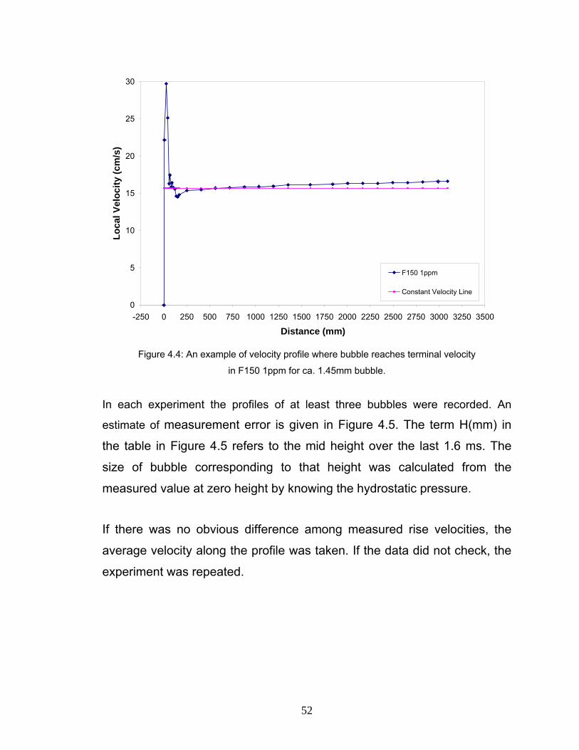
52

0

5

10

15

20

25

30

-250 0 250 500 750 1000 1250 1500 1750 2000 2250 2500 2750 3000 3250 3500

Distance (mm)

Loca

l Vel

ocity

(cm

/s)

F150 1ppm

Constant Velocity Line

Figure 4.4: An example of velocity profile where bubble reaches terminal velocity

in F150 1ppm for ca. 1.45mm bubble.

In each experiment the profiles of at least three bubbles were recorded. An

estimate of measurement error is given in Figure 4.5. The term H(mm) in

the table in Figure 4.5 refers to the mid height over the last 1.6 ms. The

size of bubble corresponding to that height was calculated from the

measured value at zero height by knowing the hydrostatic pressure.

If there was no obvious difference among measured rise velocities, the

average velocity along the profile was taken. If the data did not check, the

experiment was repeated.

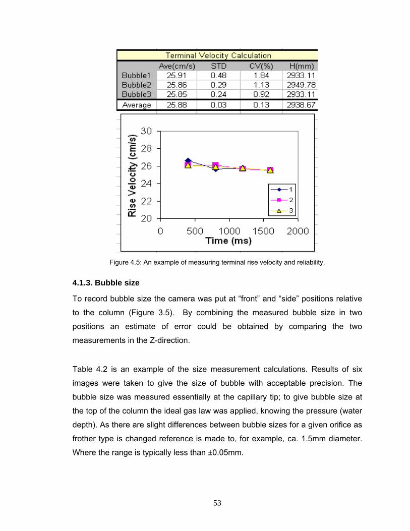
53

Figure 4.5: An example of measuring terminal rise velocity and reliability.

4.1.3. Bubble size

To record bubble size the camera was put at “front” and “side” positions relative

to the column (Figure 3.5). By combining the measured bubble size in two

positions an estimate of error could be obtained by comparing the two

measurements in the Z-direction.

Table 4.2 is an example of the size measurement calculations. Results of six

images were taken to give the size of bubble with acceptable precision. The

bubble size was measured essentially at the capillary tip; to give bubble size at

the top of the column the ideal gas law was applied, knowing the pressure (water

depth). As there are slight differences between bubble sizes for a given orifice as

frother type is changed reference is made to, for example, ca. 1.5mm diameter.

Where the range is typically less than ±0.05mm.

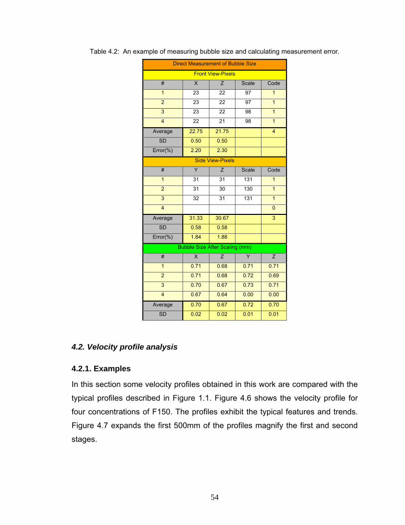
54

Table 4.2: An example of measuring bubble size and calculating measurement error.

Direct Measurement of Bubble Size

Front View-Pixels

# X Z Scale Code

1 23 22 97 1

2 23 22 97 1

3 23 22 98 1

4 22 21 98 1

Average 22.75 21.75 4

SD 0.50 0.50

Error(%) 2.20 2.30

Side View-Pixels

# Y Z Scale Code

1 31 31 131 1

2 31 30 130 1

3 32 31 131 1

4 0

Average 31.33 30.67 3

SD 0.58 0.58

Error(%) 1.84 1.88

Bubble Size After Scaling (mm)

# X Z Y Z

1 0.71 0.68 0.71 0.71

2 0.71 0.68 0.72 0.69

3 0.70 0.67 0.73 0.71

4 0.67 0.64 0.00 0.00

Average 0.70 0.67 0.72 0.70

SD 0.02 0.02 0.01 0.01

4.2. Velocity profile analysis

4.2.1. Examples

In this section some velocity profiles obtained in this work are compared with the

typical profiles described in Figure 1.1. Figure 4.6 shows the velocity profile for

four concentrations of F150. The profiles exhibit the typical features and trends.

Figure 4.7 expands the first 500mm of the profiles magnify the first and second

stages.

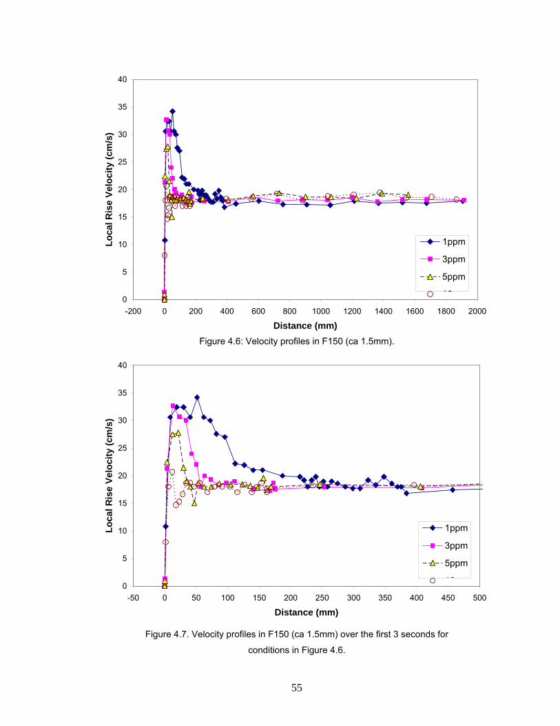
55

0

5

10

15

20

25

30

35

40

-200 0 200 400 600 800 1000 1200 1400 1600 1800 2000

Distance (mm)

Loca

l Ris

e Ve

loci

ty (c

m/s

)

1ppm

3ppm

5ppm

10

Figure 4.6: Velocity profiles in F150 (ca 1.5mm).

0

5

10

15

20

25

30

35

40

-50 0 50 100 150 200 250 300 350 400 450 500

Distance (mm)

Loca

l Ris

e Ve

loci

ty (c

m/s

)

1ppm

3ppm

5ppm

10

Figure 4.7. Velocity profiles in F150 (ca 1.5mm) over the first 3 seconds for

conditions in Figure 4.6.

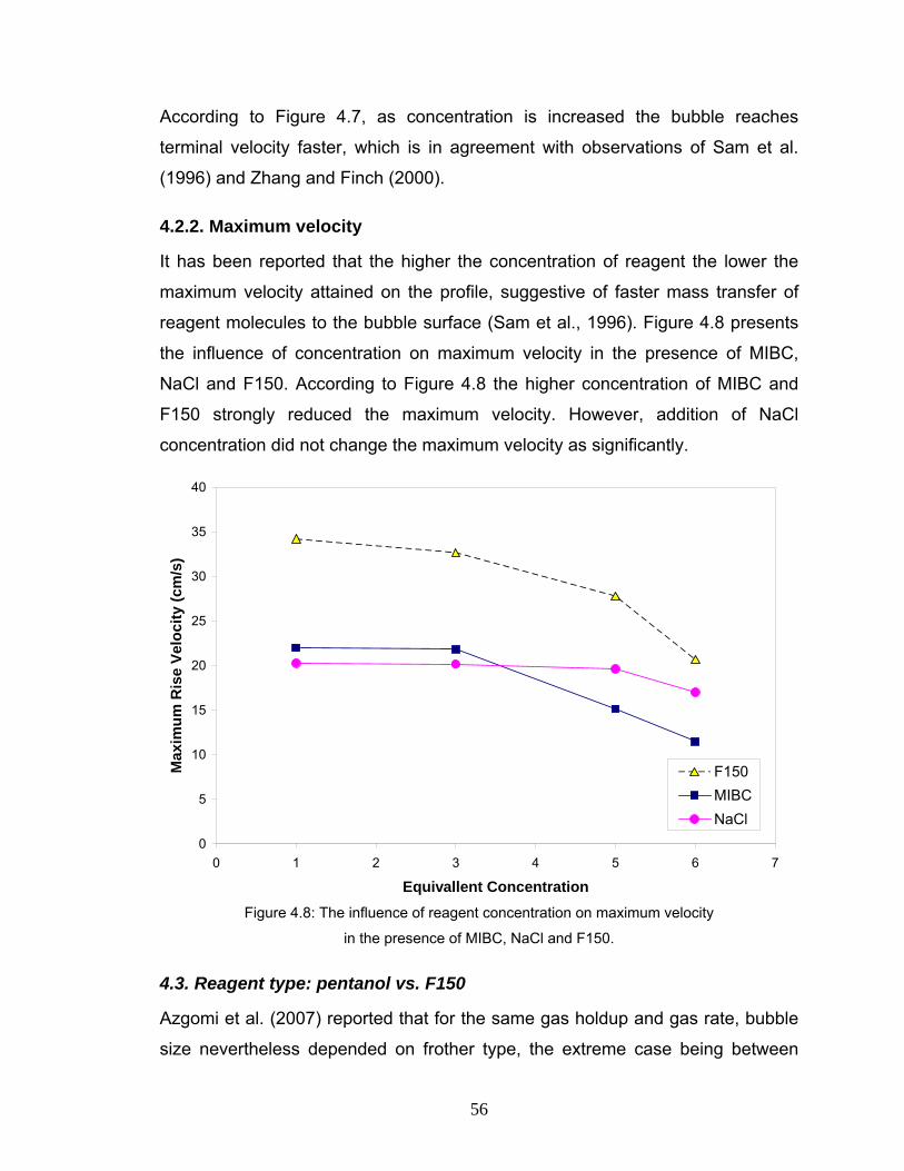
56

According to Figure 4.7, as concentration is increased the bubble reaches

terminal velocity faster, which is in agreement with observations of Sam et al.

(1996) and Zhang and Finch (2000).

4.2.2. Maximum velocity

It has been reported that the higher the concentration of reagent the lower the

maximum velocity attained on the profile, suggestive of faster mass transfer of

reagent molecules to the bubble surface (Sam et al., 1996). Figure 4.8 presents

the influence of concentration on maximum velocity in the presence of MIBC,

NaCl and F150. According to Figure 4.8 the higher concentration of MIBC and

F150 strongly reduced the maximum velocity. However, addition of NaCl

concentration did not change the maximum velocity as significantly.

0

5

10

15

20

25

30

35

40

0 1 2 3 4 5 6 7

Equivallent Concentration

Max

imum

Ris

e Ve

loci

ty (c

m/s

)

F150MIBCNaCl

Figure 4.8: The influence of reagent concentration on maximum velocity

in the presence of MIBC, NaCl and F150.

4.3. Reagent type: pentanol vs. F150

Azgomi et al. (2007) reported that for the same gas holdup and gas rate, bubble

size nevertheless depended on frother type, the extreme case being between

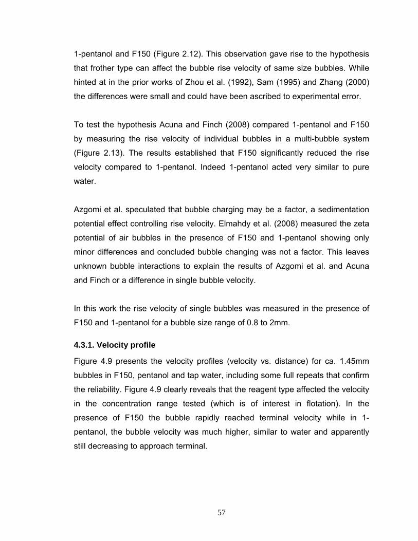
57

1-pentanol and F150 (Figure 2.12). This observation gave rise to the hypothesis

that frother type can affect the bubble rise velocity of same size bubbles. While

hinted at in the prior works of Zhou et al. (1992), Sam (1995) and Zhang (2000)

the differences were small and could have been ascribed to experimental error.

To test the hypothesis Acuna and Finch (2008) compared 1-pentanol and F150

by measuring the rise velocity of individual bubbles in a multi-bubble system

(Figure 2.13). The results established that F150 significantly reduced the rise

velocity compared to 1-pentanol. Indeed 1-pentanol acted very similar to pure

water.

Azgomi et al. speculated that bubble charging may be a factor, a sedimentation

potential effect controlling rise velocity. Elmahdy et al. (2008) measured the zeta

potential of air bubbles in the presence of F150 and 1-pentanol showing only

minor differences and concluded bubble changing was not a factor. This leaves

unknown bubble interactions to explain the results of Azgomi et al. and Acuna

and Finch or a difference in single bubble velocity.

In this work the rise velocity of single bubbles was measured in the presence of

F150 and 1-pentanol for a bubble size range of 0.8 to 2mm.

4.3.1. Velocity profile

Figure 4.9 presents the velocity profiles (velocity vs. distance) for ca. 1.45mm

bubbles in F150, pentanol and tap water, including some full repeats that confirm

the reliability. Figure 4.9 clearly reveals that the reagent type affected the velocity

in the concentration range tested (which is of interest in flotation). In the

presence of F150 the bubble rapidly reached terminal velocity while in 1-

pentanol, the bubble velocity was much higher, similar to water and apparently

still decreasing to approach terminal.

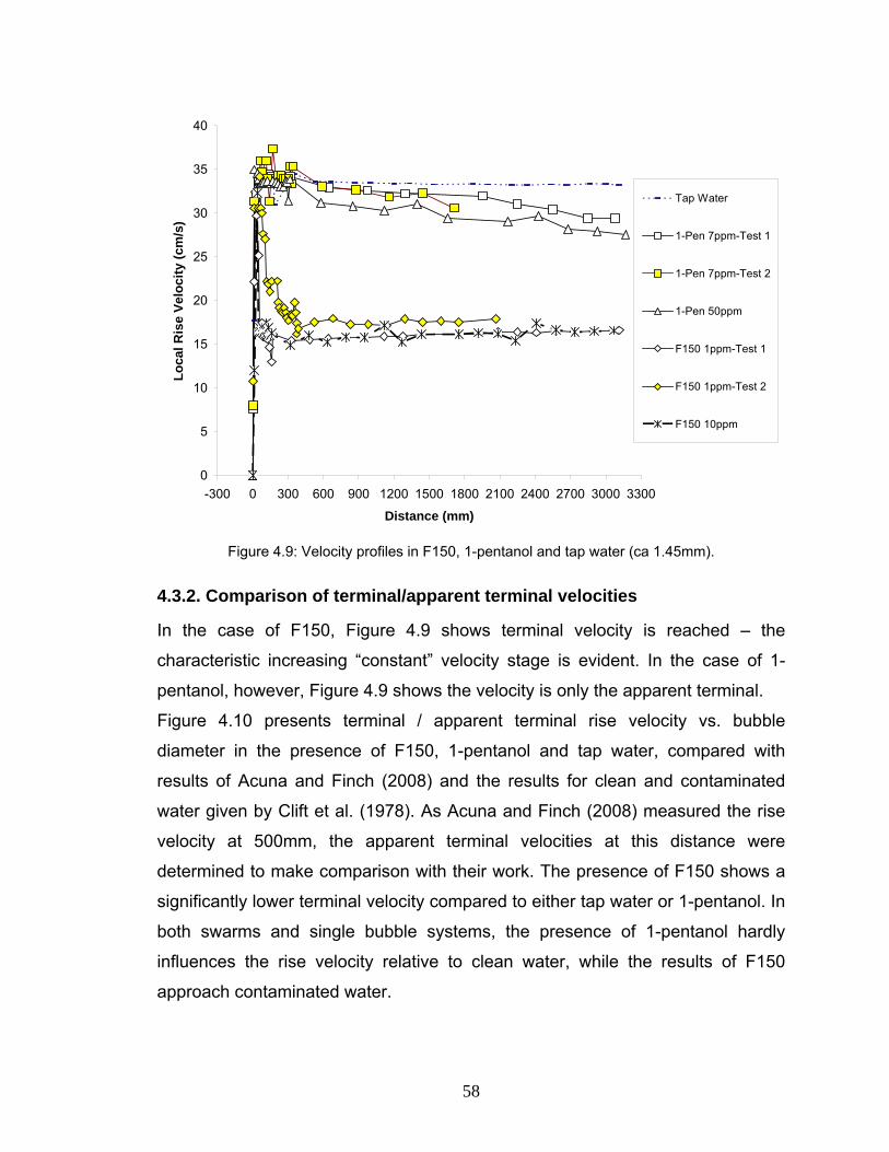
58

0

5

10

15

20

25

30

35

40

-300 0 300 600 900 1200 1500 1800 2100 2400 2700 3000 3300

Distance (mm)

Loca

l Ris

e Ve

loci

ty (c

m/s

)Tap Water

1-Pen 7ppm-Test 1

1-Pen 7ppm-Test 2

1-Pen 50ppm

F150 1ppm-Test 1

F150 1ppm-Test 2

F150 10ppm

Figure 4.9: Velocity profiles in F150, 1-pentanol and tap water (ca 1.45mm).

4.3.2. Comparison of terminal/apparent terminal velocities

In the case of F150, Figure 4.9 shows terminal velocity is reached – the

characteristic increasing “constant” velocity stage is evident. In the case of 1-

pentanol, however, Figure 4.9 shows the velocity is only the apparent terminal.

Figure 4.10 presents terminal / apparent terminal rise velocity vs. bubble

diameter in the presence of F150, 1-pentanol and tap water, compared with

results of Acuna and Finch (2008) and the results for clean and contaminated

water given by Clift et al. (1978). As Acuna and Finch (2008) measured the rise

velocity at 500mm, the apparent terminal velocities at this distance were

determined to make comparison with their work. The presence of F150 shows a

significantly lower terminal velocity compared to either tap water or 1-pentanol. In

both swarms and single bubble systems, the presence of 1-pentanol hardly

influences the rise velocity relative to clean water, while the results of F150

approach contaminated water.

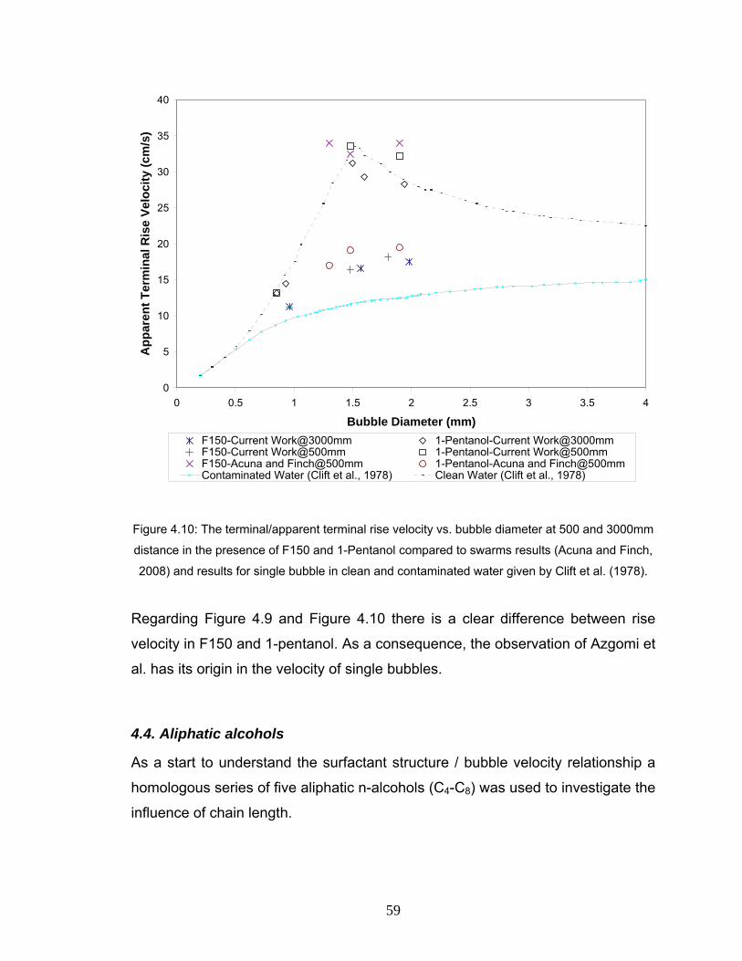
59

0

5

10

15

20

25

30

35

40

0 0.5 1 1.5 2 2.5 3 3.5 4

Bubble Diameter (mm)

App

aren

t Ter

min

al R

ise

Velo

city

(cm

/s)

F150-Current Work@3000mm 1-Pentanol-Current Work@3000mmF150-Current Work@500mm 1-Pentanol-Current Work@500mmF150-Acuna and Finch@500mm 1-Pentanol-Acuna and Finch@500mmContaminated Water (Clift et al., 1978) Clean Water (Clift et al., 1978)

Figure 4.10: The terminal/apparent terminal rise velocity vs. bubble diameter at 500 and 3000mm

distance in the presence of F150 and 1-Pentanol compared to swarms results (Acuna and Finch,

2008) and results for single bubble in clean and contaminated water given by Clift et al. (1978).

Regarding Figure 4.9 and Figure 4.10 there is a clear difference between rise

velocity in F150 and 1-pentanol. As a consequence, the observation of Azgomi et

al. has its origin in the velocity of single bubbles.

4.4. Aliphatic alcohols

As a start to understand the surfactant structure / bubble velocity relationship a

homologous series of five aliphatic n-alcohols (C4-C8) was used to investigate the

influence of chain length.

60

Figure 4.11 and Figure 4.12 show the terminal/apparent terminal rise velocity vs.

bubble diameter at 3000mm for equivalent concentrations 1 and 5, of 1-pentanol,

1-hexanol and 1-heptanol (Figure 4.11); and 1-butanol, 1-hexanol and 1-octanol

(Figure 4.12). The Figures indicate that the lower concentration of 1-hexanol

(equivalent concentration 1=5.25ppm) acted like 1-butanol and 1-pentanol, and

the higher concentration (equivalent concentration 2 =37.5ppm) acted like 1-

heptanol and 1-octanol. For 1-butanol, 1-pentanol, 1-heptanol and 1-octanol, the

change in concentration did not influence rise velocity practically.

To check if the terminal velocity was achieved, the velocity profiles were

examined. Figure 4.13 compares the profiles in 5.25ppm and 37.5ppm 1-

hexanol. The 5.25ppm velocity profile has probably not reached terminal velocity

because there is a discernable decreasing trend, while the profile at 37.5 ppm

has reached terminal velocity.

0

5

10

15

20

25

30

35

40

0 0.5 1 1.5 2 2.5 3 3.5 4

Bublble Diameter (mm)

App

aren

t Ter

min

al R

ise

Velo

city

(cm

/s)

1-Pentanol 1-Pentanol1-Hexanol 1-Hexanol1-Heptanol 1-HeptanolContaminated Water (Clift et al., 1978) Clean Water (Clift et al., 1978)

Figure 4.11: The terminal/apparent terminal rise velocity vs. bubble diameter at

3000mm in the presence of low (1) and high (5) concentrations of 1-pentanol, 1-

hexanol and 1-heptanol.

61

0

5

10

15

20

25

30

35

40

0 0.5 1 1.5 2 2.5 3 3.5 4

Bublble Diameter (mm)

Apa

rent

Ter

min

al R

ise

Velo

city

(cm

/s)

1-Butanol 1-Butano1-Hexanol 1-Hexanol1-Octanol 1-OctanolContaminated Water (Clift et al., 1978) Clean Water (Clift et al., 1978)

Figure 4.12: The terminal/apparent terminal rise velocity vs. bubble diameter at 3000mm in the

presence of low (1) and high (5) concentrations of 1-butanol, 1-hexanol and 1-octanol.

0

5

10

15

20

25

30

35

40

-300 0 300 600 900 1200 1500 1800 2100 2400 2700 3000 3300Bubble Position (mm)

Loca

l Ris

e Ve

loci

ty (c

m/s

)

1-Hexanol 5.25ppm1-Hexanol 37.5ppm

Figure 4.13: Velocity profiles in 1-hexanol (ca 1.5mm).

62

4.4.1. Concentration effect

Figure 4.11 and 4.12 indicate that 1-pentanol and 1-butanol have not reached

terminal velocity even at the highest concentration tested (5) while, the 1-

heptanol and 1-octanol have. 1-Hexanol is in between: at high concentration (5) it

acts like 1-heptanol and at low concentration (1) it acts like 1-pentanol. The

implication is that if we go to higher concentrations of 1-pentanol than tested thus

far it too will start to look like 1-heptanol; conversely, 1-heptanol at lower

concentrations than tested will take on the character of 1-pentanol. The jump in

apparent terminal velocity from 1-pentanol to 1-heptanol is then a ”concentration

effect”.

0

5

10

15

20

25

30

35

40

45

-300 0 300 600 900 1200 1500 1800 2100 2400 2700 3000 3300

Distance (mm)

Loca

l Ris

e Ve

loci

ty (c

m/s

)

Tap Water1-Butanol-11.5ppm1-Butanol-82ppm1-Butanol-125ppm1-Butanol-150ppm1-Butanol-180ppm1-Butanol-260ppm

Figure 4.14: Velocity profiles in 1-butanol (ca 1.45mm).

63

0

5

10

15

20

25

30

35

40

-300 0 300 600 900 1200 1500 1800 2100 2400 2700 3000 3300

Distance (mm)

Loca

l Ris

e Ve

loci

ty (c

m/s

)

Tap Water1-Pentanol-7ppm1-Pentanol-50ppm1-Pentanol-110ppm1-Pentanol-130ppm1-Pentanol-250ppm

Figure 4.15: Velocity profiles in 1-pentanol (ca 1.45mm).

0

5

10

15

20

25

30

35

40

-300 0 300 600 900 1200 1500 1800 2100 2400 2700 3000 3300

Distance (mm)

Loca

l Ris

e Ve

loci

ty (c

m/s

)

Tap Water1-Pentanol-7ppm1-Pentanol-50ppm1-Pentanol-110ppm1-Pentanol-130ppm1-Pentanol-225ppm1-Pentanol-275ppm

Figure 4.16: Velocity profiles in 1-pentanol (ca 1.85mm).

64

0

5

10

15

20

25

30

35

40

45

-300 0 300 600 900 1200 1500 1800 2100 2400 2700 3000 3300

Distance (mm)

Loca

l Ris

e Ve

loci

ty (c

m/s

)

Tap Water1-Hexanol-5.25ppm1-Hexanol-15ppm1-Hexanol-25ppm1-Hexanol-37.5ppm

Figure 4.17: Velocity profiles in 1-hexanol (ca 1.45mm).

This concentration effect was explored up. Figure 4.14 show the case of 1-

butanol; Figure 4.15 and Figure 4.16 show the velocity profile in 1-pentanol for

1.45mm and 1.85mm bubble sizes, respectively; and Figure 4.17 and Figure 4.18

indicates the velocity profile in 1-hexanol for 1.45mm and 1.85mm bubbles,

respectively. According to the velocity profiles for these three n-alcohols, as the

concentration increased, the rise velocity reduced to a value close to the

contaminated water result, except in the case of 1-butanol even at 260ppm.

65

0

5

10

15

20

25

30

35

40

-300 0 300 600 900 1200 1500 1800 2100 2400 2700 3000 3300

Distance (mm)

Loca

l Ris

e Ve

loci

ty (c

m/s

)

Tap Water1-Hexanol-5.25ppm1-Hexanol-15ppm1-Hexanol-25ppm1-Hexanol-37.5ppm

Figure 4.18: Velocity profiles in hexanol (ca 1.85mm).

Krzan and co-workers report velocity profiles for 1-butanol and 1-hexanol (Krzan

and Malysa, 2002) and 1-pentanol and 1-octanol (Krzan et al., 2007). They

obtained the profiles over the more limited distance of 350mm.

Taking results at 350mm as “apparent” terminal velocity in this case, Figure 4.19,

Figure 4.20 and Figure 4.21 compare the results with those of Krzan and co-

workers. The figures indicate that the results of the current work at 350mm are

close to those of Krzan and co-workers.

66

0

5

10

15

20

25

30

35

40

0 500 1000 1500 2000 2500 3000

1-Butanol Concentration (ppm)

App

aren

t Ter

min

al V

eloc

ity (c

m/s

)

Current Work-1.45mm@350mm

Krzan et al-1.42mm@350mm

Figure 4.19: Apparent terminal velocity (at 350mm) vs. concentration of single bubbles in 1-

butanol.

0

5

10

15

20

25

30

35

40

0 50 100 150 200 250 300

1-Pentanol Concentration (ppm)

App

aren

t Ter

min

al V

eloc

ity (c

m/s

)

Current Work-1.45mm@350mm

Krzan et al-1.42mm@350mm

Figure 4.20: Apparent terminal velocity (at 350mm) vs. concentration of single bubbles in 1-

pentanol.

67

0

5

10

15

20

25

30

35

0 10 20 30 40 50 60 70 801-Hexanol Concentration (ppm)

App

aren

t Ter

min

al V

eloc

ity (c

m/s

)

Current Work-1.45mm@350mm

Krzan et al-1.42mm@350mm

Figure 4.21: Apparent terminal velocity (at 350mm) vs. concentration of single bubbles in 1-

hexanol.

0

5

10

15

20

25

30

35

0.01 0.1 1 10 100 1000

Concentration (ppm)

App

aren

t Ter

min

al V

eloc

ity (c

m/s

)

1-Butanol1-Pentanol1-Hexanol1-Heptanol1-OctanolWater Only

Figure 4.22: Apparent terminal velocity (at 3000mm) vs. concentration (ppm) of single bubbles for

series of n-alcohols for ca. 1.45mm bubbles.

68

0

5

10

15

20

25

30

35

0.0000001 0.000001 0.00001 0.0001 0.001 0.01 0.1 1

Concentration (mol/L)

App

aren

t Ter

min

al V

eloc

ity (c

m/s

)

1-Butanol1-Pentanol1-Hexanol1-Heptanol1-OctanolWater Only

Figure 4.23: Apparent terminal velocity (at 3000mm) vs. concentration (mol/L) of single bubbles

for series of n-alcohols for ca. 1.45mm bubbles.

0

5

10

15

20

25

30

35

1 10 100 1000

Concentration (ppm)

App

aren

t Ter

min

al V

eloc

ity (c

m/s

)

1-Pentanol-1.45mm

1-Hexanol-1.45mm

1-Pentanol-1.85mm

1-Hexanol-1.85mm

Figure 4.24: Apparent terminal velocity (at 3000mm) vs. concentration (ppm) for ca. 1.45 and

1.85mm single bubbles in 1-pentanol and 1-hexanol.

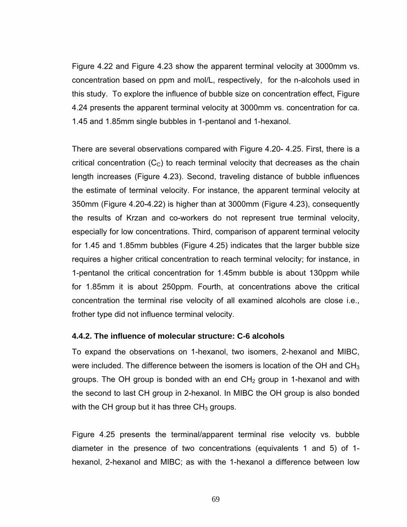
69

Figure 4.22 and Figure 4.23 show the apparent terminal velocity at 3000mm vs.

concentration based on ppm and mol/L, respectively, for the n-alcohols used in

this study. To explore the influence of bubble size on concentration effect, Figure

4.24 presents the apparent terminal velocity at 3000mm vs. concentration for ca.

1.45 and 1.85mm single bubbles in 1-pentanol and 1-hexanol.

There are several observations compared with Figure 4.20- 4.25. First, there is a

critical concentration (CC) to reach terminal velocity that decreases as the chain

length increases (Figure 4.23). Second, traveling distance of bubble influences

the estimate of terminal velocity. For instance, the apparent terminal velocity at

350mm (Figure 4.20-4.22) is higher than at 3000mm (Figure 4.23), consequently

the results of Krzan and co-workers do not represent true terminal velocity,

especially for low concentrations. Third, comparison of apparent terminal velocity

for 1.45 and 1.85mm bubbles (Figure 4.25) indicates that the larger bubble size

requires a higher critical concentration to reach terminal velocity; for instance, in

1-pentanol the critical concentration for 1.45mm bubble is about 130ppm while

for 1.85mm it is about 250ppm. Fourth, at concentrations above the critical

concentration the terminal rise velocity of all examined alcohols are close i.e.,

frother type did not influence terminal velocity.

4.4.2. The influence of molecular structure: C-6 alcohols

To expand the observations on 1-hexanol, two isomers, 2-hexanol and MIBC,

were included. The difference between the isomers is location of the OH and CH3

groups. The OH group is bonded with an end CH2 group in 1-hexanol and with

the second to last CH group in 2-hexanol. In MIBC the OH group is also bonded

with the CH group but it has three CH3 groups.

Figure 4.25 presents the terminal/apparent terminal rise velocity vs. bubble

diameter in the presence of two concentrations (equivalents 1 and 5) of 1-

hexanol, 2-hexanol and MIBC; as with the 1-hexanol a difference between low

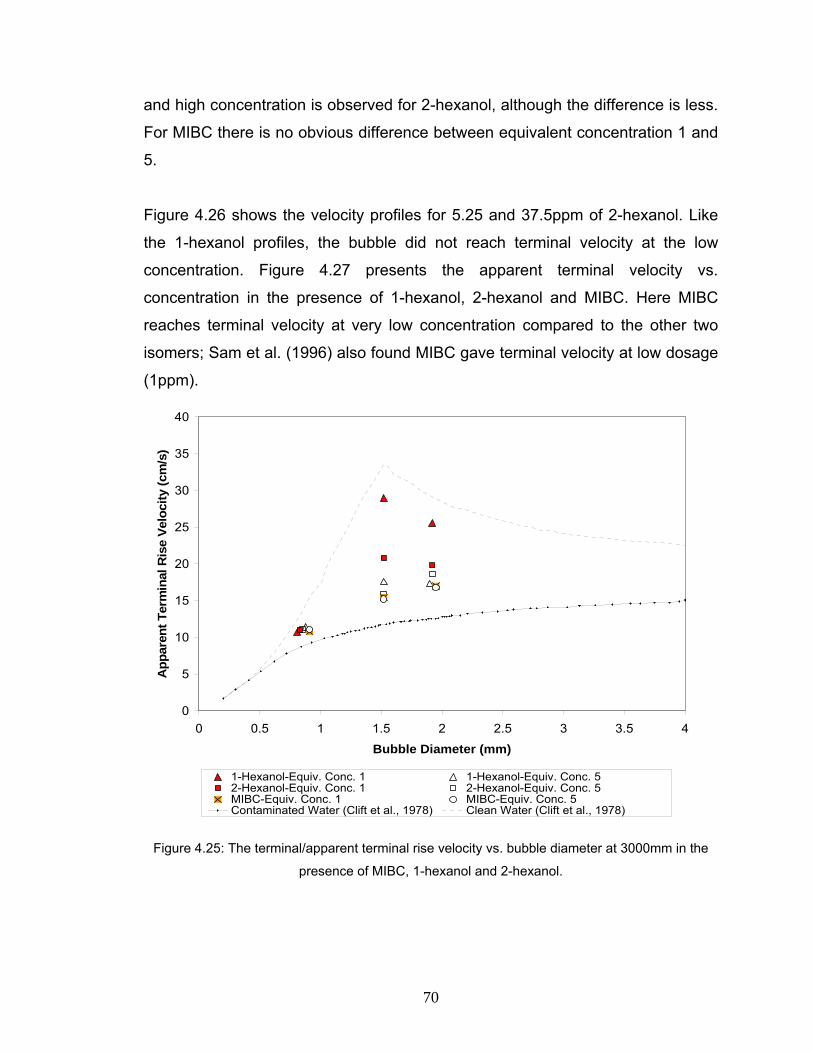
70

and high concentration is observed for 2-hexanol, although the difference is less.

For MIBC there is no obvious difference between equivalent concentration 1 and

5.

Figure 4.26 shows the velocity profiles for 5.25 and 37.5ppm of 2-hexanol. Like

the 1-hexanol profiles, the bubble did not reach terminal velocity at the low

concentration. Figure 4.27 presents the apparent terminal velocity vs.

concentration in the presence of 1-hexanol, 2-hexanol and MIBC. Here MIBC

reaches terminal velocity at very low concentration compared to the other two

isomers; Sam et al. (1996) also found MIBC gave terminal velocity at low dosage

(1ppm).

0

5

10

15

20

25

30

35

40

0 0.5 1 1.5 2 2.5 3 3.5 4

Bubble Diameter (mm)

App

aren

t Ter

min

al R

ise

Velo

city

(cm

/s)

1-Hexanol-Equiv. Conc. 1 1-Hexanol-Equiv. Conc. 52-Hexanol-Equiv. Conc. 1 2-Hexanol-Equiv. Conc. 5MIBC-Equiv. Conc. 1 MIBC-Equiv. Conc. 5Contaminated Water (Clift et al., 1978) Clean Water (Clift et al., 1978)

Figure 4.25: The terminal/apparent terminal rise velocity vs. bubble diameter at 3000mm in the

presence of MIBC, 1-hexanol and 2-hexanol.

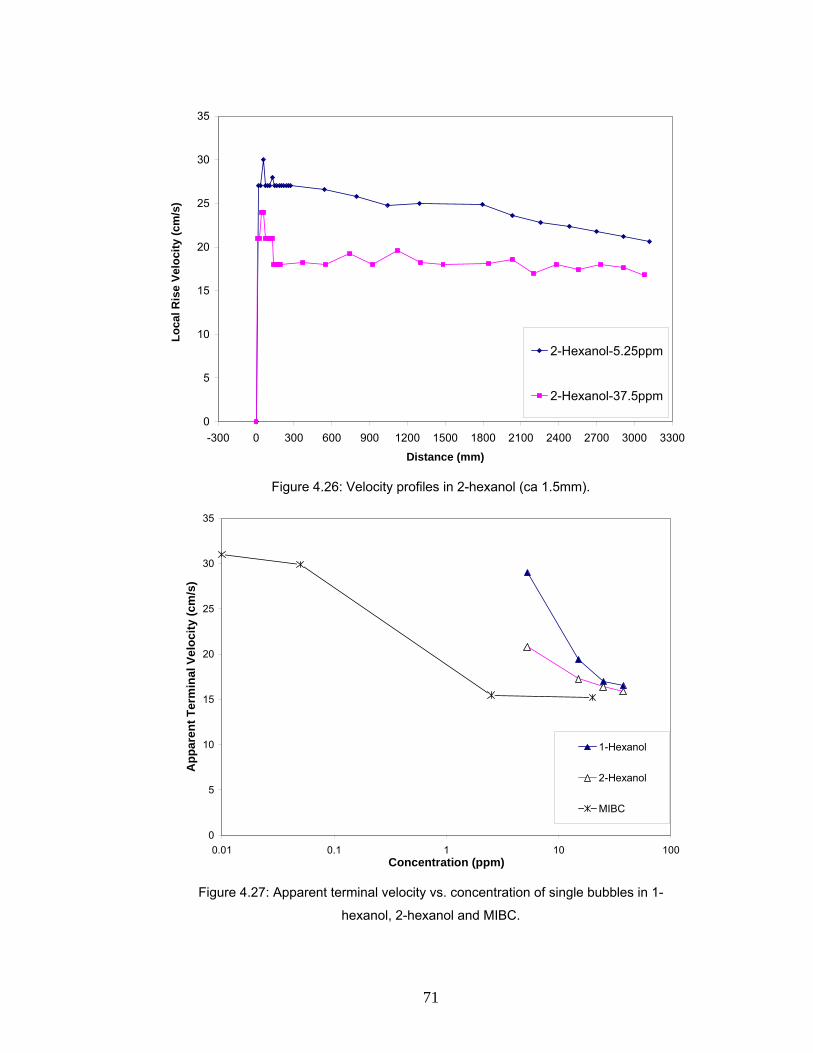
71

0

5

10

15

20

25

30

35

-300 0 300 600 900 1200 1500 1800 2100 2400 2700 3000 3300

Distance (mm)

Loca

l Ris

e Ve

loci

ty (c

m/s

)

2-Hexanol-5.25ppm

2-Hexanol-37.5ppm

Figure 4.26: Velocity profiles in 2-hexanol (ca 1.5mm).

0

5

10

15

20

25

30

35

0.01 0.1 1 10 100Concentration (ppm)

App

aren

t Ter

min

al V

eloc

ity (c

m/s

)

1-Hexanol

2-Hexanol

MIBC

Figure 4.27: Apparent terminal velocity vs. concentration of single bubbles in 1-

hexanol, 2-hexanol and MIBC.

72

According to Figures 4.25-4.27 the chemical structure of the alcohol influences

the rise velocity of single bubbles. According to the molecular structure properties

of the isomers the order of decreasing hydrophilic character is MIBC>2-

hexanol>1-hexanol which corresponds to their order of terminal velocity. The

same order was seen in solubility, for instance the solubility of MIBC and 1-

hexanol is the maximum and minimum among them that is 17 and 6g/L,

respectively.

So the solubility difference between 1-hexanol and MIBC is not enough big

(compared to the solubility difference between other alcohols) to support the

observed significant difference in bubble rise velocity. The hydrophilicity could be

determined using “Hydrophil-Lipophil Balance (HLB)” (Rao, 2004), however the

calculated HLB for MIBC and 1-hexanol are 6.1 and 6, respectively, that does not

reflects significant difference too.

It seems that the structure affects the orientation of frother molecule on the

bubble surface. Perhaps the orientation of MIBC molecules has some advantage

compared to 1-hexanol and 2-hexanol, which permits the lower concentration

control over bubble surface drag or surface viscosity.

4.4. Comparison of MIBC and NaCl

Quinn et al. (2007) compared the influence on gas holdup and bubble size of

some salts with MIBC (as a typical frother). The results indicated that a salt

solution with ionic strength of 0.4-0.5, acted similarly to that of 7-10ppm MIBC.

In this work the rise velocity of single bubbles in the presence of MIBC and NaCl

was measured to explore this reported similarity. Figure 4.28 presents the

velocity profiles in the presence of MIBC and NaCl that shows MIBC reached

terminal velocity, while NaCl may be still in the deceleration region.

73

0

5

10

15

20

25

30

35

40

-300 0 300 600 900 1200 1500 1800 2100 2400 2700 3000 3300

Distance (mm)

Loca

l Ris

e Ve

loci

ty (c

m/s

)

MIBC-Equiv. Conc. 1MIBC-Equiv. Conc. 5NaCl-Equiv. Conc. 1NaCl-Equiv. Conc. 5

Figure 4.28: Velocity profiles in MIBC (ca. 1.5mm) and NaCl (ca 1.6mm).

0

5

10

15

20

25

30

35

40

0 0.5 1 1.5 2 2.5 3 3.5 4

Bubble Diameter (mm)

App

aren

t Ter

min

al R

ise

Velo

city

(cm

/s)

MIBC NaClContaminated Water (Clift et al., 1978) Clean Water (Clift et al., 1978)

Figure 4.29: The terminal/apparent terminal rise velocity vs. bubble diameter at 3000mm in the

presence of MIBC and NaCl.

74

Figure 4.29 presents apparent terminal rise velocity vs. bubble diameter in the

presence of NaCl and MIBC. The Figure shows the velocities are close and both

reagents (eventually in the case of NaCl) slow down the bubble rise to that

approaching contaminated water. The similarity observed by Quinn et al (2007) is

also found for rise velocity of single bubbles.

Henry et al. (2008) measured the terminal rise velocity of very small single

bubbles (40μm<db<100μm) in the presence of some salts over a similar range of

concentration as here. It was reported that addition of NaCl did not reduce the

rise velocity compared to pure water. But there is a question, whether their data

reflects the terminal velocity as they measured the velocity at a distance of only

ca. 1.5mm above the capillary. According to Figure 4.28 the single bubble does

not attain terminal velocity at such a short distance, indeed the bubble required

3000mm to be even close to the terminal velocity. However, according to Figure

1.2 the addition of any reagent appears does not reduce the bubble rise velocity

for bubbles << 1mm, and therefore a salt effect may not be detectable.

4.6. Comparison of frothers

In this part three industrial frothers were tested: F150, DF250 and MIBC. Figure

4.30 presents the apparent terminal rise velocity vs. bubble diameter in the

presence of these frothers. The velocities are close and comparable to

contaminated water. Figure 4.31 presents the apparent terminal velocity at

3000mm vs. concentration in F150, DF250 and MIBC. It shows that there is a

critical concentration to reach terminal velocity; however their critical

concentrations are very low compared to many of the alcohols. DF250 has the

lowest critical concentration (in ppm).

Sam et al. (1996) measured the terminal rise velocity of two of the current

frothers, DF250 and MIBC. Figure 4.32 presents a comparison between the

results. There is good agreement between the DF250 data with slightly lower

velocities recorded for MIBC in the current work.

75

0

5

10

15

20

25

30

35

40

0 0.5 1 1.5 2 2.5 3 3.5 4

Bubble Diameter (mm)

App

aren

t Ter

min

al R

ise

Velo

city

(cm

/s)

F150 DF250MIBC Contaminated Water (Clift et al., 1978)Clean Water (Clift et al., 1978) Figure 4.30: The terminal/apparent terminal velocity at 3000mm vs. bubble

diameter in the presence of the three commercial frothers.

0

5

10

15

20

25

30

35

0.001 0.01 0.1 1 10 100

Frother Concentration (ppm)

App

aren

t Ter

min

al V

eloc

ity (c

m/s

)

F150

DF250

MIBC

Figure 4.31: Apparent terminal velocity at 3000mm vs. concentration of single

bubbles in F150, DF250 and MIBC.

76

0

5

10

15

20

25

0 0.5 1 1.5 2 2.5 3

Bubble Diameter (mm)

Term

inal

Ris

e Ve

loci

ty (c

m/s

)

Dowfroth 250 (current work)Dowfroth 250 (Sam et al.,1996)MIBC (current work)MIBC (Sam et al.,1996)

Figure 4.32: The comparison of measured terminal rise velocity of MIBC and Dowfroth 250

between the Sam et al. (1996) and the recent work.

4.7. The dependency of terminal velocity on frother properties

Sam et al. (1996) reported that terminal rise velocity is independent of frother

concentration, simply the time taken to reach terminal velocity is increased as

concentration is decreased. In practice however, since time is finite (height of

flotation cell) there are two effective concentration regimes:

i) At lower than critical concentration the frother concentration affects

bubble rise velocity.

ii) At higher than critical concentration the rise velocity is independent of

concentration and is reduced to the contaminated water value.

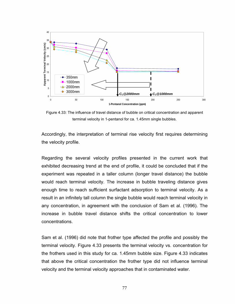
77

Figure 4.33: The influence of travel distance of bubble on critical concentration and apparent

terminal velocity in 1-pentanol for ca. 1.45mm single bubbles.

Accordingly, the interpretation of terminal rise velocity first requires determining

the velocity profile.

Regarding the several velocity profiles presented in the current work that

exhibited decreasing trend at the end of profile, it could be concluded that if the

experiment was repeated in a taller column (longer travel distance) the bubble

would reach terminal velocity. The increase in bubble traveling distance gives

enough time to reach sufficient surfactant adsorption to terminal velocity. As a

result in an infinitely tall column the single bubble would reach terminal velocity in

any concentration, in agreement with the conclusion of Sam et al. (1996). The

increase in bubble travel distance shifts the critical concentration to lower

concentrations.

Sam et al. (1996) did note that frother type affected the profile and possibly the

terminal velocity. Figure 4.33 presents the terminal velocity vs. concentration for

the frothers used in this study for ca. 1.45mm bubble size. Figure 4.33 indicates

that above the critical concentration the frother type did not influence terminal

velocity and the terminal velocity approaches that in contaminated water.

0

5

10

15

20

25

30

35

40

0 50 100 150 200 250 300

1-Pentanol Concentration (ppm)

App

aren

t Ter

min

al V

eloc

ity (c

m/s

)

350mm1000mm2000mm3000mm CC@2000mm CC@1000mm

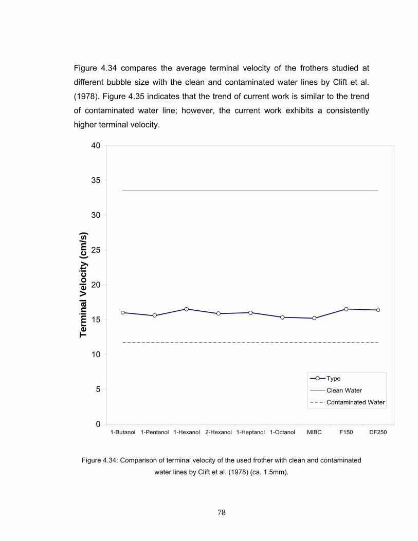
78

Figure 4.34 compares the average terminal velocity of the frothers studied at

different bubble size with the clean and contaminated water lines by Clift et al.

(1978). Figure 4.35 indicates that the trend of current work is similar to the trend

of contaminated water line; however, the current work exhibits a consistently

higher terminal velocity.

0

5

10

15

20

25

30

35

40

1-Butanol 1-Pentanol 1-Hexanol 2-Hexanol 1-Heptanol 1-Octanol MIBC F150 DF250

Term

inal

Vel

ocity

(cm

/s)

Type

Clean Water

Contaminated Water

Figure 4.34: Comparison of terminal velocity of the used frother with clean and contaminated

water lines by Clift et al. (1978) (ca. 1.5mm).

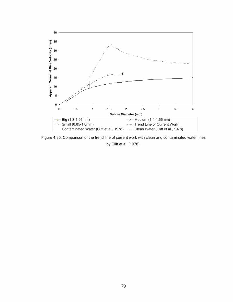
79

0

5

10

15

20

25

30

35

40

0 0.5 1 1.5 2 2.5 3 3.5 4

Bubble Diameter (mm)

App

aren

t Ter

min

al R

ise

Velo

city

(cm

/s)

Big (1.8-1.95mm) Medium (1.4-1.55mm)Small (0.85-1.0mm) Trend Line of Current WorkContaminated Water (Clift et al., 1978) Clean Water (Clift et al., 1978)

Figure 4.35: Comparison of the trend line of current work with clean and contaminated water lines

by Clift et al. (1978).

80

CHAPTER FIVE: CONCLUSIONS AND RECOMMENDATIONS

Single bubbles in the size (diameter) range 0.8-2.0 mm were generated under a

low frequency regime (<80 bubbles/min), and the bubble size and rise velocity

over ca. 3500mm were measured using image processing techniques. This

chapter summarizes the conclusions and ends with recommendations for future

work.

5.1. Conclusions

5.1.1. Bubble generation

The size of bubbles generated at a capillary at low frequency was not

materially influenced by the concentration and type of reagents.

5.1.2. Velocity profile analysis

The velocity profile was obtained by using a mobile video camera to track

and record individual bubbles.

The observed velocity profiles showed the typical properties, as first

reported by Sam et al. (1996).

Determination of true terminal rise velocity requires analysis of the profile

to establish when velocity is constant.

The “apparent terminal velocity” is introduced that gives the possibility of

comparing with the rise velocity of the bubbles reported in the literature

when distance is known.

5.1.3. Hypothesis based on observation of Azgomi et al. (2007)

The results of this work confirmed that reagent type can affect the rise

velocity profile of same size bubbles over the concentration range of

interest in flotation, which is in agreement with the previous observations

of Azgomi et al. (2007) and Acuna and Finch (2008).

The significant difference between rise velocity of F150 and 1-pentanol

shown to be because in the latter bubbles do not reach terminal velocity.

This explains the observation of Azgomi et al. (2007).

81

5.1.4. Aliphatic alcohols

Over the concentration range used in flotation, 1-butanol and 1-pentanol

approximated the trend of pure water (Clift et al., 1978); i.e., their

presence did not significantly reduce the bubble rise velocity. 1-heptanol

and 1-octanol approached the contaminated water trend.

On the concentration range of interest in flotation, 1-hexanol proved the

exception: the lowest concentration of hexanol acted like 1-butanol and 1-

pentanol and the higher concentrations exhibited the trend in 1-heptanol

and 1-octanol. Velocity profile analysis showed that the bubble did not

reach terminal rise velocity at the lowest concentration of 1-hexanol.

Comparison of 1-hexanol, 2-hexanol and MIBC confirmed that not only the

frother concentration could affect the apparent terminal velocity but also

differences in molecular structure. The former impact could be called a

“concentration effect” and the latter “molecular structure effect” that makes

a link between the mechanism of single bubble rise velocity and the

chemistry of surfactant.

To explore the concentration effect a wider concentration range was

examined and it was observed that there is critical concentration, CC, for

each alcohol to reach terminal velocity by a given distance. Below the CC

surfactant concentration affects the apparent terminal rise velocity, while

over the critical concentration (when the bubble reaches terminal velocity)

the rise velocity is independent of concentration.

There was agreement with the results of Krzan and Malysa (2002) in the

case of 1-butanol, 1-pentanol and 1-hexanol. However, they considered

the rise velocity at 350mm (35cm) as the terminal velocity where the

results here indicate the bubble does not necessarily reach the terminal

velocity at this distance location.

5.1.5. The comparison of MIBC and NaCl

Both MIBC and NaCl had similar influence on bubble rise velocity, which

agrees with the gas holdup data reported by Quinn et al. (2007).

82

5.1.6. Commercial frothers

Three commercial frothers, F150, DF250 and MIBC, were tested and

were found to reach terminal at low critical concentration (<1ppm) and

approximate the contaminated water trend.

Comparing to results of Sam et al. (1996) the terminal rise velocity in

MIBC and DF250 exhibited good agreement.

5.1.7. Dependency of terminal velocity on frother properties

The traveling distance of bubble affects the apparent terminal velocity.

The increase in travel distance results in having lower critical

concentration (CC) as more time available for the rising bubble for

reaching terminal velocity. Thus with an infinite travel distance (i.e., very

tall column) the single bubble would reach terminal velocity in any

concentration, which is in agreement with Sam et al. (1996). As the

bubble size increases, the higher critical concentration is required.

Comparing terminal velocity indicates that the frother type does not affect

terminal rise velocity, practically. As a result when the frother

concentration is sufficient to reach terminal velocity, the terminal velocity

is independent of frother type that is not in agreement with the conclusion

of Sam et al. (1996).

The influence of reagent on terminal rise velocity is strongly dependent on

bubble size. For bubble size <1mm there was no obvious difference in

rise velocity between any reagents. For the bubble sizes between 1 to

1.5mm the difference increased to a maximum; above 1.5mm the

difference started to decline once more.

5.2. Recommendations for future works

Most of studies on bubble rise velocity consider physical aspects

(bubble size, method of generation). The results of this work showed

that chemical properties of surfactants of interest in flotation play an

important role, which should be understood.

83

Study of the influence on bubble rise velocity as a function of structure

of the reagent should be expanded. It seems that the adsorption and

orientation of frother molecules on the bubble surface depends on the

molecular structure, and could influence the number of required

molecules for controlling surface mobility.

Velocity profile analysis is the only confident method to identify the

true terminal rise velocity. Any future work must include velocity profile

analysis to avoid misinterpretation.

According to the results of current work it was observed that the

applied concentration equivalency (that was based on equivalent

bubble size production) did not reflect the real impact of frother

concentration on bubble rise velocity. So the suggestions that critical

concentration (CC) concept introduced here can be considered as the

basis for comparing frothers.

84

Refferences

Abou-el-hassan, M.E., 1983. A generalized bubble rise velocity correlation. Chem. Eng.

Commun,2, pp. 243.

Abou-el-hassan, M.E., 1983. Correlations for bubble rise in gasliquid systems.

Encyclopaedia of Fluid Mechanics, Vol. 3, pp.110.

Acharya, A., 1978. Ulbrecht, J.J. Note on Influence of Viscoelasticity on Coalescence

Rate of Bubbles and Drops. AIChE J, 24(2), pp.348.

Acharya, A., Mashelkar, R.A., 1977. Ulbricht, J. Mechanics of bubble motion and

deformation in non-Newtonian media. Chem. Eng. Sci., 32, pp.863.

Acuna, C., 2008. Measurement techniques to characterize bubble motion in swarms.,

Ph.D. Thesis, McGill University, Montreal, Canada.

Acuna, C., Finch, J.A., 2008. Motion of Individual Bubbles Rising in a Swarms.,

Proceedings XXIV International Mineral Processing Congress, Beijing, Sept 24-18,

Vol.1, 891-901.

Agrawal, S.K., and Wasan, D.T., 1979. The effect of interfacial viscosities on the motion

of drops and bubbles. Chem. Eng. J., 18, 215-223.

Alves, S.S., Orvalho, S.P., Vasconcelos, J.M.T., 2005. Effect of bubble contamination on

rise velocity and mass transfer. Chemical Engineering Science, 60, pp.1-9.

Astarita, G., 1966. Spherical gas bubble motion through Maxwell liquids. Ind. Eng.

Chem. Fund.,5(4), 548.

Astarita, G., Apuzzo, G., 1965. Motion of gas bubbles in non Newtonian liquids.

AIChE,J., 11(5), 815.

Auton, T.R., 1987. The lift force on a spherical body in a rotational flow. J. Fluid Mech.,

183, 199.

85

Azgomi, F., 2006. Characterizing frothers by their bubble size control properties., M.Sc.

Thesis, McGill University, Montreal Canada.

Azgomi, F., Gomez, C.O., Finch, J.A., 2007. Correspondence of Gas Holdup and Bubble

Size in Presence of Different Frothers., International Journal of Mineral Processing,

Volume 83, Issues 1-2, 2007, 1-11.

Barnett, S.M., Humphrey, A.E., Litt, M., 1966. Bubble motion and mass transfer in non-

Newtonian fluid. AlChE J.,12(2), 253.

Bashforth, F., Adams, J.C., 1883. An attempt to test the theories of capillary action.

Cambrige University Press: Cambrige.

Beitel, A., and Heideger, W., 1971. Surfactant effects on mass transfer from drops

subject to interfacial instability. Chem. Eng. Sci., 26, 711-717.

Bergman, T.L., Webb, B.W., 1990. Simulation of pure metal melting with buoyancy and

surface tension forces in the liquid phase. Int. J. Mass Transfer, 33, 1, 139-149.

Bhaga, D., 1976. Bubbles in viscous liquids: shapes, wakes and velocities. Ph.D. Thesis,

McGill University, Montreal, Canada.

Bhaga, D., and Weber, M.E., 1980. In-line interaction of a pair of bubbles in a viscous

liquid. Chem. Eng. Sci., 35, 2467-2474.

Bhaga, D., Weber, M.E., 1981. Bubbles in viscous liquids: shapes, wakes and velocities.

J. Fluid Mech., 105, 61-85.

Binder, R.C., 1973. Fluid mechanics. Prentice-Hall, Englewood Cliffs, N.J.

Blanco, A., 1995. Quelques aspects de 1 e'coulement autour d une bulle de'formable:

une approche par simulation directe. Ph.D. Thesis, Inst. Nat. Polytech. Toulouse,

Toulouse, France

86

Bleys, G. and Joos, P., 1985. Adsorption kinetics of bolaform surfactants at the air/water

interface. J. Phys. Chern., 89(6), 1027-1032.

Boussinesq, J., 1913. Vitesse de la chute lente, devenue uniforme, d'une goutte liquide

spherique. dans un fluid visqueux de poids specifique moindre, C.R. Acad. Sci., 156,

1124-1130.

Bozzano, G., Dente, M., 2001. Shape and terminal velocity of single bubble motion: a

novel approach. Computers and Chemical Engineering, 25, pp.571-576.

Bulatovic, S.M., 2007. Handbook of flotation reagents, Vol. 1, Elsevier Publications.

Carreau, P.J., Devic, M., Kapellas, M., 1974. Dynamique des bulles en milieu

viscoelastique. Rheol. Acta, 13, 477.

Chhabra, R, 1993. Bubbles, Drops and Particles in Non-Newtonian Fluids: CRC Press:

Boca Raton. Fla.

Clift, R., Grace, J.R., and Weber, M.E., 1978. Bubbles, drops and particles. Academic

Press.

Craig, V.S.J., Ninham, B.W., Pashley, R.M., 1993. The effect of electrolytes on bubble

coalescence in water. J. Phys. Chem., 97 (39), 10192-10197.

Crozier, R.D., 1992. Flotation: theory, reagents and ore testing. Pergamon Press, pp.

95-100.

Cuenot, B., Magnaudet, J., and Spennato, B., 1997. Effects of slightly soluble

surfactants on the flow around a spherical bubble. J. FluidMech., 339,25-53.

Davidson, J.F., Harrison, D., 1971. Fluidization., academic Press, London and New

York.

87

Davidson, J.F., Schuler, O.G., 1960. Bubble formation at an orifice in a viscous liquid.,

Trans. Instn. Chem. Engr., 38, 144-154.

Davidson, J.F., Schuler, O.G., 1960. Bubble formation at an orifice in an invicid liquid.,

Trans. Instn. Chem. Engr., 38, 335-342.

Davis, R.E., 1966. Acrivos, A. The Influence of Surfactants on the Creeping Motion of

Bubbles. Chem. Eng. Sci.,21, 68l.

De Kee, D., Carreau, P.J., Modarski, J., 1986. Bubble velocity and coalescence in

viscoelastic liquids. Chem. Eng. Sci.,41, 2273.

De Kee, D., Chhabra, R.P., Dajan, A. 1990. Motion and coalescence of gas-bubbles in

non-Newtonian polymer solutions. J. Non Newtonian Fluid Mech., 37(1), 1-18.

De Vries, A.W.G. 2002. Biesheuvel, A, Wijngaarden, L. van, Notes on path and wake of

a gas bubble rising in pure water. Int. J. Multiphase Flow, 28, 1823.

De vries, A.W.G., 2001. Path and wake of a rising bubble. Ph.D. Thesis, Twente

University, Holland.

Detsch, R., Harris, I., 1989. Dissolution and rise velocity of small air bubbles in water

and salt water. Oceans 89, pp.286-291.

Dewsbury, K., Karamanev, D., Margaritis, A., 1991. Hydrodynamic characteristics of free

rise of light solid particles and gas bubbles in on-Newtonian liquids. Chem. Eng. Sci., 54,

4825-4830.

Dukhin, S. S., Kretzschmar, G., and Miller, R., 1995. Dynamics of adsorption at liquid

interfaces: theory, experiment, application. Elsevier, Amsterdam.

Eames, I., Hunt, J. C. R., 1997. Inviscid flow around bodies moving in a weak density

gradient in the absence of buoyancy effects. J. Fluid Mech., 353.

88

Elzinga, E., and Banchero, 1., 1961. Some observations on the mechanics of drops in

liquid-liquid systems. AIChE J., 7, 394-399.

Eskinazi, S., 1968. Principles of fluid mechanics. Allyn and Bacon, Boston.

Fainerman, V.B., Zholob, S.A., Miller, R., and Joos, P., 1998. Non-diffusional adsorption

dynamics of surfactants at the air/water interface: adsorption barrier or non-equilibrium

surface layer. Colloids and Surfaces, A: Physicochemical and Engineering Aspects 143,

243-249.

Fainerman, V.B., 1985. Kinetics of formation of adsorption layers at a solution-air

interface. VNIPIChermetenergoochistka, Donetsk, USSR. Usp. Khim., 54(10),1613-

1631.

Fan, L.S., and Tsuchiya, K., 1990. Bubble wake dynamics in liquids and liquid-solid

suspensions. Butterworth-Heinemann, 17-66.

Fdhila, R.B., Duineveld, P.C., 1996. The effect of surfactant on the rise of a spherical

bubble at high Reynolds and Plecet numbers. Phys. Fluids, 8(2), 310-321.

Finch, J.A., and Smith, G.W., 1972. Dynamic surface tension of alkaline dodecylamine

acetate solutions in oxide flotation. Trans IMM, 81, C213-218.

Finch, J.A., 1971. Interfacial phenomena in cationic magnetite flotation. Master Thesis,

McGill University, Montreal, Canada.

Finch, J.A., 1973. The liquid-vapor interface and adhesion in flotation. Ph. D. Thesis,

McGill University, Montreal, Canada.

Finch, J.A., Nesset, J.E., Acuna, C., 2008. Role of frother on bubble production and

behaviour in flotation. Minerals Engineering, 21, 949-957.

Frumkin, A., 1925. Phys. Chem., 116,466.

89

Frumkin, A., Levich, V.G., 1947. On the surfactants and interfacial motion. Z. Fizicheskoi

Khirnii,21,1183-1204.

Fuerstenau, D.W., and Wayman, C.H., 1958. Effect of chemical reagents on the motion

of single air bubbles in water. TransactionAIME, June, Mining Engineering, 694-699.

Garner, F.H., and Skelland, A.H.P., 1955. Some factors affecting droplet behaviour in

liquid -liquid systems. Chem. Eng. Sci., 4, 149-158.

Garner, F.H., and Hammerton, D., 1954. Circulation inside gas bubbles. Chem. Eng.

Sci., 3, I, 1-11.

Gaskell, D.R., 1992. An Introduction to transport phenomena in mineral processing.

MacmUlan Publishing Company, New York.

Gonzaleztello, P., Camacho, F., Jurado, E., Bailon, R , 1992. Influence of surfactant

concentration on the final rising rate of droplets. Can. J. Chem. Eng., 70(3), 426.

Grace, J.R., Wairegl, T., and Nguyen, T.H., 1976. Shapes and velocities of single drops

and bubbles moving freely through immiscible liquids. Trans. Instn Chem. Engrs,54,

167-173.

Griffith, R.M., 1962. The effect of surfactant on the terminal velocity of drops and

bubbles. Chem. Eng. Sci., V 17, pp.1057-1070.

Gummalam, S., 1987. Chhabra, R P. Rising velocity of a swarm of spherical bubbles in a

power law non-Newtonian liquid. Can. J. Chem. Eng., 65, 1004.

Haberman, W.L, and Morton, R.K., 1953. An experimental investigation of the drag and

shape of air bubbles rising in various liquids. Navy Department, The David W. Taylor

Model Basin, Report 802.

Hadamard, J., 1911. Mouvement permanent lent d'une sphere liquide et visqueuse dans

une liquide visqueux. C. R. Acad. Sci, 152, 1735-1738.

90

Haque, M.W., Nigam, K.D.P., Viswanathan, K., Joshi, J.B., 1988. Studies on bubble rise

velocity in bubble columns employing non-Newtonian solutions. Chem. Eng. Commun.,

73, 31.

Haque, M.W., Nigam, K.D.P., Viswanathan, K., Joshi, .J.B., 1987. Studies on gas holdup

and bubble parameters in bubblecolumns with (carboxymethyl) cellulose solutions. Ind.

Eng. Chem. Res.,26 (1), 86.

Harper, J.F., 1972. The motion of bubbles and drops through liquids. Advance Applied

Mechanics, 12,59-129.

Harper, J.F., 1974. On spherical bubbles rising steadily in dilute surfactant solutions.

Q.J. Mech. Appl. Math., V XXVII, pp.87-100.

Harper, J.F., 1988. The rear stagnation region of a bubble rising steadily in a dilute

surfactant solution. Q. J. Mech. Appl. Math., V 41, pp.203-213.

He, Z., Maldarelli, C., and Dagan, Z., 1991. The size of stagnant caps of bulk soluble

surfactant on the interfaces of translating fluid droplets. J. Colloid Interface Sci., 146(2),

442-451.

Henry, C.L., Parkinson, L., Ralston, J.R., Craig, V.S.J., 2008. A mobile gas/water

interface in electrolyte solutions. J. Phys. Chem. C, 112 (39), 15094-15097.

Horton, Y.J., Fritsch, I.R., and Kintner, R., 1965. Experimental determination of

circulation velocities inside drops. Can. J. Chem. Eng., 43, 143-146.

Huang, W., and Kintner, R.C., 1969. Effects of surfactants on mass transfer inside

drops. AlChE J., 15, 735-744.

Jameson, G. J., 1993. Bubbles in motion, Trans. lnst. Chem. Eng., 71(A), 587.

91

Jamialahmadi, M., Muller-Steinhagen, H., 1992. Effect of alcohol, organic acid and

potassium chloride concentration on bubble size rise velocity and gas hold-up in bubble

columns. The Chemical Engineering Journal, 50, pp.47-56.

Karamanev, d.G., nikolov, L.N., 1992. Free rising spheres do not obey Newton’s law for

free settling. AIChE J., 38(11), 1843-1846.

Karamanev, D.G., 1994. Rise of gas bubbles in quiescent liquids. AIChE J., 40(8), 1418-

1421.

Khurana A.K, Kumar R ,1969. Studies in bubble formation III. Chem. Eng. Sci., 24, 1711.

King, R.P., 1982. Principles of flotation, South African. Institute of Mining and Metallurgy,

Johannesburg.

Kopfsill, A.R, Homsy, G.M., 1988. Bubble motion in a Hele Shaw cell. Phys. Fluids,31(1),

18-26.

Kreischer, B.E., Moritomi, H., and Fan, L.S., 1990. Wake solids holdup characteristics

behind a single bubble in a three-dimensional liquid-solid fluidized bed. Int. J. Multiphase

Flow, 16, 2, 187200.

Krzan, M., Lunkenheimer, K., Malysa, K., 2004. On the influence of the surfactant's polar

group on the local and terminal velocities of bubbles. Colloids and Surfaces a, 250,

pp.431-441.

Krzan, M., Malysa, K., 2002. Profiles of local velocities of bubbles in n-butanol, n-

hexanol and n-nonanol solutions. Colloid and Surfaces A, 207, pp.279-291.

Krzan, M., Zawala, J., Malysa, K., 2007. Development of Steady State Adsorption

Distribution Over Interface of a Bubble Rising in Solutions of n-Alkanols (C5, C8) and n-

Alkyltrimethylammonium Bromides (C8, C12, C16)., Colloids and Surfaces A, 298, 42-51

92

Kugou, N., Ishida, K., Yoshida, A., 2003. Experimental study on motion of air bubbles in

seawater. Marine Technology, V 3, pp.145-158.

Kulkarani, A..A., Joshi, J.B., 2005. Bubble formation and bubble rise velocity in gas-

liquid systems: a review. Ind Eng. Chem. Res., 44, pp.5873-5931.

Lamb, H., 1945. Hydrodynamics, 6th ed., Dover Publications. Co.: New York, pp. 600.

Lan, C.W., and Kou, S., 1992. Heat transfer and fluid flow in flotation-zone crystal growth

with a mostly covered melt surface. Int. Heat Mass Transfer, 35, 2, 433-442.

Leal, L.G., Skoog, J., Acrivos, A., 1971. On the motion of gas bubbles in a viscoelastic

liquid. Can. J. Chem. Eng., 49, 569.

Lee, J.C., Hodgson, T.D., 1968. Film flow and coalescence-I Basic relations, film

shape and criteria for interface mobility. Chem. Eng. Sci., 23,1375-1397.

Letzel, M., 1998. Hydrodynamics and mass transfer in bubble columns at elevated

pressures, Ph.D. Thesis, Delft University.

Levich, V.G., 1962. Physicochemical hydrodynamics. Englewood Clifts, Prentice-Hall.

Liao, Y., Mclaughlin, J.B., 2000. Bubble motion in aqueous surfactant solutions. Journal

of Colloid and Interface Science, 224, pp.297-310.

Liao, Y., Mclaughlin, J.B., 2000. Dissolution of a freely rising bubble in aqueous

surfactant solutions. Chemical Engineering Sciences , 55, pp.5831-5850.

Liao, Y., Wang, J., Nunge, R.J., Mclaughlin, J.B., 2004. Comments on "Bubble motion in

aqueous surfactant solution”. Journal of Colloid and Interface Science, 272, pp.498-501.

Linton, M., and Sutherland, K.L., 1957. Dynamic surface forces, drop circulation and

liquid-liquid mass transfer. Second international congress on surface activity,

Butterworth, London, 1, 494-501.

93

Lochiel, A.C., 1965. The influence of surfactants on mass transfer around spheres. Can.

J. Chem. Eng., 43,40-44.

Lunde, K, Perkins, R,1997. Observations on wakes behind spheroidal bubbles and

particles. Proc. ASME Fluids Eng. Div. Summer Meeting, Vancouver, 97, 3530.

Luo, X., Zhang, J., Tsuchiya, K, Fan, L. S., 1997. On the rise velocity of bubbles in

liquid-solid suspensions at elevated pressure and temperature. Chem. Eng. Sci., 52(21-

22), 3693.

Magnaudet, J., Eames, I., 2000. Motion of high Reynolds number bubbles in turbulent

flows. Annu. Rev. Fluid Mech., 32,659.

Malysa, K, Masliyah, J.H., Neale, G., and van de Ven, T.G.M., 1988. Settling velocity of

a polymer coated particle. Model experiments and theory, Materials Science Forum, 25-

26, 401404.

Malysa, K., Krasowska, M., Krzan, M., 2005. Influence of surface active substances on

bubble motion and collision with various interfaces. Advanced in Colloid and Interface

science, 114-115, 205-225.

Margaritis, A., Te Bokkel, D.W., Karamanev, D., 1999. Bubble rise velocities and drag

coefficients in non-Newtonian polysaccharide solutions. Biotech. Bioeng., 64(3), 259.

Massey, B.S., 1983. Mechanics of fluids. Wokingham, Berkshire, England: Van Nostrand

Reinhold (UK).

McLaughlin, J.B., 1996. Numerical simulation of bubble motion in water. Journal of

Colloid and Interface Science, 184, pp.614-625.

Mei, R, Klausner, J. F., 1992. Unsteady force on a spherical bubble at finite Re with

small fucntions in the free stream velocity. Phys. Fluids A, 4, 63.

94

Miyahara, T., Tsuchiya, K., and Fan, L.S., 1988. Wake properties of a single gas bubble

in a three-dimensional liquid-solid fluidized bed. Int. J. Multiphase Flow, 14, 6, 749-763.

Miyahara, T., Yamanaka, S., 1993. Mechanics of motion and deformation of a single

bubble rising through quiescent highly viscous Newtonian and non-Newtonian media. J.

Chem. Eng. Jpn.,26,297.

Narayanan, S., Gossens, L.H.J., Kossen, N.W.F., 1974. Coalescence of Two Bubbles

Rising in Line at Low Reynolds Numbers”, Chem. Eng. Sci., 29, 2071-2082.

Newman, J., 1967. Retardation of falling drops. Chem. Eng. Sci., 22, 83-85.

Nguyen, A. V., 1998. Prediction of bubble terminal velocities in contaminated water.

AIChE J., 44(1), 226-230.

Oguz, H.N., and Sadhal, S.S., 1988. Effects of soluble and insoluble surfactants on the

motion of drops. J. Fluid Mech., 194, 563-579.

Okano, Y., Itoh, M., and Hirata, A., 1989. Natural and Marangoni convections in a two

dimensional rectangular open boat. J. Chemical Engineering of Japan, 22, 3, 275-281.

Okazaki, S., 1964. The velocity of ascending air bubbles in aqueous solutions of a

surface active substance and the life of the bubble on the same solution. Bull. Chem.

Soc. Japan., 37, 144-150.

Parkinson, L., Sedev, R., Fornasiero, D., Ralston, J., 2008. The terminal rise velocity of

10-100 μm diameter bubbles in water. Journal of Colloid and Interface Science, 322,

168-172.

Quinn, J.J., Kracht, W., Gomez, C.O., Gagnon, C., Finch, J.A., 2007. Comparing the

effect of salts and frother (MIBC) on gas dispersion and froth properties. Mineral

Engineering, 20, 1296-1302.

95

Quinn, J., 2006. Exploring the effect of salts on gas dispersion and froth properties in

flotation system. M.Sc. Thesis, McGill University, Montreal, Canada.

Rabiger, N., Vogelpohl, A., 1986. Bubble formation and its movement in Newtonian and

Non-Newtonian liquids. Encyclopaedia of Fluid Mechanics: Gulf Publishing: Houston, ,

59.

Ramkrishnan, S., Kumar, R, Kuloor, N.R, 1969. Studies in bubble formation - I, Bubble

formation under constant flow conditions. Chem. Eng. Sci. 1,24, 731.

Rao, S. R., 2004, Surface chemistry of froth flotation. Kluwer Academic/ Plenum

Publishers Press, New York.

Ribeiro, C.P., Mewes, D., 2007,. The effect of electrolytes on the critical velocity for

bubble coalescence. Chemical Engineering Journal, 126, 23-33.

Rodrigue, D., 2001. Generalized correlation for bubble motion. AIChE J., 47, 39.

Rodrigue, D., 2002. A simple oscillation for gas bubbles rising in power-law fluids. Can.

J. Chem. Eng., 80(2), 289.

Rodrigue, D., 2004. A general correlation for the rise velocity of single gas bubbles. Can.

J. Chern. Eng., 82 (2), 382-386.

Rodrigue, D., De Kee, D., Chan Man Fong, C.F., 1998. Bubble velocities: further

developments on the jump discontinuity. ,J. Non-Newt. Fluid Mech, 79(1), 45.

Rodrigue, D., De Kee, D., Chan Man Fong, C.F., 1996. An experimental study of the

effect of surfactants on the free rise velocity of gas bubbles. J. Non-Newtonian Fluid

Mech., 66,pp.213-232.

Rodrigue, D., de Kee, D., Chan Man Fong, C.F., 1999. The slow motion of a single

bubble in a non-Newtonian fluid containing surfactant. J. Non-Newtonian Fluid Mech.,

86,pp.211-227.

96

Sam, A., 1995.Single bubble behavior study in a flotation column. Ph.D. Thesis, McGill

University, Montreal, Canada.

Sam, a., Gomez, C.O., Finch, J.A., 1996. Axial velocity profiles of single bubbles in

water/frother solutions. International Journal of Mineral Processing, 47, 177-196.

Satyanarayana, A., Kumar, R, Kuloor N.R , 1969. Studies in bubble formation - II,

Bubble formation under constant pressure conditions. Chern. Eng. Sd.,24, 731.

Savic, P., 1953. Circulation and distortion of liquid drops falling through a viscous

medium. Nat. Res. Counc. Can. Div. Mech. Eng. Report MT -22.

Schechter, R. S., and Fairley, R. W., 1963. Interfacial tension gradients and droplet

behaviour. Can. J. Chem. Eng., 41, 103-107.

Scriven, L.E., 1960. Dynamics of a fluid interface. Chem. Eng. Sci., 12, 98-108.

Stone, H.A., and Leal, L.G., 1990. The effect of surfactant on drop deformation and

breakup, J. Fluid Mech., 220, 161-186.

Takagi, S., Matsumoto, Y., 1995. Three-dimensional calculation of a rising bubble. Proc.

Int. Conf. Multiphase Flow, 2nd, Kyoto, Japan, pp. PD2.9 16.

Takemura, F., 2005. Adsorption of surfactant onto the surface of a spherical rising

bubble and its effect on the terminal velocity of bubble. Physics of Fluids, 17, 048104.

Tate, T., 1864. On the magnitude of a drop ofliquid formed under different

circumstances. Philosophical Magazine,27, 176.

Tomiyama, A. 2004. Drag, lift and virtual mass forces acting on a Single Bubble, 3rd

International Symposium on T\vo-Phase Flow Modelling and Experimentation Pisa, 22-

24.

97

Tomiyama, A., 2002. Reconsideration of Three Fundamental Problems in Modeling

Bubbly Flows, Proc. JSME- KSME Fluid Eng. Conf. Pre-Symp., pp 47-53.

Tomiyama, A., Yoshida, S., Hosokawa, S., 2001. Surface Tension Force Dominant

Regime of Single Bubbles rising through Stagnant Liquids, on CD-ROM of 4th UK-Japan

Seminar on Multiphase Flow, pp 1-6.

Tsuchiya, K., and Fan, L.S., 1988. Near wake structure of a single gas bubble in a two

dimensional liquid-solid fluidized bed: Vortex shedding and wake size variation. Chem.

Eng. Sci., 43, 1167-1181.

Tsuchiya, K., Miyahara, T., and Fan, L.-S., 1989. Visualization of bubbles-wake

interactions for a stream of bubbles in a two-dimensional liquid-solid fluidized bed. Int. J.

Multiphase Flow, 15, 1, 35-49.

Tsuge, H., 1986. Hydrodynamics of bubble formation from submerged orifices. In.

Encyclopaedia of Fluid Mechanics, Gulf Publishing Company: New York, Vol. 3, 191.

Tsuge, H., and Hibino, S.I., 1977. The onset conditions of oscillatory motion of single

gas bubbles rising in various liquids. J. Chem. Eng. Japan, 10, 66-68.

Tsujii, K., 1997. Surface Activity, principles, phenomena, and applications. Academic

Press.

Tzounakos, A., Karamanev, D.G., Margaritis, A., Bergougnou, M.A., 2004. Effect of the

Surfactant Concentration on the Rise of Gas Bubbles in Power-Law Non-Newtonian

Liquids. Ind. Eng. Chem. Res., 43(18), 5790-5795.

Urry, D.W., 1995. Elastic biomolecular machines. Scientific American, Jan. 95.

Vennard, J.K., and Street, R.L., 1975. Fluid flow about immersed objects. John Wiley

and Sons Inc, 645-671.

98

Wu, M., Gharib, M., 2002. Experimental studies on the shape and path of small air

bubbles rising in clean water. Phys. Fluids, 14, L49.

Yamamoto, T., and Ishii, T., 1987. Effect of surface active materials on the drag

coefficient and shape of single large gas bubbles. Chem. Eng. Sci., 42(6), 1297-1303.

Ybert, C., Di Meglio, J. M., 1998. Ascending air bubbles in protein solutions. Eur. Phys.

J. B,4, 313.

Yoshida, S., Manasseh, R, 1997. Trajectories of rising bubbles, The 16th Japanese

Multiphase Flow Symposium, Touya, Hokkaido.

Zana, E., Leal, L.G., 1978. Dynamics and dissolution of gas bubbles in a viscoelastic

fluid. Int. J. Multiphase Flow, 4(3), 237-262.

Zhang, Y., 2000. Single bubble velocity profile: experimental and numerical simulation.

Ph.D. Thesis, McGill University, Montreal, Canada.

Zhang, Y., Finch, J.A., 2000. A note on single bubble motion in surfactant solutions.

Journal of Fluid Mechanics, V 429, pp.63-66.

Zhang, Y., McLaughlin, J.B., Finch, J.A., 2001, Chemical Engineering Sciences, 56,

pp.6605-6616.

Zhang, Y., Sam, A., Finch, J.A., 2003. Temperature effect on single bubble velocity

profile in water and surfactant solution. Colloids and Surfaces Eng., 223, pp.45-54.

Zhou, Z.A., Egiebor, N.O., Plitt, L.R., 1991. On Bubble Size Determination in a Flotation

Column., Proceedings of International Conference on Column Flotation, Vol. 1, 249-262.

Zhou, Z.A., Egiebor, N.O., Plitt, L.R., 1992. Frother effects on single bubble motion in a

water column., Canadian Metallurgical quarterly, 31, 1, 11-16.

Zhou, Z.A., Egiebor, N.O., Plitt, L.R., 1991. Effect of frothers on bubble rise velocity in a

flotation column – 1. Single bubble system, Column 91, 1, 249-261.

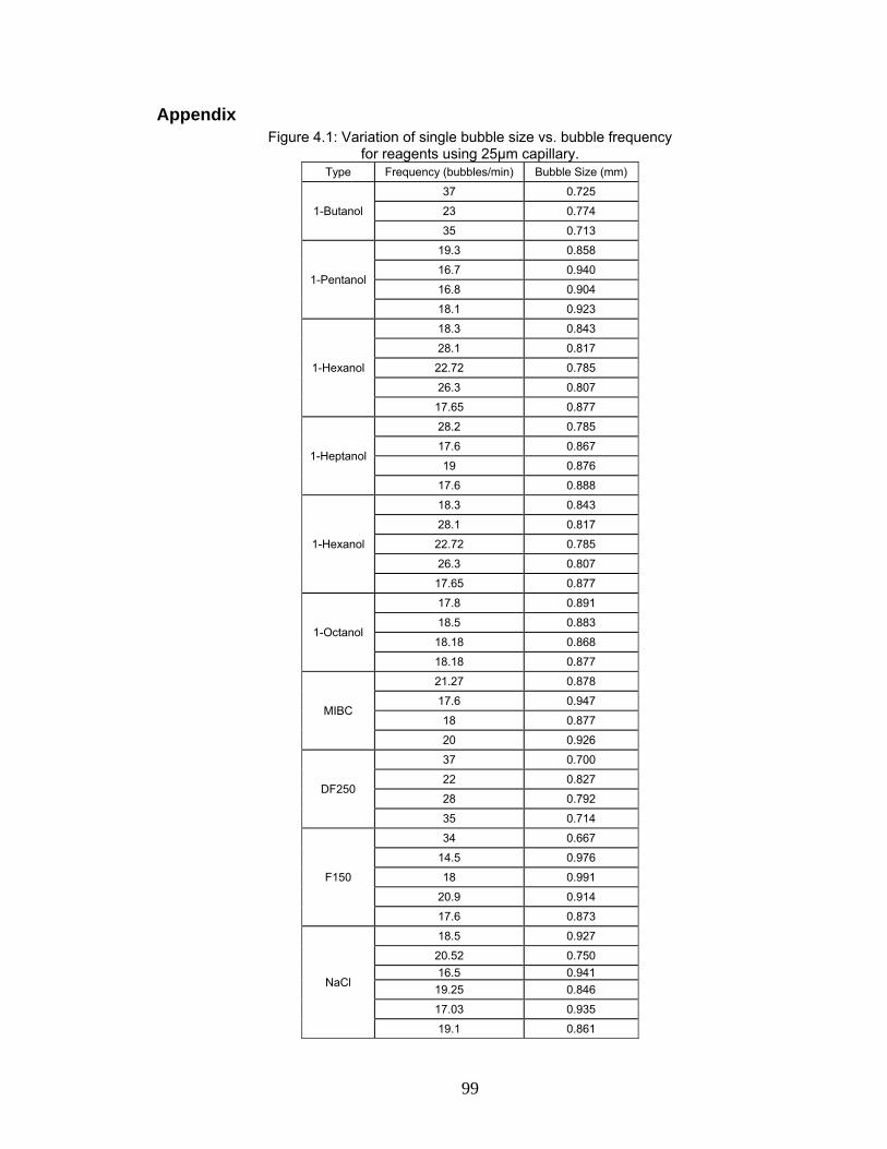
99

Appendix Figure 4.1: Variation of single bubble size vs. bubble frequency

for reagents using 25μm capillary. Type Frequency (bubbles/min) Bubble Size (mm)

1-Butanol

37 0.725

23 0.774

35 0.713

1-Pentanol

19.3 0.858

16.7 0.940

16.8 0.904

18.1 0.923

1-Hexanol

18.3 0.843

28.1 0.817

22.72 0.785

26.3 0.807

17.65 0.877

1-Heptanol

28.2 0.785

17.6 0.867

19 0.876

17.6 0.888

1-Hexanol

18.3 0.843

28.1 0.817

22.72 0.785

26.3 0.807

17.65 0.877

1-Octanol

17.8 0.891

18.5 0.883

18.18 0.868

18.18 0.877

MIBC

21.27 0.878

17.6 0.947

18 0.877

20 0.926

DF250

37 0.700

22 0.827

28 0.792

35 0.714

F150

34 0.667

14.5 0.976

18 0.991

20.9 0.914

17.6 0.873

NaCl

18.5 0.927

20.52 0.750 16.5 0.941 19.25 0.846

17.03 0.935

19.1 0.861

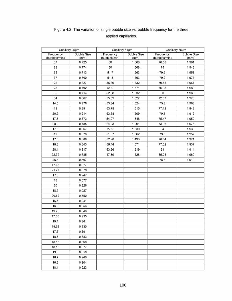
100

Figure 4.2: The variation of single bubble size vs. bubble frequency for the three

applied capillaries.

Capillary 25μm Capillary 51μm Capillary 75μm

Frequency (bubbles/min)

Bubble Size (mm)

Frequency (bubbles/min)

Bubble Size (mm)

Frequency (bubbles/min)

Bubble Size (mm)

37 0.725 50 1.568 70.58 1.961

23 0.774 50 1.568 75 1.943

35 0.713 51.7 1.563 79.2 1.953

37 0.700 51.8 1.563 79.2 1.975

22 0.827 35.86 1.832 70.58 1.967

28 0.792 51.9 1.571 76.33 1.980

35 0.714 52.88 1.532 80 1.968

34 0.667 55.09 1.527 72.87 1.978

14.5 0.976 53.84 1.524 75.3 1.963

18 0.991 53.78 1.515 77.12 1.943

20.9 0.914 53.88 1.509 70.1 1.919

17.6 0.873 54.07 1.548 75.47 1.959

28.2 0.785 24.23 1.901 73.96 1.978

17.6 0.867 27.9 1.830 84 1.936

19 0.876 51.67 1.562 79.5 1.957

17.6 0.888 52.98 1.493 78.84 1.971

18.3 0.843 56.44 1.571 77.02 1.937

28.1 0.817 53.66 1.519 91 1.914

22.72 0.785 47.39 1.526 65.25 1.969

26.3 0.807 78.5 1.919

17.65 0.877

21.27 0.878

17.6 0.947

18 0.877

20 0.926

18.5 0.927

20.52 0.750

16.5 0.941

16.9 0.956

19.25 0.846

17.03 0.935

19.1 0.861

19.68 0.830

17.8 0.891

18.5 0.883

18.18 0.868

18.18 0.877

19.3 0.858

16.7 0.940

16.8 0.904

18.1 0.923

101

Figure 4.3: Bubble size as a function of equivalent concentration for 25μm capillary.

Type Equivalent Concentration

1 3 5 6

1-Butanol 0.72 0.71 0.7

1-Heptanol 0.86 0.87 0.89 0.84

MIBC 0.93 0.92 0.92

1-Octanol 0.88 0.86 0.87 0.85

1-Pentanol 0.93 0.91 0.92 0.88

Figure 4.4: An example of velocity profile where bubble reaches terminal velocity in F150 1ppm for ca. 1.45mm bubble.

Distance (mm)

Velocity (cm/s)

Distance (mm)

Velocity (cm/s)

0 0 718.81 15.76

7.38 22.15 876.71 15.82

24.67 29.72 1035.29 15.90

42.95 25.15 1194.57 15.96

56.76 16.29 1354.95 16.12

68.00 17.43 1597.24 16.17

79.10 15.86 1839.95 16.20

89.86 16.43 2002.76 16.36

105.86 15.79 2166.38 16.36

121.57 15.57 2329.76 16.32

134.57 14.64 2493.67 16.47

152.76 14.50 2658.19 16.44

168.52 14.80 2823.00 16.53

250.86 15.39 2988.48 16.57

405.38 15.52 3093.48 16.61

561.48 15.71

102

Figure 4.6.a : Velocity profiles in F150 (ca 1.5mm). 1ppm

Distance (mm) Velocity (cm/s) Distance (mm) Velocity (cm/s) Distance (mm) Velocity (cm/s)

0.0 0.0 214.5 19.8 360.6 18.6

1.8 10.8 221.0 19.2 369.5 18.0

8.7 30.6 227.1 18.0 375.1 18.0

19.2 32.4 233.2 19.2 383.6 16.8

30.0 32.4 239.7 19.8 457.0 17.4

40.5 30.6 245.8 18.0 603.3 17.9

51.3 34.2 252.0 19.0 757.5 17.3

62.1 30.6 258.4 18.0 908.6 17.2

72.2 30.0 264.8 19.0 1059.0 17.1

81.8 27.6 274.4 18.6 1212.4 17.9

95.4 27.0 286.6 18.0 1367.3 17.5

111.8 22.2 298.5 17.7 1520.9 17.6

126.5 21.9 310.3 17.7 1674.5 17.5

140.8 21.0 322.6 19.2 1907.4 17.9

155.2 21.0 335.1 18.3

186.9 20.0 347.8 19.8

Figure 4.6.b : Velocity profiles in F150 (ca 1.5mm). 3ppm 5ppm

Distance (mm)

Velocity (cm/s)

Distance (mm)

Velocity (cm/s)

Distance (mm)

Velocity (cm/s)

Distance (mm)

Velocity (cm/s)

0.0 0.0 172.7 18.7 0.0 0.0 147.5 17.8

0.2 1.3 175.8 17.6 0.2 0.9 156.7 19.6

4.0 21.3 252.8 17.9 4.1 22.4 162.9 17.4

13.0 32.7 408.2 17.8 12.4 27.5 168.8 18.0

23.6 30.7 564.6 18.6 21.6 27.8 168.8 18.0

33.7 30.0 724.0 18.0 29.8 21.5 246.5 18.4

42.7 24.0 884.1 18.2 35.6 19.0 406.3 18.1

50.3 22.0 1042.2 18.1 40.8 18.0 567.7 18.8

57.0 18.0 1200.9 18.5 46.9 15.0 734.7 19.4

63.3 20.0 1361.0 17.8 53.1 18.6 900.9 18.6

73.1 19.3 1519.9 18.2 62.2 18.0 1064.0 18.6

85.7 18.3 1677.3 18.1 74.2 18.0 1226.1 18.4

98.0 18.7 1915.3 18.1 86.4 18.6 1391.1 19.3

110.6 19.0 104.9 18.4 1558.9 19.0

140.3 17.6 123.3 18.5

166.7 17.3 135.5 18.2

103

Figure 4.6.c : Velocity profiles in F150 (ca 1.5mm). 10ppm

Distance (mm)

Velocity (cm/s)

Distance (mm)

Velocity (cm/s)

0.0 0.0 138.6 17.0

1.3 8.0 147.2 18.0

5.7 18.0 153.3 18.7

12.1 20.7 162.1 17.0

18.0 14.7 161.9 17.7

23.0 15.3 235.8 18.2

28.3 16.7 395.8 18.3

34.2 18.7 555.8 18.2

40.4 18.7 719.8 19.3

46.6 18.0 882.8 18.0

55.8 18.7 1043.7 18.8

67.7 17.0 1209.3 19.1

79.3 18.0 1377.9 19.4

91.3 18.0 1543.7 18.5

103.3 18.0 1706.1 18.7

115.0 17.0 1867.1 18.1

Figure 4.7.a: Velocity profiles in F150 (ca 1.5mm) over the first 3 seconds.

1ppm 3ppm Distance

(mm) Velocity (cm/s)

Distance (mm)

Velocity (cm/s)

Distance (mm)

Velocity (cm/s)

Distance (mm)

Velocity (cm/s)

0.0 0.0 214.5 19.8 0.0 0.0 172.7 18.7

1.8 10.8 221.0 19.2 0.2 1.3 175.8 17.6

8.7 30.6 227.1 18.0 4.0 21.3 252.8 17.9

19.2 32.4 233.2 19.2 13.0 32.7 408.2 17.8

30.0 32.4 239.7 19.8 23.6 30.7 564.6 18.6

40.5 30.6 245.8 18.0 33.7 30.0

51.3 34.2 252.0 19.0 42.7 24.0

62.1 30.6 258.4 18.0 50.3 22.0

72.2 30.0 264.8 19.0 57.0 18.0

81.8 27.6 274.4 18.6 63.3 20.0

95.4 27.0 286.6 18.0 73.1 19.3

111.8 22.2 298.5 17.7 85.7 18.3

126.5 21.9 310.3 17.7 98.0 18.7

140.8 21.0 322.6 19.2 110.6 19.0

155.2 21.0 335.1 18.3 140.3 17.6

186.9 20.0 347.8 19.8 166.7 17.3

104

Figure 4.7.b: Velocity profiles in F150 (ca 1.5mm) over the first 3 seconds.

Figure 4.8: The influence of reagent concentration on maximum velocity

in the presence of MIBC, NaCl and F150. 1 3 5 6

MIBC 22 21.82 15.14 11.47

NaCl 20.28 20.16 19.62 17

F150 34.2 32.67 27.79 20.67

5ppm 10ppm Distance

(mm) Velocity (cm/s)

Distance (mm)

Velocity (cm/s)

Distance (mm)

Velocity (cm/s)

Distance (mm)

Velocity (cm/s)

0.0 0.0 147.5 17.8 0.0 0.0 126.8 18.3

0.2 0.9 156.7 19.6 1.3 8.0 138.6 17.0

4.1 22.4 162.9 17.4 5.7 18.0 147.2 18.0

12.4 27.5 168.8 18.0 12.1 20.7 153.3 18.7

21.6 27.8 168.8 18.0 18.0 14.7 162.1 17.0

29.8 21.5 246.5 18.4 23.0 15.3 161.9 17.7

35.6 19.0 406.3 18.1 28.3 16.7 235.8 18.2

40.8 18.0 567.7 18.8 34.2 18.7 395.8 18.3

46.9 15.0 40.4 18.7 555.8 18.2

53.1 18.6 46.6 18.0

62.2 18.0 55.8 18.7

74.2 18.0 67.7 17.0

86.4 18.6 79.3 18.0

104.9 18.4 91.3 18.0

123.3 18.5 103.3 18.0

135.5 18.2 115.0 17.0

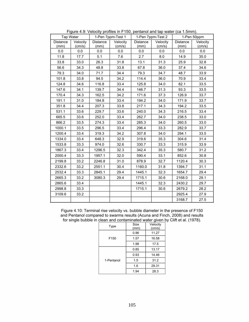
105

Figure 4.9: Velocity profiles in F150, pentanol and tap water (ca 1.5mm). Tap Water 1-Pen 7ppm-Test 1 1-Pen 7ppm-Test 2 1-Pen 50ppm

Distance (mm)

Velocity (cm/s)

Distance (mm)

Velocity (cm/s)

Distance (mm)

Velocity (cm/s)

Distance (mm)

Velocity (cm/s)

0.0 0.0 0.0 0.0 0.0 0.0 0.0 0.0 11.8 17.7 5.1 7.6 2.7 8.0 14.9 35.0 33.8 33.0 26.3 31.8 13.1 31.3 25.9 32.8 56.6 34.3 48.8 33.8 67.8 36.0 37.4 34.6 79.3 34.0 71.7 34.4 79.3 34.7 48.7 33.9 101.8 33.8 94.5 34.2 114.4 36.0 70.9 33.4 124.8 34.6 116.8 33.4 125.8 34.0 82.1 33.5 147.6 34.1 139.7 34.4 146.7 31.3 93.3 33.5 170.4 34.3 162.5 34.2 171.6 37.3 126.9 33.7 191.1 31.0 184.8 33.4 194.2 34.0 171.9 33.7 351.8 34.4 207.3 33.8 217.1 34.3 194.2 33.5 531.1 33.6 229.7 33.6 240.0 34.3 216.5 33.4 665.5 33.6 252.0 33.4 262.7 34.0 238.5 33.0 866.2 33.5 274.3 33.4 285.3 34.0 260.5 33.0

1000.1 33.5 296.5 33.4 296.4 33.3 282.9 33.7 1200.4 33.4 319.3 34.2 307.8 34.0 294.1 33.5 1334.0 33.4 648.3 32.9 319.6 35.3 304.6 31.4 1533.8 33.3 974.0 32.6 330.7 33.3 315.9 33.9 1867.3 33.4 1296.5 32.3 342.4 35.3 580.7 31.2 2000.4 33.3 1957.1 32.0 590.4 33.1 852.6 30.8 2199.8 33.2 2246.8 31.0 878.9 32.7 1120.4 30.3 2332.6 33.2 2551.1 30.4 1160.0 31.8 1394.7 31.1 2532.4 33.3 2845.1 29.4 1445.1 32.3 1654.7 29.4 2665.3 33.2 3080.3 29.4 1715.1 30.6 2168.0 29.1 2865.6 33.4 1445.1 32.3 2430.2 29.7 2998.8 33.3 1715.1 30.6 2679.2 28.2 3109.6 33.2 2925.4 27.9

3168.7 27.5

Figure 4.10: Terminal rise velocity vs. bubble diameter in the presence of F150 and Pentanol compared to swarms results (Acuna and Finch, 2008) and results

for single bubble in clean and contaminated water given by Clift et al. (1978). Type Size

(mm) Velocity (cm/s)

F150

0.96 11.27

1.57 16.58

1.98 17.5

1-Pentanol

0.85 13.17

0.93 14.46

1.5 31.2

1.6 29.31

1.94 28.3

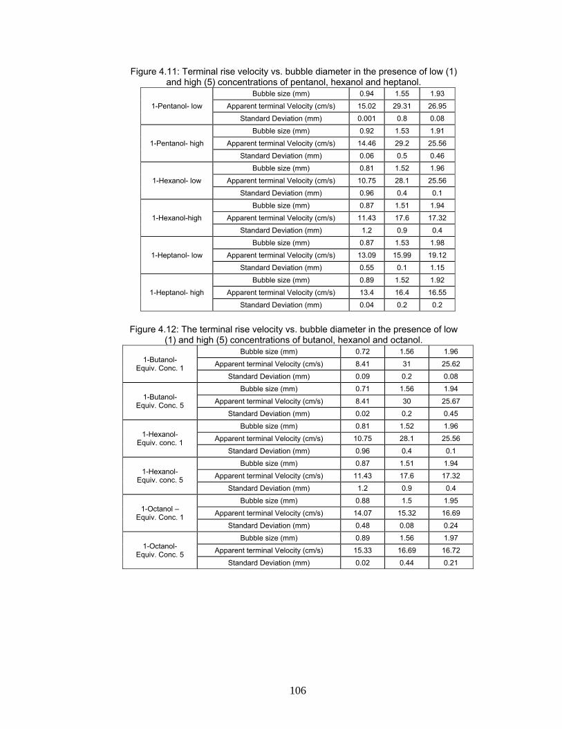
106

Figure 4.11: Terminal rise velocity vs. bubble diameter in the presence of low (1) and high (5) concentrations of pentanol, hexanol and heptanol.

1-Pentanol- low

Bubble size (mm) 0.94 1.55 1.93

Apparent terminal Velocity (cm/s) 15.02 29.31 26.95

Standard Deviation (mm) 0.001 0.8 0.08

1-Pentanol- high

Bubble size (mm) 0.92 1.53 1.91

Apparent terminal Velocity (cm/s) 14.46 29.2 25.56

Standard Deviation (mm) 0.06 0.5 0.46

1-Hexanol- low

Bubble size (mm) 0.81 1.52 1.96

Apparent terminal Velocity (cm/s) 10.75 28.1 25.56

Standard Deviation (mm) 0.96 0.4 0.1

1-Hexanol-high

Bubble size (mm) 0.87 1.51 1.94

Apparent terminal Velocity (cm/s) 11.43 17.6 17.32

Standard Deviation (mm) 1.2 0.9 0.4

1-Heptanol- low

Bubble size (mm) 0.87 1.53 1.98

Apparent terminal Velocity (cm/s) 13.09 15.99 19.12

Standard Deviation (mm) 0.55 0.1 1.15

1-Heptanol- high

Bubble size (mm) 0.89 1.52 1.92

Apparent terminal Velocity (cm/s) 13.4 16.4 16.55

Standard Deviation (mm) 0.04 0.2 0.2

Figure 4.12: The terminal rise velocity vs. bubble diameter in the presence of low

(1) and high (5) concentrations of butanol, hexanol and octanol.

1-Butanol- Equiv. Conc. 1

Bubble size (mm) 0.72 1.56 1.96

Apparent terminal Velocity (cm/s) 8.41 31 25.62

Standard Deviation (mm) 0.09 0.2 0.08

1-Butanol- Equiv. Conc. 5

Bubble size (mm) 0.71 1.56 1.94

Apparent terminal Velocity (cm/s) 8.41 30 25.67

Standard Deviation (mm) 0.02 0.2 0.45

1-Hexanol- Equiv. conc. 1

Bubble size (mm) 0.81 1.52 1.96

Apparent terminal Velocity (cm/s) 10.75 28.1 25.56

Standard Deviation (mm) 0.96 0.4 0.1

1-Hexanol- Equiv. conc. 5

Bubble size (mm) 0.87 1.51 1.94

Apparent terminal Velocity (cm/s) 11.43 17.6 17.32

Standard Deviation (mm) 1.2 0.9 0.4

1-Octanol – Equiv. Conc. 1

Bubble size (mm) 0.88 1.5 1.95

Apparent terminal Velocity (cm/s) 14.07 15.32 16.69

Standard Deviation (mm) 0.48 0.08 0.24

1-Octanol- Equiv. Conc. 5

Bubble size (mm) 0.89 1.56 1.97

Apparent terminal Velocity (cm/s) 15.33 16.69 16.72

Standard Deviation (mm) 0.02 0.44 0.21

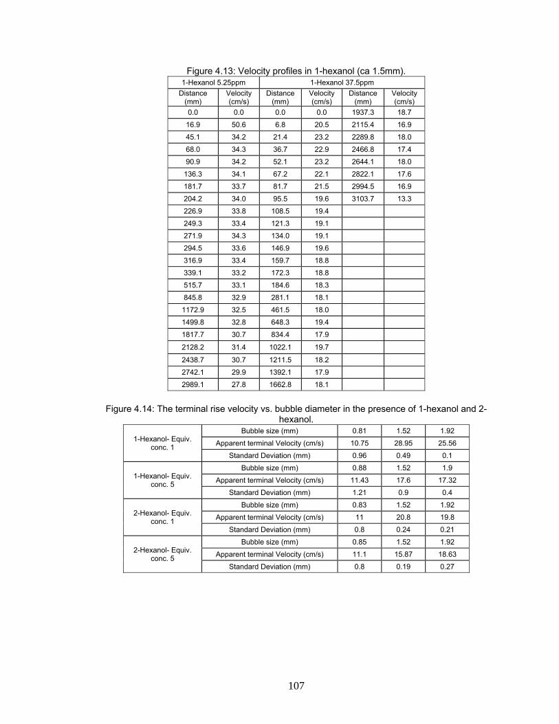
107

Figure 4.13: Velocity profiles in 1-hexanol (ca 1.5mm). 1-Hexanol 5.25ppm 1-Hexanol 37.5ppm

Distance (mm)

Velocity (cm/s)

Distance (mm)

Velocity (cm/s)

Distance (mm)

Velocity (cm/s)

0.0 0.0 0.0 0.0 1937.3 18.7

16.9 50.6 6.8 20.5 2115.4 16.9

45.1 34.2 21.4 23.2 2289.8 18.0

68.0 34.3 36.7 22.9 2466.8 17.4

90.9 34.2 52.1 23.2 2644.1 18.0

136.3 34.1 67.2 22.1 2822.1 17.6

181.7 33.7 81.7 21.5 2994.5 16.9

204.2 34.0 95.5 19.6 3103.7 13.3

226.9 33.8 108.5 19.4

249.3 33.4 121.3 19.1

271.9 34.3 134.0 19.1

294.5 33.6 146.9 19.6

316.9 33.4 159.7 18.8

339.1 33.2 172.3 18.8

515.7 33.1 184.6 18.3

845.8 32.9 281.1 18.1

1172.9 32.5 461.5 18.0

1499.8 32.8 648.3 19.4

1817.7 30.7 834.4 17.9

2128.2 31.4 1022.1 19.7

2438.7 30.7 1211.5 18.2

2742.1 29.9 1392.1 17.9

2989.1 27.8 1662.8 18.1

Figure 4.14: The terminal rise velocity vs. bubble diameter in the presence of 1-hexanol and 2-

hexanol.

1-Hexanol- Equiv. conc. 1

Bubble size (mm) 0.81 1.52 1.92

Apparent terminal Velocity (cm/s) 10.75 28.95 25.56

Standard Deviation (mm) 0.96 0.49 0.1

1-Hexanol- Equiv. conc. 5

Bubble size (mm) 0.88 1.52 1.9

Apparent terminal Velocity (cm/s) 11.43 17.6 17.32

Standard Deviation (mm) 1.21 0.9 0.4

2-Hexanol- Equiv. conc. 1

Bubble size (mm) 0.83 1.52 1.92

Apparent terminal Velocity (cm/s) 11 20.8 19.8

Standard Deviation (mm) 0.8 0.24 0.21

2-Hexanol- Equiv. conc. 5

Bubble size (mm) 0.85 1.52 1.92

Apparent terminal Velocity (cm/s) 11.1 15.87 18.63

Standard Deviation (mm) 0.8 0.19 0.27

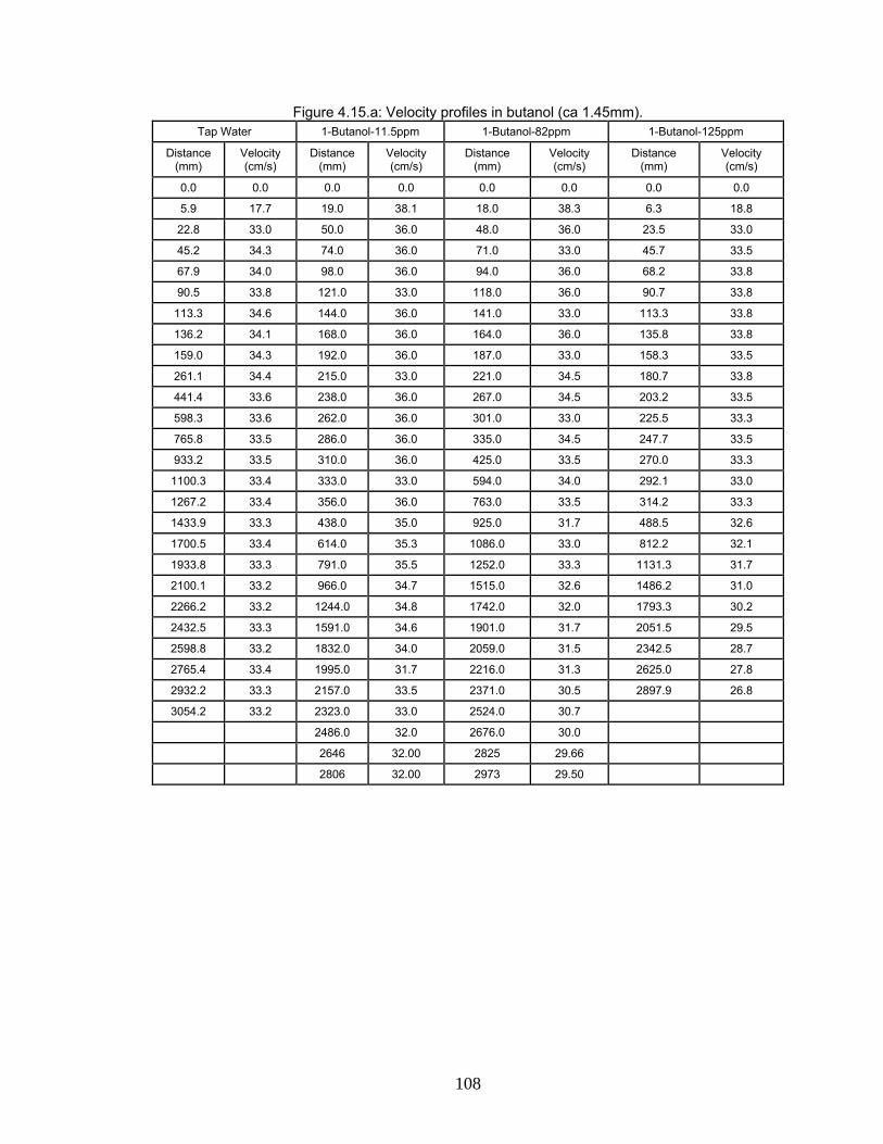
108

Figure 4.15.a: Velocity profiles in butanol (ca 1.45mm). Tap Water 1-Butanol-11.5ppm 1-Butanol-82ppm 1-Butanol-125ppm

Distance (mm)

Velocity (cm/s)

Distance (mm)

Velocity (cm/s)

Distance (mm)

Velocity (cm/s)

Distance (mm)

Velocity (cm/s)

0.0 0.0 0.0 0.0 0.0 0.0 0.0 0.0

5.9 17.7 19.0 38.1 18.0 38.3 6.3 18.8

22.8 33.0 50.0 36.0 48.0 36.0 23.5 33.0

45.2 34.3 74.0 36.0 71.0 33.0 45.7 33.5

67.9 34.0 98.0 36.0 94.0 36.0 68.2 33.8

90.5 33.8 121.0 33.0 118.0 36.0 90.7 33.8

113.3 34.6 144.0 36.0 141.0 33.0 113.3 33.8

136.2 34.1 168.0 36.0 164.0 36.0 135.8 33.8

159.0 34.3 192.0 36.0 187.0 33.0 158.3 33.5

261.1 34.4 215.0 33.0 221.0 34.5 180.7 33.8

441.4 33.6 238.0 36.0 267.0 34.5 203.2 33.5

598.3 33.6 262.0 36.0 301.0 33.0 225.5 33.3

765.8 33.5 286.0 36.0 335.0 34.5 247.7 33.5

933.2 33.5 310.0 36.0 425.0 33.5 270.0 33.3

1100.3 33.4 333.0 33.0 594.0 34.0 292.1 33.0

1267.2 33.4 356.0 36.0 763.0 33.5 314.2 33.3

1433.9 33.3 438.0 35.0 925.0 31.7 488.5 32.6

1700.5 33.4 614.0 35.3 1086.0 33.0 812.2 32.1

1933.8 33.3 791.0 35.5 1252.0 33.3 1131.3 31.7

2100.1 33.2 966.0 34.7 1515.0 32.6 1486.2 31.0

2266.2 33.2 1244.0 34.8 1742.0 32.0 1793.3 30.2

2432.5 33.3 1591.0 34.6 1901.0 31.7 2051.5 29.5

2598.8 33.2 1832.0 34.0 2059.0 31.5 2342.5 28.7

2765.4 33.4 1995.0 31.7 2216.0 31.3 2625.0 27.8

2932.2 33.3 2157.0 33.5 2371.0 30.5 2897.9 26.8

3054.2 33.2 2323.0 33.0 2524.0 30.7

2486.0 32.0 2676.0 30.0

2646 32.00 2825 29.66

2806 32.00 2973 29.50

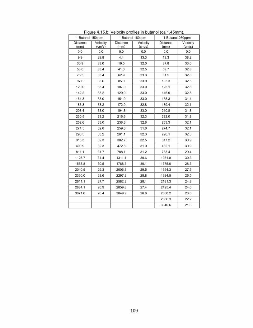
109

Figure 4.15.b: Velocity profiles in butanol (ca 1.45mm). 1-Butanol-150ppm 1-Butanol-180ppm 1-Butanol-260ppm

Distance (mm)

Velocity (cm/s)

Distance (mm)

Velocity (cm/s)

Distance (mm)

Velocity (cm/s)

0.0 0.0 0.0 0.0 0.0 0.0

9.9 29.8 4.4 13.3 13.3 38.2

30.9 33.0 19.5 32.0 37.8 33.0

53.0 33.4 41.0 32.5 59.7 32.8

75.3 33.4 62.9 33.3 81.5 32.8

97.6 33.6 85.0 33.0 103.3 32.5

120.0 33.4 107.0 33.0 125.1 32.8

142.2 33.2 129.0 33.0 146.9 32.8

164.3 33.0 151.0 33.0 168.3 31.4

186.3 33.2 172.9 32.8 189.4 32.1

208.4 33.0 194.8 33.0 210.8 31.8

230.5 33.2 216.6 32.3 232.0 31.8

252.6 33.0 238.3 32.8 253.3 32.1

274.5 32.8 259.8 31.8 274.7 32.1

296.5 33.2 281.1 32.3 296.1 32.3

318.3 32.3 302.7 32.5 317.2 30.9

490.9 32.3 472.8 31.9 482.1 30.9

811.1 31.7 788.1 31.2 783.4 29.4

1126.7 31.4 1311.1 30.6 1081.8 30.3

1588.8 30.5 1768.3 30.1 1375.0 28.3

2040.5 29.3 2006.3 29.5 1654.3 27.5

2330.0 28.6 2297.9 28.8 1924.5 26.5

2611.1 27.7 2582.3 28.1 2181.3 24.8

2884.1 26.9 2859.8 27.4 2425.4 24.0

3071.6 26.4 3049.9 26.6 2660.2 23.0

2886.3 22.2

3040.6 21.6

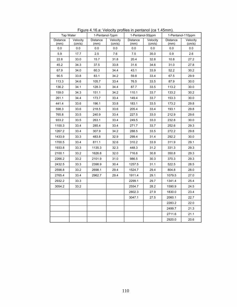
110

Figure 4.16.a: Velocity profiles in pentanol (ca 1.45mm). Tap Water 1-Pentanol-7ppm 1-Pentanol-50ppm 1-Pentanol-110ppm

Distance (mm)

Velocity (cm/s)

Distance (mm)

Velocity (cm/s)

Distance (mm)

Velocity (cm/s)

Distance (mm)

Velocity (cm/s)

0.0 0.0 0.0 0.0 0.0 0.0 0.0 0.0

5.9 17.7 2.5 7.6 7.5 35.0 0.9 2.6

22.8 33.0 15.7 31.8 20.4 32.8 10.8 27.2

45.2 34.3 37.5 33.8 31.6 34.6 31.0 27.8

67.9 34.0 60.3 34.4 43.1 33.9 52.2 30.2

90.5 33.8 83.1 34.2 59.8 33.4 67.5 29.9

113.3 34.6 105.7 33.4 76.5 33.5 87.9 30.0

136.2 34.1 128.3 34.4 87.7 33.5 113.2 30.0

159.0 34.3 151.1 34.2 110.1 33.7 133.2 30.2

261.1 34.4 173.7 33.4 149.4 33.7 153.3 30.0

441.4 33.6 196.1 33.8 183.1 33.5 173.2 29.8

598.3 33.6 218.5 33.6 205.4 33.4 193.1 29.8

765.8 33.5 240.9 33.4 227.5 33.0 212.9 29.6

933.2 33.5 263.1 33.4 249.5 33.0 232.8 30.0

1100.3 33.4 285.4 33.4 271.7 33.7 252.6 29.3

1267.2 33.4 307.9 34.2 288.5 33.5 272.2 29.8

1433.9 33.3 483.8 32.9 299.4 31.4 292.2 30.0

1700.5 33.4 811.1 32.6 310.2 33.9 311.9 29.1

1933.8 33.3 1135.3 32.3 448.3 31.2 331.3 29.3

2100.1 33.2 1626.8 32.0 716.6 30.8 350.8 29.3

2266.2 33.2 2101.9 31.0 986.5 30.3 370.3 29.3

2432.5 33.3 2398.9 30.4 1257.5 31.1 522.5 28.5

2598.8 33.2 2698.1 29.4 1524.7 29.4 804.8 28.0

2765.4 33.4 2962.7 29.4 1911.4 29.1 1079.5 27.0

2932.2 33.3 2299.1 29.7 1341.4 25.4

3054.2 33.2 2554.7 28.2 1590.9 24.5

2802.3 27.9 1830.0 23.4

3047.1 27.5 2060.1 22.7

2283.2 22.0

2499.7 21.3

2711.6 21.1

2920.0 20.6

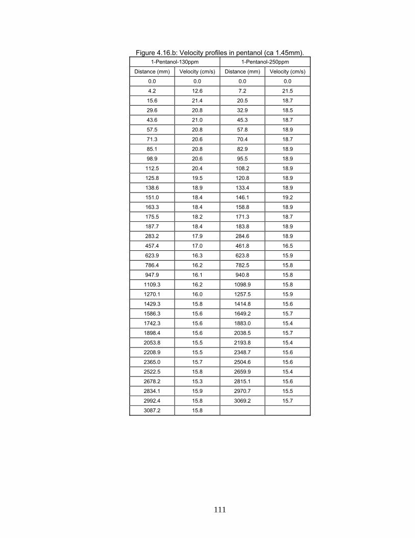
111

Figure 4.16.b: Velocity profiles in pentanol (ca 1.45mm). 1-Pentanol-130ppm 1-Pentanol-250ppm

Distance (mm) Velocity (cm/s) Distance (mm) Velocity (cm/s)

0.0 0.0 0.0 0.0

4.2 12.6 7.2 21.5

15.6 21.4 20.5 18.7

29.6 20.8 32.9 18.5

43.6 21.0 45.3 18.7

57.5 20.8 57.8 18.9

71.3 20.6 70.4 18.7

85.1 20.8 82.9 18.9

98.9 20.6 95.5 18.9

112.5 20.4 108.2 18.9

125.8 19.5 120.8 18.9

138.6 18.9 133.4 18.9

151.0 18.4 146.1 19.2

163.3 18.4 158.8 18.9

175.5 18.2 171.3 18.7

187.7 18.4 183.8 18.9

283.2 17.9 284.6 18.9

457.4 17.0 461.8 16.5

623.9 16.3 623.8 15.9

786.4 16.2 782.5 15.8

947.9 16.1 940.8 15.8

1109.3 16.2 1098.9 15.8

1270.1 16.0 1257.5 15.9

1429.3 15.8 1414.8 15.6

1586.3 15.6 1649.2 15.7

1742.3 15.6 1883.0 15.4

1898.4 15.6 2038.5 15.7

2053.8 15.5 2193.8 15.4

2208.9 15.5 2348.7 15.6

2365.0 15.7 2504.6 15.6

2522.5 15.8 2659.9 15.4

2678.2 15.3 2815.1 15.6

2834.1 15.9 2970.7 15.5

2992.4 15.8 3069.2 15.7

3087.2 15.8

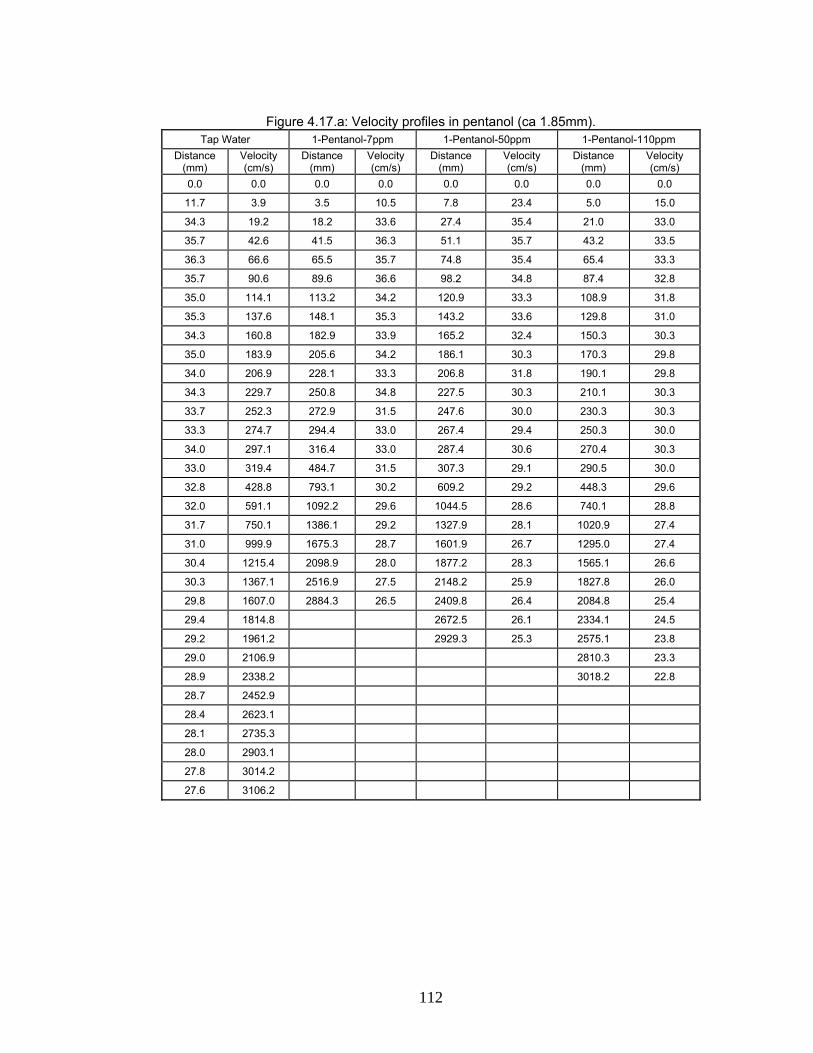
112

Figure 4.17.a: Velocity profiles in pentanol (ca 1.85mm).

Tap Water 1-Pentanol-7ppm 1-Pentanol-50ppm 1-Pentanol-110ppm Distance

(mm) Velocity (cm/s)

Distance (mm)

Velocity (cm/s)

Distance (mm)

Velocity (cm/s)

Distance (mm)

Velocity (cm/s)

0.0 0.0 0.0 0.0 0.0 0.0 0.0 0.0

11.7 3.9 3.5 10.5 7.8 23.4 5.0 15.0

34.3 19.2 18.2 33.6 27.4 35.4 21.0 33.0

35.7 42.6 41.5 36.3 51.1 35.7 43.2 33.5

36.3 66.6 65.5 35.7 74.8 35.4 65.4 33.3

35.7 90.6 89.6 36.6 98.2 34.8 87.4 32.8

35.0 114.1 113.2 34.2 120.9 33.3 108.9 31.8

35.3 137.6 148.1 35.3 143.2 33.6 129.8 31.0

34.3 160.8 182.9 33.9 165.2 32.4 150.3 30.3

35.0 183.9 205.6 34.2 186.1 30.3 170.3 29.8

34.0 206.9 228.1 33.3 206.8 31.8 190.1 29.8

34.3 229.7 250.8 34.8 227.5 30.3 210.1 30.3

33.7 252.3 272.9 31.5 247.6 30.0 230.3 30.3

33.3 274.7 294.4 33.0 267.4 29.4 250.3 30.0

34.0 297.1 316.4 33.0 287.4 30.6 270.4 30.3

33.0 319.4 484.7 31.5 307.3 29.1 290.5 30.0

32.8 428.8 793.1 30.2 609.2 29.2 448.3 29.6

32.0 591.1 1092.2 29.6 1044.5 28.6 740.1 28.8

31.7 750.1 1386.1 29.2 1327.9 28.1 1020.9 27.4

31.0 999.9 1675.3 28.7 1601.9 26.7 1295.0 27.4

30.4 1215.4 2098.9 28.0 1877.2 28.3 1565.1 26.6

30.3 1367.1 2516.9 27.5 2148.2 25.9 1827.8 26.0

29.8 1607.0 2884.3 26.5 2409.8 26.4 2084.8 25.4

29.4 1814.8 2672.5 26.1 2334.1 24.5

29.2 1961.2 2929.3 25.3 2575.1 23.8

29.0 2106.9 2810.3 23.3

28.9 2338.2 3018.2 22.8

28.7 2452.9

28.4 2623.1

28.1 2735.3

28.0 2903.1

27.8 3014.2

27.6 3106.2

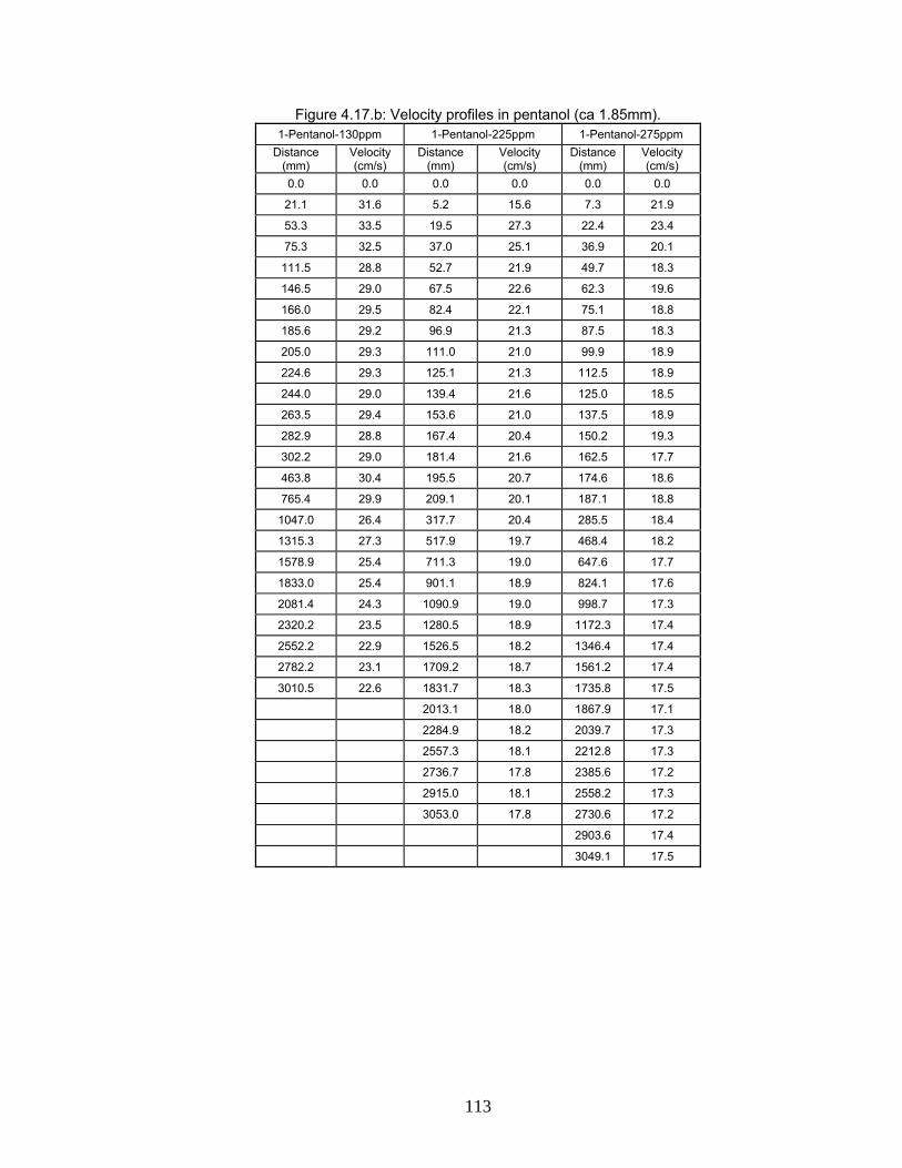
113

Figure 4.17.b: Velocity profiles in pentanol (ca 1.85mm). 1-Pentanol-130ppm 1-Pentanol-225ppm 1-Pentanol-275ppm

Distance (mm)

Velocity (cm/s)

Distance (mm)

Velocity (cm/s)

Distance (mm)

Velocity (cm/s)

0.0 0.0 0.0 0.0 0.0 0.0

21.1 31.6 5.2 15.6 7.3 21.9

53.3 33.5 19.5 27.3 22.4 23.4

75.3 32.5 37.0 25.1 36.9 20.1

111.5 28.8 52.7 21.9 49.7 18.3

146.5 29.0 67.5 22.6 62.3 19.6

166.0 29.5 82.4 22.1 75.1 18.8

185.6 29.2 96.9 21.3 87.5 18.3

205.0 29.3 111.0 21.0 99.9 18.9

224.6 29.3 125.1 21.3 112.5 18.9

244.0 29.0 139.4 21.6 125.0 18.5

263.5 29.4 153.6 21.0 137.5 18.9

282.9 28.8 167.4 20.4 150.2 19.3

302.2 29.0 181.4 21.6 162.5 17.7

463.8 30.4 195.5 20.7 174.6 18.6

765.4 29.9 209.1 20.1 187.1 18.8

1047.0 26.4 317.7 20.4 285.5 18.4

1315.3 27.3 517.9 19.7 468.4 18.2

1578.9 25.4 711.3 19.0 647.6 17.7

1833.0 25.4 901.1 18.9 824.1 17.6

2081.4 24.3 1090.9 19.0 998.7 17.3

2320.2 23.5 1280.5 18.9 1172.3 17.4

2552.2 22.9 1526.5 18.2 1346.4 17.4

2782.2 23.1 1709.2 18.7 1561.2 17.4

3010.5 22.6 1831.7 18.3 1735.8 17.5

2013.1 18.0 1867.9 17.1

2284.9 18.2 2039.7 17.3

2557.3 18.1 2212.8 17.3

2736.7 17.8 2385.6 17.2

2915.0 18.1 2558.2 17.3

3053.0 17.8 2730.6 17.2

2903.6 17.4

3049.1 17.5

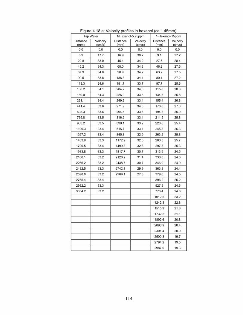
114

Figure 4.18.a: Velocity profiles in hexanol (ca 1.45mm). Tap Water 1-Hexanol-5.25ppm 1-Hexanol-15ppm

Distance (mm)

Velocity (cm/s)

Distance (mm)

Velocity (cm/s)

Distance (mm)

Velocity (cm/s)

0.0 0.0 0.0 0.0 0.0 0.0

5.9 17.7 16.9 38.2 9.1 27.2

22.8 33.0 45.1 34.2 27.6 28.4

45.2 34.3 68.0 34.3 46.2 27.5

67.9 34.0 90.9 34.2 63.2 27.5

90.5 33.8 136.3 34.1 80.1 27.2

113.3 34.6 181.7 33.7 97.7 25.6

136.2 34.1 204.2 34.0 115.8 28.8

159.0 34.3 226.9 33.8 134.3 26.8

261.1 34.4 249.3 33.4 155.4 26.8

441.4 33.6 271.9 34.3 176.6 27.0

598.3 33.6 294.5 33.6 194.3 25.9

765.8 33.5 316.9 33.4 211.5 25.8

933.2 33.5 339.1 33.2 228.6 25.4

1100.3 33.4 515.7 33.1 245.8 26.3

1267.2 33.4 845.8 32.9 263.2 25.8

1433.9 33.3 1172.9 32.5 280.3 25.7

1700.5 33.4 1499.8 32.8 297.3 25.3

1933.8 33.3 1817.7 30.7 313.9 24.5

2100.1 33.2 2128.2 31.4 330.3 24.6

2266.2 33.2 2438.7 30.7 346.9 24.9

2432.5 33.3 2742.1 29.9 363.3 24.4

2598.8 33.2 2989.1 27.8 379.6 24.5

2765.4 33.4 396.2 25.2

2932.2 33.3 527.5 24.6

3054.2 33.2 773.4 24.6

1012.5 23.2

1242.3 22.8

1515.9 21.8

1732.2 21.1

1892.6 20.8

2098.9 20.4

2301.4 20.0

2500.3 19.7

2794.2 19.5

2987.0 19.3

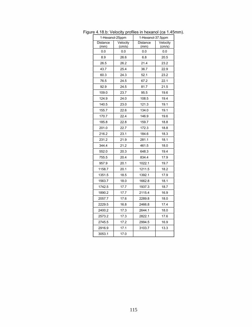
115

Figure 4.18.b: Velocity profiles in hexanol (ca 1.45mm). 1-Hexanol-25ppm 1-Hexanol-37.5ppm

Distance (mm)

Velocity (cm/s)

Distance (mm)

Velocity (cm/s)

0.0 0.0 0.0 0.0

8.9 26.6 6.8 20.5

26.5 26.2 21.4 23.2

43.7 25.4 36.7 22.9

60.3 24.3 52.1 23.2

76.5 24.5 67.2 22.1

92.9 24.5 81.7 21.5

109.0 23.7 95.5 19.6

124.9 24.0 108.5 19.4

140.5 23.0 121.3 19.1

155.7 22.6 134.0 19.1

170.7 22.4 146.9 19.6

185.8 22.8 159.7 18.8

201.0 22.7 172.3 18.8

216.2 23.1 184.6 18.3

231.2 21.9 281.1 18.1

344.4 21.2 461.5 18.0

552.0 20.3 648.3 19.4

755.5 20.4 834.4 17.9

957.9 20.1 1022.1 19.7

1158.7 20.1 1211.5 18.2

1351.5 18.5 1392.1 17.9

1563.7 18.0 1662.8 18.1

1742.5 17.7 1937.3 18.7

1890.2 17.7 2115.4 16.9

2057.7 17.6 2289.8 18.0

2229.5 16.8 2466.8 17.4

2400.2 17.3 2644.1 18.0

2573.2 17.3 2822.1 17.6

2745.5 17.2 2994.5 16.9

2916.9 17.1 3103.7 13.3

3053.1 17.0

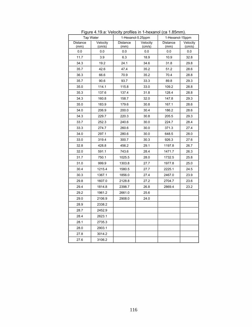
116

Figure 4.19.a: Velocity profiles in 1-hexanol (ca 1.85mm). Tap Water 1-Hexanol-5.25ppm 1-Hexanol-15ppm

Distance (mm)

Velocity (cm/s)

Distance (mm)

Velocity (cm/s)

Distance (mm)

Velocity (cm/s)

0.0 0.0 0.0 0.0 0.0 0.0

11.7 3.9 6.3 18.9 10.9 32.8

34.3 19.2 24.1 34.6 31.8 29.8

35.7 42.6 47.4 35.2 51.2 28.6

36.3 66.6 70.9 35.2 70.4 28.8

35.7 90.6 93.7 33.3 89.8 29.3

35.0 114.1 115.8 33.0 109.2 28.8

35.3 137.6 137.4 31.8 128.4 28.8

34.3 160.8 158.7 32.0 147.8 29.3

35.0 183.9 179.6 30.8 167.1 28.6

34.0 206.9 200.0 30.4 186.2 28.6

34.3 229.7 220.3 30.8 205.5 29.3

33.7 252.3 240.6 30.0 224.7 28.4

33.3 274.7 260.6 30.0 371.3 27.4

34.0 297.1 280.6 30.0 648.5 28.0

33.0 319.4 300.7 30.3 926.3 27.6

32.8 428.8 456.2 29.1 1197.8 26.7

32.0 591.1 743.6 28.4 1471.7 26.3

31.7 750.1 1025.5 28.0 1732.5 25.8

31.0 999.9 1303.8 27.7 1977.8 25.0

30.4 1215.4 1580.5 27.7 2225.1 24.5

30.3 1367.1 1856.0 27.4 2467.0 23.9

29.8 1607.0 2128.8 27.2 2704.7 23.6

29.4 1814.8 2398.7 26.8 2869.4 23.2

29.2 1961.2 2661.0 25.6

29.0 2106.9 2908.0 24.0

28.9 2338.2

28.7 2452.9

28.4 2623.1

28.1 2735.3

28.0 2903.1

27.8 3014.2

27.6 3106.2

117

Figure 4.19.b: Velocity profiles in 1-hexanol (ca 1.85mm). 1-Hexanol-25ppm 1-Hexanol-37.5ppm

Distance (mm) Velocity (cm/s) Distance (mm) Velocity (cm/s)

0.0 0.0 0.0 0.0

11.3 33.8 1.3 3.8

33.1 31.7 11.2 26.0

53.6 29.7 27.3 22.3

71.6 24.3 47.3 18.9

87.9 24.8 65.9 18.3

104.4 24.8 75.3 18.0

120.9 24.5 84.8 18.3

137.6 25.7 103.3 18.8

154.1 23.7 121.9 18.3

170.5 25.6 146.3 18.3

187.3 24.7 170.8 18.5

203.6 24.3 266.7 17.9

219.9 24.8 444.7 17.7

236.3 24.5 620.2 17.4

252.7 24.5 794.8 17.5

379.5 23.7 1056.8 17.5

620.2 24.4 1318.9 17.5

862.3 24.0 1581.1 17.5

1101.4 23.8 1843.6 17.6

1335.8 23.1 2018.8 17.5

1571.0 22.5 2193.5 17.5

1795.7 22.5 2368.9 17.6

2010.2 21.9 2544.8 17.6

2228.3 21.7 2721.0 17.6

2444.7 21.6 2897.6 17.7

2658.6 21.2

2869.1 20.9

3022.1 20.8

Figure 4.20: Apparent terminal velocity vs. concentration of single bubbles in 1-butanol.

Current Work- 1.45mm@350mm

Concentration (ppm) 11 82 125 150 180 260 2500

Velocity (cm/s) 36 34.5 33.4 32.3 32.2 30.9 20

Krzan et al- 1.42mm@350mm

Concentration (ppm) 148 370 740 2220 2368 7400

Velocity (cm/s) 18 16 16 16 16 16

Figure 4.21: Apparent terminal velocity vs. concentration of single bubbles in 1-pentanol.

Current Work-1.45mm@350mm

Concentration (ppm) 7 50 110 130 250

Velocity (cm/s) 33.8 33 29.2 17.6 17.2

Krzan et al- 1.42mm@350mm

Concentration (ppm) 8.81 44.07 88.15 132.225 264.45 440.75

Velocity (cm/s) 34 31.5 26.5 19 16.5 16.5

118

Figure 4.22: Apparent terminal velocity vs. concentration of single bubbles in 1-hexanol. Current Work-

1.45mm@350mm Concentration (ppm) 5.25 15 25 37.5

Velocity (cm/s) 33.2 24.5 21.2 18

Krzan et al- 1.42mm@350mm

Concentration (ppm) 20.43 40.87 71.52 510.9

Velocity (cm/s) 27 19.5 16.5 15.5

Figure 4.23: Apparent terminal velocity (at 3000mm over the capillary) vs. concentration (ppm) of

single bubbles for range of n-alcohols for ca. 1.45mm bubbles.

1-Butanol Concentration (ppm) 11 82 125 150 180 260 2500

Velocity (cm/s) 32 29.55 26.75 26.4 26.5 21.6 16

1-Pentanol Concentration (ppm) 7 50 110 130 250

Velocity (cm/s) 29.4 27.6 20.8 15.8 15.6

1-Hexanol Concentration (ppm) 5.25 15 25 37.5

Velocity (cm/s) 29 19.4 17 16.5

1-Heptanol Concentration (ppm) 0.05 1 4.5 33

Velocity (cm/s) 31.3 16.5 16.4 15.99

1-Octanol Concentration (ppm) 0.05 0.25 4.5 32

Velocity (cm/s) 31.3 28.6 16.69 15.32

Figure 4.24: Apparent terminal velocity (at 3000mm over the capillary) vs. concentration (mol/L)

of single bubbles for range of n-alcohols for ca. 1.45mm bubbles.

1-Butanol Concentration (ppm) 0.000149 0.001108 0.001689 0.002027 0.002432 0.003514 0.033784

Velocity (cm/s) 32 29.55 26.75 26.4 26.5 21.6 16

1-Pentanol Concentration (ppm) 7.94E-05 0.000567 0.001248 0.001475 0.002836

Velocity (cm/s) 29.4 27.6 20.8 15.8 15.6

1-Hexanol Concentration (ppm) 5.14E-05 0.000147 0.000245 0.000367

Velocity (cm/s) 29 19.4 17 16.5

1-Heptanol Concentration (ppm) 4.3E-07 8.61E-06 3.87E-05 0.000284

Velocity (cm/s) 31.3 16.5 16.4 15.99

1-Octanol Concentration (ppm) 3.84E-07 1.92E-06 3.46E-05 0.000246

Velocity (cm/s) 31.3 28.6 16.69 15.32

Figure 4.25: Apparent terminal velocity (at 3000mm over the capillary) vs. concentration (ppm) for

ca. 1.45 and 1.85mm single bubbles in 1-pentanol and 1-hexanol.

1-Pentanol

1.45mm Concentration (ppm) 7 50 110 130 250

Velocity (cm/s) 29.4 27.6 20.8 15.8 15.6

1.85mm Concentration (ppm) 7 50 110 130 225 275

Velocity (cm/s) 26 25.6 23 22.8 17.9 17.5

1-Hexanol

1.45mm Concentration (ppm) 5.25 15 25 37.5

Velocity (cm/s) 29 19.4 17 16.5

1.85mm Concentration (ppm) 5.25 15 25 37.5

Velocity (cm/s) 25 23.4 20.85 17.6

119

Figure 4.26: The apparent terminal rise velocity vs. bubble diameter at 3000mm in

the presence of MIBC, 1-hexanol and 2-hexanol. 1-Hexanol-

Equiv. Conc. 1 Vel 10.75 28.95 25.56 Size 0.81 1.52 1.92

1-Hexanol- Equiv. Conc. 5

Vel 11.43 17.6 17.32 Size 0.88 1.52 1.9

2-Hexanol- Equiv. Conc. 1

Vel 11 20.8 19.8 Size 0.83 1.52 1.92

2-Hexanol- Equiv. Conc. 5

Vel 11.1 15.87 18.63 Size 0.85 1.52 1.92

MIBC- Equiv. Conc. 1

Vel 10.8 15.46 17 Size 0.91 1.52 1.95

MIBC- Equiv. Conc. 5

Vel 11.08 15.22 16.8 Size 0.91 1.52 1.95

120

Figure 4.27: Velocity profiles in 2-hexanol (ca 1.5mm).

2-Hexanol-5.25ppm 2-Hexanol-37.5ppm

Distance (mm) Velocity (cm/s) Distance (mm) Velocity (cm/s)

0.0 0.0 0.0 0.0

18.0 27.0 14.0 21.0

36.0 27.0 28.0 21.0

56.0 30.0 44.0 24.0

74.0 27.0 60.0 24.0

92.0 27.0 74.0 21.0

110.0 27.0 88.0 21.0

130.0 28.0 102.0 21.0

148.0 27.0 114.0 21.0

166.0 27.0 128.0 21.0

184.0 27.0 140.0 18.0

202.0 27.0 152.0 18.0

220.0 27.0 166.0 18.0

238.0 27.0 178.0 18.0

256.0 27.0 190.0 18.0

274.0 27.0 372.0 18.2

540.0 26.6 552.0 18.0

798.0 25.8 744.0 19.2

1046.0 24.8 924.0 18.0

1296.0 25.0 1120.0 19.6

1794.0 24.9 1302.0 18.2

2030.0 23.6 1482.0 18.0

2258.0 22.8 1844.0 18.1

2482.0 22.4 2030.0 18.6

2700.0 21.8 2200.0 17.0

2912.0 21.2 2380.0 18.0

3118.0 20.6 2554.0 17.4 2734.0 18.0 2910.0 17.6

3078.0 16.8

3128.0 13.4

Figure 4.28: Apparent terminal velocity vs. concentration of single bubbles in 1-hexanol, 2-

hexanol and MIBC.

1-Hexanol Concentration (ppm) 5.25 15 25 37.5

Velocity (cm/s) 29 19.4 17 16.5

2-Hexanol Concentration (ppm) 5.25 15 25 37.5

Velocity (cm/s) 20.8 17.3 16.4 15.87

MIBC Concentration (ppm) 0.01 0.05 2.5 20

Velocity (cm/s) 31 29.9 15.46 15.22

121

Figure 4.29: Velocity profiles in MIBC (ca. 1.5mm) and NaCl (ca 1.6mm).

MIBC-Equiv. Conc. 1 MIBC-Equiv. Conc. 5 NaCl-Equiv. Conc. 5 NaCl-Equiv. Conc. 1 Distance

(mm) Velocity (cm/s)

Distance (mm)

Velocity (cm/s)

Distance (mm)

Velocity (cm/s)

Distance (mm)

Velocity (cm/s)

0.0 0.0 0.0 0.0 0.0 0.0 0.0 0.0

8.9 13.3 7.1 10.6 8.2 12.4 8.2 12.4

29.4 30.9 24.5 26.2 30.9 34.1 30.9 34.1

52.0 33.9 41.3 25.1 54.5 35.3 54.5 35.3

73.7 32.6 57.8 24.8 76.9 33.7 76.9 33.7

94.9 31.7 73.5 23.5 97.5 30.9 97.5 30.9

116.3 32.1 88.9 23.2 118.2 31.1 118.2 31.1

156.6 30.2 104.0 22.6 138.2 30.0 138.2 30.0

176.6 30.0 118.7 22.1 156.7 27.7 156.7 27.7

195.4 28.3 132.4 20.5 176.9 30.4 176.9 30.4

213.1 26.6 144.5 18.3 196.0 28.6 196.0 28.6

230.6 26.1 157.1 18.8 214.7 28.1 214.7 28.1

260.6 22.5 168.7 17.5 234.0 28.9 234.0 28.9

274.6 21.0 180.0 16.9 253.5 29.3 253.5 29.3

621.4 17.3 191.6 17.5 271.3 26.6 271.3 26.6

778.6 15.7 203.1 17.2 290.2 28.4 290.2 28.4

933.1 15.5 363.3 16.0 546.2 25.6 546.2 25.6

1086.0 15.3 518.4 15.5 764.0 21.8 764.0 21.8

1238.6 15.3 670.5 15.2 968.5 20.4 968.5 20.4

1390.9 15.2 822.7 15.2 1165.5 19.7 1165.5 19.7

1995.1 15.1 972.7 15.0 1357.5 19.2 1357.5 19.2

2146.3 15.1 1121.6 14.9 1896.5 18.0 1896.5 18.0

2298.3 15.2 1269.1 14.7 2067.2 17.1 2067.2 17.1

2451.1 15.3 1418.4 14.9 2402.0 16.7 2402.0 16.7

2598.3 14.7 1714.2 14.8 2571.6 17.0 2571.6 17.0

2750.0 15.2 1865.8 15.2 2747.5 17.6 2747.5 17.6

2902.3 15.2 2017.5 15.2 2919.8 17.2 2919.8 17.2

3056.3 15.4 2169.8 15.2 3091.2 17.1 3091.2 17.1

2320.9 15.1

2471.5 15.1

2622.7 15.1

2776.0 15.3

2928.9 15.3

3081.6 15.3

122

Figure 4.30: The apparent terminal rise velocity vs. bubble diameter at 3000mm in the presence

of MIBC and NaCl. MIBC NaCl

Size (mm)

Velocity (cm/s)

Size (mm)

Velocity (cm/s)

0.91 11.25 0.91 10.8

1.52 15.46 1.6 17.05

1.95 16.8 1.99 17.5

Figure 4.31: The apparent terminal rise velocity vs. bubble diameter at 3000mm in

the presence of the three commercial frothers. MIBC F150 DF250

Size (mm)

Velocity (cm/s)

Size (mm)

Velocity (cm/s)

Size (mm)

Velocity (cm/s)

0.91 11.25 0.96 11.27 0.69 8.67

1.52 15.46 1.57 16.58 0.81 9.5

1.95 16.8 1.98 17.5 1.56 16.45

1.96 18.2

Figure 4.32: Apparent terminal velocity vs. concentration of single bubbles in F150, DF250 and

MIBC.

MIBC Concentration (ppm) 0.01 0.05 2.5 20

Velocity (cm/s) 31 29.9 15.46 15.22

F150 Concentration (ppm) 0.003 0.015 0.06 1 10

Velocity (cm/s) 30.45 21.5 16.6 16.55 16.5

DF250 Concentration (ppm) 0.0232 0.06 0.9 3 25

Velocity (cm/s) 16.7 16.5 16.5 16.5 16.4

Figure 4.33: The comparison of measured terminal rise velocity of MIBC and Dowfroth 250

between the Sam et al. (1996) results and the recent work. MIBC

(Sam et al.,1996) Dowfroth 250

(Sam et al.,1996) Dowfroth 250 (current work)

MIBC (current work)

Size (mm)

Velocity (cm/s)

Size (mm)

Velocity (cm/s)

Size (mm)

Velocity (cm/s)

Size (mm)

Velocity (cm/s)

0.96 12.07 0.96 11.61 0.69 8.67 0.91 11.25

1.4 16.6 1.4 15.87 0.81 9.5 1.52 15.46

2.2 19.8 2.2 18 1.56 16.45 1.95 16.8

2.7 21.8 2.7 21 1.96 18.2

Figure 4.34: The influence of travel distance of bubble on critical concentration and rise velocity in

1-pentanol for ca. 1.45mm single bubbles.

350mm Concentration (ppm) 0 7 50 110 130 250

Velocity (cm/s) 34 33.8 33 29.2 17.6 17.2

1000mm Concentration (ppm) 0 7 50 110 130 250

Velocity (cm/s) 34 32.3 30.3 26.96 16.17 15.8

2000mm Concentration (ppm) 0 7 50 110 130 250

Velocity (cm/s) 34 31.04 29.1 22.65 15.5 15.6

3000mm Concentration (ppm) 0 7 50 110 130 250

Velocity (cm/s) 34 29.4 27.6 20.8 15.3 15.5

123

Figure 4.35: Comparison of terminal velocity of the used frother with clean and contaminated water lines by Clift et al. (1978) (ca. 1.5mm).

Type Terminal Velocity (cm/s)

Clean Water 34.5

Butanol 16

Pentanol 15.6

1-Hexanol 16.5

2-Hexanol 15.87

Heptanol 15.99

Octanol 15.32

MIBC 15.22

F150 16.5

DF250 16.4

Contaminated Water 18.5

Figure 4.36: Comparison of the trend line of current work with clean and

contaminated water lines by Clift et al. (1978). Size Big

(1.8-1.95mm) Medium

(1.4-1.55mm) Small

(0.85-1.0mm)

Data

18.2 16 8.4

17.5 16.45 8.67

16.55 16.2 11.27

17.32 16.5 11.3

16.8 15.87 11.25

17.5 15.46 10.8

16.72 16.5 13.17

17.5 16.5 14.25

Average 17.26 16.19 11.14 Standard Deviation 0.54 0.38 1.98