Effects of Flat Tax Reforms on Economic Growth in the OECD

Effects of Flat Tax Reforms on Economic Growth

in the OECD Countries

Tom Stephan Jensen

Advisor: Armando J. Pires

Master Thesis – International Business

NORGES HANDELSHØYSKOLE

This thesis was written as a part of the Master of Science in Economics and Business

Administration program - Major in International Business. Neither the institution, nor the

advisor is responsible for the theories and methods used, or the results and conclusions

drawn, through the approval of this thesis.

NORGES HANDELSHØYSKOLE Bergen, Fall 2008

ABSTRACT

This master thesis explores how a transition from progressive tax schemes to flat tax

schemes in OECD countries affects economic growth in terms of output, focusing on the

period from 1997 to 2007. I present and compare academic and empirical evidence on the

relation between taxation and economic growth in order to estimate the most probable

effect on the economy of implementing flat tax schemes in the OECD countries. A meta-

regression analysis on 18 calibration articles on the subjects of tax reforms provides robust

results of the mean tax elasticity from the studies, and also the transformation into long run

growth is robust. The average growth potential is summarized to 6.75 percent, translating

into a growth potential of 9.16 percent in real output for the OECD area based on the

2006/2007 level of tax progressivity and tax elasticity. Controlling for estimation bias in

parameter coefficients and prediction model, the conclusions remain robust.

ACKNOWLEDGEMENTS

I would like to thank Armando Pires for inspiring and constructive guidance throughout the

process of initiating and completing this master thesis. I would also like to thank Kristine

Jensen for fruitful discussions and everlasting patience. Financial support from Civita is

gratefully acknowledged.

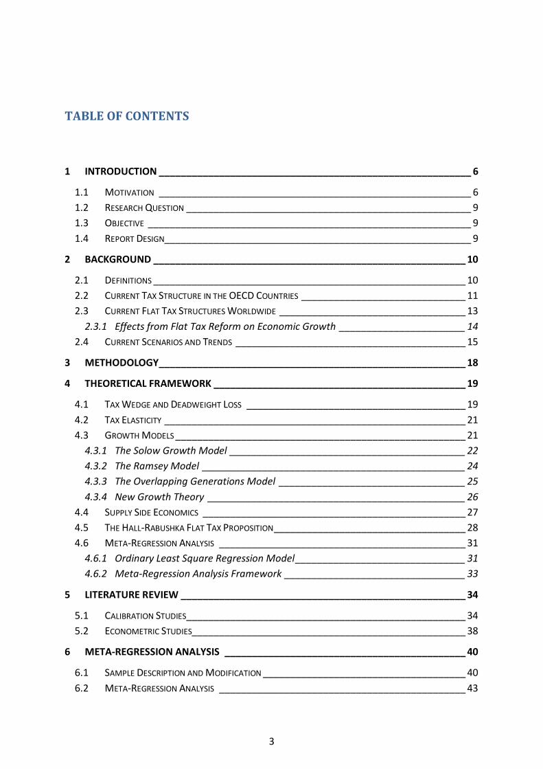
TABLE OF CONTENTS

1 INTRODUCTION _________________________________________________________ 6

1.1 MOTIVATION _________________________________________________________ 6 1.2 RESEARCH QUESTION ____________________________________________________ 9 1.3 OBJECTIVE ___________________________________________________________ 9 1.4 REPORT DESIGN________________________________________________________ 9

2 BACKGROUND _________________________________________________________ 10

2.1 DEFINITIONS _________________________________________________________ 10 2.2 CURRENT TAX STRUCTURE IN THE OECD COUNTRIES ______________________________ 11 2.3 CURRENT FLAT TAX STRUCTURES WORLDWIDE __________________________________ 13

2.3.1 Effects from Flat Tax Reform on Economic Growth _______________________ 14 2.4 CURRENT SCENARIOS AND TRENDS __________________________________________ 15

3 METHODOLOGY ________________________________________________________ 18

4 THEORETICAL FRAMEWORK ______________________________________________ 19

4.1 TAX WEDGE AND DEADWEIGHT LOSS ________________________________________ 19 4.2 TAX ELASTICITY _______________________________________________________ 21 4.3 GROWTH MODELS _____________________________________________________ 21

4.3.1 The Solow Growth Model ___________________________________________ 22 4.3.2 The Ramsey Model ________________________________________________ 24 4.3.3 The Overlapping Generations Model __________________________________ 25 4.3.4 New Growth Theory _______________________________________________ 26

4.4 SUPPLY SIDE ECONOMICS ________________________________________________ 27 4.5 THE HALL-RABUSHKA FLAT TAX PROPOSITION ___________________________________ 28 4.6 META-REGRESSION ANALYSIS _____________________________________________ 31

4.6.1 Ordinary Least Square Regression Model _______________________________ 31 4.6.2 Meta-Regression Analysis Framework _________________________________ 33

5 LITERATURE REVIEW ____________________________________________________ 34

5.1 CALIBRATION STUDIES___________________________________________________ 34 5.2 ECONOMETRIC STUDIES__________________________________________________ 38

6 META-REGRESSION ANALYSIS ____________________________________________ 40

6.1 SAMPLE DESCRIPTION AND MODIFICATION _____________________________________ 40 6.2 META-REGRESSION ANALYSIS _____________________________________________ 43

3

6.3 MODEL TESTING AND INTERPRETATION _______________________________________ 46

7 INTRODUCTION OF FLAT TAX IN THE OECD COUNTRIES ________________________ 50

7.1 EFFECTS OF FLAT TAX REFORMS ON ECONOMIC GROWTH IN THE OECD COUNTRIES _________ 52 7.2 SENSITIVITY ANALYSIS ___________________________________________________ 59 7.3 SOME INEQUALITY AND WELFARE CONSIDERATIONS _______________________________ 61

8 CONCLUSION __________________________________________________________ 63

8.1 LIMITATIONS AND AREAS FOR FURTHER RESEARCH ________________________________ 64

REFERENCES ______________________________________________________________ 66

APPENDICES ______________________________________________________________ 84

APPENDIX I: META-REGRESSION ANALYSIS: DESCRIPTIVE STATISTICS _________________________ 84 APPENDIX II: META-REGRESSION ANALYSIS: REGRESSION MODELS __________________________ 87 APPENDIX III: META-REGRESSION ANALYSIS: CONTROL OF PARAMETER VARIABLE COEFFICIENTS _______ 91 APPENDIX IV: PREDICTION PREPARATION ___________________________________________ 93

4

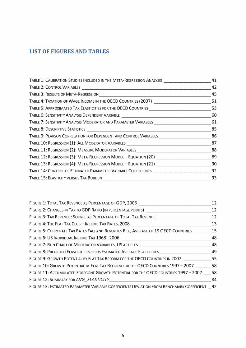
LIST OF FIGURES AND TABLES

TABLE 1: CALIBRATION STUDIES INCLUDED IN THE META-REGRESSION ANALYSIS ___________________ 41TABLE 2: CONTROL VARIABLES ____________________________________________________ 42TABLE 3: RESULTS OF META-REGRESSION _____________________________________________ 45TABLE 4: TAXATION OF WAGE INCOME IN THE OECD COUNTRIES (2007) _______________________ 51TABLE 5: APPROXIMATED TAX ELASTICITIES FOR THE OECD COUNTRIES _________________________ 53TABLE 6: SENSITIVITY ANALYSIS DEPENDENT VARIABLE ____________________________________ 60TABLE 7: SENSITIVITY ANALYSIS MODERATOR AND PARAMETER VARIABLES _______________________ 61TABLE 8: DESCRIPTIVE STATISTICS __________________________________________________ 85TABLE 9: PEARSON CORRELATION FOR DEPENDENT AND CONTROL VARIABLES _____________________ 86TABLE 10: REGRESSION (1): ALL MODERATOR VARIABLES __________________________________ 87TABLE 11: REGRESSION (2): MEASURE MODERATOR VARIABLES ______________________________ 88TABLE 12: REGRESSION (3): META-REGRESSION MODEL – EQUATION (20) ______________________ 89TABLE 13: REGRESSION (4): META-REGRESSION MODEL – EQUATION (21) ______________________ 90TABLE 14: CONTROL OF ESTIMATED PARAMETER VARIABLE COEFFICIENTS _______________________ 92TABLE 15: ELASTICITY VERSUS TAX BURDEN ___________________________________________ 93

FIGURE 1: TOTAL TAX REVENUE AS PERCENTAGE OF GDP, 2006 _____________________________ 12FIGURE 2: CHANGES IN TAX TO GDP RATIO (IN PERCENTAGE POINTS) __________________________ 12FIGURE 3: TAX REVENUE: SOURCE AS PERCENTAGE OF TOTAL TAX REVENUE ______________________ 12FIGURE 4: THE FLAT TAX CLUB – INCOME TAX RATES, 2008 ________________________________ 13FIGURE 5: CORPORATE TAX RATES FALL AND REVENUES RISE, AVERAGE OF 19 OECD COUNTRIES _______ 15FIGURE 6: US INDIVIDUAL INCOME TAX 1968 - 2006 ____________________________________ 48FIGURE 7: RUN CHART OF MODERATOR VARIABLES, US ARTICLES _____________________________ 48FIGURE 8: PREDICTED ELASTICITIES VERSUS ESTIMATED AVERAGE ELASTICITIES _____________________ 49FIGURE 9: GROWTH POTENTIAL BY FLAT TAX REFORM FOR THE OECD COUNTRIES IN 2007 ___________ 55FIGURE 10: GROWTH POTENTIAL BY FLAT TAX REFORM FOR THE OECD COUNTRIES 1997 – 2007 ______ 58FIGURE 11: ACCUMULATED FOREGONE GROWTH POTENTIAL FOR THE OECD COUNTRIES 1997 – 2007 ___ 58FIGURE 12: SUMMARY FOR AVG_ELASTICITY _________________________________________ 84FIGURE 13: ESTIMATED PARAMETER VARIABLE COEFFICIENTS DEVIATION FROM BENCHMARK COEFFICIENT _ 92

5

For what reason ought equality to be the rule in matters of taxation? For the reason, that it

ought to be so in all affairs of government. As a government ought to make no distinction of

persons or classes in the strength on their claims on it, whatever sacrifices it requires from

them should be made to bear as nearly as possible with the same pressure upon all; which, it

must be observed, is the mode by which least sacrifice is occasioned on the whole. If any one

bears less than his fair share of the burden, some other person must suffer more than his

share, and the alleviation to the one is not, on the average, so great a good to him, as the

increased pressure upon the other is an evil. Equality of taxation, therefore, as a maxim of

politics, means equality of sacrifice. It means apportioning the contribution of each person

towards the expenses of government, so that he shall feel neither more nor less

inconvenience from his share of the payment than any other person experiences from his.

This standard, like other standards of perfection, cannot be completely realized; but the first

object in every practical discussion should be to know what perfection is.

John Stuart Mill in Principles of Political Economy, Book V, Chapter II (1900)

1 INTRODUCTION

1.1 Motivation

What is the role of government in promoting economic growth? Most economists and policy

makers agree on the role of government as provider of sound economic policies in terms of

optimal framework conditions for growth and prosperity. As Mankiw (1998) states in his 8th

principle of economics: “A country’s standard of living depends on its ability to produce

goods and services.” However, highly different opinions arise when this is brought down to

government policies in action, in terms of level of interaction or measures to be used. Fiscal

policy is no exception.

6

How to design and implement a tax scheme has been an important governmental activity

ever since the origin of tax. In the well established Western European countries, as well as in

the US, the governments have over time added to and amended the tax system for

redistributive and other well-meaning purposes, or as plain political statements. Caplan

(2007) posts that voters, irrational by rational reason, yields the evident suboptimal policy

developments. This is confirmed by Avinash and Londregan (1998) in that they find

redistributive politics to favor the middle class at the expense of both rich and poor1. As a

result most of today’s tax schemes in these countries are not easily to understand and

comply with, even for professionals. A rationale for this may be the finding by Chetty,

Looney, and Kroft (2008) in that salient taxes yield more responsiveness than hidden taxes.

Unfortunately, these tax schemes create significant efficiency gaps in the economies2

One benefit of globalization is the removal of the government monopolies; as labor and

capital become increasingly mobile across country borders, governments have to face

competition from other countries in terms of framework conditions (Vietor (2007)), such as

climate, infrastructure, social security, employment, liberty, and taxation. Edwards and de

Rugy (2002) apply the public choice theory put forward by Charles Tiebout on competition

between countries, reasoning that competition between countries increases government

efficiency. As Bohacek and Kejak (2005) find; even if the aggregates are important, the

behavioral effects on individuals are crucial in obtaining the aggregates (in a fiscal sense).

Whereas some of these framework conditions are outside of the governments’ sphere of

influence (climate), the others are in many countries considered as regulatory framework

and dictated without hesitation. However, most of the OECD countries are reluctant to alter

the tax conditions in order to attract labor and capital, under the assumption of that

reducing taxes is bad for the economy. There are however signs of improvements. Devereux,

Lockwood, and Redoano (2002) find evidence for corporate tax competition between OECD

countries in terms of statutory tax rates, effective average tax rates, and effective marginal

tax rates. This is confirmed by an exposition for the Norwegian Parliament (Gotaas (2007))

.

1 Intuitively this is easily illustrated by the median voter hypothesis, which posts that political parties will make an effort to get as close as possible to satisfy the median voter in order to win the election, while simultaneously maintaining diversity from competitors. For the OECD countries the median voter is found in the middle class. 2 A less moderate understanding of the impact of taxes is found in Adams (2001) where he explains world history from a taxation perspective.

7

stating that the tax reforms in OECD countries are to improve the countries’

competitiveness. An increasing number of non-OECD countries have lowered the price of

residing and making money (i.e. tax), pressuring the high-tax OECD countries to respond in

order to retain labor and capital.

Under the current global conditions with crisis in the financial, banking and real economy

sectors one of the aids pleaded by workers and businesses is tax cuts. This could be a very

good time for introducing a flat rate tax scheme in all OECD countries. Businesses and

citizens want relief from the governments, and introducing a fundamental tax reform will

give all relief that lasts. Lower tax burden, reduced compliance costs, increased incentives,

and not least, fair treatment will be the benefits for the tax payers, whereas the benefits for

the governments are reduced compliance control costs and possibly increased tax income. A

long term recession demands a long term solution. According to the OECD Secretary-

General,

How and from whom tax is raised matters, not just how much. One can easily imagine that a

broad-based but low rate tax system is effective in resource terms. And a simple, fair and

transparent system that operates with broad social consensus is important for good

governance and compliance.

Angel Gurría, OECD Secretary-General at the International Conference on Financing for

Development, Doha, 29 November 20083

3 Source: OECD – Mobilising domestic financial resources for development. [http://www.oecd.org/document/35/0,3343,en_2649_201185_41765091_1_1_1_1,00.html] (Accessed 30.11.2008)

.

Introducing flat tax schemes in the OECD countries is a proper response to this statement.

8

1.2 Research Question

The focus of this thesis is the de facto relation between taxation and economic growth in

terms of incentive and disincentive effects from tax schemes. The research question is:

What will be the long run economic growth effects from an introduction of flat tax schemes

in the OECD countries in terms of output?

Studies and statistics indicate that flat tax schemes boost growth. To retain competitiveness

and to overcome the global recession a viable fiscal policy enhancement for the OECD

countries still having progressive tax schemes might be to follow suit and implement flat tax

schemes.

1.3 Objective

The objective for the master thesis is to present and compare academic and empirical

evidence on the relation between taxation and economic growth in order to estimate the

most probable effect on the economy of implementing flat tax schemes in the OECD

countries. Of current interest is the increasing number of countries implementing flat tax

schemes, the notion of tax competition, and a stagnating global economy. These issues will

be discussed with regards to the thesis objective.

1.4 Report Design

Section 2 presents recent issues and trends within the field of taxation. Section 3 describes

the methodology for this thesis, and section 4 presents theory and model framework,

including the Hall-Rabushka flat tax. Section 5 reviews academic literature derived with the

purpose of a meta-regression analysis by which the differences between the articles are

studied in terms of output growth effects by changes in tax progressivity.. In section 6 the

meta-regression analysis is performed, and in section 7 the results are extended into

9

qualified estimations on an OECD flat tax scenario as opposed to the current progressive tax

schemes. Section 8 concludes and suggests further research.

2 BACKGROUND

In this section I define central terms used in this paper. I provide a brief overview of current

tax structure in the OECD countries, and in countries in the flat tax club. Current scenarios

and trends within taxation are discussed where I also present some studies proving the case

for flat tax reforms.

2.1 Definitions

Economic growth is the increase in a country’s production of goods and services from one

period to the next. In this paper economic growth is measured as real gross domestic

product.

Proportional tax schemes levy one single tax rate on all income for all taxpayers regardless of

income level. No deductions are granted, and all loopholes are extinguished. Most value

added tax and social security schemes are proportional.

Flat tax schemes levy one single tax rate on all income for all taxpayers regardless of income

level. The flat tax is however not a strictly proportional tax scheme, as some progressivity

exist in that a basic deduction for persons is granted to limit the tax burden of the poor. All

other deductions and loopholes are however extinguished. Some OECD countries and

several non-OECD countries has switched from highly progressive tax schemes to flat tax

schemes, often accompanied by low tax rates.

Progressive tax schemes levy low tax rates on small incomes and high tax rates on large

incomes. Hence the share of tax burden is increasing. In addition numerous deductions are

10

often implemented for distributive or behavior-directing policy reasons. Most OECD

countries still use this type of tax scheme.

The OECD countries (i.e. OECD – Total in tables and figures) covers the 30 OECD Member

countries; Australia, Austria, Belgium, Canada, Czech Republic, Denmark, Finland, France,

Germany, Greece, Hungary, Iceland, Ireland, Italy, Japan, Korea, Luxembourg, Mexico,

Netherlands, New Zealand, Norway, Poland, Portugal, Slovak Republic, Spain, Sweden,

Switzerland, Turkey, United Kingdom and United States4

The Flat Tax Club consist of the countries and jurisdictions Albania, Belarus, Bulgaria, Czech

Republic, Estonia, Federation of Bosnia and Herzegovina, Georgia, Guernsey, Hong Kong,

Iceland, Illinois (US), Indiana (US), Iraq, Jamaica, Jersey, Kazakhstan, Kyrgyzstan, Latvia,

Lithuania, Macedonia, Massachusetts (US), Mauritius, Michigan (US), Mongolia,

Montenegro, Pennsylvania (US), Pridnestrovie, Romania, Russia, Serbia and Montenegro,

Slovak Republic, Trinidad, Ukraine, and Uri (Switzerland)

.

5

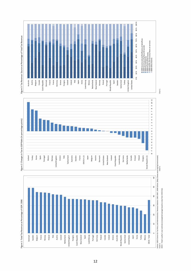
2.2 Current Tax Structure in the OECD Countries

.

Most OECD countries have as mentioned progressive tax schemes. KPMG’s Individual

Income Tax Rate Survey 2008 shows that the tax levels have been slightly reduced over the

past 5 years. For 13 countries the effective income tax and social security rates have been

reduced. The flat tax countries Czech Republic and Slovak Republic has now half of the initial

rates, whereas Iceland has seen a 20 percent increase (which the flat tax reform barely

reduced). For 12 countries the effective income tax and social security rates have not

changed at all. Figure 5 to figure 5 shows the tax structure based on OECD statistics.

4 Source: OECD country Web sites: Country Web Pages [http://www.oecd.org/countrieslist/0,3351,en_33873108_33844430_1_1_1_1_1,00.html] (Accessed 10.11.2008) 5 Source: Edwards and Mitchell (2008), Alvin Rabushka: Flat Tax – Essays on the Adoption and Results of the Flat Tax Around the Globe. [http://flattaxes.blogspot.com/], Wikipedia: Flat tax [http://en.wikipedia.org/wiki/Flat_tax] (Accessed 14.10.2008)

11

Figu

re 1

: Tot

al T

ax R

even

ue a

s Pe

rcen

tage

of G

DP,

200

6Fi

gure

2: C

hang

es in

Tax

to G

DP

Ratio

(in

perc

enta

ge p

oint

s)Fi

gure

3: T

ax R

even

ue: S

ourc

e as

Per

cent

age

of T

otal

Tax

Rev

enue

Sour

ce: O

ECD

Cen

tre

for T

ax P

olic

y an

d Ad

min

istr

atio

n, R

even

ue S

tatis

tics

1965

-200

7, 2

008

Editi

on. [

http

://w

ww

.oec

d.or

g/ct

p/re

venu

esta

ts]

Char

t A.

Char

t E.

Char

t 2.

OEC

D –

Tot

al is

aut

hor’s

ow

n es

timat

e (u

nwei

ghte

d av

erag

e) b

ased

on

data

from

OEC

D.S

tat.

010

2030

4050

60

OEC

D -

Tota

l

Mex

ico

Turk

ey

Kore

a

Japa

n

Uni

ted

Stat

es

Switz

erla

nd

Slov

ak R

epub

lic

Aust

ralia

Gre

ece

Irel

and

Cana

da

Pola

nd

Ger

man

y

Port

ugal

Luxe

mbo

urg

Spai

n

New

Zea

land

Czec

h Re

publ

ic

Hun

gary

Uni

ted

King

dom

Net

herl

ands

Icel

and

Aust

ria

Ital

y

Finl

and

Nor

way

Fran

ce

Belg

ium

Swed

en

Den

mar

k

-8-7

-6-5

-4-3

-2-1

01

23

45

67

89

1011

Slov

ak R

epub

lic (1

)

Hun

gary

Pola

nd

Finl

and

Cana

da

Net

herl

ands

Ger

man

y

Luxe

mbo

urg

Czec

h Re

publ

ic

Irel

and

New

Zea

land

Uni

ted

Stat

es

Den

mar

k

Aust

ria

Belg

ium

Japa

n

OEC

D (+

1.2)

Fran

ce

Swed

en

Aust

ralia

Switz

erla

nd

Ital

y

Gre

ece

Uni

ted

King

dom

Nor

way

Mex

ico

Port

ugal

Spai

n

Kore

a

Turk

ey

Icel

and

0 %

10 %

20 %

30 %

40 %

50 %

60 %

70 %

80 %

90 %

100

%

Uni

ted

Stat

es

Uni

ted

King

dom

Turk

ey

Switz

erla

nd

Swed

en

Spai

n

Slov

ak R

epub

lic

Port

ugal

Pola

nd

Nor

way

New

Zea

land

Net

herl

ands

Mex

ico

Luxe

mbo

urg

Kore

a

Japa

n

Ital

y

Irel

and

Icel

and

Hun

gary

Gre

ece

Ger

man

y

Fran

ce

Finl

and

Den

mar

k

Czec

h Re

publ

ic

Cana

da

Belg

ium

Aust

ria

Aust

ralia

1000

Inco

me

and

prof

its/R

even

u et

bén

éfic

es20

00 S

ocia

l sec

urity

/Sec

urité

soci

ale

3000

Pay

roll/

Sala

ires

4000

Pro

pert

y/Pa

trim

oine

5000

Goo

ds a

nd s

ervi

ces/

Bie

ns e

t ser

vice

s60

00 O

ther

/Aut

res

12

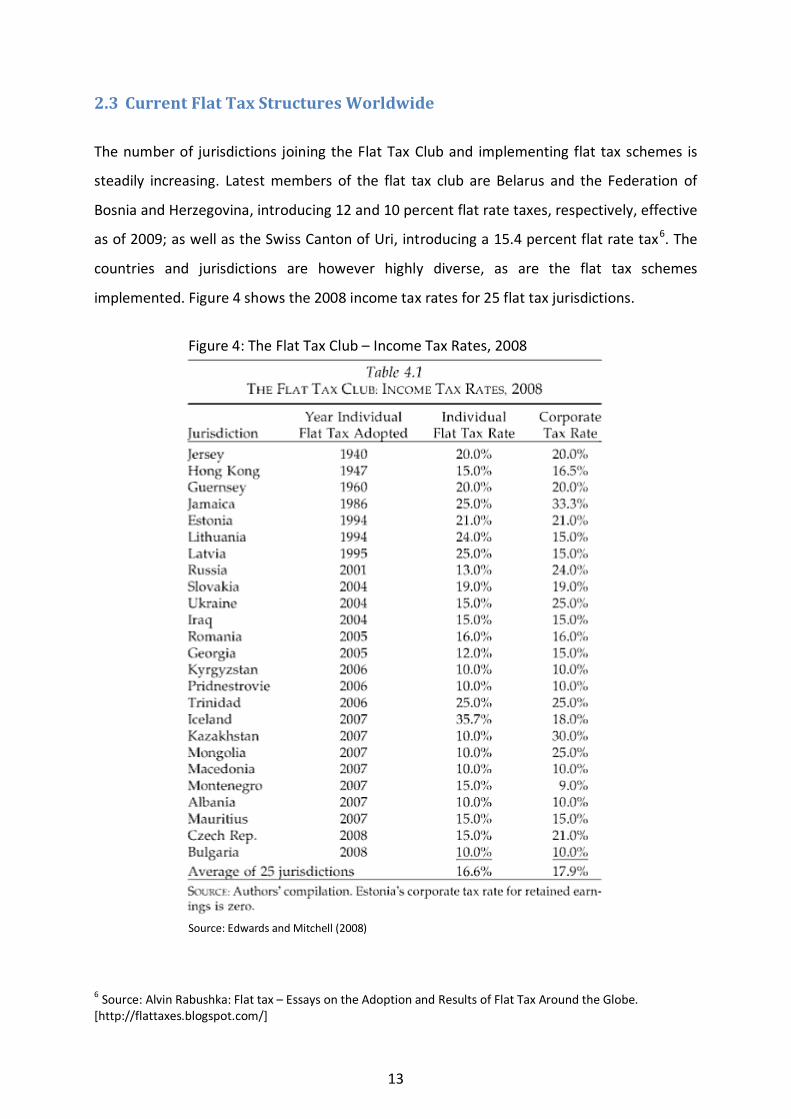
2.3 Current Flat Tax Structures Worldwide

The number of jurisdictions joining the Flat Tax Club and implementing flat tax schemes is

steadily increasing. Latest members of the flat tax club are Belarus and the Federation of

Bosnia and Herzegovina, introducing 12 and 10 percent flat rate taxes, respectively, effective

as of 2009; as well as the Swiss Canton of Uri, introducing a 15.4 percent flat rate tax6

Figure 4

. The

countries and jurisdictions are however highly diverse, as are the flat tax schemes

implemented. shows the 2008 income tax rates for 25 flat tax jurisdictions.

Figure 4: The Flat Tax Club – Income Tax Rates, 2008

Source: Edwards and Mitchell (2008)

6 Source: Alvin Rabushka: Flat tax – Essays on the Adoption and Results of Flat Tax Around the Globe. [http://flattaxes.blogspot.com/]

13

Evans and Aligica (2008) study the implementation of the flat tax in Central and Eastern

Europe (several versions, none pure Hall-Rabushka flat tax or strictly proportional tax

schemes) using a comparative study. They find that ideas, interests and consequences are

prerequisites for all cases. For some preceding cases ideas are sufficient. E.g. Mart Laar,

Prime Minister of Estonia, based the flat tax reform on the thoughts of Hayek and Friedman

(Evans (2006)). The conditions for implementing flat tax might hence be transferrable to the

OECD countries. Evans (2006) argues that belief in the normative approach to flat tax was a

key in many of the now flat tax countries. After some time, when econometric and

operational experience from the flat tax is obtained, this has been the foundation for the

other countries for implementing the flat tax. In Fraser Forum (February 2008) Patrick

Basham describes political obstacles hindering the introduction of flat tax schemes in

Western countries, namely interest groups who are willing to keep it complicated for own

benefit.

2.3.1 Effects from Flat Tax Reform on Economic Growth

Forbes (2005), Heath (2006), and Edwards and Mitchell (2008) highlight the subsequent

growth from introducing flat tax in several countries. In Gotaas (2007) the statistics for

Estonia show that whereas pre-tax reform GDP growth was negative, post-tax reform GDP

growth has ranged between 0.3 and 11.4 percent annually, averaged at 7.5 percent. As the

flat tax was implemented along with several other reforms it is however difficult to

determine the isolated tax-reform effect. This is also the case for many other tax reforms;

they are combined with other efficiency-improving reforms. However, the mere fact that

most of these countries experience significant increasing economic growth provides solid

fundament for expecting similar effects for the OECD countries.

14

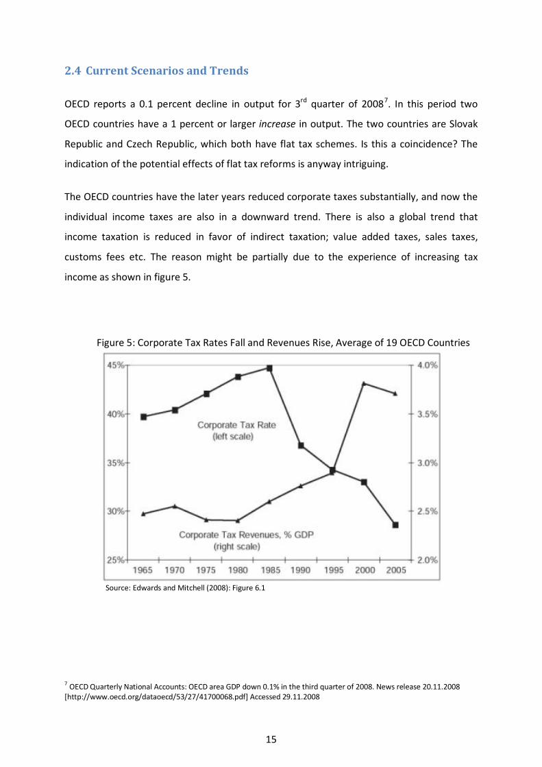
2.4 Current Scenarios and Trends

OECD reports a 0.1 percent decline in output for 3rd quarter of 20087

The OECD countries have the later years reduced corporate taxes substantially, and now the

individual income taxes are also in a downward trend. There is also a global trend that

income taxation is reduced in favor of indirect taxation; value added taxes, sales taxes,

customs fees etc. The reason might be partially due to the experience of increasing tax

income as shown in

. In this period two

OECD countries have a 1 percent or larger increase in output. The two countries are Slovak

Republic and Czech Republic, which both have flat tax schemes. Is this a coincidence? The

indication of the potential effects of flat tax reforms is anyway intriguing.

figure 5.

Figure 5: Corporate Tax Rates Fall and Revenues Rise, Average of 19 OECD Countries

Source: Edwards and Mitchell (2008): Figure 6.1

7 OECD Quarterly National Accounts: OECD area GDP down 0.1% in the third quarter of 2008. News release 20.11.2008 [http://www.oecd.org/dataoecd/53/27/41700068.pdf] Accessed 29.11.2008

15

The effect is equivalent to what Niskanen and Moore (1996) find with regards to the Reagan

tax cuts, that lower tax rates improved the US economy on 8 out of 10 key economic

variables. Similar effects can be found for the Thatcher supply-side policies in UK.

Increasing focus is paid to the distortionary effects of taxation. An OECD study on the effects

of taxation on economic growth finds that both business and individual taxes reduce

economic growth (Arnold (2008)). King and Rebelo (1990) find that national taxation can

substantially affect long-run growth rates. Similarly, Hall and Jones (1999) find that a

country’s long-run economic performance is determined primarily by the institutions and

government policies that make up the economic environment, of which physical capital and

educational attainment is only a partial reason. Romer and Romer (2007) use a narrative

methodology in analyzing the relation between legislation and changes in output. They find

that tax increases are highly contractionary. A Norwegian government exposition by Stølen,

Gjems-Onstad, Rasmussen, Røtnes, Mathisen Sletteberg, Torp, Winsnes, Berner, Gerdrup,

Moen, and Andersen (1999) states that there exist costs for the real economy associated

with high tax rates when citizens find tax planning profitable even when accompanied by

transaction costs. They also recommend that the tax scheme be less progressive.

The Pareto’s Principle, or the rule of 80/20, was derived from wealth inequality, and there is

a probability that it is still present in income distribution, and more important, in income

creation. Stokey (1980) states that while the high-income groups may be a minority in

headcount, their economic importance is not. The high-income groups also have higher tax

elasticity due to better knowledge and hence high marginal tax rates which mostly apply to

high-income groups will have severe distortionary effects on the economy.

Auerbach, Kotlikoff and Skinner (1983) study the efficiency gains from a dynamic tax reform

based on general equilibrium rational expectations growth path of life cycle economies. The

model incorporates effects of changes in tax progressivity and tax base, and is applied to a

switch from the US tax system (proportionally approximated) to proportional tax on either

consumption or labor income. They find that a flat consumption tax will increase lifetime

welfare of all future generations by 2 percent, whereas a flat labor income tax will decrease

welfare by similar amount. However, applying an initial progressive tax structure yields

increases in both reforms by 7.08 and 4.24 percent, respectively. This illustrates that even

16

minimal progressivity in the income tax structure has a large efficiency cost, and that tax

progressivity may be as important as the tax base.

Prescott (2004) finds that when the US and European tax rates were comparable the labor

supply was also comparable, and that most differences between US labor supply and

Germany and France 1970 – 1974 are due to differences in tax schemes. For Italy on the

other hand institutional constraints in the labor market and unemployment benefits are

more important.

Grecu (2004) suggests a dual fiscal system taxpayers would be able to choose between the

progressive tax system with all its reliefs and deductions, and a simple flat tax scheme with

only a basic deduction.

Kukk (2007) differ substantially from other literature on the relation between taxation and

economic growth, in that he finds that all government revenue categories have positive

effects on growth. This result is obtained by simultaneously controlling for government

expenditure and budgetary deficits. This approach is somewhat problematic however, as

revenue and expenditure in general cancels out, the result being budgetary surplus or

deficit. Implicit the growth is determined by the budget balance, regardless of government

revenue and expenditure being 10 or 90 percent of GDP – this is not very likely. Hence the

relation between government revenue and growth has to be analyzed separately in order to

infer on the associations, similarly for government expenditure. The finding in Kukk (2007) is

also contrary to the OECD study by Leibfritz, Thornton, and Bibbee (1997) which states that

“the increase in the average (weighted) tax rate of about 10 percentage points over the past

35 years may have reduced OECD annual growth rates by about 0.5 percentage point”.

The amount of academic effort on the subject of flat tax, and the increasing number of real

life examples shows a trend in tax competition between countries in order to attract capital

and labor, which inevitable paves way for more Western countries to grasp the flat tax

opportunity for increased growth.

17

3 METHODOLOGY

The fundament for the further progress of the paper is the review of academic and empirical

literature on the current topic. A search for "flat*tax*", "proportional*tax*", “linear*tax*”,

"tax reform" in JSTOR retrieves 7805 references. Limiting to articles only, still 4373

references are available. A similar search in NBER for the same subjects produces 1090

working papers. This amount will however require a more extensive research than

appropriate for this paper. Excluding “tax reform”, which obviously will remove some articles

regarding flat tax, still I find 1042 JSTOR articles on the flat tax issue. Including “economic

efficiency”, “efficiency effects” in the search results in 488 references, which is a viable

amount for reviewing, assuming that not all articles will be relevant. I have based the meta-

analysis on the JSTOR articles and other relevant resources found through the articles.

To include a study in the meta-regression analysis there are two conditions which must be

fulfilled. First, the study must concern fiscal effects on economic efficiency. Second, the

study must present an econometric or simulated estimate of the economic output or

sufficient information to calculate it. In effect, most of the studies reviewed appear

unsuitable for a meta-regression analysis. They are either reviews on the topic, or they are

based on models not described or referred to in the article, or the effects on output are not

reported and not possible to calculate for the estimates presented.

Most of the articles I use in the meta-regression analysis present more than one measure.

Stanley and Jarrell (1998) provide a useful discussion on this matter. Multiple measures from

one article are used only when representing different model frameworks. If the author(s)

have preferred one particular measure this is chosen. Otherwise I have estimated the

elasticity extremes and the used the average elasticity for the concerning article. I have

summarized the literature research in table 1, describing properties of 18 studies (n = 19) on

flat tax.

The evidence is then compared in a meta-regression analysis to infer whether the model

specifications bias the evidence. Based on the relation between taxation and economic

growth determined in the regression model I estimate the most probable effect on the

economy of implementing flat tax schemes in the OECD countries.

18

For data collection, structuring, calculations and reporting I use Microsoft Excel, Office 2007

version. For statistical reporting I use Minitab, release 15, a statistical software package.

4 THEORETICAL FRAMEWORK

This paper combines the areas of taxation and regression. Taxation comprises

microeconomic and macroeconomic theories; for the purpose of this paper the notions of

tax wedge and deadweight loss, tax elasticity, and growth models are described here. The

notion of supply side economics is also compared with the more common demand analysis

framework. Then the Hall-Rabushka flat tax proposal is discussed, before this section

concludes with a description of the regression model deployed; a multiple regression using

both binary indicator variables as well as interval variables.

4.1 Tax Wedge and Deadweight Loss

To illustrate the efficiency loss of taxes some fundamentals are explored. From the

microeconomic theory the general equilibrium in a market is the intercept between supply

and demand (𝑄𝑄𝑆𝑆∗ = 𝑄𝑄𝐷𝐷∗ ). Quantity supplied (𝑄𝑄𝑆𝑆) depends on the price (𝑃𝑃) to the supplier;

quantity demanded (𝑄𝑄𝐷𝐷 ) depends on the price to the customer. Assume linear supply and

demand functions. Introducing a proportional tax 𝜏𝜏 in this stylized model will alter this

equilibrium to

𝛼𝛼 + 𝛽𝛽𝑃𝑃𝑆𝑆 = 𝑄𝑄𝑆𝑆 = 𝑄𝑄𝐷𝐷 = 𝛾𝛾 − 𝛿𝛿𝑃𝑃𝑆𝑆(1 + 𝜏𝜏), 0 < 𝜏𝜏 < 1 (1)

where 𝛼𝛼, 𝛾𝛾 denote intercept for the supply and demand functions, 𝛽𝛽, 𝛿𝛿 denote slope, and

𝑃𝑃𝐷𝐷 = 𝑃𝑃𝑆𝑆(1 + 𝜏𝜏), i.e. the price to the buyer exceeds the price to the seller by the fraction of

tax 𝜏𝜏𝑃𝑃𝑆𝑆. The tax wedge is then given by

19

𝑊𝑊 = 𝜏𝜏𝑃𝑃𝑆𝑆𝑄𝑄𝑆𝑆,𝐷𝐷 + 0.5𝜏𝜏𝑃𝑃𝑆𝑆�𝑄𝑄𝑆𝑆,𝐷𝐷∗ − 𝑄𝑄𝑆𝑆 ,𝐷𝐷�

= 0.5𝜏𝜏𝑃𝑃𝑆𝑆�𝑄𝑄𝑆𝑆 ,𝐷𝐷 + 𝑄𝑄𝑆𝑆,𝐷𝐷∗ �

(2)

where 𝑄𝑄𝑆𝑆,𝐷𝐷 = 𝛼𝛼 + 𝛽𝛽 � 𝛾𝛾−𝛼𝛼𝛽𝛽+𝛿𝛿(1+𝜏𝜏)

� is equilibrium supply, 𝑄𝑄𝑆𝑆 ,𝐷𝐷∗ = 𝛼𝛼 + 𝛽𝛽 �𝛾𝛾−𝛼𝛼

𝛽𝛽+𝛿𝛿� is non-tax

equilibrium supply, 𝜏𝜏𝑃𝑃𝑆𝑆𝑄𝑄𝑆𝑆,𝐷𝐷 (= (𝑃𝑃𝐷𝐷 − 𝑃𝑃𝑆𝑆)𝑄𝑄𝑆𝑆,𝐷𝐷) is government revenue, and where

0.5𝜏𝜏𝑃𝑃𝑆𝑆�𝑄𝑄𝑆𝑆 ,𝐷𝐷∗ − 𝑄𝑄𝑆𝑆,𝐷𝐷�

(3)

is the deadweight loss. The market may be e.g. goods, services (𝜏𝜏 is a value added tax), or

labor (𝜏𝜏 is an income tax). In Feldstein (1999) an equivalent formula for deadweight loss is

augmented to include tax avoidance and to be based on taxable income elasticities. In

macroeconomics the tax wedge is mostly referred to in terms of the difference between

labor costs and net wage, either the tax is paid by the employer (payroll tax) or the

employee (wage tax)8, hence omitting the deadweight loss. OECD define tax wedge as the

“sum of personal income tax and employee plus employer social security contributions

together with any payroll tax less cash transfers”9

From the deadweight loss implied by the tax wedge we may hence predict that there are

efficiency gains from reducing taxes. As the stylized model was analyzed in terms of a

proportional tax, progressive taxes are likely to yield even larger deadweight loss. This is

confirmed in Feldstein (1999), and Hansen and Verdelin (2007), both of which also find

effects on increased deadweight loss from increasing tax progressivity. Extending the

deadweight loss formula to also include disincentives may yield higher effects, but as Hansen

and Verdelin (2007) find the effects varies with the level of income. The notion of a

deadweight loss implies that the other part of the tax wedge – government revenue – is

spent as efficiently as would suppliers and buyers. Additional efficiency costs arise when this

. However, e.g. Mankiw (1998) provides an

entire chapter devoted to the costs of taxation.

8 Who pays is actually irrelevant, as the tax burden depends on the elasticity of supply and demand (Mankiw (1998), Pindyck and Rubinfeld (2005)). The shares of tax burden is found by the pass-through fraction formula −𝐸𝐸𝐷𝐷

(𝐸𝐸𝑆𝑆−𝐸𝐸𝐷𝐷 ) for the seller and 𝐸𝐸𝑆𝑆

(𝐸𝐸𝑆𝑆−𝐸𝐸𝐷𝐷 ) for the buyer, where the elasticities are of the form 𝐸𝐸 = �𝑃𝑃𝑄𝑄� �∆𝑄𝑄

∆𝑃𝑃�.

9 OECD Glossary of Statistical Terms - Tax wedge Definition [http://stats.oecd.org/glossary/detail.asp?ID=7273] (Accessed 15.12.2008)

20

is not the case; however this is not captured by the deadweight loss formula10

4.2 Tax Elasticity

. Ding (2008)

finds however that a one percentage increase in the tax wedge can lead to about 0.09

percentage decrease in labor productivity growth rate for the OECD countries.

To compare the articles regardless different measures of output tax elasticities are

estimated for each article, utilizing the methodology described by Philips and Goss (1995)

where they refer to Bartik’s tax elasticity estimations11. Assume tax elasticity as the

percentage change in real output caused by a one percent change in tax progressivity, where

tax progressivity is defined as the ratio Ѳ = 1−𝜏𝜏𝑠𝑠1−𝜏𝜏𝑐𝑐

, where 𝜏𝜏𝑠𝑠 is the lowest effective marginal

tax rate and 𝜏𝜏𝑐𝑐 is the highest12

where ∆𝛾𝛾 is efficiency gain, and m is the number of elasticity estimates. Using the tax

progressivity ratio allows for inferring whether changes in output is due to changes in tax

level or tax progressivity.

. Then the average tax elasticity is

𝑌𝑌𝑖𝑖 =1𝑀𝑀 � �

∆𝛾𝛾−∆Ѳ�𝑚𝑚

𝑀𝑀

𝑚𝑚=1

(4)

4.3 Growth Models

The relationship between taxation and economic growth has been studied through

numerous growth models. A brief summary of the basic models are presented next. Some of

10 See Edwards and Mitchell (2008) for an analysis of how competitive governments are more efficient than monopolist governments. 11 Bartik, Timothy J. (1991): Who Benefits from State and Local Economic Development Policies? W.E. Upjohn Institute, Kalamazoo, Michigan. In this book Bartik estimated tax elasticities for economic activity based on 61 studies. 12 Tax progressivity ratio is a modified version of the ratio in Caucutt, Imrohoroglu and Kumar (2000). Vedder (1985) uses the definition τc − τs . Other studies use the Lorentz curve as basis for tax progressivity indices (Suits (1977), Stroup (2005)).

21

the calibration studies deploy the models directly, others use modified (adjusted or

augmented) versions for improved interpretations. See the studies for complete model

descriptions, also Farmer (1999), Romer (2001), Gärtner (2006), McCandless (2008), or other

macroeconomic literature.

4.3.1 The Solow Growth Model

The neoclassical Solow growth model provides a basic fundament for growth analysis.

Although the model has severe simplistic limitations (assuming exogenous growth, closed

economy with no government, constant returns to scale) it is a good starting point for

developing and interpreting models. The model assumes production of one single good

determined by labor and capital (savings) supplied by households. The basic production

function is of the form

𝑌𝑌𝑡𝑡 = 𝐴𝐴𝑡𝑡𝐹𝐹(𝐾𝐾𝑡𝑡 , 𝐿𝐿𝑡𝑡) (1)

where 𝑌𝑌𝑡𝑡 denotes output at time 𝑡𝑡, 𝐴𝐴 is the scale parameter, 𝐾𝐾 is capital, and 𝐿𝐿 is labor. Net

change in capital stock is given by 𝑠𝑠𝐹𝐹(𝐾𝐾𝑡𝑡 , 𝐿𝐿𝑡𝑡) − 𝛿𝛿𝐾𝐾𝑡𝑡 , where total savings is determined by

output and a savings rate assumed fixed at a level 𝑠𝑠 = 1 − 𝑐𝑐 (c = consumption rate), and

capital depreciate at a rate 𝛿𝛿. Steady state output and capital stock is found where total

savings equals capital depreciation, i.e. where actual investment equals required investment.

The golden rule of capital accumulation hence yields the highest steady state level of

consumption at a savings rate

𝑠𝑠 =𝛿𝛿𝐾𝐾0

∗

𝐴𝐴0𝐹𝐹(𝐾𝐾0∗,𝐿𝐿0)

(2)

A conceptual defect of the basic Solow model is that the model only explains differences in

observed levels of output. Plosser (1992) emphasize that the Solow growth model, despite

being a useful fundament, has severe limitations in understanding growth. By extending the

model to not be bound by diminishing marginal productivity by expanding the capital term

22

and by endogenizing technology development, public policies which affect savings and

investment in physical and human capital, and technology development are central to long

run growth. Gärtner (2006) states that the Solow model does not really explain economic

growth, but treats growth exogenously “as a residual which the model does not even

attempt to understand”.

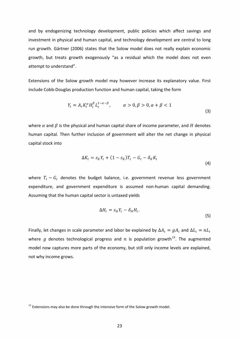
Extensions of the Solow growth model may however increase its explanatory value. First

include Cobb-Douglas production function and human capital, taking the form

𝑌𝑌𝑡𝑡 = 𝐴𝐴𝑡𝑡𝐾𝐾𝑡𝑡𝛼𝛼𝐻𝐻𝑡𝑡𝛽𝛽𝐿𝐿𝑡𝑡

1−𝛼𝛼−𝛽𝛽 , 𝛼𝛼 > 0,𝛽𝛽 > 0,𝛼𝛼 + 𝛽𝛽 < 1 (3)

where 𝛼𝛼 and 𝛽𝛽 is the physical and human capital share of income parameter, and 𝐻𝐻 denotes

human capital. Then further inclusion of government will alter the net change in physical

capital stock into

∆𝐾𝐾𝑡𝑡 = 𝑠𝑠𝐾𝐾𝑌𝑌𝑡𝑡 + (1− 𝑠𝑠𝐾𝐾)𝑇𝑇𝑡𝑡 − 𝐺𝐺𝑡𝑡 − 𝛿𝛿𝐾𝐾𝐾𝐾𝑡𝑡 (4)

where 𝑇𝑇𝑡𝑡 − 𝐺𝐺𝑡𝑡 denotes the budget balance, i.e. government revenue less government

expenditure, and government expenditure is assumed non-human capital demanding.

Assuming that the human capital sector is untaxed yields

∆𝐻𝐻𝑡𝑡 = 𝑠𝑠𝐻𝐻𝑌𝑌𝑡𝑡 − 𝛿𝛿𝐻𝐻𝐻𝐻𝑡𝑡 . (5)

Finally, let changes in scale parameter and labor be explained by ∆𝐴𝐴𝑡𝑡 = 𝑔𝑔𝐴𝐴𝑡𝑡 and ∆𝐿𝐿𝑡𝑡 = 𝑛𝑛𝐿𝐿𝑡𝑡

where 𝑔𝑔 denotes technological progress and 𝑛𝑛 is population growth13

13 Extensions may also be done through the intensive form of the Solow growth model.

. The augmented

model now captures more parts of the economy, but still only income levels are explained,

not why income grows.

23

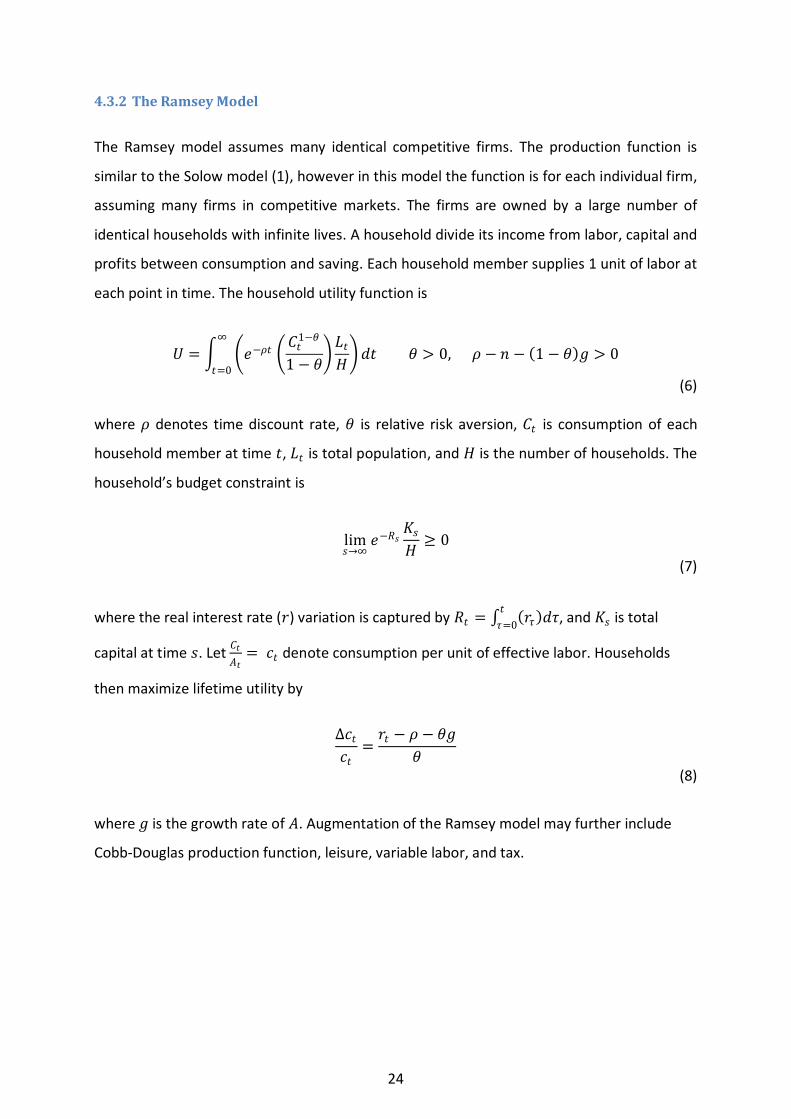
4.3.2 The Ramsey Model

The Ramsey model assumes many identical competitive firms. The production function is

similar to the Solow model (1), however in this model the function is for each individual firm,

assuming many firms in competitive markets. The firms are owned by a large number of

identical households with infinite lives. A household divide its income from labor, capital and

profits between consumption and saving. Each household member supplies 1 unit of labor at

each point in time. The household utility function is

𝑈𝑈 = � �𝑒𝑒−𝜌𝜌𝑡𝑡 �𝐶𝐶𝑡𝑡1−𝜃𝜃

1 − 𝜃𝜃�𝐿𝐿𝑡𝑡𝐻𝐻�

∞

𝑡𝑡=0𝑑𝑑𝑡𝑡 𝜃𝜃 > 0, 𝜌𝜌 − 𝑛𝑛 − (1 − 𝜃𝜃)𝑔𝑔 > 0

(6) where 𝜌𝜌 denotes time discount rate, 𝜃𝜃 is relative risk aversion, 𝐶𝐶𝑡𝑡 is consumption of each

household member at time 𝑡𝑡, 𝐿𝐿𝑡𝑡 is total population, and 𝐻𝐻 is the number of households. The

household’s budget constraint is

lim𝑠𝑠→∞

𝑒𝑒−𝑅𝑅𝑠𝑠𝐾𝐾𝑠𝑠𝐻𝐻 ≥ 0

(7)

where the real interest rate (𝑟𝑟) variation is captured by 𝑅𝑅𝑡𝑡 = ∫ (𝑟𝑟𝜏𝜏)𝑑𝑑𝜏𝜏𝑡𝑡𝜏𝜏=0 , and 𝐾𝐾𝑠𝑠 is total

capital at time 𝑠𝑠. Let 𝐶𝐶𝑡𝑡𝐴𝐴𝑡𝑡

= 𝑐𝑐𝑡𝑡 denote consumption per unit of effective labor. Households

then maximize lifetime utility by

∆𝑐𝑐𝑡𝑡𝑐𝑐𝑡𝑡

=𝑟𝑟𝑡𝑡 − 𝜌𝜌 − 𝜃𝜃𝑔𝑔

𝜃𝜃

(8)

where 𝑔𝑔 is the growth rate of 𝐴𝐴. Augmentation of the Ramsey model may further include

Cobb-Douglas production function, leisure, variable labor, and tax.

24

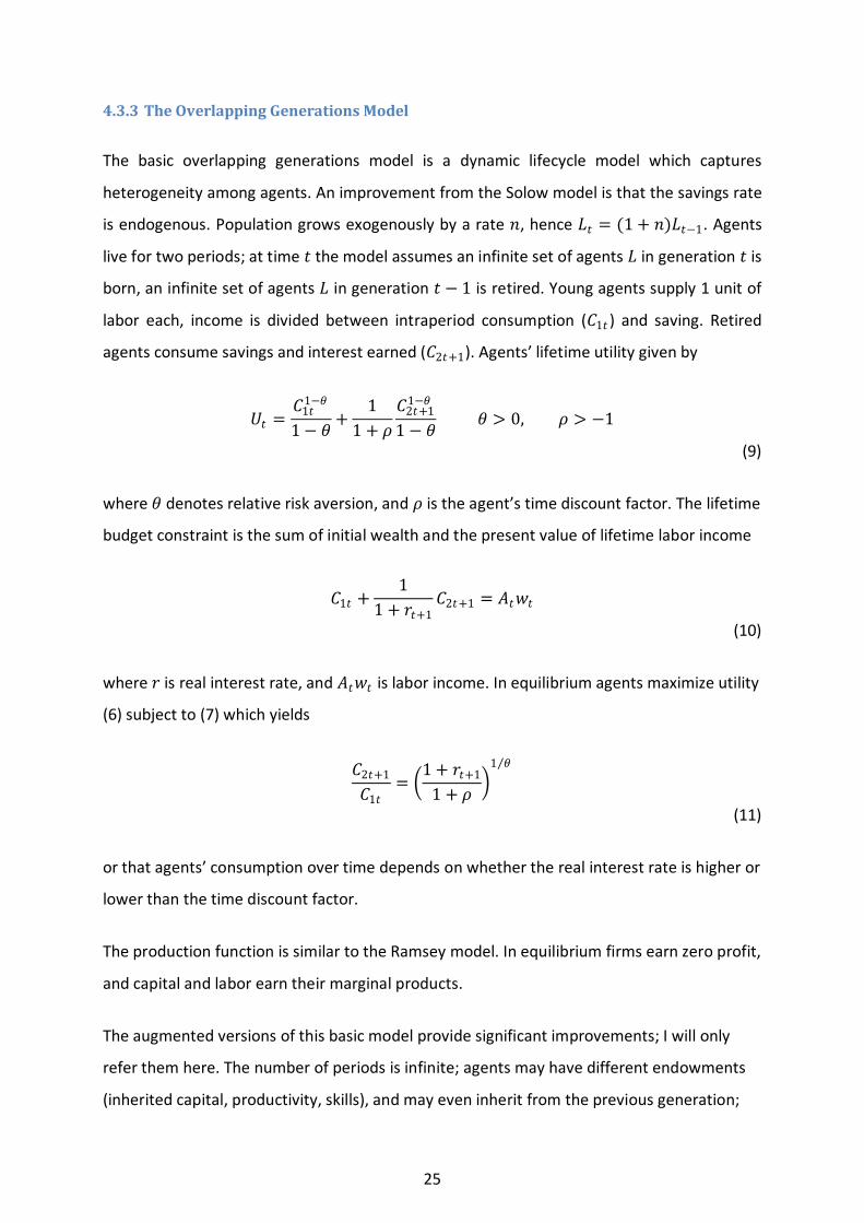
4.3.3 The Overlapping Generations Model

The basic overlapping generations model is a dynamic lifecycle model which captures

heterogeneity among agents. An improvement from the Solow model is that the savings rate

is endogenous. Population grows exogenously by a rate 𝑛𝑛, hence 𝐿𝐿𝑡𝑡 = (1 + 𝑛𝑛)𝐿𝐿𝑡𝑡−1. Agents

live for two periods; at time 𝑡𝑡 the model assumes an infinite set of agents 𝐿𝐿 in generation 𝑡𝑡 is

born, an infinite set of agents 𝐿𝐿 in generation 𝑡𝑡 − 1 is retired. Young agents supply 1 unit of

labor each, income is divided between intraperiod consumption (𝐶𝐶1𝑡𝑡 ) and saving. Retired

agents consume savings and interest earned (𝐶𝐶2𝑡𝑡+1). Agents’ lifetime utility given by

𝑈𝑈𝑡𝑡 =𝐶𝐶1𝑡𝑡

1−𝜃𝜃

1− 𝜃𝜃 +1

1 + 𝜌𝜌𝐶𝐶2𝑡𝑡+1

1−𝜃𝜃

1 − 𝜃𝜃 𝜃𝜃 > 0, 𝜌𝜌 > −1

(9)

where 𝜃𝜃 denotes relative risk aversion, and 𝜌𝜌 is the agent’s time discount factor. The lifetime

budget constraint is the sum of initial wealth and the present value of lifetime labor income

𝐶𝐶1𝑡𝑡 +1

1 + 𝑟𝑟𝑡𝑡+1𝐶𝐶2𝑡𝑡+1 = 𝐴𝐴𝑡𝑡𝑤𝑤𝑡𝑡

(10)

where 𝑟𝑟 is real interest rate, and 𝐴𝐴𝑡𝑡𝑤𝑤𝑡𝑡 is labor income. In equilibrium agents maximize utility

(6) subject to (7) which yields

𝐶𝐶2𝑡𝑡+1

𝐶𝐶1𝑡𝑡= �

1 + 𝑟𝑟𝑡𝑡+1

1 + 𝜌𝜌 �1 𝜃𝜃⁄

(11)

or that agents’ consumption over time depends on whether the real interest rate is higher or

lower than the time discount factor.

The production function is similar to the Ramsey model. In equilibrium firms earn zero profit,

and capital and labor earn their marginal products.

The augmented versions of this basic model provide significant improvements; I will only

refer them here. The number of periods is infinite; agents may have different endowments

(inherited capital, productivity, skills), and may even inherit from the previous generation;

25

each generation may consist of heterogenous agents; agents’ preference for leisure, taxation

and government expenditure, and open economy features are included. Hence this

overlapping generations model framework may provide good approximations to real-life

economies.

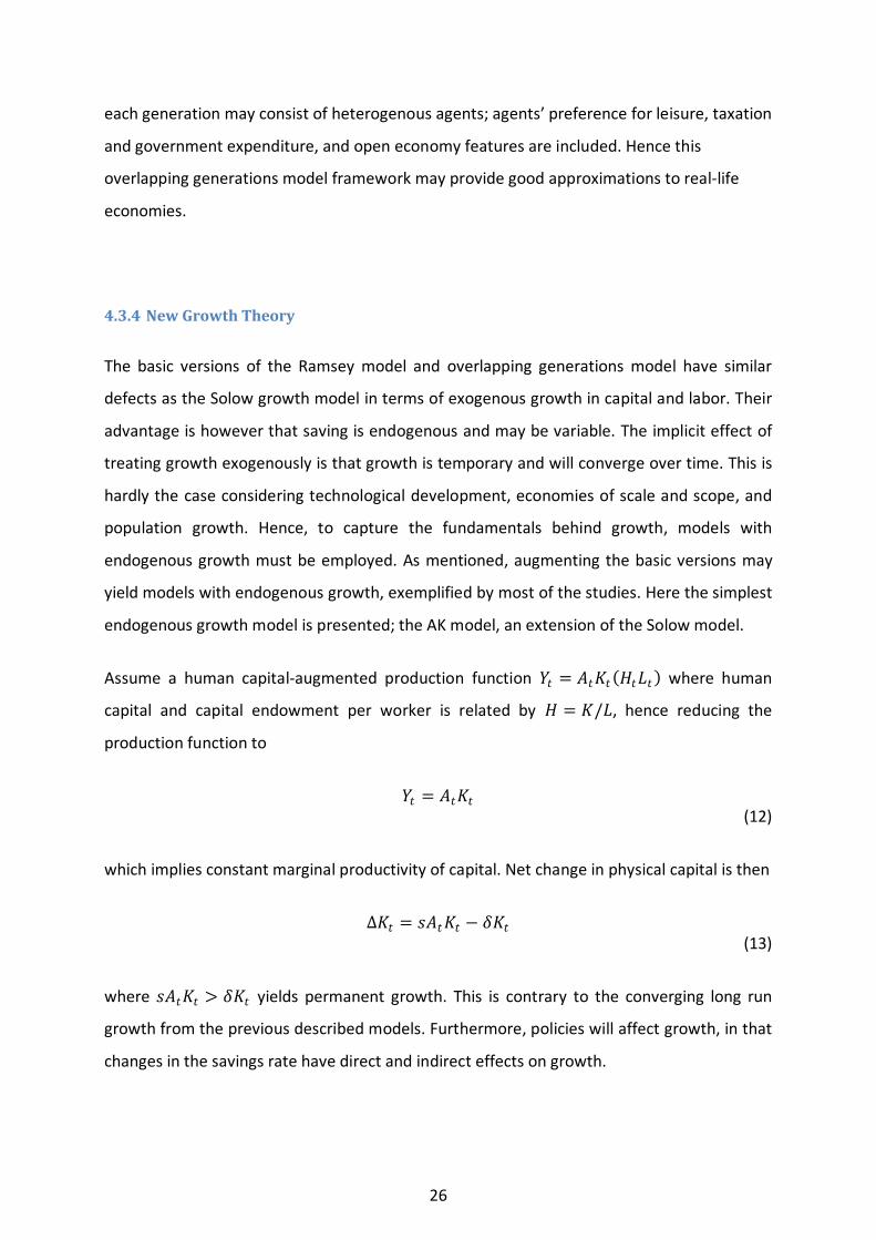
4.3.4 New Growth Theory

The basic versions of the Ramsey model and overlapping generations model have similar

defects as the Solow growth model in terms of exogenous growth in capital and labor. Their

advantage is however that saving is endogenous and may be variable. The implicit effect of

treating growth exogenously is that growth is temporary and will converge over time. This is

hardly the case considering technological development, economies of scale and scope, and

population growth. Hence, to capture the fundamentals behind growth, models with

endogenous growth must be employed. As mentioned, augmenting the basic versions may

yield models with endogenous growth, exemplified by most of the studies. Here the simplest

endogenous growth model is presented; the AK model, an extension of the Solow model.

Assume a human capital-augmented production function 𝑌𝑌𝑡𝑡 = 𝐴𝐴𝑡𝑡𝐾𝐾𝑡𝑡(𝐻𝐻𝑡𝑡𝐿𝐿𝑡𝑡) where human

capital and capital endowment per worker is related by 𝐻𝐻 = 𝐾𝐾/𝐿𝐿, hence reducing the

production function to

𝑌𝑌𝑡𝑡 = 𝐴𝐴𝑡𝑡𝐾𝐾𝑡𝑡 (12)

which implies constant marginal productivity of capital. Net change in physical capital is then

∆𝐾𝐾𝑡𝑡 = 𝑠𝑠𝐴𝐴𝑡𝑡𝐾𝐾𝑡𝑡 − 𝛿𝛿𝐾𝐾𝑡𝑡 (13)

where 𝑠𝑠𝐴𝐴𝑡𝑡𝐾𝐾𝑡𝑡 > 𝛿𝛿𝐾𝐾𝑡𝑡 yields permanent growth. This is contrary to the converging long run

growth from the previous described models. Furthermore, policies will affect growth, in that

changes in the savings rate have direct and indirect effects on growth.

26

The four basic models described are the basis for all calibration studies used in the meta-

regression analysis. Methodologies used are either augmentations as described for each

model, or extended/included into general equilibrium models or real business cycle models.

4.4 Supply Side Economics

Supply side economics is all about providing sound economic policies in terms of optimal

framework conditions for growth and prosperity. Incentives (and disincentives) for

individuals and businesses to supply capital and labor are recognized by this approach14

Although most economists agree on the role of government as provider of sound economic

policies in terms of optimal framework conditions for growth and prosperity, little attention

is paid to this when it comes down to economic modeling and research. In most

macroeconomic literature Keynesian demand side economics receives substantially more

attention, where the focus is on the role of government as provider of stabilizing fiscal

policies in terms of demand adjusting measures. However history proves the countercyclical

fiscal policy flawed due to a) decision lags; b) implementation lags; and c) impact lags of

fiscal policies (Taylor (2000)). Hence the time from a countercyclical measure would have

had the effect predicted by theory to the measure is effective may be long; so long that in

some cases the measure turns into effect after the through (or peak in an overheating

economy), amplifying the normalizing path of the economy (Bernoth, Hallett, and Lewis

(2008)). The result is then similar to driving a car from one ditch to the other. It seems as

.

There has been extensive criticism towards this economic approach; however theory and

empirics provides substantial support – as do common sense. People do not consume in

order to work, they work in order to consume. As most proponents of supply side economics

support the market as the way to organize society, most effort has been put into the

reduction of impeding government interference in terms of regulations and fiscal policies.

Taxation and tax reforms have received extensive attention, one of the propositions is the

Hall-Rabushka flat tax which is presented later.

14 Source: James D. Gwartney: Supply-Side Economics: The Concise Encyclopedia of Economics | Library of Economics and Liberty. [http://www.econlib.org/library/Enc/SupplySideEconomics.html] (Accessed 18.12.2006)

27

monetary and automatic stabilizers are better chauffeurs than the government providing

(de)stabilizing fiscal policies.

That government interference on demand factors only indirectly affects supply is also

flawed. Supply is inevitably associated with demand, but is not a linear function of demand

(as demand is not a linear function of supply). This is easily demonstrated by the fact that

less than 50 percent of new businesses survive beyond 5 years after establishment15

The obvious relation is however the cost of supply. If costs exceeds income the supply

disappears, i.e. the producer files for bankruptcy. As a major cost component for businesses

is tax the obvious linkage extends to taxation (

. Supply

depends on price (as a function of demand), costs, technology, expectations, framework

conditions, capital stock, population growth, living standards, total factor productivity

(Mankiw (1998), Miles and Scott (2005)). For labor supply there are also trade unions

involved. Hence, and corresponding with the growth models presented above, the relation

between aggregate supply and aggregate demand is not always easily observed.

figure 5 shows total tax revenue for the OECD

countries; this is the tax burden for businesses and individuals). Recalling the discussion on

tax wedge and deadweight loss, this implies that if governments want to affect the economic

growth, there is a linear relationship between taxation and supply. Because of this

relationship governments must consider the supply side effects beyond the indirect effects

of demand-side policies, if that is their path of choice. As stated initially, taxes should be

levied fairly and in the least intrusive possible way.

4.5 The Hall-Rabushka Flat Tax Proposition

Hall and Rabushka (1995) propose an integrated flat tax which applies to both individuals

and businesses. The main point is that taxing consumption is the least interruptive way of

taxation. As value-added taxes do not allow for deductions for the poor this is considered

less feasible. The indirect consumption tax (income less investment) allows for deductions,

15 Source: OECD: Measuring entrepreneurship: a digest of indicators. [http://www.oecd.org/document/31/0,3343,en_2649_34233_41663647_1_1_1_1,00.html] and OECD: Workshop On Firm-Level Statistics, 26-27 November 2001. [http://www.oecd.org/dataoecd/32/62/2669736.pdf] (Accessed 17.12.2008)

28

and is also more predictable upfront. They suggest in their flat tax reform a flat marginal tax

rate of 19 percent applicable to both business and individuals, and a fixed deduction of USD

22,500 for a family of four (Social Security is abstracted from the reform). All other

deductions, exemptions and tax credits are eliminated. The integrated flat tax form an

airtight tax system, and is fair in that all income is taxed in the same proportion and only

once, extinguishing the current double or even triple taxation of income, loopholes, and tax

evasion. Fairness is thus maintained for both horizontal and vertical equity. The efficiency

gain from removing disincentives of current tax schemes and introducing a flat tax reform is

estimated to a 6 percent upward shift in output. Resources will also be allocated away from

unproductive tax compliance expenditures, and tax planning (own effort, tax advisers, tax

attorneys) for the taxed subjects, and from tax compliance control and investigation for the

government. Tax compliance would be much easier; each of the tax forms fit on a postcard

and is completed using common records. This would yield even larger efficiency effects. E.g.

estimations by Robert E. Plamondon and David Zussman (Clemens, Emes, and Scott (2001))

show that administrative and compliance cost associated with business taxes to be 1.5

percent of total tax revenue.

The Hall-Rabushka flat tax has been used as basis for several reform proposals, such as the

flat tax proposals by US Congressmen Dick Armey and Richard Shelby (majority leader and

senator, respectively; see Bartlett (1994)), and by Steve Forbes (Forbes (2005)) in his

candidature for the 1996 presidential primaries. Hall and Rabushka also provide advisory

services to countries interested in adopting flat tax, including several of the Eastern

European countries16

Robert Eisner and Herbert Stein (Hall, Rabushka, Armey, and Stein (1996)), and Foster (2002)

put forward some criticism by arguing that human capital should be treated like physical

capital in the flat tax scheme; if not human capital investments will be less attractive.

Contrary to this, Heckman, Lochner, and Taber (1998) find that in general equilibrium skill

formation increases as the higher earnings associated with college graduation are no longer

taxed away at higher rates. Slemrod (1997) sums up main benefits and objections of the flat

tax, and also a stepwise deconstruction from the current US income tax into the Hall-

.

16 Robert E. Hall [http://www.hoover.org/bios/hall.html] Alvin Rabushka [http://www.hoover.org/bios/rabushka.html]

29

Rabushka flat tax. Robbins and Robbins (1996) provide a summary of the USA (Unlimited

Savings Allowance) tax, proposed by Senators Sam Nunn and Pete Domenici; a national sales

tax; and the Hall-Rabushka flat tax. Koenig and Huffman (1998) provide insights in the short

and long run dynamics of a Hall-Rabushka flat tax reform. The Hall-Rabushka flat tax is also

well reviewed in Clemens et al. (2001), Emes, Clemens, Basham, and Samida (2001), and

Heath (2006).

Numerous other studies are supportive in terms of reducing tax progressivity and reduce the

tax burden17

17 Famous promoters of the flat tax are Adam Smith (1776), John Stuart Mill (1900), David Ricardo (1911), Friedrich A. Hayek (1960), and Milton Friedman (1962;1980). Currently the idea of flat tax and other market-liberal thoughts are promoted by epistemic communities (think-tanks) such as Adam Smith Institute (UK), Cato Institute (US), Center for Freedom and Prosperity (US), Civita (Norway), Fraser Institute (Canada), The Heritage Foundation (US), Hoover Institution (US), Institute for Policy Innovation (US), Ludwig von Mises Institute (US), and Reform (UK).

. Slemrod (1990) argue that unless including the technology of collecting taxes

optimal tax theory has little applicability. Innovative public economics are not always for the

better. Mullen and Williams (1994) find that higher marginal tax rates are significantly

associated with slower output growth, reducing growth rates by up to 25 percent. Based on

a meta-regression analysis similar to the one applied in this paper, Phillips and Goss (1995)

find that state and local government tax policy (US) has significant effects on economic

development in that the tax elasticity range from -0.216 to -0.346. Aaberge, Dagsvik, and

Strøm (1995) find that reducing income tax progressivity removes distortionary effects on

labor. They suggest that moving further towards a flat tax scheme increases welfare and

efficiency, and that the purely proportional tax scheme may move the economy close to its

potential. Niskanen and Moore (1996), and Grecu (2004) provide statistics on US tax cuts

and corresponding increase in tax revenue. Milesi-Ferretti and Roubini (1998) find that

whereas consumption taxation only affects the choice between productive time and leisure

time in favor of the latter and by that is growth reducing, taxation of factor income has

additional distortionary effects, and is hence even more growth reducing. Carroll, Holtz-

Eakin, and Rosen (1998), and Gentry and Hubbard (2000) find that increasing marginal tax

rates reduces both the investment level of existing entrepreneurs as well as the number of

entrepreneurs entering the market. This is also confirmed in the review by Keith Godin in

Fraser Forum (February 2008). Aaberge, Colombino, and Strøm (2000) study labor supply

responses and welfare effects for Italy, Norway and Sweden in flat tax scenarios. By applying

30

revenue neutral tax rates (1992 level) at 23, 25 and 29 percent, respectively, they find

efficiency gains by shifting to a flat tax in all three countries.

4.6 Meta-Regression Analysis

4.6.1 Ordinary Least Square Regression Model

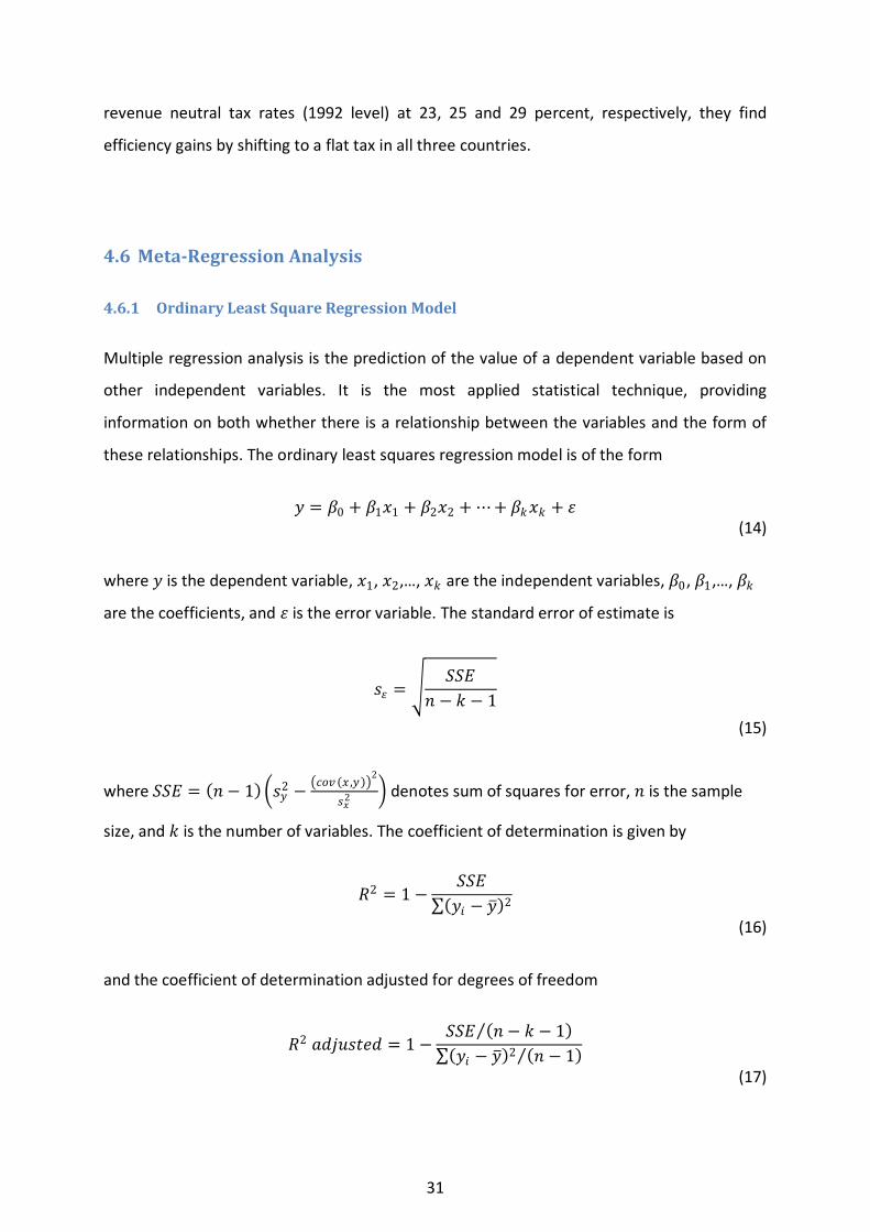
Multiple regression analysis is the prediction of the value of a dependent variable based on

other independent variables. It is the most applied statistical technique, providing

information on both whether there is a relationship between the variables and the form of

these relationships. The ordinary least squares regression model is of the form

𝑦𝑦 = 𝛽𝛽0 + 𝛽𝛽1𝑥𝑥1 + 𝛽𝛽2𝑥𝑥2 + ⋯+ 𝛽𝛽𝑘𝑘𝑥𝑥𝑘𝑘 + 𝜀𝜀 (14)

where 𝑦𝑦 is the dependent variable, 𝑥𝑥1, 𝑥𝑥2,…, 𝑥𝑥𝑘𝑘 are the independent variables, 𝛽𝛽0, 𝛽𝛽1,…, 𝛽𝛽𝑘𝑘

are the coefficients, and 𝜀𝜀 is the error variable. The standard error of estimate is

𝑠𝑠𝜀𝜀 = � 𝑆𝑆𝑆𝑆𝑆𝑆𝑛𝑛 − 𝑘𝑘 − 1

(15)

where 𝑆𝑆𝑆𝑆𝑆𝑆 = (𝑛𝑛 − 1)�𝑠𝑠𝑦𝑦2 −�𝑐𝑐𝑐𝑐𝑐𝑐 (𝑥𝑥 ,𝑦𝑦)�2

𝑠𝑠𝑥𝑥2� denotes sum of squares for error, 𝑛𝑛 is the sample

size, and 𝑘𝑘 is the number of variables. The coefficient of determination is given by

𝑅𝑅2 = 1 −𝑆𝑆𝑆𝑆𝑆𝑆

∑(𝑦𝑦𝑖𝑖 − 𝑦𝑦�)2

(16)

and the coefficient of determination adjusted for degrees of freedom

𝑅𝑅2 𝑎𝑎𝑎𝑎𝑎𝑎𝑎𝑎𝑠𝑠𝑎𝑎𝑎𝑎𝑎𝑎 = 1 −𝑆𝑆𝑆𝑆𝑆𝑆 (𝑛𝑛 − 𝑘𝑘 − 1)⁄∑(𝑦𝑦𝑖𝑖 − 𝑦𝑦�)2 (𝑛𝑛 − 1)⁄

(17)

31

The validity of the model is tested by the hypotheses

𝐻𝐻0: 𝛽𝛽1 = 𝛽𝛽2 = ⋯ = 𝛽𝛽𝑘𝑘 = 0

𝐻𝐻1: At least one 𝛽𝛽𝑎𝑎 is not equal to 0.

The null hypothesis’ rejection region is 𝐹𝐹 > 𝐹𝐹𝛼𝛼 ,𝑘𝑘 ,𝑛𝑛−𝑘𝑘−1 where 𝛼𝛼 is the significance level. The

𝐹𝐹 statistic for this test is given by

𝐹𝐹 =(∑(𝑦𝑦𝑖𝑖 − 𝑦𝑦�)2 − 𝑆𝑆𝑆𝑆𝐸𝐸) 𝑘𝑘⁄𝑆𝑆𝑆𝑆𝐸𝐸 (𝑛𝑛 − 𝑘𝑘 − 1)⁄

(18)

This implies that if the null hypothesis is true none of the moderator or parameter variables

are linearly correlated with the dependent variable, and the model is invalid. If on the other

hand at least one of the coefficients is not 0, the regression model is valid.

For the coefficients the hypotheses are

𝐻𝐻0: 𝛽𝛽𝑖𝑖 = 0

𝐻𝐻1: 𝛽𝛽𝑖𝑖 ≠ 0

with the test statistic 𝑇𝑇 = 𝑏𝑏𝑖𝑖−𝛽𝛽𝑖𝑖𝑆𝑆𝑏𝑏𝑖𝑖

which is Student t distributed with (𝜈𝜈 = 𝑛𝑛 − 𝑘𝑘 − 1 degrees of

freedom). The corresponding P-values denotes whether the null hypothesis is true (high P-

value) or not.

The regression model may be used to estimate the expected value of the dependent

variable. The confidence interval estimator of the expected value is then

𝑦𝑦� ± 𝑡𝑡𝛼𝛼 2⁄ ,𝑛𝑛−2𝑠𝑠𝜀𝜀�1𝑛𝑛 +

�𝑥𝑥𝑔𝑔 − �̅�𝑥�2

(𝑛𝑛 − 1)𝑠𝑠𝑥𝑥2

(18)

where 𝑥𝑥𝑔𝑔 is the given value of 𝑥𝑥𝑎𝑎 , holding 𝑥𝑥𝑎𝑎 ≠ 𝑥𝑥𝑔𝑔 constant.

32

4.6.2 Meta-Regression Analysis Framework

Meta-analysis is the evaluation of empirical studies using statistical analyses of methods and

data sets used in the studies. Meta-regression analysis is a form of meta-analysis designed

for analyzing econometric economic studies. Using control variables for properties like

methodology, variable definition, sample characteristics, and more, it is possible to infer

around the obtained results for different studies. Until now the analysis is used for

econometric studies only. In the field of interest there are not many econometric studies,

and too few to make a robust meta-regression analysis. There are however several

calibration studies on the topic of tax reform, not directly comparable with econometric

studies as these use a different empirical methodology. Meta-regression analysis of

calibration studies is hence a different approach which is presented in section 6 of this

paper. As calibration studies are more vulnerable than econometric studies for specification

bias, the cross-study analysis is most viable.

The ordinary least square regression model is used to compare control variables – indicator

variables for model structure, parameter variables for model parameterizations. The

methodology for meta-analysis is based on Stanley (2001) which provides a step-by-step

process for conducting an analysis. Card and Krueger (1995), Phillips and Goss (1995),

Stanley (1998), Stanley and Jarrell (1998), Görg and Strobl (2001), and Jarrell and Stanley

(2004) provides supplementary methodology in action. The meta-regression model is of the

form

𝑌𝑌𝑖𝑖 = 𝛽𝛽0 + �𝛽𝛽𝑎𝑎𝑍𝑍𝑖𝑖𝑎𝑎 + 𝜀𝜀𝑖𝑖

𝑘𝑘

𝑎𝑎=1

𝑖𝑖 = 1,2, … ,𝑛𝑛

(19)

where 𝑌𝑌𝑖𝑖 is the average reported estimate in article 𝑖𝑖, and 𝑍𝑍𝑖𝑖𝑎𝑎 are meta-independent

variables characterizing the calibration studies in the sample in order to explain the variation

in 𝑌𝑌𝑖𝑖 s across the articles. 𝛽𝛽𝑎𝑎 is the coefficient of the 𝑎𝑎th control variable as listed in Table 2,

and 𝜀𝜀𝑖𝑖 is the error term. The articles are presented next.

33

5 LITERATURE REVIEW

5.1 Calibration Studies

As the literature search illustrate, substantial academic effort has been placed on the flat tax

and tax reform subject. To fit a brief summary of these studies into the paper would have

put a viable highlight on the differences and similarities for the theoretical approach towards

the flat tax issue. I will however have to limit the number of articles reviewed, although

numerous additional articles are referred to throughout the paper. For an extensive

summary of the academic literature see e.g. Heath (2006) and Clemens et al. (2001).

Altig and Carlstrom (1991) study the interaction between inflation, taxation and

macroeconomic performance in an overlapping-generations model as described by

Auerbach and Kotlikoff18

Jensen et al. (1994) study a tax reform where marginal tax rates are reduced and the tax

base is broadened in a unionized labor market. They find that when wage formation is

governed by union behavior and unions maximize the after-tax income of their members,

the tax reform will be contractionary and welfare-reducing, yielding a long run loss of -4.1

percent in output and -1.3 percent in aggregate welfare. As other aggregate variables shows

. They find that the distortionary effects from inflation and tax

structure interactions are reduced by 0.2 to 1.1 percentage points if a flat marginal tax rate

scheme is introduced in place of the 1965 progressive tax structure. Furthermore they found

the distortions to origin in labor supply behavior.

Pecorino (1994) studies growth rate effects of US tax reforms based on the Lucas (1990)

framework with an extended human capital production function. He finds that removing tax

on physical capital earnings (from a 36 percent rate) will increase the wage tax rate from 40

to 45 percent and reduce annual per capita output growth rate by 0.13 percentage points.

On the other hand, replacing the progressive 1985 income tax structure with a consumption

tax will increase the per capita output growth rate by 1.06 percentage points annually. In

this case the distortionary effects of taxation on both growth rate and labor-leisure decisions

are reduced.

18 Auerbach, Alan and Laurence Kotlikoff (1987): Dynamic Fiscal Policy. Cambridge University Press. In this book the simulation framework is described in detail.

34

losses, a reform under these conditions is not feasible. On the other hand, when unions take

into account the disutility of work of union members, long run output increases by 5.4

percent and aggregate welfare by 4.5 percent.

Stokey and Rebelo (1995) study the implications of preferences, technology and tax policies

on potential effects of tax reform on the long run growth rate of the US economy. Modifying

four studies they find that eliminating all taxes (which equals reducing tax progressivity to 1)

will yield 0 - 0.33 percentage points increases in growth rate. The zero effect is found in their

modified Lucas (1990) model (their labor elasticity function implies inelastic labor supply

using Lucas’ parameterization). They further find that share parameters, intertemporal

substitution and labor supply elasticities, depreciation rates, and tax treatment of

depreciation and human capital production have significant effect on estimating growth

effects.

Ventura (1996) studies the implications of replacing the US income and capital income tax

structure with the Hall-Rabushka flat tax. He finds that a revenue-neutral reform will have a

flat marginal tax rate ranging from 18.5 to 30.7 percent depending on deduction levels and

agents’ relative risk aversion. Furthermore, eliminating double taxation on capital income

has a significant impact on capital accumulation, resulting in output increases ranging from

12.98 to 17.88 percent. He also finds that aggregate welfare gains from introducing a flat tax

range from 2.5 to 4.5 percent.

Jorgensen and Wilcoxen (1997a,b) study the impact of tax reforms on US economic growth;

one flat rate consumption tax similar to the Hall-Rabushka flat tax, and one flat rate income-

based value-added tax. They find that a revenue neutral flat consumption tax at 21.7 percent

yields a 3.3 percent increase in long run output, whereas the income-based tax with a rate at

20.5 percent yields 1.4 percent higher long run output. They also suggest that reductions in

compliance costs (USD 100-500 billion annually) would yield even higher gains, however this

is not captured by the model.

Rogers (1997) studies the effects of six different US tax reforms; flat marginal tax rate

income, consumption, and wage taxes, with and without exemption levels. She finds that the

more neutral tax system will have substantial efficiency effects, increasing long run output

35

by 1.72 – 6.03 percent, depending on the responsiveness in intertemporal and labor-supply

decisions.

Auerbach et al. (1997) study the macroeconomic effects of two tax reforms. They find that

moving from the current US progressive income tax system to a flat income tax rate at 25

percent with fixed deductions at USD 10 000 and USD 5 000 for each dependent will reduce

long run output by 3 percent. All other aggregate variables are also reduced; hence this

reform is not feasible. On the other hand, moving to a flat tax rate at 22.4 percent on

consumption with capital income exemptions will increase output by 7.5 percent.

Caucutt et al. (2000) study tax progressivity and economic growth. They find that reducing

tax progressivity increases growth even when reducing flat marginal tax rates shows no

effect. The effects of introducing flat rate taxes are significant, and aggregate welfare is

unambiguously higher. Growth effects of eliminating tax progressivity amounts to 0.13 –

0.53 percentage points on growth rate, welfare effects amounts to 0.38 – 1.31 percent.

Altig et al. (2001) study the welfare and macroeconomic effects of transitions to five

fundamental alternatives to the US federal income tax. They find significant long-run gains in

output and aggregate welfare in all cases. The estimated long run increases in output are:

proportional income tax, 4.9 percent; proportional consumption tax, 9.4 percent; flat tax, 4.5

percent, flat tax with transition relief, 1.9 percent; the X tax, 6.4 percent. Even in welfare

increase in general, some groups will lose.

Cassou and Lansing (2003) study the growth effects of shifting from the US progressive tax

system to a flat tax similar to the Hall-Rabushka version. They find that the growth gain by a

flat marginal tax rate at 34.37 percent and a pre-reform deduction level is between 0.009

and 0.143 percentage points per capita depending on labor supply elasticity. Furthermore, if

the pre-reform tax progressivity increases, the growth gains from introducing a flat tax will

become even larger.

Li and Sarte (2004) study progressive taxation and long run growth using progressive taxes

(as opposed to approximated flat rate taxes) in growth models for the US. They find that the

decrease in tax progressivity from the tax reform introduced by Reagan (TRA-86) increased

the growth rate of output per capita by 0.12 – 0.34 percentage points.

36

Conesa and Krueger (2005) study the optimal progressivity of the income tax code in the US

with regards to the highest expected utility of individuals (maximum social welfare). They

find that the optimal tax code will increase welfare by 1.7 percent and is equivalent with a

flat marginal tax rate of 17.2 percent and a fixed deduction of USD 9 400, yielding and a shift

in GDP per capita of 0.64 percent. They also find that in the case of a pure proportional tax

the shift would amount to 8.86 per cent.

Carroll et al. (2006) study macroeconomic responses to three tax reforms presented by the

President’s Advisory Panel on Federal Tax Reform using three economic growth models. The

panel recommended two reforms which are hybrids of an income and consumption based

tax. These are found to yield increases in output from 0.2 to 4.8 percent. The last reform, a

progressive consumption tax, was not recommended by the panel, however the growth

effects of this was even higher, ranging from 1.9 to 6 percent. This is consistent with other

research proposing that taxing consumption rather than income have less distortionary

effects on the economy. They also conclude that there are additional gains of tax reforms

not included in the models which are likely to yield even larger growth effects.

González-Torrabadella and Pijoan-Mas (2006) study a series of flat tax reforms for Spain.

They find that output increases for reforms with flat marginal tax rates up to 28.19 percent

and fixed deductions up to 0.40 percent of benchmark average income. Gains in output

range from 12.6 percent in the strictly proportional case to 0.6 percent in the most

progressive case. Increasing tax progressivity more will yield losses in all aggregate variables

and is hence not feasible. Regarding welfare of the flat tax reforms they find that a marginal

tax rate at 23.11 percent combined with a fixed deduction of 30 percent of per capita

income will reduce the tax payables for the 60 percent with lowest incomes, and still yield a

5.1 percent increase in output.

Díaz-Giménez and Pijoan-Mas (2006) study consequences of two revenue-neutral flat tax

reforms in the US. In the lower progressivity case the flat marginal tax rate is 22 percent,

fixed deduction is USD 16 000, output increase by 2.4 percent and productivity by 3.2

percent, and a welfare loss at -0.17 percent. On the other hand, in the higher progressivity

case the flat marginal tax rate is 29 percent, fixed deduction is USD 32 000, output decrease

by -2.6 percent and productivity by -1.4 percent, and a welfare gain at 0.45 percent. The

37

contractionary results make this reform less feasible. Finally they conclude that flat taxes are

better for the poor than progressive tax regimes.

Office of Tax Analysis, US Department of the Treasury (2006) studies the economic effects of

extending marginal tax reductions enacted in 2001 and 2003, set to expire ultimo 2010. They

find that a continuation will have a significant effect on US long run economic growth.

However, how the tax reduction is financed is of great importance – using future tax

increases instead of reduced government spending may yield lower increase in output, 0.3

percent comparing to 1.1 percent, and is strongly dissuaded.

Elger and Lindqvist (2007) study the effects of a flat tax reform in Sweden. They find that a

strictly proportional tax scheme with marginal tax rate at 31.95 percent increases long run

output by 7.65 percent. Increasing the marginal rate and introducing deductions up to 20

percent of benchmark income level will still yield gain in output by 0.69 percent, whereas a

flat tax rate at 42.89 percent with 30 percent deduction on labor income reduces output by

3.99 percent. The latter case yields losses in all aggregate variables and is hence not feasible.

Aggregate welfare increases in all cases except for the most progressive scheme.

5.2 Econometric Studies

A useful assessment of the calibration results is to make a comparison with econometric

findings. A number of articles on flat tax are left out of the meta-regression analysis due to

their econometric methodology. These provide a useful benchmark in validating the growth

effects on output. Some articles are presented here, others are referred to throughout the

paper.

Vedder (1985) studies the relationship between tax rates, tax structure and growth. Using

panel data for the period 1963 – 1983 he finds that economic growth is positively associated

with the flatness of the income tax, reducing tax progressivity leads to an increase in long

run output per capita by 0.85 – 1.28 percent.

38

Koester and Kormendi (1987) study the impact of tax structure on growth rate and level of

economic activity. They use panel data for 63 countries for the period 1970 – 1979. Findings

are that revenue neutral reduction of marginal tax rates by 10 percent in developed

countries yield 6.1 percent increase in per capita income (an upward shift in the growth

path). They find no significant negative relation between tax rates and economic growth,

however high marginal tax rates will shift factor utilization from labor to capital.

Colombino and del Boca (1990) study labor supply and income distribution in Italy. Using

1979 cross-section data they find that a linear tax reduces the dead-weight loss of the tax

system by 43.75 percent19

19 This equals a 3.56 percent output growth (calculation based on 1979 GDP (national currency, constant prices, OECD base year) from OECD.Stat and 1979 total population from World Bank World Development Indicators).

, but increases inequality.

Padovano and Galli (2001) study the relationship between effective marginal income tax

rates and economic growth. They use panel data for 23 OECD countries covering the period

1951 – 1990. They find that effective marginal income tax rates are negatively correlated

with economic growth, contradictory to most econometric literature which use average

measures. The effect is estimated to 0 – 1.2 percentage points on growth rate.

Lee and Gordon (2005) study the tax structure and economic growth in 70 countries. Using

cross-section and panel data from 1970 – 1997 they find that statutory corporate tax rates

are significantly negatively correlated with economic growth, whereas personal tax rates are

less clear. They estimate that a 10 percentage point reduction in corporate tax rates will

increase annual growth rate per capita by 1.1 – 1.8 percentage points.

The econometric estimates appear to fit well into the range of the calibration study

estimates. This is a confirmation both on the validity of the calibration models and the

estimated associations between tax level, tax structure and economic growth.

39

6 META-REGRESSION ANALYSIS

6.1 Sample Description and Modification

For the calibration studies I follow the lead in Phillips and Goss (1995) and choose a set of

moderator variables as shown in table 2. These are binary indicator variables (dummies)

describing the characteristics of each study regarding measure, data source, and model

structure. The meta-regression further includes the study parameterizations which Stokey

and Rebelo (1995) find to be significant correlated with output estimations. As all but one

article (González-Torrabadella and Pijoan-Mas (2006)) treat labor supply elasticity as

endogenous this parameter is not included. Tax treatment of human capital is assumed

being well covered by the dependent variable. A total of 20 control variables (k) are

analyzed.

In some cases the flat tax is in fact slightly progressive due to basic deductions (e.g. the Hall-

Rabushka flat tax), i.e. tax progressivity is larger than 1. In other cases the tax reform studied

is not aiming for a flat tax, it only implies a change in the progressivity of the tax structure.

For both of these I adjust for tax progressivity in the reform scenario when estimating tax

elasticities, assuming the change in output comprises the full potential of tax progressivity

change.

The estimated effect on output relative to change in tax progressivity is shown in the

dependent variable AVG_ELASTICITY. For all articles included in the meta-regression there is

a negative correlation between change in tax progressivity and change in output, hence

stronger effect is indicated by increasing negative elasticity. The articles are in the regression

sorted by calibration benchmark year to be able to take into account differences in model

calibrations as the modeled economies change. The descriptive statistics are shown in table

8 and figure 12 (appendix I).

40

Tabl

e 1:

Cal

ibra

tion

Stud

ies

Incl

uded

in th

e M

eta-

Regr

essi

on A

naly

sis

Aut

hor(

s)Ye

arM

easu

reEl

asti

city

est

imat

eA

ltig

and

Car

lstr

om (1

991)

1955

- 19

88In

flati

on e

ffec

ts in

diff

eren

t ta

x re

gim

es-0

.001

- -0

.007

Alt

ig, A

uerb

ach,

Kot

likof

f, Sm

ette

rs, a

nd W

allis

er (2

001)

1996

Out

put

-0.0

76 -

-0.1

74A

uerb

ach,

Kot

likof

f, Sm

ette

rs, a

nd W

allis

er (1

997)

1995

Effe

cts

of t

ax r

efor

m-0

.375

Carr

oll,

Dia

mon

d, Jo

hnso

n, a

nd M

acki

e (2

006)

2005

Mac

roec

onom

ic r

espo

nses

to

tax

refo

rm u

sing

thr

ee e

cono

mic

gro

wth

mod

els

- Sol

ow

and

Ram

sey

grow

th m

odel

s-0

.040

- -0

.436

Carr

oll,

Dia

mon

d, Jo

hnso

n, a

nd M

acki

e (2

006)

2005

Mac

roec

onom

ic r

espo

nses

to

tax

refo

rm u

sing

thr

ee e

cono

mic

gro

wth

mod

els

- ov

erla

ppin

g ge

nera

tion

s lif

e-cy

cle

mod

el-0

.180

- -0

.200

Cass

ou a

nd L

ansi

ng (2

003)

1994

Gro

wth

eff

ects

from

ado

ptin

g H

all-R

abus

hka

flat

tax

-0 -

-0.0

05Ca

ucut

t, Im

roho

rogl

u, a

nd K

umar

(200

0)19

90-1

996

Gro

wth

and

wel

fare

eff

ects

of e

limin

atin

g ta

x pr

ogre

ssiv

ity

-0.0

03 -

-0.0

05Co

nesa

and

Kru

eger

(200

5)20

04O

ptim

al p

rogr

essi

vity

of i

ncom

e ta

x-0

.038

Día

z-G

imén

ez a

nd P

ijoan

-Mas

(200

6)19

97Co

nseq

uenc

es o

f rev

enue

-neu

tral

flat

tax

ref

orm

s si

mila

r to

Hal

l-Rab

ushk

a-0

.171

Elge

r an

d Li

ndqv

ist

(200

7)20

05Ef

fect

s of

flat

tax

ref

orm

in S

wed

en-0

.010

- -0

.059

Gon

zále

z-To

rrab

adel

la a

nd P

ijoan

-Mas

(200

6)19

99Ef

fect

s of

tax

ref

orm

s in

Spa

in-0

.011

- -0

.137

Jens

en, N

iels

en, P

eder

sen,

and

Sor

ense

n (1

994)

1990

Effe

cts

from

labo

ur t

ax r

efor

m in

uni

oniz

ed la

bor

mar

ket

in D

enm

ark

-0.0

49Jo

rgen

sen

and

Wilc

oxen

(199

7a)

1998

The

impa

ct o

f tax

ref

orm

on

econ

omic

gro

wth

-0.0

34 -

-0.0

80Li

and

Sar

te (2

004)

1985

/ 1

991

Gro

wth

eff

ects

of t

he d

eclin

e in

tax

pro

gres

sivi

ty p

rodu

ced

by T

RA-8

6-0

.022

- -0

.062

Off

ice

of T

ax A

naly

sis,

US

Dep

artm

ent

of t

he T

reas

ury

(200

6)20

06Ec

onom

ic e

ffec

ts o

f ext

endi

ng m

argi

nal t

ax r

educ

tion

s-0

.367

Peco

rino

(199

4)19

85G

row

th r

ate

effe

cts

of t

ax r

efor

ms

-0.0

14 -

-0.0

33Ro

gers

(199

7)19

93Ef

fect

s of

tax

ref

orm

-0.0

32 -

-0.6

70St

okey

and

Reb

elo

(199

5)19

50 -

1985

Gro

wth

eff

ects

of f

lat-

rate

tax

es0

- -0.

074

Ven

tura

(199

6)19

94G

ener

al e

quili

briu

m im

plic

atio

ns o

f a r

even

ue n

eutr

al t

ax r

efor

m a

s pr

opos

ed b

y H

all-

Rabu

shka

-0.4

16 -

-0.5

90

41

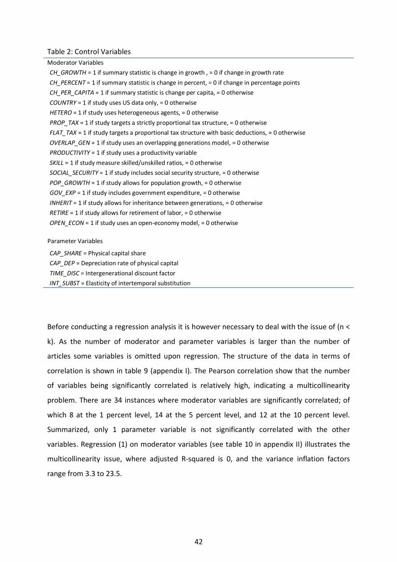
Table 2: Control Variables Moderator Variables

CH_GROWTH = 1 if summary statistic is change in growth , = 0 if change in growth rate

CH_PERCENT = 1 if summary statistic is change in percent, = 0 if change in percentage points

CH_PER_CAPITA = 1 if summary statistic is change per capita, = 0 otherwise

COUNTRY = 1 if study uses US data only, = 0 otherwise

HETERO = 1 if study uses heterogeneous agents, = 0 otherwise

PROP_TAX = 1 if study targets a strictly proportional tax structure, = 0 otherwise

FLAT_TAX = 1 if study targets a proportional tax structure with basic deductions, = 0 otherwise

OVERLAP_GEN = 1 if study uses an overlapping generations model, = 0 otherwise

PRODUCTIVITY = 1 if study uses a productivity variable

SKILL = 1 if study measure skilled/unskilled ratios, = 0 otherwise

SOCIAL_SECURITY = 1 if study includes social security structure, = 0 otherwise

POP_GROWTH = 1 if study allows for population growth, = 0 otherwise

GOV_EXP = 1 if study includes government expenditure, = 0 otherwise

INHERIT = 1 if study allows for inheritance between generations, = 0 otherwise

RETIRE = 1 if study allows for retirement of labor, = 0 otherwise

OPEN_ECON = 1 if study uses an open-economy model, = 0 otherwise

Parameter Variables

CAP_SHARE = Physical capital share

CAP_DEP = Depreciation rate of physical capital

TIME_DISC = Intergenerational discount factor

INT_SUBST = Elasticity of intertemporal substitution

Before conducting a regression analysis it is however necessary to deal with the issue of (n <

k). As the number of moderator and parameter variables is larger than the number of

articles some variables is omitted upon regression. The structure of the data in terms of

correlation is shown in table 9 (appendix I). The Pearson correlation show that the number

of variables being significantly correlated is relatively high, indicating a multicollinearity

problem. There are 34 instances where moderator variables are significantly correlated; of

which 8 at the 1 percent level, 14 at the 5 percent level, and 12 at the 10 percent level.

Summarized, only 1 parameter variable is not significantly correlated with the other

variables. Regression (1) on moderator variables (see table 10 in appendix II) illustrates the

multicollinearity issue, where adjusted R-squared is 0, and the variance inflation factors

range from 3.3 to 23.5.

42

6.2 Meta-Regression Analysis

To manage these issues a backward stepwise regression is performed to exclude redundant

moderator variables until a satisfactory model fit is reached. The backward stepwise

regression takes the following path: First the moderator variables having most weighted

instances of significant correlation is removed from the regression model, assuming the

statistical properties of these are covered by correlated variables remaining. More weight is

put on correlation at the 1 percent level than at the 10 percent level. Second, the parameter

variables are initially biased towards the mean by replacing missing values by mean values.

Each parameter variable contains from 2 to 8 missing values for different articles, which

would result in 12 eliminated studies if not using the mean value or omitting the variables.

The estimation bias is then controlled for in 18 regressions with different setups, where the

preliminary model parameter variable coefficients are compared with parameter variable

coefficients estimated under altering conditions. Finally, the least significant moderator

variables are iteratively omitted until a satisfactory model fit is reached.

Note that none of the moderator variables directly attached to measure (i.e. whether the

change in output is measured at level or growth rate, in percent or percentage points,

overall or per capita) will be omitted, even though both CH_GROWTH and CH_PER_CAPITA

are significantly correlated with CH_PERCENT. Doing so would bias the regression model

since these variables are crucial determinants of the measure, and as a result there is a

probability of inferring other moderator variables to have too much or too little effect. This

argument is verified in the following contradiction: The correlation between AVG_ELASTICITY

and the three variables is significant at the 10 percent level for CH_GROWTH and

CH_PER_CAPITA, and at the 5 percent level (close to the 1 percent level) for CH_PERCENT.

Regression (2) shows on the other hand that none of the three variables have significant

explanatory effect on AVG_ELASTICITY (see table 11 in appendix II). Furthermore, the

variance inflation factors range from 1.3 to 2.7, which indicate a moderate correlation. These

contradictory results verify the aforementioned multicollinearity.

The following moderator variables are the most correlated with other moderator variables

(count of instances at the 1 percent level; the 5 percent level ; the 10 percent level ):

CH_PERCENT (3, 4, 1 - not omitted), FLAT_TAX (2, 6, 0), SOCIAL_SECURITY (2, 4, 2),INHERIT

43

(2, 2, 3), and RETIRE (3, 0, 3). They all have at least 2 instances of correlation at the 1 percent

level, see table 10 in appendix I. The initial regression model (3) is hence

𝐴𝐴𝐴𝐴𝐺𝐺_𝐸𝐸𝐿𝐿𝐴𝐴𝑆𝑆𝑇𝑇𝐸𝐸𝐶𝐶𝐸𝐸𝑇𝑇𝑌𝑌𝑖𝑖= 𝛽𝛽0 + 𝛽𝛽1𝐶𝐶𝐻𝐻_𝐺𝐺𝑅𝑅𝐺𝐺𝑊𝑊𝑇𝑇𝐻𝐻𝑖𝑖 + 𝛽𝛽2𝐶𝐶𝐻𝐻_𝑃𝑃𝐸𝐸𝑅𝑅𝐶𝐶𝐸𝐸𝑃𝑃𝑇𝑇𝑖𝑖 + 𝛽𝛽3𝐶𝐶𝐻𝐻_𝑃𝑃𝐸𝐸𝑅𝑅_𝐶𝐶𝐴𝐴𝑃𝑃𝐸𝐸𝑇𝑇𝐴𝐴𝑖𝑖+ 𝛽𝛽4𝐶𝐶𝐺𝐺𝑈𝑈𝑃𝑃𝑇𝑇𝑅𝑅𝑌𝑌𝑖𝑖 + 𝛽𝛽5𝐻𝐻𝐸𝐸𝑇𝑇𝐸𝐸𝑅𝑅𝐺𝐺𝑖𝑖 + 𝛽𝛽6𝑃𝑃𝑅𝑅𝐺𝐺𝑃𝑃_𝑇𝑇𝐴𝐴𝑇𝑇𝑖𝑖 + 𝛽𝛽7𝐺𝐺𝐴𝐴𝐸𝐸𝑅𝑅𝐿𝐿𝐴𝐴𝑃𝑃_𝐺𝐺𝐸𝐸𝑃𝑃𝑖𝑖+ 𝛽𝛽8𝑃𝑃𝑅𝑅𝐺𝐺𝐷𝐷𝑈𝑈𝐶𝐶𝑇𝑇𝐸𝐸𝐴𝐴𝐸𝐸𝑇𝑇𝑌𝑌𝑖𝑖 + 𝛽𝛽9𝑆𝑆𝐾𝐾𝐸𝐸𝐿𝐿𝐿𝐿𝑖𝑖 + 𝛽𝛽10𝑃𝑃𝐺𝐺𝑃𝑃_𝐺𝐺𝑅𝑅𝐺𝐺𝑊𝑊𝑇𝑇𝐻𝐻𝑖𝑖 + 𝛽𝛽11𝐺𝐺𝐺𝐺𝐴𝐴_𝐸𝐸𝑇𝑇𝑃𝑃𝑖𝑖+ 𝛽𝛽12𝐺𝐺𝑃𝑃𝐸𝐸𝑃𝑃_𝐸𝐸𝐶𝐶𝐺𝐺𝑃𝑃𝑖𝑖 + 𝛽𝛽13𝐶𝐶𝐴𝐴𝑃𝑃_𝑆𝑆𝐻𝐻𝐴𝐴𝑅𝑅𝐸𝐸𝑖𝑖 + 𝛽𝛽14𝐶𝐶𝐴𝐴𝑃𝑃_𝐷𝐷𝐸𝐸𝑃𝑃𝑖𝑖 + 𝛽𝛽15𝑇𝑇𝐸𝐸𝑀𝑀𝐸𝐸_𝐷𝐷𝐸𝐸𝑆𝑆𝐶𝐶𝑖𝑖+ 𝛽𝛽16𝐸𝐸𝑃𝑃𝑇𝑇_𝑆𝑆𝑈𝑈𝑆𝑆𝑆𝑆𝑇𝑇𝑖𝑖 + 𝜀𝜀𝑖𝑖

(20)

where 𝐴𝐴𝐴𝐴𝐺𝐺_𝐸𝐸𝐿𝐿𝐴𝐴𝑆𝑆𝐸𝐸𝑇𝑇𝐸𝐸𝐶𝐶𝑇𝑇𝑌𝑌𝑖𝑖 is the estimated average tax elasticity of article 𝑖𝑖, 𝛽𝛽𝑎𝑎 𝑥𝑥 is the

coefficient of the 𝑎𝑎th moderator or parameter variable as listed in table 2, and 𝜀𝜀𝑖𝑖 is the error

term.

The initial regression model fits the data extremely well. There are however two indications

of that there is a high degree of multicollinearity still being present. First, from the Pearson

correlation test (table 9) 9 moderator and parameter variables are significantly correlated

with the dependent variable at either the 1, the 5 or the 10 percent level, which contradicts

the regression model. In addition 3 instances have correlation close to but above the 10

percent level. This test also shows that both CH_GROWTH and CH_PER_CAPITA are

significantly correlated with CH_PERCENT at the 1 and the 5 percent level. Second, the

variance inflation factors are still rather high, ranging from 3.6 to 22.2.

In addition there might be a problem that the number of independent variables is almost

equal to the sample size (16 and 19, respectively), even after removing the most correlated

variables. Additionally omitting the variables PRODUCTIVITY and HETERO solves both this

and the multicollinearity issues to a large extent. The final meta-regression model is of the

form

𝐴𝐴𝐴𝐴𝐺𝐺_𝐸𝐸𝐿𝐿𝐴𝐴𝑆𝑆𝑇𝑇𝐸𝐸𝐶𝐶𝐸𝐸𝑇𝑇𝑌𝑌𝑖𝑖= 𝛽𝛽0 + 𝛽𝛽1𝐶𝐶𝐻𝐻_𝐺𝐺𝑅𝑅𝐺𝐺𝑊𝑊𝑇𝑇𝐻𝐻𝑖𝑖 + 𝛽𝛽2𝐶𝐶𝐻𝐻_𝑃𝑃𝐸𝐸𝑅𝑅𝐶𝐶𝐸𝐸𝑃𝑃𝑇𝑇𝑖𝑖 + 𝛽𝛽3𝐶𝐶𝐻𝐻_𝑃𝑃𝐸𝐸𝑅𝑅_𝐶𝐶𝐴𝐴𝑃𝑃𝐸𝐸𝑇𝑇𝐴𝐴𝑖𝑖+ 𝛽𝛽4𝐶𝐶𝐺𝐺𝑈𝑈𝑃𝑃𝑇𝑇𝑅𝑅𝑌𝑌𝑖𝑖 + 𝛽𝛽5𝑃𝑃𝑅𝑅𝐺𝐺𝑃𝑃_𝑇𝑇𝐴𝐴𝑇𝑇𝑖𝑖 + 𝛽𝛽6𝐺𝐺𝐴𝐴𝐸𝐸𝑅𝑅𝐿𝐿𝐴𝐴𝑃𝑃_𝐺𝐺𝐸𝐸𝑃𝑃𝑖𝑖 + 𝛽𝛽7𝑆𝑆𝐾𝐾𝐸𝐸𝐿𝐿𝐿𝐿𝑖𝑖+ 𝛽𝛽8𝑃𝑃𝐺𝐺𝑃𝑃_𝐺𝐺𝑅𝑅𝐺𝐺𝑊𝑊𝑇𝑇𝐻𝐻𝑖𝑖 + 𝛽𝛽9𝐺𝐺𝐺𝐺𝐴𝐴_𝐸𝐸𝑇𝑇𝑃𝑃𝑖𝑖 + 𝛽𝛽10𝐺𝐺𝑃𝑃𝐸𝐸𝑃𝑃_𝐸𝐸𝐶𝐶𝐺𝐺𝑃𝑃𝑖𝑖+ 𝛽𝛽11𝐶𝐶𝐴𝐴𝑃𝑃_𝑆𝑆𝐻𝐻𝐴𝐴𝑅𝑅𝐸𝐸𝑖𝑖 + 𝛽𝛽12𝐶𝐶𝐴𝐴𝑃𝑃_𝐷𝐷𝐸𝐸𝑃𝑃𝑖𝑖 + 𝛽𝛽13𝑇𝑇𝐸𝐸𝑀𝑀𝐸𝐸_𝐷𝐷𝐸𝐸𝑆𝑆𝐶𝐶𝑖𝑖 + 𝛽𝛽14𝐸𝐸𝑃𝑃𝑇𝑇_𝑆𝑆𝑈𝑈𝑆𝑆𝑆𝑆𝑇𝑇𝑖𝑖+ 𝜀𝜀𝑖𝑖

(21)

44

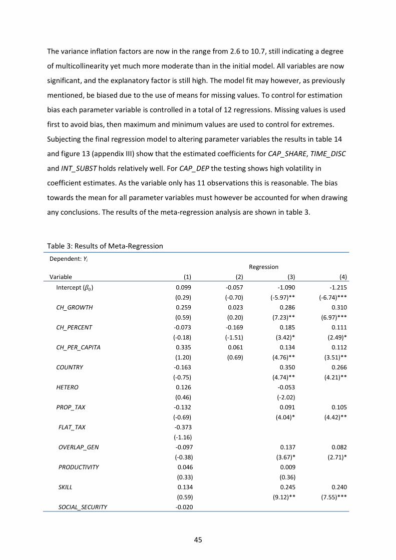
The variance inflation factors are now in the range from 2.6 to 10.7, still indicating a degree

of multicollinearity yet much more moderate than in the initial model. All variables are now

significant, and the explanatory factor is still high. The model fit may however, as previously

mentioned, be biased due to the use of means for missing values. To control for estimation

bias each parameter variable is controlled in a total of 12 regressions. Missing values is used

first to avoid bias, then maximum and minimum values are used to control for extremes.

Subjecting the final regression model to altering parameter variables the results in table 14

and figure 13 (appendix III) show that the estimated coefficients for CAP_SHARE, TIME_DISC

and INT_SUBST holds relatively well. For CAP_DEP the testing shows high volatility in

coefficient estimates. As the variable only has 11 observations this is reasonable. The bias

towards the mean for all parameter variables must however be accounted for when drawing

any conclusions. The results of the meta-regression analysis are shown in table 3.

Table 3: Results of Meta-Regression

Dependent: Yi Regression

Variable (1) (2) (3) (4)

Intercept (𝛽𝛽0) 0.099 -0.057 -1.090 -1.215

(0.29) (-0.70) (-5.97)** (-6.74)***

CH_GROWTH 0.259 0.023 0.286 0.310

(0.59) (0.20) (7.23)** (6.97)***

CH_PERCENT -0.073 -0.169 0.185 0.111

(-0.18) (-1.51) (3.42)* (2.49)*

CH_PER_CAPITA 0.335 0.061 0.134 0.112

(1.20) (0.69) (4.76)** (3.51)**

COUNTRY -0.163

0.350 0.266

(-0.75)

(4.74)** (4.21)**

HETERO 0.126

-0.053

(0.46)

(-2.02)

PROP_TAX -0.132

0.091 0.105

(-0.69)

(4.04)* (4.42)**

FLAT_TAX -0.373

(-1.16)

OVERLAP_GEN -0.097

0.137 0.082

(-0.38)

(3.67)* (2.71)*

PRODUCTIVITY 0.046

0.009

(0.33)

(0.36)

SKILL 0.134

0.245 0.240

(0.59)

(9.12)** (7.55)***

SOCIAL_SECURITY -0.020

45

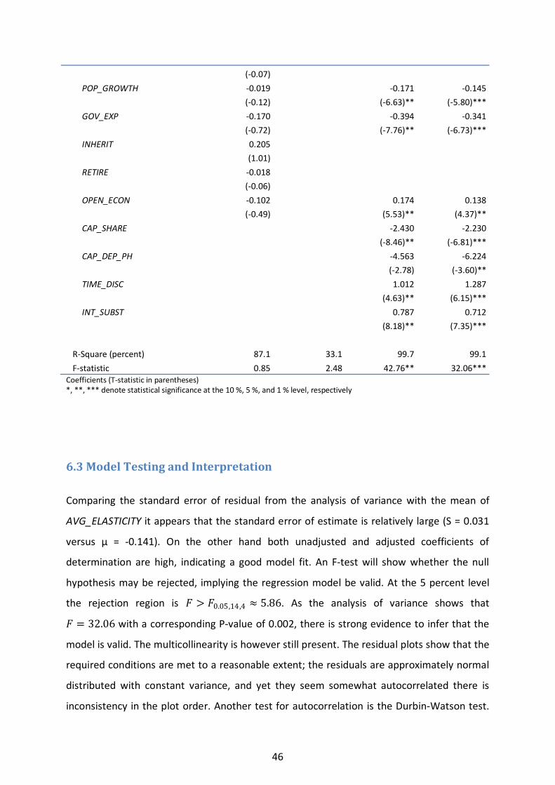
(-0.07)

POP_GROWTH -0.019

-0.171 -0.145

(-0.12)

(-6.63)** (-5.80)***

GOV_EXP -0.170

-0.394 -0.341

(-0.72)

(-7.76)** (-6.73)***

INHERIT 0.205

(1.01)

RETIRE -0.018

(-0.06)

OPEN_ECON -0.102

0.174 0.138

(-0.49) (5.53)** (4.37)**

CAP_SHARE

-2.430 -2.230

(-8.46)** (-6.81)***

CAP_DEP_PH

-4.563 -6.224

(-2.78) (-3.60)**

TIME_DISC

1.012 1.287

(4.63)** (6.15)***

INT_SUBST

0.787 0.712

(8.18)** (7.35)***

R-Square (percent) 87.1 33.1 99.7 99.1

F-statistic 0.85 2.48 42.76** 32.06***

Coefficients (T-statistic in parentheses) *, **, *** denote statistical significance at the 10 %, 5 %, and 1 % level, respectively

6.3 Model Testing and Interpretation

Comparing the standard error of residual from the analysis of variance with the mean of

AVG_ELASTICITY it appears that the standard error of estimate is relatively large (S = 0.031

versus μ = -0.141). On the other hand both unadjusted and adjusted coefficients of

determination are high, indicating a good model fit. An F-test will show whether the null

hypothesis may be rejected, implying the regression model be valid. At the 5 percent level

the rejection region is 𝐹𝐹 > 𝐹𝐹0.05,14,4 ≈ 5.86. As the analysis of variance shows that

𝐹𝐹 = 32.06 with a corresponding P-value of 0.002, there is strong evidence to infer that the

model is valid. The multicollinearity is however still present. The residual plots show that the

required conditions are met to a reasonable extent; the residuals are approximately normal

distributed with constant variance, and yet they seem somewhat autocorrelated there is

inconsistency in the plot order. Another test for autocorrelation is the Durbin-Watson test.

46

The critical values for d0.05,19,14 are dL = 0.070 and dU = 3.642 (see table 3 in Savin and

White (1977)). Testing the Durbin-Watson statistic (1.586) against these for positive and

negative autocorrelation and the combination of these, the test is inconclusive. A Pearson

test shows no evidence of correlation between average benchmark year and

AVG_ELASTICITY. Summarized the statistics show that the model’s fit is good.

It is worth mentioning that the final regression model’s statistics show slightly less fit than

the initial model, even though the variance inflation factor is reduced by more than half. This

indicates that the final model is more robust against interdependence between variables

without losing explanatory value.

For the coefficients the corresponding P-values denotes whether the null hypothesis is true

(high P-value) or not. The latter case is denoted in the regression tables with the significance

level of the T-statistic. At the 10 percent level all variables are significantly different from 0.

The intercept is -1.215 and represents the predicted tax elasticity when all moderator and

parameter variables are 0. The size and negativity of the intercept is not to be strictly

interpreted, however it fits well with the direction given by the articles studied. The measure

moderator variable coefficients are as one should expect but for CH_PERCENT and

COUNTRY. The decreasing effect of using percent as opposed to percentage points is

surprising, as the data clearly shows that the elasticities estimated for articles using

percentage points are overall much lower than for the articles using percent. The coefficient

may however be biased due to multicollinearity as its variance inflation factor is 8.7. Using

US data will reduce the predicted elasticity by 0.266, however due to the low number of

non-US studies in the regression this is not robust. If the overlapping generations model was

utilized the predicted tax elasticity is reduced by 0.082. When the study includes population

growth and government expenditure, the predicted tax elasticity increases by -0.145 and

-0.349, whereas differences in skills and modeling an open economy reduce the elasticity by

0.240 and 0.138.Not to draw any conclusions for the variables, this illustrates that more

complex economic models do not necessarily alter the conclusions. The effects gained

through some of the elements included may be eliminated by the losses from other

elements. For the parameters the regression predicts that studies using high physical capital

share and capital depreciation rate, and low intergenerational discount factor and elasticity

47

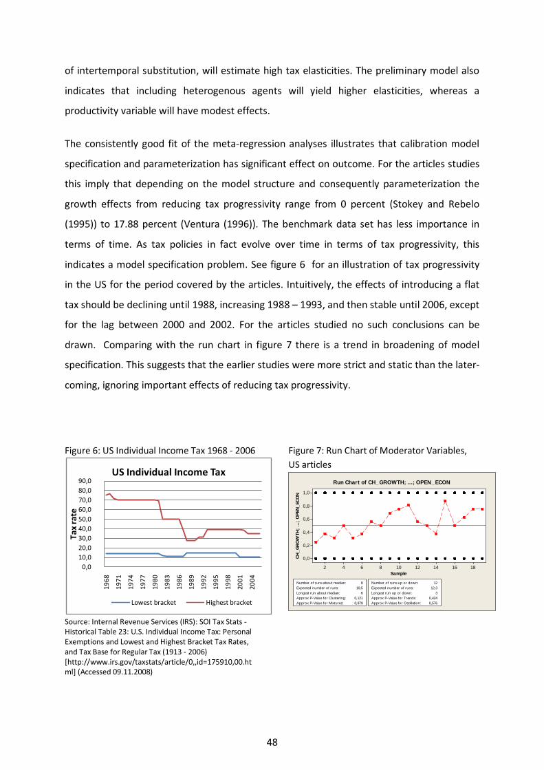
of intertemporal substitution, will estimate high tax elasticities. The preliminary model also

indicates that including heterogenous agents will yield higher elasticities, whereas a

productivity variable will have modest effects.

The consistently good fit of the meta-regression analyses illustrates that calibration model

specification and parameterization has significant effect on outcome. For the articles studies

this imply that depending on the model structure and consequently parameterization the

growth effects from reducing tax progressivity range from 0 percent (Stokey and Rebelo

(1995)) to 17.88 percent (Ventura (1996)). The benchmark data set has less importance in

terms of time. As tax policies in fact evolve over time in terms of tax progressivity, this

indicates a model specification problem. See figure 6 for an illustration of tax progressivity

in the US for the period covered by the articles. Intuitively, the effects of introducing a flat

tax should be declining until 1988, increasing 1988 – 1993, and then stable until 2006, except

for the lag between 2000 and 2002. For the articles studied no such conclusions can be

drawn. Comparing with the run chart in figure 7 there is a trend in broadening of model

specification. This suggests that the earlier studies were more strict and static than the later-

coming, ignoring important effects of reducing tax progressivity.

Figure 6: US Individual Income Tax 1968 - 2006

Source: Internal Revenue Services (IRS): SOI Tax Stats - Historical Table 23: U.S. Individual Income Tax: Personal Exemptions and Lowest and Highest Bracket Tax Rates, and Tax Base for Regular Tax (1913 - 2006) [http://www.irs.gov/taxstats/article/0,,id=175910,00.html] (Accessed 09.11.2008)

Figure 7: Run Chart of Moderator Variables, US articles

18161412108642

1,0

0,8

0,6

0,4

0,2

0,0

Sample

CH_G

RO

WTH

; ...

; O

PEN_

ECO

N

Number of runs about median: 8Expected number of runs: 10,5Longest run about median: 6Approx P-Value for Clustering: 0,121Approx P-Value for Mixtures: 0,879

Number of runs up or down: 12Expected number of runs: 12,3Longest run up or down: 3Approx P-Value for Trends: 0,424Approx P-Value for Oscillation: 0,576

Run Chart of CH_GROWTH; ...; OPEN_ECON

0,0 10,0 20,0 30,0 40,0 50,0 60,0 70,0 80,0 90,0

1968

1971

1974

1977

1980

1983

1986

1989

1992

1995

1998

2001

2004

Tax

rate

US Individual Income Tax

Lowest bracket Highest bracket

48

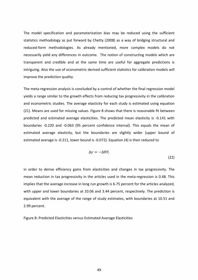
The model specification and parameterization bias may be reduced using the sufficient

statistics methodology as put forward by Chetty (2008) as a way of bridging structural and

reduced-form methodologies. As already mentioned, more complex models do not

necessarily yield any differences in outcome. The notion of constructing models which are

transparent and credible and at the same time are useful for aggregate predictions is

intriguing. Also the use of econometric derived sufficient statistics for calibration models will

improve the prediction quality.

The meta-regression analysis is concluded by a control of whether the final regression model

yields a range similar to the growth effects from reducing tax progressivity in the calibration

and econometric studies. The average elasticity for each study is estimated using equation

(21). Means are used for missing values. Figure 8 shows that there is reasonable fit between

predicted and estimated average elasticities. The predicted mean elasticity is -0.141 with

boundaries -0.220 and -0.063 (95 percent confidence interval). This equals the mean of

estimated average elasticity, but the boundaries are slightly wider (upper bound of

estimated average is -0.211, lower bound is -0.072). Equation (4) is then reduced to

∆𝛾𝛾 = −∆Ѳ𝑌𝑌𝑖𝑖 (22)

in order to derive efficiency gains from elasticities and changes in tax progressivity. The

mean reduction in tax progressivity in the articles used in the meta-regression is 0.48. This

implies that the average increase in long run growth is 6.75 percent for the articles analyzed,

with upper and lower boundaries at 10.06 and 3.44 percent, respectively. The prediction is

equivalent with the average of the range of study estimates, with boundaries at 10.51 and

2.99 percent.

Figure 8: Predicted Elasticities versus Estimated Average Elasticities

49

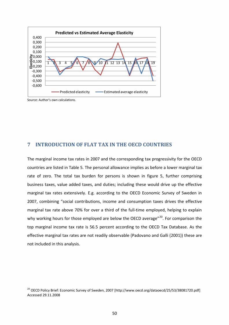
Source: Author’s own calculations.

7 INTRODUCTION OF FLAT TAX IN THE OECD COUNTRIES

The marginal income tax rates in 2007 and the corresponding tax progressivity for the OECD

countries are listed in Table 5. The personal allowance implies as before a lower marginal tax

rate of zero. The total tax burden for persons is shown in figure 5, further comprising

business taxes, value added taxes, and duties; including these would drive up the effective

marginal tax rates extensively. E.g. according to the OECD Economic Survey of Sweden in

2007, combining “social contributions, income and consumption taxes drives the effective

marginal tax rate above 70% for over a third of the full-time employed, helping to explain

why working hours for those employed are below the OECD average”20

20 OECD Policy Brief: Economic Survey of Sweden, 2007 [http://www.oecd.org/dataoecd/25/53/38081720.pdf] Accessed 29.11.2008

. For comparison the

top marginal income tax rate is 56.5 percent according to the OECD Tax Database. As the

effective marginal tax rates are not readily observable (Padovano and Galli (2001)) these are

not included in this analysis.

-0,600-0,500-0,400-0,300-0,200-0,1000,0000,1000,2000,3000,400

1 2 3 4 5 6 7 8 9 10 11 12 13 14 15 16 17 18 19

Elas

tici

tyPredicted vs Estimated Average Elasticity

Predicted elasticity Estimated average elasticity

50

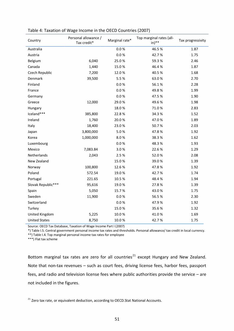
Table 4: Taxation of Wage Income in the OECD Countries (2007)

Country Personal allowance /

Tax credit* Marginal rate*

Top marginal rates (all-in)**

Tax progressivity

Australia 0.0 % 46.5 % 1.87

Austria 0.0 % 42.7 % 1.75

Belgium 6,040 25.0 % 59.3 % 2.46

Canada 1,440 15.0 % 46.4 % 1.87

Czech Republic 7,200 12.0 % 40.5 % 1.68

Denmark 39,500 5.5 % 63.0 % 2.70

Finland 0.0 % 56.1 % 2.28

France 0.0 % 49.8 % 1.99

Germany 0.0 % 47.5 % 1.90

Greece 12,000 29.0 % 49.6 % 1.98

Hungary 18.0 % 71.0 % 2.83

Iceland*** 385,800 22.8 % 34.3 % 1.52

Ireland 1,760 20.0 % 47.0 % 1.89

Italy 18,400 23.0 % 50.7 % 2.03

Japan 3,800,000 5.0 % 47.8 % 1.92

Korea 1,000,000 8.0 % 38.3 % 1.62

Luxembourg 0.0 % 48.3 % 1.93

Mexico 7,083.84 3.0 % 22.6 % 1.29

Netherlands 2,043 2.5 % 52.0 % 2.08

New Zealand 15.0 % 39.0 % 1.39

Norway 100,800 12.6 % 47.8 % 1.92

Poland 572.54 19.0 % 42.7 % 1.74

Portugal 221.65 10.5 % 48.4 % 1.94

Slovak Republic*** 95,616 19.0 % 27.8 % 1.39

Spain 5,050 15.7 % 43.0 % 1.75

Sweden 11,900 0.0 % 56.5 % 2.30

Switzerland 0.0 % 47.9 % 1.92

Turkey 15.0 % 35.6 % 1.32

United Kingdom 5,225 10.0 % 41.0 % 1.69

United States 8,750 10.0 % 42.7 % 1.75

Source: OECD Tax Database, Taxation of Wage Income Part I (2007) *) Table I.5. Central government personal income tax rates and thresholds. Personal allowance/ tax credit in local currency. **) Table I.4. Top marginal personal income tax rates for employee ***) Flat tax scheme

Bottom marginal tax rates are zero for all countries21

21 Zero tax rate, or equivalent deduction, according to OECD.Stat National Accounts.

except Hungary and New Zealand.

Note that non-tax revenues – such as court fees, driving license fees, harbor fees, passport

fees, and radio and television license fees where public authorities provide the service – are

not included in the figures.

51

7.1 Effects of Flat Tax Reforms on Economic Growth in the OECD Countries

All articles used in the meta-regression analysis in section 6 are related to an OECD country.

Also the econometric articles reviewed concern one or more (all) OECD countries.

Comparing the results from the final regression model with estimations for the OECD

countries will hence yield relevant estimates, if not directly transposable. The estimations

are based on the relation between tax elasticity, tax progressivity, and economic growth

which the meta-regression analysis find robust. As most of these studies consider long run

growth effects this is also the emphasis in the following. The studies yielding efficiency gain

as increase in growth rate are however consistent with the remaining and the effects on

economic growth will be even larger if using this approach in a long-run analysis.

The estimations on economic growth could for simplicity be based on the assumption that all

OECD countries have similar average tax elasticity. When considering the wide range of tax

burden in the OECD countries as shown in figure 1 this is however a too restrictive measure

which would yield overestimated growth effects. On the contrary the tax burden might be

partially interpreted as the realization of tax elasticity – higher tax elasticity will yield

downward pressure on governments’ fiscal policies, and lower tax burden; whereas lower

tax elasticities implies less restraint on the government from the society. This relation may

also be interpreted by a Laffer curve (Blinder (1981), Mankiw (1998), Laffer (2004), Miles and

Scott (2005)). The inverse U-shaped curve illustrates that increasing tax rates up to a certain

point yields increased government revenue; beyond this tax revenue will decrease due to

disincentive effects, i.e. reduced input and increased effort in tax avoidance. Tax elasticity

defines the curve’s path (steepness and maximum), effective marginal tax rates define the

current position at the curve, the sum being tax burden. Modeling and measuring this

relationship is outside the scope of this paper, hence the more simple linear relationship

between tax burden and tax elasticity is assumed22

22 Trabandt and Uhlig (2007) find that EU-15 is moving closer to peak of Laffer curve, yet is still at the left side of the curve. The US is also at the left side of the curve. Hence the approximation seems viable for most OECD countries.

. Still, increased tax revenue may be

expected, as a simplified and less intrusive tax scheme provides less incentive for evasion

and avoidance (Hall and Rabushka (1995)). Schneider (2005) estimates the average shadow

economy for 21 OECD countries to 16.3 percent.

52

Although the three non-US articles show elasticities well below the mean of the US articles (-

0.158), they are within the similar range (-0.503 – -0.003). A regression using the mean

elasticity for the US, the elasticities for Sweden, Spain and Denmark, and the respective tax

burdens in figure 1 indicates however that using the tax burden as proxy for tax elasticities is

a reasonable approximation, see table 15 in appendix IV. This is also confirmed by a Pearson

correlation test showing a correlation of 0.941 with a corresponding P-value of 0.059. The

results are shown in table 5. Comparing the elasticity estimations using the regression

equation for the US, Spain, Sweden and Denmark with the estimated average elasticities

shows only small deviations.

Table 5: Approximated Tax Elasticities for the OECD Countries Country Tax versus GDP Ratio Estimated elasticity Approximated elasticity Australia 30,60

-0,130

Austria 41,74

-0,074 Belgium 44,52

-0,060

Canada 33,33

-0,116 Czech Republic 36,92

-0,098

Denmark 49,14 -0,049 -0,037 Finland 43,47

-0,065

France 44,17

-0,062 Germany 35,58

-0,105

Greece 31,32

-0,126 Hungary 37,08

-0,097

Iceland 41,52

-0,075 Ireland 31,88

-0,123

Italy 42,15

-0,072 Japan 27,90

-0,143

Korea 26,77

-0,149 Luxembourg 35,90

-0,103

Mexico 20,57

-0,180 Netherlands 39,32

-0,086

New Zealand 36,71

-0,099 Norway 43,94

-0,063

Poland 33,51

-0,115 Portugal 35,70

-0,104

Slovak Republic 29,77

-0,134 Spain 36,64 -0,074 -0,099 Sweden 49,08 -0,035 -0,037 Switzerland 29,61

-0,135

Turkey 24,52

-0,160 United Kingdom 37,12

-0,097

United States OECD - Total

28,00 35,95

-0,158

-0,143 -0,103

Source: Tax versus GDP ratio is from OECD Centre for Tax Policy and Administration, Revenue Statistics 1965-2007, 2008 Edition, table 1. [http://www.oecd.org/ctp/revenuestats]. Elasticities are based on author’s own calculations.

53

The changes in tax progressivity are assumed to yield 1, i.e. a pure flat tax with no

deductions. This extreme scenario is chosen to show the inherent potential of proportional

taxes, although the Hall-Rabushka flat tax and most other suggested and implemented flat

tax schemes also include fixed deductions which imply progressivity in the tax scheme. Using

the purely flat tax also avoid entering an extensive analysis of tax rates and deduction levels,

which are likely to be different for each country in that the current tax levels differ

substantially (see table 4).

Comparing the estimated average elasticity and tax progressivity reduction shows that for

the articles studied, change in tax progressivity has a larger share of the efficiency gain than

do change in tax rate. This is a supporting evidence for the flat tax scheme in that

progressive tax structures have more adverse effects on output than do high tax rates. As

most studies concern the US, which has relatively low tax progressivity among the OECD

countries, the overall increase is expected to be somewhat larger.

Tax progressivity for each OECD country is from table 4. The reductions in tax progressivity

range from 0.29 to 2.45. By utilizing equation (22) the efficiency gains for the OECD countries

are estimated based on the approximated tax elasticities and tax progressivity calculations.

The potential effect on economic growth from shifting to a strictly proportional tax scheme

ranges from 3.9 percent (New Zealand and Iceland) to a magnitude of 17.8 percent

(Hungary). The unweighted average for the OECD countries is 9.16 percent. Figure 9 shows

the individual estimations. These are then compared with other studies to control the

validity of the estimates.

54

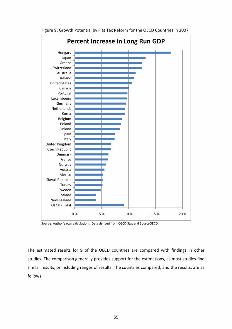
Figure 9: Growth Potential by Flat Tax Reform for the OECD Countries in 2007

Source: Author’s own calculations. Data derived from OECD.Stat and SourceOECD.

The estimated results for 9 of the OECD countries are compared with findings in other

studies. The comparison generally provides support for the estimations, as most studies find

similar results, or including ranges of results. The countries compared, and the results, are as

follows:

0 % 5 % 10 % 15 % 20 %

OECD - TotalNew Zealand

IcelandSwedenTurkey

Slovak RepublicMexicoAustria

NorwayFrance

DenmarkCzech Republic

United KingdomItaly

SpainFinlandPoland

BelgiumKorea

NetherlandsGermany

LuxembourgPortugalCanada

United StatesIreland

AustraliaSwitzerland

GreeceJapan

Hungary

Percent Increase in Long Run GDP

55

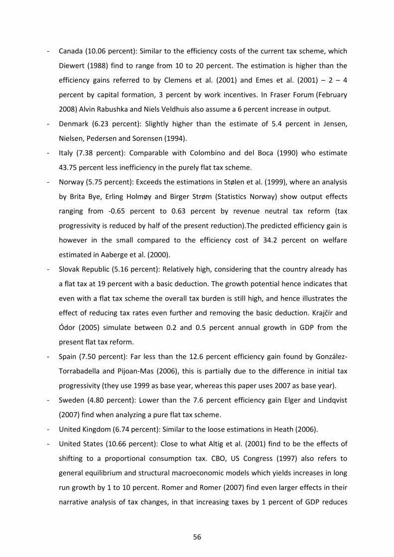
- Canada (10.06 percent): Similar to the efficiency costs of the current tax scheme, which

Diewert (1988) find to range from 10 to 20 percent. The estimation is higher than the

efficiency gains referred to by Clemens et al. (2001) and Emes et al. (2001) – 2 – 4

percent by capital formation, 3 percent by work incentives. In Fraser Forum (February

2008) Alvin Rabushka and Niels Veldhuis also assume a 6 percent increase in output.

- Denmark (6.23 percent): Slightly higher than the estimate of 5.4 percent in Jensen,

Nielsen, Pedersen and Sorensen (1994).

- Italy (7.38 percent): Comparable with Colombino and del Boca (1990) who estimate

43.75 percent less inefficiency in the purely flat tax scheme.

- Norway (5.75 percent): Exceeds the estimations in Stølen et al. (1999), where an analysis

by Brita Bye, Erling Holmøy and Birger Strøm (Statistics Norway) show output effects

ranging from -0.65 percent to 0.63 percent by revenue neutral tax reform (tax

progressivity is reduced by half of the present reduction).The predicted efficiency gain is

however in the small compared to the efficiency cost of 34.2 percent on welfare

estimated in Aaberge et al. (2000).

- Slovak Republic (5.16 percent): Relatively high, considering that the country already has

a flat tax at 19 percent with a basic deduction. The growth potential hence indicates that

even with a flat tax scheme the overall tax burden is still high, and hence illustrates the

effect of reducing tax rates even further and removing the basic deduction. Krajčír and

Ódor (2005) simulate between 0.2 and 0.5 percent annual growth in GDP from the

present flat tax reform.

- Spain (7.50 percent): Far less than the 12.6 percent efficiency gain found by González-

Torrabadella and Pijoan-Mas (2006), this is partially due to the difference in initial tax

progressivity (they use 1999 as base year, whereas this paper uses 2007 as base year).

- Sweden (4.80 percent): Lower than the 7.6 percent efficiency gain Elger and Lindqvist

(2007) find when analyzing a pure flat tax scheme.

- United Kingdom (6.74 percent): Similar to the loose estimations in Heath (2006).

- United States (10.66 percent): Close to what Altig et al. (2001) find to be the effects of

shifting to a proportional consumption tax. CBO, US Congress (1997) also refers to

general equilibrium and structural macroeconomic models which yields increases in long

run growth by 1 to 10 percent. Romer and Romer (2007) find even larger effects in their

narrative analysis of tax changes, in that increasing taxes by 1 percent of GDP reduces

56

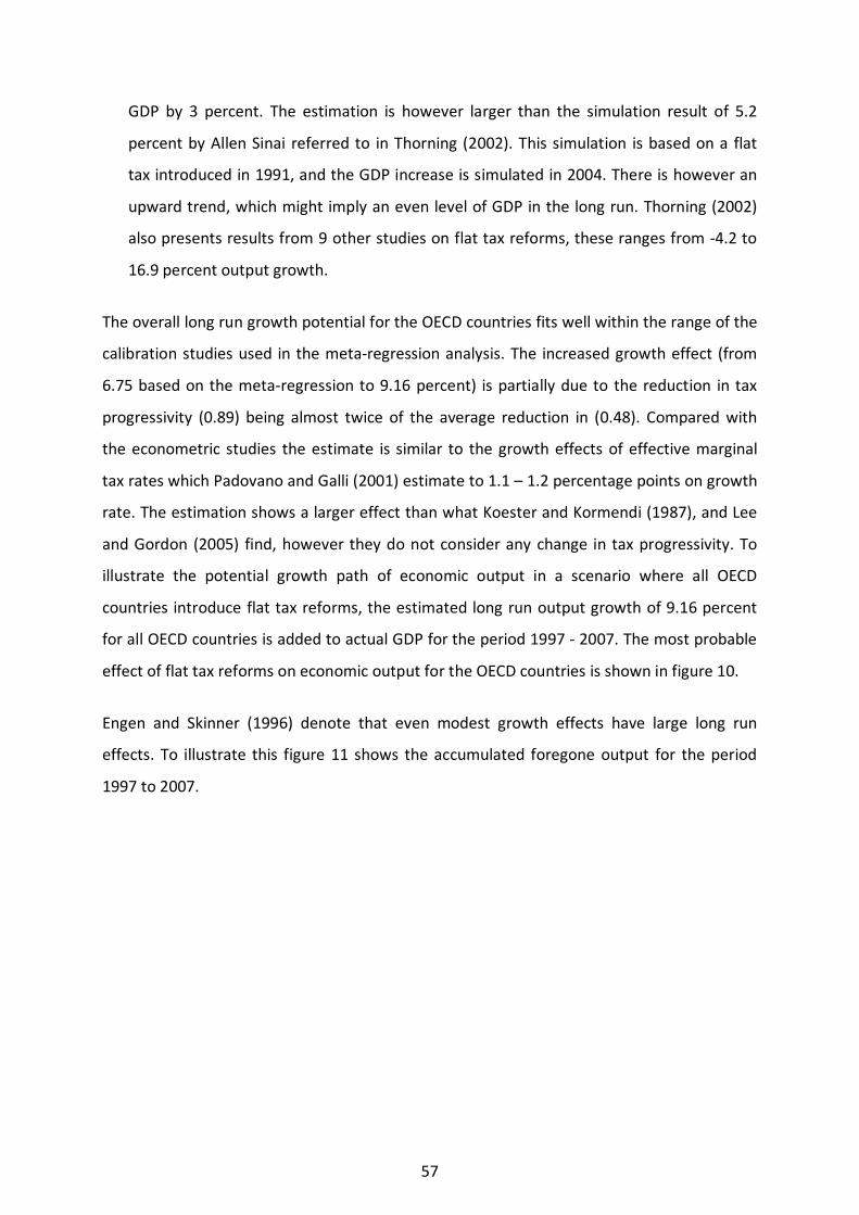
GDP by 3 percent. The estimation is however larger than the simulation result of 5.2

percent by Allen Sinai referred to in Thorning (2002). This simulation is based on a flat

tax introduced in 1991, and the GDP increase is simulated in 2004. There is however an

upward trend, which might imply an even level of GDP in the long run. Thorning (2002)

also presents results from 9 other studies on flat tax reforms, these ranges from -4.2 to

16.9 percent output growth.

The overall long run growth potential for the OECD countries fits well within the range of the

calibration studies used in the meta-regression analysis. The increased growth effect (from

6.75 based on the meta-regression to 9.16 percent) is partially due to the reduction in tax

progressivity (0.89) being almost twice of the average reduction in (0.48). Compared with

the econometric studies the estimate is similar to the growth effects of effective marginal

tax rates which Padovano and Galli (2001) estimate to 1.1 – 1.2 percentage points on growth

rate. The estimation shows a larger effect than what Koester and Kormendi (1987), and Lee

and Gordon (2005) find, however they do not consider any change in tax progressivity. To

illustrate the potential growth path of economic output in a scenario where all OECD

countries introduce flat tax reforms, the estimated long run output growth of 9.16 percent

for all OECD countries is added to actual GDP for the period 1997 - 2007. The most probable

effect of flat tax reforms on economic output for the OECD countries is shown in figure 10.

Engen and Skinner (1996) denote that even modest growth effects have large long run

effects. To illustrate this figure 11 shows the accumulated foregone output for the period

1997 to 2007.

57

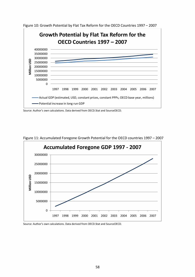
Figure 10: Growth Potential by Flat Tax Reform for the OECD Countries 1997 – 2007


Figure 11: Accumulated Foregone Growth Potential for the OECD countries 1997 – 2007


05000000

10000000150000002000000025000000300000003500000040000000

1997 1998 1999 2000 2001 2002 2003 2004 2005 2006 2007

Mill

ion

USD

Growth Potential by Flat Tax Reform for the OECD Countries 1997 – 2007

Actual GDP (estimated, USD, constant prices, constant PPPs, OECD base year, millions)

Potential increase in long run GDP

0

5000000

10000000

15000000

20000000

25000000

30000000

1997 1998 1999 2000 2001 2002 2003 2004 2005 2006 2007

Mill

ion

USD

Accumulated Foregone GDP 1997 - 2007

58

The flat tax rates necessary for revenue neutral tax reforms estimated in the calibration

studies range from 17 to 35 percent, hence the estimated growth effects imply that the flat

tax rates be within these boundaries. This simplification restricts the possibility for inferring

on the tax rates necessary for revenue neutral reforms. Intuitively, the effects on economic

output will be larger than predicted if the flat tax rate is set lower than 17 percent, and

smaller if the flat tax rate is set higher than 35 percent. See González-Torrabadella and

Pijoan-Mas (2006), and Elger and Lindqvist (2007) for quantitative studies of the diminishing

effects on output as the progressivity of flat tax schemes increases.

Reducing tax progressivity to 1 shows the largest possible effect on output. This is not a

feasible flat tax scheme for most OECD countries. The Hall-Rabushka flat tax with basic

deductions will on the other hand provide a sound and middle-ground tax scheme where the

considerations of the poor are taken care of. The tax rates and deduction levels are likely to

differ as they are associated with the tax level in each country. Determining the necessary

tax rates and the corresponding deduction levels for the flat tax schemes to be revenue

neutral is not analyzed in this paper. However, as González-Torrabadella and Pijoan-Mas

(2006) point out, setting the tax rate and corresponding deduction level too high will have

adverse effects on economic growth. For some high-tax countries the conclusion may hence

be that the fundamental flat tax reform is not feasible unless accompanied by a fundamental

reform of government expenditure.

7.2 Sensitivity Analysis

The estimated growth for the OECD countries is based on estimations on tax elasticity and

tax progressivity. The tax elasticities are based on estimated growth effects relative to

changes in tax progressivity. Hence there might be an estimation bias present. To control for

this the dependent variable is tested for the meta-regression variation and the estimation

variation, based on the 95 percent confidence interval for the estimates from the meta-

regression analysis and for the OECD countries, respectively. The moderator and parameter

variables are tested for meta-regression variation, based on ± 1 standard error of

coefficients from regression (4). The results are shown in table 6 and table 7.

59

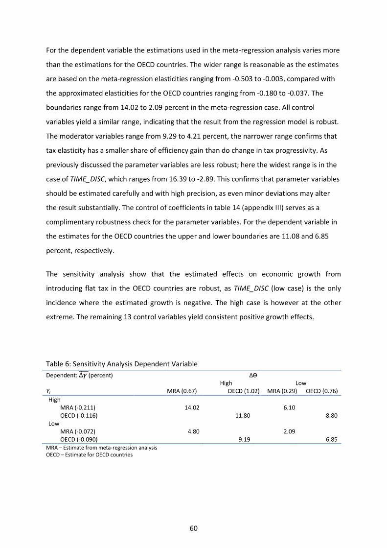
For the dependent variable the estimations used in the meta-regression analysis varies more

than the estimations for the OECD countries. The wider range is reasonable as the estimates

are based on the meta-regression elasticities ranging from -0.503 to -0.003, compared with

the approximated elasticities for the OECD countries ranging from -0.180 to -0.037. The

boundaries range from 14.02 to 2.09 percent in the meta-regression case. All control

variables yield a similar range, indicating that the result from the regression model is robust.

The moderator variables range from 9.29 to 4.21 percent, the narrower range confirms that

tax elasticity has a smaller share of efficiency gain than do change in tax progressivity. As

previously discussed the parameter variables are less robust; here the widest range is in the

case of TIME_DISC, which ranges from 16.39 to -2.89. This confirms that parameter variables

should be estimated carefully and with high precision, as even minor deviations may alter

the result substantially. The control of coefficients in table 14 (appendix III) serves as a

complimentary robustness check for the parameter variables. For the dependent variable in

the estimates for the OECD countries the upper and lower boundaries are 11.08 and 6.85

percent, respectively.

The sensitivity analysis show that the estimated effects on economic growth from

introducing flat tax in the OECD countries are robust, as TIME_DISC (low case) is the only

incidence where the estimated growth is negative. The high case is however at the other

extreme. The remaining 13 control variables yield consistent positive growth effects.

Table 6: Sensitivity Analysis Dependent Variable Dependent: ∆𝛾𝛾 ��(percent) Yi

ΔѲ High

MRA (0.67) OECD (1.02) Low

MRA (0.29) OECD (0.76) High MRA (-0.211) OECD (-0.116) Low MRA (-0.072) OECD (-0.090)

14.02

4.80

11.80

9.19

6.10

2.09

8.80

6.85 MRA – Estimate from meta-regression analysis OECD – Estimate for OECD countries

60

Table 7: Sensitivity Analysis Moderator and Parameter Variables Dependent: ∆𝛾𝛾 ��(percent)

∆Ѳ��𝑌𝑌𝑖𝑖 High Low

Moderator Variables

CH_GROWTH

CH_PERCENT

CH_PER_CAPITA

COUNTRY

PROP_TAX

OVERLAP_GEN

SKILL

POP_GROWTH

GOV_EXP

OPEN_ECON Parameter Variables CAP_SHARE

CAP_DEP

TIME_DISC

INT_SUBST

8.43

8.22

7.07

9.29

7.46

7.51

7.39

7.19

8.66

7.23

11.44

11.79

16.39

9.24

5.08

5.29

6.43

4.21

6.04

5.99

6.11

6.31

4.84

6.28

2.06

1.72

-2.89

4.27

7.3 Some Inequality and Welfare Considerations

In many studies where output is compared with equality, the efficiency gains in output from

a flat tax come at the expense of vertical inequality. On this basis some of these studies, e.g.

Decoster, De Swerdt, and Orsini (2008), Fuest, Peichl, and Schaefer (2008), draw the

conclusion that flat tax reforms are not feasible, particularly not for the OECD type of

countries. This is confirmed in Nielsen (2006) where he finds that the main obstacles to the

introduction of a flat tax in Norway have been a lack of the proposals’ ability to meet survival

criteria of value acceptability, technical and political feasibility, and budgetary implications.

The infeasibility does however stand in sharp contrast with public opinion, which in several

OECD countries opposes the current tax schemes to a large degree23

23 Teather (2005) refers to a UK survey where 81 percent of young people are more worried about high tax levels than war, environment and tuition fees. The TaxPayers' Alliance September Poll 2007 for UK shows that 77 percent think government should tax 25 percent or less from households. [http://tpa.typepad.com/about/2007/10/annual-conferen.html] In the 2007 Annual Survey of U.S. Attitudes on Taxes and Wealth, 83 percent of the respondents said the federal income tax is very complex or somewhat complex. [http://www.taxfoundation.org/files/sr154.pdf]

. Opposition might be

even stronger, as Roberts, Hite, and Bradley (1994) find that a large share of respondents

61

prefers the progressive tax scheme when questionnaires use abstract frames but flat or

regressive taxes in concrete situations, indicating that conclusions from public opinion polls

using abstract questions should be carefully interpreted. Hence, as Nielsen (2006) and Evans

and Aligica (2008) suggest, given a situation of a large policy window, or a policy champion,

where the ideas, interests and consequences are aligned, the flat tax will be politically

feasible also for the OECD countries24

Other studies also suggest that win-win scenarios might exist, where fairness is obtained

without loss of welfare, and/or increased inequality. In general this is possible if and only if

the improved incentives from tax reform result in increased efficiency and thereby increased

income which more than offset the increased tax burden for those benefiting relatively more

from current tax systems. Jensen et al. (1994) find that both efficiency and welfare increase.

Aaberge et al. (1995) find that the reduction in tax progressivity in Norway from 1979 to

1992 increased mean welfare, however the increase would have been even larger if a flat tax

(20.1 percent rate, revenue neutral) was implemented. In the latter case inequality would

also be reduced. Creedy (1996), and Cugno and Zanola (2000) find that flat tax schemes

under certain conditions are preferable to more progressive tax schemes in terms of welfare.

Seldon and Boyd (1996) find that the Armey-Shelby flat tax with a 17 percent overall tax rate

will benefit all income groups; the lowest income group most by 7.6 percent, whereas the

middle income groups benefit from 1.0 to 2.5 percent, and the highest income group benefit

2.4 percent. Teather (2005) find similar results for UK. Kakwani and Lambert (1999) find a

welfare loss of 1 percent due to the 1984 progressive tax scheme in Australia. Aaberge et al.

(2000) find that a flat tax in Norway will both have large efficiency and welfare gains, and

reduce inequality. They do however find that for Italy and Sweden only efficiency improves.

Davies and Hoy (2002) find that the flat tax may reduce inequality compared to the

.

Paulus and Peichl (2008) suggest that the long run efficiency and growth effects of flat tax

reforms might make the increasing vertical inequality acceptable. They also find that that for

some Mediterranean countries, and other countries with similar tax structure, a flat tax can

increase both equality and economic efficiency.

24 According to Alvin Rabushka and Mart Laar, policy makers must be prepared, and they must stand the fight. Source: SPECTATOR.co.uk: Flat tax and faint hearts [http://www.spectator.co.uk/print/the-magazine/cartoons/14303/flat-tax-and-faint-hearts.thtml]

62

progressive tax scheme, even without prohibitively high tax rates. Jorgenson and Yun (2002)

find welfare gains of USD 814.9 billion for the Hall-Rabushka flat tax and USD 756 billion for

the Armey-Shelby flat tax (1997 dollars).

The argument that flat taxes increase vertical inequality might hence be based on valid

concerns for some, hardly all OECD countries. On the contrary, the main reason for

government reluctance might be that flat tax schemes are less susceptible to political

pressure (Slemrod (1990)). If assuming that flat taxes do increase inequality, this should not

be seen as only negative, as the implicit increased incentives will increase factor input. The

latter is however critical dependent on whether the factor markets are provided with less

rigidity (Vietor (2007)) (i.e. labor reforms will for some countries be necessary), and also that

the masks in the social security net is widened so only those really needing may receive

social benefits. Furthermore, by referring to the initial quote by Mill (1900) what the change

in vertical inequality really shows is to what extent some groups or individuals benefit at the

expense of the others under the current fiscal systems. A necessary implication of correcting

this inequality and unfairness is hence that some lose and some gains.

8 CONCLUSION This master thesis explores the effects of flat tax reforms on economic growth in the OECD

countries, focusing on the period from 1997 to 2007. A meta-regression analysis on 18

calibration studies on the subjects of tax reforms (of which 15 concerns US) summarizes the

average growth potential to 6.75 percent. Extending the findings in the meta-regression

analysis to current tax progressivity and economic growth the most probable growth effects

for the OECD countries are estimated. The 2006/2007 level of tax progressivity and elasticity

is estimated to yield a growth potential of 9.16 percent in real output for the OECD area.

Controlling for estimation bias in parameter coefficients and prediction model, the

conclusions remain robust. A recent OECD study (Arnold (2008)) confirms to a large extent

my findings on the relation between taxation and economic growth.

63

The large Keynesian countercyclical fiscal policies currently implemented by most OECD

countries are mostly short or medium term solutions. These measures could be

accompanied, some even substituted by the long run solutions provided by flat tax schemes;

the costs, if any, would not be close to the rescue deals already passed. As Alvin Rabushka

notes in his Flat Tax blog on December 15, 2008; “Every group that benefits from a new

provision becomes another political constituency for keeping and expanding it.”25

8.1 Limitations and areas for further research

Countercyclical fiscal policies tent to yield more groups with increasing demands.

The flat tax era is still infant, but the opportunities for change have improved. Flat tax

reforms are likely to reduce the length and depth of the current worldwide economic

downturn, to speed up recovery and future growth and prosperity.

Two extensions of interest appear which are related to the measuring of the necessary flat

tax rates and corresponding deduction levels for the OECD countries in a Hall-Rabushka flat

tax scenario. First, a measure including only income and business tax is of interest. This may

be the most feasible reform today due to constraints in partisan politics. The second

extension of interest is a measure which also includes the removal of value-added taxes,

hence completely extinguishing double taxation as intended by Hall and Rabushka (1995).

Using estimations for growth rates as opposed to long run growth is also intriguing,

especially when considering short-sighted policy makers.

The meta-regression analysis might be further developed to include the endogenous labor

supply elasticities as pointed out by Stokey and Rebelo (1995). For the purpose of this paper

the exogenous parameterization is a reasonable measurement of the parameters’ effects on

output estimates. The meta-regression analysis is limited to flat tax articles using calibration

methodology. A similar analysis with articles using panel data or cross-section

methodologies (e.g. Vedder (1985), Koester and Kormendi (1987), Colombino and del Boca

25 Flat tax – Essays on the Adoption and Results of Flat Tax Around the Globe [http://flattaxes.blogspot.com/]

64

(1990), Padovano and Galli (2001), Lee and Gordon (2005)) would provide additional insights

on results of existing research, and set direction for future framework and modeling efforts.

The tax elasticities in the predictions are average for each country; an extension of the

model might be to estimate tax elasticities for different income groups for each country. A

comparable measure is the elasticity of taxable income, which Gruber and Saez (2000) find

to differ as much as the tax elasticities differ between the countries. This will also affect the

growth effect of a flat tax reform.

65

REFERENCES Adams, Charles (2001): For Good and Evil: The Impact of Taxes on the Course of Civilization.

2nd ed. Madison Books, Lanham, Maryland.

Adam Smith Institute [http://www.adamsmith.org/]

Altig, David and Charles T. Carlstrom (1991): Inflation, Personal Taxes, and Real Output: A

Dynamic Analysis. Journal of Money, Credit and Banking, Vol. 23, No. 3, Part 2: Price Stability

(August 1991), pp. 547-571, Ohio State University Press.

[http://www.jstor.org/stable/1992689]

Altig, David, Alan J. Auerbach, Laurence J. Kotlikoff, Kent A. Smetters, and Jan Walliser

(2001): Simulating Fundamental Tax Reform in the United States. The American Economic

Review, Vol. 91, No. 3 (June 2001), pp. 574-595, American Economic Association.


Arnold, Jens (2008): Do Tax Structures Affect Aggregate Economic Growth? Empirical

Evidence from a Panel of OECD Countries. OECD Economics Department Working Papers No.

643 (October 2008), Organisation for Economic Co-operation and Development.

[http://www.olis.oecd.org/olis/2008doc.nsf/LinkTo/NT00005C32/$FILE/JT03252848.PDF]

Atkinson, Anthony Barnes (1995): Public Economics in Action: The Basic Income/Flat Tax

Proposal. Oxford University Press, New York

Auerbach, Alan J. (1996): Flat Taxes - Some Economic Considerations. The California Policy

Seminar Brief Series, March 1996. [http://www.ucop.edu/cprc/documents/auerbach.pdf]

Auerbach, Alan J. (1997): The Future of Fundamental Tax Reform. The American Economic

Review, Vol. 87, No. 2, Papers and Proceedings of the Hundred and Fourth Annual Meeting

of the American Economic Association (May 1997), pp. 143-146, American Economic

Association [http://www.jstor.org/stable/2950901]

66

http://www.jstor.org/stable/1992689�

Auerbach, Alan J., Laurence J. Kotlikoff, and Jonathan Skinner (1983): The Efficiency Gains

from Dynamic Tax Reform. International Economic Review, Vol. 24, No. 1 (February 1983),

pp. 81-100, Blackwell Publishing for the Economics Department of the University of

Pennsylvania and Institute of Social and Economic Research, Osaka University.


Auerbach, Alan J., Laurence J. Kotlikoff, Kent A. Smetters, and Jan Walliser (1997):

Fundamental Tax Reform and Macroeconomic Performance. From Two Papers on

Fundamental Tax Reform, October 1997, Congressional Budget Office.

[http://www.cbo.gov/ftpdocs/2xx/doc266/twotax.pdf]

Bartlett, Bruce (1994): The Armey Flat Tax. Brief Analysis No. 136, National Center for Policy

Analysis. [http://www.ncpa.org/ba/ba136.html]

Basham, Patrick and Daniel Mitchell (2008): Lessons from Abroad – Flat Tax in Practice. From

The Impact and Cost of Taxation in Canada: The Case for Flat Tax Reform. Jason Clemens ed.

The Fraser Institute.

Bernoth, Kerstin, Andrew Hughes Hallett, and John Lewis (2008): Did Fiscal Policy Makers

Know What They Were Doing? Reassessing Fiscal Policy with Real Time Data. DNB Working

Paper No. 169 (April 2008), De Nederlansche Bank.

[http://www.dnb.nl/en/binaries/Working%20Paper%20No.%20169-2008_tcm47-

173423.pdf]

Blinder, Alan S. (1981): Some Thoughts on the Laffer Curve. From Laurence H. Meyer, ed.,

The Supply-Side Effects of Economic Policy, Center for the Study of American Business,

Washington University, St. Louis and Federal Reserve Bank of St. Louis.

[http://research.stlouisfed.org/publications/review/81/conf/1981section1-3.pdf]

Bohacek, Radim and Michal Kejak (2005): Optimal Government Policies in Models with

Heterogeneous Agents. USC FBE Macroeconomics and International Finance Workshop.

[http://www.usc.edu/schools/business/FBE/seminars/papers/M_3-31-05_BOHACEK.pdf]

Caplan, Bryan (2007): The Myth of the Rational Voter: Why Democracies Choose Bad

Policies. Princeton University Press, New Jersey.

67

Card, David and Alan B. Krueger (1995): Time-Series Minimum-Wage Studies: A Meta-

analysis. The American Economic Review, Vol. 85, No. 2, Papers and Proceedings of the

Hundredth and Seventh Annual Meeting of the American Economic Association Washington,

DC, January 6-8, 1995 (May 1995), pp. 238-243, American Economic Association.


Carroll, Robert, John Diamond, Craig Johnson, and James Mackie III (2006): A Summary of

the Dynamic Analysis of the Tax Reform Options. Prepared for the President’s Advisory Panel

on Federal Tax Reform, For the American Enterprise Institute Conference on Tax Reform and

Dynamic Analysis, May 25, 2006, Office of Tax Analysis, U.S. Department of the Treasury.

[http://www.ustreas.gov/offices/tax-policy/library/paper_AEI_Conf.pdf]

Carroll, Robert, Douglas Holtz-Eakin, Mark Rider, and Harvey S. Rosen (1998): Entrepreneurs,

Income Taxes, and Investment. NBER Working Paper No. W6374, National Bureau of

Economic Research. [http://www.nber.org/papers/w6374.pdf]

Cassou, Steven P. and Kevin J. Lansing (2003): Growth Effects of Shifting From a Graduate-

Rate Tax System to a Flat Tax. Federal Reserve Bank of San Francisco Working Papers in

Applied Economic Theory no. 2000-15. [http://ideas.repec.org/p/fip/fedfap/2000-15.html]

Cato Institute [http://www.cato.org/]

Caucutt, Elizabeth M., Selahattin Imrohoroglu, and Krishna B. Kumar (2000): Does the

Progressivity of Taxes Matter for Economic Growth? Discussion Paper 138, Institute for

Empirical Macroeconomics, Federal Reserve Bank of Minneapolis.

[http://www.mpls.frb.org/Research/dp/dp138.pdf]

Center for Freedom and Prosperity [http://www.freedomandprosperity.org/]

Chetty, Raj (2008): Sufficient Statistics for Welfare Analysis: A Bridge Between Structural and

Reduced-Form Methods. NBER Working Paper No. 14399, October 2008.

[http://www.nber.org/papers/w14399]

Chetty, Raj, Adam Looney, and Kory Kroft (2008): Salience and Taxation: Theory and

Evidence. American Economic Review, forthcoming.

[http://elsa.berkeley.edu/~chetty/papers/taxsalience_aer.pdf]

68

Clemens, Jason, Joel Emes, and Rodger Scott (2001): The Flat Tax—A Model for Reform of

Personal and Business Taxes. Published as a chapter in Tax Reform in Canada: Our Path to

Greater Prosperity. Fraser Institute, 1 March 2003.

[http://www.fraserinstitute.org/Commerce.Web/publication_details.aspx?pubID=2803]

Colombino, Ugo and Daniela del Boca (1990): The Effect of Taxes on Labor Supply in Italy.

Journal of Human Resources, Vol. 25, No. 3, Special Issue on Taxation and Labor Supply in

Industrial Countries (Summer 1990), pp. 390-414, University of Wisconsin Press.


Conesa, Juan Carlos and Dirk Krueger (2005): On the Optimal Progressivity of the Income Tax

Code. Journal of Monetary Economics Vol. 53, Issue 7 (October 2006), pp. 1425–1450,

Elsevier. [http://www.sciencedirect.com/science/article/B6VBW-4K2T5B1-

1/2/332de0328ef69595e071a08521433e58]

Congressional Budget Office (CBO, US Congress) Washington DC (1997): Economic Effects of

Comprehensive Tax Reform. The Congress of the United States.

[http://www.cbo.gov/doc.cfm?index=36]

Creedy, John (1996): Comparing Tax and Transfer Systems: Poverty, Inequality and Target

Efficiency. Economica, New Series, Vol. 63, No. 250, Supplement: Economic Policy and

Income Distribution (1996), pp. S163-S174, Blackwell Publishing on behalf of The London

School of Economics and Political Science and The Suntory and Toyota International Centres

for Economics and Related Disciplines. [http://www.jstor.org/stable/2554814]

Cugno, Franco and Roberto Zanola (2000): The Welfare of Flat Tax. SSRN Working Paper

Series, December 20, 2000. [http://papers.ssrn.com/sol3/papers.cfm?abstract_id=253066]

Davies, James B. and Michael Hoy (2002): Flat rate taxes and inequality measurement.

Journal of Public Economics Vol. 84, Issue 1 (April 2002), pp. 33–46, Elsevier Science B.V.

[http://ideas.repec.org/a/eee/pubeco/v84y2002i1p33-46.html]

Decoster, André, Kris De Swerdt, and Kristian Orsini (2008): A Belgian Flat Income Tax:

Effects on Labour Supply and Income Distribution. Centre for Economic Studies, Leuven.

[www.econ.kuleuven.be/CES/discussionpapers/Dps08/Dps0820.pdf]

69

Devereux, Michael P., Ben Lockwood, and Michela Redoano (2002): Do Countries Compete

Over Corporate Tax Rates? CSGR Working Paper No. 97/02, April 2002, University of

Warwick.

[http://www2.warwick.ac.uk/fac/soc/csgr/research/workingpapers/2002/wp9702.pdf]

Díaz-Giménez, Javier and Josep Pijoan-Mas (2006): Flat Tax Reforms in the US - a Boon for

the Income Poor. CEMFI Working Paper No. 0611, July 2006.

[http://ideas.repec.org/p/cmf/wpaper/wp2006_0611.html]

Diewert, W.E. (1988): On Tax Reform. The Canadian Journal of Economics / Revue

canadienne d'Economique, Vol. 21, No. 1 (February 1988), pp. 1-40, Blackwell Publishing on

behalf of the Canadian Economics Association. [http://www.jstor.org/stable/135208]

Ding, Hong (2008): Can Tax Wedge Affect Labor Productivity? A TSLS Fixed Model On OECD

Panel Data. International Journal of Applied Econometrics and Quantitative Studies, Vol. 5,

Issue 1 (January-June 2008), pp. 15-32, Euro-American Association of Economic

Development. [http://ideas.repec.org/a/eaa/ijaeqs/v5y2008i1_2.html]

Dixit, Avinash and John Londregan (1998): Ideology, Tactics, and Efficiency in Redistributive

Politics. The Quarterly Journal of Economics, Vol. 113, No. 2 (May 1998), pp. 497-529, The

MIT Press. [http://www.jstor.org/stable/2586911]

Edwards, Chris (2003): Replacing the Scandal-Plagued Corporate Income Tax with a Cash-

Flow Tax. Policy Analysis no. 484, August 14, 2003, Cato Institute.

[http://www.cato.org/pub_display.php?pub_id=1343]

Edwards, Chris and Veronique de Rugy (2002): International Tax Competition: A 21st-Century

Restraint on Government. Policy Analysis no. 431, April 12, 2002, Cato Institute.

[http://www.cato.org/pubs/pas/pa431.pdf]

Edwards, Chris and Daniel J. Mitchell (2008): Global Tax Revolution: The Rise of Tax

Competition and the Battle to Defend It. Cato Institute, Washington, D.C.

Elger, Paul and Gustav Lindqvist (2007): Flat Tax Reforms - A Dynamic General Equilibrium

Analysis for Sweden. Master Thesis, Stockholm School of Economics, Department of

Economics. [http://www.essays.se/essay/9f161da988/]

70

Emes, Joel, Jason Clemens, Patrick Basham, and Dexter Samida (2001): Flat Tax: Principles

and Issues. Fraser Institute, 1 May 2001.

[http://www.fraserinstitute.org/researchandpublications/publications/2511.aspx]

Engen, Eric M. and Jonathan Skinner (1996): Taxation and Economic Growth. National Tax

Journal, Vol. 49, no. 4 (December 1996), pp. 617-42.

[http://www.dartmouth.edu/~jskinner/documents/EngenSkinnerTaxEconGrowth.pdf]

Esenwein, Gregg A. and Jane G. Gravelle (2004): The Flat Tax, Value-Added Tax, and National

Retail Sales Tax: Overview of the Issues. CRS Report for Congress, RL32603, December 14,

2004, Congressional Research Service, The Library of Congress.

[http://www.opencrs.cdt.org/document/RL32603/]

Evans, Anthony John (2006): The Spread of Economic Theology - The Flat Tax in Romania.

Romanian Economic and Business Review, Vol. 1, No. 1 (June 2006), pp.41-53, The Scientific

Research Department of The Romanian American University.

[http://thefilter.blogs.com/thefilter/files/rebe-1-prt.pdf]

Evans, Anthony John and Paul Dragos Aligica (2008): The Spread of the Flat Tax in Eastern

Europe: A Comparative Study. Eastern European Economics, Vol. 46, No. 3 (May-June 2008),

pp. 49-67, M.E. Sharpe, Inc. [http://ideas.repec.org/a/mes/eaeuec/v46y2008i3p49-67.html]

Farmer, Roger E. A. (1999): The Macroeconomics of Self-fulfilling Prophecies. 2nd ed. The MIT

Press, Cambridge, MA.

Feige, Edgar L., Michele Boldrin, and Harry Huizinga (2000): Taxation for the 21st Century:

The Automated Payment Transaction (APT) Tax. Economic Policy, Vol. 15, No. 31 (October

2000), pp. 475-511, Blackwell Publishing on behalf of the Centre for Economic Policy

Research, Center for Economic Studies, and the Maison des Sciences de l'Homme.


Feldstein, Martin (1999): Tax Avoidance and The Deadweight Loss of The Income Tax. The

Review of Economics and Statistics, Vol. 81, No.4 (November 1999), pp. 674–680, President

and Fellows of Harvard College and the Massachusetts Institute of Technology.

[http://www.mitpressjournals.org/doi/pdf/10.1162/003465399558391?cookieSet=1]

71

http://ideas.repec.org/a/mes/eaeuec/v46y2008i3p49-67.html�

Forbes, Steve (2005): Flat Tax Revolution: Using a Postcard to Abolish the IRS. Regnery

Publishing, Washington, D.C.

Foster, J.D. (2002): Tax Reform and Human Capital Formation: Putting Education into the

Equation. IPI Policy Report 173, February 2002, The Road Map to Tax Reform™ Series,

Institute for Policy Innovation, IPI Center for Tax Analysis.

[http://www.ipi.org/ipi/IPIPublications.nsf/813c0981060bc223862567da0066ea06/5fd8d17

1fac5636b86256b58007cf926?OpenDocument]

Fraser Forum February 2008 - The Case for Flat Tax Reform.

[http://www.fraserinstitute.org/researchandpublications/publications/5145.aspx]

Frenkel, Jacob A. and Assaf Razin (1989): International Effects of Tax Reforms. The Economic

Journal, Vol. 99, No. 395, Supplement: Conference Papers (1989), pp. 38- 58, Blackwell

Publishing for the Royal Economic Society. [http://www.jstor.org/stable/2234069]

Friedman, Milton (1962): Capitalism and Freedom. The University of Chicago Press.

Friedman, Milton and Rose D. Friedman (1980): Free to Choose. Harcourt, San Diego.

Fuest, Clemens, Andreas Peichl, and Thilo Schaefer (2008): Is a Flat Tax Reform Feasible

in a Grown-up Democracy of Western Europe? A Simulation Study for Germany.

International Tax and Public Finance, Vol. 15, No. 5 (October 2008), pp. 620-636, Springer

Science+Business Media, LLC. Published online 24 April 2008.

[http://www.springerlink.com/content/22336767n35w3025/]

Gale, William G. (1999): Flat Tax. The Brookings Institution. The Encyclopedia of Taxation and

Tax Policy, Urban Institute Press. [http://www.urban.org/UploadedPDF/1000530.pdf]

Gentry, William M. and R. Glenn Hubbard (2000): Tax Policy and Entrepreneurial Entry. The

American Economic Review, Vol. 90, No. 2 – Papers and Proceedings of the One Hundred

Twelfth Annual Meeting of the American Economic Association (May, 2000), pp. 283- 287,

American Economic Association. [http://www.jstor.org/stable/117236]

Gjems-Onstad, Ole (2007): Veien videre mot et mer rettferdig skattesystem.

Jubileumsseminar 9 feb 2007 i anledning Knut Boyes 70 års-dag.

[http://paraplyen.nhh.no/sfiles/8/96/7/file/Gjems-Onstad.pdf]

72

González-Torrabadella, Marta and Josep Pijoan-Mas (2006): Flat Tax Reforms: A General

Equilibrium Evaluation for Spain. Investigaciones Economicas, Vol. 30, Issue 2 (May 2006),

pp. 317-351, Fundación SEPI. [http://ideas.repec.org/a/iec/inveco/v30y2006i2p317-

351.html]

Gotaas, Einar (2007): Flat skatt – Estland. Perspektiv 03/07, Stortingets utredningsseksjon.

[http://www.stortinget.no/administrasjon/Perspektiv_07_03.pdf]

Grecu, Andrei (2004): Flat Tax: The British Case. Adam Smith Institute, London.

[http://www.adamsmith.org/publications/economy/flat-tax:-the-british-case-2007111645/]

Gruber, Jon and Emmanuel Saez (2000): The Elasticity of Taxable Income: Evidence and

Implications. NBER Working Paper 7512, National Bureau of Economic Research.

[http://www.econ.berkeley.edu/users/saez/w7512.pdf]

Görg, Holger and Eric Strobl (2001): Multinational Companies and Productivity Spillovers: A

Meta-Analysis. The Economic Journal, Vol. 111, No. 475, Features (November 2001), pp.

F723-F739, Blackwell Publishing for the Royal Economic Society.


Gärtner, Manfred (2006): Macroeconomics. 2nd ed. Prentice Hall, Financial Times, Harlow.

Hall, Robert E. and Alvin Rabushka (1995): The Flat Tax. 2nd ed. Hoover Institution Press,

Stanford University, Stanford, California.

Hall, Robert E., Alvin Rabushka, Dick Armey, Robert Eisner, and Herbert Stein (1996):

Fairness and Efficiency in the Flat Tax. The AEI Press, Washington, D.C.

[http://www.aei.org/docLib/20021130_70450.pdf]

Hall, Robert E. and Charles I. Jones (1999): Why Do Some Countries Produce So Much More

Output Per Worker Than Others? The Quarterly Journal of Economics, vol. 114, no. 1

(February 1999), pp. 83-116, President and Fellows of Harvard College and the

Massachusetts Institute of Technology. [http://elsa.berkeley.edu/~chad/HallJonesQJE.pdf]

Hansen, Claus Thustrup (1999): Lower Tax Progression, Longer Hours and Higher Wages. The

Scandinavian Journal of Economics, Vol. 101, No. 1 (March 1999), pp. 49-65, Blackwell

73

http://www.adamsmith.org/publications/economy/flat-tax:-the-british-case-2007111645/�

Publishing on behalf of The Scandinavian Journal of Economics.


Hansen, Jes Winther and Nicolaj Verdelin (2007): Intertemporal Tax Wedges and Marginal

Deadweight Loss. Faculty of Economics, University of Venice, Italy/ Department of

Economics, University of Copenhagen, Denmark.

[http://venus.unive.it/sse/documents/jamboree/papers/HansenVerdelin(2007).pdf]

Hayek, Friedrich A. ([1944]2007): The Road to Serfdom: Text and Documents. The University

of Chicago Press.

Hayek, Friedrich A.(1960): The Constitution of Liberty. The University of Chicago Press.

Heath, Allister (2006): The Flat Tax - Towards a British Model. Published by the Stockholm

Network (http://www.stockholm-network.org) and The TaxPayers’ Alliance

(http://www.taxpayersalliance.com).

Heckman, James J., Lance Lochner, and Christopher Taber (1998): Tax Policy and Human-

Capital Formation. The American Economic Review, Vol. 88, No. 2, Papers and Proceedings

of the Hundred and Tenth Annual Meeting of the American Economic Association (May

1998), pp. 293-297, American Economic Association. [http://www.jstor.org/stable/116936]

Heritage Foundation [http://www.heritage.org/]

Hubbard, R. Glenn (1997): How Different are Income and Consumption Taxes? The American

Economic Review, Vol. 87, No. 2, Papers and Proceedings of the Hundred and Fourth Annual

Meeting of the American Economic Association (May 1997), pp. 138-142, American

Economic Association. [http://www.jstor.org/stable/2950900]

Hubbard, R. Glenn, Kenneth L. Judd, Robert E. Hall, and Lawrence Summers (1986): Liquidity

Constraints, Fiscal Policy, and Consumption. Brookings Papers on Economic Activity, Vol.

1986, No. 1 (1986), pp. 1-59, The Brookings Institution.


Institute for Policy Innovation [http://www.ipi.org/]

Internal Revenue Service [http://www.irs.gov/]

74

Jarrell, Stephen B. and T. D. Stanley (2004): Declining Bias and Gender Wage Discrimination?

A Meta-Regression Analysis. The Journal of Human Resources, Vol. 39, No. 3 (Summer 2004),

pp. 828-838, University of Wisconsin Press. [http://www.jstor.org/stable/3558999]

Jensen, Svend Erik Hougaard, Søren Bo Nielsen, Lars Haagen Pedersen, and Peter Birch

Sørensen (1994): Labour Tax Reform, Employment and Intergenerational Distribution. The

Scandinavian Journal of Economics, Vol. 96, No. 3, Tax Policy in Small Open Economies

(September 1994), pp. 381-401, Blackwell Publishing on behalf of The Scandinavian Journal

of Economics. [http://www.jstor.org/stable/3440499]

Jones, Larry E., Rodolfo E. Manuelli, and Peter E. Rossi (1993): Optimal Taxation in Models of

Endogenous Growth. The Journal of Political Economy, Vol. 101, No. 3 (June 1993), pp. 485-

517, The University of Chicago Press. [http://www.jstor.org/stable/2138773]

Jorgenson, Dale W. (1996): The Agenda for U.S. Tax Reform. The Canadian Journal of

Economics / Revue canadienne d'Economique, Vol. 29, Special Issue: Part 2 (April 1996), pp.

S649-S657, Blackwell Publishing on behalf of the Canadian Economics Association.


Jorgenson, Dale W. and Kun-Young Yun (2002), Lifting the Burden: Fundamental Tax Reform

and US Economic Growth. National Bank of Belgium Working Paper No. 21, May 2002.

[http://www.nbb.be/doc/oc/repec/reswpp/WP21.pdf]

Jorgensen, Dale W. and Peter J. Wilcoxen (1997a): The Effects of Fundamental Tax Reform

and the Feasibility of Dynamic Revenue Estimation. Paper prepared for the Joint Committee

on Taxation’s Symposium on Modeling the Macroeconomic Consequences of Tax Policy,

January 1997. [http://wilcoxen.maxwell.insightworks.com/papers/jct.pdf]

Jorgensen, Dale W. and Peter J. Wilcoxen (1997b): The Long-Run Dynamics of Fundamental

Tax Reform. The American Economic Review, Vol. 87, No. 2, Papers and Proceedings of the

Hundred and Fourth Annual Meeting of the American Economic Association (May 1997), pp.

126-132, American Economic Association. [http://www.jstor.org/stable/2950898]

JSTOR [http://www.jstor.org/]

75

Kakwani, Nanak C. and Peter J. Lambert (1999): Measuring Income Tax Discrimination. The

Review of Economics and Statistics, Vol. 81, No. 1 (February 1999), pp. 27-31, The MIT Press.


Keen, Michael, Yitae Kim, and Ricardo Varsano (2006): The “Flat Tax(es)”: Principles and

Evidence. IMF Working Paper 06/218, International Monetary Fund.

[www.imf.org/external/pubs/ft/wp/2006/wp06218.pdf]

Keller, Gerald and Brian Warrack (2003): Statistics for Management and Economics, 6th ed.

Thomson Learning, Pacific Grove, CA

King, Robert G. and Sergio Rebelo (1990): Public Policy and Economic Growth: Developing

Neoclassical Implications. The Journal of Political Economy, Vol. 98, No. 5, Part 2: The

Problem of Development: A Conference of the Institute for the Study of Free Enterprise

Systems (October 1990), pp. S126 -S150, The University of Chicago Press.


Koenig, Evan F. and Gregory W. Huffman (1998a): The Dynamic Impact of Fundamental Tax

Reform Part 1: The Basic Model. Economic and Financial Policy Review, Q1 1998, pp. 24-37,

Federal Reserve Bank of Dallas. [http://ideas.repec.org/a/fip/fedder/y1998iq1p24-37.html]

Koenig, Evan F. and Gregory W. Huffman (1998b): The Dynamic Impact of Fundamental Tax

Reform Part 2: Extensions. Economic and Financial Policy Review, Q2 1998, pp. 19-31,

Federal Reserve Bank of Dallas. [http://ideas.repec.org/a/fip/fedder/y1998iqiip1.html]

Koester, Reinhard Berthold and Roger C. Kormendi (1987): Taxation, Aggregate Activity and

Economic Growth: Cross-Country Evidence on Some Supply-Side Hypotheses. Working paper

no. 559, October 1987, Ross School of Business.

[http://deepblue.lib.umich.edu/handle/2027.42/35806]

KPMG's Individual Income Tax Rate Survey 2008.

[http://www.kpmg.com.sg/publications/tax_IncomeTaxSurvey2008.pdf]

Krajčír, Zdenko and Ľudovít Ódor (2005): First Year of the Tax Reform, or 19 Percent at Work.

Financial Policy Institute, Ministry of Finance of the Slovak Republic.

[http://www.finance.gov.sk/en/Default.aspx?CatID=413]

76

Kukk, Kalle (2007): Fiscal Policy Effects on Economic Growth: Short Run vs Long Run. Working

Paper 167, School of Economics and Business Administration, Tallinn University of

Technology. [http://ideas.repec.org/p/ttu/wpaper/167.html]

Laffer, Arthur B. (2004): The Laffer Curve: Past, Present, and Future. Backgrounder, No. 1765

(June 2004), The Heritage Foundation.

[http://www.heritage.org/Research/Taxes/upload/64214_1.pdf]

Landes, David (1998): The Wealth and Poverty of Nations. Abacus, London.

Lee, Young and Roger H. Gordon (2005): Tax Structure and Economic Growth. Journal of

Public Economics, Vol. 89, Issues 5-6 (June 2005), pp. 1027-1043, Elsevier.

[http://ideas.repec.org/a/eee/pubeco/v89y2005i5-6p1027-1043.html]

Leibfritz, Willi, John Thornton, and Alexandra Bibbee (1997): Taxation and Economic

Performance. OECD Economics Department Working Paper No. 176, OECD Publishing.

[doi:10.1787/668811115745]

Li, Wenli and Pierre-Daniel Sarte (2004): Progressive Taxation and Long-Run Growth. The

American Economic Review, Vol. 94, No. 5 (December 2004), pp. 1705-1716, American


Lucas, Robert E, Jr. (1990): Supply-Side Economics: An Analytical Review. Oxford Economic

Papers, New Series, Vol. 42, No. 2 (April 1990), pp. 293-316, Oxford University Press.


Ludwig von Mises Institute [http://mises.org/]

Mankiw, N. Gregory (1998): Principles of Macroeconomics. The Dryden Press, Florida.

McCandless, George (2008): The ABCs of RBCs: An Introduction to Dynamic Macroeconomic

Models. Harvard University Press, Cambridge, MA.

Miles, David and Andrew Scott (2005): Macroeconomics: Understanding the Wealth of

Nations. 2nd ed. John Wiley & Sons, England.

77

Milesi-Ferretti, Gian Maria and Nouriel Roubini (1998): Growth Effects of Income and

Consumption Taxes. Journal of Money, Credit and Banking, Vol. 30, No. 4 (November 1998),

pp. 721-744, Ohio State University Press. [http://www.jstor.org/stable/2601126]

Mill, John Stuart ([1900]2004): Principles of Political Economy. Colonial Press, New York.

Mitchell, Daniel J. (2006): Flat tax is the way of the future. Sunday Business Post (Ireland), 19

March 2006. [www.nzbr.org.nz/documents/perspectives/perspectives-2006/issue73.pdf]

Mitchell, Daniel J. (2005): Tax Competition As a Means to Control Leviathan. Speech

delivered at the 2005 International Society for Individual Liberty's Freedom Summit in

Gummersbach, Germany – July 15-20, 2005.

[http://www.isil.org/resources/fnn/2005fall/koln-spkr-txt/daniel-mitchell.html]

Mullen, John K. and Martin Williams (1994): Marginal Tax Rates and State Economic Growth.

Regional Science and Urban Economics, Vol. 24, Issue 6 (December 1994), pp. 687-705,

Elsevier Science B.V. [http://www.sciencedirect.com/science/article/B6V89-45DNR5F-

2/2/c03dc333cc0b21f90dbb0a8691f1fdb4]

National Taxpayers Union & National Taxpayers Union Foundation [http://www.ntu.org/]

NBER [http://www.nber.org/]

Nielsen, Per Kristian (2006): Making the Earth Flat: The Politics of Tax Reform in Estonia and

Norway. Thesis for the Cand.Polit degree, Department of Political Science, University of Oslo,

October 2006. [http://urn.nb.no/URN:NBN:no-14559]

Niskanen, William A. and Stephen Moore (1996): Supply-Side Tax Cuts and the Truth about

the Reagan Economic Record. Policy Analysis no. 261, October 22, 1996, Cato Institute.

[http://www.cato.org/pub_display.php?pub_id=1120&full=1]

OECD.Stat [http://stats.oecd.org/WBOS/index.aspx]

OECD Tax Database [http://www.oecd.org/ctp/taxdatabase]

Office of Tax Analysis, U.S. Department of the Treasury (2006): A Dynamic Analysis of

Permanent Extension of the President’s Tax Relief. July 25, 2006.

78

http://urn.nb.no/URN:NBN:no-14559�

[http://www.treasury.gov/press/releases/reports/treasurydynamicanalysisreporjjuly252006.

pdf]

Padovano, Fabio and Emma Galli (2001): Tax Rates and Economic Growth in the OECD

Countries (1950-1990). Economic Inquiry, Vol. 39, Issue 1 (January 2001), pp. 44-57, Oxford

University Press.

[http://findarticles.com/p/articles/mi_hb5814/is_1_39/ai_n28821192/print?tag=artBody;col

1]

Paulus, Alari and Andreas Peichl (2008): Effects of Flat Tax Reforms in Western Europe on

Equity and Efficiency. EUROMOD Working Paper No. EM2/08.

[http://ideas.repec.org/p/ese/emodwp/em2-08.html]

Pecorino, Paul (1994): The Growth Rate Effects of Tax Reform. Oxford Economic Papers, New

Series, Vol. 46, No. 3 (July 1994), pp. 492-501, Oxford University Press.


Phillips, Joseph M. and Ernest P. Goss (1995): The Effect of State and Local Taxes on

Economic Development: A Meta-Analysis. Southern Economic Journal, Vol. 62, No. 2

(October 1995), pp. 320-333, Southern Economic Association.


Pindyck, Robert S. and Daniel L. Rubinfeld (2005): Microeconomics. 6th ed. Pearson Prentice

Hall, New Jersey.

Plosser, Charles I. (1992):The Search for Growth. Proceedings, 1992, pp. 57-92, Federal

Reserve Bank of Kansas City. [www.kc.frb.org/publicat/sympos/1992/s92ploss.pdf]

Prescott, Edward (2004): Why Do Americans Work So Much More Than Western Europeans?

Federal Reserve Bank of Minneapolis Quarterly Review, Vol. 28, No. 1, July 2004, pp. 2–13,

Federal Reserve Bank of Minneapolis.

[http://www.minneapolisfed.org/research/QR/QR2811.pdf]

Rabushka, Alvin (1987): Taxation, Economic Growth, and Liberty. Cato Journal, Vol. 7, No. 1

(Spring/Summer 1987), pp. 121-148, Cato Institute.

[http://www.cato.org/pubs/journal/cj7n1/cj7n1-8.pdf]

79

http://econpapers.repec.org/article/fipfedkpr/�

Reform [http://www.reform.co.uk/]

Ricardo, David ([1911]2004): The Principles of Political Economy and Taxation. Dover

Publications, Mineola, New York.

Robbins, Gary and Aldona Robbins (1996): Which Tax Reform Plan? Developing Consistent

Tax Bases for Broad-based Reform. IPI Policy Report 135, January 1996, Institute for Policy

Innovation, IPI Center for Tax Analysis.

[http://www.ipi.org/ipi/IPIPublications.nsf/eb6b58c80993aa18862567da00686d4c/f14c724

0929a433a862567ea002277e8?OpenDocument]

Roberts, Michael L., Peggy A. Hite, and Cassie F. Bradley (1994): Understanding Attitudes

Toward Progressive Taxation. The Public Opinion Quarterly, Vol. 58, No. 2 (Summer 1994),

pp. 165-190, Oxford University Press on behalf of the American Association for Public

Opinion Research. [http://www.jstor.org/stable/2749535]

Rogers, Diane Lim (1997): Assessing the Effects of Fundamental Tax Reform With the

Fullerton-Rogers General Equilibrium Model. From Two Papers on Fundamental Tax Reform,

October 1997, Congressional Budget Office.

[http://www.cbo.gov/ftpdocs/2xx/doc266/twotax.pdf]

Romer, Christina D. and David H. Romer (2007): The Macroeconomic Effects of Tax Changes:

Estimates Based on a New Measure of Fiscal Shocks. NBER Working Paper No. 13264 (July

2007), National Bureau of Economic Research. [http://papers.nber.org/papers/w13264]

Romer, David H. (2001): Advanced Macroeconomics. 2nd ed. McGraw-Hill, Boston.

Savin, N. E. and Kenneth J. White (1977): The Durbin-Watson Test for Serial Correlation with

Extreme Sample Sizes or Many Regressors. Econometrica, Vol. 45, No. 8 (November 1977),

pp. 1989-1996, The Econometric Society. [http://www.jstor.org/stable/1914122]

Schneider, Friedrich (2005): Shadow Economies of 145 Countries all over the World: What

Do We Really Know? CREMA Working Paper No. 2005 – 13, June 2005, Center for Research

in Economics, Management and the Arts. [http://www.crema-research.ch/papers/2005-

13.pdf]

80

Seldon, Barry J. and Roy G. Boyd (1996): The Economic Effects of A Flat Tax. NCPA Policy

Report No. 205, June 1996, National Center for Policy Analysis.

[http://www.ncpa.org/studies/s205/s205.html]

Slemrod, Joel (1990): Optimal Taxation and Optimal Tax Systems. The Journal of Economic

Perspectives, Vol. 4, No. 1 (Winter 1990), pp. 157-178, American Economic Association.


Slemrod, Joel (1997): Deconstructing the Income Tax. The American Economic Review, Vol.

87, No. 2, Papers and Proceedings of the Hundred and Fourth Annual Meeting of the

American Economic Association (May 1997), pp. 151-155, American Economic Association.


Smith, Adam ([1776]1994): The Wealth of Nations. Modern Library, New York.

SourceOECD - The OECD's Online Library of Statistical Databases, Books and Periodicals

[http://miranda.sourceoecd.org/vl=1094945/cl=28/nw=1/rpsv/home.htm]

Stanley, T. D. (1998): New Wine in Old Bottles: A Meta-Analysis of Ricardian Equivalence.

Southern Economic Journal, Vol. 64, No. 3 (January 1998), pp. 713-727, Southern Economic

Association. [http://www.jstor.org/stable/1060788]

Stanley, T. D. (2001): Wheat from Chaff: Meta-Analysis as Quantitative Literature Review.

The Journal of Economic Perspectives, Vol. 15, No. 3 (Summer 2001), pp. 131-150, American


Stanley, T.D. and Stephen B. Jarrell (1998): Gender Wage Discrimination Bias? A Meta-

Regression Analysis. The Journal of Human Resources, Vol. 33, No. 4 (Autumn 1998), pp.

947-973, University of Wisconsin Press. [http://www.jstor.org/stable/146404]

Stern, Nicholas H. (1984): Optimum Taxation and Tax Policy. Staff Papers - International

Monetary Fund, Vol. 31, No. 2 (June 1984), pp. 339-378, Palgrave Macmillan Journals on

behalf of the International Monetary Fund. [http://www.jstor.org/stable/3866796]

Stokey, Nancy L. (1980): A Life-Cycle Model of the Linear Income Tax. The Review of

Economic Studies, Vol. 47, No. 4 (July 1980), pp. 777-785, The Review of Economic Studies

Ltd. [http://www.jstor.org/stable/2296943]

81

Stokey, Nancy L. and Sergio Rebelo (1995): Growth Effects of Flat-Rate Taxes. The Journal of

Political Economy, Vol. 103, No. 3 (June 1995), pp. 519-550, The University of Chicago Press.


Stroup, Michael D. (2005): An Index for Measuring Tax Progressivity. Economics Letters, Vol.

86, Issue 2 (February 2005), pp. 205-213, Elsevier B.V.

[http://www.sciencedirect.com/science?_ob=ArticleURL&_udi=B6V84-4DRBD29-

4&_user=615901&_rdoc=1&_fmt=&_orig=search&_sort=d&view=c&_acct=C000032218&_v

ersion=1&_urlVersion=0&_userid=615901&md5=c74d584925101a99c622a0bb589b2a79]

Stølen, Nils Martin, Ole Gjems-Onstad, Ingrid D. Rasmussen, Rolf A. Røtnes, Hilde Mathisen

Sletteberg, Hege Torp, Jørgen Winsnes, Kjetil Berner, Karsten R. Gerdrup, Thor Christian

Moen, and Harald J. Andersen (1999): NOU 1999:7 Flatere skatt. Utredning fra et

ekspertutvalg oppnevnt av Finans- og tolldepartementet 18. februar 1998, avgitt 15. januar

1999. (Flatter Tax. Exposition to the Norwegian Ministry of Finance.

[http://www.regjeringen.no/nb/dep/fin/dok/NOUer/1999/NOU-1999-7.html?id=116559]

Suits, Daniel B. (1977): Measurement of Tax Progressivity. The American Economic Review,

Vol. 67, No. 4 (September 1977), pp. 747-752, American Economic Association.


Tax Policy Center [http://www.taxpolicycenter.org/]

Taylor, John B. (2000): Reassessing Discretionary Fiscal Policy. Journal of Economic

Perspectives, Vol. 14, Issue 3 (2000), pp. 21-36, American Economic Association.

[http://www.stanford.edu/~johntayl/Papers/Reassessing+Revised.pdf]

Teather, Richard (2005): A Flat Tax for the UK – a Practical Reality. Adam Smith Institute,

London. [http://www.adamsmith.org/publications/economy/flat-tax-for-the-uk-

2007112088/]

Thorning, Margo (2002): U.S. Capital Formation: How the US Tax Code Discourages

Investment. IPI Policy Report 170, February 2002, The Road Map to Tax Reform™ Series,

Institute for Policy Innovation, IPI Center for Tax Analysis.

82

[http://www.ipi.org/ipi/IPIPublications.nsf/a408c134b9976342862567da00686d4d/9e72e3f

401eddc5386256b5200778c1a?OpenDocument]

Trabandt, Mathias and Harald Uhlig (2007): How Far Are We From The Slippery Slope? The

Laffer Curve Revisited.

[http://www.econ.lsa.umich.edu/uofm/content/econ/document/macro110707.pdf]

Vedder, Richard (1985): Federal Tax Reform: Lessons from the States. Cato Journal, Vol. 5,

No. 2 (Fall 1985), Cato Institute. [www.cato.org/pubs/journal/cj5n2/cj5n2-11.pdf]

Ventura, Gustavo Jaime (1996): Flat Tax Reform - A Quantitative Exploration. College of the

Liberal Arts - Department of Economic, SSRN Working Paper Series.

[http://papers.ssrn.com/sol3/papers.cfm?abstract_id=1292]

Vietor, Richard H.K. (2007): How Countries Compete: Strategy, Structure, and Government in

the Global Economy.

World Bank [http://www.worldbank.org/]

Aaberge, Rolf, John K. Dagsvik, and Steinar Strøm (1995): Labor Supply Responses and

Welfare Effects of Tax Reforms. The Scandinavian Journal of Economics, Vol. 97, No. 4 – The

Future of the Welfare State (December 1995), pp. 635-659, Blackwell Publishing on behalf of

The Scandinavian Journal of Economics. [http://www.jstor.org/stable/3440547]

Aaberge, Rolf, Ugo Colombino, and Steinar Strøm (2000): Labor Supply Responses and

Welfare Effects From Replacing Current Tax Rules by a Flat Tax: Empirical Evidence From

Italy, Norway and Sweden. Journal of Population Economics, Vol. 13, Issue 4, pp. 595-621,

Springer-Verlag. [http://ideas.repec.org/a/spr/jopoec/v13y2000i4p595-621.html]

83

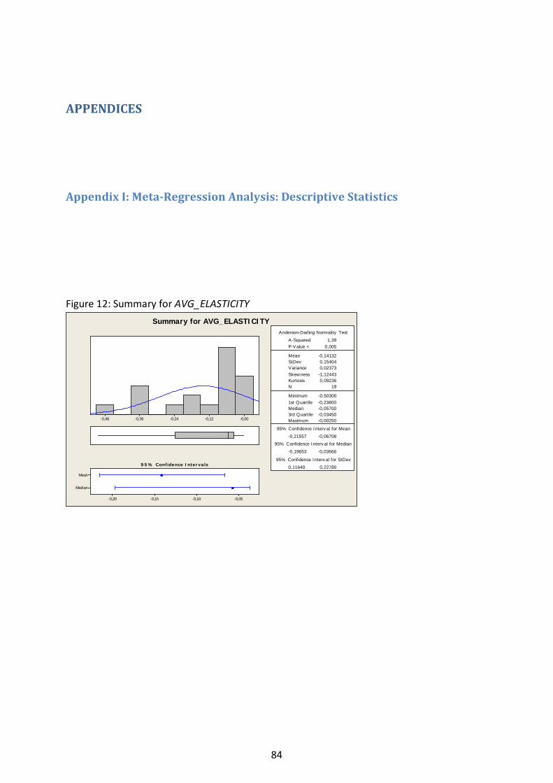
APPENDICES

Appendix I: Meta-Regression Analysis: Descriptive Statistics

Figure 12: Summary for AVG_ELASTICITY

-0,00-0,12-0,24-0,36-0,48

Median

Mean

-0,05-0,10-0,15-0,20

1st Q uartile -0,23800Median -0,057003rd Q uartile -0,03450Maximum -0,00250

-0,21557 -0,06708

-0,19653 -0,03666

0,11640 0,22780

A -Squared 1,39P-V alue < 0,005

Mean -0,14132StDev 0,15404V ariance 0,02373Skewness -1,12443Kurtosis 0,09236N 19

Minimum -0,50300

A nderson-Darling Normality Test

95% C onfidence Interv al for Mean

95% C onfidence Interv al for Median

95% C onfidence Interv al for StDev95% Confidence Intervals

Summary for AVG_ELASTICITY

84

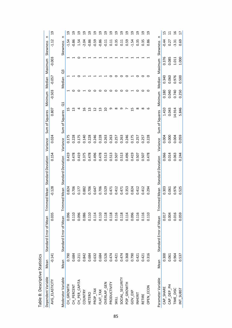
Tabl

e 8:

Des

crip

tive

Stat

istic

s

Dep

ende

nt V

aria

ble

Mea

nSt

anda

rd E

rror

of M

ean

Trim

med

Mea

nSt

anda

rd D

evia

tion

Var

ianc

eSu

m o

f Squ

ares

Min

imum

Med

ian

Max

imum

Skew

ness

nA

VG

_ELA

STIC

ITY

-0.1

410.

035

-0.1

280.

154

0.02

40.

807

-0.5

03-0

.057

-0.0

03-1

.12

19

Mod

erat

or V

aria

ble

Mea

nSt

anda

rd E

rror

of M

ean

Trim

med

Mea

nSt

anda

rd D

evia

tion

Var

ianc

eSu

m o

f Squ

ares

Q1

Med

ian

Q3

Skew

ness

nCH

_GRO

WTH

0.79

00.

096

0.82

40.

419

0.17

515

11

1-1

.54

19CH

_PER

CEN

T0.

684

0.11

00.

706

0.47

80.

228

130

11

-0.8

619

CH_P

ER_C

API

TA0.

211

0.09

60.

177

0.41

90.

175

40

00

1.54

19CO

UN

TRY

0.84

20.

086

0.88

20.

375

0.14

016

11

1-2

.04

19H

ETER

O0.

684

0.11

00.

706

0.47

80.

228

130

11

-0.8

619

PRO

P_TA

X0.

632

0.11

40.

647

0.49

60.

246

120

11

-0.5

919

FLA

T_TA

X0.

684

0.11

00.

706

0.47

80.

228

130

11

-0.8

619

OV

ERLA

P_G

EN0.

526

0.11

80.

529

0.51

30.

263

100

11

-0.1

119

PRO

DU

CTIV

ITY

0.47

40.

118

0.47

10.

513

0.26

39

00

10.

1119

SKIL

L0.

421

0.11

60.

412

0.50

70.

257

80

01

0.35

19SO

CIA

L_SE

CURI

TY0.

474

0.11

80.

471

0.51

30.

263

90

01

0.11

19PO

P_G

ROW

TH0.

368

0.11

40.

353

0.49

60.

246

70

01

0.59

19G

OV

_EXP

0.79

00.

096

0.82

40.

419

0.17

515

11

1-1

.54

19IN

HER

IT0.

421

0.11

60.

412

0.50

70.

257

80

01

0.35

19RE

TIRE

0.42

10.

116

0.41

20.

507

0.25

78

00

10.

3519

OPE

N_E

CON

0.31

60.

110

0.29

40.

478

0.22

86

00

10.

8619

Para

met

er V

aria

ble

Mea

nSt

anda

rd E

rror

of M

ean

Trim

med

Mea

nSt

anda

rd D

evia

tion

Var

ianc

eSu

m o

f Squ

ares

Min

imum

Med

ian

Max

imum

Skew

ness

nCA

P_SH

ARE

0.30

00.

017

0.30

30.

066

0.00

41.

410

0.18

00.

340

0.37

6-0

.44

15CA

P_D

EP_P

H0.

061

0.00

40.

061

0.01

40.

000

0.04

30.

040

0.06

00.

085

0.27

11TI

ME_

DIS

C0.

964

0.01

60.

976

0.06

30.

004

14.9

140.

740

0.97

61.

011

-3.3

116

INT_

SUBS

T0.

537

0.05

90.

525

0.24

40.

059

5.84

60.

250

0.50

01.

000

0.69

17

85

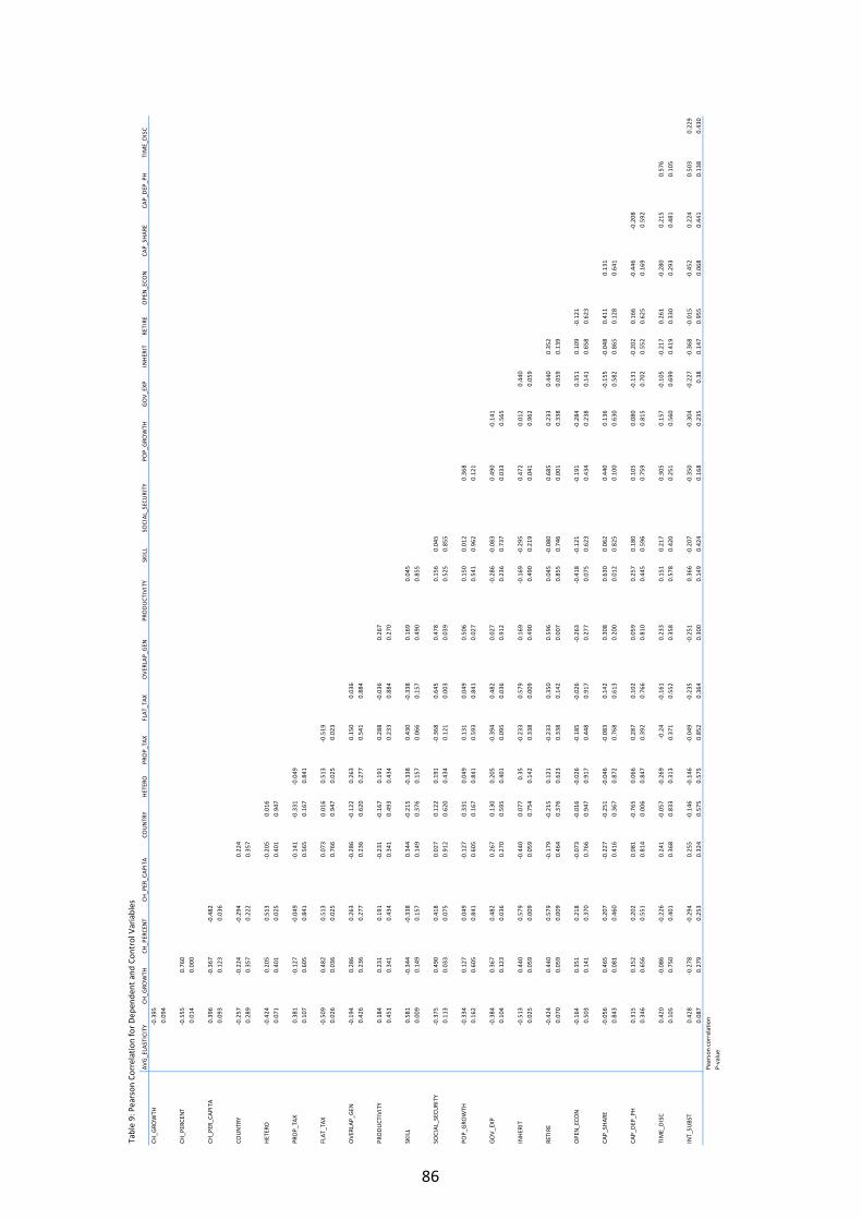
Tabl

e 9:

Pea

rson

Cor

rela

tion

for

Dep

ende

nt a

nd C

ontr

ol V

aria

bles

AV

G_E

LAST

ICIT

YCH

_GRO

WTH

CH_P

ERCE

NT

CH_P

ER_C

API

TACO

UN

TRY

HET

ERO

PRO

P_TA

XFL

AT_

TAX

OV

ERLA

P_G

ENPR

OD

UCT

IVIT

YSK

ILL

SOCI

AL_

SECU

RITY

POP_

GRO

WTH

GO

V_E

XPIN

HER

ITRE

TIRE

OPE

N_E

CON

CAP_

SHA

RECA

P_D

EP_P

HTI

ME_

DIS

CCH

_GRO

WTH

-0.3

950.

094

CH_P

ERCE

NT

-0.5

550.

760

0.01

40.

000

CH_P

ER_C

API

TA0.

396

-0.3

67-0

.482

0.09

30.

123

0.03

6

COU

NTR

Y-0

.257

-0.2

24-0

.294

0.22

40.

289

0.35

70.

222

0.35

7

HET

ERO

-0.4

240.

205

0.51

3-0

.205

0.01

60.

071

0.40

10.

025

0.40

10.

947

PRO

P_TA

X0.

381

-0.1

27-0

.049

-0.1

41-0

.331

-0.0

490.

107

0.60

50.

841

0.56

50.

167

0.84

1

FLA

T_TA

X-0

.509

0.48

20.

513

0.07

30.

016

0.51

3-0

.519

0.02

60.

036

0.02

50.

766

0.94

70.

025

0.02

3

OV

ERLA

P_G

EN-0

.194

0.28

60.

263

-0.2

86-0

.122

0.26

30.

150

0.03

60.

426

0.23

60.

277

0.23

60.

620

0.27

70.

541

0.88

4

PRO

DU

CTIV

ITY

0.18

40.

231

0.19

1-0

.231

-0.1

670.

191

0.28

8-0

.036

0.26

70.

451

0.34

10.

434

0.34

10.

493

0.43

40.

233

0.88

40.

270

SKIL

L0.

581

-0.3

44-0

.338

0.34

4-0

.215

-0.3

380.

430

-0.3

380.

169

0.04

50.

009

0.14

90.

157

0.14

90.

376

0.15

70.

066

0.15

70.

490

0.85

5

SOCI

AL_

SECU

RITY

-0.3

750.

490

0.41

80.

027

0.12

20.

191

-0.3

680.

645

0.47

80.

156

0.04

50.

113

0.03

30.

075

0.91

20.

620

0.43

40.

121

0.00

30.

039

0.52

50.

855

POP_

GRO

WTH

-0.3

340.

127

0.04

9-0

.127

0.33

10.

049

0.13

10.

049

0.50

60.

150

0.01

20.

368

0.16

20.

605

0.84

10.

605

0.16

70.

841

0.59

30.

841

0.02

70.

541

0.96

20.

121

GO

V_E

XP-0

.384

0.36

70.

482

0.26

70.

130

0.20

5-0

.394

0.48

20.

027

-0.2

86-0

.083

0.49

0-0

.141

0.10

40.

123

0.03

60.

270

0.59

50.

401

0.09

50.

036

0.91

20.

236

0.73

70.

033

0.56

5

INH

ERIT

-0.5

130.

440

0.57

9-0

.440

0.07

70.

35-0

.233

0.57

90.

169

-0.1

69-0

.295

0.47

20.

012

0.44

00.

025

0.05

90.

009

0.05

90.

754

0.14

20.

338

0.00

90.

490

0.49

00.

219

0.04

10.

962

0.05

9

RETI

RE-0

.424

0.44

00.

579

-0.1

79-0

.215

0.12

1-0

.233

0.35

00.

596

0.04

5-0

.080

0.68

50.

233

0.44

00.

352

0.07

00.

059

0.00

90.

464

0.37

60.

623

0.33

80.

142

0.00

70.

855

0.74

60.

001

0.33

80.

059

0.13

9

OPE

N_E

CON

-0.1

640.

351

0.21

8-0

.073

-0.0

16-0

.026

-0.1

85-0

.026

-0.2

63-0

.418

-0.1

21-0

.191

-0.2

840.

351

0.10

9-0

.121

0.50

30.

141

0.37

00.

766

0.94

70.

917

0.44

80.

917

0.27

70.

075

0.62

30.

434

0.23

80.

141

0.65

80.

623

CAP_

SHA

RE-0

.056

0.46

50.

207

-0.2

27-0

.251

-0.0

46-0

.083

0.14

20.

308

0.63

00.

062

0.44

00.

136

-0.1

55-0

.048

0.41

10.

131

0.84

30.

081

0.46

00.

416

0.36

70.

872

0.76

80.

613

0.20

00.

012

0.82

50.

100

0.63

00.

582

0.86

50.

128

0.64

1

CAP_

DEP

_PH

0.31

50.

152

0.20

20.

081

-0.7

650.

066

0.28

70.

102

0.05

90.

257

0.18

00.

105

0.08

0-0

.131

-0.2

020.

166

-0.4

46-0

.208

0.34

60.

656

0.55

10.

814

0.00

60.

847

0.39

20.

766

0.81

00.

445

0.59

60.

759

0.81

50.

702

0.55

20.

625

0.16

90.

592

TIM

E_D

ISC

0.42

0-0

.086

-0.2

260.

241

-0.0

57-0

.269

-0.2

4-0

.161

0.23

30.

151

0.21

70.

305

0.15

7-0

.105

-0.2

170.

261

-0.2

800.

215

0.57

60.

105

0.75

00.

401

0.36

80.

833

0.31

30.

371

0.55

20.

358

0.57

80.

420

0.25

10.

560

0.69

90.

419

0.33

00.

293

0.48

10.

105

INT_

SUBS

T0.

428

-0.2

78-0

.294

0.25

5-0

.146

-0.1

46-0

.049

-0.2

35-0

.251

0.36

6-0

.207

-0.3

50-0

.304

-0.2

27-0

.368

-0.0

15-0

.452

0.22

40.

503

0.22

90.

087

0.27

90.

253

0.32

40.

575

0.57

50.

852

0.36

40.

300

0.14

90.

424

0.16

80.

235

0.38

0.14

70.

955

0.06

80.

441

0.13

80.

430

Pear

son

corr

elat

ion

P-va

lue

86

Appendix II: Meta-Regression Analysis: Regression Models

Table 10: Regression (1): All Moderator Variables Variable Coefficient T-statistic

Intercept (𝛽𝛽0)

CH_GROWTH

CH_PERCENT

CH_PER_CAPITA

COUNTRY

HETERO

PROP_TAX

FLAT_TAX

OVERLAP_GEN

PRODUCTIVITY

SKILL

SOCIAL_SECURITY

POP_GROWTH

GOV_EXP

INHERIT

RETIRE

OPEN_ECON

0.099

0.259

-0.073

0.335

-0.163

0.126

-0.132

-0.373

-0.097

0.046

0.134

-0.020

-0.019

-0.170

0.205

-0.018

-0.102

0.29

0.59

-0.18

1.20

-0.75

0.46

-0.69

-1.16

-0.38

0.33

0.59

-0.07

-0.12

-0.72

1.01

-0.06

-0.49

Standard error of residual = 0.165865 R-Square = 87.1 % R-Square (adjusted) = 0.0 % F-statistic = 0.85 Durbin-Watson statistic = 2.10338 n = 19 Count of unusual observations = 0 *, **, *** denote statistical significance at the 10 %, 5 %, and 1 % level, respectively

87

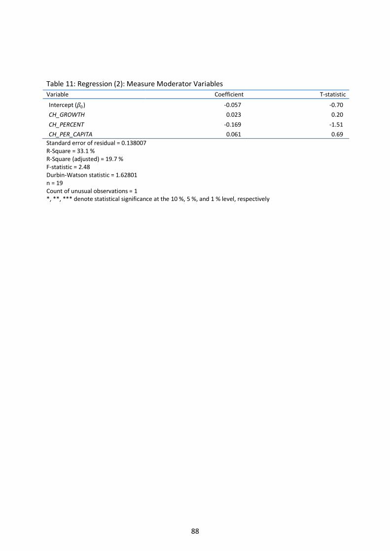
Table 11: Regression (2): Measure Moderator Variables Variable Coefficient T-statistic


CH_GROWTH

CH_PERCENT

CH_PER_CAPITA

-0.057

0.023

-0.169

0.061

-0.70

0.20

-1.51

0.69

Standard error of residual = 0.138007 R-Square = 33.1 % R-Square (adjusted) = 19.7 % F-statistic = 2.48 Durbin-Watson statistic = 1.62801 n = 19 Count of unusual observations = 1 *, **, *** denote statistical significance at the 10 %, 5 %, and 1 % level, respectively

88

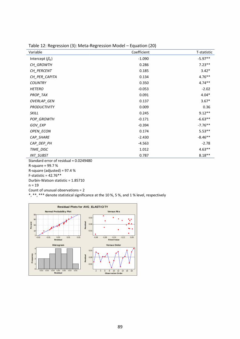
Table 12: Regression (3): Meta-Regression Model – Equation (20) Variable Coefficient T-statistic


CH_GROWTH

CH_PERCENT

CH_PER_CAPITA

COUNTRY

HETERO

PROP_TAX

OVERLAP_GEN

PRODUCTIVITY

SKILL

POP_GROWTH

GOV_EXP

OPEN_ECON

CAP_SHARE

CAP_DEP_PH

TIME_DISC

INT_SUBST

-1.090

0.286

0.185

0.134

0.350

-0.053

0.091

0.137

0.009

0.245

-0.171

-0.394

0.174

-2.430

-4.563

1.012

0.787

-5.97**

7.23**

3.42*

4.76**

4.74**

-2.02

4.04*

3.67*

0.36

9.12**

-6.63**

-7.76**

5.53**

-8.46**

-2.78

4.63**

8.18**

Standard error of residual = 0.0249480 R-square = 99.7 % R-square (adjusted) = 97.4 % F-statistic = 42.76** Durbin-Watson statistic = 1.85710 n = 19 Count of unusual observations = 2 *, **, *** denote statistical significance at the 10 %, 5 %, and 1 % level, respectively

0,020,010,00-0,01-0,02

99

90

50

10

1

Residual

Per

cent

0,00-0,12-0,24-0,36-0,48

0,01

0,00

-0,01

Fitted Value

Res

idua

l

0,0150,0100,0050,000-0,005-0,010-0,015

4

3

2

1

0

Residual

Freq

uenc

y

18161412108642

0,01

0,00

-0,01

Observation Order

Res

idua

l

Normal Probability Plot Versus Fits

Histogram Versus Order

Residual Plots for AVG_ELASTICITY

89

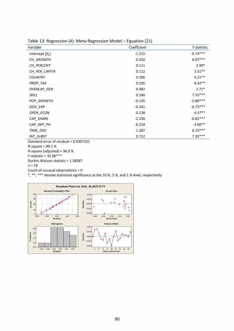
Table 13: Regression (4): Meta-Regression Model – Equation (21) Variable Coefficient T-statistic


CH_GROWTH

CH_PERCENT

CH_PER_CAPITA

COUNTRY

PROP_TAX

OVERLAP_GEN

SKILL

POP_GROWTH

GOV_EXP

OPEN_ECON

CAP_SHARE

CAP_DEP_PH

TIME_DISC

INT_SUBST

-1.215

0.310

0.111

0.112

0.266

0.105

0.082

0.240

-0.145

-0.341

0.138

-2.230

-6.224

1.287

0.712

-6.74***

6.97***

2.49*

3.51**

4.21**

4.42**

2.71*

7.55***

-5.80***

-6.73***

4.37**

-6.81***

-3.60**

6.15***

7.35***

Standard error of residual = 0.0307101 R-square = 99.1 % R-square (adjusted) = 96.0 % F-statistic = 32.06*** Durbin-Watson statistic = 1.58587 n = 19 Count of unusual observations = 0 *, **, *** denote statistical significance at the 10 %, 5 %, and 1 % level, respectively

0,040,020,00-0,02-0,04

99

90

50

10

1

Residual

Per

cent

0,00-0,12-0,24-0,36-0,48

0,030

0,015

0,000

-0,015

-0,030

Fitted Value

Res

idua

l

0,020,010,00-0,01-0,02-0,03

4,8

3,6

2,4

1,2

0,0

Residual

Freq

uenc

y

18161412108642

0,030

0,015

0,000

-0,015

-0,030

Observation Order

Res

idua

l

Normal Probability Plot Versus Fits

Histogram Versus Order

Residual Plots for AVG_ELASTICITY

90

Appendix III: Meta-Regression Analysis: Control of Parameter Variable Coefficients

91

Tabl

e 14

: Con

trol

of E

stim

ated

Par

amet

er V

aria

ble

Coef

ficie

nts

Benc

hmar

k co

effic

ient

Alte

red

coef

ficie

nt s

ourc

eRe

gres

sion

12

34

56

78

910

1112

Inte

rcep

t-1

,215

-1.3

44-0

.009

-0.4

85-1

.225

**-1

.030

**-1

.823

***

-1.2

93**

*-0

.795

-1.1

33-0

.842

-0.5

09-1

.024

CAP_

SHA

RE-1

,789

Mea

n va

lue

-2.9

55-5

.119

-2.0

87**

-3.8

75**

-2.0

27**

*-1

.277

-0.3

82-1

.082

-0.5

21

Mis

sing

/max

imum

/min

imum

val

ue-1

.947

-1.8

85**

-0.4

48

CAP_

DEP

-7,3

67M

ean

valu

e-7

.370

-16.

030

-5.8

29**

-7.0

44-3

.621

-6.4

47-2

.105

-4.2

580.

345

Mis

sing

/max

imum

/min

imum

val

ue-1

3.70

0-8

.732

*-2

.514

TIM

E_D

ISC

1,50

8M

ean

valu

e1.

899

0.94

71.

262*

*1.

221*

*2.

308*

*1.

226

1.10

20.

813

0.80

9

Mis

sing

/max

imum

/min

imum

val

ue1.

424

1.11

3***

0.80

2

INT_

SUBS

T0,

549

Mea

n va

lue

0.46

10.

644

1.49

80.

625*

*0.

847*

**0.

674*

**0.

183

0.21

00.

329*

Mis

sing

/max

imum

/min

imum

val

ue0.

676*

*0.

270

0.20

5

k13

914

1214

1414

1414

1414

14

n15

1116

1719

1919

1919

1919

19

R-Sq

uare

98.4

%94

.3 %

99.5

%99

.8 %

96.7

%98

.4 %

98.7

%92

.0 %

90.3

%92

.9 %

92.1

%92

.0 %

F-st

atis

tic4.

741.

8315

.04

78.9

88.

2717

.17

21.2

93.

282.

663.

753.

323.

28

*, *

*, *

** d

enot

e st

atis

tical

sig

nific

ance

at t

he 1

0 %

, 5 %

, and

1 %

leve

l, re

spec

tivel

y

Regr

essi

on 1

-4 u

sing

mis

sing

val

ues

for

one

para

met

er v

aria

ble,

mea

n va

lues

for

the

rem

aini

ng

Regr

essi

on 5

-8 u

sing

max

imum

val

ue fo

r on

e pa

ram

eter

var

iabl

e, m

ean

valu

es fo

r th

e re

mai

ning

Regr

essi

on 9

-12

usin

g m

inim

um v

alue

for

one

para

met

er v

aria

ble,

mea

n va

lues

for

the

rem

aini

ng

1,20

6-0

,129

-1,3

44-0

,009

-0,4

85-1

,225

-1,0

3-1

,823

-1,2

93-0

,795

-1,1

33-0

,842

-0,5

09-1

,024

Figu

re 1

3: E

stim

ated

Par

amet

er V

aria

ble

Coef

ficie

nts

Dev

iati

on F

rom

Ben

chm

ark

Coef

ficie

nt0,

73-0

,01

0,18

5-0

,608

-0,0

780,

420,

082

0,37

30,

706

0,19

1

-2,9

55-5

,119

-2,0

87-3

,875

-2,0

27-1

,277

-0,3

82-1

,082

-0,5

21-1

,947

-1,8

85-0

,448

-0,1

58-1

,166

-3,3

3-0

,298

-0,0

96-2

,086

-0,2

380,

512

1,34

11,

407

0,70

71,

268

-7,3

7-1

6,03

0-5

,829

-7,0

44-3

,621

-6,4

47-2

,105

-4,2

580,

345

-13,

700

-8,7

32-2

,514

-0,0

03-6

,333

-8,6

631,

538

0,32

3-1

,365

3,74

60,

925,

262

4,85

33,

109

7,71

2

1,89

90,

947

1,26

21,

221

2,30

81,

226

1,10

20,

813

0,80

91,

424

1,11

30,

802

0,39

1-0

,561

-0,0

84-0

,246

-0,2

870,

8-0

,395

-0,2

82-0

,406

-0,6

95-0

,706

-0,6

99

0,46

10,

644

1,49

80,

625

0,84

70,

674

0,18

30,

210

0,32

90,

676

0,27

00,

205

-0,0

880,

095

0,94

90,

127

0,07

60,

298

0,12

5-0

,279

-0,3

66-0

,339

-0,2

2-0

,344

-10-50510

12

34

56

78

910

1112

Dev

iati

on F

rom

Ben

chm

ark

Coef

ficie

nt

CAP_

SHAR

ECA

P_D

EPTI

ME_

DIS

CIN

T_SU

BST

92

Appendix IV: Prediction Preparation

Table 15: Elasticity versus Tax Burden Variable Coefficient T-statistic


TAX/GDP RATIO

-0.284

0.005

-5.35**

3.95*

Standard error of residual = 0.227430 R-Square = 88.6% R-Square (adjusted) = 83.0% F-statistic = 15.6 n = 4 Count of unusual observations = 0 *, **, *** denote statistical significance at the 10 %, 5 %, and 1 % level, respectively

93