Embed Size (px)
Citation preview

Staffordshire University Faculty of Business, Education and Law
Business School
E F F E C T S O F F D I S P I L L O V E R S O N T H E P R O D U C T I V I T Y O F D O M E S T I C F I R M S
I N S E L E C T E D T R A N S I T I O N C O U N T R I E S
Edvard Orlić
A thesis submitted in partial fulfilment of the requirement of Staffordshire University for the degree of Doctor of Philosophy
March 2016
i
ABSTRACT
The transition to a market based economy in Central and East European countries
(CEECs) was characterised by deep structural and institutional reforms. These reforms,
particularly the liberalisation of trade and capital flows, played a prominent role and
enabled the entry of these countries in the “FDI market”. It was expected that the entry
of MNCs into these countries would foster firm restructuring, change the export structure
and above all generate knowledge spillovers and create linkages with indigenous firms.
Therefore, CEECs started to offer various incentives to attract FDI, hoping that some of
the technology brought by MNCs will spill over to local firms. This would enable them
to increase their productivity and achieve higher rates of growth that would result in
convergence with more advanced countries.
The aim of this thesis is to investigate productivity spillovers from FDI to local firms in
five transition countries using firm level data for the period 2002-2010. Several elements
differentiate this study from the previous analyses. We compare the effects of horizontal
spillovers and vertical linkages from FDI across countries and two main sectors
(manufacturing and services) and assess the heterogeneity of MNCs. To the best of our
knowledge this is the first study taking into account MNCs’ origin and the extent of
foreign ownership in a group of transition economies. Given the importance of FDI in
services we further disentangle vertical linkages according to sectoral source and
investigate the moderating role of firms’ absorptive capacity. Semi-parametric approach
based on control function is applied to estimate firms’ total factor productivity (TFP)
which is then used in the estimation of horizontal and vertical spillovers from FDI along
with other firm and industry level determinants. FDI spillovers are estimated using the
dynamic panel econometric technique.
Our findings indicate that local firms in the advanced stage of transition benefit from
horizontal spillovers arising mostly in service sector and from partially owned foreign
firms while the effects of MNCs’ origin are ambiguous. We also find that net effects of
FDI spillovers are driven by vertical linkages. In particular, positive effect of backward
linkages on firm productivity are found for fully owned and non-EU MNCs. However,
for a limited set of countries, these positive effects of backward linkages are in certain

ii
cases further supported or offset by negative effects of partially owned foreign firms and
EU MNCs. On the other hand, forward linkages when positive are limited to EU MNCs
while non-EU MNCs and both partially and fully owned foreign firms exhibit mostly
negative productivity effects with the exception of two countries. Furthermore, we find
that MNCs in manufacturing and service sectors generate significant productivity
spillovers to manufacturing firms which are further strengthened with higher levels of
absorptive capacity. However, in most cases these spillovers occur through different
vertical channels, namely through manufacturing backward and services forward
spillovers thus shedding new light on the increasing importance of forward linkages and
FDI in services. Human capital and investment in intangibles are found to be strong
determinants of firm productivity together with increased competition, while firms’ age
and size have U-shape and inverse U-shape effects, respectively.
This thesis shows that the effects of FDI spillovers differ among countries suggesting
that sectoral and MNCs’ heterogeneity play an important role in driving the overall
results. Therefore, based on these findings we have developed a set of policy
recommendations for policy makers and investment promotion agencies with the aim to
maximise the benefits of MNC’s entry for indigenous firms’ productivity and their
inclusion into Global Value Chains.

iii
TABLE OF CONTENTS
Abstract………….. ..................................................................................................................................................... i
Table of contents ................................................................................................................................................. iii
List of Tables…… ................................................................................................................................................ vii
List of Figures………………………….................................................................................................................. xii
List of Abbreviations ....................................................................................................................................... xiv
Acknowledgments ............................................................................................................................................. xv
Preface………………………….. ............................................................................................................................. xv
CHAPTER 1. THEORIES OF FOREIGN DIRECT INVESTMENT ................................................... 1
1.1 Introduction ............................................................................................................................................... 2
1.2 Concept of FDI – definition, measurement and types .............................................................. 4
1.3 Theories of FDI ......................................................................................................................................... 5
1.3.1 The neoclassical theory of capital movement ..................................................................... 6
1.3.2 Industrial organization theory .................................................................................................. 7
1.3.3 Macroeconomic development approach ............................................................................... 9
1.3.4 Internalisation theories .............................................................................................................. 13
1.3.5 OLI paradigm .................................................................................................................................. 16
1.3.6 Evolutionary approaches to the theory of MNC ............................................................... 19
1.3.7 New trade theory .......................................................................................................................... 22
1.4 Motives and mode of MNCs’ entry .................................................................................................. 25
1.5 Potential benefits of FDI ..................................................................................................................... 28
1.6 Conclusions .............................................................................................................................................. 31
CHAPTER 2. FDI SPILLOVERS AND LINKAGES: THEORY AND EMPIRICAL EVIDENCE………. ................................................................................................................................................. 33
2.1 Introduction ............................................................................................................................................. 34
2.2 Knowledge spillovers from FDI ....................................................................................................... 35
2.3 Intra-industry (horizontal) spillovers .......................................................................................... 38
2.3.1 Demonstration effects ................................................................................................................. 39
2.3.2 Competition effects ...................................................................................................................... 40
2.3.3 Worker mobility ............................................................................................................................ 42
2.4 Inter-industry (vertical) spillovers ................................................................................................ 44
2.5 Determinants of FDI spillovers ........................................................................................................ 48
2.5.1 MNCs’ heterogeneity ................................................................................................................... 49
2.5.2 Domestic firms’ heterogeneity ................................................................................................ 54
iv
2.5.3 Other potential factors ................................................................................................................ 57
2.6 Review of the empirical literature ................................................................................................. 59
2.6.1 Empirical evidence on FDI spillovers ................................................................................... 60
2.6.2 Shortcomings of the studies on FDI spillovers in TEs ................................................... 71
2.7 Conclusions .............................................................................................................................................. 74
CHAPTER 3. CONTRIBUTION OF INWARD FDI TO NMS ECONOMIES – COUNTRY AND INDUSTRY ANALYSIS ....................................................................................................................................... 77
3.1 Introduction............................................................................................................................................ 78
3.2 The process of transition and the role of FDI ............................................................................ 79
3.3. Income and productivity convergence process ....................................................................... 82
3.4 Overview of FDI in new member states ....................................................................................... 87
3.4.1 Country analysis of inward FDI ............................................................................................... 88
3.4.2 Cross industry analysis of FDI ................................................................................................. 92
3.5 Impact of FDI on NMS Economies .................................................................................................. 96
3.5.1 Share of Foreign affiliates in employment.......................................................................... 98
3.5.2 Share of Foreign affiliates in value added and turnover .............................................. 99
3.5.3 The role of FATS in technology upgrading and productivity improvements.... 102
3.6 FDI and integration of NMS into GVC ......................................................................................... 108
3.7 Conclusion ............................................................................................................................................. 116
CHAPTER 4. ISSUES, METHODOLOGICAL SOLUTIONS AND ESTIMATION OF TFP AT MICRO LEVEL…… ............................................................................................................................................ 118
4.1 Introduction .......................................................................................................................................... 119
4.2 Measurement of productivity ........................................................................................................ 121
4.3 Methodological issues in estimation of TFP ............................................................................ 127
4.3.1 Simultaneity bias ........................................................................................................................ 131
4.3.2 Selection bias ............................................................................................................................... 132
4.3.3 Omitted price bias ..................................................................................................................... 132
4.3.4 Multiproduct firms ................................................................................................................... 133
4.4 Solutions to econometric problems ............................................................................................ 134
4.4.1 Traditional solutions to endogeneity of input choice ................................................. 136
4.4.2 Olley-Pakes and Levinsohn-Petrin methodology ......................................................... 137
4.4.3 Ackerberg Caves Frazer critique ......................................................................................... 142
4.4.4 Wooldridge estimator .............................................................................................................. 144
4.5 Data and descriptive statistics ...................................................................................................... 146
4.5.1 Sample Description ................................................................................................................... 147
4.5.2 Variables description and descriptive statistics ........................................................... 151
4.6 TFP estimation..................................................................................................................................... 155
4.7 Are foreign firms more productive? ........................................................................................... 162

v
4.8 Conclusion ............................................................................................................................................. 167
CHAPTER 5. PRODUCTIVITY SPILLOVERS OF FDI IN SELECTED TRANSITION COUNTRIES – THE ROLE OF MNC’S HETEROGENEITY ............................................................. 170
5.1 Introduction .......................................................................................................................................... 171
5.2 Model specification ............................................................................................................................ 173
5.3 Data and descriptive statistics ...................................................................................................... 185
5.4 Methodology ......................................................................................................................................... 192
5.5 Discussion of findings ....................................................................................................................... 196
5.5.1 Results for baseline model ..................................................................................................... 197
5.5.2 The effect of ownership structure....................................................................................... 204
5.5.3 The effects of MNC’s origin .................................................................................................... 211
5.6 Conclusion ............................................................................................................................................. 219
CHAPTER 6. THE IMPACT OF SERVICES FDI ON PRODUCTIVITY OF DOWNSTREAM MANUFACTURING FIRMS ........................................................................................................................... 223
6.1 Introduction .......................................................................................................................................... 224
6.2 Conceptual framework and related research ......................................................................... 225
6.2.1 The importance of service sector and implications for MNC’s entry ................... 226
6.2.2 Interactions between services and manufacturing ..................................................... 230
6.2.3 Review of empirical literature .............................................................................................. 233
6.3 Empirical strategy .............................................................................................................................. 236
6.3.1 Empirical model and methodology .................................................................................... 237
6.3.2 Data .................................................................................................................................................. 241
6.4 Discussion of findings ....................................................................................................................... 246
6.4.1 Results of baseline model across sectors ......................................................................... 247
6.4.2 Effects of services fdi on downstream manufacturing firms ................................... 254
6.4.3 The moderating effects of absorptive capacity.............................................................. 259
6.5 Conclusion ............................................................................................................................................. 265
CHAPTER 7. CONCLUSIONS ................................................................................................................ 268
7.1 Introduction .......................................................................................................................................... 269
7.2 Main findings ........................................................................................................................................ 270
7.3 Contribution to knowledge ............................................................................................................ 282
7.4 Policy implications ............................................................................................................................. 285
7.4.1 Attracting the right type of foreign investors ................................................................ 286
7.4.2 Promotion of linkages .............................................................................................................. 287
7.4.3 Increasing the absoprtive capacity of local firms ......................................................... 289
7.5 Limitations of research .................................................................................................................... 291
7.6 Directions for further research ..................................................................................................... 293
REFERENCES…… ............................................................................................................................................. 296
vi
Appendices……… ............................................................................................................................................. 342
APPENDIX I. SUPPLEMENT TO CHAPTER THREE ..................................................................... 342
1.1 Income and productivity convergence in NMS ...................................................................... 343
1.2 Measuring Global Value Chain participation (GVC) ............................................................. 347
1.3 Industry productivity levels and growth rates in NMS ...................................................... 349
APPENDIX II. SUPPLEMENT TO CHAPTER FOUR........................................................................ 352
2.1 Cleaning procedure ........................................................................................................................... 353
2.2 Foreign ownership calculations ................................................................................................... 354
2.3 Sample description ............................................................................................................................ 357
2.4 Output of Cobb-Douglas value added production function per industry and country ........................................................................................................................................................................... 362
2.5 Robustness checks of TFP estimates .......................................................................................... 368
2.6 Non parametric Kolmogorov Smirnov test of foreign ownership premium ............. 374
APPENDIX III. SUPPLEMENT TO CHAPTER FIVE.......................................................................... 391
3.1 Empirical results for the baseline model of productivity spillovers from FDI presented in Section 5.6.1 ...................................................................................................................... 392
3.2 Empirical results for the effects of MNCs’ origin on productivity of local firms presented in Section 5.6.3 ...................................................................................................................... 403
3.3 Empirical results for the effects of MNCs’ ownership structure on productivity of local firms presented in Section 5.6.2 ............................................................................................... 413
APPENDIX IV. SUPPLEMENT TO CHAPTER SIX ............................................................................. 425
4.1 Development of foreign firms’ output in services and foreign services inputs in manufacturing industries ....................................................................................................................... 426
4.2 Empirical results for the baseline model of productivity spillovers from FDI in manufacturing sector presented in Section 6.4.1 ......................................................................... 427
4.3 Empirical results for the baseline model of productivity spillovers from FDI in service sector presented in Section 6.4.1......................................................................................... 436
4.4 Empirical results of the effects of services and manufacturing FDI linkages on productivity of local firms in manufacturing sector presented in Section 6.4.2 ............. 446
4.5 Empirical results of the moderating effects of intangible assets on productivity spillovers from FDI in manufacturing sector presented in Section 6.4.3 ........................... 457

vii
LIST OF TABLES TABLE 2.1 TAXONOMY OF KNOWLEDGE/TECHNOLOGY SPILLOVERS .................................... 36 TABLE 3.1 GROWTH CONTRIBUTIONS OF SUPPLY SIDE FACTORS IN NMS, (%) ... 87 TABLE 3.2 SHARE OF INWARD FDI STOCK ACROSS INDUSTRIES AND COUNTRIES, 2012 ....................................................................................................................................................................... 95 TABLE 3.3 SHARE OF FOREIGN AFFILIATES IN INDUSTRY EMPLOYMENT IN %, 2011 ....................................................................................................................................................................... 99 TABLE 3.4 SHARE OF FATS IN TURNOVER AT INDUSTRY LEVEL IN %, 2011 ..... 101 TABLE 3.5 SHARE OF DIFFERENT TECHNOLOGY GROUPS IN VARIOUS FEATURES OF FOREIGN AFFILIATES , 2011 ........................................................................................................ 103 TABLE 3.6 RATIO OF LABOUR PRODUCTIVITY OF FOREIGN TO DOMETIC FIRM BY INDUSTRY, 2011 .......................................................................................................................................... 107 TABLE 3.7 RELATIVE POSITION OF COUNTRIES AND INDUSTRIES IN GVC, 2009 ................................................................................................................................................................................ 113 TABLE 4.1 REPRESENTATIVENESS OF AMADEUS DATABASE VERSUS EUROSTAT SBS 150 TABLE 4.2 COMPARISON OF FIRM SIZE DISTRIBUTION BETWEEN EUROSTAT SBS AND AMADEUS DATABASE ................................................................................................................... 150 TABLE 4.3 DISTRIBUTION OF FIRMS ACROSS COUNTRIES, INDUSTRIES AND YEARS ................................................................................................................................................................. 152 TABLE 4.4 SUMMARY STATISTICS ON SELECTED INDICATORS .................................... 154 TABLE 4.5 WITHIN INDUSTRY DISPERSION OF TFP ACROSS COUNTRIES AND ESTIMATION ALGORITHMS .................................................................................................................. 160 TABLE 4.6 EFFECTS OF EXOGENOUS SHOCK ON TFP ........................................................... 162 TABLE 4.7 KOLMOGOROV SMIRNOV TEST OF EQUALITY OF TFP DISTRIBUTIONS ................................................................................................................................................................................ 164 TABLE 4.8 TFP PREMIUM OF FOREIGN OVER DOMESTIC FIRMS ................................. 165 TABLE 5.1 DESCRIPTION OF VARIABLES ..................................................................................... 184 TABLE 5.2 DESCRIPTIVE STATISTICS ............................................................................................ 186 TABLE 5.3 DYNAMIC PANEL SYSTEM GMM ESTIMATION OF FDI SPILLOVER EFFECTS ON PRODUCTIVITY (LN TFP) OF DOMESTIC FIRMS, 2002-2010 (ALL SECTORS) ......................................................................................................................................................... 198 TABLE 5.4 DYNAMIC SYSTEM GMM ESTIMATION OF FDI SPILLOVER EFFECTS ON DOMESTIC FIRMS’ PRODUCTIVITY (LN TFP) - EXTENT OF MNC’S OWNERSHIP, 2002-2010 (ALL SECTORS) ................................................................................................................... 206 TABLE 5.5 DYNAMIC SYSTEM GMM ESTIMATION OF FDI SPILLOVER EFFECTS ON DOMESTIC FIRMS’ PRODUCTIVITY (LN TFP) – THE ROLE OF MNC’S ORIGIN, 2002-2010 (ALL SECTORS) ................................................................................................................... 215 Table 6.1 DYNAMIC PANEL SYSTEM GMM ESTIMATIONS OF FDI spillover effects on PRODUCTIVITY (LN TFP) OF DOMESTIC FIRMS (MANUFACTURING VS. SERVICES), 2002-2010 ..................................................................................................................................................................... 249 TABLE 6.2 DYNAMIC PANEL SYSTEM GMM ESTIMATION OF FDI SPILLOVER EFFECTS ON PRODUCTIVITY (LN TFP) OF DOMESTIC FIRMS IN MANUFACTURING ACCORDING TO INDUSTRY SOURCE, 2002-2010 ............................................................................................................... 255 TABLE 7.1 SUMMARY OF FINDINGS ACROSS COUNTRIES AND EMPIRICAL MODELS .... 279 Table I.1 GDP PER CAPITA (PPP) GROWTH RATES IN NMS AND EU 15 ................................ 343 Table I.2 GDP PER CAPITA (PPP) GAP, PERCENTAGE OF EU 15 ............................................... 344 Table I.3 LABOUR PRODUCTIVITY GROWTH PER PERSON EMPLOYED (CONVERTED TO 2013 PRICE LEVEL WITH 2005 PPP, 1995=100) ............................................................................. 345 Table I.4 TOTAL FACTOR PRODUCTIVITY GROWTH ...................................................................... 346
viii
Table II.1 NUMBER OF OBSERVATIONS AFTER CLEANING STEPS .......................................... 354 Table II.2 DISTRIBUTION OF FOREIGN FIRMS ACROSS TECHNOLOGY AND KNOWLEDGE INTENSIVE INDUSTRIES BY COUNTRY ................................................................................................. 357 Table II.3 IN SAMPLE DATA COVERAGE OF FIRMS ......................................................................... 360 Table II.4 DESCRIPTIVE STATISTICS OF PRODUCTION FUNCTION VARIABLES USED IN TFP ESTIMATION OF DOMESTIC FIRMS .............................................................................................. 361 Table II.5 ESTIMATION OF VALUE ADDED PRODUCTION FUNCTION BY INDUSTRIES USING WOOLDRIDGE ESTIMATOR (2009), LEVINSOHN-PETRIN ESTIMATOR (2003) AND OLS IN CZECH REPUBLIC ............................................................................................................................ 362 Table II.6 ESTIMATION OF VALUE ADDED PRODUCTION FUNCTION BY INDUSTRIES USING WOOLDRIDGE ESTIMATOR (2009), LEVINSOHN-PETRIN ESTIMATOR (2003) AND OLS IN ESTONIA .............................................................................................................................................. 363 Table II.7 ESTIMATION OF VALUE ADDED PRODUCTION FUNCTION BY INDUSTRIES USING WOOLDRIDGE ESTIMATOR (2009), LEVINSOHN-PETRIN ESTIMATOR (2003) AND OLS IN HUNGARY ........................................................................................................................................... 364 Table II.8 ESTIMATION OF VALUE ADDED PRODUCTION FUNCTION BY INDUSTRIES USING WOOLDRIDGE ESTIMATOR (2009), LEVINSOHN-PETRIN ESTIMATOR (2003) AND OLS IN SLOVAKIA ........................................................................................................................................... 365 Table II.9 ESTIMATION OF VALUE ADDED PRODUCTION FUNCTION BY INDUSTRIES USING WOOLDRIDGE ESTIMATOR (2009), LEVINSOHN-PETRIN ESTIMATOR (2003) AND OLS IN SLOVENIA ........................................................................................................................................... 366 Table II.10 DIAGNOSTICS TESTS FOR WLP ESTIMATOR .............................................................. 367 Table II.11 CORRELATION MATRICES OF TFP ESTIMATION ALGORITHMS IN CZECH REPUBLIC........................................................................................................................................................... 368 Table II.12 CORRELATION MATRICES OF TFP ESTIMATION ALGORITHMS IN ESTONIA ................................................................................................................................................................................ 368 Table II.13 CORRELATION MATRICES OF TFP ESTIMATION ALGORITHMS IN HUNGARY ................................................................................................................................................................................ 369 Table II.14 CORRELATION MATRICES OF TFP ESTIMATION ALGORITHMS IN SLOVAKIA ................................................................................................................................................................................ 370 Table II.15 CORRELATION MATRICES OF TFP ESTIMATION ALGORITHMS IN SLOVENIA ................................................................................................................................................................................ 370 Table II.16 TRANSITION MATRICES OF INTER-QUARTILE MOVEMENTS IN TFP DISTRIBUTION OF LOCAL FIRMS IN CZECH REPUBLIC ................................................................ 371 Table II.17 TRANSITION MATRICES OF INTER-QUARTILE MOVEMENTS IN TFP DISTRIBUTION OF LOCAL FIRMS IN ESTONIA .................................................................................. 371 Table II.18 TRANSITION MATRICES OF INTER-QUARTILE MOVEMENTS IN TFP DISTRIBUTION OF LOCAL FIRMS IN HUNGARY ................................................................................ 372 Table II.19 TRANSITION MATRICES OF INTER-QUARTILE MOVEMENTS IN TFP DISTRIBUTION OF LOCAL FIRMS IN SLOVAKIA ............................................................................... 372 Table II.20 TRANSITION MATRICES OF INTER-QUARTILE MOVEMENTS IN TFP DISTRIBUTION OF LOCAL FIRMS IN SLOVENIA ............................................................................... 373 Table II.21 KOLMOGOROV SMIRNOV TEST PER INDUSTRY AND FOREIGN OWNERSHIP TYPE IN SLOVENIA, PRINTOUT FROM STATA ................................................................................... 374 Table II.22 KOLMOGOROV SMIRNOV TEST PER INDUSTRY AND FOREIGN OWNERSHIP TYPE IN SLOVAKIA, PRINTOUT FROM STATA ................................................................................... 375 Table II.23 KOLMOGOROV SMIRNOV TEST PER INDUSTRY AND FOREIGN OWNERSHIP TYPE IN HUNGARY, PRINTOUT FROM STATA ................................................................................... 376 Table II.24 TABLE 4 18 KOLMOGOROV SMIRNOV TEST PER INDUSTRY AND FOREIGN OWNERSHIP TYPE IN ESTONIA, PRINTOUT FROM STATA .......................................................... 378
ix
Table II.25 KOLMOGOROV SMIRNOV TEST PER INDUSTRY AND FOREIGN OWNERSHIP TYPE IN THE CZECH REPUBLIC, PRINTOUT FROM STATA .......................................................... 379 Table II.26 KOLMOGOROV SMIRNOV TEST FOR EQUALITY OF DISTRIBUTIONS IN CZECH REPUBLIC USING OLS ESTIMATION OF TFP ...................................................................................... 381 Table II.27 KOLMOGOROV SMIRNOV TEST FOR EQUALITY OF DISTRIBUTIONS IN ESTONIA USING OLS ESTIMATION OF TFP ......................................................................................... 383 Table II.28 KOLMOGOROV SMIRNOV TEST FOR EQUALITY OF DISTRIBUTIONS IN HUNGARY USING OLS ESTIMATION OF TFP....................................................................................... 385 Table II.29 KOLMOGOROV SMIRNOV TEST FOR EQUALITY OF DISTRIBUTIONS IN SLOVAKIA USING OLS ESTIMATION OF TFP ...................................................................................... 386 Table II.30 KOLMOGOROV SMIRNOV TEST FOR EQUALITY OF DISTRIBUTIONS IN SLOVENIA USING OLS ESTIMATION OF TFP ...................................................................................... 388 Table III.1 PRINTOUT OF DYNAMIC PANEL SYSTEM GMM ESTIMATION OF FDI SPILLOVERS IN THE CZECH REPUBLIC FOR ENTIRE ECONOMY, 2002-2009 (DEP. VARIABLE LN TFP) ........................................................................................................................................ 392 Table III.2 PRINTOUT OF DYNAMIC PANEL SYSTEM GMM ESTIMATION OF FDI SPILLOVERS IN ESTONIA FOR ENTIRE ECONOMY, 2002-2010 (DEP. VARIABLE LN TFP) ................................................................................................................................................................................ 394 Table III.3 PRINTOUT OF DYNAMIC PANEL SYSTEM GMM ESTIMATION OF FDI SPILLOVERS IN HUNGARY FOR ENTIRE ECONOMY, 2002-2010 (DEP. VARIABLE LN TFP) ................................................................................................................................................................................ 397 Table III.4 PRINTOUT OF DYNAMIC PANEL SYSTEM GMM ESTIMATION OF FDI SPILLOVERS IN SLOVAKIA FOR ENTIRE ECONOMY, 2002-2009 (DEP. VARIABLE LN TFP) ................................................................................................................................................................................ 399 Table III.5 PRINTOUT OF DYNAMIC PANEL SYSTEM GMM ESTIMATION OF FDI SPILLOVERS IN SLOVENIA FOR ENTIRE ECONOMY, 2002-2010 (DEP. VARIABLE LN TFP) ................................................................................................................................................................................ 401 Table III.6 PRINTOUT OF DYNAMIC PANEL SYSTEM GMM ESTIMATION OF FDI SPILLOVERS IN THE CZECH REPUBLIC ACCORDING TO MNC’S ORIGIN, 2002-2009 (DEP. VARIABLE TFP) ............................................................................................................................................... 403 Table III.7 PRINTOUT OF DYNAMIC PANEL SYSTEM GMM ESTIMATION OF FDI SPILLOVERS IN ESTONIA ACCORDING TO MNC’S ORIGIN, 2002-2010 (DEP. VARIABLE LN TFP) ...................................................................................................................................................................... 405 Table III.8 PRINTOUT OF DYNAMIC PANEL SYSTEM GMM ESTIMATION OF FDI SPILLOVERS IN HUNGARY ACCORDING TO MNC’S ORIGIN, 2002-2010 (DEP. VARIABLE LN TFP) ............................................................................................................................................................... 407 Table III.9 PRINTOUT OF DYNAMIC PANEL SYSTEM GMM ESTIMATION OF FDI SPILLOVERS IN SLOVAKIA ACCORDING TO MNC’S ORIGIN, 2002-2009 (DEP. VARIABLE LN TFP) ............................................................................................................................................................... 409 Table III.10 PRINTOUT OF DYNAMIC PANEL SYSTEM GMM ESTIMATION OF FDI SPILLOVERS IN SLOVENIA ACCORDING TO MNC’S ORIGIN, 2002-2010 (DEP. VARIABLE LN TFP) ............................................................................................................................................................... 411 Table III.11 PRINTOUT OF DYNAMIC PANEL SYSTEM GMM ESTIMATION OF FDI SPILLOVERS IN THE CZECH REPUBLIC ACCORDING TO MNC’S OWNERSHIP, 2002-2009 (DEP. VARIABLE LN TFP) ............................................................................................................................ 413 Table III.12 PRINTOUT OF DYNAMIC PANEL SYSTEM GMM ESTIMATION OF FDI SPILLOVERS IN ESTONIA ACCORDING TO MNC’S OWNERSHIP, 2002-2010 (DEP. VARIABLE LN TFP) ........................................................................................................................................ 415 Table III.13 PRINTOUT OF DYNAMIC PANEL SYSTEM GMM ESTIMATION OF FDI SPILLOVERS IN HUNGARY ACCORDING TO MNC’S OWNERSHIP, 2002-2010 (DEP. VARIABLE LN TFP) ........................................................................................................................................ 417

x
Table III.14 PRINTOUT OF DYNAMIC PANEL SYSTEM GMM ESTIMATION OF FDI SPILLOVERS IN SLOVAKIA ACCORDING TO MNC’S OWNERSHIP, 2002-2009 (DEP. VARIABLE LN TFP) ........................................................................................................................................ 419 Table III.15 PRINTOUT OF DYNAMIC PANEL SYSTEM GMM ESTIMATION OF FDI SPILLOVERS IN SLOVENIA ACCORDING TO MNC’S OWNERSHIP, 2002-2010 (DEP. VARIABLE LN TFP) ........................................................................................................................................ 421 Table III.16 COMPARISON OF VALUES OF LAGGED DEPENDENT VARIABLE BETWEEN OLS, FE AND SYSTEM GMM ........................................................................................................................ 424 Table IV.1 PRINTOUT OF DYNAMIC PANEL SYSTEM GMM ESTIMATION OF FDI SPILLOVERS IN THE CZECH REPUBLIC FOR MANUFACTURING SECTOR, 2002-2009 (DEP. VARIABLE LN TFP) ........................................................................................................................................ 427 Table IV.2 PRINTOUT OF DYNAMIC PANEL SYSTEM GMM ESTIMATION OF FDI SPILLOVERS IN ESTONIA FOR MANUFACTURING SECTOR, 2002-2010 (DEP. VARIABLE LN TFP) ............................................................................................................................................................... 428 Table IV.3 PRINTOUT OF DYNAMIC PANEL SYSTEM GMM ESTIMATION OF FDI SPILLOVERS IN HUNGARY FOR MANUFACTURING SECTOR, 2002-2010 (DEP. VARIABLE LN TFP) ............................................................................................................................................................... 430 Table IV.4 PRINTOUT OF DYNAMIC PANEL SYSTEM GMM ESTIMATION OF FDI SPILLOVERS IN SLOVAKIA FOR MANUFACTURING SECTOR, 2002-2009 (DEP. VARIABLE LN TFP) ............................................................................................................................................................... 432 Table IV.5 PRINTOUT OF DYNAMIC PANEL SYSTEM GMM ESTIMATION OF FDI SPILLOVERS IN SLOVENIA FOR MANUFACTURING SECTOR, 2002-2010 (DEP. VARIABLE LN TFP) ............................................................................................................................................................... 434 Table IV.6 PRINTOUT OF DYNAMIC PANEL SYSTEM GMM ESTIMATION OF FDI SPILLOVERS IN THE CZECH REPUBLIC FOR SERVICES SECTOR, 2002-2009 (DEP. VARIABLE LN TFP) ........................................................................................................................................ 436 Table IV.7 PRINTOUT OF DYNAMIC PANEL SYSTEM GMM ESTIMATION OF FDI SPILLOVERS IN ESTONIA FOR SERVICES SECTOR, 2002-2010 (DEP. VARIABLE LN TFP) ................................................................................................................................................................................ 438 Table IV.8 PRINTOUT OF DYNAMIC PANEL SYSTEM GMM ESTIMATION OF FDI SPILLOVERS IN HUNGARY FOR SERVICES SECTOR, 2002-2010 (DEP. VARIABLE LN TFP) ................................................................................................................................................................................ 440 Table IV.9 PRINTOUT OF DYNAMIC PANEL SYSTEM GMM ESTIMATION OF FDI SPILLOVERS IN SLOVAKIA FOR SERVICES SECTOR, 2002-2009 (DEP. VARIABLE LN TFP) ................................................................................................................................................................................ 442 Table IV.10 PRINTOUT OF DYNAMIC PANEL SYSTEM GMM ESTIMATION OF FDI SPILLOVERS IN SLOVENIA FOR SERVICES SECTOR, 2002-2010 (DEP. VARIABLE LN TFP) ................................................................................................................................................................................ 444 Table IV.11 PRINTOUT OF DYNAMIC PANEL SYSTEM GMM ESTIMATION OF FDI SPILLOVERS IN THE CZECH REPUBLIC FOR MANUFACTURING SECTOR ACCORDING TO INDUSTRY SOURCE, 2002-2009 (DEP. VARIABLE LN TFP) ......................................................... 446 Table IV.12 PRINTOUT OF DYNAMIC PANEL SYSTEM GMM ESTIMATION OF FDI SPILLOVERS IN ESTONIA FOR MANUFACTURING SECTOR ACCORDING TO INDUSTRY SOURCE, 2002-2010 (DEP. VARIABLE LN TFP) ................................................................................ 448 Table IV.13 PRINTOUT OF DYNAMIC PANEL SYSTEM GMM ESTIMATION OF FDI SPILLOVERS IN HUNGARY FOR MANUFACTURING SECTOR ACCORDING TO INDUSTRY SOURCE, 2002-2010 (DEP. VARIABLE LN TFP) ................................................................................ 450 Table IV.14 PRINTOUT OF DYNAMIC PANEL SYSTEM GMM ESTIMATION OF FDI SPILLOVERS IN SLOVAKIA FOR MANUFACTURING SECTOR ACCORDING TO INDUSTRY SOURCE, 2002-2009 (DEP. VARIABLE LN TFP) ................................................................................ 452

xi
Table IV.15 PRINTOUT OF DYNAMIC PANEL SYSTEM GMM ESTIMATION OF FDI SPILLOVERS IN SLOVENIA FOR MANUFACTURING SECTOR ACCORDING TO INDUSTRY SOURCE, 2002-2010 (DEP. VARIABLE LN TFP) ................................................................................ 454 Table IV.16 PRINTOUT OF DYNAMIC PANEL SYSTEM GMM ESTIMATION OF FDI SPILLOVERS IN THE CZECH REPUBLIC FOR MANUFACTURING SECTOR – ABSORPTIVE CAPACITY MODEL, 2002-2009 (DEP. VARIABLE LN TFP) ........................................................... 457 Table IV.17 PRINTOUT OF DYNAMIC PANEL SYSTEM GMM ESTIMATION OF FDI SPILLOVERS IN ESTONIA FOR MANUFACTURING SECTOR – ABSORPTIVE CAPACITY MODEL, 2002-2010 (DEP. VARIABLE LN TFP) .................................................................................. 460 Table IV.18 PRINTOUT OF DYNAMIC PANEL SYSTEM GMM ESTIMATION OF FDI SPILLOVERS IN HUNGARY FOR MANUFACTURING SECTOR – ABSORPTIVE CAPACITY MODEL, 2002-2010 (DEP. VARIABLE LN TFP) .................................................................................. 463 Table IV.19 PRINTOUT OF DYNAMIC PANEL SYSTEM GMM ESTIMATION OF FDI SPILLOVERS IN SLOVAKIA FOR MANUFACTURING SECTOR – ABSORPTIVE CAPACITY MODEL, 2002-2009 (DEP. VARIABLE LN TFP) .................................................................................. 467 Table IV.20 PRINTOUT OF DYNAMIC PANEL SYSTEM GMM ESTIMATION OF FDI SPILLOVERS IN SLOVENIA FOR MANUFACTURING SECTOR – ABSORPTIVE CAPACITY MODEL, 2002-2010 (DEP. VARIABLE LN TFP) .................................................................................. 470

xii
LIST OF FIGURES FIGURE 2.1 A CONCEPTUAL FRAMEWORK FOR FDI SPILLOVER CHANNELS AND MECHANISMS AND THEIR POTENTIAL DETERMINANATS ............................................................ 49 FIGURE 3.1 GDP PER CAPITA (PPP) GROWTH CONVERGENCE, DIFFERENCES TO EU-15 AVERAGE (1995=100) .................................................................................................................................... 82 FIGURE 3.2 ABSOLUTE BETA-CONVERGENCE OF NMS DURING 1995-2013 PERIOD ........ 83 FIGURE 3.3 GDP PER CAPITA (PPP) LEVELS, PERCENT OF EU-15 .................................. 84 FIGURE 3.4 LABOR PRODUCTIVITY PER PERSON EMPLOYED (CONVERTED TO 2013 PRICE LEVEL WITH 2005 PPP, 1995=100) ....................................................................... 85 FIGURE 3.5 TOTAL FACTOR PRODUCTIVITY OF NMS AND EU-15 (1995=100) ...... 85 FIGURE 3.6 ANNUAL FDI INFLOWS PER CAPITA IN GROUPS OF NMS, EUR .............. 88 FIGURE 3.7 ANNUAL FDI INFLOWS TO NMS, MILLIONS USD ............................................. 89 FIGURE 3.8 THE STOCK OF INWARD FDI IN NMS, MILLIONS USD, 2014 .................... 90 FIGURE 3.9 AVERAGE FDI INWARD STOCK (INFLOWS) AS A PERCENTAGE OF GDP (GFCF) IN NMS, 1995-2014 ...................................................................................................................... 91 FIGURE 3.10 AVERAGE VALUE OF GREENFIELD AND M&A PROJECTS, MILLIONS USD (2003-2014) ........................................................................................................................................... 91 FIGURE 3.11 PERCENTAGE CHANGE OF FDI STOCK IN NMS BETWEEN 2004-2007 ................................................................................................................................................................................... 92 FIGURE 3.12 PERCENTAGE CHANGE OF FDI STOCK IN THE NMS BETWEEN 2008-2012 ....................................................................................................................................................................... 93 FIGURE 3.13 GROWTH OF GDP AND RATIO OF FDI STOCK TO GDP(PPP) .................. 97 FIGURE 3.14 SHARE OF FATS IN TOTAL DOMESTIC EMPLOYMENT OF BUSINESS ECONOMY ............................................................................................................................................................ 98 FIGURE 3.15 SHARE OF FATS IN TOTAL VALUE ADDED OF BUSINESS ECONOMY ................................................................................................................................................................................ 100 FIGURE 3.16 SHARE OF FATS IN TOTAL TURNOVER OF BUSINESS ECONOMY ............... 100 FIGURE 3.17 FATS SHARE OF TURNOVER IN TOTAL DOMESTIC ECONOMY IN DIFFERENT TECHNOLOGY GROUPS, 2011 .................................................................................. 104 FIGURE 3.18 FATS SHARE OF VALUE ADDED IN TOTAL DOMESTIC ECONOMY BY TECHNOLOGY INTENSITY, 2011 ........................................................................................................ 105 FIGURE 3.19 FATS SHARE OF EMPLOYMENT IN TOTAL DOMESTIC ECONOMY BY TECHNOLOGY INTENSITY, 2011 ........................................................................................................ 105 FIGURE 3.20 FATS LABOUR PRODUCTIVITY PREMIUM ...................................................... 106 FIGURE 3.21 RATIO OF LABOUR PRODUCTIVITY FOR FOREIGN TO DOMESTIC FIRM BY TECHNOLOGY INTENSITY GROUP OF MANUFACTURING INDUSTRIES, 2011 .................................................................................................................................................................... 107 FIGURE 3.22 SECTORAL CONTRIBUTION TO EXPORT GROWTH IN %, 1995-2010 ................................................................................................................................................................................ 108 FIGURE 3.23 DOMESTIC VALUE ADDED SHARE IN COUNTRY EXPORT, % ............. 110 FIGURE 3.24 PARTICIPATION OF NMS IN GVC ........................................................................ 110 FIGURE 3.25 CORRELATION BETWEEN FDI STOCK AND GVC PARTICPATION OF NMS ...................................................................................................................................................................... 111 FIGURE 3.26 CORRELATION BETWEEN FDI STOCK AND GVC PARTICPATION OF INDUSTRIES, 2009 ...................................................................................................................................... 112 FIGURE 3.27 RELATIVE POSTION OF COUNTRIES IN GVC IN 1995 AND 2009 ..... 113 FIGURE 3.28 CORRELATION BETWEEN FDI STOCK AND BACKWARD PARTICIPATION IN GVC PER INDUSTRY, 2009 ........................................................................ 115
xiii
FIGURE 3.29 CORRELATION BETWEEN FDI STOCK AND FORWARD PARTICIPATION IN GVC PER INDUSTRY, 2009 ........................................................................ 115 FIGURE 4.1 APPROACHES TO TFP MEASUREMENT AT MICRO LEVEL .................................. 123 FIGURE 4.2 WITHIN AND ACROSS INDUSTRY TFP DISPERSION ................................... 160 FIGURE 4.3 TFP DISTRIBUTION OF FOREIGN AND DOMESTIC FIRMS IN MANUFACTURING SECTOR ................................................................................................................... 163 FIGURE 4.4 TFP DISTRIBUTION OF FOREIGN AND DOMESTIC FIRMS IN SERVICE SECTOR .............................................................................................................................................................. 163 FIGURE 5.1 HORIZONTAL SPILLOVERS ACROSS INDUSTRIES AND COUNTRIES .............. 189 FIGURE 5.2 BACKWARD LINKAGES ACROSS INDUSTRIES AND COUNTRIES ...................... 190 FIGURE 5.3 FORWARD LINKAGES ACROSS INDUSTRIES AND COUNTRIES ......................... 191 FIGURE 6.1 MANUFACTURING LINKAGES ACROSS INDUSTRIES AND COUNTRIES ......... 244 FIGURE 6.2 SERVICES LINKAGES ACROSS INDUSTRIES AND COUNTRIES ........................... 245 FIGURE 6.3 AVERAGE MARGINAL EFFECTS OF INTANGIBLE ASSET RATIO AND HORIZONTAL SPILLOVERS WITH 90% CI ........................................................................................... 263 FIGURE 6.4 AVERAGE MARGINAL EFFECTS OF INTANGIBLE ASSET RATIO AND MANUFACTURING LINKAGES WITH 90% CI ...................................................................................... 264 FIGURE 6.5 AVERAGE MARGINAL EFFECTS OF INTANGIBLE ASSET RATIO AND SERVICES LINKAGES WITH 90% CI ............................................................................................................................. 265 Figure I.1 DECOMPOSITION OF GROSS EXPORTS INTO VALUE ADDED COMPONENTS . 347 Figure I.2 VISUALISATION OF VALUE ADDED COMPONENTS OF GROSS EXPORTS ......... 348 Figure I.3 AVERAGE LABOUR PRODUCTIVITY GROWTH IN MANUFACTURING INDUSTRIES OF NMS-8 VS. EU-15, 1995-2009 .................................................................................. 349 Figure I.4 AVERAGE LABOUR PRODUCTIVITY LEVELS IN MANUFACTURING INDUSTRIES OF NMS-8 VS. EU-15, 1995-2009 ............................................................................................................ 350 Figure I.5 AVERAGE LABOUR PRODUCTIVITY GROWTH IN SERVICE INDUSTRIES OF NMS-8 VS. EU-15, 1995-2009 .................................................................................................................... 350 Figure I.6 AVERAGE LABOUR PRODUCTIVITY LEVELS IN SERVICES INDUSTRIES OF NMS-8 VS. EU-15, 1995-2009 ............................................................................................................................... 351 Figure I.7 TOTAL FACTOR PRODUCTIVITY AND INDUSTRY CONTRIBUTIONS TO VALUE ADDED GROWTH, 1996–2009 .................................................................................................................. 351 Figure IV.1 DEVELOPMENT OF FOREIGN FIRMS’ OUTPUT IN SERVICES .............................. 426 Figure IV.2 AVERAGE SHARE OF FOREIGN SERVICES INPUTS IN MANUFACTURING INDUSTRIES ...................................................................................................................................................... 426

xiv
LIST OF ABBREVIATIONS
ACF – Ackerberg, Caves and Frazer
AMADEUS – Analyse MAjor Database from EUropean Sources
BEEPS – Business Environment and Enterprise Survey
CEE – Central and Eastern Europe
CEEC – Central and Eastern European Country
CIS – Commonwealth of Independent States
FATS – Foreign Affiliates Statistics
FDI – Foreign Direct Investment
FE – Fixed Effects
FTA – Free Trade Agreements
GDP – Gross Domestic Product
GFCF – Gross Fixed Capital Formation
GMM – Generalised Method of Moments
GVC – Global Value Chain
ICT – Information and Communication Technology
IV – Instrumental Variable
JV – Joint Venture
LP – Levinsohn and Petrin
LSDV – Least Squares Dummy Variable
MNC – Multinational Corporation
NACE – Nomenclature Générale des Activités Économiques dans les Communautés
Européennes
NMS – New Member States
NUTS - Nomenclature of Territorial Units for Statistics
OECD – Organisation for Economic Co-operation and Development
OLI – Ownership-Location-Internalisation
OLS – Ordinary Least Squares
OP – Olley and Pakes
R&D – Research and Development
SBS – Structural Business Statistics
TFP – Total Factor Productivity
TiVA – Trade in Value Added
UNCTAD – United Nations Conference on Trade and Development
VTT – Vertical Technology Transfer
WIIW – Vienna Institute for International Economic Studies
WIOD – World Input-Output Database
WO – Wholly Owned

xv
ACKNOWLEDGMENTS
I would like to thank Open Society Institute and Staffordshire University Business
School for their generous financial support during my PhD studies. Special gratitude goes
towards prof. Iraj Hashi as my principal supervisor owing to whose encouragement, wide
knowledge and academic guidance helped me to grow as a researcher. Your advice
during write up of the thesis as well as on my academic career is priceless. I would also
like to thank to dr. Mehtap Hisarciklilar and dr. Nebojsa Stojcic whose suggestions,
experience, constructive criticism and advice kept me on track and guided me towards
the completion of this thesis. Dear supervisors, thank you very much for everything you
have done for me.
Writing a thesis is a complex and sometimes frustrating process and the presence of
friends who share the same process and understand problems is of utmost importance for
successful completion. I had a rare opportunity to share this long journey with my partner
Merima whose advice, support and love encouraged me to endure any difficulties
encountered on the way. Having the opportunity to meet new people and share plenty of
loughs made this journey much more relaxed. Some of them became very close friends
whose sense of humour, emotional support and incentive to explore every corner of the
UK made my studies even more pleasant.
Last, but certainly not the least, I would like to thank to my family. I am deeply grateful
to my family for their support, patience and belief in me. Special thanks go to my mother
Ana and father Mirko who is unfortunately not with us anymore for all the love, caring
and simply always being there for me and for teaching me values without which I would
not be able to complete this thesis.

xvi
PREFACE
Since the collapse of the communist system Central and Eastern European Countries
(CEEC) have been characterised by significant structural changes and increased
globalisation amplified by the liberalisation of trade and capital markets. One of the most
pertinent features of CEECs’ integration into global trade and capital flows has been a
surge in FDI. Increased inflow of foreign investment in these countries was primarily
motivated by the opening of new markets. Also increased globalisation of countries
around the world enabled MNCs to become major players in global production of
tangible goods, technology and investment in R&D. The opening of CEECs to
international capital flows was closely followed by the increase in global stock of FDI
from US$ 2.1 trillion in 1990 to US$ 26 trillion in 2015 (UNCTAD, 2015). The increased
internalisation of firms has also had a profound impact on host economies since the share
of foreign firms’ output in global GDP rose from 21 percent in 1990 to 47 percent in
2014. Over the same time period the value added of foreign firms increased eightfold,
exports fourfold and employment twofold (UNCTAD, 2015). As both theoretical
(Helpman et al., 2004) and empirical literature (e.g. Mayer and Ottaviano, 2007) suggest,
MNCs are more productive due to their advanced production technology, management
and organizational know-how, marketing expertise, production networks, access to
finance and codified and tacit knowledge giving them advantage over their domestic
counterparts. In international technology diffusion, MNCs are seen as an important agent
since almost two thirds of all private R&D expenditure is conducted by them (UNCTAD,
2005). With this in mind, an investigation of the role of MNCs on the prospects of
industrial development, increase in exports, competition and technology diffusion that
ultimately determine economic growth is highly relevant for countries which lack
advanced knowledge and technology.
During the process of transition from centrally planned to market economy Central and
East European countries (CEECs) have completely transformed their economic and
institutional framework and relied on internationalisation of their trade and capital
markets. Owing to a number of reasons such as obsolete capital, technological
backwardness, lack of innovation and specialisation in industries with low value added
the performance of these countries was lagging behind those of more advanced Western
xvii
economies. The expectations were that opening to FDI would bring the necessary capital,
technology, know-how, access to new markets and open new jobs resulting in a reduction
in technology gap, enterprise restructuring, modernization of industries and ultimately
economic growth. Therefore, most countries liberalised their FDI regime and started
offering generous investment and tax incentives. The particular aim of these incentives
was the that the entry of foreign firms will increase the productivity of indigenous firms
through technology spillovers or the inclusion of latter in Global Value Chains (GVC).
However, the success of CEECs in attracting FDI has been far from uniform across the
region, depending partially on privatisation policies in early transition period and later
on institutional progress, comparative advantages, macroeconomic policies and
transition specific factors such as regional integration (Seric, 2011). The differences in
determinants were also linked to FDI motives and types. Despite clear theoretical
arguments in favour of positive effects of FDI, empirical results remain inconclusive at
both macro and micro level.
Notwithstanding the importance of the direct effects of FDI in terms of their contribution
to capital accumulation, positive changes in export structure, enterprise restructuring,
improvements in infrastructure and development of the service sector, the emphasis of
this research is on the FDI spillover process. The issue of FDI spillovers has attracted
considerable attention among policy makers as the existence of spillovers may be
regarded as indicator of efficiency of policy measure (Rugraff, 2008). The process of
transition and large influx of FDI has provided a unique opportunity to investigate the
effects of FDI spillovers on domestic firms’ productivity. As CEECs have established
their institutional frameworks and well-functioning market economies, the main question
remains how firms in these countries can become more competitive and productive. The
answer lies in FDI spillovers, occurring horizontally through demonstration, worker
mobility and competition or vertically through buyer-supplier linkages, which have
become the major factors for positioning of CEECs in GVCs and for the development of
knowledge based economy. Since technological spillovers and transfer predominantly
occur between firms, the analysis has to be conducted at firm level using firm level data.
The current empirical research on FDI spillovers has, by and large, neglected foreign
affiliates in the service sector which is somewhat surprising given the large share of FDI
in services. In addition, the existing research has focused on the characteristics of local
firms and industries that could influence the extent and magnitude of knowledge
xviii
spillovers. Notwithstanding their importance, the role of foreign affiliates’ characteristics
has received much less attention. Foreign affiliates may differ in their productivity levels,
knowledge stock, motives, mode of entry, ownership levels, autonomy, functional scope,
technological intensity and embeddedness in the local economy. There is also relatively
little research on the ability of domestic firms to enter GVCs through vertical linkages
with foreign affiliates in the service sector. Although the existing evidence points to
positive effects of backward linkages when domestic firms act as suppliers to foreign
affiliates in the manufacturing sector, little is known about the effects of linkages in the
service sector.
This research aims to fill these gaps in the literature by investigating the relationship
between total factor productivity (TFP) and FDI spillovers differentiating between firms
which are vertically integrated with MNCs and those in direct competition in the same
sector. For this reason, several empirical models are being developed at the firm level
and estimated using a rich firm level database containing firms in manufacturing and
service industries from several CEECs. In this way we aim to address one of the empirical
shortcomings in the FDI spillovers literature related to use of different data,
methodologies and models applied in single country framework. By analysing
theoretically, the reasons for MNCs’ existence and their potential benefits for the host
country economy we are able to gain insight into the possible channels of influence on
indigenous firms as well as their differential impact conditional on firm, sector and
country heterogeneity. This will inform the choice of variables used to construct the
empirical models differentiating between horizontal and vertical FDI spillover channels
and their effects conditional on across differences in MNCs such as the level of
ownership and their origin. It will also enable us to investigate specificities of domestic
firms operating in different sectors, the interrelationship between different sectors, the
moderating role of domestic firm’s absorptive capacity and to examine how these factors
determine domestic firms’ TFP in short and long run. In addition, the investigation will
address several firm specific factors such as the firms’ intangible assets, human capital,
experience and size which are found to be relevant for explaining TFP. We further control
for competition and demand effects at industry level which if not included may provide
an upward bias in FDI spillover variables. The originality of our approach also lies in the
estimation method and checking for robustness of several TFP estimates at industry level
in a multi-country framework which, to the best of our knowledge, has not been
xix
addressed in firm level productivity estimation in transition countries. When estimating
the effects of FDI spillovers we emphasize the dynamic nature of TFP and control for
the potential endogeneity between our variables of interest and TFP using instrumental
variable methods which has rarely been addressed in empirical work on FDI spillovers.
Bearing in mind the context outlined above, the aim of this thesis is to quantify the effects
of FDI spillovers on productivity of domestic firms. For this purpose, several research
objectives have been developed:
To provide a comprehensive and critical review of theories explaining the
emergence of MNCs and sources of their technological advantages and identify
potential benefits to host countries
To critically evaluate the theoretical and empirical literature related to FDI
spillovers with special emphasis on potential channels and determinants of FDI
spillovers from supply and demand sides
To provide a comprehensive analysis of productivity convergence and FDI
performance in the New Member States (NMS) at country and industry level with
special emphasis on the inclusion of NMS in GVC
To critically examine the methods used for the estimation of firm level
productivity and their application in the context of NMS
To develop an empirical model to investigate the effects of FDI spillovers on
domestic firms’ productivity in selected NMS, highlighting the sectoral and
foreign affiliates heterogeneity
To empirically evaluate the interrelationship between FDI in services and
downstream manufacturing productivity and examine the moderating role of
manufacturing firms’ absorptive capacity in selected NMS
To discuss some policy implications and provide policy recommendations to
governments and Investment Promotion Agencies in order to devise effective
policies to improve productivity effects of FDI.
The novelty of this research is reflected in: (i) the critical examination of methods
available for estimating firm level productivity and the application of relatively new
econometric method applied in the context of industry and country heterogeneity
which are theoretically more appropriate than methods employed in existing studies;
(ii) the examination of supply side factors affecting FDI spillover process in the
xx
context of European transition countries; (iii) exploring the effects of FDI in services
and manufacturing on both upstream and downstream manufacturing firms by
examining four possible channels of vertical linkages simultaneously, thus shedding
new light on the importance of supplier-client relationship in manufacturing firms.
The structure of this thesis is as follows. Chapter 1 starts with defining the concept
of FDI and continues with review of theories explaining the emergence and growth
of MNCs. The focus is on a critical examination of different approaches explaining
the motives for FDI. Despite being a relatively old concept, its explanation still
generates considerable debate among scholars in international business and
international economics literature. The purpose is to examine their suitability for the
analysis of FDI spillover process in the context of this thesis as they rest on different
assumptions regarding technology transfer and effects on economic development of
host countries. The second part of this chapter is concerned with explanation of
motives and their potential effects on host countries. In addition, we discuss other
strategically important decisions of MNCs upon their entry into host markets. Finally,
we examine the potential benefits associated with FDI, differentiating between direct
and indirect effects.
Chapter 2 examines the concept of FDI spillovers. We emphasize that term
technology is used in its broadest sense including both codified and tacit knowledge,
management and organizational skills, product and process technology. We also use
the term spillovers in broad sense including pecuniary and pure technological
externalities since it is not possible to empirically disentangle voluntary and
involuntary knowledge transfer. We continue by explaining channels of influence of
MNCs pointing out the differences between horizontal and vertical spillovers as well
as heterogeneous approaches within each main channel. We distinguish between
three strands of literature according to the way in which intra industry spillovers
occur. The earliest neoclassical approach is based on the simple notion that the mere
foreign presence explains the spillover benefits due to the public good nature of
spillovers. The second strand recognizes the costs related to absorbing the spillovers
and argues that they are endogenously determined. The most recent strand
emphasizes worker mobility as the potential channel. Regarding vertical spillovers,
theoretical studies distinguish between backward and forward linkages and discuss
their impact on host country development through increased demand for intermediate
xxi
inputs, assistance in acquisition of new technology, knowledge diffusion and
availability and quality effects.
The second part of this chapter is devoted to the critical examination of factors which
may influence the extent and intensity of spillovers with particular emphasis on
foreign and domestic firms’ heterogeneity and methodological issues pertinent to the
examination of FDI spillovers. The last part of the chapter identifies the shortcomings
of the current empirical literature which, together with insights from Chapter 1, leads
to the conceptual framework used throughout this thesis.
Chapter 3 starts with the investigation of major features of the transition process in
NMS and the role played by FDI. In the first part, we analyse the convergence process
of NMS and the distribution of FDI across countries and industries. We show that
countries which liberalised their trade and capital accounts quickly were the
forerunners in structural and institutional reforms, and succeeded in attracting large
amounts of FDI. In the second part of the chapter, we focus on the effects of FDI on
structural change and the inclusion of NMS in GVCs. We also provide a comparative
analysis of the performance of foreign and domestic firms across industries and
countries and argue that the contribution of foreign firms to structural change in NMS
has been substantial. For the analysis of this chapter we rely on several databases
such as UNCTAD FDI database to gauge the size of FDI stock and its relative
importance for each country. The Total Economy Database and the Eurostat database
are used to gain more insight into the productivity convergence and the structure of
FDI across industries. We also used the Eurostat Foreign Affiliates (FATS database
and Structural Business Statistics (SBS) when measuring performance of foreign and
domestic firms. Finally, the OECD TiVA is used to measure GVC participation of
countries and industries.
Chapter 4 discusses the importance of the correct measurement of productivity
followed by a detailed review of the available methods for the estimation of firm
level productivity. We emphasize that the choice of preferred methods depends on
several assumptions which are critically examined. In addition, we discuss the
potential problems (such as measurement errors in output and inputs, for example)
when estimating TFP in a production function framework. Furthermore, several
methodological problems related to firm level estimation of TFP such as simultaneity
xxii
bias, selection bias, omitted price bias and the presence of multiproduct firms are
discussed together with potential solutions offered by different estimation methods.
We argue that the semiparametric methods which incorporate assumptions on firms’
behaviour and timing of inputs are the most appropriate methods for the estimation
of TFP at firm level. Other issues that are considered in this chapter include a detailed
description of the Amadeus database used in this and the following empirical
chapters, estimation of TFP using several methods in order to test their robustness as
well as the estimation of foreign ownership premium using non-parametric and
parametric methods to gauge the potential for FDI spillovers.
In Chapter 5 we develop an empirical model of FDI spillovers and apply it to firms
from the Czech Republic, Estonia, Hungary, Slovakia and Slovenia. The construction
of FDI spillover variables relies on a combination of firm and industry level data
obtained from Amadeus and World Input Output Database in order to separate intra-
industry and inter-industry spillovers. A dynamic system GMM model is used in
order to capture the dynamic nature of productivity as suggested by semi parametric
techniques described in Chapter 4. Furthermore, by using internal instruments we
control for possible endogeneity of FDI spillover variables. To capture the
heterogeneity of the supply side of the spillover process the baseline model is
augmented in order to take into account different ownership levels and the country
of origin of foreign investors. In addition, the role of knowledge capital, other firms
and industry characteristics are included as potential determinants of firm level
productivity. This chapter is of particular interest as it sheds more light on the supply
side of spillovers process including firms from the service sector which differentiate
our study from previous analysis.
Chapter 6 focuses on the cross-sectoral spillovers. The goal here is to establish
whether the effects of FDI differ between manufacturing and service firms. In
addition, we test the hypothesis that the previous findings of insignificant forward
linkages were related to the fact that the relationship between services and
manufacturing sectors was ignored. It is argued that the liberalisation of services has
important implications for productivity of downstream manufacturing firms as it
provides more variety, better quality and reduced prices of intermediate inputs than
those available in local markets. This question is of interest for both economists and
policy makers because of the far-reaching liberalisation of service industries in the

xxiii
last ten years - since these countries joined the EU. The analysis follows the same
methodological approach as in Chapter 5 and employs the same control variables.
Due to the richness of firm level data we are able to test the moderating effects of
local firms’ absorptive capacity on the occurrence and magnitude of FDI spillovers
in manufacturing sector through five channels of influence, one horizontal and four
vertical. To the best of our knowledge the empirical model based on firm level data
and annual input output tables for NMS is the first study to disentangle vertical
linkages according to industry source and to measure their impact on productivity of
domestic firms in manufacturing industries which are at the same time both suppliers
and customers.
Chapter 7 formulates the conclusions of this thesis. Special emphasis is given to
contributions to knowledge, limitations of the thesis and possible directions for future
research. We also provide some policy recommendations aimed at improving the
effectiveness of policies related to attracting the right type of foreign investor, linkage
promotion, strengthening absorptive capacity and providing incentives in certain
industries which would result in improving the technological competences of local
firms.
1
CHAPTER 1. THEORIES OF FOREIGN DIRECT
INVESTMENT
1.1 Introduction ............................................................................................................................................... 2
1.2 Concept of FDI – definition, measurement and types .............................................................. 4
1.3 Theories of FDI ......................................................................................................................................... 5
1.3.1 The neoclassical theory of capital movement ..................................................................... 6
1.3.2 Industrial organization theory .................................................................................................. 7
1.3.3 Macroeconomic development approach ............................................................................... 9
1.3.4 Internalisation theories .............................................................................................................. 13
1.3.5 OLI paradigm .................................................................................................................................. 16
1.3.6 Evolutionary approaches to the theory of MNC ............................................................... 19
1.3.7 New trade theory .......................................................................................................................... 22
1.4 Motives and mode of MNCs’ entry .................................................................................................. 25
1.5 Potential benefits of FDI ..................................................................................................................... 28
1.6 Conclusions .............................................................................................................................................. 31
2
1.1 INTRODUCTION
The increased globalization over the last two decades has led to the strong growth of
international business activity and foreign direct investment (FDI) with the latter
becoming one of the core features of global economic flows. A growing number of firms
from different industries have expanded abroad through direct investment, and majority
of countries now compete to attract multinational companies (MNCs). The inflow of FDI
is widely thought to be an important channel for the diffusion of new knowledge,
technologies and various skills across national borders. In addition, by complementing
domestic savings, FDI can create new employment, transform the production structures,
upgrade the technology of production process and help diversify the export structure
resulting in overall economic growth (Alfaro, 2014).
The understanding of the theories of FDI is crucial for empirical investigation of the
effects of MNC entry on economic growth through productivity spillovers which is the
main focus of this thesis. MNCs are often perceived as a source of direct technology
transfer from home country to subsidiaries abroad and indirectly, through the public good
nature of knowledge, to host country firms. Hence, in this chapter we discuss the various
features of MNCs’ operations such as the sources of their superior advantages over host
country firms, reasons for cross border production activities, organization of value
adding activities across borders and their impact on economic development of host and
home countries. In the process of internationalisation MNCs often interact with host
country environment and thus it is expected that some of technology and knowledge
brought will spill over to host country firms and workers and increase their efficiency.
The aim of this chapter, therefore, is to provide a theoretical background to the concept
of FDI, its definition and measurement as defined by international organization (e.g.
IMF, OECD) and their types. Furthermore, we aim to explain both the existence and
growth of MNCs and the main motives of their international activities as they appear to
be important factors in determining the spillover benefits. The main objective is to
provide a comprehensive analysis of FDI from different theoretical perspectives and to
pinpoint to di(similarities) of each conceptual and theoretical approaches. Although there
are already comprehensive reviews of FDI theories there appears to be no reviews that
critically discuss and appraise the merits of each approach. This review will help us to
3
identify the determinants and strategic objectives of MNCs which affect the size and
scope of spillovers analysed in the next chapter and the potential benefits accruing to the
host economy. Moreover, we cannot discuss the literature on technology spillovers from
FDI and absorptive capacity in the next chapter without knowing what are the sources of
superior knowledge of MNCs, their underlying motives and potential benefits it can
bring.
The European economies that have undergone a transformation from a centrally planned
system towards a market system offer a rich basis for evaluation of the increasing
importance of multinational companies (MNCs). At the macroeconomic level, the
institutional and economic transformation process has produced a higher degree of
openness and a stronger integration with the world economy. From a microeconomic
perspective, the liberalisation policies have led to the emergence of private ownership
through the entry of new firms and numerous forms of privatization in both of which FDI
played a prominent role. Privatisation created new ownership structures and influenced
economic performance in various ways (Estrin et al., 2009). Foreign direct investment
(FDI) has been a particularly important element of economic integration because it has
opened possibilities for accelerated growth through providing necessary capital for the
much needed investment, the introduction of technological innovation, enterprise
restructuring and changes in export structure.
The structure of the chapter is arranged in the following manner. In section 1.2 various
concepts and definitions are explained. Section 1.3 provides a critique of the different
strands of theoretical models. The emphasis here is on the source of ownership
advantages, their preservation and exploitation in different economic and institutional
environments and the role played by the host location. Section 1.4 discusses the motives,
ownership and investment modes of MNCs which have emerged from the review of FDI
theories while Section 1.5 discuss the potential direct and indirect benefits of MNCs’
entry on host country Finally, Section 1.6 concludes.
4
1.2 CONCEPT OF FDI – DEFINITION, MEASUREMENT AND TYPES
A multinational company can be defined as a company that owns, controls and operates
assets in at least two countries with the purpose of generating income (Alfaro, 2014). The
acquisition of such assets is usually conducted through two main type of investment:
portfolio investment characterised by acquisition of securities, and foreign direct
investment involving the construction of completely new production facilities
(“greenfield FDI”) or acquisition of already existing firms (“brownfield FDI”) in other
countries. The definition of FDI is related to the extent of control of host country firms.
However, as noted by Desai (2009, p.1):
“…it used to be the case that “production or distribution might move abroad,
[while] the loci of critical managerial decision-making and the associated
headquarters functions were thought to remain bundled and fixed. Now firms are
unbundling headquarters functions and reallocating them worldwide. The
defining characteristics of what made a firm belong to a country - where it was
incorporated, where it was listed, the nationality of its investor base, the location
of its headquarters, are no longer unified nor are they bound to one country”.
Since control can be exercised in different ways due to fragmentation of production
process, the measurement of FDI becomes problematic (Alfaro, 2014). OECD (1996,
p.7-8) states that the purpose of FDI is to “obtain a lasting interest by a resident entity
in one economy (direct investor) in an entity resident in an economy other than that of
the investor (direct investment enterprise)”. The lasting interest distinguishes FDI from
portfolio investments as it implies long run strategic relationship between entities. In
other words, FDI involves not only the transfer of financial capital, but also technology,
know how, organizational and marketing expertise, tangible and intangible assets and
values. Foreign direct investor can be an individual, group of individuals, incorporated
or unincorporated private or public company which through direct investment enterprise
controls at least 10 per cent of voting rights in another company abroad (IMF, 2009). FDI
consists of equity capital, reinvested earnings, other long term and shot term capital
shown in the balance of payments. The threshold of 10 per cent enables a foreign investor
to influence or participate in the management of acquired enterprise. If foreign investor
controls more than 50 percent of voting rights direct investment enterprise is called a
5
subsidiary which enables foreign investor to appoint or remove the management board.
In cases when the extent of ownership ranges from 10 to 50 per cent, direct investment
enterprise is called an associate (OECD, 1996).
In the international trade literature FDI is usually classified as horizontal or vertical
depending on the motives of investment. Horizontal FDI arises as a substitute for exports
and the main aim is to provide host market with the same goods produced at home. The
main motive for such investments is to circumvent high trade barriers and transportation
costs (Markusen, 1984). Vertical FDI involves the breakup of value chain across different
geographical locations motivated by cost differences in factor markets (Helpman, 1984).
Both types of FDI involve substantial communication and transport costs, training costs
of personnel, language and cultural barriers, institutional barriers. So the question arises,
why is someone willing to invest abroad? The simplest answer is the pursuit of profit,
but MNCs also seek to acquire new resources to improve their competitiveness, to
diversify supplies and sales across diverse geographical locations. Finally, how can
MNCs offset local’s firm advantages? The answer to this question is provided by
different strands of literature on FDI which is critically reviewed below.
1.3 THEORIES OF FDI
The importance of, and growing interest in, the causes and consequences of FDI has led
to the development of a number of theories that try to explain why MNCs conduct FDI,
where they choose to locate their production and how they choose a particular entry
mode. Theories explaining FDI have emerged from different fields such as economics,
international business, organization and management, all trying to explain the same
phenomena from different points of view.
In general, FDI theories can be divided in several strands: 0F
1
1 Apart from theories discussed in this section there are other theories explaining FDI such as the internal
financing hypothesis (Froot and Stein, 1991) and the currency area hypothesis (Aliber, 1970) and theories
based on other factors. The latter include tax policies, agglomeration economies, institutions, political and
country risk (Hartman, 1985; Wei and Wu, 2001; Asiedu, 2002). The reason for excluding those theories
is because they mostly deal with macroeconomic factors while we are more interested in industry and
firms’ characteristics explaining MNCs’ advantages. In addition, some of the factors explained in other

6
Neoclassical theory based on perfect markets
Industrial organization and imperfect markets
Macro development approaches
Internalisation theories
Evolutionary theories
New trade theories
1.3.1 THE NEOCLASSICAL THEORY OF CAPITAL MOVEMENT
In the neoclassical financial theory of portfolio flows, multinational companies have been
viewed as simply an arbitrageur of capital in response to changes in interest rate
differentials (Nurkse, 1933; Ohlin, 1933; Iversen, 1935). The rationale for this hypothesis
is that firms investing abroad behave in such a way as to equate the marginal return and
the marginal cost of capital. The assumption of risk neutrality implies that domestic
investment and FDI are perfect substitutes. A somewhat different approach is taken by
Tobin (1958) and Markowitz (1959) in their portfolio diversification theory where the
assumption of risk neutrality is relaxed. According to them FDI occurs as a means of
reducing the average risk of international transactions. Similar view is shared by the
neoclassical models of international trade which extended studies based on trade to
capital flows, such as the Heckscher-Ohlin (H-O) model (1919; 1933) which prevailed
before 1960s. It regarded the movement of foreign investment as part of the international
factor movements. Based on the Hecksher-Ohlin (H-O) model, international movements
of factors of production, including foreign investment, are determined by different
proportions of the factor endowment available in different countries. It was assumed that
capital moves from countries where capital is abundant and marginal productivity is low
to countries where capital is scarce and marginal productivity is high. The MacDougall–
Kemp model (MacDougall, 1960; Kemp, 1964) again assumed that capital was expected
to move to the capital scarce countries with expected higher capital returns. However,
capital returns could be manipulated by imposing taxes on internationally mobile capital
theories also appear in theories discussed in this chapter. Finally, our review is mostly focused on
explanation of sources of superior technological advantages of MNCs, organization and ownership of cross
border activities and their evolution as a response to technological change. This has important implications
for MNCs’ embeddedness in host country and location choice and the potential for spillovers arising from
heterogeneous nature of MNCs.

7
to enhance their welfare. Aliber (1970) claimed that difference in capital returns is due
to a difference in capital endowments and exchange rates as interest rates include a
premium that is charged according to the expected currency depreciation. This enables
firms from countries with stronger currencies to borrow money more cheaply in countries
with weak currencies, thus enabling them to finance foreign activities more cheaply.
In summary, all the above approaches assume that capital flows from one country to
another, ignoring the firms in the process. Moreover, they are based on strong
assumptions of perfect capital markets, freely available technology, homogeneity of
inputs and absence of transaction costs which are unlikely to hold in the real world. In
addition, empirical studies estimating the relationship between relative rates of return in
a number of countries and the allocation of FDI among them found no support for this
hypothesis (Agarwal, 1980). The theory based on perfect markets is not consistent with
the observation that countries can be both receivers and sources of FDI simultaneously
(Hymer, 1976). This is because a rate of return differential assumes FDI flows from high
rate to low rate countries. Furthermore, the theory disregards the fact that the objective
of MNCs may not be only of a financial nature but rather to circumvent trade barriers
and to transfer technology and know-how. Similarly, it cannot account for the uneven
distribution of FDI among different types of industries (Tortian, 2007). Finally, as argued
by Caves (1982), under perfect markets international differences in expected returns are
not sufficient for FDI as an increase in short term profits would encourage new entry that
would eliminate any abnormal profits.
1.3.2 INDUSTRIAL ORGANIZATION THEORY
Although FDI plays an important role in the economic growth and international trade of
host countries, the theories explaining this phenomenon arose only in the second half of
the 20th century and in the framework of international production theory in which the
focus moved from the country to the firm level. In order to explain the existence of MNCs
and their incentives to invest abroad, several important theoretical frameworks emerged.
The market imperfection theory developed by Hymer (1976) emphasized the role of
MNCs as global industrial organizations. In his seminal thesis on FDI he expressed
8
dissatisfaction with market perfections emphasised by the neoclassical theory and argued
that FDI could not exist in the world of perfect competition characterised by homogenous
products, perfect information, perfect mobility of factors of production and free entry.
He argues that FDI exist because of the imperfect final output markets caused by
monopolistic advantages and entry barriers. In order to compete with indigenous firms,
foreign entrants must possess some specific monopolistic advantages including
intellectual property rights and intangible assets, superior marketing and distribution
skills, access to raw materials and finance, economies of scale, management skills and
ability for horizontal and vertical integration (Rugman et al., 2011). These firm specific
advantages are necessary in order to overcome locational disadvantages arising from
differences in language, culture, legal system and other inter-country differences
(Rugman et al., 2011). FDI is seen as a means of transferring knowledge and other firm
assets, both tangible and tacit, in order to organize production abroad for the purpose of
making a profit and maintaining market power in oligopolistic industries. 1F
2 This rent
seeking activity of FDI and the desire to invest due to imperfect markets is the main
contribution of Hymer in comparison to neoclassical theory which is more concerned
with capital movements. He was concerned with the relationship between the efficiency
with which production is organized within the firms and the extent of market power and
collusion.
Drawing upon the industrial organization theory and monopolistic competition,
Kindelberger (1969) recognised that the existence of FDI can be explained by the
following factors: market imperfections in the goods markets resulting from product
differentiation, market imperfections in factor markets arising from access to proprietary
knowledge and capital, internal or/and external economies of scale (e.g., vertical
integration), and government interference with international production. According to
Kindelberger (1969), the firm has to possess comparative advantages which are large
enough to overcome locational disadvantages and must be transferable to foreign
subsidiaries. Lall and Streeten (1977) argue that some of the firm specific advantages
cannot be sold to other firms as they are inherent in organization or difficult to define,
value and transfer. Intangible assets such as organizational and managerial capabilities
2 According to Hymer (1968), FDI is the most efficient internalisation strategy for three reasons: (i) it is
difficult to put a price on firm’s advantage; (ii) FDI does not involve contractual costs as licencing
agreement; (iii) oligopolistic power cannot be sold.
9
explain why firms can compete on international markets. Caves (1971) emphasized that
FDI is more likely to occur in oligopolistic industries. He put emphasis on product
differentiation as a necessary condition for direct investment as it stimulates rivalry
through advertising.
The above authors recognize FDI as a separate form of capital flows beyond mere
financial capital, put firms in the centre of analysis and recognize market imperfections.
However, Hymer’s theory was criticized for focusing on structural market imperfections
as a reason for FDI and for neglecting the strategic objectives of MNCs (Dunning and
Rugman, 1985). Robock and Simmonds (1983) argued that possessing firm-specific
advantages does not necessarily imply that firms will engage in FDI as they may exploit
their specific advantages through trade or licensing. Finally, Hymer’s theory does not
explain where and when FDI takes place.
1.3.3 MACROECONOMIC DEVELOPMENT APPROACH
While the market power approach is concerned with ownership advantages as a main
determinant of MNCs’ activities, the work of Vernon (1966) and Kojima (1978, 1982)
emphasized location advantages. It is worth noting that Hymer does not disregard
location but he treats it as an exogenous factor influencing MNCs’ behaviour. The
macroeconomic development approach draws extensively on neoclassical theory of
geographical distribution of factor endowments. Vernon used a microeconomic concept
based on product cycle model in order to explain the technological development
associated with the growth of US foreign direct investment in Europe in the 1950s and
1960s. He argued that the ability of US firms to innovate new products and processes
was determined by home country endowments, institutions and markets. Factors such as
high level of income per capita and domestic demand offered unique opportunities for
exploitation of knowledge and fostered innovation at home. This gave American firms
an advantage to increase exports and enabled the development of US MNCs which
engaged in import-substituting investments in Europe.
Vernon argued that the internalisation strategy of MNCs varies according to which of the
four stages of the product cycle the firms are in: innovation, growth, maturity and decline.
10
The propensity of a MNC to engage in international production changes as the product
moves from its innovatory to its mature phase and its production techniques are finally
standardized. The greatest part of new products is firstly manufactured in the home
country to satisfy the local demand and to facilitate the efficient coordination between
R&D and production units. In a later phase of the cycle as demand increases firms start
to export to countries with similar level of income. Later on, as the product becomes
more and more standardized the role of R&D becomes less important while a decisive
role is assumed by wage costs, transportation costs and higher entry barriers into
marketing and distribution channels. The importance of location characteristics in the
stage when a product becomes standardized and reaches maturity is critical as the firm
decides to invest abroad to maintain its competitive position against its domestic and
foreign rivals.
Vernon’s theory provides useful insights into the importance of the absorptive capacity
of domestic firms to imitate foreign products leading to the setting up of production
facilities by the MNC on the local markets, thus further enhancing the potential for
indirect effects of FDI. Cantwell (1995) questioned Vernon’s hypothesis that innovations
are always generated in home country and that technological leaders are predominantly
international investors. He demonstrated that innovation is dispersed within MNCs and
that the internationalization of technological development is led by firms with the
strongest records in innovation. Furthermore, Vernon’s theory is not able to explain FDI
from developing to developed countries nor does it take into account other means of
exploiting innovations abroad such as licensing. Furthermore, Clegg (1987) argues that
Vernon’s theory explains only new FDI and has little to say about already existing
investments from countries with already high outward FDI.
Micro variables such as factor endowments and intangible assets and macro elements
such as trade and industrial policy are combined in various works by Kojima (1978,
1982). Kojima views the MNC as an instrument by which the comparative trading
advantage of nations may be better advanced (Ben Hamida, 2007). He states that MNCs
invest abroad in sectors requiring intermediate and internationally mobile products that
fit the production process comparatively well, but that need to be combined with inputs
in which the host country is relatively well endowed. Hence, FDI is seen as a complement
to trade. Kojima suggested that FDI would be undertaken from a comparatively

11
disadvantaged industry in the home country to a comparatively advantaged industry in
the host country. Thus FDI would promote an upgrading of industrial structure in both
countries and accelerate trade between them. Kojima concluded that the lower the
technological gap between the investing and host countries, the easier it is to transfer and
upgrade the technology in the latter.
The change in the international position of countries through different stages of
development was also explained by the concept of “Investment Development Path”
(IDP) introduced by Dunning (1988a, 2003) and Narula (1996) who introduced the
dynamic approach to FDI. It is based on the Ownership Location Internalisation OLI
paradigm described in detail in the next section. The model assumes that development
causes structural changes within an economy and that the latter are closely related to FDI
(Lall, 1996). It provides a concept which explains how economic development influences
the environment which foreign and domestic firms face. This in turn has an impact on
inward and outward FDI. It also allows for government intervention which consequently
influences FDI flows and domestic firms’ ownership advantages. IDP identifies five
stage of development.
The first stage is characterised by very little FDI mostly oriented to resource based
sectors and labour intensive sectors and no outward FDI. Domestic firms have not yet
developed ownership advantages, and location advantages are insufficient due to limited
GDP per capita, low level of human capital, inappropriate infrastructure and political
and/or economic instability. The Government tries to improve the basic infrastructure
and macroeconomic policies to change the structure of domestic market.
The second stage is characterised by the rising levels of inward FDI due to improvement
in locational advantages. FDI is mostly oriented towards transportation, communications
and construction industries and vertical integration in labour intensive manufacturing is
expected. Ownership advantages start to emerge and are mostly based on low cost
standardised products and natural resources. As agued by Dunning (1993) improved
locational advantages generate agglomeration economies and increase labour
productivity. In this stage domestic firms start to enter MNC’s global network and start
to benefit from transfer of technology and know-how which affect their ownership
advantages.
12
The third stage is characterised by increased outward FDI and a slowdown in inward FDI
due to increasing production costs. FDI is mostly of horizontal type associated with
market access and efficiency concerns and in activities requiring more sophisticated
products or high quality of labour. Competition on domestic markets is rising due to
diffusion of ownership advantages to local firms. Ownership advantages of domestic
firms are associated with intangible asset and limited process and product innovation.
Location advantages result in created assets due to increased R&D expenditure and
investment in education. Furthermore, the government’s role is still relevant and oriented
towards a reduction in market failures and promotion of linkages with local firms with
the aim of reducing delocalisation risks (Fonseca et al., 2007).
The final two stages of IDP are characterized by outward FDI exceeding inward FDI.
Net outward investment tends to fluctuate around zero due to similarities of economic
structures (Narula and Dunning, 2010). Ownership advantages of local firms allow them
to compete in foreign markets by engaging in efficiency seeking in less developed
countries and strategic asset seeking FDI in developed countries through strategic
alliances. Location advantages are mostly based on created assets such as qualified
labour, technological capacity of high tech sectors, agglomeration economies (Fonseca
et al., 2007). The role of government is to reduce transaction costs, support innovation,
and foster economic restructuring (Narula and Dunning, 2010).
A similar macro development approach is known as the “Flying Geese” model which
explains the stages of industrial development of host countries supported by FDI (Ozawa,
1992). It describes the link between various stages of industrial development and phases
of FDI. As the home country of FDI moves up on the technology ladder, activities of
lower technological level are moved abroad through FDI. However, the “flying geese”
model is only suitable for explaining FDI in labour intensive industries, less so for high
technology industries due to difficulties in recycling comparative advantages from the
early stages based on low labour costs (Damijan et al., 2013b).
Recently, the literature on global supply chains has offered an explanation for vertical
and horizontal specialisation beyond labour intensive industries (Baldwin, 2012). It is
based on the second “unbundling of globalization” which has shifted the locus of
13
globalization from sectors to stages of production. 2F
3 Fractionalisation and dispersion are
seen as the main nucleus of supply chains. The first one is concerned with functional
unbundling of the production process into different stages and it is governed by the trade-
off between specialisation and coordination costs. The second one is concerned with
geographical location of production stages and it is governed by dispersion and
agglomeration forces (Damijan et al., 2013b). FDI is seen as the crucial part of supply
chains and recent advances in information and communication technology (ICT) have
enabled geographical dispersion of production stages at lower coordination costs. This
in turn has led to vertical specialisation between so called “headquarters” and “factory”
economies in which MNCs combine advanced technology with low wage costs. The
consequence of global supply chain for host country is their fast inclusion in international
trade and growing exports especially those arising from export of intermediate inputs. In
addition, MNCs invest in production facilities, training and technology transfer.
However, as noted by Baldwin (2012) “factory” economies can be easily supplanted by
another low wage country. Furthermore, slicing of the value chain provides only limited
gains as most of the know-how and technology is concentrated in the parent company.
Most of the activities offshored abroad are low value added activities such as assembly
and as Baldwin (2012) argues, the fabrication stages are not the development panacea as
they once were.
1.3.4 INTERNALISATION THEORIES
Hymer (1976) argued that the existence of firm specific advantages is a necessary
condition for foreign firms to invest successfully abroad, but not sufficient to explain the
motivation for moving production abroad. A firm can exploit its advantages either
through export or licencing without the need to set up a foreign subsidiary. Reasons for
wishing to set up a foreign subsidiary are referred to as internalisation advantages.
Internalisation implies the implementation and full control of production process from
raw material inputs to sales stage rather than using the arm’s length transactions. The
3 Unbundling is a term introduced by Baldwin (2011) meaning on going structural changes in the economy
and economic progress caused firstly by industrial revolution in 19th century followed by reduction of
transport and trade costs in the second half of 20th century. While these factors drove the first unbundling,
advances in information and communication technology have led to second unbundling characterised by
reduction in coordination costs and slicing up the production process into different stages located in
different countries.
14
choice to internalise is driven by market failures affecting the contractual relationship
with local firms, creating difficulties and uncertainty for MNCs to fully exploit their
ownership advantages.
The internalization theory, developed by Buckley and Casson (1976), Hennart (1977)
and Rugman (1981), explains the emergence of multinational enterprises through the
failure of markets for intermediate products. It is closely related to transaction costs
theory which views transaction costs as the main determinant of the existence and growth
of productive organizations (Coase, 1937; Williamson, 1985), and to the resource based
view (RBV) to explain efficiency aspect of firm specific advantages (Penrose, 1959).
Although the views of Buckley and Casson (1976) do not differ much from those of
transaction cost theorists, the market failure argument is somewhat different. As argued
by Hennart (1982) the transaction cost focus is primarily on market failure arising from
asset specificity, market power and contractual imperfections while internalisation theory
focuses on market failure in markets for information. Transaction costs such as
information, enforcement and bargaining costs are the result of high risk and uncertainty
arising from markets for intermediate goods (Faeth, 2009). According to Hennart (1982)
FDI will arise if MNCs are able to organize interdependencies of economic actors more
efficiently than markets. These interdependencies are related to access, combination and
management of resources such as production, marketing techniques, management skills,
intermediate inputs and financial capital across geographical locations (Rugman et al.,
2011).
Rugman (1981) argues that internalisation theory is a general theory of FDI and notes
that although firms’ specific advantages (FSA) are necessary they are not sufficient
condition for FDI to take place. The internal market permits MNCs to protect, transfer,
deploy and exploit the knowledge through foreign subsidiary without incurring the risk
of FSA dissipation as in the case of weak patent protection systems. Magee (1977) added
public good properties of technology and argued that FDI can prevent undesired
diffusion. In this way, the firm is able to better control the application of its knowledge
and to prevent it from spilling over to other firms, as would be the case in international
trade.
15
There are three sets of issues that may affect market transactions between MNCs and
local producers in host economies (Rugman et al., 2011). First, the hold-up problem
arises because of the presence of incomplete contracts when it is not possible to write
contracts covering all possible contingencies affecting the relationship between the firms
because of uncertainty (Hart and Moore, 1988). The terms of the contract can be
renegotiated ex-post, but if the investment is specific to the relationship, then the
supplier’s bargaining position will be weak causing the initial investment to be
suboptimal. Hence, the wholly owned subsidiary arises as a possible solution. The second
problem is related to the dissipation of intangible assets due to knowledge being at least
partially non-excludable, non-rival, and non-codifiable (Arrow, 1962; Romer, 1990). As
local firms learn the MNCs’ technology they become competitors and may threaten the
future profits of MNCs. Furthermore, local suppliers can produce low quality products
under high quality brands thus creating reputational risk for MNCs. The third issue is
related to principal-agent problem arising from hidden action or hidden information
about the local market (Akerlof, 1970; Stigler, 1961; Spence, 1973). For these reasons,
intangible assets such as technology are costly to exchange through market-based
transactions and internalisation emerges as a possible solution.
To sum up, the internalisation theory focuses on explaining why the international
transactions of intermediate products are organized by hierarchies rather than standard
market transactions. In this respect the answer may be that internalising the transaction
is an answer to market failure of intermediate goods because of asymmetric information,
asset specificity, uncertainty and irreversible commitment and opportunistic behaviour.
The result is the creation of MNCs which is regarded as an internal market which brings
activities under common ownership and control and provides an answer to market failure
for information (Rugman, 1985).
The internalisation hypothesis explains why firms use FDI in preference to exporting and
licensing. However, the major drawback of this theory is that it only considers internal
factors of the firm, largely ignoring external factors, such as host country environment.
Dunning (1992) argues that internalisation hypothesis is not sufficient to explain the level
and structure of the foreign production of firms. Moreover, the hypothesis cannot be
tested directly as much of the argument rests on the incidence of costs in external and
internal markets whose specification and measurement is difficult to quantify (Moosa,
16
2002, Dreyhaupt, 2006). Finally, it does not explain the reason why companies choose
to go abroad and invest in specific location.
An alternative explanation offered by property rights approach sheds more light on the
limits and costs of vertical integration i.e. governance costs disregarded by transaction
costs approach (Grossman and Hart, 1986; Hart and Moore, 1990; Hart, 1995). The
central idea of the theory is that internalisation matter because ownership of assets is a
source of power in case of incomplete contracts. The owner of the assets holds residual
rights of control and it can decide on the use of these assets to make threats that improve
their bargaining power over their supplier (Grossman and Hart, 1986). However, in the
presence of relationship specific investments vertical integration entails transaction costs
because by reducing suppliers’ bargaining power it also creates disincentive for the latter
to make investments that are specific.
Other contributions of property right approach have formalised the prevalence of FDI
over offshoring. For example, Antras and Helpman (2008) show that improvements in
contractibility of manufacturing leads to prevalence of FDI rather than offshoring which
is in contrast to transaction costs predictions. Similarly, Acemoglu et al. (2007) show
that headquarters contract with their suppliers and that internalisation decision depends
on the technological complementarity across inputs. An extension of the previous model
is provided by Antras and Chor (2013) who show that when production is conducted in
sequential steps, the make or buy decision depends on the average buyer demand
elasticity and the degree of complementarity of inputs. For instance, firms find it optimal
to vertically integrate upstream stages and outsource downstream stages if demand
elasticity is low relative to input substitutability in which case stage inputs are sequential
substitutes and vice versa.
1.3.5 OLI PARADIGM
The emergence of eclectic paradigm was a response to growing role of international
production and MNCs in the world economy. It combined several economic theories: the
macroeconomic theories of trade, international capital movements and location, the
theories of industrial organisation, and the microeconomic theories of the firm (Dunning

17
et al., 1986). Ownership advantages drew on theory of industrial organization while
macroeconomic and microeconomic theories were used to elaborate the concepts of
location advantages and internalisation advantages, respectively. The main contribution
of eclectic paradigm is provision of framework for FDI motives and a discussion of the
choice of market entry modes. In cases where production depends on resources and
capabilities of firms which are not equally endowed, traditional theory of factor
endowments and perfect markets cannot explain FDI. As argued by Dunning and Lundan
(2008) two types of market failures must exist in order for firms to engage in FDI. First,
structural market failures that give rise to monopolistic advantages through barriers to
entry. This type of market failure enables firms to control property rights and govern
geographically dispersed activities resulting in ownership advantages. Second,
transactional market failure of intermediate goods markets at lower transaction cost
compared to hierarchical mode of governance leads to internalisation advantage.
According to Dunning (1977, 1979, 1980, 1988b, 2003) international activities of MNCs
are determined by three sets of factors which must be met simultaneously:
Ownership advantages based on asset specificity, institutional assets and
transaction cost minimising advantages. The first type includes managerial and
marketing skills, intangible assets, technology. The second type is based on
organizational systems, norms and values while the third type is related to
common governance of specific and complimentary assets. All of the advantages
are combined in MNC activities, thus making them impossible to sell, as they are
closely tied to the infrastructure and culture of the firm. This is contrary to
Hymer’s assumption that all assets are tradable.
Localisation advantages related to both home and cost countries. They include
natural resources, created assets, costs, quality and productivity of factor inputs.
Furthermore, they can be related to institutional development, government
policies and incentives given to MNCs, cultural, language and legal similarities,
agglomeration economies and availability of good infrastructure, proximity to
major markets, transportation costs.
Internalisation advantages which determine the choice of transfer of ownership
advantages. Through internalisation MNCs are able to avoid transaction cost

18
arising due to risk and uncertainty and contract enforcement costs. Internalisation
also allows MNCs to save on cost through for example transfer pricing.
The eclectic paradigm further asserts that the significance of each of these advantages
and configuration between them is likely to be context specific, and is likely to vary
across industries (or types of value-added activities), regions or countries (the
geographical dimension) and among firms (Dunning, 1988b). Thus there are likely to be
differences in the ownership advantages of firms coming from different countries or even
regions. The extent of market failures influencing the decision to internalise is likely to
be different across industries, while the importance of comparative locational advantages
may be different depending on the type of FDI, strategic objectives and mode of entry of
MNCs (Faeth, 2009).
According to Dunning (1981), the importance of each component in his model is
different which determines the choice of firms whether to engage in international trade
or international production. Of the three advantages, ownership advantages are essential.
However, if the firm has only ownership advantages without the other two advantages,
it will benefit from licensing rather than FDI. In the case where the firm has ownership
and internalization but not location advantages, it will prefer to sell its products by
exporting.
Overall, eclectic paradigm provides a more comprehensive view of FDI than theories
discussed above. It acknowledges that ownership, location and internalisation advantages
are dynamic in nature and interdependent of one another. For example, firms’ specific
advantages in combination with internalisation advantages give MNCs an advantage over
domestic firms especially if local markets provide some cost savings. As argued by
Dunning (2001) the combination of OLI variables as a whole exceeds the sum of
individual benefits. However, one of the main criticisms of the eclectic paradigm is that
it includes so many variables that might be different when explaining the motives of FDI.
Dunning himself acknowledged this fact and stated that it was an inevitable consequence
of trying to incorporate several trade theories which could satisfactorily explain cross
border transactions. Dunning (1992) acknowledged that OLI characteristics change over
time, hence he incorporated some additional components in order to capture the
dynamics of MNCs’ activities and host market environment. Institutional assets are a

19
new addition to the paradigm, and cover the range of formal and informal institutions
that govern the value-added processes within firms (Dunning and Lundan, 2010). They
developed a theoretical framework that integrates the institutional theory (North, 1990;
2005) with the evolutionary theory (Nelson and Winter, 1982) in the context of the OLI
paradigm. Finally, some authors argue that ownership and internalisation activities are
jointly determined (Rugman, 1985) and former advantages are derived from latter (Itaki,
1991). Furthermore, Itaki (1991) argues that ownership advantages are determined by
location advantages emphasizing the lack of theoretical parsimony. However, despite
some of the shortcomings, OLI paradigm “undoubtedly represents the most
comprehensive framework to explain foreign entry mode choices and the economic
efficiency implications thereof” (Rugman et al., 2011, p. 762).
1.3.6 EVOLUTIONARY APPROACHES TO THE THEORY OF MNC
Theories explained above are based on the premise that the source of ownership
advantages is technological innovation in the home country which allows firms to expand
abroad. The central role in the development of technology and know-how was assumed
to take place within the parent company. For example, product life cycle theory (Vernon,
1966) supported the view that innovation activities exploring new competencies are
based in parent companies within the home country. This type of subsidiaries is often
called competence exploiting (Cantwell and Mudambi, 2005). They are characterised by
cost reduction and quality improvements of existing products and exploitation of existing
competencies transferred from the parent company. The dynamics of learning process
and allocation of competences to foreign affiliates as well as their embeddedness in local
environment are omitted in internalisation theories.
According to resource based view, firms’ growth and competence is driven by internal
factors such as its productive assets and intra-firm coordination of activities (Penrose,
1959). The evolutionary perspective emphasizes organizational capabilities and routines
which are tacit and evolve gradually (Nelson and Winter, 1982). Based on these insights,
Cantwell (1989) developed technological accumulation theory where development of
technology is a cumulative process within the firm determined by product and process
innovation with the aim to increase productivity, reduce costs and increase profits. In
20
other words, technology accumulation theory of the MNC has put emphasis on the path
dependency of existing assets and on the accumulation of new assets. MNCs are viewed
as a repository of knowledge and scholars have turned attention on the role of
competition and firms’ strategies when trying to maintain and continuously upgrade their
technological know-how. In addition, geographical dispersion is regarded as an
important factor enabling the transfer of knowledge between foreign affiliates. In this
context, location advantages of host country act both as a determinant of MNC’s
activities and source of their new knowledge and are considered endogenous due to
spillover effects.
By operating in many countries, MNCs gain access to localised knowledge which can
then be used to improve their competitive advantages. In this process subsidiaries play
an important role as a new source of knowledge, ideas and capabilities (Zanfei, 2000).
Several authors have demonstrated that the bulk of innovation activities is conducted
outside of parent company (Almeida and Phene, 2004; Kenney et al., 2009). This paved
the way to so called “double network” structure where context specific knowledge is
transferred through internal networks between subsidiaries spread across different
locations and external networks between subsidiaries and its suppliers, customers and
partners in host locations (Zanfei, 2000).
This led to different type of subsidiaries named competence creating whose aim is to
benefit from localised knowledge (Cantwell and Mudambi, 2005). Upon the initial entry
foreign subsidiaries are limited to adaption of products to local markets, but over time
they start to develop their own capabilities, thus contribution to product upgrading and
diversification of markets (Birkinshaw and Hood, 1998). Besides technological
competencies, competence creating subsidiaries also cover market competencies such as
market sales activities and supply competences evident in production, logistics and
distribution activities (Asmussen et al., 2009; Figueiredo, 2011). These competences
contribute to overall competitiveness of MNCs if they are successfully transferred to
parent company and other subsidiaries in the network through revers knowledge transfer
(Ambos et al., 2010; Frost and Zhou, 2005).
The major determinants separating competence creating subsidiaries from those based
on exploiting the existing knowledge are location and strategic interdependence. In

21
relation to first determinant, regions or countries with good infrastructure, science base
and skilled workforce are more attractive for R&D subsidiaries. In particular, the
emphasis is put on agglomeration economies which lead to specialisation externalities or
intra industry spillovers (Marshall, 1890; Jaffe et al., 1993; Almeida, 1996) and diversity
externalities or inter industry spillovers (Jacobs, 1969; Feldman and Audreutsch, 1999).
In order to take advantage from innovative activities arising from different locations,
MNC must allow greater autonomy to its subsidiary as it enables the latter to improve its
ability to form external linkages with other companies and institutions in local
environment (Birkinshaw et al., 1998; Andersson and Forsgren 2000). It has also been
argued that autonomy is an indicator of the subsidiary’s strategic importance over
production and technology, hence leading to a higher local sourcing (Liu, 2010) and
generation of independent competencies (Cantwell and Iguchi, 2005). As subsidiary
becomes more competent MNC may transfer some of the business functions to it (Yamin
and Otto, 2004). As a result, subsidiary can better respond to demand in local markets
and develop more intense linkages with domestic firms (Hansen et al., 2009).
Another approach to evolutionary theory of MNCs is taken by Kogut and Zander (1993)
who focus on the role of knowledge in explaining the boundaries of the firms. They
define MNCs or firms in general as social communities that specialise in the creation and
internal transfer of knowledge. Moreover, Kogut and Zander argue that MNCs arise due
to their superior efficiency as an organisation vehicle by which knowledge can be
transferred across borders. According to this view, tacit knowledge because of its non-
codifiability, non-teachability and complex nature is the source of MNCs’ ownership
advantages. Non-codifiability protects knowledge against imitation while non-
teachability and complexity places constraints on the extent to which a local firm can
imitate the MNC’s activities. The costs of extending it to more users is high, thus tacit
knowledge is typically transferred within MNCs as it requires a complex learning-by-
experience process that cannot be organized via markets (Kogut and Zander 1993).
The authors criticize internalisation theory arguing that limits to the firms are determined
by firm’s efficiency to acquire knowledge and not by failure of the market to protect
knowledge and transaction costs (Ietto-Gillies, 2014). The cost of technology transfer
varies with the degree of tacitness and therefore the decision between FDI and licensing
depends on accumulation of learning experience about codification procedures.
22
1.3.7 NEW TRADE THEORY
New trade theory provides an alternative framework for analysing FDI based on general
equilibrium models. It is mainly based on industrial organization approach,
internalisation theory and OLI framework combined with features of imperfect
competition such as product differentiation and economies of scale. Ownership
advantages arise from knowledge capital, location advantages from country size, trade
costs and differences in factor endowments and internalisation advantages from joint
input property of knowledge capital (Faeth, 2009). Within the new trade theory three
models have been developed based on proximity and concentration advantages,
differences in factor endowments and their integration in knowledge capital models.
Horizontal model. The first set of models is related to horizontal type of FDI as an
alternative to exports and it is based on only one factor of production and similar factor
endowments across countries (Markusen, 1995, 2002). Markusen (1984) incorporated
knowledge based ownership advantages such as R&D, marketing, scientific workers and
product complexity which enable firms to engage in FDI. This enables easy transfer of
knowledge based assets between production plants as latter has a joint input nature which
can be used in multiple locations without diminishing in value. This in turn gives rise to
firm economies of scale due to public good nature of knowledge which can be supplied
to other plants at very low costs. Under these circumstances increase in cost efficiency
gives rise to MNC.
Extensions of theoretical models (Horstmann and Markusen, 1987, 1992; Brainard,
1993) are based on trade-offs between additional fixed costs of setting up a new
production plant and benefits arising from avoiding trade and transportation costs. This
is also known as “proximity concentration hypothesis” between the advantages of
accessing the local market to avoid transportation costs (proximity) and scale economies
in production in one plant (concentration). The models predicts that FDI will arise when
transportation and tariff costs are larger than plant level fixed costs and when firm level
scale effects due to knowledge capital are larger than plant level economies of scale.
Markusen and Venables (1998, 2000) extended the models to incorporate multi country
framework to consider similarities in size of countries, technology and factor
endowments further explaining the importance of MNCs over trade.
23
Vertical model. Vertical FDI takes place by geographical fragmentation of production in
order to exploit difference in factor costs between countries. This type of FDI is modelled
under assumption that different parts of production process require different inputs.
Therefore, it becomes profitable to split production chain across several locations to
benefit from example low labour costs. Models of vertical FDI have been developed by
Helpman (1984) and Helpman and Krugman (1985) by incorporating extended
Heckscher-Ohlin trade theory with two factors of production and two sectors. The latter
assumption is based on one perfectly competitive industry with constant returns to scale
and the other producing differentiated products under increasing returns to scale. Similar
to horizontal models, firms are assumed to possess knowledge capital called “general
purpose input” (H) which is internalised by the firms. Products in differentiated industry
are produced using labour and H factor with the latter being located in the headquarters.
The driving force of the model is absence of Factor-Price-Equalisation (FPE) which
enables firms to geographically fragment their production. 3F
4 In addition, the model
assumes no trade and transportation costs thus firms have no motivation to have plants
in multiple countries. Hence, the focus of Helpman’s model was to show that MNC have
an incentive to reallocate their production across geographical space if the countries
differ in their relative factor endowments. However, vertical model has been criticised
by Zhang and Markusen (1999) as labour abundant countries do not receive much FDI.
They posit that notwithstanding that some of the labour intensive activities is undertaken
abroad, MNCs still needs skilled workforce supported by good institutions and
infrastructure in the host country.
Knowledge capital model. A more sophisticated model of MNC behaviour was
developed by Markusen et al. (1996) and Markusen (1997) that combined horizontal and
vertical motivations of MNCs. According to Markusen (1995) knowledge capital
consisting of intangible capital, trademarks, brand names and human capital is the
primary source of firms’ specific advantages and provides opportunity for MNCs to go
abroad. He argues that knowledge being partially nonexcludable, nonrival, and
4 The assumption states that factor prices of labour and capital in countries with different factor
endowments will be equalised due to international trade (Samuelson, 1948).
24
noncodifiable (Arrow, 1962; Romer, 1990) generates a risk of expropriation and thus
provides MNCs incentive to internalise and thus limit technology spillovers.
The assumption of the model is two countries, two sectors and two factors of production
which allow vertical and horizontal MNCs to emerge endogenously. Carr et al. (2001)
construct a model which allows empirical investigation of knowledge capital model and
motives for horizontal and vertical FDI. Studies such as Markusen and Maskus (2002)
showed that horizontal FDI is the most prevalent type of FDI. However, firm level data
studies showed more complex forms of FDI and only a fraction of MNCs can be purely
classified as horizontal and vertical FDI (Hanson et al., 2001; Feinberg and Keane, 2006).
This led to new theoretical model developed by Yeaple (2003) which shows how
complex internalization strategies lead to complicated FDI structures which are
determined by complementariness between host countries.
Ekholm et al. (2007) extended the model into a three-region framework with two high
cost countries and one low cost to include export-platform FDI. The latter occurs when
a firm in a large high-cost country move a part of its production to a low cost country in
order to supply the other high-cost country. Low cost country mainly imports
intermediate products and assembles final goods, combining intermediates and unskilled
labour.
Firm heterogeneity. Recently, both horizontal and vertical model of FDI have been
criticised as both assumed that firms are homogeneous in productivity. However,
empirical evidence has pointed out that international activity is conducted mostly by
large and most productive firms (Ramondo et al., 2015). Several authors have thus
incorporated heterogeneous choices of firms within the sectors to be consistent with
micro level facts. Helpman et al. (2004) developed a model in which firms display
heterogeneous levels of productivity. Decisions about market entry are made in several
sequences. First, potential entrants pay sunk costs fE in order to enter the industry upon
which they learn about their productivity. Upon observing its productivity firm may exit
the market incurring negative ex post profits -fE or decide to operate on domestic market
by paying an additional costs fD. If it chooses to produce it has the option to sell its
product variety abroad either by engaging in exporting by paying an additional fixed
costs fx or to serve the foreign market through local production in which case it incurs an
25
additional higher fixed costs fI. Concentration force depends on the difference between
the last two parameters, while proximity force stems from additional iceberg-type
transport costs of τ > 1 per unit of output sold in the export market (Arnold and Hussinger,
2011). Production abroad does not incur these additional transport costs and goods are
produced using the same level of firm’s efficiency as in the home country. The
implication of the model is that internationalization mode depends on the sales volume
on the foreign market which is a function of strictly increasing productivity levels. The
model predicts three cut off productivity levels which explain proximity concentration
trade off. Firms with the lowest productivity serve the home market, more productive
firms serve foreign market through exports and only the most productive firms engage
in FDI as their volume of sales is able to recoup higher fixed costs.
Antras and Yeaple (2013) developed a one factor (labour) model similar to Helpman’s
vertical model (1984) with the exception that cross country differences in factor prices
emerge not from relative factor endowments, but from Ricardian technological
differences. Firms in differentiated sector enter the market by incurring fixed costs fE
after which they learn about their productivity and decide whether to stay on the market
or exit. They further encounter an additional costs of FD associated with provision of
headquarter services which are combined with manufacturing production. Since the
assumption is that wage in foreign country is lower than home offshoring of
manufacturing becomes a viable alternative. However, by fragmenting their production
additional fixed costs Fi – FD > 0 arise at home country since headquarters services and
manufacturing production are geographically separated and such fragmentation entails
iceberg costs τ > 1. The latter are related to transportation costs from shipping
manufacturing goods back to home country. Antras and Yeaple (2013) show that only
the most productive firms are able to achieve high levels of profit which enable them to
engage in vertical FDI.
1.4 MOTIVES AND MODE OF MNCS’ ENTRY
In the previous section a summary of literature explaining the determinants of MNCs
activities abroad was provided. The discussion in this section is oriented towards

26
strategic objectives of MNCs and modes of entry into foreign market with the aim to
show how different motives influence type and amount of technology transfer to host
countries and the nature of potential FDI spillovers. Taxonomy used by Behrman (1972)
and later on expanded by Dunning (1992) based on OLI paradigm distinguishes between
four different motives of FDI:
1. Resource seeking
2. Market seeking
3. Efficiency seeking
4. Strategic asset seeking
As noted in Narula (2003), the first three kinds of investment are related to exploitation
of already existing firm specific advantages, while the strategic asset-seeking investment
represents an asset augmenting activity and are closely related to technological
accumulation hypothesis discussed in Section 1.3.6 whereby firms choose to acquire or
purchase the assets of existing firms additional assets with the aim to strengthen their
global competitiveness (Dunning and Lundan, 2008).
The main aim of resource seeking motive is acquisition of natural resource not available
in the home country (e.g. natural resources or raw materials) or available at lower costs
(e.g. unskilled labour). It also includes acquisition of technological and managerial
capabilities, skilled labour and marketing skills which are more available in developed
countries. Market seeking motive takes place when MNCs is interested to gain direct
access to large foreign market or one with high growth potential or indirect access where
MNC invest in one country which serves as an export platform. It has been noted that
this type of FDI is an alternative mode to serve foreign markets for companies which
previously exported to host country and decided to carry out FDI due to unfavourable
tariffs or other market restrictions (Dunning, 2008). Other reasons include proximity to
suppliers and customers, adaptation of products to local culture and tastes of the host
market and reduction of transportation and production costs. It can also reflect global
marketing strategy where market seeking FDI is a response to competitor’s investment
(Knickerbocker, 1973). In international trade models discussed in Section 1.3.7 these
motives are known as vertical and horizontal, respectively.
27
The third motive is driven by the desire to increase efficiency by taking advantage of
lower labour costs abroad thus being very closely related to resource seeking motive
(Nunennkamp and Spatz, 2002) or achieving economies of scale and scope by gaining
from common dispersed activities (Campos and Kinoshita, 2003). This type of
investment is undertaken in countries with similar economic structure and income levels
to contribute to risk diversification. Lastly, strategic asset seeking motive which is not
entirely consistent with OLI paradigm is concerned with possibility to gain access to
assets created in host countries. For example, these assets can be accessed through
existence of agglomeration economies such as availability of specialised labour, better
linkages with suppliers and customers and technological spillovers. In addition, this
localized knowledge can be the result of organizational capabilities of the firms which
are embedded in organizations and tacit making them hardly communicated and
transferred via arm’s length transactions (Kogut and Zander, 1995). This tacitness is an
embedded component of both individual skills and organizational routines (Nelson and
Winter, 1982) and gives rise to the concept of knowledge based assets. Much of the
knowledge based capital is disseminated through learning by doing and is not easily
transferable. Therefore, technology available locally requires close contacts giving rise
to asset seeking FDI where MNCs benefit from reverse technology spillovers (Sanna-
Randaccio and Veugelers, 2007).
Apart from motives which are seen as important determinants of FDI as they influence
both the likelihood of choosing FDI among other set of alternatives as well as the choice
of location, MNCs face other two strategically important decisions. First, they must make
a decision on whether they will invest in a completely new venture (greenfield) or if they
would merge /acquire an already existing firm in the host country (M&A or brownfield).
Second, they must make a decision about the ownership of the new company, i.e.,
whether it is a wholly owned subsidiary or joint venture with local firms. Recent
contributions to international trade and FDI theory discussed in Section 1.3.7 have
recognized firms’ productivity as an important factor in explaining their international
activities. A further distinction made by Nocke and Yeaple (2007, 2008) is to sort firms
according to their mode of entry in host markets. They recognize that firms are
heterogeneous in several dimensions and that this heterogeneity is embodied in
intangible asset which can be transferred across firms only through ownership. The role
of M&A is to improve the assignment of intangible asset to firms to exploit

28
complementarities. Greenfield investment occurs when firms’ relatively immobile asset
is highly valuable that it makes it profitable to move it abroad despite high relocation
costs. Nocke and Yeaple (2008) show that most productive firms tend to enter foreign
market through greenfield investment. Similar conclusions are made by Raff et al.
(2009). An alternative explanation for M&A is provided by Neary (2007) who introduces
an oligopolistic market structure in a general equilibrium framework and shows that
M&A is the result of the reduction in trade costs. Firm efficiency is also an important
determinant of ownership mode. For example, Mugele and Schnitzer (2008) showed that
the most efficient firms will choose wholly owned subsidiaries, however if there exists
large cultural differences the value of local partner increases. Javorcik and Wei (2009)
find that joint venture is preferred in countries with high levels of corruption.
1.5 POTENTIAL BENEFITS OF FDI
The attitude towards MNCs in 1960s and 1970s was generally hostile as FDI was blamed
for depleting scarce resources, exploiting host-country employees, and forming global
monopolies (Ghosh, 2001). However, Caves (1974) showed that MNCs may improve
allocative efficiency by entering into industries with high entry barriers and reducing
monopolistic distortions, and induce higher technical efficiency if the increased
competitive pressure or some demonstration effect spurs local firms to more efficient use
of existing resources. This shifted the attention to studies on the FDI’s contribution at the
macroeconomic level in terms of its impact on economic growth (e.g. Borensztein et al.,
1998; Alfaro at al. 2004, Carkovic and Levine, 2005) and at the microeconomic level in
terms of firms’ productivity (e.g. Aitken and Harrison, 1999; Javorcik, 2004a; Blalock
and Gertler, 2008). 4F
5
The characteristics of FDI discussed in previous sections provide incentive to MNCs to
transfer technology in the form of capital goods and technological and managerial know
how to their foreign subsidiaries. As noted by Blomström and Kokko (2002, p. 3), MNCs
“undertake a major part of the world’s private R&D efforts and produce, own, and
control most of the world’s advanced technology”. Bloom and Van Reenen (2010) found
5 It is worth noting that the entry of MNCs also have social, political, cultural and environmental effects.

29
that MNCs have better management practices and styles which can be transplanted
abroad resulting in higher productivity, profitability, innovation and employment
growth. Therefore, the potential for a large magnitude of technology transfer, know-how
and management practices across countries is a major motivation for governments to
provide fiscal and other type of incentives to attract MNCs (de Mello, 1997; Weber,
2010).
MNCs possess firm specific advantage that enables them to compete on foreign markets.
Higher labour or total factor productivity (TFP) is associated with higher potential for
technology transfer (UNECE, 2001). FDI is usually associated with increased
competition in product markets leading to changes in market structure such as the
breakup of local monopolies and factor markets by increasing the demand for highly
qualified personnel (Blomström and Kokko, 2002). Greater competition can also lead to
reallocation of resources from less productive to more productive foreign firms, leading
to higher aggregate productivity. However, this may lead to crowding out of local firms.
Recent empirical evidence points to the beneficial impact of foreign acquisition on
productivity of acquired firms after controlling for possible cherry picking behaviour
(Arnold and Javorcik, 2009; Guadalupe et al., 2011).
There is also ample empirical evidence that MNC pay higher wages than domestic firms
(Girma et al. 1999; Lipsey and Sjöholm, 2001; Sjöholm and Lipsey, 2006; Harrison and
Rodriguez-Clare, 2010). Besides paying higher wages, MNCs are found to undertake
substantial investments in training of their personnel contributing to skill development
(Fosfuri et al., 2001; Alfaro et al., 2009). Also, in addition to direct effect, the presence
of MNCs can indirectly encourage individuals to upgrade their skills and knowledge, and
invest in training with the aim of securing a job with MNCs. If inward FDI is oriented
towards high technology and high skill industries it may help host countries to specialize
in those activities and thus contribute to their international competitiveness by affecting
the composition of exports and ultimately their balance of payments (Resmini, 2000,
UNCTAD, 2002). The focus on industries with higher R&D content can help countries
move up the global value chain (UNCTAD, 2002; Sohinger, 2005) which in turn can
help them to generate more income, create high skilled jobs and pay higher wages. FDI
is also a significant contributor to domestic employment both directly through greenfield

30
investment and indirectly through creation of backward and forward linkages, thus
creating employment in upstream and downstream industries.
The potential effects of FDI discussed above refer to direct transfers from the parent
company to its subsidiary. However, knowledge and technology developed within MNCs
can spill over intentionally or unintentionally to local firms through multiple channels
thus affecting the industry in which foreign subsidiary operates or related industries in
downstream and upstream sectors. It is generally argued that the indirect effects of FDI
are the main reason why governments around the world offer generous incentives to
MNCs (Buckley et al., 2007a). For this reason, the next chapter is entirely devoted to the
theoretical discussion of FDI spillovers with the aim of identifying the exact channels of
such spillovers and the conditions for their occurrence, and to review the findings in the
literature which will inform our empirical model in subsequent chapters.
Although the above discussion mainly pointed to the beneficial effects of MNC’s
presence in a host economy, FDI can also have negative effects. For instance, if the level
of technology transferred to host country is low and foreign firms operate in low value
added industries positive direct and indirect effects on growth and international
competitiveness may be limited or even negative. Furthermore, if MNCs source their
intermediate inputs from abroad or buy only low value added intermediate inputs, the
inclusion of indigenous firms in GVCs may not occur, thus limiting their potential to
increase productivity. Besides positive competition effects which aims to increase the
efficiency and innovativeness of incumbent firms, MNCs may crowd out local firms due
to their larger size, higher productivity and better access to finance. Regarding the latter,
the evidence points out that MNCs finance some of their investment from local financial
markets and not bring scarce capital from abroad (Lipsey, 2002, Harrison et al., 2004).
This may in turn exacerbate local firm’s financing constraints and eventually lead to exit
from the market due to their inability to finance necessary investment. Furthermore,
MNCs can be present in strategic industries of a host country and thus may exacerbate
their influence to push for the policies which are beneficial for them but not necessarily
for local firms (Golub, 2003).
To summarise, the theoretical literature suggests diverse effects of FDI on host country
which is also corroborated by empirical evidence providing mixed findings on both direct
31
and indirect effects (e.g. Lipsey and Sjöholm, 2004; Smeets, 2008). The current
consensus is that the effects of FDI are not exogenous in most cases and depend on the
country and firms’ absorptive capacity. The most important factors moderating the
effects of FDI are human capital (Borenzstein et al.,1998; Xu, 2000; Wang and Wong,
2009), the technological level of host country/firms (Havranek and Irsova, 2011),
complementarity of different policies (Rodrik and Rosenzweig, 2009; Harrison and
Rodriguez-Clare, 2010), competitive environment (Moran, 2007), development of
financial markets (Hermes and Lensink, 2003; Alfaro et al., 2004, Alfaro and Charlton,
2013), the state of intellectual property rights system and general institutional quality
(Javorcik, 2004b: Bénassy-Quéré et al., 2007), the MNC heterogeneity (Neto et al., 2010;
Javorcik and Spatareanu, 2011), sectors of operation (Alfaro, 2003) and the length of
time since FDI entry (Merlevede et al., 2014).
1.6 CONCLUSIONS
In this chapter we have described the concept and measurement of FDI, the reasons why
MNCs choose FDI among many other internalization alternatives, and the expected
effects on host countries. The theoretical review identified several strands of literature
trying to explain the sources of MNC’s ownership advantages, the reasons for
internalisation of their activities and location characteristics of host country that
determine the motive, entry mode and ownership structure. Some theories are based on
perfect markets, while others are based on imperfect markets and general equilibrium
models. However, no theory provides a unified framework explaining international
investment, although the OLI framework tried to combine several strands of literature in
defining ownership advantages, causes of internalisation and the role of location in
attracting MNCs. The determinants and motives of FDI put forward by Dunning gained
strong theoretical and empirical support in later models combining ownership and
location advantages with technology and country characteristics in explaining both
horizontal and vertical FDI. Recent theoretical contributions are related to the subsidiary
being the relevant unit of analysis and source of FSA due to idiosyncratic resource base,
strategic motives and the role within MNCs which has implications on the amount of
32
knowledge transferred through internal networks. Furthermore, FSA can be augmented
through subsidiary autonomy and its embeddedness in host country locations.
The heterogeneity of FDI is found to be highly important when discussing the potential
impact of MNCs as the latter differ in terms of knowledge, technology and productivity
which enable them to overcome the liability of foreignness. By exploiting firm specific
advantages in combination with location characteristics MNCs increase their competitive
advantage. However, due to public good characteristics of knowledge and the need for
interaction with local environment, some of the foreign knowledge is expected to spread
across location resulting in improvements at both micro and aggregated productivity
levels. In addition, knowledge can be transferred either voluntarily to suppliers and
customers or involuntarily through knowledge spillovers. As we shall see in the next
chapter a separate theoretical literature analysing indirect effects of MNCs’ entry has
evolved explaining multiple channels of influence on indigenous firms. However,
empirical studies often fail to capture the multiple channels through which FDI spillovers
can occur, or when they do, firms are treated as homogenous entities. The provision of
government incentives to MNCs is only warranted if the effects of FDI beyond direct
effects such as direct capital financing or increase of employment are positive. Therefore,
the next chapter will provide a conceptual framework for analysing the determinants of
FDI spillovers paying attention to domestic and foreign firms’ heterogeneity, types of
linkages and other complementary factors.
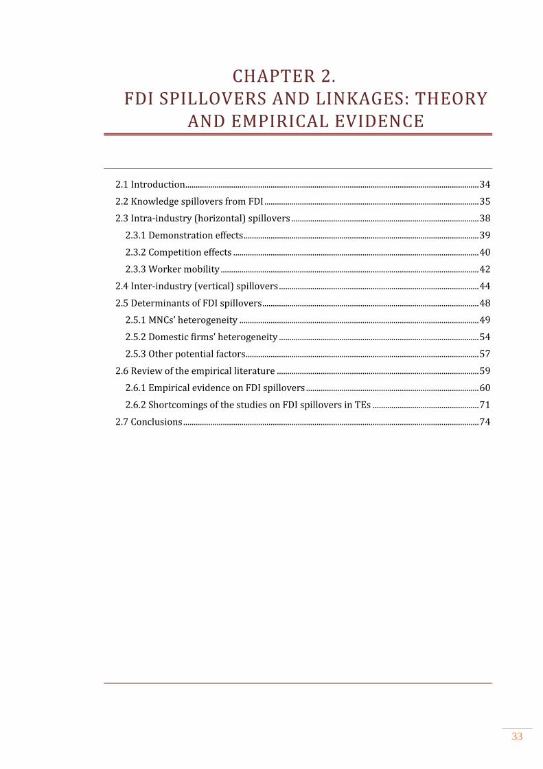
33
CHAPTER 2. FDI SPILLOVERS AND LINKAGES: THEORY
AND EMPIRICAL EVIDENCE
2.1 Introduction ............................................................................................................................................. 34
2.2 Knowledge spillovers from FDI ....................................................................................................... 35
2.3 Intra-industry (horizontal) spillovers .......................................................................................... 38
2.3.1 Demonstration effects ................................................................................................................. 39
2.3.2 Competition effects ...................................................................................................................... 40
2.3.3 Worker mobility ............................................................................................................................ 42
2.4 Inter-industry (vertical) spillovers ................................................................................................ 44
2.5 Determinants of FDI spillovers ........................................................................................................ 48
2.5.1 MNCs’ heterogeneity ................................................................................................................... 49
2.5.2 Domestic firms’ heterogeneity ................................................................................................ 54
2.5.3 Other potential factors ................................................................................................................ 57
2.6 Review of the empirical literature ................................................................................................. 59
2.6.1 Empirical evidence on FDI spillovers ................................................................................... 60
2.6.2 Shortcomings of the studies on FDI spillovers in TEs ................................................... 71
2.7 Conclusions .............................................................................................................................................. 74
34
2.1 INTRODUCTION
Governments around the world provide a range of incentives such as help with
information about local business opportunities, tax holidays, employment subsidies and
land grants to attract MNCs to their countries. The main motive for these policies is the
assumption that MNCs add value to the host country’s economy such as job creation,
provision of necessary capital and increased tax revenues identified in the previous
chapter, and also generate indirect effects resulting in productivity growth. Productivity
spillovers have been identified as one of the most important benefits of FDI (Blomstrom
and Kokko, 1998). When a MNC sets up a subsidiary, it is expected to bring in a certain
amount of firm-specific intangible assets that allow it to compete successfully with local
firms and to overcome the “liability of foreignness”. The MNCs’ superiority arises from
their advanced process and product knowledge, better managerial and organizational
know-how and scale efficiency (Kokko and Kravtsova, 2008). With this superior
knowledge, it is often expected that MNCs perform better, and are more efficient and
productive than their domestic counterparts. In the process of transferring knowledge to
their subsidiaries there is a possibility that some of this knowledge spills over to local
firms involuntarily or voluntarily through several channels. These knowledge spillovers
may affect firms within industry or across industries through backward and forward
linkages. However, empirical evidence on indirect effects of FDI are ambiguous due to
complexity of spillover channels and the mechanism through which knowledge spills
over to local firms. Furthermore, one must take into account the heterogeneity of supply
and demand side factors influencing the potential and actual spillovers. Moreover, the
spillover process is influenced by external factors such as institutional environment,
supply side factors (access to finance, skills acquisition) and spatial proximity. Recent
studies have started to acknowledge these heterogeneous factors and appear to
significantly influence the existence and magnitude of knowledge spillovers from FDI.
The failure to take them into account may thus be a source of the empirical ambiguity
(Smeets, 2008).
The chapter is structured as follows. In section 2.2 the concept and measurement of
knowledge spillovers from FDI is briefly explained. The discussion of theoretical
foundations of intra industry spillovers is provided in Section 2.3. In Section 2.4
35
theoretical models of vertical technology transfer are presented and discussed. Section
2.5 provides an overview of conceptual framework of the determinants of FDI spillover.
This is followed in Section 2.6 by a critical review of empirical literature and the
identification of shortcomings and limitations related to investigation of FDI spillovers
in transition countries. Finally, Section 2.7 concludes.
2.2 KNOWLEDGE SPILLOVERS FROM FDI
The previous chapter explained the nature of advantages of MNCs over domestic firms
and noted that by engaging in FDI, MNCs can potentially bring direct and indirect
benefits to their host economies. By expanding abroad, MNCs try to exploit the
knowledge gained in their home country for the purpose of making profit and maintaining
competitive advantage. However, some of the knowledge may spill over to local firms
due to its public good nature, first recognized by Arrow (1962), as well as other
mechanisms. Knowledge spillovers gained significance in the new economic growth
literature as an important factor explaining long run growth (Romer, 1986; Lucas, 1988;
Grossman and Helpman, 1991). The key feature of endogenous growth theory (EGT) is
that certain factors such as human capital and the utilisation of knowledge pool are not
subject to diminishing returns as investment in physical capital. Scholars in EGT argue
that knowledge is non-rival and incompletely excludable, thus making it available to all
firms in the economy. In this context FDI is seen as a source of new technology which,
with its increasing returns on output, positively influences economic growth through
spillovers.
Although the term knowledge spillovers is commonly used, it lacks a precise definition.
For example Jaffe et al. (2000, p. 215) suggest that knowledge spillovers occur as
“investments in knowledge creation by one party produce external benefits by facilitating
innovation by other parties”. This definition implies that knowledge is created by R&D
and thus knowledge spillovers are the same as technological spillovers (Hallin and
Holmström-Lind, 2012). Other taxonomies include those defined in Table 2.1.
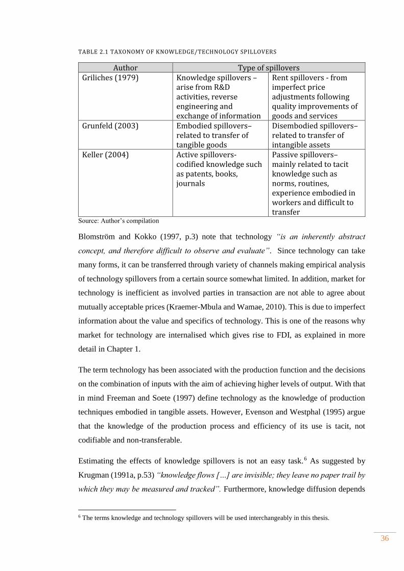
36
TABLE 2.1 TAXONOMY OF KNOWLEDGE/TECHNOLOGY SPILLOVERS
Author Type of spillovers Griliches (1979) Knowledge spillovers –
arise from R&D activities, reverse engineering and exchange of information
Rent spillovers - from imperfect price adjustments following quality improvements of goods and services
Grunfeld (2003) Embodied spillovers– related to transfer of tangible goods
Disembodied spillovers– related to transfer of intangible assets
Keller (2004) Active spillovers- codified knowledge such as patents, books, journals
Passive spillovers– mainly related to tacit knowledge such as norms, routines, experience embodied in workers and difficult to transfer
Source: Author’s compilation
Blomström and Kokko (1997, p.3) note that technology “is an inherently abstract
concept, and therefore difficult to observe and evaluate”. Since technology can take
many forms, it can be transferred through variety of channels making empirical analysis
of technology spillovers from a certain source somewhat limited. In addition, market for
technology is inefficient as involved parties in transaction are not able to agree about
mutually acceptable prices (Kraemer-Mbula and Wamae, 2010). This is due to imperfect
information about the value and specifics of technology. This is one of the reasons why
market for technology are internalised which gives rise to FDI, as explained in more
detail in Chapter 1.
The term technology has been associated with the production function and the decisions
on the combination of inputs with the aim of achieving higher levels of output. With that
in mind Freeman and Soete (1997) define technology as the knowledge of production
techniques embodied in tangible assets. However, Evenson and Westphal (1995) argue
that the knowledge of the production process and efficiency of its use is tacit, not
codifiable and non-transferable.
Estimating the effects of knowledge spillovers is not an easy task. 5F
6 As suggested by
Krugman (1991a, p.53) “knowledge flows […] are invisible; they leave no paper trail by
which they may be measured and tracked”. Furthermore, knowledge diffusion depends
6 The terms knowledge and technology spillovers will be used interchangeably in this thesis.

37
on the type of knowledge transferred from MNCs to local firms. In comparison to
codified knowledge that is easy to convey through tangible forms, tacit knowledge
requires extensive interactions and is difficult to transmit to other parties (Polanyi, 1962).
Therefore, the degree of tacitness can influence the mechanism and channels of
knowledge spillovers. Spencer (2008) argues that tacit knowledge can be mostly
transferred through worker mobility when employees previously working for MNCs
leave the company to become an entrepreneur or decide to join another company.
Since knowledge spillovers are difficult to measure, those investigating indirect effects
of FDI resort to second best solution by estimating productivity spillovers. The general
premise is that technology plays an important role in augmenting productivity. The most
common approach in evaluating the effects of FDI spillovers on host country firms is to
use a Cobb Douglas production function in which the output, value added or productivity
of domestic firms is related to a measure of foreign presence in the industry. The latter is
usually defined as a share of foreign firms in industry sales, capital or employment.
However, the problem is that productivity is a “measure of ignorance” (Abramovitz,
1956, p.11) and thus many factors apart from technological externalities may have an
impact on it. Ornaghi (2004) points that if there are other factors that affect productivity,
then estimating productivity spillovers is not a good indicator of technological
externalities. Recently, Zanfei (2012) has challenged the so called externality framework
based on production function since benefits accruing to domestic firms entails certain
costs associated with purchase, adoption and development of technology. Furthermore,
the production function is not able to disentangle pure technological externalities from
pecuniary externalities or other competition related effects (Driffield and Jindra, 2012).
The former induces changes in the firm’s technology which allows firms to use fewer
inputs for the same amount of output and affect long term competitiveness of firms. The
latter type of externalities occurs through market transactions and formation of linkages,
and affect the firms’ profit function by changing the prices of inputs. They may have an
even larger beneficial effect since they are available to a large number of firms, some of
them not involved in linkages with MNCs (Castellani, 2012). In order to properly
measure pecuniary effects, one would need to have information on input and output
prices before and after the entry of MNCs which is mostly unavailable in firm level
databases.
38
The next sections will discuss in detail the channels through which MNCs affect local
firms and provide an insight into some of the issues faced in estimating FDI spillovers.
2.3 INTRA-INDUSTRY (HORIZONTAL) SPILLOVERS
Although traditional theories of FDI answered the question of ‘under what circumstances
would MNCs invest abroad’, they did not take into account the costs and benefits as well
as the impact of technology transfer on host economies. The earliest discussion on
productivity spillovers dates back to early 1960s and is related to the works of
MacDougall (1960), Corden (1967) and Caves (1971) who investigated costs and
benefits of FDI and technology spillovers together with several other effects influencing
welfare in the host economy. Caves (1974) provided the taxonomy of various spillover
effects and concluded that MNCs contribute to allocative and technical efficiency and
technology transfer and diffusion.
In this section the main theoretical studies modelling intra industry spillover effects from
FDI will be presented and discussed. Horizontal spillovers involve involuntary leakage
of knowledge through which its codified and tacit elements are transferred from MNCs
to local firms (Hallin and Holmström-Lind, 2012). Three channels of technology transfer
are recognised. Earlier studies viewed spillovers as an increasing function of foreign
presence (Findlay, 1978). Most of these studies consider technology possessed by MNCs
as a public good which can be transferred to domestic firms without costs through
demonstration and imitation effects. The second strand of literature argues that spillovers
involve costs and are not determined only by foreign presence. They are the outcome of
interaction between foreign and domestic firms suggesting that technology diffusion and
transfer are endogenously determined (Wang and Blomstrom, 1992). The more recent
models, however, argue that spillovers occur through worker mobility where workers
previously employed and trained in MNCs’ subsidiaries take some of the knowledge
acquired to improve the efficiency of their new employers (Fosfuri et al., 2001). In what
follows, each of these strands will be critically analysed.

39
2.3.1 DEMONSTRATION EFFECTS
Knowledge spillovers are commonly expected to arise from demonstration and imitation
effects. Saggi (2002) defines demonstration effects as occurring through reverse
engineering of MNCs’ products, technologies and management practices by host country
firms. Its scope depends on the complexity of goods produced and processes used by two
types of firms (Barrios and Strobl, 2002). The entry and presence of MNCs in an industry
reduce the risk associated with development of new products and processes since
domestic firms have more information about the costs and benefits of new methods, thus
reducing the uncertainty and providing incentives to imitate. Demonstration effect occurs
without active involvement of MNCs and is based on quasi-public good characteristics
of new products and processes as firms can observe the outcome of technological
innovations at no or very little cost. In addition, demonstration effects include the foreign
firms’ knowledge of distribution networks, transport infrastructure and consumer tastes
which may help domestic firms wishing to become exporters or to enter global supply
networks (Farole and Winkler, 2014). However, as argued by Zanfei (2012), the firms’
absorptive capacity is a key conditioning factor which enables local firms to evaluate and
use external knowledge.
Koizumi and Kopecky (1977) are the first to explicitly model FDI and technology
transfer in the modified model of international capital movement. Technology transfer
is proxied by capital stock owned by foreign firms and it is assumed that technological
benefits to indigenous firms depend on the extent of foreign ownership of a country’s
capital stock. According to them the transmission of foreign technology is viewed as
automatic and technology was treated as a public good. As MNCs are unable to
internalise the total returns, host country firms can exploit the technology free of charge.
Findlay (1978) developed a similar model of international technology transfer to examine
the relationship between FDI from an advanced developed economy and technological
change in a developing country. In his model, the rate of technological diffusion to the
developing country is assumed to depend on two factors, the “relative backwardness”
and the “contagious effect”. The first factor was introduced by Veblen (1915) and
Gerschenkron (1962) who stated that the rate of technological convergence and
technology diffusion is faster the higher is the technology gap between the backward and
the advanced country. The second factor, used firstly by Arrow (1971), stresses the

40
importance of personal contacts as the most efficient way of technology diffusion
between the parties that have the knowledge and those who adopt it. Findlay captures
both effects and argues that the rate of technological change in the developing country is
an increasing function of technology gap and foreign presence. FDI spillovers occur
since increased foreign presence lead to smaller technological gap. However, Cantwell
(1989) argues that Findlay’s hypothesis does not always hold as domestic firms differ in
their capability to internalise technologies in their production process.
Models of spillovers discussed above assume that differences in the level of technology
between MNCs and domestic firms are the main determinant of demonstration and
imitation effect. Furthermore, they assume that spillovers are exogenous, do not depend
on the behaviour of foreign and domestic firms and do not take into account the
absorptive capacity of the recipient(s).
2.3.2 COMPETITION EFFECTS
Another strand of literature emphasizes the competition effects in addition to the set of
technologies available from FDI. Competition has two effects which are mainly
pecuniary in nature. First, it reduces the monopoly power of domestic firms and forces
them to benefit from new technology and management practices by introducing stricter
or more cost conscious management (Blomstrom and Kokko, 1998). Second, it
encourages more efficient allocation of resources and reduction of market distortions
across industries resulting in increased productivity. However, increased competition
may result in negative spillovers effects in the short run due to the inefficiency of
domestic firms and hence reduction in their market share. If fixed costs account for a
considerable part of the production costs, average cost curves will be downward sloping,
in which case a loss in market share will push firms up on their average cost curves and
force them to produce at a less efficient scale (Aitken and Harrison, 1999). This implies
that spillover process does not involve only MNC and is not automatic. Therefore, it must
include the costs of technology transfer as well as the effort of domestic firms.
Competition effects cannot be regarded as pure externalities as MNCs face the
transaction costs of dealing with competition policy, or offer higher wages to attract
qualified workers.

41
Das (1987) recognized the costs associated with spillovers and used a price-leadership
model from oligopoly theory to analyse the transfer of technology from the parent firm
to its subsidiary abroad. He examined the optimal behaviour of MNCs when there is a
risk that local rivals succeed in learning their production techniques. Similar to previous
models, he assumed that the rate of increase in efficiency of local firms is positively
related to the output of MNC’s subsidiary. Therefore, the latter will decide to increase
the price in order to reduce the amount of output at the expense of short term profit which
will eventually lead to fewer spillovers to local firms. However, the behaviour of local
firms is not explicitly taken into account.
In the models discussed above the advanced technology introduced by foreign firms is
considered to be a public good and transferred automatically. Furthermore, it is assumed
that technologies can be transferred without facing any difficulties and are adopted by
local firms without any adjustment cost. As a result, these models do not deal adequately
with the issue of interaction between MNCs’ subsidiaries and host country firms. The
contribution of Wang and Blomstrom’s model (1992) lies in its highlighting of the
essential role played by competition. Whereas in previous models the extent of spillovers
is determined by the degree of foreign presence, in Wang and Blomstrom’s model they
are instead endogenously generated by the technological competition between foreign
subsidiaries and domestic firms. Furthermore, the authors identified two types of costs:
the cost to the MNCs of transferring technology to its subsidiaries and the costs of
learning to domestic firms.
Wang and Blomstrom (1992) construct a model based on two firms in which the rate of
technological transfer is determined by strategic decisions of the two firms. They also
follow Findlay’s assumption of a positive relationship between the technology gap and
spillovers. Each firm solves the dynamic optimisation problem subject to other firm’s
action. The objective of MNCs is to decide on how much technology will be transferred
to local subsidiary while the domestic firm’s objective is to decide on how much to invest
in learning to capture MNC’s technology. The conclusion of the model is that the extent
of spillovers depends on the investment decisions of both types of firms. The potential
for spillovers is higher the more the MNCs invest in new technology, thus increasing the
technology gap. However, learning by domestic firms will reduce technology gap and
force the foreign subsidiary to import more advanced technology from its parent
company in order to restore its market share and profit levels. This in turn provides an

42
additional incentive to local firms to increase their investment in learning and thus more
spillovers.
Perez (1997) developed a model of spillover effects using an evolutionary perspective
(Nelson and Winter, 1982) which is different from previous models that fall in the
framework of industrial organization theory. He emphasized that domestic firms’
catching up process is path dependent and that absorptive capacity is the main source of
continuous technological development. Spillovers emerge as a result of a dynamic
interaction between foreign and domestic firms at the existing technology level. Perez
(1997) was able to show that domestic firms with high technology level are more
successful in learning from FDI and thus to stay more competitive, while firms which
lag far behind the technological level of MNCs are crowded out with increased foreign
presence.
2.3.3 WORKER MOBILITY
A third channel of intra-industry knowledge spillovers is worker mobility. Local firms
can benefit from employees previously employed in MNCs as the latter is likely to have
provide the host country workforce with a higher degree of training, education and
valuable work experience (Smeets, 2008). Given that a large part of labour training
constitutes knowledge that is not completely firm specific, this generates a positive
externality for the receiving firm by increasing the quality of its human capital. This in
turn leads to higher productivity for domestic firms that hire these workers after they
leave the MNC. Also some of the MNC’s senior managers may, at some point in time,
choose to start up their own company, and would be able to apply the knowledge acquired
in the MNC for their own firm’s benefit. Worker mobility generates both pecuniary and
pure knowledge effects. The former arises due to increased supply of trained workers
which are available at lower costs while the latter effect arises from tacit knowledge
embedded in human skills as long as the salary does not reflect accumulated knowledge.
(Ben Hamida, 2007; Zanfei, 2012). However, spillovers through this channel are more
likely to occur in medium and long run as knowledge must be absorbed by local
employees and in the short term foreign firms are more likely to offer higher wages and
other benefits resulting in negative spillover effects (Sinnai and Meyer, 2004; Crespo and

43
Fontoura, 2007). Several models were recently developed which model spillovers
through this channel.
Fosfuri et al. (2001) construct a model in which a firm has to choose between FDI and
exports to serve the foreign market, and needs to train the host country workers if it
chooses the former. When training is completed, both foreign subsidiary and local firms
compete for the services of employees previously employed by MNCs. Knowledge
spillovers occur if the local firms make a higher offer to the trained employees. Even if
workers do not change their employment status, the host country welfare might still be
improved because of pecuniary spillovers embodied in the wages that the MNC pays to
the trained workers to prevent them from moving to a local competitor. The conditions
for occurrence of spillovers depend on several assumptions: competition in the product
market is low; the training of workers is general involving organizational, marketing and
managerial skills; and the absorptive capacity of domestic firms is high.
The difference between technology spillovers which occur when worker is hired by the
local firm and pecuniary spillovers occurring when worker is retained by the
multinational subsidiary at a higher wage is shown in Glass and Saggi (2002). In contrast
to the previous model, the role of training is kept aside and the emphasis is put on the
superior technology that can be transferred to host country firms if the latter hire the
workers previously employed in a MNC. As the attractiveness of its workers to the host
country firms is recognized, the MNC weights the cost of paying higher wages to keep
them within its boundaries against the benefit of limiting technology transfer to the host
firms. In their model with multiple host and source firms the foreign firm can increase
its profits by raising the wage it pays to workers to a level which is enough to prevent
them from switching employers. Wage premium can raise foreign firm’s profit by
preventing the cost reduction for the host country firm which would otherwise occur.
Markusen and Trofimenko (2009) develop a model in which knowledge is transmitted
when foreign experts visit the host country firms and train its workers. They show that
hiring foreign experts increases the (real) wages and value added of the hiring plant. This
effect is both instantaneous (it occurs during the period of hiring) and persistent (it
remains even after the foreign expert has left the plant). They shed light on the timing
issue and find that the longer the plant postpones the decision to hire foreign experts, the
smaller their contribution to the improved wage and productivity.

44
2.4 INTER-INDUSTRY (VERTICAL) SPILLOVERS
Unlike intra-industry spillovers which are regarded as technological externalities, MNCs
also create pecuniary externalities by creating linkages with their suppliers and
customers. The reasons for engaging in vertical relationship from the viewpoint of MNC
are to overcome the deficiency of market transactions (Lall, 1980) and to prevent the
leakage of information and knowledge to direct competitors (Javorcik, 2004a). Through
linkage formation local firms can gain access to knowledge and technology of MNCs
(Kugler, 2006). The concept of backward and forward linkages was developed by
Hirschman (1958). The first type involves the benefits to domestic suppliers, while the
second type creates spillovers to domestic customers. Hirschman suggested that the
importance of backward linkages is best approximated by the percentage of inputs
purchased from other industries while forward linkages should be measured by
percentage of output sold to other industries.
By creating vertical linkages technological externalities arise as MNCs facilitate learning
by doing in local firms resulting in increased productivity (Eden, 2009). Suppliers can
benefit from inter-firm exchange of technical and managerial knowledge (Giroud, 2007).
MNCs provide technical assistance on product design, quality control and inventory
management as well as financial and procurement assistance (Zanfei, 2012). Customers
of MNCs can benefit from spillovers and knowledge embodied in products, processes
and technologies as well as improved access to enhanced or previously unavailable inputs
and products (Jindra et al., 2009). Lall (1980) has identified “complementary” activities
which may lead to spillovers through vertical linkages with suppliers:
- help prospective suppliers to set up production facilities;
- help suppliers to raise the quality of their products or facilitate innovations by
providing technical assistance or information;
- provide or assist in purchasing of raw materials and intermediaries;
- provide training and help in management and organization; and
- assist suppliers to diversity by finding additional customers.
Besides cooperation effects listed above, MNCs may force domestic suppliers to meet
the higher standards of quality, reliability, and speed of delivery of MNCs (Blomstrom
and Kokko, 1998).
45
The recent surge in the literature on industry linkages has spurred the development of
several theoretical models which have analysed the effects of MNCs on economic
development. Rodríguez-Clare (1996) developed a model with monopolistic competition
in the intermediate products sector, which domestic firms and MNCs use as inputs in
their final goods production. It is based on three premises. First, greater variety of inputs
leads to higher production efficiency in final good sector due to the “love of variety of
inputs” (Ethier 1982) by local and foreign firms. Second, intermediate goods industry is
characterised by increasing returns to scale. Third, the proximity of supplier and user is
required as the domestic firms buy all of their inputs locally. The latter is required in
order to ensure the development of final good industry. These assumptions lead to a
“good” equilibrium characterised by high wages, complex goods and high variety of
inputs while production of simple goods and small variety of inputs lead to “low”
equilibrium (Glass et al., 2002). Under the scenario of two economies, one developed
and the other developing, MNCs will establish a subsidiary overseas to enjoy the benefits
of cheap labour, similar to vertical model of FDI discussed in the previous chapter.
However, the crucial assumption is that intermediate products are not tradable and firms
cannot use them unless they have a plant operating in the country in which inputs are
produced.6F
7
The linkage coefficient developed by the author measures the ratio of employment
generated in supplier industries per unit of labour hired directly by MNCs (Glass at al.,
2002). If positive, it implies that an increase in the number of MNCs which produce more
complex goods and employ more specialized intermediate inputs will increase the variety
of inputs produced locally and thereby help develop supplier industry in the host country.
Increased demand and variety of intermediate inputs also generate positive externalities
to other final goods producers, thus establishing forward linkages. As the complexity of
final and intermediate products increases, the positive linkage effect is expected to lead
to higher productivity of domestic firms and higher wages and skill levels in host
economy. Backward linkages will be higher under conditions that MNCs use complex
intermediate inputs, the higher are the communication costs between parent company
and subsidiary and the higher is the similarity of variety of inputs produced between host
and home country.
7 This assumption implies that relying on foreign suppliers entails additional coordination costs.

46
Markusen and Venables (1999) develop a model with two imperfectly competitive
industries with increasing returns to scale, producing intermediate and final goods which
are linked by an input-output relationship. It is somewhat different from Rodriguez-Clare
model (1996) as it assumes intra industry competition. According to the model there are
three effects of MNCs’ entry. First is the competition effect as foreign investment takes
place in the final goods sector increasing total output and reducing market price, leading
to the exit of domestic firms. The second effect is the creation of backward linkages to
intermediate goods suppliers in the upstream sector. As firms operate in monopolistically
competitive markets their number increases to generate more variety of inputs which lead
to lower average costs and increase in profits. The increased entry thus causes a third
effect as the reduction in prices of inputs benefits firms in downstream sector because of
improved and cheaper intermediate products supplied by domestic firms. The stronger
the demand effect compared to the competition effect, the better is the situation for the
upstream and downstream firms.
Similarly, Pack and Saggi (2001) have developed a model of technology transfer in
which MNCs induce entry of other suppliers by transferring technology to firms in
upstream sector, thus reducing concentration and lowering prices. Given the benefit of
lower-priced inputs, downstream firms will lower prices and increase output, and new
firm entry may occur. This would induce higher output in upstream sector due to stronger
demand from downstream sectors. If the above argument holds, then benefits accrue
widely to all sectors and consumers, not only through improved productivity but also
through increased competition resulting in lower deadweight loss, thus improving
welfare.
In the models discussed above the basic premise is that MNCs alter the incentives for
entry and that the interaction between MNCs and local suppliers is based on love of
variety for inputs in final goods industry. However, as noted by Lin and Saggi (2007)
these models ignore the strategic interaction which occur in an oligopolistic market
structure and emphasize demand creation effects. In addition, the connection between
technology transfer and backward linkages and the contractual relationship which may
be used by MNCs to protect their knowledge is not addressed.
Lin and Saggi (2007) explicitly consider vertical technology transfer (VTT) through
backward linkages focusing on supply side effects. They develop a two-tier model in
47
which the production of final goods depends on intermediate goods and the market
structure if both markets are oligopolistic. Upon entry, MNC are faced with the choice
of sourcing their inputs from the market by interacting with all suppliers vs. sourcing the
intermediate good locally with selected suppliers who exclusively agree to serve MNCs
in return of VTT. Two types of contractual agreement are discussed: one in which
domestic supplier must abide by an exclusivity condition that forbids serving MNC’s
rivals and another contract in which domestic firms do not face such a restriction.
Generally, MNC is faced with a trade-off: on one hand it would like to prevent local
firms and rivals to benefit from VTT, on the other hand it would prefer to have multiple
suppliers in order to secure more competitive price. In reality, the MNC can combine
these two contracts, although the number of local suppliers that accept exclusivity
contract is likely to be smaller relative to the case where the multinational commits to
sourcing only from its exclusive suppliers. The conclusion is that while the entry of the
multinational creates additional demand for the intermediate goods, it can also reduce
the number of suppliers available to local producers. This negative supply-side effect can
dominate the positive demand-side effect so that the total output of the intermediate good
as well as the final good can shrink due to the MNC’s entry.
Recently, Alfaro et al. (2010) combined the theoretical model and the calibration exercise
in which positive backward linkages depend on local financial markets, market structure
and competition for skilled and unskilled labour. They model a small open economy in
which domestic and foreign firms compete for skilled and unskilled labour and
intermediate products in the final goods industry. In order to operate in the upstream
sector, firm must develop a new variety of inputs which requires capital investment, the
latter being conditional on developed local financial markets. Increased variety of inputs
leads to positive FDI spillovers in final goods sector. Hence, financial markets act as a
channel for realisation of linkage effects. Furthermore, their model implies also the
existence of horizontal spillovers in the final goods sector by raising productivity of
domestic firms due to greater availability of intermediate inputs.
48
2.5 DETERMINANTS OF FDI SPILLOVERS
In the previous section, we discussed the channels through which MNCs influence the
productivity of host country firms. However, spillovers do not occur automatically. In
what follows theoretical arguments derived from formalised models as well as those
without mathematical representation will be used to develop a conceptual framework
which is built on the premise that the realisation of FDI spillovers depends on domestic
firms and MNCs’ heterogeneity. This interaction is influenced by the host country
environment and institutional framework which affect foreign and domestic firms’
characteristics as well as the knowledge transmission channels. Figure 2.1 below
illustrates the channels and mechanisms through which MNCs can influence local
companies, and factors affecting their occurrence. As can be seen the realisation of
vertical linkages and thus productivity spillovers between MNCs and local firms can
occur through several mechanisms such as demand effects by requiring better and more
diverse inputs, product quality and delivery time (Farole and Winkler, 2014). Also,
assistance effects such as personnel training, leasing of machinery, sharing of production
techniques and support in product design may help domestic firms to benefit from
spillovers if MNCs is not fully compensated for these benefits (Lall 1980; Crespo and
Fontoura, 2007; Farole and Winkler, 2014).
The benefits accruing to domestic firms are however conditional on MNCs heterogeneity
such as their motives, level of ownership, country of origin, mode of entry and sourcing
strategies. The extent of knowledge diffusion effects depends on local firms’
characteristics in terms of size, absorptive capacity and spatial proximity. Finally, host
country requirements such as level of foreign control or preference for certain types of
FDI may also influence FDI spillovers. The same reasoning applies to the occurrence of
intra industry spillovers where times since foreign entry or mode of entry may induce
demonstration and competition effects as well as the type of knowledge available to local
firms. The actual benefit to local firms depends on their ability to attract employees
previously working for MNCs or their capacity to withstand fierce competition. Aspects
of host country policy such as access to finance, trade policy, development of physical
infrastructure, learning and innovation infrastructure influence domestic firms’ capacity
to learn and finance necessary investments while intellectual property right regime and
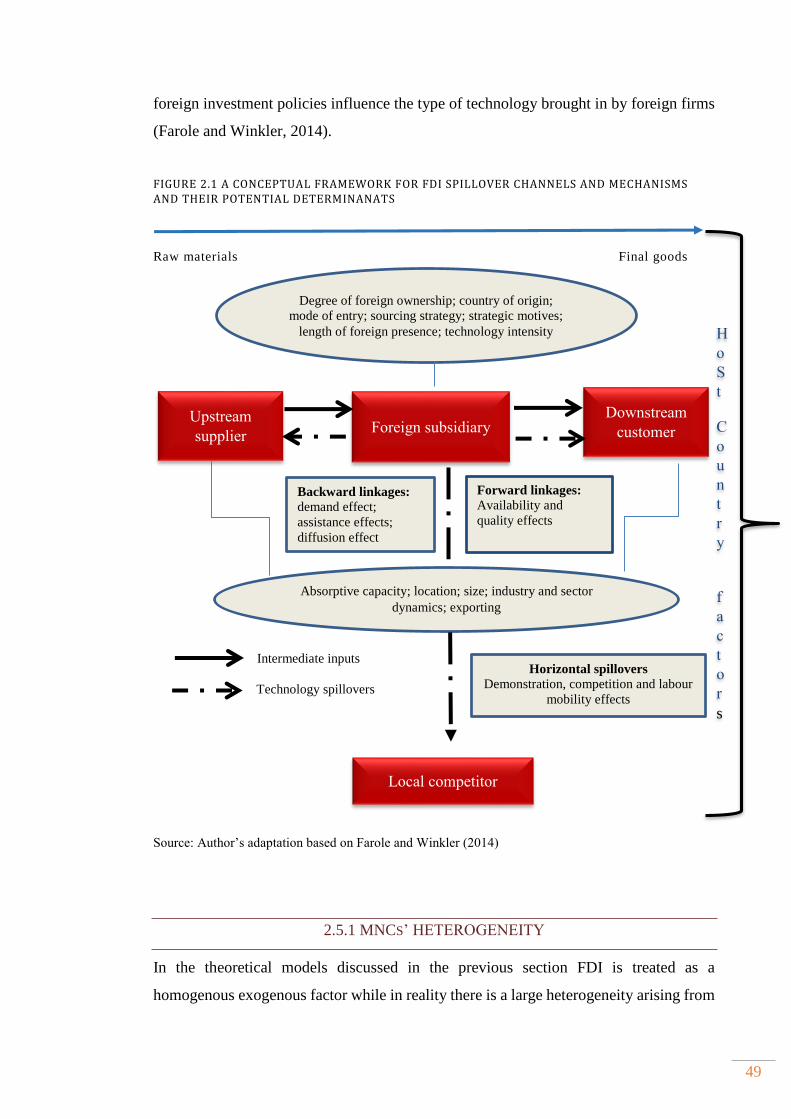
49
foreign investment policies influence the type of technology brought in by foreign firms
(Farole and Winkler, 2014).
FIGURE 2.1 A CONCEPTUAL FRAMEWORK FOR FDI SPILLOVER CHANNELS AND MECHANISMS AND THEIR POTENTIAL DETERMINANATS
Raw materials Final goods
Intermediate inputs
Technology spillovers
Source: Author’s adaptation based on Farole and Winkler (2014)
2.5.1 MNCS’ HETEROGENEITY
In the theoretical models discussed in the previous section FDI is treated as a
homogenous exogenous factor while in reality there is a large heterogeneity arising from
Degree of foreign ownership; country of origin;
mode of entry; sourcing strategy; strategic motives;
length of foreign presence; technology intensity
Foreign subsidiary Upstream
supplier
Downstream
customer
Local competitor
Absorptive capacity; location; size; industry and sector
dynamics; exporting
H
o
S
t
C
o
u
n
t
r
y
f
a
c
t
o
r
s
Backward linkages:
demand effect;
assistance effects;
diffusion effect
Forward linkages:
Availability and
quality effects
Horizontal spillovers
Demonstration, competition and labour
mobility effects
50
different motives, origins of FDI, modes of entry, ownership characteristics, trade
orientation and the complexity of technology they use. It can be argued that different
types of FDI give rise to different amount of knowledge spillovers. First, specific
spillover channels are more relevant for certain types of FDI than for others and, second,
the tacit component in knowledge spillovers may cause different spillover effects from
various types of FDI (Smeets and de Vaal, 2006). As argued by Castellani and Zanfei
(2007), “not every multinational company is a good source of externality and not every
domestic firm is equally well placed to benefit from multinational activity”. Here, we
discuss some of these heterogeneities.
Level of control (ownership). Müller and Schnitzer (2006) and Gattai and Molteni
(2007) derive a theoretical framework to study the relation between knowledge spillovers
and the choice between FDI and joint venture (JV). Both studies conclude that FDI is the
MNC’s best option where the risk of knowledge spillovers to other firms is high. Muller
and Schnitzer take into account the active role of the host country. In particular, they
examine the role of taxation and local infrastructure investments and find that these
instruments can help MNCs to align their interest with those of the host country and thus
choose to invest in JV increasing knowledge spillovers. Gattai and Molteni find that full
ownership is the optimal solution in environments characterised by weak IPR and when
local firms have high capacity to learn.
Smeets and de Vaal (2006) argue that fully owned or partially owned firms differ in
potential for transfer of knowledge as well as the time necessary to establish cooperation
with local firms. The channels and mechanism of knowledge spillovers may differ as
partially owned foreign firms are more likely to generate benefits to local firms through
pecuniary spillovers in addition to pure knowledge spillovers Knowledge based view of
the firm discussed in Section 1.3.6 pointed out that not only the ownership of specific
technology, but also the ownership of specific architectural capabilities that enable
MNCs to transfer tacit knowledge is a source of their unique competitive advantages
(Kogut and Zander, 1993; Tallman, 2003). In this respect, joint ventures are seen as an
important vehicle for transfer of tacit knowledge as they are more embedded in host
country environment. By establishing joint ventures, the interests of domestic and foreign
firm are more aligned and the incentives for knowledge sharing is high due to mutually
beneficial interest to improve performance.

51
Partial ownership can create higher potential for spillovers, especially by creating vertical
linkages since it is expected that MNCs are already integrated to a certain extent into the
local economy, thus sourcing inputs from the host market (Javorcik and Spatareanu,
2008). However, the transfer of foreign technology may be gradual, thus limiting the
scope for spillovers in early years. Joint ventures are specifically beneficial for firms with
high degree of mutual dependence characterised by frequent exchange of knowledge
where local firms have substantial scope for learning new techniques and best practices
(Konwar et al., 2014).
However, wholly owned subsidiary are more likely to transfer more sophisticated
technology. As demonstrated by Ramacharandran (1993) foreign firms are more likely
to opt for full ownership in the weak institutional environment characterised by weak
property rights. In case where knowledge transfer is complex and not easy to codify,
where the capability of potential partners is weak or there is a potential for knowledge
dissipation and MNCs pursue asset exploiting strategies, they (MNCs) will create a
wholly owned subsidiary thus try to prevent leakage of know-how and other valuable
knowledge information to competitors. Since wholly owned subsidiaries bring more
advanced technology the potential for technology transfer is also greater and more rapid
compared to joint ventures (Mansfield and Romero, 1980). However, the latter depends
on the industry in which foreign firms enter as well as absorptive capacity of domestic
firms. In summary, the volume of knowledge based assets and its quality is increasing
with higher levels of ownership. However, the diffusion of knowledge is more likely to
occur with joint ventures.
Home country characteristics. One of the important factors influencing the potential of
FDI spillovers and the extent to which local firms can benefit from MNC entry is related
to the origin of investment. Although there is no formal theoretical treatment dealing
with this element of heterogeneity, one may derive several propositions based on the
home country differences affecting the performance of MNC’s subsidiary and thus
indirectly the productivity of domestic firms (influenced by potential spillovers). Banga
(2003) argues that productivity differences according to investors’ home country are
expected, since FDI from distinct countries brings different levels of technology and
different modes of transfer. Facing different opportunities and obstacles in the

52
environment, firms in different countries can create different technologies and
management practices by exploiting the availability of specific industry knowledge,
complementary products, technologies and institutional framework (Ghemawat, 2003).
Egger and Keuschnigg (2011) argue that the innovativeness and productivity of MNCs
are related to development of their home country financial market and institutions. If a
MNC’s subsidiary relies upon technological inputs from home country, the degree of
development of financial markets and credit tightness affect their productivity and
innovativeness and impede intra firm knowledge transfer. This in turn influences the
extent of technology spillovers to host country. Exposure to different technologies and
management practices can facilitate local firms’ learning capability since “it increases
the prospect that incoming information will relate to what is already known” (Cohen and
Levinthal, 1990, p. 131). A greater variety of technologies can further strengthen and
increase local firms’ competitive advantage by enhancing economies of scale and scope
(Zhang and Li, 2010). This in turn enables local firms to compete on a global scale and
satisfy stringent supplier requirements from MNCs. Furthermore, MNCs from different
geographical locations require different inputs and offer different products and
technologies thus creating forward and backward linkages within the host country
(Zhang et al., 2010). A greater diversity of MNCs can also have beneficial effect on
worker mobility channel of FDI spillovers as employees previously employed by MNCs
can imitate some of the best practices and apply them in domestic firms. Differences in
home country can affect the production strategy and technologies used in host countries.
Finally, theoretical model of vertical linkages (Rodriguez-Clare, 1996) predicts that the
share of intermediate inputs transferred from source to host country is positively
correlated to geographical distance. Increased geographical distance creates incentives
for MNCs to source locally in order to reduce transport costs. The same line of reasoning
can also be applied to cultural, legal and social differences. Nevertheless the differences
in these latter factors could also pose problems for domestic firms in assimilating the
new technology.
Mode of entry. Another type of FDI heterogeneity affecting productivity spillover is the
mode of entry in the host market. Several authors (Mattoo et al., 2004; Görg, 2000,
Muller, 2007) have developed theoretical models to examine how the extent of
technology transfer and level of competition affect the choice of entry, but without
53
considering the possibility of spillover effects. If the cost of adaptation due to specific
production technology is high, foreign firms have a smaller cost advantage over domestic
firms and greenfield FDI is thus the preferred mode of entry. However, in the case of
marketing costs and costs of building distribution facilities, the opposite holds.
Furthermore, the intensity of competition influences the choice of entry mode in a non-
monotonic way. In the case of high or low competition greenfield entry is preferred. The
analysis also showed greenfield investment is the optimal mode of entry only if the
technological gap between the domestic firm and the MNCs is sufficiently large. Muller
(2002) explicitly modelled the effects of technology spillovers on the mode of MNCs’
entry under different forms of competition. He further introduced the notion of
asymmetric information about spillover potential and their effects on the mode of entry.
Under the assumption of perfect information and price competition, MNCs will engage
in more acquisitions while opposite holds for quantity competition. In contrast, when
MNCs are faced with imperfect information acquisition, activity will be reduced because
MNCs cannot take into considerations otherwise efficient acquisitions. In the model
spillovers can occur only under greenfield investment especially if foreign firm is R&D
intensive as in this situation it has a strong competitive advantage.
However, these models failed to recognize the variety of spillover channels associated
with the mode of entry and the speed through which spillovers occur under these two
distinct modes. It has been asserted that acquisitions delay spillovers or even restrict them
(Braconier et al., 2001). On the contrary, when FDI occurs through greenfield
investment, the potential for spillovers is high as new and advanced technology becomes
instantly available. However, the scope of spillovers may be diminished as MNCs import
a technology that may significantly differ from the one existing in the host country.
Moreover greenfield investors have incentive to protect intellectual property rights, thus
limiting the potential for knowledge spillovers. In the case of acquisition or merger the
scope for spillovers is larger as MNCs bring technology which shares similar
characteristics with the existing host country technology and thus the potential for
demonstration effects is larger (Crespo and Fontoura, 2007). In addition, MNCs are
likely to use the existing network of suppliers and customers, thus creating vertical
linkages.
MNC’s motives. Although the issue of FDI motivation in the context of FDI spillovers
is not explored, it can still affect the extent of productivity spillovers. In the previous
54
chapter we explained that FDI motivations can broadly be classified into two categories.
The first one is related to OLI paradigm and the exploitation of existing ownership
advantages brought from the home country. The second one is related to technological
accumulation hypothesis and the literature examining R&D internationalisation in which
MNCs locate near leading research centres or universities with the aim of sourcing
technology from its rivals. Fosfuri and Motta (1999) posed the question of whether high
productivity firms (leaders) or low productivity firms (laggards) engage in asset seeking
strategies. They show that a laggard MNC can choose to enter in a foreign market through
FDI even when this involves sunk costs and the transport costs of exports are zero. The
potential for positive spillovers can arise due to geographical proximity to a technological
leader in a host country. Benefits coming from spillover effects cause a reduction in the
production costs of the MNC both in the home country and in its foreign subsidiary. In
this way technology sourcing outweighs the costs associated with establishing the
subsidiary. The expectation therefore, is that spillovers to domestic firms are more likely
to occur from traditional motivations of FDI.
In this regard resource seeking investments have limited potential for spillovers, due to
their high capital and technology intensity and limited time horizon (Farole and Winkler,
2014). On the other hand, efficiency seeking FDI especially those oriented towards the
manufacturing sector are expected to contribute to spillovers due to strong requirements
for a broad range of inputs. However, it must be noted that the spillover potential arising
from efficiency seeking motives depends on technology and skill intensity of the
production process as well as sourcing behaviour of MNCs in different manufacturing
sectors (Farole and Winkler, 2014). Market seeking motives are also conducive to
spillovers, especially from MNCs in the retail sector which source a significant amount
of inputs from food sector as shown by Javorcik and Li (2013).
2.5.2 DOMESTIC FIRMS’ HETEROGENEITY
Although the presence of MNCs provides a potential for knowledge spillovers and thus
indirectly affects the productivity of indigenous firms, the actual effects are conditional
upon the receiving party’s characteristics (country, industry and firm). Failing to take

55
into account factors that transform potential spillovers into actual knowledge spillovers
may severely bias the empirical results (Smeets, 2008).
Technological gap vs. absorptive capacity. The necessary condition for turning
knowledge spillovers potential to actual is the existence of absorptive capacity. Two
views dominate the literature with respect to the role of technological capability of
domestic firms in adopting new technologies from MNCs. One view is represented by
Findlay (1978) who suggests that the wider the technology gap between the advanced
and less advanced countries (and firms), the larger is the potential for technological
imitation and adoption. Moreover, the speed of adoption is a function of contagion where
for a given level of foreign presence, the larger the technology gap between the foreign
and domestic firms, the higher the spillovers. Glass and Saggi (1998), however, argue
that the larger the technological gap the less likely are the domestic firms to have the
human capital, organizational capabilities, sources of finance, physical infrastructure and
distribution networks to benefit from spillovers. Moreover, the absorptive capacity
influences not only the actual occurrence of spillovers but also their potential by affecting
the MNCs’ decision to invest and the type of technology to employ. A large technology
gap is therefore a signal of low domestic absorptive capacity which affects the probability
of positive spillover benefits to domestic firms. Some authors suggest that technological
gap and absorptive capacity are complementary. Abramovitz (1986, p.388), for example,
argues that “a country’s potential for rapid growth is strong not when it is backward
without qualification, but rather when it is technologically backward but socially
advanced”, thus suggesting the importance of the absorptive capacity.
The importance of absorptive capacity is emphasized in a seminal paper by Cohen and
Levinthal (1989) who define absorptive capacity as a firm’s ability to learn from external
knowledge through identification, assimilation and exploitation. They hold that
absorptive capacity is a by-product of the firm’s investment in R&D. Later on Cohen and
Levinthal (1990) redefined the concept of absorptive capacity by including cognitive
aspects underlying the learning process. The firm’s level of absorptive capacity depends
upon its existing level of technological competence at the time of foreign entry as well
as the learning and investment efforts it makes afterwards in order to benefit from foreign
knowledge. As argued by Cohen and Levinthal (1990) absorptive capacity is path-
dependent because learning experience, prior organizational knowledge and problem
solving capacity facilitate the use of new knowledge, thus creating a cumulative process.

56
Similarly, Nelson and Phelps (1966) argue that human capital enables understanding of
new technological developments, their evaluation and adaptation, thus affecting firm’s
productivity. Narula and Marin (2003) suggest that absorption does not imply imitation
as each firm possess specific technology; domestic firms need to invest in their own
research and development, employee training and adapt organizational structures to be
able to efficiently exploit foreign knowledge and increase their productivity. Ben-
Hamida and Gugler (2009) show that firms which are not far behind the technological
frontier of the industry may fully exploit the advantages arising from imitation and
demonstration channels. Firms with less developed technological capabilities are able to
benefit from worker mobility since this channel provides (technical, managerial, etc.)
assistance to managers of local firms who lack the necessary experience on how to act
under competitive environment. In the case of backward linkages firms with high level
of human capital are more able to meet the quality standards by producing high quality
inputs, thus cooperation with foreign firms is more likely to arise.
The concept of absorptive capacity has been expanded to include support infrastructure
such as developed financial markets. Hermes and Lensink (2004) and Alfaro et al. (2009)
argue that developed financial system reduces the risk of undertaking investments for
domestic firms which aim to increase their absorptive capacity, thus favouring FDI
spillovers.
Trade orientation. Blomstrom and Sjoholm (1999) argue that firms engaged in export
activities already face international competition and therefore have higher absorptive
capacity and productivity levels which enable them to benefit from foreign technology.
Moreover, exporters may be in a better position to become suppliers of MNCs. However,
they may also have limited contact with local market and face less competition from
MNCs, thus having fewer incentives to improve resulting in reduced potential for intra-
industry spillovers.
Size. Crespo and Fontoura (2007) hypothesize that firms’ size also have an important
impact on FDI spillovers as larger firms are more likely to have the necessary production
scale which enables them to imitate the production processes used in MNCs or have
better access to finance which enables them to invest in production technology and
increase the quality of their products. Furthermore, their larger scale enables them to

57
compete more efficiently with MNCs. Finally, small firms are less likely to experience
large labour turnover thus limiting spillovers occurring through worker mobility.
2.5.3 OTHER POTENTIAL FACTORS
The efficiency of FDI spillover channels also depends on technological similarities
between MNCs and local firms in the industry in which they operate. Furthermore, the
extent of spillovers may be conditional on spatial proximity and institutional framework.
Industry characteristics. FDI is industry specific (Wang et al., 2009). And, therefore,
the technological intensity of industries is an important factor influencing the extent of
FDI spillovers as it is often argued that MNCs are located in industries with high value
added and have competitive advantage over local firms in technologically advanced
sectors. Hence, learning opportunities for local firms are higher in such sectors. However,
in high-tech industries, MNCs’ knowledge is characterised by more complex and tacit
elements which are difficult to codify and transfer (Spencer, 2008; Hashai, 2009).
Moreover, as argued by McCharty et al. (2010), high tech industries are characterised by
continuous change in demand, regulation, competition and technology which reduces the
chances for domestic firms to learn from MNCs. In addition, it is more likely that
domestic firms have larger technological gap in such industries which may impede
successful integration of external knowledge and force MNC to use global suppliers
(Hatani, 2009). Furthermore, the nature of knowledge flows may be different in
manufacturing and services industries. This may reflect the way in which knowledge is
protected and transferred to host country firms, thus influencing the mode of entry and
level of control and subsequently the extent of spillovers.
Spatial proximity. Economic distance discussed in previous section is concerned with
relative backwardness and absorptive capacity. It determines whether and to what extent
local firms can benefit from FDI spillovers. On the other hand, geographical distance
affects the transmission costs, thus reducing the possibilities for indigenous firms to
benefit from knowledge spillovers of foreign subsidiaries located further away. As
knowledge is mainly tacit, geographical distance inhibits its transmission and absorption.
Therefore, spatial proximity facilitates the process of knowledge diffusion influencing
the existence and magnitude of spillovers for both domestic firms and MNCs with asset

58
seeking motives. Marshall (1890) and later on Arrow (1962) and Romer (1986)
recognized that the concentration of an industry in a region promotes knowledge
spillovers between firms and facilitates innovation within industry located in the region.
These specialisation externalities arise due to specialised input markets which reduce
transportation and distribution costs and enable producers to share specialised services.
Furthermore, externalities of the labour market favour the creation of pools of specialised
workers. Finally, physical proximity facilitates the exchange of information, ideas and
knowledge in specialised areas such as clusters thanks to informal contacts and the
mobility of workers across firms.
Apart from Marshall, Arrrow, Romer (MAR) externalities, Jacobs (1969) put forward
the idea of urbanisation externalities. According to Jacobs, industrial diversity and
variety leads to exchange of existing ideas and development of new ones and
transmission of innovations from one industry to another fostering knowledge spillovers.
The more diverse the structure of industries and R&D conducted in a region, the more
the domestic firm could potentially benefit from linkages, demonstration and worker
mobility effects.
Girma (2005) argues that the relevance of geography is important for both horizontal and
vertical channels of spillovers and provides four reasons. First, demonstration effects will
be local, as the benefits are likely to spread to neighbouring firms, at least in the initial
stage of foreign entry. Second, if one considers the worker mobility channel, the low
mobility of labour can be a strong obstacle for technology spillovers. Furthermore,
skilled employee previously employed in MNC often prefers to find new employment in
the same region. Third, in the case of vertical linkages MNCs may prefer industries with
local linkage in order to minimize transaction costs and facilitate communication with
the domestic suppliers or distributors. Fourth, knowledge externalities will be transmitted
more effectively over small distances which is in accordance with the literature on
economic geography (Krugman, 1991b).
Institutional characteristics. Meyer and Sinani (2009) emphasize the importance of
institutional framework for creating incentives and business practices that facilitate the
knowledge acquisition process. North (1995) describes institutions as the rules of the
game in a society and consists of both informal constraints such as traditions and customs
and more formal rules such as laws and property rights. They shape the interaction
59
between firms and determine the knowledge acquisition, investment decisions,
innovation and overall economic performance (Acemoglu and Johnson, 2005). These
also have implications for FDI as countries at different level of technological
development will attract different types of FDI, thus affecting the potential, extent and
intensity of spillovers. The institutional environment thus has a significant impact on the
extent of technology transfer and consequently on productivity improvements and
efficiency of domestic firms (Tihanyi and Roth, 2002). It has been shown that FDI is
especially sensitive to bureaucratic inefficiency, corruption and weak enforcement of
property rights (Bénassy-Quéré et al., 2007; Wei, 2000; Antras et al., 2009). Good
investment and business climate is also seen as a strong determinant of FDI spillovers as
it encourages more dynamic FDI characterised by economies of scale, good management
practices and technology (Moran, 1998). A particularly important aspect of institutional
environment is the liberalised foreign trade regime (Keller, 1996; Hoekman et al., 2005).
Import competition is likely to enhance learning practises and enable local firms to learn
from and acquire complementary technologies that help them utilise knowledge from
MNCs. Labour market regulations affect absorptive capacity through firm’s willingness
to invest in training and thus skill intensity (Almeida and Aterido, 2011). In addition,
labour market rigidities can limit the spillover effect through low worker mobility. On
the other hand, flexible labour markets can reduce the incentive for investment in training
and possibility of workers to obtain necessary skills and knowledge (Farole and Winkler,
2014). Access to finance can inhibit firms’ investment decisions and thus negatively
influence firms’ absorptive capacity. Firms faced with financial constraints might not be
able to fully internalise the spillover potential as they do not have resources to employ
high skilled workers or invest in new technologies. It has been shown both theoretically
and empirically that the level of development of financial markets is crucial for the
positive effects of FDI to be realised (Alfaro et al., 2010; Hermes and Lensink, 2003).
2.6 REVIEW OF THE EMPIRICAL LITERATURE
In this section empirical evidence will be analysed with the aim of shedding more light
on the often contrasting evidence related to productivity spillovers. We also highlight the

60
substantive problems in previous empirical investigation, methodological approaches
and the measurement of FDI spillovers. Finally, we identify shortcomings and gaps in
the current literature investigating FDI spillovers in transition countries.
2.6.1 EMPIRICAL EVIDENCE ON FDI SPILLOVERS
The empirical literature on intra-industry spillovers was pioneered by Caves (1974),
Globerman (1979), Blomström and Persson (1983) and Blomström (1986) using data for
Australia, Canada and Mexico, respectively. These studies were based on production
function framework where labour productivity or its changes have been regressed on a
number of explanatory variables, one of them being the share of foreign presence. Using
aggregated data for the manufacturing sector, all these studies found a positive and
statistically significant coefficient for the foreign presence variable and concluded that
spillovers exist at industry level. However, the findings of these studies can be challenged
as the analysis of spillovers from FDI was limited to a very short time span using a
contemporaneous level of foreign presence while at the same time it used aggregated
data ignoring heterogeneity of industries arising from significant differences in
technological capabilities and capacities to learn and innovate. Furthermore, none of the
above mentioned channels of intra industry spillovers was taken into account explicitly.
Hence, the mechanisms of spillover occurrence and their diffusion as well as the learning
and technological changes were treated as a “black box” (Görg and Strobl, 2005).
As Aitken et al. (1997) note, cross-section studies are subject to a critical identification
problem. For example, MNCs may enter in industries which are more productive,
dynamic and innovative or acquire more efficient domestic firms (“cherry picking
behaviour”). If this is the case, the coefficients on cross-section estimates of productivity
spillovers of FDI are likely to be biased upwards and overstate the positive impact of
foreign investment. The seminal paper of Aitken and Harrison (1999) spawned a second-
generation of empirical studies of FDI spillovers in which panel data are used to deal
with the endogeneity and selection bias problem that affected cross section studies.
Furthermore, the second generation studies started to use firm level data to address
aggregation bias and included factors such as industry and regional dynamics, support
infrastructure, and general firm-level specificities that were not considered earlier.

61
The results for developing countries find mostly insignificant or even negative effects of
FDI horizontal spillovers on productivity level (e.g. Blomström and Sjöholm, 1999;
Lopez-Cordova, 2002; Kugler, 2006; Liu, 2008; Walkirch and Ofusu, 2010; Wooster and
Diebel, 2010; Hale and Long, 2011; Xu and Sheng, 2012). If positive they have been
limited to certain type of industries (Blomström and Sjöholm, 1999) or types of firms
(Abraham et al., 2010). Similar results are found in transition countries (Djankov and
Hoekman, 2000; Sgard, 2001; Konings, 2001; Damijan et al., 2003a; Torlak, 2004; Gersl
et al., 2007; Damijan et al., 2013a). However, recent studies provide some encouraging
results and find positive horizontal spillovers for export oriented firms (Yudayeva et al.,
2006), firms which invest in intangible asset (Kolasa, 2008), domestic firms with high
levels of human capital and productivity levels (Damijan et al., 2013a).
The picture is more optimistic for industrialized countries where horizontal spillovers are
mostly positive (Haskel et al., 2002; Görg and Strobl, 2003; Karpaty and Lundberg,
2004; Keller and Yeaple, 2009; Belderbos and Van Roy, 2010). Since firm data seems
to be the most appropriate level of analysis as they are able to incorporate more
heterogeneity, the empirical results based on firm panel data do not provide convincing
evidence of beneficial effects of FDI spillovers. Görg and Greenaway (2004) list several
possible reasons for mixed findings:
1. MNCs may be effective in protecting their knowledge resulting in no or very limited
knowledge spillovers to domestic firms.
2. Given that the coefficient of the horizontal spillovers variable captures the net effects
between competition and demonstration channels, the entry of MNCs may induce
crowding out effect in the short term.
3. Positive spillovers may affect only a subset of firms, industries or regions, thus calling
for incorporation of firm heterogeneity.
4. Knowledge spillovers may occur through vertical relationships which have not been
taken into account in several studies.
5. The existence of FDI spillovers may depend on complementarities such as developed
financial markets, the availability of good infrastructure and institutional framework.
62
Recent studies have attempted to incorporate some of these issues in empirical models.
Studies discussed above failed to disentangle demonstration and competition effects.
Spillovers from competition, unlike those from demonstration effects, are not
proportional to the presence of foreign firms as they depend on the interaction between
foreign and domestic firms (Kokko, 1996). Taking these considerations into account
Chen et al. (2011) include two measures of spillovers, one related to contagion effect that
is measured by employment share of foreign owned firms in industry and the second
based on productivity of competitor. They analyse the system of equations for domestic
and foreign firms and find that spillovers from contagion exhibit an inverse U-shaped
relationship, whereas spillovers from competition are more linear. Kosova (2010)
disentangled competition effects and technology spillover effects for firms in the Czech
Republic. She analysed the effects of foreign presence on growth and survival/exit of
domestic firms by developing a model that combines a dominant firm/competitive fringe
framework with a model of firm and industry dynamics by Jovanovic (1982) and Sun
(2002). She found that upon initial entry, MNCs induce crowding out effect which is
short term phenomena. This effect is offset by the increasing number of foreign
companies in the sector. Local competitors adapt their production processes to the
changing market conditions, with their growth and survival rates actually increasing as
more MNCs enter.
Castellani and Zanfei (2006) suggest the use of absolute levels of foreign activity in the
sector to measure foreign presence as the relative changes of the same magnitude in
foreign and aggregate activities within a sector have no effect on the dependent variable.
The correct assessment of horizontal spillovers further implies the recognition of time
effect (Altomonte and Pennings, 2009; Kosova, 2010; Merlevede et al., 2014).
Altomonte and Pennings (2009), using firm panel data for Romania, find that MNCs
have initial positive effects turning negative with the increase in their presence in the
sector. They also find robust evidence that after a given threshold in the FDI presence,
the spillover effect is outweighed by a marginally decreasing role of learning, as domestic
firms converge to the technology frontier and by a negative competition effects.
Furthermore, they show that industries characterised by economies of scale display the
highest FDI threshold.
Wang et al. (2011) developed two constructs (pace and regularity) to examine how local
firms benefit from the process of foreign entry. By using a panel of Chinese firms they

63
find that low to moderate and regular foreign entry is beneficial to local firms while
opposite hold for fast and irregular entry as local firms are not able to assimilate foreign
knowledge and benefit from externalities. Their analysis adds a further explanation to
crowding out effects which arise due to fast foreign entry in a short period of time.
Recently, Merlevede et al. (2014), using firm level data for Romania, analysed the time
since foreign entry starts to affect spillovers to domestic firms both within and across
industries. In order to avoid lumping together old and new FDI in a single variable they
construct separate measures based on the time since MNCs entered host country. This
helps them to identify the longevity of spillovers. They find that foreign entry initially
negatively affects the productivity of firms within a sector but, after majority-foreign-
owned firms have been present for a while, negative effects is completely offset by a
permanent positive effect on local competitors. Effects of minority foreign owned firms
are smaller, less robust, and transient.
Several studies investigate the worker mobility channel. Görg and Strobl (2005) estimate
a model of worker mobility in a panel of 228 Ghanaian manufacturing firms. They
control for the underlying capability of entrepreneurs, using years of schooling and
previous experience in the same industry to control for possible ambiguity in the direction
of causality between productivity and labour mobility. Their results indicate that an
owner’s (of a local firm) previous experience with a MNC increases the local firm’s
productivity, but only if that MNC is operating in the same sector as the local firm.
Moreover, having an owner that also received explicit training in the MNC, does not
contribute significantly to firm level productivity. Poole (2010) analyses knowledge
spillovers through worker mobility at the worker rather than firm or plant level, using
data on Brazilian formal-sector workers. The results indicate that ex-ante identical
workers in firms with a higher proportion of workers with some experience at a MNC
earn higher wages. The magnitude of wage spillovers from workers with experience at
MNC varies with sectoral characteristics, such as skill-intensity and the unionization rate.
Balsvik (2011) using data from Norwegian manufacturing industry and tracing the flow
of workers from MNCs to non-MNCs finds a robust and significantly positive correlation
between the share of workers with MNC experience and the productivity of non-MNCs.
The results hold even after controlling for unobservable worker characteristics, thus
providing evidence consistent with labour mobility channel of FDI spillovers.
64
The third generation of empirical studies estimating FDI spillovers address some of the
ambiguities by incorporating vertical linkages in the empirical model, incorporate
foreign and domestic firms’ heterogeneity and introduce some host country factors.
Vertical linkages. Javorcik (2004a) analyses vertical knowledge spillovers from MNCs
on a sample of Lithuanian firms. She finds evidence of positive knowledge spillovers
through backward linkages, but not through forward linkages or horizontal spillovers.
Moreover, she shows that the productivity effect is larger when the foreign investors are
domestic market-oriented rather than export oriented, and there is no variation of
spillovers between joint ventures and wholly owned affiliates. Kugler (2006) analyses
inter industry spillovers from FDI for eight Colombian manufacturing sectors, and finds
strong and robust evidence of backward linkages, whereas forward linkages are largely
absent. Another important contribution analysing vertical spillovers is a paper by Blalock
and Gertler (2008) who analyse plant level data in Indonesia and find positive vertical
spillovers. Furthermore, they also find that FDI in downstream sectors increases firm
output and firm value-added, while decreasing prices and market concentration. Girma
et al. (2008) show that export-oriented domestic firms face significant vertical spillovers
in the UK. Investigating 17 emerging markets, Gorodnichenko et al. (2013) find that
backward spillovers are consistently positive and that forward spillovers are positive only
for old and service sector firms. Schoors and Marlevede (2007) employ dynamic input-
output tables to construct spillover linkages for manufacturing industry and service sector
in Romania taking into account structural breaks and environmental changes into
account. The authors separate out labour market effects from other effects in their
identification of intra-industry spillovers, while inter-industry spillovers are identified
through backward, forward, and supply-backward linkage effects. 7F
8 The results suggest
that labour market effects differ from other intra-industry effects and spillovers across
industries dominate those within industries.
Studies using firm level surveys are rare. Giroud et al. (2012) find that greater autonomy
in basic and applied research of foreign subsidiary increases the intensity of backward
linkages in five transition countries. Furthermore, the authors find that MNCs’
technological intensity, measured in terms of their relative innovation intensity also have
8 In theoretical model of Markusen and Venables (1999) besides an initial backward linkage effect (from
MNCs in industry k to domestic suppliers in industry j) there is a second forward linkage effect (from local
suppliers in sector j to other local clients in sectors k).

65
positive impact on development of backward linkages. Focusing on automotive sector in
Poland, Gentile-Lüdecke and Giroud (2012) examine the mechanisms behind knowledge
spillovers of suppliers. They find that R&D intensity of suppliers does not have an impact
on knowledge acquisition, but on knowledge creation in terms of new products, services,
and technologies. The most recent study in this area, Godart and Görg (2013), examines
the underlying mechanism through which positive backward linkages occur. Using cross
section data from 25 East European and Central Asian countries they find that the
demand effect has a positive effect on productivity growth which cannot be said for the
more cooperative learning mechanisms such as technology transfer from MNCs.
The majority of empirical studies have found positive and significant backward linkages
from FDI. These findings are further corroborated in a meta regression analysis by
Havranek and Irsova (2011). However, the findings for forward spillovers are less clear.
Kolasa (2008) argues that forward spillovers may become positive only if domestic firms
have sufficient absorptive capacity. Similarly, Alfaro et al. (2010) argue that clients of
MNCs require high up-front capital investment in order to benefit from forward
spillovers.
The main problem with measuring vertical linkages is the use of industry input output
tables for one year which measures the extent of linkages based on increase in demand
from downstream sectors in which MNCs operate and do not capture changes in industry
sourcing which may be influenced by new investment (Driffiled and Jindra, 2012).
Barrios et al. (2011) further emphasize the problem with measurement of backward
linkages. It is assumed that foreign and domestic firms have the same input sourcing
behaviour and that share of domestic inputs is the same as imported inputs. Furthermore,
as argued by Smeets (2008) knowledge transfer and knowledge spillovers are distinct
albeit related concepts and should be treated separately in empirical estimations. If the
demand effect is accompanied by the desire of MNCs to increase the quality of inputs by
providing knowledge transfer directly to suppliers this will affect the level of technology
and shift the production function (Giroud et al., 2012). Spillovers from vertical linkages
will then occur if productivity improvements exceed those related to voluntary
knowledge transfer. Giroud et al. (2012) noted that what matters is also the intensity of
knowledge transfer as it reflects supply side effect modelled in Lin and Saggi (2007). If
intensity is low, this will limit the degree of knowledge transfer to suppliers and also the
extent of technology externalities to other firms in the sector.
66
MNC heterogeneity. The search for explanation of ambiguous findings of FDI spillovers
turned researchers to examine the role of MNCs’ heterogeneity. Differences in country
of origin are based on the premise of technological gaps as MNCs from different
countries bring different technologies. Buckley et al. (2007c) investigate the relation
between FDI from Hong Kong, Macau and Taiwan (HMT) and from other countries
outside China in a sample of 158 Chinese industries. They find that FDI from HMT
generate more knowledge spillovers in labour intensive industries and that FDI from
Western economies (USA, EU and Japan) generates more knowledge spillovers in
technology intensive industries. Kosteas (2008) found relatively higher positive spillover
effects of FDI from Canada than from the US and the rest of the world on a sample of
Mexican firms. Abraham et al. (2010) and Du et al. (2012) found that FDI from emerging
economies in Asia into China generate positive spillovers while FDI from Hong Kong,
Macau and Taiwan have no spillover effects due to their export orientation.
An alternative hypothesis made by Javorcik and Spatareanu (2011) is that different
effects of MNCs’ origin are due to transaction costs related to geographical distance. By
using firm-level panel data from Romania they examine whether the nationality of
foreign investors affects the degree of backward spillovers from FDI. They posit that
investments from the EU will affect knowledge spillover from FDI differently than from
other geographical origins due to Romanian membership in the EU. Their results suggest
that FDI from USA has positive knowledge spillovers in upstream sector while the effect
is negative for FDI from the European Union which is explained by crowding out effect
in downstream sector, thus affecting the demand for intermediate inputs in upstream
sector. The results hold even when controlling for differences in foreign ownership share
and in regions where the MNCs operate. The positive effect of distance is confirmed in
the meta-analysis by Havranek and Irsova (2011) too.
Gorodnichenko et al. (2014) found that FDI from non-OECD countries provides more
linkages to local firms than FDI from more developed countries. Specifically, they found
that non-OECD FDI has positive vertical linkages in larger and older firms in a sample
of 17 transition economies, and this effect is positive for the whole sample in case of
backward linkages, and only for services in case of forward linkages. On the contrary,
FDI from developed countries seems to benefit only local suppliers in services industry
and relatively new firms. Ayyagari and Kosova (2010) analysed the impact of FDI on
domestic firms’ entry in the Czech Republic and found that horizontal spillovers are
67
driven by MNCs from the EU. When they further split the non-EU countries into Slavic
versus Non-Slavic they do not find any significant differences. The positive effects of
EU investment are consistent with trade literature that emphasize geographical (Redding
and Venables, 2004) and cultural proximity (Disdier and Mayer, 2007) as a determinant
factor of increasing trade and investment flows. Similar results are found in a study of
Greek FDI within industries in Bulgaria by Monastiriotis and Alegria (2011) confirming
that cultural and geographical proximity play a role in FDI spillover process.
Another determinant of FDI spillovers is related to the level of foreign ownership.
Dimelis and Louri (2002), on a sample of Greek firms, found that minority owned foreign
firms generate positive effects on domestic firms with low and medium productivity
levels while the opposite holds for majority owned foreign firms. Javorcik (2004a) and
Javorcik and Spatareanu (2008) on the sample of firms in Lithuania and Romania
respectively find positive effects of partially owned foreign firms on development of
supplier relationship with domestic firms, while negative effects are evident from fully
owned or greenfield investment which is consistent with the view that greenfield
investments are less likely to source locally due to costs of finding a local supplier which
would meet the stringent quality requirements. However, they find that fully owned
foreign firms are more likely to provide spillovers within the industry. Positive backward
linkages from partially owned foreign firms are reported by Abraham et al. (2010) for
Chinese manufacturing industries and Almeida and Fernandes (2006) for firms in
developing countries.
Merlevede and Schoors (2007) investigated two horizontal and three vertical forms of
spillovers for Romanian firms and found positive effects of horizontal labour market
spillovers and forward linkages coming from fully owned or majority owned firms. Both
types of spillovers tend to exhibit a U-shape relationship with the level of technology
suggesting that both technology gap and absorptive capacity hypothesis are at work.
Backward spillovers are found to be positive across all firms’ size classes when local
firms supply fully owned foreign firms, but negative in case of majority or minority
owned foreign firms. Recently, Gorodnichenko et al. (2014) found that partially owned
foreign firms generate positive backward linkages, but these are limited to large firms
and firms created after year 1990. The effects of forward linkages are insignificant while
fully owned foreign firms seems to have positive within industry effects only on firms
established during the socialist system.

68
Takii (2005) reported negative spillovers from majority owned foreign firms in
Indonesia, while Blomstrom and Sjoholm (1999) and Kinoshita (2000) did not find any
significant effect of degree of foreign ownership. The prevalence of positive effects of
shared ownership on backward linkages is based on the premise that these firms face
lower costs of finding local suppliers and are more familiar with the quality of their
inputs. As far as horizontal spillovers is concerned, lower technological gap combined
with better access to knowledge by local firms may result in higher degree of knowledge
spillovers.
FDI spillovers can also vary with the motives of MNCs. Driffield and Love (2007)
analyse the manufacturing sector in the UK by distinguishing two motives. The
technology seeking motive is tested using R&D intensity differentials between home and
host countries. They found negative spillovers in sectors where MNCs are mostly
oriented to technology sourcing activities and positive in case of technology exploiting
activities. In contrast Smeets and Cantwell (2008) found support for their hypothesis that
technology seeking FDI has a larger productivity effect using industry level data of US
MNCs’ activities across 14 OECD countries.
Empirical studies investigating the mode of entry and spillover effects associated with it
are rather scarce. Few exceptions are Stancik (2009) and Balsvik and Haller (2010). The
former analysed firms in the Czech Republic. The analysis showed that both acquisitions
and greenfield investments have negative effect on domestic suppliers. In the case of
horizontal spillovers the impact of takeover is positive, while the impact of greenfield
entry remains negative. The effect on forward spillover is initially negative but in time,
positive horizontal spillovers translate into forward spillovers affecting the consumers.
The opposite holds for greenfield investment. Balsvik and Haller (2010) study
Norwegian manufacturing plants and again find opposite effects for greenfield entry and
acquisitions, the latter having positive effects on productivity of domestic plants
operating in the same industry. The explanation provided by the authors is that greenfield
investment has a larger impact on market structure by stealing market shares and on
labour demand by attracting employees from existing firms.
Domestic firm heterogeneity. The lack of consensus in empirical literature has spurred
the investigation also towards domestic firms’ heterogeneity, mainly by exploring their
absorptive capacity and technological gap. The former is measured as investment in
69
R&D, level of human capital and intangible assets, while the latter is measured as
productivity difference between domestic and foreign firms’ TFP.
Kathuria (2000) and Kinoshita (2001) are among the first studies that found
complementarities between the firms’ level of R&D expenditure and the extent of FDI
spillovers in India and the Czech Republic, respectively. Konings (2001) reported
positive horizontal spillovers only for R&D intensive firms in Bulgaria and Romania.
Keller and Yeaple (2009) found positive spillovers in US for high technology sectors
which traditionally invest more in R&D. Similar results are found in other developed
countries (Barrios and Strobl, 2002; Karpaty and Lundberg, 2004; Branstetter, 2006;
Todo, 2006) and developing countries (Blake et al., 2009; Zhao and Zhang, 2010).
Kolasa (2008) found that investment in R&D increases vertical spillovers, but not
horizontal spillovers. A possible explanation is the large technological gap in high tech
sector which is too large for domestic firms to upgrade their technology based only on
their R&D effort. Damijan et al. (2003b) analysing a group of transition countries also
found mixed evidence of the moderating effects of R&D. They are positive for Hungary
and Slovakia and negative for Estonia and Latvia. Some studies have focused on human
capital as an alternative measure of absorptive capacity and found that domestic firms in
transition countries with educated workforce benefit from FDI spillovers (Damijan et al.,
2013a; Gorodnichenko et al., 2014). Similar findings are found in Sinani and Meyer
(2004) for firms in Estonia.
Some authors have tested Findlay’s (1978) hypothesis that large technological gaps
provide greater opportunities for learning, induce more pressure for change and therefore
provide more incentives for firms to quickly adopt foreign technologies. Griffith et al.
(2002) measure backwardness as a relative distance between frontier level TFP and
domestic firms’ TFP in the UK. The former is measured as the TFP of most productive
firm at the four-digit industry level. They found a positive effect for the technological
gap. Peri and Urban (2006) also showed the positive and significant effect of large
technology gaps on the extent of spillovers for a panel of German and Italian firms.
Other studies have found negative moderating effects for technological gap. For
example, Dimelis (2005) and Blalock and Gertler (2008) found that domestic firms with
large technological gaps in Greece and Indonesia respectively do not benefit from FDI
spillovers. Flores et al. (2007) try to identify the range within which productivity
70
spillovers are maximized using firm level data for Portugal. The results suggest that
spillover potential is the largest when the average level of domestic productivity is
between fifty and eighty per cent of the corresponding productivity level of foreign firms.
Castellani and Zanfei (2003) investigate manufacturing industry in France, Italy and
Spain. They find that large TFP gaps are associated with positive spillovers, while high
levels of absorptive capacity have no effect, thus confirming catching up hypothesis
which suggest that the larger the productivity gap between host country firms and
foreign-owned firms, the larger the potential for technology transfer to the former
(Findlay, 1978). They argue that heterogeneity plays a crucial role as different sectors
have different absorptive capacities, thus high technological gaps may be associated with
high and low absorptive capacity.
All studies described above assume that spillover effects are linearly related to absorptive
capacity. Studying the manufacturing sector in the UK, Girma (2005) used three different
specifications to assess the significance of absorptive capacity measured as domestic
firms’ total factor productivity gap relative to the maximum TFP of the corresponding
industry. He applied linear, quadratic and endogenous threshold models. The potential
for spillovers is maximised at intermediate levels of absorptive capacity when it starts to
decline, thus indicating an inverse-U relationship. Using the same measure, Girma and
Görg (2007) employing quantile regression found a U-shaped relationship on the sample
of firms in electronics and engineering industries in the UK.
Host country heterogeneity. In addition to knowledge spillovers across industries, some
studies have taken a regional approach. Torlak (2004) investigated regional horizontal
productivity spillovers at NUTS2 level in five transition countries. She found evidence
for productivity spillovers at regional level for the Czech Republic and Poland. However,
when controlling for location-specific variations in productivity due to agglomeration
economies or other region-specific effects positive effect remained only in the case of
the Czech Republic, whilst a negative effect is detected in Bulgaria. Halpern and
Murakozy (2007) examined productivity spillovers in Hungary where horizontal and
vertical spillovers are weighted by distance to the foreign firm measured in kilometres.
Although vertical spillovers were insignificant indicating the limited role of transport
costs in supplier choice, horizontal spillovers were negative and significant suggesting
that the magnitude of horizontal spillovers is decreasing with distance. They also found
insignificant effects of county boundaries in determination of spillover effects. Nicolini
71
and Resmini (2010), investigating manufacturing firms operating in Bulgaria, Poland and
Romania, took into account both spatial dependence and spatial heterogeneity by
estimating a spatial error model. They document positive and significant intra and inter
industry spillovers at regional level. Negative spillovers are found outside the region,
though limited to specific groups of regions, such as the capital regions and regions
bordering with former EU-15 countries. Large firms in regions with high levels of human
capital enjoy higher total factor productivity growth rates
Finally, a set of studies have investigated the moderating role of host country factors.
Smeets and de Vaal (2015) found that increased protection of IPR leads to two opposing
effect on a sample of 17 countries. They found that stronger protection of IPR is
beneficial for local suppliers, however, it is negative for local customers and competitors.
They explain this by the ability of MNCs to exert stronger monopolistic pressures as IPR
improves.
Studies investigating the role of financial development found that spillovers are lower or
even negative for local Chinese manufacturing firms if they are credit constrained
(Agarwal et al., 2011). Similarly, Javorcik and Spatareanu (2009) found that less credit
constrained firms in the Czech Republic are more likely to become suppliers of MNCs.
Havranek and Irsova (2011) found negative FDI spillovers in more developed financial
systems suggesting that MNCs may crowd out local competitors when competing for
limited financial resources and thus reduce their absorptive capacity.
Studies investigating the moderating role of trade policy found that more open countries
benefit more from FDI spillovers (Lesher and Mirodout, 2008; Meyer and Sinani, 2009).
Recently, Du et al. (2011) found that higher tariffs on final goods and intermediate inputs
are negatively correlated with the extent of both horizontal and vertical FDI spillovers in
China. They also found that firms enjoying investment subsidies generate positive
backward linkages, while the opposite holds for firms not receiving them.
2.6.2 SHORTCOMINGS OF THE STUDIES ON FDI SPILLOVERS IN TES
The review of the literature on FDI spillovers has uncovered several shortcomings and a
number of gaps in the state of knowledge on this subject. The first one is related to the
72
geographical coverage of the studies. Most studies have focused on single CEEC with
ambiguous results due to different methodologies, empirical models and sources of data
employed (Javorcik, 2004a; Sinani and Meyer, 2004; Halpern and Murakozy, 2007;
Vahter and Masso, 2007; Kolasa, 2008, Bekes et al., 2009; Iwasaki et al., 2012; Vahter,
2011; Merlevede et al., 2014). Some studies have investigated several countries together,
but are limited to the early transition period (Konings, 2001; Damijan et al., 2003a) or
early 2000s (Gersl et al., 2007; Nicolini and Resmini, 2010; Damijan et al., 2013a) and
mainly focused on the manufacturing sector and static input output tables, thus excluding
dynamic changes in the structure of the analysed economies. Furthermore, the
institutional framework was still under development in TEs and this could have affected
inward FDI and investor characteristics. Domestic firms were still experiencing an on-
going restructuring process which influenced their absorptive capacities and productivity
levels. Very few studies have concentrated on non EU countries - mostly from Russia
and Ukraine (Yudayeva et al., 2003; Tytell and Yudaeva, 2007; Gorodnichenko et al.,
2013). Another gap is related to the length of the period covered. Most studies used
periods not exceeding five years-something which may influence the domestic firms’
learning process and the establishment of vertical linkages (Iwasaki et al., 2013;
Merlevede et al., 2014).
There is also an evident lack of research on FDI spillovers which include the service
sector where the potential for FDI spillovers may be different due to lower sunk costs,
their “footloose” nature and the character of global value chains (UNCTAD, 2004). A
related issue is the lack of positive findings on forward spillovers which are more likely
to occur through interaction between services and manufacturing sector. This issue has
largely been ignored in existing empirical studies with few exceptions such as Arnold et
al. (2011) and Fernandes and Paunov (2012). Little is known about the separate effects
of manufacturing and services linkages on manufacturing firms’ performance as existing
empirical work is focused solely on manufacturing linkages.
Another gap is related to lack of empirical analysis investigating MNCs’ heterogeneity
on a sample of TEs because foreign firms differ in terms of technology they bring to
countries, level of control, their origin, mode of entry and motives. As argued by Narula
and Dunning (2010) the potential for spillovers and linkages of one subsidiary may differ
from that of a sister subsidiary in another host location although they are controlled by
the same parent company. Only few studies investigated MNC heterogeneity but these
73
generally focused on Romanian manufacturing sector and backward linkages (Javorcik
and Spatareanu, 2011; Merlevede and Schoors, 2007; Merlevede et al., 2014; Leanerts
and Merlevede, 2014).
Furthermore, those studies that incorporated both types of vertical linkages including
manufacturing and service sectors, investor heterogeneity and analysed a group of
countries are based on cross section data and only a small number of firms
(Gorodnichenko et al., 2013). Similarly, the literature on complementarities has
emphasized the importance of the absorptive capacity of domestic firms to respond
successfully to MNCs’ entry, the technology they bring and increased competitive
pressure. Weaknesses in this area may inhibit successful absorption of new technology.
Therefore, the between country variation of absorptive capacity and its moderating
effects on manufacturing firms’ productivity according to different source of vertical
linkages may shed new light on the conflicting results in the literature.
From a methodological point of view, the issue of simultaneity between MNCs’ presence
and domestic firms’ performance have rarely been appropriately addressed. Foreign
firms may enter less productive sectors to gain a higher market share at the expense of
less productive local firms. If this is correlated with local firms’ ability to benefit from
FDI spillovers, the coefficient measuring spillovers may be downward biased (Keller,
2009). Also, other sources of endogeneity such as the measurement of FDI spillover
variables and TFP have received less attention.
Finally, most studies have used static panel estimation technique controlling for
unobserved heterogeneity which only partially addresses the issue of endogeneity and
establishing causality remains a difficult task. In addition to that, studies using firm level
productivity as dependent variable often fail to acknowledge path dependency and the
assumption of first order Markov process made in estimations methods related to
productivity estimation and place the latter in dynamic framework.

74
2.7 CONCLUSIONS
The new economic growth theory has long recognized the importance of technological
change and knowledge for economic growth. In this framework the role of FDI is
associated with development of new technology and MNCs as repositories of knowledge
enable the introduction of new technology at a faster pace and thus contribute to growth.
Since knowledge is non-excludable and non-rival, it generates a pool available to
everyone. Under these assumptions, theoretical literature on FDI spillovers has
developed several possible channels of MNCs’ influence on indigenous firms. The first
strand of literature views spillovers as a function of degree of foreign presence, implying
that knowledge spills over when MNCs come into contact with domestic firms due to its
public good nature, giving rise to demonstration or imitation effects. In the second strand
of studies spillovers are endogenously determined by technology competition and costs
faced by MNCs and domestic firms. The third strand of studies assumes that worker
mobility is an important channel of knowledge diffusion especially of its tacit elements.
The more recent theoretical models pay more attention to previously ignored potential
channel of FDI spillovers, namely vertical linkages between suppliers and customers.
The latter are mostly pecuniary in nature and affect firm’s profit function. However, they
also involve knowledge transfer which may amplify the beneficial effects on firms’
competitiveness. Since knowledge spillovers are difficult to quantify, the literature has
resorted to the estimation of productivity spillovers. In most cases the entry of MNCs is
believed to have beneficial effects on domestic firms by increasing their productivity,
improve access to foreign market and encourage new entry.
However, empirical evidence are less clear cut and provide mixed evidence due to many
factors at country, region, industry and firm level which influence the relationship
between MNCs and domestic firms. The lack of uniformly positive spillover effects can
be attributed to firm level panel analysis which addresses some of the shortcomings
present in aggregate cross sectional studies such as aggregation bias and endogeneity and
enables identifying true causal effects. Recently, empirical work has started to
incorporate firm heterogeneity, vertical linkages and other potential determinants
providing more encouraging results. Firm heterogeneity seems to play an important role
in identifying positive spillover effect. The source of such heterogeneity can be attributed
75
to both MNCs and domestic firms. Regarding the former, the literature has identified
differences such as degree of foreign ownership, mode of entry, nationality of investor,
motives, autonomy, technological capability and embeddedness of subsidiaries.
Similarly, a broad consensus in the theoretical and empirical research is that the local
firms’ absorptive capacity or initial technology gap is crucial in order to benefit from
FDI spillovers. Firms with medium technology gaps are found to benefit the most from
knowledge spillovers. The reason is that firms with high technology gap will have little
ability to absorb advanced technology due to insufficient internal knowledge resources
to recognize and assimilate a variety of knowledge elements brought by MNCs.
Similarly, those firms close to technological frontier have little to gain due to high
technological competition which may prevent closer interaction between foreign and
domestic firms. However, the factors which influence the development of absorptive
capacity are not yet fully understood as the latter is a multidimensional phenomenon
which is difficult to capture with variables typically available in firm level datasets. In
addition, spatial proximity is an important factor considered by a number of studies on
FDI spillovers as knowledge is mainly tacit in nature. Therefore the occurrence of
spillovers through worker mobility and vertical linkages depend on proximity as the latter
facilitates the transfer of tacit elements embodied in these two main channels.
Apart from firm heterogeneity, empirical work has put a significant emphasis on the
differentiation of horizontal spillovers regarded as pure knowledge spillovers and vertical
linkages which through intentional knowledge transfer have the highest potential for
development. Most empirical studies have found positive and significant effects for
backward linkages and to a lesser extent for forward linkages. Horizontal spillovers are
less likely to have beneficial impact due to efficient prevention of knowledge leakage by
MNCs. In addition, horizontal spillovers capture net effects of different intra industry
channels. They are measured as a degree of foreign presence in an industry which ignores
the competition effects and worker mobility effects. Furthermore, it is a static approach
disregarding the process of FDI accumulation in an industry and the evolution of MNCs
ownership advantages and their familiarity with local environment (Wang et al., 2011;
Merlevede et al., 2014).
Finally, one must acknowledge the shortcoming when estimating knowledge spillovers
from FDI. The most common approach is based on production function which is not able
76
to disentangle pure technological externalities from pecuniary externalities or other
competition related effects (Driffield and Jindra, 2012). Therefore, estimating
productivity spillovers is only the second best solution in the absence of information on
firm level R&D and innovation. Furthermore, in order to understand the exact
mechanisms and processes of knowledge flows and their impact on domestic firms’
development, one must resort to qualitative methods which are again cross section in
nature and lack the appropriate standards on how to measure technology indicators
(Driffield and Jindra, 2012).
This chapter has demonstrated the complex nature of FDI spillovers and provided
insights under what circumstances FDI creates spillovers and their potential
determinants. It has been shown that spillover channels, and the heterogeneity of MNCs
and domestic firms as well as their industries and countries are interrelated and coexist,
and are shaped by host country factors such as intellectual property rights protection,
labour market and trade policies. Further empirical research conducted in this thesis will
try to address some of the problems discussed in this chapter. More specifically, it will
try to shed more light on the following questions: does the productivity of domestic firms
vary with the degree of MNCs’ ownership; what is the effect of MNCs’ nationality on
different channels of spillovers; does the effect of different spillover channels vary with
sector characteristics; whether there is an interrelationship between MNCs’ presence in
the service sector and the productivity of downstream manufacturing firms; does the
effect of manufacturing firms’ absorptive capacity differ according to the source of
vertical linkages. In order to identify the true causal relationship between domestic firms’
TFP and measure of FDI spillovers, a firm level panel dataset and the dynamic
instrumental variable estimator will be employed to address the possible endogeneity and
capture the changing nature of investors’ characteristics, domestic firms learning efforts
and development of linkages over time.
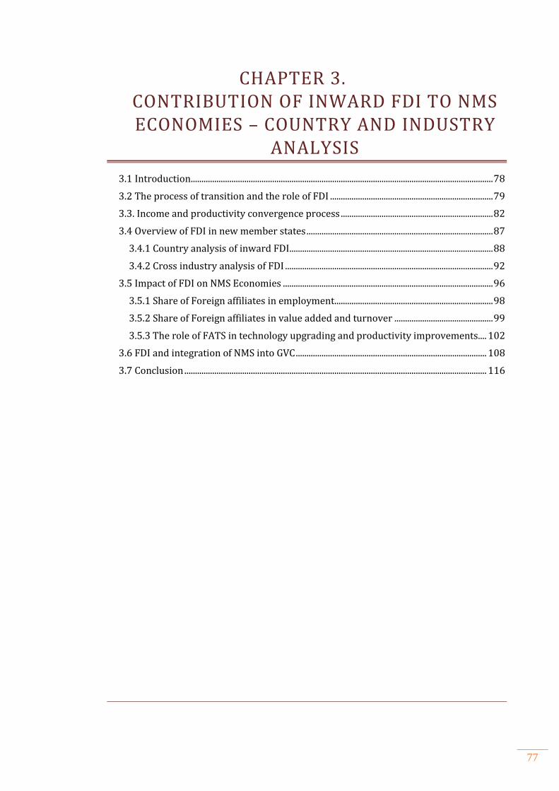
77
CHAPTER 3. CONTRIBUTION OF INWARD FDI TO NMS ECONOMIES – COUNTRY AND INDUSTRY
ANALYSIS
3.1 Introduction ............................................................................................................................................. 78
3.2 The process of transition and the role of FDI ............................................................................ 79
3.3. Income and productivity convergence process ....................................................................... 82
3.4 Overview of FDI in new member states ....................................................................................... 87
3.4.1 Country analysis of inward FDI ............................................................................................... 88
3.4.2 Cross industry analysis of FDI ................................................................................................. 92
3.5 Impact of FDI on NMS Economies .................................................................................................. 96
3.5.1 Share of Foreign affiliates in employment.......................................................................... 98
3.5.2 Share of Foreign affiliates in value added and turnover .............................................. 99
3.5.3 The role of FATS in technology upgrading and productivity improvements.... 102
3.6 FDI and integration of NMS into GVC ......................................................................................... 108
3.7 Conclusion ............................................................................................................................................. 116
78
3.1 INTRODUCTION
The breakup of the central planning system was in major part the consequence of its
lower productivity levels and technological obsolescence. Since productivity growth is
regarded as probably the most important single indicator of a country’s economic
progress, it is only through increases in productivity that domestic firms may increase
competitiveness on both domestic and international markets. Integration of formerly
centrally planned economies of Central and Eastern Europe (CEE) into global financial
and trade flows provides an interesting case for the analysis of the multiple impact of
FDI. Hence, by taking a closer look into the nature of FDI, this chapter seeks to provide
explanations for the contribution of FDI to structural changes experienced by these
economies, their international competitiveness and their integration into global
production networks.
Although this chapter aims to provide a context for the empirical analysis in the rest of
the thesis, the analysis of the transition process and its impact on economic development
is kept to a minimum as there is already a substantial amount of work undertaken on this
topic. Instead, the focus is on the key dimensions of the transition process and the role
played by FDI in alleviating some of the structural problems inherited from the previous
system. Special emphasis is paid to the process of income and productivity convergence
before moving to the analysis of FDI trends in these countries and its contribution at both
country and industry levels.
This chapter is structured as follows. Section 3.2 provides a brief overview of the
structural problems Central and East European countries (CEECs) inherited from the
previous economic system with special emphasis on their stance towards FDI and its
role. Section 3.3 is devoted to the analysis of income and productivity convergence at
national and industry level. The main features, extent and nature of FDI in CEECs are
presented in Section 3.4. Section 3.5 analyses the contribution of foreign firms to total
employment, turnover and value added and investigates the direct role of FDI in
technology upgrading and productivity convergence. Section 3.6 analyses the effects of
FDI on exports and their ability to integrate into the MNCs’ production networks.
Finally, Section 3.7 concludes.
79
3.2 THE PROCESS OF TRANSITION AND THE ROLE OF FDI
At the beginning of the transition process the CEECs were left with deep structural
distortions inherited from the socialist system, reflected in a hierarchically organized
system of ownership of production factors and products (Podkaimer, 2013). The
economy of CEECs was mainly focused on agriculture and heavy industry, while the
production of consumption goods and services were mainly neglected (Campos and
Coricelli, 2002). In addition, the allocation of resources was not led by market signals
but by centralized decisions based on annual or five year plans. The main tool for growth
strategy was the artificially low prices of strategically important inputs for basic
industries maintained through a combination of subsidies and taxes (Kornai, 1992).
Furthermore, exchange rates were fixed at low (or below the equilibrium level) so as to
facilitate the import of strategically important goods such as raw material and
intermediate goods, and the export of goods for final use abroad, mostly to countries
within the Eastern bloc (Lavigne, 1999). The fixed exchange rate was supplemented by
extensive restrictions on exports and imports beyond that arranged by the state. These
structural distortions caused shortages, misallocation of resources, low incentives,
overgrown industrial sector and underdeveloped service sector. After the beginning of
transition and the opening of the economy, countries were faced with severe
macroeconomic imbalances such as hyperinflation, high budget deficits, high current
account deficits, and debt problems (Kalotay, 2001).
In the early transition period foreign firms contributed to the elimination of shortages by
supplying the goods and services long demanded by the population, which also resulted
in an increase in trade deficits. In addition, the entry of foreign firms contributed to the
amelioration of price distortions.
Apart from structural problems, domestic enterprises were faced with obsoleted capital
and inefficient technology which prevented their successful restructuring (Filer et al.,
2001; Orts et al., 2008). The absence of private ownership acted as a disincentive for
innovation and product development. Rewards for managers were tied closely to plan
fulfilment. In addition, enterprises had to perform many non-core activities. For all these
reasons, the consumption of energy and inputs was several times higher than in market
80
based economies (Gros and Steinherr, 1995). Another source of enterprise inefficiency
in centrally planned economies was the existence of soft budget constraints (Kornai,
1986). Liquidity and insolvency problems were solved through administrative
refinancing by the so-called ‘monobanks’ which controlled central capital allocation
(Estrin, 2002). Such soft budgetary constraints acted as obstacles to the restructuring of
loss making enterprises as they were not subject to the threat of bankruptcy.
Under these circumstances, the inflow of foreign capital was needed and beneficial as it
provided the necessary funds to finance new investment in fixed assets given limited
domestic savings (Demekas et al., 2005; Sohinger, 2005). Besides source of new capital,
FDI was recognized as a source of technological progress (Campos and Kinoshita, 2002;
Uzagalieva and Kocenda, 2010). The entry of foreign firms also contributed to the
introduction of new products and management, organizational and marketing practices
which facilitated enterprise restructuring (Rojec et al., 1995; Weiszburg, 1997; Kalotay
and Hunya, 2000; Kalotay, 2001).
Since enterprises in transition economies, apart from those in former Yugoslavia,
Hungary and Poland, did not have any experience of private business, their integration
into world markets and conducting of private business was challenging (Mihalyi, 2000;
Kalotay, 2001). In these circumstances, privatisation policies were seen as an important
element in transition process. The basic aim of privatisation process was to eliminate the
inherent inefficiencies of state ownership and planning (Mihaly, 2001). With the
exception of Hungary and in major part Estonia, other countries relied on different forms
of privatisation (mass privatisation, voucher privatisation, management buy outs) and
little space was left to foreigners (Kalotay and Hunya, 2000). The reasons for the small
role of FDI in early privatisation period were non-economic reasons which emphasized
the creation of a domestic capitalist class, fairness, special treatment of residents and
political forces opposing and blocking sales of domestic firms to foreigners (Kalotay and
Hunya, 2000; Rojec, 2005). It is only in the second phase of the privatisation process,
after 1996, that foreign companies were put on equal terms with domestic investors. In
that period, efficiency remained the main motive for privatisation, but corporate
governance and firms’ restructuring replaced social considerations. With the shift in the
concept of privatisation and policies from nation-wide distribution/discount schemes to
case by case direct sales of companies, the use of foreign privatisation in CEECs
increased (Kalotay and Hunya, 2000).
81
The main benefits of privatisation by foreign firms were product quality upgrading, the
introduction of new products, transfer of technology, improved market access to foreign
markets, training of the management and workforce and improved productivity (Estrin,
1997; Hunya, 2000; Kalotay and Hunya, 2000; Kalotay, 2001; Rojec, 2005).
Furthermore, large vertical networks were broken up and sold, while core competencies
were developed to match the higher quality standards (Szanyi, 2001). Defensive
restructuring of privatised companies which was characterised by labour shedding lasted
shorter than in purely domestic companies and strategic restructuring that followed
resulted in increased employment and investment. An important feature of FDI was its
involvement in the privatisation of services sector especially network industries and
financial sector which resulted in increased quality of service and reduction in operating
costs which facilitated the development of private sector (Kalotay, 2001).
The above mentioned improvements enabled some privatized companies to experience a
new role as they became part of an international network which equipped them to meet
quality requirements better (Kurtz and Wittke, 1998). This is especially true for
companies in automotive and electronic industry that have grown in size and and operate
as specialised sub-assemblers in the MNC’s network. The success of restructuring was
also conditional on the type of FDI. Efficiency seeking FDI was characterised by the
introduction of new production programmes, reorganised marketing activities, training
and reorganisation of management, and financially consolidated acquired companies
(Rojec, 2005). On the other hand, market seeking investors did not contribute to
restructuring to the same extent. They were more interested in using local marketing
networks and maintaining a large number of products that were well established in
regional markets (Szanyi, 2001).
To summarize, considering the arguments described in Chapter 1 on the potential
benefits of FDI and the evidence on the role of FDI in early transition period discussed
above we can say that FDI has contributed to a reduction of structural and
macroeconomic distortions and helped in speeding up the transformation of economy
and enterprise restructuring. The next section aims to shed more light on the speed and
nature of catching up process given the substantial economic growth witnessed by
CEECs that joined the EU from mid-1990s to 2008. Special emphasis is put on
productivity convergence over the period.
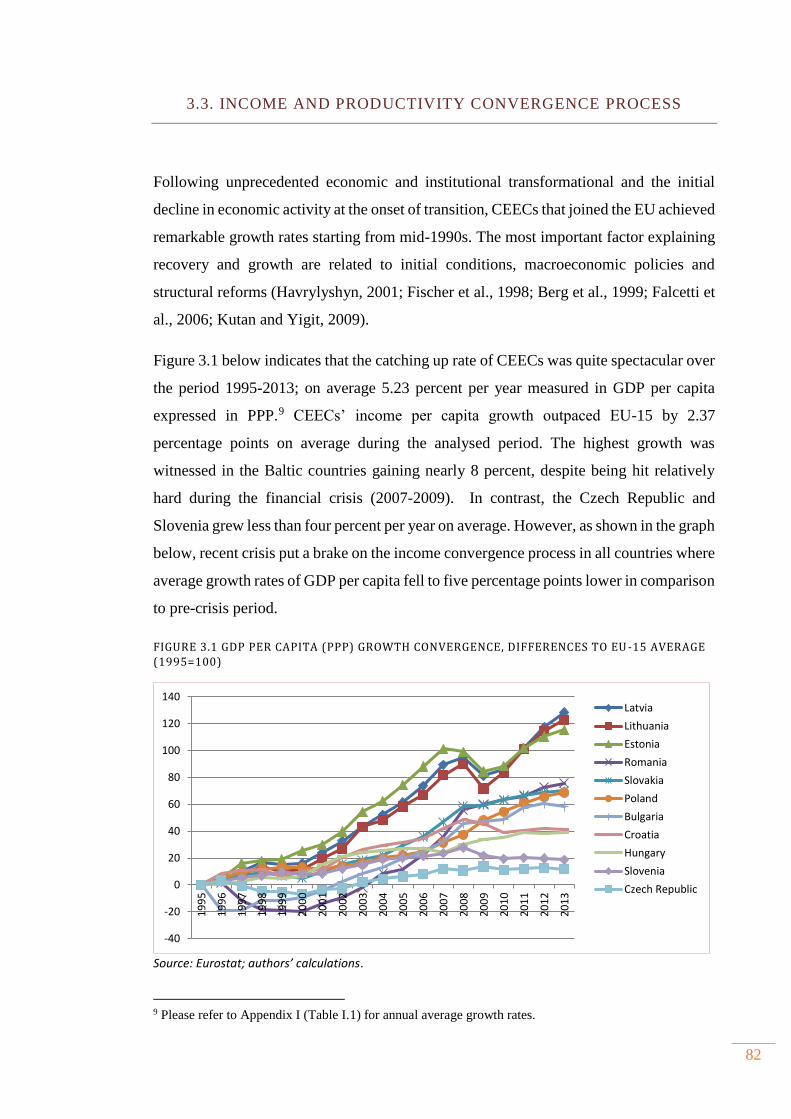
82
3.3. INCOME AND PRODUCTIVITY CONVERGENCE PROCESS
Following unprecedented economic and institutional transformational and the initial
decline in economic activity at the onset of transition, CEECs that joined the EU achieved
remarkable growth rates starting from mid-1990s. The most important factor explaining
recovery and growth are related to initial conditions, macroeconomic policies and
structural reforms (Havrylyshyn, 2001; Fischer et al., 1998; Berg et al., 1999; Falcetti et
al., 2006; Kutan and Yigit, 2009).
Figure 3.1 below indicates that the catching up rate of CEECs was quite spectacular over
the period 1995-2013; on average 5.23 percent per year measured in GDP per capita
expressed in PPP.8F
9 CEECs’ income per capita growth outpaced EU-15 by 2.37
percentage points on average during the analysed period. The highest growth was
witnessed in the Baltic countries gaining nearly 8 percent, despite being hit relatively
hard during the financial crisis (2007-2009). In contrast, the Czech Republic and
Slovenia grew less than four percent per year on average. However, as shown in the graph
below, recent crisis put a brake on the income convergence process in all countries where
average growth rates of GDP per capita fell to five percentage points lower in comparison
to pre-crisis period.
FIGURE 3.1 GDP PER CAPITA (PPP) GROWTH CONVERGENCE, DIFFERENCES TO EU -15 AVERAGE (1995=100)
Source: Eurostat; authors’ calculations.
9 Please refer to Appendix I (Table I.1) for annual average growth rates.
-40
-20
0
20
40
60
80
100
120
140
19
95
19
96
19
97
19
98
19
99
20
00
20
01
20
02
20
03
20
04
20
05
20
06
20
07
20
08
20
09
20
10
20
11
20
12
20
13
Latvia
Lithuania
Estonia
Romania
Slovakia
Poland
Bulgaria
Croatia
Hungary
Slovenia
Czech Republic
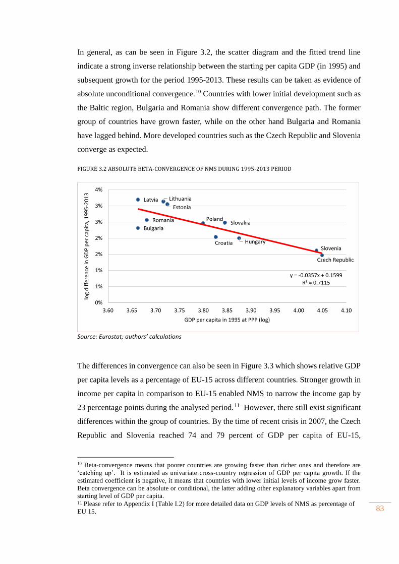
83
In general, as can be seen in Figure 3.2, the scatter diagram and the fitted trend line
indicate a strong inverse relationship between the starting per capita GDP (in 1995) and
subsequent growth for the period 1995-2013. These results can be taken as evidence of
absolute unconditional convergence.9F
10 Countries with lower initial development such as
the Baltic region, Bulgaria and Romania show different convergence path. The former
group of countries have grown faster, while on the other hand Bulgaria and Romania
have lagged behind. More developed countries such as the Czech Republic and Slovenia
converge as expected.
FIGURE 3.2 ABSOLUTE BETA-CONVERGENCE OF NMS DURING 1995-2013 PERIOD
Source: Eurostat; authors’ calculations
The differences in convergence can also be seen in Figure 3.3 which shows relative GDP
per capita levels as a percentage of EU-15 across different countries. Stronger growth in
income per capita in comparison to EU-15 enabled NMS to narrow the income gap by
23 percentage points during the analysed period. 10F
11 However, there still exist significant
differences within the group of countries. By the time of recent crisis in 2007, the Czech
Republic and Slovenia reached 74 and 79 percent of GDP per capita of EU-15,
10 Beta-convergence means that poorer countries are growing faster than richer ones and therefore are
‘catching up’. It is estimated as univariate cross-country regression of GDP per capita growth. If the
estimated coefficient is negative, it means that countries with lower initial levels of income grow faster.
Beta convergence can be absolute or conditional, the latter adding other explanatory variables apart from
starting level of GDP per capita. 11 Please refer to Appendix I (Table I.2) for more detailed data on GDP levels of NMS as percentage of
EU 15.
Bulgaria
Czech Republic
Estonia
Croatia
Latvia Lithuania
Hungary
PolandRomania
Slovenia
Slovakia
y = -0.0357x + 0.1599R² = 0.7115
0%
1%
1%
2%
2%
3%
3%
4%
3.60 3.65 3.70 3.75 3.80 3.85 3.90 3.95 4.00 4.05 4.10
log
dif
fere
nce
in G
DP
per
cap
ita,
19
95
-20
13
GDP per capita in 1995 at PPP (log)
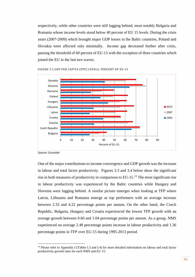
84
respectively, while other countries were still lagging behind, most notably Bulgaria and
Romania whose income levels stood below 40 percent of EU 15 levels. During the crisis
years (2007-2009) which brought major GDP losses in the Baltic countries, Poland and
Slovakia were affected only minimally. Income gap decreased further after crisis,
passing the threshold of 60 percent of EU-15 with the exception of three countries which
joined the EU in the last two waves.
FIGURE 3.3 GDP PER CAPITA (PPP) LEVELS, PERCENT OF EU-15
Source: Eurostat
One of the major contributions to income convergence and GDP growth was the increase
in labour and total factor productivity. Figures 3.3 and 3.4 below show the significant
rise in both measures of productivity in comparison to EU-15.11F
12 The most significant rise
in labour productivity was experienced by the Baltic countries while Hungary and
Slovenia were lagging behind. A similar picture emerges when looking at TFP where
Latvia, Lithuania and Romania emerge as top performers with an average increase
between 2.33 and 4.22 percentage points per annum. On the other hand, the Czech
Republic, Bulgaria, Hungary and Croatia experienced the lowest TFP growth with an
average growth between 0.60 and 1.04 percentage points per annum. As a group, NMS
experienced on average 2.48 percentage points increase in labour productivity and 1.36
percentage points in TFP over EU-15 during 1995-2013 period.
12 Please refer to Appendix I (Tables I.3 and I.4) for more detailed information on labour and total factor
productivity growth rates for each NMS and EU 15.
0 10 20 30 40 50 60 70 80 90
Bulgaria
Czech Republic
Estonia
Croatia
Latvia
Lithuania
Hungary
Poland
Romania
Slovenia
Slovakia
Percent of EU-15
2013
2007
1995
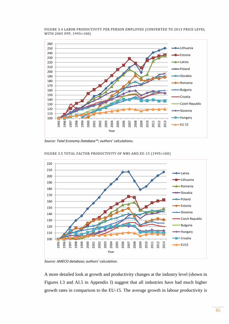
85
FIGURE 3.4 LABOR PRODUCTIVITY PER PERSON EMPLOYED (CONVERTED TO 2013 PRICE LEVEL WITH 2005 PPP, 1995=100)
Source: Total Economy Database™; authors’ calculations.
FIGURE 3.5 TOTAL FACTOR PRODUCTIVITY OF NMS AND EU-15 (1995=100)
Source: AMECO database; authors’ calculation.
A more detailed look at growth and productivity changes at the industry level (shown in
Figures I.3 and AI.5 in Appendix I) suggest that all industries have had much higher
growth rates in comparison to the EU-15. The average growth in labour productivity is
100
110
120
130
140
150
160
170
180
190
200
210
220
19
95
19
96
19
97
19
98
19
99
20
00
20
01
20
02
20
03
20
04
20
05
20
06
20
07
20
08
20
09
20
10
20
11
20
12
20
13
Year
Latvia
Lithuania
Romania
Slovakia
Poland
Estonia
Slovenia
Czech Republic
Bulgaria
Hungary
Croatia
EU15
100
110
120
130
140
150
160
170
180
190
200
210
220
230
240
250
260
19
95
19
96
19
97
19
98
19
99
20
00
20
01
20
02
20
03
20
04
20
05
20
06
20
07
20
08
20
09
20
10
20
11
20
12
20
13
Year
Lithuania
Estonia
Latvia
Poland
Slovakia
Romania
Bulgaria
Croatia
Czech Republic
Slovenia
Hungary
EU 15
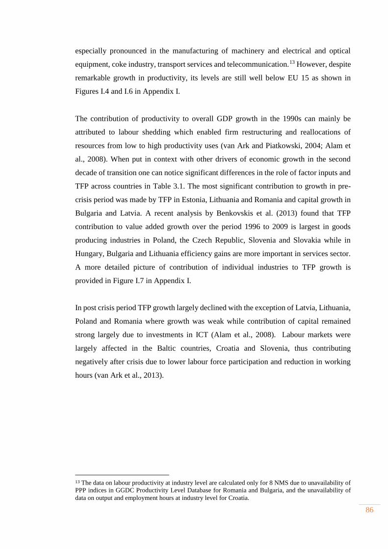
86
especially pronounced in the manufacturing of machinery and electrical and optical
equipment, coke industry, transport services and telecommunication. 12F
13 However, despite
remarkable growth in productivity, its levels are still well below EU 15 as shown in
Figures I.4 and I.6 in Appendix I.
The contribution of productivity to overall GDP growth in the 1990s can mainly be
attributed to labour shedding which enabled firm restructuring and reallocations of
resources from low to high productivity uses (van Ark and Piatkowski, 2004; Alam et
al., 2008). When put in context with other drivers of economic growth in the second
decade of transition one can notice significant differences in the role of factor inputs and
TFP across countries in Table 3.1. The most significant contribution to growth in pre-
crisis period was made by TFP in Estonia, Lithuania and Romania and capital growth in
Bulgaria and Latvia. A recent analysis by Benkovskis et al. (2013) found that TFP
contribution to value added growth over the period 1996 to 2009 is largest in goods
producing industries in Poland, the Czech Republic, Slovenia and Slovakia while in
Hungary, Bulgaria and Lithuania efficiency gains are more important in services sector.
A more detailed picture of contribution of individual industries to TFP growth is
provided in Figure I.7 in Appendix I.
In post crisis period TFP growth largely declined with the exception of Latvia, Lithuania,
Poland and Romania where growth was weak while contribution of capital remained
strong largely due to investments in ICT (Alam et al., 2008). Labour markets were
largely affected in the Baltic countries, Croatia and Slovenia, thus contributing
negatively after crisis due to lower labour force participation and reduction in working
hours (van Ark et al., 2013).
13 The data on labour productivity at industry level are calculated only for 8 NMS due to unavailability of
PPP indices in GGDC Productivity Level Database for Romania and Bulgaria, and the unavailability of
data on output and employment hours at industry level for Croatia.
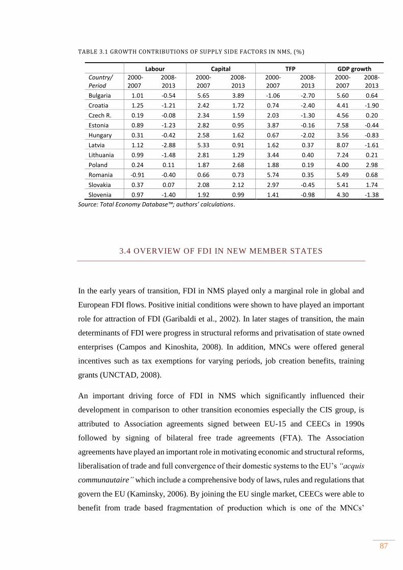
87
TABLE 3.1 GROWTH CONTRIBUTIONS OF SUPPLY SIDE FACTORS IN NMS, (%)
Labour Capital TFP GDP growth Country/ Period
2000-2007
2008-2013
2000-2007
2008-2013
2000-2007
2008-2013
2000-2007
2008-2013
Bulgaria 1.01 -0.54 5.65 3.89 -1.06 -2.70 5.60 0.64
Croatia 1.25 -1.21 2.42 1.72 0.74 -2.40 4.41 -1.90
Czech R. 0.19 -0.08 2.34 1.59 2.03 -1.30 4.56 0.20
Estonia 0.89 -1.23 2.82 0.95 3.87 -0.16 7.58 -0.44
Hungary 0.31 -0.42 2.58 1.62 0.67 -2.02 3.56 -0.83
Latvia 1.12 -2.88 5.33 0.91 1.62 0.37 8.07 -1.61
Lithuania 0.99 -1.48 2.81 1.29 3.44 0.40 7.24 0.21
Poland 0.24 0.11 1.87 2.68 1.88 0.19 4.00 2.98
Romania -0.91 -0.40 0.66 0.73 5.74 0.35 5.49 0.68
Slovakia 0.37 0.07 2.08 2.12 2.97 -0.45 5.41 1.74
Slovenia 0.97 -1.40 1.92 0.99 1.41 -0.98 4.30 -1.38
Source: Total Economy Database™; authors’ calculations.
3.4 OVERVIEW OF FDI IN NEW MEMBER STATES
In the early years of transition, FDI in NMS played only a marginal role in global and
European FDI flows. Positive initial conditions were shown to have played an important
role for attraction of FDI (Garibaldi et al., 2002). In later stages of transition, the main
determinants of FDI were progress in structural reforms and privatisation of state owned
enterprises (Campos and Kinoshita, 2008). In addition, MNCs were offered general
incentives such as tax exemptions for varying periods, job creation benefits, training
grants (UNCTAD, 2008).
An important driving force of FDI in NMS which significantly influenced their
development in comparison to other transition economies especially the CIS group, is
attributed to Association agreements signed between EU-15 and CEECs in 1990s
followed by signing of bilateral free trade agreements (FTA). The Association
agreements have played an important role in motivating economic and structural reforms,
liberalisation of trade and full convergence of their domestic systems to the EU’s “acquis
communautaire” which include a comprehensive body of laws, rules and regulations that
govern the EU (Kaminsky, 2006). By joining the EU single market, CEECs were able to
benefit from trade based fragmentation of production which is one of the MNCs’
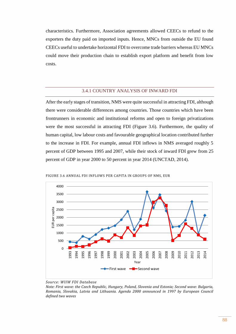
88
characteristics. Furthermore, Association agreements allowed CEECs to refund to the
exporters the duty paid on imported inputs. Hence, MNCs from outside the EU found
CEECs useful to undertake horizontal FDI to overcome trade barriers whereas EU MNCs
could move their production chain to establish export platform and benefit from low
costs.
3.4.1 COUNTRY ANALYSIS OF INWARD FDI
After the early stages of transition, NMS were quite successful in attracting FDI, although
there were considerable differences among countries. Those countries which have been
frontrunners in economic and institutional reforms and open to foreign privatizations
were the most successful in attracting FDI (Figure 3.6). Furthermore, the quality of
human capital, low labour costs and favourable geographical location contributed further
to the increase in FDI. For example, annual FDI inflows in NMS averaged roughly 5
percent of GDP between 1995 and 2007, while their stock of inward FDI grew from 25
percent of GDP in year 2000 to 50 percent in year 2014 (UNCTAD, 2014).
FIGURE 3.6 ANNUAL FDI INFLOWS PER CAPITA IN GROUPS OF NMS, EUR
Source: WIIW FDI Database Note: First wave: the Czech Republic, Hungary, Poland, Slovenia and Estonia; Second wave: Bulgaria, Romania, Slovakia, Latvia and Lithuania. Agenda 2000 announced in 1997 by European Council defined two waves
0
500
1000
1500
2000
2500
3000
3500
4000
19
93
19
94
19
95
19
96
19
97
19
98
19
99
20
00
20
01
20
02
20
03
20
04
20
05
20
06
20
07
20
08
20
09
20
10
20
11
20
12
20
13
20
14
EUR
per
cap
ita
Year
First wave Second wave
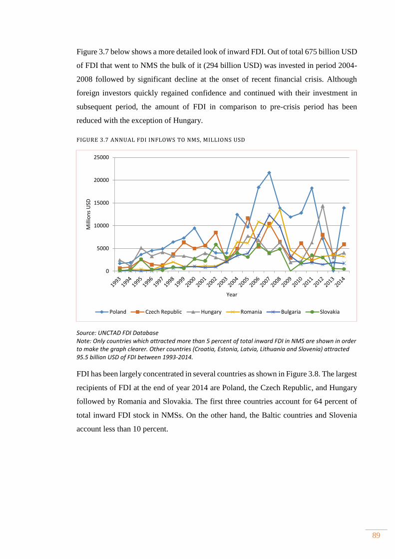
89
Figure 3.7 below shows a more detailed look of inward FDI. Out of total 675 billion USD
of FDI that went to NMS the bulk of it (294 billion USD) was invested in period 2004-
2008 followed by significant decline at the onset of recent financial crisis. Although
foreign investors quickly regained confidence and continued with their investment in
subsequent period, the amount of FDI in comparison to pre-crisis period has been
reduced with the exception of Hungary.
FIGURE 3.7 ANNUAL FDI INFLOWS TO NMS, MILLIONS USD
Source: UNCTAD FDI Database
Note: Only countries which attracted more than 5 percent of total inward FDI in NMS are shown in order to make the graph clearer. Other countries (Croatia, Estonia, Latvia, Lithuania and Slovenia) attracted 95.5 billion USD of FDI between 1993-2014.
FDI has been largely concentrated in several countries as shown in Figure 3.8. The largest
recipients of FDI at the end of year 2014 are Poland, the Czech Republic, and Hungary
followed by Romania and Slovakia. The first three countries account for 64 percent of
total inward FDI stock in NMSs. On the other hand, the Baltic countries and Slovenia
account less than 10 percent.
0
5000
10000
15000
20000
25000
Mill
ion
s U
SD
Year
Poland Czech Republic Hungary Romania Bulgaria Slovakia
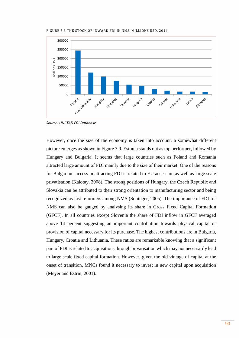
90
FIGURE 3.8 THE STOCK OF INWARD FDI IN NMS, MILLIONS USD, 2014
Source: UNCTAD FDI Database
However, once the size of the economy is taken into account, a somewhat different
picture emerges as shown in Figure 3.9. Estonia stands out as top performer, followed by
Hungary and Bulgaria. It seems that large countries such as Poland and Romania
attracted large amount of FDI mainly due to the size of their market. One of the reasons
for Bulgarian success in attracting FDI is related to EU accession as well as large scale
privatisation (Kalotay, 2008). The strong positions of Hungary, the Czech Republic and
Slovakia can be attributed to their strong orientation to manufacturing sector and being
recognized as fast reformers among NMS (Sohinger, 2005). The importance of FDI for
NMS can also be gauged by analysing its share in Gross Fixed Capital Formation
(GFCF). In all countries except Slovenia the share of FDI inflow in GFCF averaged
above 14 percent suggesting an important contribution towards physical capital or
provision of capital necessary for its purchase. The highest contributions are in Bulgaria,
Hungary, Croatia and Lithuania. These ratios are remarkable knowing that a significant
part of FDI is related to acquisitions through privatisation which may not necessarily lead
to large scale fixed capital formation. However, given the old vintage of capital at the
onset of transition, MNCs found it necessary to invest in new capital upon acquisition
(Meyer and Estrin, 2001).
0
50000
100000
150000
200000
250000
300000
Mill
ion
s U
SD
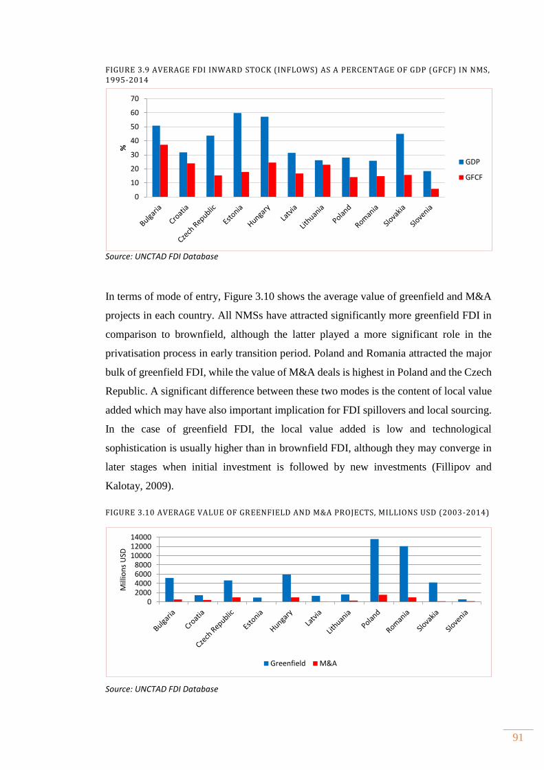
91
FIGURE 3.9 AVERAGE FDI INWARD STOCK (INFLOWS) AS A PERCENTAGE OF GDP (GFCF) IN NMS, 1995-2014
Source: UNCTAD FDI Database
In terms of mode of entry, Figure 3.10 shows the average value of greenfield and M&A
projects in each country. All NMSs have attracted significantly more greenfield FDI in
comparison to brownfield, although the latter played a more significant role in the
privatisation process in early transition period. Poland and Romania attracted the major
bulk of greenfield FDI, while the value of M&A deals is highest in Poland and the Czech
Republic. A significant difference between these two modes is the content of local value
added which may have also important implication for FDI spillovers and local sourcing.
In the case of greenfield FDI, the local value added is low and technological
sophistication is usually higher than in brownfield FDI, although they may converge in
later stages when initial investment is followed by new investments (Fillipov and
Kalotay, 2009).
FIGURE 3.10 AVERAGE VALUE OF GREENFIELD AND M&A PROJECTS, MILLIONS USD (2003-2014)
Source: UNCTAD FDI Database
02000400060008000
100001200014000
Mill
ion
s U
SD
Greenfield M&A
0
10
20
30
40
50
60
70
%
GDP
GFCF
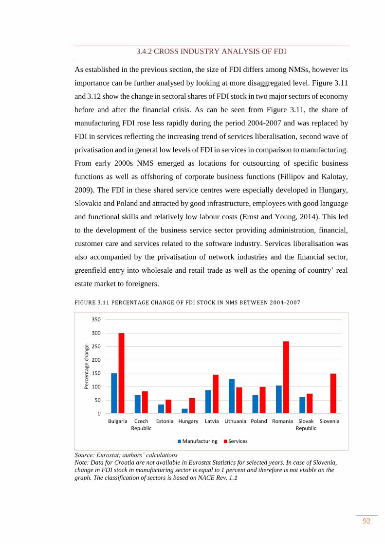
92
3.4.2 CROSS INDUSTRY ANALYSIS OF FDI
As established in the previous section, the size of FDI differs among NMSs, however its
importance can be further analysed by looking at more disaggregated level. Figure 3.11
and 3.12 show the change in sectoral shares of FDI stock in two major sectors of economy
before and after the financial crisis. As can be seen from Figure 3.11, the share of
manufacturing FDI rose less rapidly during the period 2004-2007 and was replaced by
FDI in services reflecting the increasing trend of services liberalisation, second wave of
privatisation and in general low levels of FDI in services in comparison to manufacturing.
From early 2000s NMS emerged as locations for outsourcing of specific business
functions as well as offshoring of corporate business functions (Fillipov and Kalotay,
2009). The FDI in these shared service centres were especially developed in Hungary,
Slovakia and Poland and attracted by good infrastructure, employees with good language
and functional skills and relatively low labour costs (Ernst and Young, 2014). This led
to the development of the business service sector providing administration, financial,
customer care and services related to the software industry. Services liberalisation was
also accompanied by the privatisation of network industries and the financial sector,
greenfield entry into wholesale and retail trade as well as the opening of country’ real
estate market to foreigners.
FIGURE 3.11 PERCENTAGE CHANGE OF FDI STOCK IN NMS BETWEEN 2004-2007
Source: Eurostat; authors’ calculations
Note: Data for Croatia are not available in Eurostat Statistics for selected years. In case of Slovenia,
change in FDI stock in manufacturing sector is equal to 1 percent and therefore is not visible on the
graph. The classification of sectors is based on NACE Rev. 1.1
0
50
100
150
200
250
300
350
Bulgaria CzechRepublic
Estonia Hungary Latvia Lithuania Poland Romania SlovakRepublic
Slovenia
Per
cen
tage
ch
ange
Manufacturing Services
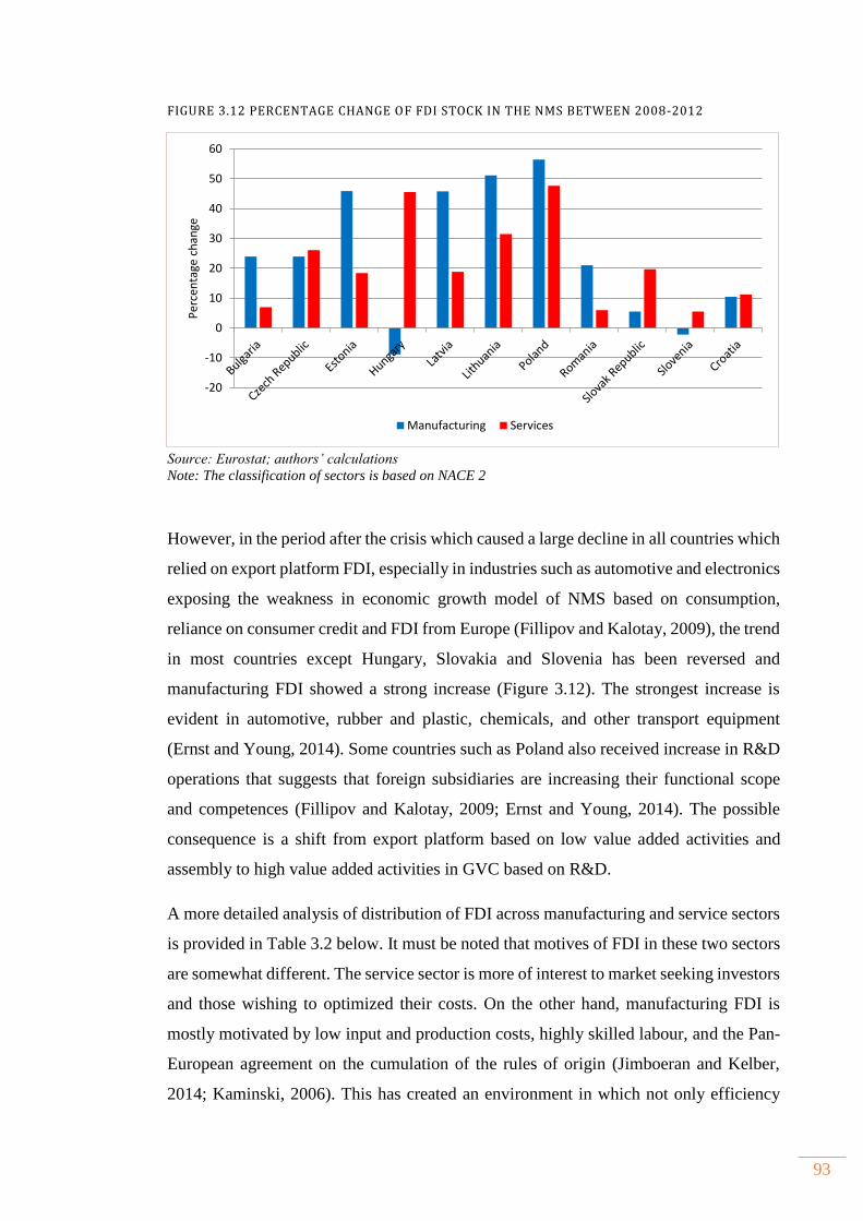
93
FIGURE 3.12 PERCENTAGE CHANGE OF FDI STOCK IN THE NMS BETWEEN 2008-2012
Source: Eurostat; authors’ calculations Note: The classification of sectors is based on NACE 2
However, in the period after the crisis which caused a large decline in all countries which
relied on export platform FDI, especially in industries such as automotive and electronics
exposing the weakness in economic growth model of NMS based on consumption,
reliance on consumer credit and FDI from Europe (Fillipov and Kalotay, 2009), the trend
in most countries except Hungary, Slovakia and Slovenia has been reversed and
manufacturing FDI showed a strong increase (Figure 3.12). The strongest increase is
evident in automotive, rubber and plastic, chemicals, and other transport equipment
(Ernst and Young, 2014). Some countries such as Poland also received increase in R&D
operations that suggests that foreign subsidiaries are increasing their functional scope
and competences (Fillipov and Kalotay, 2009; Ernst and Young, 2014). The possible
consequence is a shift from export platform based on low value added activities and
assembly to high value added activities in GVC based on R&D.
A more detailed analysis of distribution of FDI across manufacturing and service sectors
is provided in Table 3.2 below. It must be noted that motives of FDI in these two sectors
are somewhat different. The service sector is more of interest to market seeking investors
and those wishing to optimized their costs. On the other hand, manufacturing FDI is
mostly motivated by low input and production costs, highly skilled labour, and the Pan-
European agreement on the cumulation of the rules of origin (Jimboeran and Kelber,
2014; Kaminski, 2006). This has created an environment in which not only efficiency
-20
-10
0
10
20
30
40
50
60
Per
cen
tage
ch
ange
Manufacturing Services
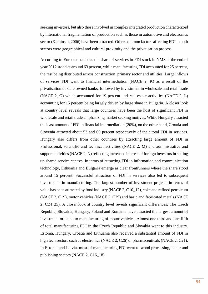
94
seeking investors, but also those involved in complex integrated production characterized
by international fragmentation of production such as those in automotive and electronics
sector (Kaminski, 2006) have been attracted. Other common factors affecting FDI in both
sectors were geographical and cultural proximity and the privatisation process.
According to Eurostat statistics the share of services in FDI stock in NMS at the end of
year 2012 stood at around 63 percent, while manufacturing FDI accounted for 25 percent,
the rest being distributed across construction, primary sector and utilities. Large inflows
of services FDI went to financial intermediation (NACE 2, K) as a result of the
privatisation of state owned banks, followed by investment in wholesale and retail trade
(NACE 2, G) which accounted for 19 percent and real estate activities (NACE 2, L)
accounting for 15 percent being largely driven by large share in Bulgaria. A closer look
at country level reveals that large countries have been the host of significant FDI in
wholesale and retail trade emphasizing market seeking motives. While Hungary attracted
the least amount of FDI in financial intermediation (20%), on the other hand, Croatia and
Slovenia attracted about 53 and 60 percent respectively of their total FDI in services.
Hungary also differs from other countries by attracting large amount of FDI in
Professional, scientific and technical activities (NACE 2, M) and administrative and
support activities (NACE 2, N) reflecting increased interest of foreign investors in setting
up shared service centres. In terms of attracting FDI in information and communication
technology, Lithuania and Bulgaria emerge as clear frontrunners where the share stood
around 15 percent. Successful attraction of FDI in services also led to subsequent
investments in manufacturing. The largest number of investment projects in terms of
value has been attracted by food industry (NACE 2, C10_12), coke and refined petroleum
(NACE 2, C19), motor vehicles (NACE 2, C29) and basic and fabricated metals (NACE
2, C24_25). A closer look at country level reveals significant differences. The Czech
Republic, Slovakia, Hungary, Poland and Romania have attracted the largest amount of
investment oriented to manufacturing of motor vehicles. Almost one third and one fifth
of total manufacturing FDI in the Czech Republic and Slovakia went to this industry.
Estonia, Hungary, Croatia and Lithuania also received a substantial amount of FDI in
high tech sectors such as electronics (NACE 2, C26) or pharmaceuticals (NACE 2, C21).
In Estonia and Latvia, most of manufacturing FDI went to wood processing, paper and
publishing sectors (NACE 2, C16_18).
95
TABLE 3.2 SHARE OF INWARD FDI STOCK ACROSS INDUSTRIES AND COUNTRIES, 2012
COUNTRY CODE BG HR CZ EE HU LV LT PL RO SK SI
INDUSTRY % SHARE OF MANUFACTURING
Manufacture of food products; beverages and tobacco products
14 8 10 15 12 16 10 19 12 6 4
Manufacture of textiles and wearing apparel
4 3 1 5 1 3 4 1 4 1 2
Manufacture of wood, paper, printing and reproduction
3 2 4 20 5 26 6 8 7 4 11
Manufacture of coke and refined petroleum products
22 40 1 0 0 0 33 0 7 10 0
Manufacture of chemicals and chemical products
8 2 4 13 4 2 16 7 5 4 7
Manufacture of basic pharmaceutical products and pharmaceutical preparations
0 16 2 2 13 1 12 3 2 0 25
Manufacture of rubber and plastic products
2 1 7 2 7 1 3 9 7 7 10
Manufacture of basic metals and fabricated metal products, except machinery and equipment
18 3 11 7 8 4 1 13 16 18 5
Manufacture of computer, electronic and optical products
1 2 3 10 14 0 0 3 2 7 3
Manufacture of machinery and equipment n.e.c.
6 2 8 2 3 1 1 4 6 9 6
Manufacture of motor vehicles, trailers and semi-trailers
2 1 30 5 15 4 1 14 15 22 8
Manufacture of other transport equipment
0 0 1 0 1 1 1 3 2 0 0
Other manufacturing 19 19 17 20 17 40 10 18 16 13 17
Total manufacturing 100 100 100 100 100 100 100 100 100 100 100
INDUSTRY % SHARE OF SERVICES Wholesale and retail trade; repair of motor vehicles and motorcycles
16 14 20 17 16 21 19 24 24 21 22
Transportation and storage 1 1 5 8 3 7 3 2 3 0 1
Accommodation and food service activities
4 4 1 1 1 1 1 1 1 1 0
Information and communication 15 11 9 4 8 5 15 7 10 8 3
Financial and insurance activities
27 53 40 33 20 43 31 42 39 47 60
Real estate activities 26 7 15 22 9 19 20 12 11 13 9
Professional, scientific and technical activities
6 8 8 12 37 2 9 10 7 7 3
Administrative and support service activities
3 1 1 4 7 1 2 2 3 3 1
Arts, entertainment and recreation
0 2 0 0 0 1 0 0 0 0 0
Other service activities 1 0 0 0 0 0 0 0 1 0 0
Total services 100 100 100 100 100 100 100 100 100 100 100
Source: Eurostat; authors’ calculations
Note: Industry classification is based on NACE 2
One of the major factors affecting the success of automotive and electronics industry in
attracting FDI was the revolution in ICT which reduced coordination and transportation
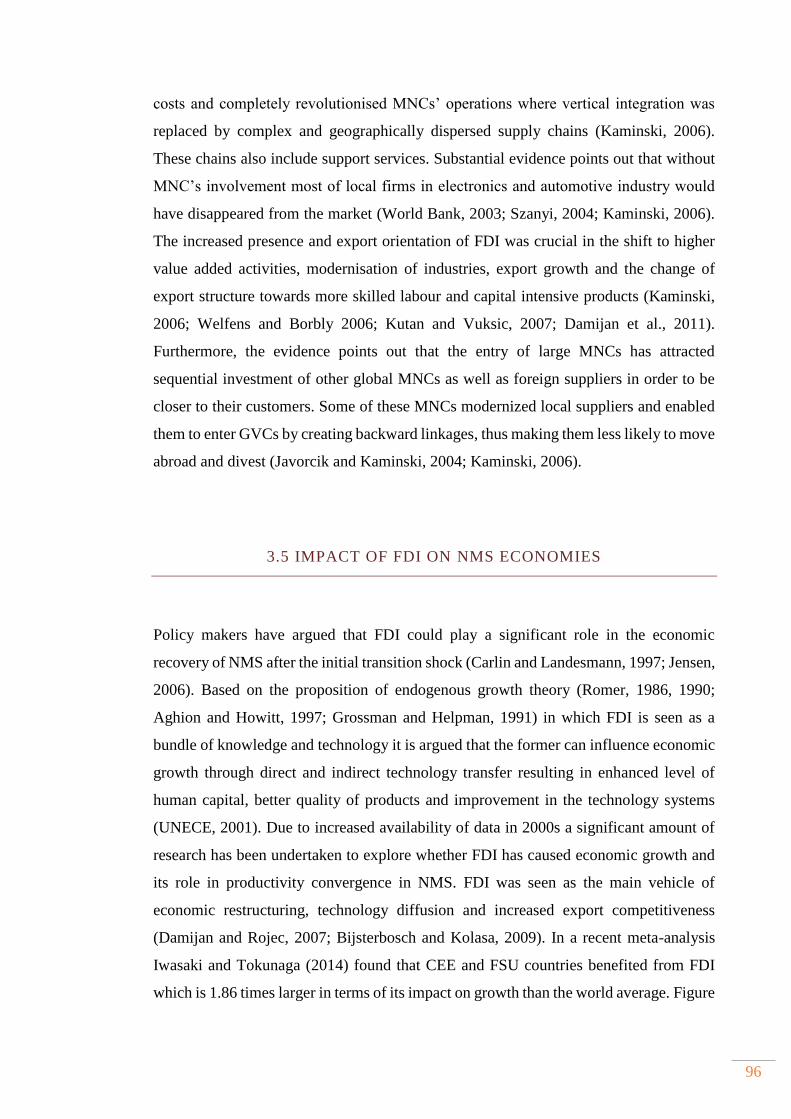
96
costs and completely revolutionised MNCs’ operations where vertical integration was
replaced by complex and geographically dispersed supply chains (Kaminski, 2006).
These chains also include support services. Substantial evidence points out that without
MNC’s involvement most of local firms in electronics and automotive industry would
have disappeared from the market (World Bank, 2003; Szanyi, 2004; Kaminski, 2006).
The increased presence and export orientation of FDI was crucial in the shift to higher
value added activities, modernisation of industries, export growth and the change of
export structure towards more skilled labour and capital intensive products (Kaminski,
2006; Welfens and Borbly 2006; Kutan and Vuksic, 2007; Damijan et al., 2011).
Furthermore, the evidence points out that the entry of large MNCs has attracted
sequential investment of other global MNCs as well as foreign suppliers in order to be
closer to their customers. Some of these MNCs modernized local suppliers and enabled
them to enter GVCs by creating backward linkages, thus making them less likely to move
abroad and divest (Javorcik and Kaminski, 2004; Kaminski, 2006).
3.5 IMPACT OF FDI ON NMS ECONOMIES
Policy makers have argued that FDI could play a significant role in the economic
recovery of NMS after the initial transition shock (Carlin and Landesmann, 1997; Jensen,
2006). Based on the proposition of endogenous growth theory (Romer, 1986, 1990;
Aghion and Howitt, 1997; Grossman and Helpman, 1991) in which FDI is seen as a
bundle of knowledge and technology it is argued that the former can influence economic
growth through direct and indirect technology transfer resulting in enhanced level of
human capital, better quality of products and improvement in the technology systems
(UNECE, 2001). Due to increased availability of data in 2000s a significant amount of
research has been undertaken to explore whether FDI has caused economic growth and
its role in productivity convergence in NMS. FDI was seen as the main vehicle of
economic restructuring, technology diffusion and increased export competitiveness
(Damijan and Rojec, 2007; Bijsterbosch and Kolasa, 2009). In a recent meta-analysis
Iwasaki and Tokunaga (2014) found that CEE and FSU countries benefited from FDI
which is 1.86 times larger in terms of its impact on growth than the world average. Figure
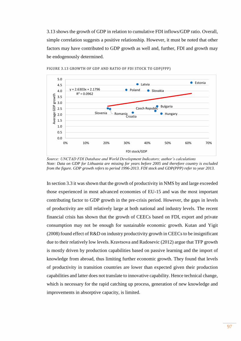
97
3.13 shows the growth of GDP in relation to cumulative FDI inflows/GDP ratio. Overall,
simple correlation suggests a positive relationship. However, it must be noted that other
factors may have contributed to GDP growth as well and, further, FDI and growth may
be endogenously determined.
FIGURE 3.13 GROWTH OF GDP AND RATIO OF FDI STOCK TO GDP(PPP)
Source: UNCTAD FDI Database and World Development Indicators; author’s calculations
Note: Data on GDP for Lithuania are missing for years before 2005 and therefore country is excluded
from the figure. GDP growth refers to period 1996-2013. FDI stock and GDP(PPP) refer to year 2013.
In section 3.3 it was shown that the growth of productivity in NMS by and large exceeded
those experienced in most advanced economies of EU-15 and was the most important
contributing factor to GDP growth in the pre-crisis period. However, the gaps in levels
of productivity are still relatively large at both national and industry levels. The recent
financial crisis has shown that the growth of CEECs based on FDI, export and private
consumption may not be enough for sustainable economic growth. Kutan and Yigit
(2008) found effect of R&D on industry productivity growth in CEECs to be insignificant
due to their relatively low levels. Kravtsova and Radosevic (2012) argue that TFP growth
is mostly driven by production capabilities based on passive learning and the import of
knowledge from abroad, thus limiting further economic growth. They found that levels
of productivity in transition countries are lower than expected given their production
capabilities and latter does not translate to innovative capability. Hence technical change,
which is necessary for the rapid catching up process, generation of new knowledge and
improvements in absorptive capacity, is limited.
Bulgaria
Croatia
Czech Republic
Estonia
Hungary
Latvia
Poland
Romania
Slovakia
Slovenia
y = 2.6303x + 2.1796R² = 0.0962
0.0
0.5
1.0
1.5
2.0
2.5
3.0
3.5
4.0
4.5
5.0
0% 10% 20% 30% 40% 50% 60% 70%
Ave
rage
GD
P g
row
th
FDI stock/GDP
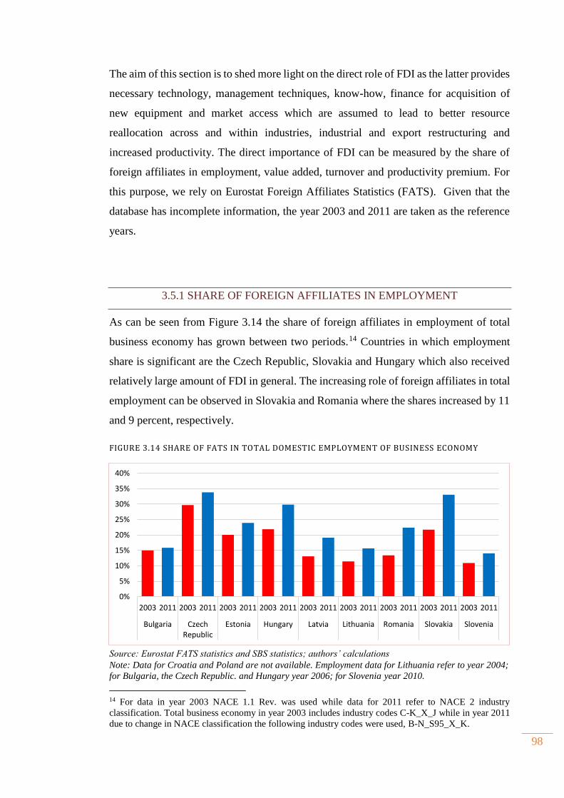
98
The aim of this section is to shed more light on the direct role of FDI as the latter provides
necessary technology, management techniques, know-how, finance for acquisition of
new equipment and market access which are assumed to lead to better resource
reallocation across and within industries, industrial and export restructuring and
increased productivity. The direct importance of FDI can be measured by the share of
foreign affiliates in employment, value added, turnover and productivity premium. For
this purpose, we rely on Eurostat Foreign Affiliates Statistics (FATS). Given that the
database has incomplete information, the year 2003 and 2011 are taken as the reference
years.
3.5.1 SHARE OF FOREIGN AFFILIATES IN EMPLOYMENT
As can be seen from Figure 3.14 the share of foreign affiliates in employment of total
business economy has grown between two periods. 13F
14 Countries in which employment
share is significant are the Czech Republic, Slovakia and Hungary which also received
relatively large amount of FDI in general. The increasing role of foreign affiliates in total
employment can be observed in Slovakia and Romania where the shares increased by 11
and 9 percent, respectively.
FIGURE 3.14 SHARE OF FATS IN TOTAL DOMESTIC EMPLOYMENT OF BUSINESS ECONOMY
Source: Eurostat FATS statistics and SBS statistics; authors’ calculations
Note: Data for Croatia and Poland are not available. Employment data for Lithuania refer to year 2004;
for Bulgaria, the Czech Republic. and Hungary year 2006; for Slovenia year 2010.
14 For data in year 2003 NACE 1.1 Rev. was used while data for 2011 refer to NACE 2 industry
classification. Total business economy in year 2003 includes industry codes C-K_X_J while in year 2011
due to change in NACE classification the following industry codes were used, B-N_S95_X_K.
0%
5%
10%
15%
20%
25%
30%
35%
40%
2003 2011 2003 2011 2003 2011 2003 2011 2003 2011 2003 2011 2003 2011 2003 2011 2003 2011
Bulgaria CzechRepublic
Estonia Hungary Latvia Lithuania Romania Slovakia Slovenia
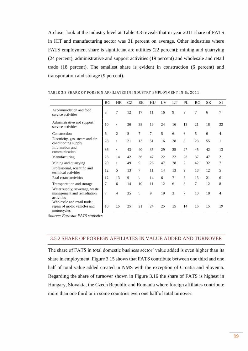
99
A closer look at the industry level at Table 3.3 reveals that in year 2011 share of FATS
in ICT and manufacturing sector was 31 percent on average. Other industries where
FATS employment share is significant are utilities (22 percent); mining and quarrying
(24 percent), administrative and support activities (19 percent) and wholesale and retail
trade (18 percent). The smallest share is evident in construction (6 percent) and
transportation and storage (9 percent).
TABLE 3.3 SHARE OF FOREIGN AFFILIATES IN INDUSTRY EMPLOYMENT IN %, 2011
BG HR CZ EE HU LV LT PL RO SK SI
Accommodation and food
service activities 8 7 12 17 11 16 9 9 7 6 7
Administrative and support
service activities 10 \ 26 38 19 24 16 13 21 18 22
Construction 6 2 8 7 7 5 6 6 5 6 4
Electricity, gas, steam and air
conditioning supply 28 \ 21 13 51 16 28 8 23 55 1
Information and
communication 36 \ 43 40 35 29 35 27 45 42 13
Manufacturing 23 14 42 36 47 22 22 28 37 47 21
Mining and quarrying 20 \ 49 9 26 47 28 2 42 32 7
Professional, scientific and
technical activities 12 5 13 7 11 14 13 9 18 12 5
Real estate activities 12 13 9 \ 14 6 7 3 15 21 6
Transportation and storage 7 6 14 10 11 12 6 8 7 12 8
Water supply; sewerage, waste
management and remediation
activities
7 4 35 \ 9 19 3 7 10 19 4
Wholesale and retail trade;
repair of motor vehicles and
motorcycles
10 15 25 21 24 25 15 14 16 15 19
Source: Eurostat FATS statistics
3.5.2 SHARE OF FOREIGN AFFILIATES IN VALUE ADDED AND TURNOVER
The share of FATS in total domestic business sector’ value added is even higher than its
share in employment. Figure 3.15 shows that FATS contribute between one third and one
half of total value added created in NMS with the exception of Croatia and Slovenia.
Regarding the share of turnover shown in Figure 3.16 the share of FATS is highest in
Hungary, Slovakia, the Czech Republic and Romania where foreign affiliates contribute
more than one third or in some countries even one half of total turnover.
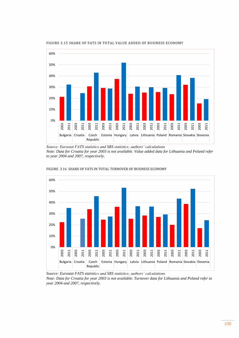
100
FIGURE 3.15 SHARE OF FATS IN TOTAL VALUE ADDED OF BUSINESS ECONOMY
Source: Eurostat FATS statistics and SBS statistics; authors’ calculations Note: Data for Croatia for year 2003 is not available. Value added data for Lithuania and Poland refer
to year 2004 and 2007, respectively. FIGURE 3.16 SHARE OF FATS IN TOTAL TURNOVER OF BUSINESS ECONOMY
Source: Eurostat FATS statistics and SBS statistics; authors’ calculations Note: Data for Croatia for year 2003 is not available. Turnover data for Lithuania and Poland refer to
year 2004 and 2007, respectively.
0%
10%
20%
30%
40%
50%
60%
20
03
20
11
20
03
20
11
20
03
20
11
20
03
20
11
20
03
20
11
20
03
20
11
20
03
20
11
20
03
20
11
20
03
20
11
20
03
20
11
20
03
20
11
Bulgaria Croatia CzechRepublic
Estonia Hungary Latvia Lithuania Poland Romania Slovakia Slovenia
0%
10%
20%
30%
40%
50%
60%
20
03
20
11
20
03
20
11
20
03
20
11
20
03
20
11
20
03
20
11
20
03
20
11
20
03
20
11
20
03
20
11
20
03
20
11
20
03
20
11
20
03
20
11
Bulgaria Croatia CzechRepublic
Estonia Hungary Latvia Lithuania Poland Romania Slovakia Slovenia
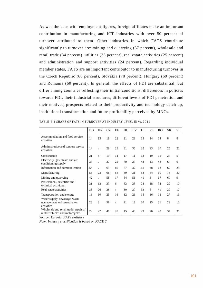
101
As was the case with employment figures, foreign affiliates make an important
contribution in manufacturing and ICT industries with over 50 percent of
turnover attributed to them. Other industries in which FATS contribute
significantly to turnover are: mining and quarrying (37 percent), wholesale and
retail trade (34 percent), utilities (33 percent), real estate activities (25 percent)
and administration and support activities (24 percent). Regarding individual
member states, FATS are an important contributor to manufacturing turnover in
the Czech Republic (66 percent), Slovakia (78 percent), Hungary (69 percent)
and Romania (60 percent). In general, the effects of FDI are substantial, but
differ among countries reflecting their initial conditions, differences in policies
towards FDI, their industrial structures, different levels of FDI penetration and
their motives, prospects related to their productivity and technology catch up,
institutional transformation and future profitability perceived by MNCs.
TABLE 3.4 SHARE OF FATS IN TURNOVER AT INDUSTRY LEVEL IN %, 2011
BG HR CZ EE HU LV LT PL RO SK SI
Accommodation and food service
activities 14 13 19 22 21 28 13 14 14 8 8
Administrative and support service
activities 14 \ 29 25 31 35 32 23 30 25 21
Construction 21 5 19 11 17 11 13 19 15 24 5
Electricity, gas, steam and air
conditioning supply 33 \ 37 22 70 29 43 13 48 64 6
Information and communication 54 \ 63 60 67 37 61 48 68 62 25
Manufacturing 53 23 66 54 69 31 58 44 60 78 30
Mining and quarrying 42 \ 58 17 54 51 41 3 67 60 9
Professional, scientific and
technical activities 31 13 23 6 32 28 24 18 34 22 10
Real estate activities 33 26 28 \ 30 27 33 6 41 29 17
Transportation and storage 18 10 25 16 32 23 15 16 16 27 13
Water supply; sewerage, waste
management and remediation
activities
28 8 38 \ 21 18 20 15 31 22 12
Wholesale and retail trade; repair of
motor vehicles and motorcycles 29 27 40 20 45 48 29 26 40 34 31
Source: Eurostat FATS statistics
Note: Industry classification is based on NACE 2

102
3.5.3 THE ROLE OF FATS IN TECHNOLOGY UPGRADING AND
PRODUCTIVITY IMPROVEMENTS
The productivity catch-up and structural change in NMS much depended on the
restructuring of their manufacturing industries. Given the importance of foreign affiliates
in selected indicators analysed in the previous subsections, an important question is how
these large inflows of foreign capital affected the competitiveness of the manufacturing
sector, especially the shift from low to high value added industries. For this purpose, we
first compare the penetration of foreign affiliates across different technology groups
presented in Table 3.5. Manufacturing industries have been classified into four groups:
high-tech; medium-high-tech; medium-low-tech; and low-tech according to OECD
(2007b) classification.
By the end of 2011, the number of enterprises in high and medium tech industries
remained below those in other groups. However, when comparing the share of turnover,
value added and employment, FATS in high and medium technology groups contribute
significantly more than the low technology group. For example, the dominance of foreign
affiliates is especially pronounced in Estonia, Hungary, the Czech Republic and Slovakia
where more than three quarters of foreign affiliates’ turnover is earned in high tech and
medium high tech industries. In contrast, in Croatia and Lithuania foreign firms’ turnover
is more concentrated in low technology industries. The same picture emerges when
comparing the share of high tech and medium high tech foreign affiliates in employment.
In all countries, but Bulgaria, Lithuania and Latvia foreign affiliates in these technology
groups employ the majority of employees indicating their superior size. In terms of value
added FATS in Estonia, Hungary, Slovakia, the Czech Republic are clear frontrunners
in creating value added in high tech and medium high tech industries. Finally, when
comparing labour productivity of each technology group with average manufacturing
productivity, results point out that FATS in high tech group are the driving force of
manufacturing productivity. However, the results are more heterogeneous across
countries. For instance, in the Czech Republic and Slovenia, foreign affiliates in medium
high and medium low industries have the highest levels of productivity. Similarly, in
Croatia and Bulgaria and to certain extent in Latvia, low tech industries are the main
drivers of productivity.
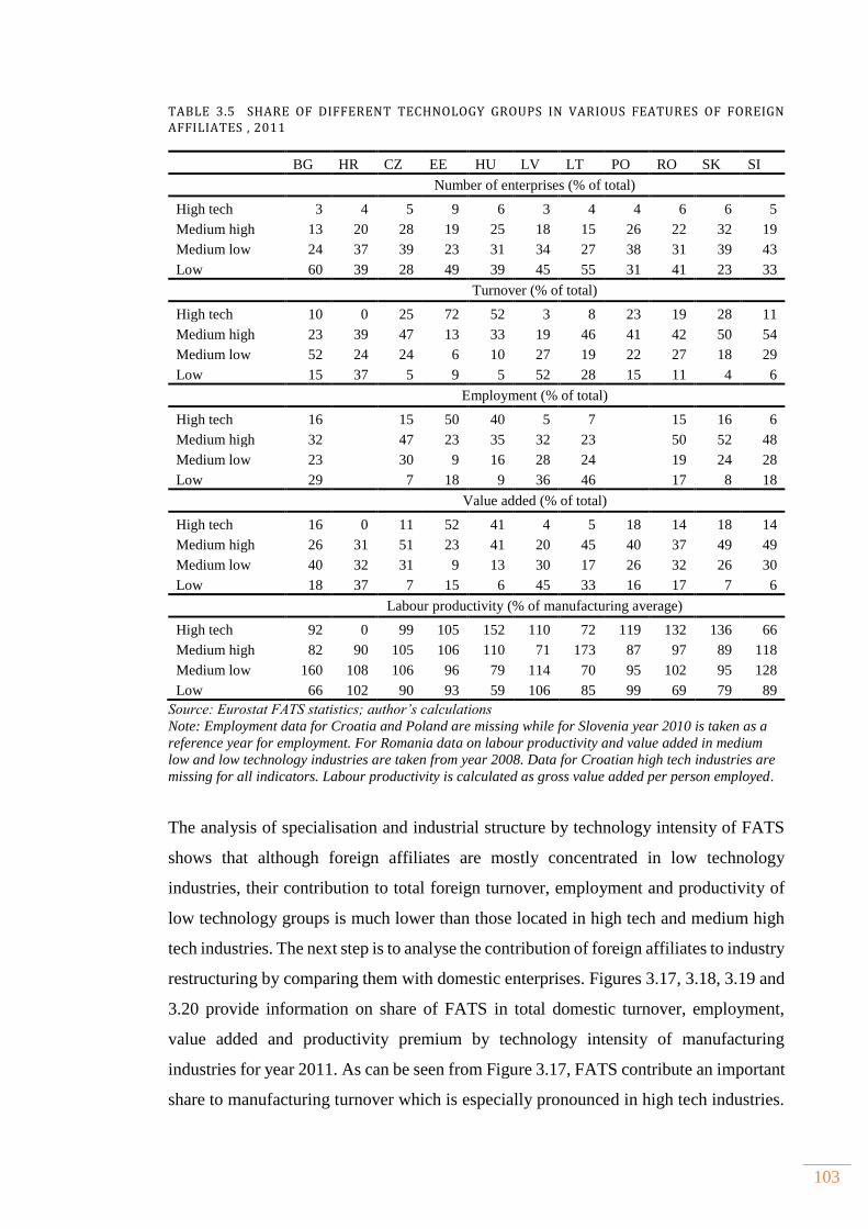
103
TABLE 3.5 SHARE OF DIFFERENT TECHNOLOGY GROUPS IN VARIOUS FEATURES OF FOREIGN AFFILIATES , 2011
BG HR CZ EE HU LV LT PO RO SK SI
Number of enterprises (% of total)
High tech 3 4 5 9 6 3 4 4 6 6 5
Medium high 13 20 28 19 25 18 15 26 22 32 19
Medium low 24 37 39 23 31 34 27 38 31 39 43
Low 60 39 28 49 39 45 55 31 41 23 33
Turnover (% of total)
High tech 10 0 25 72 52 3 8 23 19 28 11
Medium high 23 39 47 13 33 19 46 41 42 50 54
Medium low 52 24 24 6 10 27 19 22 27 18 29
Low 15 37 5 9 5 52 28 15 11 4 6
Employment (% of total)
High tech 16 15 50 40 5 7 15 16 6
Medium high 32 47 23 35 32 23 50 52 48
Medium low 23 30 9 16 28 24 19 24 28
Low 29 7 18 9 36 46 17 8 18
Value added (% of total)
High tech 16 0 11 52 41 4 5 18 14 18 14
Medium high 26 31 51 23 41 20 45 40 37 49 49
Medium low 40 32 31 9 13 30 17 26 32 26 30
Low 18 37 7 15 6 45 33 16 17 7 6
Labour productivity (% of manufacturing average)
High tech 92 0 99 105 152 110 72 119 132 136 66
Medium high 82 90 105 106 110 71 173 87 97 89 118
Medium low 160 108 106 96 79 114 70 95 102 95 128
Low 66 102 90 93 59 106 85 99 69 79 89
Source: Eurostat FATS statistics; author’s calculations
Note: Employment data for Croatia and Poland are missing while for Slovenia year 2010 is taken as a
reference year for employment. For Romania data on labour productivity and value added in medium
low and low technology industries are taken from year 2008. Data for Croatian high tech industries are
missing for all indicators. Labour productivity is calculated as gross value added per person employed.
The analysis of specialisation and industrial structure by technology intensity of FATS
shows that although foreign affiliates are mostly concentrated in low technology
industries, their contribution to total foreign turnover, employment and productivity of
low technology groups is much lower than those located in high tech and medium high
tech industries. The next step is to analyse the contribution of foreign affiliates to industry
restructuring by comparing them with domestic enterprises. Figures 3.17, 3.18, 3.19 and
3.20 provide information on share of FATS in total domestic turnover, employment,
value added and productivity premium by technology intensity of manufacturing
industries for year 2011. As can be seen from Figure 3.17, FATS contribute an important
share to manufacturing turnover which is especially pronounced in high tech industries.
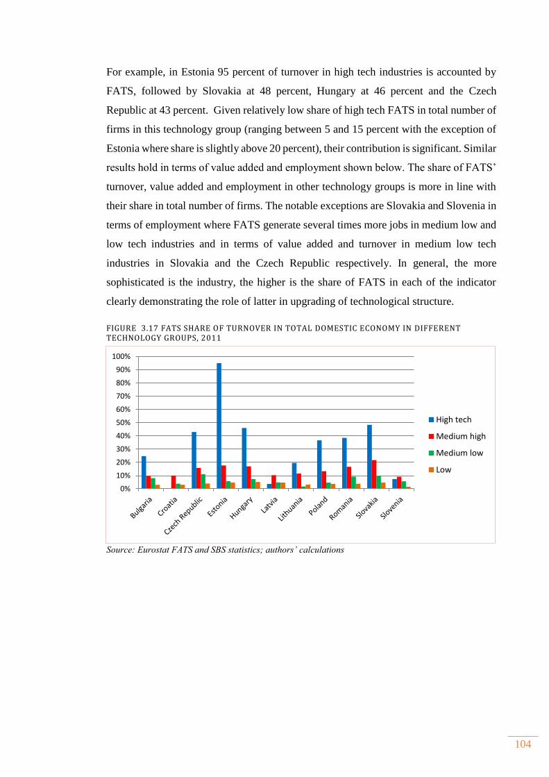
104
For example, in Estonia 95 percent of turnover in high tech industries is accounted by
FATS, followed by Slovakia at 48 percent, Hungary at 46 percent and the Czech
Republic at 43 percent. Given relatively low share of high tech FATS in total number of
firms in this technology group (ranging between 5 and 15 percent with the exception of
Estonia where share is slightly above 20 percent), their contribution is significant. Similar
results hold in terms of value added and employment shown below. The share of FATS’
turnover, value added and employment in other technology groups is more in line with
their share in total number of firms. The notable exceptions are Slovakia and Slovenia in
terms of employment where FATS generate several times more jobs in medium low and
low tech industries and in terms of value added and turnover in medium low tech
industries in Slovakia and the Czech Republic respectively. In general, the more
sophisticated is the industry, the higher is the share of FATS in each of the indicator
clearly demonstrating the role of latter in upgrading of technological structure.
FIGURE 3.17 FATS SHARE OF TURNOVER IN TOTAL DOMESTIC ECONOMY IN DIFFERENT TECHNOLOGY GROUPS, 2011
Source: Eurostat FATS and SBS statistics; authors’ calculations
0%
10%
20%
30%
40%
50%
60%
70%
80%
90%
100%
High tech
Medium high
Medium low
Low
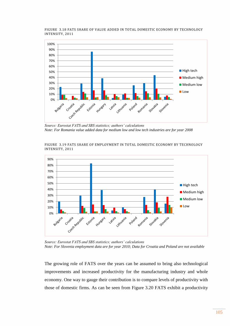
105
FIGURE 3.18 FATS SHARE OF VALUE ADDED IN TOTAL DOMESTIC ECONOMY BY TECHNOLOGY INTENSITY, 2011
Source: Eurostat FATS and SBS statistics; authors’ calculations
Note: For Romania value added data for medium low and low tech industries are for year 2008
FIGURE 3.19 FATS SHARE OF EMPLOYMENT IN TOTAL DOMESTIC ECONOMY BY TECHNOLOGY INTENSITY, 2011
Source: Eurostat FATS and SBS statistics; authors’ calculations
Note: For Slovenia employment data are for year 2010; Data for Croatia and Poland are not available
The growing role of FATS over the years can be assumed to bring also technological
improvements and increased productivity for the manufacturing industry and whole
economy. One way to gauge their contribution is to compare levels of productivity with
those of domestic firms. As can be seen from Figure 3.20 FATS exhibit a productivity
0%
10%
20%
30%
40%
50%
60%
70%
80%
90%
100%
High tech
Medium high
Medium low
Low
0%
10%
20%
30%
40%
50%
60%
70%
80%
90%
High tech
Medium high
Medium low
Low
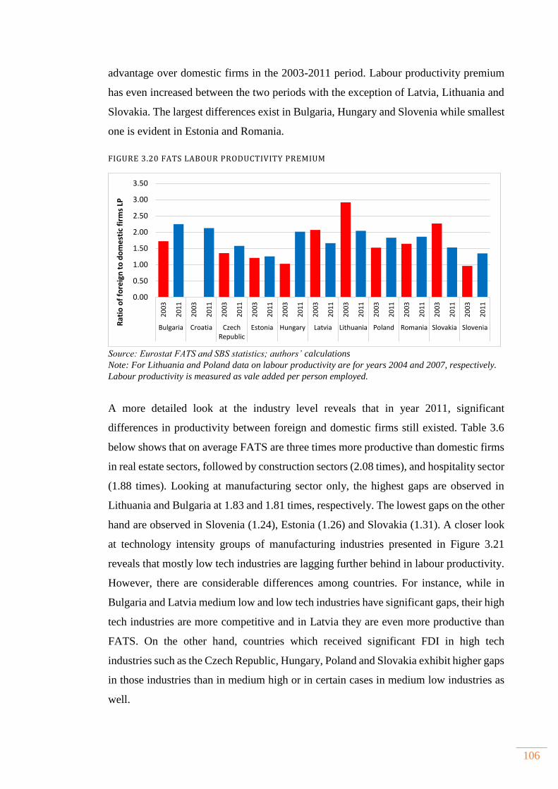
106
advantage over domestic firms in the 2003-2011 period. Labour productivity premium
has even increased between the two periods with the exception of Latvia, Lithuania and
Slovakia. The largest differences exist in Bulgaria, Hungary and Slovenia while smallest
one is evident in Estonia and Romania.
FIGURE 3.20 FATS LABOUR PRODUCTIVITY PREMIUM
Source: Eurostat FATS and SBS statistics; authors’ calculations Note: For Lithuania and Poland data on labour productivity are for years 2004 and 2007, respectively.
Labour productivity is measured as vale added per person employed.
A more detailed look at the industry level reveals that in year 2011, significant
differences in productivity between foreign and domestic firms still existed. Table 3.6
below shows that on average FATS are three times more productive than domestic firms
in real estate sectors, followed by construction sectors (2.08 times), and hospitality sector
(1.88 times). Looking at manufacturing sector only, the highest gaps are observed in
Lithuania and Bulgaria at 1.83 and 1.81 times, respectively. The lowest gaps on the other
hand are observed in Slovenia (1.24), Estonia (1.26) and Slovakia (1.31). A closer look
at technology intensity groups of manufacturing industries presented in Figure 3.21
reveals that mostly low tech industries are lagging further behind in labour productivity.
However, there are considerable differences among countries. For instance, while in
Bulgaria and Latvia medium low and low tech industries have significant gaps, their high
tech industries are more competitive and in Latvia they are even more productive than
FATS. On the other hand, countries which received significant FDI in high tech
industries such as the Czech Republic, Hungary, Poland and Slovakia exhibit higher gaps
in those industries than in medium high or in certain cases in medium low industries as
well.
0.00
0.50
1.00
1.50
2.00
2.50
3.00
3.50
20
03
20
11
20
03
20
11
20
03
20
11
20
03
20
11
20
03
20
11
20
03
20
11
20
03
20
11
20
03
20
11
20
03
20
11
20
03
20
11
20
03
20
11
Bulgaria Croatia CzechRepublic
Estonia Hungary Latvia Lithuania Poland Romania Slovakia Slovenia
Rat
io o
f fo
reig
n t
o d
om
est
ic f
irm
s LP
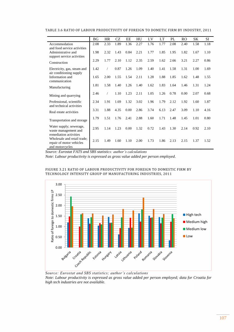
107
TABLE 3.6 RATIO OF LABOUR PRODUCTIVITY OF FOREIGN TO DOMETIC FIRM BY INDUSTRY, 2011
BG HR CZ EE HU LV LT PL RO SK SI
Accommodation
and food service activities
2.08 2.33 1.89 1.36 2.27 1.76 1.77 2.08 2.40 1.58 1.18
Administrative and
support service activities
1.98 2.32 1.43 0.84 2.21 1.77 1.85 1.95 1.82 1.67 1.10
Construction 2.29 1.77 2.10 1.12 2.35 2.59 1.62 2.66 3.21 2.27 0.86
Electricity, gas, steam and
air conditioning supply
1.42 / 0.87 1.26 1.09 1.40 1.41 1.58 1.31 1.00 1.69
Information and
communication
1.65 2.00 1.55 1.54 2.11 1.28 1.88 1.85 1.62 1.48 1.55
Manufacturing 1.81 1.58 1.40 1.26 1.40 1.62 1.83 1.64 1.46 1.31 1.24
Mining and quarrying 2.46 / 1.10 1.23 2.11 1.05 1.26 0.78 0.00 2.07 0.68
Professional, scientific
and technical activities
2.34 1.91 1.69 1.32 3.02 1.96 1.79 2.12 1.92 1.60 1.87
Real estate activities 3.31 1.88 4.35 0.00 2.86 3.74 6.13 2.47 3.09 1.10 4.16
Transportation and storage 1.79 1.51 1.76 2.41 2.88 1.60 1.71 1.48 1.45 1.01 0.80
Water supply; sewerage,
waste management and
remediation activities
2.95 1.14 1.23 0.00 1.32 0.72 1.43 1.30 2.14 0.92 2.10
Wholesale and retail trade;
repair of motor vehicles
and motorcycles
2.15 1.49 1.60 1.10 2.00 1.73 1.86 2.13 2.15 1.37 1.52
Source: Eurostat FATS and SBS statistics: author’s calculations
Note: Labour productivity is expressed as gross value added per person employed.
FIGURE 3.21 RATIO OF LABOUR PRODUCTIVITY FOR FOREIGN TO DOMESTIC FIRM BY TECHNOLOGY INTENSITY GROUP OF MANUFACTURING INDUSTRIES, 2011
Source: Eurostat and SBS statistics; author’s calculations
Note: Labour productivity is expressed as gross value added per person employed; data for Croatia for
high tech industries are not available.
0.00
0.50
1.00
1.50
2.00
2.50
3.00
Rat
io o
f fo
reig
n t
o d
om
esti
c fi
rms
LP
High tech
Medium high
Medium low
Low
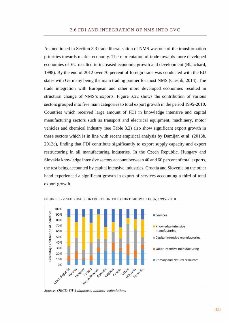
108
3.6 FDI AND INTEGRATION OF NMS INTO GVC
As mentioned in Section 3.3 trade liberalisation of NMS was one of the transformation
priorities towards market economy. The reorientation of trade towards more developed
economies of EU resulted in increased economic growth and development (Blanchard,
1998). By the end of 2012 over 70 percent of foreign trade was conducted with the EU
states with Germany being the main trading partner for most NMS (Cieslik, 2014). The
trade integration with European and other more developed economies resulted in
structural change of NMS’s exports. Figure 3.22 shows the contribution of various
sectors grouped into five main categories to total export growth in the period 1995-2010.
Countries which received large amount of FDI in knowledge intensive and capital
manufacturing sectors such as transport and electrical equipment, machinery, motor
vehicles and chemical industry (see Table 3.2) also show significant export growth in
these sectors which is in line with recent empirical analysis by Damijan et al. (2013b,
2013c), finding that FDI contribute significantly to export supply capacity and export
restructuring in all manufacturing industries. In the Czech Republic, Hungary and
Slovakia knowledge intensive sectors account between 40 and 60 percent of total exports,
the rest being accounted by capital intensive industries. Croatia and Slovenia on the other
hand experienced a significant growth in export of services accounting a third of total
export growth.
FIGURE 3.22 SECTORAL CONTRIBUTION TO EXPORT GROWTH IN %, 1995-2010
Source: OECD TiVA database; authors’ calculations
0%
10%
20%
30%
40%
50%
60%
70%
80%
90%
100%
Per
cen
tage
co
nti
bu
tio
n o
f in
du
stri
es
Services
Knowledge-intensivemanufacturing
Capital-intensive manufacturing
Labor-intensive manufacturing
Primary and Natural resources
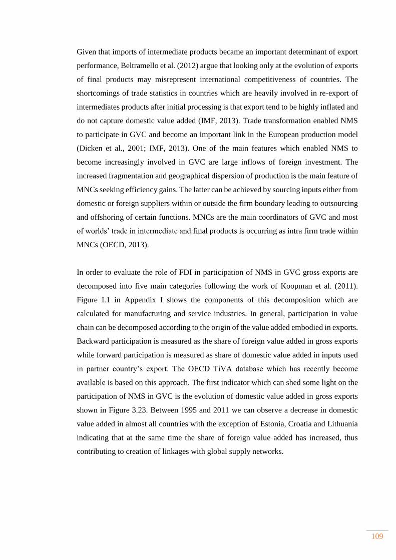
109
Given that imports of intermediate products became an important determinant of export
performance, Beltramello et al. (2012) argue that looking only at the evolution of exports
of final products may misrepresent international competitiveness of countries. The
shortcomings of trade statistics in countries which are heavily involved in re-export of
intermediates products after initial processing is that export tend to be highly inflated and
do not capture domestic value added (IMF, 2013). Trade transformation enabled NMS
to participate in GVC and become an important link in the European production model
(Dicken et al., 2001; IMF, 2013). One of the main features which enabled NMS to
become increasingly involved in GVC are large inflows of foreign investment. The
increased fragmentation and geographical dispersion of production is the main feature of
MNCs seeking efficiency gains. The latter can be achieved by sourcing inputs either from
domestic or foreign suppliers within or outside the firm boundary leading to outsourcing
and offshoring of certain functions. MNCs are the main coordinators of GVC and most
of worlds’ trade in intermediate and final products is occurring as intra firm trade within
MNCs (OECD, 2013).
In order to evaluate the role of FDI in participation of NMS in GVC gross exports are
decomposed into five main categories following the work of Koopman et al. (2011).
Figure I.1 in Appendix I shows the components of this decomposition which are
calculated for manufacturing and service industries. In general, participation in value
chain can be decomposed according to the origin of the value added embodied in exports.
Backward participation is measured as the share of foreign value added in gross exports
while forward participation is measured as share of domestic value added in inputs used
in partner country’s export. The OECD TiVA database which has recently become
available is based on this approach. The first indicator which can shed some light on the
participation of NMS in GVC is the evolution of domestic value added in gross exports
shown in Figure 3.23. Between 1995 and 2011 we can observe a decrease in domestic
value added in almost all countries with the exception of Estonia, Croatia and Lithuania
indicating that at the same time the share of foreign value added has increased, thus
contributing to creation of linkages with global supply networks.
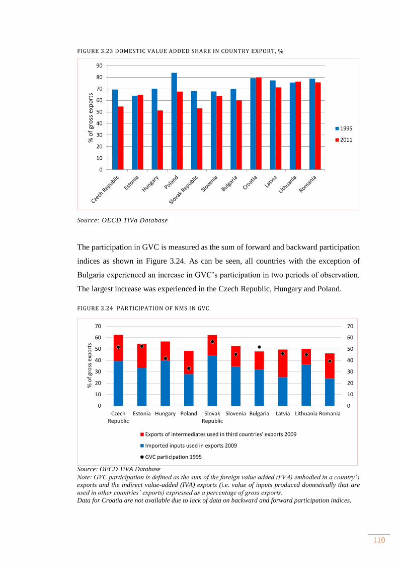
110
FIGURE 3.23 DOMESTIC VALUE ADDED SHARE IN COUNTRY EXPORT, %
Source: OECD TiVa Database
The participation in GVC is measured as the sum of forward and backward participation
indices as shown in Figure 3.24. As can be seen, all countries with the exception of
Bulgaria experienced an increase in GVC’s participation in two periods of observation.
The largest increase was experienced in the Czech Republic, Hungary and Poland.
FIGURE 3.24 PARTICIPATION OF NMS IN GVC
Source: OECD TiVA Database Note: GVC participation is defined as the sum of the foreign value added (FVA) embodied in a country’s
exports and the indirect value-added (IVA) exports (i.e. value of inputs produced domestically that are
used in other countries’ exports) expressed as a percentage of gross exports.
Data for Croatia are not available due to lack of data on backward and forward participation indices.
0
10
20
30
40
50
60
70
80
90
% o
f gr
oss
exp
ort
s
1995
2011
0
10
20
30
40
50
60
70
0
10
20
30
40
50
60
70
CzechRepublic
Estonia Hungary Poland SlovakRepublic
Slovenia Bulgaria Latvia Lithuania Romania
% o
f gr
oss
exp
ort
s
Exports of intermediates used in third countries' exports 2009
Imported inputs used in exports 2009
GVC participation 1995
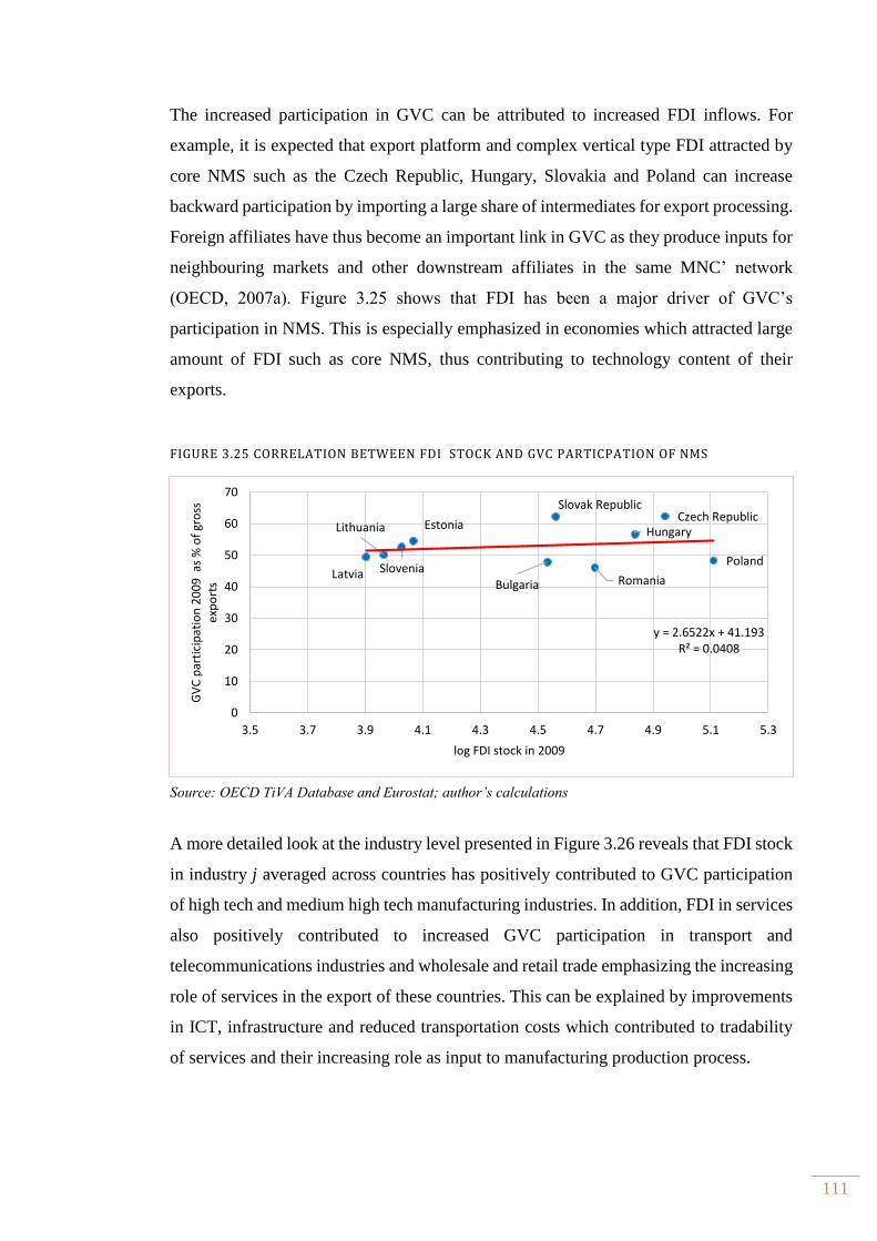
111
The increased participation in GVC can be attributed to increased FDI inflows. For
example, it is expected that export platform and complex vertical type FDI attracted by
core NMS such as the Czech Republic, Hungary, Slovakia and Poland can increase
backward participation by importing a large share of intermediates for export processing.
Foreign affiliates have thus become an important link in GVC as they produce inputs for
neighbouring markets and other downstream affiliates in the same MNC’ network
(OECD, 2007a). Figure 3.25 shows that FDI has been a major driver of GVC’s
participation in NMS. This is especially emphasized in economies which attracted large
amount of FDI such as core NMS, thus contributing to technology content of their
exports.
FIGURE 3.25 CORRELATION BETWEEN FDI STOCK AND GVC PARTICPATION OF NMS
Source: OECD TiVA Database and Eurostat; author’s calculations
A more detailed look at the industry level presented in Figure 3.26 reveals that FDI stock
in industry j averaged across countries has positively contributed to GVC participation
of high tech and medium high tech manufacturing industries. In addition, FDI in services
also positively contributed to increased GVC participation in transport and
telecommunications industries and wholesale and retail trade emphasizing the increasing
role of services in the export of these countries. This can be explained by improvements
in ICT, infrastructure and reduced transportation costs which contributed to tradability
of services and their increasing role as input to manufacturing production process.
Bulgaria
Czech RepublicEstonia
Hungary
Latvia
Lithuania
Poland
Romania
Slovak Republic
Slovenia
y = 2.6522x + 41.193R² = 0.0408
0
10
20
30
40
50
60
70
3.5 3.7 3.9 4.1 4.3 4.5 4.7 4.9 5.1 5.3
GV
C p
arti
cip
atio
n 2
00
9 a
s %
of
gro
ss
exp
ort
s
log FDI stock in 2009
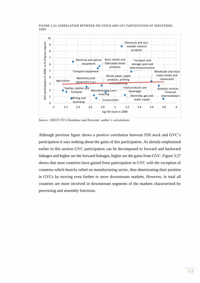
112
FIGURE 3.26 CORRELATION BETWEEN FDI STOCK AND GVC PARTICPATION OF INDUSTRIES, 2009
Source: OECD TiVA Database and Eurostat; author’s calculations
Although previous figure shows a positive correlation between FDI stock and GVC’s
participation it says nothing about the gains of this participation. As already emphasized
earlier in this section GVC participation can be decomposed to forward and backward
linkages and higher are the forward linkages, higher are the gains from GVC. Figure 3.27
shows that most countries have gained from participation in GVC with the exception of
countries which heavily relied on manufacturing sector, thus deteriorating their position
in GVCs by moving even further to more downstream markets. However, in total all
countries are more involved in downstream segments of the markets characterised by
processing and assembly functions.
Agriculture
Mining and quarrying
Food products and beverages
Textiles, leather and footwear
Wood, paper, paper products, printing
and publishing
Chemicals and non-metallic mineral
products
Basic metals and fabricated metal
products
Machinery and equipment n.e.c
Electrical and optical equipment
Transport equipment
Manufacturing n.e.c; recycling
Electricity, gas and water supplyConstruction
Wholesale and retail trade; hotels and
restaurants
Transport and storage; post and
telecommunications
Financial intermediation
Business services
0
1
2
3
4
5
6
7
8
9
10
2 2.2 2.4 2.6 2.8 3 3.2 3.4 3.6 3.8 4
GV
C p
arti
cip
atio
n in
20
09
as
% o
f gr
oss
exp
ort
s
log FDI stock in 2009
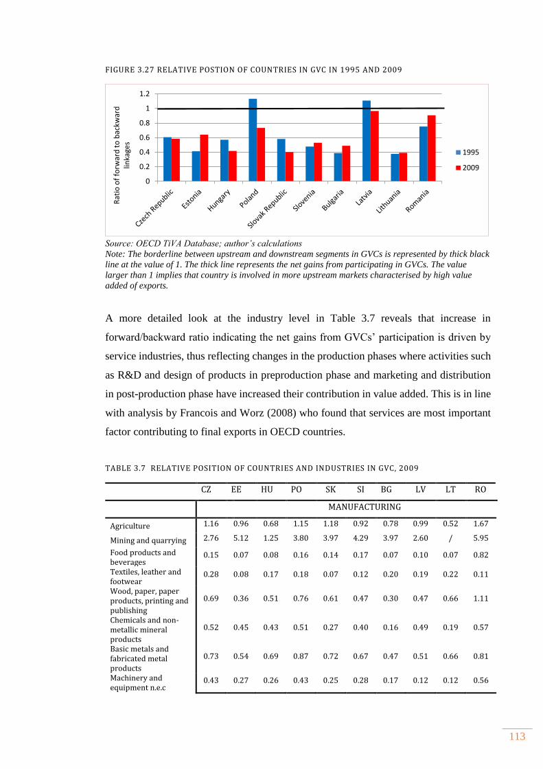
113
FIGURE 3.27 RELATIVE POSTION OF COUNTRIES IN GVC IN 1995 AND 2009
Source: OECD TiVA Database; author’s calculations
Note: The borderline between upstream and downstream segments in GVCs is represented by thick black
line at the value of 1. The thick line represents the net gains from participating in GVCs. The value
larger than 1 implies that country is involved in more upstream markets characterised by high value
added of exports.
A more detailed look at the industry level in Table 3.7 reveals that increase in
forward/backward ratio indicating the net gains from GVCs’ participation is driven by
service industries, thus reflecting changes in the production phases where activities such
as R&D and design of products in preproduction phase and marketing and distribution
in post-production phase have increased their contribution in value added. This is in line
with analysis by Francois and Worz (2008) who found that services are most important
factor contributing to final exports in OECD countries.
TABLE 3.7 RELATIVE POSITION OF COUNTRIES AND INDUSTRIES IN GVC, 2009
CZ EE HU PO SK SI BG LV LT RO
MANUFACTURING
Agriculture 1.16 0.96 0.68 1.15 1.18 0.92 0.78 0.99 0.52 1.67
Mining and quarrying 2.76 5.12 1.25 3.80 3.97 4.29 3.97 2.60 / 5.95
Food products and beverages
0.15 0.07 0.08 0.16 0.14 0.17 0.07 0.10 0.07 0.82
Textiles, leather and footwear
0.28 0.08 0.17 0.18 0.07 0.12 0.20 0.19 0.22 0.11
Wood, paper, paper products, printing and publishing
0.69 0.36 0.51 0.76 0.61 0.47 0.30 0.47 0.66 1.11
Chemicals and non-metallic mineral products
0.52 0.45 0.43 0.51 0.27 0.40 0.16 0.49 0.19 0.57
Basic metals and fabricated metal products
0.73 0.54 0.69 0.87 0.72 0.67 0.47 0.51 0.66 0.81
Machinery and equipment n.e.c
0.43 0.27 0.26 0.43 0.25 0.28 0.17 0.12 0.12 0.56
0
0.2
0.4
0.6
0.8
1
1.2
Rat
io o
f fo
rwar
d t
o b
ackw
ard
lin
kage
s
1995
2009
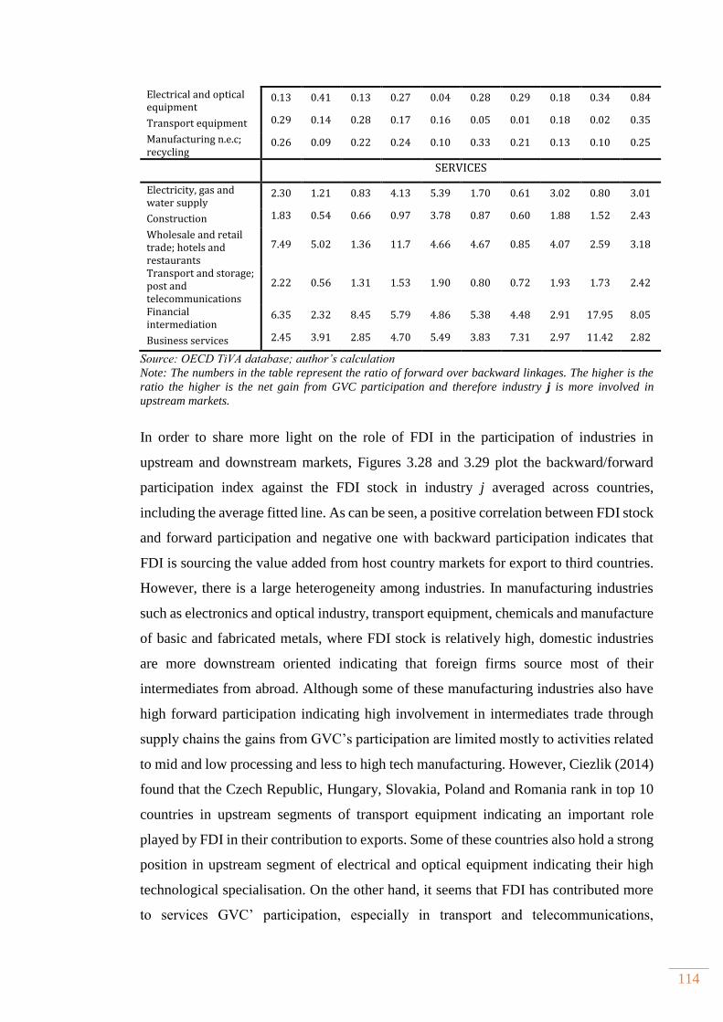
114
Electrical and optical equipment
0.13 0.41 0.13 0.27 0.04 0.28 0.29 0.18 0.34 0.84
Transport equipment 0.29 0.14 0.28 0.17 0.16 0.05 0.01 0.18 0.02 0.35
Manufacturing n.e.c; recycling
0.26 0.09 0.22 0.24 0.10 0.33 0.21 0.13 0.10 0.25
SERVICES
Electricity, gas and water supply
2.30 1.21 0.83 4.13 5.39 1.70 0.61 3.02 0.80 3.01
Construction 1.83 0.54 0.66 0.97 3.78 0.87 0.60 1.88 1.52 2.43
Wholesale and retail trade; hotels and restaurants
7.49 5.02 1.36 11.7 4.66 4.67 0.85 4.07 2.59 3.18
Transport and storage; post and telecommunications
2.22 0.56 1.31 1.53 1.90 0.80 0.72 1.93 1.73 2.42
Financial intermediation
6.35 2.32 8.45 5.79 4.86 5.38 4.48 2.91 17.95 8.05
Business services 2.45 3.91 2.85 4.70 5.49 3.83 7.31 2.97 11.42 2.82
Source: OECD TiVA database; author’s calculation
Note: The numbers in the table represent the ratio of forward over backward linkages. The higher is the
ratio the higher is the net gain from GVC participation and therefore industry j is more involved in
upstream markets.
In order to share more light on the role of FDI in the participation of industries in
upstream and downstream markets, Figures 3.28 and 3.29 plot the backward/forward
participation index against the FDI stock in industry j averaged across countries,
including the average fitted line. As can be seen, a positive correlation between FDI stock
and forward participation and negative one with backward participation indicates that
FDI is sourcing the value added from host country markets for export to third countries.
However, there is a large heterogeneity among industries. In manufacturing industries
such as electronics and optical industry, transport equipment, chemicals and manufacture
of basic and fabricated metals, where FDI stock is relatively high, domestic industries
are more downstream oriented indicating that foreign firms source most of their
intermediates from abroad. Although some of these manufacturing industries also have
high forward participation indicating high involvement in intermediates trade through
supply chains the gains from GVC’s participation are limited mostly to activities related
to mid and low processing and less to high tech manufacturing. However, Ciezlik (2014)
found that the Czech Republic, Hungary, Slovakia, Poland and Romania rank in top 10
countries in upstream segments of transport equipment indicating an important role
played by FDI in their contribution to exports. Some of these countries also hold a strong
position in upstream segment of electrical and optical equipment indicating their high
technological specialisation. On the other hand, it seems that FDI has contributed more
to services GVC’ participation, especially in transport and telecommunications,
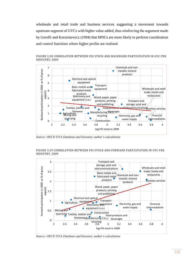
115
wholesale and retail trade and business services suggesting a movement towards
upstream segment of GVCs with higher value added, thus reinforcing the argument made
by Gereffi and Korzeniewicz (1994) that MNCs are more likely to perform coordination
and control functions where higher profits are realised.
FIGURE 3.28 CORRELATION BETWEEN FDI STOCK AND BACKWARD PARTICIPATION IN GVC PER INDUSTRY, 2009
Source: OECD TiVA Database and Eurostat; author’s calculations
FIGURE 3.29 CORRELATION BETWEEN FDI STOCK AND FORWARD PARTICIPATION IN GVC PER INDUSTRY, 2009
Source: OECD TiVA Database and Eurostat; author’s calculations
AgricultureMining and quarrying
Food products and beverages
Textiles, leather and footwear
Wood, paper, paper products, printing
and publishing
Chemicals and non-metallic mineral
products
Basic metals and fabricated metal
productsMachinery and
equipment n.e.c
Electrical and optical equipment
Transport equipment
Manufacturing n.e.c; recycling Electricity, gas and
water supplyConstruction
Wholesale and retail trade; hotels and
restaurants
Transport and storage; post and
telecommunications
Financial intermediation
Business services
0
1
2
3
4
5
6
7
2 2.2 2.4 2.6 2.8 3 3.2 3.4 3.6 3.8 4
Bac
kwar
d p
arti
cip
atio
n in
20
09
as
% o
f gr
oss
ex
po
rts
log FDI stock in 2009
Agriculture
Mining and quarrying
Food products and beverages
Textiles, leather and footwear
Wood, paper, paper products, printing
and publishing
Chemicals and non-metallic mineral
products
Basic metals and fabricated metal
products
Machinery and equipment n.e.c
Electrical and optical equipment Transport
equipment
Manufacturing n.e.c; recycling
Electricity, gas and water supply
Construction
Wholesale and retail trade; hotels and
restaurants
Transport and storage; post and
telecommunications
Financial intermediation
Business services
0
0.5
1
1.5
2
2.5
3
2 2.2 2.4 2.6 2.8 3 3.2 3.4 3.6 3.8 4
Forw
ard
par
tici
pat
ion
in 2
00
9 a
s %
of
gro
ss
exp
ort
s
log FDI stock in 2009
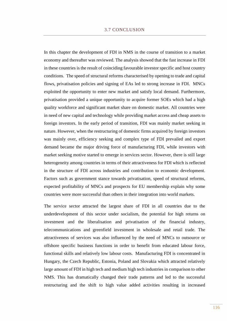
116
3.7 CONCLUSION
In this chapter the development of FDI in NMS in the course of transition to a market
economy and thereafter was reviewed. The analysis showed that the fast increase in FDI
in these countries is the result of coinciding favourable investor specific and host country
conditions. The speed of structural reforms characterised by opening to trade and capital
flows, privatisation policies and signing of EAs led to strong increase in FDI. MNCs
exploited the opportunity to enter new market and satisfy local demand. Furthermore,
privatisation provided a unique opportunity to acquire former SOEs which had a high
quality workforce and significant market share on domestic market. All countries were
in need of new capital and technology while providing market access and cheap assets to
foreign investors. In the early period of transition, FDI was mainly market seeking in
nature. However, when the restructuring of domestic firms acquired by foreign investors
was mainly over, efficiency seeking and complex type of FDI prevailed and export
demand became the major driving force of manufacturing FDI, while investors with
market seeking motive started to emerge in services sector. However, there is still large
heterogeneity among countries in terms of their attractiveness for FDI which is reflected
in the structure of FDI across industries and contribution to economic development.
Factors such as government stance towards privatisation, speed of structural reforms,
expected profitability of MNCs and prospects for EU membership explain why some
countries were more successful than others in their integration into world markets.
The service sector attracted the largest share of FDI in all countries due to the
underdevelopment of this sector under socialism, the potential for high returns on
investment and the liberalisation and privatisation of the financial industry,
telecommunications and greenfield investment in wholesale and retail trade. The
attractiveness of services was also influenced by the need of MNCs to outsource or
offshore specific business functions in order to benefit from educated labour force,
functional skills and relatively low labour costs. Manufacturing FDI is concentrated in
Hungary, the Czech Republic, Estonia, Poland and Slovakia which attracted relatively
large amount of FDI in high tech and medium high tech industries in comparison to other
NMS. This has dramatically changed their trade patterns and led to the successful
restructuring and the shift to high value added activities resulting in increased
117
international competitiveness. The efficiency seeking FDI accompanied by more
complex forms of investments in network industries enabled these countries to enter the
production fragmentation process and domestic firms to enter GVCs. However, the
integration in GVC has mainly been associated with processing and assembly of foreign
intermediates, thus providing limited gains especially in manufacturing industries. In
contrast, the service sector is involved in more upstream activities with high value added.
The analysis of the direct contribution of foreign affiliates has found their increasing role
in employment, turnover and value added activities across all countries. Their
contribution to these indicators is especially pronounced in manufacturing and certain
service industries such as ICT, administrative and support activities and wholesale and
retail trade. In general, the higher is the sophistication of industries, the larger is the
contribution of foreign firms. The analysis of productivity levels between foreign firms
and the rest of economy indicates the superiority of the former. Productivity gaps are
pronounced in all industries, especially in services and low tech manufacturing. Hence,
future productivity growth depends on the shift to knowledge based production and
innovation activities some of which may be facilitated by attracting product mandate
foreign subsidiaries involved in R&D. 14F
15 Improvements in R&D policies would help
foreign subsidiaries to shift towards competence creating activities and help local firms
strengthen their absorptive capacity. Furthermore, a shift to more upstream activities in
GVCs is conditional on the integration of domestic firms in MNCs’ networks. One way
to achieve this is to introduce programmes whose aim is to help domestic firms to
integrate with foreign firms through supply linkages. This would help domestic firms to
survive and at the same time make foreign firms less footloose.
15 Product mandate subsidiaries possess unique local technological competence and pursue asset seeking
strategies with the aim to form partnership with host country research centres or universities. They have
wide geographical and functional scope and specific product scope (Filippov and Kalotay, 2009).

118
CHAPTER 4.
ISSUES, METHODOLOGICAL SOLUTIONS AND ESTIMATION OF TFP AT MICRO
LEVEL
4.1 Introduction .......................................................................................................................................... 119
4.2 Measurement of productivity ........................................................................................................ 121
4.3 Methodological issues in estimation of TFP ............................................................................ 127
4.3.1 Simultaneity bias ........................................................................................................................ 131
4.3.2 Selection bias ............................................................................................................................... 132
4.3.3 Omitted price bias ..................................................................................................................... 132
4.3.4 Multiproduct firms ................................................................................................................... 133
4.4 Solutions to econometric problems ............................................................................................ 134
4.4.1 Traditional solutions to endogeneity of input choice ................................................. 136
4.4.2 Olley-Pakes and Levinsohn-Petrin methodology ......................................................... 137
4.4.3 Ackerberg Caves Frazer critique ......................................................................................... 142
4.4.4 Wooldridge estimator .............................................................................................................. 144
4.5 Data and descriptive statistics ...................................................................................................... 146
4.5.1 Sample Description ................................................................................................................... 147
4.5.2 Variables description and descriptive statistics ........................................................... 151
4.6 TFP estimation..................................................................................................................................... 155
4.7 Are foreign firms more productive? ........................................................................................... 162
4.8 Conclusion ............................................................................................................................................. 167
119
4.1 INTRODUCTION
In the previous chapter we have seen that countries of Central and Eastern Europe have
witnessed strong productivity gains and were able to reduce the gap with more advanced
economies in Europe largely due to increase in FDI. However, their GDP per capita is
still below the EU-15 average and therefore the need to raise productivity levels remains
an important policy goal for these countries. Since the improvement in standards of living
crucially depends on the increase in productivity, the aim of this chapter is to quantify
productivity as it is used as an important tool to evaluate different policies. The
estimation of productivity has gained considerable attention in economic literature. The
earlier work was mainly based on the quantification of the role of TFP in economic
growth to explain differences in performance across countries and industries. Macro
approach to TFP estimation was mainly based on growth accounting and growth
regression techniques. However, with the advances in economic theory, in which firms
are regarded as heterogeneous entities, and increased availability of firm level data
shifted the focus on describing mechanisms and channels through which productivity can
be enhanced and its role in the integration process. Estimation of firm level productivity
is most commonly based on some form of production function and usually the researchers
do not give serious attention to possible difficulties to the estimation of the residual. Too
often empirical work a priori assumes that chosen empirical methodology is superior to
alternatives without giving much taught on the validity of production function estimates
and assumptions employed to obtain them.
The first contribution of this chapter is to point out the difficulties arising from TFP
estimation at the firm level starting from explaining the major differences between
parametric and non-parametric techniques, their assumptions about production
technologies and problems with measurement of outputs and inputs. Second, we explain
several methodological issues arising from the use of firm level Cobb Douglas
production function and possible solutions. We pay specific attention to semi parametric
methods which assume a flexible characterization of TFP and are less prone to different
biases and measurement issues which may affect the elasticities of factor inputs.
Theoretical review of semi parametric methods together with their practical
implementation using typical firm level data obtained from the Amadeus database is the
120
second contribution. While similar studies test the assumptions of data generating
process and validity of factor inputs estimates using different methodologies they mainly
focus on one country or narrowly defined industries. In contrast this chapter contributes
by examining TFP estimates across different countries and industries.
Although different estimators make different timing assumptions about the choice of
inputs, we remain agnostic about these issues as it has been shown that these assumptions
make little difference on the production function and TFP estimates (Ornaghi and Van
Beveren, 2012). The focus is on comparison of estimates of different semi parametric
techniques and their interpretation. Specifically, we calculate TFP using OLS as a
benchmark method and two structural estimators, and test their sensitivity across several
dimensions. Finally, we compare different productivity distributions of foreign and
domestic firms as an initial indicator of potential for generating productivity spillovers.
The remainder of this chapter is structured as follows. Section 4.2 briefly describes the
origins of productivity measurement and different methodological approaches together
with their advantages and drawbacks. Section 4.3 provides a detailed overview of
methodological issues related to estimation of TFP using firm level data and Cobb
Douglas production function, namely simultaneity bias between productivity and input
choices, selection bias due to entry and exit for firms, omitted price bias and the
appropriate level of analysis when firms produce multiple products. Section 4.4 provides
theoretical overview of methodological solutions to some of the problems. Specific
attention is paid to semi parametric techniques which have been extensively used in the
literature of TFP estimation at the firm level together with more “classical” approaches
relying on parametric technique, namely OLS and fixed effects. Section 4.5 introduces
the data used in empirical estimation of TFP and subsequent empirical chapters. Specific
focus is paid to representativeness of Amadeus database to official statistics, cleaning
procedure to obtain the relevant sample and construction of foreign ownership variable.
In section 4.6 the practical implementation of some of the estimators is applied together
with comments on their relative performance. Comparison of foreign and domestic firms
in terms of their TFP distribution is provided in section 4.7. Finally, section 4.8 provides
concluding remarks.

121
4.2 MEASUREMENT OF PRODUCTIVITY
Origins of productivity measurement can be traced back to seminal papers of Tinbergen
(1942), Fabricant (1954), Abramovitz (1956) and Solow (1957) that decomposed output
growth to input growth and productivity residual. Early studies were mainly concerned
with aggregate TFP and its role in economic growth. The first empirical evidence
explaining the sources of productivity growth were provided by Abramovitz (1956) by
analysing U.S. economy. He was not able to identify any sources of productivity growth,
which led to famous comment: “Since we know little about the cause of productivity
increase, the indicated importance of this element may be taken to be some sort of
measure of our ignorance about the causes of economic growth” (Abramovitz, 1956,
p.11). Solow (1957) developed an analytical framework in which main assumption was
that productivity growth is a mirror image of exogenous technological progress. Early
work was mainly based on growth accounting methods which measure productivity
indirectly as a residual of output growth that can not be explained by factor inputs, the
former being the result of technological change. Jorgensen and Griliches (1967) continue
along somewhat different line arguing that technological progress is embodied in factor
inputs and therefore the residual can be completely eliminated. By taking into account
differences in input quality the contribution of TFP disappears.
Recently, with the emergence of new growth theory which put emphasis on imperfect
competition, increasing returns to scale, innovation, externalities and creative destruction
process TFP is regarded as an endogenous part of the development process (Del Gatto et
al., 2011). Furthermore, development of new trade models which regard firms as
heterogeneous entities within industry require detailed firm level data to explore TFP
distribution and integration process (e.g. Melitz, 2003; Melitz and Ottaviano; 2008;
Chaney, 2008). The availability of microeconomic data has created possibilities to
estimate productivity at more disaggregated levels and to explain the sources of cross
country differences in economic growth. Several empirical studies have found that TFP
growth can be decomposed into within and between components and the role of creative
destruction process. The within component is related to innovative activities of the firms
aimed to increase the efficiency of production process and choices firms make about
input and output levels. Between components is the result of reallocation of inputs across
122
firms as a result of market interactions on inputs and output markets. Finally, net entry
component reflects the difference in productivity growth of new more productive firms
in the market from those firms who exit. Foster et al. (2001) and Bartelsman et al. (2009)
decomposed aggregate TFP growth by using firm level data and came to conclusion that
within component plays the major role in productivity growth and the process of creative
destruction has a significant role in the process of reallocation of inputs and outputs.
Recently, Petrin and Levinsohn (2012) have challenged the existing decomposition of
TFP and suggested that one should focus on measuring aggregate productivity growth as
the change in aggregated final demand minus the change in the aggregated cost of
primary inputs. It is an indicator of the change in potential aggregate consumption
holding total primary input use constant. They show how to use plant-level data to
decompose aggregate productivity into technical efficiency and reallocation terms. They
were able to show that traditional measures of TFP decomposition use no information on
the differences between marginal revenue products and input prices in its assessment of
growth arising from reallocation.
Apart from productivity decomposition, data availability has also allowed to explore the
determinants of TFP at micro level, thus enabling more specific policy recommendations.
Syverson (2011) has recently summarised the determinants of TFP growth to those
specific to the firms and those arising from environment in which the firms operate.
Internal factors are related to managerial talent and quality of their practices, quality of
labour and capital inputs, information technology, product innovation, learning by doing
and firm structure decisions such as the degree of decentralisation, vertical integration
and operation in multiple industries. On the other hand, external factors may not
influence productivity directly, but they may influence the incentives to adopt previous
practices. Also, they can influence the extent and success of internal efforts at moving
producers on productivity ladder. External factors can be classified to productivity
spillovers which are the aim of this thesis, intramarket and trade competition, regulation
and flexible inputs markets which are closely related to flexibility in product markets.
Although the measurement of productivity has recently gained significant attention in
economic literature there is yet no common methodology which allows its consistent
estimates. According to Van Biesebroeck (2008) there are at least six issues related to
productivity measurement. First, different estimators make different assumption about
the production technology used by firms. Second, most methods require assumptions
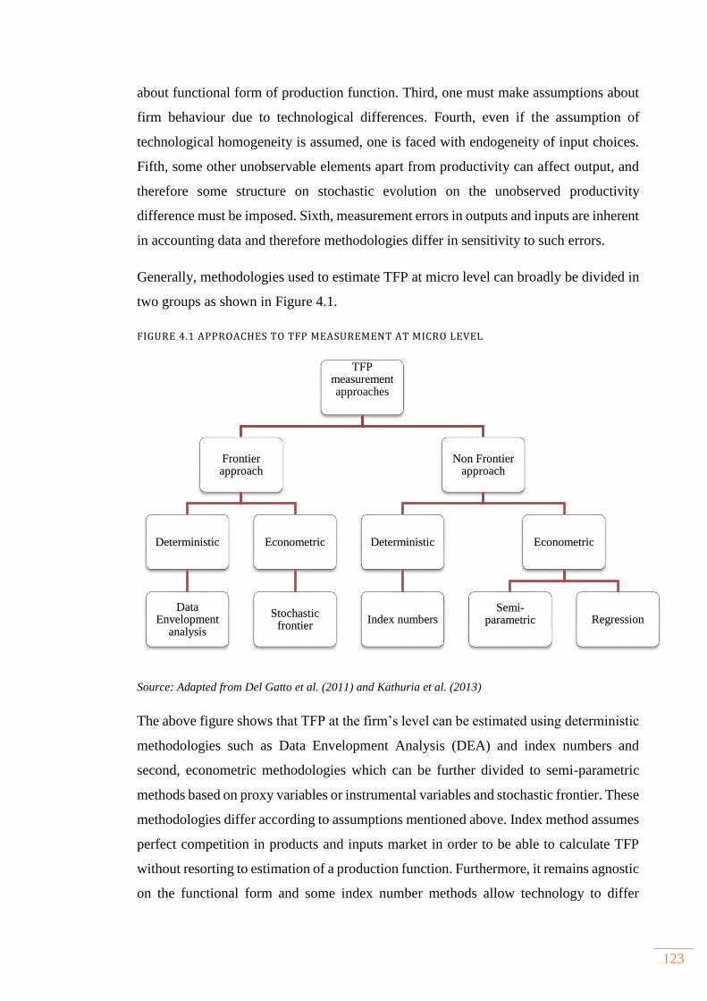
123
about functional form of production function. Third, one must make assumptions about
firm behaviour due to technological differences. Fourth, even if the assumption of
technological homogeneity is assumed, one is faced with endogeneity of input choices.
Fifth, some other unobservable elements apart from productivity can affect output, and
therefore some structure on stochastic evolution on the unobserved productivity
difference must be imposed. Sixth, measurement errors in outputs and inputs are inherent
in accounting data and therefore methodologies differ in sensitivity to such errors.
Generally, methodologies used to estimate TFP at micro level can broadly be divided in
two groups as shown in Figure 4.1.
FIGURE 4.1 APPROACHES TO TFP MEASUREMENT AT MICRO LEVEL
Source: Adapted from Del Gatto et al. (2011) and Kathuria et al. (2013)
The above figure shows that TFP at the firm’s level can be estimated using deterministic
methodologies such as Data Envelopment Analysis (DEA) and index numbers and
second, econometric methodologies which can be further divided to semi-parametric
methods based on proxy variables or instrumental variables and stochastic frontier. These
methodologies differ according to assumptions mentioned above. Index method assumes
perfect competition in products and inputs market in order to be able to calculate TFP
without resorting to estimation of a production function. Furthermore, it remains agnostic
on the functional form and some index number methods allow technology to differ
TFP measurement approaches
Frontier approach
Deterministic
Data Envelopment
analysis
Econometric
Stochastic frontier
Non Frontier approach
Deterministic
Index numbers
Econometric
Semi-parametric Regression
124
between firms which may be a very realistic assumption and in line with new trade
models which argue that productivity differences may exist even in narrowly defined
industries (Melitz, 2003). One of the main disadvantages of index methodology is that
they do not allow for measurement errors which may be large due to imperfect
measurement of output and input measures in accounting data. It also imposes necessary
assumptions of firm behaviour and market structure which may influence productivity.
DEA methodology is a non-parametric method developed by Farrell (1957) and further
extended by Charnes et al. (1978). It belongs to frontier models which assume that firms
are not fully efficient and in the presence of inefficiency productivity measurement is
also affected. Productivity is defined as the ratio of a linear combination of outputs over
a linear combination of inputs obtained using linear programming for each observation.
It requires imposing specific weights on factor inputs and output in order to maximize
productivity. The firm or linear combination of other firms are regarded efficient if it
produces more output with the same input aggregate and the latter uses the same weights
(Van Biesebroeck, 2007). The most efficient firms are located on frontier of the
production and comparison is made with other less efficient firms. The distance from the
frontier is termed technical inefficiency. The advantages of DEA are that it does not
require any specific functional form, thus allowing technology to vary across firms.
Furthermore, it is capable to disentangle two main sources of productivity growth,
namely technological change which shifts production possibility frontier upwards and
technical efficiency change which reflects the capability of firms to improve production
with given set of input and technology. The major drawback is that this methodology
does not allow for measurement errors and is very sensitive to outliers because each
observation is compared to all others and therefore may affect the productivity estimates.
Turning to econometric methodologies, parametric methods require specific functional
form of the type such as Cobb-Douglas (CB), translog or Constant Elasticity Substitution
(CES), thus assuming same input trade-offs and returns to scale for all firms within an
industry or country (Van Biesebroeck, 2007). Parametric methods are less susceptible to
measurement errors due to stochastic framework of analysis and productivity estimates
depend on the chosen functional form. Furthermore, econometric methods allow taking
into account adjustment costs arising for example by changes in factor inputs which
become costly the faster they are implemented (Schreyer and Pilat, 2001). The major
drawback of such methods is endogeneity of inputs, first discussed by Marschak and
125
Andrews (1944). It arises due the fact that firms observe their productivity level and
adjust their inputs accordingly, thus creating possible correlation between inputs and the
error term which is unobserved by econometrician. In order to deal with simultaneity
bias and other problems specific to TFP estimation, several solutions have been
proposed, the most prominent one being structural estimators discussed in more detail in
the following section and GMM estimator. The latter is explained in more detail in the
next chapter.
Briefly, GMM estimator assumes a specific functional form of production function in
which productivity is modelled as a firm fixed effect (ωit) which evolves as AR(1)
process (ωit =ωit-1 + ηit). Given this persistence in productivity, production function is
transformed from static to dynamic specification. However, transforming the production
function from static to dynamic models using OLS does not solve potential simultaneity
bias as factor input are still correlated with time invariant productivity level and
productivity shock. Blundell and Bond (2000) estimate production function in first
differences adding lagged levels of the dependent and independent variables to the right-
hand side. By doing that they eliminate time invariant productivity level and the
assumption that factor inputs are correlated with productivity level is made redundant
(Eberhardt and Helmers, 2010). However, labour and lagged dependent variable are still
correlated with productivity shock while capital is treated as predetermined. The latter
assumption is based on the notion that investment in new capital is made in the t-1 and
thus capital stock does not increase until period t. If this assumption is dropped, capital
can be treated as endogenous as well.
In practice, production function is first differenced which eliminates firm fixed effects
and lagged levels of output from t-3 and t-2 for labour and capital can be used as
instruments for equation in first differences at time t (Van Biesebroeck, 2007). One
advantage of GMM over semi-parametric techniques discussed at length in the following
section is that it its assumptions of data generating process (DGP) can be tested.
Furthermore, since it uses information in both levels and first differences it can reduce
measurement errors in both inputs and outputs in comparison to other methods.
Moreover, the inclusion of fixed effects and lagged terms accounts for differences in
production technology (Van Biesebreock, 2007). The problem with System GMM
estimation is that it is vulnerable to large downward bias if there are severe measurement
errors as found in Van Biesebroeck (2008). In addition, since productivity estimation is
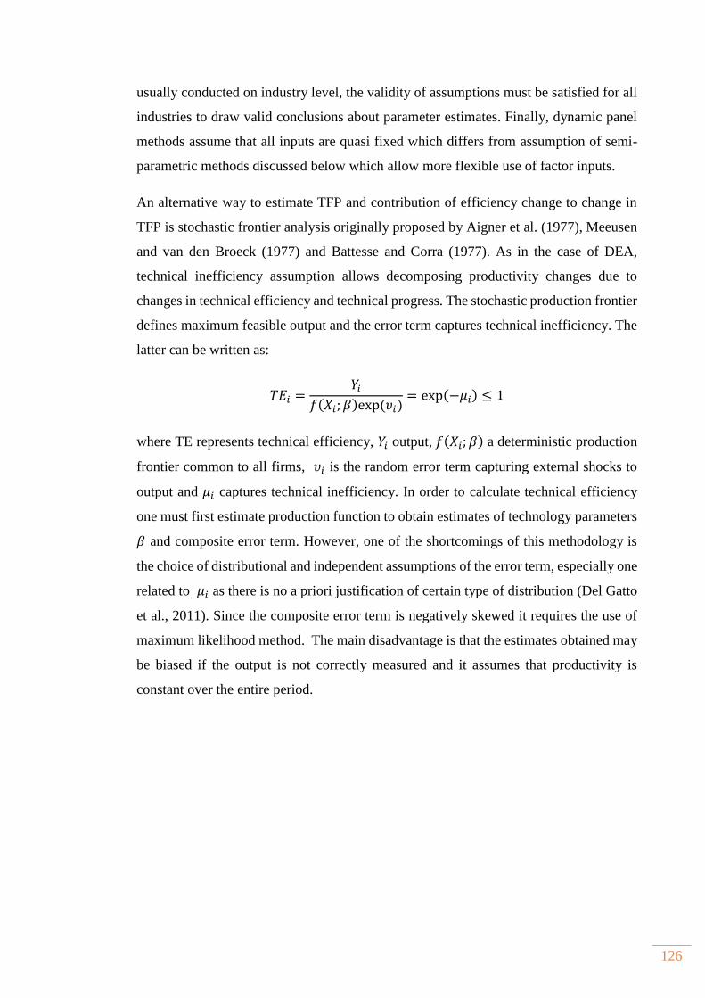
126
usually conducted on industry level, the validity of assumptions must be satisfied for all
industries to draw valid conclusions about parameter estimates. Finally, dynamic panel
methods assume that all inputs are quasi fixed which differs from assumption of semi-
parametric methods discussed below which allow more flexible use of factor inputs.
An alternative way to estimate TFP and contribution of efficiency change to change in
TFP is stochastic frontier analysis originally proposed by Aigner et al. (1977), Meeusen
and van den Broeck (1977) and Battesse and Corra (1977). As in the case of DEA,
technical inefficiency assumption allows decomposing productivity changes due to
changes in technical efficiency and technical progress. The stochastic production frontier
defines maximum feasible output and the error term captures technical inefficiency. The
latter can be written as:
𝑇𝐸𝑖 =𝑌𝑖
𝑓(𝑋𝑖; 𝛽)exp(𝜐𝑖)= exp(−𝜇𝑖) ≤ 1
where TE represents technical efficiency, 𝑌𝑖 output,𝑓(𝑋𝑖; 𝛽) a deterministic production
frontier common to all firms, 𝜐𝑖 is the random error term capturing external shocks to
output and 𝜇𝑖 captures technical inefficiency. In order to calculate technical efficiency
one must first estimate production function to obtain estimates of technology parameters
𝛽 and composite error term. However, one of the shortcomings of this methodology is
the choice of distributional and independent assumptions of the error term, especially one
related to 𝜇𝑖 as there is no a priori justification of certain type of distribution (Del Gatto
et al., 2011). Since the composite error term is negatively skewed it requires the use of
maximum likelihood method. The main disadvantage is that the estimates obtained may
be biased if the output is not correctly measured and it assumes that productivity is
constant over the entire period.

127
4.3 METHODOLOGICAL ISSUES IN ESTIMATION OF TFP
The most common approach used in estimating productivity is based on one specific
form of production function, namely Cobb-Douglas which can be written as:
Yit = AitKitβkLit
βl (4.1)
where Yit is output of firm i in time t, Ait is total factor productivity which is unobserved
by econometrician, Kit is capital and Lit is labour. βk and βl are intensities of capital and
labour respectively. The common assumption is that Ait is Hicks neutral which captures
disembodied technical change. 15F
16 TFP can be the result of both internal and external
factors mentioned in the previous section which are not directly related to any specific
factor inputs. For example, Ait may not be related only to technological differences across
firms, but can also include managerial ability, scope efficiency, expected machine
breakdown or cyclical effect (Katay and Wolf, 2008; Konings and Vanormelingen,
2010).
By taking natural logarithms Cobb-Douglas production function can easily be
transformed into linear equation suitable for empirical estimation which allows Ait to be
additively separable from other factor inputs.
ln(Yit) = β0 + βk ln(Kit) + βl ln(Lit) + ɛit (4.2)
and
ln (Ait) = β0 + ɛit
where β0 measures mean efficiency across all firms over time t and ɛit can be regarded as
deviations from the mean capturing (i) unobserved factors affecting firm output such as
managerial ability, (ii) measurement error in output and inputs, and (iii) random noise
(Eberhardt and Helmers, 2010).
Error term ɛit in eq. (4.2) can further be decomposed in anticipated productivity Hicks
neutral shock (𝜔𝑖𝑡∗ )affecting firms’ input choices and unanticipated productivity shock
16 Technical change is Hicks neutral whenever marginal rate of substitution between labour and capital
remains unchanged for a given capital/labour ratio. Therefore, it is assumed that any increase in output is
caused by disembodied technological changes such as advances in science, blueprints, diffusion of
knowledge, better marketing and organizational techniques without any changes in factor inputs.
128
or other sources of error (vit) not observed by the firms (Eberhardt and Helmers, 2010).
Unanticipated changes may include unexpected machine breakdown, workers’ strike, or
measurement problems in outputs and inputs. The productivity shock, unobserved
productivity or TFP (𝜔𝑖𝑡∗ )can be further divided into elements common to all firms and
specific to firms expressed in the following way:
𝜔𝑖𝑡∗ = ŋ𝑖 +ƴ𝑡 + 𝜔𝑖𝑡 (4.3)
where ŋi represents time invariant firm specific productivity term which arises from the
industry in which firms operate or geographical location and is captured by firm fixed
effects. This time invariant effect represents the permanent deviation of firm i from the
referene productivity level in the base year (Eberhardt and Helmers, 2010). ƴt is common
technological shock such as the introduction of new technology or macroeconomic shock
that affects all firms in the same way and represents the average productivity increase
over time. Finally, ωit is combined effect of firm specific deviation from its own TFP
level in the base period and average technological progress in period t (Eberhardt and
Helmers, 2010). 16F
17This firm and time specific effect or shock ωit can be attributed to “the
technical knowledge, the will, effort and luck of a given entrepreneur”(Marschak and
Andrews, 1944, p.145) in a given time period. In other words, technological shock does
not affect each firm in the same way as some benefit more that others. For example, firms
with higher productivity levels experience higher rate of technical progress in
comparison to firms with lower productivity levels (Eberhardt and Helmers, 2010).
Therefore, firm differences in responses to shocks observed over time are captured by
ωit.
After incorporating these elements18 into equation (4.2) we get:
ln(Yit) = βk ln(Kit) + βl ln(Lit) + β0 + ŋi + ƴt + ωit + vit (4.4)
The measure of the TFP is obtained as the residual from production function, i.e.:
ln (Ait) = β0 + ŋi + ƴt + ωit = ln(Yit) - βk ln(Kit) - βl ln(Lit) (4.5)
17 Since factor inputs can not affect output without taking into account ωit, i.e., the later “transmit to” the
input choices, this particular problem is known as the “transmission bias”. 18 “Given that the econometrician also does not observe the common productivity ƴt and that fixed
productivity effects may have a systematic relationship with the size of idiosyncratic shocks we could argue
that β0 + ŋi + ƴt + ωit are the productivity elements infuencing input choice” (Eberhardt and Helmers,
2010, p.6).
129
However, the estimation of (4.4) is not straightforward as the assumption that firms
operate on their production frontier may not be plausible due to different constraints
arising from market conditions, financing investment and hiring of employees (Kvinge,
2008). Furthermore, the assumption of perfect competition is not realistic as firms
compete selling differentiated products and charge prices above marginal costs. Also, the
Cobb-Douglas production function assumes that technology is Hicks neutral meaning
that it affects marginal product of labour and capital in the same way, which is a strong
assumption as firms operate in different industries (Van Biesebroeck, 2007). Therefore,
empirical estimation relies on relaxed assumptions by estimating production functions at
a more narrowly-defined industry level rather than at total sector level. Furthermore,
demand conditions are introduced in the model to capture pricing behaviour of firms.
An important issue not yet completely resolved in empirical work is the measurement of
variables. As a measurement of output, some studies employ gross output while others
use value added. Gross output allows to incorporate the contribution of material inputs
in addition to labour and capital. Theoretically, it is preferred measure of output because
it allows for substitution between materials and the other two inputs (Hall et al., 2009).
Basu and Fernald (1995) show that apparent productivity spillovers are the result of
specification error when using value added. They argue that in imperfect competitive
industries gross output provides a better measure. Furthermore, productivity measures
based on gross output specification are a valid representation of disembodied technical
change if production technology is assumed to be Hicks neutral (Schreyer and Pilat,
2001).
However, when using firm level data value added specification may be more appropriate
as share of materials in total output varies greatly across firms due to different degrees
of vertical integration (Hall et al., 2009). Use of value added allows comparison between
firms using heterogeneous intermediate inputs and allows taking into account different
quality of inputs (Salim and Kalirajan, 1999). Moreover, in order to properly account the
demand for intermediate inputs one should include the adjustment costs related to
stocking of material (Hall et al., 2009). Finally, as we measure TFP for services sector it
is difficult to define output since the latter is often intangible in nature and reflects quality
improvements. In addition, since data on actual quantities sold are unavailable in firm
level datasets one is able to consider only TFP based on deflated revenue. Syverson
(2011) takes into account the fact that firms produce more than one product. Therefore,
130
differences in revenues could be the result of differences of market power and this would
show up as productivity differences not arising from efficiency, but from price variation.
So far, empirical studies did not give a strong support to any specification suggesting a
more complex working of technical change (Schreyer and Pilat, 2001).
Similar critique can be applied to measurement of inputs. Griliches (1987) argued that
productivity dispersion is the result of measurement problems in inputs.17F
19 For labour, the
most common measure is the number of employees or cost of labour instead of number
of hours one actually worked. However, not all employees are equally productive and
thus usual measures of labour input do not reflect time, skills and effort of the workforce.
Capital is usually measured as a book value of fixed assets or constructed by using
observed investment and perpetual inventory method. Appropriate measure of capital
would include capital service of each asset type. However, flows of the quantity of capital
services are not usually directly observable and thus they are approximated assuming that
the quantity of an asset held by a firm is proportional to the usage obtained from that
asset (Eberhardt and Helmers, 2010). Furthermore, components of capital equipment
may be of different vintage and thus affect productivity differently (Whelan, 2002).
Transition economies face substantial measurement problems with the factor capital,
which arise due to the poor accounting standards and the tendency to misstate the value
of capital.
In the following subsections, several methodological issues will be explained in more
detail as they cause severe bias in factor elasticities and TFP estimation. Several
estimation techniques are reviewed together with their advantages and drawbacks.
Special attention is paid to structural estimators as they will be employed in estimation
of TFP. 18F
20
19 This claim disregards the fact that productivity dispersion can also be related to fixed firm characteristics.
If the latter are a significant driver of productivity, than reallocation of inputs across firms and industries
may be less effective and process of creative destruction may be needed to increase overall productivity,
thus requiring different policy responses (Fox and Smeets, 2010). 20 The review of potential econometric problems and solutions related to productivity estimation is based
on excellent reviews by Van Beveren (2012), Del Gatto et al. (2011), Eberhardt and Helmers (2010) and
Van Biesebroeck (2007).
131
4.3.1 SIMULTANEITY BIAS
The issue of simultaneity bias was raised by Marschak and Andrews (1944) who argued
that inputs in the production function are determined by the characteristics of the firm
and its reaction to external shocks. Therefore, the inherent problem in (equation 4.2) is
that firms’ choice of inputs is dependent on realized productivity shock which is only
known to the firm, but not to econometrician. The estimation of production function
using OLS requires that the inputs in the production are exogenous, i.e. determined
independently from the firm’s efficiency level. However, in empirical analysis it is not
possible to obtain unbiased and consistent estimates of the input coefficients as we do
not know how firms adjust their input choice based on productivity shocks specific to
them. Since productivity term is expected to transmit to input choices, this is known as
“transmission bias” (Griliches and Mairesse, 1995).
Hence, if there exist a positive serial correlation in firms’ productivity, a positive
productivity shock will lead to more variable inputs usage introducing an upward bias in
coefficients of labour and materials which are regarded as more flexible inputs than
capital which takes time to adjust (De Loecker, 2011). When correlation between capital
and labour is positive, capital coefficient will be biased downward and the estimation of
TFP will be difficult (Levinsohn and Petrin, 2003). Given that expected biases for
variable and quasi fixed inputs are different it is difficult to predict the impact on TFP.
For labour intensive industries and industries which use more variable inputs this implies
that TFP will be biased downward if not corrected for endogeneity. The opposite holds
for capital intensive industries (Van Beveren, 2012).
Traditional methods to deal with heterogeneity and endogeneity issues include fixed
effects and instrumental variables estimation (Wooldridge, 2009). However, both
methods are plagued by several problems discussed later. The use of Olley-Pakes (1996),
Levinsohn-Petrin (2003), Ackerberg et al. (2007) and Wooldridge (2009) estimators
solve these issues, although the data requirements and assumptions among the
methodologies differ.
132
4.3.2 SELECTION BIAS
Several theoretical models of firm growth and dynamics predict that productivity
differences are a major source of firm’s entry and exit (Jovanovic, 1982; Hopenhayn,
1992). More recently, new trade models emphasise the importance of firms’ productivity
distribution and the integration process (Melitz, 2003; Melitz and Ottaviano, 2008;
Bernard et al. 2007) as well as the determinants of these differences (Bernard and Jensen,
1999; Del Gatto et al., 2011). Therefore, when estimating production function one must
take into account selection bias which emerges because firms do not exit the market
randomly, but because of their low productivity. Decisions on the allocation of inputs in
a particular period are made conditional on its survival (Van Beveren, 2012). The latter
is a function of productivity shock and observed capital stock.
Firms with large capital stock are more likely to stay in the market. This holds even if
they experience negative productivity shock in comparison to firms with lower capital
stock which exit. This will in turn generate negative correlation between capital input
and unobserved productivity. Consequently the capital coefficient will be biased
downwards and TFP estimates will be biased upwards if dynamics of firms’ exit process
have not been taken into account (Eberhardt and Helmers, 2010). Furthermore, omitting
firms’ exit and use of balanced panels exert an additional upward bias in TFP. This is
because exiting firms tend to have low levels of capital stock and low productivity and
omitting these firms will result in lower factor elasticities and higher estimated TFP on
average. The estimation algorithm developed by Olley and Pakes (1996) takes the
selection bias explicitly into account.
4.3.3 OMITTED PRICE BIAS
Generally, firm price levels are not available, thus researchers are confined to use
industry-level price indices to deflate firm-level sales and input expenditures in
traditional production function estimates (De Loecker, 2011). The deflated values of
output and inputs namely revenue, capital and materials using industry deflators, are thus
typically used as proxies for their quantities. Therefore, given the data available, most
studies use revenue based TFP. However, the use of the price index is only valid under
the assumption of perfect competition, i.e. if all firm level prices do not deviate from
133
deflators used, if firms produce homogeneous products and face a common and infinite
price elasticity of demand (Melitz, 2001). If prices reflect market power arising from
firms’ size or production of differentiated products, deflated values of firms’ output using
single industry deflators is a second best solution to measure quality or efficiency
differences. The consequence of using industry level prices is a bias in input coefficients
since choice of inputs is dependent on unobserved firm level price variation (Klette and
Griliches, 1996).
Standard supply demand framework assumes that inputs and outputs are positively
correlated, while output and prices are negatively correlated. Thus, the correlation
between (variable) inputs and firm level prices captured in error term will be negative.
This will result in a negative bias for the coefficients of labour and materials (De Loecker,
2011)19F
21. The presence of imperfect competition can additionally be extended to input
markets as input prices are also firm specific. As with output prices, input prices usually
proxied by deflated values of inputs for capital and materials since actual quantities are
mostly unavailable. Again, failure to take into account firm price deviations of input
prices result in upward biased estimates of TFP if firms’ input prices are lower than
industry prices leading to underestimation of input use (Van Beveren, 2012). De Loecker
(2011) argues that if imperfect output markets are treated explicitly by including demand
for output in the system, the omitted input price bias can be partially solved due to their
positive correlation with output prices.
4.3.4 MULTIPRODUCT FIRMS
Bernard et al. (2009) have recently questioned the relevant level of analysis for the
estimation of a production function if firms produce multiple products. Since production
function assumes that firms have identical production techniques and final demand
(using output deflators) across products manufactured by a single firm, TFP estimates
will be biased. In practice, single firms produce multiple products which use different
production techniques and face different final demand. Bernard et al. (2010) document
that 41% of all firms in their sample of US manufacturing produce multiple products.
21 For example, if firm is more efficient and is able to charge lower prices than the rest of the industry,
the use of deflated sales will result in underestimation of firm’s output for a given level of inputs and in
underestimation of TFP and vice versa if a firm is less efficient than its competitors.
134
They find that two-thirds of firms alter their mix of five-digit SIC codes every five years.
Consistent estimation of TFP require detailed data on product types and number, product
output, inputs and prices which are almost never available to researchers. One of the
possible solutions to circumvent the data unavailability proposed by Bernard et al. (2009)
is to sort the firms into groups by products to obtain product level factor elasticities and
TFP. However, if there are synergies in the production process of different products
which raise firm efficiency, TFP may be underestimated. An alternative way to obtain
consistent and unbiased estimates of TFP is to allow for variation in production
parameters across firms with different product mix (Bernard et al., 2009).
4.4 SOLUTIONS TO ECONOMETRIC PROBLEMS
Several solutions to “transmission bias” arising from equation (4.4) have been proposed
in the literature. We begin by introducing methods which dominated the empirical
literature until recently. Then, Sections 4.4.1, 4.4.2 and 4.4.3 introduce structural models
which are now common empirical strategy when calculating TFP at the firm level.
Structural estimators explained below deal mostly with simultaneity and omitted price
bias which means that estimation of TFP will still suffer from other biases. Each
structural estimator has its own strengths and weaknesses, but for the purpose of this
research three methods will be used. OLS will serve as robustness check for Levinsohn
and Petrin (2003) and Wooldridge estimators (2009). Other econometric problems
mentioned above are partially addressed. Selection bias is solved by using unbalanced
panel as estimation of survival probability in Olley and Pakes (1996) structural estimator
which implicitly takes into account firms entry and exit could not be employed due to
lack of investment data and noisy measure of exit in Amadeus database. However, other
estimators have shown that incorporation of the survival probability has small efficiency
gains in comparison to use of unbalanced panel of firms (Levinsohn and Petrin, 2003;
Van Beveren, 2012).
In order to tackle omitted price bias two approaches have been developed so far. First,
Klette and Griliches (1996) suggest using growth in industry output as an additional
variable in firm production function. De Loecker (2011) proposes to control for within

135
industry price and demand shocks by estimating market demand. Practical
implementation of solution for omitted price bias in the Olley and Pakes estimator was
developed by De Loecker (2011) under the assumption of Dixit Stiglitz demand system.
By estimating augmented production function one can obtain true elasticities of input
coefficients by multiplying them with the relevant mark-up. The problem with this
approach is that it requires explicit assumption about market structure which leads to
question the plausibility of estimates (Dumont et al., 2014). The second approach is to
use firm level prices to deflate firm output. For example, Foster et al. (2008) found
significant differences in TFP estimates when using firm level output prices instead of
industry level on data from Colombian manufacturing sector. By using industry deflated
sales, the productivity is especially underestimated for young firms that usually charge
lower prices for their products.
However, data on price variation are not available in most firm level datasets. Therefore,
De Loecker et al. (2012) obtained product level information on prices and quantities to
obtain firm price index. Using product level data for Spanish manufacturing firms,
Ornaghi (2006) invalidates the correction proposed by Klette and Griliches (1996) due
to existence of asymmetric biases among the input coefficients. Multiplying asymmetric
coefficients with the same correction term does not yield unbiased input coefficients.
Furthermore, Mairesse and Jaumandreu (2005) argue that the use of firm level prices
when available has little effect on the estimated coefficients. Similarly, Dumont et al.
(2014) use PRODCOM database for Belgian manufacturing firms to control for possible
omitted bias when estimating firm level efficiency. They do not find many indications of
systemic bias from the use of industry price deflated revenues as indicator of output.
Correction for omitted price bias is not applied in this thesis for several reasons. First,
we do not have data on investment which is necessary for employing Olley and Pakes
(1996) estimator. Second, correction for omitted price bias employed in this estimator
only possibly corrects the omitted output bias assuming equal demand elasticities across
firms, while a formal solution for the bias induced by firm-specific input prices has yet
to be introduced. Finally, the correction of bias arising from multiproduct firms is not
possible in the absence of product level data on inputs and outputs.
The empirical specification which forms the basis of further discussion is:
136
ln(Yit) = βk ln(Kit) + βl ln(Lit) + β0 + ŋi + ƴt + ωit + vit (4.6)
4.4.1 TRADITIONAL SOLUTIONS TO ENDOGENEITY OF INPUT CHOICE
Traditional solution to the unobserved heterogeneity and endogeneity issues is related to
panel firm fixed effects (FE) by using cross sectional dummy variables or mean
differencing. In order to deal with simultaneity bias the strong assumption of constant
productivity differences across firms must hold. 20F
22 Therefore, any productivity increase
over time (ƴt) captured in the model by year dummies must disseminate to all firms
equally and within the same period (Eberhardt and Helmers, 2010). Moreover, selection
bias can be resolved since the assumption is that endogenous exit decisions are
determined by time invariant productivity and not by random component. The alternative
is to allow for firm specific productivity shocks, but allow inputs to be exogenous.
However, as noted by Wooldridge (2009) this is a strong assumption that is not likely to
hold in practice. Using fixed effects has the additional drawback of removing substantial
information from the data, since only variation over time remains to identify the
parameters (Eberhardt and Helmers, 2010). Finally, empirical estimation using FE on
both unbalanced and balanced panel has provided unreliable coefficient estimates which
is especially pronounced in very low capital coefficients leading to severely decreasing
returns to scale and selection bias (Olley and Pakes, 1996; Eberhardt and Helmers, 2010).
The problem of endogeneity can also be solved using an instrumental variable (IV)
approach. This method uses instrument which should be correlated with endogenous
variable, do not enter production function directly and are uncorrelated with firm
unobservable productivity (Greene, 2008). There are several possible instruments one
can use such as input/output prices, variables that shift demand or supply for output and
inputs and lagged levels of inputs (Ackelberg et al., 2007). By using lagged input prices
one must assume that inputs market is perfectly competitive, the assumption being
somewhat implausible. Firms with market power have more influence to set market
prices in response to the input quantities and its productivity. This induces correlation
between prices and productivity invalidating prices as good instruments (Van Beveren,
22 Since fixed effect transformation wipes away firm specific effect (ŋi) as it is time invariant it is necessary
to assume that there are no further firm specific productivity shocks in order to tackle the endogeneity
issue.
137
2012). Furthermore, prices need to be firm-specific and exhibit variation across firms to
reflect input choices in the first stage of IV regression (Eberhardt and Helmers, 2010).
Finally, most of available micro data do not report firm level prices. Using wages as
instrument for labour imply exogenous labour market conditions. However, higher wages
usually reflect better skills and qualifications (e.g. efficiency wage argument) and thus
the latter factors are correlated with productivity making wage invalid instrument (Van
Beveren, 2012).
IV deals with endogeneity of inputs, but not with selection bias. Firms facing higher input
prices will be more likely to exit because of higher costs, thus leading to correlation
between instruments and error term (Ackerberg et al., 2007). Turning to two other
possible instrument sets mentioned above does not solve the problem. Firstly, variables
that shift demand or supply are difficult to find. Second, by first differencing production
function and using lagged input levels as instruments for their changes leads to downward
biased, often insignificant capital coefficient and very large decreasing returns to scale
due to weak correlation of input levels with its changes (Blundell and Bond, 2000). 21F
23
In order to solve the problems related to “transmission bias” and selection bias several
structural models of firm behaviour were developed (Olley and Pakes, 1996; Levinsohn
and Petrin, 2003; Ackerberg et al, 2007; Wooldridge, 2009). All these models rely on
observed input decisions to control for unobserved productivity (ωit). Since ACF and
Wooldridge estimators rely heavily on the assumptions of OP and LP the latter will be
briefly discussed before explanation of Wooldridge estimator as the preferred
methodology used to estimate TFP.
4.4.2 OLLEY-PAKES AND LEVINSOHN-PETRIN METHODOLOGY
Olley and Pakes (1996) were the first who adopted assumptions of structural model of
firm behaviour and explicitly modelled the firm’s optimization problem to derive their
production function estimator. The OP approach sets up a model where companies
operate in discrete time and make decisions to maximize expected discounted value of
23 As a possible solution to weak instrument problem Blundell and Bond (1999) proposed systems of
equations which use first difference of the variables as instrument for their levels which yields more
reasonable parameter estimates.
138
net cash flows. At the start of each period, incumbent firms decide either to exit the
market or to continue their operations. If firms stay in the market they choose appropriate
level of factor inputs and investment. They solve endogeneity problem by using
information about investment Iit to proxy for unobserved productivity (ωit) and apply
control function estimator. 22F
24 Selection issues are addressed by incorporating an exit rule
into the model (Van Beveren, 2012).
In general, structural estimators discussed in this section rely on certain assumptions.
Assumption 1. Capital is assumed to be a fixed input. Capital has also dynamic
implications for the next period arising from the following process:
Kit = (1-δ)Kit-1 + Iit-1 (4.7)
Where Kit is capital, δ is depreciation rate and Iit is investment of firm i in period t-1.
Since present capital level was decided in previous period and it takes one period to be
bought and installed it is not correlated with innovation in productivity ξit between t-1
and t. In Levinsohn Petrin (2003) capital stock depends on investment in period t.
In contrast, labour input is assumed to be a variable input chosen at the same time the
productivity shock is realized and is therefore correlated with the innovation ξit.
Furthermore, labour is also a static input implying that the present levels of labour input
do not affect the cost of labour in the future.
Assumption 2. The investment function (Iit) is fully determined by capital (Kit) and
unobserved productivity ωit. This can be represented as Iit = ft(Kit, ωit). As argued by
Ackerberg et al. (2006) scalar unobservable assumption implies that any unobserved
heterogeneity in adjustment costs of capital, demand or labour market conditions across
firms is ruled out. It also assumes perfect factor and product markets. In case of imperfect
competition firm level input prices will determine the optimal level of investment and
therefore they should enter inverted function 𝑓𝑡−1 defined below (Ornaghi and Van
Beveren, 2012).
Assumption 3. Unobserved productivity ωit can be proxied using an observable firm
decision such as choice of investments. It is assumed that choice of investments is strictly
24 Control function approach is an alternative to instrumental variable approach and consists of deriving a
proxy variable that accounts for any unobserved factors which may affect endogenous variables.
139
increasing with state variables capital and unobserved productivity. This implies that
firms with higher productivity or capital invest more. As a consequence, only non-
negative values of investment can be used in the analysis. This condition needs to hold
for at least some known subset of the sample (Van Beveren, 2012). Following the
monotonicity assumption and provided that investment is positive, productivity can be
expressed as inverted investment equation.
ωit = 𝑓𝑡−1 (Iit,Kit) (4.8)
Since the 𝑓𝑡−1
would require solving complicated dynamic programming problem, its
functional form is proxied by higher order polynomial terms in investment variable and
state variables and estimated non-parametrically.
Assumption 4. Productivity follows a first order Markov process. This implies that
future productivity is determined only by information known at current period and
exogenous productivity shock which arise between time t and t+1. The latter is assumed
to be uncorrelated with productivity (ωit) and capital in t+1 (Ornaghi and Van Beveren,
2012). Therefore evolution of productivity can be represented as: ωit = Ε[ωit | ωit-1] + ξit
= g(ωit-1) + ξit where g is an unknown function and innovation term ξit is introduced
which is the deviation from the expected productivity level which is mean independent
of any information at t − 1 or before, and is thus not foreseeable by the firm.
The potential issue with Olley and Pakes estimator is that data on investment are rarely
available or large number of observations report missing values or zero investment thus
causing violation of monotonicity assumption. Levinsohn-Petrin (2003) suggested that
monotonicity condition is more likely to hold by using intermediate inputs as a proxy
variable. Using intermediate inputs increases the sample size as data on material inputs
are more widely available in firm level databases. The reason for using intermediate
inputs is that under assumption of perfect markets higher productivity implies higher
marginal product of capital and thus firms will increase production until marginal product
of capital equals its rental rate (Katay and Wolf, 2008). By increasing their output firms
also increase the usage of intermediate inputs, therefore providing information about
productivity of firms. 23F
25
25 However, firms’ productivity may be increased by better quality management or improvements in
organization of production process, thus making intermediate inputs less responsive to productivity shocks.
140
In LP estimation labour and intermediate inputs are freely available and chosen
simultaneously once that unobserved productivity is known to the firm. LP specify the
demand for intermediate inputs as Mit = ft(Kit, ωit). They use the same method of
inverting out ωit with the difference that productivity is a function of capital and
materials.
ωit = ht(Kit,Mit) (4.9)
In this way, observable variables, namely capital and material costs give information
about productivity. By substituting equation (4.9) in equation (4.6) one gets: 24F
26
ln(Yit) = β0 + βk ln(Kit) + βl ln(Lit) + ŋi + ƴt + ht(Kit,Mit) + vit (4.10)
In practice, LP or OP production function estimator is implemented in two steps. First,
by regressing output (Yit) on labour input (Lit) and a nonparametric function ϕ(Kit, Mit)
which act as a proxy for unobserved productivity. If labour had dynamic implications,
its identification would not be possible in the first stage. This is because in the case of
firing and hiring costs labour would not be perfectly adjustable, and therefore it would
enter the set of state variables on which the choice of proxy variables depends (Ornaghi
and Van beveren, 2012). The following equation can be estimated by Ordinary Least
Square (OLS):
ln(Yit) = βl ln(Lit) + ϕ(Kit, Mit) + vit (4.11)
where ϕ(Kit, Mit) = β0 + βk ln(Kit) + ht (Kit, Mit) (4.11a)
ϕ(Kit, Mit) is approximated by a higher-order polynomial in Mit and Kit (including a
constant term). 25F
27 In order to account for time variation, polynomial terms are interacted
with time or by including time dummies in first stage of regression.
The first stage provides an estimate of ϕ(Kit, Mit) and unbiased and consistent estimate
of labour.26F
28 It solves endogeneity of capital and productivity because the firm-observed
26 Structural estimators discussed here are not able to account for time invariant firm level fixed effects (ŋi)
while common shocks (ƴt) are accounted for by including year dummies or interacting the polynomial
function with time. 27 LP suggest estimation based on a third-order polynomial series expansion, but any other flexible
estimation approach is valid. 28 β0 cannot be identified as it is included in polynomial term.

141
productivity has been controlled for by ϕ(Kit, Mit). Capital is not identified in the first
stage as it is included in polynomial term and would lead to collinearity issues with non-
parametric function. Second stage identifies capital coefficient using estimated ϕ under
the assumption that ωit follows a first order Markov process defined as ωit = Ε[ωit | ωit-1]
+ ξit = g(ωit-1) + ξit. As before g is an unknown function and ξit represents productivity
innovation not foreseeable by firm at time t-1, where capital is decided, the two are
orthogonal and thereby uncorrelated. This moment condition is necessary to identify
capital. Given the obtained estimate of labour in the first step the production function can
be expressed as:
Yit - βl Lit = βk Kit + ωit + vit (4.12)
Following Markov process gives us:
Yit - βl Lit = βk Kit + g(ωit-1) + ξit + vit (4.13)
= βk Kit + g(ϕ(Mit-1, Kit-1) - βk Kit-1) + ξit + vit
Finally by using ϕ(Kit, Mit) and estimated labour coefficient from first stage LP/OP
propose the following empirical model:
Yit - βl Lit = βk Kit + ��(ϕ it-1 - βk Kit-1) + ξit + vit (4.14)
Use of non-linear least squares is required due to βk entering the equation twice and in
combination with other parameters (Eberhardt and Helmers, 2010). Due to the fact that
innovation shock (ξit) and labour input are contemporaneously correlated, LP and OP
subtract βl (Lit) from the output using the coefficient obtained in the first stage regression.
Capital stock is exogenous with respect to innovation shock (ξit) since its level is
determined in the previous period. Therefore capital cannot be affected by change in
productivity in current period (ξit) (Eberhardt and Helmers, 2010). ��(ϕ it-1 - βk (Kit-1) is
found using higher order polynomials as in the first stage and its estimate is not of
particular interest in the second stage.
In summary, both OP and LP achieve identification of labour coefficient through specific
structural assumptions. In both estimators labour is a static input chosen in time t which
does not affect cost of input in time t+1. This assumption is necessary as otherwise if
labour is chosen before investment it will become part of state space on which the optimal
142
amount of proxy is determined. In this case identification of labour would not be possible
using inverted investment function as a proxy for unobserved productivity (Katay and
Wolf, 2008). In LP labour and material costs are assumed to be perfectly variable inputs.
In other words once productivity shock is observed, they adjust immediately within the
same time period. In case materials are chosen before productivity shock, inverse demand
function for intermediate inputs would not be possible. Identification of capital has also
timing assumptions and is treated as “quasi fixed” input where its current level is
determined before the occurrence of productivity shock.
It should be noted that consistency of control function depends on how closely
unobserved productivity is approximated by polynomial function. If scalar unobservable
assumption fails, approximation error between true productivity and those approximated
by proxy variables can lead to inconsistent estimates. The failure of this assumption can
happen due to omitted observables and different investment or intermediate inputs
responses to permanent and transient changes in TFP (Stoyanov and Zubanov, 2014).
Furthermore, as argued by Ackerberg et al. (2007) productivity is a complex function of
many observables and unobservables and may not follow first order Markov process.
This is especially worrisome in case of OP as investment may respond to demand factors
that are independent of firm’s productivity, thus invalidating monotonicity condition
(Van Beveren, 2012). In case that productivity follows a higher order Markov process,
control function in the first stage is not able to capture additional lags unless additional
proxy variables are available. The same holds for second stage as consistency of results
relies on Assumption 4 (Stoyanov and Zubanov, 2014).
4.4.3 ACKERBERG CAVES FRAZER CRITIQUE
The main assumption in above described estimators is that at least one of the inputs is
flexible. In gross output specification those are intermediate inputs and labour, while in
value added specification it is only labour. As discussed in detail by Bond and Soderbom
(2005) and Ackerberg et al. (2006) in order for labour coefficient to be identified in the
first stage there must exist sample variability that is independent of other regressors. To
illustrate this we take LP estimator as a starting point. Under the assumption of perfect
competition and dynamic properties of capital coefficient, firm state variables at time t

143
are represented by ωit, Kit, Pt Wt. and Zt where output price (Pt), wages (Wt). and
intermediate input price (Zt) are assumed to be constant over firms. Ackerberg et al.
(2006) point out that the first stage of OP and LP fails to identify labour coefficient
because it is the function of the same state variables ωit and kit, i.e. it is correlated with
the non-parametric terms ϕ(Kit, Mit). The problem is more acute in the case of LP
estimator as it assumes that labour and materials are chosen simultaneously and are
allocated in similar ways. This implies that both materials (Mit) and labour (Lit) are
chosen as a function of productivity (ωit) and capital (Kit).
Mit = ft (ωit,Kit)
Lit = gt (ωit,Kit)
Therefore, there is no independent source of variation at the firm level which could help
identify labour coefficient in the first stage. Using invertibility condition from LP, where
ωit = ft-1(Mit, Kit), Ackerberg et al. (2006) showed the following:
Lit = gt [ft-1(ωit, Kit), Kit] = ht (Mit, Kit) (4.15)
Since labour is a function of both ωit and kit it is not possible to simultaneously estimate
a nonparametric function of ωit and kit together with the labour coefficient leaving the
latter unidentified. To solve the issue of collinearity, Ackerberg et al. (2006) assume that
labour is chosen by the firm at time t - b, where 0 < b < 1 as it is “less variable” than
materials which is chosen at time t. This implies that firms choose labour prior to
materials, but after capital stock has been determined in t-1. Now labour enters the
demand function for intermediate inputs as a state variable which can be expressed as:
Mit= ht (ωit, Kit, Lit ) (4.16)
Maintaining the scalar unobservable assumption in practice, the first stage is
implemented by regressing output on a polynomial function of labour, capital and
intermediate inputs. The estimated output net of ɛit is then simply the residual from the
first stage regression:
γit - ɛit = ��𝑘Kit + ��𝑙 Lit + 𝑔 (Mit, Kt, Lt) (4.17)
First stage is used only to eliminate the part of output determined by some random
component of unobservables (ɛit) such as measurement error of inputs or unanticipated
shocks at time t from productivity shock observable by the firms (Eberhardt and Helmers,
144
2010). Estimation of above equation gives an estimate of ϕ(polynomial function) which
is used to identify input coefficients in the second stage. To do this, the assumption that
productivity follows first order Markov process is defined as:
ωit = Ε[ωit | ωit-1] + ξit (4.18)
where ξit represents innovation in productivity explained earlier. Since it is assumed that
capital is uncorrelated with productivity (ωit) as investment decisions are made in t-1
identification of capital coefficient is possible as Ε[ξit | Kit] = 0. The identification of
labour coefficient depends on the timing assumptions. If labour is assumed to be
independent of innovation in productivity because of adjustment frictions or training
requirements moment conditions are defined as Ε[ξit | Lit] = 0. On the other hand, if labour
is allowed to be correlated with productivity innovation than it needs to be instrumented
and the moment conditions are Ε[ξit | Lit-1] = 0 (Ornaghi and Van Beveren, 2012). In
practice, after obtaining ϕ from the first stage regression productivity is computed as:
ωit = �� - βk ln(Kit) - βl ln(Lit) (4.19)
where starting values of input coefficients are obtained using OLS. After approximating
ωit next step is to non-parametrically regress ωit on ωit-1 (eq. 4.18) and obtain residuals,
i.e.ξit which represent innovation in productivity. The last step is to solve optimization
problem through iterative process in order to achieve a global minimum when the process
stops and final values of input coefficients are obtained (Eberhardt and Helmers, 2010).
4.4.4 WOOLDRIDGE ESTIMATOR
Wooldridge (2009) proposes that instead of two step approach, inputs can be estimated
in one step. He argues that two step estimators discussed above which require
bootstrapping technique to obtain standard errors are inefficient because of two reasons:
(i) they ignore the contemporaneous correlation in the errors across two equations and
(ii) there is no correction of autocorrelation and heteroscedasticity in the errors.
Furthermore, Wooldridge estimation technique also allows the inclusion of cross
equation restrictions and an option to test the validity of the specifications using the
Sargan-Hansen test of overidentifying restrictions.

145
The assumption in equation (4.10) is that materials, labour and capital are uncorrelated
with the errors. Wooldridge defines a stronger form to include independence of past
values of inputs:
E (vit | Lit, Kit, Mit, Li,t-1, Ki,t-1, Mi,t-1,…Li1, Ki1, Mi1) = 0 (4.20)
Second, productivity is assumed to follow a first order Markov process as in previously
described estimators:
E [ωit | ωi,t-1,…, ωi1] = E [ωit | ωi,t-1] + ξit (4.21)
where ωi,t-1 = g(Ki,t-1,Mi,t-1) and ωit = j(ωi,t-1) + ξit
He notes that in the second stage capital coefficient can be estimated by using lagged
values of intermediate inputs and labour. Therefore, to reinforce the assumption that
current levels of capital are orthogonal to productivity shock, it is also assumed that
productivity innovation ξit is uncorrelated with past values of the state variable Kit as well
as Lit-1 and the proxy variable M.
Replacing ϕ(Kit, Mit) in equation (4.11) with the term in (4.11a) and plugging ωit = f
[g(Ki,t-1,Mi,t-1)] + ξit into equation (4.6) gives two systems of equations with same
dependent variables:
ln(Yit) = β0 + βk ln(Kit) + βl ln(Lit) + h(Ki,t,Mi,t)] + vit (4.22)
ln(Yit) = β0 + βk ln(Kit) + βl ln(Lit) + f [g(Ki,t-1,Mi,t-1)] + ξit + vit (4.23)
The final result is that we have two equations (4.22 and 4.23) that identify labour and
capital. In order to estimate these two equations by GMM the orthogonally conditions
must be satisfied. The orthogonally conditions for equation (4.22) are outlined in
equation (4.20), while for equation (4.23) are:
E (uit | Kit, Li,t-1, Ki,t-1, Mi,t-1,…Li1, Ki1, Mi1) = 0 where uit = ξit + vit (4.24)
In order to take into account the ACF critique which argues that neither of the parameters
can be identified as labour is a deterministic function of polynomials of capital and proxy
variable, Wooldridge proposes to estimate a single equation model similar to equation
(4.23). Specifically, empirical model requires specifying the functions f and g and
common practice is to include the third degree polynomials in Kt-1 and Mt-1.
146
4.5 DATA AND DESCRIPTIVE STATISTICS
Central to the empirical analysis is the firm level Amadeus database. It is a commercial
database provided by Bureau van Dijk updated on a regular basis and contains financial
information on over 19 million private and publicly owned firms across different sectors
and regions in 43 European countries (update of November 2011). The time horizon goes
back to year 1996 for some European countries. However, given that the coverage was
poor prior to year 2002, we limit our analysis to data between years 2002-2010. Because
of its large scope it is suitable for economic analysis of firm behaviour across industries,
geographical areas or firms’ size. Moreover, since it collects firm level information for
up to 10 years it enables creation of longitudinal data and analysis of firm behaviour and
determinants. This advantage is rarely available in national business surveys in which
firms are selected on the basis of a rotating sample to minimise response burdens (Ribeiro
et al., 2010).27F
29
A further advantage of the database is that it provides common definition and comparable
information on 25 balance sheet items and 25 profit and loss account items which adhere
to international standards. This enables avoiding possible errors which may arise with
different sources of data, various units of measurement, uneven sector coverage and
inconsistencies in inclusion criteria (Bos and Zhang, 2013). Therefore, the maximum
level of comparability across countries is ensured as data quality for this type of
administrative information can be easily checked using basic accounting algebra. In
addition to financial information, Amadeus also provides other firm level information,
such as date of incorporation, legal status, region and city, detailed industry classification
and what is central to the analysis, detailed ownership information. Ownership Database
permits to retrieve information on the control chain and the ownership type (foreign or
domestic; industrial or individual; controlled or independent). Furthermore, an important
advantage of Amadeus is that it provides the exact percentage of equity held by foreign
investor. Hence, continuous measurement allows us to estimate the marginal effects of
29 For example, Amadeus database has been widely used to explore the effects of entry regulation on
business dynamics (Klapper et al., 2006), international rent sharing within MNCs (Budd et al., 2005),
product market regulation (Arnold et al., 2008), the effects of employment protection legislation and
financial market imperfections on investment, job reallocation and labour productivity (Cingano et al.,
2010) and effects of FDI spillovers on productivity (Javorcik and Spatareanu, 2008; Javorcik and Li, 2008;
Gersl et al., 2008, Damijan et al., 2013a).
147
foreign ownership and related heterogeneity more precisely than with the binary “yes/no”
variables.
Amadeus database also has drawbacks. The quality of data is inferior to data obtained
from National Statistical offices. For example, the amount and quality of data depend on
accounting standards in each country and legal obligation of firms to reports certain
items. This reflects the use of several national sources which have different threshold for
firms to be included in the database. Therefore, the number of firms and quality of data
is biased towards countries with more demanding accounting standards. Moreover, this
may also create sample selection bias towards larger firms. In addition, firms which do
not provide data for the last four years are removed from the database with their entire
history. Hence, any variation in information retrieved from the database can be the result
of sample fluctuations and not related to change in the indicators. As the aim of the
chapter is to estimate and explore any differences in productivity estimates across several
dimensions as well as differences between domestic and foreign firms the availability of
reliable firm level data is crucial along two important dimensions: the coverage of the
database and the quality of the data available for each country, issues explored in more
detailed in the next subsections. Despite these drawbacks Amadeus database remains the
best available database for cross country analysis (CompNet Task Force, 2014).
4.5.1 SAMPLE DESCRIPTION
The November 2011 edition of Amadeus database is used for the estimation purpose,
covering the time period of 2002-2010. The data are taken from “full” version of
Amadeus with no thresholds applied to the number and types of firms included. The
sample is restricted to the following countries: Estonia, the Czech Republic, Slovakia,
Slovenia, and Hungary. The choice of the countries was guided by data availability and
time constraint when accessing the data. The initial sample contained 1,236,219 firms.
However, after cleaning the dataset for the purposes of productivity estimations we ended
up with 96,567 firms representing around 8 per cent of the original dataset. 28F
30
30 Detailed cleaning procedure is explained in the Appendix II.
148
In order to differentiate between domestic and foreign companies Amadeus ownership
database provides information along three dimensions (independence indicator, ultimate
owner and shareholders) which are used to calculate percentage of shares held by foreign
shareholders. 29F
31 We use several information available to separate foreign and domestic
firms. These are “shareholder ID”, “shareholder name”, “shareholder direct %”,
“shareholder total %”, and “shareholder country” available for each year. The most
recent version of Amadeus enables to track ownership changes across years which is a
significant improvement over previous studies which were able to disentangle firms
based on only the most recent information, thus assuming that local firm was foreign
through entire period. In order to identify foreign firms we rely on direct ownership link
since this is taken from original source and not amended by BvD. Firm is defined as
foreign if foreign shareholder identified by “shareholder country” has acquired at least
10 per cent of equity stake in local company. This definition of foreign owned company
is in line with OECD or IMF classification. In order to be classified as foreign, data on
country of origin must be available. Therefore, private individuals are excluded since
there is no information about their nationality and in such cases it is often assumed that
the owner is located in the same country as acquired company (Rosen et al., 2013;
Merlevede et al., 2015). Furthermore, as argued by Lesher and Miroudot (2008) private
foreign individuals are less likely to have any active role in the management of company
and therefore do not represent “true foreign presence” which is important to gauge the
potential of productivity spillovers in the following chapters.
To illustrate the coverage of Amadeus database we compare the original augmented
version to Eurostat Structural Business Surveys (SBS). The comparison is limited to
manufacturing sector and service sector (NACE 1.1 Rev. at 2 digit codes 15-74) since
productivity estimation and subsequent analysis of FDI productivity spillovers in the next
chapter is based on these two broad sectors of economy. Data in Table 4.1 below are
averaged over industry-time cells by country. After assigning each firm to specific cell
we calculate average number of employees and average turnover as a share of
corresponding aggregate from SBS. The calculations are based on entire universe of
firms which report the indicated variable. As can be seen, the coverage of Amadeus in
terms of employment and turnover is high in all countries except in Slovenia for both
variables and Hungary for employment. Averaged over countries, our dataset covers at
31 Detailed calculation of foreign ownership share is provided in Appendix II.
149
least 47 per cent of employment and 63 per cent of total turnover in the economy. In
general, it seems that Amadeus includes larger firms. Since the main interest is in the
sample of firms for which productivity can be estimated the last three columns in the
table show that the number of firms reporting number of employees is very low with the
exception of Estonia and Slovakia. Further, when we impose additional restrictions on
firms reporting turnover as well, the share of firms drops slightly with the exception of
Slovakia where the drop is now significant. Finally, the last column shows the share of
firms for which productivity estimation is possible. As expected, the number of firms
drops even further. While Slovakia and Estonia keep relatively large number of firms
and may be regarded as fairly representative sample of firms, data quality for Hungary is
very poor as we end up with only 0.5 per cent of firms. This representativeness is similar
to CompNet database of the ECB Competitiveness Research Network (CompNet Task
Force, 2014). Provider of the data, Bureau-Van-Dyke (2010) does not provide any
explanation why the data on some key financial variables are missing. It may be that
firms in transition countries do not meet their legal obligations of submitting reports to
authorities since penalties are low. Dall’Ollio et al. (2013) also discuss that there is an
overall bias towards larger firms in Amadeus which is also confirmed in our case if we
look at Table 4.2 below. Overall, micro firms are underrepresented while other categories
are overrepresented. This bias even increases when we limit the comparison to TFP
estimation sample and is especially pronounced in Hungary.
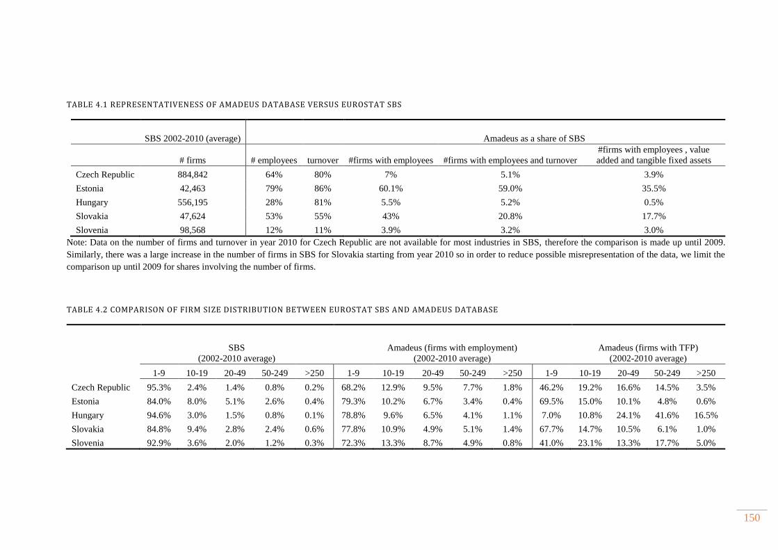
150
TABLE 4.1 REPRESENTATIVENESS OF AMADEUS DATABASE VERSUS EUROSTAT SBS
SBS 2002-2010 (average) Amadeus as a share of SBS
# firms # employees turnover #firms with employees #firms with employees and turnover
#firms with employees , value
added and tangible fixed assets
Czech Republic 884,842 64% 80% 7% 5.1% 3.9%
Estonia 42,463 79% 86% 60.1% 59.0% 35.5%
Hungary 556,195 28% 81% 5.5% 5.2% 0.5%
Slovakia 47,624 53% 55% 43% 20.8% 17.7%
Slovenia 98,568 12% 11% 3.9% 3.2% 3.0%
Note: Data on the number of firms and turnover in year 2010 for Czech Republic are not available for most industries in SBS, therefore the comparison is made up until 2009.
Similarly, there was a large increase in the number of firms in SBS for Slovakia starting from year 2010 so in order to reduce possible misrepresentation of the data, we limit the
comparison up until 2009 for shares involving the number of firms.
TABLE 4.2 COMPARISON OF FIRM SIZE DISTRIBUTION BETWEEN EUROSTAT SBS AND AMADEUS DATABASE
SBS
(2002-2010 average)
Amadeus (firms with employment)
(2002-2010 average)
Amadeus (firms with TFP)
(2002-2010 average)
1-9 10-19 20-49 50-249 >250 1-9 10-19 20-49 50-249 >250 1-9 10-19 20-49 50-249 >250
Czech Republic 95.3% 2.4% 1.4% 0.8% 0.2% 68.2% 12.9% 9.5% 7.7% 1.8% 46.2% 19.2% 16.6% 14.5% 3.5%
Estonia 84.0% 8.0% 5.1% 2.6% 0.4% 79.3% 10.2% 6.7% 3.4% 0.4% 69.5% 15.0% 10.1% 4.8% 0.6%
Hungary 94.6% 3.0% 1.5% 0.8% 0.1% 78.8% 9.6% 6.5% 4.1% 1.1% 7.0% 10.8% 24.1% 41.6% 16.5%
Slovakia 84.8% 9.4% 2.8% 2.4% 0.6% 77.8% 10.9% 4.9% 5.1% 1.4% 67.7% 14.7% 10.5% 6.1% 1.0%
Slovenia 92.9% 3.6% 2.0% 1.2% 0.3% 72.3% 13.3% 8.7% 4.9% 0.8% 41.0% 23.1% 13.3% 17.7% 5.0%
151
4.5.2 VARIABLES DESCRIPTION AND DESCRIPTIVE STATISTICS
The financial data obtained from Amadeus are downloaded in ‘000 euros at the market
exchange rate in each year. Since for productivity estimation we need to obtain
comparable values over time adjusted for price changes, OECD STAN database was used
as a primary source to deflate nominal variables using industry price indices defined at
NACE 1.1 Rev. 2 digit level for output, capital and intermediate inputs expressed at 2005
constant prices. 30F
32 Because price deflators are expressed in national currency we used
year end exchange rates from European Central Bank (ECB) to convert euros back to
original currency values and applied price deflators to them. At the second stage deflated
values are converted back to euros at 2005 exchange rate to avoid that exchange rate
fluctuations would drive cross-country productivity comparisons (Gal, 2013).
Output is measured as total sales deflated by corresponding price deflator at NACE 1.1
Rev. 2-digit level. Value added is constructed as difference between real gross output
and real intermediate inputs. The latter are defined as material costs deflated by
intermediate price index. Capital is measured by stock of tangible fixed assets. Changes
in capacity utilisation cannot be accounted for which is a common problem in firm level
databases which may result in low capital coefficients. Labour is measured as number of
employees without further breakdown of employees’ characteristics or skills levels due
to unavailable information.
Before turning to TFP estimation, we will shed some light on the descriptive statistics of
the final dataset used for productivity estimation. The data in Table 4.3 show distribution
of domestic and foreign firms across countries, technology intensive sectors and years.
32 The exception is Slovakia for which data are not fully available and therefore we used the deflators
obtained from WIOD database at more aggregated group of industries. In addition, data for year 2010 are
not available for Estonia and Slovakia at 2-digit industry level, so we used total industry prices for major
sectors in the economy or if not available for total economy.
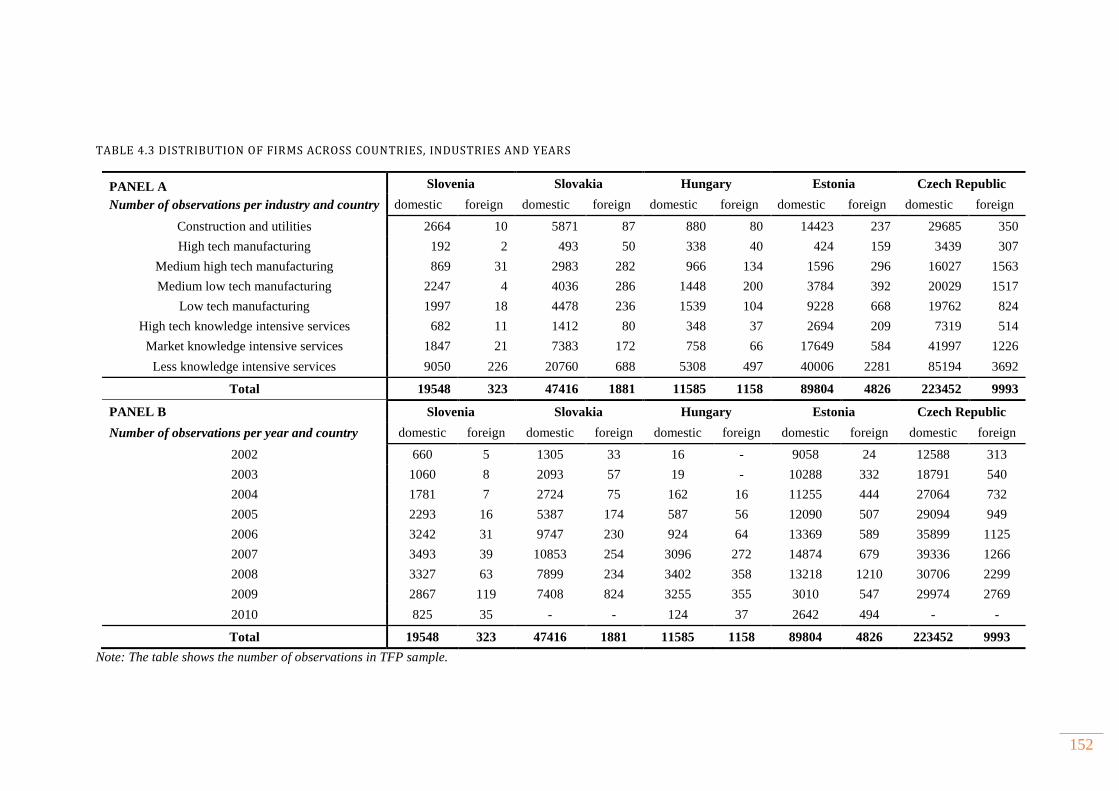
152
TABLE 4.3 DISTRIBUTION OF FIRMS ACROSS COUNTRIES, INDUSTRIES AND YEARS
PANEL A Slovenia Slovakia Hungary Estonia Czech Republic
Number of observations per industry and country domestic foreign domestic foreign domestic foreign domestic foreign domestic foreign
Construction and utilities 2664 10 5871 87 880 80 14423 237 29685 350
High tech manufacturing 192 2 493 50 338 40 424 159 3439 307
Medium high tech manufacturing 869 31 2983 282 966 134 1596 296 16027 1563
Medium low tech manufacturing 2247 4 4036 286 1448 200 3784 392 20029 1517
Low tech manufacturing 1997 18 4478 236 1539 104 9228 668 19762 824
High tech knowledge intensive services 682 11 1412 80 348 37 2694 209 7319 514
Market knowledge intensive services 1847 21 7383 172 758 66 17649 584 41997 1226
Less knowledge intensive services 9050 226 20760 688 5308 497 40006 2281 85194 3692
Total 19548 323 47416 1881 11585 1158 89804 4826 223452 9993
PANEL B Slovenia Slovakia Hungary Estonia Czech Republic
Number of observations per year and country domestic foreign domestic foreign domestic foreign domestic foreign domestic foreign
2002 660 5 1305 33 16 - 9058 24 12588 313
2003 1060 8 2093 57 19 - 10288 332 18791 540
2004 1781 7 2724 75 162 16 11255 444 27064 732
2005 2293 16 5387 174 587 56 12090 507 29094 949
2006 3242 31 9747 230 924 64 13369 589 35899 1125
2007 3493 39 10853 254 3096 272 14874 679 39336 1266
2008 3327 63 7899 234 3402 358 13218 1210 30706 2299
2009 2867 119 7408 824 3255 355 3010 547 29974 2769
2010 825 35 - - 124 37 2642 494 - -
Total 19548 323 47416 1881 11585 1158 89804 4826 223452 9993
Note: The table shows the number of observations in TFP sample.
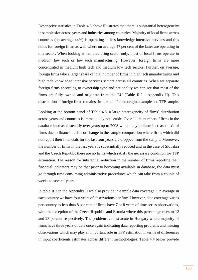
153
Descriptive statistics in Table 4.3 above illustrates that there is substantial heterogeneity
in sample size across years and industries among countries. Majority of local firms across
countries (on average 44%) is operating in less knowledge intensive services and this
holds for foreign firms as well where on average 47 per cent of the latter are operating in
this sector. When looking at manufacturing sector only, most of local firms operate in
medium low tech or low tech manufacturing. However, foreign firms are more
concentrated in medium high tech and medium low tech sectors. Further, on average,
foreign firms take a larger share of total number of firms in high tech manufacturing and
high tech knowledge intensive services sectors across all countries. When we separate
foreign firms according to ownership type and nationality we can see that most of the
firms are fully owned and originate from the EU (Table II.2 - Appendix II). This
distribution of foreign firms remains similar both for the original sample and TFP sample.
Looking at the bottom panel of Table 4.3, a large heterogeneity of firms’ distribution
across years and countries is immediately noticeable. Overall, the number of firms in the
database increased steadily over years up to 2008 which may indicate increased exit of
firms due to financial crisis or change in the sample composition where firms which did
not report their financials for the last four years are dropped from the sample. Moreover,
the number of firms in the last years is substantially reduced and in the case of Slovakia
and the Czech Republic there are no firms which satisfy the necessary condition for TFP
estimation. The reason for substantial reduction in the number of firms reporting their
financial indicators may be that prior to becoming available in database, the data must
go through time consuming administrative procedures which can take from a couple of
weeks to several years.
In table II.3 in the Appendix II we also provide in-sample data coverage. On average in
each country we have four years of observations per firm. However, data coverage varies
per country as less than 8 per cent of firms have 7 or 8 years of time series observations,
with the exception of the Czech Republic and Estonia where this percentage rises to 12
and 23 percent respectively. The problem is most acute in Hungary where majority of
firms have three years of data once again indicating data reporting problems and missing
observations which may play an important role in TFP estimation in terms of differences
in input coefficients estimates across different methodologies. Table 4.4 below provide
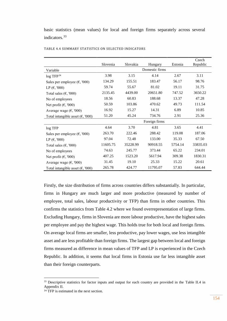
154
basic statistics (mean values) for local and foreign firms separately across several
indicators. 31F
33
TABLE 4.4 SUMMARY STATISTICS ON SELECTED INDICATORS
Firstly, the size distribution of firms across countries differs substantially. In particular,
firms in Hungary are much larger and more productive (measured by number of
employee, total sales, labour productivity or TFP) than firms in other countries. This
confirms the statistics from Table 4.2 where we found overrepresentation of large firms.
Excluding Hungary, firms in Slovenia are more labour productive, have the highest sales
per employee and pay the highest wage. This holds true for both local and foreign firms.
On average local firms are smaller, less productive, pay lower wages, use less intangible
asset and are less profitable than foreign firms. The largest gap between local and foreign
firms measured as difference in mean values of TFP and LP is experienced in the Czech
Republic. In addition, it seems that local firms in Estonia use far less intangible asset
than their foreign counterparts.
33 Descriptive statistics for factor inputs and output for each country are provided in the Table II.4 in
Appendix II. 34 TFP is estimated in the next section.
Slovenia Slovakia Hungary Estonia
Czech
Republic
Variable Domestic firms
log TFP32F
34 3.98 3.15 4.14 2.67 3.11
Sales per employee (€, '000) 134.29 155.51 183.47 56.17 98.76
LP (€, '000) 59.74 55.67 81.02 19.11 31.75
Total sales (€, '000) 2135.45 4439.00 20651.80 747.52 3650.22
No of employees 18.56 60.83 188.68 13.37 47.28
Net profit (€, '000) 50.59 103.86 470.62 49.73 111.54
Average wage (€, '000) 16.92 15.27 14.31 6.89 10.85
Total intangible asset (€, '000) 51.20 45.24 734.76 2.91 25.36
Foreign firms
log TFP 4.64 3.70 4.81 3.65 4.41
Sales per employee (€, '000) 263.70 222.46 288.42 119.08 187.06
LP (€, '000) 97.04 72.48 133.00 35.33 67.50
Total sales (€, '000) 11605.75 35228.99 90918.55 5754.14 33835.03
No of employees 74.63 245.77 373.44 65.22 234.01
Net profit (€, '000) 407.25 1523.20 5617.94 309.38 1830.31
Average wage (€, '000) 31.45 19.10 25.33 15.22 20.61
Total intangible asset (€, '000) 265.78 424.77 11795.07 57.83 644.44
155
4.6 TFP ESTIMATION
The estimation of TFP is based on pooled OLS with year dummies, Levinsohn-Petrin
(2003) and Wooldridge (2009) techniques described in detail in Section 4.4 and applied
to only domestic firms in manufacturing and market service sector. 33F
35 The Cobb Douglas
production function is estimated separately for each 2 digit industry in order to capture
the heterogeneity arising from different production technologies, quality and intensity of
inputs used in the production. However, to meet the requirement of at least 50
observations per industry (Gal, 2013), some industries are merged based on the grouping
used in the WIOD database. 34F
36 Productivity estimates for financial sector (NACE Rev 1.1
codes 65-67) and the rest of service sector are also calculated, but should be treated with
caution due to inherent difficulties in measuring output. The Wooldridge estimator is
applied in one equation framework as implemented by Petrin et al. (2011) and Petrin and
Levinsohn (2012). Standard errors for both pooled OLS and Wooldridge estimator are
clustered at the firm level to control for arbitrary heteroscedasticity and within panel
correlation. The Wooldridge estimator is the preferred choice for several reasons. First,
it provides efficient standard errors robust to both heteroscedasticity and autocorrelation
which is not the case with other structural estimators which rely on bootstrapped standard
errors. The latter is particularly worrisome in ACF case as it is demanding in data
requirements. The problem increases in unbalanced dataset with many gaps as fewer
observations are available to estimate input coefficients (Eberhardt and Helmers, 2010).
Second, Wooldridge estimator is robust to ACF (2006) critique where labour may be
unidentified in the first stage of LP estimator.
Both value added and gross output production function were employed in empirical
analysis in order to check their suitability for data in hand. However, in the case of
Levinsohn-Petrin estimation of gross output production function on 2-digit NACE Rev
1.1 level was not feasible for a number of industries and countries. The reason was the
35 Levinsohn and Petrin estimator is applied using STATA user written command “levpet” developed by
Petrin et al. (2004). 36 Due to low number of observations some industries were grouped together following the classification
of WIOD database which is used to construct vertical linkages in the following chapters. Please refer to
Tables II.5-II.9 in Appendix II were results by industry are reported. The first column is the NACE 1.1 2-
digit code which shows which industries were grouped.
156
lack of variation in data for a separate identification of input coefficients. Also, in certain
cases the material coefficients were equal to one due to imposed upper limit in the
estimation algorithm and as suggested by Arnold (2005) these estimations should be
discarded. In the case of modified Wooldridge estimator, the capital coefficient was
extremely low, while labour and materials coefficients had implausible values in certain
industries across countries. In addition, diagnostic tests used to gauge instrument validity
were not satisfied for most industries. For these reasons, we decided to continue the
analysis using value added specification. 35F
37 The decision to use value added instead of
revenue as dependent variable is also motivated by findings of Bond and Soderbom
(2005) and Ackerberg et al. (2006) who suggest that identification of perfectly variable
inputs (materials) is not possible without input price variation across firms in a gross
revenue specification of the Cobb-Douglas production function.
In order to create internal instruments for instrumental variable regression we construct
third degree polynomial approximation using first order lags of capital and intermediate
inputs and labour input as instruments for equation (4.23) which allows us to obtain all
production function coefficients in one step and at the same time controlling for
multicollinearity of labour with polynomial function. Since first order lag of labour input
is used as an external instrument for its current level, the validity of instrument is tested
using Kleibergen-Paap LM statistic (2006). The latter is used to test whether the equation
is identified, i.e., that the excluded instruments are correlated with the endogenous
regressors. The null hypothesis is that equation is under identified which is rejected
across all industries and countries. Further, since the assumption of identically and
independent distributed errors (i.i.d.) is dropped we use Kleibergen-Paap Wald F statistic
to test for weak identification which arises when excluded instruments are weakly
correlated with the endogenous regressors. The critical values obtained from Kleibergen-
Paap statistic are compared to critical values from Stock and Yogo (2005) and the null
hypothesis of weak identification is rejected. Finally, we use Stock and Wright (2000) S
statistic to test the null hypothesis that the coefficients of the endogenous regressors in
the structural equation are jointly equal to zero and that the over identifying restrictions
are valid. Again, the test rejects the null hypothesis suggesting that excluded instrument
37 By using value added specification we also tested dynamic implications of labour coefficient
instrumenting it with longer lags starting at t-2. The reason for including longer lags is that labour in t-1 is
part of the polynomial term used to invert out productivity. However, diagnostic tests did not support
instrument validity.
157
is relevant and equation is exactly identified. Overall, we can be confident that TFP
estimated by Wooldridge estimator satisfy the necessary diagnostics before turning to
interpretation of input coefficients.
In discussing the results special attention is paid to differences in parameter estimates
across different methodologies. The results for all three estimators are shown in Tables
II.5-II.9 in Appendix II. All reported estimates are based on an unbalanced sample of
firms, thus allowing for implicit entry and exit of firms. 36F
38 The results from pooled OLS
model yield a labour coefficient value between 0.7 and 0.8 across industries and countries
with the exception of Slovakia where parameter estimate of labour takes the value of 0.5
on average across industries for OLS estimates and even lower for estimates obtained
through semi parametric methods which may be the result of collinearity with
productivity term. The parameter estimates of labour are slightly higher for services
which are not surprising since the latter are more labour intensive. The labour estimates
drop when applying structural estimators suggesting a positive correlation between
labour and productivity term leading to an upward bias of labour coefficient in the case
of OLS due to possible transmission bias. In general labour coefficient obtained from all
estimators is highly significant across industries and countries. In some industries such
as transport or financial industries the labour coefficient falls outside unit interval being
larger than one suggesting a negative relationship between labour and productivity. This
is consistent with the idea that some firms within a sector are more productive and thus
employ fewer workers per unit of output (Newman et al., 2015).
The estimates of capital coefficient vary across country industry pairs and are mostly
insignificant in Hungary when applying structural estimators probably due to lower
precision of estimates arising from smaller number of observations. Furthermore, given
that large firms are overrepresented in Hungarian dataset the complexity of accounting
issues when evaluating different book values and different vintages may add to
sometimes negative and insignificant capital coefficient (Eberhardt and Helmers, 2010).
In all countries except Slovakia, the average value of capital takes the values between
0.10 and 0.20 and the estimates of LP and Wooldridge are fairly similar. In general, it
seems that structural estimators do not correct for possible downward bias of capital
38 It has been shown that including survival probability in the second stage of Olley and Pakes algorithm
did not significantly changed the value of capital estimates (Van Beveren, 2012).
158
coefficient as the estimates are in most cases lower than those obtained from OLS. It may
also suggest that firms’ use of capital is positively correlated with productivity, thus
leading to an upward bias in OLS estimates. In general, this is a common finding in firm
production function estimates as it is well known that measurement of capital is the most
complex one (Galuscak and Lizal, 2011). The poor results for capital coefficient are
possibly due to the fact that available services from this factor input are underutilised.
Also, it may be that that the variables included in the polynomial approximation of the
unobserved productivity hamper the identification of capital coefficient. However, it
could also be the results of an attrition bias where only surviving firms are selected in the
sample thus introducing a correlation between inputs and the error term which biases
both input coefficients (CompNet Task Force, 2014).
To summarize, comparison of the results across sectors and countries reveals that OLS
tend to produce higher coefficient for labour input pointing out the importance of
correcting the transmission bias. Furthermore, it is found that capital coefficient in
Wooldridge estimator tends to be relatively smaller or in very few cases larger than OLS
counterpart depending on the industry and chosen estimation algorithm which is a usual
finding in the literature (Ornaghi and Van Beveren, 2012). Similar results are also
obtained when running LP estimator, thus confirming the need to correct for biased
labour coefficient when using OLS. The heterogeneity of point estimates is even clearer
when we test whether the obtained coefficients satisfy the constant return to scale
hypothesis. In general, OLS estimates point to higher returns to scale especially in the
Czech Republic’s service sector and across all sectors in Estonia than structural
estimators. The latter mostly predict decreasing returns to scale in almost all countries
and industries. This is expected as OLS coefficient estimates tend to be upward biased.
Overall, OLS seems to confirm constant returns to scale more often than Wooldridge and
LP estimator. This heterogeneity may be the result of different characteristics of firms,
industries and countries in terms of timing assumptions of inputs and their dynamic
implications which is difficult to test form a practical point of view especially if one is
interested to make comparison of estimates using the same methodology (Ornaghi and
Van Beveren, 2012).
An important question is whether the estimates obtained have any significant differences
on the obtained TFP from different estimation algorithms. For this purpose, we have
calculated Pearson pair-wise correlation coefficients across years from three estimators
159
provided in Tables II.11-II.15 in Appendix II. For each country there is a uniformly high
correlation coefficient among different estimators (above 0.85) with the exception of
Hungary where the correlation between structural estimators and OLS is 0.49. The same
correlation matrix is calculated following several transformations, namely deviations
from firm specific means, deviations from cross section means, growth rates of TFP and
correlations in two main sectors of the economy. The correlation coefficients remain
fairly robust across these different transformations. The exception is again Hungary
where structural estimators are not strongly correlated across years and sectors. The latter
result also holds for Slovenia where in manufacturing sector the correlation between OLS
and Wooldridge/LP estimates is 0.50 and 0.57, respectively. Overall, the results indicate
that different types of productivity measures are strongly correlated across several
transformations, and especially their growth rates and within firm variation, are generally
strongly related.
A key stylized fact from firm level productivity estimations is wide dispersion even in
narrowly defined industries which drives aggregate productivity as shown theoretically
within a standard model of firm heterogeneity and international trade (Melitz and
Ottaviano, 2008). A large dispersion of productivity may indicate a large room for
improvements in aggregate productivity by reallocating resources from less productive
to more productive industries (Hsieh and Klenow, 2009). For this reason, in Table 4.5
below we report standard statistics of productivity distribution measured as the difference
between the 90th (top ten percent) and the 10th (lowest ten percent) percentile of log TFP
of firms for each estimation algorithm (Syverson, 2011; Gal, 2013). As can be seen,
productivity dispersion is larger for OLS estimates and the differences in comparison to
Wooldridge are in range of 0.04-0.49 log points. 37F
39 It is reassuring that productivity
dispersion displays very similar patterns across different structural estimators and
countries. The findings imply that firms with the highest productivity within industry
will produce between 1.5 and 2.5 times more output with the same amount of inputs in
case of Wooldridge estimator and 1.5 and 3 in case of OLS than firms within 10th
percentile of TFP distribution. The highest dispersion of productivity estimates is evident
in the Czech Republic followed by Estonia. On the other hand, lowest dispersion can be
39 In order to express the differences in percentages one needs to transform log points using this formula:
100(ediff – 1) where e is exponential taking the value of 2.71 and diff is the difference in logpoints. In our
case, the difference between OLS and WLP estimates in the Czech Republic of 0.49 log points amounts to
approximately 63 percent. The lowest difference of 4 percent can be observed in Slovenia.
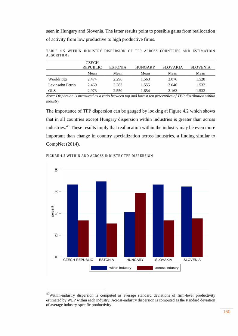
160
seen in Hungary and Slovenia. The latter results point to possible gains from reallocation
of activity from low productive to high productive firms.
TABLE 4.5 WITHIN INDUSTRY DISPERSION OF TFP ACROSS COUNTRIES AND ESTIMATION ALGORITHMS
Note: Dispersion is measured as a ratio between top and lowest ten percentiles of TFP distribution within
industry
The importance of TFP dispersion can be gauged by looking at Figure 4.2 which shows
that in all countries except Hungary dispersion within industries is greater than across
industries. 38F
40 These results imply that reallocation within the industry may be even more
important than change in country specialization across industries, a finding similar to
CompNet (2014).
FIGURE 4.2 WITHIN AND ACROSS INDUSTRY TFP DISPERSION
40
Within-industry dispersion is computed as average standard deviations of firm-level productivity
estimated by WLP within each industry. Across-industry dispersion is computed as the standard deviation
of average industry-specific productivity.
02
04
06
08
0p
erc
en
t
CZECH REPUBLIC ESTONIA HUNGARY SLOVAKIA SLOVENIA
within industry across industry
CZECH
REPUBLIC ESTONIA HUNGARY SLOVAKIA SLOVENIA
Mean Mean Mean Mean Mean
Wooldridge 2.474 2.296 1.563 2.076 1.528
Levinsohn Petrin 2.460 2.283 1.555 2.040 1.532
OLS 2.973 2.550 1.654 2.163 1.532
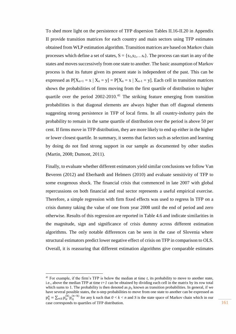
161
To shed more light on the persistence of TFP dispersion Tables II.16-II.20 in Appendix
II provide transition matrices for each country and main sectors using TFP estimates
obtained from WLP estimation algorithm. Transition matrices are based on Markov chain
processes which define a set of states, S = {s1,s2,…sr}. The process can start in any of the
states and moves successively from one state to another. The basic assumption of Markov
process is that its future given its present state is independent of the past. This can be
expressed as P[Xn+1 = x | Xn = y] = P[Xn = x | Xn-1 = y]. Each cell in transition matrices
shows the probabilities of firms moving from the first quartile of distribution to higher
quartile over the period 2002-2010.39F
41 The striking feature emerging from transition
probabilities is that diagonal elements are always higher than off diagonal elements
suggesting strong persistence in TFP of local firms. In all country-industry pairs the
probability to remain in the same quartile of distribution over the period is above 50 per
cent. If firms move in TFP distribution, they are more likely to end up either in the higher
or lower closest quartile. In summary, it seems that factors such as selection and learning
by doing do not find strong support in our sample as documented by other studies
(Martin, 2008; Dumont, 2011).
Finally, to evaluate whether different estimators yield similar conclusions we follow Van
Beveren (2012) and Eberhardt and Helmers (2010) and evaluate sensitivity of TFP to
some exogenous shock. The financial crisis that commenced in late 2007 with global
repercussions on both financial and real sector represents a useful empirical exercise.
Therefore, a simple regression with firm fixed effects was used to regress ln TFP on a
crisis dummy taking the value of one from year 2008 until the end of period and zero
otherwise. Results of this regression are reported in Table 4.6 and indicate similarities in
the magnitude, sign and significance of crisis dummy across different estimation
algorithms. The only notable differences can be seen in the case of Slovenia where
structural estimators predict lower negative effect of crisis on TFP in comparison to OLS.
Overall, it is reassuring that different estimation algorithms give comparable estimates
41 For example, if the firm’s TFP is below the median at time t, its probability to move to another state,
i.e., above the median TFP at time t+1 can be obtained by dividing each cell in the matrix by its row total
which sums to 1. The probability is then denoted as pij. known as transition probabilities. In general, if we
have several possible states, the n-step probabilities to move from one state to another can be expressed as
pijn = ∑ pir
(k)prj(n−k)
r∈S for any k such that 0 < k < n and S is the state space of Markov chain which in our
case corresponds to quartiles of TFP distribution.
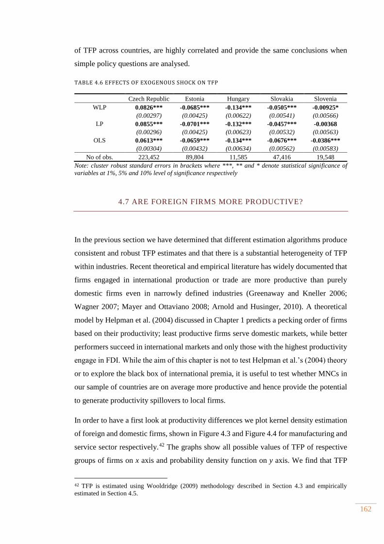
162
of TFP across countries, are highly correlated and provide the same conclusions when
simple policy questions are analysed.
TABLE 4.6 EFFECTS OF EXOGENOUS SHOCK ON TFP
Note: cluster robust standard errors in brackets where ***, ** and * denote statistical significance of
variables at 1%, 5% and 10% level of significance respectively
4.7 ARE FOREIGN FIRMS MORE PRODUCTIVE?
In the previous section we have determined that different estimation algorithms produce
consistent and robust TFP estimates and that there is a substantial heterogeneity of TFP
within industries. Recent theoretical and empirical literature has widely documented that
firms engaged in international production or trade are more productive than purely
domestic firms even in narrowly defined industries (Greenaway and Kneller 2006;
Wagner 2007; Mayer and Ottaviano 2008; Arnold and Husinger, 2010). A theoretical
model by Helpman et al. (2004) discussed in Chapter 1 predicts a pecking order of firms
based on their productivity; least productive firms serve domestic markets, while better
performers succeed in international markets and only those with the highest productivity
engage in FDI. While the aim of this chapter is not to test Helpman et al.’s (2004) theory
or to explore the black box of international premia, it is useful to test whether MNCs in
our sample of countries are on average more productive and hence provide the potential
to generate productivity spillovers to local firms.
In order to have a first look at productivity differences we plot kernel density estimation
of foreign and domestic firms, shown in Figure 4.3 and Figure 4.4 for manufacturing and
service sector respectively. 40F
42 The graphs show all possible values of TFP of respective
groups of firms on x axis and probability density function on y axis. We find that TFP
42 TFP is estimated using Wooldridge (2009) methodology described in Section 4.3 and empirically
estimated in Section 4.5.
Czech Republic Estonia Hungary Slovakia Slovenia
WLP 0.0826*** -0.0685*** -0.134*** -0.0505*** -0.00925*
(0.00297) (0.00425) (0.00622) (0.00541) (0.00566)
LP 0.0855*** -0.0701*** -0.132*** -0.0457*** -0.00368
(0.00296) (0.00425) (0.00623) (0.00532) (0.00563)
OLS 0.0613*** -0.0659*** -0.134*** -0.0676*** -0.0386***
(0.00304) (0.00432) (0.00634) (0.00562) (0.00583)
No of obs. 223,452 89,804 11,585 47,416 19,548
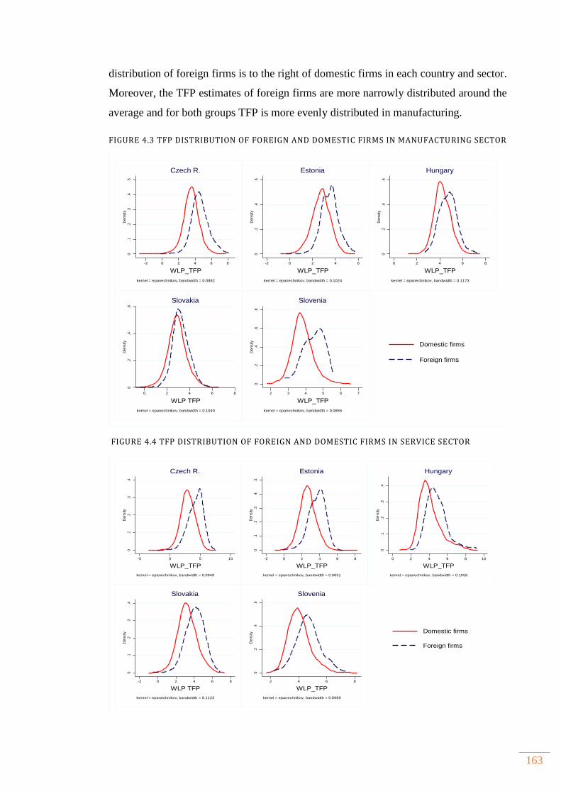
163
distribution of foreign firms is to the right of domestic firms in each country and sector.
Moreover, the TFP estimates of foreign firms are more narrowly distributed around the
average and for both groups TFP is more evenly distributed in manufacturing.
FIGURE 4.3 TFP DISTRIBUTION OF FOREIGN AND DOMESTIC FIRMS IN MANUFACTURING SECTOR
FIGURE 4.4 TFP DISTRIBUTION OF FOREIGN AND DOMESTIC FIRMS IN SERVICE SECTOR
0.1
.2.3
.4.5
De
nsity
-2 0 2 4 6 8
WLP_TFP
Domestic firms
Foreign firms
kernel = epanechnikov, bandwidth = 0.0882
Czech R.
0.2
.4.6
De
nsity
-2 0 2 4 6
WLP_TFP
kernel = epanechnikov, bandwidth = 0.1024
Estonia
0.2
.4.6
De
nsity
0 2 4 6 8
WLP_TFP
kernel = epanechnikov, bandwidth = 0.1173
Hungary
0.2
.4.6
De
nsity
0 2 4 6 8
WLP TFP
kernel = epanechnikov, bandwidth = 0.1040
Slovakia
0.2
.4.6
.8
De
nsity
2 3 4 5 6 7
WLP_TFP
kernel = epanechnikov, bandwidth = 0.0865
Slovenia
0.1
.2.3
.4
De
nsi
ty
-5 0 5 10
WLP_TFP
Domestic firms
Foreign firms
kernel = epanechnikov, bandwidth = 0.0949
Czech R.
0.1
.2.3
.4.5
De
nsi
ty
-2 0 2 4 6 8
WLP_TFP
kernel = epanechnikov, bandwidth = 0.0831
Estonia
0.1
.2.3
.4
De
nsi
ty
0 2 4 6 8 10
WLP_TFP
kernel = epanechnikov, bandwidth = 0.1558
Hungary
0.1
.2.3
.4
De
nsi
ty
-2 0 2 4 6 8
WLP TFP
kernel = epanechnikov, bandwidth = 0.1123
Slovakia
0.2
.4.6
De
nsi
ty
2 4 6 8
WLP_TFP
kernel = epanechnikov, bandwidth = 0.0969
Slovenia
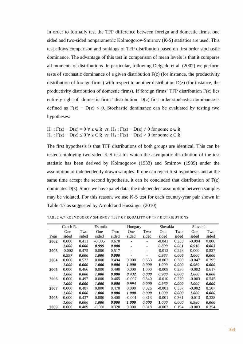
164
In order to formally test the TFP difference between foreign and domestic firms, one
sided and two-sided nonparametric Kolmogorov-Smirnov (K-S) statistics are used. This
test allows comparison and rankings of TFP distribution based on first order stochastic
dominance. The advantage of this test in comparison of mean levels is that it compares
all moments of distributions. In particular, following Delgado et al. (2002) we perform
tests of stochastic dominance of a given distribution F(z) (for instance, the productivity
distribution of foreign firms) with respect to another distribution D(z) (for instance, the
productivity distribution of domestic firms). If foreign firms’ TFP distribution F(z) lies
entirely right of domestic firms’ distribution D(z) first order stochastic dominance is
defined as F(z) − D(z) ≤ 0. Stochastic dominance can be evaluated by testing two
hypotheses:
H0 : F(z) − D(z) = 0 ∀ z ∈ Ʀ vs. H1 : F(z) − D(z) ≠ 0 for some z ∈ Ʀ
H0 : F(z) − D(z) ≤ 0 ∀ z ∈ Ʀ vs. H1 : F(z) − D(z) > 0 for some z ∈ Ʀ
The first hypothesis is that TFP distributions of both groups are identical. This can be
tested employing two sided K-S test for which the asymptotic distribution of the test
statistic has been derived by Kolmogorov (1933) and Smirnov (1939) under the
assumption of independently drawn samples. If one can reject first hypothesis and at the
same time accept the second hypothesis, it can be concluded that distribution of F(z)
dominates D(z). Since we have panel data, the independent assumption between samples
may be violated. For this reason, we use K-S test for each country-year pair shown in
Table 4.7 as suggested by Arnold and Hussinger (2010).
TABLE 4.7 KOLMOGOROV SMIRNOV TEST OF EQUALITY OF TFP DISTRIBUTIONS
Czech R. Estonia Hungary Slovakia Slovenia
Year
One
sided
Two
sided
One
sided
Two
sided
One
sided
Two
sided
One
sided
Two
sided
One
sided
Two
sided
2002 0.000 0.411 -0.005 0.670 - - -0.041 0.233 -0.094 0.806
1.000 0.000 0.999 0.000 - - 0.899 0.061 0.916 0.003
2003 -0.002 0.475 0.000 0.517 - - -0.012 0.228 0.000 0.827
0.997 0.000 1.000 0.000 - - 0.984 0.006 1.000 0.000
2004 0.000 0.522 0.000 0.494 0.000 0.653 -0.002 0.300 -0.047 0.795
1.000 0.000 1.000 0.000 1.000 0.000 1.000 0.000 0.969 0.000
2005 0.000 0.466 0.000 0.490 0.000 1.000 -0.008 0.236 -0.002 0.617
1.000 0.000 1.000 0.000 0.432 0.000 0.980 0.000 1.000 0.000
2006 0.000 0.497 0.000 0.465 -0.007 0.340 -0.010 0.270 -0.003 0.545
1.000 0.000 1.000 0.000 0.994 0.000 0.960 0.000 1.000 0.000
2007 0.000 0.487 0.000 0.470 0.000 0.326 -0.001 0.337 -0.002 0.507
1.000 0.000 1.000 0.000 1.000 0.000 1.000 0.000 1.000 0.000
2008 0.000 0.437 0.000 0.400 -0.001 0.313 -0.001 0.361 -0.013 0.338
1.000 0.000 1.000 0.000 1.000 0.000 1.000 0.000 0.980 0.000
2009 0.000 0.409 -0.001 0.328 0.000 0.318 -0.002 0.194 -0.003 0.354
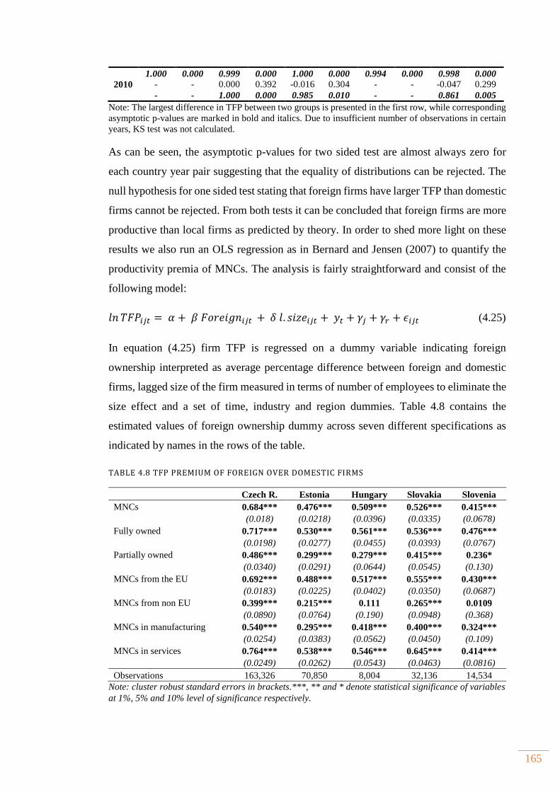
165
1.000 0.000 0.999 0.000 1.000 0.000 0.994 0.000 0.998 0.000
2010 - - 0.000 0.392 -0.016 0.304 - - -0.047 0.299
- - 1.000 0.000 0.985 0.010 - - 0.861 0.005
Note: The largest difference in TFP between two groups is presented in the first row, while corresponding
asymptotic p-values are marked in bold and italics. Due to insufficient number of observations in certain
years, KS test was not calculated.
As can be seen, the asymptotic p-values for two sided test are almost always zero for
each country year pair suggesting that the equality of distributions can be rejected. The
null hypothesis for one sided test stating that foreign firms have larger TFP than domestic
firms cannot be rejected. From both tests it can be concluded that foreign firms are more
productive than local firms as predicted by theory. In order to shed more light on these
results we also run an OLS regression as in Bernard and Jensen (2007) to quantify the
productivity premia of MNCs. The analysis is fairly straightforward and consist of the
following model:
𝑙𝑛 𝑇𝐹𝑃𝑖𝑗𝑡 = 𝛼 +𝛽𝐹𝑜𝑟𝑒𝑖𝑔𝑛𝑖𝑗𝑡 +𝛿𝑙. 𝑠𝑖𝑧𝑒𝑖𝑗𝑡 +𝑦𝑡 + 𝛾𝑗 + 𝛾𝑟 + 𝜖𝑖𝑗𝑡 (4.25)
In equation (4.25) firm TFP is regressed on a dummy variable indicating foreign
ownership interpreted as average percentage difference between foreign and domestic
firms, lagged size of the firm measured in terms of number of employees to eliminate the
size effect and a set of time, industry and region dummies. Table 4.8 contains the
estimated values of foreign ownership dummy across seven different specifications as
indicated by names in the rows of the table.
TABLE 4.8 TFP PREMIUM OF FOREIGN OVER DOMESTIC FIRMS
Czech R. Estonia Hungary Slovakia Slovenia
MNCs 0.684*** 0.476*** 0.509*** 0.526*** 0.415***
(0.018) (0.0218) (0.0396) (0.0335) (0.0678)
Fully owned 0.717*** 0.530*** 0.561*** 0.536*** 0.476***
(0.0198) (0.0277) (0.0455) (0.0393) (0.0767)
Partially owned 0.486*** 0.299*** 0.279*** 0.415*** 0.236*
(0.0340) (0.0291) (0.0644) (0.0545) (0.130)
MNCs from the EU 0.692*** 0.488*** 0.517*** 0.555*** 0.430***
(0.0183) (0.0225) (0.0402) (0.0350) (0.0687)
MNCs from non EU 0.399*** 0.215*** 0.111 0.265*** 0.0109
(0.0890) (0.0764) (0.190) (0.0948) (0.368)
MNCs in manufacturing 0.540*** 0.295*** 0.418*** 0.400*** 0.324***
(0.0254) (0.0383) (0.0562) (0.0450) (0.109)
MNCs in services 0.764*** 0.538*** 0.546*** 0.645*** 0.414***
(0.0249) (0.0262) (0.0543) (0.0463) (0.0816)
Observations 163,326 70,850 8,004 32,136 14,534
Note: cluster robust standard errors in brackets.***, ** and * denote statistical significance of variables
at 1%, 5% and 10% level of significance respectively.
166
Results point to significant foreign ownership premium across all countries, the highest
being in the Czech Republic and lowest in Slovenia where foreign firms are on average
98 per cent and 51 per cent more productive, respectively. 41F
43 Looking in more detail, fully
owned foreign firms seem to be more productive in comparison to partially owned firms,
but both groups outperform purely domestic firms. In terms of FDI origin, the TFP
premium of EU firms is two to three times higher in comparison to non EU firms.
However, one must bear in mind that there is a very low number of non-EU firms in TFP
sample, which is also indicated with insignificant coefficient in Slovenia and Hungary.
Finally, when we split the sample, we can see that MNCs in service sector are on average
70 per cent, while those in manufacturing are 48 per cent more productive than domestic
firms which is in line with Figures 4.2. and 4.3.
As a robustness check we have also compared TFP distribution of foreign and domestic
firms in manufacturing and service sector as well as the difference between foreign firms
themselves according to ownership type using K-S test. Again, the results suggest that
foreign firms’ TFP distribution stochastically dominates their counterpart in both
sectors. 42F
44 In addition, fully owned foreign firms are more productive than partially owned
foreign firms which is in line with theoretical propositions discussed more thoroughly in
the next chapter. The results hold for each country and sector, except for foreign firms in
manufacturing sector in Slovenia. Finally, we have estimated productivity difference
between domestic and foreign firms using OLS estimates of TFP and found almost
identical results except in Slovakia for the first two years of data. The estimation results
for OLS estimates are shown in the Tables II.26-II.30 in Appendix II.
Although there is evidence that foreign firms have higher productivity levels than purely
domestic firms it may be that foreign firms self-select into more productive sectors or
regions or “cherry pick” most productive domestic firms thus causing endogeneity
problem. The later can be properly addressed only if one creates a missing counterfactual
on how domestic firms would have performed in the absence of foreign investment. One
method commonly employed is a combination of propensity score matching with
difference in difference approach to control for both observable and unobservable
43 In order to get the exact percentage effects of dummy variable on ln TFP we need to apply the following
formula: 100[exp(dummy coefficient) - 1]. 44 Please take note that this comparison is made on pooled sample of firms over the entire period available
so they should be taken as indicative. The results of this exercise are shown in Tables II.21-II.25 in
Appendix II.
167
characteristics, something that we leave for further research as the aim of this thesis is
the estimation of indirect effects of FDI.
4.8 CONCLUSION
In this chapter we have provided a review of different methodologies used to estimate
TFP together with their basic assumptions about functional form, production technology
used and the impact of measurement errors on the parameter estimates. The aim was not
to test all available techniques, but to show the strengths and weaknesses of each method
as guidance for empirical work taking into account data specificities, research interests
and assumptions one is making about DGP. Since our analysis is focused on publicly
available information obtained from Amadeus database it is necessary to recognize that
although the sample of analysed countries is fairly representative in terms of total
employment and turnover when compared to official statistics it is less ideal for TFP
estimation due to large number of missing observations on input and output data. This
is especially pronounced in Hungary which also differs from other countries in above
average representativeness of large firms in the sample. Furthermore, the accounting data
do not provide detailed enough information about different products nor their
composition changes over time which may affect the measurement of output. Similarly
we are not able to control for bias arising from using industry deflators to gauge firms’
physical output. Data on factor inputs are presented in very crude form which may
additionally exacerbate measurement in inputs. These and other issues related to TFP
estimation discussed in the text affected our choice of methodology.
Several reviews have shown that semi parametric techniques are robust to measurement
issues and provide accurate productivity estimates. It assumes that productivity evolves
as Markov process which enables its flexible characterization in comparison to other
techniques. Furthermore, the problem of simultaneity bias between inputs and
unobserved productivity term is resolved without the need to use GMM estimation
techniques which require validity of instruments used for each set of regressions.
However, structural estimators are not without drawbacks as the assumption of
monotonicity between proxy variable and productivity conditional on capital has to hold.
168
Furthermore, scalar unobservable assumption may not hold if there are any other omitted
variables affecting unobserved productivity. Since TFP is used as a dependent variable
in the following empirical chapters we have used three methodologies (OLS, LP and
WLP) to test whether TFP estimates differ in several aspects. The reliance on semi
parametric methods has become very popular in recent years, however little attention has
been paid to estimates of input coefficients and TFP obtained through such procedure in
comparison to other “classical” approaches such as OLS. The result of our analysis
suggests that OLS indeed leads to overestimation of labour coefficient giving support to
the structural estimators as a possible solution to “transmission bias”. Similarity of
coefficients is also partially confirmed when comparing returns to scale. In most cases
all three estimators suggest decreasing returns to scale although the magnitude is
somewhat higher for OLS estimates. Several robustness checks such as correlation
coefficients across several dimensions, within industry dispersion of TFP and simple
regressions have indicated that productivity estimates are very robust across different
methodologies, a finding similar to other studies (Van Beveren, 2012).. In summary, if
one is interested in non-deterministic part of production function the choice of estimation
methodology is of lesser importance as shown in other studies (Van Biesebroeck, 2006;
Van Beveren, 2012). Given the advantages of Wooldridge estimator over other
estimations techniques it is chosen as our preferred method for TFP estimation and used
as dependent variable in subsequent chapters.
The main findings related to TFP estimation can be summarised as follows. Firms in
Hungary are on average the most productive while firms in Estonia are the least
productive, which is not surprising given the average size of the firms in the sample, thus
providing support to heterogenous trade models which recognized firm size as an
important determinant of productivity (Melitz, 2003) and is in accordance with some
previous empirical analysis (e.g. Mayer and Ottaviano, 2007). During the period of
analysis, domestic firms in all countries have experienced improvements in productivity
as indicated by interquartile movements, especially firms whose TFP is below median
levels in both services and manufacturing sector. However, majority of firms still
experience a strong persistence in TFP.
In terms of productivity differences between domestic and foreign firms, the empirical
findings suggest that productivity distribution of foreign firms is significantly different
from purely domestic firms across years and sectors using WLP and OLS methodology.

169
In addition, regression results point that on average foreign firms are more productive as
implied by both non parametric tests across manufacturing and services sector. This is
also confirmed in regression analysis taking into account foreign firms’ ownership
characteristics and origin as well as their sector of operation. Since potential for
productivity spillovers estimated in the next chapters relies on the assumption of superior
performance of foreign over domestic firms we may be confident that domestic firms
may benefit from indirect effects of FDI.

170
CHAPTER 5. PRODUCTIVITY SPILLOVERS OF FDI IN
SELECTED TRANSITION COUNTRIES – THE ROLE OF MNC’S HETEROGENEITY
5.1 Introduction .......................................................................................................................................... 171
5.2 Model specification ............................................................................................................................ 173
5.3 Data and descriptive statistics ...................................................................................................... 185
5.4 Methodology ......................................................................................................................................... 192
5.5 Discussion of findings ....................................................................................................................... 196
5.5.1 Results for baseline model ..................................................................................................... 197
5.5.2 The effect of ownership structure....................................................................................... 204
5.5.3 The effects of MNC’s origin .................................................................................................... 211
5.6 Conclusion ............................................................................................................................................. 219
171
5.1 INTRODUCTION
The endogenous growth theory suggests that technological progress is a key factor to
economic growth of countries (Romer, 1990; Grossman and Helpman, 1991; Aghion and
Howitt, 1997). In this context FDI is seen as bundle of intangible assets, codified and
tacit knowledge and technology which are transferred either directly or indirectly to host
economy. Through technology transfer and spillovers, endogenous growth theory
suggests that FDI can increase the development of intermediate product variety, improve
the quality of products, increase the intensity of R&D and bring new forms of human
capital (UNECE, 2001). Therefore, transition countries have made considerable efforts
in attracting FDI through various financial, fiscal and other forms of investment
incentives such as subsidies for infrastructure, regulatory concessions and certain
exemptions from labour laws. The investment policies and various incentives offered to
MNCs are based on the premise that FDI delivers important contributions to economic
development of countries through technology transfer and productivity improvements
resulting from knowledge diffusion to local firms. Although the theoretical arguments
provide strong positive relationship between FDI and economic growth, the empirical
studies on both macro and micro level are less clear cut.
As is discussed in Chapter 2 the main reason for such an ambiguity is related to the
employment of firm level data - which appear to be the most appropriate level of analysis
of FDI spillovers. Furthermore, different methodologies, data sources, and firm, industry,
country and geographical heterogeneity are mentioned as possible sources of the failure
to corroborate the expected positive effects. Recently, several improvements have been
made to alleviate these problems, the most important ones being the differentiation
between horizontal and vertical spillover channels, the incorporation of firm
heterogeneity and moderating factors such as absorptive capacity. Substantial research
in the area has found that vertical linkages are a major source of FDI productivity
spillovers and that absorptive capacity of firms and host countries also matter for these
spillovers. Furthermore, the heterogeneity of MNCs has been recognized as an important
factor for spillover potential. However, many questions still remain, especially those
related to exact mechanisms of knowledge transfer.
172
In order to shed more light on the inconclusive results of FDI spillovers found in the
transition literature, this chapter makes several contributions. First, the existing studies
of FDI spillovers reviewed in Chapter 2 have provided partial analyses of spillover
effects focusing on foreign presence in a manufacturing industry (e.g. Vahter, 2006;
Halpern and Murakozy, 2007; Nicolini and Resmini, 2010; Damijan et al., 2013a) or in
case they include all firms in the economy only horizontal spillovers is investigated
(Djankov and Hoekman, 2000; Konings, 2001; Sinani and Meyer, 2004; Vahter and
Masso, 2007; Kosova, 2010) with the exception of Kolasa (2008). The volume of FDI in
service sector has gained significant share and overpassed that in manufacturing sector,
thus influencing the changes in economic structure. The motives and strategic objectives
of such investment are inherently different and thus provide diverse knowledge spillover
potential.
The second contribution is related to MNC heterogeneity, specifically the role of partially
and fully foreign owned enterprises in generating knowledge spillovers and creation of
vertical linkages. Furthermore, the theory suggests that FDI origin brings different
managerial practices and technologies which may benefit local firms to the extent that
the latter are able to synthesize various sources of knowledge and result in higher
productivity. Therefore, we deviate from the contemporary literature which has focused
on issues such as absorptive capacity and other factors influencing the demand side of
FDI spillovers. Third, the time period of investigation is in most cases confined to the
end of 1990s or the beginning of 2000s. However, changes in macroeconomic and
business environment as well as the progress in institutions further influenced the entry,
type and motive of foreign firms at the onset of transition and integration of these
countries into international and supranational organizations. As was discussed in Chapter
3, these countries experienced a significant institutional restructuring characterised by a
slow and complex process of creating informal network of government agencies,
suppliers and research centres (Narula and Guimon, 2010). Studies investigating IDP
found significant differences across CEECs due to socio-political and economic
histories, absorptive capacity, industrial policies and legal frameworks (Bourdier, 2008;
Chobanova, 2009). Significant changes in the mode of entry, internal organisations and
motives of MNCs towards efficiency seeking and strategic assets seeking followed by
fragmentation of their activities across countries and industries are likely to have
different developmental impact on host countries.

173
Fourth, methodological and data issues as well as the model specification have
contributed to ambiguity and diversity of results among countries. The current static
approach to FDI spillovers is inadequate as it does not correspond to theoretical
transmission channels suggesting short and long run effects of MNC entry and effects on
local firms. This also has important policy implications as the incentives are warranted
only if FDI brings long term benefits to local firms. With that in mind, we use dynamic
panel estimation which enables us to control for various specification issues such as
simultaneity bias, measurement errors in foreign presence due to incomplete datasets and
possible selection issues inherent in some of the previous empirical work which did not
include small firms. Since previous research has shown that small firms lack the capacity
to benefit from FDI spillovers (Altomonte and Pennings, 2009; Blalock and Simon,
2009), excluding them leads to overestimation of true spillover effect (Eapen, 2013).
Finally, the use of a comprehensive firm level database which covers the more recent
period and the use of common methodology enable us to make cross country comparisons
of FDI spillover effects, thus partially contributing to explanation of ambiguous
empirical results witnessed so far.
The chapter is organized as follows. Section 5.2 describes the empirical model and
estimation strategy used, followed by data description and methodological approach in
Section 5.3 and 5.4 respectively. Section 5.5 provides the discussion of results from FDI
spillovers effects and their heterogeneous effects due to MNCs’ characteristics. Finally,
Section 5.6 concludes.
5.2 MODEL SPECIFICATION
The most common assumption in international business and international trade literature
discussed in Chapter 1 is that firms engaged in cross border transactions possess specific
advantages that enable them to transfer technology across borders while reaping the
benefits of host locations. Ethier and Markusen (1996) and Markusen and Venables
(1998) argue that FDI is chosen as the optimal entry strategy because it minimises the
probability of imitation, especially under imperfect state of intellectual property rights in
the host-country. In these models, productivity spillovers are less likely to arise.
Organizational choices, economies of scope stemming from product specific R&D, trade

174
secrecy and efficiency wages are means which MNCs use to protect their knowledge
(Kugler, 2006). However, as discussed in Chapter 2, a large literature has developed over
the last three decades which argue that FDI spillovers can still occur due to market failure
and the public good nature of firm specific assets (Koizumi and Kopecki, 1977; Findlay,
1978; Das, 1987; Wang and Bloomstrom, 1992; and Fosfuri et al., 2001). The major
shortcoming of this literature is that they only provide a partial picture of spillover
channels focusing on the homogenous effects of FDI within a specific industry or
country.
More recent research on FDI spillovers has focused on the role of domestic firms in the
Global Value Chains (GVC) which encompass specific activities in the production
process where individual firms and even countries are involved in just one stage of
product’s value chain (Baldwin, 2012). Since the MNC can benefit from knowledge
diffusion when it establishes connection with downstream clients and upstream suppliers,
it will cooperate with domestic firms by signing supply contracts or licensing
agreements. The creation of linkages benefits suppliers directly due to transfer of generic
knowledge increasing their specialisation and efficiency. This in turn creates pecuniary
externalities to MNCs and local firms as they are able to source intermediate inputs at
lower prices. This set of models, concerned with dynamic vertical linkages between
MNCs and local firms as well as the outcome of their interaction, is discussed more
thoroughly in Chapter 2 (Rodriguez-Clare, 1996; Markusen and Venables, 1999).
Although vertical linkages involve market transactions, they also generate technological
externalities as local firms absorb, adapt and replicate the knowledge and technology of
foreign firms, receive training and financial support, engage in joint product and process
development and share business information.
The empirical model developed in this chapter is built upon transmission channels of FDI
spillovers discussed in Chapter 2, namely horizontal spillovers and vertical linkages,
linked with the insights discussed in Section 2.5.1 in Chapter 2 emphasising MNCs’
heterogeneity. Horizontal channel of FDI spillovers in our case includes net effects of
technology or knowledge spillovers arising from a combination of demonstration,
imitation and competition effects while potential effects arising from worker mobility
are not explored due to unavailable data on worker flows. The other type of knowledge
spillovers arise from vertical linkages between MNCs and local firms. They can be
divided between backward and forward linkages. They include both pecuniary spillovers
175
arising from changes in relative prices and costs and technological spillovers such as
informal knowledge transfer (e.g. technical assistance, quality control, employee
training). Empirically it is difficult to disentangle pecuniary from technological
spillovers and thus the former are usually captured in productivity estimates. Therefore,
in this case term “spillovers” refers to FDI externalities that capture both knowledge
spillovers and voluntary technology transfer occurring through buyer supplier linkages.
Since we do not have data which would enable us to identify direct linkages between
domestic and foreign firms, it is not possible to estimate direct effects of knowledge
transfer such as technical assistance or quality assurance systems provided by foreign
firms.
As the main objective of this chapter is the analysis of economic effects of FDI spillovers,
we rely on a production function framework commonly used in the literature. In line with
endogenous growth theory productivity is not only determined by firm specific
technologies, but also by various external factors available in the economy. Therefore,
total factor productivity (TFP) estimated in Chapter 4 is related to various factors that are
internal and external to the firm. Since the main interest lies in technology shock Tit
induced by FDI, this can be expressed in the following way:
Tit = fi (Iit, Ejt) (5.1)
where (Fit, ACit) ϵ Iit
(HSjt, VTjt,ITjt) ϵ Ejt
Internal factors (Iit) are foreign ownership (Fit) and absorptive capacity (ACit) of firm i at
time t expressed in terms of intangible assets (Marroccu et al., 2012), human capital
(Blalock and Gertler, 2009), size and age. Main external factors (Eit) include various
measures of horizontal spillovers (HSjt) and vertical linkages (VTjt) together with
variables controlling for competition effects and demand conditions (ITjt) expressed at
industry level j. The basic idea underlying equation (5.1) is that firms can increase their
technology level internally through investment in human capital and intangible assets or
by changing their ownership structure. Since the main interest of this thesis lies in the
estimation of indirect effects of FDI on purely domestic firms, the term Fit indicating
direct foreign equity participation is dropped from the empirical model. An alternative
way to boost its technology is to rely on external sources of knowledge, namely those
generated by presence of MNCs in industry in which domestic firms operate or in
upstream or downstream industries acting as suppliers or customers.
176
Formally, the empirical model has the following form:
𝒍𝒏𝑻𝑭𝑷𝒊𝒕 = 𝜷𝟎 + 𝝆 𝒍𝒏 (𝑻𝑭𝑷𝒊,𝒕−𝟏)+𝜹𝟏𝑯𝑺𝒋𝒕 +𝝋𝟐𝑽𝑻𝒋𝒕 + 𝜽𝟑𝑨𝑪𝒊𝒕 + 𝝈𝟒𝑰𝑻𝒋𝒕 +
𝜸𝒋 + 𝜸𝒓 + 𝜸𝒕 + ɛ𝒊𝒋𝒕 (5.2)
Where ln 𝑇𝐹𝑃𝑖𝑡 is the logarithm of TFP of firm i at time t that is estimated in Chapter 4
and 𝑙𝑛 (𝑇𝐹𝑃𝑖,𝑡−1) is lagged level of TFP. 𝐻𝑆𝑗𝑡 and 𝑉𝑇𝑗𝑡 are defined at the industry level
and stand for horizontal spillovers and vertical linkages respectively defined below in
more detail. 𝐴𝐶𝑖𝑡 denotes the vector of firm level variables, namely the stock of human
capital and intangible assets. In addition, we control for firm’s age and size. Vector 𝐼𝑇𝑗𝑡
includes variables controlling for competition in the market and demand from
downstream sectors defined at the industry level j at time t. Finally 𝛾𝑗represents industry
dummies (defined at NACE 1.1 Rev. level) controlling for unobserved time invariant
industry specific factors that may influence both the level of FDI and productivity of
local firms. Region (defined at NUTS 3 level) dummies 𝛾𝑟 control for spatial differences
in the pattern of FDI and differences in regional performance. Year dummies 𝛾𝑡 take into
account changes in economic environment that could lead to changes in MNCs’ presence
and improvements in TFP. In the following paragraphs we present the description of
these variables and explain the rationale of including them in the empirical model.
The specification is derived from theoretical propositions, the most relevant of which is
the “partial adjustment” model. In that model, the dependent variable responds sluggishly
to changes in the explanatory variables, with geometrically declining lag weights. In this
context responses in productivity may be delayed, for example because technological
externalities take time to materialise as they depend on the formation of business links
with domestic firms in case of vertical linkages or reactions of indigenous firms to
increased competition. Since TFP follows a first order Markov process in structural
estimators discussed in more detail in the Chapter 4 it is lagged one year to capture the
dynamic process of learning by doing occurring within the firm. Furthermore, TFP is a
highly persistent variable indicating autocorrelation problems which are best addressed
in a dynamic framework.
In the literature, the methodology for calculating spillover variables is drawn from the
works of Caves (1974) and Javorcik (2004a) and it is based on an input output
framework. In the absence of detailed data on inter firm relationship, which are only
available if one conducts a survey, input-output tables provide the best possible option
177
to gauge the relationship between firms in different industries. In principle it provides
information on interconnections between industries and relies on the assumption that
sectoral R&D and technology or knowledge is embodied in output. We begin by
constructing a measure of intra-industry or horizontal spillovers calculated as following:
𝐻𝑜𝑟𝑖𝑧𝑜𝑛𝑡𝑎𝑙𝑗𝑡(𝐻𝑆) =∑ 𝐹𝑜𝑟𝑒𝑖𝑔𝑛𝑖𝑗𝑡∗𝑌𝑖𝑗𝑡𝑖𝜖𝑗
∑ 𝑌𝑖𝑗𝑡𝑖𝜖𝑗 (5.3)
where Yijt is the output (measured as revenue) produced by foreign firm i in industry j in
year t. 𝐹𝑜𝑟𝑒𝑖𝑔𝑛𝑖𝑗𝑡 is a dummy variable indicating if the firm is foreign owned. It takes
the value of one if the sum of shares of foreign investors exceeds 10% of a firm’s equity
and zero otherwise. As common in the literature intra industry spillovers are calculated
at NACE (Rev. 1.1) 2-digit industry group level defined in World Input Output Database
(WIOD) given that input output tables used to construct vertical linkages defined below
are based on this classification. Horizontal measure captures the output produced by
foreign firms i in industry j in time t and is a measure of both demonstration and imitation
effects. 43F
45
In order to calculate vertical linkages the data from WIOD is used (Timmer, 2012). 44 F
46
This database has been published only recently and provides yearly input output tables
aggregated over 35 NACE Rev. 1.1 2-digit level sectors covering 27 EU countries and
13 other major countries. Yearly data allow us to estimate time varying Input-Output
coefficients which is a significant improvement over previous studies which used I-O
tables from early/mid 2000s, thus ignoring the changing economic structure of countries
over years.
The impact of foreign suppliers or customers is assessed using the proportion of foreign
firms in upstream and downstream sectors respectively. In order to compute technical
coefficients that are used for calculating vertical linkages, we depart from the work of
Javorcik (2004a) and include inputs supplied within the same industry. 45F
47 The reason for
45 When calculating horizontal measure the total number of firms available in the database was used
regardless of whether these firms had data on all production function variables for TFP estimation. 46 This project is funded by the European Commission, Research Directorate General as part of the 7th
Framework Programme, Theme 8: Socio-Economic Sciences and Humanities. The details on how WIOD
has been constructed and sources of data can be found in Timmer (2012). 47 Measure of backward linkages employed by Javorcik (2004a) typically exclude inputs supplied within
the same industry as these are captured by horizontal spillovers. It is calculated as 𝐵𝑎𝑐𝑘𝑤𝑎𝑟𝑑𝑗𝑡 =
∑ 𝛼𝑗𝑘𝑡𝐾𝑘≠𝑗 𝐻𝑜𝑟𝑧𝑘𝑡 .
178
this lies in the fact that is unrealistic to assume no inter-industry linkages in highly
aggregated industries. For example, when calculating input/output coefficients among
industries we were constrained to use the same I-O coefficients for four NACE Rev. 1.1
sectors (30, 31, 32 and 33). Therefore, if buyer supplier linkages between those four
sectors are higher than competitive pressures measured by horizontal spillovers
backward or forward linkages will be underestimated. If we exclude inputs supplied
within the same industry we imply that productivity spillovers occurring at lower levels
of aggregation are captured by horizontal spillovers and vertical spillovers will not be
identified (Barbosa and Eiriz, 2009). Therefore, excluding/including inputs supplied
within the same industry might affect empirical results as shown by Lenaerts and
Merlevede (2012). Backward linkages at two-digit industry level are calculated as
following:
𝐵𝑎𝑐𝑘𝑤𝑎𝑟𝑑𝑗𝑡(𝑉𝑇) = ∑𝛼𝑗𝑘𝑡
𝐾
𝑘=1
𝐻𝑜𝑟𝑖𝑧𝑜𝑛𝑡𝑎𝑙𝑘𝑡(5.4)
where 𝛼𝑗𝑘𝑡 measures the proportion of industry j’s output supplied to industry k at time t
and 𝐻𝑜𝑟𝑖𝑧𝑜𝑛𝑡𝑎𝑙𝑘𝑡is share of foreign owned firms in downstream sector k. The technical
coefficients 𝛼𝑗𝑘𝑡 are calculated for domestic intermediate consumption, therefore
excluding final uses, export and imports. 46F
48 By concentrating on domestic intermediate
consumption we are able to relax the common and wrong assumption that MNCs use
domestic inputs in the same proportion as imported inputs. Although both types of inputs
can increase TFP of domestic firms, MNCs may source different inputs in host country
according to literature on international outsourcing of intermediate inputs (Barrios et al.,
2011). The backward linkage captures spillovers between MNCs and local suppliers and
it has two sources of changes. The first is related to changes in customer-supplier
relationship at the industry level, thus rejecting a restrictive assumption of stable inter-
industry relationship in transition countries. The second source of variation comes from
changes in foreign presence in downstream industry and as the latter increases so does
the extent of vertical linkages.
48 To compute technical coefficients, the inputs in the domestic intermediate IO table are used to find the
row and column totals and then each input is divided by the appropriate total (the column total for forward
spillovers, the row total for backward spillovers). No adaptations are made to the coefficients in the input-
output table.
179
Similarly, forward linkages are calculated as:
𝐹𝑜𝑟𝑤𝑎𝑟𝑑𝑗𝑡(𝑉𝑇) =∑𝛾𝑗𝑙𝑡
𝐿
𝑙=1
𝐻𝑜𝑟𝑖𝑧𝑜𝑛𝑡𝑎𝑙𝑙𝑡(5.5)
In this case technical coefficient 𝛾𝑗𝑙𝑡 the proportion of industry j’s inputs purchased from
industry l at time t. The forward linkage is a proxy for spillovers between MNCs and
their local clients in industry j. The larger the presence of MNCs in upstream sectors l
and the larger the output sold to local firms the higher is the value of the variable.
Since we are interested in examining the supply side of spillover process, the above
measures are corrected to take into account MNCs’ heterogeneity, namely their
geographical origin and the extent of foreign ownership. This enables us to partially
address the critique put forward by Barrios et al. (2011) that MNCs of different origin do
not have the same input sourcing behaviour 47F
49. Foreign firms are therefore divided among
two groups reflecting investors from EU and rest of the world. Vertical linkages and
horizontal spillovers are recalculated accordingly taking into account MNCs’ different
origins. Similarly, we recalculate vertical linkages and horizontal spillovers to capture
the heterogeneous effects of different degree of foreign ownership according to fully
owned (>99%) and partially owned foreign firms (>10% & <99%).
Most of the studies surveyed in Chapter 2 have shown the importance of firm absorptive
capacity to reap the benefits of foreign presence. Therefore, two measures of absorptive
capacity are developed and are captured within AC vector. First, human capital is
recognized as an important determinant in the context of FDI-growth effects (Romer,
1990; Barro and Sala-i-Martin, 1995; Borensztein et al., 1998) and in innovation and
learning process (Meyer and Sinani, 2009). Human capital affects TFP growth by
facilitating the adoption and implementation of new technology developed exogenously
(Nelson and Phelps, 1966), and/or by promoting the domestic production of
technological innovations (Aghion and Howitt, 1997). By incorporating the quality of
labour inputs into a production function, O’Mahony and Timmer (2009) were able to
explain the large part of the TFP growth. Haltiwanger et al. (1999) used a matched
49 Barrios et al. (2011) in addition to separate horizontal spillover according to nationality of foreign
investors also use investors’ home country IO tables to calculate IO technical coefficients.
180
employer-employee dataset and found that labour productivity is positively associated
with higher proportion of educated workers.
Apart from its direct effects on TFP, human capital is important in the context of FDI
spillovers through its multifaceted moderating role. First, firms with high levels of human
capital are more likely to benefit from direct entry of MNCs since imitation of foreign
technology, operational and management skills required to cope with increased
competition require some level of human capital. Second, in order to become a supplier
of MNCs, domestic firms need to increase their efficiency and supply quality. MNCs
provide domestic firms with information about products, prices, markets; they also
provide technical, financial, management and procurement assistance (Giroud et al.,
2012). Therefore, the higher the level of human capital, the more likely it is that firms
will meet quality standards and become suppliers of MNCs. Merlevede and Schoors
(2005) argue that domestic firms with lower levels of human capital can experience
negative backward linkages due to their inability to compete. However, higher levels of
human capital may also be detrimental as firms with skilled labour may charge higher
prices for their products. This might be the case if MNCs are more oriented to cost
savings and prevention of knowledge transfer. If cost savings are the main reason for
engaging in backward linkages, firms with lower levels of human capital are more likely
to be hired as suppliers as they are engaged in low valued added activities (Giroud et al.,
2012).
In the case of forward spillover, firms with skilled labour are more likely to benefit from
high quality inputs in their production process, thus increasing their productivity. On the
contrary, firms with lower levels of human capital are less likely to benefit from foreign
firms’ inputs and may even experience negative competition effects from both foreign
subsidiaries and local firms. Since the Amadeus database does not provide information
on skill structure of employees, another measure of the quality of human capital is
constructed for this study. Following Becker (1964), it is assumed wage rates reflect the
employee’s general human capital. Accordingly, we use average wages paid within the
firm as a measure of labour quality. Wagner (2012) demonstrated that the average wage
in a firm is a useful proxy variable for the qualification of the employees, although it
does not account for the heterogeneity of the labour force.
The second variable used as a determinant of firm TFP and as a measure of absorptive
capacity is intangible assets. Studies investigating FDI productivity spillovers have
181
found that technologically advanced industries and firms with high R&D intensity are in
a better position to benefit from the presence of MNCs (Keller and Yeaple, 2009; Aghion
et al., 2009). Recent research has recognised that a range of intangible assets grouped in
digitized information (IT capital), innovative property (scientific and non-scientific
R&D) and economic competences (brand names, firms’ specific human capital and
organizational structure) is conducive to innovation based growth and productivity
improvements (Andrews and de Serres, 2012; Corrado et al., 2009). The widespread
heterogeneity and asymmetry in the distribution of firm performance has been related to
different within-firm factors such as varying use of intangibles (Syverson, 2011). This
is in line with Resource Based Models (RBM) which views firms as distinctive bundles
of resources and capabilities (Teece, 1988) and capability based theory of the firm in
which firm’s decisions are determined mainly by the capabilities of the firm accumulated
over time (Dosi et al., 2000).
At the macro level, research has shown that intangible assets explain a larger share of
labour productivity growth than tangible assets in a number of countries (Corrado et al.,
2009; Marrano et al., 2009; Borgo et al., 2013). Similarly, micro level studies have found
a positive relationship between firm investment in intangibles and productivity level
(Bontempi and Mairesse, 2008; Marrocu et al., 2012; Hall et al., 2013; Battistini et al.,
2014). In order to include a broader measure of firms’ capabilities, intangible asset will
be used in this study. The choice of using intangible asset is driven both by the
unavailability of data on R&D expenditure in the Amadeus database and empirical
motivation. The latter can be explained by the fact that TFP estimation discussed in the
previous chapter is based on the revenue approach. Since R&D expenditure is only one
of the many variables that can influence firms’ revenue, Battistini et al. (2014) argue that
intangible assets provide more comprehensive measure of effort that firms incur in order
to improve their market position and revenues as they include R&D costs, absorptive
capability and marketing, design and technical expenditure with the goal of increasing
revenues. However, as intangibles include a broad range of factors, measuring them is a
challenging task from the accounting perspective as some items can be considered as
both current expenditure or capital accumulation (Marrocu et al., 2012). Since Amadeus
database does not provide detailed information on different factors comprising
intangibles the latter is proxied by the ‘share of intangible asset in total fixed assets’ and

182
measures firms’ endowment with specific advantages. 48 F
50 It should be noted that a large
number of firms do not report intangible asset. Since the variable is expressed in
logarithms, observations with zero values of intangible asset have been transformed to
half of the smallest observable value as it is highly likely that these are not true zeros but
very small values which are reported as such in the database. The expected effect of
intangible asset as a moderating factor of FDI spillovers is the same as in the case of
human capital. Therefore, both variables measuring absorptive capacity will
simultaneously be included in the model as they measure knowledge capital which is
expected to positively affect productivity.
Other firm specific variables include firm size and age and their quadratic terms to
control for possible nonlinear effects. It is expected that firm size measured as natural
logarithm of total assets play an important role in absorption of spillovers and
productivity enhancing process. Passive learning model of firm dynamics predicts that
larger firms are more productive due to a selection process in which more efficient firms
grow and survive (Jovanovic, 1982). New trade theory suggests that differences in firms’
performance can be attributed to heterogeneity in terms of productivity and size (Melitz,
2003). The empirical evidence has shown that the average productivity of countries is
driven by large firms (Mayer and Ottaviano, 2008, CompNet, 2014). Besides direct
effects such as learning by doing and scale and scope economies there are also indirect
effects through other variables affecting productivity which are related to firm’s size
(Barbosa and Eiriz, 2009). Larger firms usually invest more in R&D, have large number
of trained and skilled people, more competent management, and pay higher wages
increasing the probability to introduce innovation and enhance their efficiency (Huergo
and Jaumandreu, 2004; Farole and Winkler, 2012). They are also more adaptable and
flexible, thus are more likely to be selected as suppliers and become clients of MNCs
(Alfaro and Rodriguez-Clare, 2004). Therefore, the sign of this variable is expected to
be positive. However, small and medium sized firms are also likely to benefit from
spillovers, as they are more innovative and can adapt their business processes more
quickly. The inclusion of a quadratic term is motivated by the fact that size of the firm
may be relevant to TFP, i.e. there might be an optimal firm size which enables firms to
benefit from low unit costs and organizational structure. Similarly, age can also be an
50 Definition of intangible asset in Amadeus database include R&D expenditures, patents, copyrights,
software, employee training, trademarks and other similar costs and as such comprises only those
intangible assets that have been capitalized.
183
important determinant of productivity as it reflects business experience, ability to adapt
and familiarity with customer needs. Thus, it is expected that older firms have more
specific knowledge that enables them to benefit from foreign entry since they have
accumulated experience and knowledge through learning by doing. However, younger
firms may be more productive as they may use more advanced technology and innovative
business practices. By including quadratic term of age we control for the possibility that
young firms may have lower TFP due to limited access to finance and time to
accommodate to industry conditions while older firms may experience a decrease in their
productivity due to vintage capital effect.
Since a measure of horizontal spillovers may also capture the effect of competition, it is
necessary to isolate these two effects. Foreign entry may induce more competition, thus
forcing local firms to become more efficient and productive. By not incorporating a
specific variable measuring competition, increased productivity may be wrongly
attributed to spillovers. The Herfindahl-Hirshman concentration index is used to
calculate the intensity of competition. It is defined as the sum of the squares of sales
shares of all firms in industry j (defined at 2 digit NACE Rev. 1.1 level) and time t. The
sign of this variable is expected to be negative, at least in the short run. Besides
competition which may affect horizontal spillovers, we also include a demand variable
for two reasons. First, foreign firm entry may increase demand for local inputs which
may favour economies of scale. On the other hand, if MNCs import most of their
intermediates, local firms will face a decrease in productivity since fixed costs of
production will be spread to fewer units. The second reason of including the demand
variable is the fact that most firms operate in monopolistic competition or in other
imperfect market structures, thus having enough market power to influence the price. As
our measure of output in Chapter 4 is not expressed in physical quantities but as deflated
sales using industry price deflators, it may be subject to omitted price bias and therefore
not reflect the true level of productivity. Therefore, it is necessary to separate the
variation in quantities which are a measure of true efficiency from variation in prices due
to market power by including the demand variable (Van Biesebroeck, 2007). Hence, the
demand variable is calculated as:
𝐷𝑒𝑚𝑎𝑛𝑑𝑗𝑡 = ∑𝛼𝑗𝑘𝑡
𝐾
𝑘=1
𝑌𝑘𝑡(5.6)
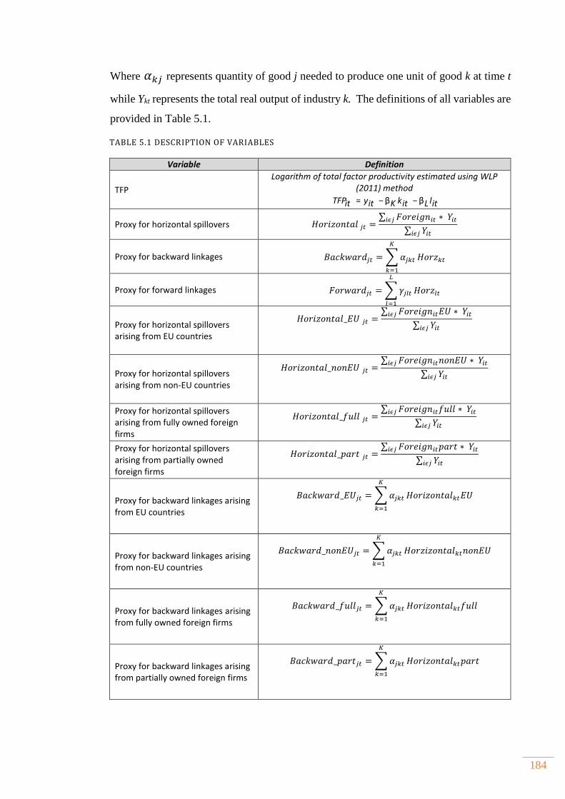
184
Where 𝛼𝑘𝑗 represents quantity of good j needed to produce one unit of good k at time t
while Ykt represents the total real output of industry k. The definitions of all variables are
provided in Table 5.1.
TABLE 5.1 DESCRIPTION OF VARIABLES
Variable Definition
TFP
Logarithm of total factor productivity estimated using WLP (2011) method
TFPit = yit − β K kit − β L lit
Proxy for horizontal spillovers 𝐻𝑜𝑟𝑖𝑧𝑜𝑛𝑡𝑎𝑙𝑗𝑡 =∑ 𝐹𝑜𝑟𝑒𝑖𝑔𝑛𝑖𝑡 ∗ 𝑌𝑖𝑡𝑖𝜖𝑗
∑ 𝑌𝑖𝑡𝑖𝜖𝑗
Proxy for backward linkages 𝐵𝑎𝑐𝑘𝑤𝑎𝑟𝑑𝑗𝑡 = ∑𝛼𝑗𝑘𝑡
𝐾
𝑘=1
𝐻𝑜𝑟𝑧𝑘𝑡
Proxy for forward linkages 𝐹𝑜𝑟𝑤𝑎𝑟𝑑𝑗𝑡 =∑𝛾𝑗𝑙𝑡
𝐿
𝑙=1
𝐻𝑜𝑟𝑧𝑙𝑡
Proxy for horizontal spillovers arising from EU countries
𝐻𝑜𝑟𝑖𝑧𝑜𝑛𝑡𝑎𝑙_𝐸𝑈𝑗𝑡 =∑ 𝐹𝑜𝑟𝑒𝑖𝑔𝑛𝑖𝑡𝐸𝑈 ∗𝑌𝑖𝑡𝑖𝜖𝑗
∑ 𝑌𝑖𝑡𝑖𝜖𝑗
Proxy for horizontal spillovers arising from non-EU countries
𝐻𝑜𝑟𝑖𝑧𝑜𝑛𝑡𝑎𝑙_𝑛𝑜𝑛𝐸𝑈𝑗𝑡 =∑ 𝐹𝑜𝑟𝑒𝑖𝑔𝑛𝑖𝑡𝑛𝑜𝑛𝐸𝑈 ∗𝑌𝑖𝑡𝑖𝜖𝑗
∑ 𝑌𝑖𝑡𝑖𝜖𝑗
Proxy for horizontal spillovers arising from fully owned foreign firms
𝐻𝑜𝑟𝑖𝑧𝑜𝑛𝑡𝑎𝑙_𝑓𝑢𝑙𝑙𝑗𝑡 =∑ 𝐹𝑜𝑟𝑒𝑖𝑔𝑛𝑖𝑡𝑓𝑢𝑙𝑙 ∗ 𝑌𝑖𝑡𝑖𝜖𝑗
∑ 𝑌𝑖𝑡𝑖𝜖𝑗
Proxy for horizontal spillovers arising from partially owned foreign firms
𝐻𝑜𝑟𝑖𝑧𝑜𝑛𝑡𝑎𝑙_𝑝𝑎𝑟𝑡𝑗𝑡 =∑ 𝐹𝑜𝑟𝑒𝑖𝑔𝑛𝑖𝑡𝑝𝑎𝑟𝑡 ∗ 𝑌𝑖𝑡𝑖𝜖𝑗
∑ 𝑌𝑖𝑡𝑖𝜖𝑗
Proxy for backward linkages arising from EU countries
𝐵𝑎𝑐𝑘𝑤𝑎𝑟𝑑_𝐸𝑈𝑗𝑡 = ∑𝛼𝑗𝑘𝑡
𝐾
𝑘=1
𝐻𝑜𝑟𝑖𝑧𝑜𝑛𝑡𝑎𝑙𝑘𝑡𝐸𝑈
Proxy for backward linkages arising from non-EU countries
𝐵𝑎𝑐𝑘𝑤𝑎𝑟𝑑_𝑛𝑜𝑛𝐸𝑈𝑗𝑡 = ∑𝛼𝑗𝑘𝑡
𝐾
𝑘=1
𝐻𝑜𝑟𝑧𝑖𝑧𝑜𝑛𝑡𝑎𝑙𝑘𝑡𝑛𝑜𝑛𝐸𝑈
Proxy for backward linkages arising from fully owned foreign firms
𝐵𝑎𝑐𝑘𝑤𝑎𝑟𝑑_𝑓𝑢𝑙𝑙𝑗𝑡 = ∑𝛼𝑗𝑘𝑡
𝐾
𝑘=1
𝐻𝑜𝑟𝑖𝑧𝑜𝑛𝑡𝑎𝑙𝑘𝑡𝑓𝑢𝑙𝑙
Proxy for backward linkages arising from partially owned foreign firms
𝐵𝑎𝑐𝑘𝑤𝑎𝑟𝑑_𝑝𝑎𝑟𝑡𝑗𝑡 = ∑𝛼𝑗𝑘𝑡
𝐾
𝑘=1
𝐻𝑜𝑟𝑖𝑧𝑜𝑛𝑡𝑎𝑙𝑘𝑡𝑝𝑎𝑟𝑡
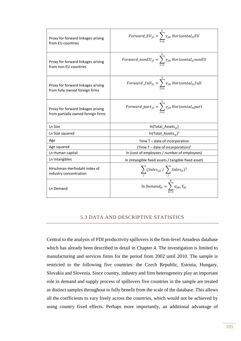
185
Proxy for forward linkages arising from EU countries
𝐹𝑜𝑟𝑤𝑎𝑟𝑑_𝐸𝑈𝑗𝑡 =∑𝛾𝑗𝑙𝑡
𝐿
𝑙=1
𝐻𝑜𝑟𝑖𝑧𝑜𝑛𝑡𝑎𝑙𝑙𝑡𝐸𝑈
Proxy for forward linkages arising from non-EU countries
𝐹𝑜𝑟𝑤𝑎𝑟𝑑_𝑛𝑜𝑛𝐸𝑈𝑗𝑡 =∑𝛾𝑗𝑙𝑡
𝐿
𝑙=1
𝐻𝑜𝑟𝑖𝑧𝑜𝑛𝑡𝑎𝑙𝑙𝑡𝑛𝑜𝑛𝐸𝑈
Proxy for forward linkages arising from fully owned foreign firms
𝐹𝑜𝑟𝑤𝑎𝑟𝑑_𝑓𝑢𝑙𝑙𝑗𝑡 =∑𝛾𝑗𝑙𝑡
𝐿
𝑙=1
𝐻𝑜𝑟𝑖𝑧𝑜𝑛𝑡𝑎𝑙𝑙𝑡𝑓𝑢𝑙𝑙
Proxy for forward linkages arising from partially owned foreign firms
𝐹𝑜𝑟𝑤𝑎𝑟𝑑_𝑝𝑎𝑟𝑡𝑗𝑡 = ∑𝛾𝑗𝑙𝑡
𝐿
𝑙=1
𝐻𝑜𝑟𝑖𝑧𝑜𝑛𝑡𝑎𝑙𝑙𝑡𝑝𝑎𝑟𝑡
Ln Size ln(Total_Assets ijt )
Ln Size squared ln(Total_Assets ijt )2
Age Time T – date of incorporation
Age squared (Time T – date of incorporation)2
Ln Human capital ln (cost of employees / number of employees)
Ln Intangibles ln (intangible fixed assets / tangible fixed asset)
Hirschman-Herfindahl index of industry concentration
∑(𝑆𝑎𝑙𝑒𝑠𝑖𝑗𝑡/∑𝑆𝑎𝑙𝑒𝑠𝑗𝑡𝑗𝑗
)2
Ln Demand ln𝐷𝑒𝑚𝑎𝑛𝑑𝑗𝑡 = ∑𝛼𝑗𝑘𝑡
𝐾
𝑘=1
𝑌𝑘𝑡
5.3 DATA AND DESCRIPTIVE STATISTICS
Central to the analysis of FDI productivity spillovers is the firm-level Amadeus database
which has already been described in detail in Chapter 4. The investigation is limited to
manufacturing and services firms for the period from 2002 until 2010. The sample is
restricted to the following five countries: the Czech Republic, Estonia, Hungary,
Slovakia and Slovenia. Since country, industry and firm heterogeneity play an important
role in demand and supply process of spillovers five countries in the sample are treated
as distinct samples throughout to fully benefit from the scale of the database. This allows
all the coefficients to vary freely across the countries, which would not be achieved by
using country fixed effects. Perhaps more importantly, an additional advantage of
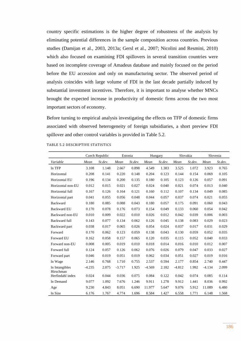
186
country specific estimations is the higher degree of robustness of the analysis by
eliminating potential differences in the sample composition across countries. Previous
studies (Damijan et al., 2003, 2013a; Gersl et al., 2007; Nicolini and Resmini, 2010)
which also focused on examining FDI spillovers in several transition countries were
based on incomplete coverage of Amadeus database and mainly focused on the period
before the EU accession and only on manufacturing sector. The observed period of
analysis coincides with large volume of FDI in the last decade partially induced by
substantial investment incentives. Therefore, it is important to analyse whether MNCs
brought the expected increase in productivity of domestic firms across the two most
important sectors of economy.
Before turning to empirical analysis investigating the effects on TFP of domestic firms
associated with observed heterogeneity of foreign subsidiaries, a short preview FDI
spillover and other control variables is provided in Table 5.2.
TABLE 5.2 DESCRIPTIVE STATISTICS
Czech Republic Estonia Hungary Slovakia Slovenia
Variable Mean St.dev. Mean St.dev. Mean St.dev. Mean St.dev. Mean St.dev.
ln TFP 3.108 1.148 2.667 0.898 4.549 1.383 3.525 1.072 3.923 0.765
Horizontal 0.208 0.141 0.220 0.148 0.204 0.123 0.144 0.154 0.069 0.105
Horizontal EU 0.196 0.134 0.200 0.135 0.180 0.105 0.123 0.126 0.057 0.091
Horizontal non-EU 0.012 0.015 0.021 0.027 0.024 0.040 0.021 0.074 0.013 0.040
Horizontal full 0.167 0.126 0.164 0.121 0.160 0.112 0.107 0.134 0.049 0.085
Horizontal part 0.041 0.055 0.056 0.048 0.044 0.057 0.037 0.074 0.021 0.055
Backward 0.180 0.085 0.088 0.043 0.180 0.057 0.175 0.091 0.060 0.043
Backward EU 0.170 0.078 0.176 0.073 0.154 0.049 0.133 0.060 0.054 0.042
Backward non-EU 0.010 0.009 0.022 0.010 0.026 0.012 0.042 0.039 0.006 0.003
Backward full 0.143 0.077 0.134 0.062 0.126 0.045 0.138 0.083 0.029 0.023
Backward part 0.038 0.017 0.065 0.026 0.054 0.024 0.037 0.017 0.031 0.029
Forward 0.170 0.062 0.123 0.059 0.138 0.043 0.130 0.059 0.052 0.035
Forward EU 0.162 0.058 0.157 0.065 0.120 0.035 0.115 0.052 0.040 0.033
Forward non-EU 0.008 0.005 0.019 0.010 0.018 0.014 0.016 0.010 0.012 0.007
Forward full 0.124 0.057 0.126 0.062 0.076 0.026 0.079 0.047 0.033 0.027
Forward part 0.046 0.019 0.051 0.019 0.062 0.034 0.051 0.027 0.019 0.016
ln Wage 2.146 0.768 1.710 0.755 2.537 0.594 2.177 0.854 2.740 0.447
ln Intangibles -4.235 2.075 -3.717 1.925 -4.569 2.182 -4.812 1.992 -4.134 2.099
Hirschman
Herfindahl index 0.024 0.044 0.036 0.075 0.084 0.122 0.042 0.074 0.085 0.114
ln Demand 9.077 1.092 7.676 1.246 9.911 1.278 9.912 1.441 8.036 0.992
Age 9.230 4.843 8.051 6.690 11.977 5.647 9.076 5.912 11.089 6.480
ln Size 6.176 1.767 4.774 1.696 8.584 1.427 6.558 1.771 6.148 1.568
187
In general, one fifth of industry output is produced by foreign firms with the exception
of Slovakia and Slovenia, indicating the importance of foreign firms across industries
and relatively high potential for productivity spillovers. A more detailed look at the
descriptive statistics indicates that fully foreign owned firms and those coming from the
EU have the highest potential for generating spillovers, but also inducing competitive
pressure on domestic firms. Turning to vertical linkages, firms in the Czech Republic,
Hungary and Slovakia have the highest potential for becoming suppliers of MNCs
judging by the mean value of backward linkages. This is somewhat expected as those
countries have strong manufacturing base and attracted a significant number of MNCs in
manufacturing industries which are thought to have strong backward linkages. The
lowest potential for development of backward linkages is evident in Slovenia. Again,
fully foreign owned firms coming from the EU have the highest potential for developing
supplier linkages with local firms. Forward linkages are most likely to occur in the Czech
Republic, especially from EU MNCs and those which are fully owned. Firms in Slovenia
and Hungary pay the highest average wages while the share of intangible asset as a proxy
for knowledge capital is highest in Slovenia, followed by Hungary and the Czech
Republic. The competitive environment measured by HHI indicates high competition in
all countries. The mean age of firms ranges between 8 and 12 years suggesting that the
sample includes relatively young firms formed after the first few years of the transition
period. The size of firms is largest in Hungary as expected due to sample structure and
smallest in Estonia.
Since FDI is not only country specific, but also industry specific the Figures 5.1, 5.2 and
5.3 below provide a more detailed picture of the development potential of FDI spillovers
related to entry and presence of foreign firms across different industries and countries.
One can immediately notice the significant heterogeneity in all measures of FDI
spillovers across countries and industries. The largest share of foreign firms’ output is
accounted in Post and Telecommunications industry (64) in all countries except Slovenia,
followed by Electrical and Optical equipment industry (30_33), Transport equipment
(34_35), Chemical industry (25) and Rubber and Plastics (26). Overall, it seems that
foreign firms in the database still have a significant influence in manufacturing industries
despite the large amount of FDI in the service sector. However, the potential for
backward linkages development shown in Figure 5.2 is more pronounced in services,
especially in Retail (51), Wholesale and commission trade (52) and Water Transport (61).

188
However, it must be noted that these averages are pulled up mainly by the Czech
Republic, Hungary and Slovakia. Within the manufacturing industries, the higher
potential for supplier development and inclusion in GVC is evident in production of
Rubber and plastics industry (25), Machinery (29) and Basic and Fabricated metals
(27_28). Finally, in terms of forward linkages shown in Figure 5.3 there is a clear
indication of the importance of transport industries (60_62) for downstream clients
followed by Chemical industry (24) and Sale, maintenance and repair of motor vehicles
(50).
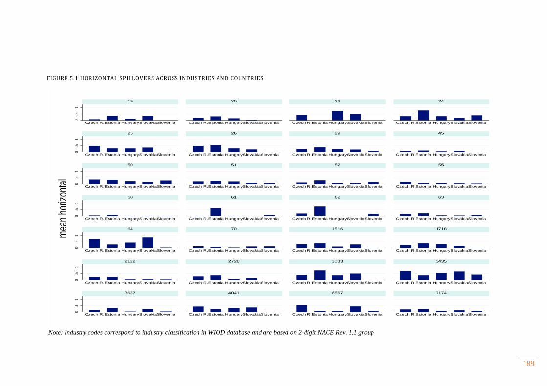
189
FIGURE 5.1 HORIZONTAL SPILLOVERS ACROSS INDUSTRIES AND COUNTRIES
Note: Industry codes correspond to industry classification in WIOD database and are based on 2-digit NACE Rev. 1.1 group
0.5
10
.51
0.5
10
.51
0.5
10
.51
0.5
1
Czech R.Estonia HungarySlovakiaSlovenia Czech R.Estonia HungarySlovakiaSlovenia Czech R.Estonia HungarySlovakiaSlovenia Czech R.Estonia HungarySlovakiaSlovenia
Czech R.Estonia HungarySlovakiaSlovenia Czech R.Estonia HungarySlovakiaSlovenia Czech R.Estonia HungarySlovakiaSlovenia Czech R.Estonia HungarySlovakiaSlovenia
Czech R.Estonia HungarySlovakiaSlovenia Czech R.Estonia HungarySlovakiaSlovenia Czech R.Estonia HungarySlovakiaSlovenia Czech R.Estonia HungarySlovakiaSlovenia
Czech R.Estonia HungarySlovakiaSlovenia Czech R.Estonia HungarySlovakiaSlovenia Czech R.Estonia HungarySlovakiaSlovenia Czech R.Estonia HungarySlovakiaSlovenia
Czech R.Estonia HungarySlovakiaSlovenia Czech R.Estonia HungarySlovakiaSlovenia Czech R.Estonia HungarySlovakiaSlovenia Czech R.Estonia HungarySlovakiaSlovenia
Czech R.Estonia HungarySlovakiaSlovenia Czech R.Estonia HungarySlovakiaSlovenia Czech R.Estonia HungarySlovakiaSlovenia Czech R.Estonia HungarySlovakiaSlovenia
Czech R.Estonia HungarySlovakiaSlovenia Czech R.Estonia HungarySlovakiaSlovenia Czech R.Estonia HungarySlovakiaSlovenia Czech R.Estonia HungarySlovakiaSlovenia
19 20 23 24
25 26 29 45
50 51 52 55
60 61 62 63
64 70 1516 1718
2122 2728 3033 3435
3637 4041 6567 7174
mea
n ho
rizon
tal
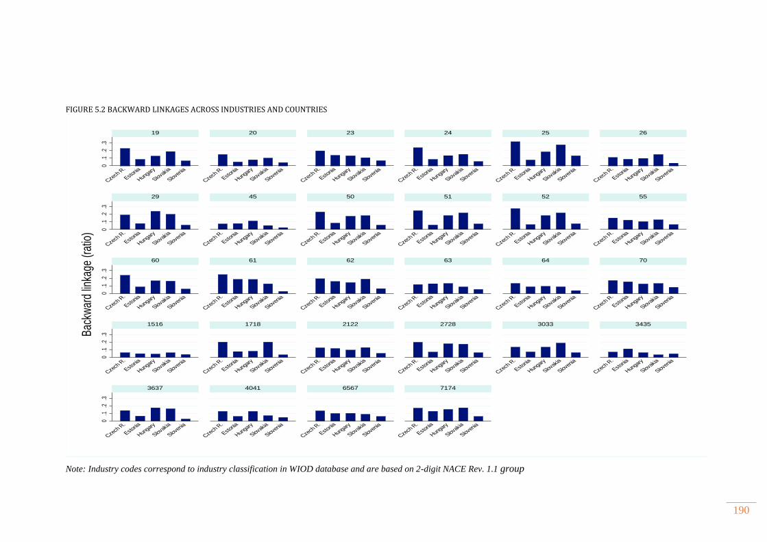
190
FIGURE 5.2 BACKWARD LINKAGES ACROSS INDUSTRIES AND COUNTRIES
Note: Industry codes correspond to industry classification in WIOD database and are based on 2-digit NACE Rev. 1.1 group
0.1
.2.3
0.1
.2.3
0.1
.2.3
0.1
.2.3
0.1
.2.3
Czech
R.
Estonia
Hunga
ry
Slovak
ia
Sloven
ia
Czech
R.
Estonia
Hunga
ry
Slovak
ia
Sloven
ia
Czech
R.
Estonia
Hunga
ry
Slovak
ia
Sloven
ia
Czech
R.
Estonia
Hunga
ry
Slovak
ia
Sloven
ia
Czech
R.
Estonia
Hunga
ry
Slovak
ia
Sloven
ia
Czech
R.
Estonia
Hunga
ry
Slovak
ia
Sloven
ia
Czech
R.
Estonia
Hunga
ry
Slovak
ia
Sloven
ia
Czech
R.
Estonia
Hunga
ry
Slovak
ia
Sloven
ia
Czech
R.
Estonia
Hunga
ry
Slovak
ia
Sloven
ia
Czech
R.
Estonia
Hunga
ry
Slovak
ia
Sloven
ia
Czech
R.
Estonia
Hunga
ry
Slovak
ia
Sloven
ia
Czech
R.
Estonia
Hunga
ry
Slovak
ia
Sloven
ia
Czech
R.
Estonia
Hunga
ry
Slovak
ia
Sloven
ia
Czech
R.
Estonia
Hunga
ry
Slovak
ia
Sloven
ia
Czech
R.
Estonia
Hunga
ry
Slovak
ia
Sloven
ia
Czech
R.
Estonia
Hunga
ry
Slovak
ia
Sloven
ia
Czech
R.
Estonia
Hunga
ry
Slovak
ia
Sloven
ia
Czech
R.
Estonia
Hunga
ry
Slovak
ia
Sloven
ia
Czech
R.
Estonia
Hunga
ry
Slovak
ia
Sloven
ia
Czech
R.
Estonia
Hunga
ry
Slovak
ia
Sloven
ia
Czech
R.
Estonia
Hunga
ry
Slovak
ia
Sloven
ia
Czech
R.
Estonia
Hunga
ry
Slovak
ia
Sloven
ia
Czech
R.
Estonia
Hunga
ry
Slovak
ia
Sloven
ia
Czech
R.
Estonia
Hunga
ry
Slovak
ia
Sloven
ia
Czech
R.
Estonia
Hunga
ry
Slovak
ia
Sloven
ia
Czech
R.
Estonia
Hunga
ry
Slovak
ia
Sloven
ia
Czech
R.
Estonia
Hunga
ry
Slovak
ia
Sloven
ia
Czech
R.
Estonia
Hunga
ry
Slovak
ia
Sloven
ia
19 20 23 24 25 26
29 45 50 51 52 55
60 61 62 63 64 70
1516 1718 2122 2728 3033 3435
3637 4041 6567 7174
Bac
kwar
d lin
kage
(rat
io)
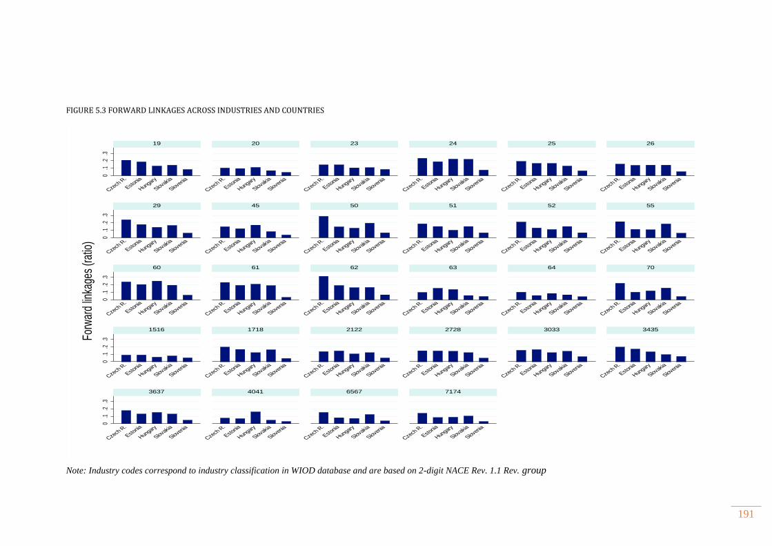
191
FIGURE 5.3 FORWARD LINKAGES ACROSS INDUSTRIES AND COUNTRIES
Note: Industry codes correspond to industry classification in WIOD database and are based on 2-digit NACE Rev. 1.1 Rev. group
0.1
.2.3
0.1
.2.3
0.1
.2.3
0.1
.2.3
0.1
.2.3
Czech R.
Estonia
Hungary
Slovakia
Slovenia
Czech R.
Estonia
Hungary
Slovakia
Slovenia
Czech R.
Estonia
Hungary
Slovakia
Slovenia
Czech R.
Estonia
Hungary
Slovakia
Slovenia
Czech R.
Estonia
Hungary
Slovakia
Slovenia
Czech R.
Estonia
Hungary
Slovakia
Slovenia
Czech R.
Estonia
Hungary
Slovakia
Slovenia
Czech R.
Estonia
Hungary
Slovakia
Slovenia
Czech R.
Estonia
Hungary
Slovakia
Slovenia
Czech R.
Estonia
Hungary
Slovakia
Slovenia
Czech R.
Estonia
Hungary
Slovakia
Slovenia
Czech R.
Estonia
Hungary
Slovakia
Slovenia
Czech R.
Estonia
Hungary
Slovakia
Slovenia
Czech R.
Estonia
Hungary
Slovakia
Slovenia
Czech R.
Estonia
Hungary
Slovakia
Slovenia
Czech R.
Estonia
Hungary
Slovakia
Slovenia
Czech R.
Estonia
Hungary
Slovakia
Slovenia
Czech R.
Estonia
Hungary
Slovakia
Slovenia
Czech R.
Estonia
Hungary
Slovakia
Slovenia
Czech R.
Estonia
Hungary
Slovakia
Slovenia
Czech R.
Estonia
Hungary
Slovakia
Slovenia
Czech R.
Estonia
Hungary
Slovakia
Slovenia
Czech R.
Estonia
Hungary
Slovakia
Slovenia
Czech R.
Estonia
Hungary
Slovakia
Slovenia
Czech R.
Estonia
Hungary
Slovakia
Slovenia
Czech R.
Estonia
Hungary
Slovakia
Slovenia
Czech R.
Estonia
Hungary
Slovakia
Slovenia
Czech R.
Estonia
Hungary
Slovakia
Slovenia
19 20 23 24 25 26
29 45 50 51 52 55
60 61 62 63 64 70
1516 1718 2122 2728 3033 3435
3637 4041 6567 7174
Forw
ard
linka
ges
(ratio
)
192
5.4 METHODOLOGY
Since we are dealing with longitudinal data, several possible estimators such as pooled
OLS, standard fixed effects estimation or corrected least square are potentially available.
However, given the possible endogeneity and the fact that the main interest is to estimate
dynamic effects of FDI spillovers, the fixed effects model or pooled OLS, which are most
commonly used in empirical literature on FDI spillovers, are prone to several drawbacks.
First, both dependent variable and FDI spillovers are measured with errors thus making
regression coefficients biased and inefficient and worsen identification difficulties
(Eapen, 2013). Second, fixed effects correct for the possible correlation between
unobserved effects and some of the independent variables, by taking deviations from
time-averaged sample means. This approach may be inappropriate in our case since the
dependent variable is stripped of its long run variation and hence any conclusion about
dynamic nature is precluded (Doytch and Uctum, 2011). Third, the most severe problem
with OLS estimation, especially when firms’ specific effects are not controlled for is
endogeneity. Since FDI is more likely to go to industries or regions which exhibit higher
productivity ex ante the positive correlation between FDI and productivity of domestic
firms might simply reflect the location decision by foreign investors rather than the
positive spillover productivity effects (Hale and Long, 2011). This may lead to upward
bias in the estimates of productivity spillovers. Fourth, since the model discussed in
Section 4.2 includes lagged dependent variable, the estimation by OLS or fixed effects
would lead to a dynamic panel bias. Nickell (1981) established that OLS estimates of the
lagged dependent variable’s coefficient in a dynamic panel model are biased due to the
correlation between the lagged dependent variable and the error term. This bias is
inversely related to panel length. Since firms in the dataset have 3 to 4 years of data on
average, the possible bias cannot be regarded as negligible. Recently, Kiviet (1995) and
Bruno (2005) proposed a bias-corrected least squares dummy variable estimator
(LSDVC) which corrects for “Nickell bias” using an estimate of the short-panel bias
computed from each firm’s data. However, this procedure assumes that the independent
variables are exogenous.
A common strategy to deal with above mentioned problems is to use a difference or
system GMM estimator (Arellano and Bond 1991; Arellano and Bover 1995; Blundell
193
and Bond 1998). Furthermore, Roodman (2009) suggests that the GMM estimator is the
proper methodological approach in cases where the number of time periods (T) is small
relative to the number of groups (N), independent variables are not strictly exogenous,
there is heteroscedasticity and autocorrelation within groups, and variables are not
normally distributed. A necessary moment condition which needs to be satisfied is the
restriction on the covariance between the error term and independent variable, i.e. (휀𝑡,) =
0. If this is not the case, coefficient estimates will be biased and inconsistent. The
problem is usually overcome by using instruments which are uncorrelated with the error
term, but correlated with endogenous variables. GMM is specifically designed to capture
the endogeneity of some explanatory variables through the creation of a matrix of internal
instruments. The latter is important for this study as it is very difficult to find external
instruments for FDI at industry level for countries under analysis. The number of
instruments can be very large, and by defining more than one moment condition per
parameter to be estimated, the information available to the estimation process is
maximised.
Using Arellano and Bond (1991), we can transform our baseline model (eq. 5.2) into
first-differences to eliminate firm-specific effects as follows:
𝒍𝒏𝑻𝑭𝑷𝒊𝒕 − 𝒍𝒏𝑻𝑭𝑷𝒊,𝒕−𝟏 = 𝜷𝟎 + 𝝆 𝒍𝒏 (𝑻𝑭𝑷𝒊𝒕−𝟏 − 𝑻𝑭𝑷𝒊,𝒕−𝟐)+𝜹𝟏(𝑯𝑺𝒋𝒕 −𝑯𝑺𝒋,𝒕−𝟏) +
𝝋𝟐(𝑽𝑻𝒋𝒕 − 𝑽𝑻𝒋,𝒕−𝟏) + 𝜽𝟑(𝑨𝑪𝒊𝒕 − 𝑨𝑪𝒊,𝒕−𝟏) + 𝝈𝟒(𝑰𝑻𝒋𝒕 − 𝑰𝑻𝒋,𝒕−𝟏) + (휀𝑖𝑡 − 휀𝑖,𝑡−1) (5.7)
Although time invariant effects are removed, simultaneity bias still remains since
differenced lagged dependent variable and differenced error term are correlated. Arellano
and Bond (1991) proposed that the lagged difference (𝑦𝑖𝑡−2 − 𝑦𝑖𝑡−3) or lagged levels 𝑦𝑖𝑡−2
of the regressors should be used as instruments. This is valid under the assumptions: (i)
the error term is not serially correlated, and (ii) the lag of the explanatory variables are
weakly exogenous.
A potential problem of the Arellano-Bond difference GMM estimator is that (i)
coefficient estimates may be biased, making lagged levels weak instruments for their
differences if variables follow a random walk, (ii) the explanatory variables are persistent
over time, and (iii) the time dimension of the sample is small (Blundell and Bond, 1998).
In order to alleviate these problems a system GMM estimator was developed which
combines the equation in first differences with the equation in levels (Arellano and
Bover, 1995; Blundell and Bond, 1998). The introduction of levels equation in the model

194
is explained by the argument that past changes may be more predictive of current levels
than the levels can be of future changes when the series are close to random walk
(Roodman, 2009). System GMM allows for the inclusion and estimation of slowly
changing variables or time invariant variables. Finally, Roodman (2009) suggests that
system GMM performs better in the case of unbalanced panels since difference
estimation magnifies gaps in the data. An additional requirement for the efficiency in
system GMM is that unobserved firm specific effect is uncorrelated with first difference
of variables (Windmeijer, 2005). In other words, the condition implies that deviations of
the initial values of the explanatory variables from their long-run values are not
systematically related to the firm-specific effects. The major shortcoming with GMM
models is the possible instrument proliferation since it may overfit endogenous variables,
weaken diagnostics used to test instrument validity and provide imprecise estimates of
the covariance matrix of the moments. The general rule of thumb suggested by Roodman
(2009) is that the number of instruments should not exceed the number of groups. One
of the ways to reduce the instrument matrix is to restrict the lag ranges that are used in
generating these instrument sets. This is done by including different instruments for each
lag, but for all time periods. Mehrhoff (2009) and Roodman (2009) suggest that
collapsing the instrument sets is an efficient way of dealing with possible instrument
proliferation. By collapsing, an instrument for each lag distance is created rather than for
each time period and each lag. It has the advantage over the truncation of the lag depth
that it retains much more information as it does not involve dropping of any lag.
Given the shortcomings of difference GMM, we decided to apply system GMM and,
since both estimators can be estimated in one or two step procedure, we decided to opt
for the second one as it is robust to heteroscedasticity and cross-correlation. The problem
with two step procedure is that standard errors are known to be downward biased when
the number of instruments is large. Therefore, Windmeijer (2005) correction, which is
found to be superior to the cluster-robust one-step standard errors (Roodman, 2009) is
applied. Furthermore, all specifications include time dummies to control for possible
cross-sectional dependencies arising from spatial dependence, economic distance or
common shocks (Sarafidis et al., 2009).
In order to verify that the moment conditions or assumptions of System GMM are
satisfied we rely on several diagnostic tests. The instrument validity is tested with the
Hansen test which is robust to heteroscedasticity. The null hypothesis of Hansen test is
195
that overidentifying restrictions are valid. Roodman (2009) suggests that p-values of
Hansen test of overidentifying restrictions lower than 0.25 and those approaching unity
should be viewed with concern. However, Blundell et al. (2000) have shown that using
system GMM on a large panel may weaken Sargan/Hansen test and over reject the null
hypothesis. Consistent with this, several studies employing system GMM on a large
panel found statistically significant Hansen test (Benito 2005; Becker and Sivadasan,
2010; Chen and Guariglia, 2013). We also rely on the difference in Hansen test to test the
subset of instruments as it can affect the overall Hansen statistics, and the choice
considerably alters the coefficients obtained for the independent variables.
The Arellano-Bond test for autocorrelation examines the hypothesis of no second-order
serial correlation in the error term of the difference equation (i.e., cov (Δεit, Δεit−k)=0 for
k≥2). In the presence of serial correlation of order n in the differenced residuals, the
instrument set for the equation in first-differences needs to be restricted to lags n + 1 and
deeper (Roodman, 2009). The GMM estimator requires that there is first-order serial
correlation (m1 test) but that there is no second-order serial correlation (m2 test) in the
residuals. Since there is no formal test of weak instrument in system GMM, Bun and
Windmeijer (2010) maintain that the both GMM estimators may suffer from small-
sample bias, but the bias for the system GMM estimator is rather small when the variance
of unobserved heterogeneity (𝜎ᵑ2) is equal to the variance of the idiosyncratic disturbance
term(𝜎𝜀2). Hence if two variances have roughly similar values it could provide a hint that
instrument are not too weak. Similarly, Bond et al. (2001) suggest that the coefficient of
lagged dependent variable can be compared to those obtained from OLS which is upward
biased and fixed effects which are downward biased. A consistent GMM estimator
should lie between two values and if not, it may be due to weak instrument problem.
Another benefit of the dynamic analysis is that it allows us to distinguish between short
and long run effects. In our case, this is important as policy makers need to be aware
whether the entry of MNCs provides long term benefits to the host country firms in order
to devise policy recommendations towards FDI. The estimated coefficients provide short
term effects which represents only a fraction of the desired change (Baltagi, 2008).
Hence, long run effects are calculated as a product of estimated coefficients and long run
multiplier1
1−𝛽1 (where β is the estimated coefficient on the lagged dependent variable).
196
The statistical significance of such obtained coefficients can be calculated using the so-
called ‘delta’ method (Papke and Wooldridge, 2005). 49F
51
5.5 DISCUSSION OF FINDINGS
Starting from the basic model discussed in Section 5.2, the empirical estimation is
conducted in statistical software Stata 12 using xtabond2 command developed by
Roodman (2009). As a starting point, the model is estimated for domestic firms only in
order to avoid aggregation bias which might arise due to inclusion of foreign firms. The
consequences of such bias are exaggerated positive productivity spillovers since foreign
firms are more productive. The lagged dependent variable and variables measuring FDI
spillovers (horizontal, backward and forward) are treated as endogenous and as such are
instrumented with their own lags and lagged differences. As suggested by Roodman
(2009) in the levels equation instruments are found among the one and more periods
lagged differences of endogenous variables. In the difference equation the endogenous
variables are instrumented with their own levels lagged two or more periods. The choice
of lags was determined by model diagnostics. The initial specifications included a
minimum number of lags, i.e. the number of instruments came from restriction to start
with one lag for levels and differences in case of lagged dependent variable and two lags
for FDI spillover variables (Roodman, 2009). However, in certain cases model
diagnostics with minimum number of lags were not satisfied and therefore the
instrumentation matrix included higher order lags (three or four) of the regressors as
instruments. Consequently we also report the AR(3)/AR(4) tests for third/fourth order
serial correlation of the differenced residuals in our tables. Furthermore, if specification
tests rejected no second order autocorrelation tests or validity of instruments, a second
lag of dependent variable was added to the right hand side of the model (Sarafidis et al.,
2009; Merikull and Room, 2014).
In this section only the result of variables of interest are presented, while coefficients of
year, industry and region dummies are excluded for presentation purposes. However, the
51 This method is based on deriving linear function that approximates non-linear combination of estimators
using Taylor’s series expansion. Stata command “nlcom” is used to transform non-linear equation and to
calculate standard error.
197
latter can be found in Appendix III together with the original printouts and syntaxes. The
following subsections explain in more detail model diagnostics and results for the
baseline model and its extensions.
5.5.1 RESULTS FOR BASELINE MODEL
As discussed in Section 5.5 system GMM uses internal instruments to correct for
endogeneity. Since there is no clear rule on the optimal number of instruments, we follow
Roodman (2009) suggestions and use lag limits and collapse option to limit the number
of instruments and obtain a more parsimonious model.50F
52 Hansen J test of overidentifying
restrictions is valid for each regression taking the p-values between 0.15 and 0.43. The
null hypothesis of no autocorrelation in differences of errors is rejected for the
autocorrelation of first order but there is no sufficient evidence to reject the null
hypothesis of no autocorrelation of second order in differences of errors. It is also
important to check the validity of subsets of instruments. For this purpose, one can use a
difference-in-Hansen test, also known as the C-test (Baum, 2006). The null hypothesis
of the C-test is that the specified variables are proper instruments, i.e. that the set of
examined instruments is exogenous. As can be seen from Tables III.1-III.5 in Appendix
III, we do not have sufficient evidence to reject this hypothesis.
In order to test for cross sectional dependence, the difference-in-Hansen test statistic for
the lagged dependent variable is examined. The corresponding p-values suggest that
there is not sufficient evidence to reject the null hypothesis that the instruments for lagged
dependent variable are valid. To check whether the steady-state assumption which states
that convergence process of TFP is independent from unobserved time invariant firm
specific effects holds, difference-in-Hansen test for level equation is used. The latter
implies that there is not sufficient evidence to reject the null hypothesis of valid
instruments. Therefore, system estimator can be preferred over the difference one.
Moreover, the value of lagged dependent variable indicates convergence as, in all cases,
it is less than unity (Roodman, 2009). Finally, following the suggestion of Bond et al.
(2001) an additional test of validity of dynamic panel estimates is performed by checking
whether the value of lagged dependent variable lies between lower bound of FE and
52 In all regressions presented below, the number of instruments is far below the number of cross
sectional units as expected due to large number of firms.
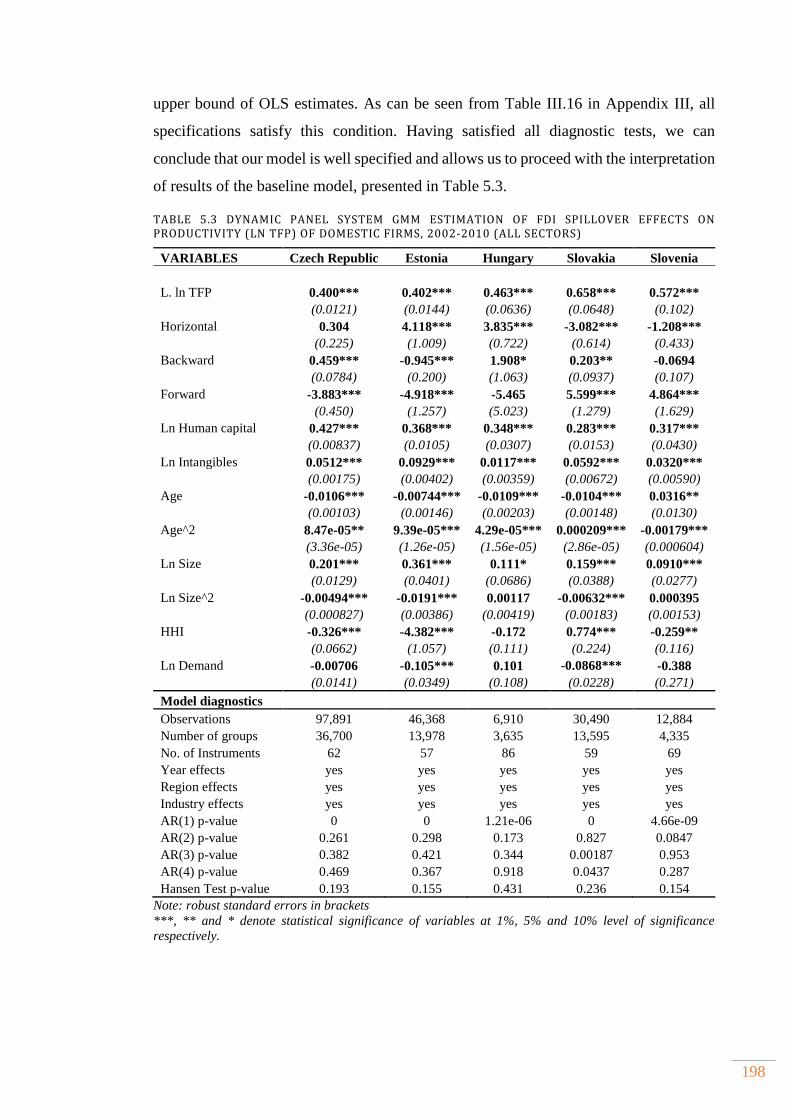
198
upper bound of OLS estimates. As can be seen from Table III.16 in Appendix III, all
specifications satisfy this condition. Having satisfied all diagnostic tests, we can
conclude that our model is well specified and allows us to proceed with the interpretation
of results of the baseline model, presented in Table 5.3.
TABLE 5.3 DYNAMIC PANEL SYSTEM GMM ESTIMATION OF FDI SPILLOVER EFFECTS ON PRODUCTIVITY (LN TFP) OF DOMESTIC FIRMS, 2002-2010 (ALL SECTORS)
Note: robust standard errors in brackets
***, ** and * denote statistical significance of variables at 1%, 5% and 10% level of significance
respectively.
VARIABLES Czech Republic Estonia Hungary Slovakia Slovenia
L. ln TFP 0.400*** 0.402*** 0.463*** 0.658*** 0.572***
(0.0121) (0.0144) (0.0636) (0.0648) (0.102)
Horizontal 0.304 4.118*** 3.835*** -3.082*** -1.208***
(0.225) (1.009) (0.722) (0.614) (0.433)
Backward 0.459*** -0.945*** 1.908* 0.203** -0.0694
(0.0784) (0.200) (1.063) (0.0937) (0.107)
Forward -3.883*** -4.918*** -5.465 5.599*** 4.864***
(0.450) (1.257) (5.023) (1.279) (1.629)
Ln Human capital 0.427*** 0.368*** 0.348*** 0.283*** 0.317***
(0.00837) (0.0105) (0.0307) (0.0153) (0.0430)
Ln Intangibles 0.0512*** 0.0929*** 0.0117*** 0.0592*** 0.0320***
(0.00175) (0.00402) (0.00359) (0.00672) (0.00590)
Age -0.0106*** -0.00744*** -0.0109*** -0.0104*** 0.0316**
(0.00103) (0.00146) (0.00203) (0.00148) (0.0130)
Age^2 8.47e-05** 9.39e-05*** 4.29e-05*** 0.000209*** -0.00179***
(3.36e-05) (1.26e-05) (1.56e-05) (2.86e-05) (0.000604)
Ln Size 0.201*** 0.361*** 0.111* 0.159*** 0.0910***
(0.0129) (0.0401) (0.0686) (0.0388) (0.0277)
Ln Size^2 -0.00494*** -0.0191*** 0.00117 -0.00632*** 0.000395
(0.000827) (0.00386) (0.00419) (0.00183) (0.00153)
HHI -0.326*** -4.382*** -0.172 0.774*** -0.259**
(0.0662) (1.057) (0.111) (0.224) (0.116)
Ln Demand -0.00706 -0.105*** 0.101 -0.0868*** -0.388
(0.0141) (0.0349) (0.108) (0.0228) (0.271)
Model diagnostics
Observations 97,891 46,368 6,910 30,490 12,884
Number of groups 36,700 13,978 3,635 13,595 4,335
No. of Instruments 62 57 86 59 69
Year effects yes yes yes yes yes
Region effects yes yes yes yes yes
Industry effects yes yes yes yes yes
AR(1) p-value 0 0 1.21e-06 0 4.66e-09
AR(2) p-value 0.261 0.298 0.173 0.827 0.0847
AR(3) p-value 0.382 0.421 0.344 0.00187 0.953
AR(4) p-value 0.469 0.367 0.918 0.0437 0.287
Hansen Test p-value 0.193 0.155 0.431 0.236 0.154
199
The model includes domestic firms in both manufacturing and market service sector (at
NACE Rev. 1.1 classification, codes 15-74). The dynamic specification, through the
lagged dependent variable, contains the entire history of the independent variables and
their influence on the current level of productivity. Therefore, we are able to identify the
additional short-run effects on local firm’s productivity of recent changes in the FDI
spillover variables, absorptive capacity and industry conditions. The coefficient on
lagged dependent variable is positive and highly significant in every country. A one
percent increase in TFP in previous period implies an increase in TFP in current period
between 0.40 and 0.66 percent. In other words, the speed of adjustment to desired level
of TFP ranges between 0.34 and 0.60. The results suggest that learning by doing has an
effect in all countries, the smallest being in the Czech Republic and the largest in
Slovakia.
Turning to our greatest concern about the relationship between FDI spillovers and TFP,
the results provide a mixed picture for horizontal and vertical spillovers. The findings
with respect to knowledge capital indicate that both human capital and intangibles have
a significant and positive role in increasing the level of productivity of domestic firms.
Turning to industry level variables, it seems that concentration and demand effects have
a negative and significant effect in most cases. Finally, a firm’s size and age exhibit
nonlinear effects in most cases indicating that there might be a turning point where the
firm’s productivity starts to rise after it accumulates experience and adapt to market and
organizational structure which impeded firms to achieve efficiency at certain point
during their business life.
In order to shed more light on the mixed effects in the case of FDI spillover, we start by
examining the effects of horizontal spillovers. These are positive and significant in the
case of Hungary and Estonia where the share of foreign firms’ output is the highest, and
negative in the case of Slovakia and Slovenia. The results suggest that a one percentage
point increase in the share of foreign owned output in an industry increases productivity
of domestic firms by 3.83 and 4.11 percent in Hungary and Estonia, respectively. The
effects are larger in the long run where horizontal spillovers increase the domestic firms’
TFP by 6.88 and 7.13 per cent respectively. It seems that domestic firms in these two
countries are able to cope with increased competition induced by increased foreign entry
either by imitating foreign firm practices or by increasing their efficiency – they are in
line with empirical work of Bekes et al. (2009) for Hungary, Sinani and Meyer (2004)
200
for Estonia and Stancik (2007), Kosova (2010) and Javorcik and Spatarenau (2011) for
the Czech Republic.51F
53 On the other hand, it seems that domestic firms in Slovakia and
Slovenia are not able to benefit from increased foreign presence in their sectors. A one
percentage point increase in foreign owned output in a sector is associated with a
decrease in productivity between 1.20 and 3.08 percent. This finding is consistent with
the literature arguing that domestic firms which do not have a certain level of absorptive
capacity are crowded out from the market as some of their markets is captured by foreign
firms. This is also confirmed in a multi country study by Damijan et al. (2013a) who
initially found negative horizontal effects, but positive after controlling for absorptive
capacity. By reducing their market share, domestic firms in Slovakia and Slovenia seem
to be operating at less efficient scale and face increased costs which may affect their
profits and result in less investment in training and technology. Furthermore, negative
horizontal effects may arise from negative effect of worker mobility as foreign firms pay
higher wages than domestic firms (Heyman et al. 2007; Earle and Telegdy, 2008), thus
leaving domestic firms with less skilled workforce affecting their ability to benefit from
potential imitation or demonstration effects.
Turning the discussion to backward linkages, the results imply that foreign presence in
downstream sector is associated with positive productivity effects in upstream sector in
the Czech Republic, Hungary and Slovakia. The positive effects of backward linkages is
highest in Hungary where a one percentage point increase of foreign firms’ output in a
downstream industry increases the demand for local inputs resulting in increase of TFP
of local firms by almost 2 percent in short run and 3.55 per cent in the long run, the latter
effects being reported in Tables III.1-III.5 in Appendix III. Similarly, in the Czech
Republic and Slovakia, this positive effect amounts to 0.45 percent and 0.20 percent in
short run and 0.76 percent and 0.59 percent in the long run, respectively. However, it
seems that foreign firms in Estonia have negative effects on upstream local suppliers.
The negative effects of backward linkages are in contrast to studies by Javorcik (2004a),
Halpern and Murakozy (2007), Gersl et al. (2007) and Kolasa (2008), but in line with
Merlevede and Schoors (2007), Stancik (2007, 2009) and Damijan et al. (2013a). 52F
54 It
seems that total negative effect of backward linkages is driven by the inability of
53 Bear in mind that these studies are based on manufacturing sector only. 54 In Damijan et al.’ (2013a) study backward linkages become positive when controlling for absorptive
capacity and domestic firms’ heterogeneity in terms of their size, productivity levels and technological
gap.
201
domestic firms to establish vertical linkages and enter supply chain of MNCs, but it is
still unclear which foreign firms are driving these results.
Forward linkages exhibit positive and statistically significant effect on productivity of
domestic firms in Slovakia and Slovenia, while for the Czech Republic and Estonia we
find a significant negative relationship. The large negative effects of forward spillovers
in the latter two countries outweigh the positive effects arising from backward linkages
in the Czech Republic and horizontal spillovers in Estonia in both short and long run. In
contrast to these two countries, the results suggest that forward spillovers are a source of
net positive productivity spillovers in Slovakia and Slovenia, a finding similar to
Gorodnichenko et al. (2014), Zajc and Kumar (2006) and Merlevede and Schoors
(2009).53F
55 This finding is again in contrast to majority of other studies which focused on
productivity spillovers within manufacturing sector (Gersl et al., 2007). However, given
the large amount of FDI in the service sector which is almost entirely motivated by
market seeking behaviour of MNCs and their concentration in sectors such as financial
services, telecommunications, transport and business services domestic firms may be
able to benefit from high quality inputs provided by foreign service firms. This has
provided strong incentives for domestic firms to switch from imports or to cope with
import competition and procure high quality inputs from local market, especially those
inputs coming from service sector as the latter have important implications for
manufacturing productivity. A more detailed analysis of these effects will be analysed in
the next chapter.
Turning to variables measuring absorptive capacity of domestic firms, namely human
capital and share of intangible assets in total fixed assets we find positive and significant
effects of knowledge capital across all specifications. The findings suggest that one
percent increase in average wage which act as a proxy for quality of human capital
increase productivity of local firms between 0.28 percent in Slovakia and 0.42 percent in
the Czech Republic. The effects are even stronger in the long run where a one percent
increase in the average wage leads to 0.62 percent increase in TFP in Estonia and 0.82
per cent in Slovakia. The magnitude of coefficient indicates that the level of human
capital is relatively high and may significantly influence the increase in productivity and
realisation of potential positive productivity spillovers coming from FDI. Since MNCs
55 A study by Gorodnichenko et al. (2014) find partially positive forward spillovers in case of older firms;
firm facing high import competition; and linkages arising with domestic oriented MNCs.

202
often require trained staff and product upgrading in order to develop linkages, it is of
utmost importance that domestic companies further invest in their human capital which
will enable them to benefit from the presence of MNCs in their sector as well as entering
the GVC of MNCs.
In the main model (eq. 5.2) presented in Table 5.3, the effects of intangibles are in line
with previous empirical estimates (Marroccu et al., 2012; Bontempi and Mairesse, 2014).
It enables domestic firms to increase their productivity between 0.01 per cent in Hungary
and 0.09 percent in Estonia in the short run. In the long run, the effects are almost
doubled. The finding may be the consequence of increased competition induced by both
domestic and foreign firms which force firms to increase investment in marketing, design
and technical expenditure with the goal of increasing market share but also to become
supplier of MNCs. Javorcik and Spatareanu (2009) found that the Czech suppliers
increased their investment in product upgrading and that vast majority of such
development came from their own effort and developed in house.
The effect of concentration measured by Hirschman-Herfindahl index is mostly negative
with the exception of Slovakia. A one percentage point increase in industry concentration
leads to a decrease in productivity between 0.25 in Slovenia and 4.38 per cent in Estonia.
The large coefficient in the case of Estonia accompanied with positive horizontal
spillovers suggests that surviving domestic firms have high absorptive capacity that
enables them to benefit from imitation or demonstration effects and at the same time
outweigh any crowding out effects. On the other hand positive productivity effects of
higher concentration of firms in Slovakia seem to be accompanied by negative market
stealing effect. The findings imply that remaining domestic firms do not have the ability
to benefit from MNC entry either because of lack of absorptive capacity, foreign firms’
successful prevention of knowledge leakage or MNCs poaching the best workers from
domestic firms.
The variable measuring increased demand for inputs suggests that both domestic and
foreign firms decrease the intermediate inputs purchase which does not allow domestic
suppliers to reap the benefits of scale economies. Demand effects is negative and
significant in Estonia and Slovakia suggesting that a one percent increase in the purchase
of intermediate inputs lead to a decrease in productivity between 0.08 percent in Slovakia
and 0.11 percent in Estonia. The negative effect of demand may explain the negative
backward linkages in Estonia as local firms are not able to achieve increasing returns to
203
scale in the production of inputs which may enable them to lower the prices of
intermediate goods and transfer the benefits to downstream firms.
The findings for firms’ age are consistent across countries (negative on age and positive
on the squared term), except in the case of Slovenia where the coefficient is positive for
the linear term and negative for the squared term. Since age is an interaction variable it
is necessary to interpret both coefficients at the same time. An additional year of
experience for an average firm leads to a decrease in TFP of 0.01 percent across all
countries. 54F
56 However, in case of Slovenia the effect is positive, indicating an increase in
productivity of 0.02 percent. Younger firms typically need to accommodate to market
conditions and therefore their performance is below existing firms in the first years of
operation. This finding is consistent with those of Jensen et al. (2001) examining the
effect of age on TFP of US firms and Harris and Moffat (2015) for UK firms, although
the former study found that the negative vintage effect of older plants is offset by positive
learning effect. Negative age effect can also be correlated with changes in organizational
structure as it influences the way firms operate and may result in decrease in TFP (Van
Witteloostuijn, 2003). The turning point after which the age of firms starts to negatively
affect TFP is around 9 years in Slovenia and given that more than 50 percent of firms are
older we can conclude that age has a decreasing effects on domestic firms’ productivity.
The opposite effect is experienced in other countries where turning point starts at 25
years in Slovakia up to 127 years in Hungary. 55F
57 Given that there are a small number of
firms which are older than the turning point in other countries we can conclude that there
is a negative selection effect due to the inability of domestic firms to learn, acquire more
advanced technology, or achieve economies of scale in the medium term.
Turning to other control variables, the results suggest that there is a strong and positive
effect of firm size in all countries. This relationship however takes the concave form in
all countries except Slovenia where the effect of quadratic term is not significant,
indicating that size has diminishing effects on the productivity levels. The positive
effects of size on TFP range from 0.09 percent in Slovenia to 0.32 percent in Estonia.
The findings are broadly consistent with theoretical models of industrial dynamics and
56 A common interpretation of coefficients in case of nonlinear variables is by taking the first partial
derivative with respect to dependent variable. In this case, the effects of age can be expressed as:𝜕𝑇𝐹𝑃
𝜕𝑎𝑔𝑒=
𝛽1 + 2𝛽2𝑎𝑔𝑒. 57 Quadratic function 𝑎𝑥2 + 𝑏𝑥has its minimum or maximum at: 𝑥 = −𝑏/2𝑎, therefore this is the point
of inflection where function changes its direction.
204
heterogeneous trade models which predict that larger firms are more productive
(Jovanovic, 1982; Melitz 2003). These are also corroborated by the findings of Van
Biesebroeck (2005b) who found significant differences between small and large firms in
nine African countries. Furthermore, Garcia-Santana and Ramos (2013) found a
significant relationship between size and labour productivity at the micro and size and
TFP at aggregate level across 104 developing countries controlling for standard
determinants of plant efficiency while Castany et al (2007) found that large firms are
more productive due to differences in endowments and returns to innovation and skilled
labour. Nonlinear effects suggest that after a certain point becoming too large has a
negative effect on productivity due to inefficiencies in coordination, management and
supervision resulting in diseconomies of scale (Fernandes, 2008).
5.5.2 THE EFFECT OF OWNERSHIP STRUCTURE
The second part of the analysis is concerned with ownership structure of foreign firms
and their effects on the extent of spillovers. Existing empirical studies disentangling the
effects of different degrees of foreign ownership on productivity of domestic firms are
mostly focused on developing countries (Almeida and Fernandes, 2008; Abraham et al.,
2010) with the exception of Javorcik and Spatareanu (2008), Merlevede and Shoors
(2007), Kolasa (2008), Merlevede et al. (2014) and Gorodnichenko et al. (2014) who
analysed the effects of ownership in Romania, Poland and Eastern European countries,
respectively. As mentioned in Chapter 2, the supply side of FDI spillover process has
gained little attention so far in empirical literature. One of the possible reasons is that the
data to conduct such analysis is not widely available. However, since the Amadeus
database provides detailed ownership information on foreign equity stakes in each firm,
we decided to investigate the effect of ownership structure on the results presented in
Section 5.6.1.
As mentioned in Section 2.5.1 the equity stake of foreign firms can reveal something
about their market entry preferences and technology they bring with them (Blomstrom
and Sjoholm, 1999). The results obtained in Section 5.6.1 can hide significant and
contrasting effects and magnitude of spillovers. To shed more light on different spillover
effects arising from different ownership structures, the total spillovers are decomposed
according to those arising from partially foreign owned firms (where the share of foreign
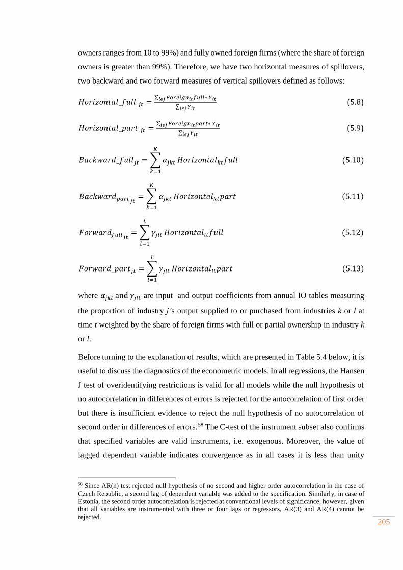
205
owners ranges from 10 to 99%) and fully owned foreign firms (where the share of foreign
owners is greater than 99%). Therefore, we have two horizontal measures of spillovers,
two backward and two forward measures of vertical spillovers defined as follows:
𝐻𝑜𝑟𝑖𝑧𝑜𝑛𝑡𝑎𝑙_𝑓𝑢𝑙𝑙𝑗𝑡 =∑ 𝐹𝑜𝑟𝑒𝑖𝑔𝑛𝑖𝑡𝑓𝑢𝑙𝑙∗𝑌𝑖𝑡𝑖𝜖𝑗
∑ 𝑌𝑖𝑡𝑖𝜖𝑗 (5.8)
𝐻𝑜𝑟𝑖𝑧𝑜𝑛𝑡𝑎𝑙_𝑝𝑎𝑟𝑡𝑗𝑡 =∑ 𝐹𝑜𝑟𝑒𝑖𝑔𝑛𝑖𝑡𝑝𝑎𝑟𝑡∗𝑌𝑖𝑡𝑖𝜖𝑗
∑ 𝑌𝑖𝑡𝑖𝜖𝑗 (5.9)
𝐵𝑎𝑐𝑘𝑤𝑎𝑟𝑑_𝑓𝑢𝑙𝑙𝑗𝑡 = ∑𝛼𝑗𝑘𝑡
𝐾
𝑘=1
𝐻𝑜𝑟𝑖𝑧𝑜𝑛𝑡𝑎𝑙𝑘𝑡𝑓𝑢𝑙𝑙(5.10)
𝐵𝑎𝑐𝑘𝑤𝑎𝑟𝑑𝑝𝑎𝑟𝑡𝑗𝑡 = ∑𝛼𝑗𝑘𝑡
𝐾
𝑘=1
𝐻𝑜𝑟𝑖𝑧𝑜𝑛𝑡𝑎𝑙𝑘𝑡𝑝𝑎𝑟𝑡(5.11)
𝐹𝑜𝑟𝑤𝑎𝑟𝑑𝑓𝑢𝑙𝑙𝑗𝑡=∑𝛾𝑗𝑙𝑡
𝐿
𝑙=1
𝐻𝑜𝑟𝑖𝑧𝑜𝑛𝑡𝑎𝑙𝑙𝑡𝑓𝑢𝑙𝑙(5.12)
𝐹𝑜𝑟𝑤𝑎𝑟𝑑_𝑝𝑎𝑟𝑡𝑗𝑡 =∑𝛾𝑗𝑙𝑡
𝐿
𝑙=1
𝐻𝑜𝑟𝑖𝑧𝑜𝑛𝑡𝑎𝑙𝑙𝑡𝑝𝑎𝑟𝑡(5.13)
where 𝛼𝑗𝑘𝑡and𝛾𝑗𝑙𝑡 are input and output coefficients from annual IO tables measuring
the proportion of industry j’s output supplied to or purchased from industries k or l at
time t weighted by the share of foreign firms with full or partial ownership in industry k
or l.
Before turning to the explanation of results, which are presented in Table 5.4 below, it is
useful to discuss the diagnostics of the econometric models. In all regressions, the Hansen
J test of overidentifying restrictions is valid for all models while the null hypothesis of
no autocorrelation in differences of errors is rejected for the autocorrelation of first order
but there is insufficient evidence to reject the null hypothesis of no autocorrelation of
second order in differences of errors. 56F
58 The C-test of the instrument subset also confirms
that specified variables are valid instruments, i.e. exogenous. Moreover, the value of
lagged dependent variable indicates convergence as in all cases it is less than unity
58 Since AR(n) test rejected null hypothesis of no second and higher order autocorrelation in the case of
Czech Republic, a second lag of dependent variable was added to the specification. Similarly, in case of
Estonia, the second order autocorrelation is rejected at conventional levels of significance, however, given
that all variables are instrumented with three or four lags or regressors, AR(3) and AR(4) cannot be
rejected.
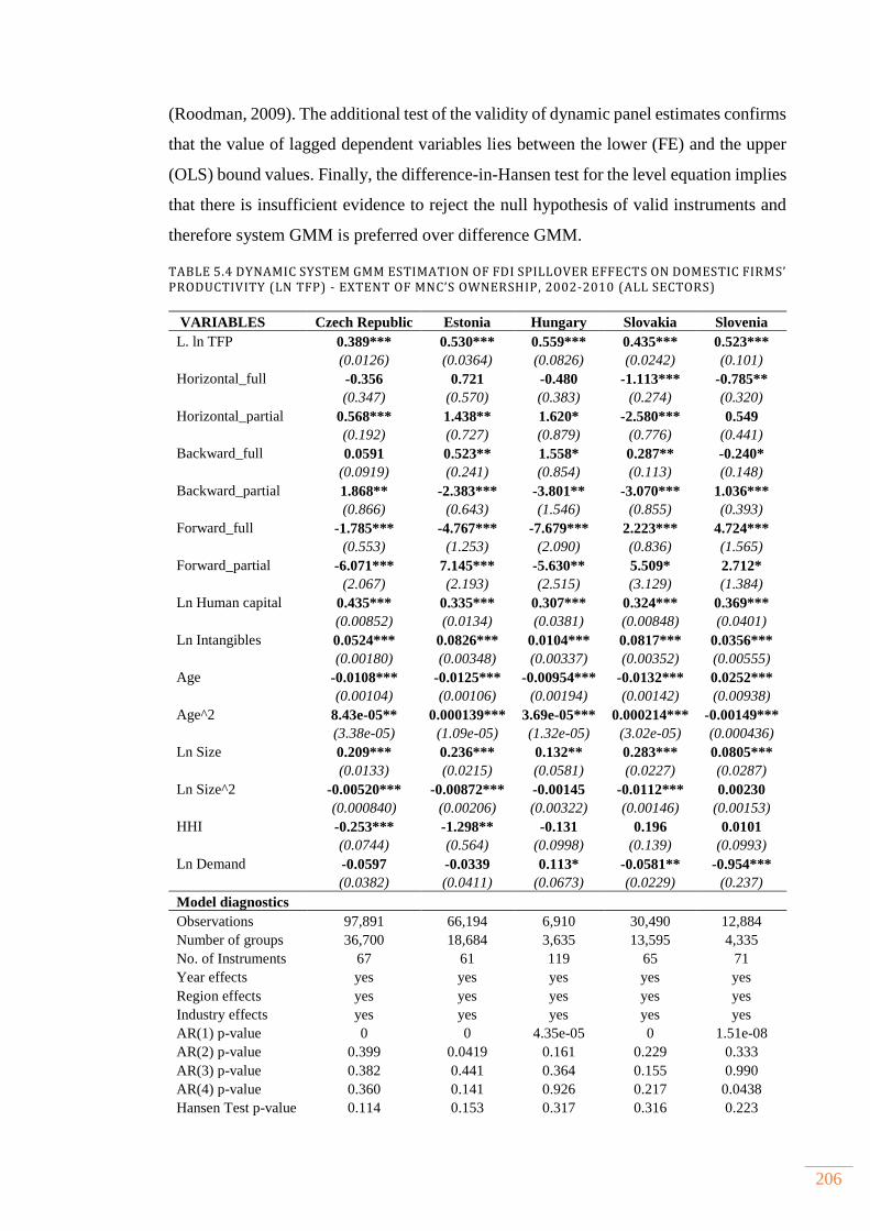
206
(Roodman, 2009). The additional test of the validity of dynamic panel estimates confirms
that the value of lagged dependent variables lies between the lower (FE) and the upper
(OLS) bound values. Finally, the difference-in-Hansen test for the level equation implies
that there is insufficient evidence to reject the null hypothesis of valid instruments and
therefore system GMM is preferred over difference GMM.
TABLE 5.4 DYNAMIC SYSTEM GMM ESTIMATION OF FDI SPILLOVER EFFECTS ON DOMESTIC FIRMS’ PRODUCTIVITY (LN TFP) - EXTENT OF MNC’S OWNERSHIP , 2002-2010 (ALL SECTORS)
VARIABLES Czech Republic Estonia Hungary Slovakia Slovenia
L. ln TFP 0.389*** 0.530*** 0.559*** 0.435*** 0.523***
(0.0126) (0.0364) (0.0826) (0.0242) (0.101)
Horizontal_full -0.356 0.721 -0.480 -1.113*** -0.785**
(0.347) (0.570) (0.383) (0.274) (0.320)
Horizontal_partial 0.568*** 1.438** 1.620* -2.580*** 0.549
(0.192) (0.727) (0.879) (0.776) (0.441)
Backward_full 0.0591 0.523** 1.558* 0.287** -0.240*
(0.0919) (0.241) (0.854) (0.113) (0.148)
Backward_partial 1.868** -2.383*** -3.801** -3.070*** 1.036***
(0.866) (0.643) (1.546) (0.855) (0.393)
Forward_full -1.785*** -4.767*** -7.679*** 2.223*** 4.724***
(0.553) (1.253) (2.090) (0.836) (1.565)
Forward_partial -6.071*** 7.145*** -5.630** 5.509* 2.712*
(2.067) (2.193) (2.515) (3.129) (1.384)
Ln Human capital 0.435*** 0.335*** 0.307*** 0.324*** 0.369***
(0.00852) (0.0134) (0.0381) (0.00848) (0.0401)
Ln Intangibles 0.0524*** 0.0826*** 0.0104*** 0.0817*** 0.0356***
(0.00180) (0.00348) (0.00337) (0.00352) (0.00555)
Age -0.0108*** -0.0125*** -0.00954*** -0.0132*** 0.0252***
(0.00104) (0.00106) (0.00194) (0.00142) (0.00938)
Age^2 8.43e-05** 0.000139*** 3.69e-05*** 0.000214*** -0.00149***
(3.38e-05) (1.09e-05) (1.32e-05) (3.02e-05) (0.000436)
Ln Size 0.209*** 0.236*** 0.132** 0.283*** 0.0805***
(0.0133) (0.0215) (0.0581) (0.0227) (0.0287)
Ln Size^2 -0.00520*** -0.00872*** -0.00145 -0.0112*** 0.00230
(0.000840) (0.00206) (0.00322) (0.00146) (0.00153)
HHI -0.253*** -1.298** -0.131 0.196 0.0101
(0.0744) (0.564) (0.0998) (0.139) (0.0993)
Ln Demand -0.0597 -0.0339 0.113* -0.0581** -0.954***
(0.0382) (0.0411) (0.0673) (0.0229) (0.237)
Model diagnostics
Observations 97,891 66,194 6,910 30,490 12,884
Number of groups 36,700 18,684 3,635 13,595 4,335
No. of Instruments 67 61 119 65 71
Year effects yes yes yes yes yes
Region effects yes yes yes yes yes
Industry effects yes yes yes yes yes
AR(1) p-value 0 0 4.35e-05 0 1.51e-08
AR(2) p-value 0.399 0.0419 0.161 0.229 0.333
AR(3) p-value 0.382 0.441 0.364 0.155 0.990
AR(4) p-value 0.360 0.141 0.926 0.217 0.0438
Hansen Test p-value 0.114 0.153 0.317 0.316 0.223

207
Note: robust standard errors in brackets
***, ** and * denote statistical significance of variables at 1%, 5% and 10% level of significance
respectively.
The lagged dependent variable is highly significant and positive in all cases, ranging
from 0.39 in the Czech Republic to 0.56 in Hungary, again indicating high persistence of
past productivity improvements and learning effects. Increased concentration in
industries has negative and significant effect only in Estonia and the Czech Republic,
although the magnitude of the coefficient in the former country is now lower. The
demand variable again indicates that the bulk of firms in Slovakia and Slovenia are not
buying inputs from domestic suppliers, thus negatively affecting productivity by 0.05
and 0.95 percent, respectively. In comparison to the baseline model, the effect of demand
is now positive in Hungary. It seems that firms benefit from increased economies of scale
as a 10 percent increase in purchased inputs leads to improvement of local firm’s
productivity by one percent.
Firm level variables, namely age and size kept the same sign, with similar magnitude and
significance levels as in the baseline model. Again, the turning point after which the
effect of the age of firms becomes positive and outweighs initial negative effects is too
large to have any significant effect in the medium term. The results suggest that older
firms in all countries except Slovenia are not capable of increasing their productivity
probably due to obsolete capital equipment or do not have the necessary knowledge or
level of investment to keep pace with advances in technology. Findings for the firm size
corroborate those from the baseline model indicating inverse U shaped effects in the case
of the Czech Republic, Estonia and Slovakia and positive linear effects throughout the
sample period for Hungary and Slovenia.
Findings related to variables measuring absorptive capacity are in line with those
obtained in the baseline model suggesting that human capital and the share of intangible
assets play a positive and significant role in increasing TFP. The effect of human capital
on TFP is largest in the Czech Republic, where a one percent increase in average wage
leads to an increase in TFP by 0.43 percent, followed by Slovenia (0.36 percent) and
being smallest in Hungary (0.30 percent). Similarly, the effect of intangible assets
confirms the positive findings from the baseline model although the magnitude of the
hor_part=hor_full 0.00636 0.136 0.0173 0.0183 0.00179
back_part=back_full 0.0385 0.000610 0.0149 0.000297 0.00895
for_part=for_full 0.0378 2.26e-06 0.550 0.263 0.0436

208
coefficient is slightly smaller. If the share of intangibles increases by 10 percentage
points the effect on TFP ranges from 0.1 percent in Hungary to 0.8 percent in Estonia
and Slovakia, whilst for other countries the effect is moderate (between 0.3 and 0.5
percent). It seems that domestic firms have either invested in the process or product
innovation or increased their stock of knowledge by adopting the fruits of other firms’
innovation efforts embodied in intangible asset purchased on the market.
Turning to FDI spillover variables, it is noticeable that the average coefficient in the
baseline model hides important information. Although the results are robust to change in
specification in terms of significance and signs, the magnitude of coefficients vary.
Partially foreign owned firms have stronger effect on productivity within the sector,
while the opposite holds for backward vertical linkages. Starting from horizontal
spillovers it seems that the percentage of foreign ownership does matter for productivity
as partially foreign owned firms seem to generate positive horizontal spillovers in the
Czech Republic, Estonia and Hungary, while fully foreign owned firms generate negative
spillovers within the industry in Slovenia and Slovakia. In the latter country, total
negative effects are driven by both types of foreign firms. The difference between
partially and fully foreign owned firms is statistically significant in all countries except
in Estonia. Overall, the productivity effects range from 0.56 percent in the Czech
Republic up to 1.6 percent in Hungary for every one percentage point increase in the
output of partially foreign owned firms in the industry. Negative effects of fully foreign
owned firms are in line with the hypothesis suggesting that these firms are bringing more
advanced technology in order to obtain higher market share. Furthermore, the full control
of operation enables them to prevent knowledge dissipation and to cope with the liability
of foreignness. At the same time, local firms are not equipped to capture potential
technology spillovers due to their higher technological gap. However, foreign firms
entering the local market through joint ventures or as a part of partial acquisitions have
beneficial effect as the technology and productivity levels are more likely to be similar
to local firms which enable them to benefit from demonstration or imitation effects.
Furthermore, as argued by Smeets and de Vaal (2006), a tacit component of knowledge
requires frequent communication and interaction providing another reason why shared
ownership is more likely to result in greater knowledge spillovers. Finally, it is more
likely that in firms with shared ownership the local partner is mostly involved in hiring
decisions of local staff and increased labour mobility may lead to technology transfer.

209
The heterogeneous effects of ownership is also evident in the case of backward linkages
where positive effects in the baseline model for the Czech Republic, Hungary and
Slovakia are driven by two different types of firms. In the former, the positive effects on
local firms’ productivity are driven by partially foreign owned firms corroborating the
findings by Javorcik and Spatereanu (2008) who hypothesize that firms with partial
foreign ownership are more likely to source their intermediate inputs from local markets
due to the knowledge of local conditions and quality of suppliers. An increase in demand
for inputs from these firms in the Czech Republic and Slovenia may also arise due to the
less stringent requirements for quality and production process which benefit domestic
suppliers who otherwise would not be able to provide inputs to more technologically
advanced foreign firms. On the other hand, the negative effect of fully foreign owned
firms in Slovenia may be attributed to the time necessary to familiarise with domestic
suppliers and provide them with training and support. In addition, greenfield investments
are usually undertaken by large firms with high bargaining power and usually require
large discounts for their inputs as a prerequisite to become supplier.
A different picture emerges in the case of other countries. In Hungary, a one percentage
point increase in the backward linkage from fully foreign owned firms is associated with
1.5 percent increase in productivity, while for the other two countries the effect is smaller
in magnitude and in the range between 0.28 in Slovakia and 0.52 percent in Estonia. On
the other hand, the positive effects from fully foreign owned firms are offset by negative
productivity effects on local suppliers from partially foreign owned firms which are
larger in magnitude and possibly explain total negative effects of backward linkages in
Estonia. In all cases, the difference between coefficients is statistically significant. The
positive effects of fully foreign owned enterprises in these countries can be explained by
the large number of these firms being established through either greenfield investment
or full acquisitions in both manufacturing and service sectors. Since fully foreign owned
investments are in general more productive and bring more advanced technology into the
host market they are more likely to induce technological improvements in existing
suppliers such as higher standards on product features, delivery schedules, quality
control, inventory holding (Godart and Gorg, 2013). In their theoretical model, Carluccio
and Fally (2013) have demonstrated that the entry of more advanced foreign firms
induces reconfiguration of the supply chain and forces technology adoption by domestic
firms that are willing to supply to MNCs. Those firms that do not adopt foreign

210
technology suffer from increased competition from foreign suppliers, while firms in
downstream sector are faced with less availability of inputs compatible with domestic
technology and are forced out of the market.
In Hungary acquired companies retained their original suppliers while other local firms
have also been successful in joining the international network of MNCs mainly
established through greenfield investment (Sass, 2008). Since fully foreign owned
enterprises, especially those that are smaller and privatised, are more independent in their
decisions about which supplier to choose and most of them exist for a certain period of
time, the positive effects reflect the increasing familiarity with domestic supply capacity
(Vince, 2001; Sass, 2007). Finally, the overall improvement in institutional progress and
especially in the protection of intellectual property rights might have induced more entry
in high tech and knowledge intensive industries through wholly owned subsidiaries
requiring more advanced inputs (Javorcik and Saggi, 2010). 59
The strong negative effect of partially foreign owned enterprises can be explained by
higher import ratio of components which may result in a loss of customers for suppliers,
reduction in profit and a decline in their productivity (Newman et al., 2015). In addition,
it is well documented that joint ventures or M&A bring less advanced technology to local
market (Mansfield, 1980). Therefore, the incentive to improve the quality and efficiency
may be weaker when domestic firms supply partially foreign owned firms with less
valuable technology and know-how which could be transferred to their local suppliers.
Alternatively, firms with shared ownership may be operating in less knowledge intensive
sectors with low value added and obsolete technology which do not require
technologically advanced inputs or may be involved more in distribution activities which
require less intermediate inputs.
59 In order to shed more light on the role of intellectual property rights in moderating the relationship
between FDI spillovers and firms’ TFP we interacted the former with Legal System and Property Right
index obtained from Fraser Institute. The expectation was that an improvement in IPR will have negative
moderating effects on horizontal spillovers due to increased competitive edge of MNCs, especially from
fully owned foreign firms which are more likely to appropriate the benefits of their advanced technology.
In case of vertical linkages the moderating effect is more ambiguous. On the one hand, stroger IPR are
likely to increase productivity enhancing effects of FDI spillovers as it enhance the enforcement
mechanism that foreign firms can utilize in case of expropriation of the obtained knowledge or encourage
MNCs to transfer more advanced technology and thus provide inputs of superior quality to local customers
(Smeets and de Vaal, 2015). On the other hand, foreign firms can gain monopoly or monopsony power,
thus requiring local suppliers reduce their prices or charge higher prices to local customers. However, the
obtained data had very little variation over time and the corresponding empirical results did not satisfy the
necessary model diagnostics or when they did the results were to mixed to shed more light on the already
heterogenous results.

211
Forward spillovers are significant and positive in Slovakia and Slovenia for both types
of foreign firms. The productivity effects on local firms are especially beneficial when
inputs come from partially foreign owned firms in Slovakia and fully foreign owned
firms in Slovenia. A one percentage point increase in output of foreign firms with shared
ownership in upstream sectors is associated with 5.50 and 2.71 percent increase in TFP
of downstream firms in Slovakia and Slovenia, respectively. This effect may stem from
domestic market orientation of these companies which are more familiar with the needs
and capabilities of domestic firms. Similarly, a one percentage point increase in output
of fully foreign owned firms is associated with 2.2 and 4.7 percent increase in TFP in
Slovakia and Slovenia, respectively, indicating that local firms in both countries have the
ability to benefit from high quality inputs. In both Slovakia and Slovenia, the net effects
of vertical linkages are positive arising mainly from the ability of local firms to benefit
from increased quality of intermediate inputs purchased from MNCs. The F test of
equality of both types of forward spillovers is rejected in all countries expect in Slovakia
and Hungary as indicated at the bottom of Table 5.4.
In the case of Estonia, the average negative effect of forward linkages is driven by fully
foreign owned firms. However, this detrimental effect is offset by the significant and
economically meaningful effects of firms with shared ownership which, by selling their
output to local firms, increase their TFP by 7.1 percent. In other countries, local firms
are not able to reap the benefits of better intermediate inputs probably due to insufficient
absorptive capacity or differences arising from sourcing behaviour of domestic firms in
different sectors. The negative effect is mostly pronounced in Hungary where both type
of foreign firms have a combined negative effect of 13.2 percent while in the Czech
Republic this negative effect amount to 7.85 percent reduction in the productivity levels
of local firms.
5.5.3 THE EFFECTS OF MNC’S ORIGIN
The third part of this chapter is concerned with the analysis of MNC’s country of origin.
As mentioned in Chapter 2 origin of MNCs can have differential impact on local firms’
productivity and their inclusion in GVCs. It has been shown that foreign affiliates from
emerging economies generate fewer positive spillovers to local firms since they rely
more on non-technological assets, mature technology, and production capabilities,

212
networks and relationships (UNCTAD, 2006; Buckley et al., 2007b). Related to this,
recent research has found that these affiliates engage in asset seeking strategies relying
on host country technology with the aim to improve the performance of its parent
company thus limiting spillovers to local firms (Driffield and Love, 2007; Chen et al.,
2012). However, Javorcik and Spatareanou (2011) drawing on theoretical model of
vertical linkages (Rodriguez-Clare, 1996) argue that geographical distance can have a
positive impact on the creation of linkages as MNCs have incentives to source more from
local companies to reduce transportation and communication costs. 57F
60
Similarly, it has been shown that services MNCs follow their clients in foreign markets
due to strong need for geographical proximity with users of business services inputs
(Nefussi and Schwellnus, 2010). Therefore, the variety of services inputs brought by
MNCs of different origin can also benefit local customers in both manufacturing and
service sectors. However, the expected sign of forward linkages is ambiguous and
depends on the level of technology brought by foreign firms and the ability of local firms
to absorb different inputs. Furthermore, free trade area within the EU can encourage
export platform FDI from MNCs located outside of the EU that are attracted by improved
market access to countries within the trading bloc. Since local firms are often not direct
competitors, export oriented MNCs do not need to worry about potential technology
leakage. Also, non-EU MNCs have to comply with the rule of origin which requires that
sufficient share of value in their product is added within the host country (Javorcik and
Spatareanou, 2011). Since our sample consist of EU member states the assumption of
increased domestic sourcing of non-EU MNCs is likely to hold in order to avoid import
tariffs.
In the case of foreign affiliates from EU political, economic, cultural and institutional
proximity induced by EU integration process facilitate the cooperation and creation of
linkages (Monastiriotis, 2014). For example, cultural and institutional similarity evident
in business laws, customs, ways of doing business and possibly familial links may induce
trust and mitigate misunderstanding (Johanson and Vahlne, 2009; Conti et al., 2014).
This in turn may result in reduction of transactions costs between suppliers and
customers, thus facilitating vertical linkages. However, EU investors are exempt from
rule of origin requirement and thus are more likely to import their intermediate inputs
60 Services may not be affected to the same extent as manufacturing goods due to improvements in ICT.
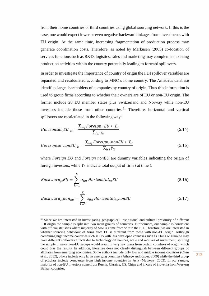
213
from their home countries or third countries using global sourcing network. If this is the
case, one would expect lower or even negative backward linkages from investments with
EU origin. At the same time, increasing fragmentation of production process may
generate coordination costs. Therefore, as noted by Markusen (2005) co-location of
services functions such as R&D, logistics, sales and marketing may complement existing
production activities within the country potentially leading to forward spillovers.
In order to investigate the importance of country of origin the FDI spillover variables are
separated and recalculated according to MNC’s home country. The Amadeus database
identifies large shareholders of companies by country of origin. Thus this information is
used to group firms according to whether their owners are of EU or non-EU origin. The
former include 28 EU member states plus Switzerland and Norway while non-EU
investors include those from other countries. 58F
61 Therefore, horizontal and vertical
spillovers are recalculated in the following way:
𝐻𝑜𝑟𝑖𝑧𝑜𝑛𝑡𝑎𝑙_𝐸𝑈𝑗𝑡 =∑ 𝐹𝑜𝑟𝑒𝑖𝑔𝑛𝑖𝑡𝐸𝑈 ∗ 𝑌𝑖𝑡𝑖𝜖𝑗
∑ 𝑌𝑖𝑡𝑖𝜖𝑗(5.14)
𝐻𝑜𝑟𝑖𝑧𝑜𝑛𝑡𝑎𝑙_𝑛𝑜𝑛𝐸𝑈𝑗𝑡 =∑ 𝐹𝑜𝑟𝑒𝑖𝑔𝑛𝑖𝑡𝑛𝑜𝑛𝐸𝑈 ∗𝑌𝑖𝑡𝑖𝜖𝑗
∑ 𝑌𝑖𝑡𝑖𝜖𝑗(5.15)
where Foreign EU and Foreign nonEU are dummy variables indicating the origin of
foreign investors, while Yit indicate total output of firm i at time t.
𝐵𝑎𝑐𝑘𝑤𝑎𝑟𝑑𝑗𝑡𝐸𝑈 = ∑𝛼𝑗𝑘𝑡
𝐾
𝑘=1
𝐻𝑜𝑟𝑖𝑧𝑜𝑛𝑡𝑎𝑙𝑘𝑡𝐸𝑈(5.16)
𝐵𝑎𝑐𝑘𝑤𝑎𝑟𝑑𝑗𝑡𝑛𝑜𝑛𝐸𝑈 = ∑𝛼𝑗𝑘𝑡
𝐾
𝑘=1
𝐻𝑜𝑟𝑖𝑧𝑜𝑛𝑡𝑎𝑙𝑘𝑡𝑛𝑜𝑛𝐸𝑈(5.17)
61 Since we are interested in investigating geographical, institutional and cultural proximity of different
FDI origin the sample is split into two main groups of countries. Furthermore, our sample is consistent
with official statistics where majority of MNCs come from within the EU. Therefore, we are interested in
whether sourcing behaviour of firms from EU is different from those with non-EU origin. Although
combining high income countries such as US with less developed countries such as China or Ukraine may
have different spillovers effects due to technology differences, scale and motives of investment, splitting
the sample in more non-EU groups would result in very few firms from certain countries of origin which
could bias the results. In addition, literature does not clearly distinguish between different groups of
affiliates from emerging economies. Some authors include only low and middle income countries (Chen
et al., 2012), others include only large emerging countries (Athreye and Kapur, 2009) while the third group
of scholars include companies from high income countries in Asia (Mathews, 2002). In our sample,
majority of non-EU investors come from Russia, Ukraine, US, China and in case of Slovenia from Western
Balkan countries.
214
𝐹𝑜𝑟𝑤𝑎𝑟𝑑𝑗𝑡𝐸𝑈 =∑𝛾𝑗𝑙𝑡
𝐿
𝑙=1
𝐻𝑜𝑟𝑖𝑧𝑜𝑛𝑡𝑎𝑙𝑙𝑡𝐸𝑈(5.18)
𝐹𝑜𝑟𝑤𝑎𝑟𝑑𝑗𝑡𝑛𝑜𝑛𝐸𝑈 =∑𝛾𝑗𝑙𝑡
𝐿
𝑙=1
𝐻𝑜𝑟𝑖𝑧𝑜𝑛𝑡𝑎𝑙𝑙𝑡𝑛𝑜𝑛𝐸𝑈(5.19)
where 𝛼𝑗𝑘𝑡(𝛾𝑗𝑙𝑡) are input (output) coefficients from annual IO tables measuring the
proportion of industry j’s output (input) supplied (purchased) to (from) industries k(l) at
time t.
Table 5.5 below provides empirical results of the combined effects of strategic,
geographical, institutional and technological diversity that MNCs from different origin
bring into host countries. Before turning to the explanation of results, the diagnostics of
the models are discussed. The Hansen J statistics of over identifying restrictions indicates
that the probability of making Type I error if rejecting the null hypothesis of the validity
of instrument ranges from 18 to 94 percent, thus providing sufficient evidence of
instrument exogeneity in all countries except the Czech Republic. In the latter country,
over identifying restrictions are not satisfied, thus casting some doubt on the validity of
results. A more detailed analysis can reveal that the difference in the Hansen test for
exogenous variables, more specifically the variable age is most likely the cause for
rejection of the test for the overall validity of the instrument. We tried different
specifications by including higher order lags of the dependent variables in the instrument
set or treating intangible assets and human capital as endogenous variables, but the
diagnostics of the model did not improve and in some cases even worsened. Second order
serial correlation cannot be rejected thus satisfying the necessary condition for the
validity of estimates. Only in the case of Estonia, the test indicates the presence of
autocorrelation in second and fourth lags at 5% significance level. However, in
specifications when second order autocorrelation is satisfied this comes at the expense
of rejecting the Hansen J test, but the signs and significance of coefficients remains
similar across different specifications providing a certain degree of confidence in the
results obtained. Overall, the results for the Czech Republic and Estonia must be taken
with these caveats in mind. The coefficient of the lagged dependent variable in all
countries lies between lower (FE) and upper (OLS) estimates, thus we can be confident
that dynamic specification satisfies Bond et al. (2001) informal test for a good estimator.
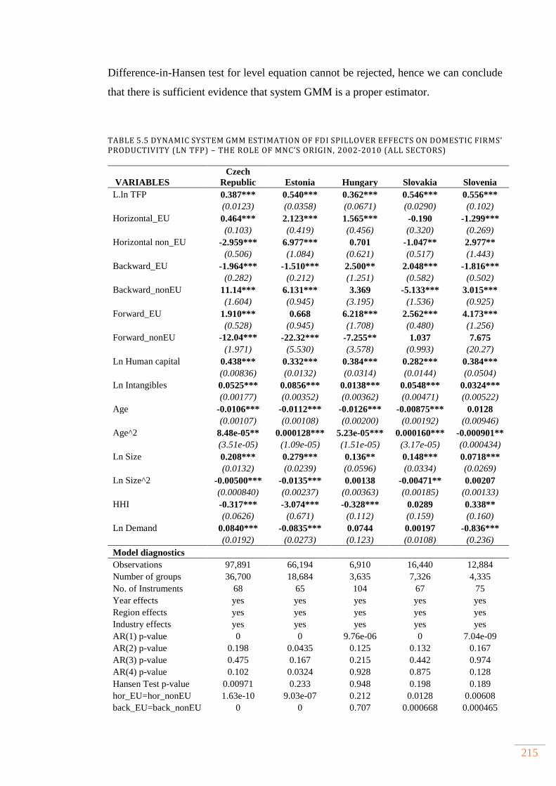
215
Difference-in-Hansen test for level equation cannot be rejected, hence we can conclude
that there is sufficient evidence that system GMM is a proper estimator.
TABLE 5.5 DYNAMIC SYSTEM GMM ESTIMATION OF FDI SPILLOVER EFFECTS ON DOMESTIC FIRMS’ PRODUCTIVITY (LN TFP) – THE ROLE OF MNC’S ORIGIN, 2002-2010 (ALL SECTORS)
VARIABLES
Czech
Republic Estonia Hungary Slovakia Slovenia
L.ln TFP 0.387*** 0.540*** 0.362*** 0.546*** 0.556***
(0.0123) (0.0358) (0.0671) (0.0290) (0.102)
Horizontal_EU 0.464*** 2.123*** 1.565*** -0.190 -1.299***
(0.103) (0.419) (0.456) (0.320) (0.269)
Horizontal non_EU -2.959*** 6.977*** 0.701 -1.047** 2.977**
(0.506) (1.084) (0.621) (0.517) (1.443)
Backward_EU -1.964*** -1.510*** 2.500** 2.048*** -1.816***
(0.282) (0.212) (1.251) (0.582) (0.502)
Backward_nonEU 11.14*** 6.131*** 3.369 -5.133*** 3.015***
(1.604) (0.945) (3.195) (1.536) (0.925)
Forward_EU 1.910*** 0.668 6.218*** 2.562*** 4.173***
(0.528) (0.945) (1.708) (0.480) (1.256)
Forward_nonEU -12.04*** -22.32*** -7.255** 1.037 7.675
(1.971) (5.530) (3.578) (0.993) (20.27)
Ln Human capital 0.438*** 0.332*** 0.384*** 0.282*** 0.384***
(0.00836) (0.0132) (0.0314) (0.0144) (0.0504)
Ln Intangibles 0.0525*** 0.0856*** 0.0138*** 0.0548*** 0.0324***
(0.00177) (0.00352) (0.00362) (0.00471) (0.00522)
Age -0.0106*** -0.0112*** -0.0126*** -0.00875*** 0.0128
(0.00107) (0.00108) (0.00200) (0.00192) (0.00946)
Age^2 8.48e-05** 0.000128*** 5.23e-05*** 0.000160*** -0.000901**
(3.51e-05) (1.09e-05) (1.51e-05) (3.17e-05) (0.000434)
Ln Size 0.208*** 0.279*** 0.136** 0.148*** 0.0718***
(0.0132) (0.0239) (0.0596) (0.0334) (0.0269)
Ln Size^2 -0.00500*** -0.0135*** 0.00138 -0.00471** 0.00207
(0.000840) (0.00237) (0.00363) (0.00185) (0.00133)
HHI -0.317*** -3.074*** -0.328*** 0.0289 0.338**
(0.0626) (0.671) (0.112) (0.159) (0.160)
Ln Demand 0.0840*** -0.0835*** 0.0744 0.00197 -0.836***
(0.0192) (0.0273) (0.123) (0.0108) (0.236)
Model diagnostics
Observations 97,891 66,194 6,910 16,440 12,884
Number of groups 36,700 18,684 3,635 7,326 4,335
No. of Instruments 68 65 104 67 75
Year effects yes yes yes yes yes
Region effects yes yes yes yes yes
Industry effects yes yes yes yes yes
AR(1) p-value 0 0 9.76e-06 0 7.04e-09
AR(2) p-value 0.198 0.0435 0.125 0.132 0.167
AR(3) p-value 0.475 0.167 0.215 0.442 0.974
AR(4) p-value 0.102 0.0324 0.928 0.875 0.128
Hansen Test p-value 0.00971 0.233 0.948 0.198 0.189
hor_EU=hor_nonEU 1.63e-10 9.03e-07 0.212 0.0128 0.00608
back_EU=back_nonEU 0 0 0.707 0.000668 0.000465
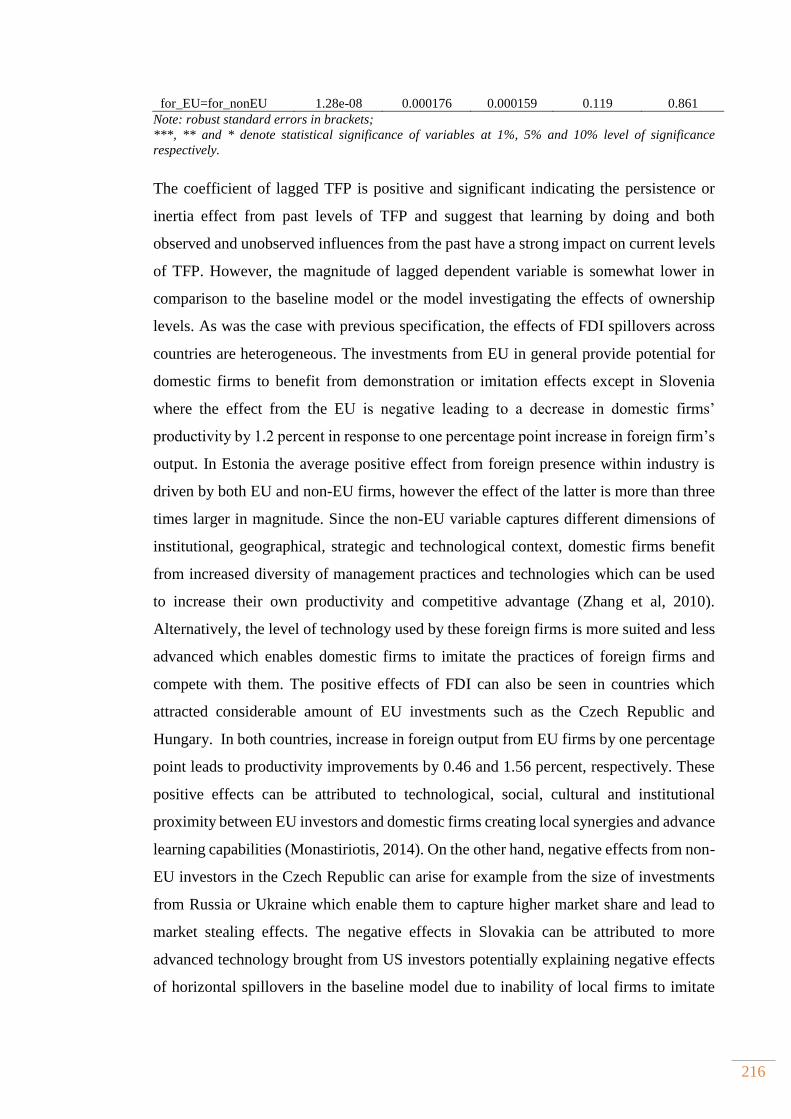
216
Note: robust standard errors in brackets;
***, ** and * denote statistical significance of variables at 1%, 5% and 10% level of significance
respectively.
The coefficient of lagged TFP is positive and significant indicating the persistence or
inertia effect from past levels of TFP and suggest that learning by doing and both
observed and unobserved influences from the past have a strong impact on current levels
of TFP. However, the magnitude of lagged dependent variable is somewhat lower in
comparison to the baseline model or the model investigating the effects of ownership
levels. As was the case with previous specification, the effects of FDI spillovers across
countries are heterogeneous. The investments from EU in general provide potential for
domestic firms to benefit from demonstration or imitation effects except in Slovenia
where the effect from the EU is negative leading to a decrease in domestic firms’
productivity by 1.2 percent in response to one percentage point increase in foreign firm’s
output. In Estonia the average positive effect from foreign presence within industry is
driven by both EU and non-EU firms, however the effect of the latter is more than three
times larger in magnitude. Since the non-EU variable captures different dimensions of
institutional, geographical, strategic and technological context, domestic firms benefit
from increased diversity of management practices and technologies which can be used
to increase their own productivity and competitive advantage (Zhang et al, 2010).
Alternatively, the level of technology used by these foreign firms is more suited and less
advanced which enables domestic firms to imitate the practices of foreign firms and
compete with them. The positive effects of FDI can also be seen in countries which
attracted considerable amount of EU investments such as the Czech Republic and
Hungary. In both countries, increase in foreign output from EU firms by one percentage
point leads to productivity improvements by 0.46 and 1.56 percent, respectively. These
positive effects can be attributed to technological, social, cultural and institutional
proximity between EU investors and domestic firms creating local synergies and advance
learning capabilities (Monastiriotis, 2014). On the other hand, negative effects from non-
EU investors in the Czech Republic can arise for example from the size of investments
from Russia or Ukraine which enable them to capture higher market share and lead to
market stealing effects. The negative effects in Slovakia can be attributed to more
advanced technology brought from US investors potentially explaining negative effects
of horizontal spillovers in the baseline model due to inability of local firms to imitate
for_EU=for_nonEU 1.28e-08 0.000176 0.000159 0.119 0.861
217
foreign technology and therefore improve their efficiency in the wake of increased
competition.
Turning the attention to backward linkages, the effect of EU MNCs are negative and
statistically significant in three out of five countries. Negative effects in the Czech
Republic, Estonia and Slovenia indicate that presence of EU firms in downstream
industries hurts productivity of domestic suppliers as they are not able to join global
production networks. Furthermore, MNCs from EU are in better position to source their
inputs from their home country supplier due to their vicinity and may be more
technologically advanced than MNCs coming from rest of the world, thus requiring
higher quality of inputs which may act as a barrier for domestic supplier to enter GSC. 59F
62
As suggested by Rodriguez and Clare (1996) the negative effect of backward linkages
may also stem from dissimilarities in terms of variety of inputs between host and home
countries. On the other hand, positive effects are experienced by local suppliers in
Hungary and Slovakia where a majority of EU investment went to industries with high
potential for developing local linkages, such as automobile and electronics, due to long
history, tradition and intense cooperation in the field of production and/or trade with
foreign partners (Sass, 2008). The magnitude of coefficients are economically
meaningful suggesting that a one percentage point increase of foreign firms’ output of
EU MNCs in downstream sectors leads to increase in TFP of domestic suppliers by 2
percent in Slovakia and 2.5 percent in Hungary.
On the other hand, non-EU investors seem to source inputs from local markets as
suggested by positive coefficients in each country except Slovakia where the effect is
negative and statistically significant indicating a decrease in TFP of 5.1 percent. Positive
effects of non-EU investors are highest in the Czech Republic where a one percentage
point increase of foreign firms’ output from outside EU in downstream sector leads to
11.1 percent increase in TFP, followed by 6.1 increase in Estonia and 3 percent increase
in Slovenia while in Hungary the effect is not significant. The difference between
coefficients is statistically significant in all countries except Hungary. The effects of non-
EU investment are in line with the proposition that distance plays a role in the extent of
62 When log TFP of foreign firms is regressed on a dummy variable taking the value of one for non-EU
and zero for EU investors controlling for industry, region and time effects the result point out that there is
a negative and statistically significant relationship between TFP and the presence of foreign firms outside
the EU in the Czech R. and Estonia. Hence, we can take this result as an indication of lower productivity
levels of non-EU MNCs. This in turn may benefit domestic firms as non-EU MNCs are able to transfer
knowledge to their local suppliers.
218
backward linkages. Most of foreign investors outside the EU were established to benefit
from relatively cheap location and at the same time enjoy access to the EU market using
countries under analysis as export platforms. In order to qualify for preferential tariff
these foreign subsidiaries are more likely to be actively involved with local suppliers.
However, as suggested by Javorcik and Spatareanu (2011), to confirm the role of distance
it is necessary to test if knowledge transfer from non- EU MNCs is larger in sectors with
high transport costs, something that is difficult to test given the data and space limitations
of this thesis and the fact that our focus is on manufacturing and service industries, the
latter being mostly a non-tradable sector for which transport costs is difficult to obtain.
Furthermore, given recent advances in ICT, the transport costs are less relevant for
services.
In the case of forward linkages EU investment seem to have a positive and significant
effects in all countries except Estonia indicating increased market seeking motives of EU
subsidiaries and at the same time a possible increase in absorptive capacity of local firms
which are able to use better quality and variety of intermediate inputs. Moreover, given
that in most cases foreign suppliers within the EU followed their customers acting as a
Tier 1 60F
63 suppliers or providers of business services, the increased presence of foreign
firms in upstream sectors may have resulted in cheaper inputs which benefit local
downstream firms (Markusen and Venables, 1999).
In general, the effects of positive forward linkages from the baseline model in Slovakia
and Slovenia are driven by EU investors entirely although there is no statistically
significant difference between the effects of EU and non-EU MNCs. In other countries,
the effect of non-EU investors is negative, being the highest in Estonia where an increase
in foreign firms’ output in upstream sector by one percentage point leads to decrease in
productivity of domestic firms in downstream sector by 22 percent. Similarly, in the
Czech Republic this negative effect amount to 12 percent and in Hungary to 7.2 percent.
The possible reason for negative forward linkages from non-EU MNCs may stem from
their motive of investment. It is likely that non-EU firms engage in export platform FDI
to circumvent the trade costs related to distance. However, such investment motive is
more oriented to supplying other neighbouring countries, thus reducing the spillovers
63 Tier 1 are more technologically capable companies which act as direct suppliers to original equipment
manufacturers (OEM) in automotive or aerospace industry which require complex and specialized
components.
219
potential for domestic firms and even crowd out existing domestic suppliers. If this is the
case, domestic firms buying inputs from foreign MNCs may be faced with higher quality
inputs and higher costs, thus resulting in decreased TFP. The difference in coefficients is
statistically significant implying that positive effects brought by EU MNCs are entirely
offset by negative effect from non-EU MNCs.
The effects of concentration ratio are significant and positive in case of Slovenia, non-
significant in Slovakia and negative in other countries confirming previous findings
suggesting that increased competition benefit productivity of domestic firms. The results
are in line with selection effects of heterogeneous producers in which competition induce
existing firms to become more efficient and force less efficient firms to exit (Syverson,
2011). However, the exact mechanism through which competition is postulated to
increase productivity cannot be discerned from the variable used in this analysis. The
effects of a one percent increase in demand for intermediate inputs in the economy leads
to diseconomies of scale resulting in decrease of TFP between 0.08 in Estonia and 0.83
percent in Slovenia confirming findings from previous models. It seems that increased
demand for inputs have positive albeit small effects on local firms’ productivity in the
Czech Republic.
Age and size kept the same signs and significance levels as in the ownership and baseline
model with the exception of age which is now insignificant at conventional levels in the
case of Slovenia. Nonlinear effects of firms’ size are again found only in the case of the
Czech Republic, Estonia and Slovakia where TFP starts to decline after firms cross
certain threshold. Firm specific variables measuring absorptive capacity are in line with
those obtained in other models suggesting that human capital and the share of intangible
assets play a positive and significant role in increasing TFP.
5.6 CONCLUSION
The literature on productivity spillovers has made significant advances in the last ten
years. A large body of empirical evidence based on micro level data has been produced
focusing predominantly on factors that condition the spillover process. Despite these
advances, the heterogeneity of MNCs has largely been ignored – except for some

220
theoretical work on the extent of technology transfer arising from differences in MNCs’
country of origin, ownership structure and heterogeneous role of subsidiaries in MNCs’
network. The aim of this chapter was to examine the size and direction of productivity
spillovers to local firms accruing from MNCs’ heterogeneity in a sample of five CEE
countries controlling for firms’ absorptive capacity, market competition and demand
effects. The novelty of this chapter is the introduction of new methodology which
controls for the potential endogeneity of FDI spillovers and dynamic effects. In addition,
unlike most other studies, the investigation takes into account not just the manufacturing
but also the service sector, shedding new light on the role of MNCs and providing
comparable results across countries by using the same data source and empirical model.
The results of the baseline model show that previous findings related to horizontal
spillovers may be misleading as in several cases it is found that local firms may benefit
from increased presence of foreign firms and that these spillovers may become even more
important than vertical linkages. In countries where MNCs reduce the TFP of local firms
due to negative competition effects or labour poaching, the results are driven by both
fully and partially foreign owned firms indicating the lack of absorptive capacity of the
average firm in the sample. On the other hand, in all countries the positive effects of
MNCs within sector can be explained by beneficial effects of partially foreign owned
firms due to their lower technological sophistication which enable local firms to obtain
technology at lower costs. It can be argued that local firms improve their productivity
relying on well diffused technology brought by partially owned foreign firms. The
findings related to the origin of foreign investment suggest that EU investment tend to
generate greater productivity spillovers within their sector except in Slovenia and
Slovakia. Overall, it appears that at least part of these increased knowledge spillovers is
related to socio-cultural and institutional proximity which facilitates the process of
learning and knowledge diffusion.
The findings for vertical linkages partially confirm the previous findings for backward
linkages. The latter are found to be significant and positive in the Czech Republic,
Hungary and Slovakia and negative in Estonia. A closer look reveals that partially foreign
owned firms are driving the total negative effects in Estonia and partially offset the
positive effects of full foreign ownership in other countries. Interestingly, it seems that
fully foreign owned firms contribute to the development of supplier linkages - the reason
for this may lie in the time period under investigation. The latter factor is related to time

221
and effort of both local firms to satisfy quality requirements and increase their absorptive
capacity and of foreign firms to become more familiar with the capabilities of local firms.
On the other hand, local firms in the Czech Republic and Slovenia seem to benefit more
from partially foreign owned firms as they are more likely to transfer less advanced
technology and be more involved in local economy, thus facilitating knowledge
absorption by local firms.
Similarly, we find that MNCs from the EU are more likely to source inputs from local
markets in Hungary and Slovakia, thus confirming the hypothesis that cultural and
institutional proximity are more likely to lead to more cooperation with local economy.
On the other hand, in other countries the productivity advantage of EU firms has
detrimental effects on local firms’ productivity which is offset by greater sourcing of
local inputs by MNCs from distant countries due to higher trade costs and motives of
investments oriented to serve local markets and neighbouring countries.
Finally, perhaps the more interesting findings is related to forward linkages where in all
countries except Hungary, the effects are statistically significant and economically larger
than backward linkages shedding new light on the role of MNCs. This result may be
driven by firms in the service sector which may explain insignificant findings in earlier
studies investigating manufacturing firms only. It seems that overall forward spillovers
follow a common pattern across countries, being negative in the Czech Republic and
Estonia and positive in Slovakia and Slovenia. This is also confirmed when considering
differences in ownership characteristics of foreign firms where the positive effects in
Slovakia and Slovenia are driven by both fully and partially foreign owned firms while
in Czech Republic and Hungary the opposite effects are observed.
However, when considering geographic heterogeneity, the effects are less clear cut. It
seems that EU investments have a positive and significant effect in all countries except
Estonia. On the other hand, non-EU investments exhibit negative effects on productivity
of local firms in downstream industries possibly due to their orientation towards
supplying third countries in the EU trading bloc. Hence, potential for forward spillovers
may be limited. The magnitude of negative effects from non-EU MNCs offset any
positive effects in the Czech Republic and Estonia, thus contributing to total negative
effects. The results for the Czech Republic, Hungary and Estonia in augmented models
suggest the importance of disentangling linkages as the average effects of forward
spillovers hide the important implications of MNCs’ heterogeneity on productivity of
222
local firms. Hence, governments should question their laissez-faire view that advocates
inflow of FDI without paying close attention to heterogeneity of MNCs and the benefits
they bring to local firms in different sectors.
Summarizing the empirical results from this chapter, we can identify several findings.
First, there is large heterogeneity across countries and any further attempt to analyse the
mechanism of FDI spillovers should take into account the country’s specificities. Second,
the MNC heterogeneity should also be taken into account as firm’s ownership and origin
have important implication for productivity spillovers. Third, forward spillovers are more
likely to influence the net benefits or costs of the foreign presence in the local economy.
Finally, local firms should continue to invest in building their human capital, innovation
capital, scientific and creative property and organizational capital incorporated in the
firms’ intangible assets as these are found to be important determinants of productivity.
223
CHAPTER 6. THE IMPACT OF SERVICES FDI ON PRODUCTIVITY OF DOWNSTREAM
MANUFACTURING FIRMS
6.1 Introduction .......................................................................................................................................... 224
6.2 Conceptual framework and related research ......................................................................... 225
6.2.1 The importance of services sector and implications for MNC’s entry ................. 226
6.2.2 Interactions between services and manufacturing ..................................................... 230
6.2.3 Review of empirical literature .............................................................................................. 233
6.3 Empirical strategy .............................................................................................................................. 236
6.3.1 Empirical model and methodology .................................................................................... 237
6.3.2 Data .................................................................................................................................................. 241
6.4 Discussion of findings ....................................................................................................................... 246
6.4.1 Results of baseline model across sectors ......................................................................... 247
6.4.2 Effects of services fdi on downstream manufacturing firms ................................... 254
6.4.3 The moderating effects of absorptive capacity.............................................................. 259
6.5 Conclusion ............................................................................................................................................. 265
224
6.1 INTRODUCTION
Motivated by recent theoretical modelling suggesting differential effects of FDI arising
from heterogeneity within and across MNCs, previous chapter focused on examining
productivity spillovers in manufacturing and service sectors combined. Given the
inherent differences between these two sectors arising from type of products and services
offered, entry barriers, productivity levels of both domestic and foreign firms, mode of
entry, motives and strategies of MNCs, this chapter aims to shed more light on the effects
of services and manufacturing FDI on productivity of local firms in these two sectors.
It is shown that productivity differences across countries can be largely attributed to
differences in services productivity (Bosworth and Triplett, 2003; Inklaar et al., 2008;
Maroto and Rubalacaba, 2008). Recent liberalisation of services due to improvements in
ICT, decreasing entry barriers and deregulation has fostered not only domestic
competition but also entry of foreign firms with the aim to benefit from increased market
opportunities arising from underdeveloped service sector in transition countries. The
large share of service sector in employment and value added increased the need to raise
the efficiency, improve availability and variety of services inputs. Better services also
contribute to manufacturing competitiveness through reduction in costs and
improvements in manufacturer’s ability to differentiate from competitors. Nordas and
Kim (2013) argue that removing restrictions on FDI in services leads to more
differentiated products for which consumers are willing to pay a premium and enables
manufacturers to obtain higher export prices in sectors with comparative advantages.
As witnessed by industry level data in Chapter 3 and firm level data in Chapter 4, main
recipients of FDI have been services, a trend which is common to majority of middle and
high income countries. Therefore, the aim of this chapter is to investigate inter-industry
linkages beyond those occurring within manufacturing sector. Although a bulk of
empirical work investigated the effects of vertical linkages with domestic firms and
externalities associated with MNC entry, little empirical work was done incorporating
MNCs in services. The area of investigation includes total spillovers accruing to
domestic firms in manufacturing and service sectors. Furthermore, the effects of vertical
linkages resulting from MNC operating in manufacturing and service sector on local
firms’ productivity in manufacturing sector is investigated in order to shed more light on
225
the customer supplier relationship between domestic and foreign firms in two main
sectors of economy.
Previous work has focused on services forward linkages with the rationale that entry of
MNCs in service sector provides more variety, better quality and reduced prices of
intermediate inputs, thus enabling domestic firms to upgrade their technological
capabilities resulting in increased TFP. This chapter adds and expands on existing work
investigating the effects of services liberalisation on both upstream and downstream
manufacturing firms by examining four possible channels of vertical linkages
simultaneously. In addition, we examine whether the scope and scale of FDI spillovers
depends on firms’ absorptive capacity.
The reminder of chapter is structured as follows. Section 6.2 presents conceptual
framework and empirical evidence related to the role of services in economy and their
interrelationship with manufacturing sector. Section 6.3 describes the data used to
construct manufacturing and services vertical linkages and explains the methodology
adopted for empirical investigation and how the possible endogeneity of FDI is dealt
with. Section 6.4 discusses the findings for baseline and augmented models applied to
manufacturing sector and the role of absorptive capacity. Finally, section 6.5 concludes.
6.2 CONCEPTUAL FRAMEWORK AND RELATED RESEARCH
The previous chapter emphasized the limitation of existing studies examining the FDI
spillovers in transition economies which focused mainly on homogenous effects of
foreign firms within manufacturing sector. Recent research has started to include vertical
linkages and horizontal spillovers simultaneously, but they only refer to manufacturing
sector (e.g. Javorcik, 2004a; Nicolini and Resmini, 2010; Damijan et al., 2013). Despite
the increases in FDI in services, which now account for almost 65 per cent of total
worldwide FDI inward stock (UNCTAD, 2014), and development of corresponding
theoretical literature on the importance of linkages between services and manufacturing
sectors and their effects on productivity and exports, empirical literature is scarce. Even
scarcer is the literature on the effects of FDI spillovers on service sector TFP or the
impact of services MNCs on productivity of downstream manufacturing firms. Given the
226
large inflows of foreign investment in services in transition countries, it is important to
separately examine the impact of MNC’s entry in services and manufacturing sectors on
productivity of manufacturing firms. This will shed new light on the effects of vertical
linkages on local firms.
6.2.1 THE IMPORTANCE OF SERVICE SECTOR AND IMPLICATIONS FOR
MNC’S ENTRY
The rising importance of service sector can be attributed to two main factors. First, rise
in income per capita increases the demand for more elastic final goods and thus increases
the need to shift resources into the sector explaining the rise in services employment
(Clark, 1940; Fourastie, 1949). In addition, Raa and Wolff (2001) and Fixler and Siegel
(1999) argue that shift to services is caused by structural changes in the economy which
moves the demand curve for services outward. They explain this by increased
outsourcing of manufacturing activities to the providers of specialist external services
and increased female participation in the labour market, hence increasing the demand for
services which were previously produced and consumed within household.
On the other hand, Baumol and Bowen (1966) and Baumol (1967) argued that increase
in share of final or consumer services in total output is the result of productivity gap
between two main sectors of the economy. Therefore, this shift would have detrimental
effects on aggregate productivity growth as services are less productive and less
technologically advanced. The increased share of services on current price basis is thus
the result of fall in relative prices of manufacturing and increased costs and prices in
stagnant sectors which rise by magnitude of productivity differential. However, the major
critique to Baumol is his focus on consumer services while ignoring the importance of
producer services (Katouzian, 1970; Francois, 1990a).
This leads to second factor emphasized by Oulton (2001). He pointed out that not all
services are demanded for final consumption. Therefore, as long as some services are an
important source of intermediate inputs to other industries and their productivity is
positive the shift to services can increase overall productivity. Wolfl (2003) emphasized
several channels through which increased share of producer services can contribute to
overall growth and productivity. The first one is related to outsourcing of certain
227
activities previously performed within manufacturing firms’ boundary which increases
the productivity of the latter. Second, the rise of producer services can help realize
economies of scale in those activities. Lastly, increased demand for intermediate services
also spurs new entry and competition, leading to increased productivity. In addition,
urban and regional economics has recognized the importance of producer services for
downstream users as an important source of agglomeration externalities (Greenfield,
1966; Jacobs, 1969; Chinitz 1961; Vernon 1960; Stanback, 1979). Recently, new
economic geography literature emphasized the role of agglomeration externalities as a
source of differences in economic performance across regions (Krugman, 1991a; Fujita
et al., 1999). As argued by Markusen et al. (2005) the source of such externalities are
producer services since the lack of tradability and higher costs due to imports from distant
markets create disadvantages for its users.
However, second unbundling has reduced the relative production, transport, trade and
coordination costs enabling the service sector to increase its share in overall economic
output and trade acting as a main impetus to structural changes within and across
economies (Baldwin, 2012). Even before the full impact of information technology on
services trade, Bhagwati (1984) argued that trade in services will expand as there is an
incentive to “splinter” the value chain geographically. The advances in information and
communication technology (ICT) allowed slicing up the value chain into different stages
where functions became more geographically and organizationally dispersed (Nordas
and Kim, 2013). The advances in ICT industry have enabled the reduction of
coordination costs leading to outsourcing and offshoring of services which are no longer
produced in house (Amiti and Wei, 2005). As a consequence, trade in intermediate goods
and services has gained momentum and now surpass the trade in final goods.
Furthermore, if trade is measured as value which is added by processing imported
components into final goods for export, the share of global services trade rises to almost
50 per cent (Francois and Hoekman, 2010). This further increases if one accounts for
sales of OECD foreign subsidiaries which were estimated at $1.5 trillion (WTO, 2008).
The expansion of outsourcing and offshoring activities led to emergence of services
MNCs which provide organisational, managerial and information processing/analysis
skills and knowledge (Miozzo and Grimshaw, 2008).
Second, unbundling has enabled MNCs to bring services into international markets and
to specialize in more upstream (R&D and design) and downstream (marketing and after
228
sale service) activities while shifting low value added activities to low cost locations.
Although improvements in ICT suggest that proximity and geographical concentration
no longer matter, knowledge intensive business services (KBIS) heavily rely on tacit or
combination of codified and tacit knowledge, high complementarity of in house
knowledge base and frequent interaction between services provider and manufacturing
firms (Landry et al., 2012). Therefore, it is expected that nature of KIBS requires physical
presence of MNCs in host country. In general, services often have an element of
“jointness in production” suggesting that other services are also needed in order for trade
to occur (Francois and Hoekman, 2010).
The reason for this is the nature of services which are characterised by intangibility,
inseparability, heterogeneity, ownership, perishability. Also, their exchange requires the
proximity of supplier and customer (Rodriguez and Nieto, 2012). The proximity burden
was the main factor inhibiting the exchange of services (Christen and Francois, 2009). In
theoretical model of Brainard (1993) discussed in Chapter 1, firms face “proximity
concentration trade-off” between fixed costs related to outward FDI and transportation
costs related to exports. In subsequent extension by Helpman et al. (2004) the model
predicts a pecking order of firms’ international activity where the most productive firms
will decide to engage in OFDI as they are able to overcome fixed costs of setting up a
new production facility while less productive firms will export or serve to home market.
Bhattacharya et al. (2010) note that in a world with tradable services, Helpman et al’s
model differ in two key aspects. First, transportation costs are irrelevant for services
offshoring as long as they are not higher than set up costs abroad. Second, the
characteristics of services mentioned above create uncertainty about the true quality of
services provided. This uncertainty dimension creates incentives for OFDI, while the
lack of transportation costs discourages it. Furthermore, services are difficult to export
since they are non-storable and require interaction between provider and customer. The
consequence of this is that a large bulk of trade in services is carried out via FDI which
is also acknowledged in Article I:2 of the General Agreement on Trade in Services
(GATS) where mode 3 is related to “commercial presence”, whereby the service is
rendered by a foreign subsidiary (Kelle et al, 2012). 61F
64
64 Other three modes are: 1. “Cross border trade” where services is produced at home and delivered to a
foreign country through ICT; 2. “Consumption abroad” where foreign customers travel to home country
to consume the services; 3. “Temporary movement of natural persons” where employee of home country
temporarily travels abroad to provide a service to a foreign customer.

229
Until recently entry of MNCs in service sector was regarded to have less potential for
provision of advanced technology, development of linkages or access to export markets
in comparison to manufacturing. However, this perception has now changed. Services
MNCs often bring both hard (equipment) and soft technology (expertise, marketing,
organizational, management and information processing and other skills). They can also
provide vital intermediate inputs to manufacturing and information about international
markets (UNCTAD, 2004). Foreign firms in host countries are more skill intensive than
those in manufacturing and rely less on labour cost difference between alternative
locations. This has implications for technology transfer as services employ a larger share
of local staff in high skilled occupations with better salaries, thus leading to potential
spillovers through worker mobility. The example of such skills are specialised skills in
risk management, management and marketing skills in banking and insurance industry.
Furthermore, local service firms may adopt similar information and systems and
electronic banking techniques leading to imitation effects (UNCTAD, 2004). Services
MNCs can easily add supply capacity in complex, capital intensive services such as
telecommunications, transport or utilities due to better access to finance and ability to
manage complex systems.
However, increased presence of services MNCs can also lead to crowding out effects in
certain industries such as hotel industry with entry of international hotel chains and retail
industry due to better pricing structures, better access to finance, firm level economies of
scale and negotiating power (UNCTAD, 2004). Since MNCs’ entry in
telecommunications industry and utilities was mostly motivated by privatisation in case
that previous domestic suppliers do not satisfy quality requirements, foreign firms can
resort to foreign supplier thus indirectly contribute to crowding out effect. In addition,
the second unbundling enabled MNCs to increase the range of their strategic options and
rank locations hierarchically depending on the character of global value chains (GVC)
within which the multinational is embedded (Gereffi and Korzeniewicz, 1994) and
availability of favourable local conditions in terms of cheap labour, infrastructure and
institutional framework (Thomas, 1997). Furthermore, there is evidence that service
MNCs are more “footloose” as investment in services is less capital intensive and
involves lower sunk costs, creating weaker linkages with local firms (UNCTAD, 2004).
As already discussed in Chapters 1 and 3 the emergence of GVCs has important
implications for technological upgrading and productivity improvements of transition
230
economies as it depends on successful integration into specific production stages of
global or regional MNCs. So far, these countries have been involved in vertical
specialization based on wage differences which enable them to restructure their
industries, improve export performance and increase their productivity (Damijan et al.,
2013b). However, as noted by Baldwin (2012) increasing internationalization and
fragmentation of GVCs mean that MNCs can easily switch to other locations to benefit
from favourable local conditions. Moreover, only specific know how of MNCs’
headquarters has been transferred leading to technology lending not transfer which is
more likely to have productivity enhancements properties in the long term.
6.2.2 INTERACTIONS BETWEEN SERVICES AND MANUFACTURING
The importance of services for manufacturing sector is manifold and has been
extensively studied. The extent of services use depends on the competitive pressure and
the need to increase efficiency, the availability of high quality services and the relative
costs of in house provision of services against outsourcing or offshoring (Banga and
Goldar, 2007). Guerrieri and Meliciani (2005) noted that application and use of new
technology has contributed to increased complexity of manufacturing production and
distribution. Therefore, increased role of producer services is attributed to coordination
problems and the need for control of specialised operations within the firm (Greenfield,
1966; Miozzo and Soete, 2001). Similar arguments are put forward by Jones and
Kierzkowski (1990) and Francois (1990a) who noted that demand for employees in
producer services increases with changes in specialization and scale of production in
order to ensure better functioning of specialized and interdependent operations.
Services are also direct inputs into economic activities, and determine the productivity
of factors of production (Hoekman and Mattoo, 2008). For example, Antonelli (1998)
found that output elasticities of business services have comparable values to more
traditional inputs and conclude that services are the engine of competencies and
knowledge accumulation. Similar results are found in Drejer (2002) and Crespi (2007).
Melvin (1989) emphasized the role of producer services as input to manufacturing as
some services facilitate transactions through space (transport and telecommunications)
and time (financial services).
231
More recently, the focus shifted on the effects of services liberalization and deregulation
and the benefits it can bring to manufacturing sector in terms of cost reduction, increased
variety, availability and better quality of inputs. Horn and Wolinsky (1988) explored the
role of entry barriers in upstream sector and concluded that input prices are often
determined in bargaining between suppliers and customers. Therefore, downstream firms
may be locked in bilateral monopoly relations with providers. They showed that
increased competition leads to lower input prices. Recently, Barone and Cingano (2011)
develop a simple framework relating services regulation to the costs of production of
downstream firms. They showed that the share of services inputs whose price is
determined under perfect competition increases while opposite holds in the case where
the price is determined by a monopolist. The consequence of deregulation is the shift in
equilibrium allocation of production and trade to those industries which use services
more intensively. Bourles et al. (2013) highlighted two main channels through which
lack of competition in service sector can have detrimental effects on manufacturing users.
First, imperfect competition in upstream sectors incurs costs for new manufacturing firms
downstream as search for intermediate inputs is costly and time consuming, thus curbing
new entry and firm growth. Second, the existence of regulation in upstream sectors can
create a hold up problem. By increasing the market power of suppliers and curbing the
incentives to improve efficiency in downstream sectors the latter is forced to share the
rents with upstream supplier.
A related literature investigated the role of producer services and the presence of MNCs
in service sector on downstream industry productivity. Markusen (1989) demonstrated
that trade in producer services has more beneficial effects than trade in final goods only,
due to the complementarity between domestic and foreign producer services. Francois
(1990b) showed that costs and availability of producer services are important to realize
the increasing returns due to specialization and that disintegration of production chain
depends on the scale and supply of producer services. Liberalisation of trade in services
either by trade or FDI can have significant productivity and growth effects and enable
less developed countries to become a part of international production chain. Rivera-Batiz
and Rivera-Batiz (1992) argued that FDI in the business service sector encourages
specialization and increases the productivity of the downstream firms. Markusen et al.
(2005) developed a theoretical model to quantitatively assess the impact of FDI
liberalisation in services and argue that foreign producer services may act as a
232
complement to domestic services. Furthermore, imported inputs may allow transition
economies to obtain the inputs which are not available or require substantial time and
resource to develop. As the entry of foreign firms increases the costs of intermediate
inputs may decrease leading to better competitiveness of manufacturers.
Apart from increased competition, which results in input price reductions, FDI can lead
to improvements in quality due to superior technology of MNCs (Mirodout, 2006).
Knowledge intensive services provide input upon which manufacturing firms can
increase their innovation and productivity (Kox and Rubalcaba, 2007). It has been found
that producer services are important vehicles for transmission of knowledge spillovers
and induce changes in production process resulting in increased productivity (ECSIP,
2014). Besides quantitative effects the development of producer services, particularity
business services is also likely to stimulate the innovation capacity of their clients by
enhancing their ability to design, develop and introduce new products and organizational
models (Evangelista et al., 2013). Moreover, use of services, such as logistics, transport
and wholesale and retail trade ease the flow of goods between different geographical
locations. R&D improve the quality and technological content of products, financial
services facilitate transaction within and across borders while telecommunications and
reliable electricity are crucial for modern use of capital equipment and software (Nordås,
2010). Transactions costs associated with the operation of financial markets and the
enforcement of contracts are greatly reduced with developed business services such as
accounting, engineering, consulting and legal service (Hoekman and Mattoo, 2008).
Availability of financial instruments, transport and telecommunication services are
necessary for productivity improvement of manufacturing firms as they increase access
to finance, limit disruption in production, reduce costs and make provision of service
more reliable (Arnold et al., 2011; Fernandes and Paunov, 2012). This is especially
relevant for transition countries in which business services played a minor role before
liberalization. The increasing variety and availability of services enable firms to exploit
international division of labour and benefit from splitting production in low cost
locations. This is also supported by Ethier (1982) who theoretically showed that greater
variety of services is beneficial for downstream manufacturing productivity. FDI can
therefore bring new and technologically advanced services and may induce domestic
provider to increase their quality.
233
Lastly, the productivity potential of services and manufacturing interactions is dependent
on information asymmetries between services provider and users. This warrants the
increased presence of MNCs in services sector. Markusen (1989) specifically focused on
producer services and argued that they are knowledge intensive and differentiated and
therefore require a big initial investment and existence of scale economies. This
knowledge intensity creates an impediment to cross border trade as local customer has
difficulties to assess their quality. Similarly, Raff and von der Ruhr (2007) developed a
model where they test information asymmetries between foreign provider and local
customer in terms of quality of services. They argue that since provision of services often
includes experience their provision entails moral hazard problem where foreign providers
misrepresent the quality of their products to capture the higher prices. Recognizing the
problem, local firms continue to purchase lower quality services from local providers.
They show that the information barrier is likely to be overcomed when there is a
significant presence of downstream foreign firms using MNC’s inputs from foreign
services provider since the former are more familiar with the quality of inputs. This
creates incentives for foreign services provider to deliver high quality inputs and
increases the likelihood that local customers will also start buying foreign services inputs.
This may have implications on the occurrence of spillovers from services FDI as the
quality of services is difficult to measure and it is often more suited for downstream
foreign firms. Only with the passage of time local firms may start to recognize the quality
and use foreign inputs more intensively or foreign firms may become more responsive
to local needs.
6.2.3 REVIEW OF EMPIRICAL LITERATURE
The existing empirical work investigating service sector and its impact on firm
performance is relatively scarce and started to emerge only recently due to increased
availability of databases including services companies. One strand of literature is related
to the process of servitization where manufacturing firms shift into production and sale
of services with the aim to increase productivity and move up the value chain. The major
impetus to such process is increased import competition and the process of offshoring
which enabled manufacturer to move some of their tasks abroad to benefit from cheap
labour. The empirical evidence largely confirms the increased use of services in
234
manufacturing production in both developed and developing countries (e.g. Pilat and
Wolfl, 2005; Nordas, 2010; Neely et al., 2011; Falk and Peng, 2012; Fernandes and
Paunov, 2012; USITC, 2013). Similarly, studies investigating the role of services export
in manufacturing found an increasing share of services such as in the export of R&D and
engineering services (Kelle, 2013). Crozet and Miller (2014) found increasing share of
services in production sales of French manufacturing firms. The authors mainly attribute
the trend to within-firm increases in sales of services although the entry and exit of firms
also contributes.
Another strand of empirical literature which is more closely related to our objective is
the role of services and FDI liberalisation and its effect on downstream manufacturing
productivity. On macro level, Eschenbach and Hoelkman (2006) utilizing EBRD
indicators of progress in banking, non-bank financial services and infrastructure
liberalization investigated the impact of changes in services policy on economic
performance for a sample of 20 transition economies. They found that changes in policies
towards services liberalisation are strongly correlated with FDI and that measures of
services policy reform are statistically significant explanatory variables for the post-1990
economic performance of the transition economies in the sample. Fernandes (2009)
found that liberalization of services in transition countries had a positive and significant
effect on labour productivity growth for most services subsectors. However, the author
found large disparities across countries and sectors. The effects were stronger for
countries joining the EU in 2004 and for the ICT sector. Finally, they found a positive
and significant effect of service liberalisation in finance and infrastructure on
downstream manufacturing productivity. Camacho and Rodriguez (2007) looked at the
effects of Knowledge Intensive Services (KIS) on 11 EU-15 countries and found in
general positive impact on productivity, although there are important differences across
countries and time.
Studies based on firm level data are relatively scarce and only few of them are related to
transition countries. Arnold et al. (2011) analysed the impact of privatization, services
liberalization, FDI penetration and the extent of competition in services industry in the
Czech Republic and found a strong positive association between liberalization in services
industries and performance of Czech firms in downstream manufacturing. They found
that FDI in services is a key channel, which affects productivity of manufacturing firms
235
through increased availability, quality and range of services inputs. In related research
using enterprise survey data from over 1,000 firms in 10 sub-Saharan African economies,
Arnold et al. (2008) also found a statistically significant positive relationship between
firm productivity and the performance of three service input industries (access to
communications, electricity and financial services). Similarly, Fernades and Paunov
(2012) using firm level data from Chile find that forward linkages from FDI in services
to downstream manufacturing industries had increased the productivity of Chilean
manufacturing firms by five percent. The novelty of their approach is the use of plant
level time varying intensity of services usage as weight for FDI penetration. Recently,
Arnold et al. (2015) found that services reforms in the telecommunications, insurance
and transport sectors significantly increased productivity of manufacturing firms in India.
The effect is stronger for foreign firms which experience a 7.5 percent increase in
productivity for one standard deviation increase in aggregate index of service
liberalisation. They also found an independent positive effect on productivity of overall
FDI and foreign presence in banking and transport, but not for telecommunications.
Using data from over 40,000 firms in Ukraine over period 2001-2007, Shepotylo and
Vakhitov (2015) analysed the impact of services liberalization on productivity. They find
that one standard deviation increase in services liberalization, taken from EBRD
indicators, leads to a 9 percent increase in TFP of Ukrainian manufacturing firms. The
authors argue that such a large increase can be attributed to initially protected services
sector. They also find that beneficial effect of services liberalisation is more pronounced
for domestic and small firms. As an important methodological innovation, this study
controls for market structure and demand shocks and also takes into account the dynamic
effect of the liberalization on investment and exit decisions, and consequently on future
productivity. Although their results may be plagued by endogeneity problem as services
reform are often followed by other economic reforms or may be induced by increased
manufacturing productivity authors argue that services liberalisation was exogenously
imposed. This is also confirmed by Copenhagen Economics (2005) which argue that
WTO accession explicitly demanded the liberalisation of services. Furthermore, they
note that FDI liberalisation would have significant welfare gains and development
stimulus to manufacturing sector.
236
Two papers which are closest to our empirical model and estimation are those by
Klishchuk and Zelenyuk (2012) and Mariotti et al. (2013). The first uses data from EBRD
transition indicators to examine the impact of services liberalisation on labour
productivity in 21 transition countries. They use firm level data on 19,912 firms obtained
from Orbis database. This is the first study that uses data from several countries using
longitudinal data. Although Arnold et al. (2008) also used data from multiple countries
they studied service sector performance as opposed to liberalisation and relied on
enterprise surveys. Klishchuk and Zelenyuk found that firm TFP is positively related to
services liberalisation of transportation services and negatively related to banking.
Second paper by Mariotti et al. (2013) examined the impact of FDI in services on
downstream manufacturing productivity using data from Italy. Their approach is
different from other papers as they investigate the impact of services MNCs on both
upstream and downstream manufacturing firms. Their results point out to both backward
and forward linkage effects, the latter being the main channel for the transmission of
knowledge to manufacturing firms. They also find that manufacturing suppliers benefit
from increased demand in downstream sectors and customers from increased competition
and absorptive capacity in upstream sectors.
6.3 EMPIRICAL STRATEGY
Following the discussion in previous section the baseline model from Chapter 5 is
replicated and applied to manufacturing and service sectors separately. The reason for
this is the expected heterogeneity of both foreign and domestic firms arising from
different productivity levels, nature of linkages and type of knowledge transferred to
local firms, motives and strategic objectives of investment. Despite increasing
importance of services in overall economic output and international trade, policy makers
do not yet have a clear understanding of potential benefits or costs of services FDI. For
example, Inklaar et al. (2008) found that cross country differences in aggregate
productivity levels and growth are entirely attributable to service sector. They found that
TFP in services is a key element explaining cross country differences. Given that a bulk
of international trade in services is still occurring through Mode 3 (Lejour and Smith,
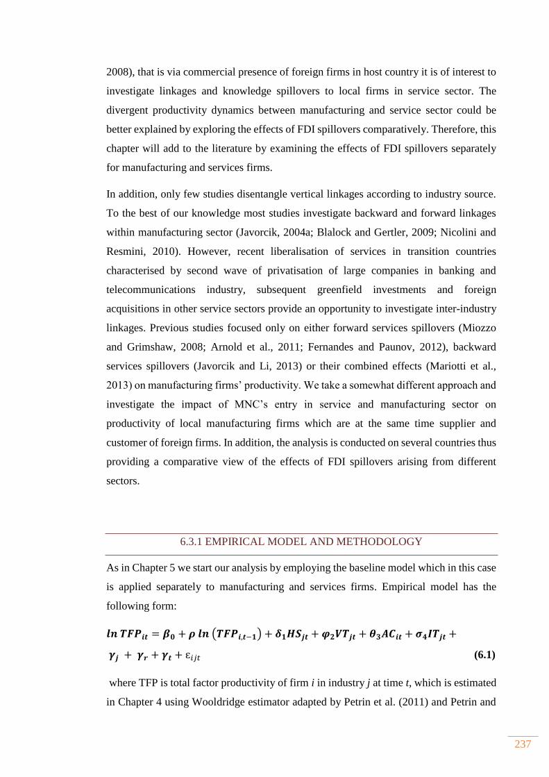
237
2008), that is via commercial presence of foreign firms in host country it is of interest to
investigate linkages and knowledge spillovers to local firms in service sector. The
divergent productivity dynamics between manufacturing and service sector could be
better explained by exploring the effects of FDI spillovers comparatively. Therefore, this
chapter will add to the literature by examining the effects of FDI spillovers separately
for manufacturing and services firms.
In addition, only few studies disentangle vertical linkages according to industry source.
To the best of our knowledge most studies investigate backward and forward linkages
within manufacturing sector (Javorcik, 2004a; Blalock and Gertler, 2009; Nicolini and
Resmini, 2010). However, recent liberalisation of services in transition countries
characterised by second wave of privatisation of large companies in banking and
telecommunications industry, subsequent greenfield investments and foreign
acquisitions in other service sectors provide an opportunity to investigate inter-industry
linkages. Previous studies focused only on either forward services spillovers (Miozzo
and Grimshaw, 2008; Arnold et al., 2011; Fernandes and Paunov, 2012), backward
services spillovers (Javorcik and Li, 2013) or their combined effects (Mariotti et al.,
2013) on manufacturing firms’ productivity. We take a somewhat different approach and
investigate the impact of MNC’s entry in service and manufacturing sector on
productivity of local manufacturing firms which are at the same time supplier and
customer of foreign firms. In addition, the analysis is conducted on several countries thus
providing a comparative view of the effects of FDI spillovers arising from different
sectors.
6.3.1 EMPIRICAL MODEL AND METHODOLOGY
As in Chapter 5 we start our analysis by employing the baseline model which in this case
is applied separately to manufacturing and services firms. Empirical model has the
following form:
𝒍𝒏𝑻𝑭𝑷𝒊𝒕 = 𝜷𝟎 + 𝝆 𝒍𝒏 (𝑻𝑭𝑷𝒊,𝒕−𝟏)+𝜹𝟏𝑯𝑺𝒋𝒕 +𝝋𝟐𝑽𝑻𝒋𝒕 + 𝜽𝟑𝑨𝑪𝒊𝒕 + 𝝈𝟒𝑰𝑻𝒋𝒕 +
𝜸𝒋 + 𝜸𝒓 + 𝜸𝒕 + ɛ𝑖𝑗𝑡(6.1)
where TFP is total factor productivity of firm i in industry j at time t, which is estimated
in Chapter 4 using Wooldridge estimator adapted by Petrin et al. (2011) and Petrin and
238
Levinsohn (2012). As in the previous chapter, 𝐻𝑆𝑗𝑡 and 𝑉𝑇𝑗𝑡 stand for horizontal
spillovers and vertical linkages respectively defined at the industry level; 𝐴𝐶𝑖𝑡 includes
firm level determinants of TFP, namely human capital, intangible assets, size and age
and their squared terms. Vector 𝐼𝑇𝑗𝑡 controls for industry competition and demand
effects. Finally γj , γr,γt denote industry, region and time dummies to control for any
unobserved effects such as economy wide technological progress, changes in
specialisation of certain industries or changes in their market and agglomeration
economies.
In order to examine the link between FDI in service sector and downstream
manufacturing productivity we need information on linkages between different sectors
of economy. Since Amadeus database does not provide information on individual firms’
reliance on services inputs our services FDI linkage draws upon measures based on input
output coefficients obtained from WIOD database that is discussed in the previous
chapter. This approach is applied in several papers (Arnold et al., 2011, Mariotti et al.,
2013) and provides information about the average inter industry sourcing behaviour of
firms within a sector. As already emphasized in the previous chapter some precision is
lost when using input output coefficients. However, using data on firm level sourcing
behaviour would lead to endogeneity as significant use of services inputs may be
correlated with firm performance (Arnold et al., 2015). An additional advantage of time
varying IO table is the ability to capture the sourcing behaviour of manufacturing and
service industries over time as the process of outsourcing and offshoring as well as
splintering the value chain has increased dramatically reflecting the ability and incentives
of firms to benefit from favourable conditions across different geographical regions
(Baldwin and Lopez-Gonzalez, 2014).
Since FDI in services can be regarded as outcome of policy reforms and some services
are more important for manufacturing it is necessary to properly measure the intensity of
which services inputs are used by manufacturing sector. Therefore, information on inter-
industry sourcing from WIOD database are combined with information on sales of
foreign firms in each sector obtained from Amadeus database. Similar reasoning applies
to the intensity of manufacturing inputs used by service industry which are constructed
in a similar fashion. In summary, total backward and total forward linkages that are
applied to manufacturing and service sectors separately in the baseline model are
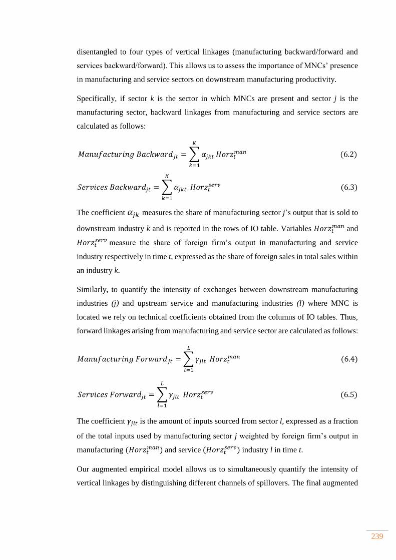
239
disentangled to four types of vertical linkages (manufacturing backward/forward and
services backward/forward). This allows us to assess the importance of MNCs’ presence
in manufacturing and service sectors on downstream manufacturing productivity.
Specifically, if sector k is the sector in which MNCs are present and sector j is the
manufacturing sector, backward linkages from manufacturing and service sectors are
calculated as follows:
𝑀𝑎𝑛𝑢𝑓𝑎𝑐𝑡𝑢𝑟𝑖𝑛𝑔𝐵𝑎𝑐𝑘𝑤𝑎𝑟𝑑𝑗𝑡 = ∑𝛼𝑗𝑘𝑡
𝐾
𝑘=1
𝐻𝑜𝑟𝑧𝑡𝑚𝑎𝑛(6.2)
𝑆𝑒𝑟𝑣𝑖𝑐𝑒𝑠𝐵𝑎𝑐𝑘𝑤𝑎𝑟𝑑𝑗𝑡 = ∑𝛼𝑗𝑘𝑡
𝐾
𝑘=1
𝐻𝑜𝑟𝑧𝑡𝑠𝑒𝑟𝑣(6.3)
The coefficient 𝛼𝑗𝑘 measures the share of manufacturing sector j’s output that is sold to
downstream industry k and is reported in the rows of IO table. Variables 𝐻𝑜𝑟𝑧𝑡𝑚𝑎𝑛and
𝐻𝑜𝑟𝑧𝑡𝑠𝑒𝑟𝑣measure the share of foreign firm’s output in manufacturing and service
industry respectively in time t, expressed as the share of foreign sales in total sales within
an industry k.
Similarly, to quantify the intensity of exchanges between downstream manufacturing
industries (j) and upstream service and manufacturing industries (l) where MNC is
located we rely on technical coefficients obtained from the columns of IO tables. Thus,
forward linkages arising from manufacturing and service sector are calculated as follows:
𝑀𝑎𝑛𝑢𝑓𝑎𝑐𝑡𝑢𝑟𝑖𝑛𝑔𝐹𝑜𝑟𝑤𝑎𝑟𝑑𝑗𝑡 =∑𝛾𝑗𝑙𝑡
𝐿
𝑙=1
𝐻𝑜𝑟𝑧𝑡𝑚𝑎𝑛(6.4)
𝑆𝑒𝑟𝑣𝑖𝑐𝑒𝑠𝐹𝑜𝑟𝑤𝑎𝑟𝑑𝑗𝑡 =∑𝛾𝑗𝑙𝑡
𝐿
𝑙=1
𝐻𝑜𝑟𝑧𝑡𝑠𝑒𝑟𝑣(6.5)
The coefficient𝛾𝑗𝑙𝑡 is the amount of inputs sourced from sector l, expressed as a fraction
of the total inputs used by manufacturing sector j weighted by foreign firm’s output in
manufacturing (𝐻𝑜𝑟𝑧𝑡𝑚𝑎𝑛)and service(𝐻𝑜𝑟𝑧𝑡
𝑠𝑒𝑟𝑣) industry l in time t.
Our augmented empirical model allows us to simultaneously quantify the intensity of
vertical linkages by distinguishing different channels of spillovers. The final augmented
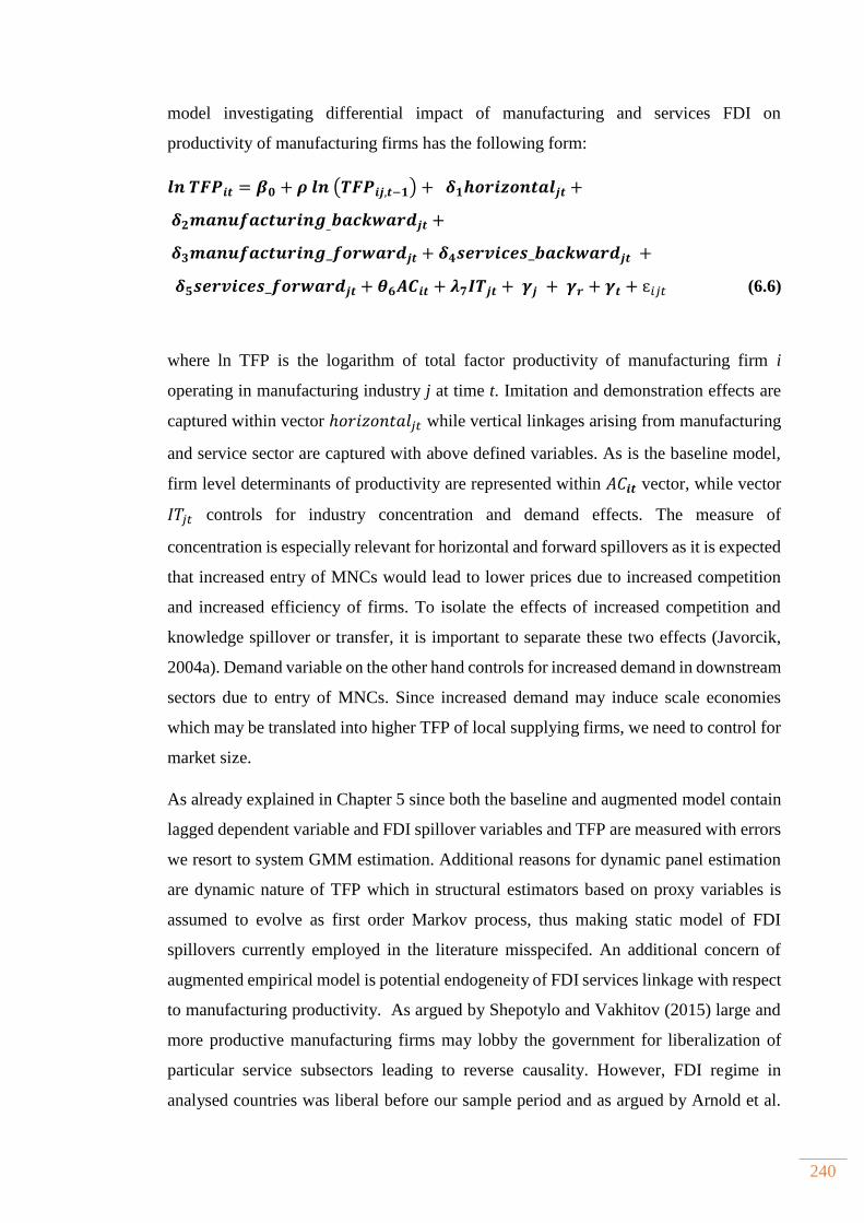
240
model investigating differential impact of manufacturing and services FDI on
productivity of manufacturing firms has the following form:
𝒍𝒏𝑻𝑭𝑷𝒊𝒕 = 𝜷𝟎 + 𝝆 𝒍𝒏 (𝑻𝑭𝑷𝒊𝒋,𝒕−𝟏)+𝜹𝟏𝒉𝒐𝒓𝒊𝒛𝒐𝒏𝒕𝒂𝒍𝒋𝒕 +
𝜹𝟐𝒎𝒂𝒏𝒖𝒇𝒂𝒄𝒕𝒖𝒓𝒊𝒏𝒈_𝒃𝒂𝒄𝒌𝒘𝒂𝒓𝒅𝒋𝒕 +
𝜹𝟑𝒎𝒂𝒏𝒖𝒇𝒂𝒄𝒕𝒖𝒓𝒊𝒏𝒈_𝒇𝒐𝒓𝒘𝒂𝒓𝒅𝒋𝒕+𝜹𝟒𝒔𝒆𝒓𝒗𝒊𝒄𝒆𝒔_𝒃𝒂𝒄𝒌𝒘𝒂𝒓𝒅𝒋𝒕 +
𝜹𝟓𝒔𝒆𝒓𝒗𝒊𝒄𝒆𝒔_𝒇𝒐𝒓𝒘𝒂𝒓𝒅𝒋𝒕 + 𝜽𝟔𝑨𝑪𝒊𝒕 + 𝝀𝟕𝑰𝑻𝒋𝒕 + 𝜸𝒋 + 𝜸𝒓 + 𝜸𝒕 + ɛ𝑖𝑗𝑡 (6.6)
where ln TFP is the logarithm of total factor productivity of manufacturing firm i
operating in manufacturing industry j at time t. Imitation and demonstration effects are
captured within vector ℎ𝑜𝑟𝑖𝑧𝑜𝑛𝑡𝑎𝑙𝑗𝑡 while vertical linkages arising from manufacturing
and service sector are captured with above defined variables. As is the baseline model,
firm level determinants of productivity are represented within 𝐴𝐶𝒊𝒕 vector, while vector
𝐼𝑇𝑗𝑡 controls for industry concentration and demand effects. The measure of
concentration is especially relevant for horizontal and forward spillovers as it is expected
that increased entry of MNCs would lead to lower prices due to increased competition
and increased efficiency of firms. To isolate the effects of increased competition and
knowledge spillover or transfer, it is important to separate these two effects (Javorcik,
2004a). Demand variable on the other hand controls for increased demand in downstream
sectors due to entry of MNCs. Since increased demand may induce scale economies
which may be translated into higher TFP of local supplying firms, we need to control for
market size.
As already explained in Chapter 5 since both the baseline and augmented model contain
lagged dependent variable and FDI spillover variables and TFP are measured with errors
we resort to system GMM estimation. Additional reasons for dynamic panel estimation
are dynamic nature of TFP which in structural estimators based on proxy variables is
assumed to evolve as first order Markov process, thus making static model of FDI
spillovers currently employed in the literature misspecifed. An additional concern of
augmented empirical model is potential endogeneity of FDI services linkage with respect
to manufacturing productivity. As argued by Shepotylo and Vakhitov (2015) large and
more productive manufacturing firms may lobby the government for liberalization of
particular service subsectors leading to reverse causality. However, FDI regime in
analysed countries was liberal before our sample period and as argued by Arnold et al.
241
(2011) policy reform was under tight supervision of EU Commission as a part of
preparation for EU accession. Nevertheless, strong productivity growth of manufacturing
firms may have attracted services MNCs due to strong demand. Also, there is ample
empirical evidence that MNCs providing services are locating near major manufacturing
locations, thus positive effects of FDI may simply reflect location decision of MNCs in
certain industries or regions (Nefussi and Schwellnus, 2010; Meliciani and Savona, 2011;
Castellani and Meliciani, 2014). The same reasoning applies to service sector itself where
successful privatisation of financial industry and telecoms may have induced other
MNCs to invest in certain location due to increased use of services by manufacturing
firms. Given the above mentioned problems system GMM based on exploitation of
internal instruments is thought to provide more efficient and unbiased estimates of FDI
spillovers. The initial specifications included minimum number of lags, i.e. the number
of instruments came from restriction to start with one lag for levels and differences in
case of predetermined variable (ln TFP) and two lags for endogenous variables, namely
FDI spillover variables (Roodman, 2009). However, in certain cases model diagnostics
with minimum number of lags were not satisfied and therefore the instrumentation matrix
included higher order lags (three or four) of the regressors as instruments.
6.3.2 DATA
The empirical analysis is based on Amadeus and WIOD databases described in Chapters
4 and 5. Since the baseline model in Chapter 5 is estimated using firm level data from
both manufacturing and service sector we continue along the same line in order to
provide a comparative view of the effects of FDI spillovers on local firms in
manufacturing and service sector. Therefore, the data applied to the models defined in
Section 6.3.1 pertain to 23 manufacturing and 20 service sector. However, due to low
number of observations in some industries WIOD industry classification is applied which
groups 2-digit industries producing similar goods or providing a similar service based on
NACE Rev 1.1 classification. 62F
65 The same grouping is applied in the previous chapters in
estimation of TFP and construction of vertical linkages, thus resulting in 14
65 NACE Rev 1.1 is used as input output tables are constructed using this classification.
242
manufacturing sectors and 13 service sectors. Namely, the presence of foreign firms in
service sector focus on the following broad NACE Rev 1.1. 2 digit categories:
Electricity, gas and water supply (NACE 1.1-E)
Construction (NACE 1.1-F)
Wholesale and retail trade; repair of motor vehicles, motorcycles and personal
and household goods (NACE 1.1-G)
Hotels and restaurants (NACE 1.1-H)
Transport, storage and communication (NACE 1.1-I)
Financial intermediation (NACE 1.1-J)
Real estate, renting and business activities (NACE 1.1-K)
The data period under investigation is the same as in previous chapters and covers period
2002-2010. In order to shed more light on the intensity of vertical linkages, Figures 6.1
and 6.2 provide mean values of manufacturing and service linkages within manufacturing
sector. A closer look at Figure 6.1 reveals that foreign firm presence in manufacturing of
rubber and plastics (25) provide the strongest potential for manufacturing backward
linkages followed by manufacture of machinery and equipment (29), manufacture of
metals and fabricated metals (27_28) and leather related products (19). On the other hand,
as expected forward manufacturing linkages provide a lower potential for spillover
development in almost all industries. The highest forward linkages are evident in
manufacture of machinery and equipment (29), chemical products (24) and other
manufacturing industries (36_37). Regardin the countries, suppliers and customers of
foreign firms within manufacturing sector in the Czech Republic, Hungary and Slovakia
are more likely to benefit from manufacturing backward and forward linkages. Given
that these countries experienced a higher productivity growth in comparison to growth
in unit labour costs (ESCIP, 2014) they were able to attract significant amount of FDI
and enter MNCs’ production networks.
Similarly, Figure 6.2 provide information on services linkages. It seems that
manufacturing suppliers in coke, refined petroleum and nuclear fuel industry (23) and
paper, publishing and printing industry (21_22) are more likely to benefit from supplying
downstream services firms over the analysed period. Similar conclusion can be made for
suppliers in other non-metallic mineral industry (26) and electrical and optical equipment
243
industry (30_33). Turning to forward services linkages we can notice the relatively high
share of services inputs, partially reflecting the increased manufacturing specialization
of analysed countries (ESCIP, 2014). This is especially the case in the Czech Republic,
Slovakia and Hungary where high quality inputs are necessary to increase the quality of
export goods and in Estonia where increased specialisation in service sector contributed
to large productivity gains in business services and manufacturing productivity (ESCIP,
2014).
The increased reliance of manufacturing industries on services inputs also reflects the
rising share of foreign output in services which increased from 8 per cent in 2002 to 30
per cent in 2010 on average (Appendix IV, Figure IV.1). The largest increase can be
observed in Slovakia where the share of foreign output increased from only 12 per cent
in year 2002 to over 33 per cent in 2010. The service sector in the Czech Republic (20 to
40 per cent) and Slovenia (4 to 25 per cent) was also characterised by large increase in
foreign output. During the same time period, the average share of foreign services inputs
rose from 4 per cent to 17 per cent due to strong increase in recent years partially
reflecting better coverage of firms in the database (Appendix IV, Figure IV.2). The
largest increase was evident in Slovakia and Estonia, where the share increased by 16
and 20 percentage point, respectively. A more detailed analysis across industries and
countries provided in Figure 6.2 illustrates that manufacturing industries in Estonia are
most reliant on foreign services inputs followed by Slovakia and the Czech Republic.
However, our measure of direct cost share of services in manufacturing total costs
measured using technical coefficients from IO tables is somewhat imperfect as some
services such as telecommunications may capture relatively small share of total cost, but
are very important for normal functioning of business. Industries with highest usage of
foreign services inputs are chemical industry (24), leather and leather products (19) and
textile and textile products (17_18) closely followed by other manufacturing industries.
Thus, these figures illustrate the increasing relevance of services FDI and diverse impact
of foreign firms in manufacturing industries in our sample, and thereby provide a
compelling motivation to investigate separately the impact of services and manufacturing
FDI linkages on the performance of manufacturing firms.
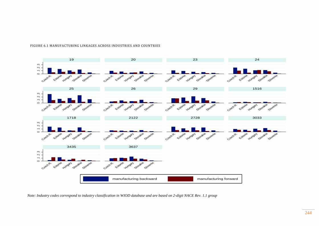
244
FIGURE 6.1 MANUFACTURING LINKAGES ACROSS INDUSTRIES AND COUNTRIES
Note: Industry codes correspond to industry classification in WIOD database and are based on 2-digit NACE Rev. 1.1 group
0.1
.2.3
0.1
.2.3
0.1
.2.3
0.1
.2.3
Czech
R.
Estonia
Hungary
Slovakia
Slovenia
Czech
R.
Estonia
Hungary
Slovakia
Slovenia
Czech
R.
Estonia
Hungary
Slovakia
Slovenia
Czech
R.
Estonia
Hungary
Slovakia
Slovenia
Czech
R.
Estonia
Hungary
Slovakia
Slovenia
Czech
R.
Estonia
Hungary
Slovakia
Slovenia
Czech
R.
Estonia
Hungary
Slovakia
Slovenia
Czech
R.
Estonia
Hungary
Slovakia
Slovenia
Czech
R.
Estonia
Hungary
Slovakia
Slovenia
Czech
R.
Estonia
Hungary
Slovakia
Slovenia
Czech
R.
Estonia
Hungary
Slovakia
Slovenia
Czech
R.
Estonia
Hungary
Slovakia
Slovenia
Czech
R.
Estonia
Hungary
Slovakia
Slovenia
Czech
R.
Estonia
Hungary
Slovakia
Slovenia
19 20 23 24
25 26 29 1516
1718 2122 2728 3033
3435 3637
manufacturing backward manufacturing forward
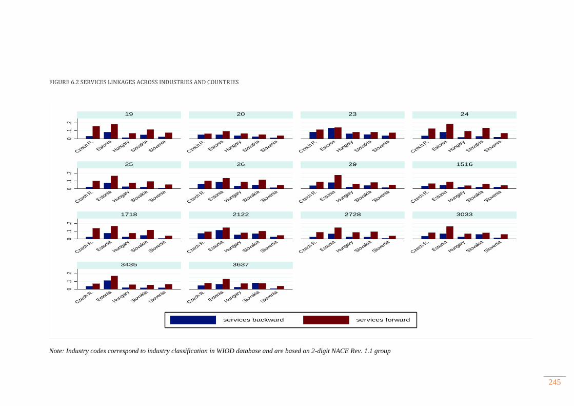
245
FIGURE 6.2 SERVICES LINKAGES ACROSS INDUSTRIES AND COUNTRIES
Note: Industry codes correspond to industry classification in WIOD database and are based on 2-digit NACE Rev. 1.1 group
0.1
.20
.1.2
0.1
.20
.1.2
Czech
R.
Estonia
Hungary
Slovakia
Slovenia
Czech
R.
Estonia
Hungary
Slovakia
Slovenia
Czech
R.
Estonia
Hungary
Slovakia
Slovenia
Czech
R.
Estonia
Hungary
Slovakia
Slovenia
Czech
R.
Estonia
Hungary
Slovakia
Slovenia
Czech
R.
Estonia
Hungary
Slovakia
Slovenia
Czech
R.
Estonia
Hungary
Slovakia
Slovenia
Czech
R.
Estonia
Hungary
Slovakia
Slovenia
Czech
R.
Estonia
Hungary
Slovakia
Slovenia
Czech
R.
Estonia
Hungary
Slovakia
Slovenia
Czech
R.
Estonia
Hungary
Slovakia
Slovenia
Czech
R.
Estonia
Hungary
Slovakia
Slovenia
Czech
R.
Estonia
Hungary
Slovakia
Slovenia
Czech
R.
Estonia
Hungary
Slovakia
Slovenia
19 20 23 24
25 26 29 1516
1718 2122 2728 3033
3435 3637
services backward services forward

246
6.4 DISCUSSION OF FINDINGS
Before turning to explanation of results, a brief comment on the model diagnostics is
made. As System GMM relies on internal instruments to deal with possible endogeneity,
Hansen J test together with autocorrelation test is reported in the model diagnostics
(Table 6-1). Further diagnostics tests for all models along with the syntax for each are
enclosed in Appendix IV (Tables IV.1-IV.10). As shown below, in both baseline models
used to estimate FDI spillovers in manufacturing and service sector, overall Hansen test
cannot be rejected providing confidence that employed instruments are valid. In all
models the p-values are always larger than the 0.25 threshold that was proposed by
Roodman (2009), except for service sector in Slovakia. Even it that case Hansen test
cannot be rejected at 10 per cent significance level. The null hypothesis of no second
order autocorrelation in the error term of differenced equation is rejected only in the case
of Estonia for baseline model applied to services. We tried to increase the lag order of
the lagged dependent variable or even add a second lag of dependent variables on the
right hand side of the model, but the diagnostics did not improve. 63F
66 However, the sign
and significance of coefficients remain robust across different specifications, though
some caution is still warranted when interpreting the results.
Next important step is to check for steady state assumption. Difference in Hansen test for
levels equation does not provide sufficient evidence to reject the null hypothesis,
therefore we can conclude that system GMM is preferred estimator. Time dummies are
included to control for time universal shocks such as financial crisis, which is expected
to affect productivity levels. However, as argued by Sarafidis et al. (2009) some cross
sectional dependence may still remain, therefore we also use difference in Hansen test to
test the validity of instruments for lagged dependent variable. The difference in Hansen
test for lagged dependent variable cannot be rejected at conventional level of significance
in most models. Some concerns can be raised in the case of Slovakia where both
difference in Hansen test for levels equation and for lagged dependent variable in services
model are rejected at 10 per cent significance. However, overall Hansen test,
66 In the case of the Czech Republic and Slovenia, inclusion of second lag of dependent variable on the
right hand side improved the model diagnostics.
247
autocorrelation tests and difference in Hansen test for endogenous variables are satisfied,
thus supporting our specification. Finally, the estimated coefficient of lagged dependent
variable is compared to those obtained by OLS which is known to be upward biased and
fixed effects which provides a lower bound of estimated coefficient. In all models the
coefficient of lagged dependent variable lies between lower and upper bound providing
sufficient evidence that system GMM estimator is a true dynamic estimator.
6.4.1 RESULTS OF BASELINE MODEL ACROSS SECTORS
Table 6.1 presents the results for both manufacturing and service sectors to allow for an
easier comparison. Starting with the lagged dependent variable (TFP), we can see that in
all models there exist a partial adjustment to the desired level of productivity. On average,
across countries a one per cent increase in past productivity leads to 0.42 per cent increase
in current productivity in manufacturing sector and 0.55 per cent increase in service
sector. This implies that past determinants of productivity have positive and significant
effects on their current levels.
Turning to our main variables of interest, we start by examining the effects of horizontal
spillovers. The latter are negative and significant across manufacturing sector, with the
exception of Slovenia, which points to a possible crowding out effect of foreign firms
within the industry. This is in line with meta regression results investigating indirect
effects of FDI in transition countries (Iwasaki and Tokunaga, 2014). Additionally, as
found by Smeets and de Vaal (2015) stronger intellectual property rights will reduce
positive knowledge spillovers and enhance negative competition effects by increasing
MNCs’ competitive position. Negative horizontal spillovers are even stronger in the long
run suggesting inability of local firms to learn (see Appendix IV, Tables IV.1-IV.5).
These results imply that local firms are not able to increase the efficiency to cope with
increased competition. The negative effect on local firms’ productivity in the short run
range from 0.40 per cent in Slovakia to 1.77 per cent in Estonia for every percentage
point increase in foreign firms’ output in the same industry. On the other hand, in service
sector the presence of foreign firms has positive effects evident in the case of the Czech
Republic, Hungary and Estonia. However, the effect is not significant in the latter case.
The results are similar to Ayyagari and Kosova (2010) investigating the impact of FDI
spillovers across services and manufacturing on domestic firms’ entry. As in

248
manufacturing sector, long run positive effects are more pronounced and lead to an
increase in TFP of services firms by 2.09 and 2.86 per cent in Hungary and the Czech
Republic, respectively (see Appendix IV, Tables IV.5-IV.10). There are several possible
explanations of beneficial effects in services. First, our sample contain more firms in
services. Second, as argued by Kugler (2006) firms in manufacturing have higher
incentives to minimize technology leakage. Third, these results suggest that local firms
are more likely to benefit from demonstration and imitation in service sectors due to
inseparability of production and consumption and where methods of production are
transferable (Gorodnichenko et al., 2014). In case of Slovakia and Slovenia, the results
suggest that MNCs in service sector are putting competitive pressure on local firms which
are not able to cope with better technology, managerial and organizational know how of
foreign firms resulting in their reduced productivity. Furthermore, since entry of MNCs
bring reduction in prices and increase the variety of services, previous monopoly rents
are reduced, thus negatively affecting revenues and TFP. These negative effects range
from 0.83 per cent in Slovenia to 1.77 per cent in Slovakia. Overall, these results suggest
that total effects of horizontal spillovers estimated in the previous chapter are largely
driven by the service sector thus shedding new light on the role of services FDI in
respective economies.
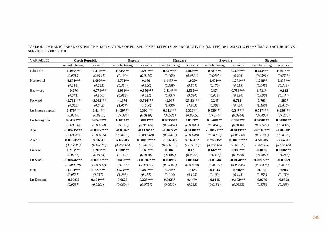
249
TABLE 6.1 DYNAMIC PANEL SYSTEM GMM ESTIMATIONS OF FDI SPILLOVER EFFECTS ON PRODUCTIVITY (LN TFP) OF DOMESTIC FIRMS (MANUFACTURING VS. SERVICES), 2002-2010
VARIABLES Czech Republic Estonia Hungary Slovakia Slovenia
manufacturing services manufacturing services manufacturing services manufacturing services manufacturing services
L.ln TFP 0.393*** 0.410*** 0.345*** 0.590*** 0.547*** 0.486*** 0.381*** 0.325*** 0.443*** 0.601***
(0.0219) (0.0144) (0.109) (0.0415) (0.103) (0.0821) (0.0407) (0.106) (0.0591) (0.0336)
Horizontal -0.671*** 1.690*** -1.774** 0.160 -1.145*** 1.075* -0.401** -1.771*** 1.948** -0.833***
(0.186) (0.215) (0.834) (0.320) (0.388) (0.594) (0.179) (0.258) (0.945) (0.311)
Backward -0.276 -0.774*** -1.936** -0.350*** -2.414*** 1.565** 0.874 0.758*** 1.731* -0.113
(0.371) (0.130) (0.882) (0.121) (0.854) (0.624) (0.819) (0.120) (0.898) (0.144)
Forward -2.792*** -5.042*** -1.374 -5.724*** -2.037 -23.13*** 0.247 0.712* 0.763 4.985*
(0.623) (0.542) (1.057) (1.240) (1.838) (4.903) (0.382) (0.430) (1.168) (2.818)
Ln Human capital 0.478*** 0.414*** 0.420*** 0.308*** 0.311*** 0.328*** 0.339*** 0.347*** 0.517*** 0.296***
(0.0140) (0.0101) (0.0394) (0.0148) (0.0526) (0.0385) (0.0144) (0.0244) (0.0495) (0.0278)
Ln Intangibles 0.0449*** 0.0526*** 0.101*** 0.0801*** 0.00956** 0.0103** 0.0608*** 0.103*** 0.0290*** 0.0186***
(0.00256) (0.00224) (0.0148) (0.00385) (0.00462) (0.00441) (0.00517) (0.0118) (0.00572) (0.00322)
Age -0.00915*** -0.00977*** -0.00167 -0.0126*** -0.00725* -0.0110*** -0.00921*** -0.0183*** -0.0103*** -0.00328*
(0.00147) (0.00155) (0.00438) (0.000968) (0.00415) (0.00249) (0.00257) (0.00234) (0.00283) (0.00198)
Age^2 8.05e-05** 3.38e-05 5.65e-05 0.000132*** -1.59e-05 3.51e-05* 8.76e-05* 0.000337*** 4.50e-05 -3.75e-05
(3.98e-05) (6.16e-05) (4.26e-05) (1.04e-05) (0.000132) (1.81e-05) (4.76e-05) (4.46e-05) (8.47e-05) (6.59e-05)
Ln Size 0.213*** 0.209*** 0.638*** 0.169*** 0.0865 0.121 0.142*** 0.386*** -0.0185 0.0906***
(0.0182) (0.0173) (0.147) (0.0160) (0.0601) (0.0957) (0.0315) (0.0688) (0.0607) (0.0265)
Ln Size^2 -0.00446*** -0.00627*** -0.0457*** -0.00307*** 0.000997 0.000660 -0.00244 -0.0158*** 0.00972** -0.00259
(0.000929) (0.00117) (0.0136) (0.00111) (0.00349) (0.00574) (0.00199) (0.00335) (0.00495) (0.00167)
HHI -0.191*** -1.327*** -3.524*** 0.489*** -0.203* -0.123 -0.0943 -0.306** -0.135 0.0904
(0.0587) (0.237) (1.298) (0.157) (0.114) (0.193) (0.109) (0.144) (0.153) (0.130)
Ln Demand -0.00930 0.198*** 0.0626 0.223*** 0.0925* 0.447* -0.0115 -0.172*** -0.0779 -0.0858
(0.0267) (0.0291) (0.0694) (0.0754) (0.0530) (0.232) (0.0151) (0.0333) (0.178) (0.308)
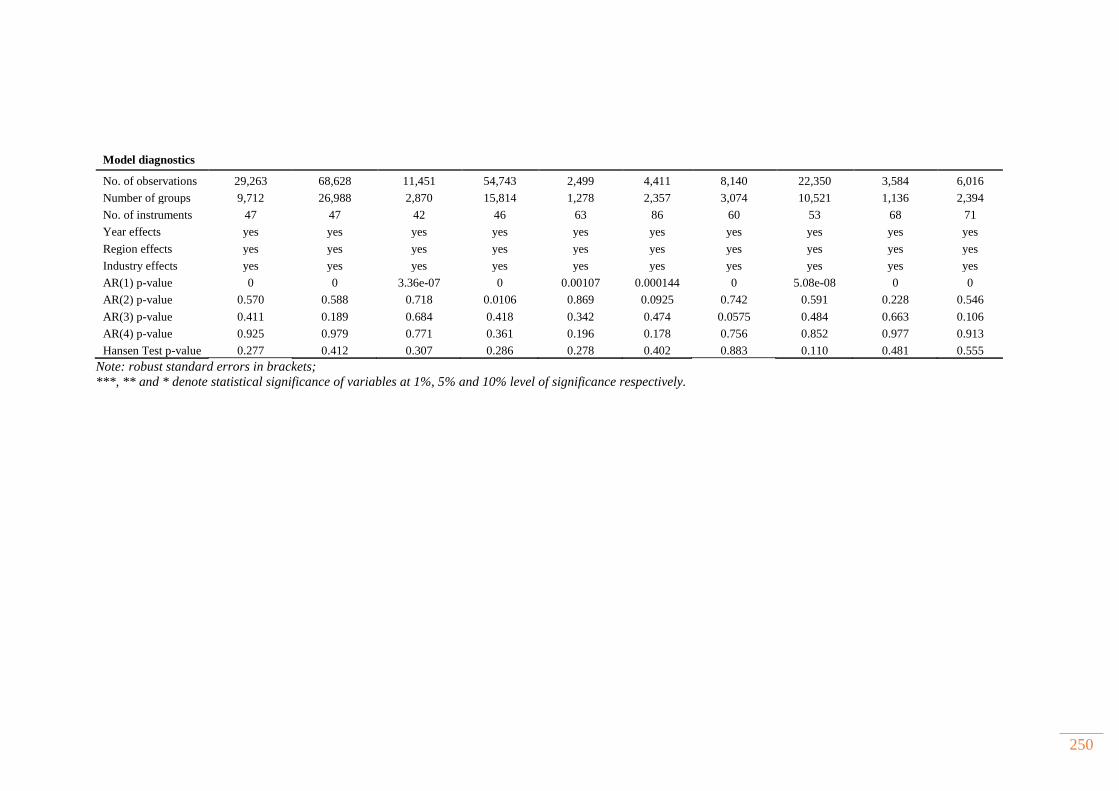
250
Model diagnostics
No. of observations 29,263 68,628 11,451 54,743 2,499 4,411 8,140 22,350 3,584 6,016
Number of groups 9,712 26,988 2,870 15,814 1,278 2,357 3,074 10,521 1,136 2,394
No. of instruments 47 47 42 46 63 86 60 53 68 71
Year effects yes yes yes yes yes yes yes yes yes yes
Region effects yes yes yes yes yes yes yes yes yes yes
Industry effects yes yes yes yes yes yes yes yes yes yes
AR(1) p-value 0 0 3.36e-07 0 0.00107 0.000144 0 5.08e-08 0 0
AR(2) p-value 0.570 0.588 0.718 0.0106 0.869 0.0925 0.742 0.591 0.228 0.546
AR(3) p-value 0.411 0.189 0.684 0.418 0.342 0.474 0.0575 0.484 0.663 0.106
AR(4) p-value 0.925 0.979 0.771 0.361 0.196 0.178 0.756 0.852 0.977 0.913
Hansen Test p-value 0.277 0.412 0.307 0.286 0.278 0.402 0.883 0.110 0.481 0.555
Note: robust standard errors in brackets;
***, ** and * denote statistical significance of variables at 1%, 5% and 10% level of significance respectively.
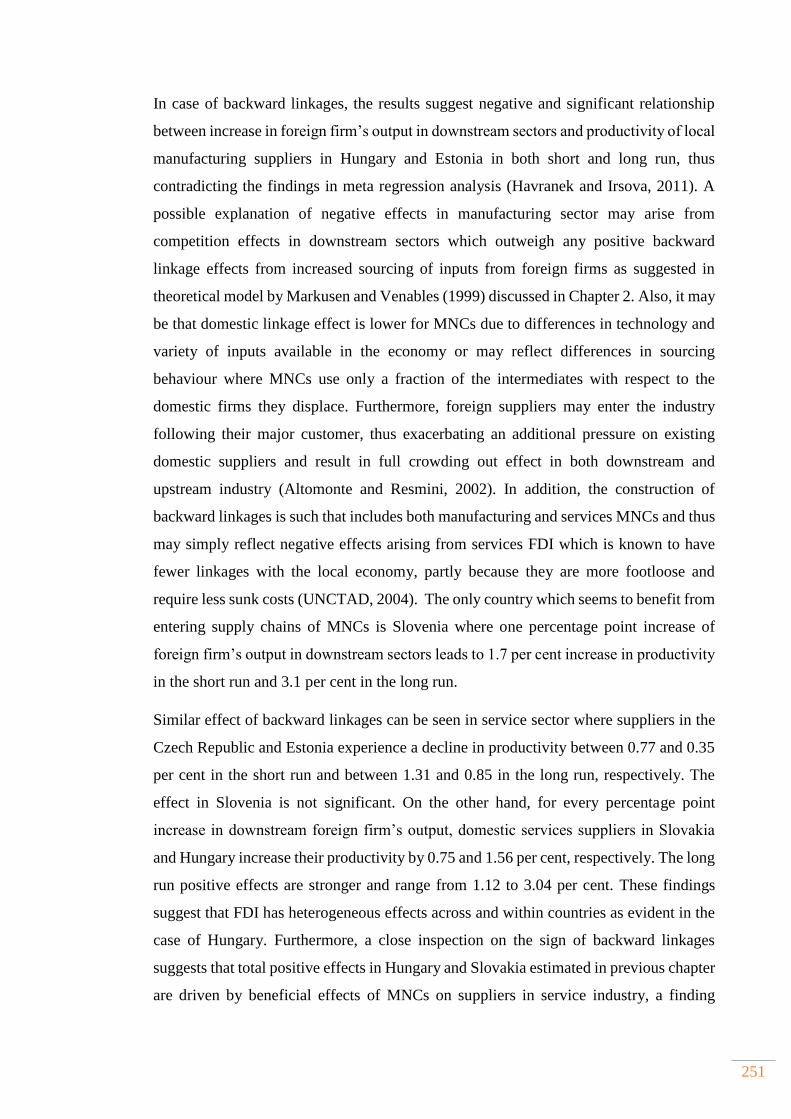
251
In case of backward linkages, the results suggest negative and significant relationship
between increase in foreign firm’s output in downstream sectors and productivity of local
manufacturing suppliers in Hungary and Estonia in both short and long run, thus
contradicting the findings in meta regression analysis (Havranek and Irsova, 2011). A
possible explanation of negative effects in manufacturing sector may arise from
competition effects in downstream sectors which outweigh any positive backward
linkage effects from increased sourcing of inputs from foreign firms as suggested in
theoretical model by Markusen and Venables (1999) discussed in Chapter 2. Also, it may
be that domestic linkage effect is lower for MNCs due to differences in technology and
variety of inputs available in the economy or may reflect differences in sourcing
behaviour where MNCs use only a fraction of the intermediates with respect to the
domestic firms they displace. Furthermore, foreign suppliers may enter the industry
following their major customer, thus exacerbating an additional pressure on existing
domestic suppliers and result in full crowding out effect in both downstream and
upstream industry (Altomonte and Resmini, 2002). In addition, the construction of
backward linkages is such that includes both manufacturing and services MNCs and thus
may simply reflect negative effects arising from services FDI which is known to have
fewer linkages with the local economy, partly because they are more footloose and
require less sunk costs (UNCTAD, 2004). The only country which seems to benefit from
entering supply chains of MNCs is Slovenia where one percentage point increase of
foreign firm’s output in downstream sectors leads to 1.7 per cent increase in productivity
in the short run and 3.1 per cent in the long run.
Similar effect of backward linkages can be seen in service sector where suppliers in the
Czech Republic and Estonia experience a decline in productivity between 0.77 and 0.35
per cent in the short run and between 1.31 and 0.85 in the long run, respectively. The
effect in Slovenia is not significant. On the other hand, for every percentage point
increase in downstream foreign firm’s output, domestic services suppliers in Slovakia
and Hungary increase their productivity by 0.75 and 1.56 per cent, respectively. The long
run positive effects are stronger and range from 1.12 to 3.04 per cent. These findings
suggest that FDI has heterogeneous effects across and within countries as evident in the
case of Hungary. Furthermore, a close inspection on the sign of backward linkages
suggests that total positive effects in Hungary and Slovakia estimated in previous chapter
are driven by beneficial effects of MNCs on suppliers in service industry, a finding
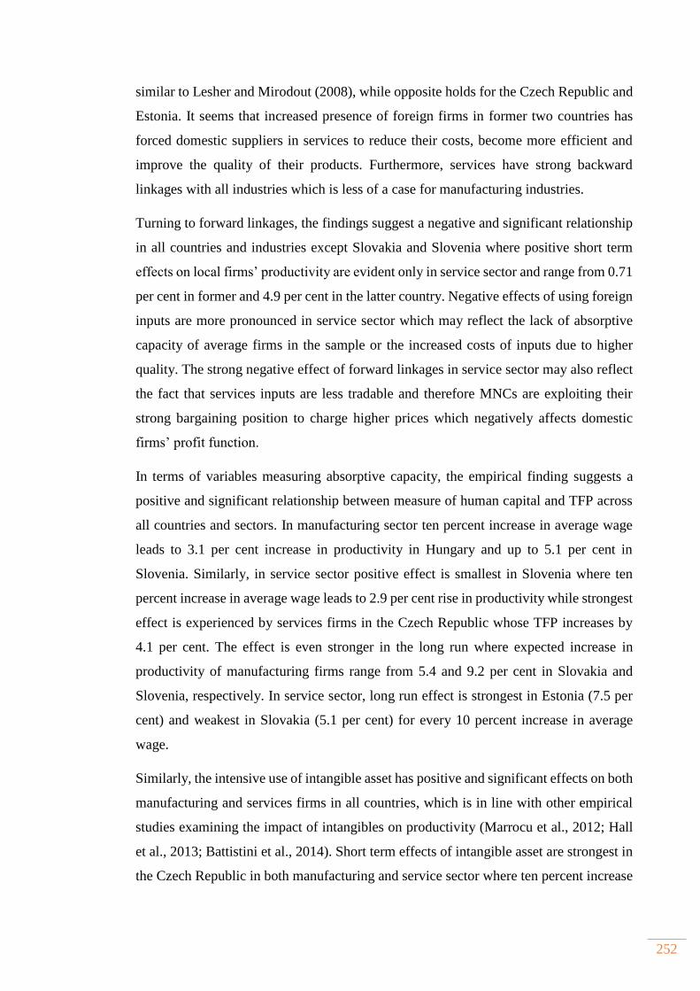
252
similar to Lesher and Mirodout (2008), while opposite holds for the Czech Republic and
Estonia. It seems that increased presence of foreign firms in former two countries has
forced domestic suppliers in services to reduce their costs, become more efficient and
improve the quality of their products. Furthermore, services have strong backward
linkages with all industries which is less of a case for manufacturing industries.
Turning to forward linkages, the findings suggest a negative and significant relationship
in all countries and industries except Slovakia and Slovenia where positive short term
effects on local firms’ productivity are evident only in service sector and range from 0.71
per cent in former and 4.9 per cent in the latter country. Negative effects of using foreign
inputs are more pronounced in service sector which may reflect the lack of absorptive
capacity of average firms in the sample or the increased costs of inputs due to higher
quality. The strong negative effect of forward linkages in service sector may also reflect
the fact that services inputs are less tradable and therefore MNCs are exploiting their
strong bargaining position to charge higher prices which negatively affects domestic
firms’ profit function.
In terms of variables measuring absorptive capacity, the empirical finding suggests a
positive and significant relationship between measure of human capital and TFP across
all countries and sectors. In manufacturing sector ten percent increase in average wage
leads to 3.1 per cent increase in productivity in Hungary and up to 5.1 per cent in
Slovenia. Similarly, in service sector positive effect is smallest in Slovenia where ten
percent increase in average wage leads to 2.9 per cent rise in productivity while strongest
effect is experienced by services firms in the Czech Republic whose TFP increases by
4.1 per cent. The effect is even stronger in the long run where expected increase in
productivity of manufacturing firms range from 5.4 and 9.2 per cent in Slovakia and
Slovenia, respectively. In service sector, long run effect is strongest in Estonia (7.5 per
cent) and weakest in Slovakia (5.1 per cent) for every 10 percent increase in average
wage.
Similarly, the intensive use of intangible asset has positive and significant effects on both
manufacturing and services firms in all countries, which is in line with other empirical
studies examining the impact of intangibles on productivity (Marrocu et al., 2012; Hall
et al., 2013; Battistini et al., 2014). Short term effects of intangible asset are strongest in
the Czech Republic in both manufacturing and service sector where ten percent increase

253
leads to 0.4 and 0.5 per cent increase in productivity, respectively. On the other hand,
weakest effects are noticeable in Hungary in both sectors where ten percent increase in
use of intangibles leads to only 0.01 per cent increase in TFP.
The effects of other firm level variable, namely age suggest a nonlinear relationship in
almost all countries and sectors with the exception of manufacturing firms in Estonia and
Hungary. In Slovenia there seems to be a negative linear effect of age in both sectors
which is somewhat surprising given the results in the previous chapter. The findings for
both sectors suggest that either very young or very old firms have positive effects on
productivity. It seems that majority of firms need to accommodate to market conditions
and are still in the learning process which negatively affects their productivity levels and
only after a very long period of operation they are able to increase their productivity.
Firm’s size has a positive and significant effect in all countries and sectors except
Hungary which may be due to this country having a very large proportion of large firms
in the sample. Inverse U shape effects can be found in both sectors in the Czech Republic
and Estonia and in service sector for Slovakia suggesting that after firms achieve a certain
size their effects on productivity starts to diminish.
Competition has mostly positive effects on firm’s productivity in manufacturing sectors
in the Czech Republic, Estonia and Hungary. The effect is less pronounced in service
sector where increased competition has beneficial effects only in the Czech Republic and
Slovakia, while increased industry concentration negatively affects TFP of services firms
in Estonia. This suggests that manufacturing firms are more responsive to changes in
market conditions. Finally, when we look at the effects of demand the findings suggest a
positive and significant effect on productivity of firms in service sector in the Czech
Republic, Estonia and Hungary and negative effects in Slovakia. It seems that increased
purchase of intermediate inputs by domestic firms partially offset negative effects of
MNCs’ backward linkages in service sector in these countries. Similar reasoning can be
applied to manufacturing firms in Hungary.
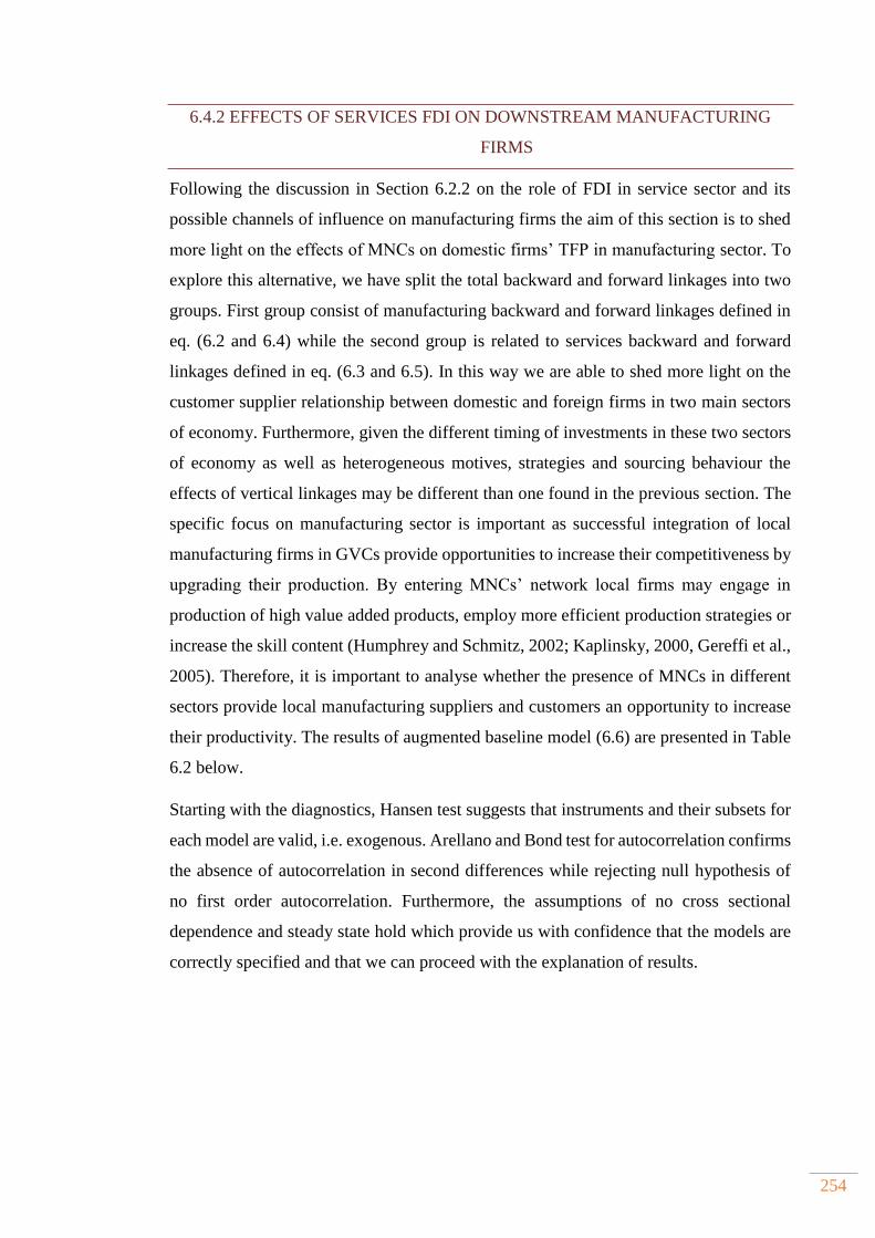
254
6.4.2 EFFECTS OF SERVICES FDI ON DOWNSTREAM MANUFACTURING
FIRMS
Following the discussion in Section 6.2.2 on the role of FDI in service sector and its
possible channels of influence on manufacturing firms the aim of this section is to shed
more light on the effects of MNCs on domestic firms’ TFP in manufacturing sector. To
explore this alternative, we have split the total backward and forward linkages into two
groups. First group consist of manufacturing backward and forward linkages defined in
eq. (6.2 and 6.4) while the second group is related to services backward and forward
linkages defined in eq. (6.3 and 6.5). In this way we are able to shed more light on the
customer supplier relationship between domestic and foreign firms in two main sectors
of economy. Furthermore, given the different timing of investments in these two sectors
of economy as well as heterogeneous motives, strategies and sourcing behaviour the
effects of vertical linkages may be different than one found in the previous section. The
specific focus on manufacturing sector is important as successful integration of local
manufacturing firms in GVCs provide opportunities to increase their competitiveness by
upgrading their production. By entering MNCs’ network local firms may engage in
production of high value added products, employ more efficient production strategies or
increase the skill content (Humphrey and Schmitz, 2002; Kaplinsky, 2000, Gereffi et al.,
2005). Therefore, it is important to analyse whether the presence of MNCs in different
sectors provide local manufacturing suppliers and customers an opportunity to increase
their productivity. The results of augmented baseline model (6.6) are presented in Table
6.2 below.
Starting with the diagnostics, Hansen test suggests that instruments and their subsets for
each model are valid, i.e. exogenous. Arellano and Bond test for autocorrelation confirms
the absence of autocorrelation in second differences while rejecting null hypothesis of
no first order autocorrelation. Furthermore, the assumptions of no cross sectional
dependence and steady state hold which provide us with confidence that the models are
correctly specified and that we can proceed with the explanation of results.
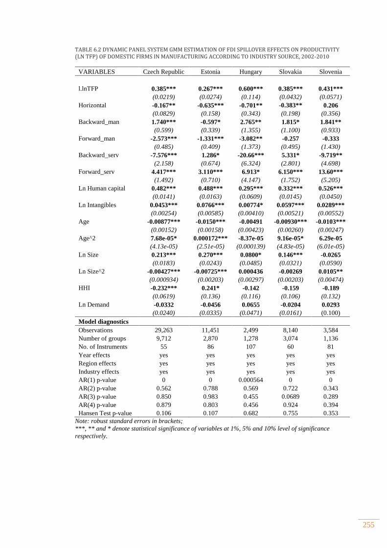
255
TABLE 6.2 DYNAMIC PANEL SYSTEM GMM ESTIMATION OF FDI SPILLOVER EFFECTS ON PRODUCTIVITY (LN TFP) OF DOMESTIC FIRMS IN MANUFACTURING ACCORDING TO INDUSTRY SOURCE, 2002-2010
Note: robust standard errors in brackets;
***, ** and * denote statistical significance of variables at 1%, 5% and 10% level of significance
respectively.
VARIABLES Czech Republic Estonia Hungary Slovakia Slovenia
l.lnTFP 0.385*** 0.267*** 0.600*** 0.385*** 0.431***
(0.0219) (0.0274) (0.114) (0.0432) (0.0571)
Horizontal -0.167** -0.635*** -0.701** -0.383** 0.206
(0.0829) (0.158) (0.343) (0.198) (0.356)
Backward_man 1.740*** -0.597* 2.765** 1.815* 1.841**
(0.599) (0.339) (1.355) (1.100) (0.933)
Forward_man -2.573*** -1.331*** -3.082** -0.257 -0.333
(0.485) (0.409) (1.373) (0.495) (1.430)
Backward_serv -7.576*** 1.286* -20.66*** 5.331* -9.719**
(2.158) (0.674) (6.324) (2.801) (4.698)
Forward_serv 4.417*** 3.110*** 6.913* 6.150*** 13.60***
(1.492) (0.710) (4.147) (1.752) (5.205)
Ln Human capital 0.482*** 0.488*** 0.295*** 0.332*** 0.526***
(0.0141) (0.0163) (0.0609) (0.0145) (0.0450)
Ln Intangibles 0.0453*** 0.0766*** 0.00774* 0.0597*** 0.0289***
(0.00254) (0.00585) (0.00410) (0.00521) (0.00552)
Age -0.00877*** -0.0150*** -0.00491 -0.00930*** -0.0103***
(0.00152) (0.00158) (0.00423) (0.00260) (0.00247)
Age^2 7.68e-05* 0.000172*** -8.37e-05 9.16e-05* 6.29e-05
(4.13e-05) (2.51e-05) (0.000139) (4.83e-05) (6.01e-05)
Ln Size 0.213*** 0.270*** 0.0800* 0.146*** -0.0265
(0.0183) (0.0243) (0.0485) (0.0321) (0.0590)
Ln Size^2 -0.00427*** -0.00725*** 0.000436 -0.00269 0.0105**
(0.000934) (0.00203) (0.00297) (0.00203) (0.00474)
HHI -0.232*** 0.241* -0.142 -0.159 -0.189
(0.0619) (0.136) (0.116) (0.106) (0.132)
Ln Demand -0.0332 -0.0456 0.0655 -0.0204 0.0293
(0.0240) (0.0335) (0.0471) (0.0161) (0.100)
Model diagnostics
Observations 29,263 11,451 2,499 8,140 3,584
Number of groups 9,712 2,870 1,278 3,074 1,136
No. of Instruments 55 86 107 60 81
Year effects yes yes yes yes yes
Region effects yes yes yes yes yes
Industry effects yes yes yes yes yes
AR(1) p-value 0 0 0.000564 0 0
AR(2) p-value 0.562 0.788 0.569 0.722 0.343
AR(3) p-value 0.850 0.983 0.455 0.0689 0.289
AR(4) p-value 0.879 0.803 0.456 0.924 0.394
Hansen Test p-value 0.106 0.107 0.682 0.755 0.353

256
For brevity, we will focus our attention on vertical linkages since horizontal spillovers
and other control variables are fairly robust to changes in specification except the effects
of industry concentration which now suggest that manufacturing firms in Estonia benefit
from less competition. As far as backward linkages are concerned we can observe that
presence of foreign firms in downstream manufacturing sectors with the exception of
Estonia benefit domestic suppliers as the effects on local firms’ productivity range from
1.7 per cent in the Czech Republic to 2.7 per cent in Hungary. The effects are even
stronger in the long run where one percentage point increase of foreign firm’s output in
downstream manufacturing sector leads to 3.23 per cent and 6.9 per cent increase in TFP
in Slovenia and Hungary, respectively. These results are now more in line with most
empirical studies (Havranek and Irsova, 2011) suggesting that countries which attracted
large amount of FDI in tradable sectors such as the Czech Republic, Hungary and
Slovakia are able to benefit from entering MNCs’ production network. However, one
must be careful in interpreting these results as our measure of backward linkages simply
measure the extent of inputs bought by MNCs and its effects on local firm’s TFP. As
shown by several studies focusing on automotive industry in CEE region which attracted
significant amount of FDI, the transfer of knowledge is somewhat limited. For example,
studies by Pavlinek and Zenka (2011) and Rugraff (2010) showed that the Czech
automotive industry is almost entirely dominated by foreign firms which act as a Tier 1
supplier whilst local firms are engaged in a system of “price-driven subcontracting”
failing to develop and produce innovative products. Furthermore, it is found that local
suppliers are mostly engaged in assembly of low to medium value-added parts finding it
difficult to increase their value added. However, there is also evidence that interaction
with MNCs lead to process and product upgrading (Domanski and Gwosdz, 2009;
Pavlinek et al., 2009) and increased knowledge transfer by autonomous foreign
subsidiaries and those which have longer presence in host economy (Gentile-Ludecke
and Giroud, 2012; Jindra et al., 2009).
Turning to backward services linkages, positive effects on local firm’s productivity are
evident only in Estonia and Slovakia and are larger in magnitude in comparison to
manufacturing backward linkages. These positive effects may reflect the change in
economic structure of these economies where service sector share in economic activities
is rising (ESCIP, 2014) which provide domestic suppliers an opportunity to increase their
productivity. As shown by Javorcik and Li (2013) in the case of global retail chains
257
increased presence of MNCs create a strong competitive pressure which results in
crowding out of local firms in service sector and at the same time increase the bargaining
power of MNCs vis a vis local suppliers. Moreover, due to their global sourcing and
increased use of ICT foreign firms have the ability to import some of their products thus
creating incentives for local firms to increase the quality of products, reduce prices and
improve efficiency. Furthermore, MNCs in certain service industries may help domestic
suppliers to reduce their distribution costs and provide access to other regional or national
markets stimulating economies of scale (Javorcik and Li, 2013).
On the other hand, negative services backward linkages are experienced by
manufacturing firms in the Czech Republic, Hungary and Slovenia, offsetting any
positive effect arising from increased domestic sourcing of MNCs in manufacturing
sector. In addition, large negative effects of services backward linkages may explain
negative backward linkages in Hungary presented in Table 6.1. These findings are in line
with those obtained by Mariotti et al. (2013) who found that four service sectors exhibit
negative effects on upstream manufacturing firms unless entry of MNCs in is able to
increase demand for intermediate manufacturing inputs. Similar result is found in
Ayyagari and Kosova (2010) when investigating the effects of services backward
linkages on domestic firm’ entry. They explain this by the fact manufacturing firms
usually supply only limited amount of intermediate inputs to services in form of
communication and information technology and office automation equipment. Since in
these industries barriers to entry may be high and foreign presence is significant services
firms may be more inclined to source from their foreign suppliers. In addition, backward
linkages are usually stronger within service sector as found in Nordas and Kim (2013)
due to less reliance on inputs from other sectors. Inability of domestic suppliers to satisfy
stringent quality requirements may pose certain difficulties to local suppliers in terms of
input adaptation. As argued by Mariotti et al. (2013) adaptation requires additional costs
evident in costs of training and investments which may negatively impact TFP.
Furthermore, some services are characterised by buyer driven GSCs. The example of
latter are large retailers or marketers of final products which require meeting high quality
standards at reduced costs (Gereffi and Lee, 2012). In certain cases, that can only be
satisfied by large MNCs in manufacturing sector which have the ability to meet stringent
and costly requirements. Iacovone et al. (2015), for example, showed that large retailers
require substantial price reductions if suppliers do not come up with product innovation
258
in a given year. Only firms with very high performance and ability to invest in innovation
become suppliers, while other firms face declining sales, productivity or even exit from
the market. Recently, there has been a trend of consolidation in supply chain (Cattaneo
et al., 2010). This has led to outsourcing being carried through a supplier tiering model
where in most cases foreign supplier is a first tier supplier managing its own production
or sourcing network (Farole and Winkler, 2014). This may explain the limited role of
domestic manufacturing firms to enter GVC of MNCs in service sector either because
they are involved in low value added activities with limited knowledge transfer or first
tier supplier follows a more internalised process.
The findings with respect to manufacturing client firms suggest that inputs supplied by
MNCs in manufacturing sector have detrimental effects on TFP in all countries, but are
only significant in the Czech Republic, Estonia and Hungary. One percentage point
increase in foreign firms’ output in upstream sector leads to decline in TFP levels
between 1.3 per cent and 3 per cent in Estonia and Slovakia, respectively. This suggests
that domestic firms do not have the capabilities to benefit from high quality inputs either
due to their higher prices or inability to effectively use them in production process.
Turning to forward spillovers from service sector the results indicate a strong positive
and significant effect of foreign services inputs on downstream manufacturing
productivity thus confirming previous findings on the beneficial effects of services FDI
(Arnold et al., 2011; Fernandes and Paunov, 2012; Mariotti et al., 2013). The short run
effects range from 3.1 per cent in Estonia to 13.6 per cent in Slovenia. Long run effects
are even stronger being smallest in Estonia (4.24 per cent) and largest in Hungary (17.3
per cent) and Slovenia (23.9 per cent). Such large semi-elasticities may reflect the FDI
penetration ratios in service sector due to recent liberalisation where effects are expected
to be larger for an increase in foreign presence from small levels than in sectors where
levels of FDI are already saturated (Gersl et al., 2007). The evidence suggests that
productivity spillovers are more easily captured by manufacturing customers which buy
inputs with high technological content from services MNCs than through backward
linkages. This may be the results of stringent quality requirements imposed by MNCs in
services which put pressure to lower the production costs and prices resulting in fewer
financial resources to finance the necessary investment in technology and product
upgrading. Positive effects of services forward linkages may also reflect market seeking
motives of MNCs which initially followed their clients, but eventually expanded their
259
operation to local manufacturing firms which are in need of high quality inputs in order
to be able to maintain and increase their international competitiveness.67
6.4.3 THE MODERATING EFFECTS OF ABSORPTIVE CAPACITY
As argued in Chapter 2, the occurrence of FDI spillovers is not an automatic process and
not all firms benefit equally from FDI. As noted by Cohen and Levinthal (1990) and later
on by Zahra and George (2002) absorptive capacity helps firms identify, assimilate,
transform and apply knowledge from external environment. Therefore, it is expected
that the benefits from FDI spillovers are more likely to occur in firms which are better
able to evaluate the technology which comes with MNCs. Assimilation of external
knowledge depends on firm’s prior knowledge base which can encourage or hinder
knowledge absorption. As argued by Rosenkopf and Nerkar (2001) prior experience can
facilitate knowledge absorption by defining the locus of knowledge search, but at the
same time it can hinder firm’s search activities to familiar and proximate areas (Stuart
and Podolny, 1996), thus ignoring other sources of knowledge (Cohen and Levintahl,
1990). Finally, absorptive capacity enables firms to transform and apply the new
technology. This in turn depends on organizational capabilities and routines which
provide an opportunity to internally disseminate external information and incorporate
technology into existing processes and routines (Nelson and Winter, 1982; Dosi et al.,
2000; Blalock and Simon, 2009).
Since absorptive capacity is a multidimensional concept its measurement in empirical
research is somewhat difficult. Various measures of absorptive capacity have been used
such as input indicators represented by R&D expenditure, R&D intensity or R&D human
capital measured as R&D employees divided by total employees (Gao et al., 2008),
percentage of higher-educated workforce (Kleinknecht and Reijnen, 1992), number of
doctorates in the R&D department (Veugelers,1997). The shortcoming of such indicators
lies in their narrow focus which cannot explain the complex nature of absorptive capacity
67 Given the large heterogeneity of manufacturing and especially service sectors, we have run two
additional models: (i) interacting FDI spillover variables in model 6.6 with a dummy variable indicating
low and high tech manufacturing sectors; (ii) separating the effects of service linkages according to less
and high knowledge intensive services using Eurostat classification. In both cases, the additional results
confirmed the extreme heterogeneity of empirical results, thus no general pattern could be found across
countries.
260
which relies on several capabilities that build on one another (Duchek, 2013). In addition,
high R&D expenditure or intensity does not necessarily imply higher output or increased
TFP as transformation from input to output depends on other variables as well. Similarly,
output measures such as the number of patents filed by firms are used since they represent
evolution or emergence of new knowledge within the firm (Duchek, 2013). Finally, some
studies use technological gap measured as distance between the level of a local firm TFP
and that of foreign firms (Girma, 2005; Nicolini and Resmini, 2010; Abraham et al.,
2010). However, the problem with technological gap is measurement error arising with
TFP estimation and the fact that TFP reflects other factors besides technology. In
addition, TFP gap may be affected by temporary shocks which do not affect absorptive
capacity (Girma and Gorg, 2007).
Keeping in mind these shortcomings of single quantitative measures of absorptive
capacity and data availability, we test whether intensity of intangible asset use has a
moderating effect on the occurrence of FDI spillovers within the manufacturing sector.
The use of intangible asset has potentially several advantages over other measures of
absorptive capacity. First, intangible capital is found to be a strong determinant of firm
productivity in many studies hence it helps to explain large productivity differences
(Syverson, 2011). Second, intangible capital is a broader measure of absorptive capacity
as it includes both innovation inputs and outputs developed either in house or acquired
in arms-length transactions. For example, knowledge capital of the firm incorporated in
intangible assets include R&D expenditure, software, patents, trademarks, organizational
processes and firm specific skills that provide competitive advantages (Ragoussis, 2014).
Third, in order to be classified as intangible asset, three criteria are used to classify
expenses identified in International Accounting Standards (IAS).64F
68 Intangible asset
reported in Amadeus database conform to these criteria and empirical evidence have
found that capitalized intangible asset is more productivity enhancing than intangible
capital based on current expenses (Bontempi and Mairesse, 2015).
However, our measure of absorptive capacity is not without drawbacks. First, we are not
able to distinguish between different types of intangible capital. Second, only externally
acquired assets can be capitalized and therefore recognized as intangible asset while
68 (i) identifiability: arising from ability of firms to separate, rent, licence and exchange the asset or the
assets need to arise from legal right regardless if they are transferable or separable;
(ii) control: arising from firm power to obtain the benefits from those assets;
(iii) asset must bring future economic benefits (IFRS, 2012)
261
those assets generated internally is often expensed (Ragoussis, 2014). Furthermore,
innovative capabilities and computerised information are reported in firm’s balance sheet
while economic competencies such as marketing expenditure or costs related to
employee training are often expensed. Bearing in mind these shortcomings we proceed
with our estimation as our analysis is conducted within countries and any asymmetries
in accounting standards and treatment of intangible asset are controlled for.
The model presented by equation 6.2 is now augmented by the interaction terms between
each FDI spillover measure and the log ratio of intangible over tangible asset:
𝒍𝒏𝑻𝑭𝑷𝒊𝒕 = 𝜷𝟎 + 𝝆 𝒍𝒏 (𝑻𝑭𝑷𝒊𝒋,𝒕−𝟏)+𝜹𝟏𝒉𝒐𝒓𝒊𝒛𝒐𝒏𝒕𝒂𝒍𝒋𝒕 + 𝜹𝟐𝒉𝒐𝒓𝒊𝒛𝒐𝒏𝒕𝒂𝒍𝒋𝒕 ∗ 𝑰𝑨𝒊𝒕 +
𝜹𝟑𝒎𝒂𝒏𝒖𝒇𝒂𝒄𝒕𝒖𝒓𝒊𝒏𝒈_𝒃𝒂𝒄𝒌𝒘𝒂𝒓𝒅𝒋𝒕 + 𝜹𝟒𝒎𝒂𝒏𝒖𝒇𝒂𝒄𝒕𝒖𝒓𝒊𝒏𝒈_𝒃𝒂𝒄𝒌𝒘𝒂𝒓𝒅𝒋𝒕 ∗ 𝑰𝑨𝒊𝒕 +
𝜹𝟓𝒎𝒂𝒏𝒖𝒇𝒂𝒄𝒕𝒖𝒓𝒊𝒏𝒈_𝒇𝒐𝒓𝒘𝒂𝒓𝒅𝒋𝒕 + 𝜹𝟔𝒎𝒂𝒏𝒖𝒇𝒂𝒄𝒕𝒖𝒓𝒊𝒏𝒈_𝒇𝒐𝒓𝒘𝒂𝒓𝒅𝒋𝒕 ∗ 𝑰𝑨𝒊𝒕 +
𝜹𝟕𝒔𝒆𝒓𝒗𝒊𝒄𝒆𝒔_𝒃𝒂𝒄𝒌𝒘𝒂𝒓𝒅𝒋𝒕 + 𝜹𝟖𝒔𝒆𝒓𝒗𝒊𝒄𝒆𝒔_𝒃𝒂𝒄𝒌𝒘𝒂𝒓𝒅𝒋𝒕 ∗
𝑰𝑨𝒊𝒕+𝜹𝟗𝒔𝒆𝒓𝒗𝒊𝒄𝒆𝒔_𝒇𝒐𝒓𝒘𝒂𝒓𝒅𝒋𝒕 + 𝜹𝟏𝟎𝒔𝒆𝒓𝒗𝒊𝒄𝒆𝒔_𝒇𝒐𝒓𝒘𝒂𝒓𝒅𝒋𝒕 ∗ 𝑰𝑨𝒊𝒕 + 𝜽𝟏𝟏𝑨𝑪𝒊𝒕 +
𝝀𝟏𝟐𝑰𝑻𝒋𝒕 + 𝜸𝒋 + 𝜸𝒓 + 𝜸𝒕 + ɛ𝒊𝒋𝒕 (6.7)
where definition of variables is the same as in eq. (6.6). However, the interpretation of
individual spillover terms is different due to presence of interaction terms. For example, 𝛅𝟏
reflects the effect of horizontal spillovers when intangible asset ratio is zero (IAit =0) and the
sum 𝛅𝟏+𝛅𝟐∗ (IAit) reflects the effect of horizontal spillovers for different values of IAit
included in the interaction terms (individual coefficient of IA is also included in AC
vector).
The estimation technique is the same as in the previous models. The number of
instruments is higher due to inclusion of interaction terms in the instrument matrix.
Turning to model diagnostics which are reported in full in Appendix IV (Tables IV.16-
IV.20), there is no sufficient evidence to reject the null hypothesis for validity of over
identifying restrictions. In addition, there is insufficient evidence to reject second order
autocorrelation in differences of residuals while first order autocorrelation is rejected in
all cases. Difference in Hansen test for the exogeneity of instruments subset suggest
instruments for endogenous variables are valid. Finally, difference in Hansen for levels
equation and lagged dependent variable suggest that steady state assumption holds and
there is no evidence of cross sectional dependence.
Detailed interpretation of alternative model is not provided given that the main interest
is to explain the effects of FDI spillovers on local firms’ TFP moderated by the measure
262
of absorptive capacity. However, we are confident in the robustness of results as the
coefficients from model 6.2 and augmented model 6.6 are similar in sign and size while
significance is now improved for variables controlling for competition and demand
effects. Since interaction terms include two continuous variables we present marginal
effects of FDI spillovers on TFP conditional on different values of intangible asset ratio.
The values of intangible asset ratio taken are 1st and 99th percentile and deciles of
respective distribution.
Starting with interpretation of horizontal spillovers presented in Figure 6.3 we find that
higher intensity of intangible asset ratio has beneficial effects on TFP of firms within
manufacturing sectors as initial negative effects are attenuated in almost all countries.
The beneficial effects are especially pronounced in Estonia and to a lesser extent in
Slovakia where negative effects are diminishing with higher levels of intangible assets.
Looking at more detail, beneficial effects of investment in intangible asset start at
different levels in Estonia and Slovenia. In the former country, manufacturing firms with
high levels of intangible asset are less likely to benefit from horizontal spillovers. They
may already possess high levels of technology and therefore have limited capacity to
learn from MNCs (Grunfeld, 2006). In case of Slovenia investment in intangible asset
has increasing positive effects on domestic firms’ ability to benefit from horizontal
knowledge spillovers. Finally, it seems that moderating effects of absorptive capacity
further increase the negative horizontal effects of manufacturing firms in the Czech
Republic, but only for firms which have above median levels of intangible assets. One
of the possible explanation of negative moderating effects of intangible asset is capability
gap in which firms have the resources but not the capability to use them effectively
(Teece, 1998). As argued by Teece and Pisano (1998) competences and capabilities are
crucial for creation of new products and processes and enable firms to react to changes
in market conditions. Since economic competencies (e.g. human capital and
organizational structure) are regarded as the most important part of intangible asset which
are most difficult to measure and therefore are not included in the balance sheet negative
effect of other components may arise. This is because investment in R&D, digitized
information technology and similar intangible asset increase the costs of firms which is
not translated into higher revenue.
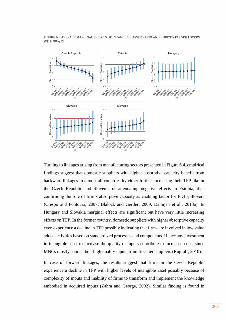
263
FIGURE 6.3 AVERAGE MARGINAL EFFECTS OF INTANGIBLE ASSET RATIO AND HORIZONTAL SPILLOVERS WITH 90% CI
Turning to linkages arising from manufacturing sectors presented in Figure 6.4, empirical
findings suggest that domestic suppliers with higher absorptive capacity benefit from
backward linkages in almost all countries by either further increasing their TFP like in
the Czech Republic and Slovenia or attenuating negative effects in Estonia, thus
confirming the role of firm’s absorptive capacity as enabling factor for FDI spillovers
(Crespo and Fontoura, 2007; Blalock and Gertler, 2009; Damijan et al., 2013a). In
Hungary and Slovakia marginal effects are significant but have very little increasing
effects on TFP. In the former country, domestic suppliers with higher absorptive capacity
even experience a decline in TFP possibly indicating that firms are involved in low value
added activities based on standardized processes and components. Hence any investment
in intangible asset to increase the quality of inputs contribute to increased costs since
MNCs mostly source their high quality inputs from first-tier suppliers (Rugraff, 2010).
In case of forward linkages, the results suggest that firms in the Czech Republic
experience a decline in TFP with higher levels of intangible asset possibly because of
complexity of inputs and inability of firms to transform and implement the knowledge
embodied in acquired inputs (Zahra and George, 2002). Similar finding is found in
-1.5
-1-.
50
.5
Effect
s on F
itted V
alu
es
(p1)
RD
(p10
) RD
(p20
) RD
(p30
) RD
(p40
) RD
(p50
) RD
(p60
) RD
(p70
) RD
(p80
) RD
(p90
) RD
(p99
) RD
at()
Czech Republic
-6-4
-20
2
Effect
s on F
itted V
alu
es
(p1)
RD
(p10
) RD
(p20
) RD
(p30
) RD
(p40
) RD
(p50
) RD
(p60
) RD
(p70
) RD
(p80
) RD
(p90
) RD
(p99
) RD
at()
Estonia
-2-1
.5-1
-.5
0.5
Effect
s on F
itted V
alu
es
(p1)
RD
(p10
) RD
(p20
) RD
(p30
) RD
(p40
) RD
(p50
) RD
(p60
) RD
(p70
) RD
(p80
) RD
(p90
) RD
(p99
) RD
at()
Hungary-1
-.5
0.5
Effect
s on F
itted V
alu
es
(p1)
RD
(p10
) RD
(p20
) RD
(p30
) RD
(p40
) RD
(p50
) RD
(p60
) RD
(p70
) RD
(p80
) RD
(p90
) RD
(p99
) RD
at()
Slovakia-1
01
23
Effect
s on F
itted V
alu
es
(p1)
RD
(p10
) RD
(p20
) RD
(p30
) RD
(p40
) RD
(p50
) RD
(p60
) RD
(p70
) RD
(p80
) RD
(p90
) RD
(p99
) RD
at()
Slovenia
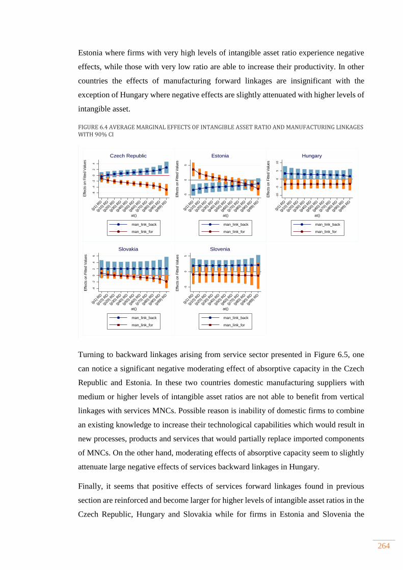
264
Estonia where firms with very high levels of intangible asset ratio experience negative
effects, while those with very low ratio are able to increase their productivity. In other
countries the effects of manufacturing forward linkages are insignificant with the
exception of Hungary where negative effects are slightly attenuated with higher levels of
intangible asset.
FIGURE 6.4 AVERAGE MARGINAL EFFECTS OF INTANGIBLE ASSET RATIO AND MANUFACTURING LINKAGES WITH 90% CI
Turning to backward linkages arising from service sector presented in Figure 6.5, one
can notice a significant negative moderating effect of absorptive capacity in the Czech
Republic and Estonia. In these two countries domestic manufacturing suppliers with
medium or higher levels of intangible asset ratios are not able to benefit from vertical
linkages with services MNCs. Possible reason is inability of domestic firms to combine
an existing knowledge to increase their technological capabilities which would result in
new processes, products and services that would partially replace imported components
of MNCs. On the other hand, moderating effects of absorptive capacity seem to slightly
attenuate large negative effects of services backward linkages in Hungary.
Finally, it seems that positive effects of services forward linkages found in previous
section are reinforced and become larger for higher levels of intangible asset ratios in the
Czech Republic, Hungary and Slovakia while for firms in Estonia and Slovenia the
-6-4
-20
24
Effect
s on F
itted V
alu
es
(p1)
RD
(p10
) RD
(p20
) RD
(p30
) RD
(p40
) RD
(p50
) RD
(p60
) RD
(p70
) RD
(p80
) RD
(p90
) RD
(p99
) RD
at()
man_link_back
man_link_for
Czech Republic
-50
5
Effect
s on F
itted V
alu
es
(p1)
RD
(p10
) RD
(p20
) RD
(p30
) RD
(p40
) RD
(p50
) RD
(p60
) RD
(p70
) RD
(p80
) RD
(p90
) RD
(p99
) RD
at()
man_link_back
man_link_for
Estonia
-10
-50
51
0
Effect
s on F
itted V
alu
es
(p1)
RD
(p10
) RD
(p20
) RD
(p30
) RD
(p40
) RD
(p50
) RD
(p60
) RD
(p70
) RD
(p80
) RD
(p90
) RD
(p99
) RD
at()
man_link_back
man_link_for
Hungary
-4-2
02
46
Effect
s on F
itted V
alu
es
(p1)
RD
(p10
) RD
(p20
) RD
(p30
) RD
(p40
) RD
(p50
) RD
(p60
) RD
(p70
) RD
(p80
) RD
(p90
) RD
(p99
) RD
at()
man_link_back
man_link_for
Slovakia
-50
5
Effect
s on F
itted V
alu
es
(p1)
RD
(p10
) RD
(p20
) RD
(p30
) RD
(p40
) RD
(p50
) RD
(p60
) RD
(p70
) RD
(p80
) RD
(p90
) RD
(p99
) RD
at()
man_link_back
man_link_for
Slovenia
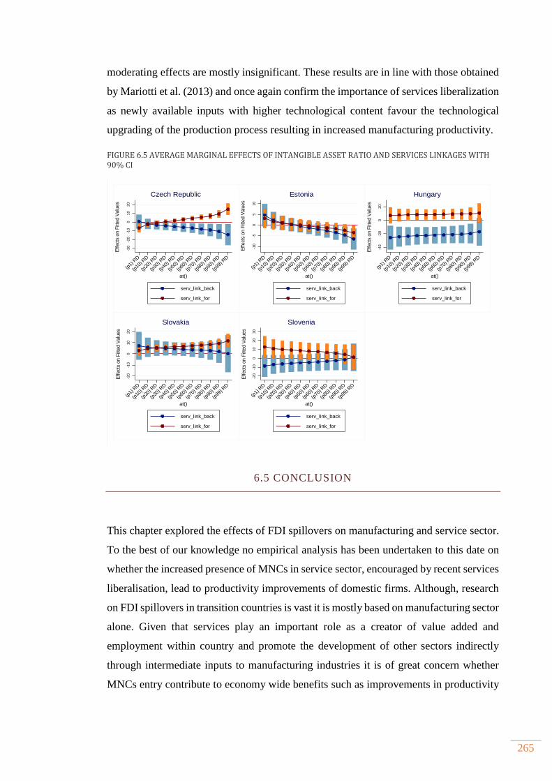
265
moderating effects are mostly insignificant. These results are in line with those obtained
by Mariotti et al. (2013) and once again confirm the importance of services liberalization
as newly available inputs with higher technological content favour the technological
upgrading of the production process resulting in increased manufacturing productivity.
FIGURE 6.5 AVERAGE MARGINAL EFFECTS OF INTANGIBLE ASSET RATIO AND SERVICES LINKAGES WITH 90% CI
6.5 CONCLUSION
This chapter explored the effects of FDI spillovers on manufacturing and service sector.
To the best of our knowledge no empirical analysis has been undertaken to this date on
whether the increased presence of MNCs in service sector, encouraged by recent services
liberalisation, lead to productivity improvements of domestic firms. Although, research
on FDI spillovers in transition countries is vast it is mostly based on manufacturing sector
alone. Given that services play an important role as a creator of value added and
employment within country and promote the development of other sectors indirectly
through intermediate inputs to manufacturing industries it is of great concern whether
MNCs entry contribute to economy wide benefits such as improvements in productivity
-30
-20
-10
01
02
0
Effect
s on F
itted V
alu
es
(p1)
RD
(p10
) RD
(p20
) RD
(p30
) RD
(p40
) RD
(p50
) RD
(p60
) RD
(p70
) RD
(p80
) RD
(p90
) RD
(p99
) RD
at()
serv_link_back
serv_link_for
Czech Republic
-10
-50
51
0
Effect
s on F
itted V
alu
es
(p1)
RD
(p10
) RD
(p20
) RD
(p30
) RD
(p40
) RD
(p50
) RD
(p60
) RD
(p70
) RD
(p80
) RD
(p90
) RD
(p99
) RD
at()
serv_link_back
serv_link_for
Estonia
-40
-20
02
0
Effect
s on F
itted V
alu
es
(p1)
RD
(p10
) RD
(p20
) RD
(p30
) RD
(p40
) RD
(p50
) RD
(p60
) RD
(p70
) RD
(p80
) RD
(p90
) RD
(p99
) RD
at()
serv_link_back
serv_link_for
Hungary
-20
-10
01
02
0
Effect
s on F
itted V
alu
es
(p1)
RD
(p10
) RD
(p20
) RD
(p30
) RD
(p40
) RD
(p50
) RD
(p60
) RD
(p70
) RD
(p80
) RD
(p90
) RD
(p99
) RD
at()
serv_link_back
serv_link_for
Slovakia
-20
-10
01
02
03
0
Effect
s on F
itted V
alu
es
(p1)
RD
(p10
) RD
(p20
) RD
(p30
) RD
(p40
) RD
(p50
) RD
(p60
) RD
(p70
) RD
(p80
) RD
(p90
) RD
(p99
) RD
at()
serv_link_back
serv_link_for
Slovenia

266
through provision of low costs and high quality inputs, increased competition and
knowledge spillovers.
Starting with the baseline model applied separately to manufacturing and service sectors,
the empirical findings suggest negative horizontal effects of manufacturing FDI which
are partially offset by positive knowledge spillovers in service sector in the Czech
Republic and Hungary. In case of backward linkages positive effects of FDI spillovers
are found only in Hungary and Slovakia for service sector and in manufacturing sector
in Slovenia casting some doubt on previous findings from the literature. Regarding
forward linkages the results suggest negative effects of foreign suppliers on local firms’
productivity which are especially pronounced in service sector with the exception of
Slovakia and Slovenia.
In order to shed more light on the impact of vertical linkages we employed an empirical
model disentangling backward and forward linkages according to industry source and
measure their impact on productivity of domestic firms in manufacturing industries
which are at the same time supplier and customer. The results suggest positive effects of
backward manufacturing linkages in all countries except Estonia, thus confirming
previous empirical findings which suggest that MNCs have a strong incentive to share
the knowledge with their suppliers. Negative effect in Estonia may reflect declining share
of manufacturing industries and increasing reliance on services. In addition, it seems that
local manufacturing supplier firms do not benefit from increased presence of services
MNCs acting as customers with the exception of firms in Slovakia and Estonia. The
positive results for the latter two countries may be explained by increased specialisation
in services and increased activity of MNCs which moved some of the headquarters and
therefore require information and communication technology or office automation
equipment.
A closer investigation on the source of forward linkages effects within manufacturing
sector reveal that presence of MNCs has dual effects on local firms’ productivity. On one
side MNCs in manufacturing have negative effects on their local customers which
outweigh positive effects on their suppliers. On the other hand, those inputs provided by
services MNCs have strong and positive effects. The findings are consistent with the
view that services liberalisation and their outcome such as increased MNCs’ presence is
associated with improved availability, range and quality of services resulting in improved
267
performance of downstream manufacturing firms. It is worth noticing that total effects
of vertical linkages calculated as the linear combination of four different channels is
positive except in the Czech Republic and Hungary due to large negative effects from
services MNCs in downstream markets. Finally, findings suggest that gains from MNCs
presence do not accrue equally to all firms. Those firms which have higher intensity of
intangible asset ratio as a proxy for absorptive capacity are more likely to benefit from
manufacturing backward and forward services linkages while negative effects of intra
industry spillovers are attenuated.
In summary, given the positive correlation between services FDI and downstream
manufacturing productivity policy makers should encourage entry of MNCs in service
sector which could constitute an important means to improve the productivity of local
firms and their competitiveness on international markets. Furthermore, the effects of
direct or indirect technology transfer by MNCs are moderated by high levels of
absorptive capacity which is crucial for assimilation and transformation of external
knowledge. This is especially pronounced in case of backward manufacturing and
forward services linkages, two channels of FDI spillovers with the highest potential for
productivity spillovers. Therefore, policy makers should put more emphasis on
improving the absorptive capacity of firms by encouraging and facilitating firms’ R&D
investment, employee training, new software applications and organizational
innovations. Finally, as FDI is the outcome of services liberalisation any remaining
barriers limiting competition, conduct regulation or FDI restrictions should be reduced.
Regarding the latter restriction, government should require that MNCs engage in supplier
development programs given current large negative effects of services MNCs on local
suppliers in some countries.
268
CHAPTER 7. CONCLUSIONS
7.1 Introduction .......................................................................................................................................... 269
7.2 Main findings ........................................................................................................................................ 270
7.3 Contribution to knowledge ............................................................................................................ 282
7.4 Policy implications ............................................................................................................................. 285
7.4.1 Attracting the right type of foreign investors ................................................................ 286
7.4.2 Promotion of linkages .............................................................................................................. 287
7.4.3 Increasing the absoprtive capacity of local firms ......................................................... 289
7.5 Limitations of research .................................................................................................................... 291
7.6 Directions for further research ..................................................................................................... 293
269
7.1 INTRODUCTION
The aim of this thesis, was to examine the potential spillover effects of FDI on
productivity of domestic firms in five transition economies (the Czech Republic, Estonia,
Hungary, Slovakia and Slovenia) which are among the most developed New Member
States of the EU. The inflow of foreign direct investment at the beginning of transition
from centrally planned to market economies was one of the main impetuses to economic
and institutional restructuring in these countries. MNCs played an important role in the
privatisation process, the subsequent firm restructuring, changes in export and market
structures, the development of service sector and technological upgrading. Apart from
direct effects, MNCs are also a major source of technology spillovers to indigenous firms.
These indirect effects are seen as an important factor for productivity catch up of
domestic firms, their participation in Global Value Chains (GVC) and ultimately their
survival in national and international markets.
Although the investigation of FDI spillovers has gained momentum in the last two
decades, empirical studies have still not reached a consensus on the indirect effects of
foreign firm’s entry on productivity of local firms. Hence, this thesis has focused on
several questions which are crucial for understanding the current ambiguous findings in
the literature. How, and through which channels, are domestic firms expected to benefit
from technology spillovers from MNCs? What is the most appropriate method for
measuring firm level productivity? What is the level of productivity of local and foreign
firms? Are there any differences between the productivity of firms in the two major
sectors of economy (manufacturing and services)? How FDI spillovers are measured and
what is their effect on productivity of domestic firms? What is the role of MNCs’
geographic origin and the extent of foreign ownership on productivity of domestic firms?
What are the factors influencing the ability of domestic firms to benefit from technology
spillovers according to the channel through which they occur? Is there any systematic
variation in FDI spillover effects across manufacturing and service sectors? Are there
any intersectoral spillovers?
270
7.2 MAIN FINDINGS
The surge of FDI after World War II resulted in various theories attempting to explain
why firms decide to go abroad and incur sunk costs. An initial review of determinants of
FDI in Chapter 1 has shown that the concept can be explained using insights from
international trade and international production theory and its variants. Although many
strands of the literature are concerned with the explanation of FDI and the emergence of
MNCs, they differ in their underlying assumptions. The majority of theoretical concepts
reviewed in Chapter 1 have failed to account for the complexity of MNCs’ decision to
engage in cross border investments. OLI paradigm combined several strands of literature
in an attempt to provide an explanation for internationalisation of production and hence
provide a general framework for analysis of the effects of FDI. Recently, the network
based theory of MNCs has emphasized the technological accumulation, firm specific
learning and roles of MNCs’ subsidiaries and their embeddedness in local environment
as a source of competitive advantages. An alternative approach explaining FDI has been
adopted by scholars in the field of international economics which combined ownership
and location advantages with technology, firm and country characteristics in explaining
different forms of FDI.
By evaluating the complementarities between different theories and incorporating recent
advances in international business and international economics literature and having in
mind data limitations, the investigation of FDI spillovers adopted in this study relied on
a production function framework in order to be able to derive changes in firm level
productivity as a proxy for technology spillovers. We argued that theoretical models of
FDI spillovers developed by scholars in the field of international economics, growth
theory and international business emphasizing both MNCs and local firms’ heterogeneity
are best suited for our research needs. This is because the focus of our research is on the
ability of local firms to benefit from variety of technologies and linkages made available
by different MNCs located across the manufacturing and service sectors. Heterogeneity
of MNCs can lead to different FDI spillovers potential and effect and thus productivity
catch up of domestic firms and ultimately their success in international markets.
Once the conceptual framework for investigating FDI spillovers was established in
Chapter 2, our analysis moved on to investigate the role of FDI in the transition process.
271
We found that the entry of MNCs was facilitated by, and became part and parcel of, the
wide ranging structural reforms pursued by transition countries. The structure of FDI
across countries and industries, and the success of countries in attracting MNCs closely
followed the government stance towards privatisation, speed of structural reforms and
prospects for EU membership. While manufacturing sector was the initial focus of
foreign investors, subsequent investments were more oriented towards underdeveloped
service sectors and hence the share of manufacturing FDI started to decline. The
exceptions were countries with strong manufacturing base such as the Czech Republic,
Hungary and Slovakia which continued to attract significant amounts of FDI in
automotive and electronics sectors.
NMS in general have witnessed strong income and productivity convergence towards the
EU-15 and we argued that FDI has played an important role in this process. The
contribution of foreign affiliates in total turnover, value added and employment, and the
levels of technological sophistication have been increasing over time. As a consequence,
FDI contributed to industry restructuring and increase in productivity, enabled the shift
from low to high value added activities and intensified NMS’s integration in GVCs.
Motivated by findings in Chapter 3 which suggested the importance of foreign firms for
economic activity of NMS and their superior performance over domestic firms, the
second part of the thesis was concerned with empirical analysis of FDI spillovers at micro
level.
The empirical part of the thesis is divided into three Chapters.
Chapter 4 was concerned with the estimation of TFP at firm level as a first step in the
investigation of FDI productivity spillovers. Given data limitations we focused on five
NMS (the Czech Republic, Estonia, Hungary, Slovakia and Slovenia) during the 2002-
2010 period, the most recent year for which data were available at the time of writing the
thesis. Although the concept of total factor productivity is well known in the literature,
its estimation is far from simple due to its unobservable nature. Our starting point was a
critical review of the various approaches available for the estimation of productivity. We
argued that a semi-parametric methods based on control functions containing observable
firm characteristics are the most appropriate when a researcher is interested in exploring
the characteristics of factors of production such as ease of adjustment and observability
272
of all factors affecting output. In addition, they are able to control for simultaneity bias
between factor inputs and unobserved productivity.
Having in mind several methodological issues explained in Chapter 4, we resorted to
estimation of TFP using OLS, Levinsohn-Petrin (2003) and Wooldridge (2009)
estimators in order to test the data properties and compare empirical results across
different estimators. After applying Cobb Douglas production framework for each
country-industry pair and comparing the obtained TFP estimates across different
estimators, we decided to choose Wooldridge TFP model as the preferred estimator as it
is able to control for identification problems mentioned in Ackerberg et al. (2006) and
are fairly similar when compared to other two estimation techniques. Our results are in
line with similar studies comparing TFP estimates across different estimators and we
may conclude that the choice of estimator is less crucial when one is interested in the
non-deterministic part of the production function. These TFP estimates were then used
as the dependent variable in the subsequent chapters.
In Chapter 4 we also tested the necessary assumptions for the occurrence of FDI
spillovers related to the productivity premium of foreign over domestic firms. We found
that foreign firms in every country and main sectors of activity were more productive.
These results hold both for non-parametric Kolmogorov-Smirnov test and parametric
estimation. We also found that MNCs’ heterogeneity in terms of their geographic origin
and the extent of foreign ownership has important implications for potential productivity
spillovers. Namely, fully owned foreign firms and firms coming from the EU were the
most productive. We also found that domestic firms have experienced an improvement
in their productivity levels over time, especially those firms whose TFP is below median
levels. However, there is a strong persistence in the position of domestic firms in TFP
distribution which is the main feature of this sample.
In Chapter 5, we developed an empirical model of FDI spillovers based on the conceptual
framework and identified shortcomings of the current empirical studies applied to
transition countries. The model was based on endogenous growth theory in which the
main interest lies in the estimation of technology shock induced by factors internal and
external to the firm. In this thesis the latter factors are represented by FDI spillover
variables. The main aim was to investigate whether the heterogeneous nature of MNCs
has different productivity spillovers effects on domestic firms in manufacturing and

273
service sectors. Rich micro panel data applied to the five countries under consideration
allowed us to incorporate variables controlling for absorptive capacity of local firms such
as the share of intangible assets in total fixed assets and a measure of human capital
proxied by average firm-level wage. We also controlled for firm age and size and the
squared terms of these factors, demand in downstream sectors and the level of
competition in the industry. The main variables of interest were related to the
construction of FDI spillovers within and across industries. For that purpose we relied
on a combination of firm level data available from Amadeus database and yearly input
output tables available from World Input Output tables thus providing us the opportunity
to examine changes in economic structure and input sourcing behaviour of foreign firms
over time.
It should be noted that our main variables of interest, namely horizontal spillovers and
vertical linkages capture different mechanisms of knowledge diffusion. In case of
horizontal spillovers we capture the net effects of pure technological externalities such
as imitation and reverse engineering reffered to as demonstration effects and competition
effects arising from changes in market structure due to MNCs’ entry. In addition,
knowledge spillovers may also arise due to worker mobility which can only be gauged
by tracing the movement of workers between companies. In comparison to unintentional
knowledge diffusion measured by demonstration effects and worker mobility, vertical
linkages involve intentional knowledge transfer and pecuniary externalities. Although,
we may find positive correlation between productivity of domestic firms in upstream
sectors with the presence of MNCs in downstream sectors or vice versa, the exisiting
measures based on industry level proxies for vertical spillovers do not pinpoint which
mechanisms are at play.
For example, positive backward spillovers which influence domestic firms’ productivity
may arise due to the direct linkage with foreign customers along the supply chain through
various forms of assistance and knowledge transfer provided by foreign firms after the
contract has been signed. Alternatively, domestic firms not direcly involved with foreign
firms in downstream sectors may also experience productivity improvements due to the
interest of foreign firms in improving the quality of sourced inputs and therefore provide
help to local suppliers before they enter into contractual relationship. Alternatively,
positive productivity shock may be the result of own firm effort motivated by lucrative
contracts with MNCs or scale economies reflecting greater demand for domestically

274
produced inputs (Javorcik, 2004; Javorcik and Spatareanu, 2009). All of these scenarios
can broadly be regarded as spillovers, however, disentagling the exact mechanisms at
play using industry level proxies is not possible.The result from dynamic panel model
used to control for potential endogeneity of FDI spillover variables and TFP suggested
that horizontal FDI spillovers have become more important over time, thus shedding new
light on the role of MNCs in host countries. A closer investigation revealed that the
positive effects were mainly driven by partially owned foreign firms indicating that
domestic firms are well equipped to benefit from well diffused technology. On the other
hand, the presence of fully owned foreign firms placed considerable pressure on local
firms as they were not able to effectively imitate foreign technology causing reduction
in their productivity levels. Alternatively, foreign firms may have been more successful
in preventing the leakage of knowledge and technology to their potential competitors.
When taking into account geographic heterogeneity of MNCs, we found that there was
positive spillovers from European MNCs in all countries except Slovenia, thus
supporting the premise that institutional and socio cultural proximity facilitated
knowledge sharing, technology diffusion and learning by domestic firms. Non-European
investors, the majority of which came from USA and China, also provided knowledge
which was used by domestic competitors to increase their productivity. However, these
results hold only for firms in Estonia and Slovenia.
The findings for backward linkages confirmed previous findings in the literature
suggesting that MNCs are more likely to share their knowledge with local suppliers. They
imply increasing impact in the Czech Republic, Hungary and Slovakia and decreasing
impact in Estonia. A new finding is that fully owned foreign firms are driving the positive
effects. On the other hand, these positive effects were offset by negative effects from
partially owned foreign firms. The exceptions were the Czech Republic and Slovenia.
When accounting for geographic heterogeneity of MNCs, the results were more
heterogeneous. While in Hungary and Slovakia EU investors were more inclined to
engage in vertical linkages, the opposite was found in other countries, thus partially
confirming the hypothesis that investors from distant countries were likely to source
inputs locally to save on transport and trade costs, thus confirming theoretical model of
Rodriguez-Clare (1996).
Perhaps, the most interesting findings were related to forward linkages. Over time these
linkages have gained more importance than backward linkages, exhibiting large
275
productivity gains/losses for domestic firms. Based on our results, forward linkages are
more likely to influence the net benefits or costs of foreign presence in the local economy.
Firms in Slovakia and Slovenia were able to benefit from increased variety and quality
of inputs, thus increasing their productivity. These positive effects hold across different
ownership structures of foreign firms and are mainly driven by EU investors. Firms in
other countries experienced a decline in their productivity and these negative effects were
driven by both partially and fully owned foreign firms with the exception of Estonia
where partially owned foreign firms have a beneficial effect on local firms’ productivity.
In addition, non-EU investors were responsible for large negative effects on productivity
which completely offset any positive effects from EU MNCs.
The empirical findings showed that other factors, such as the level of intangibles and
human capital to positively influence local firms’ productivity in all countries. Increased
competition in the industry was also found to positively influence TFP in all countries
with the exception of Slovakia, while increased demand in downstream sectors exhibited
mostly negative effects. We also found that productivity is negatively affected by firms’
age. Although after a certain period, the variable age becomes positive, the proportion of
firms in our sample that were older than estimated turning point was negligible. Also, the
findings suggested that larger firms were more likely to experience positive productivity
gains.
In Chapter 6 we explored further the different nature of FDI spillovers in firms in
manufacturing and service sectors. We divided the sample and re-estimated the baseline
model developed in Chapter 5. Furthermore, we investigated the intersectoral spillovers
between manufacturing and services. The aim was to shed more light on the direction of
vertical linkages between these two sectors and to explore their heterogeneity by
constructing four types of vertical linkages. This included splitting total backward and
forward linkages according to the main sector of MNCs’ activities. The empirical
analysis then estimated the effects of manufacturing (services) linkages on local firms’
productivity in manufacturing sector which are at the same time supplier and customer
of foreign firms located in the two main sectors of the economy. Since we found
significant positive effects of knowledge capital variables in Chapter 5, we also tested
their moderating effects by interacting them with FDI spillover variables.

276
Empirical analysis was based on a dynamic system GMM estimator as in Chapter 5 to
make results comparable. Findings from the baseline model applied separately to firms
in manufacturing and services suggested that the positive horizontal spillovers found in
Chapter 5 were mostly driven by firms in services. The negative effects of horizontal
spillovers in manufacturing sector are in line with the empirical results from other studies
indicating that local firms do not have sufficient level of absorptive capacity. On the
other hand, foreign firms in services require close interaction and communication thus
giving domestic firms the opportunity to learn and imitate some of the best practices of
MNCs. These positive effects were however observed only in Hungary and the Czech
Republic. The findings suggested the importance for separating firms from different
sectors.
In the case of backward linkages, our findings suggested that MNCs in services were
more likely to source inputs from local firms in Hungary and Slovakia while the opposite
holds for firms in the Czech Republic and Estonia. The findings related to local
manufacturing firms suggested that they were not able to enter the supply chain of MNCs
expect those in Slovenia. The heterogeneity of findings across countries was further
supported when analysing forward linkages. These have been found to be positive only
in the service sector in Slovakia and Slovenia. On the other hand MNCs in services have
large negative productivity effects as suppliers of inputs to local firms in the Czech
Republic, Estonia and Hungary.
By employing an augmented empirical model and disentangling vertical linkages
according to industry source we found that our results for backward manufacturing
linkages are in line with the current literature. In other words, local manufacturing
suppliers were able to join the global supply chains of MNCs and increase their
productivity through voluntary and involuntary knowledge transfer from foreign firms.
We also found that MNCs in services were less keen to source their inputs from local
manufacturing suppliers and more likely to resort to inputs sourced from abroad or from
other foreign firms in upstream manufacturing sectors. Only local manufacturing firms
in Slovakia and Hungary were able to benefit from engaging in backward linkages with
MNCs in services. The most interesting findings are again related to forward linkages.
Local manufacturing firms were not able to benefit from inputs bought from MNCs in
the manufacturing sector. However, we have found significant and positive effects of
services inputs for manufacturing productivity across all countries thus further

277
corroborating the notion that the liberalisation of services followed by increased foreign
entry was expected to bring substantial positive effects to downstream clients.
Further we investigated the interaction between firms’ investment in intangible asset and
FDI spillover variables. This analysis was motivated by the notion that a minimum level
of absorptive capacity is necessary for firms to identify, assimilate, transform and apply
the knowledge from external environment. According to the findings, the moderating
effects of firms’ absorptive capacity had beneficial impact on TFP of firms within the
manufacturing sector as the initial negative horizontal effects were attenuated in almost
all countries. Similar findings were found in the case of backward manufacturing
linkages where firms in the Czech Republic and Slovenia were able to increase their TFP
with higher levels of intangibles while firms in Estonia were able to attenuate initial
negative effects. However, in case of backward services linkages, the moderating effects
do not hold as manufacturing firms were not able to combine an existing knowledge to
increase their technological capabilities which would result in new or improved
intermediate inputs.
The findings related to forward linkages implied that investing in intangible assets matter
for manufacturing firms in the Czech Republic, Hungary and Slovakia seeking to
improve their productivity by buying services inputs. On the other hand, the moderating
effect of absorptive capacity does not matter for forward linkages in manufacturing. For
firms in the Czech Republic and Estonia higher levels of intangible asset have detrimental
effects on their ability to benefit from manufacturing inputs. This may be due to the
complexity of inputs and their prices, or the inability of manufacturing firms to transform
and implement the knowledge embodied in acquired inputs.
In order to summarize our empirical findings on spillover effects of FDI explored in
Chapters 5 and 6 and to better present the heterogeneity of results across countries, we
have constructed a table showing all empirical models and associated signs and statistical
significance (at least 10%) of FDI spilllover variables across countries. As can be seen
from Table 7.1 below the findings for horizontal spillovers are mostly ambiguous which
is in line with current empirical literature, further highlighting the need for better data
which would allow researchers to disentangle different mechanisms of knowledge
spillovers within industry. In general, horizontal spillovers across countries are mostly
negative in the manufacturing sector and those from fully owned foreign firms while
278
positive effects are limited to partially owned foreign firms and those coming from the
EU.
In case of backward linkages, the empirical results are in line with the exisiting literature
suggesting positive effects of MNCs on domestic suppliers’ TFP. The effect seems to be
strongest in manufacturing sector and only when domestic suppliers are supplied by
foreign firms from manufacturing sectors. Similarly, in the majority of cases positive
effects of backward linkages across countries and two major sectors are found for non-
EU MNCs and fully owned foreign firms.
Finally, the major finding in the thesis is related to positive and significant effects of
forward linkages from the service sector to domestic clients in manufacturing, thus
shedding new light on the role of MNCs in the service sector on indigenous firms’
productivity. In addition, the origin of foreign investors matters for forward spillovers as
foreign firms from the EU have unambiguous positive effects on productivity of
downstream clients while opposite holds for non-EU investors.
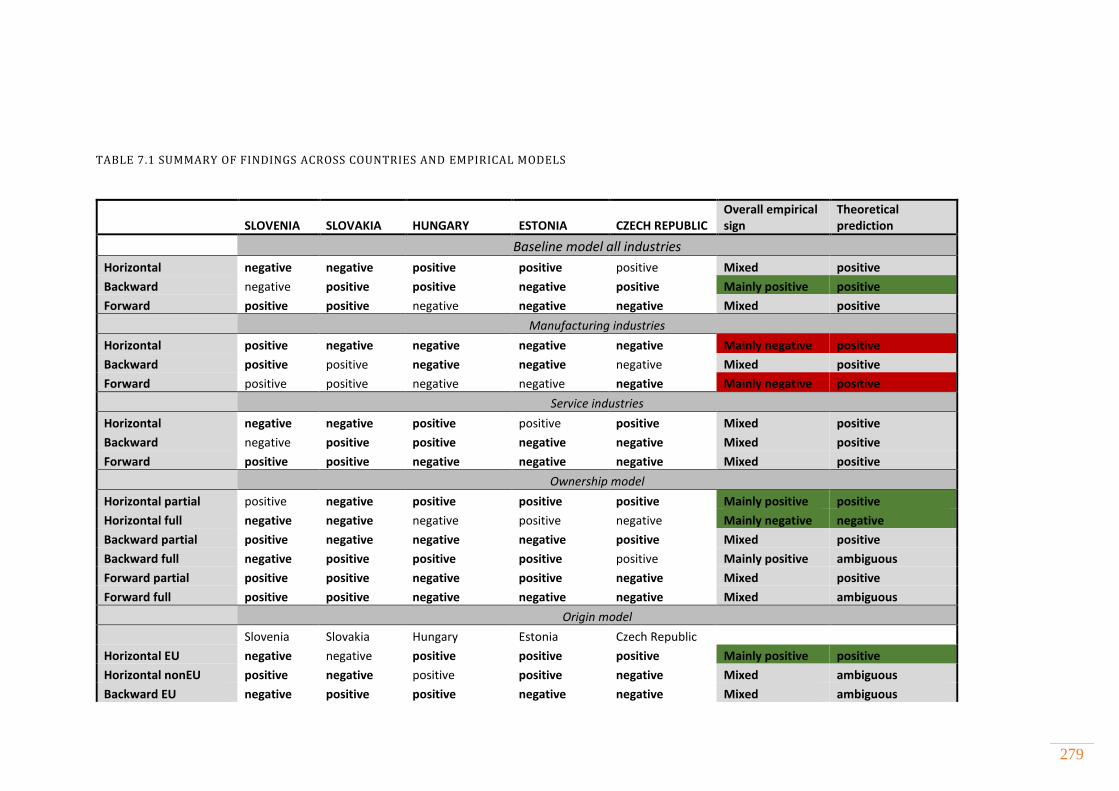
279
TABLE 7.1 SUMMARY OF FINDINGS ACROSS COUNTRIES AND EMPIRICAL MODELS
SLOVENIA SLOVAKIA HUNGARY ESTONIA CZECH REPUBLIC Overall empirical sign
Theoretical prediction
Baseline model all industries
Horizontal negative negative positive positive positive Mixed positive
Backward negative positive positive negative positive Mainly positive positive
Forward positive positive negative negative negative Mixed positive
Manufacturing industries
Horizontal positive negative negative negative negative Mainly negative positive
Backward positive positive negative negative negative Mixed positive
Forward positive positive negative negative negative Mainly negative positive
Service industries
Horizontal negative negative positive positive positive Mixed positive
Backward negative positive positive negative negative Mixed positive
Forward positive positive negative negative negative Mixed positive
Ownership model
Horizontal partial positive negative positive positive positive Mainly positive positive
Horizontal full negative negative negative positive negative Mainly negative negative
Backward partial positive negative negative negative positive Mixed positive
Backward full negative positive positive positive positive Mainly positive ambiguous
Forward partial positive positive negative positive negative Mixed positive
Forward full positive positive negative negative negative Mixed ambiguous
Origin model
Slovenia Slovakia Hungary Estonia Czech Republic
Horizontal EU negative negative positive positive positive Mainly positive positive
Horizontal nonEU positive negative positive positive negative Mixed ambiguous
Backward EU negative positive positive negative negative Mixed ambiguous
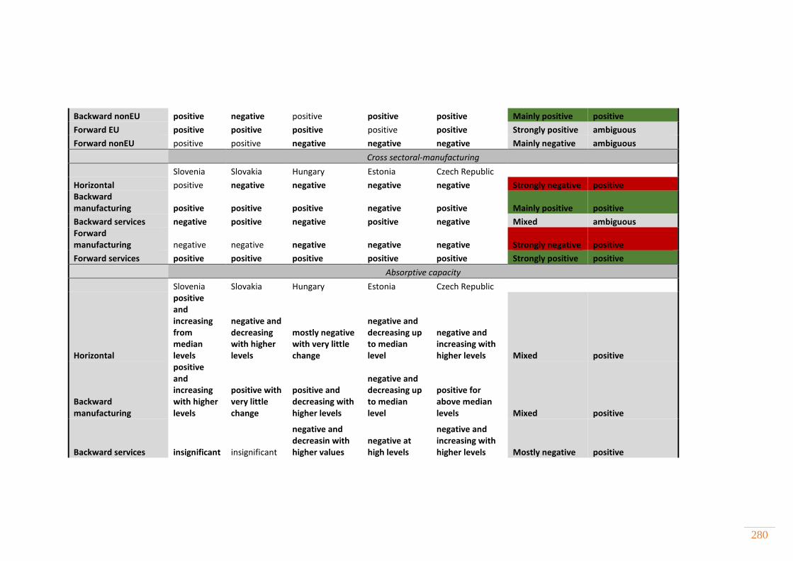
280
Backward nonEU positive negative positive positive positive Mainly positive positive
Forward EU positive positive positive positive positive Strongly positive ambiguous
Forward nonEU positive positive negative negative negative Mainly negative ambiguous
Cross sectoral-manufacturing
Slovenia Slovakia Hungary Estonia Czech Republic
Horizontal positive negative negative negative negative Strongly negative positive Backward manufacturing positive positive positive negative positive Mainly positive positive
Backward services negative positive negative positive negative Mixed ambiguous Forward manufacturing negative negative negative negative negative Strongly negative positive
Forward services positive positive positive positive positive Strongly positive positive
Absorptive capacity
Slovenia Slovakia Hungary Estonia Czech Republic
Horizontal
positive and increasing from median levels
negative and decreasing with higher levels
mostly negative with very little change
negative and decreasing up to median level
negative and increasing with higher levels Mixed positive
Backward manufacturing
positive and increasing with higher levels
positive with very little change
positive and decreasing with higher levels
negative and decreasing up to median level
positive for above median levels Mixed positive
Backward services insignificant insignificant
negative and decreasin with higher values
negative at high levels
negative and increasing with higher levels Mostly negative positive
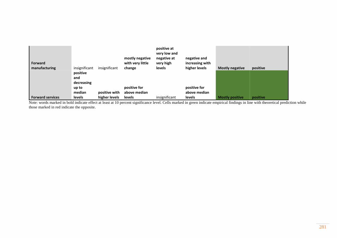
281
Forward manufacturing insignificant insignificant
mostly negative with very little change
positive at very low and negative at very high levels
negative and increasing with higher levels Mostly negative positive
Forward services
positive and decreasing up to median levels
positive with higher levels
positive for above median levels insignificant
positive for above median levels Mostly positive positive
Note: words marked in bold indicate effect at least at 10 percent significance level. Cells marked in green indicate empirical findings in line with theoretical prediction while
those marked in red indicate the opposite.
282
7.3 CONTRIBUTION TO KNOWLEDGE
This thesis has made several contributions to existing theoretical and empirical body of
knowledge on FDI spillovers. Based on review of the literature on determinants of FDI
we argued that varieties of theoretical concepts are not able to fully explain the complex
and multidimensional nature of FDI. While international business literature assumes that
MNCs possess superior firm specific advantages in comparison to domestic firms, early
studies failed to explain MNCs’ heterogeneous nature in terms of investment motives,
mode of entry, technology, knowledge or productivity. The early models of FDI
spillovers were based on the neoclassical theory assuming that the intensity of MNCs’
activities is a measure of potential for FDI spillovers to host country firms. Therefore, to
revise the assumption of MNCs’ homogeneity, commonly made in FDI spillovers studies
conducted on transition economies, we have combined recent insights from international
business and international economics literature emphasizing the heterogeneity of MNCs
and their affiliates. We have proposed that the effects of FDI spillovers may differ
according to MNCs’ observable characteristics available in the dataset and other non-
observable heterogeneities. Our conceptual framework emphasized that FDI spillovers
are determined by both demand and supply side factors and shaped by external
environment such as industry characteristics and institutional framework in which firms
operate.
We have also argued that existing theoretical models of vertical linkages between MNCs
and local firms place too much emphasis on backward linkages occurring within
manufacturing sector. Notwithstanding the importance of backward linkages for local
firms’ development in manufacturing sector, forward linkages have received less
attention. We have argued that liberalisation and deregulation of services followed by
entry of MNCs in services are an important conduit to better quality and variety of inputs
available at lower price, hence contributing to manufacturing productivity and better
functioning of specialised and interdependent operations. Since services are often
characterized by intangibility, inseparability and require frequent interaction and
proximity between supplier and customer due to information asymmetries about quality,
283
we argued that MNCs are the main conduit for technology spillovers to downstream
clients thus shedding new light on the role of forward linkages.
Our first empirical contribution is related to the estimation of TFP at firm level. Most
studies employing semi-parametric techniques lacked a critical examination of the data
generating process of different estimators, the robustness checks for TFP estimates across
different estimators was rarely performed, the elasticity of factor inputs was almost never
discussed and the potential pitfalls arising from the violation of timing assumptions of
inputs were ignored. In cases when authors extensively tested the assumptions of certain
estimators they used data from only few industries in one country framework. Therefore,
our contribution lies in the application of semi-parametric methods to a broad set of
industries and countries. Another contribution to knowledge is related to the method
employed when estimating TFP. We used Wooldridge (2009) application of semi-
parametric methods which corrects some of the problems discussed in Ackerberg et al.
(2006) not previously addressed in estimation of TFP in transition countries.
We also estimated both value added and gross output in a Cobb Douglas production
function framework and tested the timing assumptions of labour input. We have found
that value added production function treating labour as static input is suitable for our
dataset. However, none of the existing studies using TFP as a dependent variable to
evaluate the impact of policy measures such as FDI spillovers have acknowledged
potential issues in TFP estimates arising from different timing assumptions of labour
input. Thus, our findings may point to possible publication bias and be considered as
additional contribution to knowledge.
Our estimation of FDI spillovers has made several contributions to the existing literature.
First, we expand our knowledge on the effects of MNCs on their local competitors, their
suppliers and clients in transition countries by applying an empirical model to a set of
advanced NMS, simultaneously taking into account both types of vertical linkages and
horizontal spillovers. In addition, we add to the literature by employing the same
dependent variable estimated by using the unique method previously not explored in the
context of transition countries. Furthermore, by using time varying input-output tables
we were able to take into account dynamic structural changes and differences in sourcing
behaviour of MNCs in transition countries which has not been done in previous empirical
work. Second, this is the first study which treats FDI spillovers in a dynamic framework
284
thus taking into account theoretical transmission channels of knowledge spillovers which
differentiate between short and long run effects. With this in mind we used dynamic
system GMM estimation which accounts for potential endogeneity of FDI spillover
variables and the dynamics of firms’ productivity as implied by the control function
approach used to derive it. Third, our study is the first one to include the service sector
of these countries which has largely been ignored in the investigation of FDI spillovers.
Fourth, we depart from the contemporary literature which has focused on issues such as
the role of local firms’ absorptive capacity and demand size of FDI spillovers. Our
augmented empirical model is the first study which takes into account the supply side of
FDI spillovers by examining the geographic and ownership heterogeneity of MNCs in
this set of countries.
We have also separately examined FDI spillovers in manufacturing and services, adding
to the current literature which has mainly focused on the manufacturing sector. Given the
large inflows of FDI in services and the importance of its inputs for downstream clients
this thesis addressed and clarified some of the misunderstandings related to the role of
forward vertical linkages and their impact on productivity of downstream manufacturing
firms. We showed that the current measurement of vertical linkages does not permit the
measurement of overall spillover effects according to the channels through which they
occur. Construction of four types of vertical linkages enabled us to shed more light on
the customer-supplier relationship between domestic and foreign firms in the two main
sectors of economy.
The final contribution of this thesis is its temporal, sectoral and geographical coverage.
Through a critical review of the literature in Chapter 2 we came to conclusion that
existing studies investigating FDI spillovers in transition countries are mainly focused
on the manufacturing sector. Moreover, most of these studies are conducted using data
from the first decade of transition or early 2000s while the bulk of FDI inflow took place
in the later period of transition. Our empirical analysis covers the period which coincided
with the large inflows of FDI in services and changes in macroeconomic and business
environment as well as the progress in institutions which further influenced the entry,
type and motives of MNCs. Furthermore, it can be argued that in the second decade of
transition domestic firms improved their absorptive capacity and the quality of their
products. Finally, we were able to estimate the effects of FDI spillovers using common

285
data, methodology and empirical model for the five leading NMS, thus enabling us to
provide more valid and comparable results across countries.
7.4 POLICY IMPLICATIONS
Throughout this thesis we have emphasized the relationship between heterogeneous
nature of MNCs, sectoral heterogeneity and the differential impact of vertical linkages
on the one hand and the ability of indigenous firms to increase their productivity and
increase their competitiveness in national and international markets on the other. It was
stressed that NMS have been successful in attracting FDI in medium high and high
technology sectors which has enabled them to reduce the productivity gap vis-a-vis more
advanced market economies and become more specialised in production of products with
higher value added. By choosing export led strategies, NMS have successfully integrated
in international trade and stimulated their economic growth (Rugraff, 2008). However,
given the rising importance of GVCs and the prominent role played by MNCs in world
production and distribution, further development and growth of NMS depends on their
successful integration in MNCs’ networks and their orientation toward knowledge based
economy.
The main source of productivity improvements in the analysed countries emerged from
vertical linkages with MNCs accompanied by high stock of knowledge capital, namely
the share of intangible assets and high levels of human capital. However, the productivity
effects largely depend on the type of vertical linkages and the heterogeneity of MNCs.
Therefore, one of the most important issues for analysed countries is the identification of
channels through which heterogeneous MNCs contribute to indigenous firms’
productivity and measures which can facilitate the inclusion of local firms in MNCs’
supply network. In devising policy recommendations which can serve as a guideline to
governments for raising prospects for indigenous firms’ integration in GVCs, we will
primarily rely on findings from the empirical chapters. The set of policy
recommendations are organized in three areas: (i) attracting the “right” type of foreign
investors; (ii) establishing the right kind FDI incentives to promote linkages with MNCs;
and (iii) increasing the capacity of local firms to benefit from FDI spillover potential.

286
7.4.1 ATTRACTING THE RIGHT TYPE OF FOREIGN INVESTORS
One of the key messages of this thesis is that not all foreign investors are the same.
Therefore, given the importance of spillovers, FDI promotion should be designed to
allocate incentives depending on the motive and type of foreign investment as well as the
sector of operation. So far, NMS have adopted the so-called ‘Irish model’, offering
generous fiscal and financial incentives in order to attract large scale FDI with almost no
performance requirements and without formulating sufficient incentives for the foreign
firms to interact with the local environment (Rugraff, 2008; Jindra and Rojec, 2014).
Therefore, further promotion and incentives should be based on active promotion of
specific sectors and activities within the sector which can increase local firms’
participation in GVCs so as to emphasise the fragmentation of tasks and activities and
not industries anymore. Incentives offered to foreign investors should be based on the
promotion of R&D activities and the attraction of technologically more advanced, fully
owned MNCs and those engaged in activities with high value added such as services.
Although still limited, backward linkages in services are gaining importance suggesting
that besides positive effects of efficiency seeking investors on local manufacturing
suppliers, policy makers should put more emphasis on attracting market seeking
investors in services as they are less sensitive to costs consideration than efficiency
seeking investors. This is also suggested by findings in Chapter 6 where local firms were
shown to benefit from backward linkages with MNCs in services in Estonia, Hungary
and Slovakia.
Furthermore, investment promotion strategies coordinated and implemented by
investment promotion agencies should put emphasis not only on employment effects or
the amount of investment, but also on potential for technology transfer, R&D activities
and development of linkages. By attracting MNCs in services especially those in the
energy sector, telecommunications, transport, logistics and ICT, the potential for
spillovers is likely to be of cross-sectoral nature, thus improving productivity of
downstream manufacturing clients by providing high quality inputs as suggested by
findings in Chapter 6. The evaluation criteria for granting fiscal, financial or other type
of incentives should include the strategy and commitment for technology transfer and
creation of linkages with local firms. Investment incentives could take into account the
degree of foreign ownership and the country of origin of MNCs given their differential
impact on productivity of local firms across countries.
287
With increasing fragmentation of GVCs, Tier 1 suppliers followed their main customers
to host countries, thus making it very difficult for local suppliers to directly supply
MNCs, especially those in the service sector. Hence, promotion efforts should also be
targeted at Tier 2 or Tier 3 suppliers with lower quality requirements and those who have
already established contracts with Tier 1 suppliers. Although this may reduce the
potential for technology transfer due to their lower knowledge capacity, their cooperation
with local suppliers would enable the latter to learn and gradually improve the quality of
their inputs and efficiency of operations (Farole and Winkler, 2014). To the extent that
development of supplier linkages is important in a country, they should attract foreign
investors from distant countries given their reliance on localised inputs.
7.4.2 PROMOTION OF LINKAGES
Another set of FDI promotion policies is related to the integration of MNCs into host
country. The basic premise here is that the high integration of MNCs with local firms
would result in higher potential for knowledge spillovers, transfer of technology and
management know-how. One way in which the government can promote the
development of linkages with MNCs is the provision of timely information to local firms
about the technology characteristics and encouraging worker mobility in order to benefit
from the potential tacit knowledge. As argued by Farole and Winkler (2014) one way of
reducing information asymmetries is to encourage the establishment of Special
Economic Zones (SEZ) in which both foreign and local firms can engage in mutual
information sharing, exchange technology and facilitate greater integration of MNCs in
the local economy. This in turn would lead to an increase in productivity of local firms
through external economies of scale, assistance effects and knowledge diffusion. Given
the findings in Chapter 5 which pointed out the beneficial effects of well diffused
technology brought by partially owned foreign firms for local competitors and suppliers
in some of the analysed countries, closer interaction between foreign and domestic firms
in SEZ would be more likely to result in more intensive collaboration. This would enable
some local supplier firms to offset some of negative productivity effects from partially
owned foreign firms and learn about their requirements in order to establish deeper
linkages with them. Similar reasoning applies to fully-owned foreign firms which in
general are less keen to share knowledge with their competitors. However, the creation

288
of clusters which connect competitors and local suppliers or clients would be an
important step towards more intensive knowledge sharing activities.
The exchange of information aimed at matching investors’ needs with the absorptive
capacity of domestic firms is an important role for governments. For example, investor
promotion agencies could establish a database of MNCs’ requirements in terms of
quality, delivery time, scale of production and required quality certificates and at the
same time could offer to foreign investors information about domestic suppliers or
clients. The organization of exhibitions in which domestic and foreign firms can present
their product range or input and skill requirements is an alternative way of promoting
active linkages (Farole and Winkler, 2014).
Also, fiscal and financial incentives offered to MNCs could be linked to their sourcing
strategies, the scale of their R&D investments and technology brought to host countries.
In this regard, if the promotion of linkages is high on government agenda, attracting
MNCs from distant countries in general brings more benefits for local suppliers while
investors from the EU region are more likely to provide valuable inputs to downstream
firms. In addition, governments should develop supplier programmes which should
encourage the development and upgrading of domestic firms in the medium and long
term. One way to achieve this is to help domestic suppliers meet international quality
standards such as ISO which are usually the first requirement of MNCs before engaging
in vertical linkages. In addition, the government should provide information about any
industry specific requirements needed by MNCs in order to facilitate the creation of
vertical linkages and entry of indigenous firms into GVCs (Farole and Winkler, 2014).
As suggested by findings in Chapter 6, the higher intensity of the use of intangible assets
is more likely to benefit local customers in manufacturing sector buying more specialized
and advanced inputs from MNCs in services and attenuate negative productivity effects
from direct foreign competitors. Therefore, investing in R&D institutions and attracting
R&D intensive MNCs, which could become embedded in national innovation system,
would facilitate the creation of vertical linkages. As mentioned above, by focusing more
on the creation of specialized clusters and by offering incentives to foreign subsidiaries
to stimulate technological activities and cooperation between domestic and foreign firms,
knowledge spillovers from FDI can be maximised. This would at the same time reduce
the likelihood of disinvestment by MNCs and their reallocation to next low cost location

289
and encourage them to engage in asset augmenting activities characterised by higher
technological content and deeper local embeddedness.
Finally, an important role for the government is to establish the institutional framework
with emphasis on the rule of law, contract enforcement to reduce hold-up problems,
better protection of intellectual property rights and improvements in the bureaucratic
apparatus. Furthermore, given beneficial effects of intermediate input from services, any
remaining barriers limiting competition, conduct regulation or FDI restrictions in
services should be reduced.
7.4.3 INCREASING THE ABSOPRTIVE CAPACITY OF LOCAL FIRMS
The degree to which local firms benefit from foreign investors and MNCs’ integration in
host countries crucially depends on the absorptive capacity of local competitors,
suppliers and customers. The empirical analysis demonstrated large heterogeneity among
countries in terms of benefits they receive from MNCs. These findings raise several
suggestions. Given the negative effects of horizontal spillovers in general, especially
those arising in the manufacturing sector and fully owned foreign firms, governments
should actively promote investment in absorptive capacity. While there is a potentially
broad range of interventions that government may take to improve absorptive capacity
they should primarily aim to build firms’ and workers’ ability to capture foreign
technology and access opportunities arising from the presence of foreign firms.
As suggested by the findings in Chapter 6, local firms will be more likely to benefit from
joint cooperation with MNCs in the same sector. FDI in services may be particularly
important in this regard as the latter often involves frequent interaction and exchange of
ideas and generate high paid jobs, thus enabling local firms to benefit from worker
mobility and improve their human capital.
Improvements in absorptive capacity would result in the reduction of technology gap and
in turn help indigenous firms to adopt state of the art technology brought by fully owned
firms and MNCs located in high tech sectors. Provision of additional research grants to
invest in new technology and management and technical training through various
government programmes is one way to improve absorptive capacity (Farole and Winkler,

290
2014). In addition, supplier development programmes mentioned above should take into
account the heterogeneity of MNCs and local firms since successful matching
programmes require compatibility in technology, skills and ability of local firms to
upgrade in high-value added activities. Hence, any linkage promotion should be based
on programmes with clearly defined criteria that participating firms must satisfy in terms
of quality of human capital, the share of innovative products and services and the level
of productivity.
In addition, the successful adoption of foreign technologies depends on firms’ access to
finance since investments in absorptive capacity usually entail sunk costs. Therefore, the
government should put more efforts to promote affordable access to credit through
financial sector reforms. One way to achieve this would be to offer better credit terms to
local firms through loans available from private and state development banks and
guarantees backed by either MNCs engaged in vertical linkages with local supplier or
the state (Farole and Winkler, 2014).
The findings from Chapters 5 and 6 uniformly confirmed the importance of knowledge
capital for productivity and the ability of firms to attenuate possible negative FDI
spillovers or further increase positive effects. We identified two channels through which
local firms can increase their productivity. The first one is related to investments in
human capital. While governments can in general improve the quality of human capital
by improving the education system, raise the overall level of highly educated persons
and pay attention to future skill requirements when devising national curriculum,
increasing firms’ productivity also requires specific investments. One way to attract and
keep highly qualified personnel is to offer them efficiency wages or similar pay
incentives as they positively affect firms’ productivity. Additional attention should be
paid to on the job training especially in the light of increased complexity of the
technology brought in by more advanced MNCs. In order to benefit from FDI knowledge
spillovers, local firms need to be able to retain their highly qualified employees and invest
in training. One way to achieve this is through co-financing the salaries and various forms
of training of employees working on the introduction of new technology or the provision
of subsidies for requalification of employees (Jindra and Rojec, 2014). In addition, the
organization of specific training courses by industry associations should be encouraged.

291
The second channel through which local firms are able to increase their productivity is
related to investment in intangible asset. The relative importance of physical endowments
has received less attention due to their relative abundance. However, the quality and
availability of “soft” production factors such as intangible asset is becoming the driving
force of firms’ productivity and economic growth (Corrado et al., 2009; Dettori et al.,
2009; Marrocu et al., 2010; Borgo et al., 2013). This has important implications for fiscal
and financial incentives which should be designed to stimulate local firms to accumulate
intangible assets such as software, R&D, patents, employee training and economic
competences. In this regard, collaboration with research institutes and universities is
crucial as the creation of research funds, promotion of high quality research and
availability of grants can promote collaborative activities resulting in new products and
processes, skill developments, new curriculum and technology transfer.
In the long run policies should aim at improving financial markets, quality of education
system and vocational training and infrastructure which should lay the foundations for a
knowledge based economy. Improvements in physical infrastructure such as railways or
roads would also lead to more even distribution of FDI across regions and encourage
worker mobility, thus enabling employees to easily switch their jobs and employ the
knowledge gained in foreign firms. Moreover, given the goal of NMS to become
knowledge based economies, more emphasis should be placed on improvements in
energy, telecommunications and ICT infrastructure in order to attract high technological
MNCs.
7.5 LIMITATIONS OF RESEARCH
This thesis made several contributions to the existing body of knowledge on FDI
spillovers in general and in transition countries in particular. However, the research faced
several constraints and limitations which deserve further discussion. Most of the
limitations have resulted from the lack of appropriate data which had implications for the
analysis in different chapters. Our initial goal was to include two additional Baltic
countries but, because of the poor quality of output and employment data, it was not
possible to estimate TFP and, therefore, Lithuania and Latvia had to be dropped from the
292
sample. Although the Amadeus database is an ideal, and much used, source of firm level
information, it contains a large number of missing observations on input and output data
- which makes it is less ideal for TFP estimation. This is especially pronounced in the
data for Hungary. We also faced another problem in Hungarian sample: the above
average representation of large firms and the small number of observations in early years.
The latter fact raises a question about the validity of results.
It is important to note that our measure of TFP includes inputs which are not explicitly
included in the production function such as management skills and human capital skills,
capacity utilisation and intangible assets and thus is overestimated. Furthermore, our TFP
measure is estimated using monetary values and does not control for other potential
biases arising from using industry deflators to measure firm’s physical output and
assumption that firms produce only one product.
Throughout the thesis we have emphasized the importance of technology spillovers as
they are the main conduit for economic growth according to new growth theories. Since
technology is difficult to measure, we resorted to the second best solution and estimated
TFP-raising spillovers which are basically the effects of technology.
The quantitative analysis of FDI spillovers relied heavily on industry level data obtained
from input-output tables to measure the inter-industry linkages between foreign and
domestic firms- instead of the more accurate, but not available, firm level sourcing data.
Although we have contributed to the literature by using time varying input-output
coefficients, this came at the expense of using somewhat aggregated industry
classification. A consequence of this is that vertical linkages may not be fully identified
if they occur at lower levels of aggregation and thus the effects of horizontal spillovers
may be overestimated. There are two other limitations with regard to how FDI spillovers
are estimated. We adopted a conventional approach based on production function.
However, this approach did not allow us to distinguish gains from technology spillovers
and potential losses arising from increased competitive pressure, and thus what we
observed is a net effect. In addition, the effects of FDI spillovers are limited to only one
variable. However, it may be argued that FDI spillovers may affect the innovative
activities of firms as well.
In Chapter 5, in order to identify MNCs’ heterogeneity we took a headquarter-centred
perspective in which foreign firms’ superior advantage arises from the exploitation of
293
existing ownership advantages. This conceptual view ignores strategic and technological
developments where foreign subsidiaries play an important role in MNCs’ network by
increasing their capabilities, innovation activities and functional scope over time,
creating new knowledge and contributing to diversification of products and market. As
a consequence of frequent interaction with local partners and greater local embeddedness
in host economies, the potential for technology spillovers may be higher. However, the
Amadeus data did not allow us to distinguish between different types of MNCs’
subsidiaries and to incorporate the recent theoretical development in international
business literature. Due to space constraints of this thesis, the heterogeneity of service
and manufacturing sectors in Chapter 6 was not further explored to find out if the results
for vertical linkages were driven by specific service or manufacturing sectors.
Furthermore, additional heterogeneity in terms of firms’ size, technology intensity of
industries, productivity levels of both foreign and domestic firms was not explored.
Finally, limitations were also present in modelling other firm characteristics. This was
particularly true for variables controlling for absorptive capacity. The latter is a
multidimensional concept which can hardly be captured with only two variables
measured in a rather crude way. First, human capital is proxied by average wage which
may not reflect the level of education, occupational structure, the number of workers that
received training or the level of cognitive skills. Second, intangibles comprise a variety
of assets grouped as digitalized information, innovative property and economic
competences. Again, the Amadeus database does not provide detailed information on
these different groups. Furthermore, innovative capabilities and computerised
information are reported in firm’s balance sheet while economic competencies such as
costs related to employee training are not.
7.6 DIRECTIONS FOR FURTHER RESEARCH
294
Although this research has addressed some specific research questions related to the
effects of FDI spillovers on productivity of local firms in transition countries, it also
raises new questions for research. Some important areas together with limitations
discussed in the previous section worth considering for future research are discussed
below.
First, future research may explore scenarios in which foreign subsidiaries are an
important part of the mechanism for transferring knowledge from MNCs’ headquarters.
A subsidiary adopts different roles within MNCs’ network and has been argued that their
autonomy on production and technology decisions enables them to develop their
independence, use a wider range of local inputs and generate higher levels of linkages
with their host economy (Birkinshaw and Hood, 1998; Cantwell and Mudambi, 2005;
Blomkvist et al., 2010; Marin and Sasidsharan, 2010; Giroud et al., 2012). Specially
designed firm level surveys could be used as a basis for this type of research. In addition,
this type of data could better describe the quality of linkages in terms of transferred
technology, products and skills; duration of such linkages; extent of learning which
occurs due to interactions between foreign and local firms and their employees (Giroud
and Scott-Kennel, 2009).
Second, very few studies have focused on the effects of knowledge spillovers and vertical
linkages on the export propensity and intensity of local firms and possible factors within
the transmission channels which may influence export spillovers from FDI. Although the
Amadeus database contains data on the share of export in total sales they are confined
only to two countries from our sample. However, more detailed data could be obtained
from the Business Environment and Enterprise Performance Surveys (BEEPS) 65F
69 which
also has the advantage of providing additional factors influencing the transmission
channels.
Third, our empirical analysis investigated the net effects arising from benefits of
technology spillovers and potential losses arising from increased competitive pressure.
69 BEEPS is a firm level survey carried out by European Bank for Reconstruction and Development
(EBRD) whose aim is to gain understanding of firm’s perception of the environment in which they operate.
It includes questions from several broad areas such as access to finance, innovation, competition,
infrastructure and firms’ financial data.

295
One way to disentangle these two effects is to resort to estimation of entrepreneurial
spillovers usually measured by entry of new and exit of existing firms from the market.
Finally, future research on FDI spillovers may take more direct approach to trace the
flow of knowledge and technology across firms instead of relying on industry level
proxies (Driffield et al., 2010). In this regard, the use of Community Innovation Surveys
(CIS)66F
70 data can be exploited to a greater extent by using survey questions concerning
knowledge spillovers and flows between various firms in the economy. In addition, one
may investigate different stages of innovation process. Using the model developed by
Crepon et al. (1998), future research will be able to examine the impact of FDI spillovers
on the decision of firms to innovate and the amount of innovation expenditure, the
transformation of innovation input to innovation output and document the detailed
mechanism through which FDI spillovers affect performance of firms.
70 CIS is a survey of innovation activities of enterprises carried out by EU member states’ statistical offices
every two years. Its main aim is to collect detailed information on different types of innovation and other
various aspect related to development of an innovation.

296
REFERENCES
Abraham, F., Konings, J. and Slootmaekers, V. (2010). FDI spillovers in the Chinese
manufacturing sector. The Economics of Transition. 18(1). p. 143-182.
Abramovitz, M. (1956). Resource and Output Trends in the U.S. since 1870. American
Economic Review. 46(2). p. 5-23.
Abramovitz, M. (1986). Catching Up, Forging Ahead, and Falling Behind. The Journal
of Economic History. 46(2). p. 385-406.
Acemoglu, D. and Johnson, S. (2005). Unbundling Institutions. Journal of Political
Economy. 113(5). p. 949-995.
Acemoglu, D., Antràs, P. and Helpman, E. (2007). Contracts and technology adoption.
American Economic Review. 97(3). p. 916-943.
Ackerberg, D., Benkard, C.L., Berry, S. and Pakes, A. (2007). Econometric tools for
analyzing market outcomes. In: J. Heckman and E. Leamer (eds). Handbook of
Econometrics (Vol. 6(1), pp. 4171–4276). Amsterdam: North-Holland.
Ackerberg, D.A., Caves, K. and Frazer, G. (2006). Structural identification of
production functions. Unpublished manuscript.
Agarwal, J.P. (1980). Determinants of foreign direct investment: a survey.
Weltwirtschaftliches Archiv. 106(4). p. 739–773.
Aghion, P. and Howitt, P. W. (1997). Endogenous growth theory. Cambridge: MIT
Press.
Aghion, P., Blundell, R., Griffith, R. and Prantl, S. (2009). The Effects of Entry on
Incumbent Innovation and Productivity. The Review of Economics and Statistics.
91(1).p. 20-32.
Aigner J., Lovell K. and Schmidt, J. (1977). Formulation and estimation of stochastic
frontier production function models. Journal of Econometrics. 6(1). p. 21-37.
Aitken, B. J. and Harrison, A. E. (1999). Do Domestic Firms Benefit from Direct
Foreign Investment? Evidence from Venezuela. American Economic Review. 89(3). p.
605-618.
Aitken, B., Hanson, G.H. and Harrison, A.E. (1997). Spillovers, foreign investment
and export behaviour. Journal of International Economics. 43(1-2). p. 103-132.
Akerlof, G.A. (1970). The Market for Lemons: Quality Uncertainty and the Market
Mechanism. Quarterly Journal of Economics. 84(3). p. 488-500.
Alam, A., Anos Casero, P., Khan, F. and Udomsaph, C. (2008). Unleashing
Prosperity: Productivity Growth in Eastern Europe and the Former Soviet Union.
Washington DC: World Bank.

297
Alfaro, L. (2003). Foreign Direct Investment and Growth: Does the Sector Matter?
Harvard Business School. p. 1-31.
Alfaro, L. (2014). Foreign Direct Investment: Effects, Complementarities, and
Promotion. Harvard Business School Working Paper No. 15-006.
Alfaro, L. and Charlton, A. (2013). Growth and the Quality of Foreign Direct
Investment: Is All FDI Equal? In: Stiglitz, J.E. and Yifu, J.L. (eds.). The Industrial
Policy Revolution I: The Role of Government Beyond Ideology. London: Palgrave
Macmillan.
Alfaro, L. and Rodriguez-Clare, A. (2004). Multinationals and Linkages: An empirical
investigation. Economia. 4(2). p. 113-169.
Alfaro, L., Chanda, A., Kalemli-Ozcan, S and Sayek, S. (2004). FDI and Economic
Growth: The Role of Local Financial Markets. Journal of International Economics.
64(1). p. 113-134.
Alfaro, L., Chanda, A., Kalemli-Ozcan, S. and Sayek, S. (2010). How Does Foreign
Direct Investment Promote Economic Growth? Exploring the Effects of Financial
Markets on Linkages. Journal of Development Economics. 91(2). p. 242-256.
Alfaro, L., Kalemli-Ozcan, S. and Sayek, S. (2009). Foreign Direct Investment,
Productivity and Financial Development: An Empirical Analysis of
Complementarities and Channels. The World Economy. 32. p. 111-135.
Aliber, R.Z. (1970). A theory of direct foreign investment. In: Kindleberger, C. (ed.).
The International Corporation. Cambridge, MA: MIT Press.
Almeida, P. (1996). Knowledge sourcing by foreign multinationals: Patent citation
analysis in the U.S. semiconductor industry. Strategic Management Journal. 17(2). p.
155-165.
Almeida, P. and Phene, A. (2004). Subsidiaries and knowledge creation: The influence
of the MNC and host country on innovation. Strategic Management Journal. 25(8-9).
p. 847-864.
Almeida, R. and Fernandes, A.M. (2008). Openness and Technological Innovations in
Developing Countries: Evidence from Firm-Level Surveys. The Journal of
development studies. 44(5). p. 701-727.
Almeida, R., and Aterido, R. (2011). On-the-Job Training and Rigidity of Employment
Protection in the Developing World: Evidence from Differential Enforcement. Labour
Economics. 18(1). p. 71-82.
Altomonte, C. and Pennings, E. (2009). Domestic plant productivity and incremental
spillovers from foreign direct investment. Journal of International Business Studies.
40(7). p. 1131-1148.
Altomonte, C. and Resmini, L. (2002). Multinational Corporations as a Catalyst for
Local Industrial Development. The Case of Poland. Scienze Regionali. 2. p. 29-58.

298
Ambos, T., Andersson, U. and Birkinshaw, J. (2010). What are the consequences of
initiative-taking in multinational subsidiaries? Journal of International Business
Studies. 41. p.1099-1118.
Amiti, M. and Wei, S. (2005). Fear of Services Outsourcing: Is it Justified? Economic
Policy. 20(42). p. 308-47.
Andersson, U. and Forsgren, M. (2000). In search of centers of excellence: network
embeddedness and subsidiary roles in multinational corporations. Management
International Review. 40(4). p. 329-50.
Andrews, D. and de Serres, A. (2012). Intangible Assets, Resource Allocation and
Growth: A Framework for Analysis. OECD Economics Department Working Papers
No. 989.
Antonelli, C. (1998). Localized technological change, new information technology and
the Knowledge-Based Economy: the European evidence. Journal of Evolutionary
Economics. 8(2). p.177-198.
Antràs, P. and Helpman, E. (2008). Contractual frictions and global sourcing. In:
Helpman, E., Marin, D., Verdier, T. (eds.). The Organization of Firms in a Global
Economy. Harvard University Press.
Antras, P. and Chor, D. (2013). Organizing the Global Value Chain. Econometrica.
81(6). p. 2127-2204.
Antras, P. and Yeaple, S. (2013). Multinational Firms and the Structure of International
Trade. NBER Working Paper No. 18775.
Antràs, P., Desai, M. and Foley, C. F. (2009). Multinational Firms, FDI Flows and
Imperfect Capital Markets. Quarterly Journal of Economics. 124(3). p. 1171-1219.
Arellano, M. and Bond, S. (1991). Some tests of specification for panel data: Monte
Carlo evidence and an application to employment equations. Review of Economic
Studies. 58(2). p. 277-298.
Arellano, M. and Bover, O. (1995). Another look at the instrumental variable
estimation of error-components models. Journal of Econometrics. 68(1). p. 29-51.
Arnold, J. M. and Hussinger, K. (2010) Exports versus FDI in German Manufacturing:
Firm Performance and Participation in International Markets. Review of International
Economics. 18(4). p. 595-606.
Arnold, J. M., Javorcik, B., Lipscomb, M., and Mattoo, A. (2015). Services Reform
and Manufacturing Performance: Evidence from India. The Economic Journal. n/a-
n/a.
Arnold, J. M., Javorcik, B.S. and Matoo, A. (2011). Does Services Liberalization
Benefit Manufacturing Firms: Evidence from the Czech Republic. Journal of
International Economics. 85(1). p. 136-146.

299
Arnold, J., and Javorcik, B. (2009). Gifted Kids or Pushy Parents? Foreign Direct
Investment and Plant Productivity in Indonesia. Journal of International Economics.
79(1). p. 42-43.
Arnold, J., G. Nicoletti and S. Scarpetta (2008). Regulation, Allocative Efficiency and
Productivity in OECD Countries: Industry and Firm-level Evidence. OECD Economic
Department Working Paper No. 616.
Arnold, J., Mattoo, A. and Narciso, G. (2008). Services Inputs and Firm Productivity
in Sub-Saharan Africa: Evidence from Firm-Level Data. Journal of African
Economies. 17(4). p. 578-599.
Arrow, K. J. (1962). The Economic Implications of Learning by Doing. Review of
Economic Studies. 29(3). p. 155-173.
Arrow, K.J. (1971). Essays in the Theory of Risk-Bearing. Amsterdam: North-Holland.
Asiedu, E. (2002). On the Determinants of Foreign Direct Investment to Developing
Countries: Is Africa Different? World Development. 30(1). p. 107-119.
Asmussen, C. G., Pedersen, T. and Dhanaraj, C. (2009). Host-country environment
and subsidiary competence: Extending the diamond network model. Journal of
International Business Studies. 40. p. 42-57.
Athreye, S. and Kapur, S. (2009). Introduction: The internationalization of Chinese
and Indian firms—trends, motivations and strategy. Industrial and Corporate Change.
18(2). p. 209-221.
Ayyagari, M and Kosova, R. (2010). Does FDI Facilitate Domestic Entry? Evidence
from the Czech Republic. Review of International Economics. 18(1).p 14-29.
Baldwin, R. (2011). Trade and Industrialisation after Globalisation’s 2nd Unbundling:
How Building and Joining a Supply Chain Are Different and Why It Matters. NBER
Working Paper No. 17716.
Baldwin, R. (2012). Global Supply Chains: Why they emerged, why they matter, and
where they are going. The Graduate Institute Geneva, Centre for Trade and Economic
Integration Working Papers CTEI-2012-13.
Baldwin, R. and Lopez-Gonzalez, J. (2014). Supply-chain Trade: A Portrait of Global
Patterns and Several Testable Hypotheses. The World Economy. 38(11). p. 1682-1721.
Balsvik, R. and Haller, A. S. (2010). Foreign firms and host-country productivity: does
the mode of entry matter? Oxford Economic Papers. 63(1). p. 158-186.
Balsvik, R. (2011). Is Labor Mobility a Channel for Spillovers from Multinationals?
Evidence from Norwegian Manufacturing. The Review of Economics and Statistics.
93(1). p. 285-297.
Baltagi, B.H. (ed.) (2008). Econometric Analysis of Panel Data. John Wiley and Sons,
West Sussex.
300
Banga, R. (2003). Do productivity spillovers from Japanese and US FDI differ?
Mimeo. Delhi School
Banga, R. and Goldar, B. (2007). Contribution of Services to Output Growth and
Productivity in Indian Manufacturing: Pre- and Post-Reforms. Economic and Political
Weekly. 42(26). p. 2769-2777.
Barbosa, N. and Eiriz, V. (2009). Linking corporate productivity to foreign direct
investment: An empirical assessment. International Business Review. 18(1). p. 1-13.
Barone, G. and Cingano, F. (2011). Service regulation and growth: Evidence from
OECD countries. Economic Journal. 121(555). p. 931-957.
Barrios, S. and Strobl, E. (2002). Foreign Direct Investment and Productivity
Spillovers: Evidence from the Spanish Experience. Review of World Economics.
138(3). p. 459-481.
Barrios, S. H., Görg, H. and Strobl, E. (2011). Spillovers through Backward Linkages
from Multinationals: Measurement Matters! European Economic Review. 55(6). p.
862-875.
Barro, R. and Sala-i-Martin, X. (eds.) (1995). Economic Growth. McGraw-Hill, New
York.
Bartelsman, E., Haltiwanger, J. and Scarpetta, S. (2009) Measuring and Analyzing
Cross-Country Differences in Firm Dynamics. In: T. Dunne, J.B. Jensen and M.J.
Roberts (eds). Producer Dynamics. University of Chicago Press for the NBER,
Chicago, Ill.
Basu, S. and Fernald, J. (1995) Are Apparent Productive Spillovers a Figment of
Specification Error. Journal of Monetary Economics. 36 (1). p. 165-188.
Battese G. and Corra G. (1977) Estimation of a production frontier model: with
application to the pastoral zone of Eastern Australia. Australian Journal of
Agricultural Economics. 21(3). p. 169-179.
Battistini, M., Belloc, F. and Del Gatto, M. (2014). Unbundling technology adoption
and TFP at the firm level: do intangibles matter? Journal of Economics and
Management Strategy. 24(2). p. 386-410.
Baum, F. C. (2006). An Introduction to Modern Econometrics Using Stata. Texas:
Stata Press.
Baumol, W. J. (1967). Macroeconomics of Unbalanced Growth: the Anatomy of
Urban Crisis. American Economic Review. 57(3). p. 415-426.
Baumol, W.J. and Bowen, W.G. (1966). Performing Arts: The Economic Dilemma.
Twentieth Century Fund, New York.
Becker, B. and Sivadasan, J. (2010). The effects of financial development on the
investment-cash flow relationship: cross-country evidence from Europe. BE Journal
of Economic Analysis & Policy Advances. 10(1). p. 1-47.

301
Becker, G. (1964). Human Capital. The University of Chicago Press. Chicago.
Behrman, J. N. (1972). The Role of International Companies in Latin America: Autos
and Petrochemicals. Lexington, MA: Lexington Books.
Békés, G., Kleinert, J. and Toubal, F. (2009). Spillovers from multinationals to
heterogeneous domestic firms: evidence from Hungary. World Economy. 32(10). p.
1408-1433.
Belderbos, R., Van Roy, V. (2010). Productivity spillovers from foreign affiliates and
domestic firm internationalization: firm-level evidence for Belgium. Katholieke
Universiteit Leuven, Department of Managerial Economics, Strategy and Innovation
(MSI) Working Paper No.1.
Beltramello, A., De Backer, K. and Moussiegt. L. (2012). The Export Performance of
Countries within Global Value Chains (GVCs). OECD Working Papers No. 02.
Ben Hamida, L. (2007). Inward Foreign Direct Investment and Intra-Industry
Spillovers: The Swiss Case. A Thesis Submitted in partial fulfilment of the
Requirements of Fribourg University for the Degree of Doctor of Philosophy.
Fribourg: Fribourg University.
Ben Hamida, L. and Gugler, P. (2009). Are there demonstration-related spillovers from
FDI? Evidence from Switzerland. International Business Review. 18(5). p. 494-508.
Bénassy-Quéré, A, Coupet, M. and Mayer, T. (2007). Institutional Determinants of
Foreign Direct Investment. The World Economy. 30(5). p. 764-782.
Benito, A. (2005). Financial pressure, monetary policy effects and inventories: firm-
level evidence from a market-based and a bank-based financial system. Economica.
72(286). p. 201-224.
Berg, A., Borensztein, E., Sahay, R., and Zettelmeyer, J. (1999). The Evolution of
Output in Transition Economies - Explaining the Differences. IMF Working Paper No.
73.
Bernard A., and Jensen B. (1999) Exceptional Exporter Performance: Cause, Effect,
or Both? Journal of International Economics. 47(1). p. 1-25.
Bernard A., Redding S. and Schott P. (2007) Comparative Advantage and
Heterogeneous Firms. Review of Economic Studies. 74(1). p. 31-66.
Bernard, A.B., Redding, S.J. and Schott, P.K. (2009) Products and productivity.
Scandinavian Journal of Economics. 111(4). p. 681-709.
Bernard, A.B., Redding, S.J. and Schott, P.K. (2010) Multi-product firms and product
switching. American Economic Review. 100(1). p. 70-97.
Bhagwati, J. (1984). Splintering and Disembodiment of Services and Developing
Nations. The World Economy. 7(2). p.133-144.
Bhattacharya, R., Patnaik, I. and Shah, A. (2010). Export versus FDI in Services. IMF
Working Paper 10/290.

302
Bijsterbosch, M. and Kolasa, M. (2009). FDI and Productivity Convergence in Central
and Eastern Europe: An Industry-Level Investigation. ECB Working papers No. 992.
Birkinshaw, J. and Hood, N. (1998). Multinational subsidiary development: Capability
evolution and charter change in foreign-owned subsidiary companies. Academy of
Management Review. 23(4). p. 773-795.
Birkinshaw, J., Hood, N., and Johnson, S. (1998). Building firm-specific advantages
in multinational corporations: The role of subsidiary initiative. Strategic Management
Journal. 19(3). p. 221-241.
Blake, A., Deng, Z. and Falvey, R. (2009). How does the productivity of foreign direct
investment spill over to local firms in Chinese manufacturing? Journal of Chinese
Economic and Business Studies. 7(2). p. 183-197.
Blalock, G. and Gertler, P. J. (2008). Welfare gains from foreign direct investment
through technology transfer to local suppliers. Journal of International Economics.
74(2). p. 402-421.
Blalock, G. and Simon, D.H. (2009). Do all firms benefit equally from downstream
FDI? The moderating effect of local suppliers’ capabilities on productivity gains.
Journal of International Business Studies. 40(7). p. 1095-1112.
Blalock, G. and Gertler, P. J. (2009). How firm capabilities affect who benefits from
foreign technology. Journal of Development Economics. 90(2). p. 192-199.
Blanchard, O. (1998). The Economics of Post-Communist Transition. Oxford: Oxford
University Press.
Blomkvist, K., Kappen, P. and Zander, I. (2010). Quo vadis?: The entry into new
technologies in advanced foreign subsidiaries of the multinational enterprise. Journal
of International Business Studies. 41. p. 1525-1549.
Blomström, M. (1986). Foreign Investment and Productivity Efficiency: The Case of
Mexico. Journal of Industrial Economics. 35(1). p. 97-110.
Blomström, M. and Sjöholm, F. (1999). Technology Transfer and Spillovers: Does
Local Participation with Multinationals Matter? European Economic Review. 43(4-6).
p. 915-923.
Blomström, M. and Kokko, A. (1998). Multinational Corporations and Spillovers,
Journal of Economic Surveys. 12(3). p. 247-277.
Blomström, M. and Kokko, A. (2002). FDI and Human Capital: A Research Agenda.
OECD Working Paper No. 195.
Blomström, M. and Persson, H. (1983). Foreign Investment and Spillover Efficiency
in an Underdeveloped Economy: Evidence from the Mexican Manufacturing Industry.
World development. 11(6). p. 493-501.
Bloom, N. and van Reenen, J. (2010). Why Do Management Practices Differ across
Firms and Countries? Journal of Economic Perspectives. 24(1). p. 203-224.

303
Blundell R.W. and Bond S.R. (1998) Initial Conditions and Moment Restrictions in
Dynamics Panel Data Models. Journal of Econometrics. 87(1). p.115-143.
Blundell, R. and Bond, S. (2000) GMM Estimation with persistent panel data: an
application to production functions. Econometric Reviews. 19(3). p. 321-340.
Blundell, R., Bond, S. and Windmeijer, F. (2000). Estimation in dynamic panel data
models: improving on the performance of the standard GMM estimators. In: Baltagi,
B. (Ed.). Nonstationary Panels, Panel Cointegration, and Dynamic Panels. Advances
in Econometrics, vol. 15. JAI Press. Elsevier Science, Amsterdam.
Bond, S. and Soderbom, M. (2005) Adjustment costs and the identification of Cobb-
Douglas production functions. Institute for Fiscal Studies Working Paper Series
W05/04.
Bond, S., Hoeffler, A. and Temple, J. (2001). GMM estimation of empirical growth
models. CEPR discussion papers No. 3048
Bontempi, M.E. and Mairesse, J. (2015). Intangible Capital and Productivity at the
Firm Level: a Panel Data Assessment. Economics of Innovation and New Technology.
24(1-2). p. 22-51.
Borensztein, E., De Gregorio J. and Lee J.W. (1998). How does foreign direct
investment affect economic growth? Journal of International Economics. 45(1). p.
115-135.
Borgo, M.D., Goodridge, P., Haskel, J. and Pesole, A. (2013). Productivity and growth
in UK industries: an intangible investment approach. Oxford Bulletin of Economics
and Statistics. 75(6). p. 806-834.
Bos, J.W.P., and Zhang, L. (2013). Room to Move: Why Some Industries Drive the
Trade- Specialization Nexus and Others Do Not. Maastricht University Working Paper
RM/13/003.
Bosworth, B. and Triplett, J. E. (2003). Productivity Measurement Issues in Services
Industries: Baumol's Disease Has Been Cured. Economic Policy Review. 9(3). p. 23-
33.
Boudier-Bensebaa, F. (2008). FDI-assisted development in the light of the investment
development path paradigm: Evidence from Central and Eastern European countries.
Transnational Corporations. 17(1). p. 37-67.
Bourlès, R., Cette, G., Lopez, J., Mairesse, J. and Nicoletti, G. (2013). Do product
market regulations in upstream sectors curb productivity growth? Panel data evidence
for OECD Countries. Review of Economics and Statistics. 95(5).p. 1750-1768.
Braconier, H., Ekholm, K., Midelfart, K. and Karen, H. (2001). Does FDI Work as a
Channel for R&D Spillovers? Evidence Based on Swedish Data. Research Institute of
Industrial Economics Working Paper Series No. 553.
Brainard, S.L. (1993). An empirical assessment of the proximity–concentration trade-
off between multinational sales and trade. NBER Working Paper No. 4583.

304
Branstetter, L. (2006). Is Foreign Direct Investment a channel of knowledge
spillovers? Evidence from Japan’s FDI in the United States. Journal of International
Economics. 68(2). p. 325-344.
Bruno, G.S.F. (2005). Approximating the bias of the LSDV estimator for dynamic
unbalanced panel data model. Economic Letters. 87(3). p. 361–366.
Buckley, P. J., Clegg, J. and Wang, C. (2007a). Is the Relationship between Inward
FDI and Spillover Effects Linear? An Empirical Examination of the Case of China.
Journal of International Business Studies.38. p. 447-459.
Buckley, P. J., Clegg, L. J., Cross, A. R., Liu, X., Voss, H. and Zheng, P. (2007b). The
determinants of Chinese outward foreign direct investment. Journal of International
Business Studies. 38(4). p. 499–518.
Buckley, P. J., Wang, C. and Clegg, J. (2007c). The impact of foreign ownership, local
ownership and industry characteristics on spillover benefits from foreign direct
investment in China. International Business Review. 16(2). p. 142-158.
Buckley, P.J. and Casson, M. (1976). The Future of the Multinational Enterprise.
London: Macmillan.
Budd, J. W., Konings, J. and Slaughter, M. J. (2005).Wages and international rent
sharing in multinational firms. The Review of Economics and Statistics. 87(1). p.73-
84.
Bun, M. and Windmeijer, F. (2010). The weak instrument problem of the system GMM
estimator in dynamic panel data models. The Econometrics Journal. 13(1). p. 95-126.
Bureau van Dijk (2010). BvD Ownership Database. Bureau van Dijk Electronic
Publishing, Amsterdam.
Camacho, J.A. and Rodriguez, M. (2007). How important are knowledge-intensive
services for their client industries? An assessment of their impact on productivity and
innovation. In: Gallouj, F. and Djellal, F. (eds.). The Handbook of innovation and
services. Cheltenham: Elgar.
Campos, N. F. and Kinoshita, Y. (2008). Foreign Direct Investment and Structural
Reforms: Panel Evidence from Eastern Europe and Latin America. IMF Working
Papers No. 26.
Campos, N.F. and Coricelli, F. (2002). Growth in transition: What we know, what we
don’t, and what we should. William Davidson Institute Working Paper No. 470.
Campos, N.F. and Kinoshita, Y. (2003). Why Does FDI Go Where It Goes? New
Evidence From Transition Economies. IMF Working Paper No 03/228.
Campos, N.F. and Kinoshita, Y. (2002). Foreign direct investment as technology
transferred: Some panel evidence from the transition economies. William Davidson
Institute Working Paper No. 438.

305
Cantwell, J. (1989). Technological Innovation and Multinational Corporations.
Oxford: Basil Blackwell.
Cantwell, J. (1995). The Globalization of Technology: What Remains of the Product
Cycle Model? Cambridge Journal of Economics. 19 (1). p. 155-74.
Cantwell, J. and Iguchi, C. (2005). Effects of backward linkages to local suppliers’
development path: The case of the Malaysian electrical and electronics industry. In:
Giroud, A., Mohr, A.T. and Yang, D. (eds.). Multinationals and Asia: Organizational
and Institutional Relationships. London, New York: Routledge.
Cantwell, J. and Mudambi, R. (2005). MNE competence-creating subsidiary mandates.
Strategic Management Journal. 26(12). p. 1109-1128.
Carkovic, M. and Levine, R. (2005). Does Foreign Direct Investment Accelerate
Economic Growth? In: Moran, T., Grahan, E. and Blomström, M. (eds.). Does Foreign
Direct Investment Promote Development? Washington, DC: Institute for International
Economics.
Carlin, W. and Landesmann, M. (1997). From theory into practice? Restructuring and
dynamism in transition economies. Oxford Review of Economic Policy. 13(2). p.77-
105.
Carluccio, J. and Thibault, F. (2013). Foreign entry and spillovers with technological
incompatibilities in the supply chain. Journal of International Economics. 90(1). p.
123-135.
Carr, D. L., Markusen, J.R. and Maskus, K.E. (2001). Estimating the Knowledge
Capital Model of the Multinational Enterprise. American Economic Review. 91(3). p.
693-708.
Castany, L., López-Bazo, E. and Moreno, R. (2005). Differences in Total Factor
Productivity Across Firm Size. A Distributional Analysis. Xarxa de Referència en
Economia Aplicada (XREAP) Working Papers.
Castellani, D. (2012). In Praise of Pecuniary Externalities. European Journal of
Development Research. 24(1). p. 15-19.
Castellani, D. and V. Meliciani (2014). The determinants of inward investment in
business services across European regions. Regional Studies. Forthcoming.
Castellani, D. and Zanfei, A. (2003). Technology gaps, absorptive capacity and the
impact of inward investments on productivity of European firms. Economics of
Innovation and New Technology. 12(6). p. 555-576.
Castellani, D. and Zanfei, A. (2007). Multinational Firms and Productivity Spillovers:
The Role of Firms’ Heterogeneity. In: Benito, G. R. G. and Greve, H. R. (eds).
Progress in International Business Research. Vol. 1. Amsterdam: Elsevier.
Castellani, D. and Zanfei, A. (eds.) (2006). Multinational firms, innovation and
productivity. Cheltenham: Edward Elgar.

306
Cattaneo, O., Gereffi, G. and Staritz, C. (eds.) (2010). Global Value Chains in a
Postcrisis World: A Development Perspective. The World Bank, Washington, DC.
Caves, R. (1974). Multinational Firms, Competition, and Productivity in Host-Country
Markets. Economica. 41(162). p. 176-93.
Caves, R. E. (1971). International Corporation: The Industrial Economics of Foreign
Investment. Economica. 38(149). p. 1-27.
Caves, R.E. (1982). Multinational enterprise and economic analysis. Cambridge:
Cambridge University Press.
Chaney, T. (2008) Distorted Gravity: The intensive and Extensive Margins of
International Trade. American Economic Review. 98(4). p. 1707-1721.
Charnes A., Cooper W.W. and Rhodes E. (1978) Measuring the Efficiency of Decision
Making Units. European Journal of Operational Research. 2(6). p. 429-444.
Chen, M. and Guariglia, A. (2013). Internal financial constraints and firm productivity
in China: Do liquidity and export behavior make a difference? Journal of Comparative
Economics. 41(4). p. 1123-1140.
Chen, T., Kokko, A. and Tingvall, P. (2011). FDI and Spillovers in China:
Nonlinearity and Absorptive Capacity. Journal of Chinese Economic and Business
Studies. 9(1). p. 1-22.
Chen, V. Z., Li, J., and Shapiro, D. M. (2012). International reverse spillover effects
on parent firms: Evidences from emerging-market MNEs in developed markets.
European Management Journal. 30 (3). p. 204-218.
Chinitz, B. (1961). Contrast in agglomeration: New York and Pittsburgh. American
Economic Review. 51(2). p. 279-89.
Chobanova, Y. (ed.) (2009). Strategies of Multinationals in Central and Eastern
Europe. Palgrave Macmillan, Basingstoke.
Christen, E. and Francois, J. (2009). Modes of Delivery in Services. University of Linz,
mimeo.
Cieslik, E. (2014). Post-Communist European Countries in Global Value Chains.
Ekonomika. 93(3). p. 25-38.
Cingano, F., Leonardi, M., Messina, J., and Pica, G. (2010). The Effect of Employment
Protection Legislation and Financial Market Imperfections on Investment: Evidence
from a Firm-Level Panel of EU Countries. Economic Policy. 25(61). p. 117-163.
Clark, C. (1940). The Conditions of Economic Progress. London: Macmillan and
Company.
Clegg, J. (1987). Multinational Enterprise and World Competition. A comparative
study of the USA, Japan, the UK, Sweden and West Germany. London: Macmillan
Press.

307
Coase, R.H. (1937). The nature of the firm. Economica. 4(16). p. 386–405
Cohen, W. and Levinthal, D. (1989). Innovation and Learning: the Two Faces of R&D.
Economic Journal. 99(397). p. 569-596.
Cohen, W. and Levinthal, D. (1990). Absorptive Capability: a New Perspective on
Learning and Innovation. Administrative Science Quarterly. 35(1). p. 128-152.
CompNet (2014). Micro-Based Evidence of EU Competitiveness: The CompNet
Database. European Central Bank Working Paper No. 1634.
Conti, G., Lo Turco, A. and Maggioni, D. (2014). Spillovers through backward
linkages and the export performance of business services. Evidence from a sample of
Italian firms. International Business Review. 23(3). p. 552-565.
Copenhagen Economics (2005). Analysis of Economic Aspects of Ukraine‘s
Accession to the WTO: Overall Impact Assessment. Osteuropa Institut Munchen and
Institute for Economic Research, mimeo.
Corden, W. M. (1967). Protection and Foreign Investment. Economic Record. 43. p.
209-232.
Corrado, C.A., Hulten, C.R. and Sichel, D.E. (2009). Intangible Capital and US
Economic Growth. Review of Income and Wealth. 55(3). p. 661-685.
Crepon, B. Duguet, E. and Mairesse, J. (1998). Research, Innovation and Productivity:
An Econometric Analysis At The Firm Level. Economics of Innovation and New
Technology. 7(2). p. 115-158.
Crespi, F. (2007). IT services and productivity in European industries. In: Rubalcaba,
L. and Kox, H. (Eds.). Business Services in European Economic Growth. New York:
Palgrave MacMillan.
Crespo, N. and Fontoura, M. P. (2007). Determinant Factors of FDI Spillovers - What
Do We Really Know? World Development. 35(3). p. 410-425.
Crozet, M. and Milet, E. (2014). The Servitization of French Manufacturing Firms.
CEPII Working Paper No. 10.
Dall'Olio, A., Iootty, M., Kanehira, N. and Saliola, F. (2013) Productivity growth in
Europe. World Bank Policy Research Working Paper 6425.
Damijan, J. and M. Rojec. (2007). Foreign Direct Investment and Catching-up of New
EU Member States: Is There a Flying Geese Pattern? Applied Economics Quarterly.
53(2). p. 91-117.
Damijan, J., Knell, M., Majcen, B. and Rojec, M. (2003b). The role of FDI, R&D
accumulation and trade in transferring technology to transition countries: evidence
from firm panel data for eight transition countries. Economic Systems. 27(2). p. 189-
204.
308
Damijan, J., Knell, M., Majcen, B., Rojec, M. (2003a). Technology Transfer through
FDI in Top-10 Transition Countries: How Important are Direct Effects, Horizontal and
Vertical Spillovers? William Davidson Working Paper No. 549.
Damijan, J., Kostevc, C. and Rojec, M. (2013b). Global Supply Chains at Work in
Central and Eastern European Countries: Impact of FDI on export restructuring and
productivity growth. Vives Discussion paper No. 37.
Damijan, J., Kostevc, C. and Rojec, M. (2013c). Bright past, shady future? Past and
potential future export performance of CEE countries in a comparative perspective.
LICOS Discussion Paper Series No. 334.
Damijan, J., Rojec, M. and Ferjancic, M. (2011). The Growing Export Performance of
Transition Economies: EU Market Access versus Supply Capacity Factors.
Panoeconomicus. 4. p. 89-509.
Damijan, J., Rojec, M., Boris, M. and Knell, M. (2013a). Impact of firm heterogeneity
on direct and spillover effects of FDI: Micro evidence from ten transition countries.
Journal of Comparative Economics. 41(3). p. 895-922.
Das, S. (1987). Externalities, and technology Transfer through Multinational
corporations. Journal of International Economics. 22(1-2). p. 171-182.
De Loecker, J. (2011). Product differentiation, multi-product firms and estimating the
impact of trade liberalization on productivity. Econometrica. 79(5). p. 1407-1451.
De Loecker, J., Goldberg, P., Khandelwal, A. and Pavcnik, N. (2012). Prices, markups
and trade reform. NBER Working Paper No 17925.
de Mello., L.R. Jr. (1997). Foreign direct investment in developing countries and
growth: A selective survey. Journal of Development Studies. 34(1). p. 1-34.
Del Gatto M., Di Liberto, A. and Petraglia, C (2011). Measuring Productivity. Journal
of Economic Surveys. 25 (5). p. 952-1008.
Delgado, M., Farinas, J.C. and Ruano, S. (2002) Firm Productivity and Export
Markets: A Nonparametric Approach. Journal of International Economics. 57 (2). p.
397-422.
Demekas D.G., Horváth, B., Ribakova, E. and Wu, J. (2005). Foreign direct investment
in Southeastern Europe: How (and how much) can policies help? IMF Working Paper
No.110.
Desai, M. (2009). The Decentering of the Global Firm. World Economy. 32(9). p.
1271-1290.
Dicken, P., Kelly, P. and Olds, K. (2001). Chains and networks, territories and scales:
Towards a relational framework for analysing the global economy. Global Networks.
1(2). pp. 89–112.
309
Dimelis, S. P. (2005). Spillovers from Foreign Direct Investment and Firm Growth:
Technological, Financial and Market Structure Effects. International Journal of the
Economics of Business. 12. p. 85-104.
Dimelis, S. P. and Louri, H. (2002). Foreign Ownership and Production Efficiency: A
Quantile Regression Analysis. Oxford Economic Papers. 54(3). p. 449-469.
Disdier, A. C. and Mayer, T. (2007). Je t’aime, moi non plus. Bilateral Opinions and
International Trade. European Journal of Political Economy. 23(4). p. 1140-59.
Djankov, S. and Hoekman, B. (2000). Foreign Investment and Productivity Growth in
Czech Enterprises. World Bank Economic Review. 14(1). p. 49-64.
Domanski, B., and Gwosdz, K. (2009). Toward a more embedded production system?
Automotive supply networks and localized capabilities in Poland. Growth and
Change. 40(3). p. 452-482.
Dosi, G., Nelson, R.R. and Winter, S.G. (2000). Introduction. In: Dosi, G., Nelson,
R.R. and Winter, S.G. (eds.). The Nature and Dynamics of Organizational
Capabilities. Oxford University Press: New York.
Doytch, N. and Uctum, M. (2011). Does the worldwide shift of FDI from
manufacturing to services accelerate economic growth? A GMM estimation study.
Journal of International Money and Finance. 30(3). p. 410-427.
Drejer, I. (2002). Business Services as a production factor. Economic Systems
Research. 14(4). p. 389-405.
Dreyhaupt, S. J. (2006). Locational tournaments in the context of the EU competitive
environment: a new institutional economics approach to foreign direct investment
policy competition between governments in Europe. Wiesbaden: Deutscher
Universiteats-Verlag.
Driffield, N. and Jindra, B. (2012). Challenging the Production Function Approach to
Assess the Developmental Effects of FDI. European Journal of Development
Research. 24(1). p. 32-37.
Driffield, N. and Love, J.H. (2007). Linking FDI motivation and host economy
productivity effects: Conceptual and empirical analysis. Journal of International
Business Studies. 38. p. 460-473.
Driffield, N., Love, J. H. and Menghinello, S. (2010). The multinational enterprise as
a source of international knowledge flows: Direct evidence from Italy. Journal of
International Business Studies. 41(2). p. 350-359
Du, L., Harrison, A. and Jefferson, G. (2012). Testing for Horizontal and Vertical
Foreign Investment Spillovers in China, 1998–2007. Journal of Asian Economics.
23(3). p. 234–243.
Duchek, S. (2013). Capturing Absorptive Capacity: A Critical Review and Future
Prospects. Schmalenbach Business Review. 65. p. 312-329.

310
Dumont, M. (2011). A decomposition of industry-level productivity growth in
Belgium using firm-level data. Federal Planning Bureau Working paper No. 11-11.
Dumont, M., Merlevede, B., Rayp, G. and Verschelde, M. (2014). European
competitiveness: A semi-parametric stochastic metafrontier analysis at the firm level.
National Bank of Belgium Working paper series No. 261.
Dunning, J. H. (1977). Trade, Location of Economic Activity and the Multinational
Enterprise: A Search for an Eclectic Approach. In: B. Ohlin, P. O. Hesselborn, and P.
M. Wiskman (eds.). The International Allocation of Economic Activity. London, UK:
Macmillan.
Dunning, J. H. (1979). Explaining Changing Patterns of International Production: In
Defence of the Eclectic Theory. Oxford Bulletin of Economics and Statistics. 41 (4).
p. 269-295.
Dunning, J. H. (1980). Toward an Eclectic Theory of International Production: Some
Empirical Tests. Journal of International Business Studies. 11(1). p. 9-31.
Dunning, J. H. (1988a). Explaining International Production. London, UK: Unwin
Hyman.
Dunning, J. H. (1988b). The Eclectic Paradigm of International Production: A
Restatement and Possible Extensions. Journal of International Business Studies. 19(1).
p. 1-32.
Dunning, J. H. (2001). The Eclectic (OLI) Paradigm of International Production: Past,
Present and Future. International Journal of the Economics of Business. 8(2). p. 173-
190.
Dunning, J. H. (2003). The Eclectic (OLI) Paradigm of International Production: Past,
Present and Future. In: Cantwell, J. and Narula, R. (eds.). International Business and
the Eclectic Paradigm. London, UK: Routledge.
Dunning, J. H. and Lundan, S. M. (2010). The institutional origins of dynamic
capabilities in multinational enterprises. Industrial and Corporate Change. 19(4). p.
1225-1247.
Dunning, J.H. (1981). International production and the multinational enterprise.
London: Allen and Unwin.
Dunning, J.H. (1992). Multinational Enterprises and the Global Economy.
Wokingham, UK and Reading, MA: Addison-Wesley Publishing Company.
Dunning, J.H. and Lundan, S.M. (2008). Multinational enterprises and the global
economy. 2nd edition. Cheltenham: Edward Elgar Publishing.
Eapen, A. (2013). FDI spillover effects in incomplete datasets. Journal of International
Business Studies. 44. p. 719-744.
Earle, J. S. and Telegdy, A. (2008). Ownership and Wages: Estimating Public-Private
and Foreign-Domestic Differential Using LEED from Hungary, 1986-2003. In:
Andersson, F., Bender, S., Lane, J., Shaw, K. and von Wachter, T. (eds.). Analysis of

311
Firms and Employees - Qualitative and Quantitative Approaches. NBER and
University of Chicago.
Eberhardt, M. and Helmers, C. (2010). Untested Assumptions and Data Slicing: A
Critical Review of Firm-Level Production Function Estimators. University of Oxford,
Department of Economics Working Papers No. 513.
ECSIP (2014). Study on the relation between industry and services in terms of
productivity and value creation. Final report. Study for the Directorate-General for
Enterprise and Industry, the European Commission.
Eden, L. (2009). Letter from the Editor-in-Chief: FDI spillovers and linkages. Journal
of International Business Studies. 40. p. 1065-1069.
Egger, P. and Keuschnigg, C. (2011). Innovation, Trade and Finance. CEPR
Discussion Paper No.8467.
Ekholm, K., Forslid, R. and Markusen, J.R. (2007). Export-platform foreign direct
investment. Journal of the European Economic Association. 5(4). p. 776-795.
Ernst and Young (2014). EY’s attractiveness survey - Europe 2014.
Eschenbach, F. and B. Hoekman (2006). Services Policy Reform and Economic
Growth in Transition Economies, 1990-2004. Review of World Economics.
142(4).p.746-64.
Estrin, S. (1997). Privatization in Central and Eastern Europe. William Davidson
Institute Working Paper No. 87.
Estrin, S. (2002). Competition and Corporate Governance in Transition. Journal of
Economic Perspectives. 16(1). p.111-124.
Estrin, S., Hanousek, J., Kočenda, E., Svejnar, J. (2009). Effects of Privatization and
Ownership in Transition Economies. Journal of Economic Literature. 47(3). p. 699-
728.
Ethier, W. (1982). National and International Returns to Scale in the Modern Theory
of International Trade. American Economic Review. 72(3). p. 389-405.
Ethier, W. and Markusen, J.R. (1996). Multinational Firms, Technology Diffusion and
Trade. Journal of International Economics. 41(1-2). p. 1-28.
Evangelista, R., Lucchese, M. and Meliciani, V. (2013). Business services, innovation
and sectoral growth. Structural Change and Economic Dynamics. 25. p. 119-132.
Evenson, R. E. and Westphal, L. E. (1995). Technological Change and Technology
Strategy. In: Behrman, J. and Srinivasan, T. N. (eds.). Handbook of Development
Economics. Vol. III. Elsevier Science.
Fabricant, S. (1954) Economic progress and economic change. 34th Annual Report
NBER. New York: National Bureau of Economic Research.

312
Faeth, I. (2009). Determinants of foreign direct investment – A tale of nine theoretical
models. Journal of Economic Surveys. 23(1). p. 165-196.
Falcetti, E., Lysenko, T. and Sanfey, P. (2006). Reforms and growth in transition: re-
examining the evidence. Journal of Comparative Economics. 34(3).p. 421-445.
Falk, M. and Peng, F. (2012). The increasing service intensity of European
manufacturing. The Service Industries Journal. 33(15-16). p. 1686-1706.
Farole, T. and Winkler, D. (2012). Foreign firm characteristics, absorptive capacity
and the institutional framework: the role of mediating factors for FDI spillovers in low-
and middle-income countries. The World Bank Policy Research Working Paper Series
No 6265.
Farole, T. and Winkler, D. (2014). Making Foreign Direct Investment Work for Sub-
Saharan Africa: Local Spillovers and Competitiveness in Global Value Chains.
Directions in Development. Washington, DC: World Bank.
Farrell, M.J. (1957) The Measurement of Productive Efficiency. Journal of the Royal
Statistical Society. 120(3). p. 253-90.
Feinberg, S. and Keane, M.P. (2006). Accounting for the Growth of MNC-Based
Trade Using a Structural Model of US MNCs. American Economic Review. 96(5). p.
1515-58.
Feldman, M.P. and Audretsch, D. B. (1999). Innovation in cities: science-based
diversity, specialization and localized monopoly. European Economic Review. 43(2).
p. 409-429.
Fernandes, A. (2008). Firm Productivity in Bangladesh Manufacturing Industries.
World Development. 36(10). p. 1725-1744.
Fernandes, A. M. (2009). Structure and performance of the service sector in transition
economies. Economics of Transition. 17(3). p. 467-501.
Fernandes, A. M. and Paunov, C. (2012). Foreign direct investment in services and
manufacturing productivity: Evidence for Chile. Journal of Development Economics.
97(2). p. 305-321.
Figueiredo, P. (2011). The role of dual embeddedness in the innovative performance
of MNE subsidiaries: evidence from Brazil. Journal of Management Studies. 48(2). p.
417-40.
Filer, R., Gylfason, T, Jurajda, Š. and Mitchell, J. (2001). Markets and growth in the
post-communist world. Center for Economic Research and Graduate Education –
Economics Institute. Mimeo.
Fillipov, S. and Kalotay, K. (2009). Foreign direct investment in times of global
economic crisis: spotlight on New Europe. UNU-Merit Working papers No. 21.

313
Findlay, R. (1978). Relative Backwardness, Direct Foreign Investment, and the
Transfer of Technology: A Simple Dynamic Model. Quarterly Journal of Economics.
92(1). p. 1-16.
Fischer, S., Sahay, R. and Vegh, C. A. (1998). From Transition to Market: Evidence
and Growth Prospects. IMF Working Paper No. 52.
Fixler, D. J. and Siegel, D. (1999). Outsourcing and Productivity Growth in Services.
Structural Change and Economic Dynamics. 10(2). p. 177-194.
Flores, R., Fontoura, M. and Santos, R. (2007). Foreign direct investment and
spillovers: additional lessons from a country study. The European Journal of
Development Research. 19(3). p. 372-390.
Fonseca, M., Mendonca, A. and Passos, J. (2007). The Investment Development Path
Hypothesis: Evidence from the Portuguese Case – A Panel Data Analysis. ISEG
Working paper No. 021.
Fons-Rosen, C., Kalemli-Ozcan, S., Sorensen, B.E., Villegas-Sanchez, C. and
Volosovych, V. (2013). Quantifying Productivity Gains from Foreign Investment.
NBER Working Paper No. 18920.
Fosfuri A. and Motta M. (1999). Multinational without advantages. Scandinavian
Journal of Economics. 101(4). p. 617-630.
Fosfuri, A., Motta, M. and Ronde, T. (2001). Foreign Direct Investment and Spillovers
through Workers’Mobility. Journal of International Economics. 53(1). p. 205-222.
Foster, L., Haltiwanger, J., and Krizan, C. (2001) Aggregate productivity growth:
Lessons from microeconomic evidence. In: C.R. Hulten, E.R. Dean, and M.J. Harper
(eds). New Developments in Productivity Analysis, Volume 63. NBER Studies in
Income and Wealth: 303-63. University of Chicago Press. Chicago.
Foster, L., Haltiwanger, J. and Syverson, C. (2008) Reallocation, firm turnover, and
efficiency: selection on productivity or profitability? American Economic Review.
98(1). p. 394-425.
Fourastié, J. (1949). Le Grand Espoir du XXe Siècle. Presses Universitaires de France,
Paris. Reprinted as ‘Moderne Techniek en Economische Ontwikkeling’ (1965).
Amsterdam: Het Spectrum.
Francois J. and Wörz, J. (2008). Producer Services, Manufacturing Linkages and
Trade. Journal of Competition, Industry and Trade. 8(3). p. 199-229.
Francois, J. (1990a). Producer Services, Scale and the Division of Labor. Oxford
Economic Papers. 42(4). p.715-29.
Francois, J. (1990b). Trade in Producer Services and Returns Due to Specialization
under Monopolistic Competition. Canadian Journal of Economics. 23(1). p. 109-24.
Francois, J. and Hoekman, B. (2010). Service Trade and Policy. Journal of Economic
Literature. 48(3). p. 642-692.

314
Freeman, C. and Soete, L. (1997). The Economics of Industrial Innovations. 3rd
Edition. London and New York: Routledge.
Froot, K. A. and Stein, J. C. (1991). Exchange Rates and Foreign Direct Investment:
An Imperfect Capital Markets Approach. Quarterly Journal of Economics. 106(4). p.
1191–1217.
Frost, T. S. and Zhou, C. (2005). R&D co-practice and 'reverse' knowledge integration
in multinational firms. Journal of International Business Studies. 36(6). p. 676-687.
Fujita, M., Krugman, P. and Venables, A.J. (1999). The Spatial Economy: Cities,
Regions, and International Trade. MIT Press, Cambridge, Massachusetts.
Gal, P. N. (2013) Measuring Total Factor Productivity at the Firm Level using OECD-
ORBIS. OECD Economics Department Working Papers, No. 1049.
Galuscak, K. and Lizal, L. (2011). The Impact of Capital Measurement Error
Correction on Firm-Level Production Function Estimation. Czech National Bank
Working Papers No. 09.
Gao, S., Xu, K. and Yang, J. (2008). Managerial ties, absorptive capacity, and
innovation, Asia Pacific. Journal of Management. 25(3). p. 395-412.
Garcia-Santana, M. and Ramos, R. (2013). Distortions and the Size Distribution of
Plants: Evidence from Cross-Country Data. CEMFI Working Paper No. 1204.
Garibaldi, P., Mora, N., Sahay, R. and Zettelmeyer, J. (2002). What Moves Capital to
Transition Economies. IMF Working Papers No.64.
Gattai V. and Molteni C. (2007). Dissipation of Knowledge and the Boundaries of
Multinational Enterprise. Review of World Economics. 143(1). p.1-26.
Gentile–Ludecke, S. and Giroud, A. (2012). Knowledge Transfer from TNCs and
Upgrading of Domestic Firms: The Polish Automotive Sector. World Development.
40(4). p. 796-807.
Gereffi, G and Lee, Y. (2012). Why the World Suddenly Cares About Global Supply
Chains. Journal of Supply Chain Management. 48(3). p. 24-32.
Gereffi, G. and Korzeniewicz, M. (eds.) (1994). Commodity Chains and Global
Capitalism. London: Praeger.
Gereffi, G., Humphrey, J. and Sturgeon, T. (2005). The Governance of Global Value
Chains. Review of International Political Economy. 12(1).p. 78-104.
Gerschenkron, A. (1962). Economic Backwardness in Historical Perspective: A Book
of Essays. Cambridge, MA: Belknap Press.
Gersl, A., Rubene, I. and Zumer, T. (2007). Foreign Direct Investment and
Productivity Spillovers: Updated Evidence from Central and Eastern Europe. Czech
National Bank Working Paper No.8.

315
Ghemawat, P. (2003). Semiglobalization and international business strategy. Journal
of International Business Studies. 34(2). p. 138-152.
Ghosh J. (2001). Globalisation, Export-oriented Employment for Women and Social
Policy: A Case Study of India. Paper prepared for United Nations Research Institute
for Social Development (UNRISD), Geneva.
Girma, S., Greenaway, D. and Wakelin, K. (1999). Wages, productivity and foreign
ownership in UK manufacturing. Centre for Research on Globalisation and Labour
Markets, Research Paper No.14.
Girma S. (2005). Absorptive capacity and productivity spillovers from FDI: a
threshold regression analysis. Oxford Bulletin of Economics and Statistics. 67(3). p.
281-306.
Girma, S. and Gorg, H. (2007). The Role of the Efficiency Gap for Spillovers from
FDI: Evidence from the UK Electronics and Engineering Sectors. Open Economies
Review. 18(2). p. 215-232.
Girma, S., Görg, H. and Pisu, M. (2008). Exporting, linkages and productivity effects
from Foreign Direct Investment. Canadian Journal of Economics. 41(1). p. 320-40.
Giroud, A. (2007). MNEs vertical linkages: The experience of Vietnam after Malaysia.
International Business Review. 16(2). p. 159-176.
Giroud, A. and Scott-Kennel, J. (2009). MNE linkages in international business: A
framework for analysis. International Business Review. 18(6). p. 555-566.
Giroud, A., Jindra, B. and Marek, P. (2012). Heterogeneous FDI in Transition
Economies: A Novel Approach to Assess the Developmental Impact of Backward
Linkages. World Development. 40(11). p. 2206-2220.
Glass, A. M. and Saggi, K. (1998). International technology transfer and the
technology gap. Journal of Development Economics. 55(2). p. 369–398.
Glass, A. and Saggi, K. (2002). Multinational Firms and Technology Transfer.
Scandinavian Journal of Economics. 104(4). p. 495-514.
Glass, A. J., Kosteas, V. D. and Saggi, K. (2002). Linkages, multinationals and
industrial development. In: Lipsey, R. E. and Mucchielli, J.L. (eds.). Multinational
Firms and Impacts on Employment, Trade and Technology – New Perspectives for a
New Century. London: Routledge.
Globerman, S. (1979). Foreign Direct Investment and Spillover Efficiency Benefits in
Canadian Manufacturing Industries. Canadian Journal of Economics. 12(1). p. 42-56.
Godart, O. N. and Görg, H., (2013). Suppliers of multinationals and the forced linkage
effect: Evidence from firm level data. Journal of Economic Behavior & Organization.
94(C). p. 393-404.

316
Golub, S.S. (2003). Measures of restrictions on inward foreign direct investment for
OECD countries. OECD Economic Studies No. 36.
Görg H. (2000). Analysing foreign market entry: the choice between Greenfield
investments and Acquisitions. Journal of Economic Studies. 27(3). p. 165-181.
Görg, H. and Strobl, E. (2003). Multinational Companies, Technology Spillovers and
Plant Survival. Scandinavian Journal of Economics. 105(4). p. 581-595.
Görg, H. and Greenaway, D. (2004). Much Ado about Nothing? Do Domestic Firms
Really Benefit from Foreign Direct Investment? World Bank Research Observer.
19(2). p. 171-197.
Görg, H. and Strobl, E. (2005). Spillovers from foreign firms through worker mobility:
An empirical investigation. Scandinavian Journal of Economics. 107(4). p. 693-709.
Gorodnichenko, J., Svejnar, J. and Terrell, K. (2014). When Does FDI Have Positive
Spillovers? Evidence from 17 transition market economies. Journal of Comparative
Economics. 42(4). p. 954-969.
Greenaway, D. and Kneller, R., (2007) Firm heterogeneity, exporting and foreign
direct investment: a survey. The Economic Journal. 117(517). p.134-161.
Greene, W.H. (2008) Econometric Analysis (6th edn). Upper Saddle River, NJ:
Prentice Hall.
Greenfield, H.I. (1966). Manpower and the Growth of Producer Services. Columbia
University Press, New York.
Griffith, R., Redding, S. and Simpson, H. (2002). Productivity Convergence and
Foreign Ownership at the Establishment Level. Institute for Fiscal Studies Working
Paper No. 22.
Griliches, Z. (1979). Issues in assessing the contribution of Research and Development
to productivity growth. Bell Journal of Economics. 10(1). p. 92-116.
Griliches, Z. (1987). Productivity: Measurement Problems. In: J. Eatwell, M. Milgate
and P. Newman (eds.). The New Palgrave: A Dictionary of Economics.
Griliches, Z. and Mairesse, J. (1995). Production Functions: The Search for
Identification. NBER Working Papers No. 5067.
Gros, D. and Steinherr, A. (1995). Winds of Change, Economic Transition in Central
and Eastern Europe. London and New York: Longman.
Grossman G.M. and Helpman, H. (eds.) (1991). Innovation and Growth in the Global
Economy. MIT Press.
Grossman, S.J. and Hart, O.D. (1986). The costs and benefits of ownership: a theory
of vertical and lateral integration. Journal of Political Economy. 94(4). p. 691-719.

317
Grünfeld, L.A. (2003). Meet me halfway but don’t rush: Absorptive capacity and
strategic R&D investment revisited. International Journal of Industrial Organization.
21(8). p.1091-1109.
Grünfeld, L. A. (2006). Multinational production, absorptive capacity, and endogenous
R&D spillovers. Review of International Economics. 14 (5). p. 922–940.
Guadalupe, M., Kuzmina, O. and Thomas, C. (2011). Innovation and Foreign
Ownership. American Economic Review. 102(7). p. 3594-3627.
Guerrieri, P. and Meliciani, V. (2005). Technology and international competitiveness:
The interdependence between manufacturing and producer services. Structural
Change and Economic Dynamics. 16(4). p. 489-502.
Hale, G. and Long, C. (2011). Are There Productivity Spillovers From Foreign Direct
Investment In China? Pacific Economic Review. 16(2). p. 135-153.
Hall, B.H., Lotti, F. and Mairesse, J. (2013). Evidence on the impact of R&D and ICT
investments on innovation and productivity in Italian firms. Economics of Innovation
and New Technology. 22(3). p. 300-328.
Hall, B.H., Mairesse, J. and Mohnen, P. (2009). Measuring the Returns to R&D. NBER
Working Paper No. 15622.
Hallin, C. and Holmström- Lind, C. (2012). Revisiting the external impact of MNCs:
An empirical study of the mechanisms behind knowledge spillovers from MNC
subsidiaries. International Business Review. 21(2). p.167-17.
Halpern, L. and Muraközy, B. (2007). Does distance matter in spillover? Economics
of Transition. 15(4). p. 781-805.
Haltiwanger, J. C., Lane, J. I. and Spletzer, J. R (1999). Productivity Differences
Across Employers. The Roles of Employer Size, Age and Human Capital. American
Economic Review, Papers and Proceedings 89(2). p. 94-98.
Hansen, M. W., Pedersen, T., and Petersen, B. (2009). MNC Strategies and Linkage
Effects in Developing Countries. Journal of World Business. 44(2). p. 121-130.
Hanson, G. H., Mataloni, R. J. jr., Slaughter, M. J., (2001). Expansion Strategies of
U.S. Multinational Firms. NBER Working Paper No. 8433.
Harris, R. and Moffat, J. (2015). Plant-level Determinants of Total Factor Productivity
in Great Britain, 1997-2008. Journal of Productivity Analysis. Forthcoming.
Harrison, A., Love, I. and McMillan, M. S. (2004). Global Capital Flows and
Financing Constraints. Journal of Development Economics. 75(1). p. 269-301.
Harrison, A. and Rodríguez-Clare, A. (2010). Trade, Foreign Investment, and
Industrial Policy for Developing Countries. In: Rodrik, D. and Rosenzweig, M. (eds.).
Handbook of Development Economics 5. Oxford, UK: North Holland.

318
Hart, O. (1995). Firms, Contracts, and Financial Structure. New York: Oxford
University Press.
Hart, O. and Moore, J (1990). Property rights and the nature of the firm. Journal of
Political Economy. 98(6). p. 1119-1158.
Hart, O. and Moore, J. (1988). Incomplete Contracts and Renegotiation. Econometrica.
56(4). p. 755-785.
Hartman, D. G. (1985). Tax Policy and Foreign Direct Investment. Journal of Public
Economics. 26(1). p. 107–21.
Hashai, N. (2009). Knowledge transfer considerations and the future of internalization
hypothesis. International Business Review. 18(3). p.257-264.
Haskel, J. E., Pereira, S. C. and Slaughter, M. J. (2002). Does Inward Foreign
Investment Boost the Productivity of Domestic Firms? The Review of Economics and
Statistics. 89(3). p. 482–496.
Hatani, F. (2009).The logic of spillover interception: The impact of global supply
chains in China. Journal of World Business. 44(2). p.158-166.
Havranek, T. and Irsova, S. (2011). Estimating vertical spillovers from FDI: Why
results vary and what the true effect is. Journal of International Economics. 85(2). p.
234-244.
Havrylyshyn O. (2001). Recovery and Growth in Transition: A Decade of Evidence.
IMF Staff Papers. 48. Special Issue. p. 53-87.
Heckscher, E. F. (1919). The effect of foreign trade on the distribution of income.
(English translation of the original 1919 article in 1919, Ekonomisk Tidskrift).
Helpman, E. (1984). A simple theory of trade with multinational corporations. Journal
of Political Economy. 92(3). p. 451-471.
Helpman, E. and Krugman, P.R. (1985). Market Structure and Foreign Trade.
Cambridge, MA: MIT Press.
Helpman, E., Melitz, M. J. and Yeaple, S. R. (2004). Export versus FDI with
heterogeneous firms. American Economic Review. 94(1). p. 300-316.
Hennart, J. F. (1977). A theory of foreign direct investment. PhD Dissertation.
University of Maryland.
Hennart, J.F. (1982). A Theory of Multinational Enterprise. Ann Arbor, MI: University
of Michigan Press.
Hermes, N. and Lensink, R. (2003). Foreign direct investment, financial development
and economic growth. Journal of Development Economics. 40(1). p. 142-163.
Heyman, F., Sjoholm, F. and Tingvall, P. G. (2007). Is There Really a Foreign
Ownership Wage Premium? Evidence from Matched Employer-employee Data.
Journal of International Economics. 73(2). p. 355-376.

319
Hirschman, A. O. (1958). The Strategy of Economic Development. New Haven: Yale
University Press.
Hoekman, B. and Mattoo, A. (2008). Services Trade and Growth. World Bank Policy
Research Paper No. 4461.
Hoekman, B.M., Maskus, K.E., and Saggi, K. (2005). Transfer of technology to
developing countries: Unilateral and multilateral options. World Development. 33(10).
p. 1587-1602.
Hopenhayn, H.A. (1992) Entry, exit and firm dynamics in long run equilibrium.
Econometrica. 60(5). p. 1127–1150.
Horn, H. and Wolinsky, A. (1988). Bilateral monopolies and incentives for merger.
Rand Journal of Economics. 19(3). p. 408-419.
Horstmann, I. J. and Markusen, J. R. (1992). Endogenous market structures in
international trade. Journal of International Economics. 32(1-2). p. 109-129.
Horstmann, I.J. and Markusen, J.R. (1987). Licensing versus direct investment: a
model of internalization by the multinational enterprise. Canadian Journal of
Economics. 20(3). p. 464-481.
Hsieh, C.T., and Klenow, P. J. (2009). Misallocation and Manufacturing TFP in China
and India. Quarterly Journal of Economics. 124 (4). p.1403-48.
Huergo, E. and Jaumandreu, J. (2004). How does probability of innovation change
with firm age? Small Business Economics. 22. p.193–207.
Hummels, D., Ishiib, J. and Yi., K. (2001). The Nature and Growth of Vertical
Specialization in world Trade. Journal of International Economics. 54(1). p. 75-96.
Humphrey, J. and Schmitz, H. (2002). How does insertion in global value chains affect
upgrading in industrial clusters? Regional Studies. 36(9). p. 1017-1027.
Hunya, G. (2000) (ed). Integration through Foreign Direct Investment: Making
Central and Eastern European industries competitive. Cheltenham: Edward Elgar.
Hymer, S.H. (1968). The large multinational ‘corporation’. In: Casson, M. (ed.).
Multinational Corporations. London: Edward Elgar.
Hymer S. (1976). The International Operations of National Firms: A Study of Foreign
Direct Investment. Ph.D. Dissertation, MIT Press, Cambridge.
Iacovone, L., Javorcik, B.S., Keller, W. and Tybout, J. (2015). Supplier responses to
Walmart's invasion in Mexico. Journal of International Economics. 95(1). p. 1-15.
Ietto-Gillies, G. (2014). The Theory of the Transnational Corporation at 50+.
Economic Thought. 3(2). p. 38-57.
IMF (2009). Balance of payments and international investment position manual. 6th
ed. Washington, D.C.: IMF.
320
IMF (2013). German-Central European Supply Chain - Cluster Report. IMF Country
Report No. 263.
Inklaar, R., M. Timmer and B. van Ark (2008). Market Services Productivity across
Europe and the US. Economic Policy. 23(53). p. 141-94.
Itaki, M. (1991). A Critical Assessment of the Eclectic Theory of the Multinational
Enterprise. Journal of International Business Studies. 22(3). p. 445-460.
Iversen, C. (1935). Aspects of international capital movements. London: Levin &
Munksgaard.
Iwasaki, I. and Tokunaga, M. (2013). Spillover versus Ownership: A Meta-Analysis
of Transition Literature. Russian Research Center, Institute of Economic Research of
Hitotsubashi University No.42.
Iwasaki, I. and Tokunaga, M. (2014). Macroeconomic Impacts of FDI in Transition
Economies: A Meta-Analysis. World Development. 61. p. 53-69.
Iwasaki, I., Csizmadia, P. Illéssy, M., Makó, C. and Szanyi, M. (2012). The nested
variable model of FDI spillover effects: estimation using Hungarian panel data.
International Economic Journal. 26(4). p. 673-709.
Jacobs J. (1969). Economy of Cities. New York: Vintage.
Jaffe, A. B., Trajtenberg, M. and Henderson, R. (1993). Geographic Localization of
Knowledge Spillovers as Evidenced by Patent Citations. The Quarterly Journal of
Economics. 108(3). p. 577-598.
Jaffe, A., Trajtenberg, M. and Fogarty, M. (2000). Knowledge Spillovers and Patent
Citations: Evidence from a Survey of Inventors. American Economic Association.
90(2). p.215–218.
Javorcik, B. (2004a). Does Foreign Direct Investment Increase the Productivity of
Domestic Firms? In Search of Spillovers through Backward Linkages. American
Economic Review. 94(3). p. 605-627.
Javorcik, B. (2004b). The composition of foreign direct investment and protection of
intellectual property rights: Evidence from transition economies. European Economic
Review. 48(1). p. 39-62.
Javorcik, B. (2008). Can Survey Evidence Shed Light on Spillovers from Foreign
Direct Investment? World Bank Research Observer. 23(2). p. 139-159.
Javorcik, B. and Kaminski, B. (2004). The ‘EU Factor’ and Slovakia’s Globalization:
The Role of Foreign Direct Investment. Czech Review of Economics and Finance.
54(9-10). p. 456-472.
Javorcik, B. and Spatareanu, M. (2008). To share or not to share: does local
participation matter for spillovers from foreign direct investment? Journal of
Development Economics. 85(1-2). p. 194-217.

321
Javorcik, B. and Wei, S. (2009). Corruption and cross-border investment in emerging
markets: firm-level evidence. Journal of International Money and Finance. 28(4). p.
605-624.
Javorcik, B. S. and Li, Y. (2013). Do the biggest aisles serve a brighter future? Global
retail chains and their implications for Romania. Journal of International Economics.
90(2). p. 348-363.
Javorcik, B. S. and Saggi, K. (2010). Technological Asymmetry among Foreign
Investors and Mode of Entry. Economic Inquiry. 48(2). p. 415-433.
Javorcik, B.S. and Spatareanu, M. (2009). Tough Love: Do Czech Suppliers Learn
from Their Relationships with Multinationals? Scandinavian Journal of Economics.
111(4). p. 811-833.
Javorcik, B.S. and Spatareanu, M. (2011). Does it matter where you come from?
Vertical spillovers from foreign direct investment and the origin of investors. Journal
of Development Economics. 96(1). p. 126-138.
Jensen, C. (2006). Foreign direct investment and economic transition: Panacea or pain
killer? Europe-Asia Studies. 58(6). p. 881-902.
Jensen, J. B., McGuckin, R. H. and Stiroh, K. J. (2001). The Impact of Vintage and
Survival on Productivity: Evidence from Cohorts of U.S. Manufacturing Plants.
Review of Economics and Statistics. 83(2). p. 323-332.
Jimborean, R. and Kelber, A. (2014). Foreign Direct Investment Drivers and Growth
in Central and Eastern Europe in the Aftermath of the 2007 Global Financial Crisis.
Banque de France Working paper No. 488.
Jindra, B. and Rojec, M. (2014). Knowledge Spillovers from FDI and Positioning of
CEECs in Times of a Global Shift in Production and Innovation – A Policy
Perspective. GRINCOH Working Paper Series No. 214.
Jindra, B., Giroud, A. and Scott-Kennel, J. (2009). Subsidiary roles, vertical linkages
and economic development. Journal of World Business. 44(2). p. 167-179.
Johansen, J. and Vahlne, J. E. (2009). The Uppsala internationalization process model
revisited: From liability of foreignness to liability of outsidership. Journal of
International Business Studies. 40. p. 1411-1431.
Jones, R. and Kierzkowski, H. (1990). The Role of Services in Production and
International Trade: A Theoretical Framework. In: Jones, R.W. and Krueger, A.O.
(eds.). The Political Economy of International Trade. Basil Blackwell, Oxford.
Jorgenson, D.W. and Griliches, Z. (1967) The explanation of productivity change,
Review of Economic Studies. 34(99). p. 249-283.
Jovanovic, B. (1982) Selection and the evolution of industry. Econometrica. 50(3). p.
649- 670.

322
Kalotay, K. (2001). The contribution of foreign direct investment to transition
revisited. The Journal of World Investment. 2(2). p. 259-276.
Kalotay, K. (2008). FDI in Bulgaria and Romania in the wake of EU accession. Journal
of East-West Business. 14(1). p. 5-40.
Kalotay, K. and Hunya, G. (2000). Privatization and FDI in Central and Eastern
Europe. Transnational Corporations. 9(1). p. 40-66.
Kaminsky, B. (2006). Foreign Direct Investment and Central Europe’s Integration into
Global Economy. Paper prepared for the conference “The New Global Division of
Labor: Winners and Losers from Offshore Outsourcing Schedule”. Mount Holyoke
College, Massachusetts, USA.
Kaplinsky, R. (2000). Globalisation and unequalisation: What can be learned from
value chain analysis. The Journal of Development Studies. 37(2). p. 117-146.
Karpaty, P., Lundberg, L. (2004). Foreign Direct Investment and Productivity
Spillovers in Swedish Manufacturing. Trade Union Institute for Economic Research
Working Paper Series No. 194.
Katay, G. and Wolf, Z. (2008). Driving Factors of Growth in Hungary - a
Decomposition Exercise. Magyar Nemzeti Bank Working papers No 6.
Kathuria, V. (2000). Productivity spillovers from technology transfer to Indian
manufacturing firms. Journal of International Development. 12(3). p.343-369.
Kathuria, V., Raj, R. and Sen, K. (2013) Productivity Measurement In Indian
Manufacturing: A Comparison Of Alternative Methods. Journal of Quantitative
Economics. 11(1&2). p. 148-179.
Katouzian, M.A. (1970). The Development of the Service Sector: A New Approach.
Oxford Economic Papers. 22(3).p. 362-382.
Kelle, M. (2013). Crossing Industry Borders: German Manufacturers as Services
Exporters. The World Economy. 36(12). p. 1494-1515.
Kelle, M., Kleinert, J., Raff, H. and Toubal, F. (2012). Cross-Border and Foreign-
Affiliate Sales of Services: Evidence From German Micro-Data. Kiel Working Papers
No. 1771.
Keller, W. (1996). Absorptive capacity: On the creation and acquisition of technology
in development. Journal of Development Economics. 49(1). p. 199-227.
Keller, W. (2004). International technology diffusion. Journal of Economic Literature.
62(3). p. 752-782.
Keller, W. (2009). International Trade, Foreign Direct Investment, and Technology
Spillovers. NBER Working Paper No. 15442.
Keller, W. and Yeaple, S. (2009). Multinational Enterprises, International Trade, and
Productivity Growth: Firm-Level Evidence from the United States. The Review of
Economics and Statistics. 91(4). p. 821-831.
323
Kemp, M.C. (1964). The pure theory of international trade. Englewood Cliffs, NJ:
Prentice Hall.
Kenney, M., Massini, S. and Murtha, T.P. (2009). Offshoring administrative and
technical work: New fields for understanding the global enterprise. Journal of
International Business Studies. 40(6). p. 887-900.
Kindleberger, C.P. (1969). American Business Abroad: Six Lectures on Foreign Direct
Investment. New Haven, CT: Yale University Press.
Kinoshita, Y. (2001). R&D and technology spillovers through FDI: innovation and
absorptive capacity. Centre for Economic Policy Research Discussion paper No.2775.
Kiviet, J.F. (1995). On bias, inconsistency, and efficiency of various estimators in
dynamic panel data models. Journal of Econometrics. 68(1). p. 53-78.
Klapper, L., Laeven, L. and Rajan, R. (2006) Entry regulation as a barrier to
entrepreneurship. Journal of Financial Economics. 82 (3). p. 591-629.
Kleibergen, F., and Paap, R. (2006) Generalized reduced rank tests using the singular
value decomposition. Journal of Econometrics. 127(1). p. 97-126.
Kleinknecht, A. and. Reijnen, J. O. N. (1992). Why do firms cooperate on R&D? An
empirical study. Research Policy. 21(4). p. 347-60.
Klette, T.J. and Griliches, Z. (1996) The inconsistency of common scale estimators
when output prices are unobserved and endogenous. Journal of Applied Econometrics.
11(4). p. 343-361.
Klishchuk, B. and Zelenyuk, V. (2011). Impact of Services Liberalization on Firm
Level Productivity in Eastern Europe and Central Asia. Economics Education
Research Consortium Working Paper No. 12.
Kogut, B. and Zander, U. (1993). Knowledge of the Firm and the Evolutionary Theory
of the Multinational Corporation. Journal of International Business Studies. 24(4). p.
625-645.
Kogut, B. and Zander, U. (1995). Knowledge, Market Failure and the Multinational
Enterprise: A Reply. Journal of International Business Studies. 26(2). p. 417-426.
Kojima, K. (1978). Direct foreign Investment: A Japanese Model of Multinational
Business Operations. London: Croom Helm.
Kojima, K. (1982). Macroeconomic Versus International Business Approach to
Foreign Direct Investment. Hitosubashi Journal of Economics. 23(1). p. 630-640.
Kokko, A. (1996). Productivity spillovers from competition between local firms and
foreign affiliates. Journal of International Development. 8(4). p. 517-530.
Kokko, A. and Kravtsova, V. (2008). Innovative capability in MNC subsidiaries:
evidence from four European transition economies. Post Communist Economies.
20(1).p. 57-75.

324
Kolasa, M. (2008). How does FDI inflow affect productivity of domestic firms?: the
role of horizontal and vertical spillovers, absorptive capacity and competition. The
Journal of International Trade & Economic Development. 17(1). p. 155-173.
Kolmogorov, A. (1933) Sulla Determinazione Empirica di una Legge Distribuzione.
Giornale dell Istituto Italiano Degli Attuari. 4(1). p. 83-91.
Konings, J. (2001). The Effects of Foreign Direct Investment on Domestic Firms:
Evidence from Firm Level Panel Data in Emerging Economies. Economics of
Transition. 9(3). p. 619-633.
Konings, J. and Vanormelingen, S. (2010) The Impact of Training on Productivity and
Wages: Firm Level Evidence. IZA Discussion papers No. 4731.
Konwar, Z., McDonald, F., Wang, C. and Wei, J. (2014). Do Foreign Ownership
Modes Matter for FDI Spillovers? In: Konara, P., Ha, Y. J., McDondald, F., Wei, Y.
(Eds.). The Rise of Multinationals from Emerging Economies. Basingstoke, UK:
Palgrave Macmillan..
Koopman, R., Powers, W., Wang, Z. and Wei, S. J. (2011). Give Credit Where Credit
Is Due: Tracing Value Added in Global Production Chains. NBER Working Paper No.
16426.
Kopecky, K. J. and Koizumi, T. (1977). Economic Growth, Capital Movements and
the International Transfer of Technical Knowledge. Journal of International
Economics. 7(1). p. 45-65.
Kornai, J. (1986). The Soft Budget Constraint. Kyklos. 39(1). p. 3-30.
Kornai, J. (1992). The Socialist System. The Political Economy of Communism.
Oxford: Clarendon Press.
Kosova, R. (2010). Do Foreign Firms Crowd Out Domestic Firms? Evidence from the
Czech Republic. The Review of Economics and Statistics. 92(4). p. 861-881.
Kosteas, V. (2008). Foreign direct investment and productivity spillovers: a quantile
analysis. International Economic Journal. 22(1). p. 25-41.
Kox, H., and Rubalcaba, L. (2007). Analysing the contribution of business services to
European economic growth. European Economic Research Papers No. 9.
Kraemer-Mbula, E. and Wamae, W. (eds.) (2010). Innovation and the Development
Agenda. Paris: OECD Publishing.
Kravtsova, V. and Radosevic, S. (2012). Are systems of innovation in Eastern Europe
efficient? Economic Systems. 36(1). p. 109-126.
Krugman, P. (1991a). Geography and Trade. Cambridge, Massachusetts: MIT Press.
Krugman, P. (1991b). Increasing Returns and Economic Geography. Journal of
Political Economy. 99(3). p. 483-499.
325
Kugler, M. (2006). Spillovers from Foreign Direct Investment: Within or between
industries? Journal of Development Economics. 80(2). p. 444-477.
Kurtz, C. and Wittke, V. (1998). Using Industrial Capacities as a Way of Integrating
the Central and East European Economies. In: Zysman, J. and Schwartz, A. (eds.)
Enlarging Europe: The Industrial Foundations of a New Political Reality. University
of California, Berkeley.
Kutan, A. and Yigit, T.M. (2009). European integration, productivity growth and real
convergence: Evidence from the new member states. Economic Systems. 33(2). p.127-
137.
Kutan, A.M. and Vuksic, G. (2007). Foreign Direct Investment and Export
Performance. Comparative Economic Studies. 49(3). p. 430-445.
Kvinge, J.T. (2008). Essays on foreign direct investment and host country effects. PhD
Thesis. Fafo Institute for Labour and Social Research. Oslo, Norway.
Lall, S. (1980). Vertical interfirm linkages in LDCs: An empirical study. Oxford
Bulletin of Economics and Statistics. 42(3). p. 203-226.
Lall, S. (1996). The Investment Development Path: some conclusions. In: Dunning, J.
H. and Narula, R. (eds.). Foreign Direct Investment and Governments: Catalysts for
economic restructuring. London and New York: Routledge.
Lall, S. and Streeten, P. (1977). Foreign Investment, Transnationals and Developing
Countries. London, UK: Macmillan Press.
Landry, R., Amara, N. and Doloreux, D. (2012). Knowledge-exchange strategies
between KIBS firms and their clients. The Service Industries Journal. 32(2). p. 291-
320.
Lavigne, M. (1999). The Economics of Transition. Basingstoke: Palgrave. 2nd edition.
Leanerts, K. and Merlevede, B. (2014). FDI Spillovers and Multinational Firm
Heterogeneity. University of Gent Working Paper Series No. 879.
Lejour, A. M., and Smith, P. M. (2008). International trade in services. Editorial
introduction. Journal of Industry Competition and Trade. 8(3-4). p. 169–180.
Lenaerts, K. and Merlevede, B. (2012). Supply Chain Fragmentation and Spillovers
from Foreign Direct Investment. Ghent University Working Paper No.12/822.
Lesher, M. and S. Miroudot (2008). FDI Spillovers and their Interrelationships with
Trade. OECD Trade Policy Working Papers No. 80.
Levinsohn, J. and Petrin, A. (2003) Estimating production functions using inputs to
control for unobservables. Review of Economic Studies. 70(2). p. 317-341.
Lin, P. and Saggi, K. (2007). Multinational firms, exclusivity and backward linkages.
Journal of International Economics. 71(1). p. 206-220.

326
Lipsey, R. E. (2002). Home and Host Country Effects of FDI. NBER Working Paper
No. 9293.
Lipsey, R. E. and Sjöholm, F. (2001). Foreign Direct Investment and Wages in
Indonesian Manufacturing. NBER Working Paper No. 8299.
Lipsey, R. E. and Sjoholm, F. (2004). The impact of inward FDI on host countries:
Why such different answers? In: Moran, T., Graham, E.M. and Blomstrom, M. (eds).
Does foreign direct investment promote development? Washington DC: Institute for
International Economics, Centre for Global Development.
Liu, Z. (2008). Foreign direct investment and technology spillovers: Theory and
evidence. Journal of Development Economics. 85(1-2). p. 176-193.
Liu, B.J. (2010). MNEs and Local Linkages: Evidence from Taiwanese Affiliates.
World Development. 9(4). p. 633-647.
López-Córdova, J. E. (2002). NAFTA and Mexico’s Manufacturing Productivity: An
Empirical Investigation using Micro-level Data. Mimeo. Washington: Inter-American
Development Bank.
Lucas, R. (1988). On the Mechanics of Economic Development. Journal of Monetary
Economics. 22(1). p. 3-42.
MacDougall, G. D. A. (1960). The Benefits and Costs of Private Investment from
Abroad: A Theoretical Approach. Economic Record. 36(73). p.13-35.
Magee, S.P. (1977). Information and multinational corporations: an appropriability
theory of direct foreign investment. In: J. Bhagwati (ed.). The New International
Economic Order. Cambridge, MA: MIT Press.
Mairesse, J. and Jaumandreu, J. (2005). Panel-data estimates of the production function
and the revenue function: what difference does it make? Scandinavian Journal of
Economics. 107(4). p. 651-672.
Mansfield, E. and Romeo, A. (1980). Technology Transfer to Overseas Subsidiaries
by US Based Firms. Quarterly Journal of Economics. 95(4). p. 737-750.
Marin, A., and Sasidharan, S. (2010). Heterogeneous MNC subsidiaries and
technological spillovers: Explaining positive and negative effects in India. Research
Policy. 39(9). p. 1227-1241.
Mariotti, S., Nicolini, M. and Piscitello, L. (2013). Vertical linkages between foreign
MNEs in service sectors and local manufacturing firms. Structural Change and
Economic Dynamics. 25. p. 133-145.
Markowitz, H. M. (1959). Portfolio Selection: Efficient Diversification of Investments.
New York: John Wiley.
Markusen, J. R. (1989). Trade in Producer Services and in Other Specialized
Intermediate Inputs. American Economic Review. 79(1). p. 85-95.

327
Markusen, J. R. (2002). Multinational Firms and the Theory of International Trade.
Cambridge, MA: MIT Press.
Markusen, J. R. and Venables, T. (1998). Multinational firms and the new trade theory.
Journal of International Economics. 46(2). p. 183-203.
Markusen, J. R. (1984). Multinationals, Multi-Plant Economies, and the Gains from
Trade. Journal of International Economics.16 (3). p. 205-26.
Markusen, J. R. (1995). The Boundaries of Multinational Enterprises and the Theory
of International Trade. Journal of Economic Perspectives. 9(2). p. 169-89.
Markusen, J. R., and Maskus, K.E. (2002). Discriminating among alternative theories
of the multinational enterprise. Review of International Economics. 10(4). p. 694-707.
Markusen, J. R., Trofimenko, N. (2009). Teaching locals new tricks: Foreign experts
as a channel of knowledge transfers. Journal of Development Economics. 88(1). p.
120-131.
Markusen, J. R., Rutherford, T. and Tarr, D. (2005). Trade and Direct Investment in
Producer Services and the Domestic Market for Expertise. The Canadian Journal of
Economics. 38(3). p. 758-777.
Markusen, J.R. (1997). Trade versus investment liberalisation. NBER Working Paper
No. 6231.
Markusen, J.R. and Venables, A. J. (1999). Foreign direct investment as a catalyst for
industrial development. European Economic Review. 43(2). p. 335-356.
Markusen, J.R. and Venables, A.J. (2000). The theory of endowment, intra-industry,
and multinational trade. Journal of International Economics. 52(2). p. 209-234.
Markusen, J.R., Venables, A.J., Konan, D.E. and Zhang, K.H. (1996). A unified
treatment of horizontal direct investment, vertical direct investment, and the pattern of
trade in goods and services. NBER Working Paper No. 5696.
Maroto, A. and Rubalcaba, L. (2008). Services productivity revisited. The Service
Industries Journal. 28(3), p. 337-353.
Marrano, M.G., Haskel, J. and Wallis, G. (2009). What happened to the knowledge
economy? ICT, intangible investment, and Britain’s productivity record revisited.
Review of Income and Wealth. 55 (3). p. 686-716.
Marrocu, E., Paci, R. and Pontis, M. (2012). Intangible capital and firms’ productivity.
Industrial and Corporate Change. 21(2). p. 377-402.
Marschak, J. and Andrews, W. H. (1944). Random Simultaneous Equations and the
Theory of production. Econometrica. 12(3/4). p. 143-205.
Marshall A. (1890). Principles of Economics. London: Macmillan.
Martin, R. (2008) Productivity Dispersion, Competition and Productivity
Measurement. CEP Discussion Paper No 692.

328
Mathews, J. A. (2002). Dragon multinationals: A new model for global growth.
Oxford: Oxford University Press.
Mattoo, A., Olarreaga, M. and Saggi, K. (2004). Mode of foreign entry, technology
transfer, and FDI policy. Journal of Development Economics. 75(1). p. 95-111.
Mayer, T. and Ottaviano, G. (2008). The Happy Few: The Internationalisation of
European Firms. Review of European Economic Policy. 43(3). p. 135-148.
McCharty, I.P., Lawrence, T.B., Wixted, B. and Gordon, B.R. (2010). A
multidimensional conceptualisation of environmental velocity. Academy of
Management Review. 35(4). p. 604-626.
Meeusen W. and Van Den Broeck J. (1977). Efficiency estimation from Cobb-
Douglas production functions with composed error. International Economic Review.
18(2). p. 435-44.
Mehrhoff, J. (2009). A solution to the problem of too many instruments in dynamic
panel data GMM. Deutsche Bank Discussion paper Series: Economic Studies No 31.
Meliciani, V. and Savona, M. (2011). Regional specialisation in business services:
agglomeration economies, vertical linkages and innovation. SPRU Electronic Working
Paper No. 193.
Melitz M. (2001). Estimating Firm-Level Productivity in Differentiated Product
Industry. Mimeo.
Melitz, M. (2003). The Impact of Trade on Intra-Industry Reallocations and Aggregate
Industry Productivity. Econometrica. 71(6).p. 1695-1725.
Melitz, M. and Ottaviano, G. (2008). Market size, trade and productivity. Review of
Economic Studies. 75(1).p. 295-316.
Melvin, J. (1989). Trade in Producer Services: A Heckscher-Ohlin Approach. Journal
of Political Economy. 97(5). p.1180-96.
Merikull, J. and Room, T. (2014). Are Foreign-Owned Firms Different? Comparison
of Employment Volatility and Elasticity of Labour Demand. ECB Working paper
series No. 1704.
Merlevede, B. and Schoors, K. (2005). Conditional Spillovers from FDI Within and
Between Sectors: Evidence from Romania. Orebro University Working papers.
Sweden.
Merlevede, B. and Schoors, K. (2007). FDI and the Consequences: Towards more
complete capture of spillover effects. William Davidson Institute Working Paper
No.886.
Merlevede, B. and Schoors, K. (2009). Openness, competition, technology and FDI
spillovers: Evidence from Romania. FREIT Working Paper No. 42.

329
Merlevede, B., De Zwaan, M., Lenaerts, K. and Purice, V. (2015). Multinational
Networks, Domestic, and Foreign Firms in Europe. Ghent University Working Paper
2015/900.
Merlevede, B., Schoors, K. and Spatareanu, M. (2014). FDI Spillovers and Time since
Foreign Entry. World Development. 56(C). p. 108-126.
Meyer, K. E. and Sinani, E. (2009). Where and When Does Foreign Direct Investment
Generate Positive Spillovers? A Meta-Analysis. Journal of International Business
Studies. 40(7). p.1075-1094.
Meyer, K.E. and Estrin, S. (2001). Brownfield entry in emerging markets. Journal of
International Business Studies. 32(3). p. 575-584.
Mihaly, P. (2001). The evolution of Hungary's approach to FDI in post-communist
Privatization. Transnational Corporations. 10(3). p. 61-73.
Miozzo, M. and Grimshaw, D. (2008). Service multinationals and forward linkages
with client firms: The case of IT outsourcing in Argentina and Brazil. International
Business Review. 17(1). p. 8-27.
Miozzo, M. and Soete, L. (2001). Internationalization of Services: a technological
perspective. Technological Forecasting and Social Change. 67(2). p. 159-185.
Mirodout, S. (2006). The Linkages between Open Services Markets and Technology
Transfer. OECD Trade Policy Papers No. 29.
Monastiriotis V. and Alegria R. (2011). Origin of FDI and domestic spillovers: the
case of Greek and European FDI in Bulgaria. Review of Development Economics. 15
(2). p. 150-166.
Monastiriotis, V. (2014). Origin of FDI and domestic productivity spillovers: does
European FDI have a ‘productivity advantage’ in the ENP countries? LSE ‘Europe in
Question’ Discussion Paper Series No. 70.
Moosa, I. A. (2002). Foreign Direct Investment: Theory, Evidence and Practice. New
York: Palgrave.
Moran, T. H. (2007). How to Investigate the Impact of Foreign Direct Investment on
Development and Use the Results to Guide Policy. In: Collins, S. (ed.). Brookings
Trade Forum. Washington DC: Brookings Institute Press.
Moran, T. H. (1998). Foreign Direct Investment and Development. Washington, DC:
Institute for International Economics.
Mugele, C., and Schnitzer, M. (2008). Organization of multinational activities and
ownership structure. International Journal of Industrial Organisation. 26(6). p. 1274-
1289.
Müller T. (2002). Modes of Foreign Entry under Asymmetric Information about
Potential Technology Spillovers. Discussion paper No. 08, Department of Economics,
University of Munich.

330
Müller T. (2007). Analysing modes of foreign entry: Greenfield investments versus
acquisitions. Review of International Economics. 15(1). p. 93-111.
Müller T. and Schintzer M. (2006). Technology transfer and spillover in international
joint ventures. Journal of International Economics. 68(2). p. 456-468.
Narula, R. (1996). Mutinational Investment and Economic Structure. London, UK:
Routledge.
Narula, R. (2003). Globalisation and Technology: Interdependence, Innovation
Systems and Industrial Policy. Cambridge UK: Polity Press.
Narula, R. and Dunning, J. (2010). Multinational enterprises, development and
globalisation: Some clarifications and a research agenda. Oxford Development Studies.
38(3). p. 263-287.
Narula, R. and Guimon, J. (2010). The investment development path in a globalised
world: implications for Eastern Europe. Eastern Journal of European Studies. 1(2). p.
5-19.
Narula, R. and Marin, A. (2003). FDI Spillovers, Absorptive Capacities and Human
Capital Development: Evidence from Argentina. Maastricht Economic Research
Institute on Innovation and Technology Working Paper No. 16.
Neary, P. J. (2007). Cross-border mergers as instruments of comparative advantage.
Review of Economic Studies. 74(4). p. 1229-1257.
Neely, A., Benedetinni, O. and Visnjic, I. (2011). The servitization of manufacturing:
Further evidence. Academic paper presented at the 18th European Operations
Management Association Conference, Cambridge, July 2011: University of
Cambridge.
Nefussi, B. and Schwellnus, C. (2010). Does FDI in manufacturing cause FDI in
business services? Evidence from French firm-level data. Canadian Journal of
Economics. 43(1). p. 180–203.
Nelson, R. and Phelps, E. (1966). Investment in humans, technological diffusion, and
economic growth. American Economic Review. 56(1-2). p. 69-75.
Nelson, R. R. and Winter, S. J. (1982). An Evolutionary Theory of Economic Change.
Cambridge, MA: Harvard University Press.
Neto, P., Brandão, A. and Cerqueira, A. (2010). The Impact of FDI, Cross Border
Mergers and Acquisitions and Greenfield Investments on Economic Growth. Mimeo.
Nickell, S. (1981). Biases in dynamic models with fixed effects. Econometrica. 49(6).
p. 1417-1426.
Nicolini M. and Resmini L. (2010). Which firms create them and which firms really
benefit? FDI spillovers in new EU member states. Economics of Transition. 18(3). p.
487-511.

331
Nocke, V. and Yeaple, S. (2007). Cross-border mergers and acquisitions vs. greenfield
foreign direct investment: The role of firm heterogeneity. Journal of International
Economics. 72(2). p. 336-365.
Nocke, V. and Yeaple, S. (2008). An Assignment Theory of Foreign Direct
Investment. Review of Economic Studies. 75(2). p. 529-557.
Nordås, H. K. and Kim, Y. (2013). The Role of Services for Competitiveness in
Manufacturing. OECD Trade Policy Papers, No. 148.
Nordås, H.K. (2010). Trade in goods and services: Two sides of the same coin?
Economic Modelling. 27(2). p. 496-506.
North, D. C. (1995). Institutions. Journal of Economic Perspectives. 5(1). p. 97-112.
Nunnenkamp, P. and J. Spatz (2002). Determinants of FDI in Developing Countries:
Has Globalisation Changed the Rules of the Game? Transnational Corporations.
11(2). p. 1-34.
Nurkse, R., (1933). Causes and effects of capital movements. In: Dunning, J.H. (1972)
(ed.). International investment. Harmondsworth: Penguin.
O’ Mahony, M. and Timmer, M.P. (2009). Output, Input and Productivity Measures at
the Industry Level: The EU KLEMS Database. The Economic Journal. 119(538). p.
374-493.
OECD (1996). OECD Benchmark definition of foreign direct investment. 3rd ed. Paris:
OECD.
OECD (2007a). Moving Up the Value Chain: Staying Competitive in the Global
Economy. A Synthesis Report on Global Value Chains. Paris.
OECD (2007b). Science, Technology and Industry Scoreboard. Annex 1. Paris:
Directorate for Science, Technology, and Industry.
OECD (2013). Interconnected Economies: Benefiting From Global Value Chains –
Synthesis Report. Paris.
Ohlin, B. (1933). Interregional an international trade. Cambridge, MA: Harvard
University Press.
Olley, S.G. and Pakes, A. (1996). The dynamics of productivity in the
telecommunications equipment industry. Econometrica. 64(6). p. 1263-1297.
Ornaghi, C. (2004). From Innovation to Productivity. A Thesis Submitted in partial
fulfilment of the Requirements of Universidad Carlos III de Madrid for the Degree of
Doctor of Philosophy. Madrid: Universidad Carlos III de Madrid.
Ornaghi, C. (2006). Assessing the effects of measurement errors on the estimation of
production functions. Journal of Applied Econometrics. 21(6). p. 879-891.
Ornaghi, C. and Van Beveren, I. (2012). Semi-parametric estimation of production
functions: A sensitivity analysis. Unpublished manuscript.

332
Orts, V., Alguacil, M. and Cuadros A. (2008). The last enlargement of the EU and the
effects of inward foreign direct investment: a dynamic panel data approach. Review of
Development Economics. 12(3). p. 594-604.
Oulton, N. (2001). Must the growth rate decline? Baumol's unbalanced growth
revisited. Oxford Economic Papers. 53(4). p. 605-627.
Ozawa, T. (1992). Foreign Direct Investment and Economic Development.
Transnational Corporations. 1(1). p. 27-54.
Pack, H. and Saggi, K. (2001). Vertical technology transfer via international
outsourcing. Journal of Development Economics. 65(2). p. 389-415.
Papke, L. E. and Wooldridge, J. M. (2005). A computational trick for delta-method
standard errors. Economics Letters. 86(3). p. 413-417.
Pavlinek, P., and Zenka, J. (2011). Upgrading in the automotive industry: Firm-level
evidence from Central Europe. Journal of Economic Geography. 11(3). p. 559-586.
Pavlinek, P., Domanski, B., and Guzik, R. (2009). Industrial upgrading thorough
foreign direct investment in Central European automotive manufacturing. European
Urban and Regional Studies. 16(1). p. 43-63.
Penrose, E. T. (1959). The Theory of the Growth of the Firm. New York: John Wiley.
Perez, T. (1997). Multinational Enterprises and Technological Spillovers: An
Evolutionary Model. Journal of Evolutionary Economics. 7(2). p.169-192.
Peri, G. and Urban, D. (2006). Catching Up to Foreign Technology? Evidence on the
‘Veblen-Gerschenkron’ Effect of Foreign Investments. Regional Science and Urban
Economics. 36(1). p.72-98.
Petrin, A. and Levinsohn, J. (2012). Measuring aggregate productivity growth using
plant-level data. The RAND Journal of Economics. 43(4). p. 705-725.
Petrin, A., Levinsohn, J. and Poi, B.P. (2004) Production function estimation in Stata
using inputs to control for unobservables. Stata Journal. 4(2). p. 113-123.
Petrin, A., Reiter, J. and White, K. (2011) The Impact of Plant-level Resource
Reallocations and Technical Progress on U.S. Macroeconomic Growth. Review of
Economic Dynamics. 14(1). p. 3-26.
Pilat, D. and Wolfl, A. (2005). Measuring the Interaction Between Manufacturing and
Services. OECD Science, Technology and Industry Working Papers No. 05.
Podkaimer, L. (2013). Development Pattern of Central and Eastern European
Countries (in the course of transition and following EU membership). GRINCOH
Working Paper No. 1.
Polanyi, M. (1962). Personal Knowledge. Chicago: The University of Chicago Press.

333
Poole, J. P. (2013). Knowledge Transfers from Multinational to Domestic Firms:
Evidence from Worker Mobility. The Review of Economics and Statistics. 95(2). p.
393-406.
Raa, T. and Wolff, E.N. (2001). Outsourcing of Services and the Productivity
Recovery in US Manufacturing in the 1980s and 1990s. Journal of Productivity
Analysis. 16(2). p. 149-165
Raff, H. and von der Ruhr, M. (2007). Foreign Direct Investment in Producer Services:
Theory and Empirical Evidence. Applied Economics Quarterly. 53(3). p. 299-321.
Raff, H., Ryan, M. and Stähler, A. (2009). The choice of market entry mode:
Greenfield investment, M&A and joint venture. International Review of Economics
and Finance. 18(1). p. 3-10.
Ragoussis, A. (2014). Exports and Knowledge-Based Capital: New evidence using
micro-data. Academic paper presented at Sixteenth Annual Conference of European
Trade Study Group, 11-13 September, Munich.
Rahman. J. and Zhao, T. (2013). Export Performance in Europe: What Do We Know
from Supply Links? IMF Working Paper No. 62.
Ramachandaram, V. (1993). Technology transfer, Firm Ownership, and Investment in
Human Capital. Review of Economics and Statistics. 75(4). p. 664-670.
Ramondo, N. Rappoport, V. and Ruhl, K.J. (2015). Intrafirm Trade and Vertical
Fragmentation in U.S. Multinational Corporations. NBER Working Paper No. 21472.
Redding, S. and Venables, A. J. (2004). Economic Geography and International
Inequality. Journal of International Economics. 62(1). p. 53-82.
Resmini, L. (2000). The determinants of foreign direct investment in the CEECs: New
evidence from sectoral patterns. Economics of Transition. 8(3). p. 665-689.
Ribeiro, S., Menghinello, S. and Backer, K. D. (2010). The OECD ORBIS Database:
Responding to the Need for Firm-Level Micro-Data in the OECD. OECD Statistics
Working Papers No. 2010/01.
Rivera-Batiz, F. and Rivera-Batiz, L. (1992). The effects of direct foreign investment
in the presence of increasing returns due to specialization. Journal of Economic
Development. 34(2). p. 287-307.
Robock, S.H. and Simmonds, K. (1983). International business and Multinational
Enterprises. Homeword, IL: Irwin.
Rodriguez, L. and Nieto, M.J. (2012). The internationalization of knowledge-intensive
business services: the effect of collaboration and the mediating role of innovation. The
Service Industries Journal. 32(7). p. 1057-1075.
Rodríguez-Clare, A. (1996). Multinationals, linkages and economic development. The
American Economic Review. 86(4). p. 852-873.

334
Rodrik, D., and Rosenzweig, M. R. (2009). Development Policy and Development
Economics: An Introduction. In: Rodrik, D., and Rosenzweig, M. R. (eds.). Handbook
of Development Economics 5. Oxford, UK: North-Holland.
Rojec, M. (2005). Balance of privatisation policies related to foreign direct investment
in the transition countries of Central and Eastern Europe. Papeles de Este. 10. p. 1-21.
Rojec, M., Artisien, P., Dunning, J.H., Illes, M., Jermakowicz, W., Svetličič, M. and
Zemplinerova, A. (1995). Foreign Direct Investment and Privatisation in Central and
Eastern Europe: A Comparative Analysis of Concepts, Experiences and Policy Issues
in the Czech Republic, Hungary, Poland and Slovenia. ACE Research Project, Final
Research Report, Ljubljana, Centre for International Cooperation and Development.
Mimeo.
Romer, P. (1990). Human capital and growth: theory and evidence. NBER Working
Paper No. 3173.
Romer, P. M. (1986). Increasing Returns and Long-run Growth. Journal of Political
Economy. 94(5). p. 1002-37.
Roodman, D. (2009). How to do xtabond2: an introduction to ‘‘difference’’ and
‘‘system’’ GMM in stata. The Stata Journal. 9(1). p. 86-136.
Rosenkopf, L. and Nerkar, N. (2001). Beyond local search: Boundary-spanning,
exploration, and impact in the optical disk industry. Strategic Management Journal.
22(4). p. 287-306.
Ruane, F., Ugur, A. (2005). Foreign Direct Investment and Productivity Spillovers in
the Irish Manufacturing Industry: Evidence From Firm Level Panel Data. International
Journal of the Economics of Business. 12(1). p. 53-66.
Rugman, A. M. (1981). Inside the multinationals: The economics of internal markets.
London, England: Croom Helm.
Rugman, A. M. (1985). Internalization is still a general theory of foreign direct
investment. Weltwirtschaftliches Archiv. 121(3). p. 570–575.
Rugman, A.M., Verbeke, A. and Nguyen, Q.T.K. (2011). Fifty Years of International
Business Theory and Beyond. Management International Review. 51(6). p. 755-786.
Rugraff, E. (2008). Are the FDI policies of the Central European countries efficient?
Post-Communist Economies. 20(3). p. 303-316.
Rugraff, E. (2010). Foreign direct investment (FDI) and supplier-oriented upgrading
in the Czech motor vehicle industry. Regional Studies. 44(5). p. 627-638.
Saggi, K. (2002). Trade, Foreign Direct Investment, and international technology
transfer: A survey. World Bank Research Observer. 17(2). p. 191-235.
Salim, R. A. and Kalirajan, K.P. (1999) Sources of output growth in Bangladesh food
processing industries: a decomposition analysis. The Developing Economies. 37(3).
p.247-269.
335
Sanna-Randaccio, F. and Veugelers, R. (2007). Multinational knowledge spillovers
with decentralised R&D: a game-theoretic approach. Journal of International Business
Studies. 38(1). p. 47-63.
Sarafidis, V., Yamagata, T. and Robertson, D. (2009). A test of cross section
dependence for a linear dynamic panel model with regressors. Journal of
Econometrics. 148(2). p. 149-161.
Sass M. (2007). Hogyan befolyásolják a külső szereplők a magyar vállalatok
versenyképességét? Egy vállalati szintű kutatás néhány eredménye. (How outside
actors influence the competitiveness of Hungarian companies. Selected results of a
questionnaire survey.) Külgazdaság. 51(7-8). p. 37-57.
Sass. M. (2008). The use of local supplies by MNC affiliates – what are the
determining factors? ICEG European Center Opinion No. 10.
Schreyer, P. and Pilat, D. (2001) Measuring productivity. OECD Economic Studies.
33. p. 127-170.
Seric, A. (2010). Determinants of FDI location in Central and Eastern Europe (CEE).
OECD Journal: General papers. 13(2). p. 77-90.
Sgard, J. (2001). Direct Foreign Investments and Productivity Growth in Hungarian
Firms, 1992-1999. CEPII - Centre d'edutes prospectives et d'informations
internationals Working paper No. 19.
Shepotylo, O. and Vakhitov, V. (2015). Impact of services liberalization on
productivity of manufacturing firms: evidence from Ukrainian firm-level data.
Economics of Transition. 23(1). p. 1-44.
Sinani, E. and Meyer, K. (2004). Spillovers of Technology Transfer from FDI: the
Case of Estonia. Journal of Comparative Economics. 32(3). p. 445-466.
Sjöholm, F. and Lipsey, R. E. (2006). Foreign Firms and Indonesian Manufacturing
Wages: An Analysis with Panel Data. Economic Development and Cultural Change.
55(1). p. 201-221.
Smeets, R. (2008). Collecting the Pieces of the FDI Knowledge Spillovers Puzzle.
World Bank Research Observer. 23(2). p. 107-138.
Smeets, R. and Cantwell, J. (2008). FDI Motives and Host Country Productivity
Effects of US MNEs. In: De Beule, F. and Nauwelaerts, Y. (eds.). Innovation and
Creativity: Pillars of the Future Global Economy. Edward Elgar Publishing.
Smeets, R. and de Vaal, A. (2006). An integrated framework of knowledge spillovers
from FDI. NiCE Working Paper 06-103
Smeets, R. and de Vaal, A. (2015). Intellectual Property Rights and the productivity
effects of MNE affiliates on host-country firms. International Business Review.
Forthcoming.

336
Smirnov, V.I. (1939) On the Estimation of the Discrepancy between Empirical Curves
of Distribution for Two Independent Samples. Moscow University Mathematics
Bulletin. 2(2). p. 3-14.
Sohinger, J. (2005). Growth and convergence in European transition economies: The
impact of foreign direct investment. Eastern European Economics. 43(2). p. 73-94.
Solow, R. (1957) Technical Change and the Aggregate Production Function. Review
of Economics and Statistics. 39(3). p. 312-320.
Spence, M. (1973). Job market signalling. Quarterly Journal of Economics. 87(3). p.
355-374.
Spencer, J.W. (2008). The impact of multinational enterprise strategy on indigenous
enterprises: Horizontal spillovers and crowding out effects in developing countries.
Academy of Management Review. 33(2). p. 341-361.
Stanback, T.M. (1979). Understanding the Service Economy: Employment,
Productivity and Location. Johns Hopkins University Press, Baltimore.
Stancik, J. (2007). Horizontal and Vertical FDI Spillovers: Recent Evidence from the
Czech Republic. CERGE-EI Working Papers No. 340.
Stancik, J. (2009). FDI Spillovers in the Czech Republic: Takeovers vs. Greenfields.
The European Comission Economic Papers No. 369.
Stigler, G.J. (1961). Economic of information. The Journal of Political Economy.
69(3). p.213-225.
Stock, J. H. and Wright, J. H. (2000). GMM with weak identification. Econometrica.
68(5). p.1055-1096.
Stock, J. H., and Yogo, M. (2005). Testing for weak instruments in linear IV
regression. In: D. W. K. Andrews and J. H. Stock (eds). Identification and Inference
for Econometric Models: Essays in Honor of Thomas Rothenberg. Cambridge:
Cambridge University Press.
Stoyanov, A. and Zubanov, N. (2014). The distribution of the gains from spillovers
through worker mobility between workers and firms. European Economic Review. 70.
p. 17-35.
Stuart, T. E. and Podolny, J.M. (1996). Local search and the evolution of technological
capabilities. Strategic Management Journal. 17(1). p. 21-38.
Sun, S. (2002). Is Firm Growth Proportional of Disproportional? A Reconciliation with
an Application Using Franchising Data. A Thesis Submitted in partial fulfilment of the
Requirements of University of Michigan for the Degree of Doctor of Philosophy. Ann
Arbor: University of Michigan.
Syverson, C. (2011). What Determines Productivity? Journal of Economic Literature.
49(2). p. 326-265.

337
Szanyi, M. (2001). Privatization and greenfield FDI in the economic restructuring of
Hungary. Transnational Corporations. 10(3). p. 25-37.
Szanyi, M. (2004). Competitiveness and industrial renewal: The role of foreign direct
investments in the development of the Hungarian electrical industry. Paper presented
at the Seminar on Foreign Direct Investment and Multinational Corporations in
Enlarged Europe. Universidad Complutense de Madrid.
Takii, S. (2005). Productivity Spillovers and Characteristics of Foreign Multinational
Plants in Indonesian Manufacturing 1990-1995. Journal of Development Economics.
76(2). p. 521-542.
Tallman, S. (2003). The significance of Bruce Kogut’s and Udo Zander’s article,
‘Knowledge of the firm and the evolutionary theory of the multinational corporation’.
Journal of International Business Studies. 34(6). pp. 495-497.
Teece, D.J. and Pisano G. (1998). The Dynamic Capabilities of Firms: an Introduction.
In: G. Dosi, G., Teece, D. J. and Chytry, J. (eds.). Technology, Organization and
Competitiveness. Perspectives on Industrial and Corporate Change. Oxford: Oxford
University Press
Teece, D.J. (1988). Technological change and the nature of the enterprise. In: Dosi,
G., Freeman, C. Nelson, R.R., Silverberg G. and Soete, L. (eds.). Technical Change
and Economic Theory. Pinter: London.
Teece, D.J. (1998). Capturing value from knowledge assets: The new economy
markets for know-how, and intangible assets. California Management Review. 40.
p.55-79.
Thomas, K. (1997). Capital beyond borders: States and firms in the auto industry.
New York: St. Martin’s Press.
Tihanyi, L. and Roth, A.S. (2002). Technology transfer and institutional development
in Central and Eastern Europe. Journal of World Business. 37(3). p. 188-198.
Timmer, M. P. (2012). The World Input-Output Database (WIOD): Contents, Sources
and Methods. WIOD Working Paper Number 10.
Tinbergen, J. Z. T. (1942). Theorie der Langfristigen Wirtschaftsentwicklung,
Weltwirtsschaftliches Archiv. 55(1). p. 511-549.
Tobin, J. (1958). Liquidity Preference as Behaviour towards Risk. Review of
Economic Studies. 25(2). p. 65-86.
Todo, Y. (2006). Knowledge spillovers from foreign direct investment in R&D:
Evidence from Japanese firm-level data. Journal of Asian Economics. 17(6). p. 996-
1013.
Torlak, E. (2004). Foreign direct investment, technology transfer, and productivity
growth in transition countries – empirical evidence from panel data. Discussion paper
No 26, Center for European, Governance and Economic Development Research,
University of Goettingen.
338
Tortian, A. (2007). International Investment Agreements and Their Impact on Foreign
Direct Investment: Evidence From Four Emerging Central European Countries. A
Thesis Submitted in partial fulfilment of the Requirements of Universite Paris I –
Pantheon - Sorbonne for the Degree of Doctor of Philosophy. Paris: Universite Paris I
– Pantheon – Sorbonne.
Tytell, I., Yudaeva, K. (2006). The Role of FDI in Eastern Europe and New
Independent States: New Channels for the Spillover Effect. University of Milano
Working Papers, No. 217.
UNCTAD (2002). World investment report: Transnational corporations and export
competitiveness. Geneva: United Nations.
UNCTAD (2004). World investment report: The shift towards services. Geneva:
United nations
UNCTAD (2006). World Investment Report: FDI from Developing and Transition
Economies: Implications for Development. Geneva: United Nations.
UNCTAD (2008). World investment report: Transnational corporations and the
infrastructure challenge. Geneva: United Nations.
UNCTAD (2014). World Investment Report: Investing in the SDGs: An Action Plan.
Geneva: United Nations.
UNECE (2001). Economic survey of Europe 2001 No. 1. Geneva: United Nations.
USITC (2013). The Economic Effects of Significant U.S. Import Restrictions, Eighth
Update 2013 - Special Topic: Services’ Contribution to Manufacturing. United States
International Trade Commission, Investigation No. 332-325, Publication 4440.
Vahter, P. (2006). An econometric study of Estonia and Slovenia: the effect of FDI on
labor productivity. In: Stephan, J. (ed.). Technology transfer via foreign direct
investment in Central and Eastern Europe: theory, method of research and empirical
evidence. Basingstoke, UK: Palgrave Macmillan.
Vahter, P. and Masso, J. (2007). Home versus host country effects of FDI: searching
for new evidence of productivity spillovers. Applied Economics Quarterly. 53(2). p.
167-196.
Vahter, P. (2011). Does FDI Spur Productivity, Knowledge Sourcing and Innovation
by Incumbent Firms? Evidence from Manufacturing Industry in Estonia. The World
Economy. 34(8). p.1308-1326.
Van Ark, B., Chen, V., Colijn, B., Jaeger, K., Overmeer, W. and Timmer, M. (2013).
Recent Changes in Europe’s Competitive Landscape and Medium-Term Perspectives:
How the Sources of Demand and Supply Are Shaping Up. Directorate-General for
Economic and Financial Affairs Economic Papers No. 485.
Van Ark, B., Piatkowski, M. (2004). Productivity, innovation and ICT in old and new
Europe. International Economics and Economic Policy. 1(2). p. 215-246.
339
Van Beveren, I. (2012). Total Factor Productivity Estimation: A Practical Review.
Journal of Economic Surveys. 26(1). p. 98-128.
Van Biesebroeck, J. (2008) Sensitivity of productivity estimates - Revisiting three
important debates. Journal of Business and Economic Statistics. 26(3). p. 311-328.
Van Biesebroeck, J. (2005a). Exporting raises productivity in sub-Saharan African
manufacturing firms. Journal of International Economics. 67(2). p. 373-391.
Van Biesebroeck, J. (2005b). Firm size matters: growth and productivity growth in
African manufacturing. Economic Development and Cultural Change. 53(3). p. 545-
583.
Van Biesebroeck, J. (2007). Robustness of productivity estimates. The Journal of
Industrial Economics. 55(3). p. 529-569.
Van Witteloostuijn, A. (2003). Van de regen in de drup? Economisch Statistische
Berichten. 88(4402).p.24-26.
Veblen, T. (1915). Imperial Germany and the Industrial Revolution. Akron, OH:
Macmillian Publishers.
Vernon, R. (1960). Metropolis 1985. Harvard University Press, Cambridge.
Vernon, R. (1966). International investment and international trade in the product
cycle. Quarterly Journal of Economics. 80(2). p. 190–207.
Veugelers, R. (1997). Internal R&D expenditures and external technology sourcing.
Research Policy. 26(3). p. 303-15.
Vince, P. (2001). Vállalati beszerzési és értékesítési kapcsolatok rendszere (System of
backward and forward linkages of companies). Közgazdasági Szemle. 48(November).
p. 980-92.
Wagner, J. (2007) Exports and productivity: a survey of the evidence from firm-level
data. The World Economy. 30 (1). p. 60–82.
Wagner, J. (2012). Average wage, qualification of the workforce and export
performance in German enterprises: evidence from KombiFiD data. Journal for
Labour Market Research. 45(2). p. 161-170.
Waldkirch, A., and Ofosu, A. (2010). Foreign Presence, Spillovers, and Productivity:
Evidence from Ghana. World Development. 38(8). p. 1114-1126.
Wang, C., Clegg, J. and Kafouros, M. (2009).Country of origin effects of foreign direct
investment: An industry level analysis. Management International Review. 49(2). p.
179-198.
Wang, C., Deng, Z., Kafouros, M. and Chen, Y. (2012). Reconceptualising the
spillover effects from foreign direct investment: A process dependent approach.
International Business Review. 21(3). p.452-464.

340
Wang, J-Y. and Blomström, M. (1992). Foreign Investment and Technology Transfer:
A Simple Model. European Economic Review. 36(1). p. 137-155.
Wang, M. and Wong, M.C. (2009). Foreign Direct Investment and Economic Growth:
The Growth Accounting Perspective. Economic Inquiry. 47(4). p. 701-710.
Weber, E. (2010). Foreign and domestic growth drivers in Eastern Europe. Osteuropa-
Institut Regensburg Working Paper No. 286.
Wei, S.J. (2000). How Taxing Is Corruption on International Investors? Review of
Economics and Statistics. 82(1). p. 1-11.
Wei, S. J. and Wu, Y. (2001). Negative Alchemy? Corruption, Composition of Capital
Flows, and Currency Crises. NBER Working Paper No. 8187.
Weiszburg, J. (1997). General Electric Lighting-Tungsram. Study prepared for the “In
Global Competition” Research Programme. Budapest University of Economic
Sciences, Budapest.
Welfens, P. J. J. and Borbely, D. (2006). Structural Change, Innovation and Growth in
the Context of EU Eastern Enlargement. University of Wuppertal, European Institute
for International Economic Relations Discussion papers No. 140.
Whelan, K. (2002). Computers, obsolescence, and productivity. The Review of
Economics and Statistics. 84(3). p. 445-461.
Williamson, O.E. (1975). Markets and Hierarchies: Analysis and Antitrust
Implications: A Study in the Economics of Internal Organisations. New York: Free
Press, Macmillan.
Windmeijer, F. (2005). A finite sample correction for the variance of linear efficient
two-step GMM estimators. Journal of Econometrics. 126(1). p. 25-51.
Wӧlfl, A. (2003). Productivity Growth in Service Industries: An Assessment of Recent
Patterns and the Role of Measurement. OECD STI Working Paper Series No. 7.
Wooldridge, J. (2009). On Estimating Firm-Level Production Functions Using Proxy
Variables To Control For Unobservables. Economics Letters. 104(3). p.112-114.
Wooster, R.B. and Diebel, D.S. (2010). Productivity Spillovers from Foreign Direct
Investment in Developing Countries: A Meta-Regression Analysis. Review of
Development Economics. 14(3). p.640-655.
World Bank (2003). Latvia: Toward a knowledge economy: upgrading the investment
climate and enhancing technology transfers. Washington, DC: World Bank.
WTO (2008). World Trade Report 2008: Trade in a Globalizing World. Geneva:
World Trade Organization. Geneva: World Trade Organization.
WTO (2014). World Trade Report 2014: Trade and development: recent trends and
the role of the WTO. Geneva: World Trade Organization.
341
Xu, B. (2000). Multinational enterprises, technology diffusion, and host country
productivity growth. Journal of Development Economics. 62(2). p. 477-493.
Xu, X. and Sheng, Y. (2012). Productivity Spillovers from Foreign Direct Investment:
Firm-level Evidence from China. World Development. 40(1). p.62-74.
Yamin, M. and Otto, J. (2004). Patterns of knowledge flows and MNE innovative
performance, Journal of International Management. 10(2). p. 239-258.
Yeaple, S. (2003). The complex integration strategies of multinational firms and cross-
country dependencies in the structure of foreign direct investment. Journal of
International Economics. 60(2). p. 293-314.
Yudaeva, K., Kozlov, K., Melentieva, N. and Ponomareva, N. (2003). Does foreign
ownership matter? the Russian experience. Economics of Transition. 11(3). p. 383-
409.
Zahra, S. A., and George, G. (2002). Absorptive capacity: a review,
reconceptualization and extension. Academy of Management Review. 27(2).p. 185-
203.
Zajc Kejzar, K. and Kumar, A. (2006). Inward Foreign Direct Investment and
Industrial Restructuring: Micro Evidence - The Slovenian Firms' Growth Model.
Proceedings of Rijeka School of Economics: Journal of Economics and Business.
24(2). p. 185-210.
Zanfei, A. (2000). Transnational firms and the changing organisation of innovative
activities. Cambridge Journal of Economics. 24(5). p. 515-542.
Zanfei, A. (2012). Effects, Not Externalities. European Journal of Development
Research. 24(1). p. 8-14.
Zhang, K.H. and Markusen, J.R. (1999). Vertical multinational and host country
characteristics. Journal of Development Economics. 59(2). p. 233–262.
Zhang, Y. and Li, H. (2010). Innovation search of new ventures in a technology cluster:
the role of ties with service intermediaries. Strategic Management Journal. 31(1). p.
88–109.
Zhang, Y., Li, H., Li, Y. and Zhou, L.A. (2010). FDI spillovers in an emerging market:
the role of foreign firms' country origin diversity and domestic firms' absorptive
capacity. Strategic management Journal. 31(9). p. 969-989.
Zhao, Z. and Zhang, K. H. (2010). FDI and Industrial Productivity in China: Evidence
from Panel Data in 2001-06. Review of Development Economics. 14(3). p. 656-665.
342
APPENDICES
APPENDIX I. SUPPLEMENT TO CHAPTER THREE
1.1 Income and productivity convergence in NMS ...................................................................... 343
1.2 Measuring Global Value Chain participation (GVC) ............................................................. 347
1.3 Industry productivity levels and growth rates in NMS ...................................................... 349
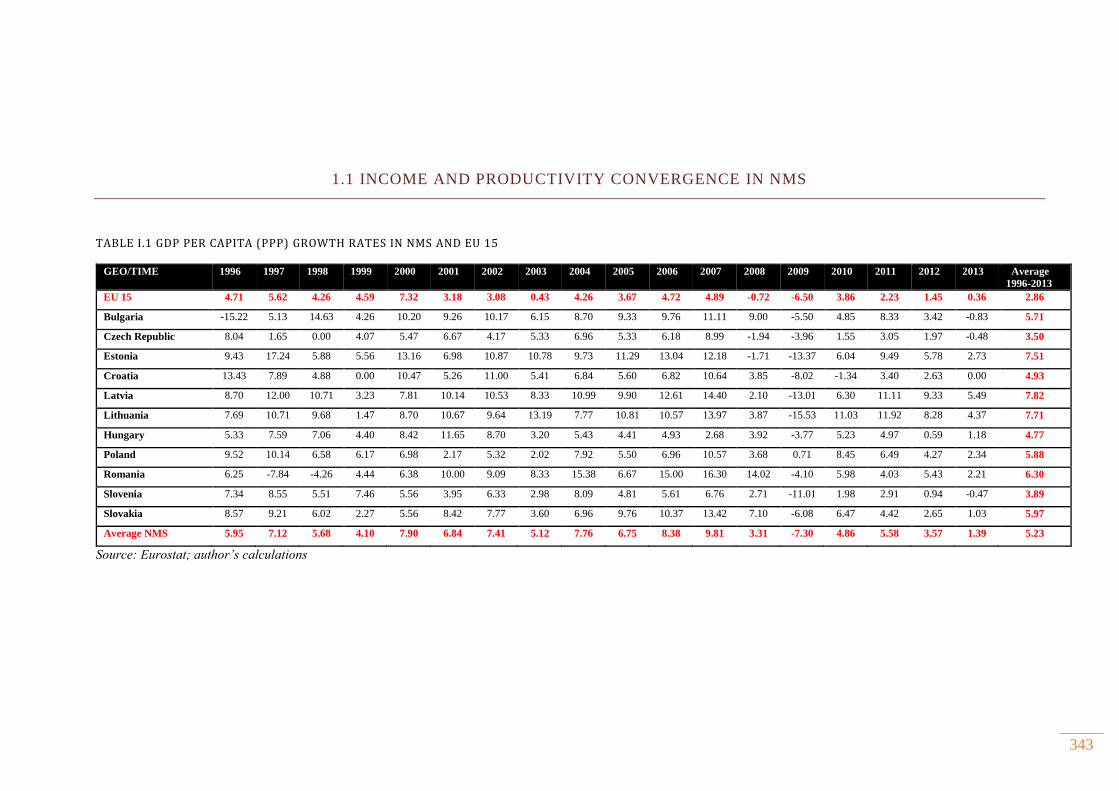
343
1.1 INCOME AND PRODUCTIVITY CONVERGENCE IN NMS
TABLE I.1 GDP PER CAPITA (PPP) GROWTH RATES IN NMS AND EU 15
GEO/TIME 1996 1997 1998 1999 2000 2001 2002 2003 2004 2005 2006 2007 2008 2009 2010 2011 2012 2013 Average
1996-2013
EU 15 4.71 5.62 4.26 4.59 7.32 3.18 3.08 0.43 4.26 3.67 4.72 4.89 -0.72 -6.50 3.86 2.23 1.45 0.36 2.86
Bulgaria -15.22 5.13 14.63 4.26 10.20 9.26 10.17 6.15 8.70 9.33 9.76 11.11 9.00 -5.50 4.85 8.33 3.42 -0.83 5.71
Czech Republic 8.04 1.65 0.00 4.07 5.47 6.67 4.17 5.33 6.96 5.33 6.18 8.99 -1.94 -3.96 1.55 3.05 1.97 -0.48 3.50
Estonia 9.43 17.24 5.88 5.56 13.16 6.98 10.87 10.78 9.73 11.29 13.04 12.18 -1.71 -13.37 6.04 9.49 5.78 2.73 7.51
Croatia 13.43 7.89 4.88 0.00 10.47 5.26 11.00 5.41 6.84 5.60 6.82 10.64 3.85 -8.02 -1.34 3.40 2.63 0.00 4.93
Latvia 8.70 12.00 10.71 3.23 7.81 10.14 10.53 8.33 10.99 9.90 12.61 14.40 2.10 -13.01 6.30 11.11 9.33 5.49 7.82
Lithuania 7.69 10.71 9.68 1.47 8.70 10.67 9.64 13.19 7.77 10.81 10.57 13.97 3.87 -15.53 11.03 11.92 8.28 4.37 7.71
Hungary 5.33 7.59 7.06 4.40 8.42 11.65 8.70 3.20 5.43 4.41 4.93 2.68 3.92 -3.77 5.23 4.97 0.59 1.18 4.77
Poland 9.52 10.14 6.58 6.17 6.98 2.17 5.32 2.02 7.92 5.50 6.96 10.57 3.68 0.71 8.45 6.49 4.27 2.34 5.88
Romania 6.25 -7.84 -4.26 4.44 6.38 10.00 9.09 8.33 15.38 6.67 15.00 16.30 14.02 -4.10 5.98 4.03 5.43 2.21 6.30
Slovenia 7.34 8.55 5.51 7.46 5.56 3.95 6.33 2.98 8.09 4.81 5.61 6.76 2.71 -11.01 1.98 2.91 0.94 -0.47 3.89
Slovakia 8.57 9.21 6.02 2.27 5.56 8.42 7.77 3.60 6.96 9.76 10.37 13.42 7.10 -6.08 6.47 4.42 2.65 1.03 5.97
Average NMS 5.95 7.12 5.68 4.10 7.90 6.84 7.41 5.12 7.76 6.75 8.38 9.81 3.31 -7.30 4.86 5.58 3.57 1.39 5.23
Source: Eurostat; author’s calculations
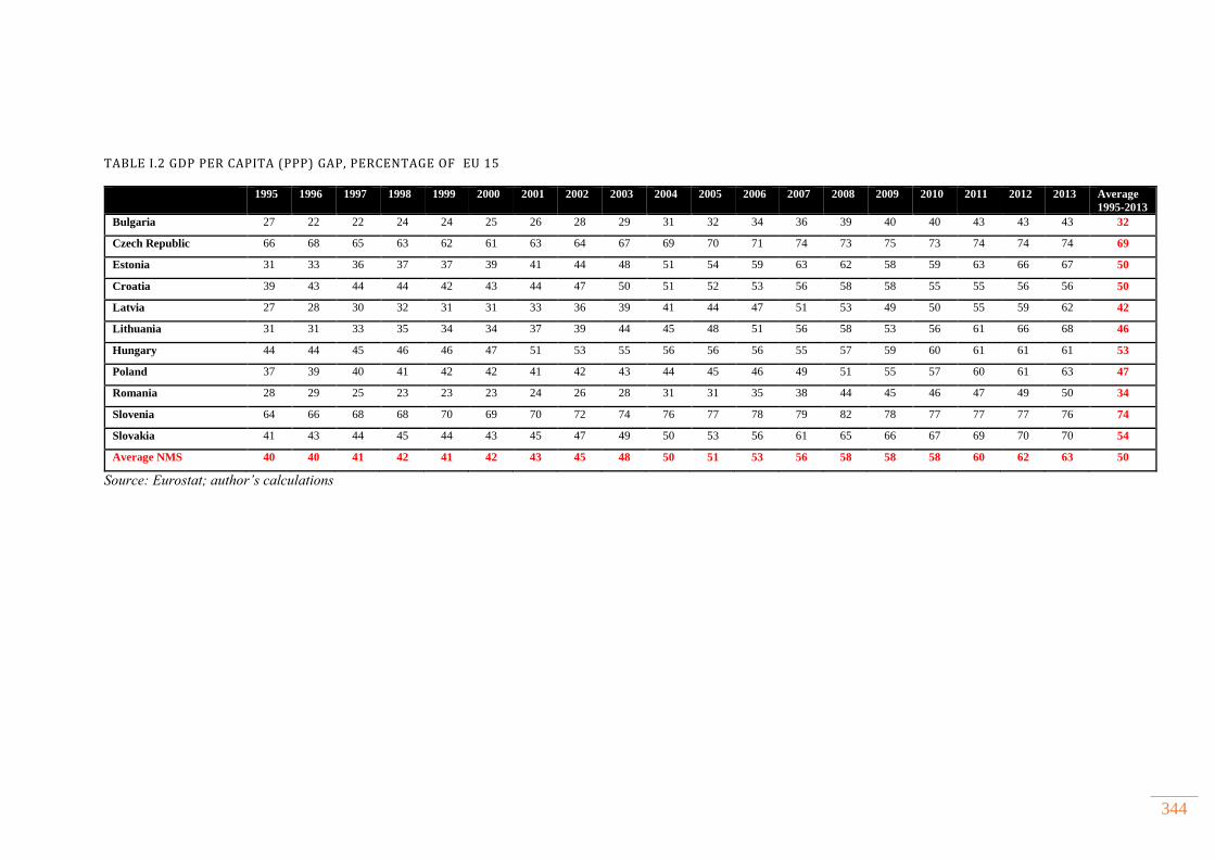
344
TABLE I.2 GDP PER CAPITA (PPP) GAP, PERCENTAGE OF EU 15
1995 1996 1997 1998 1999 2000 2001 2002 2003 2004 2005 2006 2007 2008 2009 2010 2011 2012 2013 Average
1995-2013
Bulgaria 27 22 22 24 24 25 26 28 29 31 32 34 36 39 40 40 43 43 43 32
Czech Republic 66 68 65 63 62 61 63 64 67 69 70 71 74 73 75 73 74 74 74 69
Estonia 31 33 36 37 37 39 41 44 48 51 54 59 63 62 58 59 63 66 67 50
Croatia 39 43 44 44 42 43 44 47 50 51 52 53 56 58 58 55 55 56 56 50
Latvia 27 28 30 32 31 31 33 36 39 41 44 47 51 53 49 50 55 59 62 42
Lithuania 31 31 33 35 34 34 37 39 44 45 48 51 56 58 53 56 61 66 68 46
Hungary 44 44 45 46 46 47 51 53 55 56 56 56 55 57 59 60 61 61 61 53
Poland 37 39 40 41 42 42 41 42 43 44 45 46 49 51 55 57 60 61 63 47
Romania 28 29 25 23 23 23 24 26 28 31 31 35 38 44 45 46 47 49 50 34
Slovenia 64 66 68 68 70 69 70 72 74 76 77 78 79 82 78 77 77 77 76 74
Slovakia 41 43 44 45 44 43 45 47 49 50 53 56 61 65 66 67 69 70 70 54
Average NMS 40 40 41 42 41 42 43 45 48 50 51 53 56 58 58 58 60 62 63 50
Source: Eurostat; author’s calculations
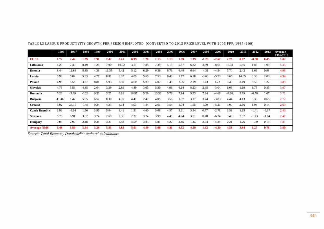
345
TABLE I.3 LABOUR PRODUCTIVITY GROWTH PER PERSON EMPLOYED (CONVERTED TO 2013 PRICE LEVEL WITH 2005 PPP, 1995=100)
1996 1997 1998 1999 2000 2001 2002 2003 2004 2005 2006 2007 2008 2009 2010 2011 2012 2013 Average
1996-2013
EU 15 1.72 2.42 1.39 1.91 2.42 0.41 0.99 1.20 2.13 1.13 1.69 1.39 -1.28 -2.62 2.25 0.87 -0.08 0.45 1.02
Lithuania 4.29 7.49 8.49 1.25 7.90 10.92 3.11 7.88 7.39 5.19 5.87 6.82 3.59 -8.61 15.31 5.55 1.85 1.99 5.35
Estonia 8.44 11.68 8.85 4.39 11.35 5.42 5.12 6.29 6.36 6.71 4.48 6.64 -4.31 -4.54 7.70 2.42 1.66 0.98 4.98
Latvia 5.99 5.04 5.93 4.77 8.81 6.07 4.09 5.60 7.53 8.40 5.77 6.18 -3.66 -5.23 3.65 14.65 3.36 2.03 4.94
Poland 4.98 5.58 3.77 8.81 5.93 3.50 4.60 5.09 4.07 1.43 2.95 2.19 1.23 1.22 3.40 3.49 5.56 1.22 3.83
Slovakia 4.76 5.53 4.85 2.64 3.39 2.89 4.49 3.65 5.30 4.96 6.14 8.23 2.45 -3.04 6.03 1.19 1.75 0.85 3.67
Romania 5.26 -5.89 -0.23 0.33 3.21 6.81 16.97 5.29 10.32 5.76 7.14 5.93 7.34 -4.69 -0.88 2.99 -0.58 1.67 3.71
Bulgaria -11.46 1.47 5.95 6.57 8.30 4.95 4.41 2.47 4.05 3.56 3.07 3.17 3.74 -3.83 4.44 4.13 3.36 0.65 2.72
Croatia 5.92 23.10 -7.43 0.34 4.33 3.14 4.03 1.44 2.61 3.54 1.04 1.55 1.00 -5.21 3.00 2.36 1.98 0.14 2.60
Czech Republic 3.99 -0.14 1.56 3.95 5.04 3.41 1.51 4.60 5.08 4.57 5.61 3.54 0.77 -2.78 3.53 1.85 -1.41 -0.37 2.46
Slovenia 5.76 6.91 3.62 3.74 2.69 2.36 2.22 3.24 3.99 4.49 4.24 3.51 0.78 -6.24 3.49 2.37 -1.73 -1.04 2.47
Hungary 0.08 2.97 2.48 0.38 3.21 3.88 4.59 3.85 5.81 4.27 3.45 -0.60 2.74 -4.39 0.21 1.26 -1.80 0.19 1.81
Average NMS 3.46 5.80 3.44 3.38 5.83 4.85 5.01 4.49 5.68 4.81 4.52 4.29 1.42 -4.30 4.53 3.84 1.27 0.76 3.50
Source: Total Economy Database™; authors’ calculations.
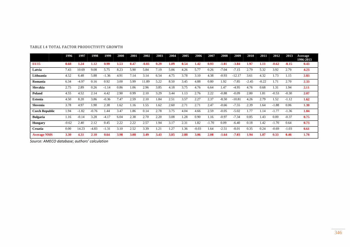
346
TABLE I.4 TOTAL FACTOR PRODUCTIVITY GROWTH
1996 1997 1998 1999 2000 2001 2002 2003 2004 2005 2006 2007 2008 2009 2010 2011 2012 2013 Average
1996-2013
EU15 0.68 1.24 1.12 0.99 1.53 0.47 -0.03 0.29 1.09 0.54 1.42 0.93 -1.01 -3.84 1.97 1.11 -0.62 -0.15 0.43
Latvia 7.43 10.69 9.08 5.75 8.23 5.90 5.84 7.19 5.06 4.26 5.77 0.26 -7.04 -7.15 2.79 5.32 3.92 2.79 4.23
Lithuania 4.52 6.48 5.88 -1.36 4.91 7.14 3.14 6.54 4.75 3.78 3.10 4.38 -0.93 -12.17 3.61 4.32 1.73 1.15 2.83
Romania 6.34 -4.97 0.16 0.92 3.00 5.99 11.89 5.22 8.50 3.45 4.88 0.80 1.92 -7.85 -2.45 -0.22 1.71 2.70 2.33
Slovakia 2.75 2.89 0.26 -1.14 0.86 1.06 2.96 3.85 4.18 3.75 4.76 6.64 1.47 -4.95 4.76 0.68 1.31 1.94 2.11
Poland 4.55 4.52 2.14 4.42 2.90 0.99 2.10 3.29 3.44 1.13 2.76 2.22 -0.88 -0.09 2.80 1.81 -0.53 -0.30 2.07
Estonia 4.50 8.20 3.86 -0.36 7.47 2.59 2.10 1.84 2.51 3.57 2.27 2.37 -8.50 -10.81 4.26 2.79 1.52 -1.12 1.62
Slovenia 3.78 4.97 1.90 2.38 1.62 1.16 1.55 1.62 2.60 2.71 2.71 2.47 -0.66 -7.55 2.39 1.64 -1.88 0.06 1.30
Czech Republic 1.94 -1.82 -0.76 1.44 3.47 1.86 0.14 2.78 3.75 4.04 4.66 2.59 -0.05 -5.02 1.77 1.14 -1.77 -1.36 1.04
Bulgaria 1.16 -0.14 3.28 -4.17 6.04 2.38 2.70 2.20 3.08 1.28 0.90 1.16 -0.97 -7.34 0.85 1.43 0.00 -0.37 0.75
Hungary -0.62 2.40 2.12 0.45 2.22 2.22 2.57 1.94 3.17 2.31 1.82 -1.70 0.09 -6.40 0.18 1.42 -1.70 0.64 0.73
Croatia 0.00 14.23 -4.83 -1.31 3.10 2.52 3.39 1.21 1.27 1.36 -0.03 1.64 -2.51 -8.01 0.35 0.24 -0.69 -1.03 0.61
Average NMS 3.30 4.31 2.10 0.64 3.98 3.08 3.49 3.43 3.85 2.88 3.06 2.08 -1.64 -7.03 1.94 1.87 0.33 0.46 1.78
Source: AMECO database; authors’ calculation
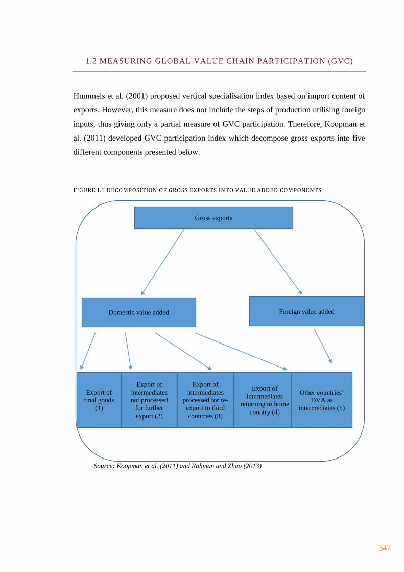
347
1.2 MEASURING GLOBAL VALUE CHAIN PARTICIPATION (GVC)
Hummels et al. (2001) proposed vertical specialisation index based on import content of
exports. However, this measure does not include the steps of production utilising foreign
inputs, thus giving only a partial measure of GVC participation. Therefore, Koopman et
al. (2011) developed GVC participation index which decompose gross exports into five
different components presented below.
FIGURE I.1 DECOMPOSITION OF GROSS EXPORTS INTO VALUE ADDED COMPONENTS
Source: Koopman et al. (2011) and Rahman and Zhao (2013)
Gross exports
Domestic value added Foreign value added
Export of
final goods
(1)
Export of
intermediates
not processed
for further
export (2)
Export of
intermediates
processed for re-
export to third
countries (3)
Export of
intermediates
returning to home
country (4)
Other countries’
DVA as
intermediates (5)
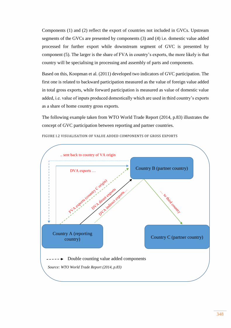
348
Components (1) and (2) reflect the export of countries not included in GVCs. Upstream
segments of the GVCs are presented by components (3) and (4) i.e. domestic value added
processed for further export while downstream segment of GVC is presented by
component (5). The larger is the share of FVA in country’s exports, the more likely is that
country will be specialising in processing and assembly of parts and components.
Based on this, Koopman et al. (2011) developed two indicators of GVC participation. The
first one is related to backward participation measured as the value of foreign value added
in total gross exports, while forward participation is measured as value of domestic value
added, i.e. value of inputs produced domestically which are used in third country’s exports
as a share of home country gross exports.
The following example taken from WTO World Trade Report (2014, p.83) illustrates the
concept of GVC participation between reporting and partner countries.
FIGURE I.2 VISUALISATION OF VALUE ADDED COMPONENTS OF GROSS EXPORTS
Double counting value added components
Source: WTO World Trade Report (2014, p.83)
Country B (partner country)
Country A (reporting
country) Country C (partner country)
DVA exports …
.. sent back to country of VA origin
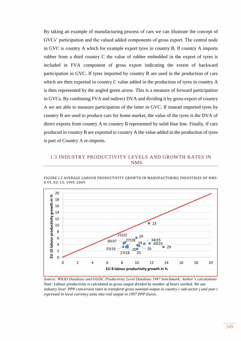
349
By taking an example of manufacturing process of cars we can illustrate the concept of
GVCs’ participation and the valued added components of gross export. The central node
in GVC is country A which for example export tyres in country B. If country A imports
rubber from a third country C the value of rubber embedded in the export of tyres is
included in FVA component of gross export indicating the extent of backward
participation in GVC. If tyres imported by country B are used in the production of cars
which are then exported in country C value added in the production of tyres in country A
is then represented by the angled green arrow. This is a measure of forward participation
in GVCs. By combining FVA and indirect DVA and dividing it by gross export of country
A we are able to measure participation of the latter in GVC. If instead imported tyres by
country B are used to produce cars for home market, the value of the tyres is the DVA of
direct exports from country A to country B represented by solid blue line. Finally, if cars
produced in country B are exported to country A the value added in the production of tyres
is part of Country A re-imports.
1.3 INDUSTRY PRODUCTIVITY LEVELS AND GROWTH RATES IN
NMS
FIGURE I.3 AVERAGE LABOUR PRODUCTIVITY GROWTH IN MANUFACTURING INDUSTRIES OF NMS-8 VS. EU-15, 1995-2009
Source: WIOD Database and GGDC Productivity Level Database 1997 benchmark; Author’s calculations
Note: Labour productivity is calculated as gross output divided by number of hours worked. We use
industry level PPP conversion rates to transform gross nominal output in country c sub-sector j and year t
expressed in local currency units into real output in 1997 PPP Euros.
15t1617t18
19
20
21t22
23
24
2526
27t28
2930t33
34t3536t37
0
2
4
6
8
10
12
14
16
18
20
0 2 4 6 8 10 12 14 16 18 20
EU 1
5 la
bo
ur
pro
du
ctiv
ity
gro
wth
in %
EU 8 labour productivity growth in %
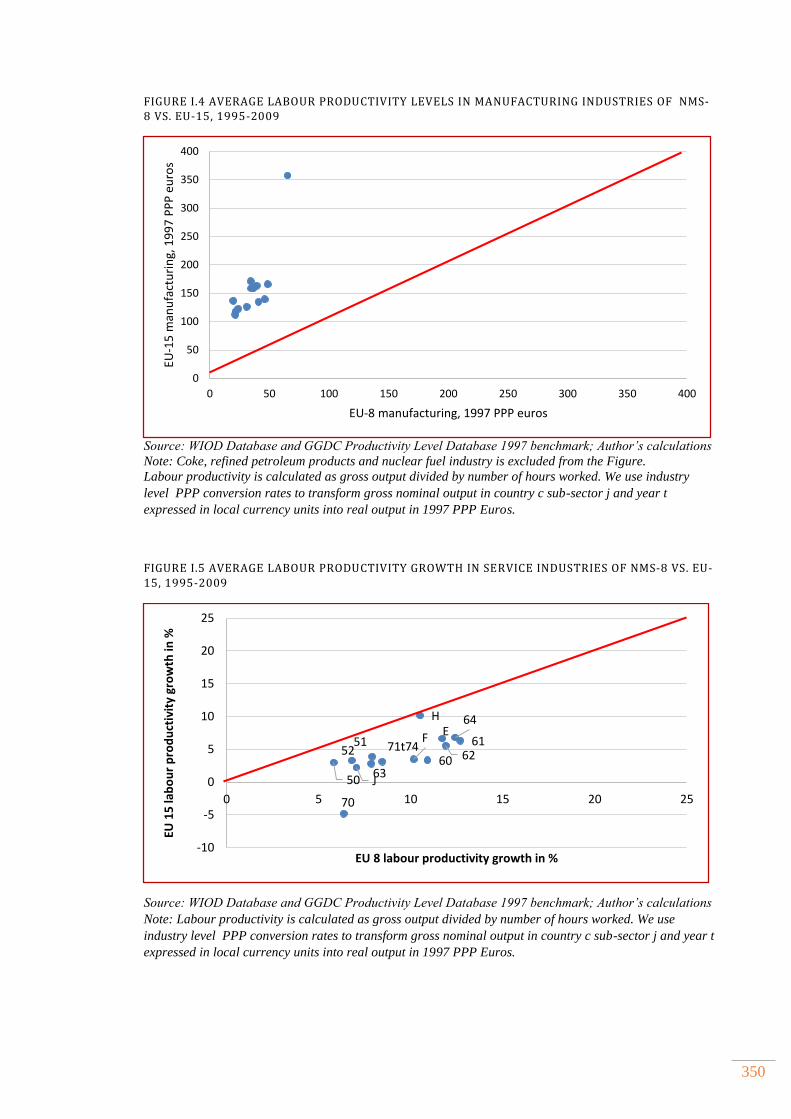
350
FIGURE I.4 AVERAGE LABOUR PRODUCTIVITY LEVELS IN MANUFACTURING INDUSTRIES OF NMS-8 VS. EU-15, 1995-2009
Source: WIOD Database and GGDC Productivity Level Database 1997 benchmark; Author’s calculations
Note: Coke, refined petroleum products and nuclear fuel industry is excluded from the Figure.
Labour productivity is calculated as gross output divided by number of hours worked. We use industry
level PPP conversion rates to transform gross nominal output in country c sub-sector j and year t
expressed in local currency units into real output in 1997 PPP Euros.
FIGURE I.5 AVERAGE LABOUR PRODUCTIVITY GROWTH IN SERVICE INDUSTRIES OF NMS-8 VS. EU-15, 1995-2009
Source: WIOD Database and GGDC Productivity Level Database 1997 benchmark; Author’s calculations
Note: Labour productivity is calculated as gross output divided by number of hours worked. We use
industry level PPP conversion rates to transform gross nominal output in country c sub-sector j and year t
expressed in local currency units into real output in 1997 PPP Euros.
0
50
100
150
200
250
300
350
400
0 50 100 150 200 250 300 350 400
EU-1
5 m
anu
fact
uri
ng,
19
97
PP
P e
uro
s
EU-8 manufacturing, 1997 PPP euros
50
5152
60
6162
63
64
70
71t74EF
J
H
-10
-5
0
5
10
15
20
25
0 5 10 15 20 25
EU 1
5 la
bo
ur
pro
du
ctiv
ity
gro
wth
in %
EU 8 labour productivity growth in %
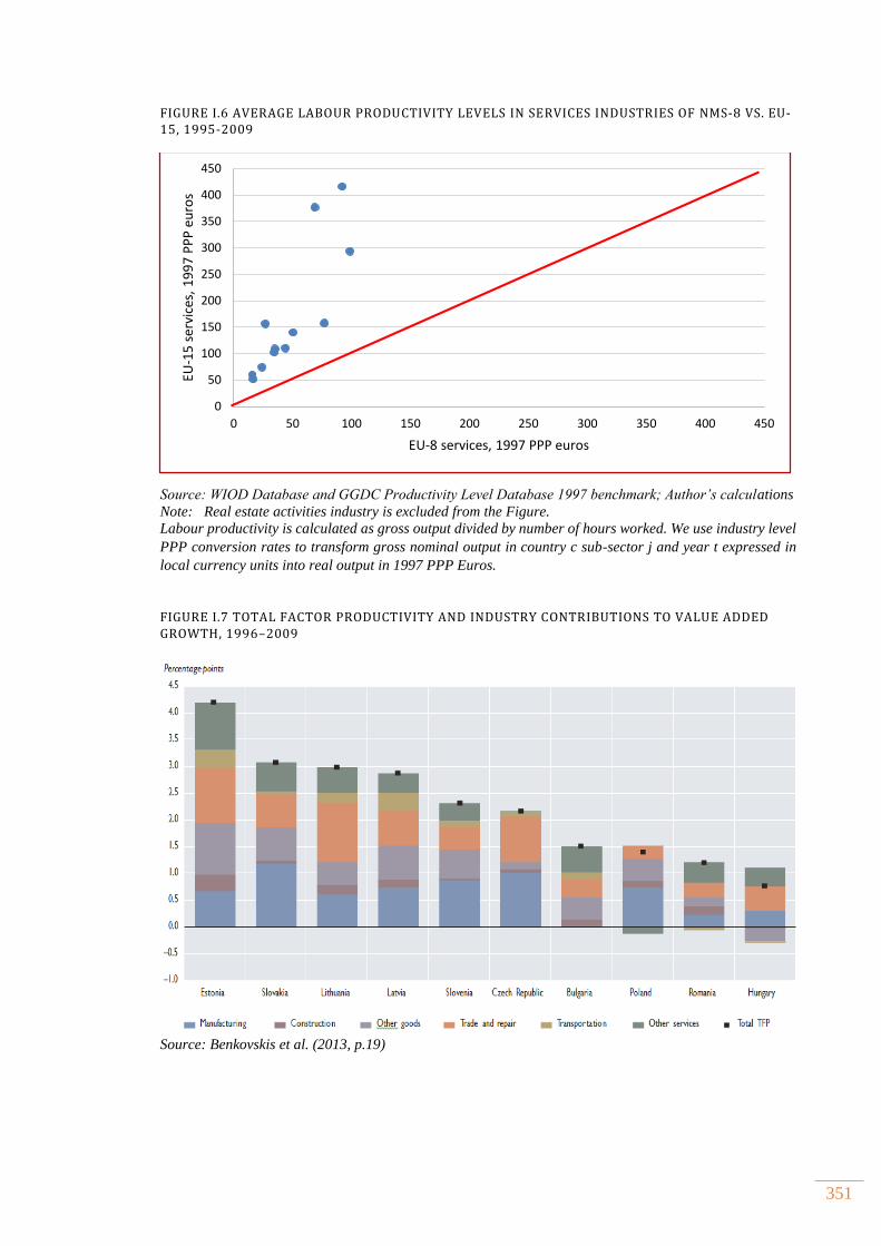
351
FIGURE I.6 AVERAGE LABOUR PRODUCTIVITY LEVELS IN SERVICES INDUSTRIES OF NMS-8 VS. EU-15, 1995-2009
Source: WIOD Database and GGDC Productivity Level Database 1997 benchmark; Author’s calculations
Note: Real estate activities industry is excluded from the Figure.
Labour productivity is calculated as gross output divided by number of hours worked. We use industry level
PPP conversion rates to transform gross nominal output in country c sub-sector j and year t expressed in
local currency units into real output in 1997 PPP Euros.
FIGURE I.7 TOTAL FACTOR PRODUCTIVITY AND INDUSTRY CONTRIBUTIONS TO VALUE ADDED GROWTH, 1996–2009
Source: Benkovskis et al. (2013, p.19)
0
50
100
150
200
250
300
350
400
450
0 50 100 150 200 250 300 350 400 450
EU-1
5 s
ervi
ces,
19
97
PP
P e
uro
s
EU-8 services, 1997 PPP euros

352
APPENDIX II. SUPPLEMENT TO CHAPTER FOUR
2.1 Cleaning procedure ............................................................................................................................ 353
2.2 Foreign ownership calculations ................................................................................................... 354
2.3 Sample description ............................................................................................................................ 357
2.4 Output of Cobb-Douglas value added production function per industry and country ........................................................................................................................................................................... 362
2.5 Robustness checks of TFP estimates .......................................................................................... 368
2.6 Non parametric Kolmogorov Smirnov test of foreign ownership premium.............. 374

353
2.1 CLEANING PROCEDURE
A unique firm level dataset was constructed using Amadeus database published by Bureau
van Dijk. This comprehensive database covers around 19.514.770 companies in Europe,
both public and private 67F
71. In this thesis the focus is on a subset of firms from five countries
in Central Europe for which financial information is available in the period 2002-2010. In
November 2011 update, Amadeus included 454.738 firms from the Czech Republic,
107.052 firms from Estonia, 377.414 firms from Hungary, 234.761 firms from Slovakia
and 62.254 firms from Slovenia resulting in 11,125,971 firm level observations.
In conducting econometric estimation, we did not apply firm’s size threshold as Eapen
(2013) suggests that in incomplete datasets such as Amadeus the effects of FDI
productivity spillovers may be overestimated due to selection effects if one exclude small
firms from the sample. Since we are interested in estimating TFP for manufacturing and
services firms, our cleaning procedure starts with eliminating certain industries from the
sample or firms for which industry code is not provided. These are Agriculture, forestry
and fishing (NACE 1.1 codes 01-03), Mining and quarrying (NACE 1.1 codes 05-09),
Public administration and defence, compulsory social security (NACE 1.1 code 84),
Education (NACE 1.1 code 85), Human health services (NACE 1.1 code 86), Residential
care and social work activities (NACE 1.1 codes 87-88), Arts, entertainment and recreation
(NACE 1.1 codes 90-93), Other services (NACE 1.1 codes 94-96).
For the construction of TFP sample we need information on firms’ sales, tangible fixed
assets, number of employees and expenditure on materials. Firms with missing
observations on either of the variables of interest are dropped from the sample.
Furthermore, firms reporting zero or negative sales, value added, total assets, total fixed
assets, tangible fixed assets, number of employees, expenditure of materials and cost of
employees from the balance sheet are deleted. We have also eliminated observations for
which accounting rules are violated such as situations where total and individual
components of fixed assets are larger than total assets or when the date of incorporation
appears after the year in which firms have reported their financial information.
71 The database was accessed in November 2011.
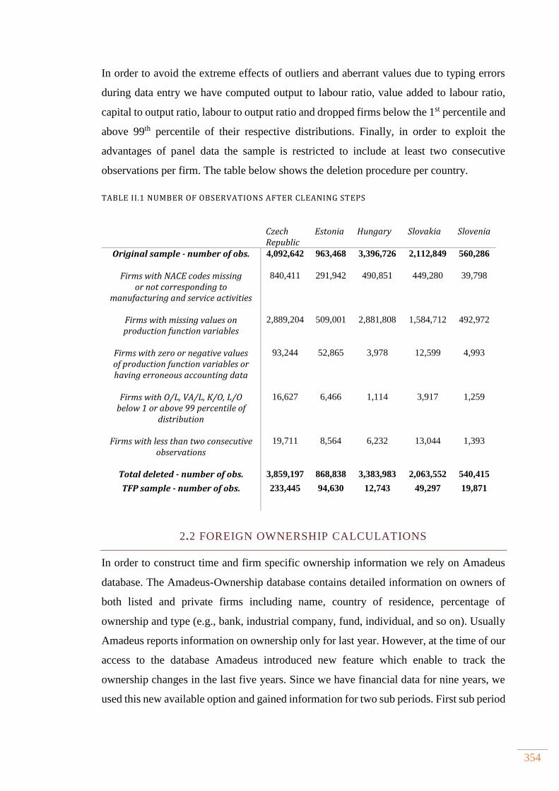
354
In order to avoid the extreme effects of outliers and aberrant values due to typing errors
during data entry we have computed output to labour ratio, value added to labour ratio,
capital to output ratio, labour to output ratio and dropped firms below the 1st percentile and
above 99th percentile of their respective distributions. Finally, in order to exploit the
advantages of panel data the sample is restricted to include at least two consecutive
observations per firm. The table below shows the deletion procedure per country.
TABLE II.1 NUMBER OF OBSERVATIONS AFTER CLEANING STEPS
2.2 FOREIGN OWNERSHIP CALCULATIONS
In order to construct time and firm specific ownership information we rely on Amadeus
database. The Amadeus-Ownership database contains detailed information on owners of
both listed and private firms including name, country of residence, percentage of
ownership and type (e.g., bank, industrial company, fund, individual, and so on). Usually
Amadeus reports information on ownership only for last year. However, at the time of our
access to the database Amadeus introduced new feature which enable to track the
ownership changes in the last five years. Since we have financial data for nine years, we
used this new available option and gained information for two sub periods. First sub period
Czech Republic
Estonia Hungary Slovakia Slovenia
Original sample - number of obs.
4,092,642 963,468 3,396,726 2,112,849 560,286
Firms with NACE codes missing or not corresponding to
manufacturing and service activities
840,411 291,942 490,851 449,280 39,798
Firms with missing values on production function variables
2,889,204 509,001 2,881,808 1,584,712 492,972
Firms with zero or negative values of production function variables or having erroneous accounting data
93,244 52,865 3,978 12,599 4,993
Firms with O/L, VA/L, K/O, L/O below 1 or above 99 percentile of
distribution
16,627 6,466 1,114 3,917 1,259
Firms with less than two consecutive observations
19,711 8,564 6,232 13,044 1,393
Total deleted - number of obs. 3,859,197 868,838 3,383,983 2,063,552 540,415
TFP sample - number of obs. 233,445 94,630 12,743 49,297 19,871

355
covers the period 2002-2006 and the second sub period covers the period 2007-2011.68F
72
Both files were merged using BvD ID number, country ISO code and Shareholder BvD
ID number to obtain the ownership changes over the analysed period.
Amadeus ownership database provide several indicators divided in three dimensions:
1. Independence indicator – measure of independence of firm with regard to its
shareholders
2. Ultimate owner – an entity which is the ultimate owner of the company obtained by
analysing shareholder’s structures of companies which according to independent indicator
are classified as independent. The company to be independent it must have an indicator of
A+, A or A- indicating that no other entity has more than 25% of shares.
3. Shareholders – provides a list of all the shareholders in the company and their
corresponding shares in company’s capital, both total and direct ownership.
In our analysis of identifying foreign owner we rely on direct ownership for several
reasons. Ultimate owner category is calculated by finding at least one owner that has more
than 25% of controlling interest in the company. The figure below is taken from Amadeus
manual and shows how ultimate owner is calculated. The ownership path of minimum
25% is followed from Company 1 to Company 3 and from Company 3 to Company 5.
Company 5 is independent and said to be the UO of Company 1. Company 5 is also the
UO of Company 3.
The problem with identifying ultimate owner is also admitted by BvD saying“even if the
scope of the BvD ownership database is very wide, BvD cannot absolutely assert that all
the existing links are recorded in the database. More importantly, because certain
ownership structures can be very complex, trying to evaluate a controlling ultimate owner
could be misleading” (Bureau van Dijk, 2010). Moreover, since we are interested in
continuous ownership over time calculated total percentage of ultimate owner cannot be
72 Ownership information was accessed in September 2012.
356
related to any specific date as it relies on information valid at different dates. Finally, as
we follow international definition of foreign ownership which states that foreign owner is
the firm which owns at least 10% of other firms’ capital, the definition of ultimate owner
clearly does not correspond to it.
Amadeus ownership database records the ownership link indicating that company A owns
a certain share of company B as direct ownership even if the percentage of foreign
ownership is 1% except for listed firms where usually the small stock holders are
unknown. Sometimes, direct ownership link does not contain actual number but indicates
if the company is WO (“wholly owned”), MO (“majority owned”), JO (“jointly owned”),
NQ (“negligible”) and CQP1 (“50% + 1 share). In this cases we have recoded these values
to 100% if WO, 51% if MO, 50% if JO and 50% if CQP1.
In order to identify foreign owner, we have relied on a variable containing the country
codes and in cases where country code is different than home country of firm, firm is
identified as foreign if it owns more than 10%. If the country code is missing, firms are
classified as domestic. The latter is especially problematic if shareholder is a private
individual as in these cases country code is almost always missing. Furthermore, as argued
by Lesher and Mirodout (2008) even if the shareholder is from foreign country they are
less likely to have an active role in the management and therefore are less relevant for
estimation of productivity spillovers which is the main research question of this thesis.
After identifying foreign owners, foreign ownership variable is calculated by summing all
the percentages owned by foreigners. For a firm i, FOit is the sum of all percentages of
direct ownership by foreigners in year t. For example, if a Company A has three foreign
owners, Italian investor with stakes of 10 percent, French investor owning 20 percent, and
German investor owning 30 percent, FO for this company is 60 percent. If foreign owner
is identified, but ownership share is missing it is set to zero. If foreign ownership share is
missing for all years up to year t, it is assumed as it was domestic. For missing observations
between years, missing values are replaced with non-missing observations from time t-1
and previous periods. The assumption behind this procedure as it like there was no
ownership change.
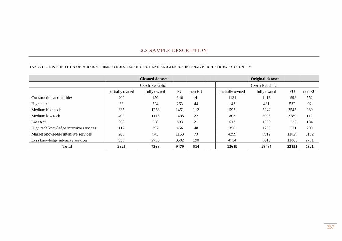
357
2.3 SAMPLE DESCRIPTION
TABLE II.2 DISTRIBUTION OF FOREIGN FIRMS ACROSS TECHNOLOGY AND KNOWLEDGE INTENSIVE INDUSTRIES BY COUNTRY
Cleaned dataset Original dataset
Czech Republic Czech Republic
partially owned fully owned EU non EU partially owned fully owned EU non EU
Construction and utilities 200 150 346 4 1131 1419 1998 552
High tech 83 224 263 44 143 481 532 92
Medium high tech 335 1228 1451 112 592 2242 2545 289
Medium low tech 402 1115 1495 22 803 2098 2789 112
Low tech 266 558 803 21 617 1289 1722 184
High tech knowledge intensive services 117 397 466 48 350 1230 1371 209
Market knowledge intensive services 283 943 1153 73 4299 9912 11029 3182
Less knowledge intensive services 939 2753 3502 190 4754 9813 11866 2701
Total 2625 7368 9479 514 12689 28484 33852 7321
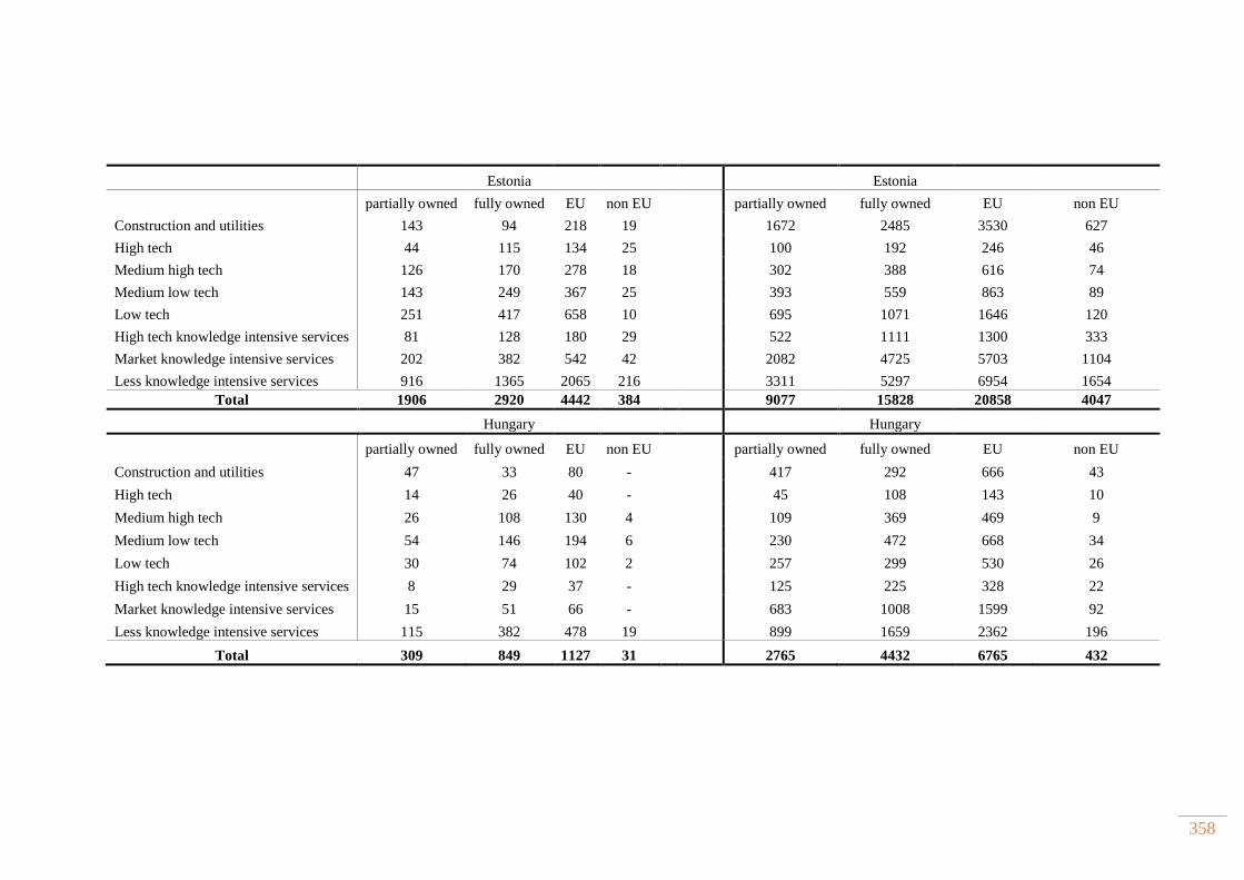
358
Estonia Estonia
partially owned fully owned EU non EU partially owned fully owned EU non EU
Construction and utilities 143 94 218 19 1672 2485 3530 627
High tech 44 115 134 25 100 192 246 46
Medium high tech 126 170 278 18 302 388 616 74
Medium low tech 143 249 367 25 393 559 863 89
Low tech 251 417 658 10 695 1071 1646 120
High tech knowledge intensive services 81 128 180 29 522 1111 1300 333
Market knowledge intensive services 202 382 542 42 2082 4725 5703 1104
Less knowledge intensive services 916 1365 2065 216 3311 5297 6954 1654
Total 1906 2920 4442 384 9077 15828 20858 4047
Hungary Hungary
partially owned fully owned EU non EU partially owned fully owned EU non EU
Construction and utilities 47 33 80 - 417 292 666 43
High tech 14 26 40 - 45 108 143 10
Medium high tech 26 108 130 4 109 369 469 9
Medium low tech 54 146 194 6 230 472 668 34
Low tech 30 74 102 2 257 299 530 26
High tech knowledge intensive services 8 29 37 - 125 225 328 22
Market knowledge intensive services 15 51 66 - 683 1008 1599 92
Less knowledge intensive services 115 382 478 19 899 1659 2362 196
Total 309 849 1127 31 2765 4432 6765 432
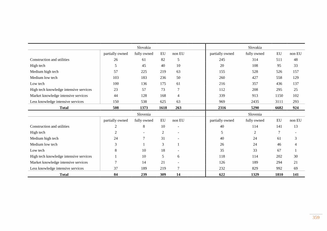
359
Slovakia Slovakia
partially owned fully owned EU non EU partially owned fully owned EU non EU
Construction and utilities 26 61 82 5 245 314 511 48
High tech 5 45 40 10 20 108 95 33
Medium high tech 57 225 219 63 155 528 526 157
Medium low tech 103 183 236 50 260 427 558 129
Low tech 100 136 175 61 216 357 436 137
High tech knowledge intensive services 23 57 73 7 112 208 295 25
Market knowledge intensive services 44 128 168 4 339 913 1150 102
Less knowledge intensive services 150 538 625 63 969 2435 3111 293
Total 508 1373 1618 263 2316 5290 6682 924
Slovenia Slovenia
partially owned fully owned EU non EU partially owned fully owned EU non EU
Construction and utilities 2 8 10 - 40 114 141 13
High tech 2 - 2 - 5 2 7 -
Medium high tech 24 7 31 - 40 24 61 3
Medium low tech 3 1 3 1 26 24 46 4
Low tech 8 10 18 - 35 33 67 1
High tech knowledge intensive services 1 10 5 6 118 114 202 30
Market knowledge intensive services 7 14 21 - 126 189 294 21
Less knowledge intensive services 37 189 219 7 232 829 992 69
Total 84 239 309 14 622 1329 1810 141
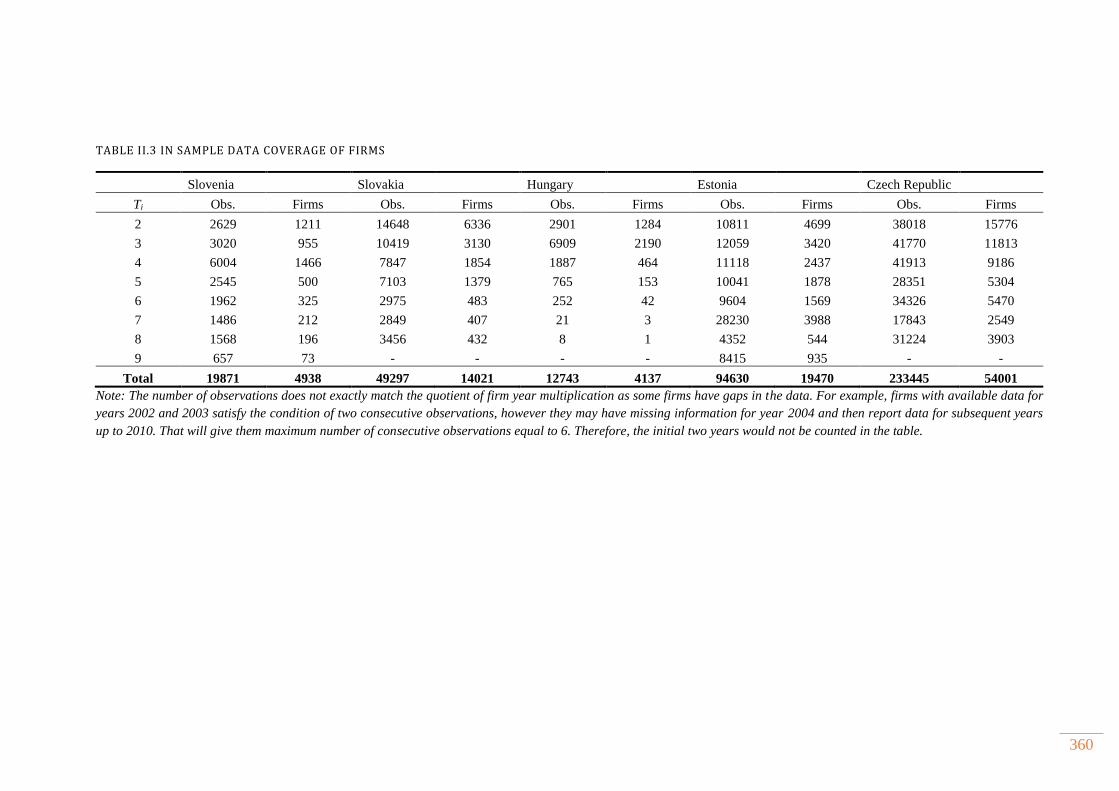
360
TABLE II.3 IN SAMPLE DATA COVERAGE OF FIRMS
Slovenia Slovakia Hungary Estonia Czech Republic
Ti Obs. Firms Obs. Firms Obs. Firms Obs. Firms Obs. Firms
2 2629 1211 14648 6336 2901 1284 10811 4699 38018 15776
3 3020 955 10419 3130 6909 2190 12059 3420 41770 11813
4 6004 1466 7847 1854 1887 464 11118 2437 41913 9186
5 2545 500 7103 1379 765 153 10041 1878 28351 5304
6 1962 325 2975 483 252 42 9604 1569 34326 5470
7 1486 212 2849 407 21 3 28230 3988 17843 2549
8 1568 196 3456 432 8 1 4352 544 31224 3903
9 657 73 - - - - 8415 935 - -
Total 19871 4938 49297 14021 12743 4137 94630 19470 233445 54001
Note: The number of observations does not exactly match the quotient of firm year multiplication as some firms have gaps in the data. For example, firms with available data for
years 2002 and 2003 satisfy the condition of two consecutive observations, however they may have missing information for year 2004 and then report data for subsequent years
up to 2010. That will give them maximum number of consecutive observations equal to 6. Therefore, the initial two years would not be counted in the table.
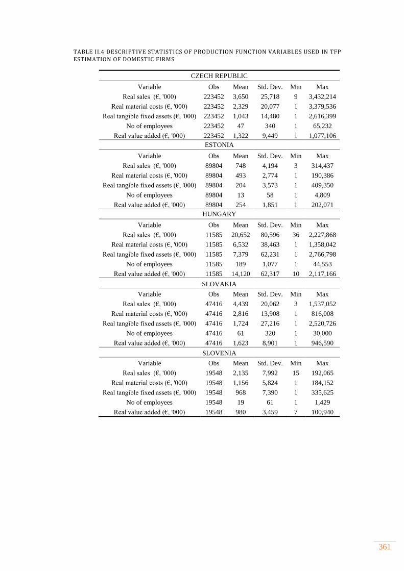
361
TABLE II.4 DESCRIPTIVE STATISTICS OF PRODUCTION FUNCTION VARIABLES USED IN TFP ESTIMATION OF DOMESTIC FIRMS
CZECH REPUBLIC
Variable Obs Mean Std. Dev. Min Max
Real sales (€, '000) 223452 3,650 25,718 9 3,432,214
Real material costs (€, '000) 223452 2,329 20,077 1 3,379,536
Real tangible fixed assets (€, '000) 223452 1,043 14,480 1 2,616,399
No of employees 223452 47 340 1 65,232
Real value added (€, '000) 223452 1,322 9,449 1 1,077,106
ESTONIA
Variable Obs Mean Std. Dev. Min Max
Real sales (€, '000) 89804 748 4,194 3 314,437
Real material costs (€, '000) 89804 493 2,774 1 190,386
Real tangible fixed assets (€, '000) 89804 204 3,573 1 409,350
No of employees 89804 13 58 1 4,809
Real value added (€, '000) 89804 254 1,851 1 202,071
HUNGARY
Variable Obs Mean Std. Dev. Min Max
Real sales (€, '000) 11585 20,652 80,596 36 2,227,868
Real material costs (€, '000) 11585 6,532 38,463 1 1,358,042
Real tangible fixed assets (€, '000) 11585 7,379 62,231 1 2,766,798
No of employees 11585 189 1,077 1 44,553
Real value added (€, '000) 11585 14,120 62,317 10 2,117,166
SLOVAKIA
Variable Obs Mean Std. Dev. Min Max
Real sales (€, '000) 47416 4,439 20,062 3 1,537,052
Real material costs (€, '000) 47416 2,816 13,908 1 816,008
Real tangible fixed assets (€, '000) 47416 1,724 27,216 1 2,520,726
No of employees 47416 61 320 1 30,000
Real value added (€, '000) 47416 1,623 8,901 1 946,590
SLOVENIA
Variable Obs Mean Std. Dev. Min Max
Real sales (€, '000) 19548 2,135 7,992 15 192,065
Real material costs (€, '000) 19548 1,156 5,824 1 184,152
Real tangible fixed assets (€, '000) 19548 968 7,390 1 335,625
No of employees 19548 19 61 1 1,429
Real value added (€, '000) 19548 980 3,459 7 100,940
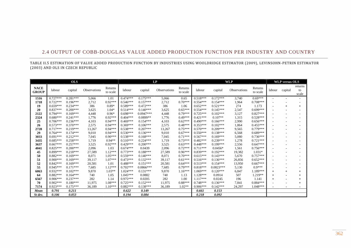
362
2.4 OUTPUT OF COBB-DOUGLAS VALUE ADDED PRODUCTION FUNCTION PER INDUSTRY AND COUNTRY
TABLE II.5 ESTIMATION OF VALUE ADDED PRODUCTION FUNCTION BY INDUSTRIES USING WOOLDRIDGE ESTIMATOR (2009), LEVINSOHN-PETRIN ESTIMATOR (2003) AND OLS IN CZECH REPUBLIC
OLS LP WLP WLP versus OLS
NACE
GROUP labour capital Observations
Returns
to scale labour capital Observations
Returns
to scale labour capital Observations
Returns
to scale labour capital
returns
to scale
1516 0.727*** 0.281*** 5,066 1.01 0.474*** 0.175*** 5,066 0.65 0.518*** 0.172*** 3,740 0.69*** - - -
1718 0.722*** 0.196*** 2,712 0.92*** 0.546*** 0.157*** 2,712 0.70*** 0.554*** 0.154*** 1,964 0.708*** - - -
19 0.659*** 0.234*** 386 0.89* 0.589*** 0.472*** 386 1.06 0.652*** 0.521*** 274 1.173 - + +
20 0.837*** 0.200*** 3,625 1.04* 0.514*** 0.140*** 3,625 0.65*** 0.554*** 0.145*** 2,547 0.699*** - - -
2122 0.794*** 0.169*** 4,448 0.96* 0.698*** 0.0947*** 4,448 0.79*** 0.725*** 0.102*** 3,127 0.827*** - - -
2324 0.680*** 0.241*** 1,776 0.92*** 0.404*** 0.0899** 1,776 0.49*** 0.421*** 0.107** 1,315 0.528*** - - -
25 0.706*** 0.236*** 4,103 0.94*** 0.469*** 0.154*** 4,103 0.62*** 0.490*** 0.166*** 2,990 0.656*** - - -
26 0.573*** 0.370*** 2,575 0.94*** 0.369*** 0.106*** 2,575 0.48*** 0.353*** 0.102*** 1,864 0.455*** - - -
2728 0.717*** 0.219*** 13,267 0.94*** 0.538*** 0.207*** 13,267 0.75*** 0.570*** 0.209*** 9,565 0.779*** - - -
29 0.764*** 0.174*** 9,010 0.94*** 0.530*** 0.136*** 9,010 0.67*** 0.550*** 0.138*** 6,568 0.689*** - - -
3033 0.691*** 0.212*** 7,045 0.90*** 0.538*** 0.168*** 7,045 0.71*** 0.567*** 0.169*** 5,080 0.736*** - - -
3435 0.685*** 0.258*** 1,719 0.94** 0.510*** 0.224*** 1,719 0.73*** 0.482*** 0.239*** 1,278 0.721*** - - -
3637 0.667*** 0.257*** 3,525 0.92*** 0.429*** 0.200*** 3,525 0.63*** 0.448*** 0.199*** 2,556 0.647*** - - -
4041 0.825*** 0.200*** 2,096 1.03 0.674*** 0.0439 2,096 0.72*** 0.711*** 0.0456* 1,561 0.756*** - - -
45 0.899*** 0.218*** 27,589 1.12*** 0.773*** 0.188*** 27,589 0.96*** 0.839*** 0.192*** 19,382 1.031* - - -
50 0.882*** 0.169*** 8,071 1.05*** 0.559*** 0.140*** 8,071 0.70*** 0.615*** 0.143*** 5,670 0.757*** - - -
51 0.900*** 0.169*** 39,117 1.07*** 0.473*** 0.132*** 39,117 0.61*** 0.516*** 0.136*** 26,856 0.652*** - - -
52 0.842*** 0.169*** 20,581 1.01 0.488*** 0.151*** 20,581 0.64*** 0.513*** 0.154*** 13,950 0.667*** - - -
55 0.945*** 0.171*** 7,685 1.12*** 0.702*** 0.0866*** 7,685 0.79*** 0.818*** 0.0823*** 5,130 0.9*** - - -
6063 0.932*** 0.102*** 9,870 1.03** 1.024*** 0.131*** 9,870 1.16*** 1.069*** 0.120*** 6,847 1.189*** + + +
64 0.882*** 0.164*** 740 1.05 1.045*** 0.0882 740 1.13 1.128*** 0.0914 507 1.219** + - +
6567 0.906*** 0.237*** 282 1.14 0.975*** 0.0205 282 1.00 1.117*** 0.0245 196 1.141 + - +
70 0.902*** 0.180*** 11,975 1.08*** 0.725*** 0.152*** 11,975 0.88*** 0.748*** 0.136*** 7,841 0.884*** - - +
7174 0.923*** 0.175*** 36,189 1.10*** 0.882*** 0.138*** 36,189 1.02** 0.906*** 0.142*** 24,297 1.048*** - - -
Mean 0.791 0.211 0.622 0.149 0.661 0.153
St dev. 0.106 0.053 0.194 0.084 0.218 0.092
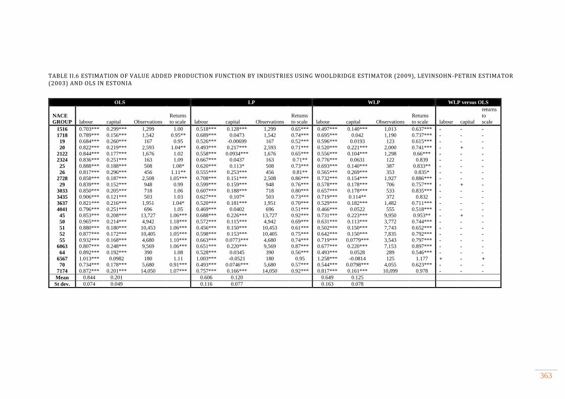
363
TABLE II.6 ESTIMATION OF VALUE ADDED PRODUCTION FUNCTION BY INDUSTRIES USING WOOLDRIDGE ESTIMATOR (2009), LEVINSOHN-PETRIN ESTIMATOR (2003) AND OLS IN ESTONIA
OLS LP WLP WLP versus OLS
NACE
GROUP labour capital Observations
Returns
to scale labour capital Observations
Returns
to scale labour capital Observations
Returns
to scale labour capital
returns
to
scale
1516 0.703*** 0.299*** 1,299 1.00 0.518*** 0.128*** 1,299 0.65*** 0.497*** 0.140*** 1,013 0.637*** - - -
1718 0.789*** 0.156*** 1,542 0.95** 0.689*** 0.0473 1,542 0.74*** 0.695*** 0.042 1,190 0.737*** - - -
19 0.684*** 0.260*** 167 0.95 0.526*** -0.00699 167 0.52*** 0.596*** 0.0193 123 0.615*** - - -
20 0.822*** 0.219*** 2,593 1.04** 0.493*** 0.217*** 2,593 0.71*** 0.520*** 0.221*** 2,000 0.741*** - + -
2122 0.844*** 0.177*** 1,676 1.02 0.558*** 0.0934*** 1,676 0.65*** 0.556*** 0.104*** 1,298 0.66*** - - -
2324 0.836*** 0.251*** 163 1.09 0.667*** 0.0437 163 0.71** 0.776*** 0.0631 122 0.839 - - -
25 0.888*** 0.188*** 508 1.08* 0.620*** 0.113* 508 0.73*** 0.693*** 0.140*** 387 0.833** - - -
26 0.817*** 0.296*** 456 1.11** 0.555*** 0.253*** 456 0.81** 0.565*** 0.269*** 353 0.835* - - -
2728 0.858*** 0.187*** 2,508 1.05*** 0.708*** 0.151*** 2,508 0.86*** 0.732*** 0.154*** 1,927 0.886*** - - -
29 0.839*** 0.152*** 948 0.99 0.599*** 0.159*** 948 0.76*** 0.578*** 0.178*** 706 0.757*** - + -
3033 0.850*** 0.205*** 718 1.06 0.607*** 0.188*** 718 0.80*** 0.657*** 0.178*** 533 0.835*** - - -
3435 0.906*** 0.121*** 503 1.03 0.627*** 0.107* 503 0.73*** 0.719*** 0.114** 372 0.832 - - -
3637 0.821*** 0.216*** 1,951 1.04* 0.520*** 0.181*** 1,951 0.70*** 0.529*** 0.182*** 1,482 0.711*** - - -
4041 0.796*** 0.251*** 696 1.05 0.469*** 0.0402 696 0.51*** 0.466*** 0.0522 555 0.518*** - - -
45 0.853*** 0.208*** 13,727 1.06*** 0.688*** 0.226*** 13,727 0.92*** 0.731*** 0.223*** 9,950 0.953** - + -
50 0.965*** 0.214*** 4,942 1.18*** 0.572*** 0.115*** 4,942 0.69*** 0.631*** 0.113*** 3,772 0.744*** - - -
51 0.880*** 0.180*** 10,453 1.06*** 0.456*** 0.150*** 10,453 0.61*** 0.502*** 0.150*** 7,743 0.652*** - - -
52 0.877*** 0.172*** 10,405 1.05*** 0.598*** 0.153*** 10,405 0.75*** 0.642*** 0.150*** 7,835 0.792*** - - -
55 0.932*** 0.168*** 4,680 1.10*** 0.663*** 0.0773*** 4,680 0.74*** 0.719*** 0.0779*** 3,543 0.797*** - - -
6063 0.807*** 0.248*** 9,569 1.06*** 0.651*** 0.220*** 9,569 0.87*** 0.677*** 0.220*** 7,153 0.897*** - - -
64 0.892*** 0.192*** 390 1.08 0.528*** 0.0345 390 0.56*** 0.493*** 0.0528 289 0.546*** - - -
6567 1.013*** 0.0982 180 1.11 1.003*** -0.0521 180 0.95 1.258*** -0.0814 125 1.177 + - +
70 0.734*** 0.178*** 5,680 0.91*** 0.493*** 0.0746*** 5,680 0.57*** 0.544*** 0.0798*** 4,055 0.623*** - - -
7174 0.872*** 0.201*** 14,050 1.07*** 0.757*** 0.166*** 14,050 0.92*** 0.817*** 0.161*** 10,099 0.978 - - -
Mean 0.844 0.201 0.606 0.120 0.649 0.125
St dev. 0.074 0.049 0.116 0.077 0.163 0.078
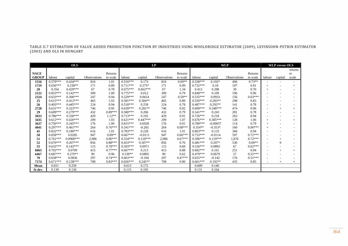
364
TABLE II.7 ESTIMATION OF VALUE ADDED PRODUCTION FUNCTION BY INDUSTRIES USING WOOLDRIDGE ESTIMATOR (2009), LEVINSOHN-PETRIN ESTIMATOR (2003) AND OLS IN HUNGARY
OLS LP WLP WLP versus OLS
NACE
GROUP labour capital Observations
Returns
to scale labour capital Observations
Returns
to scale labour capital Observations
Returns
to scale labour capital
returns to
scale
1516 0.579*** 0.434*** 816 1.01 0.516*** 0.173 816 0.69** 0.538*** 0.192* 496 0.73** - - -
1719 0.656*** 0.238** 171 0.89 0.711*** 0.275* 171 0.99 0.732*** 0.18 107 0.91 + - +
20 0.354 0.429*** 67 0.78 0.675*** 0.662*** 67 1.34 0.413 0.288 39 0.70 + - -
2122 0.853*** 0.142*** 309 1.00 0.775*** 0.012 309 0.79 0.848*** 0.109 196 0.96 - - -
2324 0.633*** 0.306*** 247 0.94 0.529*** 0.0614 247 0.59** 0.535*** 0.0933 156 0.63*** - - -
25 0.615*** 0.412*** 465 1.03 0.581*** 0.304** 465 0.89 0.550*** 0.283** 298 0.83 - - -
26 0.493*** 0.445*** 224 0.94 0.518*** 0.258 224 0.78 0.487*** 0.292** 141 0.78 - - -
2728 0.631*** 0.323*** 746 0.95 0.639*** 0.281** 746 0.92 0.609*** 0.348*** 474 0.96 - + +
29 0.609*** 0.279*** 432 0.89*** 0.580*** 0.206 432 0.79 0.541*** 0.243 281 0.78 - - -
3033 0.786*** 0.330*** 429 1.12** 0.713*** 0.192 429 0.91 0.726*** 0.218 263 0.94 - - -
3435 0.612*** 0.420*** 209 1.03 0.621*** 0.447*** 209 1.07 0.676*** 0.385*** 128 1.06 + - +
3637 0.750*** 0.245*** 176 1.00 0.815*** 0.0928 176 0.91 0.789*** -0.00057 114 0.79 + - -
4041 0.297*** 0.461*** 264 0.76*** 0.341*** -0.265 264 0.08*** 0.354** -0.353* 160 0.00*** + - -
45 0.832*** 0.180*** 616 1.01 0.783*** 0.228 616 1.01 0.803*** 0.133 384 0.94 - - -
50 0.858*** 0.0285 947 0.89** 0.667*** -0.0111 947 0.66*** 0.733*** -0.0114 597 0.72*** - - -
51 0.761*** 0.0968*** 2,986 0.86*** 0.554*** 0.118*** 2,986 0.67*** 0.596*** 0.119*** 1,876 0.72*** - + -
52 0.670*** 0.207*** 856 0.88*** 0.453*** 0.307** 856 0.76 0.481*** 0.207* 530 0.69** - 0 -
55 0.632*** 0.143*** 115 0.78*** 0.503*** 0.0971 115 0.60 0.526*** 0.0893 67 0.62*** - - -
6063 0.702*** 0.0709 415 0.77*** 0.667*** 0.213 415 0.88 0.682*** 0.161 251 0.84 - + +
6467 0.687*** 0.270** 90 0.96 0.539** 0.0805 90 0.62 0.479*** 0.0679 57 0.55*** - - -
70 0.658*** 0.0836 297 0.74*** 0.663*** -0.194 297 0.47*** 0.655*** -0.142 176 0.51*** - - -
7174 0.671*** 0.158*** 708 0.83*** 0.656*** 0.245** 708 0.90 0.661*** 0.192** 435 0.85 - + +
Mean 0.651 0.259 0.613 0.172 0.609 0.140
St dev. 0.139 0.136 0.115 0.195 0.131 0.164
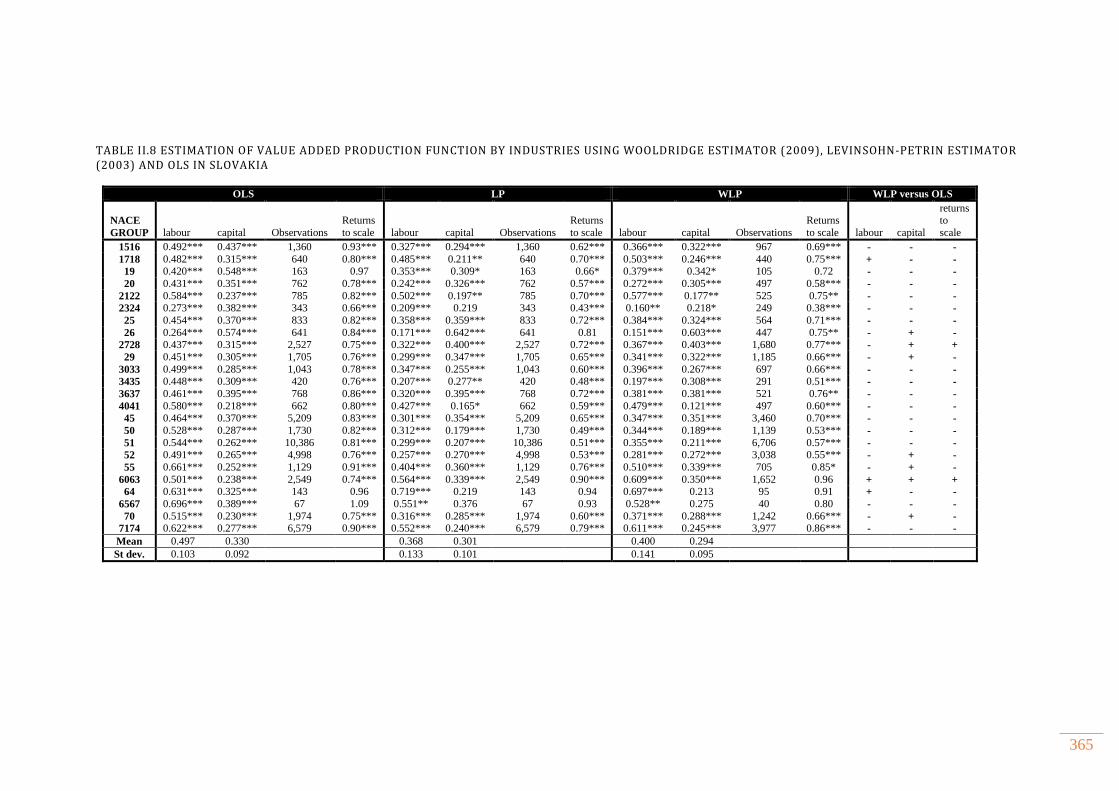
365
TABLE II.8 ESTIMATION OF VALUE ADDED PRODUCTION FUNCTION BY INDUSTRIES USING WOOLDRIDGE ESTIMATOR (2009), LEVINSOHN-PETRIN ESTIMATOR (2003) AND OLS IN SLOVAKIA
OLS LP WLP WLP versus OLS
NACE
GROUP labour capital Observations
Returns
to scale labour capital Observations
Returns
to scale labour capital Observations
Returns
to scale labour capital
returns to
scale
1516 0.492*** 0.437*** 1,360 0.93*** 0.327*** 0.294*** 1,360 0.62*** 0.366*** 0.322*** 967 0.69*** - - -
1718 0.482*** 0.315*** 640 0.80*** 0.485*** 0.211** 640 0.70*** 0.503*** 0.246*** 440 0.75*** + - -
19 0.420*** 0.548*** 163 0.97 0.353*** 0.309* 163 0.66* 0.379*** 0.342* 105 0.72 - - -
20 0.431*** 0.351*** 762 0.78*** 0.242*** 0.326*** 762 0.57*** 0.272*** 0.305*** 497 0.58*** - - -
2122 0.584*** 0.237*** 785 0.82*** 0.502*** 0.197** 785 0.70*** 0.577*** 0.177** 525 0.75** - - -
2324 0.273*** 0.382*** 343 0.66*** 0.209*** 0.219 343 0.43*** 0.160** 0.218* 249 0.38*** - - -
25 0.454*** 0.370*** 833 0.82*** 0.358*** 0.359*** 833 0.72*** 0.384*** 0.324*** 564 0.71*** - - -
26 0.264*** 0.574*** 641 0.84*** 0.171*** 0.642*** 641 0.81 0.151*** 0.603*** 447 0.75** - + -
2728 0.437*** 0.315*** 2,527 0.75*** 0.322*** 0.400*** 2,527 0.72*** 0.367*** 0.403*** 1,680 0.77*** - + +
29 0.451*** 0.305*** 1,705 0.76*** 0.299*** 0.347*** 1,705 0.65*** 0.341*** 0.322*** 1,185 0.66*** - + -
3033 0.499*** 0.285*** 1,043 0.78*** 0.347*** 0.255*** 1,043 0.60*** 0.396*** 0.267*** 697 0.66*** - - -
3435 0.448*** 0.309*** 420 0.76*** 0.207*** 0.277** 420 0.48*** 0.197*** 0.308*** 291 0.51*** - - -
3637 0.461*** 0.395*** 768 0.86*** 0.320*** 0.395*** 768 0.72*** 0.381*** 0.381*** 521 0.76** - - -
4041 0.580*** 0.218*** 662 0.80*** 0.427*** 0.165* 662 0.59*** 0.479*** 0.121*** 497 0.60*** - - -
45 0.464*** 0.370*** 5,209 0.83*** 0.301*** 0.354*** 5,209 0.65*** 0.347*** 0.351*** 3,460 0.70*** - - -
50 0.528*** 0.287*** 1,730 0.82*** 0.312*** 0.179*** 1,730 0.49*** 0.344*** 0.189*** 1,139 0.53*** - - -
51 0.544*** 0.262*** 10,386 0.81*** 0.299*** 0.207*** 10,386 0.51*** 0.355*** 0.211*** 6,706 0.57*** - - -
52 0.491*** 0.265*** 4,998 0.76*** 0.257*** 0.270*** 4,998 0.53*** 0.281*** 0.272*** 3,038 0.55*** - + -
55 0.661*** 0.252*** 1,129 0.91*** 0.404*** 0.360*** 1,129 0.76*** 0.510*** 0.339*** 705 0.85* - + -
6063 0.501*** 0.238*** 2,549 0.74*** 0.564*** 0.339*** 2,549 0.90*** 0.609*** 0.350*** 1,652 0.96 + + +
64 0.631*** 0.325*** 143 0.96 0.719*** 0.219 143 0.94 0.697*** 0.213 95 0.91 + - -
6567 0.696*** 0.389*** 67 1.09 0.551** 0.376 67 0.93 0.528** 0.275 40 0.80 - - -
70 0.515*** 0.230*** 1,974 0.75*** 0.316*** 0.285*** 1,974 0.60*** 0.371*** 0.288*** 1,242 0.66*** - + -
7174 0.622*** 0.277*** 6,579 0.90*** 0.552*** 0.240*** 6,579 0.79*** 0.611*** 0.245*** 3,977 0.86*** - - -
Mean 0.497 0.330 0.368 0.301 0.400 0.294
St dev. 0.103 0.092 0.133 0.101 0.141 0.095

366
TABLE II.9 ESTIMATION OF VALUE ADDED PRODUCTION FUNCTION BY INDUSTRIES USING WOOLDRIDGE ESTIMATOR (2009), LEVINSOHN-PETRIN ESTIMATOR (2003) AND OLS IN SLOVENIA
OLS LP WLP WLP versus OLS
NACE
GROUP labour capital Observations
Returns
to scale labour capital Observations
Returns
to scale labour capital Observations
Returns
to scale labour capital
returns to
scale
1516 0.829*** 0.178*** 288 1.01 0.548*** 0.0637 288 0.61*** 0.582*** 0.0508 207 0.63*** - - -
1719 0.797*** 0.115*** 239 0.91** 0.564*** -0.0166 239 0.55*** 0.548*** -0.0218 176 0.52*** - - -
20 0.612*** 0.251*** 305 0.86*** 0.401*** 0.112** 305 0.51*** 0.346*** 0.169*** 219 0.51*** - - -
2122 0.891*** 0.0981*** 745 0.99 0.882*** 0.113** 745 1.00 0.928*** 0.0942** 558 1.02 + - +
2324 0.615*** 0.347*** 68 0.96 0.537*** 0.135 68 0.67* 0.484*** -0.161*** 53 0.32*** - - -
25 0.603*** 0.230*** 490 0.83*** 0.390*** 0.143** 490 0.53*** 0.431*** 0.147* 364 0.57*** - - -
26 1.124*** -0.00103 172 1.12* 0.577*** 0.0222 172 0.60** 0.559*** -0.0113 125 0.54*** - + -
2728 0.767*** 0.169*** 1,562 0.94*** 0.578*** 0.238*** 1,562 0.82*** 0.595*** 0.228*** 1,163 0.82*** - + -
29 0.764*** 0.120*** 538 0.88*** 0.505*** 0.144*** 538 0.65*** 0.543*** 0.147*** 403 0.69*** - + -
3033 0.698*** 0.175*** 386 0.87*** 0.449*** 0.135 386 0.58*** 0.445*** 0.149** 283 0.59*** - - -
3435 0.815*** 0.0905 92 0.91 0.510*** 0.352*** 92 0.86 0.400*** 0.385*** 69 0.78** - + -
3637 0.648*** 0.245*** 420 0.89** 0.292*** 0.149** 420 0.44*** 0.237*** 0.156** 308 0.39*** - - -
4041 0.819*** 0.0877 87 0.91 0.806*** -0.0548 87 0.75 0.947*** -0.0804 66 0.86 + - -
45 0.793*** 0.226*** 2,577 1.02 0.601*** 0.154*** 2,577 0.76*** 0.635*** 0.159*** 1,873 0.79*** - - -
50 1.011*** 0.0572** 674 1.07** 0.855*** 0.0514 674 0.91 0.890*** 0.0484 499 0.93 - - -
51 0.834*** 0.119*** 3,773 0.95** 0.550*** 0.118*** 3,773 0.67*** 0.590*** 0.115*** 2,777 0.70*** - - -
52 0.871*** 0.0765*** 1,596 0.95** 0.633*** 0.0946*** 1,596 0.73*** 0.668*** 0.0967*** 1,157 0.76*** - + -
55 0.846*** 0.119*** 525 0.97 0.558*** 0.063 525 0.62*** 0.575*** 0.083 373 0.65*** - - -
6063 0.853*** 0.132*** 2,504 0.98 0.788*** 0.0830** 2,504 0.87** 0.860*** 0.0626* 1,786 0.92 + - -
64 0.976*** 0.222** 97 1.20 0.818*** 0.352** 97 1.17 0.915*** 0.353** 68 1.26 - + +
6567 1.108*** 0.0112 87 1.12 1.018*** -0.151 87 0.87 0.910*** -0.0685 64 0.84 - - -
70 0.761*** 0.039 145 0.80*** 0.683*** -0.0393 145 0.64*** 0.640*** -0.0177 97 0.62*** - - -
7174 0.798*** 0.142*** 2,178 0.94** 0.781*** 0.0656** 2,178 0.85*** 0.803*** 0.0499* 1,569 0.85*** + - -
Mean 0.818 0.141 0.622 0.102 0.631 0.093
St dev. 0.140 0.084 0.179 0.113 0.203 0.126
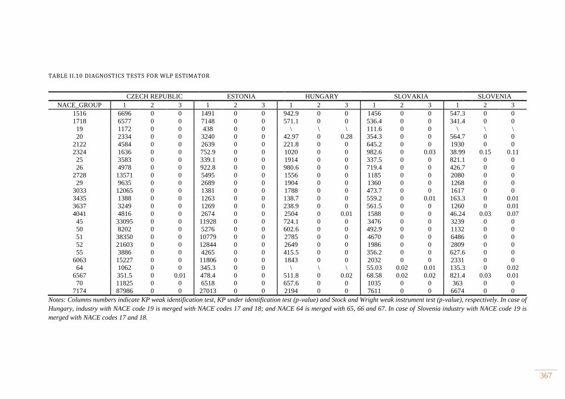
367
TABLE II.10 DIAGNOSTICS TESTS FOR WLP ESTIMATOR
Notes: Columns numbers indicate KP weak identification test, KP under identification test (p-value) and Stock and Wright weak instrument test (p-value), respectively. In case of
Hungary, industry with NACE code 19 is merged with NACE codes 17 and 18; and NACE 64 is merged with 65, 66 and 67. In case of Slovenia industry with NACE code 19 is
merged with NACE codes 17 and 18.
CZECH REPUBLIC ESTONIA HUNGARY SLOVAKIA SLOVENIA
NACE_GROUP 1 2 3 1 2 3 1 2 3 1 2 3 1 2 3
1516 6696 0 0 1491 0 0 942.9 0 0 1456 0 0 547.3 0 0
1718 6577 0 0 7148 0 0 571.1 0 0 536.4 0 0 341.4 0 0
19 1172 0 0 438 0 0 \ \ \ 111.6 0 0 \ \ \
20 2334 0 0 3240 0 0 42.97 0 0.28 354.3 0 0 564.7 0 0
2122 4584 0 0 2639 0 0 221.8 0 0 645.2 0 0 1930 0 0
2324 1636 0 0 752.9 0 0 1020 0 0 982.6 0 0.03 38.99 0.15 0.11
25 3583 0 0 339.1 0 0 1914 0 0 337.5 0 0 821.1 0 0
26 4978 0 0 922.8 0 0 980.6 0 0 719.4 0 0 426.7 0 0
2728 13571 0 0 5495 0 0 1556 0 0 1185 0 0 2080 0 0
29 9635 0 0 2689 0 0 1904 0 0 1360 0 0 1268 0 0
3033 12065 0 0 1381 0 0 1788 0 0 473.7 0 0 1617 0 0
3435 1388 0 0 1263 0 0 138.7 0 0 559.2 0 0.01 163.3 0 0.01
3637 3249 0 0 1269 0 0 238.9 0 0 561.5 0 0 1260 0 0.01
4041 4816 0 0 2674 0 0 2504 0 0.01 1588 0 0 46.24 0.03 0.07
45 33095 0 0 11928 0 0 724.1 0 0 3476 0 0 3239 0 0
50 8202 0 0 5276 0 0 602.6 0 0 492.9 0 0 1132 0 0
51 38350 0 0 10779 0 0 2785 0 0 4670 0 0 6486 0 0
52 21603 0 0 12844 0 0 2649 0 0 1986 0 0 2809 0 0
55 3886 0 0 4265 0 0 415.5 0 0 356.2 0 0 627.6 0 0
6063 15227 0 0 11806 0 0 1843 0 0 2032 0 0 2331 0 0
64 1062 0 0 345.3 0 0 \ \ \ 55.03 0.02 0.01 135.3 0 0.02
6567 351.5 0 0.01 478.4 0 0 511.8 0 0.02 68.58 0.02 0.02 821.4 0.03 0.01
70 11825 0 0 6518 0 0 657.6 0 0 1035 0 0 363 0 0
7174 87986 0 0 27013 0 0 2194 0 0 7611 0 0 6674 0 0
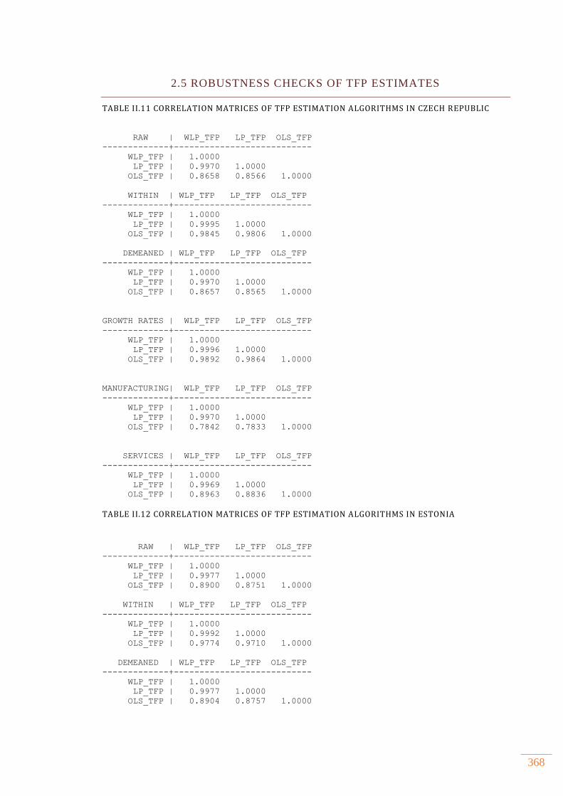
368
2.5 ROBUSTNESS CHECKS OF TFP ESTIMATES
TABLE II.11 CORRELATION MATRICES OF TFP ESTIMATION ALGORITHMS IN CZECH REPUBLIC
RAW | WLP_TFP LP_TFP OLS_TFP
-------------+---------------------------
WLP_TFP | 1.0000
LP_TFP | 0.9970 1.0000
OLS_TFP | 0.8658 0.8566 1.0000
WITHIN | WLP_TFP LP_TFP OLS_TFP
-------------+---------------------------
WLP_TFP | 1.0000
LP_TFP | 0.9995 1.0000
OLS_TFP | 0.9845 0.9806 1.0000
DEMEANED | WLP_TFP LP_TFP OLS_TFP
-------------+---------------------------
WLP_TFP | 1.0000
LP_TFP | 0.9970 1.0000
OLS_TFP | 0.8657 0.8565 1.0000
GROWTH RATES | WLP_TFP LP_TFP OLS_TFP
-------------+---------------------------
WLP_TFP | 1.0000
LP_TFP | 0.9996 1.0000
OLS_TFP | 0.9892 0.9864 1.0000
MANUFACTURING| WLP_TFP LP_TFP OLS_TFP
-------------+---------------------------
WLP_TFP | 1.0000
LP_TFP | 0.9970 1.0000
OLS_TFP | 0.7842 0.7833 1.0000
SERVICES | WLP_TFP LP_TFP OLS_TFP
-------------+---------------------------
WLP_TFP | 1.0000
LP_TFP | 0.9969 1.0000
OLS_TFP | 0.8963 0.8836 1.0000
TABLE II.12 CORRELATION MATRICES OF TFP ESTIMATION ALGORITHMS IN ESTONIA
RAW | WLP_TFP LP_TFP OLS_TFP
-------------+---------------------------
WLP_TFP | 1.0000
LP_TFP | 0.9977 1.0000
OLS_TFP | 0.8900 0.8751 1.0000
WITHIN | WLP_TFP LP_TFP OLS_TFP
-------------+---------------------------
WLP_TFP | 1.0000
LP_TFP | 0.9992 1.0000
OLS_TFP | 0.9774 0.9710 1.0000
DEMEANED | WLP_TFP LP_TFP OLS_TFP
-------------+---------------------------
WLP_TFP | 1.0000
LP_TFP | 0.9977 1.0000
OLS_TFP | 0.8904 0.8757 1.0000
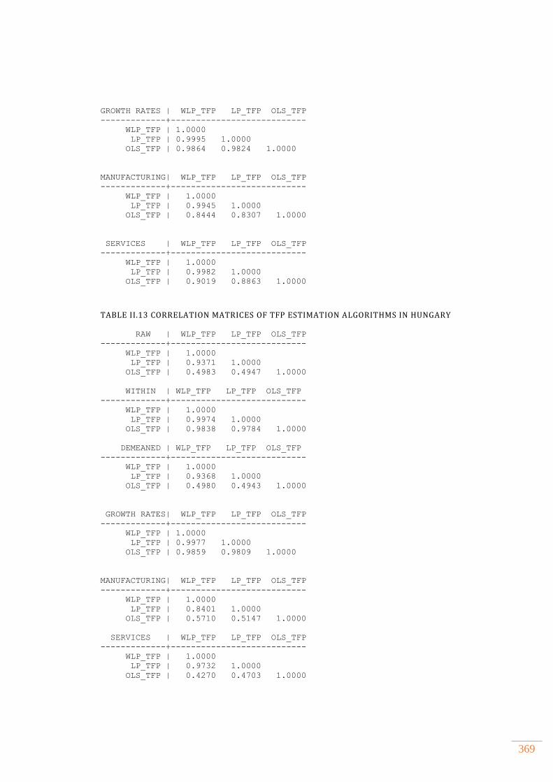
369
GROWTH RATES | WLP_TFP LP_TFP OLS_TFP
-------------+---------------------------
WLP_TFP | 1.0000
LP_TFP | 0.9995 1.0000
OLS_TFP | 0.9864 0.9824 1.0000
MANUFACTURING| WLP_TFP LP_TFP OLS_TFP
-------------+---------------------------
WLP_TFP | 1.0000
LP_TFP | 0.9945 1.0000
OLS_TFP | 0.8444 0.8307 1.0000
SERVICES | WLP_TFP LP_TFP OLS_TFP
-------------+---------------------------
WLP_TFP | 1.0000
LP_TFP | 0.9982 1.0000
OLS_TFP | 0.9019 0.8863 1.0000
TABLE II.13 CORRELATION MATRICES OF TFP ESTIMATION ALGORITHMS IN HUNGARY
RAW | WLP_TFP LP_TFP OLS_TFP
-------------+---------------------------
WLP_TFP | 1.0000
LP_TFP | 0.9371 1.0000
OLS_TFP | 0.4983 0.4947 1.0000
WITHIN | WLP_TFP LP_TFP OLS_TFP
-------------+---------------------------
WLP_TFP | 1.0000
LP_TFP | 0.9974 1.0000
OLS_TFP | 0.9838 0.9784 1.0000
DEMEANED | WLP_TFP LP_TFP OLS_TFP
-------------+---------------------------
WLP_TFP | 1.0000
LP_TFP | 0.9368 1.0000
OLS_TFP | 0.4980 0.4943 1.0000
GROWTH RATES| WLP_TFP LP_TFP OLS_TFP
-------------+---------------------------
WLP_TFP | 1.0000
LP_TFP | 0.9977 1.0000
OLS_TFP | 0.9859 0.9809 1.0000
MANUFACTURING| WLP_TFP LP_TFP OLS_TFP
-------------+---------------------------
WLP_TFP | 1.0000
LP_TFP | 0.8401 1.0000
OLS_TFP | 0.5710 0.5147 1.0000
SERVICES | WLP_TFP LP_TFP OLS_TFP
-------------+---------------------------
WLP_TFP | 1.0000
LP_TFP | 0.9732 1.0000
OLS_TFP | 0.4270 0.4703 1.0000
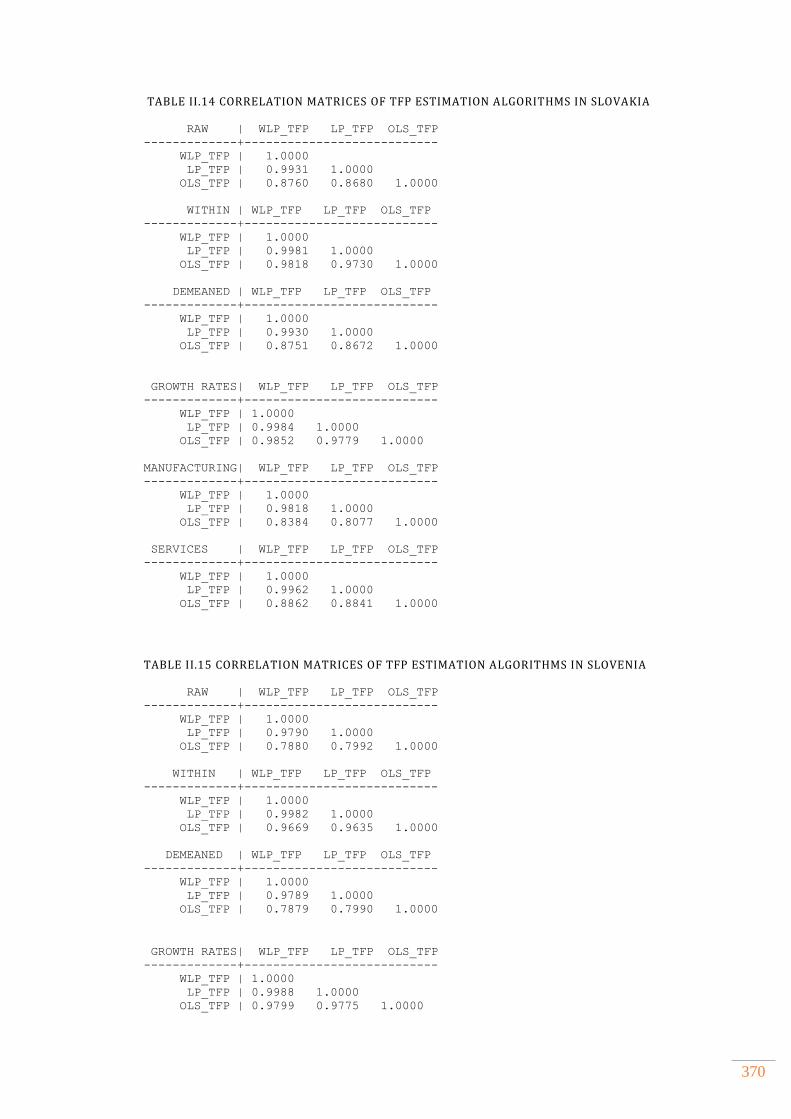
370
TABLE II.14 CORRELATION MATRICES OF TFP ESTIMATION ALGORITHMS IN SLOVAKIA
RAW | WLP_TFP LP_TFP OLS_TFP
-------------+---------------------------
WLP_TFP | 1.0000
LP_TFP | 0.9931 1.0000
OLS_TFP | 0.8760 0.8680 1.0000
WITHIN | WLP_TFP LP_TFP OLS_TFP
-------------+---------------------------
WLP_TFP | 1.0000
LP_TFP | 0.9981 1.0000
OLS_TFP | 0.9818 0.9730 1.0000
DEMEANED | WLP_TFP LP_TFP OLS_TFP
-------------+---------------------------
WLP_TFP | 1.0000
LP_TFP | 0.9930 1.0000
OLS_TFP | 0.8751 0.8672 1.0000
GROWTH RATES| WLP_TFP LP_TFP OLS_TFP
-------------+---------------------------
WLP_TFP | 1.0000
LP_TFP | 0.9984 1.0000
OLS_TFP | 0.9852 0.9779 1.0000
MANUFACTURING| WLP_TFP LP_TFP OLS_TFP
-------------+---------------------------
WLP_TFP | 1.0000
LP_TFP | 0.9818 1.0000
OLS_TFP | 0.8384 0.8077 1.0000
SERVICES | WLP_TFP LP_TFP OLS_TFP
-------------+---------------------------
WLP_TFP | 1.0000
LP_TFP | 0.9962 1.0000
OLS_TFP | 0.8862 0.8841 1.0000
TABLE II.15 CORRELATION MATRICES OF TFP ESTIMATION ALGORITHMS IN SLOVENIA
RAW | WLP_TFP LP_TFP OLS_TFP
-------------+---------------------------
WLP_TFP | 1.0000
LP_TFP | 0.9790 1.0000
OLS_TFP | 0.7880 0.7992 1.0000
WITHIN | WLP_TFP LP_TFP OLS_TFP
-------------+---------------------------
WLP_TFP | 1.0000
LP_TFP | 0.9982 1.0000
OLS_TFP | 0.9669 0.9635 1.0000
DEMEANED | WLP_TFP LP_TFP OLS_TFP
-------------+---------------------------
WLP_TFP | 1.0000
LP_TFP | 0.9789 1.0000
OLS_TFP | 0.7879 0.7990 1.0000
GROWTH RATES| WLP_TFP LP_TFP OLS_TFP
-------------+---------------------------
WLP_TFP | 1.0000
LP_TFP | 0.9988 1.0000
OLS_TFP | 0.9799 0.9775 1.0000
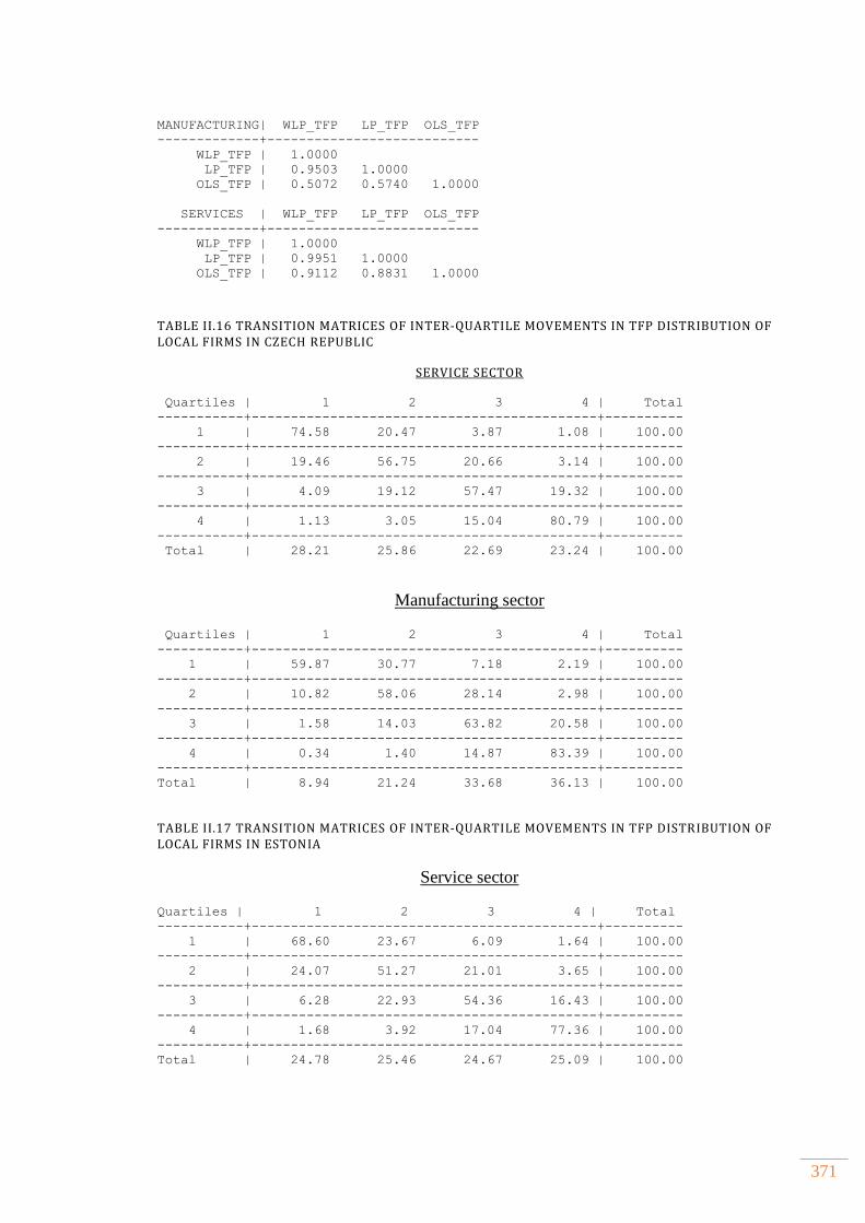
371
MANUFACTURING| WLP_TFP LP_TFP OLS_TFP
-------------+---------------------------
WLP_TFP | 1.0000
LP_TFP | 0.9503 1.0000
OLS_TFP | 0.5072 0.5740 1.0000
SERVICES | WLP_TFP LP_TFP OLS_TFP
-------------+---------------------------
WLP_TFP | 1.0000
LP_TFP | 0.9951 1.0000
OLS_TFP | 0.9112 0.8831 1.0000
TABLE II.16 TRANSITION MATRICES OF INTER-QUARTILE MOVEMENTS IN TFP DISTRIBUTION OF LOCAL FIRMS IN CZECH REPUBLIC
SERVICE SECTOR
Quartiles | 1 2 3 4 | Total
-----------+--------------------------------------------+----------
1 | 74.58 20.47 3.87 1.08 | 100.00
-----------+--------------------------------------------+----------
2 | 19.46 56.75 20.66 3.14 | 100.00
-----------+--------------------------------------------+----------
3 | 4.09 19.12 57.47 19.32 | 100.00
-----------+--------------------------------------------+----------
4 | 1.13 3.05 15.04 80.79 | 100.00
-----------+--------------------------------------------+----------
Total | 28.21 25.86 22.69 23.24 | 100.00
Manufacturing sector
Quartiles | 1 2 3 4 | Total
-----------+--------------------------------------------+----------
1 | 59.87 30.77 7.18 2.19 | 100.00
-----------+--------------------------------------------+----------
2 | 10.82 58.06 28.14 2.98 | 100.00
-----------+--------------------------------------------+----------
3 | 1.58 14.03 63.82 20.58 | 100.00
-----------+--------------------------------------------+----------
4 | 0.34 1.40 14.87 83.39 | 100.00
-----------+--------------------------------------------+----------
Total | 8.94 21.24 33.68 36.13 | 100.00
TABLE II.17 TRANSITION MATRICES OF INTER-QUARTILE MOVEMENTS IN TFP DISTRIBUTION OF LOCAL FIRMS IN ESTONIA
Service sector
Quartiles | 1 2 3 4 | Total
-----------+--------------------------------------------+----------
1 | 68.60 23.67 6.09 1.64 | 100.00
-----------+--------------------------------------------+----------
2 | 24.07 51.27 21.01 3.65 | 100.00
-----------+--------------------------------------------+----------
3 | 6.28 22.93 54.36 16.43 | 100.00
-----------+--------------------------------------------+----------
4 | 1.68 3.92 17.04 77.36 | 100.00
-----------+--------------------------------------------+----------
Total | 24.78 25.46 24.67 25.09 | 100.00
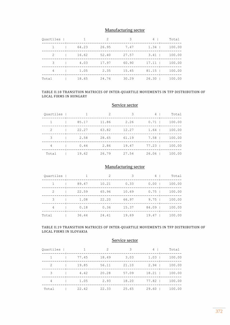
372
Manufacturing sector
Quartiles | 1 2 3 4 | Total
-----------+--------------------------------------------+----------
1 | 64.23 26.95 7.47 1.34 | 100.00
-----------+--------------------------------------------+----------
2 | 16.62 52.40 27.57 3.41 | 100.00
-----------+--------------------------------------------+----------
3 | 4.03 17.97 60.90 17.11 | 100.00
-----------+--------------------------------------------+----------
4 | 1.05 2.35 15.45 81.15 | 100.00
-----------+--------------------------------------------+----------
Total | 18.65 24.76 30.29 26.30 | 100.00
TABLE II.18 TRANSITION MATRICES OF INTER-QUARTILE MOVEMENTS IN TFP DISTRIBUTION OF LOCAL FIRMS IN HUNGARY
Service sector
Quartiles | 1 2 3 4 | Total
-----------+--------------------------------------------+----------
1 | 85.17 11.86 2.26 0.71 | 100.00
-----------+--------------------------------------------+----------
2 | 22.27 63.82 12.27 1.64 | 100.00
-----------+--------------------------------------------+----------
3 | 2.58 28.65 61.19 7.58 | 100.00
-----------+--------------------------------------------+----------
4 | 0.44 2.86 19.47 77.23 | 100.00
-----------+--------------------------------------------+----------
Total | 19.62 26.79 27.54 26.06 | 100.00
Manufacturing sector
Quartiles | 1 2 3 4 | Total
-----------+--------------------------------------------+----------
1 | 89.47 10.21 0.33 0.00 | 100.00
-----------+--------------------------------------------+----------
2 | 22.59 65.96 10.69 0.75 | 100.00
-----------+--------------------------------------------+----------
3 | 1.08 22.20 66.97 9.75 | 100.00
-----------+--------------------------------------------+----------
4 | 0.18 0.36 15.37 84.09 | 100.00
-----------+--------------------------------------------+----------
Total | 36.44 24.41 19.69 19.47 | 100.00
TABLE II.19 TRANSITION MATRICES OF INTER-QUARTILE MOVEMENTS IN TFP DISTRIBUTION OF LOCAL FIRMS IN SLOVAKIA
Service sector
Quartiles | 1 2 3 4 | Total
-----------+--------------------------------------------+----------
1 | 77.45 18.49 3.03 1.03 | 100.00
-----------+--------------------------------------------+----------
2 | 19.85 56.11 21.10 2.94 | 100.00
-----------+--------------------------------------------+----------
3 | 4.42 20.28 57.09 18.21 | 100.00
-----------+--------------------------------------------+----------
4 | 1.05 2.93 18.20 77.82 | 100.00
-----------+--------------------------------------------+----------
Total | 22.42 22.33 25.65 29.60 | 100.00
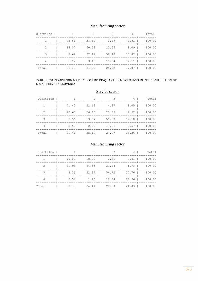
373
Manufacturing sector
Quartiles | 1 2 3 4 | Total
-----------+--------------------------------------------+----------
1 | 72.81 23.39 3.29 0.51 | 100.00
-----------+--------------------------------------------+----------
2 | 18.07 60.28 20.56 1.09 | 100.00
-----------+--------------------------------------------+----------
3 | 3.62 22.11 58.40 15.87 | 100.00
-----------+--------------------------------------------+----------
4 | 1.12 3.13 18.64 77.11 | 100.00
-----------+--------------------------------------------+----------
Total | 26.19 31.72 25.02 17.07 | 100.00
TABLE II.20 TRANSITION MATRICES OF INTER-QUARTILE MOVEMENTS IN TFP DISTRIBUTION OF LOCAL FIRMS IN SLOVENIA
Service sector
Quartiles | 1 2 3 4 | Total
-----------+--------------------------------------------+----------
1 | 71.40 22.68 4.87 1.05 | 100.00
-----------+--------------------------------------------+----------
2 | 20.60 56.65 20.09 2.67 | 100.00
-----------+--------------------------------------------+----------
3 | 3.56 19.57 59.69 17.18 | 100.00
-----------+--------------------------------------------+----------
4 | 0.59 2.89 17.96 78.57 | 100.00
-----------+--------------------------------------------+----------
Total | 21.46 25.10 27.07 26.36 | 100.00
Manufacturing sector
Quartiles | 1 2 3 4 | Total
-----------+--------------------------------------------+----------
1 | 79.08 18.20 2.31 0.41 | 100.00
-----------+--------------------------------------------+----------
2 | 21.95 54.88 21.44 1.73 | 100.00
-----------+--------------------------------------------+----------
3 | 3.33 22.19 56.72 17.76 | 100.00
-----------+--------------------------------------------+----------
4 | 0.54 1.96 12.84 84.66 | 100.00
-----------+--------------------------------------------+----------
Total | 30.75 24.41 20.80 24.03 | 100.00

374
2.6 NON PARAMETRIC KOLMOGOROV SMIRNOV TEST OF FOREIGN
OWNERSHIP PREMIUM
TABLE II.21 KOLMOGOROV SMIRNOV TEST PER INDUSTRY AND FOREIGN OWNERSHIP TYPE IN SLOVENIA, PRINTOUT FROM STATA
. ksmirnov WLP_TFPall, by( for_dom )
Two-sample Kolmogorov-Smirnov test for equality of distribution
functions
Smaller group D P-value Corrected
----------------------------------------------
0: 0.3870 0.000
1: -0.0007 1.000
Combined K-S: 0.3870 0.000 0.000
Note: ties exist in combined dataset;
there are 19831 unique values out of 19871 observations.
MANUFACTURING SECTOR
. ksmirnov WLP_TFPall if man==1, by( for_dom )
Two-sample Kolmogorov-Smirnov test for equality of distribution
functions
Smaller group D P-value Corrected
----------------------------------------------
0: 0.4452 0.000
1: -0.0117 0.985
Combined K-S: 0.4452 0.000 0.000
Note: ties exist in combined dataset;
there are 5359 unique values out of 5360 observations.
SERVICE SECTOR
. ksmirnov WLP_TFPall if man==0, by( for_dom )
Two-sample Kolmogorov-Smirnov test for equality of distribution
functions
Smaller group D P-value Corrected
----------------------------------------------
0: 0.3644 0.000
1: -0.0016 0.999
Combined K-S: 0.3644 0.000 0.000
Note: ties exist in combined dataset;
there are 14491 unique values out of 14511 observations.
DIFFERENCES BETWEEN FULL AND PARTIAL ONWERSHIP OF MNCs
. ksmirnov WLP_for if for_own!=., by( for_own )
Two-sample Kolmogorov-Smirnov test for equality of distribution
functions
Smaller group D P-value Corrected
----------------------------------------------
0: 0.1531 0.054

375
1: -0.2207 0.002
Combined K-S: 0.2207 0.005 0.003
DIFFERENCES BETWEEN FULL AND PARTIAL ONWERSHIP OF MNCs - MANUFACTURING
. ksmirnov WLP_for if for_own!=. & man==1, by( for_own )
Two-sample Kolmogorov-Smirnov test for equality of distribution
functions
Smaller group D P-value Corrected
----------------------------------------------
0: 0.2417 0.243
1: -0.4054 0.019
Combined K-S: 0.4054 0.037 0.020
DIFFERENCES BETWEEN FULL AND PARTIAL ONWERSHIP OF MNCs - SERVICES
. ksmirnov WLP_for if for_own!=. & man==0, by( for_own )
Two-sample Kolmogorov-Smirnov test for equality of distribution
functions
Smaller group D P-value Corrected
----------------------------------------------
0: 0.2994 0.001
1: -0.0960 0.490
Combined K-S: 0.2994 0.002 0.001
TABLE II.22 KOLMOGOROV SMIRNOV TEST PER INDUSTRY AND FOREIGN OWNERSHIP TYPE IN SLOVAKIA, PRINTOUT FROM STATA
. ksmirnov WLP_TFPall, by( for_dom )
Two-sample Kolmogorov-Smirnov test for equality of distribution
functions
Smaller group D P-value Corrected
----------------------------------------------
0: 0.2118 0.000
1: -0.0008 0.998
Combined K-S: 0.2118 0.000 0.000
Note: ties exist in combined dataset;
there are 49142 unique values out of 49297 observations.
MANUFACTURING
. ksmirnov WLP_TFPall if man==1, by( for_dom )
Two-sample Kolmogorov-Smirnov test for equality of distribution
functions
Smaller group D P-value Corrected
----------------------------------------------
0: 0.1822 0.000
1: -0.0026 0.989
Combined K-S: 0.1822 0.000 0.000
Note: ties exist in combined dataset;
there are 12836 unique values out of 12844 observations.
SERVICES

376
. ksmirnov WLP_TFPall if man==0, by( for_dom )
Two-sample Kolmogorov-Smirnov test for equality of distribution
functions
Smaller group D P-value Corrected
----------------------------------------------
0: 0.3554 0.000
1: -0.0009 0.998
Combined K-S: 0.3554 0.000 0.000
Note: ties exist in combined dataset;
there are 36329 unique values out of 36453 observations.
DIFFERENCES BETWEEN FULL AND PARTIAL ONWERSHIP OF MNCs
. ksmirnov WLP_for if for_own!=., by( for_own )
Two-sample Kolmogorov-Smirnov test for equality of distribution
functions
Smaller group D P-value Corrected
----------------------------------------------
0: 0.0801 0.009
1: -0.0067 0.967
Combined K-S: 0.0801 0.017 0.014
DIFFERENCES BETWEEN FULL AND PARTIAL ONWERSHIP OF MNCs - MANUFACTURING
. ksmirnov WLP_for if for_own!=. & man==1, by( for_own )
Two-sample Kolmogorov-Smirnov test for equality of distribution
functions
Smaller group D P-value Corrected
----------------------------------------------
0: 0.0536 0.350
1: -0.1071 0.015
Combined K-S: 0.1071 0.030 0.024
DIFFERENCES BETWEEN FULL AND PARTIAL ONWERSHIP OF MNCs - SERVICES
. ksmirnov WLP_for if for_own!=. & man==0, by( for_own )
Two-sample Kolmogorov-Smirnov test for equality of distribution
functions
Smaller group D P-value Corrected
----------------------------------------------
0: 0.1297 0.002
1: -0.0035 0.995
Combined K-S: 0.1297 0.004 0.003
TABLE II.23 KOLMOGOROV SMIRNOV TEST PER INDUSTRY AND FOREIGN OWNERSHIP TYPE IN HUNGARY, PRINTOUT FROM STATA
. ksmirnov WLP_TFPall, by( for_dom )
Two-sample Kolmogorov-Smirnov test for equality of distribution
functions
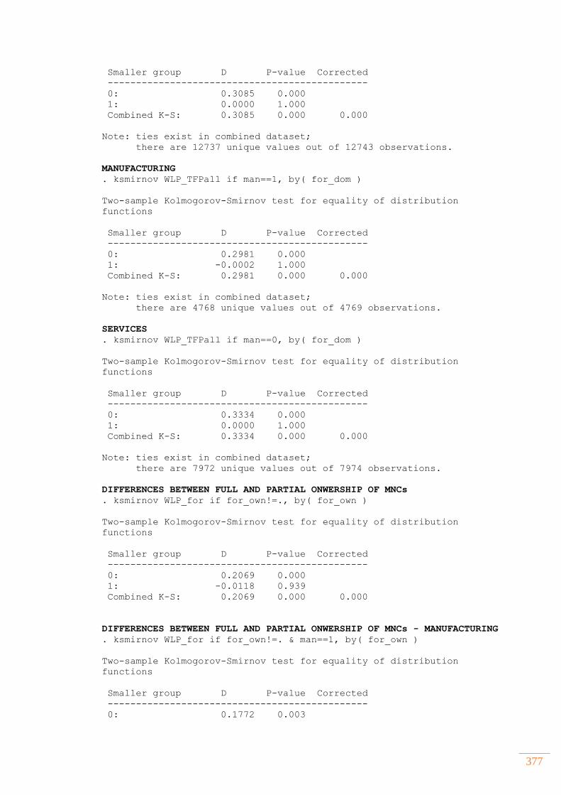
377
Smaller group D P-value Corrected
----------------------------------------------
0: 0.3085 0.000
1: 0.0000 1.000
Combined K-S: 0.3085 0.000 0.000
Note: ties exist in combined dataset;
there are 12737 unique values out of 12743 observations.
MANUFACTURING
. ksmirnov WLP_TFPall if man==1, by( for_dom )
Two-sample Kolmogorov-Smirnov test for equality of distribution
functions
Smaller group D P-value Corrected
----------------------------------------------
0: 0.2981 0.000
1: -0.0002 1.000
Combined K-S: 0.2981 0.000 0.000
Note: ties exist in combined dataset;
there are 4768 unique values out of 4769 observations.
SERVICES
. ksmirnov WLP_TFPall if man==0, by( for_dom )
Two-sample Kolmogorov-Smirnov test for equality of distribution
functions
Smaller group D P-value Corrected
----------------------------------------------
0: 0.3334 0.000
1: 0.0000 1.000
Combined K-S: 0.3334 0.000 0.000
Note: ties exist in combined dataset;
there are 7972 unique values out of 7974 observations.
DIFFERENCES BETWEEN FULL AND PARTIAL ONWERSHIP OF MNCs
. ksmirnov WLP_for if for_own!=., by( for_own )
Two-sample Kolmogorov-Smirnov test for equality of distribution
functions
Smaller group D P-value Corrected
----------------------------------------------
0: 0.2069 0.000
1: -0.0118 0.939
Combined K-S: 0.2069 0.000 0.000
DIFFERENCES BETWEEN FULL AND PARTIAL ONWERSHIP OF MNCs - MANUFACTURING
. ksmirnov WLP_for if for_own!=. & man==1, by( for_own )
Two-sample Kolmogorov-Smirnov test for equality of distribution
functions
Smaller group D P-value Corrected
----------------------------------------------
0: 0.1772 0.003

378
1: -0.0100 0.982
Combined K-S: 0.1772 0.006 0.004
DIFFERENCES BETWEEN FULL AND PARTIAL ONWERSHIP OF MNCs - SERVICES
. ksmirnov WLP_for if for_own!=. & man==0, by( for_own )
Two-sample Kolmogorov-Smirnov test for equality of distribution
functions
Smaller group D P-value Corrected
----------------------------------------------
0: 0.2406 0.000
1: -0.0196 0.902
Combined K-S: 0.2406 0.000 0.000
TABLE II.24 TABLE 4 18 KOLMOGOROV SMIRNOV TEST PER INDUSTRY AND FOREIGN OWNERSHIP TYPE IN ESTONIA, PRINTOUT FROM STATA
. ksmirnov WLP_TFPall, by( for_dom )
Two-sample Kolmogorov-Smirnov test for equality of distribution
functions
Smaller group D P-value Corrected
----------------------------------------------
0: 0.4333 0.000
1: -0.0002 1.000
Combined K-S: 0.4333 0.000 0.000
Note: ties exist in combined dataset;
there are 93528 unique values out of 94630 observations.
MANUFACTURING
. ksmirnov WLP_TFPall if man==1, by( for_dom )
Two-sample Kolmogorov-Smirnov test for equality of distribution
functions
Smaller group D P-value Corrected
----------------------------------------------
0: 0.3808 0.000
1: -0.0003 1.000
Combined K-S: 0.3808 0.000 0.000
Note: ties exist in combined dataset;
there are 16512 unique values out of 16547 observations.
SERVICES
. ksmirnov WLP_TFPall if man==0, by( for_dom )
Two-sample Kolmogorov-Smirnov test for equality of distribution
functions
Smaller group D P-value Corrected
----------------------------------------------
0: 0.4557 0.000
1: -0.0002 1.000
Combined K-S: 0.4557 0.000 0.000
Note: ties exist in combined dataset;

379
there are 77136 unique values out of 78083 observations.
DIFFERENCES BETWEEN FULL AND PARTIAL ONWERSHIP OF MNCs
. ksmirnov WLP_for if for_own!=., by( for_own )
Two-sample Kolmogorov-Smirnov test for equality of distribution
functions
Smaller group D P-value Corrected
----------------------------------------------
0: 0.1884 0.000
1: -0.0002 1.000
Combined K-S: 0.1884 0.000 0.000
Note: ties exist in combined dataset;
there are 4823 unique values out of 4826 observations.
DIFFERENCES BETWEEN FULL AND PARTIAL ONWERSHIP OF MNCs - MANUFACTURING
. ksmirnov WLP_for if for_own!=. & man==1, by( for_own )
Two-sample Kolmogorov-Smirnov test for equality of distribution
functions
Smaller group D P-value Corrected
----------------------------------------------
0: 0.2439 0.000
1: -0.0011 0.999
Combined K-S: 0.2439 0.000 0.000
Note: ties exist in combined dataset;
there are 1514 unique values out of 1515 observations.
DIFFERENCES BETWEEN FULL AND PARTIAL ONWERSHIP OF MNCs - SERVICES
. ksmirnov WLP_for if for_own!=. & man==0, by( for_own )
Two-sample Kolmogorov-Smirnov test for equality of distribution
functions
Smaller group D P-value Corrected
----------------------------------------------
0: 0.1620 0.000
1: -0.0003 1.000
Combined K-S: 0.1620 0.000 0.000
Note: ties exist in combined dataset;
there are 3310 unique values out of 3311 observations.
TABLE II.25 KOLMOGOROV SMIRNOV TEST PER INDUSTRY AND FOREIGN OWNERSHIP TYPE IN THE CZECH REPUBLIC, PRINTOUT FROM STATA
. ksmirnov WLP_TFPall, by( for_dom )
Two-sample Kolmogorov-Smirnov test for equality of distribution
functions
Smaller group D P-value Corrected
----------------------------------------------
0: 0.4479 0.000
1: -0.0001 1.000

380
Combined K-S: 0.4479 0.000 0.000
Note: ties exist in combined dataset;
there are 230509 unique values out of 233445 observations.
MANUFACTURING
. ksmirnov WLP_TFPall if man==1, by( for_dom )
Two-sample Kolmogorov-Smirnov test for equality of distribution
functions
Smaller group D P-value Corrected
----------------------------------------------
0: 0.4266 0.000
1: 0.0000 1.000
Combined K-S: 0.4266 0.000 0.000
Note: ties exist in combined dataset;
there are 63268 unique values out of 63468 observations.
SERVICES
. ksmirnov WLP_TFPall if man==0, by( for_dom )
Two-sample Kolmogorov-Smirnov test for equality of distribution
functions
Smaller group D P-value Corrected
----------------------------------------------
0: 0.4316 0.000
1: -0.0001 1.000
Combined K-S: 0.4316 0.000 0.000
Note: ties exist in combined dataset;
there are 167937 unique values out of 169977 observations.
DIFFERENCES BETWEEN FULL AND PARTIAL ONWERSHIP OF MNCs
. ksmirnov WLP_for if for_own!=., by( for_own )
Two-sample Kolmogorov-Smirnov test for equality of distribution
functions
Smaller group D P-value Corrected
----------------------------------------------
0: 0.1478 0.000
1: -0.0011 0.995
Combined K-S: 0.1478 0.000 0.000
Note: ties exist in combined dataset;
there are 9990 unique values out of 9993 observations.
DIFFERENCES BETWEEN FULL AND PARTIAL ONWERSHIP OF MNCs - MANUFACTURING
. ksmirnov WLP_for if for_own!=. & man==1, by( for_own )
Two-sample Kolmogorov-Smirnov test for equality of distribution
functions
Smaller group D P-value Corrected
----------------------------------------------
0: 0.1013 0.000
1: -0.0027 0.988
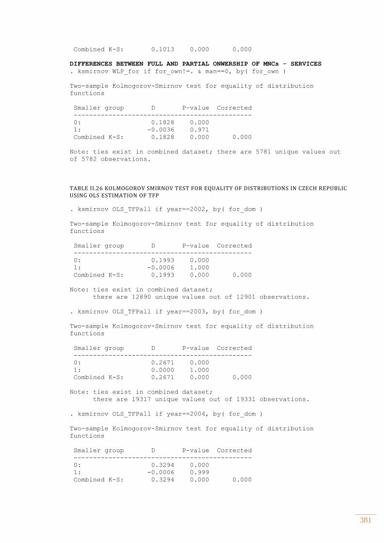
381
Combined K-S: 0.1013 0.000 0.000
DIFFERENCES BETWEEN FULL AND PARTIAL ONWERSHIP OF MNCs - SERVICES
. ksmirnov WLP_for if for_own!=. & man==0, by( for_own )
Two-sample Kolmogorov-Smirnov test for equality of distribution
functions
Smaller group D P-value Corrected
----------------------------------------------
0: 0.1828 0.000
1: -0.0036 0.971
Combined K-S: 0.1828 0.000 0.000
Note: ties exist in combined dataset; there are 5781 unique values out
of 5782 observations.
TABLE II.26 KOLMOGOROV SMIRNOV TEST FOR EQUALITY OF DISTRIBUTIONS IN CZECH REPUBLIC USING OLS ESTIMATION OF TFP
. ksmirnov OLS_TFPall if year==2002, by( for_dom )
Two-sample Kolmogorov-Smirnov test for equality of distribution
functions
Smaller group D P-value Corrected
----------------------------------------------
0: 0.1993 0.000
1: -0.0006 1.000
Combined K-S: 0.1993 0.000 0.000
Note: ties exist in combined dataset;
there are 12890 unique values out of 12901 observations.
. ksmirnov OLS_TFPall if year==2003, by( for_dom )
Two-sample Kolmogorov-Smirnov test for equality of distribution
functions
Smaller group D P-value Corrected
----------------------------------------------
0: 0.2671 0.000
1: 0.0000 1.000
Combined K-S: 0.2671 0.000 0.000
Note: ties exist in combined dataset;
there are 19317 unique values out of 19331 observations.
. ksmirnov OLS_TFPall if year==2004, by( for_dom )
Two-sample Kolmogorov-Smirnov test for equality of distribution
functions
Smaller group D P-value Corrected
----------------------------------------------
0: 0.3294 0.000
1: -0.0006 0.999
Combined K-S: 0.3294 0.000 0.000
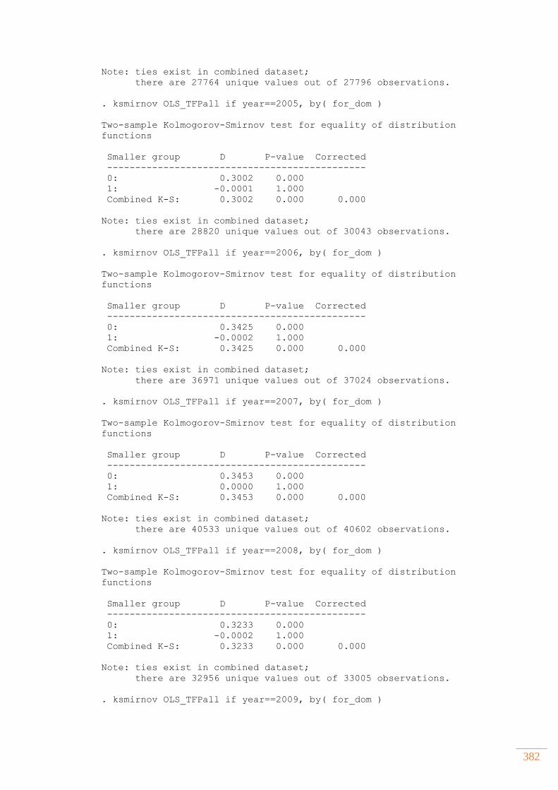
382
Note: ties exist in combined dataset;
there are 27764 unique values out of 27796 observations.
. ksmirnov OLS_TFPall if year==2005, by( for_dom )
Two-sample Kolmogorov-Smirnov test for equality of distribution
functions
Smaller group D P-value Corrected
----------------------------------------------
0: 0.3002 0.000
1: -0.0001 1.000
Combined K-S: 0.3002 0.000 0.000
Note: ties exist in combined dataset;
there are 28820 unique values out of 30043 observations.
. ksmirnov OLS_TFPall if year==2006, by( for_dom )
Two-sample Kolmogorov-Smirnov test for equality of distribution
functions
Smaller group D P-value Corrected
----------------------------------------------
0: 0.3425 0.000
1: -0.0002 1.000
Combined K-S: 0.3425 0.000 0.000
Note: ties exist in combined dataset;
there are 36971 unique values out of 37024 observations.
. ksmirnov OLS_TFPall if year==2007, by( for_dom )
Two-sample Kolmogorov-Smirnov test for equality of distribution
functions
Smaller group D P-value Corrected
----------------------------------------------
0: 0.3453 0.000
1: 0.0000 1.000
Combined K-S: 0.3453 0.000 0.000
Note: ties exist in combined dataset;
there are 40533 unique values out of 40602 observations.
. ksmirnov OLS_TFPall if year==2008, by( for_dom )
Two-sample Kolmogorov-Smirnov test for equality of distribution
functions
Smaller group D P-value Corrected
----------------------------------------------
0: 0.3233 0.000
1: -0.0002 1.000
Combined K-S: 0.3233 0.000 0.000
Note: ties exist in combined dataset;
there are 32956 unique values out of 33005 observations.
. ksmirnov OLS_TFPall if year==2009, by( for_dom )
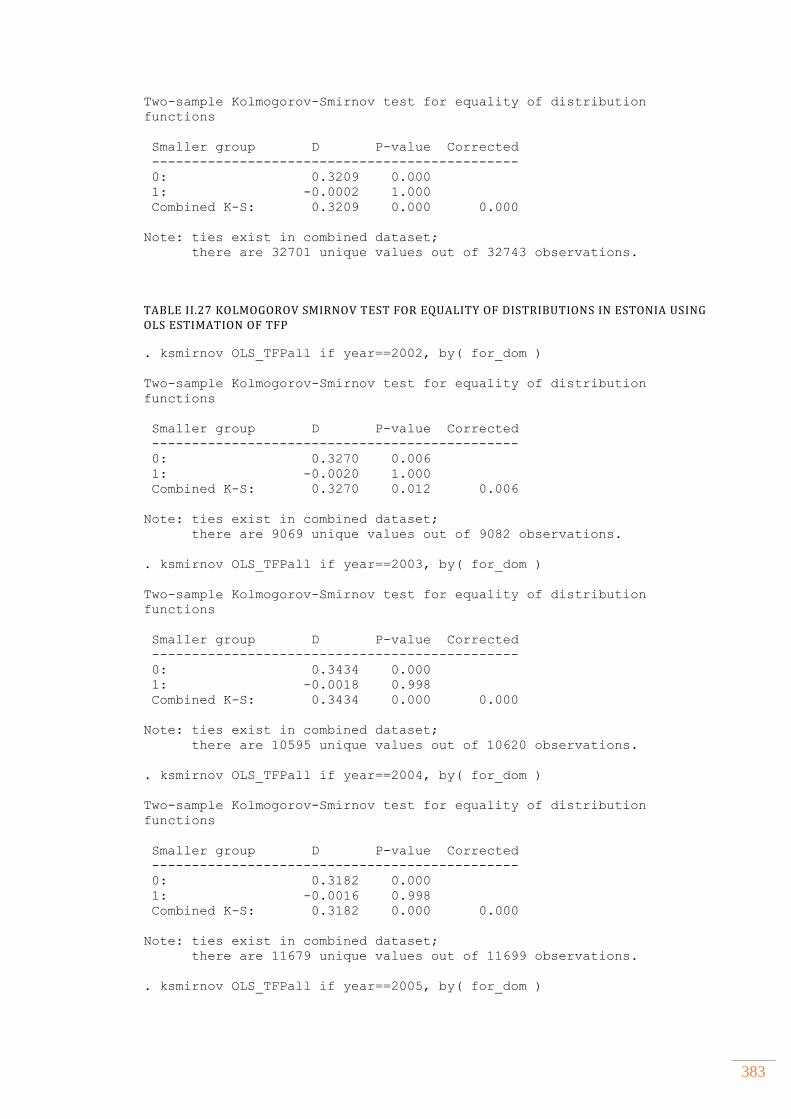
383
Two-sample Kolmogorov-Smirnov test for equality of distribution
functions
Smaller group D P-value Corrected
----------------------------------------------
0: 0.3209 0.000
1: -0.0002 1.000
Combined K-S: 0.3209 0.000 0.000
Note: ties exist in combined dataset;
there are 32701 unique values out of 32743 observations.
TABLE II.27 KOLMOGOROV SMIRNOV TEST FOR EQUALITY OF DISTRIBUTIONS IN ESTONIA USING OLS ESTIMATION OF TFP
. ksmirnov OLS_TFPall if year==2002, by( for_dom )
Two-sample Kolmogorov-Smirnov test for equality of distribution
functions
Smaller group D P-value Corrected
----------------------------------------------
0: 0.3270 0.006
1: -0.0020 1.000
Combined K-S: 0.3270 0.012 0.006
Note: ties exist in combined dataset;
there are 9069 unique values out of 9082 observations.
. ksmirnov OLS_TFPall if year==2003, by( for_dom )
Two-sample Kolmogorov-Smirnov test for equality of distribution
functions
Smaller group D P-value Corrected
----------------------------------------------
0: 0.3434 0.000
1: -0.0018 0.998
Combined K-S: 0.3434 0.000 0.000
Note: ties exist in combined dataset;
there are 10595 unique values out of 10620 observations.
. ksmirnov OLS_TFPall if year==2004, by( for_dom )
Two-sample Kolmogorov-Smirnov test for equality of distribution
functions
Smaller group D P-value Corrected
----------------------------------------------
0: 0.3182 0.000
1: -0.0016 0.998
Combined K-S: 0.3182 0.000 0.000
Note: ties exist in combined dataset;
there are 11679 unique values out of 11699 observations.
. ksmirnov OLS_TFPall if year==2005, by( for_dom )
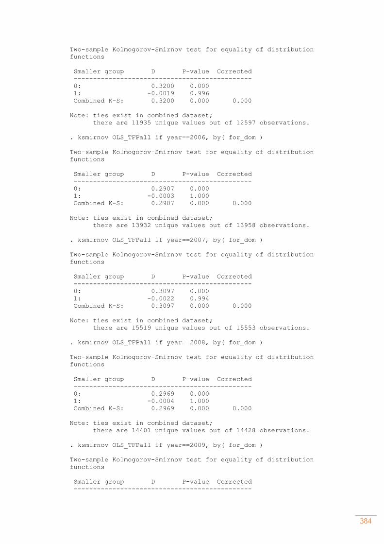
384
Two-sample Kolmogorov-Smirnov test for equality of distribution
functions
Smaller group D P-value Corrected
----------------------------------------------
0: 0.3200 0.000
1: -0.0019 0.996
Combined K-S: 0.3200 0.000 0.000
Note: ties exist in combined dataset;
there are 11935 unique values out of 12597 observations.
. ksmirnov OLS_TFPall if year==2006, by( for_dom )
Two-sample Kolmogorov-Smirnov test for equality of distribution
functions
Smaller group D P-value Corrected
----------------------------------------------
0: 0.2907 0.000
1: -0.0003 1.000
Combined K-S: 0.2907 0.000 0.000
Note: ties exist in combined dataset;
there are 13932 unique values out of 13958 observations.
. ksmirnov OLS_TFPall if year==2007, by( for_dom )
Two-sample Kolmogorov-Smirnov test for equality of distribution
functions
Smaller group D P-value Corrected
----------------------------------------------
0: 0.3097 0.000
1: -0.0022 0.994
Combined K-S: 0.3097 0.000 0.000
Note: ties exist in combined dataset;
there are 15519 unique values out of 15553 observations.
. ksmirnov OLS_TFPall if year==2008, by( for_dom )
Two-sample Kolmogorov-Smirnov test for equality of distribution
functions
Smaller group D P-value Corrected
----------------------------------------------
0: 0.2969 0.000
1: -0.0004 1.000
Combined K-S: 0.2969 0.000 0.000
Note: ties exist in combined dataset;
there are 14401 unique values out of 14428 observations.
. ksmirnov OLS_TFPall if year==2009, by( for_dom )
Two-sample Kolmogorov-Smirnov test for equality of distribution
functions
Smaller group D P-value Corrected
----------------------------------------------
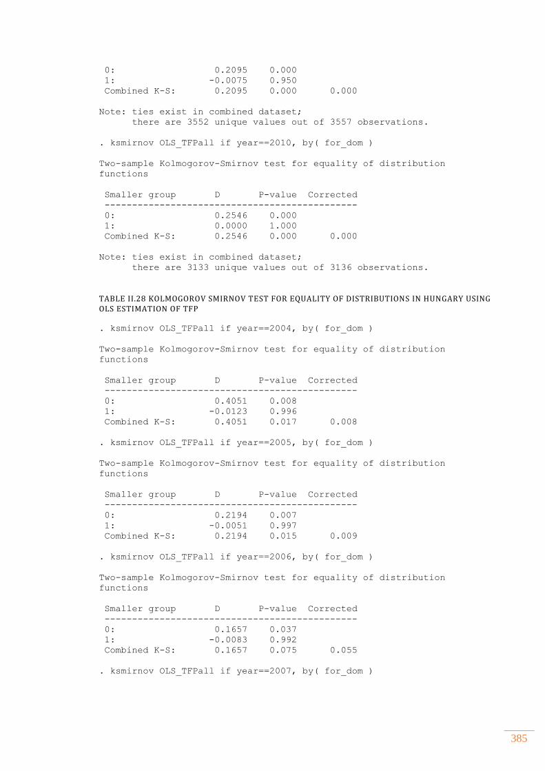
385
0: 0.2095 0.000
1: -0.0075 0.950
Combined K-S: 0.2095 0.000 0.000
Note: ties exist in combined dataset;
there are 3552 unique values out of 3557 observations.
. ksmirnov OLS_TFPall if year==2010, by( for_dom )
Two-sample Kolmogorov-Smirnov test for equality of distribution
functions
Smaller group D P-value Corrected
----------------------------------------------
0: 0.2546 0.000
1: 0.0000 1.000
Combined K-S: 0.2546 0.000 0.000
Note: ties exist in combined dataset;
there are 3133 unique values out of 3136 observations.
TABLE II.28 KOLMOGOROV SMIRNOV TEST FOR EQUALITY OF DISTRIBUTIONS IN HUNGARY USING OLS ESTIMATION OF TFP
. ksmirnov OLS_TFPall if year==2004, by( for_dom )
Two-sample Kolmogorov-Smirnov test for equality of distribution
functions
Smaller group D P-value Corrected
----------------------------------------------
0: 0.4051 0.008
1: -0.0123 0.996
Combined K-S: 0.4051 0.017 0.008
. ksmirnov OLS_TFPall if year==2005, by( for_dom )
Two-sample Kolmogorov-Smirnov test for equality of distribution
functions
Smaller group D P-value Corrected
----------------------------------------------
0: 0.2194 0.007
1: -0.0051 0.997
Combined K-S: 0.2194 0.015 0.009
. ksmirnov OLS_TFPall if year==2006, by( for_dom )
Two-sample Kolmogorov-Smirnov test for equality of distribution
functions
Smaller group D P-value Corrected
----------------------------------------------
0: 0.1657 0.037
1: -0.0083 0.992
Combined K-S: 0.1657 0.075 0.055
. ksmirnov OLS_TFPall if year==2007, by( for_dom )
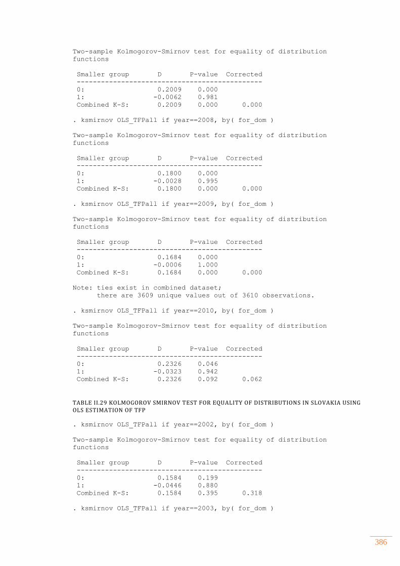
386
Two-sample Kolmogorov-Smirnov test for equality of distribution
functions
Smaller group D P-value Corrected
----------------------------------------------
0: 0.2009 0.000
1: -0.0062 0.981
Combined K-S: 0.2009 0.000 0.000
. ksmirnov OLS_TFPall if year==2008, by( for_dom )
Two-sample Kolmogorov-Smirnov test for equality of distribution
functions
Smaller group D P-value Corrected
----------------------------------------------
0: 0.1800 0.000
1: -0.0028 0.995
Combined K-S: 0.1800 0.000 0.000
. ksmirnov OLS_TFPall if year==2009, by( for_dom )
Two-sample Kolmogorov-Smirnov test for equality of distribution
functions
Smaller group D P-value Corrected
----------------------------------------------
0: 0.1684 0.000
1: -0.0006 1.000
Combined K-S: 0.1684 0.000 0.000
Note: ties exist in combined dataset;
there are 3609 unique values out of 3610 observations.
. ksmirnov OLS_TFPall if year==2010, by( for_dom )
Two-sample Kolmogorov-Smirnov test for equality of distribution
functions
Smaller group D P-value Corrected
----------------------------------------------
0: 0.2326 0.046
1: -0.0323 0.942
Combined K-S: 0.2326 0.092 0.062
TABLE II.29 KOLMOGOROV SMIRNOV TEST FOR EQUALITY OF DISTRIBUTIONS IN SLOVAKIA USING OLS ESTIMATION OF TFP
. ksmirnov OLS_TFPall if year==2002, by( for_dom )
Two-sample Kolmogorov-Smirnov test for equality of distribution
functions
Smaller group D P-value Corrected
----------------------------------------------
0: 0.1584 0.199
1: -0.0446 0.880
Combined K-S: 0.1584 0.395 0.318
. ksmirnov OLS_TFPall if year==2003, by( for_dom )
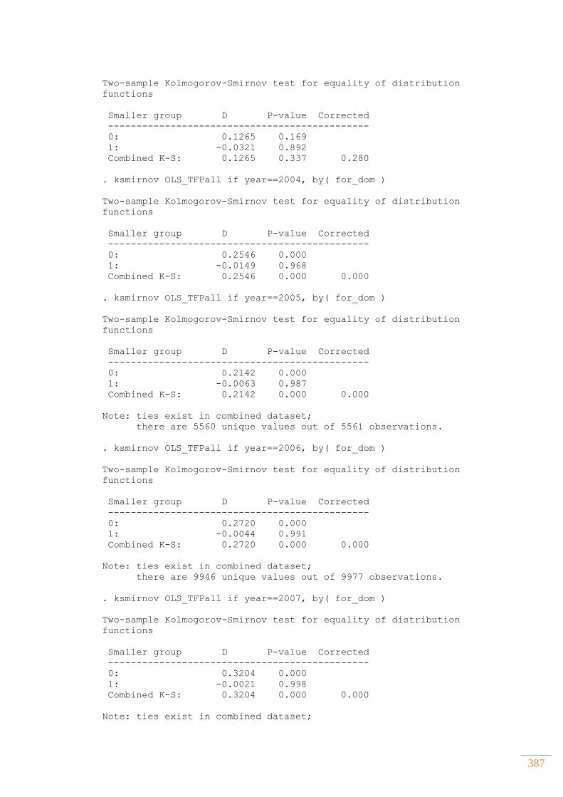
387
Two-sample Kolmogorov-Smirnov test for equality of distribution
functions
Smaller group D P-value Corrected
----------------------------------------------
0: 0.1265 0.169
1: -0.0321 0.892
Combined K-S: 0.1265 0.337 0.280
. ksmirnov OLS_TFPall if year==2004, by( for_dom )
Two-sample Kolmogorov-Smirnov test for equality of distribution
functions
Smaller group D P-value Corrected
----------------------------------------------
0: 0.2546 0.000
1: -0.0149 0.968
Combined K-S: 0.2546 0.000 0.000
. ksmirnov OLS_TFPall if year==2005, by( for_dom )
Two-sample Kolmogorov-Smirnov test for equality of distribution
functions
Smaller group D P-value Corrected
----------------------------------------------
0: 0.2142 0.000
1: -0.0063 0.987
Combined K-S: 0.2142 0.000 0.000
Note: ties exist in combined dataset;
there are 5560 unique values out of 5561 observations.
. ksmirnov OLS_TFPall if year==2006, by( for_dom )
Two-sample Kolmogorov-Smirnov test for equality of distribution
functions
Smaller group D P-value Corrected
----------------------------------------------
0: 0.2720 0.000
1: -0.0044 0.991
Combined K-S: 0.2720 0.000 0.000
Note: ties exist in combined dataset;
there are 9946 unique values out of 9977 observations.
. ksmirnov OLS_TFPall if year==2007, by( for_dom )
Two-sample Kolmogorov-Smirnov test for equality of distribution
functions
Smaller group D P-value Corrected
----------------------------------------------
0: 0.3204 0.000
1: -0.0021 0.998
Combined K-S: 0.3204 0.000 0.000
Note: ties exist in combined dataset;
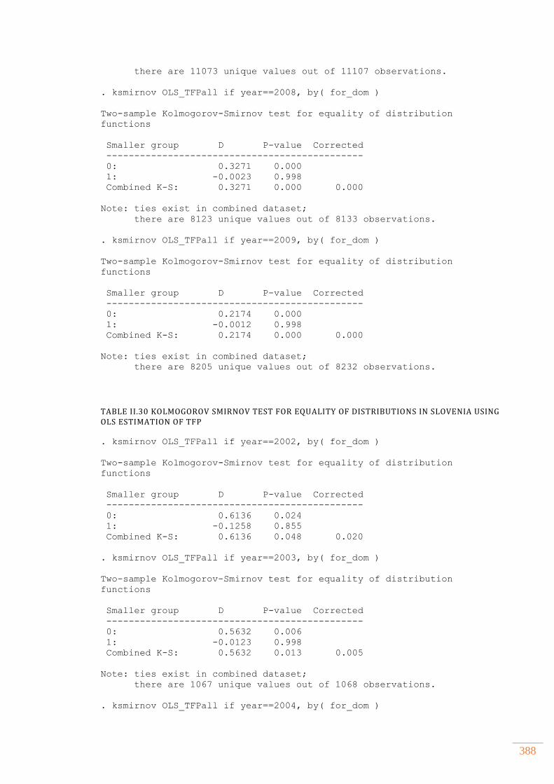
388
there are 11073 unique values out of 11107 observations.
. ksmirnov OLS_TFPall if year==2008, by( for_dom )
Two-sample Kolmogorov-Smirnov test for equality of distribution
functions
Smaller group D P-value Corrected
----------------------------------------------
0: 0.3271 0.000
1: -0.0023 0.998
Combined K-S: 0.3271 0.000 0.000
Note: ties exist in combined dataset;
there are 8123 unique values out of 8133 observations.
. ksmirnov OLS_TFPall if year==2009, by( for_dom )
Two-sample Kolmogorov-Smirnov test for equality of distribution
functions
Smaller group D P-value Corrected
----------------------------------------------
0: 0.2174 0.000
1: -0.0012 0.998
Combined K-S: 0.2174 0.000 0.000
Note: ties exist in combined dataset;
there are 8205 unique values out of 8232 observations.
TABLE II.30 KOLMOGOROV SMIRNOV TEST FOR EQUALITY OF DISTRIBUTIONS IN SLOVENIA USING OLS ESTIMATION OF TFP
. ksmirnov OLS_TFPall if year==2002, by( for_dom )
Two-sample Kolmogorov-Smirnov test for equality of distribution
functions
Smaller group D P-value Corrected
----------------------------------------------
0: 0.6136 0.024
1: -0.1258 0.855
Combined K-S: 0.6136 0.048 0.020
. ksmirnov OLS_TFPall if year==2003, by( for_dom )
Two-sample Kolmogorov-Smirnov test for equality of distribution
functions
Smaller group D P-value Corrected
----------------------------------------------
0: 0.5632 0.006
1: -0.0123 0.998
Combined K-S: 0.5632 0.013 0.005
Note: ties exist in combined dataset;
there are 1067 unique values out of 1068 observations.
. ksmirnov OLS_TFPall if year==2004, by( for_dom )
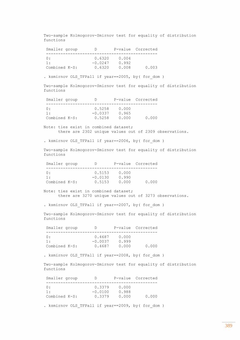
389
Two-sample Kolmogorov-Smirnov test for equality of distribution
functions
Smaller group D P-value Corrected
----------------------------------------------
0: 0.6320 0.004
1: -0.0247 0.992
Combined K-S: 0.6320 0.008 0.003
. ksmirnov OLS_TFPall if year==2005, by( for_dom )
Two-sample Kolmogorov-Smirnov test for equality of distribution
functions
Smaller group D P-value Corrected
----------------------------------------------
0: 0.5258 0.000
1: -0.0337 0.965
Combined K-S: 0.5258 0.000 0.000
Note: ties exist in combined dataset;
there are 2302 unique values out of 2309 observations.
. ksmirnov OLS_TFPall if year==2006, by( for_dom )
Two-sample Kolmogorov-Smirnov test for equality of distribution
functions
Smaller group D P-value Corrected
----------------------------------------------
0: 0.5153 0.000
1: -0.0130 0.990
Combined K-S: 0.5153 0.000 0.000
Note: ties exist in combined dataset;
there are 3270 unique values out of 3273 observations.
. ksmirnov OLS_TFPall if year==2007, by( for_dom )
Two-sample Kolmogorov-Smirnov test for equality of distribution
functions
Smaller group D P-value Corrected
----------------------------------------------
0: 0.4687 0.000
1: -0.0037 0.999
Combined K-S: 0.4687 0.000 0.000
. ksmirnov OLS_TFPall if year==2008, by( for_dom )
Two-sample Kolmogorov-Smirnov test for equality of distribution
functions
Smaller group D P-value Corrected
----------------------------------------------
0: 0.3379 0.000
1: -0.0100 0.988
Combined K-S: 0.3379 0.000 0.000
. ksmirnov OLS_TFPall if year==2009, by( for_dom )

390
Two-sample Kolmogorov-Smirnov test for equality of distribution
functions
Smaller group D P-value Corrected
----------------------------------------------
0: 0.3393 0.000
1: -0.0077 0.986
Combined K-S: 0.3393 0.000 0.000
. ksmirnov OLS_TFPall if year==2010, by( for_dom )
Two-sample Kolmogorov-Smirnov test for equality of distribution
functions
Smaller group D P-value Corrected
----------------------------------------------
0: 0.2724 0.007
1: -0.0158 0.983
Combined K-S: 0.2724 0.014 0.008

391
APPENDIX III. SUPPLEMENT TO CHAPTER FIVE
3.1 Empirical results for the baseline model of productivity spillovers from FDI presented in Section 5.6.1 ...................................................................................................................... 392
3.2 Empirical results for the effects of MNCs’ origin on productivity of local firms presented in Section 5.6.3 ...................................................................................................................... 403
3.3 Empirical results for the effects of MNCs’ ownership structure on productivity of local firms presented in Section 5.6.2 .......................................................................................................... 413
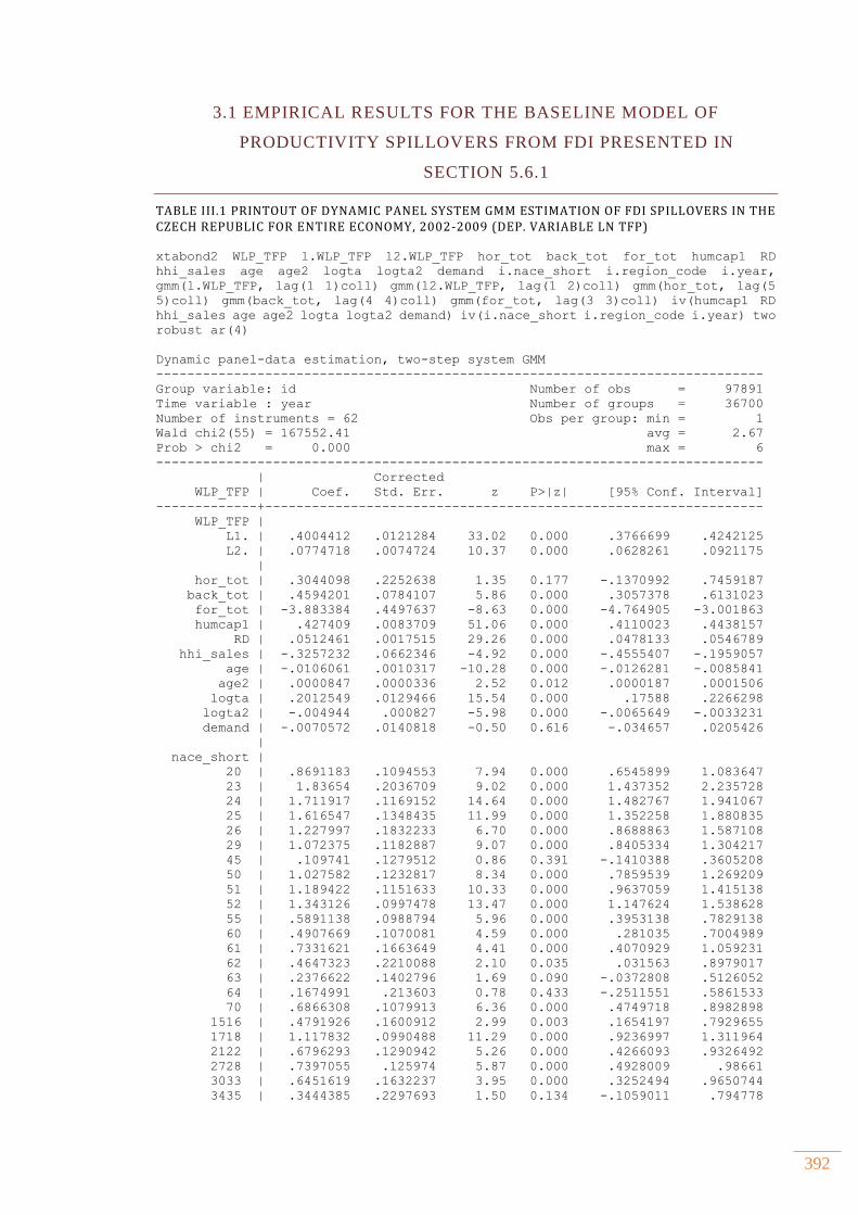
392
3.1 EMPIRICAL RESULTS FOR THE BASELINE MODEL OF
PRODUCTIVITY SPILLOVERS FROM FDI PRESENTED IN
SECTION 5.6.1
TABLE III.1 PRINTOUT OF DYNAMIC PANEL SYSTEM GMM ESTIMATION OF FDI SPILLOVERS IN THE CZECH REPUBLIC FOR ENTIRE ECONOMY, 2002-2009 (DEP. VARIABLE LN TFP)
xtabond2 WLP_TFP l.WLP_TFP l2.WLP_TFP hor_tot back_tot for_tot humcap1 RD
hhi_sales age age2 logta logta2 demand i.nace_short i.region_code i.year,
gmm(l.WLP_TFP, lag(1 1)coll) gmm(l2.WLP_TFP, lag(1 2)coll) gmm(hor_tot, lag(5
5)coll) gmm(back_tot, lag(4 4)coll) gmm(for_tot, lag(3 3)coll) iv(humcap1 RD
hhi_sales age age2 logta logta2 demand) iv(i.nace_short i.region_code i.year) two
robust ar(4)
Dynamic panel-data estimation, two-step system GMM
------------------------------------------------------------------------------
Group variable: id Number of obs = 97891
Time variable : year Number of groups = 36700
Number of instruments = 62 Obs per group: min = 1
Wald chi2(55) = 167552.41 avg = 2.67
Prob > chi2 = 0.000 max = 6
------------------------------------------------------------------------------
| Corrected
WLP_TFP | Coef. Std. Err. z P>|z| [95% Conf. Interval]
-------------+----------------------------------------------------------------
WLP_TFP |
L1. | .4004412 .0121284 33.02 0.000 .3766699 .4242125
L2. | .0774718 .0074724 10.37 0.000 .0628261 .0921175
|
hor_tot | .3044098 .2252638 1.35 0.177 -.1370992 .7459187
back_tot | .4594201 .0784107 5.86 0.000 .3057378 .6131023
for_tot | -3.883384 .4497637 -8.63 0.000 -4.764905 -3.001863
humcap1 | .427409 .0083709 51.06 0.000 .4110023 .4438157
RD | .0512461 .0017515 29.26 0.000 .0478133 .0546789
hhi_sales | -.3257232 .0662346 -4.92 0.000 -.4555407 -.1959057
age | -.0106061 .0010317 -10.28 0.000 -.0126281 -.0085841
age2 | .0000847 .0000336 2.52 0.012 .0000187 .0001506
logta | .2012549 .0129466 15.54 0.000 .17588 .2266298
logta2 | -.004944 .000827 -5.98 0.000 -.0065649 -.0033231
demand | -.0070572 .0140818 -0.50 0.616 -.034657 .0205426
|
nace_short |
20 | .8691183 .1094553 7.94 0.000 .6545899 1.083647
23 | 1.83654 .2036709 9.02 0.000 1.437352 2.235728
24 | 1.711917 .1169152 14.64 0.000 1.482767 1.941067
25 | 1.616547 .1348435 11.99 0.000 1.352258 1.880835
26 | 1.227997 .1832233 6.70 0.000 .8688863 1.587108
29 | 1.072375 .1182887 9.07 0.000 .8405334 1.304217
45 | .109741 .1279512 0.86 0.391 -.1410388 .3605208
50 | 1.027582 .1232817 8.34 0.000 .7859539 1.269209
51 | 1.189422 .1151633 10.33 0.000 .9637059 1.415138
52 | 1.343126 .0997478 13.47 0.000 1.147624 1.538628
55 | .5891138 .0988794 5.96 0.000 .3953138 .7829138
60 | .4907669 .1070081 4.59 0.000 .281035 .7004989
61 | .7331621 .1663649 4.41 0.000 .4070929 1.059231
62 | .4647323 .2210088 2.10 0.035 .031563 .8979017
63 | .2376622 .1402796 1.69 0.090 -.0372808 .5126052
64 | .1674991 .213603 0.78 0.433 -.2511551 .5861533
70 | .6866308 .1079913 6.36 0.000 .4749718 .8982898
1516 | .4791926 .1600912 2.99 0.003 .1654197 .7929655
1718 | 1.117832 .0990488 11.29 0.000 .9236997 1.311964
2122 | .6796293 .1290942 5.26 0.000 .4266093 .9326492
2728 | .7397055 .125974 5.87 0.000 .4928009 .98661
3033 | .6451619 .1632237 3.95 0.000 .3252494 .9650744
3435 | .3444385 .2297693 1.50 0.134 -.1059011 .794778
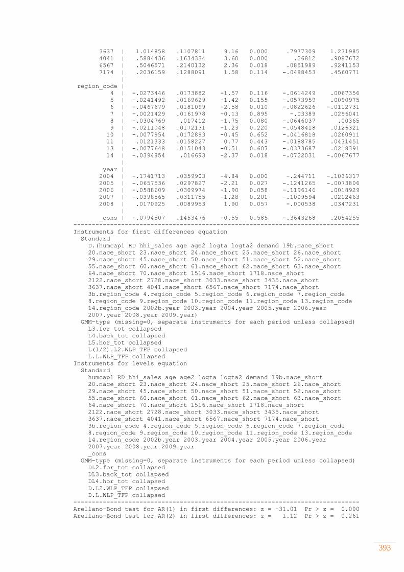
393
3637 | 1.014858 .1107811 9.16 0.000 .7977309 1.231985
4041 | .5884436 .1634334 3.60 0.000 .26812 .9087672
6567 | .5046571 .2140132 2.36 0.018 .0851989 .9241153
7174 | .2036159 .1288091 1.58 0.114 -.0488453 .4560771
|
region_code |
4 | -.0273446 .0173882 -1.57 0.116 -.0614249 .0067356
5 | -.0241492 .0169629 -1.42 0.155 -.0573959 .0090975
6 | -.0467679 .0181099 -2.58 0.010 -.0822626 -.0112731
7 | -.0021429 .0161978 -0.13 0.895 -.03389 .0296041
8 | -.0304769 .017412 -1.75 0.080 -.0646037 .00365
9 | -.0211048 .0172131 -1.23 0.220 -.0548418 .0126321
10 | -.0077954 .0172893 -0.45 0.652 -.0416818 .0260911
11 | .0121333 .0158227 0.77 0.443 -.0188785 .0431451
13 | -.0077648 .0151043 -0.51 0.607 -.0373687 .0218391
14 | -.0394854 .016693 -2.37 0.018 -.0722031 -.0067677
|
year |
2004 | -.1741713 .0359903 -4.84 0.000 -.244711 -.1036317
2005 | -.0657536 .0297827 -2.21 0.027 -.1241265 -.0073806
2006 | -.0588609 .0309974 -1.90 0.058 -.1196146 .0018929
2007 | -.0398565 .0311755 -1.28 0.201 -.1009594 .0212463
2008 | .0170925 .0089953 1.90 0.057 -.000538 .0347231
|
_cons | -.0794507 .1453476 -0.55 0.585 -.3643268 .2054255
------------------------------------------------------------------------------
Instruments for first differences equation
Standard
D.(humcap1 RD hhi_sales age age2 logta logta2 demand 19b.nace_short
20.nace_short 23.nace_short 24.nace_short 25.nace_short 26.nace_short
29.nace_short 45.nace_short 50.nace_short 51.nace_short 52.nace_short
55.nace_short 60.nace_short 61.nace_short 62.nace_short 63.nace_short
64.nace_short 70.nace_short 1516.nace_short 1718.nace_short
2122.nace_short 2728.nace_short 3033.nace_short 3435.nace_short
3637.nace_short 4041.nace_short 6567.nace_short 7174.nace_short
3b.region_code 4.region_code 5.region_code 6.region_code 7.region_code
8.region_code 9.region_code 10.region_code 11.region_code 13.region_code
14.region_code 2002b.year 2003.year 2004.year 2005.year 2006.year
2007.year 2008.year 2009.year)
GMM-type (missing=0, separate instruments for each period unless collapsed)
L3.for_tot collapsed
L4.back_tot collapsed
L5.hor_tot collapsed
L(1/2).L2.WLP_TFP collapsed
L.L.WLP_TFP collapsed
Instruments for levels equation
Standard
humcap1 RD hhi_sales age age2 logta logta2 demand 19b.nace_short
20.nace_short 23.nace_short 24.nace_short 25.nace_short 26.nace_short
29.nace_short 45.nace_short 50.nace_short 51.nace_short 52.nace_short
55.nace_short 60.nace_short 61.nace_short 62.nace_short 63.nace_short
64.nace_short 70.nace_short 1516.nace_short 1718.nace_short
2122.nace_short 2728.nace_short 3033.nace_short 3435.nace_short
3637.nace_short 4041.nace_short 6567.nace_short 7174.nace_short
3b.region_code 4.region_code 5.region_code 6.region_code 7.region_code
8.region_code 9.region_code 10.region_code 11.region_code 13.region_code
14.region_code 2002b.year 2003.year 2004.year 2005.year 2006.year
2007.year 2008.year 2009.year
_cons
GMM-type (missing=0, separate instruments for each period unless collapsed)
DL2.for_tot collapsed
DL3.back_tot collapsed
DL4.hor_tot collapsed
D.L2.WLP_TFP collapsed
D.L.WLP_TFP collapsed
------------------------------------------------------------------------------
Arellano-Bond test for AR(1) in first differences: z = -31.01 Pr > z = 0.000
Arellano-Bond test for AR(2) in first differences: z = 1.12 Pr > z = 0.261
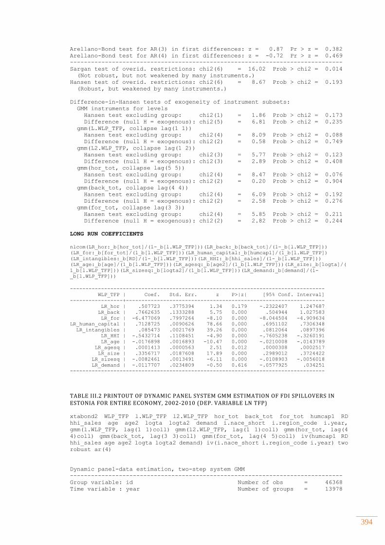
394
Arellano-Bond test for AR(3) in first differences: z = 0.87 Pr > z = 0.382
Arellano-Bond test for AR(4) in first differences: z = -0.72 Pr > z = 0.469
------------------------------------------------------------------------------
Sargan test of overid. restrictions: chi2(6) = 16.02 Prob > chi2 = 0.014
(Not robust, but not weakened by many instruments.)
Hansen test of overid. restrictions: chi2(6) = 8.67 Prob > chi2 = 0.193
(Robust, but weakened by many instruments.)
Difference-in-Hansen tests of exogeneity of instrument subsets:
GMM instruments for levels
Hansen test excluding group: chi2(1) = 1.86 Prob > chi2 = 0.173
Difference (null H = exogenous): chi2(5) = 6.81 Prob > chi2 = 0.235
gmm(L.WLP_TFP, collapse lag(1 1))
Hansen test excluding group: chi2(4) = 8.09 Prob > chi2 = 0.088
Difference (null H = exogenous): chi2(2) = 0.58 Prob > chi2 = 0.749
gmm(L2.WLP_TFP, collapse lag(1 2))
Hansen test excluding group: chi2(3) = 5.77 Prob > chi2 = 0.123
Difference (null H = exogenous): chi2(3) = 2.89 Prob > chi2 = 0.408
gmm(hor_tot, collapse lag(5 5))
Hansen test excluding group: chi2(4) = 8.47 Prob > chi2 = 0.076
Difference (null H = exogenous): chi2(2) = 0.20 Prob > chi2 = 0.904
gmm(back_tot, collapse lag(4 4))
Hansen test excluding group: chi2(4) = 6.09 Prob > chi2 = 0.192
Difference (null H = exogenous): chi2(2) = 2.58 Prob > chi2 = 0.276
gmm(for_tot, collapse lag(3 3))
Hansen test excluding group: chi2(4) = 5.85 Prob > chi2 = 0.211
Difference (null H = exogenous): chi2(2) = 2.82 Prob > chi2 = 0.244
LONG RUN COEFFICIENTS
nlcom(LR_hor:_b[hor_tot]/(1-_b[l.WLP_TFP]))(LR_back:_b[back_tot]/(1-_b[l.WLP_TFP]))
(LR_for:_b[for_tot]/(1_b[l.WLP_TFP]))(LR_human_capital:_b[humcap1]/(1_b[l.WLP_TFP])
(LR_intangibles:_b[RD]/(1-_b[l.WLP_TFP]))(LR_HHI:_b[hhi_sales]/(1-_b[l.WLP_TFP]))
(LR_age:_b[age]/(1_b[l.WLP_TFP]))(LR_agesq:_b[age2]/(1_b[l.WLP_TFP]))(LR_size:_b[logta]/(
1_b[l.WLP_TFP]))(LR_sizesq:_b[logta2]/(1_b[l.WLP_TFP]))(LR_demand:_b[demand]/(1-
_b[l.WLP_TFP]))
----------------------------------------------------------------------------------
WLP_TFP | Coef. Std. Err. z P>|z| [95% Conf. Interval]
-----------------+----------------------------------------------------------------
LR_hor | .507723 .3775394 1.34 0.179 -.2322407 1.247687
LR_back | .7662635 .1333288 5.75 0.000 .504944 1.027583
LR_for | -6.477069 .7997264 -8.10 0.000 -8.044504 -4.909634
LR_human_capital | .7128725 .0090626 78.66 0.000 .6951102 .7306348
LR_intangibles | .085473 .0021769 39.26 0.000 .0812064 .0897396
LR_HHI | -.5432714 .1108451 -4.90 0.000 -.7605238 -.3260191
LR_age | -.0176898 .0016893 -10.47 0.000 -.0210008 -.0143789
LR_agesq | .0001413 .0000563 2.51 0.012 .0000308 .0002517
LR_size | .3356717 .0187608 17.89 0.000 .2989012 .3724422
LR_sizesq | -.0082461 .0013491 -6.11 0.000 -.0108903 -.0056018
LR_demand | -.0117707 .0234809 -0.50 0.616 -.0577925 .034251
----------------------------------------------------------------------------------
TABLE III.2 PRINTOUT OF DYNAMIC PANEL SYSTEM GMM ESTIMATION OF FDI SPILLOVERS IN ESTONIA FOR ENTIRE ECONOMY, 2002-2010 (DEP. VARIABLE LN TFP)
xtabond2 WLP_TFP l.WLP_TFP l2.WLP_TFP hor_tot back_tot for_tot humcap1 RD
hhi_sales age age2 logta logta2 demand i.nace_short i.region_code i.year,
gmm(l.WLP_TFP, lag(1 1)coll) gmm(l2.WLP_TFP, lag(1 1)coll) gmm(hor_tot, lag(4
4)coll) gmm(back_tot, lag(3 3)coll) gmm(for_tot, lag(4 5)coll) iv(humcap1 RD
hhi_sales age age2 logta logta2 demand) iv(i.nace_short i.region_code i.year) two
robust ar(4)
Dynamic panel-data estimation, two-step system GMM
------------------------------------------------------------------------------
Group variable: id Number of obs = 46368
Time variable : year Number of groups = 13978
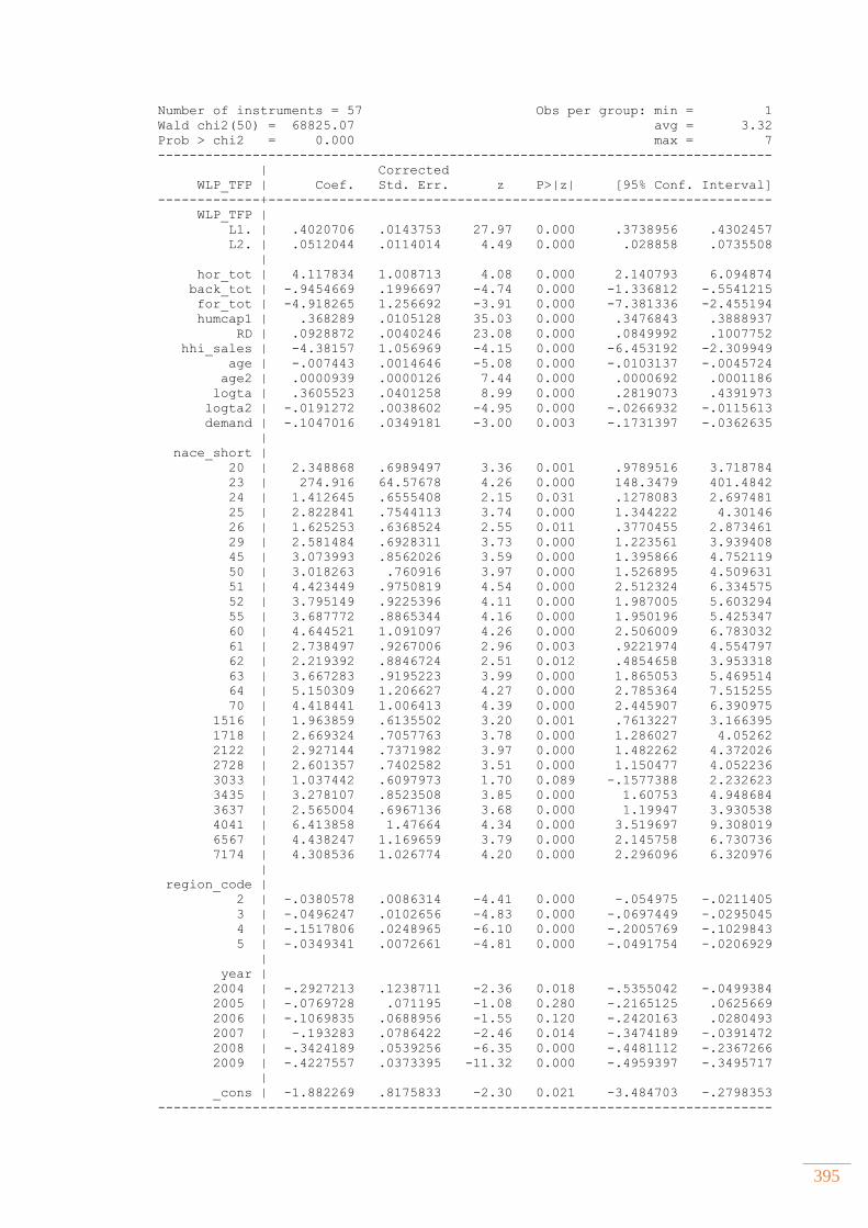
395
Number of instruments = 57 Obs per group: min = 1
Wald chi2(50) = 68825.07 avg = 3.32
Prob > chi2 = 0.000 max = 7
------------------------------------------------------------------------------
| Corrected
WLP_TFP | Coef. Std. Err. z P>|z| [95% Conf. Interval]
-------------+----------------------------------------------------------------
WLP_TFP |
L1. | .4020706 .0143753 27.97 0.000 .3738956 .4302457
L2. | .0512044 .0114014 4.49 0.000 .028858 .0735508
|
hor_tot | 4.117834 1.008713 4.08 0.000 2.140793 6.094874
back_tot | -.9454669 .1996697 -4.74 0.000 -1.336812 -.5541215
for_tot | -4.918265 1.256692 -3.91 0.000 -7.381336 -2.455194
humcap1 | .368289 .0105128 35.03 0.000 .3476843 .3888937
RD | .0928872 .0040246 23.08 0.000 .0849992 .1007752
hhi_sales | -4.38157 1.056969 -4.15 0.000 -6.453192 -2.309949
age | -.007443 .0014646 -5.08 0.000 -.0103137 -.0045724
age2 | .0000939 .0000126 7.44 0.000 .0000692 .0001186
logta | .3605523 .0401258 8.99 0.000 .2819073 .4391973
logta2 | -.0191272 .0038602 -4.95 0.000 -.0266932 -.0115613
demand | -.1047016 .0349181 -3.00 0.003 -.1731397 -.0362635
|
nace_short |
20 | 2.348868 .6989497 3.36 0.001 .9789516 3.718784
23 | 274.916 64.57678 4.26 0.000 148.3479 401.4842
24 | 1.412645 .6555408 2.15 0.031 .1278083 2.697481
25 | 2.822841 .7544113 3.74 0.000 1.344222 4.30146
26 | 1.625253 .6368524 2.55 0.011 .3770455 2.873461
29 | 2.581484 .6928311 3.73 0.000 1.223561 3.939408
45 | 3.073993 .8562026 3.59 0.000 1.395866 4.752119
50 | 3.018263 .760916 3.97 0.000 1.526895 4.509631
51 | 4.423449 .9750819 4.54 0.000 2.512324 6.334575
52 | 3.795149 .9225396 4.11 0.000 1.987005 5.603294
55 | 3.687772 .8865344 4.16 0.000 1.950196 5.425347
60 | 4.644521 1.091097 4.26 0.000 2.506009 6.783032
61 | 2.738497 .9267006 2.96 0.003 .9221974 4.554797
62 | 2.219392 .8846724 2.51 0.012 .4854658 3.953318
63 | 3.667283 .9195223 3.99 0.000 1.865053 5.469514
64 | 5.150309 1.206627 4.27 0.000 2.785364 7.515255
70 | 4.418441 1.006413 4.39 0.000 2.445907 6.390975
1516 | 1.963859 .6135502 3.20 0.001 .7613227 3.166395
1718 | 2.669324 .7057763 3.78 0.000 1.286027 4.05262
2122 | 2.927144 .7371982 3.97 0.000 1.482262 4.372026
2728 | 2.601357 .7402582 3.51 0.000 1.150477 4.052236
3033 | 1.037442 .6097973 1.70 0.089 -.1577388 2.232623
3435 | 3.278107 .8523508 3.85 0.000 1.60753 4.948684
3637 | 2.565004 .6967136 3.68 0.000 1.19947 3.930538
4041 | 6.413858 1.47664 4.34 0.000 3.519697 9.308019
6567 | 4.438247 1.169659 3.79 0.000 2.145758 6.730736
7174 | 4.308536 1.026774 4.20 0.000 2.296096 6.320976
|
region_code |
2 | -.0380578 .0086314 -4.41 0.000 -.054975 -.0211405
3 | -.0496247 .0102656 -4.83 0.000 -.0697449 -.0295045
4 | -.1517806 .0248965 -6.10 0.000 -.2005769 -.1029843
5 | -.0349341 .0072661 -4.81 0.000 -.0491754 -.0206929
|
year |
2004 | -.2927213 .1238711 -2.36 0.018 -.5355042 -.0499384
2005 | -.0769728 .071195 -1.08 0.280 -.2165125 .0625669
2006 | -.1069835 .0688956 -1.55 0.120 -.2420163 .0280493
2007 | -.193283 .0786422 -2.46 0.014 -.3474189 -.0391472
2008 | -.3424189 .0539256 -6.35 0.000 -.4481112 -.2367266
2009 | -.4227557 .0373395 -11.32 0.000 -.4959397 -.3495717
|
_cons | -1.882269 .8175833 -2.30 0.021 -3.484703 -.2798353
------------------------------------------------------------------------------
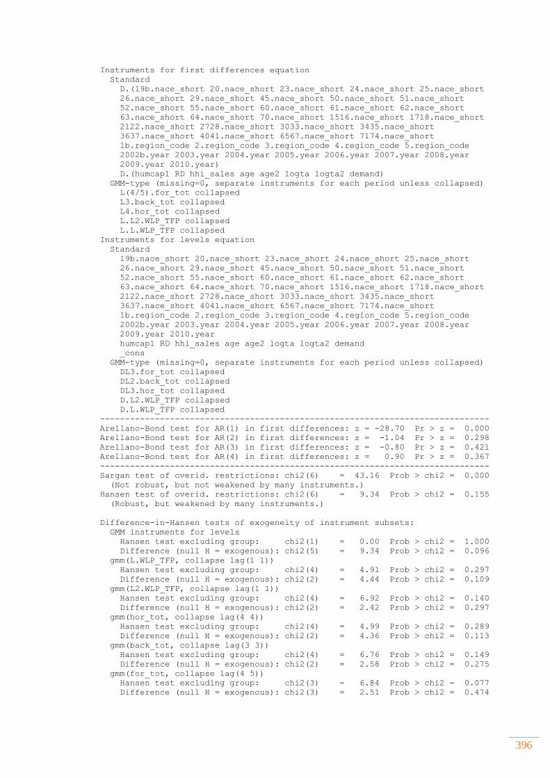
396
Instruments for first differences equation
Standard
D.(19b.nace_short 20.nace_short 23.nace_short 24.nace_short 25.nace_short
26.nace_short 29.nace_short 45.nace_short 50.nace_short 51.nace_short
52.nace_short 55.nace_short 60.nace_short 61.nace_short 62.nace_short
63.nace_short 64.nace_short 70.nace_short 1516.nace_short 1718.nace_short
2122.nace_short 2728.nace_short 3033.nace_short 3435.nace_short
3637.nace_short 4041.nace_short 6567.nace_short 7174.nace_short
1b.region_code 2.region_code 3.region_code 4.region_code 5.region_code
2002b.year 2003.year 2004.year 2005.year 2006.year 2007.year 2008.year
2009.year 2010.year)
D.(humcap1 RD hhi_sales age age2 logta logta2 demand)
GMM-type (missing=0, separate instruments for each period unless collapsed)
L(4/5).for_tot collapsed
L3.back_tot collapsed
L4.hor_tot collapsed
L.L2.WLP_TFP collapsed
L.L.WLP_TFP collapsed
Instruments for levels equation
Standard
19b.nace_short 20.nace_short 23.nace_short 24.nace_short 25.nace_short
26.nace_short 29.nace_short 45.nace_short 50.nace_short 51.nace_short
52.nace_short 55.nace_short 60.nace_short 61.nace_short 62.nace_short
63.nace_short 64.nace_short 70.nace_short 1516.nace_short 1718.nace_short
2122.nace_short 2728.nace_short 3033.nace_short 3435.nace_short
3637.nace_short 4041.nace_short 6567.nace_short 7174.nace_short
1b.region_code 2.region_code 3.region_code 4.region_code 5.region_code
2002b.year 2003.year 2004.year 2005.year 2006.year 2007.year 2008.year
2009.year 2010.year
humcap1 RD hhi_sales age age2 logta logta2 demand
_cons
GMM-type (missing=0, separate instruments for each period unless collapsed)
DL3.for_tot collapsed
DL2.back_tot collapsed
DL3.hor_tot collapsed
D.L2.WLP_TFP collapsed
D.L.WLP_TFP collapsed
------------------------------------------------------------------------------
Arellano-Bond test for AR(1) in first differences: z = -28.70 Pr > z = 0.000
Arellano-Bond test for AR(2) in first differences: z = -1.04 Pr > z = 0.298
Arellano-Bond test for AR(3) in first differences: z = -0.80 Pr > z = 0.421
Arellano-Bond test for AR(4) in first differences: z = 0.90 Pr > z = 0.367
------------------------------------------------------------------------------
Sargan test of overid. restrictions: chi2(6) = 43.16 Prob > chi2 = 0.000
(Not robust, but not weakened by many instruments.)
Hansen test of overid. restrictions: chi2(6) = 9.34 Prob > chi2 = 0.155
(Robust, but weakened by many instruments.)
Difference-in-Hansen tests of exogeneity of instrument subsets:
GMM instruments for levels
Hansen test excluding group: chi2(1) = 0.00 Prob > chi2 = 1.000
Difference (null H = exogenous): chi2(5) = 9.34 Prob > chi2 = 0.096
gmm(L.WLP_TFP, collapse lag(1 1))
Hansen test excluding group: chi2(4) = 4.91 Prob > chi2 = 0.297
Difference (null H = exogenous): chi2(2) = 4.44 Prob > chi2 = 0.109
gmm(L2.WLP_TFP, collapse lag(1 1))
Hansen test excluding group: chi2(4) = 6.92 Prob > chi2 = 0.140
Difference (null H = exogenous): chi2(2) = 2.42 Prob > chi2 = 0.297
gmm(hor_tot, collapse lag(4 4))
Hansen test excluding group: chi2(4) = 4.99 Prob > chi2 = 0.289
Difference (null H = exogenous): chi2(2) = 4.36 Prob > chi2 = 0.113
gmm(back_tot, collapse lag(3 3))
Hansen test excluding group: chi2(4) = 6.76 Prob > chi2 = 0.149
Difference (null H = exogenous): chi2(2) = 2.58 Prob > chi2 = 0.275
gmm(for_tot, collapse lag(4 5))
Hansen test excluding group: chi2(3) = 6.84 Prob > chi2 = 0.077
Difference (null H = exogenous): chi2(3) = 2.51 Prob > chi2 = 0.474
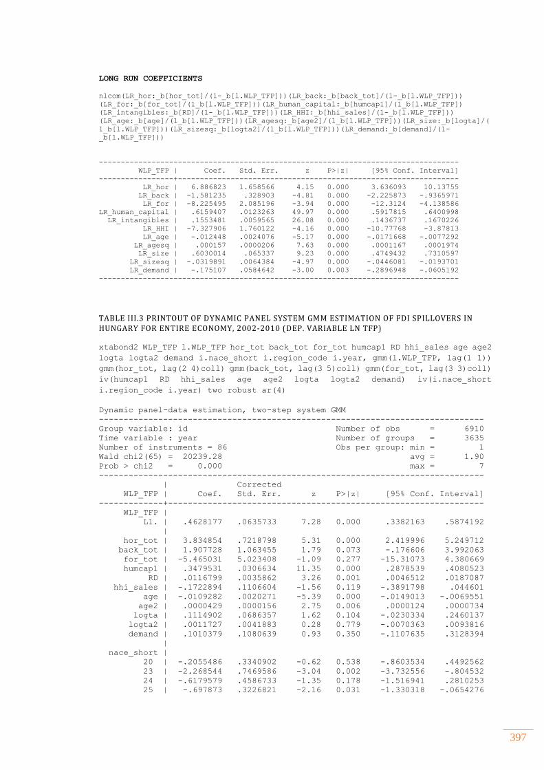
397
LONG RUN COEFFICIENTS
nlcom(LR_hor:_b[hor_tot]/(1-_b[l.WLP_TFP]))(LR_back:_b[back_tot]/(1-_b[l.WLP_TFP]))
(LR_for:_b[for_tot]/(1_b[l.WLP_TFP]))(LR_human_capital:_b[humcap1]/(1_b[l.WLP_TFP])
(LR_intangibles:_b[RD]/(1-_b[l.WLP_TFP]))(LR_HHI:_b[hhi_sales]/(1-_b[l.WLP_TFP]))
(LR_age:_b[age]/(1_b[l.WLP_TFP]))(LR_agesq:_b[age2]/(1_b[l.WLP_TFP]))(LR_size:_b[logta]/(
1_b[l.WLP_TFP]))(LR_sizesq:_b[logta2]/(1_b[l.WLP_TFP]))(LR_demand:_b[demand]/(1-
_b[l.WLP_TFP]))
----------------------------------------------------------------------------------
WLP_TFP | Coef. Std. Err. z P>|z| [95% Conf. Interval]
-----------------+----------------------------------------------------------------
LR_hor | 6.886823 1.658566 4.15 0.000 3.636093 10.13755
LR_back | -1.581235 .328903 -4.81 0.000 -2.225873 -.9365971
LR_for | -8.225495 2.085196 -3.94 0.000 -12.3124 -4.138586
LR_human_capital | .6159407 .0123263 49.97 0.000 .5917815 .6400998
LR_intangibles | .1553481 .0059565 26.08 0.000 .1436737 .1670226
LR_HHI | -7.327906 1.760122 -4.16 0.000 -10.77768 -3.87813
LR_age | -.012448 .0024076 -5.17 0.000 -.0171668 -.0077292
LR_agesq | .000157 .0000206 7.63 0.000 .0001167 .0001974
LR_size | .6030014 .065337 9.23 0.000 .4749432 .7310597
LR_sizesq | -.0319891 .0064384 -4.97 0.000 -.0446081 -.0193701
LR_demand | -.175107 .0584642 -3.00 0.003 -.2896948 -.0605192
----------------------------------------------------------------------------------
TABLE III.3 PRINTOUT OF DYNAMIC PANEL SYSTEM GMM ESTIMATION OF FDI SPILLOVERS IN HUNGARY FOR ENTIRE ECONOMY, 2002-2010 (DEP. VARIABLE LN TFP)
xtabond2 WLP_TFP l.WLP_TFP hor_tot back_tot for_tot humcap1 RD hhi_sales age age2
logta logta2 demand i.nace_short i.region_code i.year, gmm(l.WLP_TFP, lag(1 1))
gmm(hor_tot, lag(2 4)coll) gmm(back_tot, lag(3 5)coll) gmm(for_tot, lag(3 3)coll)
iv(humcap1 RD hhi_sales age age2 logta logta2 demand) iv(i.nace_short
i.region_code i.year) two robust ar(4)
Dynamic panel-data estimation, two-step system GMM
------------------------------------------------------------------------------
Group variable: id Number of obs = 6910
Time variable : year Number of groups = 3635
Number of instruments = 86 Obs per group: min = 1
Wald chi2(65) = 20239.28 avg = 1.90
Prob > chi2 = 0.000 max = 7
------------------------------------------------------------------------------
| Corrected
WLP_TFP | Coef. Std. Err. z P>|z| [95% Conf. Interval]
-------------+----------------------------------------------------------------
WLP_TFP |
L1. | .4628177 .0635733 7.28 0.000 .3382163 .5874192
|
hor_tot | 3.834854 .7218798 5.31 0.000 2.419996 5.249712
back_tot | 1.907728 1.063455 1.79 0.073 -.176606 3.992063
for_tot | -5.465031 5.023408 -1.09 0.277 -15.31073 4.380669
humcap1 | .3479531 .0306634 11.35 0.000 .2878539 .4080523
RD | .0116799 .0035862 3.26 0.001 .0046512 .0187087
hhi_sales | -.1722894 .1106604 -1.56 0.119 -.3891798 .044601
age | -.0109282 .0020271 -5.39 0.000 -.0149013 -.0069551
age2 | .0000429 .0000156 2.75 0.006 .0000124 .0000734
logta | .1114902 .0686357 1.62 0.104 -.0230334 .2460137
logta2 | .0011727 .0041883 0.28 0.779 -.0070363 .0093816
demand | .1010379 .1080639 0.93 0.350 -.1107635 .3128394
|
nace_short |
20 | -.2055486 .3340902 -0.62 0.538 -.8603534 .4492562
23 | -2.268544 .7469586 -3.04 0.002 -3.732556 -.804532
24 | -.6179579 .4586733 -1.35 0.178 -1.516941 .2810253
25 | -.697873 .3226821 -2.16 0.031 -1.330318 -.0654276
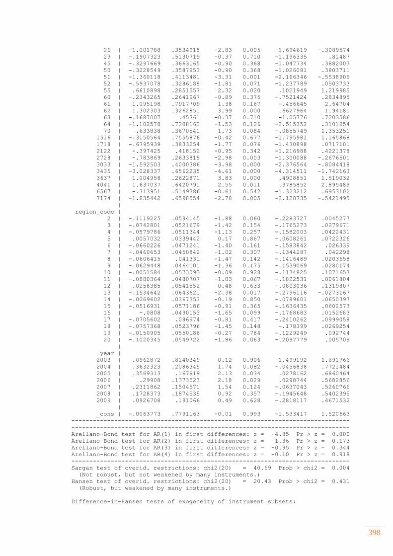
398
26 | -1.001788 .3534915 -2.83 0.005 -1.694619 -.3089574
29 | -.1907323 .5130719 -0.37 0.710 -1.196335 .81487
45 | -.3297669 .3663165 -0.90 0.368 -1.047734 .3882003
50 | -.3228549 .3587953 -0.90 0.368 -1.026081 .3803711
51 | -1.360118 .4113481 -3.31 0.001 -2.166346 -.5538909
52 | -.5937078 .3286188 -1.81 0.071 -1.237789 .0503733
55 | .6610898 .2851557 2.32 0.020 .1021949 1.219985
60 | -.2343265 .2641967 -0.89 0.375 -.7521424 .2834895
61 | 1.095198 .7917709 1.38 0.167 -.456645 2.64704
62 | 1.302303 .3262851 3.99 0.000 .6627964 1.94181
63 | -.1687007 .45361 -0.37 0.710 -1.05776 .7203586
64 | -1.102578 .7208162 -1.53 0.126 -2.515352 .3101954
70 | .633838 .3670541 1.73 0.084 -.0855749 1.353251
1516 | -.3150564 .7555876 -0.42 0.677 -1.795981 1.165868
1718 | -.6795939 .3833254 -1.77 0.076 -1.430898 .0717101
2122 | -.397425 .418152 -0.95 0.342 -1.216988 .4221378
2728 | -.783869 .2633819 -2.98 0.003 -1.300088 -.2676501
3033 | -1.592503 .4000386 -3.98 0.000 -2.376564 -.8084418
3435 | -3.028337 .6562235 -4.61 0.000 -4.314511 -1.742163
3637 | 1.004958 .2622871 3.83 0.000 .4908851 1.519032
4041 | 1.637037 .6420791 2.55 0.011 .3785852 2.895489
6567 | -.313951 .5149386 -0.61 0.542 -1.323212 .6953102
7174 | -1.835442 .6598554 -2.78 0.005 -3.128735 -.5421495
|
region_code |
2 | -.1119225 .0594145 -1.88 0.060 -.2283727 .0045277
3 | -.0742801 .0521679 -1.42 0.154 -.1765273 .0279671
4 | -.0579786 .0511344 -1.13 0.257 -.1582003 .0422431
5 | .0057032 .0339442 0.17 0.867 -.0608261 .0722326
6 | -.0660226 .0471241 -1.40 0.161 -.1583842 .026339
7 | -.0460653 .0450842 -1.02 0.307 -.1344287 .042298
8 | -.0606415 .041331 -1.47 0.142 -.1416489 .0203658
9 | -.0629448 .0464101 -1.36 0.175 -.1539069 .0280174
10 | -.0051584 .0573093 -0.09 0.928 -.1174825 .1071657
11 | -.0880364 .0480707 -1.83 0.067 -.1822531 .0061804
12 | .0258385 .0541552 0.48 0.633 -.0803036 .1319807
13 | -.1534642 .0643621 -2.38 0.017 -.2796116 -.0273167
14 | -.0069602 .0367353 -0.19 0.850 -.0789601 .0650397
15 | -.0516931 .0571186 -0.91 0.365 -.1636435 .0602573
16 | -.0808 .0490153 -1.65 0.099 -.1768683 .0152683
17 | -.0705602 .086974 -0.81 0.417 -.2410262 .0999058
18 | -.0757368 .0523796 -1.45 0.148 -.178399 .0269254
19 | -.0150905 .0550186 -0.27 0.784 -.1229249 .092744
20 | -.1020345 .0549722 -1.86 0.063 -.2097779 .005709
|
year |
2003 | .0962872 .8140349 0.12 0.906 -1.499192 1.691766
2004 | .3632323 .2086345 1.74 0.082 -.0456838 .7721484
2005 | .3569313 .167919 2.13 0.034 .0278162 .6860464
2006 | .29908 .1373523 2.18 0.029 .0298744 .5682856
2007 | .2311862 .1504571 1.54 0.124 -.0637043 .5260766
2008 | .1728373 .1874535 0.92 0.357 -.1945648 .5402395
2009 | .0926708 .191066 0.49 0.628 -.2818117 .4671532
|
_cons | -.0063773 .7791163 -0.01 0.993 -1.533417 1.520663
------------------------------------------------------------------------------
------------------------------------------------------------------------------
Arellano-Bond test for AR(1) in first differences: z = -4.85 Pr > z = 0.000
Arellano-Bond test for AR(2) in first differences: z = 1.36 Pr > z = 0.173
Arellano-Bond test for AR(3) in first differences: z = -0.95 Pr > z = 0.344
Arellano-Bond test for AR(4) in first differences: z = -0.10 Pr > z = 0.918
------------------------------------------------------------------------------
Sargan test of overid. restrictions: chi2(20) = 40.69 Prob > chi2 = 0.004
(Not robust, but not weakened by many instruments.)
Hansen test of overid. restrictions: chi2(20) = 20.43 Prob > chi2 = 0.431
(Robust, but weakened by many instruments.)
Difference-in-Hansen tests of exogeneity of instrument subsets:
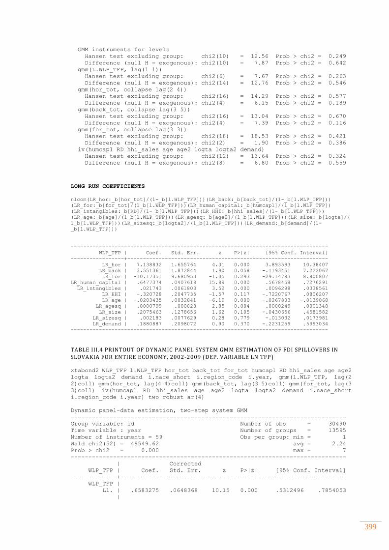
399
GMM instruments for levels
Hansen test excluding group: chi2(10) = 12.56 Prob > chi2 = 0.249
Difference (null H = exogenous): chi2(10) = 7.87 Prob > chi2 = 0.642
gmm(L.WLP_TFP, lag(1 1))
Hansen test excluding group: chi2(6) = 7.67 Prob > chi2 = 0.263
Difference (null H = exogenous): chi2(14) = 12.76 Prob > chi2 = 0.546
gmm(hor_tot, collapse lag(2 4))
Hansen test excluding group: chi2(16) = 14.29 Prob > chi2 = 0.577
Difference (null H = exogenous): chi2(4) = 6.15 Prob > chi2 = 0.189
gmm(back_tot, collapse lag(3 5))
Hansen test excluding group: chi2(16) = 13.04 Prob > chi2 = 0.670
Difference (null H = exogenous): chi2(4) = 7.39 Prob > chi2 = 0.116
gmm(for_tot, collapse lag(3 3))
Hansen test excluding group: chi2(18) = 18.53 Prob > chi2 = 0.421
Difference (null H = exogenous): chi2(2) = 1.90 Prob > chi2 = 0.386
iv(humcap1 RD hhi_sales age age2 logta logta2 demand)
Hansen test excluding group: chi2(12) = 13.64 Prob > chi2 = 0.324
Difference (null H = exogenous): chi2(8) = 6.80 Prob > chi2 = 0.559
LONG RUN COEFFICIENTS
nlcom(LR_hor:_b[hor_tot]/(1-_b[l.WLP_TFP]))(LR_back:_b[back_tot]/(1-_b[l.WLP_TFP]))
(LR_for:_b[for_tot]/(1_b[l.WLP_TFP]))(LR_human_capital:_b[humcap1]/(1_b[l.WLP_TFP])
(LR_intangibles:_b[RD]/(1-_b[l.WLP_TFP]))(LR_HHI:_b[hhi_sales]/(1-_b[l.WLP_TFP]))
(LR_age:_b[age]/(1_b[l.WLP_TFP]))(LR_agesq:_b[age2]/(1_b[l.WLP_TFP]))(LR_size:_b[logta]/(
1_b[l.WLP_TFP]))(LR_sizesq:_b[logta2]/(1_b[l.WLP_TFP]))(LR_demand:_b[demand]/(1-
_b[l.WLP_TFP]))
----------------------------------------------------------------------------------
WLP_TFP | Coef. Std. Err. z P>|z| [95% Conf. Interval]
-----------------+----------------------------------------------------------------
LR_hor | 7.138832 1.655764 4.31 0.000 3.893593 10.38407
LR_back | 3.551361 1.872844 1.90 0.058 -.1193451 7.222067
LR_for | -10.17351 9.680953 -1.05 0.293 -29.14783 8.800807
LR_human_capital | .6477374 .0407618 15.89 0.000 .5678458 .7276291
LR_intangibles | .021743 .0061803 3.52 0.000 .0096298 .0338561
LR_HHI | -.320728 .2047735 -1.57 0.117 -.7220767 .0806207
LR_age | -.0203435 .0032841 -6.19 0.000 -.0267803 -.0139068
LR_agesq | .0000799 .000028 2.85 0.004 .0000249 .0001348
LR_size | .2075463 .1278656 1.62 0.105 -.0430656 .4581582
LR_sizesq | .002183 .0077629 0.28 0.779 -.013032 .0173981
LR_demand | .1880887 .2098072 0.90 0.370 -.2231259 .5993034
----------------------------------------------------------------------------------
TABLE III.4 PRINTOUT OF DYNAMIC PANEL SYSTEM GMM ESTIMATION OF FDI SPILLOVERS IN SLOVAKIA FOR ENTIRE ECONOMY, 2002-2009 (DEP. VARIABLE LN TFP)
xtabond2 WLP_TFP l.WLP_TFP hor_tot back_tot for_tot humcap1 RD hhi_sales age age2
logta logta2 demand i.nace_short i.region_code i.year, gmm(l.WLP_TFP, lag(2
2)coll) gmm(hor_tot, lag(4 4)coll) gmm(back_tot, lag(3 5)coll) gmm(for_tot, lag(3
3)coll) iv(humcap1 RD hhi_sales age age2 logta logta2 demand i.nace_short
i.region_code i.year) two robust ar(4)
Dynamic panel-data estimation, two-step system GMM
------------------------------------------------------------------------------
Group variable: id Number of obs = 30490
Time variable : year Number of groups = 13595
Number of instruments = 59 Obs per group: min = 1
Wald chi2(52) = 49549.62 avg = 2.24
Prob > chi2 = 0.000 max = 7
------------------------------------------------------------------------------
| Corrected
WLP_TFP | Coef. Std. Err. z P>|z| [95% Conf. Interval]
-------------+----------------------------------------------------------------
WLP_TFP |
L1. | .6583275 .0648368 10.15 0.000 .5312496 .7854053
|
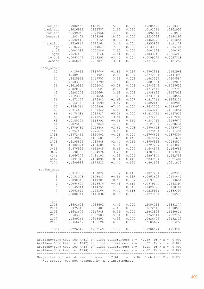
400
hor_tot | -3.082445 .6138517 -5.02 0.000 -4.285573 -1.879318
back_tot | .2026982 .0936737 2.16 0.030 .0191011 .3862953
for_tot | 5.599042 1.278966 4.38 0.000 3.092314 8.10577
humcap1 | .283401 .0153208 18.50 0.000 .2533728 .3134292
RD | .0592413 .0067165 8.82 0.000 .0460772 .0724054
hhi_sales | .7736867 .2235261 3.46 0.001 .3355837 1.21179
age | -.0104226 .0014847 -7.02 0.000 -.0133325 -.0075126
age2 | .0002089 .0000286 7.30 0.000 .0001528 .000265
logta | .1594498 .0388146 4.11 0.000 .0833746 .2355249
logta2 | -.0063172 .0018293 -3.45 0.001 -.0099027 -.0027318
demand | -.0868262 .0228071 -3.81 0.000 -.1315272 -.0421252
|
nace_short |
20 | -.20696 .1139086 -1.82 0.069 -.4302168 .0162968
23 | 1.409192 .5264923 2.68 0.007 .3772861 2.441098
24 | .4425923 .1419753 3.12 0.002 .1643259 .7208587
25 | -.5503192 .1280798 -4.30 0.000 -.801351 -.2992874
26 | -.3019585 .1002041 -3.01 0.003 -.4983548 -.1055621
29 | -.2820129 .0965521 -2.92 0.003 -.4712514 -.0927743
45 | .5203278 .1665664 3.12 0.002 .1938636 .8467919
50 | .1123333 .094656 1.19 0.235 -.0731891 .2978557
51 | -.472137 .176342 -2.68 0.007 -.817761 -.1265131
52 | -.6662163 .181598 -3.67 0.000 -1.022142 -.3102908
55 | -.7568514 .1055398 -7.17 0.000 -.9637055 -.5499972
60 | -.6914636 .1351342 -5.12 0.000 -.9563218 -.4266054
61 | -1.78086 .3229327 -5.51 0.000 -2.413796 -1.147923
62 | -1.542998 .4241249 -3.64 0.000 -2.374268 -.7117289
63 | -.0145324 .1368391 -0.11 0.915 -.282732 .2536672
64 | 2.073486 .4362048 4.75 0.000 1.21854 2.928431
70 | -.2789785 .1053444 -2.65 0.008 -.4854498 -.0725072
1516 | .8254433 .2275615 3.63 0.000 .379431 1.271456
1718 | -.4571465 .1120001 -4.08 0.000 -.6766626 -.2376304
2122 | -.1639623 .1125681 -1.46 0.145 -.3845917 .0566671
2728 | -.2195525 .089848 -2.44 0.015 -.3956513 -.0434537
3033 | 1.302874 .2194685 5.94 0.000 .8727237 1.733025
3435 | 2.576932 .4554945 5.66 0.000 1.684179 3.469685
3637 | -.2690155 .0824976 -3.26 0.001 -.4307078 -.1073233
4041 | 1.066272 .2431102 4.39 0.000 .5897844 1.542759
6567 | .1991943 .2464095 0.81 0.419 -.2837594 .6821481
7174 | -.1699989 .1179512 -1.44 0.150 -.401179 .0611812
|
region_code |
2 | .0312532 .0198874 1.57 0.116 -.0077254 .0702318
3 | -.0152078 .0158433 -0.96 0.337 -.0462602 .0158445
4 | .0090949 .0147301 0.62 0.537 -.0197755 .0379654
5 | -.0068624 .0158636 -0.43 0.665 -.0379544 .0242297
6 | -.0145014 .0144755 -1.00 0.316 -.0428729 .0138701
7 | .0061695 .014164 0.44 0.663 -.0215915 .0339304
8 | .0008741 .0145836 0.06 0.952 -.0277094 .0294575
|
year |
2003 | .3692608 .083602 4.42 0.000 .2054038 .5331177
2004 | .2975516 .066481 4.48 0.000 .1672512 .4278519
2005 | .4641672 .0917948 5.06 0.000 .2842528 .6440816
2006 | .583335 .1052983 5.54 0.000 .3769541 .7897159
2007 | .1509266 .0348403 4.33 0.000 .0826409 .2192123
2008 | .2960467 .0436126 6.79 0.000 .2105677 .3815258
|
_cons | .2226542 .1292149 1.72 0.085 -.0306024 .4759108
------------------------------------------------------------------------------
------------------------------------------------------------------------------
Arellano-Bond test for AR(1) in first differences: z = -9.59 Pr > z = 0.000
Arellano-Bond test for AR(2) in first differences: z = -0.22 Pr > z = 0.827
Arellano-Bond test for AR(3) in first differences: z = 3.11 Pr > z = 0.002
Arellano-Bond test for AR(4) in first differences: z = -2.02 Pr > z = 0.044
------------------------------------------------------------------------------
Sargan test of overid. restrictions: chi2(6) = 7.84 Prob > chi2 = 0.250
(Not robust, but not weakened by many instruments.)
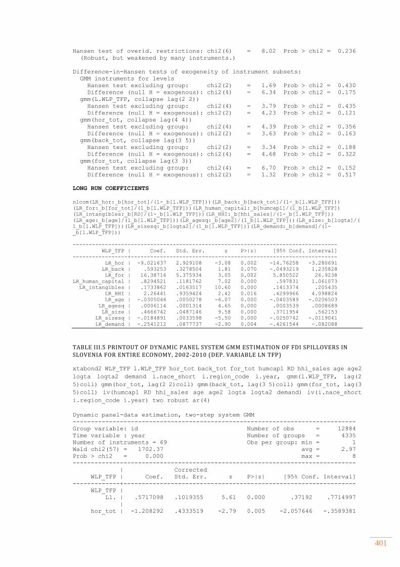
401
Hansen test of overid. restrictions: chi2(6) = 8.02 Prob > chi2 = 0.236
(Robust, but weakened by many instruments.)
Difference-in-Hansen tests of exogeneity of instrument subsets:
GMM instruments for levels
Hansen test excluding group: chi2(2) = 1.69 Prob > chi2 = 0.430
Difference (null H = exogenous): chi2(4) = 6.34 Prob > chi2 = 0.175
gmm(L.WLP_TFP, collapse lag(2 2))
Hansen test excluding group: chi2(4) = 3.79 Prob > chi2 = 0.435
Difference (null H = exogenous): chi2(2) = 4.23 Prob > chi2 = 0.121
gmm(hor_tot, collapse lag(4 4))
Hansen test excluding group: chi2(4) = 4.39 Prob > chi2 = 0.356
Difference (null H = exogenous): chi2(2) = 3.63 Prob > chi2 = 0.163
gmm(back_tot, collapse lag(3 5))
Hansen test excluding group: chi2(2) = 3.34 Prob > chi2 = 0.188
Difference (null H = exogenous): chi2(4) = 4.68 Prob > chi2 = 0.322
gmm(for_tot, collapse lag(3 3))
Hansen test excluding group: chi2(4) = 6.70 Prob > chi2 = 0.152
Difference (null H = exogenous): chi2(2) = 1.32 Prob > chi2 = 0.517
LONG RUN COEFFICIENTS
nlcom(LR_hor:_b[hor_tot]/(1-_b[l.WLP_TFP]))(LR_back:_b[back_tot]/(1-_b[l.WLP_TFP]))
(LR_for:_b[for_tot]/(1_b[l.WLP_TFP]))(LR_human_capital:_b[humcap1]/(1_b[l.WLP_TFP])
(LR_intangibles:_b[RD]/(1-_b[l.WLP_TFP]))(LR_HHI:_b[hhi_sales]/(1-_b[l.WLP_TFP]))
(LR_age:_b[age]/(1_b[l.WLP_TFP]))(LR_agesq:_b[age2]/(1_b[l.WLP_TFP]))(LR_size:_b[logta]/(
1_b[l.WLP_TFP]))(LR_sizesq:_b[logta2]/(1_b[l.WLP_TFP]))(LR_demand:_b[demand]/(1-
_b[l.WLP_TFP]))
----------------------------------------------------------------------------------
WLP_TFP | Coef. Std. Err. z P>|z| [95% Conf. Interval]
-----------------+----------------------------------------------------------------
LR_hor | -9.021637 2.929108 -3.08 0.002 -14.76258 -3.280691
LR_back | .593253 .3278504 1.81 0.070 -.0493219 1.235828
LR_for | 16.38716 5.375934 3.05 0.002 5.850522 26.9238
LR_human_capital | .8294521 .1181762 7.02 0.000 .597831 1.061073
LR_intangibles | .1733862 .0163517 10.60 0.000 .1413374 .205435
LR_HHI | 2.26441 .9359424 2.42 0.016 .4299966 4.098824
LR_age | -.0305046 .0050278 -6.07 0.000 -.0403589 -.0206503
LR_agesq | .0006114 .0001314 4.65 0.000 .0003539 .0008689
LR_size | .4666742 .0487146 9.58 0.000 .3711954 .562153
LR_sizesq | -.0184891 .0033598 -5.50 0.000 -.0250742 -.0119041
LR_demand | -.2541212 .0877737 -2.90 0.004 -.4261544 -.082088
TABLE III.5 PRINTOUT OF DYNAMIC PANEL SYSTEM GMM ESTIMATION OF FDI SPILLOVERS IN SLOVENIA FOR ENTIRE ECONOMY, 2002-2010 (DEP. VARIABLE LN TFP)
xtabond2 WLP_TFP l.WLP_TFP hor_tot back_tot for_tot humcap1 RD hhi_sales age age2
logta logta2 demand i.nace_short i.region_code i.year, gmm(l.WLP_TFP, lag(2
5)coll) gmm(hor_tot, lag(2 2)coll) gmm(back_tot, lag(3 5)coll) gmm(for_tot, lag(3
5)coll) iv(humcap1 RD hhi_sales age age2 logta logta2 demand) iv(i.nace_short
i.region_code i.year) two robust ar(4)
Dynamic panel-data estimation, two-step system GMM
------------------------------------------------------------------------------
Group variable: id Number of obs = 12884
Time variable : year Number of groups = 4335
Number of instruments = 69 Obs per group: min = 1
Wald chi2(57) = 1702.37 avg = 2.97
Prob > chi2 = 0.000 max = 8
------------------------------------------------------------------------------
| Corrected
WLP_TFP | Coef. Std. Err. z P>|z| [95% Conf. Interval]
-------------+----------------------------------------------------------------
WLP_TFP |
L1. | .5717098 .1019355 5.61 0.000 .37192 .7714997
|
hor_tot | -1.208292 .4333519 -2.79 0.005 -2.057646 -.3589381
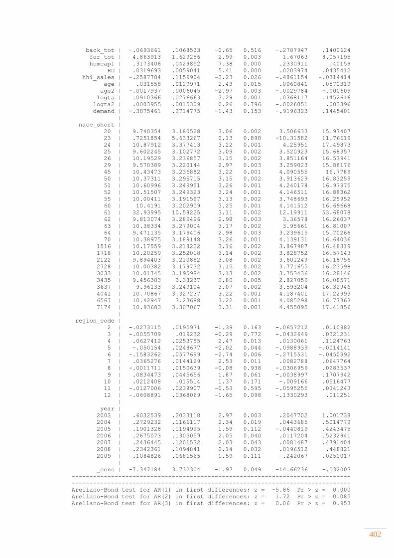
402
back_tot | -.0693661 .1068533 -0.65 0.516 -.2787947 .1400624
for_tot | 4.863913 1.629256 2.99 0.003 1.67063 8.057195
humcap1 | .3173406 .0429852 7.38 0.000 .2330911 .40159
RD | .0319693 .0059041 5.41 0.000 .0203974 .0435412
hhi_sales | -.2587784 .1159904 -2.23 0.026 -.4861154 -.0314414
age | .031558 .0129971 2.43 0.015 .0060841 .0570319
age2 | -.0017937 .0006045 -2.97 0.003 -.0029784 -.000609
logta | .0910366 .0276663 3.29 0.001 .0368117 .1452616
logta2 | .0003955 .0015309 0.26 0.796 -.0026051 .003396
demand | -.3875461 .2714775 -1.43 0.153 -.9196323 .1445401
|
nace_short |
20 | 9.740354 3.180528 3.06 0.002 3.506633 15.97407
23 | .7251854 5.633267 0.13 0.898 -10.31582 11.76619
24 | 10.87912 3.377413 3.22 0.001 4.25951 17.49873
25 | 9.602245 3.102772 3.09 0.002 3.520923 15.68357
26 | 10.19529 3.236857 3.15 0.002 3.851164 16.53941
29 | 9.570389 3.220144 2.97 0.003 3.259023 15.88176
45 | 10.43473 3.236882 3.22 0.001 4.090555 16.7789
50 | 10.37311 3.295715 3.15 0.002 3.913629 16.83259
51 | 10.60996 3.249951 3.26 0.001 4.240178 16.97975
52 | 10.51507 3.249323 3.24 0.001 4.146511 16.88362
55 | 10.00411 3.191597 3.13 0.002 3.748693 16.25952
60 | 10.4191 3.202909 3.25 0.001 4.141512 16.69668
61 | 32.93995 10.58225 3.11 0.002 12.19911 53.68078
62 | 9.813074 3.289496 2.98 0.003 3.36578 16.26037
63 | 10.38334 3.279004 3.17 0.002 3.95661 16.81007
64 | 9.471135 3.179406 2.98 0.003 3.239615 15.70266
70 | 10.38975 3.189148 3.26 0.001 4.139131 16.64036
1516 | 10.17559 3.218222 3.16 0.002 3.867987 16.48319
1718 | 10.20259 3.252018 3.14 0.002 3.828752 16.57643
2122 | 9.894403 3.210852 3.08 0.002 3.601249 16.18756
2728 | 10.00382 3.179732 3.15 0.002 3.771655 16.23598
3033 | 10.01745 3.195984 3.13 0.002 3.753436 16.28146
3435 | 9.456383 3.38237 2.80 0.005 2.827059 16.08571
3637 | 9.96133 3.249104 3.07 0.002 3.593204 16.32946
4041 | 10.70867 3.327237 3.22 0.001 4.187401 17.22993
6567 | 10.42947 3.23688 3.22 0.001 4.085298 16.77363
7174 | 10.93683 3.307067 3.31 0.001 4.455095 17.41856
|
region_code |
2 | -.0273115 .0195971 -1.39 0.163 -.0657212 .0110982
3 | -.0055709 .019232 -0.29 0.772 -.0432649 .0321231
4 | .0627412 .0253755 2.47 0.013 .0130061 .1124763
5 | -.050154 .0248677 -2.02 0.044 -.0988939 -.0014141
6 | -.1583262 .0577699 -2.74 0.006 -.2715531 -.0450992
7 | .0365276 .0144129 2.53 0.011 .0082788 .0647764
8 | -.0011711 .0150639 -0.08 0.938 -.0306959 .0283537
9 | .0834473 .0445656 1.87 0.061 -.0038997 .1707942
10 | .0212408 .015514 1.37 0.171 -.009166 .0516477
11 | -.0127006 .0238907 -0.53 0.595 -.0595255 .0341243
12 | -.0608891 .0368069 -1.65 0.098 -.1330293 .011251
|
year |
2003 | .6032539 .2033118 2.97 0.003 .2047702 1.001738
2004 | .2729232 .1166117 2.34 0.019 .0443685 .5014779
2005 | .1901328 .1194995 1.59 0.112 -.0440819 .4243475
2006 | .2675073 .1305059 2.05 0.040 .0117204 .5232941
2007 | .2436445 .1201532 2.03 0.043 .0081487 .4791404
2008 | .2342361 .1094841 2.14 0.032 .0196512 .448821
2009 | -.1084826 .0681565 -1.59 0.111 -.242067 .0251017
|
_cons | -7.347184 3.732304 -1.97 0.049 -14.66236 -.032003
------------------------------------------------------------------------------
------------------------------------------------------------------------------
Arellano-Bond test for AR(1) in first differences: z = -5.86 Pr > z = 0.000
Arellano-Bond test for AR(2) in first differences: z = 1.72 Pr > z = 0.085
Arellano-Bond test for AR(3) in first differences: z = 0.06 Pr > z = 0.953
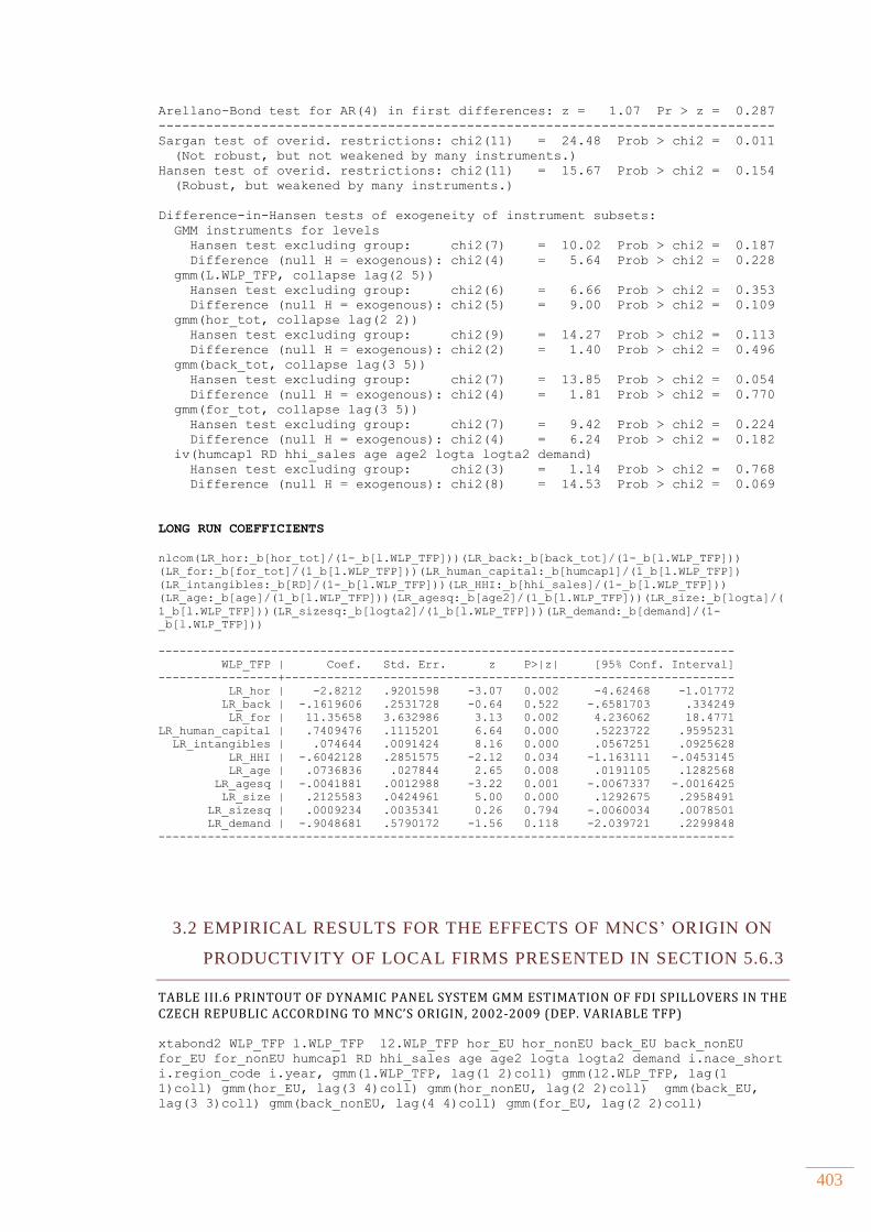
403
Arellano-Bond test for AR(4) in first differences: z = 1.07 Pr > z = 0.287
------------------------------------------------------------------------------
Sargan test of overid. restrictions: chi2(11) = 24.48 Prob > chi2 = 0.011
(Not robust, but not weakened by many instruments.)
Hansen test of overid. restrictions: chi2(11) = 15.67 Prob > chi2 = 0.154
(Robust, but weakened by many instruments.)
Difference-in-Hansen tests of exogeneity of instrument subsets:
GMM instruments for levels
Hansen test excluding group: chi2(7) = 10.02 Prob > chi2 = 0.187
Difference (null H = exogenous): chi2(4) = 5.64 Prob > chi2 = 0.228
gmm(L.WLP_TFP, collapse lag(2 5))
Hansen test excluding group: chi2(6) = 6.66 Prob > chi2 = 0.353
Difference (null H = exogenous): chi2(5) = 9.00 Prob > chi2 = 0.109
gmm(hor_tot, collapse lag(2 2))
Hansen test excluding group: chi2(9) = 14.27 Prob > chi2 = 0.113
Difference (null H = exogenous): chi2(2) = 1.40 Prob > chi2 = 0.496
gmm(back_tot, collapse lag(3 5))
Hansen test excluding group: chi2(7) = 13.85 Prob > chi2 = 0.054
Difference (null H = exogenous): chi2(4) = 1.81 Prob > chi2 = 0.770
gmm(for_tot, collapse lag(3 5))
Hansen test excluding group: chi2(7) = 9.42 Prob > chi2 = 0.224
Difference (null H = exogenous): chi2(4) = 6.24 Prob > chi2 = 0.182
iv(humcap1 RD hhi_sales age age2 logta logta2 demand)
Hansen test excluding group: chi2(3) = 1.14 Prob > chi2 = 0.768
Difference (null H = exogenous): chi2(8) = 14.53 Prob > chi2 = 0.069
LONG RUN COEFFICIENTS
nlcom(LR_hor:_b[hor_tot]/(1-_b[l.WLP_TFP]))(LR_back:_b[back_tot]/(1-_b[l.WLP_TFP]))
(LR_for:_b[for_tot]/(1_b[l.WLP_TFP]))(LR_human_capital:_b[humcap1]/(1_b[l.WLP_TFP])
(LR_intangibles:_b[RD]/(1-_b[l.WLP_TFP]))(LR_HHI:_b[hhi_sales]/(1-_b[l.WLP_TFP]))
(LR_age:_b[age]/(1_b[l.WLP_TFP]))(LR_agesq:_b[age2]/(1_b[l.WLP_TFP]))(LR_size:_b[logta]/(
1_b[l.WLP_TFP]))(LR_sizesq:_b[logta2]/(1_b[l.WLP_TFP]))(LR_demand:_b[demand]/(1-
_b[l.WLP_TFP]))
----------------------------------------------------------------------------------
WLP_TFP | Coef. Std. Err. z P>|z| [95% Conf. Interval]
-----------------+----------------------------------------------------------------
LR_hor | -2.8212 .9201598 -3.07 0.002 -4.62468 -1.01772
LR_back | -.1619606 .2531728 -0.64 0.522 -.6581703 .334249
LR_for | 11.35658 3.632986 3.13 0.002 4.236062 18.4771
LR_human_capital | .7409476 .1115201 6.64 0.000 .5223722 .9595231
LR_intangibles | .074644 .0091424 8.16 0.000 .0567251 .0925628
LR_HHI | -.6042128 .2851575 -2.12 0.034 -1.163111 -.0453145
LR_age | .0736836 .027844 2.65 0.008 .0191105 .1282568
LR_agesq | -.0041881 .0012988 -3.22 0.001 -.0067337 -.0016425
LR_size | .2125583 .0424961 5.00 0.000 .1292675 .2958491
LR_sizesq | .0009234 .0035341 0.26 0.794 -.0060034 .0078501
LR_demand | -.9048681 .5790172 -1.56 0.118 -2.039721 .2299848
----------------------------------------------------------------------------------
3.2 EMPIRICAL RESULTS FOR THE EFFECTS OF MNCS’ ORIGIN ON
PRODUCTIVITY OF LOCAL FIRMS PRESENTED IN SECTION 5.6.3
TABLE III.6 PRINTOUT OF DYNAMIC PANEL SYSTEM GMM ESTIMATION OF FDI SPILLOVERS IN THE CZECH REPUBLIC ACCORDING TO MNC’S ORIGIN , 2002-2009 (DEP. VARIABLE TFP)
xtabond2 WLP_TFP l.WLP_TFP l2.WLP_TFP hor_EU hor_nonEU back_EU back_nonEU
for_EU for_nonEU humcap1 RD hhi_sales age age2 logta logta2 demand i.nace_short
i.region_code i.year, gmm(l.WLP_TFP, lag(1 2)coll) gmm(l2.WLP_TFP, lag(1
1)coll) gmm(hor_EU, lag(3 4)coll) gmm(hor_nonEU, lag(2 2)coll) gmm(back_EU,
lag(3 3)coll) gmm(back_nonEU, lag(4 4)coll) gmm(for_EU, lag(2 2)coll)

404
gmm(for_nonEU, lag(4 4)coll) iv(humcap1 RD hhi_sales age age2 logta logta2
demand) iv(i.nace_short i.region_code i.year) two robust ar(4)
Dynamic panel-data estimation, two-step system GMM
------------------------------------------------------------------------------
Group variable: id Number of obs = 97891
Time variable : year Number of groups = 36700
Number of instruments = 68 Obs per group: min = 1
Wald chi2(58) = 163480.57 avg = 2.67
Prob > chi2 = 0.000 max = 6
------------------------------------------------------------------------------
| Corrected
WLP_TFP | Coef. Std. Err. z P>|z| [95% Conf. Interval]
-------------+----------------------------------------------------------------
WLP_TFP |
L1. | .3867443 .0122666 31.53 0.000 .3627022 .4107863
L2. | .0680729 .0074617 9.12 0.000 .0534482 .0826976
|
hor_EU | .4636075 .1028814 4.51 0.000 .2619637 .6652514
hor_nonEU | -2.95881 .5057317 -5.85 0.000 -3.950026 -1.967594
back_EU | -1.963876 .2816985 -6.97 0.000 -2.515994 -1.411757
back_nonEU | 11.13578 1.604228 6.94 0.000 7.991551 14.28001
for_EU | 1.910089 .5277166 3.62 0.000 .8757839 2.944395
for_nonEU | -12.03661 1.971361 -6.11 0.000 -15.90041 -8.172814
humcap1 | .4383052 .008362 52.42 0.000 .421916 .4546944
RD | .0525092 .001767 29.72 0.000 .049046 .0559724
hhi_sales | -.3165572 .0625763 -5.06 0.000 -.4392046 -.1939098
age | -.0106267 .0010665 -9.96 0.000 -.012717 -.0085364
age2 | .0000848 .0000351 2.41 0.016 .0000159 .0001536
logta | .2078478 .0131873 15.76 0.000 .1820012 .2336944
logta2 | -.0049956 .0008403 -5.95 0.000 -.0066425 -.0033487
demand | .0840185 .0191514 4.39 0.000 .0464824 .1215545
|
nace_short |
20 | 1.054221 .092366 11.41 0.000 .8731867 1.235255
23 | 1.615949 .2300302 7.02 0.000 1.165098 2.0668
24 | 1.439816 .1282456 11.23 0.000 1.188459 1.691173
25 | .9949897 .1462664 6.80 0.000 .7083128 1.281666
26 | 1.651396 .1091032 15.14 0.000 1.437558 1.865235
29 | 1.18529 .1013099 11.70 0.000 .9867267 1.383854
45 | .8690088 .0994775 8.74 0.000 .6740365 1.063981
50 | .8159457 .1152225 7.08 0.000 .5901138 1.041778
51 | 1.700288 .1080256 15.74 0.000 1.488561 1.912014
52 | 1.235096 .1080546 11.43 0.000 1.023313 1.44688
55 | .7342845 .0873004 8.41 0.000 .563179 .9053901
60 | .6381451 .1085025 5.88 0.000 .4254841 .8508061
61 | .5830411 .1947942 2.99 0.003 .2012515 .9648306
62 | .9238705 .2441319 3.78 0.000 .4453807 1.40236
63 | .28657 .1397231 2.05 0.040 .0127179 .5604222
64 | .3928325 .1228693 3.20 0.001 .152013 .6336519
70 | 1.059451 .0943744 11.23 0.000 .8744802 1.244421
1516 | 1.222051 .0947393 12.90 0.000 1.036365 1.407736
1718 | 1.178546 .0914225 12.89 0.000 .9993615 1.357731
2122 | 1.052318 .091326 11.52 0.000 .8733227 1.231314
2728 | .9826873 .1033888 9.50 0.000 .7800491 1.185326
3033 | 1.183201 .1025608 11.54 0.000 .9821858 1.384217
3435 | 1.020143 .1082401 9.42 0.000 .8079966 1.23229
3637 | 1.307574 .0877882 14.89 0.000 1.135513 1.479636
4041 | 1.00218 .1100217 9.11 0.000 .7865413 1.217818
6567 | .7562094 .1737694 4.35 0.000 .4156276 1.096791
7174 | 1.31642 .1199315 10.98 0.000 1.081359 1.551482
|
region_code |
4 | -.0273686 .0176365 -1.55 0.121 -.0619354 .0071983
5 | -.0214129 .0172582 -1.24 0.215 -.0552383 .0124124
6 | -.0449394 .0184355 -2.44 0.015 -.0810723 -.0088064
7 | -.0009908 .0164975 -0.06 0.952 -.0333254 .0313438
8 | -.0309211 .0176742 -1.75 0.080 -.0655618 .0037196

405
9 | -.0196525 .0175301 -1.12 0.262 -.0540107 .0147058
10 | -.0061059 .0175969 -0.35 0.729 -.0405953 .0283835
11 | .016848 .016106 1.05 0.296 -.0147192 .0484152
13 | -.0069688 .0153898 -0.45 0.651 -.0371322 .0231946
14 | -.0365081 .0170002 -2.15 0.032 -.0698279 -.0031884
|
year |
2004 | .0572053 .0340067 1.68 0.093 -.0094466 .1238572
2005 | .103776 .0276672 3.75 0.000 .0495492 .1580028
2006 | .1263278 .0285299 4.43 0.000 .0704102 .1822453
2007 | .1456909 .0283015 5.15 0.000 .0902209 .2011608
2008 | .0652287 .0090316 7.22 0.000 .047527 .0829304
|
_cons | -1.773812 .1771658 -10.01 0.000 -2.12105 -1.426573
------------------------------------------------------------------------------
------------------------------------------------------------------------------
Arellano-Bond test for AR(1) in first differences: z = -30.77 Pr > z = 0.000
Arellano-Bond test for AR(2) in first differences: z = 1.29 Pr > z = 0.198
Arellano-Bond test for AR(3) in first differences: z = 0.71 Pr > z = 0.475
Arellano-Bond test for AR(4) in first differences: z = -1.64 Pr > z = 0.102
------------------------------------------------------------------------------
Sargan test of overid. restrictions: chi2(9) = 36.27 Prob > chi2 = 0.000
(Not robust, but not weakened by many instruments.)
Hansen test of overid. restrictions: chi2(9) = 21.75 Prob > chi2 = 0.010
(Robust, but weakened by many instruments.)
Difference-in-Hansen tests of exogeneity of instrument subsets:
GMM instruments for levels
Hansen test excluding group: chi2(1) = 11.59 Prob > chi2 = 0.001
Difference (null H = exogenous): chi2(8) = 10.16 Prob > chi2 = 0.254
gmm(L.WLP_TFP, collapse lag(1 2))
Hansen test excluding group: chi2(7) = 15.93 Prob > chi2 = 0.026
Difference (null H = exogenous): chi2(2) = 5.82 Prob > chi2 = 0.054
gmm(L2.WLP_TFP, collapse lag(1 1))
Hansen test excluding group: chi2(7) = 20.07 Prob > chi2 = 0.005
Difference (null H = exogenous): chi2(2) = 1.68 Prob > chi2 = 0.431
gmm(hor_EU, collapse lag(3 4))
Hansen test excluding group: chi2(6) = 16.66 Prob > chi2 = 0.011
Difference (null H = exogenous): chi2(3) = 5.09 Prob > chi2 = 0.165
gmm(hor_nonEU, collapse lag(2 2))
Hansen test excluding group: chi2(7) = 21.35 Prob > chi2 = 0.003
Difference (null H = exogenous): chi2(2) = 0.40 Prob > chi2 = 0.817
gmm(back_EU, collapse lag(3 3))
Hansen test excluding group: chi2(7) = 20.79 Prob > chi2 = 0.004
Difference (null H = exogenous): chi2(2) = 0.96 Prob > chi2 = 0.619
gmm(back_nonEU, collapse lag(4 4))
Hansen test excluding group: chi2(7) = 21.12 Prob > chi2 = 0.004
Difference (null H = exogenous): chi2(2) = 0.63 Prob > chi2 = 0.728
gmm(for_EU, collapse lag(2 2))
Hansen test excluding group: chi2(7) = 19.30 Prob > chi2 = 0.007
Difference (null H = exogenous): chi2(2) = 2.45 Prob > chi2 = 0.294
gmm(for_nonEU, collapse lag(4 4))
Hansen test excluding group: chi2(7) = 20.66 Prob > chi2 = 0.004
Difference (null H = exogenous): chi2(2) = 1.09 Prob > chi2 = 0.580
iv(humcap1 RD hhi_sales age age2 logta logta2 demand)
Hansen test excluding group: chi2(1) = 0.02 Prob > chi2 = 0.885
Difference (null H = exogenous): chi2(8) = 21.73 Prob > chi2 = 0.005
TABLE III.7 PRINTOUT OF DYNAMIC PANEL SYSTEM GMM ESTIMATION OF FDI SPILLOVERS IN ESTONIA ACCORDING TO MNC’S ORIGIN, 2002-2010 (DEP. VARIABLE LN TFP) xtabond2 WLP_TFP l.WLP_TFP hor_EU hor_nonEU back_EU back_nonEU for_EU for_nonEU
humcap1 RD hhi_sales age age2 logta logta2 demand i.nace_short i.region_code
i.year, gmm(l.WLP_TFP, lag(2 2)coll) gmm(hor_EU, lag(4 4)coll) gmm(hor_nonEU,
lag(3 4)coll) gmm(back_EU, lag(4 5)coll) gmm(back_nonEU, lag(4 4)coll)
gmm(for_EU, lag(3 5)coll) gmm(for_nonEU, lag(4 4)coll) iv(humcap1 RD hhi_sales

406
age age2 logta logta2 demand) iv(i.nace_short i.region_code i.year) two robust
ar(4)
Dynamic panel-data estimation, two-step system GMM
------------------------------------------------------------------------------
Group variable: id Number of obs = 66194
Time variable : year Number of groups = 18684
Number of instruments = 65 Obs per group: min = 1
Wald chi2(53) = 90747.87 avg = 3.54
Prob > chi2 = 0.000 max = 8
------------------------------------------------------------------------------
| Corrected
WLP_TFP | Coef. Std. Err. z P>|z| [95% Conf. Interval]
-------------+----------------------------------------------------------------
WLP_TFP |
L1. | .5397097 .0358424 15.06 0.000 .4694598 .6099595
|
hor_EU | 2.122868 .4186632 5.07 0.000 1.302303 2.943433
hor_nonEU | 6.976797 1.084044 6.44 0.000 4.85211 9.101484
back_EU | -1.51022 .2121416 -7.12 0.000 -1.92601 -1.09443
back_nonEU | 6.131187 .945056 6.49 0.000 4.278911 7.983463
for_EU | .6678111 .9448292 0.71 0.480 -1.18402 2.519642
for_nonEU | -22.32216 5.529855 -4.04 0.000 -33.16048 -11.48385
humcap1 | .3316521 .0132046 25.12 0.000 .3057716 .3575327
RD | .0856262 .0035247 24.29 0.000 .078718 .0925344
hhi_sales | -3.0738 .6713938 -4.58 0.000 -4.389707 -1.757892
age | -.0112066 .0010793 -10.38 0.000 -.013322 -.0090912
age2 | .0001285 .0000109 11.78 0.000 .0001071 .0001498
logta | .279298 .0239451 11.66 0.000 .2323664 .3262296
logta2 | -.0135191 .0023748 -5.69 0.000 -.0181737 -.0088645
demand | -.0834589 .0272965 -3.06 0.002 -.1369591 -.0299587
|
nace_short |
20 | 2.051327 .5086046 4.03 0.000 1.05448 3.048174
23 | 127.2922 27.58956 4.61 0.000 73.21761 181.3667
24 | .404393 .4350706 0.93 0.353 -.4483298 1.257116
25 | 2.244727 .5242109 4.28 0.000 1.217292 3.272161
26 | 1.878908 .569681 3.30 0.001 .7623536 2.995462
29 | 2.392412 .5530252 4.33 0.000 1.308503 3.476322
45 | 2.670666 .587264 4.55 0.000 1.51965 3.821683
50 | 2.525673 .5691728 4.44 0.000 1.410115 3.641231
51 | 3.135089 .6205568 5.05 0.000 1.91882 4.351358
52 | 2.845715 .6281384 4.53 0.000 1.614586 4.076843
55 | 3.011074 .5741419 5.24 0.000 1.885777 4.136372
60 | 3.314857 .6591673 5.03 0.000 2.022913 4.606801
61 | 2.028286 .7097946 2.86 0.004 .6371145 3.419458
62 | 2.67894 .8484972 3.16 0.002 1.015916 4.341964
63 | 3.18914 .6614868 4.82 0.000 1.89265 4.48563
64 | 4.385969 .8599237 5.10 0.000 2.70055 6.071389
70 | 3.403302 .6259059 5.44 0.000 2.176549 4.630055
1516 | 2.251057 .5363136 4.20 0.000 1.199901 3.302212
1718 | 2.510638 .5709056 4.40 0.000 1.391684 3.629592
2122 | 2.583795 .5374468 4.81 0.000 1.530419 3.637172
2728 | 2.03353 .529003 3.84 0.000 .9967036 3.070357
3033 | 1.645447 .5951617 2.76 0.006 .4789512 2.811942
3435 | 2.36377 .5763356 4.10 0.000 1.234173 3.493367
3637 | 2.297197 .5202662 4.42 0.000 1.277494 3.3169
4041 | 4.67945 .9448669 4.95 0.000 2.827545 6.531355
6567 | 3.68272 .7758298 4.75 0.000 2.162121 5.203318
7174 | 3.177785 .6611825 4.81 0.000 1.881891 4.473678
|
region_code |
2 | -.0276117 .0079788 -3.46 0.001 -.0432498 -.0119736
3 | -.035418 .009538 -3.71 0.000 -.0541122 -.0167238
4 | -.096738 .0177933 -5.44 0.000 -.1316123 -.0618636
5 | -.0211885 .0070139 -3.02 0.003 -.0349355 -.0074415
|
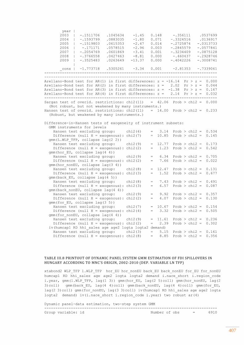
407
year |
2003 | -.1511706 .1045634 -1.45 0.148 -.356111 .0537699
2004 | -.1593799 .0883035 -1.80 0.071 -.3324516 .0136917
2005 | -.1519803 .0615353 -2.47 0.014 -.2725874 -.0313733
2006 | -.171171 .0578515 -2.96 0.003 -.2845579 -.0577841
2007 | -.2054769 .0601869 -3.41 0.001 -.3234409 -.0875128
2008 | -.3766558 .0427463 -8.81 0.000 -.460437 -.2928746
2009 | -.3525483 .0263649 -13.37 0.000 -.4042226 -.3008741
|
_cons | -1.773718 .5305261 -3.34 0.001 -2.81353 -.7339061
------------------------------------------------------------------------------
------------------------------------------------------------------------------
Arellano-Bond test for AR(1) in first differences: z = -16.14 Pr > z = 0.000
Arellano-Bond test for AR(2) in first differences: z = 2.02 Pr > z = 0.044
Arellano-Bond test for AR(3) in first differences: z = -1.38 Pr > z = 0.167
Arellano-Bond test for AR(4) in first differences: z = 2.14 Pr > z = 0.032
------------------------------------------------------------------------------
Sargan test of overid. restrictions: chi2(11) = 42.06 Prob > chi2 = 0.000
(Not robust, but not weakened by many instruments.)
Hansen test of overid. restrictions: chi2(11) = 14.00 Prob > chi2 = 0.233
(Robust, but weakened by many instruments.)
Difference-in-Hansen tests of exogeneity of instrument subsets:
GMM instruments for levels
Hansen test excluding group: chi2(4) = 3.14 Prob > chi2 = 0.534
Difference (null H = exogenous): chi2(7) = 10.85 Prob > chi2 = 0.145
gmm(L.WLP_TFP, collapse lag(2 2))
Hansen test excluding group: chi2(9) = 12.77 Prob > chi2 = 0.173
Difference (null H = exogenous): chi2(2) = 1.23 Prob > chi2 = 0.542
gmm(hor_EU, collapse lag(4 4))
Hansen test excluding group: chi2(9) = 6.34 Prob > chi2 = 0.705
Difference (null H = exogenous): chi2(2) = 7.66 Prob > chi2 = 0.022
gmm(hor_nonEU, collapse lag(3 4))
Hansen test excluding group: chi2(8) = 12.47 Prob > chi2 = 0.131
Difference (null H = exogenous): chi2(3) = 1.52 Prob > chi2 = 0.677
gmm(back_EU, collapse lag(4 5))
Hansen test excluding group: chi2(8) = 7.43 Prob > chi2 = 0.491
Difference (null H = exogenous): chi2(3) = 6.57 Prob > chi2 = 0.087
gmm(back_nonEU, collapse lag(4 4))
Hansen test excluding group: chi2(9) = 9.92 Prob > chi2 = 0.357
Difference (null H = exogenous): chi2(2) = 4.07 Prob > chi2 = 0.130
gmm(for_EU, collapse lag(3 5))
Hansen test excluding group: chi2(7) = 10.67 Prob > chi2 = 0.154
Difference (null H = exogenous): chi2(4) = 3.32 Prob > chi2 = 0.505
gmm(for_nonEU, collapse lag(4 4))
Hansen test excluding group: chi2(9) = 11.61 Prob > chi2 = 0.236
Difference (null H = exogenous): chi2(2) = 2.39 Prob > chi2 = 0.302
iv(humcap1 RD hhi_sales age age2 logta logta2 demand)
Hansen test excluding group: chi2(3) = 5.15 Prob > chi2 = 0.161
Difference (null H = exogenous): chi2(8) = 8.85 Prob > chi2 = 0.356
TABLE III.8 PRINTOUT OF DYNAMIC PANEL SYSTEM GMM ESTIMATION OF FDI SPILLOVERS IN HUNGARY ACCORDING TO MNC’S ORIGIN, 2002-2010 (DEP. VARIABLE LN TFP)
xtabond2 WLP_TFP l.WLP_TFP hor_EU hor_nonEU back_EU back_nonEU for_EU for_nonEU
humcap1 RD hhi_sales age age2 logta logta2 demand i.nace_short i.region_code
i.year, gmm(l.WLP_TFP, lag(1 3)) gmm(hor_EU, lag(2 5)coll) gmm(hor_nonEU, lag(2
3)coll) gmm(back_EU, lag(4 4)coll) gmm(back_nonEU, lag(4 4)coll) gmm(for_EU,
lag(2 3)coll) gmm(for_nonEU, lag(3 3)coll) iv(humcap1 RD hhi_sales age age2 logta
logta2 demand) iv(i.nace_short i.region_code i.year) two robust ar(4)
Dynamic panel-data estimation, two-step system GMM
------------------------------------------------------------------------------
Group variable: id Number of obs = 6910
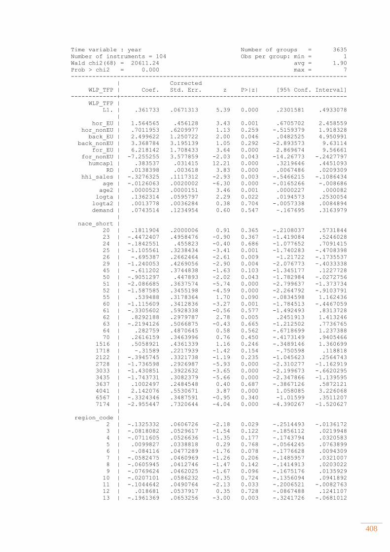
408
Time variable : year Number of groups = 3635
Number of instruments = 104 Obs per group: min = 1
Wald chi2(68) = 20611.24 avg = 1.90
Prob > chi2 = 0.000 max = 7
------------------------------------------------------------------------------
| Corrected
WLP_TFP | Coef. Std. Err. z P>|z| [95% Conf. Interval]
-------------+----------------------------------------------------------------
WLP_TFP |
L1. | .361733 .0671313 5.39 0.000 .2301581 .4933078
|
hor_EU | 1.564565 .456128 3.43 0.001 .6705702 2.458559
hor_nonEU | .7011953 .6209977 1.13 0.259 -.5159379 1.918328
back_EU | 2.499622 1.250722 2.00 0.046 .0482525 4.950991
back_nonEU | 3.368784 3.195139 1.05 0.292 -2.893573 9.63114
for_EU | 6.218142 1.708433 3.64 0.000 2.869674 9.56661
for_nonEU | -7.255255 3.577859 -2.03 0.043 -14.26773 -.2427797
humcap1 | .383537 .031415 12.21 0.000 .3219646 .4451093
RD | .0138398 .003618 3.83 0.000 .0067486 .0209309
hhi_sales | -.3276325 .1117312 -2.93 0.003 -.5466215 -.1086434
age | -.0126063 .0020002 -6.30 0.000 -.0165266 -.008686
age2 | .0000523 .0000151 3.46 0.001 .0000227 .000082
logta | .1362314 .0595797 2.29 0.022 .0194573 .2530054
logta2 | .0013778 .0036284 0.38 0.704 -.0057338 .0084894
demand | .0743514 .1234954 0.60 0.547 -.167695 .3163979
|
nace_short |
20 | .1811904 .2000006 0.91 0.365 -.2108037 .5731844
23 | -.4472407 .4958476 -0.90 0.367 -1.419084 .5246028
24 | -.1842551 .455823 -0.40 0.686 -1.077652 .7091415
25 | -1.105561 .3238434 -3.41 0.001 -1.740283 -.4708398
26 | -.695387 .2662464 -2.61 0.009 -1.21722 -.1735537
29 | -1.240053 .4269056 -2.90 0.004 -2.076773 -.4033338
45 | -.611202 .3744838 -1.63 0.103 -1.345177 .1227728
50 | -.9051297 .447893 -2.02 0.043 -1.782984 -.0272756
51 | -2.086685 .3637574 -5.74 0.000 -2.799637 -1.373734
52 | -1.587585 .3455198 -4.59 0.000 -2.264792 -.9103791
55 | .539488 .3178364 1.70 0.090 -.0834598 1.162436
60 | -1.115609 .3412836 -3.27 0.001 -1.784513 -.4467059
61 | -.3305602 .5928338 -0.56 0.577 -1.492493 .8313728
62 | .8292188 .2979787 2.78 0.005 .2451913 1.413246
63 | -.2194126 .5066875 -0.43 0.665 -1.212502 .7736765
64 | .282759 .4870645 0.58 0.562 -.6718699 1.237388
70 | .2616159 .3463996 0.76 0.450 -.4173149 .9405466
1516 | .5058921 .4361339 1.16 0.246 -.3489146 1.360699
1718 | -.31589 .2217939 -1.42 0.154 -.750598 .118818
2122 | -.3945745 .3321738 -1.19 0.235 -1.045623 .2564743
2728 | -1.736598 .2926987 -5.93 0.000 -2.310277 -1.162919
3033 | -1.430851 .3922632 -3.65 0.000 -2.199673 -.6620295
3435 | -1.743731 .3082379 -5.66 0.000 -2.347866 -1.139595
3637 | .1002497 .2484548 0.40 0.687 -.3867126 .5872121
4041 | 2.142076 .5530671 3.87 0.000 1.058085 3.226068
6567 | -.3324346 .3487591 -0.95 0.340 -1.01599 .3511207
7174 | -2.955447 .7320644 -4.04 0.000 -4.390267 -1.520627
|
region_code |
2 | -.1325332 .0606726 -2.18 0.029 -.2514493 -.0136172
3 | -.0818082 .0529617 -1.54 0.122 -.1856112 .0219948
4 | -.0711605 .0526636 -1.35 0.177 -.1743794 .0320583
5 | .0099827 .0338818 0.29 0.768 -.0564245 .0763899
6 | -.084116 .0477289 -1.76 0.078 -.1776628 .0094309
7 | -.0582475 .0460969 -1.26 0.206 -.1485957 .0321007
8 | -.0605945 .0412746 -1.47 0.142 -.1414913 .0203022
9 | -.0769624 .0462025 -1.67 0.096 -.1675176 .0135929
10 | -.0207101 .0586232 -0.35 0.724 -.1356094 .0941892
11 | -.1044642 .0490764 -2.13 0.033 -.2006521 -.0082763
12 | .018681 .0537917 0.35 0.728 -.0867488 .1241107
13 | -.1961369 .0653256 -3.00 0.003 -.3241726 -.0681012
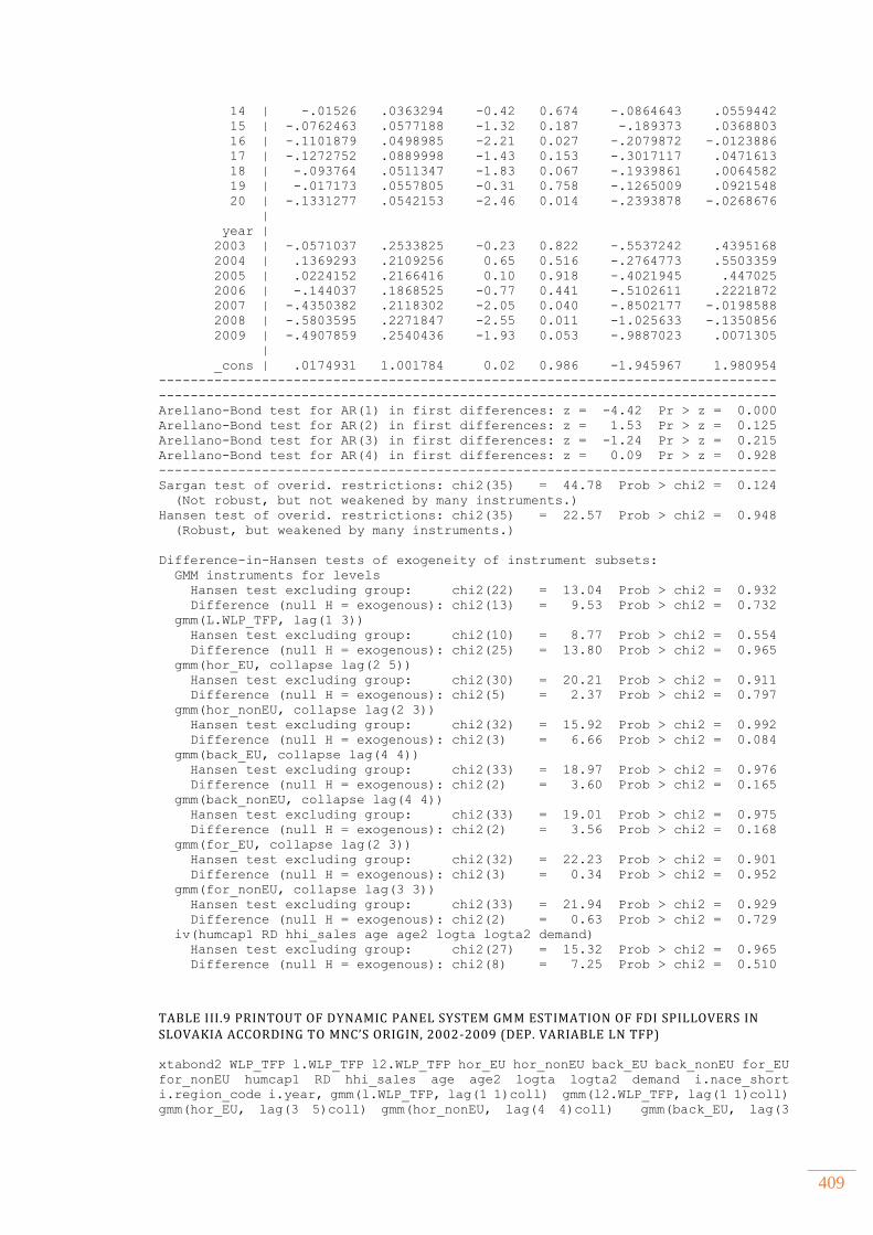
409
14 | -.01526 .0363294 -0.42 0.674 -.0864643 .0559442
15 | -.0762463 .0577188 -1.32 0.187 -.189373 .0368803
16 | -.1101879 .0498985 -2.21 0.027 -.2079872 -.0123886
17 | -.1272752 .0889998 -1.43 0.153 -.3017117 .0471613
18 | -.093764 .0511347 -1.83 0.067 -.1939861 .0064582
19 | -.017173 .0557805 -0.31 0.758 -.1265009 .0921548
20 | -.1331277 .0542153 -2.46 0.014 -.2393878 -.0268676
|
year |
2003 | -.0571037 .2533825 -0.23 0.822 -.5537242 .4395168
2004 | .1369293 .2109256 0.65 0.516 -.2764773 .5503359
2005 | .0224152 .2166416 0.10 0.918 -.4021945 .447025
2006 | -.144037 .1868525 -0.77 0.441 -.5102611 .2221872
2007 | -.4350382 .2118302 -2.05 0.040 -.8502177 -.0198588
2008 | -.5803595 .2271847 -2.55 0.011 -1.025633 -.1350856
2009 | -.4907859 .2540436 -1.93 0.053 -.9887023 .0071305
|
_cons | .0174931 1.001784 0.02 0.986 -1.945967 1.980954
------------------------------------------------------------------------------
------------------------------------------------------------------------------
Arellano-Bond test for AR(1) in first differences: z = -4.42 Pr > z = 0.000
Arellano-Bond test for AR(2) in first differences: z = 1.53 Pr > z = 0.125
Arellano-Bond test for AR(3) in first differences: z = -1.24 Pr > z = 0.215
Arellano-Bond test for AR(4) in first differences: z = 0.09 Pr > z = 0.928
------------------------------------------------------------------------------
Sargan test of overid. restrictions: chi2(35) = 44.78 Prob > chi2 = 0.124
(Not robust, but not weakened by many instruments.)
Hansen test of overid. restrictions: chi2(35) = 22.57 Prob > chi2 = 0.948
(Robust, but weakened by many instruments.)
Difference-in-Hansen tests of exogeneity of instrument subsets:
GMM instruments for levels
Hansen test excluding group: chi2(22) = 13.04 Prob > chi2 = 0.932
Difference (null H = exogenous): chi2(13) = 9.53 Prob > chi2 = 0.732
gmm(L.WLP_TFP, lag(1 3))
Hansen test excluding group: chi2(10) = 8.77 Prob > chi2 = 0.554
Difference (null H = exogenous): chi2(25) = 13.80 Prob > chi2 = 0.965
gmm(hor_EU, collapse lag(2 5))
Hansen test excluding group: chi2(30) = 20.21 Prob > chi2 = 0.911
Difference (null H = exogenous): chi2(5) = 2.37 Prob > chi2 = 0.797
gmm(hor_nonEU, collapse lag(2 3))
Hansen test excluding group: chi2(32) = 15.92 Prob > chi2 = 0.992
Difference (null H = exogenous): chi2(3) = 6.66 Prob > chi2 = 0.084
gmm(back_EU, collapse lag(4 4))
Hansen test excluding group: chi2(33) = 18.97 Prob > chi2 = 0.976
Difference (null H = exogenous): chi2(2) = 3.60 Prob > chi2 = 0.165
gmm(back_nonEU, collapse lag(4 4))
Hansen test excluding group: chi2(33) = 19.01 Prob > chi2 = 0.975
Difference (null H = exogenous): chi2(2) = 3.56 Prob > chi2 = 0.168
gmm(for_EU, collapse lag(2 3))
Hansen test excluding group: chi2(32) = 22.23 Prob > chi2 = 0.901
Difference (null H = exogenous): chi2(3) = 0.34 Prob > chi2 = 0.952
gmm(for_nonEU, collapse lag(3 3))
Hansen test excluding group: chi2(33) = 21.94 Prob > chi2 = 0.929
Difference (null H = exogenous): chi2(2) = 0.63 Prob > chi2 = 0.729
iv(humcap1 RD hhi_sales age age2 logta logta2 demand)
Hansen test excluding group: chi2(27) = 15.32 Prob > chi2 = 0.965
Difference (null H = exogenous): chi2(8) = 7.25 Prob > chi2 = 0.510
TABLE III.9 PRINTOUT OF DYNAMIC PANEL SYSTEM GMM ESTIMATION OF FDI SPILLOVERS IN SLOVAKIA ACCORDING TO MNC’S ORIGIN, 2002-2009 (DEP. VARIABLE LN TFP)
xtabond2 WLP_TFP l.WLP_TFP l2.WLP_TFP hor_EU hor_nonEU back_EU back_nonEU for_EU
for_nonEU humcap1 RD hhi_sales age age2 logta logta2 demand i.nace_short
i.region_code i.year, gmm(l.WLP_TFP, lag(1 1)coll) gmm(l2.WLP_TFP, lag(1 1)coll)
gmm(hor_EU, lag(3 5)coll) gmm(hor_nonEU, lag(4 4)coll) gmm(back_EU, lag(3

410
3)coll) gmm(back_nonEU, lag(3 3)coll) gmm(for_EU, lag(2 3)coll) gmm(for_nonEU,
lag(2 2)coll) iv(humcap1 RD hhi_sales age age2 logta logta2 demand)
iv(i.nace_short i.region_code i.year) two robust ar(4)
Dynamic panel-data estimation, two-step system GMM
------------------------------------------------------------------------------
Group variable: id Number of obs = 16440
Time variable : year Number of groups = 7326
Number of instruments = 67 Obs per group: min = 1
Wald chi2(55) = 33428.59 avg = 2.24
Prob > chi2 = 0.000 max = 6
------------------------------------------------------------------------------
| Corrected
WLP_TFP | Coef. Std. Err. z P>|z| [95% Conf. Interval]
-------------+----------------------------------------------------------------
WLP_TFP |
L1. | .5459904 .0289945 18.83 0.000 .4891622 .6028185
L2. | .0779585 .0200809 3.88 0.000 .0386007 .1173164
|
hor_EU | -.1902562 .3201752 -0.59 0.552 -.8177881 .4372757
hor_nonEU | -1.046677 .5167058 -2.03 0.043 -2.059401 -.0339519
back_EU | 2.048379 .5819804 3.52 0.000 .9077189 3.18904
back_nonEU | -5.132732 1.536052 -3.34 0.001 -8.143338 -2.122126
for_EU | 2.56245 .4803094 5.33 0.000 1.621061 3.503839
for_nonEU | 1.037034 .9926848 1.04 0.296 -.9085921 2.982661
humcap1 | .2823919 .0143896 19.62 0.000 .2541887 .3105951
RD | .0547732 .0047133 11.62 0.000 .0455353 .064011
hhi_sales | .0289473 .1588277 0.18 0.855 -.2823494 .3402439
age | -.0087532 .0019182 -4.56 0.000 -.0125128 -.0049936
age2 | .0001598 .0000317 5.03 0.000 .0000976 .000222
logta | .1475888 .0333697 4.42 0.000 .0821854 .2129923
logta2 | -.0047053 .0018478 -2.55 0.011 -.0083269 -.0010837
demand | .0019693 .0107589 0.18 0.855 -.0191177 .0230563
|
nace_short |
20 | -.0500397 .121236 -0.41 0.680 -.2876579 .1875785
23 | .5409354 .2124482 2.55 0.011 .1245445 .9573263
24 | .3992833 .1245076 3.21 0.001 .155253 .6433136
25 | -.1696908 .1461543 -1.16 0.246 -.456148 .1167665
26 | -.392111 .1068835 -3.67 0.000 -.6015988 -.1826233
29 | -.1155975 .0844529 -1.37 0.171 -.2811221 .049927
45 | .1966155 .1081441 1.82 0.069 -.0153431 .4085741
50 | -.0127159 .0935241 -0.14 0.892 -.1960198 .170588
51 | -.2204608 .1307601 -1.69 0.092 -.4767459 .0358242
52 | -.2288854 .1395984 -1.64 0.101 -.5024932 .0447224
55 | -.4778109 .1221797 -3.91 0.000 -.7172788 -.2383431
60 | -.7427398 .1356063 -5.48 0.000 -1.008523 -.4769562
61 | -.66451 .2924814 -2.27 0.023 -1.237763 -.091257
62 | -.3755205 .5249448 -0.72 0.474 -1.404393 .6533523
63 | -.1699911 .124933 -1.36 0.174 -.4148553 .074873
64 | .1370583 .1713891 0.80 0.424 -.1988582 .4729748
70 | -.2629596 .1129788 -2.33 0.020 -.484394 -.0415253
1516 | .0796228 .0982739 0.81 0.418 -.1129905 .2722361
1718 | -.1169984 .0889438 -1.32 0.188 -.291325 .0573282
2122 | .0654519 .1196595 0.55 0.584 -.1690765 .2999802
2728 | -.2866786 .0956845 -3.00 0.003 -.4742168 -.0991404
3033 | .5686124 .1859048 3.06 0.002 .2042456 .9329792
3435 | .8191594 .170504 4.80 0.000 .4849777 1.153341
3637 | -.1673406 .0948046 -1.77 0.078 -.3531542 .0184731
4041 | -.1480285 .1731062 -0.86 0.392 -.4873103 .1912534
6567 | -.7813201 .1767422 -4.42 0.000 -1.127729 -.4349116
7174 | -.5473339 .1252893 -4.37 0.000 -.7928965 -.3017714
|
region_code |
2 | .0252574 .0211627 1.19 0.233 -.0162208 .0667356
3 | -.0083889 .0203403 -0.41 0.680 -.0482551 .0314773
4 | .0074328 .0178064 0.42 0.676 -.027467 .0423326
5 | .0106587 .0188818 0.56 0.572 -.0263489 .0476663
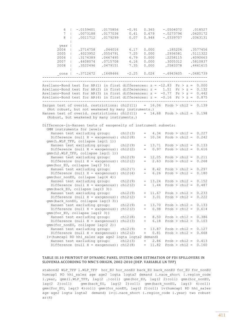
411
6 | -.0159401 .0175856 -0.91 0.365 -.0504072 .018527
7 | .0073188 .0177036 0.41 0.679 -.0273796 .0420172
8 | .0011712 .0179299 0.07 0.948 -.0339707 .0363131
|
year |
2004 | .2714758 .044016 6.17 0.000 .185206 .3577456
2005 | .4023952 .0554791 7.25 0.000 .2936581 .5111322
2006 | .3174389 .0467495 6.79 0.000 .2258115 .4090663
2007 | .4408074 .0715708 6.16 0.000 .3005312 .5810837
2008 | .3522496 .0479151 7.35 0.000 .2583378 .4461615
|
_cons | -.3712672 .1648466 -2.25 0.024 -.6943605 -.0481739
------------------------------------------------------------------------------
------------------------------------------------------------------------------
Arellano-Bond test for AR(1) in first differences: z = -12.83 Pr > z = 0.000
Arellano-Bond test for AR(2) in first differences: z = 1.51 Pr > z = 0.132
Arellano-Bond test for AR(3) in first differences: z = -0.77 Pr > z = 0.442
Arellano-Bond test for AR(4) in first differences: z = -0.16 Pr > z = 0.875
------------------------------------------------------------------------------
Sargan test of overid. restrictions: chi2(11) = 16.06 Prob > chi2 = 0.139
(Not robust, but not weakened by many instruments.)
Hansen test of overid. restrictions: chi2(11) = 14.68 Prob > chi2 = 0.198
(Robust, but weakened by many instruments.)
Difference-in-Hansen tests of exogeneity of instrument subsets:
GMM instruments for levels
Hansen test excluding group: chi2(3) = 4.34 Prob > chi2 = 0.227
Difference (null H = exogenous): chi2(8) = 10.34 Prob > chi2 = 0.242
gmm(L.WLP_TFP, collapse lag(1 1))
Hansen test excluding group: chi2(9) = 13.71 Prob > chi2 = 0.133
Difference (null H = exogenous): chi2(2) = 0.97 Prob > chi2 = 0.616
gmm(L2.WLP_TFP, collapse lag(1 1))
Hansen test excluding group: chi2(9) = 12.05 Prob > chi2 = 0.211
Difference (null H = exogenous): chi2(2) = 2.63 Prob > chi2 = 0.268
gmm(hor_EU, collapse lag(3 5))
Hansen test excluding group: chi2(7) = 8.42 Prob > chi2 = 0.297
Difference (null H = exogenous): chi2(4) = 6.26 Prob > chi2 = 0.180
gmm(hor_nonEU, collapse lag(4 4))
Hansen test excluding group: chi2(9) = 13.24 Prob > chi2 = 0.152
Difference (null H = exogenous): chi2(2) = 1.44 Prob > chi2 = 0.487
gmm(back_EU, collapse lag(3 3))
Hansen test excluding group: chi2(9) = 11.67 Prob > chi2 = 0.233
Difference (null H = exogenous): chi2(2) = 3.01 Prob > chi2 = 0.222
gmm(back_nonEU, collapse lag(3 3))
Hansen test excluding group: chi2(9) = 13.70 Prob > chi2 = 0.133
Difference (null H = exogenous): chi2(2) = 0.98 Prob > chi2 = 0.614
gmm(for_EU, collapse lag(2 3))
Hansen test excluding group: chi2(8) = 8.50 Prob > chi2 = 0.386
Difference (null H = exogenous): chi2(3) = 6.18 Prob > chi2 = 0.103
gmm(for_nonEU, collapse lag(2 2))
Hansen test excluding group: chi2(9) = 13.87 Prob > chi2 = 0.127
Difference (null H = exogenous): chi2(2) = 0.81 Prob > chi2 = 0.668
iv(humcap1 RD hhi_sales age age2 logta logta2 demand)
Hansen test excluding group: chi2(3) = 2.86 Prob > chi2 = 0.413
Difference (null H = exogenous): chi2(8) = 11.82 Prob > chi2 = 0.160
TABLE III.10 PRINTOUT OF DYNAMIC PANEL SYSTEM GMM ESTIMATION OF FDI SPILLOVERS IN SLOVENIA ACCORDING TO MNC’S ORIGIN, 2002-2010 (DEP. VARIABLE LN TFP)
xtabond2 WLP_TFP l.WLP_TFP hor_EU hor_nonEU back_EU back_nonEU for_EU for_nonEU
humcap1 RD hhi_sales age age2 logta logta2 demand i.nace_short i.region_code
i.year, gmm(l.WLP_TFP, lag(2 .)coll) gmm(hor_EU, lag(2 2)coll) gmm(hor_nonEU,
lag(2 2)coll) gmm(back_EU, lag(2 2)coll) gmm(back_nonEU, lag(3 4)coll)
gmm(for_EU, lag(3 4)coll) gmm(for_nonEU, lag(2 2)coll) iv(humcap1 RD hhi_sales
age age2 logta logta2 demand) iv(i.nace_short i.region_code i.year) two robust
ar(4)
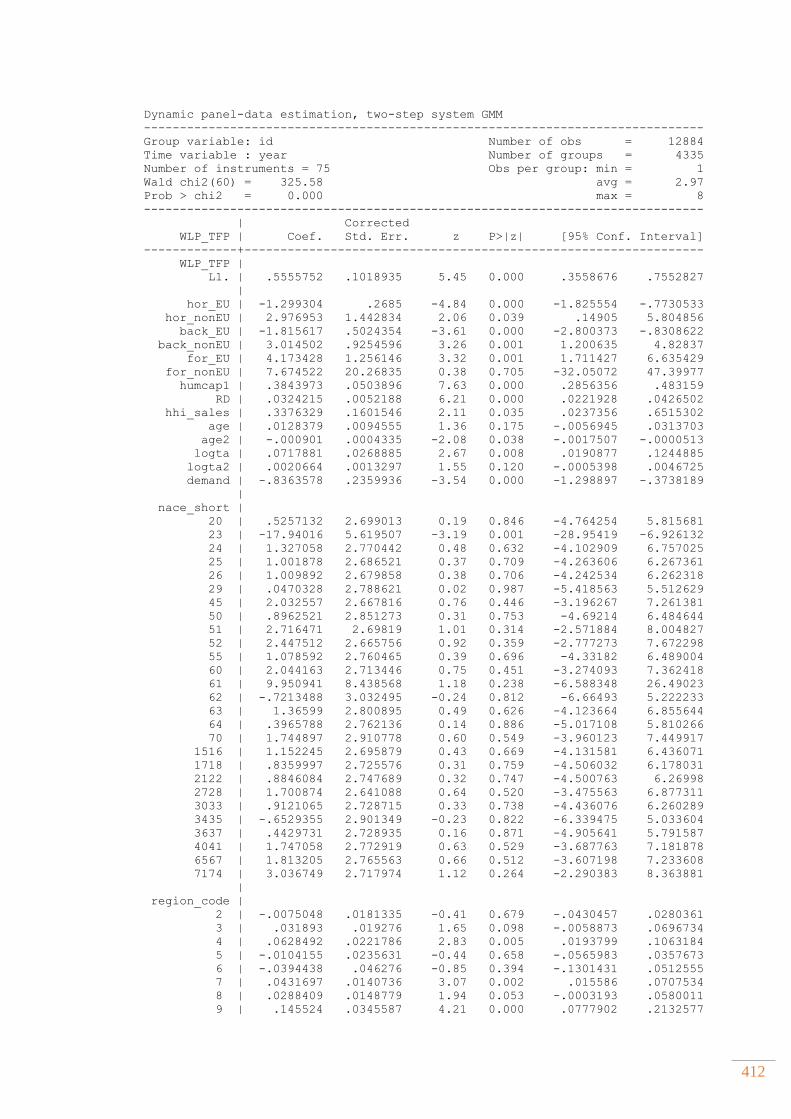
412
Dynamic panel-data estimation, two-step system GMM
------------------------------------------------------------------------------
Group variable: id Number of obs = 12884
Time variable : year Number of groups = 4335
Number of instruments = 75 Obs per group: min = 1
Wald chi2(60) = 325.58 avg = 2.97
Prob > chi2 = 0.000 max = 8
------------------------------------------------------------------------------
| Corrected
WLP_TFP | Coef. Std. Err. z P>|z| [95% Conf. Interval]
-------------+----------------------------------------------------------------
WLP_TFP |
L1. | .5555752 .1018935 5.45 0.000 .3558676 .7552827
|
hor_EU | -1.299304 .2685 -4.84 0.000 -1.825554 -.7730533
hor_nonEU | 2.976953 1.442834 2.06 0.039 .14905 5.804856
back_EU | -1.815617 .5024354 -3.61 0.000 -2.800373 -.8308622
back_nonEU | 3.014502 .9254596 3.26 0.001 1.200635 4.82837
for_EU | 4.173428 1.256146 3.32 0.001 1.711427 6.635429
for_nonEU | 7.674522 20.26835 0.38 0.705 -32.05072 47.39977
humcap1 | .3843973 .0503896 7.63 0.000 .2856356 .483159
RD | .0324215 .0052188 6.21 0.000 .0221928 .0426502
hhi_sales | .3376329 .1601546 2.11 0.035 .0237356 .6515302
age | .0128379 .0094555 1.36 0.175 -.0056945 .0313703
age2 | -.000901 .0004335 -2.08 0.038 -.0017507 -.0000513
logta | .0717881 .0268885 2.67 0.008 .0190877 .1244885
logta2 | .0020664 .0013297 1.55 0.120 -.0005398 .0046725
demand | -.8363578 .2359936 -3.54 0.000 -1.298897 -.3738189
|
nace_short |
20 | .5257132 2.699013 0.19 0.846 -4.764254 5.815681
23 | -17.94016 5.619507 -3.19 0.001 -28.95419 -6.926132
24 | 1.327058 2.770442 0.48 0.632 -4.102909 6.757025
25 | 1.001878 2.686521 0.37 0.709 -4.263606 6.267361
26 | 1.009892 2.679858 0.38 0.706 -4.242534 6.262318
29 | .0470328 2.788621 0.02 0.987 -5.418563 5.512629
45 | 2.032557 2.667816 0.76 0.446 -3.196267 7.261381
50 | .8962521 2.851273 0.31 0.753 -4.69214 6.484644
51 | 2.716471 2.69819 1.01 0.314 -2.571884 8.004827
52 | 2.447512 2.665756 0.92 0.359 -2.777273 7.672298
55 | 1.078592 2.760465 0.39 0.696 -4.33182 6.489004
60 | 2.044163 2.713446 0.75 0.451 -3.274093 7.362418
61 | 9.950941 8.438568 1.18 0.238 -6.588348 26.49023
62 | -.7213488 3.032495 -0.24 0.812 -6.66493 5.222233
63 | 1.36599 2.800895 0.49 0.626 -4.123664 6.855644
64 | .3965788 2.762136 0.14 0.886 -5.017108 5.810266
70 | 1.744897 2.910778 0.60 0.549 -3.960123 7.449917
1516 | 1.152245 2.695879 0.43 0.669 -4.131581 6.436071
1718 | .8359997 2.725576 0.31 0.759 -4.506032 6.178031
2122 | .8846084 2.747689 0.32 0.747 -4.500763 6.26998
2728 | 1.700874 2.641088 0.64 0.520 -3.475563 6.877311
3033 | .9121065 2.728715 0.33 0.738 -4.436076 6.260289
3435 | -.6529355 2.901349 -0.23 0.822 -6.339475 5.033604
3637 | .4429731 2.728935 0.16 0.871 -4.905641 5.791587
4041 | 1.747058 2.772919 0.63 0.529 -3.687763 7.181878
6567 | 1.813205 2.765563 0.66 0.512 -3.607198 7.233608
7174 | 3.036749 2.717974 1.12 0.264 -2.290383 8.363881
|
region_code |
2 | -.0075048 .0181335 -0.41 0.679 -.0430457 .0280361
3 | .031893 .019276 1.65 0.098 -.0058873 .0696734
4 | .0628492 .0221786 2.83 0.005 .0193799 .1063184
5 | -.0104155 .0235631 -0.44 0.658 -.0565983 .0357673
6 | -.0394438 .046276 -0.85 0.394 -.1301431 .0512555
7 | .0431697 .0140736 3.07 0.002 .015586 .0707534
8 | .0288409 .0148779 1.94 0.053 -.0003193 .0580011
9 | .145524 .0345587 4.21 0.000 .0777902 .2132577
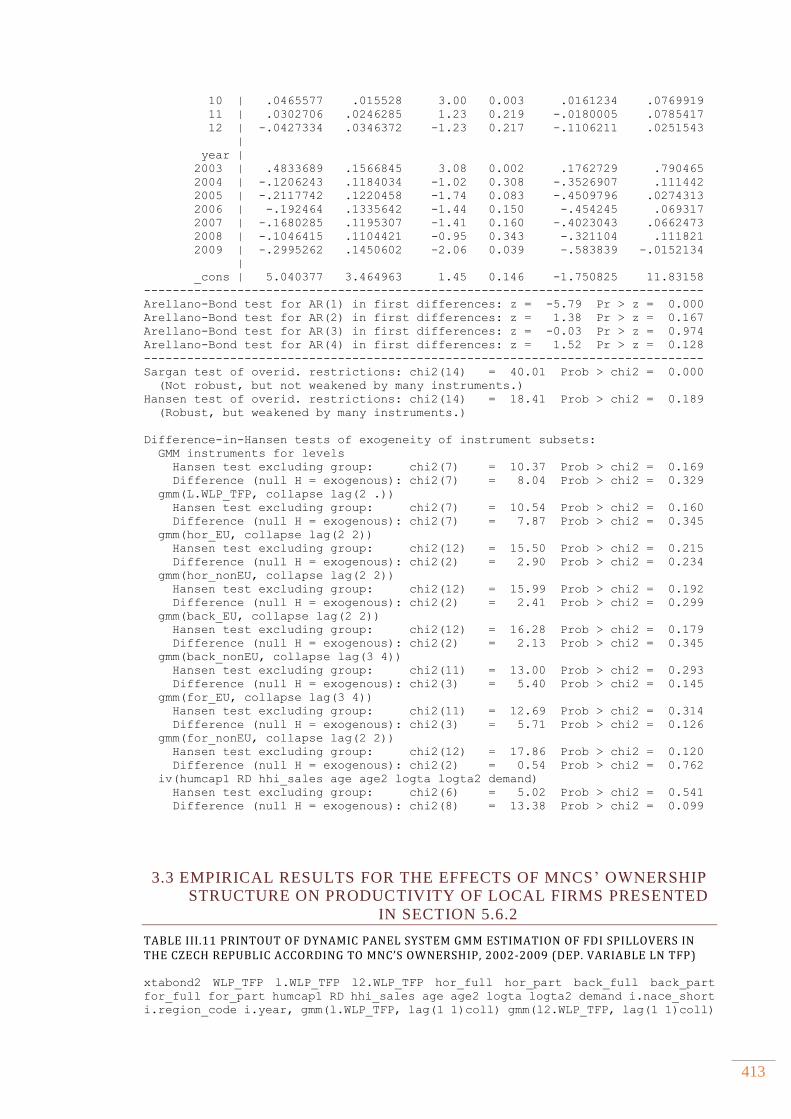
413
10 | .0465577 .015528 3.00 0.003 .0161234 .0769919
11 | .0302706 .0246285 1.23 0.219 -.0180005 .0785417
12 | -.0427334 .0346372 -1.23 0.217 -.1106211 .0251543
|
year |
2003 | .4833689 .1566845 3.08 0.002 .1762729 .790465
2004 | -.1206243 .1184034 -1.02 0.308 -.3526907 .111442
2005 | -.2117742 .1220458 -1.74 0.083 -.4509796 .0274313
2006 | -.192464 .1335642 -1.44 0.150 -.454245 .069317
2007 | -.1680285 .1195307 -1.41 0.160 -.4023043 .0662473
2008 | -.1046415 .1104421 -0.95 0.343 -.321104 .111821
2009 | -.2995262 .1450602 -2.06 0.039 -.583839 -.0152134
|
_cons | 5.040377 3.464963 1.45 0.146 -1.750825 11.83158
------------------------------------------------------------------------------
Arellano-Bond test for AR(1) in first differences: z = -5.79 Pr > z = 0.000
Arellano-Bond test for AR(2) in first differences: z = 1.38 Pr > z = 0.167
Arellano-Bond test for AR(3) in first differences: z = -0.03 Pr > z = 0.974
Arellano-Bond test for AR(4) in first differences: z = 1.52 Pr > z = 0.128
------------------------------------------------------------------------------
Sargan test of overid. restrictions: chi2(14) = 40.01 Prob > chi2 = 0.000
(Not robust, but not weakened by many instruments.)
Hansen test of overid. restrictions: chi2(14) = 18.41 Prob > chi2 = 0.189
(Robust, but weakened by many instruments.)
Difference-in-Hansen tests of exogeneity of instrument subsets:
GMM instruments for levels
Hansen test excluding group: chi2(7) = 10.37 Prob > chi2 = 0.169
Difference (null H = exogenous): chi2(7) = 8.04 Prob > chi2 = 0.329
gmm(L.WLP_TFP, collapse lag(2 .))
Hansen test excluding group: chi2(7) = 10.54 Prob > chi2 = 0.160
Difference (null H = exogenous): chi2(7) = 7.87 Prob > chi2 = 0.345
gmm(hor_EU, collapse lag(2 2))
Hansen test excluding group: chi2(12) = 15.50 Prob > chi2 = 0.215
Difference (null H = exogenous): chi2(2) = 2.90 Prob > chi2 = 0.234
gmm(hor_nonEU, collapse lag(2 2))
Hansen test excluding group: chi2(12) = 15.99 Prob > chi2 = 0.192
Difference (null H = exogenous): chi2(2) = 2.41 Prob > chi2 = 0.299
gmm(back_EU, collapse lag(2 2))
Hansen test excluding group: chi2(12) = 16.28 Prob > chi2 = 0.179
Difference (null H = exogenous): chi2(2) = 2.13 Prob > chi2 = 0.345
gmm(back_nonEU, collapse lag(3 4))
Hansen test excluding group: chi2(11) = 13.00 Prob > chi2 = 0.293
Difference (null H = exogenous): chi2(3) = 5.40 Prob > chi2 = 0.145
gmm(for_EU, collapse lag(3 4))
Hansen test excluding group: chi2(11) = 12.69 Prob > chi2 = 0.314
Difference (null H = exogenous): chi2(3) = 5.71 Prob > chi2 = 0.126
gmm(for_nonEU, collapse lag(2 2))
Hansen test excluding group: chi2(12) = 17.86 Prob > chi2 = 0.120
Difference (null H = exogenous): chi2(2) = 0.54 Prob > chi2 = 0.762
iv(humcap1 RD hhi_sales age age2 logta logta2 demand)
Hansen test excluding group: chi2(6) = 5.02 Prob > chi2 = 0.541
Difference (null H = exogenous): chi2(8) = 13.38 Prob > chi2 = 0.099
3.3 EMPIRICAL RESULTS FOR THE EFFECTS OF MNCS’ OWNERSHIP
STRUCTURE ON PRODUCTIVITY OF LOCAL FIRMS PRESENTED
IN SECTION 5.6.2
TABLE III.11 PRINTOUT OF DYNAMIC PANEL SYSTEM GMM ESTIMATION OF FDI SPILLOVERS IN THE CZECH REPUBLIC ACCORDING TO MNC’S OWNERSHIP, 2002-2009 (DEP. VARIABLE LN TFP)
xtabond2 WLP_TFP l.WLP_TFP l2.WLP_TFP hor_full hor_part back_full back_part
for_full for_part humcap1 RD hhi_sales age age2 logta logta2 demand i.nace_short
i.region_code i.year, gmm(l.WLP_TFP, lag(1 1)coll) gmm(l2.WLP_TFP, lag(1 1)coll)
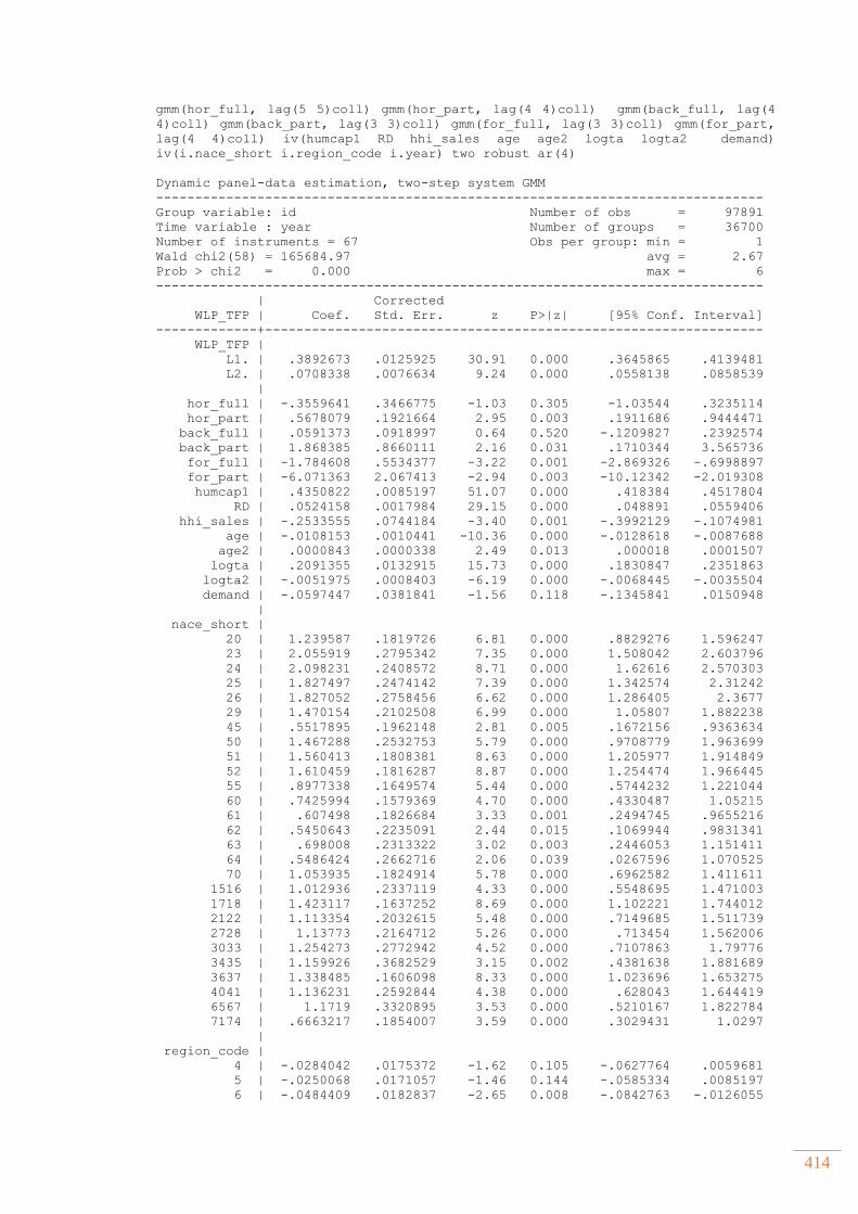
414
gmm(hor_full, lag(5 5)coll) gmm(hor_part, lag(4 4)coll) gmm(back_full, lag(4
4)coll) gmm(back_part, lag(3 3)coll) gmm(for_full, lag(3 3)coll) gmm(for_part,
lag(4 4)coll) iv(humcap1 RD hhi_sales age age2 logta logta2 demand)
iv(i.nace_short i.region_code i.year) two robust ar(4)
Dynamic panel-data estimation, two-step system GMM
------------------------------------------------------------------------------
Group variable: id Number of obs = 97891
Time variable : year Number of groups = 36700
Number of instruments = 67 Obs per group: min = 1
Wald chi2(58) = 165684.97 avg = 2.67
Prob > chi2 = 0.000 max = 6
------------------------------------------------------------------------------
| Corrected
WLP_TFP | Coef. Std. Err. z P>|z| [95% Conf. Interval]
-------------+----------------------------------------------------------------
WLP_TFP |
L1. | .3892673 .0125925 30.91 0.000 .3645865 .4139481
L2. | .0708338 .0076634 9.24 0.000 .0558138 .0858539
|
hor_full | -.3559641 .3466775 -1.03 0.305 -1.03544 .3235114
hor_part | .5678079 .1921664 2.95 0.003 .1911686 .9444471
back_full | .0591373 .0918997 0.64 0.520 -.1209827 .2392574
back_part | 1.868385 .8660111 2.16 0.031 .1710344 3.565736
for_full | -1.784608 .5534377 -3.22 0.001 -2.869326 -.6998897
for_part | -6.071363 2.067413 -2.94 0.003 -10.12342 -2.019308
humcap1 | .4350822 .0085197 51.07 0.000 .418384 .4517804
RD | .0524158 .0017984 29.15 0.000 .048891 .0559406
hhi_sales | -.2533555 .0744184 -3.40 0.001 -.3992129 -.1074981
age | -.0108153 .0010441 -10.36 0.000 -.0128618 -.0087688
age2 | .0000843 .0000338 2.49 0.013 .000018 .0001507
logta | .2091355 .0132915 15.73 0.000 .1830847 .2351863
logta2 | -.0051975 .0008403 -6.19 0.000 -.0068445 -.0035504
demand | -.0597447 .0381841 -1.56 0.118 -.1345841 .0150948
|
nace_short |
20 | 1.239587 .1819726 6.81 0.000 .8829276 1.596247
23 | 2.055919 .2795342 7.35 0.000 1.508042 2.603796
24 | 2.098231 .2408572 8.71 0.000 1.62616 2.570303
25 | 1.827497 .2474142 7.39 0.000 1.342574 2.31242
26 | 1.827052 .2758456 6.62 0.000 1.286405 2.3677
29 | 1.470154 .2102508 6.99 0.000 1.05807 1.882238
45 | .5517895 .1962148 2.81 0.005 .1672156 .9363634
50 | 1.467288 .2532753 5.79 0.000 .9708779 1.963699
51 | 1.560413 .1808381 8.63 0.000 1.205977 1.914849
52 | 1.610459 .1816287 8.87 0.000 1.254474 1.966445
55 | .8977338 .1649574 5.44 0.000 .5744232 1.221044
60 | .7425994 .1579369 4.70 0.000 .4330487 1.05215
61 | .607498 .1826684 3.33 0.001 .2494745 .9655216
62 | .5450643 .2235091 2.44 0.015 .1069944 .9831341
63 | .698008 .2313322 3.02 0.003 .2446053 1.151411
64 | .5486424 .2662716 2.06 0.039 .0267596 1.070525
70 | 1.053935 .1824914 5.78 0.000 .6962582 1.411611
1516 | 1.012936 .2337119 4.33 0.000 .5548695 1.471003
1718 | 1.423117 .1637252 8.69 0.000 1.102221 1.744012
2122 | 1.113354 .2032615 5.48 0.000 .7149685 1.511739
2728 | 1.13773 .2164712 5.26 0.000 .713454 1.562006
3033 | 1.254273 .2772942 4.52 0.000 .7107863 1.79776
3435 | 1.159926 .3682529 3.15 0.002 .4381638 1.881689
3637 | 1.338485 .1606098 8.33 0.000 1.023696 1.653275
4041 | 1.136231 .2592844 4.38 0.000 .628043 1.644419
6567 | 1.1719 .3320895 3.53 0.000 .5210167 1.822784
7174 | .6663217 .1854007 3.59 0.000 .3029431 1.0297
|
region_code |
4 | -.0284042 .0175372 -1.62 0.105 -.0627764 .0059681
5 | -.0250068 .0171057 -1.46 0.144 -.0585334 .0085197
6 | -.0484409 .0182837 -2.65 0.008 -.0842763 -.0126055
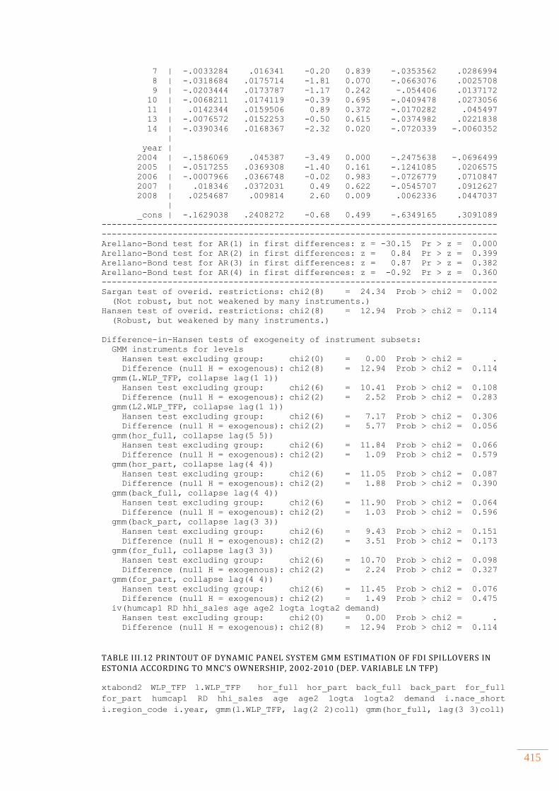
415
7 | -.0033284 .016341 -0.20 0.839 -.0353562 .0286994
8 | -.0318684 .0175714 -1.81 0.070 -.0663076 .0025708
9 | -.0203444 .0173787 -1.17 0.242 -.054406 .0137172
10 | -.0068211 .0174119 -0.39 0.695 -.0409478 .0273056
11 | .0142344 .0159506 0.89 0.372 -.0170282 .045497
13 | -.0076572 .0152253 -0.50 0.615 -.0374982 .0221838
14 | -.0390346 .0168367 -2.32 0.020 -.0720339 -.0060352
|
year |
2004 | -.1586069 .045387 -3.49 0.000 -.2475638 -.0696499
2005 | -.0517255 .0369308 -1.40 0.161 -.1241085 .0206575
2006 | -.0007966 .0366748 -0.02 0.983 -.0726779 .0710847
2007 | .018346 .0372031 0.49 0.622 -.0545707 .0912627
2008 | .0254687 .009814 2.60 0.009 .0062336 .0447037
|
_cons | -.1629038 .2408272 -0.68 0.499 -.6349165 .3091089
------------------------------------------------------------------------------
------------------------------------------------------------------------------
Arellano-Bond test for AR(1) in first differences: z = -30.15 Pr > z = 0.000
Arellano-Bond test for AR(2) in first differences: z = 0.84 Pr > z = 0.399
Arellano-Bond test for AR(3) in first differences: z = 0.87 Pr > z = 0.382
Arellano-Bond test for AR(4) in first differences: z = -0.92 Pr > z = 0.360
------------------------------------------------------------------------------
Sargan test of overid. restrictions: chi2(8) = 24.34 Prob > chi2 = 0.002
(Not robust, but not weakened by many instruments.)
Hansen test of overid. restrictions: chi2(8) = 12.94 Prob > chi2 = 0.114
(Robust, but weakened by many instruments.)
Difference-in-Hansen tests of exogeneity of instrument subsets:
GMM instruments for levels
Hansen test excluding group: chi2(0) = 0.00 Prob > chi2 = .
Difference (null H = exogenous): chi2(8) = 12.94 Prob > chi2 = 0.114
gmm(L.WLP_TFP, collapse lag(1 1))
Hansen test excluding group: chi2(6) = 10.41 Prob > chi2 = 0.108
Difference (null H = exogenous): chi2(2) = 2.52 Prob > chi2 = 0.283
gmm(L2.WLP_TFP, collapse lag(1 1))
Hansen test excluding group: chi2(6) = 7.17 Prob > chi2 = 0.306
Difference (null H = exogenous): chi2(2) = 5.77 Prob > chi2 = 0.056
gmm(hor_full, collapse lag(5 5))
Hansen test excluding group: chi2(6) = 11.84 Prob > chi2 = 0.066
Difference (null H = exogenous): chi2(2) = 1.09 Prob > chi2 = 0.579
gmm(hor_part, collapse lag(4 4))
Hansen test excluding group: chi2(6) = 11.05 Prob > chi2 = 0.087
Difference (null H = exogenous): chi2(2) = 1.88 Prob > chi2 = 0.390
gmm(back_full, collapse lag(4 4))
Hansen test excluding group: chi2(6) = 11.90 Prob > chi2 = 0.064
Difference (null H = exogenous): chi2(2) = 1.03 Prob > chi2 = 0.596
gmm(back_part, collapse lag(3 3))
Hansen test excluding group: chi2(6) = 9.43 Prob > chi2 = 0.151
Difference (null H = exogenous): chi2(2) = 3.51 Prob > chi2 = 0.173
gmm(for_full, collapse lag(3 3))
Hansen test excluding group: chi2(6) = 10.70 Prob > chi2 = 0.098
Difference (null H = exogenous): chi2(2) = 2.24 Prob > chi2 = 0.327
gmm(for_part, collapse lag(4 4))
Hansen test excluding group: chi2(6) = 11.45 Prob > chi2 = 0.076
Difference (null H = exogenous): chi2(2) = 1.49 Prob > chi2 = 0.475
iv(humcap1 RD hhi_sales age age2 logta logta2 demand)
Hansen test excluding group: chi2(0) = 0.00 Prob > chi2 = .
Difference (null H = exogenous): chi2(8) = 12.94 Prob > chi2 = 0.114
TABLE III.12 PRINTOUT OF DYNAMIC PANEL SYSTEM GMM ESTIMATION OF FDI SPILLOVERS IN ESTONIA ACCORDING TO MNC’S OWNERSHIP, 2002-2010 (DEP. VARIABLE LN TFP)
xtabond2 WLP_TFP l.WLP_TFP hor_full hor_part back_full back_part for_full
for_part humcap1 RD hhi_sales age age2 logta logta2 demand i.nace_short
i.region_code i.year, gmm(l.WLP_TFP, lag(2 2)coll) gmm(hor_full, lag(3 3)coll)
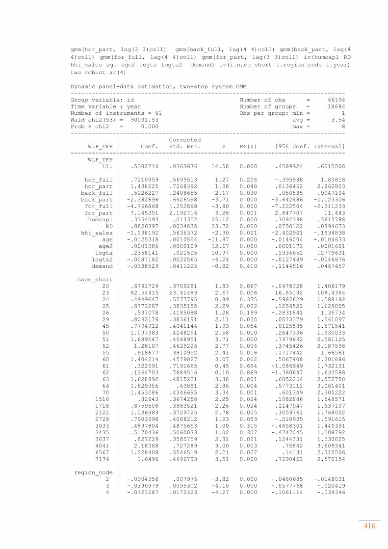
416
gmm(hor_part, lag(3 3)coll) gmm(back_full, lag(4 4)coll) gmm(back_part, lag(4
4)coll) gmm(for_full, lag(4 4)coll) gmm(for_part, lag(3 3)coll) iv(humcap1 RD
hhi_sales age age2 logta logta2 demand) iv(i.nace_short i.region_code i.year)
two robust ar(4)
Dynamic panel-data estimation, two-step system GMM
------------------------------------------------------------------------------
Group variable: id Number of obs = 66194
Time variable : year Number of groups = 18684
Number of instruments = 61 Obs per group: min = 1
Wald chi2(53) = 90031.53 avg = 3.54
Prob > chi2 = 0.000 max = 8
------------------------------------------------------------------------------
| Corrected
WLP_TFP | Coef. Std. Err. z P>|z| [95% Conf. Interval]
-------------+----------------------------------------------------------------
WLP_TFP |
L1. | .5302716 .0363676 14.58 0.000 .4589924 .6015508
|
hor_full | .7210959 .5699513 1.27 0.206 -.395988 1.83818
hor_part | 1.438225 .7268392 1.98 0.048 .0136462 2.862803
back_full | .5226227 .2408655 2.17 0.030 .050535 .9947104
back_part | -2.382896 .6426598 -3.71 0.000 -3.642486 -1.123306
for_full | -4.766868 1.252898 -3.80 0.000 -7.222504 -2.311233
for_part | 7.145351 2.192716 3.26 0.001 2.847707 11.443
humcap1 | .3354093 .013352 25.12 0.000 .3092398 .3615788
RD | .0826397 .0034835 23.72 0.000 .0758122 .0894673
hhi_sales | -1.298192 .5636372 -2.30 0.021 -2.402901 -.1934838
age | -.0125318 .0010554 -11.87 0.000 -.0146004 -.0104633
age2 | .0001386 .0000109 12.67 0.000 .0001172 .0001601
logta | .2358141 .021505 10.97 0.000 .1936652 .2779631
logta2 | -.0087182 .0020565 -4.24 0.000 -.0127489 -.0046876
demand | -.0338529 .0411225 -0.82 0.410 -.1144516 .0467457
|
nace_short |
20 | .6791729 .3709281 1.83 0.067 -.0478328 1.406179
23 | 62.54415 23.41483 2.67 0.008 16.65192 108.4364
24 | .4949647 .5577795 0.89 0.375 -.5982629 1.588192
25 | .8773287 .3835155 2.29 0.022 .1256522 1.629005
26 | .537078 .4185088 1.28 0.199 -.2831841 1.35734
29 | .8092176 .3836191 2.11 0.035 .0573379 1.561097
45 | .7794912 .4041144 1.93 0.054 -.0125585 1.571541
50 | 1.097383 .4248291 2.58 0.010 .2647336 1.930033
51 | 1.689547 .4548951 3.71 0.000 .7979692 2.581125
52 | 1.28107 .4625226 2.77 0.006 .3745426 2.187598
55 | .918677 .3810952 2.41 0.016 .1717442 1.66561
60 | 1.404214 .4579027 3.07 0.002 .5067408 2.301686
61 | .322591 .7191665 0.45 0.654 -1.086949 1.732131
62 | .1264703 .7689516 0.16 0.869 -1.380647 1.633588
63 | 1.628992 .4815221 3.38 0.001 .6852264 2.572758
64 | 1.829356 .63881 2.86 0.004 .5773112 3.081401
70 | 1.453286 .4346695 3.34 0.001 .601349 2.305222
1516 | .82843 .3674258 2.25 0.024 .1082886 1.548571
1718 | .8759508 .3883521 2.26 0.024 .1147947 1.637107
2122 | 1.036989 .3729725 2.78 0.005 .3059761 1.768002
2728 | .7903398 .4088212 1.93 0.053 -.010935 1.591615
3033 | .4897804 .4875653 1.00 0.315 -.4658301 1.445391
3435 | .5170436 .5060033 1.02 0.307 -.4747045 1.508792
3637 | .827229 .3585759 2.31 0.021 .1244331 1.530025
4041 | 2.18388 .727289 3.00 0.003 .75842 3.609341
6567 | 1.228408 .5546519 2.21 0.027 .14131 2.315506
7174 | 1.6496 .4696793 3.51 0.000 .7290452 2.570154
|
region_code |
2 | -.0304358 .007976 -3.82 0.000 -.0460685 -.0148031
3 | -.0390979 .0095302 -4.10 0.000 -.0577768 -.020419
4 | -.0727287 .0170323 -4.27 0.000 -.1061114 -.039346
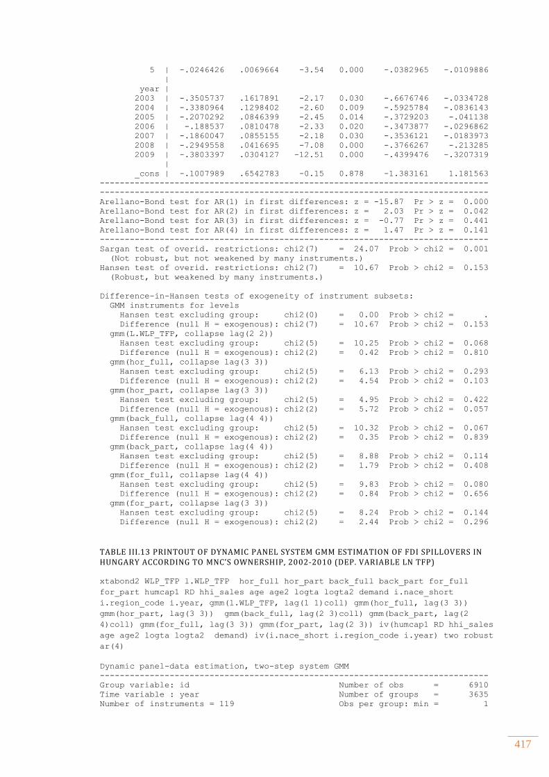
417
5 | -.0246426 .0069664 -3.54 0.000 -.0382965 -.0109886
|
year |
2003 | -.3505737 .1617891 -2.17 0.030 -.6676746 -.0334728
2004 | -.3380964 .1298402 -2.60 0.009 -.5925784 -.0836143
2005 | -.2070292 .0846399 -2.45 0.014 -.3729203 -.041138
2006 | -.188537 .0810478 -2.33 0.020 -.3473877 -.0296862
2007 | -.1860047 .0855155 -2.18 0.030 -.3536121 -.0183973
2008 | -.2949558 .0416695 -7.08 0.000 -.3766267 -.213285
2009 | -.3803397 .0304127 -12.51 0.000 -.4399476 -.3207319
|
_cons | -.1007989 .6542783 -0.15 0.878 -1.383161 1.181563
------------------------------------------------------------------------------
------------------------------------------------------------------------------
Arellano-Bond test for AR(1) in first differences: z = -15.87 Pr > z = 0.000
Arellano-Bond test for AR(2) in first differences: z = 2.03 Pr > z = 0.042
Arellano-Bond test for AR(3) in first differences: z = -0.77 Pr > z = 0.441
Arellano-Bond test for AR(4) in first differences: z = 1.47 Pr > z = 0.141
------------------------------------------------------------------------------
Sargan test of overid. restrictions: chi2(7) = 24.07 Prob > chi2 = 0.001
(Not robust, but not weakened by many instruments.)
Hansen test of overid. restrictions: chi2(7) = 10.67 Prob > chi2 = 0.153
(Robust, but weakened by many instruments.)
Difference-in-Hansen tests of exogeneity of instrument subsets:
GMM instruments for levels
Hansen test excluding group: chi2(0) = 0.00 Prob > chi2 = .
Difference (null H = exogenous): chi2(7) = 10.67 Prob > chi2 = 0.153
gmm(L.WLP_TFP, collapse lag(2 2))
Hansen test excluding group: chi2(5) = 10.25 Prob > chi2 = 0.068
Difference (null H = exogenous): chi2(2) = 0.42 Prob > chi2 = 0.810
gmm(hor_full, collapse lag(3 3))
Hansen test excluding group: chi2(5) = 6.13 Prob > chi2 = 0.293
Difference (null H = exogenous): chi2(2) = 4.54 Prob > chi2 = 0.103
gmm(hor_part, collapse lag(3 3))
Hansen test excluding group: chi2(5) = 4.95 Prob > chi2 = 0.422
Difference (null H = exogenous): chi2(2) = 5.72 Prob > chi2 = 0.057
gmm(back_full, collapse lag(4 4))
Hansen test excluding group: chi2(5) = 10.32 Prob > chi2 = 0.067
Difference (null H = exogenous): chi2(2) = 0.35 Prob > chi2 = 0.839
gmm(back_part, collapse lag(4 4))
Hansen test excluding group: chi2(5) = 8.88 Prob > chi2 = 0.114
Difference (null H = exogenous): chi2(2) = 1.79 Prob > chi2 = 0.408
gmm(for_full, collapse lag(4 4))
Hansen test excluding group: chi2(5) = 9.83 Prob > chi2 = 0.080
Difference (null H = exogenous): chi2(2) = 0.84 Prob > chi2 = 0.656
gmm(for_part, collapse lag(3 3))
Hansen test excluding group: chi2(5) = 8.24 Prob > chi2 = 0.144
Difference (null H = exogenous): chi2(2) = 2.44 Prob > chi2 = 0.296
TABLE III.13 PRINTOUT OF DYNAMIC PANEL SYSTEM GMM ESTIMATION OF FDI SPILLOVERS IN HUNGARY ACCORDING TO MNC’S OWNERSHIP, 2002-2010 (DEP. VARIABLE LN TFP)
xtabond2 WLP_TFP l.WLP_TFP hor_full hor_part back_full back_part for_full
for_part humcap1 RD hhi_sales age age2 logta logta2 demand i.nace_short
i.region_code i.year, gmm(l.WLP_TFP, lag(1 1)coll) gmm(hor_full, lag(3 3))
gmm(hor_part, lag(3 3)) gmm(back_full, lag(2 3)coll) gmm(back_part, lag(2
4)coll) gmm(for_full, lag(3 3)) gmm(for_part, lag(2 3)) iv(humcap1 RD hhi_sales
age age2 logta logta2 demand) iv(i.nace_short i.region_code i.year) two robust
ar(4)
Dynamic panel-data estimation, two-step system GMM
------------------------------------------------------------------------------
Group variable: id Number of obs = 6910
Time variable : year Number of groups = 3635
Number of instruments = 119 Obs per group: min = 1
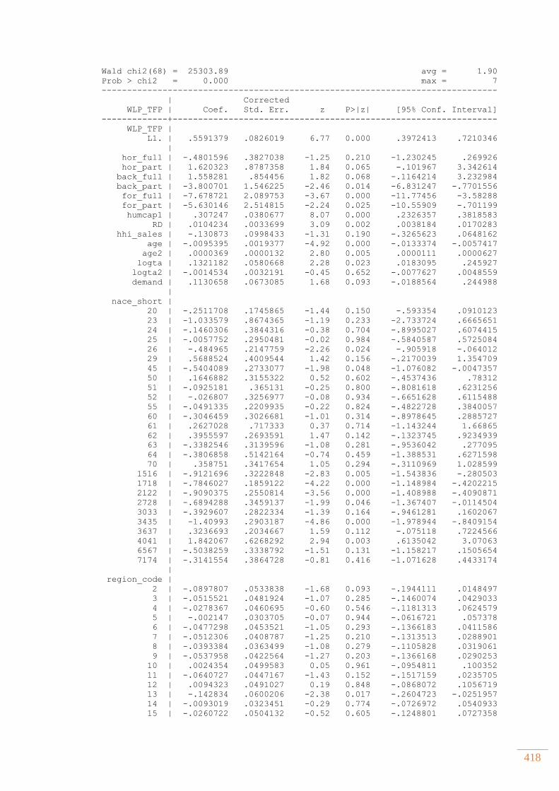
418
Wald chi2(68) = 25303.89 avg = 1.90
Prob > chi2 = 0.000 max = 7
------------------------------------------------------------------------------
| Corrected
WLP_TFP | Coef. Std. Err. z P>|z| [95% Conf. Interval]
-------------+----------------------------------------------------------------
WLP_TFP |
L1. | .5591379 .0826019 6.77 0.000 .3972413 .7210346
|
hor_full | -.4801596 .3827038 -1.25 0.210 -1.230245 .269926
hor_part | 1.620323 .8787358 1.84 0.065 -.101967 3.342614
back_full | 1.558281 .854456 1.82 0.068 -.1164214 3.232984
back_part | -3.800701 1.546225 -2.46 0.014 -6.831247 -.7701556
for_full | -7.678721 2.089753 -3.67 0.000 -11.77456 -3.58288
for_part | -5.630146 2.514815 -2.24 0.025 -10.55909 -.701199
humcap1 | .307247 .0380677 8.07 0.000 .2326357 .3818583
RD | .0104234 .0033699 3.09 0.002 .0038184 .0170283
hhi_sales | -.130873 .0998433 -1.31 0.190 -.3265623 .0648162
age | -.0095395 .0019377 -4.92 0.000 -.0133374 -.0057417
age2 | .0000369 .0000132 2.80 0.005 .0000111 .0000627
logta | .1321182 .0580668 2.28 0.023 .0183095 .245927
logta2 | -.0014534 .0032191 -0.45 0.652 -.0077627 .0048559
demand | .1130658 .0673085 1.68 0.093 -.0188564 .244988
|
nace_short |
20 | -.2511708 .1745865 -1.44 0.150 -.593354 .0910123
23 | -1.033579 .8674365 -1.19 0.233 -2.733724 .6665651
24 | -.1460306 .3844316 -0.38 0.704 -.8995027 .6074415
25 | -.0057752 .2950481 -0.02 0.984 -.5840587 .5725084
26 | -.484965 .2147759 -2.26 0.024 -.905918 -.064012
29 | .5688524 .4009544 1.42 0.156 -.2170039 1.354709
45 | -.5404089 .2733077 -1.98 0.048 -1.076082 -.0047357
50 | .1646882 .3155322 0.52 0.602 -.4537436 .78312
51 | -.0925181 .365131 -0.25 0.800 -.8081618 .6231256
52 | -.026807 .3256977 -0.08 0.934 -.6651628 .6115488
55 | -.0491335 .2209935 -0.22 0.824 -.4822728 .3840057
60 | -.3046459 .3026681 -1.01 0.314 -.8978645 .2885727
61 | .2627028 .717333 0.37 0.714 -1.143244 1.66865
62 | .3955597 .2693591 1.47 0.142 -.1323745 .9234939
63 | -.3382546 .3139596 -1.08 0.281 -.9536042 .277095
64 | -.3806858 .5142164 -0.74 0.459 -1.388531 .6271598
70 | .358751 .3417654 1.05 0.294 -.3110969 1.028599
1516 | -.9121696 .3222848 -2.83 0.005 -1.543836 -.280503
1718 | -.7846027 .1859122 -4.22 0.000 -1.148984 -.4202215
2122 | -.9090375 .2550814 -3.56 0.000 -1.408988 -.4090871
2728 | -.6894288 .3459137 -1.99 0.046 -1.367407 -.0114504
3033 | -.3929607 .2822334 -1.39 0.164 -.9461281 .1602067
3435 | -1.40993 .2903187 -4.86 0.000 -1.978944 -.8409154
3637 | .3236693 .2034667 1.59 0.112 -.075118 .7224566
4041 | 1.842067 .6268292 2.94 0.003 .6135042 3.07063
6567 | -.5038259 .3338792 -1.51 0.131 -1.158217 .1505654
7174 | -.3141554 .3864728 -0.81 0.416 -1.071628 .4433174
|
region_code |
2 | -.0897807 .0533838 -1.68 0.093 -.1944111 .0148497
3 | -.0515521 .0481924 -1.07 0.285 -.1460074 .0429033
4 | -.0278367 .0460695 -0.60 0.546 -.1181313 .0624579
5 | -.002147 .0303705 -0.07 0.944 -.0616721 .057378
6 | -.0477298 .0453521 -1.05 0.293 -.1366183 .0411586
7 | -.0512306 .0408787 -1.25 0.210 -.1313513 .0288901
8 | -.0393384 .0363499 -1.08 0.279 -.1105828 .0319061
9 | -.0537958 .0422564 -1.27 0.203 -.1366168 .0290253
10 | .0024354 .0499583 0.05 0.961 -.0954811 .100352
11 | -.0640727 .0447167 -1.43 0.152 -.1517159 .0235705
12 | .0094323 .0491027 0.19 0.848 -.0868072 .1056719
13 | -.142834 .0600206 -2.38 0.017 -.2604723 -.0251957
14 | -.0093019 .0323451 -0.29 0.774 -.0726972 .0540933
15 | -.0260722 .0504132 -0.52 0.605 -.1248801 .0727358
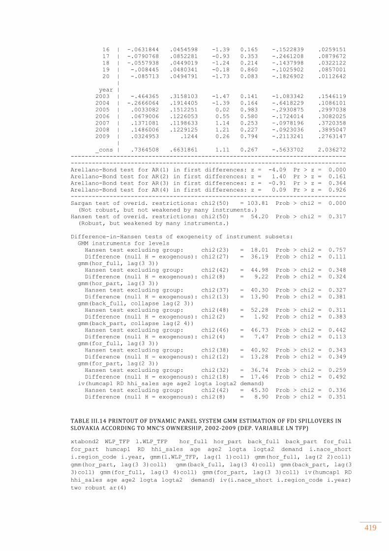
419
16 | -.0631844 .0454598 -1.39 0.165 -.1522839 .0259151
17 | -.0790768 .0852281 -0.93 0.353 -.2461208 .0879672
18 | -.0557938 .0449019 -1.24 0.214 -.1437998 .0322122
19 | -.008445 .0480341 -0.18 0.860 -.1025902 .0857001
20 | -.085713 .0494791 -1.73 0.083 -.1826902 .0112642
|
year |
2003 | -.464365 .3158103 -1.47 0.141 -1.083342 .1546119
2004 | -.2666064 .1914405 -1.39 0.164 -.6418229 .1086101
2005 | .0033082 .1512251 0.02 0.983 -.2930875 .2997038
2006 | .0679006 .1226053 0.55 0.580 -.1724014 .3082025
2007 | .1371081 .1198633 1.14 0.253 -.0978196 .3720358
2008 | .1486006 .1229125 1.21 0.227 -.0923036 .3895047
2009 | .0324953 .1244 0.26 0.794 -.2113241 .2763147
|
_cons | .7364508 .6631861 1.11 0.267 -.5633702 2.036272
------------------------------------------------------------------------------
------------------------------------------------------------------------------
Arellano-Bond test for AR(1) in first differences: z = -4.09 Pr > z = 0.000
Arellano-Bond test for AR(2) in first differences: z = 1.40 Pr > z = 0.161
Arellano-Bond test for AR(3) in first differences: z = -0.91 Pr > z = 0.364
Arellano-Bond test for AR(4) in first differences: z = 0.09 Pr > z = 0.926
------------------------------------------------------------------------------
Sargan test of overid. restrictions: chi2(50) = 103.81 Prob > chi2 = 0.000
(Not robust, but not weakened by many instruments.)
Hansen test of overid. restrictions: chi2(50) = 54.20 Prob > chi2 = 0.317
(Robust, but weakened by many instruments.)
Difference-in-Hansen tests of exogeneity of instrument subsets:
GMM instruments for levels
Hansen test excluding group: chi2(23) = 18.01 Prob > chi2 = 0.757
Difference (null H = exogenous): chi2(27) = 36.19 Prob > chi2 = 0.111
gmm(hor_full, lag(3 3))
Hansen test excluding group: chi2(42) = 44.98 Prob > chi2 = 0.348
Difference (null H = exogenous): chi2(8) = 9.22 Prob > chi2 = 0.324
gmm(hor_part, lag(3 3))
Hansen test excluding group: chi2(37) = 40.30 Prob > chi2 = 0.327
Difference (null H = exogenous): chi2(13) = 13.90 Prob > chi2 = 0.381
gmm(back_full, collapse lag(2 3))
Hansen test excluding group: chi2(48) = 52.28 Prob > chi2 = 0.311
Difference (null H = exogenous): chi2(2) = 1.92 Prob > chi2 = 0.383
gmm(back_part, collapse lag(2 4))
Hansen test excluding group: chi2(46) = 46.73 Prob > chi2 = 0.442
Difference (null H = exogenous): chi2(4) = 7.47 Prob > chi2 = 0.113
gmm(for_full, lag(3 3))
Hansen test excluding group: chi2(38) = 40.92 Prob > chi2 = 0.343
Difference (null H = exogenous): chi2(12) = 13.28 Prob > chi2 = 0.349
gmm(for_part, lag(2 3))
Hansen test excluding group: chi2(32) = 36.74 Prob > chi2 = 0.259
Difference (null H = exogenous): chi2(18) = 17.46 Prob > chi2 = 0.492
iv(humcap1 RD hhi_sales age age2 logta logta2 demand)
Hansen test excluding group: chi2(42) = 45.30 Prob > chi2 = 0.336
Difference (null H = exogenous): chi2(8) = 8.90 Prob > chi2 = 0.351
TABLE III.14 PRINTOUT OF DYNAMIC PANEL SYSTEM GMM ESTIMATION OF FDI SPILLOVERS IN SLOVAKIA ACCORDING TO MNC’S OWNERSHIP, 2002-2009 (DEP. VARIABLE LN TFP)
xtabond2 WLP_TFP l.WLP_TFP hor_full hor_part back_full back_part for_full
for_part humcap1 RD hhi_sales age age2 logta logta2 demand i.nace_short
i.region_code i.year, gmm(l.WLP_TFP, lag(1 1)coll) gmm(hor_full, lag(2 2)coll)
gmm(hor_part, lag(3 3)coll) gmm(back_full, lag(3 4)coll) gmm(back_part, lag(3
3)coll) gmm(for_full, lag(3 4)coll) gmm(for_part, lag(3 3)coll) iv(humcap1 RD
hhi_sales age age2 logta logta2 demand) iv(i.nace_short i.region_code i.year)
two robust ar(4)
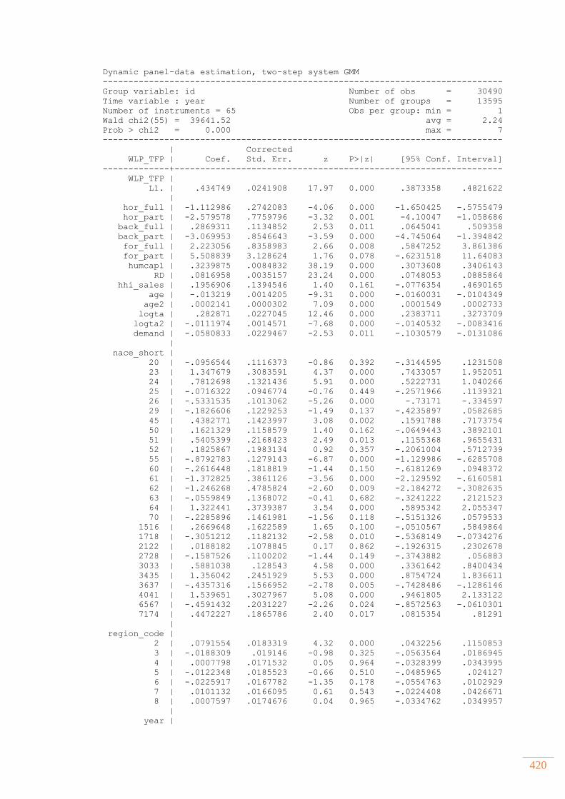
420
Dynamic panel-data estimation, two-step system GMM
------------------------------------------------------------------------------
Group variable: id Number of obs = 30490
Time variable : year Number of groups = 13595
Number of instruments = 65 Obs per group: min = 1
Wald chi2(55) = 39641.52 avg = 2.24
Prob > chi2 = 0.000 max = 7
------------------------------------------------------------------------------
| Corrected
WLP_TFP | Coef. Std. Err. z P>|z| [95% Conf. Interval]
-------------+----------------------------------------------------------------
WLP_TFP |
L1. | .434749 .0241908 17.97 0.000 .3873358 .4821622
|
hor_full | -1.112986 .2742083 -4.06 0.000 -1.650425 -.5755479
hor_part | -2.579578 .7759796 -3.32 0.001 -4.10047 -1.058686
back_full | .2869311 .1134852 2.53 0.011 .0645041 .509358
back_part | -3.069953 .8546643 -3.59 0.000 -4.745064 -1.394842
for_full | 2.223056 .8358983 2.66 0.008 .5847252 3.861386
for_part | 5.508839 3.128624 1.76 0.078 -.6231518 11.64083
humcap1 | .3239875 .0084832 38.19 0.000 .3073608 .3406143
RD | .0816958 .0035157 23.24 0.000 .0748053 .0885864
hhi_sales | .1956906 .1394546 1.40 0.161 -.0776354 .4690165
age | -.013219 .0014205 -9.31 0.000 -.0160031 -.0104349
age2 | .0002141 .0000302 7.09 0.000 .0001549 .0002733
logta | .282871 .0227045 12.46 0.000 .2383711 .3273709
logta2 | -.0111974 .0014571 -7.68 0.000 -.0140532 -.0083416
demand | -.0580833 .0229467 -2.53 0.011 -.1030579 -.0131086
|
nace_short |
20 | -.0956544 .1116373 -0.86 0.392 -.3144595 .1231508
23 | 1.347679 .3083591 4.37 0.000 .7433057 1.952051
24 | .7812698 .1321436 5.91 0.000 .5222731 1.040266
25 | -.0716322 .0946774 -0.76 0.449 -.2571966 .1139321
26 | -.5331535 .1013062 -5.26 0.000 -.73171 -.334597
29 | -.1826606 .1229253 -1.49 0.137 -.4235897 .0582685
45 | .4382771 .1423997 3.08 0.002 .1591788 .7173754
50 | .1621329 .1158579 1.40 0.162 -.0649443 .3892101
51 | .5405399 .2168423 2.49 0.013 .1155368 .9655431
52 | .1825867 .1983134 0.92 0.357 -.2061004 .5712739
55 | -.8792783 .1279143 -6.87 0.000 -1.129986 -.6285708
60 | -.2616448 .1818819 -1.44 0.150 -.6181269 .0948372
61 | -1.372825 .3861126 -3.56 0.000 -2.129592 -.6160581
62 | -1.246268 .4785824 -2.60 0.009 -2.184272 -.3082635
63 | -.0559849 .1368072 -0.41 0.682 -.3241222 .2121523
64 | 1.322441 .3739387 3.54 0.000 .5895342 2.055347
70 | -.2285896 .1461981 -1.56 0.118 -.5151326 .0579533
1516 | .2669648 .1622589 1.65 0.100 -.0510567 .5849864
1718 | -.3051212 .1182132 -2.58 0.010 -.5368149 -.0734276
2122 | .0188182 .1078845 0.17 0.862 -.1926315 .2302678
2728 | -.1587526 .1100202 -1.44 0.149 -.3743882 .056883
3033 | .5881038 .128543 4.58 0.000 .3361642 .8400434
3435 | 1.356042 .2451929 5.53 0.000 .8754724 1.836611
3637 | -.4357316 .1566952 -2.78 0.005 -.7428486 -.1286146
4041 | 1.539651 .3027967 5.08 0.000 .9461805 2.133122
6567 | -.4591432 .2031227 -2.26 0.024 -.8572563 -.0610301
7174 | .4472227 .1865786 2.40 0.017 .0815354 .81291
|
region_code |
2 | .0791554 .0183319 4.32 0.000 .0432256 .1150853
3 | -.0188309 .019146 -0.98 0.325 -.0563564 .0186945
4 | .0007798 .0171532 0.05 0.964 -.0328399 .0343995
5 | -.0122348 .0185523 -0.66 0.510 -.0485965 .024127
6 | -.0225917 .0167782 -1.35 0.178 -.0554763 .0102929
7 | .0101132 .0166095 0.61 0.543 -.0224408 .0426671
8 | .0007597 .0174676 0.04 0.965 -.0334762 .0349957
|
year |

421
2003 | .2637031 .1077481 2.45 0.014 .0525207 .4748855
2004 | .219949 .0754251 2.92 0.004 .0721185 .3677794
2005 | .3343723 .0855432 3.91 0.000 .1667107 .502034
2006 | .3500378 .1121109 3.12 0.002 .1303044 .5697712
2007 | .2272266 .0727671 3.12 0.002 .0846056 .3698475
2008 | .2560636 .0592414 4.32 0.000 .1399526 .3721747
|
_cons | .4945084 .223637 2.21 0.027 .0561879 .932829
------------------------------------------------------------------------------
------------------------------------------------------------------------------
Arellano-Bond test for AR(1) in first differences: z = -16.77 Pr > z = 0.000
Arellano-Bond test for AR(2) in first differences: z = 1.20 Pr > z = 0.229
Arellano-Bond test for AR(3) in first differences: z = 1.42 Pr > z = 0.155
Arellano-Bond test for AR(4) in first differences: z = -1.24 Pr > z = 0.217
------------------------------------------------------------------------------
Sargan test of overid. restrictions: chi2(9) = 14.45 Prob > chi2 = 0.107
(Not robust, but not weakened by many instruments.)
Hansen test of overid. restrictions: chi2(9) = 10.44 Prob > chi2 = 0.316
(Robust, but weakened by many instruments.)
Difference-in-Hansen tests of exogeneity of instrument subsets:
GMM instruments for levels
Hansen test excluding group: chi2(2) = 0.88 Prob > chi2 = 0.645
Difference (null H = exogenous): chi2(7) = 9.56 Prob > chi2 = 0.215
gmm(L.WLP_TFP, collapse lag(1 1))
Hansen test excluding group: chi2(7) = 8.00 Prob > chi2 = 0.332
Difference (null H = exogenous): chi2(2) = 2.43 Prob > chi2 = 0.297
gmm(hor_full, collapse lag(2 2))
Hansen test excluding group: chi2(7) = 9.15 Prob > chi2 = 0.242
Difference (null H = exogenous): chi2(2) = 1.28 Prob > chi2 = 0.526
gmm(hor_part, collapse lag(3 3))
Hansen test excluding group: chi2(7) = 5.16 Prob > chi2 = 0.640
Difference (null H = exogenous): chi2(2) = 5.27 Prob > chi2 = 0.072
gmm(back_full, collapse lag(3 4))
Hansen test excluding group: chi2(6) = 9.90 Prob > chi2 = 0.129
Difference (null H = exogenous): chi2(3) = 0.54 Prob > chi2 = 0.910
gmm(back_part, collapse lag(3 3))
Hansen test excluding group: chi2(7) = 8.66 Prob > chi2 = 0.278
Difference (null H = exogenous): chi2(2) = 1.78 Prob > chi2 = 0.411
gmm(for_full, collapse lag(3 4))
Hansen test excluding group: chi2(6) = 8.38 Prob > chi2 = 0.212
Difference (null H = exogenous): chi2(3) = 2.05 Prob > chi2 = 0.561
gmm(for_part, collapse lag(3 3))
Hansen test excluding group: chi2(7) = 7.56 Prob > chi2 = 0.373
Difference (null H = exogenous): chi2(2) = 2.87 Prob > chi2 = 0.238
iv(humcap1 RD hhi_sales age age2 logta logta2 demand)
Hansen test excluding group: chi2(1) = 1.30 Prob > chi2 = 0.255
Difference (null H = exogenous): chi2(8) = 9.14 Prob > chi2 = 0.331
TABLE III.15 PRINTOUT OF DYNAMIC PANEL SYSTEM GMM ESTIMATION OF FDI SPILLOVERS IN SLOVENIA ACCORDING TO MNC’S OWNERSHIP, 2002-2010 (DEP. VARIABLE LN TFP)
xtabond2 WLP_TFP l.WLP_TFP hor_full hor_part back_full back_part for_full
for_part humcap1 RD hhi_sales age age2 logta logta2 demand i.nace_short
i.region_code i.year, gmm(l.WLP_TFP, lag(2 4)coll) gmm(hor_full, lag(2 2)coll)
gmm(hor_part, lag(2 2)coll) gmm(back_full, lag(3 3)coll) gmm(back_part, lag(3
3)coll) gmm(for_full, lag(3 4)coll) gmm(for_part, lag(3 3)coll) iv(humcap1 RD
hhi_sales age age2 logta logta2 demand) iv(i.nace_short i.region_code i.year)
two robust ar(4)
Dynamic panel-data estimation, two-step system GMM
------------------------------------------------------------------------------
Group variable: id Number of obs = 12884
Time variable : year Number of groups = 4335
Number of instruments = 71 Obs per group: min = 1
Wald chi2(60) = 684.35 avg = 2.97
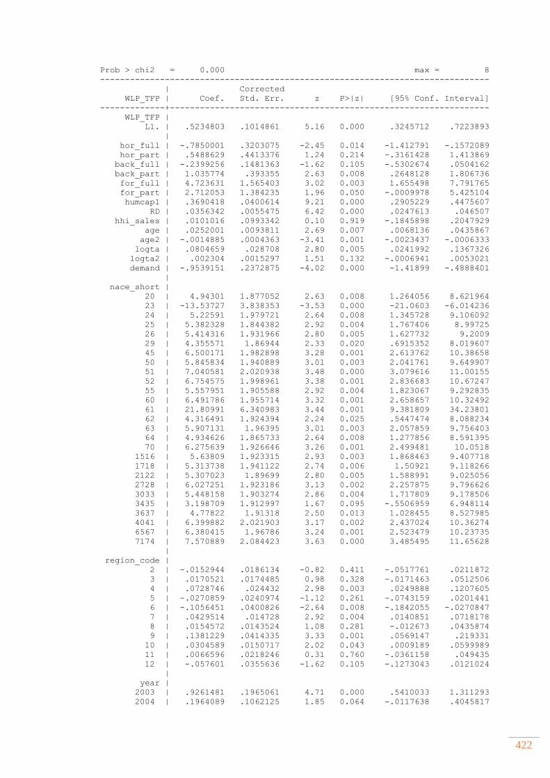
422
Prob > chi2 = 0.000 max = 8
------------------------------------------------------------------------------
| Corrected
WLP_TFP | Coef. Std. Err. z P>|z| [95% Conf. Interval]
-------------+----------------------------------------------------------------
WLP_TFP |
L1. | .5234803 .1014861 5.16 0.000 .3245712 .7223893
|
hor_full | -.7850001 .3203075 -2.45 0.014 -1.412791 -.1572089
hor_part | .5488629 .4413376 1.24 0.214 -.3161428 1.413869
back_full | -.2399256 .1481363 -1.62 0.105 -.5302674 .0504162
back_part | 1.035774 .393355 2.63 0.008 .2648128 1.806736
for_full | 4.723631 1.565403 3.02 0.003 1.655498 7.791765
for_part | 2.712053 1.384235 1.96 0.050 -.0009978 5.425104
humcap1 | .3690418 .0400614 9.21 0.000 .2905229 .4475607
RD | .0356342 .0055475 6.42 0.000 .0247613 .046507
hhi_sales | .0101016 .0993342 0.10 0.919 -.1845898 .2047929
age | .0252001 .0093811 2.69 0.007 .0068136 .0435867
age2 | -.0014885 .0004363 -3.41 0.001 -.0023437 -.0006333
logta | .0804659 .028708 2.80 0.005 .0241992 .1367326
logta2 | .002304 .0015297 1.51 0.132 -.0006941 .0053021
demand | -.9539151 .2372875 -4.02 0.000 -1.41899 -.4888401
|
nace_short |
20 | 4.94301 1.877052 2.63 0.008 1.264056 8.621964
23 | -13.53727 3.838353 -3.53 0.000 -21.0603 -6.014236
24 | 5.22591 1.979721 2.64 0.008 1.345728 9.106092
25 | 5.382328 1.844382 2.92 0.004 1.767406 8.99725
26 | 5.414316 1.931966 2.80 0.005 1.627732 9.2009
29 | 4.355571 1.86944 2.33 0.020 .6915352 8.019607
45 | 6.500171 1.982898 3.28 0.001 2.613762 10.38658
50 | 5.845834 1.940889 3.01 0.003 2.041761 9.649907
51 | 7.040581 2.020938 3.48 0.000 3.079616 11.00155
52 | 6.754575 1.998961 3.38 0.001 2.836683 10.67247
55 | 5.557951 1.905588 2.92 0.004 1.823067 9.292835
60 | 6.491786 1.955714 3.32 0.001 2.658657 10.32492
61 | 21.80991 6.340983 3.44 0.001 9.381809 34.23801
62 | 4.316491 1.924394 2.24 0.025 .5447474 8.088234
63 | 5.907131 1.96395 3.01 0.003 2.057859 9.756403
64 | 4.934626 1.865733 2.64 0.008 1.277856 8.591395
70 | 6.275639 1.926646 3.26 0.001 2.499481 10.0518
1516 | 5.63809 1.923315 2.93 0.003 1.868463 9.407718
1718 | 5.313738 1.941122 2.74 0.006 1.50921 9.118266
2122 | 5.307023 1.89699 2.80 0.005 1.588991 9.025056
2728 | 6.027251 1.923186 3.13 0.002 2.257875 9.796626
3033 | 5.448158 1.903274 2.86 0.004 1.717809 9.178506
3435 | 3.198709 1.912997 1.67 0.095 -.5506959 6.948114
3637 | 4.77822 1.91318 2.50 0.013 1.028455 8.527985
4041 | 6.399882 2.021903 3.17 0.002 2.437024 10.36274
6567 | 6.380415 1.96786 3.24 0.001 2.523479 10.23735
7174 | 7.570889 2.084423 3.63 0.000 3.485495 11.65628
|
region_code |
2 | -.0152944 .0186134 -0.82 0.411 -.0517761 .0211872
3 | .0170521 .0174485 0.98 0.328 -.0171463 .0512506
4 | .0728746 .024432 2.98 0.003 .0249888 .1207605
5 | -.0270859 .0240974 -1.12 0.261 -.0743159 .0201441
6 | -.1056451 .0400826 -2.64 0.008 -.1842055 -.0270847
7 | .0429514 .014728 2.92 0.004 .0140851 .0718178
8 | .0154572 .0143524 1.08 0.281 -.012673 .0435874
9 | .1381229 .0414335 3.33 0.001 .0569147 .219331
10 | .0304589 .0150717 2.02 0.043 .0009189 .0599989
11 | .0066596 .0218246 0.31 0.760 -.0361158 .049435
12 | -.057601 .0355636 -1.62 0.105 -.1273043 .0121024
|
year |
2003 | .9261481 .1965061 4.71 0.000 .5410033 1.311293
2004 | .1964089 .1062125 1.85 0.064 -.0117638 .4045817

423
2005 | .0733293 .1058648 0.69 0.489 -.1341619 .2808205
2006 | .1217861 .1138809 1.07 0.285 -.1014164 .3449886
2007 | .1324273 .1057407 1.25 0.210 -.0748206 .3396752
2008 | .1381718 .0959664 1.44 0.150 -.0499189 .3262624
2009 | -.2882952 .0721995 -3.99 0.000 -.4298037 -.1467867
|
_cons | 1.257602 2.300818 0.55 0.585 -3.251918 5.767121
------------------------------------------------------------------------------
------------------------------------------------------------------------------
Arellano-Bond test for AR(1) in first differences: z = -5.66 Pr > z = 0.000
Arellano-Bond test for AR(2) in first differences: z = 0.97 Pr > z = 0.333
Arellano-Bond test for AR(3) in first differences: z = 0.01 Pr > z = 0.990
Arellano-Bond test for AR(4) in first differences: z = 2.02 Pr > z = 0.044
------------------------------------------------------------------------------
Sargan test of overid. restrictions: chi2(10) = 26.09 Prob > chi2 = 0.004
(Not robust, but not weakened by many instruments.)
Hansen test of overid. restrictions: chi2(10) = 13.02 Prob > chi2 = 0.223
(Robust, but weakened by many instruments.)
Difference-in-Hansen tests of exogeneity of instrument subsets:
GMM instruments for levels
Hansen test excluding group: chi2(3) = 3.89 Prob > chi2 = 0.274
Difference (null H = exogenous): chi2(7) = 9.13 Prob > chi2 = 0.243
gmm(L.WLP_TFP, collapse lag(2 4))
Hansen test excluding group: chi2(6) = 10.24 Prob > chi2 = 0.115
Difference (null H = exogenous): chi2(4) = 2.78 Prob > chi2 = 0.595
gmm(hor_full, collapse lag(2 2))
Hansen test excluding group: chi2(8) = 11.03 Prob > chi2 = 0.200
Difference (null H = exogenous): chi2(2) = 1.99 Prob > chi2 = 0.371
gmm(hor_part, collapse lag(2 2))
Hansen test excluding group: chi2(8) = 11.09 Prob > chi2 = 0.197
Difference (null H = exogenous): chi2(2) = 1.93 Prob > chi2 = 0.381
gmm(back_full, collapse lag(3 3))
Hansen test excluding group: chi2(8) = 10.53 Prob > chi2 = 0.230
Difference (null H = exogenous): chi2(2) = 2.49 Prob > chi2 = 0.288
gmm(back_part, collapse lag(3 3))
Hansen test excluding group: chi2(8) = 8.99 Prob > chi2 = 0.343
Difference (null H = exogenous): chi2(2) = 4.03 Prob > chi2 = 0.133
gmm(for_full, collapse lag(3 4))
Hansen test excluding group: chi2(7) = 7.86 Prob > chi2 = 0.345
Difference (null H = exogenous): chi2(3) = 5.16 Prob > chi2 = 0.161
gmm(for_part, collapse lag(3 3))
Hansen test excluding group: chi2(8) = 10.53 Prob > chi2 = 0.230
Difference (null H = exogenous): chi2(2) = 2.49 Prob > chi2 = 0.288
iv(humcap1 RD hhi_sales age age2 logta logta2 demand)
Hansen test excluding group: chi2(2) = 0.01 Prob > chi2 = 0.996
Difference (null H = exogenous): chi2(8) = 13.01 Prob > chi2 = 0.111
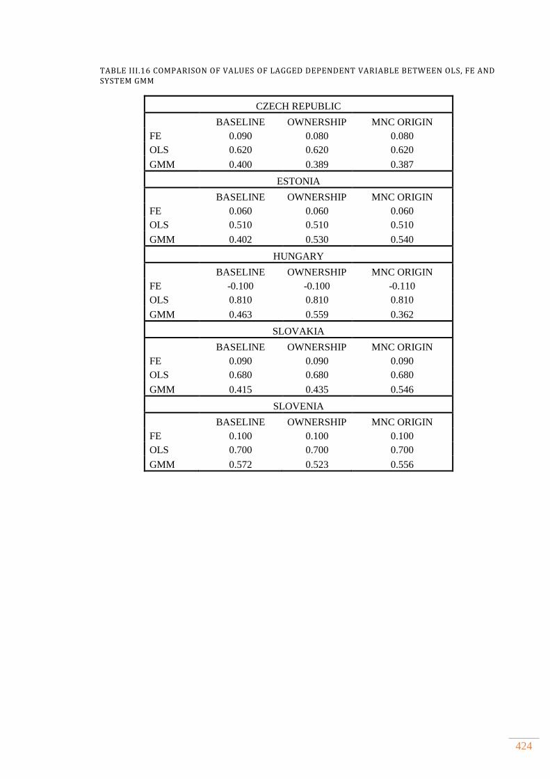
424
TABLE III.16 COMPARISON OF VALUES OF LAGGED DEPENDENT VARIABLE BETWEEN OLS, FE AND SYSTEM GMM
CZECH REPUBLIC
BASELINE OWNERSHIP MNC ORIGIN
FE 0.090 0.080 0.080
OLS 0.620 0.620 0.620
GMM 0.400 0.389 0.387
ESTONIA
BASELINE OWNERSHIP MNC ORIGIN
FE 0.060 0.060 0.060
OLS 0.510 0.510 0.510
GMM 0.402 0.530 0.540
HUNGARY
BASELINE OWNERSHIP MNC ORIGIN
FE -0.100 -0.100 -0.110
OLS 0.810 0.810 0.810
GMM 0.463 0.559 0.362
SLOVAKIA
BASELINE OWNERSHIP MNC ORIGIN
FE 0.090 0.090 0.090
OLS 0.680 0.680 0.680
GMM 0.415 0.435 0.546
SLOVENIA
BASELINE OWNERSHIP MNC ORIGIN
FE 0.100 0.100 0.100
OLS 0.700 0.700 0.700
GMM 0.572 0.523 0.556
425
APPENDIX IV. SUPPLEMENT TO CHAPTER SIX
4.1 Development of foreign firms’ output in services and foreign services inputs in manufacturing industries ....................................................................................................................... 426
4.2 Empirical results for the baseline model of productivity spillovers from FDI in manufacturing sector presented in Section 6.4.1 ......................................................................... 427
4.3 Empirical results for the baseline model of productivity spillovers from FDI in service sector presented in Section 6.4.1 ........................................................................................................ 436
4.4 Empirical results of the effects of services and manufacturing FDI linkages on productivity of local firms in manufacturing sector presented in Section 6.4.2.............. 446
4.5 Empirical results of the moderating effects of intangible assets on productivity spillovers from FDI in manufacturing sector presented in Section 6.4.3 ........................... 457
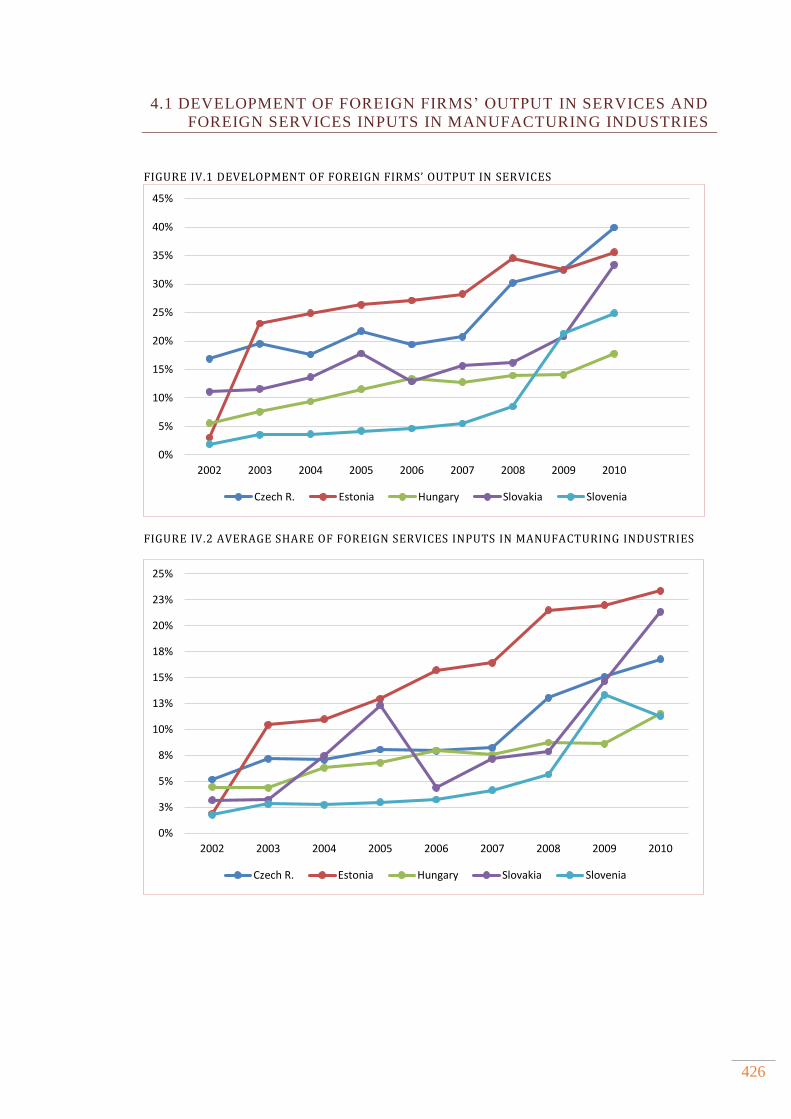
426
4.1 DEVELOPMENT OF FOREIGN FIRMS’ OUTPUT IN SERVICES AND
FOREIGN SERVICES INPUTS IN MANUFACTURING INDUSTRIES
FIGURE IV.1 DEVELOPMENT OF FOREIGN FIRMS’ OUTPUT IN SERVICES
FIGURE IV.2 AVERAGE SHARE OF FOREIGN SERVICES INPUTS IN MANUFACTURING INDUSTRIES
0%
5%
10%
15%
20%
25%
30%
35%
40%
45%
2002 2003 2004 2005 2006 2007 2008 2009 2010
Czech R. Estonia Hungary Slovakia Slovenia
0%
3%
5%
8%
10%
13%
15%
18%
20%
23%
25%
2002 2003 2004 2005 2006 2007 2008 2009 2010
Czech R. Estonia Hungary Slovakia Slovenia
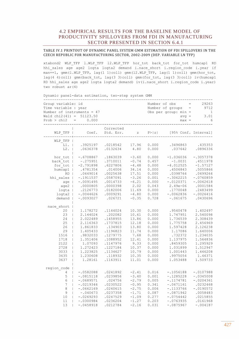
427
4.2 EMPIRICAL RESULTS FOR THE BASELINE MODEL OF
PRODUCTIVITY SPILLOVERS FROM FDI IN MANUFACTURING
SECTOR PRESENTED IN SECTION 6.4.1
TABLE IV.1 PRINTOUT OF DYNAMIC PANEL SYSTEM GMM ESTIMATION OF FDI SPILLOVERS IN THE CZECH REPUBLIC FOR MANUFACTURING SECTOR, 2002-2009 (DEP. VARIABLE LN TFP)
xtabond2 WLP_TFP l.WLP_TFP l2.WLP_TFP hor_tot back_tot for_tot humcap1 RD
hhi_sales age age2 logta logta2 demand i.nace_short i.region_code i.year if
man==1, gmm(l.WLP_TFP, lag(1 1)coll) gmm(l2.WLP_TFP, lag(1 1)coll) gmm(hor_tot,
lag(4 4)coll) gmm(back_tot, lag(3 3)coll) gmm(for_tot, lag(3 3)coll) iv(humcap1
RD hhi_sales age age2 logta logta2 demand) iv(i.nace_short i.region_code i.year)
two robust ar(4)
Dynamic panel-data estimation, two-step system GMM
------------------------------------------------------------------------------
Group variable: id Number of obs = 29263
Time variable : year Number of groups = 9712
Number of instruments = 47 Obs per group: min = 1
Wald chi2(41) = 51123.50 avg = 3.01
Prob > chi2 = 0.000 max = 6
------------------------------------------------------------------------------
| Corrected
WLP_TFP | Coef. Std. Err. z P>|z| [95% Conf. Interval]
-------------+----------------------------------------------------------------
WLP_TFP |
L1. | .3925197 .0218542 17.96 0.000 .3496863 .435353
L2. | .0636378 .0132634 4.80 0.000 .037642 .0896336
|
hor_tot | -.6708867 .1863039 -3.60 0.000 -1.036036 -.3057378
back_tot | -.275951 .3710011 -0.74 0.457 -1.0031 .4511978
for_tot | -2.791898 .6227806 -4.48 0.000 -4.012525 -1.57127
humcap1 | .4781354 .014006 34.14 0.000 .4506843 .5055866
RD | .0449014 .0025638 17.51 0.000 .0398764 .0499264
hhi_sales | -.1911537 .0587091 -3.26 0.001 -.3062215 -.0760859
age | -.0091495 .0014733 -6.21 0.000 -.0120371 -.0062618
age2 | .0000805 .0000398 2.02 0.043 2.49e-06 .0001584
logta | .2126773 .0182006 11.69 0.000 .1770048 .2483499
logta2 | -.0044626 .0009291 -4.80 0.000 -.0062836 -.0026416
demand | -.0093027 .026721 -0.35 0.728 -.061675 .0430696
|
nace_short |
20 | 1.178272 .1144024 10.30 0.000 .9540478 1.402497
23 | 2.144024 .202082 10.61 0.000 1.747951 2.540098
24 | 2.022489 .1458955 13.86 0.000 1.736539 2.308439
25 | 2.116363 .1737815 12.18 0.000 1.775758 2.456969
26 | 1.861833 .134903 13.80 0.000 1.597428 2.126238
29 | 1.405433 .1196823 11.74 0.000 1.17086 1.640006
1516 | .9832033 .1279775 7.68 0.000 .732372 1.234035
1718 | 1.351406 .1088952 12.41 0.000 1.137975 1.564836
2122 | 1.07093 .1147976 9.33 0.000 .8459305 1.295929
2728 | 1.272423 .1227184 10.37 0.000 1.031899 1.512947
3033 | 1.223825 .1134627 10.79 0.000 1.001443 1.446208
3435 | 1.230608 .118932 10.35 0.000 .9975054 1.46371
3637 | 1.28161 .1163911 11.01 0.000 1.053488 1.509733
|
region_code |
4 | -.0582088 .0241892 -2.41 0.016 -.1056188 -.0107988
5 | -.0815118 .0239856 -3.40 0.001 -.1285228 -.0345008
6 | -.0689571 .024756 -2.79 0.005 -.1174781 -.0204361
7 | -.0219346 .0230522 -0.95 0.341 -.0671161 .0232468
8 | -.0662169 .0240615 -2.75 0.006 -.1133766 -.0190572
9 | -.040673 .0237358 -1.71 0.087 -.0871942 .0058483
10 | -.0269293 .0247529 -1.09 0.277 -.0754442 .0215855
11 | -.0300984 .0236204 -1.27 0.203 -.0763935 .0161968
13 | -.0458918 .0212784 -2.16 0.031 -.0875967 -.004187
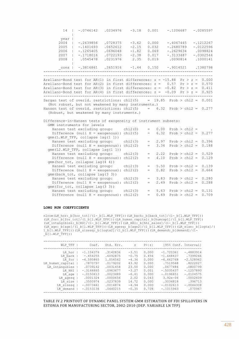
428
14 | -.0746142 .0234976 -3.18 0.001 -.1206687 -.0285597
|
year |
2004 | -.2639856 .0728375 -3.62 0.000 -.4067445 -.1212267
2005 | -.1401693 .0652612 -2.15 0.032 -.2680789 -.0122596
2006 | -.1265405 .0696048 -1.82 0.069 -.2629634 .0098824
2007 | -.1718016 .0722193 -2.38 0.017 -.3133487 -.0302544
2008 | .0545478 .0231976 2.35 0.019 .0090814 .1000141
|
_cons | -.3816861 .2651916 -1.44 0.150 -.9014521 .1380798
------------------------------------------------------------------------------
------------------------------------------------------------------------------
Arellano-Bond test for AR(1) in first differences: z = -15.88 Pr > z = 0.000
Arellano-Bond test for AR(2) in first differences: z = 0.57 Pr > z = 0.570
Arellano-Bond test for AR(3) in first differences: z = -0.82 Pr > z = 0.411
Arellano-Bond test for AR(4) in first differences: z = -0.09 Pr > z = 0.925
------------------------------------------------------------------------------
Sargan test of overid. restrictions: chi2(5) = 19.85 Prob > chi2 = 0.001
(Not robust, but not weakened by many instruments.)
Hansen test of overid. restrictions: chi2(5) = 6.32 Prob > chi2 = 0.277
(Robust, but weakened by many instruments.)
Difference-in-Hansen tests of exogeneity of instrument subsets:
GMM instruments for levels
Hansen test excluding group: chi2(0) = 0.00 Prob > chi2 = .
Difference (null H = exogenous): chi2(5) = 6.32 Prob > chi2 = 0.277
gmm(L.WLP_TFP, collapse lag(1 1))
Hansen test excluding group: chi2(3) = 2.97 Prob > chi2 = 0.396
Difference (null H = exogenous): chi2(2) = 3.34 Prob > chi2 = 0.188
gmm(L2.WLP_TFP, collapse lag(1 1))
Hansen test excluding group: chi2(3) = 2.22 Prob > chi2 = 0.529
Difference (null H = exogenous): chi2(2) = 4.10 Prob > chi2 = 0.129
gmm(hor_tot, collapse lag(4 4))
Hansen test excluding group: chi2(3) = 5.50 Prob > chi2 = 0.139
Difference (null H = exogenous): chi2(2) = 0.82 Prob > chi2 = 0.664
gmm(back_tot, collapse lag(3 3))
Hansen test excluding group: chi2(3) = 3.83 Prob > chi2 = 0.280
Difference (null H = exogenous): chi2(2) = 2.49 Prob > chi2 = 0.288
gmm(for_tot, collapse lag(3 3))
Hansen test excluding group: chi2(3) = 5.63 Prob > chi2 = 0.131
Difference (null H = exogenous): chi2(2) = 0.69 Prob > chi2 = 0.709
LONG RUN COEFFICIENTS
nlcom(LR_hor:_b[hor_tot]/(1-_b[l.WLP_TFP]))(LR_back:_b[back_tot]/(1-_b[l.WLP_TFP]))
(LR_for:_b[for_tot]/(1_b[l.WLP_TFP]))(LR_human_capital:_b[humcap1]/(1_b[l.WLP_TFP])
(LR_intangibles:_b[RD]/(1-_b[l.WLP_TFP]))(LR_HHI:_b[hhi_sales]/(1-_b[l.WLP_TFP]))
(LR_age:_b[age]/(1_b[l.WLP_TFP]))(LR_agesq:_b[age2]/(1_b[l.WLP_TFP]))(LR_size:_b[logta]/(
1_b[l.WLP_TFP]))(LR_sizesq:_b[logta2]/(1_b[l.WLP_TFP]))(LR_demand:_b[demand]/(1-
_b[l.WLP_TFP]))
----------------------------------------------------------------------------------
WLP_TFP | Coef. Std. Err. z P>|z| [95% Conf. Interval]
-----------------+----------------------------------------------------------------
LR_hor | -1.104376 .3142836 -3.51 0.000 -1.720361 -.4883914
LR_back | -.454255 .6092875 -0.75 0.456 -1.648437 .7399266
LR_for | -4.595865 1.054562 -4.36 0.000 -6.662768 -2.528962
LR_human_capital | .7870797 .0179202 43.92 0.000 .7519568 .8222027
LR_intangibles | .0739142 .0031458 23.50 0.000 .0677484 .0800799
LR_HHI | -.3146665 .0963677 -3.27 0.001 -.5035437 -.1257893
LR_age | -.0150613 .0023489 -6.41 0.000 -.0196651 -.0104575
LR_agesq | .0001324 .0000656 2.02 0.043 3.92e-06 .0002609
LR_size | .3500974 .0237839 14.72 0.000 .3034818 .396713
LR_sizesq | -.0073461 .0014874 -4.94 0.000 -.0102613 -.0044308
LR_demand | -.0153136 .0440215 -0.35 0.728 -.1015943 .070967
----------------------------------------------------------------------------------
TABLE IV.2 PRINTOUT OF DYNAMIC PANEL SYSTEM GMM ESTIMATION OF FDI SPILLOVERS IN ESTONIA FOR MANUFACTURING SECTOR, 2002-2010 (DEP. VARIABLE LN TFP)
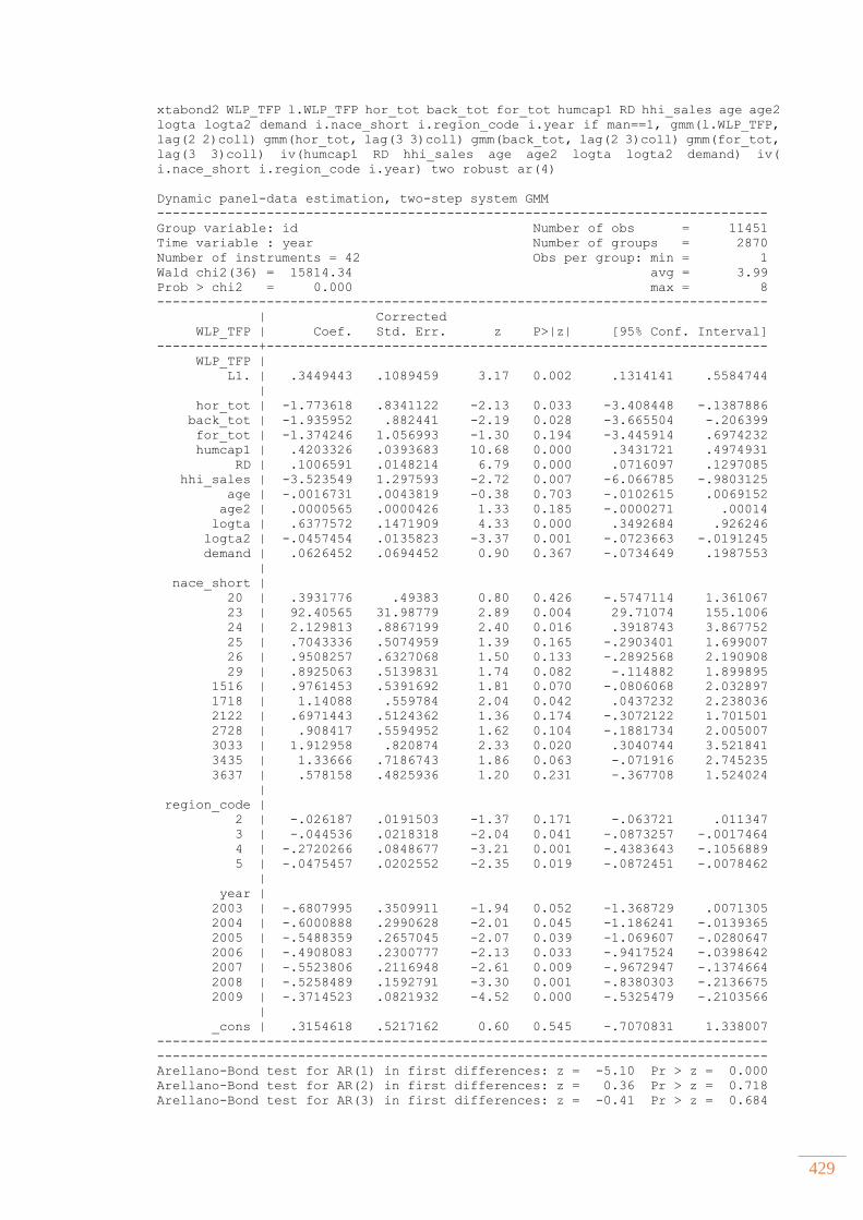
429
xtabond2 WLP_TFP l.WLP_TFP hor_tot back_tot for_tot humcap1 RD hhi_sales age age2
logta logta2 demand i.nace_short i.region_code i.year if man==1, gmm(l.WLP_TFP,
lag(2 2)coll) gmm(hor_tot, lag(3 3)coll) gmm(back_tot, lag(2 3)coll) gmm(for_tot,
lag(3 3)coll) iv(humcap1 RD hhi_sales age age2 logta logta2 demand) iv(
i.nace_short i.region_code i.year) two robust ar(4)
Dynamic panel-data estimation, two-step system GMM
------------------------------------------------------------------------------
Group variable: id Number of obs = 11451
Time variable : year Number of groups = 2870
Number of instruments = 42 Obs per group: min = 1
Wald chi2(36) = 15814.34 avg = 3.99
Prob > chi2 = 0.000 max = 8
------------------------------------------------------------------------------
| Corrected
WLP_TFP | Coef. Std. Err. z P>|z| [95% Conf. Interval]
-------------+----------------------------------------------------------------
WLP_TFP |
L1. | .3449443 .1089459 3.17 0.002 .1314141 .5584744
|
hor_tot | -1.773618 .8341122 -2.13 0.033 -3.408448 -.1387886
back_tot | -1.935952 .882441 -2.19 0.028 -3.665504 -.206399
for_tot | -1.374246 1.056993 -1.30 0.194 -3.445914 .6974232
humcap1 | .4203326 .0393683 10.68 0.000 .3431721 .4974931
RD | .1006591 .0148214 6.79 0.000 .0716097 .1297085
hhi_sales | -3.523549 1.297593 -2.72 0.007 -6.066785 -.9803125
age | -.0016731 .0043819 -0.38 0.703 -.0102615 .0069152
age2 | .0000565 .0000426 1.33 0.185 -.0000271 .00014
logta | .6377572 .1471909 4.33 0.000 .3492684 .926246
logta2 | -.0457454 .0135823 -3.37 0.001 -.0723663 -.0191245
demand | .0626452 .0694452 0.90 0.367 -.0734649 .1987553
|
nace_short |
20 | .3931776 .49383 0.80 0.426 -.5747114 1.361067
23 | 92.40565 31.98779 2.89 0.004 29.71074 155.1006
24 | 2.129813 .8867199 2.40 0.016 .3918743 3.867752
25 | .7043336 .5074959 1.39 0.165 -.2903401 1.699007
26 | .9508257 .6327068 1.50 0.133 -.2892568 2.190908
29 | .8925063 .5139831 1.74 0.082 -.114882 1.899895
1516 | .9761453 .5391692 1.81 0.070 -.0806068 2.032897
1718 | 1.14088 .559784 2.04 0.042 .0437232 2.238036
2122 | .6971443 .5124362 1.36 0.174 -.3072122 1.701501
2728 | .908417 .5594952 1.62 0.104 -.1881734 2.005007
3033 | 1.912958 .820874 2.33 0.020 .3040744 3.521841
3435 | 1.33666 .7186743 1.86 0.063 -.071916 2.745235
3637 | .578158 .4825936 1.20 0.231 -.367708 1.524024
|
region_code |
2 | -.026187 .0191503 -1.37 0.171 -.063721 .011347
3 | -.044536 .0218318 -2.04 0.041 -.0873257 -.0017464
4 | -.2720266 .0848677 -3.21 0.001 -.4383643 -.1056889
5 | -.0475457 .0202552 -2.35 0.019 -.0872451 -.0078462
|
year |
2003 | -.6807995 .3509911 -1.94 0.052 -1.368729 .0071305
2004 | -.6000888 .2990628 -2.01 0.045 -1.186241 -.0139365
2005 | -.5488359 .2657045 -2.07 0.039 -1.069607 -.0280647
2006 | -.4908083 .2300777 -2.13 0.033 -.9417524 -.0398642
2007 | -.5523806 .2116948 -2.61 0.009 -.9672947 -.1374664
2008 | -.5258489 .1592791 -3.30 0.001 -.8380303 -.2136675
2009 | -.3714523 .0821932 -4.52 0.000 -.5325479 -.2103566
|
_cons | .3154618 .5217162 0.60 0.545 -.7070831 1.338007
------------------------------------------------------------------------------
------------------------------------------------------------------------------
Arellano-Bond test for AR(1) in first differences: z = -5.10 Pr > z = 0.000
Arellano-Bond test for AR(2) in first differences: z = 0.36 Pr > z = 0.718
Arellano-Bond test for AR(3) in first differences: z = -0.41 Pr > z = 0.684
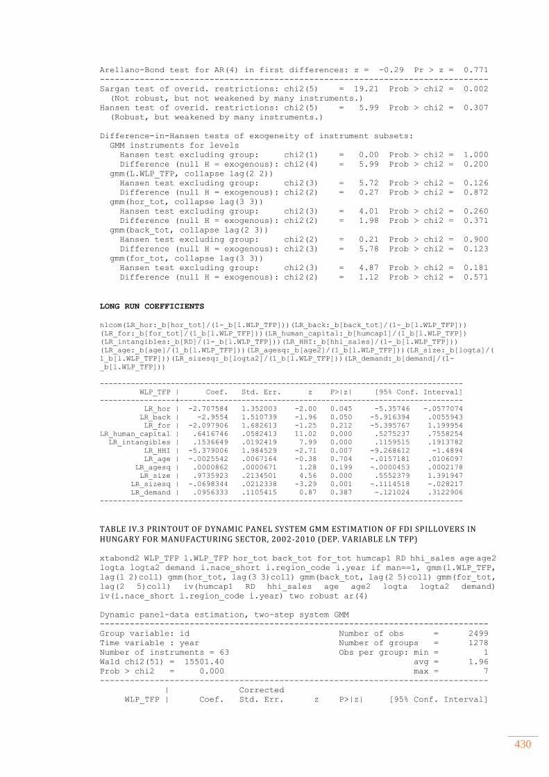
430
Arellano-Bond test for AR(4) in first differences: z = -0.29 Pr > z = 0.771
------------------------------------------------------------------------------
Sargan test of overid. restrictions: chi2(5) = 19.21 Prob > chi2 = 0.002
(Not robust, but not weakened by many instruments.)
Hansen test of overid. restrictions: chi2(5) = 5.99 Prob > chi2 = 0.307
(Robust, but weakened by many instruments.)
Difference-in-Hansen tests of exogeneity of instrument subsets:
GMM instruments for levels
Hansen test excluding group: chi2(1) = 0.00 Prob > chi2 = 1.000
Difference (null H = exogenous): chi2(4) = 5.99 Prob > chi2 = 0.200
gmm(L.WLP_TFP, collapse lag(2 2))
Hansen test excluding group: chi2(3) = 5.72 Prob > chi2 = 0.126
Difference (null H = exogenous): chi2(2) = 0.27 Prob > chi2 = 0.872
gmm(hor_tot, collapse lag(3 3))
Hansen test excluding group: chi2(3) = 4.01 Prob > chi2 = 0.260
Difference (null H = exogenous): chi2(2) = 1.98 Prob > chi2 = 0.371
gmm(back_tot, collapse lag(2 3))
Hansen test excluding group: chi2(2) = 0.21 Prob > chi2 = 0.900
Difference (null H = exogenous): chi2(3) = 5.78 Prob > chi2 = 0.123
gmm(for_tot, collapse lag(3 3))
Hansen test excluding group: chi2(3) = 4.87 Prob > chi2 = 0.181
Difference (null H = exogenous): chi2(2) = 1.12 Prob > chi2 = 0.571
LONG RUN COEFFICIENTS
nlcom(LR_hor:_b[hor_tot]/(1-_b[l.WLP_TFP]))(LR_back:_b[back_tot]/(1-_b[l.WLP_TFP]))
(LR_for:_b[for_tot]/(1_b[l.WLP_TFP]))(LR_human_capital:_b[humcap1]/(1_b[l.WLP_TFP])
(LR_intangibles:_b[RD]/(1-_b[l.WLP_TFP]))(LR_HHI:_b[hhi_sales]/(1-_b[l.WLP_TFP]))
(LR_age:_b[age]/(1_b[l.WLP_TFP]))(LR_agesq:_b[age2]/(1_b[l.WLP_TFP]))(LR_size:_b[logta]/(
1_b[l.WLP_TFP]))(LR_sizesq:_b[logta2]/(1_b[l.WLP_TFP]))(LR_demand:_b[demand]/(1-
_b[l.WLP_TFP]))
----------------------------------------------------------------------------------
WLP_TFP | Coef. Std. Err. z P>|z| [95% Conf. Interval]
-----------------+----------------------------------------------------------------
LR_hor | -2.707584 1.352003 -2.00 0.045 -5.35746 -.0577074
LR_back | -2.9554 1.510739 -1.96 0.050 -5.916394 .0055943
LR_for | -2.097906 1.682613 -1.25 0.212 -5.395767 1.199954
LR_human_capital | .6416746 .0582413 11.02 0.000 .5275237 .7558254
LR_intangibles | .1536649 .0192419 7.99 0.000 .1159515 .1913782
LR_HHI | -5.379006 1.984529 -2.71 0.007 -9.268612 -1.4894
LR_age | -.0025542 .0067164 -0.38 0.704 -.0157181 .0106097
LR_agesq | .0000862 .0000671 1.28 0.199 -.0000453 .0002178
LR_size | .9735923 .2134501 4.56 0.000 .5552379 1.391947
LR_sizesq | -.0698344 .0212338 -3.29 0.001 -.1114518 -.028217
LR_demand | .0956333 .1105415 0.87 0.387 -.121024 .3122906
----------------------------------------------------------------------------------
TABLE IV.3 PRINTOUT OF DYNAMIC PANEL SYSTEM GMM ESTIMATION OF FDI SPILLOVERS IN HUNGARY FOR MANUFACTURING SECTOR, 2002-2010 (DEP. VARIABLE LN TFP)
xtabond2 WLP_TFP l.WLP_TFP hor_tot back_tot for_tot humcap1 RD hhi_sales age age2
logta logta2 demand i.nace_short i.region_code i.year if man==1, gmm(l.WLP_TFP,
lag(1 2)coll) gmm(hor_tot, lag(3 3)coll) gmm(back_tot, lag(2 5)coll) gmm(for_tot,
lag(2 5)coll) iv(humcap1 RD hhi_sales age age2 logta logta2 demand)
iv(i.nace_short i.region_code i.year) two robust ar(4)
Dynamic panel-data estimation, two-step system GMM
------------------------------------------------------------------------------
Group variable: id Number of obs = 2499
Time variable : year Number of groups = 1278
Number of instruments = 63 Obs per group: min = 1
Wald chi2(51) = 15501.40 avg = 1.96
Prob > chi2 = 0.000 max = 7
------------------------------------------------------------------------------
| Corrected
WLP_TFP | Coef. Std. Err. z P>|z| [95% Conf. Interval]
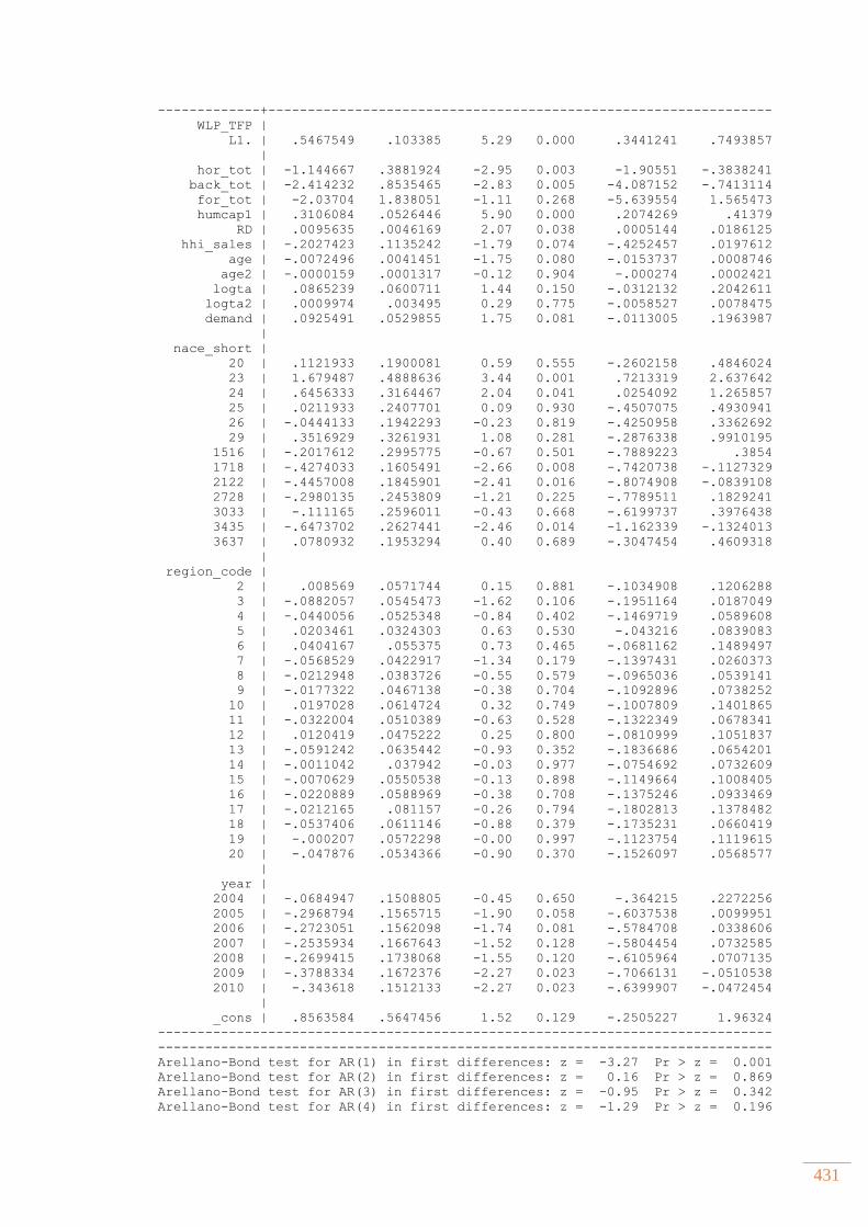
431
-------------+----------------------------------------------------------------
WLP_TFP |
L1. | .5467549 .103385 5.29 0.000 .3441241 .7493857
|
hor_tot | -1.144667 .3881924 -2.95 0.003 -1.90551 -.3838241
back_tot | -2.414232 .8535465 -2.83 0.005 -4.087152 -.7413114
for_tot | -2.03704 1.838051 -1.11 0.268 -5.639554 1.565473
humcap1 | .3106084 .0526446 5.90 0.000 .2074269 .41379
RD | .0095635 .0046169 2.07 0.038 .0005144 .0186125
hhi_sales | -.2027423 .1135242 -1.79 0.074 -.4252457 .0197612
age | -.0072496 .0041451 -1.75 0.080 -.0153737 .0008746
age2 | -.0000159 .0001317 -0.12 0.904 -.000274 .0002421
logta | .0865239 .0600711 1.44 0.150 -.0312132 .2042611
logta2 | .0009974 .003495 0.29 0.775 -.0058527 .0078475
demand | .0925491 .0529855 1.75 0.081 -.0113005 .1963987
|
nace_short |
20 | .1121933 .1900081 0.59 0.555 -.2602158 .4846024
23 | 1.679487 .4888636 3.44 0.001 .7213319 2.637642
24 | .6456333 .3164467 2.04 0.041 .0254092 1.265857
25 | .0211933 .2407701 0.09 0.930 -.4507075 .4930941
26 | -.0444133 .1942293 -0.23 0.819 -.4250958 .3362692
29 | .3516929 .3261931 1.08 0.281 -.2876338 .9910195
1516 | -.2017612 .2995775 -0.67 0.501 -.7889223 .3854
1718 | -.4274033 .1605491 -2.66 0.008 -.7420738 -.1127329
2122 | -.4457008 .1845901 -2.41 0.016 -.8074908 -.0839108
2728 | -.2980135 .2453809 -1.21 0.225 -.7789511 .1829241
3033 | -.111165 .2596011 -0.43 0.668 -.6199737 .3976438
3435 | -.6473702 .2627441 -2.46 0.014 -1.162339 -.1324013
3637 | .0780932 .1953294 0.40 0.689 -.3047454 .4609318
|
region_code |
2 | .008569 .0571744 0.15 0.881 -.1034908 .1206288
3 | -.0882057 .0545473 -1.62 0.106 -.1951164 .0187049
4 | -.0440056 .0525348 -0.84 0.402 -.1469719 .0589608
5 | .0203461 .0324303 0.63 0.530 -.043216 .0839083
6 | .0404167 .055375 0.73 0.465 -.0681162 .1489497
7 | -.0568529 .0422917 -1.34 0.179 -.1397431 .0260373
8 | -.0212948 .0383726 -0.55 0.579 -.0965036 .0539141
9 | -.0177322 .0467138 -0.38 0.704 -.1092896 .0738252
10 | .0197028 .0614724 0.32 0.749 -.1007809 .1401865
11 | -.0322004 .0510389 -0.63 0.528 -.1322349 .0678341
12 | .0120419 .0475222 0.25 0.800 -.0810999 .1051837
13 | -.0591242 .0635442 -0.93 0.352 -.1836686 .0654201
14 | -.0011042 .037942 -0.03 0.977 -.0754692 .0732609
15 | -.0070629 .0550538 -0.13 0.898 -.1149664 .1008405
16 | -.0220889 .0588969 -0.38 0.708 -.1375246 .0933469
17 | -.0212165 .081157 -0.26 0.794 -.1802813 .1378482
18 | -.0537406 .0611146 -0.88 0.379 -.1735231 .0660419
19 | -.000207 .0572298 -0.00 0.997 -.1123754 .1119615
20 | -.047876 .0534366 -0.90 0.370 -.1526097 .0568577
|
year |
2004 | -.0684947 .1508805 -0.45 0.650 -.364215 .2272256
2005 | -.2968794 .1565715 -1.90 0.058 -.6037538 .0099951
2006 | -.2723051 .1562098 -1.74 0.081 -.5784708 .0338606
2007 | -.2535934 .1667643 -1.52 0.128 -.5804454 .0732585
2008 | -.2699415 .1738068 -1.55 0.120 -.6105964 .0707135
2009 | -.3788334 .1672376 -2.27 0.023 -.7066131 -.0510538
2010 | -.343618 .1512133 -2.27 0.023 -.6399907 -.0472454
|
_cons | .8563584 .5647456 1.52 0.129 -.2505227 1.96324
------------------------------------------------------------------------------
------------------------------------------------------------------------------
Arellano-Bond test for AR(1) in first differences: z = -3.27 Pr > z = 0.001
Arellano-Bond test for AR(2) in first differences: z = 0.16 Pr > z = 0.869
Arellano-Bond test for AR(3) in first differences: z = -0.95 Pr > z = 0.342
Arellano-Bond test for AR(4) in first differences: z = -1.29 Pr > z = 0.196
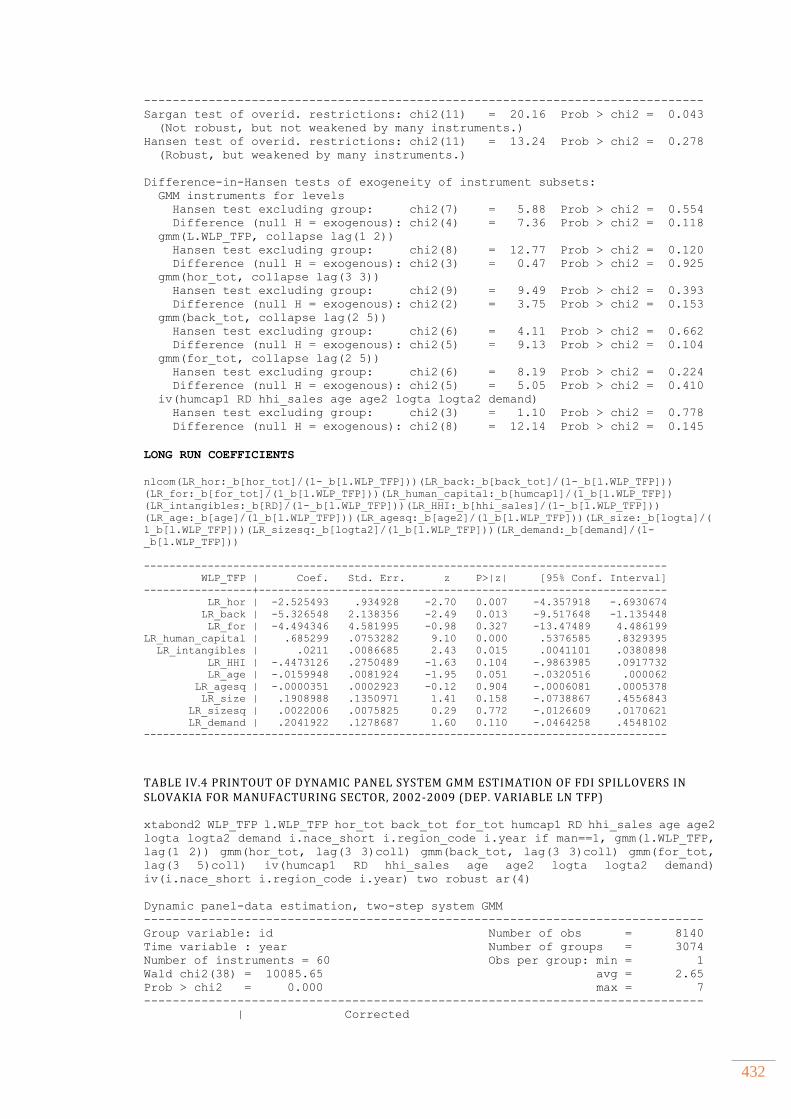
432
------------------------------------------------------------------------------
Sargan test of overid. restrictions: chi2(11) = 20.16 Prob > chi2 = 0.043
(Not robust, but not weakened by many instruments.)
Hansen test of overid. restrictions: chi2(11) = 13.24 Prob > chi2 = 0.278
(Robust, but weakened by many instruments.)
Difference-in-Hansen tests of exogeneity of instrument subsets:
GMM instruments for levels
Hansen test excluding group: chi2(7) = 5.88 Prob > chi2 = 0.554
Difference (null H = exogenous): chi2(4) = 7.36 Prob > chi2 = 0.118
gmm(L.WLP_TFP, collapse lag(1 2))
Hansen test excluding group: chi2(8) = 12.77 Prob > chi2 = 0.120
Difference (null H = exogenous): chi2(3) = 0.47 Prob > chi2 = 0.925
gmm(hor_tot, collapse lag(3 3))
Hansen test excluding group: chi2(9) = 9.49 Prob > chi2 = 0.393
Difference (null H = exogenous): chi2(2) = 3.75 Prob > chi2 = 0.153
gmm(back_tot, collapse lag(2 5))
Hansen test excluding group: chi2(6) = 4.11 Prob > chi2 = 0.662
Difference (null H = exogenous): chi2(5) = 9.13 Prob > chi2 = 0.104
gmm(for_tot, collapse lag(2 5))
Hansen test excluding group: chi2(6) = 8.19 Prob > chi2 = 0.224
Difference (null H = exogenous): chi2(5) = 5.05 Prob > chi2 = 0.410
iv(humcap1 RD hhi_sales age age2 logta logta2 demand)
Hansen test excluding group: chi2(3) = 1.10 Prob > chi2 = 0.778
Difference (null H = exogenous): chi2(8) = 12.14 Prob > chi2 = 0.145
LONG RUN COEFFICIENTS
nlcom(LR_hor:_b[hor_tot]/(1-_b[l.WLP_TFP]))(LR_back:_b[back_tot]/(1-_b[l.WLP_TFP]))
(LR_for:_b[for_tot]/(1_b[l.WLP_TFP]))(LR_human_capital:_b[humcap1]/(1_b[l.WLP_TFP])
(LR_intangibles:_b[RD]/(1-_b[l.WLP_TFP]))(LR_HHI:_b[hhi_sales]/(1-_b[l.WLP_TFP]))
(LR_age:_b[age]/(1_b[l.WLP_TFP]))(LR_agesq:_b[age2]/(1_b[l.WLP_TFP]))(LR_size:_b[logta]/(
1_b[l.WLP_TFP]))(LR_sizesq:_b[logta2]/(1_b[l.WLP_TFP]))(LR_demand:_b[demand]/(1-
_b[l.WLP_TFP]))
----------------------------------------------------------------------------------
WLP_TFP | Coef. Std. Err. z P>|z| [95% Conf. Interval]
-----------------+----------------------------------------------------------------
LR_hor | -2.525493 .934928 -2.70 0.007 -4.357918 -.6930674
LR_back | -5.326548 2.138356 -2.49 0.013 -9.517648 -1.135448
LR_for | -4.494346 4.581995 -0.98 0.327 -13.47489 4.486199
LR_human_capital | .685299 .0753282 9.10 0.000 .5376585 .8329395
LR_intangibles | .0211 .0086685 2.43 0.015 .0041101 .0380898
LR_HHI | -.4473126 .2750489 -1.63 0.104 -.9863985 .0917732
LR_age | -.0159948 .0081924 -1.95 0.051 -.0320516 .000062
LR_agesq | -.0000351 .0002923 -0.12 0.904 -.0006081 .0005378
LR_size | .1908988 .1350971 1.41 0.158 -.0738867 .4556843
LR_sizesq | .0022006 .0075825 0.29 0.772 -.0126609 .0170621
LR_demand | .2041922 .1278687 1.60 0.110 -.0464258 .4548102
----------------------------------------------------------------------------------
TABLE IV.4 PRINTOUT OF DYNAMIC PANEL SYSTEM GMM ESTIMATION OF FDI SPILLOVERS IN SLOVAKIA FOR MANUFACTURING SECTOR, 2002-2009 (DEP. VARIABLE LN TFP)
xtabond2 WLP_TFP l.WLP_TFP hor_tot back_tot for_tot humcap1 RD hhi_sales age age2
logta logta2 demand i.nace_short i.region_code i.year if man==1, gmm(l.WLP_TFP,
lag(1 2)) gmm(hor_tot, lag(3 3)coll) gmm(back_tot, lag(3 3)coll) gmm(for_tot,
lag(3 5)coll) iv(humcap1 RD hhi_sales age age2 logta logta2 demand)
iv(i.nace_short i.region_code i.year) two robust ar(4)
Dynamic panel-data estimation, two-step system GMM
------------------------------------------------------------------------------
Group variable: id Number of obs = 8140
Time variable : year Number of groups = 3074
Number of instruments = 60 Obs per group: min = 1
Wald chi2(38) = 10085.65 avg = 2.65
Prob > chi2 = 0.000 max = 7
------------------------------------------------------------------------------
| Corrected
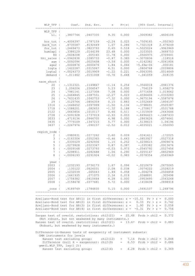
433
WLP_TFP | Coef. Std. Err. z P>|z| [95% Conf. Interval]
-------------+----------------------------------------------------------------
WLP_TFP |
L1. | .3807744 .0407335 9.35 0.000 .3009382 .4606106
|
hor_tot | -.4006397 .1787159 -2.24 0.025 -.7509165 -.050363
back_tot | .8735587 .8192449 1.07 0.286 -.7321318 2.479249
for_tot | .2469473 .3823793 0.65 0.518 -.5025024 .9963969
humcap1 | .3386129 .0144199 23.48 0.000 .3103505 .3668753
RD | .0608208 .005165 11.78 0.000 .0506975 .0709441
hhi_sales | -.0942838 .1085733 -0.87 0.385 -.3070836 .118516
age | -.0092094 .0025658 -3.59 0.000 -.0142382 -.0041806
age2 | .0000876 .0000476 1.84 0.066 -5.69e-06 .000181
logta | .1422287 .0315067 4.51 0.000 .0804768 .2039806
logta2 | -.0024373 .0019909 -1.22 0.221 -.0063395 .0014649
demand | -.011462 .0151008 -0.76 0.448 -.041059 .018135
|
nace_short |
20 | -.1312321 .1149867 -1.14 0.254 -.3566018 .0941376
23 | 1.206204 .2306547 5.23 0.000 .754129 1.658279
24 | .7981141 .1127308 7.08 0.000 .5771658 1.019062
25 | -.2464845 .1087551 -2.27 0.023 -.4596406 -.0333283
26 | -.7631435 .1042753 -7.32 0.000 -.9675194 -.5587676
29 | .0125764 .0856359 0.15 0.883 -.1552669 .1804197
1516 | -.1646652 .1097999 -1.50 0.134 -.3798691 .0505387
1718 | -.1088201 .082653 -1.32 0.188 -.270817 .0531768
2122 | .0663854 .1010117 0.66 0.511 -.1315939 .2643646
2728 | -.5091928 .1737019 -2.93 0.003 -.8496423 -.1687433
3033 | .4719134 .0946705 4.98 0.000 .2863626 .6574641
3435 | .7779109 .1347215 5.77 0.000 .5138615 1.04196
3637 | -.2267976 .090157 -2.52 0.012 -.4035021 -.050093
|
region_code |
2 | .0980831 .0377262 2.60 0.009 .0241411 .172025
3 | -.0163304 .0352365 -0.46 0.643 -.0853927 .0527318
4 | .0335529 .0292936 1.15 0.252 -.0238615 .0909674
5 | .0279928 .0323347 0.87 0.387 -.035382 .0913676
6 | -.0009168 .0273793 -0.03 0.973 -.0545792 .0527456
7 | .0298911 .0282688 1.06 0.290 -.0255147 .0852969
8 | -.0006193 .0291924 -0.02 0.983 -.0578354 .0565969
|
year |
2003 | .1232193 .0736173 1.67 0.094 -.0210679 .2675065
2004 | .130122 .0626031 2.08 0.038 .0074222 .2528219
2005 | .1232039 .065043 1.89 0.058 -.004278 .2506858
2006 | .1661935 .071075 2.34 0.019 .0268891 .305498
2007 | .1758382 .0410664 4.28 0.000 .0953495 .2563268
2008 | .2158678 .0377681 5.72 0.000 .1418438 .2898918
|
_cons | .9189749 .1784835 5.15 0.000 .5691537 1.268796
------------------------------------------------------------------------------
------------------------------------------------------------------------------
Arellano-Bond test for AR(1) in first differences: z = -10.51 Pr > z = 0.000
Arellano-Bond test for AR(2) in first differences: z = 0.33 Pr > z = 0.742
Arellano-Bond test for AR(3) in first differences: z = 1.90 Pr > z = 0.058
Arellano-Bond test for AR(4) in first differences: z = -0.31 Pr > z = 0.756
------------------------------------------------------------------------------
Sargan test of overid. restrictions: chi2(21) = 22.48 Prob > chi2 = 0.372
(Not robust, but not weakened by many instruments.)
Hansen test of overid. restrictions: chi2(21) = 13.67 Prob > chi2 = 0.883
(Robust, but weakened by many instruments.)
Difference-in-Hansen tests of exogeneity of instrument subsets:
GMM instruments for levels
Hansen test excluding group: chi2(12) = 7.14 Prob > chi2 = 0.848
Difference (null H = exogenous): chi2(9) = 6.53 Prob > chi2 = 0.686
gmm(L.WLP_TFP, lag(1 2))
Hansen test excluding group: chi2(4) = 4.28 Prob > chi2 = 0.369
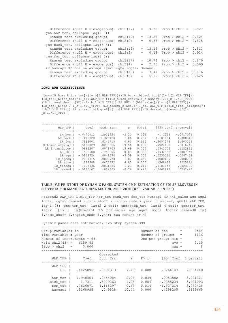
434
Difference (null H = exogenous): chi2(17) = 9.38 Prob > chi2 = 0.927
gmm(hor_tot, collapse lag(3 3))
Hansen test excluding group: chi2(19) = 13.28 Prob > chi2 = 0.824
Difference (null H = exogenous): chi2(2) = 0.38 Prob > chi2 = 0.825
gmm(back_tot, collapse lag(3 3))
Hansen test excluding group: chi2(19) = 13.49 Prob > chi2 = 0.813
Difference (null H = exogenous): chi2(2) = 0.18 Prob > chi2 = 0.914
gmm(for_tot, collapse lag(3 5))
Hansen test excluding group: chi2(17) = 10.74 Prob > chi2 = 0.870
Difference (null H = exogenous): chi2(4) = 2.93 Prob > chi2 = 0.569
iv(humcap1 RD hhi_sales age age2 logta logta2 demand)
Hansen test excluding group: chi2(13) = 7.47 Prob > chi2 = 0.876
Difference (null H = exogenous): chi2(8) = 6.19 Prob > chi2 = 0.625
LONG RUN COEFFICIENTS
nlcom(LR_hor:_b[hor_tot]/(1-_b[l.WLP_TFP]))(LR_back:_b[back_tot]/(1-_b[l.WLP_TFP]))
(LR_for:_b[for_tot]/(1_b[l.WLP_TFP]))(LR_human_capital:_b[humcap1]/(1_b[l.WLP_TFP])
(LR_intangibles:_b[RD]/(1-_b[l.WLP_TFP]))(LR_HHI:_b[hhi_sales]/(1-_b[l.WLP_TFP]))
(LR_age:_b[age]/(1_b[l.WLP_TFP]))(LR_agesq:_b[age2]/(1_b[l.WLP_TFP]))(LR_size:_b[logta]/(
1_b[l.WLP_TFP]))(LR_sizesq:_b[logta2]/(1_b[l.WLP_TFP]))(LR_demand:_b[demand]/(1-
_b[l.WLP_TFP]))
----------------------------------------------------------------------------------
WLP_TFP | Coef. Std. Err. z P>|z| [95% Conf. Interval]
-----------------+----------------------------------------------------------------
LR_hor | -.6470012 .2935254 -2.20 0.028 -1.2223 -.0717021
LR_back | 1.410728 1.325428 1.06 0.287 -1.187064 4.008519
LR_for | .3988001 .6145715 0.65 0.516 -.8057378 1.603338
LR_human_capital | .5468329 .0279556 19.56 0.000 .4920408 .6016249
LR_intangibles | .0982207 .0071763 13.69 0.000 .0841553 .1122861
LR_HHI | -.1522608 .1740006 -0.88 0.382 -.4932958 .1887741
LR_age | -.0148724 .0041474 -3.59 0.000 -.0230011 -.0067438
LR_agesq | .0001415 .0000778 1.82 0.069 -.0000109 .000294
LR_size | .229688 .0473672 4.85 0.000 .1368499 .3225261
LR_sizesq | -.003936 .0031885 -1.23 0.217 -.0101853 .0023132
LR_demand | -.0185102 .024365 -0.76 0.447 -.0662647 .0292443
----------------------------------------------------------------------------------
TABLE IV.5 PRINTOUT OF DYNAMIC PANEL SYSTEM GMM ESTIMATION OF FDI SPILLOVERS IN SLOVENIA FOR MANUFACTURING SECTOR, 2002-2010 (DEP. VARIABLE LN TFP) xtabond2 WLP_TFP l.WLP_TFP hor_tot back_tot for_tot humcap1 RD hhi_sales age age2
logta logta2 demand i.nace_short i.region_code i.year if man==1, gmm(l.WLP_TFP,
lag(1 2)) gmm(hor_tot, lag(2 2)coll) gmm(back_tot, lag(3 4)coll) gmm(for_tot,
lag(2 3)coll) iv(humcap1 RD hhi_sales age age2 logta logta2 demand0 iv(
i.nace_short i.region_code i.year) two robust ar(4)
Dynamic panel-data estimation, two-step system GMM
------------------------------------------------------------------------------
Group variable: id Number of obs = 3584
Time variable : year Number of groups = 1136
Number of instruments = 68 Obs per group: min = 1
Wald chi2(43) = 6159.85 avg = 3.15
Prob > chi2 = 0.000 max = 8
------------------------------------------------------------------------------
| Corrected
WLP_TFP | Coef. Std. Err. z P>|z| [95% Conf. Interval]
-------------+----------------------------------------------------------------
WLP_TFP |
L1. | .4425096 .0591313 7.48 0.000 .3266143 .5584048
|
hor_tot | 1.948354 .9454084 2.06 0.039 .0953882 3.801321
back_tot | 1.7311 .8979263 1.93 0.054 -.0288034 3.491003
for_tot | .7626071 1.168297 0.65 0.514 -1.527214 3.052428
humcap1 | .5168935 .049528 10.44 0.000 .4198205 .6139665
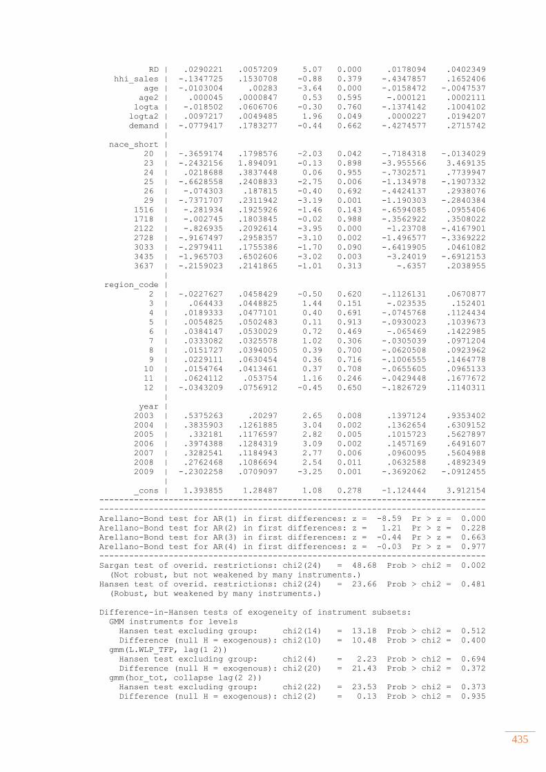
435
RD | .0290221 .0057209 5.07 0.000 .0178094 .0402349
hhi_sales | -.1347725 .1530708 -0.88 0.379 -.4347857 .1652406
age | -.0103004 .00283 -3.64 0.000 -.0158472 -.0047537
age2 | .000045 .0000847 0.53 0.595 -.000121 .0002111
logta | -.018502 .0606706 -0.30 0.760 -.1374142 .1004102
logta2 | .0097217 .0049485 1.96 0.049 .0000227 .0194207
demand | -.0779417 .1783277 -0.44 0.662 -.4274577 .2715742
|
nace_short |
20 | -.3659174 .1798576 -2.03 0.042 -.7184318 -.0134029
23 | -.2432156 1.894091 -0.13 0.898 -3.955566 3.469135
24 | .0218688 .3837448 0.06 0.955 -.7302571 .7739947
25 | -.6628558 .2408833 -2.75 0.006 -1.134978 -.1907332
26 | -.074303 .187815 -0.40 0.692 -.4424137 .2938076
29 | -.7371707 .2311942 -3.19 0.001 -1.190303 -.2840384
1516 | -.281934 .1925926 -1.46 0.143 -.6594085 .0955406
1718 | -.002745 .1803845 -0.02 0.988 -.3562922 .3508022
2122 | -.826935 .2092614 -3.95 0.000 -1.23708 -.4167901
2728 | -.9167497 .2958357 -3.10 0.002 -1.496577 -.3369222
3033 | -.2979411 .1755386 -1.70 0.090 -.6419905 .0461082
3435 | -1.965703 .6502606 -3.02 0.003 -3.24019 -.6912153
3637 | -.2159023 .2141865 -1.01 0.313 -.6357 .2038955
|
region_code |
2 | -.0227627 .0458429 -0.50 0.620 -.1126131 .0670877
3 | .064433 .0448825 1.44 0.151 -.023535 .152401
4 | .0189333 .0477101 0.40 0.691 -.0745768 .1124434
5 | .0054825 .0502483 0.11 0.913 -.0930023 .1039673
6 | .0384147 .0530029 0.72 0.469 -.065469 .1422985
7 | .0333082 .0325578 1.02 0.306 -.0305039 .0971204
8 | .0151727 .0394005 0.39 0.700 -.0620508 .0923962
9 | .0229111 .0630454 0.36 0.716 -.1006555 .1464778
10 | .0154764 .0413461 0.37 0.708 -.0655605 .0965133
11 | .0624112 .053754 1.16 0.246 -.0429448 .1677672
12 | -.0343209 .0756912 -0.45 0.650 -.1826729 .1140311
|
year |
2003 | .5375263 .20297 2.65 0.008 .1397124 .9353402
2004 | .3835903 .1261885 3.04 0.002 .1362654 .6309152
2005 | .332181 .1176597 2.82 0.005 .1015723 .5627897
2006 | .3974388 .1284319 3.09 0.002 .1457169 .6491607
2007 | .3282541 .1184943 2.77 0.006 .0960095 .5604988
2008 | .2762468 .1086694 2.54 0.011 .0632588 .4892349
2009 | -.2302258 .0709097 -3.25 0.001 -.3692062 -.0912455
|
_cons | 1.393855 1.28487 1.08 0.278 -1.124444 3.912154
------------------------------------------------------------------------------
------------------------------------------------------------------------------
Arellano-Bond test for AR(1) in first differences: z = -8.59 Pr > z = 0.000
Arellano-Bond test for AR(2) in first differences: z = 1.21 Pr > z = 0.228
Arellano-Bond test for AR(3) in first differences: z = -0.44 Pr > z = 0.663
Arellano-Bond test for AR(4) in first differences: z = -0.03 Pr > z = 0.977
------------------------------------------------------------------------------
Sargan test of overid. restrictions: chi2(24) = 48.68 Prob > chi2 = 0.002
(Not robust, but not weakened by many instruments.)
Hansen test of overid. restrictions: chi2(24) = 23.66 Prob > chi2 = 0.481
(Robust, but weakened by many instruments.)
Difference-in-Hansen tests of exogeneity of instrument subsets:
GMM instruments for levels
Hansen test excluding group: chi2(14) = 13.18 Prob > chi2 = 0.512
Difference (null H = exogenous): chi2(10) = 10.48 Prob > chi2 = 0.400
gmm(L.WLP_TFP, lag(1 2))
Hansen test excluding group: chi2(4) = 2.23 Prob > chi2 = 0.694
Difference (null H = exogenous): chi2(20) = 21.43 Prob > chi2 = 0.372
gmm(hor_tot, collapse lag(2 2))
Hansen test excluding group: chi2(22) = 23.53 Prob > chi2 = 0.373
Difference (null H = exogenous): chi2(2) = 0.13 Prob > chi2 = 0.935
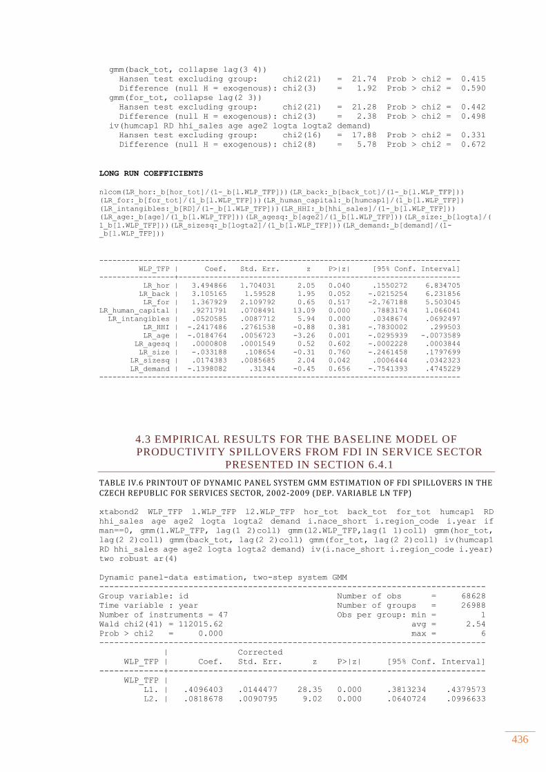
436
gmm(back_tot, collapse lag(3 4))
Hansen test excluding group: chi2(21) = 21.74 Prob > chi2 = 0.415
Difference (null H = exogenous): chi2(3) = 1.92 Prob > chi2 = 0.590
gmm(for_tot, collapse lag(2 3))
Hansen test excluding group: chi2(21) = 21.28 Prob > chi2 = 0.442
Difference (null H = exogenous): chi2(3) = 2.38 Prob > chi2 = 0.498
iv(humcap1 RD hhi_sales age age2 logta logta2 demand)
Hansen test excluding group: chi2(16) = 17.88 Prob > chi2 = 0.331
Difference (null H = exogenous): chi2(8) = 5.78 Prob > chi2 = 0.672
LONG RUN COEFFICIENTS
nlcom(LR_hor:_b[hor_tot]/(1-_b[l.WLP_TFP]))(LR_back:_b[back_tot]/(1-_b[l.WLP_TFP]))
(LR_for:_b[for_tot]/(1_b[l.WLP_TFP]))(LR_human_capital:_b[humcap1]/(1_b[l.WLP_TFP])
(LR_intangibles:_b[RD]/(1-_b[l.WLP_TFP]))(LR_HHI:_b[hhi_sales]/(1-_b[l.WLP_TFP]))
(LR_age:_b[age]/(1_b[l.WLP_TFP]))(LR_agesq:_b[age2]/(1_b[l.WLP_TFP]))(LR_size:_b[logta]/(
1_b[l.WLP_TFP]))(LR_sizesq:_b[logta2]/(1_b[l.WLP_TFP]))(LR_demand:_b[demand]/(1-
_b[l.WLP_TFP]))
----------------------------------------------------------------------------------
WLP_TFP | Coef. Std. Err. z P>|z| [95% Conf. Interval]
-----------------+----------------------------------------------------------------
LR_hor | 3.494866 1.704031 2.05 0.040 .1550272 6.834705
LR_back | 3.105165 1.59528 1.95 0.052 -.0215254 6.231856
LR_for | 1.367929 2.109792 0.65 0.517 -2.767188 5.503045
LR_human_capital | .9271791 .0708491 13.09 0.000 .7883174 1.066041
LR_intangibles | .0520585 .0087712 5.94 0.000 .0348674 .0692497
LR_HHI | -.2417486 .2761538 -0.88 0.381 -.7830002 .299503
LR_age | -.0184764 .0056723 -3.26 0.001 -.0295939 -.0073589
LR_agesq | .0000808 .0001549 0.52 0.602 -.0002228 .0003844
LR_size | -.033188 .108654 -0.31 0.760 -.2461458 .1797699
LR_sizesq | .0174383 .0085685 2.04 0.042 .0006444 .0342323
LR_demand | -.1398082 .31344 -0.45 0.656 -.7541393 .4745229
----------------------------------------------------------------------------------
4.3 EMPIRICAL RESULTS FOR THE BASELINE MODEL OF
PRODUCTIVITY SPILLOVERS FROM FDI IN SERVICE SECTOR
PRESENTED IN SECTION 6.4.1
TABLE IV.6 PRINTOUT OF DYNAMIC PANEL SYSTEM GMM ESTIMATION OF FDI SPILLOVERS IN THE CZECH REPUBLIC FOR SERVICES SECTOR, 2002-2009 (DEP. VARIABLE LN TFP)
xtabond2 WLP_TFP l.WLP_TFP l2.WLP_TFP hor_tot back_tot for_tot humcap1 RD
hhi_sales age age2 logta logta2 demand i.nace_short i.region_code i.year if
man==0, gmm(l.WLP_TFP, lag(1 2)coll) gmm(l2.WLP_TFP,lag(1 1)coll) gmm(hor_tot,
lag(2 2)coll) gmm(back_tot, lag(2 2)coll) gmm(for_tot, lag(2 2)coll) iv(humcap1
RD hhi_sales age age2 logta logta2 demand) iv(i.nace_short i.region_code i.year)
two robust ar(4)
Dynamic panel-data estimation, two-step system GMM
------------------------------------------------------------------------------
Group variable: id Number of obs = 68628
Time variable : year Number of groups = 26988
Number of instruments = 47 Obs per group: min = 1
Wald chi2(41) = 112015.62 avg = 2.54
Prob > chi2 = 0.000 max = 6
------------------------------------------------------------------------------
| Corrected
WLP_TFP | Coef. Std. Err. z P>|z| [95% Conf. Interval]
-------------+----------------------------------------------------------------
WLP_TFP |
L1. | .4096403 .0144477 28.35 0.000 .3813234 .4379573
L2. | .0818678 .0090795 9.02 0.000 .0640724 .0996633
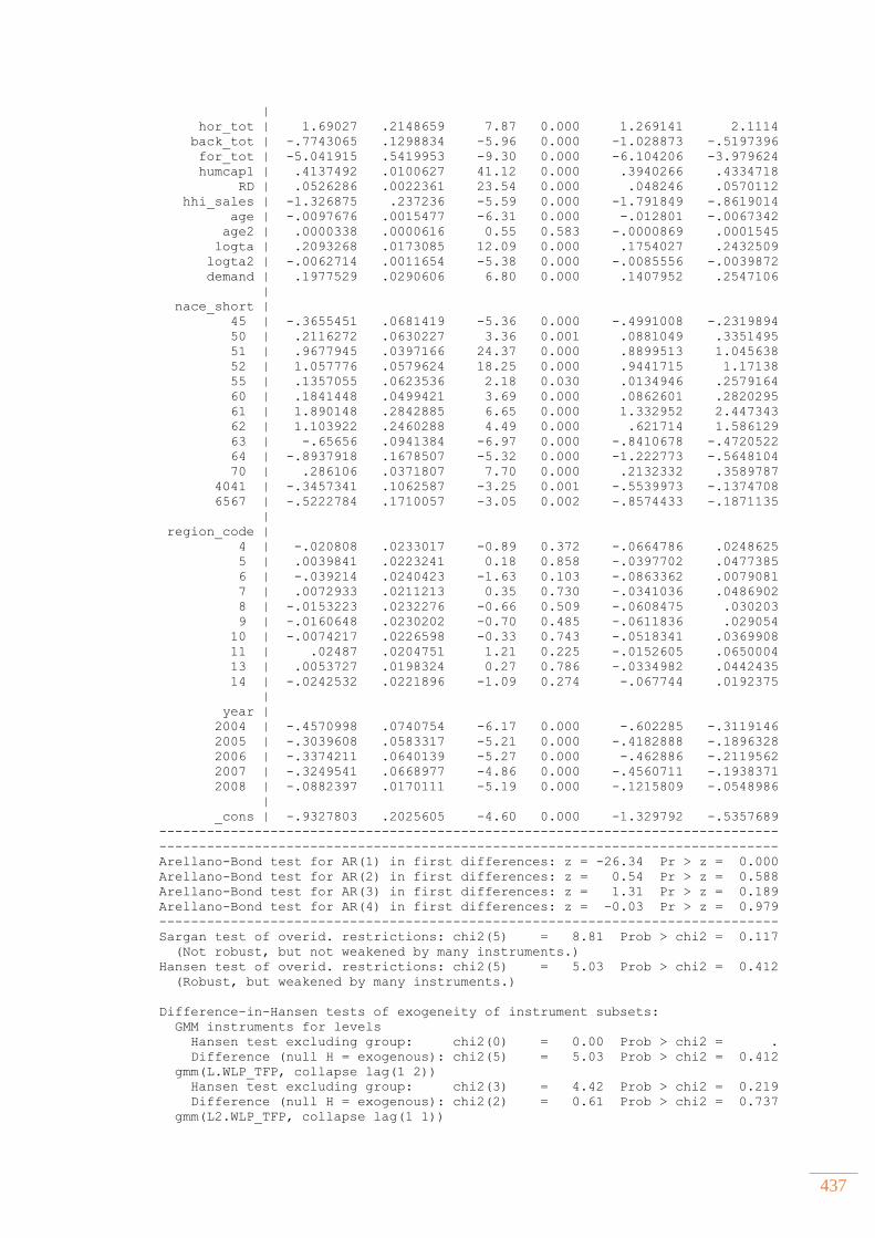
437
|
hor_tot | 1.69027 .2148659 7.87 0.000 1.269141 2.1114
back_tot | -.7743065 .1298834 -5.96 0.000 -1.028873 -.5197396
for_tot | -5.041915 .5419953 -9.30 0.000 -6.104206 -3.979624
humcap1 | .4137492 .0100627 41.12 0.000 .3940266 .4334718
RD | .0526286 .0022361 23.54 0.000 .048246 .0570112
hhi_sales | -1.326875 .237236 -5.59 0.000 -1.791849 -.8619014
age | -.0097676 .0015477 -6.31 0.000 -.012801 -.0067342
age2 | .0000338 .0000616 0.55 0.583 -.0000869 .0001545
logta | .2093268 .0173085 12.09 0.000 .1754027 .2432509
logta2 | -.0062714 .0011654 -5.38 0.000 -.0085556 -.0039872
demand | .1977529 .0290606 6.80 0.000 .1407952 .2547106
|
nace_short |
45 | -.3655451 .0681419 -5.36 0.000 -.4991008 -.2319894
50 | .2116272 .0630227 3.36 0.001 .0881049 .3351495
51 | .9677945 .0397166 24.37 0.000 .8899513 1.045638
52 | 1.057776 .0579624 18.25 0.000 .9441715 1.17138
55 | .1357055 .0623536 2.18 0.030 .0134946 .2579164
60 | .1841448 .0499421 3.69 0.000 .0862601 .2820295
61 | 1.890148 .2842885 6.65 0.000 1.332952 2.447343
62 | 1.103922 .2460288 4.49 0.000 .621714 1.586129
63 | -.65656 .0941384 -6.97 0.000 -.8410678 -.4720522
64 | -.8937918 .1678507 -5.32 0.000 -1.222773 -.5648104
70 | .286106 .0371807 7.70 0.000 .2132332 .3589787
4041 | -.3457341 .1062587 -3.25 0.001 -.5539973 -.1374708
6567 | -.5222784 .1710057 -3.05 0.002 -.8574433 -.1871135
|
region_code |
4 | -.020808 .0233017 -0.89 0.372 -.0664786 .0248625
5 | .0039841 .0223241 0.18 0.858 -.0397702 .0477385
6 | -.039214 .0240423 -1.63 0.103 -.0863362 .0079081
7 | .0072933 .0211213 0.35 0.730 -.0341036 .0486902
8 | -.0153223 .0232276 -0.66 0.509 -.0608475 .030203
9 | -.0160648 .0230202 -0.70 0.485 -.0611836 .029054
10 | -.0074217 .0226598 -0.33 0.743 -.0518341 .0369908
11 | .02487 .0204751 1.21 0.225 -.0152605 .0650004
13 | .0053727 .0198324 0.27 0.786 -.0334982 .0442435
14 | -.0242532 .0221896 -1.09 0.274 -.067744 .0192375
|
year |
2004 | -.4570998 .0740754 -6.17 0.000 -.602285 -.3119146
2005 | -.3039608 .0583317 -5.21 0.000 -.4182888 -.1896328
2006 | -.3374211 .0640139 -5.27 0.000 -.462886 -.2119562
2007 | -.3249541 .0668977 -4.86 0.000 -.4560711 -.1938371
2008 | -.0882397 .0170111 -5.19 0.000 -.1215809 -.0548986
|
_cons | -.9327803 .2025605 -4.60 0.000 -1.329792 -.5357689
------------------------------------------------------------------------------
------------------------------------------------------------------------------
Arellano-Bond test for AR(1) in first differences: z = -26.34 Pr > z = 0.000
Arellano-Bond test for AR(2) in first differences: z = 0.54 Pr > z = 0.588
Arellano-Bond test for AR(3) in first differences: z = 1.31 Pr > z = 0.189
Arellano-Bond test for AR(4) in first differences: z = -0.03 Pr > z = 0.979
------------------------------------------------------------------------------
Sargan test of overid. restrictions: chi2(5) = 8.81 Prob > chi2 = 0.117
(Not robust, but not weakened by many instruments.)
Hansen test of overid. restrictions: chi2(5) = 5.03 Prob > chi2 = 0.412
(Robust, but weakened by many instruments.)
Difference-in-Hansen tests of exogeneity of instrument subsets:
GMM instruments for levels
Hansen test excluding group: chi2(0) = 0.00 Prob > chi2 = .
Difference (null H = exogenous): chi2(5) = 5.03 Prob > chi2 = 0.412
gmm(L.WLP_TFP, collapse lag(1 2))
Hansen test excluding group: chi2(3) = 4.42 Prob > chi2 = 0.219
Difference (null H = exogenous): chi2(2) = 0.61 Prob > chi2 = 0.737
gmm(L2.WLP_TFP, collapse lag(1 1))
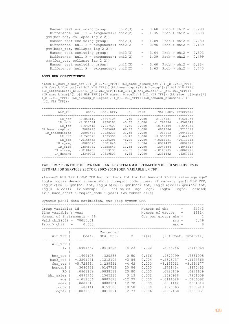
438
Hansen test excluding group: chi2(3) = 3.68 Prob > chi2 = 0.298
Difference (null H = exogenous): chi2(2) = 1.35 Prob > chi2 = 0.508
gmm(hor_tot, collapse lag(2 2))
Hansen test excluding group: chi2(3) = 1.09 Prob > chi2 = 0.780
Difference (null H = exogenous): chi2(2) = 3.95 Prob > chi2 = 0.139
gmm(back_tot, collapse lag(2 2))
Hansen test excluding group: chi2(3) = 3.64 Prob > chi2 = 0.303
Difference (null H = exogenous): chi2(2) = 1.39 Prob > chi2 = 0.499
gmm(for_tot, collapse lag(2 2))
Hansen test excluding group: chi2(3) = 3.40 Prob > chi2 = 0.334
Difference (null H = exogenous): chi2(2) = 1.63 Prob > chi2 = 0.443
LONG RUN COEFFICIENTS
nlcom(LR_hor:_b[hor_tot]/(1-_b[l.WLP_TFP]))(LR_back:_b[back_tot]/(1-_b[l.WLP_TFP]))
(LR_for:_b[for_tot]/(1_b[l.WLP_TFP]))(LR_human_capital:_b[humcap1]/(1_b[l.WLP_TFP])
(LR_intangibles:_b[RD]/(1-_b[l.WLP_TFP]))(LR_HHI:_b[hhi_sales]/(1-_b[l.WLP_TFP]))
(LR_age:_b[age]/(1_b[l.WLP_TFP]))(LR_agesq:_b[age2]/(1_b[l.WLP_TFP]))(LR_size:_b[logta]/(
1_b[l.WLP_TFP]))(LR_sizesq:_b[logta2]/(1_b[l.WLP_TFP]))(LR_demand:_b[demand]/(1-
_b[l.WLP_TFP]))
----------------------------------------------------------------------------------
WLP_TFP | Coef. Std. Err. z P>|z| [95% Conf. Interval]
-----------------+----------------------------------------------------------------
LR_hor | 2.863119 .3867104 7.40 0.000 2.105181 3.621058
LR_back | -1.311584 .2320193 -5.65 0.000 -1.766334 -.8568349
LR_for | -8.540412 1.017607 -8.39 0.000 -10.53489 -6.545939
LR_human_capital | .7008426 .0105661 66.33 0.000 .6801334 .7215519
LR_intangibles | .0891466 .0028233 31.58 0.000 .083613 .0946802
LR_HHI | -2.247571 .4095308 -5.49 0.000 -3.050237 -1.444906
LR_age | -.0165452 .0026296 -6.29 0.000 -.0216991 -.0113913
LR_agesq | .0000573 .0001046 0.55 0.584 -.0001477 .0002623
LR_size | .3545751 .0255549 13.88 0.000 .3044884 .4046617
LR_sizesq | -.0106231 .0019135 -5.55 0.000 -.0143735 -.0068726
LR_demand | .3349702 .0519509 6.45 0.000 .2331482 .4367922
----------------------------------------------------------------------------------
TABLE IV.7 PRINTOUT OF DYNAMIC PANEL SYSTEM GMM ESTIMATION OF FDI SPILLOVERS IN ESTONIA FOR SERVICES SECTOR, 2002-2010 (DEP. VARIABLE LN TFP)
xtabond2 WLP_TFP l.WLP_TFP hor_tot back_tot for_tot humcap1 RD hhi_sales age age2
logta logta2 demand i.nace_short i.region_code i.year if man==0, gmm(l.WLP_TFP,
lag(2 2)coll) gmm(hor_tot, lag(4 6)coll) gmm(back_tot, lag(3 4)coll) gmm(for_tot,
lag(4 6)coll) iv(humcap1 RD hhi_sales age age2 logta logta2 demand)
iv(i.nace_short i.region_code i.year) two robust ar(4)
Dynamic panel-data estimation, two-step system GMM
------------------------------------------------------------------------------
Group variable: id Number of obs = 54743
Time variable : year Number of groups = 15814
Number of instruments = 46 Obs per group: min = 1
Wald chi2(36) = 78015.01 avg = 3.46
Prob > chi2 = 0.000 max = 8
------------------------------------------------------------------------------
| Corrected
WLP_TFP | Coef. Std. Err. z P>|z| [95% Conf. Interval]
-------------+----------------------------------------------------------------
WLP_TFP |
L1. | .5901357 .0414605 14.23 0.000 .5088746 .6713968
|
hor_tot | .1604103 .320256 0.50 0.616 -.4672799 .7881005
back_tot | -.3501051 .1212107 -2.89 0.004 -.5876737 -.1125365
for_tot | -5.723594 1.239521 -4.62 0.000 -8.153011 -3.294177
humcap1 | .3080943 .0147712 20.86 0.000 .2791434 .3370453
RD | .0801159 .0038511 20.80 0.000 .0725679 .0876639
hhi_sales | .4893748 .1565213 3.13 0.002 .1825988 .7961509
age | -.012556 .0009678 -12.97 0.000 -.0144528 -.0106592
age2 | .0001315 .0000104 12.70 0.000 .0001112 .0001518
logta | .1688141 .0159583 10.58 0.000 .1375363 .2000918
logta2 | -.0030695 .0011094 -2.77 0.006 -.0052438 -.0008951
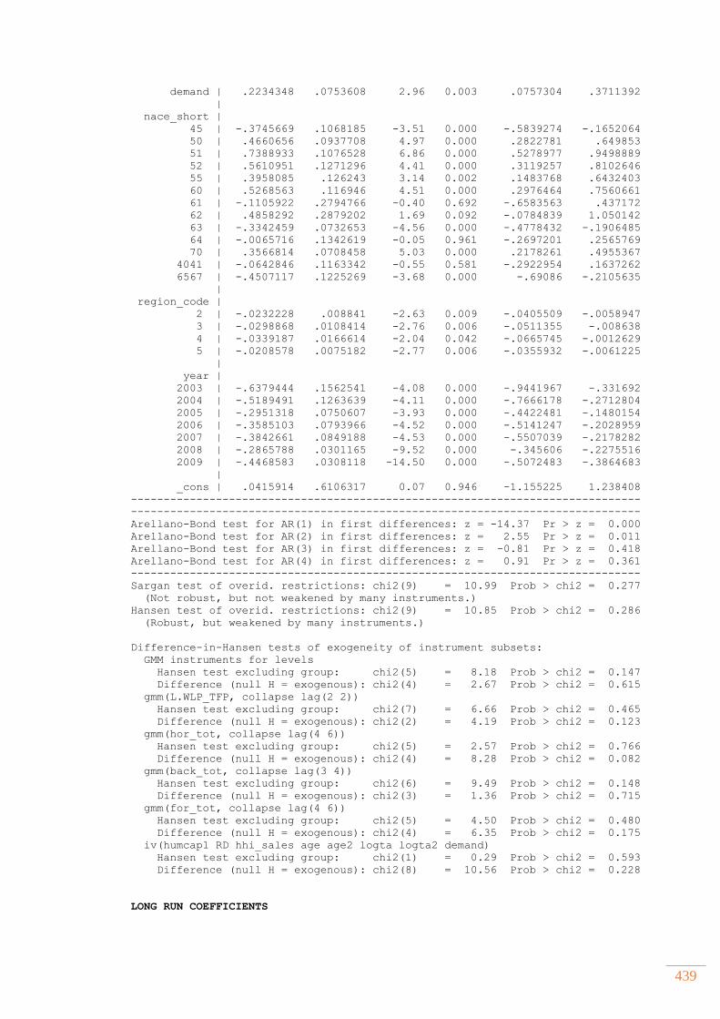
439
demand | .2234348 .0753608 2.96 0.003 .0757304 .3711392
|
nace_short |
45 | -.3745669 .1068185 -3.51 0.000 -.5839274 -.1652064
50 | .4660656 .0937708 4.97 0.000 .2822781 .649853
51 | .7388933 .1076528 6.86 0.000 .5278977 .9498889
52 | .5610951 .1271296 4.41 0.000 .3119257 .8102646
55 | .3958085 .126243 3.14 0.002 .1483768 .6432403
60 | .5268563 .116946 4.51 0.000 .2976464 .7560661
61 | -.1105922 .2794766 -0.40 0.692 -.6583563 .437172
62 | .4858292 .2879202 1.69 0.092 -.0784839 1.050142
63 | -.3342459 .0732653 -4.56 0.000 -.4778432 -.1906485
64 | -.0065716 .1342619 -0.05 0.961 -.2697201 .2565769
70 | .3566814 .0708458 5.03 0.000 .2178261 .4955367
4041 | -.0642846 .1163342 -0.55 0.581 -.2922954 .1637262
6567 | -.4507117 .1225269 -3.68 0.000 -.69086 -.2105635
|
region_code |
2 | -.0232228 .008841 -2.63 0.009 -.0405509 -.0058947
3 | -.0298868 .0108414 -2.76 0.006 -.0511355 -.008638
4 | -.0339187 .0166614 -2.04 0.042 -.0665745 -.0012629
5 | -.0208578 .0075182 -2.77 0.006 -.0355932 -.0061225
|
year |
2003 | -.6379444 .1562541 -4.08 0.000 -.9441967 -.331692
2004 | -.5189491 .1263639 -4.11 0.000 -.7666178 -.2712804
2005 | -.2951318 .0750607 -3.93 0.000 -.4422481 -.1480154
2006 | -.3585103 .0793966 -4.52 0.000 -.5141247 -.2028959
2007 | -.3842661 .0849188 -4.53 0.000 -.5507039 -.2178282
2008 | -.2865788 .0301165 -9.52 0.000 -.345606 -.2275516
2009 | -.4468583 .0308118 -14.50 0.000 -.5072483 -.3864683
|
_cons | .0415914 .6106317 0.07 0.946 -1.155225 1.238408
------------------------------------------------------------------------------
------------------------------------------------------------------------------
Arellano-Bond test for AR(1) in first differences: z = -14.37 Pr > z = 0.000
Arellano-Bond test for AR(2) in first differences: z = 2.55 Pr > z = 0.011
Arellano-Bond test for AR(3) in first differences: z = -0.81 Pr > z = 0.418
Arellano-Bond test for AR(4) in first differences: z = 0.91 Pr > z = 0.361
------------------------------------------------------------------------------
Sargan test of overid. restrictions: chi2(9) = 10.99 Prob > chi2 = 0.277
(Not robust, but not weakened by many instruments.)
Hansen test of overid. restrictions: chi2(9) = 10.85 Prob > chi2 = 0.286
(Robust, but weakened by many instruments.)
Difference-in-Hansen tests of exogeneity of instrument subsets:
GMM instruments for levels
Hansen test excluding group: chi2(5) = 8.18 Prob > chi2 = 0.147
Difference (null H = exogenous): chi2(4) = 2.67 Prob > chi2 = 0.615
gmm(L.WLP_TFP, collapse lag(2 2))
Hansen test excluding group: chi2(7) = 6.66 Prob > chi2 = 0.465
Difference (null H = exogenous): chi2(2) = 4.19 Prob > chi2 = 0.123
gmm(hor_tot, collapse lag(4 6))
Hansen test excluding group: chi2(5) = 2.57 Prob > chi2 = 0.766
Difference (null H = exogenous): chi2(4) = 8.28 Prob > chi2 = 0.082
gmm(back_tot, collapse lag(3 4))
Hansen test excluding group: chi2(6) = 9.49 Prob > chi2 = 0.148
Difference (null H = exogenous): chi2(3) = 1.36 Prob > chi2 = 0.715
gmm(for_tot, collapse lag(4 6))
Hansen test excluding group: chi2(5) = 4.50 Prob > chi2 = 0.480
Difference (null H = exogenous): chi2(4) = 6.35 Prob > chi2 = 0.175
iv(humcap1 RD hhi_sales age age2 logta logta2 demand)
Hansen test excluding group: chi2(1) = 0.29 Prob > chi2 = 0.593
Difference (null H = exogenous): chi2(8) = 10.56 Prob > chi2 = 0.228
LONG RUN COEFFICIENTS
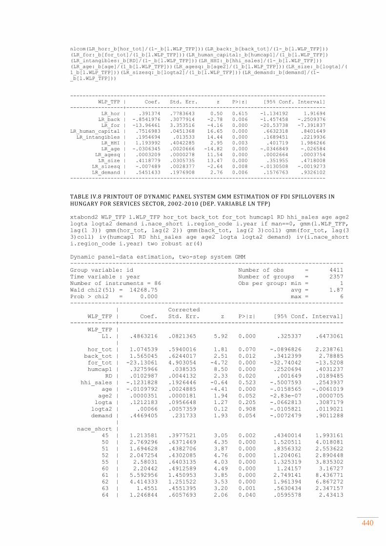
440
nlcom(LR_hor:_b[hor_tot]/(1-_b[l.WLP_TFP]))(LR_back:_b[back_tot]/(1-_b[l.WLP_TFP]))
(LR_for:_b[for_tot]/(1_b[l.WLP_TFP]))(LR_human_capital:_b[humcap1]/(1_b[l.WLP_TFP])
(LR_intangibles:_b[RD]/(1-_b[l.WLP_TFP]))(LR_HHI:_b[hhi_sales]/(1-_b[l.WLP_TFP]))
(LR_age:_b[age]/(1_b[l.WLP_TFP]))(LR_agesq:_b[age2]/(1_b[l.WLP_TFP]))(LR_size:_b[logta]/(
1_b[l.WLP_TFP]))(LR_sizesq:_b[logta2]/(1_b[l.WLP_TFP]))(LR_demand:_b[demand]/(1-
_b[l.WLP_TFP]))
----------------------------------------------------------------------------------
WLP_TFP | Coef. Std. Err. z P>|z| [95% Conf. Interval]
-----------------+----------------------------------------------------------------
LR_hor | .391374 .7783643 0.50 0.615 -1.134192 1.91694
LR_back | -.8541976 .3077914 -2.78 0.006 -1.457458 -.2509376
LR_for | -13.96461 3.353516 -4.16 0.000 -20.53738 -7.391837
LR_human_capital | .7516983 .0451368 16.65 0.000 .6632318 .8401649
LR_intangibles | .1954694 .013533 14.44 0.000 .1689451 .2219936
LR_HHI | 1.193992 .4042285 2.95 0.003 .401719 1.986266
LR_age | -.0306345 .0020666 -14.82 0.000 -.0346849 -.026584
LR_agesq | .0003209 .0000278 11.54 0.000 .0002664 .0003754
LR_size | .4118779 .0305735 13.47 0.000 .351955 .4718008
LR_sizesq | -.007489 .0028377 -2.64 0.008 -.0130508 -.0019273
LR_demand | .5451433 .1976908 2.76 0.006 .1576763 .9326102
----------------------------------------------------------------------------------
TABLE IV.8 PRINTOUT OF DYNAMIC PANEL SYSTEM GMM ESTIMATION OF FDI SPILLOVERS IN HUNGARY FOR SERVICES SECTOR, 2002-2010 (DEP. VARIABLE LN TFP)
xtabond2 WLP_TFP l.WLP_TFP hor_tot back_tot for_tot humcap1 RD hhi_sales age age2
logta logta2 demand i.nace_short i.region_code i.year if man==0, gmm(l.WLP_TFP,
lag(1 3)) gmm(hor_tot, lag(2 2)) gmm(back_tot, lag(2 3)coll) gmm(for_tot, lag(3
3)coll) iv(humcap1 RD hhi_sales age age2 logta logta2 demand) iv(i.nace_short
i.region_code i.year) two robust ar(4)
Dynamic panel-data estimation, two-step system GMM
------------------------------------------------------------------------------
Group variable: id Number of obs = 4411
Time variable : year Number of groups = 2357
Number of instruments = 86 Obs per group: min = 1
Wald chi2(51) = 14268.75 avg = 1.87
Prob > chi2 = 0.000 max = 6
------------------------------------------------------------------------------
| Corrected
WLP_TFP | Coef. Std. Err. z P>|z| [95% Conf. Interval]
-------------+----------------------------------------------------------------
WLP_TFP |
L1. | .4863216 .0821365 5.92 0.000 .325337 .6473061
|
hor_tot | 1.074539 .5940016 1.81 0.070 -.0896826 2.238761
back_tot | 1.565045 .6244017 2.51 0.012 .3412399 2.78885
for_tot | -23.13061 4.903054 -4.72 0.000 -32.74042 -13.5208
humcap1 | .3275966 .038535 8.50 0.000 .2520694 .4031237
RD | .0102987 .0044132 2.33 0.020 .001649 .0189485
hhi_sales | -.1231828 .1926446 -0.64 0.523 -.5007593 .2543937
age | -.0109792 .0024885 -4.41 0.000 -.0158565 -.0061019
age2 | .0000351 .0000181 1.94 0.052 -2.83e-07 .0000705
logta | .1212183 .0956648 1.27 0.205 -.0662813 .3087179
logta2 | .00066 .0057359 0.12 0.908 -.0105821 .0119021
demand | .4469405 .231733 1.93 0.054 -.0072479 .9011288
|
nace_short |
45 | 1.213581 .3977521 3.05 0.002 .4340014 1.993161
50 | 2.769296 .6371469 4.35 0.000 1.520511 4.018081
51 | 1.694628 .4382706 3.87 0.000 .8356332 2.553622
52 | 2.047254 .4302085 4.76 0.000 1.204061 2.890448
55 | 2.58031 .6403135 4.03 0.000 1.325319 3.835302
60 | 2.20442 .4912589 4.49 0.000 1.24157 3.16727
61 | 5.592956 1.450953 3.85 0.000 2.749141 8.436771
62 | 4.414333 1.251522 3.53 0.000 1.961394 6.867272
63 | 1.4551 .4551395 3.20 0.001 .5630434 2.347157
64 | 1.246844 .6057693 2.06 0.040 .0595578 2.43413
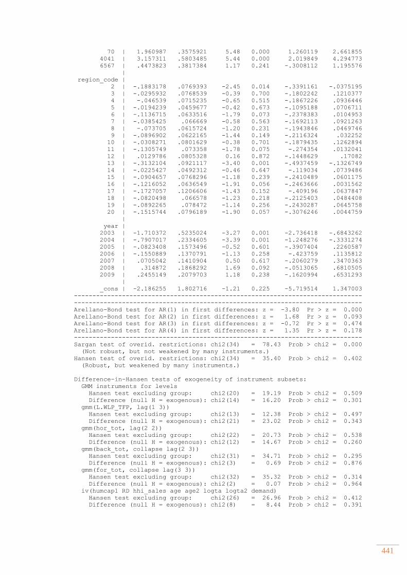
441
70 | 1.960987 .3575921 5.48 0.000 1.260119 2.661855
4041 | 3.157311 .5803485 5.44 0.000 2.019849 4.294773
6567 | .4473823 .3817384 1.17 0.241 -.3008112 1.195576
|
region_code |
2 | -.1883178 .0769393 -2.45 0.014 -.3391161 -.0375195
3 | -.0295932 .0768539 -0.39 0.700 -.1802242 .1210377
4 | -.046539 .0715235 -0.65 0.515 -.1867226 .0936446
5 | -.0194239 .0459677 -0.42 0.673 -.1095188 .0706711
6 | -.1136715 .0633516 -1.79 0.073 -.2378383 .0104953
7 | -.0385425 .066669 -0.58 0.563 -.1692113 .0921263
8 | -.073705 .0615724 -1.20 0.231 -.1943846 .0469746
9 | -.0896902 .0622165 -1.44 0.149 -.2116324 .032252
10 | -.0308271 .0801629 -0.38 0.701 -.1879435 .1262894
11 | -.1305749 .073358 -1.78 0.075 -.274354 .0132041
12 | .0129786 .0805328 0.16 0.872 -.1448629 .17082
13 | -.3132104 .0921117 -3.40 0.001 -.4937459 -.1326749
14 | -.0225427 .0492312 -0.46 0.647 -.119034 .0739486
15 | -.0904657 .0768296 -1.18 0.239 -.2410489 .0601175
16 | -.1216052 .0636549 -1.91 0.056 -.2463666 .0031562
17 | -.1727057 .1206606 -1.43 0.152 -.409196 .0637847
18 | -.0820498 .066578 -1.23 0.218 -.2125403 .0484408
19 | -.0892265 .078472 -1.14 0.256 -.2430287 .0645758
20 | -.1515744 .0796189 -1.90 0.057 -.3076246 .0044759
|
year |
2003 | -1.710372 .5235024 -3.27 0.001 -2.736418 -.6843262
2004 | -.7907017 .2334605 -3.39 0.001 -1.248276 -.3331274
2005 | -.0823408 .1573496 -0.52 0.601 -.3907404 .2260587
2006 | -.1550889 .1370791 -1.13 0.258 -.423759 .1135812
2007 | .0705042 .1410904 0.50 0.617 -.2060279 .3470363
2008 | .314872 .1868292 1.69 0.092 -.0513065 .6810505
2009 | .2455149 .2079703 1.18 0.238 -.1620994 .6531293
|
_cons | -2.186255 1.802716 -1.21 0.225 -5.719514 1.347003
------------------------------------------------------------------------------
------------------------------------------------------------------------------
Arellano-Bond test for AR(1) in first differences: z = -3.80 Pr > z = 0.000
Arellano-Bond test for AR(2) in first differences: z = 1.68 Pr > z = 0.093
Arellano-Bond test for AR(3) in first differences: z = -0.72 Pr > z = 0.474
Arellano-Bond test for AR(4) in first differences: z = 1.35 Pr > z = 0.178
------------------------------------------------------------------------------
Sargan test of overid. restrictions: chi2(34) = 78.43 Prob > chi2 = 0.000
(Not robust, but not weakened by many instruments.)
Hansen test of overid. restrictions: chi2(34) = 35.40 Prob > chi2 = 0.402
(Robust, but weakened by many instruments.)
Difference-in-Hansen tests of exogeneity of instrument subsets:
GMM instruments for levels
Hansen test excluding group: chi2(20) = 19.19 Prob > chi2 = 0.509
Difference (null H = exogenous): chi2(14) = 16.20 Prob > chi2 = 0.301
gmm(L.WLP_TFP, lag(1 3))
Hansen test excluding group: chi2(13) = 12.38 Prob > chi2 = 0.497
Difference (null H = exogenous): chi2(21) = 23.02 Prob > chi2 = 0.343
gmm(hor_tot, lag(2 2))
Hansen test excluding group: chi2(22) = 20.73 Prob > chi2 = 0.538
Difference (null H = exogenous): chi2(12) = 14.67 Prob > chi2 = 0.260
gmm(back_tot, collapse lag(2 3))
Hansen test excluding group: chi2(31) = 34.71 Prob > chi2 = 0.295
Difference (null H = exogenous): chi2(3) = 0.69 Prob > chi2 = 0.876
gmm(for_tot, collapse lag(3 3))
Hansen test excluding group: chi2(32) = 35.32 Prob > chi2 = 0.314
Difference (null H = exogenous): chi2(2) = 0.07 Prob > chi2 = 0.964
iv(humcap1 RD hhi_sales age age2 logta logta2 demand)
Hansen test excluding group: chi2(26) = 26.96 Prob > chi2 = 0.412
Difference (null H = exogenous): chi2(8) = 8.44 Prob > chi2 = 0.391
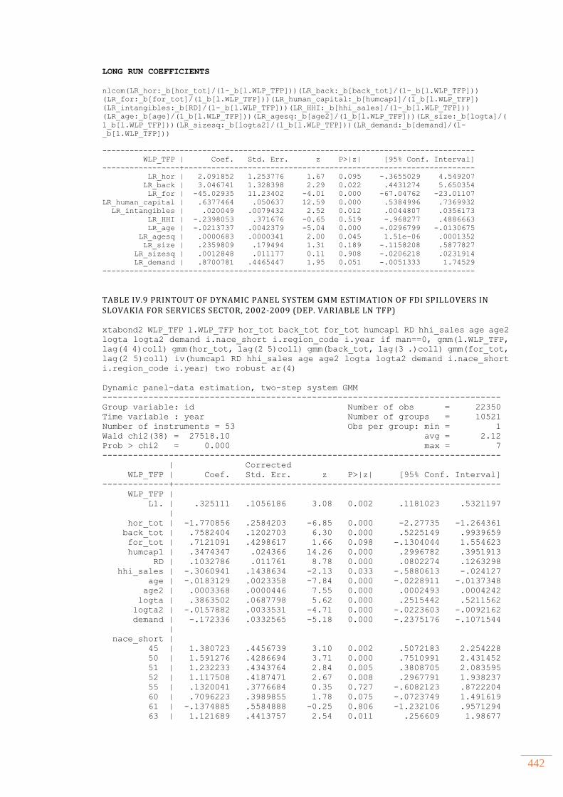
442
LONG RUN COEFFICIENTS
nlcom(LR_hor:_b[hor_tot]/(1-_b[l.WLP_TFP]))(LR_back:_b[back_tot]/(1-_b[l.WLP_TFP]))
(LR_for:_b[for_tot]/(1_b[l.WLP_TFP]))(LR_human_capital:_b[humcap1]/(1_b[l.WLP_TFP])
(LR_intangibles:_b[RD]/(1-_b[l.WLP_TFP]))(LR_HHI:_b[hhi_sales]/(1-_b[l.WLP_TFP]))
(LR_age:_b[age]/(1_b[l.WLP_TFP]))(LR_agesq:_b[age2]/(1_b[l.WLP_TFP]))(LR_size:_b[logta]/(
1_b[l.WLP_TFP]))(LR_sizesq:_b[logta2]/(1_b[l.WLP_TFP]))(LR_demand:_b[demand]/(1-
_b[l.WLP_TFP]))
----------------------------------------------------------------------------------
WLP_TFP | Coef. Std. Err. z P>|z| [95% Conf. Interval]
-----------------+----------------------------------------------------------------
LR_hor | 2.091852 1.253776 1.67 0.095 -.3655029 4.549207
LR_back | 3.046741 1.328398 2.29 0.022 .4431274 5.650354
LR_for | -45.02935 11.23402 -4.01 0.000 -67.04762 -23.01107
LR_human_capital | .6377464 .050637 12.59 0.000 .5384996 .7369932
LR_intangibles | .020049 .0079432 2.52 0.012 .0044807 .0356173
LR_HHI | -.2398053 .371676 -0.65 0.519 -.968277 .4886663
LR_age | -.0213737 .0042379 -5.04 0.000 -.0296799 -.0130675
LR_agesq | .0000683 .0000341 2.00 0.045 1.51e-06 .0001352
LR_size | .2359809 .179494 1.31 0.189 -.1158208 .5877827
LR_sizesq | .0012848 .011177 0.11 0.908 -.0206218 .0231914
LR_demand | .8700781 .4465447 1.95 0.051 -.0051333 1.74529
----------------------------------------------------------------------------------
TABLE IV.9 PRINTOUT OF DYNAMIC PANEL SYSTEM GMM ESTIMATION OF FDI SPILLOVERS IN SLOVAKIA FOR SERVICES SECTOR, 2002-2009 (DEP. VARIABLE LN TFP)
xtabond2 WLP_TFP l.WLP_TFP hor_tot back_tot for_tot humcap1 RD hhi_sales age age2
logta logta2 demand i.nace_short i.region_code i.year if man==0, gmm(l.WLP_TFP,
lag(4 4)coll) gmm(hor_tot, lag(2 5)coll) gmm(back_tot, lag(3 .)coll) gmm(for_tot,
lag(2 5)coll) iv(humcap1 RD hhi_sales age age2 logta logta2 demand i.nace_short
i.region_code i.year) two robust ar(4)
Dynamic panel-data estimation, two-step system GMM
------------------------------------------------------------------------------
Group variable: id Number of obs = 22350
Time variable : year Number of groups = 10521
Number of instruments = 53 Obs per group: min = 1
Wald chi2(38) = 27518.10 avg = 2.12
Prob > chi2 = 0.000 max = 7
------------------------------------------------------------------------------
| Corrected
WLP_TFP | Coef. Std. Err. z P>|z| [95% Conf. Interval]
-------------+----------------------------------------------------------------
WLP_TFP |
L1. | .325111 .1056186 3.08 0.002 .1181023 .5321197
|
hor_tot | -1.770856 .2584203 -6.85 0.000 -2.27735 -1.264361
back_tot | .7582404 .1202703 6.30 0.000 .5225149 .9939659
for_tot | .7121091 .4298617 1.66 0.098 -.1304044 1.554623
humcap1 | .3474347 .024366 14.26 0.000 .2996782 .3951913
RD | .1032786 .011761 8.78 0.000 .0802274 .1263298
hhi_sales | -.3060941 .1438634 -2.13 0.033 -.5880613 -.024127
age | -.0183129 .0023358 -7.84 0.000 -.0228911 -.0137348
age2 | .0003368 .0000446 7.55 0.000 .0002493 .0004242
logta | .3863502 .0687798 5.62 0.000 .2515442 .5211562
logta2 | -.0157882 .0033531 -4.71 0.000 -.0223603 -.0092162
demand | -.172336 .0332565 -5.18 0.000 -.2375176 -.1071544
|
nace_short |
45 | 1.380723 .4456739 3.10 0.002 .5072183 2.254228
50 | 1.591276 .4286694 3.71 0.000 .7510991 2.431452
51 | 1.232233 .4343764 2.84 0.005 .3808705 2.083595
52 | 1.117508 .4187471 2.67 0.008 .2967791 1.938237
55 | .1320041 .3776684 0.35 0.727 -.6082123 .8722204
60 | .7096223 .3989855 1.78 0.075 -.0723749 1.491619
61 | -.1374885 .5584888 -0.25 0.806 -1.232106 .9571294
63 | 1.121689 .4413757 2.54 0.011 .256609 1.98677
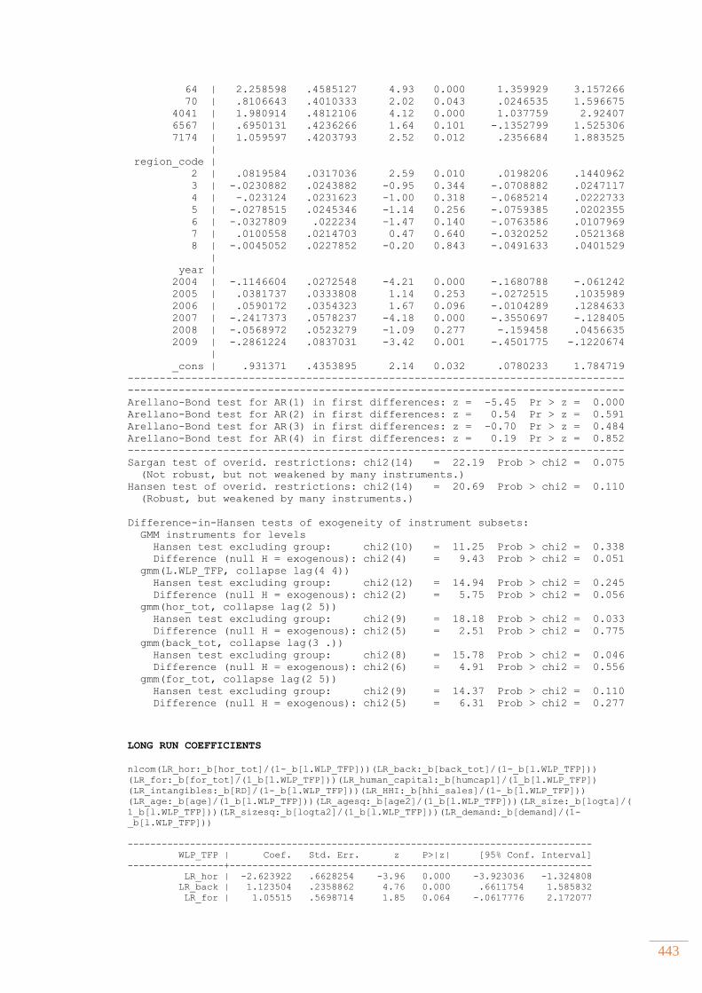
443
64 | 2.258598 .4585127 4.93 0.000 1.359929 3.157266
70 | .8106643 .4010333 2.02 0.043 .0246535 1.596675
4041 | 1.980914 .4812106 4.12 0.000 1.037759 2.92407
6567 | .6950131 .4236266 1.64 0.101 -.1352799 1.525306
7174 | 1.059597 .4203793 2.52 0.012 .2356684 1.883525
|
region_code |
2 | .0819584 .0317036 2.59 0.010 .0198206 .1440962
3 | -.0230882 .0243882 -0.95 0.344 -.0708882 .0247117
4 | -.023124 .0231623 -1.00 0.318 -.0685214 .0222733
5 | -.0278515 .0245346 -1.14 0.256 -.0759385 .0202355
6 | -.0327809 .022234 -1.47 0.140 -.0763586 .0107969
7 | .0100558 .0214703 0.47 0.640 -.0320252 .0521368
8 | -.0045052 .0227852 -0.20 0.843 -.0491633 .0401529
|
year |
2004 | -.1146604 .0272548 -4.21 0.000 -.1680788 -.061242
2005 | .0381737 .0333808 1.14 0.253 -.0272515 .1035989
2006 | .0590172 .0354323 1.67 0.096 -.0104289 .1284633
2007 | -.2417373 .0578237 -4.18 0.000 -.3550697 -.128405
2008 | -.0568972 .0523279 -1.09 0.277 -.159458 .0456635
2009 | -.2861224 .0837031 -3.42 0.001 -.4501775 -.1220674
|
_cons | .931371 .4353895 2.14 0.032 .0780233 1.784719
------------------------------------------------------------------------------
------------------------------------------------------------------------------
Arellano-Bond test for AR(1) in first differences: z = -5.45 Pr > z = 0.000
Arellano-Bond test for AR(2) in first differences: z = 0.54 Pr > z = 0.591
Arellano-Bond test for AR(3) in first differences: z = -0.70 Pr > z = 0.484
Arellano-Bond test for AR(4) in first differences: z = 0.19 Pr > z = 0.852
------------------------------------------------------------------------------
Sargan test of overid. restrictions: chi2(14) = 22.19 Prob > chi2 = 0.075
(Not robust, but not weakened by many instruments.)
Hansen test of overid. restrictions: chi2(14) = 20.69 Prob > chi2 = 0.110
(Robust, but weakened by many instruments.)
Difference-in-Hansen tests of exogeneity of instrument subsets:
GMM instruments for levels
Hansen test excluding group: chi2(10) = 11.25 Prob > chi2 = 0.338
Difference (null H = exogenous): chi2(4) = 9.43 Prob > chi2 = 0.051
gmm(L.WLP_TFP, collapse lag(4 4))
Hansen test excluding group: chi2(12) = 14.94 Prob > chi2 = 0.245
Difference (null H = exogenous): chi2(2) = 5.75 Prob > chi2 = 0.056
gmm(hor_tot, collapse lag(2 5))
Hansen test excluding group: chi2(9) = 18.18 Prob > chi2 = 0.033
Difference (null H = exogenous): chi2(5) = 2.51 Prob > chi2 = 0.775
gmm(back_tot, collapse lag(3 .))
Hansen test excluding group: chi2(8) = 15.78 Prob > chi2 = 0.046
Difference (null H = exogenous): chi2(6) = 4.91 Prob > chi2 = 0.556
gmm(for_tot, collapse lag(2 5))
Hansen test excluding group: chi2(9) = 14.37 Prob > chi2 = 0.110
Difference (null H = exogenous): chi2(5) = 6.31 Prob > chi2 = 0.277
LONG RUN COEFFICIENTS
nlcom(LR_hor:_b[hor_tot]/(1-_b[l.WLP_TFP]))(LR_back:_b[back_tot]/(1-_b[l.WLP_TFP]))
(LR_for:_b[for_tot]/(1_b[l.WLP_TFP]))(LR_human_capital:_b[humcap1]/(1_b[l.WLP_TFP])
(LR_intangibles:_b[RD]/(1-_b[l.WLP_TFP]))(LR_HHI:_b[hhi_sales]/(1-_b[l.WLP_TFP]))
(LR_age:_b[age]/(1_b[l.WLP_TFP]))(LR_agesq:_b[age2]/(1_b[l.WLP_TFP]))(LR_size:_b[logta]/(
1_b[l.WLP_TFP]))(LR_sizesq:_b[logta2]/(1_b[l.WLP_TFP]))(LR_demand:_b[demand]/(1-
_b[l.WLP_TFP]))
----------------------------------------------------------------------------------
WLP_TFP | Coef. Std. Err. z P>|z| [95% Conf. Interval]
-----------------+----------------------------------------------------------------
LR_hor | -2.623922 .6628254 -3.96 0.000 -3.923036 -1.324808
LR_back | 1.123504 .2358862 4.76 0.000 .6611754 1.585832
LR_for | 1.05515 .5698714 1.85 0.064 -.0617776 2.172077
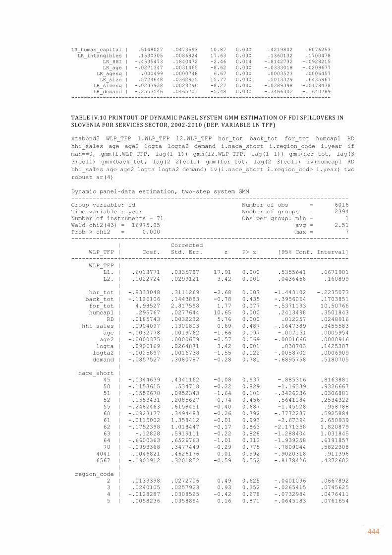
444
LR_human_capital | .5148027 .0473593 10.87 0.000 .4219802 .6076253
LR_intangibles | .1530305 .0086824 17.63 0.000 .1360132 .1700478
LR_HHI | -.4535473 .1840472 -2.46 0.014 -.8142732 -.0928215
LR_age | -.0271347 .0031465 -8.62 0.000 -.0333018 -.0209677
LR_agesq | .000499 .0000748 6.67 0.000 .0003523 .0006457
LR_size | .5724648 .0362925 15.77 0.000 .5013329 .6435967
LR_sizesq | -.0233938 .0028296 -8.27 0.000 -.0289398 -.0178478
LR_demand | -.2553546 .0465701 -5.48 0.000 -.3466302 -.1640789
----------------------------------------------------------------------------------
TABLE IV.10 PRINTOUT OF DYNAMIC PANEL SYSTEM GMM ESTIMATION OF FDI SPILLOVERS IN SLOVENIA FOR SERVICES SECTOR, 2002-2010 (DEP. VARIABLE LN TFP)
xtabond2 WLP_TFP l.WLP_TFP l2.WLP_TFP hor_tot back_tot for_tot humcap1 RD
hhi_sales age age2 logta logta2 demand i.nace_short i.region_code i.year if
man==0, gmm(l.WLP_TFP, lag(1 1)) gmm(l2.WLP_TFP, lag(1 1)) gmm(hor_tot, lag(3
3)coll) gmm(back_tot, lag(2 2)coll) gmm(for_tot, lag(2 3)coll) iv(humcap1 RD
hhi_sales age age2 logta logta2 demand) iv(i.nace_short i.region_code i.year) two
robust ar(4)
Dynamic panel-data estimation, two-step system GMM
------------------------------------------------------------------------------
Group variable: id Number of obs = 6016
Time variable : year Number of groups = 2394
Number of instruments = 71 Obs per group: min = 1
Wald chi2(43) = 16975.95 avg = 2.51
Prob > chi2 = 0.000 max = 7
------------------------------------------------------------------------------
| Corrected
WLP_TFP | Coef. Std. Err. z P>|z| [95% Conf. Interval]
-------------+----------------------------------------------------------------
WLP_TFP |
L1. | .6013771 .0335787 17.91 0.000 .5355641 .6671901
L2. | .1022724 .0299121 3.42 0.001 .0436458 .160899
|
hor_tot | -.8333048 .3111269 -2.68 0.007 -1.443102 -.2235073
back_tot | -.1126106 .1443883 -0.78 0.435 -.3956064 .1703851
for_tot | 4.98527 2.817598 1.77 0.077 -.5371193 10.50766
humcap1 | .295767 .0277644 10.65 0.000 .2413498 .3501843
RD | .0185743 .0032232 5.76 0.000 .012257 .0248916
hhi_sales | .0904097 .1301803 0.69 0.487 -.1647389 .3455583
age | -.0032778 .0019762 -1.66 0.097 -.007151 .0005954
age2 | -.0000375 .0000659 -0.57 0.569 -.0001666 .0000916
logta | .0906169 .0264871 3.42 0.001 .038703 .1425307
logta2 | -.0025897 .0016738 -1.55 0.122 -.0058702 .0006909
demand | -.0857527 .3080787 -0.28 0.781 -.6895758 .5180705
|
nace_short |
45 | -.0344639 .4341162 -0.08 0.937 -.885316 .8163881
50 | -.1153615 .534718 -0.22 0.829 -1.16339 .9326667
51 | -.1559678 .0952343 -1.64 0.101 -.3426236 .0306881
52 | -.1553431 .2085627 -0.74 0.456 -.5641184 .2534322
55 | -.2482463 .6158451 -0.40 0.687 -1.45528 .958788
60 | -.0923177 .3494483 -0.26 0.792 -.7772237 .5925884
61 | -.0115002 1.358412 -0.01 0.993 -2.67394 2.650939
62 | -.1752398 1.018447 -0.17 0.863 -2.171358 1.820879
63 | -.12828 .5919111 -0.22 0.828 -1.288404 1.031845
64 | -.6600363 .6526763 -1.01 0.312 -1.939258 .6191857
70 | -.0993368 .3477449 -0.29 0.775 -.7809044 .5822308
4041 | .0046821 .4626176 0.01 0.992 -.9020318 .911396
6567 | -.1902912 .3201852 -0.59 0.552 -.8178426 .4372602
|
region_code |
2 | .0133398 .0272706 0.49 0.625 -.0401096 .0667892
3 | .0240105 .0257923 0.93 0.352 -.0265415 .0745625
4 | -.0128287 .0308525 -0.42 0.678 -.0732984 .0476411
5 | .0058236 .0358894 0.16 0.871 -.0645183 .0761654
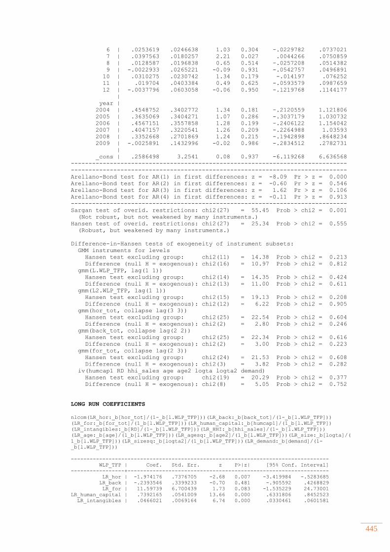
445
6 | .0253619 .0246638 1.03 0.304 -.0229782 .0737021
7 | .0397563 .0180257 2.21 0.027 .0044266 .0750859
8 | .0128587 .0196838 0.65 0.514 -.0257208 .0514382
9 | -.0022933 .0265221 -0.09 0.931 -.0542757 .0496891
10 | .0310275 .0230742 1.34 0.179 -.014197 .076252
11 | .019704 .0403384 0.49 0.625 -.0593579 .0987659
12 | -.0037796 .0603058 -0.06 0.950 -.1219768 .1144177
|
year |
2004 | .4548752 .3402772 1.34 0.181 -.2120559 1.121806
2005 | .3635069 .3404271 1.07 0.286 -.3037179 1.030732
2006 | .4567151 .3557858 1.28 0.199 -.2406122 1.154042
2007 | .4047157 .3220541 1.26 0.209 -.2264988 1.03593
2008 | .3352668 .2701869 1.24 0.215 -.1942898 .8648234
2009 | -.0025891 .1432996 -0.02 0.986 -.2834512 .2782731
|
_cons | .2586498 3.2541 0.08 0.937 -6.119268 6.636568
------------------------------------------------------------------------------
------------------------------------------------------------------------------
Arellano-Bond test for AR(1) in first differences: z = -8.09 Pr > z = 0.000
Arellano-Bond test for AR(2) in first differences: z = -0.60 Pr > z = 0.546
Arellano-Bond test for AR(3) in first differences: z = 1.62 Pr > z = 0.106
Arellano-Bond test for AR(4) in first differences: z = -0.11 Pr > z = 0.913
------------------------------------------------------------------------------
Sargan test of overid. restrictions: chi2(27) = 55.45 Prob > chi2 = 0.001
(Not robust, but not weakened by many instruments.)
Hansen test of overid. restrictions: chi2(27) = 25.34 Prob > chi2 = 0.555
(Robust, but weakened by many instruments.)
Difference-in-Hansen tests of exogeneity of instrument subsets:
GMM instruments for levels
Hansen test excluding group: chi2(11) = 14.38 Prob > chi2 = 0.213
Difference (null H = exogenous): chi2(16) = 10.97 Prob > chi2 = 0.812
gmm(L.WLP_TFP, lag(1 1))
Hansen test excluding group: chi2(14) = 14.35 Prob > chi2 = 0.424
Difference (null H = exogenous): chi2(13) = 11.00 Prob > chi2 = 0.611
gmm(L2.WLP_TFP, lag(1 1))
Hansen test excluding group: chi2(15) = 19.13 Prob > chi2 = 0.208
Difference (null H = exogenous): chi2(12) = 6.22 Prob > chi2 = 0.905
gmm(hor_tot, collapse lag(3 3))
Hansen test excluding group: chi2(25) = 22.54 Prob > chi2 = 0.604
Difference (null H = exogenous): chi2(2) = 2.80 Prob > chi2 = 0.246
gmm(back_tot, collapse lag(2 2))
Hansen test excluding group: chi2(25) = 22.34 Prob > chi2 = 0.616
Difference (null H = exogenous): chi2(2) = 3.00 Prob > chi2 = 0.223
gmm(for_tot, collapse lag(2 3))
Hansen test excluding group: chi2(24) = 21.53 Prob > chi2 = 0.608
Difference (null H = exogenous): chi2(3) = 3.82 Prob > chi2 = 0.282
iv(humcap1 RD hhi_sales age age2 logta logta2 demand)
Hansen test excluding group: chi2(19) = 20.29 Prob > chi2 = 0.377
Difference (null H = exogenous): chi2(8) = 5.05 Prob > chi2 = 0.752
LONG RUN COEFFICIENTS
nlcom(LR_hor:_b[hor_tot]/(1-_b[l.WLP_TFP]))(LR_back:_b[back_tot]/(1-_b[l.WLP_TFP]))
(LR_for:_b[for_tot]/(1_b[l.WLP_TFP]))(LR_human_capital:_b[humcap1]/(1_b[l.WLP_TFP])
(LR_intangibles:_b[RD]/(1-_b[l.WLP_TFP]))(LR_HHI:_b[hhi_sales]/(1-_b[l.WLP_TFP]))
(LR_age:_b[age]/(1_b[l.WLP_TFP]))(LR_agesq:_b[age2]/(1_b[l.WLP_TFP]))(LR_size:_b[logta]/(
1_b[l.WLP_TFP]))(LR_sizesq:_b[logta2]/(1_b[l.WLP_TFP]))(LR_demand:_b[demand]/(1-
_b[l.WLP_TFP]))
----------------------------------------------------------------------------------
WLP_TFP | Coef. Std. Err. z P>|z| [95% Conf. Interval]
-----------------+----------------------------------------------------------------
LR_hor | -1.974176 .7376705 -2.68 0.007 -3.419984 -.5283685
LR_back | -.2393546 .3399233 -0.70 0.481 -.905592 .4268829
LR_for | 11.59739 6.700439 1.73 0.083 -1.535229 24.73001
LR_human_capital | .7392165 .0541009 13.66 0.000 .6331806 .8452523
LR_intangibles | .0466021 .0069164 6.74 0.000 .0330461 .0601581
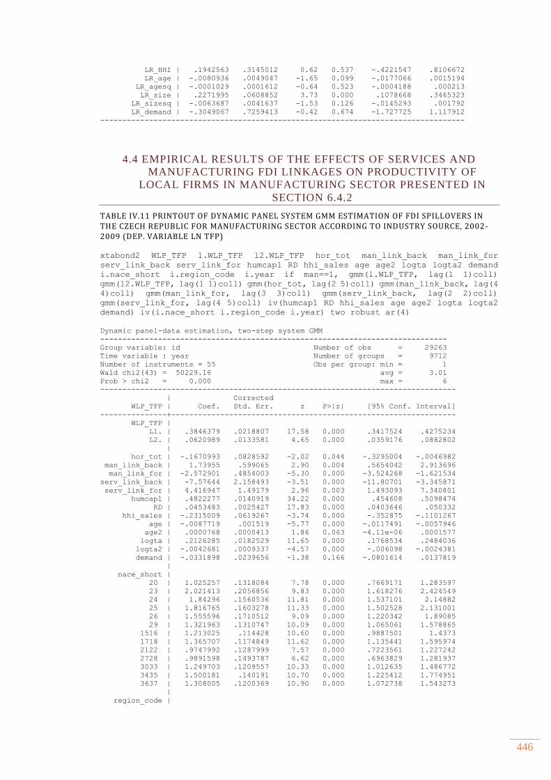
446
LR_HHI | .1942563 .3145012 0.62 0.537 -.4221547 .8106672
LR_age | -.0080936 .0049047 -1.65 0.099 -.0177066 .0015194
LR_agesq | -.0001029 .0001612 -0.64 0.523 -.0004188 .000213
LR_size | .2271995 .0608852 3.73 0.000 .1078668 .3465323
LR_sizesq | -.0063687 .0041637 -1.53 0.126 -.0145293 .001792
LR_demand | -.3049067 .7259413 -0.42 0.674 -1.727725 1.117912
----------------------------------------------------------------------------------
4.4 EMPIRICAL RESULTS OF THE EFFECTS OF SERVICES AND
MANUFACTURING FDI LINKAGES ON PRODUCTIVITY OF
LOCAL FIRMS IN MANUFACTURING SECTOR PRESENTED IN
SECTION 6.4.2
TABLE IV.11 PRINTOUT OF DYNAMIC PANEL SYSTEM GMM ESTIMATION OF FDI SPILLOVERS IN THE CZECH REPUBLIC FOR MANUFACTURING SECTOR ACCORDING TO INDUSTRY SOURCE, 2002-2009 (DEP. VARIABLE LN TFP)
xtabond2 WLP_TFP l.WLP_TFP l2.WLP_TFP hor_tot man_link_back man_link_for
serv_link_back serv_link_for humcap1 RD hhi_sales age age2 logta logta2 demand
i.nace_short i.region_code i.year if man==1, gmm(l.WLP_TFP, lag(1 1)coll)
gmm(l2.WLP_TFP, lag(1 1)coll) gmm(hor_tot, lag(2 5)coll) gmm(man_link_back, lag(4
4)coll) gmm(man_link_for, lag(3 3)coll) gmm(serv_link_back, lag(2 2)coll)
gmm(serv_link_for, lag(4 5)coll) iv(humcap1 RD hhi_sales age age2 logta logta2
demand) iv(i.nace_short i.region_code i.year) two robust ar(4)
Dynamic panel-data estimation, two-step system GMM
------------------------------------------------------------------------------
Group variable: id Number of obs = 29263
Time variable : year Number of groups = 9712
Number of instruments = 55 Obs per group: min = 1
Wald chi2(43) = 50229.16 avg = 3.01
Prob > chi2 = 0.000 max = 6
--------------------------------------------------------------------------------
| Corrected
WLP_TFP | Coef. Std. Err. z P>|z| [95% Conf. Interval]
---------------+----------------------------------------------------------------
WLP_TFP |
L1. | .3846379 .0218807 17.58 0.000 .3417524 .4275234
L2. | .0620989 .0133581 4.65 0.000 .0359176 .0882802
|
hor_tot | -.1670993 .0828592 -2.02 0.044 -.3295004 -.0046982
man_link_back | 1.73955 .599065 2.90 0.004 .5654042 2.913696
man_link_for | -2.572901 .4854003 -5.30 0.000 -3.524268 -1.621534
serv_link_back | -7.57644 2.158493 -3.51 0.000 -11.80701 -3.345871
serv_link_for | 4.416947 1.49179 2.96 0.003 1.493093 7.340801
humcap1 | .4822277 .0140919 34.22 0.000 .454608 .5098474
RD | .0453483 .0025427 17.83 0.000 .0403646 .050332
hhi_sales | -.2315009 .0619267 -3.74 0.000 -.352875 -.1101267
age | -.0087719 .001519 -5.77 0.000 -.0117491 -.0057946
age2 | .0000768 .0000413 1.86 0.063 -4.11e-06 .0001577
logta | .2126285 .0182529 11.65 0.000 .1768534 .2484036
logta2 | -.0042681 .0009337 -4.57 0.000 -.006098 -.0024381
demand | -.0331898 .0239656 -1.38 0.166 -.0801614 .0137819
|
nace_short |
20 | 1.025257 .1318084 7.78 0.000 .7669171 1.283597
23 | 2.021413 .2056856 9.83 0.000 1.618276 2.424549
24 | 1.84296 .1560536 11.81 0.000 1.537101 2.14882
25 | 1.816765 .1603278 11.33 0.000 1.502528 2.131001
26 | 1.555596 .1710512 9.09 0.000 1.220342 1.89085
29 | 1.321963 .1310747 10.09 0.000 1.065061 1.578865
1516 | 1.213025 .114428 10.60 0.000 .9887501 1.4373
1718 | 1.365707 .1174849 11.62 0.000 1.135441 1.595974
2122 | .9747992 .1287999 7.57 0.000 .7223561 1.227242
2728 | .9891598 .1493787 6.62 0.000 .6963829 1.281937
3033 | 1.249703 .1209557 10.33 0.000 1.012635 1.486772
3435 | 1.500181 .140191 10.70 0.000 1.225412 1.774951
3637 | 1.308005 .1200369 10.90 0.000 1.072738 1.543273
|
region_code |
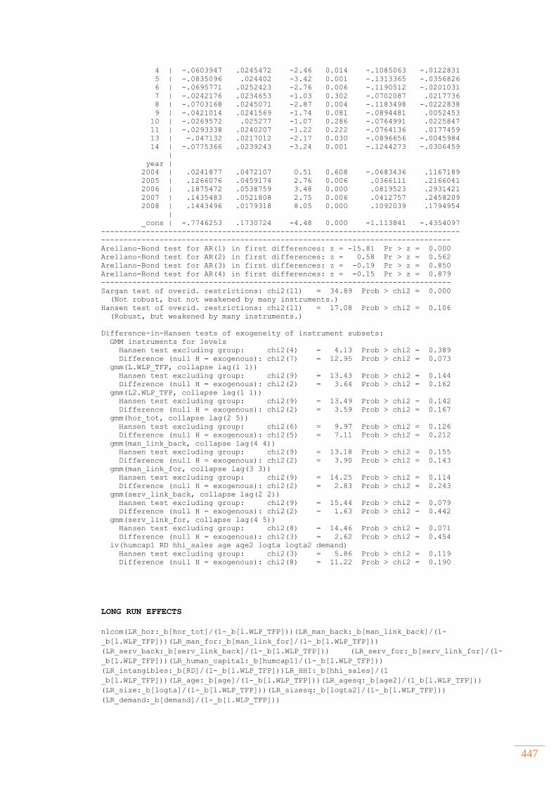
447
4 | -.0603947 .0245472 -2.46 0.014 -.1085063 -.0122831
5 | -.0835096 .024402 -3.42 0.001 -.1313365 -.0356826
6 | -.0695771 .0252423 -2.76 0.006 -.1190512 -.0201031
7 | -.0242176 .0234653 -1.03 0.302 -.0702087 .0217736
8 | -.0703168 .0245071 -2.87 0.004 -.1183498 -.0222838
9 | -.0421014 .0241569 -1.74 0.081 -.0894481 .0052453
10 | -.0269572 .025277 -1.07 0.286 -.0764991 .0225847
11 | -.0293338 .0240207 -1.22 0.222 -.0764136 .0177459
13 | -.047132 .0217012 -2.17 0.030 -.0896656 -.0045984
14 | -.0775366 .0239243 -3.24 0.001 -.1244273 -.0306459
|
year |
2004 | .0241877 .0472107 0.51 0.608 -.0683436 .1167189
2005 | .1266076 .0459174 2.76 0.006 .0366111 .2166041
2006 | .1875472 .0538759 3.48 0.000 .0819523 .2931421
2007 | .1435483 .0521808 2.75 0.006 .0412757 .2458209
2008 | .1443496 .0179318 8.05 0.000 .1092039 .1794954
|
_cons | -.7746253 .1730724 -4.48 0.000 -1.113841 -.4354097
--------------------------------------------------------------------------------
------------------------------------------------------------------------------
Arellano-Bond test for AR(1) in first differences: z = -15.81 Pr > z = 0.000
Arellano-Bond test for AR(2) in first differences: z = 0.58 Pr > z = 0.562
Arellano-Bond test for AR(3) in first differences: z = -0.19 Pr > z = 0.850
Arellano-Bond test for AR(4) in first differences: z = -0.15 Pr > z = 0.879
------------------------------------------------------------------------------
Sargan test of overid. restrictions: chi2(11) = 34.89 Prob > chi2 = 0.000
(Not robust, but not weakened by many instruments.)
Hansen test of overid. restrictions: chi2(11) = 17.08 Prob > chi2 = 0.106
(Robust, but weakened by many instruments.)
Difference-in-Hansen tests of exogeneity of instrument subsets:
GMM instruments for levels
Hansen test excluding group: chi2(4) = 4.13 Prob > chi2 = 0.389
Difference (null H = exogenous): chi2(7) = 12.95 Prob > chi2 = 0.073
gmm(L.WLP_TFP, collapse lag(1 1))
Hansen test excluding group: chi2(9) = 13.43 Prob > chi2 = 0.144
Difference (null H = exogenous): chi2(2) = 3.64 Prob > chi2 = 0.162
gmm(L2.WLP_TFP, collapse lag(1 1))
Hansen test excluding group: chi2(9) = 13.49 Prob > chi2 = 0.142
Difference (null H = exogenous): chi2(2) = 3.59 Prob > chi2 = 0.167
gmm(hor_tot, collapse lag(2 5))
Hansen test excluding group: chi2(6) = 9.97 Prob > chi2 = 0.126
Difference (null H = exogenous): chi2(5) = 7.11 Prob > chi2 = 0.212
gmm(man_link_back, collapse lag(4 4))
Hansen test excluding group: chi2(9) = 13.18 Prob > chi2 = 0.155
Difference (null H = exogenous): chi2(2) = 3.90 Prob > chi2 = 0.143
gmm(man_link_for, collapse lag(3 3))
Hansen test excluding group: chi2(9) = 14.25 Prob > chi2 = 0.114
Difference (null H = exogenous): chi2(2) = 2.83 Prob > chi2 = 0.243
gmm(serv_link_back, collapse lag(2 2))
Hansen test excluding group: chi2(9) = 15.44 Prob > chi2 = 0.079
Difference (null H = exogenous): chi2(2) = 1.63 Prob > chi2 = 0.442
gmm(serv_link_for, collapse lag(4 5))
Hansen test excluding group: chi2(8) = 14.46 Prob > chi2 = 0.071
Difference (null H = exogenous): chi2(3) = 2.62 Prob > chi2 = 0.454
iv(humcap1 RD hhi_sales age age2 logta logta2 demand)
Hansen test excluding group: chi2(3) = 5.86 Prob > chi2 = 0.119
Difference (null H = exogenous): chi2(8) = 11.22 Prob > chi2 = 0.190
LONG RUN EFFECTS
nlcom(LR_hor:_b[hor_tot]/(1-_b[l.WLP_TFP]))(LR_man_back:_b[man_link_back]/(1-
_b[l.WLP_TFP]))(LR_man_for:_b[man_link_for]/(1-_b[l.WLP_TFP]))
(LR_serv_back:_b[serv_link_back]/(1-_b[l.WLP_TFP])) (LR_serv_for:_b[serv_link_for]/(1-
_b[l.WLP_TFP]))(LR_human_capital:_b[humcap1]/(1-_b[l.WLP_TFP]))
(LR_intangibles:_b[RD]/(1-_b[l.WLP_TFP]))LR_HHI:_b[hhi_sales]/(1
_b[l.WLP_TFP]))(LR_age:_b[age]/(1-_b[l.WLP_TFP]))(LR_agesq:_b[age2]/(1_b[l.WLP_TFP]))
(LR_size:_b[logta]/(1-_b[l.WLP_TFP]))(LR_sizesq:_b[logta2]/(1-_b[l.WLP_TFP]))
(LR_demand:_b[demand]/(1-_b[l.WLP_TFP]))
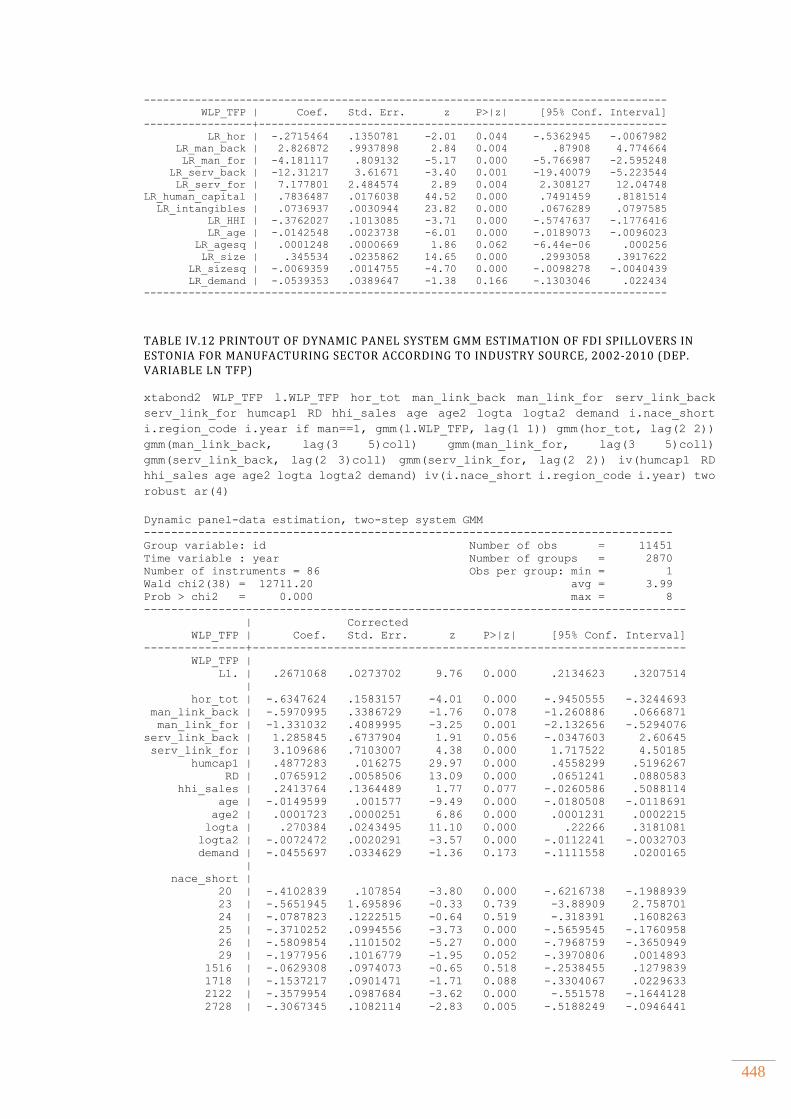
448
----------------------------------------------------------------------------------
WLP_TFP | Coef. Std. Err. z P>|z| [95% Conf. Interval]
-----------------+----------------------------------------------------------------
LR_hor | -.2715464 .1350781 -2.01 0.044 -.5362945 -.0067982
LR_man_back | 2.826872 .9937898 2.84 0.004 .87908 4.774664
LR_man_for | -4.181117 .809132 -5.17 0.000 -5.766987 -2.595248
LR_serv_back | -12.31217 3.61671 -3.40 0.001 -19.40079 -5.223544
LR_serv_for | 7.177801 2.484574 2.89 0.004 2.308127 12.04748
LR_human_capital | .7836487 .0176038 44.52 0.000 .7491459 .8181514
LR_intangibles | .0736937 .0030944 23.82 0.000 .0676289 .0797585
LR_HHI | -.3762027 .1013085 -3.71 0.000 -.5747637 -.1776416
LR_age | -.0142548 .0023738 -6.01 0.000 -.0189073 -.0096023
LR_agesq | .0001248 .0000669 1.86 0.062 -6.44e-06 .000256
LR_size | .345534 .0235862 14.65 0.000 .2993058 .3917622
LR_sizesq | -.0069359 .0014755 -4.70 0.000 -.0098278 -.0040439
LR_demand | -.0539353 .0389647 -1.38 0.166 -.1303046 .022434
----------------------------------------------------------------------------------
TABLE IV.12 PRINTOUT OF DYNAMIC PANEL SYSTEM GMM ESTIMATION OF FDI SPILLOVERS IN ESTONIA FOR MANUFACTURING SECTOR ACCORDING TO INDUSTRY SOURCE, 2002-2010 (DEP. VARIABLE LN TFP)
xtabond2 WLP_TFP l.WLP_TFP hor_tot man_link_back man_link_for serv_link_back
serv_link_for humcap1 RD hhi_sales age age2 logta logta2 demand i.nace_short
i.region_code i.year if man==1, gmm(l.WLP_TFP, lag(1 1)) gmm(hor_tot, lag(2 2))
gmm(man_link_back, lag(3 5)coll) gmm(man_link_for, lag(3 5)coll)
gmm(serv_link_back, lag(2 3)coll) gmm(serv_link_for, lag(2 2)) iv(humcap1 RD
hhi_sales age age2 logta logta2 demand) iv(i.nace_short i.region_code i.year) two
robust ar(4)
Dynamic panel-data estimation, two-step system GMM
------------------------------------------------------------------------------
Group variable: id Number of obs = 11451
Time variable : year Number of groups = 2870
Number of instruments = 86 Obs per group: min = 1
Wald chi2(38) = 12711.20 avg = 3.99
Prob > chi2 = 0.000 max = 8
--------------------------------------------------------------------------------
| Corrected
WLP_TFP | Coef. Std. Err. z P>|z| [95% Conf. Interval]
---------------+----------------------------------------------------------------
WLP_TFP |
L1. | .2671068 .0273702 9.76 0.000 .2134623 .3207514
|
hor_tot | -.6347624 .1583157 -4.01 0.000 -.9450555 -.3244693
man_link_back | -.5970995 .3386729 -1.76 0.078 -1.260886 .0666871
man_link_for | -1.331032 .4089995 -3.25 0.001 -2.132656 -.5294076
serv_link_back | 1.285845 .6737904 1.91 0.056 -.0347603 2.60645
serv_link_for | 3.109686 .7103007 4.38 0.000 1.717522 4.50185
humcap1 | .4877283 .016275 29.97 0.000 .4558299 .5196267
RD | .0765912 .0058506 13.09 0.000 .0651241 .0880583
hhi_sales | .2413764 .1364489 1.77 0.077 -.0260586 .5088114
age | -.0149599 .001577 -9.49 0.000 -.0180508 -.0118691
age2 | .0001723 .0000251 6.86 0.000 .0001231 .0002215
logta | .270384 .0243495 11.10 0.000 .22266 .3181081
logta2 | -.0072472 .0020291 -3.57 0.000 -.0112241 -.0032703
demand | -.0455697 .0334629 -1.36 0.173 -.1111558 .0200165
|
nace_short |
20 | -.4102839 .107854 -3.80 0.000 -.6216738 -.1988939
23 | -.5651945 1.695896 -0.33 0.739 -3.88909 2.758701
24 | -.0787823 .1222515 -0.64 0.519 -.318391 .1608263
25 | -.3710252 .0994556 -3.73 0.000 -.5659545 -.1760958
26 | -.5809854 .1101502 -5.27 0.000 -.7968759 -.3650949
29 | -.1977956 .1016779 -1.95 0.052 -.3970806 .0014893
1516 | -.0629308 .0974073 -0.65 0.518 -.2538455 .1279839
1718 | -.1537217 .0901471 -1.71 0.088 -.3304067 .0229633
2122 | -.3579954 .0987684 -3.62 0.000 -.551578 -.1644128
2728 | -.3067345 .1082114 -2.83 0.005 -.5188249 -.0946441
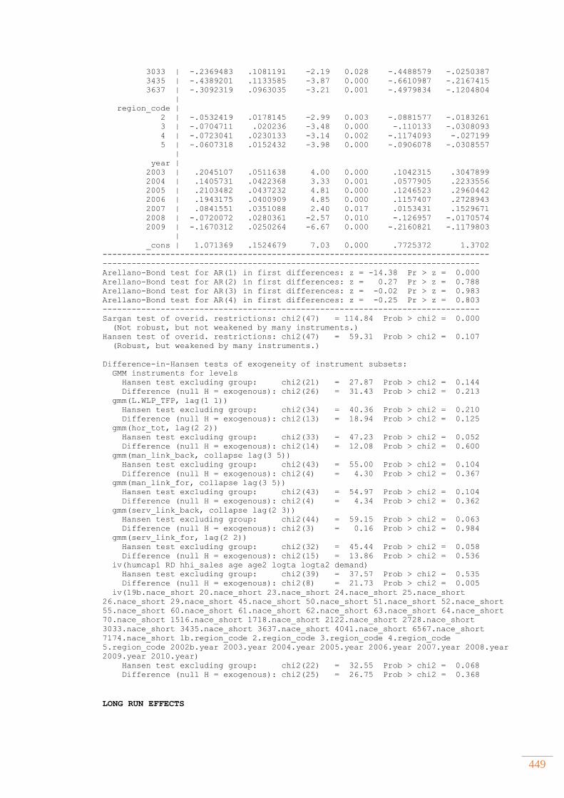
449
3033 | -.2369483 .1081191 -2.19 0.028 -.4488579 -.0250387
3435 | -.4389201 .1133585 -3.87 0.000 -.6610987 -.2167415
3637 | -.3092319 .0963035 -3.21 0.001 -.4979834 -.1204804
|
region_code |
2 | -.0532419 .0178145 -2.99 0.003 -.0881577 -.0183261
3 | -.0704711 .020236 -3.48 0.000 -.110133 -.0308093
4 | -.0723041 .0230133 -3.14 0.002 -.1174093 -.027199
5 | -.0607318 .0152432 -3.98 0.000 -.0906078 -.0308557
|
year |
2003 | .2045107 .0511638 4.00 0.000 .1042315 .3047899
2004 | .1405731 .0422368 3.33 0.001 .0577905 .2233556
2005 | .2103482 .0437232 4.81 0.000 .1246523 .2960442
2006 | .1943175 .0400909 4.85 0.000 .1157407 .2728943
2007 | .0841551 .0351088 2.40 0.017 .0153431 .1529671
2008 | -.0720072 .0280361 -2.57 0.010 -.126957 -.0170574
2009 | -.1670312 .0250264 -6.67 0.000 -.2160821 -.1179803
|
_cons | 1.071369 .1524679 7.03 0.000 .7725372 1.3702
--------------------------------------------------------------------------------
------------------------------------------------------------------------------
Arellano-Bond test for AR(1) in first differences: z = -14.38 Pr > z = 0.000
Arellano-Bond test for AR(2) in first differences: z = 0.27 Pr > z = 0.788
Arellano-Bond test for AR(3) in first differences: z = -0.02 Pr > z = 0.983
Arellano-Bond test for AR(4) in first differences: z = -0.25 Pr > z = 0.803
------------------------------------------------------------------------------
Sargan test of overid. restrictions: chi2(47) = 114.84 Prob > chi2 = 0.000
(Not robust, but not weakened by many instruments.)
Hansen test of overid. restrictions: chi2(47) = 59.31 Prob > chi2 = 0.107
(Robust, but weakened by many instruments.)
Difference-in-Hansen tests of exogeneity of instrument subsets:
GMM instruments for levels
Hansen test excluding group: chi2(21) = 27.87 Prob > chi2 = 0.144
Difference (null H = exogenous): chi2(26) = 31.43 Prob > chi2 = 0.213
gmm(L.WLP_TFP, lag(1 1))
Hansen test excluding group: chi2(34) = 40.36 Prob > chi2 = 0.210
Difference (null H = exogenous): chi2(13) = 18.94 Prob > chi2 = 0.125
gmm(hor_tot, lag(2 2))
Hansen test excluding group: chi2(33) = 47.23 Prob > chi2 = 0.052
Difference (null H = exogenous): chi2(14) = 12.08 Prob > chi2 = 0.600
gmm(man_link_back, collapse lag(3 5))
Hansen test excluding group: chi2(43) = 55.00 Prob > chi2 = 0.104
Difference (null H = exogenous): chi2(4) = 4.30 Prob > chi2 = 0.367
gmm(man_link_for, collapse lag(3 5))
Hansen test excluding group: chi2(43) = 54.97 Prob > chi2 = 0.104
Difference (null H = exogenous): chi2(4) = 4.34 Prob > chi2 = 0.362
gmm(serv_link_back, collapse lag(2 3))
Hansen test excluding group: chi2(44) = 59.15 Prob > chi2 = 0.063
Difference (null H = exogenous): chi2(3) = 0.16 Prob > chi2 = 0.984
gmm(serv_link_for, lag(2 2))
Hansen test excluding group: chi2(32) = 45.44 Prob > chi2 = 0.058
Difference (null H = exogenous): chi2(15) = 13.86 Prob > chi2 = 0.536
iv(humcap1 RD hhi_sales age age2 logta logta2 demand)
Hansen test excluding group: chi2(39) = 37.57 Prob > chi2 = 0.535
Difference (null H = exogenous): chi2(8) = 21.73 Prob > chi2 = 0.005
iv(19b.nace_short 20.nace_short 23.nace_short 24.nace_short 25.nace_short
26.nace_short 29.nace_short 45.nace_short 50.nace_short 51.nace_short 52.nace_short
55.nace_short 60.nace_short 61.nace_short 62.nace_short 63.nace_short 64.nace_short
70.nace_short 1516.nace_short 1718.nace_short 2122.nace_short 2728.nace_short
3033.nace_short 3435.nace_short 3637.nace_short 4041.nace_short 6567.nace_short
7174.nace_short 1b.region_code 2.region_code 3.region_code 4.region_code
5.region_code 2002b.year 2003.year 2004.year 2005.year 2006.year 2007.year 2008.year
2009.year 2010.year)
Hansen test excluding group: chi2(22) = 32.55 Prob > chi2 = 0.068
Difference (null H = exogenous): chi2(25) = 26.75 Prob > chi2 = 0.368
LONG RUN EFFECTS
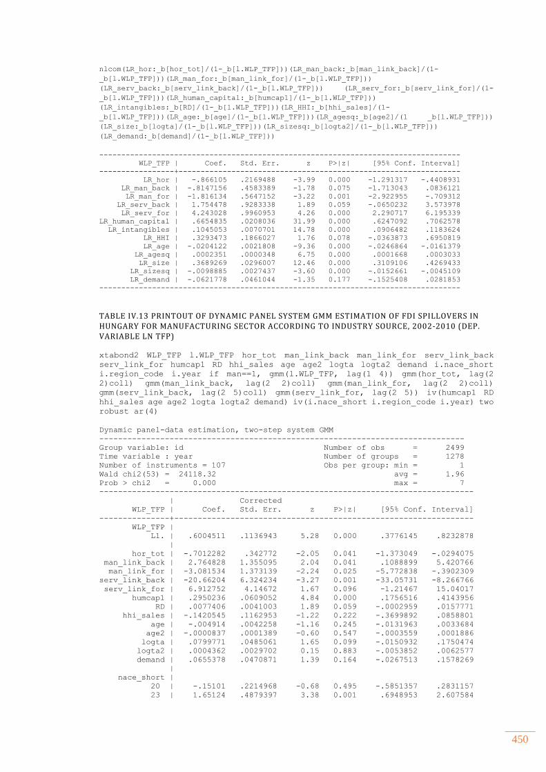
450
nlcom(LR_hor:_b[hor_tot]/(1-_b[l.WLP_TFP]))(LR_man_back:_b[man_link_back]/(1-
_b[l.WLP_TFP]))(LR_man_for:_b[man_link_for]/(1-_b[l.WLP_TFP]))
(LR_serv_back:_b[serv_link_back]/(1-_b[l.WLP_TFP])) (LR_serv_for:_b[serv_link_for]/(1-
_b[l.WLP_TFP]))(LR_human_capital:_b[humcap1]/(1-_b[l.WLP_TFP]))
(LR_intangibles:_b[RD]/(1-_b[l.WLP_TFP]))(LR_HHI:_b[hhi_sales]/(1-
_b[l.WLP_TFP]))(LR_age:_b[age]/(1-_b[l.WLP_TFP]))(LR_agesq:_b[age2]/(1 _b[l.WLP_TFP]))
(LR_size:_b[logta]/(1-_b[l.WLP_TFP]))(LR_sizesq:_b[logta2]/(1-_b[l.WLP_TFP]))
(LR_demand:_b[demand]/(1-_b[l.WLP_TFP]))
----------------------------------------------------------------------------------
WLP_TFP | Coef. Std. Err. z P>|z| [95% Conf. Interval]
-----------------+----------------------------------------------------------------
LR_hor | -.866105 .2169488 -3.99 0.000 -1.291317 -.4408931
LR_man_back | -.8147156 .4583389 -1.78 0.075 -1.713043 .0836121
LR_man_for | -1.816134 .5647152 -3.22 0.001 -2.922955 -.709312
LR_serv_back | 1.754478 .9283338 1.89 0.059 -.0650232 3.573978
LR_serv_for | 4.243028 .9960953 4.26 0.000 2.290717 6.195339
LR_human_capital | .6654835 .0208036 31.99 0.000 .6247092 .7062578
LR_intangibles | .1045053 .0070701 14.78 0.000 .0906482 .1183624
LR_HHI | .3293473 .1866027 1.76 0.078 -.0363873 .6950819
LR_age | -.0204122 .0021808 -9.36 0.000 -.0246864 -.0161379
LR_agesq | .0002351 .0000348 6.75 0.000 .0001668 .0003033
LR_size | .3689269 .0296007 12.46 0.000 .3109106 .4269433
LR_sizesq | -.0098885 .0027437 -3.60 0.000 -.0152661 -.0045109
LR_demand | -.0621778 .0461044 -1.35 0.177 -.1525408 .0281853
----------------------------------------------------------------------------------
TABLE IV.13 PRINTOUT OF DYNAMIC PANEL SYSTEM GMM ESTIMATION OF FDI SPILLOVERS IN HUNGARY FOR MANUFACTURING SECTOR ACCORDING TO INDUSTRY SOURCE, 2002-2010 (DEP. VARIABLE LN TFP)
xtabond2 WLP_TFP l.WLP_TFP hor_tot man_link_back man_link_for serv_link_back
serv_link_for humcap1 RD hhi_sales age age2 logta logta2 demand i.nace_short
i.region_code i.year if man==1, gmm(l.WLP_TFP, lag(1 4)) gmm(hor_tot, lag(2
2)coll) gmm(man_link_back, lag(2 2)coll) gmm(man_link_for, lag(2 2)coll)
gmm(serv_link_back, lag(2 5)coll) gmm(serv_link_for, lag(2 5)) iv(humcap1 RD
hhi_sales age age2 logta logta2 demand) iv(i.nace_short i.region_code i.year) two
robust ar(4)
Dynamic panel-data estimation, two-step system GMM
------------------------------------------------------------------------------
Group variable: id Number of obs = 2499
Time variable : year Number of groups = 1278
Number of instruments = 107 Obs per group: min = 1
Wald chi2(53) = 24118.32 avg = 1.96
Prob > chi2 = 0.000 max = 7
--------------------------------------------------------------------------------
| Corrected
WLP_TFP | Coef. Std. Err. z P>|z| [95% Conf. Interval]
---------------+----------------------------------------------------------------
WLP_TFP |
L1. | .6004511 .1136943 5.28 0.000 .3776145 .8232878
|
hor_tot | -.7012282 .342772 -2.05 0.041 -1.373049 -.0294075
man_link_back | 2.764828 1.355095 2.04 0.041 .1088899 5.420766
man_link_for | -3.081534 1.373139 -2.24 0.025 -5.772838 -.3902309
serv_link_back | -20.66204 6.324234 -3.27 0.001 -33.05731 -8.266766
serv_link_for | 6.912752 4.14672 1.67 0.096 -1.21467 15.04017
humcap1 | .2950236 .0609052 4.84 0.000 .1756516 .4143956
RD | .0077406 .0041003 1.89 0.059 -.0002959 .0157771
hhi_sales | -.1420545 .1162953 -1.22 0.222 -.3699892 .0858801
age | -.004914 .0042258 -1.16 0.245 -.0131963 .0033684
age2 | -.0000837 .0001389 -0.60 0.547 -.0003559 .0001886
logta | .0799771 .0485061 1.65 0.099 -.0150932 .1750474
logta2 | .0004362 .0029702 0.15 0.883 -.0053852 .0062577
demand | .0655378 .0470871 1.39 0.164 -.0267513 .1578269
|
nace_short |
20 | -.15101 .2214968 -0.68 0.495 -.5851357 .2831157
23 | 1.65124 .4879397 3.38 0.001 .6948953 2.607584
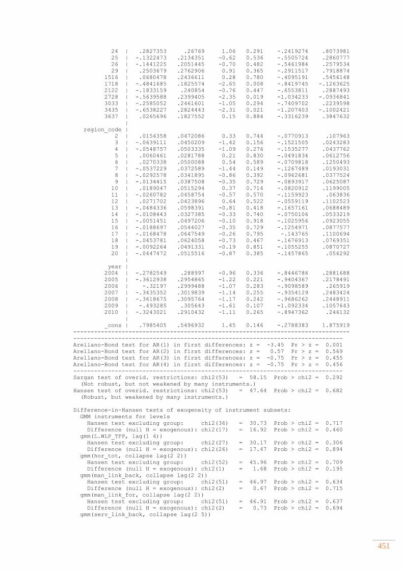
451
24 | .2827353 .26769 1.06 0.291 -.2419274 .8073981
25 | -.1322473 .2134351 -0.62 0.536 -.5505724 .2860777
26 | -.1441225 .2051445 -0.70 0.482 -.5461984 .2579534
29 | .2503679 .2762906 0.91 0.365 -.2911517 .7918874
1516 | .0680478 .2436611 0.28 0.780 -.4095191 .5456148
1718 | -.4841685 .1825574 -2.65 0.008 -.8419745 -.1263625
2122 | -.1833159 .240854 -0.76 0.447 -.6553811 .2887493
2728 | -.5639588 .2399405 -2.35 0.019 -1.034233 -.0936841
3033 | -.2585052 .2461601 -1.05 0.294 -.7409702 .2239598
3435 | -.6538227 .2824443 -2.31 0.021 -1.207403 -.1002421
3637 | .0265696 .1827552 0.15 0.884 -.3316239 .3847632
|
region_code |
2 | .0154358 .0472086 0.33 0.744 -.0770913 .107963
3 | -.0639111 .0450209 -1.42 0.156 -.1521505 .0243283
4 | -.0548757 .0503335 -1.09 0.276 -.1535277 .0437762
5 | .0060461 .0281788 0.21 0.830 -.0491834 .0612756
6 | .0270338 .0500088 0.54 0.589 -.0709818 .1250493
7 | -.0537229 .0372589 -1.44 0.149 -.1267489 .0193031
8 | -.0292578 .0341895 -0.86 0.392 -.0962681 .0377524
9 | -.0134415 .0387508 -0.35 0.729 -.0893917 .0625087
10 | .0189047 .0515294 0.37 0.714 -.0820912 .1199005
11 | -.0260782 .0458754 -0.57 0.570 -.1159923 .063836
12 | .0271702 .0423896 0.64 0.522 -.0559119 .1102523
13 | -.0484336 .0598391 -0.81 0.418 -.1657161 .0688489
14 | -.0108443 .0327385 -0.33 0.740 -.0750106 .0533219
15 | -.0051451 .0497206 -0.10 0.918 -.1025956 .0923055
16 | -.0188697 .0544027 -0.35 0.729 -.1254971 .0877577
17 | -.0168478 .0647549 -0.26 0.795 -.143765 .1100694
18 | -.0453781 .0624058 -0.73 0.467 -.1676913 .0769351
19 | -.0092264 .0491331 -0.19 0.851 -.1055255 .0870727
20 | -.0447472 .0515516 -0.87 0.385 -.1457865 .056292
|
year |
2004 | -.2782549 .288997 -0.96 0.336 -.8446786 .2881688
2005 | -.3612938 .2954865 -1.22 0.221 -.9404367 .2178491
2006 | -.32197 .2999488 -1.07 0.283 -.9098589 .265919
2007 | -.3435352 .3019839 -1.14 0.255 -.9354129 .2483424
2008 | -.3618675 .3095764 -1.17 0.242 -.9686262 .2448911
2009 | -.493285 .305643 -1.61 0.107 -1.092334 .1057643
2010 | -.3243021 .2910432 -1.11 0.265 -.8947362 .246132
|
_cons | .7985405 .5496932 1.45 0.146 -.2788383 1.875919
--------------------------------------------------------------------------------
------------------------------------------------------------------------------
Arellano-Bond test for AR(1) in first differences: z = -3.45 Pr > z = 0.001
Arellano-Bond test for AR(2) in first differences: z = 0.57 Pr > z = 0.569
Arellano-Bond test for AR(3) in first differences: z = -0.75 Pr > z = 0.455
Arellano-Bond test for AR(4) in first differences: z = -0.75 Pr > z = 0.456
------------------------------------------------------------------------------
Sargan test of overid. restrictions: chi2(53) = 58.15 Prob > chi2 = 0.292
(Not robust, but not weakened by many instruments.)
Hansen test of overid. restrictions: chi2(53) = 47.64 Prob > chi2 = 0.682
(Robust, but weakened by many instruments.)
Difference-in-Hansen tests of exogeneity of instrument subsets:
GMM instruments for levels
Hansen test excluding group: chi2(36) = 30.73 Prob > chi2 = 0.717
Difference (null H = exogenous): chi2(17) = 16.92 Prob > chi2 = 0.460
gmm(L.WLP_TFP, lag(1 4))
Hansen test excluding group: chi2(27) = 30.17 Prob > chi2 = 0.306
Difference (null H = exogenous): chi2(26) = 17.47 Prob > chi2 = 0.894
gmm(hor_tot, collapse lag(2 2))
Hansen test excluding group: chi2(52) = 45.96 Prob > chi2 = 0.709
Difference (null H = exogenous): chi2(1) = 1.68 Prob > chi2 = 0.195
gmm(man_link_back, collapse lag(2 2))
Hansen test excluding group: chi2(51) = 46.97 Prob > chi2 = 0.634
Difference (null H = exogenous): chi2(2) = 0.67 Prob > chi2 = 0.715
gmm(man_link_for, collapse lag(2 2))
Hansen test excluding group: chi2(51) = 46.91 Prob > chi2 = 0.637
Difference (null H = exogenous): chi2(2) = 0.73 Prob > chi2 = 0.694
gmm(serv_link_back, collapse lag(2 5))
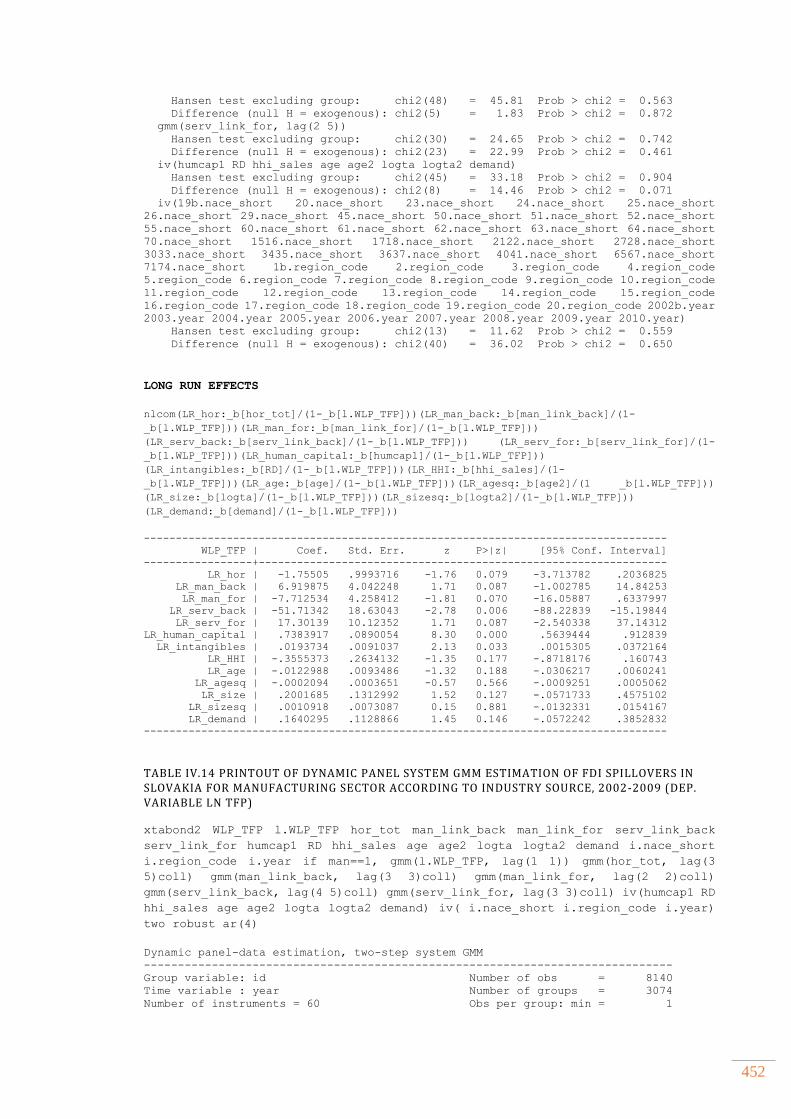
452
Hansen test excluding group: chi2(48) = 45.81 Prob > chi2 = 0.563
Difference (null H = exogenous): chi2(5) = 1.83 Prob > chi2 = 0.872
gmm(serv_link_for, lag(2 5))
Hansen test excluding group: chi2(30) = 24.65 Prob > chi2 = 0.742
Difference (null H = exogenous): chi2(23) = 22.99 Prob > chi2 = 0.461
iv(humcap1 RD hhi_sales age age2 logta logta2 demand)
Hansen test excluding group: chi2(45) = 33.18 Prob > chi2 = 0.904
Difference (null H = exogenous): chi2(8) = 14.46 Prob > chi2 = 0.071
iv(19b.nace_short 20.nace_short 23.nace_short 24.nace_short 25.nace_short
26.nace_short 29.nace_short 45.nace_short 50.nace_short 51.nace_short 52.nace_short
55.nace_short 60.nace_short 61.nace_short 62.nace_short 63.nace_short 64.nace_short
70.nace_short 1516.nace_short 1718.nace_short 2122.nace_short 2728.nace_short
3033.nace_short 3435.nace_short 3637.nace_short 4041.nace_short 6567.nace_short
7174.nace_short 1b.region_code 2.region_code 3.region_code 4.region_code
5.region_code 6.region_code 7.region_code 8.region_code 9.region_code 10.region_code
11.region_code 12.region_code 13.region_code 14.region_code 15.region_code
16.region_code 17.region_code 18.region_code 19.region_code 20.region_code 2002b.year
2003.year 2004.year 2005.year 2006.year 2007.year 2008.year 2009.year 2010.year)
Hansen test excluding group: chi2(13) = 11.62 Prob > chi2 = 0.559
Difference (null H = exogenous): chi2(40) = 36.02 Prob > chi2 = 0.650
LONG RUN EFFECTS
nlcom(LR_hor:_b[hor_tot]/(1-_b[l.WLP_TFP]))(LR_man_back:_b[man_link_back]/(1-
_b[l.WLP_TFP]))(LR_man_for:_b[man_link_for]/(1-_b[l.WLP_TFP]))
(LR_serv_back:_b[serv_link_back]/(1-_b[l.WLP_TFP])) (LR_serv_for:_b[serv_link_for]/(1-
_b[l.WLP_TFP]))(LR_human_capital:_b[humcap1]/(1-_b[l.WLP_TFP]))
(LR_intangibles:_b[RD]/(1-_b[l.WLP_TFP]))(LR_HHI:_b[hhi_sales]/(1-
_b[l.WLP_TFP]))(LR_age:_b[age]/(1-_b[l.WLP_TFP]))(LR_agesq:_b[age2]/(1 _b[l.WLP_TFP]))
(LR_size:_b[logta]/(1-_b[l.WLP_TFP]))(LR_sizesq:_b[logta2]/(1-_b[l.WLP_TFP]))
(LR_demand:_b[demand]/(1-_b[l.WLP_TFP]))
----------------------------------------------------------------------------------
WLP_TFP | Coef. Std. Err. z P>|z| [95% Conf. Interval]
-----------------+----------------------------------------------------------------
LR_hor | -1.75505 .9993716 -1.76 0.079 -3.713782 .2036825
LR_man_back | 6.919875 4.042248 1.71 0.087 -1.002785 14.84253
LR_man_for | -7.712534 4.258412 -1.81 0.070 -16.05887 .6337997
LR_serv_back | -51.71342 18.63043 -2.78 0.006 -88.22839 -15.19844
LR_serv_for | 17.30139 10.12352 1.71 0.087 -2.540338 37.14312
LR_human_capital | .7383917 .0890054 8.30 0.000 .5639444 .912839
LR_intangibles | .0193734 .0091037 2.13 0.033 .0015305 .0372164
LR_HHI | -.3555373 .2634132 -1.35 0.177 -.8718176 .160743
LR_age | -.0122988 .0093486 -1.32 0.188 -.0306217 .0060241
LR_agesq | -.0002094 .0003651 -0.57 0.566 -.0009251 .0005062
LR_size | .2001685 .1312992 1.52 0.127 -.0571733 .4575102
LR_sizesq | .0010918 .0073087 0.15 0.881 -.0132331 .0154167
LR_demand | .1640295 .1128866 1.45 0.146 -.0572242 .3852832
----------------------------------------------------------------------------------
TABLE IV.14 PRINTOUT OF DYNAMIC PANEL SYSTEM GMM ESTIMATION OF FDI SPILLOVERS IN SLOVAKIA FOR MANUFACTURING SECTOR ACCORDING TO INDUSTRY SOURCE, 2002-2009 (DEP. VARIABLE LN TFP)
xtabond2 WLP_TFP l.WLP_TFP hor_tot man_link_back man_link_for serv_link_back
serv_link_for humcap1 RD hhi_sales age age2 logta logta2 demand i.nace_short
i.region_code i.year if man==1, gmm(l.WLP_TFP, lag(1 1)) gmm(hor_tot, lag(3
5)coll) gmm(man_link_back, lag(3 3)coll) gmm(man_link_for, lag(2 2)coll)
gmm(serv_link_back, lag(4 5)coll) gmm(serv_link_for, lag(3 3)coll) iv(humcap1 RD
hhi_sales age age2 logta logta2 demand) iv( i.nace_short i.region_code i.year)
two robust ar(4)
Dynamic panel-data estimation, two-step system GMM
------------------------------------------------------------------------------
Group variable: id Number of obs = 8140
Time variable : year Number of groups = 3074
Number of instruments = 60 Obs per group: min = 1
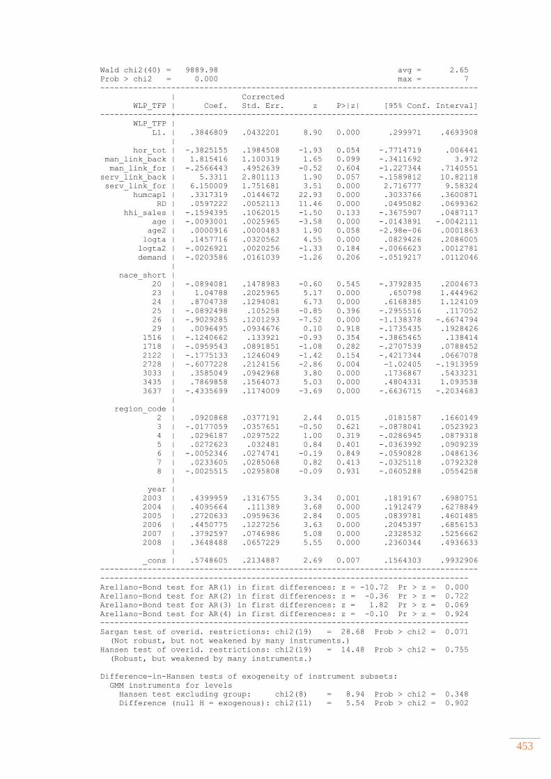
453
Wald chi2(40) = 9889.98 avg = 2.65
Prob > chi2 = 0.000 max = 7
--------------------------------------------------------------------------------
| Corrected
WLP_TFP | Coef. Std. Err. z P>|z| [95% Conf. Interval]
---------------+----------------------------------------------------------------
WLP_TFP |
L1. | .3846809 .0432201 8.90 0.000 .299971 .4693908
|
hor_tot | -.3825155 .1984508 -1.93 0.054 -.7714719 .006441
man_link_back | 1.815416 1.100319 1.65 0.099 -.3411692 3.972
man_link_for | -.2566443 .4952639 -0.52 0.604 -1.227344 .7140551
serv_link_back | 5.3311 2.801113 1.90 0.057 -.1589812 10.82118
serv_link_for | 6.150009 1.751681 3.51 0.000 2.716777 9.58324
humcap1 | .3317319 .0144672 22.93 0.000 .3033766 .3600871
RD | .0597222 .0052113 11.46 0.000 .0495082 .0699362
hhi_sales | -.1594395 .1062015 -1.50 0.133 -.3675907 .0487117
age | -.0093001 .0025965 -3.58 0.000 -.0143891 -.0042111
age2 | .0000916 .0000483 1.90 0.058 -2.98e-06 .0001863
logta | .1457716 .0320562 4.55 0.000 .0829426 .2086005
logta2 | -.0026921 .0020256 -1.33 0.184 -.0066623 .0012781
demand | -.0203586 .0161039 -1.26 0.206 -.0519217 .0112046
|
nace_short |
20 | -.0894081 .1478983 -0.60 0.545 -.3792835 .2004673
23 | 1.04788 .2025965 5.17 0.000 .650798 1.444962
24 | .8704738 .1294081 6.73 0.000 .6168385 1.124109
25 | -.0892498 .105258 -0.85 0.396 -.2955516 .117052
26 | -.9029285 .1201293 -7.52 0.000 -1.138378 -.6674794
29 | .0096495 .0934676 0.10 0.918 -.1735435 .1928426
1516 | -.1240662 .133921 -0.93 0.354 -.3865465 .138414
1718 | -.0959543 .0891851 -1.08 0.282 -.2707539 .0788452
2122 | -.1775133 .1246049 -1.42 0.154 -.4217344 .0667078
2728 | -.6077228 .2124156 -2.86 0.004 -1.02405 -.1913959
3033 | .3585049 .0942968 3.80 0.000 .1736867 .5433231
3435 | .7869858 .1564073 5.03 0.000 .4804331 1.093538
3637 | -.4335699 .1174009 -3.69 0.000 -.6636715 -.2034683
|
region_code |
2 | .0920868 .0377191 2.44 0.015 .0181587 .1660149
3 | -.0177059 .0357651 -0.50 0.621 -.0878041 .0523923
4 | .0296187 .0297522 1.00 0.319 -.0286945 .0879318
5 | .0272623 .032481 0.84 0.401 -.0363992 .0909239
6 | -.0052346 .0274741 -0.19 0.849 -.0590828 .0486136
7 | .0233605 .0285068 0.82 0.413 -.0325118 .0792328
8 | -.0025515 .0295808 -0.09 0.931 -.0605288 .0554258
|
year |
2003 | .4399959 .1316755 3.34 0.001 .1819167 .6980751
2004 | .4095664 .111389 3.68 0.000 .1912479 .6278849
2005 | .2720633 .0959636 2.84 0.005 .0839781 .4601485
2006 | .4450775 .1227256 3.63 0.000 .2045397 .6856153
2007 | .3792597 .0746986 5.08 0.000 .2328532 .5256662
2008 | .3648488 .0657229 5.55 0.000 .2360344 .4936633
|
_cons | .5748605 .2134887 2.69 0.007 .1564303 .9932906
--------------------------------------------------------------------------------
------------------------------------------------------------------------------
Arellano-Bond test for AR(1) in first differences: z = -10.72 Pr > z = 0.000
Arellano-Bond test for AR(2) in first differences: z = -0.36 Pr > z = 0.722
Arellano-Bond test for AR(3) in first differences: z = 1.82 Pr > z = 0.069
Arellano-Bond test for AR(4) in first differences: z = -0.10 Pr > z = 0.924
------------------------------------------------------------------------------
Sargan test of overid. restrictions: chi2(19) = 28.68 Prob > chi2 = 0.071
(Not robust, but not weakened by many instruments.)
Hansen test of overid. restrictions: chi2(19) = 14.48 Prob > chi2 = 0.755
(Robust, but weakened by many instruments.)
Difference-in-Hansen tests of exogeneity of instrument subsets:
GMM instruments for levels
Hansen test excluding group: chi2(8) = 8.94 Prob > chi2 = 0.348
Difference (null H = exogenous): chi2(11) = 5.54 Prob > chi2 = 0.902
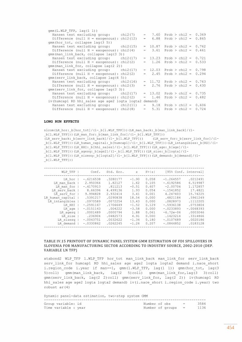
454
gmm(L.WLP_TFP, lag(1 1))
Hansen test excluding group: chi2(7) = 7.60 Prob > chi2 = 0.369
Difference (null H = exogenous): chi2(12) = 6.88 Prob > chi2 = 0.865
gmm(hor_tot, collapse lag(3 5))
Hansen test excluding group: chi2(15) = 10.87 Prob > chi2 = 0.762
Difference (null H = exogenous): chi2(4) = 3.61 Prob > chi2 = 0.461
gmm(man_link_back, collapse lag(3 3))
Hansen test excluding group: chi2(17) = 13.23 Prob > chi2 = 0.721
Difference (null H = exogenous): chi2(2) = 1.26 Prob > chi2 = 0.533
gmm(man_link_for, collapse lag(2 2))
Hansen test excluding group: chi2(17) = 12.03 Prob > chi2 = 0.798
Difference (null H = exogenous): chi2(2) = 2.45 Prob > chi2 = 0.294
gmm(serv_link_back, collapse lag(4 5))
Hansen test excluding group: chi2(16) = 11.72 Prob > chi2 = 0.763
Difference (null H = exogenous): chi2(3) = 2.76 Prob > chi2 = 0.430
gmm(serv_link_for, collapse lag(3 3))
Hansen test excluding group: chi2(17) = 13.02 Prob > chi2 = 0.735
Difference (null H = exogenous): chi2(2) = 1.46 Prob > chi2 = 0.482
iv(humcap1 RD hhi_sales age age2 logta logta2 demand)
Hansen test excluding group: chi2(11) = 9.18 Prob > chi2 = 0.606
Difference (null H = exogenous): chi2(8) = 5.31 Prob > chi2 = 0.724
LONG RUN EFFECTS
nlcom(LR_hor:_b[hor_tot]/(1-_b[l.WLP_TFP]))(LR_man_back:_b[man_link_back]/(1-
_b[l.WLP_TFP]))(LR_man_for:_b[man_link_for]/(1-_b[l.WLP_TFP]))
(LR_serv_back:_b[serv_link_back]/(1-_b[l.WLP_TFP])) (LR_serv_for:_b[serv_link_for]/(1-
_b[l.WLP_TFP]))(LR_human_capital:_b[humcap1]/(1-_b[l.WLP_TFP]))(LR_intangibles:_b[RD]/(1-
_b[l.WLP_TFP]))(LR_HHI:_b[hhi_sales]/(1-_b[l.WLP_TFP]))(LR_age:_b[age]/(1-
_b[l.WLP_TFP]))(LR_agesq:_b[age2]/(1-_b[l.WLP_TFP]))(LR_size:_b[logta]/(1-
_b[l.WLP_TFP]))(LR_sizesq:_b[logta2]/(1-_b[l.WLP_TFP]))(LR_demand:_b[demand]/(1-
_b[l.WLP_TFP]))
----------------------------------------------------------------------------------
WLP_TFP | Coef. Std. Err. z P>|z| [95% Conf. Interval]
-----------------+----------------------------------------------------------------
LR_hor | -.6216538 .3280177 -1.90 0.058 -1.264557 .0212491
LR_man_back | 2.950364 1.82127 1.62 0.105 -.6192586 6.519987
LR_man_for | -.4170913 .811213 -0.51 0.607 -2.00704 1.172857
LR_serv_back | 8.66396 4.499136 1.93 0.054 -.1541852 17.4821
LR_serv_for | 9.994828 2.932414 3.41 0.001 4.247403 15.74225
LR_human_capital | .5391217 .0290838 18.54 0.000 .4821184 .5961249
LR_intangibles | .0970589 .0072254 13.43 0.000 .0828973 .1112205
LR_HHI | -.2591167 .1706649 -1.52 0.129 -.5936138 .0753804
LR_age | -.0151143 .004222 -3.58 0.000 -.0233893 -.0068393
LR_agesq | .0001489 .0000794 1.88 0.061 -6.72e-06 .0003046
LR_size | .236904 .0482573 4.91 0.000 .1423214 .3314866
LR_sizesq | -.0043751 .0032622 -1.34 0.180 -.0107689 .0020186
LR_demand | -.0330862 .0262245 -1.26 0.207 -.0844852 .0183128
----------------------------------------------------------------------------------
TABLE IV.15 PRINTOUT OF DYNAMIC PANEL SYSTEM GMM ESTIMATION OF FDI SPILLOVERS IN SLOVENIA FOR MANUFACTURING SECTOR ACCORDING TO INDUSTRY SOURCE, 2002-2010 (DEP. VARIABLE LN TFP)
xtabond2 WLP_TFP l.WLP_TFP hor_tot man_link_back man_link_for serv_link_back
serv_link_for humcap1 RD hhi_sales age age2 logta logta2 demand i.nace_short
i.region_code i.year if man==1, gmm(l.WLP_TFP, lag(1 1)) gmm(hor_tot, lag(3
5)coll) gmm(man_link_back, lag(2 5)coll) gmm(man_link_for,lag(3 3)coll)
gmm(serv_link_back, lag(2 2)coll) gmm(serv_link_for, lag(2 2)) iv(humcap1 RD
hhi_sales age age2 logta logta2 demand) iv(i.nace_short i.region_code i.year) two
robust ar(4)
Dynamic panel-data estimation, two-step system GMM
------------------------------------------------------------------------------
Group variable: id Number of obs = 3584
Time variable : year Number of groups = 1136
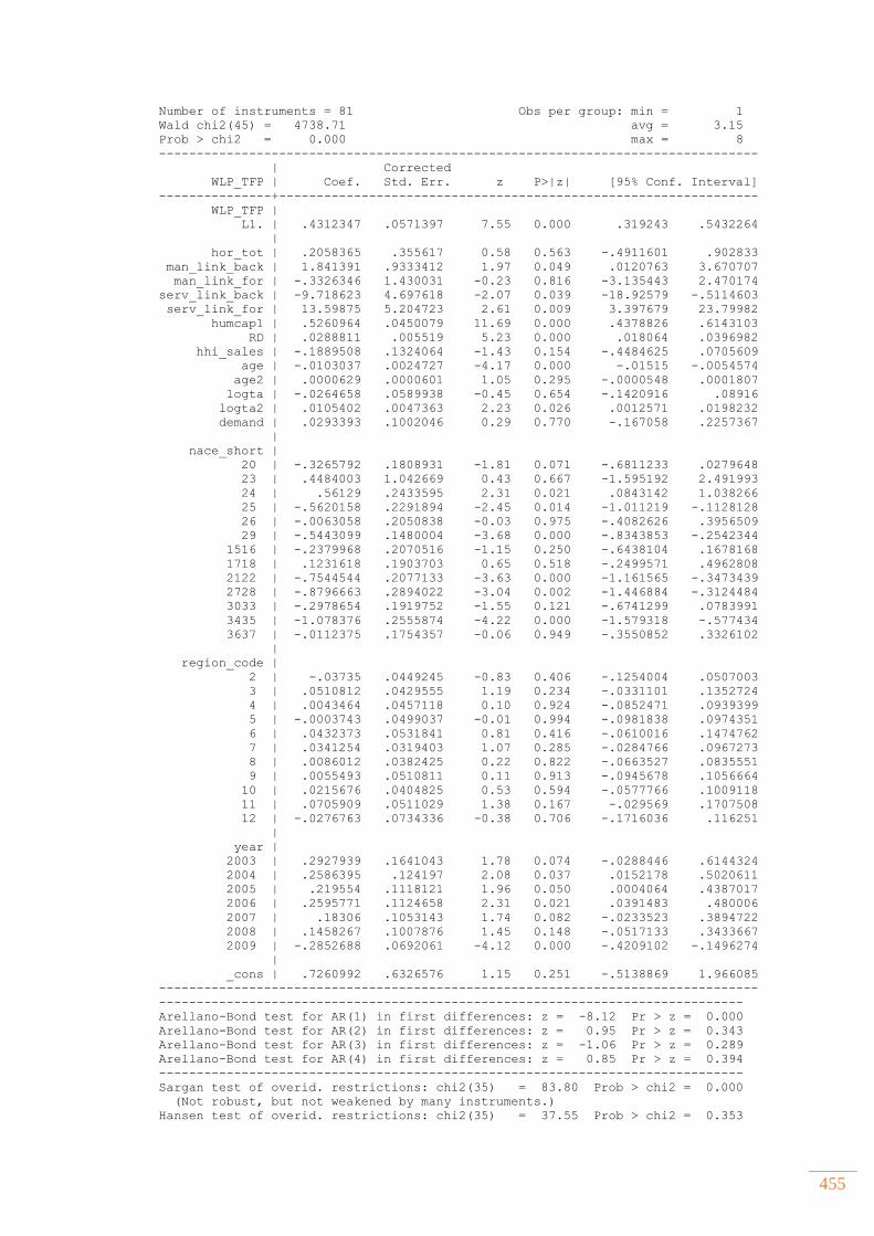
455
Number of instruments = 81 Obs per group: min = 1
Wald chi2(45) = 4738.71 avg = 3.15
Prob > chi2 = 0.000 max = 8
--------------------------------------------------------------------------------
| Corrected
WLP_TFP | Coef. Std. Err. z P>|z| [95% Conf. Interval]
---------------+----------------------------------------------------------------
WLP_TFP |
L1. | .4312347 .0571397 7.55 0.000 .319243 .5432264
|
hor_tot | .2058365 .355617 0.58 0.563 -.4911601 .902833
man_link_back | 1.841391 .9333412 1.97 0.049 .0120763 3.670707
man_link_for | -.3326346 1.430031 -0.23 0.816 -3.135443 2.470174
serv_link_back | -9.718623 4.697618 -2.07 0.039 -18.92579 -.5114603
serv_link_for | 13.59875 5.204723 2.61 0.009 3.397679 23.79982
humcap1 | .5260964 .0450079 11.69 0.000 .4378826 .6143103
RD | .0288811 .005519 5.23 0.000 .018064 .0396982
hhi_sales | -.1889508 .1324064 -1.43 0.154 -.4484625 .0705609
age | -.0103037 .0024727 -4.17 0.000 -.01515 -.0054574
age2 | .0000629 .0000601 1.05 0.295 -.0000548 .0001807
logta | -.0264658 .0589938 -0.45 0.654 -.1420916 .08916
logta2 | .0105402 .0047363 2.23 0.026 .0012571 .0198232
demand | .0293393 .1002046 0.29 0.770 -.167058 .2257367
|
nace_short |
20 | -.3265792 .1808931 -1.81 0.071 -.6811233 .0279648
23 | .4484003 1.042669 0.43 0.667 -1.595192 2.491993
24 | .56129 .2433595 2.31 0.021 .0843142 1.038266
25 | -.5620158 .2291894 -2.45 0.014 -1.011219 -.1128128
26 | -.0063058 .2050838 -0.03 0.975 -.4082626 .3956509
29 | -.5443099 .1480004 -3.68 0.000 -.8343853 -.2542344
1516 | -.2379968 .2070516 -1.15 0.250 -.6438104 .1678168
1718 | .1231618 .1903703 0.65 0.518 -.2499571 .4962808
2122 | -.7544544 .2077133 -3.63 0.000 -1.161565 -.3473439
2728 | -.8796663 .2894022 -3.04 0.002 -1.446884 -.3124484
3033 | -.2978654 .1919752 -1.55 0.121 -.6741299 .0783991
3435 | -1.078376 .2555874 -4.22 0.000 -1.579318 -.577434
3637 | -.0112375 .1754357 -0.06 0.949 -.3550852 .3326102
|
region_code |
2 | -.03735 .0449245 -0.83 0.406 -.1254004 .0507003
3 | .0510812 .0429555 1.19 0.234 -.0331101 .1352724
4 | .0043464 .0457118 0.10 0.924 -.0852471 .0939399
5 | -.0003743 .0499037 -0.01 0.994 -.0981838 .0974351
6 | .0432373 .0531841 0.81 0.416 -.0610016 .1474762
7 | .0341254 .0319403 1.07 0.285 -.0284766 .0967273
8 | .0086012 .0382425 0.22 0.822 -.0663527 .0835551
9 | .0055493 .0510811 0.11 0.913 -.0945678 .1056664
10 | .0215676 .0404825 0.53 0.594 -.0577766 .1009118
11 | .0705909 .0511029 1.38 0.167 -.029569 .1707508
12 | -.0276763 .0734336 -0.38 0.706 -.1716036 .116251
|
year |
2003 | .2927939 .1641043 1.78 0.074 -.0288446 .6144324
2004 | .2586395 .124197 2.08 0.037 .0152178 .5020611
2005 | .219554 .1118121 1.96 0.050 .0004064 .4387017
2006 | .2595771 .1124658 2.31 0.021 .0391483 .480006
2007 | .18306 .1053143 1.74 0.082 -.0233523 .3894722
2008 | .1458267 .1007876 1.45 0.148 -.0517133 .3433667
2009 | -.2852688 .0692061 -4.12 0.000 -.4209102 -.1496274
|
_cons | .7260992 .6326576 1.15 0.251 -.5138869 1.966085
--------------------------------------------------------------------------------
------------------------------------------------------------------------------
Arellano-Bond test for AR(1) in first differences: z = -8.12 Pr > z = 0.000
Arellano-Bond test for AR(2) in first differences: z = 0.95 Pr > z = 0.343
Arellano-Bond test for AR(3) in first differences: z = -1.06 Pr > z = 0.289
Arellano-Bond test for AR(4) in first differences: z = 0.85 Pr > z = 0.394
------------------------------------------------------------------------------
Sargan test of overid. restrictions: chi2(35) = 83.80 Prob > chi2 = 0.000
(Not robust, but not weakened by many instruments.)
Hansen test of overid. restrictions: chi2(35) = 37.55 Prob > chi2 = 0.353
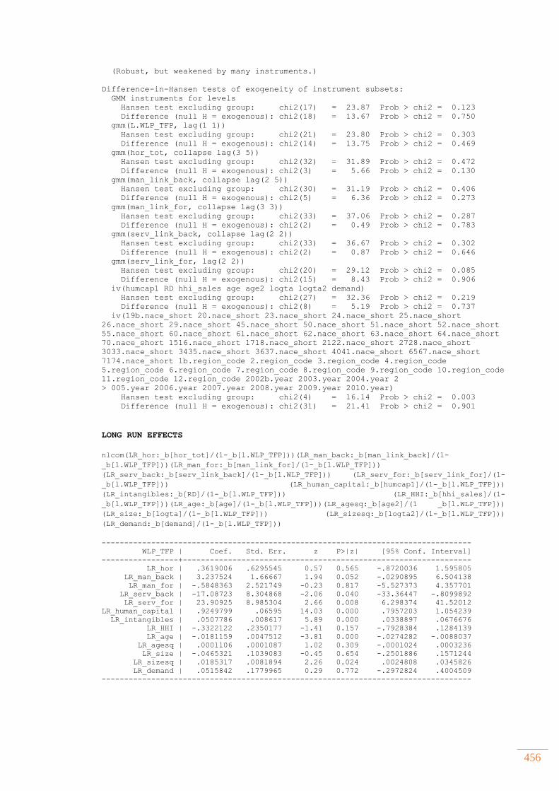
456
(Robust, but weakened by many instruments.)
Difference-in-Hansen tests of exogeneity of instrument subsets:
GMM instruments for levels
Hansen test excluding group: chi2(17) = 23.87 Prob > chi2 = 0.123
Difference (null H = exogenous): chi2(18) = 13.67 Prob > chi2 = 0.750
gmm(L.WLP_TFP, lag(1 1))
Hansen test excluding group: chi2(21) = 23.80 Prob > chi2 = 0.303
Difference (null H = exogenous): chi2(14) = 13.75 Prob > chi2 = 0.469
gmm(hor_tot, collapse lag(3 5))
Hansen test excluding group: chi2(32) = 31.89 Prob > chi2 = 0.472
Difference (null H = exogenous): chi2(3) = 5.66 Prob > chi2 = 0.130
gmm(man_link_back, collapse lag(2 5))
Hansen test excluding group: chi2(30) = 31.19 Prob > chi2 = 0.406
Difference (null H = exogenous): chi2(5) = 6.36 Prob > chi2 = 0.273
gmm(man_link_for, collapse lag(3 3))
Hansen test excluding group: chi2(33) = 37.06 Prob > chi2 = 0.287
Difference (null H = exogenous): chi2(2) = 0.49 Prob > chi2 = 0.783
gmm(serv_link_back, collapse lag(2 2))
Hansen test excluding group: chi2(33) = 36.67 Prob > chi2 = 0.302
Difference (null H = exogenous): chi2(2) = 0.87 Prob > chi2 = 0.646
gmm(serv_link_for, lag(2 2))
Hansen test excluding group: chi2(20) = 29.12 Prob > chi2 = 0.085
Difference (null H = exogenous): chi2(15) = 8.43 Prob > chi2 = 0.906
iv(humcap1 RD hhi_sales age age2 logta logta2 demand)
Hansen test excluding group: chi2(27) = 32.36 Prob > chi2 = 0.219
Difference (null H = exogenous): chi2(8) = 5.19 Prob > chi2 = 0.737
iv(19b.nace_short 20.nace_short 23.nace_short 24.nace_short 25.nace_short
26.nace_short 29.nace_short 45.nace_short 50.nace_short 51.nace_short 52.nace_short
55.nace_short 60.nace_short 61.nace_short 62.nace_short 63.nace_short 64.nace_short
70.nace_short 1516.nace_short 1718.nace_short 2122.nace_short 2728.nace_short
3033.nace_short 3435.nace_short 3637.nace_short 4041.nace_short 6567.nace_short
7174.nace_short 1b.region_code 2.region_code 3.region_code 4.region_code
5.region_code 6.region_code 7.region_code 8.region_code 9.region_code 10.region_code
11.region_code 12.region_code 2002b.year 2003.year 2004.year 2
> 005.year 2006.year 2007.year 2008.year 2009.year 2010.year)
Hansen test excluding group: chi2(4) = 16.14 Prob > chi2 = 0.003
Difference (null H = exogenous): chi2(31) = 21.41 Prob > chi2 = 0.901
LONG RUN EFFECTS
nlcom(LR_hor:_b[hor_tot]/(1-_b[l.WLP_TFP]))(LR_man_back:_b[man_link_back]/(1-
_b[l.WLP_TFP]))(LR_man_for:_b[man_link_for]/(1-_b[l.WLP_TFP]))
(LR_serv_back:_b[serv_link_back]/(1-_b[l.WLP_TFP])) (LR_serv_for:_b[serv_link_for]/(1-
_b[l.WLP_TFP])) (LR_human_capital:_b[humcap1]/(1-_b[l.WLP_TFP]))
(LR_intangibles:_b[RD]/(1-_b[l.WLP_TFP])) (LR_HHI:_b[hhi_sales]/(1-
_b[l.WLP_TFP]))(LR_age:_b[age]/(1-_b[l.WLP_TFP]))(LR_agesq:_b[age2]/(1 _b[l.WLP_TFP]))
(LR_size:_b[logta]/(1-_b[l.WLP_TFP])) (LR_sizesq:_b[logta2]/(1-_b[l.WLP_TFP]))
(LR_demand:_b[demand]/(1-_b[l.WLP_TFP]))
----------------------------------------------------------------------------------
WLP_TFP | Coef. Std. Err. z P>|z| [95% Conf. Interval]
-----------------+----------------------------------------------------------------
LR_hor | .3619006 .6295545 0.57 0.565 -.8720036 1.595805
LR_man_back | 3.237524 1.66667 1.94 0.052 -.0290895 6.504138
LR_man_for | -.5848363 2.521749 -0.23 0.817 -5.527373 4.357701
LR_serv_back | -17.08723 8.304868 -2.06 0.040 -33.36447 -.8099892
LR_serv_for | 23.90925 8.985304 2.66 0.008 6.298374 41.52012
LR_human_capital | .9249799 .06595 14.03 0.000 .7957203 1.054239
LR_intangibles | .0507786 .008617 5.89 0.000 .0338897 .0676676
LR_HHI | -.3322122 .2350177 -1.41 0.157 -.7928384 .1284139
LR_age | -.0181159 .0047512 -3.81 0.000 -.0274282 -.0088037
LR_agesq | .0001106 .0001087 1.02 0.309 -.0001024 .0003236
LR_size | -.0465321 .1039083 -0.45 0.654 -.2501886 .1571244
LR_sizesq | .0185317 .0081894 2.26 0.024 .0024808 .0345826
LR_demand | .0515842 .1779965 0.29 0.772 -.2972824 .4004509
----------------------------------------------------------------------------------
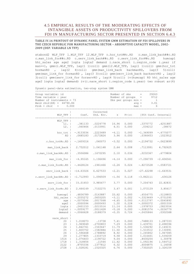
457
4.5 EMPIRICAL RESULTS OF THE MODERATING EFFECTS OF
INTANGIBLE ASSETS ON PRODUCTIVITY SPILLOVERS FROM
FDI IN MANUFACTURING SECTOR PRESENTED IN SECTION 6.4.3
TABLE IV.16 PRINTOUT OF DYNAMIC PANEL SYSTEM GMM ESTIMATION OF FDI SPILLOVERS IN THE CZECH REPUBLIC FOR MANUFACTURING SECTOR – ABSORPTIVE CAPACITY MODEL, 2002-2009 (DEP. VARIABLE LN TFP)
xtabond2 WLP_TFP l.WLP_TFP l2.WLP_TFP c.hor_tot##c.RD c.man_link_back##c.RD
c.man_link_for##c.RD c.serv_link_back##c.RD c.serv_link_for##c.RD humcap1
hhi_sales age age2 logta logta2 demand i.nace_short i.region_code i.year if
man==1, gmm(l.WLP_TFP, lag(1 1)coll) gmm(l2.WLP_TFP, lag(1 1)coll) gmm(hor_tot
hormanRD , lag(2 4)coll) gmm(man_link_back backmanRD, lag(3 5)coll)
gmm(man_link_for formanRD , lag(3 3)coll) gmm(serv_link_back backservRD , lag(2
3)coll) gmm(serv_link_for forservRD , lag(4 5)coll) iv(humcap1 RD hhi_sales age
age2 logta logta2 demand) iv(i.nace_short i.region_code i.year) two robust ar(4)
Dynamic panel-data estimation, two-step system GMM
------------------------------------------------------------------------------
Group variable: id Number of obs = 29263
Time variable : year Number of groups = 9712
Number of instruments = 73 Obs per group: min = 1
Wald chi2(48) = 44790.84 avg = 3.01
Prob > chi2 = 0.000 max = 6
---------------------------------------------------------------------------------------
| Corrected
WLP_TFP | Coef. Std. Err. z P>|z| [95% Conf. Interval]
----------------------+----------------------------------------------------------------
WLP_TFP |
L1. | .381133 .0224778 16.96 0.000 .3370772 .4251887
L2. | .060466 .0133951 4.51 0.000 .034212 .08672
|
hor_tot | -.9133034 .2223489 -4.11 0.000 -1.349099 -.4775077
RD | .0685183 .0172824 3.96 0.000 .0346453 .1023912
|
c.hor_tot#c.RD | -.1409316 .040073 -3.52 0.000 -.2194732 -.0623899
|
man_link_back | 2.752012 1.041148 2.64 0.008 .7113991 4.792625
|
c.man_link_back#c.RD | .3506086 .1670295 2.10 0.036 .0232367 .6779804
|
man_link_for | -4.95165 1.196496 -4.14 0.000 -7.296739 -2.606561
|
c.man_link_for#c.RD | -.4428124 .1961466 -2.26 0.024 -.8272528 -.0583721
|
serv_link_back | -14.63326 6.627533 -2.21 0.027 -27.62298 -1.643531
|
c.serv_link_back#c.RD | -1.712993 1.096509 -1.56 0.118 -3.862111 .436126
|
serv_link_for | 15.01653 3.985677 3.77 0.000 7.204743 22.82831
|
c.serv_link_for#c.RD | 2.464149 .7102275 3.47 0.001 1.072129 3.85617
|
humcap1 | .4836789 .0143887 33.62 0.000 .4554775 .5118803
hhi_sales | -.2035272 .0655205 -3.11 0.002 -.3319449 -.0751095
age | -.0079344 .0017068 -4.65 0.000 -.0112797 -.0045892
age2 | .0000594 .0000493 1.20 0.228 -.0000372 .0001559
logta | .2401153 .0215514 11.14 0.000 .1978753 .2823554
logta2 | -.0059177 .0011428 -5.18 0.000 -.0081574 -.0036779
demand | -.0066628 .0188379 -0.35 0.724 -.0435844 .0302588
|
nace_short |
20 | 1.018073 .13738 7.41 0.000 .7488133 1.287333
23 | 1.969049 .2700803 7.29 0.000 1.439701 2.498396
24 | 1.842761 .1563647 11.79 0.000 1.536292 2.149231
25 | 1.820752 .1582884 11.50 0.000 1.510512 2.130991
26 | 1.596468 .1788892 8.92 0.000 1.245852 1.947085
29 | 1.277805 .1333719 9.58 0.000 1.016401 1.539209
1516 | 1.076403 .1190722 9.04 0.000 .8430254 1.30978
1718 | 1.318454 .11544 11.42 0.000 1.092196 1.544712
2122 | .8705336 .1377812 6.32 0.000 .6004875 1.14058
2728 | 1.028181 .1520325 6.76 0.000 .7302025 1.326159
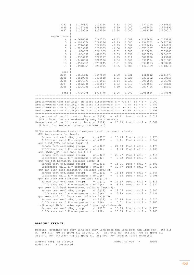
458
3033 | 1.176872 .122324 9.62 0.000 .9371215 1.416623
3435 | 1.327649 .1383925 9.59 0.000 1.056405 1.598893
3637 | 1.259026 .1229568 10.24 0.000 1.018036 1.500017
|
region_code |
4 | -.0696748 .0265765 -2.62 0.009 -.1217638 -.0175858
5 | -.1019574 .0269126 -3.79 0.000 -.1547052 -.0492096
6 | -.0770349 .0269969 -2.85 0.004 -.1299479 -.024122
7 | -.0259888 .0250963 -1.04 0.300 -.0751767 .0231991
8 | -.068321 .0261955 -2.61 0.009 -.1196632 -.0169787
9 | -.054391 .025969 -2.09 0.036 -.1052893 -.0034927
10 | -.0336439 .0269117 -1.25 0.211 -.0863898 .019102
11 | -.0478856 .0260586 -1.84 0.066 -.0989594 .0031883
13 | -.0516565 .0233845 -2.21 0.027 -.0974893 -.0058236
14 | -.0918554 .0259105 -3.55 0.000 -.1426389 -.0410718
|
year |
2004 | -.0535682 .0447539 -1.20 0.231 -.1412842 .0341477
2005 | .0519799 .0429018 1.21 0.226 -.0321062 .1360659
2006 | .1026373 .0479951 2.14 0.032 .0085686 .196706
2007 | .0562245 .0455557 1.23 0.217 -.0330631 .1455121
2008 | .1206998 .0167963 7.19 0.000 .0877796 .15362
|
_cons | -.7326205 .1805775 -4.06 0.000 -1.086546 -.378695
---------------------------------------------------------------------------------------
------------------------------------------------------------------------------
Arellano-Bond test for AR(1) in first differences: z = -15.37 Pr > z = 0.000
Arellano-Bond test for AR(2) in first differences: z = 0.75 Pr > z = 0.452
Arellano-Bond test for AR(3) in first differences: z = -0.32 Pr > z = 0.748
Arellano-Bond test for AR(4) in first differences: z = -0.39 Pr > z = 0.699
------------------------------------------------------------------------------
Sargan test of overid. restrictions: chi2(24) = 42.61 Prob > chi2 = 0.011
(Not robust, but not weakened by many instruments.)
Hansen test of overid. restrictions: chi2(24) = 25.69 Prob > chi2 = 0.369
(Robust, but weakened by many instruments.)
Difference-in-Hansen tests of exogeneity of instrument subsets:
GMM instruments for levels
Hansen test excluding group: chi2(12) = 16.28 Prob > chi2 = 0.179
Difference (null H = exogenous): chi2(12) = 9.41 Prob > chi2 = 0.667
gmm(L.WLP_TFP, collapse lag(1 1))
Hansen test excluding group: chi2(22) = 21.69 Prob > chi2 = 0.479
Difference (null H = exogenous): chi2(2) = 4.00 Prob > chi2 = 0.135
gmm(L2.WLP_TFP, collapse lag(1 1))
Hansen test excluding group: chi2(22) = 22.77 Prob > chi2 = 0.415
Difference (null H = exogenous): chi2(2) = 2.92 Prob > chi2 = 0.233
gmm(hor_tot hormanRD, collapse lag(2 4))
Hansen test excluding group: chi2(16) = 15.21 Prob > chi2 = 0.509
Difference (null H = exogenous): chi2(8) = 10.47 Prob > chi2 = 0.233
gmm(man_link_back backmanRD, collapse lag(3 5))
Hansen test excluding group: chi2(16) = 16.13 Prob > chi2 = 0.444
Difference (null H = exogenous): chi2(8) = 9.55 Prob > chi2 = 0.298
gmm(man_link_for formanRD, collapse lag(3 3))
Hansen test excluding group: chi2(20) = 22.56 Prob > chi2 = 0.311
Difference (null H = exogenous): chi2(4) = 3.13 Prob > chi2 = 0.537
gmm(serv_link_back backservRD, collapse lag(2 3))
Hansen test excluding group: chi2(18) = 19.76 Prob > chi2 = 0.347
Difference (null H = exogenous): chi2(6) = 5.93 Prob > chi2 = 0.431
gmm(serv_link_for forservRD, collapse lag(4 5))
Hansen test excluding group: chi2(18) = 20.18 Prob > chi2 = 0.323
Difference (null H = exogenous): chi2(6) = 5.51 Prob > chi2 = 0.480
iv(humcap1 RD hhi_sales age age2 logta logta2 demand)
Hansen test excluding group: chi2(16) = 15.69 Prob > chi2 = 0.475
Difference (null H = exogenous): chi2(8) = 10.00 Prob > chi2 = 0.265
MARGINAL EFFECTS
margins, dydx(hor_tot serv_link_for serv_link_back man_link_back man_link_for ) at((p1)
RD) at((p10) RD) at((p20) RD) at((p30) RD) at((p40) RD) at((p50) RD) at((p60) RD)
at((p70) RD) at((p80) RD) at((p90) RD) at((p99) RD) vsquish force level(90)
Average marginal effects Number of obs = 29263
Model VCE : Corrected
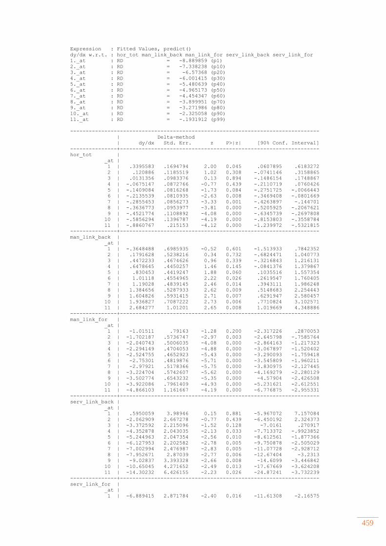
459
Expression : Fitted Values, predict()
dy/dx w.r.t. : hor_tot man_link_back man_link_for serv_link_back serv_link_for
1._at : RD = -8.889859 (p1)
2._at : RD = -7.338238 (p10)
3._at : RD = -6.57368 (p20)
4._at : RD = -6.001415 (p30)
5._at : RD = -5.480639 (p40)
6._at : RD = -4.965173 (p50)
7._at : RD = -4.454347 (p60)
8._at : RD = -3.899951 (p70)
9._at : RD = -3.271986 (p80)
10._at : RD = -2.325058 (p90)
11._at : RD = -.1931912 (p99)
--------------------------------------------------------------------------------
| Delta-method
| dy/dx Std. Err. z P>|z| [90% Conf. Interval]
---------------+----------------------------------------------------------------
hor_tot |
_at |
1 | .3395583 .1694794 2.00 0.045 .0607895 .6183272
2 | .120886 .1185519 1.02 0.308 -.0741146 .3158865
3 | .0131356 .0983376 0.13 0.894 -.1486154 .1748867
4 | -.0675147 .0872766 -0.77 0.439 -.2110719 .0760426
5 | -.1409084 .0816268 -1.73 0.084 -.2751725 -.0066443
6 | -.2135539 .0810935 -2.63 0.008 -.3469408 -.0801669
7 | -.2855453 .0856273 -3.33 0.001 -.4263897 -.144701
8 | -.3636773 .0953977 -3.81 0.000 -.5205925 -.2067621
9 | -.4521774 .1108892 -4.08 0.000 -.6345739 -.2697808
10 | -.5856294 .1396787 -4.19 0.000 -.8153803 -.3558784
11 | -.8860767 .215153 -4.12 0.000 -1.239972 -.5321815
---------------+----------------------------------------------------------------
man_link_back |
_at |
1 | -.3648488 .6985935 -0.52 0.601 -1.513933 .7842352
2 | .1791628 .5238216 0.34 0.732 -.6824471 1.040773
3 | .4472233 .4674626 0.96 0.339 -.3216843 1.216131
4 | .6478645 .4450257 1.46 0.145 -.0841376 1.379867
5 | .830453 .4419247 1.88 0.060 .1035516 1.557354
6 | 1.01118 .4554965 2.22 0.026 .2619547 1.760405
7 | 1.19028 .4839145 2.46 0.014 .3943111 1.986248
8 | 1.384656 .5287933 2.62 0.009 .5148683 2.254443
9 | 1.604826 .5931415 2.71 0.007 .6291947 2.580457
10 | 1.936827 .7087222 2.73 0.006 .7710824 3.102571
11 | 2.684277 1.01201 2.65 0.008 1.019669 4.348886
---------------+----------------------------------------------------------------
man_link_for |
_at |
1 | -1.01511 .79163 -1.28 0.200 -2.317226 .2870053
2 | -1.702187 .5736747 -2.97 0.003 -2.645798 -.7585764
3 | -2.040743 .5006035 -4.08 0.000 -2.864163 -1.217323
4 | -2.294149 .4704053 -4.88 0.000 -3.067897 -1.520402
5 | -2.524755 .4652923 -5.43 0.000 -3.290093 -1.759418
6 | -2.75301 .4819876 -5.71 0.000 -3.545809 -1.960211
7 | -2.97921 .5178366 -5.75 0.000 -3.830975 -2.127445
8 | -3.224704 .5742607 -5.62 0.000 -4.169279 -2.280129
9 | -3.502774 .6543232 -5.35 0.000 -4.57904 -2.426508
10 | -3.922086 .7961409 -4.93 0.000 -5.231621 -2.612551
11 | -4.866103 1.161667 -4.19 0.000 -6.776875 -2.955331
---------------+----------------------------------------------------------------
serv_link_back |
_at |
1 | .5950059 3.98946 0.15 0.881 -5.967072 7.157084
2 | -2.062909 2.667278 -0.77 0.439 -6.450192 2.324373
3 | -3.372592 2.215096 -1.52 0.128 -7.0161 .270917
4 | -4.352878 2.043035 -2.13 0.033 -7.713372 -.9923852
5 | -5.244963 2.047354 -2.56 0.010 -8.612561 -1.877366
6 | -6.127953 2.202582 -2.78 0.005 -9.750878 -2.505029
7 | -7.002994 2.476987 -2.83 0.005 -11.07728 -2.928712
8 | -7.952671 2.87039 -2.77 0.006 -12.67404 -3.2313
9 | -9.02837 3.393328 -2.66 0.008 -14.6099 -3.446842
10 | -10.65045 4.271652 -2.49 0.013 -17.67669 -3.624208
11 | -14.30232 6.426155 -2.23 0.026 -24.87241 -3.732239
---------------+----------------------------------------------------------------
serv_link_for |
_at |
1 | -6.889415 2.871784 -2.40 0.016 -11.61308 -2.16575
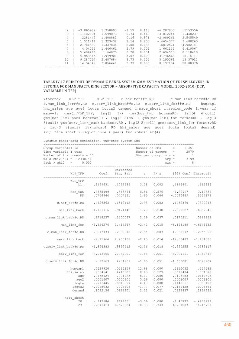
460
2 | -3.065989 1.958803 -1.57 0.118 -6.287933 .1559556
3 | -1.182004 1.599073 -0.74 0.460 -3.812244 1.448237
4 | .2281442 1.408882 0.16 0.871 -2.089261 2.545549
5 | 1.511414 1.323432 1.14 0.253 -.6654377 3.688265
6 | 2.781599 1.337838 2.08 0.038 .5810521 4.982147
7 | 4.04035 1.446461 2.79 0.005 1.661133 6.419567
8 | 5.406466 1.64875 3.28 0.001 2.694513 8.118419
9 | 6.953865 1.949901 3.57 0.000 3.746563 10.16117
10 | 9.287237 2.487684 3.73 0.000 5.195361 13.37911
11 | 14.54047 3.856441 3.77 0.000 8.197194 20.88376
--------------------------------------------------------------------------------
TABLE IV.17 PRINTOUT OF DYNAMIC PANEL SYSTEM GMM ESTIMATION OF FDI SPILLOVERS IN ESTONIA FOR MANUFACTURING SECTOR – ABSORPTIVE CAPACITY MODEL, 2002-2010 (DEP. VARIABLE LN TFP)
xtabond2 WLP_TFP l.WLP_TFP c.hor_tot##c.RD c.man_link_back##c.RD
c.man_link_for##c.RD c.serv_link_back##c.RD c.serv_link_for##c.RD humcap1
hhi_sales age age2 logta logta2 demand i.nace_short i.region_code i.year if
man==1, gmm(l.WLP_TFP, lag(2 3)) gmm(hor_tot hormanRD, lag(4 4)coll)
gmm(man_link_back backmanRD , lag(2 2)coll) gmm(man_link_for formanRD , lag(3
3)coll) gmm(serv_link_back backservRD , lag(2 2)coll) gmm(serv_link_for forservRD
, lag(3 3)coll) iv(humcap1 RD hhi_sales age age2 logta logta2 demand)
iv(i.nace_short i.region_code i.year) two robust ar(4)
Dynamic panel-data estimation, two-step system GMM
------------------------------------------------------------------------------
Group variable: id Number of obs = 11451
Time variable : year Number of groups = 2870
Number of instruments = 70 Obs per group: min = 1
Wald chi2(43) = 12430.41 avg = 3.99
Prob > chi2 = 0.000 max = 8
---------------------------------------------------------------------------------------
| Corrected
WLP_TFP | Coef. Std. Err. z P>|z| [95% Conf. Interval]
----------------------+----------------------------------------------------------------
WLP_TFP |
L1. | .3149631 .1022585 3.08 0.002 .1145401 .515386
|
hor_tot | .4835999 .863674 0.56 0.576 -1.20917 2.17637
RD | .0754844 .0407831 1.85 0.064 -.0044489 .1554178
|
c.hor_tot#c.RD | .4426563 .1512112 2.93 0.003 .1462879 .7390248
|
man_link_back | -1.101716 .9171142 -1.20 0.230 -2.899227 .6957946
|
c.man_link_back#c.RD | .2718237 .1300037 2.09 0.037 .0170211 .5266263
|
man_link_for | -3.426276 1.414267 -2.42 0.015 -6.198189 -.6543632
|
c.man_link_for#c.RD | -.8213433 .2790018 -2.94 0.003 -1.368177 -.2745099
|
serv_link_back | -7.11964 2.900438 -2.45 0.014 -12.80439 -1.434885
|
c.serv_link_back#c.RD | -1.394383 .5897412 -2.36 0.018 -2.550255 -.2385117
|
serv_link_for | -3.913665 2.087001 -1.88 0.061 -8.004111 .1767816
|
c.serv_link_for#c.RD | -.82663 .4231969 -1.95 0.051 -1.656081 .0028207
|
humcap1 | .4629926 .0365259 12.68 0.000 .3914032 .534582
hhi_sales | .2654641 .4216983 0.63 0.529 -.5610494 1.091978
age | -.0155424 .001925 -8.07 0.000 -.0193153 -.0117695
age2 | .0001607 .0000305 5.26 0.000 .0001009 .0002205
logta | .2713445 .0648397 4.18 0.000 .1442611 .398428
logta2 | -.0078032 .004408 -1.77 0.077 -.0164428 .0008364
demand | .1532136 .0664451 2.31 0.021 .0229837 .2834436
|
nace_short |
20 | -.942584 .2628651 -3.59 0.000 -1.45779 -.4273778
23 | -2.841413 8.672924 -0.33 0.743 -19.84003 14.15721
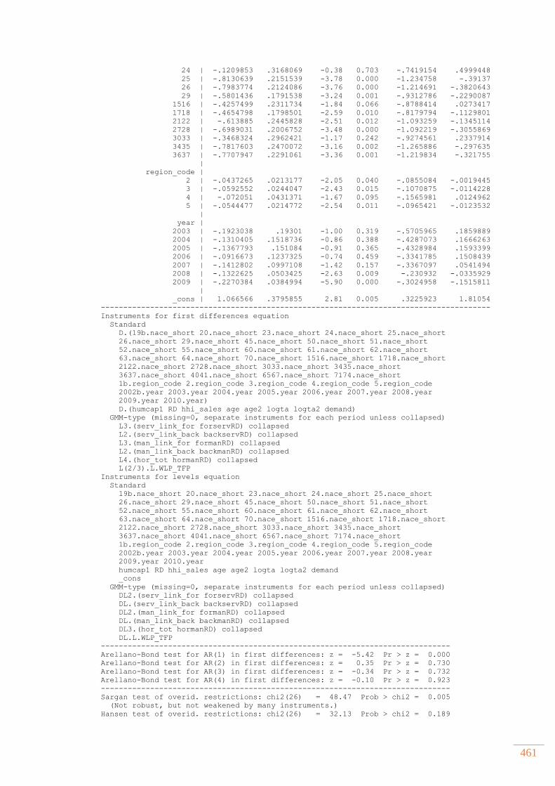
461
24 | -.1209853 .3168069 -0.38 0.703 -.7419154 .4999448
25 | -.8130639 .2151539 -3.78 0.000 -1.234758 -.39137
26 | -.7983774 .2124086 -3.76 0.000 -1.214691 -.3820643
29 | -.5801436 .1791538 -3.24 0.001 -.9312786 -.2290087
1516 | -.4257499 .2311734 -1.84 0.066 -.8788414 .0273417
1718 | -.4654798 .1798501 -2.59 0.010 -.8179794 -.1129801
2122 | -.613885 .2445828 -2.51 0.012 -1.093259 -.1345114
2728 | -.6989031 .2006752 -3.48 0.000 -1.092219 -.3055869
3033 | -.3468324 .2962421 -1.17 0.242 -.9274561 .2337914
3435 | -.7817603 .2470072 -3.16 0.002 -1.265886 -.297635
3637 | -.7707947 .2291061 -3.36 0.001 -1.219834 -.321755
|
region_code |
2 | -.0437265 .0213177 -2.05 0.040 -.0855084 -.0019445
3 | -.0592552 .0244047 -2.43 0.015 -.1070875 -.0114228
4 | -.072051 .0431371 -1.67 0.095 -.1565981 .0124962
5 | -.0544477 .0214772 -2.54 0.011 -.0965421 -.0123532
|
year |
2003 | -.1923038 .19301 -1.00 0.319 -.5705965 .1859889
2004 | -.1310405 .1518736 -0.86 0.388 -.4287073 .1666263
2005 | -.1367793 .151084 -0.91 0.365 -.4328984 .1593399
2006 | -.0916673 .1237325 -0.74 0.459 -.3341785 .1508439
2007 | -.1412802 .0997108 -1.42 0.157 -.3367097 .0541494
2008 | -.1322625 .0503425 -2.63 0.009 -.230932 -.0335929
2009 | -.2270384 .0384994 -5.90 0.000 -.3024958 -.1515811
|
_cons | 1.066566 .3795855 2.81 0.005 .3225923 1.81054
---------------------------------------------------------------------------------------
Instruments for first differences equation
Standard
D.(19b.nace_short 20.nace_short 23.nace_short 24.nace_short 25.nace_short
26.nace_short 29.nace_short 45.nace_short 50.nace_short 51.nace_short
52.nace_short 55.nace_short 60.nace_short 61.nace_short 62.nace_short
63.nace_short 64.nace_short 70.nace_short 1516.nace_short 1718.nace_short
2122.nace_short 2728.nace_short 3033.nace_short 3435.nace_short
3637.nace_short 4041.nace_short 6567.nace_short 7174.nace_short
1b.region_code 2.region_code 3.region_code 4.region_code 5.region_code
2002b.year 2003.year 2004.year 2005.year 2006.year 2007.year 2008.year
2009.year 2010.year)
D.(humcap1 RD hhi_sales age age2 logta logta2 demand)
GMM-type (missing=0, separate instruments for each period unless collapsed)
L3.(serv_link_for forservRD) collapsed
L2.(serv_link_back backservRD) collapsed
L3.(man_link_for formanRD) collapsed
L2.(man_link_back backmanRD) collapsed
L4.(hor_tot hormanRD) collapsed
L(2/3).L.WLP_TFP
Instruments for levels equation
Standard
19b.nace_short 20.nace_short 23.nace_short 24.nace_short 25.nace_short
26.nace_short 29.nace_short 45.nace_short 50.nace_short 51.nace_short
52.nace_short 55.nace_short 60.nace_short 61.nace_short 62.nace_short
63.nace_short 64.nace_short 70.nace_short 1516.nace_short 1718.nace_short
2122.nace_short 2728.nace_short 3033.nace_short 3435.nace_short
3637.nace_short 4041.nace_short 6567.nace_short 7174.nace_short
1b.region_code 2.region_code 3.region_code 4.region_code 5.region_code
2002b.year 2003.year 2004.year 2005.year 2006.year 2007.year 2008.year
2009.year 2010.year
humcap1 RD hhi_sales age age2 logta logta2 demand
_cons
GMM-type (missing=0, separate instruments for each period unless collapsed)
DL2.(serv_link_for forservRD) collapsed
DL.(serv_link_back backservRD) collapsed
DL2.(man_link_for formanRD) collapsed
DL.(man_link_back backmanRD) collapsed
DL3.(hor_tot hormanRD) collapsed
DL.L.WLP_TFP
------------------------------------------------------------------------------
Arellano-Bond test for AR(1) in first differences: z = -5.42 Pr > z = 0.000
Arellano-Bond test for AR(2) in first differences: z = 0.35 Pr > z = 0.730
Arellano-Bond test for AR(3) in first differences: z = -0.34 Pr > z = 0.732
Arellano-Bond test for AR(4) in first differences: z = -0.10 Pr > z = 0.923
------------------------------------------------------------------------------
Sargan test of overid. restrictions: chi2(26) = 48.47 Prob > chi2 = 0.005
(Not robust, but not weakened by many instruments.)
Hansen test of overid. restrictions: chi2(26) = 32.13 Prob > chi2 = 0.189
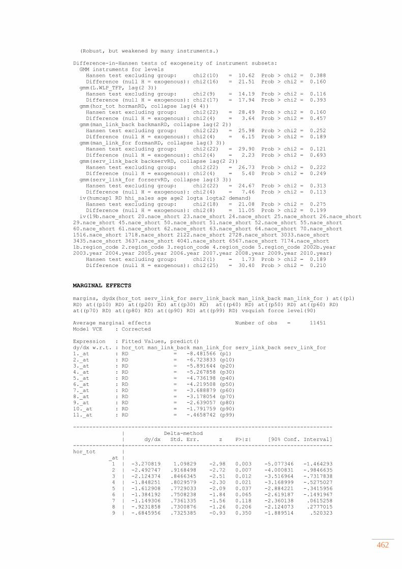
462
(Robust, but weakened by many instruments.)
Difference-in-Hansen tests of exogeneity of instrument subsets:
GMM instruments for levels
Hansen test excluding group: chi2(10) = 10.62 Prob > chi2 = 0.388
Difference (null H = exogenous): chi2(16) = 21.51 Prob > chi2 = 0.160
gmm(L.WLP_TFP, lag(2 3))
Hansen test excluding group: chi2(9) = 14.19 Prob > chi2 = 0.116
Difference (null H = exogenous): chi2(17) = 17.94 Prob > chi2 = 0.393
gmm(hor_tot hormanRD, collapse lag(4 4))
Hansen test excluding group: chi2(22) = 28.49 Prob > chi2 = 0.160
Difference (null H = exogenous): chi2(4) = 3.64 Prob > chi2 = 0.457
gmm(man_link_back backmanRD, collapse lag(2 2))
Hansen test excluding group: chi2(22) = 25.98 Prob > chi2 = 0.252
Difference (null H = exogenous): chi2(4) = 6.15 Prob > chi2 = 0.189
gmm(man_link_for formanRD, collapse lag(3 3))
Hansen test excluding group: chi2(22) = 29.90 Prob > chi2 = 0.121
Difference (null H = exogenous): chi2(4) = 2.23 Prob > chi2 = 0.693
gmm(serv_link_back backservRD, collapse lag(2 2))
Hansen test excluding group: chi2(22) = 26.73 Prob > chi2 = 0.222
Difference (null H = exogenous): chi2(4) = 5.40 Prob > chi2 = 0.249
gmm(serv_link_for forservRD, collapse lag(3 3))
Hansen test excluding group: chi2(22) = 24.67 Prob > chi2 = 0.313
Difference (null H = exogenous): chi2(4) = 7.46 Prob > chi2 = 0.113
iv(humcap1 RD hhi_sales age age2 logta logta2 demand)
Hansen test excluding group: chi2(18) = 21.08 Prob > chi2 = 0.275
Difference (null H = exogenous): chi2(8) = 11.05 Prob > chi2 = 0.199
iv(19b.nace_short 20.nace_short 23.nace_short 24.nace_short 25.nace_short 26.nace_short
29.nace_short 45.nace_short 50.nace_short 51.nace_short 52.nace_short 55.nace_short
60.nace_short 61.nace_short 62.nace_short 63.nace_short 64.nace_short 70.nace_short
1516.nace_short 1718.nace_short 2122.nace_short 2728.nace_short 3033.nace_short
3435.nace_short 3637.nace_short 4041.nace_short 6567.nace_short 7174.nace_short
1b.region_code 2.region_code 3.region_code 4.region_code 5.region_code 2002b.year
2003.year 2004.year 2005.year 2006.year 2007.year 2008.year 2009.year 2010.year)
Hansen test excluding group: chi2(1) = 1.73 Prob > chi2 = 0.189
Difference (null H = exogenous): chi2(25) = 30.40 Prob > chi2 = 0.210
MARGINAL EFFECTS
margins, dydx(hor_tot serv_link_for serv_link_back man_link_back man_link_for ) at((p1)
RD) at((p10) RD) at((p20) RD) at((p30) RD) at((p40) RD) at((p50) RD) at((p60) RD)
at((p70) RD) at((p80) RD) at((p90) RD) at((p99) RD) vsquish force level(90)
Average marginal effects Number of obs = 11451
Model VCE : Corrected
Expression : Fitted Values, predict()
dy/dx w.r.t. : hor_tot man_link_back man_link_for serv_link_back serv_link_for
1._at : RD = -8.481566 (p1)
2._at : RD = -6.723833 (p10)
3._at : RD = -5.891644 (p20)
4._at : RD = -5.267858 (p30)
5._at : RD = -4.736198 (p40)
6._at : RD = -4.219508 (p50)
7._at : RD = -3.688879 (p60)
8._at : RD = -3.178054 (p70)
9._at : RD = -2.639057 (p80)
10._at : RD = -1.791759 (p90)
11._at : RD = -.4658742 (p99)
--------------------------------------------------------------------------------
| Delta-method
| dy/dx Std. Err. z P>|z| [90% Conf. Interval]
---------------+----------------------------------------------------------------
hor_tot |
_at |
1 | -3.270819 1.09829 -2.98 0.003 -5.077346 -1.464293
2 | -2.492747 .9168498 -2.72 0.007 -4.000831 -.9846635
3 | -2.124374 .8466345 -2.51 0.012 -3.516964 -.7317838
4 | -1.848251 .8029579 -2.30 0.021 -3.168999 -.5275027
5 | -1.612908 .7729033 -2.09 0.037 -2.884221 -.3415956
6 | -1.384192 .7508238 -1.84 0.065 -2.619187 -.1491967
7 | -1.149306 .7361335 -1.56 0.118 -2.360138 .0615258
8 | -.9231858 .7300876 -1.26 0.206 -2.124073 .2777015
9 | -.6845956 .7325385 -0.93 0.350 -1.889514 .520323
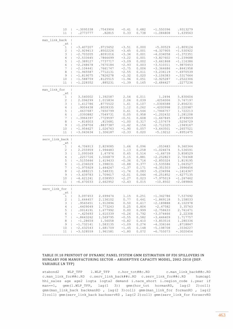
463
10 | -.3095338 .7543904 -0.41 0.682 -1.550396 .9313279
11 | .2773777 .82815 0.33 0.738 -1.084808 1.639563
---------------+----------------------------------------------------------------
man_link_back |
_at |
1 | -3.407207 .9715652 -3.51 0.000 -5.00529 -1.809124
2 | -2.929413 .8502226 -3.45 0.001 -4.327905 -1.530922
3 | -2.703205 .8091016 -3.34 0.001 -4.034058 -1.372351
4 | -2.533645 .7866699 -3.22 0.001 -3.827602 -1.239688
5 | -2.389127 .7737717 -3.09 0.002 -3.661868 -1.116386
6 | -2.248678 .7670184 -2.93 0.003 -3.510311 -.9870453
7 | -2.104441 .7661747 -2.75 0.006 -3.364686 -.8441958
8 | -1.965587 .7712131 -2.55 0.011 -3.234119 -.6970539
9 | -1.819075 .7826278 -2.32 0.020 -3.106383 -.5317664
10 | -1.588759 .8125515 -1.96 0.051 -2.925287 -.2522306
11 | -1.228352 .885231 -1.39 0.165 -2.684427 .2277236
---------------+----------------------------------------------------------------
man_link_for |
_at |
1 | 3.540002 1.392587 2.54 0.011 1.2494 5.830604
2 | 2.096299 1.015834 2.06 0.039 .4254006 3.767197
3 | 1.412786 .8775522 1.61 0.107 -.0306588 2.856231
4 | .9004438 .8028335 1.12 0.262 -.4200998 2.220987
5 | .4637687 .7650799 0.61 0.544 -.7946757 1.722213
6 | .0393882 .7549731 0.05 0.958 -1.202432 1.281208
7 | -.3964397 .7729597 -0.51 0.608 -1.667845 .8749659
8 | -.816003 .815681 -1.00 0.317 -2.157679 .5256729
9 | -1.258704 .8837387 -1.42 0.154 -2.712325 .1949167
10 | -1.954627 1.026763 -1.90 0.057 -3.643501 -.2657521
11 | -3.043634 1.306187 -2.33 0.020 -5.19212 -.8951475
---------------+----------------------------------------------------------------
serv_link_back |
_at |
1 | 4.706913 2.829085 1.66 0.096 .053483 9.360344
2 | 2.255959 1.994483 1.13 0.258 -1.024674 5.536591
3 | 1.095569 1.67976 0.65 0.514 -1.66739 3.858529
4 | .2257726 1.506879 0.15 0.881 -2.252823 2.704368
5 | -.5155646 1.419433 -0.36 0.716 -2.850324 1.819195
6 | -1.236029 1.398031 -0.88 0.377 -3.535586 1.063527
7 | -1.975929 1.444247 -1.37 0.171 -4.351503 .3996456
8 | -2.688215 1.548331 -1.74 0.083 -5.234994 -.1414367
9 | -3.439783 1.709617 -2.01 0.044 -6.251852 -.6277135
10 | -4.621241 2.038953 -2.27 0.023 -7.975019 -1.267462
11 | -6.470033 2.662952 -2.43 0.015 -10.8502 -2.089866
---------------+----------------------------------------------------------------
serv_link_for |
_at |
1 | 3.097453 2.699474 1.15 0.251 -1.342786 7.537692
2 | 1.644457 2.136102 0.77 0.441 -1.869118 5.158033
3 | .9565451 1.912896 0.50 0.617 -2.189888 4.102978
4 | .4409049 1.773243 0.25 0.804 -2.47582 3.35763
5 | .0014191 1.677992 0.00 0.999 -2.758633 2.761471
6 | -.425693 1.610339 -0.26 0.792 -3.074466 2.22308
7 | -.8643262 1.569795 -0.55 0.582 -3.446409 1.717757
8 | -1.28659 1.56058 -0.82 0.410 -3.853516 1.280336
9 | -1.732141 1.583135 -1.09 0.274 -4.336166 .8718847
10 | -2.432543 1.681709 -1.45 0.148 -5.198708 .3336227
11 | -3.528559 1.961581 -1.80 0.072 -6.755073 -.3020454
--------------------------------------------------------------------------------
TABLE IV.18 PRINTOUT OF DYNAMIC PANEL SYSTEM GMM ESTIMATION OF FDI SPILLOVERS IN HUNGARY FOR MANUFACTURING SECTOR – ABSORPTIVE CAPACITY MODEL, 2002-2010 (DEP. VARIABLE LN TFP)
xtabond2 WLP_TFP l.WLP_TFP c.hor_tot##c.RD c.man_link_back##c.RD
c.man_link_for##c.RD c.serv_link_back##c.RD c.serv_link_for##c.RD humcap1
hhi_sales age age2 logta logta2 demand i.nace_short i.region_code i.year if
man==1, gmm(l.WLP_TFP, lag(1 3)) gmm(hor_tot hormanRD, lag(2 2)coll)
gmm(man_link_back backmanRD , lag(2 3)coll) gmm(man_link_for formanRD , lag(2
2)coll) gmm(serv_link_back backservRD , lag(2 2)coll) gmm(serv_link_for forservRD
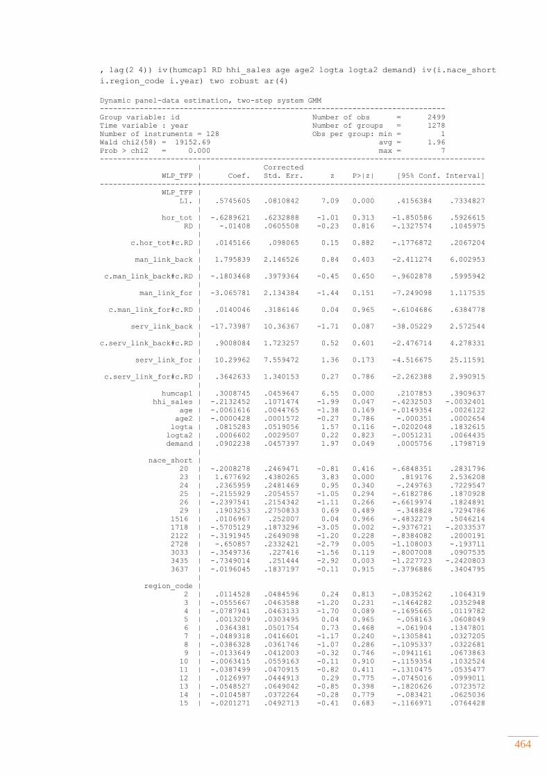
464
, lag(2 4)) iv(humcap1 RD hhi_sales age age2 logta logta2 demand) iv(i.nace_short
i.region_code i.year) two robust ar(4)
Dynamic panel-data estimation, two-step system GMM
------------------------------------------------------------------------------
Group variable: id Number of obs = 2499
Time variable : year Number of groups = 1278
Number of instruments = 128 Obs per group: min = 1
Wald chi2(58) = 19152.69 avg = 1.96
Prob > chi2 = 0.000 max = 7
---------------------------------------------------------------------------------------
| Corrected
WLP_TFP | Coef. Std. Err. z P>|z| [95% Conf. Interval]
----------------------+----------------------------------------------------------------
WLP_TFP |
L1. | .5745605 .0810842 7.09 0.000 .4156384 .7334827
|
hor_tot | -.6289621 .6232888 -1.01 0.313 -1.850586 .5926615
RD | -.01408 .0605508 -0.23 0.816 -.1327574 .1045975
|
c.hor_tot#c.RD | .0145166 .098065 0.15 0.882 -.1776872 .2067204
|
man_link_back | 1.795839 2.146526 0.84 0.403 -2.411274 6.002953
|
c.man_link_back#c.RD | -.1803468 .3979364 -0.45 0.650 -.9602878 .5995942
|
man_link_for | -3.065781 2.134384 -1.44 0.151 -7.249098 1.117535
|
c.man_link_for#c.RD | .0140046 .3186146 0.04 0.965 -.6104686 .6384778
|
serv_link_back | -17.73987 10.36367 -1.71 0.087 -38.05229 2.572544
|
c.serv_link_back#c.RD | .9008084 1.723257 0.52 0.601 -2.476714 4.278331
|
serv_link_for | 10.29962 7.559472 1.36 0.173 -4.516675 25.11591
|
c.serv_link_for#c.RD | .3642633 1.340153 0.27 0.786 -2.262388 2.990915
|
humcap1 | .3008745 .0459647 6.55 0.000 .2107853 .3909637
hhi_sales | -.2132452 .1071474 -1.99 0.047 -.4232503 -.0032401
age | -.0061616 .0044765 -1.38 0.169 -.0149354 .0026122
age2 | -.0000428 .0001572 -0.27 0.786 -.000351 .0002654
logta | .0815283 .0519056 1.57 0.116 -.0202048 .1832615
logta2 | .0006602 .0029507 0.22 0.823 -.0051231 .0064435
demand | .0902238 .0457397 1.97 0.049 .0005756 .1798719
|
nace_short |
20 | -.2008278 .2469471 -0.81 0.416 -.6848351 .2831796
23 | 1.677692 .4380265 3.83 0.000 .819176 2.536208
24 | .2365959 .2481469 0.95 0.340 -.249763 .7229547
25 | -.2155929 .2054557 -1.05 0.294 -.6182786 .1870928
26 | -.2397541 .2154342 -1.11 0.266 -.6619974 .1824891
29 | .1903253 .2750833 0.69 0.489 -.348828 .7294786
1516 | .0106967 .252007 0.04 0.966 -.4832279 .5046214
1718 | -.5705129 .1873296 -3.05 0.002 -.9376721 -.2033537
2122 | -.3191945 .2649098 -1.20 0.228 -.8384082 .2000191
2728 | -.650857 .2332421 -2.79 0.005 -1.108003 -.193711
3033 | -.3549736 .227416 -1.56 0.119 -.8007008 .0907535
3435 | -.7349014 .251444 -2.92 0.003 -1.227723 -.2420803
3637 | -.0196045 .1837197 -0.11 0.915 -.3796886 .3404795
|
region_code |
2 | .0114528 .0484596 0.24 0.813 -.0835262 .1064319
3 | -.0555667 .0463588 -1.20 0.231 -.1464282 .0352948
4 | -.0787941 .0463133 -1.70 0.089 -.1695665 .0119782
5 | .0013209 .0303495 0.04 0.965 -.058163 .0608049
6 | .0364381 .0501754 0.73 0.468 -.061904 .1347801
7 | -.0489318 .0416601 -1.17 0.240 -.1305841 .0327205
8 | -.0386328 .0361746 -1.07 0.286 -.1095337 .0322681
9 | -.0133649 .0412003 -0.32 0.746 -.0941161 .0673863
10 | -.0063415 .0559163 -0.11 0.910 -.1159354 .1032524
11 | -.0387499 .0470915 -0.82 0.411 -.1310475 .0535477
12 | .0126997 .0444913 0.29 0.775 -.0745016 .0999011
13 | -.0548527 .0649042 -0.85 0.398 -.1820626 .0723572
14 | -.0104587 .0372264 -0.28 0.779 -.083421 .0625036
15 | -.0201271 .0492713 -0.41 0.683 -.1166971 .0764428

465
16 | -.0350971 .0525557 -0.67 0.504 -.1381044 .0679102
17 | -.0372186 .0727308 -0.51 0.609 -.1797683 .1053311
18 | -.0494037 .0604681 -0.82 0.414 -.167919 .0691116
19 | -.0132848 .0517498 -0.26 0.797 -.1147125 .0881428
20 | -.0635834 .0510931 -1.24 0.213 -.1637241 .0365573
|
year |
2004 | -.293952 .2966098 -0.99 0.322 -.8752965 .2873924
2005 | -.4365163 .3051257 -1.43 0.153 -1.034552 .1615191
2006 | -.4099029 .3095513 -1.32 0.185 -1.016612 .1968065
2007 | -.4472685 .3105319 -1.44 0.150 -1.0559 .1613629
2008 | -.4690899 .3169312 -1.48 0.139 -1.090264 .1520839
2009 | -.5873773 .3135883 -1.87 0.061 -1.201999 .0272445
2010 | -.4408848 .3078028 -1.43 0.152 -1.044167 .1623976
|
_cons | .7251025 .6283147 1.15 0.248 -.5063718 1.956577
---------------------------------------------------------------------------------------
------------------------------------------------------------------------------
Arellano-Bond test for AR(1) in first differences: z = -3.68 Pr > z = 0.000
Arellano-Bond test for AR(2) in first differences: z = 0.63 Pr > z = 0.530
Arellano-Bond test for AR(3) in first differences: z = -0.90 Pr > z = 0.368
Arellano-Bond test for AR(4) in first differences: z = -0.66 Pr > z = 0.508
------------------------------------------------------------------------------
Sargan test of overid. restrictions: chi2(69) = 77.04 Prob > chi2 = 0.237
(Not robust, but not weakened by many instruments.)
Hansen test of overid. restrictions: chi2(69) = 59.76 Prob > chi2 = 0.778
(Robust, but weakened by many instruments.)
Difference-in-Hansen tests of exogeneity of instrument subsets:
GMM instruments for levels
Hansen test excluding group: chi2(41) = 40.93 Prob > chi2 = 0.473
Difference (null H = exogenous): chi2(28) = 18.83 Prob > chi2 = 0.903
gmm(L.WLP_TFP, lag(1 3))
Hansen test excluding group: chi2(47) = 46.97 Prob > chi2 = 0.474
Difference (null H = exogenous): chi2(22) = 12.79 Prob > chi2 = 0.939
gmm(hor_tot hormanRD, collapse lag(2 2))
Hansen test excluding group: chi2(66) = 56.23 Prob > chi2 = 0.799
Difference (null H = exogenous): chi2(3) = 3.54 Prob > chi2 = 0.316
gmm(man_link_back backmanRD, collapse lag(2 3))
Hansen test excluding group: chi2(63) = 57.93 Prob > chi2 = 0.657
Difference (null H = exogenous): chi2(6) = 1.84 Prob > chi2 = 0.934
gmm(man_link_for formanRD, collapse lag(2 2))
Hansen test excluding group: chi2(65) = 58.24 Prob > chi2 = 0.711
Difference (null H = exogenous): chi2(4) = 1.52 Prob > chi2 = 0.823
gmm(serv_link_back backservRD, collapse lag(2 2))
Hansen test excluding group: chi2(65) = 58.89 Prob > chi2 = 0.690
Difference (null H = exogenous): chi2(4) = 0.87 Prob > chi2 = 0.928
gmm(serv_link_for forservRD, lag(2 4))
Hansen test excluding group: chi2(28) = 25.12 Prob > chi2 = 0.621
Difference (null H = exogenous): chi2(41) = 34.64 Prob > chi2 = 0.748
iv(humcap1 RD hhi_sales age age2 logta logta2 demand)
Hansen test excluding group: chi2(61) = 49.05 Prob > chi2 = 0.864
Difference (null H = exogenous): chi2(8) = 10.71 Prob > chi2 = 0.219
iv(19b.nace_short 20.nace_short 23.nace_short 24.nace_short 25.nace_short 26.nace_short
29.nace_short 45.nace_short 50.nace_short 51.nace_short 52.nace_short 55.nace_short
60.nace_short 61.nace_short 62.nace_short 63.nace_short 64.nace_short 70.nace_short
1516.nace_short 1718.nace_short 2122.nace_short 2728.nace_short 3033.nace_short
3435.nace_short 3637.nace_short 4041.nace_short 6567.nace_short 7174.nace_short
1b.region_code 2.region_code 3.region_code 4.region_code 5.region_code 6.region_code
7.region_code 8.region_code 9.region_code 10.region_code 11.region_code 12.region_code
13.region_code 14.region_code 15.region_code 16.region_code 17.region_code 18.region_code
19.region_code 20.region_code 2002b.year 2003.year 2004.year 2005.year 2006.year
2007.year 2008.year 2009.year 2010.year)
Hansen test excluding group: chi2(29) = 19.97 Prob > chi2 = 0.894
Difference (null H = exogenous): chi2(40) = 39.79 Prob > chi2 = 0.480
MARGINAL EFFECTS
margins, dydx(hor_tot serv_link_for serv_link_back man_link_back man_link_for ) at((p1)
RD) at((p10) RD) at((p20) RD) at((p30) RD) at((p40) RD) at((p50) RD) at((p60) RD)
at((p70) RD) at((p80) RD) at((p90) RD) at((p99) RD) vsquish force level(90)
Average marginal effects Number of obs = 2499
Model VCE : Corrected
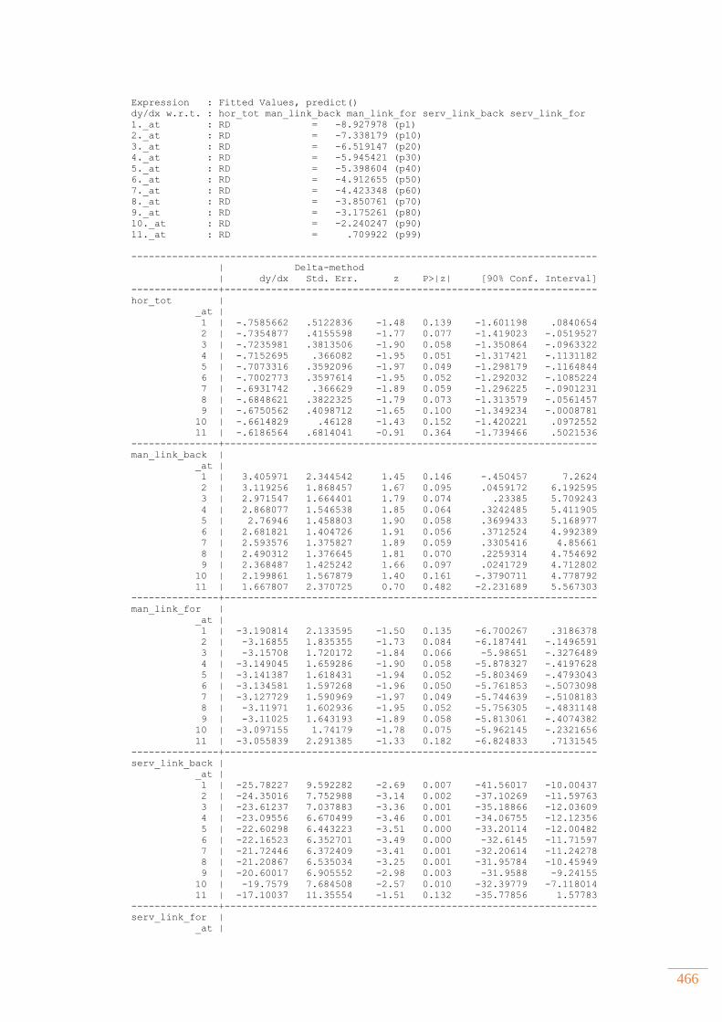
466
Expression : Fitted Values, predict()
dy/dx w.r.t. : hor_tot man_link_back man_link_for serv_link_back serv_link_for
1._at : RD = -8.927978 (p1)
2._at : RD = -7.338179 (p10)
3._at : RD = -6.519147 (p20)
4._at : RD = -5.945421 (p30)
5._at : RD = -5.398604 (p40)
6._at : RD = -4.912655 (p50)
7._at : RD = -4.423348 (p60)
8._at : RD = -3.850761 (p70)
9._at : RD = -3.175261 (p80)
10._at : RD = -2.240247 (p90)
11._at : RD = .709922 (p99)
--------------------------------------------------------------------------------
| Delta-method
| dy/dx Std. Err. z P>|z| [90% Conf. Interval]
---------------+----------------------------------------------------------------
hor_tot |
_at |
1 | -.7585662 .5122836 -1.48 0.139 -1.601198 .0840654
2 | -.7354877 .4155598 -1.77 0.077 -1.419023 -.0519527
3 | -.7235981 .3813506 -1.90 0.058 -1.350864 -.0963322
4 | -.7152695 .366082 -1.95 0.051 -1.317421 -.1131182
5 | -.7073316 .3592096 -1.97 0.049 -1.298179 -.1164844
6 | -.7002773 .3597614 -1.95 0.052 -1.292032 -.1085224
7 | -.6931742 .366629 -1.89 0.059 -1.296225 -.0901231
8 | -.6848621 .3822325 -1.79 0.073 -1.313579 -.0561457
9 | -.6750562 .4098712 -1.65 0.100 -1.349234 -.0008781
10 | -.6614829 .46128 -1.43 0.152 -1.420221 .0972552
11 | -.6186564 .6814041 -0.91 0.364 -1.739466 .5021536
---------------+----------------------------------------------------------------
man_link_back |
_at |
1 | 3.405971 2.344542 1.45 0.146 -.450457 7.2624
2 | 3.119256 1.868457 1.67 0.095 .0459172 6.192595
3 | 2.971547 1.664401 1.79 0.074 .23385 5.709243
4 | 2.868077 1.546538 1.85 0.064 .3242485 5.411905
5 | 2.76946 1.458803 1.90 0.058 .3699433 5.168977
6 | 2.681821 1.404726 1.91 0.056 .3712524 4.992389
7 | 2.593576 1.375827 1.89 0.059 .3305416 4.85661
8 | 2.490312 1.376645 1.81 0.070 .2259314 4.754692
9 | 2.368487 1.425242 1.66 0.097 .0241729 4.712802
10 | 2.199861 1.567879 1.40 0.161 -.3790711 4.778792
11 | 1.667807 2.370725 0.70 0.482 -2.231689 5.567303
---------------+----------------------------------------------------------------
man_link_for |
_at |
1 | -3.190814 2.133595 -1.50 0.135 -6.700267 .3186378
2 | -3.16855 1.835355 -1.73 0.084 -6.187441 -.1496591
3 | -3.15708 1.720172 -1.84 0.066 -5.98651 -.3276489
4 | -3.149045 1.659286 -1.90 0.058 -5.878327 -.4197628
5 | -3.141387 1.618431 -1.94 0.052 -5.803469 -.4793043
6 | -3.134581 1.597268 -1.96 0.050 -5.761853 -.5073098
7 | -3.127729 1.590969 -1.97 0.049 -5.744639 -.5108183
8 | -3.11971 1.602936 -1.95 0.052 -5.756305 -.4831148
9 | -3.11025 1.643193 -1.89 0.058 -5.813061 -.4074382
10 | -3.097155 1.74179 -1.78 0.075 -5.962145 -.2321656
11 | -3.055839 2.291385 -1.33 0.182 -6.824833 .7131545
---------------+----------------------------------------------------------------
serv_link_back |
_at |
1 | -25.78227 9.592282 -2.69 0.007 -41.56017 -10.00437
2 | -24.35016 7.752988 -3.14 0.002 -37.10269 -11.59763
3 | -23.61237 7.037883 -3.36 0.001 -35.18866 -12.03609
4 | -23.09556 6.670499 -3.46 0.001 -34.06755 -12.12356
5 | -22.60298 6.443223 -3.51 0.000 -33.20114 -12.00482
6 | -22.16523 6.352701 -3.49 0.000 -32.6145 -11.71597
7 | -21.72446 6.372409 -3.41 0.001 -32.20614 -11.24278
8 | -21.20867 6.535034 -3.25 0.001 -31.95784 -10.45949
9 | -20.60017 6.905552 -2.98 0.003 -31.9588 -9.24155
10 | -19.7579 7.684508 -2.57 0.010 -32.39779 -7.118014
11 | -17.10037 11.35554 -1.51 0.132 -35.77856 1.57783
---------------+----------------------------------------------------------------
serv_link_for |
_at |

467
1 | 7.047483 7.161442 0.98 0.325 -4.732041 18.82701
2 | 7.626589 5.601515 1.36 0.173 -1.587084 16.84026
3 | 7.924932 4.966233 1.60 0.111 -.2437954 16.09366
4 | 8.133919 4.625563 1.76 0.079 .5255445 15.74229
5 | 8.333105 4.402492 1.89 0.058 1.09165 15.57456
6 | 8.510118 4.300416 1.98 0.048 1.436564 15.58367
7 | 8.688354 4.29606 2.02 0.043 1.621965 15.75474
8 | 8.896927 4.416371 2.01 0.044 1.632643 16.16121
9 | 9.142987 4.717533 1.94 0.053 1.383335 16.90264
10 | 9.483578 5.363509 1.77 0.077 .6613901 18.30577
11 | 10.55822 8.360629 1.26 0.207 -3.193794 24.31023
--------------------------------------------------------------------------------
TABLE IV.19 PRINTOUT OF DYNAMIC PANEL SYSTEM GMM ESTIMATION OF FDI SPILLOVERS IN SLOVAKIA FOR MANUFACTURING SECTOR – ABSORPTIVE CAPACITY MODEL, 2002-2009 (DEP. VARIABLE LN TFP)
xtabond2 WLP_TFP l.WLP_TFP c.hor_tot##c.RD c.man_link_back##c.RD
c.man_link_for##c.RD c.serv_link_back##c.RD c.serv_link_for##c.RD humcap1
hhi_sales age age2 logta logta2 demand i.nace_short i.region_code i.year if
man==1, gmm(l.WLP_TFP, lag(1 1)) gmm(hor_tot hormanRD, lag(3 5)coll)
gmm(man_link_back backmanRD , lag(3 3)coll) gmm(man_link_for formanRD , lag(2
2)coll) gmm(serv_link_back backservRD, lag(4 5)coll) gmm(serv_link_for forservRD
, lag(3 3)coll) iv(humcap1 RD hhi_sales age age2 logta logta2 demand)
iv(i.nace_short i.region_code i.year) two robust ar(4)
Dynamic panel-data estimation, two-step system GMM
------------------------------------------------------------------------------
Group variable: id Number of obs = 8140
Time variable : year Number of groups = 3074
Number of instruments = 73 Obs per group: min = 1
Wald chi2(45) = 9819.81 avg = 2.65
Prob > chi2 = 0.000 max = 7
---------------------------------------------------------------------------------------
| Corrected
WLP_TFP | Coef. Std. Err. z P>|z| [95% Conf. Interval]
----------------------+----------------------------------------------------------------
WLP_TFP |
L1. | .3781589 .0430071 8.79 0.000 .2938665 .4624514
|
hor_tot | -.1759973 .4060463 -0.43 0.665 -.9718334 .6198389
RD | .0595949 .0177793 3.35 0.001 .0247482 .0944417
|
c.hor_tot#c.RD | .0401559 .0684296 0.59 0.557 -.0939636 .1742754
|
man_link_back | 2.132375 2.130756 1.00 0.317 -2.043831 6.308581
|
c.man_link_back#c.RD | .0095497 .2938846 0.03 0.974 -.5664536 .585553
|
man_link_for | -1.96545 1.330002 -1.48 0.139 -4.572206 .6413051
|
c.man_link_for#c.RD | -.2941371 .220599 -1.33 0.182 -.7265032 .1382291
|
serv_link_back | -.1984027 10.13448 -0.02 0.984 -20.06161 19.66481
|
c.serv_link_back#c.RD | -.7958473 1.735153 -0.46 0.646 -4.196684 2.60499
|
serv_link_for | 12.15999 3.849272 3.16 0.002 4.615558 19.70443
|
c.serv_link_for#c.RD | 1.001284 .5655917 1.77 0.077 -.1072554 2.109823
|
humcap1 | .3313668 .0143665 23.07 0.000 .303209 .3595246
hhi_sales | -.1777632 .1132603 -1.57 0.117 -.3997493 .044223
age | -.0099069 .0026533 -3.73 0.000 -.0151073 -.0047065
age2 | .0001 .0000495 2.02 0.043 3.02e-06 .0001969
logta | .1652801 .0355182 4.65 0.000 .0956657 .2348944
logta2 | -.0037996 .0022068 -1.72 0.085 -.0081249 .0005258
demand | -.0192314 .0163452 -1.18 0.239 -.0512674 .0128046
|
nace_short |
20 | -.1007014 .1489164 -0.68 0.499 -.3925721 .1911693
23 | 1.122005 .2183843 5.14 0.000 .6939798 1.550031
24 | .8713452 .1301722 6.69 0.000 .6162124 1.126478
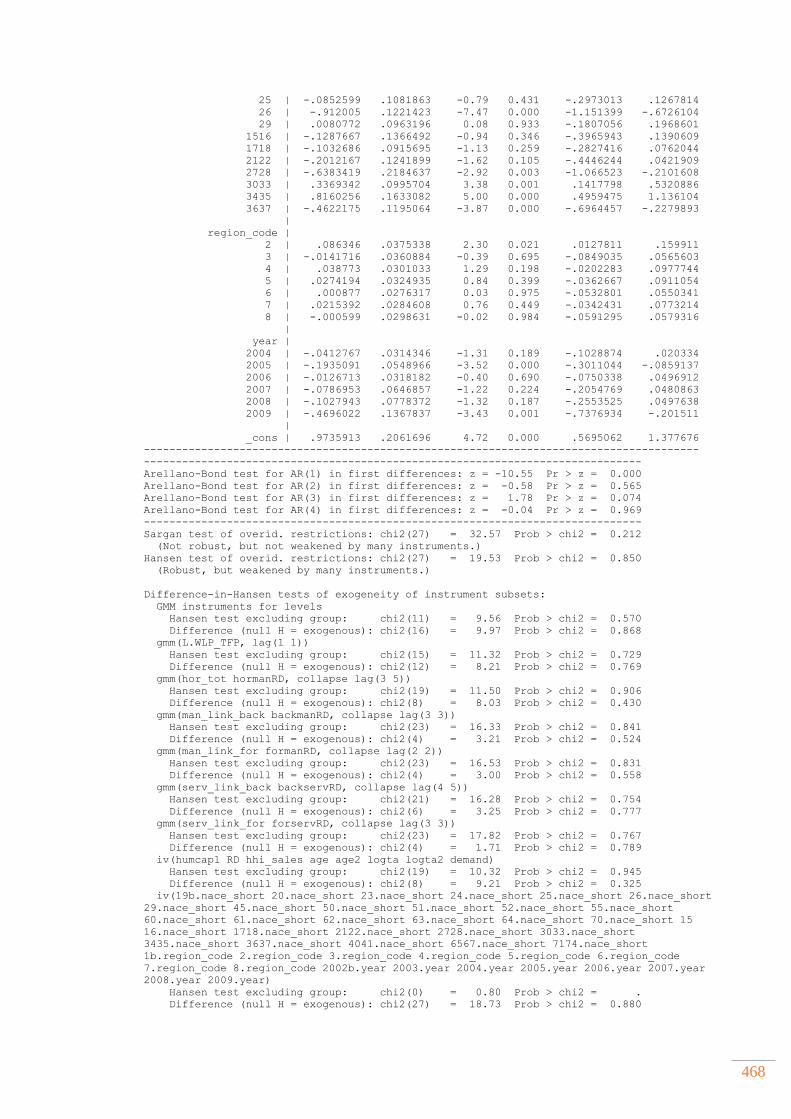
468
25 | -.0852599 .1081863 -0.79 0.431 -.2973013 .1267814
26 | -.912005 .1221423 -7.47 0.000 -1.151399 -.6726104
29 | .0080772 .0963196 0.08 0.933 -.1807056 .1968601
1516 | -.1287667 .1366492 -0.94 0.346 -.3965943 .1390609
1718 | -.1032686 .0915695 -1.13 0.259 -.2827416 .0762044
2122 | -.2012167 .1241899 -1.62 0.105 -.4446244 .0421909
2728 | -.6383419 .2184637 -2.92 0.003 -1.066523 -.2101608
3033 | .3369342 .0995704 3.38 0.001 .1417798 .5320886
3435 | .8160256 .1633082 5.00 0.000 .4959475 1.136104
3637 | -.4622175 .1195064 -3.87 0.000 -.6964457 -.2279893
|
region_code |
2 | .086346 .0375338 2.30 0.021 .0127811 .159911
3 | -.0141716 .0360884 -0.39 0.695 -.0849035 .0565603
4 | .038773 .0301033 1.29 0.198 -.0202283 .0977744
5 | .0274194 .0324935 0.84 0.399 -.0362667 .0911054
6 | .000877 .0276317 0.03 0.975 -.0532801 .0550341
7 | .0215392 .0284608 0.76 0.449 -.0342431 .0773214
8 | -.000599 .0298631 -0.02 0.984 -.0591295 .0579316
|
year |
2004 | -.0412767 .0314346 -1.31 0.189 -.1028874 .020334
2005 | -.1935091 .0548966 -3.52 0.000 -.3011044 -.0859137
2006 | -.0126713 .0318182 -0.40 0.690 -.0750338 .0496912
2007 | -.0786953 .0646857 -1.22 0.224 -.2054769 .0480863
2008 | -.1027943 .0778372 -1.32 0.187 -.2553525 .0497638
2009 | -.4696022 .1367837 -3.43 0.001 -.7376934 -.201511
|
_cons | .9735913 .2061696 4.72 0.000 .5695062 1.377676
---------------------------------------------------------------------------------------
------------------------------------------------------------------------------
Arellano-Bond test for AR(1) in first differences: z = -10.55 Pr > z = 0.000
Arellano-Bond test for AR(2) in first differences: z = -0.58 Pr > z = 0.565
Arellano-Bond test for AR(3) in first differences: z = 1.78 Pr > z = 0.074
Arellano-Bond test for AR(4) in first differences: z = -0.04 Pr > z = 0.969
------------------------------------------------------------------------------
Sargan test of overid. restrictions: chi2(27) = 32.57 Prob > chi2 = 0.212
(Not robust, but not weakened by many instruments.)
Hansen test of overid. restrictions: chi2(27) = 19.53 Prob > chi2 = 0.850
(Robust, but weakened by many instruments.)
Difference-in-Hansen tests of exogeneity of instrument subsets:
GMM instruments for levels
Hansen test excluding group: chi2(11) = 9.56 Prob > chi2 = 0.570
Difference (null H = exogenous): chi2(16) = 9.97 Prob > chi2 = 0.868
gmm(L.WLP_TFP, lag(1 1))
Hansen test excluding group: chi2(15) = 11.32 Prob > chi2 = 0.729
Difference (null H = exogenous): chi2(12) = 8.21 Prob > chi2 = 0.769
gmm(hor_tot hormanRD, collapse lag(3 5))
Hansen test excluding group: chi2(19) = 11.50 Prob > chi2 = 0.906
Difference (null H = exogenous): chi2(8) = 8.03 Prob > chi2 = 0.430
gmm(man_link_back backmanRD, collapse lag(3 3))
Hansen test excluding group: chi2(23) = 16.33 Prob > chi2 = 0.841
Difference (null H = exogenous): chi2(4) = 3.21 Prob > chi2 = 0.524
gmm(man_link_for formanRD, collapse lag(2 2))
Hansen test excluding group: chi2(23) = 16.53 Prob > chi2 = 0.831
Difference (null H = exogenous): chi2(4) = 3.00 Prob > chi2 = 0.558
gmm(serv_link_back backservRD, collapse lag(4 5))
Hansen test excluding group: chi2(21) = 16.28 Prob > chi2 = 0.754
Difference (null H = exogenous): chi2(6) = 3.25 Prob > chi2 = 0.777
gmm(serv_link_for forservRD, collapse lag(3 3))
Hansen test excluding group: chi2(23) = 17.82 Prob > chi2 = 0.767
Difference (null H = exogenous): chi2(4) = 1.71 Prob > chi2 = 0.789
iv(humcap1 RD hhi_sales age age2 logta logta2 demand)
Hansen test excluding group: chi2(19) = 10.32 Prob > chi2 = 0.945
Difference (null H = exogenous): chi2(8) = 9.21 Prob > chi2 = 0.325
iv(19b.nace_short 20.nace_short 23.nace_short 24.nace_short 25.nace_short 26.nace_short
29.nace_short 45.nace_short 50.nace_short 51.nace_short 52.nace_short 55.nace_short
60.nace_short 61.nace_short 62.nace_short 63.nace_short 64.nace_short 70.nace_short 15
16.nace_short 1718.nace_short 2122.nace_short 2728.nace_short 3033.nace_short
3435.nace_short 3637.nace_short 4041.nace_short 6567.nace_short 7174.nace_short
1b.region_code 2.region_code 3.region_code 4.region_code 5.region_code 6.region_code
7.region_code 8.region_code 2002b.year 2003.year 2004.year 2005.year 2006.year 2007.year
2008.year 2009.year)
Hansen test excluding group: chi2(0) = 0.80 Prob > chi2 = .
Difference (null H = exogenous): chi2(27) = 18.73 Prob > chi2 = 0.880
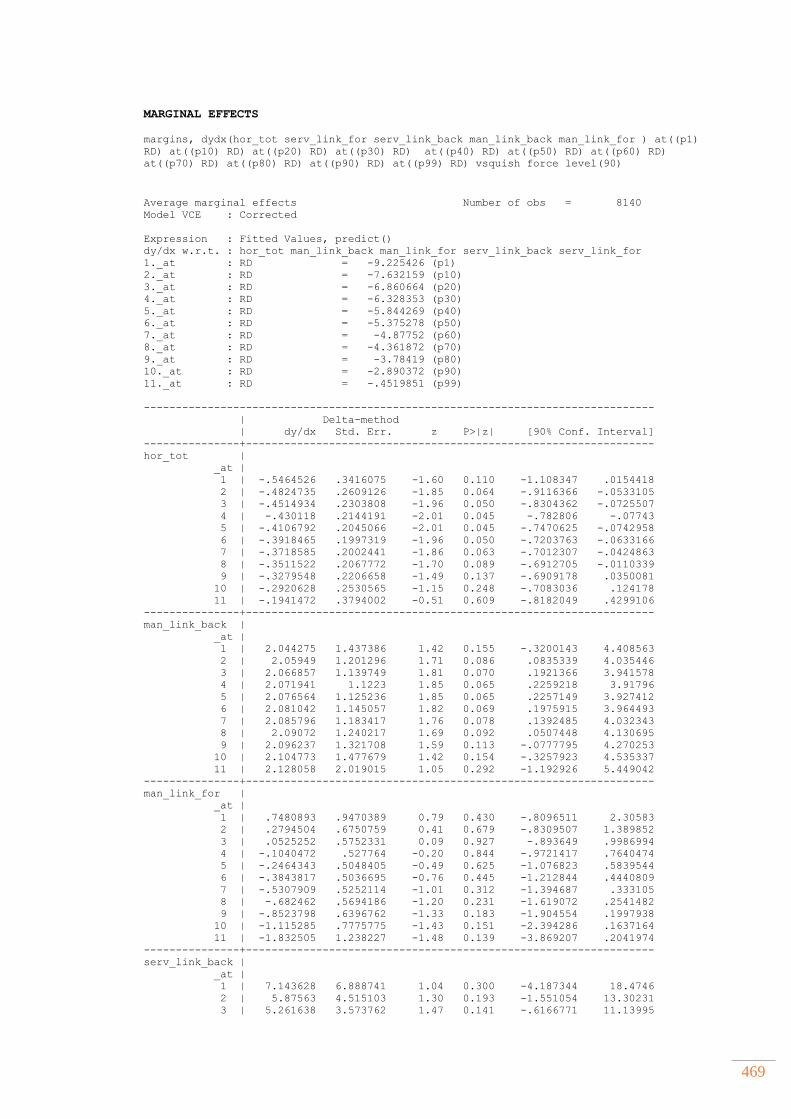
469
MARGINAL EFFECTS
margins, dydx(hor_tot serv_link_for serv_link_back man_link_back man_link_for ) at((p1)
RD) at((p10) RD) at((p20) RD) at((p30) RD) at((p40) RD) at((p50) RD) at((p60) RD)
at((p70) RD) at((p80) RD) at((p90) RD) at((p99) RD) vsquish force level(90)
Average marginal effects Number of obs = 8140
Model VCE : Corrected
Expression : Fitted Values, predict()
dy/dx w.r.t. : hor_tot man_link_back man_link_for serv_link_back serv_link_for
1._at : RD = -9.225426 (p1)
2._at : RD = -7.632159 (p10)
3._at : RD = -6.860664 (p20)
4._at : RD = -6.328353 (p30)
5._at : RD = -5.844269 (p40)
6._at : RD = -5.375278 (p50)
7._at : RD = -4.87752 (p60)
8._at : RD = -4.361872 (p70)
9._at : RD = -3.78419 (p80)
10._at : RD = -2.890372 (p90)
11._at : RD = -.4519851 (p99)
--------------------------------------------------------------------------------
| Delta-method
| dy/dx Std. Err. z P>|z| [90% Conf. Interval]
---------------+----------------------------------------------------------------
hor_tot |
_at |
1 | -.5464526 .3416075 -1.60 0.110 -1.108347 .0154418
2 | -.4824735 .2609126 -1.85 0.064 -.9116366 -.0533105
3 | -.4514934 .2303808 -1.96 0.050 -.8304362 -.0725507
4 | -.430118 .2144191 -2.01 0.045 -.782806 -.07743
5 | -.4106792 .2045066 -2.01 0.045 -.7470625 -.0742958
6 | -.3918465 .1997319 -1.96 0.050 -.7203763 -.0633166
7 | -.3718585 .2002441 -1.86 0.063 -.7012307 -.0424863
8 | -.3511522 .2067772 -1.70 0.089 -.6912705 -.0110339
9 | -.3279548 .2206658 -1.49 0.137 -.6909178 .0350081
10 | -.2920628 .2530565 -1.15 0.248 -.7083036 .124178
11 | -.1941472 .3794002 -0.51 0.609 -.8182049 .4299106
---------------+----------------------------------------------------------------
man_link_back |
_at |
1 | 2.044275 1.437386 1.42 0.155 -.3200143 4.408563
2 | 2.05949 1.201296 1.71 0.086 .0835339 4.035446
3 | 2.066857 1.139749 1.81 0.070 .1921366 3.941578
4 | 2.071941 1.1223 1.85 0.065 .2259218 3.91796
5 | 2.076564 1.125236 1.85 0.065 .2257149 3.927412
6 | 2.081042 1.145057 1.82 0.069 .1975915 3.964493
7 | 2.085796 1.183417 1.76 0.078 .1392485 4.032343
8 | 2.09072 1.240217 1.69 0.092 .0507448 4.130695
9 | 2.096237 1.321708 1.59 0.113 -.0777795 4.270253
10 | 2.104773 1.477679 1.42 0.154 -.3257923 4.535337
11 | 2.128058 2.019015 1.05 0.292 -1.192926 5.449042
---------------+----------------------------------------------------------------
man_link_for |
_at |
1 | .7480893 .9470389 0.79 0.430 -.8096511 2.30583
2 | .2794504 .6750759 0.41 0.679 -.8309507 1.389852
3 | .0525252 .5752331 0.09 0.927 -.893649 .9986994
4 | -.1040472 .527764 -0.20 0.844 -.9721417 .7640474
5 | -.2464343 .5048405 -0.49 0.625 -1.076823 .5839544
6 | -.3843817 .5036695 -0.76 0.445 -1.212844 .4440809
7 | -.5307909 .5252114 -1.01 0.312 -1.394687 .333105
8 | -.682462 .5694186 -1.20 0.231 -1.619072 .2541482
9 | -.8523798 .6396762 -1.33 0.183 -1.904554 .1997938
10 | -1.115285 .7775775 -1.43 0.151 -2.394286 .1637164
11 | -1.832505 1.238227 -1.48 0.139 -3.869207 .2041974
---------------+----------------------------------------------------------------
serv_link_back |
_at |
1 | 7.143628 6.888741 1.04 0.300 -4.187344 18.4746
2 | 5.87563 4.515103 1.30 0.193 -1.551054 13.30231
3 | 5.261638 3.573762 1.47 0.141 -.6166771 11.13995
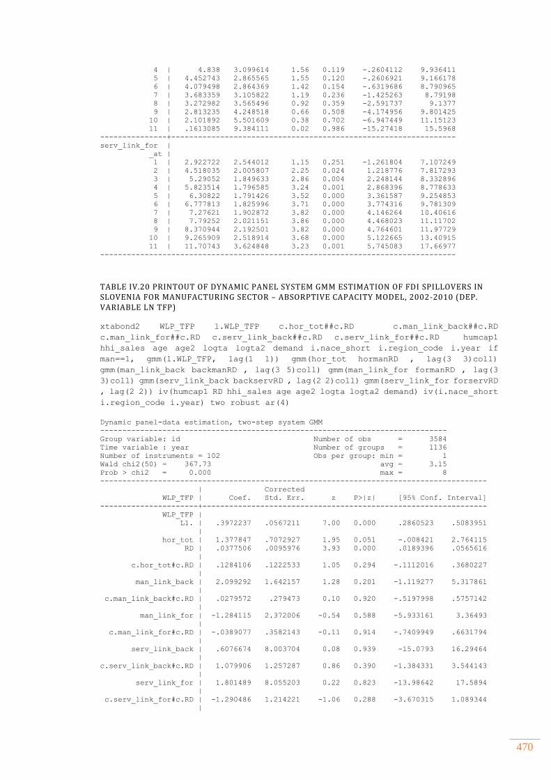
470
4 | 4.838 3.099614 1.56 0.119 -.2604112 9.936411
5 | 4.452743 2.865565 1.55 0.120 -.2606921 9.166178
6 | 4.079498 2.864369 1.42 0.154 -.6319686 8.790965
7 | 3.683359 3.105822 1.19 0.236 -1.425263 8.79198
8 | 3.272982 3.565496 0.92 0.359 -2.591737 9.1377
9 | 2.813235 4.248518 0.66 0.508 -4.174956 9.801425
10 | 2.101892 5.501609 0.38 0.702 -6.947449 11.15123
11 | .1613085 9.384111 0.02 0.986 -15.27418 15.5968
---------------+----------------------------------------------------------------
serv_link_for |
_at |
1 | 2.922722 2.544012 1.15 0.251 -1.261804 7.107249
2 | 4.518035 2.005807 2.25 0.024 1.218776 7.817293
3 | 5.29052 1.849633 2.86 0.004 2.248144 8.332896
4 | 5.823514 1.796585 3.24 0.001 2.868396 8.778633
5 | 6.30822 1.791426 3.52 0.000 3.361587 9.254853
6 | 6.777813 1.825996 3.71 0.000 3.774316 9.781309
7 | 7.27621 1.902872 3.82 0.000 4.146264 10.40616
8 | 7.79252 2.021151 3.86 0.000 4.468023 11.11702
9 | 8.370944 2.192501 3.82 0.000 4.764601 11.97729
10 | 9.265909 2.518914 3.68 0.000 5.122665 13.40915
11 | 11.70743 3.624848 3.23 0.001 5.745083 17.66977
--------------------------------------------------------------------------------
TABLE IV.20 PRINTOUT OF DYNAMIC PANEL SYSTEM GMM ESTIMATION OF FDI SPILLOVERS IN SLOVENIA FOR MANUFACTURING SECTOR – ABSORPTIVE CAPACITY MODEL, 2002-2010 (DEP. VARIABLE LN TFP)
xtabond2 WLP_TFP l.WLP_TFP c.hor_tot##c.RD c.man_link_back##c.RD
c.man_link_for##c.RD c.serv_link_back##c.RD c.serv_link_for##c.RD humcap1
hhi_sales age age2 logta logta2 demand i.nace_short i.region_code i.year if
man==1, gmm(l.WLP_TFP, lag(1 1)) gmm(hor_tot hormanRD , lag(3 3)coll)
gmm(man_link_back backmanRD , lag(3 5)coll) gmm(man_link_for formanRD , lag(3
3)coll) gmm(serv_link_back backservRD , lag(2 2)coll) gmm(serv_link_for forservRD
, lag(2 2)) iv(humcap1 RD hhi_sales age age2 logta logta2 demand) iv(i.nace_short
i.region_code i.year) two robust ar(4)
Dynamic panel-data estimation, two-step system GMM
------------------------------------------------------------------------------
Group variable: id Number of obs = 3584
Time variable : year Number of groups = 1136
Number of instruments = 102 Obs per group: min = 1
Wald chi2(50) = 367.73 avg = 3.15
Prob > chi2 = 0.000 max = 8
---------------------------------------------------------------------------------------
| Corrected
WLP_TFP | Coef. Std. Err. z P>|z| [95% Conf. Interval]
----------------------+----------------------------------------------------------------
WLP_TFP |
L1. | .3972237 .0567211 7.00 0.000 .2860523 .5083951
|
hor_tot | 1.377847 .7072927 1.95 0.051 -.008421 2.764115
RD | .0377506 .0095976 3.93 0.000 .0189396 .0565616
|
c.hor_tot#c.RD | .1284106 .1222533 1.05 0.294 -.1112016 .3680227
|
man_link_back | 2.099292 1.642157 1.28 0.201 -1.119277 5.317861
|
c.man_link_back#c.RD | .0279572 .279473 0.10 0.920 -.5197998 .5757142
|
man_link_for | -1.284115 2.372006 -0.54 0.588 -5.933161 3.36493
|
c.man_link_for#c.RD | -.0389077 .3582143 -0.11 0.914 -.7409949 .6631794
|
serv_link_back | .6076674 8.003704 0.08 0.939 -15.0793 16.29464
|
c.serv_link_back#c.RD | 1.079906 1.257287 0.86 0.390 -1.384331 3.544143
|
serv_link_for | 1.801489 8.055203 0.22 0.823 -13.98642 17.5894
|
c.serv_link_for#c.RD | -1.290486 1.214221 -1.06 0.288 -3.670315 1.089344
|
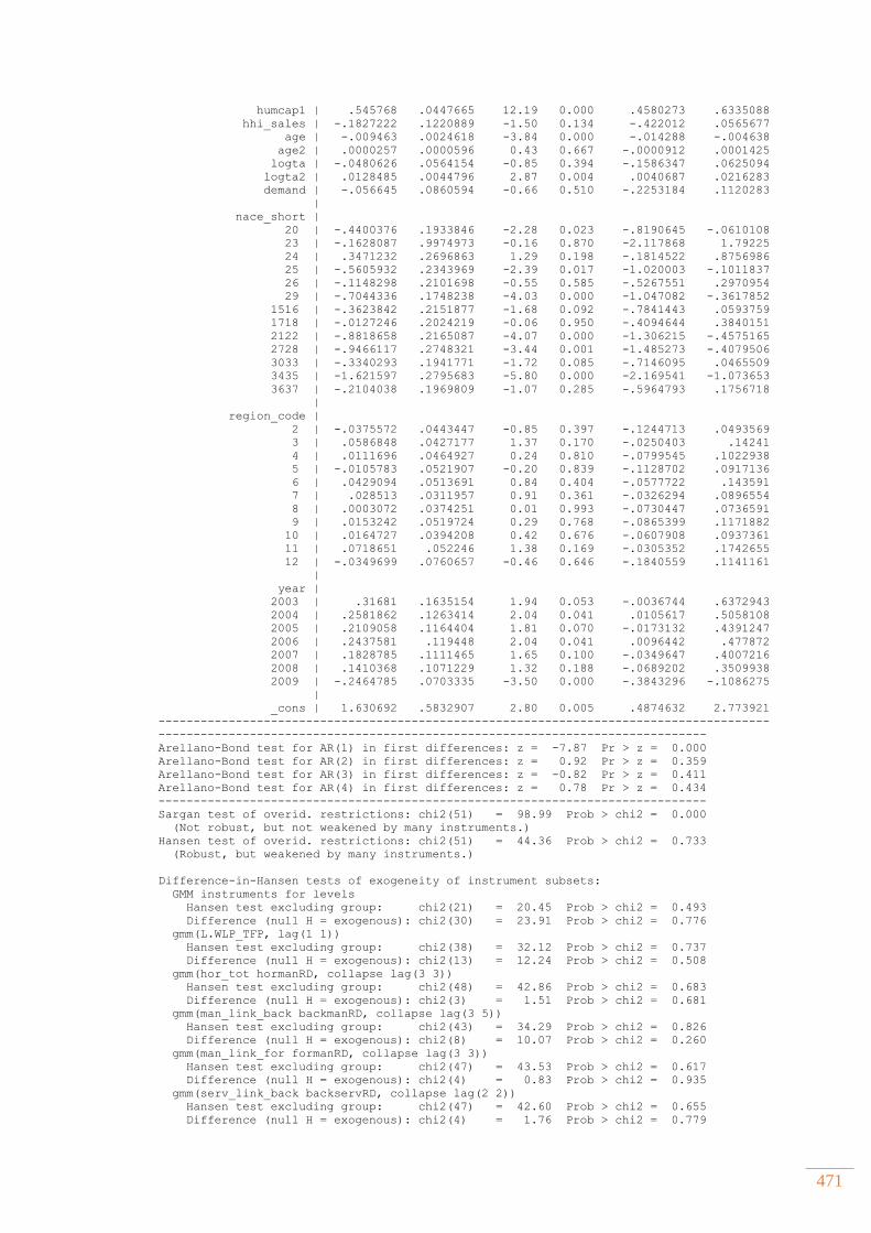
471
humcap1 | .545768 .0447665 12.19 0.000 .4580273 .6335088
hhi_sales | -.1827222 .1220889 -1.50 0.134 -.422012 .0565677
age | -.009463 .0024618 -3.84 0.000 -.014288 -.004638
age2 | .0000257 .0000596 0.43 0.667 -.0000912 .0001425
logta | -.0480626 .0564154 -0.85 0.394 -.1586347 .0625094
logta2 | .0128485 .0044796 2.87 0.004 .0040687 .0216283
demand | -.056645 .0860594 -0.66 0.510 -.2253184 .1120283
|
nace_short |
20 | -.4400376 .1933846 -2.28 0.023 -.8190645 -.0610108
23 | -.1628087 .9974973 -0.16 0.870 -2.117868 1.79225
24 | .3471232 .2696863 1.29 0.198 -.1814522 .8756986
25 | -.5605932 .2343969 -2.39 0.017 -1.020003 -.1011837
26 | -.1148298 .2101698 -0.55 0.585 -.5267551 .2970954
29 | -.7044336 .1748238 -4.03 0.000 -1.047082 -.3617852
1516 | -.3623842 .2151877 -1.68 0.092 -.7841443 .0593759
1718 | -.0127246 .2024219 -0.06 0.950 -.4094644 .3840151
2122 | -.8818658 .2165087 -4.07 0.000 -1.306215 -.4575165
2728 | -.9466117 .2748321 -3.44 0.001 -1.485273 -.4079506
3033 | -.3340293 .1941771 -1.72 0.085 -.7146095 .0465509
3435 | -1.621597 .2795683 -5.80 0.000 -2.169541 -1.073653
3637 | -.2104038 .1969809 -1.07 0.285 -.5964793 .1756718
|
region_code |
2 | -.0375572 .0443447 -0.85 0.397 -.1244713 .0493569
3 | .0586848 .0427177 1.37 0.170 -.0250403 .14241
4 | .0111696 .0464927 0.24 0.810 -.0799545 .1022938
5 | -.0105783 .0521907 -0.20 0.839 -.1128702 .0917136
6 | .0429094 .0513691 0.84 0.404 -.0577722 .143591
7 | .028513 .0311957 0.91 0.361 -.0326294 .0896554
8 | .0003072 .0374251 0.01 0.993 -.0730447 .0736591
9 | .0153242 .0519724 0.29 0.768 -.0865399 .1171882
10 | .0164727 .0394208 0.42 0.676 -.0607908 .0937361
11 | .0718651 .052246 1.38 0.169 -.0305352 .1742655
12 | -.0349699 .0760657 -0.46 0.646 -.1840559 .1141161
|
year |
2003 | .31681 .1635154 1.94 0.053 -.0036744 .6372943
2004 | .2581862 .1263414 2.04 0.041 .0105617 .5058108
2005 | .2109058 .1164404 1.81 0.070 -.0173132 .4391247
2006 | .2437581 .119448 2.04 0.041 .0096442 .477872
2007 | .1828785 .1111465 1.65 0.100 -.0349647 .4007216
2008 | .1410368 .1071229 1.32 0.188 -.0689202 .3509938
2009 | -.2464785 .0703335 -3.50 0.000 -.3843296 -.1086275
|
_cons | 1.630692 .5832907 2.80 0.005 .4874632 2.773921
---------------------------------------------------------------------------------------
------------------------------------------------------------------------------
Arellano-Bond test for AR(1) in first differences: z = -7.87 Pr > z = 0.000
Arellano-Bond test for AR(2) in first differences: z = 0.92 Pr > z = 0.359
Arellano-Bond test for AR(3) in first differences: z = -0.82 Pr > z = 0.411
Arellano-Bond test for AR(4) in first differences: z = 0.78 Pr > z = 0.434
------------------------------------------------------------------------------
Sargan test of overid. restrictions: chi2(51) = 98.99 Prob > chi2 = 0.000
(Not robust, but not weakened by many instruments.)
Hansen test of overid. restrictions: chi2(51) = 44.36 Prob > chi2 = 0.733
(Robust, but weakened by many instruments.)
Difference-in-Hansen tests of exogeneity of instrument subsets:
GMM instruments for levels
Hansen test excluding group: chi2(21) = 20.45 Prob > chi2 = 0.493
Difference (null H = exogenous): chi2(30) = 23.91 Prob > chi2 = 0.776
gmm(L.WLP_TFP, lag(1 1))
Hansen test excluding group: chi2(38) = 32.12 Prob > chi2 = 0.737
Difference (null H = exogenous): chi2(13) = 12.24 Prob > chi2 = 0.508
gmm(hor_tot hormanRD, collapse lag(3 3))
Hansen test excluding group: chi2(48) = 42.86 Prob > chi2 = 0.683
Difference (null H = exogenous): chi2(3) = 1.51 Prob > chi2 = 0.681
gmm(man_link_back backmanRD, collapse lag(3 5))
Hansen test excluding group: chi2(43) = 34.29 Prob > chi2 = 0.826
Difference (null H = exogenous): chi2(8) = 10.07 Prob > chi2 = 0.260
gmm(man_link_for formanRD, collapse lag(3 3))
Hansen test excluding group: chi2(47) = 43.53 Prob > chi2 = 0.617
Difference (null H = exogenous): chi2(4) = 0.83 Prob > chi2 = 0.935
gmm(serv_link_back backservRD, collapse lag(2 2))
Hansen test excluding group: chi2(47) = 42.60 Prob > chi2 = 0.655
Difference (null H = exogenous): chi2(4) = 1.76 Prob > chi2 = 0.779
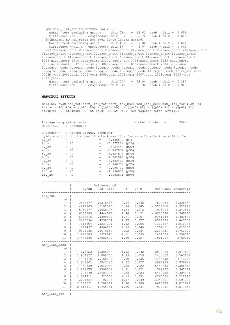
472
gmm(serv_link_for forservRD, lag(2 2))
Hansen test excluding group: chi2(21) = 18.62 Prob > chi2 = 0.609
Difference (null H = exogenous): chi2(30) = 25.74 Prob > chi2 = 0.688
iv(humcap1 RD hhi_sales age age2 logta logta2 demand)
Hansen test excluding group: chi2(43) = 39.80 Prob > chi2 = 0.611
Difference (null H = exogenous): chi2(8) = 4.57 Prob > chi2 = 0.803
iv(19b.nace_short 20.nace_short 23.nace_short 24.nace_short 25.nace_short 26.nace_short
29.nace_short 45.nace_short 50.nace_short 51.nace_short 52.nace_short 55.nace_short
60.nace_short 61.nace_short 62.nace_short 63.nace_short 64.nace_short 70.nace_short
1516.nace_short 1718.nace_short 2122.nace_short 2728.nace_short 3033.nace_short
3435.nace_short 3637.nace_short 4041.nace_short 6567.nace_short 7174.nace_short
1b.region_code 2.region_code 3.region_code 4.region_code 5.region_code 6.region_code
7.region_code 8.region_code 9.region_code 10.region_code 11.region_code 12.region_code
2002b.year 2003.year 2004.year 2005.year 2006.year 2007.year 2008.year 2009.year
2010.year)
Hansen test excluding group: chi2(20) = 23.04 Prob > chi2 = 0.287
Difference (null H = exogenous): chi2(31) = 21.32 Prob > chi2 = 0.903
MARGINAL EFFECTS
margins, dydx(hor_tot serv_link_for serv_link_back man_link_back man_link_for ) at((p1)
RD) at((p10) RD) at((p20) RD) at((p30) RD) at((p40) RD) at((p50) RD) at((p60) RD)
at((p70) RD) at((p80) RD) at((p90) RD) at((p99) RD) vsquish force level(90)
Average marginal effects Number of obs = 3584
Model VCE : Corrected
Expression : Fitted Values, predict()
dy/dx w.r.t. : hor_tot man_link_back man_link_for serv_link_back serv_link_for
1._at : RD = -8.480529 (p1)
2._at : RD = -6.977282 (p10)
3._at : RD = -6.24442 (p20)
4._at : RD = -5.762052 (p30)
5._at : RD = -5.327876 (p40)
6._at : RD = -4.901028 (p50)
7._at : RD = -4.392498 (p60)
8._at : RD = -3.740737 (p70)
9._at : RD = -2.995732 (p80)
10._at : RD = -1.994884 (p90)
11._at : RD = .5103831 (p99)
--------------------------------------------------------------------------------
| Delta-method
| dy/dx Std. Err. z P>|z| [90% Conf. Interval]
---------------+----------------------------------------------------------------
hor_tot |
_at |
1 | .2888577 .6318338 0.46 0.648 -.7504164 1.328132
2 | .4818905 .5102595 0.94 0.345 -.3574116 1.321193
3 | .5759977 .4660105 1.24 0.216 -.1905214 1.342517
4 | .6379389 .4444023 1.44 0.151 -.0930378 1.368916
5 | .6936916 .4309687 1.61 0.107 -.0151889 1.402572
6 | .7485034 .4238704 1.77 0.077 .0512986 1.445708
7 | .813804 .4237291 1.92 0.055 .1168317 1.510776
8 | .897497 .4366868 2.06 0.040 .1792111 1.615783
9 | .9931635 .4679659 2.12 0.034 .2234281 1.762899
10 | 1.121683 .5320918 2.11 0.035 .2464699 1.996896
11 | 1.443386 .7582402 1.90 0.057 .1961917 2.69058
---------------+----------------------------------------------------------------
man_link_back |
_at |
1 | 1.8622 1.286085 1.45 0.148 -.2532219 3.977622
2 | 1.904227 1.009765 1.89 0.059 .2433117 3.565142
3 | 1.924715 .9156104 2.10 0.036 .4186702 3.43076
4 | 1.938201 .8745326 2.22 0.027 .4997229 3.376679
5 | 1.950339 .8542248 2.28 0.022 .5452645 3.355414
6 | 1.962273 .8508179 2.31 0.021 .562802 3.361744
7 | 1.97649 .8684023 2.28 0.023 .5480952 3.404885
8 | 1.994711 .923003 2.16 0.031 .4765065 3.512916
9 | 2.01554 1.02226 1.97 0.049 .3340711 3.697008
10 | 2.043521 1.200367 1.70 0.089 .0690933 4.017948
11 | 2.113561 1.765741 1.20 0.231 -.7908241 5.017946
---------------+----------------------------------------------------------------
man_link_for |
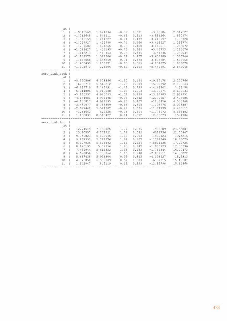
473
_at |
1 | -.9541569 1.824894 -0.52 0.601 -3.95584 2.047527
2 | -1.012645 1.546411 -0.65 0.513 -3.556264 1.530974
3 | -1.041159 1.464227 -0.71 0.477 -3.449597 1.36728
4 | -1.059927 1.433988 -0.74 0.460 -3.418627 1.298774
5 | -1.07682 1.424255 -0.76 0.450 -3.419511 1.265872
6 | -1.093427 1.431193 -0.76 0.445 -3.44753 1.260676
7 | -1.113213 1.460463 -0.76 0.446 -3.51546 1.289034
8 | -1.138572 1.529204 -0.74 0.457 -3.653889 1.376746
9 | -1.167558 1.645269 -0.71 0.478 -3.873784 1.538668
10 | -1.206499 1.850971 -0.65 0.515 -4.251075 1.838078
11 | -1.303973 2.5206 -0.52 0.605 -5.449991 2.842045
---------------+----------------------------------------------------------------
serv_link_back |
_at |
1 | -8.550506 6.578866 -1.30 0.194 -19.37178 2.270766
2 | -6.92714 5.512212 -1.26 0.209 -15.99392 2.139643
3 | -6.135719 5.165991 -1.19 0.235 -14.63302 2.36158
4 | -5.614806 5.018038 -1.12 0.263 -13.86874 2.639133
5 | -5.145937 4.945053 -1.04 0.298 -13.27983 2.987951
6 | -4.684981 4.931495 -0.95 0.342 -12.79657 3.426606
7 | -4.135817 4.991195 -0.83 0.407 -12.3456 4.073968
8 | -3.431977 5.183309 -0.66 0.508 -11.95776 5.093807
9 | -2.627442 5.544902 -0.47 0.636 -11.74799 6.493111
10 | -1.54662 6.2225 -0.25 0.804 -11.78172 8.688482
11 | 1.158833 8.518427 0.14 0.892 -12.85273 15.1704
---------------+----------------------------------------------------------------
serv_link_for |
_at |
1 | 12.74549 7.182025 1.77 0.076 .932109 24.55887
2 | 10.80557 6.202921 1.74 0.082 .6026736 21.00847
3 | 9.859823 5.873946 1.68 0.093 .1980423 19.5216
4 | 9.237333 5.722976 1.61 0.107 -.1761249 18.65079
5 | 8.677036 5.635893 1.54 0.124 -.5931835 17.94726
6 | 8.126195 5.59756 1.45 0.147 -1.080973 17.33336
7 | 7.469944 5.614353 1.33 0.183 -1.764844 16.70473
8 | 6.628856 5.733864 1.16 0.248 -2.802511 16.06022
9 | 5.667438 5.996804 0.95 0.345 -4.196427 15.5313
10 | 4.375858 6.533109 0.67 0.503 -6.37015 15.12187
11 | 1.142847 8.5119 0.13 0.893 -12.85798 15.14368
--------------------------------------------------------------------------------


![ISSN: 2299 9922 e-ISSN 2391-9418 [Online] Religious and ...philology.knu.ua/files/2015/slipushko_article.pdf · e-ISSN 2391-9418 [Online] Religious and Sacred Poetry: An International](https://img.pdfslide.us/doc/110x75/5c78787909d3f27b458b48f9/issn-2299-9922-e-issn-2391-9418-online-religious-and-e-issn-2391-9418.jpg)