Effects of Acid Additives on Spent Acid Flowback through ...oaktrust.library.tamu.edu/bitstream/handle/1969.1/ETD-TAMU-2012-05... · EFFECTS OF ACID ADDITIVES ON SPENT ACID FLOWBACK

EFFECTS OF ACID ADDITIVES ON SPENT ACID FLOWBACK

THROUGH CARBONATE CORES

A Thesis

by

EHSAAN AHMAD NASIR

Submitted to the Office of Graduate Studies of Texas A&M University

in partial fulfillment of the requirements for the degree of

MASTER OF SCIENCE

May 2012

Major Subject: Petroleum Engineering

Effects of Acid Additives on Spent Acid Flowback through Carbonate Cores

Copyright 2012 Ehsaan Ahmad Nasir

EFFECTS OF ACID ADDITIVES ON SPENT ACID FLOWBACK

THROUGH CARBONATE CORES

A Thesis

by

EHSAAN AHMAD NASIR

Submitted to the Office of Graduate Studies of Texas A&M University

in partial fulfillment of the requirements for the degree of

MASTER OF SCIENCE

Approved by:

Chair of Committee, A.D. Hill Committee Members, Ding Zhu Yuefeng Sun Head of Department, A. D. Hill

May 2012

Major Subject: Petroleum Engineering

iii

ABSTRACT

Effects of Acid Additives on Spent Acid Flowback through Carbonate Cores. (May

2012)

Ehsaan Ahmad Nasir, B.E., NED University of Engineering and Technology

Chair of Advisory Committee: Dr. A. Daniel Hill

Matrix acidizing is a well stimulation technique used to remove formation

damage in the near wellbore region. But it comes with an associated set of challenges

such as corrosion of the tubulars and iron precipitation in the formation. To counter these

challenges, different chemicals, or additives, are added to the acid solution such as

corrosion inhibitors and iron control agents. These additives may change the relative

permeability of the spent acid, and formation wettability, and may either hinder or

improve spent acid clean-up. Such effects of additives on the spent acid clean-up have

not been documented.

The aim of this research effort was to document the aforementioned change in

the spent acid concentration (by using one additive at a time) before and after gas

flowback. This was achieved by acidizing cores and creating wormholes halfway

through them, then CT scanning them to observe the spent acid region. Later on, gas was

flown through the core opposite to the direction of acid injection for 2 hours, and another

CT scan was taken. The difference between the two CT scans was documented. Using a

iv

different additive each time, a series of such CT scans was obtained to develop an idea

about whether the said additive was beneficial or detrimental to spent acid clean-up.

It was found that the corrosion inhibitor FA-CI performed the best in terms of

spent acid recovery after gas flowback for both Indiana Limestone and Texas Cream

Chalk cores. Moreover, the corrosion inhibitor MI-CI was the worst for Indiana

Limestone and the non-emulsifying agent M-NEA the worst for Texas Cream Chalk for

spent acid recovery after gas flowback.

v

DEDICATION

To my wife and family, who saw me through the difficult times

vi

ACKNOWLEDGEMENTS

I would like to thank my committee chair, Dr. A. Daniel Hill, and my committee

members, Dr. Zhu and Dr. Sun, for their guidance and support throughout the course of

this research.

I’d also like to show my gratitude to my friends and colleagues and the PETE

department faculty and staff for their help throughout my research effort and for making

my time at Texas A&M University a fantastic academic experience.

vii

NOMENCLATURE

ICA Iron Control Agent

CI Corrosion Inhibitor

NEA Non-Emulsifying Agent

CT Computed Tomography

Pr. Pressure

no. number

µ Linear Attenuation Coefficient

Io Intensity of the emitted x-ray beam

I Intensity of the detected x-ray beam

H Thickness of the object being scanned

PPE Personal Protective Equipment

MSDS Material Safety Data Sheet

PVC Polyvinyl chloride

exp. Experiment

FA-CI Formic Acid based Corrosion Inhibitor

MI-CI Methanol and Isopropanol based Corrosion Inhibitor

CA-ICA Citric Acid based Iron Control Agent

T-ICA Trisodium nitrotriacetate based Iron Control Agent

M-NEA Methanol based Non-Emulsifying Agent

viii

TABLE OF CONTENTS

Page

ABSTRACT .............................................................................................................. iii

DEDICATION .......................................................................................................... v

ACKNOWLEDGEMENTS ...................................................................................... vi

NOMENCLATURE .................................................................................................. vii

TABLE OF CONTENTS .......................................................................................... viii

LIST OF FIGURES ................................................................................................... x

LIST OF TABLES .................................................................................................... xiii

1. INTRODUCTION ............................................................................................... 1

1.1 Matrix Acidizing ................................................................................. 2 1.2 Literature Review ................................................................................. 4

2. PROBLEM DEFINITION .................................................................................. 6

2.1 Description of the Problem ..................................................................... 6 2.1.1 CT Scanning Theory and Beam Hardening ................................ 7

3. EXPERIMENTAL PROCEDURE ..................................................................... 9

3.1 Acidizing and Flowback Apparatus ..................................................... 9 3.2 CT Scanner ........................................................................................... 16

3.3 Description of the Cores ....................................................................... 17 3.4 Acid Additives ...................................................................................... 18 3.5 Acidizing and Gas Flowback Procedure .............................................. 21 3.6 CT Scanning Procedure ........................................................................ 25

4. EXPERIMENTAL RESULTS ............................................................................ 26

4.1 Comparison of Mean CT Numbers Before and After Gas Flowback .. 26 4.1.1 Indiana Limestone ....................................................................... 27

4.1.1.1 No additive ...................................................................... 27

ix

Page 4.1.1.2 T-ICA .............................................................................. 30 4.1.1.3 CA-ICA ........................................................................... 34 4.1.1.4 FA-CI .............................................................................. 37 4.1.1.5 MI-CI ............................................................................... 40 4.1.1.6 M-NEA ............................................................................ 43 4.1.1.7 Combined Difference Plot ............................................... 46

4.1.2 Texas Cream Chalk ..................................................................... 47 4.1.2.1 No additive ...................................................................... 48 4.1.2.2 T-ICA .............................................................................. 51 4.1.2.3 CA-ICA ........................................................................... 54 4.1.2.4 FA-CI .............................................................................. 57 4.1.2.5 MI-CI ............................................................................... 60 4.1.2.6 M-NEA ............................................................................ 63 4.1.2.7 Combined Difference Plot ............................................... 72

5. CONCLUSIONS AND RECOMMENDATIONS ................................................ 74

REFERENCES .......................................................................................................... 76

APPENDIX A............................................................................................................ 79 VITA.......................................................................................................................... 109

x

LIST OF FIGURES

FIGURE Page

1.1 Wormholes and the spent acid region. ....................................................... 3 3.1 Teledyne ISCO 500D syringe pump .......................................................... 10 3.2 Acid accumulator ....................................................................................... 10 3.3 PVC refill container ................................................................................... 10 3.4 TEMCO stainless steel coreholder ............................................................. 11 3.5 ENERPAC hand pump ............................................................................... 11 3.6 Mity-Mite back pressure regulator ............................................................. 12 3.7 FOXBORO pressure transducer ................................................................. 12 3.8 OMEGA gas volume flowmeter ................................................................ 13 3.9 Industrial grade nitrogen cylinders ............................................................. 14 3.10 Schematic of the acidizing and flowback apparatus .................................. 15 3.11a Hollow aluminum cylinder ........................................................................ 16 3.11b CT Scanner ................................................................................................ 16 3.12a Indiana Limestone core ............................................................................. 17 3.12b Texas Cream Chalk core ........................................................................... 17 3.13 Corrosion inhibitor FA-CI .......................................................................... 18 3.14 Corrosion inhibitor MI-CI .......................................................................... 18 3.15 Iron control agent CA-ICA ........................................................................ 19

xi

FIGURE Page

3.16 Iron control agent T-ICA ............................................................................ 19 3.17 Non-emulsifying agent M-NEA ................................................................. 20 3.18 Sodium Iodide ............................................................................................ 20 3.19 A 15 wt% HCl solution with 2 wt% NaI added ......................................... 21 3.20 Inlet faces of acidized Indiana Limestone and Texas Cream Chalk cores . 23 4.1a Mean CT number plot for Indiana Limestone (no additive) ...................... 29 4.1b Difference plot for Indiana Limestone (no additive) ................................. 30 4.2a Mean CT number plot for Indiana Limestone (T-ICA) ............................. 32 4.2b Difference plot for Indiana Limestone (T-ICA) ......................................... 33 4.3a Mean CT number plot for Indiana Limestone (CA-ICA) .......................... 35 4.3b Difference plot for Indiana Limestone (CA-ICA) ...................................... 36 4.4a Mean CT number plot for Indiana Limestone (FA-CI) .............................. 38 4.4b Difference plot for Indiana Limestone (FA-CI) ......................................... 39 4.5a Mean CT number plot for Indiana Limestone (MI-CI) .............................. 41 4.5b Difference plot for Indiana Limestone (MI-CI) ......................................... 42 4.6a Mean CT number plot for Indiana Limestone (M-NEA) ........................... 44 4.6b Difference plot for Indiana Limestone (M-NEA) ...................................... 45 4.7 Combined Difference plot for Indiana Limestone (all additives) .............. 46 4.8a Mean CT number plot for Texas Cream Chalk (no additive) .................... 49 4.8b Difference plot for Texas Cream Chalk (no additive) ................................ 50

xii

FIGURE Page

4.9a Mean CT number plot for Texas Cream Chalk (T-ICA) ........................... 52 4.9b Difference plot for Texas Cream Chalk (T-ICA) ....................................... 53 4.10a Mean CT number plot for Texas Cream Chalk (CA-ICA) ....................... 55 4.10b Difference plot for Texas Cream Chalk (CA-ICA) ................................... 56 4.11a Mean CT number plot for Texas Cream Chalk (FA-CI) ........................... 58 4.11b Difference plot for Texas Cream Chalk (FA-CI) ...................................... 59 4.12a Mean CT number plot for Texas Cream Chalk (MI-CI) ........................... 61 4.12b Difference plot for Texas Cream Chalk (MI-CI) ...................................... 62 4.13a Mean CT number plot for Texas Cream Chalk (M-NEA) ........................ 64 4.13b Difference plot for Texas Cream Chalk (M-NEA) ................................... 65 4.13c Mean CT number plot for Texas Cream Chalk (M-NEA); 2nd exp .......... 67 4.13d Difference plot for Texas Cream Chalk (M-NEA); 2nd exp ...................... 68 4.13e Mean CT number plot for Texas Cream Chalk (M-NEA); 3rd exp ........... 70 4.13f Difference plot for Texas Cream Chalk (M-NEA); 3rd exp ....................... 71 4.14 Combined Difference plot for Texas Cream Chalk (all additives) ............ 73

xiii

LIST OF TABLES

TABLE Page

4.1 Back pressure and overburden pressure values .......................................... 27

4.2a Acid flow parameters (Indiana Limestone; no additive) ............................ 27 4.2b Acid formulation (Indiana Limestone; no additive) ................................... 27

4.2c Flowback parameters (Indiana Limestone; no additive) ............................ 28

4.3a Acid flow parameters (Indiana Limestone; T-ICA) ................................... 30

4.3b Acid formulation (Indiana Limestone; T-ICA) .......................................... 31

4.3c Flowback parameters (Indiana Limestone; T-ICA) ................................... 31

4.4a Acid flow parameters (Indiana Limestone; CA-ICA) ................................ 34

4.4b Acid formulation (Indiana Limestone; CA-ICA) ....................................... 34

4.4c Flowback parameters (Indiana Limestone; CA-ICA) ................................ 34

4.5a Acid flow parameters (Indiana Limestone; FA-CI) ................................... 37

4.5b Acid formulation (Indiana Limestone; FA-CI) .......................................... 37

4.5c Flowback parameters (Indiana Limestone; FA-CI) ................................... 37

4.6a Acid flow parameters (Indiana Limestone; MI-CI) ................................... 40

4.6b Acid formulation (Indiana Limestone; MI-CI) .......................................... 40

4.6c Flowback parameters (Indiana Limestone; MI-CI) .................................... 40

4.7a Acid flow parameters (Indiana Limestone; M-NEA) ................................ 43

4.7b Acid formulation (Indiana Limestone; M-NEA)........................................ 43

4.7c Flowback parameters (Indiana Limestone; M-NEA) ................................. 43

xiv

TABLE Page

4.8a Acid flow parameters (Texas Cream Chalk; no additive) .......................... 48

4.8b Acid formulation (Texas Cream Chalk; no additive) ................................. 48

4.8c Flowback parameters (Texas Cream Chalk; no additive) .......................... 48

4.9a Acid flow parameters (Texas Cream Chalk; T-ICA) ................................. 51

4.9b Acid formulation (Texas Cream Chalk; T-ICA) ........................................ 51

4.9c Flowback parameters (Texas Cream Chalk; T-ICA) ................................. 51

4.10a Acid flow parameters (Texas Cream Chalk; CA-ICA) ............................. 54

4.10b Acid formulation (Texas Cream Chalk; CA-ICA) .................................... 54

4.10c Flowback parameters (Texas Cream Chalk; CA-ICA) ............................. 54

4.11a Acid flow parameters (Texas Cream Chalk; FA-CI) ................................ 57

4.11b Acid formulation (Texas Cream Chalk; FA-CI) ....................................... 57

4.11c Flowback parameters (Texas Cream Chalk; FA-CI) ................................. 57

4.12a Acid flow parameters (Texas Cream Chalk; MI-CI) ................................ 60

4.12b Acid formulation (Texas Cream Chalk; MI-CI) ....................................... 60

4.12c Flowback parameters (Texas Cream Chalk; MI-CI) ................................. 60

4.13a Acid flow parameters (Texas Cream Chalk; M-NEA) .............................. 63

4.13b Acid formulation (Texas Cream Chalk; M-NEA) ..................................... 63

4.13c Flowback parameters (Texas Cream Chalk; M-NEA) .............................. 63

4.13d Acid flow parameters (Texas Cream Chalk; M-NEA; 2nd exp) ................ 66

4.13e Acid formulation (Texas Cream Chalk; M-NEA; 2nd exp) ....................... 66

4.13f Flowback parameters (Texas Cream Chalk; M-NEA; 2nd exp) ................ 66

xv

TABLE Page

4.13g Acid flow parameters (Texas Cream Chalk; M-NEA; 3rd exp) ................ 69

4.13h Acid formulation (Texas Cream Chalk; M-NEA; 3rd exp) ....................... 69

4.13i Flowback parameters (Texas Cream Chalk; M-NEA; 3rd exp) ................. 69

1

1. INTRODUCTION

Formation damage is a phenomenon that starts as early as drilling in the life of a well.

There are several techniques that are used to rectify formation damage and stimulate the

well, depending on the type of the damage. One of those well stimulation methods is

acidizing, or more specifically, matrix acidizing.

In matrix acidizing, an acid (usually HCl for carbonates or an HCl/HF mixture for

sandstones) is pumped down a well to remove the damage and increase permeability

within a few feet of the well. The acid is pumped downhole at pressures lower than the

formation’s breakdown pressure i.e. the pressure at which the formation starts to

fracture. The main mode of permeability increase with matrix acidizing is the chemical

reaction of the acid with the minerals present downhole, which are dissolved by the acid.

This is in contrast to acid fracturing, which is another technique used for well

stimulation, where an acid is pumped downhole at pressures higher than the formation

breakdown pressure so as to improve permeability both by the chemical reaction, and by

forming a hydraulic fracture.

Wormholes are large channels, relative to pores, caused by the non-uniform dissolution This thesis follows the style of the journal SPE Production and Operations.

2

of carbonate formations by the acid. Unlike sandstone acidizing, in which the acid

actually dissolves the formation, in carbonates the acid forms wormholes which provide

a very low pressure drop thoroughfare for the fluids being produced to pass through, and

flow into the wellbore.

1.1 Matrix Acidizing

Matrix acidizing, as with any other formation damage removal techniques, comes with

its own set of challenges. When the acid reacts with the formation, it forms carbon

dioxide and water. The chemical equations are as follows:

CaCO3 + 2HCl CaCl2 + H2O + CO2

MgCO3 + 2HCl MgCl2 + H2O + CO2

The reaction products actually move ahead of the wormhole forming a front, which from

now on we will call the “spent acid front”. The spent acid droplets become lodged in the

pores and pore throat, and serve to decrease the formation permeability by water-

blocking the pores (see Fig 1.1). Furthermore, different additives are pumped along with

the acid down the wellbore, which may change the wettability of the formation from

water-wet to oil-wet, or vice versa.

3

Figure 1.1 Wormholes and the spent acid region; also shown is a spent acid

droplet blocking a pore throat.

A brief description of some of the additives used in matrix acidizing, along with the

challenges they are used to counter, is given below:

o The downhole tubulars are susceptible to corrosion upon coming into contact

with the acid, and the relatively high temperatures downhole only serve to speed

up the corrosion reaction. To prevent the tubulars, valves, chokes and everything

downhole that may corrode due to the acid, “corrosion inhibitors” are used.

Corrosion inhibitors are one of the most important additives used in an acidizing

job. Sometimes, the selection of the corrosion inhibitor may also govern the

choice of the acid used, due to the costs and difficulty involved.

o Iron precipitation is also one of the mechanisms that lead to a significant

permeability reduction. It is caused by the precipitation of Ferric (Fe3+) ions

present downhole to form Ferric Hydroxide Fe(OH)3. “Iron control agents”, such

as EDTA (ethylenediaminetetraacetic acid), are used to prevent the Ferric ions

from precipitating.

4

o “Non-emulsifying agents” are used to prevent emulsions from forming in the

acid as it is being transferred downhole. The emulsion might hinder the reaction

between the formation rock and the acid.

o Corrosion inhibitors may also change the formation wettability to oil-wet by

adsorbing into the formation rock. To rectify this, “mutual solvents”, such as

EGMBE (ethylene glycol monobutyl ether), are used to dissolve the adsorbed

corrosion inhibitor, and any acid-insoluble residue that may have been left

behind as a result of the acidizing reaction.

o Many other additives are also used other than the ones mentioned, such as H2S

scavengers for capturing hydrogen sulfide, surfactants to reduce interfacial

tension to speed clean-up, and diverting agents to divert the acid to desired parts

of the formation.

1.2 Literature Review

Mahadevan and Sharma (2005) conducted gas displacement experiments to displace

brine from a fully saturated brine rock sample. They concluded that rock type

(permeability), along with several other factors such as relative permeability curves,

govern how effective the water blockage clean-up is going to be. Moreover, the change

in the rock’s wettability from water-wet to oil-wet also caused the rock (Texas Cream

limestone and Berea sandstone) to clean up faster.

5

Kamathe and Laroche (2003) addressed the decrease in gas well productivity due to

water blockage by carrying out experiments using different fluids and saturation states.

Their results show that water blockage is a transient phenomenon that depends on the

amount and type of the fluid lost, gas flowrate, and the pressure drawdown in the

reservoir. The gas deliverability was found to recover in two phases: the first phase is the

liquid production which lasts for a few hours; the second phase is evaporation of the

water blocked region with continuous gas flow and takes several days. Adding methanol

to the fluid resulted in drastically reducing the time required for the second phase.

Nasr-El-Din et al. (2004) documented experimental studies carried out to observe the

change in surface tension of HCl-based stimulation fluids. Similarly, Saneifar et al.

(2011) discussed the effects of high pressure and temperature on the surface tension of

spent acids. But so far, there hasn’t been any work done that touches on how effectively

the water blockage effects of spent acid are removed, and what is the effect, if any, of

different stimulation fluids on the spent acid clean-up. That is what will be addressed in

this study.

6

2. PROBLEM DEFINITION

2.1 Description of the Problem

Several different additives are used in acidizing to tackle challenges encountered

downhole, but the truth is that these additives may also alter the formation properties

such as permeability and wettability. Hence, the selection process of additives has to

include the upsides and downsides associated with each additive, and how they stack up

in order to achieve the ultimate goal of stimulating the damaged well.

In matrix acidizing, the spent acid (which is the name given to the reaction products of

the acidizing reaction plus the unused acid) actually penetrates farther into the formation

than the wormholes. The spent acid may block pores and pore throats by clogging them

with water droplets. Some of it may flow back during the initial phase of production of a

well, along with the fluids being produced and a rather efficient clean-up may be

achieved. But depending on the acid additives being used (and their effect on the

formation wettability) the spent acid clean-up might not be significant and it might keep

blocking the pores, or change the wettability of the rock near the wellbore, thereby

causing a decrease in relative permeability and hence production.

The goal of this study is to experimentally simulate and document this process, i.e. the

change in formation properties caused by the additives used resulting in an inefficient

7

spent acid clean-up, that may lead to a decrease in relative permeabilities of the fluids

flowing through the formation, and hence and overall decrease in production.

2.1.1 CT Scanning Theory and Beam Hardening

When an object is CT scanned, it is bombarded by x-rays from different angles by an x-

ray source. The sources revolve around the object to be scanned and the transmitted x-

rays intensity is measured by a series of detectors. The main quantity measured is the

linear attenuation coefficient µ, which is related to the incident x-ray intensity Io by

Beer’s law as:

I / Io = exp-µh

where I is the intensity of the x-ray after it has passed through the object being scanned,

and h is the thickness of the scanned object.

Beer’s law assumes that the x-ray beam used to scan the object was monochromatic i.e.

it has a single frequency. That is not the case in reality, and the x-ray beams are

polychromatic. This causes low energy x-ray photons to be absorbed more readily at the

air-object interface and also by the object itself. This leads to an error in the

determination of the linear attenuation coefficient µ called “beam hardening”. For a

8

cylindrical object such a core, the error shows up as higher CT numbers in the periphery

of the core and lower CT numbers at the center.

Akin and Kovscek (2003) suggested that beam hardening can be corrected by

surrounding the coreholder with a cylindrical water-jacket, or with a crushed-rock jacket,

or using aluminum and composite carbon-fiber coreholders.

9

3. EXPERIMENTAL PROCEDURE

In this section, we will discuss the procedure followed to obtain the results shown. We

will first describe the acidizing and the flowback apparatus and how it is set up, the CT

scanning procedure used to visualize the changes in the core during various phases of the

experiment, then the additives employed in this study, and finally the actual procedure of

how the experiments were carried out.

3.1 Acidizing and Flowback Apparatus

For the purpose of our study, we used a basic coreflood apparatus, which is comprised of

the following parts:

o A syringe pump (Fig 3.1), which provides the driving force to push the fluids

trough the acidizing apparatus. The pump forces hydraulic oil through the

interconnecting tubes. The oil in turn pushes on a piston housed in a component

called accumulator. On the other side of the piston is the fluid to be pumped.

o An accumulator (Fig 3.2), which holds the fluid that is to be pumped through the

acidizing apparatus.

o A PVC container (Fig 3.3), which is used to refill the accumulator with the fluid

to be pumped. The fluid is first poured into the PVC container, and then is forced

pneumatically into the accumulator.

10

Figure 3.2 Acid

accumulator

Figure 3.3 PVC

refill container

Figure 3.1 Teledyne ISCO

500D syringe pump

11

o A coreholder (Fig 3.4), which holds the core housed in a Hessler sleeve, through

which the desired fluid is to be pumped.

o An overburden pump (Fig 3.5), which is used to simulate overburden pressure,

by pressuring oil around the Hessler sleeve inside the coreholder. The sleeve, in

turn, grips the core tightly, and compressing it as overburden would.

Figure 3.5 ENERPAC hand pump

Figure 3.4 TEMCO stainless steel coreholder

12

o A back pressure regulator (Fig 3.6), to keep the pressure at the coreholder’s

outlet at a desired value. It’s also used to keep the pressure inside the coreholder

high enough to ensure the carbon dioxide produced as a result of the acidizing

reaction remains dissolved in solution.

o Pressure transducers (Fig 3.7), hooked up to a computer, to monitor the pressure

drop across the core.

Figure 3.6 Mity-Mite back pressure

regulator

Figure 3.7 FOXBORO

pressure transducer

13

o A gas flowmeter (Fig 3.8), to measure the gas flowrate at the outlet of the

acidized cores.

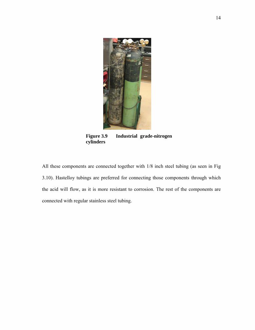
o Nitrogen cylinders (Fig 3.9) were used as the source of the gas that will flow

through the acidized cores.

Figure 3.8 OMEGA gas volume flowmeter

14

All these components are connected together with 1/8 inch steel tubing (as seen in Fig

3.10). Hastelloy tubings are preferred for connecting those components through which

the acid will flow, as it is more resistant to corrosion. The rest of the components are

connected with regular stainless steel tubing.

Figure 3.9 Industrial grade-nitrogen

cylinders

15

Fig

ure

3.1

0

Sch

ema

tic

of

the

aci

diz

ing a

nd

flo

wb

ack

ap

para

tus;

a m

od

ifie

d v

ersi

on

of

the

on

e u

sed

by N

evit

o (

2006)

16

3.2 CT Scanner

The CT scanner (Fig 3.11b) was used three times during the course of a single

experiment. Beam hardening was seen in the initial scans which cause the CT numbers

at the edges of a CT scan to be higher than at the center. A ¾ inch thick and 21 inches

long hollow aluminum cylinder (see Fig 3.11a) was used to encase the cores during CT

scans to remove beam hardening from the results.

Figure 3.11a Hollow aluminum cylinder; for encasing cores during CT scans to

remove beam hardening

Figure 3.11b CT Scanner

17

3.3 Description of the Cores

Indiana Limestone (Fig 3.12a) and Texas Cream Chalk (Fig 3.12b) carbonate cores were

used in the study. The cores were 1.5 inch in diameter and 20 inch in length. The

permeability for both types of cores was in the 1 to 10 md range.

Figure 3.12a Indiana Limestone core

Figure 3.12b Texas Cream Chalk core

18

3.4 Acid Additives

The following acid additives were used in this study:

o A formic acid based corrosion inhibitor, which for the purpose of this study will

be called FA-CI (Fig 3.13). It is a liquid, dark reddish-brown in color with a

sharp odor. It is also flammable in nature. It was found that FA-CI plugs the 1/8”

tubings coming out of the PVC refill container which had to be replaced later on.

o A methanol and isopropanol based corrosion inhibitor, which for the purpose of

this study will be called MI-CI (Fig 3.14). It is also a liquid, with a dark red-

amber color and an alcoholic odor. It is also flammable. Similar to FA-CI, MI-CI

also plugs the 1/8” tubings coming out of the PVC refill container.

Figure 3.13 Corrosion inhibitor FA-CI

Figure 3.14 Corrosion inhibitor

MI-CI

19

o A citric acid based iron control agent, which for the purpose of this study will be

called CA-ICA (Fig 3.15). It is originally in the form of powder or granules, and

is odorless. It is not flammable.

o A trisodium nitrotriacetate (trisodium NTA) based iron control agent, which for

the purpose of this study will be called T-ICA (Fig 3.16). It is a liquid, pale

yellow in color with a slight ammonia odor. It is a combustible compound.

Figure 3.15 Iron control agent

CA-ICA

Figure 3.16 Iron control agent

T-ICA

20

o A methanol based non-emulsifying agent, which for the purpose of this study

will be called M-NEA (Fig 3.17). It is a colorless liquid, and has a sweet smell. It

is also flammable.

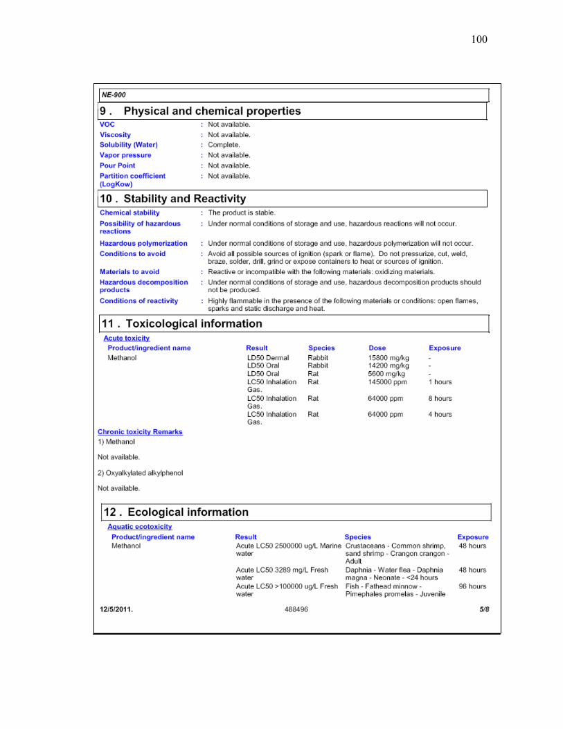
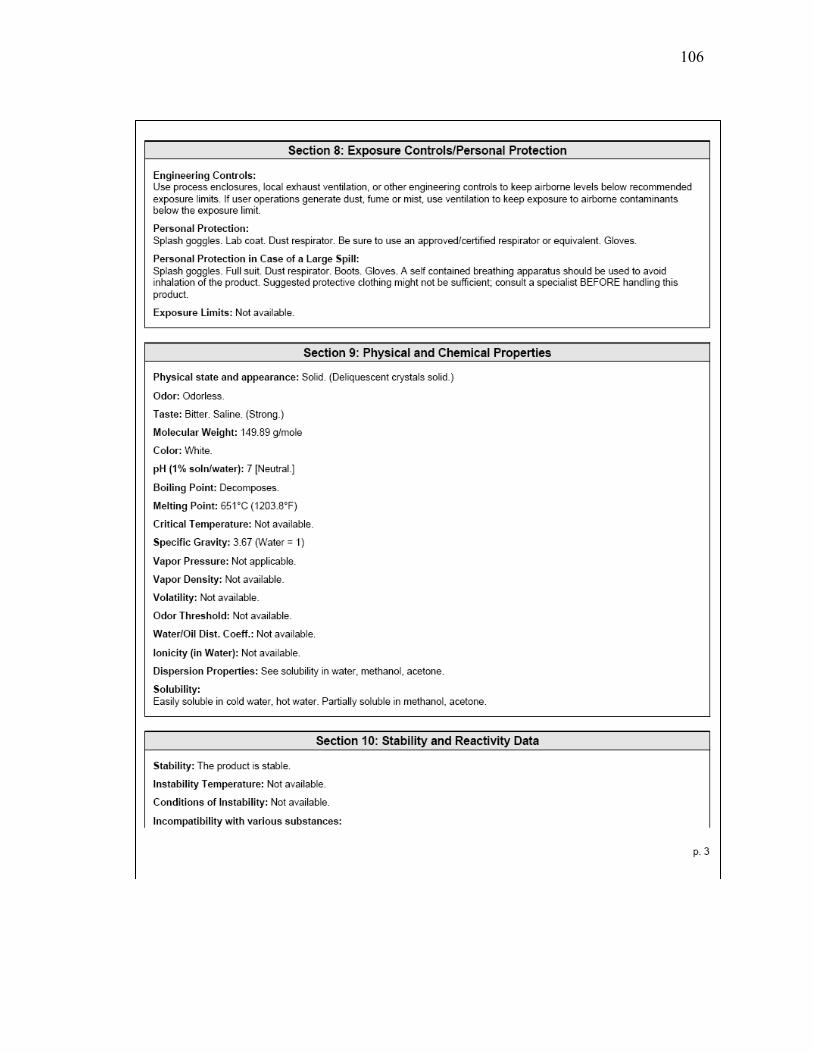
All these additives were obtained from BJ Services (now a part of Baker Hughes). The

additives are all toxic. Proper PPEs should be used when handling them as mentioned in

their respective MSDS.

Moreover, a radio opaque salt (or tracer) sodium iodide NaI (Fig 3.18) was added to the

acid solution to increase the contrast between gas-saturated and spent acid-permeated

areas in a core during CT scans.

Figure 3.17 Non-emulsifying agent

M-NEA

Figure 3.18 Sodium Iodide

21

3.5 Acidizing and Gas Flowback Procedure

The procedure is composed of the following steps:

o Take a carbonate core and determine its permeability to gas. By applying a back

pressure at the core’s outlet when finding the gas permeability, the gas slippage

effect can be eliminated leading to an accurate (and lower) determination of the

permeability (Li et al., 2004).

o The gas saturated core is then CT scanned to serve as a control for future scans.

This is the base scan to which future scans will be compared with to determine

the extent the spent acid has permeated in the core. We will call this scan the

“Gas saturated” scan.

o Next, a 15 wt% HCl solution is prepared for acidizing the cores. To this solution,

2 wt% of the additive being tested and 5 wt% of sodium iodide is added. The

sodium iodide gives a yellow color to the acid solution (Fig 3.19).

Figure 3.19 A 15 wt% HCl solution

with 2 wt% NaI added

22

o Before acidizing, the acidizing apparatus is first flushed with water to rid it of

any contaminants present in the system.

o Before starting the experiment, make sure that there is no air in the pump and the

apparatus.

o The acid solution prepared earlier is pushed pneumatically into the accumulator;

this is done by pouring the acid solution into the PVC container and using the lab

air supply to push it into the accumulator. Afterwards again make sure that there

is no air in the system.

o Place the core to be acidized in the coreholder, and connect the coreholder to the

acidizing apparatus.

o Pump oil into the coreholder using the hand pump to simulate the overburden

pressure. The overburden pressure should be at least 200-300 psi higher than the

core outlet pressure. This is to ensure that the acid actually goes through the core

instead of flowing through the area between the core and the Hessler sleeve.

o Next, pressurize the back pressure regulator connected to the outlet of the

coreholder to a 1000 psi. This will ensure that the flow will only occur through it

once the pressure at the core outlet is larger than 1000 psi. It also ensures that the

CO2 formed as a result of the acidizing reaction remains in solution.

o Acid is then pumped at the rate of 8 ml/min (or cc/min) all the while recording

the pressure drop across the core measured by the pressure transducers. In our

case this function was performed by LabVIEW.

23

o Let the acid flow for around 5-7 minutes. Usually for Indiana Limestone the

pressure drop across the core should be above 500 psi. For Texas Cream Chalk it

should be above 200 psi. This would ensure that the wormhole has penetrated a

sufficient distance into the core to begin the next phase of experiment.

o After pumping acid for 5-7 minutes, stop the pump.

o Depressurize the apparatus starting with the core inlet and then overburden and

lastly the back pressure regulator.

o Take the core out of the core holder and encase it in the hollow aluminum

cylinder. Fig 3.20 shows what an acidized core looks like.

o CT scan the acidized core for a second time. This scan will show us how far the

spent acid front has travelled inside the core. We will call this scan the “ After

acidizing” scan.

o Flush the whole apparatus again with water to ensure there is no acid left in the

apparatus.

Figure 3.20 Inlet faces of acidized Indiana Limestone (left) and Texas Cream

Chalk (right) cores

24

o After the second scan, put the core in the core holder again and prepare the

apparatus for gas flowback. Make sure the direction of gas flow is opposite to

that of the acid flow. The core outlet during acid injection will become the inlet

for gas injection and vice versa.

o Also connect the back pressure regulator to the gas injection core outlet and

pressurize it up to 300 psi. This will mimic the Bottom Hole Pressure.

o Connect a gas flow meter to the outlet of the back pressure regulator to gage the

gas flow rate at atmospheric conditions (or standard conditions).

o Ensure the gas inlet pressure is high enough (800-1000 psi in our case) to have a

gas flow rate of at least 3L/min. This value, of course, will depend on the core’s

gas permeability and the length of the wormhole.

o Let the gas flowback continue for 2 hours, then stop the gas supply.

o Depressurize the gas pressure regulator and then the overburden.

o Once the apparatus has been depressurized, take the core out from the core

holder.

o Put the core in the hollow aluminum cylinder and CT scan it for the third time.

We will call this scan the “After flowback” scan.

o We will now look at the three CT scans and see how much the spent acid front

has been pushed back for 2 hours of gas flowback.

25

3.6 CT Scanning Procedure

The procedure for CT scanning is as follows:

o Encase the core to be scanned in a hollow aluminum cylinder to get rid of beam

hardening.

o Before placing the encased core in the CT scanner, make sure that the surface it’s

being placed on is perfectly horizontally with the help of a level gage.

o We used the following parameters for the scan:

Image size: 120

Index: 4 mm; this is the distance between two consecutive scans.

Thickness of the beam: 2mm; this means that a slice 2 mm thick will be

scanned.

Number of scans: 125; a single 20 inches long core will have 125 slices in

a single scan.

o Make sure to preheat the CT scanner before starting the scan.

o If the CT scanner heats up above its specified limit, stop the scan.

o Wait for the CT scanner to cool down, and then restart the scan.

Because of beam hardening errors, several works were studied to formulate a correct

acidizing and CT scanning methodology, including Al-Muthana and Okasha (2008),

Angulo and Ortiz (1992), Bartko (1995), Coles et. al (1996), Hove et. al (1987), Hunt et.

al (1988), Wellington and Vinegar (1987), Withjack (1988) and Withjack et.al (2003).

26

4. EXPERIMENTAL RESULTS

4.1 Comparison of Mean CT Numbers Before and After Gas Flowback

In the section we will compare the CT number obtained from the three different scans

performed in a single experiment. Each plot will have three curves, namely:

o “Gas saturated”, which comprises of the CT numbers of the gas saturated core

before being acidized

o “After acidizing”, which comprises of the CT numbers of the core after being

acidized, and

o “After flowback”, which comprises of the CT numbers of the acidized core after

gas has been flown through it for 2 hours.

Another way to look at the results is a “Difference Plot” which is simply found out by

subtracting the CT numbers after flowback from the CT numbers after acidizing (or

before gas flowback). In these plots the magnitude of the peaks obtained is directly

proportional to the drop in CT numbers after gas flowback i.e. how much the spent acid

front has been pushed back and cleared up by the produced gas.

Constant backpressure and overburden pressure were used throughout the acidizing

experiments, and their values are tabulated as under (Table 4.1):

27

TABLE 4.1-BACK PRESSURE AND OVERBURDEN

PRESSURE VALUES

1 Back pressure 1000 psi 2 Overburden pressure 1500 psi

4.1.1 Indiana Limestone

Six experiments were performed in total with Indiana Limestone cores. One experiment

was done without any additive to serve as a control. The results are as under:

4.1.1.1 No additive

For the experiment, the acidizing and flowback parameters are as follows (see Tables

4.2a, 4.2b and 4.2c):

TABLE 4.2a-ACID FLOW PARAMETERS (INDIANA

LIMESTONE; NO ADDITIVE)

1 Acid Injection Rate 8 cc/min 2 Injection time 10 Min 30 sec

TABLE 4.2b-ACID FORMULATION

(INDIANA LIMESTONE; NO ADDITIVE)

1 Water 189 cc 2 HCl (15 wt%) 111 cc 3 NaI (5 wt%) 15.8 g

28

TABLE 4.2c-FLOWBACK PARAMETERS

(INDIANA LIMESTONE; NO ADDITIVE)

1 Back pressure 300 psi 2 Overburden pressure 1500 psi 3 Inlet pr. 800 psi 4 Pr. drop across the core 523 psi 5 Flowrate 19.5 L/min 6 Flow time 45 min 7 Flow meter zero error 0.5 L/min

The plot of mean CT numbers after acidizing and after flowback can be seen below (Fig

4.1a). The recession of the spent acid front is visible in the area marked “Region of

interest”. The end of the wormhole is also mentioned in the plot.

29

Figure 4.1a Mean CT number plot for Indiana Limestone (no additive)

The Difference plot plots the difference in CT numbers after acidizing and after

flowback (see Fig 4.1b). Positive peak shows the recession of the spent acid front with

the magnitude of the peak corresponding to how much of the spent acid has been

produced during flowback.

30

Figure 4.1b Difference plot for Indiana Limestone (no additive)

4.1.1.2 T-ICA


4.3a, 4.3b and 4.3c):


LIMESTONE; T-ICA)

1 Gas Permeability 3.4 md 2 Acid Injection Rate 8 cc/min

3 Injection time 9 min 30 sec

31


(INDIANA LIMESTONE;T-ICA) 1 Water 189 cc 2 HCl (15 wt%) 111 cc 3 NaI (5 wt%) 15.8 g 4 T-ICA (2 wt%) 6.3 g


(INDIANA LIMESTONE;T-ICA)


The plot of mean CT numbers after acidizing and after flowback (Fig 4.2a) and the

Difference plot (Fig 4.2b) are seen below.

32

Figure 4.2a Mean CT number plot for Indiana Limestone (T-ICA)

33

Figure 4.2b Difference plot for Indiana Limestone (T-ICA)

34

4.1.1.3 CA-ICA


4.4a, 4.4b and 4.4c):


LIMESTONE; CA-ICA)




(INDIANA LIMESTONE; CA-ICA)

1 Water 189 cc 2 HCl (15 wt%) 111 cc 3 NaI (5 wt%) 15.8 g 4 CA-ICA (2 wt%) 6.3 g


(INDIANA LIMESTONE; CA-ICA)


35



Figure 4.3a Mean CT number plot for Indiana Limestone (CA-ICA)

36

Figure 4.3b Difference plot for Indiana Limestone (CA-ICA)

37

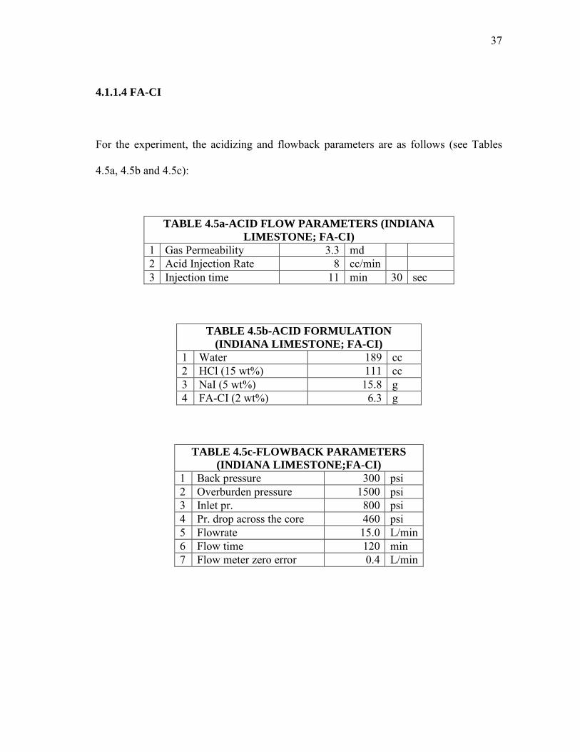
4.1.1.4 FA-CI


4.5a, 4.5b and 4.5c):


LIMESTONE; FA-CI)




(INDIANA LIMESTONE; FA-CI)

1 Water 189 cc 2 HCl (15 wt%) 111 cc 3 NaI (5 wt%) 15.8 g 4 FA-CI (2 wt%) 6.3 g


(INDIANA LIMESTONE;FA-CI)


38



Figure 4.4a Mean CT number plot for Indiana Limestone (FA-CI)

39

Figure 4.4b Difference plot for Indiana Limestone (FA-CI)

40

4.1.1.5 MI-CI


4.6a, 4.6b and 4.6c):


LIMESTONE; MI-CI)




(INDIANA LIMESTONE; MI-CI)

1 Water 189 cc 2 HCl (15 wt%) 111 cc 3 NaI (5 wt%) 15.8 g 4 MI-CI (2 wt%) 6.3 g


(INDIANA LIMESTONE; MI-CI)


41



Figure 4.5a Mean CT number plot for Indiana Limestone (MI-CI)

42

Figure 4.5b Difference plot for Indiana Limestone (MI-CI)

43

4.1.1.6 M-NEA


4.7a, 4.7b and 4.7c):


LIMESTONE; M-NEA)

1 Gas Permeability 2 Acid Injection Rate 8 cc/min



(INDIANA LIMESTONE; M-NEA)

1 Water 189 cc 2 HCl (15 wt%) 111 cc 3 NaI (5 wt%) 15.8 g 4 M-NEA (2 wt%) 6.3 g


(INDIANA LIMESTONE; M-NEA)


44



Figure 4.6a Mean CT number plot for Indiana Limestone (M-NEA)

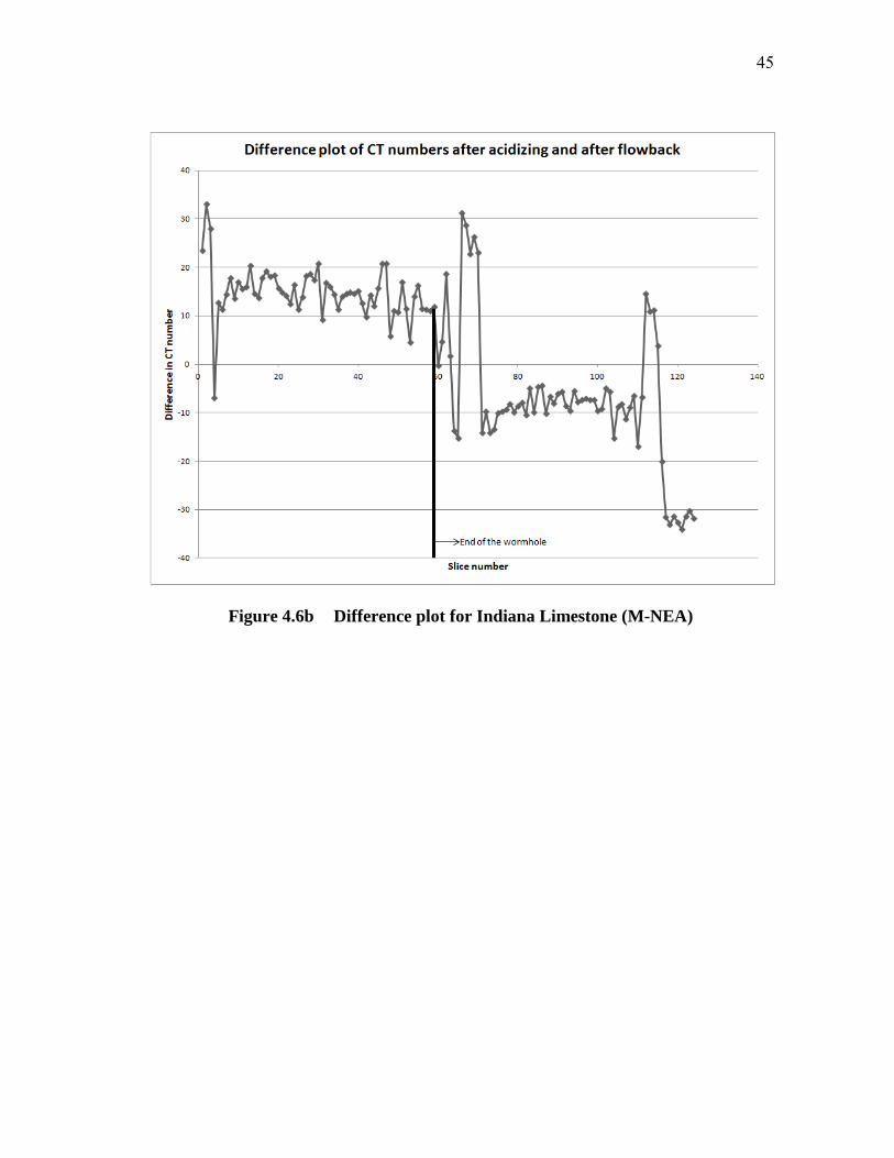
45

Figure 4.6b Difference plot for Indiana Limestone (M-NEA)

46

4.1.1.7 Combined Difference Plot

The Combined Difference Plot (Fig 4.7) is a collection of all the Difference Plots, and is

centered at the end of the wormhole. 15 data points before and after the end of the

wormhole are taken, and are plotted in the same chart to compare the difference in

height of the peaks, to form an idea of the efficiency of the spent acid clean-up.

Figure 4.7 Combined Difference plot for Indiana Limestone (all additives)

47

As seen from the chart, the additives according to the peak height (highest peak to

lowest) are listed below:

1. FA-CI

2. M-NEA

3. T-ICA

4. CA-ICA

5. No additive

6. MI-CI

The plot shows that for all the additives, the spent acid clean-up was comparable to the

control i.e. no additive case. However, the change in CT number range is too small to

call which additive performed the best in terms of spent acid clean-up, or the worst.

4.1.2 Texas Cream Chalk

Similar to Indiana Limestone, six experiments were performed in total with Texas

Cream Chalk cores. One experiment was done without any additive to serve as a control.

The results are as under:

48

4.1.2.1 No additive


4.8a, 4.8b and 4.8c):

TABLE 4.8a-ACID FLOW PARAMETERS

(TEXAS CREAM CHALK; NO ADDITIVE)

1 Acid Injection Rate 8 cc/min 2 Injection time 10 min



1 Water 189 cc 2 HCl (15 wt%) 111 cc 3 NaI (5 wt%) 15.8 g



1 Back pressure 300 psi 2 Overburden pressure 1500 psi 3 Inlet pr. 1000 psi 4 Pr. drop across the core 713 psi 5 Flowrate 3.3 L/min 6 Flow time 27 min

The plot of mean CT numbers after acidizing and after flowback (Fig 4.8a) can be seen

below. Similar to the Indiana Limestone plots seen earlier, the recession of the spent acid

front is visible in the area marked “Region of interest”. The end of the wormhole is also

mentioned in the plot.

49

Figure 4.8a Mean CT number plot for Texas Cream Chalk (no additive)

The Difference plot (Fig 4.8b) plots the difference in CT numbers after acidizing and

after flowback. Positive peak shows the recession of the spent acid front with the

magnitude of the peak corresponding to how much of the spent acid has been produced

during flowback.

50

Figure 4.8b Difference plot for Texas Cream Chalk (no additive)

51

4.1.2.2 T-ICA


4.9a, 4.9b and 4.9c):

TABLE4.9a-ACID FLOW PARRAMETERS

(TEXAS CREAM CHALK; T-ICA)

1 Gas Permeability 3.5 md 2 Acid Injection Rate 8 cc/min 2 Injection time 9 min

TABLE 4.9b-ACID FORMULATION (TEXAS

CREAM CHALK; T-ICA)

1 Water 189 cc 2 HCl (15 wt%) 111 cc 3 NaI (5 wt%) 15.8 g 4 T-ICA (2 wt%) 6.3 g


(TEXAS CREAM CHALK; T-ICA)


52



Figure 4.9a Mean CT number plot for Texas Cream Chalk (T-ICA)

53

Figure 4.9b Difference plot for Texas Cream Chalk (T-ICA)

54

4.1.2.3 CA-ICA


4.10a, 4.10b and 4.10c):

TABLE 4.10a-ACID FLOW PARAMETERS (TEXAS

CREAM CHALK; CA-ICA)

1 Acid Injection Rate 8 cc/min 2 Injection time 10 min 40 sec


(TEXAS CREAM CHALK; CA-ICA)

1 Water 189 cc 2 HCl (15 wt%) 111 cc 3 NaI (5 wt%) 15.8 g 4 ICA Ferrotrol-300L (2 wt%) 6.3 g


(TEXAS CREAM CHALK; CA-ICA)


55



Figure 4.10a Mean CT number plot for Texas Cream Chalk (CA-ICA)

56

Figure 4.10b Difference plot for Texas Cream Chalk (CA-ICA)

57

4.1.2.4 FA-CI


4.11a, 4.11b and 4.11c):


(TEXAS CREAM CHALK; FA-CI)

1 Gas Permeability 4 md 2 Acid Injection Rate 8 cc/min 3 Injection time 7 min



1 Water 189 cc 2 HCl (15 wt%) 111 cc 3 NaI (5 wt%) 15.8 g 4 FA-CI (2 wt%) 6.3 g




58



Figure 4.11a Mean CT number plot for Texas Cream Chalk (FA-CI)

59

Figure 4.11b Difference plot for Texas Cream Chalk (FA-CI)

60

4.1.2.5 MI-CI


4.12a, 4.12b and 4.12c):

TABLE 4.12a-ACID FLOW PARAMETERS (TEXAS

CREAM CHALK; MI-CI)




(TEXAS CREAM CHALK; MI-CI)

1 Water 94.5 cc 2 HCl (15 wt%) 55.5 cc 3 NaI (5 wt%) 7.9 g 4 MI-CI (2 wt%) 3.2 g


(TEXAS CREAM CHALK; MI-CI)


61



Figure 4.12a Mean CT number plot for Texas Cream Chalk (MI-CI)

62

Figure 4.12b Difference plot for Texas Cream Chalk (MI-CI)

The negative peak in the Difference plot shows that the spent acid clean-up was not

effective for the Corrosion Inhibitor MI-CI.

63

4.1.2.6 M-NEA


4.13a, 4.13b and 4.13c):


(TEXAS CREAM CHALK; M-NEA)

1 Gas Permeability 3.2 md 2 Acid Injection Rate 8 cc/min 3 Injection time 10 min

TABLE 4.13b-ACID FORMULATION (TEXAS

CREAM CHALK; M-NEA)

1 Water 189 cc 2 HCl (15 wt%) 111 cc 3 NaI (5 wt%) 15.8 g 4 M-NEA (2 wt%) 6.3 g


(TEXAS CREAM CHALK; M-NEA)


64



Figure 4.13a Mean CT number plot for Texas Cream Chalk (M-NEA)

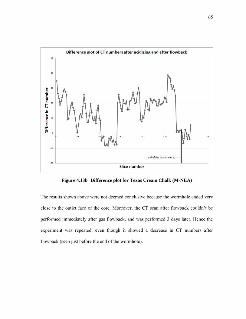
65

Figure 4.13b Difference plot for Texas Cream Chalk (M-NEA)

The results shown above were not deemed conclusive because the wormhole ended very

close to the outlet face of the core. Moreover, the CT scan after flowback couldn’t be

performed immediately after gas flowback, and was performed 3 days later. Hence the

experiment was repeated, even though it showed a decrease in CT numbers after

flowback (seen just before the end of the wormhole).

66

For the second experiment, the acidizing and flowback parameters are as follows (see

Tables 4.13d, 4.13e and 4.13f):

TABLE 4.13d-ACID FLOW PARAMETERS (TEXAS

CREAM CHALK; M-NEA; 2nd

EXPERIMENT)



TABLE 4.13d-ACID FORMULATION

(TEXAS CREAM CHALK; M-NEA; 2nd

EXPERIMENT) 1 Water 189 cc 2 HCl (15 wt%) 111 cc 3 NaI (5 wt%) 15.8 g 4 M-NEA (2 wt%) 6.3 g

TABLE 4.13f-FLOWBACK

PARAMETERS (TEXAS CREAM

CHALK; M-NEA; 2nd

EXPERIMENT)


The plot of mean CT numbers after acidizing and after flowback (Fig 4.13c) and the

Difference plot (Fig 4.13d) are seen below.

67

Figure 4.13c Mean CT number plot for Texas Cream Chalk (M-NEA); 2nd

experiment

68

Figure 4.13d Difference plot for Texas Cream Chalk (M-NEA); 2nd

experiment

The negative peak in the Difference plot shows that the spent acid clean-up was not

effective for the non-emulsifying agent. This result was unexpected; hence it was

repeated for a third time.

69

For the third experiment, the acidizing and flowback parameters are as follows (see

Tables 4.13g, 4.13h and 4.13i):

TABLE 4.13g-ACID FLOW PARAMETERS (TEXAS

CREAM CHALK; M-NEA; 3rd

EXPERIMENT)



TABLE 4.13h-ACID FORMULATION

(TEXAS CREAM CHALK; M-NEA; 3rd

EXPERIMENT)

1 Water 94.5 cc 2 HCl (15 wt%) 55.5 cc 3 NaI (5 wt%) 7.9 g 4 M-NEA (2 wt%) 3.2 g

TABLE 4.13i-FLOWBACK PARAMETERS

(TEXAS CREAM CHALK; M-NEA; 3rd

EXPERIMENT)

1 Back pressure 300 Psi 2 Overburden pressure 1500 Psi 3 Inlet pr. 800 Psi 4 Pr. drop across the core 463 Psi 5 Flowrate 8.7 L/min 6 Flow time 120 Min 7 Flow meter zero error 0.4 L/min

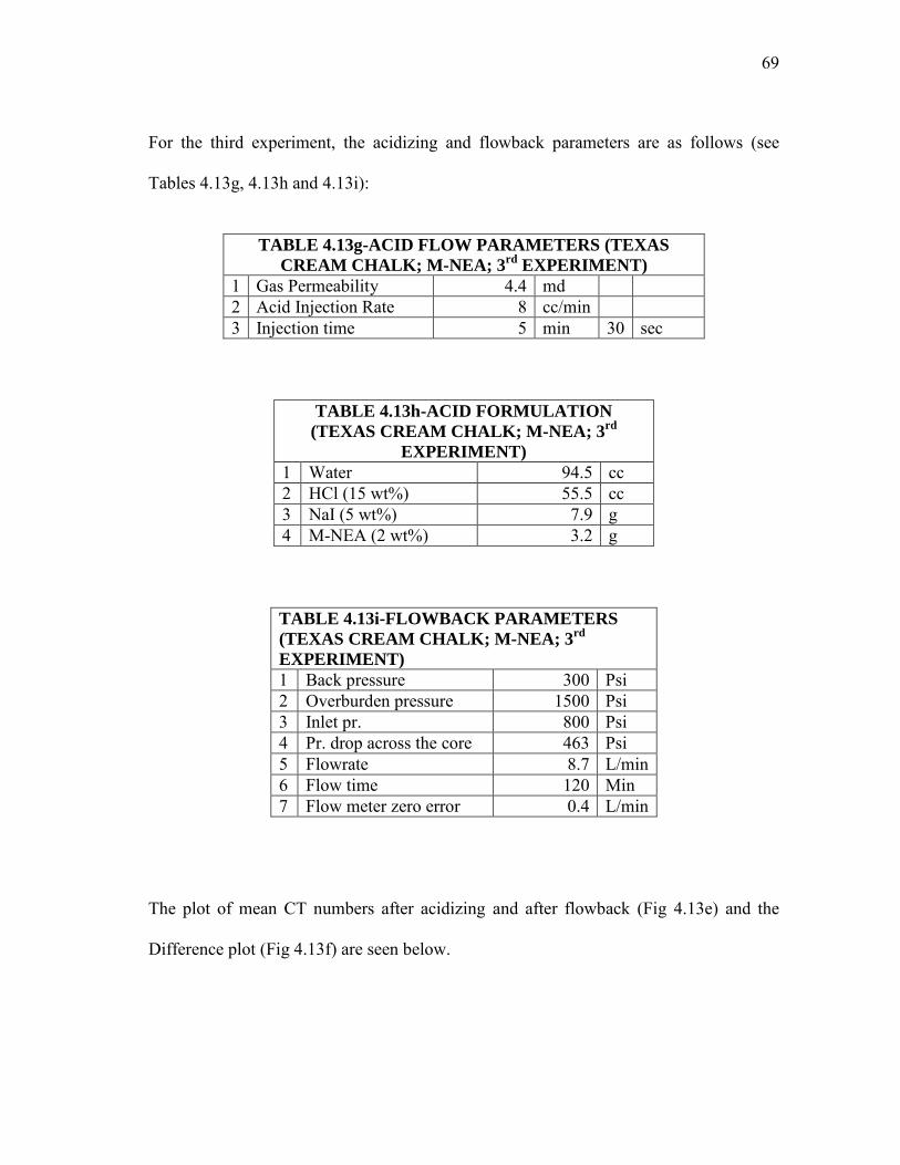
The plot of mean CT numbers after acidizing and after flowback (Fig 4.13e) and the

Difference plot (Fig 4.13f) are seen below.

70

Figure 4.13e Mean CT number plot for Texas Cream Chalk (M-NEA); 3rd

experiment

71

Figure 4.13f Difference plot for Texas Cream Chalk (M-NEA); 3rd

experiment

Quite like the previous result, the spent acid clean-up wasn’t effective for this case. It

can be observed that the spent acid has permeated deeper into the core. Hence this result

was finally deemed to be conclusive.

72

4.1.2.7 Combined Difference Plot

Similar to the Indiana Limestone, we can see the Combined Difference Plot for Texas

Cream Chalk below (Fig 4.14). The additives according to the peak height (highest peak

to lowest) are listed below:

1. FA-CI

2. No additive

3. T-ICA

4. CA-ICA

5. MI-CI

6. M-NEA

The Combined Difference Plot for Texas Cream Chalk can be seen below. For M-NEA,

the last (or the 3rd experiment) result was used.

73

Figure 4.14 Combined Difference Plot for Texas Cream Chalk (all additives)

The plot shows that for FA-CI, CA-ICA and T-ICA, the spent acid clean-up was

comparable to the control i.e. no additive case. The worst clean-up was found when MI-

CI and M-NEA were used.

74

5. CONCLUSIONS AND RECOMMENDATIONS

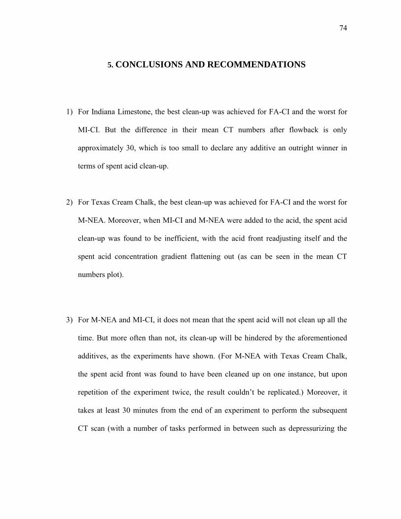
1) For Indiana Limestone, the best clean-up was achieved for FA-CI and the worst for

MI-CI. But the difference in their mean CT numbers after flowback is only

approximately 30, which is too small to declare any additive an outright winner in

terms of spent acid clean-up.

2) For Texas Cream Chalk, the best clean-up was achieved for FA-CI and the worst for

M-NEA. Moreover, when MI-CI and M-NEA were added to the acid, the spent acid

clean-up was found to be inefficient, with the acid front readjusting itself and the

spent acid concentration gradient flattening out (as can be seen in the mean CT

numbers plot).

3) For M-NEA and MI-CI, it does not mean that the spent acid will not clean up all the

time. But more often than not, its clean-up will be hindered by the aforementioned

additives, as the experiments have shown. (For M-NEA with Texas Cream Chalk,

the spent acid front was found to have been cleaned up on one instance, but upon

repetition of the experiment twice, the result couldn’t be replicated.) Moreover, it

takes at least 30 minutes from the end of an experiment to perform the subsequent

CT scan (with a number of tasks performed in between such as depressurizing the

75

equipment or pre-heating the CT scanner). This is ample time for the spent acid front

to imbibe deeper into the core, and give a negative peak on the difference plot.

4) FA-CI was found to perform the best in terms of reduction in CT numbers after

flowback (i.e. spent acid clean-up) for both Indiana Limestone and Texas Cream

Chalk.

5) This series of experiments should be repeated for water or brine saturated cores

(instead of gas saturated) to have a condition similar to actual conditions.

6) Moreover, the experiments should be conducted with an aluminum coreholder so as

to scan the acidized core without taking it out of the coreholder and disturbing or

contaminating it.

76

REFERENCES

Akin, S. and Kovscek, R. 2003. Computed Tomography in Petroleum Engineering

Research. Geological Society Special Publications 215: 23-38. Geological Society

of London, London, United Kingdom

Al-Muthana, A.S., Ma, S.M., and Okasha, T. 2008. Best Practices in Conventional Core

Analysis - a Laboratory Investigation. Paper 120814-MS presented at the SPE Saudi

Arabia Section Technical Symposium Al-Khobar, Saudi Arabia.

Angulo, R. and Ortiz, N. 1992. X-Ray Tomography Application in Porous Media

Evaluation. Paper 23670 presented at the SPE Latin America Petroleum

Engineering Conference Caracas, Venezuela.

Bartko, K.M., Newhouse, D.P., Andersen, C.A. et al. 1995. The Use of Ct Scanning in

the Investigation of Acid Damage to Sandstone Core. Paper 30457 presented at the

SPE Annual Technical Conference and Exhibition Dallas, Texas.

Coles, M.E., Hazlett, R.D., Spanne, P. et al. 1996. Characterization of Reservoir Core

Using Computed Microtomography. SPE Journal 9. 30542

Economides, M. J., Hill, A. D., and Economides, C. E.: Petroleum Production Systems,

First edition, PTR Prentice Hall, Englewood Cliffs, N.J., (1994).

Hove, A.O., Ringen, J.K., and Read, P.A. 1987. Visualization of Laboratory Corefloods

with the Aid of Computerized Tomography of X-Rays. SPE Reservoir Engineering

5. 13654

77

Hunt, P.K., Engler, P., and Bajsarowicz, C. 1988. Computed Tomography as a Core

Analysis Tool: Applications, Instrument Evaluation, and Image Improvement

Techniques. SPE Journal of Petroleum Technology 9. 16952

Kamath, J. and Laroche, C. 2003. Laboratory-Based Evaluation of Gas Well

Deliverability Loss Caused by Water Blocking. SPE Journal 3. 83659

Li, S., Dong, M., Dai, L. et al. 2004. Determination of Gas Permeability of Tight

Reservoir Cores without Using Klinkenberg Correlation. Paper 88472 presented at

the SPE Asia Pacific Oil and Gas Conference and Exhibition Perth, Australia.

Mahadevan, J. and Sharma, M.M. 2005. Factors Affecting Cleanup of Water Blocks: A

Laboratory Investigation. SPE Journal 9. 84216-PA

Nasr-El-Din, H.A., Al-Othman, A.M., Taylor, K.C. et al. 2004. Surface Tension of Hcl-

Based Stimulation Fluids at High Temperatures. Journal of Petroleum Science and

Engineering 43 (1–2): 57-73.

Nevito, J. 2006. Design, Set-up and Testing of a Matrix Acidizing Apparatus. MSc

Thesis, Texas A&M University, College Station, USA.

Saneifar, M., Nasralla, R.A., Nasr-El-Din, H.A. et al. 2011. Surface Tension of Spent

Acids at High Temperature and Pressure. Paper 149109-MS presented at the

SPE/DGS Saudi Arabia Section Technical Symposium and Exhibition Al-Khobar,

Saudi Arabia.

Schechter, R. S., Oil Well Stimulation, First edition, Prentice Hall, Englewood Cliff,

N.J., (1992).

78

Wellington, S.L. and Vinegar, H.J. 1987. X-Ray Computerized Tomography. SPE

Journal of Petroleum Technology 8. 16983

Withjack, E.M. 1988. Computed Tomography for Rock-Property Determination and

Fluid-Flow Visualization. SPE Formation Evaluation 12. 16951

Withjack, E.M., Devier, C., and Michael, G. 2003. The Role of X-Ray Computed

Tomography in Core Analysis. Paper 83467 presented at the SPE Western

Regional/AAPG Pacific Section Joint Meeting Long Beach, California.

79

APPENDIX A

MSDSs of the Additives Used

80

A-1 T-ICA MSDS

81

82

A-2 CA-ICA MSDS

83

84

85

86

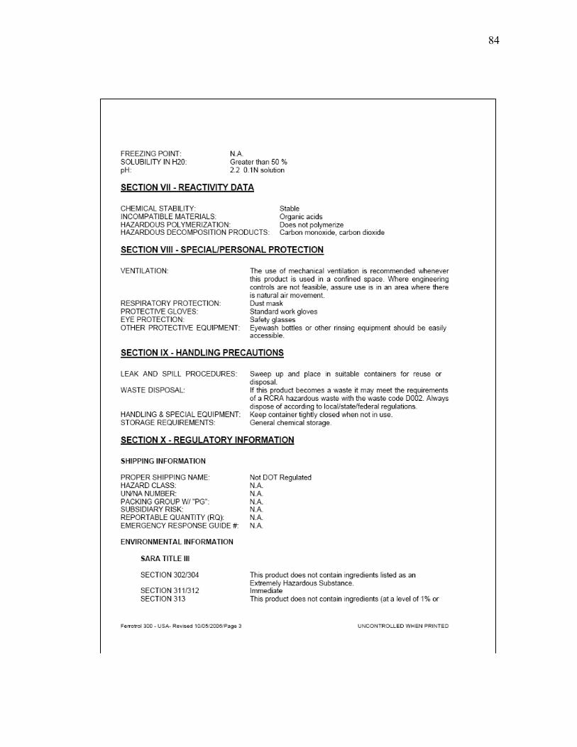
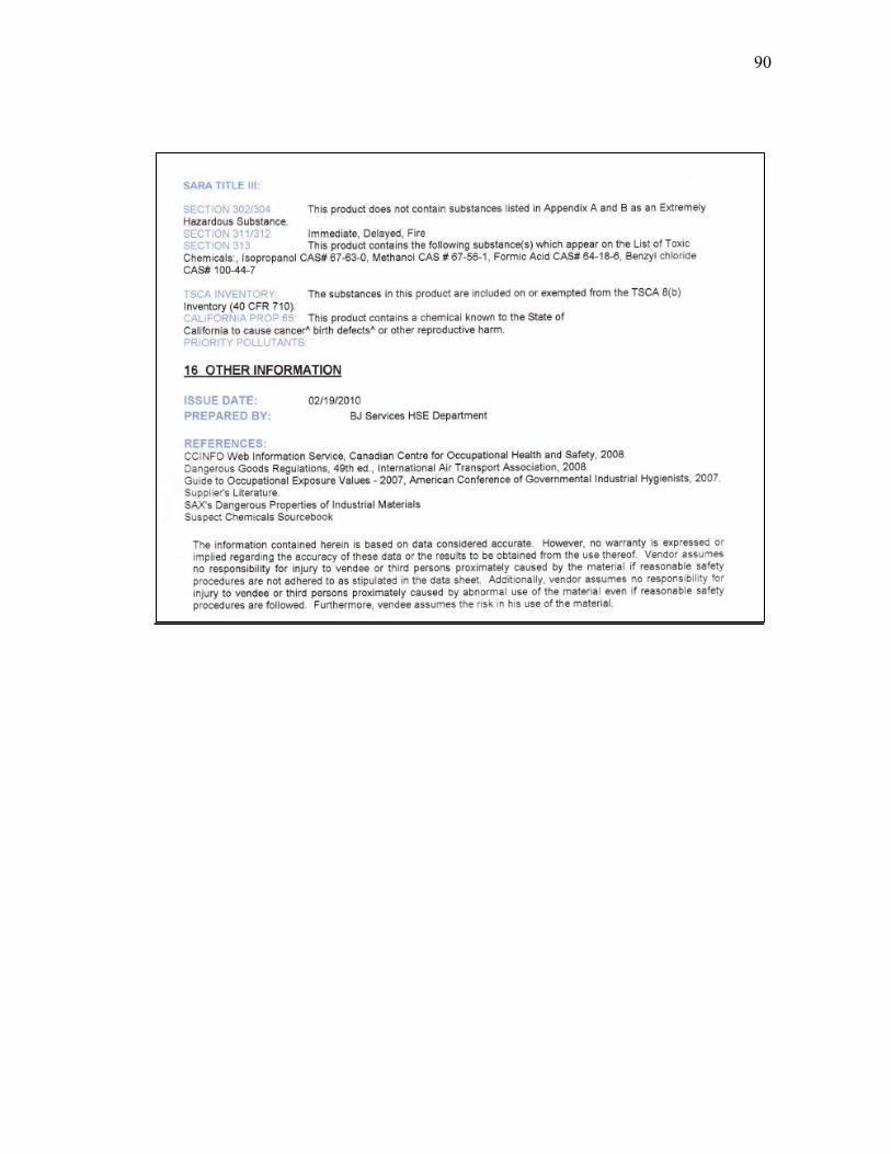
A-3 FA-CI MSDS

87

88

89

90

91

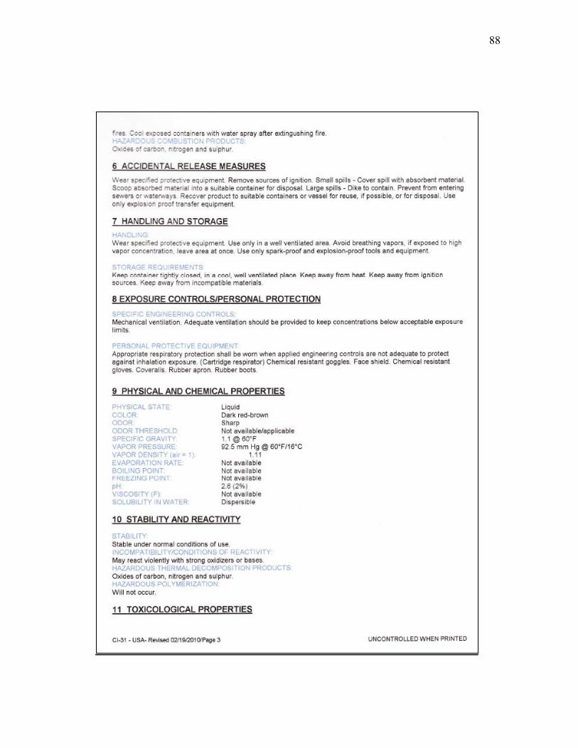
A-4 MI-CI MSDS

92

93

94

95

96

A-5 M-NEA MSDS

97

98

99

100

101

102

103

104

A-6 Sodium Iodide MSDS

105

106

107

108

109

VITA

Name: Ehsaan Ahmad Nasir

Address: Petroleum Engineering, 507 Richardson Building 3116 TAMU, College Station, TX, 77843-3116 Email Address: [email protected] Education: B.E., Mechanical Engineering, NED University of Engineering and

Technology, 2008 M.S., Petroleum Engineering, Texas A&M University, 2012 Employment Engro Polymer and Chemicals Ltd., Karachi, Pakistan 2008-2009 History:

Documents

Effects of Acid Additives on Spent Acid Flowback through ...oaktrust.library.tamu.edu/bitstream/handle/1969.1/ETD-TAMU-2012-05... · EFFECTS OF ACID ADDITIVES ON SPENT ACID FLOWBACK