Embed Size (px)
Citation preview

EFFECTIVNESS OF INORGANIC CONCRETE COATING MATRICES AND THEIR SELF CLEANING PROPERTIES
by
AHMED AMER
A thesis submitted to
The Graduate School-New Brunswick
Rutgers, The State University of New Jersey
in partial fulfillment of the requirements
for the degree of
Masters of Science
Graduate Program in Civil And Environmental Engineering
Written under the direction of
Professor P.N. Balaguru
and approved by
New Brunswick, New Jersey
January , 2008
ABSTRACT OF THE THESIS
EFFECTIVNESS OF INORGANIC CONCRETE COATING MATRICES AND THEIR SELF CLEANING PROPERTIES
BY AHMED AMER
Thesis Director: Dr. P. Balaguru
Concrete Coatings are becoming more popular to protect concrete surfaces for
infrastructures. The coating improves the durability of concrete structures. Inorganic
concrete coatings are better than organic coatings because they allow the release of vapor
pressure. The results presented in this thesis deals with the behavior of the inorganic
matrices which are based on silicates. The coating is compatible with concrete, brick and
wooden surfaces.
The objective of the research presented in this thesis is to evaluate the matrices for
workability, ease of application and self cleaning properties. Cracking characteristics
were also evaluated using high magnification. The self cleaning properties of the coating
matrices were studied using Rohdamine B dye to detect the degradation rate of the
organic chemicals that represent the organic pollutants in the atmosphere.
ii

Advanced technology such as X-ray photoelectron spectroscopy and Atomic force
microscope was used to measure the curing period and its effect on the matrices self
cleaning properties. The degradation of the organic chemicals represents a breakthrough
in the development of the inorganic matrices because they can be used in many
applications. Matrix combination that provides workable mix and minimum nano-level
cracking are recommended.
iii

ACKNOWLEDGEMENTS
First I would like to thank God the Gracious for all the blessing during my years of
study. I would like to extend my gratitude to Prof. N. Balaguru for his support and advice
through out the years of study. I would like to thank Dr. Maher and Dr. Najim for taking time
to be on my thesis committee. I would like to thank Prof. Theodore Madey and Dr. Boris
Yakshinskiy ( Rutgers Physics Deprtement) for their support in XPS testing. Moreover, I
would like to thank Dr. Elizabeth Pugel (NASA) for her support and advice.
I would like to thank my Father, for all his teachings. I would like to thank my
mother, sisters and my cousin Dr. Mohamed Nazier who supported me through all this.
Without you all I would not have been able to achieve anything. Thank you for supporting
me, being patient and for the love that was and will always be my encouragement for
achievements.
I would like to thank my co-workers and friends, Mohamed Arafa, Christian Defazio,
Patrick Szary, Linda Szary, Connie Dellamura, Edward Wass and Tom Bennet. I would like
also to thank Salah Hammed ,Waleed zakaria, Islam zakaria, Ahmed El-halawany, Amr
Bedeir , and Yehia Tokal for their help. Finally, I would like to thank all my friends here and
back home for their support and help.
iv

TABLE OF CONTENTS
ABSTRACT OF THE THESIS................................................................................................................II
ACKNOWLEDGEMENTS .................................................................................................................... IV
TABLE OF CONTENTS..........................................................................................................................V
CHAPTER 1 – INTRODUCTION............................................................................................................1
1.1 SCOPE AND OBJECTIVE OF THIS STUDY ................................................................................................1
CHAPTER 2 – STATE OF THE ART .....................................................................................................2
2.1 INTRODUCTION AND HISTORICAL BACKGROUND .................................................................................2
2.2 CHARACTERIZATION OF THE INORGANIC COATING MATRIX.................................................................3
2.3 EVALUATION OF THE INORGANIC COATING MATRIX ............................................................................4
2.3.1 Workability..................................................................................................................................5
2.3.2 Ease of application ......................................................................................................................5
2.3.3 Cracks development ....................................................................................................................5
2.4 SURFACE PREPARATION.......................................................................................................................6
CHAPTER 3 – EXPERIMENTAL DESIGN...........................................................................................7
3.1 INTRODUCTION....................................................................................................................................7
3.2 MIX COMPONENTS...............................................................................................................................8
3.2.1 Silicate Solution...........................................................................................................................8
3.2.2 Silicate Powder............................................................................................................................9
3.2.3 Hardeners...................................................................................................................................10
3.2.4 Fillers.........................................................................................................................................11
3.2.5 Titanium dioxide .......................................................................................................................11
3.2.6 Admixtures ................................................................................................................................12
3.2.7 Retarders....................................................................................................................................13
3.2.8 Glowing Powder........................................................................................................................13
3.3 SAMPLE PREPARATION ......................................................................................................................13
v
3.4 PREPARATION OF BASE MIXES ...........................................................................................................14
3.5 PREPARATION OF THE OTHER MIXES..................................................................................................15
3.5.1 Retarder Mixes ..........................................................................................................................15
3.5.2 Admixtures Mixes .....................................................................................................................15
3.5.3 Glowing Powder Mixes .............................................................................................................15
3.6 ULTIMATE COATING MIX APPLICATION..............................................................................................15
3.7 CURING METHOD ...............................................................................................................................15
3.8 LAB INVESTIGATION..........................................................................................................................15
3.8 LAB INVESTIGATION..........................................................................................................................16
3.9 SAMPLE SCORING SCALE BASIS..........................................................................................................18
3.10 MATRICES (SILICA FUMES 1) ...........................................................................................................19
3.11 MATRICES (SILICA FUMES 2) ...........................................................................................................59
CHAPTER 4 –EXPERIMENTAL INVESTIGATION.........................................................................72
4.1 INTRODUCTION..................................................................................................................................72
4.2 MECHANISM OF TITANIUM DIOXIDE IN THE BASE MIX........................................................................73
4.3 SAMPLE PREPARATION AND APPLICATION .........................................................................................77
4.3.1 Preparation of Base Mixes.........................................................................................................77
4.4 PREPARATION OF THE OTHER MIXES..................................................................................................77
4.4.1 Retarder Mixes ..........................................................................................................................77
4.4.2 Admixture Mixes.......................................................................................................................77
4.4.3 Glowing Powder Mixes .............................................................................................................78
4.5 CURING METHOD ...............................................................................................................................78
4.6 SELF CLEANING TEST SETUP ..............................................................................................................78
4.6.1 Using Artificial Light ................................................................................................................78
4.6.2 CIE Color System......................................................................................................................79
4.6.3 Using Sunlight...........................................................................................................................81
4.7 X-RAY PHOTOELECTRON SPECTROSCOPY ..........................................................................................82
4.8 XPS SAMPLE PREPARATION...............................................................................................................84
vi

4.9 XPS TESTING AND EXPERIMENTATION ..............................................................................................84
4.10 ATOMIC FORCE MICROSCOPE TESTING.............................................................................................85
4.11 AFM SAMPLE PREPARATION ...........................................................................................................85
CHAPTER 5 – TEST RESULTS AND DISCUSSION .........................................................................87
5.1 INTRODUCTION..................................................................................................................................87
5.2 MATRIX COATING RESULTS ...............................................................................................................87
5.3 SELF CLEANING RESULTS...................................................................................................................89
5.4 XPS AND AFM RESULTS.................................................................................................................104
CHAPTER 6 – CONCLUSIONS ..........................................................................................................108
6.1 CONCLUSIONS .................................................................................................................................108
6.2 SUGGESTIONS FOR FUTHER RESEARCH ............................................................................................109
REFERENCES .....................................................................................................................................111
vii
1
CHAPTER 1. INTRODUCTION
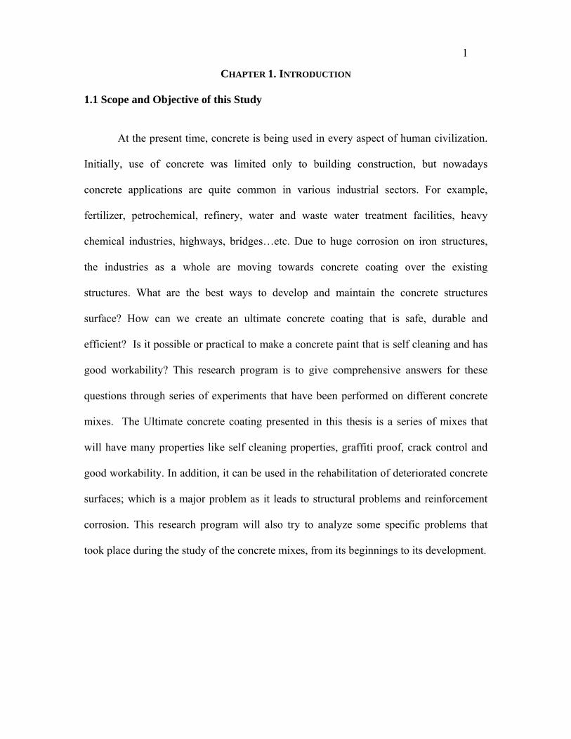
1.1 Scope and Objective of this Study
At the present time, concrete is being used in every aspect of human civilization.
Initially, use of concrete was limited only to building construction, but nowadays
concrete applications are quite common in various industrial sectors. For example,
fertilizer, petrochemical, refinery, water and waste water treatment facilities, heavy
chemical industries, highways, bridges…etc. Due to huge corrosion on iron structures,
the industries as a whole are moving towards concrete coating over the existing
structures. What are the best ways to develop and maintain the concrete structures
surface? How can we create an ultimate concrete coating that is safe, durable and
efficient? Is it possible or practical to make a concrete paint that is self cleaning and has
good workability? This research program is to give comprehensive answers for these
questions through series of experiments that have been performed on different concrete
mixes. The Ultimate concrete coating presented in this thesis is a series of mixes that
will have many properties like self cleaning properties, graffiti proof, crack control and
good workability. In addition, it can be used in the rehabilitation of deteriorated concrete
surfaces; which is a major problem as it leads to structural problems and reinforcement
corrosion. This research program will also try to analyze some specific problems that
took place during the study of the concrete mixes, from its beginnings to its development.

2
CHAPTER 2. LITERATURE REVIEW
2.1 Introduction and historical background:
Before discussing the areas in which concrete coating must be used, the purpose
and the history of concrete coatings should be identified. Concrete coating is a barrier
coating which is applied on the concrete structures surface to ensure considerable
durability and give further protection against penetration of carbon dioxide, water and
other aggressive chemicals that can have a significant effect on the behavior of these
concrete structures. The intrusion of water and other chemicals is the major reason for
deterioration of concrete structures. For the plain concrete, the failure occurs by the
exposure and popping of aggregates. However, for reinforced concrete, steel
reinforcement corrosion is the main reason foe the deterioration of concrete.
Reinforcement corrosion accelerates the degradation process by creating more cracks and
further chemical access.
Any history of concrete coating usually starts with the famous ancient Egyptian
Temples and cave paintings of Europe. Starting the mid to late 1800s, paint was usually
made by professional painters, craftsmen who both prepared paint and applied it. In that
time, the majority of the paint was prepared on site. Interior surfaces were often coated
with whitewash, distempers or casein paints which had either no binder at all, or binders
such as animal glue or casein which had poor durability. Casein paints remained popular
into the 20th century, purchased as powders to be mixed with water just before use &
some are still available commercially (Vanketsh, 1999). Exterior paints were made by
mixing white lead paste into oil. Lead functioned both as white pigment and as drying

3
agent for curing of the oil. The industrial revolution brought about centralized
manufacturing of paint dispersions as well as the production of a variety of resin
technologies. The first appearance for ready mixed paints in the US was granted in 1867.
Sales began in earnest in the mid 1880s and paint factories started. By 1900 nearly 20
million gallons per year of ready mixed paint were sold in the US, and this volume rose
steadily. By 1930, lithopone and zinc oxide had mostly replaced lead for interior paints;
however, lead was still used widely for exterior paints and metal coatings.
The first titanium dioxide pigments were introduced in the 1930s. The early
versions of titanium dioxide were mainly in crystal form. Exterior paints for a time were
intentionally formulated with a TiO2 as self cleaning paints for a small amount of
chalking which allows dirt to be removed by rain. Titanium dioxide was commercialized
after World War II and finally allowed the formulation of durable paints that do not
contain lead (Vanketsh, 1999).
2.2 Characterization of the inorganic coating matrix:
Portland cement is the most widely used inorganic binder in the civil industry.
On the other hand, the size of the Portland cement grains is one of the major
disadvantages of the Portland cement system because it is relatively large. Thus, it
prevents the formation of thin binders. Other common room temperature matrices such as
alluminomsilicates and phosphate based compounds were introduced as an alternative to
Portland cement. One of the major advantages of the silicate compounds is that they are
not 100% impermeable thus allowing the concrete surface to breath or in other words to
release the vapor pressure. In addition, they are not toxic and they have proven to be UV
light resistant and fire resistant.

4
One of the inorganic resins which are currently available is a potassium alluminosilicate,
or poly (sialate-siloxo), with the general chemical structure.
Kn{-(SiO2)z – AlO2 } • wH2O Where z>>n ( Garon, 2000) There are many research programs and studies that have been conducted on the
performance of inorganic polymers as a protective coating. Protective concrete coating
can be simply described as the coating that protects the surface from the intrusion of
water and other chemicals that cause deterioration and failure of concrete structures.
These coatings act as a barrier that prevents the ingress of liquids and other chemicals but
at the same time they do not allow the concrete to breathe or in other words they do not
allow the release of water that is already inside the concrete. Accumulation of water at
the interface eventually led to the peeling of the organic coatings (Balaguru, 1998). The
results reported in Balaguru and Nazier, 2004, deal with an experimental study on the
performance of the inorganic concrete coating. The results of the research program shows
that the inorganic coating is resistant to UV light, releases vapor pressure and is fire
resistant. Moreover, the inorganic coating is durable under scaling, wet-dry and freeze-
thaw conditions (Nazier, 2004 ).
2.3 Evaluation of the inorganic coating matrix:
There are many studies that discuss many means of concrete coating evaluation.
However, all these studies has took in consideration three important factors which are :
1) Coating Workability
2) Ease of application
3) Cracks development

5
In order to understand the basis of for evaluation of the inorganic matrix, those points
have to be identified and clarified.
2.3.1 Workability:
Workability is the term used to describe the property of concrete coating that determines
the ease with which it can be mixed, applied, and finished to a homogenous condition
(ACI 116R-00, 73). The homogeneity and the consistency of the coating mix is very
important for the application. The mix can have low viscosity and yet it is not workable.
For example, there are lots of mixes that form lumps or in case of very thin mixes or in
other words very low viscosity mixes.
2.3.2 Ease of application:
There are many techniques to apply the concrete coating. The most widely used
techniques are brush, roller, and spraying. A large number of commercial brushes, rollers
and sprayers are available in the market. For the inorganic binders, the preferred methods
are by brush or rollers because this technique provides better wetting. Ease of application
is directly proportional to workability. Thus, the more workable the coating, the easier it
can be applied.
2.3.3 Cracks development:
Concrete coatings crack for many reasons. Shrinkage is the primary cause of cracking
development. It is a very well known fact that as concrete coating hardens and dries, it
shrinks. This is due to the loss of excess mixing fluids such as chemical admixtures or
water. Thus, in most cases, the wetter or soupier the coating mix, the greater the
shrinkage will be. This shrinkage causes forces in the mix which literally pull the coating
particles apart and cracks are the end result of these forces. One of the main reasons of
6
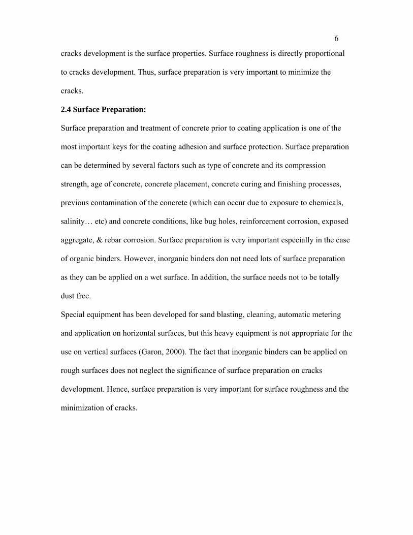
cracks development is the surface properties. Surface roughness is directly proportional
to cracks development. Thus, surface preparation is very important to minimize the
cracks.
2.4 Surface Preparation:
Surface preparation and treatment of concrete prior to coating application is one of the
most important keys for the coating adhesion and surface protection. Surface preparation
can be determined by several factors such as type of concrete and its compression
strength, age of concrete, concrete placement, concrete curing and finishing processes,
previous contamination of the concrete (which can occur due to exposure to chemicals,
salinity… etc) and concrete conditions, like bug holes, reinforcement corrosion, exposed
aggregate, & rebar corrosion. Surface preparation is very important especially in the case
of organic binders. However, inorganic binders don not need lots of surface preparation
as they can be applied on a wet surface. In addition, the surface needs not to be totally
dust free.
Special equipment has been developed for sand blasting, cleaning, automatic metering
and application on horizontal surfaces, but this heavy equipment is not appropriate for the
use on vertical surfaces (Garon, 2000). The fact that inorganic binders can be applied on
rough surfaces does not neglect the significance of surface preparation on cracks
development. Hence, surface preparation is very important for surface roughness and the
minimization of cracks.

7
CHAPTER 3. EXPERIMENTAL DESIGN
3.1 Introduction
Geopolymers are inorganic polymers widely used in many applications for more
than thirty five years. Geopolymer was first applied to these materials by Joseph
Davidovits in the 1970s, although similar materials had been developed in the former
Soviet Union since the 1950s under the name Soil Cements. Davidovits proposed in 1978
that a single aluminum and silicon-containing compound, most likely geological in
origin, could react in a polymerization process with an alkaline solution. The binders
created were termed "geopolymers" (Wikipedia, 2004). They are an attractive
replacement to cement as they have lower carbon dioxide emissions. Geopolymers can be
produced using residual waste products such as fly ash and red mud. Geopolymer based
material has many advantages such as high chemical and thermal resistance at both
atmospheric and extreme conditions. One of the geopolymers applications is coatings and
paintings.
In this chapter, geopolymers based concrete coatings are being discussed in
detail. Fifty mixes were prepared and the components were introduced in a form of a
matrix named “Ultimate Concrete Coating Matrix”. Those mixes were evaluated in terms
of workability, ease of application and cracks development. Using advanced technology,
color pigments were added to the mix giving it some glowing properties. This coat can
now be used not only as a protection coat but also for traffic signals and night
applications.
8
3.2 Mix Components
The Mixes of the concrete coating matrix is composed of the following:
1) Silicate solution (Part A)
2) Silicate powder (Part B)
3) Hardeners
4) Fillers
5) Titanium dioxide (TiO2)
6) Distilled Water (H2O).
7) Admixtures
8) Retarders
9) Glowing powder
The components are described briefly in the following sections.
3.2.1 Silicate Solution
Silicate solutions are extensively used in the painting and coating industry. They
play an important role in the chemical industry and they are used to manufacture many
industrial as well as commercial goods and products, for example chemical reagents and
neutralization of acids, further as basic standard in analytics and many more applications.
Silicate solutions are based on high single or mixed silicon dioxide to alkali metal oxide
mol ratio inorganic alkali metal silicates. Silicate solution is produced from a starter
alkali metal silicate aqueous solution by mixing the solution with a silicone monomer and
agitating until hydrolysis is essentially complete. A silica gel is then added as an aqueous
9
slurry and blended until the silica gel is at least partially dissolved. Thereafter, the
mixture is agitated to a smooth consistency and recovered as a binder composition (Brito,
1998). Silicate solution serves as a binder in the mix and it gives the mix higher
workability and makes it easier to be applied on variety of surfaces.
3.2.2 Silicate Powder
Silicate powder is mainly composed of mineral geopolymers and silicates
byproducts which are considered as residuals from production of some silicon alloys
.Geopolymer are created from aluminum silicate materials and they act as an alternative
for Portland-based cements. Geopolymers are generally formed by reaction of an
aluminum silicate powder with an alkaline silicate solution at roughly normal
atmospheric conditions.
Fly ash is a commonly used material for the manufacturing of geopolymers, and
is generated by thermal activation of coal residual in the generating plants.
The chemical reaction that takes place to form geopolymers follows a multi-step process
which can be summarized in the following points (geopolymers institute, 2005):
1) Dissolution of Si and Al atoms from the source material due to hydroxide ions in
solution
2) Reorientation of precursor ions in solution, and Setting through polycondensation
reactions into an inorganic polymer.
3) The inorganic polymer network is in general a highly-coordinated 3-dimensional
aluminum silicate gel, with the negative charges on tetrahedral Al(III) sites
charge-balanced by alkali metal cations.

10
The ratio of Silicate: Aluminum in the polysilicate structure determines the
mechanical properties of the geopolymers and their application fields. A low ratio
Silicate: Aluminum initiates a three dimension Network that is very rigid. A high ratio
Silicate: Aluminum provides polymeric character to the geopolymeric material. The
silicate :Aluminum ratio is case sensitive because the coating should prevent the access
such as salts and chlorides from accessing the surface and in the same time it should
allow the concrete to breath. Otherwise, the coating will delaminate due to liquid
collection at the interface (Balaguru, 2006). Silicate powder together with the silicate
solution is the cementing agent that acts as a binder for the coating.
3.2.3 Hardeners
A Hardener is substance or mixture added that is added to a the coating mix to
take part in and promote or control the curing action, Also a substance added to control
the degree of hardness of the cured coating. The hardeners used in the coating mix were
mainly composed of metal oxides that are nearly insoluble in water but soluble in acids
and alkalis. Many metal oxide pigments are used in the painting industry and also used in
coatings for paper. Some Metal oxides particles absorbs both UVA and UVB rays of
ultraviolet light, they can be used in ointments, creams, and lotions to protect against
sunburn and other damage to the skin caused by ultraviolet light. Metal oxide mixture
provide curing and hardening to the concrete coating at the room temperature.
11
3.2.4 Fillers
Fillers are something that fills the gaps or in other words the air voids in the
coating mix giving it strength and helps to minimize the cracks. In the coating mix, fillers
are mainly composed of fibers, metallic fibers and silicate compounds. Fibers are widely
used in many applications such as fabrics and textile industry. Fibers are mainly created
from polyester and polyamides. However, metallic fibers are composed of metal, plastic-
coated metal, metal-coated plastic, or a core completely covered by metal. The mixture of
fibers and silicate compounds gives strength to the mix and minimizes the cracks. In
addition, it gives the coating thermal resistance properties which make the coating
suitable for high temperature conditions.
3.2.5 Titanium Dioxide (TiO2)
Titanium dioxide is the naturally occurring oxide of titanium and it was first
produced commercially in 1923. Its chemical formula is TiO2 and when used as a
pigment, it is called titanium white, Pigment White 6, or CI 77891 (Wikipedia, 2004). It
is commonly used in many application applications that such as painting, sunscreen and
food coloring. In 2004, 4.4 million of titanium dioxide tones were produced worldwide.
Most titanium dioxide pigment is produced from titanium mineral concentrates by the
chloride or sulfate process, either as the rutile or the anatase form (the crystalline
structure of existing TiO2 in the ores). The primary particles are typically between 0.2
and 0.3 μm in diameter, although larger aggregates and agglomerates are formed.
Ultrafine grades of titanium dioxide have a primary particle size of 10–50 nm and are
used extensively as ultraviolet blockers in sunscreens and plastics, and in catalysts

12
(Henrich and Cox, 1994). Most commercial titanium dioxide products are coated with
inorganic; for example alumina, zircon, silica, and organic; for example polyols, esters
and silanes, compounds to control and improve surface properties. Titanium dioxide is
also known to be photocatalyst that can break down almost any organic compound it get
in contact with when exposed to UV light whether it was artificial light or sunlight.
Nowadays, many products are developed that uses the photocatalytic action of titanium
dioxide. These products include self-cleaning fabrics, paintings, and ceramic tiles.
Moreover, titanium dioxide is used in the manufacture of paving stone that uses the
catalytic properties of TiO2 to remove nitrogen oxide from the air, breaking it down into
more environmentally basic substances. Hence, it plays in an important role in the
degradation and decomposition of organic pollutants. Titanium was added to the coating
mix to give it self cleaning properties which will be discussed in details in chapter 3.
3.2.6 Admixtures
Admixtures are generally used as a solvent for many substances and they are used in the
manufacture of many industries such as paintings, scents, colorings, and medicine. They
are also used in the fuel industry for the internal combustion engines because they make
fuel environmental friendly as it burns cleanly. Admixtures added to the mix are
flammable, colorless, slightly toxic chemical compounds. Admixtures were added to the
coating mix to improve surface smoothness and workability.
13
3.2.7 Retarders
Retarder is the term used to express chemical agent that slows down a chemical reaction;
thus, increasing the setting time and decreasing the strengthening rate during the early
age. For example, the admixtures that is added to concrete mixes to slow down their
chemical hardening. Retarders used in the coating mix were added to delay the chemical
hardening of the coating mix without affecting the long-term mechanical properties so
that it can be used in variety of applications.
3.2.8 Glowing Powder
Glowing powder pigments was added to the coating mix to give the mix glowing
properties at the dark; hence, it can be use for traffic signals and night applications. The
mechanism of the glowing coating is that the glowing powder absorbs light and then
releases it creating the glow in the dark effect.
3.3 Sample Preparation
Three types of specimen were made. The first type of samples was made on
concrete bricks 7.5 X 3.5 x 2.5 inch or circular samples of diameter 4 inch from
commercially available concrete blocks. The circular samples were cut using a wet saw.
The samples were let to dry for about 48 hours days. The second type of specimens was
made of red bricks of 7.5 X 3.5 X 2.5 inch. After that the samples were cleaned using a
piece of cloth to remove any lose particles. The third type of samples was made on James
hardy board in the CAIT Materials laboratory in Livingston. The board surface was
cleaned using piece of cloth and lose particles were removed. The area to be coated was

14
outlined using mask tape to achieve a perfect rectangle. Multiple mixes were made to
cover the large area.
3.4 Preparation of Base mixes
The Ultimate coating is prepared as follows. A mixture of 100 grams of silicate solution
and 135 grams of silicate powder is placed in a high-shear mixer containing notched
stainless steel blades and mixed for one minute at speed of 1,500 RPM. Few powder
particles stick to the wall of the mixer. A putty knife was used to collect the particles sticking
to the mixer wall and the mixture is mixed for 1 minute. A mixture of 10 grams of metal
oxide, 15 grams of micro fibers, 5 grams of titanium dioxide and 3 grams of fibers is added to
the mix and mixed for one minute. Putty knife is used again to collect all the mixture
particles sticking to the mixer wall and mixed for one more minute. Ten grams of distilled
water is added to the mix and mixed for one minute. Some problems appear during the
mixing procedure for the silicon dioxide based mixes due to high shrinkage. The steel blades
of the mixer were stopped by the formation of big sized patches as shown in
Fig 2.1. These problems were solved
by adjusting the Silicate solution :
silicate powder ratio.
Fig. 3.1 shows the patch formation during the mixing procedure

15
3.5 Preparation of Other mixes:
3.5.1 Retarder Mixes
Same procedure of mixing as in the base mixes is used. The retarder is dissolved in
distilled water then added to the mixture & mixed for one minute.
3.5.2 Admixtures Mixes
Same procedure of mixing as in the base mixes is used. Admixtures were added to the
mixture and mixed for one minute. Then, distilled water is added to the mix and mixed
for one more minute.
3.5.3 Glowing Powder Mixes
The glowing powder was added to the mixture during the second step and mixed for one
minute. Then, distilled water is added to the mix and mixed for one minute.
3.6 Ultimate Coating Mix application
Initially, Self cleaning coating mix is stiff and eventually mixes to a thick liquid that can
be applied using brush or roller. The mix was applied on the three types of samples using
a smooth brush or a roller. The samples were left at room temperature for at least 21 days
before testing.
3.7 Curing Method The coating was cured at room temperature. At room temperature, the sample has to be
protected from running water or direct rain for 3 days. After 24 hours, the samples are

16
water resistant. However, running water could damage the surface by leaching out small
amounts of mix components.
3.8 Lab Investigation
The performance of the inorganic coating was evaluated with time. Visual inspection
along with digital microscopic photography
will be used to evaluate the performance of
the ultimate coatings. The microscope used for
lab investigation is Olympus model GX41 and
it is attached to a digital camera that is
connected to a personal computer. Small
samples were cut from the bricks using a wet
saw so that the samples can fit the
microscopic stage.
Samples made were checked under 50X
lens (scale 500 µm) and 4X lens (scale 25
µm). The main goals of the lab
investigation were to evaluate the coating
mixes on the following Basis:
1) Workability
2) Ease of Application
3) Cracks Development
Fig 3.2 shows the sample on the microscopic stage
Fig 3.3 shows the sample under 50X (500 µm) magnification lens

17
The digital microscopic pictures taken under the 50X lens (500 µm) were similar to a
great extent and the cracks was not shown clearly. Thus, 4X (25 µm scale) lens was used
to take the digital microscopic pictures and the cracks were identified. Each sample
scanned under the microscope and a representative picture was taken that shows the main
cracking spot or the main defects in the sample. The setting time for each mix was
calculated by pouring small amount of each coating mix in a small plastic cup and the
mix was checked every minute till hardening using a putty knife.
Fig 2.4 shows the coating mix sample placed in a plastic cup to measure the setting time
Fig 2.5 shows the sample mix during the hardening time

18
Table 3.1 and Table 3.2 give the main components of the samples coating mixes made in
the lab with the different mixtures weights. The tables show the chemical composition of
the different samples. Then, each sample mix was identified exclusively and three
pictures were taken for the sample. The three pictures taken represent the following:
1) General layout of the sample.
2) A magnified picture was cut from the general layout picture using Adobe
Photoshop software representing the main visual observation on the sample.
3) Digital microscopic picture under 4X lens (scale 25 µm) represents the main
cracking spots or defects on the sample.
3.9 Sample Scoring scale basis
Each sample was given a score ranging from 0 to 5 according to its workability, ease of
application and cracks development. Score Zero means that sample has a very low
workability and cannot be easily applied on the surface. Score five means that the sample
has a very high workability and can be easily applied. For cracks development, Score
Zero means that the sample has almost no cracks or cracks less than 1 µm and score five
means that the sample is full of cracks.

19
Table 3.1 (Silica Powder 1)
A (gms) B (gms) C (gms) Micro fiber (gms)
Ground Filler (gms)
TiO2 (gms)
Fibers (gms)
H2O (gms)
Retarder 1 (gms) Admixture 1 Admixture 2
(Percentage)Retarder2
(gms)Glowing
Powder (gms)
Base Mixes 1 100 125 10 15 30 10 3 10 - - - - -2 100 125 10 15 30 5 3 10 - - - - -3 100 125 10 15 30 5 - 7.5 - - - - -
Water Mixes 4 100 125 10 15 30 - 3 10 - - - - -5 100 125 10 15 30 - 3 15 - - - - -6 100 125 10 15 30 - 3 20 - - - - -
Retarder 1 Mixes 7 100 125 10 15 30 - 3 10 0.25 - - - -8 100 125 10 15 30 - 3 10 0.5 - - - -9 100 125 10 15 30 - 3 10 1 - - - -10 100 125 10 15 30 - 3 10 2 - - - -11 100 125 10 15 30 - 3 10 4 - - - -
Admixture 112 100 125 10 15 30 5 3 10 0.5 1 - - -13 100 125 10 15 30 5 3 10 0.5 2 - - -14 100 125 10 15 30 5 3 10 0.5 3 - - -15 100 125 10 15 30 5 3 10 0.5 4 - - -
Admixture 2 Mixes 16 100 125 10 15 30 5 3 10 0.5 - 1 - -17 100 125 10 15 30 5 3 10 0.5 - 2 - -18 100 125 10 15 30 5 3 10 0.5 - 3 - -19 100 125 10 15 30 5 3 10 0.5 - 4 - -
Remarks
Using Nano TiO2
Components
Mix No.
Using Coarse TiO2Using Nano TiO2
20
A (gms) B (gms) C (gms) Micro fiber (gms)
Ground Filler (gms)
TiO2 (gms)
Fibers (gms)
H2O (gms)
Retarder 1 (gms) Admixture 1 Admixture 2
(Percentage)Retarder2
(gms)Glowing
Powder (gms)
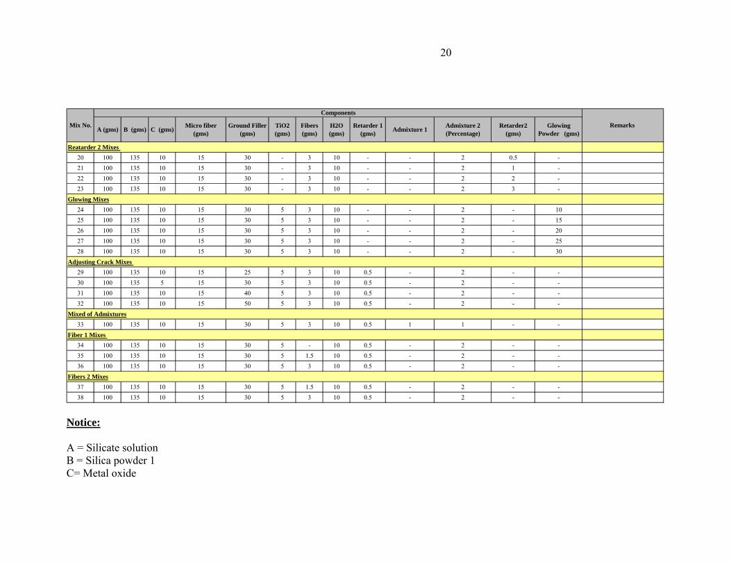
Reatarder 2 Mixes 20 100 135 10 15 30 - 3 10 - - 2 0.5 -21 100 135 10 15 30 - 3 10 - - 2 1 -22 100 135 10 15 30 - 3 10 - - 2 2 -23 100 135 10 15 30 - 3 10 - - 2 3 -
Glowing Mixes24 100 135 10 15 30 5 3 10 - - 2 - 1025 100 135 10 15 30 5 3 10 - - 2 - 1526 100 135 10 15 30 5 3 10 - - 2 - 2027 100 135 10 15 30 5 3 10 - - 2 - 2528 100 135 10 15 30 5 3 10 - - 2 - 30
Adjusting Crack Mixes 29 100 135 10 15 25 5 3 10 0.5 - 2 - -30 100 135 5 15 30 5 3 10 0.5 - 2 - -31 100 135 10 15 40 5 3 10 0.5 - 2 - -32 100 135 10 15 50 5 3 10 0.5 - 2 - -
Mixed of Admixtures33 100 135 10 15 30 5 3 10 0.5 1 1 - -
Fiber 1 Mixes 34 100 135 10 15 30 5 - 10 0.5 - 2 - -35 100 135 10 15 30 5 1.5 10 0.5 - 2 - -36 100 135 10 15 30 5 3 10 0.5 - 2 - -
Fibers 2 Mixes37 100 135 10 15 30 5 1.5 10 0.5 - 2 - -38 100 135 10 15 30 5 3 10 0.5 - 2 - -
Remarks
Components
Mix No.
Notice: A = Silicate solution B = Silica powder 1 C= Metal oxide
21
Matrix No. 1 Table 1
Mix Content weight (gms)
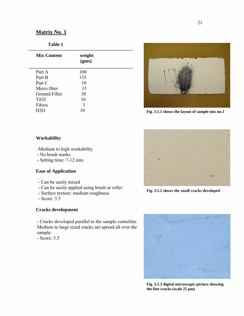
Part A 100 Part B 135 Part C 10 Micro fiber 15 Ground Filler 30 TiO2 10 Fibers 3 H2O 10 Workability -Medium to high workability - No brush marks - Setting time: 7-12 min. Ease of Application - Can be easily mixed - Can be easily applied using brush or roller - Surface texture: medium roughness - Score: 3.5 Cracks development - Cracks developed parallel to the sample centerline. Medium to large sized cracks are spread all over the sample. - Score: 3.5
Fig. 3.1.1 shows the layout of sample mix no.1
Fig. 3.1.3 digital microscopic picture showing the fine cracks (scale 25 µm)
Fig. 3.1.2 shows the small cracks developed

22
Matrix No. 2
Table 2
Mix Content weight (gms)
Part A 100 Part B 135 Part C 10 Micro fiber 15 Ground Filler 30 TiO2 5 Fibers 3 H2O 10 Workability - Medium to high workability - No brush marks - Setting time: 7-12 min. Ease of Application - Can be easily mixed - Can be easily applied using brush or roller - Surface Texture: Medium to high roughness - Score: 3.5
Cracks development
- Cracks developed diagonally to the sample centerline. The cracks are small sized cracks with slightly lower elevations than the surrounding surface. - Score: 2.0
Fig. 3.2.2 shows no cracks under visual observation
Fig. 3.2.1 shows the layout of sample mix no. 2
Fig. 3.2.3 digital microscopic picture showing minimal cracks (scale 25 µm)
23
Matrix No. 3 Table 3
Mix Content weight (gms)
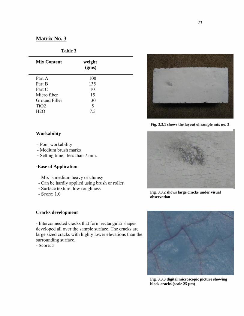
Part A 100 Part B 135 Part C 10 Micro fiber 15 Ground Filler 30 TiO2 5 H2O 7.5 Workability - Poor workability - Medium brush marks - Setting time: less than 7 min. -Ease of Application - Mix is medium heavy or clumsy - Can be hardly applied using brush or roller - Surface texture: low roughness - Score: 1.0
Cracks development
- Interconnected cracks that form rectangular shapes developed all over the sample surface. The cracks are large sized cracks with highly lower elevations than the surrounding surface. - Score: 5
Fig. 3.3.2 shows large cracks under visual observation
Fig. 3.3.1 shows the layout of sample mix no. 3
Fig. 3.3.3 digital microscopic picture showing block cracks (scale 25 µm)

24
Matrix No. 4 Table 4
Mix Content weight (gms)
Part A 100 Part B 135 Part C 10 Micro fiber 15 Ground Filler 30 Fibers 3 H2O 10 Workability -Medium to high workability - No brush marks - Setting time: 10-12 min. -Ease of Application - Can be easily mixed - Can be easily applied using brush or roller - Surface Texture: Medium roughness - Score: 3.5
Cracks development - Cracks developed parallel to the sample centerline. Medium sized cracks are spotted in different places of the sample. - Score: 2.5
Fig. 3.4.2 shows no cracks under visual observation
Fig. 3.4.1 shows the layout of sample mix no. 4
Fig. 3.4.3 digital microscopic picture showing medium sized cracks (scale 25 µm)
25
Matrix No. 5 Table 5
Mix Content weight (gms)
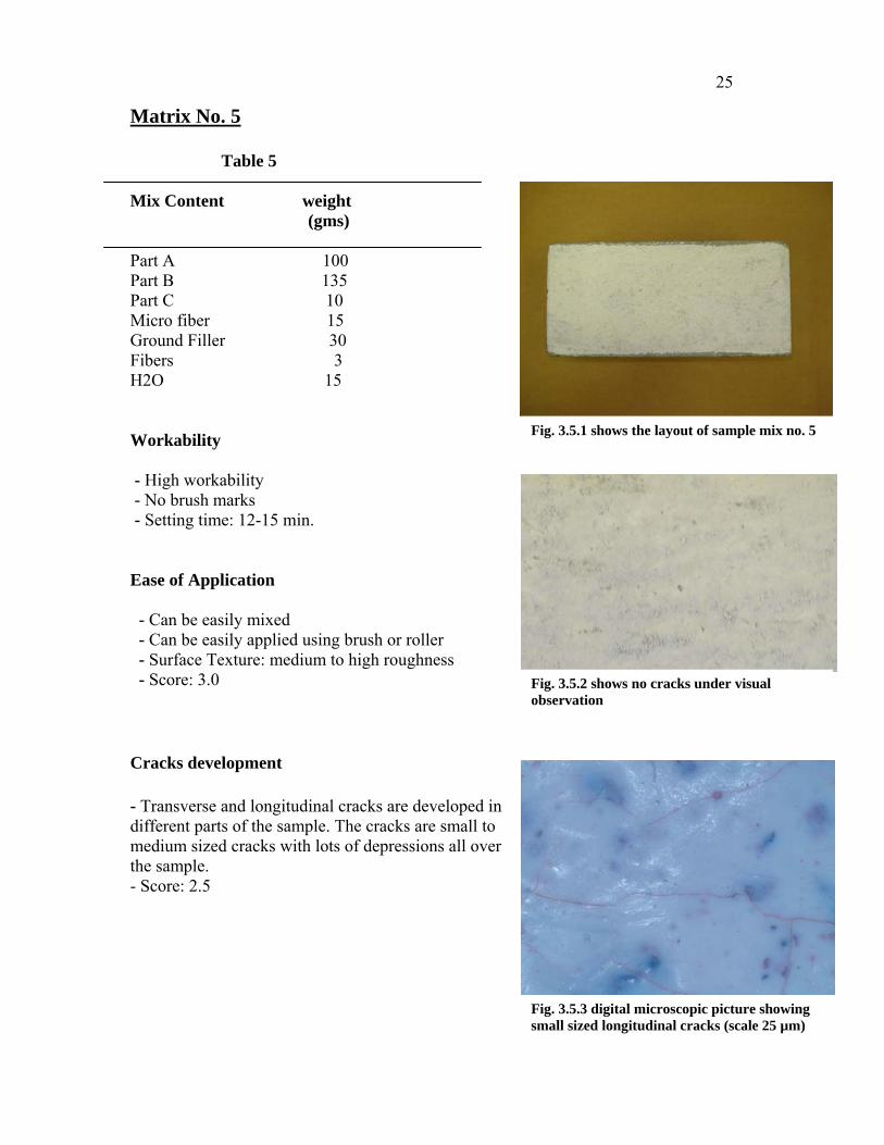
Part A 100 Part B 135 Part C 10 Micro fiber 15 Ground Filler 30 Fibers 3 H2O 15 Workability - High workability - No brush marks - Setting time: 12-15 min. Ease of Application - Can be easily mixed - Can be easily applied using brush or roller - Surface Texture: medium to high roughness - Score: 3.0 Cracks development - Transverse and longitudinal cracks are developed in different parts of the sample. The cracks are small to medium sized cracks with lots of depressions all over the sample. - Score: 2.5
Fig. 3.5.1 shows the layout of sample mix no. 5
Fig. 3.5.2 shows no cracks under visual observation
Fig. 3.5.3 digital microscopic picture showing small sized longitudinal cracks (scale 25 µm)

26
Matrix No. 6 Table 6
Mix Content weight (gms)
Part A 100 Part B 135 Part C 10 Micro fiber 15 Ground Filler 30 Fibers 3 H2O 20 Workability -Very high workability - No brush marks - Setting time: 15-20 min. Ease of Application - Mix is very thing and form patches - Can be easily applied using brush or roller - Surface Texture: High roughness - Score: 4.5 Cracks development - Transverse and longitudinal cracks are developed in different parts of the sample. The cracks are very small sized cracks with lots of depressions all over the sample. - Score: 2.0
Fig. 3.6.1 shows the layout of sample mix no. 6
Fig. 3.6.2 shows no cracks under visual observation
Fig. 3.6.3 digital microscopic picture showing minimal cracks (scale 25 µm)

27
Matrix No. 7 Table 7
Mix Content weight (gms)
Part A 100 Part B 135 Part C 10 Micro fiber 15 Ground Filler 30 Fibers 3 H2O 10 Retarder 1 0.25 Workability -Medium to high workability - No brush marks - Setting time: 20-25 min. Ease of Application - Can be easily mixed - Can be easily applied using brush or roller - Surface Texture: low roughness - Score: 3.5 Cracks development - Transverse and diagonal cracks are developed all over the sample. The cracks are medium to large sized cracks that can be easily observed. - Score: 4.0
Fig. 3.7.1 shows mix no. 7 with two layers at the left side and one layer at the right side
Fig. 3.7.3 digital microscopic picture showing medium sized cracks (scale 25 µm)
Fig. 3.7.2 shows fine longitudinal cracks all across the sample

28
Matrix No. 8 Table 8
Mix Content weight (gms)
Part A 100 Part B 135 Part C 10 Micro fiber 15 Ground Filler 30 Fibers 3 H2O 10 Retarder 1 0.5 Workability -Medium to high workability - No brush marks - Setting time: 50- 60 min. Ease of Application - Can be easily mixed - Can be easily applied using brush or roller - Surface Texture: low roughness - Score: 3.5 Cracks development - No cracks are can be noticed. Very few depressions can be seen in few parts of the sample. - Score: 0.5
Fig. 3.8.2 shows no cracks under visual observation
Fig. 3.8.1 shows the layout of sample mix no. 8
Fig. 3.8.3 digital microscopic picture showing no cracks (scale 25 µm)

29
Matrix No. 9 Table 9
Mix Content weight (gms)
Part A 100 Part B 135 Part C 10 Micro fiber 15 Ground Filler 30 Alu. Fibers 3 H2O 10 Retarder 1 1 Workability - High workability - No brush marks - Setting time: 60-75 min. Ease of Application - Can be easily mixed - Can be easily applied using brush or roller - Surface Texture: low roughness - Score: 3.5 Cracks development - Longitudinal and diagonal cracks are developed all over the sample. The cracks are medium to large sized cracks that can be easily observed. - Score: 4.0
Fig. 3.9.1 shows the layout of sample mix no. 9
Fig. 3.9.2 shows almost no cracks under visual observation
Fig. 3.9.3 digital microscopic picture showing minimal cracks (scale 25 µm)
30
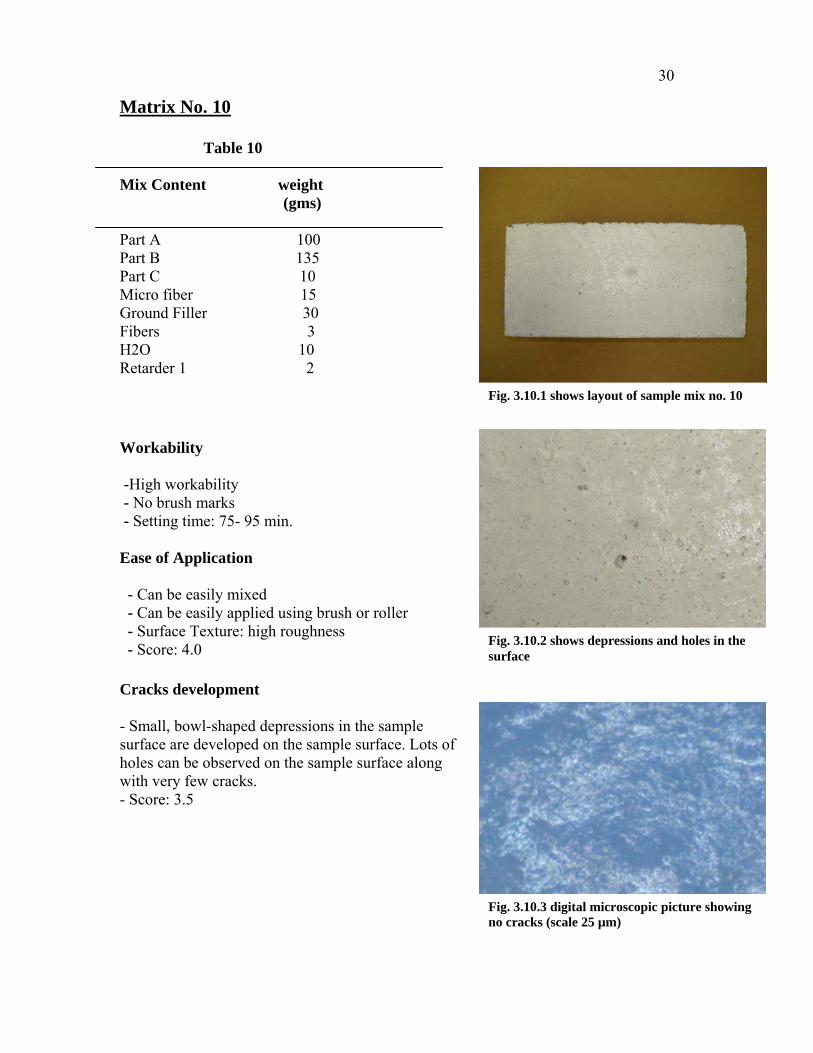
Matrix No. 10 Table 10
Mix Content weight (gms)
Part A 100 Part B 135 Part C 10 Micro fiber 15 Ground Filler 30 Fibers 3 H2O 10 Retarder 1 2 Workability -High workability - No brush marks - Setting time: 75- 95 min. Ease of Application - Can be easily mixed - Can be easily applied using brush or roller - Surface Texture: high roughness - Score: 4.0 Cracks development - Small, bowl-shaped depressions in the sample surface are developed on the sample surface. Lots of holes can be observed on the sample surface along with very few cracks. - Score: 3.5
Fig. 3.10.1 shows layout of sample mix no. 10
Fig. 3.10.2 shows depressions and holes in the surface
Fig. 3.10.3 digital microscopic picture showing no cracks (scale 25 µm)

31
Matrix No. 11 Table 11
Mix Content weight (gms)
Part A 100 Part B 135 Part C 10 Micro fiber 15 Ground Filler 30 Fibers 3 H2O 10 Retarder 1 4 Workability -High to very high workability - No brush marks - Setting time: 100- 115 min Ease of Application - Can be easily mixed - Can be easily applied using brush or roller - Surface Texture: high roughness - Score: 4.0 Cracks development - Many depressions and holes observed on the sample surface. Interconnected cracks of small to medium size have been developed on different spots of the sample. - Score: 3.5
Fig. 3.11.2 shows lots of small depressions and holes
Fig. 3.11.1 shows layout of sample mix no. 11
Fig. 3.11.3 digital microscopic picture showing no cracks (scale 25 µm)

32
Matrix No. 12 Table 12
Mix Content weight (gms)
Part A 100 Part B 135 Part C 10 Micro fiber 15 Ground Filler 30 TiO2 5 Fibers 3 H2O 10 Retarder 1 0.5 Admixture 1 3.1 Workability -High workability - No brush marks - Setting time: 50- 60 min Ease of Application - Mix is very consistent and has smooth texture - Can be easily applied using brush or roller - Surface Texture: very low roughness - Score: 3.5 Cracks development - No cracks can be observed on the sample surface. Few depressions are developed in various parts of the sample. - Score: 0.5 Fig. 3.12.3 digital microscopic picture showing
no cracks (scale 25 µm)
Fig. 3.12.1 shows layout of sample mix no. 12
Fig. 3.12.2 shows no cracks under visual observation

33
Matrix No. 13 Table 13
Mix Content weight (gms)
Part A 100 Part B 135 Part C 10 Micro fiber 15 Ground Filler 30 TiO2 5 Fibers 3 H2O 10 Retarder 1 0.5 Admixture 1 6.2 Workability -High workability - No brush marks - Setting time: 50- 60 min Ease of Application - Mix is very consistent and has smooth texture - Can be easily applied using brush or roller - Surface Texture: low roughness - Score: 4.0 Cracks development - Very fine transverse cracks can be seen under the microscope with almost no depressions. - Score: 0.5
Fig. 3.13.3 digital microscopic picture showing very fine cracks < 1 µm (scale 25 µm)
Fig. 3.13.1 shows layout of sample mix no. 13
Fig. 3.13.2 shows no cracks under visual observation

34
Matrix No. 14 Table 14
Mix Content weight (gms)
Part A 100 Part B 135 Part C 10 Micro fiber 15 Ground Filler 30 TiO2 5 Fibers 3 H2O 10 Retarder 1 0.5 Admixture 1 9.3 Workability -High workability - No brush marks - Setting time: 50- 60 min Ease of Application - Mix is very consistent and has smooth texture - Can be easily applied using brush or roller - Surface Texture: medium roughness - Score: 4.5 Cracks development - Interconnected cracks are developed all over the sample surface. Longitudinal cracks are large sized cracks that can be clearly seen on Fig 3.14.2. - Score: 4.0 Fig. 3.14.3 digital microscopic picture showing
block cracks (scale 25 µm)
Fig. 3.14.1 shows layout of sample mix no. 14
Fig. 3.14.2 shows the major cracks in the sample surface

35
Matrix No. 15 Table 15
Mix Content weight (gms)
Part A 100 Part B 135 Part C 10 Micro fiber 15 Ground Filler 30 TiO2 5 Fibers 3 H2O 10 Retarder 1 0.5 Admixture 2 12.4 Workability - Very high workability - No brush marks - Setting time: 50- 60 min Ease of Application - Mix is very consistent and has smooth texture - Can be easily applied using brush or roller - Surface Texture: very high roughness - Score: 4.5 Cracks development - Large interconnected cracks along with large holes are developed all over the sample surface. This is can be illustrated on Fig. 3.15.2 - Score: 5.0 Fig. 3.15.3 digital microscopic picture showing
large cracks (scale 25 µm)
Fig. 3.15.1 shows layout of sample mix no. 15
Fig. 3.15.2 shows large cracks and large pot holes all across the sample surface
36
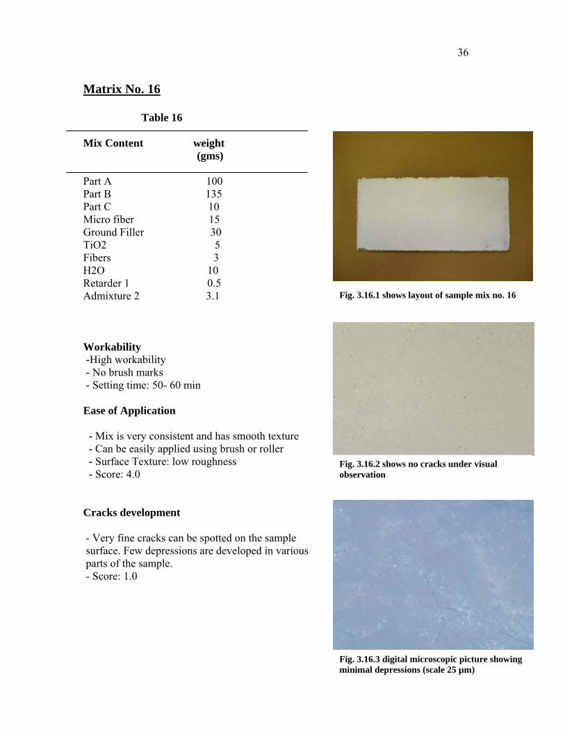
Matrix No. 16 Table 16
Mix Content weight (gms)
Part A 100 Part B 135 Part C 10 Micro fiber 15 Ground Filler 30 TiO2 5 Fibers 3 H2O 10 Retarder 1 0.5 Admixture 2 3.1 Workability -High workability - No brush marks - Setting time: 50- 60 min Ease of Application - Mix is very consistent and has smooth texture - Can be easily applied using brush or roller - Surface Texture: low roughness - Score: 4.0 Cracks development - Very fine cracks can be spotted on the sample surface. Few depressions are developed in various parts of the sample. - Score: 1.0
Fig. 3.16.3 digital microscopic picture showing minimal depressions (scale 25 µm)
Fig. 3.16.1 shows layout of sample mix no. 16
Fig. 3.16.2 shows no cracks under visual observation
37
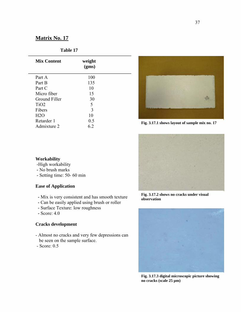
Matrix No. 17 Table 17
Mix Content weight (gms)
Part A 100 Part B 135 Part C 10 Micro fiber 15 Ground Filler 30 TiO2 5 Fibers 3 H2O 10 Retarder 1 0.5 Admixture 2 6.2 Workability -High workability - No brush marks - Setting time: 50- 60 min Ease of Application - Mix is very consistent and has smooth texture - Can be easily applied using brush or roller - Surface Texture: low roughness - Score: 4.0 Cracks development - Almost no cracks and very few depressions can be seen on the sample surface. - Score: 0.5
Fig. 3.17.3 digital microscopic picture showing
no cracks (scale 25 µm)
Fig. 3.17.2 shows no cracks under visual observation
Fig. 3.17.1 shows layout of sample mix no. 17

38
Matrix No. 18 Table 18
Mix Content weight (gms)
Part A 100 Part B 135 Part C 10 Micro fiber 15 Ground Filler 30 TiO2 5 Fibers 3 H2O 10 Retarder 1 0.5 Admixture 2 9.3 Workability -High workability - No brush marks - Setting time: 50- 60 min Ease of Application - Mix is very consistent and has smooth texture - Can be easily applied using brush or roller - Surface Texture: medium roughness - Score: 4.5 Cracks development - Interconnected cracks along with depressions are developed all over the sample surface. The cracks are large sized cracks that can be identified by visual observation. - Score: 4.5
Fig. 3.18.3 digital microscopic picture showing cracks and depressions (scale 25 µm)
Fig. 3.18.1 shows layout of sample mix no. 18
Fig. 3.18.2 shows cracks all across the sample surface

39
Matrix No. 19 Table 19
Mix Content weight (gms)
Part A 100 Part B 135 Part C 10 Micro fiber 15 Ground Filler 30 TiO2 5 Fibers 3 H2O 10 Retarder 1 0.5 Admixture 2 12.4 Workability - Very high workability - No brush marks - Setting time: 50- 60 min Ease of Application - Mix is very consistent and has smooth texture - Can be easily applied using brush or roller - Surface Texture: very high roughness - Score: 4.5 Cracks development - Large interconnected cracks along with few depressions are developed all over the sample surface. This can be illustrated through Fig.3.19.2 - Score: 5.0
Fig. 3.19.3 digital microscopic picture showing large block cracks (scale 25 µm)
Fig. 3.19.1 shows layout of sample mix no. 19
Fig. 3.19.2 shows large cracks all across the sample surface
40
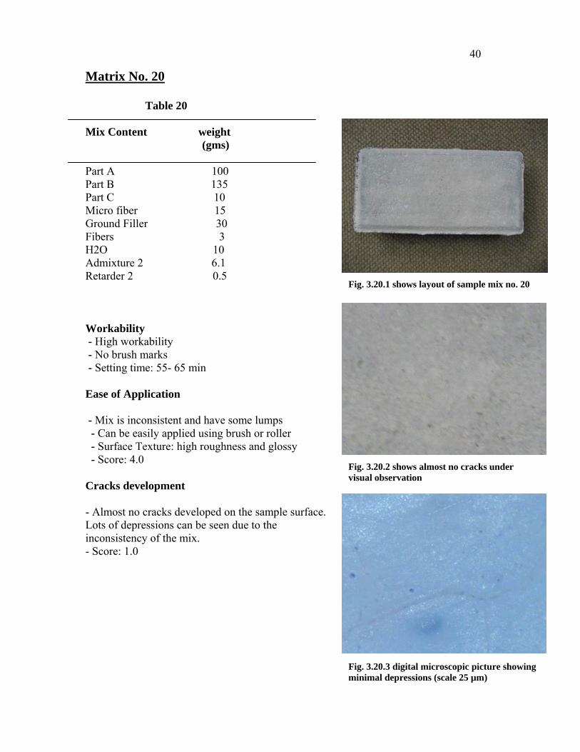
Matrix No. 20 Table 20
Mix Content weight (gms)
Part A 100 Part B 135 Part C 10 Micro fiber 15 Ground Filler 30 Fibers 3 H2O 10 Admixture 2 6.1 Retarder 2 0.5 Workability - High workability - No brush marks - Setting time: 55- 65 min Ease of Application - Mix is inconsistent and have some lumps - Can be easily applied using brush or roller - Surface Texture: high roughness and glossy - Score: 4.0 Cracks development - Almost no cracks developed on the sample surface. Lots of depressions can be seen due to the inconsistency of the mix. - Score: 1.0 Fig. 3.20.3 digital microscopic picture showing
minimal depressions (scale 25 µm)
Fig. 3.20.1 shows layout of sample mix no. 20
Fig. 3.20.2 shows almost no cracks under visual observation

41
Matrix No. 21 Table 21
Mix Content weight (gms)
Part A 100 Part B 135 Part C 10 Micro fiber 15 Ground Filler 30 Fibers 3 H2O 10 Admixture 2 6.1 Retarder 2 1 Workability - High workability - No brush marks - Setting time: 75- 80 min Ease of Application - Mix is inconsistent and full of lumps - Can be easily applied using brush or roller - Surface Texture: high roughness and glossy - Score: 4.5 Cracks development - Large depressions can be spotted all over the sample surface with very fine and few cracks as shown in Fig. 3.12.2 - Score: 1.5
Fig. 3.21.3 digital microscopic picture showing almost no cracks with minimal depressions (scale 25 µm)
Fig. 3.21.1 shows layout of sample mix no. 21
Fig. 3.21.2 shows almost pot holes and depressions all over the sample surface

42
Matrix No. 22 Table 22
Mix Content weight (gms)
Part A 100 Part B 135 Part C 10 Micro fiber 15 Ground Filler 30 Fibers 3 H2O 10 Admixture 2 6.1 Retarder 2 2 Workability - Very high workability - No brush marks - Setting time: 90- 100 min Ease of Application - Mix is lumpy and inconsistent - Can be easily applied using brush or roller - Surface Texture: high roughness and glossy - Score: 4.5 Cracks development - Large depressions can be seen all over the sample surface with very fine cracks -Score: 1.5
Fig. 3.22.3 digital microscopic picture showing very fine cracks < 1 µm (scale 25 µm)
Fig. 3.22.1 shows layout of sample mix no. 22
Fig. 3.22.2 shows almost no cracks with lots of depressions and holes
43
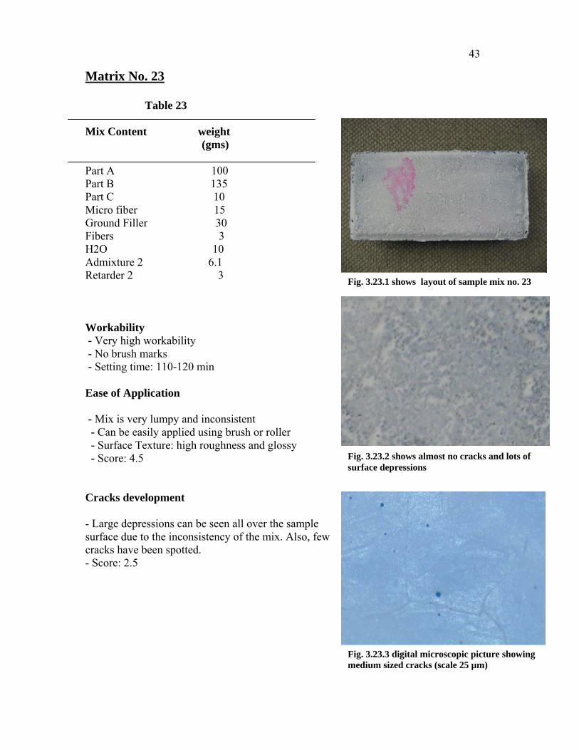
Matrix No. 23 Table 23
Mix Content weight (gms)
Part A 100 Part B 135 Part C 10 Micro fiber 15 Ground Filler 30 Fibers 3 H2O 10 Admixture 2 6.1 Retarder 2 3 Workability - Very high workability - No brush marks - Setting time: 110-120 min Ease of Application - Mix is very lumpy and inconsistent - Can be easily applied using brush or roller - Surface Texture: high roughness and glossy - Score: 4.5 Cracks development - Large depressions can be seen all over the sample surface due to the inconsistency of the mix. Also, few cracks have been spotted. - Score: 2.5
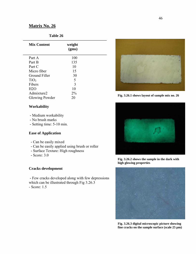
Fig. 3.23.3 digital microscopic picture showing medium sized cracks (scale 25 µm)
Fig. 3.23.1 shows layout of sample mix no. 23
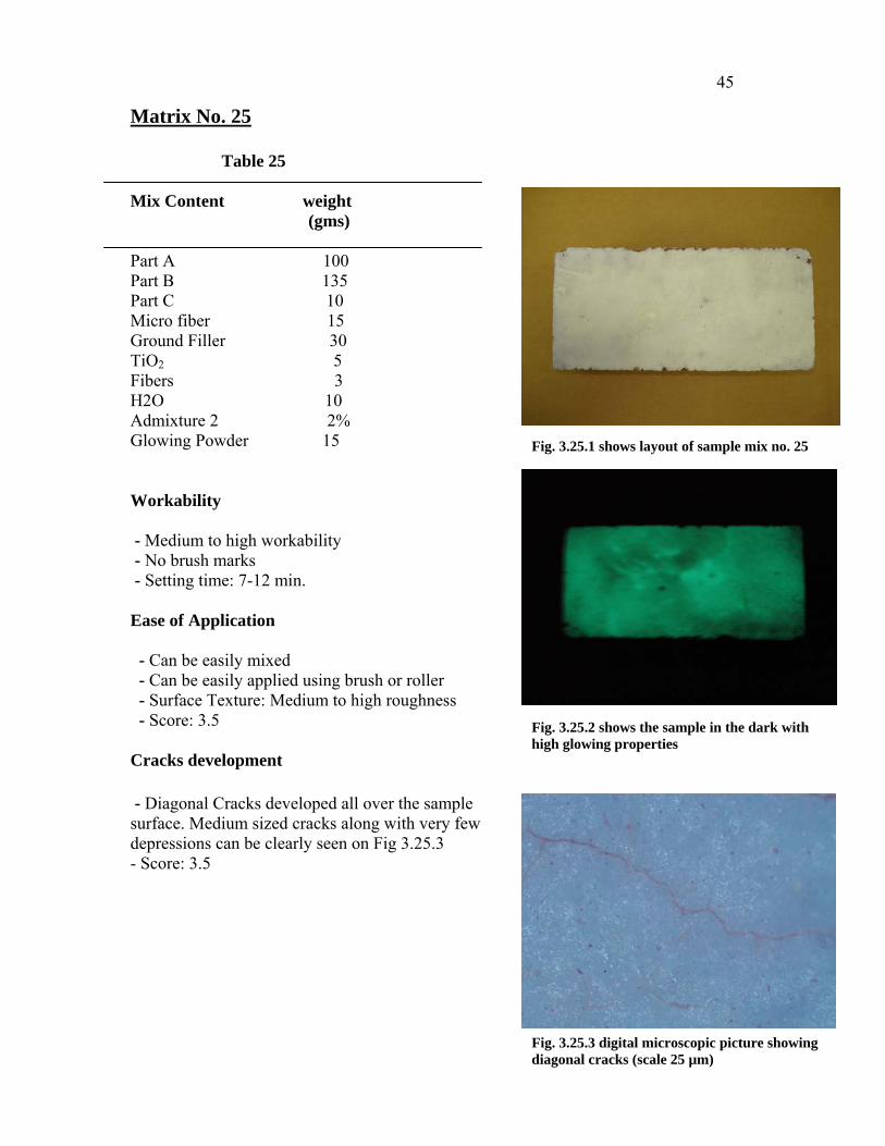
Fig. 3.23.2 shows almost no cracks and lots of surface depressions

44
Matrix No. 24 Table 24
Mix Content weight (gms)
Part A 100 Part B 135 Part C 10 Micro fiber 15 Ground Filler 30 TiO2 5 Fibers 3 H2O 10 Admixture 2 2% Glowing Powder 10 Workability - High workability - No brush marks - Setting time: 10-15 min. Ease of Application - Can be easily mixed - Can be easily applied using brush or roller - Surface Texture: Medium roughness - Score: 4.0 Cracks development - Cracks developed parallel and perpendicular to the sample centerline. Medium sized cracks along with depressions are spread all over the sample surface. - Score: 3.5 Fig. 3.24.3 digital microscopic picture showing
longitudinal and transverse cracks (scale 25 µm)
Fig. 3.24.1 shows layout of sample mix no. 24
Fig. 3.24.2 shows the sample in the dark with very little glowing properties
45
Matrix No. 25 Table 25
Mix Content weight (gms)
Part A 100 Part B 135 Part C 10 Micro fiber 15 Ground Filler 30 TiO2 5 Fibers 3 H2O 10 Admixture 2 2% Glowing Powder 15 Workability - Medium to high workability - No brush marks - Setting time: 7-12 min. Ease of Application - Can be easily mixed - Can be easily applied using brush or roller - Surface Texture: Medium to high roughness - Score: 3.5 Cracks development - Diagonal Cracks developed all over the sample surface. Medium sized cracks along with very few depressions can be clearly seen on Fig 3.25.3 - Score: 3.5
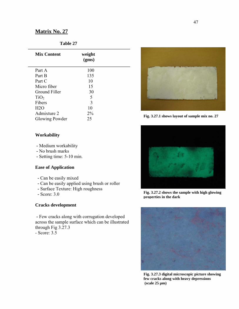
Fig. 3.25.3 digital microscopic picture showing diagonal cracks (scale 25 µm)
Fig. 3.25.1 shows layout of sample mix no. 25
Fig. 3.25.2 shows the sample in the dark with high glowing properties
46
Matrix No. 26 Table 26
Mix Content weight (gms)
Part A 100 Part B 135 Part C 10 Micro fiber 15 Ground Filler 30 TiO2 5 Fibers 3 H2O 10 Admixture2 2% Glowing Powder 20 Workability - Medium workability - No brush marks - Setting time: 5-10 min. Ease of Application - Can be easily mixed - Can be easily applied using brush or roller - Surface Texture: High roughness - Score: 3.0 Cracks development - Few cracks developed along with few depressions which can be illustrated through Fig 3.26.3 - Score: 1.5 Fig. 3.26.3 digital microscopic picture showing
fine cracks on the sample surface (scale 25 µm)
Fig. 3.26.1 shows layout of sample mix no. 26
Fig. 3.26.2 shows the sample in the dark with high glowing properties
47
Matrix No. 27 Table 27
Mix Content weight (gms)
Part A 100 Part B 135 Part C 10 Micro fiber 15 Ground Filler 30 TiO2 5 Fibers 3 H2O 10 Admixture 2 2% Glowing Powder 25 Workability - Medium workability - No brush marks - Setting time: 5-10 min. Ease of Application - Can be easily mixed - Can be easily applied using brush or roller - Surface Texture: High roughness - Score: 3.0 Cracks development - Few cracks along with corrugation developed across the sample surface which can be illustrated through Fig 3.27.3 - Score: 3.5 Fig. 3.27.3 digital microscopic picture showing
few cracks along with heavy depressions (scale 25 µm)
Fig. 3.27.1 shows layout of sample mix no. 27
Fig. 3.27.2 shows the sample with high glowing properties in the dark

48
Matrix No. 28 Table 28
Mix Content weight (gms)
Part A 100 Part B 135 Part C 10 Micro fiber 15 Ground Filler 30 TiO2 5 Fibers 3 H2O 10 Admixture 2 2% Glowing Powder 30 Workability - Medium workability - No brush marks - Setting time: 5-10 min. Ease of Application - Can be easily mixed - Can be easily applied using brush or roller - Surface Texture: High to very high roughness - Score: 3.0 Cracks development - Medium sized transverse cracks developed on different parts of the sample surface. Also, few depressions can be spotted in random places of the sample - Score: 3.0
Fig. 3.28.3 digital microscopic picture showing longitudnal cracks (scale 25 µm)
Fig. 3.28.1 shows layout of sample mix no. 28
Fig. 3.28.2 shows the sample in the dark with high glowing properties

49
Matrix No. 29 Table 29
Mix Content weight (gms)
Part A 100 Part B 135 Part C 10 Micro fiber 15 Ground Filler 25 TiO2 5 Fibers 3 H2O 10 Retarder 1 0.5 Admixture 2 2% Workability - High workability - No brush marks - Setting time: 10-13 min. Ease of Application - Mix is thin and of medium consistency - Can be easily applied using brush or roller - Surface Texture: High roughness - Score: 3.5 Cracks development - No cracks are can be spotted on the sample surface. Some depressions are developed in various parts of the sample. - Score: 1.0
Fig. 3.29.3 digital microscopic picture showing
no cracks (scale 25 µm)
Fig. 3.29.1 shows layout of sample mix no. 29
Fig. 3.29.2 shows almost no cracks under visual observation

50
Matrix No. 30 Table 30
Mix Content weight (gms)
Part A 100 Part B 135 Part C 10 Micro fiber 30 Ground Filler 25 TiO2 5 Fibers 3 H2O 10 Retarder 1 0.5 Admixture 2 2% Workability - Medium to high workability - No brush marks - Setting time: 7-12 min. Ease of Application - Mix is of medium consistency with some lumps - Can be easily applied using brush or roller - Surface Texture: High to very high roughness - Score: 3.0 Cracks development - Small size cracks are can be spotted on different parts of the sample surface. Lots of depressions are developed in various parts of the sample. - Score: 2.5
Fig. 3.30.1 shows layout of sample mix no. 30
Fig. 3.30.2 shows small cracks and depressions all over the sample surface
Fig. 3.30.3 digital microscopic picture showing a very big depression and minimal cracking (scale 25 µm)

51
Matrix No. 31 Table 31
Mix Content weight (gms)
Part A 100 Part B 135 Part C 10 Micro fiber 15 Ground Filler 40 TiO2 5 Fibers 3 H2O 10 Retarder 1 0.5 Admixture 2 2% Workability - Low to Medium workability - No brush marks - Setting time: 5-10 min. Ease of Application - Medium consistency with few lumps - Can be easily applied using brush or roller - Surface Texture: low roughness - Score: 2.5 Cracks development - Transverse and diagonal cracks are developed all over the sample. The cracks are medium to large sized cracks that can be spotted all over the sample under visual observation. - Score: 4.0
Fig. 3.31.1 shows layout of sample mix no. 31
Fig. 3.31.2 shows cracks all over the sample surface
Fig. 3.31.3 digital microscopic picture showing transverse cracks (scale 25 µm)

52
Matrix No. 32 Table 32
Mix Content weight (gms)
Part A 100 Part B 135 Part C 10 Micro fiber 15 Ground Filler 50 TiO2 5 Fibers 3 H2O 10 Retarder 1 0.5 Admixture 2 2% Workability - Low to medium workability - No brush marks - Setting time: 5-8 min. Ease of Application - Bad consistency with lots of lumps - Can be applied using a roller as lumps stick to brush - Surface Texture: Very high roughness - Score: 2.0 Cracks development - Interconnected cracks are developed in different places of the sample. Large depressions can be spotted as shown in Fig. 3.32.2 - Score: 4.0
Fig. 3.32.1 shows layout of sample mix no. 32
Fig. 3.32.2 shows heavy depressions all over the sample surface
Fig. 3.32.3 digital microscopic picture showing cracks all over the surface (scale 25 µm)

53
Matrix No. 33 Table 33
Mix Content weight (gms)
Part A 100 Part B 135 Part C 10 Micro fiber 15 Ground Filler 25 TiO2 5 Fibers 3 H2O 10 Retarder 1 0.5 Admixture 1 1% Admixture 2 1% Workability -High workability - No brush marks - Setting time: 50- 60 min Ease of Application - Mix is very consistent and has smooth texture - Can be easily applied using brush or roller - Surface Texture: low roughness - Score: 4.0 Cracks development - No cracks are can be spotted on the sample surface. Some depressions and holes are developed in various parts of the sample. - Score: 2.0
Fig. 3.33.1 shows layout of sample mix no. 33
Fig. 3.33.2 shows no cracks with few depressions on the sample surface
Fig. 3.33.3 digital microscopic picture showing no cracks (scale 25 µm)

54
Matrix No. 34 Table 34
Mix Content weight (gms)
Part A 100 Part B 135 Part C 10 Micro fiber 15 Ground Filler 25 TiO2 5 H2O 10 Retarder 1 0.5 Admixture 2 2% Workability - High workability - No brush marks - Setting time: 50-60 min. Ease of Application - Mix is consistent and has a smooth texture - Can be easily applied using brush or roller - Surface Texture: very low roughness - Score: 4.0 Cracks development - No cracks can be seen on the sample surface. Very Few depressions are developed in various parts of the sample. - Score: 0.5
Fig. 3.34.1 shows layout of sample mix no. 34
Fig. 3.34.2 shows no cracks and smooth surface
Fig. 3.34.3 microscopic picture showing no cracks with very few depressions (scale 25 µm)

55
Matrix No. 35 Table 35
Mix Content weight (gms)
Part A 100 Part B 135 Part C 10 Micro fiber 15 Ground Filler 25 TiO2 5 Fibers 3 H2O 10 Retarder 1 0.5 Admixture 2 2% Workability - Medium to high workability - No brush marks - Setting time: 50-60 min. Ease of Application - Mix is very consistent and has a smooth texture - Can be easily applied using brush or roller - Surface Texture: very low roughness - Score: 3.5 Cracks development -Very few cracks less than 1 µm are developed on the sample surface. Few depressions can be identified on different parts of the sample. - Score: 1.0
Fig. 3.35.1 shows layout of sample mix no. 35
Fig. 3.35.2 shows no cracks with few depressions
Fig. 3.35.3 digital microscopic picture showing no cracks (scale 25 µm)
56
Matrix No. 36 Table 36
Mix Content weight (gms)
Part A 100 Part B 135 Part C 10 Micro fiber 15 Ground Filler 25 TiO2 5 Fibers 3 H2O 10 Retarder 1 0.5 Admixture 2 2% Workability - Medium to high workability - No brush marks - Setting time: 50-60 min. Ease of Application - Mix is consistent and has a smooth texture - Can be easily applied using brush or roller - Surface Texture: low roughness - Score: 3.5 Cracks development - Very few cracks less than 1 µm are developed on the sample surface. Few large depressions can be seen in very few spots. - Score: 1.0
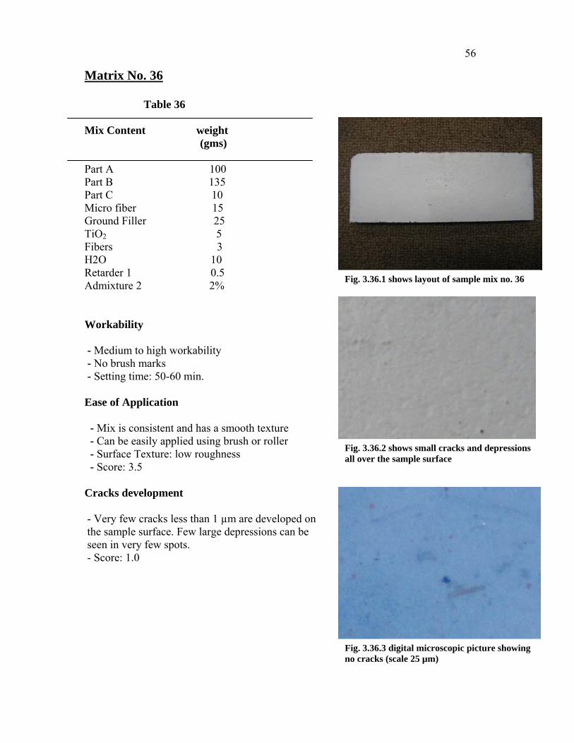
Fig. 3.36.1 shows layout of sample mix no. 36
Fig. 3.36.2 shows small cracks and depressions all over the sample surface
Fig. 3.36.3 digital microscopic picture showing no cracks (scale 25 µm)
57
Matrix No. 37 Table 37
Mix Content weight (gms)
Part A 100 Part B 135 Part C 10 Micro fiber 15 Ground Filler 25 TiO2 5 Fibers 2 1.5 H2O 10 Retarder 1 0.5 Admixture 2 2% Workability - Medium to high workability - No brush marks - Setting time: 50-60 min. Ease of Application - Mix is very consistent and has a smooth texture - Can be easily applied using brush or roller - Surface Texture: very low roughness - Score: 3.5 Cracks development - Few cracks are developed on the sample surface. Large depressions were created on the fibers locations which can be clearly seen on Fig. 3.37.3 - Score: 2.0
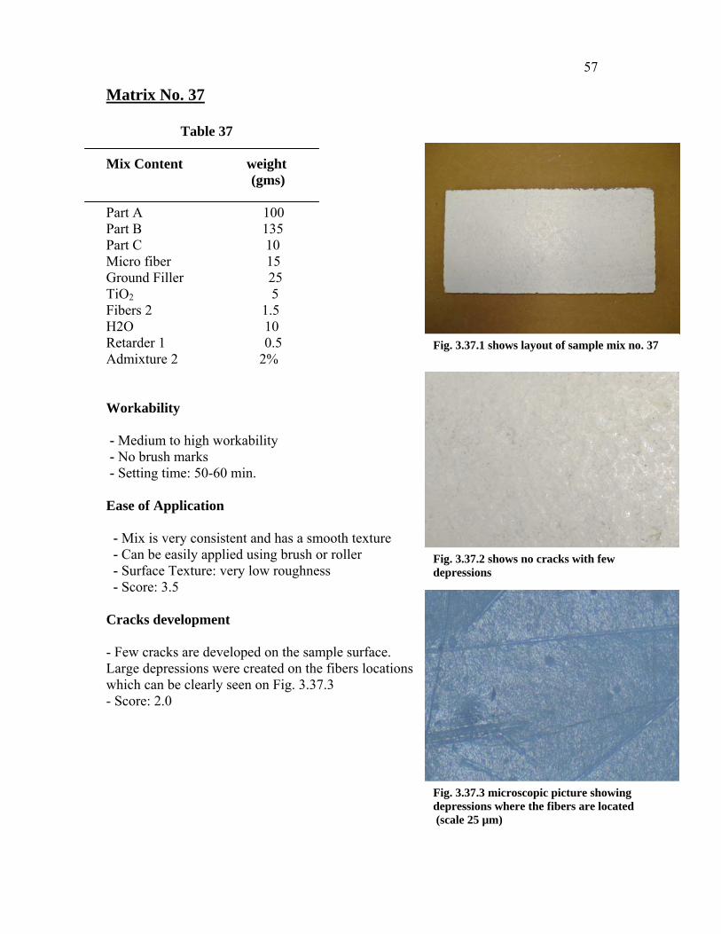
Fig. 3.37.1 shows layout of sample mix no. 37
Fig. 3.37.2 shows no cracks with few depressions
Fig. 3.37.3 microscopic picture showing depressions where the fibers are located (scale 25 µm)

58
Matrix No. 38 Table 38
Mix Content weight (gms)
Part A 100 Part B 135 Part C 10 Micro fiber 15 Ground Filler 25 TiO2 5 Fibers 2 3 H2O 10 Retarder 1 0.5 Admixture 2 2% Workability - Medium to high workability - No brush marks - Setting time: 50-60 min. Ease of Application - Mix is consistent and has a smooth texture - Can be easily applied using brush or roller - Surface Texture: very low roughness - Score: 3.5 Cracks development -Lots of large depressions were developed on the fibers locations which can be clearly seen on Fig. 3.38.3. Fine cracks can be seen on few parts of the sample. -Score: 2.5
Fig. 3.38.1 shows layout of sample mix no. 38
Fig. 3.38.2 shows no cracks with heavy depressions all over the sample surface
Fig. 3.38.3 digital microscopic picture showing cracks and heavy depressions (scale 25 µm)

59
Table 2.2 ( Silica Powder 2)
Notes: A = Silicate Solution B = Silicate Powder 2 D= Metal oxide
A (gms) B (gms) C (gms) Microfibers(gms)
Ground Filler (gms)
TiO2 (gms)
Fibers1 (gms)
Fibers2 (gms)
H2O (gms) Admixture 2
Base Mixes
39 100 120 10 15 30 - 1 - 10 -
40 100 100 10 15 30 - 1 - 10 -
Titanium dioxide Mixes
41 100 120 10 15 30 5 1 - 10 -
42 100 100 10 15 30 5 1 - 10 -
43 100 100 10 15 30 10 1 - 10 -
Admixture 2 Mixes
44 100 100 10 15 30 5 1 - 10 1%
45 100 100 10 15 30 5 1 - 10 2%
46 100 100 10 15 30 5 1 - 10 3%
47 100 100 10 15 30 5 1 - 4 3.3 gms
48 100 120 10 15 30 5 1 - 4 3.3 gms
Fibers 2 Mixes
49 100 120 10 15 30 5 1 1.5 4 3.3 gms
50 100 120 10 15 30 5 1 3 4 3.3 gms
Coarse TiO2
Remarks
Ingredients
Mix No.
Coarse TiO2
Coarse TiO2

60
Matrix No. 39 Table 39
Mix Content weight (gms)
Part A 100 Part B 120 Part C 10 Micro fiber 15 Ground Filler 30 TiO2 - Fibers 1 H2O 10 Workability - Very low workability - Heavy brush marks - Setting time: less than 7 min. Ease of Application - Mix is like paste with no lumps - Can be hardly applied using brush or roller - Surface Texture: Low to Medium roughness - Score: 1.5 Cracks development - Large interconnected and diagonal cracks along with some depressions are developed all over the sample surface. - Score: 5.0
Fig. 3.39.1 shows layout of sample mix no. 39
Fig. 3.39.2 shows large cracks all over the sample surface
Fig. 3.39.3 digital microscopic picture showing a big transverse crack (scale 25 µm)

61
Matrix No. 40 Table 40
Mix Content weight (gms)
Part A 100 Part B 100 Part C 10 Micro fiber 15 Ground Filler 30 TiO2 - Fibers 1 H2O 10 Workability - Medium workability - No brush marks - Setting time: 7-12 min. Ease of Application - Mix is of consistent with no lumps - Can be easily applied using brush or roller - Surface Texture: low to medium roughness - Score: 3.0 Cracks development - Small to medium size cracks diagonally developed all over the sample surface. Also, few depressions were developed across the surface. - Score: 3.5
Fig. 3.40.1 shows layout of sample mix no. 40
Fig. 3.40.2 shows small cracks and depressions all over the sample surface
Fig. 3.40.3 digital microscopic picture showing medium size transverse cracks (scale 25 µm)

62
Matrix No. 41 Table 41
Mix Content weight (gms)
Part A 100 Part B 120 Part C 10 Micro fiber 15 Ground Filler 30 TiO2 5 Fibers 1 H2O 10 Workability - Very low workability - Heavy brush marks - Setting time: less than 7 min. Ease of Application - Mix is of medium consistency with no lumps - Can be hardly applied using brush or roller - Surface Texture: medium roughness - Score: 1.0 Cracks development - Large interconnected cracks forming rectangular shapes along with some depressions are developed all over the sample surface. - Score: 5.0
Fig. 3.41.1 shows layout of sample mix no. 41
Fig. 3.41.2 shows very big cracks along with medium size cracks all over the sample surface
Fig. 3.41.3 digital microscopic picture showing large longitudinal and transverse cracks (scale 25 µm)
63
Matrix No. 42 Table 42
Mix Content weight (gms)
Part A 100 Part B 100 Part C 10 Micro fiber 15 Ground Filler 30 TiO2 5 Fibers 1 H2O 10 Workability - Very low to low workability - Heavy brush marks - Setting time: less than 7 min. Ease of Application - Mix is of medium consistency with no lumps - Can be hardly applied using brush or roller - Surface Texture: low to medium roughness - Score: 1.0 Cracks development - Small size cracks can be spotted on different parts of the sample surface. Lots of depressions are developed in various parts of the sample. - Score: 2.5
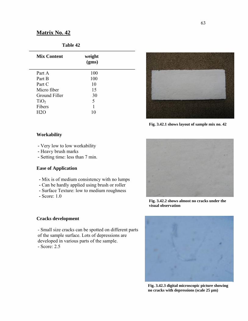
Fig. 3.42.1 shows layout of sample mix no. 42
Fig. 3.42.2 shows almost no cracks under the visual observation
Fig. 3.42.3 digital microscopic picture showing no cracks with depressions (scale 25 µm)

64
Matrix No. 43 Table 43
Mix Content weight (gms)
Part A 100 Part B 100 Part C 10 Micro fiber 15 Ground Filler 30 TiO2 10 Fibers 1 H2O 10 Workability - Very low workability - Heavy brush marks - Setting time: less than 7 min. Ease of Application - Mix is of medium to high consistency with no lumps - Can be hardly applied using brush or roller - Surface Texture: High roughness - Score: 1.5 Cracks development - Medium to large size cracks can be observed on various parts of the sample surface. Lots of depressions are developed all over the sample Score: 4.0
Fig. 3.43.1 shows layout of sample mix no. 43
Fig. 3.43.2 shows medium size cracks all over the sample surface
Fig. 3.43.3 digital microscopic picture different light shades due to surface roughness (scale 25 µm)

65
Matrix No. 44 Table 44
Mix Content weight (gms)
Part A 100 Part B 100 Part C 10 Micro fiber 15 Ground Filler 30 TiO2 5 Fibers 1 H2O 10 Admixture 2 1% Workability - Very high workability - No brush marks - Setting time: 60-70 min. Ease of Application - Mix is of very thin and has a very low viscosity - Can be easily applied using brush or roller - Surface Texture: Medium roughness - Score: 4.5 Cracks development -Almost no cracks developed on the sample surface. Corrugation and surface shoving can be seen due to the thin mix. - Score: 1.0
Fig. 3.44.1 shows layout of sample mix no. 44
Fig. 3.44.2 shows no cracks and depressions all over the sample surface
Fig. 3.44.3 digital microscopic picture showing no cracks (scale 25 µm)

66
Matrix No. 45 Table 45
Mix Content weight (gms)
Part A 100 Part B 100 Part C 10 Micro fiber 15 Ground Filler 30 TiO2 5 Fibers 1 H2O 10 Admixture 2 2% Workability - Very high workability - No brush marks - Setting time: 80-90 min. Ease of Application - Mix is very thin and inconsistent - Can be easily applied using brush or roller - Surface Texture: Medium roughness - Score: 5.0 Cracks development -Almost no cracks developed on the sample surface. Heavy surface depression can be seen due to the thin mix. -Score: 1.0
Fig. 3.45.1 shows layout of sample mix no. 45
Fig. 3.45.2 shows no cracks depressions all over the sample surface
Fig. 3.45.3 digital microscopic picture showing no cracks (scale 25 µm)

67
Matrix No. 46 Table 46
Mix Content weight (gms)
Part A 100 Part B 100 Part C 10 Micro fiber 15 Ground Filler 30 TiO2 5 Fibers 1 H2O 10 Admixture 2 3% Workability - Very high workability - No brush marks - Setting time: 90-100 min. Ease of Application - Mix is very thin and inconsistent - Can be easily applied using brush or roller - Surface Texture: Medium roughness - Score: 5.0 Cracks development - Few small size cracks developed on the sample surface. Lots of large surface depressions can be observed all over the sample due to the very thin mix. - Score: 2.0
Fig. 3.46.1 shows layout of sample mix no. 46
Fig. 3.46.2 shows no cracks depressions all over the sample surface
Fig. 3.46.3 digital microscopic picture showing medium size transverse cracks (scale 25 µm)
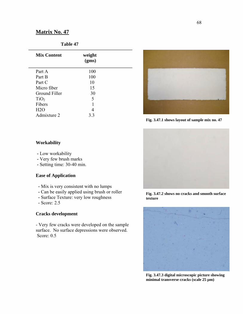
68
Matrix No. 47 Table 47
Mix Content weight (gms)
Part A 100 Part B 100 Part C 10 Micro fiber 15 Ground Filler 30 TiO2 5 Fibers 1 H2O 4 Admixture 2 3.3 Workability - Low workability - Very few brush marks - Setting time: 30-40 min. Ease of Application - Mix is very consistent with no lumps - Can be easily applied using brush or roller - Surface Texture: very low roughness - Score: 2.5 Cracks development - Very few cracks were developed on the sample surface. No surface depressions were observed. Score: 0.5
Fig. 3.47.1 shows layout of sample mix no. 47
Fig. 3.47.2 shows no cracks and smooth surface texture
Fig. 3.47.3 digital microscopic picture showing minimal transverse cracks (scale 25 µm)

69
Matrix No. 48 Table 48
Mix Content weight (gms)
Part A 100 Part B 120 Part C 10 Micro fiber 15 Ground Filler 30 TiO2 5 Fibers 1 H2O 4 Admixture 2 3.3 Workability - Medium to high workability - No brush marks - Setting time: 40-45 min. Ease of Application - Mix is very consistent with no lumps - Can be easily applied using brush or roller - Surface Texture: very low roughness - Score: 3.5 Cracks development - Some fine cracks were developed on the sample surface. No surface depressions were noticed. - Score: 1.5
Fig. 3.48.1 shows layout of sample mix no. 48
Fig. 3.48.2 shows no cracks and very smooth surface texture
Fig. 3.48.3 digital microscopic picture showing small to medium size transverse cracks (scale 25 µm)
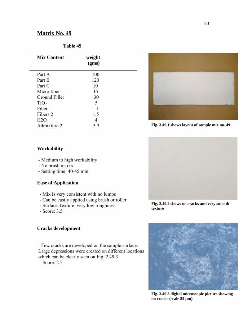
70
Matrix No. 49 Table 49
Mix Content weight (gms)
Part A 100 Part B 120 Part C 10 Micro fiber 15 Ground Filler 30 TiO2 5 Fibers 1 Fibers 2 1.5 H2O 4 Admixture 2 3.3 Workability - Medium to high workability - No brush marks - Setting time: 40-45 min. Ease of Application - Mix is very consistent with no lumps - Can be easily applied using brush or roller - Surface Texture: very low roughness - Score: 3.5 Cracks development - Few cracks are developed on the sample surface. Large depressions were created on different locations which can be clearly seen on Fig. 2.49.3 - Score: 2.5
Fig. 3.49.1 shows layout of sample mix no. 49
Fig. 3.49.2 shows no cracks and very smooth texture
Fig. 3.49.3 digital microscopic picture showing no cracks (scale 25 µm)

71
Matrix No. 50 Table 50
Mix Content weight (gms)
Part A 100 Part B 120 Part C 10 Micro fiber 15 Ground Filler 30 TiO2 5 Fibers 1 Fibers 2 3 H2O 4 Admixture 2 3.3 Workability - Medium to high workability - No brush marks - Setting time: 40-45 min. Ease of Application - Mix is of consistent with no lumps - Can be easily applied using brush or roller (Two layers were applied on the sample) - Surface Texture: low to medium roughness - Score: 3.0 Cracks development
- Lots of large depressions were developed on the fibers locations. Small to medium sized cracks can be seen on many parts of the sample.
Score:4.5
Fig. 3.50.1 shows layout of sample mix no. 50
Fig. 3.50.2 shows medium size cracks all over the sample surface
Fig. 3.50.3 digital microscopic picture showing longitudinal and transverse cracks (scale 25 µm)

72
CHAPTER 4. EXPERIMENTAL INVESTIGATION
4.1 Introduction
It is well known that the green building movement is all about the efficient use of
resources to create and maintain a clean environment. This creates a great interest in the
design and development of the so-called “self cleaning concrete coating”, referring to a
coating that provides a self-cleaning surface. The achievement of such coatings means,
not only a reduction in the problems of pollution and in health risks, but also a reduction
or elimination in the consumption of toxic industrial detergents. Achieving these
properties on a surface is possible by means of using different coating mixes (Ultimate
coating Matrix), and in which nano particles & coarse particles of titanium dioxide
(TiO2) plays a key role. Most of these coatings acquire their self-cleaning capacity
through the photocatalytic properties of titanium oxide (TiO2).
` In order to understand the mechanism of the self concrete coating, the
photocatalytic behavior of TiO2 has to be identified and investigated. This chapter
presents the experimental work which was done by applying the self cleaning coatings on
cement bricks. Self cleaning properties were recorded through colorimetric measurements
of the degradation of the colored dye. The colored dye is composed of organic pollutants
which has similar chemical composition like pollutants in the atmosphere.

73
4.2 Mechanism of TiO2 in the Base Mixes
Photocatalytic self cleaning performance has been acquired through the usage of
the nano particles & coarse particles of titanium dioxide in the mix. The main philosophy
of the TiO2 photocatalytic action is the exposure of TiO2 particles to Ultra Violet rays.
TiO2 particles store the light photons of energy equal to or greater than the energy gap
which is the region where a particle is forbidden from propagating. The energy stored in
TiO2 particles is sufficient to make an electron excites from the Valence band to the
Conduction band. Hence, the movement of the electron will create a positive charge in
the valence bond called hole (h+) and the free electron liberated to the conduction bond
will carry a negative charge (e-). This can be illustrated from the following diagram.
Fig 4.1 shows the electron excited from the valence band to conduction band (Wikipedia)

74
TiO2 + hγ TiO2 (h+ vb + e- cb) ( Eq. a, Henrich, 1994)
Where:
h = Blanks constant
γ= frequency of Ultraviolet light Rays
h+= positive charge in the valence band
e-= free electron liberated to the conduction band.
The extra absorbed energy from light photons will be released as heat. The
positive carrier charges or in other words the holes (h+) will react with the surface
hydroxyl groups (OH-) and the surface adsorbed water molecules to form hydroxyl
radicals. Radicals are high reactive species which has one unpaired electron. This can be
clarified through the following diagram:
OH- + h+ OH. ( Eq. b, Henrich, 1994)
H2O + h+ OH. + H+ ( Eq. c, Henrich, 1994)
Fig 4.2 shows the formation of hydroxyl Radicals (Wikipedia)

75
Where:
OH- = The hydroxyl group
OH. = The hydroxyl radical
h+ = positive charge in the valence band
H2O = Surface adsorbed water molecule
H+ = Hydrogen
Moreover, the negative electron (e-) can react with oxygen (O2) in the air and
super oxide anion (O2-) will be formed. The formation of the superoxide will maintain the
electric neutrality within the TiO2 particle and will prevent it from decomposition. The
final result of this process will be hydroxide radicals (OH.) and hydroperoxyl radical
HO2. .
2O2. + 2H+ 2OH. + O2
- ( Eq. d, Henrich, 1994)
2O2. + 2H+ 2H2O. ( Eq. e, Henrich, 1994)
Fig 4.3 shows the formation of superoxide anions and hydroxide radicals (Wikipedia)
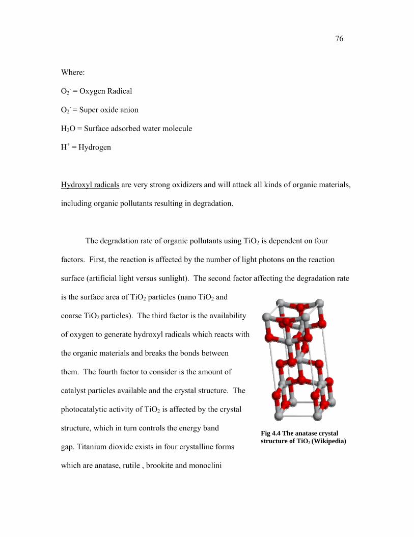
76
Where:
O2. = Oxygen Radical
O2- = Super oxide anion
H2O = Surface adsorbed water molecule
H+ = Hydrogen
Hydroxyl radicals are very strong oxidizers and will attack all kinds of organic materials,
including organic pollutants resulting in degradation.
The degradation rate of organic pollutants using TiO2 is dependent on four
factors. First, the reaction is affected by the number of light photons on the reaction
surface (artificial light versus sunlight). The second factor affecting the degradation rate
is the surface area of TiO2 particles (nano TiO2 and
coarse TiO2 particles). The third factor is the availability
of oxygen to generate hydroxyl radicals which reacts with
the organic materials and breaks the bonds between
them. The fourth factor to consider is the amount of
catalyst particles available and the crystal structure. The
photocatalytic activity of TiO2 is affected by the crystal
structure, which in turn controls the energy band
gap. Titanium dioxide exists in four crystalline forms
which are anatase, rutile , brookite and monoclini
Fig 4.4 The anatase crystal structure of TiO2 (Wikipedia)

77
c-TiO2. In terms of the photocatalytic activity, anatase is more catalytically active than
the rutile form. The TiO2 used on the experiments was in anatase crystalline form.
4.3 Sample Preparation and application 4.3.1 Preparation of Base mixes
The self cleaning coating is prepared as follows. A mixture of 100 grams of
silicate solution and 135 grams of silicate powder is placed in a high-shear mixer
containing notched stainless steel blades and mixed for one minute at speed of 1,500
RPM. Few geopolymers particles stick to the wall of the mixer. A putty knife was used to
collect the particles sticking to the mixer wall and the mixture is mixed for 1 minute. A
mixture of 10 grams of silica fumes, 10 grams of metal oxide, 15 grams of micro fibers, 5
grams of titanium dioxide and 3 grams of fibers is added to the mix and mixed for one
minute. Putty knife is used again to collect all the mixture particles sticking to the mixer
wall and mixed for one more minute. Ten grams of distilled water is added to the mix and
mixed for one minute.
4.4 Preparation of Other mixes
4.4.1 Retarder Mixes
Same procedure of mixing as in the base mixes is used. The retarder is dissolved
in distilled water then added to the mixture & mixed for one minute.
4.4.2 Admixture Mixes
Same procedure of mixing as in the base mixes is used. Admixture is added to the
mixture and mixed for one minute. Then, distilled water is added to the mix and mixed
for one more minute.

78
4.4.3 Glowing Powder Mixes
The glowing powder was added to the mixture during the second step and mixed for one
minute. Then, distilled water is added to the mix and mixed for one minute.
Self Cleaning Coating Mix application:
Initially, Self cleaning coating mix is stiff and eventually mixes to a thick liquid that can
be applied using brush or roller. The mix was applied on concrete blocks using a smooth
brush or a roller. The concrete blocks were cleaned using a piece of cloth before coating
application. The concrete blocks dimensions are 24 X 24 X 8 inch . The samples were left
at room temperature for at least 21 days before testing.
4.5 Curing Method The coating was cured at room temperature. At room temperature, the sample has to be
protected from running water or direct rain for 3 days. After 24 hours, the samples are
water resistant. However, running water could damage the surface by leaching out small
amounts of mix components.
4.6 Self Cleaning Test Setup
4.6.1 Using Artificial Light
The purpose of this test is to measure the rate of the
degradation of the organic pollutants on the self
cleaning coating surface. In order to achieve that, an
organic dye of rhodamine B is used. Rhodamine B is
an organic dye that acts like the organic pollutants
Fig 4.5 Rhodamine B organic structure (Wikipedia, 2006)

79
found in the atmosphere and it is used also as a tracer dye within water to determine the
rate and direction of flow and transport. Rhodamine B pigments was added to water to
form a red solution. Nine circles of 1.7 inch diameter were drawn using the pencil on the
surface of the self cleaning coating. The solution was applied inside the circles using a
small brush.
After 24 hours of the dye application, the concrete blocks was exposed to Ultra
Violet radiation for 30 hours period and the reading were taken every hour (22 readings
were taken during the 30 hours). The
UV light source is 300 W lamp
placed at a distance of 1.1 Feet from
the concrete block. The artificial
light source provides a wavelength
that is similar to the sunlight.
However, the experiments were
performed using an artificial light
source and sunlight as mentioned
later.
4.6.2 CIELAB color system
The degradation rate of the organic dye was measured using a Color reader CR-10
(Konica Minolta Sensing colorimeter). The results are shown in form of a table using the
CIE (1976) L*a*b* Color system. The L*a*b* color system is the most widely used
Fig 4.6 shows the concrete blocks subjected to artificial light
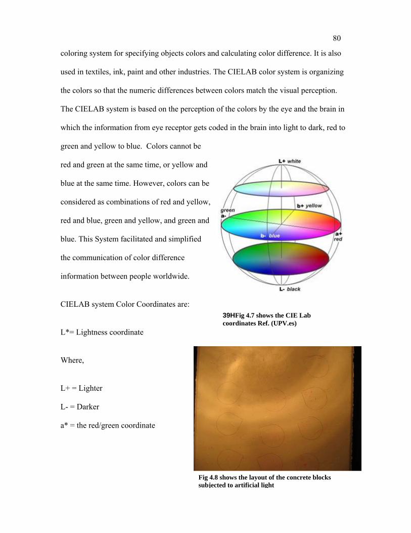
80
coloring system for specifying objects colors and calculating color difference. It is also
used in textiles, ink, paint and other industries. The CIELAB color system is organizing
the colors so that the numeric differences between colors match the visual perception.
The CIELAB system is based on the perception of the colors by the eye and the brain in
which the information from eye receptor gets coded in the brain into light to dark, red to
green and yellow to blue. Colors cannot be
red and green at the same time, or yellow and
blue at the same time. However, colors can be
considered as combinations of red and yellow,
red and blue, green and yellow, and green and
blue. This System facilitated and simplified
the communication of color difference
information between people worldwide.
CIELAB system Color Coordinates are:
L*= Lightness coordinate
Where,
L+ = Lighter
L- = Darker
a* = the red/green coordinate
39HFig 4.7 shows the CIE Lab coordinates Ref. (UPV.es)
Fig 4.8 shows the layout of the concrete blocks subjected to artificial light

81
Where,
a+ = redder
a- = greener.
b* = the yellow/blue coordinate
Where,
b+ = yellower
b- = bluer
4.6.3 Using Sunlight
The purpose of this test is to measure the rate of the degradation of the organic
pollutants on the self cleaning coating surface. An organic dye of rhodamine B was used
that acts like the organic pollutants found in the atmosphere. Four circles of 1.7 inch
diameter were drawn inside a circular concrete sample of 4 inch diameter and 0.25 inch
thickness. The circles were drawn using the pencil on the surface of the self cleaning
coating. The solution was applied inside the circles using a small brush.
After 24 hours of the dye application, the circular samples were exposed to Ultra
Violet radiation for 48 hours period and two readings were taken before and after the
exposure to the sunlight.
The degradation rate of the organic dye was measured using a Color reader CR-10
(Konica Minolta Sensing colorimeter). The results are shown in form of a table using the
CIE (1976) L*a*b* Color system.

82
4.7 X-Ray Photoelectron Spectroscopy (XPS)
X-Ray Photoelectron Spectroscopy (XPS) or in other words Electron Spectroscopy is a
quantitative technique that analyses the chemical composition of the surface of solid
materials. X-ray photoelectron spectroscopy works by irradiating the sample placed is an
ultrahigh vacuum environment with monoenergetic soft x-rays. The exposure of the
sample material to this irradiation causes electrons to be ejected from the atomic shells of
the elements at the surface. The energy of these electrons is characteristic of the surface
from which they are ejected. Or in other words, identification of the elements in the
sample can be made directly from the kinetic energies of these ejected photoelectrons.
The number of electrons ejected is counted as a function of energy and the
chemical surface composition is obtained.
The electron binding energy or the kinetic energy required to eject an electron is
characteristic of the chemical element as mentioned before and it can be determined
using the following equation:
Ebinding = Ephoton - Ekinetic - Φ (Ernest Rutherford, 1914)
Where,
Ebinding = The energy of the electron emitted from one electron configuration within the
Atom
Ephoton = The energy of the X-ray photons being used.
Ekinetic = The kinetic energy of the emitted electron as measured by the instrument
Φ = The work function of the spectrometer.
Fig 4.9 show the main components of the XPS instrument (Wikipedia)
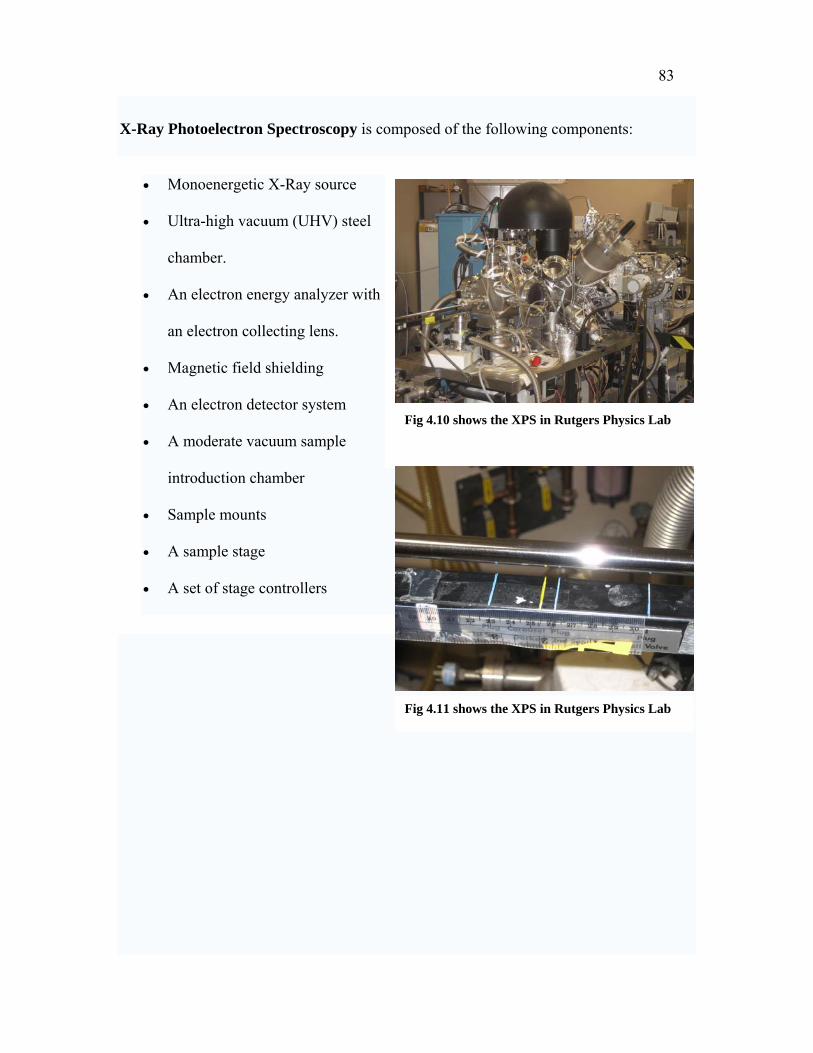
83
X-Ray Photoelectron Spectroscopy is composed of the following components:
• Monoenergetic X-Ray source
• Ultra-high vacuum (UHV) steel
chamber.
• An electron energy analyzer with
an electron collecting lens.
• Magnetic field shielding
• An electron detector system
• A moderate vacuum sample
introduction chamber
• Sample mounts
• A sample stage
• A set of stage controllers
Fig 4.10 shows the XPS in Rutgers Physics Lab
Fig 4.11 shows the XPS in Rutgers Physics Lab

84
X-Ray Photoelectron Spectroscopy has many capabilities such as the detection of
the chemical state of one or more of the elements in the sample, the binding energy of
one or more electronic states, identification of the thickness of one or more thin layers
(1–8 nm) of different materials within the top 10 nm of the surface. However, the
XPS was used in the experimental investigation to determine the depth of TiO2 in the
surface of the self concrete coating. The depth of TiO2 in the coating plays an
important role in the photocatalytic action, hence; it affects the degradation rate of the
organic dye and this will be mentioned later on the results chapter.
4.8 XPS Sample preparation
Five samples of dimension 8mm X 20-30mm X 3mm (approx.) were cut from the self
cleaning coating mixes using the electric saw. The samples were then cleaned using piece
of cloth to remove all the cement particles during the cutting process.
4.9 XPS testing and experimentation
The sample is placed in the sample
stage for one to ten minutes for a survey
scan that measures the amount of all
elements. Then, one to ten minutes for
high energy resolution scans that reveal
chemical state differences. Then, one to
four hours for a depth profile that
Fig 4.12 shows the XPS sample dimensions

85
measures the Titanium dioxide TiO2 as a function of fixed depth. XPS testing accuracy
depends on several factors such as the sample homogeneity, accuracy of sensitivity
factors, correction for electron transmission function, correction for energy dependency
of electron mean free path, and degree of sample degradation due to analysis. However,
under the normal testing conditions, the accuracy ranges from 80 to 90 percent which is
close enough to determine the element (TiO2) on the coating surface.
4.10 Atomic force microscope Testing
Atomic force microscope is a very high-resolution type of scanning microscope,
with resolution of fractions of a nanometer, more than 1000 times better than the optical
diffraction limit. The AFM consists of a microscale cantilever with a sharp tip (probe) at
its end that is used to scan the specimen surface. The cantilever is typically silicon or
silicon nitride with a tip radius of curvature of nanometers. When the tip is brought into
proximity of a sample surface, forces between the tip and the sample lead to a deflection
of the cantilever according to Hooke's law. This tip is expose to a laser and as it moves on
the surface of the sample, the deflection on the tip due
to the surface topography is reflected on the laser
beam. The laser beam part is connected to a computer
that shows the scanned pictures of the sample on the
monitor and the roughness average is calculated.
Fig 4.13 the Mechanism of AFM (Wikipedia)
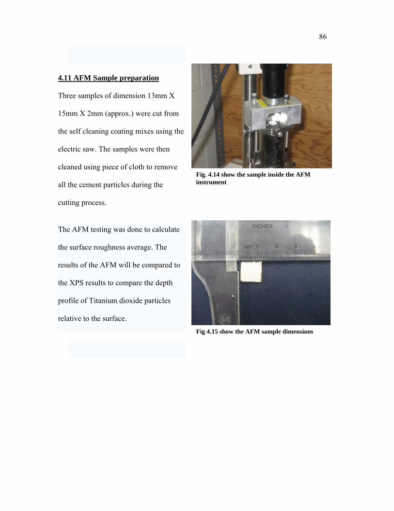
86
4.11 AFM Sample preparation
Three samples of dimension 13mm X
15mm X 2mm (approx.) were cut from
the self cleaning coating mixes using the
electric saw. The samples were then
cleaned using piece of cloth to remove
all the cement particles during the
cutting process.
The AFM testing was done to calculate
the surface roughness average. The
results of the AFM will be compared to
the XPS results to compare the depth
profile of Titanium dioxide particles
relative to the surface.
Fig. 4.14 show the sample inside the AFM instrument
Fig 4.15 show the AFM sample dimensions

87
CHAPTER 5. TEST RESULTS AND DISCUSSION 5.1 Introduction
In this chapter, the test results and discussion of the coating matrix will be presented. The
test variables investigated were the classification of the coating mixes according to their
workability, ease of application & cracks development (as mentioned in chapter two). In
chapter two, each mix was identified solely to show its properties; however, the most
efficient mix that can be used in practical applications will be introduced in this chapter.
Second, the self cleaning test which was represented by the degradation of the organic
pollutant (Rhodamine B organic dye). The decomposition of the organic pollutants can be
considered as a breakthrough in the coating mix design. The mix will not only be used as
a protective coating but it can be used in many applications such as highways and roads,
exterior paintings, kitchens, bathrooms…etc. Third, the depth profile of titanium dioxide
was investigated using the X-Ray Photoelectron Spectroscopy machine testing and
Atomic force microscope.
5.2 Matrix Coating Results:
From the coating matrix introduced in chapter two, it is obvious that there are lots of
mixes that did not develop any cracks or minimal cracks less than one micron. The
coating mixes were classified according to the scoring system. From the scoring results
introduced in chapter two, the following results can be concluded:
1) Mix 12, mix 13, mix 16, and mix 17 are highly recommended for the coating
applications as they have high workability, no brush marks, and setting time of 50 to 60
min. In addition, the mixes are very consistent, can be easily applied using brush or

88
roller and they have a very low roughness. In addition, no cracks can be observed on the
samples surface and very few depressions were developed. The mixes consistency is due
to the addition of admixtures which really enhanced the workability and the surface
texture of the mix. The setting time was adjusted to be 50 to 60 minutes due to the
addition of the retarders. The few depressions that developed on the sample surface were
a result of surface depressions. The surface was prepared using a piece of cloth to
remove the lose particles. However, there were still lots of surface depressions and holes
on the sample surface.
2) Mix 20, mix 21, mix 22, and mix 23 develop almost no cracks or minimal cracks. In
addition, the mixes have high workability, no brush marks, and setting time that varies
from 55 to 120 min. However, the mixes were very inconsistent, have lots of lumps, and
high roughness. The inconsistency of the mix is a result of the addition of retarder 2 was
not dissolved in water which leads to the formation of the lumps. Retarder 2 mixes
samples are characterized by the glossy surface that they have. Therefore, those mixes
can be used on graffiti proof applications.
3) Mixes 35 and mix 36 develop almost no cracks or minimal cracks. Their chemical
composition is pretty much similar to mixes no. 12, 13, 16 and 17 except for the silicate
powder: fillers ratio. From the chemical composition of those mixes, it can be inferred
that slight change in silicate powder: fillers ratio will not affect the coating. However, a
big change in this ratio will highly affect the consistency of the mix and will develop lots
of cracks.

89
4) Mix 43 develops very few cracks and is highly recommended for practical
applications. However, the addition of retarders and admixture develop lots of cracks.
Mix 43 is characterized by its very low roughness and smooth surface.
5.3 Self cleaning Results: Table 5.1, 5.2 and 5.3 shows the color change rate of the samples for Mix 1, mix 2, and
mix 3. The color change is due to the decomposition of the organic because of the photo
catalytic effect of Titanium dioxide. This can be clearly illustrated through the graphs of
the samples Fig 5.1 to Fig 5.9. A review of the degradation curves mentioned in Figures
5.1 to 5.9 shows the overall effect of nano and coarse titanium dioxide particles on the
decomposition of organic pollutants. Those degradation curves present the following:
1) The rate of degradation of Rohadamine B organic dye was the highest for Mix B in
which coarse titanium dioxide particles were used. This could be due to the fact that the
amount of the stored energy of those particles is higher than that stored by nano titanium
dioxide particles. Thus, the formation of hydroxyl radicals will be more in mix 2 than in
Mix 1 or mix 3 which will increase the degradation rate of the organic dye.
2) The curves represented in fig. 5.8 and 5.9 are not linear as the other curves. This is due
to the colorimeter reading error. The circles were drawn on the sample surface to
minimize that error as they have the same diameter as the Colorimeter lens. However, it
is very hard to take readings exactly at the same point which results in some disturbance
in the previously mentioned curves.
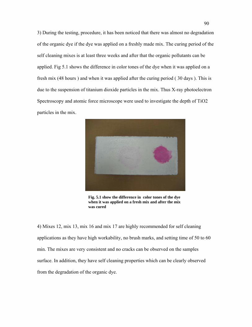
90
3) During the testing, procedure, it has been noticed that there was almost no degradation
of the organic dye if the dye was applied on a freshly made mix. The curing period of the
self cleaning mixes is at least three weeks and after that the organic pollutants can be
applied. Fig 5.1 shows the difference in color tones of the dye when it was applied on a
fresh mix (48 hours ) and when it was applied after the curing period ( 30 days ). This is
due to the suspension of titanium dioxide particles in the mix. Thus X-ray photoelectron
Spectroscopy and atomic force microscope were used to investigate the depth of TiO2
particles in the mix.
4) Mixes 12, mix 13, mix 16 and mix 17 are highly recommended for self cleaning
applications as they have high workability, no brush marks, and setting time of 50 to 60
min. The mixes are very consistent and no cracks can be observed on the samples
surface. In addition, they have self cleaning properties which can be clearly observed
from the degradation of the organic dye.
Fig. 5.1 show the difference in color tones of the dye when it was applied on a fresh mix and after the mix was cured

91
5) Table 5.5, 5.6, and 5.7 shows the degradation of the organic dye on the sunlight in
which the sample were left for 48 hours. The end results show that the degradation in the
sunlight is similar to the results under the artificial light.

92
Table 5.1
Sample Hours L a b
1 78.5 21.2 -11.7
2 82.5 13.1 -7
3 78.3 24.2 -12.3
1 79 20.7 -10.7
2 82.4 13.3 -6.3
3 78.3 24.8 -12
1 80.1 18.8 -9.5
2 82.9 12.7 -5.6
3 79.7 21.7 -9.9
1 80.3 18.4 -9.1
2 82.9 12.7 -5.4
3 79.3 21.9 -10.4
1 80.6 18.2 -8.3
2 83.1 12.4 -4.73 79.7 21.3 -9.41 80.7 17.6 -7.8
2 83.2 12.3 -4.6
3 79.7 21.6 -9.2
1 80.4 16.4 -7.2
2 83.4 12 -4.3
3 80.1 20.7 -8.6
1 80.5 17.1 -7.1
2 83.7 11.3 -3.9
3 80.3 20.6 -8.3
1 80.7 17.9 -6.9
2 84.8 10.8 -2.9
3 80.8 19.8 -7.7
1 81.1 17.1 -6.2
2 84.7 10.8 -2.9
3 81.2 18.6 -5.4
1 81.8 16.7 -5.5
2 85.1 9.4 -1.9
3 81.9 17.3 -5.6
9
10
11
5
6
7
8
1
2
3
4

93
Sample Hours L a b
1 81.7 16.9 -5.4
2 85.2 9.3 -1.9
3 82.2 17.3 -5.3
1 82.1 16 -5
2 85.4 9.1 -1.7
3 83.2 14.6 -4.2
1 81.9 16.9 -5.2
2 85.4 9.1 -1.8
3 83.6 13.9 -3.8
1 82.5 15.3 -4.6
2 85.7 9 -1.6
3 83.7 13.1 -3.6
1 82.8 15.5 -4.3
2 86.2 8.4 -1.2
3 83.5 14.8 -4.1
1 83.4 14.4 -3.8
2 86.2 8.2 -1.2
3 83.9 13.9 -3.6
1 83.5 14.6 -2.2
2 87.4 5.7 0.5
3 84.4 13.7 -1.9
1 85 11 -1
2 87.5 5.1 0.7
3 84.7 13.2 -1.5
1 85.1 11.4 -0.5
2 87.9 4.6 1.1
3 85.7 10.9 -0.5
1 84.6 12.1 -2.4
2 88 4.5 0.9
3 84.9 11.3 -2.5
1 85.1 11.3 -0.5
2 87.7 4.3 1.1
3 85.7 10.9 -0.5
21
22
16
17
19
18
13
14
15
20
12

94
Table 5.2
Sample Hours L a b
1 85.9 8.2 -2
2 86.3 4.9 -1.1
3 86.7 8 -1.3
1 87.7 7.9 -1.3
2 87.1 4.8 -0.8
3 88.3 7.8 -2.6
1 86.4 7.8 -1
2 87.1 4.4 0.2
3 87 7.7 -0.5
1 86.8 7 -0.7
2 87.2 4 0.5
3 87.2 7.3 -0.2
1 87 6.8 -0.1
2 87.1 4.2 0.2
3 87.5 7 0.4
1 86.9 6.8 0
2 87.3 3.8 0.8
3 87.4 6.9 0.6
1 87 6.6 0.1
2 87.3 3.8 0.7
3 87.4 6.6 0.8
1 87.1 6.6 0.4
2 87.2 3.8 0.3
3 87.6 6.6 1
1 87.1 6.3 0.4
2 87.2 3.9 0.3
3 87.6 6.1 0.8
1 87.9 5.4 0.6
2 87.9 3.2 0.4
3 88.9 5.6 2.8
1 88.1 4.7 1.4
2 87.8 2.7 1.4
3 88.4 4.9 2
9
10
11
5
6
7
8
1
2
3
4

95
Sample Hours L a b1 85 9 8 2 21 88.1 4.7 1.4
2 87.8 2.8 1.4
3 88.4 4.8 2
1 88.1 4.7 1.4
2 87.9 2.8 1.4
3 88.3 4.8 2.1
1 88.2 4.4 1.5
2 88 2.7 1.3
3 88.6 4.6 2.3
1 88.4 4.3 1.7
2 88 2.5 1.5
3 88.7 4.4 2.4
1 88.4 4.2 1.7
2 88 2.5 1.7
3 88.7 4.2 2.5
1 89.2 3.1 2.4
2 88.6 1.7 1.9
3 89.6 2.9 3.1
1 89.2 2.7 2.4
2 88.6 1.8 1.9
3 89.6 2.7 3.1
1 89.4 2.4 2.6
2 88.5 1.3 1.8
3 89.7 2.4 3.2
1 89.3 2.5 2.4
2 88.4 1.6 1.8
3 89.7 2.3 3.2
1 89.6 1.9 2.7
2 88.7 1.2 2.3
3 90 1.8 3.3
1 90.1 1.8 2.7
2 88.9 1.1 2.4
3 90 1.8 3.2
21
22
17
18
19
20
13
14
15
16
12

96
Table 5.3
Sample Hours L a b
1 87.8 11.4 -4
2 87.9 11.7 -4.1
3 86.7 9.4 -1.6
1 87.7 10.2 -3.7
2 87.1 10.3 -3.6
3 88.3 8.6 -2.4
1 87.5 10.6 -3.8
2 87.6 9.3 -2.8
3 88.2 9 -2.5
1 88.1 9.5 -3
2 87.7 9.4 -2.9
3 88.3 8.8 -2.3
1 88.7 8.6 -2.2
2 87.2 10.5 -3.1
3 88.3 9 -2
1 88.4 8.9 -2.4
2 87.1 10.7 -3.2
3 88 9.5 -2.3
1 88.3 9.2 -2.4
2 86.6 11.5 -3.6
3 87.9 9.9 -2.4
1 88.6 8.6 -2.2
2 86.2 12.6 -4
3 87.9 9.8 -2.2
1 88.6 8.6 -2.2
2 86.3 12.3 -3.6
3 88.1 9.2 -2.3
1 88.7 8.9 -1.9
2 86.4 11.9 -3.6
3 88.1 9.2 -2.4
1 89.1 7.8 -1.1
2 86.9 11.6 -1.9
3 88.7 8.8 -0.5
9
10
11
5
6
7
8
1
2
3
4
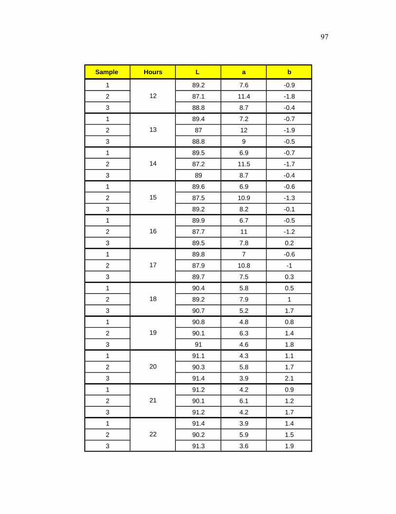
97
Sample Hours L a b1 87 8 11 4 41 89.2 7.6 -0.9
2 87.1 11.4 -1.8
3 88.8 8.7 -0.4
1 89.4 7.2 -0.7
2 87 12 -1.9
3 88.8 9 -0.5
1 89.5 6.9 -0.7
2 87.2 11.5 -1.7
3 89 8.7 -0.4
1 89.6 6.9 -0.6
2 87.5 10.9 -1.3
3 89.2 8.2 -0.1
1 89.9 6.7 -0.5
2 87.7 11 -1.2
3 89.5 7.8 0.2
1 89.8 7 -0.6
2 87.9 10.8 -1
3 89.7 7.5 0.3
1 90.4 5.8 0.5
2 89.2 7.9 1
3 90.7 5.2 1.7
1 90.8 4.8 0.8
2 90.1 6.3 1.4
3 91 4.6 1.8
1 91.1 4.3 1.1
2 90.3 5.8 1.7
3 91.4 3.9 2.1
1 91.2 4.2 0.9
2 90.1 6.1 1.2
3 91.2 4.2 1.7
1 91.4 3.9 1.4
2 90.2 5.9 1.5
3 91.3 3.6 1.9
21
22
17
18
19
20
13
14
15
16
12
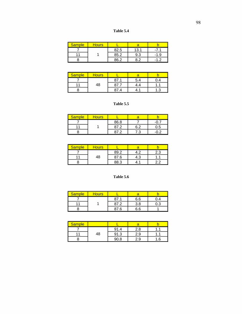
98
Table 5.4
Table 5.5
Table 5.6
Sample Hours L a b7 82.5 13.1 -7.111 85.2 9.3 -1.98 86.2 8.2 -1.2
Sample Hours L a b7 87.1 5.4 0.411 87.7 4.4 1.18 87.4 4.1 1.3
1
48
Sample Hours L a b7 86.8 7 -0.711 87.2 6.2 0.58 87.2 7.3 -0.2
Sample Hours L a b7 89.2 4.2 2.311 87.6 4.3 1.18 88.3 4.1 2.2
1
48
Sample Hours L a b7 87.1 6.6 0.411 87.2 3.8 0.38 87.6 6.6 1
Sample L a b7 91.4 2.8 1.111 91.3 2.9 1.18 90.8 2.9 1.6
1
48
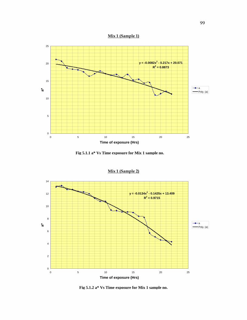
99
Mix 1 (Sample 2)
y = -0.0134x2 - 0.1425x + 13.409R2 = 0.9715
0
2
4
6
8
10
12
14
0 5 10 15 20 25
Time of exposure (Hrs)
a*
aPoly. (a)
Mix 1 (Sample 1)
y = -0.0082x2 - 0.217x + 20.071R2 = 0.8873
0
5
10
15
20
25
0 5 10 15 20 25
Time of exposure (Hrs)
a*
aPoly. (a)
Fig 5.1.1 a* Vs Time exposure for Mix 1 sample no.
Fig 5.1.2 a* Vs Time exposure for Mix 1 sample no.
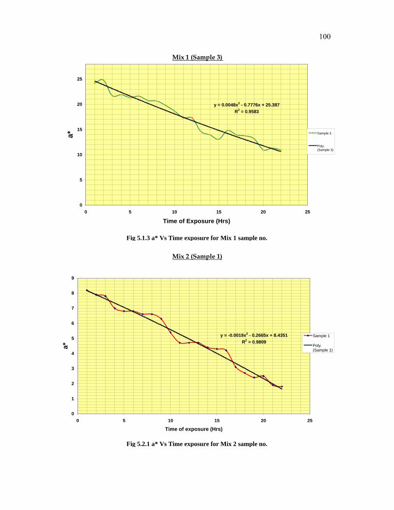
100
Mix 1 (Sample 3)
y = 0.0048x2 - 0.7776x + 25.387R2 = 0.9583
0
5
10
15
20
25
0 5 10 15 20 25
Time of Exposure (Hrs)
a* Sample 3
Poly.(Sample 3)
Mix 2 (Sample 1)
y = -0.0019x2 - 0.2665x + 8.4351R2 = 0.9809
0
1
2
3
4
5
6
7
8
9
0 5 10 15 20 25
Time of exposure (Hrs)
a*
Sample 1
Poly.(Sample 1)
Fig 5.1.3 a* Vs Time exposure for Mix 1 sample no.
Fig 5.2.1 a* Vs Time exposure for Mix 2 sample no.

101
Mix 2 (Sample 2)
y = -0.0007x2 - 0.1628x + 4.9773R2 = 0.9681
0
1
2
3
4
5
6
0 5 10 15 20 25
Time of exposure (Hrs)
a*
aPoly. (a)
Mix 2 (Sample 3)
y = -0.0038x2 - 0.2262x + 8.3156R2 = 0.9852
0
1
2
3
4
5
6
7
8
9
0 5 10 15 20 25
Time of exposure (Hrs)
a*
aPoly. (a)
Fig 5.2.2 a* Vs Time exposure for Mix 2 sample no.
Fig 5.2.3 a* Vs Time exposure for Mix 2 sample no.

102
Fig 4.3 a* Vs Time exposure for Mix 1 sample no. 3
Mix 3 Sample 2
y = -0.0401x2 + 0.7194x + 8.713R2 = 0.7967
0
2
4
6
8
10
12
14
0 5 10 15 20 25
Time of exposure (Hrs)
a*
a
Poly. (a)
Fig 5.3.1 a* Vs Time exposure for Mix 3 sample no.
Fig 5.3.2 a* Vs Time exposure for Mix 3 sample no.
Mix 3 Sample 1
y = -0.005x2 - 0.1992x + 10.764R2 = 0.9482
0
2
4
6
8
10
12
0 5 10 15 20 25
Time of Exposure (Hrs)
a* Sample 1
Poly. (Sample 1)

103
Mix 3 sample 3
y = -0.029x2 + 0.4081x + 8.1604R2 = 0.935
0
2
4
6
8
10
12
0 5 10 15 20 25
Time of exposure (Hrs)
a*
aPoly. (a)
Fig 5.3.3 a* Vs Time exposure for Mix 3 sample no.

104
5.4 X-Ray Photoelectron Spectroscopy (XPS) and Atomic force microscope
(AFM) results:
The binding energy of titanium dioxide particles was calculated using the following
formulas:
(Einstien Relationship)
Where,
h = the X-ray photon energy
Ek = the kinetic energy of photoelectron (measured by the energy analyzer)
= the work function induced by the analyzer ( can be compensated artificially so it is eliminated).
Then, the depth profile was calculated relative to the carbon and oxygen which always
exist on the top surface of the sample. Fig 5.2 and fig 5.3 shows the depth profile of
titanium dioxide molecules compared to the carbon and oxygen molecules. The average
depth profile is equal to 4 nanometers. This average was calculated from the randomly
dispersed titanium molecules on the sample compared to the oxygen and carbon
molecules. The XPS results was compared to the average roughness obtained form the
AFM testing. The average roughness obtained from AFM equals 75.6 nanometer. Fig 5.4
and 5.5 shows the pictures of the sample being scanned using the AFM instrument.
Therefore, the titanium dioxide particles exist at the top surface of the sample after the
curing period.
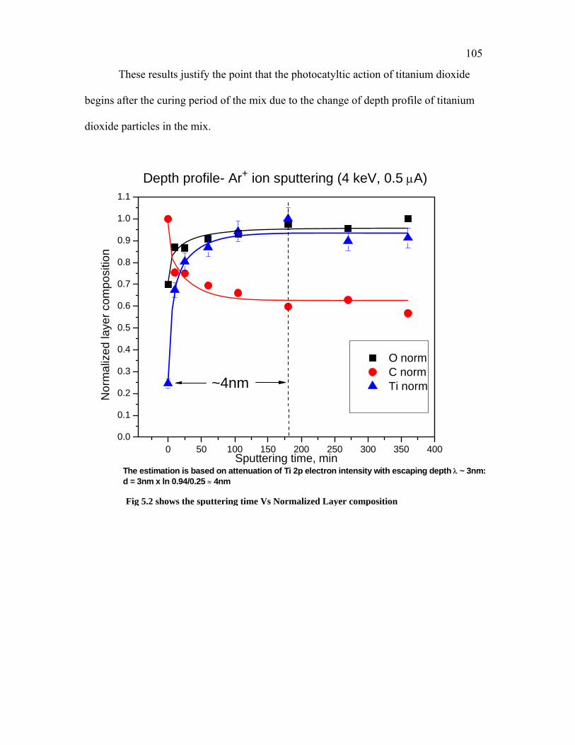
105
These results justify the point that the photocatyltic action of titanium dioxide
begins after the curing period of the mix due to the change of depth profile of titanium
dioxide particles in the mix.
0 50 100 150 200 250 300 350 4000.0
0.1
0.2
0.3
0.4
0.5
0.6
0.7
0.8
0.9
1.0
1.1
Depth profile- Ar+ ion sputtering (4 keV, 0.5 μA)
O norm C norm Ti norm
Nor
mal
ized
laye
r com
posi
tion
Sputtering time, min
~4nm
The estimation is based on attenuation of Ti 2p electron intensity with escaping depth λ ~ 3nm:d = 3nm x ln 0.94/0.25 ≈ 4nm Fig 5.2 shows the sputtering time Vs Normalized Layer composition

106
0 50 100 150 200 250 300 350 400
0
5
10
15
20
25
30
35
40
45
50
55
60
65
70
Oxygen (O 1s) Carbon (C 1s) Titanium (Ti 2p)Rel
ativ
e co
mpo
sitio
n, a
rb. u
n.
Sputtering time, min
Depth profile- Ar+ ion sputtering (4 keV, 0.5 μA)
Fig 5.3 shows the sputtering time Vs Relative composition

107
Fig 5.5 shows the 3D model of the sample scanned using the AFM instrument
Fig 5.4 shows the picture of the sample scanned using the AFM instrument

108
CHAPTER 6. CONCLUSIONS
6.1 Conclusions
The results presented in the thesis focus on characteristics and properties of the coating
matrix so that it can be used in many applications. Based on the results form the
experimental design and experimental investigation, the following points will highlight
the significant conclusions:
• The addition of water to the mix is case sensitive because the excess amount of
water affects the consistency of the mix and ability of samples to develop cracks.
However, the addition of small amount of water will significantly affect the
workability of the mix.
• Small change in the Silicate powder: fillers ratio will not affect the coating mix.
On the other hand, big change on the previously mentioned ratio will affect the
mix significantly.
• The addition of the admixtures plays an important role in the workability and
consistency of the mix. The admixtures shall be added within 1% to 2% of the
mix weight because the extra addition of the admixture will increase the cracks on
the coating.
• The addition of the retarders can be used to improve the setting time. The addition
of half a gram to the mix has increased the setting time from 10 min. (approx.) to
60 min. (approx.).
• Retarder 2 mixes are really characterized by their glossy surface which makes
them very good mixes for the graffiti proof applications. Nevertheless, the mix
consistency and the formation of lumps makes the coating hard to be applied.
109
• The addition of the glowing powder to the mix gives the coating mix glowing
properties and makes it very useful for night applications. Yet, the cracks
development on glowing mixes has to be treated.
• The degradation rate of the organic dye is really a breakthrough in the mix design
as it gives the coating mix self cleaning properties. Thus, it can be used in roads,
highways, buildings exterior and many other applications.
• Titanium dioxide is not used in the photocatalytic reaction (as mentioned before
in chapter 3) which will make the coating mix always have self cleaning
properties.
• The use of XPS and AFM instruments clarifies the idea of the curing period for
the coating mixes. The curing time is a key role in the self cleaning properties of
the mix. Thus, the coated surface has to be covered at least for three weeks to
make sure that the titanium dioxide molecules are existing at the top surface of the
mix and the photocatalytic actions takes place.
6.2 Suggestions for Further research
The following are recommendations for further research in the development of
Inorganic concrete coating matrices and their self cleaning properties:
• Retarder 2 mixes shall be further investigated as they develop no cracks and they
have a glossy surface that can be used in graffiti proof applications. However, the
inconsistency of the mix and the formation of lumps is the major disadvantage of
those matrices.

110
• The behavior of the self cleaning coating matrices shall be further studied to
determine the rate of degradation of organic pollutants using more organic dyes.
• Further studies on the depth profile for freshly made mixes shall be done to
determine the suspension of nano titanium dioxide particles in the mixes and the
curing phases.

111
REFERENCES
Arafa, M. “ High strength- High Temprature Laminated Sandwich Beams,” Doctorate Dissertation, Rutgers University, New Jersey (2007). Balaguru, P., Kurtz, S. and Rudolph, J. “Geopolymer for repair and rehabilitation of reinforced conrete beams.” Civil Engineering Report 96-14, Rutgers University (1996). Balaguru, P., “Geopolymer for Protective Coating of Transportation Infrastructures” FHWA NJ (1998). Celiker, Yucel, Uslusoy, Aydin, and Cakaz, Umit. “ New Photocatalytic Exterior and Interior Wall Coatings for Clean Surfaces.” Science direct (2003). Davidovits, J. “Geopolymers: inorganic polymeric new materials.” Journal of Thermal Analysis 37 (1991). Davidovits, J. “Journal of Materials Education” 16 [2-3] 91-137 (1994). TiO2 optical coating layers for self-cleaning applications Defazio, C. “High temperature/high strength discrete fiber reinforced composites” Master Thesis, Rutgers University, New jersey (2007). Euvananont, Junin, Inpor, Limthongkul and Thanachayanont, C. “TiO2 optical coating layers for self-cleaning applications” Ceramics International, Corrected Proof Press (2007). Foden, A. “Mechanical properties and characterization of polysialate structural composites,” Doctorate Dissertation, Rutgers University, New Jersey (1999). Foden, A., Balaguru, P., and Lyon, R. “Mechanical properties of carbon composites made using an inorganic polymer.” ANTEC (1996): 3013 – 3018. Garon R.J. “Effectiveness of high strength composites as structural and protective coatings for structural elements,” Doctorate Dissertation, Rutgers University, New Jersey (2000). Giancaspro J.W. “Influence of reinforcement type on the mechanical behavior and fire response of hybrid composites and sandwich structures,” Doctorate Dissertation, Rutgers University, New Jersey (2004). Golovin, V. “Multilayer protective polymeric coatings: Providing for their Continuity” Journal of Protection of Metals, Vol. 43 ,No.7 (2007). Henrich and Cox, P.A. “The surface science of Metal Oxides” Cambridge University Press, Cambridge, Great Britain (1994): 317-333.
112
Moon, Shin, and Choi “Evaluation of the durability of mortar and concrete applied with inorganic coating material and surface treatment system”Construction and Building Materials, Volume 21, Issue 2, February 2007, Pages 362-369 Nazier M., “Evaluation of high strength composites and new construction techniques for their effective use.” Doctorate Dissertation, Rutgers University, New Jersey (2004). NASA [Online], Available:www.NASA.gov Pugel, E., “Method for Nondestructive Evaluation of Thermal Protection System Materials and Other Materials via Ultraviolet Spectroscopy” Presentation, SAMPE 2007. Shriver, D.F., Atkins, P.W., and Langford, C.H. “Inorganic Chemistry.” W.H. Freeman and Company, New York, (1990). Spirkova, Brus, Brozova, Strachota, Baldrain, Urbanova, Kotek, Strachotova and Slouf “A view from inside onto the surface of self-assembled nanocomposite coatings” Progress in Organic Coatings, Corrected Proof Press, (2007) Vallee, Ruot, Bonafous, Guilot, Piminelli, Cassar, Strini, Mapeli, Schiavi, Gobin, Andre, Moussiopoulus, Bartzis, Maggos, Mclntyre, Lehaut-Burnouf, Henrichsen, Laugesen, Amadelli, Kotiaz, and Pichat, P. “ Innovative self cleaning and depolluting façade surfaces” CIB World Building Congress (2004). Venkatesh, Ramanan. “Mechanical properties of alumina fiber/glass matrix composites with and without a tin dioxide interface.” Materials Science and Engineering A268 (1999): 47 – 54. Wang, Li, Zhang, Sun, Xu, Xie, Xing and Zhang, X., “Efficient photocatalytic degradation of organic dyes over titanium dioxide coating upconversion luminescence agent under visible and sunlight irradiation” Corrected Proof Press (2007). Weldon, D. “The Importance of Sample Taking in Failure Analysis of Paints and Coatings “ Journal of failure Analysis and prevention, Vol. 7, No. 6 (2007).
Wikepedia [Online] www.wikepedia.com
Wilson , Dicarlo, and Yun, H. “Ceramic fibers”, Composites, ASM Hand book, Vol 21 (2003). Xu and Deventer, J. “The Geopolymerization of Alumino-silicate Minerals,” International Journal of Miner Process (2000).