PROJECTE O TESINA D’ESPECIALITAT Títol

“Effectiveness of traffic congestion management on

intersection delay”

Autor/a MANEL TERRAZA FARRÉ

Tutor/a FRANCESC ROBUSTÉ

ZONGHZI LI

Departament INFRASTRUCTURA DEL TRANSPORT I DEL TERRITORI

Intensificació TRANSPORTS

Data JUNY 2014

! ! !!

! !

EFFECTIVENESS OF TRAFFIC CONGESTION MANAGEMENT ON

INTERSECTION DELAY

BY:

MANEL TERRAZA FARRÉ

DEPARTMENT OF CIVIL, ARCHITECTURAL AND ENVIRONMENTAL

ENGINEERING

ILLINOIS INSTITUTE OF TECHNOLOGY

Submitted in partial fulfillment of the

requirements for the degree of

“Ingeniero de Caminos, Canales i Puertos”

in the Escola Técnica Superior d’Enginyeria de Camins, Canals i Ports

Universitat Politècnica de Catalunya

Approved____________________

Advisor

Chicago, Illinois

December 2013

! ! !!

! !

! ! !!

! ! """!

ACKNOWLEDGEMENT

I would like to show my profound gratitude to everyone that has helped me

through the elaboration of this research project. I am deeply thankful to my advisors

at the Illinois Institute of Technology, Professor Zongzhi Li and Dr. Arash M.

Roshandeh who have allowed me to join the Transportation Engineering Program at

Illinois Institute of Technology (IIT), Chicago, USA. Especially thankful to the latter,

with whom I have worked on a day-to-day basis and from whom I have learned not

only about the subject on this project but also about the necessary skills to produce a

good research paper. His comments and guidance are a big part of the final product of

this research project and have been invaluable to me.

I would also like to thank the graduate research assistants at the Transportation

Laboratory of IIT and the Department of Civil, Architectural and Environmental

Engineering. I am thankful for the way they have welcomed me and assisted me

during my stay at IIT. Their comments and help through this period of research have

been enormously helpful.

Last but not least, I would like to thank my parents Sergi and Mª Emilia and

my girlfriend Alejandra for helping me and encouraging me during my stay in

Chicago while working on this study.

! ! !!

! ! "#!

TABLE OF CONTENTS

Page

ACKNOWLEDGEMENT........................................................................................... iii

LIST OF TABLES....................................................................................................... vi

LIST OF FIGURES.................................................................................................... vii

ABSTRACT................................................................................................................. ix

CHAPTER

1. INTRODUCTION................................................................................. 1

2. LITERATURE REVIEW...................................................................... 4

2.1 Traffic Signal Timing Plan Optimization Model............................ 5

2.2 Intersection Delay Calculation Models........................................... 9

3. PROPOSED METHODOLOGY......................................................... 15

3.1 Justification of the Proposed Methodology................................... 15

3.2 HCM Methodology for Calculating Intersection Delay................ 16

4. MODEL DESCRIPTIONS.................................................................. 21

4.1 TRANSIMS Simulation Tool........................................................ 21

4.2 Hypotheses and Data Preparation.................................................. 23

4.3 Model Algorithm........................................................................... 31

4.4 Aggregation of Results.................................................................. 33

4.5 Test Example................................................................................. 37

5. MODEL APPLICATION.................................................................... 45

5.1 Application Procedure................................................................... 45

5.2 Analysis of Results........................................................................ 46

5.3 Results Overview........................................................................... 55

6. SUMMARY AND CONCLUSION.................................................... 57

6.1 Summary....................................................................................... 57

6.2 Conclusion.................................................................................... 57

! ! !!

! ! #!

REFERENCES............................................................................................................ 60

APPENDIX

A. REDUCTIONS ON INTERSECTION DELAY FOR EACH AREA USING THE BASIC MODEL............................................................ 62

B. REDUCTIONS ON INTERSECTION DELAY FOR EACH AREA USING THE FIRST ENHANCED MODEL WITH PEDESTRIAN DELAY CALCULATED WITH THE HCM METHOD.................... 64

C. REDUCTIONS ON INTERSECTION DELAY FOR EACH AREA USING THE SECOND ENHANCED MODEL WITH PEDESTRIAN DELAY CALCULATED WITH THE HSL METHOD......................74

D. MATLAB CODE FOR CALCULATING INTERSECTION DELAY................................................................................................ 84

! ! !!

! ! #"!

LIST OF TABLES

Table Page

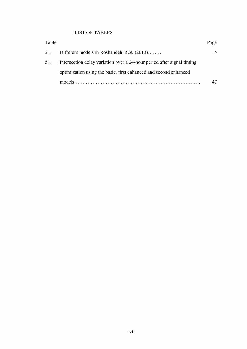
2.1 Different models in Roshandeh et al. (2013)……… 5

5.1 Intersection delay variation over a 24-hour period after signal timing

optimization using the basic, first enhanced and second enhanced

models…………………………………………………………………. 47

! ! !!

! ! #""!

LIST OF FIGURES

Figure Page

2.1 Reductions in travel time using the first enhanced model in

Roshandeh et al. (2013)…………………………………………….…….. 7

2.2 Reductions in vehicle delay using the first enhanced model in

Roshandeh et al. (2013)…………………………………………….…….. 8

2.3 Reductions in travel time using the second enhanced model in

Roshandeh et al .(2013).…………………………………………….……. 8

2.4 Reductions in vehicle delay using the second enhanced model in

Roshandeh et al (2013).…………………….……………………….……. 8

4.1 Snapshot of the first tab at the time-static worksheet. First column is node

number and other columns are names of links arriving at the node……..... 24

4.2 Snapshot of the first tab (Hour 00-01) at the traffic volume (veh/h)

worksheet. First column is node number and other columns are

volumes at links arriving at the node………………………………..……. 25

4.3 Real lane distribution situation. v and c are volumes and capacity

in that lane…………………………………………………………….…... 27

4.4 Simplified lane distribution situation. v and c are volumes and capacity

in that lane……………………………………………………………...…. 28

4.5 Timing and phases associated to each movement in a Node……………... 29

4.6 Length of each phase (sec) in a node………………………...…………... 30

4.7 Green times for each movement (sec) in a node………..………………... 30

4.8 Flowchart of the algorithm used for computing intersection delay………. 32

4.9 Node-link matrix for node 1000………………….……………………... 37

4.10 Node-capacity (veh/h) matrix for node 1000……..……………………... 38

4.11 Node-cycle length (s) matrix for node 1000……..……………………... 38

4.12 Node-number of through lanes matrix for node 1000…..……………... 38

4.13 Node- number of left lanes matrix for node 1000…....………………... 38

4.14 Node- number of right lanes matrix for node 1000.....……….………... 38

! ! !!

! ! #"""!

4.15 Node-green through time (sec) matrix for node 1000…...……...……... 39

4.16 Node-green left time (sec) matrix for node 1000…..…………...……... 39

4.17 Node-green right time (sec) matrix for node 1000…..........…….....…... 39

4.18 Node-volume (veh/h) matrix for node 1000……....……………...……... 39

4.19 Node-value of X matrix for node 1000…...…………….………...……... 40

4.20 Node-uniform delay (sec) for through lanes matrix for node 1000…... 40

4.21 Node-uniform delay (sec) for left lanes matrix for node 1000…...….... 40

4.22 Node-uniform delay (sec) for right lanes matrix for node 1000…...….. 40

4.23 Node-incremental delay (sec) for through lanes matrix for node 1000.. 41

4.24 Node-incremental delay (sec) for left lanes matrix for node 1000…..... 41

4.25 Node-incremental delay (sec) for right lanes matrix for node 1000…... 41

4.26 Node-initial queue (veh) matrix for node 1000…………………...….….. 41

4.27 Node-queue at the end of the analysis period for v>c and zero

initial queue (veh) matrix for Node 1000……………………..…...….….. 41

4.28 Node-Adjusted duration of unmet demand in the analysis period (sec)

matrix for Node 1000……………………………………………...….….. 42

4.29 Node-queue at the end of the analysis period (veh) matrix

for Node 1000…………………………………………..…...….……….... 42

4.30 Node-initial queue delay (sec) matrix for node 1000………..……......... 42

4.31 Node-approach delay (sec) matrix for node 1000…………………......... 42

4.32 Node-intersection delay (sec) matrix for node 1000………….……......... 43

4.33 Node-intersection delay (sec) matrix for node 1000 on an imaginary

optimized situation……………………...………..………….………......... 43

4.34 Node-reduction on intersection delay (%) matrix for node 1000…......... 43

5.1 Division of the CBD in th four areas of study…………………………..... 45

5.2 Variation of reduction in intersection delay with relative weight in each

group of areas for the basic and first optimization models…………….. 49

5.3 Variation of reduction in intersection delay with relative weight in each

group of areas for the basic and second optimization models……..….... 52

! ! !!

! ! "$!

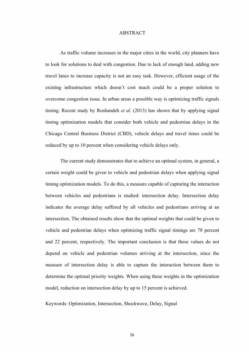
ABSTRACT

As traffic volume increases in the major cities in the world, city planners have

to look for solutions to deal with congestion. Due to lack of enough land, adding new

travel lanes to increase capacity is not an easy task. However, efficient usage of the

existing infrastructure which doesn’t cost much could be a proper solution to

overcome congestion issue. In urban areas a possible way is optimizing traffic signals

timing. Recent study by Roshandeh et al. (2013) has shown that by applying signal

timing optimization models that consider both vehicle and pedestrian delays in the

Chicago Central Business District (CBD), vehicle delays and travel times could be

reduced by up to 10 percent when considering vehicle delays only.

The current study demonstrates that to achieve an optimal system, in general, a

certain weight could be given to vehicle and pedestrian delays when applying signal

timing optimization models. To do this, a measure capable of capturing the interaction

between vehicles and pedestrians is studied: intersection delay. Intersection delay

indicates the average delay suffered by all vehicles and pedestrians arriving at an

intersection. The obtained results show that the optimal weights that could be given to

vehicle and pedestrian delays when optimizing traffic signal timings are 78 percent

and 22 percent, respectively. The important conclusion is that these values do not

depend on vehicle and pedestrian volumes arriving at the intersection, since the

measure of intersection delay is able to capture the interaction between them to

determine the optimal priority weights. When using these weights in the optimization

model, reduction on intersection delay by up to 15 percent is achieved.

Keywords: Optimization, Intersection, Shockwave, Delay, Signal

! "!

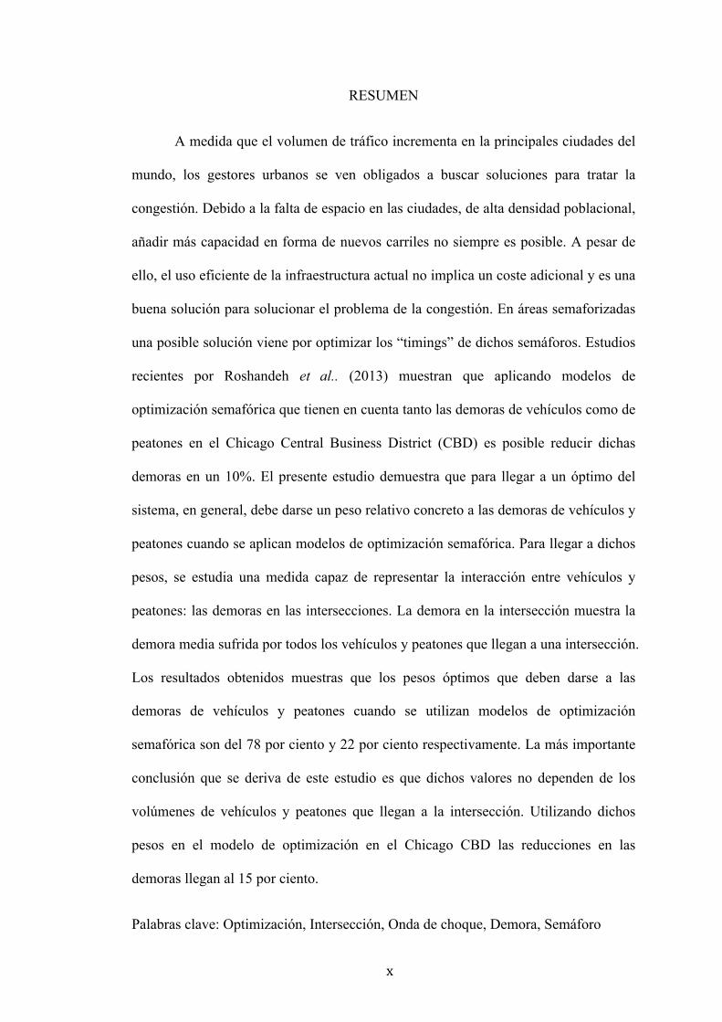
RESUMEN

A medida que el volumen de tráfico incrementa en la principales ciudades del

mundo, los gestores urbanos se ven obligados a buscar soluciones para tratar la

congestión. Debido a la falta de espacio en las ciudades, de alta densidad poblacional,

añadir más capacidad en forma de nuevos carriles no siempre es posible. A pesar de

ello, el uso eficiente de la infraestructura actual no implica un coste adicional y es una

buena solución para solucionar el problema de la congestión. En áreas semaforizadas

una posible solución viene por optimizar los “timings” de dichos semáforos. Estudios

recientes por Roshandeh et al.. (2013) muestran que aplicando modelos de

optimización semafórica que tienen en cuenta tanto las demoras de vehículos como de

peatones en el Chicago Central Business District (CBD) es posible reducir dichas

demoras en un 10%. El presente estudio demuestra que para llegar a un óptimo del

sistema, en general, debe darse un peso relativo concreto a las demoras de vehículos y

peatones cuando se aplican modelos de optimización semafórica. Para llegar a dichos

pesos, se estudia una medida capaz de representar la interacción entre vehículos y

peatones: las demoras en las intersecciones. La demora en la intersección muestra la

demora media sufrida por todos los vehículos y peatones que llegan a una intersección.

Los resultados obtenidos muestras que los pesos óptimos que deben darse a las

demoras de vehículos y peatones cuando se utilizan modelos de optimización

semafórica son del 78 por ciento y 22 por ciento respectivamente. La más importante

conclusión que se deriva de este estudio es que dichos valores no dependen de los

volúmenes de vehículos y peatones que llegan a la intersección. Utilizando dichos

pesos en el modelo de optimización en el Chicago CBD las reducciones en las

demoras llegan al 15 por ciento.

Palabras clave: Optimización, Intersección, Onda de choque, Demora, Semáforo

! ! !!

! !

1

CHAPTER 1

INTRODUCTION

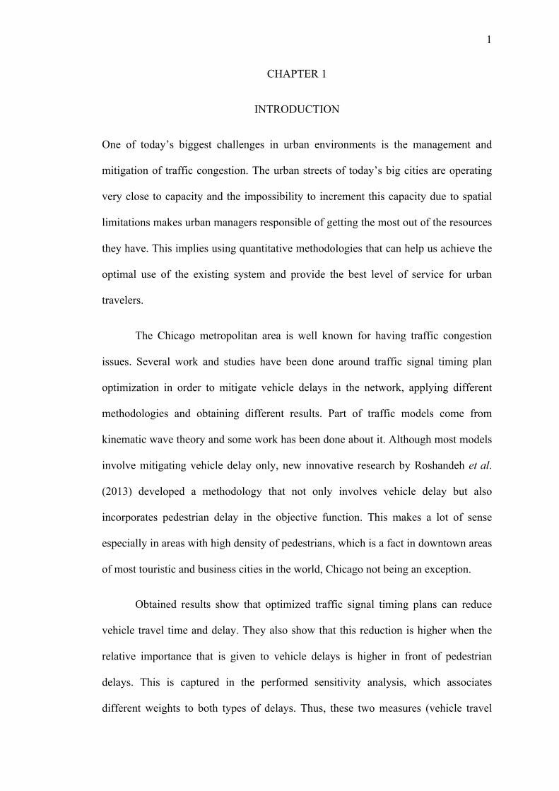
One of today’s biggest challenges in urban environments is the management and

mitigation of traffic congestion. The urban streets of today’s big cities are operating

very close to capacity and the impossibility to increment this capacity due to spatial

limitations makes urban managers responsible of getting the most out of the resources

they have. This implies using quantitative methodologies that can help us achieve the

optimal use of the existing system and provide the best level of service for urban

travelers.

The Chicago metropolitan area is well known for having traffic congestion

issues. Several work and studies have been done around traffic signal timing plan

optimization in order to mitigate vehicle delays in the network, applying different

methodologies and obtaining different results. Part of traffic models come from

kinematic wave theory and some work has been done about it. Although most models

involve mitigating vehicle delay only, new innovative research by Roshandeh et al.

(2013) developed a methodology that not only involves vehicle delay but also

incorporates pedestrian delay in the objective function. This makes a lot of sense

especially in areas with high density of pedestrians, which is a fact in downtown areas

of most touristic and business cities in the world, Chicago not being an exception.

Obtained results show that optimized traffic signal timing plans can reduce

vehicle travel time and delay. They also show that this reduction is higher when the

relative importance that is given to vehicle delays is higher in front of pedestrian

delays. This is captured in the performed sensitivity analysis, which associates

different weights to both types of delays. Thus, these two measures (vehicle travel

! ! !!

! !

2

time and delay) do not capture the real performance of the system since it is

suggesting the manager of the urban network to neglect pedestrian delay in order to

obtain the highest reductions in vehicle delays, which obviously makes sense.

Observing these results also suggests that another driver must be observed to

find an optimal relative weight of vehicle versus pedestrian delays in order to have the

system running and using its resources effectively. In other words, the interaction

between different vehicles needs to be considered as well. This paper focuses on the

concept that best captures the interaction between vehicles and pedestrians to finally

find out link (road segment)’s travel time and delay reductions.

However, intersection delay and its variation is another main issue which

should not be forgotten when the proposed optimization methodologies are applied.

Intersection delay is defined in the Highway Capacity Manual (HCM) (TRB, 2010) as

“Total additional travel time experienced by vehicles as a result of optimizing traffic

signals timing and interaction with other users, divided by the volume departing from

the corresponding cross section of the intersection”. Signals timing optimization may

cause intersection delay to either go up or down.

The main objective of this thesis is to analyze intersection delay when the

optimized traffic signal timing plan methodology proposed by Roshandeh et al.

(2013) is applied. Furthermore, this study wants to prove that there should be an

optimal weight that could be given to vehicle and pedestrian delays respectively in

order to achieve the system’s optimal performance. It seems intuitive that vehicle

delay should have a higher relative weight, but, how much higher? What is the exact

weight that should be given in order to have the system running effectively?

! ! !!

! !

3

Determining that weight will help urban and traffic planners design their traffic signal

timing plans and contribute to the mitigation of traffic congestion on today’s cities.

This thesis is organized in five chapters as follows:

Chapter 1: Introduces the concept of intersection delay and proposes the main

study objectives.

Chapter 2: Presents a literature review and state of the art of the most

innovative research work related to intersection delay. Different proposed models to

calculate intersection delay are studied.

Chapter 3: Describes the proposed methodology that is used for calculating

intersection delay.

Chapter 4: Provides details of the applied model. A focus on data filtering and

preparation is given since its treatment has been important to establish the model.

Chapter 5: Presents the application of the model and the obtained results.

Partial but interesting results are also discussed to see the turning points in the

research process.

Chapter 6: Summarizes the most important results and states the obtained

conclusions. Further research on the topic is also proposed.

! ! !!

! !

4

CHAPTER 2

LITERATURE REVIEW

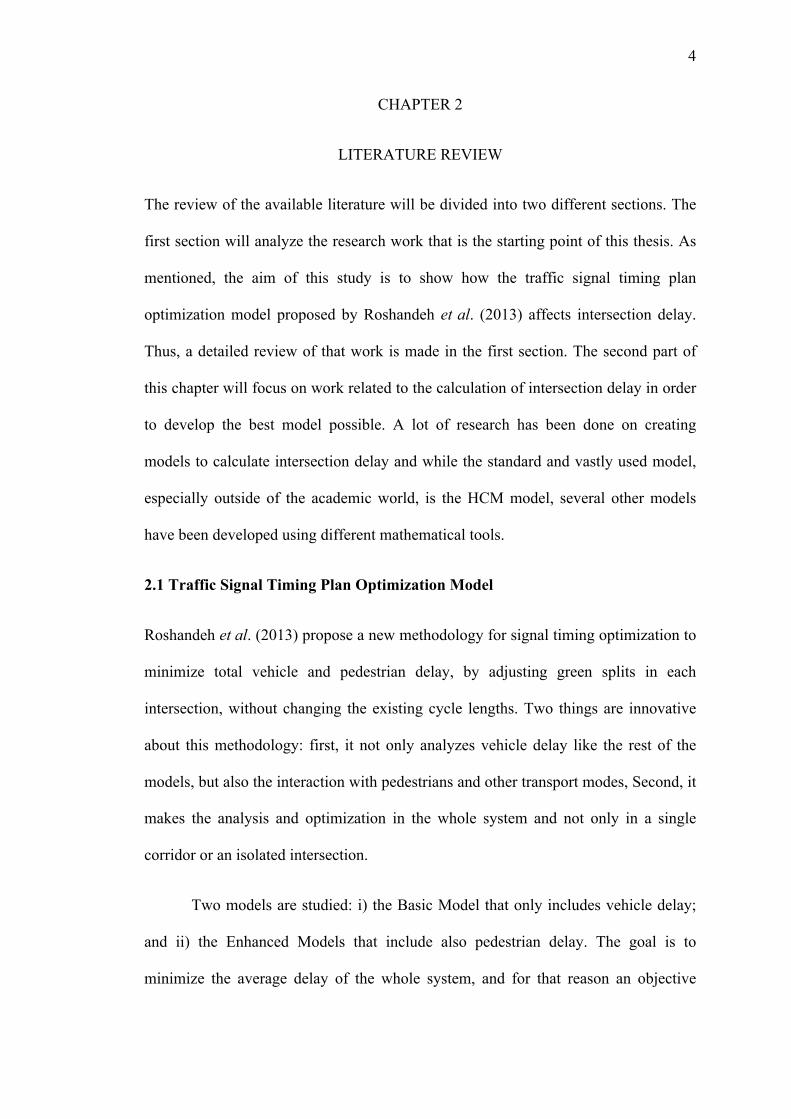
The review of the available literature will be divided into two different sections. The

first section will analyze the research work that is the starting point of this thesis. As

mentioned, the aim of this study is to show how the traffic signal timing plan

optimization model proposed by Roshandeh et al. (2013) affects intersection delay.

Thus, a detailed review of that work is made in the first section. The second part of

this chapter will focus on work related to the calculation of intersection delay in order

to develop the best model possible. A lot of research has been done on creating

models to calculate intersection delay and while the standard and vastly used model,

especially outside of the academic world, is the HCM model, several other models

have been developed using different mathematical tools.

2.1 Traffic Signal Timing Plan Optimization Model

Roshandeh et al. (2013) propose a new methodology for signal timing optimization to

minimize total vehicle and pedestrian delay, by adjusting green splits in each

intersection, without changing the existing cycle lengths. Two things are innovative

about this methodology: first, it not only analyzes vehicle delay like the rest of the

models, but also the interaction with pedestrians and other transport modes, Second, it

makes the analysis and optimization in the whole system and not only in a single

corridor or an isolated intersection.

Two models are studied: i) the Basic Model that only includes vehicle delay;

and ii) the Enhanced Models that include also pedestrian delay. The goal is to

minimize the average delay of the whole system, and for that reason an objective

! ! !!

! !

5

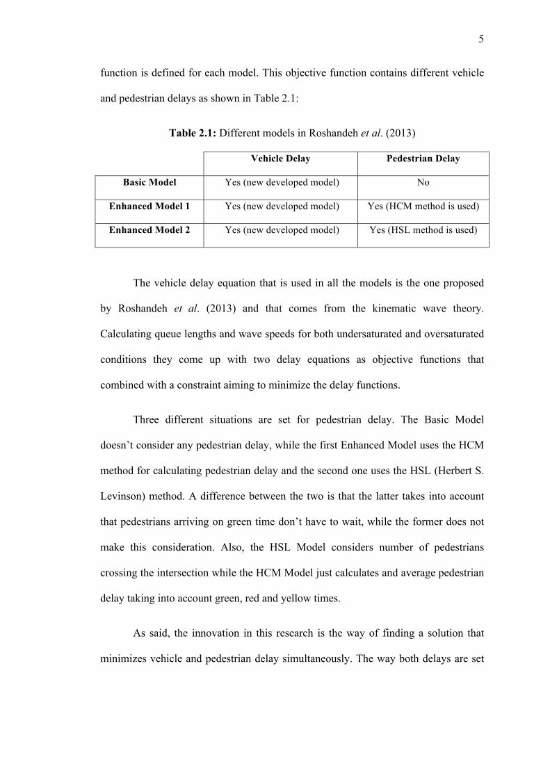
function is defined for each model. This objective function contains different vehicle

and pedestrian delays as shown in Table 2.1:

Table 2.1: Different models in Roshandeh et al. (2013)

Vehicle Delay Pedestrian Delay

Basic Model Yes (new developed model) No

Enhanced Model 1 Yes (new developed model) Yes (HCM method is used)

Enhanced Model 2 Yes (new developed model) Yes (HSL method is used)

The vehicle delay equation that is used in all the models is the one proposed

by Roshandeh et al. (2013) and that comes from the kinematic wave theory.

Calculating queue lengths and wave speeds for both undersaturated and oversaturated

conditions they come up with two delay equations as objective functions that

combined with a constraint aiming to minimize the delay functions.

Three different situations are set for pedestrian delay. The Basic Model

doesn’t consider any pedestrian delay, while the first Enhanced Model uses the HCM

method for calculating pedestrian delay and the second one uses the HSL (Herbert S.

Levinson) method. A difference between the two is that the latter takes into account

that pedestrians arriving on green time don’t have to wait, while the former does not

make this consideration. Also, the HSL Model considers number of pedestrians

crossing the intersection while the HCM Model just calculates and average pedestrian

delay taking into account green, red and yellow times.

As said, the innovation in this research is the way of finding a solution that

minimizes vehicle and pedestrian delay simultaneously. The way both delays are set

! ! !!

! !

6

up together in the objective function for both enhanced models is shown in equation

(2-1):

Min w !DELAYSVEH

+ 1 "w( ) !DELAYSPED

(2-1)

where

DELAYSVEH: Vehicle delay (sec). It is calculated the same way for both

Enhanced models as shown in Table 2.1;

DELAYSPED: Pedestrian delay (sec). Calculated differently for two

Enhanced models as shown in Table 2.1; and

w : Vehicle delay weight (in percent). It is the relative importance assigned to

vehicle delays to determine optimal signal timing plans yielding to the lowest

level of average overall delay per cycle. It varies between 10 and 100 percent,

representing the two extreme cases of emphasizing vehicle delays or

pedestrian delays only.

An iterative process is then applied and new green splits are obtained. New

timings are then applied to a modeled traffic network through the Transportation

Analysis and Simulation System (TRANSIMS) model and travel times and delays are

found. The variations, positive or negative, between these travel times and delays

before and after the optimization are used to tell the usefulness of the methodology.

Also, a sensitivity analysis is made using different relative weights for both the

vehicle delay and the pedestrian delay.

The obtained results show that the effectiveness of the model depends vastly

on the area and traffic conditions where it is applied. Applied to the Chicago Business

! ! !!

! !

7

District it shows that some areas could see delays reduction by 13 percent when

applying the proposed methodology. Another important result comes from the

sensitivity analysis. As commented in the introduction, it is shown that the greatest

reductions in vehicle travel time and delay are obtained when the basic model is

applied, which gives vehicle delay a weight of 100 percent.

The basic and enhanced models were applied to the Chicago Central Business

District (CBD). The studied area was split in four parts: the core area of Chicago

Loop bounded by Wacker Drive along the Chicago River, Roosevelt Road and

Lakeshore Drive (Area 1); the near north of Loop bounded by the Chicago River,

North Avenue and Lakeshore Drive (Area 2); the Near West Loop bounded by I-

90/94, the Chicago River, North Avenue and Roosevelt Road (Area 3) and the West

Loop bounded by Ashland Avenue, I90/94, North Avenue and Roosevelt Road (Area

4). Details are shown later in this report in Figure 5.1.

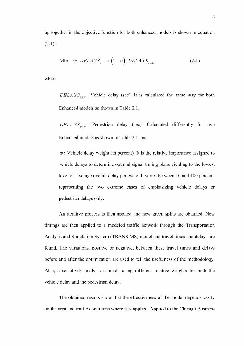
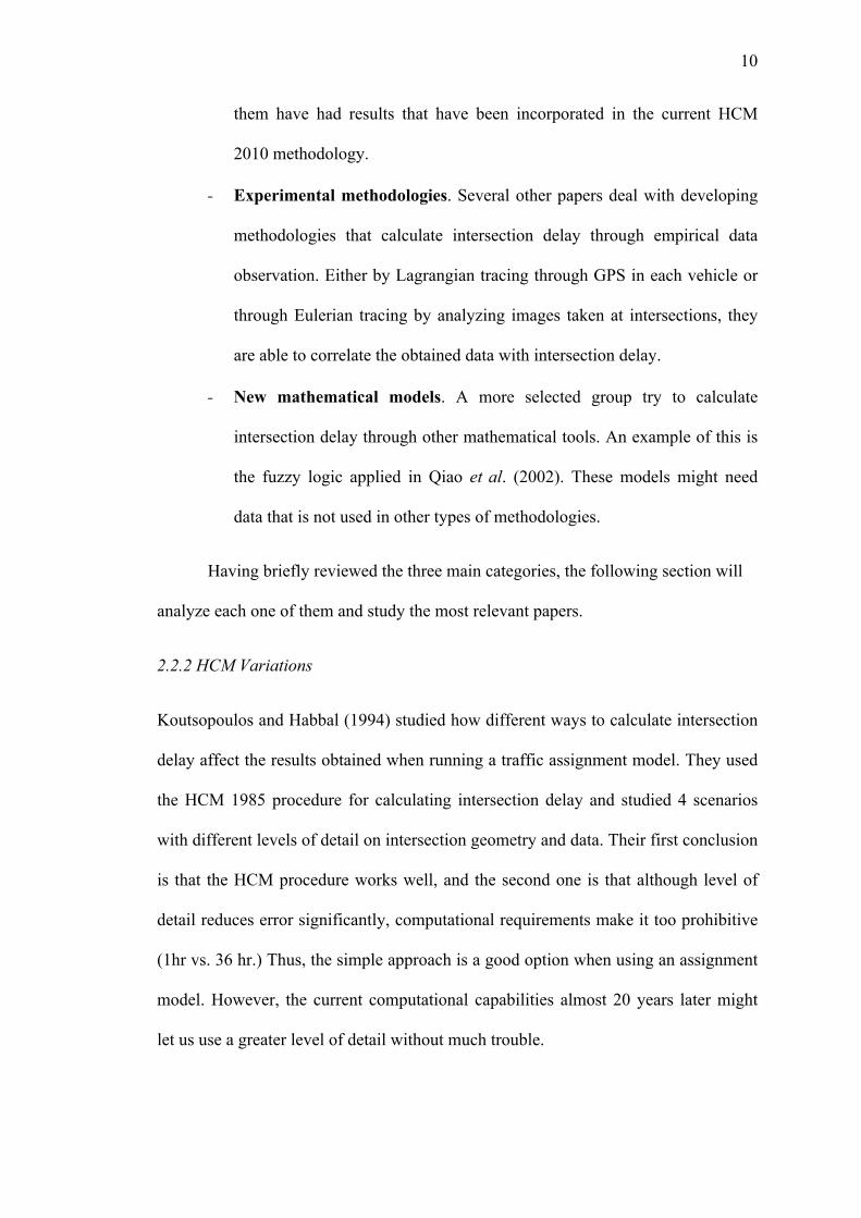
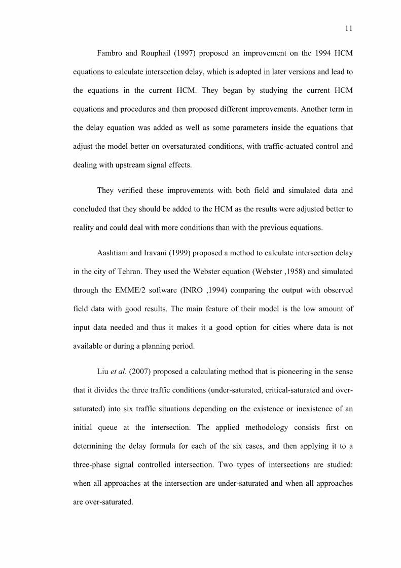
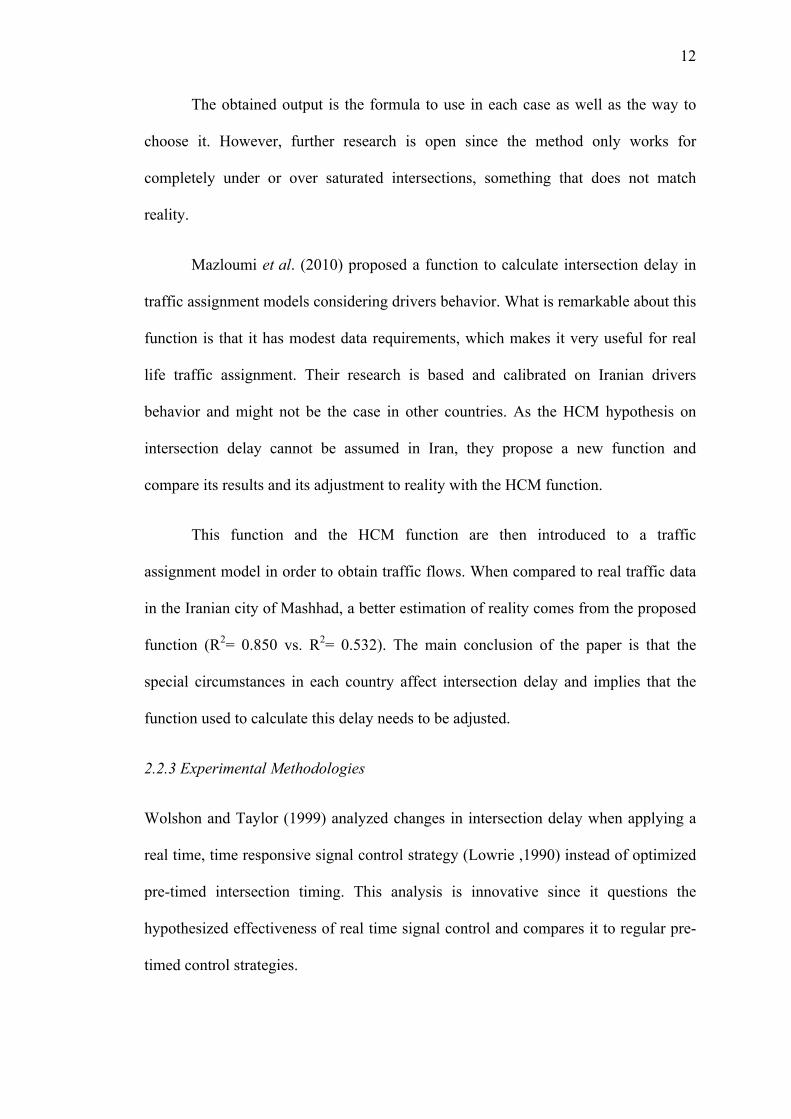
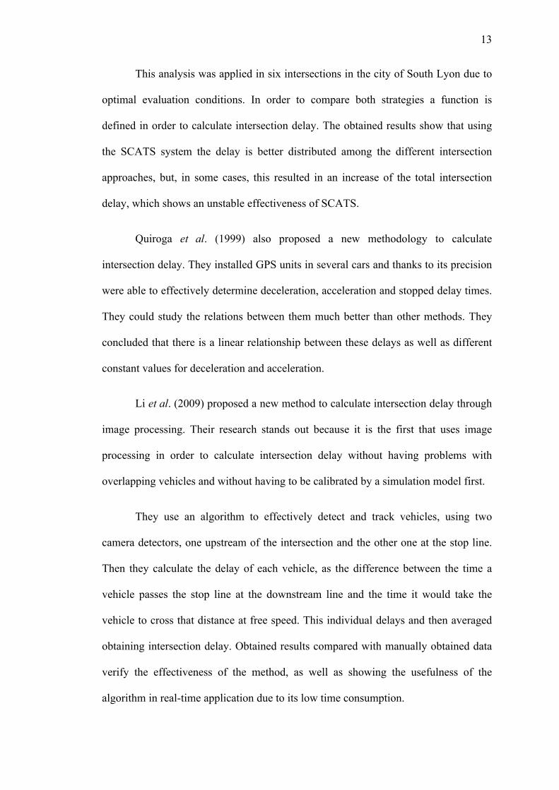
In Figures 2.1, -2.4, when two or more digits appear in the legend, it means

that the associated curve shows results for a combination of two or more areas. For

instance, curve 34 is showing the combined results for areas 3 and 4.

Figure 2.1: Reductions in Travel Time Using the First Enhanced Model in Roshandeh et al. (2013).

! ! !!

! !

8

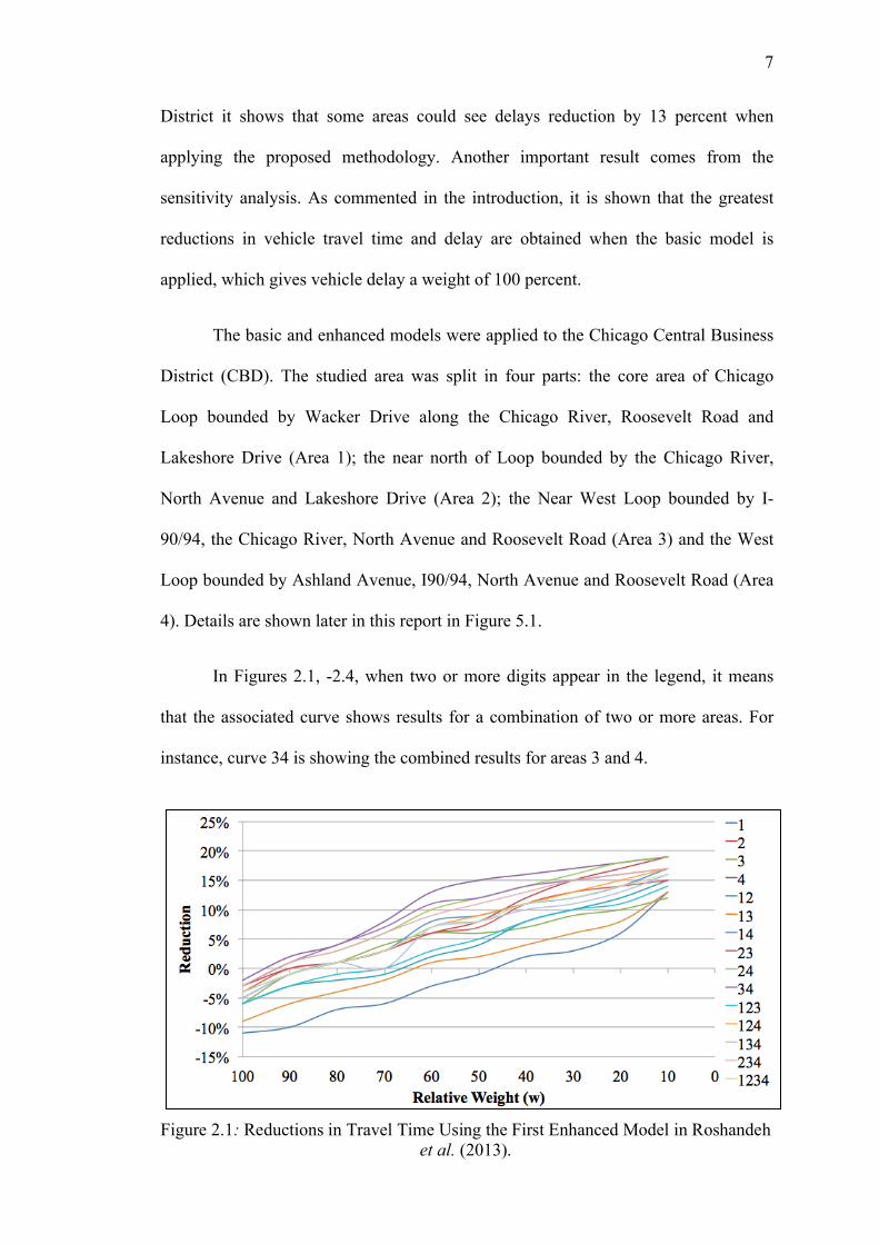
Figure 2.2: Reductions in Vehicle Delays Using the First Enhanced Model in Roshandeh et al. (2013).

Figure 2.3: Reductions in Travel Time Using the Second Enhanced Model in Roshandeh et al .(2013).

Figure 2.4: Reductions in Vehicle Delay Using the Second enhanced model in Roshandeh et al (2013).

! ! !!

! !

9

As it can be observed from Figures 2.1, - 2.4 there is a clear linear relationship

between the reductions on vehicle delay and travel time and the weight (w) given to

vehicle delay in each of the areas and any the combination of them (1, 2, 3 and 4).

This is especially strong in the first enhanced model which used HCM method for

calculating pedestrian’s delay, as seen in Figure 2.1 and 2.2. This opens the new

research line that is followed in this thesis by looking at another driver, intersection

delay, and tries to find an optimal relative weight for both delays. Different ways this

intersection delay can be calculated are presented in the following section.

2.2 Intersection Delay Calculation Models

The current literature proposes different ways to calculate intersection delay. This

section will analyze different types of proposed methods and will explain deeply each

one of them.

2.2.1 Types of Proposed Methodologies

While the HCM methodology, which will be explained shortly, is the most commonly

used method for calculating intersection delay, we can identify three different groups

of improved methodologies in the literature:

- HCM variations. Most of the studied papers try to improve the HCM

methodology by applying different parameters that adjust better the on-site

measured intersection delay with the obtained results of the HCM

methodology. These improved methods have two characteristics: first, they

are usually based on countries outside the United States where HCM

hypothesis might not be valid or might differ somehow; second, some of

! ! !!

! !

10

them have had results that have been incorporated in the current HCM

2010 methodology.

- Experimental methodologies. Several other papers deal with developing

methodologies that calculate intersection delay through empirical data

observation. Either by Lagrangian tracing through GPS in each vehicle or

through Eulerian tracing by analyzing images taken at intersections, they

are able to correlate the obtained data with intersection delay.

- New mathematical models. A more selected group try to calculate

intersection delay through other mathematical tools. An example of this is

the fuzzy logic applied in Qiao et al. (2002). These models might need

data that is not used in other types of methodologies.

Having briefly reviewed the three main categories, the following section will

analyze each one of them and study the most relevant papers.

2.2.2 HCM Variations

Koutsopoulos and Habbal (1994) studied how different ways to calculate intersection

delay affect the results obtained when running a traffic assignment model. They used

the HCM 1985 procedure for calculating intersection delay and studied 4 scenarios

with different levels of detail on intersection geometry and data. Their first conclusion

is that the HCM procedure works well, and the second one is that although level of

detail reduces error significantly, computational requirements make it too prohibitive

(1hr vs. 36 hr.) Thus, the simple approach is a good option when using an assignment

model. However, the current computational capabilities almost 20 years later might

let us use a greater level of detail without much trouble.

! ! !!

! !

11

Fambro and Rouphail (1997) proposed an improvement on the 1994 HCM

equations to calculate intersection delay, which is adopted in later versions and lead to

the equations in the current HCM. They began by studying the current HCM

equations and procedures and then proposed different improvements. Another term in

the delay equation was added as well as some parameters inside the equations that

adjust the model better on oversaturated conditions, with traffic-actuated control and

dealing with upstream signal effects.

They verified these improvements with both field and simulated data and

concluded that they should be added to the HCM as the results were adjusted better to

reality and could deal with more conditions than with the previous equations.

Aashtiani and Iravani (1999) proposed a method to calculate intersection delay

in the city of Tehran. They used the Webster equation (Webster ,1958) and simulated

through the EMME/2 software (INRO ,1994) comparing the output with observed

field data with good results. The main feature of their model is the low amount of

input data needed and thus it makes it a good option for cities where data is not

available or during a planning period.

Liu et al. (2007) proposed a calculating method that is pioneering in the sense

that it divides the three traffic conditions (under-saturated, critical-saturated and over-

saturated) into six traffic situations depending on the existence or inexistence of an

initial queue at the intersection. The applied methodology consists first on

determining the delay formula for each of the six cases, and then applying it to a

three-phase signal controlled intersection. Two types of intersections are studied:

when all approaches at the intersection are under-saturated and when all approaches

are over-saturated.

! ! !!

! !

12

The obtained output is the formula to use in each case as well as the way to

choose it. However, further research is open since the method only works for

completely under or over saturated intersections, something that does not match

reality.

Mazloumi et al. (2010) proposed a function to calculate intersection delay in

traffic assignment models considering drivers behavior. What is remarkable about this

function is that it has modest data requirements, which makes it very useful for real

life traffic assignment. Their research is based and calibrated on Iranian drivers

behavior and might not be the case in other countries. As the HCM hypothesis on

intersection delay cannot be assumed in Iran, they propose a new function and

compare its results and its adjustment to reality with the HCM function.

This function and the HCM function are then introduced to a traffic

assignment model in order to obtain traffic flows. When compared to real traffic data

in the Iranian city of Mashhad, a better estimation of reality comes from the proposed

function (R2= 0.850 vs. R2= 0.532). The main conclusion of the paper is that the

special circumstances in each country affect intersection delay and implies that the

function used to calculate this delay needs to be adjusted.

2.2.3 Experimental Methodologies

Wolshon and Taylor (1999) analyzed changes in intersection delay when applying a

real time, time responsive signal control strategy (Lowrie ,1990) instead of optimized

pre-timed intersection timing. This analysis is innovative since it questions the

hypothesized effectiveness of real time signal control and compares it to regular pre-

timed control strategies.

! ! !!

! !

13

This analysis was applied in six intersections in the city of South Lyon due to

optimal evaluation conditions. In order to compare both strategies a function is

defined in order to calculate intersection delay. The obtained results show that using

the SCATS system the delay is better distributed among the different intersection

approaches, but, in some cases, this resulted in an increase of the total intersection

delay, which shows an unstable effectiveness of SCATS.

Quiroga et al. (1999) also proposed a new methodology to calculate

intersection delay. They installed GPS units in several cars and thanks to its precision

were able to effectively determine deceleration, acceleration and stopped delay times.

They could study the relations between them much better than other methods. They

concluded that there is a linear relationship between these delays as well as different

constant values for deceleration and acceleration.

Li et al. (2009) proposed a new method to calculate intersection delay through

image processing. Their research stands out because it is the first that uses image

processing in order to calculate intersection delay without having problems with

overlapping vehicles and without having to be calibrated by a simulation model first.

They use an algorithm to effectively detect and track vehicles, using two

camera detectors, one upstream of the intersection and the other one at the stop line.

Then they calculate the delay of each vehicle, as the difference between the time a

vehicle passes the stop line at the downstream line and the time it would take the

vehicle to cross that distance at free speed. This individual delays and then averaged

obtaining intersection delay. Obtained results compared with manually obtained data

verify the effectiveness of the method, as well as showing the usefulness of the

algorithm in real-time application due to its low time consumption.

! ! !!

! !

14

Zhu et al. (2011) proposed a real-time road network model to be applied on

vehicle navigation that considers intersection delay. The significance of this new

model is not only that it includes intersection delay, something others don’t consider

or consider a constant, but it also re-optimizes the vehicles path every time new

information is gathered and in a simpler way than other methods.

The methodology applied consisted on improve the Dijkstra algorithm by

updating its optimal once new information is obtained. This model was then tested on

the city of Chongqing in China obtaining good results in the optimality of the path as

well as the matching with reality. Its major problem, however, is the gathering of the

data since it must come from vehicles in the public transport fleet (taxis or vehicles)

and thus hard to get.

2.2.4 New Mathematical Models

Qiao et al. (2002) proposed a methodology to calculate intersection delay through

fuzzy logic. The big difference with the rest of methods for calculating intersection

delay is that using fuzzy logic enables to not only include technical factors but also

non-technical factors that affect delay such as weather. They set up a fuzzy model that

includes as input flow ratio, green time, cycle time and weather.

After setting up the fuzzy model they ran it alongside with the Webster model

and the HCM model comparing them to field data on an intersection in Hong Kong.

The error of the fuzzy logic model is significantly lower than the errors for the

Webster and HCM models and it is then concluded that it is a model that should be

considered when calculating intersection delay.

! ! !!

! !

15

CHAPTER 3

PROPOSED METHODOLOGY

After reviewing the different methodologies that have been developed for calculating

intersection delay, this chapter will define the one that is going to be used. It will

justify why it is chosen and the hypothesis that have been made in order to apply it. It

also defines the data that is needed to use this methodology.

3.1 Justification of the Proposed Methodology

Focusing on the main objective of this thesis, an appropriate methodology needs to be

chosen. After reviewing different types of methodologies, this work chose the HCM

2010 model for analyzing intersection’s delay. This decision is made for the following

reasons:

1. The HCM model is widely used in both the academia and the industry.

Although it might not be valid in some countries as drivers behavior is very

different, the HCM model has seemed to work well in the U.S.A. Taking into

account that this study will calculate intersection delay in downtown Chicago,

the HCM model seems a good choice.

2. The available data is the output of the TRANSIMS model application in

Roshandeh et al. (2013). TRANSIMS gives results on a lot of variables, but

the transcendental ones in intersection delay deal with speed, volume,

maximum queue lengths and travel times. There is also a big constrain on

input data. This means that a methodology cannot be chosen that takes input

that differs from these variables. This also means that neither the empirical

methodologies can’t be used nor the new mathematical models like Qiao et al.

! ! !!

! !

16

(2002), that have input variables like weather that are not results from

TRANSIMS modeling.

3. The hypotheses of the HCM methodology are applicable in the Chicago

network as will be shown in the following section. This makes the HCM

methodology useful in this case.

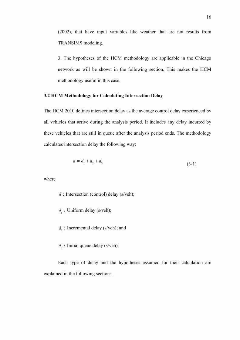
3.2 HCM Methodology for Calculating Intersection Delay

The HCM 2010 defines intersection delay as the average control delay experienced by

all vehicles that arrive during the analysis period. It includes any delay incurred by

these vehicles that are still in queue after the analysis period ends. The methodology

calculates intersection delay the following way:

(3-1)

where

d : Intersection (control) delay (s/veh);

d1: Uniform delay (s/veh);

d2: Incremental delay (s/veh); and

d3: Initial queue delay (s/veh).

Each type of delay and the hypotheses assumed for their calculation are

explained in the following sections.

d = d1+ d

2+ d

3

! ! !!

! !

17

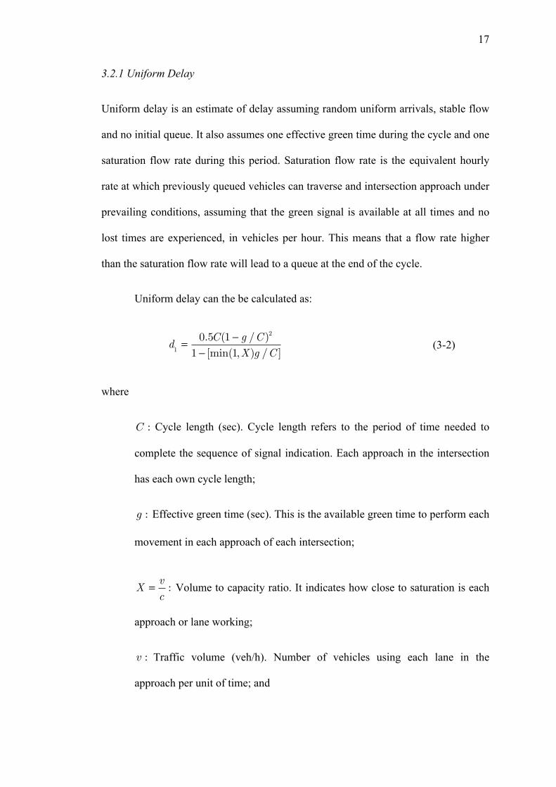
3.2.1 Uniform Delay

Uniform delay is an estimate of delay assuming random uniform arrivals, stable flow

and no initial queue. It also assumes one effective green time during the cycle and one

saturation flow rate during this period. Saturation flow rate is the equivalent hourly

rate at which previously queued vehicles can traverse and intersection approach under

prevailing conditions, assuming that the green signal is available at all times and no

lost times are experienced, in vehicles per hour. This means that a flow rate higher

than the saturation flow rate will lead to a queue at the end of the cycle.

Uniform delay can the be calculated as:

(3-2)

where

C : Cycle length (sec). Cycle length refers to the period of time needed to

complete the sequence of signal indication. Each approach in the intersection

has each own cycle length;

g : Effective green time (sec). This is the available green time to perform each

movement in each approach of each intersection;

X = vc: Volume to capacity ratio. It indicates how close to saturation is each

approach or lane working;

v : Traffic volume (veh/h). Number of vehicles using each lane in the

approach per unit of time; and

d1= 0.5C(1 ! g /C )2

1 ! [min(1,X)g /C ]

! ! !!

! !

18

c : Capacity (veh/h). It is the maximum sustainable flow rate at which vehicles

can be expected to drive through the approach during a specified time period.

3.2.2 Incremental Delay

Incremental delay, as described in 2010 HCM, is used to estimate the extra delay due

to non-uniform arrivals and temporary cycle failures (random delay) as well as delay

caused by sustained periods of oversaturation (TRB, 2010). The equation assumes

that there is no unmet demand that causes initial queues at the start of the analysis

period. It consists of two components. The first one is associated to the fluctuations in

demand during the cycle, taking into account that it can exceed capacity at some point.

The second component accounts for the delay caused by a sustained oversaturation

during the analysis period. It is calculated as:

(3-3)

where

T : Duration of the analysis period (sec). It is the period of time during which

we consider each variable and parameter a constant;

k : Incremental delay factor. It is a factor used to incorporate the effect of the

type of signal control. For pre-timed signals HCM (2010) recommends a value

of 0.5 (obtained from experimental tests); and

I : Upstream filtering/metering adjustment factor. It incorporates the effects

of metering arrivals for upstream signals. For the analysis of an isolated

intersection a value of 1.0 is suggested in the 2010 HCM.

3.2.3 Initial Queue Delay

d2= 900T X ! 1( ) + X ! 1( )2 + 8KIX cT"

#$

%

&'

! ! !!

! !

19

The equation used to estimate incremental delay is based on the assumption that there

is no initial queue present at the start of the analysis period. The initial queue delay

term accounts for the additional delay caused by an existing initial queue. This queue

is the result of unmet demand in the previous time period. Initial queue delay is

computed as:

(3-4)

with (3-5)

(3-6)

if , then

(3-7)

(3-8)

ifv < c , then Qeo= 0.0veh (3-9)

(3-10)

where

i : Period of calculation. It takes values from 1 to 24 since we worked on 24

analysis periods of 1 hour each to compute for all day;

t : Adjusted duration of unmet demand in the analysis period (h). This is the

period of time where the approach is working on dissipating a queue. If traffic

volume is higher than capacity the initial queue will never disappear while it

will if capacity exceeds traffic volume;

d3= 3600vT

tQb+Q

e!Q

eo

2+Qe2 !Q

eo2

2c!Qb2

2c

"

#$

%

&'

Qb(i) =Q

b(i ! 1) +T(v(i) ! c)

Qe=Q

b+ t(v ! c)

v > c Qeo=T v ! c( )

t =T

t =Qb

c ! v

! ! !!

! !

20

Qb: Initial queue at the start of the analysis period (veh);

Qe: Queue at the end of the analysis period (veh); and

Qeo: Queue at the end of the analysis period when traffic volume exceeds

capacity and there is no initial queue (veh).

The important difference between initial queue delay and uniform and

incremental delay is that initial queue delay is computed directly for the whole

approach, and not for every lane group like with d1 and d

2. This is because initial

queue delay takes as inputs different types of queues, and the distribution of these

queues among the different lanes is unknown. Thus, when calculating total approach

delay, while d1 and d

2 will have to be averaged in the approach, d

3 will just be added

since it will already be a delay associated to the approach and not a lane group.

! ! !!

! !

21

CHAPTER 4

MODEL DESCRIPTIONS

This chapter will focus on defining the model used in this research that follows the

HCM (2010) intersection delay calculating methodology defined in Chapter 3. The

first section of this chapter will explain how the TRANSIMS simulation tool is used

and how it works since it is the one providing the used data in this research. The

second part will show how the output of the TRANSIMS model obtained by

Roshandeh et al. (2013) is prepared in order to be input-ready data for our algorithm.

The third part of the chapter will explain how the algorithm developed in this study

works. Then, the fourth part will explain the way results are aggregated and treated.

The last part of the chapter will show a simple example proving the effectiveness of

the algorithm.

4.1 TRANSIMS Simulation Tool

Before defining how the data was set-up to run the model effectively it is important to

understand where it comes from: TRANSIMS. TRANSIMS is an abbreviation for

TRansportation ANalysis and SIMulation System, and is an integrated set of tools to

conduct regional transportation system analysis based on a cellular automata

microsimulator. It is capable of conducting large-scale simulation on a second-by-

second basis for detailed regional multimodal transportation planning, traffic

operations and evacuation planning/emergency management analyses. Its approach is

based on modeling individual travelers and their multi-modal transportation based on

synthetic populations and their activities. Compared to traditional traffic planning

approaches, TRANSIMS requires a significant amount of data and computing

resources.

! ! !!

! !

22

Li et al. (2012) used TRANSIMS to calibrate and validate the Chicago model

using field data on traffic volumes, speeds and travel times in the Chicago

Metropolitan Area collected from over 800 continuous traffic counting stations and

1,200 urban street mid-block counting locations.

The Chicago TRANSIMS model was first applied for regional traffic

assignments using the regional daily O-D travel demand matrix and the existing (i.e.,

the original situation in this study) traffic signal timing plans. The existing traffic

signal timing plans were obtained from the Chicago Department of Transportation.

Next, Roshandeh et al. (2013) applied the iterative process from their model to

obtain new signal timing plans by adjusting the existing green splits of all signal

phases for AM peak, PM peak and rest of the day time period without changing the

existing cycle lengths and signal coordination. This implies having nineteen new and

different signal timing plans: the basic optimized model signal timing plan, the first

enhanced optimized model signal timing plan which incorporated HCM (2010)

method for computing pedestrian’s delay (9 different signal timing plans associated to

9 weighting factors ranging from 90 to 10 percent) and the second enhanced

optimized model signal timing plan which applied HSL method for pedestiran’s delay

computation (9 different signals timing plans). These new signal timing plans were

then used as input set of data in TRANSIMS to be able to obtain traffic volume on

each link (road segment).

TRANSIMS was then ran twenty different times, once for each new traffic

signal timing plan, and one time using original signal timing plans. Basically, signal

timing plan is was the only input value varying among different scenarios. Results on

a lot of variables including travel times, traffic volumes, maximum queues and speeds

! ! !!

! !

23

were obtained. This study uses the traffic volume results given by TRANSIMS as

well as the twenty different signal timing plans (one original and nineteen optimized)

obtained in Roshandeh et al. (2013) in order to calculate intersection delay. The idea

is to compare how intersection delay changes when applying the different optimized

plans.

4.2 Hypotheses and Data Preparation

MATLAB is used to conduct this part. In order to understand how the algorithm is

coded in MATLAB it is important to know how the data is set up. The delay in each

intersection is a weighted average delay from all the approaches in the intersection. At

the same time, the delay associated to each approach is another weighted average

delay from each of the three lane groups (through lanes, right-turn lanes and left-turn

lanes). Thus, the proposed algorithm is applied to each lane group of each approach

on the intersection and then aggregated, as it will be shown later.

To do that, for each iteration to calculate delay the code picks up information

from two Microsoft Excel files. The first one contains the time-static information of

each approach and the second one contains associated volume. Information on traffic

volume for each hour of the day is available, so this procedure is repeated 24 times for

each intersection. There are 4 major situations: the original situation, the optimized

situation with the basic model, the optimized situation with the first enhanced model

and the optimized situation with the second enhanced model. Also, a sensitivity

analysis is made in the enhanced models, so in each one of them the code has been

run for several times.

! ! !!

! !

24

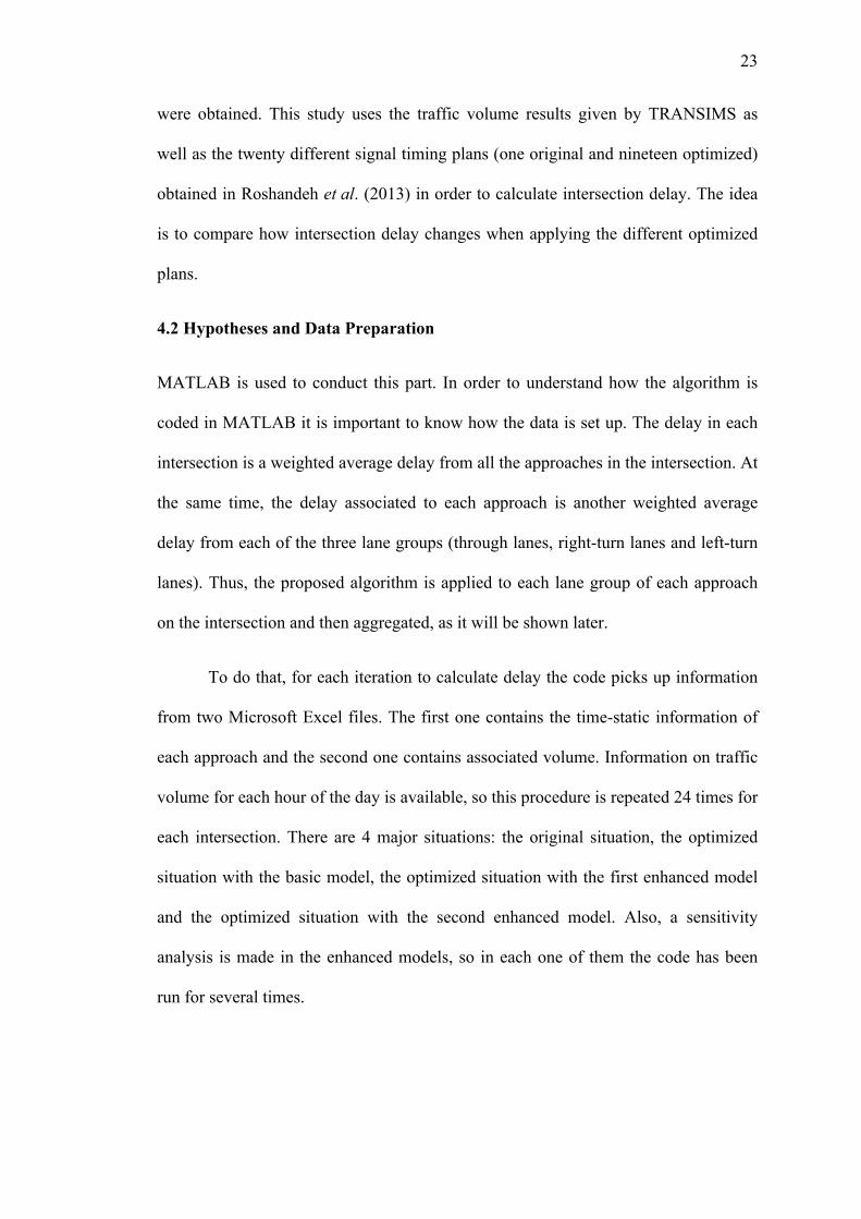
The set-up of the data is illustrated in figures 4.1 and 4.2. Figure 4.1 shows the

first 20 rows (out of 934, one for each node) of the first tab of the time-static

worksheet for the original situation. In this worksheet, the first column corresponds to

the node (i.e., intersection ID), while the rest of the columns correspond to

information about each link (i.e., road segment) arriving at the node. In other words,

figure 4.1 shows the first tab of the worksheet, which is the name (number or ID) of

each link arriving at the node. When there is a zero it means that no more links are

related to that node. For example, at node 14862 (row 15) the arriving links are 15860,

15908 and 15911. Since the maximum number of links arriving at an intersection is 6,

the matrix has 7 columns (1 for nodes and 6 for links).

Other tabs are information related to each link. Thus, the basic structure of the

934x7 matrix is maintained for all of them, but obviously information varies. Apart

from each links name arriving at the node, as shown in figure 4.1, the eight other tabs

Figure 4.1: Snapshot of the first tab at the time-static worksheet. First column is node number and other columns are names of links arriving at the node.

! ! !!

! !

25

contain: cycle length, capacity, number of through lanes, number of left lanes, number

of right lanes, green through times, green left times and green right times. Obviously,

all cells in the rest of the tabs will have a value of 0 where the link tab has a value of 0

since the non-existance of a link implies no information about it. The other way

implication is not true. It is possible that a link doesn’t have all type of lanes, so an

extra zero may appear in the number of lanes or green times if that link doesn’t

contain lanes for that movement. As said, this information is time-static, since it

doesn’t vary through the 24-hour day. However, part of this data will vary when

switching between the four different situations (original, basic optimization, first

enhanced optimization and second enhanced optimization). While the links arriving at

the intersection, capacity of links and number of through, left and right lanes will be

maintained, cycle lengths and green times will change.

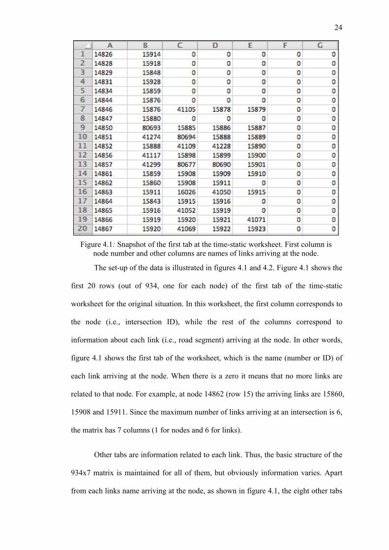
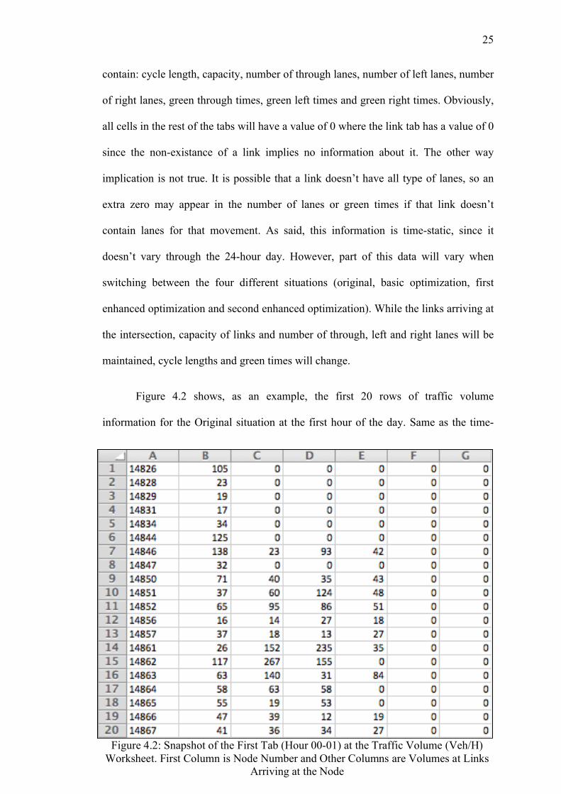
Figure 4.2 shows, as an example, the first 20 rows of traffic volume

information for the Original situation at the first hour of the day. Same as the time-

Figure 4.2: Snapshot of the First Tab (Hour 00-01) at the Traffic Volume (Veh/H) Worksheet. First Column is Node Number and Other Columns are Volumes at Links

Arriving at the Node

! ! !!

! !

26

static information worksheet, the first column is node (i.e., intersection ID), and the

rest of the columns are volume at each link. This worksheet has 24 tabs, since we

obtain volume for each hour of the day. For example, for link 14862, the traffic

volumes on that link arriving at the node are 117, 267 and 155 vehicles for links

15860, 15908 and 15911 respectively. As it can be seen, all matrices are consistent

with each other, and information of each link is in the same position in all matrices,

which makes it easy to reference when calling from the MATLAB script.

As it can be seen, the set-up of the data is very robust and makes the

programming of the MATLAB script very easy. The way the data is set up allows to

reference each value very easily and is the key element to simplify the code and to

speed up computations.

4.2.1 Time-Static Information

Having seen the variables and parameters used by the algorithm, this section will

describe each one of them. Time-static information is the information about the node

that only changes, partially, between each optimization, and not during the day. It

contains several 934-row matrices that contain the following information:

a) Links

Each node has associated the identification number of each link that arrives to the

node.

b) Capacity

Each links capacity. It is assumed that each lane in each approach has the same

capacity, since the total number of lanes divides the total capacity of the approach.

Approach capacity is obtained from the Chicago GIS Network available at the Illinois

! ! !!

! !

27

Institute of Technology. When determining the number of through, left and right lanes,

the capacity obtained from the GIS Network might be modified as it will be seen in

the next section.

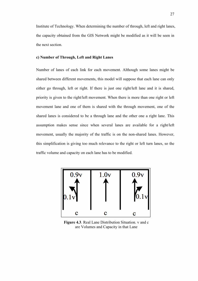
c) Number of Through, Left and Right Lanes

Number of lanes of each link for each movement. Although some lanes might be

shared between different movements, this model will suppose that each lane can only

either go through, left or right. If there is just one right/left lane and it is shared,

priority is given to the right/left movement. When there is more than one right or left

movement lane and one of them is shared with the through movement, one of the

shared lanes is considered to be a through lane and the other one a right lane. This

assumption makes sense since when several lanes are available for a right/left

movement, usually the majority of the traffic is on the non-shared lanes. However,

this simplification is giving too much relevance to the right or left turn lanes, so the

traffic volume and capacity on each lane has to be modified.

Figure 4.3. Real Lane Distribution Situation. v and c are Volumes and Capacity in that Lane

! ! !!

! !

28

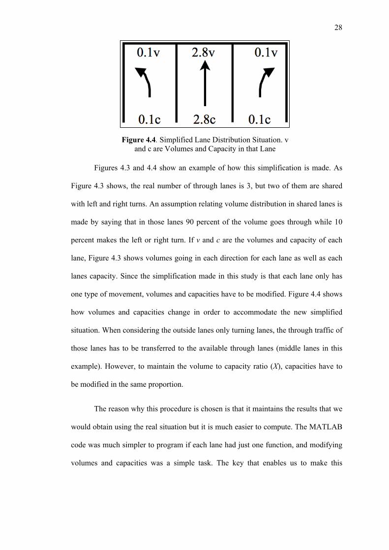
Figures 4.3 and 4.4 show an example of how this simplification is made. As

Figure 4.3 shows, the real number of through lanes is 3, but two of them are shared

with left and right turns. An assumption relating volume distribution in shared lanes is

made by saying that in those lanes 90 percent of the volume goes through while 10

percent makes the left or right turn. If v and c are the volumes and capacity of each

lane, Figure 4.3 shows volumes going in each direction for each lane as well as each

lanes capacity. Since the simplification made in this study is that each lane only has

one type of movement, volumes and capacities have to be modified. Figure 4.4 shows

how volumes and capacities change in order to accommodate the new simplified

situation. When considering the outside lanes only turning lanes, the through traffic of

those lanes has to be transferred to the available through lanes (middle lanes in this

example). However, to maintain the volume to capacity ratio (X), capacities have to

be modified in the same proportion.

The reason why this procedure is chosen is that it maintains the results that we

would obtain using the real situation but it is much easier to compute. The MATLAB

code was much simpler to program if each lane had just one function, and modifying

volumes and capacities was a simple task. The key that enables us to make this

Figure 4.4. Simplified Lane Distribution Situation. v and c are Volumes and Capacity in that Lane

! ! !!

! !

29

simplification is that all the traffic volume in each link are considered to be evenly

distributed on all lanes.

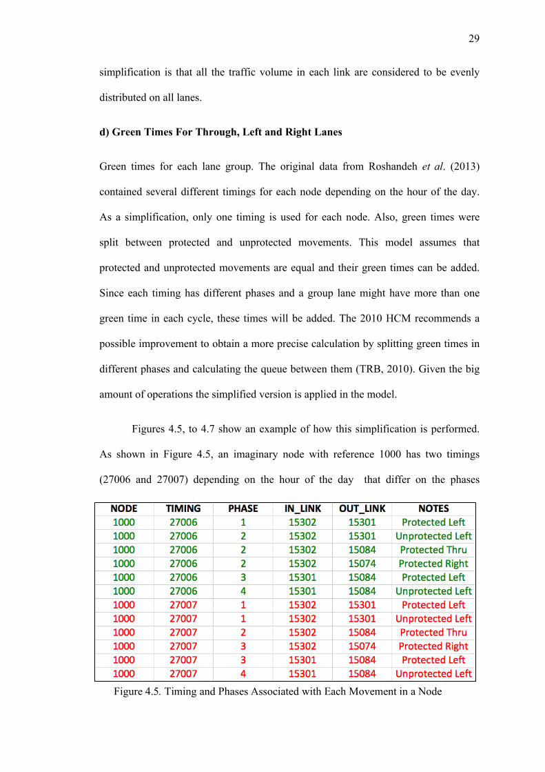
d) Green Times For Through, Left and Right Lanes

Green times for each lane group. The original data from Roshandeh et al. (2013)

contained several different timings for each node depending on the hour of the day.

As a simplification, only one timing is used for each node. Also, green times were

split between protected and unprotected movements. This model assumes that

protected and unprotected movements are equal and their green times can be added.

Since each timing has different phases and a group lane might have more than one

green time in each cycle, these times will be added. The 2010 HCM recommends a

possible improvement to obtain a more precise calculation by splitting green times in

different phases and calculating the queue between them (TRB, 2010). Given the big

amount of operations the simplified version is applied in the model.

Figures 4.5, to 4.7 show an example of how this simplification is performed.

As shown in Figure 4.5, an imaginary node with reference 1000 has two timings

(27006 and 27007) depending on the hour of the day that differ on the phases

Figure 4.5. Timing and Phases Associated with Each Movement in a Node

! ! !!

! !

30

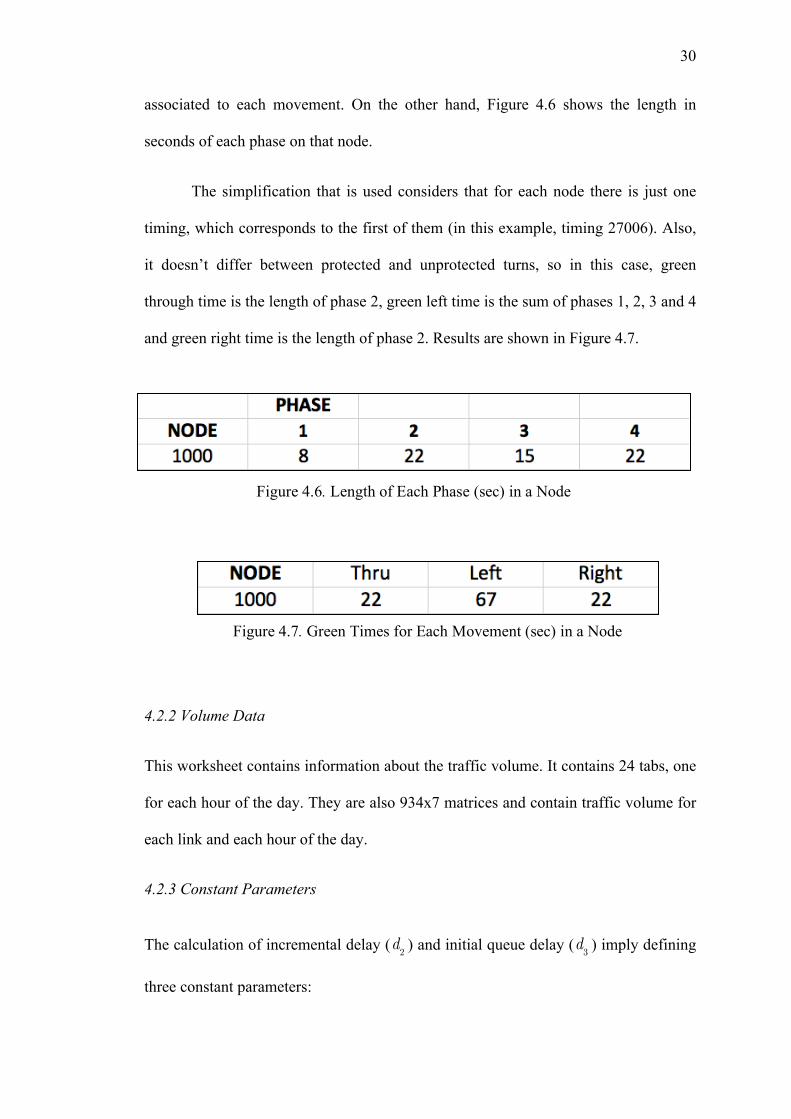
associated to each movement. On the other hand, Figure 4.6 shows the length in

seconds of each phase on that node.

The simplification that is used considers that for each node there is just one

timing, which corresponds to the first of them (in this example, timing 27006). Also,

it doesn’t differ between protected and unprotected turns, so in this case, green

through time is the length of phase 2, green left time is the sum of phases 1, 2, 3 and 4

and green right time is the length of phase 2. Results are shown in Figure 4.7.

4.2.2 Volume Data

This worksheet contains information about the traffic volume. It contains 24 tabs, one

for each hour of the day. They are also 934x7 matrices and contain traffic volume for

each link and each hour of the day.

4.2.3 Constant Parameters

The calculation of incremental delay (d2 ) and initial queue delay (d3 ) imply defining

three constant parameters:

Figure 4.6. Length of Each Phase (sec) in a Node

Figure 4.7. Green Times for Each Movement (sec) in a Node

! ! !!

! !

31

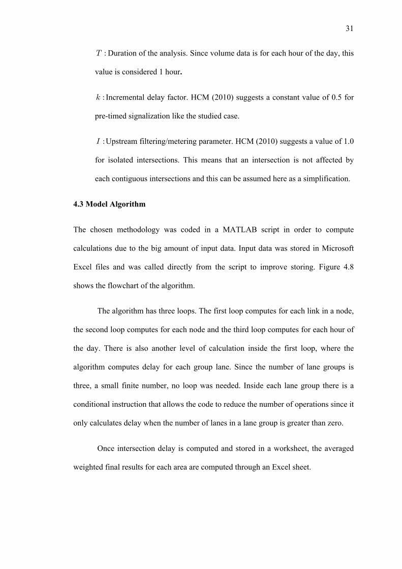
T :Duration of the analysis. Since volume data is for each hour of the day, this

value is considered 1 hour.

k : Incremental delay factor. HCM (2010) suggests a constant value of 0.5 for

pre-timed signalization like the studied case.

I :Upstream filtering/metering parameter. HCM (2010) suggests a value of 1.0

for isolated intersections. This means that an intersection is not affected by

each contiguous intersections and this can be assumed here as a simplification.

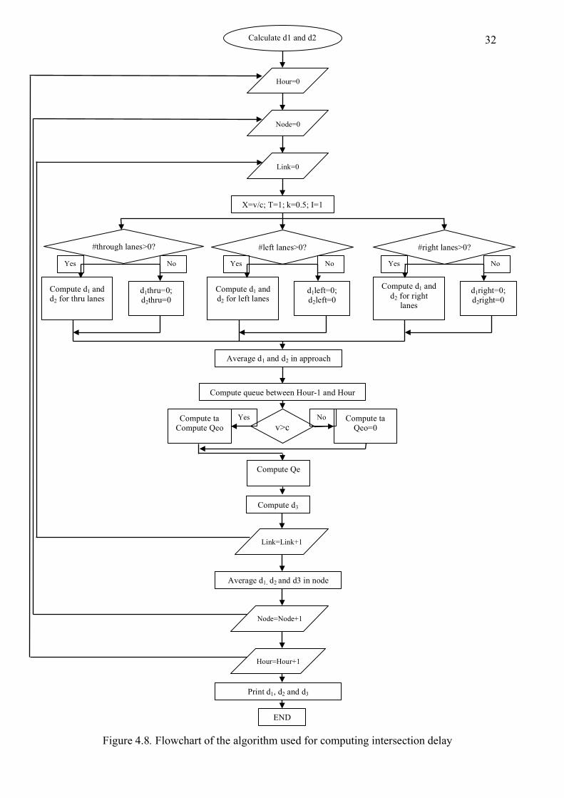
4.3 Model Algorithm

The chosen methodology was coded in a MATLAB script in order to compute

calculations due to the big amount of input data. Input data was stored in Microsoft

Excel files and was called directly from the script to improve storing. Figure 4.8

shows the flowchart of the algorithm.

The algorithm has three loops. The first loop computes for each link in a node,

the second loop computes for each node and the third loop computes for each hour of

the day. There is also another level of calculation inside the first loop, where the

algorithm computes delay for each group lane. Since the number of lane groups is

three, a small finite number, no loop was needed. Inside each lane group there is a

conditional instruction that allows the code to reduce the number of operations since it

only calculates delay when the number of lanes in a lane group is greater than zero.

Once intersection delay is computed and stored in a worksheet, the averaged

weighted final results for each area are computed through an Excel sheet.

! ! !!

! !

32

#left lanes>0?

Calculate d1 and d2

Hour=0

Node=0

Link=0

X=v/c; T=1; k=0.5; I=1

d1left=0; d2left=0

Compute d1 and d2 for left lanes

#right lanes>0? #through lanes>0?

d1right=0; d2right=0

Compute d1 and d2 for right

lanes

d1thru=0; d2thru=0

Compute d1 and d2 for thru lanes

Average d1 and d2 in approach

Link=Link+1

Average d1, d2 and d3 in node

Node=Node+1

Hour=Hour+1

v>c?

Compute queue between Hour-1 and Hour

Compute ta Qeo=0

Compute ta Compute Qeo

Compute Qe

Compute d3

Print d1, d2 and d3

END

Yes Yes Yes

Yes

No No No

No

Figure 4.8. Flowchart of the algorithm used for computing intersection delay

! ! !!

! !

33

4.4 Aggregation of Results

Once the previous algorithm is applied to each lane group for each approach in an

intersection and for each hour of the day, a delay will be obtained that should be

aggregated in order to obtain total intersection delay reduction. This comprises of five

steps:

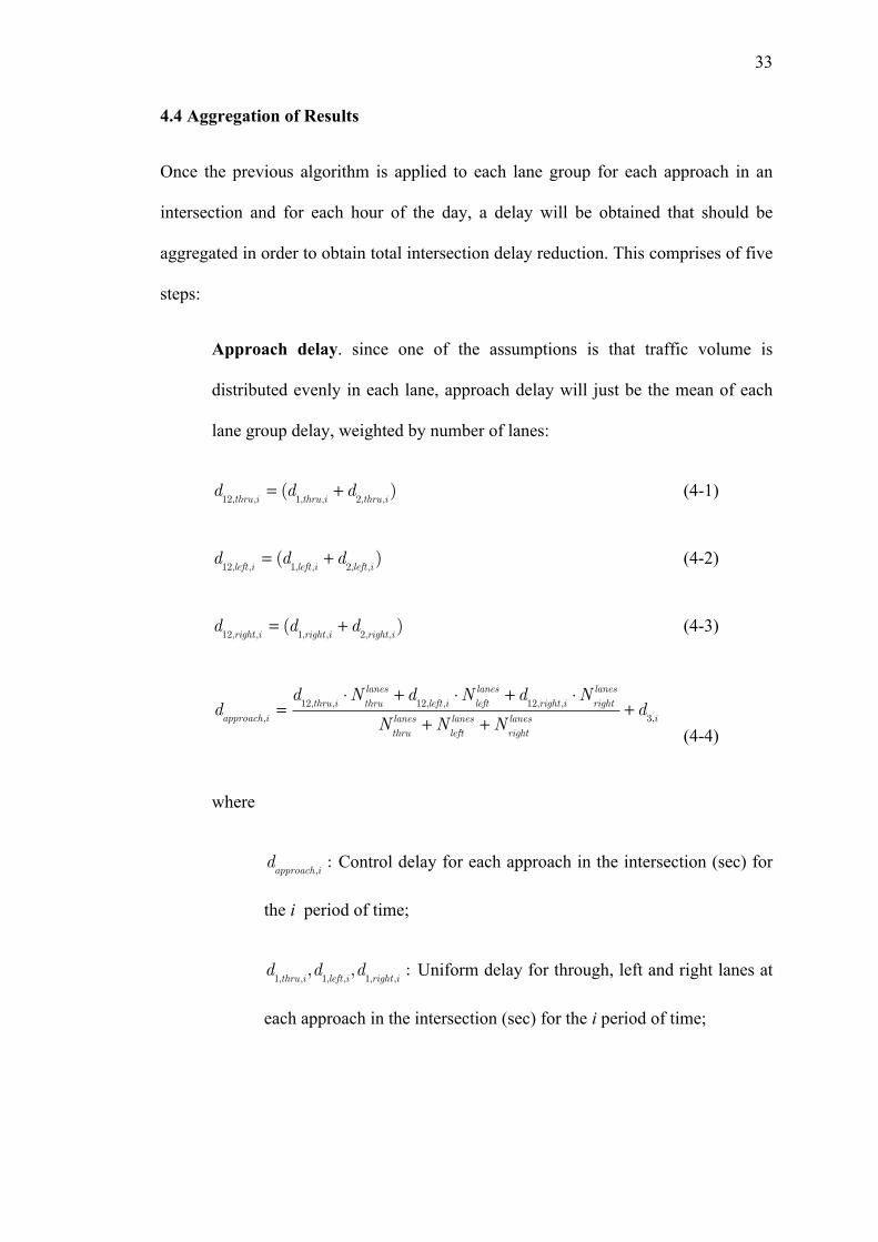
Approach delay. since one of the assumptions is that traffic volume is

distributed evenly in each lane, approach delay will just be the mean of each

lane group delay, weighted by number of lanes:

d12,thru,i

= (d1,thru,i

+ d2,thru,i) (4-1)

d12,left,i

= (d1,left,i

+ d2,left,i) (4-2)

d12,right,i

= (d1,right,i

+ d2,right,i

) (4-3)

dapproach,i

=d12,thru,i

!Nthrulanes + d

12,left,i!N

leftlanes + d

12,right,i!N

rightlanes

Nthrulanes +N

leftlanes +N

rightlanes

+ d3,i

(4-4)

where

dapproach,i

: Control delay for each approach in the intersection (sec) for

the i period of time;

d1,thru,i,d1,left,i,d1,right,i

: Uniform delay for through, left and right lanes at

each approach in the intersection (sec) for the i period of time;

! ! !!

! !

34

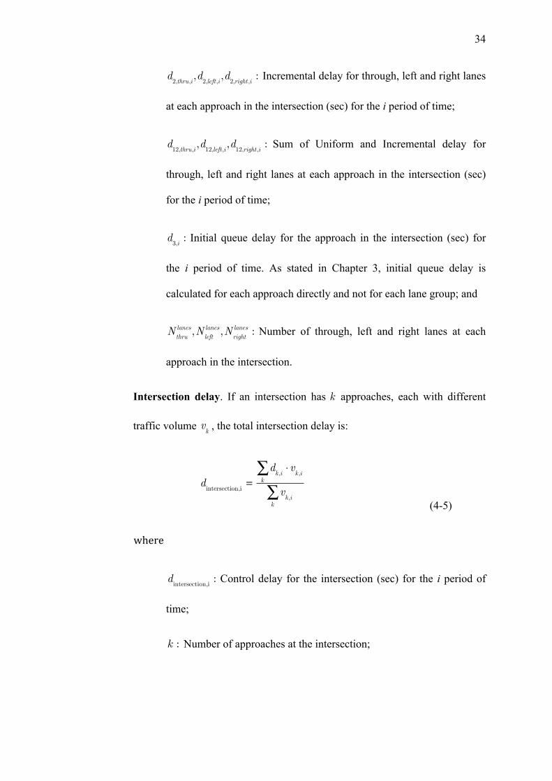
d2,thru,i,d2,left,i,d2,right,i

: Incremental delay for through, left and right lanes

at each approach in the intersection (sec) for the i period of time;

d12,thru,i

,d12,left,i,d12,right,i

: Sum of Uniform and Incremental delay for

through, left and right lanes at each approach in the intersection (sec)

for the i period of time;

d3,i: Initial queue delay for the approach in the intersection (sec) for

the i period of time. As stated in Chapter 3, initial queue delay is

calculated for each approach directly and not for each lane group; and

Nthrulanes,N

leftlanes,N

rightlanes : Number of through, left and right lanes at each

approach in the intersection.

Intersection delay. If an intersection has k approaches, each with different

traffic volume vk , the total intersection delay is:

dintersection,i

=dk,i!vk,i

k"

vk,i

k"

(4-5)!

! %&'('

dintersection,i

: Control delay for the intersection (sec) for the i period of

time;

k : Number of approaches at the intersection;

! ! !!

! !

35

dk,i: Control delay for the k approach in the intersection (sec) for the i

period of time; and

vk,i: Traffic volume at the k approach in the intersection (veh/h) for the

i period of time.

Delay reduction. Once intersection delay for each node is obtained, the

percent decrease between the Original and Optimized situations can be

calculated. A negative number means a reduction while a positive number

means an increase:

%REDi=dintersection,i,OPT

! dintersection,i,BASIC

dintersection,i,BASIC

"100 (4-6)

where

%REDi: Reduction on intersection delay (percent) for the i period of

time and for the studied model;

dintersection,i,OPT

: Intersection delay (sec) for the i period of time and the

optimized solution; and

dintersection,i,BASIC

: Intersection delay (sec) for the i period of time and the

basic solution.

Average daily delay reduction. Once delay reduction for each node and each

hour of the day is calculated an average daily value needs to be computed.

Since delays are units of time per vehicle, it makes sense to average delays

! ! !!

! !

36

weighting by number of cars. That is, weighting by total traffic volume

arriving at the intersection at each hour of the day:

%RED =%RED

i!Vi

VTOTi=1

24

" ! ! ! ! (4-7)!

Vi= v

k,ik! ! ! ! ! ! ! (4-8)!

VTOT

= Vi

i=1

24

! (4-9)

where

%RED : Average daily delay reduction (percent);

Vi: Sum of all volumes arriving at the intersection in the i period of

time (veh); and

VTOT:Sum of all volumes arriving at the intersection in a 24-hour

period (veh).

Area average daily delay reduction. Once average daily delay reduction for

each node is obtained, the average for each of the studied areas (which will be

defined in Chapter 5) needs to be found. Those areas are just an aggrupation of

nodes depending on their situation in the Central Business District (CBD).

%REDAREA

=%RED

AREA,jj=1

n

!nAREA

(4-10)

where

! ! !!

! !

37

%REDAREA: Area average daily delay reduction (percent);

AREA : Name of study area. For example, if area 1 is considered, then

AREA = 1 . As it will be shown in Chapter 5, it can take the values of

1, 2, 3 or 4; and

nAREA: Number of nodes in the study area

Combined area average daily delay reduction. In order to obtain average

results for a combination of the studied areas, an average delay is calculated

the following way:

%REDCOMB

=nAREA

!%REDAREA

AREA

"nAREA

AREA

" (4-11)

where

COMB : Combination of areas. For example, if the combined average

daily delay reduction for areas 1 and 3 are needed, COMB is 13.

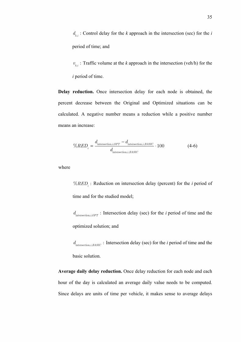
4.5 Test Example

This section will test the model with a simple example. It will calculate the delay

reduction for an imaginary node numbered as 1000 for one hour during the day. Node

1000 has three links approaching called 100, 200 and 300, so the associated row in the

node-link matrix (equivalent to Figure 4.1) is shown in Figure 4.9:!

Figure 4.9. Link Number for Node 1000

! ! !!

! !

38

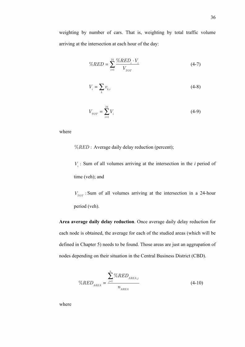
As explained earlier in this chapter, other tabs of the time-static data

worksheet (node-link matrix is the first tab) will have information about each link in

the same position as the link is in the node-link matrix. So for example if links 100,

200 and 300 have capacities of 1000, 1200 and 900 veh/h, respectively, the

correspondent row for node 1000 in node-capacity matrix would be the one showed in

Figure 4.10:

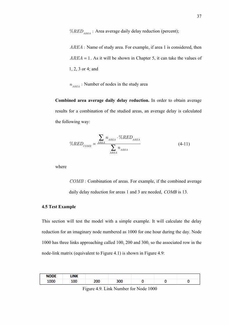
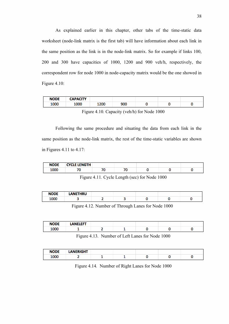
Following the same procedure and situating the data from each link in the

same position as the node-link matrix, the rest of the time-static variables are shown

in Figures 4.11 to 4.17:

!

Figure 4.10. Capacity (veh/h) for Node 1000

Figure 4.11. Cycle Length (sec) for Node 1000!

Figure 4.12. Number of Through Lanes for Node 1000!

Figure 4.13. Number of Left Lanes for Node 1000!

Figure 4.14. Number of Right Lanes for Node 1000!

! ! !!

! !

39

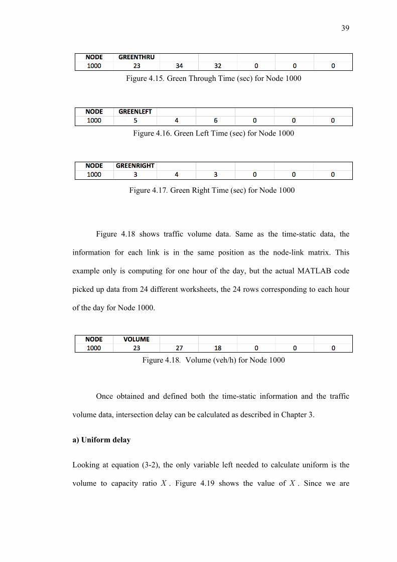
Figure 4.18 shows traffic volume data. Same as the time-static data, the

information for each link is in the same position as the node-link matrix. This

example only is computing for one hour of the day, but the actual MATLAB code

picked up data from 24 different worksheets, the 24 rows corresponding to each hour

of the day for Node 1000.

Once obtained and defined both the time-static information and the traffic

volume data, intersection delay can be calculated as described in Chapter 3.

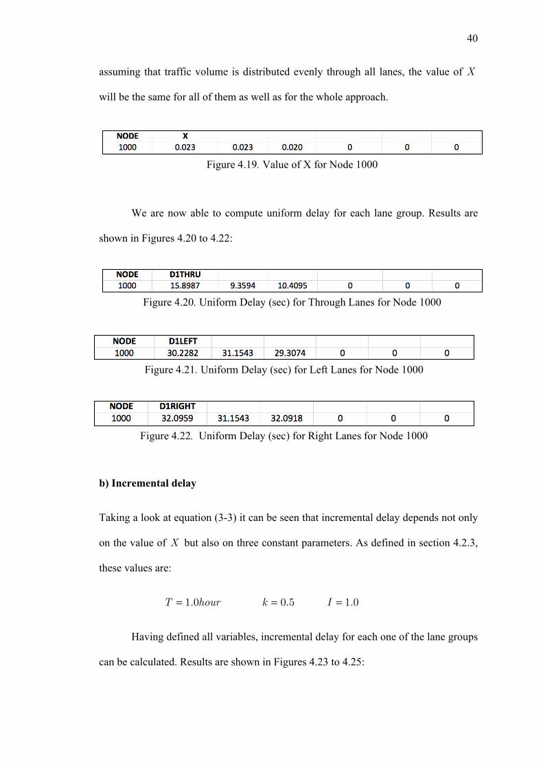
a) Uniform delay

Looking at equation (3-2), the only variable left needed to calculate uniform is the

volume to capacity ratio X . Figure 4.19 shows the value of X . Since we are

Figure 4.15. Green Through Time (sec) for Node 1000!

Figure 4.16. Green Left Time (sec) for Node 1000!

Figure 4.17. Green Right Time (sec) for Node 1000!

Figure 4.18. Volume (veh/h) for Node 1000!

! ! !!

! !

40

assuming that traffic volume is distributed evenly through all lanes, the value of X

will be the same for all of them as well as for the whole approach.

We are now able to compute uniform delay for each lane group. Results are

shown in Figures 4.20 to 4.22:

b) Incremental delay

Taking a look at equation (3-3) it can be seen that incremental delay depends not only

on the value of X but also on three constant parameters. As defined in section 4.2.3,

these values are:

T = 1.0hour k = 0.5 I = 1.0

Having defined all variables, incremental delay for each one of the lane groups

can be calculated. Results are shown in Figures 4.23 to 4.25:

Figure 4.19. Value of X for Node 1000!

Figure 4.20. Uniform Delay (sec) for Through Lanes for Node 1000!

Figure 4.21. Uniform Delay (sec) for Left Lanes for Node 1000!

Figure 4.22. Uniform Delay (sec) for Right Lanes for Node 1000!

! ! !!

! !

41

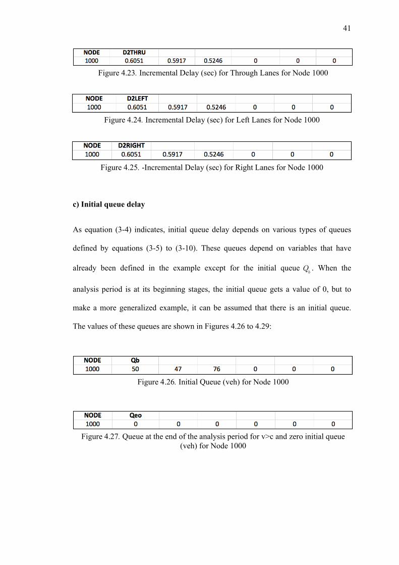
c) Initial queue delay

As equation (3-4) indicates, initial queue delay depends on various types of queues

defined by equations (3-5) to (3-10). These queues depend on variables that have

already been defined in the example except for the initial queue Qb. When the

analysis period is at its beginning stages, the initial queue gets a value of 0, but to

make a more generalized example, it can be assumed that there is an initial queue.

The values of these queues are shown in Figures 4.26 to 4.29:

Figure 4.23. Incremental Delay (sec) for Through Lanes for Node 1000!

Figure 4.24. Incremental Delay (sec) for Left Lanes for Node 1000!

Figure 4.25. -Incremental Delay (sec) for Right Lanes for Node 1000!

Figure 4.26. Initial Queue (veh) for Node 1000!

Figure 4.27. Queue at the end of the analysis period for v>c and zero initial queue (veh) for Node 1000!

! ! !!

! !

42

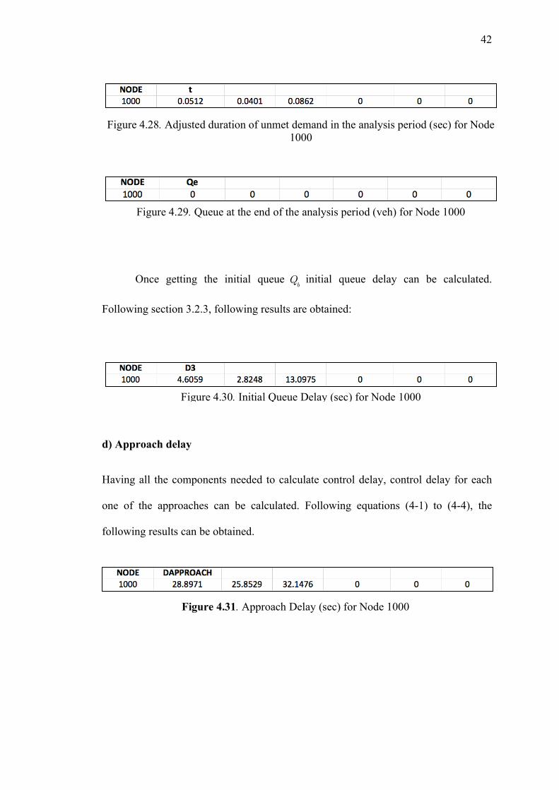
Once getting the initial queue Qb

initial queue delay can be calculated.

Following section 3.2.3, following results are obtained:

d) Approach delay

Having all the components needed to calculate control delay, control delay for each

one of the approaches can be calculated. Following equations (4-1) to (4-4), the

following results can be obtained.

Figure 4.28. Adjusted duration of unmet demand in the analysis period (sec) for Node 1000!

Figure 4.29. Queue at the end of the analysis period (veh) for Node 1000!

Figure 4.30. Initial Queue Delay (sec) for Node 1000!

Figure 4.31. Approach Delay (sec) for Node 1000!

! ! !!

! !

43

e) Intersection delay

Once delay for each one of the three approaches arriving at Node 1000 in this

example are calculated, the control delay in the intersection will be computed by

following equation (4-5) Results are shown in Figure 4.32.

f) Delay reduction

Since this example only had information about one situation (and not for both the

Original situation and an Optimized situation) delay reduction cannot be calculated.

But in order to make a more detailed example, let’s imagine that the earlier situation

was the original case (i.e., without signals timing optimization). Using the same

methodology for an imaginary optimized situation, which would have different data

on volumes and green times, following result as shown in Figure 4.33 is obtained:

Then, having calculated delay for both the Original and the Optimized

situations, delay reduction can be calculated following equation (4-6) which shows

the result in Figure 4.34.

Figure 4.32. Intersection Delay (sec) for Node 1000!

Figure 4.33. Intersection Delay (sec) for Node 1000 on an imaginary Optimized situation!

Figure 4.34. Reduction on Intersection Delay (%)for Node 1000!

! ! !!

! !

44

The result shown in Figure 4.34 is the ultimate result the one is looking for in

each intersection. This example has shown the calculation of delay reduction for one

node and one hour of the day. If the same procedure is performed for the 24 hours of

the day (which would mean changing 24 times the volume information) the average

daily delay reduction will be obtained by following equations (4-7) to (4-9).

When calculating this average daily delay reduction for all nodes in the same

study area, and by following equation (4-10) the area average daily delay reduction

can be computed.

If it is desired to analyze average daily delay reduction for a combination of

different areas, and then obtain the combined area average daily delay reduction,

equation (4-11) would be used.

! ! !!

! !

45

CHAPTER 5

MODEL APPLICATION

Taking into account that a network of 934 nodes (i.e., intersections) is analyzed and a

sensibility analysis is made for the two enhanced optimization models,varying the

relative weight of vehicle to pedestrian delay between 10 percent and 100 percent, it

means that around 0.5 million times of calculation is conducted for intersection delays

are via applying the MATLAB code. Calculation time was around 2 hours with a 2.2

GHz processor and 2MB of RAM memory. This chapter will describe the procedure

used to apply the code and analyze the obtained results.

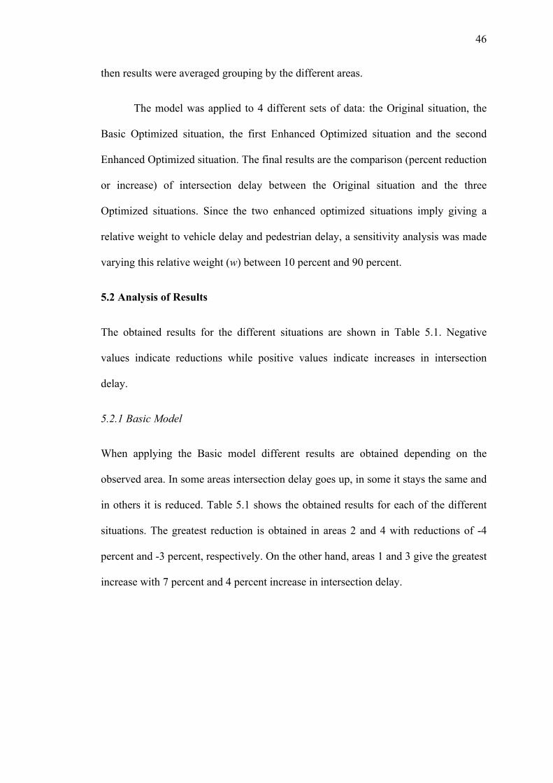
5.1 Application Procedure

The Chicago Business District (CBD) was divided in four parts as shown in Figure

5.1. The different computations of intersection delay were applied to each node and

Figure 5.1. Division of the CBD in the four areas of study

! ! !!

! !

46

then results were averaged grouping by the different areas.

The model was applied to 4 different sets of data: the Original situation, the

Basic Optimized situation, the first Enhanced Optimized situation and the second

Enhanced Optimized situation. The final results are the comparison (percent reduction

or increase) of intersection delay between the Original situation and the three

Optimized situations. Since the two enhanced optimized situations imply giving a

relative weight to vehicle delay and pedestrian delay, a sensitivity analysis was made

varying this relative weight (w) between 10 percent and 90 percent.

5.2 Analysis of Results

The obtained results for the different situations are shown in Table 5.1. Negative

values indicate reductions while positive values indicate increases in intersection

delay.

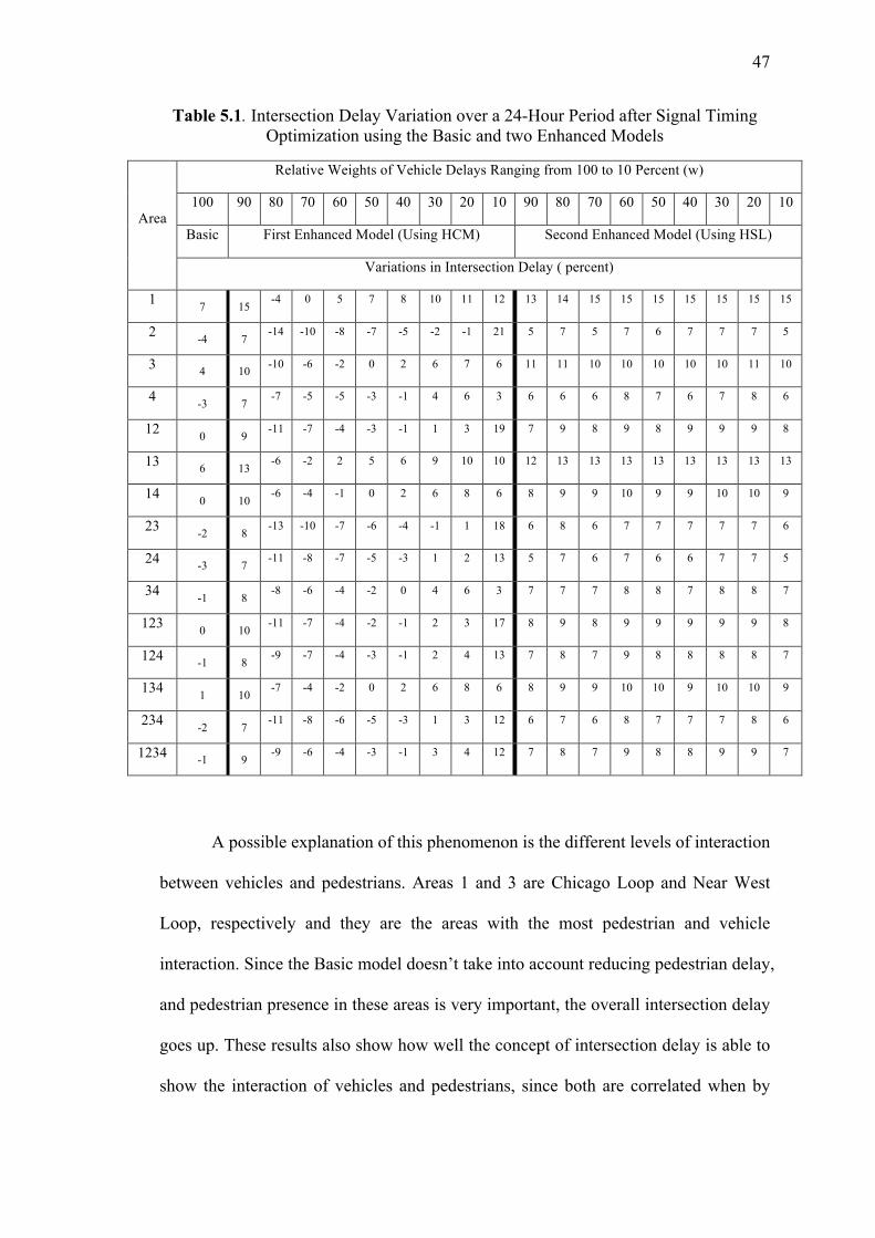
5.2.1 Basic Model

When applying the Basic model different results are obtained depending on the

observed area. In some areas intersection delay goes up, in some it stays the same and

in others it is reduced. Table 5.1 shows the obtained results for each of the different

situations. The greatest reduction is obtained in areas 2 and 4 with reductions of -4

percent and -3 percent, respectively. On the other hand, areas 1 and 3 give the greatest

increase with 7 percent and 4 percent increase in intersection delay.

!!

! ! !!

! !

47

Table 5.1. Intersection Delay Variation over a 24-Hour Period after Signal Timing Optimization using the Basic and two Enhanced Models

Area

Relative Weights of Vehicle Delays Ranging from 100 to 10 Percent (w)

100 90 80 70 60 50 40 30 20 10 90 80 70 60 50 40 30 20 10

Basic First Enhanced Model (Using HCM) Second Enhanced Model (Using HSL)

Variations in Intersection Delay ( percent)

1 7 15 -4 0 5 7 8 10 11 12 13 14 15 15 15 15 15 15 15

2 -4 7 -14 -10 -8 -7 -5 -2 -1 21 5 7 5 7 6 7 7 7 5

3 4 10 -10 -6 -2 0 2 6 7 6 11 11 10 10 10 10 10 11 10

4 -3 7 -7 -5 -5 -3 -1 4 6 3 6 6 6 8 7 6 7 8 6

12 0 9 -11 -7 -4 -3 -1 1 3 19 7 9 8 9 8 9 9 9 8

13 6 13 -6 -2 2 5 6 9 10 10 12 13 13 13 13 13 13 13 13

14 0 10 -6 -4 -1 0 2 6 8 6 8 9 9 10 9 9 10 10 9

23 -2 8 -13 -10 -7 -6 -4 -1 1 18 6 8 6 7 7 7 7 7 6

24 -3 7 -11 -8 -7 -5 -3 1 2 13 5 7 6 7 6 6 7 7 5

34 -1 8 -8 -6 -4 -2 0 4 6 3 7 7 7 8 8 7 8 8 7

123 0 10 -11 -7 -4 -2 -1 2 3 17 8 9 8 9 9 9 9 9 8

124 -1 8 -9 -7 -4 -3 -1 2 4 13 7 8 7 9 8 8 8 8 7

134 1 10 -7 -4 -2 0 2 6 8 6 8 9 9 10 10 9 10 10 9

234 -2 7 -11 -8 -6 -5 -3 1 3 12 6 7 6 8 7 7 7 8 6

1234 -1 9 -9 -6 -4 -3 -1 3 4 12 7 8 7 9 8 8 9 9 7

A possible explanation of this phenomenon is the different levels of interaction

between vehicles and pedestrians. Areas 1 and 3 are Chicago Loop and Near West

Loop, respectively and they are the areas with the most pedestrian and vehicle

interaction. Since the Basic model doesn’t take into account reducing pedestrian delay,

and pedestrian presence in these areas is very important, the overall intersection delay

goes up. These results also show how well the concept of intersection delay is able to

show the interaction of vehicles and pedestrians, since both are correlated when by

! ! !!

! !

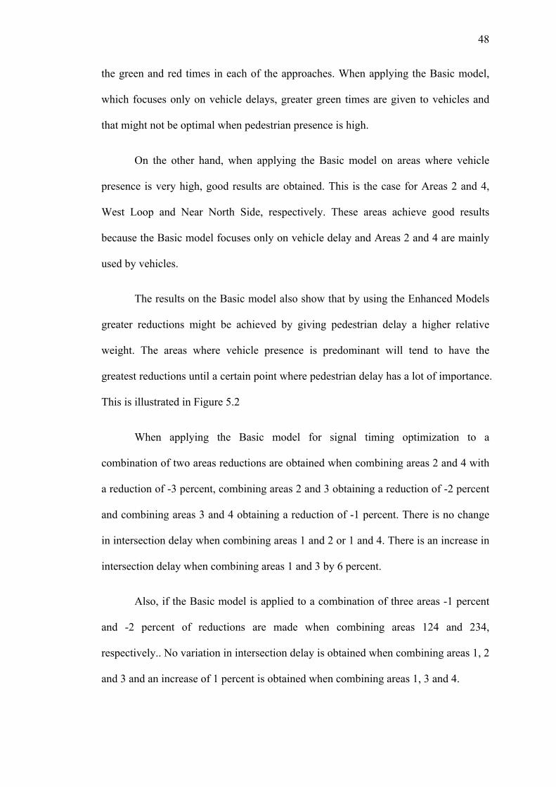
48

the green and red times in each of the approaches. When applying the Basic model,

which focuses only on vehicle delays, greater green times are given to vehicles and

that might not be optimal when pedestrian presence is high.

On the other hand, when applying the Basic model on areas where vehicle

presence is very high, good results are obtained. This is the case for Areas 2 and 4,

West Loop and Near North Side, respectively. These areas achieve good results

because the Basic model focuses only on vehicle delay and Areas 2 and 4 are mainly

used by vehicles.

The results on the Basic model also show that by using the Enhanced Models

greater reductions might be achieved by giving pedestrian delay a higher relative

weight. The areas where vehicle presence is predominant will tend to have the

greatest reductions until a certain point where pedestrian delay has a lot of importance.

This is illustrated in Figure 5.2

When applying the Basic model for signal timing optimization to a

combination of two areas reductions are obtained when combining areas 2 and 4 with

a reduction of -3 percent, combining areas 2 and 3 obtaining a reduction of -2 percent

and combining areas 3 and 4 obtaining a reduction of -1 percent. There is no change

in intersection delay when combining areas 1 and 2 or 1 and 4. There is an increase in

intersection delay when combining areas 1 and 3 by 6 percent.

Also, if the Basic model is applied to a combination of three areas -1 percent

and -2 percent of reductions are made when combining areas 124 and 234,

respectively.. No variation in intersection delay is obtained when combining areas 1, 2

and 3 and an increase of 1 percent is obtained when combining areas 1, 3 and 4.

! ! !!

! !

49

The overall variation for the combination of areas 1, 2, 3 and 4 when applying

the Basic Model is a reduction of -1 percent.

5.2.2 First Enhanced Model

When using the first enhanced model that applies HCM method for calculating

pedestrian’s delay, three important points are observed. The first one is that switching

from the Basic Model, which gives vehicle delay a 100 percent relative weight, to the

Enhanced Model that gives 90 percent weight to vehicle delay at first, a

general increase in intersection delay is observed as it can be seen in Figure 5.2 where

the enhanced Model results and sensitivity analysis are compared alongside with the

Basic Model.

Figure 5.2. Variation of Reduction In Intersection Delay with Relative Weight in Each Group of Areas for the Basic and First Enhanced Models

! ! !!

! !

50

A possible explanation is that the first reaction of the model when introducing

pedestrian delay in the optimization is to increase intersection delay because another

source of delay is involved into the equation and the results are affected by it. At that

point of the sensitivity analysis the aggregation of another cause of delay makes

intersection delay to go up.

The second important point is that from a 90 percent relative weight until

some point close to 80 percent relative weight there is a generalized decrease in

intersection delay. This means that the Enhanced Model is applied, considering the

existence of pedestrians and passing a certain threshold where vehicle delay is still

very powerful, intersection delay starts to go down. This shows the power of using a

model that considers both pedestrian and vehicle delay, since it will be evaluating the

interaction between both and that is something extremely important in the overall

performance of the network. Again, the general pattern of having the greatest

reductions in areas where vehicle presence is predominant is valid, since vehicle delay

is still having a very high relative weight.

The third important thing is that there is a point when intersection delay starts

to increase. This means that there is an optimal relative weight that achieves the

maximum reductions and after that point results are getting worse. Also, as it can be

seen in Figure 5.2, there is a pattern shift once vehicle delay is around 20 percent

(which means that pedestrian delay is much more important, at 80 percent). The areas

where vehicle presence is more important will now get higher increases in

intersection delay than the areas where pedestrian presence is more important. This

appears almost at the end of the sensitivity analysis, since until that point vehicle

delay has been weighted much higher. Vehicle delay is obviously much more

! ! !!

! !

51

powerful in the model, equation 2-1, and a really high relative weight 1-w must be

given to pedestrian delay in order to make the pattern shift.

The important result that is then obtained by analyzing the behavior of the first

enhanced optimization model is that there is an optimal value of the relative weight

that could be given to vehicle delay to produce the greatest reductions in intersection

delay. Disagreeing with the intuitive conclusion that this value might depend on the

volumes of vehicles and pedestrians that arrive to the intersection, there is a unique

value that can be found independently of these volumes. This value is 78 percent and

it is a common value for all of the studied areas. The reason why this value is unique

is that the HCM model for intersection delay only captures vehicle volumes and not

pedestrian volumes but at the same time can capture the interaction of both with the

green time variable. Then an optimal value can be found that lets having the greatest

reductions in intersection delay without looking at the vehicle and pedestrian volumes.

As commented, when applying the first Enhanced model varying the weight w

between 90 percent and 20 percent the same order is maintained when looking at what

areas or combination of areas have the highest reductions (or lowest increases) in

intersection delay. When looking at results of individual areas it is obtained that

between these two values of 90 percent and 20 percent for the weight, the best results

are for areas 2, 3, 4 and 1 in that order. For example, at the system optimal (w=78

percent) the respective reductions for these areas are -14 percent, -10 percent, -7

percent and -4 percent, respectively. This order is maintained until w=20 percent

where intersection delay is reduced in area 2 by -1 percent and increased in areas 3, 4

and 1 by 7 percent, 6 percent and 11 percent. As it can be seen in Figure 5.2, at this

point the pattern changes and areas where pedestrian presence is higher (areas 3 and

1) start to get better results than areas where vehicle presence is more important. At

! ! !!

! !

52

w=10 percent the best results are obtained in area 4 with an increase of 3 percent

while the worst result is obtained in area 2 (which had the best results until now) by

an increase of 21 percent.

Focusing now on the results obtained in the optimal weight (w=78 percent)

when looking at a combination of two areas reductions of intersection delay between -

6 percent and -13 percent are obtained. Specifically, these reductions are -6 percent

for a combination of areas 1 and 3, -6 percent for a combination of areas 1 and 4, -8

percent for a combination of areas 3 and 4, -11 percent for a combination of areas 2

and 4, -11 percent for a combination of areas 1 and 2 and -13 percent for a

combination of areas 2 and 3.

When looking at a combination of three areas at the system optimal reductions

between -7 percent and -11 percent are obtained. Combining areas 1, 3 and 4 a

reduction of -7 percent, combining areas 1, 2 and 4 a reduction of -9 percent and the

best results are obtained when combining areas 1, 2 and 3 or 2, 3 and 4 with

reductions of -11 percent.

Applying the first enhanced model to the whole CBD, which means

combining areas 1, 2, 3 and 4, a reduction in intersection delay of -9 percent is

obtained

5.2.3 Second Enhanced Model

The second enhanced model, which recruits HSL method for computing pedestrian’s

delay, shows very different results than the first enhanced model. While the first

enhanced Model has a strong pattern where optimal solutions can be found and where

clear conclusions can be drawn, the second enhanced Model gives a steady and

! ! !!

! !

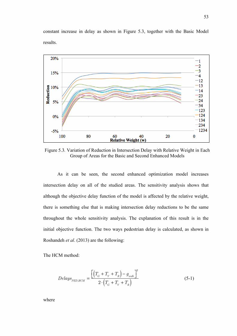
53

constant increase in delay as shown in Figure 5.3, together with the Basic Model

results.

As it can be seen, the second enhanced optimization model increases

intersection delay on all of the studied areas. The sensitivity analysis shows that

although the objective delay function of the model is affected by the relative weight,

there is something else that is making intersection delay reductions to be the same

throughout the whole sensitivity analysis. The explanation of this result is in the

initial objective function. The two ways pedestrian delay is calculated, as shown in

Roshandeh et al. (2013) are the following:

The HCM method:

DelaysPED,HCM

=TG+T

Y+T

R( ) ! gwalk"#

$%2

2 & TG+T

Y+T

R( ) (5-1)

where

Figure 5.3. Variation of Reduction in Intersection Delay with Relative Weight in Each Group of Areas for the Basic and Second Enhanced Models

! ! !!

! !

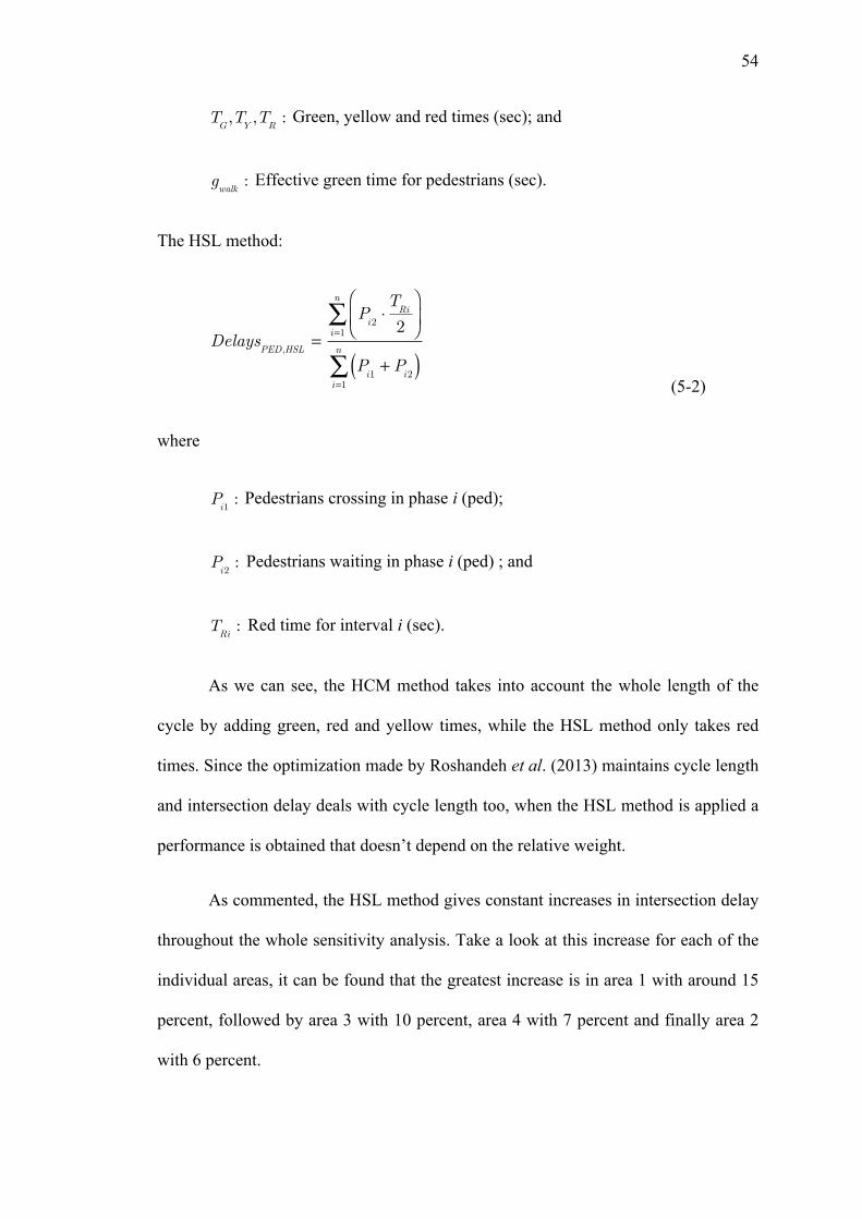
54

TG,TY,TR: Green, yellow and red times (sec); and

gwalk: Effective green time for pedestrians (sec).

The HSL method:

DelaysPED,HSL

=Pi2!TRi

2

"

#$%

&'i=1

n

(

Pi1+ P

i2( )i=1

n

( (5-2)

where

Pi1: Pedestrians crossing in phase i (ped);

Pi2: Pedestrians waiting in phase i (ped) ; and

TRi: Red time for interval i (sec).

As we can see, the HCM method takes into account the whole length of the

cycle by adding green, red and yellow times, while the HSL method only takes red

times. Since the optimization made by Roshandeh et al. (2013) maintains cycle length

and intersection delay deals with cycle length too, when the HSL method is applied a

performance is obtained that doesn’t depend on the relative weight.

As commented, the HSL method gives constant increases in intersection delay

throughout the whole sensitivity analysis. Take a look at this increase for each of the

individual areas, it can be found that the greatest increase is in area 1 with around 15

percent, followed by area 3 with 10 percent, area 4 with 7 percent and finally area 2

with 6 percent.

! ! !!

! !

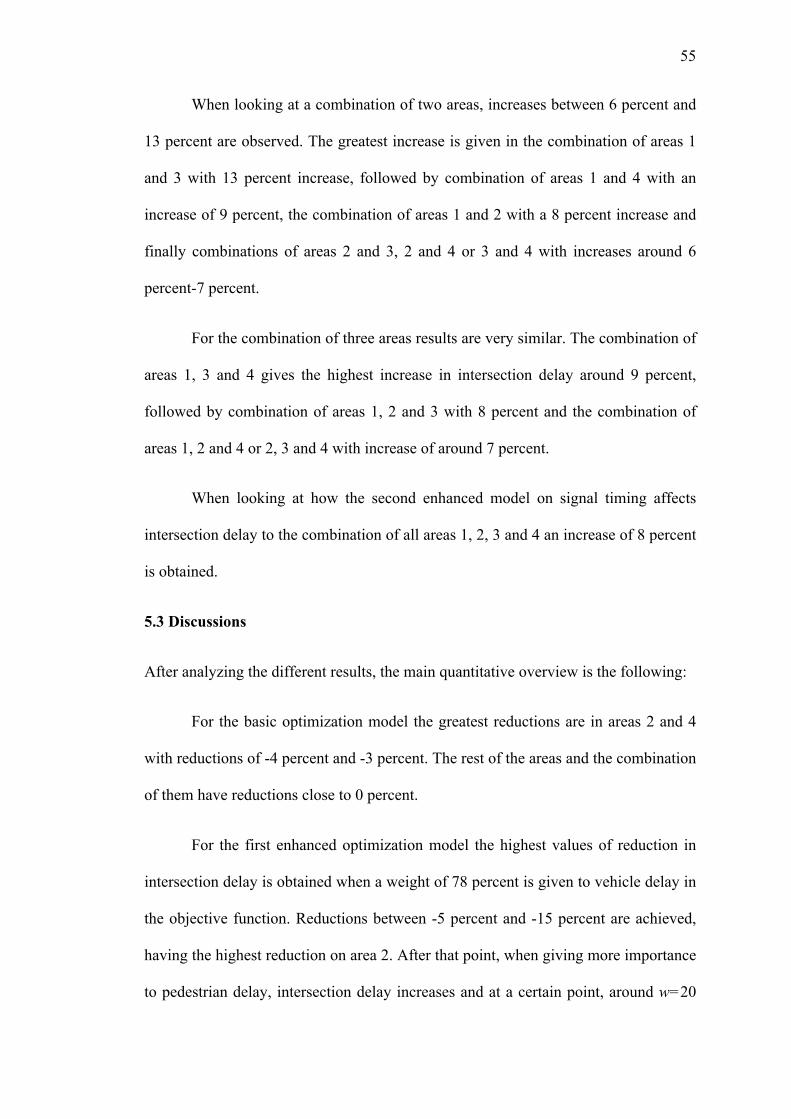
55

When looking at a combination of two areas, increases between 6 percent and

13 percent are observed. The greatest increase is given in the combination of areas 1

and 3 with 13 percent increase, followed by combination of areas 1 and 4 with an

increase of 9 percent, the combination of areas 1 and 2 with a 8 percent increase and

finally combinations of areas 2 and 3, 2 and 4 or 3 and 4 with increases around 6

percent-7 percent.

For the combination of three areas results are very similar. The combination of

areas 1, 3 and 4 gives the highest increase in intersection delay around 9 percent,

followed by combination of areas 1, 2 and 3 with 8 percent and the combination of

areas 1, 2 and 4 or 2, 3 and 4 with increase of around 7 percent.

When looking at how the second enhanced model on signal timing affects

intersection delay to the combination of all areas 1, 2, 3 and 4 an increase of 8 percent

is obtained.

5.3 Discussions

After analyzing the different results, the main quantitative overview is the following:

For the basic optimization model the greatest reductions are in areas 2 and 4

with reductions of -4 percent and -3 percent. The rest of the areas and the combination

of them have reductions close to 0 percent.

For the first enhanced optimization model the highest values of reduction in

intersection delay is obtained when a weight of 78 percent is given to vehicle delay in

the objective function. Reductions between -5 percent and -15 percent are achieved,

having the highest reduction on area 2. After that point, when giving more importance

to pedestrian delay, intersection delay increases and at a certain point, around w=20

! ! !!

! !

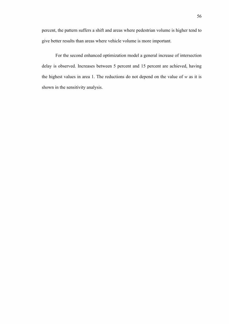
56

percent, the pattern suffers a shift and areas where pedestrian volume is higher tend to

give better results than areas where vehicle volume is more important.

For the second enhanced optimization model a general increase of intersection

delay is observed. Increases between 5 percent and 15 percent are achieved, having

the highest values in area 1. The reductions do not depend on the value of w as it is

shown in the sensitivity analysis.

! ! !!

! !

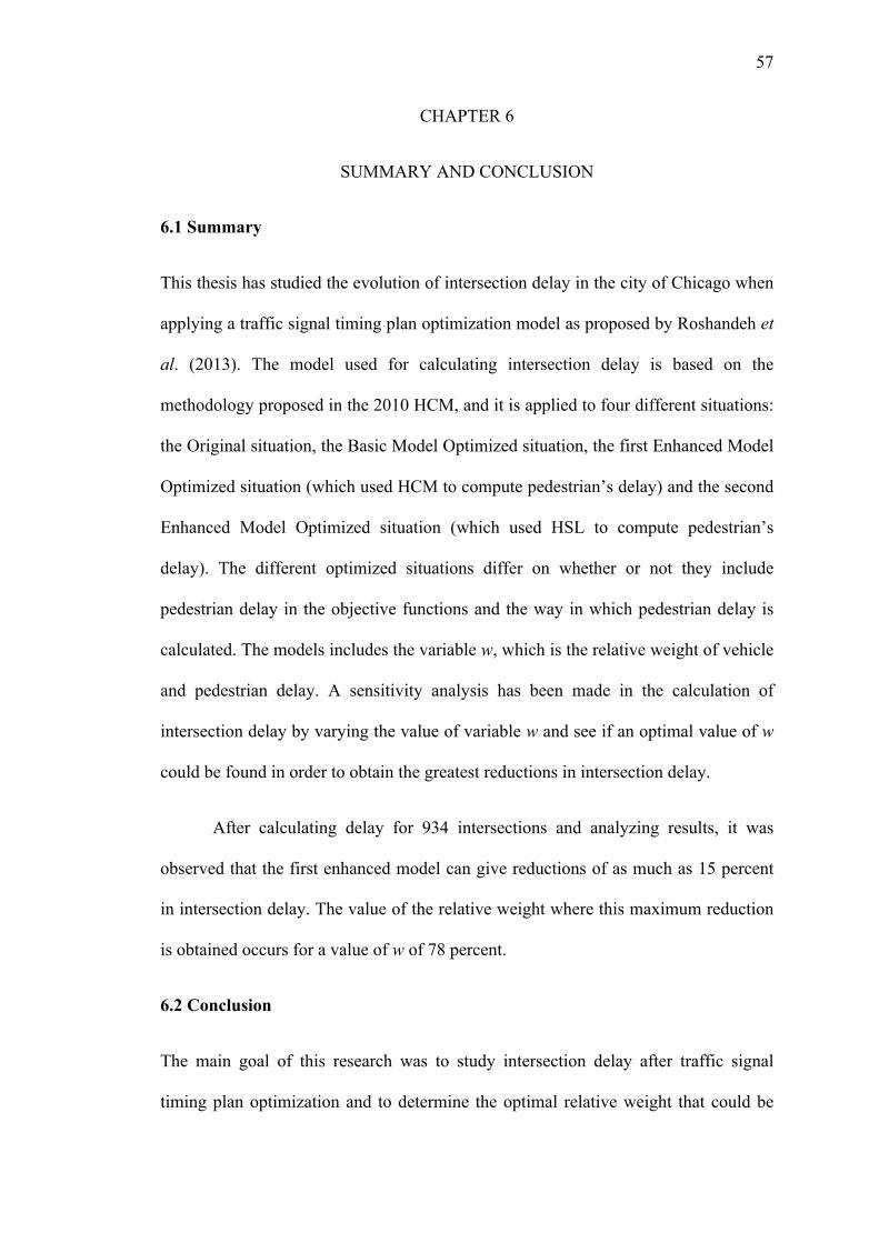
57

CHAPTER 6

SUMMARY AND CONCLUSION

6.1 Summary

This thesis has studied the evolution of intersection delay in the city of Chicago when

applying a traffic signal timing plan optimization model as proposed by Roshandeh et

al. (2013). The model used for calculating intersection delay is based on the

methodology proposed in the 2010 HCM, and it is applied to four different situations:

the Original situation, the Basic Model Optimized situation, the first Enhanced Model

Optimized situation (which used HCM to compute pedestrian’s delay) and the second

Enhanced Model Optimized situation (which used HSL to compute pedestrian’s

delay). The different optimized situations differ on whether or not they include

pedestrian delay in the objective functions and the way in which pedestrian delay is

calculated. The models includes the variable w, which is the relative weight of vehicle

and pedestrian delay. A sensitivity analysis has been made in the calculation of

intersection delay by varying the value of variable w and see if an optimal value of w

could be found in order to obtain the greatest reductions in intersection delay.

After calculating delay for 934 intersections and analyzing results, it was

observed that the first enhanced model can give reductions of as much as 15 percent

in intersection delay. The value of the relative weight where this maximum reduction

is obtained occurs for a value of w of 78 percent.

6.2 Conclusion

The main goal of this research was to study intersection delay after traffic signal

timing plan optimization and to determine the optimal relative weight that could be

! ! !!

! !

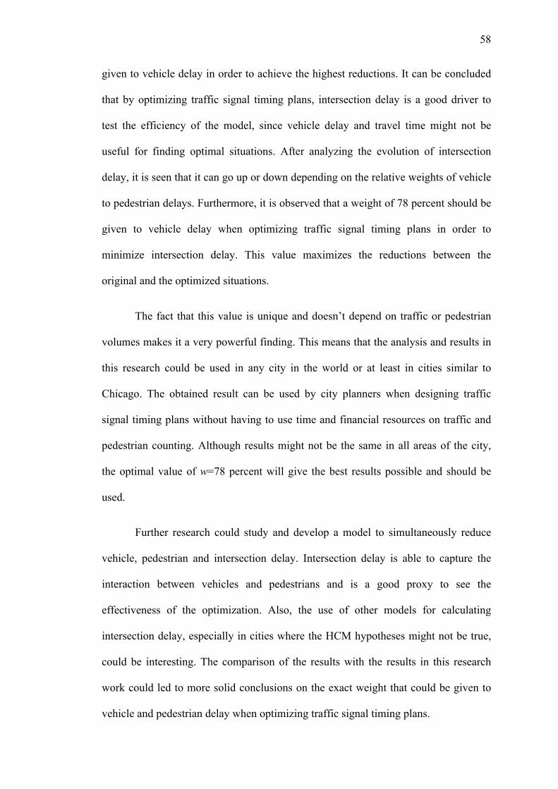
58

given to vehicle delay in order to achieve the highest reductions. It can be concluded

that by optimizing traffic signal timing plans, intersection delay is a good driver to

test the efficiency of the model, since vehicle delay and travel time might not be

useful for finding optimal situations. After analyzing the evolution of intersection

delay, it is seen that it can go up or down depending on the relative weights of vehicle

to pedestrian delays. Furthermore, it is observed that a weight of 78 percent should be

given to vehicle delay when optimizing traffic signal timing plans in order to

minimize intersection delay. This value maximizes the reductions between the

original and the optimized situations.

The fact that this value is unique and doesn’t depend on traffic or pedestrian

volumes makes it a very powerful finding. This means that the analysis and results in

this research could be used in any city in the world or at least in cities similar to

Chicago. The obtained result can be used by city planners when designing traffic

signal timing plans without having to use time and financial resources on traffic and

pedestrian counting. Although results might not be the same in all areas of the city,

the optimal value of w=78 percent will give the best results possible and should be

used.

Further research could study and develop a model to simultaneously reduce

vehicle, pedestrian and intersection delay. Intersection delay is able to capture the

interaction between vehicles and pedestrians and is a good proxy to see the

effectiveness of the optimization. Also, the use of other models for calculating

intersection delay, especially in cities where the HCM hypotheses might not be true,

could be interesting. The comparison of the results with the results in this research

work could led to more solid conclusions on the exact weight that could be given to

vehicle and pedestrian delay when optimizing traffic signal timing plans.

! ! !!

! !

59

! ! !!

! !

60

REFERENCES

Aashtiani H.Z., H. Iravani (1999). Use of intersection delay functions to improve

reliability of traffic assignment models. Proceedings of the 14th Annual International

EMME/2 Conference, Chicago, Illinois. 20-28.

Fambro D.B., N.M. Rouphail (2007). Generalized delay model for signalized

intersections and arterial streets. Transportation Research Record: Journal of the

Transportation Research Board, 1572, 112-121.

INRO (1994). EMME/2 User’s Manual, Software Release 7. INRO Consultant,

Montreal, Canada.

Koutsopoulos H.N., M. Habbal (1994). Effect of intersection delay modeling on the

performance of traffic equilibrium models. Transportation Research Part A, 28(2),

133-149.

Li, Z., N. Li, F. Liu (2009). An effective calculating method of signalized intersection

delay. International Conference on Digital Image Processing 2009. 211-215.

Liu, G.P., R.P. Zhai, Y.L. Pei (2007). A calculating method of intersection delay

under signal control. Intelligent Transportation Systems Conference, 2007. ISTC 2007,

IEEE, 648-653.

Lowrie, P.R. (1982). The Sydney co-ordinated adaptive traffic system- principles,

methodology, algorithms. Proceeding of the International Conference on Road

Traffic Signaling, 67-80.

! ! !!

! !

61

Mazloumi, E., S. Moridpour, H. Mohsenian (2010). Delay function for signalized

intersections in traffic assignment models. Journal of Urban Planning and

Development, 136(1), 67-74.

Qiao F., P. Yi, H. Yang, S. Devarakonda (2002). Fuzzy logic based intersection delay

estimation. Mathematical and Computer Modelling, 36(11-13), 1425-1434.

Quiroga C.A., D. Bullock (1999) Measuring control delay at signalized intersections.

Journal of Transportation Engineering, 125(4), 271-280.

Roshandeh, A.M., H.S. Levinson, Z. Li, B. Zhou (2013). A new methodology for

intersection signal timing optimization to simultaneously minimize vehicle and

pedestrian delays. ASCE Journal of Transportation Engineering. (In Press).

TRB. (2010). 2010 Highway Capacity Manual. Transportation Research Board,

National Academic Press Washington, D.C.

Webster F.V. (1958). Traffic Signal Settings. Road Research Laboratory, Crowthorne.

United Kingdom.

Wolshon, B., W.C. Taylor (1999). Analysis of intersection delay under real-time

adaptive signal control. Transportation Research Part C, 7(1), 53-72.

Zhu, Z., W. Liu, L. Liu, M. Cui, J. Li (2011). A simplified real-time road network

model considering intersection delay and its application on vehicle navigation.

Applied Mechanics and Materials, 58-60, 1959-1965.

! ! !!

! !

62

APPENDIX A

REDUCTIONS ON INTERSECTION VEHICLE DELAY FOR EACH AREA

USING THE BASIC MODEL

! ! !!

! !

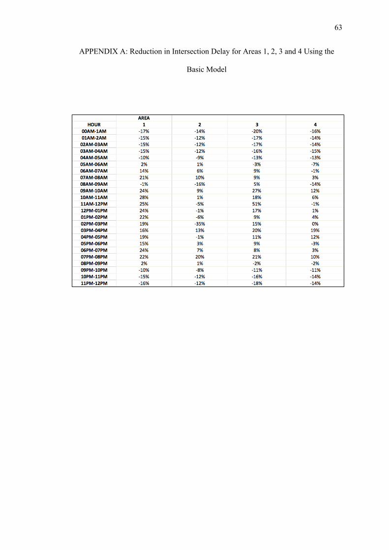
63

APPENDIX A: Reduction in Intersection Delay for Areas 1, 2, 3 and 4 Using the

Basic Model

! ! !!

! !

64

APPENDIX B

REDUCTIONS ON INTERSECTION VEHICLE AND PEDESTRIAN DELAY FOR

EACH AREA USING THE FIRST ENHANCED MODEL WITH PEDESTRIAN

DELAY CALCULATED USING THE HCM METHOD

! ! !!

! !

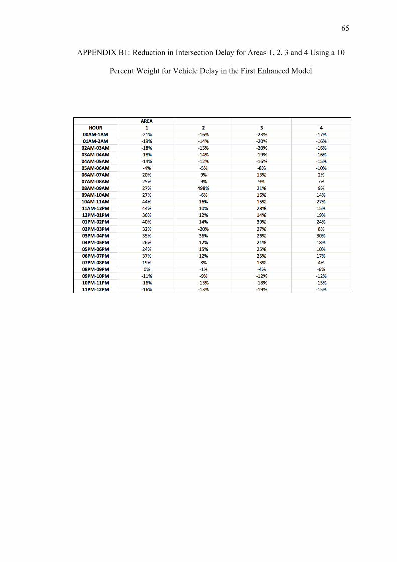
65

APPENDIX B1: Reduction in Intersection Delay for Areas 1, 2, 3 and 4 Using a 10

Percent Weight for Vehicle Delay in the First Enhanced Model

! ! !!

! !

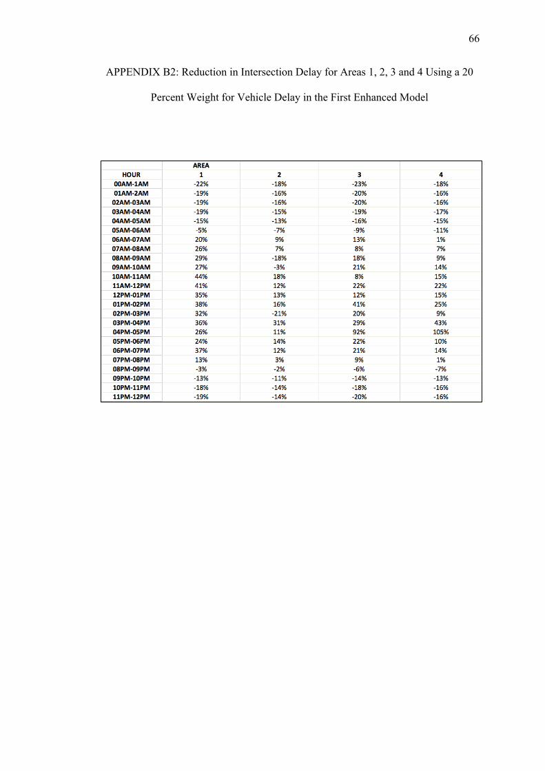
66

APPENDIX B2: Reduction in Intersection Delay for Areas 1, 2, 3 and 4 Using a 20

Percent Weight for Vehicle Delay in the First Enhanced Model

! ! !!

! !

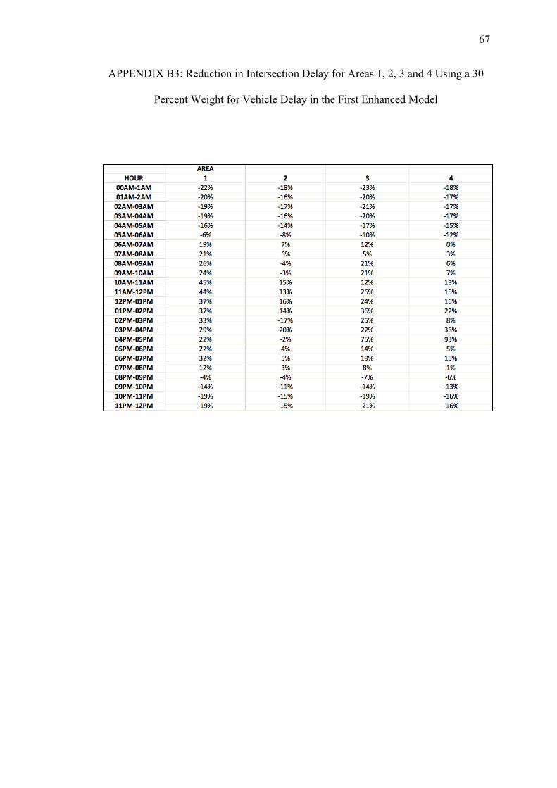
67

APPENDIX B3: Reduction in Intersection Delay for Areas 1, 2, 3 and 4 Using a 30

Percent Weight for Vehicle Delay in the First Enhanced Model

! ! !!

! !

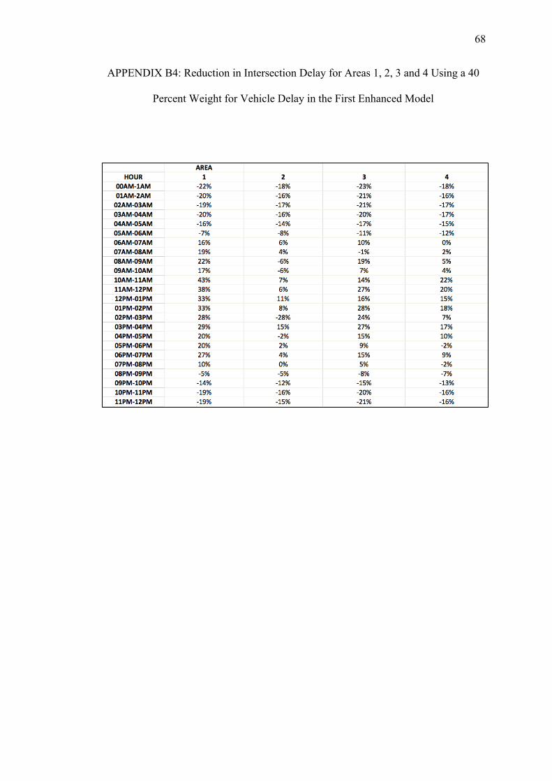
68

APPENDIX B4: Reduction in Intersection Delay for Areas 1, 2, 3 and 4 Using a 40

Percent Weight for Vehicle Delay in the First Enhanced Model

! ! !!

! !

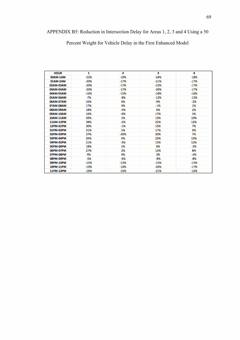
69

APPENDIX B5: Reduction in Intersection Delay for Areas 1, 2, 3 and 4 Using a 50

Percent Weight for Vehicle Delay in the First Enhanced Model

! ! !!

! !

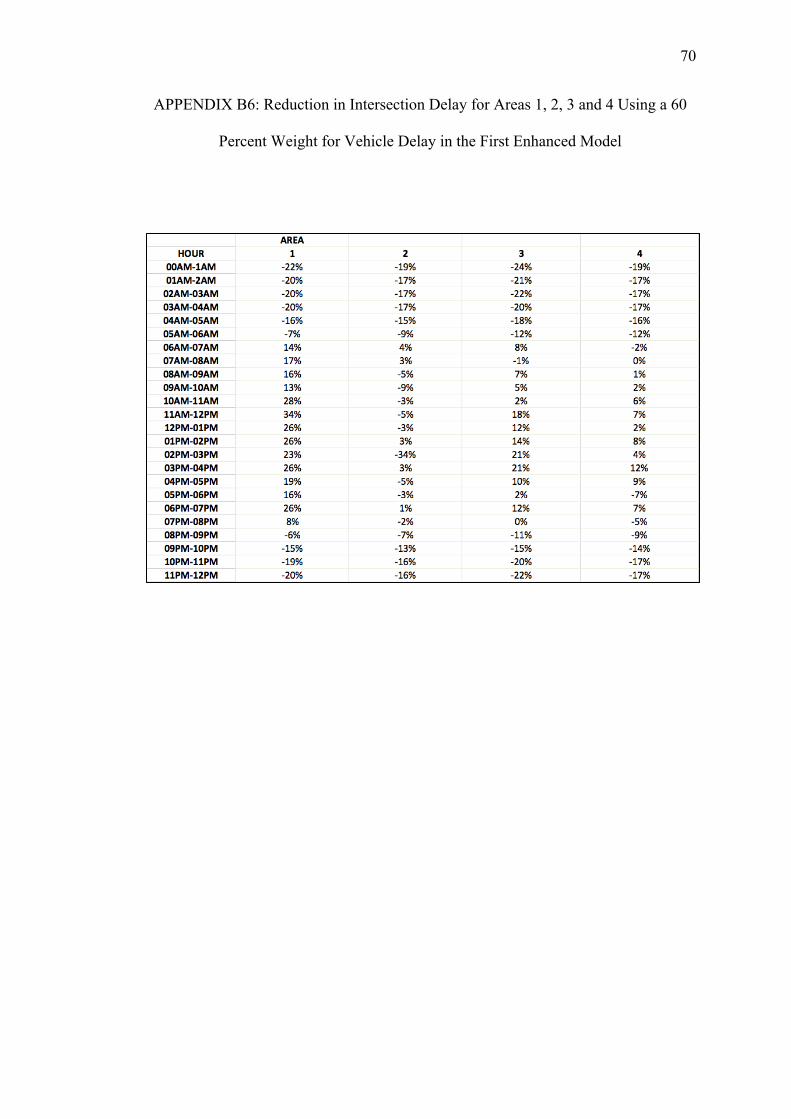
70

APPENDIX B6: Reduction in Intersection Delay for Areas 1, 2, 3 and 4 Using a 60

Percent Weight for Vehicle Delay in the First Enhanced Model

! ! !!

! !

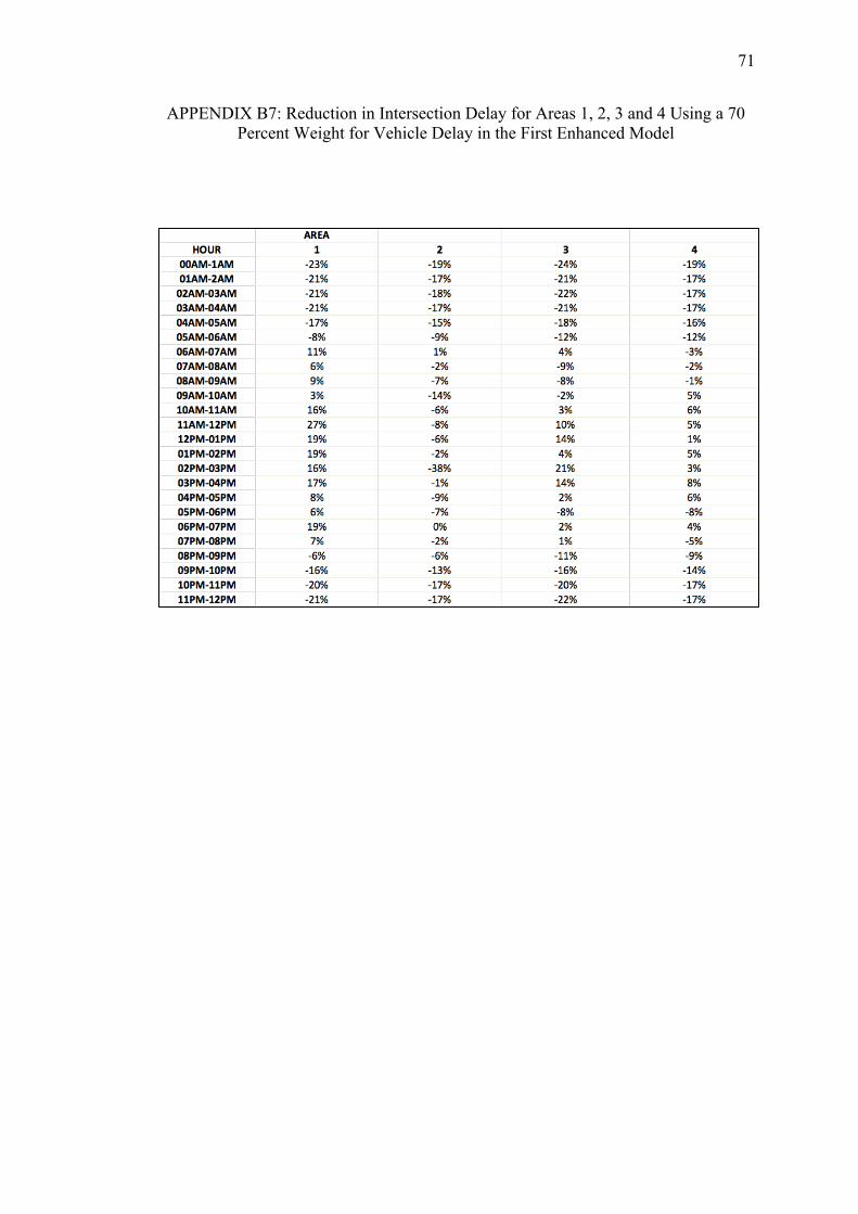
71

APPENDIX B7: Reduction in Intersection Delay for Areas 1, 2, 3 and 4 Using a 70 Percent Weight for Vehicle Delay in the First Enhanced Model

! ! !!

! !

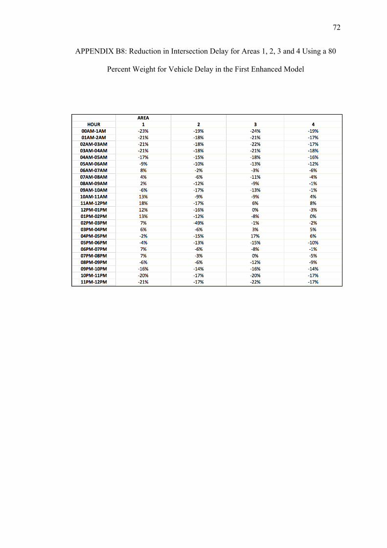
72

APPENDIX B8: Reduction in Intersection Delay for Areas 1, 2, 3 and 4 Using a 80

Percent Weight for Vehicle Delay in the First Enhanced Model

! ! !!

! !

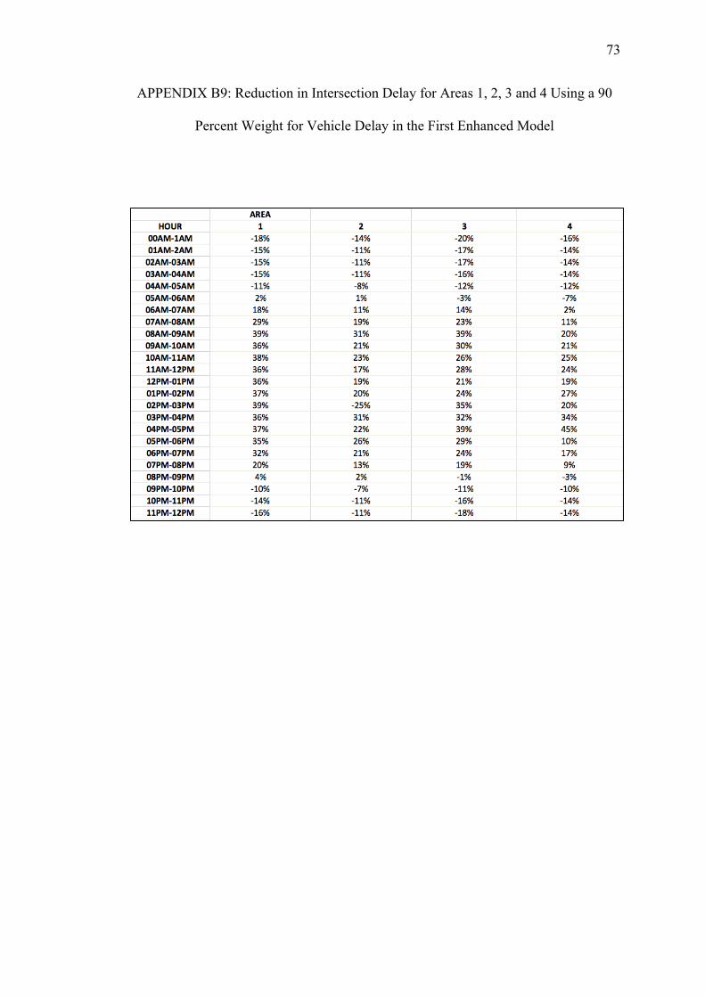
73

APPENDIX B9: Reduction in Intersection Delay for Areas 1, 2, 3 and 4 Using a 90

Percent Weight for Vehicle Delay in the First Enhanced Model

! ! !!

! !

74

APPENDIX C

REDUCTIONS IN INTERSECTION VEHICLE AND PEDESTRIAN DELAY FOR

EACH AREA USING THE SECOND ENHANCED MODEL WITH PEDESTRIAN

DELAY ESTIMATED USING THE HSL METHOD

! ! !!

! !

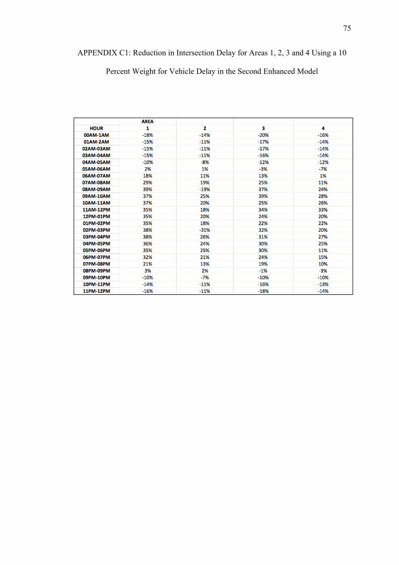
75

APPENDIX C1: Reduction in Intersection Delay for Areas 1, 2, 3 and 4 Using a 10

Percent Weight for Vehicle Delay in the Second Enhanced Model

! ! !!

! !

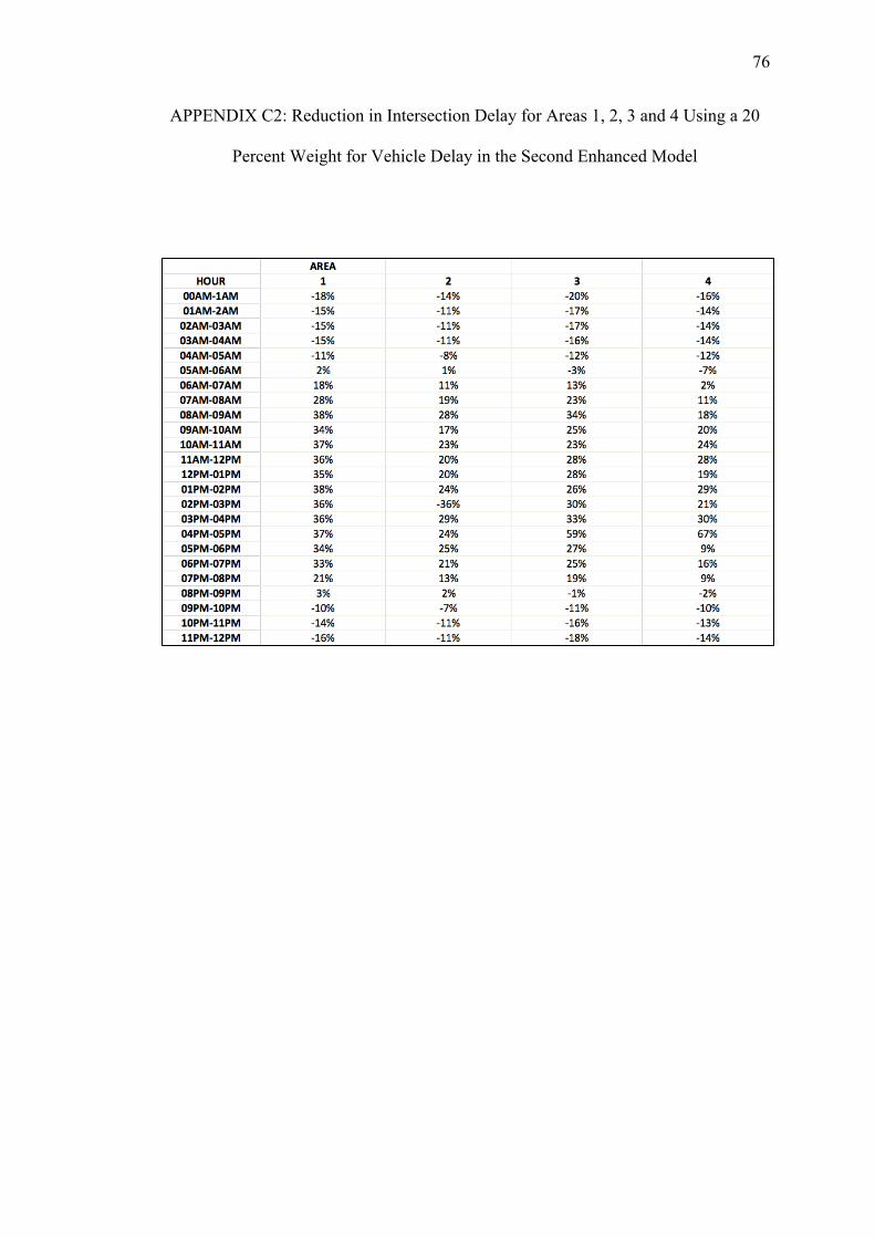
76

APPENDIX C2: Reduction in Intersection Delay for Areas 1, 2, 3 and 4 Using a 20

Percent Weight for Vehicle Delay in the Second Enhanced Model

! ! !!

! !

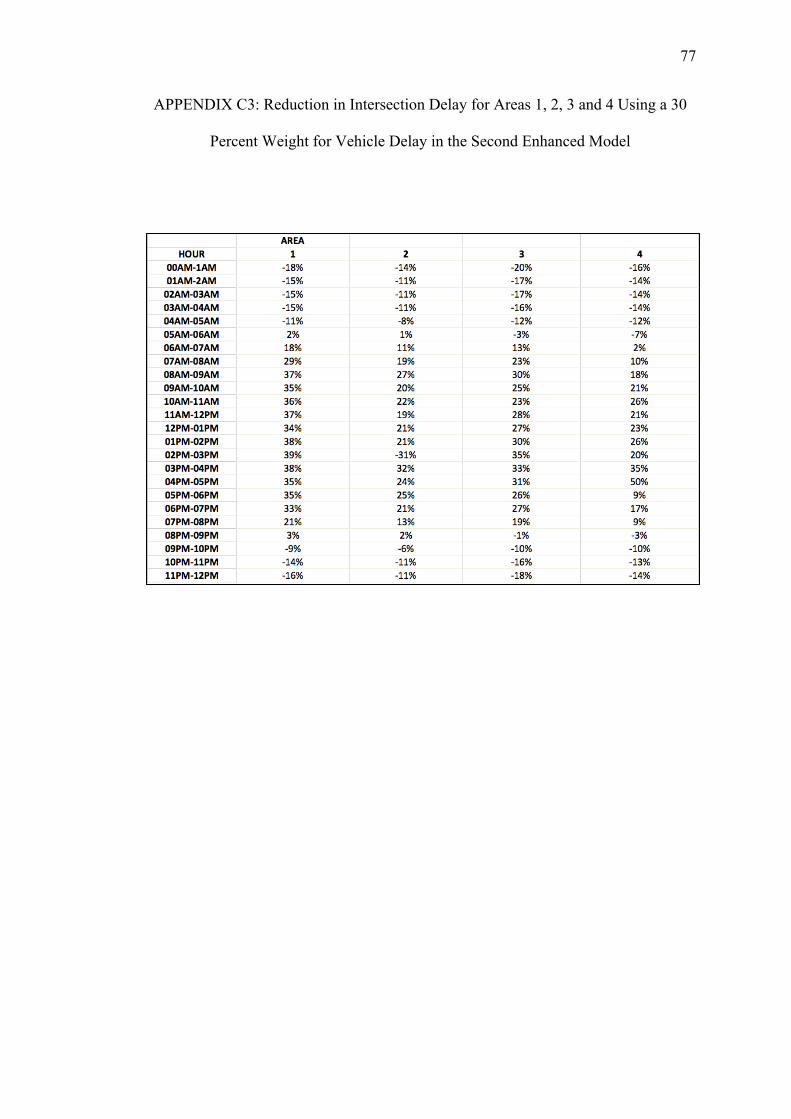
77

APPENDIX C3: Reduction in Intersection Delay for Areas 1, 2, 3 and 4 Using a 30

Percent Weight for Vehicle Delay in the Second Enhanced Model

! ! !!

! !

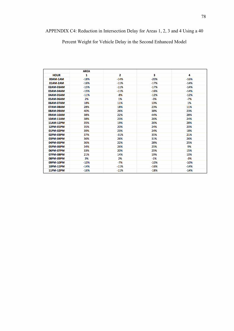
78

APPENDIX C4: Reduction in Intersection Delay for Areas 1, 2, 3 and 4 Using a 40

Percent Weight for Vehicle Delay in the Second Enhanced Model

! ! !!

! !

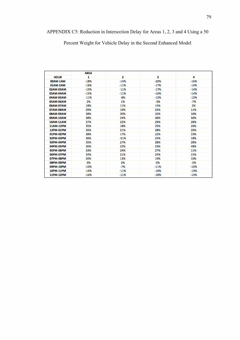
79

APPENDIX C5: Reduction in Intersection Delay for Areas 1, 2, 3 and 4 Using a 50

Percent Weight for Vehicle Delay in the Second Enhanced Model

! ! !!

! !

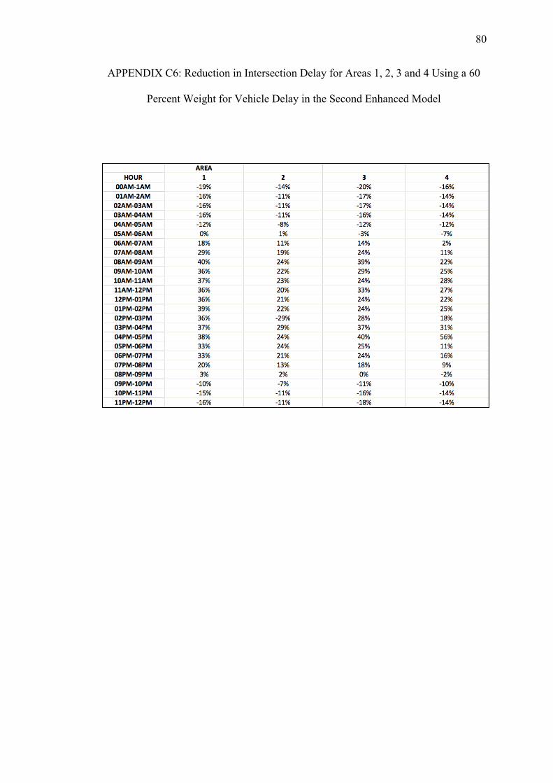
80

APPENDIX C6: Reduction in Intersection Delay for Areas 1, 2, 3 and 4 Using a 60

Percent Weight for Vehicle Delay in the Second Enhanced Model

! ! !!

! !

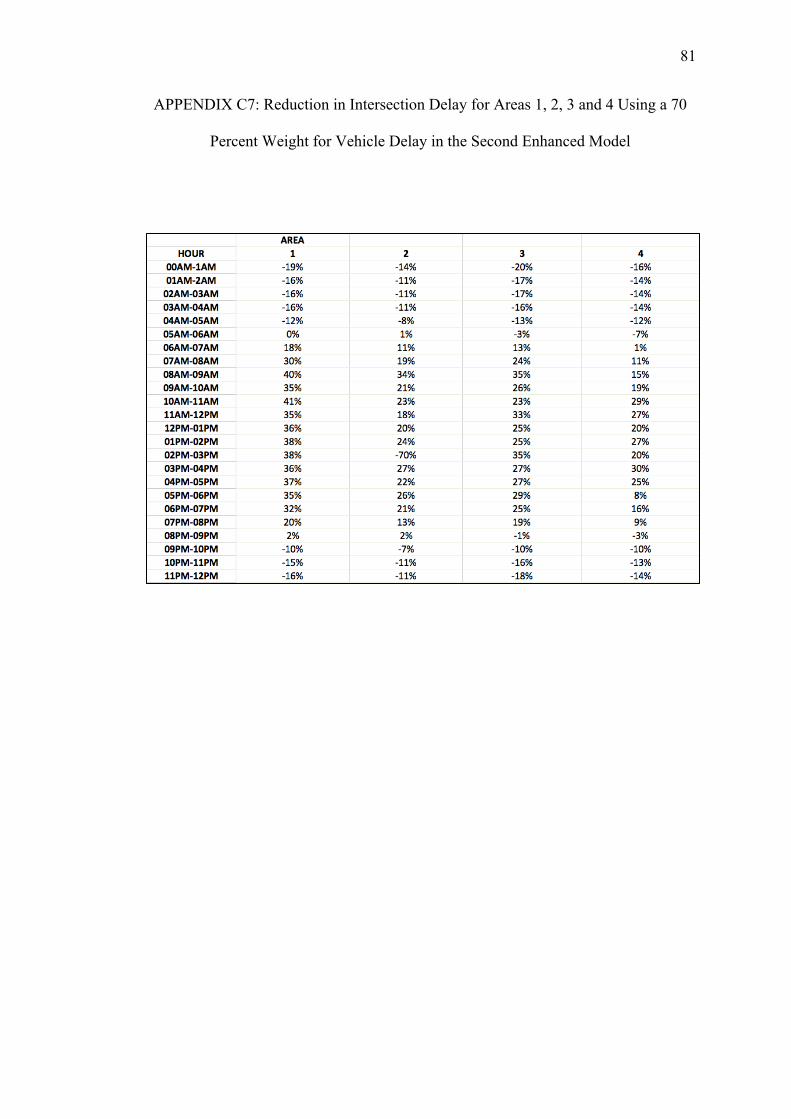
81

APPENDIX C7: Reduction in Intersection Delay for Areas 1, 2, 3 and 4 Using a 70

Percent Weight for Vehicle Delay in the Second Enhanced Model

! ! !!

! !

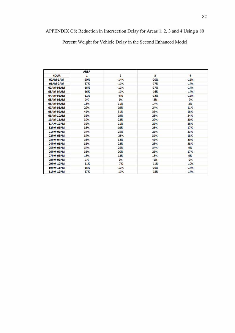
82

APPENDIX C8: Reduction in Intersection Delay for Areas 1, 2, 3 and 4 Using a 80

Percent Weight for Vehicle Delay in the Second Enhanced Model

! ! !!

! !

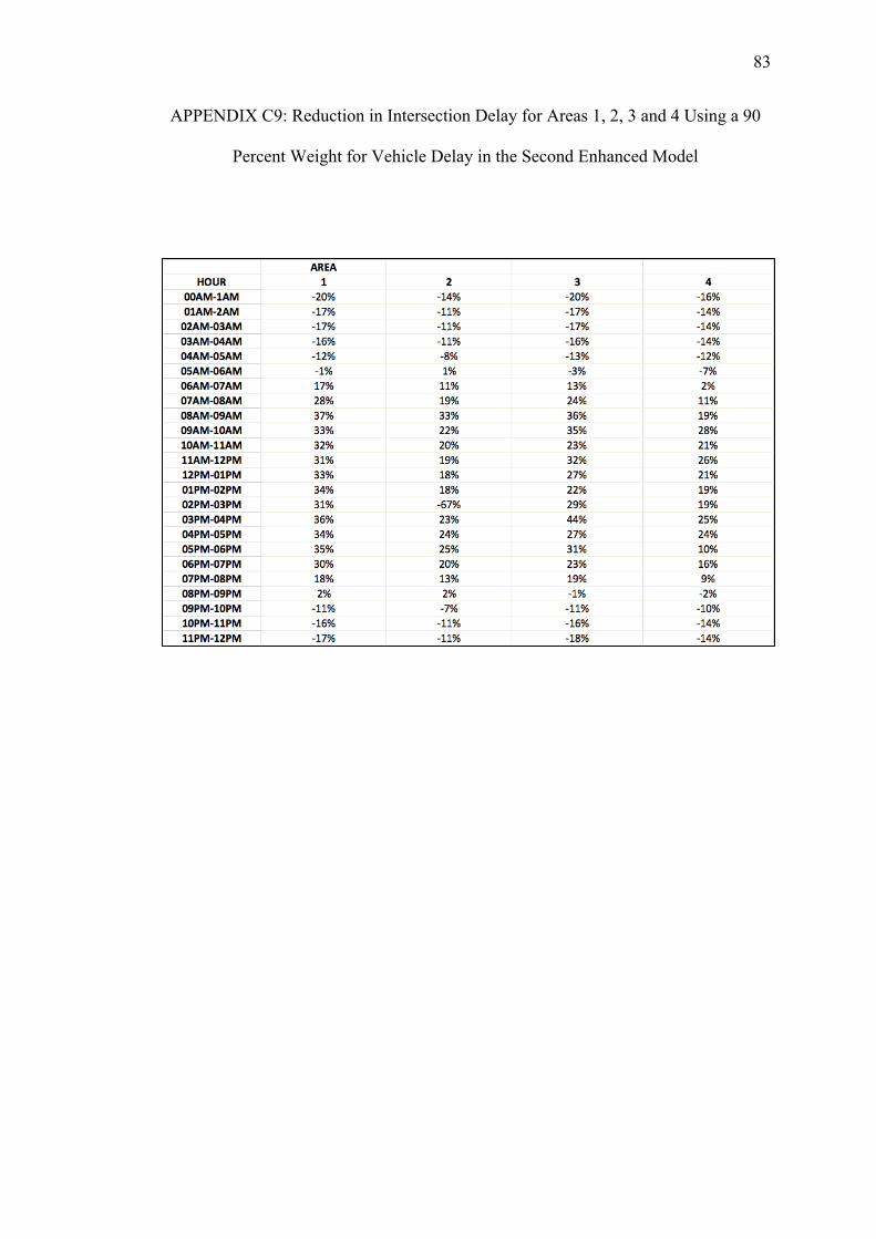
83

APPENDIX C9: Reduction in Intersection Delay for Areas 1, 2, 3 and 4 Using a 90

Percent Weight for Vehicle Delay in the Second Enhanced Model

! ! !!

! !

84

APPENDIX D

MATLAB CODE FOR CALCULATING INTERSECTION DELAY

! ! !!

! !

85

%Program to calculate d1 and d2 %%%THIS IS ONLY FOR ONE HOUR!! BNodeLink=xlsread('BeforeBasic_info','BNodeLink'); numnode=size(BNodeLink); n=numnode(1); %number of nodes q=numnode(2); %number of columns in the node-link column (not the same as number of links since some are empty) numlink=zeros(n,1); CycleLength=xlsread('BeforeBasic_info','CycleLength'); %reads CycleLength sheet and gets node+cyclelenght CycleLength=CycleLength(:,2); %Column vector for cycle lenghts VolumeAB=xlsread('BeforeBasic_Vol','Vol2324'); %%reads VolumeAB sheet and gets node+volume %CHANGE VolumeAB=VolumeAB(1:n,2:q); %deletes node column VolumeNode=(sum(VolumeAB'))'; %column vector for the total in_link volume in each node CapacityAB=xlsread('BeforeBasic_info','CapacityAB'); %%reads CapacityAB sheet and gets node+volume CapacityAB=CapacityAB(1:n,2:q); %deletes node column LaneThru=xlsread('BeforeBasic_info','LaneThru'); %%reads LaneThru sheet and gets node+volume LaneThru=LaneThru(1:n,2:q); %deletes node column LaneLeft=xlsread('BeforeBasic_info','LaneLeft'); %%reads LaneLeft sheet and gets node+volume LaneLeft=LaneLeft(1:n,2:q); %deletes node column LaneRight=xlsread('BeforeBasic_info','LaneRight'); %%reads LaneRight sheet and gets node+volume LaneRight=LaneRight(1:n,2:q); %deletes node column LaneTotal=LaneThru+LaneLeft+LaneRight; %total number of lanes in the approach GreenThru=xlsread('BeforeBasic_info','GreenThru'); %%reads GreenThru sheet and gets node+volume GreenThru=GreenThru(1:n,2:q); %deletes node column GreenLeft=xlsread('BeforeBasic_info','GreenLeft'); %%reads GreenLeft sheet and gets node+volume GreenLeft=GreenLeft(1:n,2:q); %deletes node column GreenRight=xlsread('BeforeBasic_info','GreenRight'); %%reads GreenRight sheet and gets node+volume GreenRight=GreenRight(1:n,2:q); %deletes node column X=zeros(n,q-1); d1thru=zeros(n,q-1); d2thru=zeros(n,q-1); d1left=zeros(n,q-1); d1right=zeros(n,q-1); d1app=zeros(n,q-1); d1nodeprev=zeros(n,q-1); d2nodeprev=zeros(n,q-1); for i=1:n for j=2:q if BNodeLink(i,j)>0 %if the column contains a link, count numlink(i,1)=numlink(i,1)+1; else numlink(i,1)=numlink(i,1); %if it doesnt contain a link, don't count end %numlink is a column vector containg the number of links in each node end for k=1:numlink(i) X(i,k)=VolumeAB(i,k)./CapacityAB(i,k); %matrix containing x for each link and each node T=1; % time of observation 1 hour

! ! !!

! !

86

K=0.5; % pretimed signals I=1; % we consider each intersection as isolated %%%D1 and D2 CALCULATION if LaneThru(i,k)>0 %will calculate dthru if there are thru lanes only d1thru(i,k)=(0.5.*CycleLength(i,1).*(1-GreenThru(i,k)/CycleLength(i,1)).^2)/(1-(min(1,X(i,k))).*(GreenThru(i,k)./CycleLength(i,1))); d2thru(i,k)=900.*T.*((X(i,k)-1)+((X(i,k)-1).^2+(8.*K.*I.*X(i,k)./(CycleLength(i,1).*T)))^(1/2)); else d1thru(i,k)=0; end if LaneLeft(i,k)>0 %will calculate dleft if there are left lanes only d1left(i,k)=(0.5.*CycleLength(i,1).*(1-GreenLeft(i,k)/CycleLength(i,1)).^2)/(1-(min(1,X(i,k))).*(GreenLeft(i,k)./CycleLength(i,1))); else d1left(i,k)=0; end if LaneRight(i,k)>0 %will calculate dthru if there are right lanes only d1right(i,k)=(0.5.*CycleLength(i,1).*(1-GreenRight(i,k)/CycleLength(i,1)).^2)/(1-(min(1,X(i,k))).*(GreenRight(i,k)./CycleLength(i,1))); else d1right(i,k)=0; end d2left=d2thru; d2right=d2thru; % We now calculate average delay at the approach weighting by % number of lanes (because we suppose equal distribution of traffic % per lane d1app(i,k)=d1thru(i,k).*(LaneThru(i,k)./LaneTotal(i,k))+d1left(i,k).*(LaneLeft(i,k)./LaneTotal(i,k))+d1right(i,k).*(LaneRight(i,k)./LaneTotal(i,k)); d2app=d2thru; %Now we calculate delay for the intersection weighting by traffic %volume in each approach d1nodeprev(i,k)=d1app(i,k).*VolumeAB(i,k)./VolumeNode(i,1); d2nodeprev(i,k)=d2app(i,k).*VolumeAB(i,k)./VolumeNode(i,1); end end d1node=(sum(d1nodeprev'))'; d2node=(sum(d2nodeprev'))'; %%Program to calculate d3 %%%THIS IS ONLY FOR ONE HOUR!! BNodeLink=xlsread('BeforeBasic_info','BNodeLink'); numnode=size(BNodeLink); n=numnode(1); %number of nodes q=numnode(2); %number of columns in the node-link column (not the same as number of links since some are empty) numlink=zeros(n,1);

! ! !!

! !

87

CapacityAB=xlsread('BeforeBasic_info','CapacityAB'); %%reads CapacityAB sheet and gets node+volume CapacityAB=CapacityAB(1:n,2:q); %deletes node column VolumeAB1=xlsread('BeforeBasic_Vol','Vol0001'); VolumeAB1=VolumeAB1(1:n,2:q); %deletes node column VolumeAB2=xlsread('BeforeBasic_Vol','Vol0102'); VolumeAB2=VolumeAB2(1:n,2:q); %deletes node column VolumeAB3=xlsread('BeforeBasic_Vol','Vol0203'); VolumeAB3=VolumeAB3(1:n,2:q); %deletes node column VolumeAB4=xlsread('BeforeBasic_Vol','Vol0304'); VolumeAB4=VolumeAB4(1:n,2:q); %deletes node column VolumeAB5=xlsread('BeforeBasic_Vol','Vol0405'); VolumeAB5=VolumeAB5(1:n,2:q); %deletes node column VolumeAB6=xlsread('BeforeBasic_Vol','Vol0506'); VolumeAB6=VolumeAB6(1:n,2:q); %deletes node column VolumeAB7=xlsread('BeforeBasic_Vol','Vol0607'); VolumeAB7=VolumeAB7(1:n,2:q); %deletes node column VolumeAB8=xlsread('BeforeBasic_Vol','Vol0708'); VolumeAB8=VolumeAB8(1:n,2:q); %deletes node column VolumeAB9=xlsread('BeforeBasic_Vol','Vol0809'); VolumeAB9=VolumeAB9(1:n,2:q); %deletes node column VolumeAB10=xlsread('BeforeBasic_Vol','Vol0910'); VolumeAB10=VolumeAB10(1:n,2:q); %deletes node column VolumeAB11=xlsread('BeforeBasic_Vol','Vol1011'); VolumeAB11=VolumeAB11(1:n,2:q); %deletes node column VolumeAB12=xlsread('BeforeBasic_Vol','Vol1112'); VolumeAB12=VolumeAB12(1:n,2:q); %deletes node column VolumeAB13=xlsread('BeforeBasic_Vol','Vol1213'); VolumeAB13=VolumeAB13(1:n,2:q); %deletes node column VolumeAB14=xlsread('BeforeBasic_Vol','Vol1314'); VolumeAB14=VolumeAB14(1:n,2:q); %deletes node column VolumeAB15=xlsread('BeforeBasic_Vol','Vol1415'); VolumeAB15=VolumeAB15(1:n,2:q); %deletes node column VolumeAB16=xlsread('BeforeBasic_Vol','Vol1516'); VolumeAB16=VolumeAB16(1:n,2:q); %deletes node column VolumeAB17=xlsread('BeforeBasic_Vol','Vol1617'); VolumeAB17=VolumeAB17(1:n,2:q); %deletes node column VolumeAB18=xlsread('BeforeBasic_Vol','Vol1718'); VolumeAB18=VolumeAB18(1:n,2:q); %deletes node column VolumeAB19=xlsread('BeforeBasic_Vol','Vol1819'); VolumeAB19=VolumeAB19(1:n,2:q); %deletes node column VolumeAB20=xlsread('BeforeBasic_Vol','Vol1920'); VolumeAB20=VolumeAB20(1:n,2:q); %deletes node column VolumeAB21=xlsread('BeforeBasic_Vol','Vol2021'); VolumeAB21=VolumeAB21(1:n,2:q); %deletes node column VolumeAB22=xlsread('BeforeBasic_Vol','Vol2122'); VolumeAB22=VolumeAB22(1:n,2:q); %deletes node column VolumeAB23=xlsread('BeforeBasic_Vol','Vol2223'); VolumeAB23=VolumeAB23(1:n,2:q); %deletes node column VolumeAB24=xlsread('BeforeBasic_Vol','Vol2324'); VolumeAB24=VolumeAB24(1:n,2:q); %deletes node column Qb1=zeros(n,q-1);Qb2=zeros(n,q-1); Qeo1=zeros(n,q-1);Qeo2=zeros(n,q-1); ta1=zeros(n,q-1);ta2=zeros(n,q-1); Qe1=zeros(n,q-1);Qe2=zeros(n,q-1); T=1; %This is t and T and is one hour (duration of the analysis and time where volume is constant) t=ones(n,q-1); d3nodeprev=zeros(n,q-1); for i=1:n

! ! !!

! !

88

for j=2:q if BNodeLink(i,j)>0 %if the column contains a link, count numlink(i,1)=numlink(i,1)+1; else numlink(i,1)=numlink(i,1); %if it doesnt contain a link, don't count end %numlink is a column vector containg the number of links in each node end for k=1:numlink(i) Qb2(i,k)=max(Qb1(i,k)-(CapacityAB(i,k)-VolumeAB24(i,k)).*T,0); %CHANGE if VolumeAB24(i,k)>CapacityAB(i,k) %CHANGE ta2(i,k)=t(i,k); Qeo2(i,k)=ta2(i,k).*(VolumeAB24(i,k)-CapacityAB(i,k)); %CHANGE else ta2(i,k)=Qb2(i,k)./(CapacityAB(i,k)-VolumeAB24(i,k)); %CHANGE end Qe2(i,k)=Qb2(i,k)+ta2(i,k).*(VolumeAB24(i,k)-CapacityAB(i,k)); %CHANGE d3nodeprev(i,k)=(3600/VolumeAB24(i,k).*T).*((ta2(i,k)./2).*(Qb2(i,k)+Qe2(i,k)-Qeo2(i,k))+(Qe2(i,k).^2-Qeo2(i,k).^2)./(2.*CapacityAB(i,k))-(Qb2(i,k).^2)./(2.*CapacityAB(i,k))); end end d3node=(sum(d3nodeprev'))'; dnode=d1node+d2node+d3node