Embed Size (px)
Citation preview

Effective medium approach to nanostructures
strengths and weaknesses
Josef Humlíček, CEITEC, Masaryk University
Brno, Czech Republic
EPIOPTICS-15, Erice, July 2018
1
Outline:
• Linear optical response: bulk and nanostructured materials
• Average fields and effective permittivity for small contrast
3D, 2D and 1D systems
• Established mixing rules
• Tests of EMA:
macroscopic scale (glass spheres in liquids)
molecular scale (water solutions of sucrose)
• Differences between mixing rules for binary dielectric mixtures
• EMA and exact solutions for layered structures
• Resonant behavior of EMA mixtures.
2
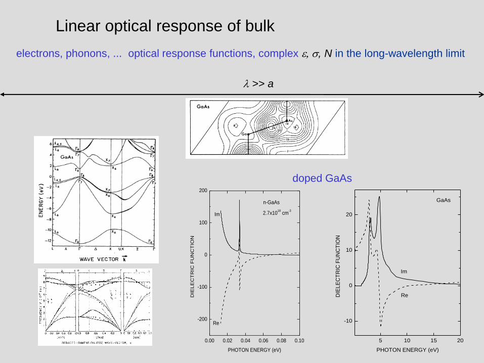
Linear optical response of bulk
electrons, phonons, ... optical response functions, complex e, s, N in the long-wavelength limit
doped GaAs
0.00 0.02 0.04 0.06 0.08 0.10
-200
-100
0
100
200
2.7x10¹⁸
cm-3
Im
Re
n-GaAs
DIE
LE
CT
RIC
FU
NC
TIO
N
PHOTON ENERGY (eV)
5 10 15 20
-10
0
10
20
Im
Re
GaAs
DIE
LE
CT
RIC
FU
NC
TIO
N
PHOTON ENERGY (eV)
l >> a
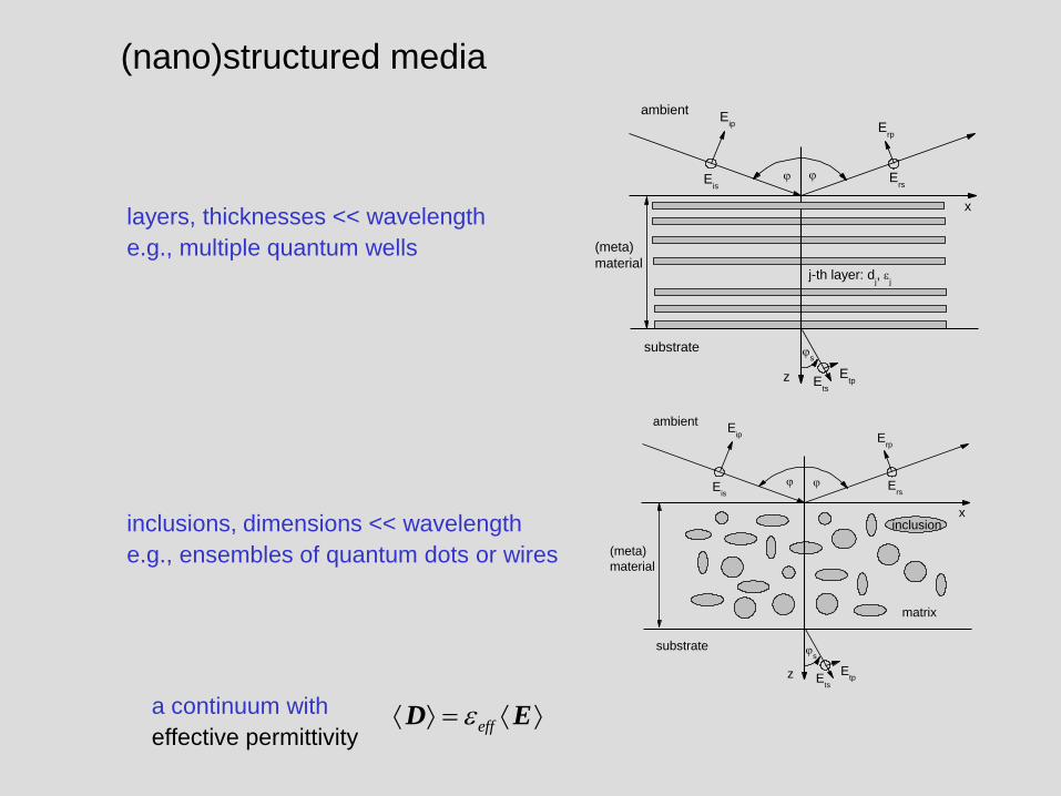
(nano)structured media
layers, thicknesses << wavelength
e.g., multiple quantum wells
j-th layer: dj, e
j
substrate
Ets
Etp
Ers
Erp
Eis
Eip
s
(meta)
material
ambient
z
x
effe D Ea continuum with
effective permittivity
matrix
substrate
Ets
Etp
Ers
Erp
Eis
Eip
s
(meta)
material
ambient
z
xinclusioninclusions, dimensions << wavelength
e.g., ensembles of quantum dots or wires
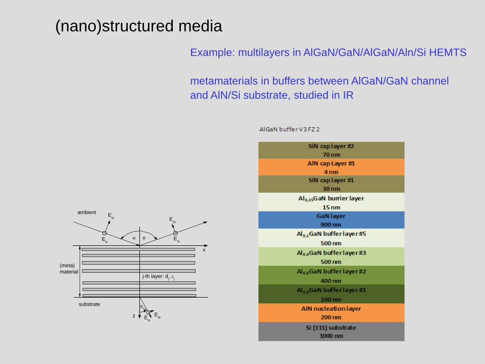
(nano)structured media
Example: multilayers in AlGaN/GaN/AlGaN/Aln/Si HEMTS
metamaterials in buffers between AlGaN/GaN channel
and AlN/Si substrate, studied in IR
j-th layer: dj, e
j
substrate
Ets
Etp
Ers
Erp
Eis
Eip
s
(meta)
material
ambient
z
x
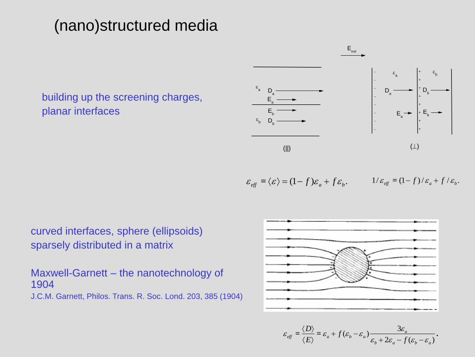
(nano)structured media
building up the screening charges,
planar interfaces
()
EbE
a
Db
Da
-
-
-
-
-
-
-
-
ebe
a
Db
Ea
eb
Eext
ea D
a
Eb
+
+
+
+
+
+
+
+
(||)
curved interfaces, sphere (ellipsoids)
sparsely distributed in a matrix
Maxwell-Garnett – the nanotechnology of 1904 J.C.M. Garnett, Philos. Trans. R. Soc. Lond. 203, 385 (1904)
(1 ) .eff a bf fe e e e = 1/ (1 ) / / .eff a bf fe e e =
3( )
2 ( )
aeff a b a
b a b a
Df
E f
ee e e e
e e e e
= = .
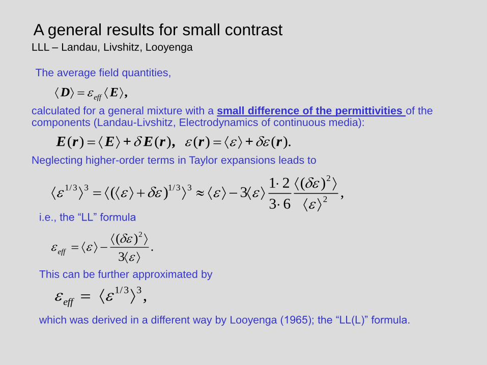
A general results for small contrast LLL – Landau, Livshitz, Looyenga
The average field quantities,
calculated for a general mixture with a small difference of the permittivities of the components (Landau-Livshitz, Electrodynamics of continuous media):
effe D E ,
( ) ( ) ( ) ( ). e e e E r E + E r , r + r
Neglecting higher-order terms in Taylor expansions leads to
21/3 3 1/3 3
2
1 2 ( )( ) 3 ,
3 6
ee e e e e
e
i.e., the “LL” formula
1/3 3 ,effe e
which was derived in a different way by Looyenga (1965); the “LL(L)” formula.
2( ).
3eff
ee e
e
This can be further approximated by
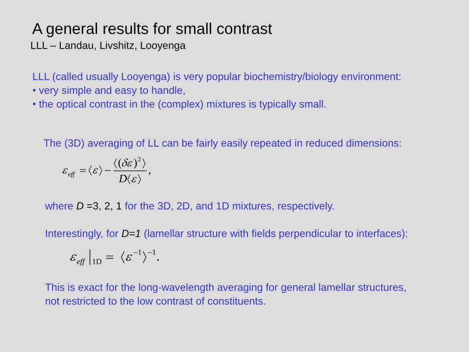
A general results for small contrast LLL – Landau, Livshitz, Looyenga
The (3D) averaging of LL can be fairly easily repeated in reduced dimensions:
where D =3, 2, 1 for the 3D, 2D, and 1D mixtures, respectively.
Interestingly, for D=1 (lamellar structure with fields perpendicular to interfaces):
This is exact for the long-wavelength averaging for general lamellar structures,
not restricted to the low contrast of constituents.
2( ),eff
D
ee e
e
1 1
1D .effe e
LLL (called usually Looyenga) is very popular biochemistry/biology environment:
• very simple and easy to handle,
• the optical contrast in the (complex) mixtures is typically small.
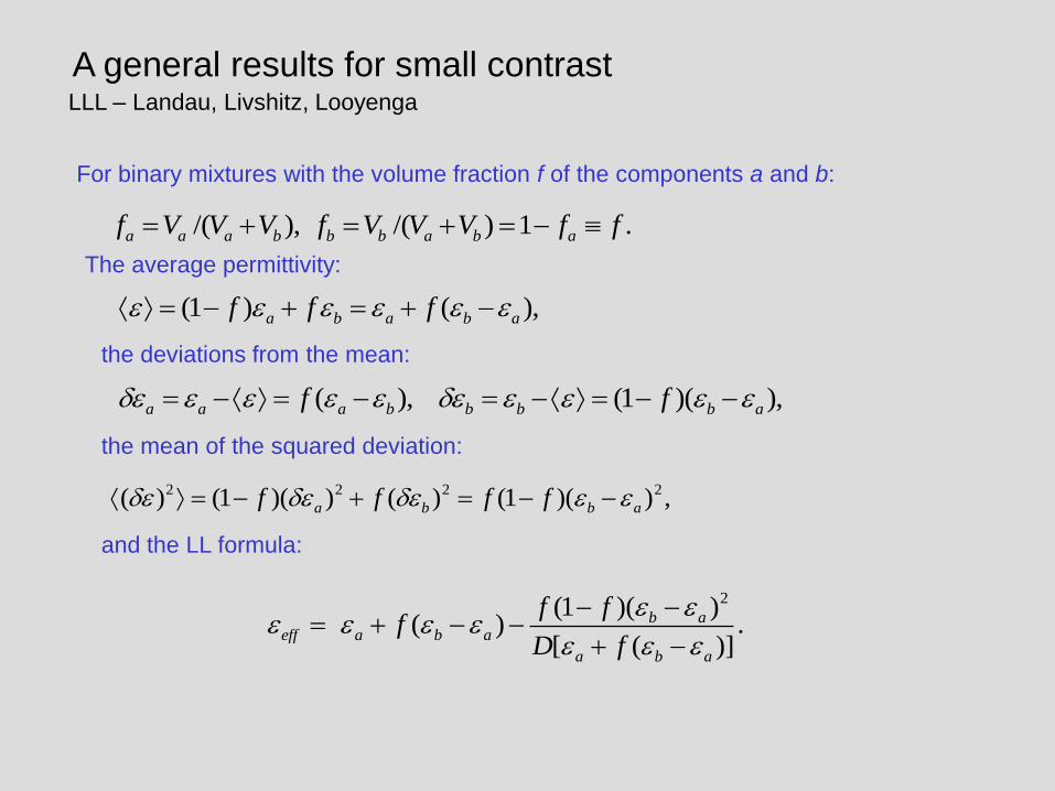
A general results for small contrast LLL – Landau, Livshitz, Looyenga
For binary mixtures with the volume fraction f of the components a and b:
The average permittivity:
the deviations from the mean:
/( ), /( ) 1 .a a a b b b a b af V V V f V V V f f
(1 ) ( ),a b a b af f fe e e e e e
( ), (1 )( ),a a a b b b b af fe e e e e e e e e e
the mean of the squared deviation:
2 2 2 2( ) (1 )( ) ( ) (1 )( ) ,a b b af f f fe e e e e
and the LL formula:
2(1 )( ) ( ) .
[ ( )]
b aeff a b a
a b a
f ff
D f
e ee e e e
e e e
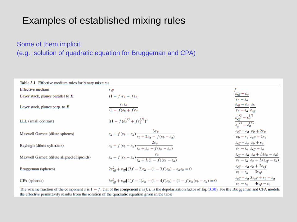
Examples of established mixing rules
Some of them implicit:
(e.g., solution of quadratic equation for Bruggeman and CPA)
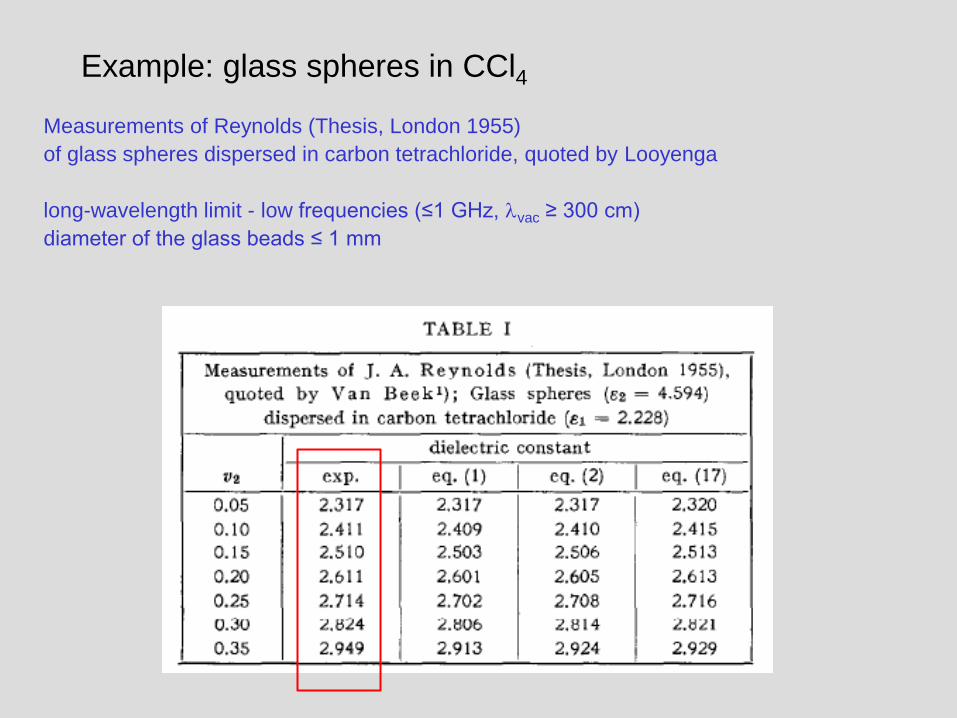
Example: glass spheres in CCl4
Measurements of Reynolds (Thesis, London 1955)
of glass spheres dispersed in carbon tetrachloride, quoted by Looyenga
long-wavelength limit - low frequencies (≤1 GHz, lvac ≥ 300 cm)
diameter of the glass beads ≤ 1 mm
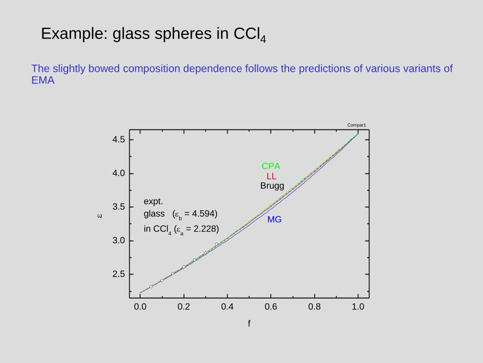
Example: glass spheres in CCl4
The slightly bowed composition dependence follows the predictions of various variants of EMA
0.0 0.2 0.4 0.6 0.8 1.0
2.5
3.0
3.5
4.0
4.5
expt.
glass (eb = 4.594)
in CCl4 (e
a = 2.228)
LLCPA
MG
Brugg
Compar1
e
f
Example: glass spheres in CCl4
0.0 0.1 0.2 0.3 0.4
-0.04
-0.02
0.00
expt.
glass (eb = 4.594)
in CCl4 (e
a = 2.228)
LL, 0.008
CPA,0.006
MG, 0.023
Brugg, 0.011
Compar3
e eff
ee
xp
t
f
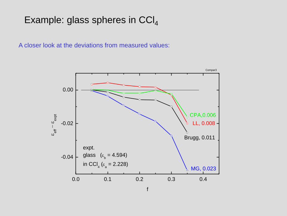
A closer look at the deviations from measured values:
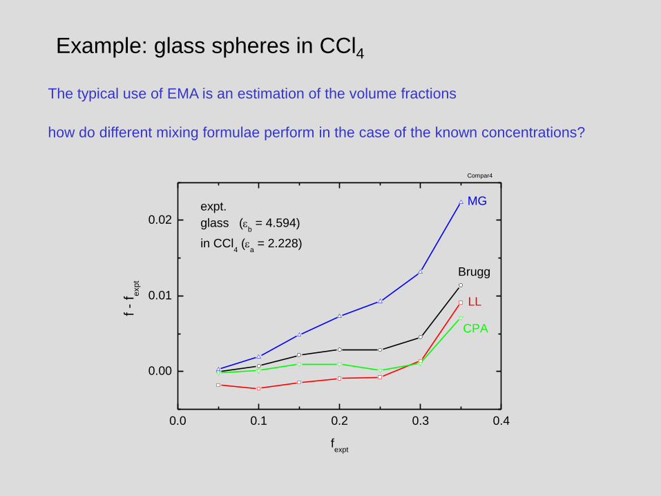
Example: glass spheres in CCl4
0.0 0.1 0.2 0.3 0.4
0.00
0.01
0.02expt.
glass (eb = 4.594)
in CCl4 (e
a = 2.228)
LL
CPA
MG
Brugg
Compar4
f -
f exp
t
fexpt
The typical use of EMA is an estimation of the volume fractions
how do different mixing formulae perform in the case of the known concentrations?
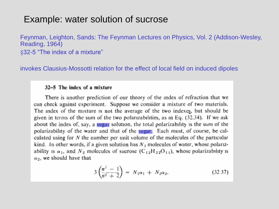
Example: water solution of sucrose
Feynman, Leighton, Sands: The Feynman Lectures on Physics, Vol. 2 (Addison-Wesley, Reading, 1964)
§32-5 “The index of a mixture”
invokes Clausius-Mossotti relation for the effect of local field on induced dipoles
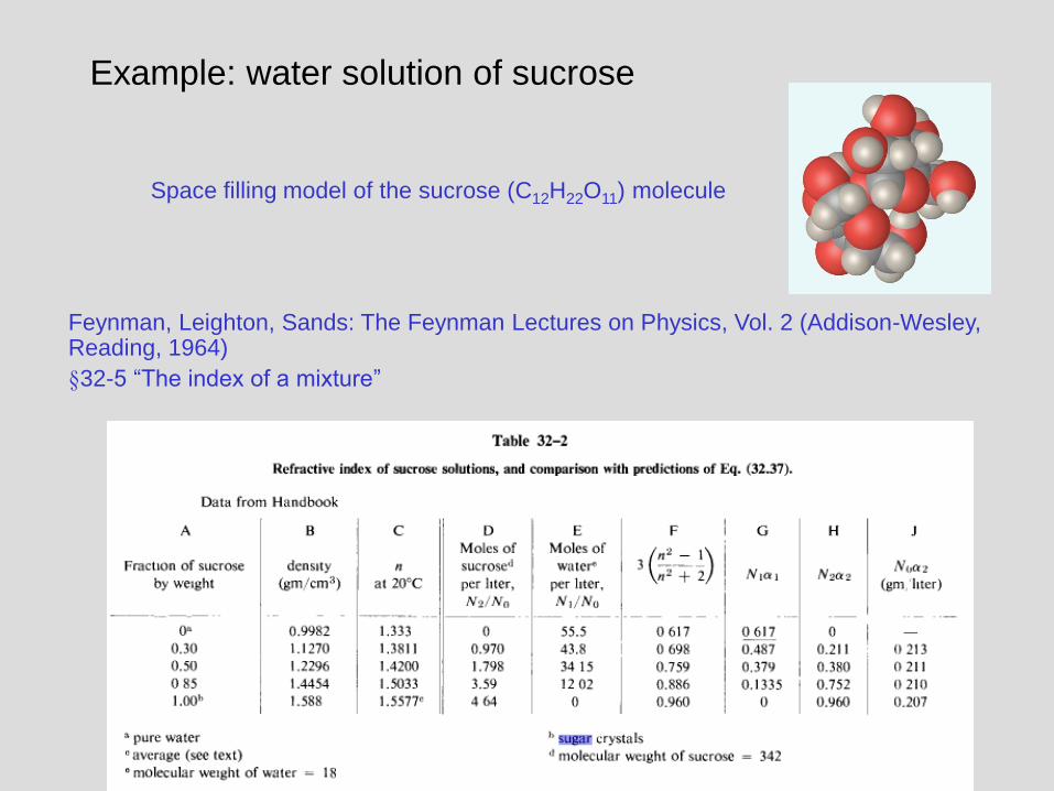
Example: water solution of sucrose
Feynman, Leighton, Sands: The Feynman Lectures on Physics, Vol. 2 (Addison-Wesley, Reading, 1964)
§32-5 “The index of a mixture”
Space filling model of the sucrose (C12H22O11) molecule
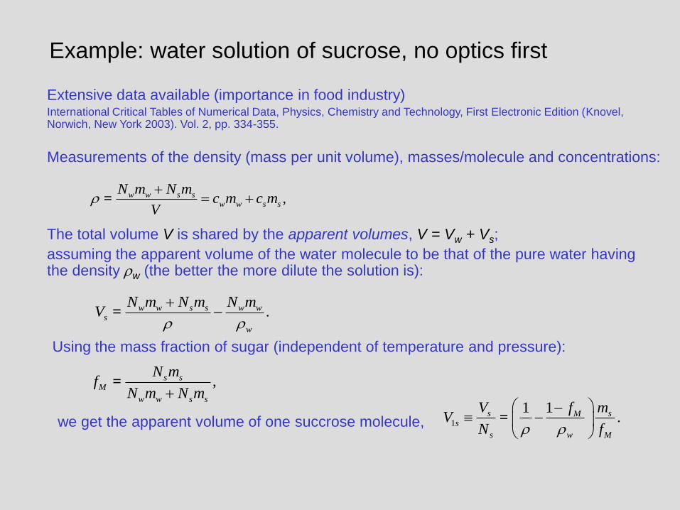
Example: water solution of sucrose, no optics first
Extensive data available (importance in food industry) International Critical Tables of Numerical Data, Physics, Chemistry and Technology, First Electronic Edition (Knovel, Norwich, New York 2003). Vol. 2, pp. 334-355.
Measurements of the density (mass per unit volume), masses/molecule and concentrations:
The total volume V is shared by the apparent volumes, V = Vw + Vs;
assuming the apparent volume of the water molecule to be that of the pure water having the density rw (the better the more dilute the solution is):
,w w s sw w s s
N m N mc m c m
Vr
=
.w w s s w ws
w
N m N m N mV
r r
=
Using the mass fraction of sugar (independent of temperature and pressure):
,s sM
w w s s
N mf
N m N m=
we get the apparent volume of one succrose molecule, 1
11.s sM
s
s w M
V mfV
N fr r
=
Example: water solution of sucrose, no optics first
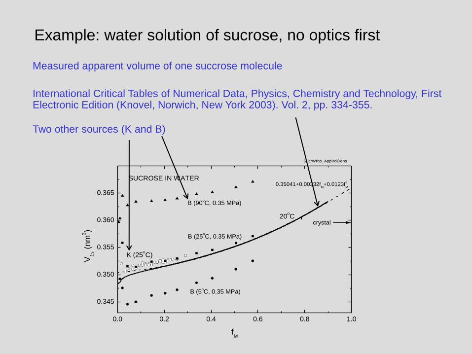
Measured apparent volume of one succrose molecule
International Critical Tables of Numerical Data, Physics, Chemistry and Technology, First Electronic Edition (Knovel, Norwich, New York 2003). Vol. 2, pp. 334-355.
Two other sources (K and B)
0.0 0.2 0.4 0.6 0.8 1.0
0.345
0.350
0.355
0.360
0.365
0.35041+0.00332fM+0.0123f
2
M
B (90oC, 0.35 MPa)
B (25oC, 0.35 MPa)
B (5oC, 0.35 MPa)
20oC
SUCROSE IN WATER
K (25oC)
V1
s (
nm
3)
fM
SucrWrho_AppVolDens
crystal
Example: water solution of sucrose
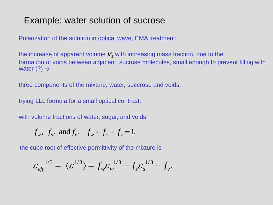
Polarization of the solution in optical wave, EMA treatment:
the increase of apparent volume Vs with increasing mass fraction, due to the
formation of voids between adjacent sucrose molecules, small enough to prevent filling with water (?) →
three components of the mixture, water, succrose and voids.
trying LLL formula for a small optical contrast;
with volume fractions of water, sugar, and voids
the cube root of effective permittivity of the mixture is
1/3 1/3 1/3 1/3 .eff w w s s vf f fe e e e
, , and , 1,w s v w s vf f f f f f
Example: water solution of sucrose
0.0 0.2 0.4 0.6 0.8 1.0
0.00
0.01
0.02
0.03
0.04
0.0 0.2 0.4 0.6 0.8 1.0-0.1
0.0
0.1
-0.1
0.0
0.1
lD (589.3 nm)
f(r)
v
2.466
2.46
es = 2.47
sucrose in water
t = 20 C
f v
fM
Voids_fvICUMSA-InvRhoF
2.46
es = 2.47
0.08595fM+0.03328f
2
M+0.00715f
3
M
e1
/3-e
1/3
LL
L ,
x10
e1
/3-e
1/3
w
fM
(msd = 1.3x10⁻⁵
)
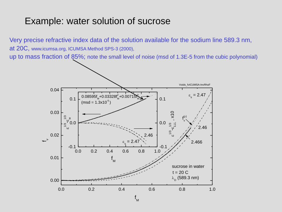
Very precise refractive index data of the solution available for the sodium line 589.3 nm,
at 20C, www.icumsa.org, ICUMSA Method SPS-3 (2000),
up to mass fraction of 85%; note the small level of noise (msd of 1.3E-5 from the cubic polynomial)
Example: water solution of sucrose
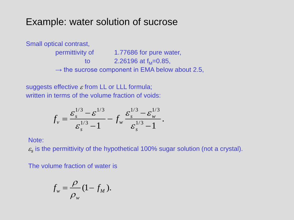
Small optical contrast,
permittivity of 1.77686 for pure water,
to 2.26196 at fM=0.85,
→ the sucrose component in EMA below about 2.5,
suggests effective e from LL or LLL formula;
written in terms of the volume fraction of voids:
1/3 1/3 1/3 1/3
1/3 1/3.
1 1
s s wv w
s s
f fe e e e
e e
Note:
es is the permittivity of the hypothetical 100% sugar solution (not a crystal).
The volume fraction of water is
(1 ).w M
w
f fr
r
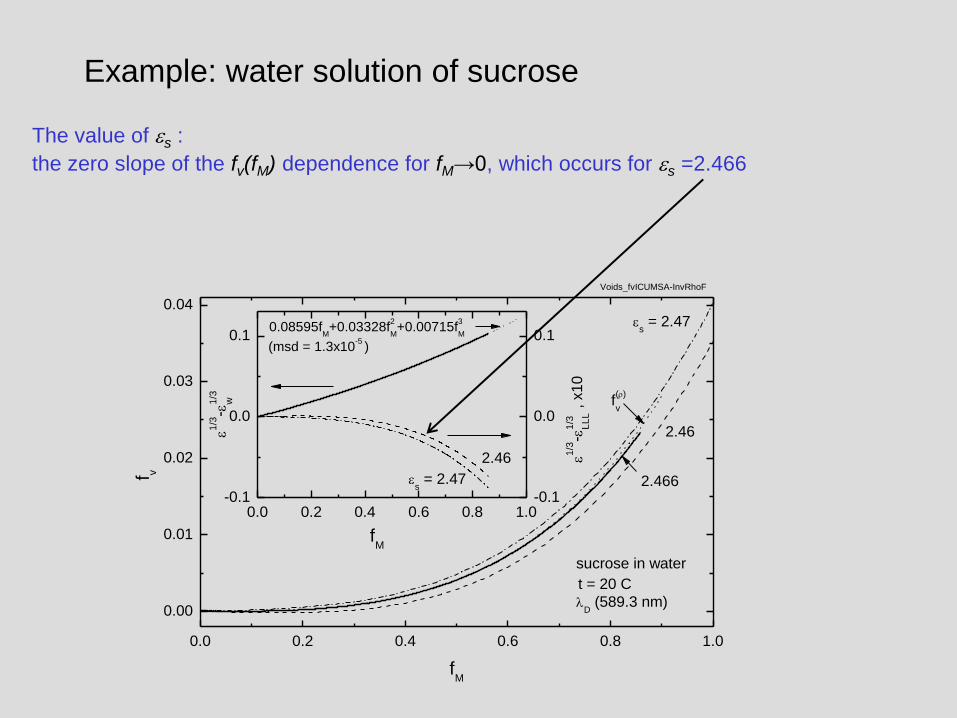
Example: water solution of sucrose
The value of es :
the zero slope of the fv(fM) dependence for fM→0, which occurs for es =2.466
0.0 0.2 0.4 0.6 0.8 1.0
0.00
0.01
0.02
0.03
0.04
0.0 0.2 0.4 0.6 0.8 1.0-0.1
0.0
0.1
-0.1
0.0
0.1
lD (589.3 nm)
f(r)
v
2.466
2.46
es = 2.47
sucrose in water
t = 20 C
f v
fM
Voids_fvICUMSA-InvRhoF
2.46
es = 2.47
0.08595fM+0.03328f
2
M+0.00715f
3
M
e1
/3-e
1/3
LL
L ,
x10
e1
/3-e
1/3
w
fM
(msd = 1.3x10⁻⁵
)
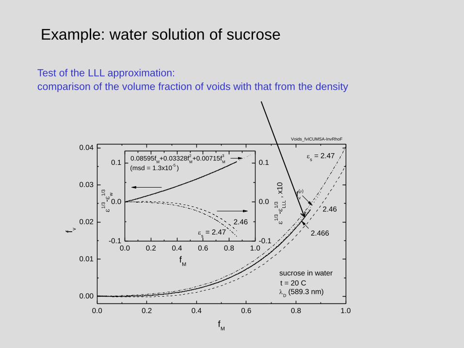
Example: water solution of sucrose
Test of the LLL approximation:
comparison of the volume fraction of voids with that from the density
0.0 0.2 0.4 0.6 0.8 1.0
0.00
0.01
0.02
0.03
0.04
0.0 0.2 0.4 0.6 0.8 1.0-0.1
0.0
0.1
-0.1
0.0
0.1
lD (589.3 nm)
f(r)
v
2.466
2.46
es = 2.47
sucrose in water
t = 20 C
f v
fM
Voids_fvICUMSA-InvRhoF
2.46
es = 2.47
0.08595fM+0.03328f
2
M+0.00715f
3
M
e1
/3-e
1/3
LL
L ,
x10
e1
/3-e
1/3
w
fM
(msd = 1.3x10⁻⁵
)
Example: water solution of sucrose
Fairly good agreement of optical data with EMA for the very small volume of the sugar molecule (0.35 nm3 at RT) !
Confirms the basic lines of Feynman’s approach, except for the use of polarizability of the succrose molecules, obtained from the average of refractive indices of (anisotropic) crystal.
Selected concerns:
• uncertainty in choosing the “EMA rule”,
• oversimplified introduction of the voids
(also in the apparent free volume from the density),
• ...
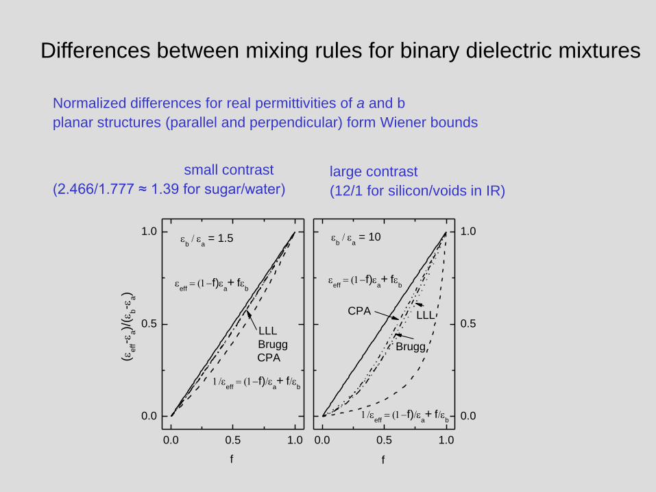
Differences between mixing rules for binary dielectric mixtures
Normalized differences for real permittivities of a and b
planar structures (parallel and perpendicular) form Wiener bounds
0.0 0.5 1.0
0.0
0.5
1.0
Brugg
LLL
CPA
eeff
f)ea+ fe
b
eeff
f)ea+ fe
b
eb e
a = 1.5
(ee
ff-e
a)/
(eb-e
a)
f
0.0 0.5 1.0
0.0
0.5
1.0
f
CPA
Brugg
LLL
eeff
f)ea+ fe
b
eeff
f)ea+ fe
b
eb e
a = 10
small contrast
(2.466/1.777 ≈ 1.39 for sugar/water)
large contrast
(12/1 for silicon/voids in IR)
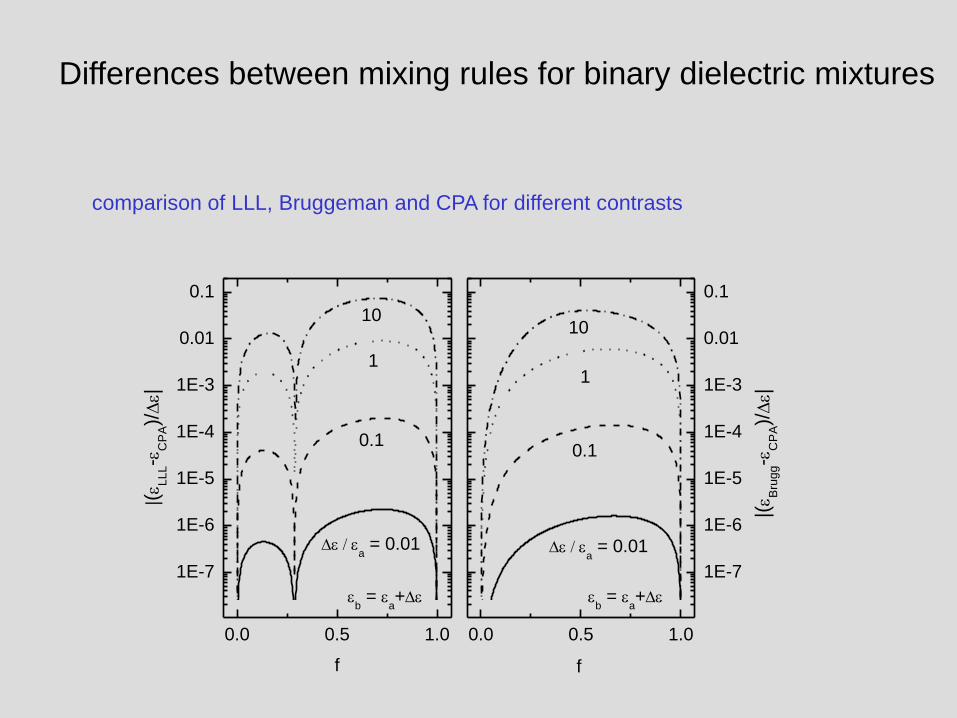
Differences between mixing rules for binary dielectric mixtures
comparison of LLL, Bruggeman and CPA for different contrasts
0.0 0.5 1.0
1E-7
1E-6
1E-5
1E-4
1E-3
0.01
0.1
10
1
0.1
e ea = 0.01
eb = e
a+e
|(e L
LL-e
CP
A)/
e|
f
0.0 0.5 1.0
1E-7
1E-6
1E-5
1E-4
1E-3
0.01
0.1
10
1
0.1
e ea = 0.01
eb = e
a+e
|(e B
rug
g-e
CP
A)/
e|
f
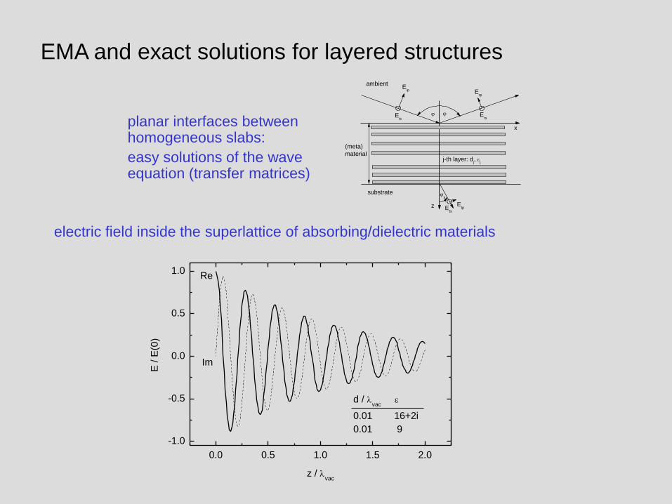
EMA and exact solutions for layered structures
electric field inside the superlattice of absorbing/dielectric materials
0.0 0.5 1.0 1.5 2.0
-1.0
-0.5
0.0
0.5
1.0
d / lvac
e
0.01 16+2i
0.01 9
Re
Im
E / E
(0)
z / lvac
planar interfaces between homogeneous slabs:
easy solutions of the wave equation (transfer matrices)
j-th layer: dj, e
j
substrate
Ets
Etp
Ers
Erp
Eis
Eip
s
(meta)
material
ambient
z
x
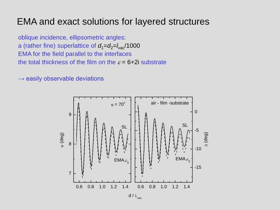
EMA and exact solutions for layered structures
oblique incidence, ellipsometric angles:
a (rather fine) superlattice of d1=d2=lvac/1000
EMA for the field parallel to the interfaces
the total thickness of the film on the e = 6+2i substrate
→ easily observable deviations
0.6 0.8 1.0 1.2 1.4
7
8
9
= 70o
SL
EMA,e||
(
de
g)
d / lvac
0.6 0.8 1.0 1.2 1.4
-15
-10
-5
0
EMA,e||
SL
air - film -substrate
(
de
g)
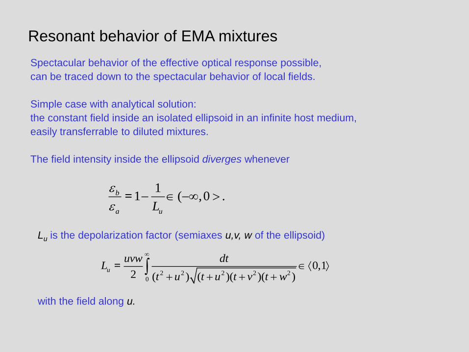
Resonant behavior of EMA mixtures
Spectacular behavior of the effective optical response possible,
can be traced down to the spectacular behavior of local fields.
Simple case with analytical solution:
the constant field inside an isolated ellipsoid in an infinite host medium,
easily transferrable to diluted mixtures.
The field intensity inside the ellipsoid diverges whenever
11 ( ,0 .=
e
e b
a uL
Lu is the depolarization factor (semiaxes u,v, w of the ellipsoid)
2 2 2 2 20
0,12 ( ) ( )( )( )
u
uvw dtL
t u t u t v t w
=
with the field along u.
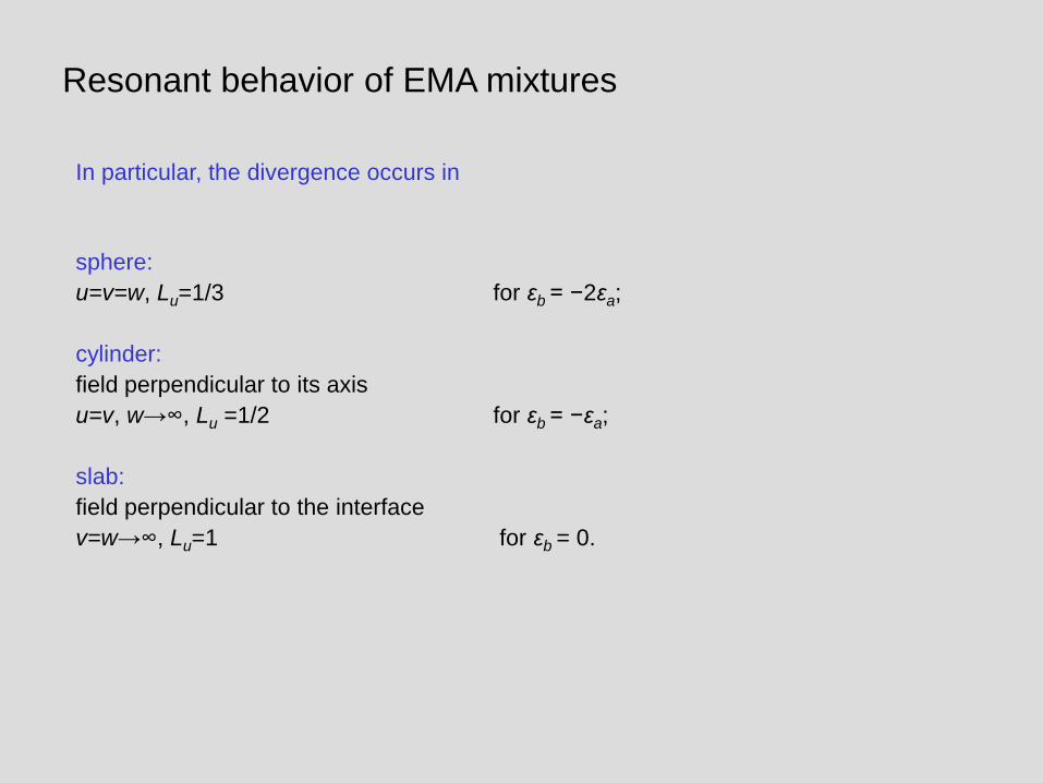
Resonant behavior of EMA mixtures
In particular, the divergence occurs in
sphere:
u=v=w, Lu=1/3 for εb = −2εa;
cylinder:
field perpendicular to its axis
u=v, w→∞, Lu =1/2 for εb = −εa;
slab:
field perpendicular to the interface
v=w→∞, Lu=1 for εb = 0.
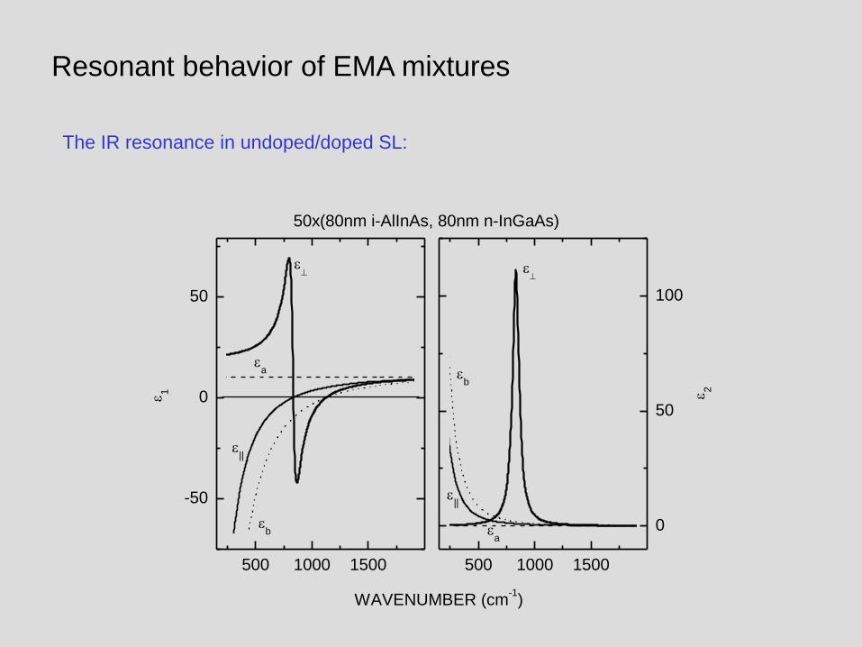
Resonant behavior of EMA mixtures
The IR resonance in undoped/doped SL:
500 1000 1500
-50
0
50
e||
e
e
e||
eb
ea
e 1
WAVENUMBER (cm-1)
500 1000 1500
0
50
100
50x(80nm i-AlInAs, 80nm n-InGaAs)
ea
eb
e 2
Conclusion
• EMA can be attractive and helpful.
• EMA can easily fail – if improperly used.
• Using it with caution is recommended.
A selection from the (vast) literature:
L.D. Landau and E.M. Lifshitz, Electrodynamics of continuous media, Second edition (Pergamon Press,
Oxford, 1984), Sec. 9.
R.P. Feynman, R.B. Leighton, and M. Sands, The Feynman Lectures on Physics, Vol. II (Addison-Wesley,
1964), § 32-5.
A. Sihvola, Electromagnetic mixing formulas and applications (IEE, Stevenage, 1999).
D.E. Aspnes, Am. J. Phys. 50, 704 (1982).
Ellipsometry at the Nanoscale , M. Losurdo and K. Hingerl, eds., (Springer 2013).
THANK YOU FOR YOUR ATTENTION
32