Embed Size (px)
Citation preview
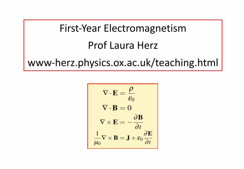
First-Year ElectromagnetismProf Laura Herz
www-herz.physics.ox.ac.uk/teaching.html
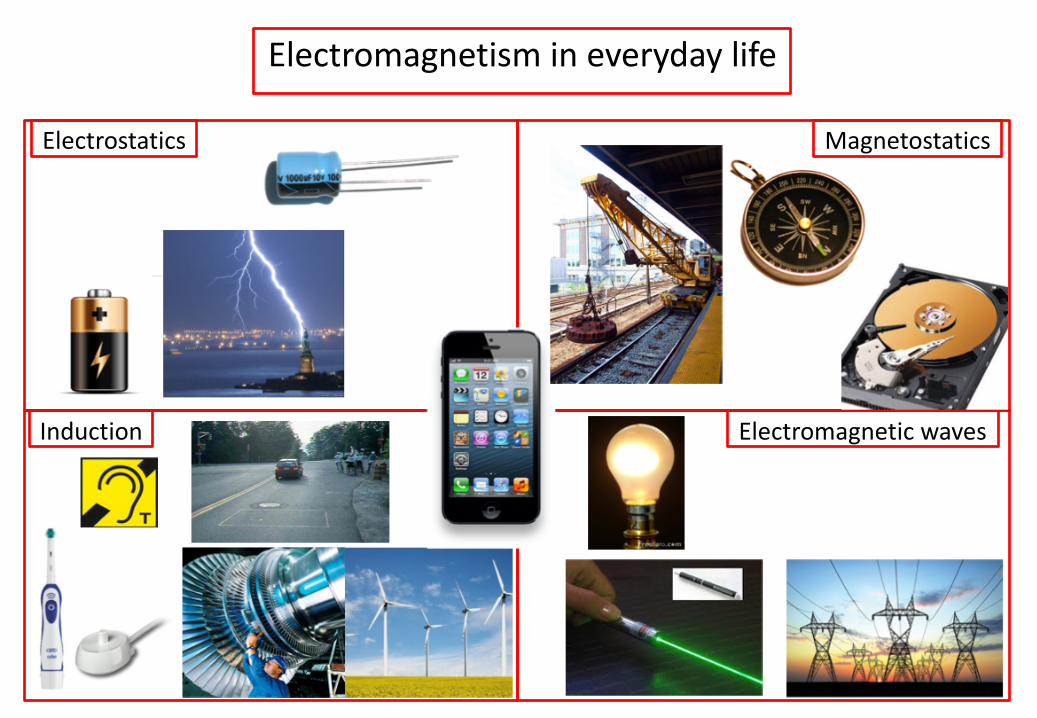
Electromagnetism in everyday life
Electrostatics
Induction Electromagnetic waves
Magnetostatics
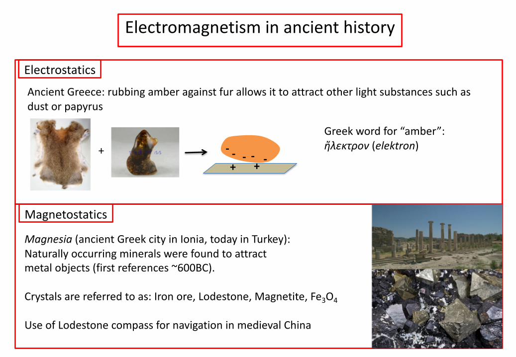
Electromagnetism in ancient history
Magnetostatics
Electrostatics
Magnesia (ancient Greek city in Ionia, today in Turkey):Naturally occurring minerals were found to attract metal objects (first references ~600BC).
Crystals are referred to as: Iron ore, Lodestone, Magnetite, Fe3O4
Use of Lodestone compass for navigation in medieval China
Ancient Greece: rubbing amber against fur allows it to attract other light substances such as dust or papyrus
+ -- - --++
Greek word for “amber”: ἤλεκτρον (elektron)
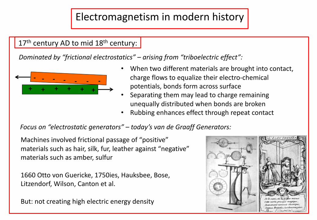
Electromagnetism in modern history
17th century AD to mid 18th century:
Dominated by “frictional electrostatics” – arising from “triboelectric effect”:
- - - - - - -++++++
• When two different materials are brought into contact,
charge flows to equalize their electro-chemical
potentials, bonds form across surface
• Separating them may lead to charge remaining
unequally distributed when bonds are broken
• Rubbing enhances effect through repeat contact
Focus on “electrostatic generators” – today’s van de Graaff Generators:
Machines involved frictional passage of “positive”
materials such as hair, silk, fur, leather against “negative”
materials such as amber, sulfur
1660 Otto von Guericke, 1750ies, Hauksbee, Bose,
Litzendorf, Wilson, Canton et al.
But: not creating high electric energy density
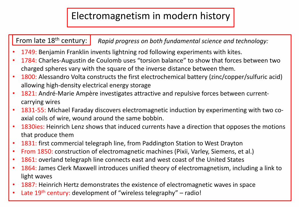
Electromagnetism in modern history
From late 18th century: Rapid progress on both fundamental science and technology: • 1749: Benjamin Franklin invents lightning rod following experiments with kites. • 1784: Charles-Augustin de Coulomb uses “torsion balance” to show that forces between two
charged spheres vary with the square of the inverse distance between them.• 1800: Alessandro Volta constructs the first electrochemical battery (zinc/copper/sulfuric acid)
allowing high-density electrical energy storage• 1821: André-Marie Ampère investigates attractive and repulsive forces between current-
carrying wires• 1831-55: Michael Faraday discovers electromagnetic induction by experimenting with two co-
axial coils of wire, wound around the same bobbin.• 1830ies: Heinrich Lenz shows that induced currents have a direction that opposes the motions
that produce them• 1831: first commercial telegraph line, from Paddington Station to West Drayton• From 1850: construction of electromagnetic machines (Pixii, Varley, Siemens, et al.)• 1861: overland telegraph line connects east and west coast of the United States• 1864: James Clerk Maxwell introduces unified theory of electromagnetism, including a link to
light waves• 1887: Heinrich Hertz demonstrates the existence of electromagnetic waves in space• Late 19th century: development of “wireless telegraphy” – radio!
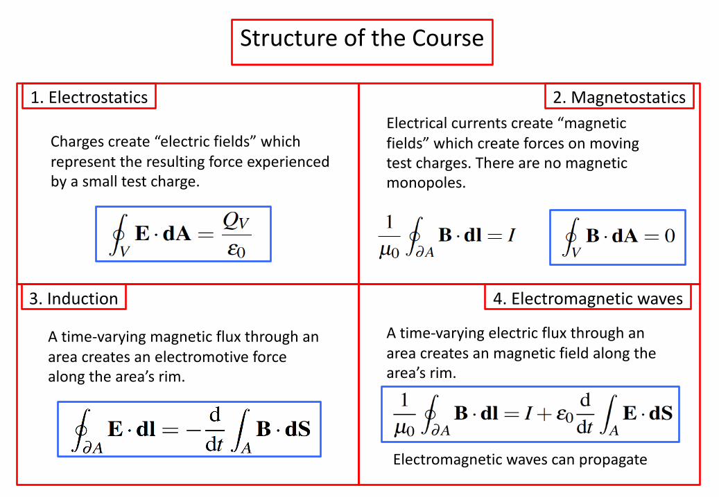
Structure of the Course
1. Electrostatics
3. Induction 4. Electromagnetic waves
2. Magnetostatics
Charges create “electric fields” which represent the resulting force experienced by a small test charge.
Electrical currents create “magnetic fields” which create forces on moving test charges. There are no magnetic monopoles.
A time-varying magnetic flux through an area creates an electromotive force along the area’s rim.
A time-varying electric flux through an area creates an magnetic field along the area’s rim.
Electromagnetic waves can propagate
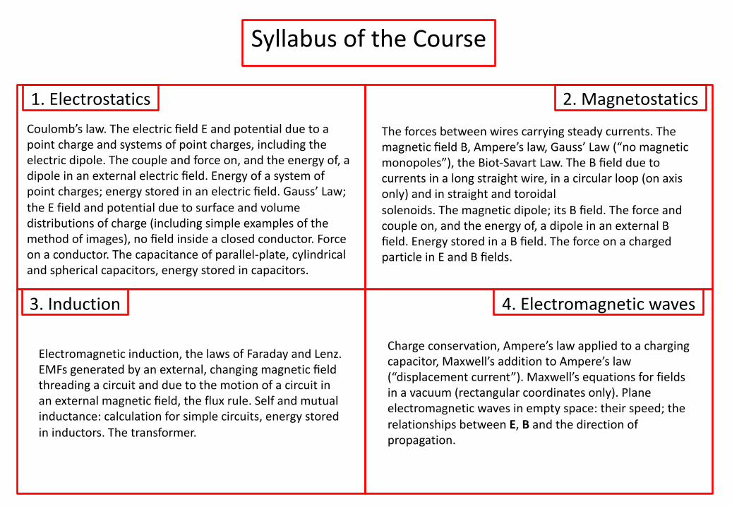
Syllabus of the Course
1. Electrostatics
3. Induction 4. Electromagnetic waves
2. Magnetostatics
Coulomb’s law. The electric field E and potential due to a
point charge and systems of point charges, including the
electric dipole. The couple and force on, and the energy of, a
dipole in an external electric field. Energy of a system of
point charges; energy stored in an electric field. Gauss’ Law;
the E field and potential due to surface and volume
distributions of charge (including simple examples of the
method of images), no field inside a closed conductor. Force
on a conductor. The capacitance of parallel-plate, cylindrical
and spherical capacitors, energy stored in capacitors.
The forces between wires carrying steady currents. The
magnetic field B, Ampere’s law, Gauss’ Law (“no magnetic
monopoles”), the Biot-Savart Law. The B field due to
currents in a long straight wire, in a circular loop (on axis
only) and in straight and toroidal
solenoids. The magnetic dipole; its B field. The force and
couple on, and the energy of, a dipole in an external B
field. Energy stored in a B field. The force on a charged
particle in E and B fields.
Electromagnetic induction, the laws of Faraday and Lenz.
EMFs generated by an external, changing magnetic field
threading a circuit and due to the motion of a circuit in
an external magnetic field, the flux rule. Self and mutual
inductance: calculation for simple circuits, energy stored
in inductors. The transformer.
Charge conservation, Ampere’s law applied to a charging
capacitor, Maxwell’s addition to Ampere’s law
(“displacement current”). Maxwell’s equations for fields
in a vacuum (rectangular coordinates only). Plane
electromagnetic waves in empty space: their speed; the
relationships between E, B and the direction of
propagation.
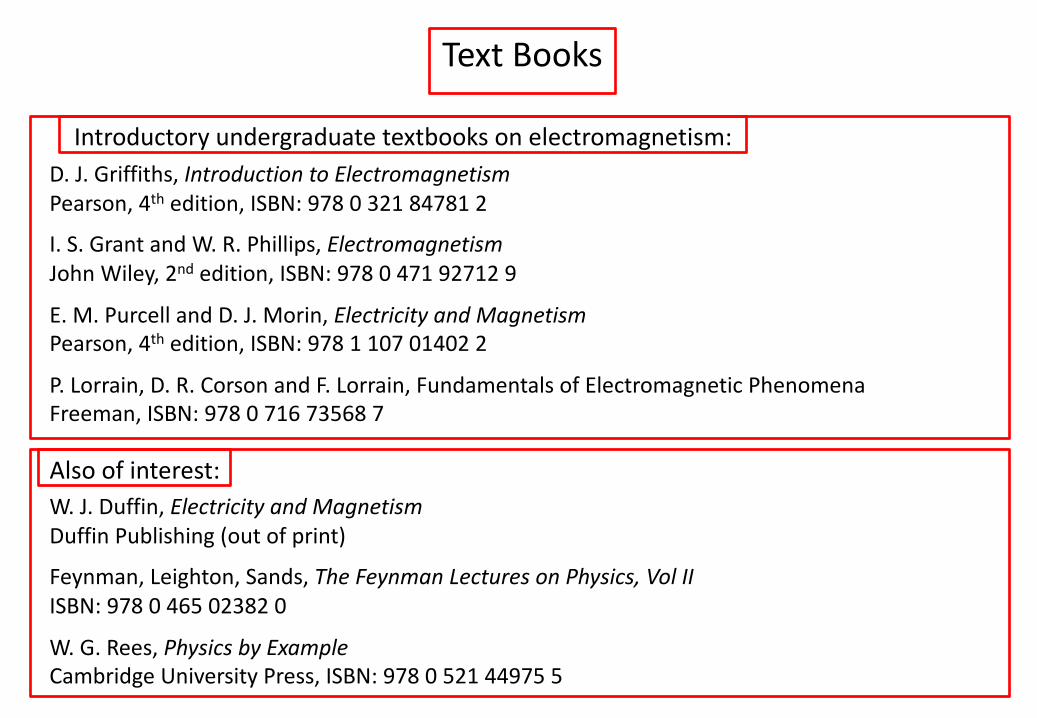
Text Books
D. J. Griffiths, Introduction to ElectromagnetismPearson, 4th edition, ISBN: 978 0 321 84781 2
I. S. Grant and W. R. Phillips, ElectromagnetismJohn Wiley, 2nd edition, ISBN: 978 0 471 92712 9
E. M. Purcell and D. J. Morin, Electricity and MagnetismPearson, 4th edition, ISBN: 978 1 107 01402 2
P. Lorrain, D. R. Corson and F. Lorrain, Fundamentals of Electromagnetic PhenomenaFreeman, ISBN: 978 0 716 73568 7
W. J. Duffin, Electricity and MagnetismDuffin Publishing (out of print)
Feynman, Leighton, Sands, The Feynman Lectures on Physics, Vol IIISBN: 978 0 465 02382 0
W. G. Rees, Physics by ExampleCambridge University Press, ISBN: 978 0 521 44975 5
Introductory undergraduate textbooks on electromagnetism:
Also of interest:
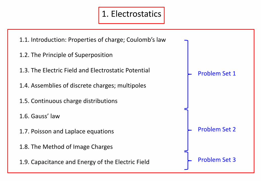
1. Electrostatics
1.1. Introduction: Properties of charge; Coulomb’s law
1.2. The Principle of Superposition
1.3. The Electric Field and Electrostatic Potential
1.4. Assemblies of discrete charges; multipoles
1.5. Continuous charge distributions
1.6. Gauss’ law
1.7. Poisson and Laplace equations
1.8. The Method of Image Charges
1.9. Capacitance and Energy of the Electric Field
Problem Set 1
Problem Set 2
Problem Set 3
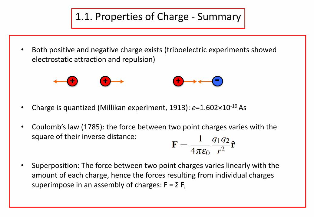
1.1. Properties of Charge - Summary
• Both positive and negative charge exists (triboelectric experiments showed
electrostatic attraction and repulsion)
• Charge is quantized (Millikan experiment, 1913): e=1.602×10⁻¹⁹ As
• Coulomb’s law (1785): the force between two point charges varies with the
square of their inverse distance:
• Superposition: The force between two point charges varies linearly with the
amount of each charge, hence the forces resulting from individual charges
superimpose in an assembly of charges: F = Σ Fi
-+ + +
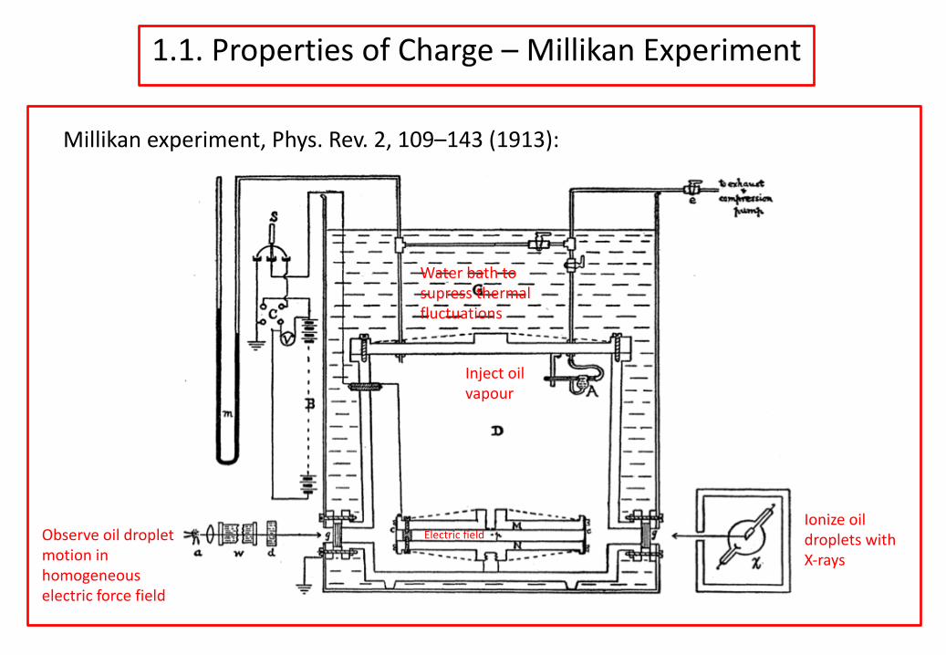
1.1. Properties of Charge – Millikan Experiment
Millikan experiment, Phys. Rev. 2, 109–143 (1913):
Inject oil vapour
Ionize oil droplets with X-rays
Observe oil droplet motion in homogeneous electric force field
Electric field
Water bath to supress thermal fluctuations
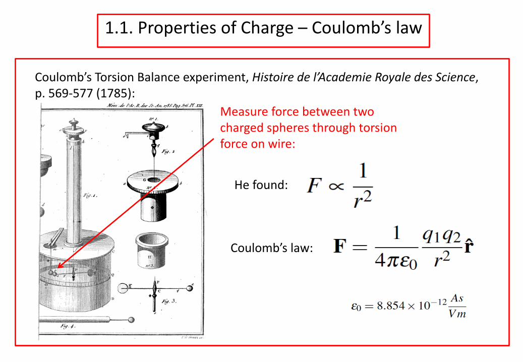
1.1. Properties of Charge – Coulomb’s law
Coulomb’s Torsion Balance experiment, Histoire de l’Academie Royale des Science, p. 569-577 (1785):
Measure force between two charged spheres through torsion force on wire:
He found:
Coulomb’s law:
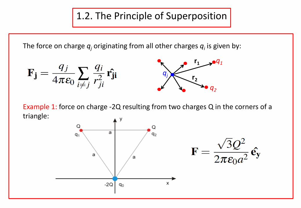
The force on charge qj originating from all other charges qi is given by:
Example 1: force on charge -2Q resulting from two charges Q in the corners of a triangle:
qj
q1r1
r2q2
1.2. The Principle of Superposition
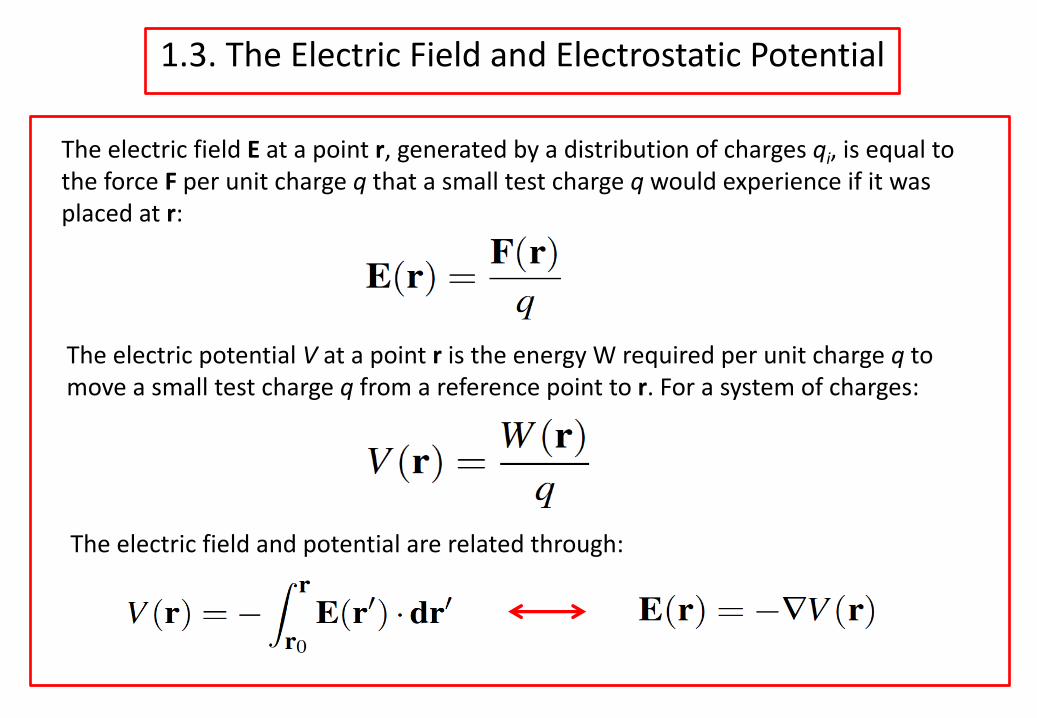
The electric field E at a point r, generated by a distribution of charges qi, is equal to the force F per unit charge q that a small test charge q would experience if it was placed at r:
1.3. The Electric Field and Electrostatic Potential
The electric potential V at a point r is the energy W required per unit charge q to move a small test charge q from a reference point to r. For a system of charges:
The electric field and potential are related through:
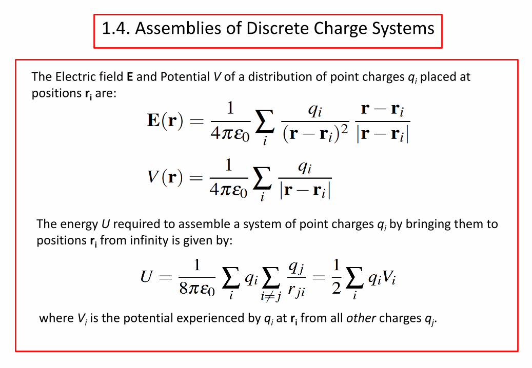
The Electric field E and Potential V of a distribution of point charges qi placed at positions ri are:
1.4. Assemblies of Discrete Charge Systems
The energy U required to assemble a system of point charges qi by bringing them to positions ri from infinity is given by:
where Vi is the potential experienced by qi at ri from all other charges qj.
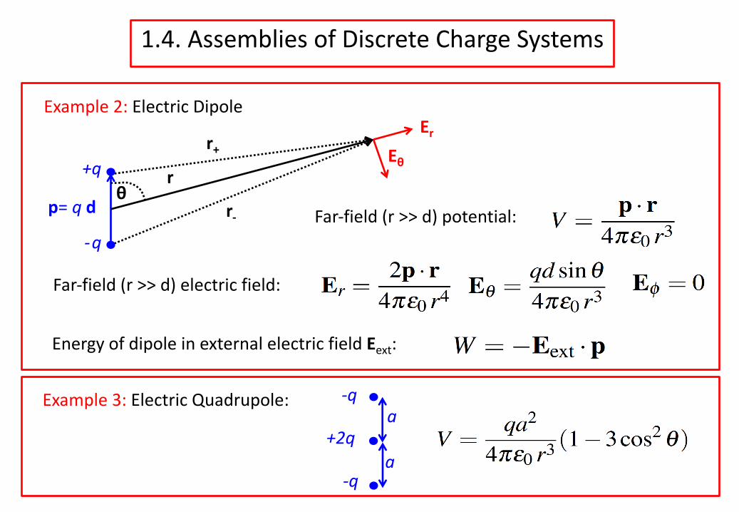
Example 2: Electric Dipole
1.4. Assemblies of Discrete Charge Systems
+q
-q
p= q d
r+
r-
rEθ
Er
θFar-field (r >> d) potential:
Far-field (r >> d) electric field:
Energy of dipole in external electric field Eext:
Example 3: Electric Quadrupole: -q
+2q
-q
a
a
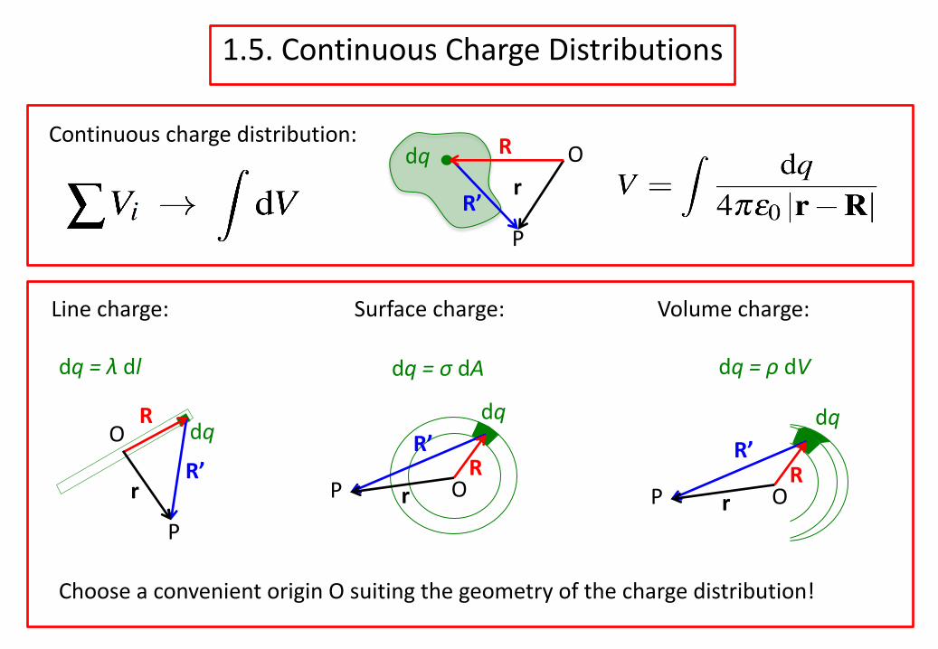
Continuous charge distribution:
1.5. Continuous Charge Distributions
dq
R’ rR
Choose a convenient origin O suiting the geometry of the charge distribution!
Line charge: Surface charge: Volume charge:
dq = λ dl dq = σ dA dq = ρ dV
O
P
R’r
O
P
dqR
P OR
r
R’dq
P OR
r
R’dq
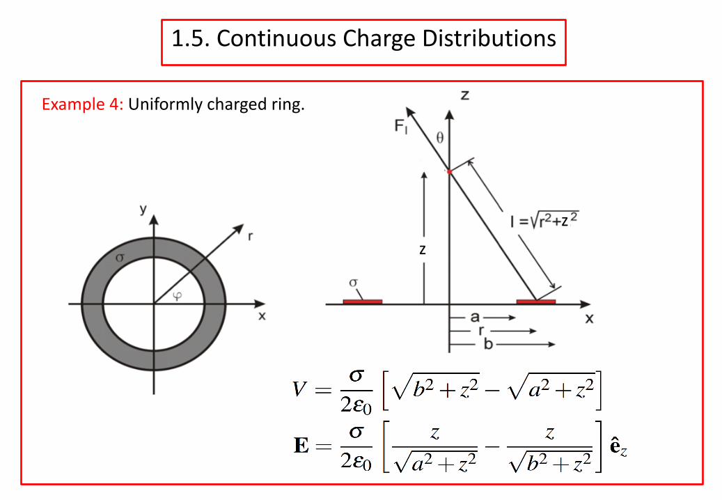
1.5. Continuous Charge Distributions
zz
Example 4: Uniformly charged ring.
1.5. Continuous Charge Distributions
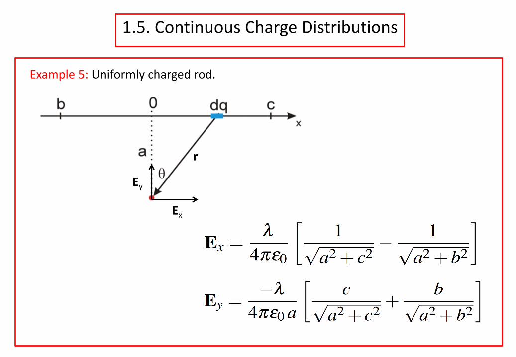
Example 5: Uniformly charged rod.
r
Ex
Ey
Principle of superposition
1.6. Gauss’s Law
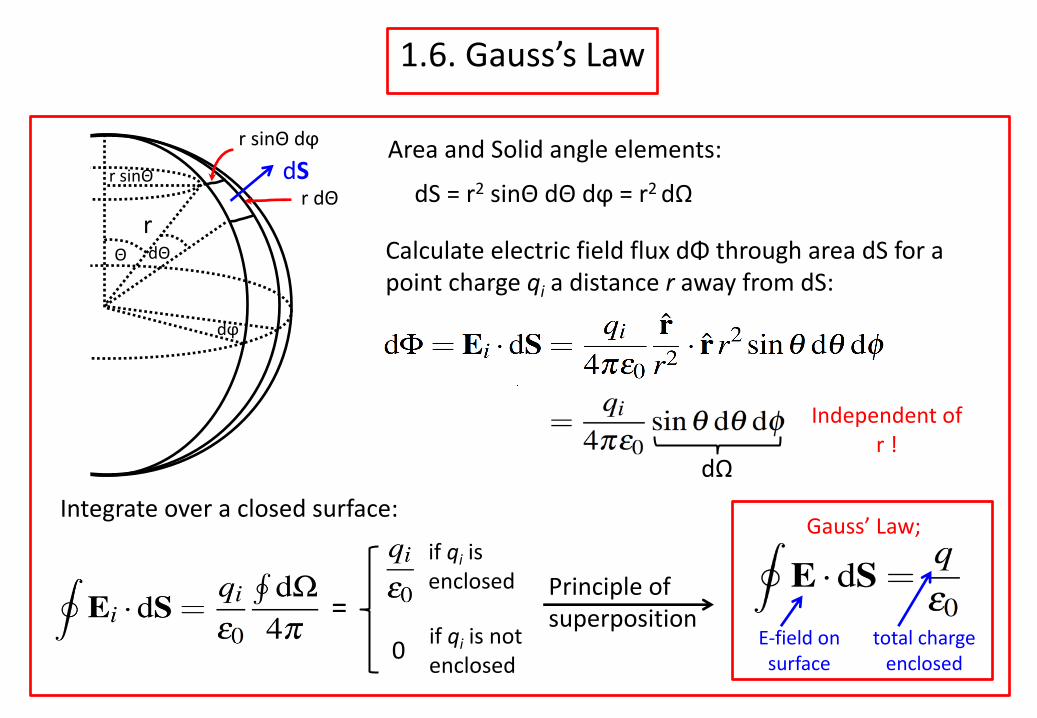
Area and Solid angle elements: dS = r2 sinΘ dΘ dϕ = r2 dΩ
rdΘΘ
dϕ
r sinΘr dΘ
r sinΘ dϕdS
Calculate electric field flux dΦ through area dS for a point charge qi a distance r away from dS:
dΩ
Independent of r !
Integrate over a closed surface:
0
if qi is enclosed
if qi is not enclosed
Gauss’ Law;
total charge enclosed
E-field on surface
=
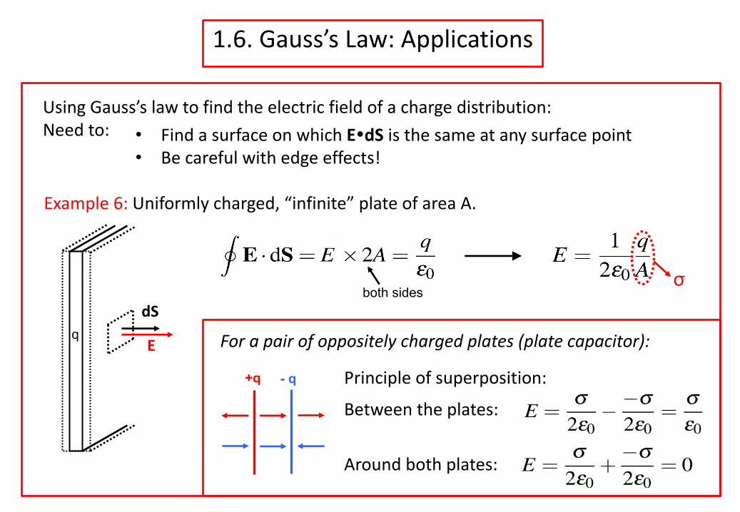
1.6. Gauss’s Law: Applications
Using Gauss’s law to find the electric field of a charge distribution:Need to: • Find a surface on which E�dS is the same at any surface point
• Be careful with edge effects!
Example 6: Uniformly charged, “infinite” plate of area A.
qE
dSboth sides
σ
+q - q
For a pair of oppositely charged plates (plate capacitor):
Principle of superposition:Between the plates:
Around both plates:
1.6. Gauss’s Law: Applications
Example 7: Spherically symmetric charge distributions.
(ii) hollow sphere with q spread evenly across surface:
(i) point charge q:
(iii) Sphere carrying uniform volume charge ρ:
qr
for any r
r R
For 0 < r < R (inside sphere):
For R < r (outside sphere):
0
r R
For 0 < r < R (inside sphere):
For R < r (outside sphere):
1.6. Gauss’s Law: Applications
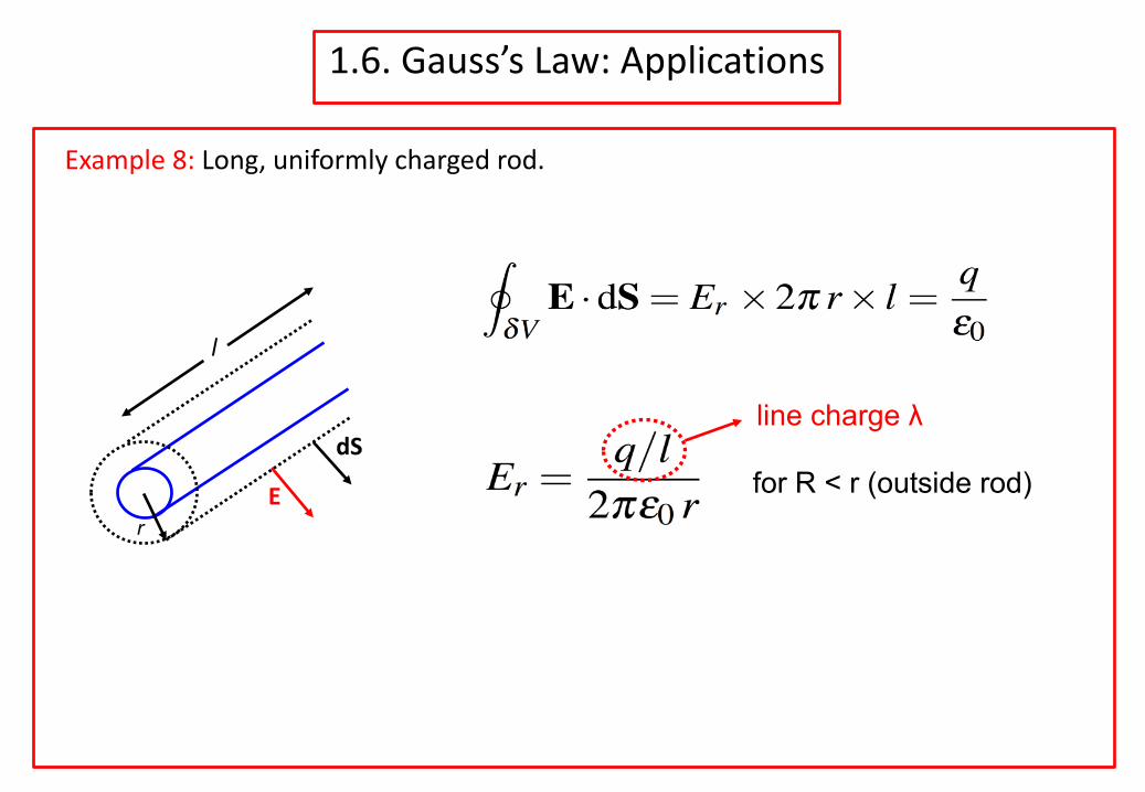
Example 8: Long, uniformly charged rod.
E
dS
l
r
for R < r (outside rod)
line charge λ
= 0
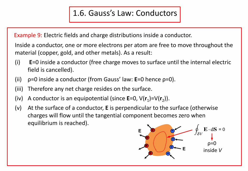
1.6. Gauss’s Law: Conductors
Inside a conductor, one or more electrons per atom are free to move throughout the material (copper, gold, and other metals). As a result:(i) E=0 inside a conductor (free charge moves to surface until the internal electric
field is cancelled).(ii) ρ=0 inside a conductor (from Gauss’ law: E=0 hence ρ=0).(iii) Therefore any net charge resides on the surface.(iv) A conductor is an equipotential (since E=0, V(r1)=V(r2)).(v) At the surface of a conductor, E is perpendicular to the surface (otherwise
charges will flow until the tangential component becomes zero when equilibrium is reached).
Example 9: Electric fields and charge distributions inside a conductor.
+ -+
++
---
E
Eρ=0
inside V
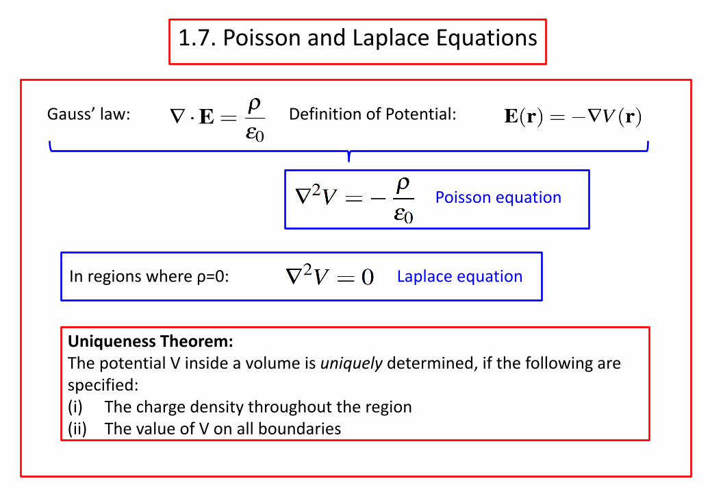
1.7. Poisson and Laplace Equations
Gauss’ law: Definition of Potential:
Poisson equation
In regions where ρ=0: Laplace equation
Uniqueness Theorem:The potential V inside a volume is uniquely determined, if the following are specified:(i) The charge density throughout the region(ii) The value of V on all boundaries
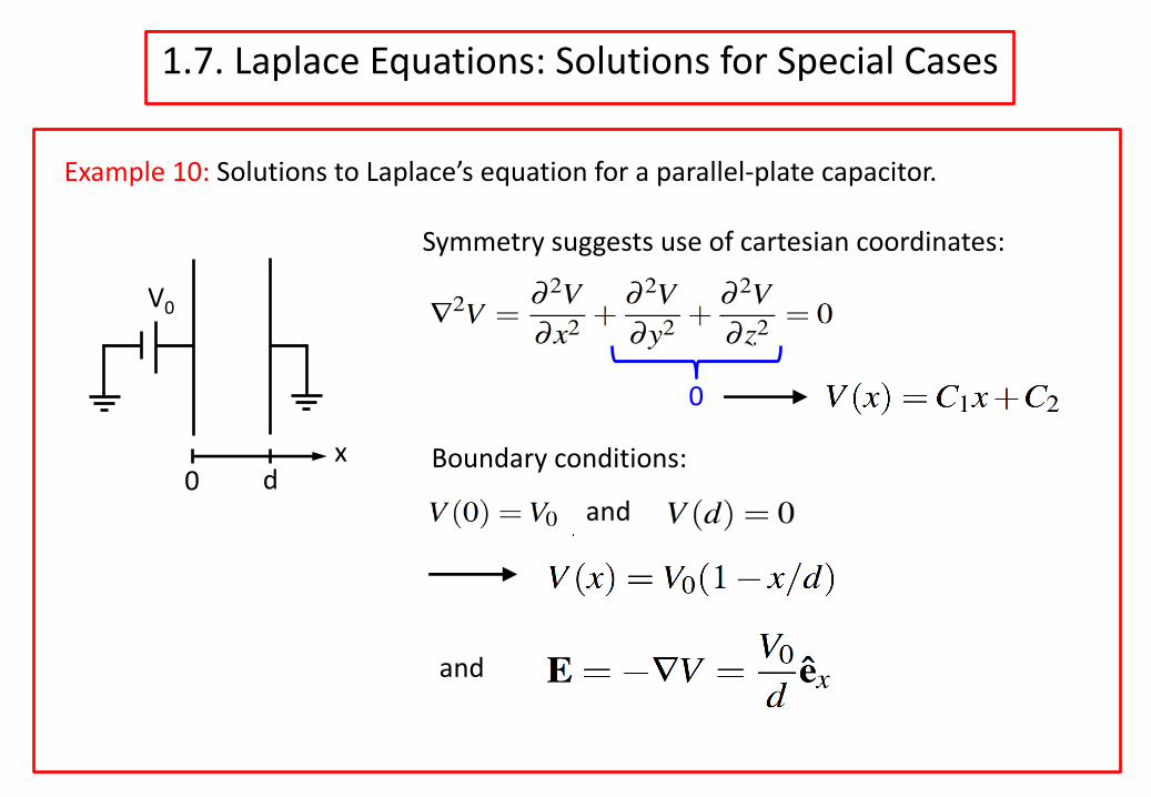
1.7. Laplace Equations: Solutions for Special Cases
Example 10: Solutions to Laplace’s equation for a parallel-plate capacitor.
Boundary conditions:
Symmetry suggests use of cartesian coordinates:
0
and
and
V0
xd0
1.7. Laplace Equations: Solutions for Special Cases
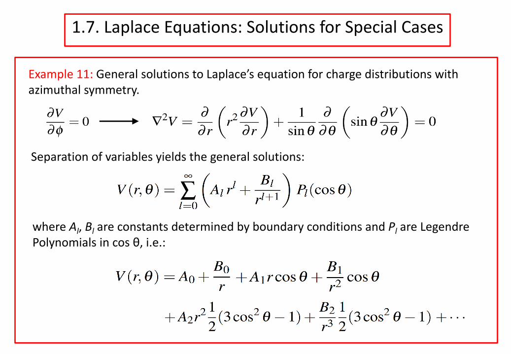
Example 11: General solutions to Laplace’s equation for charge distributions with azimuthal symmetry.
Separation of variables yields the general solutions:
where Al, Bl are constants determined by boundary conditions and Pl are Legendre Polynomials in cos θ, i.e.:
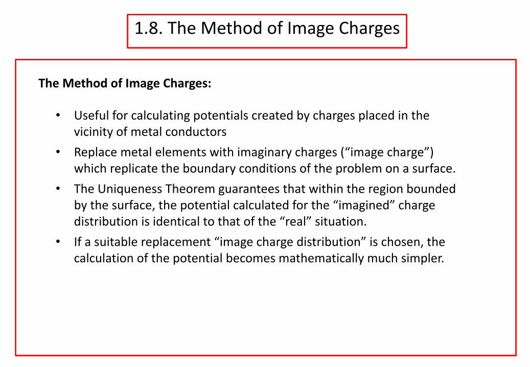
1.8. The Method of Image Charges
The Method of Image Charges:
• Useful for calculating potentials created by charges placed in the vicinity of metal conductors
• Replace metal elements with imaginary charges (“image charge”) which replicate the boundary conditions of the problem on a surface.
• The Uniqueness Theorem guarantees that within the region bounded by the surface, the potential calculated for the “imagined” charge distribution is identical to that of the “real” situation.
• If a suitable replacement “image charge distribution” is chosen, the calculation of the potential becomes mathematically much simpler.
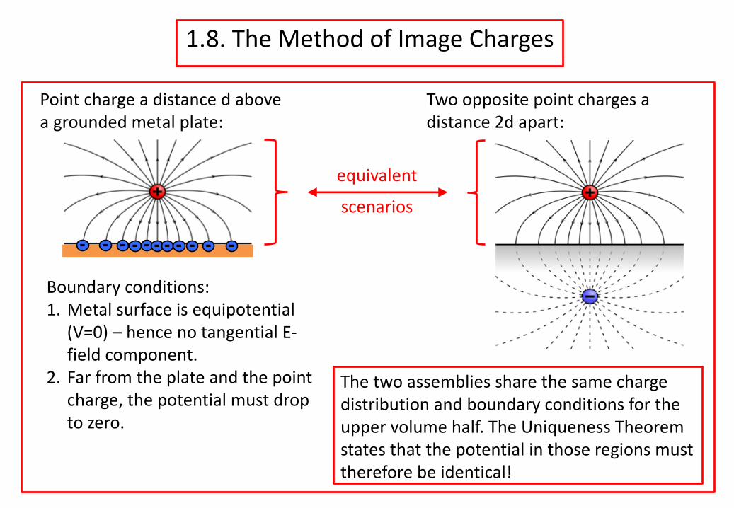
1.8. The Method of Image Charges
Point charge a distance d above
a grounded metal plate:
- -- - - - - - - - -
Boundary conditions:
1. Metal surface is equipotential
(V=0) – hence no tangential E-
field component.
2. Far from the plate and the point
charge, the potential must drop
to zero.
Two opposite point charges a
distance 2d apart:
The two assemblies share the same charge
distribution and boundary conditions for the
upper volume half. The Uniqueness Theorem
states that the potential in those regions must
therefore be identical!
equivalent
scenarios
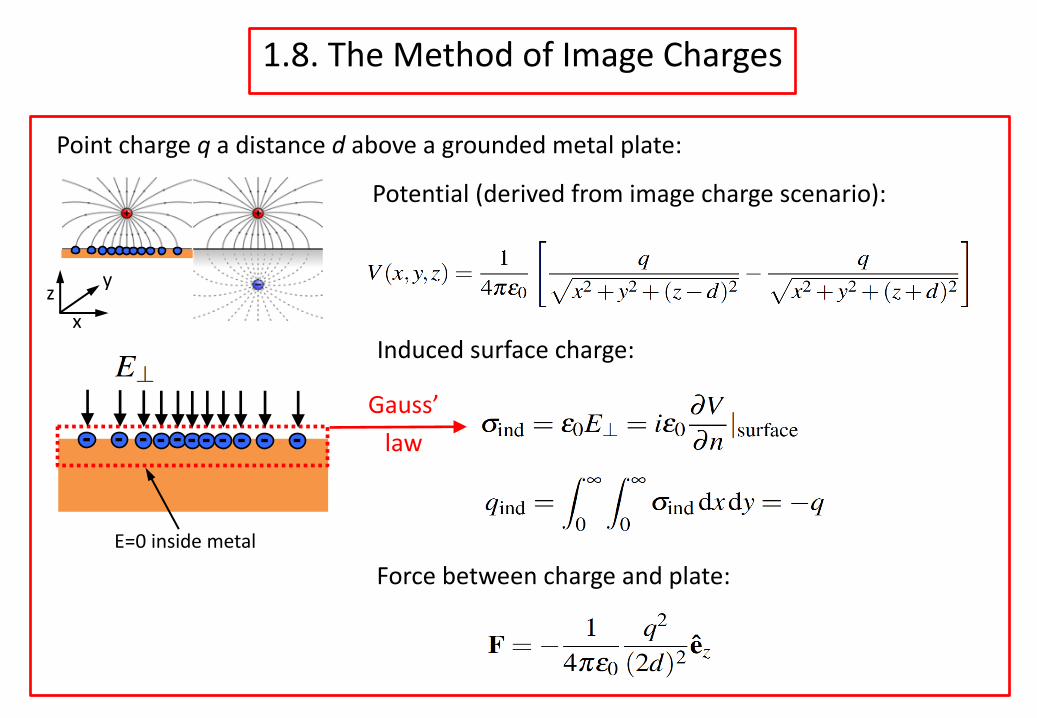
1.8. The Method of Image Charges
Point charge q a distance d above a grounded metal plate:
Potential (derived from image charge scenario):
Induced surface charge:
Force between charge and plate:
- -- - - - - - - - -
E=0 inside metal
Gauss’law
zx
y
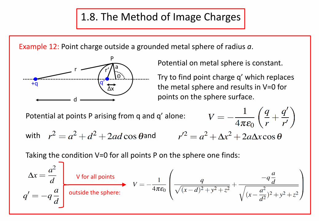
1.8. The Method of Image Charges
Potential on metal sphere is constant.
Try to find point charge q’ which replaces the metal sphere and results in V=0 for points on the sphere surface.
Example 12: Point charge outside a grounded metal sphere of radius a.
d
r
Δx+q q’
aΘ
r’
P
Potential at points P arising from q and q’ alone:
with and
Taking the condition V=0 for all points P on the sphere one finds:
V for all points
outside the sphere:
1.9. Capacitance
Capacitance: Storage of energy through separation of two oppositely poled charge accumulations
Capacitance C = charge Qvoltage V applied
V+Q- Q
(i) parallel-plate capacitor:
(ii) cylindrical capacitor:
(iii) spherical capacitor:
area Ad
a
b
l
a
b
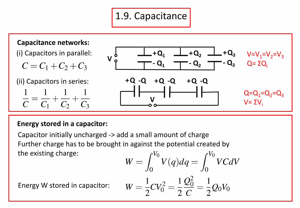
1.9. Capacitance
Capacitance networks:
Capacitor initially uncharged -> add a small amount of charge Further charge has to be brought in against the potential created by the existing charge:
Energy stored in a capacitor:
(i) Capacitors in parallel:
(ii) Capacitors in series:
+Q1- Q1
+Q2- Q2
+Q3- Q3
V
V
+Q -Q +Q -Q +Q -Q
V=V1=V2=V3Q= ΣQi
Q=Q1=Q2=Q3V= ΣVi
Energy W stored in capacitor:
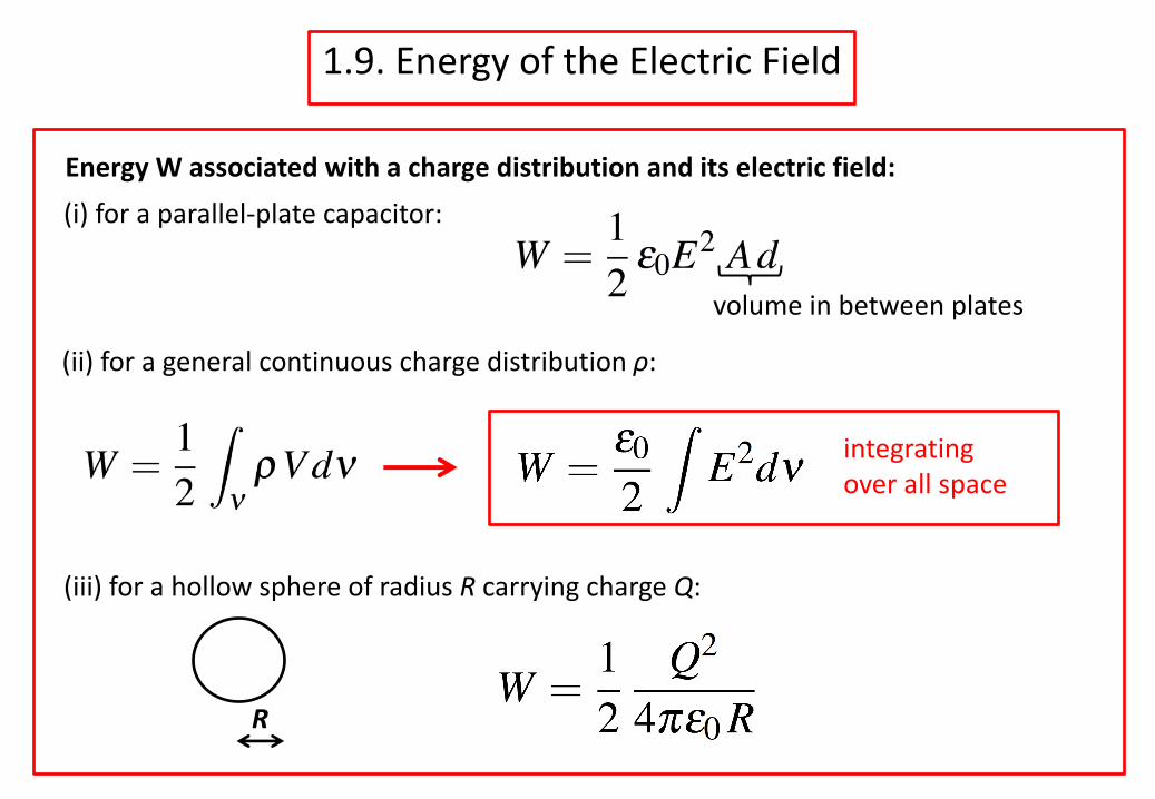
1.9. Energy of the Electric Field
(i) for a parallel-plate capacitor:
(ii) for a general continuous charge distribution ρ:
Energy W associated with a charge distribution and its electric field:
integrating over all space
(iii) for a hollow sphere of radius R carrying charge Q:
R
volume in between plates
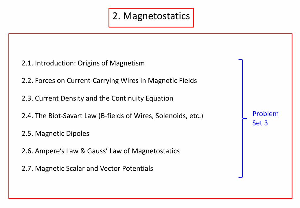
2. Magnetostatics
2.1. Introduction: Origins of Magnetism
2.2. Forces on Current-Carrying Wires in Magnetic Fields
2.3. Current Density and the Continuity Equation
2.4. The Biot-Savart Law (B-fields of Wires, Solenoids, etc.)
2.5. Magnetic Dipoles
2.6. Ampere’s Law & Gauss’ Law of Magnetostatics
2.7. Magnetic Scalar and Vector Potentials
Problem Set 3
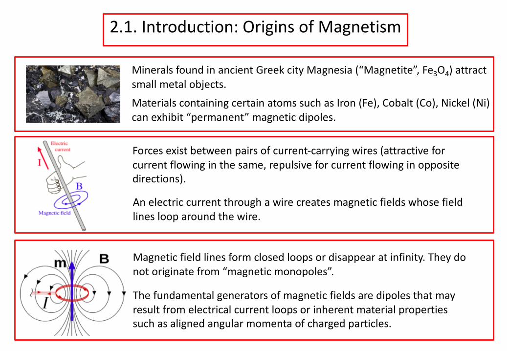
2.1. Introduction: Origins of Magnetism
Minerals found in ancient Greek city Magnesia (“Magnetite”, Fe3O4) attract small metal objects. Materials containing certain atoms such as Iron (Fe), Cobalt (Co), Nickel (Ni) can exhibit “permanent” magnetic dipoles.
An electric current through a wire creates magnetic fields whose field lines loop around the wire.
Forces exist between pairs of current-carrying wires (attractive for current flowing in the same, repulsive for current flowing in opposite directions).
Magnetic field lines form closed loops or disappear at infinity. They do not originate from “magnetic monopoles”.
The fundamental generators of magnetic fields are dipoles that may result from electrical current loops or inherent material properties such as aligned angular momenta of charged particles.
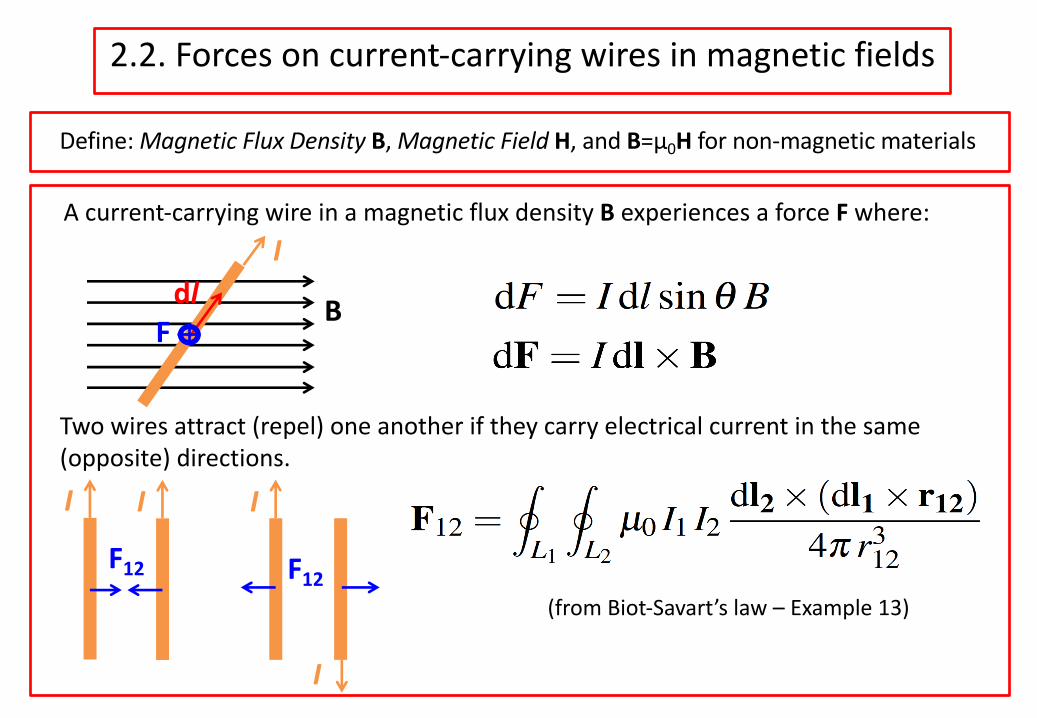
2.2. Forces on current-carrying wires in magnetic fields
Two wires attract (repel) one another if they carry electrical current in the same (opposite) directions.
A current-carrying wire in a magnetic flux density B experiences a force F where:
dlI
F B
I I
F12
I
I
F12(from Biot-Savart’s law – Example 13)
Define: Magnetic Flux Density B, Magnetic Field H, and B=μ0H for non-magnetic materials
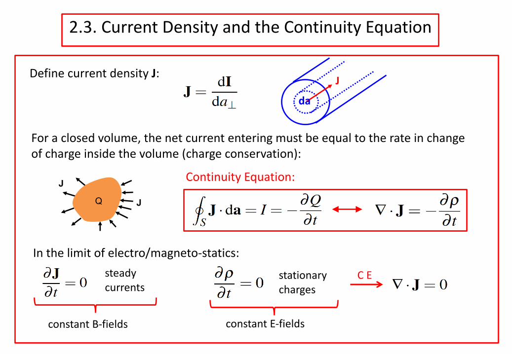
2.3. Current Density and the Continuity Equation
Define current density J: Jda
For a closed volume, the net current entering must be equal to the rate in change of charge inside the volume (charge conservation):
In the limit of electro/magneto-statics:steadycurrents
stationarycharges
constant B-fields constant E-fields
Continuity Equation:
C E
J
JQ
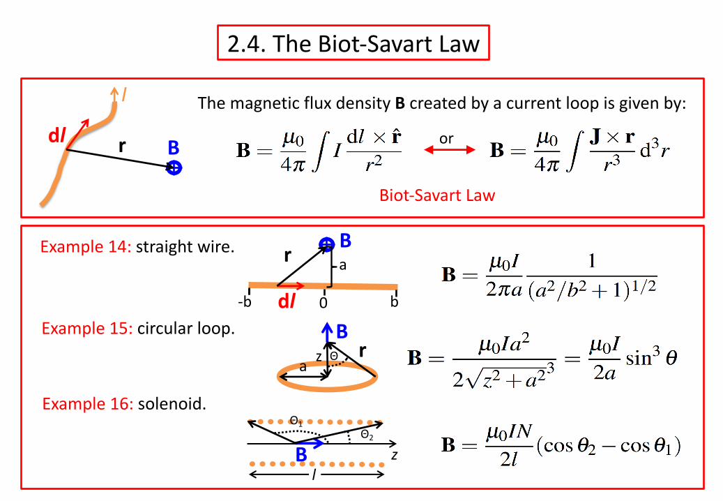
2.4. The Biot-Savart Law
The magnetic flux density B created by a current loop is given by:
dl
I
Br
Biot-Savart Law
or
B
dl
r
-b b0
aExample 14: straight wire.
Example 15: circular loop.
Example 16: solenoid.
Bza
rΘ
B zΘ2
Θ1
l
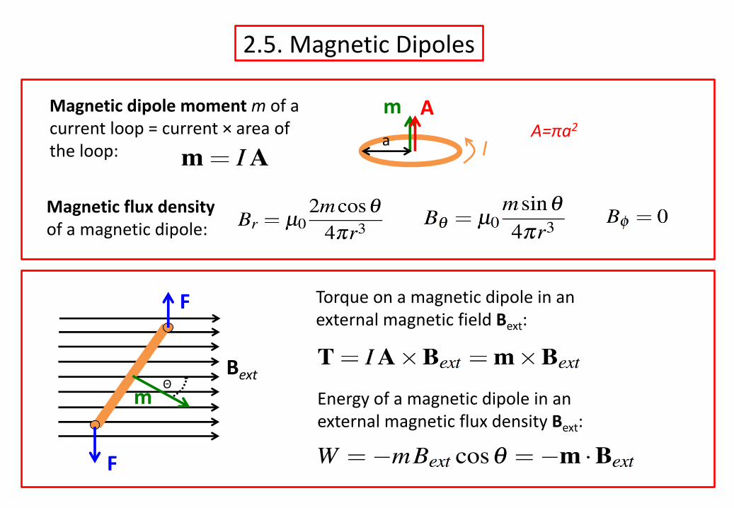
2.5. Magnetic Dipoles
Magnetic dipole moment m of a current loop = current × area of the loop:
Magnetic flux density of a magnetic dipole:
Energy of a magnetic dipole in an external magnetic flux density Bext:
Torque on a magnetic dipole in an external magnetic field Bext:
ma I
AA=πa2
F
Bextm
F
Θ
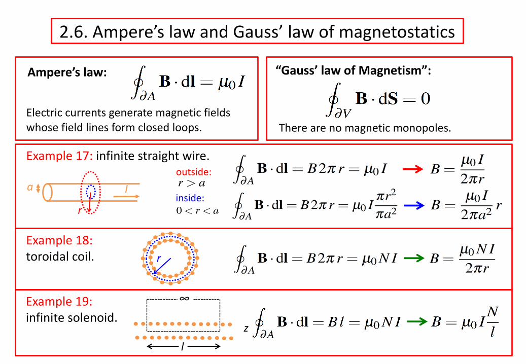
2.6. Ampere’s law and Gauss’ law of magnetostatics
Ampere’s law: “Gauss’ law of Magnetism”:
Electric currents generate magnetic fields whose field lines form closed loops. There are no magnetic monopoles.
Example 17: infinite straight wire.
Example 18: toroidal coil.
Example 19: infinite solenoid.
Ioutside:
inside:a
r
z
r
l
∞
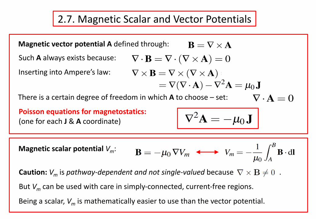
2.7. Magnetic Scalar and Vector Potentials
Magnetic vector potential A defined through:
Magnetic scalar potential Vm:
Such A always exists because:
Inserting into Ampere’s law:
There is a certain degree of freedom in which A to choose – set:
Poisson equations for magnetostatics:(one for each J & A coordinate)
But Vm can be used with care in simply-connected, current-free regions.
Being a scalar, Vm is mathematically easier to use than the vector potential.
Caution: Vm is pathway-dependent and not single-valued because .
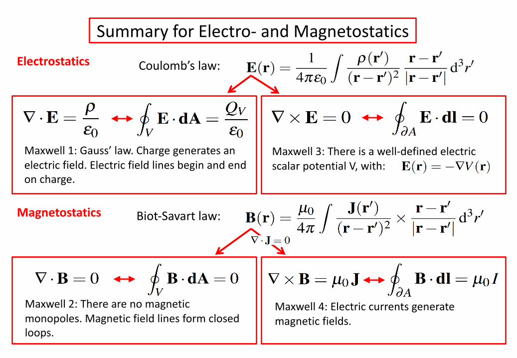
Summary for Electro- and Magnetostatics
Biot-Savart law:
Coulomb’s law:Electrostatics
Magnetostatics
Maxwell 1: Gauss’ law. Charge generates an electric field. Electric field lines begin and end on charge.
Maxwell 2: There are no magnetic monopoles. Magnetic field lines form closed loops.
Maxwell 4: Electric currents generate magnetic fields.
Maxwell 3: There is a well-defined electric scalar potential V, with:

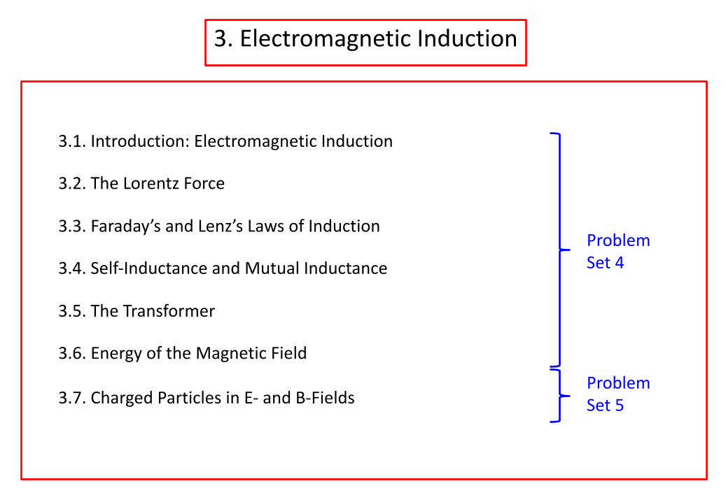
3. Electromagnetic Induction
3.1. Introduction: Electromagnetic Induction
3.2. The Lorentz Force
3.3. Faraday’s and Lenz’s Laws of Induction
3.4. Self-Inductance and Mutual Inductance
3.5. The Transformer
3.6. Energy of the Magnetic Field
3.7. Charged Particles in E- and B-Fields
Problem Set 4
Problem Set 5
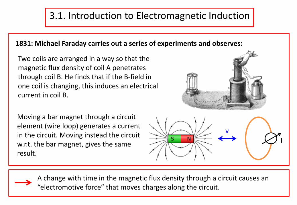
3.1. Introduction to Electromagnetic Induction
1831: Michael Faraday carries out a series of experiments and observes:
Two coils are arranged in a way so that the magnetic flux density of coil A penetrates through coil B. He finds that if the B-field in one coil is changing, this induces an electrical current in coil B.
Moving a bar magnet through a circuit element (wire loop) generates a current in the circuit. Moving instead the circuit w.r.t. the bar magnet, gives the same result.
A change with time in the magnetic flux density through a circuit causes an “electromotive force” that moves charges along the circuit.
Iv
3.2. The Lorentz Force
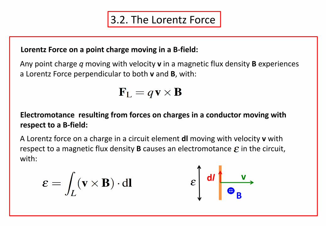
Lorentz Force on a point charge moving in a B-field:Any point charge q moving with velocity v in a magnetic flux density B experiences a Lorentz Force perpendicular to both v and B, with:
Electromotance resulting from forces on charges in a conductor moving with respect to a B-field:
dl
B
v
A Lorentz force on a charge in a circuit element dl moving with velocity v with respect to a magnetic flux density B causes an electromotance in the circuit, with:
3.3. Faraday’s and Lenz’s Laws of Induction
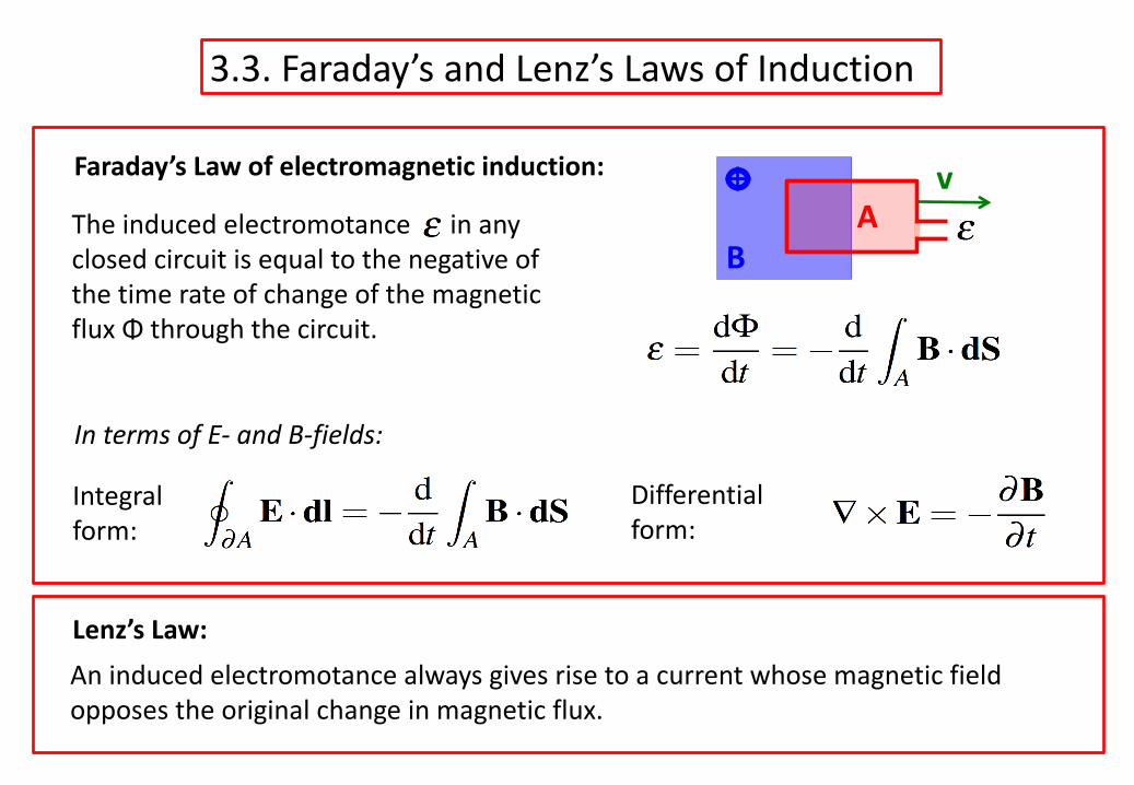
Faraday’s Law of electromagnetic induction:
An induced electromotance always gives rise to a current whose magnetic field opposes the original change in magnetic flux.
Lenz’s Law:
In terms of E- and B-fields:
The induced electromotance in any closed circuit is equal to the negative of the time rate of change of the magnetic flux Φ through the circuit.
BA
v
Integral form:
Differential form:
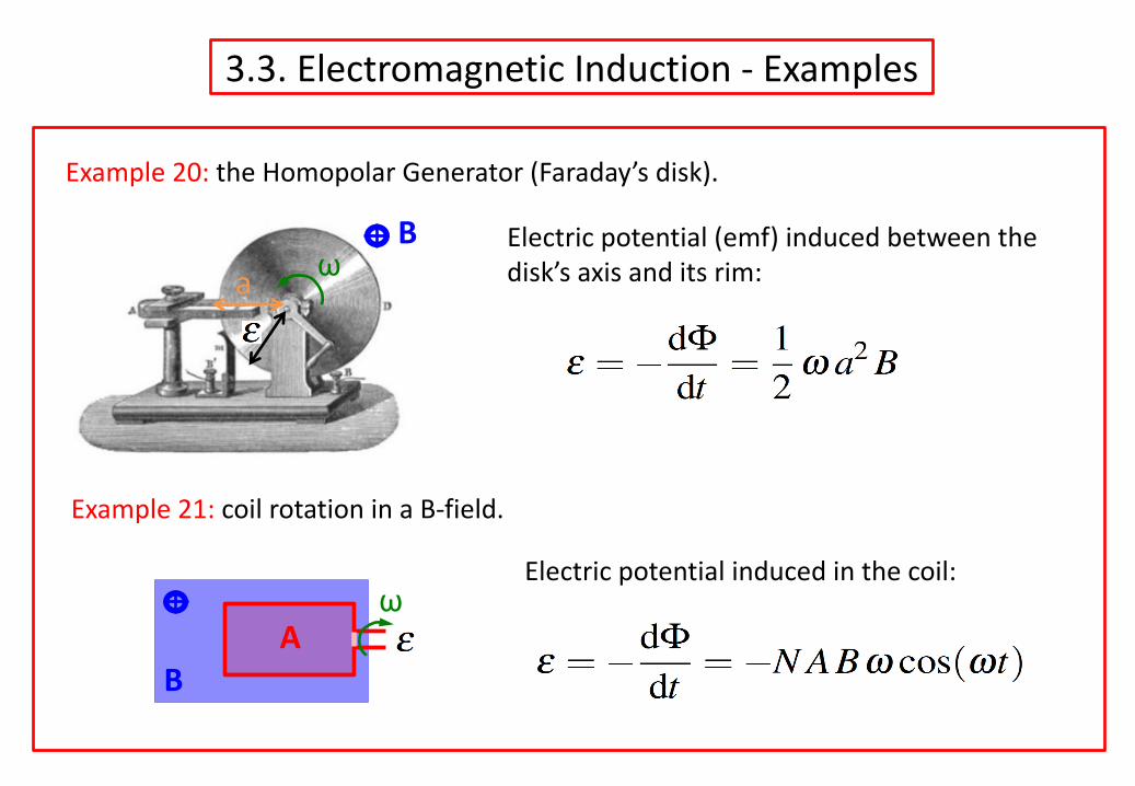
3.3. Electromagnetic Induction - Examples
Electric potential (emf) induced between the disk’s axis and its rim:
Example 20: the Homopolar Generator (Faraday’s disk).
Example 21: coil rotation in a B-field.
BA
ω
Ba ω
Electric potential induced in the coil:
3.4. Self-Inductance
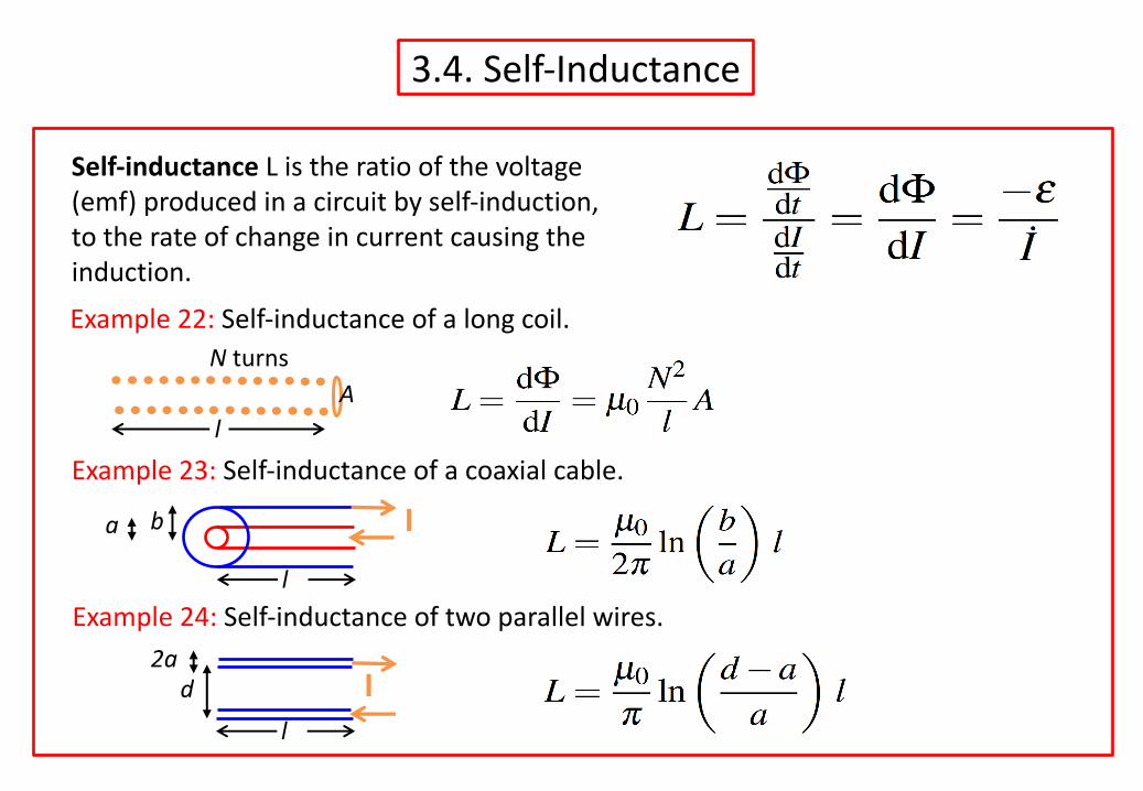
Self-inductance L is the ratio of the voltage (emf) produced in a circuit by self-induction, to the rate of change in current causing the induction.Example 22: Self-inductance of a long coil.
Example 23: Self-inductance of a coaxial cable.
Example 24: Self-inductance of two parallel wires.
lA
N turns
Iba
l
Id2a
l
3.4. Mutual Inductance
Mutual Inductance M: is the ratio of the voltage (emf) produced in a circuit by self-induction, to the rate of change in current causing the induction.
Example 25: Mutual inductance of two coaxial solenoids.
Neumannformula
l1
A1
N1 turns
A2
l2
N2 turns
I1
I2
B1
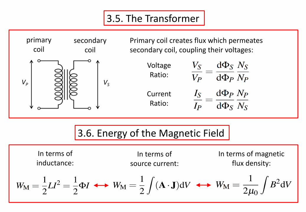
3.5. The Transformer
primarycoil
3.6. Energy of the Magnetic Field
secondarycoil
VP VS
Voltage Ratio:
CurrentRatio:
Primary coil creates flux which permeates secondary coil, coupling their voltages:
In terms of inductance:
In terms of source current:
In terms of magnetic flux density:
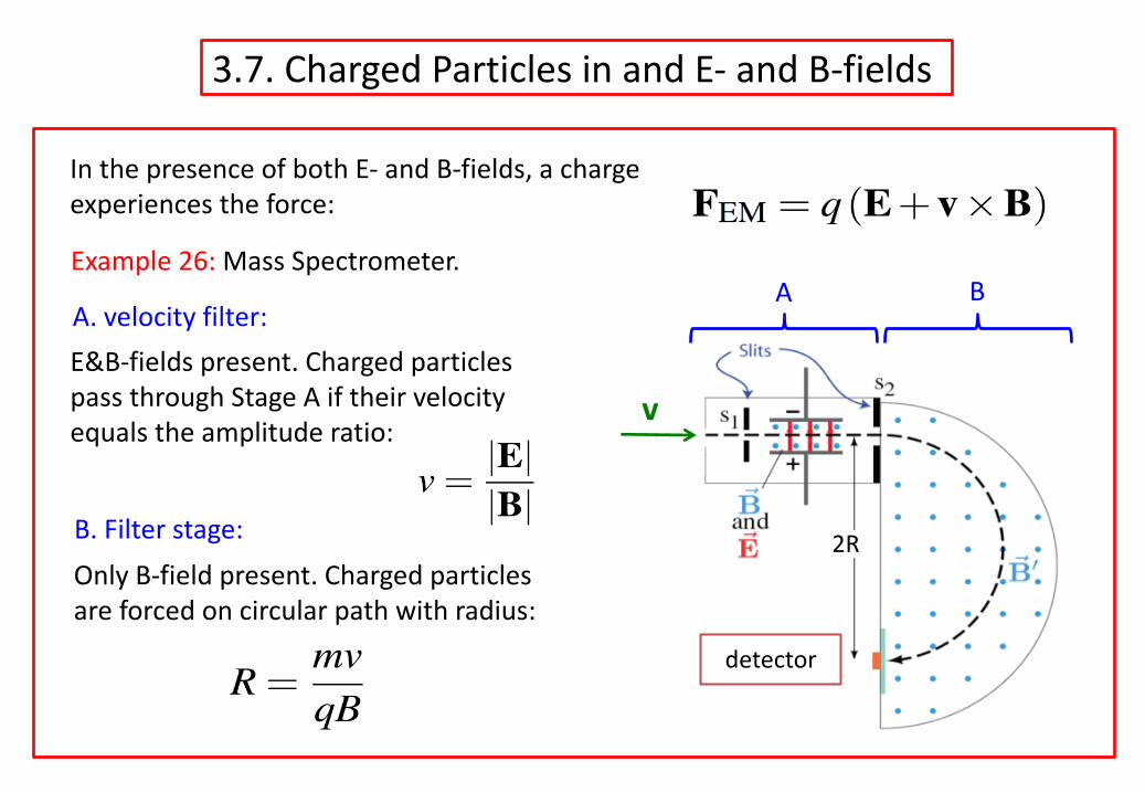
3.7. Charged Particles in and E- and B-fields
Example 26: Mass Spectrometer.
In the presence of both E- and B-fields, a charge experiences the force:
A. velocity filter:
B. Filter stage: 2R
detector
v
BA
E&B-fields present. Charged particles pass through Stage A if their velocity equals the amplitude ratio:
Only B-field present. Charged particles are forced on circular path with radius:
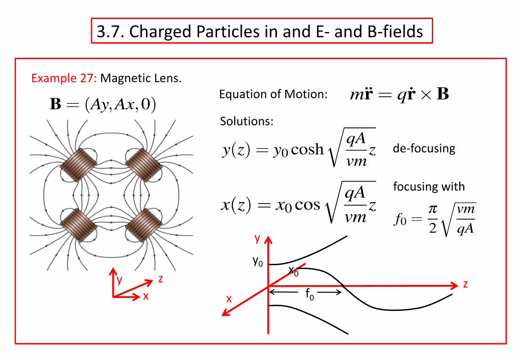
3.7. Charged Particles in and E- and B-fields
Example 27: Magnetic Lens.Equation of Motion:
yx
z
Solutions:
de-focusing
focusing with
y0
xz
y
x0
f0
4. Maxwell’s Equations and Electromagnetic Waves
4.1. Ampere’s Law and the Displacement Current
4.2. Maxwell’s Equations
4.3. Electromagnetic Waves in Vacuum
4.4. Energy Flow and The Poynting Vector
Problem Set 5
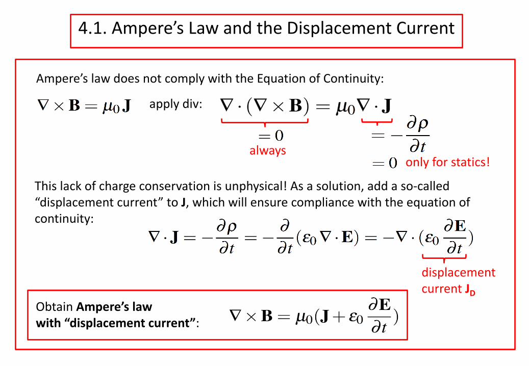
4.1. Ampere’s Law and the Displacement Current
Ampere’s law does not comply with the Equation of Continuity:
apply div:
This lack of charge conservation is unphysical! As a solution, add a so-called “displacement current” to J, which will ensure compliance with the equation of continuity:
alwaysonly for statics!
Obtain Ampere’s law with “displacement current”:
displacement current JD
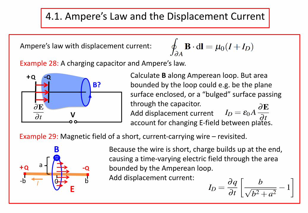
Calculate B along Amperean loop. But area bounded by the loop could e.g. be the plane surface enclosed, or a “bulged” surface passing through the capacitor.Add displacement current to account for changing E-field between plates.
4.1. Ampere’s Law and the Displacement Current
Ampere’s law with displacement current:
Example 28: A charging capacitor and Ampere’s law.
Example 29: Magnetic field of a short, current-carrying wire – revisited.
V
+Q -QB?
Because the wire is short, charge builds up at the end, causing a time-varying electric field through the area bounded by the Amperean loop. Add displacement current:
B
-b b
a+Q -Q
IE
0
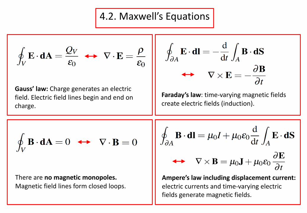
4.2. Maxwell’s Equations
Gauss’ law: Charge generates an electric field. Electric field lines begin and end on charge.
Faraday’s law: time-varying magnetic fields create electric fields (induction).
There are no magnetic monopoles.Magnetic field lines form closed loops.
Ampere’s law including displacement current: electric currents and time-varying electric fields generate magnetic fields.
4.3. Electromagnetic Waves in Vacuum
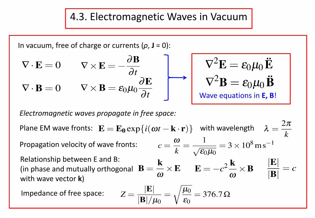
In vacuum, free of charge or currents (ρ, J = 0):
Wave equations in E, B!
Electromagnetic waves propagate in free space:
Propagation velocity of wave fronts:
Relationship between E and B:(in phase and mutually orthogonal with wave vector k)
Impedance of free space:
Plane EM wave fronts: with wavelength
4.4. Energy Flow and the Poynting Vector
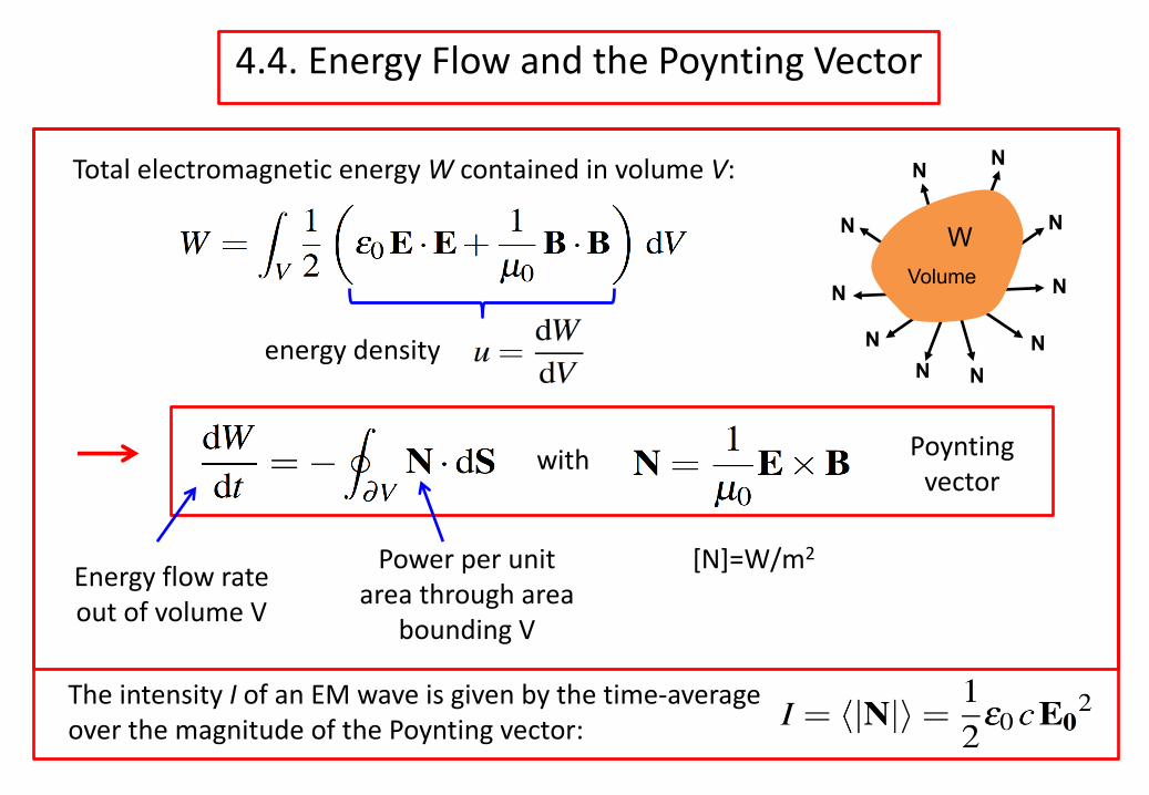
Total electromagnetic energy W contained in volume V:
energy density
N N
N
N
N
N
N
N
NN
WVolume
Energy flow rate out of volume V
Power per unit area through area
bounding V
with Poyntingvector
The intensity I of an EM wave is given by the time-average over the magnitude of the Poynting vector:
[N]=W/m2
4.4. Energy Flow and the Poynting Vector
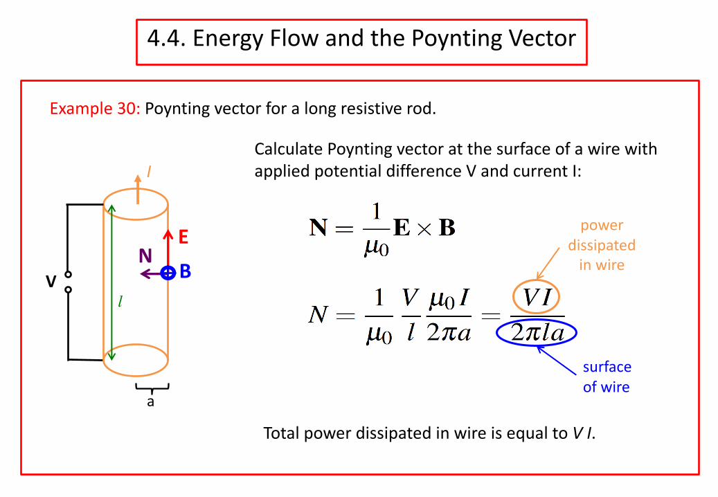
Calculate Poynting vector at the surface of a wire with applied potential difference V and current I:
Example 30: Poynting vector for a long resistive rod.
power dissipated
in wire
surface of wire
Total power dissipated in wire is equal to V I.
I
Vl
B
a
EN