WorkingPaper 303May2016

reap.fsi.stanford.edu

May2016

EffectofParentalMigrationontheAcademicPerformance

ofLeft-behindChildreninNorthwesternChina

YuBai,LinxiuZhang,ChengfangLiu,YaojiangShi,DiMo,ScottRozelle

Abstract

China’s rapid development and urbanization has induced large numbers of rural residents to migrate from their homes in the countryside to urban areas in search of higher wages. As a consequence, it is estimated that more than 60 million children in rural China are left behind and live with relatives, typically their paternal grandparents. These children are called Left Behind Children (or LBCs). There are concerns about the potential negative effects of parental migration on the academic performance of the LBCs that could be due to the absence of parental care. However, it might also be that when a child’s parents work in the city away from home, their remittances can increase the household’s income and provide more resources and that this can lead to better academic performance. Hence, the net impact of out-migration on the academic performance of LBCs is unclear.

This paper examines changes in academic performance before and after the parents of students out-migrate. We draw on a panel dataset collected by the authors of more than 13,000 students at 130 rural primary schools in ethnic minority areas of rural China. Using difference-in-difference and propensity score matching approaches, our results indicate that generally parental migration has significant, positive impacts on the academic performance of LBCs (which we measure using standardized English test scores). Heterogeneous analysis using our data demonstrates that the positive impact on LBCs is greater for poorer performing students.

Effect of Parental Migration on the Academic Performance of Left-behind Children in Northwestern China

Yu Bai1,2, Linxiu Zhang1, Chengfang Liu3, *, Yaojiang Shi4, Di Mo5,

Scott Rozelle5 1 Center for Chinese Agricultural Policy, Institute of Geographic Sciences and Natural Resources Research, Chinese Academy of Sciences, Beijing 100101, China

2 University of Chinese Academy of Sciences, Beijing 100049, China

3 Center for Chinese Agricultural Policy, School of Advanced Agricultural Sciences, Peking University, Beijing 100871, China

4 Center for Experimental Economics in Education (CEEE), Shaanxi Normal University, Xi’an 710119, China

5 Freeman Spogli Institute for International Studies, Stanford University, Stanford, USA

Corresponding author: Dr. Chengfang Liu Center for Chinese Agricultural Policy School of Advanced Agricultural Sciences, Peking University Yiheyuan Road No. 5, Haidian District, Beijing, 100871, China Email : cfliu.ccap@pku.edu.cn; Phone : 86-180-117-5311; Fax: 86-10-6485-6533

Acknowledgments The authors acknowledge the financial support from the National Natural Science Foundation of China (grant numbers 71473240, 71333012).

2

Effect of Parental Migration on the Academic Performance of Left-behind Children in Northwestern China

Abstract:

China’s rapid development and urbanization has induced large numbers of rural residents to migrate from their homes in the countryside to urban areas in search of higher wages. As a consequence, it is estimated that more than 60 million children in rural China are left behind and live with relatives, typically their paternal grandparents. These children are called Left Behind Children (or LBCs). There are concerns about the potential negative effects of parental migration on the academic performance of the LBCs that could be due to the absence of parental care. However, it might also be that when a child’s parents work in the city away from home, their remittances can increase the household’s income and provide more resources and that this can lead to better academic performance. Hence, the net impact of out-migration on the academic performance of LBCs is unclear. This paper examines changes in academic performance before and after the parents of students out-migrate. We draw on a panel dataset collected by the authors of more than 13,000 students at 130 rural primary schools in ethnic minority areas of rural China. Using difference-in-difference and propensity score matching approaches, our results indicate that generally parental migration has significant, positive impacts on the academic performance of LBCs (which we measure using standardized English test scores). Heterogeneous analysis using our data demonstrates that the positive impact on LBCs is greater for poorer performing students. Keywords: migration, academic performance, left-behind children, difference-in-difference, rural China JEL classification: O12, O15

1

Effect of Parental Migration on the Academic Performance of Left-behind

Children in Northwestern China

Introduction

China’s rapid development and urbanization has induced large numbers of

rural residents to migrate from their homes in the countryside to urban areas (Hu et al.,

2008; Wen and Lin, 2012; MHRSS, 2013). In the course of migration, it is common

for migrants to leave their children behind in their home communities with a surrogate

caregiver (Ye et al., 2006). As a consequence, in the past decade a new population has

emerged in China known as Left Behind Children, henceforth LBCs (Duan and Zhou,

2005). Statistics from the Sixth Population Census show that there were more than 61

million LBCs in China (ACWF, 2013), of which one-third are still enrolled in

compulsory education (MOE, 2014).

The education of LBCs has drawn attention from researchers, though the

literature is mixed concerning the direction of the effect of parental migration on the

academic performance of LBCs (Yang, 2008; Chen et al., 2009; Lahaie et al., 2009;

Giannelli and Mangiavacchi, 2010; Chang et al., 2011; Antman, 2012; Lu, 2012;

Wang, 2014; Xu and Xie, 2015; Roy et al., 2015). In some cases, researchers have

found a positive relationship between parental migration and academic performance

of LBCs (Yang, 2008; Chen et al., 2009; Roy et al., 2015). Research finds that this

may occur through mechanisms such as relaxing household liquidity constraints (Du

et al., 2005) and encouraging higher investments in LBCs (Edwards and Ureta, 2003;

Yang, 2008; Lu and Treiman, 2011; Antman, 2012; Ambler et al., 2015; Malik, 2015).

However, some researchers claim that they have identified negative effects of parental

migration on the educational outcomes of LBCs (Meyerhoefer and Chen, 2011; Zhao

et al., 2014; Zhou et al., 2014; Zhang et al., 2014). These researchers find that the

2

negative effects are mainly due to the absence of parental care (Lahaie et al., 2009; Ye

and Lu, 2011) or to the increased time LBCs spend at home doing on-farm or in-home

work (Chang et al., 2011; Mckenzie and Rapoport; 2011). Additionally, other studies

have found that there is no relationship between parental migration and the academic

performance of LBCs (Zhou et al., 2015).

While many studies have examined the effect of being an LBC on learning

and other educational outcomes, there are a number of systematic weaknesses in the

literature that may account for the mixed impacts. First, some of the studies do not

have a valid comparison group (e.g. Lahied, 2009; Meyerhoefer and Chen, 2011;

Zhou et al., 2014). Second, many of the previous studies are based on samples that are

quite small (Ye and Lu, 2011; Lu, 2012; Zhou et al., 2014). Third, some of the studies

do not use careful measures of academic performance which may not serve as an

objective measure of educational outcomes (Chen et al., 2009).

In addition, most studies only examine the overall effect of being an LBC on

educational outcomes and do not consider the fact that there may be important

heterogeneous effects which may account for the differences in findings among the

studies. For example, only a limited number of previous studies distinguish between

the effects of the paternal and maternal migrant status when estimating the impact on

academic performance of LBCs (Chen et al., 2009; Antman, 2013; Wang, 2014). Also,

some studies show that the effect of parental migration on academic performance

varies by the gender of LBCs (Wang, 2014) or the mother’s level of education

(Sawyer, 2014).

The overall goal of this study is to examine the effects of parental migration

on the academic performance of LBCs. To meet this goal, we have three specific

objectives. First, we compare the distribution of children’s scores across different

3

types of households. Second, we use difference-in-difference and propensity score

matching approaches to examine whether parental migration affects the academic

performance of LBCs. Third, we examine how the impact of parental migration varies

by different sample characteristics, such as a student’s gender, his/her starting

academic performance, his/her household social economic status, and the level of

his/her mother’s education. These analyses will help us identify the heterogeneous

impact of different types of household migration on the educational outcomes of

LBCs.

Data

In order to achieve our objectives, we conducted two rounds of surveys: a

baseline survey and an endline survey. A total of 13,055 students in 130 elementary

schools participated in our study. In the following subsections, we present the study’s

sampling protocol and data collection approach.

Sampling

Our sampling frame was restricted to Haidong Prefecture, a poor minority area

in Qinghai Province in northwest China. In order to create a sample with enough

variation in household migration status to conduct our analysis, we chose to focus our

study on poor, rural areas with high population densities and high rates of off-farm

employment. A quarter of the population of Qinghai lives in Haidong Prefecture, even

though it accounts for only about 2% of the province’s total area. Additionally, of the

six counties in the prefecture, five of the counties are nationally designated poor

counties (National Bureau of Statistics of China, 2014). For these reasons, Haidong

Prefecture was determined to be a suitable location to select our sample.

The next step in the sampling protocol was to choose the sample schools. We

obtained a comprehensive list of schools in our six sample counties from each

4

county’s education bureau. Based on these lists, we randomly selected 130 schools

with classes in grades 1 to 6 in the six sample counties to be included in our sample.

We decided to focus on students in the fourth and fifth grades for two reasons.

We believe that students of this age were old enough to be able to fill out their own

survey forms and take a standardized examination, but also young enough that they

could be followed for a sufficient period of time. In each grade, we randomly selected

2 classes (if there were more than 2 classes in the grade). On average there were 1.3

fourth grade classes and 1.4 fifth grade classes per school. All students in sample

classes participated in our survey. In total, the sample included 13,055 students.

Descriptive statistics generated from our data show that the profile of sample

students is fairly typical of students from rural areas. Approximately 48.2% of the

sample students were girls. In the annual yearbook published by the Ministry of

Education (2014), girls in rural China account for nearly the same percentage, 47

percent, of each of China’s cohorts that are in rural schools.1 The age of the students

ranged between 9 and 18 years in 2003 when we conducted the baseline survey.

However, 99% of the students were between the ages of 9 and 13 years.

Although at the time of the baseline survey the sample included a total of 130

schools and 13,055 students, there was some attrition (848 students) by the end of the

study, primarily due to school transfers or absence due to illness/injury. This rate of

attrition is low compared to other studies conducted with children in rural China (Mo

et al., 2014; Lai et al., 2015) and unlikely to impact our findings. By the time of the

endline survey in 2014, we were able to follow up with 12,207 students.

Data collection 1 According to our calculation using data published by statistical yearbooks of Shaanxi, Ningxia, Qinghai, Gansu and Xinjiang, in 2013, girls in rural areas of northwest China also account for nearly the same percentage, namely, 47%, of the class.

5

The research group conducted two waves of surveys in the 130 sample schools.

The first round of survey was a baseline survey conducted with all students in all

sample schools in September 2013 at the beginning of the academic school year. The

second wave of the survey was our endline survey, which was conducted at the end of

June in 2014, a time that coincided with the end of the 2013-2014 academic year.

Academic performance

In each wave of the survey, the enumeration team visited all 130 schools and

conducted a three-part survey. In the first part students were given a 30-minute

standardized English test, the scores of which we used as our measure of student

academic performance. Before each round of the survey, we tested the English test

items with over two hundred 4th and 5th grade students to ensure the quality of the

baseline and endline English examinations. All the questions in the endline test were

different from those in the baseline test. We administered and printed the test

ourselves to ensure that it was not possible for the students to prepare for the

examination. Also, our enumeration team strictly proctored the test in order to

minimize cheating. The team also enforced time limits for the examinations.

We use the standardized English test scores as our measure of academic

performance. English test scores were measured during the endline and baseline

surveys using a 30 minute English tests. The English tests were constructed by trained

psychometricians. Mathematics test items for the endline and baseline tests were first

selected from the standardized English curricula for primary school students in China

(and Qinghai provinces in particular) and the content validity of these test items was

checked by multiple experts. The psychometric properties of the test were then

checked using data from extensive pilot testing. We use standardized test scores rather

than raw test scores to make student performance comparable across different grades

6

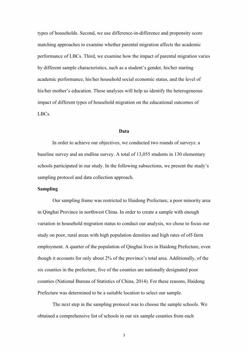
and classes, different periods, and different cohorts. Specifically, in order to

standardize each individual observation we subtracted the mean of the comparison

group and divided by the standard deviation (SD) of the distribution of the

comparison group (the comparison group consists of the households that neither

mother nor father out migrated between the two rounds of surveys—for more details

of the group, please see the subsection below). Therefore, a standardized score of 0.2

represents someone who scored 0.2 standard deviations above the average of the

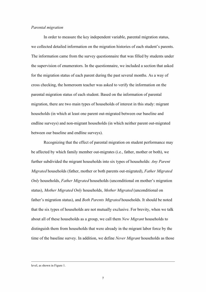
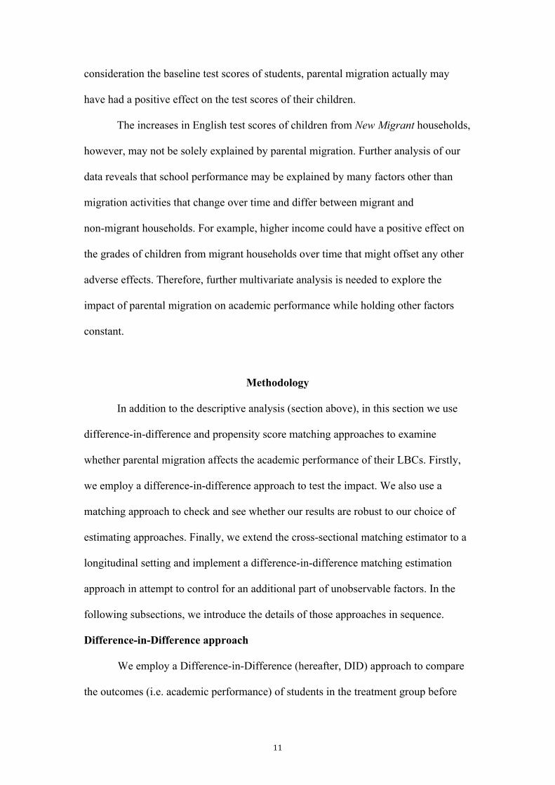
comparison group. We standardized scores by the grades of the students separately.

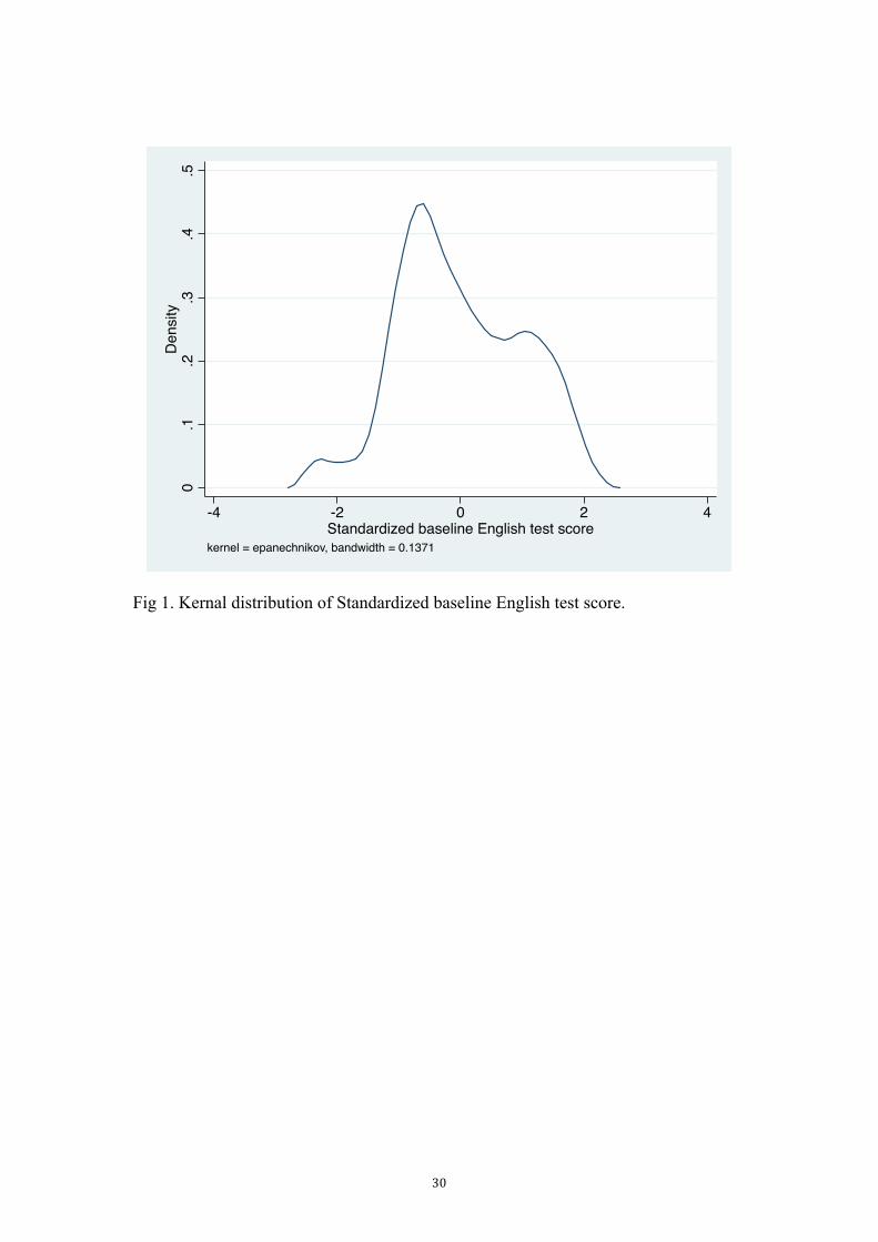
Figure 1 depicts the distribution of the standardized baseline English test scores.

We chose English as our subject of study interest for two reasons. First,

English is one of the main subjects included as part of the competitive examination

system in China that determines entrance into both senior high school and college

(McKay, 2002; Bolton and Graddol, 2012). It is a fact that for the past decade or more

English takes up nearly the same share as Math and Chinese in China’s national high

school and college entrance exams (zhongkao and gaokao). Specifically, the share of

English in the overall exam ranges from 20 percent to 25 percent.

Second, English teaching and English learning are particularly weak in poor

areas of rural China (Li, 2002; Zhao, 2003; Hu, 2005; Hu, 2009). Studies have shown

that a low English score is one of the largest impediments against keeping rural

students from attending senior high school in China (Loyalka, 2014). Because of this,

it must certainly be true that low competency in English would seriously hinder the

academic progress of rural students. Due to these reasons we believe that English is

an appropriate subject that we can use in the our study to measure student academic

performance.2

2 Before each round of the survey, we tested the English test items with over 200 fourth and fifth grade students to construct baseline and endline English exams. In doing so, our test is with moderate difficulty and high distinction

7

Parental migration

In order to measure the key independent variable, parental migration status,

we collected detailed information on the migration histories of each student’s parents.

The information came from the survey questionnaire that was filled by students under

the supervision of enumerators. In the questionnaire, we included a section that asked

for the migration status of each parent during the past several months. As a way of

cross checking, the homeroom teacher was asked to verify the information on the

parental migration status of each student. Based on the information of parental

migration, there are two main types of households of interest in this study: migrant

households (in which at least one parent out-migrated between our baseline and

endline surveys) and non-migrant households (in which neither parent out-migrated

between our baseline and endline surveys).

Recognizing that the effect of parental migration on student performance may

be affected by which family member out-migrates (i.e., father, mother or both), we

further subdivided the migrant households into six types of households: Any Parent

Migrated households (father, mother or both parents out-migrated), Father Migrated

Only households, Father Migrated households (unconditional on mother’s migration

status), Mother Migrated Only households, Mother Migrated (unconditional on

father’s migration status), and Both Parents Migrated households. It should be noted

that the six types of households are not mutually exclusive. For brevity, when we talk

about all of these households as a group, we call them New Migrant households to

distinguish them from households that were already in the migrant labor force by the

time of the baseline survey. In addition, we define Never Migrant households as those

level, as shown in Figure 1.

8

in which both parents stayed at home in both 2013 and 2014. Appendix Table 1

contains a list of the key independent variable names and definitions.

We use these types of parental migration variables to evaluate the effects of

parental migration on the academic performance of LBCs. We make use of the

variation in household migration status during the period of time between the baseline

and endline surveys to evaluate the effect of migration status on school outcomes. In

doing so, conceptually, our sample students are being divided into a treatment group

(New Migrant households) and a comparison group (Never Migrant households).

Sub-treatments in this framework are carried out using the six different types of

migrant households.

Other covariates

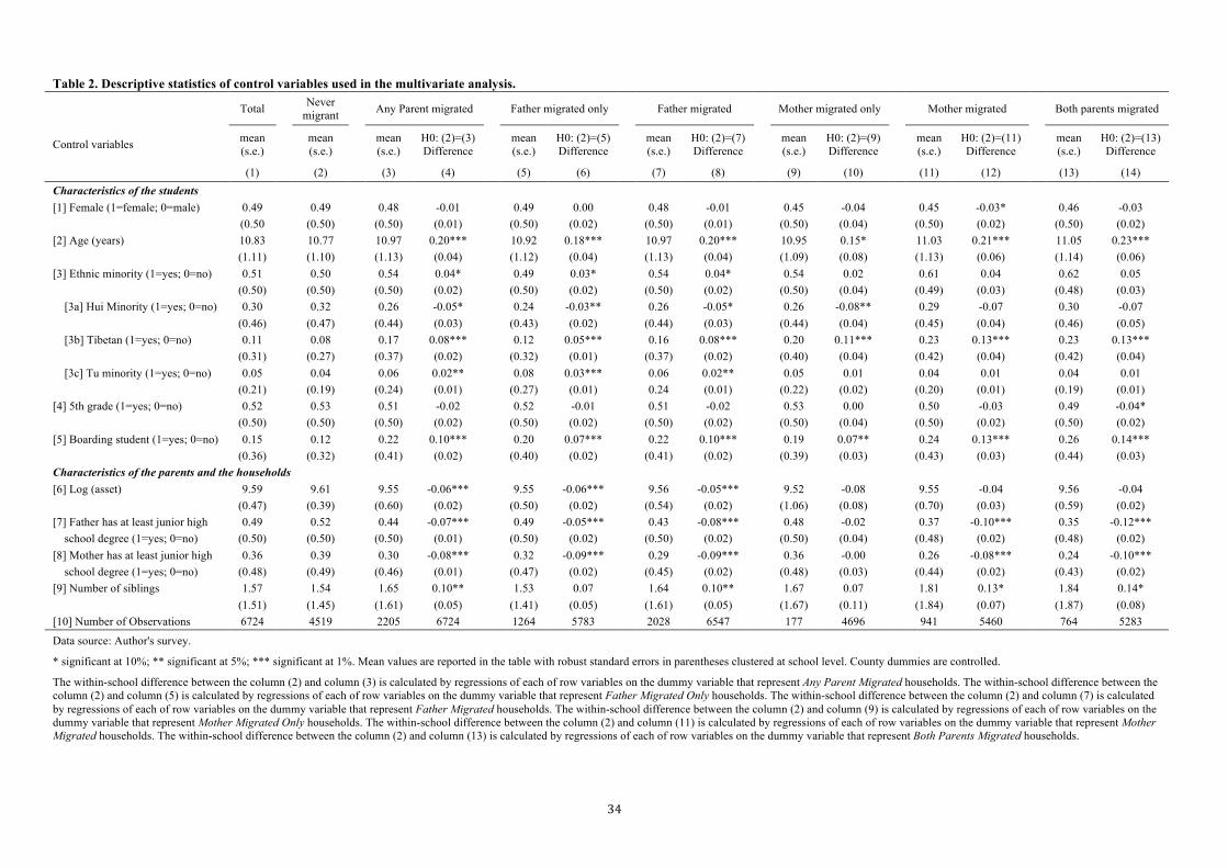
In the third part of the survey we collected data on the characteristics of the

sample students. From this part of the survey we were able to create a set of

demographic and socioeconomic variables. The dataset includes measures of each

student’s characteristics, such as female, age, ethnic minority, 5th grade, boarding

student. We also created a number of variables measuring family characteristics,

including assets,3 father has junior high school or higher degrees, mother has junior

high school or higher degrees, and number of siblings. This information is beneficial

to our research for two reasons: first, it allows us to explore whether the effects of

parental migration on the school performance of LBCs are heterogeneous across

children and households; second, these variables may directly affect school

performance and by controlling for them we may more efficiently measure the effect

of parental migration on school performance.

3 Asset is calculated by each account of family durable goods multiplying by their prices, then sum all index

and take the logarithm.

9

Parental Migration and Academic Performance

In this section we seek to compare the distribution of children’s scores across

households of different migrant status. To do so, we first describe the prevalence of

migrant households. Then, we present the correlations between migration and

academic performance by comparing changes in academic performance of LBCs in

the periods before and after their parents out-migrated with changes in migration

status.

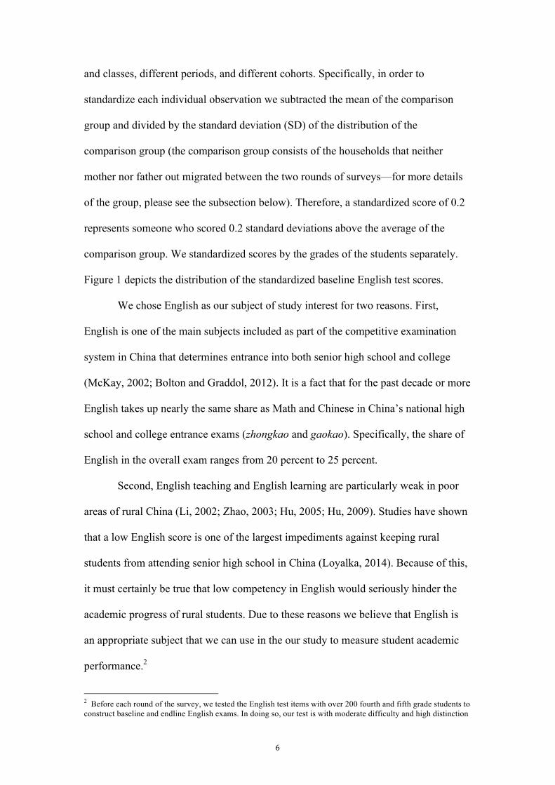
Prevalence of Migrant Households

Similar to the state of migration in many other rural areas in China (Rozelle et

al., 1999), many households were already in the migrant labor force in 2013 when we

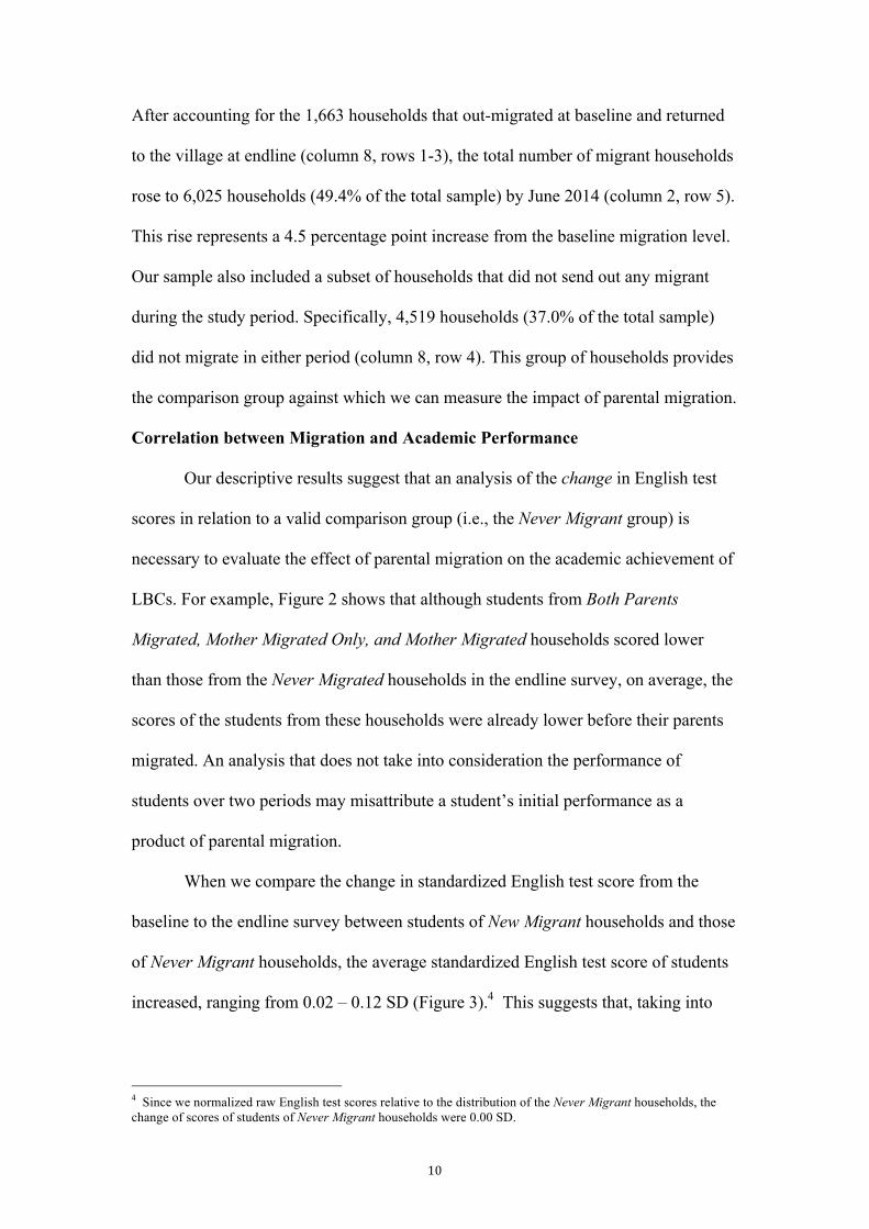
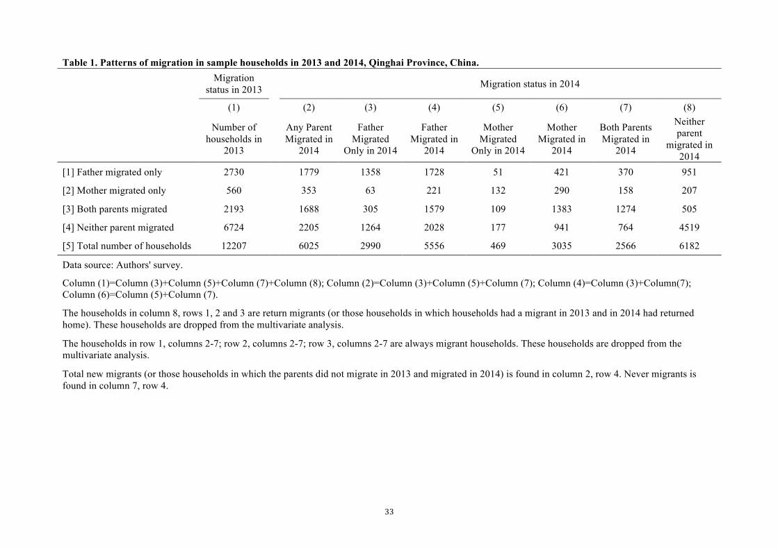
conducted the baseline survey. Of the 12,207 households in our sample, there were

5,483 (44.9%) households in which at least one parent out-migrated (Table 1, column

1, rows 1-3). Within our sample of migrant households, we found differences in

prevalence among types of migration. Of the 5,483 households with out-migrants,

only the father out-migrated in 2,730 households, this accounts for 22.4% of the total

number of households or 49.8% of the migrant households (column 1, row 1). In

contrast, only the mother out-migrated in 560 households, which accounts for 4.6% of

the total households or 10.2% of migrant households (column 1, row 2). According to

our data, both parents out-migrated in 2,193 households, which is 18.0% of the total

number of households or 40.0% of migrant households (column 1, row 3).

In addition, our study finds that the number of new migrant households in our

sample rose rapidly during the study period. Among the 6,724 households that did not

have any migrating parents in 2013 (column 1, row 4), at least one of the parents in

2,205 (32.8%) of these households entered the migrant labor force between the

September 2013 baseline survey and the June 2014 endline survey (column 2, row 4).

10

After accounting for the 1,663 households that out-migrated at baseline and returned

to the village at endline (column 8, rows 1-3), the total number of migrant households

rose to 6,025 households (49.4% of the total sample) by June 2014 (column 2, row 5).

This rise represents a 4.5 percentage point increase from the baseline migration level.

Our sample also included a subset of households that did not send out any migrant

during the study period. Specifically, 4,519 households (37.0% of the total sample)

did not migrate in either period (column 8, row 4). This group of households provides

the comparison group against which we can measure the impact of parental migration.

Correlation between Migration and Academic Performance

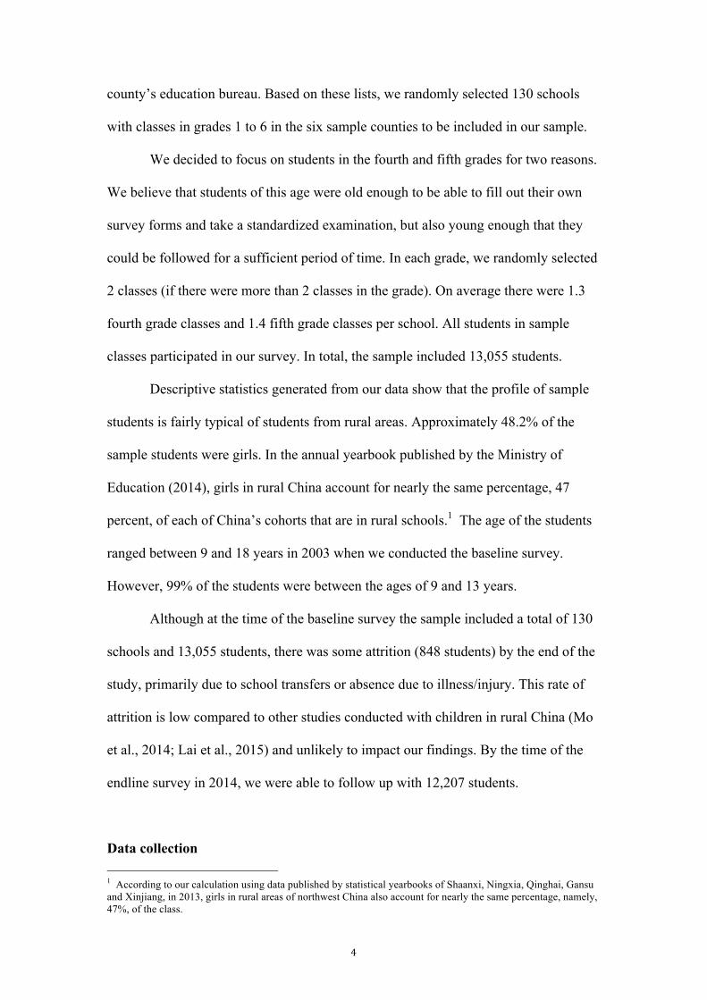
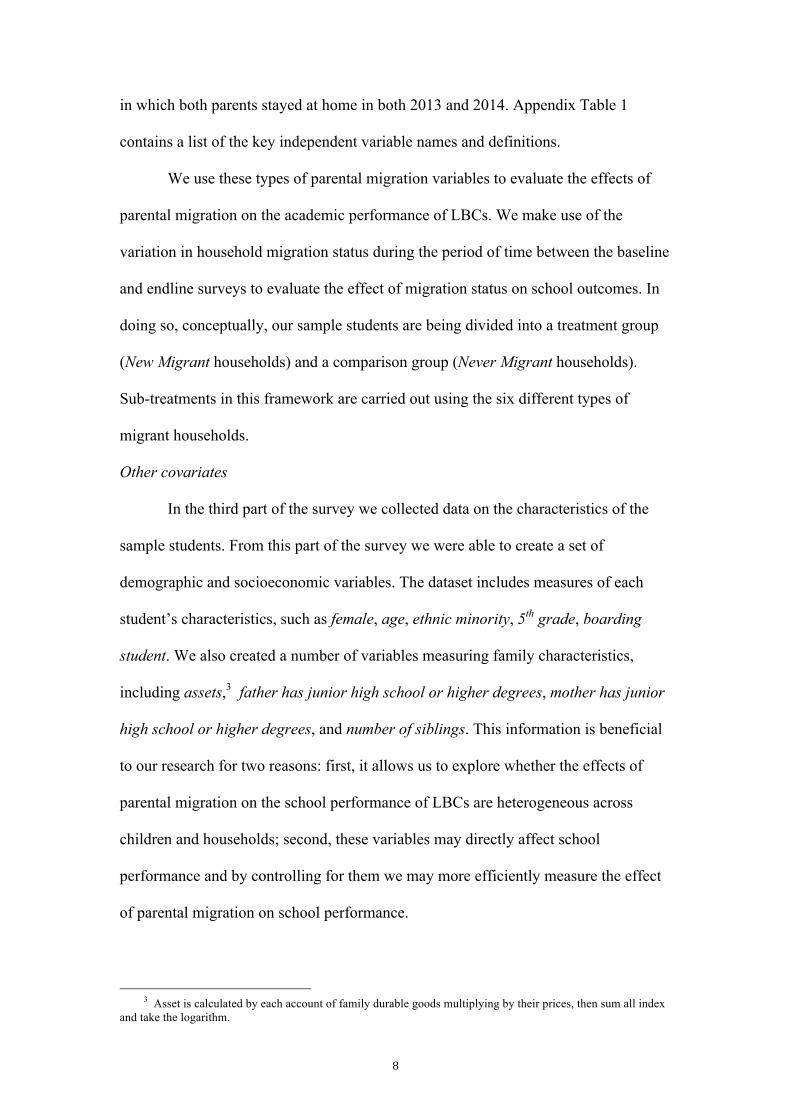
Our descriptive results suggest that an analysis of the change in English test

scores in relation to a valid comparison group (i.e., the Never Migrant group) is

necessary to evaluate the effect of parental migration on the academic achievement of

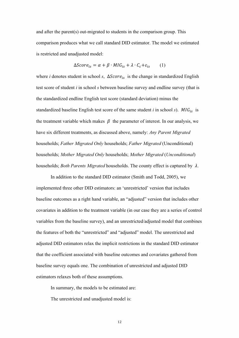
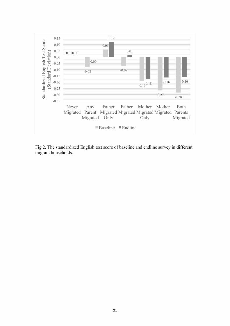
LBCs. For example, Figure 2 shows that although students from Both Parents

Migrated, Mother Migrated Only, and Mother Migrated households scored lower

than those from the Never Migrated households in the endline survey, on average, the

scores of the students from these households were already lower before their parents

migrated. An analysis that does not take into consideration the performance of

students over two periods may misattribute a student’s initial performance as a

product of parental migration.

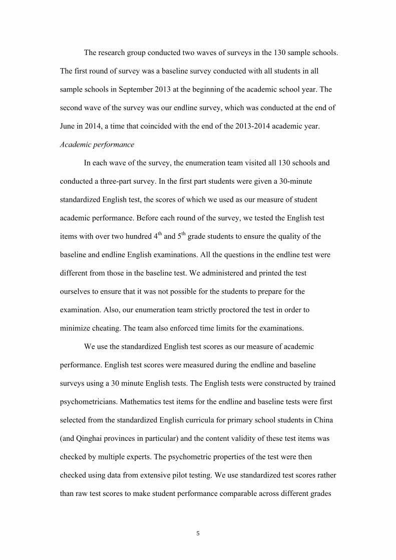
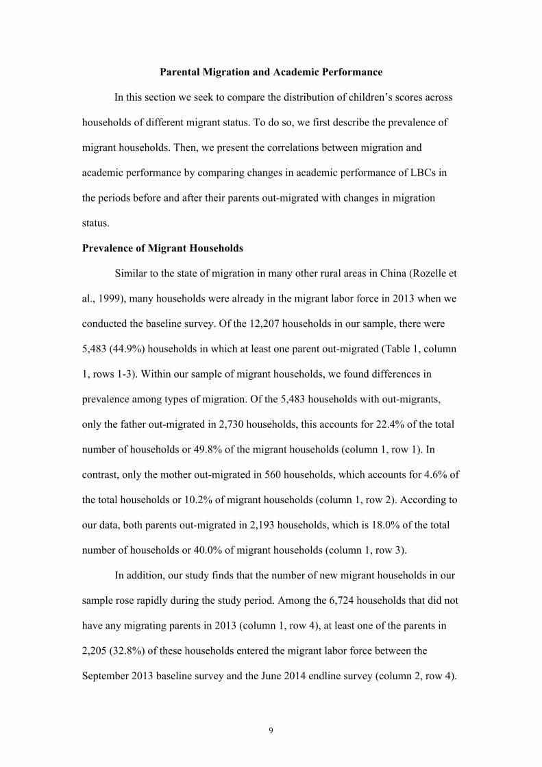
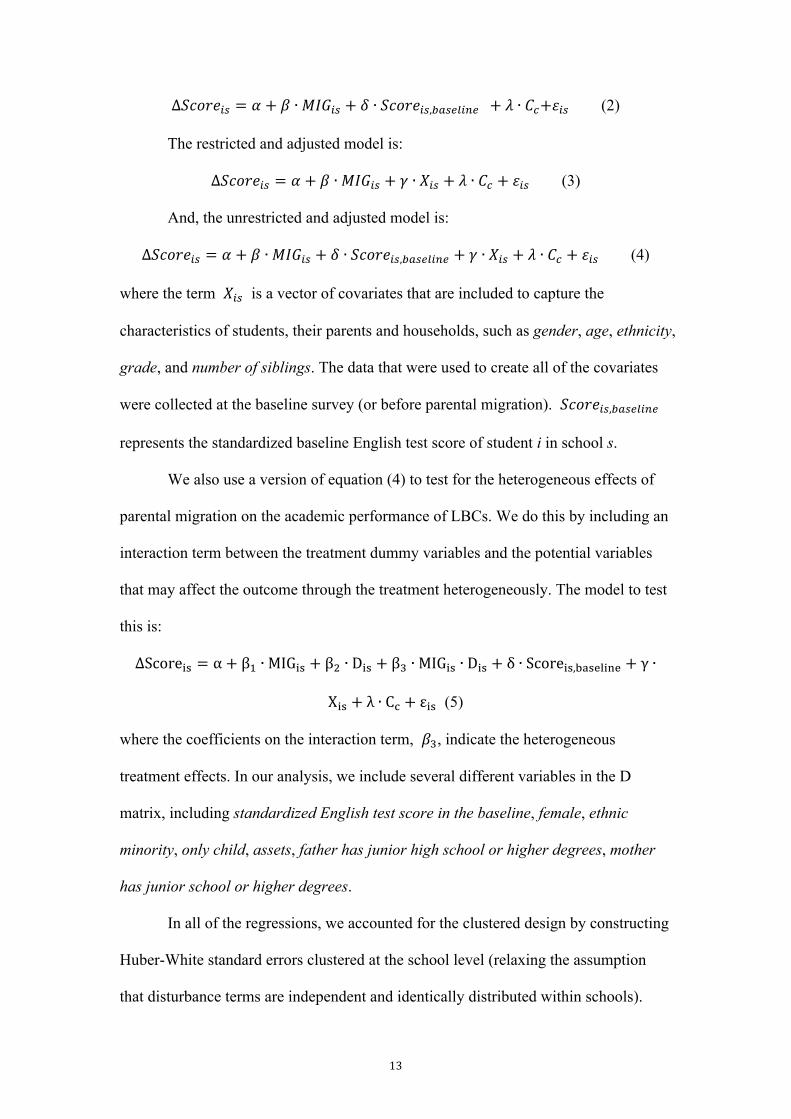
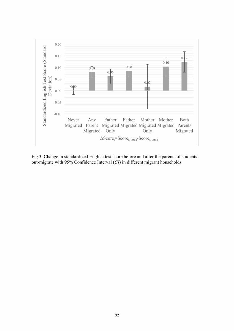
When we compare the change in standardized English test score from the

baseline to the endline survey between students of New Migrant households and those

of Never Migrant households, the average standardized English test score of students

increased, ranging from 0.02 – 0.12 SD (Figure 3).4 This suggests that, taking into

4 Since we normalized raw English test scores relative to the distribution of the Never Migrant households, the change of scores of students of Never Migrant households were 0.00 SD.

11

consideration the baseline test scores of students, parental migration actually may

have had a positive effect on the test scores of their children.

The increases in English test scores of children from New Migrant households,

however, may not be solely explained by parental migration. Further analysis of our

data reveals that school performance may be explained by many factors other than

migration activities that change over time and differ between migrant and

non-migrant households. For example, higher income could have a positive effect on

the grades of children from migrant households over time that might offset any other

adverse effects. Therefore, further multivariate analysis is needed to explore the

impact of parental migration on academic performance while holding other factors

constant.

Methodology

In addition to the descriptive analysis (section above), in this section we use

difference-in-difference and propensity score matching approaches to examine

whether parental migration affects the academic performance of their LBCs. Firstly,

we employ a difference-in-difference approach to test the impact. We also use a

matching approach to check and see whether our results are robust to our choice of

estimating approaches. Finally, we extend the cross-sectional matching estimator to a

longitudinal setting and implement a difference-in-difference matching estimation

approach in attempt to control for an additional part of unobservable factors. In the

following subsections, we introduce the details of those approaches in sequence.

Difference-in-Difference approach

We employ a Difference-in-Difference (hereafter, DID) approach to compare

the outcomes (i.e. academic performance) of students in the treatment group before

12

and after the parent(s) out-migrated to students in the comparison group. This

comparison produces what we call standard DID estimator. The model we estimated

is restricted and unadjusted model:

∆𝑆𝑐𝑜𝑟𝑒!" = 𝛼 + 𝛽 ∙𝑀𝐼𝐺!" + 𝜆 ∙ 𝐶!+𝜀!" (1)

where i denotes student in school s, ∆𝑆𝑐𝑜𝑟𝑒!" is the change in standardized English

test score of student i in school s between baseline survey and endline survey (that is

the standardized endline English test score (standard deviation) minus the

standardized baseline English test score of the same student i in school s). 𝑀𝐼𝐺!" is

the treatment variable which makes 𝛽 the parameter of interest. In our analysis, we

have six different treatments, as discussed above, namely: Any Parent Migrated

households; Father Migrated Only households; Father Migrated (Unconditional)

households; Mother Migrated Only households; Mother Migrated (Unconditional)

households; Both Parents Migrated households. The county effect is captured by 𝜆.

In addition to the standard DID estimator (Smith and Todd, 2005), we

implemented three other DID estimators: an ‘unrestricted’ version that includes

baseline outcomes as a right hand variable, an “adjusted” version that includes other

covariates in addition to the treatment variable (in our case they are a series of control

variables from the baseline survey), and an unrestricted/adjusted model that combines

the features of both the “unrestricted” and “adjusted” model. The unrestricted and

adjusted DID estimators relax the implicit restrictions in the standard DID estimator

that the coefficient associated with baseline outcomes and covariates gathered from

baseline survey equals one. The combination of unrestricted and adjusted DID

estimators relaxes both of these assumptions.

In summary, the models to be estimated are:

The unrestricted and unadjusted model is:

13

∆𝑆𝑐𝑜𝑟𝑒!" = 𝛼 + 𝛽 ∙𝑀𝐼𝐺!" + 𝛿 ∙ 𝑆𝑐𝑜𝑟𝑒!",!"#$%&'$ + 𝜆 ∙ 𝐶!+𝜀!" (2)

The restricted and adjusted model is:

∆𝑆𝑐𝑜𝑟𝑒!" = 𝛼 + 𝛽 ∙𝑀𝐼𝐺!" + 𝛾 ∙ 𝑋!" + 𝜆 ∙ 𝐶! + 𝜀!" (3)

And, the unrestricted and adjusted model is:

∆𝑆𝑐𝑜𝑟𝑒!" = 𝛼 + 𝛽 ∙𝑀𝐼𝐺!" + 𝛿 ∙ 𝑆𝑐𝑜𝑟𝑒!",!"#$%&'$ + 𝛾 ∙ 𝑋!" + 𝜆 ∙ 𝐶! + 𝜀!" (4)

where the term 𝑋!" is a vector of covariates that are included to capture the

characteristics of students, their parents and households, such as gender, age, ethnicity,

grade, and number of siblings. The data that were used to create all of the covariates

were collected at the baseline survey (or before parental migration). 𝑆𝑐𝑜𝑟𝑒!",!"#$%&'$

represents the standardized baseline English test score of student i in school s.

We also use a version of equation (4) to test for the heterogeneous effects of

parental migration on the academic performance of LBCs. We do this by including an

interaction term between the treatment dummy variables and the potential variables

that may affect the outcome through the treatment heterogeneously. The model to test

this is:

∆Score!" = α+ β! ∙MIG!" + β! ∙ D!" + β! ∙MIG!" ∙ D!" + δ ∙ Score!",!"#$%&'$ + γ ∙

X!" + λ ∙ C! + ε!" (5)

where the coefficients on the interaction term, 𝛽!, indicate the heterogeneous

treatment effects. In our analysis, we include several different variables in the D

matrix, including standardized English test score in the baseline, female, ethnic

minority, only child, assets, father has junior high school or higher degrees, mother

has junior school or higher degrees.

In all of the regressions, we accounted for the clustered design by constructing

Huber-White standard errors clustered at the school level (relaxing the assumption

that disturbance terms are independent and identically distributed within schools).

14

Propensity Score Matching Approach

In addition to the set of DID estimators, we also used a matching approach to

check and see whether our results are robust to our choice of estimators. Rosenbaum

and Rubin (1983) proposed Propensity Score Matching (henceforth, PSM) as a way to

reduce the bias in the estimation of treatment effects with observational data sets.

PSM allows the analyst to match a student in the treatment group with a similar

student from the comparison group and interpret the difference in their academic

performance as the effect of the parental migration activities when observable

characteristics of Never Migrant and New Migrant households are continuous, or

when the set of explanatory factors that determine parental migration contains

multiple variables (Rosenbaum and Rubin, 1985). With the right data, it is possible to

estimate the propensity scores of all households and compare the outcomes of Never

Migrant and New Migrant households that have similar propensity scores.

In order to implement the matching estimator successfully, we follow a series

of well-established steps (Caliendo and Kopeinig, 2008). First, since matching is only

justified over the common support region, we check whether there is a large overlap

in the support of the covariates between the New Migrant and Never Migrant

households. Intuitively, wide common support means that there is a fairly large

overlap in the propensity scores. In our study, the common support is fairly wide in

our sample (Appendix Figure 1). This means that we can estimate the average

treatment effect for the treated of a large portion of the sample.

In the second step, we choose the method of matching. In this study, we use

the nearest neighbor matching method with replacement. The standard errors are

bootstrapped using 1,000 replications. The last step is to assess the matching quality.

Since we do not condition on all covariates but on the propensity score alone in PSM,

15

it has to be checked whether the matching procedure is able to balance the distribution

of the relevant covariates in both the comparison and treatment group. To do so, we

use balance tests described in Dehejia and Wahba (1999, 2002). The balancing tests

were satisfied for all covariates.

In order to guard against the potential source of bias (shown by Abadie and

Imbens, 2002), we also implemented the Bias-Corrected Matching (henceforth, BCM)

estimator developed by Abadie and Imbens (2006). To minimize geographic

mismatch, we enforce exact matching by county. Each treatment observation is

matched to three control observations with replacement, which is few enough to

enable exact matching by county for nearly all observations but enough to reduce the

asymptotic efficiency loss significant (Abadie and Imbens, 2006). Matching is based

on a set of 9 covariates, including female, age, ethnic minority, 5th grade, boarding

student, assets, father has junior high school or higher degrees, mother has junior or

higher degrees, and number of siblings, which are time-invariant or were measured in

the baseline survey (see Table 2). The weighting matrix uses the Mahalanobis metric,

which is the inverse of the sample covariance matrix of the matching variables.

Finally, since all matching methods only match observations based upon

observable covariates, they do not account for all unobservable covariates. To control

for part of the unobservable factors, in particular, those factors that are time-invariant,

we extended the cross-sectional matching estimator to a longitudinal setting and

implemented a Difference-in-Difference Matching estimator (henceforth, DDM).

When implementing DDM, we use both PSM and BCM methods.

Results of Multivariate Analysis

16

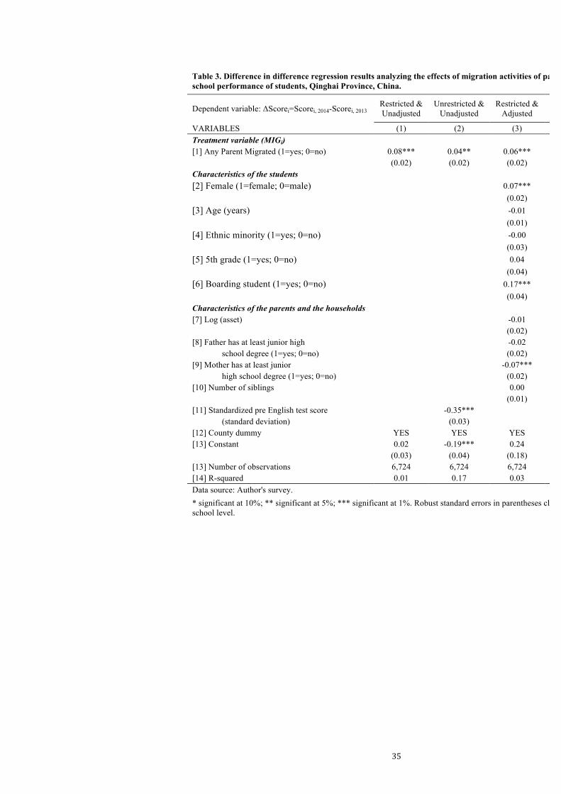
The results from the DID analysis using Models (1) - (4) for the version of

model that uses the Any Parent Migrated household variable as the treatment

demonstrate that the models perform fairly well and are consistent with our intuition.

The coefficients on some of the control variables are also in accordance with our

intuition (Table 3). For example, when we use the unrestricted and adjusted

specification of the empirical model (column 4), the scores of older students drop

relatively more than those of younger students (column 4, row 3). This finding might

be considered reasonable since, ceteris paribus, students that enter elementary school

at an older age may have an initial advantage (because they are relatively more

mature) that gradually disappears as younger children catch up over the course of

primary school, which is consistent with other findings (for example, Fredriksson and

Öckert, 2005). Additionally, when a student is from a household that is part of a

non-Han ethnic minority group, the student’s score drops relatively more than Han

students. There are many studies that show the academic performance of ethnic

minority students in China lags substantially behind those of Han students

(Gustafsson and Sai, 2014; Yang et al., 2015). In the rest of paper, we focus mainly

on the results from the unrestricted and adjusted model. We do so because this

regression has a higher goodness of fit (or R-square) statistic. In part, almost certainly,

this better fit reflects the importance of capturing beginning scores, which embodies

the unobserved ability of a student as well as other covariates.

One of the most important findings in Table 3 is that we reject the hypothesis

that parental migration negatively affects the academic performance of children. In all

four models, the coefficient of the Any Parent Migrated household dummy variable is

not negative. In fact, the coefficients are all positive and significantly different from

zero. The magnitudes of the coefficients range from 0.04 to 0.08 SD. This means that,

17

everything else held constant, after any parent in a household out-migrated between

baseline and endline surveys, their child’s standardized English test scores actually

rose relative to the children of Never Migrant households. In other words, unlike

claims made by some researchers (Meyerhoefer and Chen, 2011; Zhao et al., 2014;

Zhou et al., 2014; Zhang et al., 2014), according to the results of the analysis in Table

3, parental migration did not hurt the academic performance of LBCs. At least in the

migrant households in our sample area, migration led to improved school

performance.

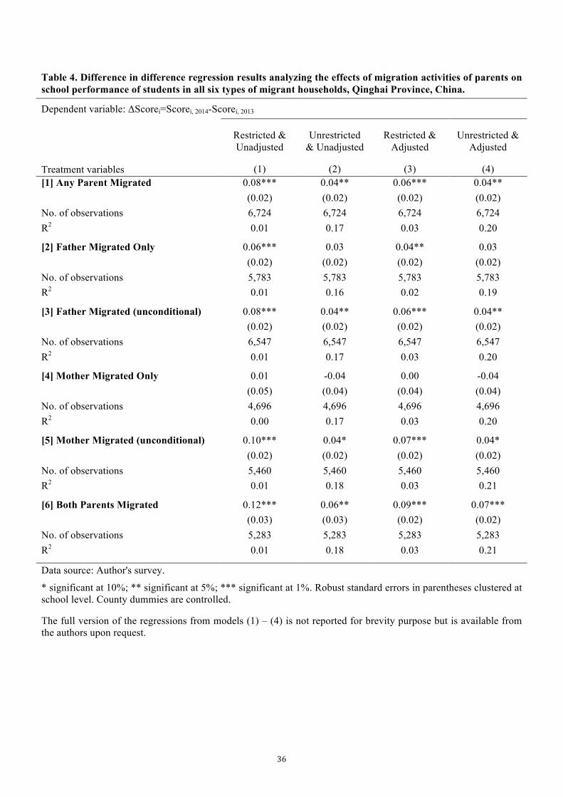
The results hold when we examine other types of migrant households: we do

not find any negative effects of parental migration on the academic performance of

children (Table 4). For each of the four specifications, we look at the effect of

parental migration on academic performance in all six types of migrant households.5

In 22 out of the 24 cases the coefficient is positive. The coefficients are only negative

for Mother Migrated Only households (column 2, row 4). In each of these two cases,

however, there is no statistically significant effect of parental migration on academic

performance. Interestingly, when the father out migrated (column 4, row 3) or mother

out migrated (unconditional) (column 4, row 5) or both parents out migrated (column

4, row 6), the standardized English test scores of LBCs improved significantly.

So why is it that parental migration does not appear to have a negative effect

on the academic performance of LBCs and in some cases even appears to have a

positive effect? Although we cannot answer this question from our analyses, one

possible reason is that the income effect of remittances is relatively large compared to

the adverse effect of less parental care. If parental migration leads to higher income,

5 In Table 3, we only report the coefficients on the treatment variable. The rest of the results are suppressed

for brevity but are available from the authors upon request. We report the results for 24 different regressions. For completeness in Table 4, we include the results of the effect of Any Parent Migrated on school performance, but, in fact, this is a duplication of the results from Table 3, row 1.

18

as found in Du et al. (2005), the migrant households that experience rising incomes

may be able to provide better nutrition, improved access to educational supplies and

burden their children with less housework. With the addition of these household

resources and the lessening of burdens, parental migration may have a positive effect

on the academic performance of children. The positive income effect is probably

behind our finding that the largest positive effects are found in the Both Parents

Migrated households (Table 4, row 6). This result may arise since the family income

would improve more when both parents out migrated comparing to other types of

New Migrant households. This income effect also appears to be largely offsetting any

negative effects of parental absence—such as the decline in parental care and

oversight. Thus, on the whole, our results strongly suggest that parental migration is

having net positive effect on the academic performance of LBCs when both parents

out-migrate.

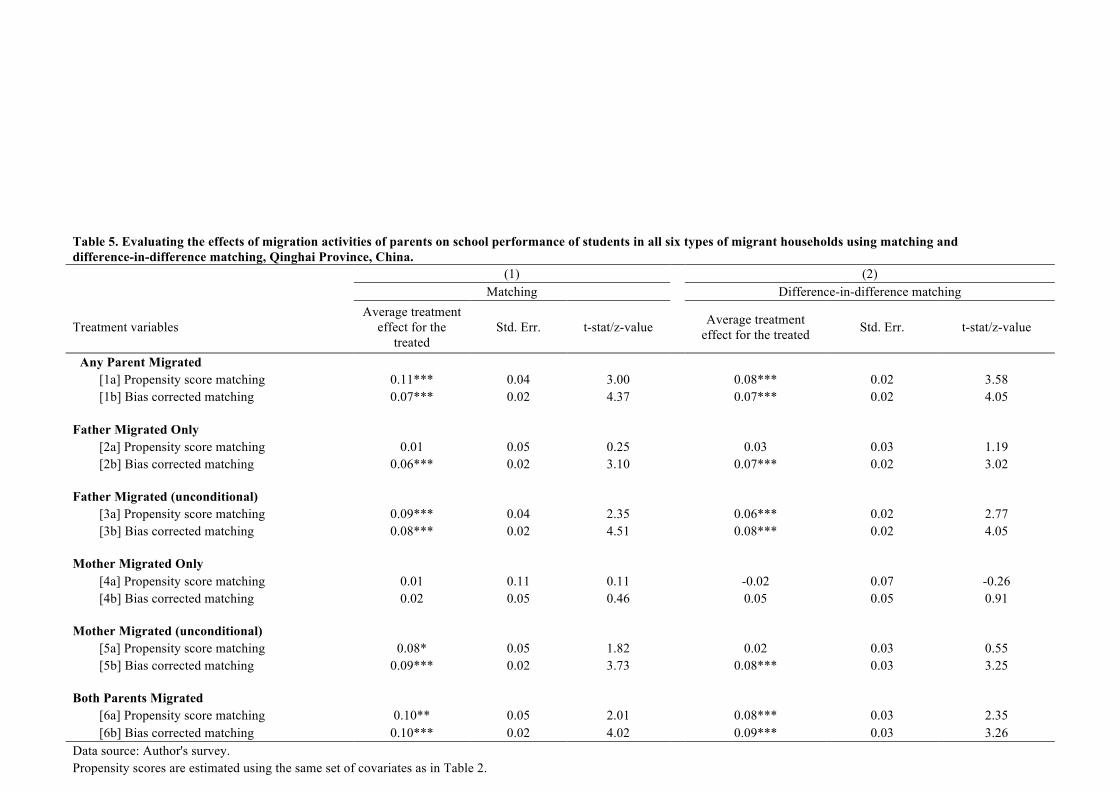
Results from Matching

The results of the cross-sectional matching analysis, regardless of the method

of matching, also reveal that parental migration has no significant negative effect on

the academic performance of LBCs. When propensity score matching is used to

examine the effect of parental migration on academic performance for all six types of

New Migrant households, there are no cases in which the coefficient on the treatment

variable is negative and statistically significant (Table 4, column 1, rows 1a, 2a, 3a, 4a,

5a and 6a). The same is true when Bias-Corrected Matching is used (column 1, rows

1b, 2b, 3b, 4b, 5b and 6b).

In fact, results from matching are quite similar to those from the DID analyses.

When we use Bias-Corrected Matching, which arguably is generating more reliable

19

estimates and standard errors, we find that the coefficients on the treatment variables

in the Any Parent Migrated household, the Father Migrated (unconditional)

household, the Mother Migrated household and the Both Parents Migrated household

are positive and statistically significant. The magnitudes of the coefficients also are

similar to those from the DID analyses.

In addition, and importantly, the findings remain largely the same when the

DDM estimator is used (Table 4, column 2). Regardless of whether we use PSM or

BCM, none of the coefficients of any of the treatment variables are significantly

negative. In fact, most of them are positive and significant. Hence, whether using DID,

PSM or DDM, we find no significant negative effects of parental migration on the

academic performance of left-behind children.

Heterogeneous Effect of Parental Migration on Academic Performance

While we have found no significant negative impacts, mostly positive impacts,

of parental migration on the academic performance of LBCs, all of these results have

been for the average household (that is, for the typical migrant households). It is

possible, however, that the impacts could vary for different subgroups, i.e., different

types of migrant households, of our sample. In this section we use model (5) which is

presented in Section 4 to test the heterogeneous effects of several variables.

Specifically, we will look at the heterogeneous effects of parental migration on:

students who are poor and higher performing (using standardized English test score

in the baseline); students of different gender (female); students who are Han and

non-Han (ethnic minority); students who are an only child or who have siblings (only

child); students from poorer and richer families (assets), students with parents who

have lower and higher levels of education (using either father has junior high school

20

or higher degrees, or mother has junior high school or higher degrees). For brevity,

we only report the results of the unrestricted and adjusted model, but the results are

robust to this specification of the model.

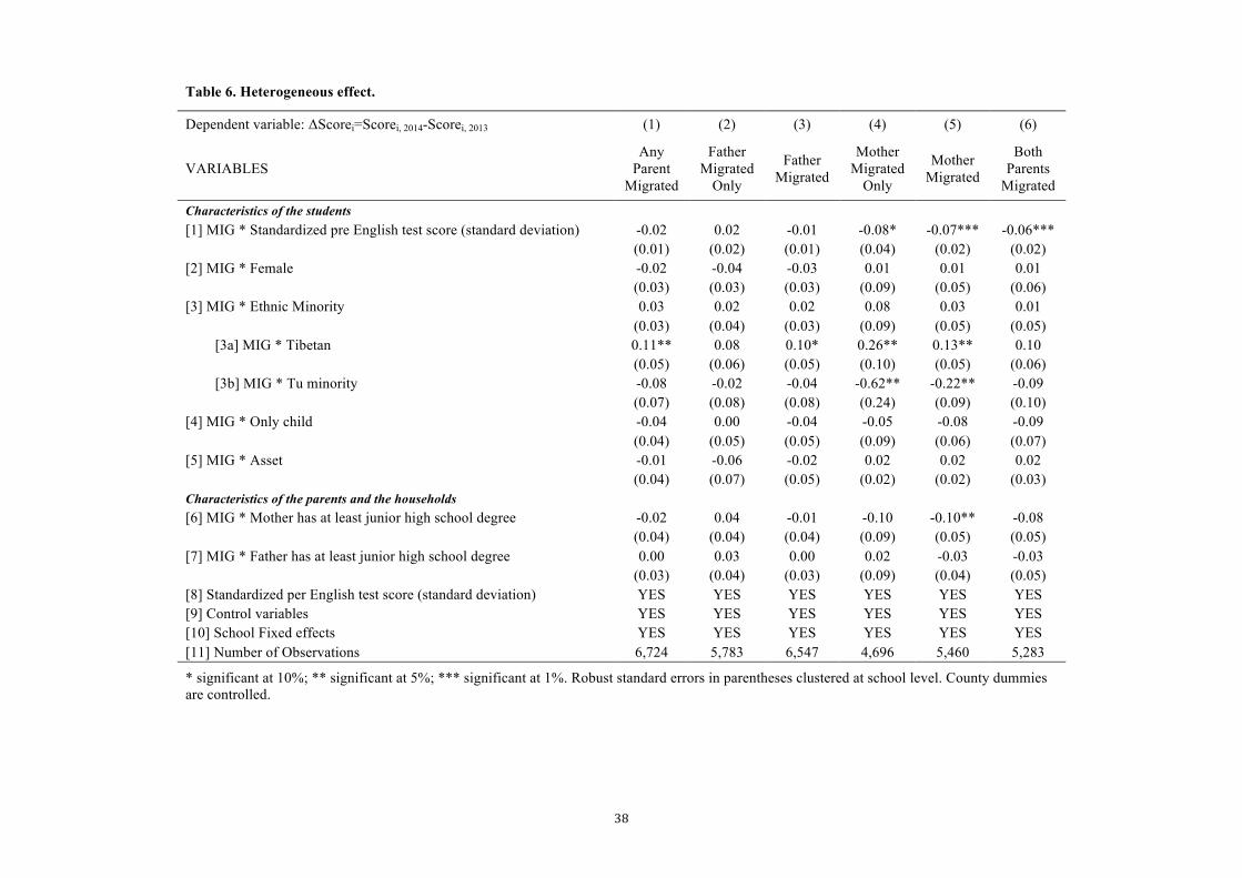
The heterogeneous analysis shows that the positive impact of parental

migration on LBCs is greater for poor performing students (Table 6, columns 4-6, row

1). These results mean that, everything else held constant, parental migration affects

academic performance of LBCs with different starting academic performance in a

heterogeneous way. Although it is beyond the scope of this paper to isolate the exact

reason why parental out-migration helps poorer performing students more than higher

performing students, it may be the additional resources that are available to

households from newly out-migrating parents are able to overcome one or more of the

educational barriers that were limiting the performance of the students (making them

poorer performing). For example, it has been shown in a number of papers that when

students are better nourished, their academic performance rises (Luo et al., 2012). If

the newly available remittances were used to improve nutrition in the households

where parents had recently left, this might lead to better academic performance by

students that originally were not being provided enough nutrition and, hence,

performed at a sub-par level. Remittances might also be used for other

performance-enhancing investments of households with poorer performing students,

such as, remedial tutoring or additional books or learning software and associated

computer hardware.

The results of the heterogeneous analysis also demonstrate that the positive

impact of parental migration on LBCs maybe offset if the mother of an LBC has at

least junior high school degree. The coefficient on the interaction term between that

variable indicating Mother Migrated (unconditional) households and mother’s

21

education level – Mother has at least junior high school degree or not – is -0.10 SDs

and is significant at the 5% level (Table 6, columns 5, row 6). Hence, if a student’s

mother does not have at least junior high school degree, the scores of LBCs would

improve when mothers out-migrate or both parents migrate. In contrast, in the case of

mothers with higher levels of education, the positive effects of out-migration (that are

found for the average student) could be offset. While (again) we do not know exactly

why, the results are consistent with the interpretation that there is a parental

care-household resources trade-off when the mother of the student has the ability

(from her higher level of education) to provide academic performance-enhancing care

(e.g., from time spent tutoring her child). However, when a student’s mother is poorly

educated, she may not have the ability to help her child with his/her studies and so

when she leaves and begins to earn an income providing the household with

additional resources there is a net positive gain. Since our subject of interest is

English, this interpretation is more reasonable. Compared to math or mandarin, higher

education is probably needed for the mother of an LBC so that she could tutor her

child in learning English. The results are similar to those found in previous studies

which find that the impact of parental migration on academic performance of LBCs

differs based on the background of parents, especially for the education levels of

parents (e.g. Sawyer, 2014).

As is shown in Table 6, we find no significant evidence of heterogeneous

effects for other student demographic and family characteristics, including gender,

ethnic minority, only child, asset and father education level (Table 5, rows 2-5, 7). In

other words, like the results for the average households reported in Tables 3 to 5, the

results from DID analysis demonstrate that there are no significant effects of parental

migration on the academic performance of LBCs and this is true in the case of either:

22

boys or girls; Han or non-Han ethnic minorities; only children or children with

siblings; as well as children from families in which the father has at least a junior high

school degree or not.

Interestingly, although ethnicity does not matter when we aggregate all ethnic

minorities into a single group, the impacts do differ when we differentiate minorities

by sub-population. In other words, we do find heterogeneous impacts when students

are Tibetan (versus the impacts when they are non-Tibetan) and when students are

members of the Tu minority. Compared to the students in the Never Migrant

households, Tibetan students in the Any Parent Migrated households (+0.11 SDs),

Father Migrated households (+0.10 SDs), Mother Migrated Only households (+0.26

SDs) and Mother Migrated households (+0.13 SDs) improved more in their

standardized English test scores than Han students (Columns 1, 3-5, row 3a). In

contrast, Tu students in Mother Migrated Only households (-0.62 SDs) and Mother

Migrated (-0.22 SDs) lagged behind in their standardized English test scores than Han

students in those treatment subgroups, respectively (Columns 4-5, row 3b).

So what is happening? From our data, we find that Tibetan students perform

worse than other students (t=10.49, p<0.01). This result is consistent with results from

above that the positive impact on LBCs is greater for poor performing students. Our

data also show that the education level of parents of Tu students is significantly

higher than that of other non-Han ethnic minorities (t=4.70, p<0.01). As what we

have discussed above, when mothers of LBCs have the ability (from their higher level

of education) to provide academic performance-enhancing care, the positive impact of

parental migration on LBCs may be offset.

Conclusions

23

In this paper, we have tried to understand whether or not the academic

performance of LBCs suffers when their father, mother or both parents migrate from

their home communities to the city (or at least away from home). Despite the

perception that is commonly found in the literature and the popular press, our results –

somewhat surprisingly – show that there seem to be no significant negative effects of

parental migration on the academic performance of LBCs. Comparing the change in

the standardized English test scores before and after parents out-migrated between

children from migrant households and those from non-migrant households, we can

reject the hypothesis that parental migration negatively affects the academic

performance of LBCs. In fact, in the analysis of most migrant households, especially

in those in which any parent migrated, father migrated, mother migrated or both

parents migrated, migration is shown to have a statistically significant and positive

effects on the academic performance of LBCs.

In addition, we also sought to explain how the impacts of parental migration

vary for different subgroups, i.e., different types of migrant households, of our sample.

Results from our data show that the positive impact of parental migration on LBCs is

greater for poor performing students. However, the positive impact maybe offset if

the mother of an LBC has at least junior high school degree. In contrast, we find no

evidence of heterogeneous effects by other student demographic and family

characteristics, including gender, ethnic minority, only child, asset and father

education level.

Based on these results, it might be tempting to conclude that policy makers do

not need to take any action (to help LBCs) since there are no measurable negative

effects of migration on school performance. If there were, education officials might

want to reduce class sizes or hire more qualified teachers to improve the mentoring

24

program in schools in which there were many LBCs. Boarding schools might offer

some of the services that parents originally carried out before they entered the migrant

labor force. Ultimately, measures can be promoted to offer the children of migrants

who lived in China’s cities better access to urban schools so parents would not have to

leave their children behind. However, all of these programs are costly. Although there

might be good reason to implement such policies anyhow, according to our results,

they should not be carried out on the ground of the negative effect of migration on

school performance. In addition, since both groups of children (children from migrant

households and non-migrant households) perform poorly on academic performance,

we recommend that special programs designed by policy makers to improve

education among left-behind children be expanded to cover all children in rural

China.

Although we have tried a number of alternative approaches to identify the

effect of migration, and although the findings are largely robust, if the assumptions

underlying our methodologies were not valid, our estimates could be bias. Even

though we controlled for many observed and time-invariant unobserved factors, there

still may be factors that are known to the parents of migrants and potential migrants

but are not be observable to the econometrician. For example, it may be that all

parents who were in the village with their children in the baseline survey worry about

whether or not their migration decision would negatively affect the academic

performance of their children. If it is the case that those parents who – though having

an opportunity to migrate – believed that the grades of their children would suffer

decided not to migrate, while those that believed their children’s grades would not

suffer decided to migrate, then our results would be subject to selection bias.

25

If there was, in fact, such a selection bias and we did not account for it (as we

were unable to – due to the absence of any effective instrumental variable), would our

results be useless? We believe not. We believe even if there was a selection bias our

results are showing that when rural parents out-migrate, the academic performance of

their children do not suffer. It is true that part of the reason for the non-negative effect

may be exactly this selection effect – parents do not go when they believe the scores

of the children would suffer. But, from society’s point of view, there is less cost in

terms of academic performance of its children due to parental migration.

26

References Abadie, A., & Imbens, G. W. (2002). Simple and bias-corrected matching estimators

for average treatment effects. Abadie, A., & Imbens, G. W. (2006). Large sample properties of matching estimators

for average treatment effects. Econometrica, 74(1), 235-267. All-China Women’s Federation(ACWF). (2013). Research report into the situation of

rural left behind children and rural to urban migrant children in China. Ambler, K., Aycinena, D., & Yang, D. (2015). Channeling Remittances to Education:

A Field Experiment among Migrants from El Salvador. American economic journal. Applied economics, 7(2), 207.

Antman, F. M. (2012). Gender, educational attainment, and the impact of parental migration on children left behind. Journal of Population Economics, 25(4), 1187-1214.

Antman, F. M. (2013). 16 The impact of migration on family left behind. International Handbook on the Economics of Migration, 293.

Bai, Y., Mo D., Zhang L., Boswell M., Rozelle S. (2015). The impact of integrating ICT with teaching: evidence from a randomized controlled trial in rural schools in China. Working paper.

Bolton, K., & Graddol, D. (2012). English in China today. English Today, 28(03), 3-9.

Caliendo, M., & Kopeinig, S. (2008). Some practical guidance for the implementation of propensity score matching. Journal of economic surveys, 22(1), 31-72.

Chang, H., Dong, X. Y., & MacPhail, F. (2011). Labor migration and time use patterns of the left-behind children and elderly in rural China. World Development, 39(12), 2199-2210.

Chen, X., Huang, Q., Rozelle, S., Shi, Y., & Zhang, L. (2009). Effect of migration on children's educational performance in rural China. Comparative Economic Studies, 51(3), 323-343.

Dehejia, R. H., & Wahba, S. (1999). Causal effects in nonexperimental studies: Reevaluating the evaluation of training programs. Journal of the American Statistical Association, 94(448), 1053-1062.

Dehejia, R. H., & Wahba, S. (2002). Propensity score-matching methods for nonexperimental causal studies. Review of Economics and statistics, 84(1), 151-161.

Du, Y., Park, A., & Wang, S. (2005). Migration and rural poverty in China. Journal of comparative economics, 33(4), 688-709.

Duan, C., & Zhou, F. (2005). A study on children left behind. Population Research, 29(1), 29-36.

Edwards, A. C., & Ureta, M. (2003). International migration, remittances, and schooling: evidence from El Salvador. Journal of development economics, 72(2), 429-461.

Fredriksson, P., & Öckert, B. (2005). Is early learning really more productive? The effect of school starting age on school and labor market performance. IZA Discussion Paper No. 1659, Institute for the Study of Labor (IZA).

Giannelli, G. C., & Mangiavacchi, L. (2010). Children's Schooling and Parental Migration: Empirical Evidence on the ‘Left-behind’Generation in Albania. Labour, 24(s1), 76-92.

Gustafsson, B., & Sai, D. (2014). Mapping and Understanding Ethnic Disparities in Length of Schooling: The Case of the Hui Minority and the Han Majority in Ningxia Autonomous Region, China. Social Indicators Research, 1-19.

27

Hu, G. (2005). English language education in China: Policies, progress, and problems. Language Policy, 4(1), 5-24.

Hu, X. (2009). The quality of English teacher of the primary school in rural China--Evidence from Heilongjiang Province (in Chinese). China Adult Education, 18, 89-90

Hu, X., Cook, S., & Salazar, M. A. (2008). Internal migration and health in China. The Lancet, 372(9651), 1717-1719.

Lahaie, C., Hayes, J. A., Piper, T. M., & Heymann, J. (2009). Work and family divided across borders: The impact of parental migration on Mexican children in transnational families. Community, Work & Family, 12(3), 299-312.

Lai, F., Luo, R., Zhang, L., Huang, X., & Rozelle, S. (2015). Does computer-assisted learning improve learning outcomes? Evidence from a randomized experiment in migrant schools in Beijing. Economics of Education Review, 47, 34-48.

Li S. (2002). Status and development of English teaching in minority areas (in Chinese). Foreign Language Teaching & Research in Basic Education. 11:34-39.

Loyalka, P., Shi Z., Chu J., Johnson N., Wei J. and Rozelle S. (2014). Is the high school admissions process fair? Explaining inequalities in elite high school enrollments in developing countries. REAP working paper #276.

Lu, Y. (2012). Education of children left behind in rural China. Journal of Marriage and Family, 74(2), 328-341.

Lu, Y., & Treiman, D. J. (2011). Migration, remittances and educational stratification among blacks in apartheid and post-apartheid South Africa. Social Forces, 89(4), 1119-1143.

Luo, R., Shi, Y., Zhang, L., Liu, C., Rozelle, S., Sharbono, B., ... & Martorell, R. (2012). Nutrition and educational performance in rural China’s elementary schools: Results of a randomized control trial in Shaanxi Province. Economic development and cultural change, 60(4), 735-772.

Malik, K. (2015). Examining the Relationship Between Received Remittances and Education in Malawi. CMC Senior Theses. Paper 1096.

McKay, S. L. (2002). Teaching English as an international language: Rethinking goals and perspectives. NY: OUP.

McKenzie, D., & Rapoport, H. (2011). Can migration reduce educational attainment? Evidence from Mexico. Journal of Population Economics, 24(4), 1331-1358.

Meyerhoefer, C. D., & Chen, C. J. (2011). The effect of parental labor migration on children’s educational progress in rural China. Review of Economics of the Household, 9(3), 379-396.

Ministry of Human Resources and Social Security (MHRSS). (2013). Annual Statistical Bulletin of Human Resources and Social Security Development in 2013. [in Chinese] Retrieved from: http://www.mohrss.gov.cn/SYrlzyhshbzb/zwgk/szrs/ndtjsj/tjgb/201405/t20140529_131147.htm

Ministry of Education (MOE). (2014) Statistical Communiqué of the People's Republic of China on the 2013 National Educational Development. Retrieved from: http://www.moe.edu.cn/publicfiles/business/htmlfiles/moe/moe_633/201407/171144.html

Mo, D., Zhang, L., Luo, R., Qu, Q., Huang, W., Wang, J., ... & Rozelle, S. (2014). Integrating computer-assisted learning into a regular curriculum: evidence

28

from a randomised experiment in rural schools in Shaanxi. Journal of Development Effectiveness, 6(3), 300-323.

National Bureau of Statistics of China (NBSC). 2014. China National Statistical Yearbook, 2014. China State Statistical Press: Beijing, China.

Rosenbaum, P. R., & Rubin, D. B. (1983). The central role of the propensity score in observational studies for causal effects. Biometrika, 70(1), 41-55.

Rosenbaum, P. R., & Rubin, D. B. (1985). Constructing a control group using multivariate matched sampling methods that incorporate the propensity score. The American Statistician, 39(1), 33-38.

Roy, A. K., Singh, P., & Roy, U. N. (2015). Impact of Rural-urban Labour Migration on Education of Children: A Case Study of Left behind and Accompanied Migrant Children in India. Space and Culture, India, 2(4), 17-34.

Rozelle, S., Guo, L., Shen, M., Hughart, A., & Giles, J. (1999). Leaving China's farms: survey results of new paths and remaining hurdles to rural migration. The China Quarterly, 158, 367-393.

Sawyer, A. (2014). Is Money Enough?: The Effect of Migrant Remittances on Parental Aspirations and Youth Educational Attainment in Rural Mexico. International Migration Review.

Smith, J. A., & Todd, P. E. (2005). Does matching overcome LaLonde's critique of nonexperimental estimators?. Journal of econometrics, 125(1), 305-353.

Wang, S. X. (2014). The effect of parental migration on the educational attainment of their left-behind children in rural China. The BE Journal of Economic Analysis & Policy, 14(3), 1037-1080.

Wen, M., & Lin, D. (2012). Child development in rural China: Children left behind by their migrant parents and children of nonmigrant families. Child development, 83(1), 120-136.

Xu, H., & Xie, Y. (2015). The Causal Effects of Rural-to-Urban Migration on Children’s Well-being in China. European Sociological Review, jcv009.

Yang, D. (2008). International migration, remittances and household investment: Evidence from philippine migrants’ exchange rate shocks*. The Economic Journal, 118(528), 591-630.

Yang, Y., Wang, H., Zhang, L., Sylvia, S., Luo, R., Shi, Y., ... & Rozelle, S. (2015). The Han-Minority Achievement Gap, Language, and Returns to Schools in Rural China. Economic development and cultural change, 63(2), 319.

Ye J, Wang Y, Zhang K, Lu J. (2006). Life affection of parents going out for work to left behind children. [in Chinese]. Chinese Rural Economy. (1):57–65.

Ye J., & Lu, P. (2011). Differentiated childhoods: impacts of rural labor migration on left-behind children in China. The Journal of peasant studies, 38(2), 355-377.

Zhao H. (2003). Exploring Resources of Local Courses an Effective Way of Developing Teaching Body in Ethnic Minority Regions. Journal of Research on Education for Ethnic Minorities. 2003, (4): 60-64.

Zhao, Q., Yu, X., Wang, X., & Glauben, T. (2014). The impact of parental migration on children's school performance in rural China. China Economic Review, 31, 43-54.

Zhang, H., Behrman, J. R., Fan, C. S., Wei, X., & Zhang, J. (2014). Does parental absence reduce cognitive achievements? evidence from rural china. Journal of Development Economics, 111, 181–195.

Zhou, C., Sylvia S., Zhang L., Luo R., Yi H., Liu C., Shi Y., Loyalka P., Chu J., Medina A. & Rozelle S. (2015) China's Left-Behind Children: Impact of

29

Parental Migration On Health, Nutrition, And Educational Outcomes. Health Affairs, 34, no.11:1964-1971. doi: 10.1377/hlthaff.2015.0150

Zhou, M., Murphy, R., & Tao, R. (2014). Effects of parents' migration on the education of children left behind in rural China. Population and Development Review, 40(2), 273-292.

30

Fig 1. Kernal distribution of Standardized baseline English test score.

0.1

.2.3

.4.5

Den

sity

-4 -2 0 2 4Standardized baseline English test score

kernel = epanechnikov, bandwidth = 0.1371

31

0.00

-0.08

0.06

-0.07

-0.19

-0.27 -0.28

0.00

0.00

0.12

0.01

-0.18 -0.16 -0.16

-0.35

-0.30

-0.25

-0.20

-0.15

-0.10

-0.05

0.00

0.05

0.10

0.15

Never Migrated

Any Parent

Migrated

Father Migrated

Only

Father Migrated

Mother Migrated

Only

Mother Migrated

Both Parents

Migrated

Stan

dard

ized

Eng

lish

Test

Sco

re

(Sta

ndar

d D

evia

tion)

Baseline Endline

Fig 2. The standardized English test score of baseline and endline survey in different migrant households.

32

0.00

0.08 0.06

0.08

0.02

0.10 0.12

-0.10

-0.05

0.00

0.05

0.10

0.15

0.20

Never Migrated

Any Parent

Migrated

Father Migrated

Only

Father Migrated

Mother Migrated

Only

Mother Migrated

Both Parents

Migrated

Stan

dard

ized

Eng

lish

Test

Sco

re (S

tand

ard

Dev

iatio

n)

ΔScorei=Scorei, 2014-Scorei, 2013

Fig 3. Change in standardized English test score before and after the parents of students out-migrate with 95% Confidence Interval (CI) in different migrant households.

33

Table 1. Patterns of migration in sample households in 2013 and 2014, Qinghai Province, China.

Migration status in 2013 Migration status in 2014

(1) (2) (3) (4) (5) (6) (7) (8)

Number of

households in 2013

Any Parent Migrated in

2014

Father Migrated

Only in 2014

Father Migrated in

2014

Mother Migrated

Only in 2014

Mother Migrated in

2014

Both Parents Migrated in

2014

Neither parent

migrated in 2014

[1] Father migrated only 2730 1779 1358 1728 51 421 370 951

[2] Mother migrated only 560 353 63 221 132 290 158 207

[3] Both parents migrated 2193 1688 305 1579 109 1383 1274 505

[4] Neither parent migrated 6724 2205 1264 2028 177 941 764 4519

[5] Total number of households 12207 6025 2990 5556 469 3035 2566 6182

Data source: Authors' survey.

Column (1)=Column (3)+Column (5)+Column (7)+Column (8); Column (2)=Column (3)+Column (5)+Column (7); Column (4)=Column (3)+Column(7); Column (6)=Column (5)+Column (7).

The households in column 8, rows 1, 2 and 3 are return migrants (or those households in which households had a migrant in 2013 and in 2014 had returned home). These households are dropped from the multivariate analysis.

The households in row 1, columns 2-7; row 2, columns 2-7; row 3, columns 2-7 are always migrant households. These households are dropped from the multivariate analysis.

Total new migrants (or those households in which the parents did not migrate in 2013 and migrated in 2014) is found in column 2, row 4. Never migrants is found in column 7, row 4.

34

Table 2. Descriptive statistics of control variables used in the multivariate analysis.

Total Never migrant Any Parent migrated Father migrated only Father migrated Mother migrated only Mother migrated Both parents migrated

Control variables mean (s.e.) mean

(s.e.) mean (s.e.)

H0: (2)=(3) Difference mean

(s.e.) H0: (2)=(5) Difference mean

(s.e.) H0: (2)=(7) Difference mean

(s.e.) H0: (2)=(9) Difference mean

(s.e.) H0: (2)=(11) Difference mean

(s.e.) H0: (2)=(13) Difference

(1) (2) (3) (4) (5) (6) (7) (8) (9) (10) (11) (12) (13) (14) Characteristics of the students [1] Female (1=female; 0=male) 0.49 0.49 0.48 -0.01 0.49 0.00 0.48 -0.01 0.45 -0.04 0.45 -0.03* 0.46 -0.03 (0.50 (0.50) (0.50) (0.01) (0.50) (0.02) (0.50) (0.01) (0.50) (0.04) (0.50) (0.02) (0.50) (0.02) [2] Age (years) 10.83 10.77 10.97 0.20*** 10.92 0.18*** 10.97 0.20*** 10.95 0.15* 11.03 0.21*** 11.05 0.23*** (1.11) (1.10) (1.13) (0.04) (1.12) (0.04) (1.13) (0.04) (1.09) (0.08) (1.13) (0.06) (1.14) (0.06) [3] Ethnic minority (1=yes; 0=no) 0.51 0.50 0.54 0.04* 0.49 0.03* 0.54 0.04* 0.54 0.02 0.61 0.04 0.62 0.05 (0.50) (0.50) (0.50) (0.02) (0.50) (0.02) (0.50) (0.02) (0.50) (0.04) (0.49) (0.03) (0.48) (0.03) [3a] Hui Minority (1=yes; 0=no) 0.30 0.32 0.26 -0.05* 0.24 -0.03** 0.26 -0.05* 0.26 -0.08** 0.29 -0.07 0.30 -0.07 (0.46) (0.47) (0.44) (0.03) (0.43) (0.02) (0.44) (0.03) (0.44) (0.04) (0.45) (0.04) (0.46) (0.05) [3b] Tibetan (1=yes; 0=no) 0.11 0.08 0.17 0.08*** 0.12 0.05*** 0.16 0.08*** 0.20 0.11*** 0.23 0.13*** 0.23 0.13*** (0.31) (0.27) (0.37) (0.02) (0.32) (0.01) (0.37) (0.02) (0.40) (0.04) (0.42) (0.04) (0.42) (0.04) [3c] Tu minority (1=yes; 0=no) 0.05 0.04 0.06 0.02** 0.08 0.03*** 0.06 0.02** 0.05 0.01 0.04 0.01 0.04 0.01 (0.21) (0.19) (0.24) (0.01) (0.27) (0.01) 0.24 (0.01) (0.22) (0.02) (0.20) (0.01) (0.19) (0.01) [4] 5th grade (1=yes; 0=no) 0.52 0.53 0.51 -0.02 0.52 -0.01 0.51 -0.02 0.53 0.00 0.50 -0.03 0.49 -0.04* (0.50) (0.50) (0.50) (0.02) (0.50) (0.02) (0.50) (0.02) (0.50) (0.04) (0.50) (0.02) (0.50) (0.02) [5] Boarding student (1=yes; 0=no) 0.15 0.12 0.22 0.10*** 0.20 0.07*** 0.22 0.10*** 0.19 0.07** 0.24 0.13*** 0.26 0.14*** (0.36) (0.32) (0.41) (0.02) (0.40) (0.02) (0.41) (0.02) (0.39) (0.03) (0.43) (0.03) (0.44) (0.03) Characteristics of the parents and the households [6] Log (asset) 9.59 9.61 9.55 -0.06*** 9.55 -0.06*** 9.56 -0.05*** 9.52 -0.08 9.55 -0.04 9.56 -0.04 (0.47) (0.39) (0.60) (0.02) (0.50) (0.02) (0.54) (0.02) (1.06) (0.08) (0.70) (0.03) (0.59) (0.02) [7] Father has at least junior high 0.49 0.52 0.44 -0.07*** 0.49 -0.05*** 0.43 -0.08*** 0.48 -0.02 0.37 -0.10*** 0.35 -0.12*** school degree (1=yes; 0=no) (0.50) (0.50) (0.50) (0.01) (0.50) (0.02) (0.50) (0.02) (0.50) (0.04) (0.48) (0.02) (0.48) (0.02) [8] Mother has at least junior high 0.36 0.39 0.30 -0.08*** 0.32 -0.09*** 0.29 -0.09*** 0.36 -0.00 0.26 -0.08*** 0.24 -0.10*** school degree (1=yes; 0=no) (0.48) (0.49) (0.46) (0.01) (0.47) (0.02) (0.45) (0.02) (0.48) (0.03) (0.44) (0.02) (0.43) (0.02) [9] Number of siblings 1.57 1.54 1.65 0.10** 1.53 0.07 1.64 0.10** 1.67 0.07 1.81 0.13* 1.84 0.14* (1.51) (1.45) (1.61) (0.05) (1.41) (0.05) (1.61) (0.05) (1.67) (0.11) (1.84) (0.07) (1.87) (0.08) [10] Number of Observations 6724 4519 2205 6724 1264 5783 2028 6547 177 4696 941 5460 764 5283

Data source: Author's survey.

* significant at 10%; ** significant at 5%; *** significant at 1%. Mean values are reported in the table with robust standard errors in parentheses clustered at school level. County dummies are controlled.

The within-school difference between the column (2) and column (3) is calculated by regressions of each of row variables on the dummy variable that represent Any Parent Migrated households. The within-school difference between the column (2) and column (5) is calculated by regressions of each of row variables on the dummy variable that represent Father Migrated Only households. The within-school difference between the column (2) and column (7) is calculated by regressions of each of row variables on the dummy variable that represent Father Migrated households. The within-school difference between the column (2) and column (9) is calculated by regressions of each of row variables on the dummy variable that represent Mother Migrated Only households. The within-school difference between the column (2) and column (11) is calculated by regressions of each of row variables on the dummy variable that represent Mother Migrated households. The within-school difference between the column (2) and column (13) is calculated by regressions of each of row variables on the dummy variable that represent Both Parents Migrated households.

35

Table 3. Difference in difference regression results analyzing the effects of migration activities of parents on school performance of students, Qinghai Province, China.

Dependent variable: ΔScorei=Scorei, 2014-Scorei, 2013 Restricted & Unadjusted

Unrestricted & Unadjusted

Restricted & Adjusted

Unrestricted & Adjusted

VARIABLES (1) (2) (3) (4) Treatment variable (MIGi) [1] Any Parent Migrated (1=yes; 0=no) 0.08*** 0.04** 0.06*** 0.04**

(0.02) (0.02) (0.02) (0.02) Characteristics of the students [2] Female (1=female; 0=male) 0.07*** 0.15***

(0.02) (0.02) [3] Age (years) -0.01 -0.05***

(0.01) (0.01) [4] Ethnic minority (1=yes; 0=no) -0.00 -0.05*

(0.03) (0.02) [5] 5th grade (1=yes; 0=no) 0.04 0.07**

(0.04) (0.03) [6] Boarding student (1=yes; 0=no) 0.17*** 0.08**

(0.04) (0.04) Characteristics of the parents and the households [7] Log (asset) -0.01 -0.00

(0.02) (0.01) [8] Father has at least junior high -0.02 0.03** school degree (1=yes; 0=no) (0.02) (0.01) [9] Mother has at least junior -0.07*** -0.03 high school degree (1=yes; 0=no) (0.02) (0.02) [10] Number of siblings 0.00 -0.01

(0.01) (0.01) [11] Standardized pre English test score -0.35*** 0.29* (standard deviation) (0.03) (0.16) [12] County dummy YES YES YES YES [13] Constant 0.02 -0.19*** 0.24 6,724

(0.03) (0.04) (0.18) 0.20 [13] Number of observations 6,724 6,724 6,724 6,724 [14] R-squared 0.01 0.17 0.03 0.20 Data source: Author's survey. * significant at 10%; ** significant at 5%; *** significant at 1%. Robust standard errors in parentheses clustered at school level.

36

Table 4. Difference in difference regression results analyzing the effects of migration activities of parents on school performance of students in all six types of migrant households, Qinghai Province, China.

Dependent variable: ΔScorei=Scorei, 2014-Scorei, 2013

Restricted & Unadjusted

Unrestricted & Unadjusted

Restricted & Adjusted

Unrestricted & Adjusted

Treatment variables (1) (2) (3) (4) [1] Any Parent Migrated 0.08*** 0.04** 0.06*** 0.04** (0.02) (0.02) (0.02) (0.02) No. of observations 6,724 6,724 6,724 6,724 R2 0.01 0.17 0.03 0.20

[2] Father Migrated Only 0.06*** 0.03 0.04** 0.03 (0.02) (0.02) (0.02) (0.02) No. of observations 5,783 5,783 5,783 5,783 R2 0.01 0.16 0.02 0.19

[3] Father Migrated (unconditional) 0.08*** 0.04** 0.06*** 0.04** (0.02) (0.02) (0.02) (0.02) No. of observations 6,547 6,547 6,547 6,547 R2 0.01 0.17 0.03 0.20

[4] Mother Migrated Only 0.01 -0.04 0.00 -0.04 (0.05) (0.04) (0.04) (0.04) No. of observations 4,696 4,696 4,696 4,696 R2 0.00 0.17 0.03 0.20

[5] Mother Migrated (unconditional) 0.10*** 0.04* 0.07*** 0.04* (0.02) (0.02) (0.02) (0.02) No. of observations 5,460 5,460 5,460 5,460 R2 0.01 0.18 0.03 0.21

[6] Both Parents Migrated 0.12*** 0.06** 0.09*** 0.07*** (0.03) (0.03) (0.02) (0.02) No. of observations 5,283 5,283 5,283 5,283 R2 0.01 0.18 0.03 0.21

Data source: Author's survey.

* significant at 10%; ** significant at 5%; *** significant at 1%. Robust standard errors in parentheses clustered at school level. County dummies are controlled.

The full version of the regressions from models (1) – (4) is not reported for brevity purpose but is available from the authors upon request.

37

Table 5. Evaluating the effects of migration activities of parents on school performance of students in all six types of migrant households using matching and difference-in-difference matching, Qinghai Province, China. (1) (2) Matching Difference-in-difference matching

Treatment variables Average treatment

effect for the treated

Std. Err. t-stat/z-value Average treatment effect for the treated Std. Err. t-stat/z-value

Any Parent Migrated [1a] Propensity score matching 0.11*** 0.04 3.00 0.08*** 0.02 3.58 [1b] Bias corrected matching 0.07*** 0.02 4.37 0.07*** 0.02 4.05

Father Migrated Only [2a] Propensity score matching 0.01 0.05 0.25 0.03 0.03 1.19 [2b] Bias corrected matching 0.06*** 0.02 3.10 0.07*** 0.02 3.02

Father Migrated (unconditional) [3a] Propensity score matching 0.09*** 0.04 2.35 0.06*** 0.02 2.77 [3b] Bias corrected matching 0.08*** 0.02 4.51 0.08*** 0.02 4.05

Mother Migrated Only [4a] Propensity score matching 0.01 0.11 0.11 -0.02 0.07 -0.26 [4b] Bias corrected matching 0.02 0.05 0.46 0.05 0.05 0.91

Mother Migrated (unconditional) [5a] Propensity score matching 0.08* 0.05 1.82 0.02 0.03 0.55 [5b] Bias corrected matching 0.09*** 0.02 3.73 0.08*** 0.03 3.25

Both Parents Migrated [6a] Propensity score matching 0.10** 0.05 2.01 0.08*** 0.03 2.35 [6b] Bias corrected matching 0.10*** 0.02 4.02 0.09*** 0.03 3.26 Data source: Author's survey. Propensity scores are estimated using the same set of covariates as in Table 2. * significant at 10%; ** significant at 5%; *** significant at 1%. t-stats are reported for propensity score matching and z-values are reported for bias-corrected matching in parentheses. We use propensity scores as a tool to enforce a common support. We use the nearest neighbor matching with replacement. Following Smith and Todd (2005), we match students based on the log odds ratio and standard errors are bootstrapped using 1,000 replications. To minimize geographic mismatch, we enforce exact matching by county. Each treatment observation is matched to 3 control observations with replacement. The weighting matrix uses the Mahalanobis metric, which is the inverse of the sample covariance matrix of the matching variables.

38

Table 6. Heterogeneous effect.

Dependent variable: ΔScorei=Scorei, 2014-Scorei, 2013 (1) (2) (3) (4) (5) (6)

VARIABLES Any

Parent Migrated

Father Migrated

Only

Father Migrated

Mother Migrated

Only

Mother Migrated

Both Parents

Migrated

Characteristics of the students [1] MIG * Standardized pre English test score (standard deviation) -0.02 0.02 -0.01 -0.08* -0.07*** -0.06*** (0.01) (0.02) (0.01) (0.04) (0.02) (0.02) [2] MIG * Female -0.02 -0.04 -0.03 0.01 0.01 0.01 (0.03) (0.03) (0.03) (0.09) (0.05) (0.06) [3] MIG * Ethnic Minority 0.03 0.02 0.02 0.08 0.03 0.01 (0.03) (0.04) (0.03) (0.09) (0.05) (0.05) [3a] MIG * Tibetan 0.11** 0.08 0.10* 0.26** 0.13** 0.10 (0.05) (0.06) (0.05) (0.10) (0.05) (0.06) [3b] MIG * Tu minority -0.08 -0.02 -0.04 -0.62** -0.22** -0.09 (0.07) (0.08) (0.08) (0.24) (0.09) (0.10) [4] MIG * Only child -0.04 0.00 -0.04 -0.05 -0.08 -0.09 (0.04) (0.05) (0.05) (0.09) (0.06) (0.07) [5] MIG * Asset -0.01 -0.06 -0.02 0.02 0.02 0.02 (0.04) (0.07) (0.05) (0.02) (0.02) (0.03) Characteristics of the parents and the households [6] MIG * Mother has at least junior high school degree -0.02 0.04 -0.01 -0.10 -0.10** -0.08 (0.04) (0.04) (0.04) (0.09) (0.05) (0.05) [7] MIG * Father has at least junior high school degree 0.00 0.03 0.00 0.02 -0.03 -0.03 (0.03) (0.04) (0.03) (0.09) (0.04) (0.05) [8] Standardized per English test score (standard deviation) YES YES YES YES YES YES [9] Control variables YES YES YES YES YES YES [10] School Fixed effects YES YES YES YES YES YES [11] Number of Observations 6,724 5,783 6,547 4,696 5,460 5,283

* significant at 10%; ** significant at 5%; *** significant at 1%. Robust standard errors in parentheses clustered at school level. County dummies are controlled.

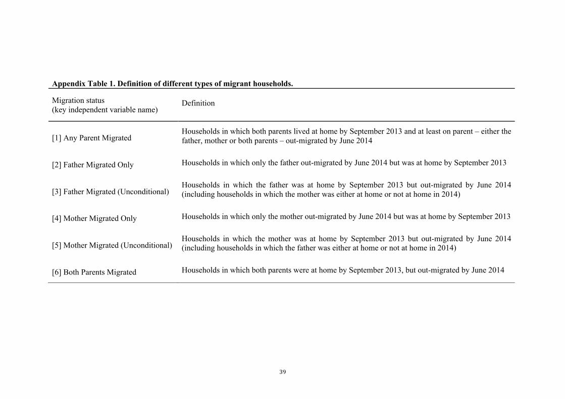
39

Appendix Table 1. Definition of different types of migrant households.

Migration status (key independent variable name)

Definition

[1] Any Parent Migrated Households in which both parents lived at home by September 2013 and at least on parent – either the father, mother or both parents – out-migrated by June 2014

[2] Father Migrated Only Households in which only the father out-migrated by June 2014 but was at home by September 2013

[3] Father Migrated (Unconditional) Households in which the father was at home by September 2013 but out-migrated by June 2014 (including households in which the mother was either at home or not at home in 2014)

[4] Mother Migrated Only Households in which only the mother out-migrated by June 2014 but was at home by September 2013

[5] Mother Migrated (Unconditional) Households in which the mother was at home by September 2013 but out-migrated by June 2014 (including households in which the father was either at home or not at home in 2014)

[6] Both Parents Migrated Households in which both parents were at home by September 2013, but out-migrated by June 2014

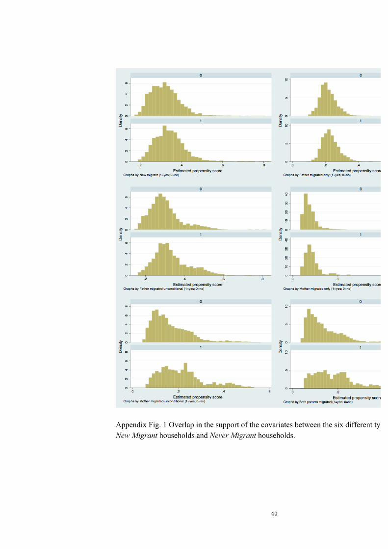
40

Appendix Fig. 1 Overlap in the support of the covariates between the six different types of New Migrant households and Never Migrant households.