Embed Size (px)
Citation preview
DI
SC
US
SI
ON
P
AP
ER
S
ER
IE
S
Forschungsinstitut zur Zukunft der ArbeitInstitute for the Study of Labor
Children of Migrants:The Impact of Parental Migration on Their Children’s Education and Health Outcomes
IZA DP No. 9165
June 2015
Xin MengChikako Yamauchi
Children of Migrants:
The Impact of Parental Migration on Their Children’s Education and Health Outcomes
Xin Meng Australian National University
and IZA
Chikako Yamauchi National Graduate Institute for Policy Studies
Discussion Paper No. 9165 June 2015
IZA
P.O. Box 7240 53072 Bonn
Germany
Phone: +49-228-3894-0 Fax: +49-228-3894-180
E-mail: [email protected]
Any opinions expressed here are those of the author(s) and not those of IZA. Research published in this series may include views on policy, but the institute itself takes no institutional policy positions. The IZA research network is committed to the IZA Guiding Principles of Research Integrity. The Institute for the Study of Labor (IZA) in Bonn is a local and virtual international research center and a place of communication between science, politics and business. IZA is an independent nonprofit organization supported by Deutsche Post Foundation. The center is associated with the University of Bonn and offers a stimulating research environment through its international network, workshops and conferences, data service, project support, research visits and doctoral program. IZA engages in (i) original and internationally competitive research in all fields of labor economics, (ii) development of policy concepts, and (iii) dissemination of research results and concepts to the interested public. IZA Discussion Papers often represent preliminary work and are circulated to encourage discussion. Citation of such a paper should account for its provisional character. A revised version may be available directly from the author.
IZA Discussion Paper No. 9165 June 2015
ABSTRACT
Children of Migrants: The Impact of Parental Migration on Their Children’s Education and Health Outcomes
In the past 15 years around 160 million Chinese rural workers migrated to cities to work. Because of restrictions on migrant access to local health and education system a large cohort of migrant children are left-behind in rural villages and growing up without parental care. This paper examines how parental migration affects children’s health and education outcomes. Using the Rural-Urban Migration Survey in China (RUMiC) data we are able to measure the share of children’s lifetime during which parents migrated away from home. By instrumenting this measure of parental migration with weather changes in their home village when they were young we find a sizable adverse impact of exposure to parental migration on children’s health and education outcomes. We also find that what the literature has always done (using contemporaneous measure for parental migration) is likely to underestimate the effect of exposure to parental migration on children’s outcomes. JEL Classification: J38, I28 Keywords: migration, children, education, health, China Corresponding author: Xin Meng Research School of Economics College of Business and Economics Australian National University HW Arndt Building 25a ACT 0200 Australia E-mail: [email protected]
1 Introduction
The human capital development of children has long been a great interest to economists.
This is so not only because children’s education and health outcomes today have a sig-
nificant implication about their own social and economic wellbeing in the future, but also
because children are the future of a society and how they are doing today as a group will
predict the quality of human capital supply in the future for the society as a whole.
The unprecedented economic growth in China in the past few decades has led to a
large scale rural-urban migration. In 2011, 160 million rural workers have migrated to
cities to work (NBS 2012). This number is expected to grow rapidly in the coming years,
with rural-urban migrant workers already accounting for more than 40 percent of the total
urban labor force.
The large scale rural-urban migration may have significant impact on the human
capital development of future generations. In particular, China’s institutional restrictions
on rural-urban migration prevent adult migrants from bringing their children with them
when they choose to work in cities. The Household Registration System (hukou) limits
rural migrant workers and their families’ access to subsidized education, health care and
other public services which are available to local residents in cities. As a result, rural
parents often leave their children behind in rural villages when they migrate to cities.
Children who remain in rural areas either live with other family members or enroll in
boarding schools, without the care and supervision of their parents.
A significant number of children is being left-behind by their migrating parents in rural
China. A study by the All-Women Federation China in 2006 estimates that 58 million
children aged 0-18 are left-behind in rural villages due to parental migration (40 million
0-15 years of age), accounting for 28 per cent of all rural children. Also, the survey of
5000 migrant households, conducted by the Rural-Urban Migration in China (RUMiC)
Project, suggests that around 57% of the migrant children aged 0-15 were left-behind in
rural villages in 2008.
Although parental migration often brings higher income and hence potentially more
economic resources for children’s education and health investment, lack of parental care
can also have adverse effects on left-behind children.1 The net effect of parental migration
depends on the relative magnitude of the two effects and it is largely an empirical issue.
Several studies have found the positive income effect. For example, Yang (2008) finds
1There is a large body of literature on the determinants of children’s development and learning pro-cesses, which clearly demonstrates the importance of parental care (see, for example Whitebook et al.,1989; Love et al., 1996; Lamb, 1998; McLanahan and Sandefur, 1994; Sigle-Rushton and McLanahan,2002; Ginther and Pollak, 2003).
2
that remittances from migrants increase educational expenditures and children’s schooling
in the Philippines. Similar positive impact on schooling is also found for El Salvador
(Edwards and Ureta, 2003). For Mexico, girls from less educated families are found
to obtain more years of schooling if one of their household member migrated to the
U.S. (Hanson and Woodruff, 2003), or if their fathers migrated when they were very
young (Antman, 2011). Other studies however have found the negative effect of parental
migration. For instance, parental migration in China is followed by an increase in chores
carried out by children aged around 7-12 (Chang et al., 2011; de Brauw and Mu, 2011).
In Mexico, paternal migration is found to reduce children’s study hours and increase work
hours, particularly among boys aged 12-15 years. McKenzie and Rapoport (2011) also
report that girls aged 16-18 in Mexico become more engaged in household chores if a
member in the household is a migrant.
Despite the fact that a large number of left-behind children have been exposed to
parental migration for a long time in China, many studies on the impact of parents’
migration on left-behind children’s human capital development focus on the immediate
impact of parental absence. They are also based on small sample size and/or data from
limited geographic regions. Partly reflecting geographic heterogeneity, their findings are
mixed. For instance, Meyerhoefer and Chen (2011) uses the data for two northeastern
provinces of Hebei and Liaoning and finds that parental migration is correlated with a
delay in educational enrolment among girls aged 7-15. Zhang et al. (2014) uses the
longitudinal data on test scores from a county in Hunan Province and shows that a
significant negative effect arises only for children left behind by both of the parents.
On the other hand, Chen et al. (2009) uses data from inland province of Shaanxi and
finds that paternal out-migration is associated with an improvement in the children’s test
scores. Using the longitudinal data from the western province of Gansu, Lee and Park
(2010) also finds positive impacts on the enrollment for boys and test scores for girls, but
negative impacts on the psychological well-being of both gender. While the mixed finding
may be attributed to differences in the identification strategies, it is also likely that small
and unrepresentative data play a role. Notable exceptions in terms of geographic coverage
include the studies based on the China Health and Nutrition Survey. De Brauw and Mu
(2011) reports that children aged 7-12 are more likely to be underweight while younger
children aged 2-6 are less likely to be overweight when a member of their household has
migrated between the waves of 1997, 2000, 2004 and 2006. Using the same data for a
different time period however, Chen (2013) does not find a significant impact on the body
mass index for children aged 6-16.
It is unfortunate that, due to data limitation, these existing studies tend to focus on
3
the short-run effects of parental migration, by either comparing before and after the start
of parental migration or using the migration status in the previous year as the variable of
interest. An more important issue, however, is how a cumulative parental migration affects
children’s health and education outcomes. That is, how an increase in the amount of time
children spend in the absent of parental care affects their outcomes; or in other words,
the “dose- or exposure-effect” of parental absence. Even if there are only small changes in
children’s outcomes associated with changes in parental migration status within a year,
these effects can cumulate if parents are away from home for many years. Although the
effect of parental migration in the previous year might partially reflect such a cumulative
effect, it cannot fully capture the effect.
This paper contributes to the literature in the following ways. First, we use a large
representative panel survey data of 8000 rural households, covering nine provinces from
different regions in China. The data come from the Rural Household Survey of the Rural-
Urban Migration in China (RUMiC) Project.
Second, the RUMiC survey has detailed information on parental migration activities.
As such, we are able to measure the cumulative duration of migration during which parents
were absent from children’s life. To the best of our knowledge, this is the only study which
examines the cumulative effect of parental migration on children’s health and education
outcomes.
Third, we not only investigate the impact of parental migration on children’s outcome
but try to examine the channels through which such effect occurs. In particular, we
examine the impact of parental migration on various investment into children’s education.
Finally, we are aware of the issue of endogeneity in parental migration decision and try
to mitigate the problem by adopting the Instrumental Variable (IV) approach. We use
as instruments the weather shocks occurred when parents were young and before children
were born, and the distance between one’s home village and the provincial capital cities.
The validity of the first IV lies on the fact that rural individuals are most likely to migrate
for work when they are aged around late teens and early 20s, weather shocks, which can
reduce agricultural income, are likely to induce rural youth to emigrate to cities. However,
these shocks are unlikely to directly affect children who have not yet born. The second
IV, distance to the provincial capital city, is valid because it captures both cost and the
need to migrate and hence should be highly correlated with parental migration. At the
same time as the household registration system (hukou) in China restricted people from
re-allocating in the past 60 year2 and hence where one’s home village is is likely to be
2The rural-urban migration in China is under a “guest worker” system, whereby migrants are unableto settle in cities (see Meng, 2012).
4
exogenously determined.
Our results suggest that children’s lifetime exposure to parental migration significantly
worsens health and education outcomes. We also find that left-behind children spent
less time studying after schools and their families invest less on tutoring outside school
environment relative to children whose parents were not migrated. It is also found that
left-behind children are more likely to be enrolled in boarding schools, which has been
found to provide low quality cares (REAP, 2009).
The remaining of the paper is structured as follows. The next section provides some
institutional background which is important in understanding the issue. Section 3 dis-
cusses the data. Empirical methods are presented in Section 4, which is followed by the
discussion of the results. Section 6 investigates the channels through which parental mi-
gration affects left-behind children’s outcomes. Concluding remarks are given in Section
7.
2 Background
Ever since the Communist Party rose to power in 1949, China has had segregated rural and
urban economies. Rural-urban migration was strictly restricted before the mid 1980s. As
market oriented economic reform deepened, demand for unskilled labor in cities increased.
To meet this demand, the government gradually relaxed the migration restrictions, but up
until today migrants are still treated differentially from urban local people. In particular,
migrant workers are restricted in the type of job they can obtain and in access to urban
social welfare and social services, such as education, health care, unemployment benefits,
and pensions (Meng and Manning, 2010). These restrictions prevent migrant workers
from staying in cities for long and from bringing their families to cities. They often work
in the cities for a few years, depending on their personal and family circumstances and
then go back to their country home. Sometimes, they migrate back and forth.
As access to schools and health care in cities are very costly for migrants, many of
them leave their children behind in rural villages. For example, the RUMiC 2008 survey
of migrant household in cities show that among the 2300 children aged 0 to 15, 57% were
left-behind in rural areas. Out of these left-behind children, 30% of them were looked
after by one of the parents who stayed behind, and 59% of them were with grandparents
or other relatives. The remaining 8% were at boarding schools.
Left-behind children may be disadvantaged with regard to their nutrition intake, health
outcomes, and school performance if alternative caretakers of left-behind children have
less time to spend with the children or pay less attention to their day-to-day needs. Alter-
5
natively if left-behind children are taken care of in boarding schools, the living conditions
and management system of boarding schools could be important. In rural China, anecdo-
tal evidence suggests that “the quality of the facilities and the nature of the management
(of the boarding schools) might best be described as horrific. The safety, hygiene, su-
pervision, diet and nutrition are all serious problems to these boarding schools.” (REAP,
2009).3 A resent study has reported that boarding school students in rural areas are 9
centimeters shorter than the relevant median height set by WHO (Shi and Zhang, 2010).
Another study finds boarding schools have a negative impact on students’ school perfor-
mance as well (Mo, Yi, Zhang, Shi, Rozelle, and Medina, 2012).
3 Data
3.1 Data sources
The analysis is drawn from the data collected for the Rural-Urban Migration in China
(RUMiC) Project, which is an annual longitudinal survey in China. The survey started in
2008, covering nine provinces or municipalities that are major sending or receiving areas
of rural-to-urban migration. In each province, three separate random samples were drawn:
rural households, urban local households, and a rural-to-urban migrant households. The
sample size of the three samples is 8,000, 5,000, and 5,000, respectively. In this paper, we
mainly utilize the sample of rural households from the second and third waves (2009 and
2010).4
The rural surveys were conducted by National Bureau of Statistics (NBS). The 8000
households (in 800 rural villages) in our survey provinces which are included in the regular
NBS annual Rural Household Sruvey (RHS) are surveyed between March and June each
year. All household members who are officially registered in the household are included
in the survey. Members who are not officially registered in the household but have been
living there for 6 months or more are also included in the survey. Information on household
members who were not present at the time of the survey was reported by other household
members.
The RUMiC survey has a very rich array of information. It includes basic information
for adults (who are aged 16 years or above) such as education, employment, migration
3The situation may have improved in recent years after the significant investment into rural schoolsafter 2009. The authors recently visited some rural schools in one county and found that most schoolshave had new buildings and the living conditions at these schools have improved significantly.
4The first wave is not used because, as discussed below, two of the key outcome variables were notavailable in the first wave data and one of the key questions on the duration of parental migration wasonly asked in the second wave.
6
experience and anthropometry. The survey also asked parents or guardians to report their
children’s anthropometry (if aged 0-15 years) and school test scores (if aged 7-15 years).
In addition, the survey conducted a uniformed mathematics test for most primary school
children (grade one to six) in five out of the nine rural sample provinces in 2011.5
3.2 Outcome variables
Our main outcome variables for children’s health status are the z-scores for height-for-age
and weight-for-age (see Appendix A for details on how these z-scores are generated). If
parental migration has any impact on the child’s health status, it is likely to be found in
his/her height-for-age, which reflects the health and nutrition conditions in the long-run.
While weight-for-age reflects both height-for-age and weight-for-height, if wasting is not
prevalent, it is also likely to indicate the long-run health/nutritional conditions (de Onis
and Blossner, 1997). We do not use weight-for-height or BMI as outcomes because they
are more likely to reflect temporary changes in nutrition and health conditions.
The outcome variables we use for children’s school achievement are the final exam
scores attained in the last school term for the subjects of Chinese and mathematics. If
parental absence leads to limited supervision and discipline of children, their study habits
may not develop as well as they might develop under parental care, which can result in
lower test scores.
These outcome variables were reported by parents or guardians, who are likely to have
good knowledge of the children’s anthropometry and test scores. For health outcomes,
rural primary schools normally measure height and weight during its annual basic health
check-up. Younger children who have not started schooling are also invited by village
clinics to have similar annual regular check-up. Regarding the test scores, most schools
in China have good communication channels with parents. In addition to the parental
meetings regularly organised each semester, parents also receive reporting cards, in the
form of a booklet, which records the child’s assignments as well as final test scores (see, for
example, Chen and Feng, 2007). Even if some parents are not fully aware of the children’s
outcomes, to the extent that these measurement errors occur randomly, it does not affect
our estimates.
The test scores are likely to be comparable across children in the sample. The contents
of exam papers are likely to be consistent across different regions because all the schools
use one of the three textbook series, all of which closely follow the National Curriculum
Standard - the standard for basic education (grade one through to grade nine) designed
5The test was not conducted in the remaining four rural sample provinces because of the cost andcomplexity of conducting the test in rural areas.
7
by the Ministry of Education. This is particularly true for the core subjects of Chinese,
Mathematics, and English. While the full test scores may vary across schools, we nor-
malize test scores by dividing them by the full test score used in the child’s school, which
were also reported by parents/guardiants. To control any remaining differences that may
exist, we include provincial dummy variables in the regression analysis.6
As a robustness check for both potential parental reporting errors and the inconsistency
of exam papers across different regions, we also use the mathematics score obtained from
the uniformed test we conducted in the 2011.7
The analysis for children’s height-for-age and weight-for-age Z-scores includes children
ages 0-15 years, and the analysis for the test scores is conducted using the sample of
children aged 7-15 years. The outcome variables are likely to be comparable among these
groups of children because the Z-scores take into account differential growth patterns for
each group defined by age and gender, and the test scores are in terms of percentage. We
also control a set of age- and gender-specific dummy variables in the regression.
Instead of raw values of these outcomes, we use the average value over the 2009 and
2010 waves because the original data contain missing values and a large variance.8 The
use of the average value reduces the cases with missing values or reporting errors.
3.3 Key treatment variables
As discussed earlier, we focus mainly on the cumulative exposure effect of parental mi-
gration on children. A frequently used indicator for parental migration is based on very
recent migration experience, such as the number of months during which parents or house-
hold members were away from home in the previous year or whether parents were away
in the past few years. However, the parental inputs provided before the previous year (or
the time of the survey) are also likely to be important in shaping current health status
and educational achievement of the children. In order to measure the children’s exposure
to parental migration more comprehensively, we define the share of a child’s lifetime in
6Provincial governments have the flexibility to choose from three different textbook series. Usuallythe same textbook series is used within a province or prefecture.
7The test instruments were designed specifically for RUMiC project by the Research Institute forEducation Statistics and Measurement (RIESM) at Beijing Normal University. The RIESM organizedteachers from the nine sample provinces (including the sample province without rural areas) in order todesign and test the instruments. They created two types of instruments: one for Year 1-3 and the otherfor Year 4-6. These instruments are designed to take about 30 minutes. University students were sent tothe sample households to conduct the test during the months of July through August.
8For the small number of cases with obvious reporting errors, we replaced the original data with thelikely values. For instance, we use the adjusted score of 0.7 when the original own score is 700 while thefull score is 100; we use the average between 120 and 125 when the original height was reported to be120cm in 2008, 600cm in 2009, and 125cm in 2010.
8
which his/her parents were away from rural home, hereafter refers to as ‘lifetime exposure
to parental migration’, as:
# of months parents were away since the child was born
total # of months since the child was born.
If a parent has never migrated, this share takes the value of zero. If a parent has been
away all the time since a child was born, this share takes the value of one. If a parent
started working away from home some time after a child was born, this share takes a
value somewhere between zero and one. We use the following two pieces of information
regarding when parents started migration to construct the numerator of our lifetime-
exposure measure. The first is the start year of the first migration spell. This is available
for parents who have ever migrated for work. The second is the month and year in which
the 2008 migration spell started, which was asked for parents who were away from home
for three months or more in 2008.9
More specifically, RUMiC survey 2008, 2009, and 2010 waves report detailed informa-
tion of the number of months parents were away in the previous year (2007, 2008, and
2009). Thus, if the start year of the first spell of parental migration (or the start year of
the 2008 migration spell) was before the birth year of the child, we assume that parents
were away in all the months since the birth of the child till the end of 2006. We count the
number of months in that period, and this duration is added to the number of months
the parents were away from home between 2007 and 2009. If the the start year of the
first migration spell (or the start of the 2008 migration spell) was after the child’s birth
year, we count how many months had past since the start of parental migration till the
end of 2006. Then, we add that to the duration of migration between 2007 and 2009.
We calculate these two types of numerators for each parent (see Appendix A for more
details). The numerator is then divided by the child’s age measured in months.
The two numerators generated from either initial migration or the start of the 2008
spell may both suffer from measurement error problemes. First, the duration calculated
based on the first migration spell is likely to overestimate the true duration of parental
migration, because we assume that parents were away in all the months between their
first migration and the end of 2006. However, churning back amd forth between city jobs
and villages among migrants in China is very common. Our calculation counts periods
which migrants return to home villages as part of their migration period.10 Second, the
9All the adults were asked whether they were away in the previous year, and if so, when the episodeof migration started. This question was not asked in the 2008 and 2010 waves.
10For example, one third of the people who have ever migrated and reported the initial year of migration
9
duration of parental migration calculated based on the start of the 2008 migration spell
is likely to underestimate the true duration of parental migration because parents may
have had other spells prior to the 2008 spell.11 In order to purge a possible bias which
might stem from these measurement errors, we use the instrumental variable method (see
estimation strategy section for detailed discussion).
To compare our results with the existing literature, we also estimate the effect of
contemporaneous parental migration using the following two measures: (1) the share of
the average number of months the mother and/or father was away from home in 2008
and 2009 (divided by 12), and (2) a dummy variable indicating whether mother or father
was away in either 2008 or 2009.
3.4 Sample
There are 5,043, 4,762 and 4,326 children aged 0-15 years in 2008, 2009 and 2010 waves,
respectively.
Our education outcome variables are only available in 2009 and 2010 waves. To maxi-
mize the working sample size and also minimize the measurement errors, we take averages
of the outcome, the treatment and the control variables between 2009 and 2010 waves.
Our measure for parental migration requires the information on the duration of migra-
tion reported in each wave of the RUMiC data. In order to calculate parental migration
history up to 2009, our analytical sample is based on the group of children who were
surveyed in both 2008 and 2009 waves. If the child also have 2010 information, he/she
need to be surveyed in all three waves. There are 4,548 children aged 0-14 years in the
2008 wave of the RUMiC survey.12 These are the children who can potentially be included
in either the 2009 and/or 2010 waves because they would still be classified as children
aged under 16 years in the 2009 or 2010 waves.13 In addition we exclude 359 children
in the three waves of the RUMiC data spent the entire previous year in rural homes. This indicates thatparents with migration experience might have had years without migration between the initial year and2006.
11For those who migrated in 2008, the average duration between the year in which the 2008 episodestarted and 2008 is 2.4 years, whereas the duration between the start year of the first migration spell and2008 averages to 7.1 years. This huge difference indicates that, on average, these parents had more thanone episode of migration, with their first migration spell starting in 2000, and the current spell startingin 2005.
12Among the original sample of children aged 0-14 years, 142 (3.1%) attrit in the second wave, andadditional 845 (19%) attrit in the third wave. There was a changing survey team within NBS between2009 and 2010. As a result around 11 villages which were in the 2009 wave were not included in the 2010wave, another 8 villages included in the 2010 wave were not included in the 2009 wave. In total there are19 villages not matched between the two waves.
13The RUMiC asked child-specific questions for children aged 0-15 years. Thus, once they turn 16years of age, they are classified as adults under the RUMiC framework, and the test scores and other
10
who spend sometime in 2007, 2008 or 2009 outside their rural homes in order to focus
on children who are left-behind in rural areas. Excluding all the missing values, our final
analytical samples for health and education outcomes are 2,988 and 2,233, respectively.14
These samples will also be used for our contemporaneous effect analysis.
To assess whether our final sample is random, we compare those who are included in
the final sample with those who were excluded. Table 1 presents the results. Column
1 shows the results of regressing the dummy variables indicating whether the child is
included in the analytical health sample or not on a vector of child, parental and household
characteristics controlling for provincial fixed effects. Column 2 presents the results for
the education sample. These results suggest that in both samples, there is no statistically
significant differences in the outcome variable between children who are included and those
who are excluded from our final sample. However, we observe some statistically significant
differences for children and parental characteristics, as well as for village level information.
For example, children included in the health sample are older and have slightly lower birth
weight (35 grams), whereas those included in the education sample are 3.6 percentage
point more likely to be girls. In addition, fathers of children who are included in our
health sample are one year older and have 0.16 fewer years of education than fathers of
children who are not included in the sample. For the education sample, however, we do
not observe any statistically significant difference in parental characteristics. With regard
to village characteristics, there are slight differences in distance to the nearest junior high
school and bus station, but the differences are very small.
3.5 Summary Statistics
Table 2 presents the summary statistics of the outcome, treatment, and other explanatory
variables for the health and education samples. Panel A of the table presents children’s
outcome and treatment variables, while Panel B shows summary statistics for children,
parents, and households’ characteristics.
The average height and weight z-scores are -1.49 and 0.16, respectively. Note that z-
scores compare each child’s height and weight with the U.S. age specific height and weight
distribution. Thus, the average of -1.49 of height z-score indicates that on average our
sample children are 1.49 standard deviation below the U.S. age-standardized height dis-
tribution, whereas the 0.16 weight z-score indicates that they are 0.16 standard deviation
school-related information are no longer collected for them. The RUMiC also contains the child-specificquestions for children older than 15 but still in school, regardless of where they live. However, this paperfocuses on children aged 0-15 years residing in the rural households.
14The sample for education measures excludes children who were not at school (aged 0-6).
11
above the age-standardized weight distribution for the U.S. children. Panel A of Figure
1 presents the distributions of these z-scores. It shows that the height z-score distribu-
tion is skewed to the left, while the weight z-score almost follows a normal distribution.
Both weight and height z-scores are trimmed as they contain extreme values (see Data
Appendix for details). For the school aged children (the education sample) the Chinese
and maths test scores are averaged around 82 and 84 percent, respectively. Panel B of
Figure 1 shows that there are more children with above 90 mathematics test scores than
those for the Chinese test score.
The treatment indicators are reported for fathers and mothers, separately. The indi-
cator for children’s lifetime exposure using the start of the 2008 migration spell as the
measure suggests that, for our health sample, on average, the father was away from home
for 17 percent of children’s life time, and the mother was away for 11 percent of their
life time. The alternative indicators for children’s lifetime exposure using the start of the
initial migration spell exhibit higher values: for an average child, the father (mother) was
away from home for 49 (34) percent of the child’s life time. This is not surprising because
the alternative indicators are more likely to overestimate the true duration of parental
migration since the birth of the child.
Figure 2 presents the distribution of children’s lifetime exposure based on the 2008
parental migration episode. It shows that around half of the children whose fathers were
away for some period of their life, whereas around 31% of the children whose mothers were
away for some period of their lives (Panel A of Figure 2). Among those children whose
father and/or mother was away for at least a month since they were born, 3 to 4 percent
of father/mother were away for the entire of the children’s life (Panel B of Figure 2). The
average duration of the father’s absence from home amounts to 32 percent of the child’s
life time if we exclude children whose father was never away. The equivalent figure for
the mother is 30 percent. These statistics indicate that both fathers and mothers spend
about the same length of time away from their children once they leave home, although
mothers are less likely to do so.
For the contemporaneous migration measure we find that in the previous year, fathers
(mothers) on average were away for 3.5 (2.3) months for the health sample, while for the
education sample the average months father and mother being away was slightly shorter.
This may reflect that parents are less likely to migrate when their children are at school.
Among the health sample, 44% children has their fathers being away in the previous year
and 30% mothers were away. For the education sample, again, both ratios are lower: 40%
and 25%, respectively.
Panel B of Table 2 presents children, parents, and household characteristics. Children
12
in the health and education samples are, on average, 9.5 and 11.5 years old, respectively.
Around 55% of them are males and their average birth weight is 3.2kg for both sample.
Their fathers and mothers are on average around 168cm and 160cm in height with around
8 and 7 years of schooling,15 respectively. The average age of fathers is 37 and 39 years of
age for the health and education samples, respectively. On average, mothers are 2 years
younger than fathers in both samples. Finally, the households in our samples, on average,
have around 5 people. Approximately one third of the household members are children
between age 0 and 15.
4 Estimation Strategy
In this paper we examine the effect of parental migration on health and education out-
comes of children who are left-behind in rural hometown. Consider the following equation:
Yijt = β1Mijt−1 + β2Xijt + νijt, (1)
where Yijt is the health or education outcome for child i, in village j, at time t (the
average of the outcome variables over the year 2009 and 2010). Mijt−1 measures either
the contemporaneous parental migration in time t − 1, or the child i′s lifetime exposure
to parental migration at time t − 1. Xijt is a vector of child-, parent-, and village-level
characteristics which may affect children’s outcomes. These variables include child’s birth
weight, a set of gender specific age dummy variables for children, parental age, education
and height, and a set of four village-level characteristics which measures village public
facility accessibility (the distance from the village to the nearest primary school, junior
high school, health clinic and the bus station). We also control for the provincial fixed
effects. νijt is the error term.16
It is important to remember that our conceptual framework indicates that parental
migration may affect children’s outcomes in two directions: It reduces direct care from
parents on children’s health and education, which in turn, could have adverse effect on
these outcomes. At the same time, parental migration could increase households income
and hence may potentially have a positive effect on children’s health and education out-
comes. Thus, the estimated effect of parental migration, β2 in Equation (1), is a net of
15Note that around 1% and 5% of fathers and mothers, respectively, have missing values for the yearsof schooling variable. We included them as zero years of schooling and using a dummy variable to identifythis group.
16The error term, vijt, is assumed to be independent across households in the basic OLS estimation.In the IV estimation, we assume that it is independent across groups defined by county and cohort. Asdiscussed below, our IVs vary across counties and cohorts.
13
the two effects. The reason we do not directly control for the household per capita income
or parental remittances variables is mainly due to the potential endogeneity problem they
may introduce.
Equation (1) is first estimated using OLS regressions. However, the estimated results
are by no means causal effects. This is because parental migration is an endogenous
variable. First, parental migration decisions may be affected by children’s health and
education outcomes. Parents of children who are healthy and doing well at school may
be more likely to choose to migrate or stay away for longer time. If this is the case, the
OLS estimates will be underestimates of the true effects of migration. Second, it is also
possible that healthier and more able parents are more likely to choose to migrate. These
unobserved characteristics can be inherited by their children, and hence, are positively
related to children’s health and education outcomes. If so, this will also cause underesti-
mation of the actual effect of parental migration on children’s outcomes. Third, our major
independent variable, Mijt−1, may suffer from measurement error problem (see discussions
in Section 3), which can also bias our estimated results if Equation (1) is estimated using
OLS. Note that the contemporaneous parental migration measure is less likely to suffer
from the measurement problem than that of the accumulated parental migration measure.
Considering these problems, the ideal way to investigate the causal relationship is
probably to adopt the Instrumental Variable (IV) approach. We use two potential in-
struments for children’s lifetime exposure to parent migration and the contemporaneous
parental migration measures.
The first instrument is the number of weather shocks occurred when a parent (for father
and mother separately) was aged 16-25, which is the time when individuals are most likely
to initiate migration (Meng, 2012). For each parent, we specify the years in which she or
he was aged 16-25 years. In those ten years, we count how many times extraordinarily
little rain or high temperature happened in spring.17 If parents experienced too little rain
or too high temperature in spring, that can reduce agricultural outputs of the year. If
this happened many times during youth, parents might have decided to migrate to cope
with the income losses. On the other hand, these weather shocks occurred before children
were born. Our oldest sample children were 15 years of age in 2009, or born in 1994. On
average, their fathers were aged 27 at their births.
More specifically, we measure rainfall or temperature shocks based on the 30-year
(between 1980 and 2010) overall annual spring months averages. If, in a particular year a
weather station observed 1.5 standard deviation below the 30 year rainfall average or 1.5
17We focuse on the spring months because March through May (or in Chinese Calendar term, ChunFen to Xiao Man) is the period which is believed to be crucial to the harvest of the year.
14
standard deviation above the 30 year temperature average we define them as rainfall or
temperature shocks. We count the number of these two types of shocks in the ten-year
during which the parent were aged 16-25, then the interaction term is created between the
number of years with very high temperature and the number of years with little rain in
spring. While we tested for many other specifications for weather shocks, this interaction
term is most correlated with children’s lifetime exposure to parental migration.
The ten-year youth interval is unlikely to be sensible for older parents who turned 25
years of age before 1980, because the migration to cities was not a realistic option before
1980. Thus, for these cohorts, we assign the equivalent interaction term for years between
1980 and 1989.
The weather data are from the China’s National Meteorological Information Centre
(NMIC). The historical daily rainfall and temperature information is available for 824
weather stations across China between 1980 and 2010. Out of these 824 stations, 75 have
been assigned to our 82 sample counties as the nearest weather stations.18
The second instrument is the distance between home village and the capital city of
the province where the child lives. This instrument captures the combination of potential
migration cost (the further away the village is from the provincial capital city, the higher
the cost) and the need to migrate (the closer the village is to the capital city the less need
to migrate to city to get a job). The validity of this instrument depends on the fact that
over the past 60 years it has always been extremely difficult for rural people to change their
hukou registration status from rural to urban or even from one rural village to another.
Normally individuals who are born in a rural village are registered with a rural hukou at
their birth village for the rest of their life. There are very few exceptions. This feature
of China’s Household Registration System implies that in general where individuals live
is exogenous. This basic exogeneity in household registration location insures that how
far away one’s home village is from the capital city of one’s home province, whether one’s
own village is rich or poor, whether one’s own village suffered from natural disasters or
not are exogenous, out of individuals’ control. We derive this instrument from the Google
Earth, where we measured the straight line distance between our 82 survey counties and
their respective provincial capital cities. We add this distant measure to the measure
we obtained from tthe 2008 RUMiC Rural Village Survey which inquires the distance
between the village and the county city.
However, there may remain concerns over the two instruments. The weather shocks
are measured at the time when parents were aged 16 to 25. During that period some
18To allocate the nearest weather station for our sample counties, we marked all the counties and thestations in Google Earth based on their latitude and longitude and then measured their straight linedistance.
15
children might have born and hence their health and education outcomes may be affected
by these weather events. In the sensitivity test section, we will test the robustness of using
weather event occured when parents were aged 16 to 21 as the Chinese legal marriage
age for men and women are 23 and 21 years, respectively, and out of wedlock birth is
extremly rare in rural China. The distance variable may also suffer from the concern that
the closer to the provincial capital city the better the economic conditions of the village.
To mitigate this possibility, we include in our regression a vector of village public facility
accessibility indicators, plus the average per capita income for the village, in addition to
the provincial fixed effects.
5 The Empirical Results
Before discussing empirical results an important technical issue needs to be mentioned.
Ideally, one would like to include both father’s and mother’s migration duration separately
as measures of Mijt−1 in the estimation of equation (1). However, these two variables are
highly correlated. The correlation coefficient between the share of father’s and mother’s
migration durations in child’s life time for our sample is 78 percent. This level of correla-
tion may be tolerable in the case of OLS estimation but not in the case of the IV (or 2SLS)
estimation, where the correlation coefficient between the predicted lifetime exposure for
father’s and mother’s migrations is 96 percent. Such a high level of multicollinearity re-
sults in insignificant estimates for either treatmental variables. Due to this problem, we
estimate Equation (1) for mother’s and father’s impact separately.
5.1 The OLS results
The OLS results from the regressions of the relationship between children’s lifetime expo-
sure as well as contemporaneous parental migration variables and outcome variables are
presented in Table 3. The results for the lifetime exposure regression indicate that, fathers’
and mothers’ accumulated migration years as proportion of children’s life time are nega-
tively but statistically significantly associated with children’s height-for-age (Columns 1
to 2). For weight-for-age Z-scores the negative effect from exposure to mothers’ migration
becomes statistically significant. With regard to the education outcomes, however, we find
small but statistically significant positive correlation between children’s lifetime exposure
to mothers’ migration and children’s education outcomes except for fathers’ migration
and children’s Chinese test score, which is positive but statistically insignificant. These
positive relationship can also be revealed from the unconditional relationship plotted in
16
Figure 3, where we observe strong positive relationship between outcome variables, except
height, and the parental migration ratio, especially for mothers.
Is this counterintuitive? Not necessarily. As discussed earlier, in the presence of re-
verse causality, omitted variable, and measurement errors, the unconditional relationship
and the OLS estimations are more likely to be under-estimations of the actual causal ef-
fect children’s lifetime exposure to parental migration on children’s health and education
outcomes. Intuitively it is easy to understand that parents make decisions to migrate.
When their children are doing well, they may choose to leave, whereas when their children
are not doing well they will choose to stay. At the same time, we understand that parents
who choose to migrate may be a special group. They may be more risk loving, more
competitive and more driven. These characteristics could be inherited by their children.
As our regressions fail to control for these characteristics, the correlation observed from
the regression may simply be a reflection of the artefact that driven parents have driven
children.
In addition, the fact that our measure for long-run parental migration is very likely to
suffer from measurement error problem also tend to generate under-estimated coefficients.
There may be some evidence of this. As we know that the measures of the contempo-
raneous parental migration is less likely to suffer from large measurement errors than
the long-run parental migration measures. The fact that we find statistically significantly
negative correlation between the proportion of last year parents migrated away from home
and children’s health outcome variables whereas no relationship is observed when using
children’s lifetime exposure to parental migration as the treatment may suggest that the
measurement errors play a role even though the magnitudes of the coefficients from the
two parental migration measures are not directly comparable. Panel C of Table 3 further
strengthen this argument: the treatment variable used in this panel is a dummy variable
indicating if the father or mother ever migrated during the 2008 and 2009 period. Rela-
tive to the ‘number of months migration’ measure, this measure is even less likely to be
measured with error. Here we observe that not only the health outcomes but also educa-
tion outcome variables for fathers’ migration indicator become statistically significantly
negative.
With regard to other independent variables, we find that controlling for children’s age,
gender and birth weight, parental height is closely related to children’s health outcome
variables, while parental years of schooling is closely related to children’s education out-
come variables. Household size has some negative association with both children’s health
and education outcomes.
17
5.2 The IV Results
We now discuss the IV results, which provide indications on how parental accumulated
migration during the children’s life time or their contemporaneous migration have affected
children’s health and education outcomes.
Table 4 reports the selected results from the first stage estimations. The results
indicate that all instruments are highly significantly related to the variables of children’s
life-time exposure to parental migration (Panel A) or parental contemporaneous migration
(Panel B). The instruments are stronger for parental contemporaneous migration measures
than for the parental long-run migration measures. This is understandable as the latter
involves not only whether parents migrated or not, but also the duration of parental
migration and the age of the children at which parents started the 2008 spell of migration.
We observe that the more the severe drought occurred over the 10 years window when
parents were age 16 to 25, the more likely the parents stayed longer away from the children.
Also the farther away the parents went, the longer they stayed away from the children.
As discussed before, the distance between own village and provincial capital city is
used to capture the combination of potential migration cost and the need to migrate to
get a job in the city (the closer the village is to the capital city the less need to migrate).
The sign for the relationship between the distance and migration measure is, therefore,
ambiguous a priori. If distance captures the cost of migration, it should be negatively
correlated with parental migration. But even here, because our migration measure has a
duration component in it (accumulated parental migration during children’s lifetime or
number of months parents migrated last year), it could be argued that when the cost of
migrating away is higher, the probability of stay away longer should also be higher. In
addition, the closer one’s own village is from the provincial capital cities, the less need
for parents to live away from their children to be able to get a job in cities. In other
words, they could travel daily to go to work. We observe a positive relationship between
the distance and our endogenous variables. Thus, the IV is likely to capture the absence
of nearby job opportunities and the costs of returning home.
Other coviarates in the first stage regression, which are statistically significant, include
the child’s birth weight, father’s education level and age, household composition, as well as
some of the village level economic conditions. All of the statistically significant covariates
seem to have expected signs. The heavier the children at birth, the longer the parent
migrated away from them. This seems to suggest reverse causality. Further, educated
and younger fathers seem to have longer duration being away from their children. Parents
from large families are more likely to move away for longer. Finally, parents from villages
which have lower income are more likely to be away for longer period.
18
The first three panel of Table 5 reports the IV results of children’s long-term exposure
to parental migration, while the last two panels report the IV results of contemporaneous
parental migration effect.
Panel A of Table 5 reports the results from the full sample. We find that long-term
exposure to parental migration is negatively and most of the time statistically significantly
related to children’s health and education outcomes.
The estimated long-term exposure effects suggest that every 10 percentage point in-
crease in mother’s migration duration reduces the child’s height z-score by 0.34, which is
19 percent of a standard deviation for the height-for-age z-score distribution for our sample
(see Table 2 for the measure of standard deviations). For this sample, the average chil-
dren’s lifetime exposure to mother’s migration is 9.5%. Thus, for this sample, on average,
long-term exposure will reduce children’s height z-score by around 0.32 (= 0.34 × 0.95).
This effect is the average over all children whether the mother was away or not.
If we confine the calculation to those whose mother were actually migrated, the effect
is larger. Among our sample, 32% of the children experienced mother migration and
for them the average share of their lifetime with mother being absent is 30%. Thus, for
this group of children the long-term exposure to mother’s migration is a 1.02 (= 0.34× 3)
reduction in height-for-age z-score, which is 60% of the standard deviation for the sample.
The effect of father’s migration duration, as share of the child’s lifetime, on children’s
height-for-age z-score is also negative but much smaller and statistically insignificant.
Exposure to both parents’ migration, however, has negative and statistically significant
impact on weight-for-age z-score. Although weight-for-age-z score on itself may be not
very meaningful, taking it together with the negative impact on height-for-age z-score
may suggest that long-term exposure to parental migration can cause underweight in
left-behind children.
We now turn to the education outcomes of children (Columns 5 to 8 of Table 5). With
this sample, every 10 percentage point increase in long-term exposure to father’s migration
reduces the Chinese and mathematics test scores by 2.8 and 1.7 percentage points (25 and
15 percent of a standard deviation of the Chinese and mathematics test scores for the
sample), respectively. On average for the whole sample of children, regardless whether
the father has ever been away or not, fathers were away 11% of the children’s lifetime,
hence on average the fathers’ migration effect on this sample is 3.1 and 1.9 percentage
point reduction of Chinese and mathematics test scores, respectively. For the 44 percent
of children whose fathers ever migrated – they were away 24% of the child’s lifetime – the
reduction on their Chinese and mathematics test scores caused by their fathers’ migration
is a 6.7 and 4.2 percentage points, respectively, and this accounts for 61 and 38 percent of
19
the standard deviation of the Chinese and mathematics scores for the sample, respectively,
which are very large effects.
For children whose mother have been away, the negative effect is larger for Chinese
test score. A 10 percentage point increase in a child’s long-term exposure to mother’s
migration reduces the child’s Chinese test score by 3.6 percentage points. For this sample,
the mothers have been away for an average of 6.3% of the children’s lifetime and the
effect for this sample as a whole is 2.3 percentage points reduction in Chinese test scores.
There are 30% of children whose mothers have been away sometime in their lives, and
the duration of mother’s migration as percentage of the child’s lifetime averages to 23%.
Thus, the treatment for this group is a reduction of 8.3 percentage points in Chinese
scores, which accounts for 73.5 percent of the standard deviation of the Chinese scores
for the sample. This is an even larger effect than the effects generated from the exposure
to father’s migration.
Panels B and C of Table 5 present the results by gender. In general, the negative
significant effect persist in most cases for sons while the effects for daughters, although
negative, are often not precisely estimated due, probably, to the instruments being too
weak.
When we examine the contemporaneous effect of parental migration (Panels E and F
of Table 5) we find that children with parents who migrated away in the previous year
in general have negative outcomes both in terms of health and education. The IV esti-
mates indicate larger negative effects, confirming the upward bias in the OLS estimates.
Understandably, the size of the coefficients is smaller for the contemporaneous effect than
those using the long-run exposure measure as the long-term exposure encompasses the
contemporaneous effect. The literature often uses contemporaneous measure to capture
parental migration effect. Our finding indicates that this is likely to underestimate the
true effect of parental migration on children’s outcomes.
5.2.1 Robustness tests
In this subsection we conduct three different sensitivity tests.
The first test is associated with how the ‘long-run’ parental migration is measured.
Up until now, we have used the measure for parental migration calculated based on the
start of the 2008 migration spell. As discussed earlier, this measure may under-estimate
the actuall duration of parental migration since the child was born due to the possibility
of multiple spells. The other measure we could use is to calculate the duration based on
the start of the first migration spell. The migration indicator based on this spell is likely
to overestimate the duration of parental migration, and thus, the estimated coefficient
20
is likely to provide the lower bound for the effect of parental migration. We present the
estimated results using this lower-bound measure of parental migration in Panel A of
Table 6. The results are consistent with those observed using the 2008 spell (Panel A of
the table) but the magnitude of the coefficients are indeed smaller.
The second set of tests is related to the concern that the extrem spring drought is
measured for the time when parents were between age 16 and 25. Duing this time if the
child was born, this could have direct effect on children’s outcomes as well. To test this
directly we redefine the drought variable to restrict it to the period when parents were
between age 16 and 21. The 1980 Chinese Marriage Law stipulate that the marriage age
for females and males are no earlier than 20 and 22, respectively. This age restriction
has not changed since then. Restricting the measure for drought to when parents aged
16 to 21 will minimize the potential direct effect on children’s outcomes. These results
are reported in Panel B of Table 6. The results show that a such change in the definition
of the IV does not affect the sign and the size of the coefficients much, especially for
the education outcomes. Most coefficients are still statistically significant. However, the
impact on height for both mother and father are not precisely estimated now.
Finally, we test the comparability of our education outcome variable. As discussed
earlier even though we normalise the test scores obtained from the survey, the content
of exam papers may be different across regions. To test whether our results obtained
above on education is sensitive to the way our education outcome is measured we use
data collected from a uniformed mathematical test conducted in 2011 for RUMiC sample
households. We re-estimate the IV regression reported in Table 5 for a sub-group of
children with consistent math-test results. The mathematical test was conducted only
in five out of nine RUMiC rural sampling provinces and it was only for primary school
children (years one to six). Thus, the number of observation for this test is much smaller.
The detailed information on test instruments is presented in footnote 8.
The selected results using the consistent mathematics test score as dependent variable
are reported in Panel C of Table 6. Due to the small sample size, the strength of the IVs
has reduced dramatically. Nevertheless, the estimated coefficients from these equations
all have the right sign and statistically significant at the 5% level.
The above sensitivity tests seem, to some extent, confirm that there is a strong negative
impact of parental migration on left-behind children’s education outcomes. The effect on
health outcomes is found to be relatively weak and not stable.
21
6 How Parental Migration Affect Test Scores
Why is it that parental migration has negative effect on children’s school outcomes? In
this section we look into whether and to what extent parental migration affect the level of
inputs into children’s schooling. In particular, we examine school starting age, distance to
school, whether or not the child attends a boarding school, the number of hours the child
studies after school, and various annual fees paid to school as well as private tutoring.
We also include a variable which measures the difference between the child’s current age
and current grade. The normal gap should be 6 or 7 depending on when the child went
to school. If the gap is larger, then it may suggest schooling repetition.
The model specification for these input equations is exactly the same as that specified
in Equation (1). The IV results are reported in Table 7. We find that left-behind children
are going to school earlier, but have larger gap between age and grade, they are more likely
to be in boarding schools, they spend less time studying after-school and their family are
paying less private tutoring fees.
A priori, it is not clear whether an early school starting age is good or bad for children’s
education. However, combining it with the fact that left-behind children are older for
their grades even though they started school at younger age suggests that there might
be considerable grade repetitions. This finding is consistent with Meyerhoefer and Chen
(2011), who also find that left-behind children are more likely to repeat school grade.
The magnitude of the effects for the above statistically significant findings are rather
large. Every 10 percentage points increase in long-term exposure to father and mother
migration increases the child’s age-grade gap by 0.28 and 0.41 of a year; increases the
child’s probability of going to boarding school by 8.6 and 7.1 percent; reduces the number
of hours children study after-school by 2.1 and 2.7 hours per week, respectively. Note
that on average our sample children spend 7 hours weekly studying after school. These
are 30 to 42 percent reduction. Parental migration also reduces the private tutoring fee
paid by 58 and 55 yuan, respectively. Perhaps the negative impact of parental migration
on these inputs into children’s schooling outcomes are all part of the reason why parental
migration durations as share of children’s lifetime have negative impact on left-behind
children’s education outcomes.
7 Conclusion
Using the RUMiC data, this paper has examined the impact of long-run exposure to
parental migration on children’s health and education outcomes. Unlike most studies in
22
this area, we are able to measure the share of children’s lifetime during which their parents
were away from home. To the best of our knowledge, this is the first study providing the
evidence on the effect of lifetime exposure to parental migration.
The unconditional relationships between our treatment (parental migration) and chil-
dren’s outcomes have revealed that there may exist a high degree of reverse causality
problem. To mitigate this problem and problems of omitted variable and measurement
errors, we adopted the instrumental variable approach. We instrumented the exposure to
parental migration using the weather shocks which happened during parental youth and
prior to child birth, as well as the distance to the provincial capital city.
One of our major findings is that both father and mother being away at some stage of
children’s life adversely affect children’s school achievement measured by both Chinese and
mathematics test scores. Exposure to mother’s migration also negatively affects children’s
height-for-age and weight-for-age, whereas the effect of exposure to father’s migration is
negative but often not precisely estimated.
The size of the impact are quite large. For example, if a child’s father was away for
one quarter of the child’s life, the child’ Chinese and mathematic test scores are likely to
be 7 and 4.3 percentage points lower, respectively, than a child whose father was never
away. The same effect for exposure to mothers being away is a reduction of 9 percentage
points for Chinese test scores.
Note that our estimated impact is a combination of the negative parental absent effect
and a positive income effect generated from parental migration. Had we been able to
control for the income effect the estimated parental absent effect could be even larger.
The other finding of importance is that when parents migrate and leave their children
behind in the rural villages, children are more likely to go to boarding schools, and
they spend considerably less time studing after school. Interestingly although parental
migration increases household income, spending on children’s private tutoring fees is lower
for children whose parents migrate. All these negative effect on inputs into children’s
schooling should contribute to the negative impact on their school outcomes.
Finally, when comparing our results for children’s lifetime exposure with contempo-
raneous effects we find that what the literature has always done (using contemporaneous
measure) is likely to reflect the lower bound of the exposure effect.
China’s rural-urban migration has affected tens of millions of rural children. More than
60 percent of migrant children are left-behind in rural villages, primarily because migrant
children are have limited access in cities to public services such as education and health
care. The large negative impact of parental migration on left-behind children’s health
and education outcomes uncovered by this study is alarming. If allowed to continue, the
23

negative intergenerational impact of parental migration on future adults will affect the
quality of future labour supply, reinforcing the lack of skills and widen income inequality.
24
References
[1] All-China Women’s Federation (2006), ‘Quanguo nongcun liushou ertong gongzuo
dianshi dianhua huiyi zaijing zhaokai’ [National video conference on rural left-behind
children], available at http://www.women.org.cn/manguage/big1.jsp?id=33853
[2] Antman, F., 2011, “The Impact of Migration on Family Left Behind”, working paper,
University of Colorado at Boulder.
[3] Black, D., Smith, J. and Daniel, K., 2005, “College quality and wages in the United
States”, German Economic Review, 6(3), pp. 415-443.
[4] Chang, Hongqin, Xiao-yuan Dong and Finona Macphail, 2011, “Labor Migration
and Time Use Patterns of the Left-behind Children and Elderly in Rural China,”
World Development, 39(12), 2199-2210.
[5] Chen, Joyce J., 2013, “Identifying non-cooperative behavior among spouses: Child
outcomes in migrant-sending households ”, Journal of Development Economics, 100,
1-18.
[6] Chen, Xinxin, Qiuqiong Huang, Scott Rozelle, and Linxiu Zhang, “Migration, money
and mother: The effect of migration on children’s educational performance in rural
China”, Paper presented at the American Agricultural Economics Association An-
nual Meeting, Portland, OR, July 29-August 1, 2007.
[7] de Brauw, A., Mu, R., 2011, “Migration and the Overweight and Underweight Status
of Children in Rural China”, Food Policy 36(1), pp. 88-100.
[8] de Onis, Mercedes and Monika Blossner, 1997, WHO Global Database on Child
Growth and Malnutrition, World Health Organization.
[9] de Onis, Mercedes, Adelheid W. Onyango, Elaine Borghi, Amani Siyam, Chizuru
Nishidaa and Jonathan Siekmanna, 2007, Development of a WHO growth reference
for school-aged children and adolescents, Bulletin of the World Health Organization
2007;85:660¨C667.
[10] Du, Y., Gregory, R.G., and Meng, X., 2006, “Impact of the guest worker system
on poverty and wellbeing of migrant workers in urban China” in Ross Gaunaut and
Ligang Song (eds.) The Turning Point in China’s economic Development, Canberra:
Asia Pacific Press.
25
[11] Edwards, A., Ureta, M., 2003, “International Migration, Remittances and Schooling:
Evidence from El Salvador”, Journal of Development Economics 72, pp. 429-461.
[12] Feng, Shuaizhang and Yuanyuan Chen, “School type and education of migrant chil-
dren: Evidence from Shanghai”, (in Chinese), forthcoming, Economics Quarterly.
[13] Ginther, D., and R. Pollak, 2003, “Does Family Structure Affect Children’s Educa-
tional Outcomes?” NBER Working Paper 9628.
[14] Han, Jialing. 2003. Report on Migrant Children’s Education in Beijing. In Peasant
Migrants: Socioeconomic analysis of Peasant Workers in the Cities, edited by P. Li.
Beijing: Social Science Publishing House.
[15] Hanson, G., Woodruff, C., 2003, “Emigration and Education Attainment in Mexico”,
working paper, University of California.
[16] Kuczmarski RJ, Ogden CL, Guo SS, et al., 2002, ”2000 CDC growth charts for the
United States: Methods and development” National Center for Health Statistics,
Vital Health Stat 11(246).
[17] Lamb, M. 1998. Non-parental childcare: context, quality, correlates and conse-
quences. In Child Psychology in Practice, edited by I. Sigel and K. Renninger. New
York: Wiley.
[18] Liang, Z., and Y.P. Chen. 2007. “The Educational Consequences of Migration for
Children in China,” Social Science Research, forthcoming.
[19] Lee, L., Park A., 2010, “Parental Migration and Child Development in China”, Work-
ing Paper, Oxford University.
[20] Love, J. , P. Schochet, and A. Meckstroh. 1996, “Are they in danger? What re-
search does–and doesn’t–Tell us about childcare quality and children well-being”.
Mathematica Research Inc. [cited from http://www.mathematica-mpr.com].
[21] McKenzie, D., Rapoport, H., 2011, “Can Migration Reduce Educational Attainment?
Evidence from Mexico”, Journal of Population Economics, 24(4), pp. 1331-1358.
[22] McLanahan, S., and G. Sandefur. 1994. Growing Up with a Single Parent: What
Helps, What Hurts. Cambridge: Harvard University Press.
[23] Meng, X. “Regional wage gap, information flow, and rural-urban migration,” in Yao-
hui Zhao and Loraine West (eds) Rural Labor Flows in China, Berkeley: University
of California Press, 251-277.
26
[24] Meng, X., 2012, “Labor market outcomes and reforms in China”, Journal of Eco-
nomic Perspectives, 26(4), pp.75-102.
[25] Meng, X. and Zhang, J. “The Two Tier Labor Market in Urban China: Occupational
and Wage Differentials Between Residents and Rural Migrants in Shanghai,” Journal
of Comparative Economics, 2001, 29(3), 485-504.
[26] Meng, X. and Manning, C., 2010, “The great migration in china and indonesia—
trend and institutions” in X. Meng and C. Manning, with S. Li, and T.Effendi (eds)
The Great Migration: Rural-Urban Migration in China and Indonesia, Edward Elgar
Publishing Ltd.
[27] Meyerhoefer, c., Chen, C., 2011, “The Effect of Parental Labour Migration on Chil-
dren’s Educational Progress in Rural China”, Review of Economics of the Household,
9(3), pp. 379-396.
[28] Mo, D, Yi, H. M., Zhang, L.X., Shi Y.J., Rozelle, S., and Medina, A., 2010, “Transfer
paths and academic performance: The primary school merger program in China”,
REAP Working Paper 216.
[29] National Bureau of Statistics of China (NBS), 2012, China Statistical Yearbook, China
Statistics Press, Beijin
[30] REAP, 2009, Boarding Schools, http://reap.stanford.edu/docs/boarding schools/
[31] Rivkin, S. G., Hanushek, E. A., and Kain, J. F., 2005, “Teachers, Schools, and
Academic Achievement”, Econometrica, 73(2), pp.417-458.
[32] Rozelle, S., Ma, X.C., Zhang, L.X., and Liu, C.F., 2009, “Educating Beijing’s mi-
grants: A profile of the weakest link in China’s education system”, REAP Working
Paper 212.
[33] Shi, Yaojiang and Linxiu Zhang, “Boarding school management (and PTAs) in
China’s poor rural areas”,
[34] Sigle-Rusthon, W., and S. McLanahan. 2002. “Father Absence and Child Well-Being:
A Critical Review,” Center for Research on Well-Being Working Paper #02-20.
[35] Yang, D., 2008, “International Migration, Remittances and Household Investment:
Evidence from Philippine Migrants’ Exchange Rate Shocks”, The Economic Journal,
118(528), pp. 591-630.
27
[36] Ye, Jingzhong, James Murray, and Wang Yi Huan, eds. 2005. Left-behind children
in rural China: Impact study of rural labor migration on left-behind children in Mid-
West China. Beijing: Socail Sciences Academic Press.
[37] Whitebook, M, C. Howes, and D. Phillips. 1989. ”Who cares? Child care teachers
and the quality of care in America: Final report National Child Care Staffing Study.”
Oakland, CA: Child Care Employee Project.
[38] World Health Organization, 2006, WHO Child Growth Standards: Length/height-
for-age, weight-for-age, weight-for-length, weight-for-height and body mass index-
for-age: Methods and development, WHO.
[39] Zhang, Hongliang, Jere R. Behrman, C. Simon Fan, Xiangdong Wei, and Junsen
Zhanga, 2014, “Does parental absence reduce cognitive achievements? Evidence
from rural China,” Journal of Development Economics, 111, 181-195.
[40] Zhao, Zhong, “Migration, Labor Market Flexibility, and Wage Determination in
China: A Review,” The Developing Economies, Jul. 2005, 43(2), 285-312.
28
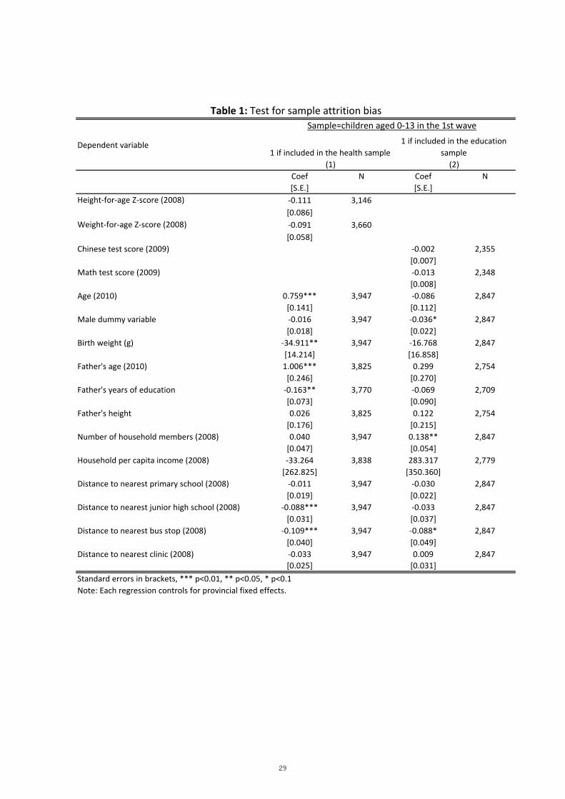
Dependent variable
Coef N Coef N[S.E.] [S.E.]
Height-for-age Z-score (2008) -0.111 3,146[0.086]
Weight-for-age Z-score (2008) -0.091 3,660[0.058]
Chinese test score (2009) -0.002 2,355[0.007]
Math test score (2009) -0.013 2,348[0.008]
Age (2010) 0.759*** 3,947 -0.086 2,847[0.141] [0.112]
Male dummy variable -0.016 3,947 -0.036* 2,847[0.018] [0.022]
Birth weight (g) -34.911** 3,947 -16.768 2,847[14.214] [16.858]
Father's age (2010) 1.006*** 3,825 0.299 2,754[0.246] [0.270]
Father's years of education -0.163** 3,770 -0.069 2,709[0.073] [0.090]
Father's height 0.026 3,825 0.122 2,754[0.176] [0.215]
Number of household members (2008) 0.040 3,947 0.138** 2,847[0.047] [0.054]
Household per capita income (2008) -33.264 3,838 283.317 2,779[262.825] [350.360]
Distance to nearest primary school (2008) -0.011 3,947 -0.030 2,847[0.019] [0.022]
Distance to nearest junior high school (2008) -0.088*** 3,947 -0.033 2,847[0.031] [0.037]
Distance to nearest bus stop (2008) -0.109*** 3,947 -0.088* 2,847[0.040] [0.049]
Distance to nearest clinic (2008) -0.033 3,947 0.009 2,847[0.025] [0.031]
Standard errors in brackets, *** p<0.01, ** p<0.05, * p<0.1Note: Each regression controls for provincial fixed effects.
(1) (2)1 if included in the health sample
1 if included in the education sample
Table 1: Test for sample attrition biasSample=children aged 0-13 in the 1st wave
29
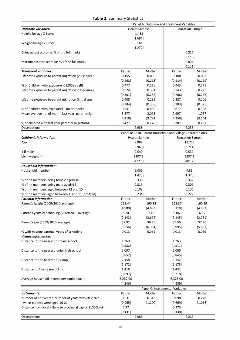
Outcome variables:Height-for-age Z-Score
Weight-for-age Z-Score
Chinese test score (as % of the full mark)
Mathmatics test score (as % of the full mark)
Treatment variables: Father Mother Father MotherLifetime exposure to parent migration (2008 spell) 0.155 0.095 0.108 0.063
[0.263] [0.213] [0.214] [0.169]% of Children with exposure>0 (2008 spell) 0.477 0.315 0.443 0.279Lifetime exposure to parent migration if exposure>0 0.324 0.301 0.243 0.225
[0.301] [0.287] [0.266] [0.256]Lifetime exposure to parent migration (initial spell) 0.408 0.231 0.387 0.206
[0.384] [0.338] [0.383] [0.325]% of Children with exposure>0 (initial spell) 0.641 0.430 0.617 0.398Mean average no. of month last year parent mig 3.377 2.095 2.997 1.767
[4.418] [3.784] [4.259] [3.564]% of children with last year parental migration>0 0.427 0.270 0.387 0.231Observations
Children's information:Age
1 if malebirth weight (g)
Household information:Household member
% of hh members being female aged>16% of hh members being male aged>16% of hh members aged between 12 and 15% of hh members aged between 0 and 11 (omitted)Parental information: Father Mother Father MotherParent's height (2009/2010 average) 168.44 160.32 168.37 160.29
[4.989] [4.893] [5.118] [4.882]Parent's years of schooling (2009/2010 average) 8.20 7.19 8.06 6.99
[2.142] [2.674] [2.145] [2.751]Parent's age (2009/2010 average) 37.92 36.35 39.56 37.96
[6.556] [6.334] [5.995] [5.601]% with missing parental years of schooling 0.013 0.051 0.013 0.059Village information:Distance to the nearest primary school 1.269 1.263
[0.532] [0.511]Distance to the nearest junior high school 2.007 2.006
[0.852] [0.845]Distance to the nearest bus stop 2.158 2.142
[1.172] [1.175]Distance to the nearest clinic 1.416 1.432
[0.697] [0.718]Average household income per capita (yuan) 6,237.00 6,328.00
[4,246] [4,689]
Instruments: Father Mother Father MotherNumber of hot years * Number of years with little rain 0.231 0.346 0.098 0.218 when parents were aged 16-21 [0.965] [1.200] [0.669] [1.016]Distance from local village to provincial capital (1000km?) 0.27 0.273
[0.131] [0.130]Observations
4.83[1.373]0.3320.309
Table 2: Summary Statistics Panel A: Outcome and Treatment Variables
Panel B: Child, Parent Household and Village Characteristics2,988 2,233
2,988 2,233
0.222
0.3190.1080.234
0.136
Panel C: Instrumental Variables
Health Sample Education Sample
Education SampleHealth Sample-1.488[1.694]0.161
0.817[1.272]
[0.110]0.834
[0.113]
3207.1[401.7]
9.988[3.969]0.549
11.755[2.714]0.539
5.005[1.423]0.338
3207.3[412.5]
30
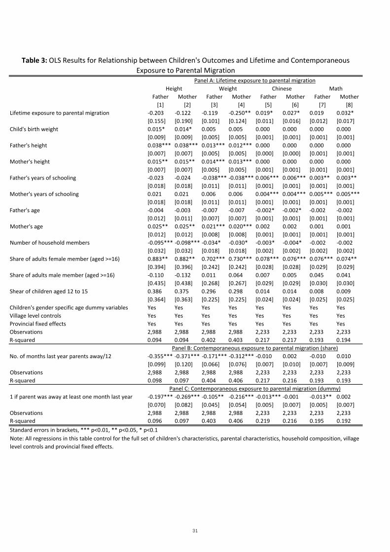
Father Mother Father Mother Father Mother Father Mother[1] [2] [3] [4] [5] [6] [7] [8]
Lifetime exposure to parental migration -0.203 -0.122 -0.119 -0.250** 0.019* 0.027* 0.019 0.032*[0.155] [0.190] [0.101] [0.124] [0.011] [0.016] [0.012] [0.017]
Child's birth weight 0.015* 0.014* 0.005 0.005 0.000 0.000 0.000 0.000[0.009] [0.009] [0.005] [0.005] [0.001] [0.001] [0.001] [0.001]
Father's height 0.038*** 0.038*** 0.013*** 0.012*** 0.000 0.000 0.000 0.000[0.007] [0.007] [0.005] [0.005] [0.000] [0.000] [0.001] [0.001]
Mother's height 0.015** 0.015** 0.014*** 0.013*** 0.000 0.000 0.000 0.000[0.007] [0.007] [0.005] [0.005] [0.001] [0.001] [0.001] [0.001]
Father's years of schooling -0.023 -0.024 -0.038*** -0.038*** 0.006*** 0.006*** 0.003** 0.003**[0.018] [0.018] [0.011] [0.011] [0.001] [0.001] [0.001] [0.001]
Mother's years of schooling 0.021 0.021 0.006 0.006 0.004*** 0.004*** 0.005*** 0.005***[0.018] [0.018] [0.011] [0.011] [0.001] [0.001] [0.001] [0.001]
Father's age -0.004 -0.003 -0.007 -0.007 -0.002* -0.002* -0.002 -0.002[0.012] [0.011] [0.007] [0.007] [0.001] [0.001] [0.001] [0.001]
Mother's age 0.025** 0.025** 0.021*** 0.020*** 0.002 0.002 0.001 0.001[0.012] [0.012] [0.008] [0.008] [0.001] [0.001] [0.001] [0.001]
Number of household members -0.095*** -0.098*** -0.034* -0.030* -0.003* -0.004* -0.002 -0.002[0.032] [0.032] [0.018] [0.018] [0.002] [0.002] [0.002] [0.002]
Share of adults female member (aged >=16) 0.883** 0.882** 0.702*** 0.730*** 0.078*** 0.076*** 0.076*** 0.074**[0.394] [0.396] [0.242] [0.242] [0.028] [0.028] [0.029] [0.029]
Share of adults male member (aged >=16) -0.110 -0.132 0.011 0.064 0.007 0.005 0.045 0.041[0.435] [0.438] [0.268] [0.267] [0.029] [0.029] [0.030] [0.030]
Shear of children aged 12 to 15 0.386 0.375 0.296 0.298 0.014 0.014 0.008 0.009[0.364] [0.363] [0.225] [0.225] [0.024] [0.024] [0.025] [0.025]
Children's gender specific age dummy variables Yes Yes Yes Yes Yes Yes Yes YesVillage level controls Yes Yes Yes Yes Yes Yes Yes YesProvincial fixed effects Yes Yes Yes Yes Yes Yes Yes YesObservations 2,988 2,988 2,988 2,988 2,233 2,233 2,233 2,233R-squared 0.094 0.094 0.402 0.403 0.217 0.217 0.193 0.194
No. of months last year parents away/12 -0.355*** -0.371*** -0.171*** -0.312*** -0.010 0.002 -0.010 0.010[0.099] [0.120] [0.066] [0.076] [0.007] [0.010] [0.007] [0.009]
Observations 2,988 2,988 2,988 2,988 2,233 2,233 2,233 2,233R-squared 0.098 0.097 0.404 0.406 0.217 0.216 0.193 0.193
1 if parent was away at least one month last year -0.197*** -0.269*** -0.105** -0.216*** -0.013*** -0.001 -0.013** 0.002[0.070] [0.082] [0.045] [0.054] [0.005] [0.007] [0.005] [0.007]
Observations 2,988 2,988 2,988 2,988 2,233 2,233 2,233 2,233R-squared 0.096 0.097 0.403 0.406 0.219 0.216 0.195 0.192Standard errors in brackets, *** p<0.01, ** p<0.05, * p<0.1Note: All regressions in this table control for the full set of children's characteristics, parental characteristics, household composition, village level controls and provincial fixed effects.
Table 3: OLS Results for Relationship between Children's Outcomes and Lifetime and Contemporaneous Exposure to Parental Migration
Panel A: Lifetime exposure to parental migration
Panel B: Contemporaneous exposure to parental migration (share)
Panel C: Contemporaneous exposure to parental migration (dummy)
Height Weight Chinese Math
31
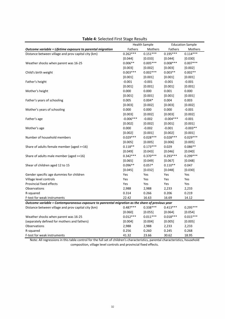
Fathers Mothers Fathers MothersDistance between village and prov capital city (km) 0.262*** 0.151*** 0.195*** 0.114***
[0.044] [0.033] [0.044] [0.030]Weather shocks when parent was 16-25 0.006** 0.005*** 0.008*** 0.007***
[0.003] [0.002] [0.003] [0.002]Child's birth weight 0.003*** 0.002*** 0.003** 0.002**
[0.001] [0.001] [0.001] [0.001]Father's height -0.001 -0.001 -0.001 -0.001
[0.001] [0.001] [0.001] [0.001]Mother's height 0.000 0.000 0.001 0.000
[0.001] [0.001] [0.001] [0.001]Father's years of schooling 0.005 0.004* 0.004 0.003
[0.003] [0.002] [0.003] [0.002]Mother's years of schooling 0.000 0.000 0.000 -0.001
[0.003] [0.002] [0.003] [0.002]Father's age -0.006*** -0.002 -0.004*** -0.001
[0.002] [0.002] [0.001] [0.001]Mother's age 0.000 -0.002 -0.001 -0.003**
[0.002] [0.001] [0.002] [0.001]Number of household members 0.029*** 0.028*** 0.028*** 0.029***
[0.005] [0.005] [0.006] [0.005]Share of adults female member (aged >=16) 0.118** 0.173*** 0.029 0.086**
[0.049] [0.043] [0.046] [0.040]Share of adults male member (aged >=16) 0.342*** 0.370*** 0.293*** 0.299***
[0.065] [0.049] [0.067] [0.048]Shear of children aged 12 to 15 0.096** 0.057* 0.110** 0.047
[0.045] [0.032] [0.048] [0.030]Gender specific age dummies for children Yes Yes Yes YesVillage level controls Yes Yes Yes YesProvincial fixed effects Yes Yes Yes YesObservations 2,988 2,988 2,233 2,233R-squared 0.314 0.266 0.206 0.219F-test for weak instruments 22.42 16.63 16.69 14.12Outcome variable = Contemporaneous exposure to panrental migration as the share of previous yearDistance between village and prov capital city (km) 0.487*** 0.338*** 0.413*** 0.295***
[0.060] [0.055] [0.064] [0.054]Weather shocks when parent was 16-25 0.012*** 0.011*** 0.018*** 0.015***(separately defined for mothers and fathers) [0.004] [0.004] [0.005] [0.005]Observations 2,988 2,988 2,233 2,233R-squared 0.256 0.260 0.245 0.268F-test for weak instruments 41.32 23.66 30.62 18.95
Health Sample Education SampleTable 4: Selected First Stage Results
Outcome variable = Lifetime exposure to parental migration
Note: All regressions in this table control for the full set of children's characteristics, parental characteristics, household composition, village level controls and provincial fixed effects.
32
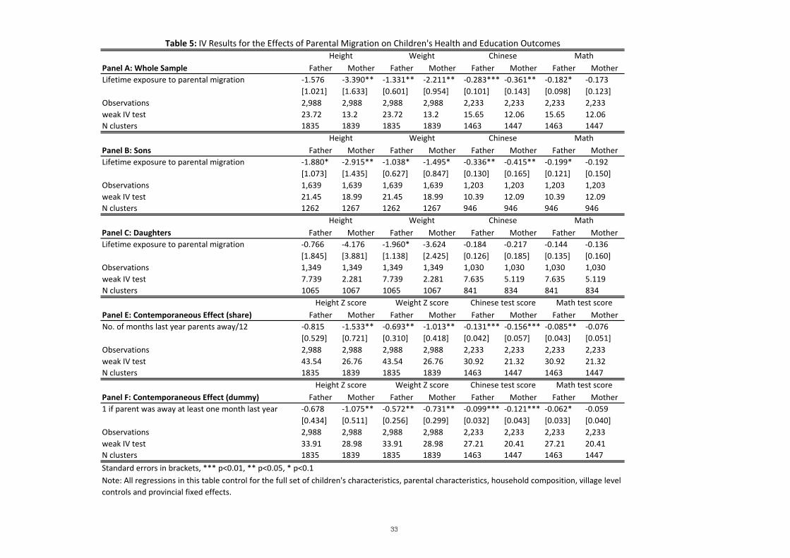
Panel A: Whole Sample Father Mother Father Mother Father Mother Father MotherLifetime exposure to parental migration -1.576 -3.390** -1.331** -2.211** -0.283*** -0.361** -0.182* -0.173
[1.021] [1.633] [0.601] [0.954] [0.101] [0.143] [0.098] [0.123]Observations 2,988 2,988 2,988 2,988 2,233 2,233 2,233 2,233weak IV test 23.72 13.2 23.72 13.2 15.65 12.06 15.65 12.06N clusters 1835 1839 1835 1839 1463 1447 1463 1447
Panel B: Sons Father Mother Father Mother Father Mother Father MotherLifetime exposure to parental migration -1.880* -2.915** -1.038* -1.495* -0.336** -0.415** -0.199* -0.192
[1.073] [1.435] [0.627] [0.847] [0.130] [0.165] [0.121] [0.150]Observations 1,639 1,639 1,639 1,639 1,203 1,203 1,203 1,203weak IV test 21.45 18.99 21.45 18.99 10.39 12.09 10.39 12.09N clusters 1262 1267 1262 1267 946 946 946 946
Panel C: Daughters Father Mother Father Mother Father Mother Father MotherLifetime exposure to parental migration -0.766 -4.176 -1.960* -3.624 -0.184 -0.217 -0.144 -0.136
[1.845] [3.881] [1.138] [2.425] [0.126] [0.185] [0.135] [0.160]Observations 1,349 1,349 1,349 1,349 1,030 1,030 1,030 1,030weak IV test 7.739 2.281 7.739 2.281 7.635 5.119 7.635 5.119N clusters 1065 1067 1065 1067 841 834 841 834
Panel E: Contemporaneous Effect (share) Father Mother Father Mother Father Mother Father MotherNo. of months last year parents away/12 -0.815 -1.533** -0.693** -1.013** -0.131*** -0.156*** -0.085** -0.076
[0.529] [0.721] [0.310] [0.418] [0.042] [0.057] [0.043] [0.051]Observations 2,988 2,988 2,988 2,988 2,233 2,233 2,233 2,233weak IV test 43.54 26.76 43.54 26.76 30.92 21.32 30.92 21.32N clusters 1835 1839 1835 1839 1463 1447 1463 1447
Panel F: Contemporaneous Effect (dummy) Father Mother Father Mother Father Mother Father Mother1 if parent was away at least one month last year -0.678 -1.075** -0.572** -0.731** -0.099*** -0.121*** -0.062* -0.059
[0.434] [0.511] [0.256] [0.299] [0.032] [0.043] [0.033] [0.040]Observations 2,988 2,988 2,988 2,988 2,233 2,233 2,233 2,233weak IV test 33.91 28.98 33.91 28.98 27.21 20.41 27.21 20.41N clusters 1835 1839 1835 1839 1463 1447 1463 1447Standard errors in brackets, *** p<0.01, ** p<0.05, * p<0.1
Chinese Math
Height Weight Chinese Math
Weight Chinese Math
Note: All regressions in this table control for the full set of children's characteristics, parental characteristics, household composition, village level controls and provincial fixed effects.
Table 5: IV Results for the Effects of Parental Migration on Children's Health and Education Outcomes
Height Z score Weight Z score Chinese test score Math test score
Height
Height Z score Weight Z score Chinese test score Math test score
Height Weight
33
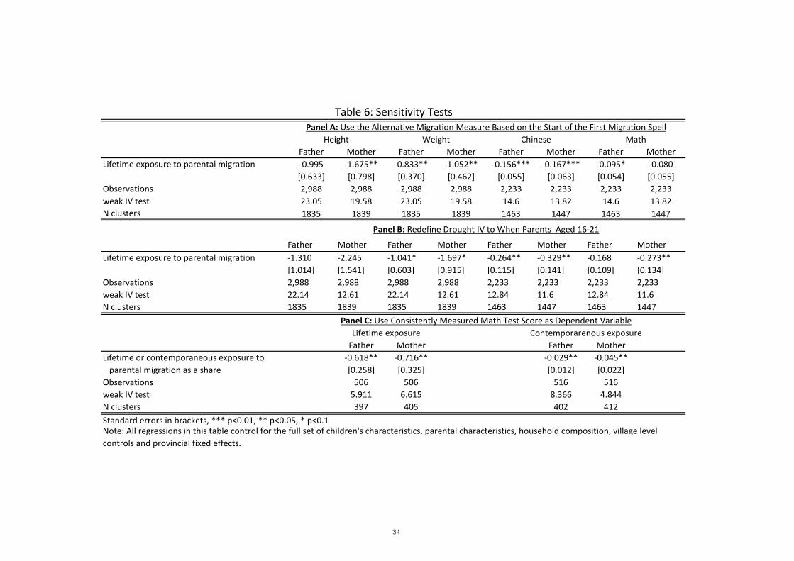
Father Mother Father Mother Father Mother Father MotherLifetime exposure to parental migration -0.995 -1.675** -0.833** -1.052** -0.156*** -0.167*** -0.095* -0.080
[0.633] [0.798] [0.370] [0.462] [0.055] [0.063] [0.054] [0.055]Observations 2,988 2,988 2,988 2,988 2,233 2,233 2,233 2,233weak IV test 23.05 19.58 23.05 19.58 14.6 13.82 14.6 13.82N clusters 1835 1839 1835 1839 1463 1447 1463 1447
Father Mother Father Mother Father Mother Father MotherLifetime exposure to parental migration -1.310 -2.245 -1.041* -1.697* -0.264** -0.329** -0.168 -0.273**
[1.014] [1.541] [0.603] [0.915] [0.115] [0.141] [0.109] [0.134]Observations 2,988 2,988 2,988 2,988 2,233 2,233 2,233 2,233weak IV test 22.14 12.61 22.14 12.61 12.84 11.6 12.84 11.6N clusters 1835 1839 1835 1839 1463 1447 1463 1447
Father Mother Father MotherLifetime or contemporaneous exposure to -0.618** -0.716** -0.029** -0.045** parental migration as a share [0.258] [0.325] [0.012] [0.022]Observations 506 506 516 516weak IV test 5.911 6.615 8.366 4.844N clusters 397 405 402 412Standard errors in brackets, *** p<0.01, ** p<0.05, * p<0.1
Table 6: Sensitivity Tests
Panel B: Redefine Drought IV to When Parents Aged 16-21
Note: All regressions in this table control for the full set of children's characteristics, parental characteristics, household composition, village level controls and provincial fixed effects.
Panel C: Use Consistently Measured Math Test Score as Dependent Variable
Panel A: Use the Alternative Migration Measure Based on the Start of the First Migration Spell
Lifetime exposure Contemporarenous exposure
Height Weight Chinese Math
34
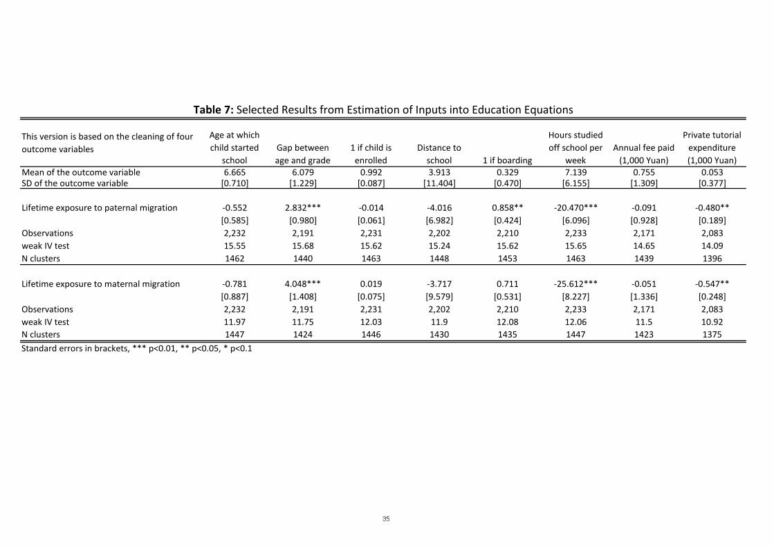
This version is based on the cleaning of four outcome variables
Age at which child started
schoolGap between age and grade
1 if child is enrolled
Distance to school 1 if boarding
Hours studied off school per
weekAnnual fee paid
(1,000 Yuan)
Private tutorial expenditure (1,000 Yuan)
Mean of the outcome variable 6.665 6.079 0.992 3.913 0.329 7.139 0.755 0.053SD of the outcome variable [0.710] [1.229] [0.087] [11.404] [0.470] [6.155] [1.309] [0.377]
Lifetime exposure to paternal migration -0.552 2.832*** -0.014 -4.016 0.858** -20.470*** -0.091 -0.480**[0.585] [0.980] [0.061] [6.982] [0.424] [6.096] [0.928] [0.189]
Observations 2,232 2,191 2,231 2,202 2,210 2,233 2,171 2,083weak IV test 15.55 15.68 15.62 15.24 15.62 15.65 14.65 14.09N clusters 1462 1440 1463 1448 1453 1463 1439 1396
Lifetime exposure to maternal migration -0.781 4.048*** 0.019 -3.717 0.711 -25.612*** -0.051 -0.547**[0.887] [1.408] [0.075] [9.579] [0.531] [8.227] [1.336] [0.248]
Observations 2,232 2,191 2,231 2,202 2,210 2,233 2,171 2,083weak IV test 11.97 11.75 12.03 11.9 12.08 12.06 11.5 10.92N clusters 1447 1424 1446 1430 1435 1447 1423 1375Standard errors in brackets, *** p<0.01, ** p<0.05, * p<0.1
Table 7: Selected Results from Estimation of Inputs into Education Equations
35
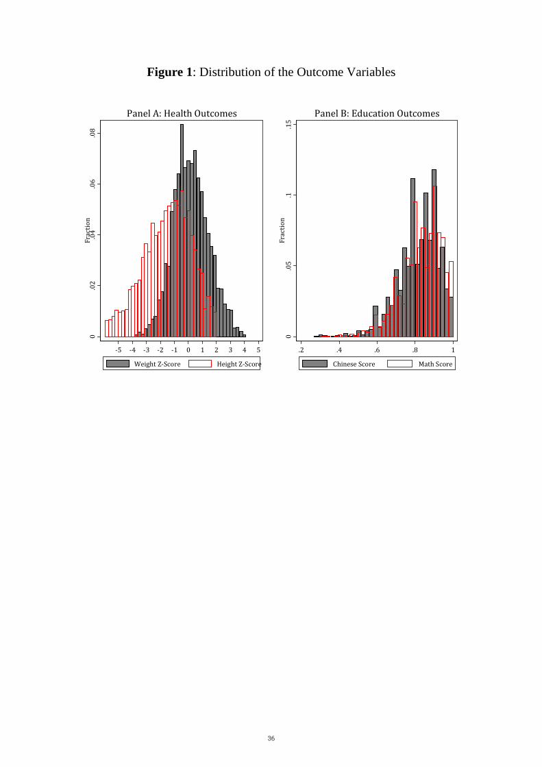
Figure 1: Distribution of the Outcome Variables
0.0
2.0
4.0
6.0
8Fr
actio
n
-5 -4 -3 -2 -1 0 1 2 3 4 5
Weight Z-Score Height Z-Score
Panel A: Health Outcomes
0.0
5.1
.15
Frac
tion
.2 .4 .6 .8 1
Chinese Score Math Score
Panel B: Education Outcomes
36
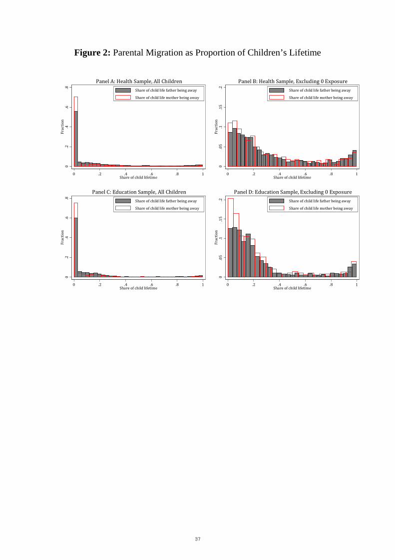
Figure 2: Parental Migration as Proportion of Children’s Lifetime
0.2
.4.6
.8Fr
actio
n
0 .2 .4 .6 .8 1Share of child lifetime
Share of child life father being away
Share of child life mother being away
Panel A: Health Sample, All Children
0.0
5.1
.15
.2Fr
actio
n
0 .2 .4 .6 .8 1Share of child lifetime
Share of child life father being away
Share of child life mother being away
Panel B: Health Sample, Excluding 0 Exposure
0.2
.4.6
.8Fr
actio
n
0 .2 .4 .6 .8 1Share of child lifetime
Share of child life father being away
Share of child life mother being away
Panel C: Education Sample, All Children
0.0
5.1
.15
.2Fr
actio
n
0 .2 .4 .6 .8 1Share of child lifetime
Share of child life father being away
Share of child life mother being away
Panel D: Education Sample, Excluding 0 Exposure
37
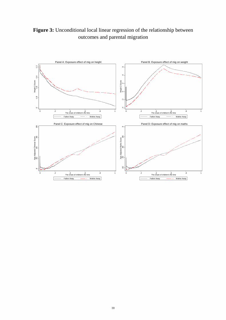
Figure 3: Unconditional local linear regression of the relationship between outcomes and parental migration
-2-1
.8-1
.6-1
.4-1
.2H
eigh
t Z-S
core
0 .2 .4 .6 .8 1The share of children's life time
Father Away Mother Away
Panel A: Exposure effect of mig on height
-.4-.2
0.2
.4.6
Hei
ght Z
-Sco
re
0 .2 .4 .6 .8 1The share of children's life time
Father Away Mother Away
Panel B: Exposure effect of mig on weight
.8.8
2.8
4.8
6.8
8Ag
e Ad
just
ed C
hine
se S
core
0 .2 .4 .6 .8 1The share of children's life time
Father Away Mother Away
Panel C: Exposure effect of mig on Chinese.8
2.8
4.8
6.8
8.9
Age
Adju
sted
Mat
hs S
core
0 .2 .4 .6 .8 1The share of children's life time
Father Away Mother Away
Panel D: Exposure effect of mig on maths
38
Appendix A: Data Appendix
The share of child life in which parents were away: The RUMiC Study provides two types
of information. One is the number of months in the previous year during which parents
were away from home. This information is available from all the waves. Thus, we know
the number of months parents were away in 2007, 2008, and 2009. The other piece of
information is when parents started migration. This was asked only in the 2009 wave for
individuals who reported to have been away in 2008. In order to construct the number of
months parents were away since the beginning of migration asked in the 2009 survey till
the end of 2009, we first aggregated the number of months in which parents were away in
2007 through 2009. For individuals who answered that their migration had started before
2007, we have added the number of months between the beginning of the migration till
the end of 2006.
Individual test scores were asked for the previous semester, together with the full score
for each subject. The ratio of the individual score over the full score is used as our outcome
variables.
Distance to public facilities is coded using five categories: 1:<2km, 2:2-5 km, 3:5-10
km, 4:10-20 km, 5:>20km.
The height-for-age Z-score is created using parameters from the CDC 2000 Growth
Charts and 2006 WHO Growth Charts (Kuczmarski RJ, Ogden CL, Guo SS, et al. 2000;
WHO, 2006; de Onis, et al., 2007). The results do not change substantively depending
on the choice over the two parameter sources. In this paper, we report the estimates
based on the CDC parameters because they provide a more suitable reference group for
our analysis. In the WHO growth charts, the comparison group for children aged 0-5 are
children following optimal health practices. Thus, the charts depict the standard which is
likely to realize under optimal conditions, rather than just a reference. However, the same
standard was not used for the comparison group for 5-19 year-olds, and it is based on the
U.S. reference children used in the 1977 NCHS Growth Charts. On the other hand, the
CDC 2000 charts provide a more consistent reference for children in our sample, based on
a group of children in the U.S.
We apply the CDC parameters for infants (based on length) to observations aged 0-
24 months, and the parameters for children (based on statue) observations aged 25-180
months. The transition between these two charts have been made smooth in the 2000
CDC charts (Kuczmarski RJ, Ogden CL, Guo SS, et al. 2000).
Since our anthropometric data are based on reports by parents, there are likely to be
measurement errors. Several methods have been suggested to deal with them. The WHO
recommends the use of different formula for those children whose z-scores are larger than 3
39
in the absolute terms. The CDC training modules contain a note suggesting to distinguish
“biologically implausible values,”19 which are observations whose z-scores are larger than
certain values, or are away from the mean z-score in terms of standard deviations. We
report the results that are commonly found regardless of the choice over these alternative
adjustments to the measures for outcomes.
19http://www.cdc.gov/nccdphp/dnpa/growthcharts/resources/BIV-cutoffs.pdf, downloaded on Jan-uary 28th, 2013.
40