Effect of different emission inventories on modeled … T. Amnuaylojaroen et al.: Effect of different emission inventories 1 Introduction Southeast Asia, which includes the Indochina

Atmos. Chem. Phys., 14, 12983–13012, 2014

www.atmos-chem-phys.net/14/12983/2014/

doi:10.5194/acp-14-12983-2014

© Author(s) 2014. CC Attribution 3.0 License.

Effect of different emission inventories on modeled ozone and

carbon monoxide in Southeast Asia

T. Amnuaylojaroen1,2, M. C. Barth2, L. K. Emmons2, G. R. Carmichael3, J. Kreasuwun1,4, S. Prasitwattanaseree5,

and S. Chantara1

1Environmental Science Program and the Center for Environmental Health, Toxicology and

Management of Chemical, Chiang Mai University, Faculty of Science, Chiang Mai, Thailand2Atmospheric Chemistry Division (ACD), National Center for Atmospheric Research (NCAR),

Boulder, CO, USA3Center for Global and Regional Environmental Research, The University of Iowa, Iowa City, IA, USA4Department of Physics and Materials Science, Faculty of Science, Chiang Mai University, Chiang Mai,

Thailand5Department of Statistics, Faculty of Science, Chiang Mai University, Chiang Mai, Thailand

Correspondence to: T. Amnuaylojaroen ([email protected]) and M. C. Barth ([email protected])

Received: 5 March 2014 – Published in Atmos. Chem. Phys. Discuss.: 7 April 2014

Revised: 17 September 2014 – Accepted: 8 October 2014 – Published: 8 December 2014

Abstract. In order to improve our understanding of air qual-

ity in Southeast Asia, the anthropogenic emissions inven-

tory must be well represented. In this work, we apply differ-

ent anthropogenic emission inventories in the Weather Re-

search and Forecasting Model with Chemistry (WRF-Chem)

version 3.3 using Model for Ozone and Related Chem-

ical Tracers (MOZART) gas-phase chemistry and Global

Ozone Chemistry Aerosol Radiation and Transport (GO-

CART) aerosols to examine the differences in predicted car-

bon monoxide (CO) and ozone (O3) surface mixing ra-

tios for Southeast Asia in March and December 2008. The

anthropogenic emission inventories include the Reanaly-

sis of the TROpospheric chemical composition (RETRO),

the Intercontinental Chemical Transport Experiment-Phase

B (INTEX-B), the MACCity emissions (adapted from the

Monitoring Atmospheric Composition and Climate and

megacity Zoom for the Environment projects), the Southeast

Asia Composition, Cloud, Climate Coupling Regional Study

(SEAC4RS) emissions, and a combination of MACCity and

SEAC4RS emissions. Biomass-burning emissions are from

the Fire Inventory from the National Center for Atmospheric

Research (NCAR) (FINNv1) model. WRF-Chem reasonably

predicts the 2 m temperature, 10 m wind, and precipitation. In

general, surface CO is underpredicted by WRF-Chem while

surface O3 is overpredicted. The NO2 tropospheric column

predicted by WRF-Chem has the same magnitude as obser-

vations, but tends to underpredict the NO2 column over the

equatorial ocean and near Indonesia. Simulations using dif-

ferent anthropogenic emissions produce only a slight vari-

ability of O3 and CO mixing ratios, while biomass-burning

emissions add more variability. The different anthropogenic

emissions differ by up to 30 % in CO emissions, but O3 and

CO mixing ratios averaged over the land areas of the model

domain differ by∼ 4.5 % and∼ 8 %, respectively, among the

simulations. Biomass-burning emissions create a substantial

increase for both O3 and CO by ∼ 29 % and ∼ 16 %, respec-

tively, when comparing the March biomass-burning period to

the December period with low biomass-burning emissions.

The simulations show that none of the anthropogenic emis-

sion inventories are better than the others for predicting O3

surface mixing ratios. However, the simulations with differ-

ent anthropogenic emission inventories do differ in their pre-

dictions of CO surface mixing ratios producing variations of

∼ 30 % for March and 10–20 % for December at Thai surface

monitoring sites.

Published by Copernicus Publications on behalf of the European Geosciences Union.

12984 T. Amnuaylojaroen et al.: Effect of different emission inventories

1 Introduction

Southeast Asia, which includes the Indochina peninsula and

the Indonesian archipelago, can have significant air qual-

ity problems. Understanding the contribution of different

sources of tropospheric ozone (O3) and its precursors, carbon

monoxide (CO) and nitrogen oxides (NOx = NO+NO2), for

Southeast Asia provides valuable information on maintaining

good air quality for both human well being and ecosystems.

Previous studies examining air pollutants and their sources

via regional model simulations have focused primarily on

China (e.g., Wang et al., 2005; Geng et al., 2011), eastern

Asia (Han et al., 2008; Tanimoto et al., 2009), and India (Ad-

hikary et al., 2007; Kumar et al., 2012; Ghude et al., 2013).

Here, we examine the effect of different emission inventories

on modeled surface O3 and CO for Southeast Asia, a region

generally ignored in previous studies.

Previous studies have indicated that both local anthro-

pogenic and biomass-burning emissions, as well as emissions

upstream are important for local O3 air quality in Asia. In

eastern Asia, Tanimoto et al. (2009) noted relatively small

changes in decadal O3 trends at sites near the Japanese coast,

but a larger increase in measured O3 at a remote mountain-

ous site in Japan. Using a regional chemistry transport model,

Tanimoto et al. (2009) attributed half of the observed in-

crease at the mountainous site to increasing anthropogenic

emissions in Asia. The results from this study suggested that

the actual growth in emissions between 1998 and 2007 was

significantly underestimated. Using a nested eastern Asia do-

main within a global chemistry transport model, Wang et

al. (2011) found that local sources of O3 precursors produced

much of the O3 in the region; however, O3 transported from

Europe, North America, India, and Southeast Asia also im-

pacted O3 concentrations in eastern China depending on the

season. Liu et al. (2008), using a regional air quality model,

determined that fossil fuel and biomass-burning emissions

from eastern Asia increased surface CO and O3 in Taiwan by

70–150 % and 50–100 %, respectively, compared to model

results that excluded background emissions. They attributed

up to 20 % of the surface CO and O3 in Taiwan to biomass-

burning emissions from eastern China. Both the aerosol opti-

cal depth and O3 concentrations in the Pearl River delta were

also found to be affected by biomass-burning emissions oc-

curring upstream in Southeast Asia (Deng et al., 2008).

Southeast Asia is subject to the outflow of pollution from

the main continent, yet the region itself is rapidly grow-

ing and has increasing anthropogenic and biomass-burning

emissions, which are especially high during the dry sea-

son (November–April). To simulate O3 production and con-

centrations in Southeast Asia, realistic estimates of emis-

sions from both local and regional sources, including fos-

sil fuel use, other anthropogenic activities, and biomass

burning, must be available. Emission inventories for Asia

have been developed by several groups (e.g., Akimoto and

Narita, 1994; Streets et al., 2003; Ohara et al., 2007; Zhang

et al., 2009; Kurokawa et al., 2013) for both chemistry–

climate and air quality studies. For example, the REanal-

ysis of the TROpospheric chemical composition (RETRO)

and the Emission Database for Global Atmospheric Research

(EDGAR) emissions inventories (Olivier et al., 2005; Schultz

et al., 2007) are global emissions inventories developed for

chemistry–climate studies. Streets et al. (2003) developed a

2001 emission inventory for the ACE-Asia (Asian Pacific Re-

gional Aerosol Characterization Experiment) and TRACE-

P (Transport and Chemical Evolution over the Pacific) field

campaigns which took place in the eastern Asian and west-

ern Pacific region during spring 2001. Zhang et al. (2009)

developed a 2006 emissions inventory for Asia to support

the Intercontinental Chemical Transport Experiment-Phase

B (INTEX-B) field campaign. The INTEX-B field campaign

emphasized China emissions because they dominate the Asia

pollutant outflow to the Pacific. Ohara et al. (2007) devel-

oped the Regional Emission inventory in Asia (REAS) for

1980–2020 in order to conduct air quality studies for re-

cent past, present-day, and near-future time periods. More

recently, Kurokawa et al. (2013) released REAS version 2.1,

providing updated emissions for each year from 2000 to

2008 for Asian countries east of ∼ 55◦ E. The MACCity

(adapted from the Monitoring Atmospheric Composition and

Climate and megacity Zoom for the Environment projects)

emissions inventory (Granier et al., 2011), which is an out-

come from two European Commission projects (MACC and

CityZen), is a 1980–2010 global emissions inventory for

chemistry–climate studies. Most recently the Southeast Asia

Composition, Cloud, Climate Coupling by Regional Study

(SEAC4RS) emissions inventory (Lu and Streets, 2012) for

2012 emissions has been released for field campaign sup-

port. Four emission inventories, RETRO, INTEX-B, MACC-

ity, and SEAC4RS, will be described in more detail in Sect. 3.

While previous studies (e.g., Ohara et al., 2007) have com-

pared different emission inventories, a comparison of simu-

lated surface CO and O3 mixing ratios resulting from differ-

ent emission inventories, yet using the same model frame-

work, has not been done. Here, the Weather and Forecasting

Model coupled with Chemistry (WRF-Chem) is used to ex-

amine the variability of predicted O3 and CO surface mixing

ratios when five different anthropogenic emission inventories

(RETRO, INTEX-B, MACCity, SEAC4RS and a modified

SEAC4RS) are used as inputs. By conducting this compari-

son using the same model, differences in results due to model

meteorology are mitigated. We focus this study on Southeast

Asia, an area that has received little attention, yet has sub-

stantial anthropogenic and biomass-burning emissions. As

part of our study, we examine the effect of biomass-burning

emissions on surface O3 and CO by the contrasting results

from a low biomass-burning period (December) with a high

biomass-burning period (March).

We begin this paper by describing the model configura-

tion (Sect. 2) and emission inventories (Sect. 3) applied in

the model simulations. We then evaluate the model results

Atmos. Chem. Phys., 14, 12983–13012, 2014 www.atmos-chem-phys.net/14/12983/2014/

T. Amnuaylojaroen et al.: Effect of different emission inventories 12985

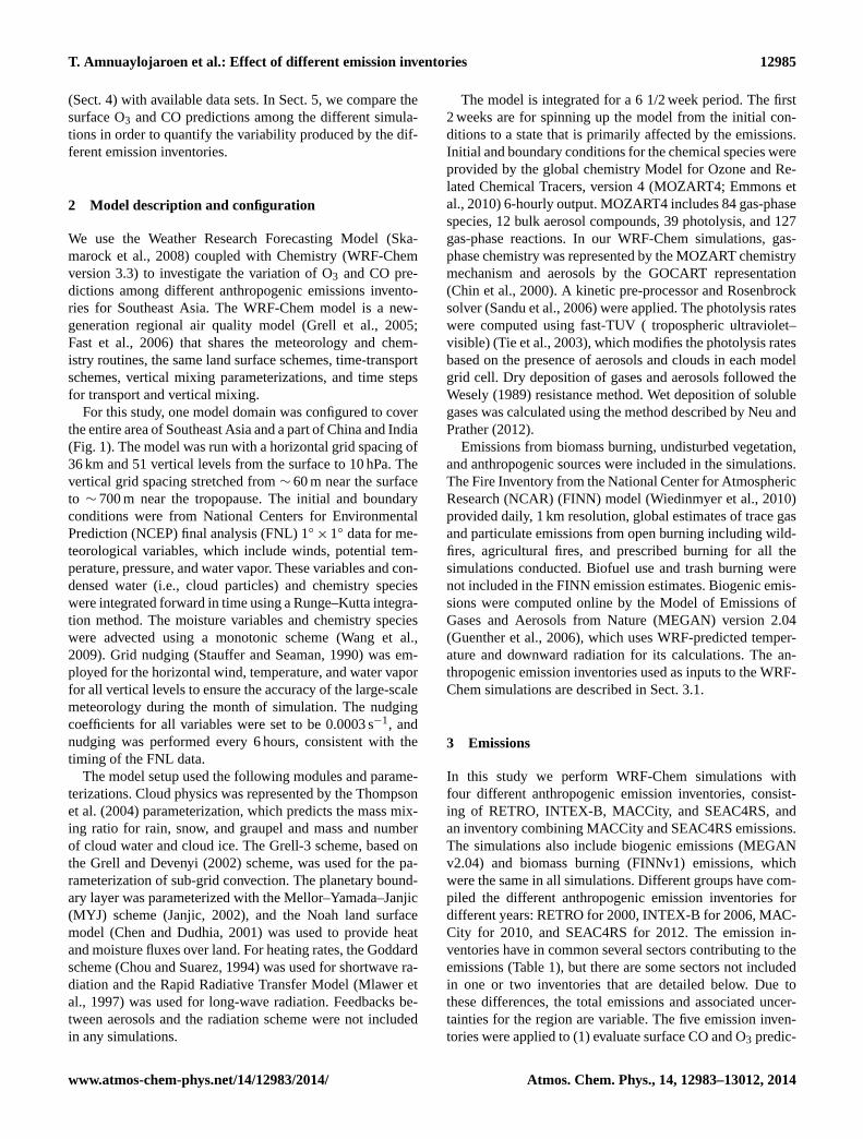
(Sect. 4) with available data sets. In Sect. 5, we compare the

surface O3 and CO predictions among the different simula-

tions in order to quantify the variability produced by the dif-

ferent emission inventories.

2 Model description and configuration

We use the Weather Research Forecasting Model (Ska-

marock et al., 2008) coupled with Chemistry (WRF-Chem

version 3.3) to investigate the variation of O3 and CO pre-

dictions among different anthropogenic emissions invento-

ries for Southeast Asia. The WRF-Chem model is a new-

generation regional air quality model (Grell et al., 2005;

Fast et al., 2006) that shares the meteorology and chem-

istry routines, the same land surface schemes, time-transport

schemes, vertical mixing parameterizations, and time steps

for transport and vertical mixing.

For this study, one model domain was configured to cover

the entire area of Southeast Asia and a part of China and India

(Fig. 1). The model was run with a horizontal grid spacing of

36 km and 51 vertical levels from the surface to 10 hPa. The

vertical grid spacing stretched from ∼ 60 m near the surface

to ∼ 700 m near the tropopause. The initial and boundary

conditions were from National Centers for Environmental

Prediction (NCEP) final analysis (FNL) 1◦× 1◦ data for me-

teorological variables, which include winds, potential tem-

perature, pressure, and water vapor. These variables and con-

densed water (i.e., cloud particles) and chemistry species

were integrated forward in time using a Runge–Kutta integra-

tion method. The moisture variables and chemistry species

were advected using a monotonic scheme (Wang et al.,

2009). Grid nudging (Stauffer and Seaman, 1990) was em-

ployed for the horizontal wind, temperature, and water vapor

for all vertical levels to ensure the accuracy of the large-scale

meteorology during the month of simulation. The nudging

coefficients for all variables were set to be 0.0003 s−1, and

nudging was performed every 6 hours, consistent with the

timing of the FNL data.

The model setup used the following modules and parame-

terizations. Cloud physics was represented by the Thompson

et al. (2004) parameterization, which predicts the mass mix-

ing ratio for rain, snow, and graupel and mass and number

of cloud water and cloud ice. The Grell-3 scheme, based on

the Grell and Devenyi (2002) scheme, was used for the pa-

rameterization of sub-grid convection. The planetary bound-

ary layer was parameterized with the Mellor–Yamada–Janjic

(MYJ) scheme (Janjic, 2002), and the Noah land surface

model (Chen and Dudhia, 2001) was used to provide heat

and moisture fluxes over land. For heating rates, the Goddard

scheme (Chou and Suarez, 1994) was used for shortwave ra-

diation and the Rapid Radiative Transfer Model (Mlawer et

al., 1997) was used for long-wave radiation. Feedbacks be-

tween aerosols and the radiation scheme were not included

in any simulations.

The model is integrated for a 6 1/2 week period. The first

2 weeks are for spinning up the model from the initial con-

ditions to a state that is primarily affected by the emissions.

Initial and boundary conditions for the chemical species were

provided by the global chemistry Model for Ozone and Re-

lated Chemical Tracers, version 4 (MOZART4; Emmons et

al., 2010) 6-hourly output. MOZART4 includes 84 gas-phase

species, 12 bulk aerosol compounds, 39 photolysis, and 127

gas-phase reactions. In our WRF-Chem simulations, gas-

phase chemistry was represented by the MOZART chemistry

mechanism and aerosols by the GOCART representation

(Chin et al., 2000). A kinetic pre-processor and Rosenbrock

solver (Sandu et al., 2006) were applied. The photolysis rates

were computed using fast-TUV ( tropospheric ultraviolet–

visible) (Tie et al., 2003), which modifies the photolysis rates

based on the presence of aerosols and clouds in each model

grid cell. Dry deposition of gases and aerosols followed the

Wesely (1989) resistance method. Wet deposition of soluble

gases was calculated using the method described by Neu and

Prather (2012).

Emissions from biomass burning, undisturbed vegetation,

and anthropogenic sources were included in the simulations.

The Fire Inventory from the National Center for Atmospheric

Research (NCAR) (FINN) model (Wiedinmyer et al., 2010)

provided daily, 1 km resolution, global estimates of trace gas

and particulate emissions from open burning including wild-

fires, agricultural fires, and prescribed burning for all the

simulations conducted. Biofuel use and trash burning were

not included in the FINN emission estimates. Biogenic emis-

sions were computed online by the Model of Emissions of

Gases and Aerosols from Nature (MEGAN) version 2.04

(Guenther et al., 2006), which uses WRF-predicted temper-

ature and downward radiation for its calculations. The an-

thropogenic emission inventories used as inputs to the WRF-

Chem simulations are described in Sect. 3.1.

3 Emissions

In this study we perform WRF-Chem simulations with

four different anthropogenic emission inventories, consist-

ing of RETRO, INTEX-B, MACCity, and SEAC4RS, and

an inventory combining MACCity and SEAC4RS emissions.

The simulations also include biogenic emissions (MEGAN

v2.04) and biomass burning (FINNv1) emissions, which

were the same in all simulations. Different groups have com-

piled the different anthropogenic emission inventories for

different years: RETRO for 2000, INTEX-B for 2006, MAC-

City for 2010, and SEAC4RS for 2012. The emission in-

ventories have in common several sectors contributing to the

emissions (Table 1), but there are some sectors not included

in one or two inventories that are detailed below. Due to

these differences, the total emissions and associated uncer-

tainties for the region are variable. The five emission inven-

tories were applied to (1) evaluate surface CO and O3 predic-

www.atmos-chem-phys.net/14/12983/2014/ Atmos. Chem. Phys., 14, 12983–13012, 2014


Figure 1. CO emissions for March 2008 from different emission inventories: (a) MACCity–SEAC4RS, (b) biomass burning, (c) RETRO

- MACCity–SEAC4RS, (d) INTEX-B - MACCity–SEAC4RS, (e) MACCity - MACCity–SEAC4RS, and (f) SEAC4RS - MACCity–

SEAC4RS.

tions with monitoring station observations and (2) determine

the extent to which the model predictions are limited by vari-

ations in the emissions inventories.

3.1 Description of the anthropogenic emission

inventories

The RETRO project aimed at analyzing the long-term

changes in the atmospheric budget of trace gases and aerosols

over the time period from 1960 to 2000. The RETRO anthro-

pogenic emissions (Schultz et al., 2007) are derived from a

preliminary version of the TNO (Netherlands Organization

for Applied Scientific Research) emissions, for the 1960–

2000 time period with spatial resolution of 0.5◦× 0.5◦. The

anthropogenic emissions in the RETRO inventory include

mainly combustion sources (Granier et al., 2011), but sol-

vent use and other industrial processes are included (Ta-

ble 1). Schultz et al. (2007) report several uncertainties as-

sociated with the RETRO emissions. These uncertainties in-

clude omission of specific sectors (e.g., railway traffic or

cement manufacturing), underestimation of CO combustion

emissions and NOx ship traffic emissions, and the lack of



Figure 2. CO emissions for December 2008 from different emission inventories: (a) MACCity–SEAC4RS, (b) biomass burning, (c)

RETRO - MACCity–SEAC4RS, (d) INTEX-B - MACCity–SEAC4RS, (e) MACCity - MACCity–SEAC4RS, and (f) SEAC4RS - MACCity–

SEAC4RS.

weekly and diurnal profiles of emissions. For the Southeast

Asia region the RETRO seasonal cycle is based on the Long

Term Ozone Simulation and European Operational Smog

(LOTOS-EUROS) European monthly pattern (Schaap et al.,

2005; which is derived from a critical review of the monthly

variation by emission sector), but has a reduced amplitude.

Kurokawa et al. (2013) show that there is very little sea-

sonal cycle for anthropogenic emissions of NOx and black

carbon over India, which is a region similar to Southeast

Asia in terms of climate. The RETRO inventory provided

regional information for the emissions of a variety of non-

methane volatile organic compounds (NMVOCs) including

ethane, propane, butanes, pentanes, hexanes and higher alka-

nes, ethene, propene, ethyne, other alkenes and alkynes, ben-

zene, toluene, xylene, trimethyl benzenes and other aromat-

ics, organic alcohols, esters, ethers, chlorinated hydrocar-

bons, formaldehyde and other aldehydes, ketones, organic

acids, and other VOCs.

As part of the INTEX-B field campaign, which was con-

ducted by the National Aeronautics and Space Administra-

tion (NASA) in spring 2006, anthropogenic emissions were

developed for the specific year and season as the field cam-



Figure 3. Nitrogen oxides emissions for March 2008 from different emission inventories: (a) MACCity–SEAC4RS, (b) biomass burning, (c)

RETRO - MACCity–SEAC4RS, (d) INTEX-B - MACCity–SEAC4RS, (e) MACCity - MACCity–SEAC4RS, and (f) SEAC4RS - MACCity–

SEAC4RS.

paign (Zhang et al., 2009). The emissions are estimated for

eight major chemical species, sulfur dioxide (SO2), NOx,

CO, NMVOCs, PM10, PM2.5, black carbon (BC) and or-

ganic carbon (OC), with a spatial resolution of 0.5◦×0.5◦. To

represent the individual VOCs represented in the MOZART

mechanism, the NMVOC emissions are speciated based on

the ratios of the individual VOC to the total NMVOCs de-

rived from the RETRO inventory; that is, the individual VOC

fraction from the RETRO inventory is multiplied with the

total INTEX-B NMVOC to get the individual VOC emis-

sions. The INTEX-B emissions contain four major sectors

(Table 1): power generation, industry, residential, and trans-

portation. The uncertainty of the INTEX-B emissions for

the Southeast Asian countries is estimated to be similar to

the TRACE-P emissions uncertainty (Zhang et al., 2009),

e.g., ± 37 % for NOx emissions and ± 185 % for CO emis-

sions. The INTEX-B emissions uncertainties for China are

smaller (± 31 % for NOx and ± 70 % for CO).

The MACCity emissions (Granier et al., 2011) are

an outcome of two European Commission projects,

MACC (Hollingsworth et al., 2008) and CityZen (http:

//cityzen-project.eu) and are an extension of the the At-


http://cityzen-project.eu

http://cityzen-project.eu


Figure 4. Nitrogen oxides emissions for December 2008 from different emission inventories: (a) MACCity–SEAC4RS, (b) biomass burn-

ing, (c) RETRO - MACCity–SEAC4RS, (d) INTEX-B - MACCity–SEAC4RS, (e) MACCity - MACCity–SEAC4RS, and (f) SEAC4RS -

MACCity–SEAC4RS.

mospheric Chemistry and Climate Model Intercomparison

Project (ACCMIP) historical emissions data set (Lamarque

et al., 2010). The goal of the MACCity emissions inven-

tory is to support the IPCC-AR5 (Intergovernmental Panel

for Climate Change Assessment Report 5), providing histor-

ical emissions from a variety of emission sectors (Table 1)

on a decadal basis from 1960 to 2020, as well as for future

emissions scenarios based on RCPs (Representation Concen-

tration Pathways; van Vuuren et al., 2011). Anthropogenic

emissions have been interpolated on a yearly basis between

the base years 1990, 2000, 2005, and 2010. The MACCity

emissions are estimated for 19 chemical species: CO, ethane,

ethene, propane, propene, butane and higher alkanes, butene

and higher alkenes, methanol, other alcohols, formaldehyde,

other aldehydes, acetone, other ketones, total aromatics, am-

monia, NOx, SO2, BC, and OC, with spatial resolution of

0.5◦× 0.5◦ . Because the 2000 MACCity emissions inven-

tory does not have substantial biases compared to other emis-

sions inventories, it is expected that the 2010 MACCity emis-

sions inventory has uncertainties similar to those discussed



Figure 5. March 2008 monthly averaged (a) 2 m temperature (◦C) from MERRA, (b) 2 m temperature (◦C) from WRF, (c) 10 m wind speed

(m s−1) from MERRA, (d) 10 m wind speed (m s−1) from WRF, (e) 10 m wind direction from MERRA, and (f) 10 m wind direction from

WRF. (g) Locations of ground-based CO and O3 measurements (red dot) and ozonesonde sites (green triangle) are marked.



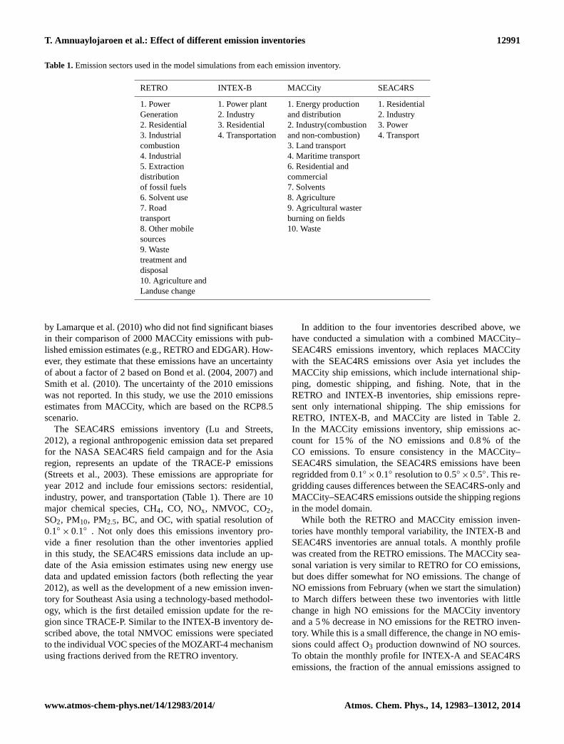
Table 1. Emission sectors used in the model simulations from each emission inventory.

RETRO INTEX-B MACCity SEAC4RS

1. Power 1. Power plant 1. Energy production 1. Residential

Generation 2. Industry and distribution 2. Industry

2. Residential 3. Residential 2. Industry(combustion 3. Power

3. Industrial 4. Transportation and non-combustion) 4. Transport

combustion 3. Land transport

4. Industrial 4. Maritime transport

5. Extraction 6. Residential and

distribution commercial

of fossil fuels 7. Solvents

6. Solvent use 8. Agriculture

7. Road 9. Agricultural waster

transport burning on fields

8. Other mobile 10. Waste

sources

9. Waste

treatment and

disposal

10. Agriculture and

Landuse change

by Lamarque et al. (2010) who did not find significant biases

in their comparison of 2000 MACCity emissions with pub-

lished emission estimates (e.g., RETRO and EDGAR). How-

ever, they estimate that these emissions have an uncertainty

of about a factor of 2 based on Bond et al. (2004, 2007) and

Smith et al. (2010). The uncertainty of the 2010 emissions

was not reported. In this study, we use the 2010 emissions

estimates from MACCity, which are based on the RCP8.5

scenario.

The SEAC4RS emissions inventory (Lu and Streets,

2012), a regional anthropogenic emission data set prepared

for the NASA SEAC4RS field campaign and for the Asia

region, represents an update of the TRACE-P emissions

(Streets et al., 2003). These emissions are appropriate for

year 2012 and include four emissions sectors: residential,

industry, power, and transportation (Table 1). There are 10

major chemical species, CH4, CO, NOx, NMVOC, CO2,

SO2, PM10, PM2.5, BC, and OC, with spatial resolution of

0.1◦× 0.1◦ . Not only does this emissions inventory pro-

vide a finer resolution than the other inventories applied

in this study, the SEAC4RS emissions data include an up-

date of the Asia emission estimates using new energy use

data and updated emission factors (both reflecting the year

2012), as well as the development of a new emission inven-

tory for Southeast Asia using a technology-based methodol-

ogy, which is the first detailed emission update for the re-

gion since TRACE-P. Similar to the INTEX-B inventory de-

scribed above, the total NMVOC emissions were speciated

to the individual VOC species of the MOZART-4 mechanism

using fractions derived from the RETRO inventory.

In addition to the four inventories described above, we

have conducted a simulation with a combined MACCity–

SEAC4RS emissions inventory, which replaces MACCity

with the SEAC4RS emissions over Asia yet includes the

MACCity ship emissions, which include international ship-

ping, domestic shipping, and fishing. Note, that in the

RETRO and INTEX-B inventories, ship emissions repre-

sent only international shipping. The ship emissions for

RETRO, INTEX-B, and MACCity are listed in Table 2.

In the MACCity emissions inventory, ship emissions ac-

count for 15 % of the NO emissions and 0.8 % of the

CO emissions. To ensure consistency in the MACCity–

SEAC4RS simulation, the SEAC4RS emissions have been

regridded from 0.1◦×0.1◦ resolution to 0.5◦×0.5◦. This re-

gridding causes differences between the SEAC4RS-only and

MACCity–SEAC4RS emissions outside the shipping regions

in the model domain.

While both the RETRO and MACCity emission inven-

tories have monthly temporal variability, the INTEX-B and

SEAC4RS inventories are annual totals. A monthly profile

was created from the RETRO emissions. The MACCity sea-

sonal variation is very similar to RETRO for CO emissions,

but does differ somewhat for NO emissions. The change of

NO emissions from February (when we start the simulation)

to March differs between these two inventories with little

change in high NO emissions for the MACCity inventory

and a 5 % decrease in NO emissions for the RETRO inven-

tory. While this is a small difference, the change in NO emis-

sions could affect O3 production downwind of NO sources.

To obtain the monthly profile for INTEX-A and SEAC4RS

emissions, the fraction of the annual emissions assigned to



Figure 6. Accumulated precipitation (mm) (a) GPCC, March, (b) TRMM, March, (c) WRF, March (d) GPCC, December (e) TRMM,

December, (f) WRF, December.

each month (FracMonthly) was calculated from the ratio of the

RETRO monthly emissions (RETROMonthly) to the RETRO

annual emissions (RETROAnnual). The monthly fraction was

then multiplied by the annual emissions of both the INTEX-

B and SEAC4RS inventories to estimate the monthly emis-

sions. This procedure is described by the following equa-

tions:

RETROAnnual =

12∑i=1

RETROMonthly, (1)

FracMonthly(i)=RETROMonthly(i)

RETROAnnual

, (2)

EmissionMonthly(i)= FracMonthly(i)×EmissionAnnual, (3)

where the EmissionMonthly is the monthly emissions for the

INTEX or SEAC4RS inventory and EmissionAnnual is the an-

nual emissions from the INTEX or SEAC4RS inventory.

3.2 Emission comparison

The monthly emissions from the five different anthropogenic

emissions inventories and the biomass-burning emissions

calculated by the FINN model for CO and NOx are compared

for both March and December in Fig. 1–4. The sum of these

emissions over the entire model domain is listed in Table 2.

In March, the biomass-burning sources dominate the emis-

sions of CO. The biomass burning occurs primarily over the

Indochina peninsula and Southeast China where CO biomass

emissions dominate the inventory. In March in Southeast

Asia,∼ 70 % of the total CO emissions is from biomass burn-

ing and only ∼ 30 % is from anthropogenic emissions. This

partitioning is true for all the emission inventories applied in

this study. In December, the biomass-burning emissions are

much smaller.

Anthropogenic emissions of CO vary between emissions

inventories, with RETRO and MACCity emissions having

higher values, particularly in northeast India and South-

east China. Over the entire domain, the anthropogenic

NOx emissions are quite similar between RETRO, INTEX-

B, MACCity, and MACCity–SEAC4RS emissions, but are

much smaller in the SEAC4RS inventory, since this inven-

tory alone does not include ship emissions. By comparing

RETRO emissions to MACCity–SEAC4RS emissions, the

total anthropogenic emissions in Southeast Asia decreased

by ∼ 30 % for CO and ∼ 13 % for NO between 2000 and

2012 with 2010 ship emissions.



Figure 7. Monthly mean, surface mixing ratios for (a) and (b) CO, (c) and (d) O3 (e) and (f) NOx predicted by WRF-Chem using the average

from five emission inventories for March (left) and December (right panels) 2008.

Comparison of the total CO emissions from the various

inventories across Southeast Asia (Table 2) shows that in

March, the RETRO inventory is within± 5 % of the INTEX-

B and MACCity inventories, but is ∼ 20 % greater than the

MACCity–SEAC4RS and SEAC4RS inventories. In Decem-

ber, the CO MACCity–SEAC4RS inventory is 35 % lower

than the RETRO emissions inventory. The SEAC4RS NO

emissions are substantially less (∼ 45 %) than the other in-

ventories in both March and December because of the lack

of ship emissions in the SEAC4RS inventory. NO emissions

in the INTEX-B and MACCity inventories are similar to each

other and ∼ 10 % lower than the RETRO emissions. In De-

cember, the INTEX-B, MACCity, and MACCity–SEAC4RS

NO emissions are similar and are ∼ 25 % lower than the

RETRO inventory.

The CO and NO emissions used in our study are larger

than the REAS v1 emissions (Ohara et al., 2007) for our

modeling domain (Table 2). The REAS v1 estimate in



Figure 8. Variations of surface mixing ratios for (a) and (b) CO, (c) and (d) O3 (e) and (f) NOx predicted by WRF-Chem using the averaged

from five emission inventories for March (left) and December (right panels) 2008.

Table 2 comes from the Emissions of atmospheric Com-

pounds and Compilation of Ancillary Data (ECCAD) web

site (http://eccad.sedoo.fr) to obtain emission estimates for

the same region as our model domain, which encompasses

small regions of India and China that are not included in

the Southeast Asia region denoted by Ohara et al. (2007).

For our model domain the REAS v1 annual emissions

are 91.4 Tg yr−1 for CO and 4.81 Tg yr−1 for NOx. For

the Southeast Asia region, Ohara et al. (2007) report in

their Table 6 annual CO and NOx emissions of 54.5 and

3.77 Tg yr−1, respectively, but these exclude international

aviation, international shipping, and open biomass burn-

ing. The REAS v1 emissions are even greater than the

TRACE-P, EDGAR 3.2, and IIASA (the International In-

stitute for Applied Systems Analysis) CO emissions (34.0,

42.6, 39.8 Tg CO yr−1, respectively) but are more similar to

TRACE-P, EDGAR 3.2, and IIASA NOx emissions (3.06,

3.91, 3.94 Tg NOx yr−1, respectively) for Southeast Asia

(Ohara et al., 2007) as well as REAS v2.1 (Kurakawa et al.,

2013), which were 36.2 Tg CO yr−1 and 3.00 Tg NOx yr−1.

Thus, the emissions used here are larger than the REAS emis-

sions inventories as well as other previous inventories.


http://eccad.sedoo.fr


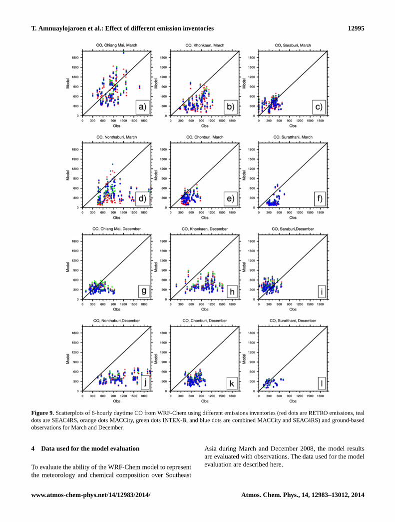
Figure 9. Scatterplots of 6-hourly daytime CO from WRF-Chem using different emissions inventories (red dots are RETRO emissions, teal

dots are SEAC4RS, orange dots MACCity, green dots INTEX-B, and blue dots are combined MACCity and SEAC4RS) and ground-based

observations for March and December.

4 Data used for the model evaluation

To evaluate the ability of the WRF-Chem model to represent

the meteorology and chemical composition over Southeast

Asia during March and December 2008, the model results

are evaluated with observations. The data used for the model

evaluation are described here.



Table 2. Summation of CO emissions and NO emissions (mole km−2 h−1) from all grids in the model domain for each month.

Emission Inventory E_CO (mole km−2 h−1) E_NO (mole km−2 h−1)

March December March December

RETRO–2000 410 840 496 860 30 590 39 320

INTEX-B–2006 396 170 406 240 27 410 29 640

MACCity–2010 436 750 454 250 27 440 28 280

MACCity–SEAC4RS 319 420 320 310 29 810 30 910

SEAC4RS–2012 305 542 300 369 16 610 17 290

Biomass Burning–2008 717 940 58 780 10 220 700

RETRO-Ship 3404 3364 5097 5186

INTEX-B-Ship 5888 5785 3273 3301

MACCity-Ship 3569 3717 3980 5138

REAS v1a – 2000 282 120 13 828

a REAS v1 emissions are from the ECCAD web site (http://eccad.sedoo.fr) and are the annual emissions converted to hourly

emissions assuming constant emissions for the year over the WRF-Chem model domain.

4.1 Meteorology data description

The predicted meteorology from the WRF simulations,

which is the same for all model simulations, was evaluated

by comparing 2 m temperature, 10 m winds, and precipita-

tion with existing observations. The observations used for

this evaluation include the Modern-Era Retrospective Anal-

ysis For Research And Applications (MERRA) products, the

Tropical Rainfall Measuring Mission (TRMM) satellite data,

and data from the Global Precipitation Climatology Center

(GPCC).

The MERRA product (Rienecker et al., 2011) is gener-

ated using version 5.2.0 of the GEOS-5 DAS (Goddard Earth

Observing System Model Data Assimilation System) with

the model and analysis each at about 0.5◦× 0.6◦ resolution.

MERRA has complete analysis of over 30 years (from 1979

to present) of data. The 2 m temperature and 10 m winds pro-

duced by the MERRA analysis system are hourly. However,

the provided monthly averaged data were used here to evalu-

ate the WRF results.

The main objective of the TRMM satellite (Huffman et al.,

1997), which is a joint mission between NASA and Japan

Aerospace Exploration Agency (JAXA), is to monitor rain-

fall in the tropics. We compare the WRF-Chem monthly sur-

face rainfall to the TRMM product that is a combination of

instruments, including the precipitation radar and TRMM

microwave imager, allowing us to compare model results

with the high-resolution data from the precipitation radar

filled in by data from the TRMM Microwave Imager. The

precipitation gauge analysis is used to correct any biases in

the satellite data (Huffman and Bolvin, 2012).

Monthly precipitation from the GPCC data set (Rudolf et

al., 2005a,b) is obtained from global station data that is grid-

ded onto a 1◦×1◦ global domain. The GPCC monthly precip-

itation product is based on anomalies from the climatological

mean at each station. The anomalies are spatially interpolated

by using a modified version of the robust empirical interpola-

tion method SPHEREMAP. The method constitutes a spher-

ical adaptation (Willmott et al., 1985) of Shepard’s empirical

weighting scheme (Shepard, 1968; Schneider et al., 2011).

4.2 Chemistry data description

Observations from four measurement platforms are used to

evaluate the WRF-Chem predictions of CO, O3, and NO2:

a ground-based monitoring network in Thailand, ozoneson-

des in the Southeast Asia region, version 6 Measurement

of Pollution In the Troposphere (MOPITT) satellite instru-

ment, and the Ozone Monitoring Instrument (OMI) satel-

lite instrument. The ground-based chemistry observations in

Thailand are provided by the Thai Pollution Control De-

partment (PCD). The Thai PCD monitors the hourly sur-

face concentrations of five chemical species: O3, CO, NO2,

SO2, and PM10 at six locations (Fig. 5g). The measure-

ment sites in Thailand are located in urban areas and there-

fore are dominated by urban (especially motor vehicles)

emissions. These data are measured by using the refer-

ence method or equivalent methods. Almost all O3 obser-

vation instruments are from Teledyne Advanced Pollution

Instrumentation Model 400 (http://www.teledyne-api.com/

products/400e.asp). The instrument has a lower detection

limit of 0.6 ppbv and a precision of 1 %. Almost all CO

observation instruments are from Teledyne Advanced Pol-

lution Instrumentation Model 300 (http://www.teledyne-api.

com/products/300e.asp), which has a lower detection limit

of 40 ppbv and a precision of 0.5 %. The PCD measurements

periodically have missing data, but the missing data are only

∼ 15 % of the time.

The SHADOZ ozonesonde network (Thompson et al.,

2012) was initiated to provide vertical profiles of O3 in the

tropics for satellite data verification, model evaluation, and

insights into tropical chemistry and dynamics. SHADOZ has

collected more than 3000 O3 profiles from 14 sites in tropical

and subtropical regions using balloon-borne electrochemical


http://eccad.sedoo.fr

http://www.teledyne-api.com/products/400e.asp





Figure 10. Carbon monoxide from WRF-Chem and MOPITT in March (a) MOPITT (b) WRF-Chem simulation with RETRO emission

inventory, (c) WRF-Chem simulation with INTEX-B emission inventory, (d) WRF-Chem simulation with MACCity emission inventory, (e)

WRF-Chem simulation with SEAC4RS emission inventory, (f) WRF-Chem simulation with MACCity–SEAC4RS emission inventory.

concentration cell (ECC) O3 detectors flown with standard

radiosondes. It is estimated that the accuracy and precision

of the O3 measurement is 5 %, but biases can be found with

individual stations. Ozonesondes from three stations (Kuala

Lumpur, Malaysia; Hanoi, Vietnam; and Watukosek, Java)

(Fig. 5g) are used in the model evaluation presented in this

manuscript. Total O3 column at these stations can be 5–10 %

lower than total O3 measured by the OMI satellite instrument

(Thompson et al., 2012).



Figure 11. Same as Fig. 10 but for December.

Satellite observations are quite valuable for model evalu-

ation, but require careful interpretation to be used quantita-

tively. In many cases (as in MOPITT CO and OMI NO2) the

retrieved mixing ratios or column densities can be expressed

as a linear combination of the true atmospheric profile (x)

and a priori information (xa), balanced according to the av-

eraging kernels (A) (I is the identity matrix):

xret = Ax+ (I−A)xa. (4)

The averaging kernels represent the sensitivity of the re-

trievals to the actual concentration profiles, and vary in time

and space depending on the temperature profile, the thermal



Figure 12. Scatterplots of 6-hourly daytime O3 from WRF-Chem using different emissions inventories (red dots are RETRO emissions, teal

dots are SEAC4RS, orange dots MACCity, green dots INTEX-B, and blue dots are combined MACCity and SEAC4RS) and ground-based

observations for March and December.



Figure 13. O3 vertical profiles from WRF-Chem, MOZART4, and ozonesondes at three SHADOZ ozonesonde locations for (a) Watukosek-

Java, Indonesia in March, (b) Watukosek-Java, Indonesia in December, (c) Kuala Lumpur, Malaysia in March, (d) Kuala Lumpur, Malaysia

in December, and (e) Hanoi, Vietnam in March. Note that there are no SHADOZ data at Hanoi during December 2008.

contrast between air and surface temperatures, the concentra-

tion profile, and surface emissivity.

The new versions of MOPITT data (versions 5 and 6;

Deeter et al. 2011, 2012, 2013; Worden et al., 2010), which

we used in this paper, have improved near-surface CO re-



trievals over version 4. The V6 MOPITT uses both near-

infrared and thermal-infrared observations simultaneously to

enhance the retrieval sensitivity of CO in the lower tropo-

sphere. This feature is important to air quality analyses and

studies of CO sources. The V5 MOPITT surface-level CO

validation shows biases on the order of a few percent, and

V6 is very similar (Deeter et al., 2012).

The OMI Level-3 Global Gridded NO2 data product,

archived at the NASA Goddard Earth Sciences Data and In-

formation Service Center (GES DISC), has a spatial resolu-

tion of about 13 km× 24 km at nadir in normal operational

mode. OMI measures the backscattered radiation over the

0.27–0.5 µm wavelength range to obtain the total column

of trace species, such as NO2, O3, formaldehyde, SO2 and

aerosols. The tropospheric NO2 column retrieval algorithm

follows Bucsela et al. (2006) who use the DOAS (differential

optical absorption spectroscopy) methodology, air mass fac-

tors, and typical NO2 profiles from chemical transport mod-

els to obtain the vertical column density. The OMI tropo-

spheric NO2 column data have been shown to have a good

correlation with INTEX-B aircraft measurements (Boersma

et al., 2008). Good agreement of OMI tropospheric NO2

column has also been found with MAX-DOAS (multi-axis

differential optical absorption spectroscopy) ground-based

measurements (Kramer et al., 2008). However, some recent

studies have suggested that the OMI retrieval has a positive

bias of 0–30 % (e.g., Boersma et al., 2009; Zhou et al., 2009).

To evaluate NO2 from model results, we compare the tropo-

spheric column of NO2 from the OMI Level-3 Global Grid-

ded NO2 data product with WRF-Chem NO2 columns that

have been adjusted using the averaging kernel and a priori

information (following Eq. 4) provided with the data product

(e.g., Emmons et al., 2004).

5 Model results and evaluation

5.1 Meteorology evaluation

Monthly averaged 2 m temperature, wind speed and direc-

tion are compared to the MERRA reanalysis data set. In

general, the model-predicted temperature agrees well with

the MERRA output (Fig. 5) for the March 2008 simulation,

although some regions, e.g., Indochina peninsula, have 2–

3 ◦C lower temperatures than the monthly averaged reanaly-

sis output. The WRF-predicted wind speed pattern is similar

to the MERRA output for March. However, the wind speed is

overpredicted in the South China Sea by∼ 2 m s−1. The wind

direction agrees quite well with MERRA output (Fig. 5e, f).

For December 2008 (not shown), the simulated 2 m temper-

ature, 10 m wind speed and wind direction, in general, also

agree well with the MERRA output; however, the tempera-

ture is slightly underpredicted over land and the wind speed

is overpredicted over the South China Sea. The low bias

in temperature and high bias in wind speed can impact the

prediction of chemical species mixing ratios. For example,

the chemical reactions likely will proceed at a slightly lower

rate (because of their dependence on temperature) resulting

in formation of products further away from the source. Ad-

ditionally, biogenic emissions may be underpredicted, since

these emissions increase with increasing temperatures and a

low bias in temperature can lead to lower emissions.

WRF reasonably predicts the precipitation pattern in

March (Fig. 6a–c) when compared to TRMM and GPCC

data. Low precipitation is observed over the coast of Burma,

the northern part of the South China Sea, and the tip of the

Indochina peninsula, and high precipitation is predicted near

the equator over the oceans, Malaysian peninsula, and In-

donesia. However, the WRF results overestimate precipita-

tion near the equator by 10 to 100 mm for March. In De-

cember (Fig. 6d–f), WRF also overpredicts the magnitude

of precipitation over the water, but shows reasonable agree-

ment north of 10◦ N especially over land. The precipitation

in this region is dominated by rain from convection, which

is controlled by mesoscale processes. The WRF simulations

presented here have a 36 km horizontal resolution, and at this

resolution, the model relies on a cumulus parameterization to

produce the rain. Due to the coarse model resolution for a re-

gion with plenty of tropical convection, a situation which is

notoriously difficult to represent in models, the poor predic-

tion of precipitation near the equator is not unexpected. Koo

and Hong (2010) also found oceanic convection to be over-

predicted by the WRF model. However, over land, where the

chemical predictions of this study are evaluated, the WRF

precipitation has better agreement with observations. As a

consequence of the higher precipitation predicted by WRF,

WRF-Chem may overpredict the removal of soluble trace

gases (e.g., nitric acid), thereby affecting the photochemistry

in the region.

5.2 Evaluation of chemistry

5.2.1 Ensemble surface means and variations

To show the distribution of the monthly mean surface mix-

ing ratios for CO, O3, and NOx in March and December,

the WRF-Chem results from all five simulations (with dif-

ferent emissions inventories) have been averaged giving an

ensemble mean (Fig. 7). In general, surface-level CO and

NOx mixing ratios have the highest values over the land re-

gions and the lowest values over the ocean near the equator.

By comparing the model results from March (high biomass-

burning emissions) to those from December (low biomass-

burning emissions), the influence of biomass-burning emis-

sions can be seen for all three species. CO mixing ratios are

> 500 ppbv over Burma and northern Thailand during March

compared to 200–500 ppbv during December. Monthly av-

eraged O3 mixing ratios, which reach 70–90 ppbv, are the

largest during March over the regions where biomass burn-

ing is occurring and downwind of these emissions. With a



Figure 14. March 2008 monthly NO2 total column (a) OMI, (b) WRF-Chem + RETRO, (c) WRF-Chem + INTEX-B, (d) WRF-Chem +

MACCity, (e) WRF-Chem + SEAC4RS, and (f) WRF-Chem +MACCity-SEAC4RS

shorter lifetime, high NOx mixing ratios of 4–30 ppbv are

confined to regions close to the NOx sources.

The variation, which is defined as the standard deviation of

the five simulations, in the predicted monthly averaged sur-

face mixing ratios of CO, O3, and NOx across the five sim-

ulations is highlighted in Fig. 8. Because we conducted each

simulation with the same meteorology and biomass-burning

emissions, the primary cause for the variations are the differ-

ences in the anthropogenic emissions. CO mixing ratios vary

across simulations by < 20 %, but variations of ∼ 30–60 %

are found near Bangladesh and Indonesia for both March

and December. O3 mixing ratios have up to 30 % variation

near the tip of the Malaysian peninsula and near Indonesia,

but have much smaller variability elsewhere. Mixing ratios of

NOx have the most variation among the simulations. The 70–

100 % variations for NOx, especially over the South China

Sea, are from the differences in ship emissions from each in-

ventory. There are also high NOx variations in several cities



Figure 15. Same as Fig. 19 but for December.

as seen by the locally high values in Fig. 8e and f, due to

different emission strengths in each inventory and to miss-

ing emission sectors in some inventories (e.g., shipping emis-

sions in the SEAC4RS inventory).

5.2.2 CO evaluation

The 6-hourly daytime (00:00, 06:00, 12:00 UTC) CO mix-

ing ratios from WRF-Chem with each of the five inventories

are compared to observations from the six ground-site mea-

surements: Chiang Mai (CM) in northwest Thailand, Khon

Kaen (KK) in eastern Thailand, Nonthaburi (NTB) in the

Bangkok metropolitan region, Saraburi (SRB) just north of

Bangkok, Chonburi (CB) southeast of Bangkok, and Surat

Thani (SRT) in the southern peninsula (Fig. 5g). These sites

are located in urban environments with background condi-

tions ranging from high biomass burning in northern Thai-

land to more marine conditions in southern Thailand. For

March when biomass-burning emissions are a large source of

CO, the WRF-Chem simulations agree well with the monthly

mean mixing ratio for Chiang-Mai in northwest Thailand and



Table 3. Monthly-average correlation coefficients (r) of daytime (00:00, 06:00, 12:00 UTC) CO.

Emission

Inventories CM KK SRB NTB CBR SRT

Mar Dec Mar Dec Mar Dec Mar Dec Mar Dec Mar Dec

RETRO 0.49 0.13 0.35 0.10 0.27 0.15 0.40 0.31 0.48 0.15 0.52 0.03

INTEX-B 0.51 0.14 0.42 0.20 0.17 0.17 0.33 0.38 0.44 0.17 0.58 0.03

MACCity 0.50 0.14 0.45 0.10 0.11 0.19 0.26 0.33 0.43 0.19 0.55 0.003

SEAC4RS 0.48 0.15 0.42 0.04 0.09 0.18 0.21 0.33 0.42 0.18 0.52 0.01

MACCity/ 0.48 0.15 0.41 0.07 0.12 0.14 0.26 0.33 0.44 0.14 0.54 0.004

SEAC4RS

Table 4. Monthly-average biases of daytime (00:00, 06:00, 12:00 UTC) carbon monoxide.

Emission



RETRO −104 −147 −396 −581 −219 −314 −721 −770 −253 23 −267 −89

INTEX-B −16 −114 −316 −529 −150 −283 −662 −747 −203 46 −234 −109

MACCity −18 −112 −292 −530 −116 −263 −636 −733 −195 60 −238 −112

SEAC4RS −22 −107 −324 −548 −129 −267 −645 −734 −197 58 −234 −120

MACCity/ −47 −157 −35 −601 −165 −328 −674 −785 −218 10 −243 −93

SEAC4RS

Chonburi in southeast Thailand (Fig. 9), with moderate cor-

relation coefficients (Table 3) of r2= 0.48 to 0.51. However,

WRF-Chem generally underpredicts CO at the other stations,

especially Nonthaburi. In December, the predicted 6-hourly

daytime surface CO for all simulations is much less than the

observations, with the exception of the Chonburi site. The

large underprediction is reflected by the bias calculation (Ta-

ble 4). Part of the underprediction is a result of the coarse

model resolution (36 km), which cannot capture the highly

variable emissions and high CO concentrations in an ur-

ban setting where the measurement site is located. However,

the underprediction of CO could also be due to low anthro-

pogenic emissions (discussed further in Section 5), a high

planetary boundary layer height, which would cause dilu-

tion of surface mixing ratios, and/or missing chemistry in the

model such as heterogeneous chemistry. Mao et al. (2013)

suggest uptake of HO2 to aerosols undergo reaction with

transition metal ions to convert HO2 to H2O, removing hy-

drogen oxides from the atmosphere. They show that this pro-

posed mechanism decreases OH at the surface, as simulated

by the GEOS-Chem model, and consequently increases CO

mixing ratios by 20–30 ppbv. While a 20–30 ppbv increase

in CO over Thailand will not remove the high CO bias in our

simulation, this heterogeneous chemistry may explain some

of the underprediction of CO. When comparing the CO con-

centrations from the different WRF-Chem simulations with

the measurements in Thailand, we find the different WRF-

Chem results to be quite similar. An examination of the cor-

relation coefficients (Table 3) reveals that these values are

quite similar from simulation to simulation. This can be due

in part to the fact that none of the emission inventories are

specific to the modeled time period. However, a paired dif-

ference test (Kruskal and Wallis, 1952) shows that there are

statistical differences for CO among the different emission

inventories at Khon Kaen, Saraburi, Nonthaburi, and Chon-

buri for both March and December and for Chiang Mai for

December. The variability in the biases of the modeled CO

mixing ratios (Table 4) also suggests that the different emis-

sion inventories are causing the different CO mixing ratios

between the model simulations. Because the simulation us-

ing RETRO emissions, especially for March, has larger bi-

ases than the other simulations, the more recent CO emission

inventories either better represent the emissions in general or

are more similar to what the emissions were for 2008.

The modeled CO surface mixing ratios are compared to

the MOPITT V6 gridded Level 3 near-surface CO retrievals

to evaluate the modeled spatial distribution (Figs. 10 and

11). The MOPITT V6 data (Deeter et al., 2011, 2012, 2013;

Worden et al., 2010), used in this paper, has improved near-

surface CO retrievals. This improvement is accomplished by

using near-infrared and thermal-infrared observations simul-

taneously to enhance the retrieval sensitivity of CO in the

lower troposphere. WRF-Chem is able to capture well the

patterns of high CO over Southeast Asia and Southern China

in March (Fig. 10), but overpredicts CO over northern Thai-

land and Burma. These regions of high CO coincide with the



Figure 16. March monthly averaged CO vertical profiles at Yangon,

Burma. WRF-Chem results with the plumerise feature of biomass-

burning emissions are given for the MACCity–SEAC4RS emissions

case (blue line), SEAC4RS emissions (dark green line), MACCity

emissions (red line), INTEX-B emissions (green line), and RETRO

emissions (dark red line). The MOZART global model results are

shown as the gold line. WRF-Chem results without the plumerise

feature (i.e., biomass-burning emissions injected into the lowest

model level) are shown as the purple line.

location of biomass burning, indicating the FINN fire emis-

sions are too high in this region. The predicted CO mixing ra-

tios are similar in magnitude to MOPITT over the Malay and

southern Indochina peninsulas. For December when biomass

burning is less important, the general spatial pattern of CO is

represented by WRF-Chem for all the simulations (Fig. 11).

The modeled CO in December is generally higher than MO-

PITT, particularly in the regions of the highest mixing ratios

in southern China and easternmost India.

5.2.3 O3 evaluation

Scatterplots of the 6-hourly daytime O3 mixing ratios com-

pared to the measurements at the six ground sites show that

O3 is generally overpredicted for each of the different emis-

sion inventories for both March and December (Fig. 12)

by up to 100 ppbv. Locations that showed good agreement

for CO (e.g., Chiang Mai in March) have very poor agree-

ment for O3. Despite the large scatter of model results for

O3 (Fig. 12), the correlation coefficients are generally 0.5

and higher (Table 5) indicating that the model captures the

O3 trend well, but has a high bias. WRF-Chem O3 bi-

ases (Table 6) range from -1 to 40 ppbv with MACCity and

MACCity–SEAC4RS having the highest bias at Chiang Mai.

In December (Fig. 12), the model–observation agreement is

generally better than in March, although WRF-Chem tends

to overpredict O3, especially at Khon Kaen and Saraburi in

northeastern and central Thailand. In general, the comparison

of the model results among the different emission inventories

shows fairly similar results for O3 mixing ratios, correlation

coefficients, and biases. The correlation coefficients among

simulations mostly vary by < 0.1, suggesting that the differ-

ent anthropogenic emission inventories produce very little

variation in modeled O3. A paired difference test (Kruskal

and Wallis, 1952) of these surface O3 mixing ratios shows

that there are not any statistical differences for O3 among

the different emission inventories. Likewise, variation among

the monthly mean O3 biases among the different simula-

tions are < 15 ppbv and mostly < 7 ppbv. The higher O3 bias

in March compared to December, especially in Chiang Mai

where there are large biomass-burning sources (Amnuaylo-

jaroen and Kreasuwun, 2012), suggests that biomass-burning

emissions are more uncertain than anthropogenic emissions.

The O3 vertical profiles resulting from the WRF-Chem

simulations are compared to SHADOZ ozonesondes and

MOZART4 model results at three locations (Hanoi, Vietnam;

Watukosek-Java, Indonesia; and Kuala Lumpur, Malaysia)

(Fig. 13). Both Hanoi and Watukosek-Java are near the WRF-

Chem model domain boundaries (Fig. 5g). At Watukosek-

Java in March, the WRF-Chem prediction is low below the

700 hPa level and too high above 600 hPa (Fig. 13a), while

the MOZART4 prediction is more similar to observations

near the surface. In December, the WRF-Chem results agree

well with the observations at Watukosek-Java from the sur-

face to 300 hPa (Fig. 13c). Above 300 hPa, the model over-

predicts the O3 mixing ratios until it reaches the stratosphere.

At Kuala Lumpur, the WRF-Chem results have very good

agreement with O3 observations for March (Fig. 13b), while

the MOZART4 results are high compared to the observations

below the 600 hPa level. In December at Kuala Lumpur, the

observations are higher than the model results in the free

troposphere (Fig. 13d). The free troposphere mixing ratios

are likely from outside the domain where MOZART4 results

are used as boundary conditions. The O3 measurements from

Hanoi, a subtropical location, show multiple layers of O3 in

the free troposphere with the lowest O3 values of 20 ppbv oc-

curring at 200 hPa for the March time period (Fig. 13e). The

WRF-Chem and MOZART4 results are not able to replicate

the layering structure, but the WRF-Chem results do have

high O3 values from 900 to 600 hPa, while MOZART4 O3

remains below 60 ppbv throughout the troposphere. Neither

model is able to predict the 20 ppbv minimum O3 at 200 hPa.

There is very little difference between the WRF-Chem re-

sults from the simulations with different emission inventories

for Hanoi and Watukosek-Java, except for near the surface at

Watukosek-Java in March. At Kuala Lumpur, there is much

more variation between model results with different emis-

sion inventories. O3 from the SEAC4RS emissions inventory

simulation is less than the O3 from the other simulations and

has the worst agreement with observations at Kuala Lumpur.



Table 5. Monthly-average correlation coefficients of daytime (00:00, 06:00, 12:00 UTC) O3.

Emission



RETRO 0.69 0.84 0.68 0.34 0.56 0.50 0.47 0.71 0.11 0.52 0.49 0.16

INTEX-B 0.74 0.89 0.72 0.33 0.70 0.48 0.45 0.72 0.05 0.56 0.44 0.09

MACCity 0.68 0.78 0.71 0.33 0.69 0.48 0.44 0.68 0.02 0.55 0.43 0.08

SEAC4RS 0.70 0.79 0.73 0.42 0.75 0.56 0.41 0.71 0.001 0.49 0.45 0.14

MACCity/ 0.70 0.78 0.73 0.37 0.76 0.52 0.48 0.78 0.02 0.54 0.45 0.08

SEAC4RS

Table 6. Monthly-average biases of daytime (00:00, 06:00, 12:00 UTC) O3.

Emission



RETRO 36.48 8.28 23.83 19.36 7.77 13.58 12.15 3.07 17.82 6.96 9.52 31.29

INTEX-B 37.76 4.05 32.62 18.26 15.31 12.42 18.54 2.67 23.64 5.58 14.57 29.56

MACCity 39.67 6.19 30.24 15.68 14.62 8.69 18.53 −1.34 24.88 3.04 15.76 30.36

SEAC4RS 38.53 3.75 31.45 20.14 17.29 13.98 27.90 4.61 24.38 6.33 11.26 29.15

MACCity/ 39.72 5.31 32.45 19.92 16.59 13.37 18.19 −0.25 24.95 5.52 15.38 32.22

SEAC4RS

This difference could be because the SEAC4RS emissions

inventory lacks ship emissions. When the SEAC4RS emis-

sions are combined with MACCity emissions, the O3 mixing

ratios are more similar to the other simulations.

5.2.4 NO2 evaluation

The spatial distribution of the WRF-Chem and OMI tropo-

spheric column NO2 are shown in Figs. 14 and 15 for March

and December, respectively. In general, the WRF-Chem sim-

ulation is able to capture the NO2 pattern well over land in

March with high NO2 columns over China, Burma, Viet-

nam, Laos, and Thailand and low values over the south-

ern and southeast region of the model domain. The WRF-

Chem NO2 column is generally less than the OMI NO2 col-

umn. In March, the OMI NO2 column values over land are

> 2× 1015 molecules cm−2 with peak values of ∼ 5× 1015

molecules cm−2 over the Pearl River delta, while WRF-

Chem predicts 1× 1015 molecules NO2 cm−2 or more. The

WRF-Chem peaks of ∼ 5× 1015 occur in northern Thai-

land and Burma and not over the Pearl River delta. On the

other hand, the WRF-Chem model underpredicts NO2 col-

umn in the southeastern region of the model domain. For

March, the WRF-Chem NO2 column mostly reflects the

biomass-burning emissions pattern (Fig. 3), while for De-

cember WRF-Chem is more similar to the anthropogenic

emissions (Fig. 4). The OMI NO2 column does not show

the high NO2 over northern Thailand and Burma where the

model has high biomass-burning emissions in March. To ex-

plain this difference, WRF-Chem fire emissions could be too

high, or OMI may miss the high NO2 because of clouds in-

terfering with the instrument’s view. In situ measurements

would allow us to evaluate better the performance of the

model.

The largest variation among the model simulations is in

the region near Indonesia and is a result of both low NO2

mixing ratios from the MOZART boundary conditions and

different estimates for shipping emissions among the differ-

ent inventories (Table 2, Figs. 3 and 4). Both the RETRO

ship emissions, which are 75–80 % smaller than INTEX-B

and MACCity ship emissions, and the SEAC4RS only sim-

ulation, which does not have ship emissions, contribute to

the variation. When the MACCity ship emissions are com-

bined with the SEAC4RS emissions (MACCity–SEAC4RS),

the agreement with OMI NO2 column is much better than

the SEAC4RS only simulation. For example, the MACCity–

SEAC4RS simulation agrees better with OMI NO2 col-

umn than the SEAC4RS only simulation. The NO2 col-

umn model-observation comparison for December (Fig. 15)

shows that WRF-Chem slightly underpredicts the NO2 col-

umn, especially over the mainland. All five simulations pre-

dict relatively low NO2 column over Burma with values of

∼ 1× 1014 molecules cm−2 while OMI NO2 column reports

values of 5–10× 1014 molecules cm−2. Figure 4 shows that

NO emissions in Burma are lower than the surrounding re-

gions. The comparison to satellite data suggests that perhaps

these emissions are too low.



6 Discussion

There are several aspects of the simulations that contribute

to the underprediction of CO at the surface and the overpre-

diction of O3 at the surface. One is that the model simula-

tion is for 2008 while the emission inventories are appropri-

ate for other years (RETRO for 2000, INTEX-B for 2006,

MACCity for 2010, and SEAC4RS for 2012). While the grid

spacing of 36 km is better than global chemistry transport

models, it is likely that small-scale features, e.g., urban re-

gions and orography are not adequately represented in this

simulation. For example, Chiang Mai is in a mountain val-

ley where pollutants can easily accumulate. Another pos-

sible error could arise from the fire emissions. One issue

with coarse resolution modeling of biomass-burning emis-

sions is that multiple fires in one model grid cell are aggre-

gated into a single, bigger fire area. This aggregated informa-

tion is used by the plumerise model in WRF-Chem, which

may erroneously apply too much thermal buoyancy associ-

ated with the fires, resulting in emissions placed too high

above the ground. For example, WRF-Chem results without

the plumerise feature of biomass-burning emissions, as illus-

trated by the March monthly averaged CO vertical profiles at

Yangon, Burma (Fig. 16), show that injection into the low-

est model level gives vertical profiles more consistent with

MOZART results, which injects fire emissions into the low-

est model level. Thus, in the simulations with the plumerise

feature, O3 precursor species (NMVOCs and NOx) may be

placed in an environment where O3 production is more pro-

ductive than if the precursors were placed near the surface.

While these results indicate a substantial difference in CO

mixing ratios in the lowest 500 hPa of the atmosphere, obser-

vations of CO vertical profiles are needed to help evaluate the

model predictions. In addition, trash burning emissions are

not included in this study, yet have been shown to have a sig-

nificant contribution to the air quality (Hodzic et al., 2012).

In reality, Southeast Asia has complex emission sources that

not only include biomass burning and anthropogenic activ-

ities, but also biofuel and trash burning. To improve simu-

lations of CO in the future, these other emissions should be

included.

Another possible cause of the CO underprediction and O3

overprediction at the surface is that the anthropogenic emis-

sions are too low. Global estimates of CO sources (Kopacz

et al., 2010) based on satellite, aircraft, and surface observa-

tions suggest that CO emissions over Southeast Asia are un-

derestimated by nearly a factor of 2. For the INTEX-B emis-

sions, Zhang et al. (2009) reported an uncertainty of 185 %

and 37 % for CO and NO emissions, respectively. We con-

ducted sensitivity simulations with higher CO emissions by

a factor of 2 and higher NO emissions by 40 %. Additional

sensitivity simulations were performed with only CO emis-

sions greater by a factor of 2 (NO emissions remained the

same as the original inventory). The sensitivity simulations

were performed for March when biomass burning is a major

contribution to the results. The results were compared to the

six ground sites shown in Fig. 5g. The higher emissions im-

prove agreement for both O3 and CO concentrations at the six

monitoring sites. For example, the O3 prediction from the in-

creased emission simulations, on average, improved the cor-

relation term by ∼ 18 % and reduced the bias from 24 ppbv

to 8 ppbv. The high emissions simulations decreased, on av-

erage, the correlation for CO surface mixing ratios by 23–

34 %, but reduced the average bias from 250–264 ppbv to

184–224 ppbv. Interestingly, the high emissions simulations

produced too much CO at Chiang Mai by over 400 ppbv, yet

the O3 bias at Chiang Mai was reduced to 2–4 ppbv (from

38 to 40 ppbv). This suggests that either the CO emissions

from biomass burning are too high, or co-emitted VOCs

should have higher emissions. The Saraburi site, downwind

of Bangkok, went from too little CO (bias =−150 ppbv for

INTEX-B) to too much CO (bias= 173 ppbv for INTEX-

B high emissions simulations) with only a 2 ppbv decrease

in bias of O3. CO at Surat Thani changed very little, be-

cause Surat Thani is located away from urban and biomass-

burning regions. At the same time, Khon Kaen, Nonthaburi,

and Chonburi all have a better correspondence to observa-

tions as shown by the decreased bias. However, WRF-Chem

still underpredicts CO at these sites. The higher emissions

slightly improved the prediction of NO2 mixing ratios in-

creasing the correlation coefficient by 18 % but not chang-

ing the bias on average. By comparing the simulation with

increased CO and NO emissions to the simulation with only

increase CO emissions, the results for O3 and CO are very

similar indicating that increased CO emissions caused the de-

crease in O3 concentrations.

Our WRF-Chem simulations did not include heteroge-

neous chemistry, which can affect OH concentrations (Mao

et al., 2013) and therefore CO oxidation. Kumar et al. (2014)

also found decreased OH and O3 mixing ratios when het-

erogeneous chemistry was included for a simulation of a

dust event over India. For this high dust-loading example of

the effect of heterogeneous chemistry, O3 decreased by 10–

20 ppbv.

The underprediction of NO2 in all the WRF-Chem sim-

ulations suggests that the anthropogenic NOx emissions are

underestimated over the Southeast Asia. These errors in an-

thropogenic emission estimates are likely due to uncertain-

ties in including all the CO or NOx sources from the differ-

ent emission sectors and estimating the emission factors from

the different sources. The variation in NO shipping emis-

sions, as seen by the comparison of the simulation using only

the SEAC4RS emissions without shipping emissions with the

simulation using MACCity-SEAC4RS emissions, does pro-

duce substantial variation among model predictions of NO2

(Fig. 14) and O3 (Fig. 13). Therefore, it is important to in-

clude the shipping sector as part of the emissions inventory.

This paper did not include the REAS emissions inventory.

For Southeast Asia the REAS v2.1 CO emissions are similar

to the TRACE-P (Streets et al., 2003) and INTEX-B (Zhang



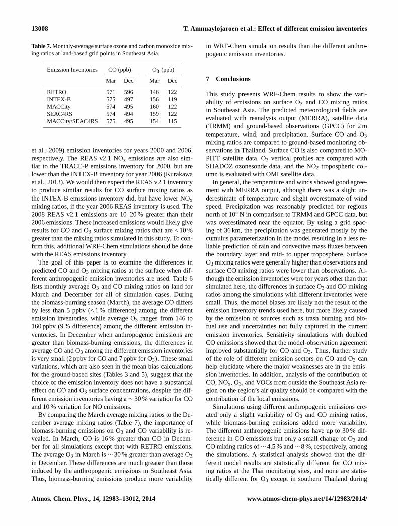
Table 7. Monthly-average surface ozone and carbon monoxide mix-

ing ratios at land-based grid points in Southeast Asia.

Emission Inventories CO (ppb) O3 (ppb)

Mar Dec Mar Dec

RETRO 571 596 146 122

INTEX-B 575 497 156 119

MACCity 574 495 160 122

SEAC4RS 574 494 159 122

MACCity/SEAC4RS 575 495 154 115

et al., 2009) emission inventories for years 2000 and 2006,

respectively. The REAS v2.1 NOx emissions are also sim-

ilar to the TRACE-P emissions inventory for 2000, but are

lower than the INTEX-B inventory for year 2006 (Kurakawa

et al., 2013). We would then expect the REAS v2.1 inventory

to produce similar results for CO surface mixing ratios as

the INTEX-B emissions inventory did, but have lower NOx

mixing ratios, if the year 2006 REAS inventory is used. The

2008 REAS v2.1 emissions are 10–20 % greater than their

2006 emissions. These increased emissions would likely give

results for CO and O3 surface mixing ratios that are < 10 %

greater than the mixing ratios simulated in this study. To con-

firm this, additional WRF-Chem simulations should be done

with the REAS emissions inventory.

The goal of this paper is to examine the differences in

predicted CO and O3 mixing ratios at the surface when dif-

ferent anthropogenic emission inventories are used. Table 6

lists monthly average O3 and CO mixing ratios on land for

March and December for all of simulation cases. During

the biomass-burning season (March), the average CO differs

by less than 5 ppbv (< 1 % difference) among the different

emission inventories, while average O3 ranges from 146 to

160 ppbv (9 % difference) among the different emission in-

ventories. In December when anthropogenic emissions are

greater than biomass-burning emissions, the differences in

average CO and O3 among the different emission inventories

is very small (2 ppbv for CO and 7 ppbv for O3). These small

variations, which are also seen in the mean bias calculations

for the ground-based sites (Tables 3 and 5), suggest that the

choice of the emission inventory does not have a substantial

effect on CO and O3 surface concentrations, despite the dif-

ferent emission inventories having a∼ 30 % variation for CO

and 10 % variation for NO emissions.

By comparing the March average mixing ratios to the De-

cember average mixing ratios (Table 7), the importance of

biomass-burning emissions on O3 and CO variability is re-

vealed. In March, CO is 16 % greater than CO in Decem-

ber for all simulations except that with RETRO emissions.

The average O3 in March is ∼ 30 % greater than average O3

in December. These differences are much greater than those

induced by the anthropogenic emissions in Southeast Asia.

Thus, biomass-burning emissions produce more variability

in WRF-Chem simulation results than the different anthro-

pogenic emission inventories.

7 Conclusions

This study presents WRF-Chem results to show the vari-

ability of emissions on surface O3 and CO mixing ratios

in Southeast Asia. The predicted meteorological fields are

evaluated with reanalysis output (MERRA), satellite data

(TRMM) and ground-based observations (GPCC) for 2 m

temperature, wind, and precipitation. Surface CO and O3

mixing ratios are compared to ground-based monitoring ob-

servations in Thailand. Surface CO is also compared to MO-

PITT satellite data. O3 vertical profiles are compared with

SHADOZ ozonesonde data, and the NO2 tropospheric col-

umn is evaluated with OMI satellite data.

In general, the temperature and winds showed good agree-

ment with MERRA output, although there was a slight un-

derestimate of temperature and slight overestimate of wind

speed. Precipitation was reasonably predicted for regions

north of 10◦ N in comparison to TRMM and GPCC data, but

was overestimated near the equator. By using a grid spac-

ing of 36 km, the precipitation was generated mostly by the

cumulus parameterization in the model resulting in a less re-

liable prediction of rain and convective mass fluxes between

the boundary layer and mid- to upper troposphere. Surface

O3 mixing ratios were generally higher than observations and

surface CO mixing ratios were lower than observations. Al-

though the emission inventories were for years other than that

simulated here, the differences in surface O3 and CO mixing

ratios among the simulations with different inventories were

small. Thus, the model biases are likely not the result of the

emission inventory trends used here, but more likely caused

by the omission of sources such as trash burning and bio-

fuel use and uncertainties not fully captured in the current

emission inventories. Sensitivity simulations with doubled

CO emissions showed that the model-observation agreement

improved substantially for CO and O3. Thus, further study

of the role of different emission sectors on CO and O3 can

help elucidate where the major weaknesses are in the emis-

sion inventories. In addition, analysis of the contribution of

CO, NOx, O3, and VOCs from outside the Southeast Asia re-

gion on the region’s air quality should be compared with the

contribution of the local emissions.

Simulations using different anthropogenic emissions cre-

ated only a slight variability of O3 and CO mixing ratios,

while biomass-burning emissions added more variability.

The different anthropogenic emissions have up to 30 % dif-

ference in CO emissions but only a small change of O3 and

CO mixing ratios of∼ 4.5 % and∼ 8 %, respectively, among

the simulations. A statistical analysis showed that the dif-

ferent model results are statistically different for CO mix-

ing ratios at the Thai monitoring sites, and none are statis-

tically different for O3 except in southern Thailand during



March. By comparing March (when biomass burning is at its

peak) surface mixing ratios to December values, it is found

that biomass-burning emissions substantially increase both

O3 and CO mixing ratios by ∼ 30 % and ∼ 16 %.

Southeast Asia is a region with complex terrain and emis-

sion sources at small scales. Thus, one important test to im-

prove the regional-scale simulations of air quality in South-

east Asia would be to use model grid spacing of the order

of 10 km or less. A higher grid resolution should also re-

duce errors in the injection height of biomass-burning emis-

sions. However, a high-resolution simulation needs emis-

sion inventories at equally high resolution. Inclusion of other

types of emissions, e.g., trash emissions, in the current in-

ventories could also improve the representation of the atmo-

spheric chemistry in Southeast Asia. Lastly, particulate mat-

ter (aerosols) was not addressed in this study. Not only should

their contribution to air quality be evaluated, but their impact

on gas-phase photochemistry should be addressed.

Acknowledgements. The authors would like to thank the National

Center for Atmospheric Research (NCAR) Advanced Study Pro-

gram (ASP) for the scholarship to visit the Atmospheric Chemistry

Division (ACD), the Center for Environmental Health, Toxicology

and Management of Chemical, Chiang Mai University, Faculty

of Science, Chiang Mai, Thailand for Ph.D. scholarship, and the

Graduate School Chiang Mai University for partial support. The

study was partially supported by NSF CHEM award 1049058.

We are thankful for the Thai Pollution Control Department (PCD)

providing their O3 and CO observation data. We also acknowledge

the Global Modeling and Assimilation Office (GMAO) and

the GES DISC for the dissemination of MERRA, the NASA

Goddard Space Flight Center for providing SHADOZ data, and

the NASA Langley Research Center Atmospheric Science Data

Center for providing MOPITT data. Analyses and visualizations

used in this paper were produced with the Giovanni online data

system, developed and maintained by the NASA GES DISC. We

acknowledge Gabriele Pfister and Sachin Ghude for their assistance

with WRF-Chem simulations. The comments from the anonymous

reviewers, Christine Wiedinmyer and Rajesh Kumar are greatly

appreciated. NCAR is operated by the University Corporation for

Atmospheric Research (UCAR) under sponsorship of the National

Science Foundation.

Edited by: H. Su

References

Adhikary, B., Carmichael, G. R., Tang, Y., Leung, L. R.,

Qian, Y., Schauer, J. J., Stone, E. A., Ramanathan, V., and

Ramana, M. V.: Characterization of South Asian Aerosols

during the ABC-Post Monsoon Experiment (ABC-APMEX):

a regional-scale modeling analysis, J. Geophys. Res., 112,

D22S22, doi:10.1029/2006JD008143, 2007.

Akimoto, H. and Narita, H.: Distribution of SO2, NOx, and CO2

emissions from fuel combustion and industrial activities in Asia

with 1◦× 1◦ resolution, Atmos. Environ., 28, 213–225, 1994.

Amnuaylojaroen, T. and Kreasuwun, J.: Investigation of fine and

coarse particulate matter from burning areas in Chiang Mai,

Thailand using the WRF/CALPUFF, Chiang Mai, J. Sci., 39, 1–

16, 2012.

Boersma, K. F., Jacob, D. J., Eskes, H. J., Pinder, R. W., Wand, J.,

and Vander A, R. J.: Intercomparison of SCIAMACHY and OMI

tropospheric NO2 columns: observing the diurnal evolution of

chemistry and emissions from space, J. Geophys. Res., 113,

D16S26, doi:10.1029/2007JD008816, 2008.

Boersma, K. F., Jacob, D. J., Trainic, M., Rudich, Y., DeSmedt, I.,

Dirksen, R., and Eskes, H. J.: Validation of urban NO2 concen-

trations and their diurnal and seasonal variations observed from

the SCIAMACHY and OMI sensors using in situ surface mea-

surements in Israeli cities, Atmos. Chem. Phys., 9, 3867–3879,

doi:10.5194/acp-9-3867-2009, 2009.

Bucsela, E. J., Celarier, E. A., Wening, M. O., Gleason, J. F.,

Veefkind, J. P., Boersma, K. F., and Brinksma, E. J.: Algorithm

for NO2 vertical column retrieval from the Ozone Monitoring

Instrument, IEEE T. Geosci. Remote, 44, 1245–1258, 2006.

Chen, F. and Dudhia, J.: Coupling an advanced land-

surface/hydrology model with the Penn State/NCAR MM5

modeling system, Part 1: Model description and implementation,

Mon. Weather. Rev., 129, 569–585, 2001.

Chin, M., Rood, R. B., Lin, S.-J., Muller, J. F., and Thomp-

son, A. M.: Atmospheric sulfur cycle in the global model GO-

CART: model description and global properties, J. Geophys.

Res., 105, 24671–24687, 2000.

Chou, M.-D. and Suarez, M. J.: An efficient thermal infrared ra-

diation parameterization for use in general circulation models,

NASA Tech. Memo. 104606, 3, 85 pp., NASA/GSFC, Greenbelt,

MD, 1994.

Deeter, M. N.: MOPITT (Measurement of Pollution in the

Troposphere) Version6 Product User’sGuide, available at:

http://www2.acd.ucar.edu/sites/default/files/mopitt/v6_users_

guide_201309.pdf (last access: 12 September 2014), 2013.

Deeter, M. N., Worden, H. M., Gille, J. C., Edwards, D. P., Mao,

D., and Drummond, J. R.: MOPITT multispectral CO retrievals:

Origins and effects of geophysical radiance errors, J. Geophys.

Res.,116, D15303, doi:10.1029/2011JD015703, 2011.

Deeter, M. N., Worden, H. M., Edwards, D. P., Gille, J. C., and

Andrews, A. E.: Evaluation of MOPITT retrievals of lower-

tropospheric carbon monoxide over the United States, J. Geo-

phys. Res., 117, D13306, doi:10.1029/2012JD017553, 2012.

Deeter, M. N., Martinez-Alonso, S., Edwards, D. P., Emmons, L. K.,

Gille, J. C., Worden, H. M., Pittman, J. V., Daube, B. C.,

and Wofsy, S. C.: Validation of MOPITT version 5 thermal-

infrared, near-infrared, and multispectral carbon monoxide pro-

file retrievals for 2000–2011, J. Geophys. Res., 118, 6710–6725,

doi:10.1002/jgrd.50272, 2013.

Deng, X., Tie, X., and Zhou, X.: Effects of Southeast Asia biomass

burning on aerosols and ozone concentrations over the Pearl

River Delta (PRD) region, Atmos. Environ., 42, 8493–8501,

doi:10.1016/j.atmosenv.2008.08.013, 2008.

Emmons, L. K., Deeter, M. N., Gille, J. C., Edwards, D. P., At-

tie, J.-L., Warner, J., Ziskin, D., Francis, G., Khattatov, B.,

Yudin, V., Lamarque, J. -F., Ho, S. -P., Mao, D., Chen, J. S.,


http://dx.doi.org/10.1029/2006JD008143

http://dx.doi.org/10.1029/2007JD008816

http://dx.doi.org/10.5194/acp-9-3867-2009

http://www2.acd.ucar.edu/sites/default/files/mopitt/v6_users_guide_201309.pdf

http://www2.acd.ucar.edu/sites/default/files/mopitt/v6_users_guide_201309.pdf

http://dx.doi.org/10.1029/2011JD015703

http://dx.doi.org/10.1029/2012JD017553

http://dx.doi.org/10.1002/jgrd.50272

http://dx.doi.org/10.1016/j.atmosenv.2008.08.013


Drummond, J., Novelli, P., Sachse, G., Coffey, M.., Hannigan,

J. W., Gerbig, C., Kawakami, S., Kondo, Y., Takegawa, N.,

Schlager, H., Baehr, J., and Ziereis, H.: Validation of Measure-

ments of Pollution in the Troposphere (MOPITT) CO retrievals

with aircraft in situ profiles, J. Geophys. Res., 109, D03309,

doi:10.1029/2003JD004101, 2004.

Emmons, L. K., Pfister, G. G., Edwards, D. P., Gille, J. C.,

Sachse, G., Blake, D., Wofsy, S., Gerbig, C., Matross, D.,

and Nedelec, P.: Measurements of Pollution in the Troposphere

(MOPITT) validation exercises during summer 2004 field cam-

paigns over North America, J. Geophys. Res., 112, D12S02,

doi:10.1029/2006JD007833, 2007.

Emmons, L. K., Edwards, D. P., Deeter, M. N., Gille, J. C., Cam-

pos, T., Nédélec, P., Novelli, P., and Sachse, G.: Measurements

of Pollution In The Troposphere (MOPITT) validation through

2006, Atmos. Chem. Phys., 9, 1795–1803, doi:10.5194/acp-9-

1795-2009, 2009.

Emmons, L. K., Walters, S., Hess, P. G., Lamarque, J.-F., Pfister,

G. G., Fillmore, D., Granier, C., Guenther, A., Kinnison, D.,

Laepple, t., Orlando, J., Tie, X., Tyndall, G., Wiedinmyer, C.,

Baughcum, S. L., and Kloser, S.: Description and evaluation of

the Model for Ozone and Related chemical Tracers, version 4

(MOZART4), Geosci. Model. Dev., 3, 43–67, 2010.

Fast, J. D., Gustafson Jr, W. I., Easter, R. C., Zaveri, R. A.,

Barnard, J. C., Chapman, E. G., and Grell, G. A.: Evolu-

tion of ozone, particulates, and aerosol direct forcing in an

urban area using a new fully-coupled meteorology, chem-

istry, and aerosol model, J. Geophys. Res., 111, D21305,

doi:10.1029/2005JD006721, 2006.

Geng, F., Tie, X., Guenther, A., Li, G., Cao, J., and Harley, P.: Effect

of isoprene emissions from major forests on ozone formation in

the city of Shanghai, China, Atmos. Chem. Phys., 11, 10449–

10459, doi:10.5194/acp-11-10449-2011, 2011.

Ghude, S. D., Pfister, G. G., Jena, C. K., Van der A, R. J., Em-

mons, L. K., and Kumar, R.: Satellite constraints of nitrogen

oxide (NOx) emissions from India based on OMI observa-

tions and WRF-Chem simulations, Geophys. Res. Lett., 40, 1–6,

doi:10.1029/2012GL053926, 2013.

Granier, C., Bessagnet, B., Bond, T., Angiola, A. D., Van Der

Gon, H. D.., Frost, G. J., Heil, A., Kaiser, J. W., Kinne, S.,

Klimont, Z., Kloster, S., Lamarque, J. -F., Liousse, C., Masui,

T., Meleux, F., Mieville, A., Ohara, T., Raut, J.-C., Riahi, K.,

Schultz, M. G., Smith, S. J., Thompson, A., Aardenne, J. V.,

Vander Werf, G. R., and Van Vuuren, D. P.: Evolution of anthro-

pogenic and biomass burning emission of air pollutants at global

and regional scales during the 1980–2010 period, Clim. Change,

109, 163–190, 2011.

Grell, G. A. and Devenyi, D.: A generalized approach to

parameterizing convection combining ensemble and data

assimilation techniques, Geophys. Res. Lett., 29, 1693,

doi:10.1029/2002GL015311, 2002.

Grell, G. A., Peckham, S. E., Schmitz, R., McKeen, S. A., Frost, G.,

Skamarock, W. C., and Eder, B.: Fully coupled “online” chem-

istry within the WRF model, Atmos. Environ., 29, 6957–6975,

2005.

Guenther, A., Karl, T., Harley, P., Wiedinmyer, C., Palmer, P. I.,

and Geron, C.: Estimates of global terrestrial isoprene emissions

using MEGAN (Model of Emissions of Gases and Aerosols from

Nature), Atmos. Chem. Phys., 6, 3181–3210, doi:10.5194/acp-6-

3181-2006, 2006.

Han, Z., Sakurai, T., Ueda, H., Matsuda, K., Hozumi, Y.,

Carmichael, G. R., Streets, D. G., Park, S. U., Fung, C.,

Chang, A., Kajino, M., Thongboonchoo, N., Engardt, M., Ben-

net, C., Hayami, H., Sartelet, K., Holloway, T., Wang, Z., and

Amann, M.: Model intercomparison and evaluation of ozone and

relevant species – MICS-Asia phase II study, Atmos. Environ.,

42, 3491–3509, 2008.

Hodzic, A., Wiedinmyer, C., Salcedo, D., and Jimenez, J. L.: Im-

pact of trash burning on air quality in Mexico City, Environ. Sci.

Technol., 46, 4950–4957, doi:10.1021/es203954r, 2012.

Hollingsworth, A., Engelen, R. J., Textor, C., Benedetti, A.,

Boucher, O., Chevallier, F., Dethof, A., Elbern, H., Eskes, H.,

Flemming, J., Granier, C., Morcrette, J. J., Rayner, P., Peuch, V.-

H., Rouil, L., Schultz, M., and Simmons, A. J.: Toward a mon-

itoring and forecasting system for atmospheric composition:

the GEMS project, B. Am. Meteorol. Soc., 89, 1147–1164,

doi:10.1175/2008BAMS2355.1, 2008.

Huffman, G. J. and Bolvin, D. T.: TRMM and Other Data Precipita-

tion Data Set Document, available at: ftp://precip.gsfc.nasa.gov/

pub/trmmdocs/3B42_3B43_doc.pdf (last access: 14 September

2014), 2012

Huffman, G. J., Adler, R. F., Arkin, P., Chang, A., Ferraro, R., Gru-

ber, A., Janowiak, J., McNab, A., Rudolph, B., and Schneide, U.:

The Global Precipitation Climatology Project (GPCP) combined

precipitation dataset, B. Am. Meteorol. Soc., 78, 5–20, 1997.

Janjic, Z. I.: Nonsingular Implementation of the Mellor–Yamada

Level 2.5 Scheme in the NCEP Meso model, National Oceanic

and Atmospheric Administration Science Center, Camp Springs,

MD, NCEP Office Note, No. 437, 61, 2002.

Koo, M.-S. and Hong, S.-Y.: Diurnal variations of simulated pre-

cipitation over East Asia in two regional climate models, J. Geo-

phys. Res., 115, D05105, doi:10.1029/2009JD012574, 2010.

Kopacz, M., Jacob, D. J., Fisher, J. A., Logan, J. A., Zhang, L.,

Megretskaia, I. A., Yantosca, R. M., Singh, K., Henze, D. K.,

Burrows, J. P., Buchwitz, M., Khlystova, I., McMillan, W. W.,

Gille, J. C., Edwards, D. P., Eldering, A., Thouret, V., and

Nedelec, P.: Global estimates of CO sources with high resolu-

tion by adjoint inversion of multiple satellite datasets (MOPITT,

AIRS, SCIAMACHY, TES), Atmos. Chem. Phys., 10, 855–876,

doi:10.5194/acp-10-855-2010, 2010.

Kramer, L. J., Leigh, R. J., Remedios, J. J., and Monks, P. S.: Com-

parison of OMI and ground-based in situ and MAX-DOAS mea-

surements of tropospheric nitrogen dioxide in an urban area, J.

Geophys. Res., 113, D16S39, doi:10.1029/2007jd009168, 2008.

Kruskal, W. H. and Wallis, W. A.: Use of ranks in one-

criterion variance analysis, J. Am. Statist. Assoc., 47, 583–621,

doi:10.1080/01621459.1952.10483441, 1952.

Kumar, R., Naja, M., Pfister, G. G., Barth, M. C., and

Brasseur, G. P.: Source attribution of carbon monoxide in In-

dia and surrounding regions during wintertime, J. Geophys. Res.,

118, 1981–1995, doi:10.1002/jgrd.50134, 2013.

Kumar, R., Barth, M. C., Madronich, S., Naja, M., Carmichael,

G. R., Pfister, G. G., Knote, C., Brasseur, G. P., Ojha, N., and

Sarangi, T.: Effects of dust aerosols on tropospheric chemistry

during a typical pre-monsoon season dust storm in northern In-

dia, Atmos. Chem. Phys., 14, 6813–6834, doi:10.5194/acp-14-

6813-2014, 2014.


http://dx.doi.org/10.1029/2003JD004101

http://dx.doi.org/10.1029/2006JD007833



http://dx.doi.org/10.1029/2005JD006721


http://dx.doi.org/10.1029/2012GL053926

http://dx.doi.org/10.1029/2002GL015311



http://dx.doi.org/10.1021/es203954r

http://dx.doi.org/10.1175/2008BAMS2355.1

ftp://precip.gsfc.nasa.gov/pub/trmmdocs/3B42_3B43_doc.pdf

ftp://precip.gsfc.nasa.gov/pub/trmmdocs/3B42_3B43_doc.pdf

http://dx.doi.org/10.1029/2009JD012574


http://dx.doi.org/10.1029/2007jd009168

http://dx.doi.org/10.1080/01621459.1952.10483441

http://dx.doi.org/10.1002/jgrd.50134




Kurokawa, J., Ohara, T., Morikawa, T., Hanayama, S., Janssens-

Maenhout, G., Fukui, T., Kawashima, K., and Akimoto, H.:

Emissions of air pollutants and greenhouse gases over Asian re-

gions during 2000–2008: Regional Emission inventory in ASia

(REAS) version 2, Atmos. Chem. Phys., 13, 11019–11058,

doi:10.5194/acp-13-11019-2013, 2013.

Lamarque, J.-F., Bond, T. C., Eyring, V., Granier, C., Heil, A.,

Klimont, Z., Lee, D., Liousse, C., Mieville, A., Owen, B.,

Schultz, M. G., Shindell, D., Smith, S. J., Stehfest, E., Van Aar-

denne, J., Cooper, O. R., Kainuma, M., Mahowald, N., Mc-

Connell, J. R., Naik, V., Riahi, K., and van Vuuren, D. P.: His-

torical (1850–2000) gridded anthropogenic and biomass burning

emissions of reactive gases and aerosols: methodology and ap-

plication, Atmos. Chem. Phys., 10, 7017–7039, doi:10.5194/acp-

10-7017-2010, 2010.

Liu, C.-H., Yeh, M. T., and Paul, S.: Effect of anthropogenic emis-

sions in East Asia on regional ozone levels during spring cold

continental outbreaks near Taiwan: a case study, Environ. Mod-

ell. Softw., 23, 579–591, 2008.

Lu, Z. and Streets, D. G.: The Southeast Asia Composition, Cloud,

Climate Coupling Regional Study Emission Inventory, available

at: http://bio.cgrer.uiowa.edu/SEAC4RS/emission.html (last ac-

cess: 26 March 2014), 2012.

Mao, J., Fan, S., Jacob, D. J., and Travis, K. R.: Radical loss in

the atmosphere from Cu-Fe redox coupling in aerosols, Atmos.

Chem. Phys., 13, 509–519, doi:10.5194/acp-13-509-2013, 2013.

Mlawer, E. J., Taubman, S. J., Brown, P. D., Iacono, M. J., and

Clough, S. A.: Radiative transfer for inhomogeneous atmo-

sphere: RRTM, a validated correlated-k model for the long-

wave, J. Geophys. Res., 102, 16663–16682, 1997.

Neu, J. L. and Prather, M. J.: Toward a more physical representation

of precipitation scavenging in global chemistry models: cloud

overlap and ice physics and their impact on tropospheric ozone,

Atmos. Chem. Phys., 12, 3289–3310, doi:10.5194/acp-12-3289-

2012, 2012.

Ohara, T., Akimoto, H., Kurokawa, J., Horii, N., Yamaji, K.,

Yan, X., and Hayasaka, T.: An Asian emission inventory of

anthropogenic emission sources for the period 1980–2020, At-

mos. Chem. Phys., 7, 4419–4444, doi:10.5194/acp-7-4419-2007,

2007.

Olivier, J. G. J., Van Aardenne, J. A., Dentener, F., Ganzeveld, L.,

and Peters, J. A. H. W.: Recent trends in global greenhouse gas

emissions: regional trends and spatial distribution of key sources,

Environ. Sci., 2, 81–99, doi:10.1080/15693430500400345, 2005.

Rienecker, M. M., Suarez, M. J., Gelaro, R., Todling, R., Bacmeis-

ter, J., Liu, E., Bosilovich, M. G., Schubert, S. D., Takacs, L.,

Kim, G.-K., Bloom, S., Chen, J., Collins, D., Conaty, A., Da

Silva, A., Gu, W., Joiner, J., Koster, R. D., Lucchesi, R., Molod,

A., Owens, T., Pawson, S., Pegion, P., Redder, C. R., Re-

ichle, R., Robertson, F. R., Ruddick, A. G., Sienkiewicz, M.,

and Woollen, J.: MERRA – NASA’s Modern-Era Retrospective

Analysis for Research and Applications, J. Climate, 24, 3624–

3648, doi:10.1175/JCLI-D-11-00015.1, 2011.

Rudolf, B. and Schneider, U.: Calculation of Gridded Precipita-

tion Data for the Global Land-Surface using in-situ Gauge Ob-

servations, Proceedings of the 2nd Workshop of the Interna-

tional Precipitation Working Group IPWG, Monterey, 25–28 Oc-

tober 2004, EUMETSAT, 231–247, 2005.

Sandu, A. and Sander, R.: Technical note: Simulating chemical

systems in Fortran90 and Matlab with the Kinetic PreProcessor

KPP-2.1, Atmos. Chem. Phys., 6, 187–195, doi:10.5194/acp-6-

187-2006, 2006.

Schaap. M., Roemer, M., Sauter, F., Boersen, G., Tim-

mermans, R., Builtjes, P. J. H., and Vermeulen, A. T.:

LOTOS-EUROS: Documentation, TNO-report: B&O-A

R 2005/297, available at: http://www.lotos-euros.nl/doc/

LOTOS-EUROS-v11-documentation.pdf (last access: 12

September 2014), 2005.

Schneider, U., Becker, A., and Meyer-Christofer, A.: Global

Precipitation Analysis Products of the GPCC, available

at: ftp://ftp-anon.dwd.de/pub/data/gpcc/PDF/GPCC_intro_

products_2008.pdf (last access: 12 September 2014), 2011a.

Schneider, U., Becker, A., Finger, P., Meyer-Christoffer, A.,

Rudolf, B., Ziese, M.: GPCC Full Data Reanalysis Ver-

sion 6.0 at 1.0deg: Monthly Land-Surface Precipitation

from Rain-Gauges built on GTS-based and Historic Data,

doi:10.5676/DWD_GPCC/FD_M_V6_100, 2011b.

Schultz, M., Rast, S., van het Bolscher, M., Pulles, T., Pereira, J.,

Spessa, A., Dalsøren, S., van Nojie, T., and Szopa, S.: RE-

analysis of the TROpospheric chemical composition over the

past 40 years, a long-term global modeling study of tropospheric

chemistry funded under the 5th EU framework programme, Tech.

rep., EU-Contract No. EVK2-CT-2002-00170, available at: http:

//retro.enes.org/reports/D1-6_final.pdf (last access: 12 Septem-

ber 2014), 2007.

Skamarock, W. C., Klemp, J. B., Duhia, J., Gill, D. O.,

Barker, D. M., Duda, M. G., Huang, X.-Y., Wang, W., and Pow-

ers, J. G.: A Description of the Advanced Research WRF Version

3, NCAR Technical note, National Center for Atmospheric Re-

search, Boulder, CO, USA, 2008.

Shepard, D.: A two-dimensional interpolation function for irregu-

larly spaced data, in Proceedings of the 1968 23rd ACM National

Conference, ACM, New York, NY, USA, 517–524, 1968.

Stauffer, D. R. and Seaman, N. L.: Use of four-dimensional data as-

similation in a limited area mesoscale model, Part 1: Experiments

with synoptic-scale data, Mon. Weather. Rev., 118, 1250–1277,

1990.

Streets, D. G., Bond, T. C., Carmichael, G. R., Fernandes, S. D.,

Fu, Q., He, D., Klimont, Z., Nelson, S. M., Tsai, N. Y.,

Wang, M. Q., Woo, J.-H., and Yarber, K. F.: An inventory

of gaseous and primary aerosol emissions in Asia in the year

2000, J. Geophys. Res., 108, 8809, doi:10.1029/2002JD003093,

2003.

Tanimoto, H., Ohara, T., and Uno, I.: Asian anthropogenic emis-

sions and decadal trends in springtime tropospheric ozone

over Japan: 1998–2007, Geophys. Res. Lett., 36, L23802,

doi:10.1029/2009GL041382, 2009.

Thompson, A. M., Miller, S. K., Tilmes, S., Kollonige, D. W., Witte,

J. C., Oltmans, S. J., Johnson, B. J., Fujiwara, M., Schmidlin,

F. J., Coetzee, G. J. R., Komala, N., Maata, M., Mohamad,

M., Nguyo, J., Mutai, C., Ogino, S. -Y., Da Silva, R. F., Paes

Leme, N. M., Posny, F., Scheele, R., Selkirk, H. B., Shiotani,

M., Stubi, R., Levrat, G., Calpini, B., Thouret, V., Tsuruta, H.,

Canossa, J. V., Vomel, H., Yonemura, S., Diaz, J. A., Tan Thanh,

N. T., and Ha, T.: Southern Hemisphere Additional Ozoneson-

des (SHADOZ) ozone climatology (2005–2009): Tropospheric

and tropical tropopause layer (TTL) profiles with comparisons





http://bio.cgrer.uiowa.edu/SEAC4RS/emission.html





http://dx.doi.org/10.1080/15693430500400345

http://dx.doi.org/10.1175/JCLI-D-11-00015.1



http://www.lotos-euros.nl/doc/LOTOS-EUROS-v11-documentation.pdf

http://www.lotos-euros.nl/doc/LOTOS-EUROS-v11-documentation.pdf

ftp://ftp-anon.dwd.de/pub/data/gpcc/PDF/GPCC_intro_products_2008.pdf

ftp://ftp-anon.dwd.de/pub/data/gpcc/PDF/GPCC_intro_products_2008.pdf

http://dx.doi.org/10.5676/DWD\T1\textunderscore GPCC/FD\T1\textunderscore M\T1\textunderscore V6\T1\textunderscore 100

http://retro.enes.org/reports/D1-6_final.pdf

http://retro.enes.org/reports/D1-6_final.pdf

http://dx.doi.org/10.1029/2002JD003093

http://dx.doi.org/10.1029/2009GL041382


to OMI-based ozone products, J. Geophys. Res., 117, D23301,

doi:10.1029/2011JD016911, 2012.

Thompson, G., Rasmussen, R. M., and Manning, K.: Explicit fore-

casts of winter precipitation using an improved bulk micro-

physics scheme, Part 1: Description and sensitivity analysis,

Mon. Weather. Rev., 132, 519–542, 2004.

Tie, X., Madronich, S., Walters, S., Zhang, R., Rasch, P.,

and Collins, W.: Effects of clouds on photolysis and ox-

idants in the troposphere, J. Geophys. Res., 108, 4642,

doi:10.1029/2003JD003659, 2003.

Van Vuuren, D. P., Edmonds, J., Kainuma, M., Riahi, K., Thom-

son, A., Hibbard, K., Hurtt, G. C., Kram, T., Krey, V., and

Lamarque, J.-F.: The representative concentration pathways: an

overview, Climatic Change, 109, 5–31, 2011.

Wang, H., Skamarock, W. C., and Feingold, G.: Evaluation of scalar

advection schemes in the advanced research WRF model us-

ing large-eddy simulations of aerosol–cloud interactions, Mon.

Weather. Rev., 137, 2547–2558, 2009.

Wang, X., Carmichael, G. R., Chen, D., Tang, Y., and Wang, T.:

Impacts of different emission sources on air quality during

March 2001 in the Pearl River Delta (PRD) region, Atmos. Envi-

ron., 39, 5227–5241, doi:10.1016/j.atmosenv.2005.04.035, 2005.

Wang, Y., Zhang, Y., Hao, J., and Luo, M.: Seasonal and spatial

variability of surface ozone over China: contributions from back-

ground and domestic pollution, Atmos. Chem. Phys., 11, 3511–

3525, doi:10.5194/acp-11-3511-2011, 2011.

Wesley, M. L.: Parameterization of surface resistance to gaseous

dry deposition in regional numerical models, Atmos. Environ.,

16, 1293–1304, 1989.

Wiedinmyer, C., Akagi, S. K., Yokelson, R. J., Emmons, L. K., Al-

Saadi, J. A., Orlando, J. J., and Soja, A. J.: The Fire INventory

from NCAR (FINN): a high resolution global model to estimate

the emissions from open burning, Geosci. Model Dev., 4, 625–

641, doi:10.5194/gmd-4-625-2011, 2011.

Willmott, C. J., Rowe, C. M., Philpot, W. D.: Small scale climate

maps: a sensitivity analysis of some common assumption associ-

ated with grid point interpolation and contouring, Am. Cartogra-

pher, 12, 5–16, 1985.

Worden, H. M., Deeter, M. N., Edwards, D. P., Gille, J. C., Drum-

mond, J. R., and Nédélec, P.: Observations of near-surface carbon

monoxide from space using MOPITT multispectral retrievals,

J. Geophys., Res., 115, D18314, doi:10.1029/2010JD014242,

2010.

Zhang, Q., Streets, D. G., Carmichael, G. R., He, K. B., Huo, H.,

Kannari, A., Klimont, Z., Park, I. S., Reddy, S., Fu, J. S.,

Chen, D., Duan, L., Lei, Y., Wang, L. T., and Yao, Z. L.:

Asian emissions in 2006 for the NASA INTEX-B mission, At-

mos. Chem. Phys., 9, 5131–5153, doi:10.5194/acp-9-5131-2009,

2009.

Zhou, Y., Brunner, D., Boersma, K. F., Dirksen, R., and Wang, P.:

An improved tropospheric NO2 retrieval for OMI observations

in the vicinity of mountainous terrain, Atmos. Meas. Tech., 2,

401–416, doi:10.5194/amt-2-401-2009, 2009.


http://dx.doi.org/10.1029/2011JD016911

http://dx.doi.org/10.1029/2003JD003659

http://dx.doi.org/10.1016/j.atmosenv.2005.04.035


http://dx.doi.org/10.5194/gmd-4-625-2011

http://dx.doi.org/10.1029/2010JD014242


http://dx.doi.org/10.5194/amt-2-401-2009

Documents

Effect of different emission inventories on modeled … T. Amnuaylojaroen et al.: Effect of different emission inventories 1 Introduction Southeast Asia, which includes the Indochina