Effect of Cascade Tuning on Control Loop Performance

Effect of Cascade Tuning on Control Loop Performance Assessment Claudio Scali (*), Elena Marchetti (*), Andrea Esposito (**)

(*) Chemical Process Control Laboratory (CPLab), Department of Chemical Engineering (DICCISM), University of Pisa,

Via Diotisalvi n.2, 56126, Pisa (Italy), e-mail: [email protected]

** ENI, Refining & Marketing, Refinery of Livorno, Via Aurelia n.7, 57017, Livorno (Italy)

Abstract: The effect of cascade tuning on control loop performance is analyzed in the framework of a

monitoring system implemented in a refinery plant. Improper (too conservative) tuning of the inner loop

may bring to ambiguous or apparently wrong verdicts on the evaluation of single loop performance.

Starting from the evidence that operators actions can be different from suggestions given by the

monitoring system, the effect of cascade controllers tuning is examined through the illustration of

possible scenarios, generated in simulation with different tuning policies. Explanation of the observed

behavior and general guidelines to assist operators in the procedure of controller retuning are given.

Keywords: Process Control, Performance Monitoring, Controller Retuning, Cascade control

1. INTRODUCTION

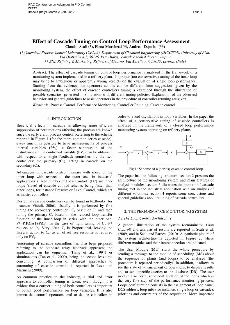
Beneficial effects of cascade in allowing more efficient

suppression of perturbations affecting the process are known

since the early era of process control. Referring to the scheme

reported in Figure 1 (for the more common series cascade),

every time it is possible to have measurements of process

internal variables (PVi), a faster suppression of the

disturbance on the controlled variable (PVe) can be obtained,

with respect to a single feedback controller, by the two

controllers: the primary (Ce), acting in cascade on the

secondary (Ci),

Advantages of cascade control increase with speed of the

inner loop with respect to the outer one; in industrial

applications a large number of Flow Control (FC) are inner

loops (slave) of cascade control scheme, being faster than

outer loops, for instance Pressure or Level Control, which act

as master controllers.

Design of cascade controllers can be found in textbooks (for

instance: Visioli, 2006). Usually it is performed by first

tuning the secondary controller Ci based on Pi and then

tuning the primary Ce based on the closed loop transfer

function of the inner loop in series with the outer one:

P*=PePiCi/(1+PiCi). In the case of tight tuning of Ci, P*

reduces to Pe. Very often Ci is Proportional, leaving the

Integral action to Ce, as an offset free response is required

only on PVe.

Autotuning of cascade controllers has also been proposed

referring to the standard relay feedback approach; the

application can be sequential (Hang et al., 1994) or

simultaneous (Tan et al., 2000), being the second less time

consuming. A comparison of different approaches to

autotuning of cascade controls is reported in Leva and

Marinelli (2009).

As common practice in the industry, a trial and error

approach to controller tuning is taken, even though it is

evident that a correct tuning of both controllers is important

to obtain good performance on loop variables. It is also

known that control operators tend to detune controllers in

order to avoid oscillations in loop variables. In the paper the

effect of a conservative tuning of cascade controllers is

analysed in the framework of a closed loop performance

monitoring system operating on refinery plants.

Fig.1: Scheme of a (series) cascade control loop

The paper has the following structure: section 2 presents the

architecture of the monitoring system and main features of

analysis modules; section 3 illustrates the problem of cascade

tuning met in the industrial application with an analysis of

different solutions; section 4 reports some conclusions and

general guidelines about retuning of cascade controllers.

2. THE PERFORMANCE MONITORING SYSTEM

2.1 The Loop Control Architecture

A general illustration of the system (denominated Loop

Control) and analysis of results are reported in Scali et al.

(2009) and in Scali and Farnesi (2010). A synthetic picture of

the system architecture is depicted in Figure 2, where

different modules and their interconnection are indicated.

The User Module (MU) starts the whole procedure by

sending a message to the module of scheduling (MS) about

the sequence of plants (and loops) to be analysed (the

procedure is repeated periodically). In addition, it allows to

see the state of advancement of operations, to display results

and to send specific queries to the database (DB). The user

module also permits the configuration of the loops which is

the very first step of the performance monitoring process.

Loops configuration consists in the assignment of loop name,

DCS address, loop info (for instance: single loop or cascade),

priorities and constraints of the acquisition. More important

IFAC Conference on Advances in PID Control PID'12 Brescia (Italy), March 28-30, 2012 FrB1.1

loops can have higher frequency of acquisition, cascade loops

are acquired simultaneously, loops of the same process unit

are analysed in the same data acquisition run.

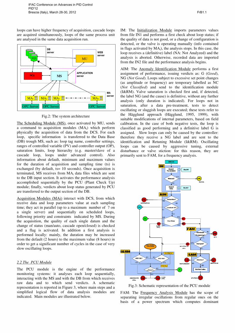
Fig.2: The system architecture

The Scheduling Module (MS), once activated by MU, sends

a command to acquisition modules (MAi) which perform

physically the acquisition of data from the DCS. For each

loop, specific information is transferred to the Data Base

(DB) trough MS, such as: loop tag name, controller settings,

ranges of controlled variable (PV) and controller output (OP),

saturation limits, loop hierarchy (e.g. master/slave of a

cascade loop, loops under advanced control). Also

information about default, minimum and maximum values

for the duration of acquisition and sampling time (ts) is

exchanged (by default, ts= 10 seconds). Once acquisition is

terminated, MS receives from MAi data files which are sent

to the DB input section. It activates the performance analysis

accomplished sequentially by the PCU (Plant Check Up)

module; finally, verdicts about loop status generated by PCU

are transferred to the output section of the DB.

Acquisition Modules (MAi) interact with DCS, from which

receive data and loop parameters value at each sampling

time; they act in parallel (up to a maximum number of 7 on

a single server) and sequentially on scheduled loops,

following priority and constraints indicated by MS. During

the acquisition, the quality of each single datum and the

change of status (man/auto, cascade open/closed) is checked

and a flag is activated. In addition a first analysis is

performed locally: mainly, the duration may be increased

from the default (2 hours) to the maximum value (8 hours) in

order to get a significant number of cycles in the case of very

slow oscillating loops.

2.2 The PCU Module

The PCU module is the engine of the performance

monitoring systems: it analyses each loop sequentially,

interacting with the MS and with the DB from which receives

raw data and to which send verdicts. A schematic

representation is reported in Figure 3, where main steps and a

simplified logical flow of data analysis modules are

indicated. Main modules are illustrated below.

IM: The Initialization Module imports parameters values

from file IN1 and performs a first check about loop status; if

the quality of data is not good, or a change of configuration is

detected, or the valve is operating manually (info contained

in flags activated by MAi), the analysis stops. In this case, the

loop receives a (definitive) label (NA: Not Analyzed) and the

analysis is aborted. Otherwise, recorded data are imported

from the IN2 file and the performance analysis begins.

AIM: The Anomaly Identification Module performs a first

assignment of performance, issuing verdicts as: G (Good),

NG (Not Good). Loops subject to excessive set point changes

(as amplitude or frequency) are temporary labelled as NC

(Not Classified) and send to the identification module

(I&RM). Valve saturation is checked first and, if detected,

the label NG (and the cause) is definitive, without any further

analysis (only duration is indicated). For loops not in

saturation, after a data pre-treatment, tests to detect

oscillating or sluggish loops are executed; these tests refer to

the Hägglund approach (Hägglund, 1995, 1999), with

suitable modifications of internal parameters, based on field

calibration. In the case of both negative tests, the loop is

classified as good performing and a definitive label G is

assigned. Slow loops can only be caused by the controller:

therefore they receive a NG label and are sent to the

identification and Retuning Module (I&RM). Oscillating

loops can be caused by aggressive tuning, external

disturbance or valve stiction: for this reason, they are

primarily sent to FAM, for a frequency analysis.

Fig.3: Schematic representation of the PCU module

FAM: The Frequency Analysis Module has the scope of

separating irregular oscillations from regular ones on the

basis of a power spectrum which computes dominant

OPC Server

MA1 MA2 MA3 MAn

MSMIC

SQL MU

OPC Server OPC ServerOPC Server

MA1 MA2 MA3 MAn

MSMIC

SQLSQL MU

OPC Server OPC Server

DB

server WEB

server

APPLICATION

server

MA

server

PCU


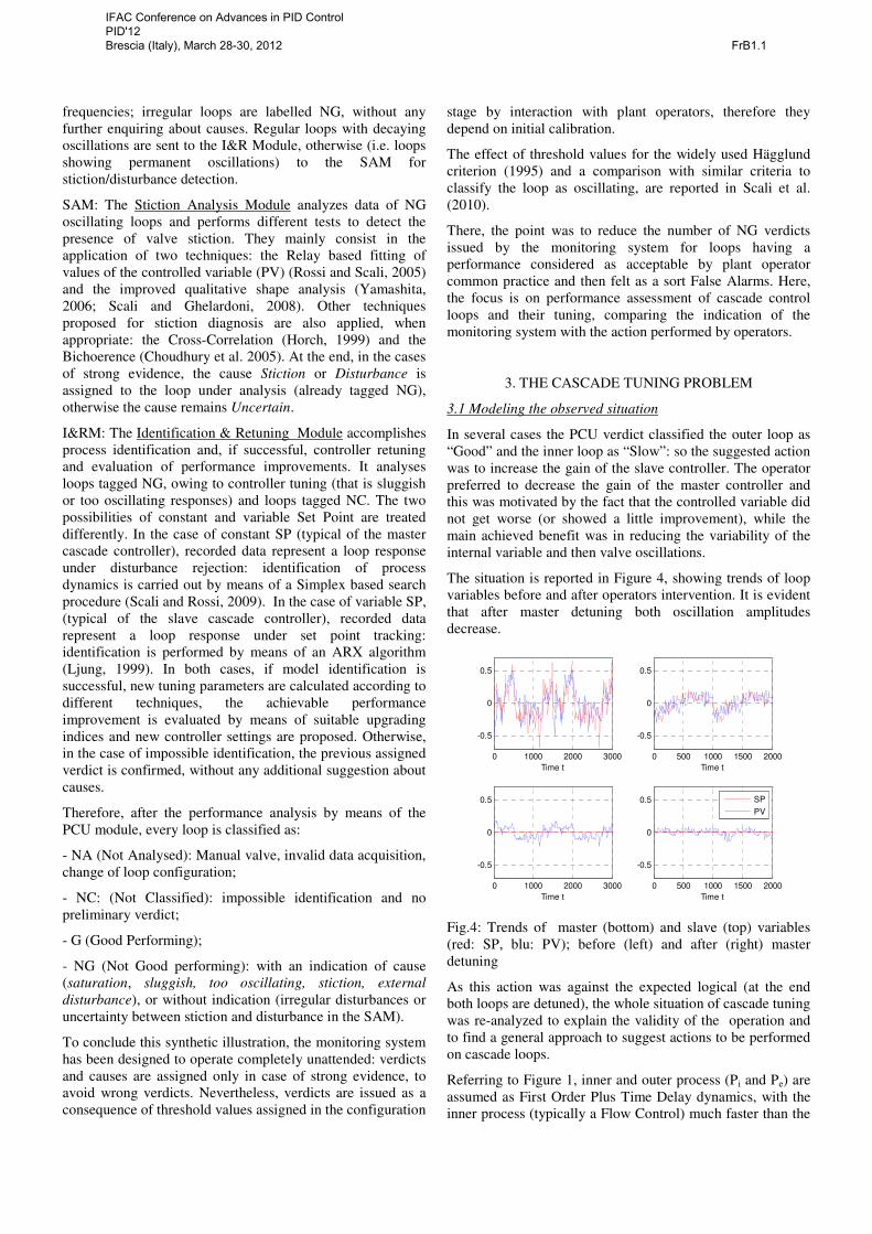
frequencies; irregular loops are labelled NG, without any

further enquiring about causes. Regular loops with decaying

oscillations are sent to the I&R Module, otherwise (i.e. loops

showing permanent oscillations) to the SAM for

stiction/disturbance detection.

SAM: The Stiction Analysis Module analyzes data of NG

oscillating loops and performs different tests to detect the

presence of valve stiction. They mainly consist in the

application of two techniques: the Relay based fitting of

values of the controlled variable (PV) (Rossi and Scali, 2005)

and the improved qualitative shape analysis (Yamashita,

2006; Scali and Ghelardoni, 2008). Other techniques

proposed for stiction diagnosis are also applied, when

appropriate: the Cross-Correlation (Horch, 1999) and the

Bichoerence (Choudhury et al. 2005). At the end, in the cases

of strong evidence, the cause Stiction or Disturbance is

assigned to the loop under analysis (already tagged NG),

otherwise the cause remains Uncertain.

I&RM: The Identification & Retuning Module accomplishes

process identification and, if successful, controller retuning

and evaluation of performance improvements. It analyses

loops tagged NG, owing to controller tuning (that is sluggish

or too oscillating responses) and loops tagged NC. The two

possibilities of constant and variable Set Point are treated

differently. In the case of constant SP (typical of the master

cascade controller), recorded data represent a loop response

under disturbance rejection: identification of process

dynamics is carried out by means of a Simplex based search

procedure (Scali and Rossi, 2009). In the case of variable SP,

(typical of the slave cascade controller), recorded data

represent a loop response under set point tracking:

identification is performed by means of an ARX algorithm

(Ljung, 1999). In both cases, if model identification is

successful, new tuning parameters are calculated according to

different techniques, the achievable performance

improvement is evaluated by means of suitable upgrading

indices and new controller settings are proposed. Otherwise,

in the case of impossible identification, the previous assigned

verdict is confirmed, without any additional suggestion about

causes.

Therefore, after the performance analysis by means of the

PCU module, every loop is classified as:

- NA (Not Analysed): Manual valve, invalid data acquisition,

change of loop configuration;

- NC: (Not Classified): impossible identification and no

preliminary verdict;

- G (Good Performing);

- NG (Not Good performing): with an indication of cause

(saturation, sluggish, too oscillating, stiction, external

disturbance), or without indication (irregular disturbances or

uncertainty between stiction and disturbance in the SAM).

To conclude this synthetic illustration, the monitoring system

has been designed to operate completely unattended: verdicts

and causes are assigned only in case of strong evidence, to

avoid wrong verdicts. Nevertheless, verdicts are issued as a

consequence of threshold values assigned in the configuration

stage by interaction with plant operators, therefore they

depend on initial calibration.

The effect of threshold values for the widely used Hägglund

criterion (1995) and a comparison with similar criteria to

classify the loop as oscillating, are reported in Scali et al.

(2010).

There, the point was to reduce the number of NG verdicts

issued by the monitoring system for loops having a

performance considered as acceptable by plant operator

common practice and then felt as a sort False Alarms. Here,

the focus is on performance assessment of cascade control

loops and their tuning, comparing the indication of the

monitoring system with the action performed by operators.

3. THE CASCADE TUNING PROBLEM

3.1 Modeling the observed situation

In several cases the PCU verdict classified the outer loop as

“Good” and the inner loop as “Slow”: so the suggested action

was to increase the gain of the slave controller. The operator

preferred to decrease the gain of the master controller and

this was motivated by the fact that the controlled variable did

not get worse (or showed a little improvement), while the

main achieved benefit was in reducing the variability of the

internal variable and then valve oscillations.

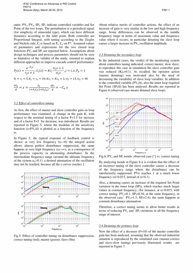
The situation is reported in Figure 4, showing trends of loop

variables before and after operators intervention. It is evident

that after master detuning both oscillation amplitudes

decrease.

Fig.4: Trends of master (bottom) and slave (top) variables

(red: SP, blu: PV); before (left) and after (right) master

detuning

As this action was against the expected logical (at the end

both loops are detuned), the whole situation of cascade tuning

was re-analyzed to explain the validity of the operation and

to find a general approach to suggest actions to be performed

on cascade loops.

Referring to Figure 1, inner and outer process (Pi and Pe) are

assumed as First Order Plus Time Delay dynamics, with the

inner process (typically a Flow Control) much faster than the

0 1000 2000 3000

-0.5

0

0.5

Time t

0 500 1000 1500 2000

-0.5

0

0.5

Time t

0 1000 2000 3000

-0.5

0

0.5

Time t

0 500 1000 1500 2000

-0.5

0

0.5

Time t

SP

PV


outer. PVi, PVe, SPi, SPe indicate controlled variables and Set

Point of the two loops. The perturbation is a periodical signal

(for simplicity of sinusoidal type), which can have different

dynamics according to the inlet point. Both controller are

Proportional Integral, with tuning according to the Ziegler

and Nichols rule; Ci is based on Pi, Ce on P*. Assumed values

of parameters and expressions for the two closed loop

functions PVe and SPi are reported below. Assumptions about

design techniques and process parameters should not be seen

as limitative of the validity of the study, oriented to explain

different approaches to improve cascade control performance.

�� =��

�� + 1, �� = ��

�� + 1

��, � = �, �, �� = 1

�� = �� = 5, �� = �� = 10;�� = �� = 1; �� = 13, �� = 40

��

�= ! =

�

"#�$%$�"#� % �,&�$

�= −��!

3.2 Effect of controllers tuning

As first, the effect of master and slave controller gain on loop

performance was examined. A change in the gain Kc with

respect to the nominal tuning of a factor F=1.5 for increase

and of a factor F=5 for decrease, was introduced. Results are

reported in Figure 5, where the modulus of the sensitivity

function (ε=PVe/d) is plotted as a function of the frequency

ω.

In Figure 5, the typical response of feedback control is

shown: at very low frequency (ω→0) the integral action

allows almost perfect disturbance suppression; the same

happens at very high frequency (ω→∞), as a consequence of

the process capacity in attenuating disturbance. In the

intermediate frequency range (around the ultimate frequency

of the system ωu≈0.1), a desired attenuation of the oscillation

may not be reached, because all the ε curves reaches 1.

Fig.5: Effect of controller tuning on disturbance suppression;

correct tuning (red); master (green); slave (blu)

About relative merits of controller actions, the effect of an

increase of gain is very similar in the low and high frequency

range. Some differences can be observed in the middle

frequency range in terms of maximum value and frequency

value where it occurs; in particular detuning the slave loop

causes a larger increase in PVe oscillation amplitude.

3.3 Detuning the secondary loop

In the industrial cases, the verdict of the monitoring system

about controllers tuning indicated: correct master, slow slave;

to reproduce this case in simulation the slave controller gain

was reduced (Kci=0.1). As recalled, the operator action

(master detuning) was motivated also by the need of

decreasing the variability of slave loop variables. In addition

to the controlled variable (PVe/d), also the inner loop required

Set Point (SPi/d) has been analysed. Results are reported in

Figure 6 (observed case means detuned slave loop).

Fig.6: PVe and SPi trends: observed case [°] vs. correct tuning

By analyzing trends in Figure 6 it is evident that the effect of

an incorrect tuning of the slave controller causes a decrease

of the frequency range where the disturbance can be

satisfactorily suppressed: PVe reaches 1 at a much lower

frequency (ω≈0.015, instead of ω≈0.1).

Also, a detuning causes an increase of the required Set Point

variation in the inner loop (SPi), which reaches much larger

values at constant frequency; (for instance, at ω≈0.015, with

correct tuning: PVe=0.1, SPi=0.18; at the same frequency, in

the observed case: PVe=1.3, SPi=2.4); the same happens at

constant disturbance attenuation.

Therefore, a correct tuning seems to allow better results in

terms of reducing PVe and SPi variations in all the frequency

range of interest.

3.4 Detuning the primary loop

Now the effect of a decrease (F=10) of the master controller

gain has been analysed, assuming that the observed industrial

situation is reproduced by the simulated case (master-correct

and slave-slow tuning) previously illustrated; results are

reported in Figure 7.

10-3

10-2

10-1

100

10-3

10-2

10-1

100

10-3

10-2

10-1

100

10-3

10-2

10-1

100

Frequency ω

AR

Detuning

Retuning

10-4

10-3

10-2

10-1

100

101

10-6

10-5

10-4

10-3

10-2

10-1

100

101

Frequency ω

AR

PVe°

PVe

SPi

SPi°


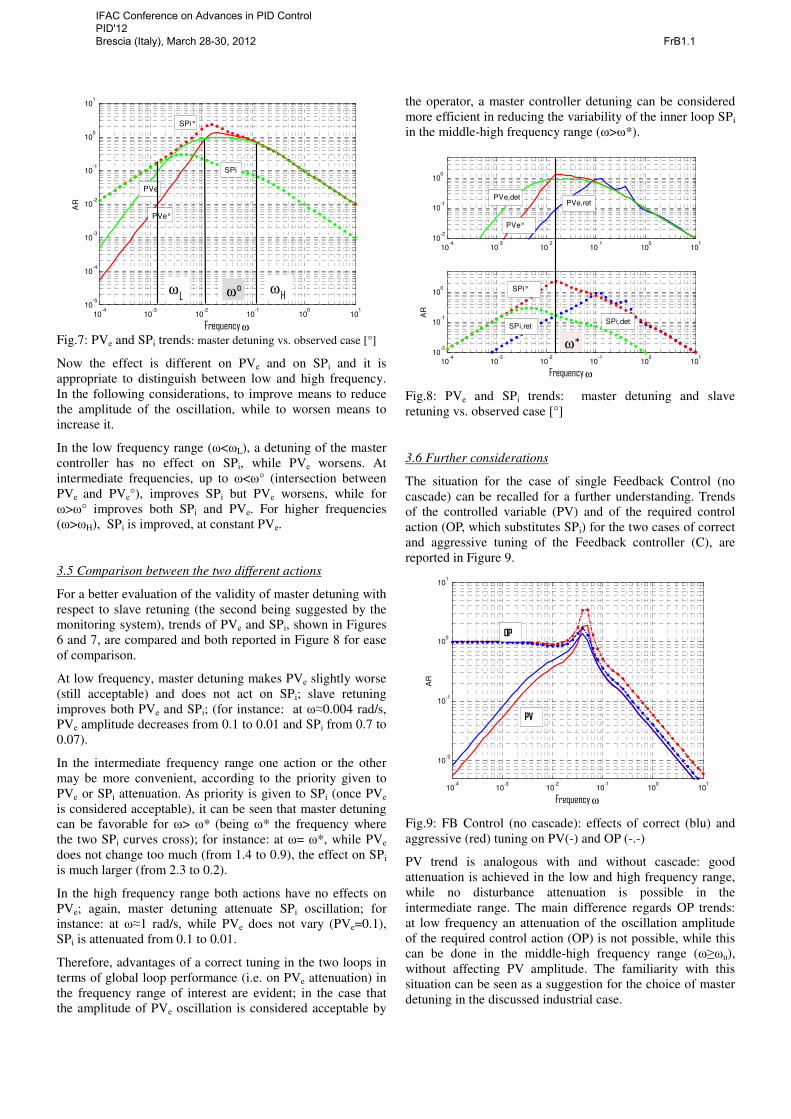
Fig.7: PVe and SPi trends: master detuning vs. observed case [°]

Now the effect is different on PVe and on SPi and it is

appropriate to distinguish between low and high frequency.

In the following considerations, to improve means to reduce

the amplitude of the oscillation, while to worsen means to

increase it.

In the low frequency range (ω<ωL), a detuning of the master

controller has no effect on SPi, while PVe worsens. At

intermediate frequencies, up to ω<ω° (intersection between

PVe and PVe°), improves SPi but PVe worsens, while for

ω>ω° improves both SPi and PVe. For higher frequencies

(ω>ωH), SPi is improved, at constant PVe.

3.5 Comparison between the two different actions

For a better evaluation of the validity of master detuning with

respect to slave retuning (the second being suggested by the

monitoring system), trends of PVe and SPi, shown in Figures

6 and 7, are compared and both reported in Figure 8 for ease

of comparison.

At low frequency, master detuning makes PVe slightly worse

(still acceptable) and does not act on SPi; slave retuning

improves both PVe and SPi; (for instance: at ω≈0.004 rad/s,

PVe amplitude decreases from 0.1 to 0.01 and SPi from 0.7 to

0.07).

In the intermediate frequency range one action or the other

may be more convenient, according to the priority given to

PVe or SPi attenuation. As priority is given to SPi (once PVe

is considered acceptable), it can be seen that master detuning

can be favorable for ω> ω* (being ω* the frequency where

the two SPi curves cross); for instance: at ω= ω*, while PVe

does not change too much (from 1.4 to 0.9), the effect on SPi

is much larger (from 2.3 to 0.2).

In the high frequency range both actions have no effects on

PVe; again, master detuning attenuate SPi oscillation; for

instance: at ω≈1 rad/s, while PVe does not vary (PVe=0.1),

SPi is attenuated from 0.1 to 0.01.

Therefore, advantages of a correct tuning in the two loops in

terms of global loop performance (i.e. on PVe attenuation) in

the frequency range of interest are evident; in the case that

the amplitude of PVe oscillation is considered acceptable by

the operator, a master controller detuning can be considered

more efficient in reducing the variability of the inner loop SPi

in the middle-high frequency range (ω>ω*).

Fig.8: PVe and SPi trends: master detuning and slave

retuning vs. observed case [°]

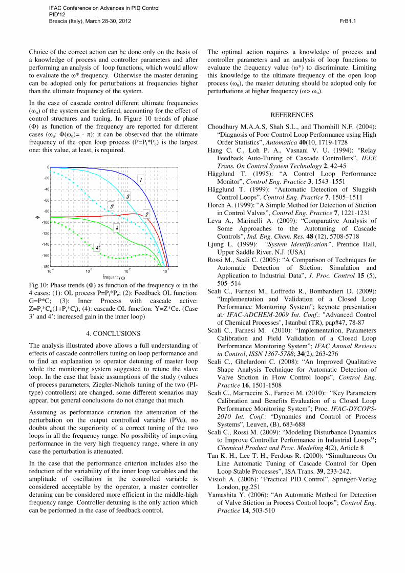
3.6 Further considerations

The situation for the case of single Feedback Control (no

cascade) can be recalled for a further understanding. Trends

of the controlled variable (PV) and of the required control

action (OP, which substitutes SPi) for the two cases of correct

and aggressive tuning of the Feedback controller (C), are

reported in Figure 9.

Fig.9: FB Control (no cascade): effects of correct (blu) and

aggressive (red) tuning on PV(-) and OP (-.-)

PV trend is analogous with and without cascade: good

attenuation is achieved in the low and high frequency range,

while no disturbance attenuation is possible in the

intermediate range. The main difference regards OP trends:

at low frequency an attenuation of the oscillation amplitude

of the required control action (OP) is not possible, while this

can be done in the middle-high frequency range (ω≥ωu),

without affecting PV amplitude. The familiarity with this

situation can be seen as a suggestion for the choice of master

detuning in the discussed industrial case.

10-4

10-3

10-2

10-1

100

101

10-5

10-4

10-3

10-2

10-1

100

101

Frequency ω

AR

PVe°

PVe

SPi°

SPi

ω°ωL

ωH

10-4

10-3

10-2

10-1

100

101

10-2

10-1

100

10-4

10-3

10-2

10-1

100

101

10-2

10-1

100

Frequency ω

AR

PVe,detPVe,ret

PVe°

SPi°

ω*

SPi,detSPi,ret

10-4

10-3

10-2

10-1

100

101

10-2

10-1

100

101

Frequency ω

AR

PV

OP


Choice of the correct action can be done only on the basis of

a knowledge of process and controller parameters and after

performing an analysis of loop functions, which would allow

to evaluate the ω* frequency. Otherwise the master detuning

can be adopted only for perturbations at frequencies higher

than the ultimate frequency of the system.

In the case of cascade control different ultimate frequencies

(ωu) of the system can be defined, accounting for the effect of

control structures and tuning. In Figure 10 trends of phase

(Φ) as function of the frequency are reported for different

cases (ωu: Φ(ωu)= - π); it can be observed that the ultimate

frequency of the open loop process (P=Pi*Pe) is the largest

one: this value, at least, is required.

Fig.10: Phase trends (Φ) as function of the frequency ω in the

4 cases: (1): OL process P=Pi*Pe; (2): Feedback OL function:

G=P*C; (3): Inner Process with cascade active:

Z=Pi*Ci/(1+Pi*Ci); (4): cascade OL function: Y=Z*Ce. (Case

3’ and 4’: increased gain in the inner loop)

4. CONCLUSIONS

The analysis illustrated above allows a full understanding of

effects of cascade controllers tuning on loop performance and

to find an explanation to operator detuning of master loop

while the monitoring system suggested to retune the slave

loop. In the case that basic assumptions of the study (values

of process parameters, Ziegler-Nichols tuning of the two (PI-

type) controllers) are changed, some different scenarios may

appear, but general conclusions do not change that much.

Assuming as performance criterion the attenuation of the

perturbation on the output controlled variable (PVe), no

doubts about the superiority of a correct tuning of the two

loops in all the frequency range. No possibility of improving

performance in the very high frequency range, where in any

case the perturbation is attenuated.

In the case that the performance criterion includes also the

reduction of the variability of the inner loop variables and the

amplitude of oscillation in the controlled variable is

considered acceptable by the operator, a master controller

detuning can be considered more efficient in the middle-high

frequency range. Controller detuning is the only action which

can be performed in the case of feedback control.

The optimal action requires a knowledge of process and

controller parameters and an analysis of loop functions to

evaluate the frequency value (ω*) to discriminate. Limiting

this knowledge to the ultimate frequency of the open loop

process (ωu), the master detuning should be adopted only for

perturbations at higher frequency (ω> ωu).

REFERENCES

Choudhury M.A.A.S, Shah S.L., and Thornhill N.F. (2004):

“Diagnosis of Poor Control Loop Performance using High

Order Statistics”, Automatica 40(10, 1719-1728

Hang C. C., Loh P. A., Vasnani V. U. (1994): “Relay

Feedback Auto-Tuning of Cascade Controllers”, IEEE

Trans. On Control System Technology 2, 42-45

Hägglund T. (1995): “A Control Loop Performance

Monitor”, Control Eng. Practice 3, 1543–1551

Hägglund T. (1999): “Automatic Detection of Sluggish

Control Loops”, Control Eng. Practice 7, 1505–1511

Horch A. (1999): “A Simple Method for Detection of Stiction

in Control Valves”, Control Eng. Practice 7, 1221-1231

Leva A., Marinelli A. (2009): “Comparative Analysis of

Some Approaches to the Autotuning of Cascade

Controls”, Ind. Eng. Chem. Res. 48 (12), 5708-5718

Ljung L. (1999): “System Identification”, Prentice Hall,

Upper Saddle River, N.J. (USA)

Rossi M., Scali C. (2005): “A Comparison of Techniques for

Automatic Detection of Stiction: Simulation and

Application to Industrial Data”, J. Proc. Control 15 (5),

505–514

Scali C., Farnesi M., Loffredo R., Bombardieri D. (2009):

“Implementation and Validation of a Closed Loop

Performance Monitoring System”; keynote presentation

at: IFAC-ADCHEM-2009 Int. Conf.: "Advanced Control

of Chemical Processes", Istanbul (TR), pap#47, 78-87

Scali C., Farnesi M. (2010): “Implementation, Parameters

Calibration and Field Validation of a Closed Loop

Performance Monitoring System”; IFAC Annual Reviews

in Control, ISSN 1367-5788; 34(2), 263-276

Scali C., Ghelardoni C. (2008): “An Improved Qualitative

Shape Analysis Technique for Automatic Detection of

Valve Stiction in Flow Control loops”, Control Eng.

Practice 16, 1501-1508

Scali C., Marraccini S., Farnesi M. (2010): “Key Parameters

Calibration and Benefits Evaluation of a Closed Loop

Performance Monitoring System”; Proc. IFAC-DYCOPS-

2010 Int. Conf.: “Dynamics and Control of Process

Systems”, Leuven, (B), 683-688

Scali C., Rossi M. (2009): “Modeling Disturbance Dynamics

to Improve Controller Performance in Industrial Loops”;

Chemical Product and Proc. Modeling 4(2), Article 8

Tan K. H., Lee T. H., Ferdous R. (2000): “Simultaneous On

Line Automatic Tuning of Cascade Control for Open

Loop Stable Processes”, ISA Trans. 39, 233-242.

Visioli A. (2006): “Practical PID Control”, Springer-Verlag

London, pg.251

Yamashita Y. (2006): “An Automatic Method for Detection

of Valve Stiction in Process Control loops”; Control Eng.

Practice 14, 503-510

10-4

10-3

10-2

10-1

-180

-160

-140

-120

-100

-80

-60

-40

-20

0

Frequency ω

φ

1

2

3

3'

4'

4


Documents

Effect of Cascade Tuning on Control Loop Performance