Effec of Depreciation on Exports and Imports

8/7/2019 Effec of Depreciation on Exports and Imports

http://slidepdf.com/reader/full/effec-of-depreciation-on-exports-and-imports 1/48

Exports, Imports and the Trade Balance

Paddy Jilek

Andrew Johnson

Bruce Taplin

This document is based on the research and development work undertaken in recent years in theModelling Section of the Treasury. It has been released in the interests of evaluating the researchresults embodied in the model and to encourage public discussion.

The authors are employees of the Australian Treasury. We would like to thank Brett Ryder, Mark Upcher and Annette Beacher for their earlier work that formed a basis for this paper, and Barry Grayfor his comments and suggestions on drafts of this paper. Of course any remaining errors andomissions are the responsibility of the authors. The views in this paper are those of the authors andare not necessarily those of the Government or the Treasury.



2

This document is one of a series presented at the June 1993 Treasury Conference on The TRYM

Model of the Australian Economy . Papers presented at the Conference also included:

• An Introduction to the Treasury Macroeconomic (TRYM) Model of the Australian Economy

(TRYM paper no. 2)

• Employment, Investment, Inflation and Productivity: Decisions by the Firm

(TRYM paper No. 3)

• Exports, Imports and the Trade Balance

(TRYM paper No. 4)

• Savings, Dwelling Investment and the Labour Market: Decisions by Households

(TRYM paper No. 5)

• Australia's Trade Linkages with the World

(TRYM paper No. 6)

• The Macroeconomic Effects of Higher Productivity

(TRYM paper No. 7)



3

TABLE OF CONTENTS

1. INTRODUCTION.................................................................................................................5

2. EXPORTS OF GOODS AND SERVICES...........................................................................6

2.1 Trends in the Export Sector .....................................................................................6

2.2 Major Factors Affecting Export Behaviour in the TRYM model ...........................7

2.21 Price Competition ......................................................................................7

2.22 Simplifying the Analysis............................................................................9

2.23 World Growth............................................................................................ 11

2.24 Measuring World Activity and Competitiveness in the TRYM model.....11

2.3 Estimated Equations for Commodity Exports .........................................................12

2.31 Commodity Demand..................................................................................12

3.32 Commodity Supply ....................................................................................16

2.4 Estimated Equation for Non-Commodity Exports .................................................. 18

2.41 Non-Commodity Demand.......................................................................... 18

2.42 Supply of Non-Commodity Exports Identity.............................................20

3. IMPORTS OF GOODS AND SERVICES ...........................................................................22

3.1 Trends in the Imports Sector ...................................................................................22

3.2 Major Factors Affecting Import Behaviour in the TRYM model ...........................24

3.3 Import Demand........................................................................................................24

3.31 Measuring Income .....................................................................................25

3.32 Measuring Cost Competitiveness ..............................................................26

3.33 The TRYM Model Measures of Import Penetration and

Competitiveness.........................................................................................27



4

3.34 Interpretation of Import Penetration Trend................................................28

3.4 Import Supply ..........................................................................................................28

3.41 Measuring World Prices and Exchange Rate ............................................29

3.42 Measuring Trend and Compositional Influences .......................................29

3.5 Estimated Import Equations ....................................................................................31

3.51 Import Demand ..........................................................................................31

3.52 Import Supply ............................................................................................ 32

4. TRADE BALANCE AND CURRENT ACCOUNT ............................................................37

4.1 Trends in the Balance on Goods and Services, Net Transfers Overseas

and the Current Account..........................................................................................37

5. EFFECT OF A DEPRECIATION UPON THE BALANCE OF TRADE............................39

5.1 Nature of the Shock.................................................................................................39

5.2 Summary of Results.................................................................................................41

5.3 The J-Curve and the Response of the Balance of Goods and Services in

the TRYM model.....................................................................................................42

6. CONCLUSIONS ................................................................................................................... 45

7. APPENDIX A .......................................................................................................................46

7.1 Description of a Ceteris Paribus Exchange Rate Shock to the Trade Sector...........46

8. REFERENCES......................................................................................................................48



5

1. INTRODUCTION

This paper outlines the approach taken in analysing the external sector of the Australian economywithin the framework of the Commonwealth Treasury's macroeconomic TRYM model.

Although there is some discussion of recent trends, the focus is on examining factors that affect thespeed, timing and composition of the adjustment of Australia's external sector within the TRYMmodel framework. The paper is divided into three sections.

The first section examines the export sector, within a simple demand and supply framework,incorporating both the external and the internal competitiveness of Australia's exports. Externalcompetitiveness is defined as the price of Australia's goods and services relative to world prices andis a primary determinant of the demand for exports. Internal competitiveness is defined as theincentive for domestic producers to export and is a primary factor determining the supply of exports.Particular attention is also given to the dynamic adjustment of Australia's trade prices to changes inthe growth of our major trading partners.

The second section examines the import side of the trade balance. Again, a simple demand andsupply framework is utilised with price determined in world markets and volume driven bydomestic demand and external (or import) competitiveness. The analysis considers the relativeimportance of domestic demand and relative prices on import volumes, as well as the timing and

magnitude of pass-through of world prices and the exchange rate into import prices.

The final section combines the analysis of the previous two sections to examine the direct impact of a depreciation of Australia's exchange rate on the trade balance. The resultant adjustment iscompared with that implied by the J-curve theory.

A summary of the results and directions for future work are outlined in the conclusion.



6

2. EXPORTS OF GOODS AND SERVICES

2.1 Trends in the Export Sector

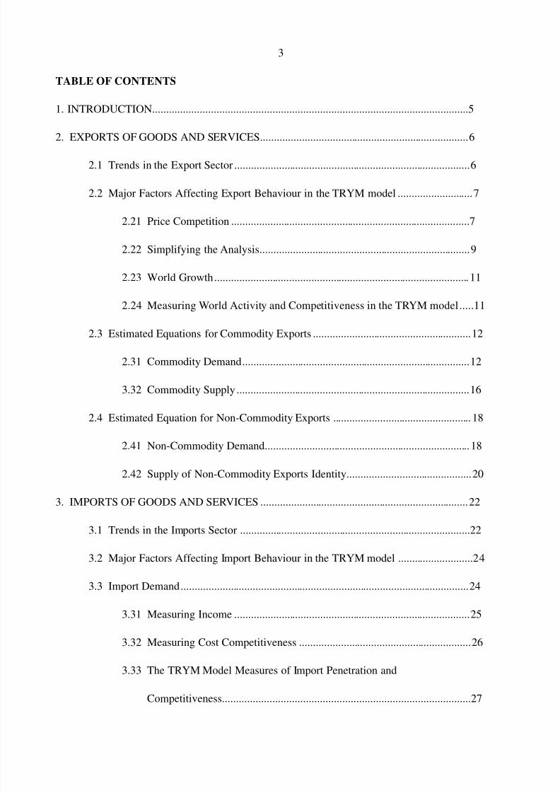
During the 1970s and early 1980s, exports were about 13 per cent of GDP, but have since increasedrapidly to around 20 per cent, driven by increases in the relative importance of the mining,manufacturing and services sectors. Within TRYM, aggregate exports are split into commodity(agricultural and mining) and non-commodity (manufacturing and service) categories. Althoughcomponents of these can behave differently and respond to different factors, this level of disaggregation is appropriate - particularly given the preference for simplicity.

Commodity exports have declined as a proportion of total exports of goods and services, from about75 per cent (in value terms) in the early 1970s to around 63 per cent today. Most of the fall inrelative importance has occurred since the mid-1980s.

Chart 1: Trends in the Export Sector

Quarters

1989-90 Prices (%)

10

12

14

16

18

20

22

Dec-75

Dec-76

Dec-77

Dec-78

Dec-79

Dec-80

Dec-81

Dec-82

Dec-83

Dec-84

Dec-85

Dec-86

Dec-87

Dec-88

Dec-89

Dec-90

Dec-91

Dec-92

60

62

64

66

68

70

72

74

76

78

Current Prices (%)

Commodity Exports as a Proportion of Total Exports (RHS)

Total Exports as a Proportion of GDP (LHS)

It is particularly evident for agricultural exports, which in the past have accounted for up to half of total exports. Since the mid 1980s alone, this proportion has fallen from about 32 per cent toaround 22 per cent (in value terms); domestic supply constraints, weakness of world prices andslower population growth in developed countries have all been influences.

In contrast, mining exports have remained strong, contributing around 40 per cent of total exports,despite the shift in developed countries away from resource intensive industries toward services. Aprimary reason for the continuing strength of the mining sector has been the low costs of productionand large improvements in productivity. Furthermore, in contrast to the agricultural sector, supply



7

in the mining sector has been maintained over the last decade with the introduction of large newprojects like the North West Shelf.

Exports of manufactures as a proportion of Australia's total exports have increased rapidly since the

mid-1980s from about 11 per cent to 18 per cent. Similarly, there has been strong growth in serviceexports which now account for around 20 per cent of total exports, or almost as much as theagricultural sector. These movements are consistent with global trends, reflecting the higherdemand elasticities in developed countries for manufactured goods and the higher trade barriersfacing agricultural products. However, increased price competitiveness, growth of our majortrading partners (particularly in Asia), and increased export awareness in the manufacturing andservice sectors have also been important determinants of Australia's relative performance.

2.2 Major Factors Affecting Export Behaviour in the TRYM model

2.21 Price Competition

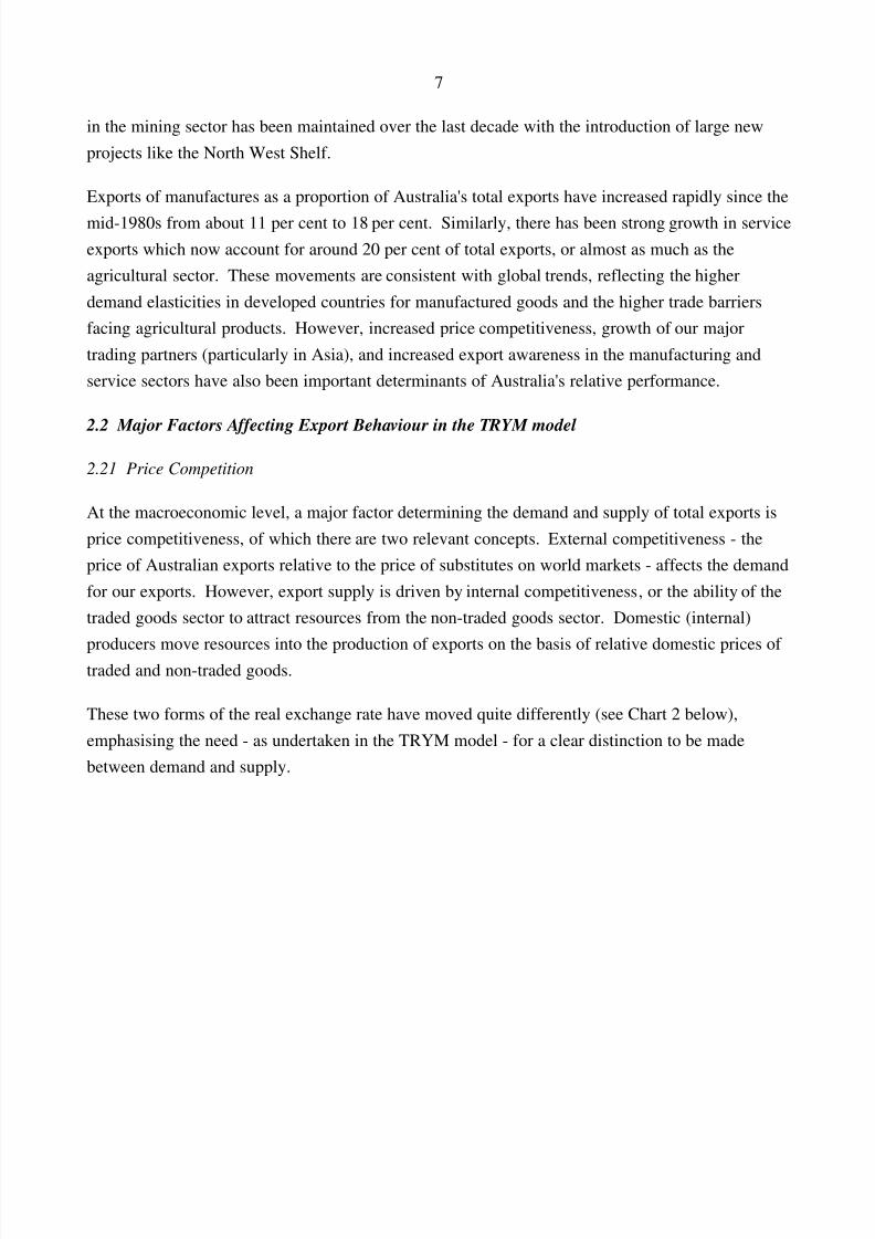
At the macroeconomic level, a major factor determining the demand and supply of total exports isprice competitiveness, of which there are two relevant concepts. External competitiveness - theprice of Australian exports relative to the price of substitutes on world markets - affects the demandfor our exports. However, export supply is driven by internal competitiveness, or the ability of thetraded goods sector to attract resources from the non-traded goods sector. Domestic (internal)

producers move resources into the production of exports on the basis of relative domestic prices of traded and non-traded goods.

These two forms of the real exchange rate have moved quite differently (see Chart 2 below),emphasising the need - as undertaken in the TRYM model - for a clear distinction to be madebetween demand and supply.



8

Chart 2: Competitiveness of Exports

Index (March 1985=1)

0.5

0.6

0.7

0.8

0.9

1

1.1

1.2

1.3

1.4

Dec-74

Dec-75

Dec-76

Dec-77

Dec-78

Dec-79

Dec-80

Dec-81

Dec-82

Dec-83

Dec-84

Dec-85

Dec-86

Dec-87

Dec-88

Dec-89

Dec-90

Dec-91

Dec-92

Internal Competitiveness

External Competitiveness

Note: a fall in each series implies an increase in competitiveness

It is apparent from Chart 2 that internal competitiveness has been less volatile than externalcompetitiveness, and that the two measures exhibit divergent trends. In particular, current levels of external competitiveness are a significant improvement on the averages of the past 20 years, whileuntil very recently, the internal competitiveness measure has tended to deteriorate.

The behaviour of external and internal competitiveness for commodities is different to that of non-commodities, implying differences in their relative price elasticities of demand and supply.

The supply of commodity exports is price inelastic, reflecting limitations on the amount of arableland and known mineral resources. However, demand is very elastic, consistent with the view that,at an aggregate level, Australia is a price taker. An elastic demand curve is also consistent with thehomogeneity of the international commodity market 1.

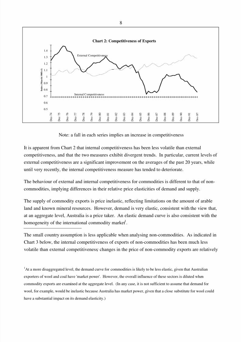
The small country assumption is less applicable when analysing non-commodities. As indicated inChart 3 below, the internal competitiveness of exports of non-commodities has been much lessvolatile than external competitiveness ; changes in the price of non-commodity exports are relatively

1At a more disaggregated level, the demand curve for commodities is likely to be less elastic, given that Australian

exporters of wool and coal have 'market power'. However, the overall influence of these sectors is diluted when

commodity exports are examined at the aggregate level. (In any case, it is not sufficient to assume that demand for

wool, for example, would be inelastic because Australia has market power, given that a close substitute for wool could

have a substantial impact on its demand elasticity.)



9

small compared with changes in domestic non-commodity prices. Given that the supply of exportsis driven by internal competitiveness, a highly elastic supply curve is implied, with non-commodityexport prices primarily determined by the domestic price level. This outcome is consistent withAustralian producers of non-commodities exporting a much smaller proportion of their output thancommodity producers.

Chart 3: Growth in the Competitiveness of Non-Commodity Exports

Through the year growth (%)

-30

-20

-10

0

10

20

30

Dec-75

Dec-76

Dec-77

Dec-78

Dec-79

Dec-80

Dec-81

Dec-82

Dec-83

Dec-84

Dec-85

Dec-86

Dec-87

Dec-88

Dec-89

Dec-90

Dec-91

Dec-92

External Competitiveness

Internal Competitiveness

Note: A negative growth implies an increase in competitiveness over the previous year.

In contrast, the volatility of the external competitiveness of non-commodity exports suggests a moreinelastic demand. The small open economy assumption does not appear to hold for non-commodityexports, probably because output from the manufacturing and services sectors tends to be highlydifferentiated. In other words, demanders of Australia's non-commodities tend to focus on factorsother than relative prices, an explanation that seems plausible in tourism for example, whereAustralia can offer a unique product.

2.22 Simplifying the Analysis

Exports are modelled in the TRYM model using a simplified demand and supply framework. Thisframework incorporates the two different types of competitiveness and recognises that the demandand supply elasticities for exports of commodities and non-commodities differ substantially.Indeed, the TRYM model framework is simplified greatly by exploiting the following dichotomy.

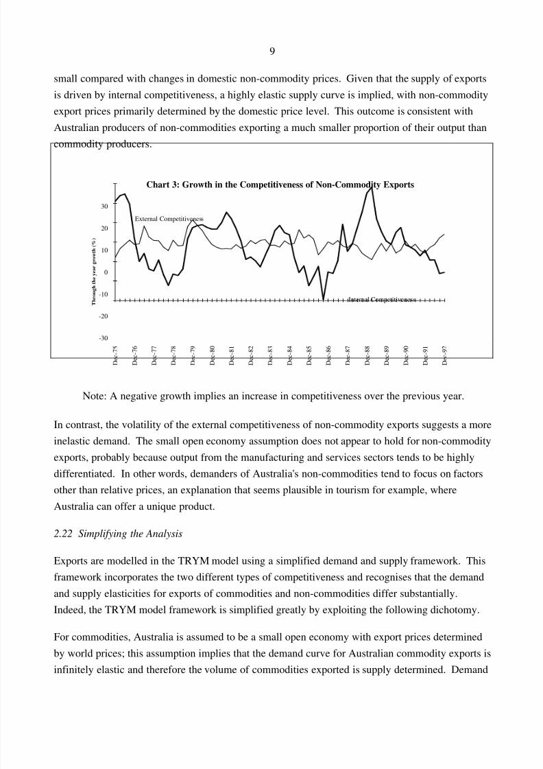
For commodities, Australia is assumed to be a small open economy with export prices determinedby world prices; this assumption implies that the demand curve for Australian commodity exports is

infinitely elastic and therefore the volume of commodities exported is supply determined. Demand



10

and supply curves are estimated for commodity exports. The former determines the $A exportcommodity price and the latter determines the quantity of commodities produced.

Supply

PriceDemand

Quantity

Commodity Exports

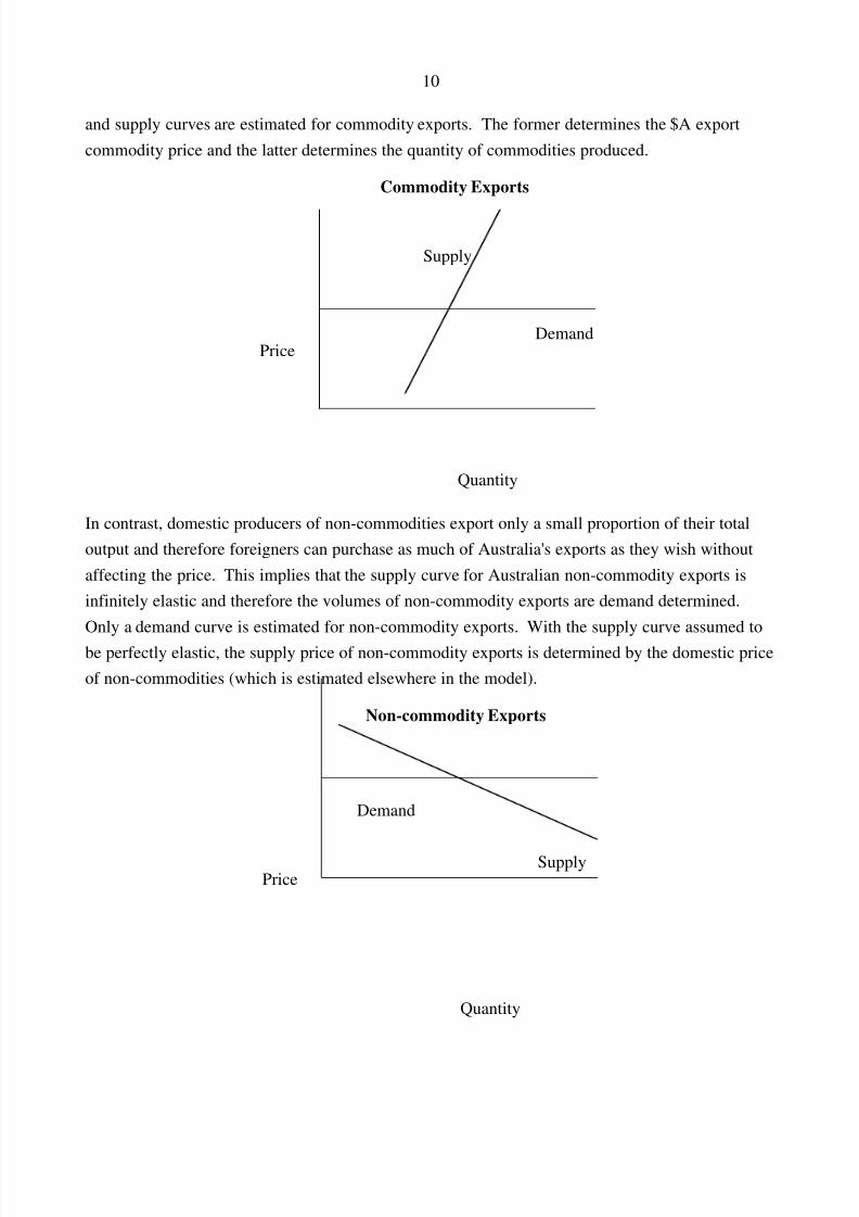
In contrast, domestic producers of non-commodities export only a small proportion of their totaloutput and therefore foreigners can purchase as much of Australia's exports as they wish withoutaffecting the price. This implies that the supply curve for Australian non-commodity exports isinfinitely elastic and therefore the volumes of non-commodity exports are demand determined.Only a demand curve is estimated for non-commodity exports. With the supply curve assumed tobe perfectly elastic, the supply price of non-commodity exports is determined by the domestic priceof non-commodities (which is estimated elsewhere in the model).

SupplyPrice

Quantity

Non-commodity Exports

Demand



11

2.23 World Growth

While the relationships between exports and competitiveness are used to establish an analyticalframework, special attention is also given to providing a direct link between exports and world

growth. World activity influences the demand for both categories of exports; stronger world growthwill, other things equal, increase demand for our exports. However, in the TRYM modelframework, the transmission mechanisms that relate world activity to exports are different forcommodities and non-commodities.

For commodities, world conditions determine export prices because the demand curve forcommodity exports determines prices. A fall in world growth leads to a fall in commodity pricesand a corresponding fall in Australia's terms of trade.

On the other hand, world conditions are linked to non-commodity export volumes because thedemand curve for non-commodity exports determines volumes. A fall in world activity thereforeleads to a fall in the volume of non-commodities exported.

These linkages between Australia and the world are explored in more detail in TRYM paper number6 on Australia's Trade Linkages with the World .

World supply is also likely to have an influence on Australia's external sector, particularly in thelong run. World growth is an important factor affecting world trade prices and volumes in the shortrun, but there would be consequent supply responses in the longer term. However, the TRYMmodel does not (directly) capture these world supply responses.

2.24 Measuring World Activity and Competitiveness in the TRYM model

World growth is expressed in terms of our major trading partners' growth, using a refined world database, which includes detailed information on Australia's trading partners in Asia. Bilateral exportweights, varying over time in accordance with shifts in trading patterns 2, have been applied toquarterly GDP data for our major trading partners to construct a trade weighted 'world growth index'(WGTM) 3.

2Weights have been smoothed to abstract from one-off influences.

3GDP and the price of GDP were chosen as measures of world economic growth and world prices because they were

readily available on a consistent basis for most of Australia's major trading partners. Furthermore, Australian exports

are assumed to be both intermediate goods in foreign production and final goods in foreign consumption, and GDP

encompasses elements of both foreign production and foreign incomes.



12

The world data base is also used to construct a trade weighted exchange rate (RTWI) 4 and a tradeweighted 'world price index' (WPGTM); GDP deflators form the basis for the price index. Externalcompetitiveness is measured as the level of foreign prices, adjusted for movements in the exchangerate, compared with domestic export prices. Ideally external competitiveness should account forcompetition between Australian exporters and foreign producers operating in their domesticmarkets, and competition between Australian exporters and other foreign producers selling to thesame market. The TRYM model measure of external competitiveness does not (directly) capturethe third country competition faced by Australia in export markets.

Internal competitiveness is measured by comparing the domestic price Australian producers receivefor their exports with the domestic price of non-commodities. An ideal measure would compare thedomestic price of exported goods and services with the domestic price of non-traded goods and

services. However, practical difficulties in distinguishing traded and non-traded goods, precludesuch an approach.

2.3 Estimated Equations for Commodity Exports

Both of the equations estimated for commodity exports are in error correction form, ensuring thatthere is a clear distinction between the long run relationship and the short to medium termrelationships. The equations are estimated jointly.

2.31 Commodity Demand

In the long run, the price of commodity exports (PXC) is assumed to fully adjust to changes in thelevel of world prices (WPGTM) and the exchange rate (RTWI). In equilibrium, PXC is also afunction of a time trend (QTIME), capturing the effects of a trend fall in world commodity pricesrelative to WPGTM due to various factors, including protectionist trade policies and a shift awayfrom resource intensive industries in developed countries.

The assumption that the demand for exports is perfectly elastic was tested by including the quantity

of commodity exports (XC) in the equation for PXC, but the influence of XC was found to beinsignificant; in aggregate, Australian commodity exports do not appear to influence worldcommodity prices. As noted above, analysing commodity exports in aggregate appears to havediluted the effects of those commodities in which Australia has some 'market power'.

4RTWI differs from the Reserve Bank of Australia's trade weighted index (TWI); RTWI is based on variable export

weights rather than the fixed export and import weights used in constructing the TWI.



13

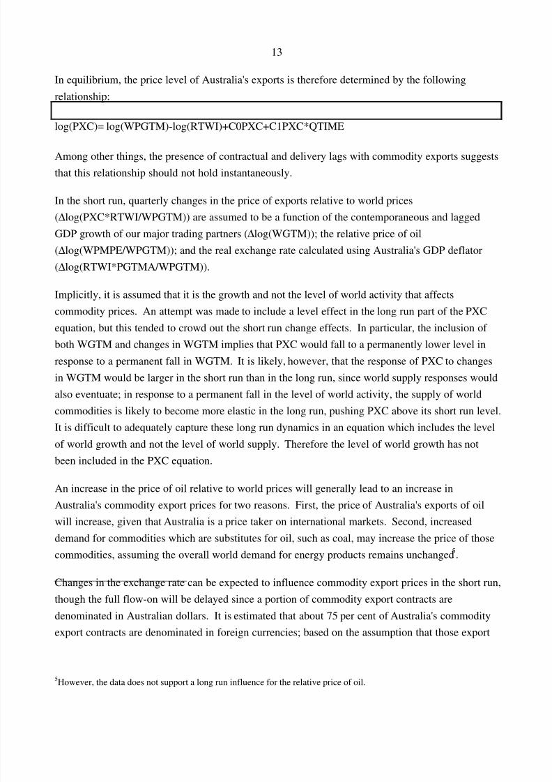
In equilibrium, the price level of Australia's exports is therefore determined by the followingrelationship:

log(PXC)= log(WPGTM)-log(RTWI)+C0PXC+C1PXC*QTIME

Among other things, the presence of contractual and delivery lags with commodity exports suggeststhat this relationship should not hold instantaneously.

In the short run, quarterly changes in the price of exports relative to world prices(∆ log(PXC*RTWI/WPGTM)) are assumed to be a function of the contemporaneous and laggedGDP growth of our major trading partners ( ∆ log(WGTM)); the relative price of oil(∆ log(WPMPE/WPGTM)); and the real exchange rate calculated using Australia's GDP deflator(∆ log(RTWI*PGTMA/WPGTM)).

Implicitly, it is assumed that it is the growth and not the level of world activity that affectscommodity prices. An attempt was made to include a level effect in the long run part of the PXCequation, but this tended to crowd out the short run change effects. In particular, the inclusion of both WGTM and changes in WGTM implies that PXC would fall to a permanently lower level inresponse to a permanent fall in WGTM. It is likely, however, that the response of PXC to changesin WGTM would be larger in the short run than in the long run, since world supply responses wouldalso eventuate; in response to a permanent fall in the level of world activity, the supply of world

commodities is likely to become more elastic in the long run, pushing PXC above its short run level.It is difficult to adequately capture these long run dynamics in an equation which includes the levelof world growth and not the level of world supply. Therefore the level of world growth has notbeen included in the PXC equation.

An increase in the price of oil relative to world prices will generally lead to an increase inAustralia's commodity export prices for two reasons. First, the price of Australia's exports of oilwill increase, given that Australia is a price taker on international markets. Second, increaseddemand for commodities which are substitutes for oil, such as coal, may increase the price of thosecommodities, assuming the overall world demand for energy products remains unchanged 5.

Changes in the exchange rate can be expected to influence commodity export prices in the short run,though the full flow-on will be delayed since a portion of commodity export contracts aredenominated in Australian dollars. It is estimated that about 75 per cent of Australia's commodityexport contracts are denominated in foreign currencies; based on the assumption that those export

5

However, the data does not support a long run influence for the relative price of oil.



14

contracts denominated in Australian dollars are not quickly re-negotiated, the coefficient on the realexchange rate (A2PXC) has been constrained to equal 0.25.

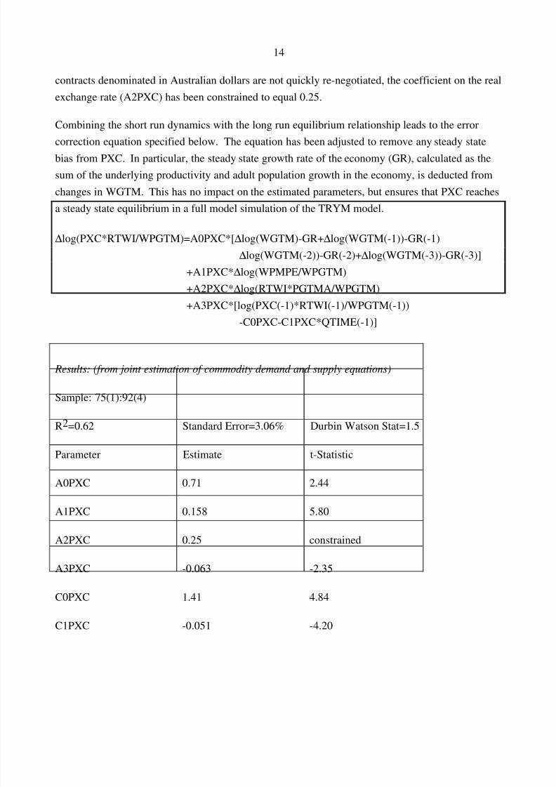
Combining the short run dynamics with the long run equilibrium relationship leads to the error

correction equation specified below. The equation has been adjusted to remove any steady statebias from PXC. In particular, the steady state growth rate of the economy (GR), calculated as thesum of the underlying productivity and adult population growth in the economy, is deducted fromchanges in WGTM. This has no impact on the estimated parameters, but ensures that PXC reachesa steady state equilibrium in a full model simulation of the TRYM model.

∆ log(PXC*RTWI/WPGTM)=A0PXC*[ ∆ log(WGTM)-GR+ ∆ log(WGTM(-1))-GR(-1)∆ log(WGTM(-2))-GR(-2)+ ∆ log(WGTM(-3))-GR(-3)]

+A1PXC*∆

log(WPMPE/WPGTM)+A2PXC* ∆ log(RTWI*PGTMA/WPGTM)+A3PXC*[log(PXC(-1)*RTWI(-1)/WPGTM(-1))

-C0PXC-C1PXC*QTIME(-1)]

Results: (from joint estimation of commodity demand and supply equations)

Sample: 75(1):92(4)

R2=0.62 Standard Error=3.06% Durbin Watson Stat=1.5

Parameter Estimate t-Statistic

A0PXC 0.71 2.44

A1PXC 0.158 5.80

A2PXC 0.25 constrained

A3PXC -0.063 -2.35

C0PXC 1.41 4.84

C1PXC -0.051 -4.20



15

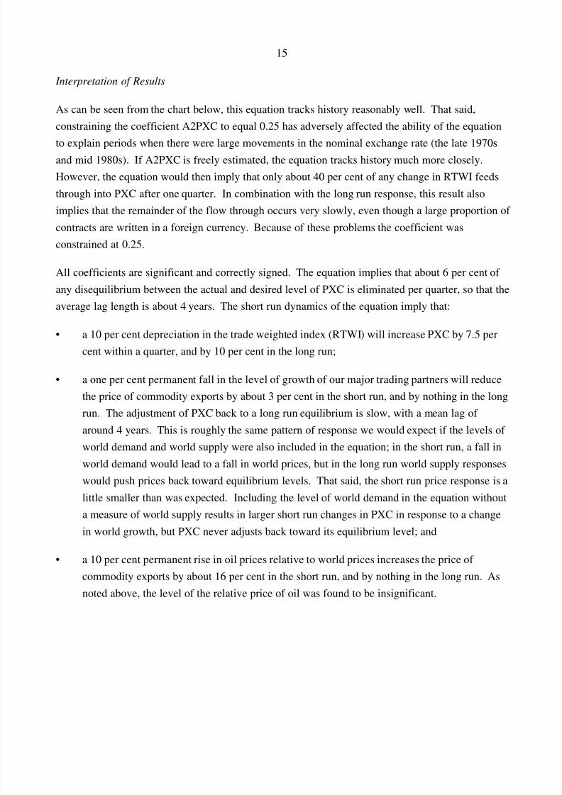
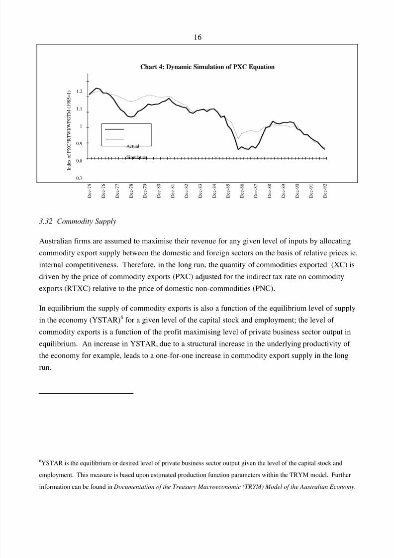
Interpretation of Results

As can be seen from the chart below, this equation tracks history reasonably well. That said,constraining the coefficient A2PXC to equal 0.25 has adversely affected the ability of the equation

to explain periods when there were large movements in the nominal exchange rate (the late 1970sand mid 1980s). If A2PXC is freely estimated, the equation tracks history much more closely.However, the equation would then imply that only about 40 per cent of any change in RTWI feedsthrough into PXC after one quarter. In combination with the long run response, this result alsoimplies that the remainder of the flow through occurs very slowly, even though a large proportion of contracts are written in a foreign currency. Because of these problems the coefficient wasconstrained at 0.25.

All coefficients are significant and correctly signed. The equation implies that about 6 per cent of any disequilibrium between the actual and desired level of PXC is eliminated per quarter, so that theaverage lag length is about 4 years. The short run dynamics of the equation imply that:

• a 10 per cent depreciation in the trade weighted index (RTWI) will increase PXC by 7.5 percent within a quarter, and by 10 per cent in the long run;

• a one per cent permanent fall in the level of growth of our major trading partners will reducethe price of commodity exports by about 3 per cent in the short run, and by nothing in the long

run. The adjustment of PXC back to a long run equilibrium is slow, with a mean lag of around 4 years. This is roughly the same pattern of response we would expect if the levels of world demand and world supply were also included in the equation; in the short run, a fall inworld demand would lead to a fall in world prices, but in the long run world supply responseswould push prices back toward equilibrium levels. That said, the short run price response is alittle smaller than was expected. Including the level of world demand in the equation withouta measure of world supply results in larger short run changes in PXC in response to a changein world growth, but PXC never adjusts back toward its equilibrium level; and

• a 10 per cent permanent rise in oil prices relative to world prices increases the price of commodity exports by about 16 per cent in the short run, and by nothing in the long run. Asnoted above, the level of the relative price of oil was found to be insignificant.



16

Chart 4: Dynamic Simulation of PXC Equation

Index of PXC*RTWI/WPGTM (1985=1)

0.7

0.8

0.9

1

1.1

1.2

Dec-75

Dec-76

Dec-77

Dec-78

Dec-79

Dec-80

Dec-81

Dec-82

Dec-83

Dec-84

Dec-85

Dec-86

Dec-87

Dec-88

Dec-89

Dec-90

Dec-91

Dec-92

Actual

Simulation

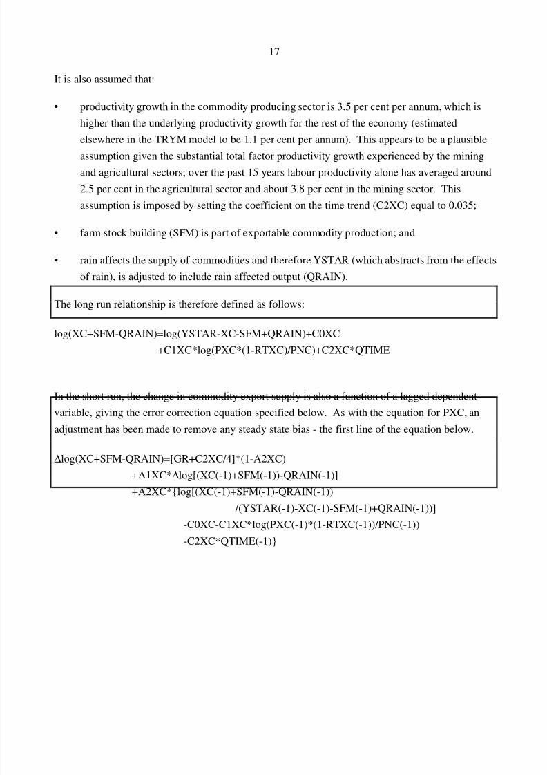
3.32 Commodity Supply

Australian firms are assumed to maximise their revenue for any given level of inputs by allocatingcommodity export supply between the domestic and foreign sectors on the basis of relative prices ie.internal competitiveness. Therefore, in the long run, the quantity of commodities exported (XC) isdriven by the price of commodity exports (PXC) adjusted for the indirect tax rate on commodityexports (RTXC) relative to the price of domestic non-commodities (PNC).

In equilibrium the supply of commodity exports is also a function of the equilibrium level of supplyin the economy (YSTAR) 6 for a given level of the capital stock and employment; the level of commodity exports is a function of the profit maximising level of private business sector output inequilibrium. An increase in YSTAR, due to a structural increase in the underlying productivity of the economy for example, leads to a one-for-one increase in commodity export supply in the longrun.

6YSTAR is the equilibrium or desired level of private business sector output given the level of the capital stock and

employment. This measure is based upon estimated production function parameters within the TRYM model. Further

information can be found in Documentation of the Treasury Macroeconomic (TRYM) Model of the Australian Economy .





18

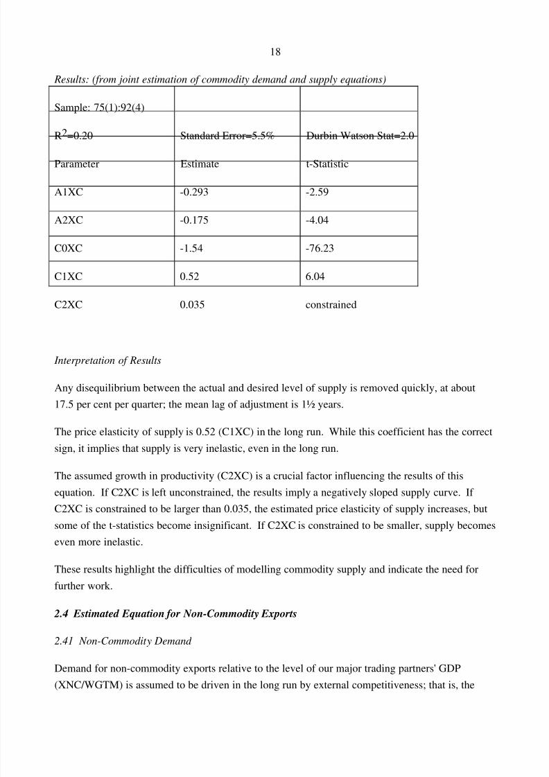
Results: (from joint estimation of commodity demand and supply equations)

Sample: 75(1):92(4)

R2=0.20 Standard Error=5.5% Durbin Watson Stat=2.0


A1XC -0.293 -2.59

A2XC -0.175 -4.04

C0XC -1.54 -76.23

C1XC 0.52 6.04

C2XC 0.035 constrained


Any disequilibrium between the actual and desired level of supply is removed quickly, at about

17.5 per cent per quarter; the mean lag of adjustment is 1½ years.

The price elasticity of supply is 0.52 (C1XC) in the long run. While this coefficient has the correctsign, it implies that supply is very inelastic, even in the long run.

The assumed growth in productivity (C2XC) is a crucial factor influencing the results of thisequation. If C2XC is left unconstrained, the results imply a negatively sloped supply curve. If C2XC is constrained to be larger than 0.035, the estimated price elasticity of supply increases, butsome of the t-statistics become insignificant. If C2XC is constrained to be smaller, supply becomes

even more inelastic.

These results highlight the difficulties of modelling commodity supply and indicate the need forfurther work.

2.4 Estimated Equation for Non-Commodity Exports

2.41 Non-Commodity Demand

Demand for non-commodity exports relative to the level of our major trading partners' GDP

(XNC/WGTM) is assumed to be driven in the long run by external competitiveness; that is, the





20

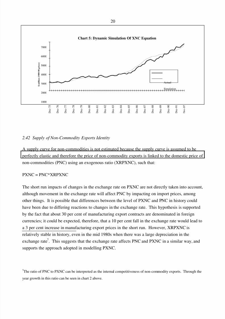
Chart 5: Dynamic Simulation Of XNC Equation

$ million (1989-90 prices)

1000

2000

3000

4000

5000

6000

7000

Dec-75

Dec-76

Dec-77

Dec-78

Dec-79

Dec-80

Dec-81

Dec-82

Dec-83

Dec-84

Dec-85

Dec-86

Dec-87

Dec-88

Dec-89

Dec-90

Dec-91

Dec-92

Actual

Simulation

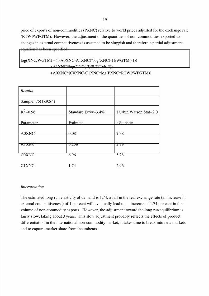
2.42 Supply of Non-Commodity Exports Identity

A supply curve for non-commodities is not estimated because the supply curve is assumed to beperfectly elastic and therefore the price of non-commodity exports is linked to the domestic price of non-commodities (PNC) using an exogenous ratio (XRPXNC), such that:

PXNC = PNC*XRPXNC

The short run impacts of changes in the exchange rate on PXNC are not directly taken into account,although movement in the exchange rate will affect PNC by impacting on import prices, amongother things. It is possible that differences between the level of PXNC and PNC in history couldhave been due to differing reactions to changes in the exchange rate. This hypothesis is supportedby the fact that about 30 per cent of manufacturing export contracts are denominated in foreigncurrencies; it could be expected, therefore, that a 10 per cent fall in the exchange rate would lead toa 3 per cent increase in manufacturing export prices in the short run. However, XRPXNC isrelatively stable in history, even in the mid 1980s when there was a large depreciation in theexchange rate 7. This suggests that the exchange rate affects PNC and PXNC in a similar way, andsupports the approach adopted in modelling PXNC.

7The ratio of PNC to PXNC can be interpreted as the internal competitiveness of non-commodity exports. Through the

year growth in this ratio can be seen in chart 2 above.



21

The estimated equation for PNC is in the Business Sector of the TRYM model and is presented inThe Documentation of the Treasury Macroeconomic (TRYM) Model of the Australian Economy.



22

3. IMPORTS OF GOODS AND SERVICES

3.1 Trends in the Imports Sector

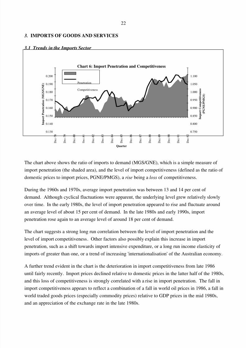
Chart 6: Import Penetration and Competitiveness

Quarter

Import Penetration (MGS/GNE)

0.130

0.140

0.150

0.160

0.170

0.180

0.190

0.200

Dec-78

Dec-79

Dec-80

Dec-81

Dec-82

Dec-83

Dec-84

Dec-85

Dec-86

Dec-87

Dec-88

Dec-89

Dec-90

Dec-91

Dec-92

0.750

0.800

0.850

0.900

0.950

1.000

1.050

1.100

Import Competitiveness

(PGNE/PMGS)

Penetration

Competitiveness

The chart above shows the ratio of imports to demand (MGS/GNE), which is a simple measure of import penetration (the shaded area), and the level of import competitiveness (defined as the ratio of domestic prices to import prices, PGNE/PMGS), a rise being a loss of competitiveness.

During the 1960s and 1970s, average import penetration was between 13 and 14 per cent of demand. Although cyclical fluctuations were apparent, the underlying level grew relatively slowlyover time. In the early 1980s, the level of import penetration appeared to rise and fluctuate aroundan average level of about 15 per cent of demand. In the late 1980s and early 1990s, importpenetration rose again to an average level of around 18 per cent of demand.

The chart suggests a strong long run correlation between the level of import penetration and thelevel of import competitiveness. Other factors also possibly explain this increase in importpenetration, such as a shift towards import intensive expenditure, or a long run income elasticity of imports of greater than one, or a trend of increasing 'internationalisation' of the Australian economy.

A further trend evident in the chart is the deterioration in import competitiveness from late 1986until fairly recently. Import prices declined relative to domestic prices in the latter half of the 1980s,and this loss of competitiveness is strongly correlated with a rise in import penetration. The fall inimport competitiveness appears to reflect a combination of a fall in world oil prices in 1986, a fall inworld traded goods prices (especially commodity prices) relative to GDP prices in the mid 1980s,

and an appreciation of the exchange rate in the late 1980s.



23

Chart 7: Imports, Demand and Competitiveness Growth

Quarter

Through the year growth (per cent)

-20

-15

-10

-5

0

5

10

15

20

25

30

Dec-78

Dec-79

Dec-80

Dec-81

Dec-82

Dec-83

Dec-84

Dec-85

Dec-86

Dec-87

Dec-88

Dec-89

Dec-90

Dec-91

Dec-92

Demand

Imports

Competitiveness

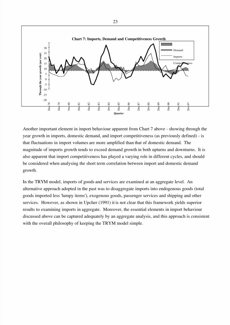
Another important element in import behaviour apparent from Chart 7 above - showing through theyear growth in imports, domestic demand, and import competitiveness (as previously defined) - isthat fluctuations in import volumes are more amplified than that of domestic demand. Themagnitude of imports growth tends to exceed demand growth in both upturns and downturns. It isalso apparent that import competitiveness has played a varying role in different cycles, and shouldbe considered when analysing the short term correlation between import and domestic demand

growth.

In the TRYM model, imports of goods and services are examined at an aggregate level. Analternative approach adopted in the past was to disaggregate imports into endogenous goods (totalgoods imported less 'lumpy items'), exogenous goods, passenger services and shipping and otherservices. However, as shown in Upcher (1991) it is not clear that this framework yields superiorresults to examining imports in aggregate. Moreover, the essential elements in import behaviourdiscussed above can be captured adequately by an aggregate analysis, and this approach is consistentwith the overall philosophy of keeping the TRYM model simple.



24

3.2 Major Factors Affecting Import Behaviour in the TRYM model

The primary factors determining the demand for imports at the macro-economic level are domesticincome and the competitiveness of the domestic tradeable goods and services sector. A rise in

income will lead to an increase in import demand, and an increase in the price of imports relative todomestic substitutes (an increase in Australia's import competitiveness) will lead to a fall in demandfor imports.

The supply curve for imports is horizontal or infinitely price elastic; Australia is assumed to be asmall open economy that cannot influence world prices. The price of imports is therefore a functionof world prices and the exchange rate, such that an increase in world prices or a depreciation of theexchange rate will lead to an increase in import prices. Allowance is made for the time taken formovements in the exchange rate and world prices to pass through into import prices, and for thediffering pass-through of world oil prices and world prices more generally.

In the TRYM model, equations are estimated jointly for import demand and import supply. Underthe small open economy assumption, the import demand equation determines the quantity imported,while the supply equation determines the price of those imports (the world price of those goods),and the flow-through from exchange rate and world price movements into import prices.

3.3 Import Demand

A consideration when analysing the demand for imports is whether they should be treated asintermediate or final goods. Analysis of imports in the TRYM model follows the traditionalapproach, which is to treat imports as a final good. In particular, consumers and firms in Australiaare assumed to allocate their purchases between imports, domestic tradeable goods and non-tradeable goods. This suggests that import demand is a function of income and the prices of imports, domestic tradeables and non-tradeables. An alternative approach is to treat imports as anintermediate good, suggesting that they should be included as a factor in the production function,along with other inputs like capital, labour and other intermediate inputs. Import demand would

then be derived as a function of income, and the prices of imports, capital, labour and otherintermediate inputs.

Whether imports are primarily a final or an intermediate good is not clear. Balance of paymentsdata indicates that other endogenous goods (excludes consumption and capital goods) and fuelimports - a broad proxy for intermediate goods - were around 37 per cent of the value of allimported goods and services in 1991-92. Foreign trade data on imports by broad economic categoryindicates that food and beverages mainly for industry, industrial supplies, fuels and lubricants, and



25

parts and accessories for capital goods and transport equipment - another broad proxy forintermediate goods - were around 38 per cent of all imports of goods and services.

3.31 Measuring Income

There are a variety of ways of measuring the domestic income variable used to explain the demandfor imports. Horton (1989) estimates import demand equations using both GNE and GDP, and theestimates suggest little to discriminate between either as an explanator of import demand.

In the TRYM model, a National Accounts expenditure aggregate is used, consistent with theanalysis of imports as a final good. In addition, an attempt is made to allow for differing importpenetration across the different components of domestic demand expenditure. In particular, aweighted average of the expenditure side demand components (DDMGS) has been used to proxythe income variable. The weights, which reflect the incidence of imports from the various types of expenditure, are based on results from the Commonwealth Treasury's micro economic model,PRISMOD 8.

Results from PRISMOD indicate that imports account for 33 per cent of government marketdemand (GMD), which is equal to government final demand less government expenditure on capitaland labour; 29 per cent of business investment (IB), which includes plant and equipment investmentand investment in non-dwelling building and construction; 25 per cent of exports of non-

commodities (XNC); 20 per cent of the statistical discrepancy (DISA); 17 per cent of private non-rent consumption (CNR); 13 per cent of dwelling investment (IDW); 10 per cent of exports of commodities (XC); and 3 per cent of consumption of rents (CRE).

Another result from PRISMOD suggests that the most import intensive component of expenditure isnon-farm stock-building, with imports making a 51 per cent contribution to any expenditure in thisarea. However, it was felt that increased imports cause increased non-farm stock-building ratherthan vice versa, and therefore non-farm stock building is excluded when calculating DDMGS. Thisapproach is consistent with the assumption in the TRYM model that final demand causes import

growth.

DDMGS is defined as:

8The response of imports after increasing various components of domestic demand was examined using PRISMOD.

The marginal propensity to import was subsequently assessed for each component of domestic expenditure.



26

DDMGS = 0.17*CNR+0.03*CRE+0.29*IB+0.13*IDW+0.25*XNC+0.10*XC+0.33*GMD+0.20*DISA

Conceptually, DDMGS is a better explanator of import demand than either GNE or GDP as itaccounts for the differing import penetration of the various types of expenditure. Furthermore,DDMGS was found to better explain movements in import demand than GNE.

3.32 Measuring Cost Competitiveness

The prices that are relevant in determining import competitiveness and its effect on the demand forimports are the prices of imports, domestic tradeables (domestically produced substitutes) anddomestic non-tradeables. Under some simple assumptions 9, an appropriate theoretical measure of import competitiveness commonly used is the price of imports relative to the price of domestictradeables. Many empirical studies, however, use the price of imports relative to an aggregateexpenditure price deflator, such as the GNE deflator (PGNE) or the GDP deflator (PGDP), tomeasure import competitiveness. PGNE and PGDP implicitly include the price of some non-tradedgoods and therefore, to make these measures valid, it must be assumed that the elasticity of importdemand with respect to traded and non-traded goods is equal 10.

In practice, it is difficult to construct an aggregate price for tradeable goods that excludes the priceof non-tradeables. The proxy for the price of domestic tradeables used in the TRYM model is

PDDMGS, the implicit price deflator (at factor cost) of our income variable DDMGS. PDDMGSmay also be contaminated by the price of domestic non-tradeables. Nevertheless, it is aconceptually superior measure to either PGNE or PGDP because a low or zero weight is placed onthe components that have a low or zero tradeable component (for example, the implicit pricedeflators for consumption of rent, and general government expenditure on labour services andcapital services are excluded).

It is also apparent from the data that a combination of DDMGS determining income and PDDMGSdetermining the relative price provides a superior explanation for movements in import demandthan a combination of either PGNE and GNE or PGDP and GDP.

9Goldstein (1980) demonstrates that assuming homogeneity of degree zero in these three prices and separability in the

consumption choice between tradeables and non-tradeables, implies the import function can be written with merely the

relative price of imports to domestic tradeables as the price argument. Further, he finds support for these assumptions

using his estimated traded and non-traded goods price series.

10

Goldstein (1980) does not find support for this constraint.



27

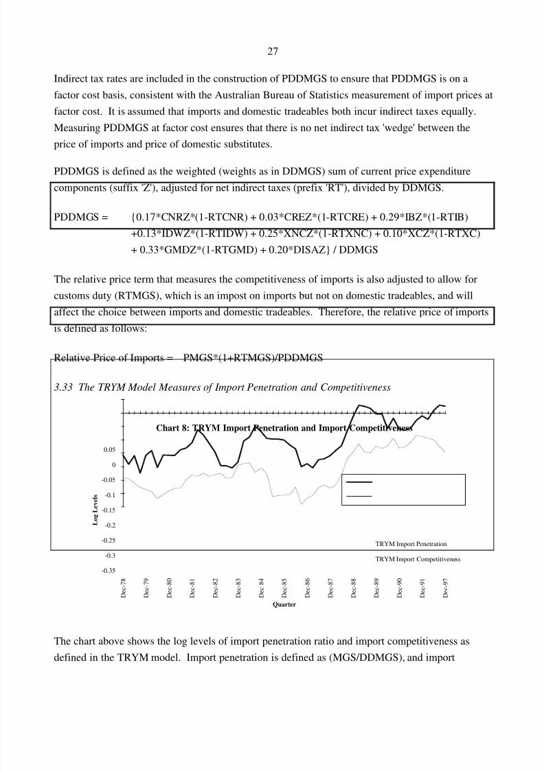
Indirect tax rates are included in the construction of PDDMGS to ensure that PDDMGS is on afactor cost basis, consistent with the Australian Bureau of Statistics measurement of import prices atfactor cost. It is assumed that imports and domestic tradeables both incur indirect taxes equally.Measuring PDDMGS at factor cost ensures that there is no net indirect tax 'wedge' between theprice of imports and price of domestic substitutes.

PDDMGS is defined as the weighted (weights as in DDMGS) sum of current price expenditurecomponents (suffix 'Z'), adjusted for net indirect taxes (prefix 'RT'), divided by DDMGS.

PDDMGS = {0.17*CNRZ*(1-RTCNR) + 0.03*CREZ*(1-RTCRE) + 0.29*IBZ*(1-RTIB)+0.13*IDWZ*(1-RTIDW) + 0.25*XNCZ*(1-RTXNC) + 0.10*XCZ*(1-RTXC)+ 0.33*GMDZ*(1-RTGMD) + 0.20*DISAZ} / DDMGS

The relative price term that measures the competitiveness of imports is also adjusted to allow forcustoms duty (RTMGS), which is an impost on imports but not on domestic tradeables, and willaffect the choice between imports and domestic tradeables. Therefore, the relative price of importsis defined as follows:

Relative Price of Imports = PMGS*(1+RTMGS)/PDDMGS

3.33 The TRYM Model Measures of Import Penetration and Competitiveness

Chart 8: TRYM Import Penetration and Import Competitiveness

Quarter

Log Levels

-0.35

-0.3

-0.25

-0.2

-0.15

-0.1

-0.05

0

0.05

Dec-78

Dec-79

Dec-80

Dec-81

Dec-82

Dec-83

Dec-84

Dec-85

Dec-86

Dec-87

Dec-88

Dec-89

Dec-90

Dec-91

Dec-92

TRYM Import Penetration

TRYM Import Competitiveness

The chart above shows the log levels of import penetration ratio and import competitiveness asdefined in the TRYM model. Import penetration is defined as (MGS/DDMGS), and import



28

competitiveness is defined as the inverse of the relative price of imports(PDDMGS/PMGS/(1+RTMGS)).

The apparent structural increase in import penetration in the early 1980s noted earlier in Chart 6

(based upon a MGS/GNE ratio), is no longer evident when import penetration is based upon thedemand measure DDMGS. Allowing for compositional changes between different types of expenditure with differing import intensiveness explains the apparent movement in the simplermeasure of import penetration in the early to mid 1980s. Nevertheless, some upward trend inimport penetration is still evident in the data. In particular, there is still a large rise in importpenetration in the late 1980s.

There appears to be a long term correlation between the level of import penetration and the relativeprice of imports. In particular, the strong rise in the inverse relative price in the late 1980s isstrongly correlated with a large increase in import penetration. Wilkinson (1992) has attributed alarge part of this rise to movements in the competitiveness (relative price) of imports.

3.34 Interpretation of Import Penetration Trend

The apparent trend increase in import penetration over the sample period requires someinterpretation. Freely estimating an equation over the sample would result in a long run incomeelasticity greater than one. Conceptually, this result is a problem because it implies that, in the very

long run, imports will eventually exceed income. In the interests of sensible long run simulationproperties, the long run income elasticity has been constrained to equal one, and a time trend hasbeen added to the import demand equation to soak up some of this trend increase in importpenetration. This gives the equation the capacity to interpret history and produce forecasts, as wellas provide sensible input into policy simulations.

• For forecasting purposes, it is desirable to maintain this characteristic of the data into theimmediate future and leave the time trend on; however, in policy simulations, where sensiblelong run properties are desirable, the time trend can be turned off.

The trend increase in import penetration over the sample may be due to the 'internationalisation' of the Australian economy, or increased exposure to world conditions. This is consistent with anincreasing ratio of exports to GDP noted earlier, and with the experience of many other countries,and could reflect increasing specialisation of production and trade between countries. It may alsoreflect an increase in wealth and affluence resulting in a change of consumer tastes in favour of imported goods.



29

3.4 Import Supply

The supply curve is assumed to be infinitely price elastic. In other words, it is assumed thatAustralia is a small country, whose demand does not affect world prices. The small open economy

assumption implies that the Australian price of imports will equal the world price adjusted for theexchange rate. Around three quarters of Australia's imports are non-commodities, and thereforeassuming infinitely elastic import supply is consistent with the approach taken in determining non-commodity export supply.

3.41 Measuring World Prices and Exchange Rate

World non-commodity prices are proxied by the world GDP deflator WPGTM as defined in theexports sector. This measure is export weighted and therefore is probably not the best measure of the world price of our imports (reflecting the export weighting and inclusion of non-traded goodsprices). Nevertheless, WPGTM was adopted in the interests of keeping the TRYM model simple.

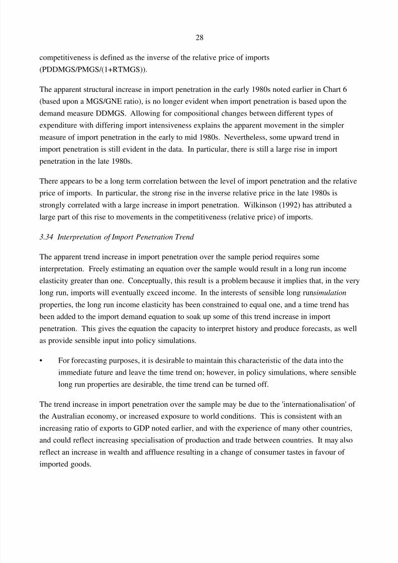
3.42 Measuring Trend and Compositional Influences

Chart 9: Foreign Currency Price of Australian Imports Relative to WorldPrices

Quarters

Log Levels

1.80

1.90

2.00

2.10

2.20

2.30

2.40

2.50

Dec-78

Dec-79

Dec-80

Dec-81

Dec-82

Dec-83

Dec-84

Dec-85

Dec-86

Dec-87

Dec-88

Dec-89

Dec-90

Dec-91

Dec-92

PMGS*RTWI/WPGTM

The above chart shows the price of Australian imports in foreign currency terms relative to theworld price (PMGS*RTWI/WPGTM). The small open economy assumption would suggest thatthis ratio should be constant in the long run, as movements in world prices are fully reflected inAustralian import prices (after adjusting for the exchange rate). However, as is apparent from theabove chart, this ratio has been declining over the sample; in particular, the ratio fell significantly inthe mid 1980s. This secular and/or shift movement appears to reflect the performance of WPGTM

as a proxy for the world price of our imports.



30

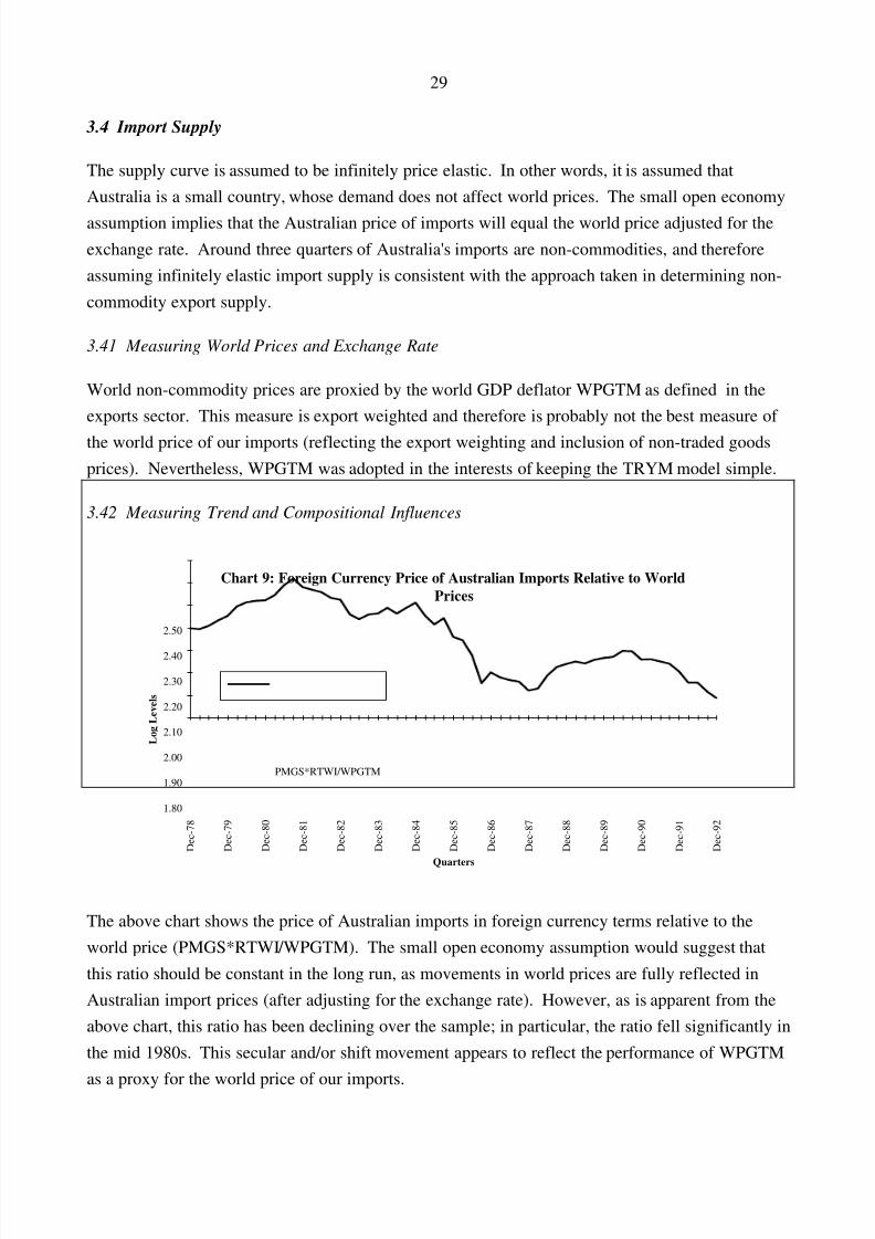
The composition of goods and services implicit in WPGTM is almost certainly different to that inPMGS. This becomes a serious problem when a particular good has a significantly different sharein import prices from that in world prices, and its price is moving in a significantly different way toall other prices. More generally, WPGTM is based on GDP prices and will be less suitable whenthe price of tradeable goods and services are trending in a different manner to world GDP prices.

Chart 10: World Relative Price of Oil and World Ratio of Export Pricesto GDP Prices

Quarters

Relative Oil Price

(WPMPE/WPGTM)-Log Level

1.50

1.70

1.90

2.10

2.302.50

2.70

2.90

3.10

3.30

Dec-78

Dec-79

Dec-80

Dec-81

Dec-82

Dec-83

Dec-84

Dec-85

Dec-86

Dec-87

Dec-88

Dec-89

Dec-90

Dec-91

Dec-92

-0.20

-0.15

-0.10

-0.05

0.00

0.05

Ratio of OECD Export Price

Deflator to GDP Price Deflator

(XRWPXGS) - Log Level

WPMPE/WPGTM

XRWPXGS

Two proxies have been included in the import supply equation to account for these compositionaleffects. In particular, proxies are included to model world oil prices, and world traded goods prices,relative to world GDP prices. The above chart shows the foreign currency price of Australian oilimports relative to world prices (WPMPE/WPGTM), and the ratio of OECD export implicit pricedeflators to OECD GDP implicit price deflators (XRWPXGS).

• Oil prices have been moving quite differently to world GDP prices over the sample, and arelikely to have a greater direct weight in import prices than in WPGTM. The oil price rises of the early and late 1970s, and oil price decline in the mid 1980s are likely to have a

proportionately greater impact upon the price of Australian imports than on world GDPdeflators.

• More generally, a shift occurred in the mid 1980s in the relationship between world tradedgoods prices and GDP deflator prices. The reasons for this shift are unclear.

Both of these proxies appear to have fallen around 1986, and may be useful in explaining the shift inthe relationship between WPGTM and PMGS (adjusted for RTWI) at that time.



31

3.5 Estimated Import Equations

3.51 Import Demand

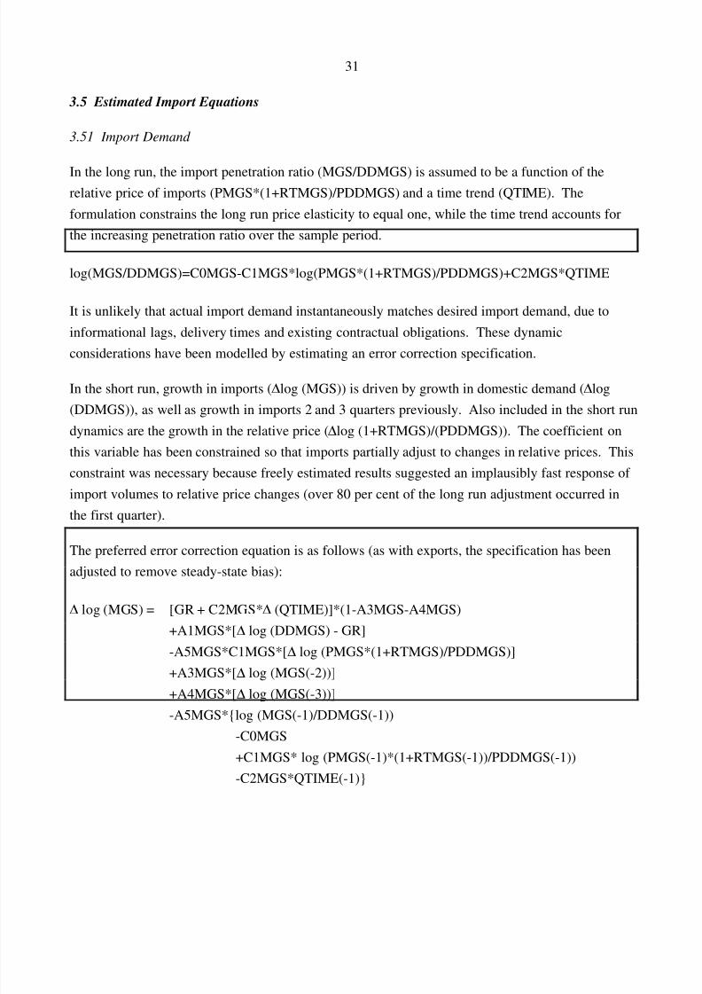
In the long run, the import penetration ratio (MGS/DDMGS) is assumed to be a function of therelative price of imports (PMGS*(1+RTMGS)/PDDMGS) and a time trend (QTIME). Theformulation constrains the long run price elasticity to equal one, while the time trend accounts forthe increasing penetration ratio over the sample period.

log(MGS/DDMGS)=C0MGS-C1MGS*log(PMGS*(1+RTMGS)/PDDMGS)+C2MGS*QTIME

It is unlikely that actual import demand instantaneously matches desired import demand, due toinformational lags, delivery times and existing contractual obligations. These dynamic

considerations have been modelled by estimating an error correction specification.

In the short run, growth in imports ( ∆ log (MGS)) is driven by growth in domestic demand ( ∆ log(DDMGS)), as well as growth in imports 2 and 3 quarters previously. Also included in the short rundynamics are the growth in the relative price ( ∆ log (1+RTMGS)/(PDDMGS)). The coefficient onthis variable has been constrained so that imports partially adjust to changes in relative prices. Thisconstraint was necessary because freely estimated results suggested an implausibly fast response of import volumes to relative price changes (over 80 per cent of the long run adjustment occurred in

the first quarter).

The preferred error correction equation is as follows (as with exports, the specification has beenadjusted to remove steady-state bias):

∆ log (MGS) = [GR + C2MGS* ∆ (QTIME)]*(1-A3MGS-A4MGS)+A1MGS*[ ∆ log (DDMGS) - GR]-A5MGS*C1MGS*[ ∆ log (PMGS*(1+RTMGS)/PDDMGS)]+A3MGS*[ ∆ log (MGS(-2))]

+A4MGS*[ ∆ log (MGS(-3))]-A5MGS*{log (MGS(-1)/DDMGS(-1))

-C0MGS+C1MGS* log (PMGS(-1)*(1+RTMGS(-1))/PDDMGS(-1))-C2MGS*QTIME(-1)}



32

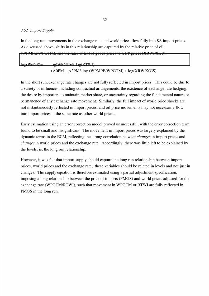
3.52 Import Supply

In the long run, movements in the exchange rate and world prices flow fully into $A import prices.As discussed above, shifts in this relationship are captured by the relative price of oil

(WPMPE/WPGTM), and the ratio of traded goods prices to GDP prices (XRWPXGS).

log(PMGS)= log(WPGTM)-log(RTWI)+A0PM + A2PM* log (WPMPE/WPGTM) + log(XRWPXGS)

In the short run, exchange rate changes are not fully reflected in import prices. This could be due toa variety of influences including contractual arrangements, the existence of exchange rate hedging,the desire by importers to maintain market share, or uncertainty regarding the fundamental nature orpermanence of any exchange rate movement. Similarly, the full impact of world price shocks arenot instantaneously reflected in import prices, and oil price movements may not necessarily flowinto import prices at the same rate as other world prices.

Early estimation using an error correction model proved unsuccessful, with the error correction termfound to be small and insignificant. The movement in import prices was largely explained by thedynamic terms in the ECM, reflecting the strong correlation between changes in import prices andchanges in world prices and the exchange rate. Accordingly, there was little left to be explained bythe levels, ie. the long run relationship.

However, it was felt that import supply should capture the long run relationship between importprices, world prices and the exchange rate; these variables should be related in levels and not just inchanges. The supply equation is therefore estimated using a partial adjustment specification,imposing a long relationship between the price of imports (PMGS) and world prices adjusted for theexchange rate (WPGTM/RTWI), such that movement in WPGTM or RTWI are fully reflected inPMGS in the long run.



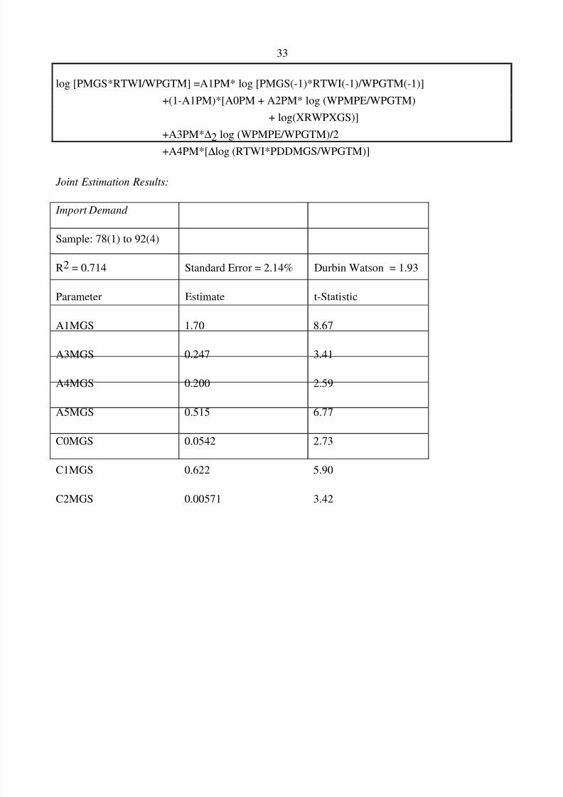
33

log [PMGS*RTWI/WPGTM] =A1PM* log [PMGS(-1)*RTWI(-1)/WPGTM(-1)]+(1-A1PM)*[A0PM + A2PM* log (WPMPE/WPGTM)

+ log(XRWPXGS)]

+A3PM*∆

2 log (WPMPE/WPGTM)/2+A4PM*[ ∆ log (RTWI*PDDMGS/WPGTM)]

Joint Estimation Results:

Import Demand

Sample: 78(1) to 92(4)

R2 = 0.714 Standard Error = 2.14% Durbin Watson = 1.93


A1MGS 1.70 8.67

A3MGS 0.247 3.41

A4MGS 0.200 2.59

A5MGS 0.515 6.77

C0MGS 0.0542 2.73

C1MGS 0.622 5.90

C2MGS 0.00571 3.42





35

Chart 12: Dynamic Simulation of PMGS Equation

Quarter

Index (1989-90 = 1)

0.400

0.500

0.600

0.700

0.800

0.900

1.000

1.100

1.200

Dec-78

Dec-79

Dec-80

Dec-81

Dec-82

Dec-83

Dec-84

Dec-85

Dec-86

Dec-87

Dec-88

Dec-89

Dec-90

Dec-91

Dec-92

Actual

Simulation


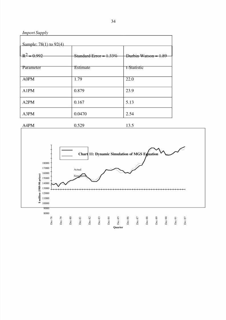
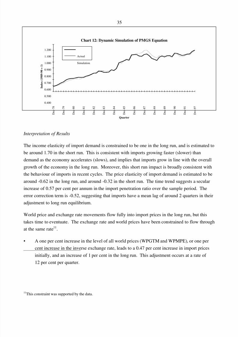
The income elasticity of import demand is constrained to be one in the long run, and is estimated tobe around 1.70 in the short run. This is consistent with imports growing faster (slower) thandemand as the economy accelerates (slows), and implies that imports grow in line with the overallgrowth of the economy in the long run. Moreover, this short run impact is broadly consistent withthe behaviour of imports in recent cycles. The price elasticity of import demand is estimated to bearound -0.62 in the long run, and around -0.32 in the short run. The time trend suggests a secularincrease of 0.57 per cent per annum in the import penetration ratio over the sample period. Theerror correction term is -0.52, suggesting that imports have a mean lag of around 2 quarters in theiradjustment to long run equilibrium.

World price and exchange rate movements flow fully into import prices in the long run, but thistakes time to eventuate. The exchange rate and world prices have been constrained to flow throughat the same rate 11.

• A one per cent increase in the level of all world prices (WPGTM and WPMPE), or one percent increase in the inverse exchange rate, leads to a 0.47 per cent increase in import pricesinitially, and an increase of 1 per cent in the long run. This adjustment occurs at a rate of 12 per cent per quarter.

11

This constraint was supported by the data.



36

• Exchange rate and world price pass-through is 47 per cent initially, 69 per cent after 1 year, 82per cent after 2 years and 89 per cent after 3 years.

A one per cent increase in world oil prices relative to world prices (WPMPE/WPGTM), will tend to

increase import prices by:

• 0.04 per cent initially, and another 0.04 per cent after one quarter. This result is broadlyconsistent with full pass-through of world oil prices into petroleum imports, which are around5 per cent of total imports; and

• 0.17 per cent in the long run, consistent with the increase in oil prices increasing the price of other imports that are oil intensive in their production (such as chemicals, port service debitsand travel and passenger service debits).



37

4. TRADE BALANCE AND CURRENT ACCOUNT

4.1 Trends in the Balance on Goods and Services, Net Transfers Overseas and the Current

Account

Chart 13: Balance on Goods and Services, Net Transfers Deficit andCurrent Account Deficit

Per cent of Nominal GDP

-8.00

-6.00

-4.00

-2.00

0.00

2.00

4.00

1959-60

1961-62

1963-64

1965-66

1967-68

1969-70

1971-72

1973-74

1975-76

1977-78

1979-80

1981-82

1983-84

1985-86

1987-88

1989-90

1991-92

CAD

Net Transfers

Goods and Services

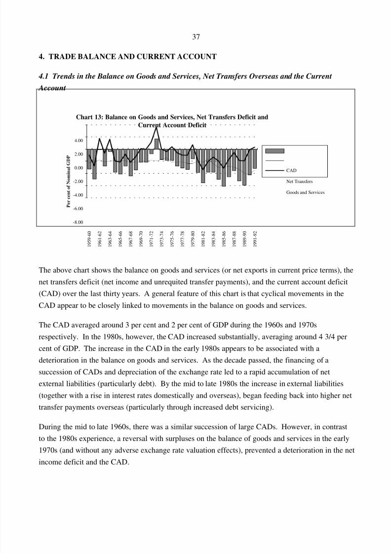
The above chart shows the balance on goods and services (or net exports in current price terms), thenet transfers deficit (net income and unrequited transfer payments), and the current account deficit

(CAD) over the last thirty years. A general feature of this chart is that cyclical movements in theCAD appear to be closely linked to movements in the balance on goods and services.

The CAD averaged around 3 per cent and 2 per cent of GDP during the 1960s and 1970srespectively. In the 1980s, however, the CAD increased substantially, averaging around 4 3/4 percent of GDP. The increase in the CAD in the early 1980s appears to be associated with adeterioration in the balance on goods and services. As the decade passed, the financing of asuccession of CADs and depreciation of the exchange rate led to a rapid accumulation of net

external liabilities (particularly debt). By the mid to late 1980s the increase in external liabilities(together with a rise in interest rates domestically and overseas), began feeding back into higher nettransfer payments overseas (particularly through increased debt servicing).

During the mid to late 1960s, there was a similar succession of large CADs. However, in contrastto the 1980s experience, a reversal with surpluses on the balance of goods and services in the early1970s (and without any adverse exchange rate valuation effects), prevented a deterioration in the netincome deficit and the CAD.



38

In the TRYM model, the balance on goods and services is a function of export and import volumesequations (determining net exports), and export and import price equations (determining the termsof trade). The remainder of the current account balance (ie. the net transfers deficit), is a product of a set of identities that determine the dynamics between current account financing, net externalliability accumulation, and the servicing of these liabilities. These identities are detailed inDocumentation of the Treasury Macroeconomic (TRYM) Model of the Australian Economy.



39

5. EFFECT OF A DEPRECIATION UPON THE BALANCE OF TRADE

5.1 Nature of the Shock

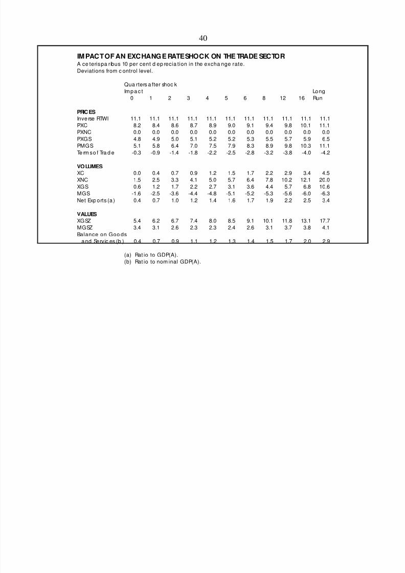
This section examines the direct impact of a depreciation of the exchange rate on the trade sector inthe TRYM model framework. The purpose of this shock is to demonstrate the responses and lags of various components of the trade sector. The underlying causes of this movement in the exchangerate are ignored, and it is assumed that the economy is initially in equilibrium. Furthermore, noallowance is made for the second round effects on the trade sector from the rest of the economy.The simulation of a world demand shock analysed in the TRYM Paper No. 6 provides a betteroverall picture of a full model response to changes in the exchange rate. That said, the simulationpresented here is sufficient to gauge the reaction of the trade sector alone, and gives an overview of this sector's role in the TRYM model.

The exchange rate is assumed to depreciate by 10 per cent (the inverse exchange rate appreciates by11.1 per cent), and remains permanently at this lower level. Domestic and world prices are assumedto remain unchanged, and both nominal and real exchange rates depreciate.

The results are presented in the table and charts shown below. They can be can be interpreted asshowing the difference between the level (not the growth rate) of each variable if the economy wasin equilibrium and the corresponding level of each variable as a result of the shock. The whole

economy is initially assumed to be in equilibrium; this analysis abstracts from the impact of any pre-existing disequilibrium in the economy.



40

IM PACT OF AN EXC HANG E RATE SHOCK ON THE TRADE SECTORA ce teris pa ribus 10 per cent d ep recia tion in the excha nge rate.Deviations from c ontrol level.

Qua rters a fter shoc kImp a c t Long

0 1 2 3 4 5 6 8 12 16 Run

PRIC ES

Inve rse RTWI 11.1 11.1 11.1 11.1 11.1 11.1 11.1 11.1 11.1 11.1 11.1PXC 8.2 8.4 8.6 8.7 8.9 9.0 9.1 9.4 9.8 10.1 11.1PXNC 0.0 0.0 0.0 0.0 0.0 0.0 0.0 0.0 0.0 0.0 0.0PXGS 4.8 4.9 5.0 5.1 5.2 5.2 5.3 5.5 5.7 5.9 6.5PMGS 5.1 5.8 6.4 7.0 7.5 7.9 8.3 8.9 9.8 10.3 11.1Te rm s o f Tra d e -0.3 -0.9 -1.4 -1.8 -2.2 -2.5 -2.8 -3.2 -3.8 -4.0 -4.2

VO LUMES

XC 0.0 0.4 0.7 0.9 1.2 1.5 1.7 2.2 2.9 3.4 4.5XNC 1.5 2.5 3.3 4.1 5.0 5.7 6.4 7.8 10.2 12.1 20.0XGS 0.6 1.2 1.7 2.2 2.7 3.1 3.6 4.4 5.7 6.8 10.6MGS -1.6 -2.5 -3.6 -4.4 -4.8 -5.1 -5.2 -5.3 -5.6 -6.0 -6.3

Net Exp orts (a ) 0.4 0.7 1.0 1.2 1.4 1.6 1.7 1.9 2.2 2.5 3.4

VALUES

XGSZ 5.4 6.2 6.7 7.4 8.0 8.5 9.1 10.1 11.8 13.1 17.7MGSZ 3.4 3.1 2.6 2.3 2.3 2.4 2.6 3.1 3.7 3.8 4.1Balance on Goo ds

a nd Servic es (b ) 0.4 0.7 0.9 1.1 1.2 1.3 1.4 1.5 1.7 2.0 2.9

(a) Rat io to GDP(A).(b) Rat io to nom inal GDP(A).



41

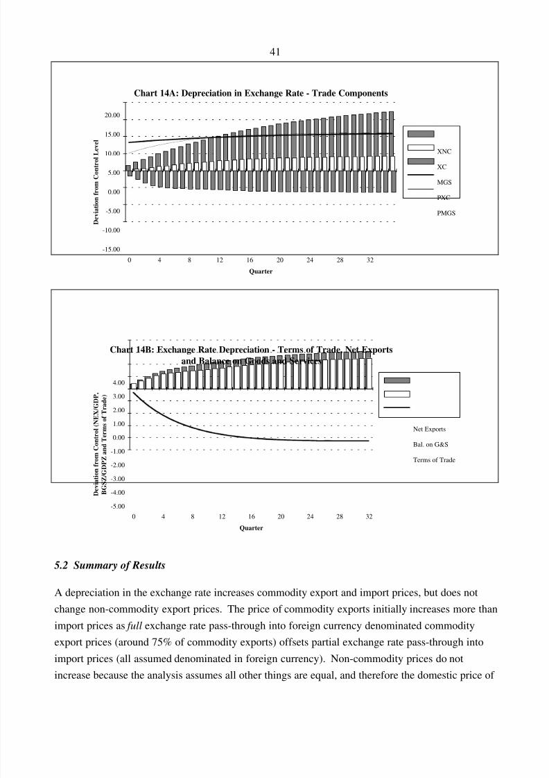
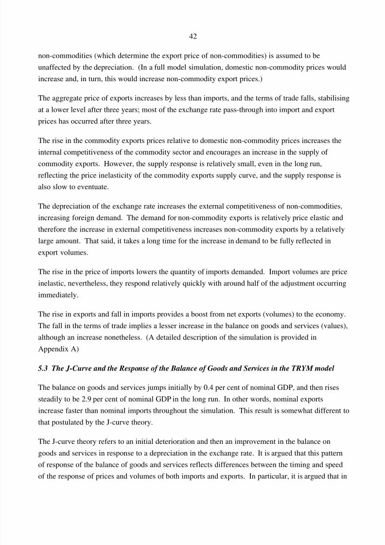
Chart 14A: Depreciation in Exchange Rate - Trade Components

Quarter

Deviation from Control Level

-15.00

-10.00

-5.00

0.00

5.00

10.00

15.00

20.00

0 4 8 12 16 20 24 28 32

XNC

XC

MGS

PXC

PMGS

Chart 14B: Exchange Rate Depreciation - Terms of Trade, Net Exportsand Balance on Goods and Services

Quarter

Deviation from Control (NEX/GDP,

BGSZ/GDPZ and Terms of Trade)

-5.00

-4.00

-3.00

-2.00

-1.00

0.00

1.00

2.00

3.00

4.00

0 4 8 12 16 20 24 28 32

Net Exports

Bal. on G&S

Terms of Trade

5.2 Summary of Results

A depreciation in the exchange rate increases commodity export and import prices, but does notchange non-commodity export prices. The price of commodity exports initially increases more thanimport prices as full exchange rate pass-through into foreign currency denominated commodityexport prices (around 75% of commodity exports) offsets partial exchange rate pass-through intoimport prices (all assumed denominated in foreign currency). Non-commodity prices do notincrease because the analysis assumes all other things are equal, and therefore the domestic price of



42

non-commodities (which determine the export price of non-commodities) is assumed to beunaffected by the depreciation. (In a full model simulation, domestic non-commodity prices wouldincrease and, in turn, this would increase non-commodity export prices.)

The aggregate price of exports increases by less than imports, and the terms of trade falls, stabilisingat a lower level after three years; most of the exchange rate pass-through into import and exportprices has occurred after three years.

The rise in the commodity exports prices relative to domestic non-commodity prices increases theinternal competitiveness of the commodity sector and encourages an increase in the supply of commodity exports. However, the supply response is relatively small, even in the long run,reflecting the price inelasticity of the commodity exports supply curve, and the supply response isalso slow to eventuate.

The depreciation of the exchange rate increases the external competitiveness of non-commodities,increasing foreign demand. The demand for non-commodity exports is relatively price elastic andtherefore the increase in external competitiveness increases non-commodity exports by a relativelylarge amount. That said, it takes a long time for the increase in demand to be fully reflected inexport volumes.

The rise in the price of imports lowers the quantity of imports demanded. Import volumes are price

inelastic, nevertheless, they respond relatively quickly with around half of the adjustment occurringimmediately.

The rise in exports and fall in imports provides a boost from net exports (volumes) to the economy.The fall in the terms of trade implies a lesser increase in the balance on goods and services (values),although an increase nonetheless. (A detailed description of the simulation is provided inAppendix A)

5.3 The J-Curve and the Response of the Balance of Goods and Services in the TRYM model

The balance on goods and services jumps initially by 0.4 per cent of nominal GDP, and then risessteadily to be 2.9 per cent of nominal GDP in the long run. In other words, nominal exportsincrease faster than nominal imports throughout the simulation. This result is somewhat different tothat postulated by the J-curve theory.

The J-curve theory refers to an initial deterioration and then an improvement in the balance ongoods and services in response to a depreciation in the exchange rate. It is argued that this patternof response of the balance of goods and services reflects differences between the timing and speed

of the response of prices and volumes of both imports and exports. In particular, it is argued that in



43

the initial period following a depreciation of the exchange rate, import prices will increase by largeramounts and more rapidly than export prices, while import and exports volumes will remain roughlyunchanged; there is an initial deterioration in the balance on goods and services. After a period,however, net export volumes respond to the changes in relative prices, with exports volumesincreasing and import volumes falling, and the balance on goods and services subsequentlyimproves.

In the model simulation results displayed above, prices move in a way that is consistent with the J-curve hypothesis. The price of imports does grow faster than the price of exports and the terms of trade falls, however the initial gap between import and export prices is not large (although it doesgrow over time).

• The growth in aggregate export prices is restrained (in a partial analysis) by having unchangednon-commodity prices, however the depreciation flows through very quickly into a largeproportion of commodity prices. Import prices do not immediately reflect the depreciation asthe pass-through is only about 47 per cent in the first quarter. Therefore, import price rises areonly slightly larger than export price rises initially, and are probably not as large as envisagedin the J-curve argument.

While prices in the simulation move in a manner that is qualitatively consistent with the J-curvehypothesis, export and import volumes do not. In particular, volumes react strongly enough in the

initial periods following a depreciation to overcome the price effects and prevent a deterioration inthe balance on goods and services. Non-commodity export volumes increase by a small amount inthe first quarter after the depreciation and import volumes fall (about 25 per cent of the totaladjustment in import volumes occurs in the first quarter). Over subsequent periods, commodityexport volumes begin to respond, complementing further increases in non-commodity exports andfurther falls in imports. These factors combine to give a continuous improvement in net exportvolumes and the balance on goods and services throughout the simulation.

The simulation presented above suffers from a number of important limitations. In particular, itignores:

• the direct effects that higher import prices have on domestic prices and therefore the price of non-commodity exports;

• the indirect second round effects that an exchange rate depreciation has on wages, interestrates, domestic demand, and government policy;



44

• the cause of the depreciation. The results are likely to differ, for example, if the depreciationwas in response to a change in world demand, world interest rates, or an increase in a risk premium on $A assets, or some combination of these factors; and

• the effect of other shocks that may be influencing the economy. This analysis assumes thatthe economy is in equilibrium prior to the depreciation in the exchange rate.

The conclusion from all this is that a partial analysis has substantial limitations when attempting topredict outcomes. A more complete analysis of the exchange rate impacts on the trade balance canbe gained by examining a full model simulation. Even then, some of the above limitations will stillapply.



45

6. CONCLUSIONS

This paper has outlined the framework used to analyse the trade sector in the TRYM model. It hasbeen shown that factors influencing the demand and supply of both exports and imports can be

examined separately, and in a simple and transparent way.

Exports have been analysed by paying particular attention to the differing impacts of internal andexternal competitiveness on supply and demand respectively. It has also been shown that thegrowth of Australia's major trading partners can be directly linked to domestic activity via thedemand for exports. Future work on the exports sector will involve improving the supply sideanalysis of both commodity and non-commodity exports. For commodity exports, this couldinvolve attempting to include factors other than relative prices in determining supply. For non-commodity export supply, dynamic linkages between export prices and the exchange rate will beexamined. Modelling the supply side more precisely may involve further disaggregation, althoughdisaggregation is not an end in itself.

Imports have been analysed with demand determining the quantity of imports, where demand isdriven by domestic activity and import (external) competitiveness. Supply has been assumed todetermine import prices in accordance with world prices and the exchange rate. Particular effort hasbeen made to construct measures of domestic demand and domestic prices that reflect the importintensiveness of the various components of expenditure. Future work will focus on constructing a

better world price variable that reflects the relative importance of other countries' import trade withAustralia, rather than using export trade weights.

Finally, the response of the trade sector in the TRYM model to a change in the exchange rate hasbeen examined. While this analysis relies heavily on all other things being equal, it shows thedirection, timing and speed of response of the trade sector to a one-off shock, and emphasises thesimplicity and intuitiveness of the TRYM model framework.



46

7. APPENDIX A

7.1 Description of a Ceteris Paribus Exchange Rate Shock to the Trade Sector

Details of Results

The following dot points provide details of the response of prices and volumes of imports andexports.

Long Run Response of Export and Import Prices and the Terms of Trade

• The price of commodity exports and imports of goods and services rise by 11.1 per cent,consistent with full exchange rate pass-through.

• The price of non-commodity exports remain unchanged, reflecting no change in the domesticprice of non-commodities.

• The price of all exports of goods and services rises by 6.5 per cent, consistent with a weightedaverage of the increases in price of commodities and non-commodities.

• The terms of trade (TOT) falls by 4.2 per cent, consistent with a fall in exports prices and arise in import prices.

Short to Medium Run Response of Export and Import Prices and the Terms of Trade

• The price of commodity exports rise immediately by 8.2 per cent, reflecting the highproportion of commodity export contracts denominated in foreign currency; it is assumed thatexchange rate movements are immediately and fully passed through on those commodityexports denominated in foreign currency, while the remaining $A denominated commodityexport prices have a slower adjustment. After one year 80% of the pass-through has occurred,and this increases to 84% and 88% after two and three years respectively.

• The price of imports of goods and services rises immediately by 5.1 per cent (46% of the longrun pass-through). As most of Australia's imports are likely to be denominated in foreigncurrency, this result suggests importers squeeze their profit margins initially, deferring someof the price increase in order to protect their market share. After one year 67% of the pass-through has occurred, and this increases to 80% and 88% after two and three yearsrespectively. (Note these number differ slightly from that in the import sector due to roundingin the table of results.)



47

• The terms of trade falls initially by 0.3 per cent (7% of the long run adjustment). Total exportprices grow more slowly than import prices throughout the shock, resulting in a fall in theterms of trade. After one year, 52% of the adjustment has occurred, this increases to 76%after two years and over 90% of the adjustment has occurred after three years.

Long Run Response of Export and Import Volumes and Net Exports

• The supply of commodity exports is price inelastic and therefore commodity export volumesrise by only 4.5 per cent.

• The demand for non-commodity exports is price elastic and therefore non-commodity exportvolumes rise by 20 per cent.

• Overall exports of goods and services increase by 10.6 per cent.

• The demand for imports is price inelastic and import volumes fall by 6.3 per cent.

• Net export volumes improve by 3.4 per cent of GDP(A).

Short to Medium Term Response of Export and Import Volumes and Net Exports

• Commodity exports respond slowly to the increase in prices, not increasing at all in the firstquarter. After one year 27% of the adjustment has occurred, and this increases to 49% aftertwo years.

• Non-commodity exports initially increase by 1.5 per cent (8% of the long run adjustment).Adjustment to the new long run level is relatively slow. After one year 25% of the adjustmenthas occurred, and this increases to 39%, 51% and 60% after two, three and four yearsrespectively.

• Imports initially fall by 1.6 per cent (25% of the long run adjustment) and then adjustrelatively quickly to new long run levels ( in comparison with exports). After one year 76% of the adjustment has occurred, and this increases to 84%, 88% and 94% after two, three andfour years respectively.

• Net exports increase initially by 0.4 per cent of GDP(A) (12% of the long run adjustment),then increase fairly slowly to the long run level, reflecting the slow adjustment of commodityexports. After one year, 41% of the adjustment has occurred, and this increases to 55%, 66%and 74% after two, three and four years respectively.



48

8. REFERENCES

Coppel, J, Simes, R, Horn, P, "The Current Account in the NIF88 Model", Paper presented at TheAustralian Macro-economy and the NIF88 Model, February 1988, Background Paper No. 13.

CS First Boston Australia Research, "Economic Prospects 1992: Q4", Economics , October 1992.

Dywer, J, "The Tradeable Non-Tradeable Dichotomy: A Practical Approach", Australian Economic

Papers , December 1992, pp 443-459.

Dywer, J, Kent, C, Pease, A, "Exchange Rate Pass-Through: The Different responses of Importersand Exporters", Research Discussion Paper , Number 9304, May 1993, Reserve Bank of Australia.

Goldstein, M, Khan, M, Officer, l, "Prices of Tradable and Nontradable Goods in the Demand forTotal Imports", The Review of economics and Statistics, 1980.

Horton, T, Wilkinson, J, "An Analysis of the Determinants of Imports", Research Discussion Paper ,Number 8910, December 1989, Reserve Bank of Australia.

Lipp, L, Bailey, G, "Australian Imports in the 1970s", Paper presented to the Eleventh Conference of

Economists , August 1982.

Ryder, B, Beacher, A "Modelling Australian Exports", Paper prepared for the Conference Economic

Modelling of Australia , June 1990.

Treasury (1981), The NIF-10 Model of the Australian Economy , AGPS.

Talbot, S, "The Determination of Australian Import Demand", Paper presented to the Second

Conference of Economists , August 1971.

Wilkinson, J, "Explaining Australia's Imports: 1974-1989", Economic Record , June 1992, pp151-164.

Upcher, M, Ryder, B, "The Trade Balance in the TRYM Model", Paper presented to the Twentieth

Conference of Economists , 1991.

Documents

Effec of Depreciation on Exports and Imports