Embed Size (px)
Citation preview
INTERNATIONAL JOURNAL FOR NUMERICAL METHODS IN FLUIDS
Int. J. Numer. Meth. Fluids 2011; 00:2–34
Published online in Wiley InterScience (www.interscience.wiley.com). DOI: 10.1002/fld
Efficiency and scalability of a two-level Schwarz Algorithm
for incompressible and compressible flows
H. Alcin1, B. Koobus2, O. Allain3, A. Dervieux1
1 INRIA Sophia Antipolis, 2004 route de Lucioles, 06902 Sophia-Antipolis, France
2 Institut de Mathematiques et de Modelisation de Montpellier, Universite Montpellier 2,
Case Courrier 051, Place Eugene Bataillon, 34095 Montpellier, France
3 LEMMA - 2000 route des Lucioles - Les Algorithmes - Bt. Le Thales A, Biot, 06410, France
SUMMARY
This paper studies the application of two-level Schwarz algorithms to several models of Computational Fluid
Dynamics. The purpose is to build an algorithm suitable for elliptic and convective models. The sub-domain
approximated solution relies on the incomplete lower-upper factorisation (ILU). The algebraic coupling
between the coarse grid and the Schwarz preconditioner is discussed. The Deflation Method (DM) and the
Balancing Domain Decomposition (BDD) Method are studied for introducing the coarse grid correction as
a preconditioner. Standard coarse grids are built with the characteristic or indicator functions of the sub-
domains. The building of a set of smooth basis functions (analogous to smoothed-aggregation methods) is
considered. A first test problem is the Poisson problem with a discontinuous coefficient. The two options
are compared for the standpoint of coarse-grid consistency and for the gain in scalability of the global
Schwarz iteration. The advection-diffusion model is then considered as a second test problem. Extensions
to compressible flows (together with incompressible flows for comparison) are then proposed. Parallel
applications are presented and their performance measured. Copyright c© 2011 John Wiley & Sons, Ltd.
Received . . .
KEY WORDS: domain decomposition, Schwarz, coarse grid, deflation, balancing, incompressible,
compressible
†E-mail: [email protected]
Copyright c© 2011 John Wiley & Sons, Ltd.
Prepared using fldauth.cls [Version: 2010/05/13 v2.00]
2 H. ALCIN, O. ALLAIN, B. KOOBUS, A. DERVIEUX
1. INTRODUCTION
The parallel resolution of Computational Fluid Dynamics (CFD) models, and in particular
compressible ones such as the Navier-Stokes equations for compressible gas, remains an important
issue in efficient modelling and design. While Multigrid methods appeared, at least for a while, as
the best CFD solution algorithm, Domain Decomposition methods (DDM) emerged as a new star
first in Computational Structural Mechanics due to matrix stiffness issues and then in CFD. A DDM
relies on a partition of the computational domain into sub-domains and assumes that representative
sub-problems on sub-domains can be rather easily computed and can help convergence towards the
global problem’s solution.
DDM methods commonly try to map a target multiprocessor computer onto the domain
decomposition. Their practical efficiency may then depend on this architecture and primarily on
the number of processors, or equivalently subdomains. The question that immediately arises is the
measure of this dependence. At the beginning of parallel (and vector) computing, the emerging
notion was the speedup also refered as strong scalability or fixed-size scalability. According to G.
Amdahl the speedup of a program using multiple processors in parallel computing is limited by
the time needed for the sequential fraction of the program. In fact, in this formulation, the program
is identified to a particular execution of it with a given set of data. In [15], the strong scalability
is measured through the parallel time divided by the time of the fastest serial algorithm. John L.
Gustafson pointed out in 1988 that people are often not interested in solving a fixed problem in the
shortest possible period of time, as Amdahl’s Law describes, but rather in solving the largest possible
problem in a fixed ”reasonable” amount of time. Gustafson law takes into account the number of
parallel processor and evaluates with his law what he calls the scaled speedup. Indeed the program
scales if its behavior is good when the quantity of data to process increases. Weak scaling or fixed-
work-per-processor scalability refers to how the solution time varies with the number of processors
for a fixed problem size per processor.
∗Correspondence to: INRIA Sophia Antipolis, 2004 route de Lucioles, 06902 Sophia-Antipolis, France
Copyright c© 2011 John Wiley & Sons, Ltd. Int. J. Numer. Meth. Fluids (2011)
Prepared using fldauth.cls DOI: 10.1002/fld
TWO-LEVEL SCHWARZ ALGORITHM FOR COMPRESSIBLE FLOWS 3
This useful notion was adopted by mathematicians analysing solution algorithm for linear and
nonlinear systems, independantly of parallel implementation. In particular, a DDM algorithm
(weakly) scales in convergence rate if the ratio of (asymptotic or numerically observed) convergence
rate to number of subdomains is O(1) as the number of domains increases. In particular, in the case
of asymptotic analysis, the DD algorithm scalability is considered on an undiscretised domain.
Two families of DDM algorithms are usually identified. In Schur methods the set of local
problems allows for reducing the unknowns to interface degrees of freedom. Schur methods apply
very efficiently to elliptic systems such as those arising in Structural Mechanics and therefore
are also applied to incompressible Navier-Stokes. In an Additive Schwarz (AS) DDM, the set of
local problems preconditions a global loop updating all degrees of freedom. Boundary conditions
for each sub-domain problem are fetched in neighboring domains. This assumes some overlap
but involves block Jacobi as no-overlapping limiting case. The resulting iterative solver generally
involves a Krylov iteration and is often refered as Newton-Krylov-Schwarz [6]. In contrast to the
incompressible case, compressible flows are quasi exclusively addressed with Additive Schwarz
methods. More precisely, the Restrictive Additive Schwarz algorithm (RAS), which was initially
introduced for elliptic models [7], was early extended with success to compressible flow models,
[5, 31]. Schwarz and RAS algorithms combine well with various local preconditoners. In [31] the
ILU local preconditioner is used. In [12], colored Gauss-Seidel is used.
However, Schwarz methods are subject to a, sometimes moderate, lack of scalability, in the sense
that increasing the number of domains results in degrading the convergence rate. It has been shown
by Brenner [4] that this algorithm is not scalable, unless an extension called coarse grid is added.
In [4], the coarse grid correction is computed on a particular coarser mesh, embedded into the main
mesh. A similar approach was applied in [1] to compressible CFD. The advantage of this approach
is to produce a coarse mesh solution which converges to continuous solution. However the coarse
mesh option is not practical in many cases, in particular for arbitrary unstructured meshes. As a
result, it was tried later to build a coarse level basis using other principles and then to algebraically
derive a coarse system.
Copyright c© 2011 John Wiley & Sons, Ltd. Int. J. Numer. Meth. Fluids (2011)
Prepared using fldauth.cls DOI: 10.1002/fld
4 H. ALCIN, O. ALLAIN, B. KOOBUS, A. DERVIEUX
I
J
(a) (b)
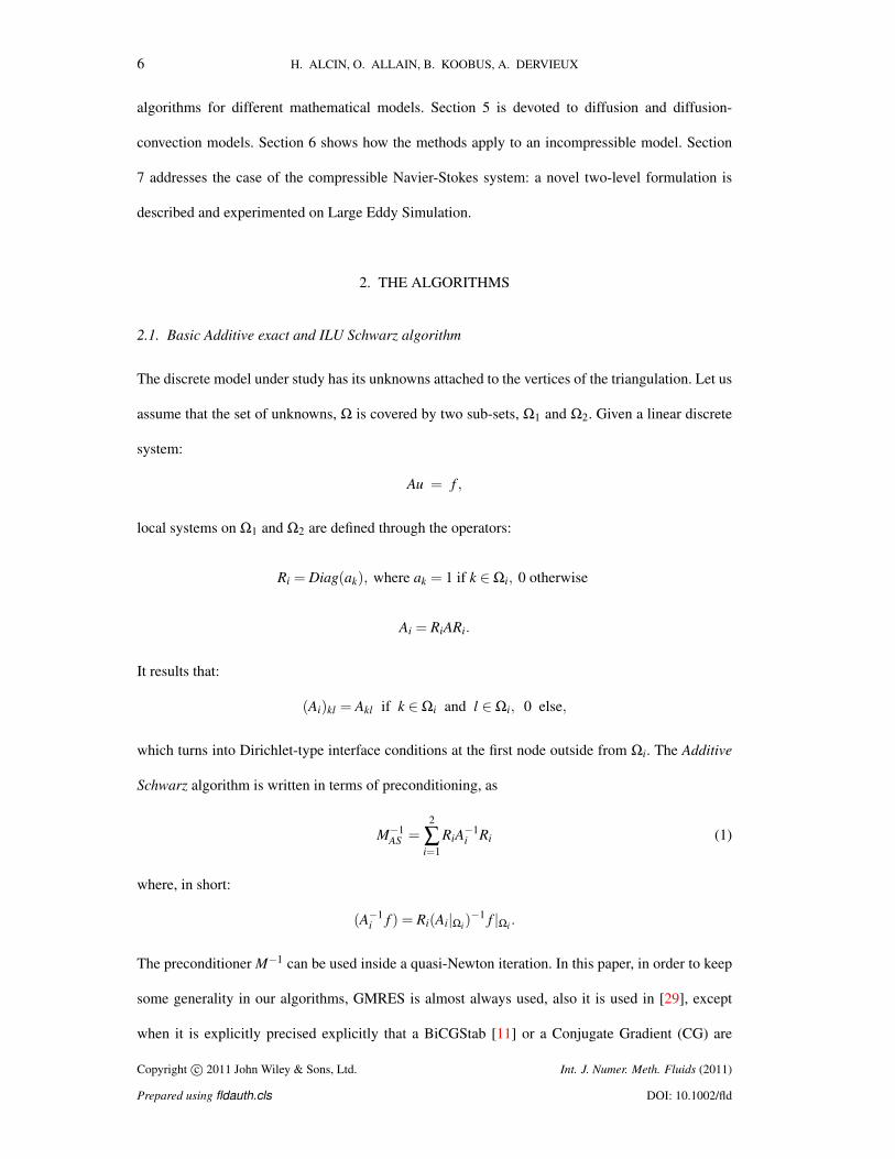
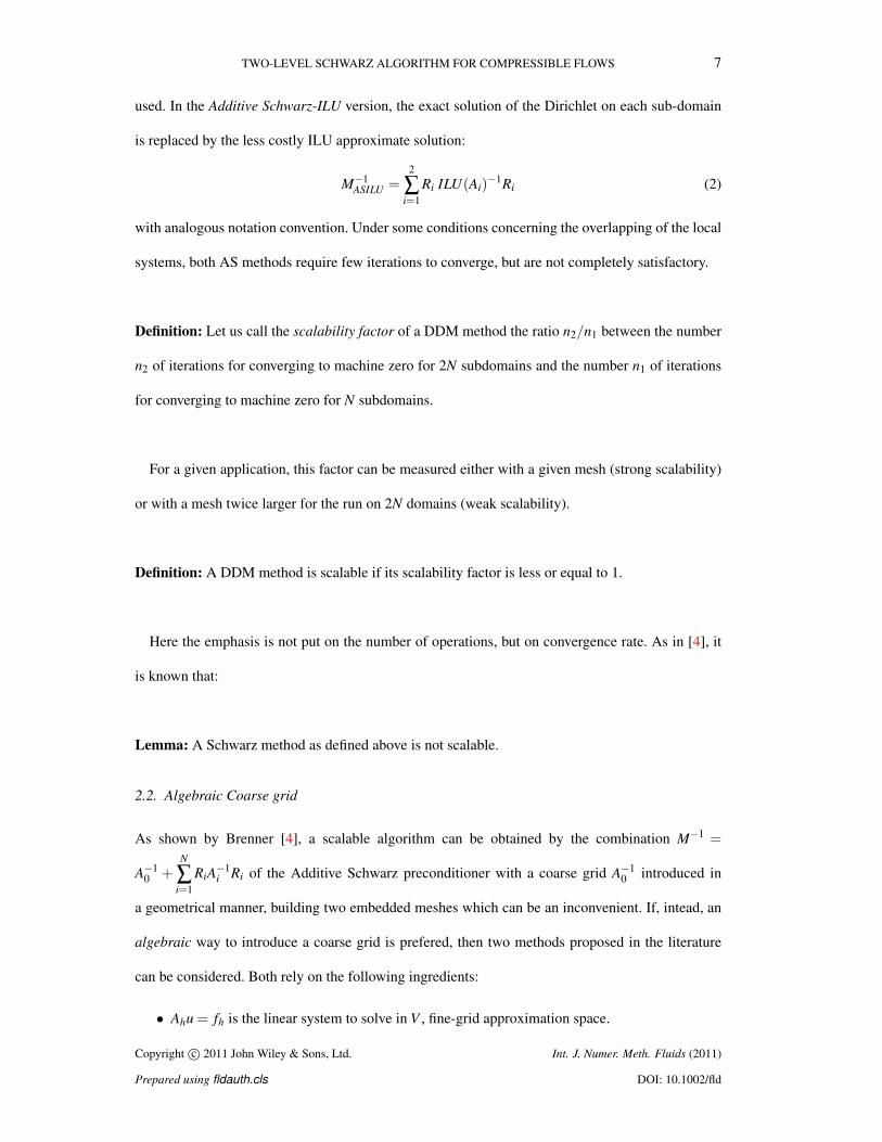
Figure 1. (a) Finite-Volume partition built as dual of a triangulation. (b) Greedy Algorithm for finite-volume
cell agglomeration: four fine cells (left) are grouped into a coarse cell.
A very simple coarse level basis is the set of characteristic functions of the subdomains. This
option will be the main one studied in this paper.
A second option is to look for a few global eigenvectors of the operator, see for example [29].
For CPU cost reasons, these eigenvectors should not be exactly computed but only approximated.
In a recent study [25],[26], it is proposed to compute eigenvectors of the local Dirichlet-to-
Neumann operator, which can be computed in parallel on each sub-domain. However, for convection
and compressible models, the favorite application of Finite-Volume Methods (FVM), the matrix
has a dominant Jordan behavior. The eigenvectors evaluation is difficult and their pertinence for
convergence acceleration is doubtful.
A third way to generate the basis, also discussed in the present paper is coarse grid generation
based on Volume Agglomeration. The idea of Volume Agglomeration is directly inspired by the
multigrid idea, but inside the context of FVM. In this paper we consider meshes made of triangles
or tetrahedra. On the mesh we consider a vertex centered approximation, similar to the P1 finite
element. A finite-volume partition is built from the dual cells derived from triangles (or tetrahedra),
Figure 1(a).
In order to build a coarser grid, it is possible to build coarse cells by sticking together neighboring
cells for example with a greedy algorithm, Figure 1(b). The coarser grid is a priori unstructured as is
the fine one. In the case of FVM, a consistent coarse discretisation of a divergence-based first-order
PDE is directly available. Indeed, we can consider that the new unknown is constant over the coarse
cell and it remains to apply a Godunov quadrature of the fluxes between any couple of two coarse
cells. Elliptic PDE can also be addressed in a similar although more complicated way, [20]. As a
Copyright c© 2011 John Wiley & Sons, Ltd. Int. J. Numer. Meth. Fluids (2011)
Prepared using fldauth.cls DOI: 10.1002/fld
TWO-LEVEL SCHWARZ ALGORITHM FOR COMPRESSIBLE FLOWS 5
result, consistent linear and non-linear coarse grid approximations are built using the agglomeration
principle. Linear and nonlinear multigrid (MG) have been derived, in contrast with Algebraic MG
algorithms. This method extends to Discontinuous Galerkin approximations [24]. More elaborated
versions and their analysis have been made, such as the aggregated methods in [14]. But the efficient
extension of Agglomeration MG to multi-processor parallel computing are less easily achieved, as
compared to Domain Decomposition Methods, see however [9]. The many works on multi-level
methods as introduced by Bramble, Pasciak and Xu [3] have drawn attention to the question of
basis smoothness. Indeed, the underlying basis function in volume-agglomeration is a characteristic
function equal to zero or one. In [23], the agglomeration basis is extended to H1 consistent ones
in an analogous way to smoothed-aggregation. In [10], a Bramble-Pasciak-Xu algorithm is built on
these bases for an optimal design application. The present study tries to build a convergent coarse
mesh basis for an arbitrary unstructured fine mesh. It defines a convergent basis and examine how it
behaves as a coarse grid preconditioner. Different ways in partitioning are also recalled.
The coarse systems produce coarse grid corrections which are now frequently introduced as
preconditioners, either through the Deflation Method or the Balancing Decomposition method,
although a simpler formulation can be found in [30]. Deflation and Balancing methods were
respectively introduced by Nicolaides [27] and Mandel [22] and in [34] it is shown that they can have
very similar convergence properties. Very simplified coarse basis can be used, like characteristic
functions of subdomains. In particular, Deflation and Balancing allow for coarse basis without
considering the convergence of the coarse grid solution to continuous solution. These methods are
progressively compared with multigrid like ones, and are sometimes found more efficient, see [33].
In the present paper, different steps of the assembly of an algebraic coarse level with an additive
Schwarz formulation are revisited. Section 2 recalls the Deflation and Balancing formulations,
and presents a particular construction of a coarse basis. In Section 3, the main options in
subdomain overlapping are discussed. Section 4 defines the precise Deflation and Balancing two-
level algorithms which we propose. The three last sections present numerical evaluations of these
Copyright c© 2011 John Wiley & Sons, Ltd. Int. J. Numer. Meth. Fluids (2011)
Prepared using fldauth.cls DOI: 10.1002/fld
6 H. ALCIN, O. ALLAIN, B. KOOBUS, A. DERVIEUX
algorithms for different mathematical models. Section 5 is devoted to diffusion and diffusion-
convection models. Section 6 shows how the methods apply to an incompressible model. Section
7 addresses the case of the compressible Navier-Stokes system: a novel two-level formulation is
described and experimented on Large Eddy Simulation.
2. THE ALGORITHMS
2.1. Basic Additive exact and ILU Schwarz algorithm
The discrete model under study has its unknowns attached to the vertices of the triangulation. Let us
assume that the set of unknowns, Ω is covered by two sub-sets, Ω1 and Ω2. Given a linear discrete
system:
Au = f ,
local systems on Ω1 and Ω2 are defined through the operators:
Ri = Diag(ak), where ak = 1 if k ∈Ωi, 0 otherwise
Ai = RiARi.
It results that:
(Ai)kl = Akl if k ∈Ωi and l ∈Ωi, 0 else,
which turns into Dirichlet-type interface conditions at the first node outside from Ωi. The Additive
Schwarz algorithm is written in terms of preconditioning, as
M−1AS =
2
∑i=1
RiA−1i Ri (1)
where, in short:
(A−1i f ) = Ri(Ai|Ωi)
−1 f |Ωi .
The preconditioner M−1 can be used inside a quasi-Newton iteration. In this paper, in order to keep
some generality in our algorithms, GMRES is almost always used, also it is used in [29], except
when it is explicitly precised explicitly that a BiCGStab [11] or a Conjugate Gradient (CG) are
Copyright c© 2011 John Wiley & Sons, Ltd. Int. J. Numer. Meth. Fluids (2011)
Prepared using fldauth.cls DOI: 10.1002/fld
TWO-LEVEL SCHWARZ ALGORITHM FOR COMPRESSIBLE FLOWS 7
used. In the Additive Schwarz-ILU version, the exact solution of the Dirichlet on each sub-domain
is replaced by the less costly ILU approximate solution:
M−1ASILU =
2
∑i=1
Ri ILU(Ai)−1Ri (2)
with analogous notation convention. Under some conditions concerning the overlapping of the local
systems, both AS methods require few iterations to converge, but are not completely satisfactory.
Definition: Let us call the scalability factor of a DDM method the ratio n2/n1 between the number
n2 of iterations for converging to machine zero for 2N subdomains and the number n1 of iterations
for converging to machine zero for N subdomains.
For a given application, this factor can be measured either with a given mesh (strong scalability)
or with a mesh twice larger for the run on 2N domains (weak scalability).
Definition: A DDM method is scalable if its scalability factor is less or equal to 1.
Here the emphasis is not put on the number of operations, but on convergence rate. As in [4], it
is known that:
Lemma: A Schwarz method as defined above is not scalable.
2.2. Algebraic Coarse grid
As shown by Brenner [4], a scalable algorithm can be obtained by the combination M−1 =
A−10 +
N
∑i=1
RiA−1i Ri of the Additive Schwarz preconditioner with a coarse grid A−1
0 introduced in
a geometrical manner, building two embedded meshes which can be an inconvenient. If, intead, an
algebraic way to introduce a coarse grid is prefered, then two methods proposed in the literature
can be considered. Both rely on the following ingredients:
• Ahu = fh is the linear system to solve in V , fine-grid approximation space.
Copyright c© 2011 John Wiley & Sons, Ltd. Int. J. Numer. Meth. Fluids (2011)
Prepared using fldauth.cls DOI: 10.1002/fld
8 H. ALCIN, O. ALLAIN, B. KOOBUS, A. DERVIEUX
• V0 ⊂V coarse approximation space, V0 = span[Φ1, · · · ,ΦN ].
• Z an extension operator from V0 into V and ZT a restriction operator from V in V0.
• ZT AhZuH = ZT fh is the coarse system.
DM has been used by many authors. Saad et al. [29] encapsulated it into a Conjugate Gradient.
Aubry et al. [2, 21] applied it to a pressure Poisson equation. In DM, the projection operator is
defined as:
PD = In−AhZ(ZT AhZ)−1ZT with Ah ∈ Rn×n and Z ∈ Rn×N
The DM algorithm consists in solving first the coarse system ZT AhZuH = ZT fh, then the projected
system PDAhu = PD fh in order to get finally u = (In−PTD )u+PT
D u = Z(ZT AhZ)−1ZT fh +PTD u.
BDD has been applied to a complex system in [32]. In [34] a formulation close to DM is proposed.
It consists in replacing the original preconditioner M−1 (ex.: global ILU, Schwarz, or Schwarz-ILU)
by:
PB = PTD M−1PD +Z(ZT AhZ)−1ZT .
The two above algorithms are close to each other. Vuik and Nabben [34] showed in a particular
context that their convergence rate should be the same. With DM preconditioning, some eigenvalues
are replaced by zero. With BDD, they are replaced by one. A consequence is that DM involves the
solution by the fixed point iteration of an ill-posed problem, and this may induce difficulties in
obtaining an iterative convergence reaching machine zero and staying there. BDD does not have
this problem, but involves a larger number of operations. It can be about twice more expensive.
Both methods need the specification of a coarse basis.
2.3. Smooth and non-smooth coarse grid
The coarse grid is defined by a set of basis functions. A central question is the smoothness of these
functions. Let us assume that the discrete system is the finite-element approximation of a Poisson
problem
−∇ ·∇u = f in Ω ; u = 0 on ∂Ω (3)
Copyright c© 2011 John Wiley & Sons, Ltd. Int. J. Numer. Meth. Fluids (2011)
Prepared using fldauth.cls DOI: 10.1002/fld
TWO-LEVEL SCHWARZ ALGORITHM FOR COMPRESSIBLE FLOWS 9
with the standard globally continuous elementwise P1 discrete space. According to Galerkin-
MG, a sufficiently smooth coarse basis provide consistent coarse-grid solutions. Conversely, DDM
methods preferably use the characteristic functions of the sub-domains, Φi(x j) = 1 i f x j ∈ Ωi.
In the case of P1 finite-elements, for example, the typical basis function corresponds to set to 1 all
degrees of freedom in the corresponding sub-domain. According to [23], the coarse system
UH(x) = ∑i
UiΦi(x) ;∫
∇UH∇Φi =
∫f Φi ∀i
produces a solution UH which does not converge towards the continuous solution U when H tends
to 0.
In order to build a better basis, a hierarchical coarsening process from the fine grid to a coarse
grid G j needs be built. Level j is made of N j macro-cells C jk, i.e.:
G j = u,u|C jk = const..
Transfer operators are defined between successive levels (from coarse to fine):
P ji : Gi→ G j P j
i (u)(Cik′) = u(C jk) with Cik′ ⊂C jk
Following [23] the following smoothing operator is introduced:
(L ju)l = ∑k∈N (l)∪l
meas(C jk) uk/ ∑k∈N (l)∪l
meas(C jk)
where N (l) holds for the set of cells which are direct neighbors of cell l, and meas(C jk) stands for
the measure of cell k at grid level j. The smoothing is applied at each level between the coarse level
p defining the characteristic basis Φpk and the finest level identified by the index 1 :
Ψ1k = (L1P21 L2 · · ·Pp−1
p−2 Lp−1Ppp−1)Φpk.
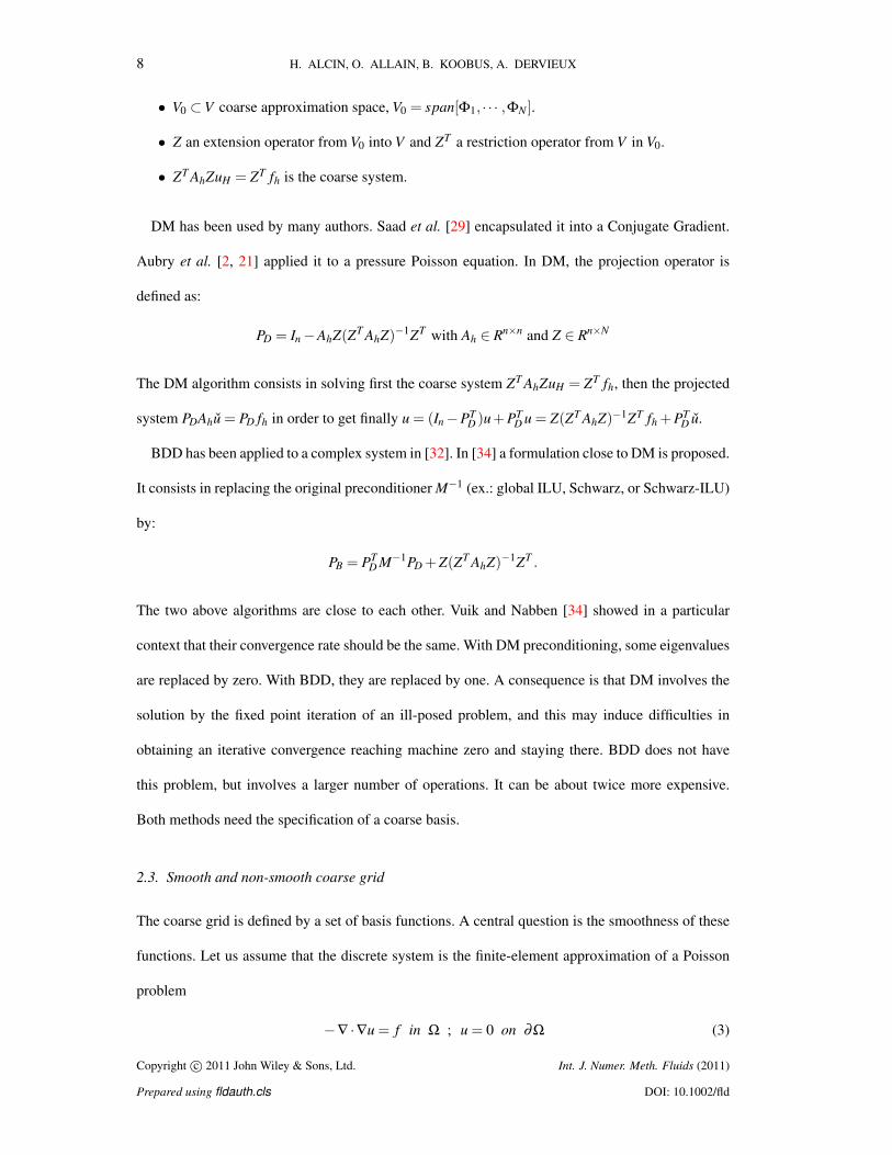
The resulting smooth basis function is compared with the characteristic one in Figure 2. The
inconsistency of the characteristic basis and the convergence of this new smooth basis is illustrated
by the solution of a Poisson equation with a sine function as exact solution, Figure 3.
Copyright c© 2011 John Wiley & Sons, Ltd. Int. J. Numer. Meth. Fluids (2011)
Prepared using fldauth.cls DOI: 10.1002/fld
10 H. ALCIN, O. ALLAIN, B. KOOBUS, A. DERVIEUX
(a) (b)
Figure 2. (a) Characteristic coarse grid basis function. (b) Smooth coarse grid basis function.
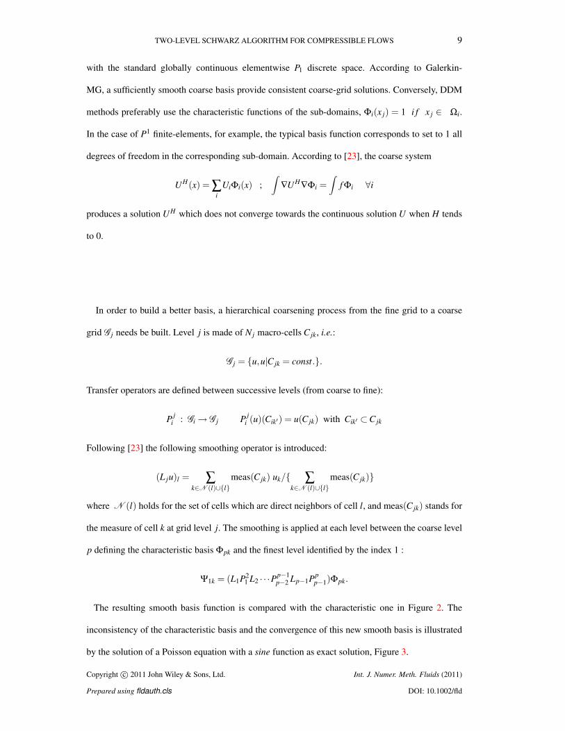
(a) (b)
Figure 3. Accuracy of the coarse grid approximation (four basis functions) for a Poisson problem with a sin
function (of amplitude 2.) as exact solution. (a) Coarse grid solution with the characteristic basis (amplitude
is 0.06). (b) Coarse grid solution with a smooth basis (amplitude is 1.8).
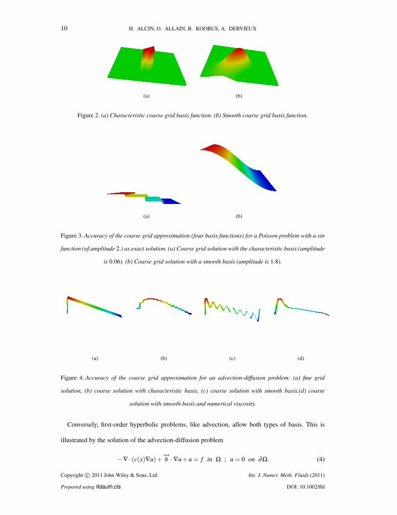
(a) (b) (c) (d)
Figure 4. Accuracy of the coarse grid approximation for an advection-diffusion problem: (a) fine grid
solution, (b) coarse solution with characteristic basis, (c) coarse solution with smooth basis,(d) coarse
solution with smooth basis and numerical viscosity.
Conversely, first-order hyperbolic problems, like advection, allow both types of basis. This is
illustrated by the solution of the advection-diffusion problem
−∇ · (c(x)∇u)+−→b ·∇u+u = f in Ω ; u = 0 on ∂Ω. (4)
Copyright c© 2011 John Wiley & Sons, Ltd. Int. J. Numer. Meth. Fluids (2011)
Prepared using fldauth.cls DOI: 10.1002/fld
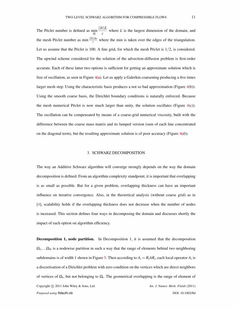
TWO-LEVEL SCHWARZ ALGORITHM FOR COMPRESSIBLE FLOWS 11
The Peclet number is defined as minΩ
||b||Lc
where L is the largest dimension of the domain, and
the mesh Peclet number as min ||b||∆xc where the min is taken over the edges of the triangulation.
Let us assume that the Peclet is 100. A fine grid, for which the mesh Peclet is 1/2, is considered.
The upwind scheme considered for the solution of the advection-diffusion problem is first-order
accurate. Each of these latter two options is sufficient for getting an approximate solution which is
free of oscillation, as seen in Figure 4(a). Let us apply a Galerkin coarsening producing a five times
larger mesh step. Using the characteristic basis produces a not so bad approximation (Figure 4(b)).
Using the smooth coarse basis, the Dirichlet boundary conditions is naturally enforced. Because
the mesh numerical Peclet is now much larger than unity, the solution oscillates (Figure 4(c)).
The oscillation can be compensated by means of a coarse-grid numerical viscosity, built with the
difference between the coarse mass matrix and its lumped version (sum of each line concentrated
on the diagonal term), but the resulting approximate solution is of poor accuracy (Figure 4(d)).
3. SCHWARZ DECOMPOSITION
The way an Additive Schwarz algorithm will converge strongly depends on the way the domain
decomposition is defined. From an algorithm complexity standpoint, it is important that overlapping
is as small as possible. But for a given problem, overlapping thickness can have an important
influence on iterative convergence. Also, in the theoretical analysis (without coarse grid) as in
[4], scalability holds if the overlapping thickness does not decrease when the number of nodes
is increased. This section defines four ways in decomposing the domain and discusses shortly the
impact of each option on algorithm efficiency.
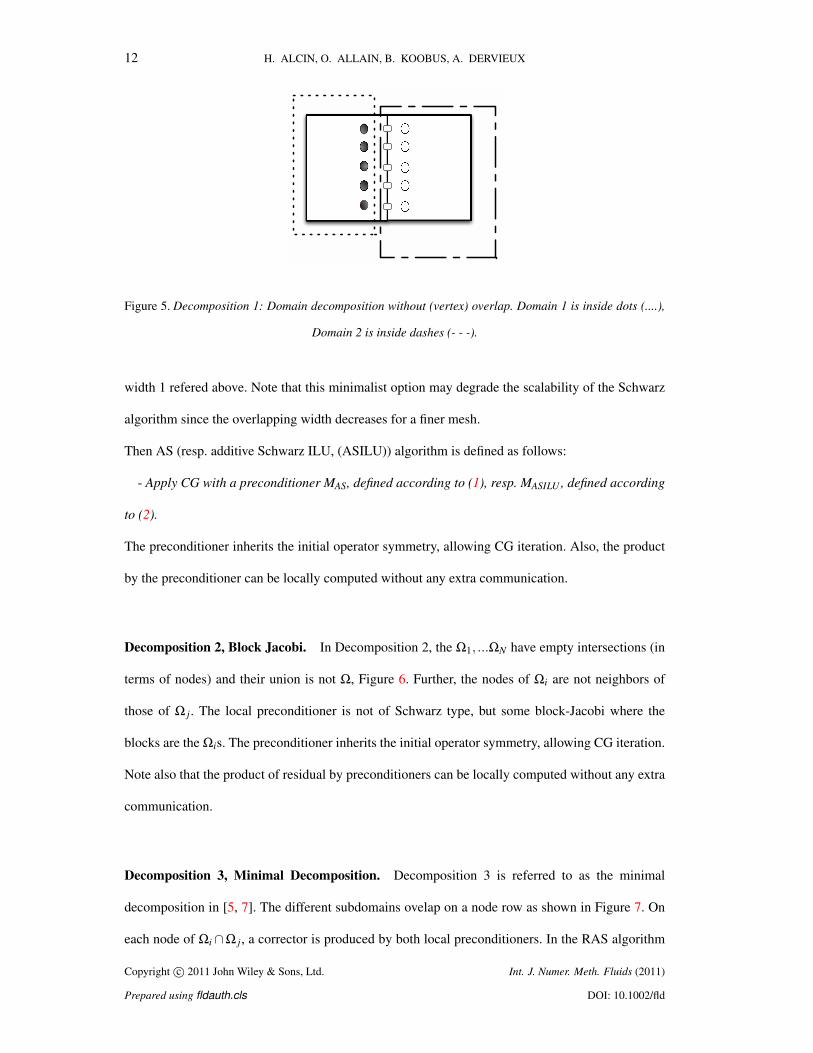
Decomposition 1, node partition. In Decomposition 1, it is assumed that the decomposition
Ω1, ...ΩN is a nodewise partition in such a way that the range of elements behind two neighboring
subdomains is of width 1 shown in Figure 5. Then according to Ai = RiARi, each local operator Ai is
a discretisation of a Dirichlet problem with zero condition on the vertices which are direct neighbors
of vertices of Ωi, but not belonging to Ωi. The geometrical overlapping is the range of element of
Copyright c© 2011 John Wiley & Sons, Ltd. Int. J. Numer. Meth. Fluids (2011)
Prepared using fldauth.cls DOI: 10.1002/fld
12 H. ALCIN, O. ALLAIN, B. KOOBUS, A. DERVIEUX
Figure 5. Decomposition 1: Domain decomposition without (vertex) overlap. Domain 1 is inside dots (....),
Domain 2 is inside dashes (- - -).
width 1 refered above. Note that this minimalist option may degrade the scalability of the Schwarz
algorithm since the overlapping width decreases for a finer mesh.
Then AS (resp. additive Schwarz ILU, (ASILU)) algorithm is defined as follows:
- Apply CG with a preconditioner MAS, defined according to (1), resp. MASILU , defined according
to (2).
The preconditioner inherits the initial operator symmetry, allowing CG iteration. Also, the product
by the preconditioner can be locally computed without any extra communication.
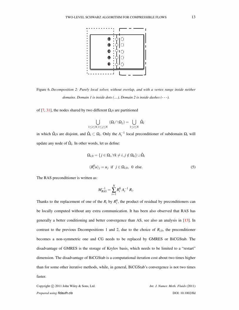
Decomposition 2, Block Jacobi. In Decomposition 2, the Ω1, ...ΩN have empty intersections (in
terms of nodes) and their union is not Ω, Figure 6. Further, the nodes of Ωi are not neighbors of
those of Ω j. The local preconditioner is not of Schwarz type, but some block-Jacobi where the
blocks are the Ωis. The preconditioner inherits the initial operator symmetry, allowing CG iteration.
Note also that the product of residual by preconditioners can be locally computed without any extra
communication.
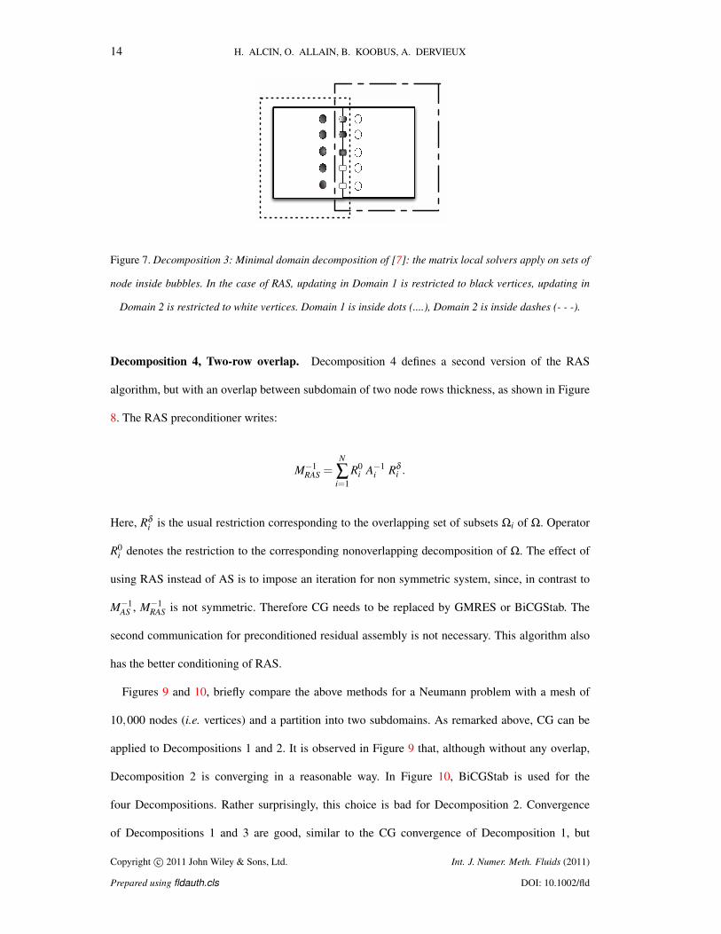
Decomposition 3, Minimal Decomposition. Decomposition 3 is referred to as the minimal
decomposition in [5, 7]. The different subdomains ovelap on a node row as shown in Figure 7. On
each node of Ωi∩Ω j, a corrector is produced by both local preconditioners. In the RAS algorithm
Copyright c© 2011 John Wiley & Sons, Ltd. Int. J. Numer. Meth. Fluids (2011)
Prepared using fldauth.cls DOI: 10.1002/fld
TWO-LEVEL SCHWARZ ALGORITHM FOR COMPRESSIBLE FLOWS 13
Figure 6. Decomposition 2: Purely local solver, without overlap, and with a vertex range inside neither
domains. Domain 1 is inside dots (....), Domain 2 is inside dashes (- - -).
of [7, 31], the nodes shared by two different Ωis are partitioned
⋃1≤i≤N,1≤ j≤N
(Ωi∩Ω j) =⋃
1≤i≤N
Ωi
in which Ωis are disjoint, and Ωi ⊂ Ωi. Only the A−1i local preconditioner of subdomain Ωi will
update any node of Ωi. In other words, let us define:
Ωi,0 = j ∈Ωi,∀k 6= i, j /∈Ωk∪ Ωi
(R0i u) j = u j if j ∈Ωi,0, 0 else. (5)
The RAS preconditioner is written as:
M−1RAS =
N
∑i=1
R0i A−1
i Ri.
Thanks to the replacement of one of the Ri by R0i , the product of residual by preconditioners can
be locally computed without any extra communication. It has been also observed that RAS has
generally a better conditioning and better convergence than AS, see also an analysis in [13]. In
contrast to the previous Decompositions 1 and 2, due to the choice of Ri,0, the preconditioner
becomes a non-symmetric one and CG needs to be replaced by GMRES or BiCGStab. The
disadvantage of GMRES is the storage of Krylov basis, which needs to be limited to a “restart”
dimension. The disadvantage of BiCGStab is a computational iteration cost about two times higher
than for some other iterative methods, while, in general, BiCGStab’s convergence is not two times
faster.
Copyright c© 2011 John Wiley & Sons, Ltd. Int. J. Numer. Meth. Fluids (2011)
Prepared using fldauth.cls DOI: 10.1002/fld
14 H. ALCIN, O. ALLAIN, B. KOOBUS, A. DERVIEUX
Figure 7. Decomposition 3: Minimal domain decomposition of [7]: the matrix local solvers apply on sets of
node inside bubbles. In the case of RAS, updating in Domain 1 is restricted to black vertices, updating in
Domain 2 is restricted to white vertices. Domain 1 is inside dots (....), Domain 2 is inside dashes (- - -).
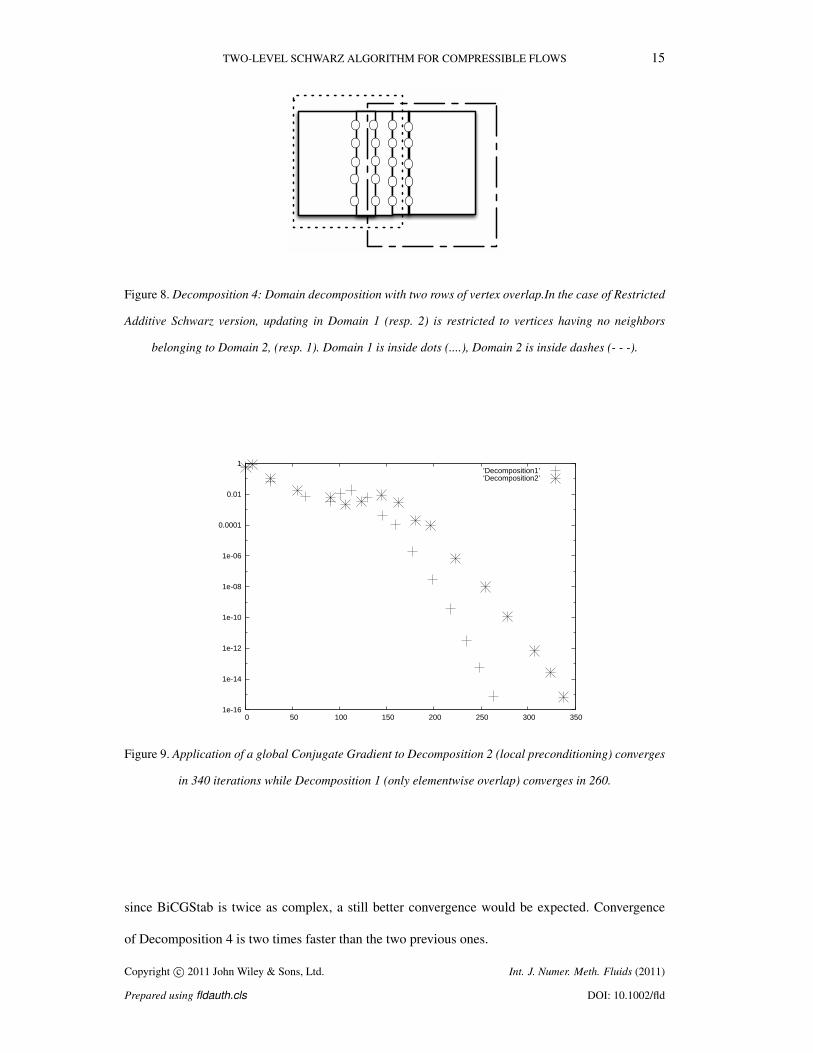
Decomposition 4, Two-row overlap. Decomposition 4 defines a second version of the RAS
algorithm, but with an overlap between subdomain of two node rows thickness, as shown in Figure
8. The RAS preconditioner writes:
M−1RAS =
N
∑i=1
R0i A−1
i Rδi .
Here, Rδi is the usual restriction corresponding to the overlapping set of subsets Ωi of Ω. Operator
R0i denotes the restriction to the corresponding nonoverlapping decomposition of Ω. The effect of
using RAS instead of AS is to impose an iteration for non symmetric system, since, in contrast to
M−1AS , M−1
RAS is not symmetric. Therefore CG needs to be replaced by GMRES or BiCGStab. The
second communication for preconditioned residual assembly is not necessary. This algorithm also
has the better conditioning of RAS.
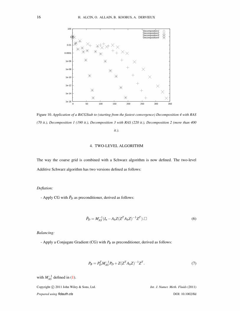
Figures 9 and 10, briefly compare the above methods for a Neumann problem with a mesh of
10,000 nodes (i.e. vertices) and a partition into two subdomains. As remarked above, CG can be
applied to Decompositions 1 and 2. It is observed in Figure 9 that, although without any overlap,
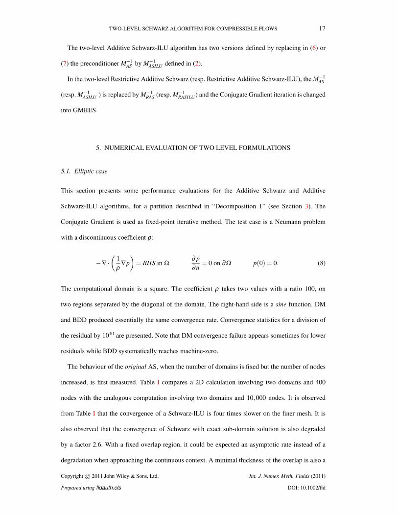
Decomposition 2 is converging in a reasonable way. In Figure 10, BiCGStab is used for the
four Decompositions. Rather surprisingly, this choice is bad for Decomposition 2. Convergence
of Decompositions 1 and 3 are good, similar to the CG convergence of Decomposition 1, but
Copyright c© 2011 John Wiley & Sons, Ltd. Int. J. Numer. Meth. Fluids (2011)
Prepared using fldauth.cls DOI: 10.1002/fld
TWO-LEVEL SCHWARZ ALGORITHM FOR COMPRESSIBLE FLOWS 15
Figure 8. Decomposition 4: Domain decomposition with two rows of vertex overlap.In the case of Restricted
Additive Schwarz version, updating in Domain 1 (resp. 2) is restricted to vertices having no neighbors
belonging to Domain 2, (resp. 1). Domain 1 is inside dots (....), Domain 2 is inside dashes (- - -).
1e-16
1e-14
1e-12
1e-10
1e-08
1e-06
0.0001
0.01
1
0 50 100 150 200 250 300 350
’Decomposition1’’Decomposition2’
Figure 9. Application of a global Conjugate Gradient to Decomposition 2 (local preconditioning) converges
in 340 iterations while Decomposition 1 (only elementwise overlap) converges in 260.
since BiCGStab is twice as complex, a still better convergence would be expected. Convergence
of Decomposition 4 is two times faster than the two previous ones.
Copyright c© 2011 John Wiley & Sons, Ltd. Int. J. Numer. Meth. Fluids (2011)
Prepared using fldauth.cls DOI: 10.1002/fld
16 H. ALCIN, O. ALLAIN, B. KOOBUS, A. DERVIEUX
1e-16
1e-14
1e-12
1e-10
1e-08
1e-06
0.0001
0.01
1
100
0 50 100 150 200 250 300 350
’Decomposition1’’Decomposition2’’Decomposition3’’Decomposition4’
Figure 10. Application of a BiCGStab to (starting from the fastest convergence) Decomposition 4 with RAS
(70 it.), Decomposition 1 (190 it.), Decomposition 3 with RAS (220 it.), Decomposition 2 (more than 400
it.).
4. TWO-LEVEL ALGORITHM
The way the coarse grid is combined with a Schwarz algorithm is now defined. The two-level
Additive Schwarz algorithm has two versions defined as follows:
Deflation:
- Apply CG with PD as preconditioner, derived as follows:
PD = M−1AS (In−AhZ(ZT AhZ)−1ZT ). (6)
Balancing:
- Apply a Conjugate Gradient (CG) with PB as preconditioner, derived as follows:
PB = PTD M−1
AS PD +Z(ZT AhZ)−1ZT . (7)
with M−1AS defined in (1).
Copyright c© 2011 John Wiley & Sons, Ltd. Int. J. Numer. Meth. Fluids (2011)
Prepared using fldauth.cls DOI: 10.1002/fld
TWO-LEVEL SCHWARZ ALGORITHM FOR COMPRESSIBLE FLOWS 17
The two-level Additive Schwarz-ILU algorithm has two versions defined by replacing in (6) or
(7) the preconditioner M−1AS by M−1
ASILU defined in (2).
In the two-level Restrictive Additive Schwarz (resp. Restrictive Additive Schwarz-ILU), the M−1AS
(resp. M−1ASILU ) is replaced by M−1
RAS (resp. M−1RASILU ) and the Conjugate Gradient iteration is changed
into GMRES.
5. NUMERICAL EVALUATION OF TWO LEVEL FORMULATIONS
5.1. Elliptic case
This section presents some performance evaluations for the Additive Schwarz and Additive
Schwarz-ILU algorithms, for a partition described in “Decomposition 1” (see Section 3). The
Conjugate Gradient is used as fixed-point iterative method. The test case is a Neumann problem
with a discontinuous coefficient ρ:
−∇ ·(
1ρ
∇p)
= RHS in Ω∂ p∂n
= 0 on ∂Ω p(0) = 0. (8)
The computational domain is a square. The coefficient ρ takes two values with a ratio 100, on
two regions separated by the diagonal of the domain. The right-hand side is a sine function. DM
and BDD produced essentially the same convergence rate. Convergence statistics for a division of
the residual by 1010 are presented. Note that DM convergence failure appears sometimes for lower
residuals while BDD systematically reaches machine-zero.
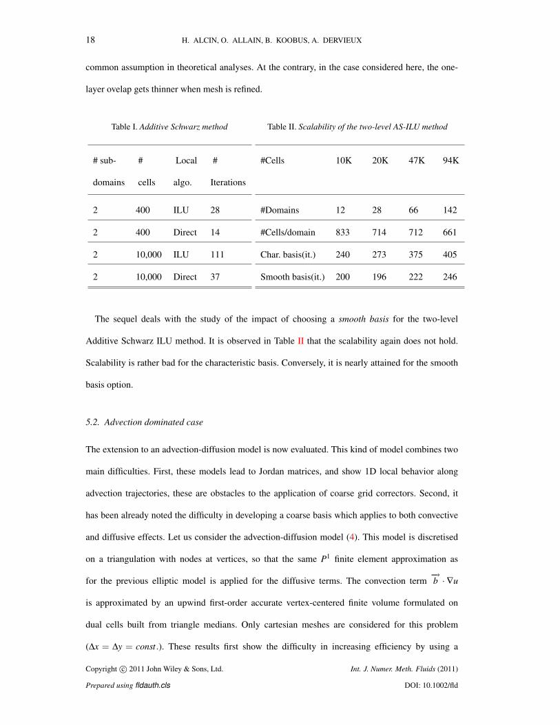
The behaviour of the original AS, when the number of domains is fixed but the number of nodes
increased, is first measured. Table I compares a 2D calculation involving two domains and 400
nodes with the analogous computation involving two domains and 10,000 nodes. It is observed
from Table I that the convergence of a Schwarz-ILU is four times slower on the finer mesh. It is
also observed that the convergence of Schwarz with exact sub-domain solution is also degraded
by a factor 2.6. With a fixed overlap region, it could be expected an asymptotic rate instead of a
degradation when approaching the continuous context. A minimal thickness of the overlap is also a
Copyright c© 2011 John Wiley & Sons, Ltd. Int. J. Numer. Meth. Fluids (2011)
Prepared using fldauth.cls DOI: 10.1002/fld
18 H. ALCIN, O. ALLAIN, B. KOOBUS, A. DERVIEUX
common assumption in theoretical analyses. At the contrary, in the case considered here, the one-
layer ovelap gets thinner when mesh is refined.
Table I. Additive Schwarz method
# sub- # Local #
domains cells algo. Iterations
2 400 ILU 28
2 400 Direct 14
2 10,000 ILU 111
2 10,000 Direct 37
Table II. Scalability of the two-level AS-ILU method
#Cells 10K 20K 47K 94K
#Domains 12 28 66 142
#Cells/domain 833 714 712 661
Char. basis(it.) 240 273 375 405
Smooth basis(it.) 200 196 222 246
The sequel deals with the study of the impact of choosing a smooth basis for the two-level
Additive Schwarz ILU method. It is observed in Table II that the scalability again does not hold.
Scalability is rather bad for the characteristic basis. Conversely, it is nearly attained for the smooth
basis option.
5.2. Advection dominated case
The extension to an advection-diffusion model is now evaluated. This kind of model combines two
main difficulties. First, these models lead to Jordan matrices, and show 1D local behavior along
advection trajectories, these are obstacles to the application of coarse grid correctors. Second, it
has been already noted the difficulty in developing a coarse basis which applies to both convective
and diffusive effects. Let us consider the advection-diffusion model (4). This model is discretised
on a triangulation with nodes at vertices, so that the same P1 finite element approximation as
for the previous elliptic model is applied for the diffusive terms. The convection term−→b ·∇u
is approximated by an upwind first-order accurate vertex-centered finite volume formulated on
dual cells built from triangle medians. Only cartesian meshes are considered for this problem
(∆x = ∆y = const.). These results first show the difficulty in increasing efficiency by using a
Copyright c© 2011 John Wiley & Sons, Ltd. Int. J. Numer. Meth. Fluids (2011)
Prepared using fldauth.cls DOI: 10.1002/fld
TWO-LEVEL SCHWARZ ALGORITHM FOR COMPRESSIBLE FLOWS 19
1e-18
1e-16
1e-14
1e-12
1e-10
1e-8
1e-6
1e-4
1e-2
1
100
0 100 200 300 400 500 600
’RAS’’Balancing’
(a)
1e-18
1e-16
1e-14
1e-12
1e-10
1e-8
1e-6
1e-4
1e-2
1
100
0 50 100 150 200 250
’RAS1000’’Balancing1000’
(b)
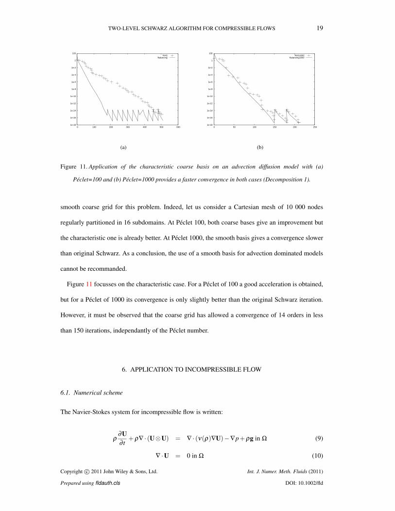
Figure 11. Application of the characteristic coarse basis on an advection diffusion model with (a)
Peclet=100 and (b) Peclet=1000 provides a faster convergence in both cases (Decomposition 1).
smooth coarse grid for this problem. Indeed, let us consider a Cartesian mesh of 10 000 nodes
regularly partitioned in 16 subdomains. At Peclet 100, both coarse bases give an improvement but
the characteristic one is already better. At Peclet 1000, the smooth basis gives a convergence slower
than original Schwarz. As a conclusion, the use of a smooth basis for advection dominated models
cannot be recommanded.
Figure 11 focusses on the characteristic case. For a Peclet of 100 a good acceleration is obtained,
but for a Peclet of 1000 its convergence is only slightly better than the original Schwarz iteration.
However, it must be observed that the coarse grid has allowed a convergence of 14 orders in less
than 150 iterations, independantly of the Peclet number.
6. APPLICATION TO INCOMPRESSIBLE FLOW
6.1. Numerical scheme
The Navier-Stokes system for incompressible flow is written:
ρ∂U∂ t
+ρ∇ · (U⊗U) = ∇ · (ν(ρ)∇U)−∇p+ρg in Ω (9)
∇ ·U = 0 in Ω (10)
Copyright c© 2011 John Wiley & Sons, Ltd. Int. J. Numer. Meth. Fluids (2011)
Prepared using fldauth.cls DOI: 10.1002/fld
20 H. ALCIN, O. ALLAIN, B. KOOBUS, A. DERVIEUX
where U denotes the fluid velocity, p the pressure, ρ the density, and ν(ρ) the viscosity. Let
V = ψ ∈ C 0(Ω)∣∣ ψ|K is affine ∀K ∈ H which is the usual P1 Finite Element space. V is
spanned by the set of basis functions ψi where ψi verifies for any vertex xi of H , ψi(xi) = 1
and ∀ j 6= i, ψi(x j) = 0. Let V = V d , where d is the space dimension. The discretized multi-fluid
variables are:
U = ∑i
Uiψi , p = ∑i
piψi and φ = ∑i
φiψi .
A transfer operator into V is defined as follows: for any u ∈ L2(Ω), we denote by Pu : L2 7→V
the function such that for any vertex xi of H :
Pu(xi) =∫
Ωuψi dx∫
Ωψi dx
.
And, for all U = (u,v)∈ (L2(Ω))2, we denote by PU = (Pu,Pv) the transfer into V. The transfer
operator P will be used for transforming a discrete field that is constant by element into a discrete
field that is continuous and piecewise linear.
The global algorithm for advancing in time is written as follows.
Stage 1 is an explicit prediction step:
Ui = Uni −
∆t|Ci|
∫Ω
ψi
(∇ · (U⊗U)− 1
ρ∇ · (ν(ρ)∇U) − g
)dx ,
where |Ci|= ∑j
∫Ω
ψiψ j dx .
Stage 2 is a projection step imposing Relation (10):∫ 1ρ
∇pn+1 ·∇ψ dx =1∆t
∫∇ψ · Udx ∀ ψ ∈V ,
Un+1 = U+∆t P(
1ρ
∇pn+1)
and Un+1 = 0 on ∂Ω .
Only the projection step needs the solution of a matrix system and that this matrix system is the same
as in our model problem (8). The linear system arising from the projection step was originally solved
with a RAS algorithm for an overlapping domain decomposition as defined by Decomposition 4,
combined with a GMRES fixed point. A two-level version of this algorithm is defined by combining
the Deflation preconditioner into the RAS one.
Copyright c© 2011 John Wiley & Sons, Ltd. Int. J. Numer. Meth. Fluids (2011)
Prepared using fldauth.cls DOI: 10.1002/fld
TWO-LEVEL SCHWARZ ALGORITHM FOR COMPRESSIBLE FLOWS 21
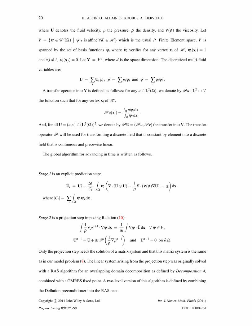
Figure 12. Mesh and pressure in a pump (Decomposition 4). Courtesy of PCM.
Table III. Incompressible flow through a pump, comparison of # of iterations for convergence
Type of preconditioner M−1 # sub-domains Iterations CPU
RAS-ILU 40 2364 291 sec.
Deflated-RAS-ILU 40 186 30 sec.
6.2. Example: Incompressible flow in a pump
The steady flow through a pump is computed. The geometry is depicted in Figure 12 and is similar
to a duct with an inflow and an outflow section. The rotor blades are considered fixed. When
partitioned in slices normal to flow, the error correction slowly propagate. Further, the flow involves
thin boundary layers. In the proposed calculations the mesh involves 2M cells and is partitioned on
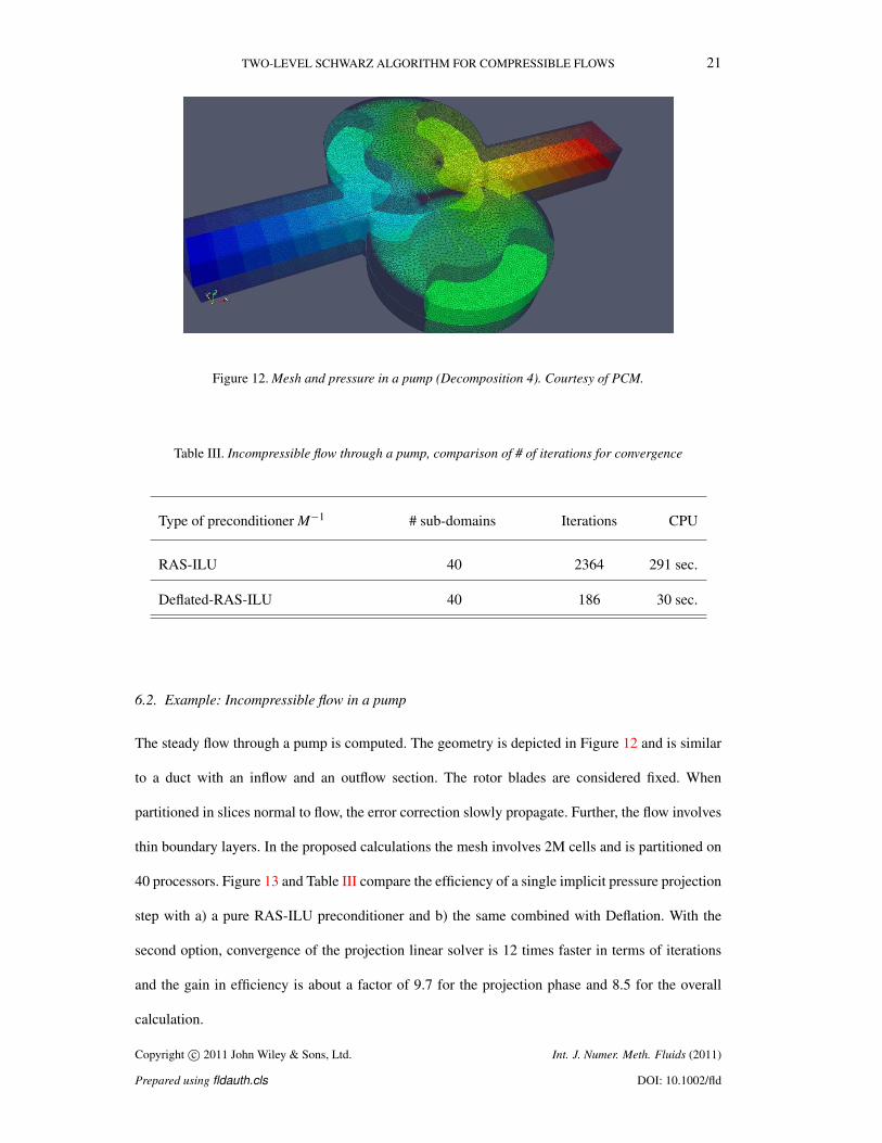
40 processors. Figure 13 and Table III compare the efficiency of a single implicit pressure projection
step with a) a pure RAS-ILU preconditioner and b) the same combined with Deflation. With the
second option, convergence of the projection linear solver is 12 times faster in terms of iterations
and the gain in efficiency is about a factor of 9.7 for the projection phase and 8.5 for the overall
calculation.
Copyright c© 2011 John Wiley & Sons, Ltd. Int. J. Numer. Meth. Fluids (2011)
Prepared using fldauth.cls DOI: 10.1002/fld
22 H. ALCIN, O. ALLAIN, B. KOOBUS, A. DERVIEUX
1e-05
0.0001
0.001
0.01
0.1
1
0 500 1000 1500 2000 2500
’RAS’’Balancing’
Figure 13. Incompressible flow through a pump.Comparison between RAS and two-level RAS solution
algorithms (Decomposition 4). Residuals (normalised at 1 at first iteration) as functions of iterations.
7. APPLICATION TO COMPRESSIBLE FLOW
7.1. Numerical scheme
DM and BDD preconditioners are adapted to a parallel software which computes three-dimensional
turbulent compressible flows. In the original numerical scheme, the spatial approximation is a vertex
centered mixed-element-volume approximation stabilised by an upwind term introducing a sixth-
order dissipation, see [8]. The flow equations are advanced in time with an implicit scheme, based
on a second-order time-accurate backward difference scheme, that are briefly written as
F(W n+1,W n,W n−1) = 0 (11)
where W is the five-component discretisation of (ρ,ρu,ρE), with ρ the density, u the velocity
vector, and ρE the total energy per unit volume. This non-linear system has to be solved at each
time step in order to obtain W n+1. It is solved by a (Newton-like) defect-correction iteration
A(W (α+1)−W (α)) =−F(W (α),W n,W n−1) (12)
in which a simplified Jabobian A is used. Since Equation (11) has 5 fields as unknown, A is defined
as a block 5× 5 sparse matrix. The Jacobian is built from the sum of a first-order discretisation
Copyright c© 2011 John Wiley & Sons, Ltd. Int. J. Numer. Meth. Fluids (2011)
Prepared using fldauth.cls DOI: 10.1002/fld
TWO-LEVEL SCHWARZ ALGORITHM FOR COMPRESSIBLE FLOWS 23
of the linearized Euler fluxes and of a linearization of the second-order accurate diffusive fluxes.
Typically, 2 defect-correction iterations are performed, each of them requiring two linear solutions.
The performance of this algorithm has been studied for example in [18]. The most CPU consuming
part of the algorithm is the resolution of the sparse linear system in (12). It is solved by a RAS, in the
formulation proposed in [31], which we now describe. The linear system (12) is first transformed
with the block diagonal D = BlockDiag(A) with 5×5 blocks as follows:
D−1A δW = D−1 f (13)
where δW stands for W (α+1)−W (α).
The domain decomposition is Decomposition 3 as defined in Section 3. For the local, i.e.
subdomain solver, a minimum fill ILU(0) factorisation is applied to the product D−1i Ai. It is denoted
hereafter ILU(D−1i Ai). The preconditioner is then written as
M−1 =N
∑i=1
R0i(ILU(D−1
i Ai))−1
R1i . (14)
This is a right-preconditioned system, i.e. the iteration solves
(D−1A)M−1 v = D−1 f ,
and then put δW = M−1v. This keeps the same residual D−1AδW − D−1 f as for the
unpreconditioned iteration. The RAS formulation (14) needs less communication (due to the use
of R0i ) and has proved to have better convergence properties than the analogous AS formulation [7].
7.2. New linear solution algorithm.
Now DM or BDD are applied to the solution of (13). They are used as right preconditioners, and
the residual is again the same as for the unpreconditioned iteration. Using the same notation for
the coarse grid matrix E = Zt(D−1A)Z, the Deflation-RAS iteration is defined by the use of the
following preconditioners
P = I− (D−1A)ZE−1Zt
Q = I−ZE−1Zt(D−1A)
Copyright c© 2011 John Wiley & Sons, Ltd. Int. J. Numer. Meth. Fluids (2011)
Prepared using fldauth.cls DOI: 10.1002/fld
24 H. ALCIN, O. ALLAIN, B. KOOBUS, A. DERVIEUX
the iteration solves
(D−1A)QM−1v = PD−1 f
and finally put
δW = (M−1)v
δW = ZE−1ZtD−1 f +QδW .
As for the Balancing preconditioner,
PB = Z(E−1)Zt +QM−1P
(15)
then the iteration solves
(D−1A)(PB)v = (D−1) f
and finally put δW = (PB)v.
7.3. Example: Compressible flow around a cylinder
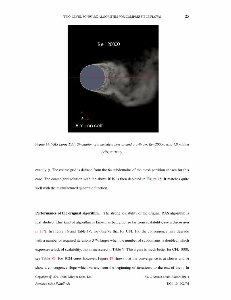
Test case. The compressible 3D flow (Mach=0.1) around a circular cylinder (Figure 14) is
computed using a Smagorinsky Large Eddy Simulation combined with the Variational Multiscale
numerical filter, as described in [19]. The Reynolds number is 20,000. The mesh has 1.8 M cells
and is stretched near the cylinder wall with a maximum aspect ratio of 500. It is decomposed into
64 to 1024 subdomains, one computer core being attributed to each subdomain for the simulations.
The convergence of a single implicit phase for a CFL 100 and 1000 is first examined.
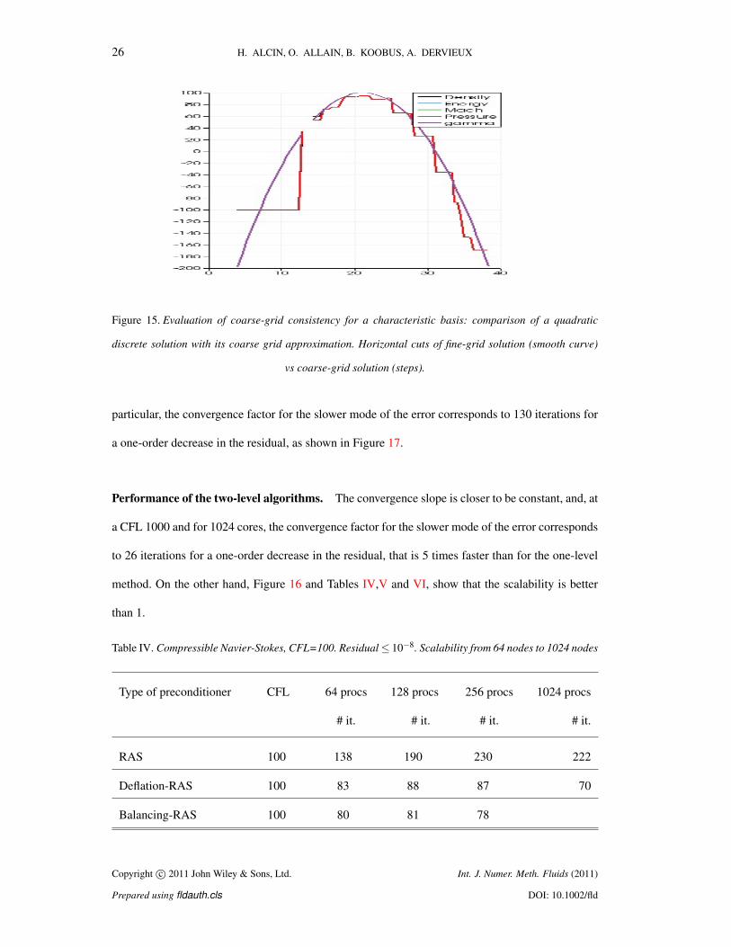
The flow is convection dominant and a characteristic coarse basis, i.e. built from the characteristic
functions of the subdomains as defined in Section 2.3, can be a reasonable choice. To confirm this,
the consistency of the characteristic coarse grid is evaluated by introducing a manufactured solution
φ in the linearised system. The function φ is a quadratic one for each component. The right-hand
side (RHS) of the linear system is chosen in such a way that the solution of the linearised system is
Copyright c© 2011 John Wiley & Sons, Ltd. Int. J. Numer. Meth. Fluids (2011)
Prepared using fldauth.cls DOI: 10.1002/fld
TWO-LEVEL SCHWARZ ALGORITHM FOR COMPRESSIBLE FLOWS 25
Figure 14. VMS Large Eddy Simulation of a turbulent flow around a cylinder, Re=20000, with 1.8 million
cells; vorticity.
exactly φ . The coarse grid is defined from the 64 subdomains of the mesh partition chosen for this
case. The coarse grid solution with the above RHS is then depicted in Figure 15. It matches quite
well with the manufactured quadratic function.
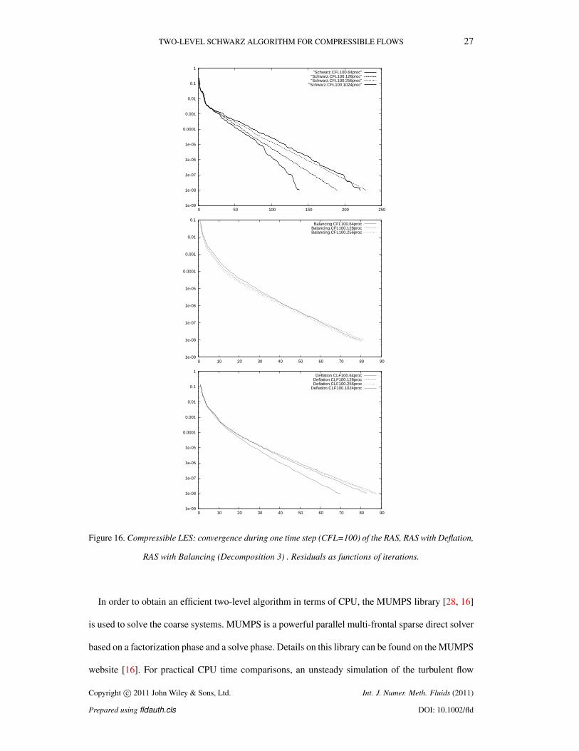
Performance of the original algorithm. The strong scalability of the original RAS algorithm is
first studied. This kind of algorithm is known as being not so far from scalability, see a discussion
in [17]. In Figure 16 and Table IV, we observe that for CFL 100 the convergence may degrade
with a number of required iterations 37% larger when the number of subdomains is doubled, which
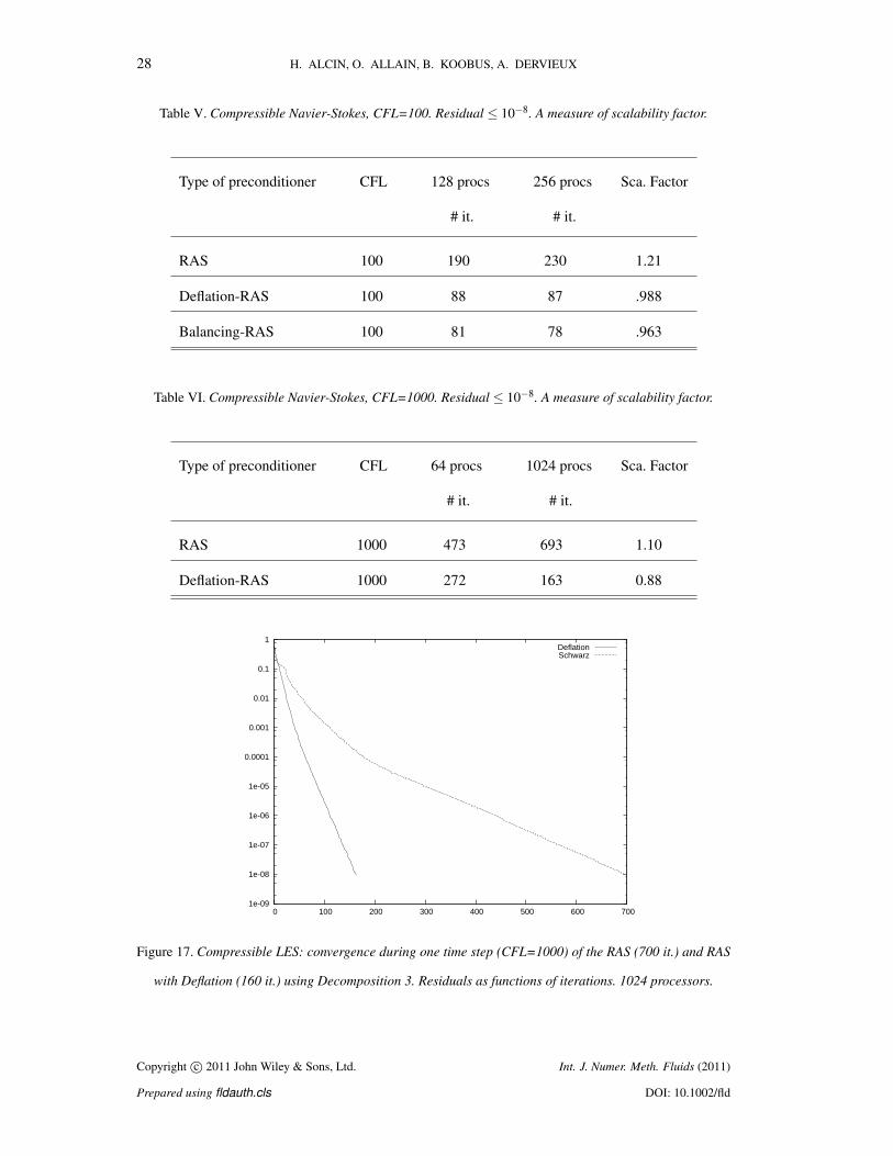
expresses a lack of scalability, that is measured in Table V. This figure is much better for CFL 1000,
see Table VI. For 1024 cores however, Figure 17 shows that the convergence is a) slower and b)
show a convergence slope which varies, from the beginning of iterations, to the end of them. In
Copyright c© 2011 John Wiley & Sons, Ltd. Int. J. Numer. Meth. Fluids (2011)
Prepared using fldauth.cls DOI: 10.1002/fld
26 H. ALCIN, O. ALLAIN, B. KOOBUS, A. DERVIEUX
Figure 15. Evaluation of coarse-grid consistency for a characteristic basis: comparison of a quadratic
discrete solution with its coarse grid approximation. Horizontal cuts of fine-grid solution (smooth curve)
vs coarse-grid solution (steps).
particular, the convergence factor for the slower mode of the error corresponds to 130 iterations for
a one-order decrease in the residual, as shown in Figure 17.
Performance of the two-level algorithms. The convergence slope is closer to be constant, and, at
a CFL 1000 and for 1024 cores, the convergence factor for the slower mode of the error corresponds
to 26 iterations for a one-order decrease in the residual, that is 5 times faster than for the one-level
method. On the other hand, Figure 16 and Tables IV,V and VI, show that the scalability is better
than 1.
Table IV. Compressible Navier-Stokes, CFL=100. Residual≤ 10−8. Scalability from 64 nodes to 1024 nodes
Type of preconditioner CFL 64 procs 128 procs 256 procs 1024 procs
# it. # it. # it. # it.
RAS 100 138 190 230 222
Deflation-RAS 100 83 88 87 70
Balancing-RAS 100 80 81 78
Copyright c© 2011 John Wiley & Sons, Ltd. Int. J. Numer. Meth. Fluids (2011)
Prepared using fldauth.cls DOI: 10.1002/fld
TWO-LEVEL SCHWARZ ALGORITHM FOR COMPRESSIBLE FLOWS 27
1e-09
1e-08
1e-07
1e-06
1e-05
0.0001
0.001
0.01
0.1
1
0 50 100 150 200 250
"Schwarz.CFL100.64proc""Schwarz.CFL100.128proc""Schwarz.CFL100.256proc"
"Schwarz.CFL100.1024proc"
1e-09
1e-08
1e-07
1e-06
1e-05
0.0001
0.001
0.01
0.1
0 10 20 30 40 50 60 70 80 90
Balancing.CFL100.64procBalancing.CFL100.128procBalancing.CFL100.256proc
1e-09
1e-08
1e-07
1e-06
1e-05
0.0001
0.001
0.01
0.1
1
0 10 20 30 40 50 60 70 80 90
Deflation.CLF100.64procDeflation.CLF100.128procDeflation.CLF100.256proc
Deflation.CLF100.1024proc
Figure 16. Compressible LES: convergence during one time step (CFL=100) of the RAS, RAS with Deflation,
RAS with Balancing (Decomposition 3) . Residuals as functions of iterations.
In order to obtain an efficient two-level algorithm in terms of CPU, the MUMPS library [28, 16]
is used to solve the coarse systems. MUMPS is a powerful parallel multi-frontal sparse direct solver
based on a factorization phase and a solve phase. Details on this library can be found on the MUMPS
website [16]. For practical CPU time comparisons, an unsteady simulation of the turbulent flow
Copyright c© 2011 John Wiley & Sons, Ltd. Int. J. Numer. Meth. Fluids (2011)
Prepared using fldauth.cls DOI: 10.1002/fld
28 H. ALCIN, O. ALLAIN, B. KOOBUS, A. DERVIEUX
Table V. Compressible Navier-Stokes, CFL=100. Residual ≤ 10−8. A measure of scalability factor.
Type of preconditioner CFL 128 procs 256 procs Sca. Factor
# it. # it.
RAS 100 190 230 1.21
Deflation-RAS 100 88 87 .988
Balancing-RAS 100 81 78 .963
Table VI. Compressible Navier-Stokes, CFL=1000. Residual ≤ 10−8. A measure of scalability factor.
Type of preconditioner CFL 64 procs 1024 procs Sca. Factor
# it. # it.
RAS 1000 473 693 1.10
Deflation-RAS 1000 272 163 0.88
1e-09
1e-08
1e-07
1e-06
1e-05
0.0001
0.001
0.01
0.1
1
0 100 200 300 400 500 600 700
DeflationSchwarz
Figure 17. Compressible LES: convergence during one time step (CFL=1000) of the RAS (700 it.) and RAS
with Deflation (160 it.) using Decomposition 3. Residuals as functions of iterations. 1024 processors.
Copyright c© 2011 John Wiley & Sons, Ltd. Int. J. Numer. Meth. Fluids (2011)
Prepared using fldauth.cls DOI: 10.1002/fld
TWO-LEVEL SCHWARZ ALGORITHM FOR COMPRESSIBLE FLOWS 29
around a circular cylinder at CFL 1000 is performed using 1024 cores on an SGI Altix ICE 8200
(CINES, France). Two defect-correction iterations are done per time step, in which the linear system
is solved so that a one-order decrease in the residual is obtained for the slower mode of the error.
On the other part, the coarse grid matrix is frozen in the preconditioner during 10 consecutive time
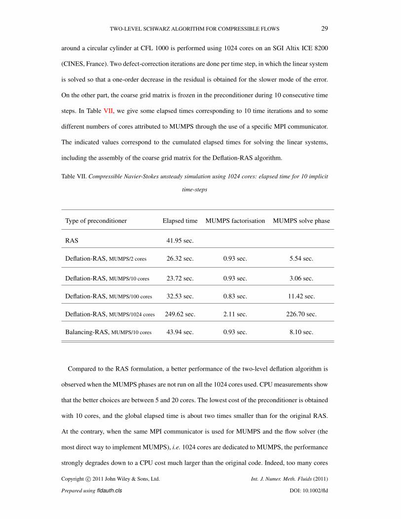
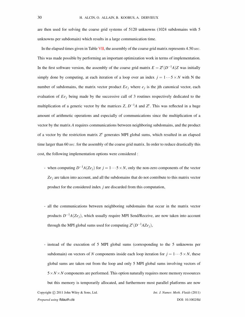
steps. In Table VII, we give some elapsed times corresponding to 10 time iterations and to some
different numbers of cores attributed to MUMPS through the use of a specific MPI communicator.
The indicated values correspond to the cumulated elapsed times for solving the linear systems,
including the assembly of the coarse grid matrix for the Deflation-RAS algorithm.
Table VII. Compressible Navier-Stokes unsteady simulation using 1024 cores: elapsed time for 10 implicit
time-steps
Type of preconditioner Elapsed time MUMPS factorisation MUMPS solve phase
RAS 41.95 sec.
Deflation-RAS, MUMPS/2 cores 26.32 sec. 0.93 sec. 5.54 sec.
Deflation-RAS, MUMPS/10 cores 23.72 sec. 0.93 sec. 3.06 sec.
Deflation-RAS, MUMPS/100 cores 32.53 sec. 0.83 sec. 11.42 sec.
Deflation-RAS, MUMPS/1024 cores 249.62 sec. 2.11 sec. 226.70 sec.
Balancing-RAS, MUMPS/10 cores 43.94 sec. 0.93 sec. 8.10 sec.
Compared to the RAS formulation, a better performance of the two-level deflation algorithm is
observed when the MUMPS phases are not run on all the 1024 cores used. CPU measurements show
that the better choices are between 5 and 20 cores. The lowest cost of the preconditioner is obtained
with 10 cores, and the global elapsed time is about two times smaller than for the original RAS.
At the contrary, when the same MPI communicator is used for MUMPS and the flow solver (the
most direct way to implement MUMPS), i.e. 1024 cores are dedicated to MUMPS, the performance
strongly degrades down to a CPU cost much larger than the original code. Indeed, too many cores
Copyright c© 2011 John Wiley & Sons, Ltd. Int. J. Numer. Meth. Fluids (2011)
Prepared using fldauth.cls DOI: 10.1002/fld
30 H. ALCIN, O. ALLAIN, B. KOOBUS, A. DERVIEUX
are then used for solving the coarse grid systems of 5120 unknowns (1024 subdomains with 5
unknowns per subdomain) which results in a large communication time.
In the elapsed times given in Table VII, the assembly of the coarse grid matrix represents 4.50 sec.
This was made possible by performing an important optimization work in terms of implementation.
In the first software version, the assembly of the coarse grid matrix E = Zt(D−1A)Z was initially
simply done by computing, at each iteration of a loop over an index j = 1 · · ·5×N with N the
number of subdomains, the matrix vector product Ee j where e j is the jth canonical vector, each
evaluation of Ee j being made by the successive call of 3 routines respectively dedicated to the
multiplication of a generic vector by the matrices Z, D−1A and Zt . This was reflected in a huge
amount of arithmetic operations and especially of communications since the multiplication of a
vector by the matrix A requires communications between neighboring subdomains, and the product
of a vector by the restriction matrix Zt generates MPI global sums, which resulted in an elapsed
time larger than 60 sec. for the assembly of the coarse grid matrix. In order to reduce drastically this
cost, the following implementation options were considered :
- when computing D−1A(Ze j) for j = 1 · · ·5×N, only the non-zero components of the vector
Ze j are taken into account, and all the subdomains that do not contribute to this matrix vector
product for the considered index j are discarded from this computation,
- all the communications between neighboring subdomains that occur in the matrix vector
products D−1A(Ze j), which usually require MPI Send/Receive, are now taken into account
through the MPI global sums used for computing Zt(D−1AZe j),
- instead of the execution of 5 MPI global sums (corresponding to the 5 unknowns per
subdomain) on vectors of N components inside each loop iteration for j = 1 · · ·5×N, these
global sums are taken out from the loop and only 5 MPI global sums involving vectors of
5×N×N components are performed. This option naturally requires more memory ressources
but this memory is temporarily allocated, and furthermore most parallel platforms are now
Copyright c© 2011 John Wiley & Sons, Ltd. Int. J. Numer. Meth. Fluids (2011)
Prepared using fldauth.cls DOI: 10.1002/fld
TWO-LEVEL SCHWARZ ALGORITHM FOR COMPRESSIBLE FLOWS 31
made of cores with memory of several gigabytes. It is noted that these 5 MPI global sums are
the only communications performed in the optimized assembly of the coarse grid matrix.
In the last line of Table VII, the best performance obtained with the BDD version for this benchmark
is displayed. Although the convergence is better than for DM, the efficiency is disappointing, not
better than for one-level RAS, due to the cost of the building of the Balancing preconditioner.
8. CONCLUDING REMARKS
This paper has addressed several aspects of the application of algebraic coarse grid methods for
Aerodynamics, considering elliptic, advection-diffusion, incompressible and compressible models.
Several types of overlapping are compared for the basic AS algorithm, and show that the no-overlap
option is not necessarily a bad one. High order overlapping can also appear as an efficient option.
The building of a coarse grid for DM or BDD is then presented. The effect of coarse-grid consistency
is also studied. Choosing a consistent coarse grid with smooth basis functions can help for a better
scalability in the case of a diffusion dominated model. However, the case of diffusion-convection
is better addressed with characteristic bases for Peclet as small as 100. Probably, a zonal strategy
adapted to phenomena for which one part of the domain is convection dominated and diffusion
dominated in the other part might be of extra efficiency.
Applications of the two-level methods combined with the Restrictive Additive Schwarz algorithm
are presented for the elliptic step of an incompressible flow. The best option is Deflation. In some
favourable case the gain in efficiency can reach 8.5 for a rather small number of processors,
e.g. 40. An application to a compressible flow is then presented. The pure Restrictive-Additive-
Schwarz algorithm has not a uniform behavior but sometimes appears of rather good scalability.
Non-symmetric two-level versions with right preconditioning are defined. Although Balancing
is converging slightly faster, the most efficient option (in terms of CPU time) is Deflation. The
improvement factor in convergence carried by the two-level methods is smaller than for the elliptic
case, even for a number of processors as high as 1024, but it is still interesting (about 4). It is shown,
Copyright c© 2011 John Wiley & Sons, Ltd. Int. J. Numer. Meth. Fluids (2011)
Prepared using fldauth.cls DOI: 10.1002/fld

32 H. ALCIN, O. ALLAIN, B. KOOBUS, A. DERVIEUX
by performing an unsteady turbulent flow simulation, that the proposed RAS-Deflation algorithm
can be more efficient (up to a factor almost two) than the RAS formulation in terms of CPU time.
9. ACKNOWLEDGEMENTS
The authors wish to thank Mathieu Cloirec of CINES for the kind and efficient support he provided
when running their software on many processors. The authors thank Guillaume Houzeaux and
Mariano Vazquez for the fruitful discussions they had with them. This work has been supported
by French National Research Agency (ANR) through COSINUS program (project ECINADS no
ANR-09-COSI-003). HPC resources from GENCI-[CINES] (Grant 2010-x2010026386 and 2010-
c2009025067) are also gratefully acknowledged.
REFERENCES
1. R. Aitbayev, X.-C. Cai, and M. Paraschivoiu. Parallel two-level methods for three-dimensional transonic
compressible flow simulations on unstructured meshes. In J. Periaux D. E. Keyes, A. Ecer and N. Satofuka, editors,
Proceedings of Parallel CFD’99, Williamsburg, Virginia, May 23-26,1999. Elsevier, 2000.
2. R. Aubry, F. Mut, R. Lohner, and J. R. Cebral. Deflated preconditioned conjugate gradient solvers for the pressure-
Poisson equation. Journal of Computational Physics, 227:24:10196–10208, 2008.
3. J. Bramble, J. Pasciak, and J. Xu. Parallel multilevel preconditioners. Mathematics of Computation, 55(191):1–22,
1990.
4. S.C. Brenner. Two-level additive Schwarz preconditioners for plate elements. Wuhan University Journal of Natural
Sciences, 1:658–667, 1996.
5. X.-C. Cai, C. Farhat, and M. Sarkis. A minimum overlap restricted additive Schwarz preconditioner and
applications in 3D flow simulations. In C. Farhat J. Mandel and AMS X.-C. Cai, eds, editors, The Tenth
International Conference on Domain Decomposition Methods for Partial Differential Equations, August 10-14,
1997 Boulder, Colorado, volume 218. Contemporary Mathematics, 1998.
6. X. C. Cai, W.D. Gropp, D. E. Keyes, and M. D. Tidriri. Newton-Krylov-Schwarz methods in CFD. In F. Hebeker
and R. Rannacher, editors, Proceedings of the International Workshop on Numerical Methods for the Navier-Stokes
Equations, Notes in Numerical Fluid Dynamics, volume 47, pages 17–30. Vieweg Verlag, 1994.
7. X.-C. Cai and M. Sarkis. A Restricted Additive Schwarz preconditioner for general sparse linear systems. SIAM
Journal of Scientific Computing, 21:792–797, 1999.
Copyright c© 2011 John Wiley & Sons, Ltd. Int. J. Numer. Meth. Fluids (2011)
Prepared using fldauth.cls DOI: 10.1002/fld
TWO-LEVEL SCHWARZ ALGORITHM FOR COMPRESSIBLE FLOWS 33
8. S. Camarri, B. Koobus, M.-V. Salvetti, and A. Dervieux. A low-diffusion MUSCL scheme for LES on unstructured
grids. Computers and Fluids, 33:1101–1129, 2004.
9. G. Carre, L. Fournier, and S. Lanteri. Parallel linear multigrid algorithms for the acceleration of compressible flow
calculations. Computer Methods in Applied Mechanics and Engineering, 184(2:22):427–448, 2000.
10. F. Courty and A. Dervieux. Multilevel functional preconditioning for shape optimisation. International Journal
for Computational Fluid Dynamics, 20:7:481–490, 2006.
11. H. A. Van der Vorst. Bi-CGstab: A fast and smoothly converging variant of Bi-CG for the solution of nonsymmetric
linear systems. SIAM Journal on Scientific and Statistical Computing, 13:631–644, 1992.
12. R. Walters E. Nielsen, W. K. Anderson and D. Keyes. Application of Newton-Krylov methodology to a three
dimensional unstructured Euler code. In AIAA 95-1733-CP, June, 1995.
13. A. Frommer and D.B. Szyld. An algebraic convergence theory for Restricted Additive Schwarz methods using
weighted max norms. SIAM Journal on Numerical Analysis, 39:2:463–479, 2001.
14. H. Guillard, A. Janka, and P. Vanek. Analysis of an algebraic Petrov-Galerkin smoothed aggregation multigrid
method. Applied Numerical Mathematics, (58):18611874, 2008.
15. J.L. Hennessy and D.A. Patterson. Computer Architecture: A Quantitative Approach (5th edition). Morgan
Kaufmann, 2011.
16. http://graal.ens lyon.fr/MUMPS.
17. D.E. Keyes. How scalable is domain decomposition in practice? In C.-H. Lai et al., editor, Proceedings of the 11
th International Conference on Domain Decomposition Methods, London, 1998. DDM.org, Augsburg, 1999.
18. B. Koobus, S. Camarri, M.V. Salvetti, S. Wornom, and A. Dervieux. Parallel simulation of three-dimensional
complex flows: Application to two-phase compressible flows and turbulent wakes. Advances in Engineering
Software, 38:328–337, 2007.
19. B. Koobus and C. Farhat. A variational multiscale method for the large eddy simulation of compressible turbulent
flows on unstructured meshes-application to vortex shedding. Computer Methods in Applied Mechanics and
Engineering, 193:1367–1383, 2004.
20. B. Koobus, M.-H. Lallemand, and A. Dervieux. Unstructured volume-agglomeration MG: solution of the Poisson
equation. International Journal for Numerical Methods in Fluids, 18:27–42, 1994.
21. R. Lohner, F. Mut, J.R. Cebral, R. Aubry, and G. Houzeaux. Deflated preconditioned conjugate gradient solvers
for the pressure-Poisson equation: Extensions and improvements. Int. J. Numer. Meth. Engng, Special Issue: In
Memory of Professor Olgierd C. Zienkiewicz (19212009), 87, Issue 1-5:2–14, 2011.
22. J. Mandel. Balancing domain decomposition. Communications in Numerical Methods in Engineering, 9:233–241,
1993.
23. N. Marco, B. Koobus, and A. Dervieux. An additive multilevel preconditioning method and its application to
unstructured meshes. Journal of Scientific Computing, 12:3:233–251, 1997.
24. C.R. Nastase and D. J. Mavriplis. High-order discontinuous galerkin methods using an hp-multigrid approach.
Journal of Computational Physics, 213:1:330–357, 2006.
Copyright c© 2011 John Wiley & Sons, Ltd. Int. J. Numer. Meth. Fluids (2011)
Prepared using fldauth.cls DOI: 10.1002/fld
34 H. ALCIN, O. ALLAIN, B. KOOBUS, A. DERVIEUX
25. F. Nataf, H. Xiang, and V. Dolean. A two level domain decomposition preconditioner based on local Dirichlet-
to-Neumann maps. Comptes Rendus de l’Academie des Sciences Paris, Serie I, Mathematiques, 348:21-22:1163–
1167, 2010.
26. F. Nataf, H. Xiang, V. Dolean, and N. Spillane. A coarse space construction based on local Dirichlet to Neumann
maps. SIAM Journal on Scientific Computing, 33:1623–1642, 2011.
27. R.A. Nicolaides. Deflation of conjugate gradients with applications to boundary value problem. SIAM Journal on
Numerical Analysis, 24:355–365, 1987.
28. I.S. Duff P.R. Amestoy and J.-Y. L’Excellent. Multifrontal parallel distributed symmetric and unsymmetric solvers.
Computer Methods in Applied Mechanics and Engineering, 184:501–520, 2000.
29. Y. Saad, M. Yeung, J. Erhel, and F. Guyomarc’H. A deflated version of the conjugate gradient algorithm. SIAM
Journal on Scientific Computing, 21:5:1909–1926, 2000.
30. M. Sala. An algebraic 2-level domain decomposition preconditioner with applications to the compressible Euler
equations. International Journal for Numerical Methods in Fluids, 40:1551–1560, 2002.
31. M. Sarkis and B. Koobus. A scaled and minimum overlap restricted additive Schwarz method with application on
aerodynamics. Computer Methods in Applied Mechanics and Engineering, 184:391–400, 2000.
32. P. Le Tallec, J. Mandel, and M. Vidrascu. Balancing domain decomposition for plates. Eigth International
Symposium on Domain Decomposition Methods for Partial Differential Equations, Penn State, October 1993,
Contemporary Mathematics, AMS, Providence, 180:515–524, 1994.
33. J.M. Tang, S.P. MacLachlan, R. Nabben, and C. Vuik. A comparison of two-level preconditioners based on
multigrid and deflation. SIAM Journal on Matrix Analysis and Applications, 31:4:1715–1739, 2010.
34. C. Vuik and R. Nabben. A comparison of deflation and the balancing preconditionner. SIAM Journal on Scientific
Computing, 27:5:1742–1759, 2006.
Copyright c© 2011 John Wiley & Sons, Ltd. Int. J. Numer. Meth. Fluids (2011)
Prepared using fldauth.cls DOI: 10.1002/fld