Effects of Spatial Management on Fishing Effort in California’s Groundfish Trawl Fishery:

Results from a Rational Expectations Model with Dynamically Interrelated Variables

March 31, 2006

Michael Dalton

California State University Monterey Bay

1. Introduction

Fisheries are an important source of income for many coastal communities. Starting in

1999, the National Marine Fisheries Service declared several West Coast rockfish species

to be overfished under standards of the Sustainable Fisheries Act (SFA). In response, the

Pacific Fishery Management Council (PFMC) implemented stringent regulations to prevent

further overfishing and rebuild rockfish stocks, with severe economic consequences for many

communities. In 2001, the entire West Coast groundfish fishery was declared a Federal

Disaster. Managing this fishery is a complex task. The fishery’s management plan regulates

commercial and recreational fleets, includes several types of gear, and covers more than

ninety species in three states. Bottom trawling is among the most important sectors of the

fishery, and is managed closely through a limited entry program. Historically, the PFMC

used bimonthly limits on landings to regulate trawlers. The economic objective of these

limits was to produce a uniform flow of groundfish over the year to meet total allowable

catch for each stock. However, bycatch is a problem for trawlers, and as limits on rockfish

landings decreased, regulatory discard by these vessels became critical. To avoid closing

the fishery, the PFMC implemented a Rockfish Conservation Area (RCA) that closed large

parts of the continental shelf to bottom trawling and other types of fishing. The RCA was

established to eliminate, or drastically reduce, levels of fishing effort in areas with the highest

levels of rockfish bycatch.

The RCA is expected to remain intact during the rebuilding period for rockfish stocks, which

could last several decades. During this period, boundaries of the RCA may be adjusted,

depending on stock status and other factors. In some areas, permanent closures to all

types of fishing, known as marine reserves, are being proposed. An important question for

fishery managers in these cases is how the spatial distribution of fishing effort would respond

to the proposed changes. To address this question, this paper develops a microeconomic

model of groundfish trawlers that is both dynamic and spatial, which is based on a rational

expectations competitive equilibrium. Advantages of a rational expectations model for the

work in this paper include an explicit representation of information sets held by individuals at

1

each point in time. In addition, this model has an operational, and thus testable, mechanism

for translating information sets held by individuals into predictions about the future that can

affect aggregate outcomes. While perhaps not strictly necessary in every economic study,

these features of the model are important for understanding economic behavior in settings,

such as fisheries, that are characterized by a high degree of uncertainty.

Uncertainty is a fundamental part of many fisheries that can affect decisions about fishing

effort. Marine economics contains a substantial literature on effects of uncertainty, and this

topic is also important in other areas of economics. In a fisheries setting, some studies use

linear rational expectations models to analyze how information available to fishermen may

be used to make forecasts of future variables that affect current decisions (Rosenman, 1986;

Rosenman, 1987; Rosenman and Whiteman, 1987; Dalton, 2001; Dalton and Ralston, 2004).

Rosenman (1986) analyzed theoretical implications of the rational expectations hypothesis

for fisheries management in a bioeconomic fisheries model. Rosenman (1987) applied the

bioeconomic model to fisheries data using rational expectations to derive a set of identifying

restrictions. Dalton (2001) extended this type of analysis to test rational expectations, and

other assumptions in the model, for a diverse set of fisheries, but limited geographically,

to a few adjacent ports in California. Recently, Dalton and Ralston (2004) developed a

spatial version of the linear rational expectations model, and applied it to time series data

for groundfish trawlers at a single port in California to test for spatial differences within

this group of vessels. While that analysis was given primarily to detect whether spatial

heterogeneity is measurable, the model in that analysis is spatially restricted because it

excludes dynamic relationships among spatial variables. In other words, by excluding these

relationships, even significant spatial heterogeneity is neutral, from the point of view of

spatial management, in the model without dynamically interrelated variables because closing

an area, such as the RCA, has at most minor and indirect effects on future fishing effort in

the open area.

The use of spatial management, including marine reserves, is increasing in fisheries manage-

ment, and this type of zoning to regulate use has a long tradition in terrestrial conservation

and management, too. To evaluate aggregate impacts of a change in spatial regulations,

which is typically a legal requirement in the U.S., resource managers should, according to

Lucas (1976), use dynamic models that are consistent with microeconomic theory. How-

ever, a model that is both dynamic and spatial is obviously more complex than its dynamic

or spatial counterparts, and this additional complexity has been confronted recently in the

literature on spatial management in marine resource economics. Because of the analytical

2

challenges associated with the complexity of spatial dynamics, and the effects of uncertainty,

this literature has emphasized the spatial dimension of the problem, and the treatment of

microeconomic dynamics, including the use of information in decision making under uncer-

tainty, has been limited. Several recent studies use discrete choice random utility models

(RUMs) to analyze spatial distributions of fishing effort from panel data that incorporate

effects for individual fishermen (e.g. Holland, et al., 2004). These models provide an appro-

priate and tractable framework for modeling spatial management and other issues in many

fisheries.

However an alternative approach, based on time series methods, may be better suited in some

cases for analyzing fishery dynamics. For example, open access is sometimes used to justify

an assumption that current decisions do not depend on expectations about future conditions,

thus profit maximization for individuals is essentially a static decision in some models. While

the assumption of open access is plausible in many fisheries, groundfish trawlers on the

West Coast are part of a limited entry program, and ignoring information about future

conditions for regulations, stock abundance, or climate would not be optimal. In addition,

Rosenman (1986) showed that a type of open access equilibrium can occur with behavior

that is forward looking, and the dynamic policy implications for fishery managers in this case

are different from those of a static model. Therefore, assumptions about dynamic behavior

should be tested. Practical experience supports this type of testing: Fishermen on the West

Coast are known to modify behavior based on expectations of future conditions. Therefore,

forward looking behavior is a plausible response to uncertainty about future regulations,

price changes, climate fluctuations, or other events. The model in this paper is identical to

the spatial model of fishing effort and dynamic adjustment costs under rational expectations

described in Dalton and Ralston (2004), except that adjustment costs in this paper include

a term for dynamically interrelated variables, which is the underlying mechanism for shifts

in fishing effort analyzed below.

Sec. 2 of the paper describes the rational expectations model, and presents the model’s

regression equations, which are derived in Appendix A. In Sec. 3, the model’s value function

is used to analyze competing dynamic effects of spatial management, and this analysis implies

a dynamic equimarginal principle that is used in the paper to predict shifts in fishing effort

between areas following a closure. Maximum likelihood estimation and test procedures are

described in Sec. 4, and Sec. 5 describes spatial time series data for ten ports that participate

in California’s groundfish trawl fishery that are used with the model. Sec. 6 of the paper

presents results of estimation and tests with the model, and describes simulations with the

3

model that analyze effects of the Rockfish Conservation Area on fishing effort outside of

the closure. In addition, Appendix B gives test results for normality of the residuals, plus

several other types of residual diagnostics, and Appendix C gives results from tests of Granger

causality among the time series for each port.

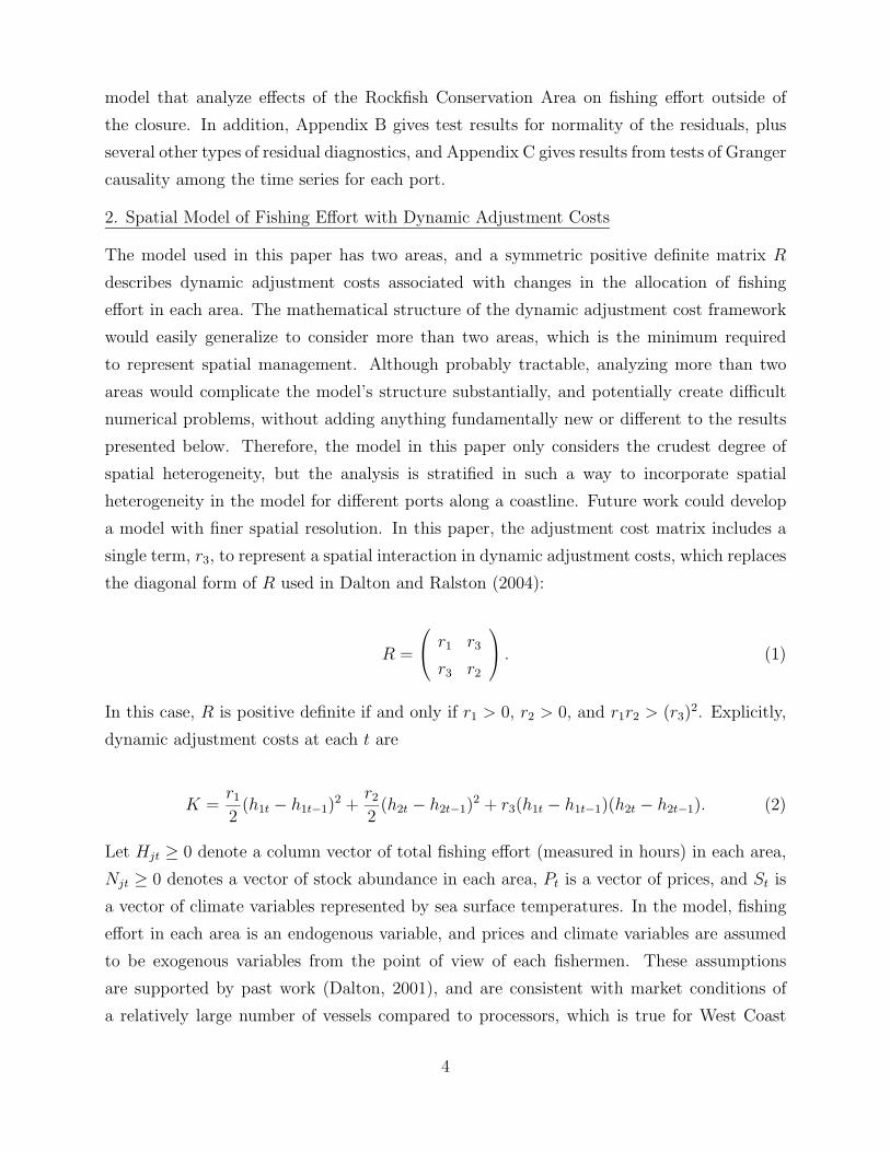
2. Spatial Model of Fishing Effort with Dynamic Adjustment Costs

The model used in this paper has two areas, and a symmetric positive definite matrix R

describes dynamic adjustment costs associated with changes in the allocation of fishing

effort in each area. The mathematical structure of the dynamic adjustment cost framework

would easily generalize to consider more than two areas, which is the minimum required

to represent spatial management. Although probably tractable, analyzing more than two

areas would complicate the model’s structure substantially, and potentially create difficult

numerical problems, without adding anything fundamentally new or different to the results

presented below. Therefore, the model in this paper only considers the crudest degree of

spatial heterogeneity, but the analysis is stratified in such a way to incorporate spatial

heterogeneity in the model for different ports along a coastline. Future work could develop

a model with finer spatial resolution. In this paper, the adjustment cost matrix includes a

single term, r3, to represent a spatial interaction in dynamic adjustment costs, which replaces

the diagonal form of R used in Dalton and Ralston (2004):

R =

r1 r3

r3 r2

. (1)

In this case, R is positive definite if and only if r1 > 0, r2 > 0, and r1r2 > (r3)2. Explicitly,

dynamic adjustment costs at each t are

K =r1

2(h1t − h1t−1)

2 +r2

2(h2t − h2t−1)

2 + r3(h1t − h1t−1)(h2t − h2t−1). (2)

Let Hjt ≥ 0 denote a column vector of total fishing effort (measured in hours) in each area,

Njt ≥ 0 denotes a vector of stock abundance in each area, Pt is a vector of prices, and St is

a vector of climate variables represented by sea surface temperatures. In the model, fishing

effort in each area is an endogenous variable, and prices and climate variables are assumed

to be exogenous variables from the point of view of each fishermen. These assumptions

are supported by past work (Dalton, 2001), and are consistent with market conditions of

a relatively large number of vessels compared to processors, which is true for West Coast

4

groundfish trawlers. Sea surface temperatures in the model are an observed factor that

affects a random shock Xjt to stock dynamics in each area, which is also affected by an

unobservable shock Yjt. Let At, Ht, Nt, Xt, and Yt denote the corresponding column vectors

for each variable. Vectors or matrices with a prime denotes the transpose operator.

Prices of output are exogenous and assumed to be the same for both activities, and are

represented by a scalar Pt. This assumption is easily relaxed, and is made here to simplify

the model with both areas producing a homogeneous output. The shock to the stock in

each area depends on sea surface temperatures, a scalar St, which is assumed to be the same

in both areas. This assumption also easily generalizes, but in this case, variability in sea

surface temperatures is essentially the same in both areas. Let O denote a column vector

of ones, (1, 1)′. Column vectors represent prices Pt = PtO and random variables St = StO.

The εkt are least-squares residuals, each with finite variance and mean zero.

The stochastic process for ex-vessel prices, Pt, has a simple first order form that is interpreted

as a deviation from mean, and may be affected by the exogenous variable for climate,

Pt = φ1Pt−1 + φ2St−1 + εpt. (3)

The random variables that describe climate are also interpreted as a deviation from mean,

in this case sea surface temperature anomalies St. These are assumed to be a first order

Markov process that is not affected by ex-vessel prices,

St = ρ1St−1 + εst. (4)

Effects of exogenous shocks to each stock variable depends on coefficients τj so that Xjt =

τjSt + Yjt. Let T denote the diagonal matrix with components given by τj. The random

variables Yjt are also assumed to be a first order Markov process, in this case described

by parameters λj. Let Λ denote the diagonal matrix with components given by λj. These

diagonal matrices could be generalized, but that would lose the commutative property, which

is used in the derivation of the regression equations presented below. Let Φ be a matrix with

its first row given by each φi, and ρ1 on the diagonal in the second row. This matrix

summarizes dynamics of the vector process qt = (Pt, St)′ for the exogenous variables, which

is important below for deriving optimal forecasts of these variables.

Fishermen are assumed to be identical, and have a discount factor of β = 0.95. Empirical

5

results presented below are conditional on these assumptions. In particular, no attempt is

made in this paper to estimate β, and a value that is typical in economic growth models is

assumed. An assumption of identical agents is typical in the literature on rational expecta-

tions to facilitate the analysis of a symmetric rational expectations competitive equilibrium,

which is the justification in this paper. While convenient, the assumption of identical fish-

ermen, or more presicely fishing operations, may not be justified in some cases, which are

described in the results and discussion below.

Real parameters f0j > 0, f1j ≤ 0, f2j ≥ 0, and f3j ≥ 0 describe the relationship between

productivity in each area, and aggregate levels of fishing effort, stock abundance, and the

price of output for a homogenous product. Real parameters g0j, g1j ≤ 0, and |g2j| < 1

describe the law of motion between aggregate fishing effort and stock abundance. Let Fi

and Gi denote diagonal matrices stacked respectively with fij and gij, for each j = 1, 2. Let

f0 and g0 denote column vectors with components of f0j and g0j for each j = 1, 2. Because

the model is fit to data that are deviations from means, constant terms are collected, and

subsequently, dropped from the regression equations below. In general, constant terms

that would appear in the final form of the regression equations are complicated nonlinear

combinations of values in f0 and g0, and these structural parameters are probably difficult

to identify. Dropping these terms from the regressions, which represent fixed effects in the

model, is consistent with, and perhaps aids, the assumption of identical fishing operations.

Fishing operations are assumed perfectly competitive and fishermen view prices, stock abun-

dance, and aggregate levels of fishing effort, as exogenous variables. These effects are sum-

marized by an exogenous term for net revenue per unit effort, expressed in matrix form

by

At = f0 + F1Ht + F2Nt + F3Pt. (5)

Let E denote the unconditional expectations operator, and Et, the expectation conditional

on information available at date t. The firms’s problem is to choose a sequence of random

vectors ht ≥ 0 that solve

max E∑∞

t=0 βt(At · ht − 1

2(ht − ht−1)

′R(ht − ht−1))

s.t. Ajt = f0j + f1jHjt + f2jNjt + f3jPt,

Njt = g0j + g1jHjt − g1jg2jHjt−1 + g2jNjt−1 + Xjt.

(6)

6

Solution of the stochastic dynamic optimization problem in (6) is not the topic of this paper.

Its key steps are described by Dalton and Ralston (2004), and only final results of the

solution, in the form of regression equations for fishing effort in each area, are presented.

Under rational expectations, these equations contain several terms that are complicated

functions of the model’s underlying structural parameters, including a constant vector c that

is safely ignored in the regressions because data for variables are represented as deviations

from means.

Each Γi is a matrix factor of the model’s characteristic equation that depends on the struc-

tural parameters in F1, F2, G1, and R. Each Θi is a matrix term that summarizes fisher-

men’s optimal forecasts (i.e. rational expectations) of prices and climate according to the

Wiener-Kolmogorov least-squares prediction formula. These terms are derived from a Jor-

dan decomposition of Φ, matrix factors of the model’s characteristic polynomial Γi, and a

matrix version of the geometric formula. To conform with each Θi, block diagonal matrices

Φ, and Qt, are defined with copies of Φ, and qt, respectively, in the upper and lower blocks.

Recall that O is a column vector of ones.

Decision rules for fishing effort in a symmetric rational expectations competitive equilibrium

are the same for each individual, or hjt = Hjt, without loss of generality. These optimal

decision rules are characterized by the construction of a vector of conditional mean zero

random variables, Ut, which are rational in the sense these are orthogonal to all variables in

the model dated t − 1 or earlier, or Et−1Ut = 0. Thus, these conditional mean zero random

variables appear as disturbances in the optimal decision rules.

The optimal decision rules are expressed here as a stochastic difference equation in matrix

notation:

Ht = c + (Λ + Γ1 + Γ3)Ht−1 − (ΛΓ1 + ΛΓ3 + Γ1Γ3) Ht−2 + ΛΓ1Γ3Ht−3 +1

β(ΘpΦ − ΛΘp)Qt−1R

−1F3O +1

β(ΘsΦ − ΛΘs)Qt−1R

−1F2TO −1

βG2ΘpQt−1R

−1F3O +1

βΛG2ΘpQt−2R

−1F3O + Ut. (7)

The optimal decision rules desribed by (7), and dynamics of exogenous variables given by

(3) and (4), are a system of regression equations that may be estimated in the time domain

using a maximum likelihood approach, which is described below. An interpretation of (7) is

complicated because the matrix coefficients embody nonlinear restrictions implied by rational

7

expectations on structural parameters in the model. A special case of the model with F2 = 0,

F3 = 1, and r3 = 0, is similar to Sargent’s (1978) model of dynamic labor demand under

rational expectations. A notable difference is that F1 represents effects of a congestion

externality on net productivity in (5), but this term appears as an internal cost in Sargent’s

model. For cases with r3 = 0, Sargent notes that components of these matrices depend on

the terms (f1i + f2ig1i)/ri, and in particular, stable roots and inverses of the unstable roots

are decreasing functions of these terms. Therefore, an increase in adjustment costs causes

increases in the stable roots of Γ1, and decreases in the unstable roots of Γ2, which implies

that firms respond more slowly to new information.

3. Dynamic Effects of Spatial Management

The optimal decision rules in (7) may be substituted into the objective function in (6) to

define the model’s value function V (H1, H2) from stochastic dynamic programming (e.g.

Stokey and Lucas, 1989). With initial levels of fishing effort in each area as input, this

function gives the long run expected value for a fishery that follows the optimal decision

rules in (7). The value function, and the term for adjustment costs in (2), provide a theoret-

ical framework for analyzing the dynamic response of groundfish trawlers to closure of the

Rockfish Conservation Area (RCA) after the 2001 fishing season.

The RCA was established in a relatively rapid process following the declaration of several

overfished stocks, and in this case, implementation of spatial management on a coast-wide

scale may be characterized to a first approximation as a sudden and unforeseen structural

shift such that H2t = 0 in the model after 2001. In this case, the conditional value function

V (H, 0) determines the long run economic benefit of choosing a level H of trawl effort for

the open area in 2002. However according to (2), changes in H incur two distinct types

of adjustment costs. The first type is the usual sort of dynamic adjustment cost that is

proportional to the squared difference of H, in 2002, with its value in 2001. The second type

arises from dynamically interrelated variables, in this case, between trawl effort in areas

inside, and outside, the RCA. Implementation of the RCA after the 2001 fishery imposes a

specific type of irreversibility on dynamic decisions because the negative adjustment of effort

inside the RCA between 2001 and 2002 is unavoidable, and thus, a sunk cost. To describe

these effects, denote levels of trawl effort in areas outside, and inside, the RCA in 2001 by

H1, and H2, respectively. Minimizing adjustment costs in the short run, by differentiating

(2), implies that r1(H − H1) − r3H2 = 0, or

8

H − H1 =r3

r1

H2. (8)

From assumptions above, r1 > 0, but r3 may be positive, or negative. Therefore, according

to (8), the direction of dynamic shifts in effort following an area closure are indeterminate

in the adjustment cost framework with dynamically interrelated variables. In other words

increases, or reductions, in fishing effort are possible in the area that remains open following

a closure, and which occurs depends on if dynamic variables that represent fishing effort in

each area are positively, or negatively, interrelated. If r3 > 0, then effort that is displaced

from the closed area moves into the open area, and these areas may be considered to exhibit

a type of substitution in production, but greater adjustment costs in the open area, as

represented by larger values of r1, diminish this effect. On the other hand, if r3 < 0, then

the two areas tend to complement each other in production, and closing one area leads to

reduced effort in the other. In general, rational fishermen would balance the competing

effects of short run adjustment costs, and long run economic benefits, by choosing a change

in effort that satisfies

r1(H − H1) − r3H2 = β∂V

∂H(H, 0). (9)

This equation is a dynamic equimarginal principle for spatial resource management that

equates marginal adjustment costs r1(H − H1), net of an effort shift term proportional to

H2 that minimizes adjustment costs from the closure, with the marginal expected present

value of the resource. The next section describes how the regression model defined by (3),

(4), and (7) is estimated, and tested. These estimates are used to simulate the model, and in

particular, to compute values for the partial derivative in (9), which is done by simulating the

model’s value function. Estimation and testing is a separate, and preliminary, step to model

simulation, but is interesting by itself because rational expectations have not been tested

for fisheries on this spatial scale before, or with dynamically interrelated variables. Results

from model simulations are included in this paper to demonstrate exactly how rational

expectations models can contribute to informed resource management, and specifically, on

issues of spatial management. For these issues, complications introduced by dynamically

interrelated variables may very well reinforce Lucas’ (1976) critique of econometric policy

evaluation that does not explicitly model the structural decision rules of individuals.

4. Maximum Likelihood Estimation and Testing Procedure

9

For the maximum likelihood procedure, define a stacked vector of residuals for (3), (4), and

(7) by u′t = (U1t, U2t, εpt, εst). Assume that ut has a multivariate normal distribution with

zero mean Eut = 0, and finite covariance matrix Eutu′t = Σ. The likelihood function for a

sample of observations with residuals ut, t = 1, . . . ,m is

L = (2π)−m|Σ|− 12m exp

(−1

2

m∑t=1

u′tΣ

−1ut

). (10)

Following Sargent (1978), the maximum likelihood estimate of Σ is the sample covariance

matrix

Σ =1

m

m∑t=1

utu′t. (11)

The determinant of the covariance matrix |Σ| is minimized with respect to each of the model’s

parameters to obtain maximum likelihood estimates. Note that the maximum likelihood es-

timates computed using this procedure provide an estimate of the sample covariance matrix,

which determine variance estimates for the processes in (3) and (4). A procedure based on

the conjugate gradient method of Fletcher-Reeves-Polak-Ribiere (Press et al., 1996) is used

to minimize (10) with respect to structural parameters in F1, F2, F3, G1, G2, R, T , Λ, and

Φ conditional on data in Ht, Pt, and St. A separate procedure is used for hypothesis test-

ing based on a standard likelihood ratio statistic described in Sargent (1978), or Hamilton

(1994). In this case, the likelihood ratio is m(ln |Σr| − ln |Σu|), where Σr and Σu are the

restricted and unrestricted estimates of Σ, respectively. The asymptotic distribution of this

statistic is chi-squared, with degrees of freedom equal to the number of restrictions implied

by rational expectations, or other hypothesis under consideration. Fortran code that was

developed for estimation, testing, and model simulation, is available by request.

5. Fisheries Data

Data from the Pacific Fisheries Information Network (PacFIN) are used for estimation and

testing of the rational expectations model. PacFIN is an ongoing census, starting in 1981, of

commercial fishing vessels that operate off the coasts of California, Oregon, and Washington.

These data are extensive, and the scope of analysis in this paper is limited to the most

prevalent fishing strategy of groundfish trawlers in California, which is to target the Dover

sole-Thornyheads-Sablefish (DTS) complex. Only trawlers that landed DTS species are

included in the analysis, and only tows that yielded DTS species are counted as fishing effort.

10

Important structural changes occured in the West Coast groundfish trawl fishery after 2001,

including the Rockfish Conservation Areas and a vessel buyback program. Therefore, time

series data used for estimation and testing are limited to the period from 1981-2001. Logbook

data from the West Coast Limited Entry Groundfish Trawl Fishery have information on

species composition and location of individual tows by each vessel in the fishery. Data

from the trawl logbooks are linked to corresponding data in PacFIN fish tickets, which are

available for all commercial landings in California, Oregon, and Washington. Data from fish

tickets are used to calculate ex-vessel revenues and landed weights of different species for

each fishing trip, and these variables are used to construct an index of ex-vessel prices.

An untested assumption used in this paper is that ex-vessel prices are the same across vessels

at each port in a given year, which may not be accurate at a finer spatial or temporal scale.

For example, size or other characteristics of target species may be influenced by location,

but spatial information in the fish tickets is limited and is often not consistent with the

logbook records. Standard economic assumptions imply price-taking behavior on the part

of individual vessel operators, and prices are the same for all vessels at each port. These

assumptions may be be violated in practice, but testing these is left for future work. The

working assumption in this paper is that a simple ex-vessel price index, formed by the total

ex-vessel value divided by the total landed weight of DTS species in a year at each port,

adequately and exogenously describes the return for all vessels there.

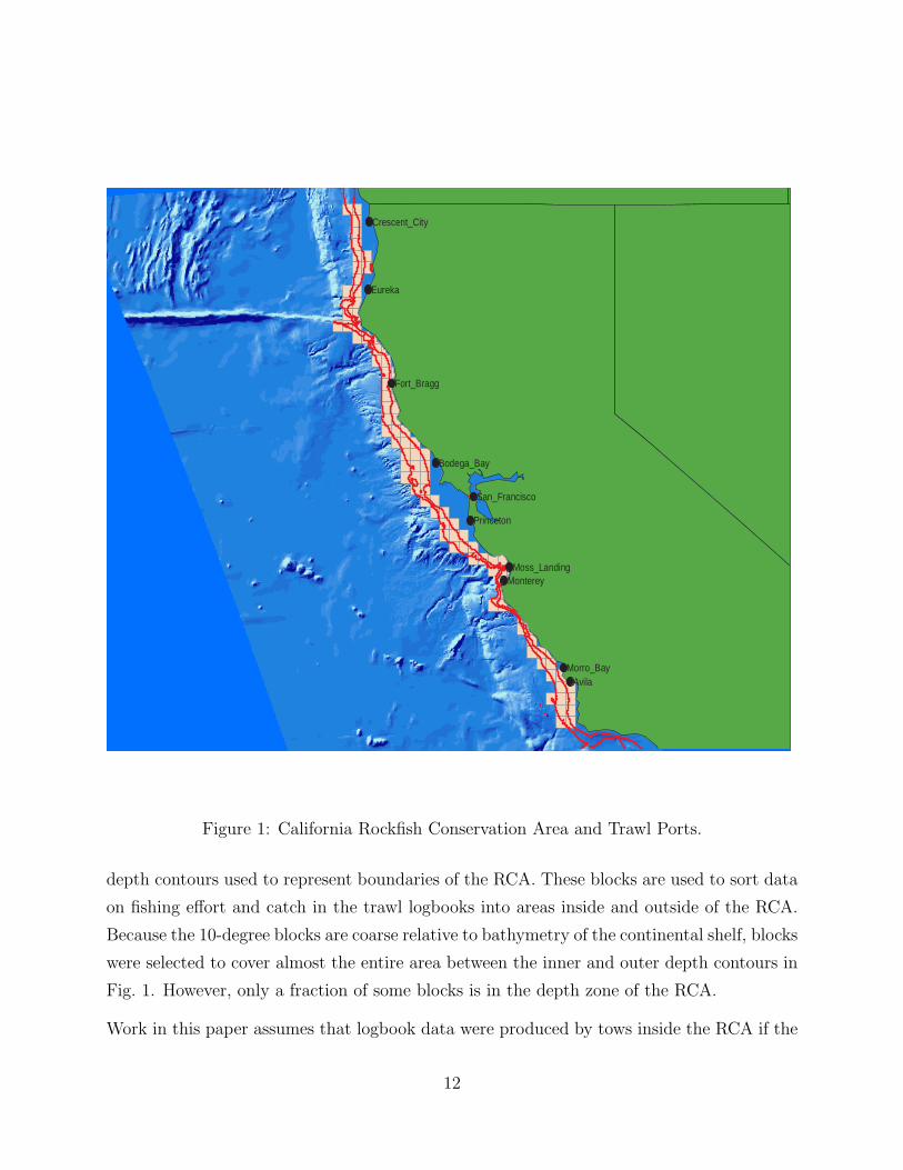
Fig. 1 is a map of California, with bathymetry of the adjacent Exclusive Economic Zone

(EEZ), north of Point Conception, the southern limit for most trawling. The map shows

ten ports that participate in California’s groundfish trawl fishery which are included in the

analysis of this paper. Note the geographic ordering of ports from north to south because

this order is used to present data and results below. The two curves along the coast in Fig. 1

identify the depth contours that represent the inner and outer boundaries of the RCA in

California. The contours in the figure are at 100 and 450 meters, respectively, and are based

on bathymetry data available in GIS files from California Department of Fish and Game

(CDFG). These depth contours are closest in the bathymetry data to the original depth

contours in the RCA of 50-250 fathoms.

CDFG collects logbooks, and records data from these for PacFIN. CDFG manages data

on the location of individual tows using a system of statistical fishing blocks, composed

typically of 10-degree grid cells. GIS files for the statistical fishing blocks are also available

from CDFG. The fishing blocks highlighted in Fig. 1 are contained in, or intersect, the

11

Avila

Eureka

Monterey

Princeton

Morro_Bay

Fort_Bragg

Bodega_Bay

Moss_Landing

San_Francisco

Crescent_City

Figure 1: California Rockfish Conservation Area and Trawl Ports.

depth contours used to represent boundaries of the RCA. These blocks are used to sort data

on fishing effort and catch in the trawl logbooks into areas inside and outside of the RCA.

Because the 10-degree blocks are coarse relative to bathymetry of the continental shelf, blocks

were selected to cover almost the entire area between the inner and outer depth contours in

Fig. 1. However, only a fraction of some blocks is in the depth zone of the RCA.

Work in this paper assumes that logbook data were produced by tows inside the RCA if the

12

corresponding fishing block where the tow occurred has more than 10% of its area in the

depth zone of the RCA. The rationale for this assumption is that trawling for DTS species

is often done by locating a particular depth, starting a tow, and maintaining the starting

depth for the duration of the tow. Blocks that intersect the inner boundary are typically

close to land, and therefore, also affected by California’s ban on trawling within two miles

of the coast. Areas outside of the RCA are further from port and less safe. In addition,

blocks that intersect the outer boundary of the RCA often have sharp changes in bathymetry

along features unsuitable for bottom trawling such as Monterey Canyon, or the edge of the

continental shelf, which are both visible in Fig. 1. Therefore, a reasonable assumption for

fishing blocks that intersect the depth contours in Fig. 1 is that trawling was concentrated

in the area now inside the RCA.

The data used for the analysis in this paper consist of annual time series for ex-vessel prices

and fishing effort at each port, inside and outside of the RCA, for individual trawlers on

trips that yielded DTS landings at the ports in Fig. 1. Aggregating to annual levels is

for convenience, and avoids effects of seasonality in the underlying data. Logbook records

provide information on species composition and duration of individual tows for each fishing

trip by a vessel. The total duration over a year of tows that yielded DTS species within an

area for an individual vessel on trips that landed at a particular port is the basic unit of data

for analysis in this paper. These data form a time-series of ex-vessel prices for each port that

is associated with a panel of fishing effort, measured in terms of tow hours per year, inside

and outside of the RCA.

The maximum number of individual vessels at a single port is thirty-seven, and the minimum

is three, which just satisfies the conventional rule-of-three for preserving confidentiality, a

legal requirement of using PacFIN data. The condition used in this paper for associating a

vessel with a port are records for at least six years of landings there, which is generally nec-

essary for convergence of the estimation procedure used in a separate set of panel regressions

based on data for individual vessels (Dalton, 2005). These panel regressions are not the topic

of this paper, but some results from these are presented below to evaluate the significance

of assuming identical fishermen in the model, and of using pooled time series data for the

analysis. A separate analysis is conducted for each port, treating each as indepedent. In

particular, effort levels at different ports by a single vessel are assumed to be independent

events, but the effects of this assumption are probably small. Of the one hundred vessels

considered in the panel, seventeen satisfy the landings condition at two or more ports, and

seven of these involve two adjacent ports in Northern California: Crescent City and Fort

13

Bragg. Only one vessel, which is in the group of seven, satisfies the minimum landings

condition at three ports. Future work could include choice of port as another factor in the

analysis.

The spatial distribution of fishing effort is typically symmetric about a port, and therefore,

transportation costs to a particular location for a set of tows are likely to be roughly pro-

portional to the straight line distance to that location, and fuel costs during a set of tows

roughly proportional to duration. Therefore, costs incurred traveling from port to the loca-

tion of a tow are treated as a separate fixed factor at each port for areas inside and outside

of the RCA. This assumption ignores variation in travel and other variable costs within each

area, which are assumed to be smaller than the variation in travel costs to the areas outside

the RCA, which are not only further from port, but can also require gear modifications such

as more line for the trawl net to accomodate bottom trawling in deeper water.

14

1 2 3 4 5 6 7 8 9 10 11 12 13 14 15 16 17 18 19 20 21

0

2000

4000

6000

TOW

HOU

RS

0.0

0.2

0.4

0.6

0.8

1.0

PRIC

E ($

/LB.

)

CRESCENT CITY

RCAOUTPRICE

1 2 3 4 5 6 7 8 9 10 11 12 13 14 15 16 17 18 19 20 211000

3000

5000

7000

9000

11000

TOW

HOU

RS

0.0

0.2

0.4

0.6

0.8

1.0

PRIC

E ($

/LB.

)

EUREKA

RCAOUTPRICE

1 2 3 4 5 6 7 8 9 10 11 12 13 14 15 16 17 18 19 20 210

2000

4000

6000

8000

TOW

HOU

RS

0.0

0.2

0.4

0.6

0.8

1.0

PRIC

E ($

/LB.

)

FORT BRAGG

RCAOUTPRICE

1 2 3 4 5 6 7 8 9 10 11 12 13 14 15 16 17 18 19 20 21

0

1000

2000

3000

4000

TOW

HOU

RS

0.0

0.2

0.4

0.6

0.8

1.0

PRIC

E ($

/LB.

)

BODEGA BAY

RCAOUTPRICE

1 2 3 4 5 6 7 8 9 10 11 12 13 14 15 16 17 18 19 20 21

0

500

1000

1500

2000

2500

TOW

HOU

RS

0.0

0.2

0.4

0.6

0.8

1.0

PRIC

E ($

/LB.

)

SAN FRANCISCO

RCAOUTPRICE

1 2 3 4 5 6 7 8 9 10 11 12 13 14 15 16 17 18 19 20 21

0

500

1000

1500

2000

TOW

HOU

RS

0.0

0.2

0.4

0.6

0.8

1.0

PRIC

E ($

/LB.

)

PRINCETON

RCAOUTPRICE

1 2 3 4 5 6 7 8 9 10 11 12 13 14 15 16 17 18 19 20 21

0

500

1000

1500

2000

TOW

HOU

RS

0.0

0.2

0.4

0.6

0.8

1.0

PRIC

E ($

/LB.

)

MOSS LANDING

RCAOUTPRICE

1 2 3 4 5 6 7 8 9 10 11 12 13 14 15 16 17 18 19 20 21

0

500

1000

1500

TOW

HOU

RS

0.0

0.2

0.4

0.6

0.8

1.0

PRIC

E ($

/LB.

)

MONTEREY

RCAOUTPRICE

1 2 3 4 5 6 7 8 9 10 11 12 13 14 15 16 17 18 19 20 21

0

2000

4000

6000

8000

TOW

HOU

RS

0.0

0.2

0.4

0.6

0.8

1.0

PRIC

E ($

/LB.

)

MORRO BAY

RCAOUTPRICE

1 2 3 4 5 6 7 8 9 10 11 12 13 14 15 16 17 18 19 20 21

0

500

1000

1500

TOW

HOU

RS

0.0

0.2

0.4

0.6

0.8

1.0

PRIC

E ($

/LB.

)

AVILA

RCAOUTPRICE

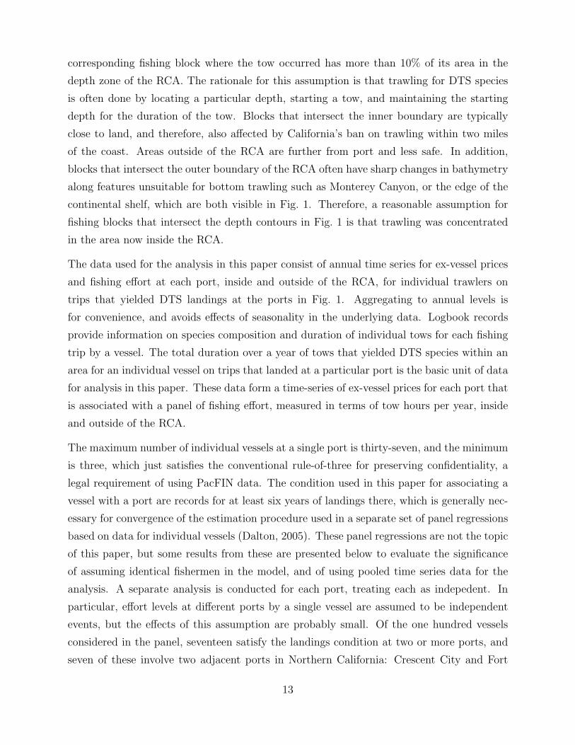
Figure 2: Port Total Tow Hours and Average Ex-Vessel Prices, 1981-2001.

15

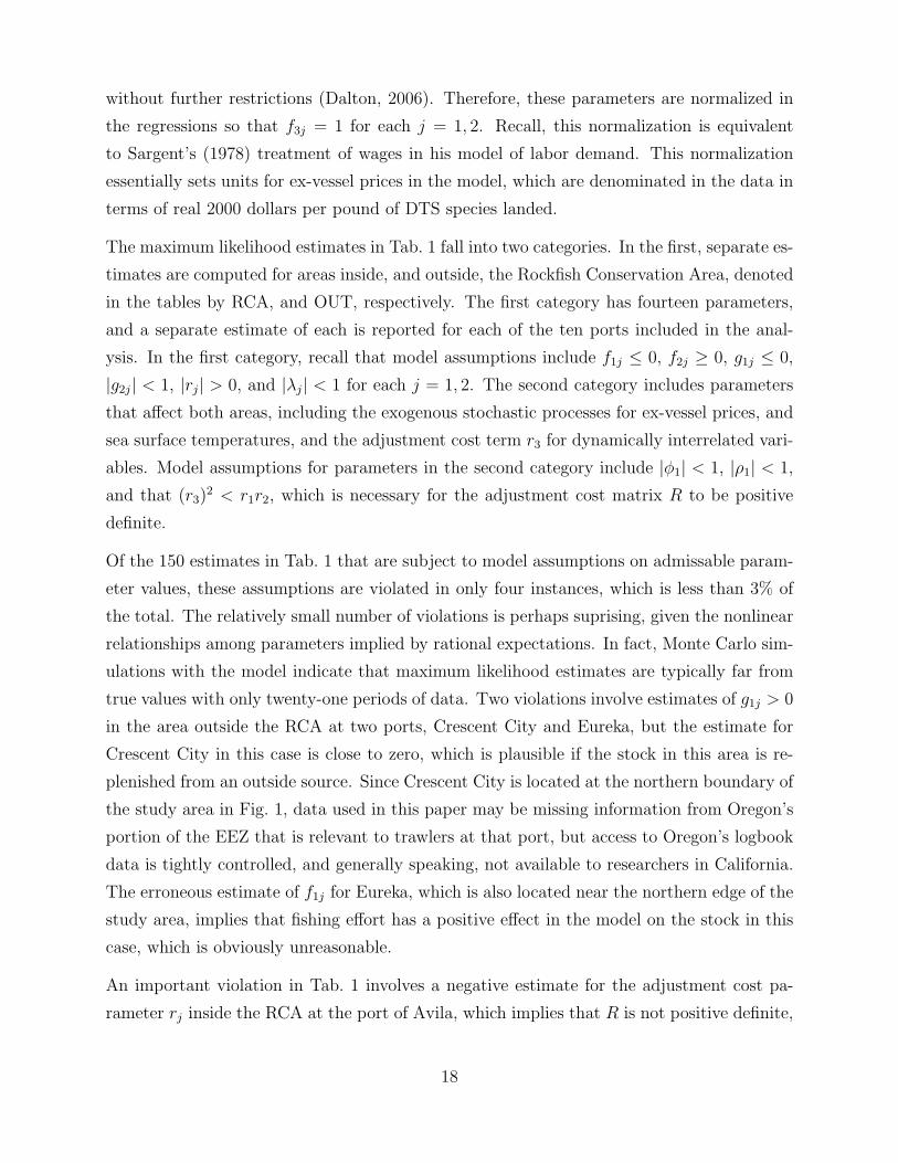
Fig. 2 shows ex-vessel prices, and total tow hours inside and outside of the RCA for DTS

species in the twenty-one years between 1981-2001 at ten ports in California’s groundfish

trawl fishery. Disaggregated data from Fig. 2, for individual vessels, are used for analysis. A

separate analysis is conducted for each of the ten ports in Fig. 1. The plots in Fig. 2 show

an interesting mix of relationships across ports. A downward trend in tow hours after about

1997 is noticeable across ports, which is caused by reductions in bimonthly landings limits

for each vessel. Future work using monthly or bimonthly data could include these landings

limits as a factor for individual vessels, and explicitly consider effects of seasonality. Ex-

vessel prices in Fig. 2 exhibit relatively little variation until about 1994, after which prices

increase for a few years at all ports, and fluctuate thereafter. This rise in prices appears

to be associated with an increase in tow hours at each port, both inside and outside of the

RCA. There is no clear pattern of correlation between tow hours inside and outside of the

RCA, but these do seem related at several ports.

6. Results

Analysis with the model, and time series for each port, is divided into two sets of results.

The first set gives results of estimation and testing using the maximum likelihood procedures

described above, and the second set reports on model simulations that use the maximum

likelihood estimates to evaluate model performance over the period that generated the time

series, 1981-2001, and to forecast effort shifts after 2001, in response to closure of the RCA.

The forecasting strategy is fully dynamic, and is based on simulating the model’s value

function, as described in Sec. 3. Numerical derivatives of the value function are computed

to estimate marginal benefits, which are compared to short run adjustment costs, of shifts

in fishing effort following the closure. The key finding of Sec. 3 is that both expansion and

contraction of fishing effort in the open area following a closure are consistent with dynamic

optimization in the model. In other words, predicting whether an expansion or contraction

occurs is strictly an empirical issue, which is addressed below with maximum likelihood

estimates of a dynamic adjustment cost parameter for dynamically interrelated variables,

and model simulations.

Estimation and Testing

The first set of results are presented in Tab. 1 and Tab. 2. The maximum likelihood estimates

are presented first. As described above, these estimates are computed using the regression

model in (3), (4), and (7), applied to time series data for the ten ports in Fig. 2. Monte Carlo

simulations with the model indicate that parameters in F3 are not identified in the model,

16

Tab

le1:

Max

imum

Lik

elih

ood

Est

imat

esat

Eac

hPor

t,In

side

the

Rock

fish

Con

serv

atio

nA

rea

(RC

A)

and

Outs

ide

(OU

T),

and

Nor

thto

Sou

th:

CR

Sis

Cre

scen

tC

ity,

ER

Kis

Eure

ka,B

RG

isFor

tB

ragg

,B

DG

isB

odeg

aB

ay,SF

isSan

Fra

nci

sco,

PR

Nis

Pri

nce

ton,M

OS

isM

oss

Lan

din

g,M

NT

isM

onte

rey,

MR

Ois

Mor

roB

ay,an

dAV

Lis

Avila.

Por

tC

odes

Par

amet

erA

rea

CR

SE

RK

BR

GB

DG

SF

PR

NM

OS

MN

TM

RO

AV

L

f 1R

CA

-0.3

41-0

.670

-0.2

62-1

.148

-0.3

98-0

.235

-1.1

09-1

.035

-0.5

76-0

.165

OU

T-0

.100

-0.2

14-0

.714

-1.1

18-0

.265

-0.3

74-1

.159

-1.0

99-0

.576

-0.2

04

f 2R

CA

0.46

50.

557

0.46

90.

791

0.48

90.

485

0.65

00.

620

0.54

00.

487

OU

T0.

476

0.53

60.

538

0.78

90.

479

0.50

20.

646

0.62

30.

540

0.48

0

f 3R

CA

1.00

01.

000

1.00

01.

000

1.00

01.

000

1.00

01.

000

1.00

01.

000

OU

T1.

000

1.00

01.

000

1.00

01.

000

1.00

01.

000

1.00

01.

000

1.00

0

g 1R

CA

-0.1

08-0

.289

-0.0

74-0

.536

-0.1

43-0

.067

-0.5

22-0

.478

-0.2

40-0

.042

OU

T0.

024

0.34

0-0

.303

-0.5

06-0

.078

-0.1

35-0

.544

-0.5

09-0

.241

-0.0

42

g 2R

CA

0.27

0-0

.078

-0.7

120.

002

-0.0

330.

644

-0.0

12-0

.187

0.38

30.

139

OU

T-0

.220

0.15

50.

287

0.08

0-0

.380

0.19

50.

196

0.23

60.

702

0.24

7

rR

CA

0.50

81.

369

1.46

00.

258

0.08

90.

182

0.32

20.

502

0.90

2-0

.153

OU

T1.

429

1.11

00.

406

1.07

91.

596

0.28

30.

528

0.58

40.

976

1.76

4

τR

CA

0.02

40.

094

-0.0

60-0

.571

-0.0

040.

003

-0.0

070.

001

0.01

60.

031

OU

T0.

089

0.04

40.

009

0.66

50.

031

-0.0

07-0

.004

0.00

2-0

.004

0.00

8

λR

CA

-0.1

20-0

.078

0.08

70.

335

-0.0

37-0

.306

-0.0

39-0

.042

0.29

70.

330

OU

T-0

.294

-0.3

33-0

.056

0.57

7-0

.427

-0.1

510.

229

0.31

8-0

.356

-0.1

38

φ1

0.89

80.

882

0.81

50.

688

0.67

40.

782

0.78

10.

869

1.28

20.

827

φ2

-0.0

39-0

.022

0.00

80.

027

-0.0

110.

000

-0.0

01-0

.003

-0.0

410.

011

ρ1

-0.0

75-0

.075

-0.0

75-0

.075

-0.0

75-0

.075

-0.0

75-0

.075

-0.0

75-0

.075

r 30.

282

-0.4

390.

280

0.03

10.

079

0.02

3-0

.296

-0.4

54-0

.752

-0.2

82

17

without further restrictions (Dalton, 2006). Therefore, these parameters are normalized in

the regressions so that f3j = 1 for each j = 1, 2. Recall, this normalization is equivalent

to Sargent’s (1978) treatment of wages in his model of labor demand. This normalization

essentially sets units for ex-vessel prices in the model, which are denominated in the data in

terms of real 2000 dollars per pound of DTS species landed.

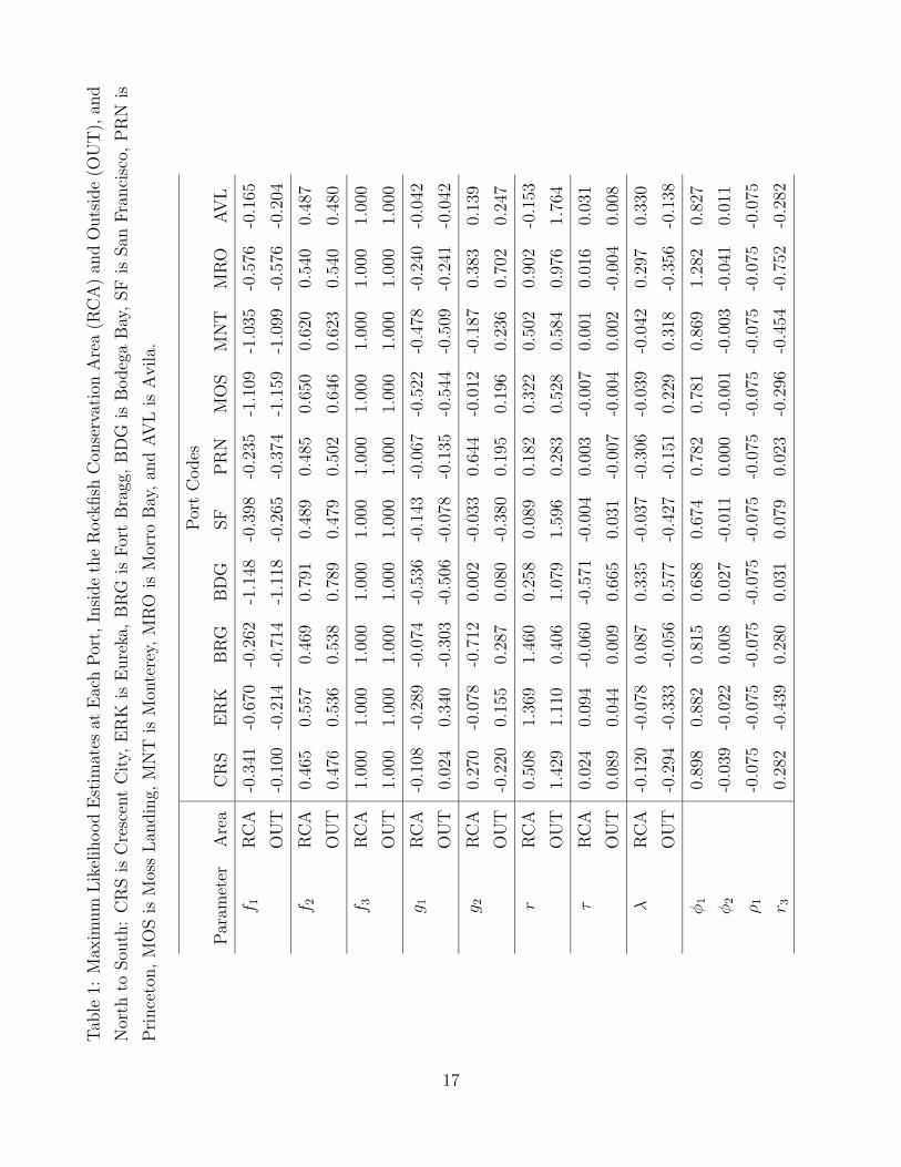
The maximum likelihood estimates in Tab. 1 fall into two categories. In the first, separate es-

timates are computed for areas inside, and outside, the Rockfish Conservation Area, denoted

in the tables by RCA, and OUT, respectively. The first category has fourteen parameters,

and a separate estimate of each is reported for each of the ten ports included in the anal-

ysis. In the first category, recall that model assumptions include f1j ≤ 0, f2j ≥ 0, g1j ≤ 0,

|g2j| < 1, |rj| > 0, and |λj| < 1 for each j = 1, 2. The second category includes parameters

that affect both areas, including the exogenous stochastic processes for ex-vessel prices, and

sea surface temperatures, and the adjustment cost term r3 for dynamically interrelated vari-

ables. Model assumptions for parameters in the second category include |φ1| < 1, |ρ1| < 1,

and that (r3)2 < r1r2, which is necessary for the adjustment cost matrix R to be positive

definite.

Of the 150 estimates in Tab. 1 that are subject to model assumptions on admissable param-

eter values, these assumptions are violated in only four instances, which is less than 3% of

the total. The relatively small number of violations is perhaps suprising, given the nonlinear

relationships among parameters implied by rational expectations. In fact, Monte Carlo sim-

ulations with the model indicate that maximum likelihood estimates are typically far from

true values with only twenty-one periods of data. Two violations involve estimates of g1j > 0

in the area outside the RCA at two ports, Crescent City and Eureka, but the estimate for

Crescent City in this case is close to zero, which is plausible if the stock in this area is re-

plenished from an outside source. Since Crescent City is located at the northern boundary of

the study area in Fig. 1, data used in this paper may be missing information from Oregon’s

portion of the EEZ that is relevant to trawlers at that port, but access to Oregon’s logbook

data is tightly controlled, and generally speaking, not available to researchers in California.

The erroneous estimate of f1j for Eureka, which is also located near the northern edge of the

study area, implies that fishing effort has a positive effect in the model on the stock in this

case, which is obviously unreasonable.

An important violation in Tab. 1 involves a negative estimate for the adjustment cost pa-

rameter rj inside the RCA at the port of Avila, which implies that R is not positive definite,

18

and thus, the dynamic optimization problem in the model for this case is not well defined.

In simulations of the model for Avila, the negative estimate of rj is simply replaced by a

value of one for this parameter. The fourth violation involves the estimate of φ1 > 1 at

Morro Bay. This violation is driven by the sharp increase in ex-vessel prices after 1999 that

can be seen for this port in Fig. 2. The final data point in this series, for 2001, is more than

a dollar per pound, which is well outside the range for other ports, hence an outlier, and

could be an anomaly in the PacFIN data. If this data point is dropped from the regressions,

the estimate of φ1 is similar to other ports, about 0.8, and this value is used instead of the

estimate in Tab. 1 in this case for model simulations.

Other than these four violations, parameter estimates in Tab. 1 appear to be reasonable.

Estimates of f1j are negative, indicating the presence of congestion externalities among

fishing vessels at all ports in the analysis, and these estimates are generally similar inside

and outside the RCA, except for the northern ports. However, estimates of f1j exhibit

substantial variation across ports, and the effects of the congestion externality are greatest

at Bodega Bay, and the ports in Monterey Bay. Estimates of f2j are all positive, and roughly

similar across ports and areas, indicating that larger stocks imply an increase in revenue per

unit effort, which of course makes sense. Estimates of g1j measure the effect of fishing effort

on the stock, and these estimates vary both across ports, and between areas. Like the

congestion externality, impacts of fishing effort on the stock are greatest at Bodega Bay, and

the Monterey Bay ports, which may not be a coincidence. The dynamic stock externality,

which is the hallmark of bioeconomic fisheries models, operates through the impact of fishing

effort on the stock, measured by g1j, and the feedback effect of lower stock sizes on revenue

per unit effort as measured by f2j. Each estimate g2j is within the bounds necessary for

stability of the model at each port, but the estimates vary in sign between areas, and among

ports. Positive and negative estimates of g2j imply that stock dynamics are stable, but differ

qualitatively. In particular, a positive estimate of g2j implies the stock returns to equilibrium

monotonically after a perturbation, but a negative value implies a trajectory that oscillates

back to equilibrium. Estimates of the adjustment cost parameters rj, j = 1, 2, vary among

ports and across areas, and values for these estimates are smallest for ports located in the

middle of the study area, namely Princeton and the Monterey Bay ports. Lower adjustment

costs may be due to the relative accessibility from these ports to the area between Monterey

Bay and San Francisco Bay.

Estimates of τj, which measure effects of sea surface temperatures on stock size in each area,

are typically small. The relatively large, and opposing, values for the two areas at Bodega

19

Bay are probably caused by issues with numerical precision from a weak climate signal for

this port in the middle of the study area. Estimates for Crescent City and Eureka, in the

northern part of the study area, exhibit a slight positive effect from warmer sea surface

temperatures, as do ports of Morro Bay and Avila in the southern part, but the effects are

even smaller in the south than in the north.

Estimates of parameters in (3) and (4) are identified separately, and thus, have more sta-

tistical power in Monte Carlo test than estimates derived from (7). Therefore, the climate

signal observed in ex-vessel prices may be considered stronger than the signal derived from

fishing effort. The signal in ex-vessel prices confirms the geographical pattern described for

estimates of τj. In general, ex-vessel prices exihibit strong positive autocorrelation across

ports, between 0.6−0.9, except for the anomaly at the port of Avila described above. Effects

of warmer sea surface temperatures on ex-vessel prices are typically negligible for ports in

the central part of the study area, such as Princeton or Monterey Bay. However, warmer

temperatures have a negative effect on these prices at the northern ports of Crescent City

and Eureka, which is consistent with larger stocks from warmer temperatures, as indicated

by estimates for these ports of τj > 0, because more landings tend to occur in this case. This

mechanism does not explain results for the southern ports of Morro Bay and Avila, but the

next table shows the sample size is much smaller at these ports. Estimates of λj measure

dynamic effects outside of the model, and these estimates vary among ports and areas. On

the other hand, estimates of autocorrelation in sea surface temperatures are identical at each

port, which is expected, because identical time series for these temperatures are used.

Estimates of r3 indicate the type of dynamic relationship between fishing effort in the two

areas. Recall that positive and negative values of this parameter have different implications

for spatial management. In particular, a positive estimate of r3 implies the two areas are

subsitutes in production, or in other words, that a closure would cause displaced effort to

move into the open area. In contrast, a negative estimate of r3 implies the two areas are

complements in production, and therefore, closing one area could cause a reduction of fishing

effort in the other, but the size of this effect depends on other factors. Half the ports have

positive estimates of r3 in Tab. 1, and with the important exception of Eureka, negative

values are associated with ports in, or south of, Monterey Bay. As described above, negative

values of r3 imply that adjustment costs associated with the closure are greater, and in this

case, the dynamic relationship between variables discourages shifts in fishing effort to the

open area. These predictions of the model could be checked with PacFIN data for 2002, but

a large scale trawl buyback program about that time is a potentially confounding factor.

20

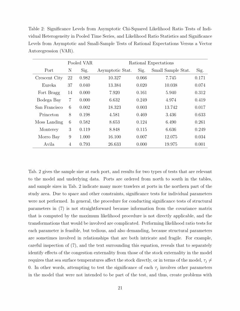
Table 2: Significance Levels from Asymptotic Chi-Squared Likelihood Ratio Tests of Indi-

vidual Heterogeneity in Pooled Time Series, and Likelihood Ratio Statistics and Significance

Levels from Asymptotic and Small-Sample Tests of Rational Expectations Versus a Vector

Autoregression (VAR).

Pooled VAR Rational Expectations

Port N Sig. Asymptotic Stat. Sig. Small Sample Stat. Sig.

Crescent City 22 0.982 10.327 0.066 7.745 0.171

Eureka 37 0.040 13.384 0.020 10.038 0.074

Fort Bragg 14 0.000 7.920 0.161 5.940 0.312

Bodega Bay 7 0.000 6.632 0.249 4.974 0.419

San Francisco 6 0.002 18.323 0.003 13.742 0.017

Princeton 8 0.198 4.581 0.469 3.436 0.633

Moss Landing 6 0.582 8.653 0.124 6.490 0.261

Monterey 3 0.119 8.848 0.115 6.636 0.249

Morro Bay 9 1.000 16.100 0.007 12.075 0.034

Avila 4 0.793 26.633 0.000 19.975 0.001

Tab. 2 gives the sample size at each port, and results for two types of tests that are relevant

to the model and underlying data. Ports are ordered from north to south in the tables,

and sample sizes in Tab. 2 indicate many more trawlers at ports in the northern part of the

study area. Due to space and other constraints, significance tests for individual parameters

were not performed. In general, the procedure for conducting significance tests of structural

parameters in (7) is not straightforward because information from the covariance matrix

that is computed by the maximum likelihood procedure is not directly applicable, and the

transformations that would be involved are complicated. Performing likelihood ratio tests for

each parameter is feasible, but tedious, and also demanding, because structural parameters

are sometimes involved in relationships that are both intricate and fragile. For example,

careful inspection of (7), and the text surrounding this equation, reveals that to separately

identify effects of the congestion externality from those of the stock externality in the model

requires that sea surface temperatures affect the stock directly, or in terms of the model, τj �=0. In other words, attempting to test the significance of each τj involves other parameters

in the model that were not intended to be part of the test, and thus, create problems with

21

interpretation. Some of these problems are addressed in a paper that describes Monte Carlo

simulations with the model presented above (Dalton, 2006).

The first test in Tab. 2 is for significance of restrictions on parameters, at the level of

individual vessels, to obtain unbiased estimates from each pooled time series used in this

paper. Because these results were produced with a different model and analysis, which are

described in a separate paper (Dalton, 2005), only significance levels for the pooled vector

autogression (VAR) are reported as a summary here. A separate likelihood model was

developed to handle the disaggregated panel data used to test the pooled VAR because zero

effort in an area or year by an individual vessel is a frequent event. Aggregating to avoid these

events is a major advantage of using pooled time series because censored variables violate

an assumption that underlies the likelihood procedure used in this paper, which is that error

terms and regressors are uncorrelated. A numerical likelihood simulator was developed to

handle events with zero effort, and an analysis of covariance was performed on the panel

data to test various restrictions on individual heterogeneity. In contrast to the elaborate

regression equations implied by rational expectations in (7), the analysis of covariance uses a

relatively simple first order autoregressive model of fishing effort in two areas, with ex-vessel

prices and sea surface temperatures treated as exogenous fixed factors. The econometric

issues involved with the simulated maximum likelihood approach are outside the scope of

this paper, and only the most relevant test result from that analysis is reported here to inform

the assessment of the model in this paper. The restrictions on individual heterogeneity in a

pooled VAR are clearly rejected at three ports, Fort Bragg, Bodega Bay, and San Francisco,

and marginally rejected (at the 5% level) at another, Eureka. A case could be made to drop

these ports from further analysis, but test results of the pooled VAR may not be conclusive,

and thus, additional tests and model simulations are conducted for each port.

The second test in Tab. 2 is for significance of restrictions on parameters implied by rational

expectations, which are embodied in the regression equations for fishing effort in (7). The

model used as the null hypothesis in the second test is an unrestricted VAR with a general

form that is congruent with (7). In particular, the unrestricted VAR has third order terms

for fishing effort in each area, for each effort equation, and second order terms for ex-vessel

prices and climate. The total number of parameters in the unrestricted VAR is twenty-three,

whereas the rational expectations model has eighteen. Therefore, the chi-squared test has

five degrees of freedom. Two versions of the second test are presented, one based on the

asymptotic distribution, and another adjusted for small samples. Values are given in Tab. 2

for the likelihood ratio statistic and significance level for each version of the test, at each

22

of the ten ports. The small sample test rejects the rational expectations model at the 5%

level for three ports: San Francisco, and the southern most ports of Morro Bay, and Avila.

In addition, the asymptotic test rejects the rational expectations model for Eureka, and

comes close to rejecting the model for Crescent City. It is worth noting here that both tests

of rational expectations performed well in the Monte Carlo simulations cited above, and

generally produced no Type 1 or Type 2 errors, even with time series of the length used

in this paper. In other words, Monte Carlo simulations provide more confidence in the test

results of Tab. 2 than in the estimates of Tab. 1.

Model Simulations

Simulations with the model are divided into two groups. The first group simulates the

regression equations in (7), starting at two different points in time. The first starting point

for the model is 1981, the initial year of the time series, and after filling the three lag variables

for fishing effort on the right hand side of (7), a deterministic projection is computed for the

period 1984-2001. This projection is used to evaluate the model. The second starting point

is 1999. In this case, the final three years of the time series fill the three lag variables, and

the model is projected forward from 2001 to form a baseline for comparison with closure

of the RCA. The second group is based on closing the RCA, which involves simulating the

value function for the model at each port.

23

1 2 3 4 5 6 7 8 9 10 11 12 13 14 15 16 17 18 19 20 21

0

2000

4000

6000

TOW

HO

URS

RCA MODELRCA OBSERVEDOUT MODELOUT OBSERVED

CRESCENT CITY

1 2 3 4 5 6 7 8 9 10 11 12 13 14 15 16 17 18 19 20 21

1000

3000

5000

7000

9000

11000

TOW

HO

URS

RCA MODELRCA OBSERVEDOUT MODELOUT OBSERVED

EUREKA

1 2 3 4 5 6 7 8 9 10 11 12 13 14 15 16 17 18 19 20 21

0

2000

4000

6000

8000

TOW

HO

URS

RCA MODELRCA OBSERVEDOUT MODELOUT OBSERVED

FORT BRAGG

1 2 3 4 5 6 7 8 9 10 11 12 13 14 15 16 17 18 19 20 21

0

1000

2000

3000

4000

TOW

HO

URS

RCA MODELRCA OBSERVEDOUT MODELOUT OBSERVED

BODEGA BAY

1 2 3 4 5 6 7 8 9 10 11 12 13 14 15 16 17 18 19 20 21

0

500

1000

1500

2000

2500

TOW

HO

URS

RCA MODELRCA OBSERVEDOUT MODELOUT OBSERVED

SAN FRANCISCO

1 2 3 4 5 6 7 8 9 10 11 12 13 14 15 16 17 18 19 20 21

0

500

1000

1500

2000

TOW

HO

URS

RCA MODELRCA OBSERVEDOUT MODELOUT OBSERVED

PRINCETON

1 2 3 4 5 6 7 8 9 10 11 12 13 14 15 16 17 18 19 20 21

0

500

1000

1500

2000

TOW

HO

URS

RCA MODELRCA OBSERVEDOUT MODELOUT OBSERVED

MOSS LANDING

1 2 3 4 5 6 7 8 9 10 11 12 13 14 15 16 17 18 19 20 21

0

500

1000

1500

TOW

HO

URS

RCA MODELRCA OBSERVEDOUT MODELOUT OBSERVED

MONTEREY

1 2 3 4 5 6 7 8 9 10 11 12 13 14 15 16 17 18 19 20 21

0

2000

4000

6000

8000

TOW

HO

URS

RCA MODELRCA OBSERVEDOUT MODELOUT OBSERVED

MORRO BAY

1 2 3 4 5 6 7 8 9 10 11 12 13 14 15 16 17 18 19 20 21

0

500

1000

1500

TOW

HO

URS

RCA MODELRCA OBSERVEDOUT MODELOUT OBSERVED

AVILA

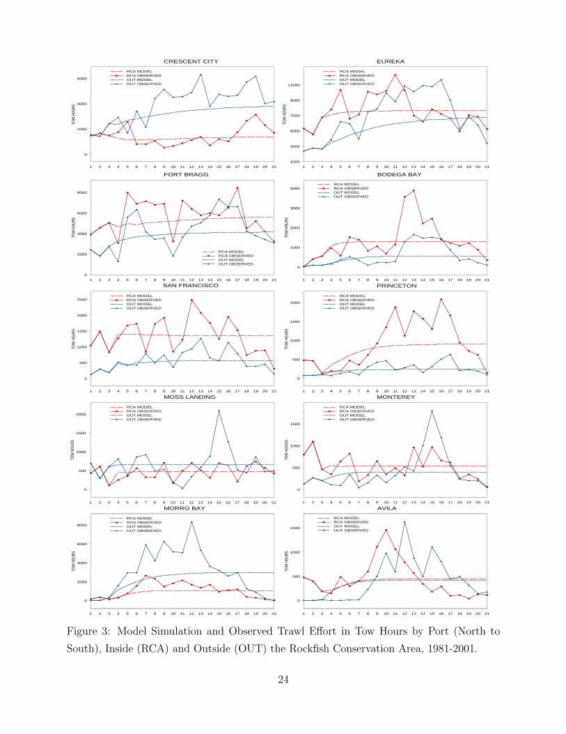
Figure 3: Model Simulation and Observed Trawl Effort in Tow Hours by Port (North to

South), Inside (RCA) and Outside (OUT) the Rockfish Conservation Area, 1981-2001.

24

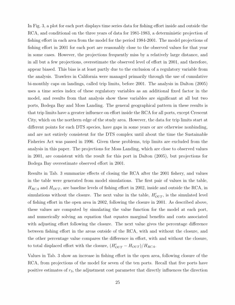
In Fig. 3, a plot for each port displays time series data for fishing effort inside and outside the

RCA, and conditional on the three years of data for 1981-1983, a deterministic projection of

fishing effort in each area from the model for the period 1984-2001. The model projections of

fishing effort in 2001 for each port are reasonably close to the observed values for that year

in some cases. However, the projections frequently miss by a relatively large distance, and

in all but a few projections, overestimate the observed level of effort in 2001, and therefore,

appear biased. This bias is at least partly due to the exclusion of a regulatory variable from

the analysis. Trawlers in California were managed primarily through the use of cumulative

bi-monthly caps on landings, called trip limits, before 2001. The analysis in Dalton (2005)

uses a time series index of these regulatory variables as an additional fixed factor in the

model, and results from that analysis show these variables are significant at all but two

ports, Bodega Bay and Moss Landing. The general geographical pattern in these results is

that trip limits have a greater influence on effort inside the RCA for all ports, except Crescent

City, which on the northern edge of the study area. However, the data for trip limits start at

different points for each DTS species, have gaps in some years or are otherwise nonbinding,

and are not entirely consistent for the DTS complex until about the time the Sustainable

Fisheries Act was passed in 1996. Given these problems, trip limits are excluded from the

analysis in this paper. The projections for Moss Landing, which are close to observed values

in 2001, are consistent with the result for this port in Dalton (2005), but projections for

Bodega Bay overestimate observed effort in 2001.

Results in Tab. 3 summarize effects of closing the RCA after the 2001 fishery, and values

in the table were generated from model simulations. The first pair of values in the table,

HRCA and HOUT , are baseline levels of fishing effort in 2002, inside and outside the RCA, in

simulations without the closure. The next value in the table, H ′OUT , is the simulated level

of fishing effort in the open area in 2002, following the closure in 2001. As described above,

these values are computed by simulating the value function for the model at each port,

and numerically solving an equation that equates marginal benefits and costs associated

with adjusting effort following the closure. The next value gives the percentage difference

between fishing effort in the areas outside of the RCA, with and without the closure, and

the other percentage value compares the difference in effort, with and without the closure,

to total displaced effort with the closure, (H ′OUT − HOUT )/HRCA.

Values in Tab. 3 show an increase in fishing effort in the open area, following closure of the

RCA, from projections of the model for seven of the ten ports. Recall that five ports have

positive estimates of r3, the adjustment cost parameter that directly influences the direction

25

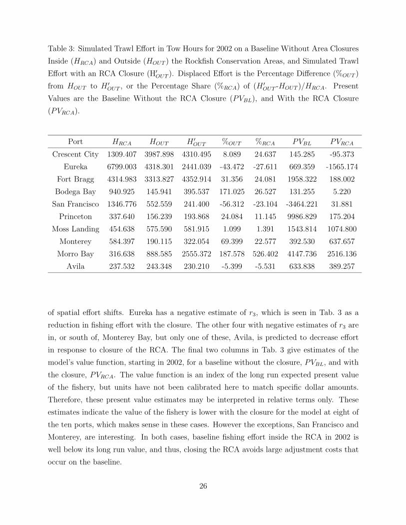
Table 3: Simulated Trawl Effort in Tow Hours for 2002 on a Baseline Without Area Closures

Inside (HRCA) and Outside (HOUT ) the Rockfish Conservation Areas, and Simulated Trawl

Effort with an RCA Closure (H′OUT ). Displaced Effort is the Percentage Difference (%OUT )

from HOUT to H ′OUT , or the Percentage Share (%RCA) of (H ′

OUT -HOUT )/HRCA. Present

Values are the Baseline Without the RCA Closure (PVBL), and With the RCA Closure

(PVRCA).

Port HRCA HOUT H ′OUT %OUT %RCA PVBL PVRCA

Crescent City 1309.407 3987.898 4310.495 8.089 24.637 145.285 -95.373

Eureka 6799.003 4318.301 2441.039 -43.472 -27.611 669.359 -1565.174

Fort Bragg 4314.983 3313.827 4352.914 31.356 24.081 1958.322 188.002

Bodega Bay 940.925 145.941 395.537 171.025 26.527 131.255 5.220

San Francisco 1346.776 552.559 241.400 -56.312 -23.104 -3464.221 31.881

Princeton 337.640 156.239 193.868 24.084 11.145 9986.829 175.204

Moss Landing 454.638 575.590 581.915 1.099 1.391 1543.814 1074.800

Monterey 584.397 190.115 322.054 69.399 22.577 392.530 637.657

Morro Bay 316.638 888.585 2555.372 187.578 526.402 4147.736 2516.136

Avila 237.532 243.348 230.210 -5.399 -5.531 633.838 389.257

of spatial effort shifts. Eureka has a negative estimate of r3, which is seen in Tab. 3 as a

reduction in fishing effort with the closure. The other four with negative estimates of r3 are

in, or south of, Monterey Bay, but only one of these, Avila, is predicted to decrease effort

in response to closure of the RCA. The final two columns in Tab. 3 give estimates of the

model’s value function, starting in 2002, for a baseline without the closure, PVBL, and with

the closure, PVRCA. The value function is an index of the long run expected present value

of the fishery, but units have not been calibrated here to match specific dollar amounts.

Therefore, these present value estimates may be interpreted in relative terms only. These

estimates indicate the value of the fishery is lower with the closure for the model at eight of

the ten ports, which makes sense in these cases. However the exceptions, San Francisco and

Monterey, are interesting. In both cases, baseline fishing effort inside the RCA in 2002 is

well below its long run value, and thus, closing the RCA avoids large adjustment costs that

occur on the baseline.

26

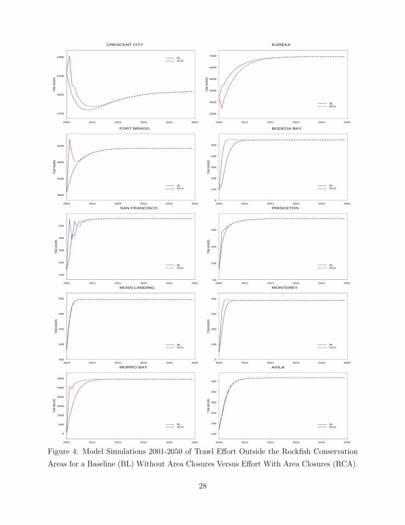
Final results for the analysis of effort shifts are given in Fig. 4. These plots show the

dynamics of fishing effort, in the open area, along a simulated baseline without the closure,

and a simulated response to closure of the RCA. These plots provide a dynamic view of

the simulated data for 2002 in Tab. 3. In particular, the dynamic pattern of effort shifts is

the same as in the table, with closure of the RCA predicted to add effort in the open area

for most ports. Exceptions are Avila, and Moss Landing, where differences are small, San

Francisco where the effort shift is negative in some years, and Eureka, which is predicted to

have substantially lower fishing effort in the open area after the closure. In the figure, the

total shift in effort over time is seen as the area between the baseline and response curves.

The largest positive shifts in fishing effort are predicted to occur at Morro Bay, Bodega Bay,

Fort Bragg, and Crescent City.

Parameter values for each port imply a stable model, and the equilibrium levels of fishing

effort in the open area are the same with, and without, the closure. Therefore, effort shifts

are transitory in the model, and appear that way in Fig. 4, but the speed of convergence

is an interesting property that varies among models for different ports. For example, effort

for most ports stabilizes after the effort shift within about ten years, but this process takes

longer at a few ports, around twenty years for Crescent City and Fort Bragg. Note that

Crescent City is the only port for which fishing effort is predicted to fall in the simulation,

and fishing effort is predicted to increase both along the baseline, and with the RCA closure,

in every other case. For Crescent City, closure of the RCA temporarily reverses the trend

of decreasing effort. A temporary reversal of the baseline trend is also true for Eureka, but

in this case, the closure reduces effort, while it is increasing along the baseline. The process

is similar for San Francisco, but the effort shift is not strong enough to reverse the baseline

trend. In other cases, closure of the RCA creates a shift that reinforces the baseline trend

towards more effort.

27

2001 2011 2021 2031 2041 2051

3700

3900

4100

4300TO

W H

OUR

S

CRESCENT CITY

BLRCA

2001 2011 2021 2031 2041 2051

2000

3000

4000

5000

6000

7000

TOW

HO

URS

EUREKA

BLRCA

2001 2011 2021 2031 2041 2051

3000

3400

3800

4200

TOW

HOU

RS

FORT BRAGG

BLRCA

2001 2011 2021 2031 2041 20510

100

200

300

400

500

TOW

HOU

RS

BODEGA BAY

BLRCA

2001 2011 2021 2031 2041 2051

100

200

300

400

500

TOW

HOU

RS

SAN FRANCISCO

BLRCA

2001 2011 2021 2031 2041 205150

100

150

200

TOW

HOU

RSPRINCETON

BLRCA

2001 2011 2021 2031 2041 2051450

500

550

600

650

TOW

HOU

RS

MOSS LANDING

BLRCA

2001 2011 2021 2031 2041 20510

100

200

300

400

TOW

HOU

RS

MONTEREY

BLRCA

2001 2011 2021 2031 2041 2051

0

500

1000

1500

2000

2500

3000

TOW

HOU

RS

MORRO BAY

BLRCA

2001 2011 2021 2031 2041 2051

150

200

250

300

350

400

TOW

HOU

RS

AVILA

BLRCA

Figure 4: Model Simulations 2001-2050 of Trawl Effort Outside the Rockfish Conservation

Areas for a Baseline (BL) Without Area Closures Versus Effort With Area Closures (RCA).

28

7. Discussion

Responses to spatial management have been an important topic in marine resource manage-

ment recently. Overfished stocks in the U.S. have lead to large closures off both the East

and West Coasts, and globally, there is a large and growing interest in using reserves, and

other types of protected areas, as regulatory tools for the conservation and management of

marine ecosystems. This paper uses a linear rational expectations model to analyze spatial

and dynamic responses of groundfish trawlers to a closure of the Rockfish Conservation Area

(RCA) off the U.S. West Coast.

The model is presented as a set of reression equations that embody the cross equation

parameter restrictions implied by rational expectations. A maximum likelihood approach is

used to estimate and test the model under these restrictions using pooled time series data on

fishing effort, ex-vessel prices, and sea surface temperatures during the period 1981-2001 for

trawl vessels from ten ports in California. The model has several features that recommend

it for this type of analysis, including congestion and stock externalities that are part of

fisheries management, ex-vessel prices and climate as exogenous factors that are known to

affect fisheries, and dynamically interrelated variables to describe spatial interactions in

fishing effort inside and outside the RCA. Explicit treatment of how information is used on

a microeconomic level under rational expectations is a key part of the analysis in this paper,

and subject to validation and testing, structural parameters that are estimated for the model

of each port are considered appropriate for policy analysis.

Maximum likelihood estimates reported in the paper for each port are consistent with as-

sumptions on both the sign, and size, of different parameters in the model for more than 97%

of 150 cases. These assumptions are necessary for model stability, or for dynamic optimiza-

tion in the model to be well defined. Ports with a violation include Crescent City, Eureka,

Morro Bay, and Avila, but two of the four erroneous estimates, one for Crecent City and the

other for Morro Bay, have plausible explanations. Results of an analysis of covariance using

the disaggregated time series are reported in the paper, which indicates that estimates for

Fort Bragg, Bodega Bay, and San Francisco are probably biased.

The parameter restrictions associated with rational expectations are tested by using an

unconstrained vector autoreression (VAR) as an alternative model. A small sample version

of the test rejects rational expectations for San Francisco, Morro Bay, and Avila. Note

the last two are the southern ports in the study area, and are isolated from the others

by the remote Big Sur coastline. Monte Carlo simulations with the model indicate that

29

test results for rational expectations are probably robust to the use of pooled data, in all

cases. Ignoring the potential bias in estimates for Fort Bragg and Bodega Bay, these results

conclude that rational expectations models for seven of the ten ports are suitable for policy

analysis. However for a complete picture, simulations and analysis of the RCA closure

are also presented for the three rejected models. Results of model simulations for a baseline

without closing the RCA are presented in the paper to compare with the closure. Comparison

of the model simulations, and observed time series, over the period 1981-2001 gives mixed

results. The model projections are accurate in 2001 for a few cases, but aside from these,

other projections overestimate the level of fishing effort in 2001, by a substantial amount in

some cases, and the bias seems worse for projections inside the RCA.

The paper shows that an adjustment cost parameter for dynamically interrelated variables is

the most important parameter in the model from the point of view of spatial management. In

particular, the model shows that positive or negative shifts in fishing effort are theoretically

possible in an open area following a closure. This feature of the dynamic adjustment cost

model may be qualitatively different from some models used to estimate site demand, or

other discrete choices, if some degree of substitutability has been imposed on the different

alteranatives in the demand framework. A positive value for the parameter that represents

dynamically interrelated variables indicates the two areas are substitutable in production,

and shifting effort into the open area offsets part of the cost of displaced effort from a closure.

A negative value indicates the two areas complement each other in production, and in this

case, shifting effort into the open area after a closure creates an additional cost. However,

adjustment costs for displaced effort are temporary in the model, and equilibrium levels of

fishing effort in the open area are the same with, and without, the RCA closure.

To predict fishing effort in the open area after a closure, short run adjustment costs are

compared to the long run benefits of displaced effort in the open area using a dynamic

equimarginal principle for spatial management that is satisfied by optimal effort shifts. Solv-

ing for the level of fishing effort that maximizes net benefits in the open area following a

closure involves simulating the model’s value function, and in particular, the marginal value

of fishing effort in the open area, conditional on the closure. A standard numerical procedure,

described in the paper, is used to solve for the level of fishing effort with marginal adjustment

costs equal to the marginal value of effort in the open area. Results for the ten ports in the

analysis show that in most cases a positive shift in displaced effort is expected for an open

area following the RCA closure. However, the port of Eureka is a major exception because

it has thirty-seven vessels, which is almost a third of the sample. The next largest, Crescent

30

City, has twenty-two, and the sample average is about twelve vessels per port. The negative

shift in effort predicted for Eureka is large enough to temporarily reverse a strong upward

trend in baseline fishing effort. In a few cases, effort shifts following the RCA closure are

predicted to be small, such as Princeton, or negligible, such as Moss Landing and Avila, but

each of these also exhibits an upward trend in baseline fishing effort. Model simulations for

five ports have both upward trends in baseline effort in the open area, and exhibit positive

shifts in effort, which are modest to large, following the RCA closure.

Results from the model confirm that displaced effort is a legitimate concern for spatial

management. While that concern is not new, the dynamics of displaced effort is poorly

understood by both fishery managers, and managers of other marine resources. The main

contribution of this paper is to provide a tractable framework for analyzing and forecasting

dynamic responses to spatial management. The model in this paper shows that shifts in

fishing effort following a closure are dynamic and transitory, and that both size and direction

of a shift are empirically driven because both positive and negative shifts are consistent with

microeconomic theory. In other words, both types of behavior can be derived from dynamic

optimization under rational expectations. This paper demonstrates how to estimate and test

a rational expectations model with externalities and dynamically interrelated variables using

spatial time series, and how to analyze the effects of spatial management with simulations

of the model and its value function. While use of the model in this paper applies to area

closures in fisheries, the range of applications for the model, in other types of spatial resource

management, is enormous.

While the rational expectations model in this paper performed reasonably well, it was re-

jected in a few cases, and could be improved in other ways. At a minimum, a version of

the model in this paper based on panel data could provide a major improvement in results

for some ports, such as San Francisco, where both rational expectations and pooled VAR

models are rejected. In addition, a model based on panel data would provide unbiased esti-

mates for the three other ports where the pooled VAR is rejected, including Eureka, which

recall has the most vessels in the sample. However, the major advantage of a linear rational

expectations model based on panel data is the potential gain in statistical power for key

dynamic parameters, including the adjustment cost for dynamically interrelated variables.

The bottom line from Monte Carlo simulations with the model, which are described in

Dalton (2006), is that maximum likelihood estimates can require extremely long time series,

of hundreds or even thousands of periods, to approach true values. These series are much

31

longer than the twenty-one years of data used in this paper, which is a concern. In fact,

spatial time series longer than a few decades, such as data for Pacific halibut, are rare in

fisheries, and in other areas of resource management. Two ways of increasing statistical power

in a given time series seem feasible. One way is to consider a shorter time step, of less than a

year, if the data support it. The fisheries data used in this paper could support a change in

the temporal resolution of the model. A natural time step would be the bi-monthly periods

used to manage the fishery, but this step would also force issues with seasonality, which

could be interesting. Another way to increase statistical power is through disaggregation of

the time series into a panel, which in some ways is more interesting, because this approach

confronts censored data. A panel Tobit model has been developed to deal with censored

fisheries data (Dalton, 2005). The next step in this research is to develop a linear rational

expectations version of the panel Tobit model for simulated maximum likelihood estimation

and testing.

References

Dalton, M.G. (2001). El Nino, Expectations, and Fishing Effort in Monterey Bay, Califor-

nia, J. Environ. Econom. Management 42: 336-359.

Dalton, M.G. (2005). Simulated Maximum Likelihood Estimation and Analysis of Co-

variance in a Panel Tobit Model of California’s Groundfish Trawl Fishery, 1981-2001.

Unpublished manuscript, California State University Monterey Bay, September 1.

Dalton, M.G. (2006). Monte Carlo Simulations of a Linear Rational Expectations Model

with Static and Stock Externalities and Dynamically Interrelated Variables. Unpub-

lished manuscript, California State University Monterey Bay, March 18.

Dalton, M.G. and S. Ralston (2004). The California Rockfish Conservation Area and

Groundfish Trawlers at Moss Landing Harbor, Marine Res. Econ., 19(1), 67-83.

Hamilton, J. 1994. Time Series Analysis, Princeton Univ. Press, Princeton, NJ.

Holland, D., J. Sanchirico, R. Curtis, R. Hicks. An Introduction to Spatial Modelling in

Fisheries Economics, Marine Res. Econ., 19(1), 1-6, 2004.

Lucas, R.E. (1976). Econometric Policy Evaluation: A Critique, The Phillips Curve and

Labor Markets, Carnegie-Rochester Conference Series on Public Policy, Vol. 1, K.

Bruner and A.H. Meltzer, eds. Amsterdam: North-Holland.

32

Mantua, N.J., S.R. Hare, Y. Zhang, J.M. Wallace, and R.C. Francis. 1997. A Pacific inter-

decadal climate oscillation with impacts on salmon production, Bull. Amer. Meteor.

Soc. 78: 1069-1079.

Press, W., S. Teukolsky, W. Vetterling, B. Flannery (1996). Numerical Recipes in Fortran

(2nd Ed.), Cambridge University Press.

Rosenman, R.E. (1986). The Optimal Tax for Maximum Economic Yield: Fishery Regula-

tion under Rational Expectations, J. Environ. Econom. Management, 13: 348-362.

Rosenman, R.E. and C.H. Whiteman. (1987). Fishery Regulation under Rational Expec-

tations and Costly Dynamic Adjustment, Nat. Res. Modeling 1(2): 297-320.

Sargent, T.J. (1978). Estimation of Dynamic Labor Demand Schedules under Rational

Expectations, J. Polit. Econ. 86(6): 1009-1044.

Stokey, N., and R. Lucas, 1989, Recursive Methods in Economic Dynamics, Harvard Uni-

versity Press, Cambridge MA.

33

Appendix A: Derivation of Regression Equations

The Euler equations for the solution to (6) are equivalent to

r1Eth1t+1 + r3Eth2t+1 − 1 + β

β(r1h1t + r3h2t) +

1

β(r1h1t−1 + r3h2t−1) = − 1

βA1t, (12)

r3Eth1t+1 + r2Eth2t+1 − 1 + β

β(r3h1t + r2h2t) +

1

β(r3h1t−1 + r2h2t−1) = − 1

βA2t. (13)

In a symmetric competitive equilibrium, hjt = Hjt for all j and t. Using the lag operator L

and the 2 × 2 identity matrix I, the pair of dynamic equations can be expressed compactly

in matrix form

(I − IL)(I − 1

βIL)Ht = − 1

βR−1At−1. (14)

Let δ = 1/(r1r2 − r23), and note the inverse of R in (1) is explicitly

R−1 = δ

r2 −r3

−r3 r1

. (15)

Note also that R−1 commutes with other matrix factors on the left hand side of (14) because

each is proportional to the identity matrix. The right hand side of (14) includes terms with

labor Ht, and these are factored in the model’s characteristic equation. Recall that revenue

per unit equation in (6) is expressed in matrix form by (5).

For simplicity, assume that G2 = g2I, or in other words that g21 = g22. Capital dynamics

take the form

(I − G2L)Nt−1 = g0 + G1(I − G2L)Ht−1 + Xt−1. (16)

Note that

(I−G2L)At−1 = (I−G2)f0 +F1(I−G2L)Ht−1 +F2(I−G2L)Nt−1 +F3(I−G2L)Pt−1. (17)

Multiply both sides of (14) by (I − G2L) to obtain

34

(I − G2L)(I − IL)(I − 1

βIL)Ht = − 1

βR−1(I − G2L)At−1. (18)

Note that G2 is proportional to the identity matrix and therfore commutes with R−1. Use

(16) in (17) to eliminate the capital variables from the right hand side of (18). Let c =

(I − G2)f0 + F2g0 and collect terms to obtain

(I − G2L)At−1 = c + (F1 + F2G1)Ht−1 + F3(I − G2L)Pt−1 + F2Xt−1. (19)

Collecting labor terms on the right hand side of (18) gives

(I − G2L)

((I − IL)(I − 1

βIL) +

1

βR−1(F1 + F2G1)L

)Ht =

− 1

βR−1 (c + F3(I − G2L)Pt−1 + F2Xt−1) . (20)

The model’s characteristic equation is obtained from the left hand side of (20) by replacing

the lag operator L with a real variable z, and is defined by the determinant of a matrix

polynomial

∣∣∣∣∣(I − G2z)((I − Iz)(I − 1

βIz) +

1

βR−1(F1 + F2G1)z)

∣∣∣∣∣ = 0. (21)

The matrix polynomial in (21) has an equivalent factorization in terms of matrices Γi, i =

1, 2, 3 such that

|(I − Γ1z)(I − Γ2z)(I − Γ3z)| = 0. (22)

Let Γ3 = G2 and the remaining quadratic factors satisfy

∣∣∣∣∣I +

(1

βR−1(F1 + F2G1) − 1 + β

βI

)z +

1

βIz2

∣∣∣∣∣ = 0. (23)

An equivalent problem is to solve for the factors from the system transformed by x = 1/z

∣∣∣∣∣Ix2 +

(1

βR−1(F1 + F2G1) − 1 + β

βI

)x +

1

βI

∣∣∣∣∣ = 0. (24)

35

This equation may be simplified to

∣∣∣∣∣∣x2 +

(δr2

β(f11 + f21g11) − 1+β

β

)x + 1

β− δr3

β(f12 + f22g12)x

− δr3

β(f11 + f21g11)x x2 +

(δr1

β(f12 + f22g12) − 1+β

β

)x + 1

β

∣∣∣∣∣∣ = 0. (25)

Let a1 = f11 + f21g11 and a2 = f12 + f22g12 and the remaining factors in (22) are determined

by the roots

(x2 + (

δr2

βa1 − 1 + β

β)x +

1

β

) (x2 + (

δr1

βa2 − 1 + β

β)x +

1

β

)−

(δr3

β

)2

a1a2x2 = 0. (26)

Under conditions assumed here, the solutions come as two pairs of real numbers. Each pair

is composed of one stable root, with an absolute value that is less than 1, and one unstable

root with an absolute value greater than 1/β. Note that if r3 = 0 then the quadratic formula

applied to each of the remaining terms gives the two pairs of stable and unstable roots. In

other cases, Mathematica’s Solve procedure applied to (26) produces a closed form solution

for each of the four distinct roots. Roots from the quadratic formula for each i are explicitly

1 + β

2β− (2βri)

−1(f1i + f2ig1i) ±√√√√(

1 + β

2β− (2βri)−1(f1i + f2ig1i)

)2

− 1

β. (27)

The quadratic roots are an important case that exhibits non-linear relationships in the

parameters fij, gij, ri, and β. Identification of these parameters in the likelihood function is

determined by non-zero coefficients for specific parameters in the model, such as τ .

To complete the factorization in (22), stack the two stable roots of (26) along the diagonal

of Γ1, and stack the two unstable roots along the diagonal of Γ2.

Returning to the original system in terms of the lag operator, (20) implies that

(I − Γ1L)(I − Γ2L)(I − Γ3)Ht = − 1

βR−1 (c + F3(I − G2L)Pt−1 + F2Xt−1) . (28)

The Γi are diagonal and commute. Premultiplying both sides of (28) by (I − Γ2L)−1 gives

a forward solution to the model

(I − Γ1L)(I − Γ3)Ht = − 1

β(I − Γ2L)−1R−1 (c + F3(I − G2L)Pt−1 + F2Xt−1) . (29)

36

However Γ2 and R−1 do not in general commute and further adjustments to the right hand

side of (29) are necessary. Expanding terms gives

(I − Γ1L)(I − Γ3L)Ht = − 1

β(I − Γ2L)−1R−1 (c+

F3(I − G2L)Pt−1 + F2TSt−1 + F2Yt−1) . (30)

Since G2 is proportional to the identity matrix, it commutes with R−1, and the scalars

(1 − g2L), Pt−1, and St−1 may be rearranged in (30) to get

(I − Γ1L)(I − Γ3L)Ht = − 1

β

(c + (I − G2L)(I − Γ2L)−1Pt−1R

−1F3O+

(I − Γ2L)−1St−1R−1F2TO + (I − Γ2L)−1R−1F2Yt−1

). (31)

Note that the constant vector c has been redefined without loss of generality because the

model will be estimated using deviations from mean values. The unstable roots in Γ2 require

solving these terms forward, thus involving expectations of future values Pt+j, St+j, and Yt+j

conditional on information in the model, represented at least by observed values of variables

dated t− 1 or earlier. In general, these conditional expectations may be nonlinear functions

of information in the model, but Sargent (1978) notes that linear functions are convenient for

empirical work. A Wiener-Kolmogorov prediction formula, based on a linear least-squares

projection, is used to define the conditional expectations. Solving for these optimal forecasts

requires a matrix version of the geometric formula. Construct a transition matrix for the

stacked system qt = (Pt, St)′ from (3) and (4) so that

Φ =

φ1 φ2

0 ρ

. (32)

Stack the residuals in a column vector εqt = (εpt, εst)′ and the transition equation for the

stacked system is qt = Φqt−1 + εqt. Factor Φ = JMJ−1. Assumptions require that Pt and St

are of exponential order less than 1/β, which implies the eigenvalues of Φ are also less than

1/β in absolute value. The matrix J contains the eigenvectors, and M is a diagonal matrix

of eigenvalues for Φ. The factors give a k-step ahead least squares forecast of Etqt+k =

JMkJ−1qt. Let cp = (1, 0) and cs = (0, 1) so that EtPt+k = cpJMkJ−1qt and EtSt+k =

csJMkJ−1qt. Note that

37

(I − Γ2)−1Pt−1 = −

∞∑k=0

Γ−k2 EtPt+k. (33)

Let γij denote the diagonal components of Γi. Components of the limit matrix on the right

hand side of (33) are explicitly

− cpJ

∑∞k=0

(1

γ21

)kMkJ−1qt 0

0 cpJ∑∞

k=0

(1

γ22

)kMkJ−1qt

. (34)

Similarly,

(I − Γ2)−1St−1 = −

∞∑k=0

Γ−k2 EtSt+k. (35)

Components of the limit matrix on the right hand side of (35) are explicitly

− csJ

∑∞k=0

(1

γ21

)kMkJ−1qt 0

0 csJ∑∞

k=0

(1

γ22

)kMkJ−1qt

. (36)

The matrix series in (34) and (36) converge. To calculate the limits, let µi denote the

eigenvalues of Φ, and for each j = 1, 2, let Mj denote the diagonal matrix with diagonal

components given by 1/(1 − µi/γ2j), i = 1, 2, 3.

Let −Pt and −St denote (33) and (35), respectively. Then,

(I − Γ1L)(I − Γ3)Ht = c +1

β(I − G2L)PtR

−1F3O +

1

βStR

−1F2TO +1

β(I − Γ2L)−1R−1F2Yt−1. (37)

To solve for the remaining term, define a new variable Yt−1 = R−1F2Yt−1. Let Λ denote a

matrix that is proportional to the identity matrix so that it commutes with R−1. Otherwise,

Λ and R−1 commute if both are diagonal. A geometric formula and the Wiener-Kolmogorov

least squares prediction formula applied to the last term on the right hand side of the equation

above implies

38

(I − Γ2L)−1Yt−1 = −∞∑

k=0

(Γ−12 )kEtYt+k

= −∞∑

k=0

(Γ−12 Λ)kYt. (38)

Then,∑∞

k=0(Γ−12 Λ)k converges to a diagonal matrix with components 1/(1− λ/γ2j). Denote

the limit matrix by M3. Define the matrix coefficient Θy = 1βM3R

−1F2, and let Yt = ΘyYt.

Then Et−1Yt = ΘyΛYt−1 = ΛYt−1, and note that (37) becomes

(I − Γ1L)(I − Γ3)Ht = c +1

β(I − G2L)PtR

−1F3O +1

βStR

−1F2TO + Yt. (39)

Note that

ΛYt−1 = c+Λ(I −Γ1L)(I −Γ3)Ht−1 − 1

βΛ(I −G2L)Pt−1R

−1F3O− 1

βΛSt−1R

−1F2TO. (40)

Define matrix coefficients

θpj = cp

(JMjJ

−1)

θsj = cs

(JMjJ

−1). (41)

Stack the coefficients for j = 1, 2 in a block diagonal format into matrices Θp, Θs, and Θy.

For example, each price coefficient is a 1 × 2 matrix so the stacked matrix is 2 × 4,

Θp =

θp1 0

0 θp2

. (42)

Define Θs similarly. Also define a 4 × 2 stacked matrix that duplicates qt

Qt =

qt 0

0 qt

. (43)

Then Pt = ΘpQt and St = ΘsQt, and (39) becomes

39

Ht = c + (Γ1 + Γ3)Ht−1 − Γ1Γ3Ht−2 +1

β

(ΘpQtR

−1F3O+

ΘsQtR−1F2TO

)− 1

βG2ΘpQt−1R

−1F3O + Yt. (44)

Note that

ΛYt−1 = c + ΛHt−1 − Λ(Γ1 + Γ3)Ht−2 + ΛΓ1Γ3Ht−3 − 1

βΛ

(ΘpQt−1R

−1F3O+

ΘsQt−1R−1F2TO

)+

1

βΛG2ΘpQt−2R

−1F3O. (45)

The next step is to replace the Qt in (45). Define a stacked transition matrix

Φ =

Φ 0

0 Φ

. (46)

Then replace Qt in (44) by Qt = ΦQt−1 + εQt, where the vector of residuals is a stacked

duplicate of εqt with a form like (44). This replacement produces a sum of random variables

with mean zero

νt =1

βΘpεQtR

−1F3O + ΘsεQtR−1F2TO. (47)

With this expression, (45) becomes

Ht = c + (Γ1 + Γ3)Ht−1 − Γ1Γ3Ht−2 +1

β

(ΘpΦQt−1R

−1F3O+

ΘsΦQt−1R−1F2TO

)− 1

βG2ΘpQt−1R

−1F3O + Yt + νt. (48)

Define a mean zero random variable Ut = Yt −Et−1Yt +νt. Add (45) to, and subtract Et−1Yt

from, the right hand side of (48) to obtain (7).

40

Appendix B: Residual Diagnostics

Figures in this appendix give information on residuals from the rational expectations model

for each variable: effort inside the RCA, effort outside the RCA, ex-vessel prices, and sea

surface temperatures. The first three years of time series for each plot are used to assign

values to the lag variables in (3), (4), and (7), and thus, results are based on the period

1984-2001. Information for each type of residual includes a time series plot of the unscaled

residuals, the empirical autocorrelation function, a histogram of the residuals, and a qq-plot

that shows quantiles of each model’s residuals versus quantiles of the normal distibution.

For the latter, a straight line for the residuals is consistent with the normal distribution.

41

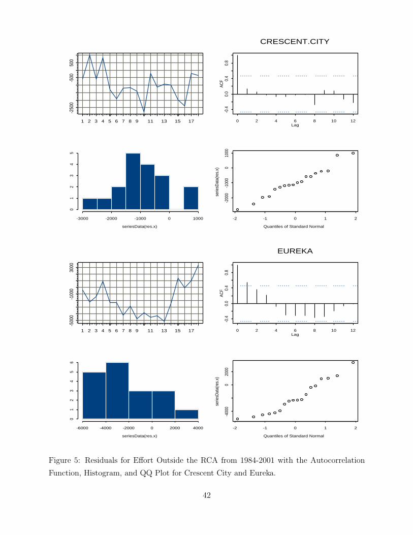
1 2 3 4 5 6 7 8 9 11 13 15 17

-250

0-5

0050

0

Lag

ACF

0 2 4 6 8 10 12

-0.4

0.0

0.4

0.8

CRESCENT.CITY

-3000 -2000 -1000 0 1000

01

23

45

seriesData(res.x) Quantiles of Standard Normal

serie

sDat

a(re

s.x)

-2 -1 0 1 2

-200

0-1

000

010

00

1 2 3 4 5 6 7 8 9 11 13 15 17

-500

0-1

000

3000

Lag

ACF

0 2 4 6 8 10 12

-0.4

0.0

0.4

0.8

EUREKA

-6000 -4000 -2000 0 2000 4000

01

23

45

6

seriesData(res.x) Quantiles of Standard Normal

serie

sDat

a(re

s.x)

-2 -1 0 1 2

-400

00

2000

Figure 5: Residuals for Effort Outside the RCA from 1984-2001 with the Autocorrelation

Function, Histogram, and QQ Plot for Crescent City and Eureka.

42

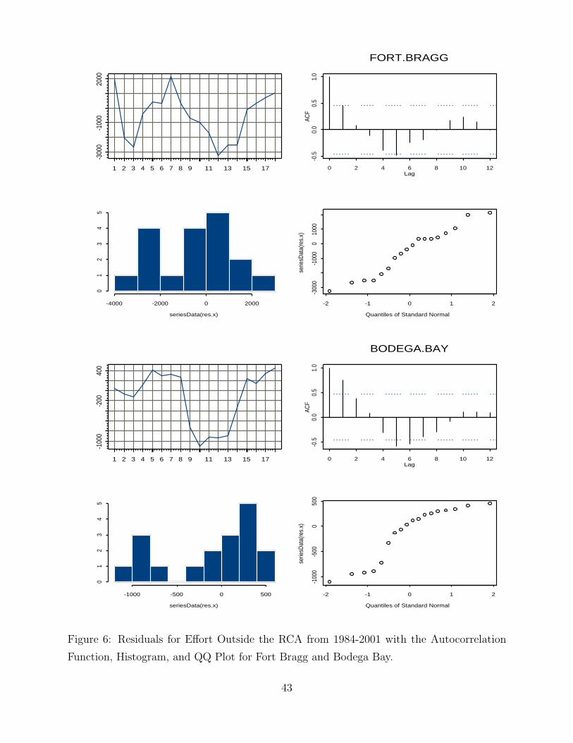
1 2 3 4 5 6 7 8 9 11 13 15 17

-300

0-1

000

2000

Lag

ACF

0 2 4 6 8 10 12

-0.5

0.0

0.5

1.0

FORT.BRAGG

-4000 -2000 0 2000

01

23

45

seriesData(res.x) Quantiles of Standard Normal

serie

sDat

a(re

s.x)

-2 -1 0 1 2

-300

0-1

000

010

00

1 2 3 4 5 6 7 8 9 11 13 15 17

-100

0-2

0040

0

Lag

ACF

0 2 4 6 8 10 12

-0.5

0.0

0.5

1.0

BODEGA.BAY

-1000 -500 0 500

01

23

45

seriesData(res.x) Quantiles of Standard Normal

serie

sDat

a(re

s.x)

-2 -1 0 1 2

-100

0-5

000

500

Figure 6: Residuals for Effort Outside the RCA from 1984-2001 with the Autocorrelation

Function, Histogram, and QQ Plot for Fort Bragg and Bodega Bay.

43

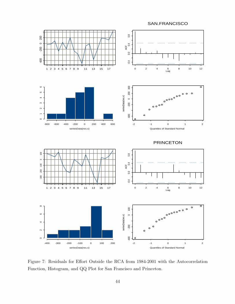
1 2 3 4 5 6 7 8 9 11 13 15 17

-600

-200

020

0

Lag

ACF

0 2 4 6 8 10 12

-0.4

0.0

0.4

0.8

SAN.FRANCISCO

-800 -600 -400 -200 0 200 400 600

01

23

45

6

seriesData(res.x) Quantiles of Standard Normal

serie

sDat

a(re

s.x)

-2 -1 0 1 2

-600

-200

020

040

0

1 2 3 4 5 6 7 8 9 11 13 15 17

-300

-200

-100

010

0

Lag

ACF

0 2 4 6 8 10 12

-0.4

0.0

0.4

0.8

PRINCETON

-400 -300 -200 -100 0 100 200

02

46

8

seriesData(res.x) Quantiles of Standard Normal

serie

sDat

a(re

s.x)

-2 -1 0 1 2

-400

-200

010

0

Figure 7: Residuals for Effort Outside the RCA from 1984-2001 with the Autocorrelation

Function, Histogram, and QQ Plot for San Francisco and Princeton.

44

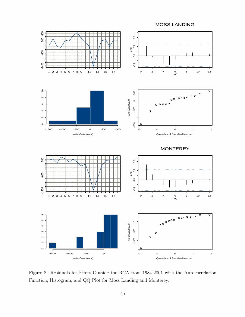
1 2 3 4 5 6 7 8 9 11 13 15 17

-140

0-6

0020

060

0

Lag

ACF

0 2 4 6 8 10 12

-0.4

0.0

0.4

0.8

MOSS.LANDING

-1500 -1000 -500 0 500 1000

02

46

810

seriesData(res.x) Quantiles of Standard Normal

serie

sDat

a(re

s.x)

-2 -1 0 1 2

-150

0-5

000

500

1 2 3 4 5 6 7 8 9 11 13 15 17

-140

0-6

0020

0

Lag

ACF

0 2 4 6 8 10 12

-0.4

0.0

0.4

0.8

MONTEREY

-1500 -1000 -500 0

01

23

45

6

seriesData(res.x) Quantiles of Standard Normal

serie

sDat

a(re

s.x)

-2 -1 0 1 2

-100

0-5

000

Figure 8: Residuals for Effort Outside the RCA from 1984-2001 with the Autocorrelation

Function, Histogram, and QQ Plot for Moss Landing and Monterey.

45

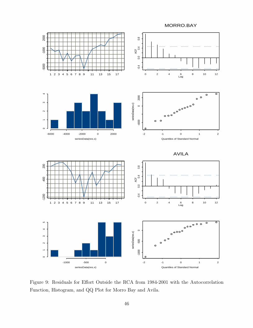
1 2 3 4 5 6 7 8 9 11 13 15 17

-500

0-1

000

2000

Lag

ACF

0 2 4 6 8 10 12

-0.4

0.0

0.4

0.8

MORRO.BAY

-6000 -4000 -2000 0 2000

01

23

4

seriesData(res.x) Quantiles of Standard Normal

serie

sDat

a(re

s.x)

-2 -1 0 1 2

-400

00

2000

1 2 3 4 5 6 7 8 9 11 13 15 17

-120

0-4

0020

0

Lag

ACF

0 2 4 6 8 10 12

-0.4

0.0

0.4

0.8

AVILA

-1000 -500 0

01

23

45

seriesData(res.x) Quantiles of Standard Normal

serie

sDat

a(re

s.x)

-2 -1 0 1 2

-100

0-5

000

Figure 9: Residuals for Effort Outside the RCA from 1984-2001 with the Autocorrelation

Function, Histogram, and QQ Plot for Morro Bay and Avila.

46

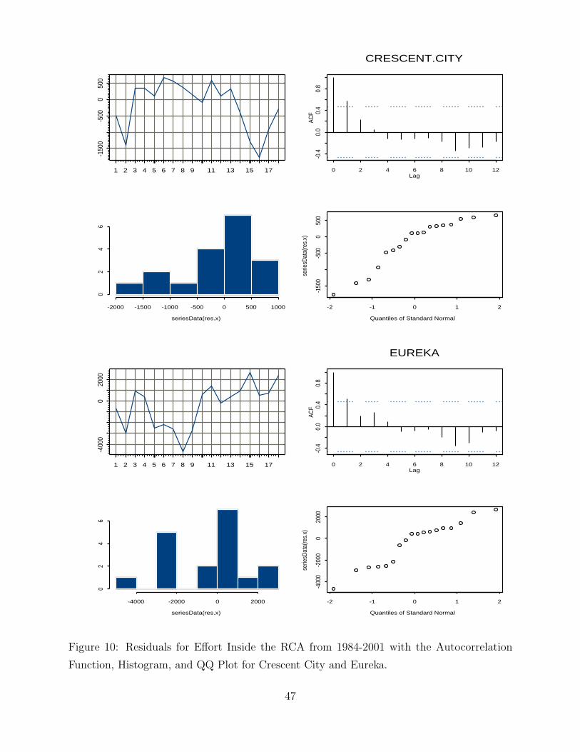
1 2 3 4 5 6 7 8 9 11 13 15 17

-150

0-5

000

500

Lag

ACF

0 2 4 6 8 10 12

-0.4

0.0

0.4

0.8

CRESCENT.CITY

-2000 -1500 -1000 -500 0 500 1000

02

46

seriesData(res.x) Quantiles of Standard Normal

serie

sDat

a(re

s.x)

-2 -1 0 1 2

-150

0-5

000

500

1 2 3 4 5 6 7 8 9 11 13 15 17

-400

00

2000

Lag

ACF

0 2 4 6 8 10 12

-0.4

0.0

0.4

0.8

EUREKA

-4000 -2000 0 2000

02

46

seriesData(res.x) Quantiles of Standard Normal

serie

sDat

a(re

s.x)

-2 -1 0 1 2

-400

0-2

000

020

00

Figure 10: Residuals for Effort Inside the RCA from 1984-2001 with the Autocorrelation

Function, Histogram, and QQ Plot for Crescent City and Eureka.

47

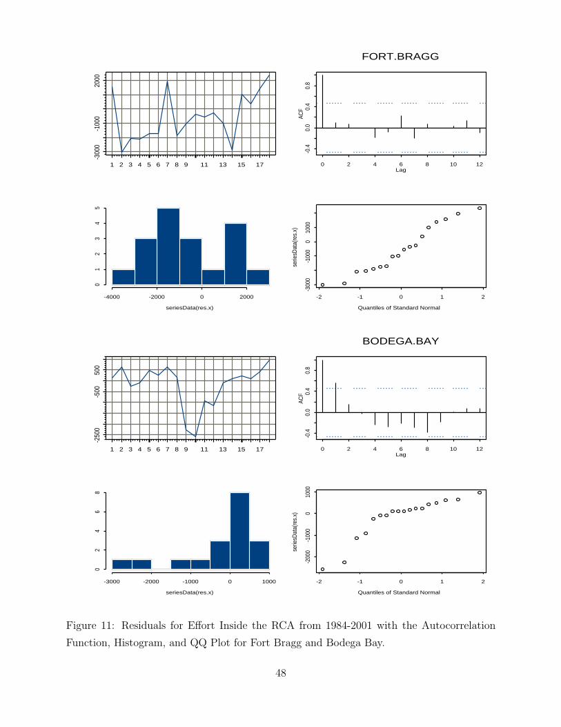
1 2 3 4 5 6 7 8 9 11 13 15 17

-300

0-1

000

2000

Lag

ACF

0 2 4 6 8 10 12

-0.4

0.0

0.4

0.8

FORT.BRAGG

-4000 -2000 0 2000

01

23

45

seriesData(res.x) Quantiles of Standard Normal

serie

sDat

a(re

s.x)

-2 -1 0 1 2

-300

0-1

000

010

00

1 2 3 4 5 6 7 8 9 11 13 15 17

-250

0-5

0050

0

Lag

ACF

0 2 4 6 8 10 12

-0.4

0.0

0.4

0.8

BODEGA.BAY

-3000 -2000 -1000 0 1000

02

46

8

seriesData(res.x) Quantiles of Standard Normal

serie

sDat

a(re

s.x)

-2 -1 0 1 2

-200

0-1

000

010

00

Figure 11: Residuals for Effort Inside the RCA from 1984-2001 with the Autocorrelation

Function, Histogram, and QQ Plot for Fort Bragg and Bodega Bay.

48

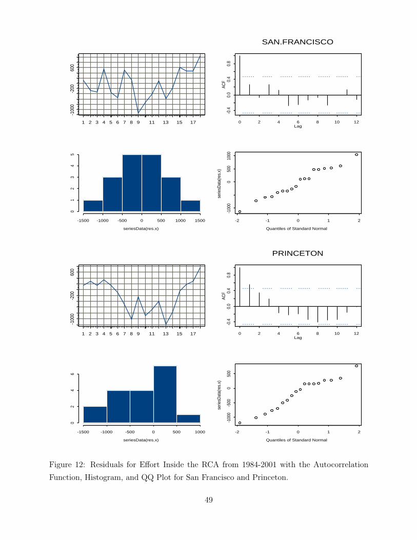
1 2 3 4 5 6 7 8 9 11 13 15 17

-100

0-2

0060

0

Lag

ACF

0 2 4 6 8 10 12

-0.4

0.0

0.4

0.8

SAN.FRANCISCO

-1500 -1000 -500 0 500 1000 1500

01

23

45

seriesData(res.x) Quantiles of Standard Normal

serie

sDat

a(re

s.x)

-2 -1 0 1 2

-100

00

500

1000

1 2 3 4 5 6 7 8 9 11 13 15 17

-100

0-2

0060

0

Lag

ACF

0 2 4 6 8 10 12

-0.4

0.0

0.4

0.8

PRINCETON

-1500 -1000 -500 0 500 1000

02

46

seriesData(res.x) Quantiles of Standard Normal

serie

sDat

a(re

s.x)

-2 -1 0 1 2

-100

0-5

000

500

Figure 12: Residuals for Effort Inside the RCA from 1984-2001 with the Autocorrelation

Function, Histogram, and QQ Plot for San Francisco and Princeton.

49

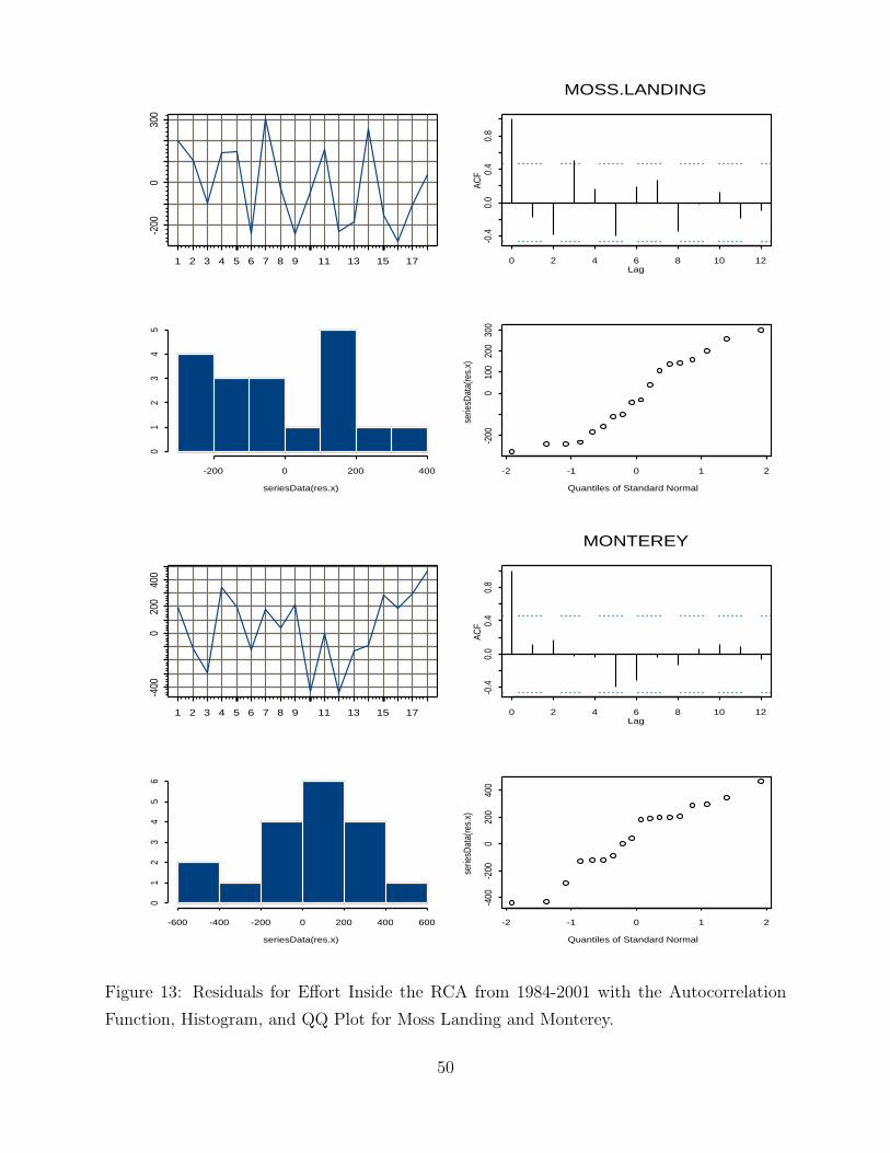
1 2 3 4 5 6 7 8 9 11 13 15 17

-200

030

0

Lag

ACF

0 2 4 6 8 10 12

-0.4

0.0

0.4

0.8

MOSS.LANDING

-200 0 200 400

01

23

45

seriesData(res.x) Quantiles of Standard Normal

serie

sDat

a(re

s.x)

-2 -1 0 1 2

-200

010

020

030

0

1 2 3 4 5 6 7 8 9 11 13 15 17

-400

020

040

0

Lag

ACF

0 2 4 6 8 10 12

-0.4

0.0

0.4

0.8

MONTEREY

-600 -400 -200 0 200 400 600

01

23

45

6

seriesData(res.x) Quantiles of Standard Normal

serie

sDat

a(re

s.x)

-2 -1 0 1 2

-400

-200

020

040

0

Figure 13: Residuals for Effort Inside the RCA from 1984-2001 with the Autocorrelation

Function, Histogram, and QQ Plot for Moss Landing and Monterey.

50

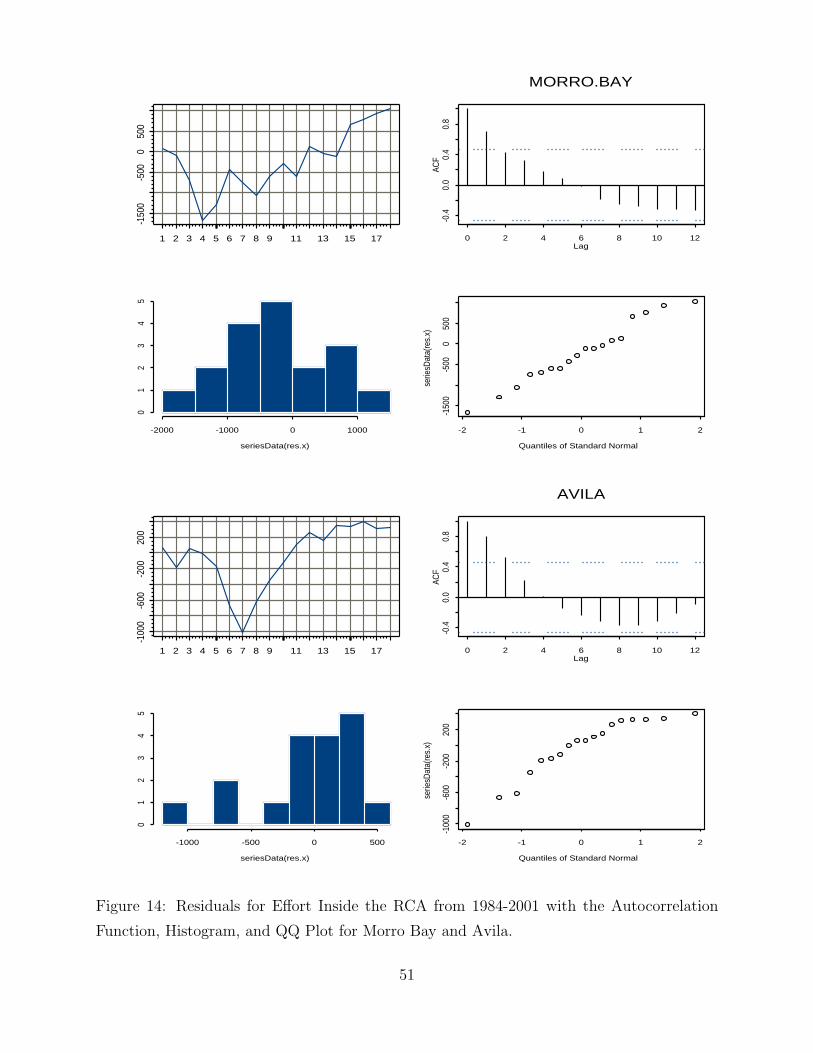
1 2 3 4 5 6 7 8 9 11 13 15 17

-150

0-5

000

500

Lag

ACF

0 2 4 6 8 10 12

-0.4

0.0

0.4

0.8

MORRO.BAY

-2000 -1000 0 1000

01

23

45

seriesData(res.x) Quantiles of Standard Normal

serie

sDat

a(re

s.x)

-2 -1 0 1 2

-150

0-5

000

500

1 2 3 4 5 6 7 8 9 11 13 15 17

-100

0-6

00-2

0020

0

Lag

ACF

0 2 4 6 8 10 12

-0.4

0.0

0.4

0.8

AVILA

-1000 -500 0 500

01

23

45

seriesData(res.x) Quantiles of Standard Normal

serie

sDat

a(re

s.x)

-2 -1 0 1 2

-100

0-6

00-2

0020

0

Figure 14: Residuals for Effort Inside the RCA from 1984-2001 with the Autocorrelation

Function, Histogram, and QQ Plot for Morro Bay and Avila.

51

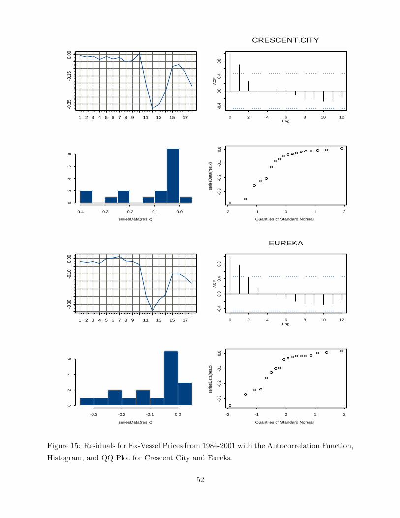
1 2 3 4 5 6 7 8 9 11 13 15 17

-0.3

5-0

.15

0.00

Lag

ACF

0 2 4 6 8 10 12

-0.4

0.0

0.4

0.8

CRESCENT.CITY

-0.4 -0.3 -0.2 -0.1 0.0

02

46

8

seriesData(res.x) Quantiles of Standard Normal

serie

sDat

a(re

s.x)

-2 -1 0 1 2

-0.3

-0.2

-0.1

0.0

1 2 3 4 5 6 7 8 9 11 13 15 17

-0.3

0-0

.10

0.00

Lag

ACF

0 2 4 6 8 10 12

-0.4

0.0

0.4

0.8

EUREKA

-0.3 -0.2 -0.1 0.0

02

46

seriesData(res.x) Quantiles of Standard Normal

serie

sDat

a(re

s.x)

-2 -1 0 1 2

-0.3

-0.2

-0.1

0.0

Figure 15: Residuals for Ex-Vessel Prices from 1984-2001 with the Autocorrelation Function,

Histogram, and QQ Plot for Crescent City and Eureka.

52

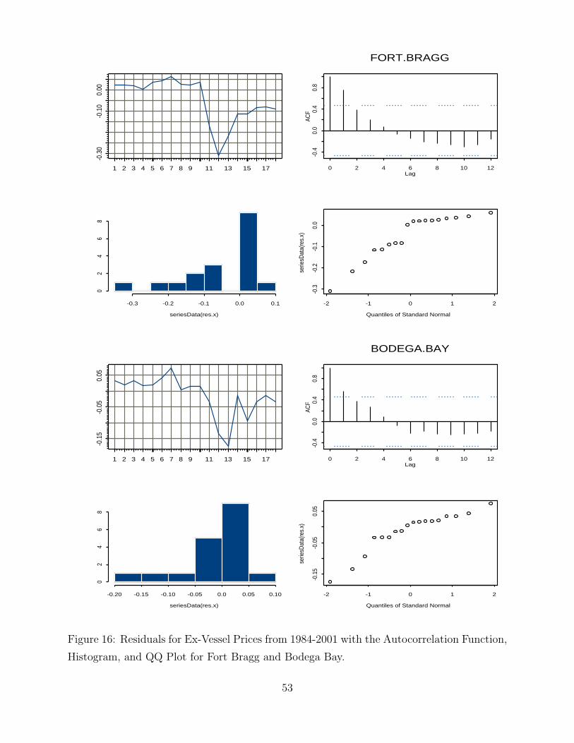
1 2 3 4 5 6 7 8 9 11 13 15 17

-0.3

0-0

.10

0.00

Lag

ACF

0 2 4 6 8 10 12

-0.4

0.0

0.4

0.8

FORT.BRAGG

-0.3 -0.2 -0.1 0.0 0.1

02

46

8

seriesData(res.x) Quantiles of Standard Normal

serie

sDat

a(re

s.x)

-2 -1 0 1 2

-0.3

-0.2

-0.1

0.0

1 2 3 4 5 6 7 8 9 11 13 15 17

-0.1

5-0

.05

0.05

Lag

ACF

0 2 4 6 8 10 12

-0.4

0.0

0.4

0.8

BODEGA.BAY

-0.20 -0.15 -0.10 -0.05 0.0 0.05 0.10

02

46

8

seriesData(res.x) Quantiles of Standard Normal

serie

sDat

a(re

s.x)

-2 -1 0 1 2

-0.1

5-0

.05

0.05

Figure 16: Residuals for Ex-Vessel Prices from 1984-2001 with the Autocorrelation Function,

Histogram, and QQ Plot for Fort Bragg and Bodega Bay.

53

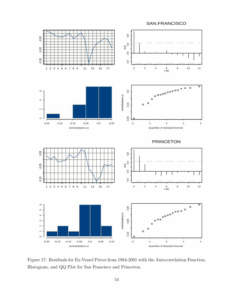
1 2 3 4 5 6 7 8 9 11 13 15 17

-0.1

8-0

.10

-0.0

2

Lag

ACF

0 2 4 6 8 10 12

-0.4

0.0

0.4

0.8

SAN.FRANCISCO

-0.20 -0.15 -0.10 -0.05 0.0 0.05

02

46

seriesData(res.x) Quantiles of Standard Normal

serie

sDat

a(re

s.x)

-2 -1 0 1 2

-0.2

0-0

.10

0.0

1 2 3 4 5 6 7 8 9 11 13 15 17

-0.1

5-0

.05

0.05

Lag

ACF

0 2 4 6 8 10 12

-0.4

0.0

0.4

0.8

PRINCETON

-0.20 -0.15 -0.10 -0.05 0.0 0.05 0.10

01

23

45

6

seriesData(res.x) Quantiles of Standard Normal

serie

sDat

a(re

s.x)

-2 -1 0 1 2

-0.1

5-0

.05

0.05

Figure 17: Residuals for Ex-Vessel Prices from 1984-2001 with the Autocorrelation Function,

Histogram, and QQ Plot for San Francisco and Princeton.

54

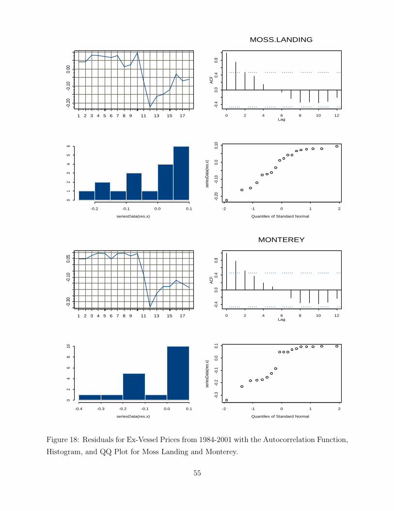
1 2 3 4 5 6 7 8 9 11 13 15 17

-0.2

0-0

.10

0.00

Lag

ACF

0 2 4 6 8 10 12

-0.4

0.0

0.4

0.8

MOSS.LANDING

-0.2 -0.1 0.0 0.1

01

23

45

6

seriesData(res.x) Quantiles of Standard Normal

serie

sDat

a(re

s.x)

-2 -1 0 1 2

-0.2

0-0

.10

0.0

0.10

1 2 3 4 5 6 7 8 9 11 13 15 17

-0.3

0-0

.10

0.05

Lag

ACF

0 2 4 6 8 10 12

-0.4

0.0

0.4

0.8

MONTEREY

-0.4 -0.3 -0.2 -0.1 0.0 0.1

02

46

810

seriesData(res.x) Quantiles of Standard Normal

serie

sDat

a(re

s.x)

-2 -1 0 1 2

-0.3

-0.2

-0.1

0.0

0.1

Figure 18: Residuals for Ex-Vessel Prices from 1984-2001 with the Autocorrelation Function,

Histogram, and QQ Plot for Moss Landing and Monterey.

55

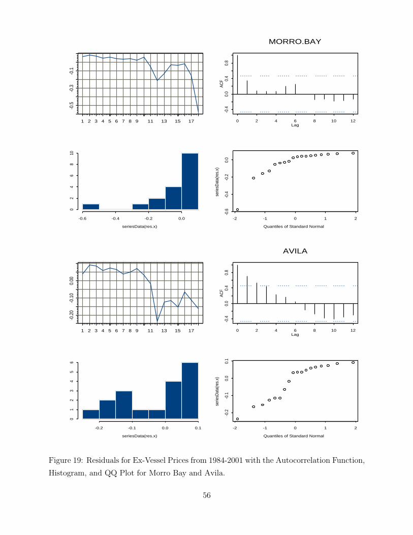
1 2 3 4 5 6 7 8 9 11 13 15 17

-0.5

-0.3

-0.1

Lag

ACF

0 2 4 6 8 10 12

-0.4

0.0

0.4

0.8

MORRO.BAY

-0.6 -0.4 -0.2 0.0

02

46

810

seriesData(res.x) Quantiles of Standard Normal

serie

sDat

a(re

s.x)

-2 -1 0 1 2

-0.6

-0.4

-0.2

0.0

1 2 3 4 5 6 7 8 9 11 13 15 17

-0.2

0-0

.10

0.00

Lag

ACF

0 2 4 6 8 10 12

-0.4

0.0

0.4

0.8

AVILA

-0.2 -0.1 0.0 0.1

01

23

45

6

seriesData(res.x) Quantiles of Standard Normal

serie

sDat

a(re

s.x)

-2 -1 0 1 2

-0.2

-0.1

0.0

0.1

Figure 19: Residuals for Ex-Vessel Prices from 1984-2001 with the Autocorrelation Function,

Histogram, and QQ Plot for Morro Bay and Avila.

56

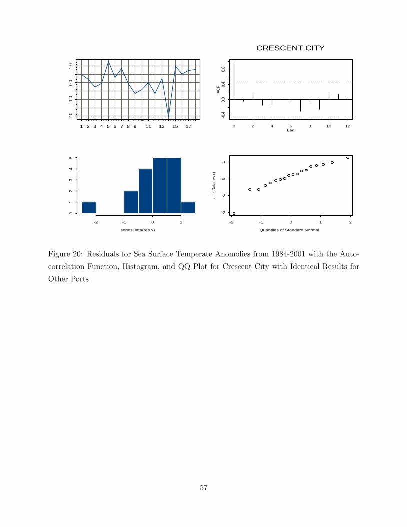
1 2 3 4 5 6 7 8 9 11 13 15 17

-2.0

-1.0

0.0

1.0

Lag

ACF

0 2 4 6 8 10 12

-0.4

0.0

0.4

0.8

CRESCENT.CITY

-2 -1 0 1

01

23

45

seriesData(res.x) Quantiles of Standard Normal

serie

sDat

a(re

s.x)

-2 -1 0 1 2-2

-10

1

Figure 20: Residuals for Sea Surface Temperate Anomolies from 1984-2001 with the Auto-

correlation Function, Histogram, and QQ Plot for Crescent City with Identical Results for

Other Ports

57

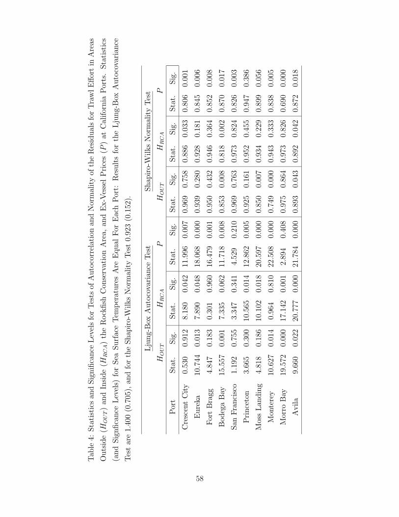
Tab

le4:

Sta

tist

ics

and

Sig

nifi

cance

Lev

els

for

Tes

tsof

Auto

corr

elat

ion

and

Nor

mal

ity

ofth

eR

esid

ual

sfo

rTra

wlE

ffor

tin

Are

as

Outs

ide

(HO

UT)

and

Insi

de

(HR

CA)

the

Rock

fish

Con

serv

atio

nA

rea,

and

Ex-V

esse

lP

rice

s(P

)at

Cal

ifor

nia

Por

ts.

Sta

tist

ics

(and

Sig

nfica

nce

Lev

els)

for

Sea

Surf

ace

Tem

per

ature

sA

reE

qual

For

Eac

hPor

t:R

esult

sfo

rth

eLju

ng-

Box

Auto

cova

rian

ce

Tes

tar

e1.

400

(0.7

05),

and

for

the

Shap

iro-

Wilks

Nor

mal

ity

Tes

t0.

923

(0.1

52).

Lju

ng-

Box

Auto

cova

rian

ceTes

tShap

iro-

Wilks

Nor

mal

ity

Tes

t

HO

UT

HR

CA

PH

OU

TH

RC

AP

Por

tSta

t.Sig

.Sta

t.Sig

.Sta

t.Sig

.Sta

t.Sig

.Sta

t.Sig

.Sta

t.Sig

.

Cre

scen

tC

ity

0.53

00.

912

8.18

00.

042

11.9

960.

007

0.96

90.

758

0.88

60.

033

0.80

60.

001

Eure

ka10

.744

0.01

37.

890

0.04

818

.068

0.00

00.

939

0.28

00.

928

0.18

10.

845

0.00

6

For

tB

ragg

4.84

70.

183

0.30

10.

960

16.4

790.

001

0.95

00.

432

0.94

60.

364

0.85

20.

008

Bodeg

aB

ay15

.557

0.00

17.

335

0.06

211

.718

0.00

80.

853

0.00

80.

818

0.00

20.

870

0.01

7

San

Fra

nci

sco

1.19

20.

755

3.34

70.

341

4.52

90.

210

0.96

90.

763

0.97

30.

824

0.82

60.

003

Pri

nce

ton

3.66

50.

300

10.5

650.

014

12.8

620.

005

0.92

50.

161

0.95

20.

455

0.94

70.

386

Mos

sLan

din

g4.

818

0.18

610

.102

0.01

820

.597

0.00

00.

850

0.00

70.

934

0.22

90.

899

0.05

6

Mon

tere

y10

.627

0.01

40.

964

0.81

022

.508

0.00

00.

749

0.00

00.

943

0.33

30.

838

0.00

5

Mor

roB

ay19

.572

0.00

017

.142

0.00

12.

894

0.40

80.

975

0.86

40.

973

0.82

60.

690

0.00

0

Avila

9.66

00.

022

20.7

770.

000

21.7

840.

000

0.89

30.

043

0.89

20.

042

0.87

20.

018

58

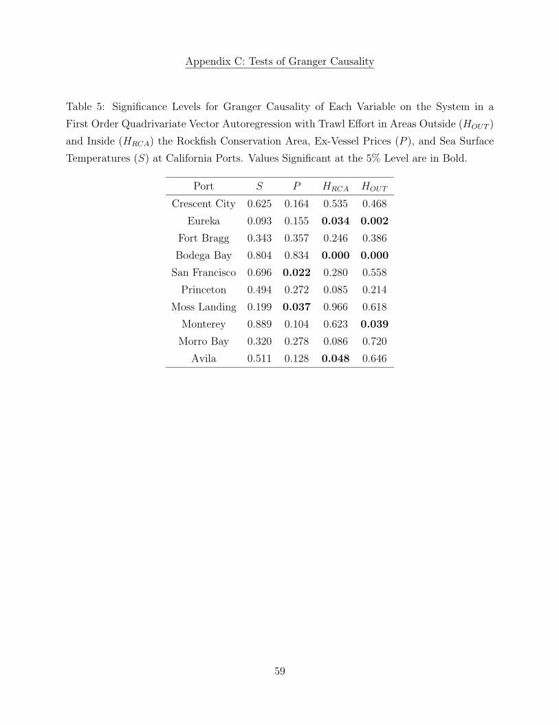
Appendix C: Tests of Granger Causality

Table 5: Significance Levels for Granger Causality of Each Variable on the System in a

First Order Quadrivariate Vector Autoregression with Trawl Effort in Areas Outside (HOUT )

and Inside (HRCA) the Rockfish Conservation Area, Ex-Vessel Prices (P ), and Sea Surface

Temperatures (S) at California Ports. Values Significant at the 5% Level are in Bold.

Port S P HRCA HOUT

Crescent City 0.625 0.164 0.535 0.468

Eureka 0.093 0.155 0.034 0.002

Fort Bragg 0.343 0.357 0.246 0.386

Bodega Bay 0.804 0.834 0.000 0.000

San Francisco 0.696 0.022 0.280 0.558

Princeton 0.494 0.272 0.085 0.214

Moss Landing 0.199 0.037 0.966 0.618

Monterey 0.889 0.104 0.623 0.039

Morro Bay 0.320 0.278 0.086 0.720

Avila 0.511 0.128 0.048 0.646

59

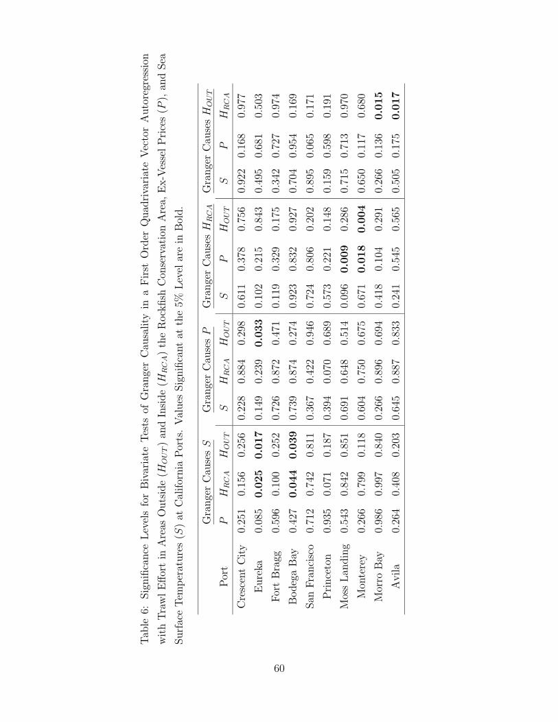
Tab

le6:

Sig

nifi

cance

Lev

els

for

Biv

aria

teTes

tsof

Gra

nge

rC

ausa

lity

ina

Fir

stO

rder

Quad

riva

riat

eV

ecto

rA

uto

regr

essi

on

wit

hTra

wlE

ffor

tin

Are

asO

uts

ide

(HO

UT)

and

Insi

de

(HR

CA)

the

Rock

fish

Con

serv

atio

nA

rea,

Ex-V

esse

lP

rice

s(P

),an

dSea

Surf

ace

Tem

per

ature

s(S

)at

Cal

ifor

nia

Por

ts.

Val

ues

Sig

nifi

cant

atth

e5%

Lev

elar

ein

Bol

d.

Gra

nge

rC

ause

sS

Gra

nge

rC

ause

sP

Gra

nge

rC

ause

sH

RC

AG

range

rC

ause

sH

OU

T

Por

tP

HR

CA

HO

UT

SH

RC

AH

OU

TS

PH

OU

TS

PH

RC

A

Cre

scen

tC

ity

0.25

10.

156

0.25

60.

228

0.88

40.

298

0.61

10.

378

0.75

60.

922

0.16

80.

977

Eure

ka0.

085

0.0

25

0.0

17

0.14

90.

239

0.0

33

0.10

20.

215

0.84

30.

495

0.68

10.

503

For

tB

ragg

0.59

60.

100

0.25

20.

726

0.87

20.

471

0.11

90.

329

0.17

50.

342

0.72

70.

974

Bodeg

aB

ay0.

427

0.0

44

0.0

39

0.73

90.

874

0.27

40.

923

0.83

20.

927

0.70

40.

954

0.16

9

San

Fra

nci

sco

0.71

20.

742

0.81

10.

367

0.42

20.

946

0.72

40.

806

0.20

20.

895

0.06

50.

171

Pri

nce

ton

0.93

50.

071

0.18

70.

394

0.07

00.

689

0.57

30.

221

0.14

80.

159

0.59

80.

191

Mos

sLan

din

g0.

543

0.84

20.

851

0.69

10.

648

0.51

40.

096

0.0

09

0.28

60.

715

0.71

30.

970

Mon

tere

y0.

266

0.79

90.

118

0.60

40.

750

0.67

50.

671

0.0

18

0.0

04

0.65

00.

117

0.68

0

Mor

roB

ay0.

986

0.99

70.

840

0.26

60.

896

0.69

40.

418

0.10

40.

291

0.26

60.

136

0.0

15

Avila

0.26

40.

408

0.20

30.

645

0.88

70.

833

0.24

10.

545

0.56

50.

505

0.17

50.0

17

60