EECS 473Advanced Embedded Systems

Lecture 13

Start on Wireless

Upcoming

• MS2 report due on 11/7

– MS2 meetings on Tuesday 11/12

• PCBs

– Class survey

– All are to be out by 11/5.

• Who has registered for the Design Expo?

Team status updates:What is your current largest roadblock?

• Team updates.– Balloon

– Hiking

– Fish

– Ear

– Fence

– Drone

– Cane

• Communicate your issues to us.– Sometimes we can help.

Fixed point

• Review:

– Write a function which multiplies two 8-bit Q7 numbers and generates an 8-bit Q7. Ignore overflow, round to the nearest value (either way if both are equally close*)

• We generally will do this in-line rather than writing a function…

*The standard thing to do is round 0.5 to the nearest even number. Why?

Wireless communications

• Next 2.5 lectures are going to cover wireless

communication

– Both theory and practice.

• If you’ve had a communication systems class,

there will be some overlap

– And we will be focusing on digital where we can

• Though that’s still a lot of analog.

Introduction to embedded wireless

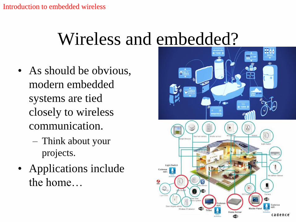
Wireless and embedded?

• As should be obvious,

modern embedded

systems are tied

closely to wireless

communication.

– Think about your

projects.

• Applications include

the home…

Introduction to embedded wireless

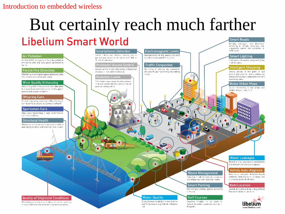
But certainly reach much farther

Introduction to embedded wireless

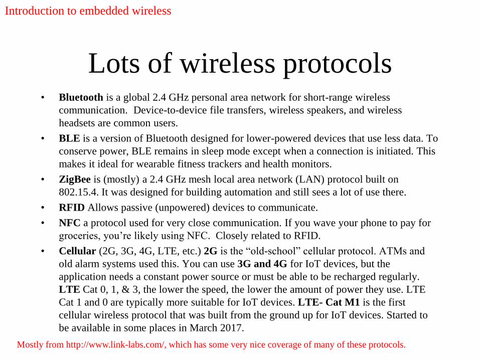
Lots of wireless protocols• Bluetooth is a global 2.4 GHz personal area network for short-range wireless

communication. Device-to-device file transfers, wireless speakers, and wireless

headsets are common users.

• BLE is a version of Bluetooth designed for lower-powered devices that use less data. To

conserve power, BLE remains in sleep mode except when a connection is initiated. This

makes it ideal for wearable fitness trackers and health monitors.

• ZigBee is (mostly) a 2.4 GHz mesh local area network (LAN) protocol built on

802.15.4. It was designed for building automation and still sees a lot of use there.

• RFID Allows passive (unpowered) devices to communicate.

• NFC a protocol used for very close communication. If you wave your phone to pay for

groceries, you’re likely using NFC. Closely related to RFID.

• Cellular (2G, 3G, 4G, LTE, etc.) 2G is the “old-school” cellular protocol. ATMs and

old alarm systems used this. You can use 3G and 4G for IoT devices, but the

application needs a constant power source or must be able to be recharged regularly.

LTE Cat 0, 1, & 3, the lower the speed, the lower the amount of power they use. LTE

Cat 1 and 0 are typically more suitable for IoT devices. LTE- Cat M1 is the first

cellular wireless protocol that was built from the ground up for IoT devices. Started to

be available in some places in March 2017.

Mostly from http://www.link-labs.com/, which has some very nice coverage of many of these protocols.

Introduction to embedded wireless

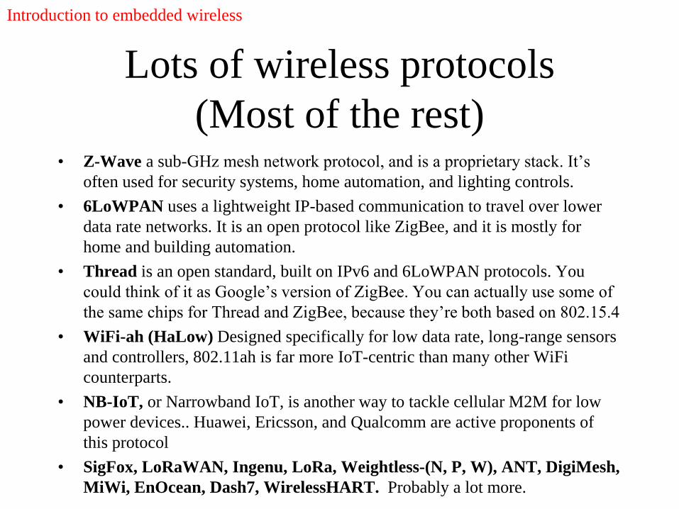
Lots of wireless protocols

(Most of the rest)• Z-Wave a sub-GHz mesh network protocol, and is a proprietary stack. It’s

often used for security systems, home automation, and lighting controls.

• 6LoWPAN uses a lightweight IP-based communication to travel over lower

data rate networks. It is an open protocol like ZigBee, and it is mostly for

home and building automation.

• Thread is an open standard, built on IPv6 and 6LoWPAN protocols. You

could think of it as Google’s version of ZigBee. You can actually use some of

the same chips for Thread and ZigBee, because they’re both based on 802.15.4

• WiFi-ah (HaLow) Designed specifically for low data rate, long-range sensors

and controllers, 802.11ah is far more IoT-centric than many other WiFi

counterparts.

• NB-IoT, or Narrowband IoT, is another way to tackle cellular M2M for low

power devices.. Huawei, Ericsson, and Qualcomm are active proponents of

this protocol

• SigFox, LoRaWAN, Ingenu, LoRa, Weightless-(N, P, W), ANT, DigiMesh,

MiWi, EnOcean, Dash7, WirelessHART. Probably a lot more.

Introduction to embedded wireless

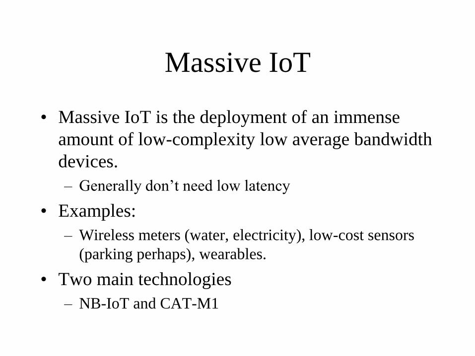
Massive IoT

• Massive IoT is the deployment of an immense

amount of low-complexity low average bandwidth

devices.

– Generally don’t need low latency

• Examples:

– Wireless meters (water, electricity), low-cost sensors

(parking perhaps), wearables.

• Two main technologies

– NB-IoT and CAT-M1

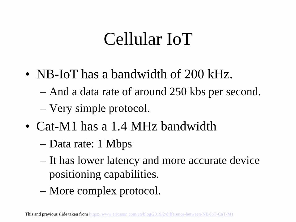
Cellular IoT

• NB-IoT has a bandwidth of 200 kHz.

– And a data rate of around 250 kbs per second.

– Very simple protocol.

• Cat-M1 has a 1.4 MHz bandwidth

– Data rate: 1 Mbps

– It has lower latency and more accurate device

positioning capabilities.

– More complex protocol.

This and previous slide taken from https://www.ericsson.com/en/blog/2019/2/difference-between-NB-IoT-CaT-M1

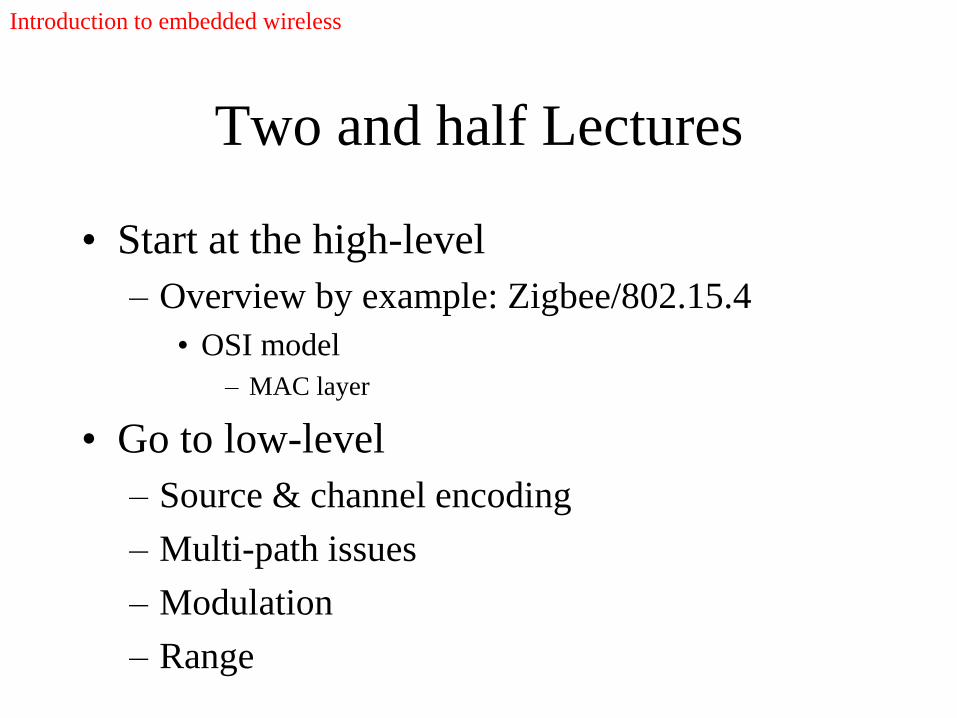
Two and half Lectures

• Start at the high-level

– Overview by example: Zigbee/802.15.4

• OSI model

– MAC layer

• Go to low-level

– Source & channel encoding

– Multi-path issues

– Modulation

– Range

Introduction to embedded wireless

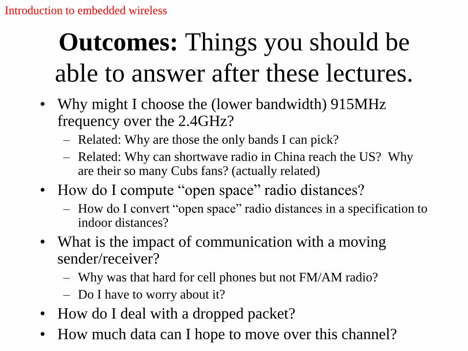
Outcomes: Things you should be

able to answer after these lectures.• Why might I choose the (lower bandwidth) 915MHz

frequency over the 2.4GHz?

– Related: Why are those the only bands I can pick?

– Related: Why can shortwave radio in China reach the US? Why are their so many Cubs fans? (actually related)

• How do I compute “open space” radio distances?

– How do I convert “open space” radio distances in a specification to indoor distances?

• What is the impact of communication with a moving sender/receiver?

– Why was that hard for cell phones but not FM/AM radio?

– Do I have to worry about it?

• How do I deal with a dropped packet?

• How much data can I hope to move over this channel?

Introduction to embedded wireless

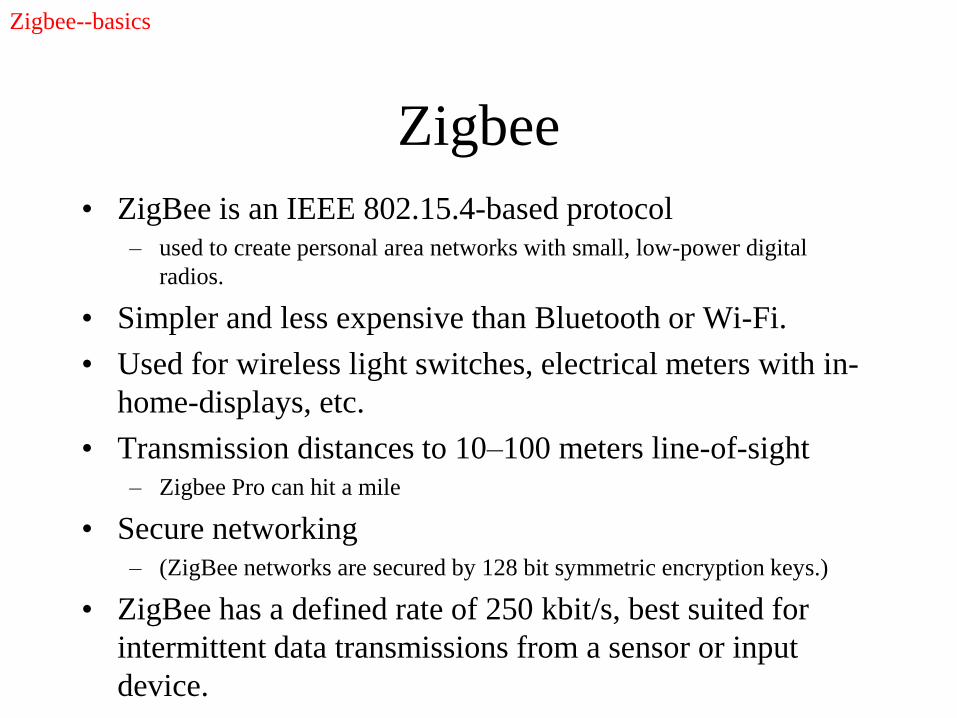
Zigbee

• ZigBee is an IEEE 802.15.4-based protocol

– used to create personal area networks with small, low-power digital

radios.

• Simpler and less expensive than Bluetooth or Wi-Fi.

• Used for wireless light switches, electrical meters with in-

home-displays, etc.

• Transmission distances to 10–100 meters line-of-sight

– Zigbee Pro can hit a mile

• Secure networking

– (ZigBee networks are secured by 128 bit symmetric encryption keys.)

• ZigBee has a defined rate of 250 kbit/s, best suited for

intermittent data transmissions from a sensor or input

device.

Zigbee--basics

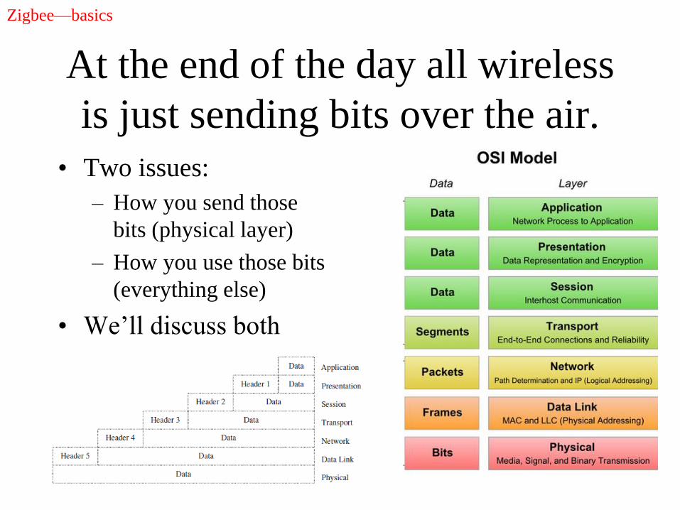
At the end of the day all wireless

is just sending bits over the air.

• Two issues:

– How you send those

bits (physical layer)

– How you use those bits

(everything else)

• We’ll discuss both

Zigbee—basics

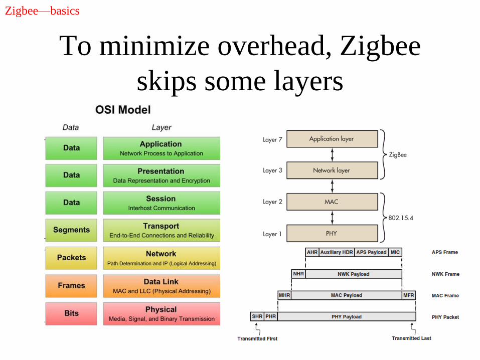
To minimize overhead, Zigbee

skips some layers

Zigbee—basics

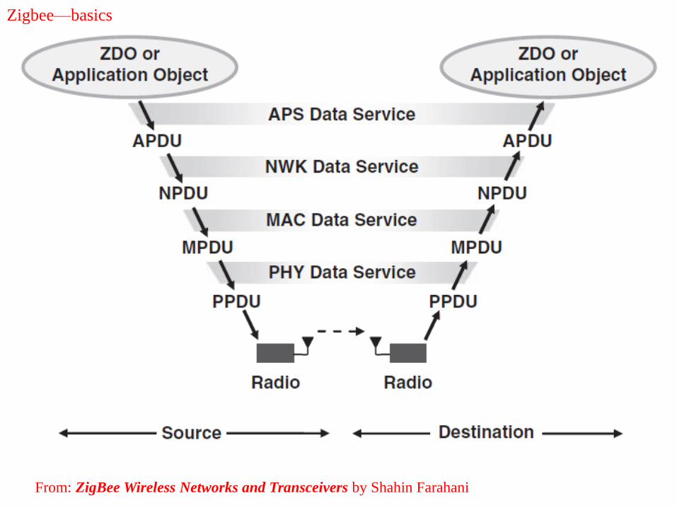
From: ZigBee Wireless Networks and Transceivers by Shahin Farahani

Zigbee—basics

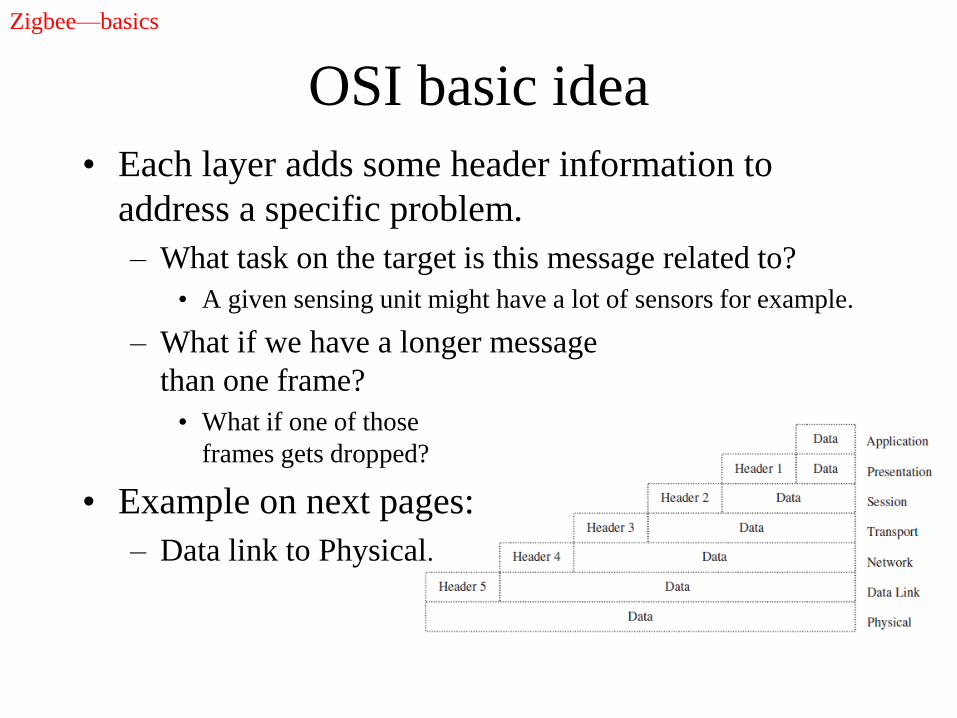
OSI basic idea

• Each layer adds some header information to

address a specific problem.

– What task on the target is this message related to?

• A given sensing unit might have a lot of sensors for example.

– What if we have a longer message

than one frame?

• What if one of those

frames gets dropped?

• Example on next pages:

– Data link to Physical.

Zigbee—basics

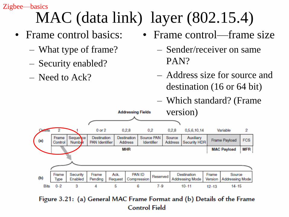
MAC (data link) layer (802.15.4)• Frame control basics:

– What type of frame?

– Security enabled?

– Need to Ack?

• Frame control—frame size

– Sender/receiver on same

PAN?

– Address size for source and

destination (16 or 64 bit)

– Which standard? (Frame

version)

Zigbee—basics

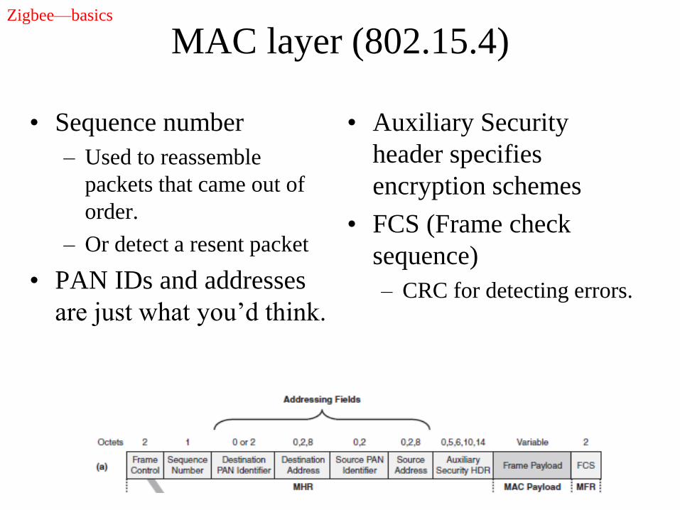
MAC layer (802.15.4)

• Sequence number

– Used to reassemble

packets that came out of

order.

– Or detect a resent packet

• PAN IDs and addresses

are just what you’d think.

• Auxiliary Security

header specifies

encryption schemes

• FCS (Frame check

sequence)

– CRC for detecting errors.

Zigbee—basics

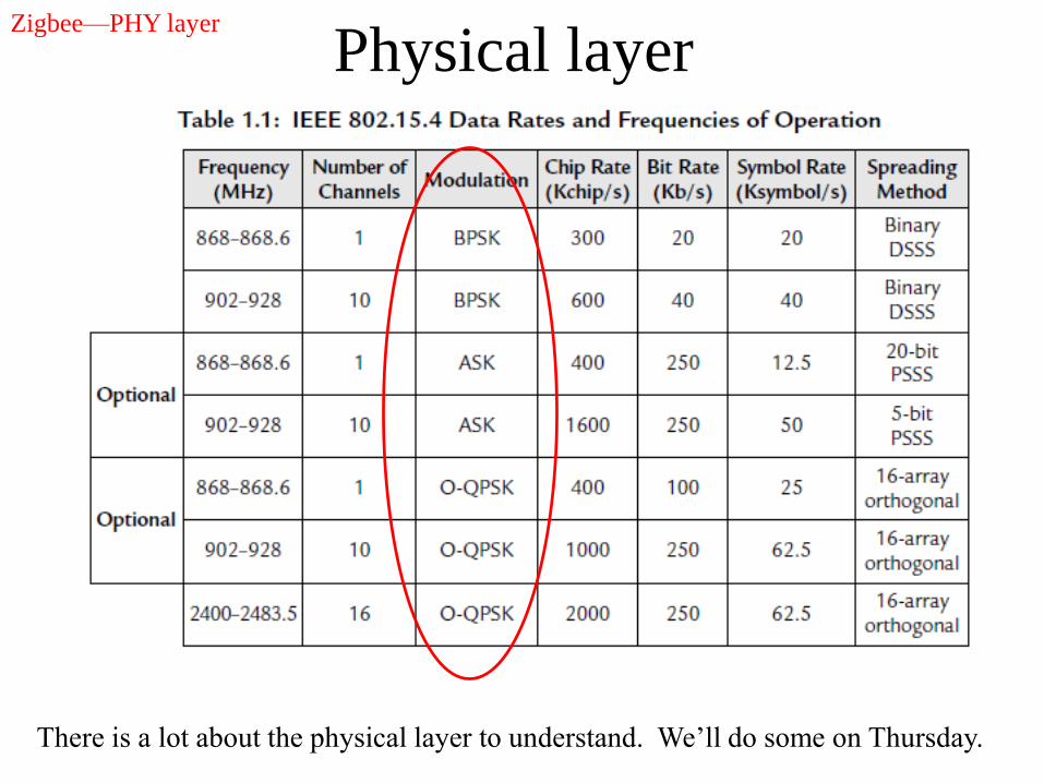
Physical layer

There is a lot about the physical layer to understand. We’ll do some on Thursday.

Zigbee—PHY layer

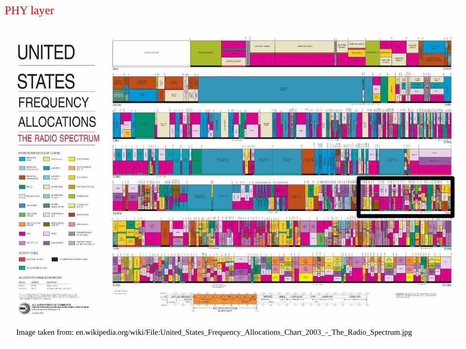
PHY layer

Image taken from: en.wikipedia.org/wiki/File:United_States_Frequency_Allocations_Chart_2003_-_The_Radio_Spectrum.jpg

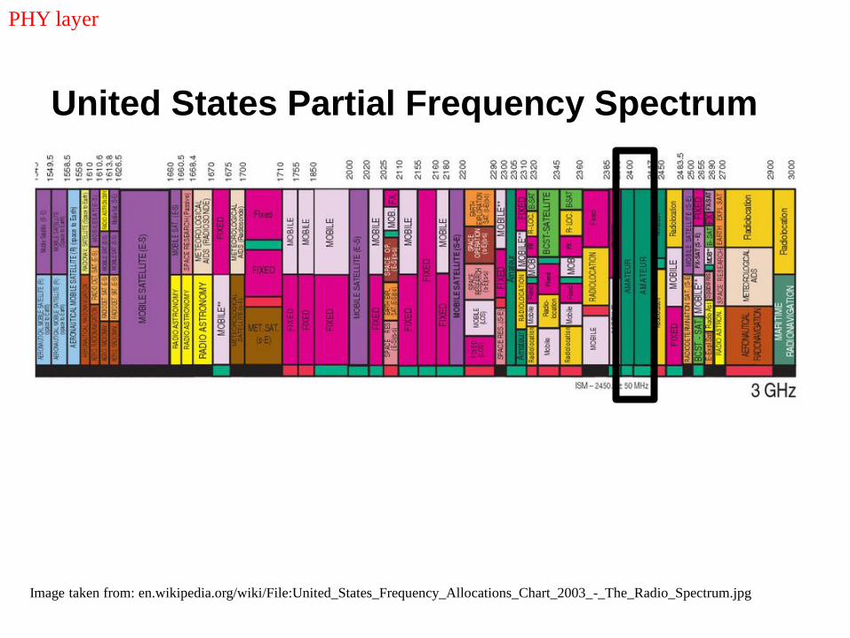
United States Partial Frequency Spectrum

Image taken from: en.wikipedia.org/wiki/File:United_States_Frequency_Allocations_Chart_2003_-_The_Radio_Spectrum.jpg

PHY layer

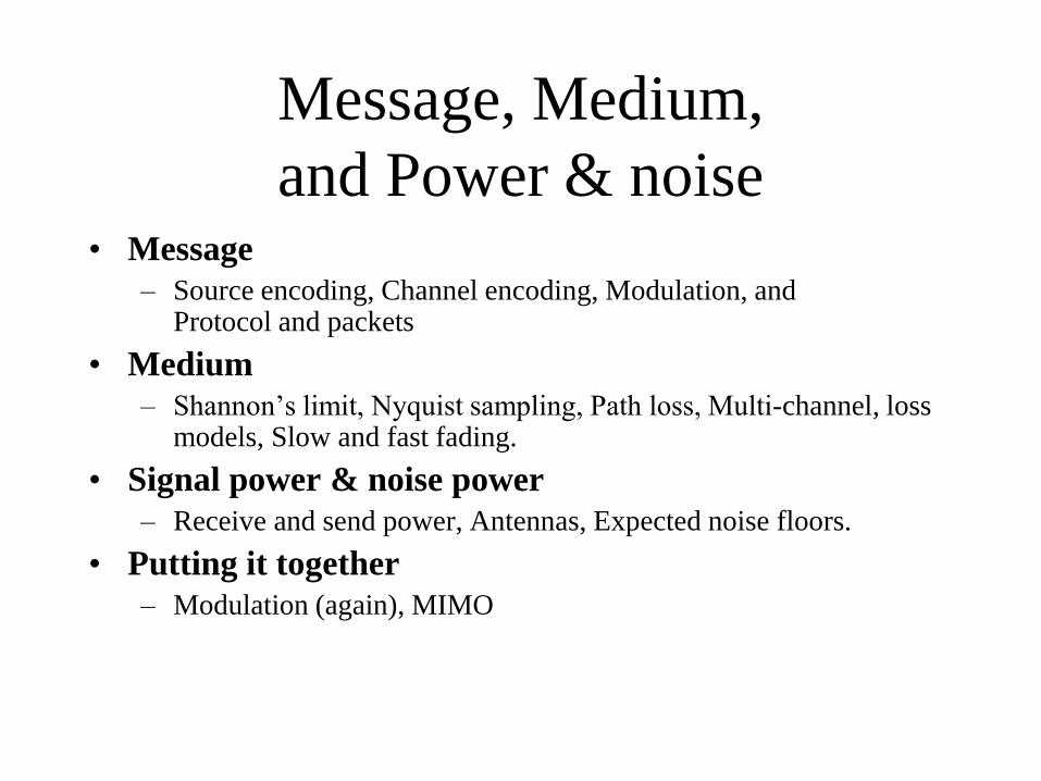
Message, Medium,

and Power & noise• Message

– Source encoding, Channel encoding, Modulation, andProtocol and packets

• Medium

– Shannon’s limit, Nyquist sampling, Path loss, Multi-channel, loss models, Slow and fast fading.

• Signal power & noise power

– Receive and send power, Antennas, Expected noise floors.

• Putting it together

– Modulation (again), MIMO

PHY layer

So starting with the message

• We are trying to send data from one point to the

next over some channel.

– What should we do to get that message ready to go?

– The basic steps are

• Convert it to binary (if needed)

• Compress as much as we can

– to make the message as small as we can

• Add error correction

– To reduce errors

– But, unexpectedly, also to speed up communication over the

channel.

– The receiver will need to undo all that work.

PHY layer

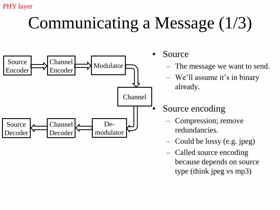
Communicating a Message (1/3)

• Source

– The message we want to send.

– We’ll assume it’s in binary

already.

• Source encoding

– Compression; remove

redundancies.

– Could be lossy (e.g. jpeg)

– Called source encoding

because depends on source

type (think jpeg vs mp3)

Source

Encoder

Channel

EncoderModulator

Channel

Source

Decoder

Channel

Decoder

De-

modulator

PHY layer

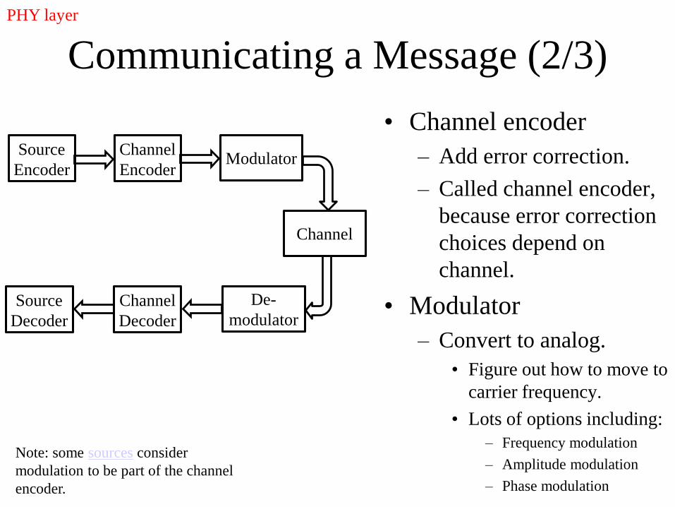
Communicating a Message (2/3)

• Channel encoder

– Add error correction.

– Called channel encoder,

because error correction

choices depend on

channel.

• Modulator

– Convert to analog.

• Figure out how to move to

carrier frequency.

• Lots of options including:

– Frequency modulation

– Amplitude modulation

– Phase modulation

Source

Encoder

Channel

EncoderModulator

Channel

Source

Decoder

Channel

Decoder

De-

modulator

Note: some sources consider

modulation to be part of the channel

encoder.

PHY layer

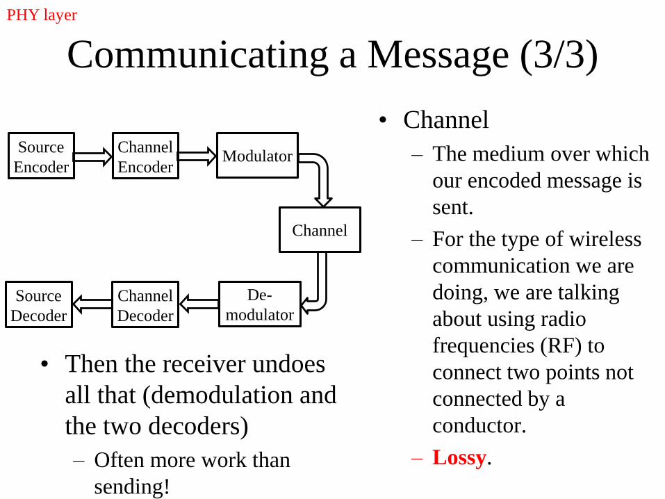
Communicating a Message (3/3)

• Channel

– The medium over which

our encoded message is

sent.

– For the type of wireless

communication we are

doing, we are talking

about using radio

frequencies (RF) to

connect two points not

connected by a

conductor.

– Lossy.

• Then the receiver undoes

all that (demodulation and

the two decoders)

– Often more work than

sending!

Source

Encoder

Channel

EncoderModulator

Channel

Source

Decoder

Channel

Decoder

De-

modulator

PHY layer

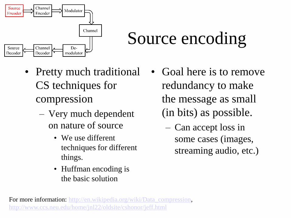
Source encoding

• Pretty much traditional

CS techniques for

compression

– Very much dependent

on nature of source

• We use different

techniques for different

things.

• Huffman encoding is

the basic solution

• Goal here is to remove

redundancy to make

the message as small

(in bits) as possible.

– Can accept loss in

some cases (images,

streaming audio, etc.)

For more information: http://en.wikipedia.org/wiki/Data_compression,

http://www.ccs.neu.edu/home/jnl22/oldsite/cshonor/jeff.html

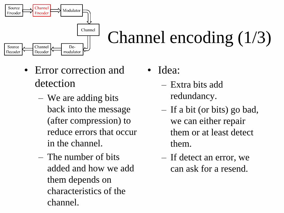
Channel encoding (1/3)

• Error correction and

detection

– We are adding bits

back into the message

(after compression) to

reduce errors that occur

in the channel.

– The number of bits

added and how we add

them depends on

characteristics of the

channel.

• Idea:

– Extra bits add

redundancy.

– If a bit (or bits) go bad,

we can either repair

them or at least detect

them.

– If detect an error, we

can ask for a resend.

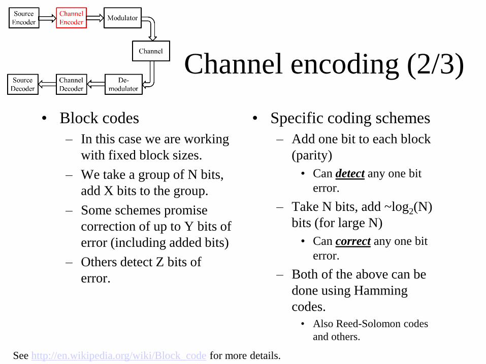
Channel encoding (2/3)

• Block codes

– In this case we are working

with fixed block sizes.

– We take a group of N bits,

add X bits to the group.

– Some schemes promise

correction of up to Y bits of

error (including added bits)

– Others detect Z bits of

error.

• Specific coding schemes

– Add one bit to each block

(parity)

• Can detect any one bit

error.

– Take N bits, add ~log2(N)

bits (for large N)

• Can correct any one bit

error.

– Both of the above can be

done using Hamming

codes.

• Also Reed-Solomon codes

and others.

See http://en.wikipedia.org/wiki/Block_code for more details.

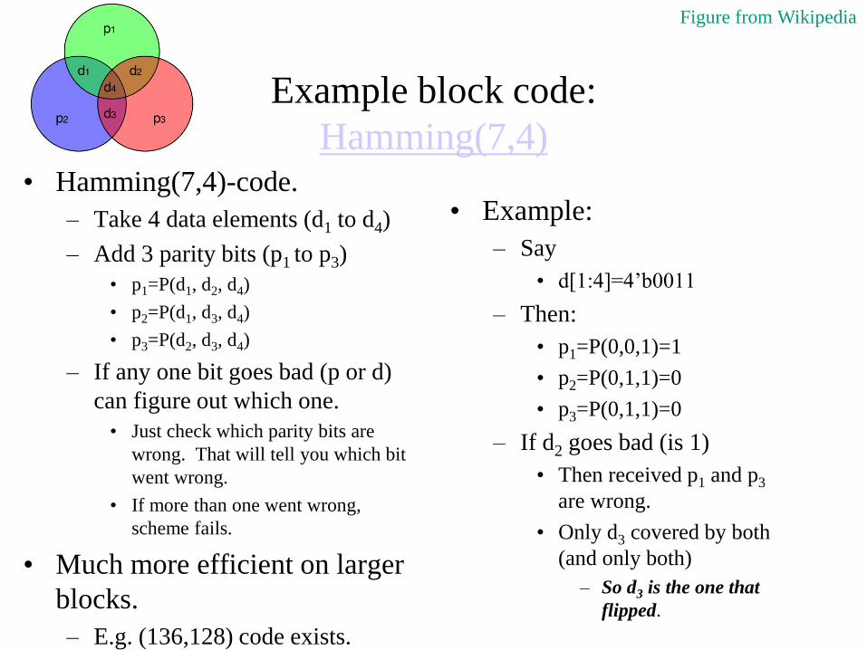
Example block code:

Hamming(7,4)• Hamming(7,4)-code.

– Take 4 data elements (d1 to d4)

– Add 3 parity bits (p1 to p3)

• p1=P(d1, d2, d4)

• p2=P(d1, d3, d4)

• p3=P(d2, d3, d4)

– If any one bit goes bad (p or d)

can figure out which one.

• Just check which parity bits are

wrong. That will tell you which bit

went wrong.

• If more than one went wrong,

scheme fails.

• Much more efficient on larger

blocks.

– E.g. (136,128) code exists.

• Example:

– Say

• d[1:4]=4’b0011

– Then:

• p1=P(0,0,1)=1

• p2=P(0,1,1)=0

• p3=P(0,1,1)=0

– If d2 goes bad (is 1)

• Then received p1 and p3

are wrong.

• Only d3 covered by both

(and only both)

– So d3 is the one that

flipped.

Figure from Wikipedia

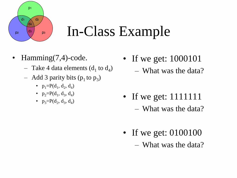
In-Class Example

• If we get: 1000101

– What was the data?

• If we get: 1111111

– What was the data?

• If we get: 0100100

– What was the data?

• Hamming(7,4)-code.

– Take 4 data elements (d1 to d4)

– Add 3 parity bits (p1 to p3)

• p1=P(d1, d2, d4)

• p2=P(d1, d3, d4)

• p3=P(d2, d3, d4)

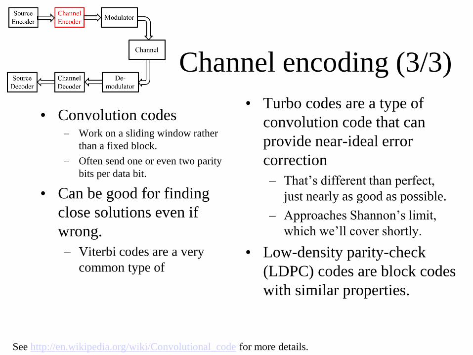
Channel encoding (3/3)

• Convolution codes– Work on a sliding window rather

than a fixed block.

– Often send one or even two parity

bits per data bit.

• Can be good for finding

close solutions even if

wrong.

– Viterbi codes are a very

common type of

• Turbo codes are a type of

convolution code that can

provide near-ideal error

correction

– That’s different than perfect,

just nearly as good as possible.

– Approaches Shannon’s limit,

which we’ll cover shortly.

• Low-density parity-check

(LDPC) codes are block codes

with similar properties.

See http://en.wikipedia.org/wiki/Convolutional_code for more details.

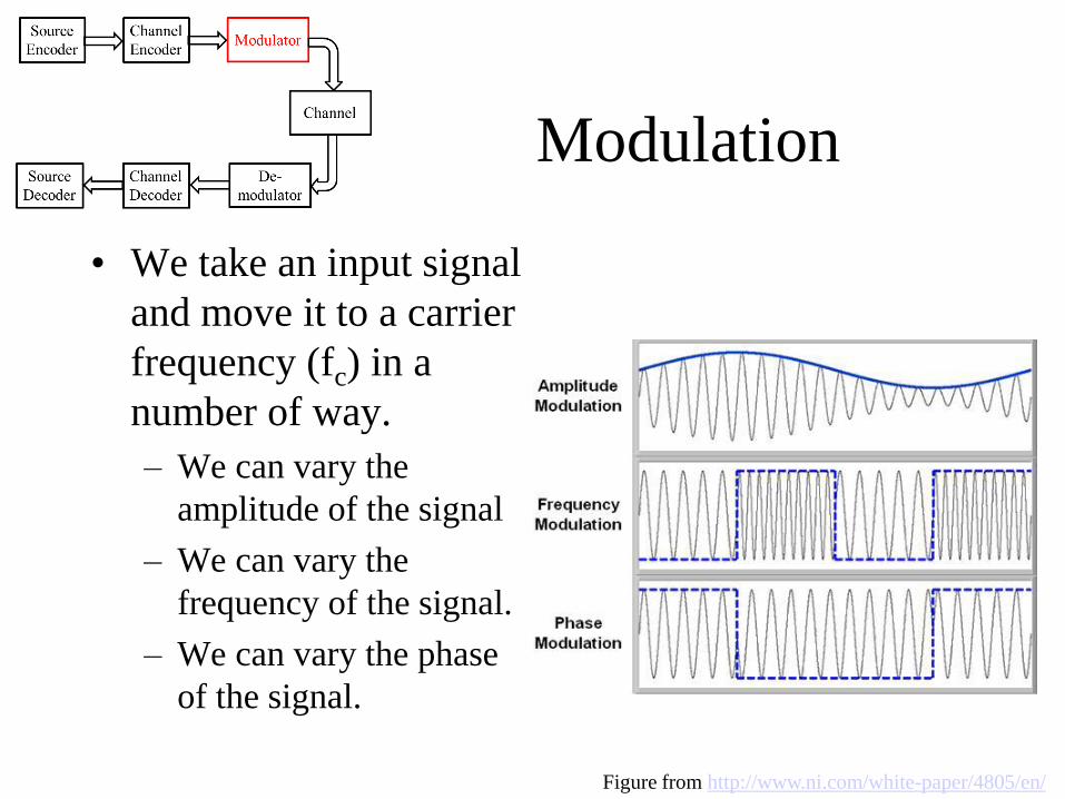
Modulation

• We take an input signal

and move it to a carrier

frequency (fc) in a

number of way.

– We can vary the

amplitude of the signal

– We can vary the

frequency of the signal.

– We can vary the phase

of the signal.

Figure from http://www.ni.com/white-paper/4805/en/

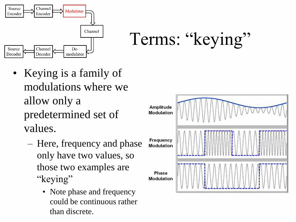
Terms: “keying”

• Keying is a family of

modulations where we

allow only a

predetermined set of

values.

– Here, frequency and phase

only have two values, so

those two examples are

“keying”

• Note phase and frequency

could be continuous rather

than discrete.

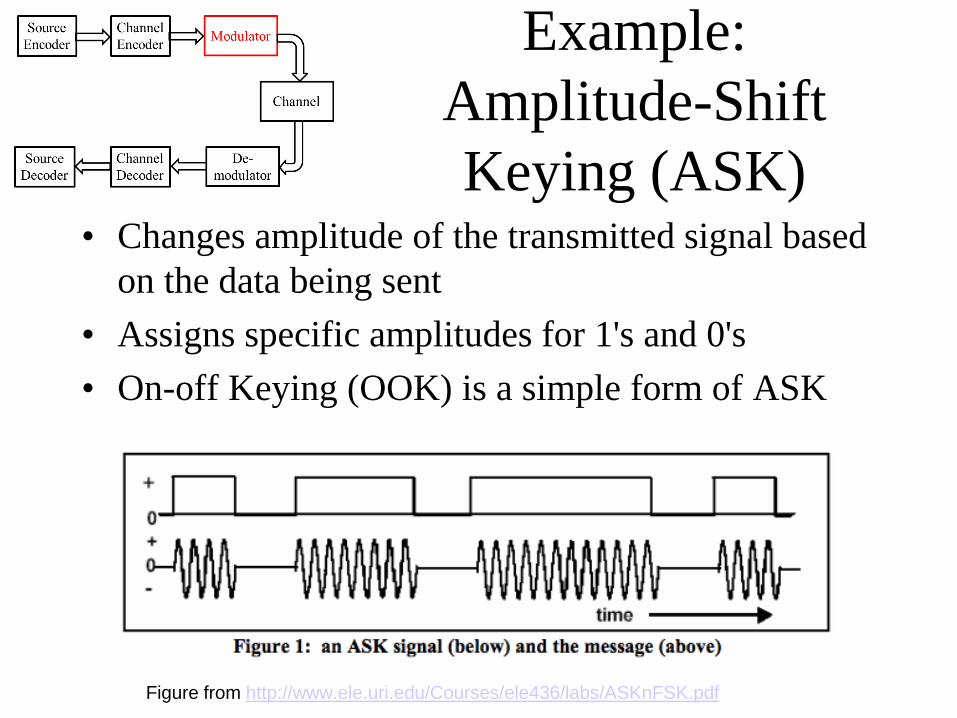
Example:

Amplitude-Shift

Keying (ASK)• Changes amplitude of the transmitted signal based

on the data being sent

• Assigns specific amplitudes for 1's and 0's

• On-off Keying (OOK) is a simple form of ASK

Figure from http://www.ele.uri.edu/Courses/ele436/labs/ASKnFSK.pdf

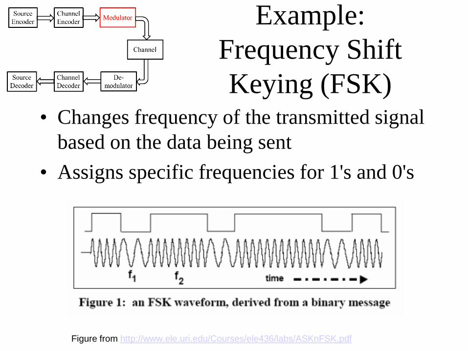
Example:

Frequency Shift

Keying (FSK)• Changes frequency of the transmitted signal

based on the data being sent

• Assigns specific frequencies for 1's and 0's

Figure from http://www.ele.uri.edu/Courses/ele436/labs/ASKnFSK.pdf

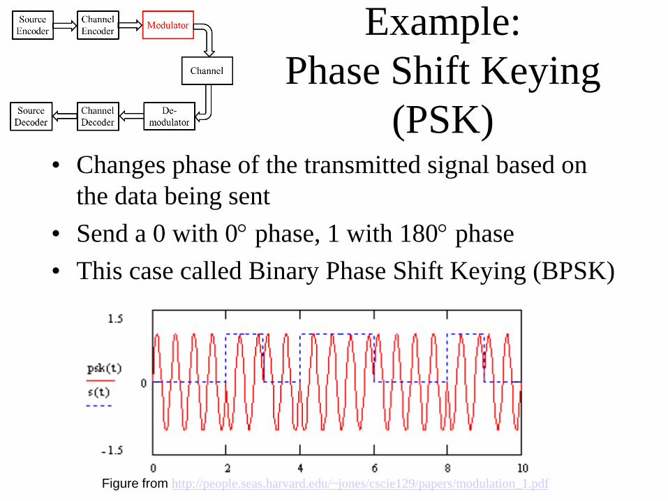
Example:

Phase Shift Keying

(PSK)• Changes phase of the transmitted signal based on

the data being sent

• Send a 0 with 0 phase, 1 with 180 phase

• This case called Binary Phase Shift Keying (BPSK)

Figure from http://people.seas.harvard.edu/~jones/cscie129/papers/modulation_1.pdf

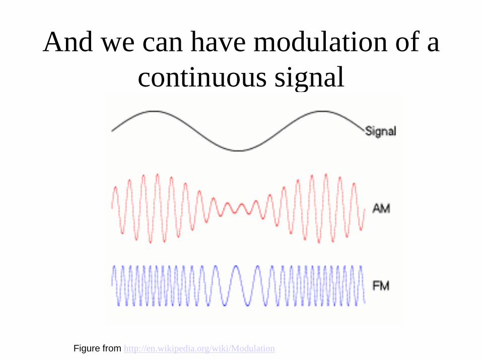
And we can have modulation of a

continuous signal

Figure from http://en.wikipedia.org/wiki/Modulation

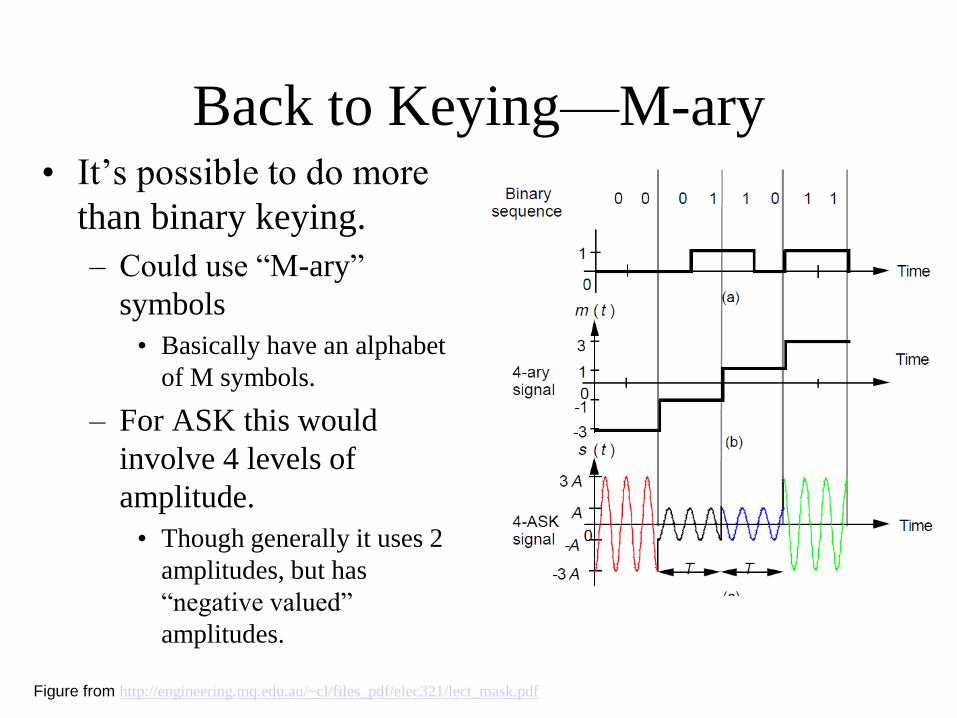
Back to Keying—M-ary• It’s possible to do more

than binary keying.

– Could use “M-ary”

symbols

• Basically have an alphabet

of M symbols.

– For ASK this would

involve 4 levels of

amplitude.

• Though generally it uses 2

amplitudes, but has

“negative valued”

amplitudes.

Figure from http://engineering.mq.edu.au/~cl/files_pdf/elec321/lect_mask.pdf

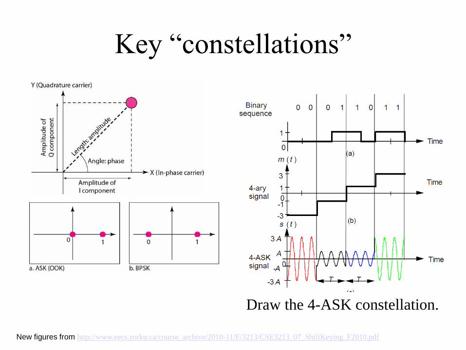
Key “constellations”

New figures from http://www.eecs.yorku.ca/course_archive/2010-11/F/3213/CSE3213_07_ShiftKeying_F2010.pdf

Draw the 4-ASK constellation.

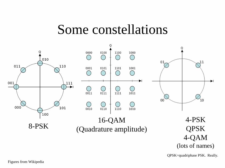
Some constellations

8-PSK16-QAM

(Quadrature amplitude)

Figures from Wikipedia

4-PSK

QPSK

4-QAM(lots of names)

QPSK=quadriphase PSK. Really.

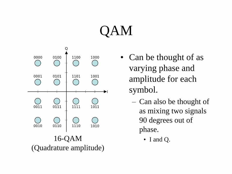
QAM

• Can be thought of as

varying phase and

amplitude for each

symbol.

– Can also be thought of

as mixing two signals

90 degrees out of

phase.

• I and Q.16-QAM

(Quadrature amplitude)

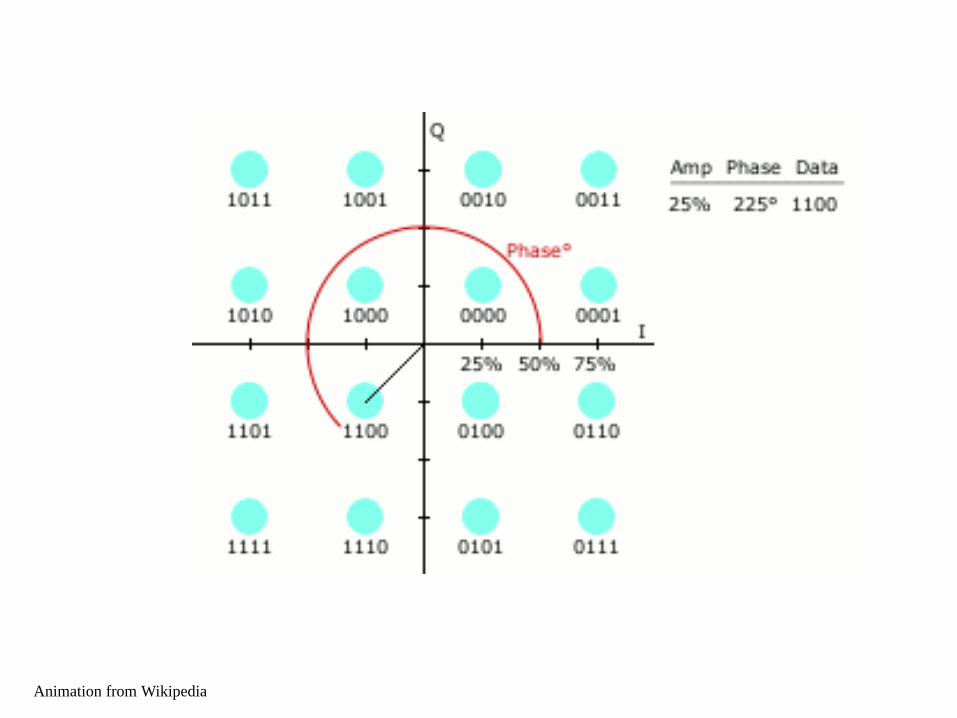
Animation from Wikipedia

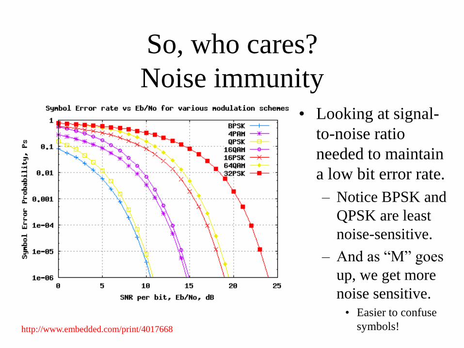
So, who cares?

Noise immunity• Looking at signal-

to-noise ratio

needed to maintain

a low bit error rate.

– Notice BPSK and

QPSK are least

noise-sensitive.

– And as “M” goes

up, we get more

noise sensitive.

• Easier to confuse

symbols!http://www.embedded.com/print/4017668

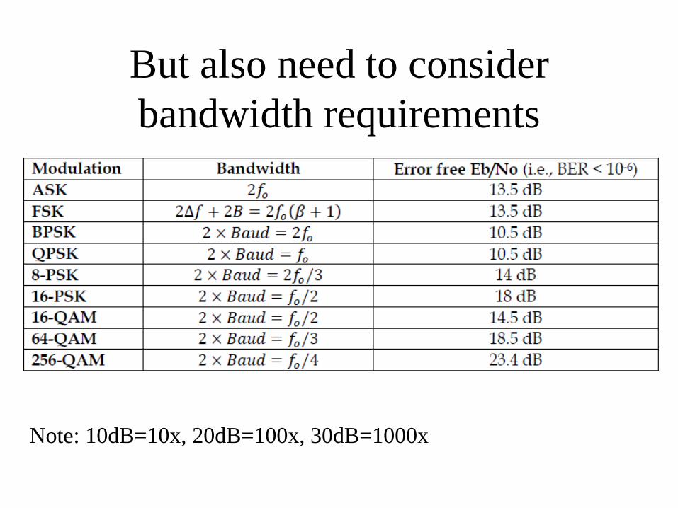
But also need to consider

bandwidth requirements

Note: 10dB=10x, 20dB=100x, 30dB=1000x

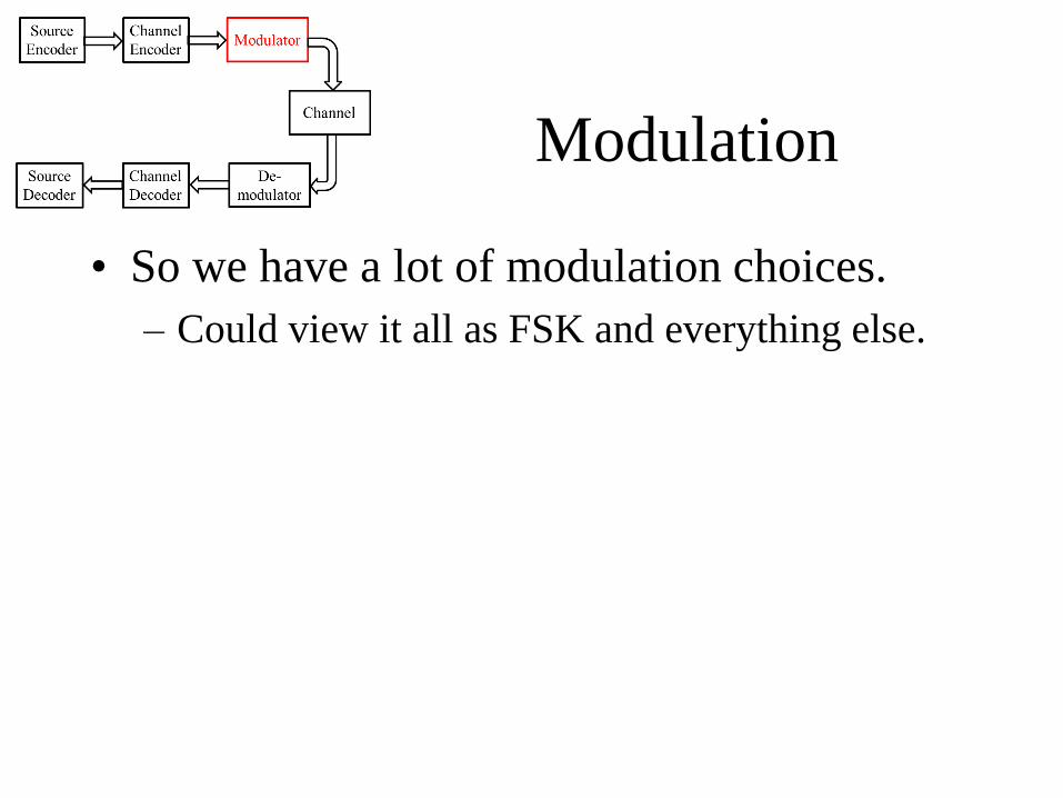
Modulation

• So we have a lot of modulation choices.

– Could view it all as FSK and everything else.

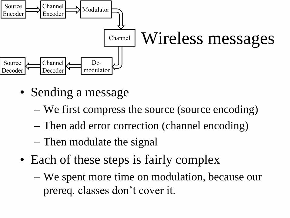
Wireless messages

• Sending a message

– We first compress the source (source encoding)

– Then add error correction (channel encoding)

– Then modulate the signal

• Each of these steps is fairly complex

– We spent more time on modulation, because our

prereq. classes don’t cover it.

Shannon’s limit

• First question about the medium:

– How fast can we hope to send data?

• Answered by Claude Shannon (given some

reasonable assumptions)

– Assuming we have only Gaussian noise,

provides a bound on the rate of information that

can be reliably moved over a channel.

• That includes error correction and whatever other

games you care to play.

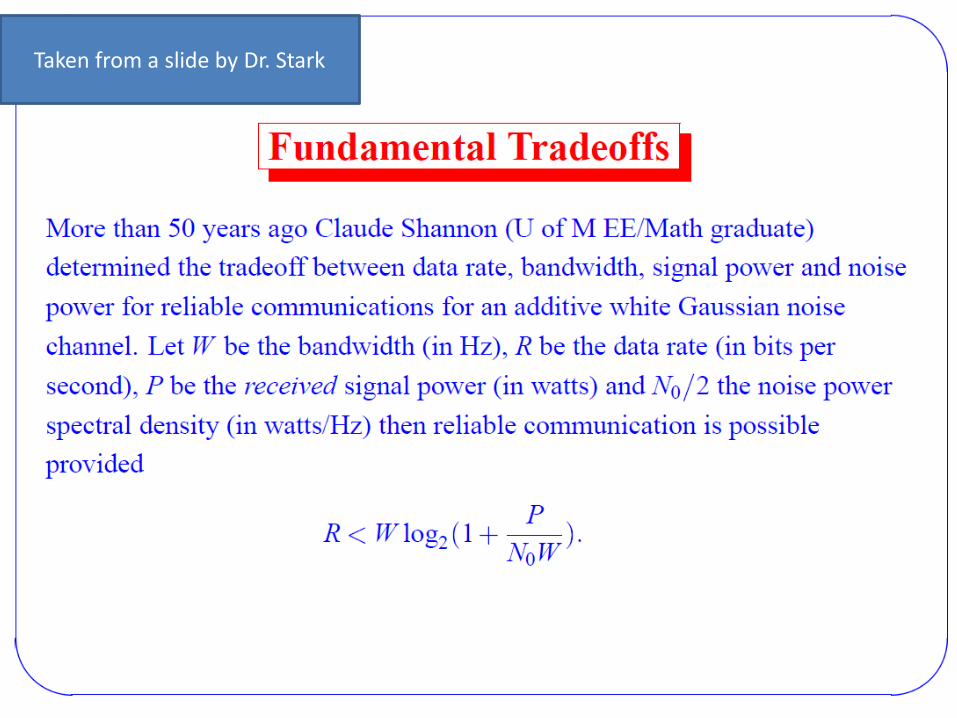
Taken from a slide by Dr. Stark

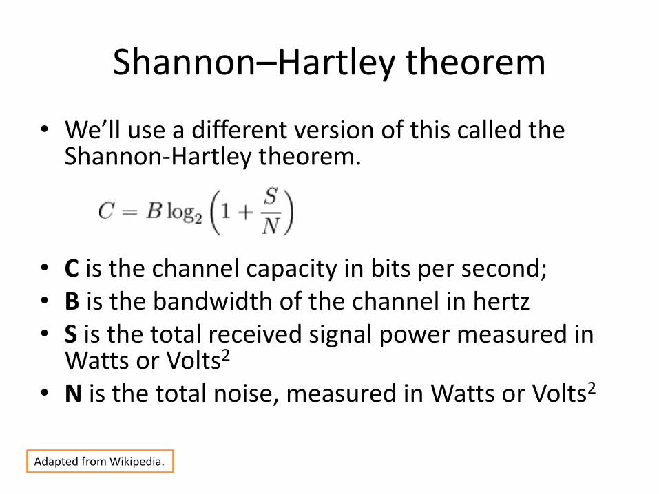
Shannon–Hartley theorem

• We’ll use a different version of this called the Shannon-Hartley theorem.

• C is the channel capacity in bits per second;• B is the bandwidth of the channel in hertz• S is the total received signal power measured in

Watts or Volts2

• N is the total noise, measured in Watts or Volts2

Adapted from Wikipedia.

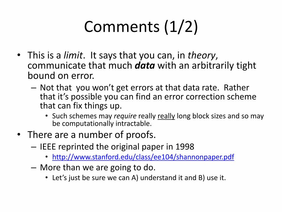
Comments (1/2)

• This is a limit. It says that you can, in theory, communicate that much data with an arbitrarily tight bound on error.– Not that you won’t get errors at that data rate. Rather

that it’s possible you can find an error correction scheme that can fix things up.• Such schemes may require really really long block sizes and so may

be computationally intractable.

• There are a number of proofs. – IEEE reprinted the original paper in 1998

• http://www.stanford.edu/class/ee104/shannonpaper.pdf

– More than we are going to do.• Let’s just be sure we can A) understand it and B) use it.

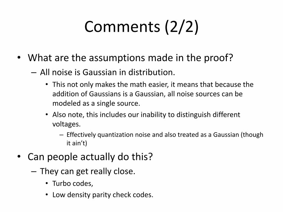
Comments (2/2)

• What are the assumptions made in the proof?

– All noise is Gaussian in distribution.• This not only makes the math easier, it means that because the

addition of Gaussians is a Gaussian, all noise sources can be modeled as a single source.

• Also note, this includes our inability to distinguish different voltages.

– Effectively quantization noise and also treated as a Gaussian (though it ain’t)

• Can people actually do this?

– They can get really close. • Turbo codes,

• Low density parity check codes.

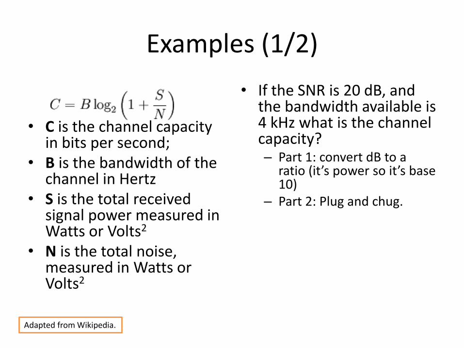
Examples (1/2)

• C is the channel capacity in bits per second;

• B is the bandwidth of the channel in Hertz

• S is the total received signal power measured in Watts or Volts2

• N is the total noise, measured in Watts or Volts2

• If the SNR is 20 dB, and the bandwidth available is 4 kHz what is the channel capacity?– Part 1: convert dB to a

ratio (it’s power so it’s base 10)

– Part 2: Plug and chug.

Adapted from Wikipedia.

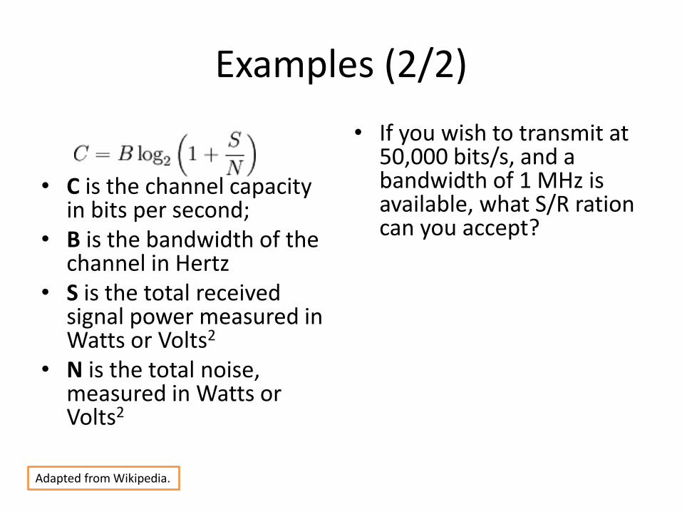
Examples (2/2)

• C is the channel capacity in bits per second;

• B is the bandwidth of the channel in Hertz

• S is the total received signal power measured in Watts or Volts2

• N is the total noise, measured in Watts or Volts2

• If you wish to transmit at 50,000 bits/s, and a bandwidth of 1 MHz is available, what S/R ration can you accept?

Adapted from Wikipedia.

Summary of Shannon’s limit

• Provides an upper-bound on information over a channel

– Makes assumptions about the nature of the noise.

• To approach this bound, need to use channel encoding and modulation.

– Some schemes (Turbo codes, Low density parity check codes) can get very close.

Acknowledgments and sources

• A 9 hour talk by David Tse has been extremely useful and is a basis for me actually understanding anything (though I’m by no means through it all)

• A talk given by Mike Denko, Alex Motalleb, and Tony Qian two years ago for this class proved useful and I took a number of slides from their talk.

• An hour long talk with Prabal Dutta formed the basis for the coverage of this talk.

• Some other sources:– http://www.cs.cmu.edu/~prs/wirelessS12/Midterm12-solutions.pdf

-- A nice set of questions that get at some useful calculations.

– http://people.seas.harvard.edu/~jones/es151/prop_models/propagation.html all the path loss/propagation models in one place

– http://people.seas.harvard.edu/~jones/cscie129/papers/modulation_1.pdf very nice modulation overview.

• I’m grateful for the above sources. All mistakes are my own.

Additional sources/references

General

• http://www.cs.cmu.edu/~prs/wirelessS12/Midterm12-solutions.pdf

Modulation

• https://fetweb.ju.edu.jo/staff/ee/mhawa/421/Digital%20Modulation.pdf

• http://www.ece.umd.edu/class/enee623.S2006/ch2-5_feb06.pdf

• https://www.nhk.or.jp/strl/publica/bt/en/le0014.pdf

• http://engineering.mq.edu.au/~cl/files_pdf/elec321/lect_mask.pdf (ASK)

• http://www.eecs.yorku.ca/course_archive/2010-

11/F/3213/CSE3213_07_ShiftKeying_F2010.pdf

Message, Medium,

and Power & noise• Message

– Source encoding, Channel encoding, Modulation, andProtocol and packets

• Medium

– Shannon’s limit, Nyquist sampling, Path loss, Multi-channel, loss models, Slow and fast fading.

• Signal power & noise power

– Receive and send power, Antennas, Expected noise floors.

• Putting it together

– Modulation (again), MIMO

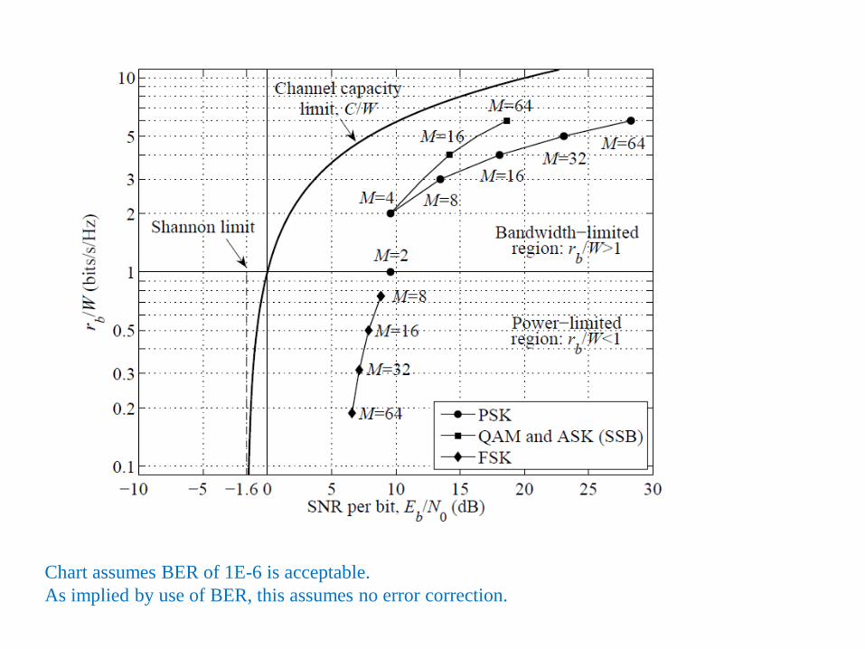
Chart assumes BER of 1E-6 is acceptable.

As implied by use of BER, this assumes no error correction.