Embed Size (px)
Citation preview
EECE 574 - Adaptive ControlLaguerre-based Adaptive Control - Part I
Guy Dumont
Department of Electrical and Computer EngineeringUniversity of British Columbia
January 2013
Guy Dumont (UBC EECE) EECE 574 - Adaptive Control January 2013 1 / 39

History
History
Edmond Laguerre, Frenchmathematician,(Bar-le-Duc, 1834-1886)
He studied approximationmethods and is bestremembered for the specialfunctions: the Laguerrepolynomials
Guy Dumont (UBC EECE) EECE 574 - Adaptive Control January 2013 2 / 39
History
Mathematical Premise
Consider the set of square-(Lebesgue) integrable functions y(t):∫∞
0‖y(t)‖2dt < ∞
This set of signals is denoted as the Lebesgue space L2[0,∞).
The impulse response of an asymptotically stable system lies in L2.
Such a system is said to be L2-stable. Obviously, neither a pure oscillatoror an integrator is in L2.
Guy Dumont (UBC EECE) EECE 574 - Adaptive Control January 2013 3 / 39

History
Mathematical Premise
Now, define the inner product as
< x,y >=∫
∞
0x(t)y(t)dt
We can define an orthonormal sequence {ψi} if it satisfies:
< ψi,ψj >= δi,j
where δi,j is the Dirac delta-function.
Guy Dumont (UBC EECE) EECE 574 - Adaptive Control January 2013 4 / 39
History
Mathematical Premise
The set {ψi} is said to be complete if every y ∈ L2[0,∞) can be expandedinto the series:
y =∞
∑i=0
< y,ψi > ψi
Then, for any real ε > 0, there exists a positive integer N such that
‖y−N
∑i=0
< y,ψi > ψi‖< ε
Guy Dumont (UBC EECE) EECE 574 - Adaptive Control January 2013 5 / 39
History
Mathematical Premise
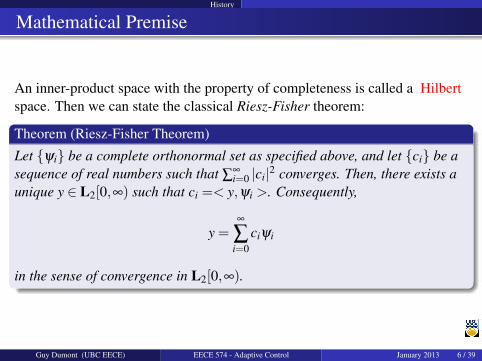
An inner-product space with the property of completeness is called a Hilbertspace. Then we can state the classical Riesz-Fisher theorem:
Theorem (Riesz-Fisher Theorem)
Let {ψi} be a complete orthonormal set as specified above, and let {ci} be asequence of real numbers such that ∑
∞i=0 |ci|2 converges. Then, there exists a
unique y ∈ L2[0,∞) such that ci =< y,ψi >. Consequently,
y =∞
∑i=0
ciψi
in the sense of convergence in L2[0,∞).
Guy Dumont (UBC EECE) EECE 574 - Adaptive Control January 2013 6 / 39
History
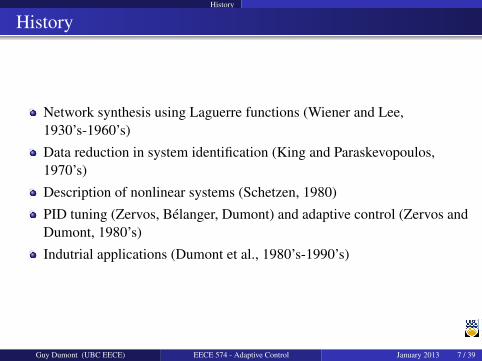
History
Network synthesis using Laguerre functions (Wiener and Lee,1930’s-1960’s)
Data reduction in system identification (King and Paraskevopoulos,1970’s)
Description of nonlinear systems (Schetzen, 1980)
PID tuning (Zervos, Bélanger, Dumont) and adaptive control (Zervos andDumont, 1980’s)
Indutrial applications (Dumont et al., 1980’s-1990’s)
Guy Dumont (UBC EECE) EECE 574 - Adaptive Control January 2013 7 / 39
History
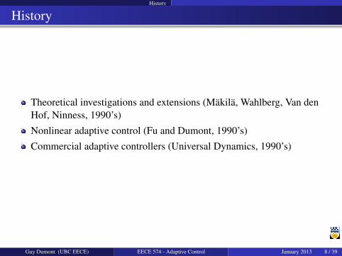
History
Theoretical investigations and extensions (Mäkilä, Wahlberg, Van denHof, Ninness, 1990’s)
Nonlinear adaptive control (Fu and Dumont, 1990’s)
Commercial adaptive controllers (Universal Dynamics, 1990’s)
Guy Dumont (UBC EECE) EECE 574 - Adaptive Control January 2013 8 / 39
Laguerre Functions Continuous Laguerre Functions
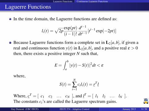
Laguerre Functions
In the time domain, the Laguerre functions are defined as:
li(t) =√
2pexp(pt)(i−1)!
di−1
dti−1 [ti−1 exp(−2pt)]
Because Laguerre functions form a complete set in L2[a,b], if given areal and continuous function y(t) in L2[a,b], and a positive real ε > 0then, there exists a positive integer N such that,
E =∫ b
a|y(t)−S(t)|2dt < ε
where,
S(t) =N
∑i=1
cili(t) = rT l
Where, cT = [ c1 c2 . . . cN ], and lT = [ l1 l2 . . . lN ].The constants ci’s are called the Laguerre spectrum gains.
Guy Dumont (UBC EECE) EECE 574 - Adaptive Control January 2013 9 / 39
Laguerre Functions Continuous Laguerre Functions
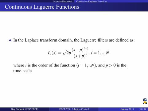
Continuous Laguerre Functions
In the Laplace transform domain, the Laguerre filters are defined as:
Li(s) =√
2p(s−p)i−1
(s+p)i , i = 1, ..,N
where i is the order of the function (i = 1, ..N), and p > 0 is thetime-scale
Guy Dumont (UBC EECE) EECE 574 - Adaptive Control January 2013 10 / 39

Laguerre Functions Continuous Laguerre Functions
Continuous Laguerre Functions
-√
2ps+p
U(s)- s−p
s+pL1(s)
- q q qL2(s)- s−p
s+pLN(s)p
?
p?
p?
c1 c2 cN
? ? ?
Summing Circuit�Y(s)
Figure: Representation of plant dynamics using a truncated continuous Laguerreladder network
Guy Dumont (UBC EECE) EECE 574 - Adaptive Control January 2013 11 / 39
Laguerre Functions Continuous Laguerre Functions
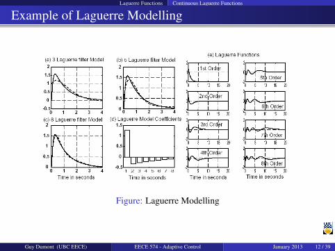
Example of Laguerre Modelling
Figure: Laguerre Modelling
Guy Dumont (UBC EECE) EECE 574 - Adaptive Control January 2013 12 / 39
Laguerre Functions Discrete Laguerre Functions
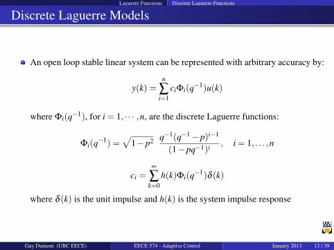
Discrete Laguerre Models
An open loop stable linear system can be represented with arbitrary accuracy by:
y(k) =n
∑i=1
ciΦi(q−1)u(k)
where Φi(q−1), for i = 1, · · · ,n, are the discrete Laguerre functions:
Φi(q−1) =√
1−p2 q−1(q−1−p)i−1
(1−pq−1)i , i = 1, . . . ,n
ci =∞
∑k=0
h(k)Φi(q−1)δ (k)
where δ (k) is the unit impulse and h(k) is the system impulse response
Guy Dumont (UBC EECE) EECE 574 - Adaptive Control January 2013 13 / 39
Laguerre Functions Discrete Laguerre Functions
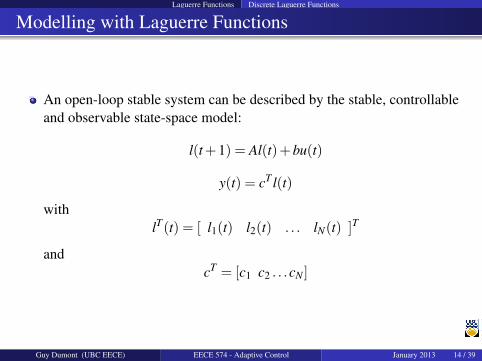
Modelling with Laguerre Functions
An open-loop stable system can be described by the stable, controllableand observable state-space model:
l(t+1) = Al(t)+bu(t)
y(t) = cT l(t)
withlT(t) = [ l1(t) l2(t) . . . lN(t) ]T
andcT = [c1 c2 . . .cN ]
Guy Dumont (UBC EECE) EECE 574 - Adaptive Control January 2013 14 / 39

Identification of Laguerre Models
Identification of Laguerre Models
The classical method is to compute the Laguerre spectrum of a signalusing the correlation method, i.e.
ci =∫ b
ah(t)li(t)dt
where h(t) is the plant impulse response and li(t) is the ith Laguerrefunction
In practice, it is more realistic to use a least-squares type algorithm
Guy Dumont (UBC EECE) EECE 574 - Adaptive Control January 2013 15 / 39

Identification of Laguerre Models
Identification of Laguerre Models
Consider the real plant described by
y(t) =N
∑i=1
ciLi(q)+∞
∑i=N+1
ciLi(q)+w(t)
where w(t) is a disturbance
This model has an output-error structure, is linear in the parameters, andgives a convex identification problem
Guy Dumont (UBC EECE) EECE 574 - Adaptive Control January 2013 16 / 39

Identification of Laguerre Models
Identification of Laguerre Models
With the following standard notations:
φT(k) = [ l1(kT) l2(kT) . . . lN(kT) ]
φTU(k) = [ lN+1(kT) lN+2(kT) . . . . . . ]
This is somewhat of an abuse of notation, as in theory the true plant isrepresented as an infinite series. However, for all practical purposes, the trueplant can be exactly described by a large but truncated series.
ΦT = [ φ(T) φ(2T) . . . φ(nT) ]
ΦTU = [ φ
U(T) φ
U(2T) . . . φ
U(nT) ]
YT = [ y(T) y(2T) . . . y(nT) ]
WT = [ w(T) w(2T) . . . w(nT) ]
Guy Dumont (UBC EECE) EECE 574 - Adaptive Control January 2013 17 / 39
Identification of Laguerre Models
Identification of Laguerre Models
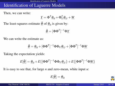
Then, we can write:Y = Φ
Tθ 0 +Φ
TUθ U +W
The least-squares estimate θ of θ 0 is given by:
θ = [ΦΦT ]−1
ΦY
We can write the estimate as:
θ = θ 0 +[ΦΦT ]−1
ΦΦUθ U +[ΦΦT ]−1
ΦW
Taking the expectation yields:
E[θ ] = θ 0 +E{[ΦΦT ]−1
ΦΦUθ U}+E{[ΦΦT ]−1
ΦW}
It is easy to see that, for large n and zero-mean, white input u:
E[θ ] = θ 0
Guy Dumont (UBC EECE) EECE 574 - Adaptive Control January 2013 18 / 39
Identification of Laguerre Models
Identification of Laguerre Models
Even if w(t) it coloured and non-zero mean, simple least-squares provideconsistent estimates of the ci’s.
The estimate of the nominal plant, i.e. of ci, for i = 1, · · · ,N is unaffectedby the presence of the unmodelled dynamics represented by ci, fori = N +1, · · · ,∞.
This provides us with a robust estimator, one of the two key ingredientsin a robust adaptive controller.
Guy Dumont (UBC EECE) EECE 574 - Adaptive Control January 2013 19 / 39

Identification of Laguerre Models
Identification of Laguerre Models
The mapping (1+aeiω)/(eiω +a) improves the condition number of theleast-squares covariance matrix.
The implicit assumption that the system is low-pass in nature reduces theasymptotic covariance of the estimate at high frequenciesFor least-squares, the mean square error of the transfer function estimatecan be approximated by
π(eiω ) =12
(N(1−λ )
1−a2
|eiω −a|2Φv(eiω )
Φu(eiω )+
µ2
1−λr1(eiω )
)
Guy Dumont (UBC EECE) EECE 574 - Adaptive Control January 2013 20 / 39
Identification of Laguerre Models
Identification of Laguerre Models
The case a = 0 corresponds to a FIR model. The MSE is proportional tothe number of parameters. Compared with a FIR model, an orthonormalseries representation requires less parameters and thus gives a smallerMSE.The disturbance spectrum is scaled by
1−a2
|eiω −a|2
thus reducing the detrimental effect of disturbances at high frequencies.
Guy Dumont (UBC EECE) EECE 574 - Adaptive Control January 2013 21 / 39
Non Linear Systems
Extension to Nonlinear Systems
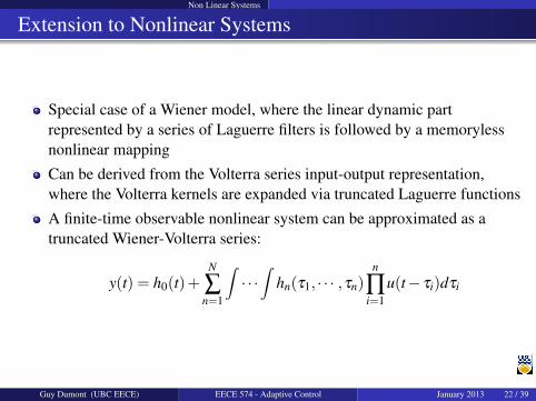
Special case of a Wiener model, where the linear dynamic partrepresented by a series of Laguerre filters is followed by a memorylessnonlinear mapping
Can be derived from the Volterra series input-output representation,where the Volterra kernels are expanded via truncated Laguerre functions
A finite-time observable nonlinear system can be approximated as atruncated Wiener-Volterra series:
y(t) = h0(t)+N
∑n=1
∫· · ·∫
hn(τ1, · · · ,τn)n
∏i=1
u(t− τi)dτi
Guy Dumont (UBC EECE) EECE 574 - Adaptive Control January 2013 22 / 39

Non Linear Systems
Extension to Nonlinear Systems
For instance, truncating the series after the second-order kernel:
y(t) = h0(t)+∫
∞
0h1(τ1)u(t− τ1)dτ1 +∫
∞
0
∫∞
0h2(τ1,τ2)u(t− τ1)u(t− τ2)dτ1dτ2
Assuming that the Volterra kernels are in L2[,∞), they can be expandedand approximated as:
h1(τ1) =N
∑k=1
ckφk(τ1)
h2(τ1,τ2) =N
∑n=1
N
∑m=1
cnmφn(τ1)φn(τ2)
Guy Dumont (UBC EECE) EECE 574 - Adaptive Control January 2013 23 / 39
Non Linear Systems
Extension to Nonlinear Systems
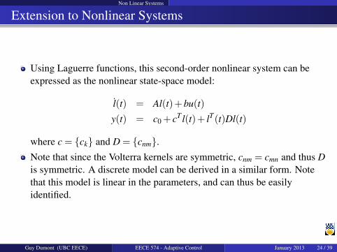
Using Laguerre functions, this second-order nonlinear system can beexpressed as the nonlinear state-space model:
l(t) = Al(t)+bu(t)
y(t) = c0 + cT l(t)+ lT(t)Dl(t)
where c = {ck} and D = {cnm}.Note that since the Volterra kernels are symmetric, cnm = cmn and thus Dis symmetric. A discrete model can be derived in a similar form. Notethat this model is linear in the parameters, and can thus be easilyidentified.
Guy Dumont (UBC EECE) EECE 574 - Adaptive Control January 2013 24 / 39
Non Linear Systems
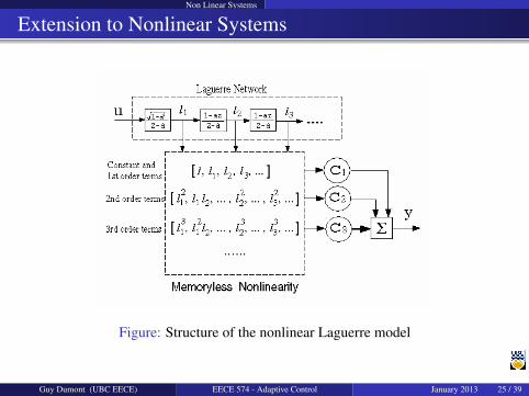
Extension to Nonlinear Systems
Figure: Structure of the nonlinear Laguerre model
Guy Dumont (UBC EECE) EECE 574 - Adaptive Control January 2013 25 / 39

Laguerre-based Control A Simple Predictive Control Law
Laguerre EHC
Given the discrete Laguerre model
l(k+1) = Al(k)+bu(k)
y(k) = Cl(k)
We can predict the plant output for the future d-steps based on using thecurrently measured output y(k), which is:
y(k+d) = y(k)+C[l(k+d)− l(k)]
Guy Dumont (UBC EECE) EECE 574 - Adaptive Control January 2013 26 / 39
Laguerre-based Control A Simple Predictive Control Law
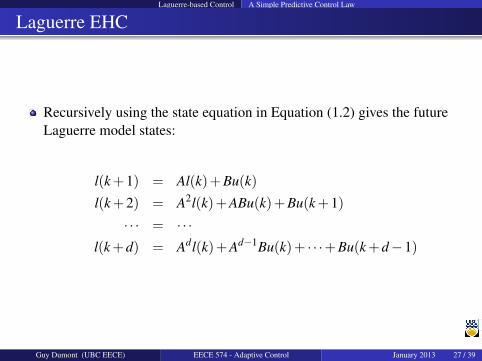
Laguerre EHC
Recursively using the state equation in Equation (1.2) gives the futureLaguerre model states:
l(k+1) = Al(k)+Bu(k)
l(k+2) = A2l(k)+ABu(k)+Bu(k+1)
· · · = · · ·l(k+d) = Adl(k)+Ad−1Bu(k)+ · · ·+Bu(k+d−1)
Guy Dumont (UBC EECE) EECE 574 - Adaptive Control January 2013 27 / 39
Laguerre-based Control A Simple Predictive Control Law
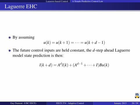
Laguerre EHC
By assumingu(k) = u(k+1) = · · ·= u(k+d−1)
The future control inputs are held constant, the d-step ahead Laguerremodel state prediction is then:
l(k+d) = Adl(k)+(Ad−1 + · · ·+ I)Bu(k)
Guy Dumont (UBC EECE) EECE 574 - Adaptive Control January 2013 28 / 39
Laguerre-based Control A Simple Predictive Control Law
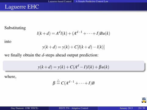
Laguerre EHC
Substitutingl(k+d) = Adl(k)+(Ad−1 + · · ·+ I)Bu(k)
intoy(k+d) = y(k)+C[l(k+d)− l(k)]
we finally obtain the d-steps ahead output prediction:
y(k+d) = y(k)+C(Ad− I)l(k)+βu(k)
where,β4= C(Ad−1 + · · ·+ I)B
Guy Dumont (UBC EECE) EECE 574 - Adaptive Control January 2013 29 / 39
Laguerre-based Control A Simple Predictive Control Law
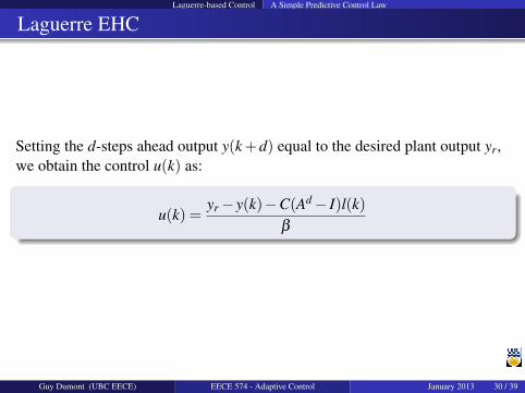
Laguerre EHC
Setting the d-steps ahead output y(k+d) equal to the desired plant output yr,we obtain the control u(k) as:
u(k) =yr− y(k)−C(Ad− I)l(k)
β
Guy Dumont (UBC EECE) EECE 574 - Adaptive Control January 2013 30 / 39
Laguerre-based Control A Simple Predictive Control Law
Laguerre EHC
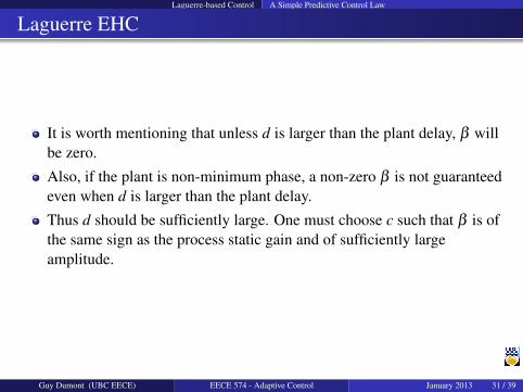
It is worth mentioning that unless d is larger than the plant delay, β willbe zero.
Also, if the plant is non-minimum phase, a non-zero β is not guaranteedeven when d is larger than the plant delay.
Thus d should be sufficiently large. One must choose c such that β is ofthe same sign as the process static gain and of sufficiently largeamplitude.
Guy Dumont (UBC EECE) EECE 574 - Adaptive Control January 2013 31 / 39
Laguerre-based Control A Simple Predictive Control Law
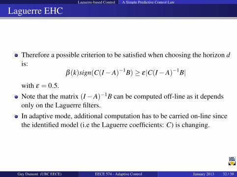
Laguerre EHC
Therefore a possible criterion to be satisfied when choosing the horizon dis:
β (k)sign(C(I−A)−1B)≥ ε|C(I−A)−1B|
with ε = 0.5.
Note that the matrix (I−A)−1B can be computed off-line as it dependsonly on the Laguerre filters.
In adaptive mode, additional computation has to be carried on-line sincethe identified model (i.e the Laguerre coefficients: C) is changing.
Guy Dumont (UBC EECE) EECE 574 - Adaptive Control January 2013 32 / 39

Laguerre-based Control A Simple Predictive Control Law
Laguerre EHC
Sometimes, the control signal is expressed in velocity form. The controllercan be rewritten as:
u(t) = (yr− y(t))/β −CS(Al(t)−Al(t−1)−Bu(t−1))/β (1)
Using the definition of β and rearranging, one gets
∆u(t) =yr− y(t)− f T∆l(t)
β
where S = (Ad−1 + · · ·+ I), f T = cTSA, ∆u(t) = u(t)−u(t−1), and∆l(t) = l(t)− l(t−1).
Guy Dumont (UBC EECE) EECE 574 - Adaptive Control January 2013 33 / 39
Laguerre-based Control Feedforward Control
Feedforward Control
Inclusion of a feedforward variable uf requires an additional Laguerrenetwork
lf (k+1) = Af lf (k)+Bf uf (k)
The plant output is then described by
y(k) = CT l(k)+CTf lf (k)
Following the same derivations as before but using the above modifiedmodel will give a control law that automatically incorporatesfeedforward compensation.
Guy Dumont (UBC EECE) EECE 574 - Adaptive Control January 2013 34 / 39
Laguerre-based Control Integrating Systems
Integrating Systems
Time delay integrating systems are common in the process industries.
Although Laguerre functions are particularly appealing to describe stabledynamic systems, they cannot be used to represent dynamics that containan unstable or an integrating mode.
Guy Dumont (UBC EECE) EECE 574 - Adaptive Control January 2013 35 / 39
Laguerre-based Control Integrating Systems
Integrating Systems
In case of an integrator, we can generally assume knowledge of itspresence. We can then simply remove the effect of the integrator fromthe data by differentiating it.
The Laguerre network is then employed to model only the stable part ofthe plant as in
l(k) = Al(k)+Bu(k)
∆y(k) = Cl(k)
where ∆y(k) = y(k)− y(k−1)
Guy Dumont (UBC EECE) EECE 574 - Adaptive Control January 2013 36 / 39

Laguerre-based Control Integrating Systems
Integrating Systems
Good adaptive control of those systems requires estimation of thedisturbance
Assuming both known and unknown disturbances, the model states areupdated based on:
l(k+1) = Al(k)+Bu(k)
lf (k+1) = Af lf (k)+Bf uf (k)
ld(k+1) = Adld(k)+Bdud(k)
Guy Dumont (UBC EECE) EECE 574 - Adaptive Control January 2013 37 / 39
Laguerre-based Control Integrating Systems
Integrating Systems
The output estimations are defined as:
y(k) = y(k−1)+C(k)l(k)+ yf (k)+ yd(k)
yf (k) = yf (k−1)+Cf (k)lf (k)
yd(k) = yd(k−1)+Cd(k)ld(k)
where f denotes a feedforward variable and d a variable associated withthe unmeasured disturbance model.
Guy Dumont (UBC EECE) EECE 574 - Adaptive Control January 2013 38 / 39
Laguerre-based Control Integrating Systems
Integrating Systems
The disturbance is then estimated using an extended Kalman filter with
ud(k) = (y(k)+ yff (k)+ yd(k))− y(k)
where y(k), yd(k) and yff (k) are the estimated plant, known and unknowndisturbance model outputs.
A GPC type control law can then be derived.
Guy Dumont (UBC EECE) EECE 574 - Adaptive Control January 2013 39 / 39