EE699 (06790)

ADAPTIVE NEUROFUZZY CONTROL

Instructor: Dr. YuMing Zhang223 CRMS Building

Phone: 257-6262 Ext. 223 245-4518 (Home)

Email: ymzhang@engr.uky.edu

Adaptive control and neurofuzzy control are two advanced methods for time-varying and non-linear processes. This course will begin with adaptive control of linear systems. Nonlinear systems and related control issues will be then briefly reviewed. Neural network and fuzzy model will be described as general structures for approximating non-linear functions and dynamic processes. Based on the comparison of the two methods, neurofuzzy model will be proposed as a promising technology for the control and adaptive control of nonlinear processes.

This course will emphasize basic concepts, design procedures, and practical examples. The assignments include two design projects: adaptive control of a linear system and neurofuzzy method based modeling and adaptive control of a nonlinear system. A presentation on a selected subject is required.

TR 03:30 PM-04:45 PM Funkhouser 313

1

ADAPTIVE NEUROFUZZY CONTROL

Introduction (1-2): Actually 3 including 2 for the example

Adaptive Control of Linear Systems (3-5)

Identification of Linear Models (2-3)

Project 1

Control of Nonlinear Systems (1-2)

Neural and Fuzzy Control (1-2)

Neural and Fuzzy Modeling (4-6)

Project 2: Modeling

Adaptive Neurofuzzy Control Design (7-9) & Project 2: Control

Design Examples (2)

Presentation (2)

Final Examination (1)

Projects:

1. Adaptive control of a linear system2. Neurofuzzy modeling and control of a non-linear system

2

CHAPTER I: INTRODUCTION

Primary References:

Y. M. Zhang and R. Kovacevic, “Neurofuzzy model based control of weld fusion zone geometry," IEEE Transactions on Fuzzy Systems, 6(3): 389-401.

R. Kovacevic and Y. M. Zhang, "Neurofuzzy model-based weld fusion state estimation," IEEE Control Systems, 17(2): 30-42, 1997.

1. Linear Systems

Classical Control, Linear Control (LQG, Optimal Control)

Model Mismatch between the process and the nominal model.

Reasons: -Substantial range of physical conditions, modeling error (actual model is fixed, but different with the nominal model) Robust control or adaptive control-Time-varying model: Varying physical condition Robust control or adaptive control

Adaptive Control: Identify the real parameters of the model to minimize the mismatch Robust Control: Allow the mismatch

2. Non-linear Systems

Lack of unified models, a variety of models and design methods

Unified model structure for non-linear systems: neural network models and fuzzy models

Comparison Modeling: Disadvantage: large number of parameters Advantages: adequate accuracy, simplicity Control: Disadvantages: performance evaluation Advantage: unified methods Neural network and fuzzy methods

Modeling: Neural networks: large number of parameters, but automated algorithm Fuzzy models: moderate number of parameters, lack of automated algorithmControl design: Neural networks: large number of parameters Fuzzy models: moderate number of parameters, time consuming

Neurofuzzy Control

3

Compared with Fuzzy Logic: automated identification algorithm, easier designCompared with Neural Networks: less number of parameters, faster adaptation

3. Adaptive Non-Linear Control

Acceptable convergence speed (number of parameters), general model

4. Example: Neurofuzzy Control of Arc Welding Process

4

CHAPTER 2: ADAPTIVE CONTROL

Primary Reference:D. W. Clarke, “Self-tuning control,” in The Control Handbook edited by W. S. Levine. IEEE Press, 1996.

1. Introduction

Most Control Theory: assuming (1) time-invariant, known (nominal) model, (2) no difference between the nominal and actual model Problems: initial model uncertainties (a difference between the nominal and actual model), actual model varies during process Examples: Solutions

Robust fixed controllerAdaptive controller (self-tuning controller)

For unknown but constant dynamics, identify the model during initial period (auto-tuning or self-tuning).

For time-varying system, identify and update the model all the time (adaptive control). Structure of self-tuning control system

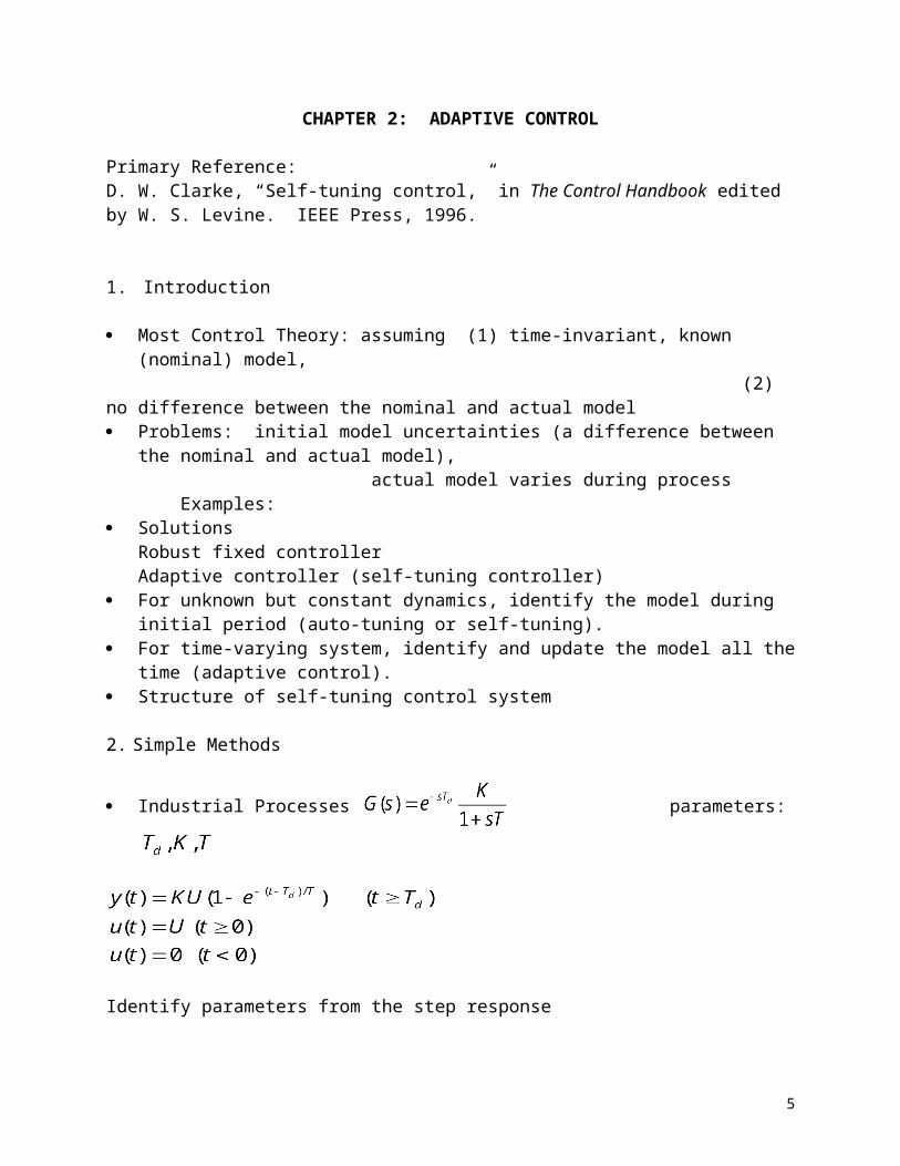
2. Simple Methods

Industrial Processes parameters:

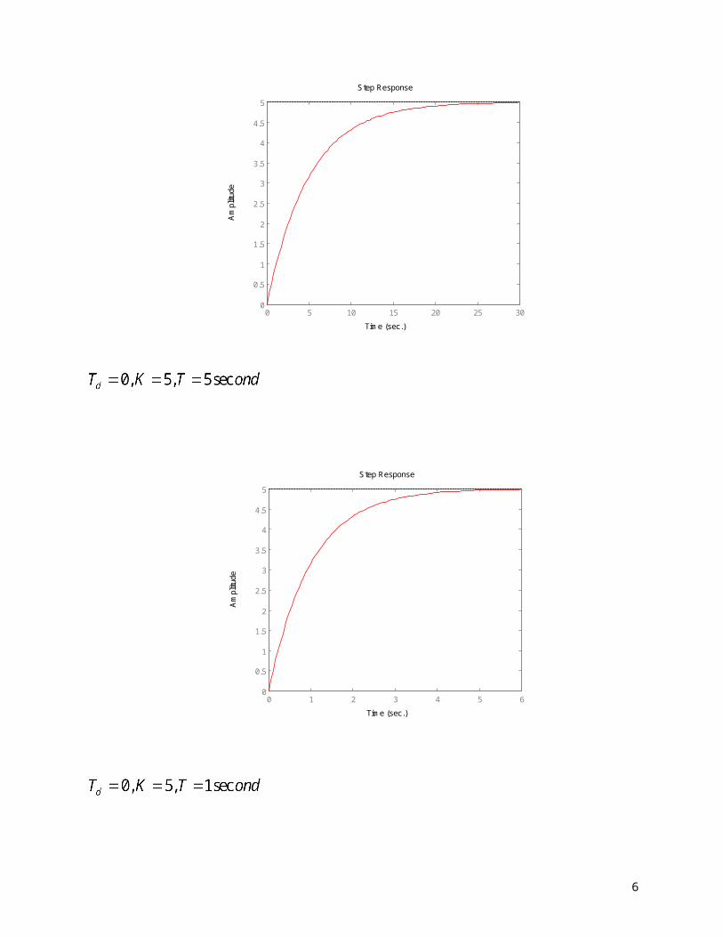
Identify parameters from the step response

5

6

Time (sec.)

Am

plitu

de

Step Response

0 1 2 3 4 5 60

0.5

1

1.5

2

2.5

3

3.5

4

4.5

5

Time (sec.)

Am

plitu

de

Step Response

0 5 10 15 20 25 300

0.5

1

1.5

2

2.5

3

3.5

4

4.5

5

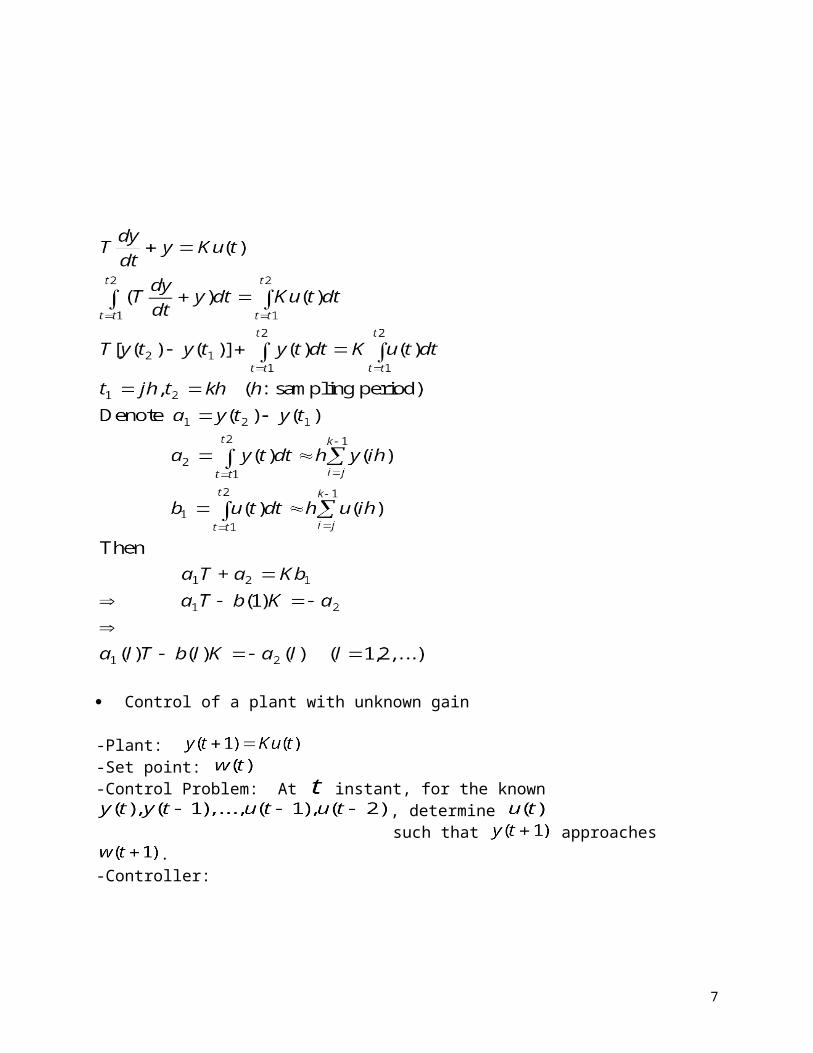
Control of a plant with unknown gain

-Plant: -Set point: -Control Problem: At instant, for the known , determine

such that approaches .-Controller:

-On-line Identification

At instant: the estimate of the gain is Predicted output

At instant: becomes available The prediction error generated: In order to eliminate the prediction error,

7

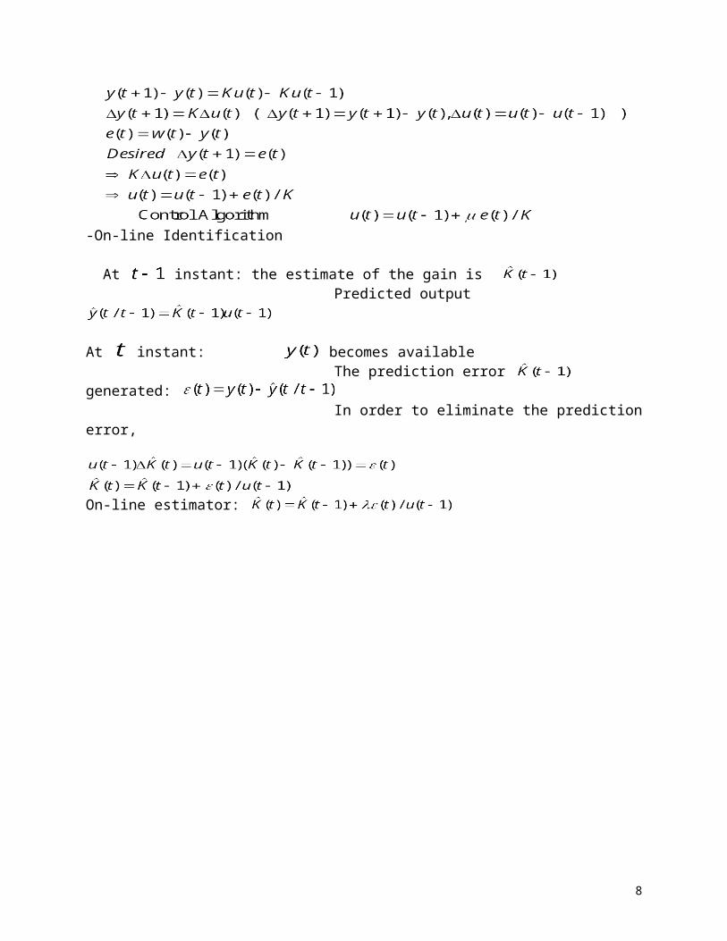
On-line estimator:

8

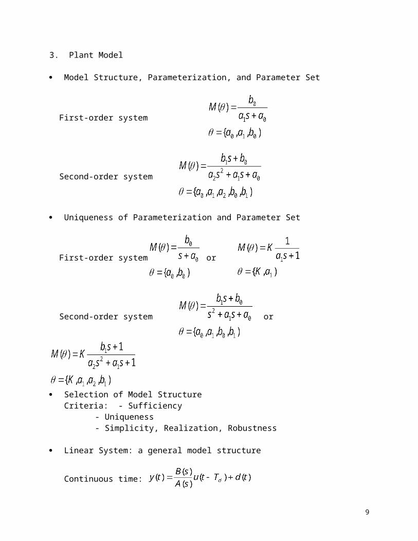
3. Plant Model

Model Structure, Parameterization, and Parameter Set

First-order system

Second-order system

Uniqueness of Parameterization and Parameter Set

First-order system or

Second-order system or

Selection of Model StructureCriteria: - Sufficiency

- Uniqueness- Simplicity, Realization, Robustness

Linear System: a general model structure

Continuous time:

Dead time : mass transport, approximation of complex dynamics Disturbance : measurement noise, unmodeled dynamics, nonlinear effects, disturbance (load) On-line identification: Faster faster tracking of the changed dynamics, less robust to noise (easier to be affected by noise) Slower slower tracking of the changed dynamics, more robust to noise Pulse Response

Discrete-Time: (for open-loop stable system)

9

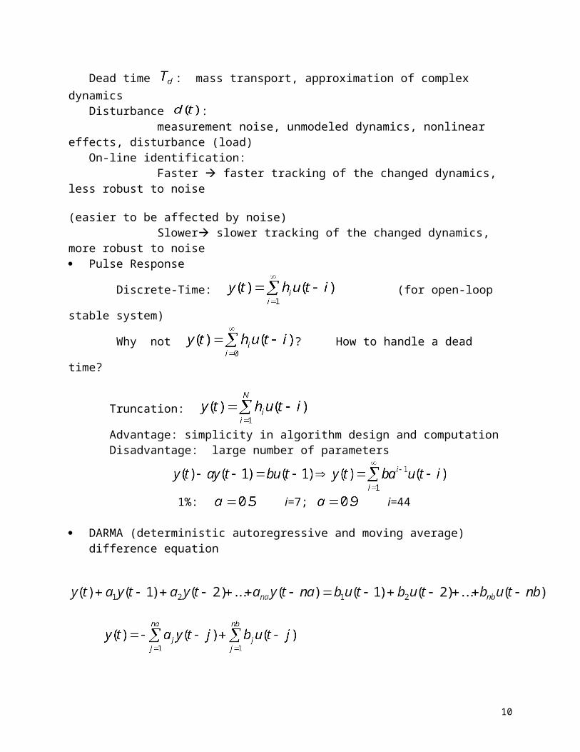
Why not ? How to handle a dead time?

Truncation:

Advantage: simplicity in algorithm design and computation Disadvantage: large number of parameters

1%: i=7; i=44

DARMA (deterministic autoregressive and moving average) difference equation

Backward-shift operator :

Disturbance Modeling: zero-mean disturbance

Additive disturbance

Modeling of disturbance: (stationary random sequence)

Uncorrelated Random Sequence (while noise):

Random Sequence: partially predictable Uncorrelated Random Sequence: unpredictable CARMA (controlled autoregressive and moving average) difference equation

10

Disturbance Modeling: non zero-mean disturbance

unknown constant or slowly changing)

(Difference operator

CARIMA model:

4A. Least Squares Method

Model:

For :

11

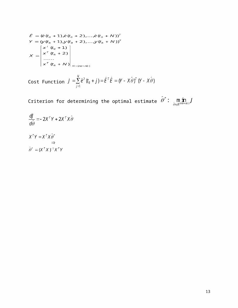
Cost Function

Criterion for determining the optimal estimate

12

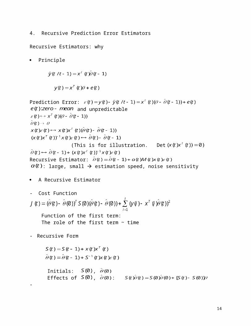
4. Recursive Prediction Error Estimators

Recursive Estimators: why

Principle

Prediction Error:

and unpredictable

(This is for illustration. Det

Recursive Estimator: : large, small estimation speed, noise sensitivity

A Recursive Estimator

- Cost Function

Function of the first term: The role of the first term ~ time

- Recursive Form

Initials: , Effects of , : -

Gain vector:

Parameter Update:

Covariance Update:

Initials: and

13

Forgetting Factor

Why? Filter effectSolution:

Recursive Equations:

Gain vector:

Parameter Update:

Covariance Update:

14

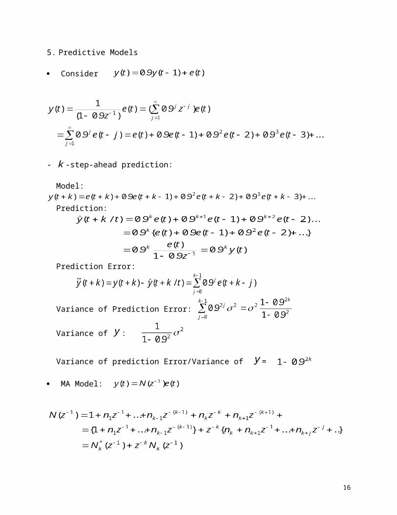
5. Predictive Models

Consider

- -step-ahead prediction:

Model: Prediction:

Prediction Error:

Variance of Prediction Error:

Variance of :

Variance of prediction Error/Variance of =

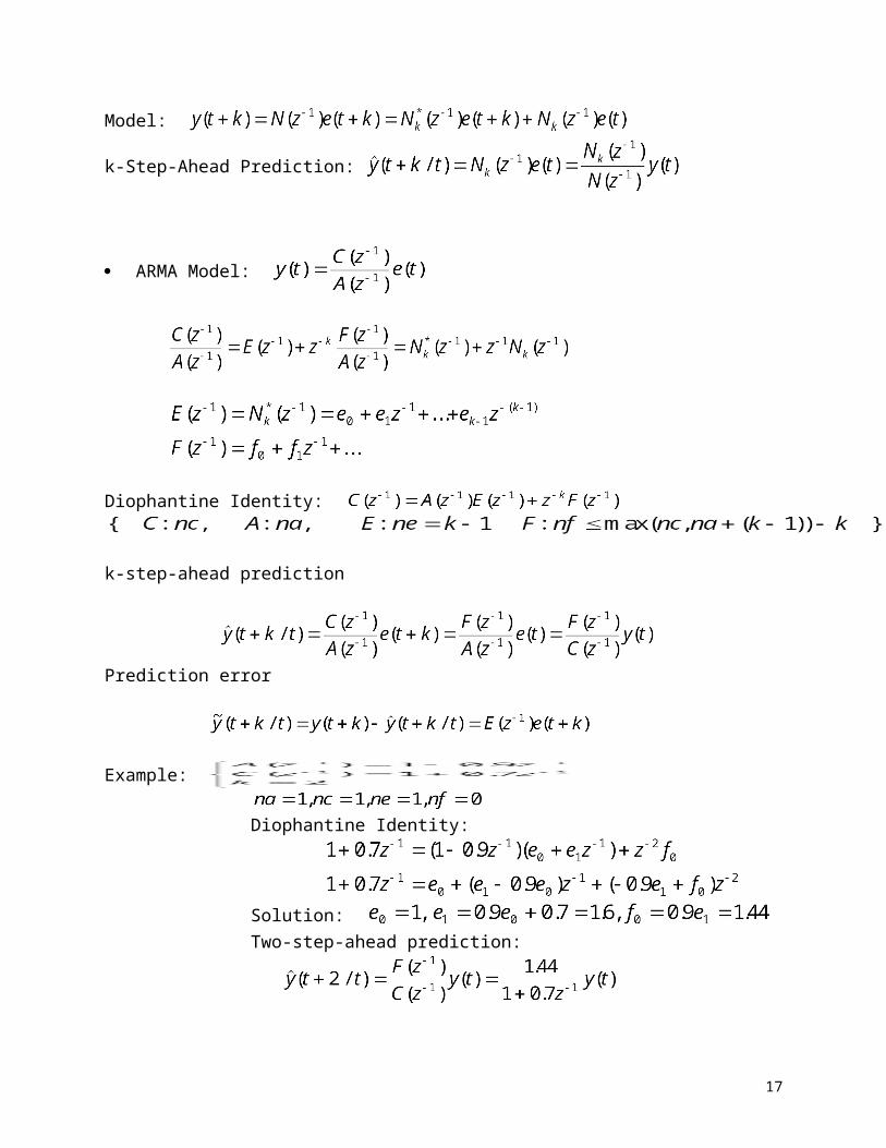
MA Model:

Model:

k-Step-Ahead Prediction:

ARMA Model:

15

Diophantine Identity:

k-step-ahead prediction

Prediction error

Example: Diophantine Identity:

Solution: Two-step-ahead prediction:

16

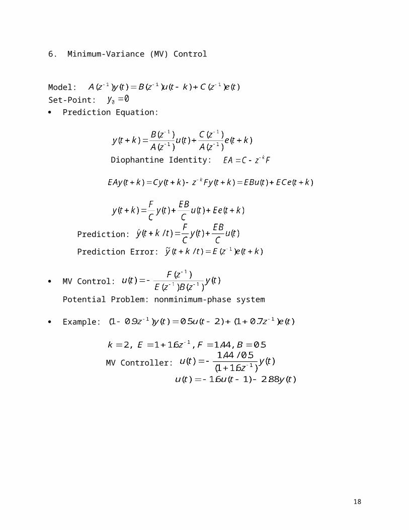
6. Minimum-Variance (MV) Control

Model: Set-Point: Prediction Equation:

Diophantine Identity:

Prediction:

Prediction Error:

MV Control:

Potential Problem: nonminimum-phase system

Example:

MV Controller:

17

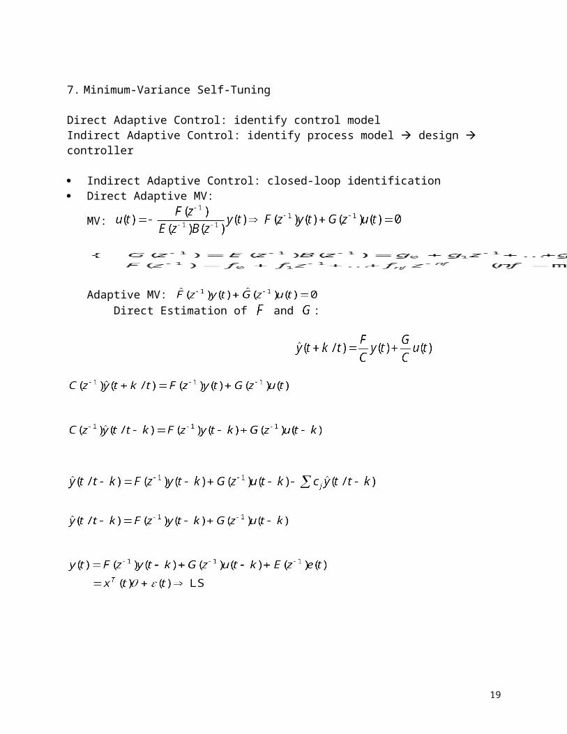
7. Minimum-Variance Self-Tuning

Direct Adaptive Control: identify control model Indirect Adaptive Control: identify process model design controller

Indirect Adaptive Control: closed-loop identification Direct Adaptive MV:

MV:

Adaptive MV:

Direct Estimation of and :

18

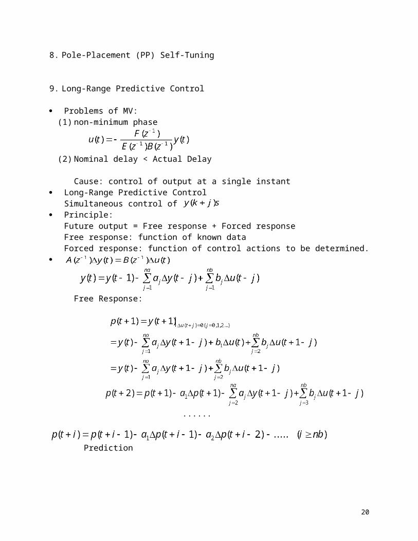
8. Pole-Placement (PP) Self-Tuning

9. Long-Range Predictive Control

Problems of MV: (1) non-minimum phase

(2) Nominal delay < Actual Delay

Cause: control of output at a single instant Long-Range Predictive Control

Simultaneous control of Principle:

Future output = Free response + Forced responseFree response: function of known dataForced response: function of control actions to be determined.

Free Response:

...... Prediction

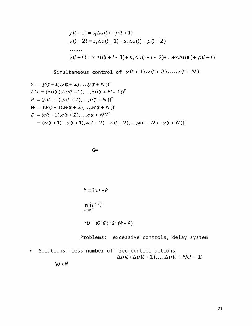
Simultaneous control of

19

G=

Problems: excessive controls, delay system

Solutions: less number of free control actions

20

ADAPTIVE CONTROL SYSTEM DESIGN

EE 699 Project I

Consider the following process

The parameters of the process are time-varying:

Design an adaptive system to control for set-point .

Report Requirements:

(1) Method selection(2) System Design(3) Program (4) Simulation Results(5) Results Analysis(6) Conclusions

Report Due: Nov. 22, 1998

21

CHAPTER 3 FUZZY LOGIC SYSTEMS

Primary Reference: J. M. Mendel, "Fuzzy Logic Systems for Engineering: A Tutorial," IEEE Proceedings, 83(3): 345-377, 1995.

I. INTRODUCTION

A. Problem Knowledge

Objective Knowledge (mathematical models)Subjective knowledge: linguistic information, difficult to quantify using traditional mathematics

Importance of Subjective Knowledge: idea development, high level decision making and overall design

Coordination of Two Forms of Knowledge - Model based approach: Objective information: mathematical models

Subjective information: linguistic statement Rules FL based Quantification- Model-free approach: Numerical data rules + linguistic information.

B. Purpose of the Chapter

Basic Parts for synthesis of FLS

FLS: numbers to numbers mapping: fuzzifier, defuzzifier (inputs: numbers, output: numbers, mechanism: fuzzy logic)

C. What is a Fuzzy Logic System

Input-output characteristic: nonlinear mapping of an input vector into a scalar output Mechanism: linguistic statement based IF-THEN inference or its mathematical variants

D. Potential of FLS's

E. Rationale for FL in Engineering

Lotfi Zadeh, 1965: imprecisely defined "classes" play an important role in human thinking(fuzzy logic) Lotfi Zadeh, 1973: Principle of Incompatibility (engineering application)

F. Fuzzy Concepts in Engineering: examples

22

G. Fuzzy Logic System: A High-Level Introduction

Crisp inputs to crisp outputs mapping: y=f(x)Four Components: Fuzzifier, rules, inference engine, defuzzifier

Rules (Collection of IF-THEN statements): provided by experts or extracted from numerical data Understanding of (1) linguistic variables ~ numerical values (2) Quantification of linguistic variables: terms (3) Logical connections: "or" "and" (4) Implications: "IF A Then B" (5) Combination of rules Fuzzifier: crisp numbers fuzzy sets that will be used to activate rules

Inference Engine: maps fuzzy sets into fuzzy sets based on the rules

Defuzzifier: fuzzy sets crisp output

23

II. SHORT PRIMER ON FUZZY SETS

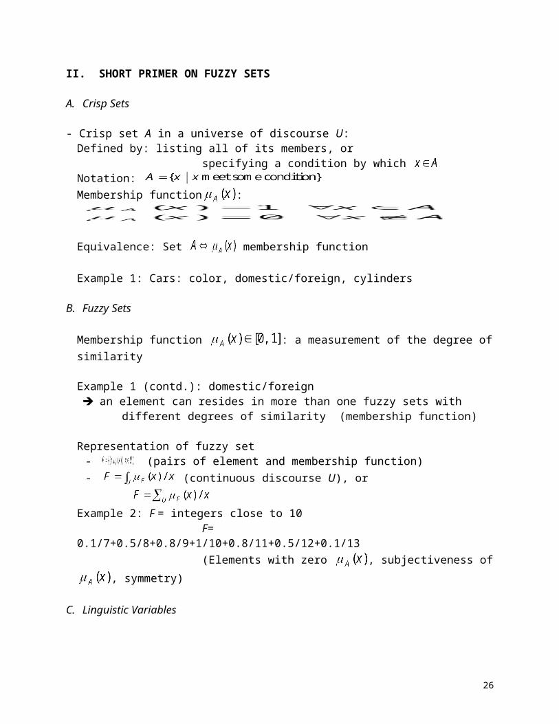
A. Crisp Sets

- Crisp set A in a universe of discourse U:Defined by: listing all of its members, or specifying a condition by which Notation: Membership function :

Equivalence: Set membership function

Example 1: Cars: color, domestic/foreign, cylinders

B. Fuzzy Sets

Membership function : a measurement of the degree of similarity

Example 1 (contd.): domestic/foreign an element can resides in more than one fuzzy sets with different degrees of similarity (membership function)

Representation of fuzzy set - (pairs of element and membership function)- (continuous discourse U), or

Example 2: F = integers close to 10 F= 0.1/7+0.5/8+0.8/9+1/10+0.8/11+0.5/12+0.1/13 (Elements with zero , subjectiveness of , symmetry)

C. Linguistic Variables

Linguistic Variables: variables when their values are not given by numbers but by words or sentences

u: name of a (linguistic) variable x: numerical value of a (linguistic) variable (often interchangeable with u when u is a single letter)Set of Terms T(u): linguistic values of a (linguistic) variableSpecification of terms: fuzzy sets (names of the terms and membership functions)

Example 3: Pressure - Name of the variable: pressure- Terms: T(pressure)={week, low, okay, strong, high} - Universe of discourse U=[100 psi, 2300 psi]

24

- Week: below 200 psi, low: close to 700 psi, okay: close to 1050 psi, strong: close to 1500 psi, high: above 2200 psi linguistic descriptions membership functions

D. Membership Functions

Examples

Number of membership functions (terms) Resolution Computational Complexity

Overlap (glass can be partially full and partially empty at the same time)

E. Some Terminology

The support of a fuzzy set

Crossover point

Fuzzy singleton: a fuzzy set whose support is a single point with unity membership function.

F. Set Theoretic Operations

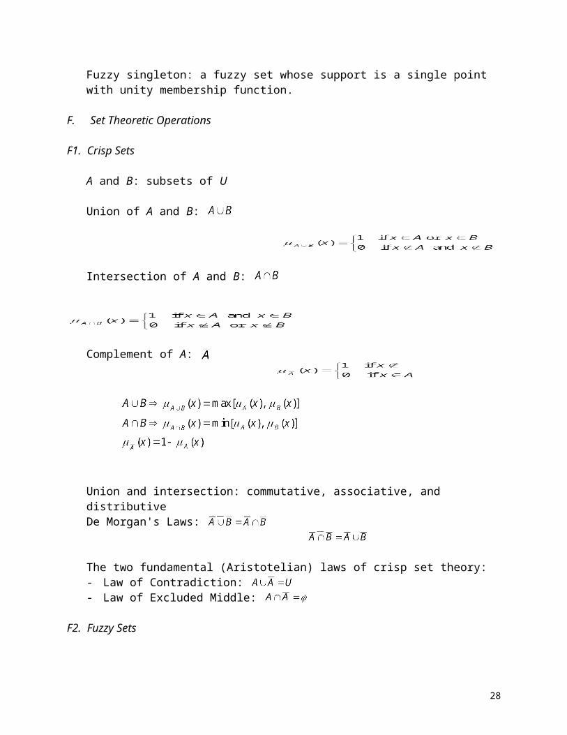
F1. Crisp Sets

A and B: subsets of U

Union of A and B:

Intersection of A and B:

Complement of A:

Union and intersection: commutative, associative, and distributive

25

De Morgan's Laws:

The two fundamental (Aristotelian) laws of crisp set theory:- Law of Contradiction: - Law of Excluded Middle:

F2. Fuzzy Sets

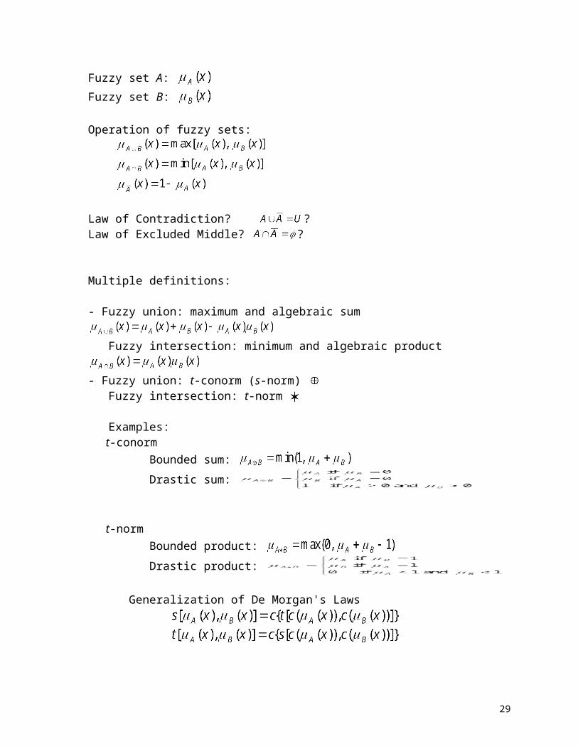
Fuzzy set A: Fuzzy set B:

Operation of fuzzy sets:

Law of Contradiction? ?Law of Excluded Middle? ?

Multiple definitions:

- Fuzzy union: maximum and algebraic sum Fuzzy intersection: minimum and algebraic product - Fuzzy union: t-conorm (s-norm) Fuzzy intersection: t-norm

Examples: t-conorm Bounded sum: Drastic sum:

t-norm Bounded product: Drastic product:

Generalization of De Morgan's Laws

26

III. SHORT PRIMER ON FUZZY LOGIC

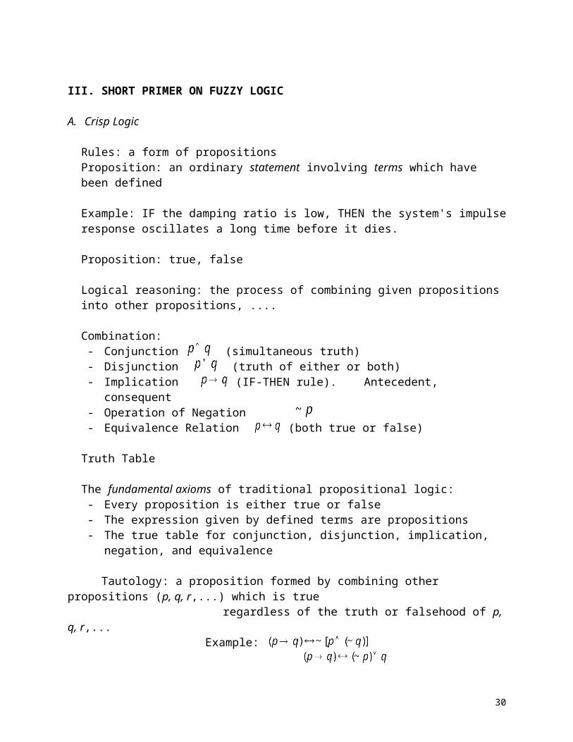
A. Crisp Logic

Rules: a form of propositionsProposition: an ordinary statement involving terms which have been defined

Example: IF the damping ratio is low, THEN the system's impulse response oscillates a long time before it dies.

Proposition: true, false

Logical reasoning: the process of combining given propositions into other propositions, ....

Combination:- Conjunction (simultaneous truth)- Disjunction (truth of either or both)- Implication (IF-THEN rule). Antecedent, consequent- Operation of Negation - Equivalence Relation (both true or false)

Truth Table

The fundamental axioms of traditional propositional logic:- Every proposition is either true or false- The expression given by defined terms are propositions- The true table for conjunction, disjunction, implication, negation, and equivalence

Tautology: a proposition formed by combining other propositions (p, q, r,...) which is true regardless of the truth or falsehood of p, q, r,...

Example:

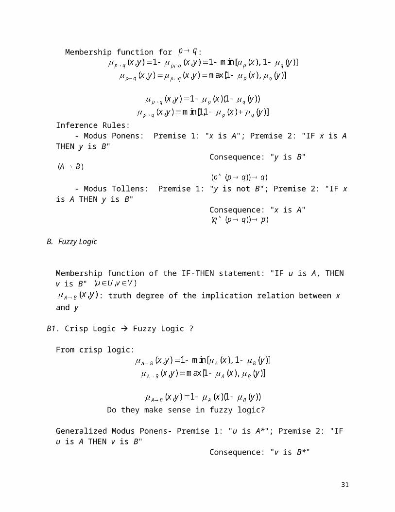
Membership function for :

Inference Rules: - Modus Ponens: Premise 1: "x is A"; Premise 2: "IF x is A THEN y is B" Consequence: "y is B" - Modus Tollens: Premise 1: "y is not B"; Premise 2: "IF x is A THEN y is B" Consequence: "x is A"

27

B. Fuzzy Logic

Membership function of the IF-THEN statement: "IF u is A, THEN v is B" : truth degree of the implication relation between x and y

B1. Crisp Logic Fuzzy Logic ?

From crisp logic:

Do they make sense in fuzzy logic?

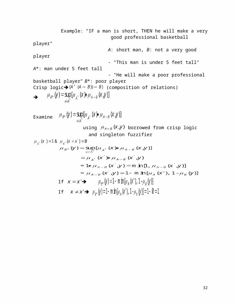
Generalized Modus Ponens- Premise 1: "u is A*"; Premise 2: "IF u is A THEN v is B" Consequence: "v is B*" Example: "IF a man is short, THEN he will make a very good professional basketball player" A: short man, B: not a very good player - "This man is under 5 feet tall" A*: man under 5 feet tall - "He will make a poor professional basketball player" B*: poor playerCrisp logic (composition of relations)

Examine

using borrowed from crisp logic and singleton fuzzifier

If

If

28

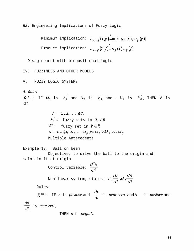
B2. Engineering Implications of Fuzzy Logic

Minimum implication:

Product implication:

Disagreement with propositional logic

IV. FUZZINESS AND OTHER MODELS

V. FUZZY LOGIC SYSTEMS

A. Rules:)(lR IF 1u is lF1 and 2u is lF2 and … pu is l

pF , THEN v is lG

Ml ..., ,2 ,1

liF s: fuzzy sets in RU i

lG : fuzzy set in RV pp UUUuuuu ...) ..., , ,(col 2121 Multiple Antecedents

Example 18: Ball on beam Objective: to drive the ball to the origin and maintain it at origin

Control variable: 2

2

dtd

Nonlinear system, states: dtd

dtdr

r

, , ,

Rules:

)1(R : IF r is positive and dtdr

is near zero and is positive and dtd

is near zero,

THEN u is negative

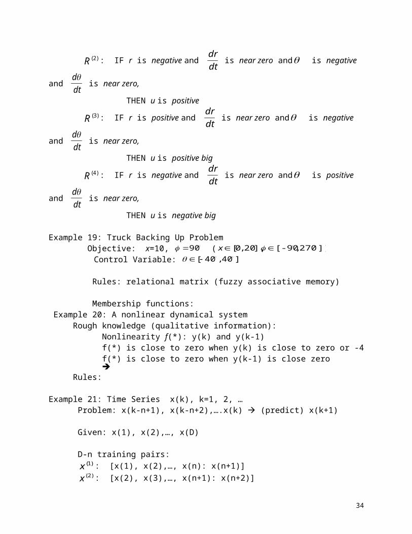
)2(R : IF r is negative and dtdr

is near zero and is negative and dtd

is near zero,

THEN u is positive

)3(R : IF r is positive and dtdr

is near zero and is negative and dtd

is near zero,

THEN u is positive big

)4(R : IF r is negative and dtdr is near zero and is positive and

dtd is near zero,

THEN u is negative big Example 19: Truck Backing Up Problem Objective: x=10, 90 ( ])270 ,[-90 ],20 ,0[ x Control Variable: ]40 ,40[

29

Rules: relational matrix (fuzzy associative memory)

Membership functions: Example 20: A nonlinear dynamical system Rough knowledge (qualitative information): Nonlinearity f(*): y(k) and y(k-1) f(*) is close to zero when y(k) is close to zero or -4 f(*) is close to zero when y(k-1) is close zero Rules: Example 21: Time Series x(k), k=1, 2, … Problem: x(k-n+1), x(k-n+2),….x(k) (predict) x(k+1)

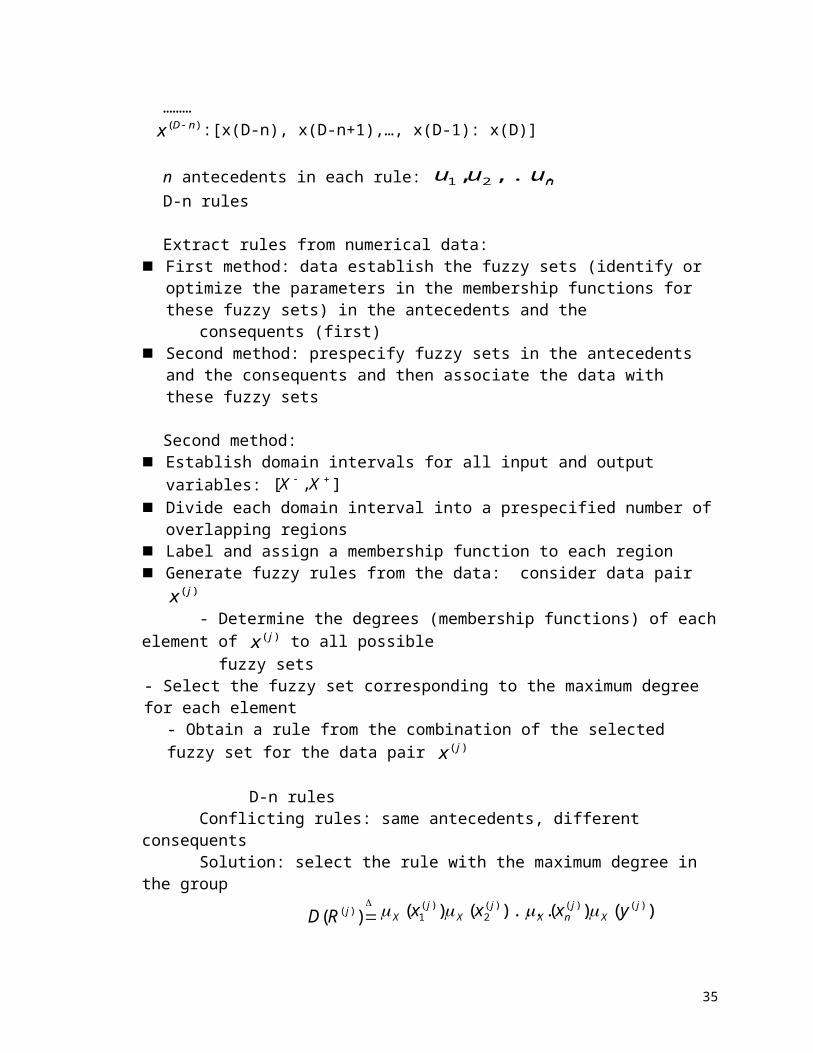
Given: x(1), x(2),…, x(D) D-n training pairs: )1(x : [x(1), x(2),…, x(n): x(n+1)] )2(x : [x(2), x(3),…, x(n+1): x(n+2)] ……… )( nDx :[x(D-n), x(D-n+1),…, x(D-1): x(D)] n antecedents in each rule: nuuu ,...,, 21

D-n rules

Extract rules from numerical data: First method: data establish the fuzzy sets (identify or optimize the parameters in the

membership functions for these fuzzy sets) in the antecedents and the consequents (first) Second method: prespecify fuzzy sets in the antecedents and the consequents and then

associate the data with these fuzzy sets

Second method: Establish domain intervals for all input and output variables: ],[ XX Divide each domain interval into a prespecified number of overlapping regions Label and assign a membership function to each region Generate fuzzy rules from the data: consider data pair )( jx - Determine the degrees (membership functions) of each element of )( jx to all possible fuzzy sets- Select the fuzzy set corresponding to the maximum degree for each element

- Obtain a rule from the combination of the selected fuzzy set for the data pair )( jx

D-n rules Conflicting rules: same antecedents, different consequents Solution: select the rule with the maximum degree in the group

30

)( )( jRD )()()....()( )()()(2

)(1

jX

jnX

jX

jX yxxx

Nonobvious Rules:

31

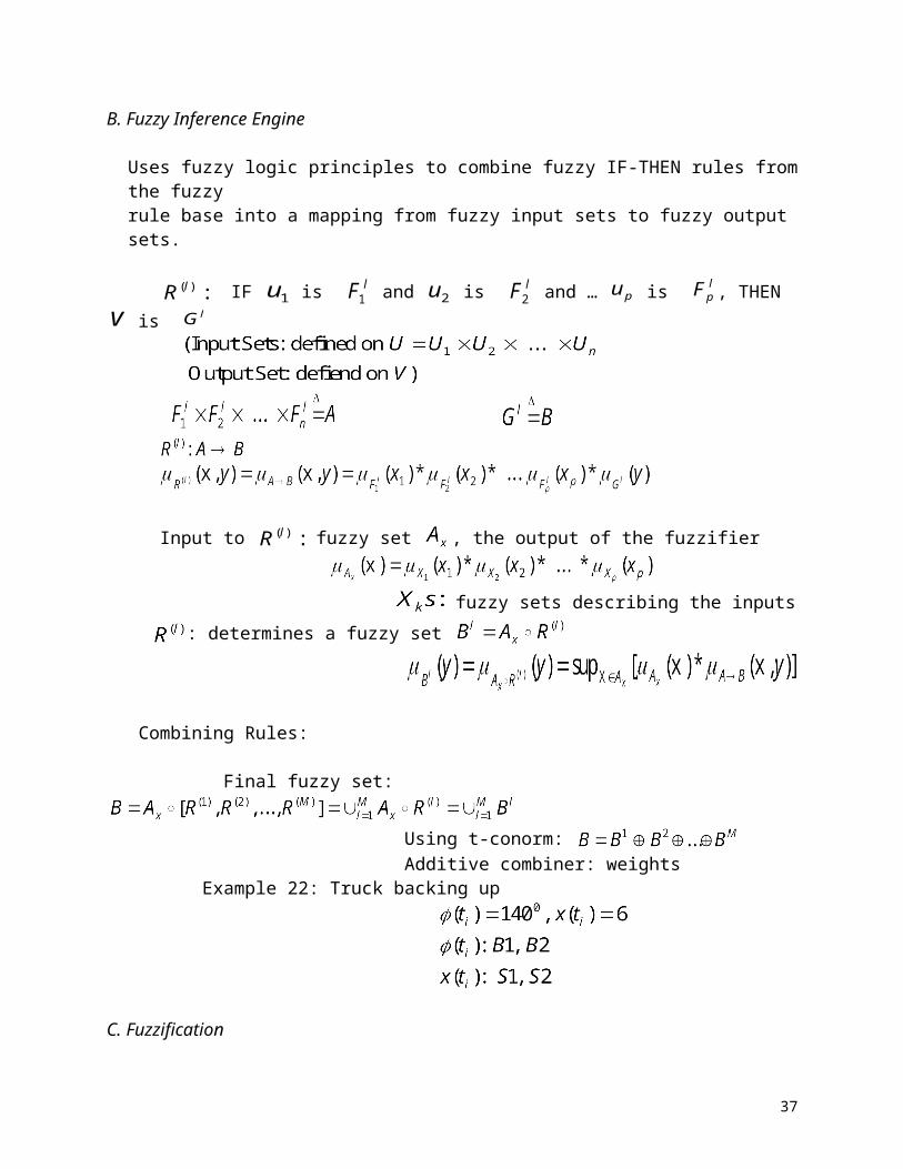
B. Fuzzy Inference Engine

Uses fuzzy logic principles to combine fuzzy IF-THEN rules from the fuzzy rule base into a mapping from fuzzy input sets to fuzzy output sets.

:)(lR IF 1u is lF1 and 2u is lF2 and … pu is lpF , THEN v is lG

Input to :)(lR fuzzy set , the output of the fuzzifier fuzzy sets describing the inputs

: determines a fuzzy set

Combining Rules:

Final fuzzy set: Using t-conorm: Additive combiner: weights Example 22: Truck backing up

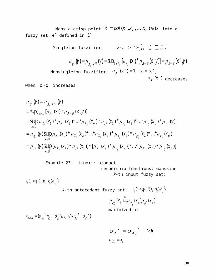
C. Fuzzification Maps a crisp point into a fuzzy set defined in Singleton fuzzifier:

Nonsingleton fuzzifier: , decreases when increases

32

Example 23: t-norm: product membership functions: Gaussian k-th input fuzzy set:

k-th antecedent fuzzy set:

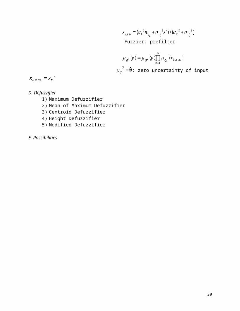
maximized at

Fuzzier: prefilter

: zero uncertainty of input

D. Defuzzifier 1) Maximum Defuzzifier2) Mean of Maximum Defuzzifier3) Centroid Defuzzifier4) Height Defuzzifier5) Modified Defuzzifier

E. Possibilities

33

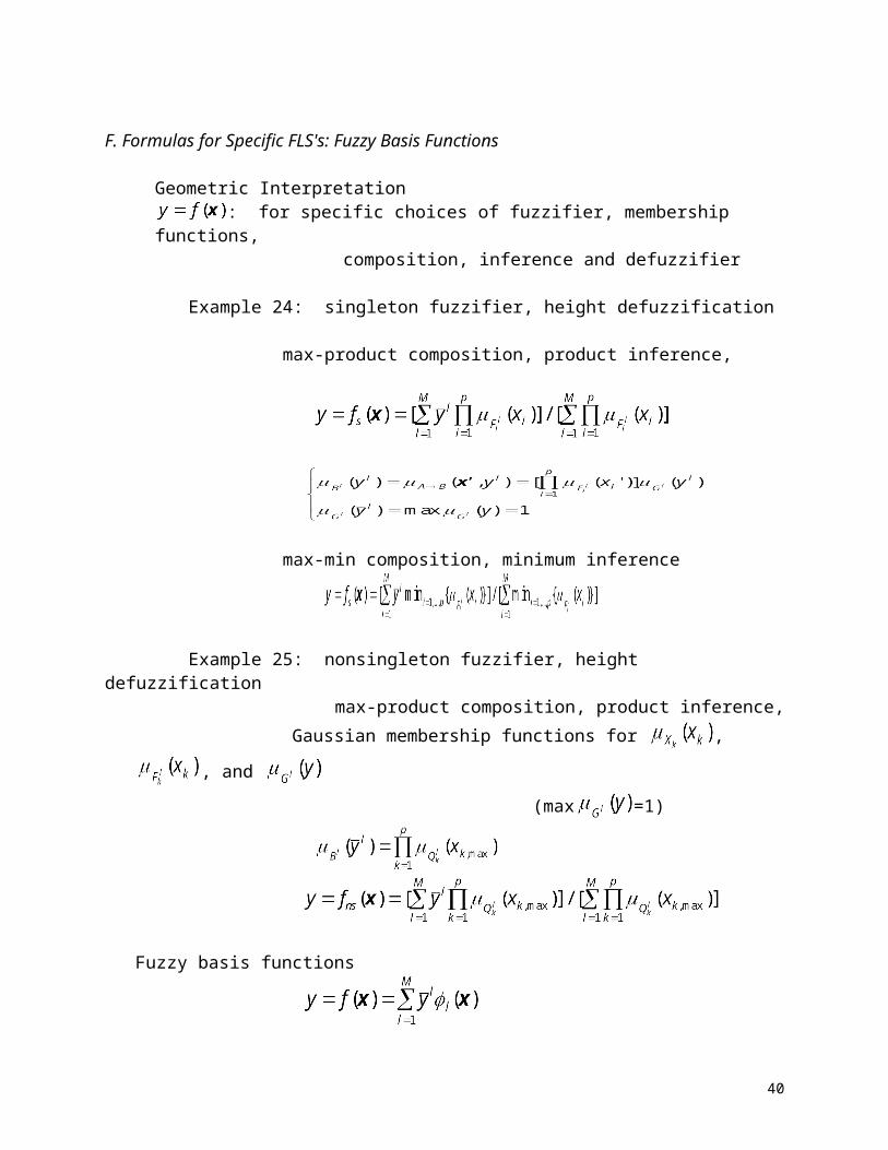
F. Formulas for Specific FLS's: Fuzzy Basis Functions

Geometric Interpretation: for specific choices of fuzzifier, membership functions,

composition, inference and defuzzifier

Example 24: singleton fuzzifier, height defuzzification max-product composition, product inference,

max-min composition, minimum inference

Example 25: nonsingleton fuzzifier, height defuzzification max-product composition, product inference,

Gaussian membership functions for , , and

(max =1)

Fuzzy basis functions

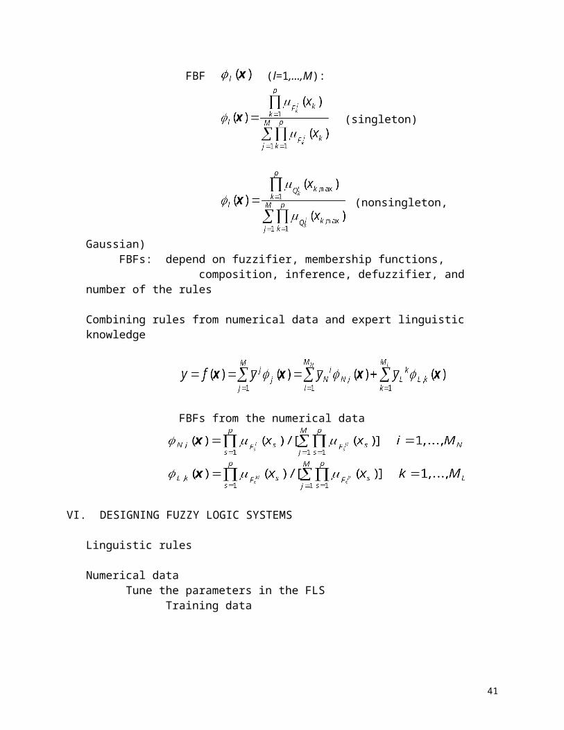
FBF (l=1,...,M):

(singleton)

34

(nonsingleton, Gaussian)

FBFs: depend on fuzzifier, membership functions, composition, inference, defuzzifier, and number of the rules

Combining rules from numerical data and expert linguistic knowledge

FBFs from the numerical data

VI. DESIGNING FUZZY LOGIC SYSTEMS

Linguistic rules

Numerical data Tune the parameters in the FLS Training data

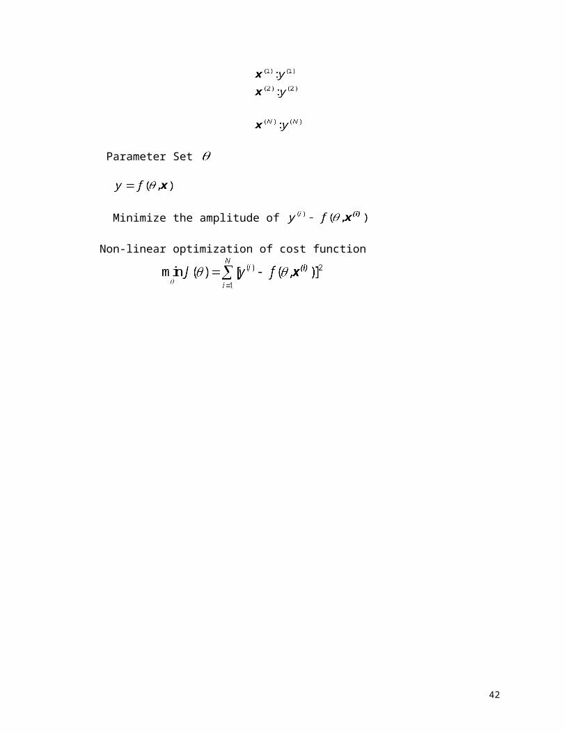
Parameter Set

Minimize the amplitude of

Non-linear optimization of cost function

35

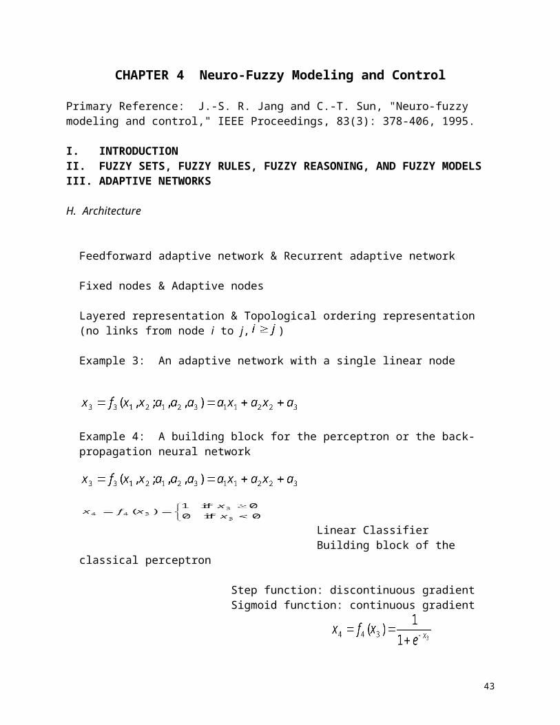
CHAPTER 4 Neuro-Fuzzy Modeling and Control

Primary Reference: J.-S. R. Jang and C.-T. Sun, "Neuro-fuzzy modeling and control," IEEE Proceedings, 83(3): 378-406, 1995.

I. INTRODUCTIONII. FUZZY SETS, FUZZY RULES, FUZZY REASONING, AND FUZZY MODELSIII. ADAPTIVE NETWORKS

H. Architecture

Feedforward adaptive network & Recurrent adaptive network

Fixed nodes & Adaptive nodes

Layered representation & Topological ordering representation (no links from node i to j, )

Example 3: An adaptive network with a single linear node

Example 4: A building block for the perceptron or the back-propagation neural network Linear Classifier Building block of the classical perceptron

Step function: discontinuous gradient Sigmoid function: continuous gradient

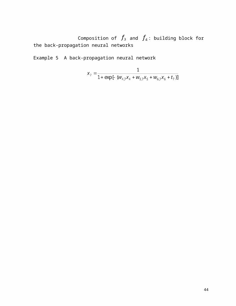
Composition of and : building block for the back-propagation neural networks

Example 5 A back-propagation neural network

36

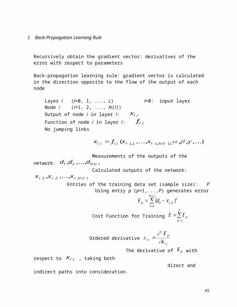
I. Back-Propagation Learning Rule

Recursively obtain the gradient vector: derivatives of the error with respect to parameters

Back-propagation learning rule: gradient vector is calculated in the direction opposite to the flow of the output of each node

Layer l (l=0, 1, ..., L) l=0: input layer Node i (i=1, 2, ..., N(l)) Output of node i in layer l: Function of node i in layer l: No jumping links

Measurements of the outputs of the network: Calculated outputs of the network: Entries of the training data set (sample size): P Using entry p (p=1,...,P) generates error

Cost Function for Training

Ordered derivative

The derivative of with respect to , taking both direct and indirect paths into consideration.

Example 6: Ordinary partial derivative and the ordered derivative

Back-Propagation Equation:

37

il

ilil

il

pp ffxEE ,

,,

,

or

*

**

fxEE p

Sx

p

(S: the set of nodes containing as a parameter)

The derivative of the overall error measure

P

ppEE

1 will be

P

p

pEE1

Update formula:

E : learning rate

: can be determined by

2)( E

: step size (changing the speed of the convergence)

Off-line learning & On-line learning

Recurrent network: transform into an equivalent feedforward network by using “unfolding of time” technique

J. Hybrid Learning Rule: Combining BP and LSE

Off-Line Learning

On-Line Learning

Different Ways of Combining GD and LSE

K. Neural Networks as Special Cases of Adaptive Networks

D1. Back Propagation Neural Networks (BPNN's)

38

Node function: composition of weighted sum and a nonlinear function (activation function or transfer function)

Activation function: differentiable sigmoidal or hyper-tangent type function which approximates the step function

Four types of activation functions Step function

Sigmoidal function

Hyper-tangent function

Identity function

Example: three inputs node Inputs: Output of the node:

Weighted sum:

Sigmoid function:

: Example: two-layer BPNN with 3 inputs and 2 outputs

D2. The Radial Basis Function Networks (RBFN's) Radial basis function approximation: local receptive fields

Example: An RBFN with five receptive field units

Activation level of the ith receptive filed:

Gaussian function

or

Logistic function

39

Maximized at the center Final output:

or

Parameters: nonlinear: linear: Identification: : clustering techniques : heuristic then least squares method

IV. ANFIS: ADAPTIVE NEURO-FUZZY INFERENCE SYSTEMS

A. ANFIS Architecture

Example: A two inputs (x and y) and one output (z) ANFIS

Rule 1 : IF x is and y is , then Rule 2 : IF x is and y is , then

ANFIS architecture Layer 1: adaptive nodes

and : any appropriate parameterized membership functions

} premise parameters Layer 2: fixed nodes with function of multiplication (firing strength of a rule)

Layer 3: fixed nodes with function of normalization

40

(normalized firing strength)

Layer 4: adaptive nodes consequent parameters Layer 5: a fixed node with function of summation

Example: A two-input first-order Sugeno fuzzy model with nine rules

B. Hybrid Learning Algorithm

When the premise parameters are fixed:

linear function of consequent parameters

Hybrid learning scheme

C. Application to Chaotic Time Series Prediction Example: Mackey Glass differential delay

Prediction problem 1000 data pairs 500 pairs for training, 500 for verification Input partition: 2 Rules: 16 number of parameters: 104 (premise: 24, consequent: 80) Prediction results: no significant difference in prediction error for training and validating

41

Reasons for excellence

42

V. NEURO-FUZZY CONTROL

Dynamic Model: Desired Trajectory: Control Law:

Discrete SystemDynamic Model: Desired Trajectory: Control Law:

A. Mimicking Another Working Controller

Skilled human operatorsNonlinear approximation ability Refining the membership functions

B. Inverse Control

Minimizing the control error

C. Specialized Learning

Minimizing the output error: needs the model of the process

D. Back-Propagation Through Time and Real Time Recurrent Learning

PrincipleComputation and Implementation: Off-Line On-line

L. Feedback Linearization and Sliding Control

M. Gain Scheduling

Sugeno fuzzy controllerIf pole is short, then If pole is medium, then If pole is long, then

Operating Points linear controllers fuzzy control rules

G. Analytic Design

43

Project 2: Neuro-Fuzzy Non-Linear Control System Design

1. Given Process is described by the following fuzzy model

A. Rules: Rule 1: IF is VERY SMALL, then Rule 2: IF is SMALL, then Rule 3: IF is MEDIUM, then Rule 4: IF is LARGE, then Rule 5: IF is VERY LARGE, then

where is the input, is the output from Rule i, and and are the

consequent parameters.

B. Membership functions:

C. System output

where is the firing strength of Rule i.

44

2. The desired trajectory of the system output is:

3. Assume that the consequent parameters and are unknown. Design an adaptive control system for the given system to achieve the desired trajectory of the output under the constraint . (Off-line identification procedure may be used to obtain the initials of the premise parameters.)

Report Requirements:

(1) Method selectionSystem DesignProgram Simulation ResultsResults AnalysisConclusions

Due: 12/14/98

45

EE 699 Final Examination Fall 1998

Name: Grade:

1. What are the major elements of a fuzzy logic system? What are their functions? (20%)2. Describe an approach which can be used to extract fuzzy rules from numerical data. (20%)3. The system is described by a Takagi and Sugeno's fuzzy model with the following rules and membership functions, Rules:

Rule 1: IF is VERY SMALL, then Rule 2: IF is SMALL, then Rule 3: IF is MEDIUM, then Rule 4: IF is LARGE, then Rule 5: IF is VERY LARGE, then where is the input, is the output from Rule i, Membership functions:

If the output of the system is given by

,

explain the role of and give a way to determine . (20%)

4. The system is where and : parameters of the system and : output and input at instant k, and

46

: system's noise at instant k, , and . Given data pairs s ( ), determine the Least Squares estimates of the parameters and ? (20%)

5. The system is

where output at instant k, input at instant k, noise at instant k, , and , parameters of the system.At instant t, s ( ) and are known. Give an equation which predicts

. (20%)

47