1

1 Lecture14-Frequency Response

EE105 – Fall 2014 Microelectronic Devices and Circuits

Prof. Ming C. Wu

wu@eecs.berkeley.edu

511 Sutardja Dai Hall (SDH)

2 Lecture14-Frequency Response

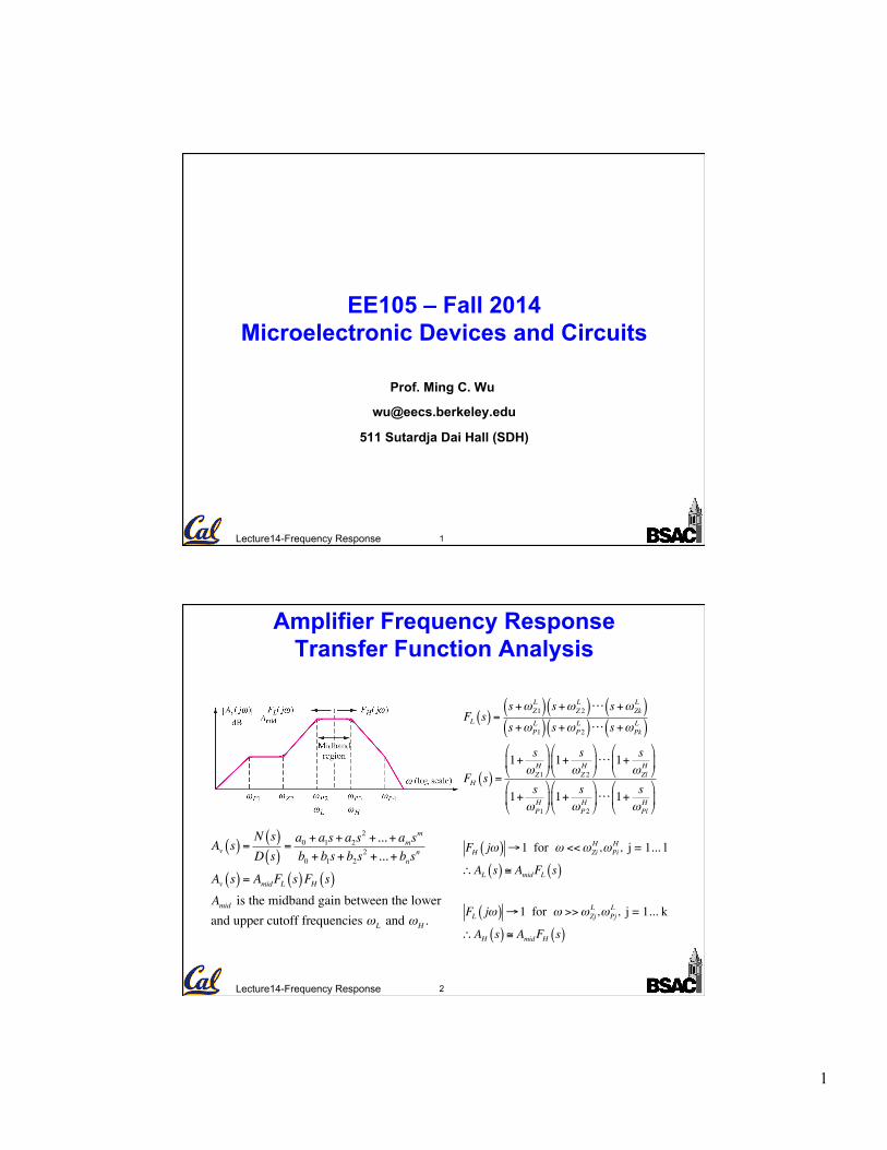
Amplifier Frequency Response Transfer Function Analysis

Av s( ) =N s( )D s( )

=a0 + a1s+ a2s

2 +...+ amsm

b0 + b1s+ b2s2 +...+ bns

n

Av s( ) = AmidFL s( )FH s( )Amid is the midband gain between the lower and upper cutoff frequencies ωL and ωH .

FL s( ) =s+ωZ1

L( ) s+ωZ 2L( ) ⋅ ⋅ ⋅ s+ωZk

L( )s+ωP1

L( ) s+ωP2L( ) ⋅ ⋅ ⋅ s+ωPk

L( )

FH s( ) =1+ s

ωZ1H

"

#$

%

&' 1+ s

ωZ 2H

"

#$

%

&'⋅ ⋅ ⋅ 1+ s

ωZlH

"

#$

%

&'

1+ sωP1

H

"

#$

%

&' 1+ s

ωP2H

"

#$

%

&'⋅ ⋅ ⋅ 1+ s

ωPlH

"

#$

%

&'

FH jω( ) →1 for ω <<ωZiH ,ωPi

H , j = 1... l

∴AL s( ) ≅ AmidFL s( )

FL jω( ) →1 for ω >>ωZjL ,ωPj

L , j = 1... k

∴AH s( ) ≅ AmidFH s( )

2

3 Lecture14-Frequency Response

Low Frequency Dominant Pole Approximation

•  A Dominant Pole exists if one of the low frequency poles is much larger than the others.

–  In the graph below case ω = 1000 rad/sec is a dominant pole. All other poles and zeros are at low enough frequencies that they do not affect the lower cutoff frequency ωL.

FL s( ) ≅ ss+1000

Amid = 200ωL ≅1000 rad / sec

4 Lecture14-Frequency Response

Lower Cutoff Frequency Calculations If there is no dominant pole at low frequencies,the poles and zeros interact to determine the lower cutoff frequency ωL. For example, suppose:

AL s( ) = AmidFL s( ) = Amids+ωZ1( ) s+ωZ 2( )s+ωP1( ) s+ωP2( )

For s = jωL, AL jωL( ) = Amid2

12=

ωL2 +ωZ1

2( ) ωL2 +ωZ 2

2( )ωL

2 +ωP12( ) ωL

2 +ωP22( )

12=ωL

4 + ωZ12 +ωZ 2

2( )ωL2 +ωZ1

2 ωZ 22

ωL4 + ωP1

2 +ωP22( )ωL

2 +ωP12 ωP2

2

Lower cutoff frequency ωL will begreater than all the individual polezero frequencies.

∴ωL ≅ ωP12 +ωP2

2 − 2ωZ12 − 2ωZ 2

2 In general, for n poles and n zeros,

ωL ≅ ωPn2

n∑ − 2 ωZ1

2

n∑

3

5 Lecture14-Frequency Response

Dominant Pole Example

•  Problem: Find midband gain, FL(s) and fL for

•  Analysis: Rearranging the given transfer function into standard form,

AL s( ) = 2000s s100

+1!

"#

$

%&

0.1s+1( ) s+1000( )

AL s( ) = 200s s+100( )

s+10( ) s+1000( )= AmidFL s( )→ Amid = 200 FL s( ) =

s s+100( )s+10( ) s+1000( )

Zeros: s = 0 and s = -100 Poles: s = -100 and s = -1000

The poles and zeros are all widely separated. ∴AL s( ) ≅ 200 ss+1000

The dominant pole is at ω =1000 and fL ≅10002π

=159 Hz.

The more exact calculation is fL =1

2π102 +10002 − 2×02 − 2×1002 =158 Hz

6 Lecture14-Frequency Response

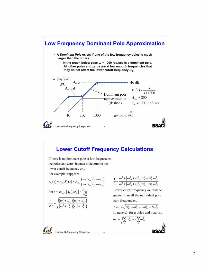
High-Frequency Dominant Pole

•  The lowest of all high frequency poles is called the dominant high-frequency pole.

•  If there is no dominant pole at high frequencies, the poles and zeros interact to determine ωH.

AH s( ) ≅ AmidFH s( )

FH s( ) ≅ 11+ s ωP3( )

ωH ≅ωP3

AH s( ) = AmidFH s( ) = Amid1+ s

ωZ1

!

"#

$

%& 1+ s

ωZ 2

!

"#

$

%&

1+ sωP1

!

"#

$

%& 1+ s

ωP2

!

"#

$

%&

For s = jωH , Amid jωH( ) = Amid2

12=

1+ ωH

ωZ1

!

"#

$

%&

2'

())

*

+,,

1+ ωH

ωZ 2

!

"#

$

%&

2'

())

*

+,,

1+ ωH

ωP1

!

"#

$

%&

2'

())

*

+,,

1+ ωH

ωP2

!

"#

$

%&

2'

())

*

+,,

1ωH

≅1ωP1

2 +1ωP2

2 −2ωZ1

2 −2ωZ 2

2

For the general case of n poles and n zeros,

1ωH

≅1ωPn

2n∑ − 2 1

ωZn2

n∑

4

7 Lecture14-Frequency Response

High Frequency Dominant Pole Approximation

AH s( ) = AmidFH s( )Amid = 200

FH s( ) ≅ 11+ s 106 =

106

s+106

ωH ≅106 rad / sec

fH =ωH

2π≅159 kHz

8 Lecture14-Frequency Response

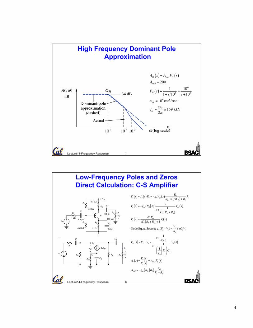
Low-Frequency Poles and Zeros Direct Calculation: C-S Amplifier

C2

C3

C2

Vo s( ) = Io s( )R3 = −gmVgs s( )RD

RD + 1 sC3( )+ R3

R3

Vo s( ) = −gm RD R3( ) s

s+ 1C3 RD + R3( )

Vgs s( )

Vg s( ) =sC1RG

sC1 RI + RG( )+1Vi s( )

Node Eq. at Source: gm (Vg −Vs ) =VsRs+ sC2Vs

Vgs s( ) =Vg −Vs =s+ 1

RSC2

s+ 11gm

RS"

#$

%

&'C2

Vg s( )

Av s( ) =Vo s( )Vi s( )

= AmidFL s( )

Amid = −gm RD R3( ) RGRI + RG

5

9 Lecture14-Frequency Response

Low-Frequency Poles and Zeros Direct Calculation: C-S Amplifier (cont.)

Each independent capacitor in the circuit contributes one pole and one zero. Series capacitors C1 and C3 contribute the two zeros at s = 0 (dc), blocking propagation of dc signals through the amplifier. The third zero due to the parallel combination of C2 and RS occurs at frequency where signal current propagation through the MOSFET is blocked (output voltage is zero).

FL s( ) =s2 s+ 1

RSC2

!

"#

$

%&

s+ 1RI + RG( )C1

'

())

*

+,,s+ 1

1 gm RS( )C2'

())

*

+,,s+ 1

RD + R3( )C3

'

())

*

+,,

The three zero locations are: s = 0, 0, −1/ RSC2

The three pole locations are: s = − 1RI + RG( )C1

, − 11 gm RS( )C2

, − 1RD + R3( )C3