Preliminary draftComments welcome

Cite at your own risk

Education and Labor-Market Discrimination

Kevin Lang Michael Manove

Boston University

December 1, 2004

Abstract: We propose a model that combines statistical discrimination and educational sortingthat explains why blacks get more education than do whites of similar cognitive ability. Our modelexplains the difference between blacks and whites in the relations between education and AFQTand between wages and education. It cannot easily explain why, conditional only on AFQT, blacksearn no more than do whites. It does, however, suggest, that when comparing the earnings ofblacks and whites, one should control for both AFQT and education in which case a substantialblack-white wage differential reemerges. We explore and reject the hypothesis that differences inschool quality between blacks and whites explain the wage and education differentials. Our findingssupport the view that some of the black-white wage differential reflects the operation of the labormarket.

JEL classification: .

Authors’ Addresses:

Kevin Lang Michael Manovelang@bu.edu manove@bu.edu

Dept. of EconomicsBoston University270 Bay State RoadBoston MA 02215

Acknowledgment: This research was supported in part by NSF grant SEC-0339149. Wethank Carlos Sepulveda-Rico for able research assistance, Derek Neal for helpful discussions andparticipants in seminars and workshops at Boston College, Boston University, Carnegie-MellonUniversity, George Washington University, the NBER, Syracuse, the University of Western Ontarioand the University of Houston/Rice for helpful comments and criticisms. The usual caveat applies.

1 Introduction

In a highly influential article, Derek Neal and William Johnson (1996) argue that wage differen-

tials between blacks and whites can be explained by productivity-related premarket factors. They

show that the black-white differential is dramatically reduced, and in some cases eliminated, by

controlling for performance on the Armed Forces Qualifications Test (AFQT). Since, for their sam-

ple, AFQT was administered before the individual entered the labor market, it cannot be affected

directly by labor market discrimination. Therefore, either premarket factors explain wage differ-

entials or AFQT must be affected by anticipated discrimination in the labor market. However,

Neal and Johnson (hereafter NJ) show that the effect of AFQT on the earnings of blacks is at least

as large as on the earnings of whites. Therefore blacks should not anticipate a smaller return to

investment in cognitive skills. Thus they conclude that premarket factors and not labor market

discrimination account for black-white earnings differentials.1

This paper shows that wage differentials are substantially larger when we control for education

as well as AFQT than when we control for AFQT alone. The reason is that conditional on AFQT,

blacks get significantly more education than do whites. This, in turn raises two issues. The first is

what explains higher levels of education among blacks than among whites with the same AFQT.

The second is whether the wage differential that arises when we control for both education and

AFQT can be attributed to labor market discrimination.

We focus primarily on the first question. We explore two hypotheses. The first is that blacks

attend lower quality schools. If AFQT is mostly determined by school inputs and blacks get less of

an AFQT benefit from schooling than do whites, for a fixed amount of schooling, blacks will have

lower AFQT scores. If we inadvertently run the reverse regression, for a given AFQT score, blacks

will have more education. We test this directly by controlling for measurable differences in school

quality and find that school quality cannot explain the education differential.

We therefore explore an alternative hypothesis: that education is a more valuable signal of

productivity for blacks than it is for whites, at least at lower levels of education. As a result blacks

invest more heavily in the signal and get more education for a given level of ability. Our model

implies that blacks and whites with similar levels of ability should get the same education at low

and high levels of ability but that blacks should get more education at intermediate levels of ability.

This is confirmed in the data using either AFQT or, for younger cohorts, AFQT conditional on

educational attainment in 1980 (when the sample took the AFQT) as our proxy for ability. The

model also implies that they should have similar earnings at very low and high levels of education

but that blacks should earn less at intermediate levels. We also confirm this prediction.

However, our model does not explain why blacks and have earnings that are similar or somewhat

1See also Johnson and Neal (1998) and the critique in Darity and Mason (1998) and the reply by Heckman (1998).

— 1 —

lower than those of whites conditional on only AFQT. Since for a given AFQT, blacks get more

education than do whites, they should also earn more than whites not somewhat less. The remaining

difference could reflect either missing variables or labor market discrimination. This is an old debate

that precedes NJ, and it is not one we will pretend to resolve. We do explore whether the wage

differential can be explained by differences in the quality of schools attended by blacks and whites

and find little evidence to support this hypothesis.

The paper is organized as follows. We begin with the principle empirical finding: that condi-

tional on AFQT, blacks get more education than do whites. We show that this differential cannot

be explained by differences in the quality of the schools attended by blacks and whites. We then

present our model of statistical discrimination/educational sorting and show that it implies that

blacks get more education than whites except at very low and very high levels of ability. We also

develop the implications of the model for wage/education profiles. We then return to the data and

test the implications of the model. We then turn our attention to the Neal/Johnson findings and

show that, as would be expected from the earlier results, a substantial black-white wage differential

reemerges when we control for education as well as AFQT. In the conclusion we explore the impli-

cations of the failure of our model’s prediction that blacks will earn more than whites conditional

only on AFQT.

2 Data

Although our initial focus is on differences in educational attainment not wages, later in the paper

we will want to place our results in juxtaposition with those of Neal and Johnson. Therefore

to a large extent, we mimic their procedures. Following NJ, we rely on data from the National

Longitudinal Survey of Youth (NLSY79). Since 1979 the NLSY has followed individuals born

between 1957 and 1964. Initially surveys were conducted annually. More recently, they have

been administered every other year. The NLSY oversamples blacks and Hispanics as well as people

from poor families and the military. We drop the military subsample and use sampling weights to

generate representative results.2

Education is given by the highest grade completed as of 2000. For those missing the 2000

variable, we used highest grade completed as of 1998 and for those missing 1998 as well, we used

the 1996 variable. Where available we used the 1996 weight. For observations missing the 1996

weight, we imputed the weight from the 1998 and 2000 weights using the predicted value from

regressions of the 1996 weights on the 1998 and/or 2000 weights.

We determined race and sex on the basis of the sub-sample to which the individual belongs.

Thus all members of the male-Hispanic cross-section sample were deemed to be male and Hispanic

regardless of how they were coded by the interviewer.

2Neal and Johnson also drop the over-sample of poor whites. Since having a larger sample is helpful, we retainthis group and, as noted above, use sampling weights. It will become apparent that this is not an important sourceof differences.

— 2 —

In 1980, the NLSY administered the Armed Services Vocational Aptitude Battery (ASVAB) to

members of the sample. A subset of the ASVAB is used to generate the Armed Forces Qualifying

Test (AFQT) score. The AFQT is generally viewed as an aptitude test comparable to other

measures of general intelligence. Like other such measures, it is generally regarded as reflecting a

combination of environmental and hereditary factors. The AFQT was recalibrated in 1989. The

NLSY data provide the 1989 AFQT measure. Following NJ, we regressed the AFQT score on age

(using the 1981 weights) and adjusted the AFQT score by subtracting age times the coefficient on

age. We then renormed adjusted AFQT to have mean zero and variance one.

In the later part of the paper, we also examine wages. Because of the difficulties in addressing

differential selection into labor force participation of black and white women (Neal, 2004), we

limit our estimates using wages to men. In order to minimize the problem of missing data, we

used earnings and hours data from the 1996, 1998 and 2000 waves of the survey. If a respondent

reported more than 4000 hours in a year, we coded hours as 4000. We then divided annual earnings

by annual hours to get an hourly wage for each year. Next we took all observations with hourly

wages between $1 and $100 in all three years and calculated (unweighted) mean hourly earnings for

this balanced panel. We used the average changes in hourly wages to adjust 1996 and 2000 wages

to 1998 wages. Note that this adjustment includes both an economy-wide nominal wage growth

factor and an effect of increased experience. We then used the adjusted 1996, 1998 and 2000 wages

for the entire sample to calculate mean adjusted wages for all respondents. We limited ourselves to

observation/years in which the wage was between $1 and $100. If the respondent had three valid

wage observations, we used the mean of those three. If the respondent had two observations, we

used the average of those two. For those with only one observation, the wage measure corresponds

to that adjusted wage. There were 204 observations of men who were interviewed in at least one

of the three years but who did not have a valid wage in any of the three years. In the quantile

regressions, these individuals are given low imputed wages except for a two cases coded as missing

for which the reported wage in at least one of the three years exceeded $100 per hour and for which

there was no year with a valid reported wage.

3 The Basic Result

Most labor economists are aware that average education is lower among blacks than among whites.

In our sample blacks get about three-quarters of a year less education than do whites. It is less

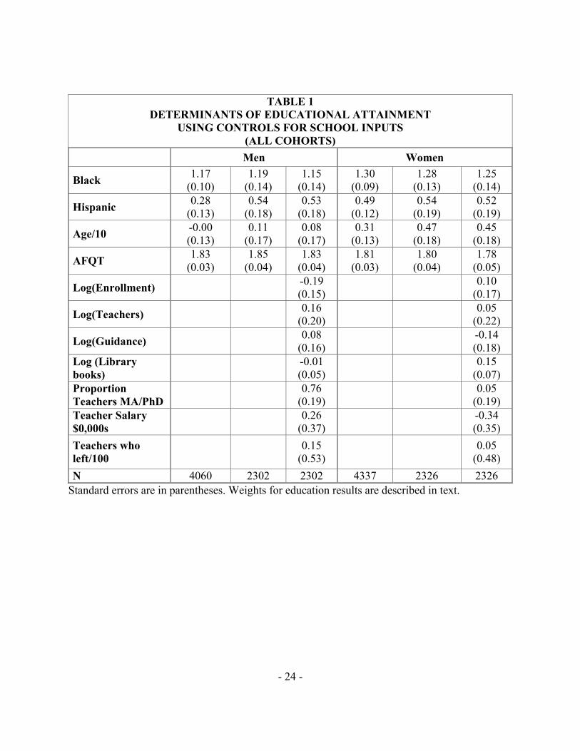
well known that conditional on AFQT, blacks get more education than whites do. This is shown

in Table 1. In the first and fourth columns, we show the difference in educational attainment

between blacks and non-Hispanic whites among men and among women conditional on age and

AFQT. Black men get about 1.2 years more education than do white men with the same AFQT.

Among women the difference is about 1.3 years. There are also smaller but statistically significant

differences between Hispanics and non-Hispanic whites.

Why should blacks, and to a lesser extent Hispanics, obtain more education than whites with

the same measured cognitive skills? There are, of course, a large number of potential hypotheses.

— 3 —

We will focus on two. The first is that AFQT is largely determined by schooling. The second is

that statistical discrimination in the labor market leads them to over-invest in education.

The first explanation can be summarized as follows. Since blacks attend lower quality schools,

on average they gain fewer cognitive skills from a given level of education. Under this view, it is not

surprising that blacks have more schooling given their AFQT; they require more schooling to reach

a given level of cognitive skills. When we regress education on AFQT, we are, in effect, estimating

a reverse regression.

For lower school quality among blacks to explain their greater education given their AFQT, it is

important that the effect of schooling on AFQT be sufficiently large. To see this, let us consider the

opposite extreme. Suppose that AFQT were fully determined before age 15 (the youngest age at

which members of the sample were tested) and therefore before students typically dropout. Then

AFQT would be exogenous to the dropout decision. The question then would only be whether

raising school quality increases or decreases educational attainment. Put differently, of two people

with IQ’s of 100 (or normalized AFQT’s of 0), would we expect the one in a higher quality school

to get more or less education than the one in the lower quality school?

Most labor economists would expect that holding other factors constant, lower school quality

would lower years of education. Standard theoretical models do not offer us unambiguous results

about the effect of school quality on years of schooling. In these models, the sign of the effect

depends on second derivatives. The data, however, suggest a positive correlation between school

quality and years of schooling (e.g. Card and Krueger 1992a&b).

To summarize, if AFQT is heavily influenced by education and if most sample members had

completed their education at the time that they took the AFQT, then school quality differences

would provide a plausible explanation for the higher education among blacks given their AFQT. If

school quality has little effect on AFQT or if most sample members had not completed schooling,

then we would expect blacks to get less education given their AFQT or given their AFQT and

completed schooling at the time they took the test. Our own view is that the AFQT measures

skills that are more heavily affected by preadolescent and early adolescent education so that the

endogeneity of AFQT to ultimate educational attainment is not likely to be a major issue. However,

others certainly disagree. Therefore we address the question empirically.

Our first approach is to measure the education differential conditional on measured school

inputs. Because the NLSY was unable to obtain school quality information for a significant minority

of respondents, the middle column of each panel of table 1 replicates the first column for the sample

with school input information. The principal results do not change. The estimated black/white

education gaps differ by a couple of hundredths. For Hispanic men, the estimate education gap

does increase.

The third column in each panel controls for standard inputs into the education production

function. Almost none of the individual coefficients is statistically significant. Among men, attend-

ing a school with more highly educated teachers is associated with greater educational attainment.

Among women this variable and attending a school with more library books is associated with get-

— 4 —

ting more education. In part, the paucity of individually significant factors reflects multicollinearity

among the measured inputs. In both cases, the coefficients on the school inputs are jointly sig-

nificant. More importantly, controlling for these factors has almost no effect on the estimated

education gaps.

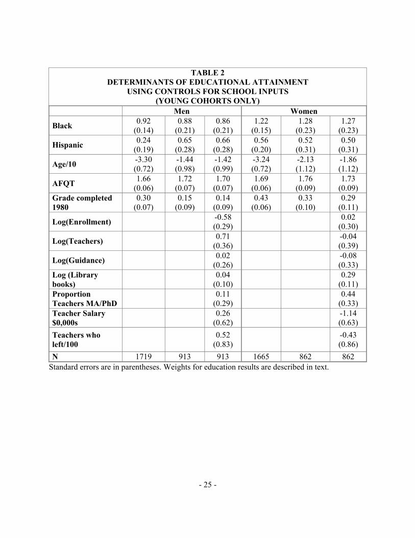
Table 2 repeats the exercise for individuals born after 1961 (the sample used by NJ). Only about

5% of this sample had completed schooling when they took the AFQT. While their AFQT may

have been influenced by their education up to this point, future education should be caused by skills

acquired up to this point and not the other way around. In addition to controlling for AFQT, we

now control for grade completed as of 1980. As can be seen, the coefficient on completed schooling,

although statistically significant, is small. Not surprisingly therefore, the results are similar when

we do not control for completed schooling as of 1980, and we therefore do not show the results.

For women, the education differences are similar to those obtained in table 1. Relative to non-

Hispanic white women, black women get about 1.3 years more education and Hispanic women get

about half a year more education. For men, the numbers are somewhat different from those in

table 1. For blacks, the education differential is somewhat smaller than in table 1 but still quite

large. For Hispanics the differential is larger and the somewhat puzzling difference between those

with and without school quality data remains.

Because inputs may be a very poor proxy for school quality, in table 3 we control for measures of

school composition and student behavior. These are designed to capture some of the elements that

people think about when they think about struggling schools: high proportions of disadvantaged

students, high dropout rates and poor attendance. The results are very similar to those we obtained

in tables 1 and 2. Among all men, the estimated education differentials are similar to those obtained

with all men without controls for both blacks and Hispanics. For the younger cohorts the estimated

differentials are both somewhat larger than those obtained without controls. For women there is

little difference from the results we obtain without controls both for all women and for the younger

women.

Before we move on, it is important to make it clear what we are not claiming. We are not

claiming that AFQT is innate or even unaffected by education and school quality. And we are not

claiming that school quality is unrelated to educational attainment. To the contrary, individuals

who attend higher quality schools both have higher AFQT’s and get more education. It is beyond

the scope of the paper to address whether these relations are causal. However, from our perspective,

the simplest and most probable explanation for our results is that the effect of school quality on

AFQT and the effect of school quality on educational attainment roughly cancel so that AFQT

given educational attainment is roughly independent of school quality.

4 Why Blacks Get More Education than Whites

Why then do blacks get more education than do whites with the same measured ability? In this

section, we argue that statistical discrimination against blacks creates incentives for them to signal

— 5 —

ability through education. We believe that ethnographic evidence supports the view that blacks

see education as a means of getting ahead. Newman (1999) finds that blacks in low-skill jobs in

Harlem view education as crucial to getting a good job and that blacks with low levels of education

have difficulty obtaining even jobs that we would not normally think of as requiring a high school

diploma. Kirschenman and Neckerman (1991) also find that employers are particularly circumspect

in their assessment of low-skill blacks, a finding consistent with our approach.

Our theoretical model merges the standard model of statistical discrimination (Aigner and Cain,

1977) with a conventional sorting model. In a sense, it stands Lundberg and Startz (1983) on its

head, by dealing with observable investment in contrast with the unobservable investment in that

paper. As is standard in the statistical discrimination literature, we assume that the productivity

of blacks is less easily observed than the productivity of whites. However, consistent with our

reading of the ethnographic literature, we make one nonstandard assumption. We assume that as

education levels increase the ability of firms to assess the productivity of black and white workers

converges.

We assume that the ability of firms to observe worker productivity increases with the worker’s

education and that for sufficiently high levels of education, firms observe productivity. We recognize

that even at high levels of education, there is uncertainty about how productive a worker will be.

What the assumption really captures is the view that firms are as informed about a highly-educated

worker’s productivity as that worker is himself. Economics departments may have considerable

uncertainty about the future productivity of a freshly-minted Ph.D., but their predictions may be

as accurate as those of the job candidate. We assume that, in contrast, absent revealing information

from the level of education itself, employers at lower levels of education would not know as much

about potential employees’ productivity as those workers do.

We find this assumption to be a natural way of generating convergence in the observability of

blacks’ and whites’ productivities. However, the results would not change substantively if at that

level there was additional uncertainty about productivity but that was orthogonal to information

available to either workers or firms.

The principal result is that since they have greater difficulty observing blacks’ productivity,

employers put more weight on the observable signal of productivity, education when making wage

offers to blacks than they do when making offers to whites. In response, blacks choose to get more

education.

4.1 The Wage/Education Game

Consider a game between a continuum of workers of different innate ability levels a, where a is

continuously distributed over some fixed interval. Each worker must choose a level of education

s. Because we assume that education and ability are complementary inputs in the creation of

productivity (in a sense defined below), we shall search for a separating equilibrium in which the

workers’ strategy profile is described by a continuous function s(a) that is strictly increasing in a.

— 6 —

Firms in our model simply follow the rules of a competitive labor market–they play no strategic

role in the game.

Suppose that a worker’s productivity p∗, conditional on his education level s and innate abilitya, has the log-normal distribution given by

p∗ = Q(s, a) ε, (1)

where Q(s, a) is a deterministic function of education and ability and where ε ≡ ln ε is a normalrandom variable with mean 0 and variance σ2ε. Log productivity, then, can be written as

ln p∗ = q(s, a) + ε, (2)

where q(s, a) ≡ lnQ(s, a) is the mean of ln p∗. We assume that the effect of education on log-productivity is characterized by diminishing returns (qss < 0) but that innate ability complements

the productivity-increasing effects of education (qsa > 0).

A potential employer can observe a worker’s education level s but not his true productivity p∗.However, the employer does observe a productivity signal p given by

ln p = ln p∗ + u, (3)

where u is a random error of observation. The error term u has variance σ2u(s), which is common to

all firms, continuous and decreasing in s. We assume that ε and u are independently distributed.

Let λ(s) ∈ [0, 1] be given byλ(s) ≡ σ2ε

σ2ε + σ2u(s).

If λ(s) is near 0, then σ2u(s) must be very large, so that the employer’s ability to observe worker

productivity directly is poor. Conversely, if λ(s) = 1, then σ2u(s) = 0, so that the employer can

observe worker productivity perfectly. In that case workers would have no incentive to signal their

productivity to employers, and they would obtain the efficient level of education.

4.1.1 The Equilibrium Competitive Wage

In the competitive labor market, an employer will offer a worker with observed productivity signal p

and education level s the wage w(p, s) ≡ E[p∗ | p, s]. In our candidate separating equilibrium s(a),

an employer can infer a worker’s innate ability a from his knowledge s, and then calculate q(s, a).

The employer’s equilibrium inference about q(s, a) conditional on s is denoted by q(s) ≡ q(s, a(s))

where a(s) is the inverse of the workers’ strategy profile, s(a). We denote the competitive wage in

the separating equilibrium by w(p, s). We demonstrate the following:

Proposition 1 The log of the equilibrium competitive wage is given by

ln w(p, s) = λ(s) ln p+ (1− λ(s))¡q(s) + .5σ2e

¢. (4)

— 7 —

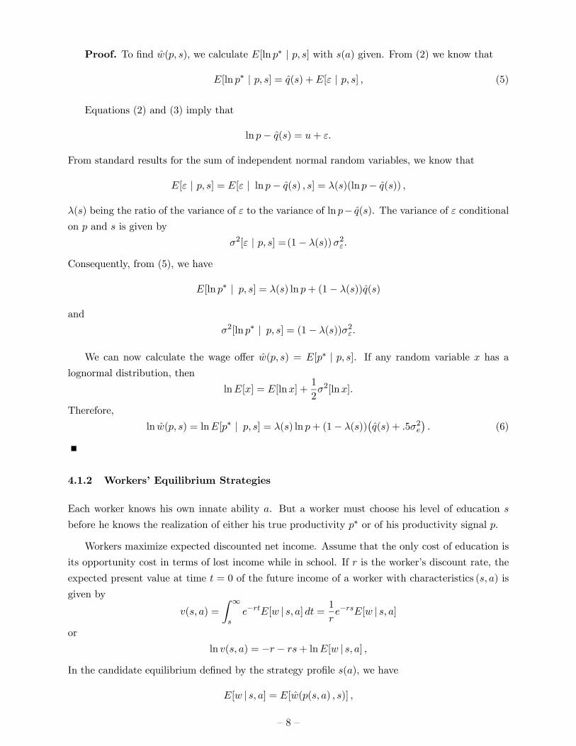
Proof. To find w(p, s), we calculate E[ln p∗ | p, s] with s(a) given. From (2) we know that

E[ln p∗ | p, s] = q(s) +E[ε | p, s] , (5)

Equations (2) and (3) imply that

ln p− q(s) = u+ ε.

From standard results for the sum of independent normal random variables, we know that

E[ε | p, s] = E[ε | ln p− q(s) , s] = λ(s)(ln p− q(s)) ,

λ(s) being the ratio of the variance of ε to the variance of ln p− q(s). The variance of ε conditional

on p and s is given by

σ2[ε | p, s] =(1− λ(s))σ2ε.

Consequently, from (5), we have

E[ln p∗ | p, s] = λ(s) ln p+ (1− λ(s))q(s)

and

σ2[ln p∗ | p, s] = (1− λ(s))σ2ε.

We can now calculate the wage offer w(p, s) = E[p∗ | p, s]. If any random variable x has a

lognormal distribution, then

lnE[x] = E[lnx] +1

2σ2[lnx].

Therefore,

ln w(p, s) = lnE[p∗ | p, s] = λ(s) ln p+ (1− λ(s))¡q(s) + .5σ2e

¢. (6)

4.1.2 Workers’ Equilibrium Strategies

Each worker knows his own innate ability a. But a worker must choose his level of education s

before he knows the realization of either his true productivity p∗ or of his productivity signal p.

Workers maximize expected discounted net income. Assume that the only cost of education is

its opportunity cost in terms of lost income while in school. If r is the worker’s discount rate, the

expected present value at time t = 0 of the future income of a worker with characteristics (s, a) is

given by

v(s, a) =

Z ∞

se−rtE[w | s, a] dt = 1

re−rsE[w | s, a]

or

ln v(s, a) = −r − rs+ lnE[w | s, a] ,In the candidate equilibrium defined by the strategy profile s(a), we have

E[w | s, a] = E[w(p(s, a) , s)] ,

— 8 —

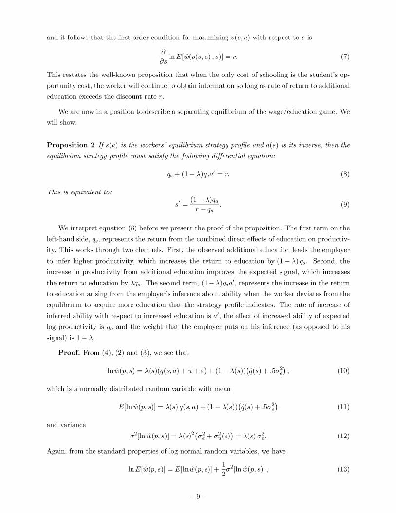
and it follows that the first-order condition for maximizing v(s, a) with respect to s is

∂

∂slnE[w(p(s, a) , s)] = r. (7)

This restates the well-known proposition that when the only cost of schooling is the student’s op-

portunity cost, the worker will continue to obtain information so long as rate of return to additional

education exceeds the discount rate r.

We are now in a position to describe a separating equilibrium of the wage/education game. We

will show:

Proposition 2 If s(a) is the workers’ equilibrium strategy profile and a(s) is its inverse, then the

equilibrium strategy profile must satisfy the following differential equation:

qs + (1− λ)qaa0 = r. (8)

This is equivalent to:

s0 =(1− λ)qar − qs

. (9)

We interpret equation (8) before we present the proof of the proposition. The first term on the

left-hand side, qs, represents the return from the combined direct effects of education on productiv-

ity. This works through two channels. First, the observed additional education leads the employer

to infer higher productivity, which increases the return to education by (1− λ) qs. Second, the

increase in productivity from additional education improves the expected signal, which increases

the return to education by λqs. The second term, (1− λ)qaa0, represents the increase in the return

to education arising from the employer’s inference about ability when the worker deviates from the

equilibrium to acquire more education that the strategy profile indicates. The rate of increase of

inferred ability with respect to increased education is a0, the effect of increased ability of expectedlog productivity is qa and the weight that the employer puts on his inference (as opposed to his

signal) is 1− λ.

Proof. From (4), (2) and (3), we see that

ln w(p, s) = λ(s)(q(s, a) + u+ ε) + (1− λ(s))¡q(s) + .5σ2e

¢, (10)

which is a normally distributed random variable with mean

E[ln w(p, s)] = λ(s) q(s, a) + (1− λ(s))¡q(s) + .5σ2e

¢(11)

and variance

σ2[ln w(p, s)] = λ(s)2¡σ2e + σ2u(s)

¢= λ(s)σ2e. (12)

Again, from the standard properties of log-normal random variables, we have

lnE[w(p, s)] = E[ln w(p, s)] +1

2σ2[ln w(p, s)] , (13)

— 9 —

so that

lnE[w(p, s)] = λ(s) q(s, a) + (1− λ(s))¡q(s) + .5σ2e

¢+ .5λ(s)σ2e, (14)

lnE[w(p, s)] = λ(s) q(s, a) + (1− λ(s))q(s) + .5σ2e, (15)

which yields the differential equation

∂

∂s

¡λ(s) q(s, a) + (1− λ(s))q(s) + .5σ2e

¢= r. (16)

or

λ0(s) q(s, a) + λ(s)qs(s, a)− λ0(s) q(s) + (1− λ(s))¡qs(s, a(s)) + qa(s, a(s)) a

0(s)¢= r. (17)

In equilibrium a = a(s) and q(s, a) = q(s). Consequently, in equilibrium (17) reduces to (8).

Equation (9) follows from the fact that the derivative of s(a) is the reciprocal of the derivative of

a(s).

The following proposition pins down a unique solution of (9).

Proposition 3 If the range of worker abilities is known to be described by the interval [a0, a1],

and if a separating equilibrium s(a) has s0(a) > 0, then the education level s(a0) must be efficient

and not influenced by signaling.

In an equilibrium with s(a) strictly increasing, the employer would infer that a worker with

education s(a0) has ability a0, the lowest possible level. If s(a0) were inefficiently high, the worker

of ability a0 could safely deviate to the lower efficient level of education without lowering the

employer’s inference of his ability, and so raise his payoff. If s(a0) were inefficiently low, the worker

of ability a0 would choose to get s > s(a0) since qs > r and therefore qs + (1− λ(s))qaa0 > r.

4.1.3 Example: Ability as the capacity to be educated

We now analyze a special case of this model in which ability is viewed as the capacity to be educated:

each year of education less than a increases productivity p∗ by a fixed amount, but education inexcess of a has no effect. We can write

p∗ = min{s, a} ε

where ε = exp(ε) is a lognormal random variable. This yields a special case of (2) in which q(s, a)

is given by

q(s, a) = min{ln s, ln a} .For s < a (9) yields the equilibrium condition

s0(a) = 0,

which contradicts our assumption of a separating equilibrium. For s > a, however, (9) yields the

equilibrium condition

s0(a) =1− λ(s)

r

1

a. (18)

— 10 —

We normalize a so that the lowest level of ability is given by a0 = 1. By Proposition 3 , we have

s(1) = 1, the efficient level of education for a = 1.

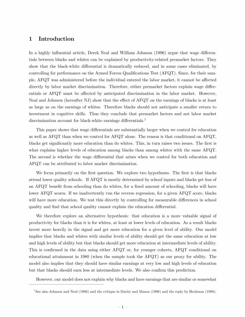
For constant λ(s) = λ0 and with s(1) = 1, the solution of (18)is

s(a) =1− λ

rln a+ 1, (19)

which defines a unique separating equilibrium. This is graphed in Figure 1 for λ = .5 and r = .1.

a

s

( )s a

45° a

s

( )s a

45°

Figure 1:

Note that with this discount rate and perfect information, s = a for a ≤ 20. For higher values ofa, workers still choose s = 20 because the discounted productivity benefit of further education does

not outweigh the cost of foregone earnings. With λ = .5, all workers with a > 1 get more education

than they would if information were perfect until a is somewhat greater than 14. For a above this

level, workers choose the perfect information level of education because the return to signaling

becomes to small. The fact that the imperfect and perfect information education levels converge

for sufficiently high a is a special feature of this production function which creates a discontinuity

in the return to education at s = a.

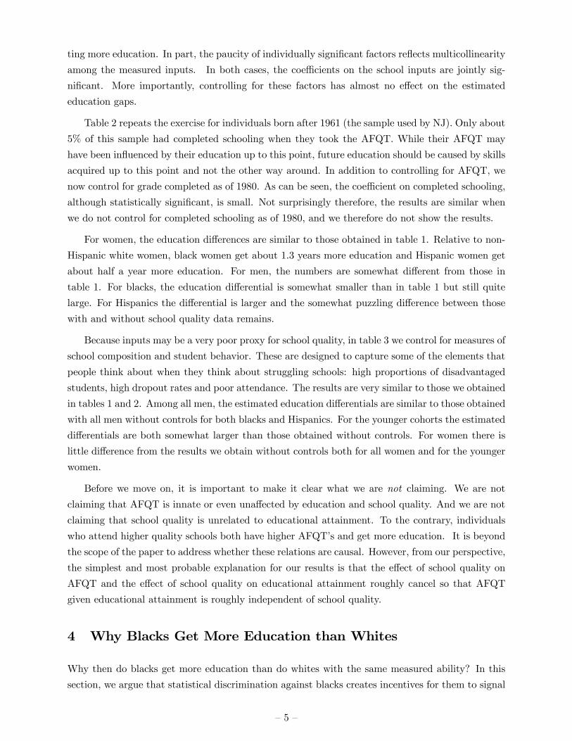
Suppose now that λ(s) = s/b, so that λ increases linearly in s and reaches 1 at s = b. In that

case, the differential equation for an equilibrium becomes

s0(a) =b− s

br

1

a, (20)

and if we require s(1) = 1, the unique solution is

s(a) = b+(1− b) a−1

br

— 11 —

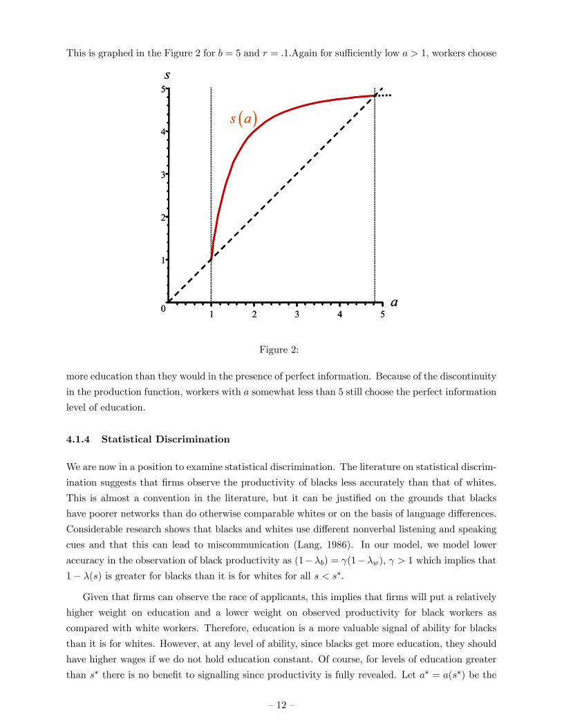
This is graphed in the Figure 2 for b = 5 and r = .1.Again for sufficiently low a > 1, workers choose

0

1

2

3

4

5

1 2 3 4 5a

s

( )s a

0

1

2

3

4

5

1 2 3 4 5a

s

( )s a

Figure 2:

more education than they would in the presence of perfect information. Because of the discontinuity

in the production function, workers with a somewhat less than 5 still choose the perfect information

level of education.

4.1.4 Statistical Discrimination

We are now in a position to examine statistical discrimination. The literature on statistical discrim-

ination suggests that firms observe the productivity of blacks less accurately than that of whites.

This is almost a convention in the literature, but it can be justified on the grounds that blacks

have poorer networks than do otherwise comparable whites or on the basis of language differences.

Considerable research shows that blacks and whites use different nonverbal listening and speaking

cues and that this can lead to miscommunication (Lang, 1986). In our model, we model lower

accuracy in the observation of black productivity as (1−λb) = γ(1−λw), γ > 1 which implies that

1− λ(s) is greater for blacks than it is for whites for all s < s∗.

Given that firms can observe the race of applicants, this implies that firms will put a relatively

higher weight on education and a lower weight on observed productivity for black workers as

compared with white workers. Therefore, education is a more valuable signal of ability for blacks

than it is for whites. However, at any level of ability, since blacks get more education, they should

have higher wages if we do not hold education constant. Of course, for levels of education greater

than s∗ there is no benefit to signalling since productivity is fully revealed. Let a∗ = a(s∗) be the

— 12 —

ability level of white workers who get education s∗. Then black workers of ability a∗ will also chooses∗, and for a > a∗ blacks and whites will choose the same level of education.

Empirical Implications. Intuitively, since when making wage offers to blacks, firms put more

weight on education and less on measured productivity, blacks will get more education for a∗ >a > a0. This means that at any level of education, blacks will be of lower ability and have lower

wages. We derive these results formally below.

Theorem 4 sb(a) > sw(a),∀a∗ > a > a0 where b and w denote black and white.

Proof. Suppose that

sb(a) ≤ sw(a)

for some ea 6= a0. Then

qs(sw(ea),ea) + (1− λw)qa(sw(ea),ea)dads |w

≥ qs(sw(ea),ea) + (1− λb)qa(sw(ea),ea)dads |b

(21)

which impliesda

ds |w>

da

ds |bor

ds

da |w<

ds

da |b.

Since sb(ao) = sw(a0) by assumption and since any time sb(a) = sw(a),dsda |w < ds

da |b, sb(a) > sw(a)

whenever a∗ > a > a0.

Corollary 1 eqb(s) < eqw(s),∀s(a∗) > s > s(a0).

Thus, at all education levels at which information is imperfect, except the lowest, blacks earn

less than do whites (not holding ability constant). It follows that the return to education measured

by comparing wages at any level of education at which information is imperfect with wages at the

lowest level of education should be lower for blacks than for whites. Conversely, if we measure the

return to education by comparing wages in the range where information is imperfect with wages in

the range where it is perfect, the measured return to education should be higher for blacks. This

suggests that the measured return to education, not controlling for ability, should initially be lower

for blacks than for whites and become higher than the return for whites over some range.

It is important to note that this conclusion refers to the measured return. The actual private

return to education is the common interest rate, r, for all workers.

Corollary 2 There is some a0 such that a0 < a0 < a∗ such that for all a < a0 the return to abilityfor blacks is higher than the return to ability for whites and for a > a0 the return to ability forblacks is no higher than the return to for blacks and strictly lower if a < a∗ (not holding educationconstant).

— 13 —

We note that the “ability to learn” example above demonstrates that our results apply more

generally than simply to the case in which there is no asymmetric information beyond some level

of education. In the case graphed in Figure 1, with imperfect information the wage paid to workers

with a given level of education is lower than it is with perfect information whenever the two

education levels diverge. Relative to the case of perfect information, with imperfect information,

the estimated return to education would be lower at low levels of education and higher at high

levels of education.

5 Evidence

We begin with the prediction about the relation between educational attainment and ability. We

have already seen that conditional on AFQT, blacks get more education relative to whites. Our

model suggests that this should be true at intermediate levels of ability but not at very low or very

high levels of ability.

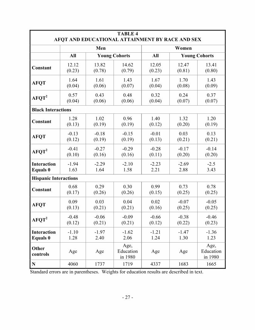
Table 4 shows the relation between education and AFQT, separately for men and women.

Within each sex the younger cohorts, who had not completed school at the time that they took

the AFQT, are shown separately, both with and without a control for their completed education at

the time they took the test. In every specification, the interaction of race and the AFQT-squared

term has its predicted negative sign. This is true for Hispanics as well as for blacks.

Although the individual interaction terms are generally not statistically significant when we

limited the sample to the younger cohorts, in no case do the differences between the young and

older cohorts in the three black interaction terms, the three Hispanic interaction terms or the six

interaction terms approach statistical significance.3 Thus the results are not driven by the causal

impact of education on AFQT.

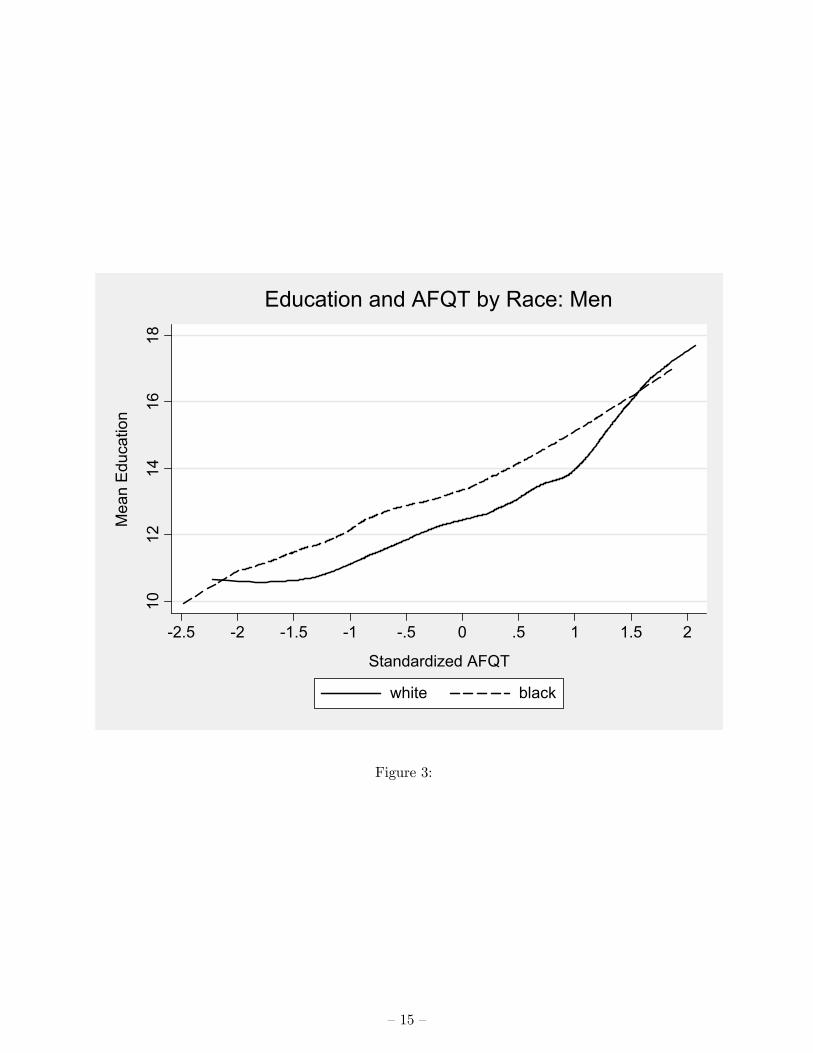
For men, the black-white education differential is maximized at an AFQT about one-sixth

standard deviation below the mean where it is about 1.3 years. Educational attainment is equal

for blacks and whites at almost two standard deviations below the mean and at one and two-

thirds standard deviations above the mean. For women, the black-white education differential is

maximized just about at the mean AFQT where it is about 1.4 years. The education levels of blacks

and whites are estimated to be equalized pretty much at the extremes of the AFQT distribution.

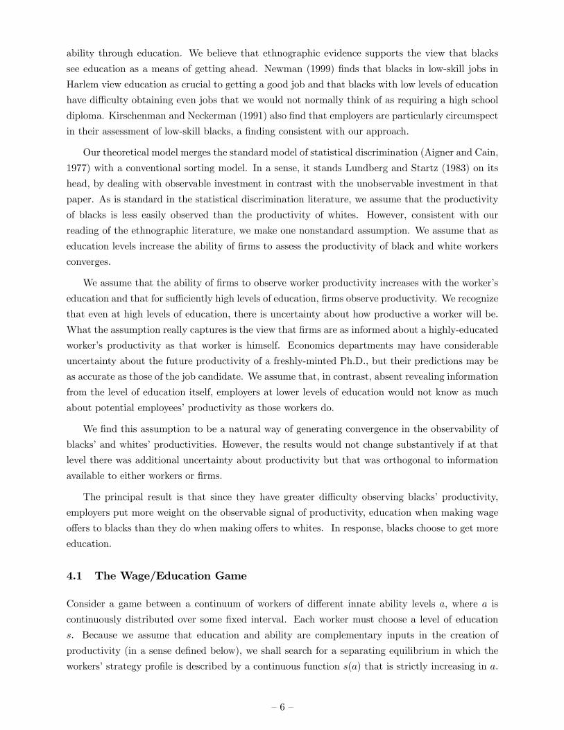
Figure 3 shows the smoothed relation between education and AFQT for men. The nonpara-

metric approach (which ignores the relation between age and education) confirms the parametric

approach. Education levels for blacks and whites converge around a standardized AFQT of -2 and

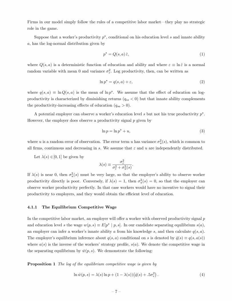
a little above 1.5. Figure 4 is less consistent with the parametric estimates. It shows that education

levels for all three groups converge at a standardized AFQT between -2 and -2.5. However, educa-

tion levels for black women remain higher than for white women even at very high AFQT levels.

3The interaction between Hispanic and AFQT2 does differ at the .05 level for men. However, given that we aretesting twelve different equalities as well as some combinations, it is not surprising that we would find one “significant”test statistic.

— 14 —

1012

1416

18

Mea

n Ed

ucat

ion

-2.5 -2 -1.5 -1 -.5 0 .5 1 1.5 2

Standardized AFQT

white black

Education and AFQT by Race: Men

Figure 3:

— 15 —

1012

1416

18

Mea

n Ed

ucat

ion

-2.5 -2 -1.5 -1 -.5 0 .5 1 1.5 2

Standardized AFQT

white black

Education and AFQT by Race: Women

Figure 4:

One potential explanation for this difference is the very high rate of labor force participation of

high-skill black women relative to white women discussed in Neal (2004).

Because of the complications associated with differences in the selection of black and white

women into the labor force, our discussion of the wage predictions is restricted to men. Our

model implies that the wages of blacks and whites will be similar at low levels of education and

at high levels but that blacks will have lower wages at intermediate levels of education. To test

this prediction, we regress the log wage on education and its square and interaction with race and

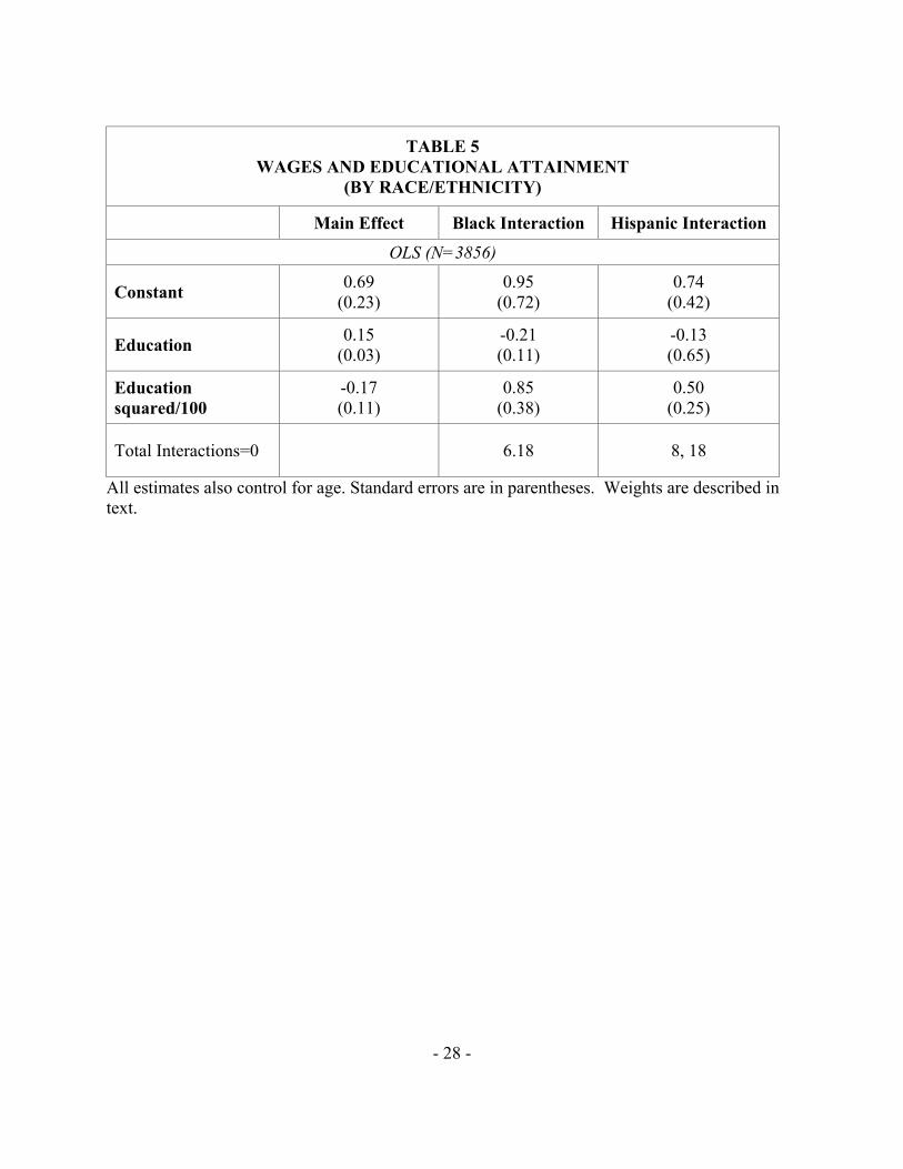
ethnicity as well as direct effects of age, race and ethnicity. Table 5 shows the results. As predicted,

the return to education is initially lower for blacks than for whites and then turns more positive.

Wages for blacks are estimated to be equal for those with a six grade education and those with

eighteen years of completed education although these points of equality are imprecisely estimated.

The results for the Hispanic/non-Hispanic white comparison are similar.

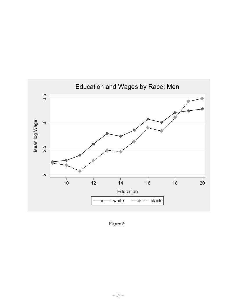
Figure 5 shows this nonparametrically. It plots average log wages for men by education and

race. There are very few individuals without any high school education and very few blacks with

more than eighteen years of education. The estimates suggest that, as predicted by the model,

wages are very similar for blacks and whites at low and high levels of education.

— 16 —

22.

53

3.5

Mea

n lo

g W

age

10 12 14 16 18 20

Education

white black

Education and Wages by Race: Men

Figure 5:

— 17 —

22.

53

3.5

log

Wag

e

-2 -1.5 -1 -.5 0 .5 1 1.5 2

Standardized AFQT

white black

log Wages and AFQT by Race: Young Cohorts

Figure 6:

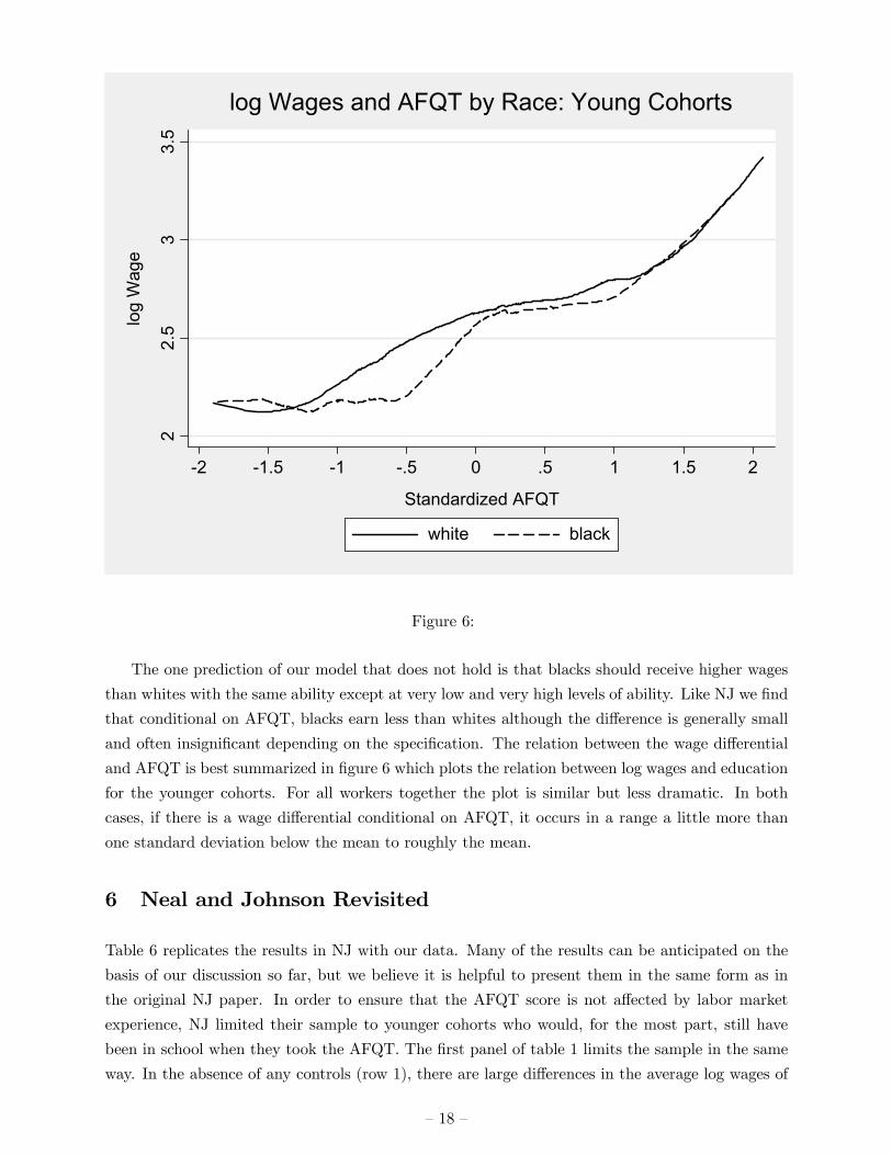
The one prediction of our model that does not hold is that blacks should receive higher wages

than whites with the same ability except at very low and very high levels of ability. Like NJ we find

that conditional on AFQT, blacks earn less than whites although the difference is generally small

and often insignificant depending on the specification. The relation between the wage differential

and AFQT is best summarized in figure 6 which plots the relation between log wages and education

for the younger cohorts. For all workers together the plot is similar but less dramatic. In both

cases, if there is a wage differential conditional on AFQT, it occurs in a range a little more than

one standard deviation below the mean to roughly the mean.

6 Neal and Johnson Revisited

Table 6 replicates the results in NJ with our data. Many of the results can be anticipated on the

basis of our discussion so far, but we believe it is helpful to present them in the same form as in

the original NJ paper. In order to ensure that the AFQT score is not affected by labor market

experience, NJ limited their sample to younger cohorts who would, for the most part, still have

been in school when they took the AFQT. The first panel of table 1 limits the sample in the same

way. In the absence of any controls (row 1), there are large differences in the average log wages of

— 18 —

blacks, Hispanics and whites. In fact, the differences reported here are somewhat larger than those

reported in NJ.4

The second row shows the effect of controlling for years of education completed, this reduces the

black-white wage differential and largely eliminates the Hispanic-white differential. However, there

remains a significant black-white wage differential. The third row adds AFQT instead of education.5

This produces a very substantial reduction in the estimated black-white wage differential and turns

the Hispanic-white wage differential positive albeit insignificant.

Row (3) is the basic result in NJ. Since all the variables in this row were determined before

individuals entered the labor market, this result seems to create a strong prima facie case that the

black-white wage differential is largely due to premarket factors that lower the AFQT of blacks

relative to whites.

Row (4) presents the principal result of this paper. If we control for AFQT and education, the

black-white wage differential reappears. The 13% wage differential implied by row (4) is both sta-

tistically and socially significant. The Hispanic-white differential remains small and insignificantly

positive. Put differently, after controlling for education, accounting for AFQT differences explains

slightly less than half of the black-white wage differential While the premarket factors captured by

AFQT are an important component of the black-white wage differential, there remains a substantial

differential that could be attributable to labor market discrimination.

The difference between rows (3) and (4) is a simple application of the omitted variables bias

formula since we have established that blacks get about one year more education than do whites

with the same AFQT. Yet blacks earn about the same as whites with the same AFQT. Blacks do

not appear to be rewarded for their additional year of education relative to whites, or, equivalently,

must spend an extra year in school to attain the same level of compensation.6

Restricting the sample to the younger cohorts substantially reduces the number of observations.

The middle panel in table 6 explores what happens when we remove this restriction. There are

few substantive differences between the top and middle panel It remains true that controlling

for education significantly reduces the Hispanic-white differential but leaves a substantial black-

white differential. Controlling for AFQT alone, eliminates both differentials. Controlling for both

variables simultaneously eliminates the Hispanic-white differential but leaves a black-white wage

differential equal to roughly half that observed when we control for education and not AFQT.

4Derek Neal was very helpful, supplying us with the code to replicate his and William Johnson’s results. Themodest difference in our results derives from a number of differences including our decision to use the low-incomewhite sample, our choice of wage variables (average hourly wage rather than average hourly wage on main job), NJ’suse of the “class of worker” variable and time period. Carneiro, Heckman and Mastrov (2004) explores the issue oftime variation in the black-white wage differential using various specifications including those used by NJ. See alsothe discussion of this issue in Haider and Solon (2004).

5NJ include AFQT-squared as well as AFQT. However, since the squared term is never significant and the inter-pretation of the equation with only a linear term simpler, we drop the squared term.

6Carneiro et al (2004) use a specification similar to that in row (4) but adjust AFQT for schooling completed atthe time the respondent took the AFQT. They find much larger wage differentials.

— 19 —

Because the results are unaffected by cohort restriction, for most of the remainder of this paper, we

will focus on the full sample but show results for the younger cohorts especially in settings when

we are concerned about the endogeneity of AFQT.

The bottom panel of table 6 addresses the problem of nonparticipation. We treat nonpartic-

ipants as having a low wage and estimate the wage equation by least absolute deviations. Not

surprisingly since nonparticipation is greater among blacks than among whites, this increases the

estimated black-white wage differential in all specifications. However, in the final specification,

the effect is modest. Controlling for both educational attainment and AFQT, we find a residual

black-white wage differential of about 14% or again about half of the differential that remains when

we control only for education.

If, as is generally accepted among labor economists, education is rewarded in the labor market,

then in the absence of labor market discrimination, blacks should earn more than whites with the

same AFQT. Given the education differential, the absence of a wage differential favoring blacks

when we control only for AFQT suggests that blacks are not rewarded fully for their skills.

Although NJ explore the effect of also controlling for education to some extent, they explicitly

reject including education in their main estimating equation. They provide two arguments for

their position. First, they maintain that we should examine black-white wage differentials without

conditioning on education because education is endogenous. Their argument would be much more

compelling if blacks obtained less education than equivalent whites. In that case, we might argue

that blacks get less education because they expect to face discrimination in the labor market, and

therefore controlling for education understates the importance of discrimination.

However, if blacks obtain more education because they anticipate labor market discrimination

as we argue in this paper, failing to control for education understates the impact of discrimination.

Consider the following example. Suppose that the market discriminates against blacks by paying

them exactly what it would pay otherwise equivalent whites with exactly one less year of educa-

tion. Then, to a first approximation,7 all blacks will get one year more education than otherwise

equivalent whites. Controlling only for ability, we find that blacks and whites will have the same

earnings, but controlling for education as well as ability, we see that blacks earn less than whites

by an amount equal to the return to one year of education.

Note that even if the higher educational attainment among blacks reflects premarket factors,

it may still be appropriate to control for education when measuring discrimination in the labor

market. After all, we would still anticipate that the labor market would compensate blacks for

their additional education regardless of their reason for getting more education.

The second argument that NJ make is that education is a poor proxy for skills. In particular,

on average, blacks attend lower quality schools than do whites. Whites will have more effective

education than do blacks with the same nominal years of completed education. We have already

7This statement is precise if all workers maximize the present discounted value of lifetime earnings, lifetimes areinfinite, there are no direct costs of education and the return to experience is zero.

— 20 —

noted that students who attend lower quality schools tend to get less education. Therefore if blacks

attend lower quality schools, for any given level of education, they will have higher unmeasured

ability. Differential school quality could lead to a spurious positive or negative coefficient on race.

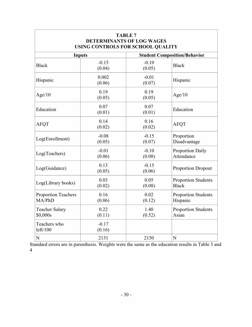
We address this question directly in table 7 by controlling for measures of school quality in

the wage equation. Most of the coefficients have the anticipated sign. Holding other resources

constant, larger schools are associated with lower wages although the coefficient is significant at

only the .1 level. Holding enrollment constant, schools with more guidance counsellors and library

books are associated with higher wages. Having more educated teachers and higher paid teachers

is associated with higher student earnings while teacher turnover has an insignificantly negative

effect. The one coefficient that has the “wrong” sign is the number of teachers which is small and

insignificantly negative. The six measures of school inputs with the correct sign are jointly highly

significant (F(6,2118)=5.65). Thus, the school input measures do predict wages.

Yet, controlling for inputs indicates that there is almost no effect on the measured black-white

wage differential. The difference between the coefficients with and without school quality controls

reflects differences in the sample rather than the effect of adding the controls. The coefficient on

black using the observations for which we have school input measures is -0.15. At least as measured

by inputs, differences in school quality do not account for the black-white wage differential.

The right-side of table 7 controls for measures of student composition and behavior. Perhaps

surprisingly, this effort is in some ways less successful than the estimation using school inputs.

While a higher fraction of disadvantaged students and dropouts are associated with lower wages,

average daily attendance and the fraction of students who are black are not. The results are again

quite similar to those obtained without controls for school quality which for this sample is also -.10.

Thus we find no evidence that the wage and education differentials are driven by differences in

school quality. It is important to note that the absence of evidence for the role of these premarket

factors does not depend on a causal interpretation of the relation between education quality and

outcomes. It is entirely possible that attending a school with a higher dropout rate does not make

any individual more likely to dropout. Students who attend schools with high dropout rates may

have characteristics that make them more likely to dropout. Even if the dropout rate were merely a

proxy for these unmeasured characteristics, we would expect including the dropout rate to lower the

black-white education differential. The fact that it does not, supports the view that such premarket

differences do not explain the wage and education differentials.

7 Discussion and Conclusion

While some of the principal predictions of the theory we presented are consistent with the data, it

is important to recognize that the combination of statistical discrimination and educational sorting

that we discuss cannot fully explain the data. Our model implies that, conditional on ability,

relative to whites, blacks get more education. This, in turn, implies that conditional on AFQT,

blacks should earn more than whites. But neither our results nor those of Neal and Johnson support

— 21 —

that conclusion for men.

One potential explanation is that education is a pure signal at the margin. This is the case in

our “ability to learn” example. In that example, while education is productive up to some point

that depends on the worker’s ability, it is unproductive beyond that point. In order to signal their

ability, most workers invest in education beyond the point at which it increases their productivity.

However, we view this model as extreme.

Our model and the supporting empirical evidence identifies statistical discrimination as one

source of differences in outcomes for blacks and whites. Altonji and Pierret (2001) also provide

evidence of its importance. We have focused our attention on only one effect, increased investment

in the observed signal. Blacks may also invest less in unobservable skills as in Lundberg and Startz

which would lead to them have lower wages even conditional on AFQT. In addition, the work of

Bertrand et al (2004) on names and job applications suggests to us that statistical discrimination is

of particular importance in the presence of search frictions. They find that applicants with African

American names are less likely to receive calls for interviews than are similar applicants with names

common among whites. If evaluating workers is costly, statistical discrimination may prevent large

numbers of African American workers from consideration for many jobs. We expect that in this

setting our principle results would hold: African Americans would have greater incentives to signal

their productivity and would earn less conditional on their education. However, it is also likely

that they would earn less conditional on their ability.

Thus the results in this paper cast doubt on an emerging consensus that the origins of the black-

white wage differential lie in premarket rather than labor market factors. Blacks earn noticeably less

than whites with the same education and cognitive score. The evidence is not consistent with the

view that the unexplained differential reflects differences in school quality, the principal premarket

explanation. Thus, there are good grounds for believing that at least some of the black-white wage

differential reflects differential treatment in the labor market.

References

Aigner, Dennis, and Cain, Glen, “Statistical Theories of Discrimination in Labor Markets,” In-

dustrial and Labor Relations Review, 30 (1977): 175-87.

Altonji, Joseph G. and Pierret, Charles R., “Employer Learning and Statistical Discrimination,”

Quarterly Journal of Economics, 116 (February 2001): 313-50.

Bertrand, Marianne and Mullainathan, Sendhil, “Are Emily and Brendan More Employable than

Lakisha and Jamal? A Field Experiment on Labor Market Discrimination,” American Eco-

nomic Review, 94 (September 2004): 991-1013.

Card, David, and Krueger, Alan B., “School Quality and Black-White Relative Earnings: A Direct

Assessment,” Quarterly Journal of Economics, 107 (February 1992a): 151-200.

______, “Does School Quality Matter? Returns to Education and the Characteristics of Public

Schools in the United States,” Journal of Political Economy 100(February 1992b): 1-40

— 22 —

Carneiro, Pedro, Heckman, James J. and Masterov, Dimitriy, “Labor Market Discrimination and

Racial Differences in Pre-Market Factors,” Journal of Law and Economics (2004), forthcom-

ing.

Darity, William A., Jr. and Mason, Patrick L., “Evidence on Discrimination in Employment:

Codes of Color, Codes of Gender,” Journal of Economic Perspectives, 12 (Spring 1998): 63-

90.

Heckman, James J. “Detecting Discrimination,” Journal of Economic Perspectives, Spring 1998;

12(2): 101-16.

Johnson, William and Neal Derek, “Basic Skills and the Black-White Earnings Gap,” in Christo-

pher Jencks and Meredith Phillips, eds., The Black-White Test Score Gap, Washington, DC:

Brookings Institution Press, 1998.

Kirschenman, Joleen and Neckerman, Kathryn M., “‘We’d Love to Hire Them, But...’: The

Meaning of Race for Employers,” in Christopher Jencks and Paul E. Peterson, eds., The

Urban Underclass, Washington, DC: Brookings Institution Press, 1991.

Lang, K. “A Language Theory of Discrimination,” Quarterly Journal of Economics, 101 (May

1986): 363-382.

Lundberg, Shelly J. and Startz, Richard, “Private Discrimination and Social Intervention in Com-

petitive Labor Markets,” American Economic Review, 73 (1983): 340-7

Neal, Derek, “The Measured Black-White Wage Gap Among Women is Too Small,” Journal of

Political Economy, 112 (February 2004): S1-28.

Neal, Derek A. and Johnson, William R., “The Role of Premarket Factors in Black-White Wage

Differences,” Journal of Political Economy 104 (October 1996): 869-95.

Newman, Katherine S., No Shame in My Game, New York: Vintage Books, 1999.

— 23 —

- 24 -

TABLE 1 DETERMINANTS OF EDUCATIONAL ATTAINMENT

USING CONTROLS FOR SCHOOL INPUTS (ALL COHORTS)

Men Women

Black 1.17 (0.10)

1.19 (0.14)

1.15 (0.14)

1.30 (0.09)

1.28 (0.13)

1.25 (0.14)

Hispanic 0.28 (0.13)

0.54 (0.18)

0.53 (0.18)

0.49 (0.12)

0.54 (0.19)

0.52 (0.19)

Age/10 -0.00 (0.13)

0.11 (0.17)

0.08 (0.17)

0.31 (0.13)

0.47 (0.18)

0.45 (0.18)

AFQT 1.83 (0.03)

1.85 (0.04)

1.83 (0.04)

1.81 (0.03)

1.80 (0.04)

1.78 (0.05)

Log(Enrollment) -0.19 (0.15) 0.10

(0.17)

Log(Teachers) 0.16 (0.20) 0.05

(0.22)

Log(Guidance) 0.08 (0.16) -0.14

(0.18) Log (Library books) -0.01

(0.05) 0.15 (0.07)

Proportion Teachers MA/PhD 0.76

(0.19) 0.05 (0.19)

Teacher Salary $0,000s 0.26

(0.37) -0.34 (0.35)

Teachers who left/100 0.15

(0.53) 0.05 (0.48)

N 4060 2302 2302 4337 2326 2326 Standard errors are in parentheses. Weights for education results are described in text.

- 25 -

TABLE 2 DETERMINANTS OF EDUCATIONAL ATTAINMENT

USING CONTROLS FOR SCHOOL INPUTS (YOUNG COHORTS ONLY)

Men Women

Black 0.92 (0.14)

0.88 (0.21)

0.86 (0.21)

1.22 (0.15)

1.28 (0.23)

1.27 (0.23)

Hispanic 0.24 (0.19)

0.65 (0.28)

0.66 (0.28)

0.56 (0.20)

0.52 (0.31)

0.50 (0.31)

Age/10 -3.30 (0.72)

-1.44 (0.98)

-1.42 (0.99)

-3.24 (0.72)

-2.13 (1.12)

-1.86 (1.12)

AFQT 1.66 (0.06)

1.72 (0.07)

1.70 (0.07)

1.69 (0.06)

1.76 (0.09)

1.73 (0.09)

Grade completed 1980

0.30 (0.07)

0.15 (0.09)

0.14 (0.09)

0.43 (0.06)

0.33 (0.10)

0.29 (0.11)

Log(Enrollment) -0.58 (0.29) 0.02

(0.30)

Log(Teachers) 0.71 (0.36) -0.04

(0.39)

Log(Guidance) 0.02 (0.26) -0.08

(0.33) Log (Library books) 0.04

(0.10) 0.29 (0.11)

Proportion Teachers MA/PhD 0.11

(0.29) 0.44 (0.33)

Teacher Salary $0,000s 0.26

(0.62) -1.14 (0.63)

Teachers who left/100 0.52

(0.83) -0.43 (0.86)

N 1719 913 913 1665 862 862 Standard errors are in parentheses. Weights for education results are described in text.

- 26 -

TABLE 3

DETERMINANTS OF EDUCATIONAL ATTAINMENT USING CONTROLS FOR SCHOOL COMPOSITION/BEHAVIOR

Men Women All Cohorts Young

Cohorts All Cohorts Young Cohorts

Black 1.11 (0.16)

1.04 (0.25)

1.29 (0.16)

1.28 (0.26)

Hispanic 0.25 (0.22)

0.46 (0.34)

0.56 (0.21)

0.56 (0.35)

Age/10 0.06 (0.17)

-1.72 (0.98)

0.25 (0.18)

-2.26 (1.10)

AFQT 1.75 (0.04)

1.60 (0.07)

1.78 (0.05)

1.72 (0.09)

Grade completed 1980 0.05

(0.09) 0.31 (0.10)

Proportion Disadvantaged

-0.49 (0.22)

-0.51 (0.35)

-0.32 (0.23)

-0.18 (0.39)

Proportion Daily Attendance

0.14 (0.27)

0.31 (0.47)

-0.39 (0.27)

-0.38 (0.42)

Proportion Dropout

-0.49 (0.20)

-0.55 (0.28)

-0.20 (0.20)

0.01 (0.28)

Proportion Students Asian

4.71 (1.67)

-0.27 (2.61)

0.69 (0.14)

-0.75 (2.08)

Proportion Students Hispanic

0.52 (0.39)

0.15 (0.61)

0.18 (0.35)

-0.44 (0.57)

Proportion Students Blacks

0.10 (0.25)

-0.38 (0.40)

0.01 (0.23)

-0.23 (0.39)

N 2336 914 2385 889 Standard errors are in parentheses. Weights for education results are described in text.

- 27 -

TABLE 4 AFQT AND EDUCATIONAL ATTAINMENT BY RACE AND SEX

Men Women All Young Cohorts All Young Cohorts

Constant 12.12 (0.23)

13.82 (0.78)

14.62 (0.79)

12.05 (0.23)

12.47 (0.81)

13.41 (0.80)

AFQT 1.64 (0.04)

1.61 (0.06)

1.43 (0.07)

1.67 (0.04)

1.70 (0.08)

1.43 (0.09)

AFQT2 0.57 (0.04)

0.43 (0.06)

0.48 (0.06)

0.32 (0.04)

0.24 (0.07)

0.37 (0.07)

Black Interactions

Constant 1.28 (0.13)

1.02 (0.19)

0.96 (0.19)

1.40 (0.12)

1.32 (0.20)

1.20 (0.19)

AFQT -0.13 (0.12)

-0.18 (0.19)

-0.15 (0.19)

-0.01 (0.13)

0.03 (0.21)

0.13 (0.21)

AFQT2 -0.41 (0.10)

-0.27 (0.16)

-0.29 (0.16)

-0.28 (0.11)

-0.17 (0.20)

-0.14 (0.20)

Interaction Equals 0

-1.94 1.63

-2.29 1.64

-2.10 1.58

-2.23 2.21

-2.69 2.88

-2.5 3.43

Hispanic Interactions

Constant 0.68 (0.17)

0.29 (0.26)

0.30 (0.26)

0.99 (0.15)

0.73 (0.25)

0.78 (0.25)

AFQT 0.09 (0.13)

0.03 (0.21)

0.04 (0.21)

0.02 (0.16)

-0.07 (0.25)

-0.05 (0.25)

AFQT2 -0.48 (0.12)

-0.06 (0.21)

-0.09 (0.21)

-0.66 (0.12)

-0.38 (0.22)

-0.46 (0.23)

Interaction Equals 0

-1.10 1.28

-1.97 2.40

-1.62 2.06

-1.21 1.24

-1.47 1.30

-1.36 1.23

Other controls Age Age

Age, Education

in 1980 Age Age

Age, Education

in 1980 N 4060 1737 1719 4337 1683 1665

Standard errors are in parentheses. Weights for education results are described in text.

- 28 -

TABLE 5 WAGES AND EDUCATIONAL ATTAINMENT

(BY RACE/ETHNICITY)

Main Effect Black Interaction Hispanic Interaction

OLS (N=3856)

Constant 0.69 (0.23)

0.95 (0.72)

0.74 (0.42)

Education 0.15 (0.03)

-0.21 (0.11)

-0.13 (0.65)

Education squared/100

-0.17 (0.11)

0.85 (0.38)

0.50 (0.25)

Total Interactions=0 6.18 8, 18

All estimates also control for age. Standard errors are in parentheses. Weights are described in text.

- 29 -

TABLE 6 DETERMINANTS OF LOG HOURLY WAGES

Black Hispanic Age/10 Education AFQT OLS (Younger Cohorts)

(1) -0.34 (0.04)

-0.15 (0.06)

0.25 (0.17) - -

(2) -0.27 (0.04)

-0.06 (0.05)

0.26 (0.15)

0.10 (0.01) -

(3) -0.07 (0.04)

0.04 (0.06)

0.15 (0.15) - 0.28

(0.01)

(4) -0.14 (0.04)

0.02 (0.05)

0.22 (0.15)

0.07 (0.01)

0.16 (0.02)

OLS (Full Sample)

(5) -0.34 (0.03)

-0.21 (0.04)

0.23 (0.04) - -

(6) -0.27 (0.03)

-0.09 (0.04)

0.23 (0.04)

0.10 (0.00) -

(7) -0.04 (0.03)

0.03 (0.04)

0.20 (0.04) - 0.28

(0.01)

(8) -0.12 (0.03)

0.00 (0.04)

0.21 (0.04)

0.07 (0.00)

0.15 (0.01)

Quantile Regression (selection adjusted)

(9) -0.42 (0.03)

-0.21 (0.03)

0.20 (0.06) - -

(10) -0.35 (0.02)

-0.11 (0.02)

0.25 (0.05)

0.10 (0.00) -

(11) -0.08 (0.03)

0.04 (0.03)

0.19 (0.05) - 0.30

(0.01)

(12) -0.15 (0.03)

0.00 (0.03)

0.20 (0.05)

0.06 (0.01)

0.19 (0.02)

- 30 -

TABLE 7 DETERMINANTS OF LOG WAGES

USING CONTROLS FOR SCHOOL QUALITY

Inputs Student Composition/Behavior

Black -0.15 (0.04)

-0.10 (0.05) Black

Hispanic 0.002 (0.06)

-0.01 (0.07) Hispanic

Age/10 0.19 (0.05)

0.19 (0.05) Age/10

Education 0.07 (0.01)

0.07 (0.01) Education

AFQT 0.14 (0.02)

0.16 (0.02) AFQT

Log(Enrollment) -0.08 (0.05)

-0.15 (0.07)

Proportion Disadvantage

Log(Teachers) -0.01 (0.06)

-0.10 (0.08)

Proportion Daily Attendance

Log(Guidance) 0.13 (0.05)

-0.15 (0.06) Proportion Dropout

Log(Library books) 0.03 (0.02)

0.05 (0.08)

Proportion Students Black

Proportion Teachers MA/PhD

0.16 (0.06)

0.02 (0.12)

Proportion Students Hispanic

Teacher Salary $0,000s

0.22 (0.11)

1.40 (0.52)

Proportion Students Asian

Teachers who left/100

-0.17 (0.16)

N 2131 2150 N Standard errors are in parenthesis. Weights were the same as the education results in Table 3 and 4