Embed Size (px)
Citation preview
Edinburgh Research Explorer
Vector-acoustic Reverse-time Migration of Volve OBC Datasetwithout Up/Down Decomposed Wavefields
Citation for published version:Ravasi, M, Vasconcelos, I, Curtis, A & Kritski, A 2014, 'Vector-acoustic Reverse-time Migration of VolveOBC Dataset without Up/Down Decomposed Wavefields' Paper presented at Second EAGE/SBGfWorkshop 2014 Broadband Seismic, Rio de Janeiro, Brazil, 4/11/14 - 5/11/14, .
Link:Link to publication record in Edinburgh Research Explorer
Document Version:Peer reviewed version
General rightsCopyright for the publications made accessible via the Edinburgh Research Explorer is retained by the author(s)and / or other copyright owners and it is a condition of accessing these publications that users recognise andabide by the legal requirements associated with these rights.
Take down policyThe University of Edinburgh has made every reasonable effort to ensure that Edinburgh Research Explorercontent complies with UK legislation. If you believe that the public display of this file breaches copyright pleasecontact [email protected] providing details, and we will remove access to the work immediately andinvestigate your claim.
Download date: 03. Jul. 2018
Second EAGE/SBGf Workshop 2014
Broadband Seismic 4-5 November 2014, Rio de Janeiro, Brazil
Tu C01Vector-acoustic Reverse-time Migration of VolveOBC Dataset without Up/Down DecomposedWavefieldsM. Ravasi (University of Edinburgh), I. Vasconcelos* (Schlumberger GouldResearch), A. Curtis (University of Edinburgh) & A. Kritski (Statoil)
SUMMARYWavefield separation based on the combination of pressure and particle velocity data is generally used toextract the up- and down-going components from multi-component seabed or towed marine seismicrecordings prior to imaging. By carefully combining vector-acoustic (VA) data in the extrapolation of shotgathers in reverse-time migration (RTM) we show that wavefield separation (deghosting) can beperformed ‘on-the-fly’ at no extra cost. We call such a strategy VARTM and we successfully apply it to aNorth Sea OBC field dataset, acquired in the Volve field. We also discuss additional advantages ofVARTM over standard RTM of up-going only waves such as improved handling of directivity informationcontained in the acquired vector-acoustic data for clearer shallow sections and imaging of the down-goingcomponent of the recorded field (mirror VARTM) without the need for an additional finite differencemodelling.
Second EAGE/SBGf Workshop 2014
Broadband Seismic 4-5 November 2014, Rio de Janeiro, Brazil
Introduction
Current standard acoustic migration algorithms are based on ray-theory or a wave-equation formulation (Biondi, 2006). These use a single input data type that is generally the recorded pressure data or a pre-processed version of it, to create an image of the subsurface. If up/down wavefield separation (i.e., the weighted sum of pressure and velocity data – Claerbout, 1971) is not included in the pre-processing, up- and down-going (ghost) fields contribute to the generation of both real and spurious reflectors in the image, respectively. Vasconcelos (2013) formulated migration in a vector-acoustic (VA) fashion (i.e., using both pressure and particle velocity data) and showed that reverse-time migration (RTM) can produce images deprived of ghost reflectors even taking as input non-decomposed data. The decomposition step can be avoided because vector-acoustic fields enable directional injection at the receiver surface (Blanch, 2012; Amundsen et al., 2014), meaning that any wavefront is back-propagated only towards its direction of arrival. El Yadari and Hou (2013) have extended this vector-acoustic framework to Kirchhoff migration. Vector-Acoustic wavefield extrapolation
Define p and vn to be the time-reversed pressure and normal particle velocity data recorded by multi-component receivers, with vn=v·n where v is the particle velocity vector and n is the outward pointing normal vector at the recording surface. Similarly q and fn refer to the propagators used to extrapolate the recorded data by means of monopole- and dipole-type (gradient) sources, respectively, where gradients fn are also in the n direction. The symbol ⇒ is used to define the back-propagation of a data component (on the left) with a specific source type (on the right), so p⇒ q means that recorded pressure data are back-propagated with monopole source Green’s function propagators. Current practice RTM uses only monopole injection sources to estimate the receiver wavefield, independently of the choice of the data to be injected. If the latter is the full recorded pressure field (for example, with single-component acquisition systems)
p⇒ q (1)
and each wavefront injected in the finite-difference scheme propagates both up- and downward, thus creating a wavefield artifact for every physical arrival present in the data. Although extrapolation can be done with an absorbing boundary (in place of the free-surface) to attenuate the waves propagating upward, each down-going component of the data that is erroneously back-propagated downward instead of upward interacts with the source wavefield and generates crosstalk artifacts in the image. Where multi-component data are recorded, up/down wavefield decomposition can applied prior to imaging to suppress some of the events that are incorrectly handled by the injection procedure. Thereafter it is preferred to use only the up-going field
p− ⇒ q. (2)
Note that an image of the down-going field can be also constructed by means of mirror imaging (Grion et al., 2007). VARTM (Vasconcelos, 2013) solves the injection limitations of standard RTM without requiring any pre-processing of the data. Back-propagation of the full pressure and normal particle velocity with two different types of injection sources (monopole and dipole) allows for separation ‘on-the-fly’ into the up- and down-going components of the recorded field, with up-going waves that are injected only downward and down-going waves that back-propagate only upward
p⇒ fn( )− vn ⇒ q( ). (3)
Intuitively, we can think that the application of dipolar injection sources on pressure data has the same effect of correcting for the different directions of arrival of seismic events in the velocity gather (by means of the so-called obliquity factor) when wavefield separation is performed in the f-k (or τ-p) domain. Ravasi and Curtis (2013) extended this method to elastic (e.g., land or hard-seabed) datasets.
Second EAGE/SBGf Workshop 2014
Broadband Seismic 4-5 November 2014, Rio de Janeiro, Brazil
Example: Volve OBC dataset
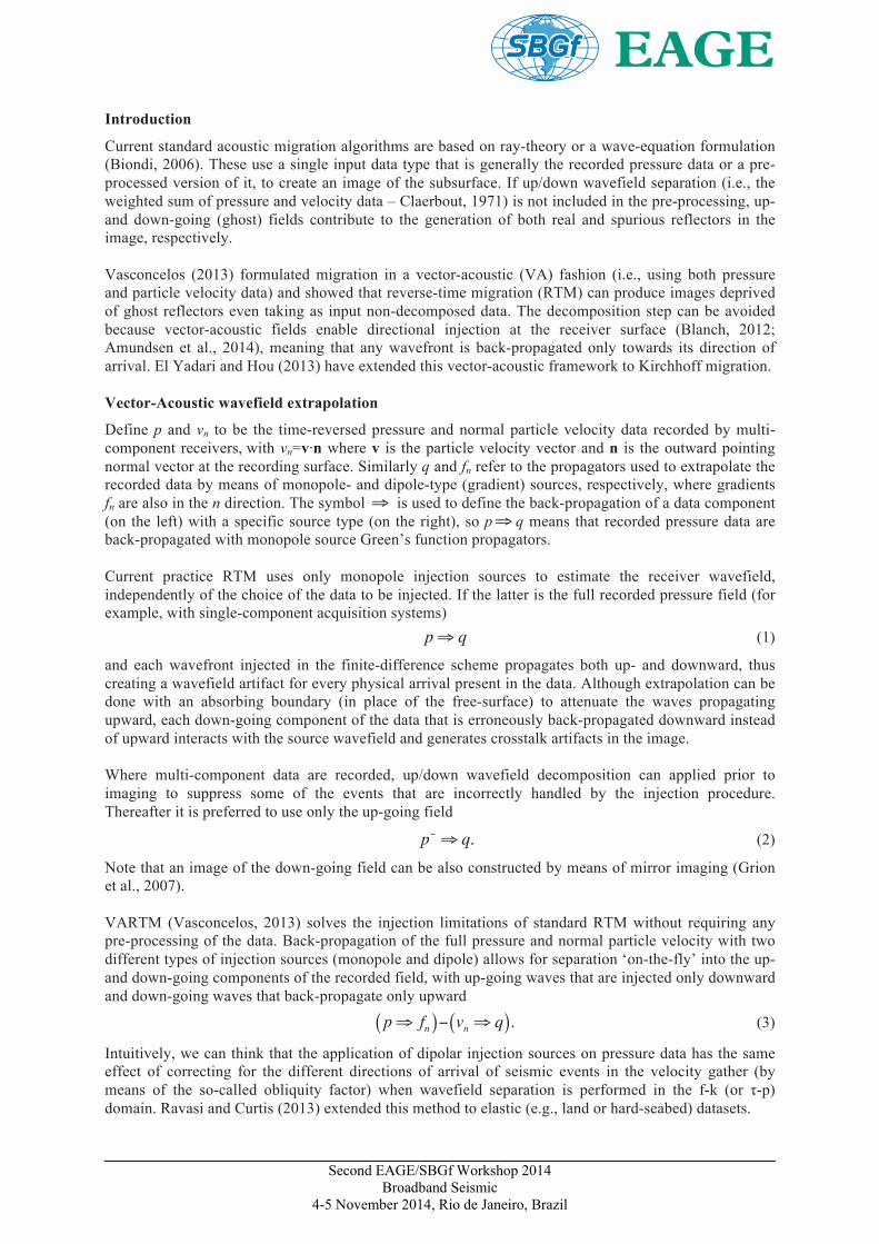
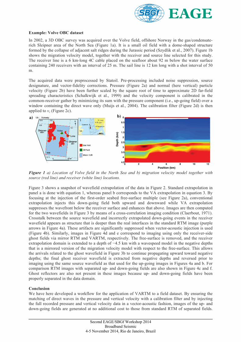
In 2002, a 3D OBC survey was acquired over the Volve field, offshore Norway in the gas/condensate-rich Sleipner area of the North Sea (Figure 1a). It is a small oil field with a dome-shaped structure formed by the collapse of adjacent salt ridges during the Jurassic period (Szydlik et al., 2007). Figure 1b shows the migration velocity model, together with the receiver and source line selected for this study. The receiver line is a 6 km-long 4C cable placed on the seafloor about 92 m below the water surface containing 240 receivers with an interval of 25 m. The sail line is 12 km long with a shot interval of 50 m. The acquired data were preprocessed by Statoil. Pre-processing included noise suppression, source designature, and vector-fidelity corrections. Pressure (Figure 2a) and normal (here vertical) particle velocity (Figure 2b) have been further scaled by the square root of time to approximate 2D far-field spreading characteristics (Schalkwijk et al., 1999) and the velocity component is calibrated in the common-receiver gather by minimizing its sum with the pressure component (i.e., up-going field) over a window containing the direct wave only (Muijs et al., 2004). The calibration filter (Figure 2d) is then applied to vz (Figure 2c).
Position (km)
Dep
th (
km)
0 2 4 6 8 10 12
0
0.5
1
1.5
2
2.5
3
3.5
4
4.5
a) b)
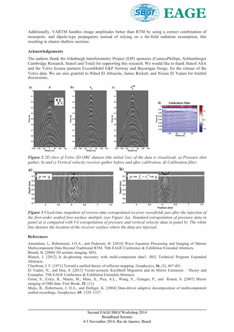
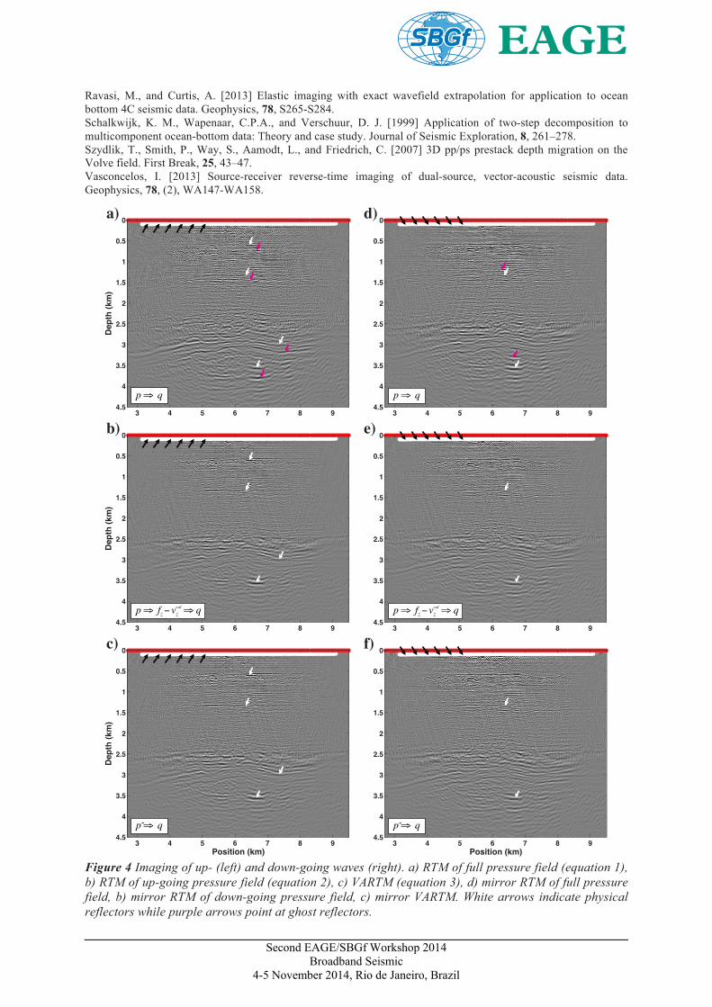
Figure 1 a) Location of Volve field in the North Sea and b) migration velocity model together with source (red line) and receiver (white line) locations. Figure 3 shows a snapshot of wavefield extrapolation of the data in Figure 2. Standard extrapolation in panel a is done with equation 1, whereas panel b corresponds to the VA extrapolation in equation 3. By focusing at the injection of the first-order seabed free-surface multiple (see Figure 2a), conventional extrapolation injects this down-going field both upward and downward while VA extrapolation suppresses the wavefront below the receiver surface and enhances that above. Images are then computed for the two wavefields in Figure 3 by means of a cross-correlation imaging condition (Claerbout, 1971). Crosstalk between the source wavefield and incorrectly extrapolated down-going events in the receiver wavefield appears as structure that is deeper than the real interfaces in the standard RTM image (purple arrows in Figure 4a). These artifacts are significantly suppressed when vector-acoustic injection is used (Figure 4b). Similarly, images in Figure 4d and e correspond to imaging using only the receiver-side ghost fields via mirror RTM and VARTM, respectively. The free-surface is removed, and the receiver extrapolation domain is extended to a depth of −4.5 km with a wavespeed model in the negative depths that is a mirrored version of the migration velocity model with respect to the free-surface. This allows the arrivals related to the ghost wavefield in Figure 3b to continue propagating upward toward negative depths; the final ghost receiver wavefield is extracted from negative depths and reversed prior to imaging using the same source wavefield as that used for the up-going images in Figures 4a and b. For comparison RTM images with separated up- and down-going fields are also shown in Figure 4c and f. Ghost reflectors are also not present in these images because up- and down-going fields have been properly separated in the data domain. Conclusion We have here developed a workflow for the application of VARTM to a field dataset. By ensuring the matching of direct waves in the pressure and vertical velocity with a calibration filter and by injecting the full recorded pressure and vertical velocity data in a vector-acoustic fashion, images of the up- and down-going fields are generated at no additional cost to those from standard RTM of separated fields.
Second EAGE/SBGf Workshop 2014
Broadband Seismic 4-5 November 2014, Rio de Janeiro, Brazil
Additionally, VARTM handles image amplitudes better than RTM by using a correct combination of monopole- and dipole-type propagators instead of relying on a far-field radiation assumption, this resulting in clearer shallow sections. Acknowledgements
The authors thank the Edinburgh Interferometry Project (EIP) sponsors (ConocoPhillips, Schlumberger Cambridge Research, Statoil and Total) for supporting this research. We would like to thank Statoil ASA and the Volve license partners ExxonMobil E&P Norway and Bayerngas Norge, for the release of the Volve data. We are also grateful to Nihed El Allouche, James Rickett, and Nizare El Yadari for fruitful discussions.
vzcal
Offset (m)
Tim
e (s
)
−150 −100 −50 0 50 100 150
0
0.1
0.2
0.3
0.4
0.5
0.6
0.7
0.8
0.9
1
vz
Offset (m)
Tim
e (s
)
−150 −100 −50 0 50 100 150
0
0.1
0.2
0.3
0.4
0.5
0.6
0.7
0.8
0.9
1
Offset (m)
Tim
e (s
)
Calibration filter
-150 -50 50 150
0
0.01
0.02
0.03
0.04
0.05
0.06
0.07 −0.5
0
0.5
1
1.5
2
b) c)
d)
p
Offset (m)
Tim
e (s
)
−150 −100 −50 0 50 100 150
0
0.1
0.2
0.3
0.4
0.5
0.6
0.7
0.8
0.9
1
a)
Figure 2 2D slice of Volve 3D OBC dataset (the initial 1sec of the data is visualized). a) Pressure shot gather, b) and c) Vertical velocity receiver gather before and after calibration. d) Calibration filter.
Dep
th (
km)
0
0.1
0.2
0.3
0.4
0.5
0.6
0.7
Dep
th (
km)
0
0.1
0.2
0.3
0.4
0.5
0.6
0.7
p p fz vz q
a) b)calq
5 5.5 6 6.5 7 7.5 5 5.5 6 6.5 7 7.5
Position (km) Figure 3 Fixed-time snapshots of reverse-time extrapolated receiver wavefields just after the injection of the first-order seabed free-surface multiple (see Figure 2a). Standard extrapolation of pressure data in panel a) is compared with VA extrapolation of pressure and vertical velocity data in panel b). The white line denotes the location of the receiver surface where the data are injected.
References Amundsen, L, Robertsson, J.O.A., and Pedersen, Ø. [2014] Wave Equation Processing and Imaging of Marine Multicomponent Data Beyond Traditional RTM. 76th EAGE Conference & Exhibition Extended Abstracts. Biondi, B. [2006] 3D seismic imaging. SEG. Blanch, J. [2012] Is de-ghosting necessary with multi-component data?. SEG Technical Program Expanded Abstracts. Claerbout, J. F. [1971] Toward a unified theory of reflector mapping. Geophysics, 36, (3), 467-481. El Yadari, N., and Hou, S. [2013] Vector-acoustic Kirchhoff Migration and its Mirror Extension – Theory and Examples. 75th EAGE Conference & Exhibition Extended Abstracts. Grion, S., Exley, R., Manin, M., Miao, X., Pica, A.L., Wang, Y., Granger, P., and Ronen, S. [2007] Mirror imaging of OBS data. First Break, 25, (11). Muijs, R., Robertsson, J. O.A., and Holliger, K. [2004] Data-driven adaptive decomposition of multicomponent seabed recordings. Geophysics, 69, 1329–1337.
Second EAGE/SBGf Workshop 2014
Broadband Seismic 4-5 November 2014, Rio de Janeiro, Brazil
Ravasi, M., and Curtis, A. [2013] Elastic imaging with exact wavefield extrapolation for application to ocean bottom 4C seismic data. Geophysics, 78, S265-S284. Schalkwijk, K. M., Wapenaar, C.P.A., and Verschuur, D. J. [1999] Application of two-step decomposition to multicomponent ocean-bottom data: Theory and case study. Journal of Seismic Exploration, 8, 261–278. Szydlik, T., Smith, P., Way, S., Aamodt, L., and Friedrich, C. [2007] 3D pp/ps prestack depth migration on the Volve field. First Break, 25, 43–47. Vasconcelos, I. [2013] Source-receiver reverse-time imaging of dual-source, vector-acoustic seismic data. Geophysics, 78, (2), WA147-WA158.
Dep
th (
km)
3 4 5 6 7 8 9
0
0.5
1
1.5
2
2.5
3
3.5
4
4.5
Dep
th (
km)
3 4 5 6 7 8 9
0
0.5
1
1.5
2
2.5
3
3.5
4
4.5
Dep
th (
km)
3 4 5 6 7 8 9
0
0.5
1
1.5
2
2.5
3
3.5
4
4.5
Position (km)
a)
b)
c)
p q
p- q
p fz vzcal q
3 4 5 6 7 8 9
0
0.5
1
1.5
2
2.5
3
3.5
4
4.5
3 4 5 6 7 8 9
0
0.5
1
1.5
2
2.5
3
3.5
4
4.5
3 4 5 6 7 8 9
0
0.5
1
1.5
2
2.5
3
3.5
4
4.5
Position (km)
d)
e)
f)
p q
p- q
p fz vzcal q
Figure 4 Imaging of up- (left) and down-going waves (right). a) RTM of full pressure field (equation 1), b) RTM of up-going pressure field (equation 2), c) VARTM (equation 3), d) mirror RTM of full pressure field, b) mirror RTM of down-going pressure field, c) mirror VARTM. White arrows indicate physical reflectors while purple arrows point at ghost reflectors.