Embed Size (px)
Citation preview
Edinburgh Research Explorer
Learning k-Modal Distributions via Testing
Citation for published version:Daskalakis, C, Diakonikolas, I & Servedio, RA 2014, 'Learning k-Modal Distributions via Testing' Theory ofComputing, vol 10, no. 20, pp. 535-570. DOI: 10.4086/toc.2014.v010a020
Digital Object Identifier (DOI):10.4086/toc.2014.v010a020
Link:Link to publication record in Edinburgh Research Explorer
Document Version:Peer reviewed version
Published In:Theory of Computing
General rightsCopyright for the publications made accessible via the Edinburgh Research Explorer is retained by the author(s)and / or other copyright owners and it is a condition of accessing these publications that users recognise andabide by the legal requirements associated with these rights.
Take down policyThe University of Edinburgh has made every reasonable effort to ensure that Edinburgh Research Explorercontent complies with UK legislation. If you believe that the public display of this file breaches copyright pleasecontact [email protected] providing details, and we will remove access to the work immediately andinvestigate your claim.
Download date: 02. Jul. 2018
THEORY OF COMPUTING, Volume 10 (20), 2014, pp. 535–570www.theoryofcomputing.org
Learning k-Modal Distributions via Testing
Constantinos Daskalakis∗ Ilias Diakonikolas† Rocco A. Servedio‡
Received April 11, 2013; Revised November 9, 2014; Published December 31, 2014
Abstract: A k-modal probability distribution over the discrete domain 1, . . . ,n is onewhose histogram has at most k “peaks” and “valleys.” Such distributions are natural gener-alizations of monotone (k = 0) and unimodal (k = 1) probability distributions, which havebeen intensively studied in probability theory and statistics.
In this paper we consider the problem of learning (i. e., performing density estimationof) an unknown k-modal distribution with respect to the L1 distance. The learning algorithmis given access to independent samples drawn from an unknown k-modal distribution p, andit must output a hypothesis distribution p such that with high probability the total variationdistance between p and p is at most ε . Our main goal is to obtain computationally efficientalgorithms for this problem that use (close to) an information-theoretically optimal numberof samples.
We give an efficient algorithm for this problem that runs in time poly(k, log(n),1/ε).For k ≤ O(logn), the number of samples used by our algorithm is very close (within an
A preliminary version of this work appeared in the Proceedings of the Twenty-Third Annual ACM-SIAM Symposium onDiscrete Algorithms (SODA 2012) [8].∗[email protected]. Research supported by NSF CAREER award CCF-0953960 and by a Sloan Foundation
Fellowship.†[email protected]. Most of this research was done while the author was at UC Berkeley supported by a Simons
Postdoctoral Fellowship. Some of this work was done at Columbia University, supported by NSF grant CCF-0728736, and byan Alexander S. Onassis Foundation Fellowship.
‡[email protected]. Supported by NSF grants CNS-0716245, CCF-0915929, and CCF-1115703.
ACM Classification: F.2.2, G.3
AMS Classification: 68W20, 68Q25, 68Q32
Key words and phrases: computational learning theory, learning distributions, k-modal distributions
© 2014 Constantinos Daskalakis, Ilias Diakonikolas, and Rocco A. Servediocb Licensed under a Creative Commons Attribution License (CC-BY) DOI: 10.4086/toc.2014.v010a020
CONSTANTINOS DASKALAKIS, ILIAS DIAKONIKOLAS, AND ROCCO A. SERVEDIO
O(log(1/ε)) factor) to being information-theoretically optimal. Prior to this work computa-tionally efficient algorithms were known only for the cases k = 0,1 (Birgé 1987, 1997).
A novel feature of our approach is that our learning algorithm crucially uses a newalgorithm for property testing of probability distributions as a key subroutine. The learningalgorithm uses the property tester to efficiently decompose the k-modal distribution into k(near-)monotone distributions, which are easier to learn.
1 Introduction
This paper considers a natural unsupervised learning problem involving k-modal distributions over thediscrete domain [n] =1, . . . ,n. A distribution is k-modal if the plot of its probability density function(pdf) has at most k “peaks” and “valleys” (see Section 2.1 for a precise definition). Such distributionsarise both in theoretical (see, e. g., [7, 19, 6]) and applied (see, e. g., [20, 1, 13]) research; they naturallygeneralize the simpler classes of monotone (k = 0) and unimodal (k = 1) distributions that have beenintensively studied in probability theory and statistics (see the discussion of related work below).
Our main aim in this paper is to give an efficient algorithm for learning an unknown k-modaldistribution p to total variation distance ε , given access only to independent samples drawn from p. Asdescribed below there is an information-theoretic lower bound of Ω(k log(n/k)/ε3) samples for thislearning problem, so an important goal for us is to obtain an algorithm whose sample complexity is asclose as possible to this lower bound. An equally important goal is for our algorithm to be computationallyefficient, i. e., to run in time polynomial in the size of its input sample. Our main contribution in thispaper is a computationally efficient algorithm that has nearly optimal sample complexity for small (butsuper-constant) values of k.
1.1 Background and relation to previous work
There is a rich body of work in the statistics and probability literatures on estimating distributions undervarious kinds of “shape” or “order” restrictions. In particular, many researchers have studied the riskof different estimators for monotone (k = 0) and unimodal (k = 1) distributions; see for example theworks of [23, 26, 17, 3, 4, 5], among many others. These and related papers from the probability/statisticsliterature mostly deal with information-theoretic upper and lower bounds on the sample complexity oflearning monotone and unimodal distributions. In contrast, a central goal of the current work is to obtaincomputationally efficient learning algorithms for larger values of k.
It should be noted that some of the works cited above do give efficient algorithms for the casesk = 0 and k = 1; in particular we mention the results of Birgé [4, 5], which give computationallyefficient O(log(n)/ε3)-sample algorithms for learning unknown monotone or unimodal distributions over[n] respectively. (Birgé [3] also showed that this sample complexity is asymptotically optimal, as wediscuss below; we describe the algorithm of [4] in more detail in Section 2.2, and indeed use it as aningredient of our approach throughout this paper.) However, for these relatively simple k = 0,1 classesof distributions the main challenge is in developing sample-efficient estimators, and the algorithmicaspects are typically rather straightforward (as is the case in [4]). In contrast, much more challenging andinteresting algorithmic issues arise for the general values of k which we consider here.
THEORY OF COMPUTING, Volume 10 (20), 2014, pp. 535–570 536
LEARNING k-MODAL DISTRIBUTIONS VIA TESTING
1.2 Our results
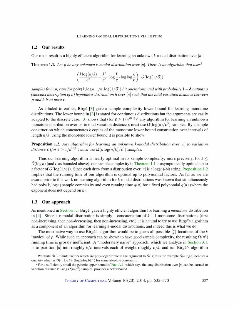
Our main result is a highly efficient algorithm for learning an unknown k-modal distribution over [n]:
Theorem 1.1. Let p be any unknown k-modal distribution over [n]. There is an algorithm that uses1(k log(n/k)
ε3 +k2
ε3 · logkε· log log
kε
)· O(log(1/δ ))
samples from p, runs for poly(k, logn,1/ε, log(1/δ )) bit operations, and with probability 1−δ outputs a(succinct description of a) hypothesis distribution h over [n] such that the total variation distance betweenp and h is at most ε .
As alluded to earlier, Birgé [3] gave a sample complexity lower bound for learning monotonedistributions. The lower bound in [3] is stated for continuous distributions but the arguments are easilyadapted to the discrete case; [3] shows that (for ε ≥ 1/nΩ(1))2 any algorithm for learning an unknownmonotone distribution over [n] to total variation distance ε must use Ω(log(n)/ε3) samples. By a simpleconstruction which concatenates k copies of the monotone lower bound construction over intervals oflength n/k, using the monotone lower bound it is possible to show:
Proposition 1.2. Any algorithm for learning an unknown k-modal distribution over [n] to variationdistance ε (for ε ≥ 1/nΩ(1)) must use Ω(k log(n/k)/ε3) samples.
Thus our learning algorithm is nearly optimal in its sample complexity; more precisely, for k ≤O(logn) (and ε as bounded above), our sample complexity in Theorem 1.1 is asymptotically optimal up toa factor of O(log(1/ε)). Since each draw from a distribution over [n] is a log(n)-bit string, Proposition 1.2implies that the running time of our algorithm is optimal up to polynomial factors. As far as we areaware, prior to this work no learning algorithm for k-modal distributions was known that simultaneouslyhad poly(k, logn) sample complexity and even running time q(n) for a fixed polynomial q(n) (where theexponent does not depend on k).
1.3 Our approach
As mentioned in Section 1.1 Birgé, gave a highly efficient algorithm for learning a monotone distributionin [4]. Since a k-modal distribution is simply a concatenation of k+ 1 monotone distributions (firstnon-increasing, then non-decreasing, then non-increasing, etc.), it is natural to try to use Birgé’s algorithmas a component of an algorithm for learning k-modal distributions, and indeed this is what we do.
The most naive way to use Birgé’s algorithm would be to guess all possible(n
k
)locations of the k
“modes” of p. While such an approach can be shown to have good sample complexity, the resulting Ω(nk)running time is grossly inefficient. A “moderately naive” approach, which we analyze in Section 3.1,is to partition [n] into roughly k/ε intervals each of weight roughly ε/k, and run Birgé’s algorithm
1We write O(·) to hide factors which are poly-logarithmic in the argument to O(·); thus for example O(a logb) denotes aquantity which is O((a logb) · (log(a logb))c) for some absolute constant c.
2For ε sufficiently small the generic upper bound of Fact A.1, which says that any distribution over [n] can be learned tovariation distance ε using O(n/ε2) samples, provides a better bound.
THEORY OF COMPUTING, Volume 10 (20), 2014, pp. 535–570 537
CONSTANTINOS DASKALAKIS, ILIAS DIAKONIKOLAS, AND ROCCO A. SERVEDIO
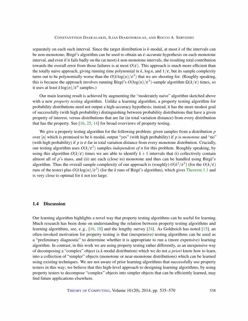
separately on each such interval. Since the target distribution is k-modal, at most k of the intervals canbe non-monotone; Birgé’s algorithm can be used to obtain an ε-accurate hypothesis on each monotoneinterval, and even if it fails badly on the (at most) k non-monotone intervals, the resulting total contributiontowards the overall error from those failures is at most O(ε). This approach is much more efficient thanthe totally naive approach, giving running time polynomial in k, logn, and 1/ε , but its sample complexityturns out to be polynomially worse than the O(k log(n)/ε3) that we are shooting for. (Roughly speaking,this is because the approach involves running Birgé’s O(log(n)/ε3)-sample algorithm Ω(k/ε) times, soit uses at least k log(n)/ε4 samples.)
Our main learning result is achieved by augmenting the “moderately naive” algorithm sketched abovewith a new property testing algorithm. Unlike a learning algorithm, a property testing algorithm forprobability distributions need not output a high-accuracy hypothesis; instead, it has the more modest goalof successfully (with high probability) distinguishing between probability distributions that have a givenproperty of interest, versus distributions that are far (in total variation distance) from every distributionthat has the property. See [16, 25, 14] for broad overviews of property testing.
We give a property testing algorithm for the following problem: given samples from a distribution pover [n] which is promised to be k-modal, output “yes” (with high probability) if p is monotone and “no”(with high probability) if p is ε-far in total variation distance from every monotone distribution. Crucially,our testing algorithm uses O(k/ε2) samples independent of n for this problem. Roughly speaking, byusing this algorithm O(k/ε) times we are able to identify k+ 1 intervals that (i) collectively containalmost all of p’s mass, and (ii) are each (close to) monotone and thus can be handled using Birgé’salgorithm. Thus the overall sample complexity of our approach is (roughly) O(k2/ε3) (for the O(k/ε)runs of the tester) plus O(k log(n)/ε3) (for the k runs of Birgé’s algorithm), which gives Theorem 1.1 andis very close to optimal for k not too large.
1.4 Discussion
Our learning algorithm highlights a novel way that property testing algorithms can be useful for learning.Much research has been done on understanding the relation between property testing algorithms andlearning algorithms, see, e. g., [16, 18] and the lengthy survey [24]. As Goldreich has noted [15], anoften-invoked motivation for property testing is that (inexpensive) testing algorithms can be used asa “preliminary diagnostic” to determine whether it is appropriate to run a (more expensive) learningalgorithm. In contrast, in this work we are using property testing rather differently, as an inexpensive wayof decomposing a “complex” object (a k-modal distribution) which we do not a priori know how to learn,into a collection of “simpler” objects (monotone or near-monotone distributions) which can be learnedusing existing techniques. We are not aware of prior learning algorithms that successfully use propertytesters in this way; we believe that this high-level approach to designing learning algorithms, by usingproperty testers to decompose “complex” objects into simpler objects that can be efficiently learned, mayfind future applications elsewhere.
THEORY OF COMPUTING, Volume 10 (20), 2014, pp. 535–570 538
LEARNING k-MODAL DISTRIBUTIONS VIA TESTING
2 Preliminaries
2.1 Notation and problem statement
For n ∈ Z+, denote by [n] the set 1, . . . ,n; for i, j ∈ Z+, i ≤ j, denote by [i, j] the set i, i+1, . . . , j.We write v(i) to denote the i-th element of vector v ∈ Rn. For v = (v(1), . . . ,v(n)) ∈ Rn denote by
‖v‖1 =n
∑i=1|v(i)|
its L1-norm.We consider discrete probability distributions over [n], which are functions p : [n]→ [0,1] such that
∑ni=1 p(i) = 1. For S ⊆ [n] we write p(S) to denote ∑i∈S p(i). For S ⊆ [n], we write pS to denote the
conditional distribution over S that is induced by p. We use the notation P for the cumulative distributionfunction (cdf) corresponding to p, i. e., P : [n]→ [0,1] is defined by P( j) = ∑
ji=1 p(i).
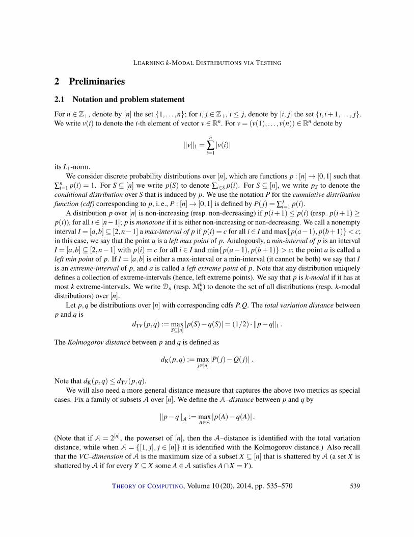
A distribution p over [n] is non-increasing (resp. non-decreasing) if p(i+1)≤ p(i) (resp. p(i+1)≥p(i)), for all i∈ [n−1]; p is monotone if it is either non-increasing or non-decreasing. We call a nonemptyinterval I = [a,b]⊆ [2,n−1] a max-interval of p if p(i) = c for all i ∈ I and maxp(a−1), p(b+1)< c;in this case, we say that the point a is a left max point of p. Analogously, a min-interval of p is an intervalI = [a,b]⊆ [2,n−1] with p(i) = c for all i ∈ I and minp(a−1), p(b+1)> c; the point a is called aleft min point of p. If I = [a,b] is either a max-interval or a min-interval (it cannot be both) we say that Iis an extreme-interval of p, and a is called a left extreme point of p. Note that any distribution uniquelydefines a collection of extreme-intervals (hence, left extreme points). We say that p is k-modal if it has atmost k extreme-intervals. We write Dn (resp. Mk
n) to denote the set of all distributions (resp. k-modaldistributions) over [n].
Let p,q be distributions over [n] with corresponding cdfs P,Q. The total variation distance betweenp and q is
dTV (p,q) := maxS⊆[n]|p(S)−q(S)|= (1/2) · ‖p−q‖1 .
The Kolmogorov distance between p and q is defined as
dK(p,q) := maxj∈[n]|P( j)−Q( j)| .
Note that dK(p,q)≤ dTV (p,q).We will also need a more general distance measure that captures the above two metrics as special
cases. Fix a family of subsets A over [n]. We define the A–distance between p and q by
‖p−q‖A := maxA∈A|p(A)−q(A)| .
(Note that if A = 2[n], the powerset of [n], then the A–distance is identified with the total variationdistance, while when A = [1, j], j ∈ [n] it is identified with the Kolmogorov distance.) Also recallthat the VC–dimension of A is the maximum size of a subset X ⊆ [n] that is shattered by A (a set X isshattered by A if for every Y ⊆ X some A ∈A satisfies A∩X = Y ).
THEORY OF COMPUTING, Volume 10 (20), 2014, pp. 535–570 539
CONSTANTINOS DASKALAKIS, ILIAS DIAKONIKOLAS, AND ROCCO A. SERVEDIO
Learning k-modal Distributions. Given independent samples from an unknown k-modal distributionp ∈Mk
n and ε > 0, the goal is to output a hypothesis distribution h such that with probability 1−δ wehave dTV (p,h) ≤ ε . We say that such an algorithm A learns p to accuracy ε and confidence δ . Theparameters of interest are the number of samples and the running time required by the algorithm.
2.2 Basic tools
We recall some useful tools from probability theory.
The VC inequality. Given m independent samples s1, . . . ,sm, drawn from p : [n]→ [0,1], the empiricaldistribution pm : [n]→ [0,1] is defined as follows: for all i ∈ [n],
pm(i) =| j ∈ [m] | s j = i|
m.
Fix a family of subsets A over [n] of VC–dimension d. The VC inequality states that for m = Ω(d/ε2),with probability 9/10 the empirical distribution pm will be ε-close to p in A-distance. This sample boundis asymptotically optimal.
Theorem 2.1 (VC inequality, [12, p.31]). Let pm be an empirical distribution of m samples from p. LetA be a family of subsets of VC–dimension d. Then
E [‖p− pm‖A]≤ O(√
d/m) .
Uniform convergence. We will also use the following uniform convergence bound:
Theorem 2.2 ([12, p.17]). Let A be a family of subsets over [n], and pm be an empirical distribution ofm samples from p. Let X be the random variable ‖p− pm‖A. Then we have
Pr [X−E[X ]> η ]≤ e−2mη2.
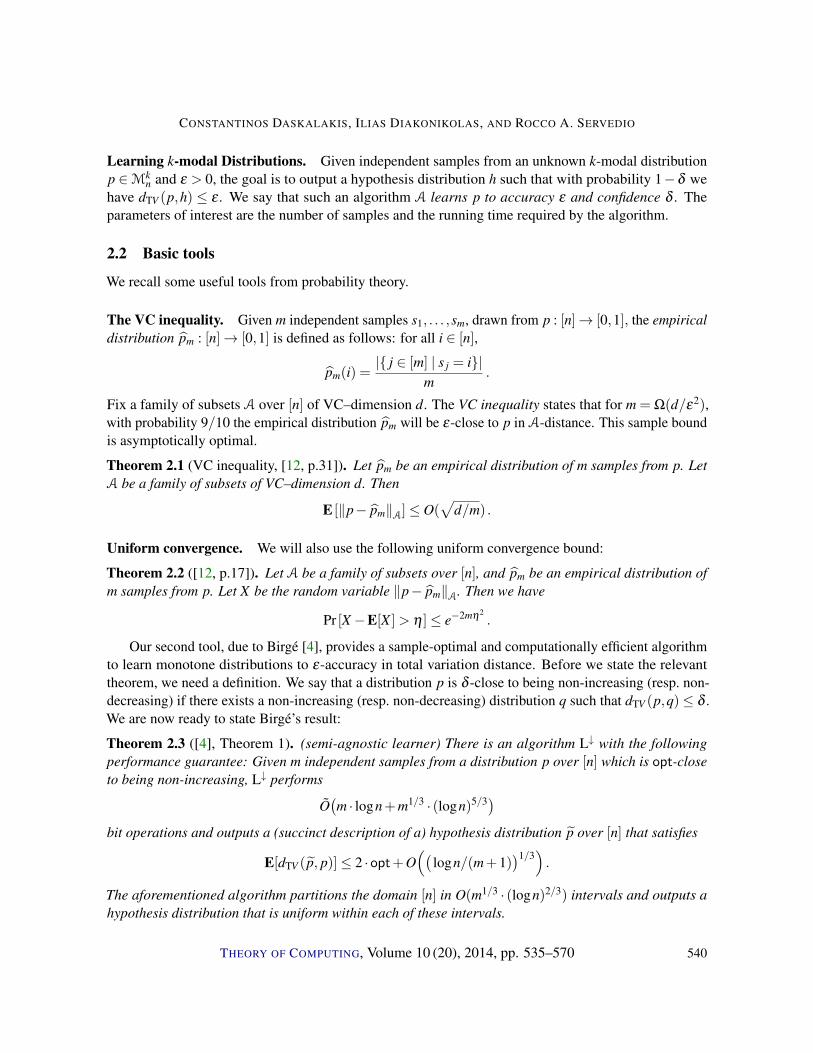
Our second tool, due to Birgé [4], provides a sample-optimal and computationally efficient algorithmto learn monotone distributions to ε-accuracy in total variation distance. Before we state the relevanttheorem, we need a definition. We say that a distribution p is δ -close to being non-increasing (resp. non-decreasing) if there exists a non-increasing (resp. non-decreasing) distribution q such that dTV (p,q)≤ δ .We are now ready to state Birgé’s result:
Theorem 2.3 ([4], Theorem 1). (semi-agnostic learner) There is an algorithm L↓ with the followingperformance guarantee: Given m independent samples from a distribution p over [n] which is opt-closeto being non-increasing, L↓ performs
O(m · logn+m1/3 · (logn)5/3)
bit operations and outputs a (succinct description of a) hypothesis distribution p over [n] that satisfies
E[dTV (p, p)]≤ 2 ·opt+O((
logn/(m+1))1/3
).
The aforementioned algorithm partitions the domain [n] in O(m1/3 · (logn)2/3) intervals and outputs ahypothesis distribution that is uniform within each of these intervals.
THEORY OF COMPUTING, Volume 10 (20), 2014, pp. 535–570 540
LEARNING k-MODAL DISTRIBUTIONS VIA TESTING
By taking m = Ω(logn/ε3), one obtains a hypothesis such that E[dTV (p, p)]≤ 2 ·opt+ ε . We stressthat Birgé’s algorithm for learning non-increasing distributions [4] is in fact “semi-agnostic,” in the sensethat it also learns distributions that are close to being non-increasing; this robustness will be crucial forus later (since in our final algorithm we will use Birgé’s algorithm on distributions identified by ourtester, that are close to monotone but not necessarily perfectly monotone). This semi-agnostic propertyis not explicitly stated in [4] but it can be shown to follow easily from his results. We show how thesemi-agnostic property follows from Birgé’s results in Appendix A. Let L↑ denote the correspondingsemi-agnostic algorithm for learning non-decreasing distributions.
Our final tool is a routine to do hypothesis testing, i. e., to select a high-accuracy hypothesis distributionfrom a collection of hypothesis distributions one of which has high accuracy. The need for such a routinearises in several places; in some cases we know that a distribution is monotone, but do not know whetherit is non-increasing or non-decreasing. In this case, we can run both algorithms L↑ and L↓ and then choosea good hypothesis using hypothesis testing. Another need for hypothesis testing is to “boost confidence”that a learning algorithm generates a high-accuracy hypothesis. Our initial version of the algorithm forTheorem 1.1 generates an ε-accurate hypothesis with probability at least 9/10; by running it O(log(1/δ ))times using a hypothesis testing routine, it is possible to identify an O(ε)-accurate hypothesis withprobability 1−δ . Routines of the sort that we require have been given in, e. g., [12] and [9]; we use thefollowing theorem from [9]:
Theorem 2.4. There is an algorithm Choose-Hypothesisp(h1,h2,ε′,δ ′) which is given sample access
to p, two hypothesis distributions h1,h2 for p, an accuracy parameter ε ′, and a confidence parameterδ ′. It makes m = O(log(1/δ ′)/ε ′2) draws from p and returns a hypothesis h ∈ h1,h2. If one of h1,h2has dTV (hi, p)≤ ε ′ then with probability 1−δ ′ the hypothesis h that Choose-Hypothesis returns hasdTV (h, p)≤ 6ε ′.
For the sake of completeness, we describe and analyze the Choose-Hypothesis algorithm in Ap-pendix B.
3 Learning k-modal distributions
In this section, we present our main result: a nearly sample-optimal and computationally efficientalgorithm to learn an unknown k-modal distribution. In Section 3.1 we present a simple learningalgorithm with a suboptimal sample complexity. In Section 3.2 we present our main result which involvesa property testing algorithm as a subroutine.
3.1 Warm-up: A simple learning algorithm
In this subsection, we give an algorithm that runs in time poly(k, logn,1/ε, log(1/δ )) and learns anunknown k-modal distribution to accuracy ε and confidence δ . The sample complexity of the algorithmis essentially optimal as a function of k (up to a logarithmic factor), but suboptimal as a function of ε , bya polynomial factor.
In the following pseudocode we give a detailed description of the algorithm Learn-kmodal-simple(a precise description appears as Algorithm 1, below); the algorithm outputs an ε-accurate hypothesis
THEORY OF COMPUTING, Volume 10 (20), 2014, pp. 535–570 541
CONSTANTINOS DASKALAKIS, ILIAS DIAKONIKOLAS, AND ROCCO A. SERVEDIO
with confidence 9/10 (see Theorem 3.3). We explain how to boost the confidence to 1−δ after the proofof the theorem.
Algorithm Learn-kmodal-simple works as follows: We start by partitioning the domain [n] intoconsecutive intervals of mass “approximately ε/k.” To do this, we draw Θ(k/ε3) samples from p andgreedily partition the domain into disjoint intervals of empirical mass roughly ε/k. (Some care is neededin this step, since there may be “heavy” points in the support of the distribution; however, we gloss overthis technical issue for the sake of this intuitive explanation.) Note that we do not have a guaranteethat each such interval will have true probability mass Θ(ε/k). In fact, it may well be the case that theadditive error δ between the true probability mass of an interval and its empirical mass (roughly ε/k)is δ = ω(ε/k). The error guarantee of the partitioning is more “global” in that the sum of these errorsacross all such intervals is at most ε . In particular, as a simple corollary of the VC inequality, we candeduce the following statement that will be used several times throughout the paper:
Fact 3.1. Let p be any distribution over [n] and pm be the empirical distribution of m samples from p.For
m = Ω((d/ε
2) log(1/δ )),
with probability at least 1−δ , for any collection J of (at most) d disjoint intervals in [n], we have that
∑J∈J|p(J)− pm(J)| ≤ ε .
Proof. Note that∑J∈J|p(J)− pm(J)|= 2|p(A)− pm(A)| , (3.1)
whereA = J ∈ J : p(J)> pm(J) .
Since J is a collection of at most d intervals, it is clear that A is a union of at most d intervals. If Ad is thefamily of all unions of at most d intervals, then the right hand side of (3.1) is at most 2‖p− pm‖Ad . Sincethe VC–dimension of Ad is 2d, Theorem 2.1 implies that the quantity (3.1) has expected value at mostε/2. The claim now follows by an application of Theorem 2.2 with η = ε/2.
If this step is successful, we have partitioned the domain into a set of O(k/ε) consecutive intervals ofprobability mass “roughly ε/k.” The next step is to apply Birgé’s monotone learning algorithm to eachinterval.
A caveat comes from the fact that not all such intervals are guaranteed to be monotone (or even closeto being monotone). However, since our input distribution is assumed to be k-modal, all but (at most) kof these intervals are monotone. Call a non-monotone interval “bad.” Since all intervals have empiricalprobability mass at most ε/k and there are at most k bad intervals, it follows from Fact 3.1 that theseintervals contribute at most O(ε) to the total mass. So even though Birgé’s algorithm gives no guaranteesfor bad intervals, these intervals do not affect the error by more than O(ε).
Let us now focus on the monotone intervals. For each such interval, we do not know if it is monotoneincreasing or monotone decreasing. To overcome this difficulty, we run both monotone algorithms L↓
and L↑ for each interval and then use hypothesis testing to choose the correct candidate distribution.
THEORY OF COMPUTING, Volume 10 (20), 2014, pp. 535–570 542
LEARNING k-MODAL DISTRIBUTIONS VIA TESTING
Also, note that since we have O(k/ε) intervals, we need to run each instance of both the monotonelearning algorithms and the hypothesis testing algorithm with confidence 1−O(ε/k), so that we canguarantee that the overall algorithm has confidence 9/10. Note that Theorem 2.3 and Markov’s inequalityimply that if we draw Ω(logn/ε3) samples from a non-increasing distribution p, the hypothesis p outputby L↓ satisfies dTV (p, p) ≤ ε with probability 9/10. We can boost the confidence to 1− δ with anoverhead of
O(log(1/δ ) log log(1/δ ))
in the sample complexity:
Fact 3.2. Let p be a non-increasing distribution over [n]. There is an algorithm L↓δ with the followingperformance guarantee: Given
(logn/ε3) · O(log(1/δ )))
samples from p, L↓δ performsO((log2 n/ε
3) · log2(1/δ ))
bit operations and outputs a (succinct description of a) hypothesis distribution p over [n] that satisfiesdTV (p, p)≤ ε with probability at least 1−δ .
Algorithm L↓δ runs L↓ O(log(1/δ )) times and performs a tournament among the candidate hypothe-ses using Choose-Hypothesis. Let L↑δ denote the corresponding algorithm for learning non-decreasingdistributions with confidence δ . We postpone further details on these algorithms to Appendix C.
Theorem 3.3. Algorithm Learn-kmodal-simple (Algorithm 1) uses
k lognε4 · O(log(k/ε))
samples, performs poly(k, logn,1/ε) bit operations, and learns a k-modal distribution to accuracy O(ε)with probability 9/10.
Proof. First, it is easy to see that the algorithm has the claimed sample complexity. Indeed, the algorithmdraws a total of r+m+m′ samples in Steps 1, 4 and 5. The running time is also easy to analyze, as it iseasy to see that every step can be performed in polynomial time (in fact, nearly linear time) in the samplesize.
We need to show that with probability 9/10 (over its random samples), algorithm Learn-kmodal-simple outputs a hypothesis h such that dTV (h, p)≤ O(ε).
Since r = Θ(d/ε2) samples are drawn in Step 1, Fact 3.1 implies that with probability of failure atmost 1/100, for each family J of at most d disjoint intervals from [n], we have
∑J∈J|p(J)− pm(J)| ≤ ε . (3.2)
For the rest of the analysis of Learn-kmodal-simple we condition on this “good” event.Since every atomic interval I ∈ I has p(I)≥ ε/(10k) (except potentially the rightmost one), it follows
that the number ` of atomic intervals constructed in Step 2 satisfies `≤ 10 · (k/ε). By the construction
THEORY OF COMPUTING, Volume 10 (20), 2014, pp. 535–570 543
CONSTANTINOS DASKALAKIS, ILIAS DIAKONIKOLAS, AND ROCCO A. SERVEDIO
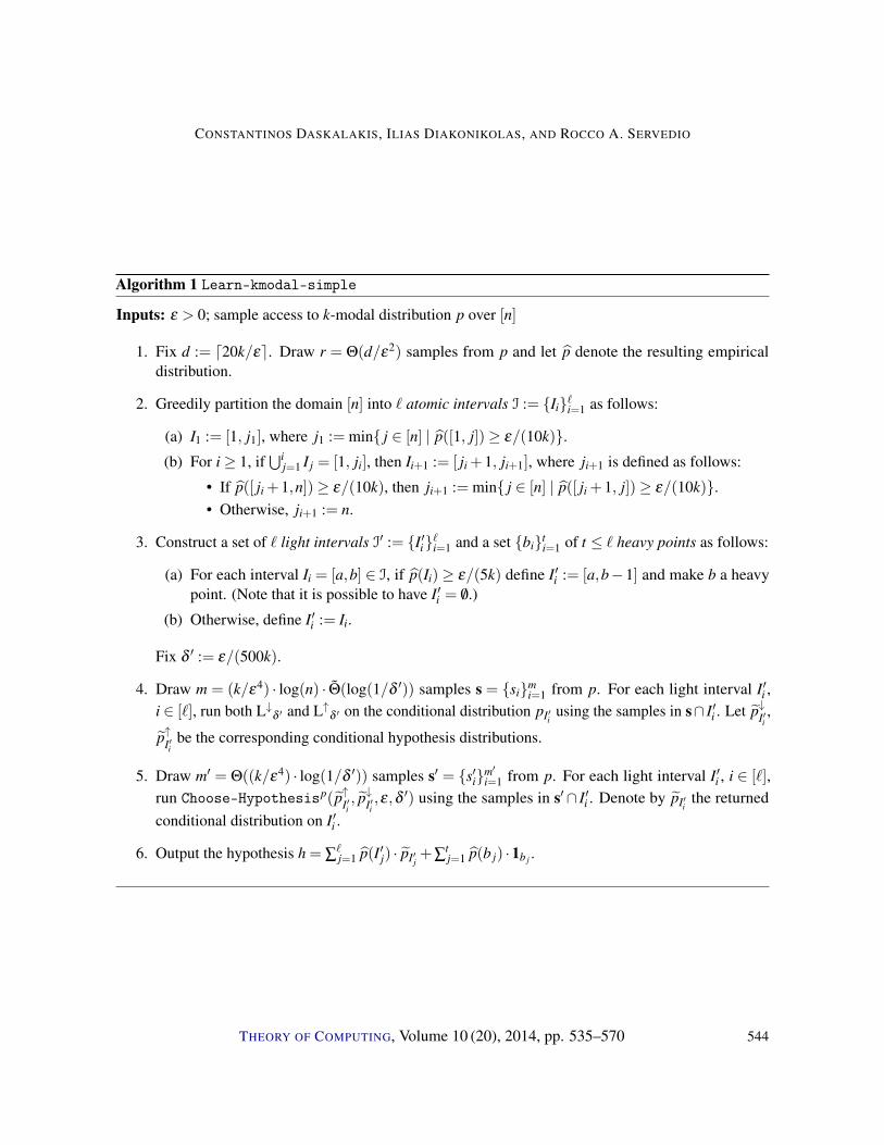
Algorithm 1 Learn-kmodal-simple
Inputs: ε > 0; sample access to k-modal distribution p over [n]
1. Fix d := d20k/εe. Draw r = Θ(d/ε2) samples from p and let p denote the resulting empiricaldistribution.
2. Greedily partition the domain [n] into ` atomic intervals I := Ii`i=1 as follows:
(a) I1 := [1, j1], where j1 := min j ∈ [n] | p([1, j])≥ ε/(10k).(b) For i≥ 1, if
⋃ij=1 I j = [1, ji], then Ii+1 := [ ji +1, ji+1], where ji+1 is defined as follows:
• If p([ ji +1,n])≥ ε/(10k), then ji+1 := min j ∈ [n] | p([ ji +1, j])≥ ε/(10k).• Otherwise, ji+1 := n.
3. Construct a set of ` light intervals I′ := I′i`i=1 and a set biti=1 of t ≤ ` heavy points as follows:
(a) For each interval Ii = [a,b] ∈ I, if p(Ii)≥ ε/(5k) define I′i := [a,b−1] and make b a heavypoint. (Note that it is possible to have I′i = /0.)
(b) Otherwise, define I′i := Ii.
Fix δ ′ := ε/(500k).
4. Draw m = (k/ε4) · log(n) · Θ(log(1/δ ′)) samples s = simi=1 from p. For each light interval I′i ,
i ∈ [`], run both L↓δ ′ and L↑δ ′ on the conditional distribution pI′i using the samples in s∩ I′i . Let p↓I′i ,
p↑I′i be the corresponding conditional hypothesis distributions.
5. Draw m′ = Θ((k/ε4) · log(1/δ ′)) samples s′ = s′im′i=1 from p. For each light interval I′i , i ∈ [`],
run Choose-Hypothesisp(p↑I′i , p↓I′i ,ε,δ′) using the samples in s′∩ I′i . Denote by pI′i the returned
conditional distribution on I′i .
6. Output the hypothesis h = ∑`j=1 p(I′j) · pI′j +∑
tj=1 p(b j) ·1b j .
THEORY OF COMPUTING, Volume 10 (20), 2014, pp. 535–570 544
LEARNING k-MODAL DISTRIBUTIONS VIA TESTING
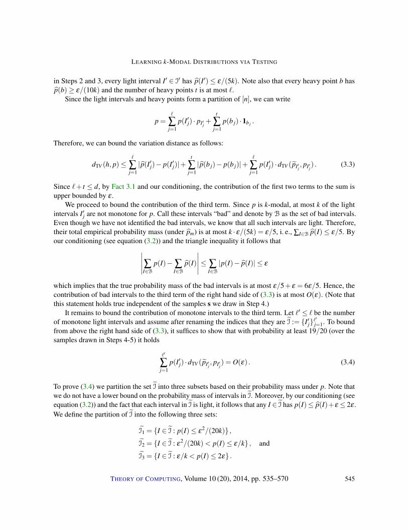
in Steps 2 and 3, every light interval I′ ∈ I′ has p(I′)≤ ε/(5k). Note also that every heavy point b hasp(b)≥ ε/(10k) and the number of heavy points t is at most `.
Since the light intervals and heavy points form a partition of [n], we can write
p =`
∑j=1
p(I′j) · pI′j +t
∑j=1
p(b j) ·1b j .
Therefore, we can bound the variation distance as follows:
dTV (h, p)≤`
∑j=1|p(I′j)− p(I′j)|+
t
∑j=1|p(b j)− p(b j)|+
`
∑j=1
p(I′j) ·dTV (pI′j , pI′j) . (3.3)
Since `+ t ≤ d, by Fact 3.1 and our conditioning, the contribution of the first two terms to the sum isupper bounded by ε .
We proceed to bound the contribution of the third term. Since p is k-modal, at most k of the lightintervals I′j are not monotone for p. Call these intervals “bad” and denote by B as the set of bad intervals.Even though we have not identified the bad intervals, we know that all such intervals are light. Therefore,their total empirical probability mass (under pm) is at most k · ε/(5k) = ε/5, i. e., ∑I∈B p(I)≤ ε/5. Byour conditioning (see equation (3.2)) and the triangle inequality it follows that∣∣∣∣∣∑I∈B p(I)−∑
I∈Bp(I)
∣∣∣∣∣≤ ∑I∈B|p(I)− p(I)| ≤ ε
which implies that the true probability mass of the bad intervals is at most ε/5+ ε = 6ε/5. Hence, thecontribution of bad intervals to the third term of the right hand side of (3.3) is at most O(ε). (Note thatthis statement holds true independent of the samples s we draw in Step 4.)
It remains to bound the contribution of monotone intervals to the third term. Let `′ ≤ ` be the numberof monotone light intervals and assume after renaming the indices that they are I := I′j`
′j=1. To bound
from above the right hand side of (3.3), it suffices to show that with probability at least 19/20 (over thesamples drawn in Steps 4-5) it holds
`′
∑j=1
p(I′j) ·dTV (pI′j , pI′j) = O(ε) . (3.4)
To prove (3.4) we partition the set I into three subsets based on their probability mass under p. Note thatwe do not have a lower bound on the probability mass of intervals in I. Moreover, by our conditioning (seeequation (3.2)) and the fact that each interval in I is light, it follows that any I ∈ I has p(I)≤ p(I)+ε ≤ 2ε .We define the partition of I into the following three sets:
I1 = I ∈ I : p(I)≤ ε2/(20k) ,
I2 = I ∈ I : ε2/(20k)< p(I)≤ ε/k , and
I3 = I ∈ I : ε/k < p(I)≤ 2ε .
THEORY OF COMPUTING, Volume 10 (20), 2014, pp. 535–570 545

CONSTANTINOS DASKALAKIS, ILIAS DIAKONIKOLAS, AND ROCCO A. SERVEDIO
We bound the contribution of each subset in turn. It is clear that the contribution of I1 to (3.4) is atmost
∑I∈I1
p(I)≤ |I1| · ε2/(20k)≤ `′ · ε2/(20k)≤ ` · ε2/(20k)≤ ε/2 .
To bound from above the contribution of I2 to (3.4), we partition I2 into
g2 = dlog2(20/ε)e= Θ(log(1/ε))
groups. For i ∈ [g2], the set (I2)i consists of those intervals in I2 that have mass under p in the range(
2−i · (ε/k),2−i+1 · (ε/k)]. The following statement establishes the variation distance closeness between
the conditional hypothesis for an interval in the i-th group (I2)i and the corresponding conditional
distribution.
Claim 3.4. With probability at least 19/20 (over the sample s,s′), for each i ∈ [g2] and each monotonelight interval I′j ∈ (I2)
i we have dTV (pI′j , pI′j) = O(2i/3 · ε).
Proof. Since in Step 4 we draw m samples, and each interval I′j ∈ (I2)i has
p(I′j) ∈[2−i · (ε/k),2−i+1 · (ε/k)
],
a standard coupon collector argument [22] tells us that with probability 99/100, for each (i, j) pair, theinterval I′j will get at least 2−i · (log(n)/ε3) · Ω(log(1/δ ′)) many samples. Let’s rewrite this as(
log(n)/(2i/3 · ε)3) · Ω(log(1/δ′))
samples. We condition on this event.Fix an interval I′j ∈ (I2)
i. We first show that with failure probability at most ε/(500k) after Step 4,
either p↓I′j or p↑I′j will be (2i/3 · ε)-accurate. Indeed, by Fact 3.2 and taking into account the number of
samples that landed in I′j, with probability 1− ε/(500k) over s,
dTV (pαiI′j, pI′j)≤ 2i/3
ε ,
where αi =↓ if pI′j is non-increasing and αi =↑ otherwise. By a union bound over all (at most ` many)
(i, j) pairs, it follows that with probability at least 49/50, for each interval I′j ∈ (I2)i one of the two
candidate hypothesis distributions is (2i/3ε)-accurate. We condition on this event.Now consider Step 5. Since this step draws m′ samples, and each interval I′j ∈ (I2)
i has
p(I′j) ∈(2−i · (ε/k),2−i+1 · (ε/k)
],
as before a standard coupon collector argument [22] tells us that with probability 99/100, for each (i, j)pair, the interval I′j will get at least (
1/(2i/3 · ε)3) · Ω(log(1/δ′))
THEORY OF COMPUTING, Volume 10 (20), 2014, pp. 535–570 546
LEARNING k-MODAL DISTRIBUTIONS VIA TESTING
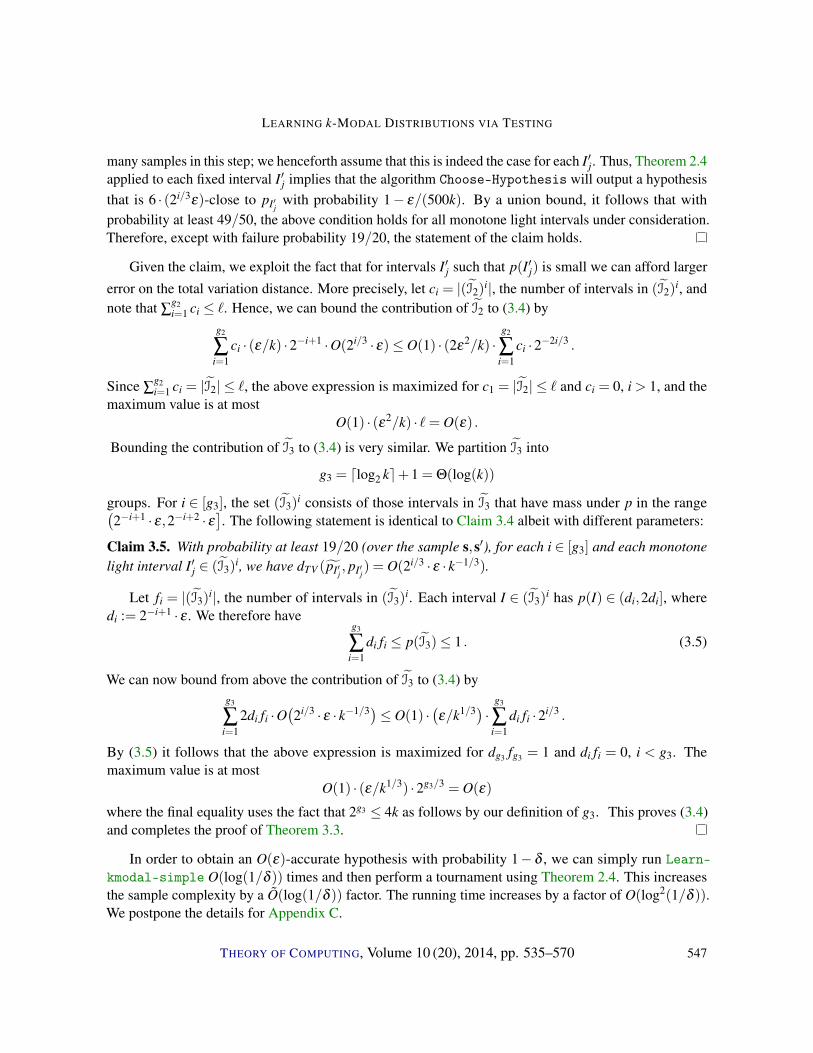
many samples in this step; we henceforth assume that this is indeed the case for each I′j. Thus, Theorem 2.4applied to each fixed interval I′j implies that the algorithm Choose-Hypothesis will output a hypothesisthat is 6 · (2i/3ε)-close to pI′j with probability 1− ε/(500k). By a union bound, it follows that withprobability at least 49/50, the above condition holds for all monotone light intervals under consideration.Therefore, except with failure probability 19/20, the statement of the claim holds.
Given the claim, we exploit the fact that for intervals I′j such that p(I′j) is small we can afford larger
error on the total variation distance. More precisely, let ci = |(I2)i|, the number of intervals in (I2)
i, andnote that ∑
g2i=1 ci ≤ `. Hence, we can bound the contribution of I2 to (3.4) by
g2
∑i=1
ci · (ε/k) ·2−i+1 ·O(2i/3 · ε)≤ O(1) · (2ε2/k) ·
g2
∑i=1
ci ·2−2i/3 .
Since ∑g2i=1 ci = |I2| ≤ `, the above expression is maximized for c1 = |I2| ≤ ` and ci = 0, i > 1, and the
maximum value is at mostO(1) · (ε2/k) · `= O(ε) .
Bounding the contribution of I3 to (3.4) is very similar. We partition I3 into
g3 = dlog2 ke+1 = Θ(log(k))
groups. For i ∈ [g3], the set (I3)i consists of those intervals in I3 that have mass under p in the range(
2−i+1 · ε,2−i+2 · ε]. The following statement is identical to Claim 3.4 albeit with different parameters:
Claim 3.5. With probability at least 19/20 (over the sample s,s′), for each i ∈ [g3] and each monotonelight interval I′j ∈ (I3)
i, we have dTV (pI′j , pI′j) = O(2i/3 · ε · k−1/3).
Let fi = |(I3)i|, the number of intervals in (I3)
i. Each interval I ∈ (I3)i has p(I) ∈ (di,2di], where
di := 2−i+1 · ε . We therefore haveg3
∑i=1
di fi ≤ p(I3)≤ 1 . (3.5)
We can now bound from above the contribution of I3 to (3.4) byg3
∑i=1
2di fi ·O(2i/3 · ε · k−1/3)≤ O(1) ·
(ε/k1/3) · g3
∑i=1
di fi ·2i/3 .
By (3.5) it follows that the above expression is maximized for dg3 fg3 = 1 and di fi = 0, i < g3. Themaximum value is at most
O(1) · (ε/k1/3) ·2g3/3 = O(ε)
where the final equality uses the fact that 2g3 ≤ 4k as follows by our definition of g3. This proves (3.4)and completes the proof of Theorem 3.3.
In order to obtain an O(ε)-accurate hypothesis with probability 1− δ , we can simply run Learn-kmodal-simple O(log(1/δ )) times and then perform a tournament using Theorem 2.4. This increasesthe sample complexity by a O(log(1/δ )) factor. The running time increases by a factor of O(log2(1/δ )).We postpone the details for Appendix C.
THEORY OF COMPUTING, Volume 10 (20), 2014, pp. 535–570 547

CONSTANTINOS DASKALAKIS, ILIAS DIAKONIKOLAS, AND ROCCO A. SERVEDIO
3.2 Main result: Learning k-modal distributions using testing
Here is some intuition to motivate our k-modal distribution learning algorithm and give a high-level ideaof why the dominant term in its sample complexity is O(k log(n/k)/ε3).
Let p denote the target k-modal distribution to be learned. As discussed above, optimal (in termsof time and sample complexity) algorithms are known for learning a monotone distribution over [n],so if the locations of the k modes of p were known then it would be straightforward to learn p veryefficiently by running the monotone distribution learner over k+1 separate intervals. But it is clear that ingeneral we cannot hope to efficiently identify the modes of p exactly (for instance it could be the case thatp(a) = p(a+2) = 1/n while p(a+1) = 1/n+1/2n). Still, it is natural to try to decompose the k-modaldistribution into a collection of (nearly) monotone distributions and learn those. At a high level that iswhat our algorithm does, using a novel property testing algorithm.
More precisely, we give a distribution testing algorithm with the following performance guarantee:Let q be a k-modal distribution over [n]. Given an accuracy parameter τ , our tester takes poly(k/τ)samples from q and outputs “yes” with high probability if q is monotone and “no” with high probability ifq is τ-far from every monotone distribution. (We stress that the assumption that q is k-modal is essentialhere, since an easy argument given in [2] shows that Ω(n1/2) samples are required to test whether ageneral distribution over [n] is monotone versus Θ(1)-far from monotone.)
With some care, by running the above-described tester O(k/ε) times with accuracy parameter τ , wecan decompose the domain [n] into
• at most k+1 “superintervals,” which have the property that the conditional distribution of p overeach superinterval is almost monotone (τ-close to monotone);
• at most k+1 “negligible intervals,” which have the property that each one has probability mass atmost O(ε/k) under p (so ignoring all of them incurs at most O(ε) total error); and
• at most k+1 “heavy” points, each of which has mass at least Ω(ε/k) under p.
We can ignore the negligible intervals, and the heavy points are easy to handle; however some care mustbe taken to learn the “almost monotone” restrictions of p over each superinterval. A naive approach,using a generic log(n)/ε3-sample monotone distribution learner that has no performance guaranteesif the target distribution is not monotone, leads to an inefficient overall algorithm. Such an approachwould require that τ (the closeness parameter used by the tester) be at most 1/(the sample complexityof the monotone distribution learner), i. e., τ < ε3/ log(n). Since the sample complexity of the tester ispoly(k/τ) and the tester is run Ω(k/ε) times, this approach would lead to an overall sample complexitythat is unacceptably high.
Fortunately, instead of using a generic monotone distribution learner, we can use the semi-agnosticmonotone distribution learner of Birgé (Theorem 2.3) that can handle deviations from monotonicity farmore efficiently than the above naive approach. Recall that given draws from a distribution q over [n] thatis τ-close to monotone, this algorithm uses O(log(n)/ε3) samples and outputs a hypothesis distributionthat is (2τ + ε)-close to monotone. By using this algorithm we can take the accuracy parameter τ forour tester to be Θ(ε) and learn the conditional distribution of p over a given superinterval to accuracy
THEORY OF COMPUTING, Volume 10 (20), 2014, pp. 535–570 548
LEARNING k-MODAL DISTRIBUTIONS VIA TESTING
O(ε) using O(log(n)/ε3) samples from that superinterval. Since there are k+1 superintervals overall, acareful analysis shows that O(k log(n)/ε3) samples suffice to handle all the superintervals.
We note that the algorithm also requires an additional additive poly(k/ε) samples (independent of n)besides this dominant term (for example, to run the tester and to estimate accurate weights with which tocombine the various sub-hypotheses). The overall sample complexity we achieve is stated in Theorem 3.6below.
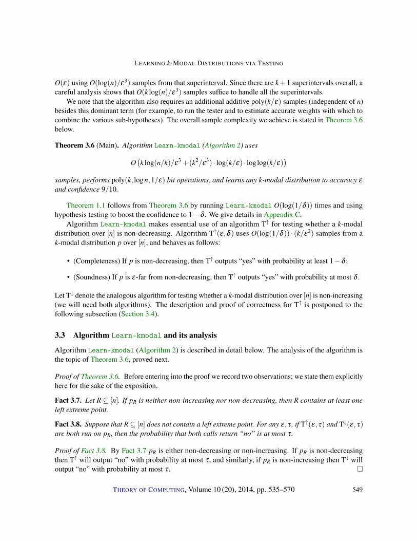
Theorem 3.6 (Main). Algorithm Learn-kmodal (Algorithm 2) uses
O(k log(n/k)/ε
3 +(k2/ε3) · log(k/ε) · log log(k/ε)
)samples, performs poly(k, logn,1/ε) bit operations, and learns any k-modal distribution to accuracy ε
and confidence 9/10.
Theorem 1.1 follows from Theorem 3.6 by running Learn-kmodal O(log(1/δ )) times and usinghypothesis testing to boost the confidence to 1−δ . We give details in Appendix C.
Algorithm Learn-kmodal makes essential use of an algorithm T↑ for testing whether a k-modaldistribution over [n] is non-decreasing. Algorithm T↑(ε,δ ) uses O(log(1/δ )) · (k/ε2) samples from ak-modal distribution p over [n], and behaves as follows:
• (Completeness) If p is non-decreasing, then T↑ outputs “yes” with probability at least 1−δ ;
• (Soundness) If p is ε-far from non-decreasing, then T↑ outputs “yes” with probability at most δ .
Let T↓ denote the analogous algorithm for testing whether a k-modal distribution over [n] is non-increasing(we will need both algorithms). The description and proof of correctness for T↑ is postponed to thefollowing subsection (Section 3.4).
3.3 Algorithm Learn-kmodal and its analysis
Algorithm Learn-kmodal (Algorithm 2) is described in detail below. The analysis of the algorithm isthe topic of Theorem 3.6, proved next.
Proof of Theorem 3.6. Before entering into the proof we record two observations; we state them explicitlyhere for the sake of the exposition.
Fact 3.7. Let R⊆ [n]. If pR is neither non-increasing nor non-decreasing, then R contains at least oneleft extreme point.
Fact 3.8. Suppose that R⊆ [n] does not contain a left extreme point. For any ε,τ , if T↑(ε,τ) and T↓(ε,τ)are both run on pR, then the probability that both calls return “no” is at most τ .
Proof of Fact 3.8. By Fact 3.7 pR is either non-decreasing or non-increasing. If pR is non-decreasingthen T↑ will output “no” with probability at most τ , and similarly, if pR is non-increasing then T↓ willoutput “no” with probability at most τ .
THEORY OF COMPUTING, Volume 10 (20), 2014, pp. 535–570 549
CONSTANTINOS DASKALAKIS, ILIAS DIAKONIKOLAS, AND ROCCO A. SERVEDIO
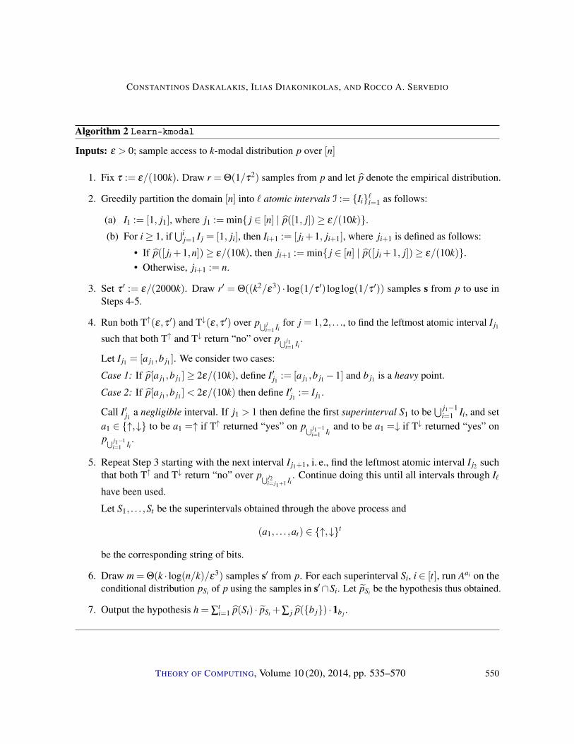
Algorithm 2 Learn-kmodal
Inputs: ε > 0; sample access to k-modal distribution p over [n]
1. Fix τ := ε/(100k). Draw r = Θ(1/τ2) samples from p and let p denote the empirical distribution.
2. Greedily partition the domain [n] into ` atomic intervals I := Ii`i=1 as follows:
(a) I1 := [1, j1], where j1 := min j ∈ [n] | p([1, j])≥ ε/(10k).(b) For i≥ 1, if
⋃ij=1 I j = [1, ji], then Ii+1 := [ ji +1, ji+1], where ji+1 is defined as follows:
• If p([ ji +1,n])≥ ε/(10k), then ji+1 := min j ∈ [n] | p([ ji +1, j])≥ ε/(10k).• Otherwise, ji+1 := n.
3. Set τ ′ := ε/(2000k). Draw r′ = Θ((k2/ε3) · log(1/τ ′) log log(1/τ ′)) samples s from p to use inSteps 4-5.
4. Run both T↑(ε,τ ′) and T↓(ε,τ ′) over p⋃ ji=1 Ii
for j = 1,2, . . ., to find the leftmost atomic interval I j1
such that both T↑ and T↓ return “no” over p⋃ j1i=1 Ii
.
Let I j1 = [a j1 ,b j1 ]. We consider two cases:
Case 1: If p[a j1 ,b j1 ]≥ 2ε/(10k), define I′j1 := [a j1 ,b j1−1] and b j1 is a heavy point.
Case 2: If p[a j1 ,b j1 ]< 2ε/(10k) then define I′j1 := I j1 .
Call I′j1 a negligible interval. If j1 > 1 then define the first superinterval S1 to be⋃ j1−1
i=1 Ii, and seta1 ∈ ↑,↓ to be a1 =↑ if T↑ returned “yes” on p⋃ j1−1
i=1 Iiand to be a1 =↓ if T↓ returned “yes” on
p⋃ j1−1i=1 Ii
.
5. Repeat Step 3 starting with the next interval I j1+1, i. e., find the leftmost atomic interval I j2 suchthat both T↑ and T↓ return “no” over p⋃ j2
i= j1+1 Ii. Continue doing this until all intervals through I`
have been used.
Let S1, . . . ,St be the superintervals obtained through the above process and
(a1, . . . ,at) ∈ ↑,↓t
be the corresponding string of bits.
6. Draw m = Θ(k · log(n/k)/ε3) samples s′ from p. For each superinterval Si, i ∈ [t], run Aai on theconditional distribution pSi of p using the samples in s′∩Si. Let pSi be the hypothesis thus obtained.
7. Output the hypothesis h = ∑ti=1 p(Si) · pSi +∑ j p(b j) ·1b j .
THEORY OF COMPUTING, Volume 10 (20), 2014, pp. 535–570 550

LEARNING k-MODAL DISTRIBUTIONS VIA TESTING
Since r = Θ(1/τ2) samples are drawn in the first step, Fact 3.1 (applied for d = 1) implies that withprobability of failure at most 1/100 each interval I ⊆ [n] has |p(I)− p(I)| ≤ 2τ . For the rest of the proofwe condition on this good event.
Since every atomic interval I ∈ I has p(I)≥ ε/(10k) (except potentially the rightmost one), it followsthat the number ` of atomic intervals constructed in Step 2 satisfies ` ≤ 10 · (k/ε). Moreover, by ourconditioning, each atomic interval Ii has p(Ii)≥ 8ε/(100k).
Note that in Case (1) of Step 4, if p[a j1 ,b j1 ]≥ 2ε/(10k) then it must be the case that p(b j1)≥ ε/(10k)(and thus p(b j1)≥ 8ε/(100k)). In this case, by definition of how the interval I j1 was formed, we musthave that I′j1 = [a j1 ,b j1−1] satisfies p(I′j1)< ε/(10k). So both in Case 1 and Case 2, we now have thatp(I′j1)≤ 2ε/(10k), and thus p(I′j1)≤ 22ε/(100k). Entirely similar reasoning shows that every negligibleinterval constructed in Steps 4 and 5 has mass at most 22ε/(100k) under p.
In Steps 4–5 we invoke the testers T↓ and T↑ on the conditional distributions of (unions of contiguous)atomic intervals. Note that we need enough samples in every atomic interval, since otherwise the testersprovide no guarantees. We claim that with probability at least 99/100 over the sample s of Step 3, eachatomic interval gets b = Ω
((k/ε2) · log(1/τ ′)
)samples. This follows by a standard coupon collector’s
argument, which we now provide. As argued above, each atomic interval has probability mass Ω(ε/k)under p. So, we have ` = O(k/ε) bins (atomic intervals), and we want each bin to contain b balls(samples). It is well-known [22] that after taking Θ(` · log`+ ` · b · log log`) samples from p, withprobability 99/100 each bin will contain the desired number of balls. The claim now follows by ourchoice of parameters. Conditioning on this event, any execution of the testers T↑(ε,τ ′) and T↓(ε,τ ′) inSteps 4 and 5 will have the guaranteed completeness and soundness properties.
In the execution of Steps 4 and 5, there are a total of at most ` occasions when T↑(ε,τ ′) and T↓(ε,τ ′)are both run over some union of contiguous atomic intervals. By Fact 3.8 and a union bound, theprobability that (in any of these instances the interval does not contain a left extreme point and yet bothcalls return “no”) is at most (10k/ε)τ ′ ≤ 1/200. So with failure probability at most 1/200 for this step,each time Step 4 identifies a group of consecutive intervals I j, . . . , I j+r such that both T↑ and T↓ output“no,” there is a left extreme point in
⋃ j+ri= j Ii. Since p is k-modal, it follows that with failure probability at
most 1/200 there are at most k+1 total repetitions of Step 4, and hence the number t of superintervalsobtained is at most k+1.
We moreover claim that with very high probability each of the t superintervals Si is very close tonon-increasing or non-decreasing (with its correct orientation given by ai):
Claim 3.9. With failure probability at most 1/100, each i ∈ [t] satisfies the following: if ai =↑ then pSi isε-close to a non-decreasing distribution and if ai =↓ then pSi is ε-close to a non-increasing distribution.
Proof. There are at most 2` ≤ 20k/ε instances when either T↓ or T↑ is run on a union of contiguousintervals. For any fixed execution of T↓ over an interval I, the probability that T↓ outputs “yes” while pI
is ε-far from every non-increasing distribution over I is at most τ ′, and similarly for T↑. A union boundand the choice of τ ′ conclude the proof of the claim.
Thus we have established that with overall failure probability at most 5/100, after Step 5 the interval[n] has been partitioned into:
THEORY OF COMPUTING, Volume 10 (20), 2014, pp. 535–570 551
CONSTANTINOS DASKALAKIS, ILIAS DIAKONIKOLAS, AND ROCCO A. SERVEDIO
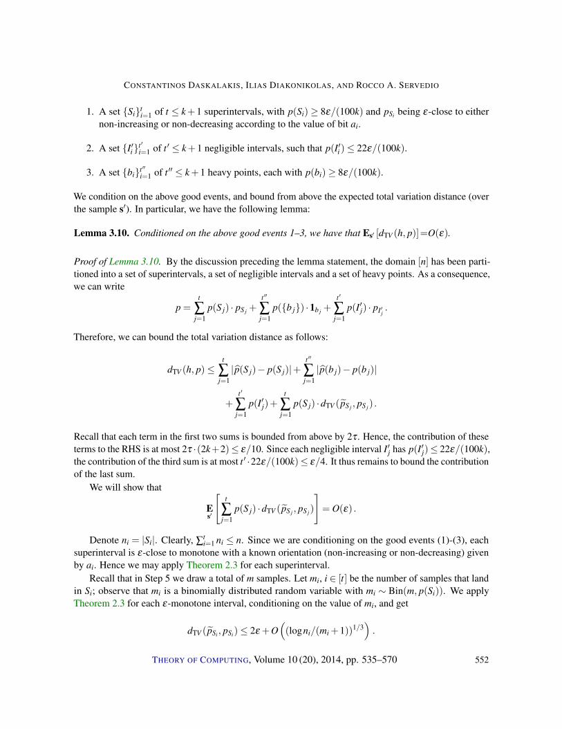
1. A set Siti=1 of t ≤ k+1 superintervals, with p(Si)≥ 8ε/(100k) and pSi being ε-close to either
non-increasing or non-decreasing according to the value of bit ai.
2. A set I′it ′i=1 of t ′ ≤ k+1 negligible intervals, such that p(I′i )≤ 22ε/(100k).
3. A set bit ′′i=1 of t ′′ ≤ k+1 heavy points, each with p(bi)≥ 8ε/(100k).
We condition on the above good events, and bound from above the expected total variation distance (overthe sample s′). In particular, we have the following lemma:
Lemma 3.10. Conditioned on the above good events 1–3, we have that Es′ [dTV (h, p)]=O(ε).
Proof of Lemma 3.10. By the discussion preceding the lemma statement, the domain [n] has been parti-tioned into a set of superintervals, a set of negligible intervals and a set of heavy points. As a consequence,we can write
p =t
∑j=1
p(S j) · pS j +t ′′
∑j=1
p(b j) ·1b j +t ′
∑j=1
p(I′j) · pI′j .
Therefore, we can bound the total variation distance as follows:
dTV (h, p)≤t
∑j=1|p(S j)− p(S j)|+
t ′′
∑j=1|p(b j)− p(b j)|
+t ′
∑j=1
p(I′j)+t
∑j=1
p(S j) ·dTV (pS j , pS j) .
Recall that each term in the first two sums is bounded from above by 2τ . Hence, the contribution of theseterms to the RHS is at most 2τ ·(2k+2)≤ ε/10. Since each negligible interval I′j has p(I′j)≤ 22ε/(100k),the contribution of the third sum is at most t ′ ·22ε/(100k)≤ ε/4. It thus remains to bound the contributionof the last sum.
We will show that
Es′
[t
∑j=1
p(S j) ·dTV (pS j , pS j)
]= O(ε) .
Denote ni = |Si|. Clearly, ∑ti=1 ni ≤ n. Since we are conditioning on the good events (1)-(3), each
superinterval is ε-close to monotone with a known orientation (non-increasing or non-decreasing) givenby ai. Hence we may apply Theorem 2.3 for each superinterval.
Recall that in Step 5 we draw a total of m samples. Let mi, i ∈ [t] be the number of samples that landin Si; observe that mi is a binomially distributed random variable with mi ∼ Bin(m, p(Si)). We applyTheorem 2.3 for each ε-monotone interval, conditioning on the value of mi, and get
dTV (pSi , pSi)≤ 2ε +O((logni/(mi +1))1/3
).
THEORY OF COMPUTING, Volume 10 (20), 2014, pp. 535–570 552
LEARNING k-MODAL DISTRIBUTIONS VIA TESTING
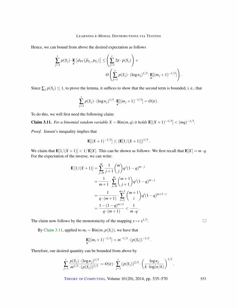
Hence, we can bound from above the desired expectation as follows
t
∑j=1
p(S j) ·Es′
[dTV (pS j , pS j)
]≤
(t
∑j=1
2ε · p(S j)
)+
O
(t
∑j=1
p(S j) · (logn j)1/3 ·E
s′[(m j +1)−1/3]
).
Since ∑ j p(S j)≤ 1, to prove the lemma, it suffices to show that the second term is bounded, i. e., that
t
∑j=1
p(S j) · (logn j)1/3 ·E
s′[(m j +1)−1/3] = O(ε) .
To do this, we will first need the following claim:
Claim 3.11. For a binomial random variable X ∼ Bin(m,q) it holds E[(X +1)−1/3]< (mq)−1/3.
Proof. Jensen’s inequality implies that
E[(X +1)−1/3]≤ (E[1/(X +1)])1/3 .
We claim that E[1/(X +1)]< 1/E[X ]. This can be shown as follows: We first recall that E[X ] = m ·q.For the expectation of the inverse, we can write:
E [1/(X +1)] =m
∑j=0
1j+1
(mj
)q j(1−q)m− j
=1
m+1·
m
∑j=0
(m+1j+1
)q j(1−q)m− j
=1
q · (m+1)·
m+1
∑i=1
(m+1
i
)qi(1−q)m+1−i
=1− (1−q)m+1
q · (m+1)<
1m ·q
.
The claim now follows by the monotonicity of the mapping x 7→ x1/3.
By Claim 3.11, applied to mi ∼ Bin(m, p(Si)), we have that
Es′[(mi +1)−1/3]< m−1/3 · (p(Si))
−1/3 .
Therefore, our desired quantity can be bounded from above by
t
∑j=1
p(S j) · (logn j)1/3
m1/3 · (p(S j))1/3 = O(ε) ·t
∑j=1
(p(S j))2/3 ·
(logn j
k · log(n/k)
)1/3
.
THEORY OF COMPUTING, Volume 10 (20), 2014, pp. 535–570 553
CONSTANTINOS DASKALAKIS, ILIAS DIAKONIKOLAS, AND ROCCO A. SERVEDIO
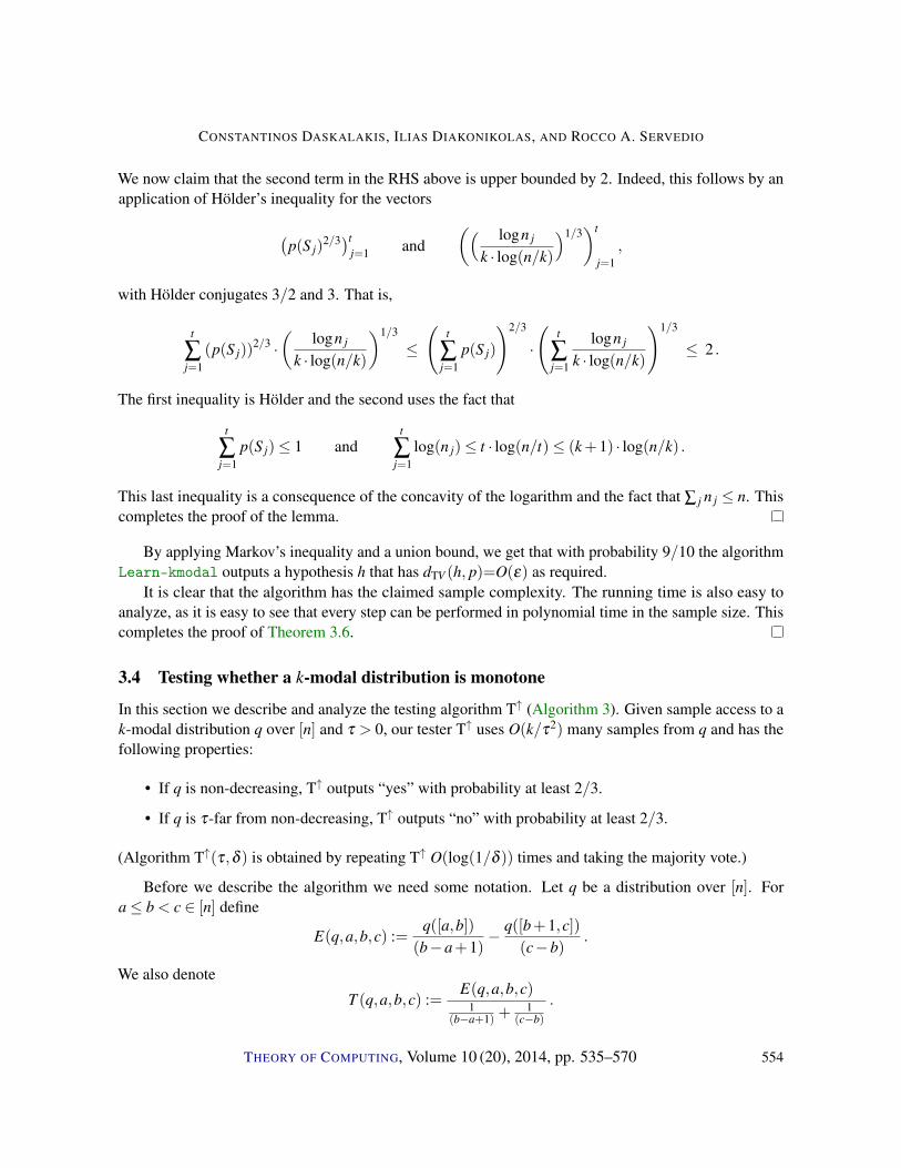
We now claim that the second term in the RHS above is upper bounded by 2. Indeed, this follows by anapplication of Hölder’s inequality for the vectors
(p(S j)
2/3)tj=1 and
(( logn j
k · log(n/k)
)1/3)t
j=1,
with Hölder conjugates 3/2 and 3. That is,
t
∑j=1
(p(S j))2/3 ·
(logn j
k · log(n/k)
)1/3
≤
(t
∑j=1
p(S j)
)2/3
·
(t
∑j=1
logn j
k · log(n/k)
)1/3
≤ 2 .
The first inequality is Hölder and the second uses the fact that
t
∑j=1
p(S j)≤ 1 andt
∑j=1
log(n j)≤ t · log(n/t)≤ (k+1) · log(n/k) .
This last inequality is a consequence of the concavity of the logarithm and the fact that ∑ j n j ≤ n. Thiscompletes the proof of the lemma.
By applying Markov’s inequality and a union bound, we get that with probability 9/10 the algorithmLearn-kmodal outputs a hypothesis h that has dTV (h, p)=O(ε) as required.
It is clear that the algorithm has the claimed sample complexity. The running time is also easy toanalyze, as it is easy to see that every step can be performed in polynomial time in the sample size. Thiscompletes the proof of Theorem 3.6.
3.4 Testing whether a k-modal distribution is monotone
In this section we describe and analyze the testing algorithm T↑ (Algorithm 3). Given sample access to ak-modal distribution q over [n] and τ > 0, our tester T↑ uses O(k/τ2) many samples from q and has thefollowing properties:
• If q is non-decreasing, T↑ outputs “yes” with probability at least 2/3.
• If q is τ-far from non-decreasing, T↑ outputs “no” with probability at least 2/3.
(Algorithm T↑(τ,δ ) is obtained by repeating T↑ O(log(1/δ )) times and taking the majority vote.)
Before we describe the algorithm we need some notation. Let q be a distribution over [n]. Fora≤ b < c ∈ [n] define
E(q,a,b,c) :=q([a,b])
(b−a+1)− q([b+1,c])
(c−b).
We also denote
T (q,a,b,c) :=E(q,a,b,c)
1(b−a+1) +
1(c−b)
.
THEORY OF COMPUTING, Volume 10 (20), 2014, pp. 535–570 554

LEARNING k-MODAL DISTRIBUTIONS VIA TESTING
Intuitively, the quantity E(q,a,b,c) captures the difference between the average value of q over [a,b]versus over [b+1,c]; it is negative iff the average value of q is higher over [b+1,c] than it is over [a,b].The quantity T (q,a,b,c) is a scaled version of E(q,a,b,c).
The idea behind tester T↑ is simple. It is based on the observation that if q is a non-decreasingdistribution, then for any two consecutive intervals [a,b] and [b+ 1,c] the average of q over [b+ 1,c]must be at least as large as the average of q over [a,b]. Thus any non-decreasing distribution will passa test that checks “all” pairs of consecutive intervals looking for a violation. Our tester T↑ checks “all”sums of (at most) k consecutive intervals looking for a violation. Our analysis shows that in fact such atest is complete as well as sound if the distribution q is guaranteed to be k-modal. The key ingredientis a structural result (Lemma 3.13 below), which is proved using a procedure reminiscent of “Myersonironing” [21] to convert a k-modal distribution to a non-decreasing distribution.
Algorithm 3 Tester T↑(τ)
Inputs: τ > 0; sample access to k-modal distribution q over [n]
1. Draw r = Θ(k/τ2) samples s from q and let q be the resulting empirical distribution.
2. If there exists ` ∈ [k] and ai,bi,ci`i=1 ∈ s∪n with ai ≤ bi < ci < ai+1, i ∈ [`−1], such that
`
∑i=1
T (q,ai,bi,ci−1)≥ τ/4 (3.6)
then output “no,” otherwise output “yes.”
The following theorem establishes correctness of the tester.
Theorem 3.12. Algorithm T↑ (Algorithm 3) uses O(k/τ2) samples from q, performs poly(k/τ) · logn bitoperations and satisfies the desired completeness and soundness properties.
Proof. We start by showing that the algorithm has the claimed completeness and soundness properties.Let us say that the sample s is good if for every collection I of (at most) 3k intervals in [n] it holds
∑I∈I|q(I)− q(I)| ≤ τ/20 .
By Fact 3.1 with probability at least 2/3 the sample s is good. We henceforth condition on this event.For a≤ b < c∈ [n] let us denote γ = |q([a,b])− q([a,b])| and γ ′ = |q([b+1,c])− q([b+1,c])|. Then
we can write
|E(q,a,b,c)−E(q,a,b,c)| ≤ γ
b−a+1+
γ ′
c−b≤ (γ + γ
′) ·(
1b−a+1
+1
c−b
)which implies that
|T (q,a,b,c)−T (q,a,b,c)| ≤ γ + γ′ . (3.7)
THEORY OF COMPUTING, Volume 10 (20), 2014, pp. 535–570 555
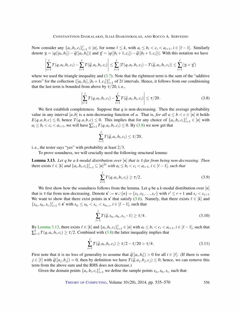
CONSTANTINOS DASKALAKIS, ILIAS DIAKONIKOLAS, AND ROCCO A. SERVEDIO
Now consider any ai,bi,ci`i=1 ∈ [n], for some ` ≤ k, with ai ≤ bi < ci < ai+1, i ∈ [`− 1]. Similarlydenote γi = |q([ai,bi])− q([ai,bi])| and γ ′i = |q([bi +1,ci])− q([bi +1,ci])|. With this notation we have∣∣∣∣∣ `
∑i=1
T (q,ai,bi,ci)−`
∑i=1
T (q,ai,bi,ci)
∣∣∣∣∣≤ `
∑i=1|T (q,ai,bi,ci)−T (q,ai,bi,ci)| ≤
`
∑i=1
(γi + γ′i )
where we used the triangle inequality and (3.7). Note that the rightmost term is the sum of the “additiveerrors” for the collection [ai,bi], [bi +1,ci]`i=1 of 2` intervals. Hence, it follows from our conditioningthat the last term is bounded from above by τ/20, i. e.,∣∣∣∣∣ `
∑i=1
T (q,ai,bi,ci)−`
∑i=1
T (q,ai,bi,ci)
∣∣∣∣∣≤ τ/20 . (3.8)
We first establish completeness. Suppose that q is non-decreasing. Then the average probabilityvalue in any interval [a,b] is a non-decreasing function of a. That is, for all a ≤ b < c ∈ [n] it holdsE(q,a,b,c) ≤ 0, hence T (q,a,b,c) ≤ 0. This implies that for any choice of ai,bi,ci`i=1 ∈ [n] withai ≤ bi < ci < ai+1, we will have ∑
`i=1 T (q,ai,bi,ci)≤ 0. By (3.8) we now get that
`
∑i=1
T (q,ai,bi,ci)≤ τ/20 ,
i. e., the tester says “yes” with probability at least 2/3.To prove soundness, we will crucially need the following structural lemma:
Lemma 3.13. Let q be a k-modal distribution over [n] that is τ-far from being non-decreasing. Thenthere exists ` ∈ [k] and ai,bi,ci`i=1 ⊆ [n]3` with ai ≤ bi < ci < ai+1, i ∈ [`−1], such that
`
∑i=1
T (q,ai,bi,ci)≥ τ/2 . (3.9)
We first show how the soundness follows from the lemma. Let q be a k-modal distribution over [n]that is τ-far from non-decreasing. Denote s′ := s∪n= s1,s2, . . . ,sr′ with r′ ≤ r+1 and s j < s j+1.We want to show that there exist points in s′ that satisfy (3.6). Namely, that there exists ` ∈ [k] andsai ,sbi ,sci`i=1 ∈ s′ with sai ≤ sbi < sci < sai+1 , i ∈ [`−1], such that
`
∑i=1
T (q,sai ,sbi ,sci−1)≥ τ/4 . (3.10)
By Lemma 3.13, there exists ` ∈ [k] and ai,bi,ci`i=1 ∈ [n] with ai ≤ bi < ci < ai+1, i ∈ [`−1], such that∑`i=1 T (q,ai,bi,ci)≥ τ/2. Combined with (3.8) the latter inequality implies that
`
∑i=1
T (q,ai,bi,ci)≥ τ/2− τ/20 > τ/4 . (3.11)
First note that it is no loss of generality to assume that q([ai,bi]) > 0 for all i ∈ [`]. (If there is somej ∈ [`] with q([a j,b j]) = 0, then by definition we have T (q,a j,b j,c j) ≤ 0; hence, we can remove thisterm from the above sum and the RHS does not decrease.)
Given the domain points ai,bi,ci`i=1 we define the sample points sai ,sbi ,sci such that:
THEORY OF COMPUTING, Volume 10 (20), 2014, pp. 535–570 556
LEARNING k-MODAL DISTRIBUTIONS VIA TESTING
(i) [sai ,sbi ]⊆ [ai,bi],
(ii) [sbi +1,sci−1]⊇ [bi +1,ci],
(iii) q([sai ,sbi ]) = q([ai,bi]) and
(iv) q([sbi +1,sci−1]) = q([bi +1,ci]).
To achieve these properties we select:
• sai to be the leftmost point of the sample in [ai,bi]; sbi to be the rightmost point of the sample in[ai,bi] (note that by our assumption that q([ai,bi])> 0 at least one sample falls in [ai,bi]);
• sci to be the leftmost point of the sample in [ci +1,n]; or the point n if [ci +1,n] has no samples oris empty.
We can rewrite (3.11) as follows:
`
∑i=1
q([ai,bi])
1+ bi−ai+1ci−bi
≥ τ/4+`
∑i=1
q([bi +1,ci])
1+ ci−bibi−ai+1
. (3.12)
Now note that by properties (i) and (ii) above it follows that
bi−ai +1≥ sbi− sai +1 and ci−bi ≤ sci− sbi−1 .
Combining with properties (iii) and (iv) we get
q([ai,bi])
1+ bi−ai+1ci−bi
=q([sai ,sbi ])
1+ bi−ai+1ci−bi
≤ q([sai ,sbi ])
1+sbi−sai+1sci−sbi−1
(3.13)
and similarlyq([bi +1,ci])
1+ ci−bibi−ai+1
=q([sbi +1,sci−1])
1+ ci−bibi−ai+1
≥ q([sbi +1,sci−1])
1+sci−sbi−1sbi−sai+1
. (3.14)
A combination of (3.12), (3.13), (3.14) yields the desired result (3.10).
It thus remains to prove Lemma 3.13.
Proof of Lemma 3.13. We will prove the contrapositive. Let q be a k-modal distribution over [n] suchthat for any `≤ k and ai,bi,ci`i=1 ⊆ [n]3` such that ai ≤ bi < ci < ai+1, i ∈ [`−1], we have
`
∑i=1
T (q,ai,bi,ci)≤ τ/2 . (3.15)
We will construct a non-decreasing distribution q that is τ-close to q.The high level idea of the argument is as follows: the construction of q proceeds in (at most) k
stages where in each stage, we reduce the number of modes by at least one and incur small error in
THEORY OF COMPUTING, Volume 10 (20), 2014, pp. 535–570 557
CONSTANTINOS DASKALAKIS, ILIAS DIAKONIKOLAS, AND ROCCO A. SERVEDIO
the total variation distance. In particular, we iteratively construct a sequence of distributions q(i)`i=0,q(0) = q and q(`) = q, for some `≤ k, such that for all i ∈ [`] we have that q(i) is (k− i)-modal anddTV (q(i−1),q(i)) ≤ 2τi, where the quantities τi will be defined in the course of the analysis below. Byappropriately using (3.15), we will show that
`
∑i=1
τi ≤ τ/2 . (3.16)
Assuming this, it follows from the triangle inequality that
dTV (q,q)≤`
∑i=1
dTV (q(i),q(i−1))≤ 2 ·`
∑i=1
τi ≤ τ
as desired, where the last inequality uses (3.16).
Consider the graph (histogram) of the discrete density q. The x-axis represents the n points of thedomain and the y-axis the corresponding probabilities. We first informally describe how to obtain q(1)
from q. The construction of q(i) from q(i−1), i ∈ [`], is essentially identical. Let j1 be the leftmost (i. e.,having minimum x-coordinate) left-extreme point (mode) of q, and assume that it is a local maximum withheight (probability mass) q( j1). (A symmetric argument works for the case that it is a local minimum.)The idea of the proof is based on the following simple process (reminiscent of Myerson’s ironingprocess [21]): We start with the horizontal line y = q( j1) and move it downwards until we reach a heighth1 < q( j1) so that the total mass “cut-off” equals the mass “missing” to the right; then we make thedistribution “flat” in the corresponding interval (hence, reducing the number of modes by at least one).
We now proceed with the formal argument, assuming as above that the leftmost left-extreme pointj1 of q is a local maximum. We say that the line y = h intersects a point i ∈ [n] in the domain of qif q(i) ≥ h. The line y = h, h ∈ [0,q( j1)], intersects the graph of q at a unique interval I(h) ⊆ [n] thatcontains j1. Suppose I(h) = [a(h),b(h)], where a(h),b(h) ∈ [n] depend on h. By definition this meansthat q(a(h))≥ h and q(a(h)−1)< h (since q is supported on [n], we adopt the convention that q(0) = 0).Recall that the distribution q is non-decreasing in the interval [1, j1] and that j1 ≥ a(h). The term “themass cut-off by the line y = h” means the quantity
A(h) = q(I(h))−h · (b(h)−a(h)+1) ,
i. e., the “mass of the interval I(h) above the line.”The height h of the line y = h defines the points a(h),b(h) ∈ [n] as described above. We consider
values of h such that q is unimodal (increasing then decreasing) over I(h). In particular, let j′1 be theleftmost mode of q to the right of j1, i. e., j′1 > j1 and j′1 is a local minimum. We consider values of h ∈(q( j′1),q( j1)). For such values, the interval I(h) is indeed unimodal (as b(h)< j′1). For h ∈ (q( j′1),q( j1))we define the point c(h) ≥ j′1 as follows: It is the rightmost point of the largest interval containing j′1whose probability mass does not exceed h. That is, all points in [ j′1,c(h)] have probability mass at most hand q(c(h)+1)> h (or c(h) = n).
Consider the interval J(h) = [b(h)+ 1,c(h)]. This interval is non-empty, since b(h) < j′1 ≤ c(h).(Note that J(h) is not necessarily a unimodal interval; it contains at least one mode j′1 of q, but it may
THEORY OF COMPUTING, Volume 10 (20), 2014, pp. 535–570 558
LEARNING k-MODAL DISTRIBUTIONS VIA TESTING
also contain more modes.) The term “the mass missing to the right of the line y = h” means the quantity
B(h) = h · (c(h)−b(h))−q(J(h)) .
Consider the function C(h) = A(h)−B(h) over [q( j′1),q( j1)]. This function is continuous in itsdomain; moreover, we have that
C (q( j1)) = A(q( j1))−B(q( j1))< 0 ,
as A(q( j1)) = 0, andC(q( j′1)
)= A
(q( j′1)
)−B
(q( j′1)
)> 0 ,
as B(q( j′1)) = 0. Therefore, by the intermediate value theorem, there exists a value h1 ∈ (q( j′1),q( j1))such that
A(h1) = B(h1) .
The distribution q(1) is constructed as follows: We move the mass τ1 = A(h1) from I(h1) to J(h1).Note that the distribution q(1) is identical to q outside the interval [a(h1),c(h1)], hence the leftmost modeof q(1) is in (c(h1),n]. It is also clear that
dTV (q(1),q)≤ 2τ1 .
Let us denote a1 = a(h1), b1 = b(h1) and c1 = c(h1). We claim that q(1) has at least one mode lessthan q. Indeed, q(1) is non-decreasing in [1,a1−1] and constant in [a1,c1]. (By our “flattening” process,all the points in the latter interval have probability mass exactly h1.) Recalling that
q(1)(a1) = h1 ≥ q(1)(a1−1) = q(a1−1) ,
we deduce that q(1) is non-decreasing in [1,c1].We will now argue that
τ1 = T (q,a1,b1,c1) . (3.17)
Recall that we have A(h1) = B(h1) = τ1, which can be written as
q([a1,b1])−h1 · (b1−a1 +1) = h1 · (c1−b1)−q([b1 +1,c1]) = τ1 .
From this, we get
q([a1,b1])
(b1−a1 +1)− q([b1 +1,c1])
(c1−b1)=
τ1
(b1−a1 +1)+
τ1
(c1−b1)
or equivalently
E (q,a1,b1,c1) =τ1
(b1−a1 +1)+
τ1
(c1−b1)
which gives (3.17).
THEORY OF COMPUTING, Volume 10 (20), 2014, pp. 535–570 559
CONSTANTINOS DASKALAKIS, ILIAS DIAKONIKOLAS, AND ROCCO A. SERVEDIO
We construct q(2) from q(1) using the same procedure. Recalling that the leftmost mode of q(1) lies inthe interval (c1,n] an identical argument as above implies that
dTV (q(2),q(1))≤ 2τ2
whereτ2 = T (q(1),a2,b2,c2)
for some a2,b2,c2 ∈ [n] satisfying c1 < a2 ≤ b2 < c2. Since q(1) is identical to q in (c1,n], it follows that
τ2 = T (q,a2,b2,c2) .
We continue this process iteratively for `≤ k stages until we obtain a non-decreasing distribution q(`).(Note that we remove at least one mode in each iteration, hence it may be the case that ` < k.) Itfollows inductively that for all i ∈ [`], we have that dTV (q(i),q(i−1))≤ 2τi where τi = T (q,ai,bi,ci), forci−1 < ai ≤ bi < ci.
We therefore conclude that`
∑i=1
τi =`
∑i=1
T (q,ai,bi,ci)
which is bounded from above by τ/2 by (3.15). This establishes (3.16) completing the proof ofLemma 3.13.
The upper bound on the sample complexity of the algorithm is straightforward, since only Step 1 usessamples.
It remains to analyze the running time. The only non-trivial computation is in Step 2 where we needto decide whether there exist `≤ k “ordered triples” ai,bi,ci`i=1 ∈ s′ with ai ≤ bi < ci < ai+1, i ∈ [`−1],such that ∑
`i=1 T (q,ai,bi,ci− 1) ≥ τ/4. Even though a naive brute-force implementation would need
time Ω(rk) · logn, there is a simple dynamic programming algorithm that runs in poly(r,k) · logn time.We now provide the details. Consider the objective function
T(`) = max
`
∑i=1
T (q,ai,bi,ci−1)
∣∣∣∣∣ ai,bi,ci`i=1 ∈ s′ with ai ≤ bi < ci < ai+1, i ∈ [`−1]
,
for ` ∈ [k]. We want to decide whether max`≤kT(`) ≥ τ/4. For ` ∈ [k] and j ∈ [r′], we use dynamicprogramming to compute the quantities
T(`, j) = max
`
∑i=1
T (q,ai,bi,ci−1)
∣∣∣∣∣ ai,bi,ci`i=1 ∈ s′ with ai ≤ bi < ci < ai+1,i ∈ [`−1] and c` = s j
.
(This clearly suffices as T(`) = max j∈[r′]T(`, j).) The dynamic program is based on the recursive identity
T(`+1, j) = maxj′∈[r′], j′< j
T(`, j′)+T′( j′+1, j) ,
where we defineT′(α,β ) = maxT (q,a,b,β ) | a,b ∈ s′,α ≤ a≤ b < β .
THEORY OF COMPUTING, Volume 10 (20), 2014, pp. 535–570 560

LEARNING k-MODAL DISTRIBUTIONS VIA TESTING
Note that all the values T′( j′+1, j) (where j′, j ∈ [r′] and j′ < j) can be computed in O(r3) time. Fix` ∈ [k]. Suppose we have computed all the values T(`, j′), j′ ∈ [r′]. Then, for fixed j ∈ [r′], we cancompute the value T(`+1, j) in time O(r) using the above recursion. Hence, the total running time ofthe algorithm is O(kr2 + r3). This completes the run time analysis and the proof of Theorem 3.12.
4 Conclusions and future work
At the level of techniques, this work illustrates the viability of a new general strategy for developingefficient learning algorithms, namely by using “inexpensive” property testers to decompose a complexobject (for us these objects are k-modal distributions) into simpler objects (for us these are monotonedistributions) that can be more easily learned. It would be interesting to apply this paradigm in othercontexts such as learning Boolean functions.
At the level of the specific problem we consider—learning k-modal distributions—our results showthat k-modality is a useful type of structure which can be strongly exploited by sample-efficient andcomputationally efficient learning algorithms. Our results motivate the study of computationally ef-ficient learning algorithms for distributions that satisfy other kinds of “shape restrictions.” Possibledirections here include multivariate k-modal distributions, log-concave distributions, monotone hazardrate distributions and more.
At a technical level, any improvement in the sample complexity of our property testing algorithm ofSection 3.4 would directly improve the “extraneous” additive O(k2/ε3) term in the sample complexity ofour algorithm. We suspect that it may be possible to improve our testing algorithm (although we note thatit is easy to give an Ω(
√k/ε2) lower bound using standard constructions).
Our learning algorithm is not proper, i. e., it outputs a hypothesis that is not necessarily k-modal.Obtaining an efficient proper learning algorithm is an interesting question. Finally, it should be noted thatour approach for learning k-modal distributions requires a priori knowledge of the parameter k. We leavethe case of unknown k as an intriguing open problem.
Acknowledgement
We thank the anonymous reviewers for their helpful comments.
A Birgé’s algorithm as a semi-agnostic learner
In this section we briefly explain why Birgé’s algorithm [4] also works in the semi-agnostic setting, thusjustifying the claims about its performance made in the statement of Theorem 2.3. To do this, we need toexplain his approach. For this, we will need the following fact (which follows as a special case of theVC inequality, Theorem 2.1), which gives a tight bound on the number of samples required to learn anarbitrary distribution with respect to total variation distance.
Fact A.1. Let p be any distribution over [n]. We have: E[dTV (p, pm)] = O(√
n/m).
THEORY OF COMPUTING, Volume 10 (20), 2014, pp. 535–570 561
CONSTANTINOS DASKALAKIS, ILIAS DIAKONIKOLAS, AND ROCCO A. SERVEDIO
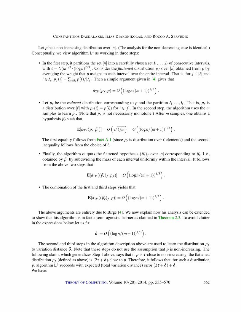
Let p be a non-increasing distribution over [n]. (The analysis for the non-decreasing case is identical.)Conceptually, we view algorithm L↓ as working in three steps:
• In the first step, it partitions the set [n] into a carefully chosen set I1, . . . , I` of consecutive intervals,with `= O(m1/3 · (logn)2/3). Consider the flattened distribution p f over [n] obtained from p byaveraging the weight that p assigns to each interval over the entire interval. That is, for j ∈ [`] andi ∈ I j, p f (i) = ∑t∈I j p(t)/|I j|. Then a simple argument given in [4] gives that
dTV (p f , p) = O((logn/(m+1))1/3
).
• Let pr be the reduced distribution corresponding to p and the partition I1, . . . , I`. That is, pr isa distribution over [`] with pr(i) = p(Ii) for i ∈ [`]. In the second step, the algorithm uses the msamples to learn pr. (Note that pr is not necessarily monotone.) After m samples, one obtains ahypothesis pr such that
E[dTV (pr, pr)] = O(√
`/m)= O
((logn/(m+1))1/3
).
The first equality follows from Fact A.1 (since pr is distribution over ` elements) and the secondinequality follows from the choice of `.
• Finally, the algorithm outputs the flattened hypothesis (pr) f over [n] corresponding to pr, i. e.,obtained by pr by subdividing the mass of each interval uniformly within the interval. It followsfrom the above two steps that
E[dTV ((pr) f , p f )] = O((logn/(m+1))1/3
).
• The combination of the first and third steps yields that
E[dTV ((pr) f , p)] = O((logn/(m+1))1/3
).
The above arguments are entirely due to Birgé [4]. We now explain how his analysis can be extendedto show that his algorithm is in fact a semi-agnostic learner as claimed in Theorem 2.3. To avoid clutterin the expressions below let us fix
δ := O((logn/(m+1))1/3
).
The second and third steps in the algorithm description above are used to learn the distribution p f
to variation distance δ . Note that these steps do not use the assumption that p is non-increasing. Thefollowing claim, which generalizes Step 1 above, says that if p is τ-close to non-increasing, the flatteneddistribution p f (defined as above) is (2τ +δ )-close to p. Therefore, it follows that, for such a distributionp, algorithm L↓ succeeds with expected (total variation distance) error (2τ +δ )+δ .We have:
THEORY OF COMPUTING, Volume 10 (20), 2014, pp. 535–570 562
LEARNING k-MODAL DISTRIBUTIONS VIA TESTING
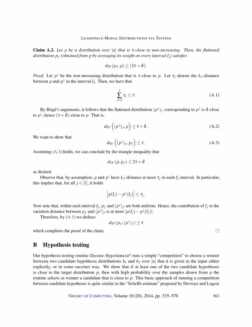
Claim A.2. Let p be a distribution over [n] that is τ-close to non-increasing. Then, the flatteneddistribution p f (obtained from p by averaging its weight on every interval I j) satisfies
dTV (p f , p)≤ (2τ +δ ) .
Proof. Let p↓ be the non-increasing distribution that is τ-close to p. Let τ j denote the L1-distancebetween p and p↓ in the interval I j. Then, we have that
`
∑j=1
τ j ≤ τ . (A.1)
By Birgé’s arguments, it follows that the flattened distribution (p↓) f corresponding to p↓ is δ -closeto p↓, hence (τ +δ )-close to p. That is,
dTV
((p↓) f , p
)≤ τ +δ . (A.2)
We want to show thatdTV
((p↓) f , p f
)≤ τ . (A.3)
Assuming (A.3) holds, we can conclude by the triangle inequality that
dTV (p, p f )≤ 2τ +δ
as desired.Observe that, by assumption, p and p↓ have L1-distance at most τ j in each I j interval. In particular,
this implies that, for all j ∈ [`], it holds ∣∣∣p(I j)− p↓(I j)∣∣∣≤ τ j .
Now note that, within each interval I j, p f and (p↓) f are both uniform. Hence, the contribution of I j to thevariation distance between p f and (p↓) f is at most |p(I j)− p↓(I j)|.
Therefore, by (A.1) we deducedTV (p f ,(p↓) f )≤ τ
which completes the proof of the claim.
B Hypothesis testing
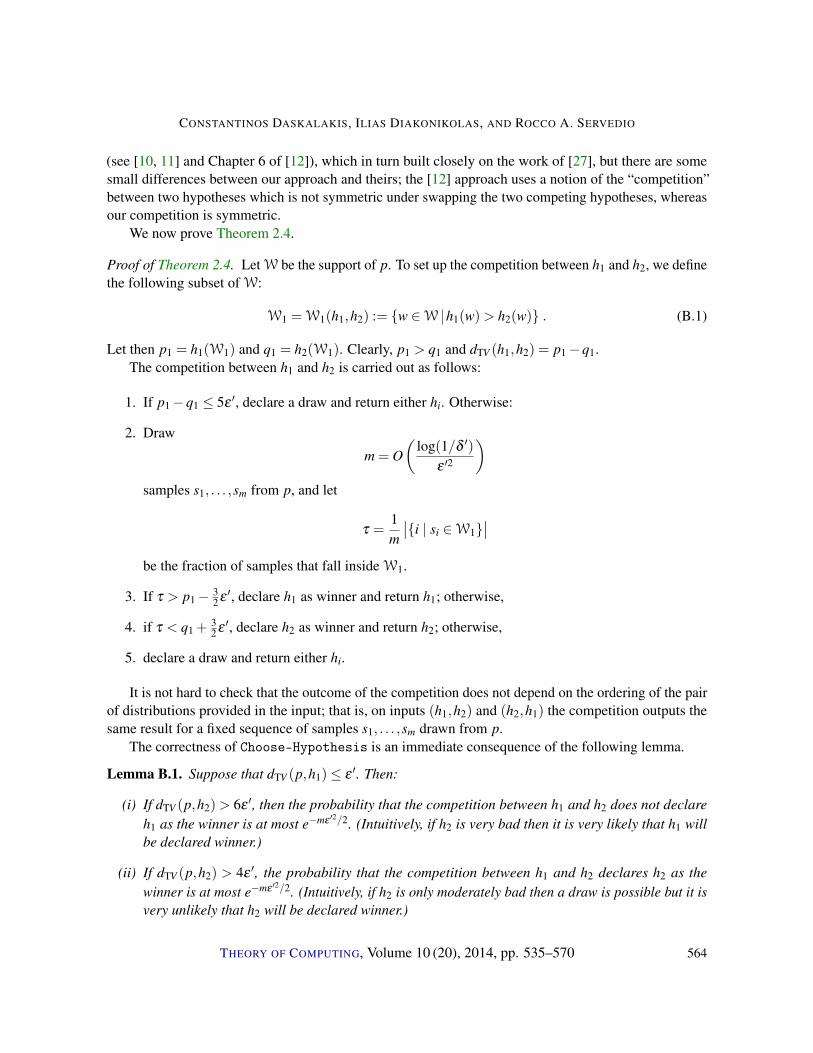
Our hypothesis testing routine Choose-Hypothesisp runs a simple “competition” to choose a winnerbetween two candidate hypothesis distributions h1 and h2 over [n] that it is given in the input eitherexplicitly, or in some succinct way. We show that if at least one of the two candidate hypothesesis close to the target distribution p, then with high probability over the samples drawn from p theroutine selects as winner a candidate that is close to p. This basic approach of running a competitionbetween candidate hypotheses is quite similar to the “Scheffé estimate” proposed by Devroye and Lugosi
THEORY OF COMPUTING, Volume 10 (20), 2014, pp. 535–570 563
CONSTANTINOS DASKALAKIS, ILIAS DIAKONIKOLAS, AND ROCCO A. SERVEDIO
(see [10, 11] and Chapter 6 of [12]), which in turn built closely on the work of [27], but there are somesmall differences between our approach and theirs; the [12] approach uses a notion of the “competition”between two hypotheses which is not symmetric under swapping the two competing hypotheses, whereasour competition is symmetric.
We now prove Theorem 2.4.
Proof of Theorem 2.4. Let W be the support of p. To set up the competition between h1 and h2, we definethe following subset of W:
W1 =W1(h1,h2) := w ∈W h1(w)> h2(w) . (B.1)
Let then p1 = h1(W1) and q1 = h2(W1). Clearly, p1 > q1 and dTV (h1,h2) = p1−q1.The competition between h1 and h2 is carried out as follows:
1. If p1−q1 ≤ 5ε ′, declare a draw and return either hi. Otherwise:
2. Draw
m = O(
log(1/δ ′)
ε ′2
)samples s1, . . . ,sm from p, and let
τ =1m
∣∣i | si ∈W1∣∣
be the fraction of samples that fall inside W1.
3. If τ > p1− 32 ε ′, declare h1 as winner and return h1; otherwise,
4. if τ < q1 +32 ε ′, declare h2 as winner and return h2; otherwise,
5. declare a draw and return either hi.
It is not hard to check that the outcome of the competition does not depend on the ordering of the pairof distributions provided in the input; that is, on inputs (h1,h2) and (h2,h1) the competition outputs thesame result for a fixed sequence of samples s1, . . . ,sm drawn from p.
The correctness of Choose-Hypothesis is an immediate consequence of the following lemma.
Lemma B.1. Suppose that dTV (p,h1)≤ ε ′. Then:
(i) If dTV (p,h2)> 6ε ′, then the probability that the competition between h1 and h2 does not declareh1 as the winner is at most e−mε ′2/2. (Intuitively, if h2 is very bad then it is very likely that h1 willbe declared winner.)
(ii) If dTV (p,h2) > 4ε ′, the probability that the competition between h1 and h2 declares h2 as thewinner is at most e−mε ′2/2. (Intuitively, if h2 is only moderately bad then a draw is possible but it isvery unlikely that h2 will be declared winner.)
THEORY OF COMPUTING, Volume 10 (20), 2014, pp. 535–570 564
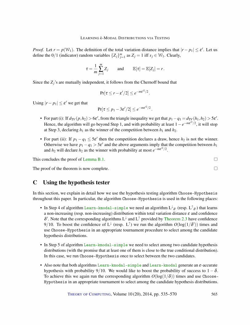
LEARNING k-MODAL DISTRIBUTIONS VIA TESTING
Proof. Let r = p(W1). The definition of the total variation distance implies that |r− p1| ≤ ε ′. Let usdefine the 0/1 (indicator) random variables Z jm
j=1 as Z j = 1 iff s j ∈W1. Clearly,
τ =1m
m
∑j=1
Z j and E[τ] = E[Z j] = r .
Since the Z j’s are mutually independent, it follows from the Chernoff bound that
Pr[τ ≤ r− ε′/2]≤ e−mε ′2/2 .
Using |r− p1| ≤ ε ′ we get thatPr[τ ≤ p1−3ε
′/2]≤ e−mε ′2/2 .
• For part (i): If dTV (p,h2)> 6ε ′, from the triangle inequality we get that p1−q1 = dTV (h1,h2)> 5ε ′.Hence, the algorithm will go beyond Step 1, and with probability at least 1− e−mε ′2/2, it will stopat Step 3, declaring h1 as the winner of the competition between h1 and h2.
• For part (ii): If p1− q1 ≤ 5ε ′ then the competition declares a draw, hence h2 is not the winner.Otherwise we have p1−q1 > 5ε ′ and the above arguments imply that the competition between h1and h2 will declare h2 as the winner with probability at most e−mε ′2/2.
This concludes the proof of Lemma B.1.
The proof of the theorem is now complete.
C Using the hypothesis tester
In this section, we explain in detail how we use the hypothesis testing algorithm Choose-Hypothesisthroughout this paper. In particular, the algorithm Choose-Hypothesis is used in the following places:
• In Step 4 of algorithm Learn-kmodal-simple we need an algorithm L↓δ ′ (resp. L↑δ ′) that learnsa non-increasing (resp. non-increasing) distribution within total variation distance ε and confidenceδ ′. Note that the corresponding algorithms L↓ and L↑ provided by Theorem 2.3 have confidence9/10. To boost the confidence of L↓ (resp. L↑) we run the algorithm O(log(1/δ ′)) times anduse Choose-Hypothesis in an appropriate tournament procedure to select among the candidatehypothesis distributions.
• In Step 5 of algorithm Learn-kmodal-simple we need to select among two candidate hypothesisdistributions (with the promise that at least one of them is close to the true conditional distribution).In this case, we run Choose-Hypothesis once to select between the two candidates.
• Also note that both algorithms Learn-kmodal-simple and Learn-kmodal generate an ε-accuratehypothesis with probability 9/10. We would like to boost the probability of success to 1− δ .To achieve this we again run the corresponding algorithm O(log(1/δ )) times and use Choose-Hypothesis in an appropriate tournament to select among the candidate hypothesis distributions.
THEORY OF COMPUTING, Volume 10 (20), 2014, pp. 535–570 565
CONSTANTINOS DASKALAKIS, ILIAS DIAKONIKOLAS, AND ROCCO A. SERVEDIO
We now formally describe the “tournament” algorithm to boost the confidence to 1−δ .
Lemma C.1. Let p be any distribution over a finite set W. Suppose that Dε is a collection of Ndistributions over W such that there exists q ∈Dε with dTV (p,q)≤ ε . Then there is an algorithm thatuses O(ε−2 logN log(1/δ )) samples from p and with probability 1− δ outputs a distribution p′ ∈Dε
that satisfies dTV (p, p′)≤ 6ε .
Devroye and Lugosi (Chapter 7 of [12]) prove a similar result by having all pairs of distributionsin the cover compete against each other using their notion of a competition, but again there are somesmall differences: their approach chooses a distribution in the cover which wins the maximum number ofcompetitions, whereas our algorithm chooses a distribution that is never defeated (i. e., won or achieved adraw against all other distributions in the cover). Instead we follow the approach from [9].
Proof. The algorithm performs a tournament by running the competition Choose-Hypothesisp(hi,h j,ε,δ/(2N)) for every pair of distinct distributions hi,h j in the collection Dε . It outputs a distribution q? ∈Dε
that was never a loser (i. e., won or achieved a draw in all its competitions). If no such distribution existsin Dε then the algorithm outputs “failure.”
By definition, there exists some q ∈ Dε such that dTV (p,q) ≤ ε . We first argue that with highprobability this distribution q never loses a competition against any other q′ ∈Dε (so the algorithm doesnot output “failure”). Consider any q′ ∈Dε . If dTV (p,q′)> 4ε , by Lemma B.1(ii) the probability that qloses to q′ is at most 2e−mε2/2 = O(1/N). On the other hand, if dTV (p,q′)≤ 4δ , the triangle inequalitygives that dTV (q,q′) ≤ 5ε and thus q draws against q′. A union bound over all N distributions in Dε
shows that with probability 1−δ/2, the distribution q never loses a competition.We next argue that with probability at least 1−δ/2, every distribution q′ ∈Dε that never loses has
small variation distance from p. Fix a distribution q′ such that dTV (q′, p)> 6ε; Lemma B.1(i) impliesthat q′ loses to q with probability 1−2e−mε2/2 ≥ 1−δ/(2N). A union bound gives that with probability1−δ/2, every distribution q′ that has dTV (q′, p)> 6ε loses some competition.
Thus, with overall probability at least 1−δ , the tournament does not output “failure” and outputssome distribution q? such that dTV (p,q?) is at most 6ε . This proves the lemma.
We now explain how the above lemma is used in our context: Suppose we perform O(log(1/δ ))runs of a learning algorithm that constructs an ε-accurate hypothesis with probability at least 9/10.Then, with failure probability at most δ/2, at least one of the hypotheses generated is ε-close tothe true distribution in variation distance. Conditioning on this good event, we have a collection ofdistributions with cardinality O(log(1/δ )) that satisfies the assumption of the lemma. Hence, usingO((1/ε2) · log log(1/δ ) · log(1/δ )
)samples we can learn to accuracy 6ε and confidence 1−δ/2. The
overall sample complexity is O(log(1/δ )) times the sample complexity of the learning algorithm runwith confidence 9/10, plus this additional O
((1/ε2) · log log(1/δ ) · log(1/δ )
)term.
In terms of running time,we make the following easily verifiable remarks: When the hypothesistesting algorithm Choose-Hypothesis is run on a pair of distributions that are produced by Birgé’salgorithm, its running time is polynomial in the succinct description of these distributions, i. e., inlog2(n)/ε . Similarly, when Choose-Hypothesis is run on a pair of outputs of Learn-kmodal-simpleor Learn-kmodal, its running time is polynomial in the succinct description of these distributions. More
THEORY OF COMPUTING, Volume 10 (20), 2014, pp. 535–570 566
LEARNING k-MODAL DISTRIBUTIONS VIA TESTING
specifically, in the former case, the succinct description has bit complexity O(k · log2(n)/ε2
)(since
the output consists of O(k/ε) monotone intervals, and the conditional distribution on each interval isthe output of Birgé’s algorithm for that interval). In the latter case, the succinct description has bitcomplexity O
(k · log2(n)/ε
), since the algorithm Learn-kmodal constructs only k monotone intervals.
Hence, in both cases, each execution of the testing algorithm performs poly(k, logn,1/ε) bit operations.Since the tournament invokes the algorithm Choose-Hypothesis O(log2(1/δ )) times (for every pair ofdistributions in our pool of O(log(1/δ )) candidates) the upper bound on the running time follows.
References
[1] GUILLERMO ALVAREZ DE TOLEDO AND JULIO M. FERNANDEZ: Patch-clamp measurementsreveal multimodal distribution of granule sizes in rat mast cells. J. Cell Biology, 110(4):1033–1039,1990. [doi:10.1083/jcb.110.4.1033] 536
[2] TUGKAN BATU, RAVI KUMAR, AND RONITT RUBINFELD: Sublinear algorithms for testingmonotone and unimodal distributions. In Proc. 36th STOC, pp. 381–390. ACM Press, 2004.[doi:10.1145/1007352.1007414] 548
[3] LUCIEN BIRGÉ: Estimating a density under order restrictions: Nonasymptotic minimax risk. Annalsof Statistics, 15(3):995–1012, 1987. Available at JSTOR. 536, 537
[4] LUCIEN BIRGÉ: On the risk of histograms for estimating decreasing densities. Annals of Statistics,15(3):1013–1022, 1987. Available at JSTOR. 536, 537, 540, 541, 561, 562
[5] LUCIEN BIRGÉ: Estimation of unimodal densities without smoothness assumptions. Annals ofStatistics, 25(3):970–981, 1997. Available at JSTOR. 536
[6] KUNG-SIK CHAN AND HOWELL TONG: Testing for multimodality with dependent data.Biometrika, 91(1):113–123, 2004. [doi:10.1093/biomet/91.1.113] 536
[7] LOREN COBB, PETER KOPPSTEIN, AND NENG HSIN CHEN: Estimation and moment recursionrelations for multimodal distributions of the exponential family. J. American Statistical Association,78(381):124–130, 1983. [doi:10.1080/01621459.1983.10477940] 536
[8] CONSTANTINOS DASKALAKIS, ILIAS DIAKONIKOLAS, AND ROCCO A. SERVEDIO: Learningk-modal distributions via testing. In Proc. 23rd Ann. ACM-SIAM Symp. on Discrete Algorithms(SODA’12), pp. 1371–1385. ACM Press, 2012. Available at ACM DL. 535
[9] CONSTANTINOS DASKALAKIS, ILIAS DIAKONIKOLAS, AND ROCCO A. SERVEDIO: Learn-ing Poisson binomial distributions. In Proc. 44th STOC, pp. 709–728. ACM Press, 2012.[doi:10.1145/2213977.2214042, arXiv:1107.2702] 541, 566
[10] LUC DEVROYE AND GÁBOR LUGOSI: A universally acceptable smoothing factor for kernel densityestimates. Annals of Statistics, 24(6):2499–2512, 1996. Available at JSTOR. 564
THEORY OF COMPUTING, Volume 10 (20), 2014, pp. 535–570 567
CONSTANTINOS DASKALAKIS, ILIAS DIAKONIKOLAS, AND ROCCO A. SERVEDIO
[11] LUC DEVROYE AND GÁBOR LUGOSI: Nonasymptotic universal smoothing factors, kernel com-plexity and Yatracos classes. Annals of Statistics, 25(6):2626–2637, 1997. Available at JSTOR.564
[12] LUC DEVROYE AND GÁBOR LUGOSI: Combinatorial Methods in Density Estimation. Springer,2001. 540, 541, 564, 566
[13] FRANCESCO R. FERRARO, BARBARA PALTRINIERI, FLAVIO FUSI PECCI, ROBERT T. ROOD,AND BEN DORMAN: Multimodal distributions along the horizontal branch. The AstrophysicalJournal, 500(1):311–319, 1998. [doi:10.1086/305712] 536
[14] ODED GOLDREICH, editor. Property Testing: Current Research and Surveys. Springer, 2010.LNCS 6390. 538
[15] ODED GOLDREICH: Highlights of the Bertinoro workshop on Sublinear Algorithms (unpublishedcomments). Available at author’s website, 2011. 538
[16] ODED GOLDREICH, SHAFI GOLDWASSER, AND DANA RON: Property testing and its connectionto learning and approximation. J. ACM, 45(4):653–750, 1998. Preliminary version at FOCS’96.[doi:10.1145/285055.285060] 538
[17] PIET GROENEBOOM: Estimating a monotone density. In Proc. of the Berkeley Conference in Honorof Jerzy Neyman and Jack Kiefer, pp. 539–555, 1985. Available at CWI. 536
[18] MICHAEL J. KEARNS AND DANA RON: Testing problems with sublearning sample com-plexity. J. Comput. System Sci., 61(3):428–456, 2000. Preliminary version in COLT’98.[doi:10.1006/jcss.1999.1656] 538
[19] JOHANNES H. B. KEMPERMAN: Mixtures with a limited number of modal intervals. Annals ofStatistics, 19(4):2120–2144, 1991. Available at JSTOR. 536
[20] EDMOND A. MURPHY: One cause? many causes?: The argument from the bimodal distribution. J.Chronic Diseases, 17(4):301–324, 1964. [doi:10.1016/0021-9681(64)90073-6] 536
[21] ROGER B. MYERSON: Optimal auction design. Mathematics of Operations Research, 6(1):58–73,1981. [doi:10.1287/moor.6.1.58] 555, 558
[22] DONALD J. NEWMAN AND LAWRENCE SHEPP: The double dixie cup problem. AmericanMathematical Monthly, 67(1):58–61, 1960. [doi:10.2307/2308930] 546, 551
[23] B. L. S. PRAKASA RAO: Estimation of a unimodal density. Sankhya Ser. A, 31(1):23–36, 1969.Available at JSTOR. 536
[24] DANA RON: Property Testing: A Learning Theory Perspective. Foundations and Trends in MachineLearning, 1(3):307–402, 2008. [doi:10.1561/2200000004] 538
[25] DANA RON: Algorithmic and analysis techniques in property testing. Foundations and Trends inTheoretical Computer Science, 5:73–205, 2010. [doi:10.1561/0400000029] 538
THEORY OF COMPUTING, Volume 10 (20), 2014, pp. 535–570 568
LEARNING k-MODAL DISTRIBUTIONS VIA TESTING
[26] EDWARD J. WEGMAN: Maximum likelihood estimation of a unimodal density. I. and II. Ann. Math.Statist., 41:457–471, 2169–2174, 1970. Available at JSTOR. 536
[27] YANNIS G. YATRACOS: Rates of convergence of minimum distance estimators and Kolmogorov’sentropy. Annals of Statistics, 13(2):768–774, 1985. Available at JSTOR. 564
AUTHORS
Constantinos DaskalakisAssociate professorDepartment of Electrical Engineering and Computer ScienceMassachussetts Institute of Technologycostis csail mit eduhttp://people.csail.mit.edu/costis/
Ilias DiakonikolasAssistant professorSchool of InformaticsUniversity of Edinburghilias.d ed ac ukhttp://www.iliasdiakonikolas.org
Rocco A. ServedioAssociate professorDepartment of Computer Science Columbia Universityrocco cs columbia eduhttp://www.cs.columbia.edu/~rocco
ABOUT THE AUTHORS
CONSTANTINOS DASKALAKIS (addressed as “Costis” by friends and colleagues) is anassociate professor in the Department of Electrical Engineering and Computer Scienceat MIT. He holds a diploma in Electrical and Computer Engineering from the NationalTechnical University of Athens, and a Ph. D. in Electrical Engineering and ComputerSciences from UC Berkeley, where his Ph. D. was supervised by Christos Papadimitriou.His research interests lie in the interface of computation with economics and probability,in particular the complexity of equilibria and fixed points, mechanism design, andmachine learning.
THEORY OF COMPUTING, Volume 10 (20), 2014, pp. 535–570 569
CONSTANTINOS DASKALAKIS, ILIAS DIAKONIKOLAS, AND ROCCO A. SERVEDIO
ILIAS DIAKONIKOLAS is an assistant professor in the School of Informatics at the Universityof Edinburgh. He obtained a diploma in Electrical and Computer Engineering fromthe National Technical University of Athens, and a Ph. D. in Computer Science fromColumbia University advised by Mihalis Yannakakis. His research interests lie inalgorithms, learning, statistics, and game theory. The current focus of his work is onalgorithms for machine learning.
ROCCO SERVEDIO is an associate professor in the Department of Computer Science atColumbia University. He graduated from Harvard University, where his Ph. D. was su-pervised by Les Valiant. He is interested in computational learning theory, computationalcomplexity, and property testing, with the study of Boolean functions as an underlyingtheme tying these topics together. He enjoys spending time with his family and hopes toshare a bottle of Cutty Sark with H. M. in the afterlife.
THEORY OF COMPUTING, Volume 10 (20), 2014, pp. 535–570 570