1

Volume IX | Issue 6 | 2014 

  

 

 

 

 

 

 

 

 

 

 

 

 

 

 

 

 

 

 

 

 

 

 

 

 

 

 

 

 

 

 

 

 

 

 

 

 

 

 

 

 

 

 

 

 

 

 

 

 

 

 

 

  

Stylianos G. Gogos Economic Analyst sgogos@eurobank.gr   Olga Kosma Economic Analyst okosma@eurobank.gr  

DISCLAIMER This  report has been  issued by Eurobank Ergasias  S.A.  (“Eurobank”)  and may  not be reproduced in any manner or provided to  any  other  person.  Each  person  that receives  a  copy  by  acceptance  thereof represents  and  agrees  that  it  will  not distribute  or  provide  it  to  any  other person. This  report  is not an offer to buy or sell or a solicitation of an offer to buy or sell  the  securities  mentioned  herein. Eurobank  and  others  associated  with  it may  have  positions  in,  and  may  effect transactions  in  securities  of  companies mentioned  herein  and may  also  perform or  seek  to  perform  investment  banking services  for  those  companies.  The investments discussed  in  this  report may be unsuitable for  investors, depending on the  specific  investment  objectives  and financial  position.  The  information contained  herein  is  for  informative purposes  only  and  has  been  obtained from sources believed to be reliable but it has  not  been  verified  by  Eurobank.  The opinions  expressed  herein  may  not necessarily  coincide  with  those  of  any member of Eurobank. No  representation or warranty  (express or  implied)  is made as  to  the  accuracy,  completeness, correctness,  timeliness  or  fairness  of  the information  or  opinions  herein,  all  of which  are  subject  to  change  without notice.  No  responsibility  or  liability whatsoever  or  howsoever  arising  is accepted  in  relation  to  the  contents hereof by Eurobank or any of its directors, officers or employees.  Any  articles,  studies,  comments  etc. reflect  solely  the  views  of  their  author. Any unsigned notes are deemed  to have been produced by the editorial team. Any articles,  studies,  comments  etc.  that  are signed by members of  the editorial  team express  the  personal  views  of  their author. 

Unemployment Rate in Greece: 

“The” Long Run Macroeconomic Challenge 

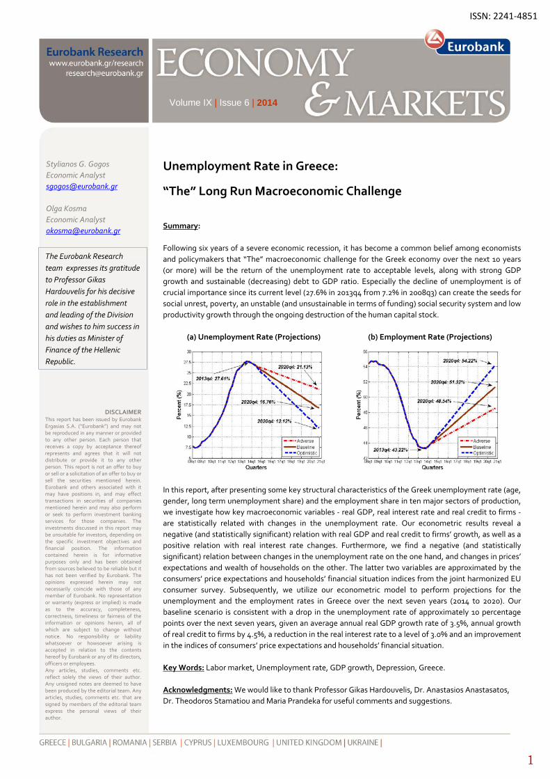
Summary:  Following six years of a severe economic recession, it has become a common belief among economists and policymakers that “The” macroeconomic challenge  for the Greek economy over the next 10 years (or more) will  be  the  return  of  the  unemployment  rate  to  acceptable  levels,  along with  strong GDP growth and  sustainable  (decreasing) debt  to GDP  ratio. Especially  the decline of unemployment  is of crucial importance since its current level (27.6% in 2013q4 from 7.2% in 2008q3) can create the seeds for social unrest, poverty, an unstable (and unsustainable in terms of funding) social security system and low productivity growth through the ongoing destruction of the human capital stock.  

(a) Unemployment Rate (Projections)  (b) Employment Rate (Projections) 

    In this report, after presenting some key structural characteristics of the Greek unemployment rate (age, gender, long term unemployment share) and the employment share in ten major sectors of production, we investigate how key macroeconomic variables ‐ real GDP, real interest rate and real credit to firms ‐ are  statistically  related  with  changes  in  the  unemployment  rate.  Our  econometric  results  reveal  a negative (and statistically significant) relation with real GDP and real credit to firms’ growth, as well as a positive  relation  with  real  interest  rate  changes.  Furthermore,  we  find  a  negative  (and  statistically significant) relation between changes in the unemployment rate on the one hand, and changes in prices’ expectations and wealth of households on the other. The  latter two variables are approximated by the consumers’ price expectations and households’ financial situation indices from the joint harmonized EU consumer  survey.  Subsequently,  we  utilize  our  econometric  model  to  perform  projections  for  the unemployment  and  the  employment  rates  in Greece  over  the  next  seven  years  (2014  to  2020). Our baseline scenario  is consistent with a drop  in  the unemployment  rate of approximately 10 percentage points over the next seven years, given an average annual real GDP growth rate of 3.5%, annual growth of real credit to firms by 4.5%, a reduction in the real interest rate to a level of 3.0% and an improvement in the indices of consumers’ price expectations and households’ financial situation.  Key Words: Labor market, Unemployment rate, GDP growth, Depression, Greece.  Acknowledgments: We would like to thank Professor Gikas Hardouvelis, Dr. Anastasios Anastasatos, Dr. Theodoros Stamatiou and Maria Prandeka for useful comments and suggestions.  

ISSN: 2241‐4851 

The Eurobank Research team  expresses its gratitude to Professor Gikas Hardouvelis for his decisive role in the establishment and leading of the Division and wishes to him success in his duties as Minister of Finance of the Hellenic Republic.  

 

 

June 2014 

2

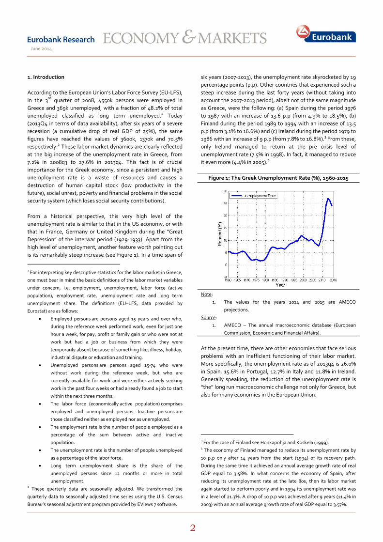
1. Introduction  According to the European Union’s Labor Force Survey (EU‐LFS), in  the  3rd  quarter  of  2008,  4550k  persons  were  employed  in Greece and 369k unemployed, with a  fraction of 48.2% of  total unemployed  classified  as  long  term  unemployed.1  Today (2013Q4  in terms of data availability), after six years of a severe recession  (a  cumulative  drop  of  real  GDP  of  25%),  the  same figures  have  reached  the  values  of  3600k,  1370k  and  70.5% respectively.2 These  labor market dynamics are clearly reflected at  the big  increase  of  the  unemployment  rate  in Greece,  from 7.2%  in  2008q3  to  27.6%  in  2013q4.  This  fact  is  of  crucial importance  for  the Greek economy, since a persistent and high unemployment  rate  is  a  waste  of  resources  and  causes  a destruction  of  human  capital  stock  (low  productivity  in  the future), social unrest, poverty and financial problems in the social security system (which loses social security contributions).  From  a  historical  perspective,  this  very  high  level  of  the unemployment rate is similar to that in the US economy, or with that  in  France, Germany or United Kingdom during  the  “Great Depression” of  the  interwar period  (1929‐1933). Apart  from  the high level of unemployment, another feature worth pointing out is  its remarkably steep  increase (see Figure 1).  In a time span of 

                                                            1 For interpreting key descriptive statistics for the labor market in Greece, 

one must bear in mind the basic definitions of the labor market variables 

under  concern,  i.e.  employment,  unemployment,  labor  force  (active 

population),  employment  rate,  unemployment  rate  and  long  term 

unemployment  share.  The  definitions  (EU–LFS,  data  provided  by 

Eurostat) are as follows: 

• Employed persons are persons  aged  15  years  and over who, 

during the reference week performed work, even for just one 

hour a week, for pay, profit or family gain or who were not at 

work  but  had  a  job  or  business  from  which  they  were 

temporarily absent because of something like, illness, holiday, 

industrial dispute or education and training. 

• Unemployed  persons are  persons  aged  15‐74  who  were 

without  work  during  the  reference  week,  but  who  are 

currently available  for work and were either actively  seeking 

work in the past four weeks or had already found a job to start 

within the next three months.  

• The  labor  force  (economically active  population) comprises 

employed  and  unemployed  persons.  Inactive  persons are 

those classified neither as employed nor as unemployed. 

• The employment rate is the number of people employed as a 

percentage  of  the  sum  between  active  and  inactive 

population. 

• The unemployment rate is the number of people unemployed 

as a percentage of the labor force. 

• Long  term  unemployment  share  is  the  share  of  the 

unemployed  persons  since  12  months  or  more  in  total 

unemployment. 2  These  quarterly  data  are  seasonally  adjusted.  We  transformed  the 

quarterly data  to  seasonally adjusted  time  series using  the U.S. Census 

Bureau’s seasonal adjustment program provided by EViews 7 software. 

six years (2007‐2013), the unemployment rate skyrocketed by 19 percentage points (p.p). Other countries that experienced such a steep  increase  during  the  last  forty  years  (without  taking  into account the 2007‐2013 period), albeit not of the same magnitude as Greece, were  the  following:  (a) Spain during  the period 1976 to  1987 with  an  increase  of  13.6  p.p  (from  4.9%  to  18.5%),  (b) Finland during  the period 1989 to 1994 with an  increase of 13.5 p.p (from 3.1% to 16.6%) and (c) Ireland during the period 1979 to 1986 with an increase of 9 p.p (from 7.8% to 16.8%).3 From these, only  Ireland  managed  to  return  at  the  pre  crisis  level  of unemployment rate (7.5% in 1998). In fact, it managed to reduce it even more (4.4% in 2005).4  

Figure 1: The Greek Unemployment Rate (%), 1960‐2015 

 Note: 

1. The  values  for  the  years  2014  and  2015  are  AMECO 

projections. 

Source: 

1. AMECO  –  The  annual  macroeconomic  database  (European 

Commission, Economic and Financial Affairs). 

 At the present time, there are other economies that face serious problems with  an  inefficient  functioning  of  their  labor market. More specifically, the unemployment rate as of 2013q4  is 26.0% in Spain, 15.6%  in Portugal, 12.7%  in  Italy and 11.8%  in  Ireland. Generally  speaking,  the  reduction of  the unemployment  rate  is “the” long run macroeconomic challenge not only for Greece, but also for many economies in the European Union.                                                                  3 For the case of Finland see Honkapohja and Koskela (1999). 4 The economy of Finland managed to reduce its unemployment rate by 

10  p.p  only  after  14  years  from  the  start  (1994)  of  its  recovery  path. 

During the same time  it achieved an annual average growth rate of real 

GDP  equal  to  3.58%.  In  what  concerns  the  economy  of  Spain,  after 

reducing  its  unemployment  rate  at  the  late  80s,  then  its  labor market 

again started to perform poorly and  in 1994  its unemployment rate was 

in a level of 21.3%. A drop of 10 p.p was achieved after 9 years (11.4% in 

2003) with an annual average growth rate of real GDP equal to 3.57%. 

 

 

June 2014 

3

Table 1: The Unemployment Rate, % 

Countries  2007  2013  Change (in p.p) 

Highest Change 

(Ordering) USA  4.6  7.4  +2.8  8 Japan  3.9  4  +0.1  16 Austria  4.4  4.9  +0.5  15 Belgium  7.5  8.4  +0.9  14 Germany  8.7  5.3  ‐2.4  17 Denmark  3.8  7  +3.2  6 Greece  8.3  27.3  +19  1 Spain  8.3  26.4  +18.1  2 Finland  6.9  8.2  +1.3  13 France  8.4  10.8  +2.4  9 Ireland  4.7  13.1  +8.4  3 Italy  6.1  12.2  +6.1  5 

Luxembourg  4.2  5.9  +1.7  12 Netherlands  3.6  6.7  +3.1  7 Portugal  8.9  16.5  +7.6  4 Sweden  6.1  8  +1.9  11 

United Kingdom  5.3  7.6  +2.3  10 Note: 

1. In  this Table  the  values  for  the unemployment  rate  are  in  a 

yearly  base.  Given  that  the  unemployment  rate  is  a  stock 

variable, there are small differences (in the reported data from 

Eurostat) between the yearly  rate and that of the 4th quarter 

for each year. For example  in Greece: 27.3%  (2013, year) and 

27.6% (2013, 4th quarter). 

Source: 

1. AMECO  –  The  annual  macroeconomic  database  (European 

Commission, Economic and Financial Affairs). 

 Table 1 documents a general upward trend in the unemployment rate  during  the  period  2007‐2013  for  the  majority  of  the economies  in  our  sample  (USA,  Japan  and  all  EU‐15  group  of countries).  Table  2  shows  that  unemployment  increase  was accompanied  by  poor  economic  performance,  as measured  by proportional changes  in  real GDP. Especially, during  the period 2007‐2009  that  is  characterized  by  many  economists  as  the Great  Recession,  real  GDP  contracted  in  most  developed economies  and  this  resulted  in  a  significant  increase  in  the unemployment  rate.  The  only  exception  to  this  general  trend was  the  economy  of Germany, where  the  unemployment  rate actually  fell.5  Furthermore,  the  sensitivity  between  changes  in the  unemployment  rate  and  proportional  changes  in  real GDP varied  significantly across our  sample economies. For example, while  in  Spain  real  GDP  fell  slightly  less  compared  to  the economies of Ireland and Italy (‐1.01% vs ‐1.21% and ‐1.51%), the unemployment  rate  increased by 2.15  times more compared  to 

                                                            5  According  to  Balakrishnan  et  al.  (2010)  the  economy  of  Germany 

massively expanded its short‐time work program (Kurzarbeit) during the 

recession period of 2007  to 2009 and  this  fact can partially explain why 

some of  the adjustment occurred  in hours worked per employee  rather 

than in job losses. 

the  former economy and by 2.97  times more  compared  to  the latter.  Finally, while  the  increase  in  the  unemployment  rate  in Greece was of  the  same magnitude as  that  in Spain  (19 p.p  vs 18.1 p.p), the depression, measured in terms of real GDP growth rate, was 4.32 times higher (in absolute terms).  

Table 2: Annual Average Growth Rate of Real GDP, %  

Countries  

2007‐2013  Highest Growth Rate (Ordering) 

USA  0.97  1 Japan  0.06  8 Austria  0.55  4 Belgium  0.38  5 Germany  0.69  3 Denmark  ‐0.71  11 Greece  ‐4.37  17 Spain  ‐1.01  13 Finland  ‐0.84  12 France  0.12  6 Ireland  ‐1.21  15 Italy  ‐1.51  16 

Luxembourg  0.06  7 Netherlands  ‐0.25  10 Portugal  ‐1.19  14 Sweden  0.88  2 

United Kingdom  ‐0.21  9 Note: 

1. The growth  rates have been computed by  taking  the annual 

difference  of  the  natural  logarithm  of  real  GDP  for  each 

country. 

Source: 

1. AMECO  –  The  annual  macroeconomic  database  (European 

Commission, Economic and Financial Affairs). 

 Against this background, in this report we provide a quantitative description of the unemployment rate in Greece, followed by an econometric analysis. Our work proceeds as follows: In Section 2 we present a historical description of the unemployment rate  in Greece and we compare this with the experience  in USA, Japan and all EU‐15 group of countries. We show that other economies as  well  have  experienced  sudden  high  increases  in  their unemployment  rate, however not of  the  same magnitude with Greece  (e.g.  Spain  (1976‐1987,  2007‐2013),  Finland  (1989‐1993) and Ireland (1980‐1985, 2007‐2011)). In Section 3, we present the structure  of  the  unemployment  rate,  in  terms  of  age,  gender, long  term  unemployment  share  and  the  employment  share  in ten major sectors of production.  It  is worth pointing out the big drop (almost 50%)  in the employment share of the construction sector,  the high  level of  the unemployment  rate  (57%, 2013q4) among people with age 15 to 24 years old and the large increase of  the  long  term unemployment  share  from 41.4%  (2009q4)  to 70.5% (2013q4). In Section 4, we perform a regression analysis in terms of  testing  the  contribution of  real GDP growth  to  yearly changes in the unemployment rate (the well known Okun’s law), and we compare our findings for Greece with that from our  

 

 

June 2014 

4

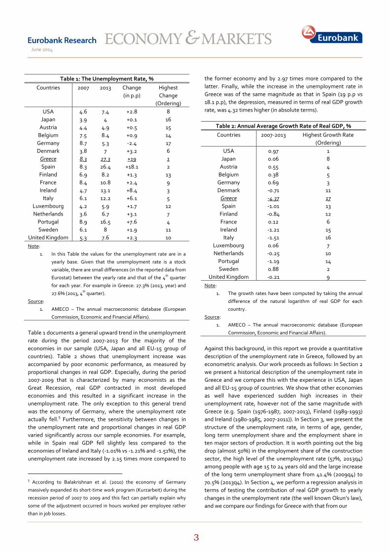
Figure 2: The Unemployment Rate, % (USA, Japan and EU‐15)

       (a) USA  (b) Japan  (c) Austria  (d) Belgium 

       (e) Germany  (f) Denmark  (g) Spain  (h) Finland 

       (i) France  (j) Ireland  (k) Italy  (l) Luxembourg 

       (m) Netherlands  (n) Portugal  (o) Sweden  (p) United Kingdom 

Note: 

1. For Germany data until 1990 refer to West Germany. 

2. For Luxembourg data start in 1978. 

Source: 

1. AMECO – The annual macroeconomic database (European Commission, Economic and Financial Affairs).

sample  economies.  We  find  that  real  GDP  growth  has  a statistically  significant  relation  with  changes  in  the unemployment rate (and Okun’s coefficient becomes higher ‐ in absolute  terms  ‐  if  we  include  to  our  sample  the  2007‐2013 period).  In  Section  5,  using  quarterly  data  from  1999q2  to 2013q4,  we  investigate  how  key  macroeconomic  variables, namely  real GDP  (growth),  real  interest  rate  (change)  and  real credit to firms (growth), are statistically related with changes  in the  unemployment  rate.  Our  econometric  results  suggest  a negative (and statistically significant) relation with real GDP and 

real  credit  to  firms  growth,  and  a  positive  relation  with  real interest  rate  changes.  Furthermore,  we  find  a  negative  (and statistically  significant)  relation  between  changes  in  the unemployment  rate  and  changes  in  prices’  expectations  and wealth of households. The latter two variables are approximated by  the  consumers’ price expectations and households’  financial situation indices from the joint harmonized EU consumer survey. Subsequently,  we  utilize  our  econometric  model  and  three different  scenarios  for  our  explanatory  variables  to  perform projections for the unemployment and the employment rates  in 

 

 

June 2014 

5

Greece  over  the  next  seven  years.  Our  baseline  scenario  is consistent  with  a  drop  in  the  unemployment  rate  of approximately 10 p.p over  the next seven years  (2014  to 2020), given  an  average  annual  real  GDP  growth  of  3.5%,  annual  growth  of  real  credit  to  firms  by  4.5%,  a  reduction  in  the  real interest rate to a level of 3.0% and an improvement in the indices of  consumers’  price  expectations  and  households’  financial situation. This compares to a projection of the Second Economic Adjustment Programme for Greece (fourth review, April 2014) of  a 10 p.p  fall  in  the unemployment  rate by 2018  (which  is more close to our optimistic scenario, see Section 5). Finally, Section 6 concludes.  2. The unemployment rate from a historical perspective  In  this  section,  we  present  a  comparison  between  the unemployment rate in Greece and the respective figure from our sample economies. To this end, we use yearly data from 1960 to 2013. Looking at Figure 2, we can  identify  four  time phases  for the Greek unemployment  rate. The  first  starts at  the early 60s and ends at  the  late  70s. The  second  is  from  the early 80s and ends at  the  late 90s. The  third  covers  the period  1999  to 2008 and, finally, the fourth is the current depression.  During the first phase, the Greek economy managed to achieve an  annual  average  unemployment  rate  equal  to  3.71%.  This performance was  accompanied by  strong  economic  expansion, with an annual average real GDP growth equal to 6.62% during the  period  1960‐1979.  This was  not  a  phenomenon  specific  to Greece;  all  the  economies  in  our  sample  had  a  low  level  of unemployment, especially until the first oil crisis (October 1973). For  Greece,  admittedly,  immigration  abroad  in  that  period contributed  in  containing unemployment,  apart  from  the  rapid growth.  In  what  concerns  the  second  phase,  the  unemployment  rate increased  by  9.3  p.p  (2.7%  in  1980  to  12%  in  1999)  and  the average annual growth rate of real GDP fell to a  level of 1.35%. According  to  Demekas  and  Kontolemis  (1996),  this  increase reflected  the  slowdown  in  growth,  the  restructuring  of production,  the  increased  mismatch  between  jobs  and  jobs seekers, and most  important of all, the persistence of real wage aspirations.6 As was the case in the former subperiod, the Greek case was not an exception. Looking at Figure 2, we observe that from the mid 70s (or early 80s) the unemployment rate increased in most of our sample economies, and it has never returned to its former  level.7 Another  interesting  point  about  this  time  period 

                                                            6 Alogoskoufis and Manning (1988) conclude that the reluctance from the 

side of workers to revise downward their wage aspiration can explain the 

difference  in  persistence  of  the  unemployment  rate  between  Europe 

(excluding  the  Scandinavian  countries,  Austria  and  Switzerland)  and, 

USA and Japan during the 80s.     7 The economies of USA  (Fig 2a.),  Ireland  (Fig 2j.) and Netherlands  (Fig 

2m.) are exceptions, since in the early 2000s managed to return to a level 

was  the  fact  that  the US economy started  to perform better  in terms  of  its  level  of  unemployment  rate  compared  to  the European  economies.  This  phenomenon  made  economists  to start  investigating  for  possible  factors  that  lie  behind  this increase in the unemployment rate in Europe. In two of the most influential  studies,  Nickell  (1997)  and  Siebert  (1997)  conclude that  rigidities  and  institutional  factors  can  explain  the  poor European labor market performance.8  The third phase for the Greek economy  lasts until 2008. From a record high of 12% in 1999, the unemployment rate fell to a level of  7.7%  in 2008. At  the  same  time,  the annual average growth rate increased to a level of 3.55%. The construction works for the Olympic Games of 2004 contributed positively to this reduction by  creating  many  jobs  (directly  and  indirectly  through complement products and services).  In what concerns the other economies,  the  unemployment  rate  increased  only  in  the USA (Fig2a.),  in  Ireland  (Fig2j.),  in Luxembourg  (Fig2l.) and Portugal (Fig2n.), by 1.6 p.p, 0.8 p.p, 2.5 p.p and 3.5 p.p, respectively. The economies  of  Finland  (Fig2h.),  France  (Fig2i)  and  Italy  (Fig2k.) are more  close  to  the  case of Greece, with  a decrease of  their unemployment rate by 3.8 p.p, 2.6 p.p and 4.2 p.p, respectively.   Finally,  the  last  phase  of  the  Greek  economy, which  starts  in 2008, was characterized by explosive unemployment due to the huge  contraction of  real GDP. However, unemployment  seems  

                                                                                                   of unemployment rate similar (or lower for the case of Ireland) to that of 

the early 70s.      8  Not  all  of  the  rigidities  can  be  considered  to  contribute  to 

unemployment  as,  according  to  Nickell  (1997),  many  labor  market 

institutions that conventionally come under the heading of rigidities have 

no observable impact on unemployment. More specifically, Nickell (1997) 

argues  that  high  unemployment  is  associated with  the  following  labor 

market  characteristics:  1)  generous  unemployment  benefits  that  are 

allowed to run on indefinitely, combined with little or no pressure on the 

unemployed  to  obtain  work  and  low  levels  of  active  intervention  to 

increase  the ability and willingness of  the unemployed  to work; 2) high 

unionization  with  wages  bargained  collectively  and  no  coordination 

between either unions or employers  in wage bargaining; 3) high overall 

taxes  impinging  on  labor  or  combination  of  high minimum wages  for 

young people associated with high payroll taxes; and 4) poor educational 

standards at the bottom end of the labor market. On the other hand, the 

author supports the  idea that  labor market rigidities that do not appear 

to have serious implications for average levels of unemployment include 

the  following:  1)  strict  employment  protection  legislation  and  general 

legislation  on  labor  market  standards;  2)  generous  levels  of 

unemployment benefit, so long as these are accompanied by pressure on 

the  unemployed  to  take  jobs  by,  for  example,  fixing  the  duration  of 

benefit  and  providing  resources  to  raise  the  ability/willingness  of  the 

unemployed  to  take  jobs;  and  3) high  levels of unionization  and union 

coverage,  so  long  as  they  are  offset  by  high  levels  of  coordination  in 

wage bargaining, particularly among employers.  

 

 

June 2014 

6

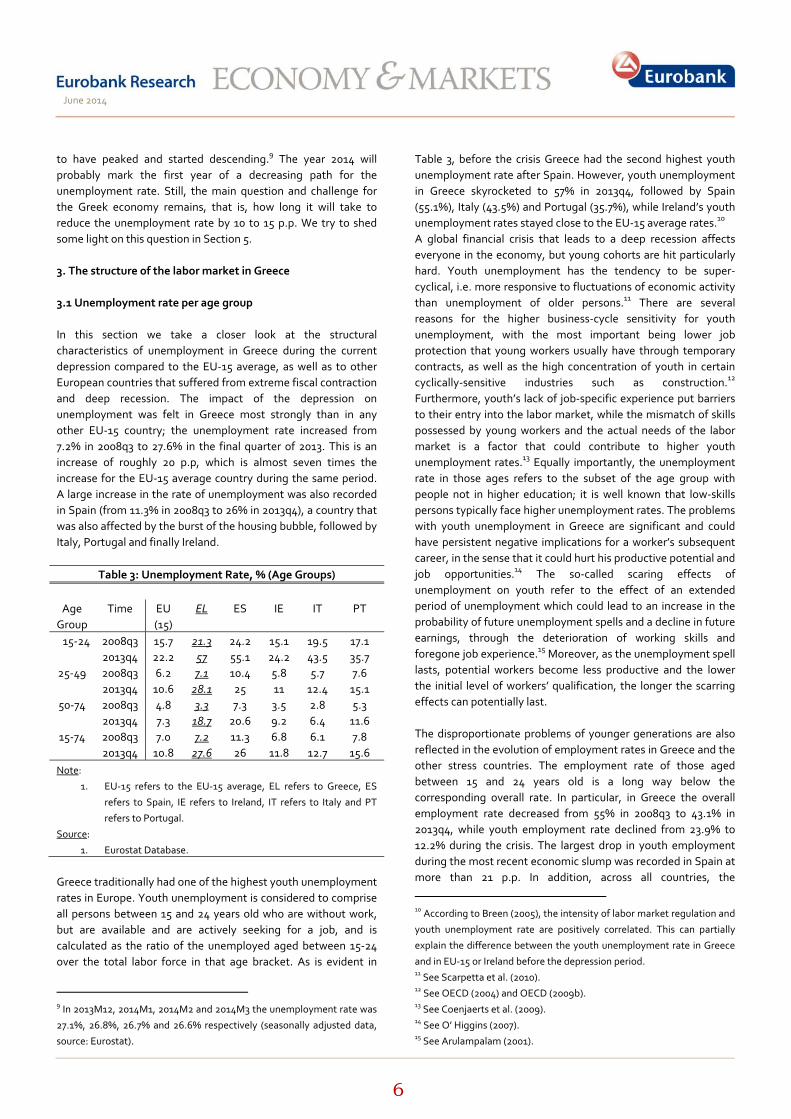
to  have  peaked  and  started  descending.9  The  year  2014  will probably  mark  the  first  year  of  a  decreasing  path  for  the unemployment  rate. Still,  the main  question  and  challenge  for the  Greek  economy  remains,  that  is,  how  long  it will  take  to reduce  the unemployment  rate by 10  to 15 p.p. We  try  to shed some light on this question in Section 5.  3. The structure of the labor market in Greece  3.1 Unemployment rate per age group  In  this  section  we  take  a  closer  look  at  the  structural characteristics  of  unemployment  in  Greece  during  the  current depression compared  to  the EU‐15 average, as well as  to other European countries that suffered from extreme fiscal contraction and  deep  recession.  The  impact  of  the  depression  on unemployment  was  felt  in  Greece  most  strongly  than  in  any other  EU‐15  country;  the  unemployment  rate  increased  from 7.2%  in 2008q3  to 27.6%  in  the  final quarter of 2013. This  is an increase  of  roughly  20  p.p,  which  is  almost  seven  times  the increase for the EU‐15 average country during the same period. A large increase in the rate of unemployment was also recorded in Spain (from 11.3% in 2008q3 to 26% in 2013q4), a country that was also affected by the burst of the housing bubble, followed by Italy, Portugal and finally Ireland.  

Table 3: Unemployment Rate, % (Age Groups) 

 Age Group 

Time  EU (15) 

EL  ES  IE  IT  PT 

15‐24  2008q3  15.7  21.3  24.2  15.1  19.5  17.1 2013q4  22.2  57  55.1  24.2  43.5  35.7 

25‐49  2008q3  6.2  7.1  10.4  5.8  5.7  7.6 2013q4  10.6  28.1  25  11  12.4  15.1 

50‐74  2008q3  4.8  3.3  7.3  3.5  2.8  5.3 2013q4  7.3  18.7  20.6  9.2  6.4  11.6 

15‐74  2008q3  7.0  7.2  11.3  6.8  6.1  7.8 2013q4  10.8  27.6  26  11.8  12.7  15.6 

Note: 

1. EU‐15  refers  to  the  EU‐15  average,  EL  refers  to Greece,  ES 

refers  to Spain,  IE  refers  to  Ireland,  IT  refers  to  Italy and PT 

refers to Portugal. 

Source: 

1. Eurostat Database. 

 Greece traditionally had one of the highest youth unemployment rates in Europe. Youth unemployment is considered to comprise all persons between 15 and 24 years old who are without work, but  are  available  and  are  actively  seeking  for  a  job,  and  is calculated as  the  ratio of  the unemployed aged between 15‐24 over  the  total  labor  force  in  that  age  bracket. As  is  evident  in 

                                                            9 In 2013M12, 2014M1, 2014M2 and 2014M3 the unemployment rate was 

27.1%, 26.8%, 26.7% and 26.6%  respectively  (seasonally adjusted data, 

source: Eurostat). 

Table 3, before  the  crisis Greece had  the  second highest youth unemployment rate after Spain. However, youth unemployment in  Greece  skyrocketed  to  57%  in  2013q4,  followed  by  Spain (55.1%), Italy (43.5%) and Portugal (35.7%), while Ireland’s youth unemployment rates stayed close to the EU‐15 average rates.10 A  global  financial  crisis  that  leads  to  a  deep  recession  affects everyone  in the economy, but young cohorts are hit particularly hard.  Youth  unemployment  has  the  tendency  to  be  super‐cyclical, i.e. more responsive to fluctuations of economic activity than  unemployment  of  older  persons.11  There  are  several reasons  for  the  higher  business‐cycle  sensitivity  for  youth unemployment,  with  the  most  important  being  lower  job protection  that young workers usually have  through  temporary contracts, as well as  the high concentration of youth  in  certain cyclically‐sensitive  industries  such  as  construction.12 Furthermore, youth’s  lack of  job‐specific experience put barriers to their entry into the labor market, while the mismatch of skills possessed by young workers and  the actual needs of  the  labor market  is  a  factor  that  could  contribute  to  higher  youth unemployment  rates.13 Equally  importantly,  the unemployment rate  in  those  ages  refers  to  the  subset  of  the  age  group with people not  in higher  education;  it  is well  known  that  low‐skills persons typically face higher unemployment rates. The problems with  youth  unemployment  in Greece  are  significant  and  could have persistent negative  implications  for a worker’s subsequent career, in the sense that it could hurt his productive potential and job  opportunities.14  The  so‐called  scaring  effects  of unemployment  on  youth  refer  to  the  effect  of  an  extended period of unemployment which could  lead to an  increase  in the probability of future unemployment spells and a decline in future earnings,  through  the  deterioration  of  working  skills  and foregone job experience.15 Moreover, as the unemployment spell lasts,  potential workers  become  less  productive  and  the  lower the  initial  level of workers’ qualification,  the  longer  the scarring effects can potentially last.   The disproportionate problems of younger generations are also reflected in the evolution of employment rates in Greece and the other  stress  countries.  The  employment  rate  of  those  aged between  15  and  24  years  old  is  a  long  way  below  the corresponding  overall  rate.  In  particular,  in  Greece  the  overall employment  rate  decreased  from  55%  in  2008q3  to  43.1%  in 2013q4, while  youth  employment  rate  declined  from  23.9%  to 12.2% during  the  crisis. The  largest drop  in youth employment during the most recent economic slump was recorded in Spain at more  than  21  p.p.  In  addition,  across  all  countries,  the 

                                                            10 According to Breen (2005), the intensity of labor market regulation and  

youth  unemployment  rate  are  positively  correlated.  This  can  partially 

explain the difference between the youth unemployment rate  in Greece 

and in EU‐15 or Ireland before the depression period. 11 See Scarpetta et al. (2010). 12 See OECD (2004) and OECD (2009b). 13 See Coenjaerts et al. (2009). 14 See O’ Higgins (2007). 15 See Arulampalam (2001). 

 

 

June 2014 

7

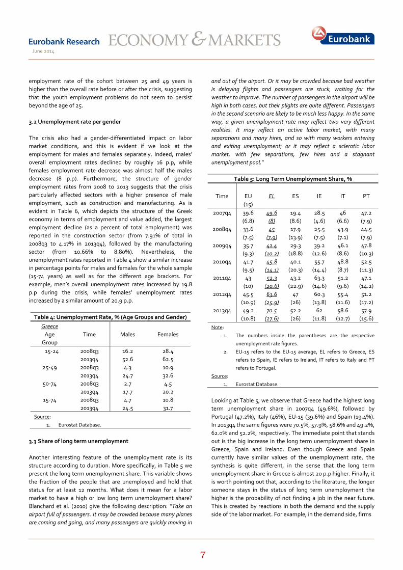
employment  rate  of  the  cohort  between  25  and  49  years  is higher than the overall rate before or after the crisis, suggesting that  the  youth  employment  problems  do  not  seem  to  persist beyond the age of 25.  3.2 Unemployment rate per gender  The  crisis  also  had  a  gender‐differentiated  impact  on  labor market  conditions,  and  this  is  evident  if  we  look  at  the employment  for males  and  females  separately.  Indeed, males’ overall  employment  rates  declined  by  roughly  16  p.p,  while females  employment  rate  decrease was  almost  half  the males decrease  (8  p.p).  Furthermore,  the  structure  of  gender employment  rates  from  2008  to  2013  suggests  that  the  crisis particularly  affected  sectors  with  a  higher  presence  of  male employment,  such  as  construction  and  manufacturing.  As  is evident  in  Table  6,  which  depicts  the  structure  of  the  Greek economy  in  terms of employment and value added,  the  largest employment  decline  (as  a  percent  of  total  employment)  was reported  in  the  construction  sector  (from  7.91%  of  total  in 2008q3  to  4.17%  in  2013q4),  followed  by  the  manufacturing sector  (from  10.66%  to  8.80%).  Nevertheless,  the unemployment rates reported in Table 4 show a similar increase in percentage points for males and females for the whole sample (15‐74  years)  as  well  as  for  the  different  age  brackets.  For example, men’s  overall  unemployment  rates  increased  by  19.8 p.p  during  the  crisis,  while  females’  unemployment  rates increased by a similar amount of 20.9 p.p.   Table 4: Unemployment Rate, % (Age Groups and Gender) 

Greece       Age Group 

Time  Males  Females 

15‐24  2008q3  16.2  28.4 2013q4  52.6  62.5 

25‐49  2008q3  4.3  10.9 2013q4  24.7  32.6 

50‐74  2008q3  2.7  4.5 2013q4  17.7  20.2 

15‐74  2008q3  4.7  10.8 2013q4  24.5  31.7 

Source: 

1. Eurostat Database.  3.3 Share of long term unemployment   Another  interesting  feature  of  the  unemployment  rate  is  its structure according to duration. More specifically,  in Table 5 we present the long term unemployment share. This variable shows the  fraction  of  the  people  that  are  unemployed  and  hold  that status  for  at  least  12 months. What  does  it mean  for  a  labor market  to have a high or  low  long  term unemployment  share? Blanchard et al.  (2010) give  the  following description:  “Take an airport full of passengers. It may be crowded because many planes are coming and going, and many passengers are quickly moving in 

and out of the airport. Or it may be crowded because bad weather is  delaying  flights  and  passengers  are  stuck,  waiting  for  the weather to improve. The number of passengers in the airport will be high in both cases, but their plights are quite different. Passengers in the second scenario are likely to be much less happy. In the same way,  a  given  unemployment  rate may  reflect  two  very  different realities.  It  may  reflect  an  active  labor  market,  with  many separations  and many hires,  and  so with many workers  entering and  exiting  unemployment;  or  it  may  reflect  a  sclerotic  labor market,  with  few  separations,  few  hires  and  a  stagnant unemployment pool.”  

Table 5: Long Term Unemployment Share, % 

   Time  EU 

(15) EL  ES  IE  IT  PT 

2007q4  39.6 (6.8) 

49.6 (8) 

19.4 (8.6) 

28.5 (4.6) 

46 (6.6) 

47.2 (7.9) 

2008q4  33.6 (7.5) 

45 (7.9) 

17.9 (13.9) 

25.5 (7.5) 

43.9 (7.1) 

44.5 (7.9) 

2009q4  35.7 (9.3) 

41.4 (10.2) 

29.3 (18.8) 

39.2 (12.6) 

46.1 (8.6) 

47.8 (10.3) 

2010q4  41.7 (9.5) 

45.8 (14.1) 

40.1 (20.3) 

55.7 (14.4) 

48.8 (8.7) 

52.5 (11.3) 

2011q4  43 (10) 

52.3 (20.6) 

43.2 (22.9) 

63.3 (14.6) 

51.2 (9.6) 

47.1 (14.2) 

2012q4  45.5 (10.9) 

63.6 (25.9) 

47 (26) 

60.3 (13.8) 

55.4 (11.6) 

51.2 (17.2) 

2013q4  49.2 (10.8) 

70.5 (27.6) 

52.2 (26) 

62 (11.8) 

58.6 (12.7) 

57.9 (15.6) 

Note: 

1. The  numbers  inside  the  parentheses  are  the  respective 

unemployment rate figures. 

2. EU‐15  refers  to  the  EU‐15  average,  EL  refers  to Greece,  ES 

refers  to Spain,  IE  refers  to  Ireland,  IT  refers  to  Italy and PT 

refers to Portugal. 

Source: 

1. Eurostat Database. 

 Looking at Table 5, we observe that Greece had the highest long term  unemployment  share  in  2007q4  (49.6%),  followed  by Portugal  (47.2%),  Italy  (46%), EU‐15  (39.6%) and Spain  (19.4%). In 2013q4 the same figures were 70.5%, 57.9%, 58.6% and 49.2%, 62.0% and 52.2%, respectively. The immediate point that stands out  is the big  increase  in the  long term unemployment share  in Greece,  Spain  and  Ireland.  Even  though  Greece  and  Spain currently  have  similar  values  of  the  unemployment  rate,  the synthesis  is  quite  different,  in  the  sense  that  the  long  term unemployment share in Greece is almost 20 p.p higher. Finally, it is worth pointing out that, according to the literature, the longer someone  stays  in  the  status  of  long  term  unemployment  the higher  is  the probability of not  finding a  job  in  the near  future. This  is created by reactions  in both the demand and the supply side of the labor market. For example, in the demand side, firms   

 

 

June 2014 

8

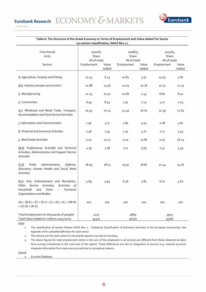
Table 6: The Structure of the Greek Economy in Terms of Employment and Value Added Per Sector (10 sectors classification, NACE Rev 2.) 

       Time Period  2000Q1  2008Q3  2013Q4 

Units  Share  (% of total) 

Share  (% of total) 

Share  (% of total) 

Sectors  Employment  Value Added 

Employment  Value Added 

Employment  Value Added 

             A: Agriculture, Forestry and Fishing  17.45  6.13  10.82  3.51  13.05  4.87              B‐E: Industry (except construction)  12.88  13.56  12.03  10.76  10.31  12.13              C: Manufacturing  11.23  10.52  10.66  7.45  8.80  8.41              F: Construction  6.95  8.34  7.91  7.13  4.17  2.03              G‐I: Wholesale  and  Retail  Trade,  Transport, Accommodation and Food Service Activities  

30.35  20.74  31.49  26.62  31.39  21.63 

             J: Information and Communication  1.90  3.17  1.85  5.03  2.08  4.82              K: Financial and Insurance Activities  2.46  7.35  2.31  5.71  2.71  5.43              L: Real Estate Activities  0.04  13.21  0.10  12.87  0.05  16.23              M‐N:  Professional,  Scientific  and  Technical Activities, Administrative and Support Service Activities 

4.79  7.58  7.11  5.69  7.47  4.55 

             O‐Q:  Public  Administration,  Defense, Education,  Human  Health  and  Social  Work Activities 

18.59  18.75  19.97  18.87  22.44  23.76 

             R‐U:  Arts,  Entertainment  and  Recreation, Other  Service  Activities,  Activities  of Household  and  Extra  –  Territorial Organizations and Bodies. 

4.69  3.94  6.46  3.83  6.07  4.62 

             (A) + (B‐E) + (F) + (G‐I) + (J) + (K) + (L) + (M‐N) + (O‐Q) + (R‐U) 

100  100  100  100  100  100 

             Total Employment (in thousands of people)  4217  4869  3903 Total Value Added (in millions 2005 euro)  34527  46270  35760 Note: 

1. The  classification of  sectors  follows NACE Rev 2.  ‐ Statistical Classification of Economic Activities  in  the European Community. See 

Appendix A for a detailed definition for each sector. 

2. The vertical sum for each column is not exactly equal to 100 due to rounding.  

3. The above figures for total employment (which  is the sum of the employees  in all sectors) are different from those obtained by  labor 

force  surveys  (mentioned  in  the main  text of  the  report). These differences are due  to  integration of  sources  (e.g. national accounts 

integrate information from many sources) and due to conceptual reasons. 

Source: 

1. Eurostat Database.  

 

 

 

June 2014 

9

receive the long term status of an unemployed person as a signal of low productivity (e.g. see Krueger et al. 2014).   3.4 Employment share and value added in ten major sectors of production Another thing that is interesting to investigate is how the current Greek  depression  has  changed  the  synthesis  (or  structure)  of total employment and total value added per sector of the Greek economy. We do so by presenting the shares (% of total) of ten   major  sectors of production  in  terms of employment and value added. The classification is according to NACE Rev 2. (Statistical classification of economic activities in the European community).   The taxonomy is as follows: Agriculture, forestry and fishing (A), Industry  (B‐E,  except  construction),  construction  (F), wholesale and  retail  trade,  transport,  accommodation  and  food  service activities (G‐I), information and communication (J), financial and insurance  activities  (K),  real  estate  activities  (L),  professional, scientific  and  technical  activities,  administrative  and  support service  activities  (M‐N),  public  administration,  defense, education,  human  health  and  social work  activities  (O‐Q)  and arts,  entertainment  and  recreation,  other  service  activities, activities of household and extra –  territorial organizations and bodies (R‐U).16  As Table 6 depicts, sectors G‐I, O‐Q, A, B‐E and F had the highest shares  in  total  employment  in  2000q1. More  specifically,  their shares  were  30.35%,  18.59%,  17.45%,  12.88%  and  6.95% respectively.  In  2008q3,  after  7  years  of  continuous  aggregate economic expansion  (including  the adoption of Euro  in 2001 as the  official  currency  unit,  which  was  the  most  important institutional  change)  there  was  a  major  drop  in  the  share  of Agriculture, Forestry and Fishing by 6.63 p.p, followed by subtle decreases  in  the  shares  of  industry  (except  construction), information  and  communication  and  financial  and  insurance activities.  Furthermore,  these  decreases  were  absorbed  by increases  in  the  shares  of  construction  (from  6.95%  to  7.91%), wholesale and  retail  trade,  transport, accommodation and  food service activities (from 30.35% to 31.49%) and sectors, M‐N (from 

                                                            16  Sector  B‐E  (industry  except  construction)  includes  the  following 

categories:  Mining  and  quarrying  (B),  electricity,  gas,  steam  and  air 

conditioning  supply  (D),  water  supply,  sewerage,  waste  management 

and  remediation activities  (E). Sector G‐I  includes: Wholesale and  retail 

trade,  repair of motor vehicles and motorcycles  (G),  transportation and 

storage (H) and accommodation and food service activities (I). Sector M‐

N  includes:  Professional,  scientific  and  technical  activities  (M)  and 

administrative  and  support  service  activities  (N).  Sector O‐Q  includes: 

Public  administration  and  defense,  compulsory  social  security  (O), 

education  (P), human health  and  social work  activities  (Q). Sector R‐U 

includes: Arts, entertainment and  recreation  (R), other service activities 

(S),  activities  of  households’  as  employers,  undifferentiated  goods  and 

services  –  producing  activities  of  households’  for  own  use  (T)  and 

activities of extraterritorial organizations and bodies  (U). See Appendix 

A. for further details. 

4.79%  to  7.11%), O‐Q  (from  18.59%  to  19.97%)  and R‐U  (from 4.69% to 6.46%).  In 2013q4, after 22 quarters of continuous depression, the largest changes  in  the  shares  of  total  employment were  these  in  the construction sector (a decrease from 7.91% to 4.17%), in industry (except construction, a decrease from 12.03% to 10.31%) and  in public  administration,  defense,  education,  human  health  and social work  activities  (an  increase  from  19.97%  to  22.44%).  In what  concerns  the  construction  sector,  this  decrease  was  the result of a major reduction in its share in total value added from 7.13% to 2.03%. The credit crunch, along with the over supply of the past, forced many firms  in this sector to reduce their output rapidly or even go bankrupt. Finally, the  increase  in the share of public  administration,  defense,  education,  human  health  and social work activities can be explained by the nature of the labor contracts  in  these  economic  activities  (the  existence  of permanent civil servants), and also by the increase in its share in total  value  added  from  18.87%  to  23.76%.17  Changes  in  the remaining sectors,  in  terms of  their share  in  total employment, were negligible.  4. Changes  in  the unemployment  rate and  real GDP growth: Okun’s Law  In this Section, we attempt to  investigate the statistical relation between  the  unemployment  rate  and  other  macroeconomic variables. We do not test a theory of unemployment, our aim  is to  explore  and  quantify  the  statistical  relation  between  the unemployment  rate  and  other  economic  variables  that mostly affect the demand side of the economy.18 We choose as our first candidate explanatory variable the growth rate of real GDP. This formulation  is  the  well  known  Okun’s  Law  (e.g.  see  Okun, 1962).19  It  describes  a  statistical  relation  between  short  run changes  in the unemployment rate and proportional changes  in real  GDP  (i.e.  growth  rate).  The  rationale  that  underlies  this relation  is as follows: An  increase  (decrease)  in demand  induces firms  to  increase  (decrease)  their  production.  To  accomplish that,  they  hire  (fire)  more  workers,  employment  increases (decrease)  and,  consequently,  unemployment  decreases (increases).  Using  the  same  notation  as  Ball  et  al.  (2013),  we derive a mathematical form of Okun’s law as follows:  

( )* *t t t t tE E Y Yγ η− = − +                (1) 

 

                                                            17 Increases (decreases) in shares can be interpreted in the following way: The  percentage  change  of  the  figure  in  the  numerator  (for  example employment  in  sector  i)  is  higher  (lower)  compared  to  the  percentage change of the figure in the denominator (for example total employment). 18  For an analytical description of  theories of unemployment  (efficiency wage theories, contracting models and search and matching models) see Romer (2006) chapter 9. 19  It  is based on a paper published  in 1962 by professor (Yale University) Arthur Okun.  

 

 

June 2014 

10

( )* *t t t t tU U E Eδ μ− = − +                (2) 

 

Where  tE   is the  log of employment  in year  t ,  tY   is the  log of 

real GDP in year  t ,  tU  is the unemployment rate in year  t  and 

tη , tμ  denote disturbance terms. Furthermore, the asterisk * , 

denotes potential or natural levels in year  t . Finally,  0γ >  and 

0δ < .20  Now,  by  inserting  equation  (1)  into  (2)  we  derive  the mathematical form of Okun’s law:  

( )( )* *t t t t t tU U Y Yδ γ η μ− = − + +  

    

( )* *t t t t tU U Y Yβ ε⇒ − = − +               (3) 

 

Where β δγ=  and  t t tε δη μ= + . Equation (3) is the level or 

the  gap  version  of  Okun’s  law.  The  coefficient  β   (Okun’s 

coefficient)  denotes  the  percentage  difference  between  the current  unemployment  rate  and  its  natural  level  that  is statistically  associated  with  a  1%  difference  between  current output and its potential level. A drawback with this version is the unobservable  time  series  for  the  natural  level  of  the 

unemployment rate *tU  and the potential output

*tY .21 In many 

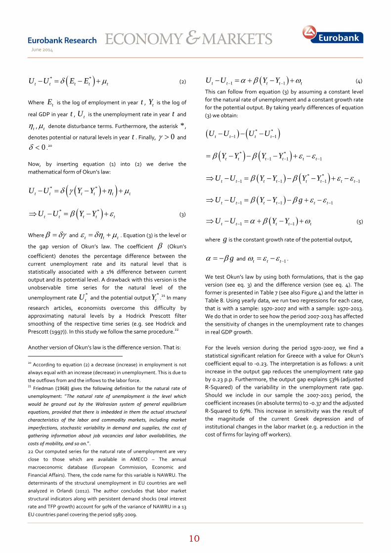
research  articles,  economists  overcome  this  difficulty  by approximating  natural  levels  by  a  Hodrick  Prescott  filter smoothing  of  the  respective  time  series  (e.g.  see Hodrick  and Prescott (1997)). In this study we follow the same procedure.22  Another version of Okun’s law is the difference version. That is:                                                             20 According to equation  (2) a decrease  (increase)  in employment  is not 

always equal with an increase (decrease) in unemployment. This is due to 

the outflows from and the inflows to the labor force. 21 Friedman  (1968)  gives  the  following definition  for  the natural  rate of unemployment:  “The  natural  rate  of  unemployment  is  the  level  which would  be  ground  out  by  the Walrasian  system  of  general  equilibrium equations, provided that there  is  imbedded  in them the actual structural characteristics  of  the  labor  and  commodity  markets,  including  market imperfections,  stochastic  variability  in demand and  supplies,  the  cost of gathering  information  about  job  vacancies  and  labor  availabilities,  the costs of mobility, and so on.”. 22 Our computed series  for  the natural  rate of unemployment are very 

close  to  those  which  are  available  in  AMECO  –  The  annual 

macroeconomic  database  (European  Commission,  Economic  and 

Financial Affairs). There, the code name for this variable is NAWRU. The 

determinants of  the  structural unemployment  in EU  countries  are well 

analyzed  in  Orlandi  (2012).  The  author  concludes  that  labor  market 

structural  indicators along with persistent demand  shocks  (real  interest 

rate and TFP growth) account for 90% of the variance of NAWRU in a 13 

EU countries panel covering the period 1985‐2009.

( )1 1t t t t tU U Y Yα β ω− −− = + − +                                             (4) 

This  can  follow  from equation  (3) by assuming a  constant  level for the natural rate of unemployment and a constant growth rate for the potential output. By taking yearly differences of equation (3) we obtain:  

( ) ( )* *1 1t t t tU U U U− −− − −  

 

( ) ( )* *1 1 1t t t t t tY Y Y Yβ β ε ε− − −= − − − + −  

 

( ) ( )* *1 1 1 1t t t t t t t tU U Y Y Y Yβ β ε ε− − − −⇒ − = − − − + −  

 

( )1 1 1t t t t t tU U Y Y gβ β ε ε− − −⇒ − = − − + −  

 

( )1 1t t t t tU U Y Yα β ω− −⇒ − = + − +                                      (5) 

 where  g is the constant growth rate of the potential output,  

 

gα β= −  and  1t t tω ε ε −= − . 

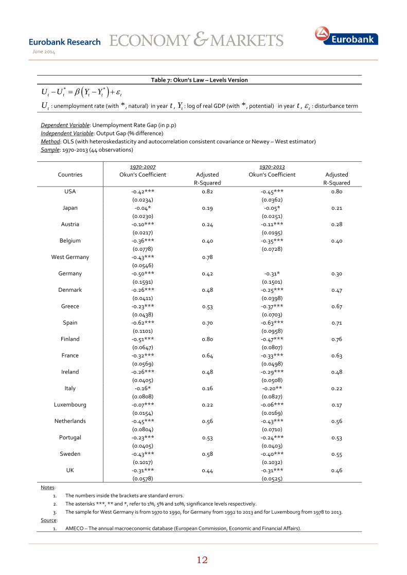
 We  test Okun’s  law by using both  formulations,  that  is  the gap version  (see  eq.  3)  and  the  difference  version  (see  eq.  4).  The former is presented in Table 7 (see also Figure 4) and the latter in Table 8. Using yearly data, we run two regressions for each case, that  is with a sample: 1970‐2007 and with a sample: 1970‐2013. We do that in order to see how the period 2007‐2013 has affected the sensitivity of changes  in the unemployment rate to changes in real GDP growth.  For  the  levels  version  during  the  period  1970‐2007,  we  find  a statistical significant relation for Greece with a value for Okun’s coefficient equal to ‐0.23. The interpretation is as follows: a unit increase  in the output gap reduces the unemployment rate gap by 0.23 p.p. Furthermore, the output gap explains 53% (adjusted R‐Squared)  of  the  variability  in  the  unemployment  rate  gap. Should  we  include  in  our  sample  the  2007‐2013  period,  the coefficient increases (in absolute terms) to ‐0.37 and the adjusted R‐Squared  to 67%. This  increase  in  sensitivity was  the  result of the  magnitude  of  the  current  Greek  depression  and  of institutional changes in the labor market (e.g. a reduction in the cost of firms for laying off workers). 

 

 

June 2014 

11

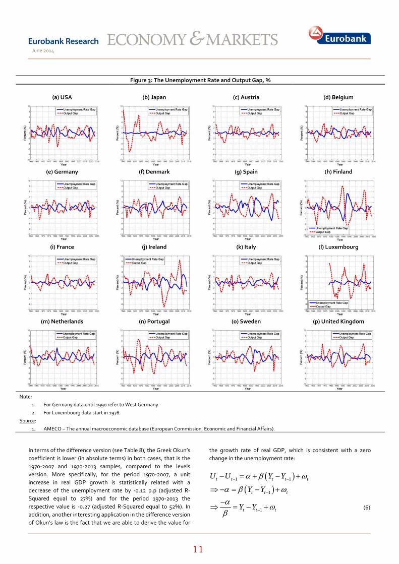
Figure 3: The Unemployment Rate and Output Gap, %

       (a) USA  (b) Japan  (c) Austria  (d) Belgium 

       (e) Germany  (f) Denmark  (g) Spain  (h) Finland 

       (i) France  (j) Ireland  (k) Italy  (l) Luxembourg 

       (m) Netherlands  (n) Portugal  (o) Sweden  (p) United Kingdom 

Note: 

1. For Germany data until 1990 refer to West Germany. 

2. For Luxembourg data start in 1978. 

Source: 

1. AMECO – The annual macroeconomic database (European Commission, Economic and Financial Affairs).

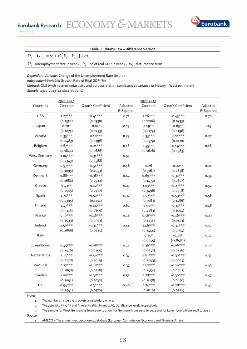
In terms of the difference version (see Table 8), the Greek Okun’s coefficient  is  lower (in absolute terms)  in both cases, that  is the 1970‐2007  and  1970‐2013  samples,  compared  to  the  levels version.  More  specifically,  for  the  period  1970‐2007,  a  unit increase  in  real  GDP  growth  is  statistically  related  with  a decrease  of  the  unemployment  rate  by  ‐0.12  p.p  (adjusted  R‐Squared  equal  to  27%)  and  for  the  period  1970‐2013  the respective  value  is  ‐0.27  (adjusted R‐Squared equal  to  52%).  In addition, another interesting application in the difference version of Okun’s  law  is the fact that we are able to derive the value for 

the  growth  rate  of  real  GDP,  which  is  consistent  with  a  zero change in the unemployment rate:  

( )1 1t t t t tU U Y Yα β ω− −− = + − +  

( )1t t tY Yα β ω−⇒ − = − +  

1t t tY Yα ωβ −−

⇒ = − +                                                                        (6) 

 

 

 

June 2014 

12

Table 7: Okun’s Law – Levels Version 

( )* *t t t t tU U Y Yβ ε− = − +  

tU : unemployment rate (with * , natural)  in year  t ,  tY : log of real GDP (with * , potential)   in year  t ,  tε : disturbance term 

 Dependent Variable: Unemployment Rate Gap (in p.p) Independent Variable: Output Gap (% difference) Method: OLS (with heteroskedasticity and autocorrelation consistent covariance or Newey – West estimator) Sample: 1970‐2013 (44 observations)  

  1970‐2007    1970‐2013   Countries  Okun’s Coefficient  Adjusted 

R‐Squared Okun’s Coefficient  Adjusted 

R‐Squared USA  ‐0.42*** 

(0.0234) 0.82  ‐0.45*** 

(0.0362) 0.80 

Japan  ‐0.04* (0.0230) 

0.19  ‐0.05* (0.0251) 

0.21 

Austria  ‐0.10*** (0.0217) 

0.24  ‐0.11*** (0.0195) 

0.28 

Belgium  ‐0.36*** (0.0778) 

0.40  ‐0.35*** (0.0728) 

0.40 

West Germany  ‐0.43*** (0.0546) 

0.78     

Germany  ‐0.50*** (0.1591) 

0.42  ‐0.31* (0.1501) 

0.30 

Denmark  ‐0.26*** (0.0411) 

0.48  ‐0.25*** (0.0398) 

0.47 

Greece  ‐0.23*** (0.0438) 

0.53  ‐0.37*** (0.0703) 

0.67 

Spain  ‐0.62*** (0.1101) 

0.70  ‐0.63*** (0.0958) 

0.71 

Finland  ‐0.51*** (0.0647) 

0.80  ‐0.47*** (0.0807) 

0.76 

France  ‐0.32*** (0.0569) 

0.64  ‐0.33*** (0.0498) 

0.63 

Ireland  ‐0.26*** (0.0405) 

0.48  ‐0.29*** (0.0508) 

0.48 

Italy  ‐0.16* (0.0808) 

0.16  ‐0.20** (0.0827) 

0.22 

Luxembourg  ‐0.07*** (0.0154) 

0.22  ‐0.06*** (0.0169) 

0.17 

Netherlands  ‐0.45*** (0.0804) 

0.56  ‐0.43*** (0.0710) 

0.56 

Portugal  ‐0.23*** (0.0405) 

0.53  ‐0.24*** (0.0403) 

0.53 

Sweden  ‐0.43*** (0.1017) 

0.58  ‐0.40*** (0.1032) 

0.55 

UK  ‐0.31*** (0.0578) 

0.44  ‐0.31*** (0.0525) 

0.46 

Notes: 

1. The numbers inside the brackets are standard errors.  

2. The asterisks ***, ** and *, refer to 1%, 5% and 10%, significance levels respectively. 

3. The sample for West Germany is from 1970 to 1990, for Germany from 1992 to 2013 and for Luxembourg from 1978 to 2013. 

Source: 

1. AMECO – The annual macroeconomic database (European Commission, Economic and Financial Affairs). 

 

 

 

June 2014 

13

Table 8: Okun’s Law – Difference Version 

( )1 1t t t t tU U Y Yα β ω− −− = + − +  

tU : unemployment rate in year  t ,  tY : log of real GDP in year  t ,  tω : disturbance term 

 Dependent Variable: Change of the Unemployment Rate (in p.p) Independent Variable: Growth Rate of Real GDP (%) Method: OLS (with heteroskedasticity and autocorrelation consistent covariance or Newey – West estimator)  Sample: 1970‐2013 (44 observations) 

           1970‐2007    1970‐2013   

Countries  Constant  Okun’s Coefficient  Adjusted R‐Squared 

Constant  Okun’s Coefficient  Adjusted R‐Squared 

USA  1.27*** (0.1354) 

‐0.41*** (0.0330) 

0.71  1.26*** (0.1206) 

‐0.43*** (0.0333) 

0.70 

Japan  0.20* (0.1075) 

‐0.04* (0.0233) 

0.13  0.19** (0.0779) 

‐0.05** (0.0198) 

015 

Austria  0.35*** (0.0483) 

‐0.10*** (0.0196) 

0.23  0.33*** (0.0579) 

‐0.11*** (0.0170) 

0.27 

Belgium  0.67*** (0.1844) 

‐0.21*** (0.0686) 

0.18  0.55*** (0.1628) 

‐0.19*** (0.0583) 

0.16 

West Germany  1.04*** (0.2343) 

‐0.31*** (0.0588) 

0.57       

Germany  0.97*** (0.1095) 

‐0.51*** (0.1053) 

0.56  0.26 (0.3167) 

‐0.22** (0.0838) 

0.21 

Denmark  0.88*** (0.1684) 

‐0.38*** (0.0912) 

0.42  0.69*** (0.1479) 

‐0.31*** (0.0627) 

0.39 

Greece  0.43** (0.2015) 

‐0.12*** (0.0407) 

0.27  1.03*** (0.3496) 

‐0.27*** (0.0958) 

0.52 

Spain  1.71*** (0.4395) 

‐0.50*** (0.1751) 

0.37  2.07*** (0.3083) 

‐0.59*** (0.1486) 

0.56 

Finland  1.47*** (0.3316) 

‐0.44*** (0.0896) 

0.62  0.91** (0.4283) 

‐0.31*** (0.1004) 

0.48 

France  0.57*** (0.1599) 

‐0.16*** (0.0563) 

0.18  0.56*** (0.1138) 

‐0.16*** (0.0473) 

0.23 

Ireland  1.50*** (0.2866) 

‐0.31*** (0.0415) 

0.44  1.46*** (0.3444) 

‐0.31*** (0.0564) 

0.51 

Italy        0.35* (0.0545) 

‐0.10* (‐1.8582) 

0.11 

Luxembourg  0.45*** (0.1416) 

‐0.08*** (0.0209) 

0.14  0.36*** (0.0847) 

‐0.06*** (0.0126) 

0.13 

Netherlands  1.13*** (0.2578) 

‐0.40*** (0.1019) 

0.37  0.81*** (0.2593) 

‐0.30*** (0.0904) 

0.32 

Portugal  0.77*** (0.1858) 

‐0.18*** (0.0518) 

0.37  0.87*** (0.1454) 

‐0.20*** (0.0462) 

0.43 

Sweden  1.00*** (0.3091) 

‐0.38*** (0.1032) 

0.53  0.78*** (0.2658) 

‐0.30*** (0.0850) 

0.47 

UK  0.94*** (0.2541) 

‐0.32*** (0.0770) 

0.40  0.74*** (0.1819) 

‐0.28*** (0.0521) 

0.41 

Notes: 

1. The numbers inside the brackets are standard errors.  

2. The asterisks ***, ** and *, refer to 1%, 5% and 10%, significance levels respectively. 

3. The sample for West Germany is from 1970 to 1990, for Germany from 1992 to 2013 and for Luxembourg from 1978 to 2013. 

Source: 

1. AMECO – The annual macroeconomic database (European Commission, Economic and Financial Affairs). 

 

 

 

June 2014 

14

As  a  result,  on  average,  the  growth  rate  of  real  GDP  that  is consistent with a constant path for the unemployment rate is:  

1t tY Y αβ−−

− =                                                                                            (7) 

 For  Greece,  during  the  period  1970‐2007  and  1970‐2013,  the above growth rate was equal to 3.58% and 3.81%, respectively. In our  sample  economies  the  same  figure  has  an  average  value equal to 3.3%.  As far as our sample economies are concerned (USA, Japan and EU‐15), we find statistically significant relations for both versions of Okun’s  law (an exception  is  Italy during the period 1970‐2007 for the difference version).  In terms of the  levels version, we do not  observe  quantitatively  significant  changes  between  1970‐2007  and  1970‐2013.  The  only  exception  is  the  economy  of Germany, where Okun’s  coefficient  decreased  from  ‐0.50  to  ‐0.31  in  absolute  terms.  This  was  a  result  of  a  poor  growth performance, accompanied by a decreasing unemployment rate during the period 2007‐2013 (see Tables 1,2 and Footnote 5).23  The  economy  with  the  highest  sensitivity  in  changes  of unemployment  rate  (or unemployment gap) due  to  changes  in real GDP growth rate (or output gap) is Spain (Okun’s coefficient equal to ‐0.63 (levels) and ‐0.59 (differences) for the period 1970‐2013), while  the economy with  the  lowest sensitivity  is Japan  (‐0.05  in  both  versions),  followed  by  Luxembourg  (‐0.06  in  both versions) and Austria  (‐0.11).24 Furthermore,  looking at Table 8 (difference  version) we  observe  that with  the  inclusion  of  the period  2007‐2013,  the  value  of  Okun’s  coefficient  changes quantitatively,  not  only  for Greece  and Germany,  but  also  for Denmark  (from  ‐0.38  to  ‐0.31),  Spain  (from  ‐0.50  to  ‐0.59), Finland (from ‐0.44 to ‐0.31) Italy (from zero and insignificant to ‐0.10), Netherlands (from ‐0.40 to ‐0.30) and Sweden (from ‐0.38 to ‐0.30). Generally speaking, based on the difference version of Okun’s  law,  the period 2007‐2013  resulted  in an  increase  in  the sensitivity of  changes  in  the unemployment  rate  to  changes  in 

                                                            23 The robustness of Okun’s  law for OECD countries  is well tested  in Lee 

(2000). Furthermore, for the case of USA see Knotek (2007).  24 Ball et al. (2013) point out that  in Spain the high coefficient of Okun’s law  can  be  explained  by  the  existence  of  temporary  employment contracts. More specifically, the authors write: “Labor market reforms  in the 1980s made  it easier for Spanish employers to hire workers on fixed‐term  contracts,  without  the  employment  protection  guaranteed  to permanent  workers...Temporary  contracts  make  it  easier  for  firms  to adjust employment when output changes,  raising  the Okun coefficient.”. In  the  same work,  the  authors  also  give  an  explanation  about  the  low value  in  the  Japanese  Okun  coefficient.  According  to  their  view,  the existence  in  Japan  of  a  tradition  of  lifetime  employment makes  firms reluctant  to  lay  off workers.  Finally  in  another  study  for  the  Japanese economy, that  is Weiner (1987), the author attributes the stable path of the  Japanese  unemployment  rate  to  the  following  factors:  wage flexibility, hours flexibility, and labor force participation flexibility. 

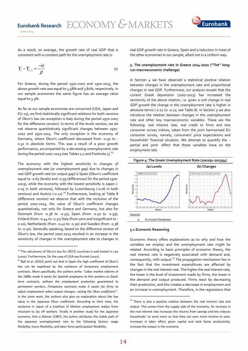
real GDP growth rate in Greece, Spain and a reduction in most of the other economies in our sample, albeit not in a uniform way.   5. The unemployment  rate  in Greece 2014‐2020  (“The”  long‐run macroeconomic challenge)  In  Section  4  we  have  observed  a  statistical  positive  relation between  changes  in  the  unemployment  rate  and  proportional changes  in real GDP. Furthermore, our analysis reveals that the current  Greek  depression  (2007‐2013)  has  increased  the sensitivity of  the above  relation,  i.e. given a unit change  in  real GDP growth  the change  in  the unemployment  rate  is higher  in absolute terms (‐0.12 to ‐0.27, see Table 8). In Section 5 we also introduce  the  relation  between  changes  in  the  unemployment rate  and  other  key  macroeconomic  variables.  These  are  the following:  real  interest  rate,  real  credit  to  firms  and  two consumer  survey  indices,  taken  from  the  joint  harmonised  EU consumer  survey,  namely,  consumers’  price  expectations  and households’  financial  situation. We  attempt  to  quantify  the  –partial  and  joint‐  effect  that  these  variables  have  on  the employment rate.   

Figure 4: The Greek Unemployment Rate (2002q1‐2013q4) 

(a) Levels  (b) Changes 

Source: 

1. Eurostat Database.  5.1 Economic Reasoning  Economic  theory  offers  explanations  as  to  why  and  how  the variables  we  employ  and  the  unemployment  rate  might  be related.  According  to  basic  principles  of  economic  theory,  the real  interest  rate  is  negatively  associated  with  demand  and, consequently, with output.25 The propagation mechanism lies in the  fact  that  the  investment  expenditures  are  affected  by changes in the real interest rate. The higher the real interest rate, the  lower  is the  level of  investment made by firms, the  lower  is the  demand  and  output  produced.  Firms  react  by  decreasing their production, and this creates a decrease in employment and an increase in unemployment. Therefore, in the regressions that 

                                                            25  There  is  also  a  positive  relation  between  the  real  interest  rate  and output. This comes from the supply side of the economy. An  increase  in the real interest rate increases the returns from savings and this induces households’  to work more  so  that  they  can earn more  income  to  save. Increases  in  labor  effort,  given  capital  and  total  factor  productivity, increase the output in the economy. 

 

 

June 2014 

15

follow, we expect a positive (negative) relation between changes in the unemployment rate (employment rate) and changes in the real interest rate.    

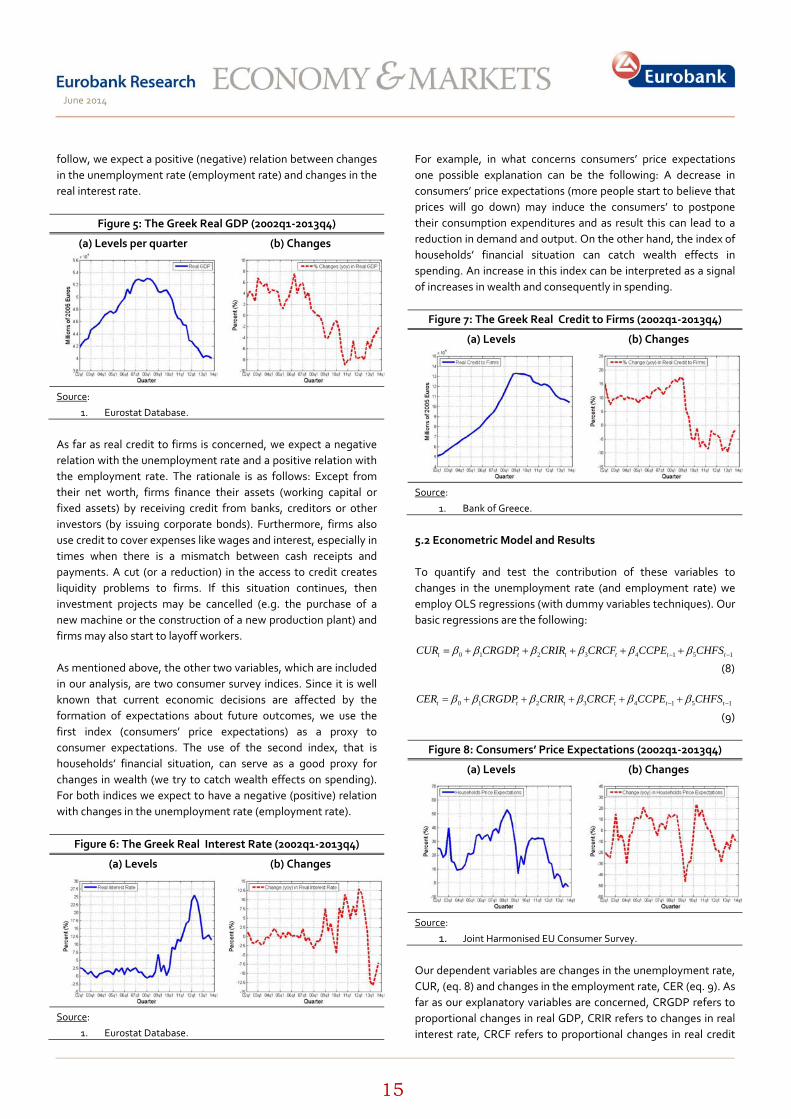
Figure 5: The Greek Real GDP (2002q1‐2013q4) 

(a) Levels per quarter  (b) Changes 

Source: 

1. Eurostat Database. 

 As far as real credit to firms  is concerned, we expect a negative relation with the unemployment rate and a positive relation with the  employment  rate.  The  rationale  is  as  follows:  Except  from their  net  worth,  firms  finance  their  assets  (working  capital  or fixed  assets) by  receiving  credit  from banks,  creditors  or  other investors  (by  issuing  corporate bonds). Furthermore,  firms also use credit to cover expenses like wages and interest, especially in times  when  there  is  a  mismatch  between  cash  receipts  and payments. A cut  (or a  reduction)  in  the access  to credit creates liquidity  problems  to  firms.  If  this  situation  continues,  then investment  projects may  be  cancelled  (e.g.  the  purchase  of  a new machine or the construction of a new production plant) and firms may also start to layoff workers.   As mentioned above, the other two variables, which are included in our analysis, are two consumer survey  indices. Since  it  is well known  that  current  economic  decisions  are  affected  by  the formation  of  expectations  about  future  outcomes, we  use  the first  index  (consumers’  price  expectations)  as  a  proxy  to consumer  expectations.  The  use  of  the  second  index,  that  is households’  financial  situation,  can  serve  as  a  good  proxy  for changes  in wealth  (we try to catch wealth effects on spending). For both indices we expect to have a negative (positive) relation with changes in the unemployment rate (employment rate).  

Figure 6: The Greek Real  Interest Rate (2002q1‐2013q4) 

(a) Levels  (b) Changes 

Source: 

1. Eurostat Database. 

For  example,  in  what  concerns  consumers’  price  expectations one  possible  explanation  can  be  the  following:  A  decrease  in consumers’ price expectations (more people start to believe that prices  will  go  down) may  induce  the  consumers’  to  postpone their consumption expenditures and as  result  this can  lead  to a reduction in demand and output. On the other hand, the index of households’  financial  situation  can  catch  wealth  effects  in spending. An increase in this index can be interpreted as a signal of increases in wealth and consequently in spending.  

Figure 7: The Greek Real  Credit to Firms (2002q1‐2013q4) 

(a) Levels  (b) Changes 

Source: 

1. Bank of Greece. 

 5.2 Econometric Model and Results  To  quantify  and  test  the  contribution  of  these  variables  to changes  in  the unemployment  rate  (and  employment  rate) we employ OLS regressions (with dummy variables techniques). Our basic regressions are the following:  

0 1 2 3 4 1 5 1t t t t t tCUR CRGDP CRIR CRCF CCPE CHFSβ β β β β β− −= + + + + +  

                                                                                                                                (8)  

0 1 2 3 4 1 5 1t t t t t tCER CRGDP CRIR CRCF CCPE CHFSβ β β β β β− −= + + + + +  

                                                                                                                                (9)  

Figure 8: Consumers’ Price Expectations (2002q1‐2013q4) 

(a) Levels  (b) Changes 

Source: 

1. Joint Harmonised EU Consumer Survey.  Our dependent variables are changes in the unemployment rate, CUR, (eq. 8) and changes in the employment rate, CER (eq. 9). As far as our explanatory variables are concerned, CRGDP refers to proportional changes in real GDP, CRIR refers to changes in real interest  rate, CRCF  refers  to proportional changes  in  real credit 

 

 

June 2014 

16

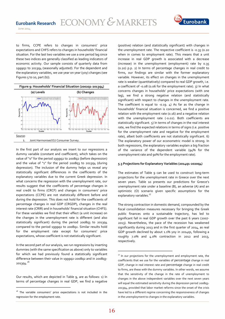
to  firms,  CCPE  refers  to  changes  in  consumers’  price expectations and CHFS refers to changes in households’ financial situation. For the last two variables we use a one period lag since these two indices are generally classified as leading indicators of economic  activity. Our  sample  consists  of  quarterly  data  from 1999q2 to 2013q4  (seasonally adjusted). For the dependent and the explanatory variables, we use year on year (yoy) changes (see Figures 5 to 10, part (b)).   

Figure 9: Households’ Financial Situation (2002q1‐2013q4) 

(a) Levels  (b) Changes 

Source: 

1. Joint Harmonised EU Consumer Survey.  In  the  first  part  of  our  analysis we  insert  to  our  regressions  a dummy  variable  (constant and  coefficient), which  takes on  the value of “0” for the period 1999q2 to 2008q2 (before depression) and  the  value  of  “1”  for  the  period  2008q3  to  2013q4  (during depression).  The  inclusion  of  the  dummy  helps  us  reveal  any statistically  significant  differences  in  the  coefficients  of  the explanatory  variables  due  to  the  current  Greek  depression.  In what concerns  the  regression with  the unemployment  rate, our results  suggest  that  the  coefficients  of  percentage  changes  in real  credit  to  firms  (CRCF)  and  changes  in  consumers’  price expectations  (CCPE)  are  not  statistically  different  before  and during the depression. This does not hold for the coefficients of percentage  changes  in  real GDP  (CRGDP),  changes  in  the  real interest rate (CRIR) and in households’ financial situation (CHFS). For  these variables we  find  that  their effect  (a unit  increase) on the  changes  in  the  unemployment  rate  is  different  (and  also statistically  significant)  during  the  period  2008q3  to  2013q4 compared  to  the period 1999q2  to 2008q2. Similar  results hold for  the  employment  rate  except  for  consumers’  price expectations, whose coefficient is not statistically significant.  In the second part of our analysis, we run regressions by inserting dummies (with the same specification as above) only to variables for  which  we  had  previously  found  a  statistically  significant difference between their value in 1999q2‐2008q2 and in 2008q3‐2013q4.26    Our  results, which are depicted  in Table 9, are as  follows: 1)  In terms  of  percentage  changes  in  real GDP, we  find  a  negative 

                                                            26  The  variable  consumers’  price  expectations  is  not  included  in  the regression for the employment rate. 

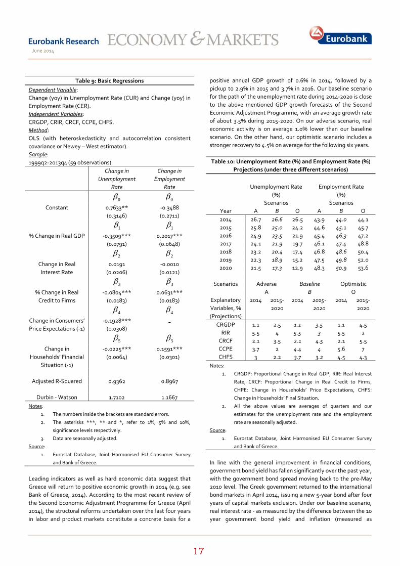
(positive)  relation  (and  statistically  significant) with  changes  in the unemployment rate. The respective coefficient is ‐0.35 (0.20 when  in  comes  to  employment  rate).  This means  that  a  unit increase  in  real  GDP  growth  is  associated  with  a  decrease (increase)  in  the  unemployment  (employment)  rate  by  0.35 (0.20)  p.p.  2)  In  terms  of  percentage  changes  in  real  credit  to firms,  our  findings  are  similar  with  the  former  explanatory variable. However,  its  effect  on  changes  in  the  unemployment rate is weaker (quantitatively) compared to real GDP growth, i.e. a coefficient of ‐0.08 (0.06 for the employment rate). 3)  In what concerns  changes  in  households’  price  expectations  (with  one lag),  we  find  a  strong  negative  relation  (and  statistically significant) with  respect  to changes  in  the unemployment  rate. The  coefficient  is  equal  to  ‐0.19.  4)  As  far  as  the  change  in households’  financial  situation  is  concerned, we  find  a  positive relation with the employment rate (0.16) and a negative relation with  the  unemployment  rate  (‐0.02).  Both  coefficients  are statistically significant. 5) In terms of changes in the real interest rate, we find the expected relations in terms of signs (i.e. positive for  the  unemployment  rate  and  negative  for  the  employment rate), albeit both  coefficients are not  statistically  significant. 6) The  explanatory  power  of  our  econometric model  is  strong.  In both regressions, the explanatory variables explain a big fraction of  the  variance  of  the  dependent  variable  (94%  for  the unemployment rate and 90% for the employment rate).  5.3 Projections for Explanatory Variables (2014q1‐2020q4)  The  estimates  of  Table  9  can  be  used  to  construct  long‐term projections  for  the unemployment  rate  in Greece over  the next seven  years.  Table  10  presents  our  predictions  for  Greece’s unemployment rate under a baseline  (B), an adverse  (A) and an optimistic  (O)  scenario  given  specific  assumptions  for  the explanatory variables.27  The strong contraction in domestic demand, compounded by the fiscal  consolidation measures  necessary  for  bringing  the Greek public  finances  onto  a  sustainable  trajectory,  has  led  to significant  fall  in  real GDP growth over  the past 6 years  (2007‐2013).  Nevertheless,  the  pace  of  the  recession  has  weakened significantly during 2013 and  in the first quarter of 2014, as real GDP growth declined by about 1.1% yoy  in 2014q1,  following a roughly  7.0%  and  4.0%  contraction  in  2012  and  2013, respectively.   

                                                            27  In  our  projections  for  the  unemployment  and  employment  rate,  the coefficients that we use  for the variables of percentage change  in  real GDP, change  in real  interest rate and percentage change  in real credit to firms, are these with the dummy variables. In other words, we assume 

that  the  sensitivity  of  the  change  in  the  rate  of  unemployment  to 

changes  in  the  above  independent  variables over  the next  seven  years 

will equal the estimated sensitivity during the depression period 2008q3‐

2013q4, provided that  labor market reforms since the onset of the crisis 

have led to a different regime concerning the responsiveness of changes 

in the unemployment to changes in the explanatory variables. 

 

 

June 2014 

17

Table 9: Basic Regressions 

Dependent Variable: Change (yoy) in Unemployment Rate (CUR) and Change (yoy) in Employment Rate (CER). Independent Variables:  CRGDP, CRIR, CRCF, CCPE, CHFS. Method: OLS  (with  heteroskedasticity  and  autocorrelation  consistent covariance or Newey – West estimator). Sample: 1999q2‐2013q4 (59 observations) 

  Change in Unemployment 

Rate 

Change in Employment 

Rate  

0β   0β  

Constant  0.7633** (0.3146) 

‐0.3488 (0.2711) 

 1β   1β  

% Change in Real GDP  ‐0.3509*** (0.0791) 

0.2017*** (0.0648) 

 2β   2β  

Change in Real Interest Rate 

0.0191 (0.0206) 

‐0.0010 (0.0121) 

 3β   3β  

% Change in Real Credit to Firms 

‐0.0804*** (0.0183) 

0.0631*** (0.0183) 

 4β   4β  

Change in Consumers’ Price Expectations (‐1) 

‐0.1928*** (0.0308) 

‐  

5β   5β  

Change in Households’ Financial 

Situation (‐1) 

‐0.0225*** (0.0064) 

0.1591*** (0.0301) 

     Adjusted R‐Squared  0.9362  0.8967 

     Durbin ‐ Watson  1.7102  1.1667 

Notes: 

1. The numbers inside the brackets are standard errors.  

2. The  asterisks  ***,  **  and  *,  refer  to  1%,  5%  and  10%, 

significance levels respectively. 

3. Data are seasonally adjusted. 

Source: 

1. Eurostat  Database,  Joint  Harmonised  EU  Consumer  Survey 

and Bank of Greece. 

 Leading  indicators  as well  as hard  economic data  suggest  that Greece will return to positive economic growth in 2014 (e.g. see Bank of Greece, 2014). According  to  the most  recent  review of the Second Economic Adjustment Programme for Greece (April 2014), the structural reforms undertaken over the last four years in  labor  and  product markets  constitute  a  concrete  basis  for  a 

positive  annual  GDP  growth  of  0.6%  in  2014,  followed  by  a pickup  to 2.9%  in 2015 and 3.7%  in 2016. Our baseline scenario for the path of the unemployment rate during 2014‐2020 is close to  the  above mentioned GDP  growth  forecasts  of  the  Second Economic Adjustment Programme, with an average growth rate of about  3.5% during 2015‐2020. On our adverse  scenario,  real economic  activity  is  on  average  1.0%  lower  than  our  baseline scenario. On  the other hand, our optimistic  scenario  includes a stronger recovery to 4.5% on average for the following six years.  Table 10: Unemployment Rate (%) and Employment Rate (%) 

Projections (under three different scenarios) 

   Unemployment Rate 

(%) Employment Rate 

(%)   Scenarios  Scenarios 

Year  Α  Β  Ο  Α  Β  Ο 2014  26.7  26.6  26.5  43.9  44.0  44.1 2015  25.8  25.0  24.2  44.6  45.1  45.7 2016  24.9  23.5  21.9  45.4  46.3  47.2 2017  24.1  21.9  19.7  46.1  47.4  48.8 2018  23.2  20.4  17.4  46.8  48.6  50.4 2019  22.3  18.9  15.2  47.5  49.8  52.0 2020  21.5  17.3  12.9  48.3  50.9  53.6              

Scenarios  Adverse  Baseline  Optimistic   A  B  O 

Explanatory Variables, % (Projections) 

2014  2015‐2020 

2014  2015‐2020 

2014  2015‐2020 

CRGDP  1.1  2.5  1.1  3.5  1.1  4.5 RIR  5.5  4  5.5  3  5.5  2 CRCF  2.1  3.5  2.1  4.5  2.1  5.5 CCPE  3.7  2  4.4  4  5.6  7 CHFS  3  2.2  3.7  3.2  4.5  4.3 

Notes: 

1. CRGDP: Proportional Change  in Real GDP, RIR: Real  Interest 

Rate,  CRCF:  Proportional  Change  in  Real  Credit  to  Firms, 

CHPE:  Change  in  Households’  Price  Expectations,  CHFS: 

Change in Households’ Final Situation. 2. All  the  above  values  are  averages  of  quarters  and  our 

estimates  for  the  unemployment  rate  and  the  employment 

rate are seasonally adjusted. 

Source: 

1. Eurostat  Database,  Joint  Harmonised  EU  Consumer  Survey 

and Bank of Greece. 

 In  line  with  the  general  improvement  in  financial  conditions, government bond yield has fallen significantly over the past year, with  the government bond spread moving back  to  the pre‐May 2010  level. The Greek government returned to the  international bond markets in April 2014, issuing a new 5‐year bond after four years of capital markets exclusion. Under our baseline scenario, real interest rate ‐ as measured by the difference between the 10 year  government  bond  yield  and  inflation  (measured  as 

 

 

June 2014 

18

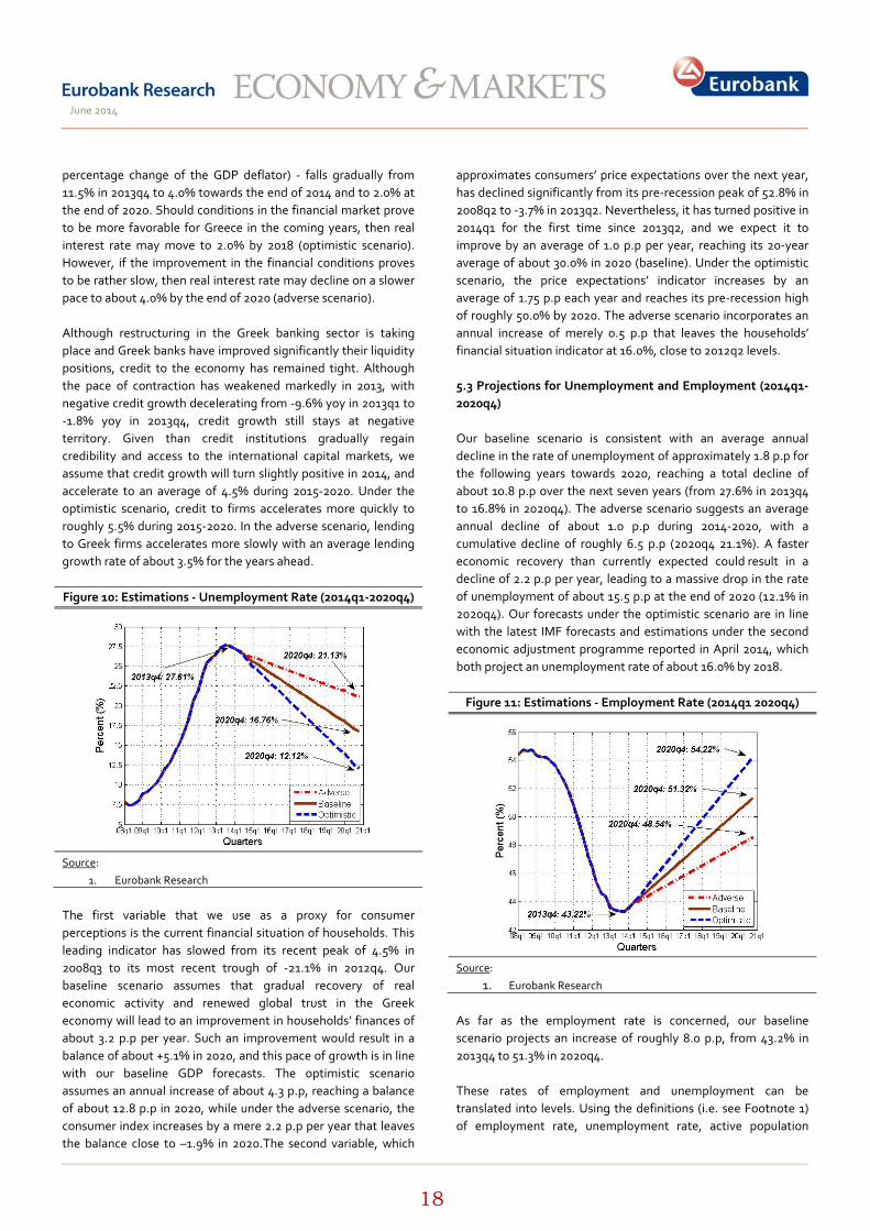
percentage  change  of  the GDP  deflator)  ‐  falls  gradually  from 11.5% in 2013q4 to 4.0% towards the end of 2014 and to 2.0% at the end of 2020. Should conditions in the financial market prove to be more  favorable  for Greece  in  the coming years,  then  real interest  rate may move  to  2.0%  by  2018  (optimistic  scenario). However,  if  the  improvement  in  the  financial conditions proves to be rather slow, then real interest rate may decline on a slower pace to about 4.0% by the end of 2020 (adverse scenario).  Although  restructuring  in  the  Greek  banking  sector  is  taking place and Greek banks have improved significantly their liquidity positions,  credit  to  the  economy has  remained  tight. Although the  pace  of  contraction  has weakened markedly  in  2013, with negative credit growth decelerating from ‐9.6% yoy in 2013q1 to ‐1.8%  yoy  in  2013q4,  credit  growth  still  stays  at  negative territory.  Given  than  credit  institutions  gradually  regain credibility  and  access  to  the  international  capital markets, we assume that credit growth will turn slightly positive in 2014, and accelerate  to  an  average of 4.5% during 2015‐2020. Under  the optimistic  scenario,  credit  to  firms  accelerates more  quickly  to roughly 5.5% during 2015‐2020. In the adverse scenario, lending to Greek firms accelerates more slowly with an average  lending growth rate of about 3.5% for the years ahead.  Figure 10: Estimations ‐ Unemployment Rate (2014q1‐2020q4) 

 Source: 

1. Eurobank Research  

 The  first  variable  that  we  use  as  a  proxy  for  consumer perceptions  is the current financial situation of households. This leading  indicator  has  slowed  from  its  recent  peak  of  4.5%  in 2008q3  to  its  most  recent  trough  of  ‐21.1%  in  2012q4.  Our baseline  scenario  assumes  that  gradual  recovery  of  real economic  activity  and  renewed  global  trust  in  the  Greek economy will lead to an improvement in households’ finances of about 3.2 p.p per year. Such an  improvement would  result  in a balance of about +5.1% in 2020, and this pace of growth is in line with  our  baseline  GDP  forecasts.  The  optimistic  scenario assumes an annual increase of about 4.3 p.p, reaching a balance of about 12.8 p.p  in 2020, while under the adverse scenario, the consumer index increases by a mere 2.2 p.p per year that leaves the balance  close  to  –1.9%  in 2020.The  second  variable, which 

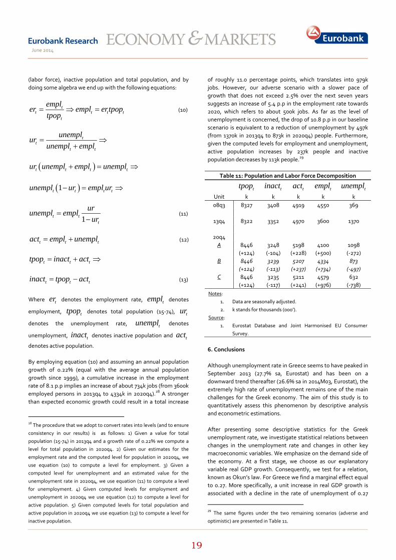
approximates consumers’ price expectations over the next year, has declined significantly from its pre‐recession peak of 52.8% in 2008q2 to ‐3.7% in 2013q2. Nevertheless, it has turned positive in 2014q1  for  the  first  time  since  2013q2,  and  we  expect  it  to improve by an average of 1.0 p.p per year,  reaching  its 20‐year average of about 30.0%  in 2020 (baseline). Under the optimistic scenario,  the  price  expectations’  indicator  increases  by  an average of 1.75 p.p each year and reaches  its pre‐recession high of roughly 50.0% by 2020. The adverse scenario incorporates an annual  increase  of merely  0.5  p.p  that  leaves  the  households’ financial situation indicator at 16.0%, close to 2012q2 levels.   5.3 Projections for Unemployment and Employment (2014q1‐2020q4)  Our  baseline  scenario  is  consistent  with  an  average  annual decline in the rate of unemployment of approximately 1.8 p.p for the  following  years  towards  2020,  reaching  a  total  decline  of about 10.8 p.p over the next seven years (from 27.6%  in 2013q4 to 16.8%  in 2020q4). The adverse scenario suggests an average annual  decline  of  about  1.0  p.p  during  2014‐2020,  with  a cumulative decline of  roughly 6.5 p.p  (2020q4 21.1%). A  faster economic  recovery  than  currently  expected  could result  in  a decline of 2.2 p.p per year, leading to a massive drop in the rate of unemployment of about 15.5 p.p at the end of 2020 (12.1% in 2020q4). Our  forecasts under  the optimistic scenario are  in  line with  the  latest  IMF  forecasts and estimations under  the second economic adjustment programme reported  in April 2014, which both project an unemployment rate of about 16.0% by 2018.   Figure 11: Estimations ‐ Employment Rate (2014q1 2020q4) 

 Source: 

1. Eurobank Research  As  far  as  the  employment  rate  is  concerned,  our  baseline scenario projects an  increase of  roughly 8.0 p.p,  from 43.2%  in 2013q4 to 51.3% in 2020q4.   These  rates  of  employment  and  unemployment  can  be translated  into  levels. Using the definitions  (i.e. see Footnote 1) of  employment  rate,  unemployment  rate,  active  population 

 

 

June 2014 

19

(labor  force),  inactive  population  and  total  population,  and  by doing some algebra we end up with the following equations:  

tt t t t

t

empler empl ertpoptpop

= ⇒ =                                             (10) 

 

tt

t t

unemplurunempl empl

= ⇒+

 

 

( )t t t tur unempl empl unempl+ = ⇒  

 

( )1t t t tunempl ur empl ur− = ⇒  

 

1t tt

urunempl emplur

=−

                                                                (11) 

 

t t tact empl unempl= +                                                                   (12) 

 

t t ttpop inact act= + ⇒  

 

t t tinact tpop act= −                                                                          (13) 

 

Where  ter   denotes  the  employment  rate,  templ   denotes employment,  ttpop   denotes  total  population  (15‐74),  tur  denotes  the  unemployment  rate,  tunempl   denotes 

unemployment,  tinact  denotes  inactive population and  tact  denotes active population.   By employing equation (10) and assuming an annual population growth  of  0.22%  (equal  with  the  average  annual  population growth  since  1999),  a  cumulative  increase  in  the  employment rate of 8.1 p.p implies an increase of about 734k jobs (from 3600k employed persons  in 2013q4  to 4334k  in 2020q4).28 A  stronger than expected economic growth could  result  in a  total  increase 

                                                            28 The procedure that we adopt to convert rates into levels (and to ensure 

consistency  in  our  results)  is    as  follows:  1)  Given  a  value  for  total 

population  (15‐74)  in 2013q4 and a growth  rate of 0.22% we compute a 

level  for  total  population  in  2020q4.  2)  Given  our  estimates  for  the 

employment  rate and  the computed  level  for population  in 2020q4, we 

use  equation  (10)  to  compute  a  level  for  employment.  3)  Given  a 

computed  level  for  unemployment  and  an  estimated  value  for  the 

unemployment rate  in 2020q4, we use equation  (11) to compute a  level 

for  unemployment.  4)  Given  computed  levels  for  employment  and 

unemployment  in  2020q4 we use  equation  (12)  to  compute  a  level  for  

active  population.  5)  Given  computed  levels  for  total  population  and 

active population  in 2020q4 we use equation (13) to compute a  level for  

inactive population. 

of  roughly  11.0  percentage  points,  which  translates  into  979k jobs.  However,  our  adverse  scenario  with  a  slower  pace  of growth  that  does  not  exceed  2.5%  over  the  next  seven  years suggests an  increase of 5.4 p.p  in the employment rate towards 2020,  which  refers  to  about  500k  jobs.  As  far  as  the  level  of unemployment is concerned, the drop of 10.8 p.p in our baseline scenario  is equivalent  to a  reduction of unemployment by 497k (from 1370k  in 2013q4  to 873k  in 2020q4) people. Furthermore, given the computed  levels for employment and unemployment, active  population  increases  by  237k  people  and  inactive population decreases by 113k people.29  

Table 11: Population and Labor Force Decomposition 

 ttpop   tinact   tact   templ   tunempl  

Unit  k  k  k  k  k 08q3  8327  3408  4919  4550  369            

13q4  8322  3352  4970  3600  1370            

20q4           A  8446  3248  5198  4100  1098   (+124)  (‐104)  (+228)  (+500)  (‐272) B  8446  3239  5207  4334  873   (+124)  (‐113)  (+237)  (+734)  (‐497) C  8446  3235  5211  4579  632 

    (+124)  (‐117)  (+241)  (+976)  (‐738) Notes: 

1. Data are seasonally adjusted. 

2. k stands for thousands (000’). 

Source: 

1. Eurostat  Database  and  Joint  Harmonised  EU  Consumer 

Survey. 

 6. Conclusions  Although unemployment rate in Greece seems to have peaked in September  2013  (27.7%  sa,  Eurostat)  and  has  been  on  a downward trend thereafter (26.6% sa in 2014M03, Eurostat), the extremely high rate of unemployment remains one of the main challenges  for  the Greek  economy. The  aim  of  this  study  is  to quantitatively  assess  this  phenomenon  by  descriptive  analysis and econometric estimations.   After  presenting  some  descriptive  statistics  for  the  Greek unemployment rate, we investigate statistical relations between changes  in  the  unemployment  rate  and  changes  in  other  key macroeconomic variables. We emphasize on the demand side of the  economy.  At  a  first  stage,  we  choose  as  our  explanatory variable  real GDP growth. Consequently, we  test  for a  relation, known as Okun’s law. For Greece we find a marginal effect equal to 0.27. More specifically, a unit  increase  in  real GDP growth  is associated with  a decline  in  the  rate of unemployment of 0.27 

                                                            29  The  same  figures  under  the  two  remaining  scenarios  (adverse  and 

optimistic) are presented in Table 11. 

 

 

June 2014 

20

p.p. We  observe  that  the  Greek  depression  of  2007‐2013  has actually  increased  the  responsiveness of unemployment  rate  to changes  in  real  economic  activity,  as  for  the  pre‐crisis  period (1970‐2007) a unit increase in real GDP growth is consistent with a  decline  in  the  rate  of  unemployment  of  only  0.12  p.p.  This increase in sensitivity is also observed in Spain and Italy. For the remaining  of  our  sample  economies  (USA,  Japan  and  EU‐15 group of countries) we observe a decrease.      At a  second  stage, using quarterly data  from  199q2  to 2013q4, we  employ  a  simple  linear  econometric  model  that  relates changes in the unemployment rate, not only with changes in real GDP  growth,  but  also  with  changes  in  real  interest  rate, percentage changes in real credit to firms, changes in consumers’ price  expectations  and  changes  in  households’  financial situation.  Our  results  suggest  a  negative  and  statistically significant relation between changes  in the unemployment rate and real GDP growth (‐0.35), real credit to firms’ growth (‐0.08), and changes  in the two consumer  indices (‐0.19 and ‐0.02) from the  joint harmonized EU  consumer  survey. On  the other hand, there  is a positive but statistically  insignificant relation between changes  in the unemployment rate and changes  in real  interest rate  (0.02).  Finally, we  also  quantify  the  effect  that  the  above mentioned variables have on the employment rate.    Given  these  estimated  coefficients  and  by  making  some hypotheses on the path of our explanatory variables, we produce projections  over  the  period  2014‐2020.  We  present  three scenarios,  i.e.  an  adverse,  a  baseline  and  a  conservative. According  to  our  baseline  scenario,  we  estimate  that  the unemployment  rate  in Greece will decline by approximately  10 percentage  points  over  the  next  seven  years  ‐from  27.6%  in 2013q4  to  16.8%  in  2020q4‐  given  an  average GDP  growth  of 3.5%, real credit to firms’ growth of 4.5%, a real  interest rate of 3.0%  and  a  gradual  improvement  in  consumers’  price expectations  and  in  households’  financial  situation.  As  far  as employment  is  concerned, we  expect  a  cumulative  increase  of 8.1  p.p  in  the  employment  rate  during  2014‐2020,  which translates into an increase of about 734k jobs.  Subsequently, we estimate  the  level of  the unemployment  rate under  a  more  optimistic  and  an  adverse  scenario.  A  faster economic  recovery  that  includes  an  average  GDP  growth  of 4.5%, real credit growth of 5.5%, a real interest rate of 2.0% and a  sharper  improvement  in  consumer  indices  could result  in  a sharp  drop  in  the  unemployment  rate  of  more  than  15 percentage points at  the end of 2020.  In  the adverse  scenario, where GDP and credit growth are 1 percentage point lower than in the baseline scenario, real  interest rate  is 4.0% and consumer indices  improve with  a  lesser  degree,  the  unemployment  rate declines by only 6.5 p.p in the next seven years.       

                                                        

 

 

June 2014 

21

References   Alogoskoufis G. S. and Manning A.,  (1988), “On the Persistence 

of Unemployment”, Economic Policy, Vol. 3, No. 7, pp. 429‐469. 

 Arulampalam  W.,  (2001),  “Is  Unemployment  Really  Scarring? 

Effects of Unemployment on Wages”, Economic Journal, Vol. 111, pp. 585‐606. 

 Ball L. M., Leigh D. and Loungani P., (2013), “Okun’s Law: Fit At 

Fifty?”,  National  Bureau  of  Economic  Research,  Working Paper No. 18668. 

 Balakrishnan  R.,  Das  M.,  and  Kannan  P.,  (2010),  “Chapter  3: 

Unemployment  Dynamics  During  Recessions  and Recoveries:  Okun’s  Law  and  Beyond”,  International Monetary Fund. 

 Bank of Greece, (2014), “Monetary Policy 2013‐2014”, June 2014, 

Bank of Greece.  Blanchard O. and Katz L. F.,  (1997), “What We Know About the 

Natural  Rate  of  Unemployment”,  Journal  of  Economic Perspectives, Vol. 11, No. 1, pp. 51‐72. 

 Blanchard  O.,  Amighini  A.,  and  Giavazzi  F.,  (2010), 

“Macroeconomics  A  European  Perspective”,  Prentice  Hall Financial Times. 

 Breen R., (2005), “Explaining Cross – National Variation in Youth 

Unemployment, Market and Institutional Factors”, European Sociological Review, Vol. 21, No. 2, pp. 125‐134. 

 Coenjaerts C., Ernst C., Fortuny M., Rei D. and Pilgrim M., (2009), 

“Youth  Unemployment”,  in:  OECD,  2009,  Promoting  Pro‐Poor Growth: Employment, Paris. 

 Demekas D. G. and Kontolemis Z. G., (1996), “Unemployment in 

Greece:  A  Survey  of  the  Issues”,  IMF Working  Paper,  No. 96/91. 

 European  Commission,  (2014),  “The  Second  Economic 

Adjustment  Programme  for  Greece,  Fourth  Review”, European Economy, Occasional Papers 192.  

 Eurostat  ‐  European  Commission,  (2008),  “NACE  Rev.  2, 

Statistical  Classification  of  Economic  Activities  in  the European  Community”,  Eurostat  Methodologies  and Working Papers. 

 Friedman M.,  (1968),  “The Role of Monetary Policy”, American 

Economic Review, Vol. 58, pp. 1‐21.  

Hodrick R.  J. and Prescott E. C.,  (1997),  "Postwar U.S. Business Cycles: An Empirical Investigation," Journal of Money, Credit, and Banking, Vol. 29, No. 1, pp. 1‐16.  

 Honkapohja S. and Koskela E.,  (1999),  “The Economic Crisis of 

the 1990s in Finland”, Economic Policy, Vol. 14, Issue 29, pp. 399‐436. 

 Knotek  E.  S.,  (2007),  “How  Useful  is  Okun’s  Law”,  Federal 

Reserve  Bank  of  Kansas  City  Economic  Review,  Fourth Quarter 2007, pp. 73‐103.  

 Krueger A. B., Cramer J. and Cho D., (2014), “Are the Long Term 

Unemployed  on  the  Margins  of  the  Labor  Market?”, Economic  Studies  at  Brookings,  Brookings  Panel  on Economic Activity. 

 Lee  J.,  (2000),  “The Robustness  of Okun’s  Law: Evidence  from 

OECD Countries”, Journal of Macroeconomics, Vol. 22, No. 2, pp. 331‐356. 

 Orlandi  F.,  (2012),  “Structural  Unemployment  and  its 

Determinants  in  the  EU  Coutnries”,  European  Commission Economic Papers 455. 

 Nickell S.,  (1997), “Unemployment and Labor Market Rigidities: 

Europe  versus  North  America”,  Journal  of  Economic Perspectives, Vol. 11, No. 3, pp. 55‐74. 

 Nordström  Skans,  Oskar,  (2004),  "Scarring  effects  of  the  first 

labor market experience: A sibling based analysis", Working Paper Series 2004:14, IFAU ‐ Institute for Evaluation of Labor Market and Education Policy. 

 OECD,  (2004),  “OECD  Employment  Outlook  2004”,  OECD 

Publishing, Paris.  OECD,  (2009a),  “OECD  Employment  Outlook  2004”,  OECD 

Publishing, Paris.  OECD,  (2009b),  “Jobs  for  Youth/Des    emplois  pour  les  jeunes: 

Australia”, OECD Multilingual Summaries, OECD Publishing, Paris. 

 O’Higgins  N.,  (2007),  “Trends  in  the  Youth  Labor  Market  in 

Developing  and  Transitions  Countries”,  International Security Review, 50 (4/97), 63‐93. 

 Okun  A.,  (1962),  “Potential  GNP:  Its  Measurement  and 

Significance”, American Statistical Association, Proceedings of the Business and Economics Statistics Section, pp. 98‐104.  

 Romer D.,  (2006),  “Advanced Macroeconomics”,  Third  Edition, 

McGraw ‐ Hill.  

 

 

June 2014 

22

Scarpetta S., Sonnet A. and Manfredi T.,  (2010),  “Rising Youth Unemployment During  the Crisis: How  to Prevent Negative Long Term Consequances on a Generation?”, OECD Social, Employment and Migration, Working Paper No. 106, OECD Publishing, Paris. 

 Siebert H.,  (1997), “Labor Market Rigidities and Unemployment 

in Europe”, Kiel Working Papers, No. 787.  Weiner S. E., (1987), “Why is Japan’s Unemployment Rate so Low 

and  so  Stable”,  Federal  Reserve  Bank  of  Kansas  City Economic Review, Vol. 72, No. 4, pp. 3‐19. 

                                            

                                                        

 

 

June 2014 

23

Appendix A.   In this Appendix we present the basic definitions for each of the economic activities presented  in Table 6. These are  the official definitions  from  NACE  Rev  2.  ‐  Statistical  Classification  of Economic  Activities  in  the  European  Community  (e.g.  see Eurostat – European Commission (2008)).  Economic Activity A – Agriculture, Forestry and Fishing:  It  includes  the  exploitation  of  vegetal  and  animal  natural resources, comprising  the activities of growing of crops,  raising and breeding of animals, harvesting of timber and other plants, animals or animal products from a farm or their natural habitats.  Economic Activity B – Mining and Quarrying:  It includes the extraction of minerals occurring naturally as solids (coal  and  ores),  liquids  (petroleum)  or  gases  (natural  gas). Extraction  can  be  achieved  by  different  methods  such  as underground  or  surface mining, well  operation,  seabed mining etc.  It also  includes supplementary activities aimed at preparing the  crude  materials  for  marketing,  for  example,  crushing, grinding,  cleaning,  drying,  sorting,  concentrating  ores, liquefaction  of  natural  gas  and  agglomeration  of  solid  fuels. These  operations  are  often  accomplished  by  the  units  that extracted the resource and/or others located nearby.  Economic Activity C – Manufacturing:  It  includes the physical or chemical transformation of materials, substances,  or  components  into  new  products.  The materials, substances, or  components  transformed are  raw materials  that are products of agriculture, forestry, fishing, mining or quarrying as well as products of other manufacturing activities. Substantial alteration,  renovation  or  reconstruction  of  goods  is  generally considered to be manufacturing. The output of a manufacturing process may be finished in the sense that it is ready for utilisation or consumption, or it may be semi‐finished in the sense that it is to become an input for further manufacturing. For example, the output  of  alumina  refining  is  the  input  used  in  the  primary production  of  aluminium;  primary  aluminium  is  the  input  to aluminium wire drawing; and aluminium wire is the input for the manufacture of fabricated wire products.   Economic  Activity  D  –  Electricity,  Gas,  Steam  and  Air Conditioning Supply:  It includes the provision of electric power, natural gas, steam, hot water and the like through a permanent infrastructure (network) of  lines, mains and pipes. The dimension of  the network  is not decisive;  also  included  are  the  distribution  of  electricity,  gas, steam,  hot water  and  the  like  in  industrial  parks  or  residential buildings.  Therefore  this  economic  activity  includes  the operation  of  electric  and  gas  utilities, which  generate,  control and  distribute  electric  power  or  gas.  Also  included  is  the 

provision  of  steam  and  air‐conditioning  supply.  Operation  of water  and  sewerage  utilities  and  transport  of  gas  through pipelines are excluded.  Economic  Activity  E  –  Water  Supply;  Sewerage,  Waste Management and Remediation Activities:  It  includes  activities  related  to  the  management  (including collection,  treatment  and  disposal)  of  various  forms  of waste, such as solid or non‐solid  industrial or household waste, as well as  contaminated  sites.  The  output  of  the  waste  or  sewage treatment process can either be disposed of or become an input into  other  production  processes. Activities  of water  supply  are also  grouped  in  this  economic  activity,  since  they  are  often carried out  in connection with, or by units also engaged  in,  the treatment of sewage.  Economic Activity F – Construction:  It  includes  general  construction  and  specialized  construction activities  for  buildings  and  civil  engineering  works.  It  includes new  work,  repair,  additions  and  alterations,  the  erection  of prefabricated  buildings  or  structures  on  the  site  and  also construction of a temporary nature.  Economic  Activity  G  – Wholesale  and  Retail  Trade;  Repair  of Motor Vehicles and Motorcycles:  It  includes  wholesale  and  retail  sale  (i.e.  sale  without transformation)  of  any  type  of  goods,  and  rendering  services incidental to the sale of merchandise. Wholesaling and retailing are  the  final  steps  in  the  distribution  of  merchandise.  Also included in this economic activity are the repair of motor vehicles and motorcycles.  Economic Activity H – Transportation and Storage:  It  includes  the  provision  of  passenger  or  freight  transport, whether scheduled or not, by rail, pipeline, road, water or air and associated activities such as terminal and parking facilities, cargo handling,  storage  etc.  Included  in  this  economic  activity  is  the renting  of  transport  equipment  with  driver  or  operator.  Also included are postal and courier activities.  Economic  Activity  I  –  Accommodation  and  Food  Service Activities:  It includes the provision of short‐stay accommodation for visitors and  other  travellers  and  the  provision  of  complete meals  and drinks  fit  for  immediate consumption. The amount and  type of supplementary  services  provided  within  this  section  can  vary widely. It excludes the provision of long‐term accommodation as primary  residences,  which  is  classified  in  real  estate  activities (economic activity L). Also excluded is the preparation of food or drinks that are either not fit for  immediate consumption or that are sold through independent distribution channels, i.e. through 

 

 

June 2014 

24

wholesale  or  retail  trade  activities.  The  preparation  of  these foods is classified in manufacturing (economic activity C).  Economic Activity J – Information and Communication:  It  includes  the  production  and  distribution  of  information  and cultural  products,  the  provision  of  the  means  to  transmit  or distribute  these  products,  as well  as  data  or  communications, information technology activities and the processing of data and other information service activities.  Economic Activity K – Financial and Insurance Activities:  It  includes  financial  service  activities,  including  insurance, reinsurance  and  pension  funding  activities  and  activities  to support financial services. It also includes the activities of holding assets, such as activities of holding companies and the activities of trusts, funds and similar financial entities.  Economic Activity L – Real Estate Activities:  It includes acting as lessors, agents and/or brokers in one or more of the following: selling or buying real estate, renting real estate, providing other real estate services such as appraising real estate or acting as real estate escrow agents. These economic activities may be carried out on own or leased property and may be done on  a  fee  or  contract  basis.  Also  included  is  the  building  of structures,  combined with maintaining  ownership  or  leasing  of such structures and real estate property managers.  Economic  Activity  M  –  Professional,  Scientific  and  Technical Activities:  It  includes  specialised  professional,  scientific  and  technical activities. These activities require a high degree of training, and make  specialised  knowledge  and  skills  available  to  users  (legal and accounting activities, activities of head offices; management consultancy  activities,  architectural  and  engineering  activities; technical  testing  and  analysis,  scientific  research  and development,  advertising  and  market  research,  other professional,  scientific  and  technical  activities  and  veterinary activities).  Economic  Activity  N  –  Administrative  and  Support  Service Activities:  It  includes a variety of economic activities  that support general business  operations.  These  activities  differ  from  those  in economic  activity  M,  since  their  primary  purpose  is  not  the transfer of  specialised  knowledge  (rental  and  leasing  activities, employment  activities,  travel  agency,  tour  operator  and  other reservation  service  and  related  activities,  security  and investigation  activities,  services  to  buildings  and  landscape activities, office administrative, office support and other business support activities).  

Economic  Activity  O  –  Public  Administration  and  Defense; Compulsory Social Security:  It  includes activities of a governmental nature, normally carried out  by  the  public  administration.  This  includes  the  enactment and  judicial  interpretation of  laws and their pursuant regulation, as well  as  the  administration  of  programmes  based  on  them, legislative activities, taxation, national defense, public order and safety,  immigration  services,  foreign  affairs  and  the administration  of  government  programmes.  The  legal  or institutional status  is not,  in  itself, the determining factor for an activity  to belong  in  this specific economic activity,  rather  than the activity being of a nature specified in the previous paragraph. This means  that  activities  classified  elsewhere  in NACE do not fall  under  economic  activity  O,  even  if  carried  out  by  public entities. For example, administration of  the  school  system  (i.e. regulations,  checks,  curricula)  falls  under  economic  activity O, but  teaching  itself  does  not  (see  economic  activity  P),  and  a prison or military hospital is classified to health (see Q). Similarly, some of the economic activities described above may be carried out by non‐government units. Finally, economic activity O, also includes compulsory social security activities.  Economic Activity P – Education:  It  includes  education  at  any  level  or  for  any  profession.  The instructions  may  be  oral  or  written  and  may  be  provided  by radio,  television,  Internet  or  via  correspondence.  It  includes education  by  the  different  institutions  in  the  regular  school system at  its different  levels as well as adult education,  literacy programmes  etc.  Also  included  are  military  schools  and academies, prison schools etc. at their respective  levels. Finally, this  economic  activity  includes  public  as  well  as  private education.  Economic Activity Q – Human Health and Social Work Activities:  It includes the provision of health and social work activities. They are included a wide range of activities, starting from health care provided by trained medical professionals  in hospitals and other facilities, over residential care activities that still involve a degree of  health  care  activities  to  social  work  activities  without  any involvement of health care professionals.  Economic Activity R – Arts, Entertainment and Recreation:  It  includes  a  wide  range  of  activities  to meet  varied  cultural, entertainment  and  recreational  interests  of  the  general  public, including  live  performances,  operation  of  museum  sites, gambling, sports and recreation activities.  Economic Activity S – Other Service Activities:  It  includes  (as a  residual category)  the activities of membership organisations,  the  repair  of  computers  and  personal  and 

 

 

June 2014 

25

household goods and a variety of personal service activities not covered elsewhere in the classification.  Economic  Activity  T  –  Activities  of Households’  as  Employers; Undifferentiated  Goods  and  Services  –  Producing  Activities  of Households’ for Own Use:  It includes the activities of households’ as employers of domestic personnel  such  as  maids,  cooks,  waiters,  valets,  butlers, laundresses,  gardeners,  gatekeepers,  stable‐lads,  chauffeurs, caretakers,  governesses,  babysitters,  tutors,  secretaries  etc.  It allows the domestic personnel employed to state the activity of their employer in censuses or studies, even though the employer is  an  individual.  The  product  produced  by  this  activity  is consumed by the employing household. Furthermore  it  includes the undifferentiated  subsistence goods‐producing and  services‐producing  activities  of  households’.  Households’  should  be classified here only if it is impossible to identify a primary activity for the subsistence activities of the household.  If the household engages  in market activities,  it should be classified according to the primary market activity carried out.   Economic Activity U – Activities of Extraterritorial Organizations and Bodies:  It  includes  activities  of  international  organisations  such  as  the United  Nations  and  the  specialised  agencies  of  the  United Nations system, regional bodies etc., the International Monetary Fund,  the World  Bank,  the World  Customs  Organisation,  the Organisation  for Economic Co‐operation and Development,  the organization  of  Petroleum  Exporting  Countries,  the  European Communities,  the  European  Free  Trade  Association  etc. Furthermore  it  includes:  activities  of  diplomatic  and  consular missions when being determined by the country of their location  rather than by the country they represent.                      

                                                        

 

 

June 2014 

26

Appendix B.  We use  two variables  from  the Joint Harmonised EU Consumer Survey  that  capture  households’’  perceptions  about  their financial  situation,  as  well  as  their  expectations  about  price developments  over  the  next  12 months. More  specifically,  the variables are aggregate balances for the following two questions:  Consumer Price Expectations over the next 12 months:  By comparison with the past 12 months, how do you expect that consumer prices will develop in the next 12 months? They will…    + + increase more rapidly  + increase at the same rate  = increase at a slower rate  − stay about the same  − − fall  N don't know.  Statement on financial situation of households’ ‐ Capacity to save:  Which of  these  statements best describes  the  current  financial situation of your household?    + + we are saving a lot  + we are saving a little  = we are just managing to make ends meet on our income  − we are having to draw on our savings  − − we are running into debt  N don't know.  Balances  are  the  difference  between  positive  and  negative answering  options,  measured  as  percentage  points  of  total answers. In particular, if a question has three alternative options, “positive”  (“up”,  “more”,  “more  than  sufficient”,  “good”,  “too large”,  “increase”,  “improve”, etc.),  “neutral”  (“unchanged”,  “as much”,  “sufficient”,  “satisfactory”,  “adequate”,  etc.)  and “negative”  (“down”,  “less”,  “not  sufficient”,  “too  small”, “decline”, etc.), and  if P, E and M (with P+E+M=100) denote the percentages  of  respondents  having  chosen  respectively  the option positive, neutral, and negative,  the balance  is calculated as B = P − M.   In  the  case of questions with  six options,  i.e.  the  three options above  plus  “very  positive”  (“got/get  a  lot  better”,  “very much higher”, “increase sharply”, etc.), “very negative”  (“got/get a  lot worse”,  “very  unfavourable”,  “fall  sharply”,  etc.)  and  “don’t know”,  the  balances  are  calculated  on  the  basis  of  weighted averages. If P, E and M have the same meaning as in the previous paragraph,  while  PP  denotes  the  percentage  of  respondents having chosen the option “very positive”, MM the percentage of respondents having chosen  the option “very negative” and N  is the  percentage  of  respondents  without  any  opinion  (so  that PP+P+E+M+MM+N=100),  balances  are  calculated  as  B  =  (PP  + ½P)  −  (½M + MM).  It  is  clear  from  the expressions above  that 

balance  values  range  from  −100, when  all  respondents  choose the negative option (or the most negative one in the case of five‐option  questions)  to  +100,  when  all  respondents  choose  the positive (or the most positive) option.                                                     

 

 

June 2014 

27

                               

   

Eurobank, 20 Amalias Av & 5 Souri Str, 10557 Athens, tel: +30.210.333 .7365, fax: +30.210.333.7687, contact email: Research@eurobank.gr 

Economic Research Team  

Economic Research & Forecasting Division Tasos Anastasatos:  Senior Economist Ioannis Gkionis:  Research Economist Stylianos Gogos: Economic Analyst Vasilis Zarkos:  Economic Analyst Olga Kosma:  Economic Analyst 

Maria Prandeka:  Economic Analyst Theodoros Stamatiou: Research Economist 

 

Eurobank Economic Research More research editions available at http://www.eurobank.gr/research •  New  Europe:  Economics  &  Strategy Monthly  edition  on  the  economies    and the markets of New Europe • Economy & Markets: Monthly economic research edition  • Global Economic & Market Outlook: Quarterly review of the  international     economy and financial markets  

 Subscribe electronically at http://www.eurobank.gr/research  Follow as on twitter: http://twitter.com/Eurobank_Group