Embed Size (px)
Citation preview
Introduction to macroeconomics ǀ 5. Unemployment rate, inflation rate, and business cycle ǀ 27 April 2015 09:12 ǀ 1
5. Unemployment rate, inflation rate, and business cycle 1. Unemployment rate 2. Types of unemployment 3. Okun’s law
4. Phillips curve 5. Swan diagram 6. Involuntary unemployment
7. Orthodox labour market model 8. Involuntary unemployment in
the orthodox model
9. Involuntary unemployment
and trade unions
10. Wage and price setting model 11. Segmented labour market model 12. The E‐PIS model
13‐17. Business cycles and its facts 18‐21. Deflation 22‐23. Balance sheet recession theory
24. Say’s law 25. Explaining recessions 26‐28. Profit/wage‐led regimes
29. Modelling growth rates 30‐35. The AS‐AD model 36. Expenditure multiplier effect
1. Unemployment rate and participation rate
Definition 1.1. Employment is the number of people having a job. Unemployment is the number of
people not having a job but looking for one. The labour force is employment plus unemployment.
Definition 1.2. Unemployment rate = Unemployment / Labour force.
Definition 1.3. Participation rate = Labour force / Economically active population.
Fig. 1. Unemployment rates, Spain, 2002‐2014 Fig. 2. Unemployment rates, Catalonia, 2001‐2014
2. Basic types of unemployment
Actual unemployment is usually divided into three categories (the first two define “natural
unemployment”).
Frictional. Occurs while workers are changing jobs.
Structural. Due to structural changes in the economy that create and eliminate jobs and to the institu‐
tions that match workers and firms (firing and hiring costs, minimum wages, unemployment benefits,
mobility restrictions, lack of training…).
Cyclical. Generated by the short‐run fluctuations of GDP (rises with recessions, falls with booms)
Introduction to macroeconomics ǀ 5. Unemployment rate, inflation rate, and business cycle ǀ 27 April 2015 09:12 ǀ 2
3. Okun’s law
Okun’s law is an empirical relationship suggested in 1962 by the US economist Arthur Okun (1928‐80).
Definition 1 is just one of the alternative ways of expressing this relationship formally.
Definition 3.1. Okun’s law states that there is a negative relationship between the change ∆� = � − ���
in the unemployment rate and �� =�����
��� , the rate of growth �� of real GDP �. A simple formal
expression of the law is
∆� = � − � ·��
where � and � are positive constants that depend on the economy considered and the period with
respect to which the variables are measured.
Example 3.2. Expressing the variables as annual percentages, in the US, � ≈ 1.5 and � ≈ 0.5. Therefore
∆� = 1.5 − ��/2 or � = ��� + 1.5− ��/2.
� represents the increase in � that occurs when the economy does not grow: if �� = 0, then ∆� = �.
Example 3.3. If ��� = 2% and �� = 0, then � = ��� + � − ��/2 = 2+ 1.5 − 0/2 = 3.5. Hence, if the unem‐
ployment rate at the beginning of the year is 2% and the economy does not grow, at the end of the year
the rate is 3.5%
� measures the ability of the economy to transform GDP growth into a smaller unemployment rate:
� ≈ 0.5 means that increasing � by one point reduces � by 0.5 points.
Example 3.4. If �� = 2%, then � = ��� + 1.5− ��/2 = ��� + 1.5− 2/2= ��� + 0.5. If �� = 3%, then
� = ��� + 1.5− ��/2 = ��� + 1.5− 3/2= ���. Therefore, increasing � from 2% to 3% reduces � from ���
+ 0.5 to ���. There is a gain of 0.5 points: an additional 1% in � becomes 0.5 points less of �.
Fig. 3. Okun’s law, US, 1951‐2008 Fig. 4. Okun’s law, Spain, 1977‐1998
https://www2.bc.edu/~murphyro/EC204/PPT/CHAP09.ppt http://www.ine.es
Introduction to macroeconomics ǀ 5. Unemployment rate, inflation rate, and business cycle ǀ 27 April 2015 09:12 ǀ 3
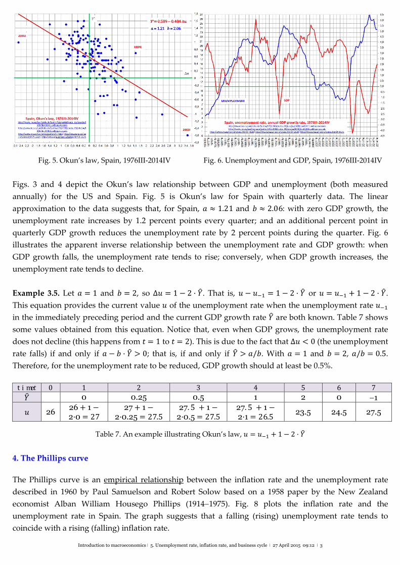
Fig. 5. Okun’s law, Spain, 1976III‐2014IV Fig. 6. Unemployment and GDP, Spain, 1976III‐2014IV
Figs. 3 and 4 depict the Okun’s law relationship between GDP and unemployment (both measured
annually) for the US and Spain. Fig. 5 is Okun’s law for Spain with quarterly data. The linear
approximation to the data suggests that, for Spain, � ≈ 1.21 and � ≈ 2.06: with zero GDP growth, the
unemployment rate increases by 1.2 percent points every quarter; and an additional percent point in
quarterly GDP growth reduces the unemployment rate by 2 percent points during the quarter. Fig. 6
illustrates the apparent inverse relationship between the unemployment rate and GDP growth: when
GDP growth falls, the unemployment rate tends to rise; conversely, when GDP growth increases, the
unemployment rate tends to decline.
Example 3.5. Let � = 1 and � = 2, so ∆� = 1− 2·��. That is, � − ��� = 1− 2·�� or � = ��� + 1− 2 ·�� .
This equation provides the current value � of the unemployment rate when the unemployment rate ���
in the immediately preceding period and the current GDP growth rate �� are both known. Table 7 shows
some values obtained from this equation. Notice that, even when GDP grows, the unemployment rate
does not decline (this happens from � = 1 to � = 2). This is due to the fact that ∆� < 0 (the unemployment
rate falls) if and only if � − � ·�� > 0; that is, if and only if �� > �/�. With � = 1 and � = 2, �/� = 0.5.
Therefore, for the unemployment rate to be reduced, GDP growth should at least be 0.5%.
time� 0 1 2 3 4 5 6 7
�� 0 0.25 0.5 1 2 0 1
� 26 26+1− 2·0 = 27
27+1− 2·0.25 = 27.5
27. 5+1− 2·0.5 = 27.5
27. 5+1− 2·1 = 26.5
23.5 24.5 27.5
Table 7. An example illustrating Okun’s law, � = ��� + 1− 2·��
4. The Phillips curve
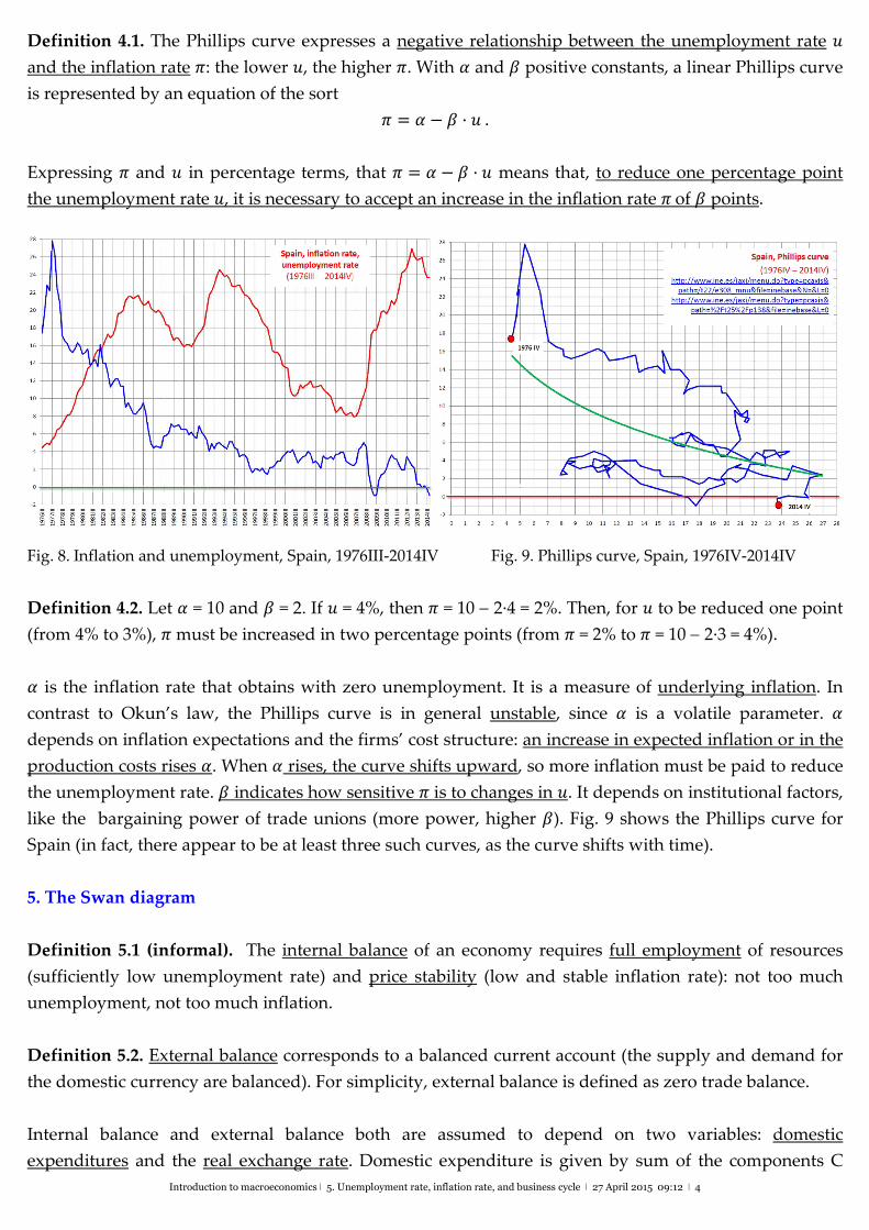
The Phillips curve is an empirical relationship between the inflation rate and the unemployment rate
described in 1960 by Paul Samuelson and Robert Solow based on a 1958 paper by the New Zealand
economist Alban William Housego Phillips (19141975). Fig. 8 plots the inflation rate and the
unemployment rate in Spain. The graph suggests that a falling (rising) unemployment rate tends to
coincide with a rising (falling) inflation rate.
Introduction to macroeconomics ǀ 5. Unemployment rate, inflation rate, and business cycle ǀ 27 April 2015 09:12 ǀ 4
Definition 4.1. The Phillips curve expresses a negative relationship between the unemployment rate �
and the inflation rate �: the lower �, the higher �. With � and � positive constants, a linear Phillips curve
is represented by an equation of the sort
� = � − � ·�.
Expressing � and � in percentage terms, that � = � − � ·� means that, to reduce one percentage point
the unemployment rate �, it is necessary to accept an increase in the inflation rate �of � points.
Fig. 8. Inflation and unemployment, Spain, 1976III‐2014IV Fig. 9. Phillips curve, Spain, 1976IV‐2014IV
Definition 4.2. Let � = 10 and � = 2. If � = 4%, then � = 10 2·4 = 2%. Then, for � to be reduced one point
(from 4% to 3%), � must be increased in two percentage points (from � = 2% to � = 10 2·3 = 4%).
� is the inflation rate that obtains with zero unemployment. It is a measure of underlying inflation. In
contrast to Okun’s law, the Phillips curve is in general unstable, since � is a volatile parameter. �
depends on inflation expectations and the firms’ cost structure: an increase in expected inflation or in the
production costs rises �. When � rises, the curve shifts upward, so more inflation must be paid to reduce
the unemployment rate. � indicates how sensitive � is to changes in �. It depends on institutional factors,
like the bargaining power of trade unions (more power, higher �). Fig. 9 shows the Phillips curve for
Spain (in fact, there appear to be at least three such curves, as the curve shifts with time).
5. The Swan diagram
Definition 5.1 (informal). The internal balance of an economy requires full employment of resources
(sufficiently low unemployment rate) and price stability (low and stable inflation rate): not too much
unemployment, not too much inflation.
Definition 5.2. External balance corresponds to a balanced current account (the supply and demand for
the domestic currency are balanced). For simplicity, external balance is defined as zero trade balance.
Internal balance and external balance both are assumed to depend on two variables: domestic
expenditures and the real exchange rate. Domestic expenditure is given by sum of the components C
Introduction to macroeconomics ǀ 5. Unemployment rate, inflation rate, and business cycle ǀ 27 April 2015 09:12 ǀ 5
(consumption), I (investment), and G (government purchases) of aggregate demand. The remaining
component, NX (net exports), depends on competitiveness, which is measured by the real exchange rate.
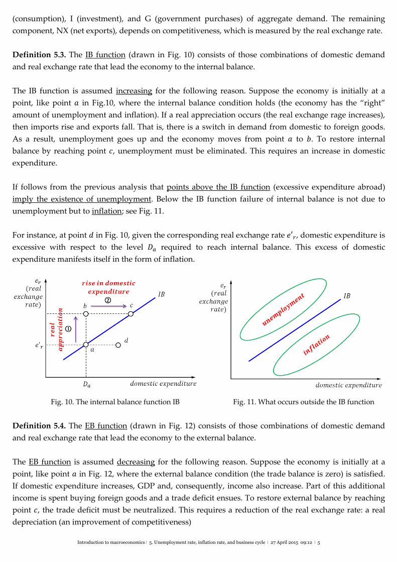
Definition 5.3. The IB function (drawn in Fig. 10) consists of those combinations of domestic demand
and real exchange rate that lead the economy to the internal balance.
The IB function is assumed increasing for the following reason. Suppose the economy is initially at a
point, like point � in Fig.10, where the internal balance condition holds (the economy has the “right”
amount of unemployment and inflation). If a real appreciation occurs (the real exchange rage increases),
then imports rise and exports fall. That is, there is a switch in demand from domestic to foreign goods.
As a result, unemployment goes up and the economy moves from point � to �. To restore internal
balance by reaching point �, unemployment must be eliminated. This requires an increase in domestic
expenditure.
If follows from the previous analysis that points above the IB function (excessive expenditure abroad)
imply the existence of unemployment. Below the IB function failure of internal balance is not due to
unemployment but to inflation; see Fig. 11.
For instance, at point � in Fig. 10, given the corresponding real exchange rate �′�, domestic expenditure is
excessive with respect to the level �� required to reach internal balance. This excess of domestic
expenditure manifests itself in the form of inflation.
Fig. 10. The internal balance function IB Fig. 11. What occurs outside the IB function
Definition 5.4. The EB function (drawn in Fig. 12) consists of those combinations of domestic demand
and real exchange rate that lead the economy to the external balance.
The EB function is assumed decreasing for the following reason. Suppose the economy is initially at a
point, like point � in Fig. 12, where the external balance condition (the trade balance is zero) is satisfied.
If domestic expenditure increases, GDP and, consequently, income also increase. Part of this additional
income is spent buying foreign goods and a trade deficit ensues. To restore external balance by reaching
point �, the trade deficit must be neutralized. This requires a reduction of the real exchange rate: a real
depreciation (an improvement of competitiveness)
Introduction to macroeconomics ǀ 5. Unemployment rate, inflation rate, and business cycle ǀ 27 April 2015 09:12 ǀ 6
If follows from the previous analysis that points above the EB function (excessive domestic expenditure)
generate a trade deficit. Below the EB function failure of external balance is not due to a trade deficit but
to trade surplus; see Fig. 13.
For instance, at point � in Fig. 12, given the corresponding level �� of domestic expenditure, the real
exchange rate is smaller than the value �′� required to reach external balance with ��. That is, the
economy is “too competitive” and therefore runs a trade surplus.
Fig. 12. The external balance function EB Fig. 13. What occurs outside the EB function
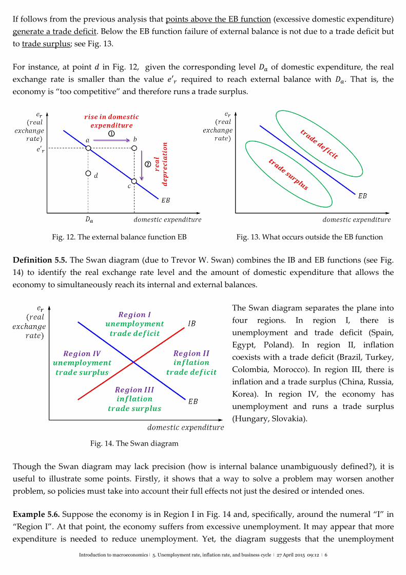
Definition 5.5. The Swan diagram (due to Trevor W. Swan) combines the IB and EB functions (see Fig.
14) to identify the real exchange rate level and the amount of domestic expenditure that allows the
economy to simultaneously reach its internal and external balances.
The Swan diagram separates the plane into
four regions. In region I, there is
unemployment and trade deficit (Spain,
Egypt, Poland). In region II, inflation
coexists with a trade deficit (Brazil, Turkey,
Colombia, Morocco). In region III, there is
inflation and a trade surplus (China, Russia,
Korea). In region IV, the economy has
unemployment and runs a trade surplus
(Hungary, Slovakia).
Fig. 14. The Swan diagram
Though the Swan diagram may lack precision (how is internal balance unambiguously defined?), it is
useful to illustrate some points. Firstly, it shows that a way to solve a problem may worsen another
problem, so policies must take into account their full effects not just the desired or intended ones.
Example 5.6. Suppose the economy is in Region I in Fig. 14 and, specifically, around the numeral “I” in
“Region I”. At that point, the economy suffers from excessive unemployment. It may appear that more
expenditure is needed to reduce unemployment. Yet, the diagram suggests that the unemployment
Introduction to macroeconomics ǀ 5. Unemployment rate, inflation rate, and business cycle ǀ 27 April 2015 09:12 ǀ 7
problem this economy faces is not solved by changing expenditure (increasing it) but by shifting
expenditure. To reach the intersection of the IB and EB lines, domestic expenditure must be reduced and
net exports increased (through depreciation). If only the unemployment problem is attacked by boosting
domestic expenditure, internal balance could be reached at a price: the trade deficit worsens.
Indeed, in an economy that lies in Region I in Fig. 14 moves horizontally towards the IB function (by
increasing domestic expenditure) to solve the unemployment problem, the consequence is that the
economy moves away from the EB function (the trade deficit worsens, as more expenditure lead to more
income and more income boosts imports).
And secondly, the Swan diagram alerts against the orthodox principle “one size fits all”, according to
which solutions to macroeconomic problems need not take into account particular features of the
economy suffering from those problems. To put it in a nutshell, the principle maintains that if it works
once, it works always.
Example 5.7. Suppose two economies are in Region I in Fig. 14, one situated on the letter “r” in “trade”
and the other on the letter “c” in “deficit”. If both economies want to meet the conditions of internal and
external balance, it is plain that both should reduce the real exchange rate (become more competitive to
reduce the trade deficit). But, to reach internal balance, the economy on r should expand domestic
expenditure, whereas the economy on c should contract domestic expenditure. Hence, there is not a
single recommendation for both economies to attain internal and external balance.
6. Involuntary unemployment
Definition 6.1. Involuntary unemployment is the unemployment that occurs when, at the prevailing
wage rate in the economy, there are people willing to work but are not given a job.
The models developed next illustrate basic reasons for the existence and persistence of involuntary
unemployment:
“too high” wage rates (classical or orthodox explanation);
insufficient labour demand, due to insufficient aggregate demand (Keynesian explanation);
existence of market power on the supply side (because of trade unions);
existence of labour discrimination; and
structural reasons (an economy does not exist to employ every one willing to be employed).
7. The orthodox (classical) labour market model
Definition 7.1. The orthodox labour market is a standard competitive market model in which “price” is
represented by the real wage � (the nominal or monetary wage W divided by some price level P, like the
CPI) and “quantity” is labour (labour supplied and demanded, where labour can be measured as
number of persons or as number of hours of work).
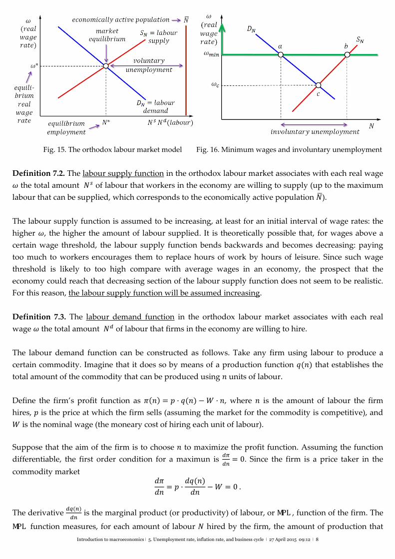
Fig. 15 represents graphically the orthodox labour market.
Introduction to macroeconomics ǀ 5. Unemployment rate, inflation rate, and business cycle ǀ 27 April 2015 09:12 ǀ 8
Fig. 15. The orthodox labour market model Fig. 16. Minimum wages and involuntary unemployment
Definition 7.2. The labour supply function in the orthodox labour market associates with each real wage
� the total amount �� of labour that workers in the economy are willing to supply (up to the maximum
labour that can be supplied, which corresponds to the economically active population ��).
The labour supply function is assumed to be increasing, at least for an initial interval of wage rates: the
higher �, the higher the amount of labour supplied. It is theoretically possible that, for wages above a
certain wage threshold, the labour supply function bends backwards and becomes decreasing: paying
too much to workers encourages them to replace hours of work by hours of leisure. Since such wage
threshold is likely to too high compare with average wages in an economy, the prospect that the
economy could reach that decreasing section of the labour supply function does not seem to be realistic.
For this reason, the labour supply function will be assumed increasing.
Definition 7.3. The labour demand function in the orthodox labour market associates with each real
wage � the total amount �� of labour that firms in the economy are willing to hire.
The labour demand function can be constructed as follows. Take any firm using labour to produce a
certain commodity. Imagine that it does so by means of a production function �(�) that establishes the
total amount of the commodity that can be produced using � units of labour.
Define the firm’s profit function as �(�)= � ·�(�)−� ·�, where � is the amount of labour the firm
hires, � is the price at which the firm sells (assuming the market for the commodity is competitive), and
� is the nominal wage (the moneary cost of hiring each unit of labour).
Suppose that the aim of the firm is to choose � to maximize the profit function. Assuming the function
differentiable, the first order condition for a maximun is ��
��= 0. Since the firm is a price taker in the
commodity market ��
��= � ·
��(�)
��−� = 0.
The derivative ��(�)
�� is the marginal product (or productivity) of labour, or MPL , function of the firm. The
MPL function measures, for each amount of labour � hired by the firm, the amount of production that
Introduction to macroeconomics ǀ 5. Unemployment rate, inflation rate, and business cycle ǀ 27 April 2015 09:12 ǀ 9
can be attributed to the last unit of labour in �. Loosely speaking, the MPL function indicates how much
an additional worker can produce.
It seems plausible that the first workers will be highly productive and that this productivity is increasing:
more workers can make better use of the firm’s means of production. When the production function �(�)
is initially convex, increasing � in a certain percentage makes � increase in a larger percentage, which
means that the derivative ��(�)
�� is increasing.
But it appears plausible that, eventually, simply adding more workers will not be enough to increase
MPL . Otherwise, a small plot of land could feed the whole world or a single factory produce all the
commodities the world consumes. Consequently, it is reasonable to expect that the firm’s MPL function
will become decreasing: each additional worker contributes to increase production but each time less.
Equivalently, to rise production in a given amount, the firm needs each time more workers owing to the
fact that each additional worker is less productive.
Example 7.4. If �(�)= 2 · ��/�, then MPL(�)=��(�)
��= 2 ·
�
�·��/��� = ���/� =
�
��/�. This function is
always downward sloping: a rise in � leads to a fall in MPL .
The profit maximizing condition for the firm is then � ·MPL(�)= �. Equivalently, MPL(�)= �/�. This
expression implicitly defines the firm’s labour demand function: the firm hires labour until the marginal
product of the last worker (what the firm obtains in real terms from hiring the worker) equals the cost (in
real terms) of the last worker (the real wage �/�).
Remark 7.5. The condition MPL = �/� lies behind the orthodox prescription that real wages should “get
in line” with productivity: workers cannot expect be granted a higher real wage without becoming more
productive. In fact, the condition MPL = �/� captures the idea that labour is paid according to the value
of its marginal productivity: � = � ·MPL (since MPL is amount of commodity produced and � is the
price of the commodity, � ·MPL is the monetary value of what the last worker hired produces).
Example 7.4 (continued). With MPL(�)=�
��/�, the condition MPL(�)= �/� amounts to
�
��/�=
�
�.
Solving for �,
� =1
(�/�)�or� =
��
��
This says that the demand for labour is stimulated by a rise in the price of the commodity the firm
produces or by a fall in the nominal wage rate. The expression � =�
(�/�)� represents the firm’s demand
for labour. Insofar as a rise in �
� causes a fall in the demand for labour �, the firm’s demand for labour is
a decreasing function of the real wage �
�.
Since the labour demand of each firm is inversely correlated with a certain wage rate, by disregarding
the fallacy of composition, one may jump to the conclusion that the aggregate demand for labour in an
economy is inversely correlated with the economy’s real wage. This is what Fig. 15 represents: the labour
demand function corresponding to the whole economy is assumed downward sloping: the higher the
real wage �, the lower the aggregate demand for labour ��.
Introduction to macroeconomics ǀ 5. Unemployment rate, inflation rate, and business cycle ǀ 27 April 2015 09:12 ǀ 10
Definition 7.6. The equilibrium real wage rate �* is the real wage rate such that labour supplied at �*
equals labour demanded at �*.
Given �*, there is no involuntary unemployment: everyone willing to get hired at �* is hired. The
difference �� − �* can be viewed as voluntary unemployment, as the people represented by �� − �*
regard the equilibrium wage rate as insufficient to encourage them to supply labour. On the other hand, �∗
��would be the participation rate.
8. Involuntary unemployment in the orthodox labour market model
Establishing a mininum real wage ���� above the equilibrium wage rate �* generates involuntary
unemployment in a competitive labour market. This possibility is shown in Fig. 16, where market
equilibrium occurs at point �. If the minimum wage rate ���� is set, the market state is no longer
represented by � but by �: although workers are willing to reach �, firms cannot be forced to hire more
workers than the amount given by �. At the prevailing wage rate ���� there is an excess supply,
interpreted as involuntary unemployment.
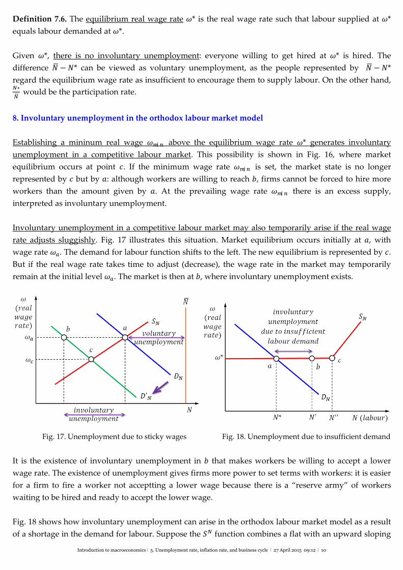
Involuntary unemployment in a competitive labour market may also temporarily arise if the real wage
rate adjusts sluggishly. Fig. 17 illustrates this situation. Market equilibrium occurs initially at �, with
wage rate ��. The demand for labour function shifts to the left. The new equilibrium is represented by �.
But if the real wage rate takes time to adjust (decrease), the wage rate in the market may temporarily
remain at the initial level ��. The market is then at �, where involuntary unemployment exists.
Fig. 17. Unemployment due to sticky wages Fig. 18. Unemployment due to insufficient demand
It is the existence of involuntary unemployment in � that makes workers be willing to accept a lower
wage rate. The existence of unemployment gives firms more power to set terms with workers: it is easier
for a firm to fire a worker not acceptting a lower wage because there is a “reserve army” of workers
waiting to be hired and ready to accept the lower wage.
Fig. 18 shows how involuntary unemployment can arise in the orthodox labour market model as a result
of a shortage in the demand for labour. Suppose the �� function combines a flat with an upward sloping
Introduction to macroeconomics ǀ 5. Unemployment rate, inflation rate, and business cycle ǀ 27 April 2015 09:12 ǀ 11
section. The flact section at real wage �* would mean that, when the real wage is �*, (i) workers are, in
principle, indifferent between supplying labour or not, and (ii) some random variable determines the
amount actually supplied. Market equilibrium occurs at �, where employment is �*. If workers finally
choose to supply �′ (effective labour supply given by �), there is involuntary unemployment represented
by the difference �� − �*.
What the orthodox model seems to miss is that firms do not hire workers because they aim at
accumulating workers. The labour force is a means to produce commodities and obtain a profit by selling
the commodities produced. For that reason, the demand for labour by firms is a derived demand: it
arises as an intermediate step in the process of reaching the firms’ final goal, which is making profits.
Accordingly, the demand for labour crucially depends on sales expectations: no matter how “cheap”
labour is, workers will not be hired if firms do not expect to sell what these workers would produce. This
is the fundamental insight behind heredox explanation of involuntary unemployment: making cheaper
to firms the production of commodities by reducing the wage rate is not in general enough to encourage
firms to hire more workers. The crucial factor to induce firms to hire more workers is that firms expect to
sell what the additional workers will produce.
9. Involuntary unemployment and trade unions
http://en.wikipedia.org/wiki/Trade_unions_in_the_United_Kingdom
Supply‐side market power in the labour market is typically associated with the existence of trade unions.
For any given amount of labour �, the wage rate unions demand to supply � will be higher than the
wage rate dictated by the supply of labour function. This follows from the fact that unions (since they
can organize strikes) have more bargaining power over wages than individual workers
As a result, the function ������� associating with each amount of labour � the wage rate that unions will
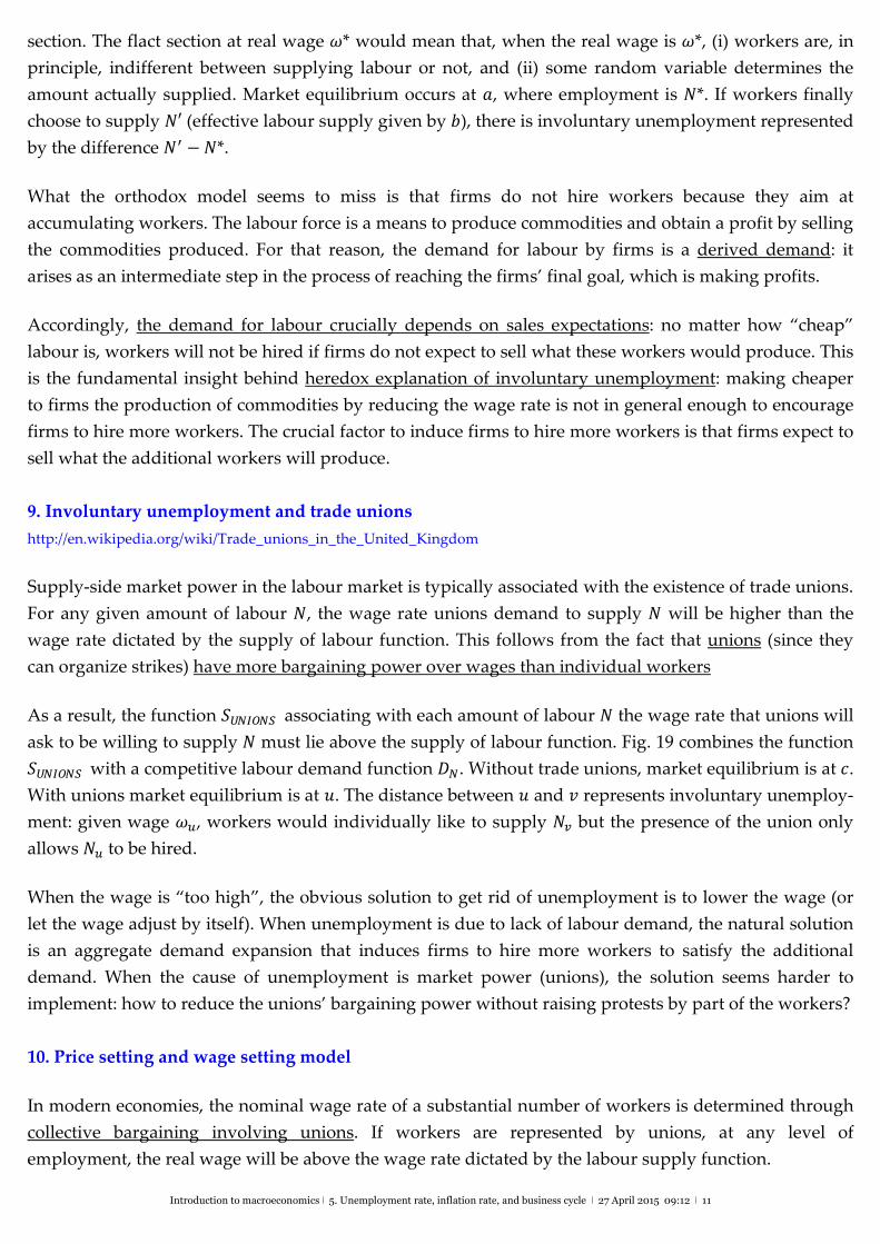
ask to be willing to supply � must lie above the supply of labour function. Fig. 19 combines the function
������� with a competitive labour demand function ��. Without trade unions, market equilibrium is at �.
With unions market equilibrium is at �. The distance between � and � represents involuntary unemploy‐
ment: given wage �� , workers would individually like to supply �� but the presence of the union only
allows �� to be hired.
When the wage is “too high”, the obvious solution to get rid of unemployment is to lower the wage (or
let the wage adjust by itself). When unemployment is due to lack of labour demand, the natural solution
is an aggregate demand expansion that induces firms to hire more workers to satisfy the additional
demand. When the cause of unemployment is market power (unions), the solution seems harder to
implement: how to reduce the unions’ bargaining power without raising protests by part of the workers?
10. Price setting and wage setting model
In modern economies, the nominal wage rate of a substantial number of workers is determined through
collective bargaining involving unions. If workers are represented by unions, at any level of
employment, the real wage will be above the wage rate dictated by the labour supply function.
Introduction to macroeconomics ǀ 5. Unemployment rate, inflation rate, and business cycle ǀ 27 April 2015 09:12 ǀ 12
Fig. 19. Unemployment due to trade unions Fig. 20. The PS‐WS employment model
It is assumed that unions establish the real wage using a wage setting function �� sloping upward and
lying above the labour supply function ��; see Fig. 20. The higher the unions’ bargaining power, the
larger the vertical distance between between �� and ��.
The assumption that �� is increasing follows from the interpretation of unemployment as a device to
discipline the unions’ demands for higher wages. When employment � is small, unemployment is high,
for which reason the bargaining power of unions is small: firms could fire workers with high
unemployment because there are workers willing to accept the conditions that fired workers would like
to improve. With small bargaining power of unions come lower real wages. Conversely, when
employment � is high, unemployment is low, the bargaining power of unions is high and, as a result,
firms are more willing to accept higher wages: if they fire a worker, it is harder to replaced him or her
due to the low unemployment.
Whereas workers (through unions) are assumed to set the nominal wage, firms are supposed to fix the
prices of the commodities they produce. A simple price setting rule consists of adding a mark‐up ��> 0
to labour costs:
� = (1+ ��)·�
���.
�is measured in money (EUR ) and ��� in units of product per worker. Thus, �
��� is the money paid to
workers divided by what they produce. In other words, �
��� is the (labour) cost of producing a unit of the
commodity (unit labour costs). Rearranging,
1
1 + ��·��� =
�
�.
Given that ��> 0, it must that �
����< 1. Therefore, for some � > 0,
�
����= 1− �. Consequently,
(1− �)·��� =�
�.
In sum,
��� =�
�+ � ·��� .
production per worker =real wage per worker +real profit per worker
Introduction to macroeconomics ǀ 5. Unemployment rate, inflation rate, and business cycle ǀ 27 April 2015 09:12 ǀ 13
Under perfect competition in the labour and product markets, �
�= ��� . If the prices of goods are set by
firms as a marking up of labour costs per worker, then �
�= (1− �)·��� . This equation represents the
price setting function ��. Since 0 < � < 1, �
�= (1− �)·��� means that
�
�< ��� . The parameter �
measures the amount of the workers’ productivity appropiated by the firms
As the ��� function is downward sloping, the �� function is downward sloping as well. �� lies below
��� because �� is a fraction of ��� (the constant 1− � is smaller than 1); see Fig. 6. In this figure the
wage and price setting decisions are consistent only at point �, where, at the prevailing wage ��, there is
involuntary unemployment represented by the difference �� − ��.
11. Segmented labour market model
Suppose workers may have or not some (perhaps economically irrelevant) feature that firms (the owners
of firms to be more accurate) may like or not (for instance, being a man or not).
Firms classify workers in two types (I and II) depending on whether they possess the feature or not.
Some firms (type I firms) prefer type I workers; the rest (type II firms) prefer type II workers.
Each type of firms defines a different (competitive) labour market. Workers are unaware of the fact that
there are two types of firms. From their perspective, the labour market is not segmented.
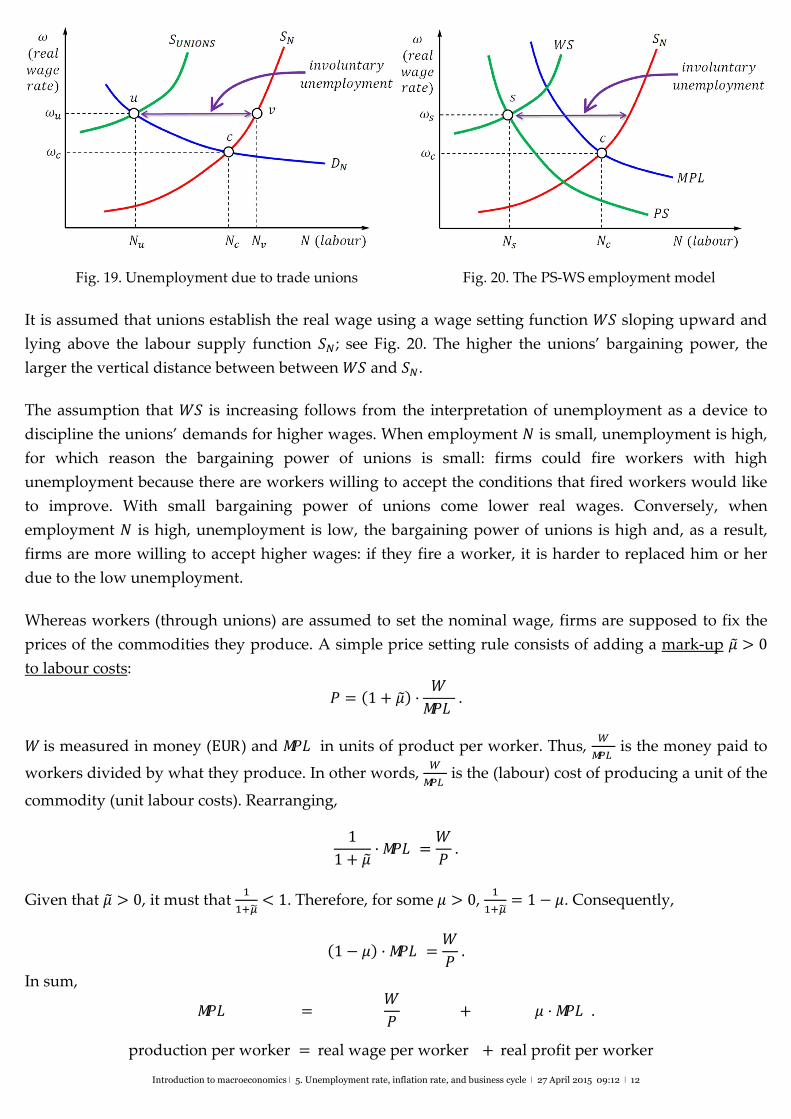
Example 11.1. The analysis proceeds in terms of a numerical example, with the following characteristics.
Supply of labour function of type I workers: ��� = 4 ·� (� is the real wage rate).
Demand for labour function of type I firms: ��� = 60− 2 ·� (��
� = 0 if � > 30).
Market equilibrium (type I): (��,��)= (40,10).
Supply of labour function of type II workers: ���� = 12·�.
Demand for labour function of type II firms: ���� = 80− 4·� (���
� = 0 if � > 20).
Market equilibrium (type II): (���,���)= (60,5).
In this case, ��
�����=
�
�= 40% of employment corresponds to type I workers and
��
�����=
�
�= 60% to type
II. Using these weights, the average real wage rate would be �� =�
�·�� +
�
�·��� =
�
�·10+
�
�·5 = 7.
At �� = 7, no more type I workers than are actually employed would like to be hired. But, at �� = 7, type
II workers would like to supply ���� = 12·�� = 84. Since employment of type II workers equals ��� = 60,
involuntary unemployment appears to be ����(�� = 7)− ��� = 84− 60= 24 (unemployment rate =
24 (24+ �� + ���)= 19.3%⁄ ).
Fig. 21 represents Example 11.1 graphically. Though each segment is in equilibrium, there is a sense in
which involuntary unemployment exists.
Introduction to macroeconomics ǀ 5. Unemployment rate, inflation rate, and business cycle ǀ 27 April 2015 09:12 ǀ 14
Fig. 21. Segmented labour market example
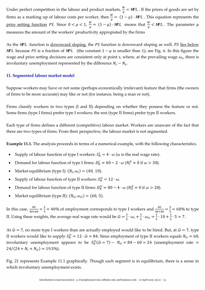
12. The employmentproductionincomespending (E-PIS) model
It postulates three linear relations linking employment with production, income, and spending.
�� relation (production employment): establishes the amount of employment required to reach a
certain GDP level; see Fig. 22. �� relation (income employment): identifies the amount of labour supplied for every value of
aggregate income; see Fig. 24. �� relation (employment expenditure): indicates the aggregate level of spending associated with
any given amount of employment; see Fig. 23.
Fig. 22. The production‐employment relation Fig. 23. The employment‐expenditure relation
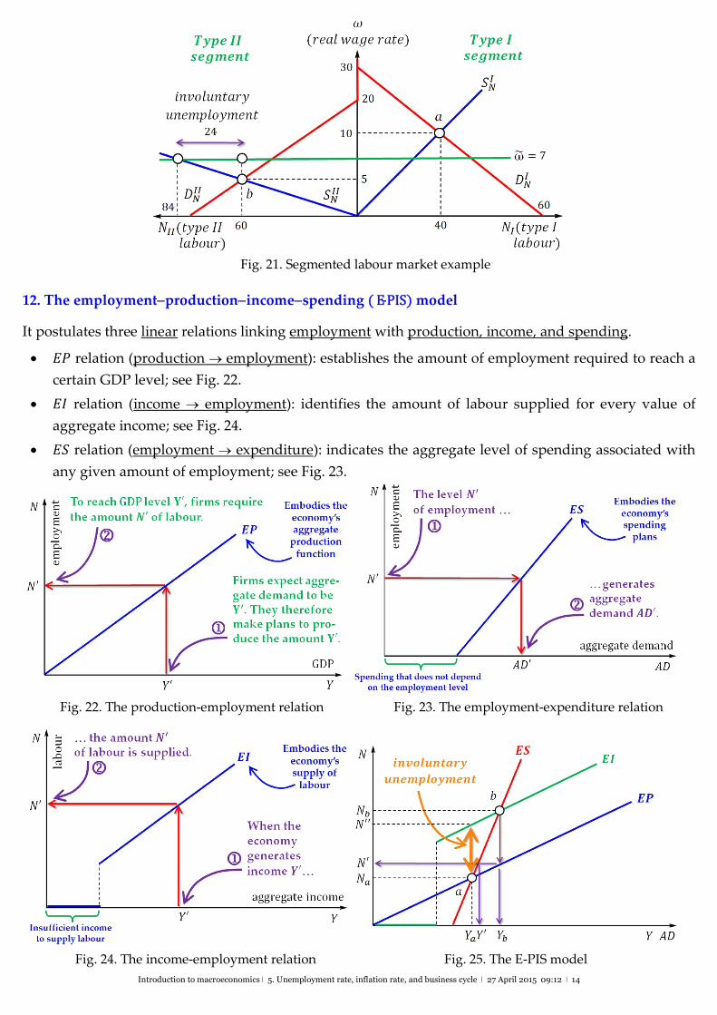
Fig. 24. The income‐employment relation Fig. 25. The E‐PIS model
Introduction to macroeconomics ǀ 5. Unemployment rate, inflation rate, and business cycle ǀ 27 April 2015 09:12 ǀ 15
When the three relations are drawn simultaneously, as in Fig. 25, there is no point at which the three
lines intersect. Without delving into details, assume that the solution is found at a point when two lines
intersect. Leaving the origin aside, there are two candidates: point � and point �.
Point � is not stable in the sense that it is not self‐sustained). At �, employment is �� and aggregate
demand is ��. But, according to ��, to produce ��, the economy only needs the amount �� < �� of
labour. Hence, � does not represent a consistent state of the economy.
At �, employment is �� and aggregate demand is ��. To generate a GDP equal to �� firms demand
exactly the amount �� of labour. In addition, the level �� of employment generates precisely the level ��
of aggregate demand. This state of the economy appears self‐consistent and stable.
The problem is that there is involuntary unemployment at point �. Given income ��, workers would like
to supply the amount ��� of labour. Since employment at � is only ��, ��� − �� defines the level of
involuntary unemployment. Further investigations of the model are left as an exercise (for instance, what
shifts in the lines would reduce involuntary unemployment?).
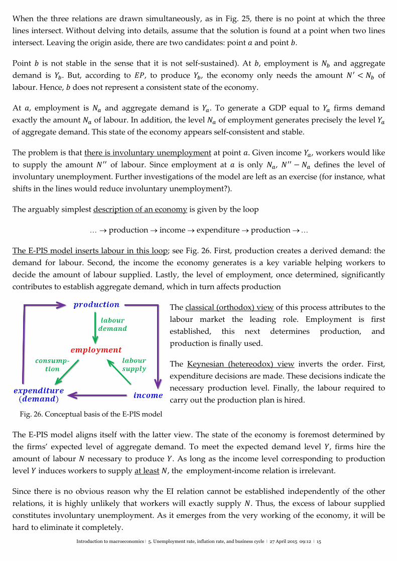
The arguably simplest description of an economy is given by the loop
production income expenditure production
The E‐PIS model inserts labour in this loop; see Fig. 26. First, production creates a derived demand: the
demand for labour. Second, the income the economy generates is a key variable helping workers to
decide the amount of labour supplied. Lastly, the level of employment, once determined, significantly
contributes to establish aggregate demand, which in turn affects production
The classical (orthodox) view of this process attributes to the
labour market the leading role. Employment is first
established, this next determines production, and
production is finally used.
The Keynesian (hetereodox) view inverts the order. First,
expenditure decisions are made. These decisions indicate the
necessary production level. Finally, the labour required to
carry out the production plan is hired. Fig. 26. Conceptual basis of the E‐PIS model
The E‐PIS model aligns itself with the latter view. The state of the economy is foremost determined by
the firms’ expected level of aggregate demand. To meet the expected demand level �, firms hire the
amount of labour � necessary to produce �. As long as the income level corresponding to production
level � induces workers to supply at least �, the employment‐income relation is irrelevant.
Since there is no obvious reason why the EI relation cannot be established independently of the other
relations, it is highly unlikely that workers will exactly supply �. Thus, the excess of labour supplied
constitutes involuntary unemployment. As it emerges from the very working of the economy, it will be
hard to eliminate it completely.

Introduction to macroeconomics ǀ 5. Unemployment rate, inflation rate, and business cycle ǀ 27 April 2015 09:12 ǀ 16
13. Business cycle
Definition 13.1. The business cycle consists of the ups and downs in overall economic activity.
If real GDP is considered a good indicator of overall economic activity, then the business cycle can be
roughly identified with fluctuations of (real) GDP. Fig. 27 shows a stylized view of the business cycle.
Definition 13.2. The period during
which economic activity falls is a
contraction or a recession.
A depression is a severe recession.
The trough is the lowest point in the
recession.
Definition 13.3. The period during
which economic activity grows is an
expansion or a boom.
Fig. 27. Stylized view of the business cycle (Source: Wikipedia)
The highest point in the boom is called the peak. A business cycle is given by a decline‐recovery
sequence from peak to peak or by a recovery‐decline sequence from trough to trough.
An empirical regularity of modern economies is that they experience business cycles (see Fig. 28). Basic
questions in macroeconomics are: (i) what causes the business cycle?; (ii) can it be smoothed?; (iii) if so,
how can the business cycle be smoothed?
Fig. 28. Eurozone and US business cycles
http://www.cepr.org/data/eurocoin/recession/ http://www.nber.org/cycles/cyclesmain.html
Introduction to macroeconomics ǀ 5. Unemployment rate, inflation rate, and business cycle ǀ 27 April 2015 09:12 ǀ 17
14. Classifying macroeconomic variables according to the direction of movement during the cycle
All cycles are alike in that there is a tendency of many variables to correlate their behaviour (move
together) as the cycle unfolds.
Definition 14.1. A procyclical variable tends to move in the same direction as overall economic activity
(up in an expansion, down in a contraction).
Definition 14.2. A countercyclical variable tends to move in opposite direction to overall economic
activity.
Definition 14.3. An acyclical variable is one that shows no typical pattern over the business cycle.
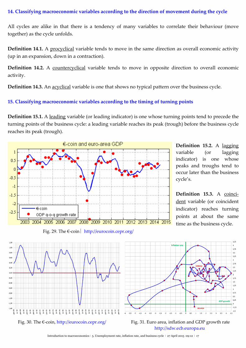
15. Classifying macroeconomic variables according to the timing of turning points
Definition 15.1. A leading variable (or leading indicator) is one whose turning points tend to precede the
turning points of the business cycle: a leading variable reaches its peak (trough) before the business cycle
reaches its peak (trough).
Definition 15.2. A lagging
variable (or lagging
indicator) is one whose
peaks and troughs tend to
occur later than the business
cycle’s.
Definition 15.3. A coinci‐
dent variable (or coincident
indicator) reaches turning
points at about the same
time as the business cycle.
Fig. 29. The €‐coin http://eurocoin.cepr.org/
Fig. 30. The €‐coin, http://eurocoin.cepr.org/ Fig. 31. Euro area, inflation and GDP growth rate
http://sdw.ecb.europa.eu
Introduction to macroeconomics ǀ 5. Unemployment rate, inflation rate, and business cycle ǀ 27 April 2015 09:12 ǀ 18
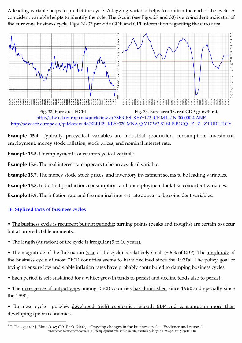
A leading variable helps to predict the cycle. A lagging variable helps to confirm the end of the cycle. A
coincident variable helpts to identify the cyle. The €‐coin (see Figs. 29 and 30) is a coincident indicator of
the eurozone business cycle. Figs. 31‐33 provide GDP and CPI information regarding the euro area.
Fig. 32. Euro area HCPI Fig. 33. Euro area 18, real GDP growth rate
http://sdw.ecb.europa.eu/quickview.do?SERIES_KEY=122.ICP.M.U2.N.000000.4.ANR
http://sdw.ecb.europa.eu/quickview.do?SERIES_KEY=320.MNA.Q.Y.I7.W2.S1.S1.B.B1GQ._Z._Z._Z.EUR.LR.GY
Example 15.4. Typically procyclical variables are industrial production, consumption, investment,
employment, money stock, inflation, stock prices, and nominal interest rate.
Example 15.5. Unemployment is a countercyclical variable.
Example 15.6. The real interest rate appears to be an acyclical variable.
Example 15.7. The money stock, stock prices, and inventory investment seems to be leading variables.
Example 15.8. Industrial production, consumption, and unemployment look like coincident variables. Example 15.9. The inflation rate and the nominal interest rate appear to be coincident variables.
16. Stylized facts of business cycles
• The business cycle is recurrent but not periodic: turning points (peaks and troughs) are certain to occur
but at unpredictable moments.
• The length (duration) of the cycle is irregular (5 to 10 years).
• The magnitude of the fluctuation (size of the cycle) is relatively small (5% of GDP). The amplitude of
the business cycle of most OECDcountries seems to have declined since the 1970s1. The policy goal of
trying to ensure low and stable inflation rates have probably contributed to damping business cycles.
• Each period is self‐sustained for a while: growth tends to persist and decline tends also to persist.
• The divergence of output gaps among OECDcountries has diminished since 1960and specially since
the 1990s.
• Business cycle puzzle2: developed (rich) economies smooth GDPand consumption more than
developing (poor) economies.
1 T. Dalsgaard; J. Elmeskov; C‐Y Park (2002): “Ongoing changes in the business cycle – Evidence and causes”.
Introduction to macroeconomics ǀ 5. Unemployment rate, inflation rate, and business cycle ǀ 27 April 2015 09:12 ǀ 19
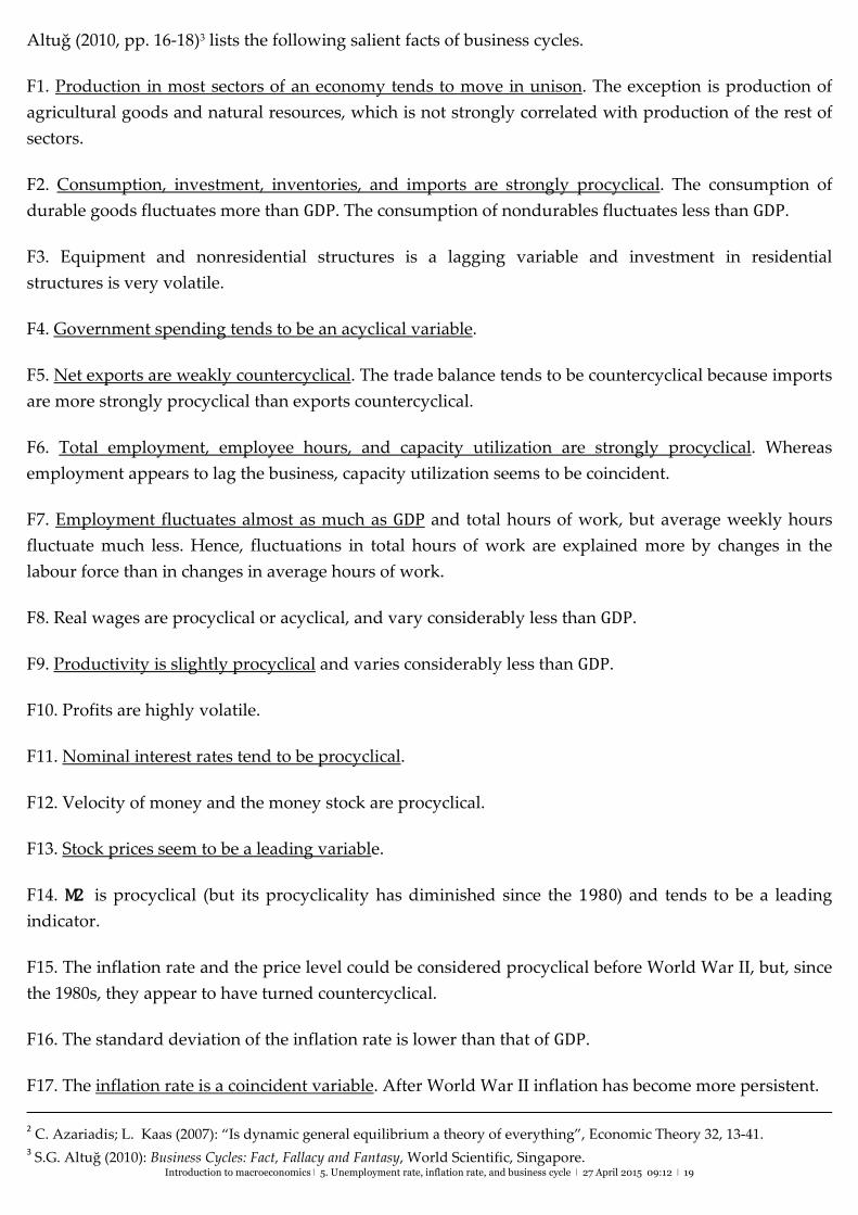
Altuğ (2010, pp. 16‐18)3 lists the following salient facts of business cycles.
F1. Production in most sectors of an economy tends to move in unison. The exception is production of
agricultural goods and natural resources, which is not strongly correlated with production of the rest of
sectors.
F2. Consumption, investment, inventories, and imports are strongly procyclical. The consumption of
durable goods fluctuates more than GDP. The consumption of nondurables fluctuates less than GDP.
F3. Equipment and nonresidential structures is a lagging variable and investment in residential
structures is very volatile.
F4. Government spending tends to be an acyclical variable.
F5. Net exports are weakly countercyclical. The trade balance tends to be countercyclical because imports
are more strongly procyclical than exports countercyclical.
F6. Total employment, employee hours, and capacity utilization are strongly procyclical. Whereas
employment appears to lag the business, capacity utilization seems to be coincident.
F7. Employment fluctuates almost as much as GDP and total hours of work, but average weekly hours
fluctuate much less. Hence, fluctuations in total hours of work are explained more by changes in the
labour force than in changes in average hours of work.
F8. Real wages are procyclical or acyclical, and vary considerably less than GDP.
F9. Productivity is slightly procyclical and varies considerably less than GDP.
F10. Profits are highly volatile.
F11. Nominal interest rates tend to be procyclical.
F12. Velocity of money and the money stock are procyclical.
F13. Stock prices seem to be a leading variable.
F14. M2 is procyclical (but its procyclicality has diminished since the 1980) and tends to be a leading
indicator.
F15. The inflation rate and the price level could be considered procyclical before World War II, but, since
the 1980s, they appear to have turned countercyclical.
F16. The standard deviation of the inflation rate is lower than that of GDP.
F17. The inflation rate is a coincident variable. After World War II inflation has become more persistent.
2 C. Azariadis; L. Kaas (2007): “Is dynamic general equilibrium a theory of everything”, Economic Theory 32, 13‐41.
3 S.G. Altuğ (2010): Business Cycles: Fact, Fallacy and Fantasy, World Scientific, Singapore.
Introduction to macroeconomics ǀ 5. Unemployment rate, inflation rate, and business cycle ǀ 27 April 2015 09:12 ǀ 20
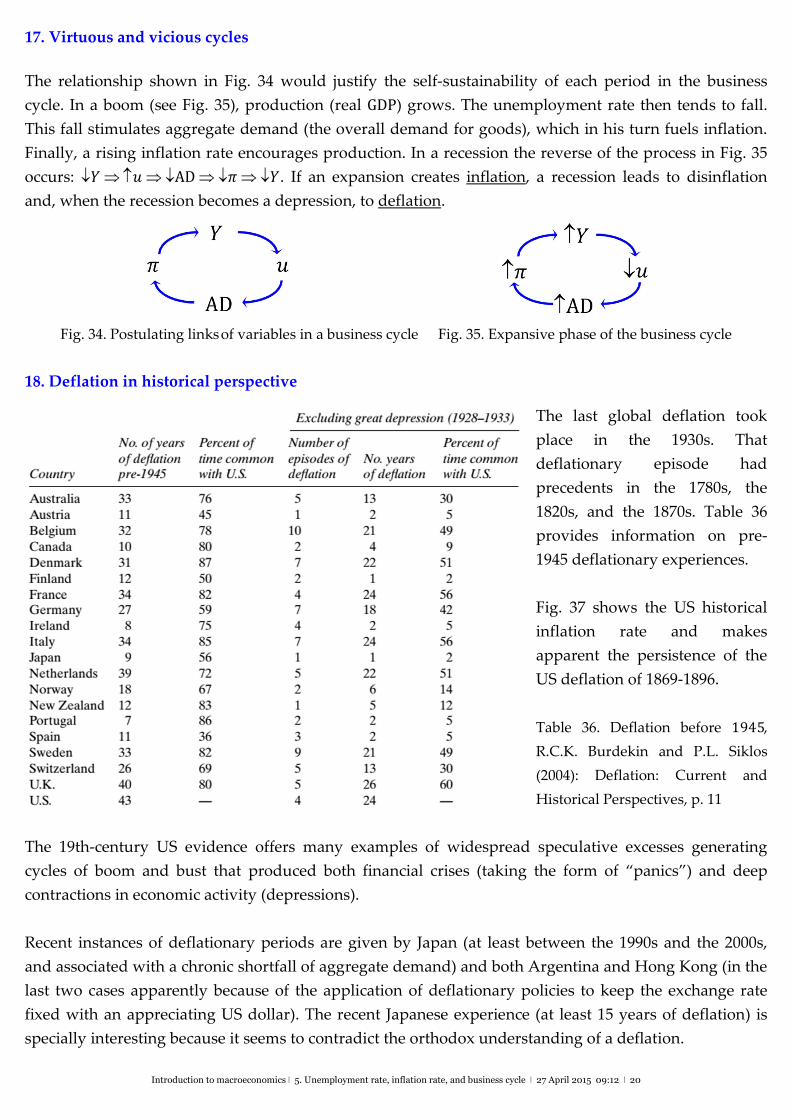
17. Virtuous and vicious cycles
The relationship shown in Fig. 34 would justify the self‐sustainability of each period in the business
cycle. In a boom (see Fig. 35), production (real GDP) grows. The unemployment rate then tends to fall.
This fall stimulates aggregate demand (the overall demand for goods), which in his turn fuels inflation.
Finally, a rising inflation rate encourages production. In a recession the reverse of the process in Fig. 35
occurs: ��AD��. If an expansion creates inflation, a recession leads to disinflation
and, when the recession becomes a depression, to deflation.
Fig. 34. Postulating links of variables in a business cycle Fig. 35. Expansive phase of the business cycle
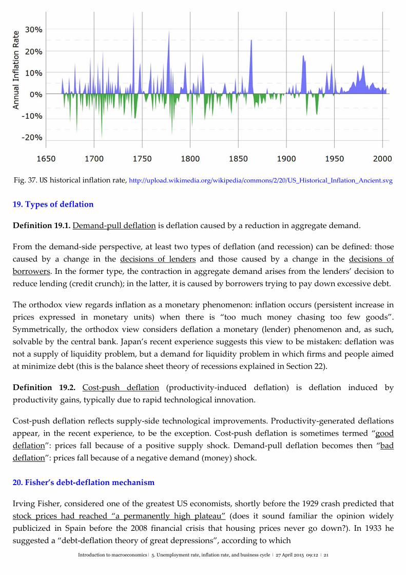
18. Deflation in historical perspective
The last global deflation took
place in the 1930s. That
deflationary episode had
precedents in the 1780s, the
1820s, and the 1870s. Table 36
provides information on pre‐
1945 deflationary experiences.
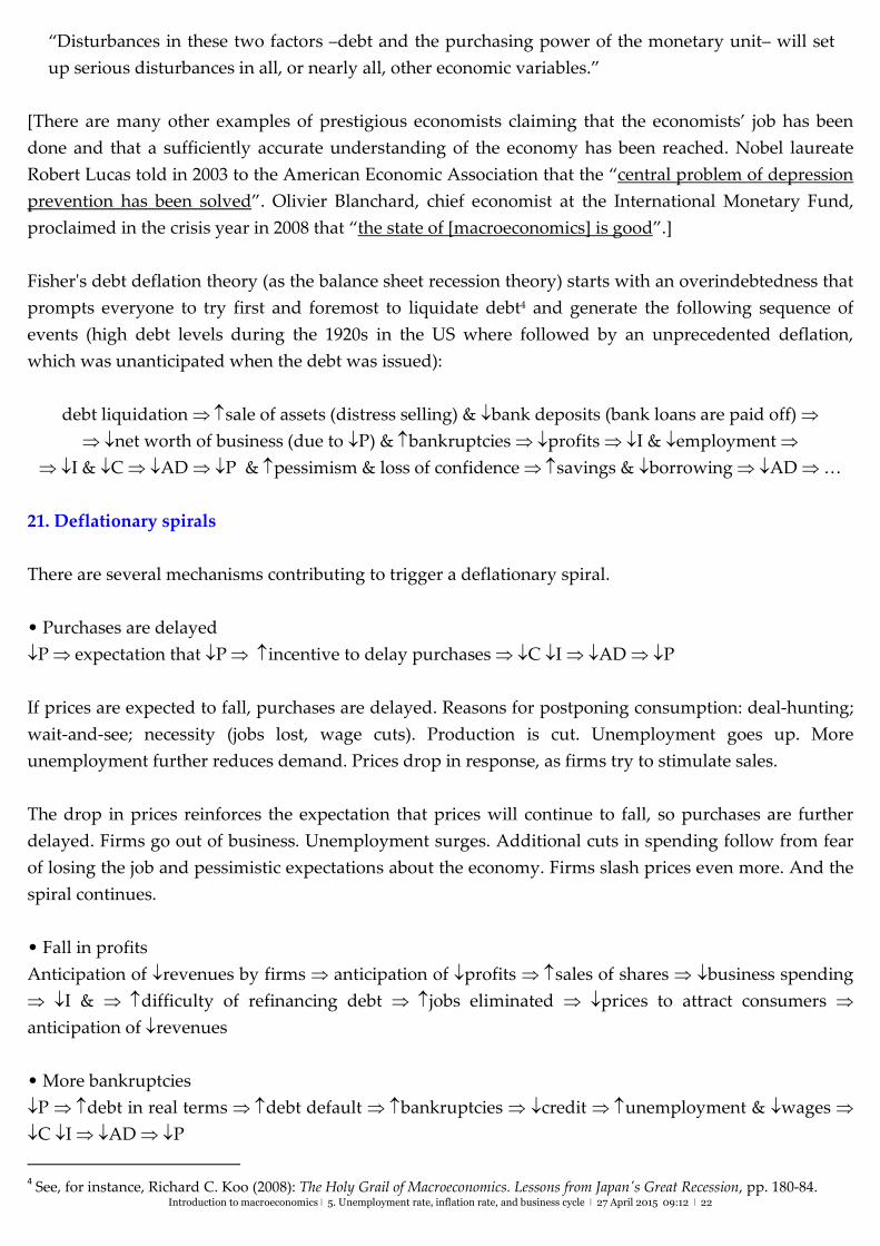
Fig. 37 shows the US historical
inflation rate and makes
apparent the persistence of the
US deflation of 1869‐1896.
Table 36. Deflation before 1945,
R.C.K. Burdekin and P.L. Siklos
(2004): Deflation: Current and
Historical Perspectives, p. 11
The 19th‐century US evidence offers many examples of widespread speculative excesses generating
cycles of boom and bust that produced both financial crises (taking the form of “panics”) and deep
contractions in economic activity (depressions).
Recent instances of deflationary periods are given by Japan (at least between the 1990s and the 2000s,
and associated with a chronic shortfall of aggregate demand) and both Argentina and Hong Kong (in the
last two cases apparently because of the application of deflationary policies to keep the exchange rate
fixed with an appreciating US dollar). The recent Japanese experience (at least 15 years of deflation) is
specially interesting because it seems to contradict the orthodox understanding of a deflation.
Introduction to macroeconomics ǀ 5. Unemployment rate, inflation rate, and business cycle ǀ 27 April 2015 09:12 ǀ 21
Fig. 37. US historical inflation rate, http://upload.wikimedia.org/wikipedia/commons/2/20/US_Historical_Inflation_Ancient.svg
19. Types of deflation
Definition 19.1. Demand‐pull deflation is deflation caused by a reduction in aggregate demand.
From the demand‐side perspective, at least two types of deflation (and recession) can be defined: those
caused by a change in the decisions of lenders and those caused by a change in the decisions of
borrowers. In the former type, the contraction in aggregate demand arises from the lenders’ decision to
reduce lending (credit crunch); in the latter, it is caused by borrowers trying to pay down excessive debt.
The orthodox view regards inflation as a monetary phenomenon: inflation occurs (persistent increase in
prices expressed in monetary units) when there is “too much money chasing too few goods”.
Symmetrically, the orthodox view considers deflation a monetary (lender) phenomenon and, as such,
solvable by the central bank. Japan’s recent experience suggests this view to be mistaken: deflation was
not a supply of liquidity problem, but a demand for liquidity problem in which firms and people aimed
at minimize debt (this is the balance sheet theory of recessions explained in Section 22).
Definition 19.2. Cost‐push deflation (productivity‐induced deflation) is deflation induced by
productivity gains, typically due to rapid technological innovation.
Cost‐push deflation reflects supply‐side technological improvements. Productivity‐generated deflations
appear, in the recent experience, to be the exception. Cost‐push deflation is sometimes termed “good
deflation”: prices fall because of a positive supply shock. Demand‐pull deflation becomes then “bad
deflation”: prices fall because of a negative demand (money) shock.
20. Fisher’s debt‐deflation mechanism
Irving Fisher, considered one of the greatest US economists, shortly before the 1929 crash predicted that
stock prices had reached “a permanently high plateau” (does it sound familiar the opinion widely
publicized in Spain before the 2008 financial crisis that housing prices never go down?). In 1933 he
suggested a “debt‐deflation theory of great depressions”, according to which
Introduction to macroeconomics ǀ 5. Unemployment rate, inflation rate, and business cycle ǀ 27 April 2015 09:12 ǀ 22
“Disturbances in these two factors –debt and the purchasing power of the monetary unit– will set
up serious disturbances in all, or nearly all, other economic variables.”
[There are many other examples of prestigious economists claiming that the economists’ job has been
done and that a sufficiently accurate understanding of the economy has been reached. Nobel laureate
Robert Lucas told in 2003 to the American Economic Association that the “central problem of depression
prevention has been solved”. Olivier Blanchard, chief economist at the International Monetary Fund,
proclaimed in the crisis year in 2008 that “the state of [macroeconomics] is good”.]
Fisher's debt deflation theory (as the balance sheet recession theory) starts with an overindebtedness that
prompts everyone to try first and foremost to liquidate debt4 and generate the following sequence of
events (high debt levels during the 1920s in the US where followed by an unprecedented deflation,
which was unanticipated when the debt was issued):
debt liquidation sale of assets (distress selling) & bank deposits (bank loans are paid off)
net worth of business (due to P) & bankruptcies profits I & employment
I & C AD P & pessimism & loss of confidence savings & borrowing AD …
21. Deflationary spirals
There are several mechanisms contributing to trigger a deflationary spiral.
• Purchases are delayed
P expectation that P incentive to delay purchases C I AD P
If prices are expected to fall, purchases are delayed. Reasons for postponing consumption: deal‐hunting;
wait‐and‐see; necessity (jobs lost, wage cuts). Production is cut. Unemployment goes up. More
unemployment further reduces demand. Prices drop in response, as firms try to stimulate sales.
The drop in prices reinforces the expectation that prices will continue to fall, so purchases are further
delayed. Firms go out of business. Unemployment surges. Additional cuts in spending follow from fear
of losing the job and pessimistic expectations about the economy. Firms slash prices even more. And the
spiral continues.
• Fall in profits
Anticipation of revenues by firms anticipation of profits sales of shares business spending
I & difficulty of refinancing debt jobs eliminated prices to attract consumers
anticipation of revenues
• More bankruptcies
P debt in real terms debt default bankruptcies credit unemployment & wages
C I AD P
4 See, for instance, Richard C. Koo (2008): The Holy Grail of Macroeconomics. Lessons from Japan's Great Recession, pp. 180‐84.
Introduction to macroeconomics ǀ 5. Unemployment rate, inflation rate, and business cycle ǀ 27 April 2015 09:12 ǀ 23
In a deflation, the real value of nominal debt increases: since money gains purchasing power, monetary
payments involve a higher transfer of purchasing power. People and firms that are highly indebted
decrease expenditures to cope with the higher value (in real terms) of their debts.
Debt deleveraging may substantially contribute to sustain a deflation process (Spain in 2008‐14?). If
businessmen think deflation will persist, they may delay investment projects (less spending) and/or close
down factories (higher unemployment).
• Wealth reduction
P debt default purchases of financial assets prices of financial assets wealth C I
AD P
prices of financial assets collateral (due to wealth) loans C I AD P
Under a deflation, falling prices cause a drop in the firms’ profits. This reduces the value of shares, so the
financial wealth of consumers decrease. Morevoer, deflation discourages borrowing money. A declining
salary lowers the repayment chances. A fall in prices means paying the loan back with money that is
worth more than the borrowed money.
Summarizing, deflation mechanisms exacerbating deflationary pressures include:
financial distress caused by falling prices;
credit restriction;
difficulties to pay back money borrowed at a time when prices were higher; and
reverse causation: asset price deflation leading to CPI deflation
To combat inflation, further rises of the interest rate are always possible. To combat deflation (trying to
stimulate spending), the (nominal) interest rate cannot be below zero (Japan in the 1990s), so monetary
policy becomes ineffective.
Deflation also affects negatively the government: High debt/Y & Y taxes collected G and/or
tax rates AD P & Y debt/Y (this is the current situation in Spain)
22. The balance sheet recession theory
Definition 22.1. Suggested by Richard Koo (see footnote 4) to explain Japan’s recent deflation, the
balance sheet recession theory holds that: (i) a fall in asset prices forces a shift in the focus of businesses
from profit maximization to debt minimization; and (ii) the shift initiates a spiral of declining aggregate
demand and leaves the economy unresponsive to changes in interest rates.
In Fisher’s explanation, deflation is the driver of the recession and the real sector is affected after many
steps (price and monetary changes occur first). In Koo’s explanation, the driving force behind the reces‐
sion is the fall in the value of assets and deflation is an effect not a cause of the recession: in a balance
sheet recession, GDP declines first, as firms stop borrowing and spending, and redirect cash flows to
debt repayment. As a result, demand drops, the economy slumps, and prices (of goods and assets) fall.
The contraction in asset prices ignites a vicious cycle by making more urgent for firms to reduce debt.
Introduction to macroeconomics ǀ 5. Unemployment rate, inflation rate, and business cycle ǀ 27 April 2015 09:12 ǀ 24
Fisher’s process relies on a fall in prices faster than the debt contraction: for debt to grow in real terms, a
reduction in nominal debt by �% must be accompanied by a drop in prices greater than �%. In Koo’s
view the source of the problem is the contraction in the firms’ borrowing.
Example 22.2. Suppose a firm has a nominal debt of �=1,000 EUR and the price level is �=100. Then,
in real terms, the firm owes �/�=1,000/100=10. Imagine that the firm pays 10% of the debt but the
price level falls by 20%. Now the firm owes �′=900 EUR and the price level is �′=80. Consequently, in
real terms, the firm’s debt is �′/�′=900/80=11.25. Thus, the firm’s real debt has increased (by 12.5%)
despite the fact that the debt has been lowered (by 10%) in nominal terms.
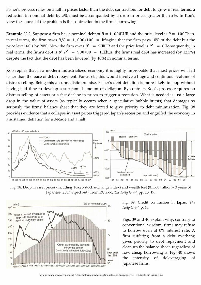
Koo replies that in a modern industrialized economy it is highly improbable that most prices will fall
faster than the pace of debt repayment. For assets, this would involve a huge and continuous volume of
distress selling. Being this an unrealistic premise, Fisher's debt deflation is more likely to stop without
having had time to develop a substantial amount of deflation. By contrast, Koo’s process requires no
distress selling of assets or a fast decline in prices to trigger a recession. What is needed is just a large
drop in the value of assets (as typically occurs when a speculative bubble bursts) that damages so
seriously the firms’ balance sheet that they are forced to give priority to debt minimization. Fig. 38
provides evidence that a collapse in asset prices triggered Japan’s recession and engulfed the economy in
a sustained deflation for a decade and a half.
Fig. 38. Drop in asset prices (incuding Tokyo stock exchange index) and wealth lost (¥1,500 trillion = 3 years of
Japanese GDP wiped out), from RC Koo, The Holy Grail, pp. 13, 17.
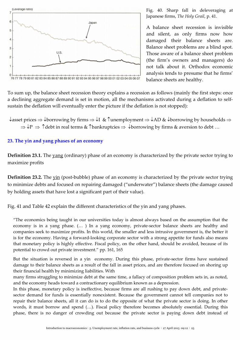
Fig. 39. Credit contraction in Japan, The
Holy Grail, p. 40.
Figs. 39 and 40 explain why, contrary to
conventional wisdom, firms may refuse
to borrow even at 0% interest rate. A
firm suffering from a debt overhang
gives priority to debt repayment and
clean up the balance sheet, regardless of
how cheap borrowing is. Fig. 40 shows
the intensity of deleveraging of
Japanese firms.
Introduction to macroeconomics ǀ 5. Unemployment rate, inflation rate, and business cycle ǀ 27 April 2015 09:12 ǀ 25
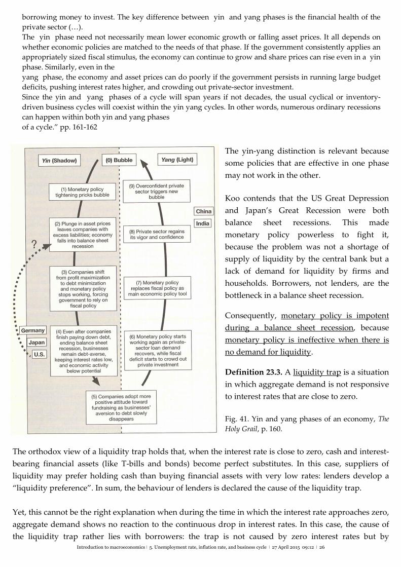
Fig. 40. Sharp fall in deleveraging at
Japanese firms, The Holy Grail, p. 41. A balance sheet recession is invisible
and silent, as only firms now how
damaged their balance sheets are.
Balance sheet problems are a blind spot.
Those aware of a balance sheet problem
(the firm’s owners and managers) do
not talk about it. Orthodox economic
analysis tends to presume that he firms’
balance sheets are healthy.
To sum up, the balance sheet recession theory explains a recession as follows (mainly the first steps: once
a declining aggregate demand is set in motion, all the mechanisms activated during a deflation to self‐
sustain the deflation will eventually enter the picture if the deflation is not stopped):
asset prices borrowing by firms I & unemployment AD & borrowing by households
P debt in real terms & bankruptcies borrowing by firms & aversion to debt …
23. The yin and yang phases of an economy
Definition 23.1. The yang (ordinary) phase of an economy is characterized by the private sector trying to
maximize profits
Definition 23.2. The yin (post‐bubble) phase of an economy is characterized by the private sector trying
to minimize debts and focused on repairing damaged (“underwater”) balance sheets (the damage caused
by holding assets that have lost a significant part of their value).
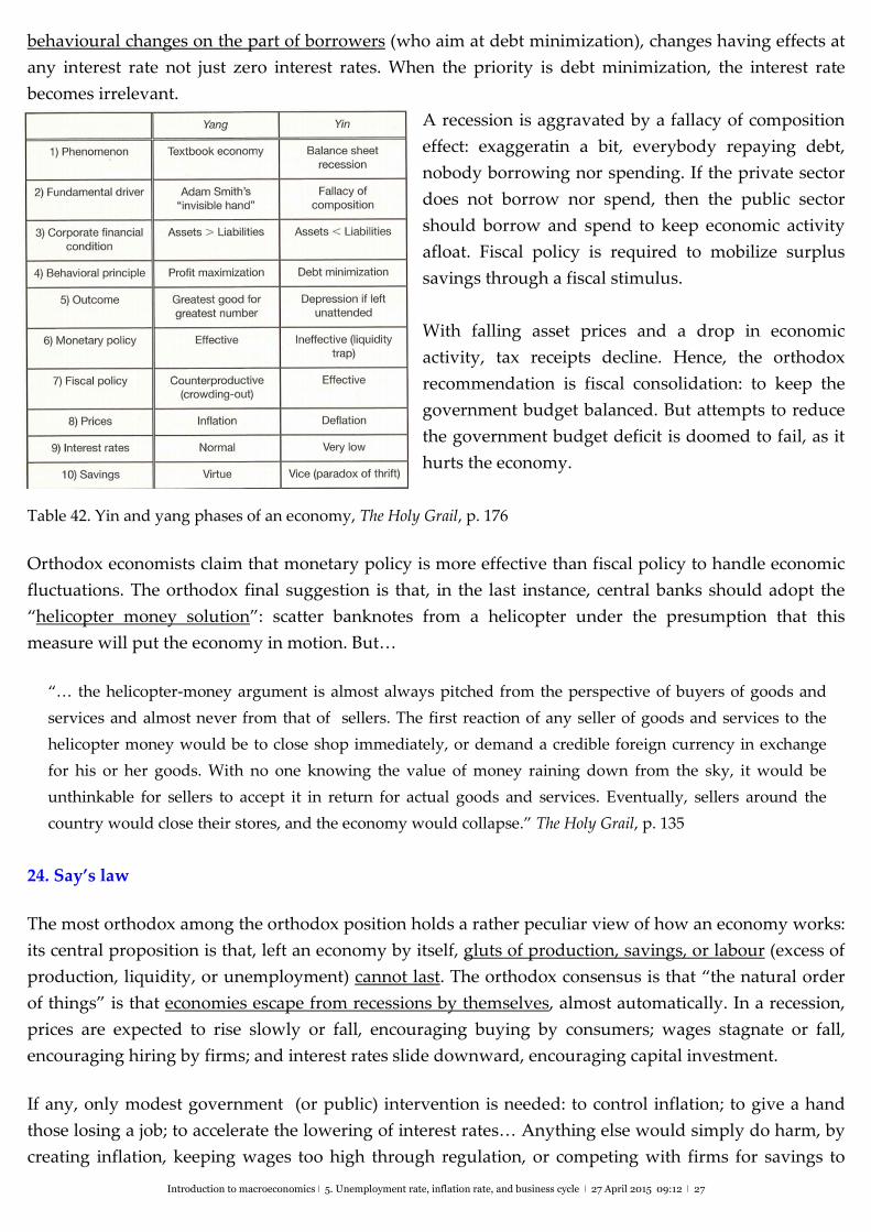
Fig. 41 and Table 42 explain the different characteristics of the yin and yang phases.
“The economics being taught in our universities today is almost always based on the assumption that the
economy is in a yang phase. (… ) In a yang economy, private‐sector balance sheets are healthy and
companies seek to maximize profits. In this world, the smaller and less intrusive government is, the better it
is for the economy. Having a forward‐looking corporate sector with a strong appetite for funds also means
that monetary policy is highly effective. Fiscal policy, on the other hand, should be avoided, because of its
potential to crowd out private investment.” pp. 161, 165 But the situation is reversed in a yin economy. During this phase, private‐sector firms have sustained
damage to their balance sheets as a result of the fall in asset prices, and are therefore focused on shoring up
their financial health by minimizing liabilities. With
many firms struggling to minimize debt at the same time, a fallacy of composition problem sets in, as noted,
and the economy heads toward a contractionary equilibrium known as a depression.
In this phase, monetary policy is ineffective, because firms are all rushing to pay down debt, and private‐
sector demand for funds is essentially nonexistent. Because the government cannot tell companies not to
repair their balance sheets, all it can do is to do the opposite of what the private sector is doing. In other
words, it must borrow and spend (…). Fiscal policy therefore becomes absolutely essential. During this
phase, there is no danger of crowding out because the private sector is paying down debt instead of
Introduction to macroeconomics ǀ 5. Unemployment rate, inflation rate, and business cycle ǀ 27 April 2015 09:12 ǀ 26
borrowing money to invest. The key difference between yin and yang phases is the financial health of the
private sector (…).
The yin phase need not necessarily mean lower economic growth or falling asset prices. It all depends on
whether economic policies are matched to the needs of that phase. If the government consistently applies an
appropriately sized fiscal stimulus, the economy can continue to grow and share prices can rise even in a yin
phase. Similarly, even in the
yang phase, the economy and asset prices can do poorly if the government persists in running large budget
deficits, pushing interest rates higher, and crowding out private‐sector investment.
Since the yin and yang phases of a cycle will span years if not decades, the usual cyclical or inventory‐
driven business cycles will coexist within the yin yang cycles. In other words, numerous ordinary recessions
can happen within both yin and yang phases
of a cycle.” pp. 161‐162
The yin‐yang distinction is relevant because
some policies that are effective in one phase
may not work in the other.
Koo contends that the US Great Depression
and Japan’s Great Recession were both
balance sheet recessions. This made
monetary policy powerless to fight it,
because the problem was not a shortage of
supply of liquidity by the central bank but a
lack of demand for liquidity by firms and
households. Borrowers, not lenders, are the
bottleneck in a balance sheet recession.
Consequently, monetary policy is impotent
during a balance sheet recession, because
monetary policy is ineffective when there is
no demand for liquidity.
Definition 23.3. A liquidity trap is a situation
in which aggregate demand is not responsive
to interest rates that are close to zero.
Fig. 41. Yin and yang phases of an economy, The
Holy Grail, p. 160.
The orthodox view of a liquidity trap holds that, when the interest rate is close to zero, cash and interest‐
bearing financial assets (like T‐bills and bonds) become perfect substitutes. In this case, suppliers of
liquidity may prefer holding cash than buying financial assets with very low rates: lenders develop a
“liquidity preference”. In sum, the behaviour of lenders is declared the cause of the liquidity trap.
Yet, this cannot be the right explanation when during the time in which the interest rate approaches zero,
aggregate demand shows no reaction to the continuous drop in interest rates. In this case, the cause of
the liquidity trap rather lies with borrowers: the trap is not caused by zero interest rates but by
Introduction to macroeconomics ǀ 5. Unemployment rate, inflation rate, and business cycle ǀ 27 April 2015 09:12 ǀ 27
behavioural changes on the part of borrowers (who aim at debt minimization), changes having effects at
any interest rate not just zero interest rates. When the priority is debt minimization, the interest rate
becomes irrelevant.
A recession is aggravated by a fallacy of composition
effect: exaggeratin a bit, everybody repaying debt,
nobody borrowing nor spending. If the private sector
does not borrow nor spend, then the public sector
should borrow and spend to keep economic activity
afloat. Fiscal policy is required to mobilize surplus
savings through a fiscal stimulus.
With falling asset prices and a drop in economic
activity, tax receipts decline. Hence, the orthodox
recommendation is fiscal consolidation: to keep the
government budget balanced. But attempts to reduce
the government budget deficit is doomed to fail, as it
hurts the economy.
Table 42. Yin and yang phases of an economy, The Holy Grail, p. 176
Orthodox economists claim that monetary policy is more effective than fiscal policy to handle economic
fluctuations. The orthodox final suggestion is that, in the last instance, central banks should adopt the
“helicopter money solution”: scatter banknotes from a helicopter under the presumption that this
measure will put the economy in motion. But…
“… the helicopter‐money argument is almost always pitched from the perspective of buyers of goods and
services and almost never from that of sellers. The first reaction of any seller of goods and services to the
helicopter money would be to close shop immediately, or demand a credible foreign currency in exchange
for his or her goods. With no one knowing the value of money raining down from the sky, it would be
unthinkable for sellers to accept it in return for actual goods and services. Eventually, sellers around the
country would close their stores, and the economy would collapse.” The Holy Grail, p. 135
24. Say’s law
The most orthodox among the orthodox position holds a rather peculiar view of how an economy works:
its central proposition is that, left an economy by itself, gluts of production, savings, or labour (excess of
production, liquidity, or unemployment) cannot last. The orthodox consensus is that “the natural order
of things” is that economies escape from recessions by themselves, almost automatically. In a recession,
prices are expected to rise slowly or fall, encouraging buying by consumers; wages stagnate or fall,
encouraging hiring by firms; and interest rates slide downward, encouraging capital investment.
If any, only modest government (or public) intervention is needed: to control inflation; to give a hand
those losing a job; to accelerate the lowering of interest rates… Anything else would simply do harm, by
creating inflation, keeping wages too high through regulation, or competing with firms for savings to
Introduction to macroeconomics ǀ 5. Unemployment rate, inflation rate, and business cycle ǀ 27 April 2015 09:12 ǀ 28
finance budget deficits. The main concern of the government, in this view, is to keep the budget
balanced. The theoretical underpinning of this view goes by the name of “Say’s law”.
Definition 24.1. Say's law (after Jean‐Baptiste Say (1805) or “law of the markets”) is often reduced to the
motto “supply creates its own demand” Keynes tried to prove in The General Theory of Employment,
Interest, and Money (note the term appearing first) that Say’s law does not apply to a modern economy.
Say’s law relies on the contention that the creation of value added by production activities is the source
for demand: the sale of goods provides the source of the income that finances purchases. Individuals
must first sell to the market to be able to buy from the market. To buy (to demand) one must first sell
(supply). The answer to a glut (excess) of goods, workers, or savings is to make more goods, thereby
employing workers. Prices, wages, and interest rates will adjust to balance supply and demand.
By Say’s law, if businesses make products, the wages paid to the workers employed will enable them to
buy all that is produced. Similarly, if individuals and businesses save, all the savings will be allocated to
capital investment. Finally, there will never be too many workers because their wages would fall until all
are hired. Thus, any glut of goods, savings, or workers will be only temporary. Summing up, according
to Say’s law, demand is constituted by supply and, thus, demand failure is a symptom, not a cause.
25. What explains severe contractions of economic activity?
Explanation 1. It is associated with the so‐called (orthodox or mainstream) ‘fresh‐water’ economists.
They hold that the market system works well as long as market forces are free from government
interferences (like lowering interest rates too much or worsening the crisis through stimulus packages).
Explanation 2. It is associated with the so‐called (orthodox or mainstream) ‘salt‐water’ economists. In
their view, crises and recessions are caused by market failures, insufficient information, and/or lack of
appropriate regulation and supervision.
Explanation 3. It is associated with heterodox, non‐mainstream economists. Explanation 2 is deepened
by invoking the existence of deeper structural causes of crises and recessions, like income distribution.
These economists point out that, since the 1980s (see Tables 44 and 45):
(i) economic policies are no longer aimed at promoting full employment but at targeting low
inflation levels;
(ii) society has come to accept conservative (“neoliberal”) views and precepts;
(iii) firms do not attempt to make profits through investment but by reducing the workforce;
(iv) the bargaining power of labour has been weakened and this has been reflected in a decline in
the share of wage in aggregate income and an increase in wage and income inequality; and
(v) the growth of the economy does no longer rely on wage‐led consumption supported by wages
rising in parallel with labour productivity, but is now based on household debt (‘debt‐led
growth’) or on “competitive” (low) wages able to sustain exports (‘export‐led growth’).
According to Explanation 3, the debt and export‐led growth strategies have proved to be unsustainable.
Introduction to macroeconomics ǀ 5. Unemployment rate, inflation rate, and business cycle ǀ 27 April 2015 09:12 ǀ 29
26. Profit‐led and wage‐led demand regimes
Orthodox macroeconomic models put more emphasis on the supply side of the economy and presume
that demand follows supply. In this regard, it is customary in orthodox analysis to treat wages as just a
cost of production and neglect that wages are also a source of demand.
Definition 26.1. An aggregate demand regime is wage‐led when a raise in the wage share (or a fall in the
profit share) increases aggregate demand.
Demand is wage‐led if the increase in consumption resulting from a rise in the real wage (or a rise in the
wage share or a fall in the profit share) more than compensates the reduction in private investment and
exports caused by a higher real wage. Conversely, the decrease in consumption resulting from a fall in
the real wage exceeds the increase in private investment and exports that tends to be associated with a
lower real wage.
Definition 26.2. An aggregate demand regime is profit‐led when a raise in the profit share (or a
reduction in the wage share) increases aggregate demand.
Demand is profit‐led if the reduction in consumption resulting from a fall in the real wage (or a fall in the
wage share or a rise in the profit share) is more than compensated by an increase in private investment
and exports derived from a lower real wage. Conversely, the increase in consumption resulting from a
rise in the real wage does not compensate the presumed contraction in private investment and exports
derived from a higher real wage.
It follows from Definitions 26.1 and 26.2 that:
an increase in the wage share expands aggregate demand if the demand regime is wage‐led;
an increase in the wage share contracts aggregate demand if the demand regime is profit‐led;
an increase in the profit share expands aggregate demand if the demand regime is profit‐led;
an increase in the profit share contracts aggregate demand if the demand regime is wage‐led.
The four components of aggregate demand are private consumption expenditure C, private investment
expenditure I, government expenditure G, and net exports (NX, exports minus imports). The domestic
components of aggregate demand are C, I, and G. Since G can be considered essentially as exogenous, to
determine the domestic demand regime it is enough to assess how a change in income distribution
affects C and I.
The orthodox presumption is that income distribution plays no role in establishing aggregate demand,
because the proportion of income that is consumed (the propensity to consume) out of wages is
supposed to be the same as the proportion consumed out of profits.
Empirical evidence suggests that the propensity to consume (save) out of profits is smaller (higher) than
the propensity to consume (save) out of wages. In this case, a shift in income distribution towards wages
will increases consumption. But is this favourable effect on aggregate demand overturned by the
negative impact of a higher wage rate on on private investment?
Introduction to macroeconomics ǀ 5. Unemployment rate, inflation rate, and business cycle ǀ 27 April 2015 09:12 ǀ 30
View 1 (Michael Kalecki). An increase in the wage share is not detrimental to investment because
investment depends on expected profitability, which to a great extent depends on realized profitability
(sales). Investment is seen as the result of an accelerator effect: the multiplier effect (I AD Y) is
reinforced by the accelerator effect Y I arising from the fact that an expanding economy stimulates
further investment (as previous investment proved to be profitable).
View 2 (Marxists and company). Expected profitability is a function of the profit share in aggregate
income or, more precisely, of the profit rate firms expect to obtain from its productive capacity under
normal circumstances. With everyting else given, higher real wages are paid off the profit margin. As a
result, a higher real wage lowers profitability and this reduces investment.
Under View 1, the domestic demand regime is wage‐led: an increase in the wage share also increases
aggregate consumption and investment. Under View 2, the domestic demand regime could be profit‐led:
an increase in the wage share would reduce the sum of aggregate consumption and investment
whenever the change in consumption is smaller than the change in investment.
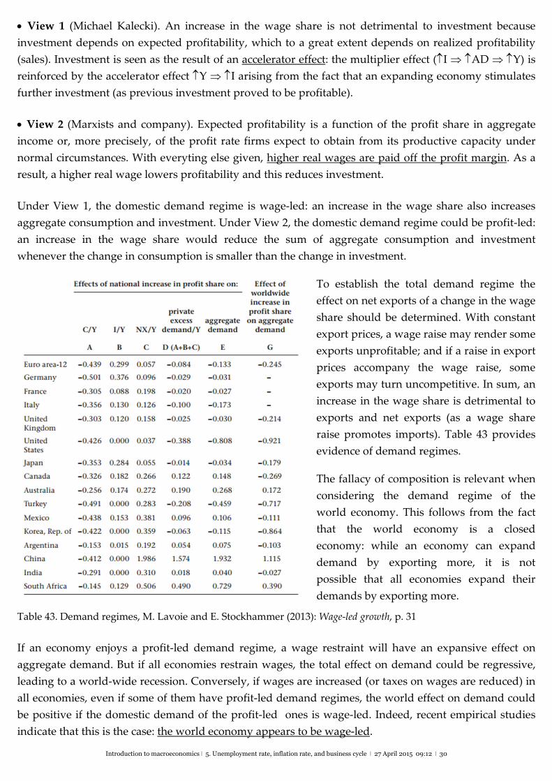
To establish the total demand regime the
effect on net exports of a change in the wage
share should be determined. With constant
export prices, a wage raise may render some
exports unprofitable; and if a raise in export
prices accompany the wage raise, some
exports may turn uncompetitive. In sum, an
increase in the wage share is detrimental to
exports and net exports (as a wage share
raise promotes imports). Table 43 provides
evidence of demand regimes.
The fallacy of composition is relevant when
considering the demand regime of the
world economy. This follows from the fact
that the world economy is a closed
economy: while an economy can expand
demand by exporting more, it is not
possible that all economies expand their
demands by exporting more.
Table 43. Demand regimes, M. Lavoie and E. Stockhammer (2013): Wage-led growth, p. 31
If an economy enjoys a profit‐led demand regime, a wage restraint will have an expansive effect on
aggregate demand. But if all economies restrain wages, the total effect on demand could be regressive,
leading to a world‐wide recession. Conversely, if wages are increased (or taxes on wages are reduced) in
all economies, even if some of them have profit‐led demand regimes, the world effect on demand could
be positive if the domestic demand of the profit‐led ones is wage‐led. Indeed, recent empirical studies
indicate that this is the case: the world economy appears to be wage‐led.
Introduction to macroeconomics ǀ 5. Unemployment rate, inflation rate, and business cycle ǀ 27 April 2015 09:12 ǀ 31
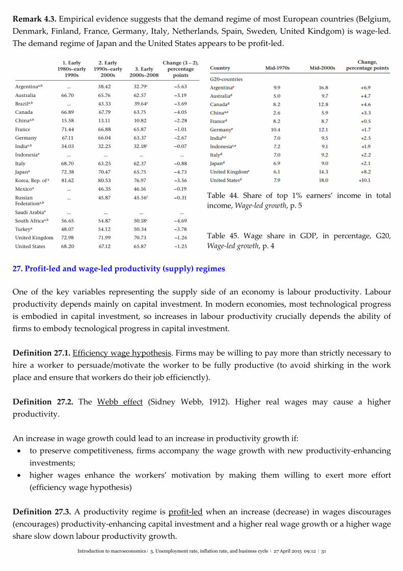
Remark 4.3. Empirical evidence suggests that the demand regime of most European countries (Belgium,
Denmark, Finland, France, Germany, Italy, Netherlands, Spain, Sweden, United Kindgom) is wage‐led.
The demand regime of Japan and the United States appears to be profit‐led.
Table 44. Share of top 1% earners’ income in total
income, Wage-led growth, p. 5
Table 45. Wage share in GDP, in percentage, G20,
Wage-led growth, p. 4
27. Profit‐led and wage‐led productivity (supply) regimes
One of the key variables representing the supply side of an economy is labour productivity. Labour
productivity depends mainly on capital investment. In modern economies, most technological progress
is embodied in capital investment, so increases in labour productivity crucially depends the ability of
firms to embody tecnological progress in capital investment.
Definition 27.1. Efficiency wage hypothesis. Firms may be willing to pay more than strictly necessary to
hire a worker to persuade/motivate the worker to be fully productive (to avoid shirking in the work
place and ensure that workers do their job efficienctly).
Definition 27.2. The Webb effect (Sidney Webb, 1912). Higher real wages may cause a higher
productivity.
An increase in wage growth could lead to an increase in productivity growth if:
to preserve competitiveness, firms accompany the wage growth with new productivity‐enhancing
investments;
higher wages enhance the workers’ motivation by making them willing to exert more effort
(efficiency wage hypothesis)
Definition 27.3. A productivity regime is profit‐led when an increase (decrease) in wages discourages
(encourages) productivity‐enhancing capital investment and a higher real wage growth or a higher wage
share slow down labour productivity growth.
Introduction to macroeconomics ǀ 5. Unemployment rate, inflation rate, and business cycle ǀ 27 April 2015 09:12 ǀ 32
Definition 27.4. A productivity regime is wage‐led when an increase in wages encourages productivity‐
enhancing capital investment (the adoption of more capital‐intensive methods of production) and/or has
a positive effect on labour effort and a higher real wage growth or a higher wage share leads to a faster
labour productivity growth.
Remark 27.5. Orthodox economists will claim that a higher real wage promotes the substitution of labour
for capital and stimulates the adoption of more capital‐intensive technologies. Under this presumption,
they will regard productivity regimes as wage‐led.
Definition 27.6. The Kaldor‐Verdoorn effect (or KV effect, after PJ Verdoorn, 1949, and Nicholas Kaldor,
1966) asserts that the GDP growth rate has a positive effect on the growth rate of labour productivity
(and maybe even on the growth rate of the labour force).
The KV effect is an expression of the heteredox view: demand affects supply (demand‐led growth has a
favourable impact on labour productivity, a supply‐side variable).
The link between GDP and productivity may be explained by:
the existence of increasing returns to scale (the more is produced, the lower the average cost);
the fact that one of the components of aggregate demand (investment) determines the capital stock
and average productivity;
the deepening of the division of labour and specialization encouraged by aggregate demand
growth;
faster learning‐by‐doing in firms (process which, like the division of labour, are likely to eventually
get increase labour productivity growth).
The KV effect reinforces the positive impact on the growth rate of an economy of an increase in the wage
share (or in the growth rate of real wages) in a wage‐led demand regime. A higher wage rate in a wage‐
led demand regime, increases aggregate demand and thereby stimulates GDP growth. Through the KV,
the higher GDP growth leads to a higher productivity growth, which in turn contributes to reinforce
GDP growth.
Remark 27.7. The feedback effects of productivity growth on GDP growth may transform an at first
profit‐led demand regime into a wage‐led one (the productiviy boost caused by a wage increase offsets
the negative effect on demand resulting in a profit‐led demand regime). The opposite is not possible.
Remark 27.8. According to recent empirical studies, the partial productivity regime (the productivity
regime without taking into account the KV effect) of OECD countries seems to be wage‐led.
In a profit‐led demand regime, higher real wages may still have a positive effect on labour productivity.
This will occur if the result of the productivity‐enhancing capital investment encouraged by higher
wages wipes out the negative impact on labour productivity of the KV effect (in a profit‐led demand
regime, a higher real wage slows down the GDP growth rate, which in turn slows down labour
productivity growth).
Introduction to macroeconomics ǀ 5. Unemployment rate, inflation rate, and business cycle ǀ 27 April 2015 09:12 ǀ 33
A lower real wage growth slows down labour productivity growth
through Kaldor‐Verdoorn effect, as a fall in the growth of aggregate demand cause by real wage
growth restraint reduces productivity growth; and
by retarding the rate adoption of labour‐saving technological progress, insofar as lower wage growth
reduces the firms’ incentives to invest in labour‐saving technologies.
28. Profit‐led and wage‐led economies (or economic regimes)
Definition 28.1 (informal). A economy is profit‐led (or the economy is in a profit‐led economic regime) if
a shift towards profits has a favourable effect on the economy. A economy is wage‐led (or the economy is
in a wage‐led economic regime) if a shift towards wages has a favourable effect on the economy.
A wage‐led economy poses a serious challenge to orthodox economic wisdom. This “wisdom”
recommends austerity policies (which, in requiring a reduction of public expenditure, adversely affect
the recipients of the lowest wages) and “structural reforms” (the euphemistic term meaning “cut wage
rates”). The application of those measures in a wage‐led economy has a negative impact on economic
activity. This negative impact worsens the budget deficit (so governments are told to deepen and pursue
further austerity policies) and renews the call for more structural reforms (inasmuch as wage reduction
are deemed insufficient). The result is a devilish spiral of austerity policies, structural reforms, and
contraction of economic activity, as seen in the last three years in Spain.
The obvious alternative to the orthodox medicine in a wage‐led economy is to implement a wage‐led
growth strategy. This strategy will be even more successful if coordinated internationally, given that the
world economy is most likely to be wage‐led.
29. A model of GDP, employment, and productivity interaction
The model is taken from Servaas Storm and CWM Naastepad (2012), Macroeconomics beyond the NAIRU,
and consists of three equations, (1), (2), and (3) below. All the variables in the model are expressed as
rates of change: �� is the rate of change of GDP, �� the rate of change of the real wage rate, �� the rate of
change of labour productivity, and �� the rate of change of employment.
The demand regime: equation (1)
GDP, aggregate production Y, is assumed to correspond, as in the macroeconomic national accounts, to
effective aggregate demand: consumption plus investment plus government expediture plus net exports.
Equations determining the value of these four components could be specified (see Storm and Naastepad
for details) but what is actually needed is the summarizing expression that relates aggregate demand
growth with real wage growth and productivity growth. Equation (1) is the summarizing expression.
�� = � + � ·(�� − ��) (1)
Introduction to macroeconomics ǀ 5. Unemployment rate, inflation rate, and business cycle ǀ 27 April 2015 09:12 ǀ 34
To explain (1), define the real wage share � as � =�·�
�·�; that is, the total amount of money wages received
by the employed workers divided by nominal GDP (� represents a price index and � is real GDP).
Defining the average real productivity in the economy as � =�
� (what a worker produces on average),
the real wage share can be expressed as
� =� ·�
� ·�=�
�·�
�= � ·
1
��
=�
�·
Accordingly, �� ≈ �� − ��. Hence, (1)asserts that the GDP growth rate depends �� on the rate of growth of
the real wage share �� − �� : a change in the real wage share growth of one unit causes a change of � units
in GDP growh. If the parameter � in (1)is positive, then the demand regime is wage‐led: an increase in
the real wage share has a positive impact on GDP growth. The interpretation of � < 0 is that the demand
regime is profit‐led. Finally, the parameter � captures the influence on GDP growth of factors different
from the real wage share.
Example 29.1. Storm and Naastepad contend that, for both the European Union (EU) on average and for
individual EU economies, � = 0.3, whereas, for the US, � = −0.23 appears realistic. In this respect, the
demand regime of the EU economy is wage‐led and the demand regime of the US is profit‐led.
The productivity regime: equation (2)
Equation (2)describes how aggregate labour productivity growth reacts to GDP growth �� and real wage
growth ��.
�� = �� + �� ·�� + �� ·�� (2)
Parameter �� > 0 in (2)captures influences on labour productivity growth from factors different from
GDP growth and real wage growth. For example, the more regulated the labour market, the higher the
labor productivity growth: pro‐worker (or protective) regulations improve labour productivity by
promoting workers’ motivation and by stimulating investment in human capital formation.
Parameter �� in (2)is the Kaldor‐Verdoorn coefficient: it measures how of demand‐determined GDP
growth affects labor productivity growth. It is assumed that 0 < �� < 1.
Parameter �� > 0 in (2)represents the extent to which tecnological progress is wage‐led: the higher ��,
the more firms intensify the search for production methods that improve the labour productivity in
response to an increase in the real wage. The idea is that higher wages stimulate capital deepening, drive
inefficient firms off the market, increase the proportion of high‐skilled workers, and promote labour‐
saving technological progress.
Remark 29.2. The orthodox approach views labour productivity growth as exogenous: labour
productivity does not respon to real GDP growth or real wage growth. This amounts to postulating
�� = �� = 0 in (2).
Introduction to macroeconomics ǀ 5. Unemployment rate, inflation rate, and business cycle ǀ 27 April 2015 09:12 ǀ 35
Remark 29.3. Storm and Naastepad claim that the simple average value of �� for the OECD economies is
0.46 and that estimates for individual countries are close to this average. They also observe that long‐run
evidence for 19 OECD (1960‐2004) indicates that �� is between 0.31 and 0.39 and that estimates of �� for
individual economies (France, Germany, the Netherlands, UK, US, nd the Scandinavian economies,
among them) are consistent with the simple average value of 0.38 for the group of OECD economies. In
sum, �� = 0.46 and �� = 0.38 appear to reasonable values for the parameters. For instance, �� = 0.38
means that an increase in real wage growth by 1 percent point causes an increase in labour productivity
growth by 0.38 percent points.
The employment regime: equation (3)
It follows from the definition � =�
� that �� ≈ �� − ��, which is equation (3).
�� =�� − �� (3)
According to (3), the rate of growth of employment is approximately equal to the difference between the
rate of growth of real GDP and the rate of growth of labour productivity.
From(2) and (3),
�� =−�� + (1− ��)·�� − �� · ��
From (1) and (2),
�� =� − � ·��1 + � ·��
+ � ·(1− ��)
1 + � ·��·��(4)
�� =�� + � ·��1 + � ·��
+ �� + � ·��1 + � ·��
·��(5)
��=� ·(1− ��)− (1+ �)·��
1 + � ·��+
� ·(1− �� − ��)− ��1 + � ·��
·��(6)
Equations (4), (5)and (6) establish the link between real wage growth ��, on the one hand, and GDP
growth �� , labour productivity growth ��, and employment growth ��. The sign of the derivative ���
���
indicates whether the demand regime is wage‐led or profit‐led and the sign of the derivate ���
��� indicates
whether the productivity regime is wage‐led or profit‐led.
���
���=
� ·(1− ��)
1+ � ·��(7)
���
���=
�� + � ·��1 + � ·��
(8)
���
���=
� ·(1− �� − ��)− ��1 + � ·��
(9)
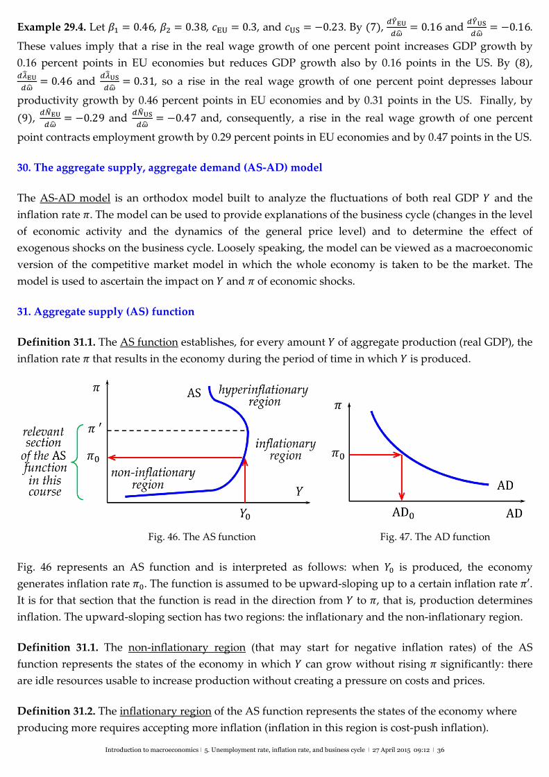
Introduction to macroeconomics ǀ 5. Unemployment rate, inflation rate, and business cycle ǀ 27 April 2015 09:12 ǀ 36
Example 29.4. Let �� = 0.46, �� = 0.38, ��� = 0.3, and ��� = −0.23. By (7), �����
���= 0.16 and
�����
���= −0.16.
These values imply that a rise in the real wage growth of one percent point increases GDP growth by
0.16 percent points in EU economies but reduces GDP growth also by 0.16 points in the US. By (8), �����
���= 0.46 and
�����
���= 0.31, so a rise in the real wage growth of one percent point depresses labour
productivity growth by 0.46 percent points in EU economies and by 0.31 points in the US. Finally, by
(9), �����
���= −0.29 and
�����
���= −0.47 and, consequently, a rise in the real wage growth of one percent
point contracts employment growth by 0.29 percent points in EU economies and by 0.47 points in the US.
30. The aggregate supply, aggregate demand (AS‐AD) model
The AS‐AD model is an orthodox model built to analyze the fluctuations of both real GDP � and the
inflation rate �. The model can be used to provide explanations of the business cycle (changes in the level
of economic activity and the dynamics of the general price level) and to determine the effect of
exogenous shocks on the business cycle. Loosely speaking, the model can be viewed as a macroeconomic
version of the competitive market model in which the whole economy is taken to be the market. The
model is used to ascertain the impact on � and � of economic shocks.
31. Aggregate supply (AS) function
Definition 31.1. The AS function establishes, for every amount � of aggregate production (real GDP), the
inflation rate � that results in the economy during the period of time in which � is produced.
Fig. 46. The AS function Fig. 47. The AD function
Fig. 46 represents an AS function and is interpreted as follows: when �� is produced, the economy
generates inflation rate ��. The function is assumed to be upward‐sloping up to a certain inflation rate �′.
It is for that section that the function is read in the direction from � to �, that is, production determines
inflation. The upward‐sloping section has two regions: the inflationary and the non‐inflationary region.
Definition 31.1. The non‐inflationary region (that may start for negative inflation rates) of the AS
function represents the states of the economy in which � can grow without rising � significantly: there
are idle resources usable to increase production without creating a pressure on costs and prices.
Definition 31.2. The inflationary region of the AS function represents the states of the economy where
producing more requires accepting more inflation (inflation in this region is cost‐push inflation).
Introduction to macroeconomics ǀ 5. Unemployment rate, inflation rate, and business cycle ǀ 27 April 2015 09:12 ǀ 37
Basic reasons for the speed‐up of inflation in the inflationary region are listed next.
Competition for resources. The amount of resources is finite. Hence, as the economy approaches
potential GDP, firms encounter resource bottlenecks. Eventually, firms can only obtain more inputs
by detracting them from other firms. This requires paying more for those inputs to attract them.
Training costs. More production eventually demands hiring more workers, who in general should
be trained to be able to operate efficiently
Reorganization costs. Changing the scale of production may require a production process redesign,
which is costly.
Diminishing marginal productivity. All production process eventually face the law of diminishing
marginal productivity: each additional unit of input will in the long run add less to total production.
So, to produce the same again, more inputs are needed and costs therefore increase.
Example 31.3. Hours of study is the input to produce knowledge. With all likelihood, the tenth hour of
study of a given subject does not add as much knowledge as the first one.
Example 31.4. Threshold effects seem to contradict the diminishing marginal productivity principle. For
instance, there is the “10,000 hours rule” (see chapter 2 in Malcolm Gladwell (2008): Outliers: The Story
of Success): “ten thousand hours of practice is required to achieve the level of mastery associated with
being a world‐class expert—in anything" (Daniel Levitin, neurologist).
Definition 31.5. The hyperinflationary region of the AS function represents the states of the economy
where the production activities no longer run smooth, because prices are changing so fast (there is
hyperinflation) that agents in the economy are more concerned with preserving purchasing power than
with carrying the normal economic activities.
The AS function on the hyperinflationary region is assumed downward‐sloping: above a certain inflation
rate (�′ in Fig. 46), the higher the inflation rate, the smaller aggregate production. The normal operation
of the productive system is disturbed (it is hard to make correct decisions when prices may vary every
minute). It is then reasonable to expect a drop in � when � goes up under hyperinflation. As advanced
economies do not experience hyperinflations, the hyperinflationary region will be disregarded.
32. Aggregate demand (AD) function
Remark 32.1. The aggregate demand concept was Keynes’ analytical, intellectual response to the events
of the Great Depression in the 1930s.
Definition 32.2. Aggregate demand AD is the sum of four components: C (aggregate planned
consumption), I (aggregate planned investment), G (planned government purchases), and NX (aggregate
planned net exports).
Definition 32.3. The AD function establishes, for each inflation rate �, the amount AD of planned
aggregate expenditure.
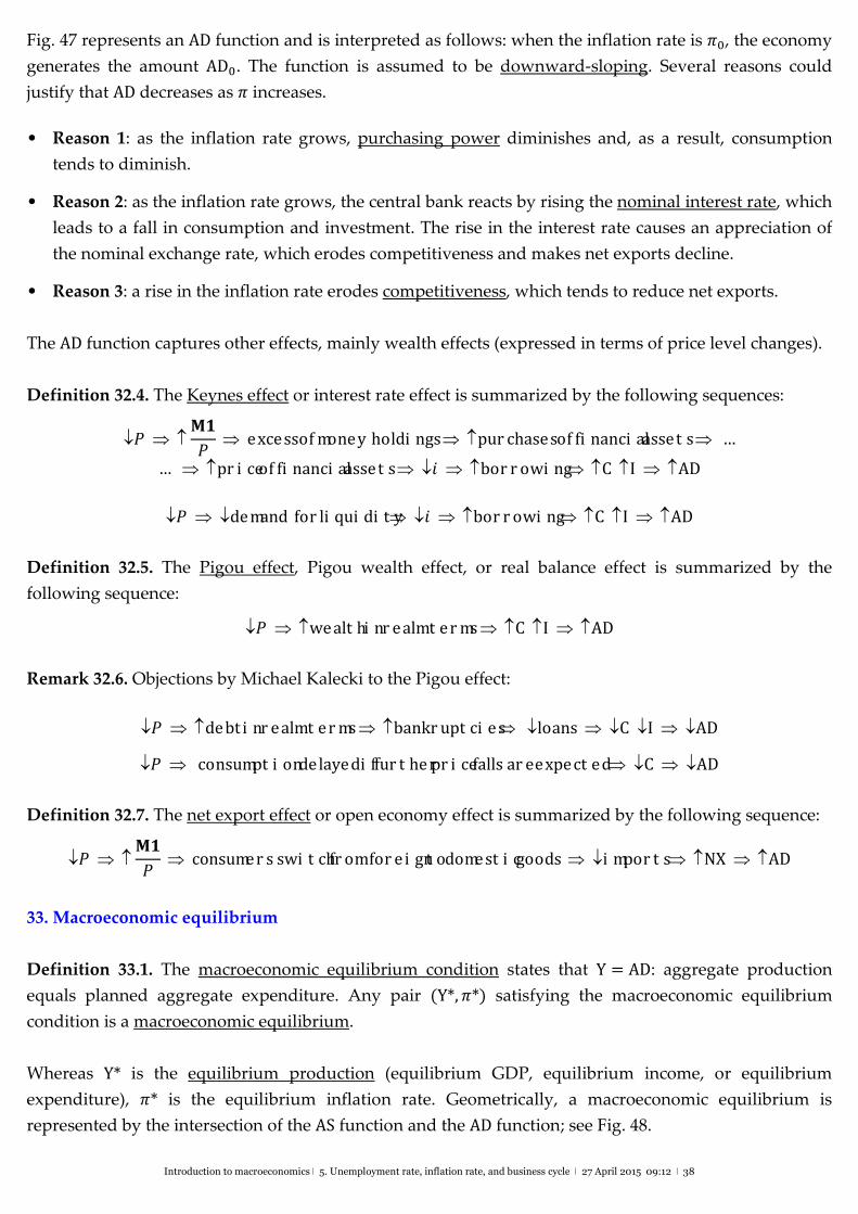
Introduction to macroeconomics ǀ 5. Unemployment rate, inflation rate, and business cycle ǀ 27 April 2015 09:12 ǀ 38
Fig. 47 represents an AD function and is interpreted as follows: when the inflation rate is ��, the economy
generates the amount AD�. The function is assumed to be downward‐sloping. Several reasons could
justify that AD decreases as � increases.
• Reason 1: as the inflation rate grows, purchasing power diminishes and, as a result, consumption
tends to diminish.
• Reason 2: as the inflation rate grows, the central bank reacts by rising the nominal interest rate, which
leads to a fall in consumption and investment. The rise in the interest rate causes an appreciation of
the nominal exchange rate, which erodes competitiveness and makes net exports decline.
• Reason 3: a rise in the inflation rate erodes competitiveness, which tends to reduce net exports.
The AD function captures other effects, mainly wealth effects (expressed in terms of price level changes).
Definition 32.4. The Keynes effect or interest rate effect is summarized by the following sequences:
���
�excessofmoneyholdingspurchasesoffinancialassets…
…priceoffinancialassets�borrowingCIAD
�demandforliquidity�borrowingCIAD
Definition 32.5. The Pigou effect, Pigou wealth effect, or real balance effect is summarized by the
following sequence:
�wealthinrealmtermsCIAD
Remark 32.6. Objections by Michael Kalecki to the Pigou effect:
�debtinrealmtermsbankruptciesloansCIAD
�consumptiondelayediffurtherpricefallsareexpectedCAD
Definition 32.7. The net export effect or open economy effect is summarized by the following sequence:
���
�consumersswitchfromforeigntodomesticgoodsimportsNXAD
33. Macroeconomic equilibrium
Definition 33.1. The macroeconomic equilibrium condition states that Y = AD: aggregate production
equals planned aggregate expenditure. Any pair (Y*,�*) satisfying the macroeconomic equilibrium
condition is a macroeconomic equilibrium.
Whereas Y* is the equilibrium production (equilibrium GDP, equilibrium income, or equilibrium
expenditure), �* is the equilibrium inflation rate. Geometrically, a macroeconomic equilibrium is
represented by the intersection of the AS function and the AD function; see Fig. 48.
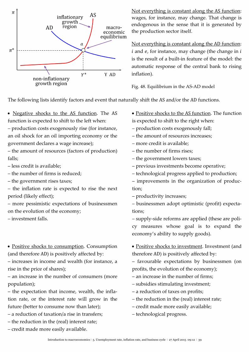
Introduction to macroeconomics ǀ 5. Unemployment rate, inflation rate, and business cycle ǀ 27 April 2015 09:12 ǀ 39
Not everything is constant along the AS function:
wages, for instance, may change. That change is
endogenous in the sense that it is generated by
the production sector itself.
Not everything is constant along the AD function:
� and �, for instance, may change (the change in �
is the result of a built‐in feature of the model: the
automatic response of the central bank to rising
inflation).
Fig. 48. Equilibrium in the AS‐AD model
The following lists identify factors and event that naturally shift the AS and/or the AD functions.
Negative shocks to the AS function. The AS
function is expected to shift to the left when:
– production costs exogenously rise (for instance,
an oil shock for an oil importing economy or the
government declares a wage increase);
– the amount of resources (factors of production)
falls;
– less credit is available;
– the number of firms is reduced;
– the government rises taxes;
– the inflation rate is expected to rise the next
period (likely effect);
– more pessimistic expectations of businessmen
on the evolution of the economy;
– investment falls.
Positive shocks to the AS function. The function
is expected to shift to the right when:
– production costs exogenously fall;
– the amount of resources increases;
– more credit is available;
– the number of firms rises;
– the government lowers taxes;
– previous investments become operative;
– technological progress applied to production;
– improvements in the organization of produc‐
tion;
– productivity increases;
– businessmen adopt optimistic (profit) expecta‐
tions;
– supply‐side reforms are applied (these are poli‐
cy measures whose goal is to expand the
economy’s ability to supply goods).
Positive shocks to consumption. Consumption
(and therefore AD) is positively affected by:
– increases in income and wealth (for instance, a
rise in the price of shares);
– an increase in the number of consumers (more
population);
– the expectation that income, wealth, the infla‐
tion rate, or the interest rate will grow in the
future (better to consume now than later);
– a reduction of taxation/a rise in transfers;
– the reduction in the (real) interest rate;
– credit made more easily available.
Positive shocks to investment. Investment (and
therefore AD) is positively affected by:
– favourable expectations by businessmen (on
profits, the evolution of the economy);
– an increase in the number of firms;
– subsidies stimulating investment;
– a reduction of taxes on profits;
– the reduction in the (real) interest rate;
– credit made more easily available;
– technological progress.
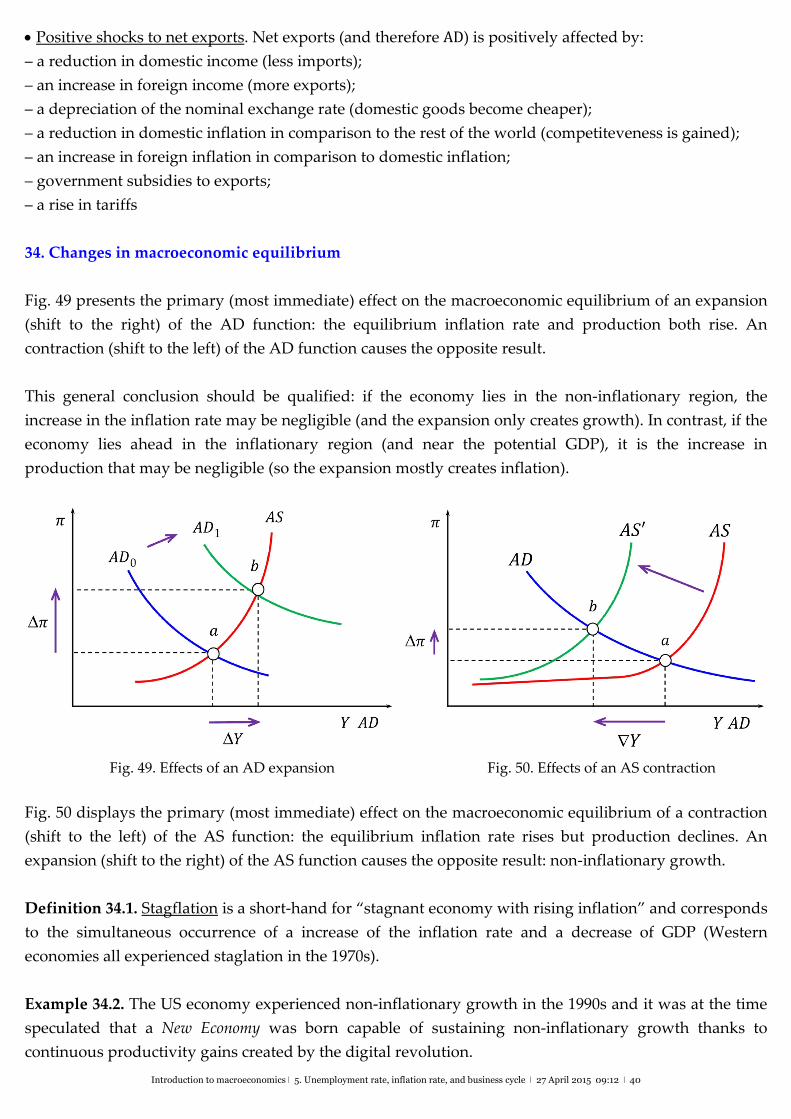
Introduction to macroeconomics ǀ 5. Unemployment rate, inflation rate, and business cycle ǀ 27 April 2015 09:12 ǀ 40
Positive shocks to net exports. Net exports (and therefore AD) is positively affected by:
– a reduction in domestic income (less imports);
– an increase in foreign income (more exports);
– a depreciation of the nominal exchange rate (domestic goods become cheaper);
– a reduction in domestic inflation in comparison to the rest of the world (competiteveness is gained);
– an increase in foreign inflation in comparison to domestic inflation;
– government subsidies to exports;
– a rise in tariffs
34. Changes in macroeconomic equilibrium
Fig. 49 presents the primary (most immediate) effect on the macroeconomic equilibrium of an expansion
(shift to the right) of the AD function: the equilibrium inflation rate and production both rise. An
contraction (shift to the left) of the AD function causes the opposite result.
This general conclusion should be qualified: if the economy lies in the non‐inflationary region, the
increase in the inflation rate may be negligible (and the expansion only creates growth). In contrast, if the
economy lies ahead in the inflationary region (and near the potential GDP), it is the increase in
production that may be negligible (so the expansion mostly creates inflation).
Fig. 49. Effects of an AD expansion Fig. 50. Effects of an AS contraction
Fig. 50 displays the primary (most immediate) effect on the macroeconomic equilibrium of a contraction
(shift to the left) of the AS function: the equilibrium inflation rate rises but production declines. An
expansion (shift to the right) of the AS function causes the opposite result: non‐inflationary growth.
Definition 34.1. Stagflation is a short‐hand for “stagnant economy with rising inflation” and corresponds
to the simultaneous occurrence of a increase of the inflation rate and a decrease of GDP (Western
economies all experienced staglation in the 1970s).
Example 34.2. The US economy experienced non‐inflationary growth in the 1990s and it was at the time
speculated that a New Economy was born capable of sustaining non‐inflationary growth thanks to
continuous productivity gains created by the digital revolution.
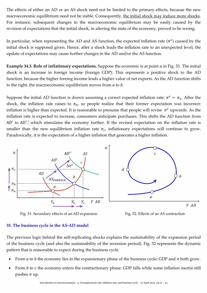
Introduction to macroeconomics ǀ 5. Unemployment rate, inflation rate, and business cycle ǀ 27 April 2015 09:12 ǀ 41
The effects of either an AD or an AS shock need not be limited to the primary effects, because the new
macroeconomic equilibrium need not be stable. Consequently, the initial shock may induce more shocks.
For instance, subsequent changes in the macroeconomic equilibrium may be easily caused by the
revision of expectations that the initial shock, in altering the state of the economy, proved to be wrong.
In particular, when representing the AD and AS function, the expected inflation rate (��) caused by the
initial shock is supposed given. Hence, after a shock leads the inflation rate to an unexpected level, the
update of expectations may cause further changes in the AD and/or the AS function.
Example 34.3. Role of inflationary expectations. Suppose the economic is at point � in Fig. 51. The initial
shock is an increase in foreign income (foreign GDP). This represents a positive shock to the AD
function, because the higher foreing income leads a higher value of net exports. As the AD function shifts
to the right, the macroeconomic equilibrium moves from � to �.
Suppose the initial AD function is drawn assuming a correct expected inflation rate: �� =��. After the
shock, the inflation rate raises to ��, so people realize that their former expectation was incorrect:
inflation is higher than expected. It is reasonable to presume that people will revise �� upwards. As the
inflation rate is expected to increase, consumers anticipate purchases. This shifts the AD function from
AD′ to AD′′, which stimulates the economy further. If the revised expectation on the inflation rate is
smaller than the new equilibrium inflation rate ��, inflationary expectations will continue to grow.
Paradoxically, it is the expectation of a higher inflation that generates a higher inflation.
Fig. 51. Secondary effects of an AD expansion Fig. 52. Effects of an AS contraction
35. The business cycle in the AS‐AD model
The previous logic behind the self‐replicating shocks explains the sustainability of the expansion period
of the business cycle (and also the sustainability of the recession period). Fig. 52 represents the dynamic
pattern that is reasonable to expect during the business cycle.
From � to � the economy lies in the expansionary phase of the business cycle: GDP and � both grow.
From � to � the economy enters the contractionary phase: GDP falls while some inflation inertia still
pushes � up.
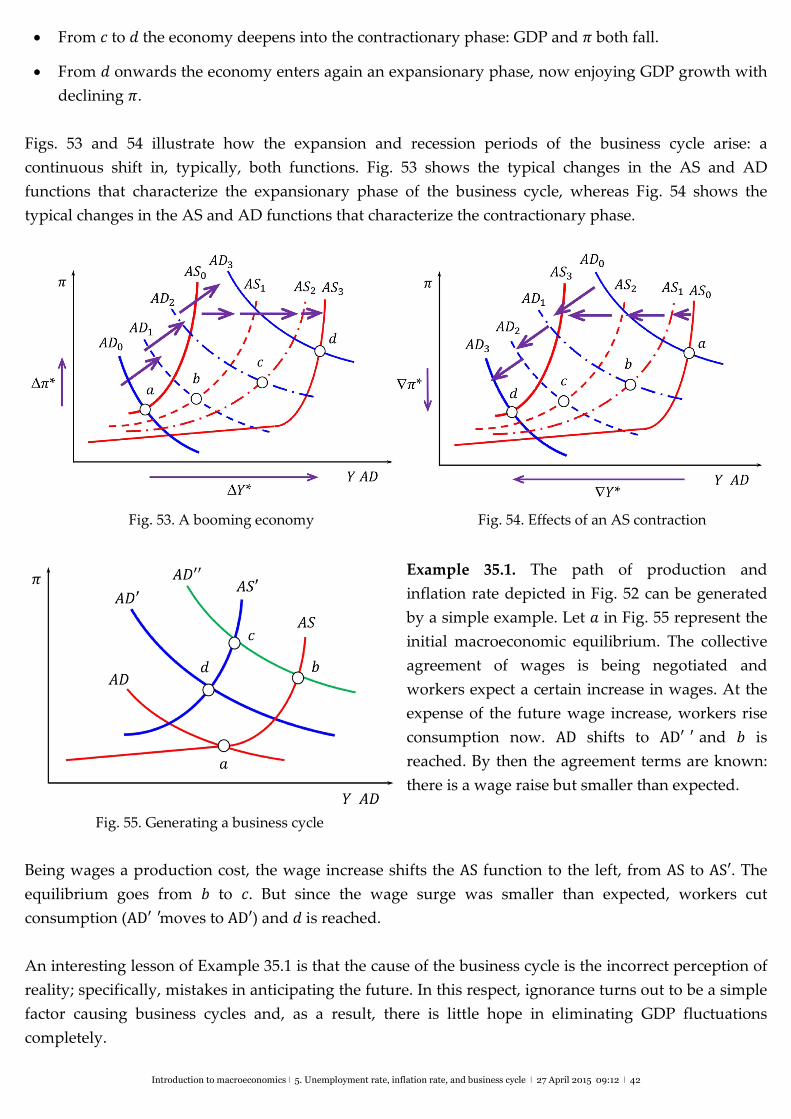
Introduction to macroeconomics ǀ 5. Unemployment rate, inflation rate, and business cycle ǀ 27 April 2015 09:12 ǀ 42
From � to � the economy deepens into the contractionary phase: GDP and � both fall.
From � onwards the economy enters again an expansionary phase, now enjoying GDP growth with
declining �.
Figs. 53 and 54 illustrate how the expansion and recession periods of the business cycle arise: a
continuous shift in, typically, both functions. Fig. 53 shows the typical changes in the AS and AD
functions that characterize the expansionary phase of the business cycle, whereas Fig. 54 shows the
typical changes in the AS and AD functions that characterize the contractionary phase.
Fig. 53. A booming economy Fig. 54. Effects of an AS contraction
Example 35.1. The path of production and
inflation rate depicted in Fig. 52 can be generated
by a simple example. Let � in Fig. 55 represent the
initial macroeconomic equilibrium. The collective
agreement of wages is being negotiated and
workers expect a certain increase in wages. At the
expense of the future wage increase, workers rise
consumption now. AD shifts to AD′′ and � is
reached. By then the agreement terms are known:
there is a wage raise but smaller than expected.
Fig. 55. Generating a business cycle
Being wages a production cost, the wage increase shifts the AS function to the left, from AS to AS′. The
equilibrium goes from � to �. But since the wage surge was smaller than expected, workers cut
consumption (AD′′ moves to AD′) and � is reached.
An interesting lesson of Example 35.1 is that the cause of the business cycle is the incorrect perception of
reality; specifically, mistakes in anticipating the future. In this respect, ignorance turns out to be a simple
factor causing business cycles and, as a result, there is little hope in eliminating GDP fluctuations
completely.
Introduction to macroeconomics ǀ 5. Unemployment rate, inflation rate, and business cycle ǀ 27 April 2015 09:12 ǀ 43
Remark 35.2. Heterodox economists emphasize the impact on economic activity of fundamental
uncertainty: events that are unknown and unknowable. Orthodox economist, instead, ground their
analyses on the presumption of complete information: economic agents (mainly, private agents) know
everything and act accordingly (yet, ignorance is typically ascribed to public authorities).
Remark 35.3. Long‐run and short‐run macroeconomics. Textbooks make production converge to a long
run fixed production level representing potential GDP, which is (unrealistically) presumed to be given
and unaffected by short run decisions. This is a quite debatable assumption (in fact, there does not
appear to be a long run but a sequence of short runs). Concretely, this analysis side‐steps two relevant
considerations:
AD and AS are interdependent (investment is an AD component but also contributes to the
productive capacity of the economy); and
the phenomenon of hysteresis, according to which short run decisions may have long run
permanent and very different consequences (the butterfly effect), so the state eventually reaches an
economy depends on the path taken (the sequence of decisions that made each short run).
Remark 35.4. The butterfly effect. States that chaotic and/or complex systems are sensitively dependent
on initial conditions: a trivially small change in the characteristics of an economy can lead to large
qualitative changes in economic outcomes (a butterfly flapping its wings could in theory cause a large‐
scale change in the weather on the other side of the planet). For economic modeling and analysis, the
butterfly effect means that small errors in data, or criteria to aggregate or round off data, could
drastically alter the predicted results.
Remark 35.5. J. M. Keynes on the long run. “The long run is a misleading guide to current affairs. In the
long run we are all dead. Economists set themselves too easy, too useless a task if in tempestuous
seasons they can only tell us that when the storm is past the ocean is flat again.” A Tract on Monetary
Reform, 1923, chapter 3.
36. The expenditure multiplier effect
The expenditure multiplier effect explains how the transition from � to � in Fig. 49 unfolds. To illustrate
the concept and the mechanism generating the multiplier effect, consider the following example.
Example 36.1. Let the AD function only depend on � and �, so �� = � + �. Let � be constant. Specifically,
� = 4 + 0.8� − � and � = 10 (where � is a percentage and the value 0.8 is the marginal propensity � to
consume: which fraction of an additional unit of income is consumed). The �� function is � = 30·�. The
macroeconomic equilibrium (�*, �*) is obtained from the equilibrium condition � = ��. That is,
� = 4 + 0.8 ·� − � + 10. Therefore, 0.2 ·� = 14− �. As � = 30·�, �* = 2 is the equilibrium inflation
rate. Given �* = 2, the AS function yields the equilibrium production level �* = 30·2 = 60.
Suppose that some component in the AD function changes. Specifically, suppose that the constant
representing investment increases. This may be due to the fact that businessmen’s expectations suddenly
become more optimistic about the level of economic activity or the expected level of profits.
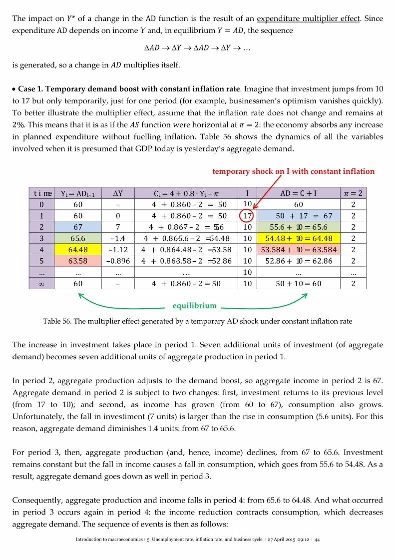
Introduction to macroeconomics ǀ 5. Unemployment rate, inflation rate, and business cycle ǀ 27 April 2015 09:12 ǀ 44
The impact on �* of a change in the AD function is the result of an expenditure multiplier effect. Since
expenditure AD depends on income Y and, in equilibrium � = ��, the sequence
�� � �� � …
is generated, so a change in �� multiplies itself.
Case 1. Temporary demand boost with constant inflation rate. Imagine that investment jumps from 10
to 17 but only temporarily, just for one period (for example, businessmen’s optimism vanishes quickly).
To better illustrate the multiplier effect, assume that the inflation rate does not change and remains at
2%. This means that it is as if the �� function were horizontal at � = 2: the economy absorbs any increase
in planned expenditure without fuelling inflation. Table 56 shows the dynamics of all the variables
involved when it is presumed that GDP today is yesterday’s aggregate demand.
temporary shock on I with constant inflation
time Yt=ADt–1 Y Ct=4+0.8·Yt–� I AD=C+I �=2
0 60 – 4+0.8·60–2=50 10 60 2
1 60 0 4+0.8·60–2=50 17 50+17=67 2
2 67 7 4+0.8·67–2=55.6 10 55.6+10=65.6 2
3 65.6 –1.4 4+0.8·65.6–2=54.48 10 54.48+10=64.48 2
4 64.48 –1.12 4+0.8·64.48–2=53.58 10 53.584+10=63.584 2
5 63.58 –0.896 4+0.8·63.58–2=52.86 10 52.86+10=62.86 2
… … … … 10 … …
60 – 4+0.8·60–2=50 10 50+10=60 2
equilibrium
Table 56. The multiplier effect generated by a temporary AD shock under constant inflation rate
The increase in investment takes place in period 1. Seven additional units of investment (of aggregate
demand) becomes seven additional units of aggregate production in period 1.
In period 2, aggregate production adjusts to the demand boost, so aggregate income in period 2 is 67.
Aggregate demand in period 2 is subject to two changes: first, investment returns to its previous level
(from 17 to 10); and second, as income has grown (from 60 to 67), consumption also grows.
Unfortunately, the fall in investiment (7 units) is larger than the rise in consumption (5.6 units). For this
reason, aggregate demand diminishes 1.4 units: from 67 to 65.6.
For period 3, then, aggregate production (and, hence, income) declines, from 67 to 65.6. Investment
remains constant but the fall in income causes a fall in consumption, which goes from 55.6 to 54.48. As a
result, aggregate demand goes down as well in period 3.
Consequently, aggregate production and income falls in period 4: from 65.6 to 64.48. And what occurred
in period 3 occurs again in period 4: the income reduction contracts consumption, which decreases
aggregate demand. The sequence of events is then as follows:
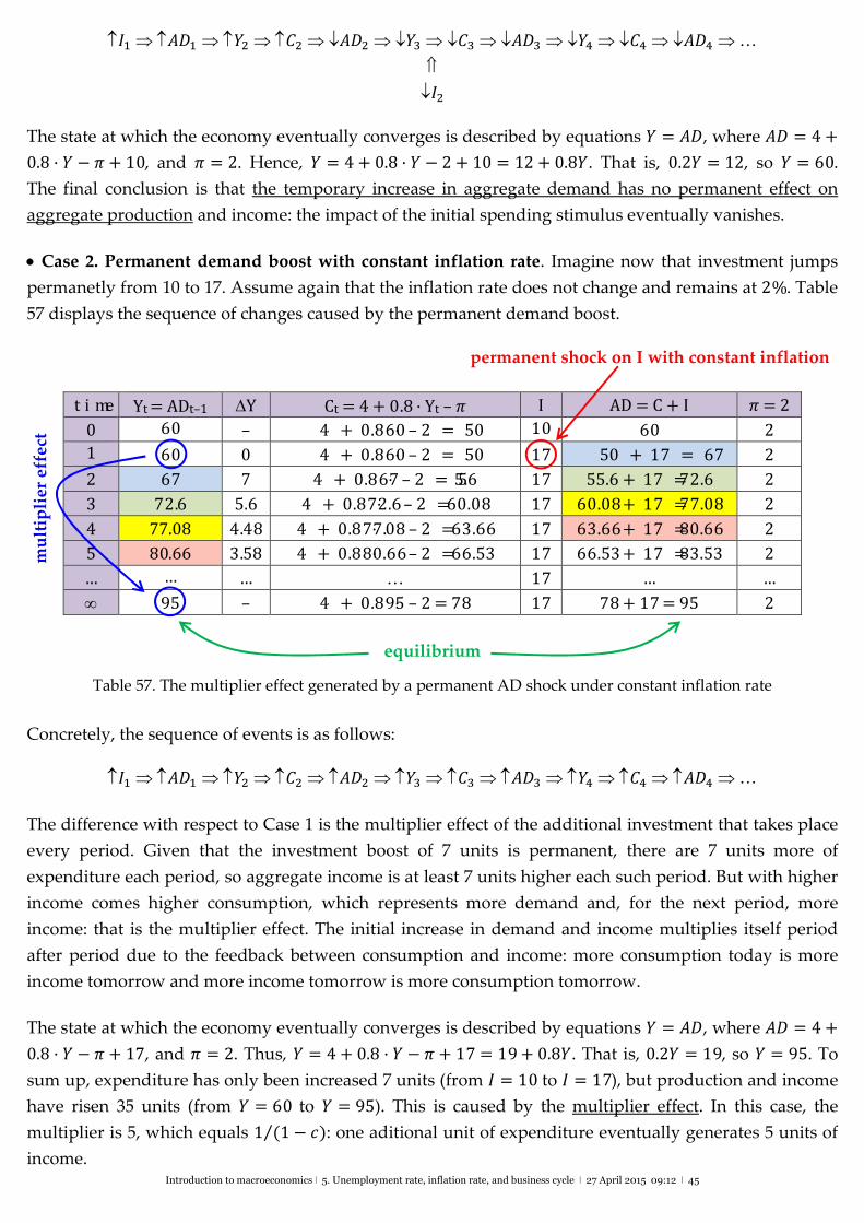
Introduction to macroeconomics ǀ 5. Unemployment rate, inflation rate, and business cycle ǀ 27 April 2015 09:12 ǀ 45
�� ��� �� �� ��� �� �� ��� �� �� ��� …
��
The state at which the economy eventually converges is described by equations � = ��, where �� = 4+
0.8 ·� − � + 10, and � = 2. Hence, � = 4 + 0.8 ·� − 2 + 10 = 12 + 0.8�. That is, 0.2� = 12, so � = 60.
The final conclusion is that the temporary increase in aggregate demand has no permanent effect on
aggregate production and income: the impact of the initial spending stimulus eventually vanishes.
Case 2. Permanent demand boost with constant inflation rate. Imagine now that investment jumps
permanetly from 10 to 17. Assume again that the inflation rate does not change and remains at 2%. Table
57 displays the sequence of changes caused by the permanent demand boost.
permanent shock on I with constant inflation
time Yt=ADt–1 Y Ct=4+0.8·Yt–� I AD=C+I �=2
0 60 – 4+0.8·60–2=50 10 60 2
1 60 0 4+0.8·60–2=50 17 50+17=67 2
2 67 7 4+0.8·67–2=55.6 17 55.6+17=72.6 2
3 72.6 5.6 4+0.8·72.6–2=60.08 17 60.08+17=77.08 2
4 77.08 4.48 4+0.8·77.08–2=63.66 17 63.66+17=80.66 2
5 80.66 3.58 4+0.8·80.66–2=66.53 17 66.53+17=83.53 2
… … … … 17 … …
95 – 4+0.8·95–2=78 17 78+17=95 2
equilibrium
Table 57. The multiplier effect generated by a permanent AD shock under constant inflation rate
Concretely, the sequence of events is as follows:
�� ��� �� �� ��� �� �� ��� �� �� ��� …
The difference with respect to Case 1 is the multiplier effect of the additional investment that takes place
every period. Given that the investment boost of 7 units is permanent, there are 7 units more of
expenditure each period, so aggregate income is at least 7 units higher each such period. But with higher
income comes higher consumption, which represents more demand and, for the next period, more
income: that is the multiplier effect. The initial increase in demand and income multiplies itself period
after period due to the feedback between consumption and income: more consumption today is more
income tomorrow and more income tomorrow is more consumption tomorrow.
The state at which the economy eventually converges is described by equations � = ��, where �� = 4+
0.8 ·� − � + 17, and � = 2. Thus, � = 4+ 0.8 ·� − � + 17= 19 + 0.8�. That is, 0.2� = 19, so � = 95. To
sum up, expenditure has only been increased 7 units (from � = 10 to � = 17), but production and income
have risen 35 units (from � = 60 to � = 95). This is caused by the multiplier effect. In this case, the
multiplier is 5, which equals 1 (1− �)⁄ : one aditional unit of expenditure eventually generates 5 units of
income.
mu
ltip
lier
eff
ect
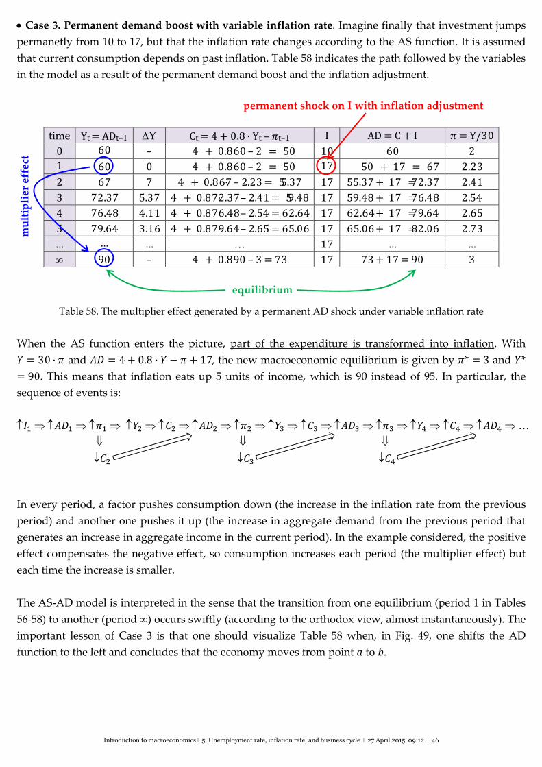
Introduction to macroeconomics ǀ 5. Unemployment rate, inflation rate, and business cycle ǀ 27 April 2015 09:12 ǀ 46
Case 3. Permanent demand boost with variable inflation rate. Imagine finally that investment jumps
permanetly from 10 to 17, but that the inflation rate changes according to the AS function. It is assumed
that current consumption depends on past inflation. Table 58 indicates the path followed by the variables
in the model as a result of the permanent demand boost and the inflation adjustment.
permanent shock on I with inflation adjustment
time Yt=ADt–1 Y Ct=4+0.8·Yt–�t–1 I AD=C+I �=Y/30
0 60 – 4+0.8·60–2=50 10 60 2
1 60 0 4+0.8·60–2=50 17 50+17=67 2.23
2 67 7 4+0.8·67–2.23=55.37 17 55.37+17=72.37 2.41
3 72.37 5.37 4+0.8·72.37–2.41=59.48 17 59.48+17=76.48 2.54
4 76.48 4.11 4+0.8·76.48–2.54=62.64 17 62.64+17=79.64 2.65
5 79.64 3.16 4+0.8·79.64–2.65=65.06 17 65.06+17=82.06 2.73
… … … … 17 … …
90 – 4+0.8·90–3=73 17 73+17=90 3
equilibrium
Table 58. The multiplier effect generated by a permanent AD shock under variable inflation rate
When the AS function enters the picture, part of the expenditure is transformed into inflation. With
� = 30·� and �� = 4+ 0.8 ·� − � + 17, the new macroeconomic equilibrium is given by �* = 3 and �*
= 90. This means that inflation eats up 5 units of income, which is 90 instead of 95. In particular, the
sequence of events is:
�� ��� �� �� �� ��� �� �� �� ��� �� �� �� ��� …
�� �� ��
In every period, a factor pushes consumption down (the increase in the inflation rate from the previous
period) and another one pushes it up (the increase in aggregate demand from the previous period that
generates an increase in aggregate income in the current period). In the example considered, the positive
effect compensates the negative effect, so consumption increases each period (the multiplier effect) but
each time the increase is smaller.
The AS‐AD model is interpreted in the sense that the transition from one equilibrium (period 1 in Tables
56‐58) to another (period ) occurs swiftly (according to the orthodox view, almost instantaneously). The
important lesson of Case 3 is that one should visualize Table 58 when, in Fig. 49, one shifts the AD
function to the left and concludes that the economy moves from point � to �.
mu
ltip
lier
eff
ect