ECONOMICS

BUFFER EFFECT AND PRICE EFFECT OF A PERSONAL CARBON TRADING SCHEME

by

Jin Fan School of Management

University of Science and Technology of China

Shanyong Wang School of Management

University of Science and Technology of China

Yanrui Wu Business School

University of Western Australia

Jun Li School of Management

University of Science and Technology of China

Dingtao Zhao School of Management

University of Science and Technology of China

DISCUSSION PAPER 15.07

BUFFER EFFECT AND PRICE EFFECT OF A PERSONAL

CARBON TRADING SCHEME

Jin Fana, Shanyong Wanga, Yanrui Wub, Jun Lia, Dingtao Zhaoa

DISCUSSION PAPER 15.07

ABSTRACT: Personal carbon trading (PCT) is a downstream cap-and-trade scheme used to reduce carbon emissions from the household sector. It is argued that the PCT scheme could provide a buffer between the energy price and the total energy price, and thus energy demand remains stable. However these effects have never been verified. To fill in this gap in the literature, a price effect analysis is conducted. Firstly, a general utility optimization (GUO) model is proposed to obtain the general formulae of the price effect, substitution effect and income effect under the PCT scheme. Secondly, a specific version of the GUO model, namely a Cobb-Douglas utility function model, is employed to obtain the specific effect formulae to verify the buffer effect. Finally, a numerical example and a sensitive analysis are presented to demonstrate these effects. The results indicate that, under the PCT scheme, the total energy price and energy demand are less sensitive to the energy price changes. Thus, when energy prices fluctuate, the PCT scheme is capable of providing certainty in emissions reduction and is more effective than carbon taxes. On the basis of these results, implications of this research are discussed and suggestions for future research are provided. Keywords: Personal Carbon Trading; Buffer effect; Price effect; Energy demand; Energy price; Allowance price

a School of Management, University of Science and Technology of China, P.R. China b Business School, University of Western Australia, Australia Citation: Fan, Jin, Shanyong Wang, Yanrui Wu, Jun Li and Dingtao Zhao, 2015, “Buffer Effect and Price Effect of a Personal Carbon Trading Scheme”, Energy: The International Journal (Impact factor: 4.159).

1. Introduction

Carbon emissions caused by household energy consumption have become a

major source of total emissions and have attracted worldwide attention (Jaehn and

Letmathe, 2010; Rout et al., 2011; Feng et al., 2011). For instance, at present about 30%

of carbon emissions in China are generated in the household sector (NBSC, 2013).

There is no doubt that these emissions will continue to grow due to the rapid

economic growth and urbanization in the coming decades (Liu et al., 2011; Rout et al.,

2011; Fan et al., 2012).

Personal carbon trading (PCT) has been proposed as a radical policy to start

translating the consumption perspective into carbon reduction practice at the

household level (Fleming, 1996). It is a downstream cap-and-trade scheme which

could be used to reduce carbon emissions from the household sector, and which is

analogous to the upstream emissions trading system operating in the industrial sector

(Harwatt et al., 2011; Roberts and Thumin, 2006; Fleming, 1996). In fact, there are

links between these two schemes. In an upstream carbon trading scheme (such as the

EU Emission Trading Scheme), generators surrender allowances for the carbon

contained in the electricity sales. In a PCT scheme, consumers surrender allowances

for their electricity consumption. These two trading schemes will interfere with each

other and produce two interaction results: double regulation and double counting

(Sorrell, 2010). Namely, consumers would face two sets of carbon prices (i.e. the EU

ETS price and the PCT price) and they would also surrender two separate carbon

allowances (Sorrell and Sijm, 2003). Establishing links between the upstream trading

scheme and PCT scheme will improve liquidity and reduce the risk of participants

using their market power to influence the allowance prices (Sorrell, 2010). At the

same time, to avoid double regulation and double counting, the PCT scheme would

need to ensure that the energy and fuel purchased by consumers would not include the

price of the carbon allowance in the upstream trading scheme (Sorrell, 2010).

Under the PCT scheme, emission allowances are allocated equally and freely to

each adult by the government and the allowances allocation is reduced year by year

1

(Harwatt et al., 2011; Fawcett et al., 2007; Meyer, 2000). However, taking into

account that some low income consumers with greater energy need may use older and

energy-intensive appliances, for instance living in lower insulated house, a supporting

system is proposed to address this equity issue. Bristow et al. (2010) argued that

equity is addressed through a supporting system with higher allocations or financial

support to those with greater need. This system is similar to the Clean Development

Mechanism (CDM) foreseen in Kyoto Protocol to close the gap between the low

economical class and middle/high class. Carbon allowance trading among consumers

is the key feature of the PCT scheme. In this scheme, the over-emitters (allowance

buyers) who emit more than their initial allowances have to buy permits in the market

from the under-emitters (allowance sellers) who emit less than their initial allowances

(Cohen, 2011). Although no one is compelled to sell or buy allowances in this system,

one’s utility would be improved if one chooses to do so.

Compared with an upstream carbon trading scheme, PCT is a progressive

scheme in which the poorer consumers are mostly 'winners', as their levels of

emissions are generally lower. To some extent, the capacity to reduce carbon

emissions under the PCT scheme is much larger. Weitzman et al. (1974) noted that

carbon taxes and tradable permits are theoretically equivalent in terms of efficiency

and effectiveness. However, a carbon tax policy is mainly a price-based

environmental regulation which fixes the allowance price and lets the market

determine the amount of carbon emissions emitted, whilst a PCT scheme is mainly a

quantity-based one which fixes the quantity emitted and lets the allowance price to be

determined by the market. The emission cap under the PCT scheme can directly affect

the carbon reduction targets. If there is uncertainty over the cost function, it is better

to fix the price through a tax policy, and if there is uncertainty over the damage

function, fixing the quantity through a tradable system is more appropriate (Pizer,

2002; Stranlund and Ben-Haim, 2008).

PCT has attracted widespread attention in both research and policy domains. In

2010, the Climate Policy journal published a special issue on PCT with 10 articles.

Most research on PCT focuses on equity, effectiveness, public acceptability, barriers 2

to implementation and its potential advantages over the existing climate policy

instruments, such as upstream “cap and trade” systems and carbon taxes (Harwatt,

2008; Jagers, 2010; Eyre, 2010; Bristow et al., 2010; Parag and Eyre, 2010; Fawcett

et al., 2007; Wallace et al., 2010; Sorrell, 2010; Parag et al., 2011; Wadud, 2011;

Starkey, 2012). Compared with a simple tax system the costs of PCT, which include

implementation cost, participation cost and transaction cost, may be higher (Fawcett,

2010). However, the short-term elasticities of demand for vehicle fuel and domestic

energy are low, which means that the effect of a carbon tax will be fairly limited

(Lockwood, 2010). At the same time, the attitude of the public is another factor that

needs to be considered. It is argued that consumers are more likely to oppose the

carbon tax and accept the PCT (Harwatt, 2008).

Lane et al. (2008) argued that the allowance price significantly influences energy

price and furthermore affects energy demand and associated lifestyles. Wadud (2011)

noted that one of the advantages of a personal tradable permit approach over the

carbon tax is the buffer it provides when the price of oil in the world market changes

suddenly. When the price of oil increases, the price of the permits would fall. Then the

total amount (price of the permits + price of pre-tax gasoline) paid by consumers

would remain stable, and thus the gasoline demand would also remain stable.

However this conclusion is based on qualitative judgments. A more rigorous

investigation is thus required.

The buffer effect would influence energy demand under the PCT scheme.

Wadud’s (2007) argued that the buffer effect would help stablise energy demand.

However, this conclusion does not take into account the allowance price change and

its further influence on consumers’ full budget (money budget plus the product of the

allowance price and initial allowance allocation). Due to the buffer effect, an increase

of the energy price would lead to the fall in the allowance price and hence a decrease

in the full budget (Varian, 1992). Therefore energy demand would become uncertain.

To illustrate this, a price effect (PE) analysis might be appropriate. According to

economic theory when consumer’s income is constant, changes in commodity prices

will lead to changes in quantity demanded (Klein and Rubin, 1947; Varian, 1992). 3

This is known as the price effect. The price effect is determined by the substitution

effect (SE) and income effect (IE) (William, 1973; Neary and Roberts, 1980). On the

one hand, changes in commodity prices will lead to relative changes in other prices,

and thus lead to changes in the quantities demanded. This phenomenon is known as

the substitution effect. On the other hand, changes in commodity prices will also lead

to changes in real income levels, and thus lead to changes in quantities demanded.

This phenomenon is called the income effect (William, 1973). For different

commodities (normal goods, inferior goods and Giffen goods), the influences of price

effect, substitution effect and income effect on quantities demanded are quite different

(Varian, 1992).

However, whether there is a buffer effect or not remains a question. It is also

unclear whether or not energy demand is stable under the PCT scheme. In the

following sections, nonlinear optimization models will be proposed to explore these

questions. The remainder of this paper is organized as follows. Section 2 introduces a

general utility optimization (GUO) model to obtain the general formulae of the price

effect, substitution effect and income effect under the PCT scheme. Section 3 presents

a specific version of the GUO model and a Cobb-Douglas utility function model is

employed to obtain the specific formulae of these effects under the with-PCT and

without-PCT scenarios. Section 4 describes the data calibration results. Finally

Section 5 concludes the paper and points out the implications and limitations of the

results.

2. A GUO model under the PCT scheme

We assume that commodities can be classified into two categories, namely

energy commodities X and non-energy commodities Y . The general utility

function can be expressed as ( , )U U X Y= . Given that consumers need to pay money

as well as surrender certain carbon allowances when they purchase energy, their utility

optimization is subject to two constraints, namely, the money budget and the carbon

allowance allocation (Absi et al., 2013). Furthermore the rationale for the allocation

4

of these allowances is critical in the design of the PCT scheme. Most authors have

focused on an equal per capita allowance allocation which is based on the argument

that everyone has equal rights to the environment (Pezzey, 2003; Wadud, 2011). For

example, Harwatt et al. (2011) noted that the initial carbon allowance could be

allocated equally to individuals free of charge. Thus, we assume an equal initial

allowance ω for all consumers.

Under the PCT scheme, consumers should solve the following utility

maximization problem.

/ /

/

ax ( , )

. . c

x

M U U X Y

p X q Y p Is t

c Xψ

ψ ω

=

+ + ≤

− ≤

(1)

where 1 2( , ,..., )mX x x x Τ= is the energy consumption vector and 1 2( , ,..., )nY y y y Τ=

is the non-energy consumption vector. /1 2( , ,..., )mp p p p= is the energy price vector

and /1 2( , ,..., )nq q q q= is the non-energy commodity price vector.

1 2

/ ( , ,..., )mx x x xc c c c= is the vector of energy emission rates. cp is the carbon

allowance price. ψ is the allowances bought (or sold) by consumers. I is the

money budget. According to the constraint conditions of equation (1), we have

/ / /( )c x cp p c X q Y I p ω+ + = + (2)

Let / /c xP p p c= + and /

cY I p ω= + , and thus we have

/ /PX q Y Y+ = (3)

where P is the total price vector of energy and /Y is the full budget. We define

equation (3) as a full price constraint.

According to equation (1), we define the indirect utility function, / /( , , )v P q Y , as

the highest level of utility the consumer could reach given prices P and /q , and

budget /Y . According to the duality theorem (Yano, 2012), we have

/ / / /( , , ) , ( , , )i iX P q Y h P v P q Y = (4)

5

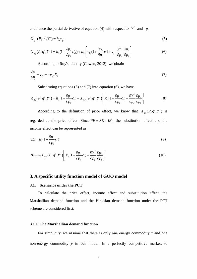
and hence the partial derivative of equation (4) with respect to /Y and ip

/ // /( , , ) iviY Y

X P q Y h v= (5)

/

// / /( , , ) (1 ) (1 )

i i

c c cip ii xi iv P i Y

i i c i

p p pYX P q Y h c h v c vp p p p

∂ ∂ ∂∂= + + + + ∂ ∂ ∂ ∂

(6)

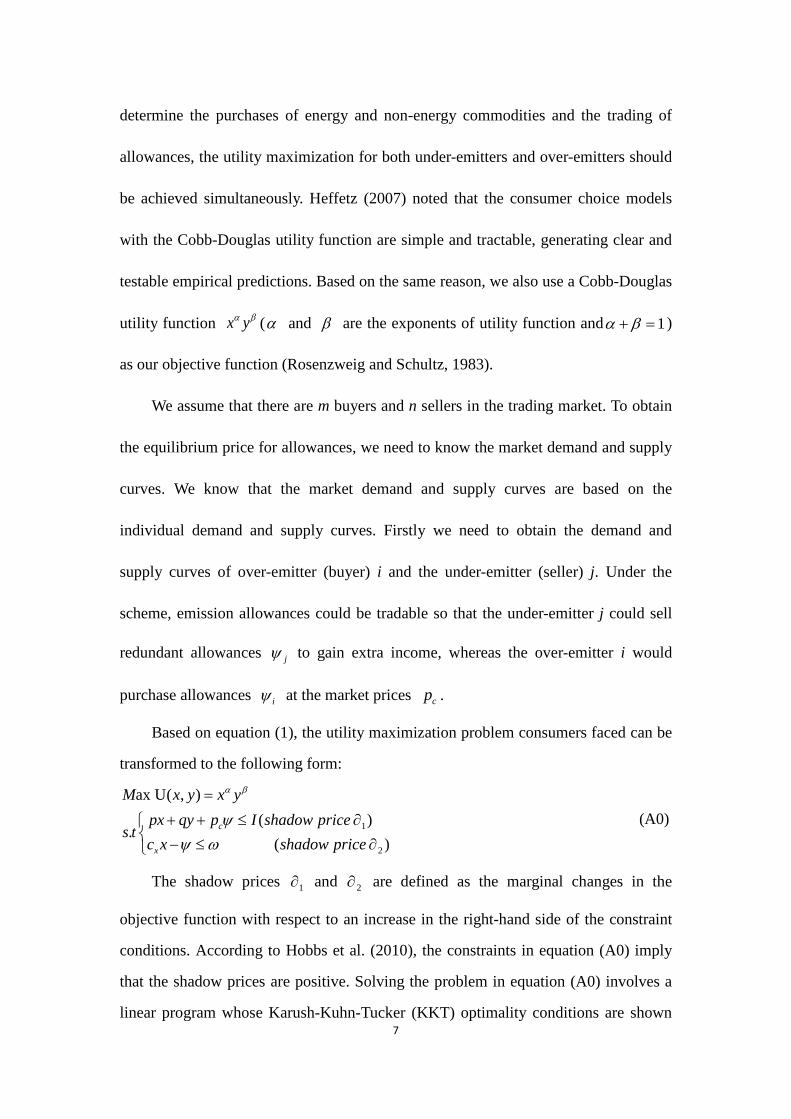
According to Roy's identity (Cowan, 2012), we obtain

/iP iYi

v v v XP

∂= = −

∂ (7)

Substituting equations (5) and (7) into equation (6), we have

/

// / / /( , , ) (1 ) ( , , ) (1 )

i

c c cip ii i i iiY

i i c i

p p pYX P q Y h c X P q Y X cp p p p

∂ ∂ ∂∂= + − + − ∂ ∂ ∂ ∂

(8)

According to the definition of price effect, we know that / /( , , )iipX P q Y is

regarded as the price effect. Since PE SE IE= + , the substitution effect and the

income effect can be represented as

(1 )cii i

i

pSE h cp

∂= +

∂ (9)

/

// /( , , ) (1 )c c

i iiYi c i

p pYIE X P q Y X cp p p

∂ ∂∂= − + − ∂ ∂ ∂

(10)

3. A specific utility function model of GUO model

3.1. Scenarios under the PCT

To calculate the price effect, income effect and substitution effect, the

Marshallian demand function and the Hicksian demand function under the PCT

scheme are considered first.

3.1.1. The Marshallian demand function

For simplicity, we assume that there is only one energy commodity x and one

non-energy commodity y in our model. In a perfectly competitive market, to

6

determine the purchases of energy and non-energy commodities and the trading of

allowances, the utility maximization for both under-emitters and over-emitters should

be achieved simultaneously. Heffetz (2007) noted that the consumer choice models

with the Cobb-Douglas utility function are simple and tractable, generating clear and

testable empirical predictions. Based on the same reason, we also use a Cobb-Douglas

utility function x yα β (α and β are the exponents of utility function and 1α β+ = )

as our objective function (Rosenzweig and Schultz, 1983).

We assume that there are m buyers and n sellers in the trading market. To obtain

the equilibrium price for allowances, we need to know the market demand and supply

curves. We know that the market demand and supply curves are based on the

individual demand and supply curves. Firstly we need to obtain the demand and

supply curves of over-emitter (buyer) i and the under-emitter (seller) j. Under the

scheme, emission allowances could be tradable so that the under-emitter j could sell

redundant allowances jψ to gain extra income, whereas the over-emitter i would

purchase allowances iψ at the market prices cp .

Based on equation (1), the utility maximization problem consumers faced can be

transformed to the following form:

1

2

ax U( , )( )

.( )

c

x

M x y x ypx qy p I shadow price

s tc x shadow price

α β

ψψ ω

=

+ + ≤ ∂ − ≤ ∂

(A0)

The shadow prices 1∂ and 2∂ are defined as the marginal changes in the

objective function with respect to an increase in the right-hand side of the constraint

conditions. According to Hobbs et al. (2010), the constraints in equation (A0) imply

that the shadow prices are positive. Solving the problem in equation (A0) involves a

linear program whose Karush-Kuhn-Tucker (KKT) optimality conditions are shown 7

in Appendix A.

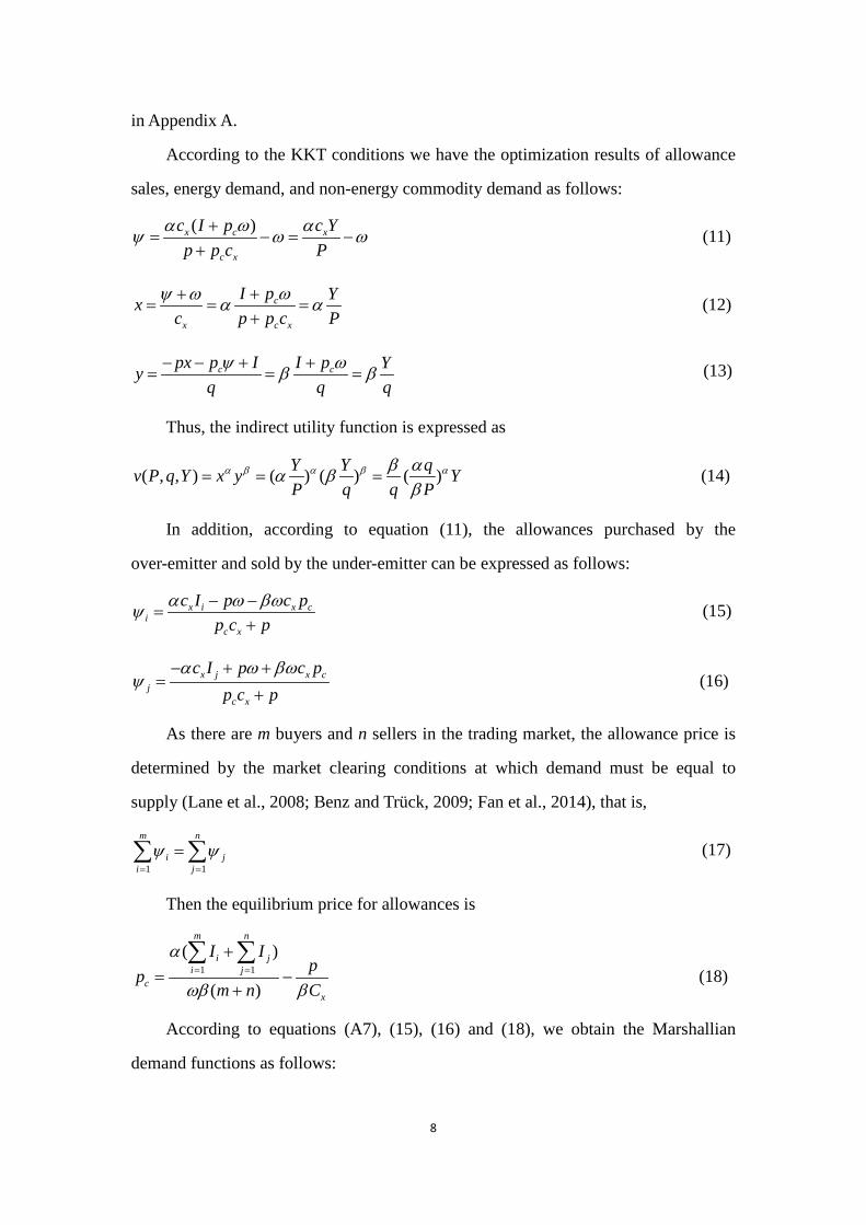
According to the KKT conditions we have the optimization results of allowance

sales, energy demand, and non-energy commodity demand as follows:

( )x c x

c x

c I p c Yp p c P

α ω αψ ω ω+= − = −

+ (11)

c

x c x

I p Yxc p p c P

ωψ ω α α++= = =

+ (12)

c cpx p I I p Yyq q q

ψ ωβ β− − + += = = (13)

Thus, the indirect utility function is expressed as

( , , ) ( ) ( ) ( )Y Y qv P q Y x y YP q q P

α β α β αβ αα ββ

= = = (14)

In addition, according to equation (11), the allowances purchased by the

over-emitter and sold by the under-emitter can be expressed as follows:

x i x ci

c x

c I p c pp c p

α ω βωψ − −=

+ (15)

x j x cj

c x

c I p c pp c p

α ω βωψ

− + +=

+ (16)

As there are m buyers and n sellers in the trading market, the allowance price is

determined by the market clearing conditions at which demand must be equal to

supply (Lane et al., 2008; Benz and Trück, 2009; Fan et al., 2014), that is,

1 1

m n

i ji j

ψ ψ= =

=∑ ∑ (17)

Then the equilibrium price for allowances is

1 1( )

( )

m n

i ji j

cx

I Ipp

m n C

α

ωβ β= =

+= −

+

∑ ∑ (18)

According to equations (A7), (15), (16) and (18), we obtain the Marshallian

demand functions as follows:

8

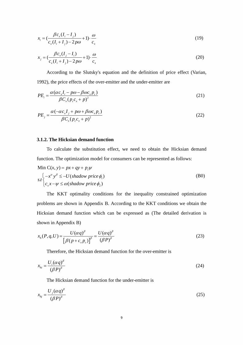
( )( 1)

( ) 2x i j

ix i j x

c I Ix

c I I p cβ ω

ω−

= + ⋅+ −

(19)

( )( 1)

( ) 2x j i

jx i j x

c I Ix

c I I p cβ ω

ω−

= + ⋅+ −

(20)

According to the Slutsky's equation and the definition of price effect (Varian,

1992), the price effects of the over-emitter and the under-emitter are

2

( )( )

x i x ci

x c x

c I p c pPEC p c p

α α ω βωβ

− −=

+ (21)

2

( )( )

x j x cj

x c x

c I p c pPE

C p c pα α ω βω

β− + +

=+

(22)

3.1.2. The Hicksian demand function

To calculate the substitution effect, we need to obtain the Hicksian demand

function. The optimization model for consumers can be represented as follows:

1

2

Min C( , )

( ).

( )

c

x

x y px qy p

x y U shadow prices t

c x shadow price

α β

ψ

φψ ω φ

= + +

− ≤ −

− ≤

(B0)

The KKT optimality conditions for the inequality constrained optimization

problems are shown in Appendix B. According to the KKT conditions we obtain the

Hicksian demand function which can be expressed as (The detailed derivation is

shown in Appendix B)

[ ]( ) ( )( , , )

( )( )h

x c

U q U qx P q UPp c p

β β

β β

α αββ

= =+

(23)

Therefore, the Hicksian demand function for the over-emitter is

( )( )

ihi

U qxP

β

β

αβ

= (24)

The Hicksian demand function for the under-emitter is

( )( )

jhj

U qx

P

β

β

αβ

= (25)

9

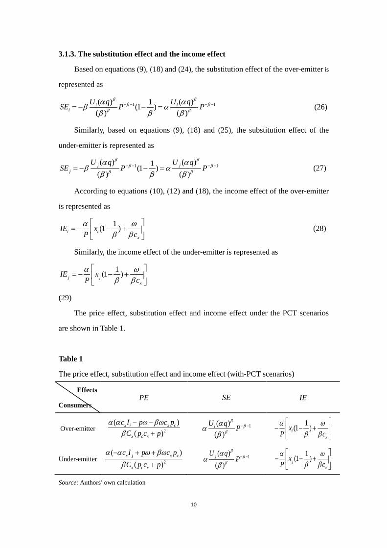
3.1.3. The substitution effect and the income effect

Based on equations (9), (18) and (24), the substitution effect of the over-emitter is

represented as

1 1( ) ( )1(1 )( ) ( )i i

iU q U qSE P P

β ββ β

β β

α αβ αβ β β

− − − −= − − = (26)

Similarly, based on equations (9), (18) and (25), the substitution effect of the

under-emitter is represented as

1 1( ) ( )1(1 )( ) ( )j j

j

U q U qSE P P

β ββ β

β β

α αβ α

β β β− − − −= − − =

(27)

According to equations (10), (12) and (18), the income effect of the over-emitter

is represented as

1(1 )i ix

IE xP cα ω

β β

= − − +

(28)

Similarly, the income effect of the under-emitter is represented as

1(1 )j jx

IE xP cα ω

β β

= − − +

(29)

The price effect, substitution effect and income effect under the PCT scenarios

are shown in Table 1.

Table 1

The price effect, substitution effect and income effect (with-PCT scenarios)

Effects

Consumers PE SE IE

Over-emitter 2

( )( )

x i x c

x c x

c I p c pC p c p

α α ω βωβ

− −+

1( )( )iU q P

ββ

β

ααβ

− − 1(1 )i

x

xP cα ω

β β

− − +

Under-emitter 2

( )( )

x j x c

x c x

c I p c pC p c p

α α ω βωβ

− + +

+ 1( )

( )jU q

Pβ

ββ

αα

β− −

1(1 )jx

xP cα ω

β β

− − +

Source: Authors’ own calculation

10

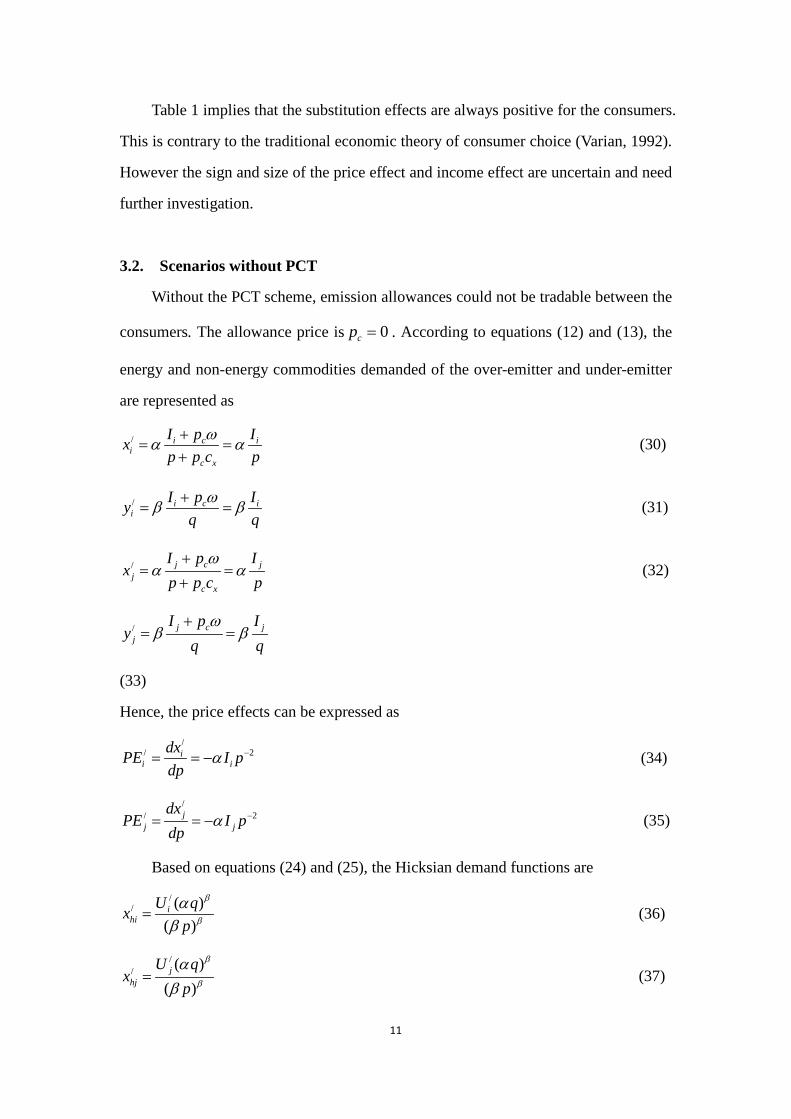
Table 1 implies that the substitution effects are always positive for the consumers.

This is contrary to the traditional economic theory of consumer choice (Varian, 1992).

However the sign and size of the price effect and income effect are uncertain and need

further investigation.

3.2. Scenarios without PCT

Without the PCT scheme, emission allowances could not be tradable between the

consumers. The allowance price is 0cp = . According to equations (12) and (13), the

energy and non-energy commodities demanded of the over-emitter and under-emitter

are represented as

/ i c ii

c x

I p Ixp p c p

ωα α+= =

+ (30)

/ i c ii

I p Iyq q

ωβ β+= = (31)

/ j c jj

c x

I p Ix

p p c pω

α α+

= =+

(32)

/ j c jj

I p Iy

q qω

β β+

= =

(33)

Hence, the price effects can be expressed as

// 2ii i

dxPE I pdp

α −= = −

(34)

// 2jj j

dxPE I p

dpα −= = −

(35)

Based on equations (24) and (25), the Hicksian demand functions are

// ( )

( )i

hiU qx

p

β

β

αβ

= (36)

// ( )

( )j

hj

U qx

p

β

β

αβ

= (37)

11

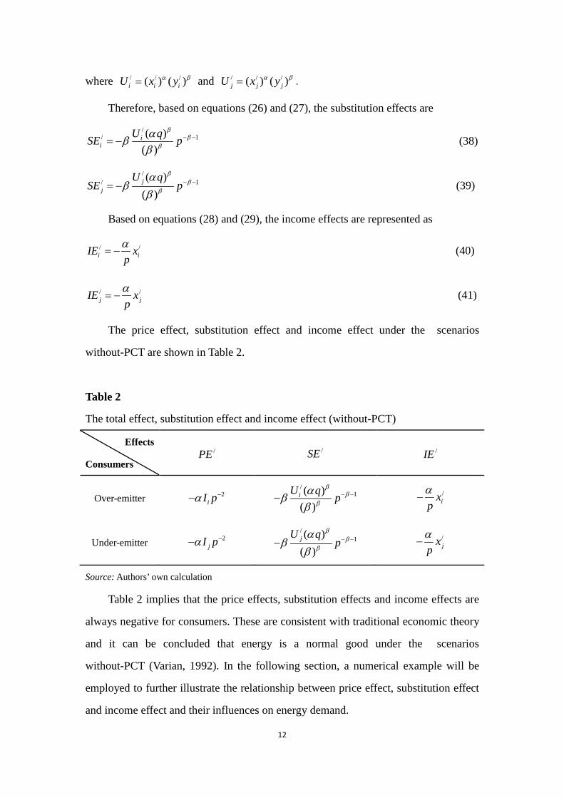
where / / /( ) ( )i i iU x yα β= and / / /( ) ( )j j jU x yα β= .

Therefore, based on equations (26) and (27), the substitution effects are

// 1( )

( )i

iU qSE p

ββ

β

αββ

− −= −

(38)

// 1( )

( )j

j

U qSE p

ββ

β

αβ

β− −= −

(39)

Based on equations (28) and (29), the income effects are represented as

/ /i iIE x

pα

= − (40)

/ /j jIE x

pα

= −

(41)

The price effect, substitution effect and income effect under the scenarios

without-PCT are shown in Table 2.

Table 2

The total effect, substitution effect and income effect (without-PCT)

Effects

Consumers /PE /SE /IE

Over-emitter 2iI pα −−

/1( )

( )iU q p

ββ

β

αββ

− −− /ix

pα

−

Under-emitter 2jI pα −−

/1( )

( )jU q

pβ

ββ

αβ

β− −−

/jx

pα

−

Source: Authors’ own calculation

Table 2 implies that the price effects, substitution effects and income effects are

always negative for consumers. These are consistent with traditional economic theory

and it can be concluded that energy is a normal good under the scenarios

without-PCT (Varian, 1992). In the following section, a numerical example will be

employed to further illustrate the relationship between price effect, substitution effect

and income effect and their influences on energy demand.

12

4. Data Calibration

In this section the influence of the buffer effect on the energy price is analyzed

through numerical simulation. For this purpose, some model parameters are based on

Chinese statistics. In China major energy sources include coal, petroleum and natural

gas (Huang and Yan, 2009). For simplicity we take gasoline as an example to conduct

the data calibration. The current price of gasoline is about $4.46/gallon and the

emission rate of gasoline is about 9.84 kg/gallon in China.1 In this paper, we specify

that the energy price ranges from $4.50 /gallon to $9.00 /gallon and the emission rate

is 10.00xc = kg/gallon. According to the distribution of per capita disposable income

in China, we specify the consumption budget as 12 0$ ,00iI = and 4 5 0$ , 0jI = , and

the exponents of the utility function as 0.10α = and 0.90β = ( NBSC, 2013). Other

parameters, such as the price of non-energy commodities and the initial allowance

were specified as q =$1.00/unit and 800ω = (kg/year). In addition, we assume that

there are 400 buyers and 500 sellers in the trading market, namely m=400 and n=500.

In addition the system’s fixed operational cost η , which includes audit,

verification and reporting requirements, should be considered in the PCT scheme.

This is because the portion of this cost as part of the household annual consumption

cost is expected to be higher than that of the industrial sector in relation to its turnover.

This cost has a significant influence on the PCT scheme (Fawcett, 2010). Based on

Harwatt et al. (2011) and the statistics of OECD2, we specify the fixed operational

cost η as $0.05/gallon. Thus, the total energy price of gasoline can be represented as

0.05c x c xP p p c p p cη= + + = + + . In section 4.1 to section 4.3, five propositions will

be proposed. These propositions are concerned with the relationships between the

energy price, allowance price, total energy price and total energy demand.

1 See detail at http://www.cngold.org/crude/qiyou.html and http://urbanian.org/infor_news.asp?sid=34&nid=35&lid=79&id=320 2 See detail at http://www.oecd.org/statistics/

13

4.1. Buffer effect and price effect under the PCT scheme

4.1.1. Buffer effect

As mentioned above, the buffer effect has been proposed by researchers but has

never been verified. To fill in this gap, in this section we will propose several

propositions and prove them using our models.

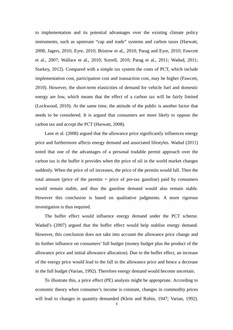
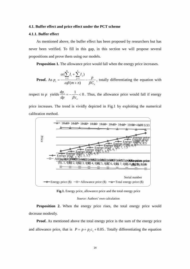
Proposition 1. The allowance price would fall when the energy price increases.

Proof. As 1 1( )

( )

m n

i ji j

cx

I Ipp

m n C

α

ωβ β= =

+= −

+

∑ ∑, totally differentiating the equation with

respect to p yields 1 0c

xdpdp

cβ− <= . Thus, the allowance price would fall if energy

price increases. The trend is vividly depicted in Fig.1 by exploiting the numerical

calibration method.

Fig.1. Energy price, allowance price and the total energy price

Source: Authors’ own calculation

Proposition 2. When the energy price rises, the total energy price would

decrease modestly.

Proof. As mentioned above the total energy price is the sum of the energy price

and allowance price, that is 0.05c xP p p c= + + . Totally differentiating the equation

Energy price ($), 1, 4.5

Energy price ($), 2, 5

Energy price ($), 3, 5.5

Energy price ($), 4, 6

Energy price ($), 5, 6.5

Energy price ($), 6, 7

Energy price ($), 7, 7.5

Energy price ($), 8, 8

Energy price ($), 9, 8.5

Energy price ($), 10, 9

Allowance price ($), 1, 0.59

Allowance price ($), 2, 0.53

Allowance price ($), 3, 0.48

Allowance price ($), 4, 0.42

Allowance price ($), 5, 0.37

Allowance price ($), 6, 0.31

Allowance price ($), 7, 0.25

Allowance price ($), 8, 0.20

Allowance price ($), 9, 0.14

Allowance price ($), 10, 0.09

10.43 10.37 10.32 10.26 10.21 10.15 10.10 10.04 9.99 9.93

Energy price ($) Allowance price ($) Total energy price ($)Serial number

Price

14

yields x cdP dp c dp= + . As 1c

x

pp

dcd β

= − , we have 1dP dp dpβ

= − . Where 1 dpβ

− is

the buffer effect (BE) of energy price on total energy price. β is a constant

parameter that measures the share of non-energy commodities in total consumption.

1β

− represents the buffer multiplier. Since 0 1β< < , we have 1 dp dpβ

− > , which

means that the BE dominates the energy price changes. As the energy price rises, the

allowance price will decrease and the total energy price will also decrease only

modestly (See Fig.1). This phenomenon is consistent with the works of Wadud (2011)

and Gittell (2008) and it could be explained by the buffer effect.

4.1.2. Price effect

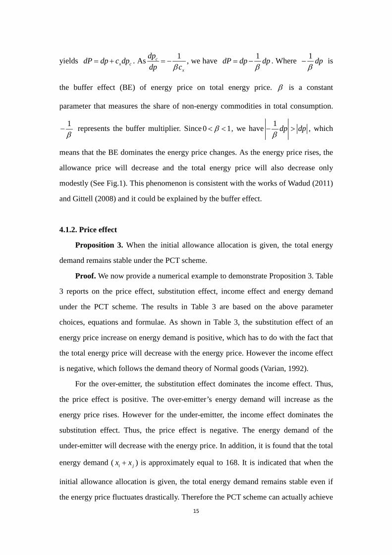
Proposition 3. When the initial allowance allocation is given, the total energy

demand remains stable under the PCT scheme.

Proof. We now provide a numerical example to demonstrate Proposition 3. Table

3 reports on the price effect, substitution effect, income effect and energy demand

under the PCT scheme. The results in Table 3 are based on the above parameter

choices, equations and formulae. As shown in Table 3, the substitution effect of an

energy price increase on energy demand is positive, which has to do with the fact that

the total energy price will decrease with the energy price. However the income effect

is negative, which follows the demand theory of Normal goods (Varian, 1992).

For the over-emitter, the substitution effect dominates the income effect. Thus,

the price effect is positive. The over-emitter’s energy demand will increase as the

energy price rises. However for the under-emitter, the income effect dominates the

substitution effect. Thus, the price effect is negative. The energy demand of the

under-emitter will decrease with the energy price. In addition, it is found that the total

energy demand ( i jx x+ ) is approximately equal to 168. It is indicated that when the

initial allowance allocation is given, the total energy demand remains stable even if

the energy price fluctuates drastically. Therefore the PCT scheme can actually achieve

15

emission reduction targets.

Table 3

Price effects and energy demand under the PCT scheme.

p cp P

Over-emitter Under-emitter

i jx x+

ix iPE iSE iIE jx jPE jSE jIE

4.50 0.59 10.43 119.95 0.42 1.15 -0.72 47.66 -0.35 0.46 -0.80 167.61

5.00 0.53 10.37 120.16 0.43 1.16 -0.73 47.48 -0.35 0.46 -0.81 167.65

5.50 0.48 10.32 120.38 0.43 1.16 -0.73 47.31 -0.35 0.46 -0.81 167.69

6.00 0.42 10.26 120.60 0.44 1.17 -0.74 47.13 -0.36 0.46 -0.82 167.73

6.50 0.37 10.21 120.82 0.44 1.18 -0.74 46.95 -0.36 0.46 -0.82 167.77

7.00 0.31 10.15 121.04 0.45 1.19 -0.74 46.77 -0.37 0.46 -0.82 167.81

7.50 0.25 10.10 121.27 0.45 1.20 -0.75 46.59 -0.37 0.46 -0.83 167.86

8.00 0.20 10.04 121.50 0.46 1.21 -0.75 46.40 -0.37 0.46 -0.83 167.90

8.50 0.14 9.99 121.73 0.46 1.22 -0.75 46.22 -0.38 0.46 -0.84 167.95

9.00 0.09 9.93 121.96 0.47 1.22 -0.76 46.03 -0.38 0.46 -0.84 167.99

Source: Authors’ own calculation

Note: p represents energy price, cp represents allowance price, P represents the total energy

price, PE represents the price effect, SE represents the substitution effect, IE represents

the income effect, x represents the energy demand and i jx x+ represents the total energy

demand.

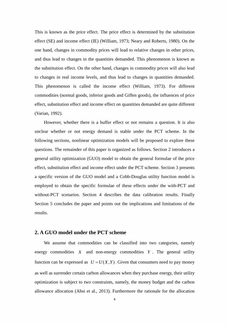
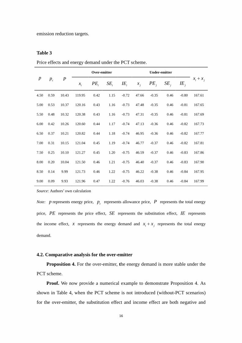
4.2. Comparative analysis for the over-emitter

Proposition 4. For the over-emitter, the energy demand is more stable under the

PCT scheme.

Proof. We now provide a numerical example to demonstrate Proposition 4. As

shown in Table 4, when the PCT scheme is not introduced (without-PCT scenarios)

for the over-emitter, the substitution effect and income effect are both negative and

16

thus the price effect is negative. The over-emitter’s energy demand will decrease as

the energy price increases (Fig.2). However under the with-PCT scenarios, the

substitution effect dominates the income effect. Thus the price effect is positive, and

the energy demand will increase with the energy price (Fig. 2).

In addition it is found that the price effect will decrease dramatically when the

PCT scheme is not introduced. The proportions of the price effect under the with- and

without-PCT scenarios range from -0.71% to -3.15%. The reason can be attributed to

the influence of the buffer effect. Under the PCT scheme the buffer effect can keep

the price effect, substitution effect and income effect from fluctuating dramatically.

Thus, the over-emitter’s energy demand under the PCT scheme is stable (Fig.2).

Table 4

Comparative analysis for the over-emitter.

p Without-PCT With-PCT

//i iPE PE /

iPE /iSE /

iIE iPE iSE iIE

4.50 -59.26 -53.33 -5.93 0.42 1.15 -0.72 -0.71%

5.00 -48.00 -43.20 -4.80 0.43 1.16 -0.73 -0.89%

5.50 -39.67 -35.70 -3.97 0.43 1.16 -0.73 -1.09%

6.00 -33.33 -30.00 -3.33 0.44 1.17 -0.74 -1.31%

6.50 -28.40 -25.56 -2.84 0.44 1.18 -0.74 -1.55%

7.00 -24.49 -22.04 -2.45 0.45 1.19 -0.74 -1.82%

7.50 -21.33 -19.20 -2.13 0.45 1.20 -0.75 -2.11%

8.00 -18.75 -16.88 -1.88 0.46 1.21 -0.75 -2.43%

8.50 -16.61 -14.95 -1.66 0.46 1.22 -0.75 -2.78%

9.00 -14.81 -13.33 -1.48 0.47 1.22 -0.76 -3.15%-3.20%

Source: Authors’ own calculation

Note: p represents energy price, PE represents the price effect, SE represents the

substitution effect and IE represents the income effect.

17

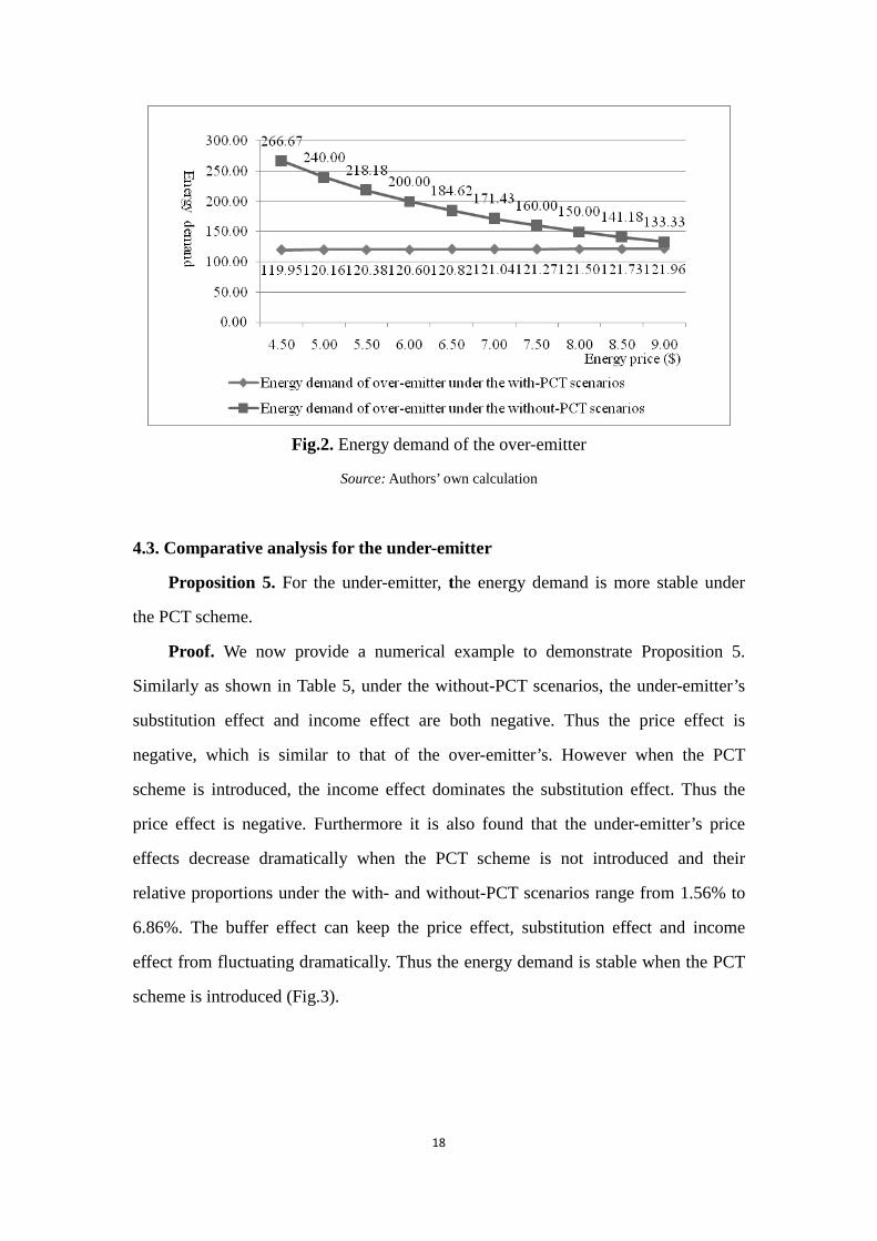
Fig.2. Energy demand of the over-emitter

Source: Authors’ own calculation

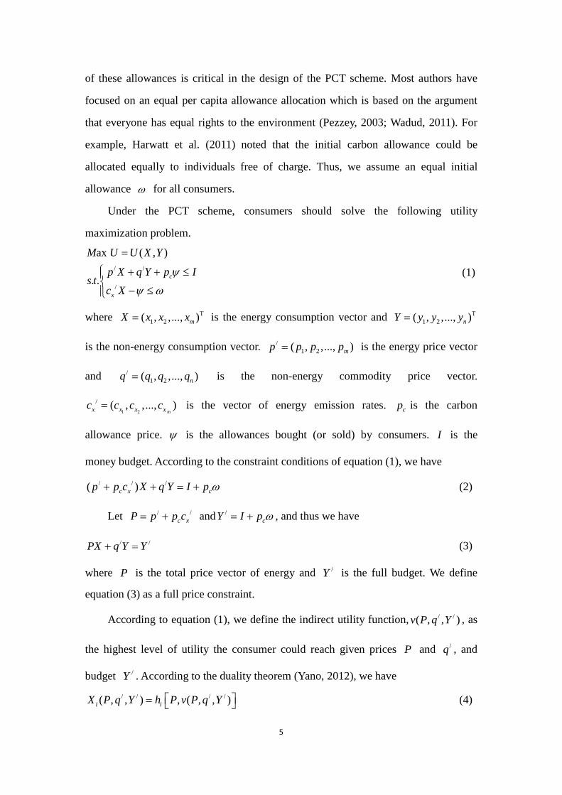
4.3. Comparative analysis for the under-emitter

Proposition 5. For the under-emitter, the energy demand is more stable under

the PCT scheme.

Proof. We now provide a numerical example to demonstrate Proposition 5.

Similarly as shown in Table 5, under the without-PCT scenarios, the under-emitter’s

substitution effect and income effect are both negative. Thus the price effect is

negative, which is similar to that of the over-emitter’s. However when the PCT

scheme is introduced, the income effect dominates the substitution effect. Thus the

price effect is negative. Furthermore it is also found that the under-emitter’s price

effects decrease dramatically when the PCT scheme is not introduced and their

relative proportions under the with- and without-PCT scenarios range from 1.56% to

6.86%. The buffer effect can keep the price effect, substitution effect and income

effect from fluctuating dramatically. Thus the energy demand is stable when the PCT

scheme is introduced (Fig.3).

18

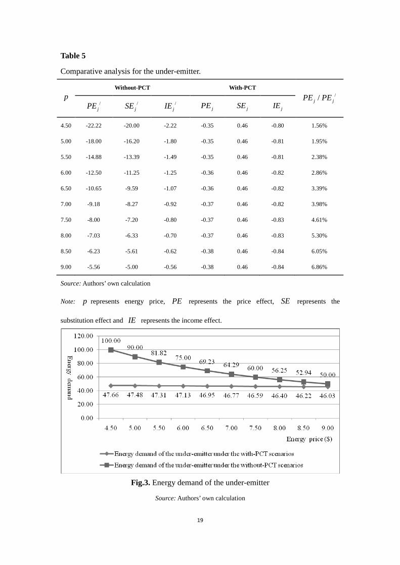
Table 5

Comparative analysis for the under-emitter.

p Without-PCT With-PCT

//j jPE PE /

jPE /jSE /

jIE jPE jSE jIE

4.50 -22.22 -20.00 -2.22 -0.35 0.46 -0.80 1.56%

5.00 -18.00 -16.20 -1.80 -0.35 0.46 -0.81 1.95%

5.50 -14.88 -13.39 -1.49 -0.35 0.46 -0.81 2.38%

6.00 -12.50 -11.25 -1.25 -0.36 0.46 -0.82 2.86%

6.50 -10.65 -9.59 -1.07 -0.36 0.46 -0.82 3.39%

7.00 -9.18 -8.27 -0.92 -0.37 0.46 -0.82 3.98%

7.50 -8.00 -7.20 -0.80 -0.37 0.46 -0.83 4.61%

8.00 -7.03 -6.33 -0.70 -0.37 0.46 -0.83 5.30%

8.50 -6.23 -5.61 -0.62 -0.38 0.46 -0.84 6.05%

9.00 -5.56 -5.00 -0.56 -0.38 0.46 -0.84 6.86%

Source: Authors’ own calculation

Note: p represents energy price, PE represents the price effect, SE represents the

substitution effect and IE represents the income effect.

Fig.3. Energy demand of the under-emitter

Source: Authors’ own calculation

19

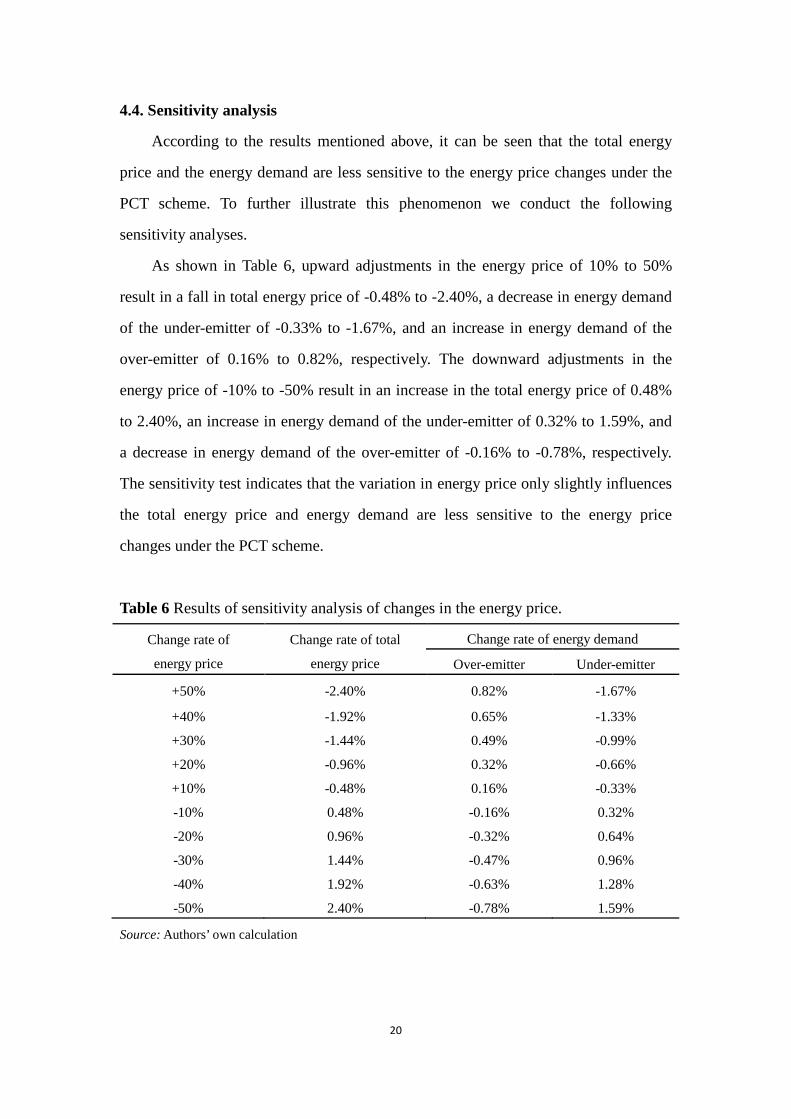
4.4. Sensitivity analysis

According to the results mentioned above, it can be seen that the total energy

price and the energy demand are less sensitive to the energy price changes under the

PCT scheme. To further illustrate this phenomenon we conduct the following

sensitivity analyses.

As shown in Table 6, upward adjustments in the energy price of 10% to 50%

result in a fall in total energy price of -0.48% to -2.40%, a decrease in energy demand

of the under-emitter of -0.33% to -1.67%, and an increase in energy demand of the

over-emitter of 0.16% to 0.82%, respectively. The downward adjustments in the

energy price of -10% to -50% result in an increase in the total energy price of 0.48%

to 2.40%, an increase in energy demand of the under-emitter of 0.32% to 1.59%, and

a decrease in energy demand of the over-emitter of -0.16% to -0.78%, respectively.

The sensitivity test indicates that the variation in energy price only slightly influences

the total energy price and energy demand are less sensitive to the energy price

changes under the PCT scheme.

Table 6 Results of sensitivity analysis of changes in the energy price.

Change rate of

energy price

Change rate of total

energy price

Change rate of energy demand

Over-emitter Under-emitter

+50% -2.40% 0.82% -1.67%

+40% -1.92% 0.65% -1.33%

+30% -1.44% 0.49% -0.99%

+20% -0.96% 0.32% -0.66%

+10% -0.48% 0.16% -0.33%

-10% 0.48% -0.16% 0.32%

-20% 0.96% -0.32% 0.64%

-30% 1.44% -0.47% 0.96%

-40% 1.92% -0.63% 1.28%

-50% 2.40% -0.78% 1.59%

Source: Authors’ own calculation

20

5. Conclusions and implications

PCT scheme is a new and effective policy proposal to reduce carbon emissions at

the household level by using carbon rationing and tradable emission allowances

(Parag, 2008). PCT is an extension of the ‘cap and trade’ scheme in production sectors,

with the aim to provide market signals and incentives for consumers to adapt to

lower-carbon consumption and lifestyles. However the influence of the PCT scheme

on low-carbon behavior seems to be complex and uncertain.

This paper mainly focuses on the buffer effect on energy price. Our analysis

reflects that the PCT scheme provides a buffer between energy price and total energy

price. The allowance price will fall when the energy price increases, keeping the total

energy price stable and will thus help stabilizing the energy market and keeping the

economic development running smoothly. Furthermore under the influence of the

buffer effect, the price effect, substitution effect, income effect and energy demand in

the PCT scheme are less sensitive to the energy price changes. The policy effect of the

PCT scheme is certain and easier to control.

In addition we found that under the PCT scheme the substitution effect of an

energy price increase on energy demand is positive, which is contrary to the

traditional economic theory of consumer choice. However the buffer effect can

explain this result. The total energy price will decrease with the energy price due to

the fact that the buffer effect is negative and dominates the energy price increase.

Furthermore the relationship between the substitution effect and the income effect is

different for the over-emitter and the under-emitter. For the over-emitter, the

substitution effect dominates the income effect. Thus the price effect is positive. The

over-emitter’s energy demand will increase as energy price increases. In fact the

energy demand of the over-emitter is determined by the total energy price. Under the

PCT scheme, when the total energy price increases, the energy demand will decrease.

This is the control function of PCT scheme. For the under-emitter the income effect

dominates the substitution effect. Thus the price effect is negative. The energy

demand of the under-emitter will decrease with the energy price.

21

The findings in the research could be useful for decision makers to introduce and

implement PCT in the future. As stated above the PCT has the potential to act as a

buffer to smooth out the energy price fluctuations. At the same time under the

influence of buffer effect, the energy demand will also remain stable, even when

facing a sudden energy price spikes. Therefore the PCT can also be effective when the

energy price fluctuates considerably. For comparison, a carbon tax will always add a

constant amount (or proportion) to the energy price, even if the total energy price is

higher than that required to achieve a target reduction. Thus a tax policy is susceptible

to the energy price in its effectiveness and is unable to provide certainty in emissions

reduction (Wadud, 2011). When the underlying energy prices fluctuate, the PCT

scheme is more effective than carbon taxes. In the past year, the average Brent crude

oil price decreased by about 50%.3 Considering the fluctuation of energy price for the

past few years, the PCT could become an attractive option in the presence of

uncertainty in future prices (Wadud, 2011).

Although the research has some interesting findings, we are mindful of the fact

that the model has ignored a number of other factors that are also likely to be of

first-order importance in practice. For instance, the paper has ignored the banking and

borrowing of allowances (Parsons et al., 2009). Establishing a model which allows for

banking and borrowing would bring our analysis a significant step closer to the

realities of the PCT system. Additionally we assumed that the trading market is

perfectly competitive and that all the participants are price-takers. If we relax this

assumption, the model could yield more interesting results, which would be more

informative for decision-makers. Thus, these two aspects need to be considered in

future research and these are what we set out to do in the following studies.

Acknowledgements

The authors are grateful to the National Natural Science Foundation of China

(71301157, 71171183) for generous financial support. They also acknowledge the

3 See detail at http://finance.sina.com.cn/futures/quotes/OIL.shtml. 22

editor and three anonymous referees of the journal for their careful reading and

constructive comments.

References

Absi N, Dauzère-Pérès S, Kedad-Sidhoum S, Penz, B, Rapine C. (). Lot sizing with

carbon emission constraints. European Journal of Operational Research

2013; 227 (1),55-61.

Benz E, Trück S. Modeling the price dynamics of CO2 emission allowances. Energy

Economics 2009;31, 4-15.

Bristow AL, Wardman M, Zanni AM, Chintakayala PK. Public acceptability of

personal carbon trading and carbon tax. Ecological Economics 2010;

69,1824-1837.

Chen Y, Liu AL, Hobbs BF. Economic and Emissions Implications of Load-Based,

Source-Based, and First-Seller Emissions Trading Programs Under California

AB32. Operations Research 2011;59, 696-712.

Cohen MJ. Is the UK preparing for “war”? Military metaphors, personal carbon

allowances, and consumption rationing in historical perspective. Climatic change

2011;104 (2), 199-222.

Cowan S. Third-Degree price discrimination and consumer surplus. The Journal of

Industrial Economics 2012;60(2), 333-345.

Eyre N. Policing carbon: design and enforcement options for personal carbon trading.

Climate Policy2010;10, 432-446.

Falkner R, Stephan H, Vogler J. International climate policy after Copenhagen:

Towards a ‘building blocks’ approach. Global Policy 2010;1(3), 252-262.

Fan J, Guo XM., Marinova D, Wu YR, Zhao, DT. Embedded carbon footprint of

Chinese urban households: structure and changes. Journal of Cleaner Production

2012;33, 50-59.

Fan J, Zhao DT, Wu YR, Wei JC.. Carbon pricing and electricity market reforms in

China. Clean Technologies and Environmental Policy 2014;16(5),921-933.

23

Fawcett T, Bottrill C, Boardman B, Lye G. Trialling personal carbon allowances. UK

Energy Research Centre 2007.

Fawcett T. Personal carbon trading: a policy ahead of its time? Energy Policy 2010,38,

6868-6876.

Feng ZH, Zou LL, Wei YM. The impact of household consumption on energy use and

CO2 emissions in China. Energy 2011;36, 656-670.

Fleming D. Stopping the traffic. Country Life 1996;140, 62-65.

Gittell R. Economic Impact in New Hampshire of the Regional Greenhouse Gas

Initiative (RGGI): An Independent Assessment. University of New Hampshire

2008.

Harwatt H. Reducing carbon emissions from personal road transport through the

application of a tradable carbon permit scheme: empirical findings and policy

implications from the UK. Proceedings Presented at the International Transport

Forum, Leipzig; 2008.

Harwatt H, Tight M, Bristow AL, Gühnemann A. Personal Carbon Trading and fuel

price increases in the transport sector: an exploratory study of public response in

the UK. European Transport\Trasporti Europei 2011;47, 47-70.

Heffetz O. Cobb-Douglas utility with nonlinear Engel curves in a conspicuous

consumption model. Available at SSRN 1004544; 2007.

Hobbs BF, Bushnell J, Wolak FA. Upstream vs. downstream CO2 trading: A

comparison for the electricity context. Energy Policy 2010;38, 3632-3643.

Huang HL, Yan Z. Present situation and future prospect of hydropower in China.

Renewable and Sustainable Energy Reviews 2009;13, 1652-1656.

Jaehn F, Letmathe P. The emissions trading paradox. European Journal of Operational

Research 2010;202(1), 248-254.

Jagers SC, Löfgren Å, Stripple J. Attitudes to personal carbon allowances: political

trust, fairness and ideology. Climate Policy 2010;10(4), 410-431.

Klein LR, Rubin H. A constant-utility index of the cost of living. The Review of

Economic Studies 1947;15, 84-87.

Lane C, Harris B, Roberts S. An analysis of the technical feasibility and potential cost 24

of a personal carbon trading scheme: A report to the Department for Environment,

Food and Rural Affairs. Accenture, with the Centre for Sustainable Energy (CSE).

Defra, London; 2008.

Liu W, Lund H, Mathiesen BV, Zhang XL. Potential of renewable energy systems in

China. Applied Energy 2011;88, 518-525.

Lockwood M. The economics of personal carbon trading. Climate Policy 2010;10(4),

447-461.

Meyer A. Contraction and Convergence: The Global Solution to Climate Change.

Green Books, Totnes, UK; 2000.

Müller B, Höhne N, Ellermann C. Differentiating (historic) responsibilities for

climate change. Climate Policy 2009;9(6), 593-611.

National Bureau of Statistics of China (NBSC). China Statistical Yearbook 2013.

China Statistics Press, Beijing (in Chinese); 2013.

Neary JP, Roberts KWS. The theory of household behaviour under rationing.

European Economic Review 1980;13, 25-42.

Parag Y. Cross policy learning: drawing lessons for personal carbon trading (PCT)

policy from food labeling schemes. APPAM: The Next Decade-what are the Big

Policy Challenges, US; 2008.

Parag Y, Capstick S, Poortinga W. Policy attribute framing: a comparison between

three policy instruments for personal emissions reduction. Journal of Policy

Analysis and Management 2011;30, 889-905.

Parag Y, Eyre N. Barriers to personal carbon trading in the policy arena. Climate

Policy 2010;10(4), 353-368.

Parsons JE, Ellerman DA, Feilhauer S. Designing a US market for CO2. Journal of

Applied Corporate Finance 2009;21, 79-86.

Pezzey JCV. Emission taxes and tradable permits: a comparison of views on long run

efficiency. Environmental and Resource Economics 2003;26, 329-342.

Pizer WA. Combining price and quantity controls to mitigate global climate change.

Journal of Public Economics 2002; 85: 409-434.

25

Roberts S, Thumin J. A rough guide to individual carbon trading. Centre for

sustainable energy, Report to Department for Environment, Food and Rural

Affairs; 2006.

Rosenzweig MR, Schultz TP. Estimating a household production function:

Heterogeneity, the demand for health inputs, and their effects on birth weight.

The Journal of Political Economy 1983;723-746.

Rout,UK, Voβ A, Singh A, Fahl U, Blesl M, Gallachóira BPO. Energy and emissions

forecast of China over a long-time horizon. Energy 2011;36, 1-11.

Sorrell S, Sijm J. Carbon trading in the policy mix. Oxford Review of Economic

Policy 2003;19(3), 420-437.

Sorrell S. An upstream alternative to personal carbon trading. Climate Policy

2010;10(4), 481-486.

Starkey R. Personal carbon trading: A critical survey Part 1: Equity. Ecological

Economics 2012;73, 7-18.

Stranlund JK, Ben-Haim Y. Price-based vs. quantity-based environmental regulation

under Knightian uncertainty: An info-gap robust satisficing perspective. Journal

of Environmental Management 2008;87,443-449.

Varian HR. Microeconomics Analysis (3rd edition) Norton, New York; 1992.

Wadud Z. Personal tradable carbon permits for road transport: heterogeneity of

demand responses and distributional analysis (Doctoral dissertation, Imperial

College London); 2007.

Wadud Z. Personal tradable carbon permits for road transport: why, why not and who

wins? Transportation Research Part A: Policy and Practice 2011;45, 1052-1065.

Wallace AA, Irvine KN, Wright AJ. Public attitudes to personal carbon allowances:

findings from a mixed-method study. Climate Policy 2010;10, 385-409.

Weitzman ML. Prices vs. quantities. The Review of Economic Studies 1974; 41:

477-491.

William JB. Income and Substitution Effects in the Linder Theorem. The Quarterly

26

Journal of Economics 1973;87, 629-633.

Yano M. The von Neumann-McKenzie facet and the Jones Duality theorem in

two-sector optimal growth. International Journal of Economic Theory 2012;8,

213-226.

Zhang J, Wang C. Co-benefits and additionality of the clean development mechanism:

An empirical analysis. Journal of Environmental Economics and Management

2011;62(2), 140-154.

Zhao J, Hobbs BF, Pang JS. Long-run equilibrium modeling of emissions allowance

allocation systems in electric power markets. Operations research 2010;58,

529-548.

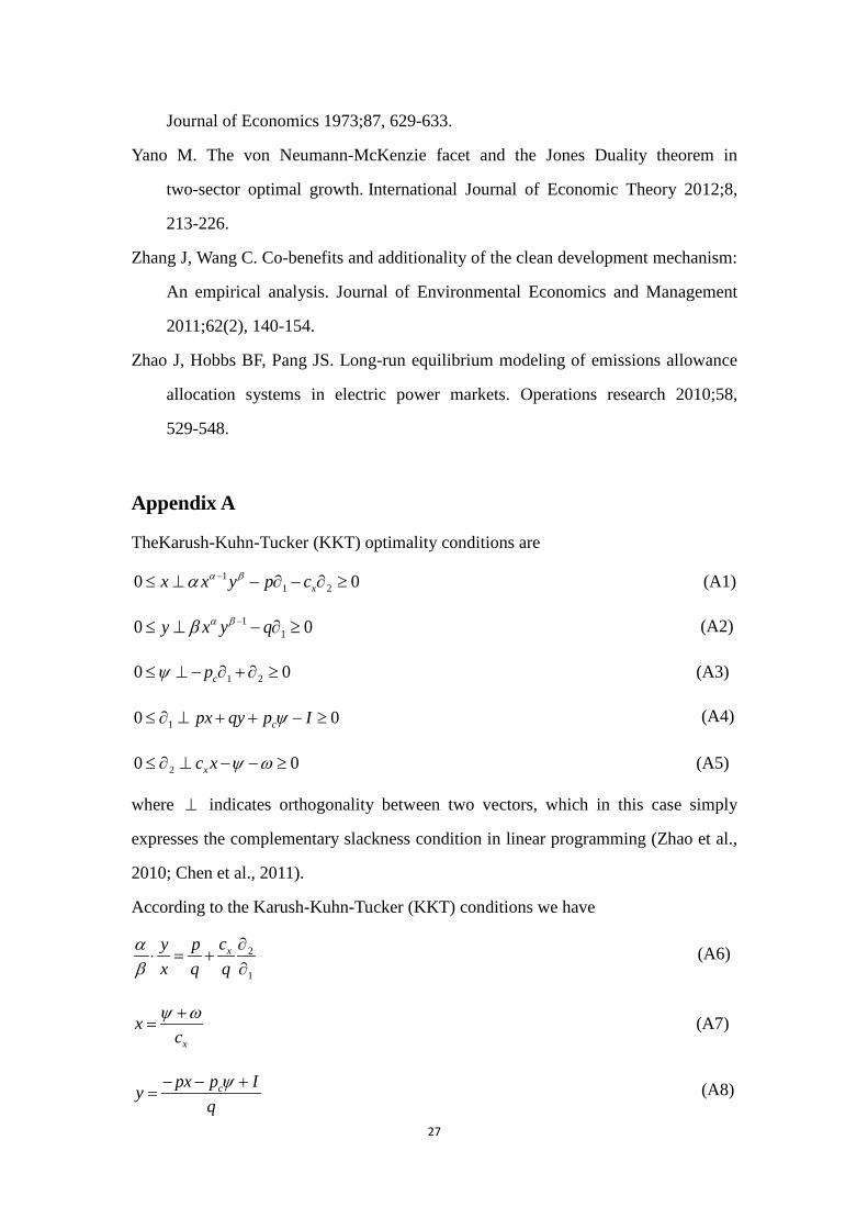
Appendix A

TheKarush-Kuhn-Tucker (KKT) optimality conditions are

11 20 0xx x y p cα βα −≤ ⊥ − ∂ − ∂ ≥ (A1)

110 0y x y qα ββ −≤ ⊥ − ∂ ≥ (A2)

1 20 0cpψ≤ ⊥ − ∂ + ∂ ≥ (A3)

10 0cpx qy p Iψ≤ ∂ ⊥ + + − ≥ (A4)

20 0xc x ψ ω≤ ∂ ⊥ − − ≥ (A5)

where ⊥ indicates orthogonality between two vectors, which in this case simply

expresses the complementary slackness condition in linear programming (Zhao et al.,

2010; Chen et al., 2011).

According to the Karush-Kuhn-Tucker (KKT) conditions we have

2

1

xcy px q q

αβ

∂⋅ = +

∂ (A6)

x

xc

ψ ω+= (A7)

cpx p Iyq

ψ− − += (A8)

27

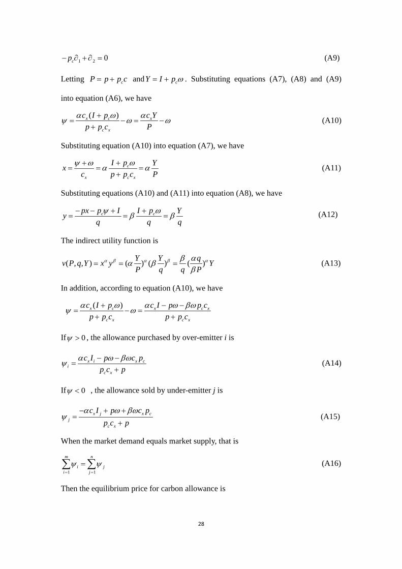
1 2 0cp− ∂ + ∂ = (A9)

Letting cP p p c= + and cY I p ω= + . Substituting equations (A7), (A8) and (A9)

into equation (A6), we have

( )x c x

c x

c I p c Yp p c P

α ω αψ ω ω+= − = −

+ (A10)

Substituting equation (A10) into equation (A7), we have

c

x c x

I p Yxc p p c P

ωψ ω α α++= = =

+ (A11)

Substituting equations (A10) and (A11) into equation (A8), we have

c cpx p I I p Yyq q q

ψ ωβ β− − + += = = (A12)

The indirect utility function is

( , , ) ( ) ( ) ( )Y Y qv P q Y x y YP q q P

α β α β αβ αα ββ

= = = (A13)

In addition, according to equation (A10), we have

( )x c x c x

c x c x

c I p c I p p cp p c p p c

α ω α ω βωψ ω+ − −= − =

+ +

If 0ψ > , the allowance purchased by over-emitter i is

x i x ci

c x

c I p c pp c p

α ω βωψ − −=

+ (A14)

If 0ψ < , the allowance sold by under-emitter j is

x j x cj

c x

c I p c pp c p

α ω βωψ

− + +=

+ (A15)

When the market demand equals market supply, that is

1 1

m n

i ji j

ψ ψ= =

=∑ ∑ (A16)

Then the equilibrium price for carbon allowance is

28

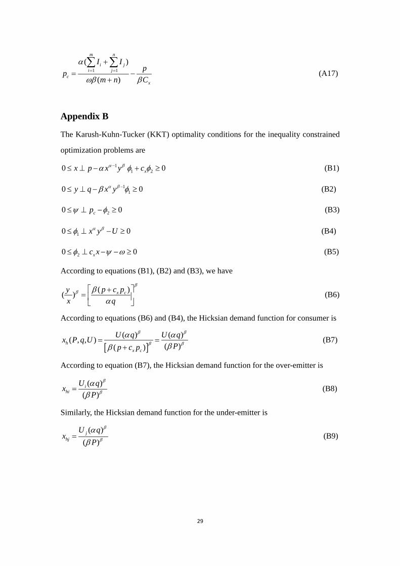
1 1( )

( )

m n

i ji j

cx

I Ipp

m n C

α

ωβ β= =

+= −

+

∑ ∑ (A17)

Appendix B

The Karush-Kuhn-Tucker (KKT) optimality conditions for the inequality constrained

optimization problems are

11 20 0xx p x y cα βα φ φ−≤ ⊥ − + ≥ (B1)

110 0y q x yα ββ φ−≤ ⊥ − ≥ (B2)

20 0cpψ φ≤ ⊥ − ≥ (B3)

10 0x y Uα βφ≤ ⊥ − ≥ (B4)

20 0xc xφ ψ ω≤ ⊥ − − ≥ (B5)

According to equations (B1), (B2) and (B3), we have

( )( ) x cp c pyx q

ββ β

α +

=

(B6)

According to equations (B6) and (B4), the Hicksian demand function for consumer is

[ ]( ) ( )( , , )

( )( )h

x c

U q U qx P q UPp c p

β β

β β

α αββ

= =+

(B7)

According to equation (B7), the Hicksian demand function for the over-emitter is

( )( )

ihi

U qxP

β

β

αβ

= (B8)

Similarly, the Hicksian demand function for the under-emitter is

( )( )

jhj

U qx

P

β

β

αβ

= (B9)

29

Editor, UWA Economics Discussion Papers: Sam Hak Kan Tang University of Western Australia 35 Sterling Hwy Crawley WA 6009 Australia Email: ecoadmin@biz.uwa.edu.au The Economics Discussion Papers are available at: 1980 – 2002: http://ecompapers.biz.uwa.edu.au/paper/PDF%20of%20Discussion%20Papers/ Since 2001: http://ideas.repec.org/s/uwa/wpaper1.html Since 2004: http://www.business.uwa.edu.au/school/disciplines/economics

ECONOMICS DISCUSSION PAPERS 2013

DP NUMBER AUTHORS TITLE

13.01 Chen, M., Clements, K.W. and Gao, G.

THREE FACTS ABOUT WORLD METAL PRICES

13.02 Collins, J. and Richards, O. EVOLUTION, FERTILITY AND THE AGEING POPULATION

13.03 Clements, K., Genberg, H., Harberger, A., Lothian, J., Mundell, R., Sonnenschein, H. and Tolley, G.

LARRY SJAASTAD, 1934-2012

13.04 Robitaille, M.C. and Chatterjee, I. MOTHERS-IN-LAW AND SON PREFERENCE IN INDIA

13.05 Clements, K.W. and Izan, I.H.Y. REPORT ON THE 25TH PHD CONFERENCE IN ECONOMICS AND BUSINESS

13.06 Walker, A. and Tyers, R. QUANTIFYING AUSTRALIA’S “THREE SPEED” BOOM

13.07 Yu, F. and Wu, Y. PATENT EXAMINATION AND DISGUISED PROTECTION

13.08 Yu, F. and Wu, Y. PATENT CITATIONS AND KNOWLEDGE SPILLOVERS: AN ANALYSIS OF CHINESE PATENTS REGISTER IN THE US

13.09 Chatterjee, I. and Saha, B. BARGAINING DELEGATION IN MONOPOLY

13.10 Cheong, T.S. and Wu, Y. GLOBALIZATION AND REGIONAL INEQUALITY IN CHINA

13.11 Cheong, T.S. and Wu, Y. INEQUALITY AND CRIME RATES IN CHINA

13.12 Robertson, P.E. and Ye, L. ON THE EXISTENCE OF A MIDDLE INCOME TRAP

13.13 Robertson, P.E. THE GLOBAL IMPACT OF CHINA’S GROWTH

13.14 Hanaki, N., Jacquemet, N., Luchini, S., and Zylbersztejn, A.

BOUNDED RATIONALITY AND STRATEGIC UNCERTAINTY IN A SIMPLE DOMINANCE SOLVABLE GAME

13.15 Okatch, Z., Siddique, A. and Rammohan, A.

DETERMINANTS OF INCOME INEQUALITY IN BOTSWANA

13.16 Clements, K.W. and Gao, G. A MULTI-MARKET APPROACH TO MEASURING THE CYCLE

30

13.17 Chatterjee, I. and Ray, R. THE ROLE OF INSTITUTIONS IN THE INCIDENCE OF CRIME AND CORRUPTION

13.18 Fu, D. and Wu, Y. EXPORT SURVIVAL PATTERN AND DETERMINANTS OF CHINESE MANUFACTURING FIRMS

13.19 Shi, X., Wu, Y. and Zhao, D. KNOWLEDGE INTENSIVE BUSINESS SERVICES AND THEIR IMPACT ON INNOVATION IN CHINA

13.20 Tyers, R., Zhang, Y. and Cheong, T.S.

CHINA’S SAVING AND GLOBAL ECONOMIC PERFORMANCE

13.21 Collins, J., Baer, B. and Weber, E.J. POPULATION, TECHNOLOGICAL PROGRESS AND THE EVOLUTION OF INNOVATIVE POTENTIAL

13.22 Hartley, P.R. THE FUTURE OF LONG-TERM LNG CONTRACTS

13.23 Tyers, R. A SIMPLE MODEL TO STUDY GLOBAL MACROECONOMIC INTERDEPENDENCE

13.24 McLure, M. REFLECTIONS ON THE QUANTITY THEORY: PIGOU IN 1917 AND PARETO IN 1920-21

13.25 Chen, A. and Groenewold, N. REGIONAL EFFECTS OF AN EMISSIONS-REDUCTION POLICY IN CHINA: THE IMPORTANCE OF THE GOVERNMENT FINANCING METHOD

13.26 Siddique, M.A.B. TRADE RELATIONS BETWEEN AUSTRALIA AND THAILAND: 1990 TO 2011

13.27 Li, B. and Zhang, J. GOVERNMENT DEBT IN AN INTERGENERATIONAL MODEL OF ECONOMIC GROWTH, ENDOGENOUS FERTILITY, AND ELASTIC LABOR WITH AN APPLICATION TO JAPAN

13.28 Robitaille, M. and Chatterjee, I. SEX-SELECTIVE ABORTIONS AND INFANT MORTALITY IN INDIA: THE ROLE OF PARENTS’ STATED SON PREFERENCE

13.29 Ezzati, P. ANALYSIS OF VOLATILITY SPILLOVER EFFECTS: TWO-STAGE PROCEDURE BASED ON A MODIFIED GARCH-M

13.30 Robertson, P. E. DOES A FREE MARKET ECONOMY MAKE AUSTRALIA MORE OR LESS SECURE IN A GLOBALISED WORLD?

13.31 Das, S., Ghate, C. and Robertson, P. E.

REMOTENESS AND UNBALANCED GROWTH: UNDERSTANDING DIVERGENCE ACROSS INDIAN DISTRICTS

13.32 Robertson, P.E. and Sin, A. MEASURING HARD POWER: CHINA’S ECONOMIC GROWTH AND MILITARY CAPACITY

13.33 Wu, Y. TRENDS AND PROSPECTS FOR THE RENEWABLE ENERGY SECTOR IN THE EAS REGION

13.34 Yang, S., Zhao, D., Wu, Y. and Fan, J.

REGIONAL VARIATION IN CARBON EMISSION AND ITS DRIVING FORCES IN CHINA: AN INDEX DECOMPOSITION ANALYSIS

31

ECONOMICS DISCUSSION PAPERS 2014

DP NUMBER AUTHORS TITLE

14.01 Boediono, Vice President of the Republic of Indonesia

THE CHALLENGES OF POLICY MAKING IN A YOUNG DEMOCRACY: THE CASE OF INDONESIA (52ND SHANN MEMORIAL LECTURE, 2013)

14.02 Metaxas, P.E. and Weber, E.J. AN AUSTRALIAN CONTRIBUTION TO INTERNATIONAL TRADE THEORY: THE DEPENDENT ECONOMY MODEL

14.03 Fan, J., Zhao, D., Wu, Y. and Wei, J. CARBON PRICING AND ELECTRICITY MARKET REFORMS IN CHINA

14.04 McLure, M. A.C. PIGOU’S MEMBERSHIP OF THE ‘CHAMBERLAIN-BRADBURY’ COMMITTEE. PART I: THE HISTORICAL CONTEXT

14.05 McLure, M. A.C. PIGOU’S MEMBERSHIP OF THE ‘CHAMBERLAIN-BRADBURY’ COMMITTEE. PART II: ‘TRANSITIONAL’ AND ‘ONGOING’ ISSUES

14.06 King, J.E. and McLure, M. HISTORY OF THE CONCEPT OF VALUE

14.07 Williams, A. A GLOBAL INDEX OF INFORMATION AND POLITICAL TRANSPARENCY

14.08 Knight, K. A.C. PIGOU’S THE THEORY OF UNEMPLOYMENT AND ITS CORRIGENDA: THE LETTERS OF MAURICE ALLEN, ARTHUR L. BOWLEY, RICHARD KAHN AND DENNIS ROBERTSON

14.09

Cheong, T.S. and Wu, Y. THE IMPACTS OF STRUCTURAL RANSFORMATION AND INDUSTRIAL UPGRADING ON REGIONAL INEQUALITY IN CHINA

14.10 Chowdhury, M.H., Dewan, M.N.A., Quaddus, M., Naude, M. and Siddique, A.

GENDER EQUALITY AND SUSTAINABLE DEVELOPMENT WITH A FOCUS ON THE COASTAL FISHING COMMUNITY OF BANGLADESH

14.11 Bon, J. UWA DISCUSSION PAPERS IN ECONOMICS: THE FIRST 750

14.12 Finlay, K. and Magnusson, L.M. BOOTSTRAP METHODS FOR INFERENCE WITH CLUSTER-SAMPLE IV MODELS

14.13 Chen, A. and Groenewold, N. THE EFFECTS OF MACROECONOMIC SHOCKS ON THE DISTRIBUTION OF PROVINCIAL OUTPUT IN CHINA: ESTIMATES FROM A RESTRICTED VAR MODEL

14.14 Hartley, P.R. and Medlock III, K.B. THE VALLEY OF DEATH FOR NEW ENERGY TECHNOLOGIES

14.15 Hartley, P.R., Medlock III, K.B., Temzelides, T. and Zhang, X.

LOCAL EMPLOYMENT IMPACT FROM COMPETING ENERGY SOURCES: SHALE GAS VERSUS WIND GENERATION IN TEXAS

14.16 Tyers, R. and Zhang, Y. SHORT RUN EFFECTS OF THE ECONOMIC REFORM AGENDA

14.17 Clements, K.W., Si, J. and Simpson, T. UNDERSTANDING NEW RESOURCE PROJECTS

14.18 Tyers, R. SERVICE OLIGOPOLIES AND AUSTRALIA’S ECONOMY-WIDE PERFORMANCE

14.19 Tyers, R. and Zhang, Y. REAL EXCHANGE RATE DETERMINATION AND THE CHINA PUZZLE

32

ECONOMICS DISCUSSION PAPERS 2014

DP NUMBER AUTHORS TITLE

14.20 Ingram, S.R. COMMODITY PRICE CHANGES ARE CONCENTRATED AT THE END OF THE CYCLE

14.21 Cheong, T.S. and Wu, Y. CHINA'S INDUSTRIAL OUTPUT: A COUNTY-LEVEL STUDY USING A NEW FRAMEWORK OF DISTRIBUTION DYNAMICS ANALYSIS

14.22 Siddique, M.A.B., Wibowo, H. and Wu, Y.

FISCAL DECENTRALISATION AND INEQUALITY IN INDONESIA: 1999-2008

14.23 Tyers, R. ASYMMETRY IN BOOM-BUST SHOCKS: AUSTRALIAN PERFORMANCE WITH OLIGOPOLY

14.24 Arora, V., Tyers, R. and Zhang, Y. RECONSTRUCTING THE SAVINGS GLUT: THE GLOBAL IMPLICATIONS OF ASIAN EXCESS SAVING

14.25 Tyers, R. INTERNATIONAL EFFECTS OF CHINA’S RISE AND TRANSITION: NEOCLASSICAL AND KEYNESIAN PERSPECTIVES

14.26 Milton, S. and Siddique, M.A.B. TRADE CREATION AND DIVERSION UNDER THE THAILAND-AUSTRALIA FREE TRADE AGREEMENT (TAFTA)

14.27 Clements, K.W. and Li, L. VALUING RESOURCE INVESTMENTS

14.28 Tyers, R. PESSIMISM SHOCKS IN A MODEL OF GLOBAL MACROECONOMIC INTERDEPENDENCE

14.29 Iqbal, K. and Siddique, M.A.B. THE IMPACT OF CLIMATE CHANGE ON AGRICULTURAL PRODUCTIVITY: EVIDENCE FROM PANEL DATA OF BANGLADESH

14.30 Ezzati, P. MONETARY POLICY RESPONSES TO FOREIGN FINANCIAL MARKET SHOCKS: APPLICATION OF A MODIFIED OPEN-ECONOMY TAYLOR RULE

14.31 Tang, S.H.K. and Leung, C.K.Y. THE DEEP HISTORICAL ROOTS OF MACROECONOMIC VOLATILITY

14.32 Arthmar, R. and McLure, M. PIGOU, DEL VECCHIO AND SRAFFA: THE 1955 INTERNATIONAL ‘ANTONIO FELTRINELLI’ PRIZE FOR THE ECONOMIC AND SOCIAL SCIENCES

14.33 McLure, M. A-HISTORIAL ECONOMIC DYNAMICS: A BOOK REVIEW

14.34 Clements, K.W. and Gao, G. THE ROTTERDAM DEMAND MODEL HALF A CENTURY ON

33

ECONOMICS DISCUSSION PAPERS 2015

DP NUMBER

AUTHORS TITLE

15.01 Robertson, P.E. and Robitaille, M.C. THE GRAVITY OF RESOURCES AND THE TYRANNY OF DISTANCE

15.02 Tyers, R. FINANCIAL INTEGRATION AND CHINA’S GLOBAL IMPACT

15.03 Clements, K.W. and Si, J. MORE ON THE PRICE-RESPONSIVENESS OF FOOD CONSUMPTION

15.04 Tang, S.H.K. PARENTS, MIGRANT DOMESTIC WORKERS, AND CHILDREN’S SPEAKING OF A SECOND LANGUAGE: EVIDENCE FROM HONG KONG

15.05 Tyers, R. CHINA AND GLOBAL MACROECONOMIC INTERDEPENDENCE

15.06 Fan, J., Wu, Y., Guo, X., Zhao, D. and Marinova, D.

REGIONAL DISPARITY OF EMBEDDED CARBON FOOTPRINT AND ITS SOURCES IN CHINA: A CONSUMPTION PERSPECTIVE

15.07 Fan, J., Wang, S., Wu, Y., Li, J. and Zhao, D.

BUFFER EFFECT AND PRICE EFFECT OF A PERSONAL CARBON TRADING SCHEME

15.08 Neill, K. WESTERN AUSTRALIA’S DOMESTIC GAS RESERVATION POLICY THE ELEMENTAL ECONOMICS

15.09 Collins, J., Baer, B. and Weber, E.J. THE EVOLUTIONARY FOUNDATIONS OF ECONOMICS

15.10 Siddique, A., Selvanathan, E. A. and Selvanathan, S.

THE IMPACT OF EXTERNAL DEBT ON ECONOMIC GROWTH: EMPIRICAL EVIDENCE FROM HIGHLY INDEBTED POOR COUNTRIES

15.11 Wu, Y. LOCAL GOVERNMENT DEBT AND ECONOMIC GROWTH IN CHINA

15.12 Tyers, R. and Bain, I. THE GLOBAL ECONOMIC IMPLICATIONS OF FREER SKILLED MIGRATION

15.13 Chen, A. and Groenewold, N. AN INCREASE IN THE RETIREMENT AGE IN CHINA: THE REGIONAL ECONOMIC EFFECTS

34