Embed Size (px)
Citation preview
ECONOMICS
AUSTRALIA AND THE GFC: SAVED BY ASTUTE FISCAL POLICY?
by
Nicolaas Groenewold
Business School University of Western Australia
DISCUSSION PAPER 12.28
AUSTRALIA AND THE GFC: SAVED BY ASTUTE FISCAL POLICY?
Nicolaas Groenewold,*
Economics,
UWA Business School,
University of Western Australia,
Crawley, WA 6009
email: [email protected]
DISCUSSION PAPER 12.28
ABSTRACT
Both before and after the federal election campaign in 2010, Australians were frequently told that
they were spared the worst effects of the Global Financial Crisis because of the government’s
timely and decisive fiscal stimulus. However, there are at least two other possibilities: monetary
policy and foreign demand. This paper assesses the relative importance of these possibilities in
driving output in the past few years. It does this within the framework of a structural vector-
autoregressive model based on recent literature measuring the effects of fiscal and/or monetary
policy on output. The results suggest that the government’s claims are considerably exaggerated.
*I am grateful for comments on earlier drafts of this paper received at an Economics “Brown Bag” seminar at UWA, May 2011, at a seminar at Deakin University in July 2011 and at a Workshop on VAR modelling at the University of Tasmania in February 2012. Mardi Dungey and Graeme Wells have given me useful and encouraging advice at various stages of the research underlying the paper.
1
I Introduction
It has been a common claim in recent years that Australia was spared the worst
effects of the Global Financial Crisis (GFC) by the Rudd/Gillard government’s astute
fiscal expansions in 2008 and 2009. Three items from the web-site of Australian
Treasurer Wayne Swan in his “Treasurer’s Economic Notes” series from the first half
of 2009 give the flavour of such claims: 1
• “The Government has taken decisive action to stimulate our economy and
cushion Australians from the worst the world can throw at us – targeting first
household incomes, then shovel-ready projects, and now larger-scale
infrastructure in the Budget. The one thing we know for sure about our first
quarter [2009] GDP outcome, is that without the Government's substantial
economic stimulus, the result would be much worse.” (31/5/2009)
• “The Government's cash stimulus payments to households are working to
support jobs and growth in our economy. In fact, Treasury estimates that
without these cash payments, the Australian economy would have contracted
by around 0.2 per cent in the quarter [rather than growing by 0.6%].”
(7/6/2009).
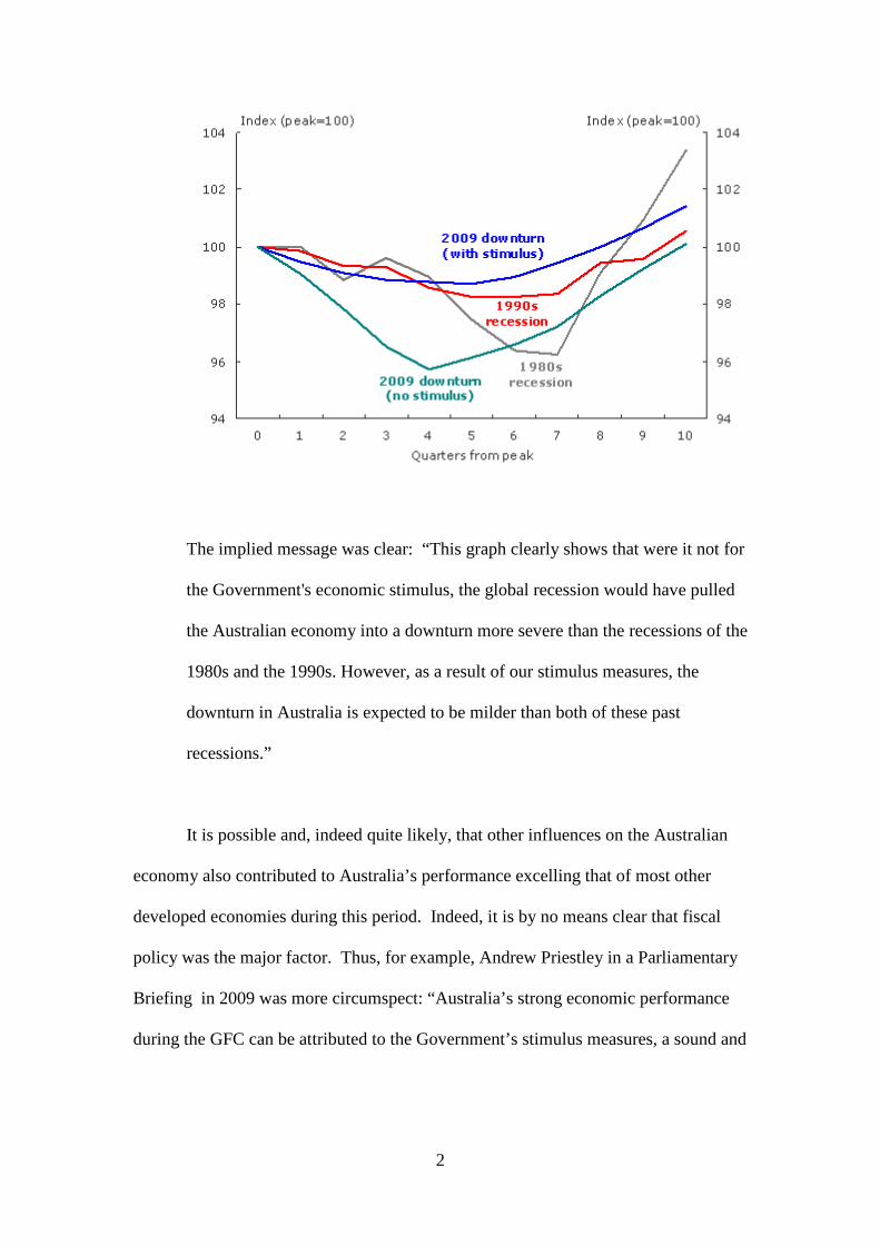
• The following graph of an index of the level of GDP and commentary:
1 See http://www.treasurer.gov.au/listdocs.aspx?pageid=012&doctype=4&year=2009&min=wms
2
The implied message was clear: “This graph clearly shows that were it not for
the Government's economic stimulus, the global recession would have pulled
the Australian economy into a downturn more severe than the recessions of the
1980s and the 1990s. However, as a result of our stimulus measures, the
downturn in Australia is expected to be milder than both of these past
recessions.”
It is possible and, indeed quite likely, that other influences on the Australian
economy also contributed to Australia’s performance excelling that of most other
developed economies during this period. Indeed, it is by no means clear that fiscal
policy was the major factor. Thus, for example, Andrew Priestley in a Parliamentary
Briefing in 2009 was more circumspect: “Australia’s strong economic performance
during the GFC can be attributed to the Government’s stimulus measures, a sound and
3
liquid banking system and not least China’s robust demand for energy and minerals
imported from Australia.”2
It is the purpose of this paper to evaluate the relative importance of possible
alternative factors which might account for Australia’s above-average performance. I
do this by estimating a minimal structural vector-autoregressive (SVAR) model and
simulating it under the counterfactual assumptions reflecting no fiscal stimulus, a
neutral monetary policy and no extraordinary assistance from overseas. The main
finding is that the contributions of fiscal policy and foreign demand were, at best,
modest; if anything, monetary policy is what saved us from the worst effects of the
GFC. These findings are robust to a large variety of alternative modelling
assumptions – variable definitions, lag structure, sample period, identification
assumptions and additional variables.
The structure of the paper is as follows. In section II the literature is briefly
reviewed. I set out the model, including the scheme used to identify policy shocks, in
section III. In section IV the data are described and data transformations and the
results of tests for stationarity are reported. The results for the base model are
reported in section V and section VI is devoted to presenting the outcomes of a range
of tests of the robustness of the results. Conclusions are drawn in the final section.
II Literature Review
There has been a considerable empirical literature on the effects of fiscal and
monetary policy. A variety of models has been used for the analysis of these effects,
ranging from single-equation models (e.g., Alesina and Ardagna, 2009, and Candelon,
et al., 2010) to structural models (such as Muscatelli et al., 2004, Smets and Wouters,
2 See http://www.aph.gov.au/library/pubs/BriefingBook43p/australia-china-gfc.htm
4
2007, Fragetta and Kirsanova, 2010, Freedman et al., 2010, Coenen et al., 2012 and
Kollmann et al., 2012) and, most commonly, a variant of the vector-autoregressive
(VAR) model. While some papers report analyses of both fiscal and monetary policy,
most focus on one or the other and this division is followed in the review of the
literature, beginning with fiscal policy. Papers which investigate policy specifically
for the Australian economy are dealt with separately at the end of the section.
While in the standard Keynesian model of first-year economics courses in
which prices are rigid and there are unemployed resources, it is straightforward to
show that the fiscal policy multiplier is positive and generally greater than unity, the
outcome of a fiscal expansion is considerably less certain when model assumptions
are relaxed. Then private expenditure may be partially of wholly crowded out and, in
the extreme, the multiplier may become negative if the fiscal expansion crowds out an
equal amount of more productive private expenditure. It is not surprising, therefore,
that the size of the fiscal policy multiplier has become the subject of considerable
empirical research recently.
Relatively little of this work has been carried out within the context of an
empirical macro model although some examples of this approach exist; Muscatelli et
al. (2004) use a dynamic stochastic general equilibrium (DSGE) model to analyse
both fiscal and monetary policy, as do Smets and Wouters (2007). Freedman at al.
(2010), on the other hand, use a large numerical New-Keynesian model, the IMF
Global Integrated Monetary and Fiscal Model, and focus on the analysis of various
fiscal multipliers. All find government expenditure multipliers to be positive but
varying in magnitude from considerably less than 1 to greater than 2.
Most of the empirical literature on fiscal policy uses a variant of the VAR
model. An important part of this approach involves the identification of the fiscal
5
policy component of government expenditure and taxes since, with at least a part of
both government expenditure and tax revenues being endogenous, simply shocking
expenditure or tax receipts as a whole is generally inappropriate. Some papers, such
as Muscatelli et al. (2002), Beetsma and Giuliodori (2010) and Monacelli et al. (2010)
use the common identification based (partly, at least) on the Cholesky decomposition
of the covariance matric of model residuals. Others use more sophisticated schemes.
An early and seminal paper in this literature, Blanchard and Perotti (2002), use what
they call a “mixed structural VAR/event study approach” which involves the use of
outside information to identify the fiscal shocks combined with Bernanke-Sims style
restrictions on the VAR model. This approach is applied to a number of countries in
Perotti (2005). Favero and Giavazzi (2007) also apply the Blanchard-Perotti method
but emphasise the importance of adding debt to the model as do Chung and Leeper
(2007). Monacelli et al. (2010) combine the Blanchard-Perotti scheme with a
Cholesky-based identification method in a VAR framework. Auerbach and
Gorodnichenko (2012) extend the Blanchard and Perotti approach to incorporate
regime-switching between recessions and expansions. Romer and Romer (2010) use
a “narrative” approach to the identification of fiscal shocks – they use the record of
policy decisions to identify policy changes based on policy-makers’ own stated
intentions. Ramey (2011) argues that with standard VAR shock-identification
procedures, shocks are partly predictable and therefore cannot be considered to be
unexpected shocks as generally assumed in the theoretical analysis. She shows that
macroeconomic response to news is greater than to actual expenditure changes.
Finally, a recent paper by Mountford and Uhlig (2009) uses sign restrictions on the
model multipliers to identify policy shocks.3 Thus, there has been a recent
3 See Fry and Pagan (2011) for a recent survey and critiques of this approach to identification.
6
proliferation of methods of identification of policy shocks. Despite this, most papers
report positive, often small, effects on output of fiscal expansions. Exceptions are the
papers by Perotti (2005), Mountford and Uhlig (2009) and Auerbach and
Gorodnichenko (2012) all of which report several negative multipliers.
The literature which deals with the effects of monetary policy has been more
limited. In an early paper Cochrane (1998) emphasised the importance of the
distinction between anticipated and unanticipated policy shocks and demonstrates the
empirical significance of this distinction in a VAR framework but, unfortunately, does
not suggest a method for making the distinction in practice. The paper by Bernanke
and Mihov (1998) is also concerned with the identification of the monetary policy
shock in a VAR model, using external information in the form of a model of the
central bank’s operating method to restrict the VAR model. They show that the
procedure is also applicable to the case where there is more than one policy
instrument in which case a policy index is derived from the data. The papers by Kasa
and Popper (1997) and Nakashima (2006) both exploit the Bernanke and Mihov
model to analyse the effects of monetary policy in Japan. Finally, an interesting paper
by Olivei and Tenreyro (2007) argues that the effectiveness of monetary policy
depends on the quarter of the year in which it is implemented. They show that this is
important empirically as well as providing a theoretical rationalisation of the effect.
In addition to papers which consider either fiscal policy or monetary policy in
isolation, there are various which analyse both, frequently focussing on the interaction
between them. Thus, two papers by Muscatelli et al. (2002 and 2004) consider
strategic interaction between fiscal and monetary policy, the first in a standard VAR
model as well as in a Bayesian VAR model while the second uses a New Keynesian
DSGE model.
7
Finally there is a limited literature on the effects of fiscal and/or monetary
policy in Australia. Foremost amongst these is the work by Dungey and others which
uses one variant or another of the VAR model – Dungey and Pagan (2000, 2009) and
Dungey and Fry (2009, 2010). In addition, there has been some recent discussion of
fiscal policy, some of it within the context of the GFC – the papers by Day (2011)
and Makin (2010) are examples.
The pair of papers by Dungey and Pagan (2000 and 2009) are closely related,
the second being an update and extension of the first. Both are VAR models of the
Australian economy and neither is specifically designed for the analysis of policy. In
fact, neither has an explicit fiscal policy variable although both analyse monetary
policy using the cash rate as the instrument. Identification is achieved by short-run
restrictions in the first paper while the second extends the model to include non-
stationary variables and long-run restrictions. The paper by Dungey and Fry (2009) is
also a VAR model and is specifically focussed on the identification of monetary and
fiscal policy shocks. It uses a more complex set of identification restrictions
including short-run, long-run and sign restrictions. The paper is not focussed on
Australia’s experience during the GFC; indeed, it uses data for New Zealand for the
period 1983(2) to 2006(4) and thus finishes before the beginning of the GFC. Finally,
the paper by Dungey and Fry (2010) is also specifically focussed on fiscal and
monetary policy and uses Australian data; the sample period is not clearly stated but
appears to be the same as that for Dungey and Pagan (2009) and so ends before the
GFC. In all papers the policy shocks are shown to have their expected effects. A rise
in short-term interest rates has a negative effect on GDP in all models although the
magnitude varies. In Dungey and Pagan (2000) monetary policy was shown to have
contributed considerable counter-cyclical effects to the evolution of GDP over time.
8
Monetary policy was not always so beneficial, however – in an early application of a
VAR model to the analysis of monetary policy in Australia, Weber (1994) finds that
the 1989 recession in Australia was significantly exacerbated by monetary policy.
Moreover, the later (2009) Dungey and Pagan paper argued that the magnitude of the
monetary-policy effect was overstated according to the more sophisticated model
analysed there. In Dungey and Fry (2010) a government expenditure shock was
shown to have a persistent and unambiguously positive effect on output while the
effect on output of a rise in the short-term interest rate is initially positive (but small)
and negative thereafter.
Finally, there has been a number of papers which have analysed the GFC in
Australia in a less formal manner. Makin (2010) uses an historical decomposition of
the changes in output over the period of the GFC to argue that “it was the behaviour
of exports and imports, and not increased fiscal activity, that was primarily
responsible for offsetting the fall in private investment due to the Global Financial
Crisis” (p.5). Similarly, Day (2011), using similar methods to those of Makin,
attributes much of the above-average performance of the Australian economy during
the GFC to the resilience of Chinese imports from Australia driven by the Chinese
fiscal stimulus.
To sum up, while there has been extensive analysis of policy effects on output,
particularly fiscal policy, relatively little has been carried out for the Australian
economy and none of the existing formal analysis is focussed on the contributions of
policy to saving Australia from the adverse effects of the GFC. This paper sets out to
begin to fill this gap within the framework of a small VAR model of the Australian
economy which is used to decompose the historical evolution of GDP according to
contributions from fiscal and monetary policy and foreign factors.
9
III The Model
Given that this is a first attempt at analysing this question for Australia, the
simplest model possible is used. In the first place, like Blanchard and Perotti (2002)
who use only three variables (output, a fiscal policy variable and a monetary policy
variable), I begin with a model with the minimal number of variables. In particular, I
specify a model with just the four variables of interest: real output, a fiscal policy
variable, a monetary policy variable and a foreign demand variable. Secondly, the
model structure is that of an SVAR identified using only short-run identification
restrictions, rather than the more complicated methods used by Dungey et al. or
extraneous information such as used in the approach pioneered by Blanchard and
Perotti (2002).
In the base model real output is measured using real GDP (Y), the fiscal policy
variable is measured by real government expenditure plus transfers (G), the cash rate
(R) is used as the monetary-policy variable and real exports of goods and services (X)
are used to capture foreign demand. The structural model from which the VAR
model is derived may be written as:
AZt = B(L)Zt-1 + εt (1)
where Z is a vector (X,G,R,Y)’, A is a matrix of coefficients, B(L) is a matrix
polynomial in the lag operator, L, and ε is a vector of independent error terms which
include the policy shocks. To enable the (structural) errors in ε to be shocked, the
model in (1) must be estimated in such a way as to enable the retrieval of estimates of
the elements of ε. However, since all equations in (1) are identical, the structural
shocks cannot be identified and the system must be restricted to achieve identification.
Another and useful way of viewing this is to re-write the model as a reduced
form:
10
Zt =A-1B(L)Zt-1+A-1 εt ≡ C(L)Zt-1+ut (2)
which can be estimated with OLS and estimates of the residuals retrieved. However,
the reduced-form VAR errors, u, are linear combinations of the structural shocks,
A-1εt, from which estimates of the structural shocks can be derived only with further
restrictions.
A common way of identifying these errors is based on the Cholesky
decomposition of the covariance matrix of the reduced-form errors, Σ,
Σ = PP’ (3)
where P is a lower triangular (4×4) matrix. The structural errors can then be written
in terms of the reduced-form errors as:
ε = P-1u (4)
which are contemporaneously uncorrelated as required, given the properties of the P
matrix. While this scheme achieves the aim of identifying the structural errors from
the estimated system so that the model can be simulated under various alternative
policy assumptions, the method has two disadvantages – the simulation results
generally depend on the order of the variables in the system and, for any particular
variable-ordering, the restrictions may not make much economic sense. Instead, I use
a simple generalisation of the Cholesky approach which imposes restrictions directly
on the structural model on the basis of economic priors. In particular, the following
restrictions are applied:
(i) Exports are affected contemporaneously only by their own shock.
(ii) Government expenditure is affected contemporaneously by its own shock
as well as by output. Thus there is no within-the-period feedback from the
cash rate and exports but there may be an endogenous component of G
which reacts to output.
11
(iii) The cash rate is affected contemporaneously by its own shock as well as
by output. Thus monetary policy reacts within the period to output but
not to exports or government expenditure.
(iv) Output is affected contemporaneously by all four shocks. This follows
from the observation that both X and G are part of aggregate demand and
that it is quite possible for the cash rate to affect output within the quarter,
especially for cash rate changes in the first month of the quarter.
These assumptions allow the system of equations to be wrtitten as (assuming a
single lag for ease of exposition):
1 1 1 1 11 1 1 1 1 1 1 1 1 12 2 2 2 2 41 1 1 1 1 1 1 1 2 2 4 43 3 3 3 3 41 1 1 1 1 1 1 1 3 3 4 44 4 4 4 4 4 4 41 1 1 1 1 1 1 1 1 1 2 2 3 3 4 4
t t t t t t
t t t t t t t
t t t t t t t
t t t t t t t t t
X X G R YG X G R YR X G R YY X G R Y
α β γ δ λ ε
α β γ δ λ ε λ ε
α β γ δ λ ε λ ε
α β γ δ λ ε λ ε λ ε λ ε
− − − −
− − − −
− − − −
− − − −
= + + + +
= + + + + +
= + + + + +
= + + + + + + +
(5)
with the restrictions used to disentangle the relationship between the reduced-form
errors, uit and the structural errors, εit. The structural errors are interpreted as follows:
ε1t as the export (or foreign) shock, ε2t as the fiscal-policy shock, ε3t as the monetary-
policy shock and ε4t as the (other) output shock. Thus all contemporaneous and
lagged responses of G to the other variables are excluded from the fiscal-policy shock
and similarly for the monetary-policy shock.
IV The Data
The data used are quarterly and were collected for the period 1959(3) to
2011(4). The variables of the model were measured as follows:
Y: GDP, seasonally adjusted, real
G: central government, national, non-defence final consumption expenditure and
12
gross fixed capital formation (both seasonally adjusted and real) plus total
personal benefit payments which are not seasonally adjusted or real. Benefit
payments were deflated by the personal consumption deflator and tested for
seasonal components but found to have none and so are not seasonally
adjusted.
R: monthly cash rate for the period July 1998 to March 2011 and the 11 am
call rate for the period March 1959 to June 1998. The monthly data were
averaged to obtain quarterly data. They were found not to have any detectable
seasonal components and are therefore not seasonally adjusted.
X: exports of goods and services, real, seasonally adjusted.
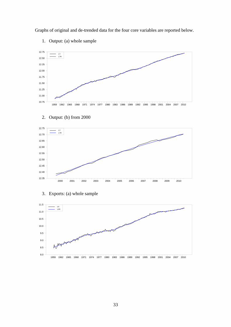
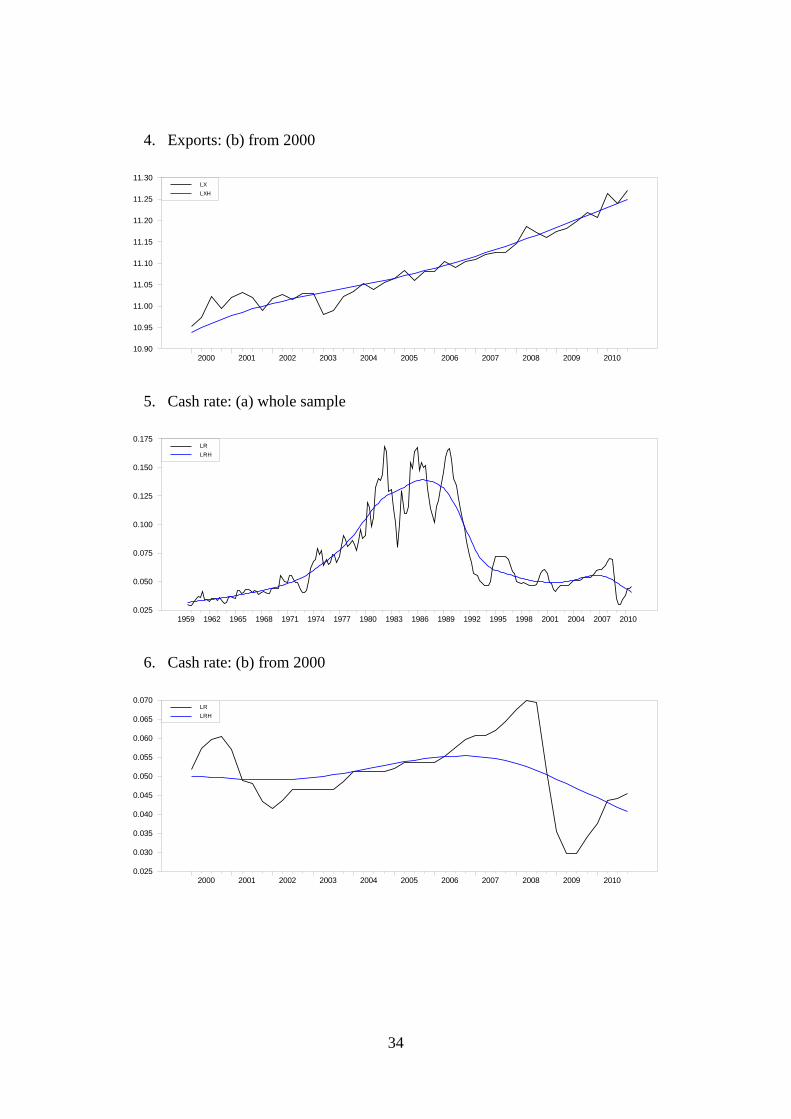
All data are in logs (R as the log(1+cash rate)) and had a trend removed using the
Hodrick-Prescott (HP) filter using a standard value of 1,600 for the lambda parameter.
The data were de-trended since the focus is on the short-term fluctuations of output
about trend. De-trending is also likely to avoid the issue of non-stationarity and
(possible) cointegration. The HP trend rather than, say, a linear trend was removed
because of the obvious non-linearity of the trend component in (at least) exports and
the cash rate. These properties of the data can be seen from the graphs of the data and
HP trends which are reported in Appendix 1 which also contains details of the sources
of the data. Alternatives to the HP method of de-trending are explored in section VI.
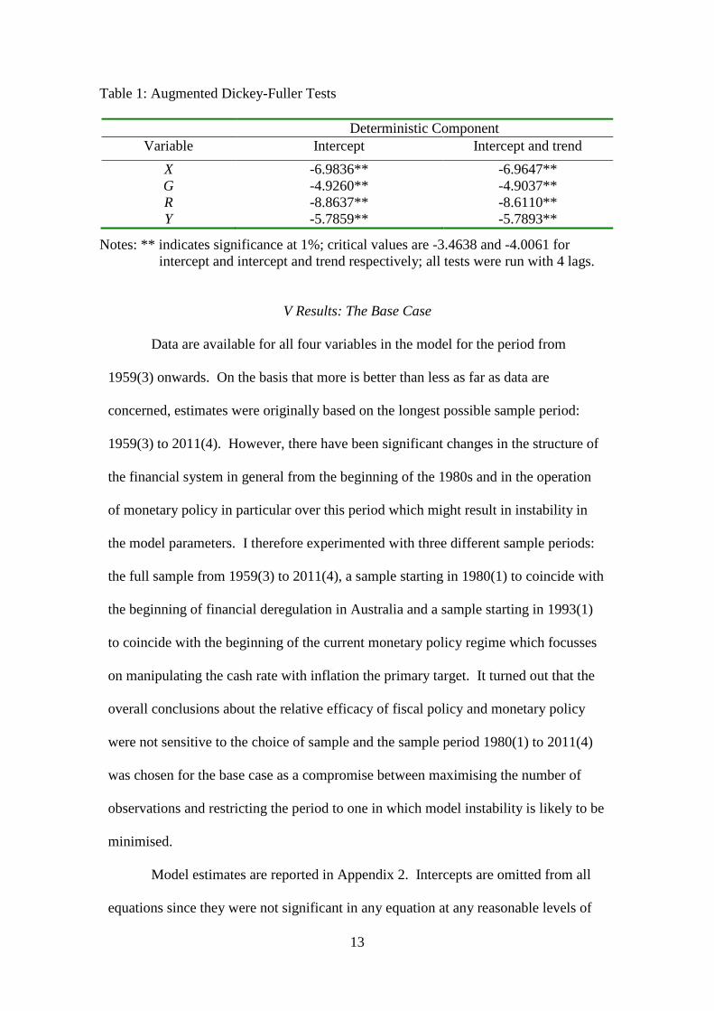
The de-trended data were tested for stationarity using the standard ADF test
and the results are reported in Table 1 below. Clearly, all variables are stationary at
the 1% level; this is independent of deterministic specification of the testing equation
and is also independent of the number of lags. The variables were therefore modelled
using a stationary SVAR.
13
Table 1: Augmented Dickey-Fuller Tests
Deterministic Component Variable Intercept Intercept and trend
X -6.9836** -6.9647** G -4.9260** -4.9037** R -8.8637** -8.6110** Y -5.7859** -5.7893**
Notes: ** indicates significance at 1%; critical values are -3.4638 and -4.0061 for intercept and intercept and trend respectively; all tests were run with 4 lags.
V Results: The Base Case
Data are available for all four variables in the model for the period from
1959(3) onwards. On the basis that more is better than less as far as data are
concerned, estimates were originally based on the longest possible sample period:
1959(3) to 2011(4). However, there have been significant changes in the structure of
the financial system in general from the beginning of the 1980s and in the operation
of monetary policy in particular over this period which might result in instability in
the model parameters. I therefore experimented with three different sample periods:
the full sample from 1959(3) to 2011(4), a sample starting in 1980(1) to coincide with
the beginning of financial deregulation in Australia and a sample starting in 1993(1)
to coincide with the beginning of the current monetary policy regime which focusses
on manipulating the cash rate with inflation the primary target. It turned out that the
overall conclusions about the relative efficacy of fiscal policy and monetary policy
were not sensitive to the choice of sample and the sample period 1980(1) to 2011(4)
was chosen for the base case as a compromise between maximising the number of
observations and restricting the period to one in which model instability is likely to be
minimised.
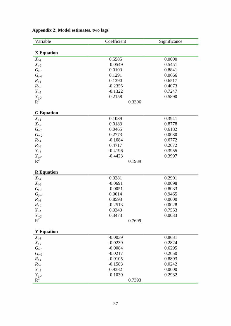
Model estimates are reported in Appendix 2. Intercepts are omitted from all
equations since they were not significant in any equation at any reasonable levels of
14
significance. Lag-choice criteria gave mixed results with the Akaike criterion
suggesting five lags and the Schwarz and Hannan-Quinn criteria suggesting one.
There was some evidence of autocorrelation in a model with one lag which was
largely removed by moving to two lags. In view of this, the base case reported in this
section is based on one lag; results for two lags are presented as part of the sensitivity
analysis in the next section.
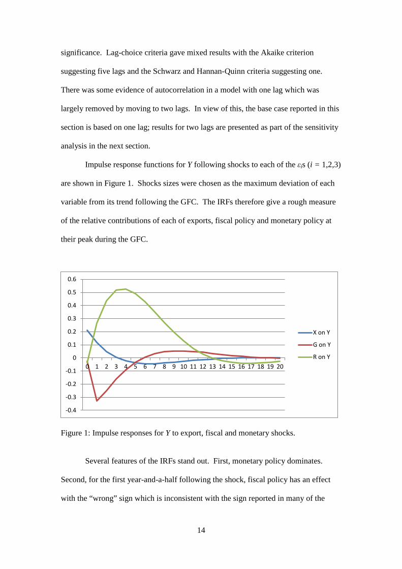
Impulse response functions for Y following shocks to each of the εis (i = 1,2,3)
are shown in Figure 1. Shocks sizes were chosen as the maximum deviation of each
variable from its trend following the GFC. The IRFs therefore give a rough measure
of the relative contributions of each of exports, fiscal policy and monetary policy at
their peak during the GFC.
Figure 1: Impulse responses for Y to export, fiscal and monetary shocks.
Several features of the IRFs stand out. First, monetary policy dominates.
Second, for the first year-and-a-half following the shock, fiscal policy has an effect
with the “wrong” sign which is inconsistent with the sign reported in many of the
-0.4
-0.3
-0.2
-0.1
0
0.1
0.2
0.3
0.4
0.5
0.6
0 1 2 3 4 5 6 7 8 9 10 11 12 13 14 15 16 17 18 19 20
X on Y
G on Y
R on Y
15
papers reviewed in Section 2 although some, such as Dungey and Fry (2009), Perotti
(2005), Mountford and Uhlig (2009) and Auerbach and Gorodnichenko (2012) report
some negative fiscal-policy multipliers. Third, the effect of the export shock is mostly
positive but quite small compared to that of the monetary-policy shock; this contrasts
with the widespread belief that the continued growth of exports to China during the
GFC was a major influence in Australia’s relatively good performance (see, e.g., Day,
2011).
But the results reported in Figure 1 are at best indicative measures of the
response of the economy to anti-GFC policy reactions. An historical decomposition
of the output variable over the GFC period will provide a more systematic account of
the dynamic effects on output of each of the four shocks and this is reported in Table
2 for the period 2007(1) to 2011(4). The decomposition computes each period’s Y as
the accumulated effects of past and present shocks to exports, government
expenditure, the cash rate and (other) output as indicated. Recall that output is in
terms of deviations of the log from HP trend so units of measurement are proportional
deviations from trend. They have all been multiplied by 100 to convert them to
percentages.
16
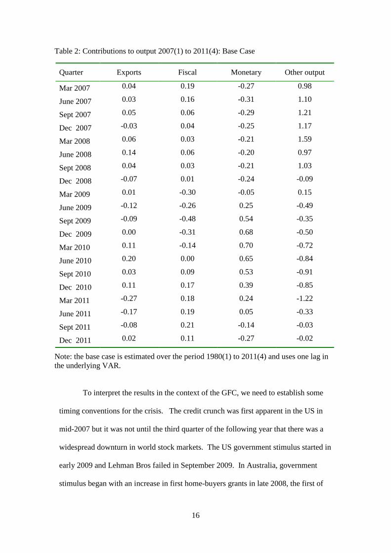
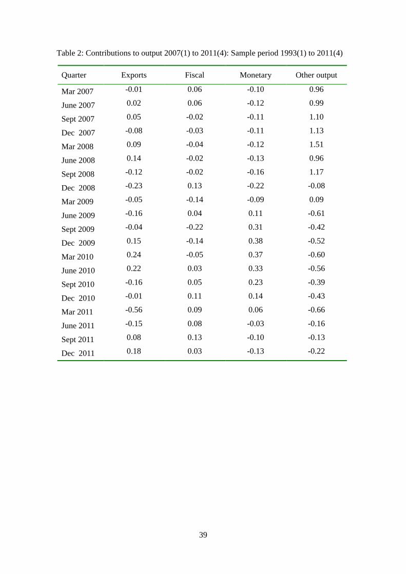
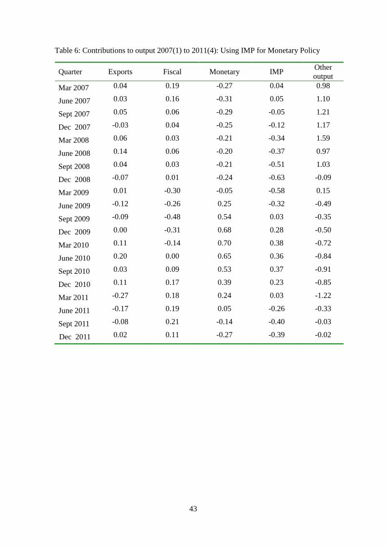
Table 2: Contributions to output 2007(1) to 2011(4): Base Case
Note: the base case is estimated over the period 1980(1) to 2011(4) and uses one lag in the underlying VAR.
To interpret the results in the context of the GFC, we need to establish some
timing conventions for the crisis. The credit crunch was first apparent in the US in
mid-2007 but it was not until the third quarter of the following year that there was a
widespread downturn in world stock markets. The US government stimulus started in
early 2009 and Lehman Bros failed in September 2009. In Australia, government
stimulus began with an increase in first home-buyers grants in late 2008, the first of
Quarter Exports Fiscal Monetary Other output
Mar 2007 0.04 0.19 -0.27 0.98
June 2007 0.03 0.16 -0.31 1.10
Sept 2007 0.05 0.06 -0.29 1.21
Dec 2007 -0.03 0.04 -0.25 1.17
Mar 2008 0.06 0.03 -0.21 1.59
June 2008 0.14 0.06 -0.20 0.97
Sept 2008 0.04 0.03 -0.21 1.03
Dec 2008 -0.07 0.01 -0.24 -0.09
Mar 2009 0.01 -0.30 -0.05 0.15
June 2009 -0.12 -0.26 0.25 -0.49
Sept 2009 -0.09 -0.48 0.54 -0.35
Dec 2009 0.00 -0.31 0.68 -0.50
Mar 2010 0.11 -0.14 0.70 -0.72
June 2010 0.20 0.00 0.65 -0.84
Sept 2010 0.03 0.09 0.53 -0.91
Dec 2010 0.11 0.17 0.39 -0.85
Mar 2011 -0.27 0.18 0.24 -1.22
June 2011 -0.17 0.19 0.05 -0.33
Sept 2011 -0.08 0.21 -0.14 -0.03
Dec 2011 0.02 0.11 -0.27 -0.02
17
the cash hand-outs in February, 2009 and the second in March and April of the same
year. Thus we might reasonably count the GFC to have begun (for Australia, at least)
at the earliest from the middle of 2008. Inspection of the data in Figure 2 in Appendix
1 indicates that Australian seasonally adjusted real GDP fell below its HP trend for
the first time in the fourth quarter of 2008. Thus in our discussion the effectiveness of
policy based on the model results, we will focus particularly on how the economy
fared in 2009 and 2010.
Several features of the results in the table stand out. First, the other output
shocks substantially drive output over the period. The correlation of this component
with output over the 2007-2011 period was 87%. Other components could be
considered counter-cyclical if they are negatively correlated with the other output
component since they would then offset the effects on output of the other output
shocks. By this measure, exports were weakly pro-cyclical with a correlation of 27%
(-1% since 2009). Fiscal policy also showed pro-cyclical behaviour over the 2007-
2011 period with a correlation of 19% (but -25% for the period 2009-2011) while
monetary policy showed strong counter-cyclical behaviour with a correlation of -79%
over 2007-2011 and -65% over 2009-2011. On the timing and magnitude of the
policy effects, fiscal policy was actually counter-productive until the middle of 2010
by which time GDP had returned to trend while monetary policy made a positive
contribution from the second quarter of 2009 just as the effect of the other output
shock was about to turn negative. Thus, on the basis of these results we could
conclude that the government’s repeated claims that fiscal expansion saved Australia
from the worst of the effects of the GFC are considerably exaggerated and that
monetary policy made a larger, more timely and more consistent contribution; the
effects of external shocks were mixed and weak.
18
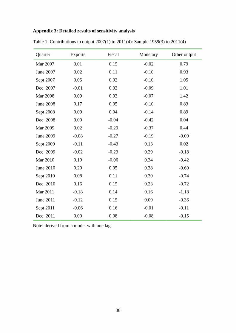
VI Results: Sensitivity Analysis
It goes without saying that the conclusions above are dependent on the
modelling assumptions made along the way, many of which might reasonably have
been made differently. It is useful, therefore, to identify some of these assumptions
and examine what would have happened had I made them otherwise. The alternatives
are divided into three groups: (i) sample period, lags and variable definition; (ii)
identification assumptions including the use of the HP de-trending procedure; and (iii)
additional variables. In this section I report only the outcomes of the analysis – tables
with decompositions for each case are reported in Appendix 3.
(i) Sample period, lags and variable definition
The sensitivity analysis begins with a point made earlier that the choice of
sample period is not crucial to the thrust of the results. In particular, the
decomposition was recomputed for two alternatives to the base case: 1959(3) to
2011(4) and 1993(1) to 2011(4). The results are in Tables 1 and 2 in Appendix 3. For
all three sample periods the basic conclusion holds that fiscal policy made a positive
contribution about a year later than monetary policy and the contribution was weaker.
The conclusion drawn from the base case results in the previous section are therefore
not dependent on the choice of sample period.
In the specification of the base case, there was some uncertainty as to the
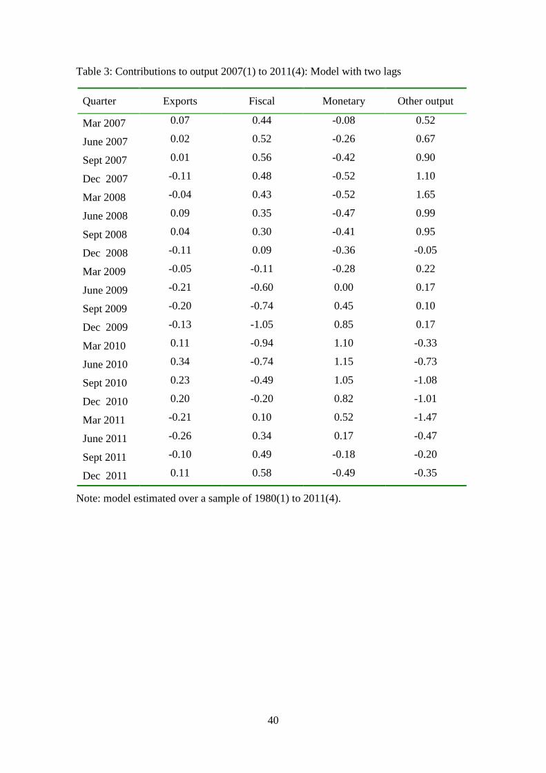
appropriate lag length for the VAR model. A lag of one was chosen but two lags
might also have been imposed. In Table 3 in Appendix 3 the decomposition is
reported for the model estimated over the 1980(1) to 2011(4) sample period but using
two lags in the VAR model. The results for the two-lag case are more strongly
19
supportive of our base-case conclusion that fiscal policy was weak and late in
offsetting the GFC compared to monetary policy.
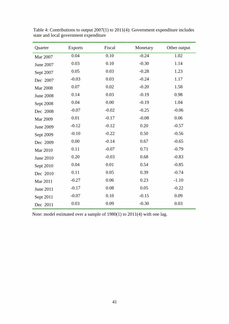
I now turn to variable definition, beginning with the fiscal policy variable, G.
In a recent paper, Aizenman and Pasricha (2011) show that, for the US, it was quite
misleading to measure fiscal stimulus using only central government expenditure
during the response to the GFC because expansions in central government
expenditure were substantially offset by contractions in spending at the state and local
levels. This may be an important issue for the measurement of fiscal policy in
Australia since expenditure by state and local governments exceeds that of the central
government although they have no direct responsibility for fiscal policy. It is
straightforward to assess the effect of this on the output decomposition reported
earlier for the base case by expanding the definition of government expenditure to
include that by state and local governments. Data used for this conform to the
definition of that used earlier for central government expenditure and are obtained
from the same source. The resulting contributions for exports, fiscal policy and
monetary policy are reported in Table 4 of Appendix 3 The results show a boost in
the efficacy of monetary policy relative to fiscal policy, thus strengthening our base-
case conclusions.
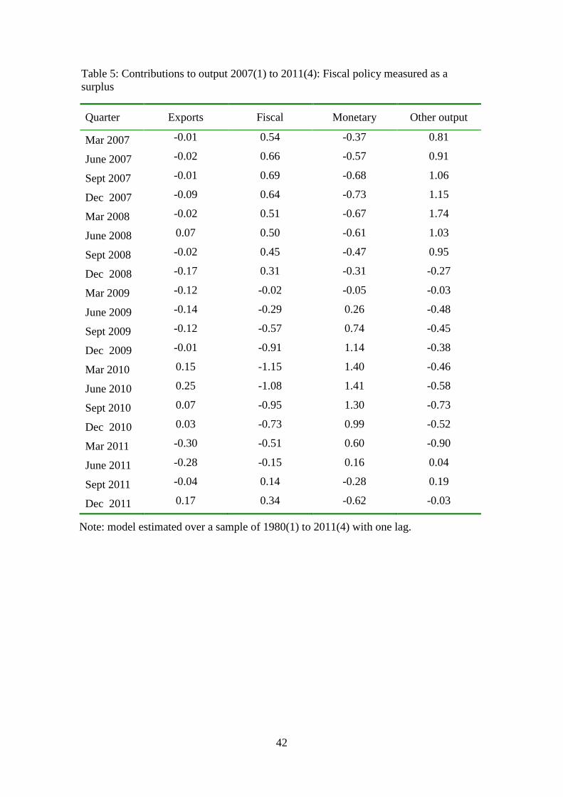
A different possible weakness of the use of G in the base model is that it
ignores taxes; it is possible that some of fiscal policy is implemented via tax changes
rather than expenditure shocks although popular discussion of fiscal policy during the
GFC focussed very much on the expenditure side. This potential weakness was
addressed by defining a “surplus” as the difference between taxes on production,
imports and income and the government expenditure used in the base case. The data
were taken from the National Accounts, as were the expenditure data used earlier.
20
Like the transfers included in the expenditure measure, tax data were not seasonally
adjusted or deflated. A regression-based test for seasonality showed no significant
seasonality in the data and they were therefore not seasonally adjusted. They were
deflated by the consumption deflator following the procedure used for the transfer
data included in G. The decomposition for the model using the surplus in the place of
G is reported in Table 5 of Appendix 3. The results reported there do not require a
change in conclusions drawn from the base-case simulations.
Another possible omission from the fiscal policy measure is the First Home
Buyers grants which were a prominent early part of the government’s strategy to
combat the adverse effects of the GFC. A recent analysis of these grants is by
Dungey et al. (2011) who provide extensive data on schemes operated by both the
federal and state governments. Unfortunately, they provide no data on total
expenditure on the scheme by the federal government which would be needed to
supplement the G variable used in the base model. The ABS records the expenditure
on this scheme in the item “capital transfer” in the “Government Finance Statistics”
(Catalogue No. 5519.0.55.001) and data were taken from this source and added to G
to test the sensitivity of the conclusions to the omission of this item. The data are not
seasonally adjusted and not deflated. There was no significant seasonality so they
were left unadjusted and they were deflated by the consumption deflator.
Unfortunately the data are available only from 2002(3). To provide a sensible basis
for comparison, the base model was first re-estimated over the period 2002(3) to
2011(4) after which the transfers were included in G to assess the difference they
made to the outcome. The inclusion of the grants made almost no difference to the
decomposition for the shorter sample period suggesting that the omission of these
grants from the measure of G used in the base model is not important for the results.
21
Next I consider the measure of monetary policy used. Dungey and Pagan
(2000) proposed a broader measure of monetary policy than just the innovation to the
cash rate, namely one which adds to the effect already measured above (which they
call the “direct effect”) the response of the cash rate to lagged changes in variables
other than the cash rate itself (the “indirect effects”), it being argued that these were
properly part of the monetary-policy response to economic conditions. The results for
the model with 1 lag are reported in Table 6 of Appendix 3 which is the base case
with an “IMP” column added which contains the Dungey-Pagan Index of Monetary
Policy (IMP). A comparison of the results in the two monetary policy columns shows
little effect on the overall conclusions of this change in the measurement of monetary
policy. Fiscal policy has a positive contribution starting only in the second half of
2010 whereas monetary policy starts having a positive impact a year earlier. The
magnitudes for monetary policy are smaller when measured with IMP but still larger
than those of fiscal policy. Thus it appears that the relatively strong contribution
attributed to monetary policy in the base case are not sensitive to the way in which it
is measured.
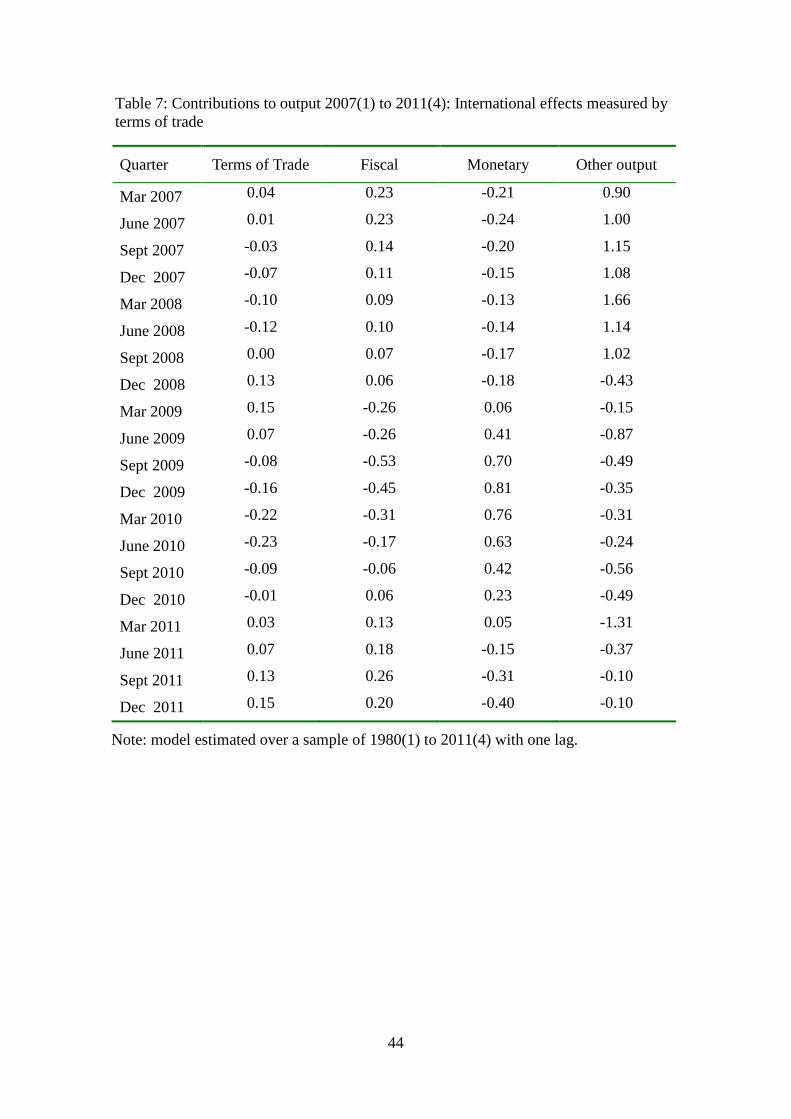
Finally consider a variation on the variable used to measure international
shocks, exports in the base model. As an alternative I use the terms of trade, the data
for which were obtained from the RBA’s web-site. The results of this variation are in
Table 7 of Appendix 3. From a comparison to the results for the base case in Table 2
above it is clear that little changes as a result of this alteration to the model
specification; external influences still did little to help Australia through the GFC, the
effects of fiscal policy become positive only late in 2010 and the effects of monetary
policy are beneficial from early in 2009 and are sustained until early in 2011. Thus,
22
little changes when exports are replaced by the terms of trade as the variable capturing
international effects.
In summary, none of the eight variations of the base model reported in this
sub-section require any change to the overall conclusions drawn from the base-case
decomposition; in fact, in many cases the earlier conclusions were strengthened.
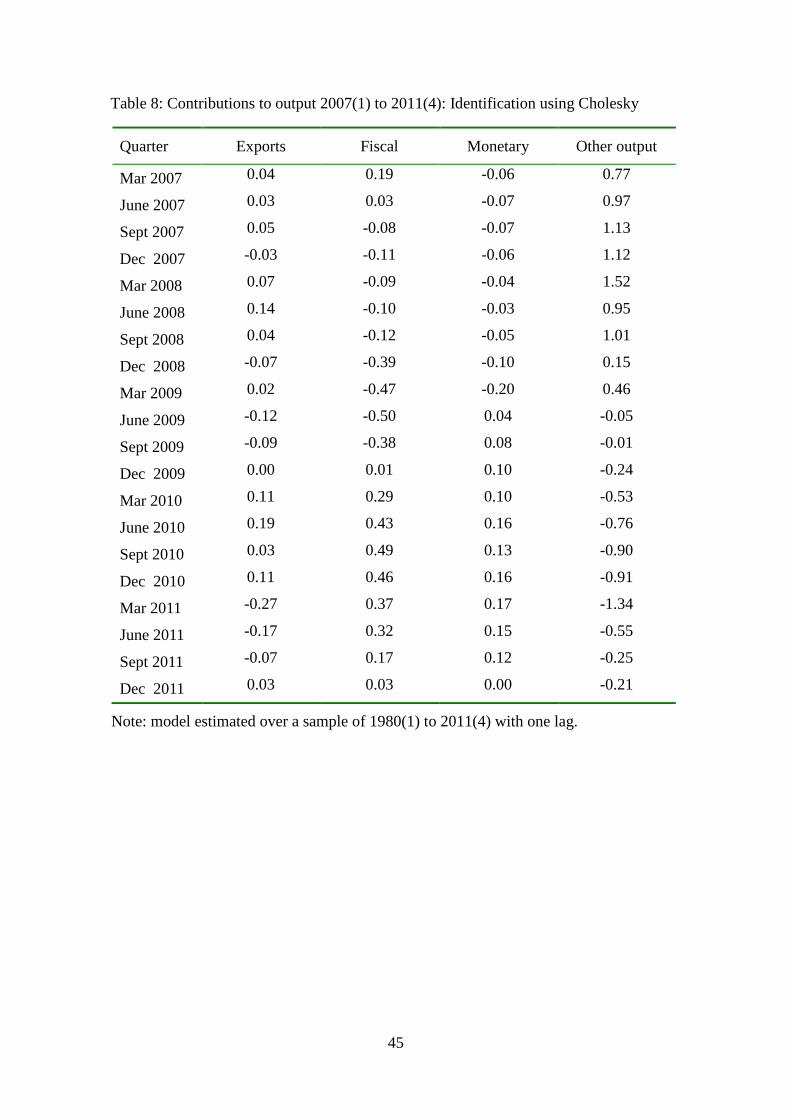
(ii) Model identification and de-trending
Next I consider the sensitivity of the conclusions to the method of identifying
the shocks and to the HP method used to de-trend the data.
In the base case the shocks were identified using short-run identifying
restrictions of the Bernanke-Sims type as set out in equation (5). An alternative is to
use the standard identification scheme based on the more common Cholesky
decomposition of the covariance matrix of the VAR model residuals. Applying this
method for an ordering of the variables X, G, R, and Y are reported in Table 8 in
Appendix 3. In this case the beneficial effects of fiscal policy are felt earlier but not
as early as those of monetary policy and in this sense the results are similar to those
generated in the base case. However, there is a strong contrast between the
magnitudes. If the Cholesky identification scheme is used, the relative magnitudes of
the effects of fiscal policy and monetary policy are reversed with fiscal policy far
more powerful than monetary policy. Since there are many differences between the
Cholesky and the Bernake-Sims identification restrictions, it is worth exploring the
source of the differences between the model predictions. Both sets of restrictions can
be formulated in terms of zero restrictions on the matrix relating the structural and
reduced-form errors, A in equations (1) and (2). Since G is in the second position, I
focussed on the second row and column and a little experimentation with alternatives
23
shows that the greater magnitude of the fiscal policy effects depends crucially on the
presence of a non-zero element in the third position of the second column.
Economically, it is crucial that the fiscal-policy shock have a contemporaneous effect
on the cash rate, something that seems to be difficult to rationalise a priori. All other
variations of the restrictions experimented with predict the usual predominance of
monetary policy over fiscal policy. I, therefore, do not consider the Cholesky-based
results to significantly undermine the thrust of the results so far obtained.
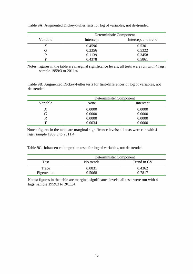
A related issue is the de-trending of the data using the HP filter. Since the HP
procedure uses both past and future observations to compute the trend, the de-trended
series will be contaminated by future data which might compromise the identification
of the policy shocks. I experiment with a number of alternatives. First the log of
variables are tested for stationarity and, not surprisingly, they are all found to be I(1)
but not cointegrated. Results are reported in Tables 9A, 9B and 9C of Appendix 3.
Thus the use of a VECM to accommodate the stochastic trends is not appropriate.
Increasingly in recent literature, modelling of apparently non-stationary variables has
proceeded by largely ignoring non-stationarity; examples are Olivei and Tenreyo
(2007), Mountford and Uhlig (2009), Romer and Romer (2010), Monacelli et al.
(2010), Ramey (2011), Beetsma and Giuliodori (2011), Coibion (2012) and Auerbach
and Gorodnichenko (2012).4 Following this literature, I consider first estimating the
VAR in log levels ignoring trends. The resulting decomposition is reported in Table
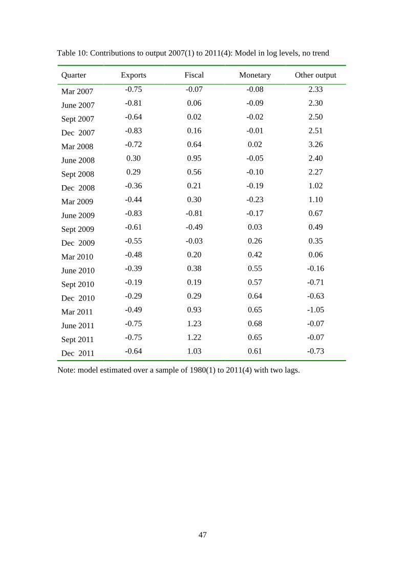
10 of Appendix 3. It shows that the overall thrust of the earlier conclusions stands up:
4 See also the earlier paper by Toda and Yamamoto (1995) who show that a range of tests can be applied to VAR models estimated in levels even if some or all the variables in the model are non-stationary.
24
monetary policy starts having a positive offsetting effect earlier and, at least until the
end of 2010, has a larger effect than fiscal policy.5
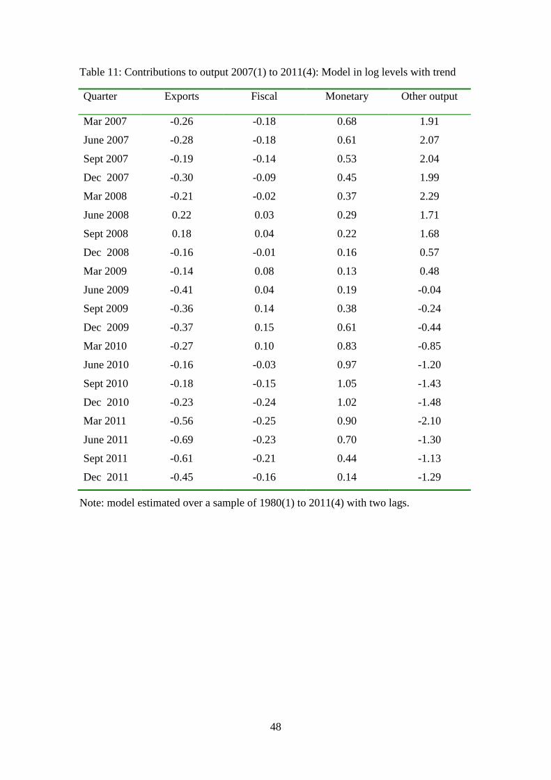
A further alternative to HP-de-trending, consistent with the literature cited
above, is to include a linear trend in the model. The results for a decomposition based
on such a model are reported in Table 11 of Appendix 3. Clearly the earlier
conclusions regarding the relative efficacy of monetary and fiscal policy continue to
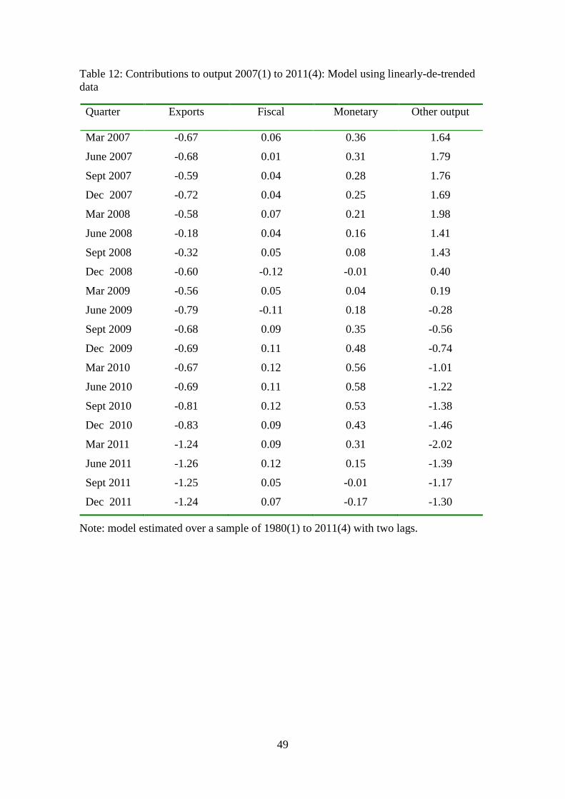
hold.6 A final alternative is linear de-trending of the data before estimating the
model – a method used, inter alia, by Dungey and Fry (2009). The decomposition
resulting from such a procedure are reported in Table 12 of Appendix 3. The
conclusions that monetary policy dominates fiscal policy during the GFC continue to
hold for this variation.
In conclusion, while there may be objections to the use of the HP filter to deal
with the obvious trends in the data, alternatives explored here based on recent
literature, show that the overall conclusions regarding the dominance of monetary
policy in helping Australia through the GFC continue to hold.
(iii) Additional variables
I argued in section III that, given the paucity of analysis of policy effects
during the GFC in Australia, it is sensible to start with the simplest possible model –
in the present case one in the four variables of interest: output and variables
representing fiscal policy, monetary policy and foreign demand. While there are
eminent precedents for such a simple approach (see, e.g., Blanchard and Perotti, 2002,
who have three variables), the final subsection on sensitivity analysis addresses a 5 The results in Table 10 are based on a model with two lags; if one lag is used, there is extensive autocorrelation which is substantially removed with two lags. Results for a model with one lag show a reversal of the relative importance of fiscal and monetary policies. 6 In this case, too, two lags were needed to remove (most) autocorrelation; but results are not sensitive to whether one or two lags are chosen.
25
common criticism of VAR models: missing variables. Most commentators will have
one (or more) suggestions for additional variables and below I report on the effects of
adding a number of popular variables to the base model, one-at-a-time. A brief
survey of the literature cited in section II suggests the following candidates: prices
(inflation), imports, the exchange rate, commodity prices, tax rates and government
debt. Consider the effects of adding each one of these variables. In all variants of the
model, only the four components computed previously will be reported since the
question is whether the addition of a variable will affect earlier conclusions regarding
the relative efficacy of fiscal and monetary policy. In each case identification
assumptions need to be made for the expanded model and I start with the assumption
that the additional variable affects only itself and is affected only by itself,
contemporaneously. Alternative restrictions were experimented with in some cases
and are reported as appropriate.
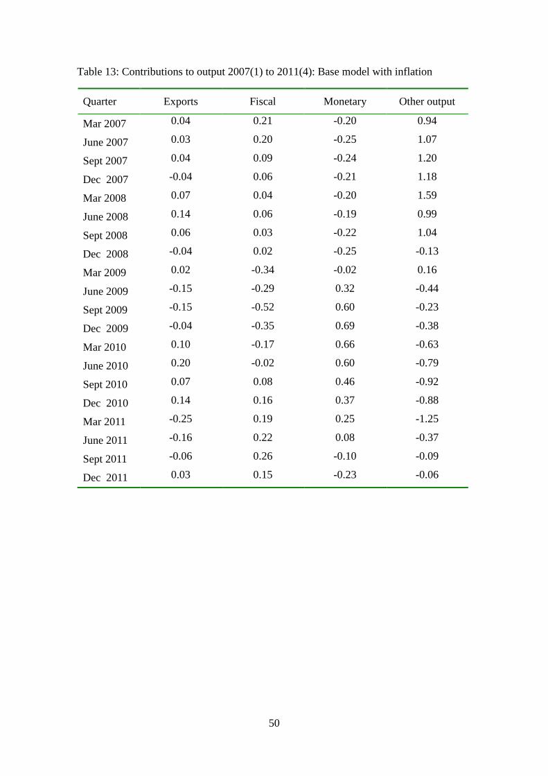
I begin with prices/inflation. Results for a model with the inflation rate
calculated from the GDP deflator are reported in Table 13. They support the earlier
conclusion that, compared to fiscal policy, monetary policy has a beneficial effect
several quarters earlier and, at least when it counts, has a stronger effect on output.
Nothing much changes when the CPI is used instead of the GDP deflator.
Next, an additional source of foreign influence was considered by adding real
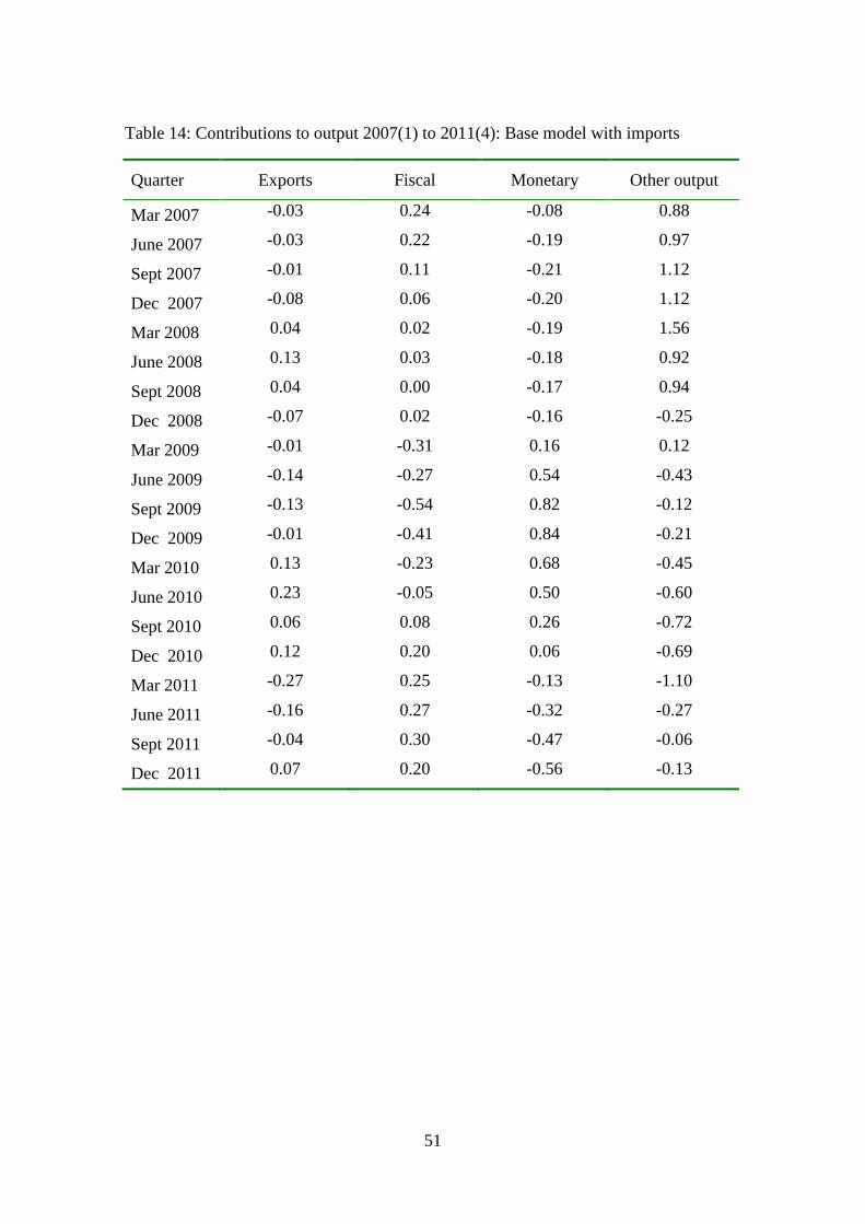
imports as a fifth variable to the base model. The results are in Table 14 in Appendix
3 and show that the conclusions are largely unaffected: fiscal policy is late and small
while monetary policy is timely and generally has a stronger effect. This outcome is
not changed when the identification assumption is expanded to allow for a
contemporaneous effect of output on imports.
26
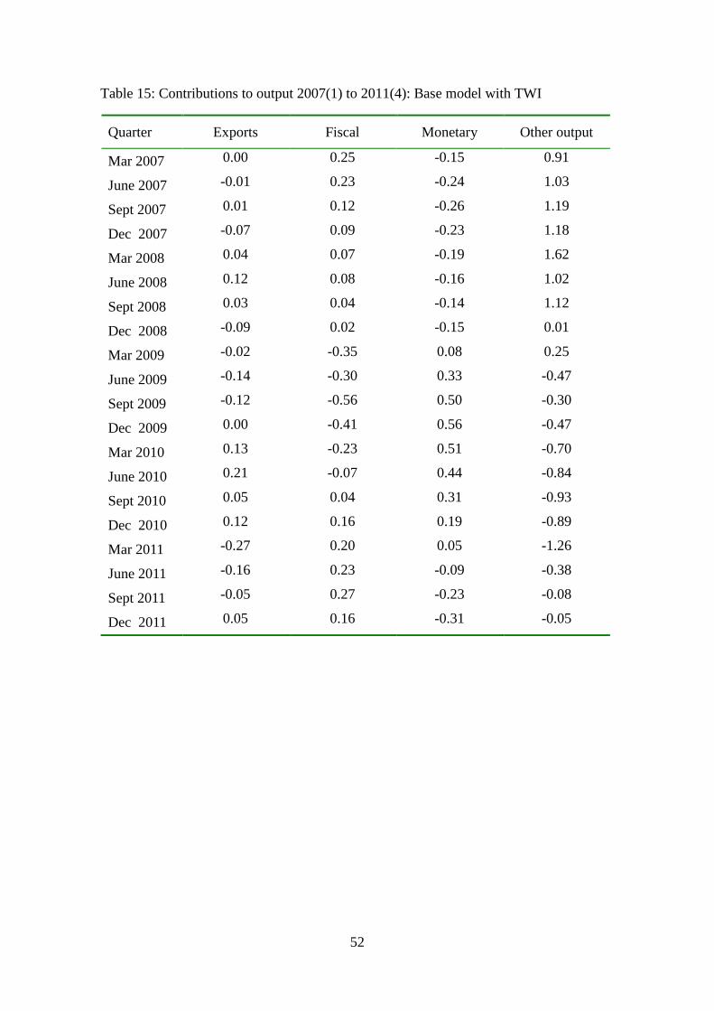
Another variable frequently included in models surveyed is a measure of the
exchange rate. I experimented with three alternatives: the trade-weighted index (TWI)
produced by the Reserve Bank, the US dollar exchange and a measure of the real
exchange rate. The results are reported in Table 15 of Appendix 3 and show that the
earlier conclusions continue to hold. This outcome is unaffected by assuming that the
exchange rate has a contemporaneous effect on the cash rate and by using the US
dollar exchange rate in the place of the TWI. The Reserve Bank also publishes a
series on the real exchange rate and I also experimented with adding this to the base
model. The resulting decomposition of output is shown in Table 16 and clearly
support the earlier conclusions regarding the relative effectiveness of fiscal and
monetary policy during the GFC.
A number of papers surveyed have included a measure of commodity prices as
part of the model and it might be argued that this is especially important for a country
like Australia which, it has been argued, was heavily dependent on commodity
exports to see it through the GFC. A commodity price series is available from the
RBA web-site although only for the period from 1982(3) so that for this experiment
the sample period was truncated accordingly. The decomposition of output using the
base model expanded to include commodity prices is reported in Table 17 of
Appendix 3 and shows, as before, that the conclusions drawn earlier are not
significantly affected – monetary policy continues to dominate fiscal policy during the
GFC period.
In the previous sub-section I included tax revenue as part of the fiscal policy
measure by replacing government expenditure with a government deficit variable. In
several papers, tax rates have been considered as a variable additional to government
expenditure and this is briefly considered here. Three alternative tax rates were
27
experimented with: two calculated as the ratio of income tax revenue received by the
central government to household income and the other the labour-income tax rate
from the Treasury’s NIF model data base. All produced vary similar results (only
those for the NIF-based tax rate are reported in Table 18 of Appendix 3) : monetary
policy had a greater effect earlier and fiscal policy had a later effect than the base case.
Thus, this experiment does nothing to change the broad conclusions reached on the
relative efficacy of monetary and fiscal policy to offset effects of the GFC on GDP in
Australia which were reached on the basis of the base case.
Finally I consider the inclusion of government debt in the model. Various
papers have argued strongly for the importance of this variable in a model used to
analyse the effects of fiscal policy; see, for example, Favero and Giavazzi (2007) and
Chung and Leeper (2007). I experimented with both the level of debt and the
debt/GDP ratio and with two alternative identification assumptions – the standard one
and a variant in which fiscal policy is allowed to have a contemporaneous effect on
debt. All produced similar results. The case using the debt/GDP ratio is reported in
Table 19 of Appendix 3. The results show that while monetary policy is weaker in
this case, it still has a greater and earlier effect than fiscal policy and in this sense the
earlier conclusion continues to hold.
The purpose of analysis reported in this section was to assess the sensitivity of
the results derived in the base case to a variety of assumptions. A large number of
variants of the base model were reported and with only one exception showed the
original results to be remarkably robust: the government’s claim that fiscal policy was
instrumental in helping Australia weather the GFC is unwarranted. Fiscal policy did
little to offset the adverse effects of the GFC until quite late (usually the second half
28
of 2010) while monetary policy had a positive effect on output a year earlier and had a
larger effect throughout the GFC period.
VI Conclusions
This paper has subjected the assertion that fiscal policy made a major
contribution to saving the Australian economy from the worst effects of the GFC to
systematic econometric evaluation within a simple four-variable VAR model. The
evidence does not support the assertion. To the contrary, monetary policy has had the
greatest effect. In addition the beneficial effects stemming from export growth were
found to be modest. These conclusions are robust to a large range of variants of the
base model: definitions of the monetary and fiscal policy and external shocks,
identification assumptions, de-trending method and variable addition.
29
References Alesina, A. and S. Ardagna (2009), “Large Changes in Fiscal Policy: Taxes versus
Spending”, NBER Working Paper No. 15438. Aizenman, J. and G. K. Pasricha (2011), “The Net Fiscal Expenditure Stimulus in the
US, 2008-9: Less than What You Might Think and Less than the Fiscal Stimulus of Most OECD Countries”, The Economist’s Voice, 8, 1-6.
Auerbach, A. J. and Y. Gorodnichenko (2012), “Measuring the Output Responses to Fiscal Policy”, American Economic Journal: Economic Policy, 4, 1-27.
Beetsma, R. and M. Giuliodori (2010), “Discretionary Fiscal Policy: Review and Estimates for the EU”, CESifo Working Paper No. 2948.
Bernanke, B. S. and I. Mihov (1998), “Measuring Monetary Policy”, Quarterly Journal of Economics, 113, 869-902.
Blanchard, O. and R. Perotti (2002), “An Empirical Characterization of the Dynamic Effects of Changes in Government Spending and Taxes on Output”, Quarterly Journal of Economics, 116, 1329-1368.
Candelon, B., J. Muysken and R. Vermeulen (2010), “Fiscal Policy and Monetary Integration in Europe”, Oxford Economic Papers, 62, 323-349.
Chung, H. and E. M. Leeper (2007), “What Has Financed Government Debt?” NBER Working Paper No. 13425.
Cochrane, J. H. (1998), “What Do the VARs Mean? Measuring the Output Effects of Monetary Policy”, Journal of Monetary Economics, 41, 277-300.
Coenen, G., R. Straub and M. Traband (2012), “Fiscal Policy and the Great Recession in the Euro Area”, American Economic Review (Papers and Proceedings), 102, 71-76.
Coibion, O. (2012), “Are the Effects of Monetary Policy Shocks Big or Small?”, American Economic Journal: Macroeconomics, 4, 1-32.
Day, C. (2011), “China’s Fiscal Stimulus and the Recession Australia Never Had: Is a Growth Slowdown Now Inevitable?”, Agenda, 18, 23-34.
Dungey, M. and R. Fry (2009), “The Identification of Fiscal and Monetary Policy in a Structural VAR”, Economic Modelling, 26, 1147-1160.
Dungey, M. and R. Fry (2010), “Fiscal and Monetary Policy in Australia: An SVAR Model”, working paper.
Dungey, M. and A. Pagan (2000), “A Structural VAR Model of the Australian Economy”, Economic Record, 76, 321-342.
Dungey, M. and A. Pagan (2009), “Extending a SVAR Model of the Australian Economy”, Economic Record, 85, 1-20.
Dungey, M., G. Wells and S. Thompson (2011), “First Home Buyers’ Support Schemes in Australia”, Australian Economic Review, 44, 468-479.
Favero, C. and F. Giavazzi (2007), “Debt and the Effects of Fiscal Policy”, NBER Working Paper 12822.
Fragetta, M. and T. Kirsanova (2010), “Strategic Monetary and Fiscal Policy Interactions: An Empirical Investigation”, European Economic Review, 54, 856-879.
Freedman, C., Kumhof, M., Laxton, D., Muir, D. and S. Mursula (2010), “Global Effects of Fiscal Stimulus During the Crisis”, Journal of Monetary Economics, 57, 506-526.
Fry, R. and A. Pagan (2011), “Sign Restrictions in Structural Vector Autoregressions: A Critical Survey”, Journal of Economic Literature, 49, 938-960.
30
Kasa, K. and H. Popper (1997), “Monetary Policy in Japan: A Structural VAR Analysis”, Journal of the Japanese and International Economies, 11, 275-295.
Kollmann, R., W. Roeger and J. in ‘t Veld (2012), “Fiscal Policy in a Financial Crisis: Standard Policy versus Bank Rescue Measures”, American Economic Review (Papers and Proceedings), 102, 77-81.
Makin, A. J. (2010), “Did Australia’s Fiscal Stimulus Counter Recession?: Evidence from the National Accounts”, Agenda, 17, 5-16.
Monacelli, T., R. Perotti and A. Trigari (2010), “Unemployment Fiscal Multipliers”, Journal of Monetary Economics, 57, 531-553.
Mountford, A. and H. Uhlig (2009), “What Are the Effects of Fiscal Policy?”, Journal of Applied Econometrics, 24, 960-992.
Muscatelli, V. A., P. Tirelli and C. Trecroci (2002), “Monetary and Fiscal Policy over the Cycle: Some Empirical Evidence”, CESifo Working Paper No. 817.
Muscatelli, V. A., P. Tirelli and C. Trecroci (2004), “Fiscal and Monetary Policy Interactions: Empirical Evidence and Optimal Policy using a Structural New-Keynesian Model”, Journal of Monetary Economics, 26, 257-280.
Nakashima, K. (2006), “The Bank of Japan’s Operating Procedures and the Identification of Monetary Policy Shocks: A Reexamination using the Bernanke-Mihov Approach”, The Japanese and International Economies, 20, 406-433.
Olivei, G. and S. Tenreyro (2007), “The Timing of Monetary Policy Shocks”, American Economic Review, 97, 636-663.
Perotti, R. (2005), “Estimating the Effects of Fiscal Policy in OECD Countries”, CEPR Discussion Paper No. 4842.
Ramey, V. A. (2011), “Identifying Government Spending Shocks: It’s All in the Timing”, Quarterly Journal of Economics, 126, 11-50.
Romer, C. D. and D. H. Romer (2010), “The Macroeconomic Effects of Tax Changes: Empirical Estimates Based on a New Measure of Fiscal Shocks”, American Economic Review, 100, 763-801.
Smets, F. and R. Wouters (2007), “Shocks and Frictions in US Business Cycles: A Bayesian DSGE Approach”, American Economic Review, 97, 586-606.
Toda, H. Y. and T. Yamamoto (1995), “Statistical Inference in Vector Autoregressions with Possibly Integrated Processes”, Journal of Econometrics, 66, 225-250.
Weber, E. J. (1994), “The Role of Money during the Recession in Australia in 1990-92”, Applied Financial Economics, 4, 355-361.
31
Appendix 1: Data
The data used are quarterly and the sample period runs from 1959(3) to 2011(4). The
definitions of the variables and sources of the data are:
Y: GDP, seasonally adjusted, real; source: Australian Bureau of Statistics web-
site (www.abs.gov.au)
G: central government, national, non-defence final consumption expenditure and
gross fixed capital formation (both seasonally adjusted and real) plus total
personal benefit payments which are not seasonally adjusted or real. Benefit
payments were deflated by the personal consumption deflator and tested for
seasonal components but found to have none and so are not seasonally
adjusted. Source: Australian Bureau of Statistics web-site (www.abs.gov.au)
R: monthly cash rate for the period July 1998 to December 2011 and the 11 am
call rate for the period March 1959 to June 1998. The monthly data were
averaged to obtain quarterly data. They were found not to have any detectable
seasonal components and are therefore not seasonally adjusted.
Source: Reserve Bank of Australia web-site (www.rba.gov.au).
X: exports of goods and services, real, seasonally adjusted; source: Australian
Bureau of Statistics web-site (www.abs.gov.au)
GDP Deflator: deflator for GDP, seasonally adjusted; source: Australian Bureau of
Statistics web-site (www.abs.gov.au)
CPI: All groups, Australia; source: Australian Bureau of Statistics web-site
(www.abs.gov.au)
Imports: chain volume measure, seasonally adjusted; source: Australian Bureau of
Statistics web-site (www.abs.gov.au)
Government debt:” Total Commonwealth Government Securities on Issue” for 1974

32
from the RBA plus accumulation of “Net Saving”, central government,
nominal, not seasonally adjusted; source: Australian Bureau of Statistics web-
site (www.abs.gov.au) and Reserve Bank of Australia web-site
(www.rba.gov.au). Deflated using the GDP deflator.
Commodity prices: RBA Index of Commodity Prices, all items, A$; source: Reserve
Bank of Australia web-site (www.rba.gov.au).
TWI: Monthly data converted to quarterly by averaging; not seasonally adjusted;
source: Reserve Bank of Australia web-site (www.rba.gov.au).
USD exchange rate: Monthly data converted to quarterly by averaging; not seasonally
adjusted; source: Reserve Bank of Australia web-site (www.rba.gov.au).
Real exchange rate: real trade-weighted; not seasonally adjusted; source: Reserve
Bank of Australia web-site (www.rba.gov.au).
Income tax rates: Tax on income/income where tax on income is taken from Taxes on
income – individuals: Central Government Income. Two definitions of
income are used: Total primary income receivable and Total gross income
receivable. All from the National Accounts
Labour-income tax rate: from the NIF data base accessed on dXtime
33
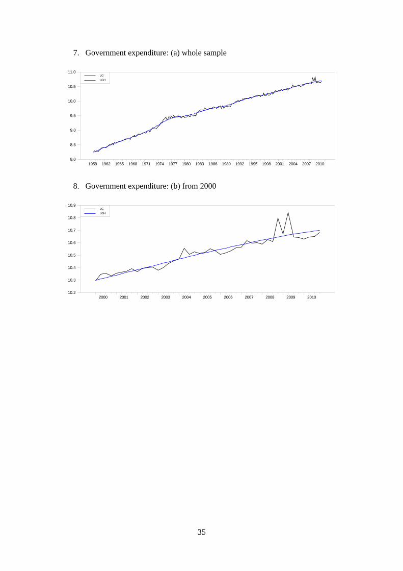
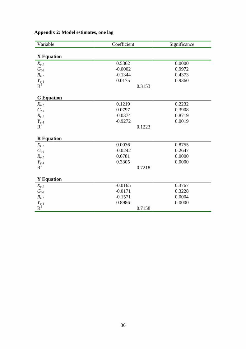
Graphs of original and de-trended data for the four core variables are reported below.
1. Output: (a) whole sample
2. Output: (b) from 2000
3. Exports: (a) whole sample
1959 1962 1965 1968 1971 1974 1977 1980 1983 1986 1989 1992 1995 1998 2001 2004 2007 201010.75
11.00
11.25
11.50
11.75
12.00
12.25
12.50
12.75LYLYH
2000 2001 2002 2003 2004 2005 2006 2007 2008 2009 201012.35
12.40
12.45
12.50
12.55
12.60
12.65
12.70
12.75LYLYH
1959 1962 1965 1968 1971 1974 1977 1980 1983 1986 1989 1992 1995 1998 2001 2004 2007 20108.0
8.5
9.0
9.5
10.0
10.5
11.0
11.5LXLXH
34
4. Exports: (b) from 2000
5. Cash rate: (a) whole sample
6. Cash rate: (b) from 2000
2000 2001 2002 2003 2004 2005 2006 2007 2008 2009 201010.90
10.95
11.00
11.05
11.10
11.15
11.20
11.25
11.30LXLXH
1959 1962 1965 1968 1971 1974 1977 1980 1983 1986 1989 1992 1995 1998 2001 2004 2007 20100.025
0.050
0.075
0.100
0.125
0.150
0.175LRLRH
2000 2001 2002 2003 2004 2005 2006 2007 2008 2009 20100.025
0.030
0.035
0.040
0.045
0.050
0.055
0.060
0.065
0.070LRLRH
35
7. Government expenditure: (a) whole sample
8. Government expenditure: (b) from 2000
1959 1962 1965 1968 1971 1974 1977 1980 1983 1986 1989 1992 1995 1998 2001 2004 2007 20108.0
8.5
9.0
9.5
10.0
10.5
11.0LGLGH
2000 2001 2002 2003 2004 2005 2006 2007 2008 2009 201010.2
10.3
10.4
10.5
10.6
10.7
10.8
10.9LGLGH
36
Appendix 2: Model estimates, one lag
Variable Coefficient Significance X Equation
Xt-1 0.5362 0.0000 Gt-1 -0.0002 0.9972 Rt-1 -0.1344 0.4373 Yy-1 0.0175 0.9360 R2 0.3153 G Equation Xt-1 0.1219 0.2232 Gt-1 0.0797 0.3908 Rt-1 -0.0374 0.8719 Yy-1 -0.9272 0.0019 R2 0.1223 R Equation Xt-1 0.0036 0.8755 Gt-1 -0.0242 0.2647 Rt-1 0.6781 0.0000 Yy-1 0.3305 0.0000 R2 0.7218 Y Equation Xt-1 -0.0165 0.3767 Gt-1 -0.0171 0.3228 Rt-1 -0.1571 0.0004 Yy-1 0.8986 0.0000 R2 0.7158
37
Appendix 2: Model estimates, two lags
Variable Coefficient Significance X Equation
Xt-1 0.5585 0.0000 Xt-2 -0.0549 0.5451 Gt-1 0.0103 0.8841 Gy-2 0.1291 0.0666 Rt-1 0.1390 0.6517 Rt-2 -0.2355 0.4073 Yt-1 -0.1322 0.7247 Yy-2 0.2158 0.5890 R2 0.3306 G Equation Xt-1 0.1039 0.3941 Xt-2 0.0183 0.8778 Gt-1 0.0465 0.6182 Gy-2 0.2773 0.0030 Rt-1 -0.1684 0.6772 Rt-2 0.4717 0.2072 Yt-1 -0.4196 0.3955 Yy-2 -0.4423 0.3997 R2 0.1939 R Equation Xt-1 0.0281 0.2991 Xt-2 -0.0691 0.0098 Gt-1 -0.0051 0.8033 Gy-2 0.0014 0.9465 Rt-1 0.8593 0.0000 Rt-2 -0.2513 0.0028 Yt-1 0.0340 0.7553 Yy-2 0.3473 0.0033 R2 0.7699 Y Equation Xt-1 -0.0039 0.8631 Xt-2 -0.0239 0.2824 Gt-1 -0.0084 0.6295 Gy-2 -0.0217 0.2050 Rt-1 -0.0105 0.8893 Rt-2 -0.1583 0.0242 Yt-1 0.9382 0.0000 Yy-2 -0.1030 0.2932 R2 0.7393
38
Appendix 3: Detailed results of sensitivity analysis
Table 1: Contributions to output 2007(1) to 2011(4): Sample 1959(3) to 2011(4)
Note: derived from a model with one lag.
Quarter Exports Fiscal Monetary Other output
Mar 2007 0.01 0.15 -0.02 0.79
June 2007 0.02 0.11 -0.10 0.93
Sept 2007 0.05 0.02 -0.10 1.05
Dec 2007 -0.01 0.02 -0.09 1.01
Mar 2008 0.09 0.03 -0.07 1.42
June 2008 0.17 0.05 -0.10 0.83
Sept 2008 0.09 0.04 -0.14 0.89
Dec 2008 0.00 -0.04 -0.42 0.04
Mar 2009 0.02 -0.29 -0.37 0.44
June 2009 -0.08 -0.27 -0.19 -0.09
Sept 2009 -0.11 -0.43 0.13 0.02
Dec 2009 -0.02 -0.23 0.29 -0.18
Mar 2010 0.10 -0.06 0.34 -0.42
June 2010 0.20 0.05 0.38 -0.60
Sept 2010 0.08 0.11 0.30 -0.74
Dec 2010 0.16 0.15 0.23 -0.72
Mar 2011 -0.18 0.14 0.16 -1.18
June 2011 -0.12 0.15 0.09 -0.36
Sept 2011 -0.06 0.16 -0.01 -0.11
Dec 2011 0.00 0.08 -0.08 -0.15
39
Table 2: Contributions to output 2007(1) to 2011(4): Sample period 1993(1) to 2011(4)
Quarter Exports Fiscal Monetary Other output
Mar 2007 -0.01 0.06 -0.10 0.96
June 2007 0.02 0.06 -0.12 0.99
Sept 2007 0.05 -0.02 -0.11 1.10
Dec 2007 -0.08 -0.03 -0.11 1.13
Mar 2008 0.09 -0.04 -0.12 1.51
June 2008 0.14 -0.02 -0.13 0.96
Sept 2008 -0.12 -0.02 -0.16 1.17
Dec 2008 -0.23 0.13 -0.22 -0.08
Mar 2009 -0.05 -0.14 -0.09 0.09
June 2009 -0.16 0.04 0.11 -0.61
Sept 2009 -0.04 -0.22 0.31 -0.42
Dec 2009 0.15 -0.14 0.38 -0.52
Mar 2010 0.24 -0.05 0.37 -0.60
June 2010 0.22 0.03 0.33 -0.56
Sept 2010 -0.16 0.05 0.23 -0.39
Dec 2010 -0.01 0.11 0.14 -0.43
Mar 2011 -0.56 0.09 0.06 -0.66
June 2011 -0.15 0.08 -0.03 -0.16
Sept 2011 0.08 0.13 -0.10 -0.13
Dec 2011 0.18 0.03 -0.13 -0.22
40
Table 3: Contributions to output 2007(1) to 2011(4): Model with two lags
Note: model estimated over a sample of 1980(1) to 2011(4).
Quarter Exports Fiscal Monetary Other output
Mar 2007 0.07 0.44 -0.08 0.52
June 2007 0.02 0.52 -0.26 0.67
Sept 2007 0.01 0.56 -0.42 0.90
Dec 2007 -0.11 0.48 -0.52 1.10
Mar 2008 -0.04 0.43 -0.52 1.65
June 2008 0.09 0.35 -0.47 0.99
Sept 2008 0.04 0.30 -0.41 0.95
Dec 2008 -0.11 0.09 -0.36 -0.05
Mar 2009 -0.05 -0.11 -0.28 0.22
June 2009 -0.21 -0.60 0.00 0.17
Sept 2009 -0.20 -0.74 0.45 0.10
Dec 2009 -0.13 -1.05 0.85 0.17
Mar 2010 0.11 -0.94 1.10 -0.33
June 2010 0.34 -0.74 1.15 -0.73
Sept 2010 0.23 -0.49 1.05 -1.08
Dec 2010 0.20 -0.20 0.82 -1.01
Mar 2011 -0.21 0.10 0.52 -1.47
June 2011 -0.26 0.34 0.17 -0.47
Sept 2011 -0.10 0.49 -0.18 -0.20
Dec 2011 0.11 0.58 -0.49 -0.35
41
Table 4: Contributions to output 2007(1) to 2011(4): Government expenditure includes state and local government expenditure
Note: model estimated over a sample of 1980(1) to 2011(4) with one lag.
Quarter Exports Fiscal Monetary Other output
Mar 2007 0.04 0.10 -0.24 1.02
June 2007 0.03 0.10 -0.30 1.14
Sept 2007 0.05 0.03 -0.28 1.23
Dec 2007 -0.03 0.03 -0.24 1.17
Mar 2008 0.07 0.02 -0.20 1.58
June 2008 0.14 0.03 -0.19 0.98
Sept 2008 0.04 0.00 -0.19 1.04
Dec 2008 -0.07 -0.02 -0.25 -0.06
Mar 2009 0.01 -0.17 -0.08 0.06
June 2009 -0.12 -0.12 0.20 -0.57
Sept 2009 -0.10 -0.22 0.50 -0.56
Dec 2009 0.00 -0.14 0.67 -0.65
Mar 2010 0.11 -0.07 0.71 -0.79
June 2010 0.20 -0.03 0.68 -0.83
Sept 2010 0.04 0.01 0.54 -0.85
Dec 2010 0.11 0.05 0.39 -0.74
Mar 2011 -0.27 0.06 0.23 -1.10
June 2011 -0.17 0.08 0.05 -0.22
Sept 2011 -0.07 0.10 -0.15 0.09
Dec 2011 0.03 0.09 -0.30 0.03
42
Table 5: Contributions to output 2007(1) to 2011(4): Fiscal policy measured as a surplus
Note: model estimated over a sample of 1980(1) to 2011(4) with one lag.
Quarter Exports Fiscal Monetary Other output
Mar 2007 -0.01 0.54 -0.37 0.81
June 2007 -0.02 0.66 -0.57 0.91
Sept 2007 -0.01 0.69 -0.68 1.06
Dec 2007 -0.09 0.64 -0.73 1.15
Mar 2008 -0.02 0.51 -0.67 1.74
June 2008 0.07 0.50 -0.61 1.03
Sept 2008 -0.02 0.45 -0.47 0.95
Dec 2008 -0.17 0.31 -0.31 -0.27
Mar 2009 -0.12 -0.02 -0.05 -0.03
June 2009 -0.14 -0.29 0.26 -0.48
Sept 2009 -0.12 -0.57 0.74 -0.45
Dec 2009 -0.01 -0.91 1.14 -0.38
Mar 2010 0.15 -1.15 1.40 -0.46
June 2010 0.25 -1.08 1.41 -0.58
Sept 2010 0.07 -0.95 1.30 -0.73
Dec 2010 0.03 -0.73 0.99 -0.52
Mar 2011 -0.30 -0.51 0.60 -0.90
June 2011 -0.28 -0.15 0.16 0.04
Sept 2011 -0.04 0.14 -0.28 0.19
Dec 2011 0.17 0.34 -0.62 -0.03
43
Table 6: Contributions to output 2007(1) to 2011(4): Using IMP for Monetary Policy
Quarter Exports Fiscal Monetary IMP Other output
Mar 2007 0.04 0.19 -0.27 0.04 0.98
June 2007 0.03 0.16 -0.31 0.05 1.10
Sept 2007 0.05 0.06 -0.29 -0.05 1.21
Dec 2007 -0.03 0.04 -0.25 -0.12 1.17
Mar 2008 0.06 0.03 -0.21 -0.34 1.59
June 2008 0.14 0.06 -0.20 -0.37 0.97
Sept 2008 0.04 0.03 -0.21 -0.51 1.03
Dec 2008 -0.07 0.01 -0.24 -0.63 -0.09
Mar 2009 0.01 -0.30 -0.05 -0.58 0.15
June 2009 -0.12 -0.26 0.25 -0.32 -0.49
Sept 2009 -0.09 -0.48 0.54 0.03 -0.35
Dec 2009 0.00 -0.31 0.68 0.28 -0.50
Mar 2010 0.11 -0.14 0.70 0.38 -0.72
June 2010 0.20 0.00 0.65 0.36 -0.84
Sept 2010 0.03 0.09 0.53 0.37 -0.91
Dec 2010 0.11 0.17 0.39 0.23 -0.85
Mar 2011 -0.27 0.18 0.24 0.03 -1.22
June 2011 -0.17 0.19 0.05 -0.26 -0.33
Sept 2011 -0.08 0.21 -0.14 -0.40 -0.03
Dec 2011 0.02 0.11 -0.27 -0.39 -0.02
44
Table 7: Contributions to output 2007(1) to 2011(4): International effects measured by terms of trade
Note: model estimated over a sample of 1980(1) to 2011(4) with one lag.
Quarter Terms of Trade Fiscal Monetary Other output
Mar 2007 0.04 0.23 -0.21 0.90
June 2007 0.01 0.23 -0.24 1.00
Sept 2007 -0.03 0.14 -0.20 1.15
Dec 2007 -0.07 0.11 -0.15 1.08
Mar 2008 -0.10 0.09 -0.13 1.66
June 2008 -0.12 0.10 -0.14 1.14
Sept 2008 0.00 0.07 -0.17 1.02
Dec 2008 0.13 0.06 -0.18 -0.43
Mar 2009 0.15 -0.26 0.06 -0.15
June 2009 0.07 -0.26 0.41 -0.87
Sept 2009 -0.08 -0.53 0.70 -0.49
Dec 2009 -0.16 -0.45 0.81 -0.35
Mar 2010 -0.22 -0.31 0.76 -0.31
June 2010 -0.23 -0.17 0.63 -0.24
Sept 2010 -0.09 -0.06 0.42 -0.56
Dec 2010 -0.01 0.06 0.23 -0.49
Mar 2011 0.03 0.13 0.05 -1.31
June 2011 0.07 0.18 -0.15 -0.37
Sept 2011 0.13 0.26 -0.31 -0.10
Dec 2011 0.15 0.20 -0.40 -0.10
45
Table 8: Contributions to output 2007(1) to 2011(4): Identification using Cholesky
Note: model estimated over a sample of 1980(1) to 2011(4) with one lag.
Quarter Exports Fiscal Monetary Other output
Mar 2007 0.04 0.19 -0.06 0.77
June 2007 0.03 0.03 -0.07 0.97
Sept 2007 0.05 -0.08 -0.07 1.13
Dec 2007 -0.03 -0.11 -0.06 1.12
Mar 2008 0.07 -0.09 -0.04 1.52
June 2008 0.14 -0.10 -0.03 0.95
Sept 2008 0.04 -0.12 -0.05 1.01
Dec 2008 -0.07 -0.39 -0.10 0.15
Mar 2009 0.02 -0.47 -0.20 0.46
June 2009 -0.12 -0.50 0.04 -0.05
Sept 2009 -0.09 -0.38 0.08 -0.01
Dec 2009 0.00 0.01 0.10 -0.24
Mar 2010 0.11 0.29 0.10 -0.53
June 2010 0.19 0.43 0.16 -0.76
Sept 2010 0.03 0.49 0.13 -0.90
Dec 2010 0.11 0.46 0.16 -0.91
Mar 2011 -0.27 0.37 0.17 -1.34
June 2011 -0.17 0.32 0.15 -0.55
Sept 2011 -0.07 0.17 0.12 -0.25
Dec 2011 0.03 0.03 0.00 -0.21
46
Table 9A: Augmented Dickey-Fuller tests for log of variables, not de-trended
Deterministic Component Variable Intercept Intercept and trend
X 0.4596 0.5301 G 0.2356 0.5322 R 0.1139 0.3458 Y 0.4378 0.5861
Notes: figures in the table are marginal significance levels; all tests were run with 4 lags; sample 1959:3 to 2011:4
Table 9B: Augmented Dickey-Fuller tests for first-differences of log of variables, not de-trended Deterministic Component
Variable None Intercept X 0.0000 0.0000 G 0.0000 0.0000 R 0.0000 0.0000 Y 0.0034 0.0000
Notes: figures in the table are marginal significance levels; all tests were run with 4 lags; sample 1959:3 to 2011:4
Table 9C: Johansen cointegration tests for log of variables, not de-trended Deterministic Component
Test No trends Trend in CV Trace 0.0831 0.4362
Eigenvalue 0.5068 0.7817
Notes: figures in the table are marginal significance levels; all tests were run with 4 lags; sample 1959:3 to 2011:4
47
Table 10: Contributions to output 2007(1) to 2011(4): Model in log levels, no trend
Note: model estimated over a sample of 1980(1) to 2011(4) with two lags.
Quarter Exports Fiscal Monetary Other output
Mar 2007 -0.75 -0.07 -0.08 2.33
June 2007 -0.81 0.06 -0.09 2.30
Sept 2007 -0.64 0.02 -0.02 2.50
Dec 2007 -0.83 0.16 -0.01 2.51
Mar 2008 -0.72 0.64 0.02 3.26
June 2008 0.30 0.95 -0.05 2.40
Sept 2008 0.29 0.56 -0.10 2.27
Dec 2008 -0.36 0.21 -0.19 1.02
Mar 2009 -0.44 0.30 -0.23 1.10
June 2009 -0.83 -0.81 -0.17 0.67
Sept 2009 -0.61 -0.49 0.03 0.49
Dec 2009 -0.55 -0.03 0.26 0.35
Mar 2010 -0.48 0.20 0.42 0.06
June 2010 -0.39 0.38 0.55 -0.16
Sept 2010 -0.19 0.19 0.57 -0.71
Dec 2010 -0.29 0.29 0.64 -0.63
Mar 2011 -0.49 0.93 0.65 -1.05
June 2011 -0.75 1.23 0.68 -0.07
Sept 2011 -0.75 1.22 0.65 -0.07
Dec 2011 -0.64 1.03 0.61 -0.73
48
Table 11: Contributions to output 2007(1) to 2011(4): Model in log levels with trend
Note: model estimated over a sample of 1980(1) to 2011(4) with two lags.
Quarter Exports Fiscal Monetary Other output
Mar 2007 -0.26 -0.18 0.68 1.91
June 2007 -0.28 -0.18 0.61 2.07
Sept 2007 -0.19 -0.14 0.53 2.04
Dec 2007 -0.30 -0.09 0.45 1.99
Mar 2008 -0.21 -0.02 0.37 2.29
June 2008 0.22 0.03 0.29 1.71
Sept 2008 0.18 0.04 0.22 1.68
Dec 2008 -0.16 -0.01 0.16 0.57
Mar 2009 -0.14 0.08 0.13 0.48
June 2009 -0.41 0.04 0.19 -0.04
Sept 2009 -0.36 0.14 0.38 -0.24
Dec 2009 -0.37 0.15 0.61 -0.44
Mar 2010 -0.27 0.10 0.83 -0.85
June 2010 -0.16 -0.03 0.97 -1.20
Sept 2010 -0.18 -0.15 1.05 -1.43
Dec 2010 -0.23 -0.24 1.02 -1.48
Mar 2011 -0.56 -0.25 0.90 -2.10
June 2011 -0.69 -0.23 0.70 -1.30
Sept 2011 -0.61 -0.21 0.44 -1.13
Dec 2011 -0.45 -0.16 0.14 -1.29
49
Table 12: Contributions to output 2007(1) to 2011(4): Model using linearly-de-trended data
Note: model estimated over a sample of 1980(1) to 2011(4) with two lags.
Quarter Exports Fiscal Monetary Other output
Mar 2007 -0.67 0.06 0.36 1.64
June 2007 -0.68 0.01 0.31 1.79
Sept 2007 -0.59 0.04 0.28 1.76
Dec 2007 -0.72 0.04 0.25 1.69
Mar 2008 -0.58 0.07 0.21 1.98
June 2008 -0.18 0.04 0.16 1.41
Sept 2008 -0.32 0.05 0.08 1.43
Dec 2008 -0.60 -0.12 -0.01 0.40
Mar 2009 -0.56 0.05 0.04 0.19
June 2009 -0.79 -0.11 0.18 -0.28
Sept 2009 -0.68 0.09 0.35 -0.56
Dec 2009 -0.69 0.11 0.48 -0.74
Mar 2010 -0.67 0.12 0.56 -1.01
June 2010 -0.69 0.11 0.58 -1.22
Sept 2010 -0.81 0.12 0.53 -1.38
Dec 2010 -0.83 0.09 0.43 -1.46
Mar 2011 -1.24 0.09 0.31 -2.02
June 2011 -1.26 0.12 0.15 -1.39
Sept 2011 -1.25 0.05 -0.01 -1.17
Dec 2011 -1.24 0.07 -0.17 -1.30
50
Table 13: Contributions to output 2007(1) to 2011(4): Base model with inflation
Quarter Exports Fiscal Monetary Other output
Mar 2007 0.04 0.21 -0.20 0.94
June 2007 0.03 0.20 -0.25 1.07
Sept 2007 0.04 0.09 -0.24 1.20
Dec 2007 -0.04 0.06 -0.21 1.18
Mar 2008 0.07 0.04 -0.20 1.59
June 2008 0.14 0.06 -0.19 0.99
Sept 2008 0.06 0.03 -0.22 1.04
Dec 2008 -0.04 0.02 -0.25 -0.13
Mar 2009 0.02 -0.34 -0.02 0.16
June 2009 -0.15 -0.29 0.32 -0.44
Sept 2009 -0.15 -0.52 0.60 -0.23
Dec 2009 -0.04 -0.35 0.69 -0.38
Mar 2010 0.10 -0.17 0.66 -0.63
June 2010 0.20 -0.02 0.60 -0.79
Sept 2010 0.07 0.08 0.46 -0.92
Dec 2010 0.14 0.16 0.37 -0.88
Mar 2011 -0.25 0.19 0.25 -1.25
June 2011 -0.16 0.22 0.08 -0.37
Sept 2011 -0.06 0.26 -0.10 -0.09
Dec 2011 0.03 0.15 -0.23 -0.06
51
Table 14: Contributions to output 2007(1) to 2011(4): Base model with imports
Quarter Exports Fiscal Monetary Other output
Mar 2007 -0.03 0.24 -0.08 0.88
June 2007 -0.03 0.22 -0.19 0.97
Sept 2007 -0.01 0.11 -0.21 1.12
Dec 2007 -0.08 0.06 -0.20 1.12
Mar 2008 0.04 0.02 -0.19 1.56
June 2008 0.13 0.03 -0.18 0.92
Sept 2008 0.04 0.00 -0.17 0.94
Dec 2008 -0.07 0.02 -0.16 -0.25
Mar 2009 -0.01 -0.31 0.16 0.12
June 2009 -0.14 -0.27 0.54 -0.43
Sept 2009 -0.13 -0.54 0.82 -0.12
Dec 2009 -0.01 -0.41 0.84 -0.21
Mar 2010 0.13 -0.23 0.68 -0.45
June 2010 0.23 -0.05 0.50 -0.60
Sept 2010 0.06 0.08 0.26 -0.72
Dec 2010 0.12 0.20 0.06 -0.69
Mar 2011 -0.27 0.25 -0.13 -1.10
June 2011 -0.16 0.27 -0.32 -0.27
Sept 2011 -0.04 0.30 -0.47 -0.06
Dec 2011 0.07 0.20 -0.56 -0.13
52
Table 15: Contributions to output 2007(1) to 2011(4): Base model with TWI
Quarter Exports Fiscal Monetary Other output
Mar 2007 0.00 0.25 -0.15 0.91
June 2007 -0.01 0.23 -0.24 1.03
Sept 2007 0.01 0.12 -0.26 1.19
Dec 2007 -0.07 0.09 -0.23 1.18
Mar 2008 0.04 0.07 -0.19 1.62
June 2008 0.12 0.08 -0.16 1.02
Sept 2008 0.03 0.04 -0.14 1.12
Dec 2008 -0.09 0.02 -0.15 0.01
Mar 2009 -0.02 -0.35 0.08 0.25
June 2009 -0.14 -0.30 0.33 -0.47
Sept 2009 -0.12 -0.56 0.50 -0.30
Dec 2009 0.00 -0.41 0.56 -0.47
Mar 2010 0.13 -0.23 0.51 -0.70
June 2010 0.21 -0.07 0.44 -0.84
Sept 2010 0.05 0.04 0.31 -0.93
Dec 2010 0.12 0.16 0.19 -0.89
Mar 2011 -0.27 0.20 0.05 -1.26
June 2011 -0.16 0.23 -0.09 -0.38
Sept 2011 -0.05 0.27 -0.23 -0.08
Dec 2011 0.05 0.16 -0.31 -0.05
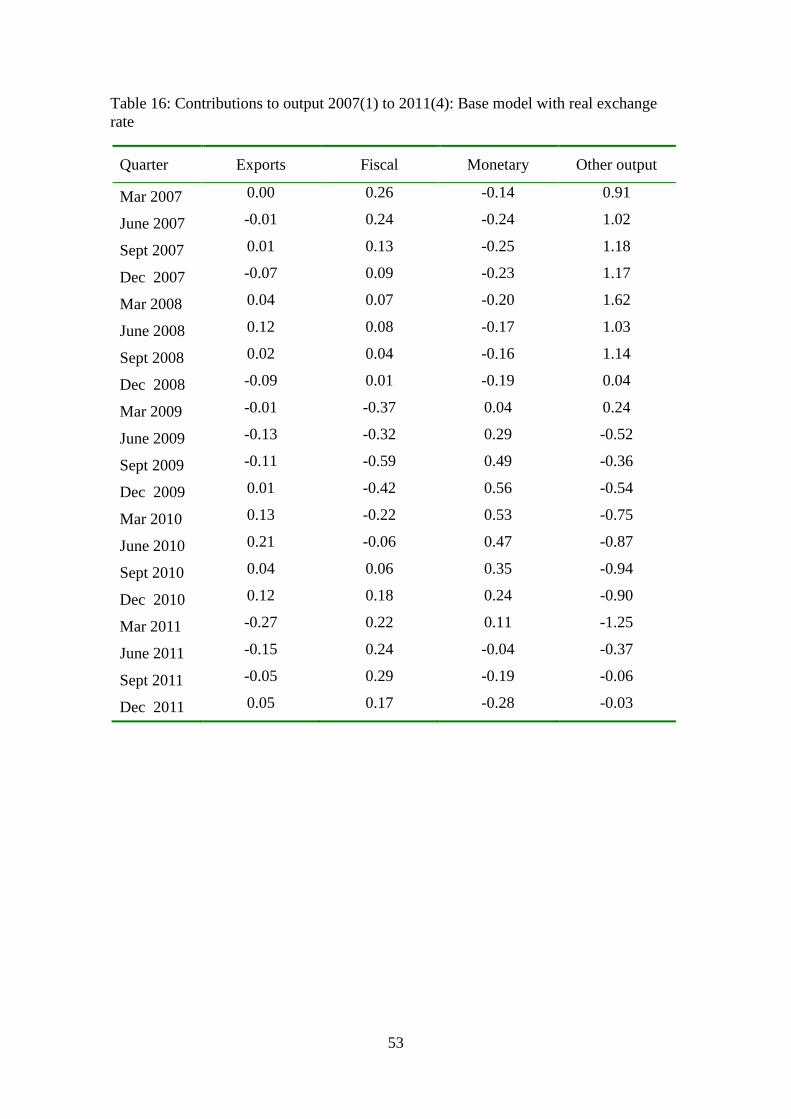
53
Table 16: Contributions to output 2007(1) to 2011(4): Base model with real exchange rate
Quarter Exports Fiscal Monetary Other output
Mar 2007 0.00 0.26 -0.14 0.91
June 2007 -0.01 0.24 -0.24 1.02
Sept 2007 0.01 0.13 -0.25 1.18
Dec 2007 -0.07 0.09 -0.23 1.17
Mar 2008 0.04 0.07 -0.20 1.62
June 2008 0.12 0.08 -0.17 1.03
Sept 2008 0.02 0.04 -0.16 1.14
Dec 2008 -0.09 0.01 -0.19 0.04
Mar 2009 -0.01 -0.37 0.04 0.24
June 2009 -0.13 -0.32 0.29 -0.52
Sept 2009 -0.11 -0.59 0.49 -0.36
Dec 2009 0.01 -0.42 0.56 -0.54
Mar 2010 0.13 -0.22 0.53 -0.75
June 2010 0.21 -0.06 0.47 -0.87
Sept 2010 0.04 0.06 0.35 -0.94
Dec 2010 0.12 0.18 0.24 -0.90
Mar 2011 -0.27 0.22 0.11 -1.25
June 2011 -0.15 0.24 -0.04 -0.37
Sept 2011 -0.05 0.29 -0.19 -0.06
Dec 2011 0.05 0.17 -0.28 -0.03
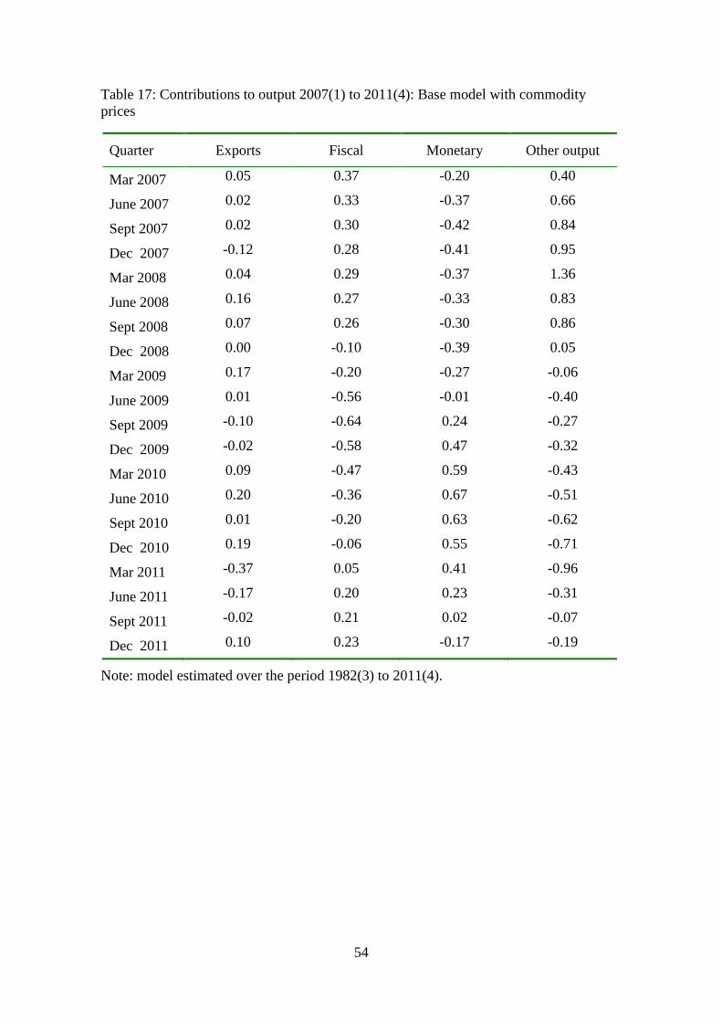
54
Table 17: Contributions to output 2007(1) to 2011(4): Base model with commodity prices
Note: model estimated over the period 1982(3) to 2011(4).
Quarter Exports Fiscal Monetary Other output
Mar 2007 0.05 0.37 -0.20 0.40
June 2007 0.02 0.33 -0.37 0.66
Sept 2007 0.02 0.30 -0.42 0.84
Dec 2007 -0.12 0.28 -0.41 0.95
Mar 2008 0.04 0.29 -0.37 1.36
June 2008 0.16 0.27 -0.33 0.83
Sept 2008 0.07 0.26 -0.30 0.86
Dec 2008 0.00 -0.10 -0.39 0.05
Mar 2009 0.17 -0.20 -0.27 -0.06
June 2009 0.01 -0.56 -0.01 -0.40
Sept 2009 -0.10 -0.64 0.24 -0.27
Dec 2009 -0.02 -0.58 0.47 -0.32
Mar 2010 0.09 -0.47 0.59 -0.43
June 2010 0.20 -0.36 0.67 -0.51
Sept 2010 0.01 -0.20 0.63 -0.62
Dec 2010 0.19 -0.06 0.55 -0.71
Mar 2011 -0.37 0.05 0.41 -0.96
June 2011 -0.17 0.20 0.23 -0.31
Sept 2011 -0.02 0.21 0.02 -0.07
Dec 2011 0.10 0.23 -0.17 -0.19
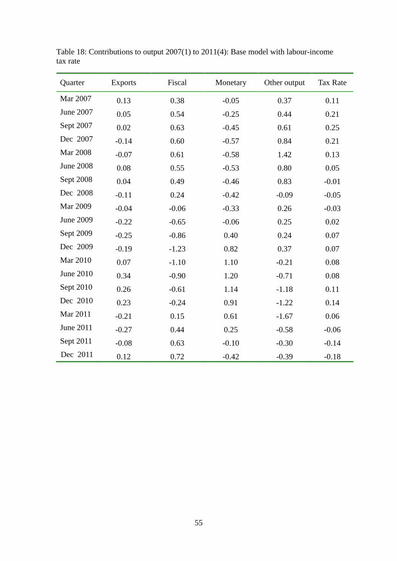
55
Table 18: Contributions to output 2007(1) to 2011(4): Base model with labour-income tax rate
Quarter Exports Fiscal Monetary Other output Tax Rate
Mar 2007 0.13 0.38 -0.05 0.37 0.11 June 2007 0.05 0.54 -0.25 0.44 0.21 Sept 2007 0.02 0.63 -0.45 0.61 0.25 Dec 2007 -0.14 0.60 -0.57 0.84 0.21 Mar 2008 -0.07 0.61 -0.58 1.42 0.13 June 2008 0.08 0.55 -0.53 0.80 0.05 Sept 2008 0.04 0.49 -0.46 0.83 -0.01 Dec 2008 -0.11 0.24 -0.42 -0.09 -0.05 Mar 2009 -0.04 -0.06 -0.33 0.26 -0.03 June 2009 -0.22 -0.65 -0.06 0.25 0.02 Sept 2009 -0.25 -0.86 0.40 0.24 0.07 Dec 2009 -0.19 -1.23 0.82 0.37 0.07 Mar 2010 0.07 -1.10 1.10 -0.21 0.08 June 2010 0.34 -0.90 1.20 -0.71 0.08 Sept 2010 0.26 -0.61 1.14 -1.18 0.11 Dec 2010 0.23 -0.24 0.91 -1.22 0.14 Mar 2011 -0.21 0.15 0.61 -1.67 0.06 June 2011 -0.27 0.44 0.25 -0.58 -0.06 Sept 2011 -0.08 0.63 -0.10 -0.30 -0.14 Dec 2011 0.12 0.72 -0.42 -0.39 -0.18
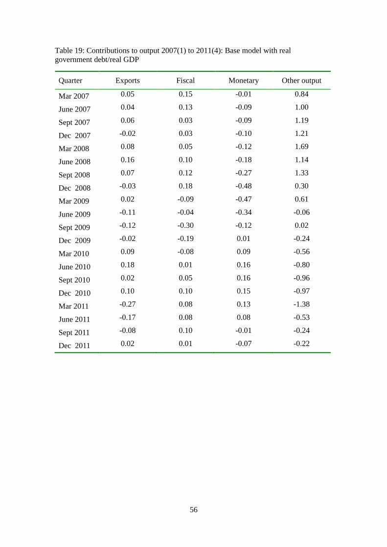
56
Table 19: Contributions to output 2007(1) to 2011(4): Base model with real government debt/real GDP
Quarter Exports Fiscal Monetary Other output
Mar 2007 0.05 0.15 -0.01 0.84
June 2007 0.04 0.13 -0.09 1.00
Sept 2007 0.06 0.03 -0.09 1.19
Dec 2007 -0.02 0.03 -0.10 1.21
Mar 2008 0.08 0.05 -0.12 1.69
June 2008 0.16 0.10 -0.18 1.14
Sept 2008 0.07 0.12 -0.27 1.33
Dec 2008 -0.03 0.18 -0.48 0.30
Mar 2009 0.02 -0.09 -0.47 0.61
June 2009 -0.11 -0.04 -0.34 -0.06
Sept 2009 -0.12 -0.30 -0.12 0.02
Dec 2009 -0.02 -0.19 0.01 -0.24
Mar 2010 0.09 -0.08 0.09 -0.56
June 2010 0.18 0.01 0.16 -0.80
Sept 2010 0.02 0.05 0.16 -0.96
Dec 2010 0.10 0.10 0.15 -0.97
Mar 2011 -0.27 0.08 0.13 -1.38
June 2011 -0.17 0.08 0.08 -0.53
Sept 2011 -0.08 0.10 -0.01 -0.24
Dec 2011 0.02 0.01 -0.07 -0.22
57
Editor, UWA Economics Discussion Papers: Ernst Juerg Weber Business School – Economics University of Western Australia 35 Sterling Hwy Crawley WA 6009 Australia Email: [email protected] The Economics Discussion Papers are available at: 1980 – 2002: http://ecompapers.biz.uwa.edu.au/paper/PDF%20of%20Discussion%20Papers/ Since 2001: http://ideas.repec.org/s/uwa/wpaper1.html Since 2004: http://www.business.uwa.edu.au/school/disciplines/economics
ECONOMICS DISCUSSION PAPERS 2011
DP NUMBER AUTHORS TITLE
11.01 Robertson, P.E. DEEP IMPACT: CHINA AND THE WORLD ECONOMY
11.02 Kang, C. and Lee, S.H. BEING KNOWLEDGEABLE OR SOCIABLE? DIFFERENCES IN RELATIVE IMPORTANCE OF COGNITIVE AND NON-COGNITIVE SKILLS
11.03 Turkington, D. DIFFERENT CONCEPTS OF MATRIX CALCULUS
11.04 Golley, J. and Tyers, R. CONTRASTING GIANTS: DEMOGRAPHIC CHANGE AND ECONOMIC PERFORMANCE IN CHINA AND INDIA
11.05 Collins, J., Baer, B. and Weber, E.J. ECONOMIC GROWTH AND EVOLUTION: PARENTAL PREFERENCE FOR QUALITY AND QUANTITY OF OFFSPRING
11.06 Turkington, D. ON THE DIFFERENTIATION OF THE LOG LIKELIHOOD FUNCTION USING MATRIX CALCULUS
11.07 Groenewold, N. and Paterson, J.E.H. STOCK PRICES AND EXCHANGE RATES IN AUSTRALIA: ARE COMMODITY PRICES THE MISSING LINK?
11.08 Chen, A. and Groenewold, N. REDUCING REGIONAL DISPARITIES IN CHINA: IS INVESTMENT ALLOCATION POLICY EFFECTIVE?
11.09 Williams, A., Birch, E. and Hancock, P. THE IMPACT OF ON-LINE LECTURE RECORDINGS ON STUDENT PERFORMANCE
11.10 Pawley, J. and Weber, E.J. INVESTMENT AND TECHNICAL PROGRESS IN THE G7 COUNTRIES AND AUSTRALIA
11.11 Tyers, R. AN ELEMENTAL MACROECONOMIC MODEL FOR APPLIED ANALYSIS AT UNDERGRADUATE LEVEL
11.12 Clements, K.W. and Gao, G. QUALITY, QUANTITY, SPENDING AND PRICES

58
11.13 Tyers, R. and Zhang, Y. JAPAN’S ECONOMIC RECOVERY: INSIGHTS FROM MULTI-REGION DYNAMICS
11.14 McLure, M. A. C. PIGOU’S REJECTION OF PARETO’S LAW
11.15 Kristoffersen, I. THE SUBJECTIVE WELLBEING SCALE: HOW REASONABLE IS THE CARDINALITY ASSUMPTION?
11.16 Clements, K.W., Izan, H.Y. and Lan, Y. VOLATILITY AND STOCK PRICE INDEXES
11.17 Parkinson, M. SHANN MEMORIAL LECTURE 2011: SUSTAINABLE WELLBEING – AN ECONOMIC FUTURE FOR AUSTRALIA
11.18 Chen, A. and Groenewold, N. THE NATIONAL AND REGIONAL EFFECTS OF FISCAL DECENTRALISATION IN CHINA
11.19 Tyers, R. and Corbett, J. JAPAN’S ECONOMIC SLOWDOWN AND ITS GLOBAL IMPLICATIONS: A REVIEW OF THE ECONOMIC MODELLING
11.20 Wu, Y. GAS MARKET INTEGRATION: GLOBAL TRENDS AND IMPLICATIONS FOR THE EAS REGION
11.21 Fu, D., Wu, Y. and Tang, Y. DOES INNOVATION MATTER FOR CHINESE HIGH-TECH EXPORTS? A FIRM-LEVEL ANALYSIS
11.22 Fu, D. and Wu, Y. EXPORT WAGE PREMIUM IN CHINA’S MANUFACTURING SECTOR: A FIRM LEVEL ANALYSIS
11.23 Li, B. and Zhang, J. SUBSIDIES IN AN ECONOMY WITH ENDOGENOUS CYCLES OVER NEOCLASSICAL INVESTMENT AND NEO-SCHUMPETERIAN INNOVATION REGIMES
11.24 Krey, B., Widmer, P.K. and Zweifel, P. EFFICIENT PROVISION OF ELECTRICITY FOR THE UNITED STATES AND SWITZERLAND
11.25 Wu, Y. ENERGY INTENSITY AND ITS DETERMINANTS IN CHINA’S REGIONAL ECONOMIES

59
ECONOMICS DISCUSSION PAPERS 2012
DP NUMBER AUTHORS TITLE
12.01 Clements, K.W., Gao, G., and Simpson, T.
DISPARITIES IN INCOMES AND PRICES INTERNATIONALLY
12.02 Tyers, R. THE RISE AND ROBUSTNESS OF ECONOMIC FREEDOM IN CHINA
12.03 Golley, J. and Tyers, R. DEMOGRAPHIC DIVIDENDS, DEPENDENCIES AND ECONOMIC GROWTH IN CHINA AND INDIA
12.04 Tyers, R. LOOKING INWARD FOR GROWTH
12.05 Knight, K. and McLure, M. THE ELUSIVE ARTHUR PIGOU
12.06 McLure, M. ONE HUNDRED YEARS FROM TODAY: A. C. PIGOU’S WEALTH AND WELFARE
12.07 Khuu, A. and Weber, E.J. HOW AUSTRALIAN FARMERS DEAL WITH RISK
12.08 Chen, M. and Clements, K.W. PATTERNS IN WORLD METALS PRICES
12.09 Clements, K.W. UWA ECONOMICS HONOURS
12.10 Golley, J. and Tyers, R. CHINA’S GENDER IMBALANCE AND ITS ECONOMIC PERFORMANCE
12.11 Weber, E.J. AUSTRALIAN FISCAL POLICY IN THE AFTERMATH OF THE GLOBAL FINANCIAL CRISIS
12.12 Hartley, P.R. and Medlock III, K.B. CHANGES IN THE OPERATIONAL EFFICIENCY OF NATIONAL OIL COMPANIES
12.13 Li, L. HOW MUCH ARE RESOURCE PROJECTS WORTH? A CAPITAL MARKET PERSPECTIVE
12.14 Chen, A. and Groenewold, N. THE REGIONAL ECONOMIC EFFECTS OF A REDUCTION IN CARBON EMISSIONS AND AN EVALUATION OF OFFSETTING POLICIES IN CHINA
12.15 Collins, J., Baer, B. and Weber, E.J. SEXUAL SELECTION, CONSPICUOUS CONSUMPTION AND ECONOMIC GROWTH
12.16 Wu, Y. TRENDS AND PROSPECTS IN CHINA’S R&D SECTOR
12.17 Cheong, T.S. and Wu, Y. INTRA-PROVINCIAL INEQUALITY IN CHINA: AN ANALYSIS OF COUNTY-LEVEL DATA
12.18 Cheong, T.S. THE PATTERNS OF REGIONAL INEQUALITY IN CHINA
12.19 Wu, Y. ELECTRICITY MARKET INTEGRATION: GLOBAL TRENDS AND IMPLICATIONS FOR THE EAS REGION
12.20 Knight, K. EXEGESIS OF DIGITAL TEXT FROM THE HISTORY OF ECONOMIC THOUGHT: A COMPARATIVE EXPLORATORY TEST
12.21 Chatterjee, I. COSTLY REPORTING, EX-POST MONITORING, AND COMMERCIAL PIRACY: A GAME THEORETIC ANALYSIS
12.22 Pen, S.E. QUALITY-CONSTANT ILLICIT DRUG PRICES
12.23 Cheong, T.S. and Wu, Y. REGIONAL DISPARITY, TRANSITIONAL DYNAMICS AND CONVERGENCE IN CHINA
60
12.24 Ezzati, P. FINANCIAL MARKETS INTEGRATION OF IRAN WITHIN THE MIDDLE EAST AND WITH THE REST OF THE WORLD
12.25 Kwan, F., Wu, Y. and Zhuo, S. RE-EXAMINATION OF THE SURPLUS AGRICULTURAL LABOUR IN CHINA
12.26 Wu. Y. R&D BEHAVIOUR IN CHINESE FIRMS
12.27 Tang, S.H.K. and Yung, L.C.W. MAIDS OR MENTORS? THE EFFECTS OF LIVE-IN FOREIGN DOMESTIC WORKERS ON SCHOOL CHILDREN’S EDUCATIONAL ACHIEVEMENT IN HONG KONG
12.28 Groenewold, N. AUSTRALIA AND THE GFC: SAVED BY ASTUTE FISCAL POLICY?
ECONOMICS DISCUSSION PAPERS 2013
DP NUMBER AUTHORS TITLE
13.01 Chen, M., Clements, K.W. and Gao, G.
THREE FACTS ABOUT WORLD METAL PRICES
13.02 Collins, J. and Richards, O. EVOLUTION, FERTILITY AND THE AGEING POPULATION


![Mer for optimum allocation accross investment alternatives [autosaved]-gfc-office-gfc-office-gfc-office-gfc-office](https://img.pdfslide.us/doc/110x75/58e91bcf1a28ab6e0e8b5dbd/mer-for-optimum-allocation-accross-investment-alternatives-autosaved-gfc-office-gfc-office-gfc-office-gfc-office.jpg)