ECONOMIC IMPLICATIONS OF OPEN VERSUS CLOSED CYCLECOOLING FOR NEW STEAM ELECTRIC POWER PLANTS:

A NATIONAL AND REGIONAL SURVEY

by

John J. Shaw, E. Eric Adams, Robert J. BarberaBruce C. Arntzen and Donald R.F. Harleman

Energy Laboratory Report No. MIT-EL 79-038September 1979

A

COO-4114-9

ECONOMIC IMPLICATIONS OF OPEN VERSUS CLOSED CYCLE

COOLING FOR NEW STEAM ELECTRIC POWER PLANTS:

A NATIONAL AND REGIONAL SURVEY

by

John J. Shaw

E. Eric Adams

Robert J. Barbera

Bruce C. Arntzen

and

Donald R.F. Harleman

Energy Laboratoryand

Ralph M. Parsons Laboratoryfor

Water Resources and HydrodynamicsDepartment of Civil Engineering

Massachusetts Institute of TechnologyCambridge, Massachusetts 02139

Prepared under the support ofEnvironmental Control Technology Division

Office of the Assistant Secretary for EnvironmentU.S. Department of Energy

Contract No. EY-76-S-02-4114.AO01

Energy Laboratory Report No. MIT-EL 79-038

September 1979

ABSTRACT

Current and anticipated thermal pollution regulations will preventmany new steam electric power plants from operating with once-throughcooling. Alternative cooling systems acceptable from an environmentalview fail to operate with the same efficiencies, in terms of resourcesconsumed per Kwh of electricity produced, offered by once-throughcooling systems. As a consequence there are clear conflicts betweenmeeting environmental objectives and meeting minimum cost and minimumresource consumption objectives. This report examines, at both theregional and national level, the costs of satisfying environmental objec-tives through the existing thermal pollution regulations.

This study forecasts the costs of operating those megawatts ofnew generating capacity to be installed between the years 1975 and 2000which will be required to install closed cycle cooling solely tocomply with thermal regulations. A regionally disaggregated approachis used in the forecasts in order to preserve as much of the anticipatedinter-regional variation in future capacity growth rates and economictrends as possible. The net costs of closed cycle cooling over once-through cooling are based on comparisons of the costs of owning andoperating optimal closed and open-cycle cooling configurations inseparate regions, using computer codes to simulate joint power plant/cooling system operation. The expected future costs of current thermalpollution regulations are determined for the mutually exclusive -collectively exhaustive eighteen Water Resources Council Regions withinthe contiguous U.S., and are expressed in terms of additional dollarexpenditures, water losses and energy consumption. These costs are thencompared with the expected resource commitments associated with thenormal operation of the steam electric power industry. It is found thatwhile energy losses appear to be small, the dollar costs could threatenthe profitability of those utility systems which have historically usedonce-through cooling extensively throughout their system. In additionthe additional water demands of closed cycle cooling are likely to disruptthe water supplies in those coastal areas having few untapped freshwatersupplies available.

ii

ACKNOWLEDGMENTS

This report is part of an interdisciplinary effort by the MIT

Energy Laboratory to examine issues of power plant cooling system design

and operation under environmental constraints. The effort has involved

participation by researchers in the R.M. Parsons Laboratory for ater

Resources and Hydrodynamics of the Civil Engineering Department and the

Heat Transfer Laboratory of the Mechanical Engineering Department.

Financial support for this research effort has been provided by the

Division of Environmental Control Technology, U.S. Dept. of Energy, under

Contract No. EY-76-S-02-4114.AO01. The assistance of Dr. William Mott,

Dr. Myron Gottlieb and Mr. Charles Grua of DOE/ECT is gratefully acknowledged.

Reports published under this sponsorship include:

"Computer Optimization of Dry and Wet/Dry Cooling Tower Systemsfor Large Fossil and Nuclear Plants," by Choi, M., andGlicksman, L.R., MIT Energy Laboratory Report No. MIT-EL 79-034,February 1979.

"Computer Optimization of the MIT Advanced Wet/Dry Cooling TowerConcept for Power Plants," by Choi, M., and Glicksman, L.R.,MIT Energy Laboratory Report No. MIT-EL 79-035, September 1979.

"Operational Issues Involving Use of Supplementary Cooling Towersto Meet Stream Temperature Standards with Application to theBrowns Ferry Nuclear Plant," by Stolzenbach, K.D., Freudberg, S.A.,Ostrowski, P., and Rhodes, J.A., MIT Energy Laboratory Report No.MIT-EL 79-036, January 1979.

"An Environmental and Economic Comparison of Cooling SystemDesigns for Steam-Electric Power Plants," by Najjar, K.F., Shaw, J.J.,Adams, E.E., Jirka, G.H., and Harleman, D.R.F,, MIT EnergyLaboratory Report No. MIT-EL 79-037, January 1979.

"Economic Implications of Open versus Closed Cycle Cooling forNew Steam-Electric Power Plants: A National and Regional Survey,"by Shaw, J.J., Adams, E.E., Barbera, R.J., Arntzen, B.C,, andHarleman, D.R.F., MIT Energy Laboratory Report No. MIT-EL 79-038,September 1979.

iii

"Mathematical Predictive Models for Cooling Ponds and Lakes,"Part B: User's Manual and Applications of MITEMP by Octavio, K.H.,Watanabe, M., Adams, E.E., Jirka, G.H., Helfrich, K.R., andHarleman, D.R.F.; and Part C: A Transient Analytical Model forShallow Cooling Ponds, by Adams, E.E., and Koussis, A., MITEnergy Laboratory Report No. MIT-EL 79-039, December 1979.

"Summary Report of Waste Heat Management in the Electric PowerIndustry: Issues of Energy Conservation and Station Operationunder Environmental Constraints," by Adams, E.E., and Harleman,D.R.F., MIT Energy Laboratory Report No. MIT-EL 79-040, December1979.

iv

Table of Contents

Page

Title Page i

Abstract ii

Acknowledgements iii

Table of Contents v

List of Figures vii

List of Tables viii

Chapter I Introduction 1

1.1 Background 11.2 Current Thermal Pollution Regulations for New Plants 21.3 Development of Once-Through Cooling Under Existing 4

Regulations1.4 Objectives of this Study 51.5 Outline of Presentation 5

Chapter II Estimates of the Number of New Power Plants and the 7Cooling Systems they will Employ to the Year 2000

2.1 Introduction 72.2 Energy Demand Scenarios 82.3 New Once-Through Cooling Development 13

Alternative Pattern 1 19Alternative Pattern 2 21Alternative Pattern 3 22Alternative Pattern 4 23

Chapter III Comparisons of Cost and Resource Consumption 32between Open and Closed Cycle Cooling Systems:Individual Plant Level

3.1 Introduction 323.2 Simulation Algorithm 333.3 Site Selection by Region 423.4 Economic Parameters 433.5 Simulation Results 50

v

Page

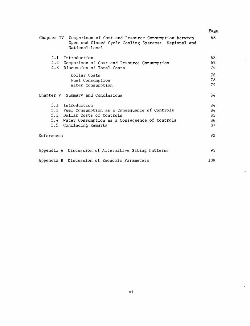
Chapter IV Comparison of Cost and Resource Consumption between 68Open and Closed Cycle Cooling Systems: Regional andNational Level

4.1 Introduction 684.2 Comparison of Cost and Resource Consumption 694.3 Discussion of Total Costs 76

Dollar Costs 76Fuel Consumption 78Water Consumption 79

Chapter V Summary and Conclusions 84

5.1 Introduction 845.2 Fuel Consumption as a Consequence of Controls 845.3 Dollar Costs of Controls 855.4 Water Consumption as a Consequence of Controls 865.5 Concluding Remarks 87

References 92

Appendix A Discussion of Alternative Siting Patterns 95

Appendix B Discussion of Economic Parameters 109

vi

List of Figures

Figure Page

2.1 Water Resources Council Regions for the Contiguous U.S. 11

2.2 Location of Rivers in the United States where Once-Through 14Cooling could be Installed for a 1000 MW Fossil SteamElectric Plant in the Absence of Thermal Standards

2.3 Expected Distribution of New Capacity by Cooling Water 16Source and by Cooling System under Existing ThermalRegulations by the Year 2000 for the Contiguous U.S.

3.1 Evaporation from Representative Wet Towers as a Function 41of Wet-Bulb Temperature (TWB) and Dry-Bulb Temperature(TDB)

5.1 Distribution of Potential Once-Through Cooling Develop- 90ment by Water Body Size over Currently ProjectedDevelopment

A.1 Cooling Systems in use Before 1973 as a Function of the 99Design Condenser Flow vs. the Average River Flow Pastthe Plant

A.2 Cooling Systems in use Before 1973 as a Function of the 100Design Plant Capacity vs. the Average River Flow Pastthe Plant

Regional Plant Cost Escalation Rates Over TimeB. 1 114

List of Tables

Table Page

2.1 Representative Energy and Electricity Demand Scenarios 9found in the Literature

2.2 Percentages of New Capacity Expected to be Installed 17Between 1975 and 2000 that could use Once-ThroughCooling (High Energy Demand Scenario)

2.3 Percentages of New Capacity Expected to be Installed 18Between 1975 and 2000 that could use Once-ThroughCooling (Low Energy Demand Scenario)

2.4 NERA Survey Results Indicating Cooling System Use for 25New Proposed Generating Capacity to be InstalledBetween 1977-1990

2.5 Comparison Between NERA's Estimates of the Percentage 28of New Capacity that will Install Closed Cycle Coolingfor Environmental Reasons and this Study's Estimates ofthe same

2.6 Estimated Megawatts of New Capacity Requiring Closed 30Cycle Cooling for Purposes of Meeting EnvironmentalStandards under the High Energy Demand Scenario

2.7 Estimated Megawatts of New Capacity Requiring Closed 31Cycle Cooling for Purposes of Meeting EnvironmentalStandards under the Low Energy Demand Scenario

3.1 Projected Real Dollar Price Escalation Rates for Select 46Resources

3.2 Real Dollar Price Escalation Rates used in this Study 47

3.3 Projected 1980 Component Costs ($1977); High Price 48Escalation Scenario

3.4 Projected 1980 Component Costs ($1977); Low Price 49Escalation Scenario

3.5 Incremental Annual Operating Cost of Closed Cycle Cooling; 52High Price Escalation Scenario

3.6 Incremental Annual Operating Cost of Closed Cycle Cooling; 58Low Price Escalation Scenario

3.7 Incremental Present Valued Cost of Closed Cycle Cooling; 64High Price Escalation Scenario

viii

Table Page

3.8 Incremental Present Valued Cost of Closed Cycle Cooling; 65Low Price Escalation Scenario

3.9 Relative Incremental Annual Resource Costs Associated 66with Closed Cycle Cooling for Fossil Plants

3.10 Relative Incremental Annual Resource Costs Associated 67with Closed Cycle Cooling for Nuclear Plants

4.1 Expected Annual Cost of Current Thermal Regulations 70by Region (High Energy Demand)

4.2 Expected Annual Cost of Current Thermal Regulations 71by Region (Low Energy Demand)

4.3 Incremental Fuel Consumption in the Year 2000 Due to 73Thermal Controls

4.4 Incremental Freshwater Consumption in the Year 2000 74without the Installation of Salt-Water Towers atCoastal Sites

4.5 Incremental Freshwater Consumption in the Year 2000 75with the Installation of Salt-Water Towers atCoastal Sites

4.6 Impact of Thermal Control Induced Freshwater Demands 81in Relation to Regional Freshwater Demands (HighEnergy Demand Scenario)

4.7 Comparison of Thermal Control Induced Freshwater 83Requirements with New Freshwater Imports Authorizedfor the Period 1975 - 2000

5.1 Distribution of Potential Once-Through Cooling 91Development by Water Body Size Over Currently ProjectedDevelopment

ix

I

I INTRODUCTION

1.1 Background

At present in the U.S. efforts are being made to control domestic

energy consumption and protect the environment. The concomitant pur-

suit of these two objectives are in obvious conflict in those sectors

where environmental controls require additional energy use. One such

sector is the Steam Electric Power Industry. Concerned that waste heat

will have deleterious effects o aquatic environments, state and federal

agencies have promulgated regulations that limit the discharge of waste

heat to natural water bodies. For many new plants, these regulations

require electric utilities to modify plant operating practices or

adopt closed cycle cooling in place of open-cycle cooling. Neither of

these two remedies allows a plant to operate with the same net thermo-

dynamic efficiency offered by open-cycle cooling. Consequently, plants

operating with thermal controls incur higher fuel costs than do plants

operating without similar controls. In addition, closed cycle systems

have higher capital costs and generally consume greater amounts of

water (through evaporation) than do comparable open-cycle systems.

Therefore, it must be recognized that implicit in any policy limiting

once-through cooling there will be tradeoffs among cost, environ-

mental impacts and resource consumption.

A fair amount of literature has been prepared asserting that the

total costs of thermal controls (retrofitting existing plants and out-

fitting new plants) will have significant effects on the electric

1

industry's ability to finance its operations, including capitalization

for new plant and equipment (UWAG, 1974, 1977; Teknekron, 1976).

Concern for these effects was a major consideration in the decision by

a U.S. Court of Appeals remanding the EPA's thermal regulations and

instructing that agency to consider the relationship between environ-

mental protection and the costs of retrofitting closed cycle cooling

systems at existing plants. Much of the current debate over thermal

regulations surrounds the question of backfitting existing plants with

the issue of outfitting new plants receiving less attention. There is

a rationale for this disparity in emphasis: backfitting is more expen-

sive than outfitting (due to the inflexibilities of working with an

existing plant designed for open cycle cooling) and poses the most

immediate costs. Nevertheless, we feel that the emphasis of the current

debate has left the issue of outfitting without benefit of proper

analysis. We, therefore, chose to examine the costs and resource

commitments, at both a regional and national level, of outfitting new

power plants to meet current thermal pollution regulations.

1.2 Current Thermal Pollution Regulations for New Plants

Public Law 92-500 (The Federal Water Pollution Control Act

Amendments of 1972) instructs the Environmental Protection Agency to

develop and promulgate effluent limitations for new steam electric

power plants which will assure protection and propagation of indigenous

aquatic ecosystems (§301(b)(2); §302(a); 306(b)(1)). At the same

time, section 316(a) of this law provides for alternative thermal

effluent standards for an individual plant when it can be demonstrated

2

that the thermal discharge from such plant will assure protection and

propagation of the indigenous aquatic ecosystem at that plant site.

The EPA's effluent limitations for new plants (40 CFR 423, 1974)

call for no discharge of heat from the main condensers into natural

bodies of water, with the exception of heat released with the circula-

ting water blowdown, thereby prohibiting once-through cooling for new

plants. However, a particular plant may be exempt from this general

effluent limitation and be allowed to install once-through cooling under

the section 316(a) provision if it can be demonstrated that the thermal

effluent from the once-through system will not harm the indigenous aqua-

tic community (40 CFD 122, 1974). This demonstration must be presented

either before the appropriate state or interstate agency if the agency

has a discharge permit program approved by the EPA, or before the EPA

if the state within which the discharge will occur has not received

EPA approval for a discharge permit program. The EPA's water quality

criteria for determining whether the protection objectives have been

satisfied are based on a consideration of incremental temperature rises

1 In addition to the §316(a) provision for effluent standards, PL 92-500contains a section, §316b, mandating that the design, construction andcapacity of cooling water intake structures shall minimize undesirable,environmental impacts, primarily the impingement of organisms on theintake structure or the entrainment of these organisms into the conden-ser cooling system. While intake considerations alone may determinethe acceptability of once-through cooling in particular locations, itis generally felt that the severity of intake impacts (eg. measuredby the size of the intake's zone of influence relative to the size ofthe receiving waterbody) is correlated with the severity of the dis-charge impact (eg. measured by the size of the mixing zone or the over-all temperature rise). At any rate the ability of a once-throughcooling system to meet thermal standards will be used herein as thebasis of acceptability for once-through cooling.

3

above the ambient temperature and the amount of time important species

are expected to be exposed to these increases (EPA, 1976).

State water quality criteria for determining whether the

protection objectives have been satisfied are incorporated into water

quality standards which generally specify both the allowable temperature

rise and the maximum allowable temperature within a body of water.

For streams and rivers, the thermal standards are generally defined

for a critical low flow (eg. 7-day, ten-year low flow). In addition

most states set separate standards for streams or sections of

streams which support cold water fisheries and for streams or sections

of streams which support warm water fisheries.

1.3 Development of Once-Through Cooling Under Existing Regulations

Given the current state and federal water quality standards

and criteria, the effluent limitation exemption provision under §316(a)

allows new once-through cooling development, but at a much lower

level than has been observed historically. Peterson, et al.(1973)

estimates that even if plants located on streams were spaced to maximize

the amount of once-through cooling possible within existing thermal stan-

dards, the share of steam electric capacity installed with once-through

cooling on rivers would drop from 38% in 1970 to roughly 15% in 1990.

The Federal Energy Regulatory Commission (1977) estimates the share of

steam electric capacity installed with once-through cooling on all

water bodies (lakes, rivers and oceans) will drop from 65% in 1975 to

23% in the year 2000. The U.S. Water Resources Council (1977) estimates

that the share of steam electric capacity installed with once-through

cooling on all bodies will drop to 16% in the year 2000. In addition,

4

the U.S. Water Resources Council anticipates the overwhelming share of

new capacity installed with once-through cooling between 1975 and 2000

will be located on the oceans with an absolute decline in the number of

megawatts installed with freshwater once-through cooling systems. Thus,

as a consequence of thermal pollution regulations, it is expected that

the share of both new and total steam electric capacity installed with

once-through cooling will fall below pre-1972 shares, with further

once-through cooling development occurring primarily at coastal sites.

1.4 Objectives of this Study

In this study we assess the regional and national costs that may

result as a consequence of restrictions on new once-through cooling

development. In keeping with the intent of Congress that all costs

of thermal control be identified (§302(b)(1), §304(b)(1)(B), §306(b)(1)

(B)) we evaluate costs in terms of dollars spent and additional water

and energy consumed in order to comply with water quality regulations.

1.5 Outline of Presentation

Chapter II presents our estimates of the new steam electric

generating capacity to be installed between 1975 and 2000 which will be

required to install closed cycle cooling in order to comply with

water quality regulation. We assess the shares of new capacity that

could be installed with once-through cooling both under current water

quality regulations and with relaxed thermal regulations. Chapter III

presents our assessment of the incremental costs of closed cycle

cooling over once-through cooling for representative fossil and nuclear

5

plants. Using power plant operating simulation models originally

developed by Crowley, et al.,(1975) and modified at M.I.T. (Najjar,

et al., 1978) we make separate cost estimates for various regions in

the contiguous United States. In Chapter IV we combine our estimates

of the new steam electric capacity which will be required by law to

install closed cycle cooling with our assessment of the incremental

costs of closed cycle cooling for representative plants. The result

is our assessment, in terms of dollars spent and additional water and

energy consumed, of the costs of complying with current thermal

regulations. We represent these costs in terms of the annual costs

between 1975 and 2000 of having new plants comply with existing

standards of performance.

6

II ESTIMATES OF THE NUMBER OF NEW POWER PLANTS AND THECOOLING SYSTEMS THEY WILL EMPLOY TO THE YEAR 2000

2.1 Introduction

The objective of this chapter is to estimate the number of

new plants (or alternatively the amount of new electric generating

capacity) to be built between the years 1975 and 2000 that will be re-

quired to install closed cycle cooling systems in order to comply with

current thermal pollution regulations. That is, of the new plants that

will be built between 1975 and the year 2000 a small percentage will be

able to install once-through cooling under the current thermal regulations

while a larger percentage of these new plants would be able to install

once-through cooling were these regulations relaxed or removed altogether.

Therefore, the difference between the number of new plants that could

install once through cooling without thermal controls and the number of

new plants that will install once-through cooling under the existing reg-

ulations represents the net number of new electric generating stations that

will be required to install closed cycle cooling to comply with current

thermal pollution regulations.

Our estimates of the net electric generating capacity affected

by current thermal regulations are made in two steps. In section 2.2

we estimate the total number of megawatts of new generating capacity that

could be installed between the years 1975-2000. These estimates are made

for separate regions covering the contiguous United States and are devel-

oped from energy demand projections found in the literature. In section

2.3 we investigate a number of potential new facility siting patterns that

7

incorporate water availability considerations to indicate where new gener-

ating stations could be located, in every region, for the purposes of

making greater use of once-through cooling were the current thermal controls

relaxed or removed. Because water availability is a determining factor

for whether once-through cooling can be installed at any site, each fac-

ility siting pattern represents a separate estimate of the potential for

being able to use once-through cooling at new power plants were thermal

controls not binding.

The analyses performed in sections 2.2 and 2.3 are carried out by

Water Resource Council Region and aggregated to the national level.

(Figure 2.1 indicates the location of the 18 WRC Regions withing the cont-

iguous United States.) Our national estimates for the net percentage of

new plants that will install closed cycle cooling to comply with thermal

regulations are then compared to similar estimates prepared for the Utility

Water Act Group (UWAG) by National Economic Research Associates.

2.2 Energy Demand Scenarios

The scenarios projecting future electric capacity additions used in

this study come from the published literature. Since 1972 at least

thirteen different government agencies, industry groups and universities

have published eighteen separate studies which, in all, provide forty-

seven energy demand scenarios for the United States. Of these 47 forecasts,

20 offer projections to the year 2000, and are summarized in Table 2.1.

In these estimates the anticipated new capacity is generally

computed from an electric energy demand forecast, in MWH, which can be

forecast separately or can in turn be calculated from a total energy

demand forecast and an electrification forecast. The initial step in

3

a5.

~o4-I4-

O0

0-4

0'1uI,

. IT ,F , , i ll L , - ,f · , ,- - - **----' C- I --- . -

04 tr14 0NU - ,t %O 14 OC4 - J1-

I K 1 | N | uCI 1 1I1

00~J crr -Ic

c~ ~ ~ ~ ~ ~~~~o~< cc ~-0. -4 Lr ~~~~--40%1N %O (r O- -4 - - T - 1 4 Cy%

Vr~ tX C~00 N 00 ( 0 0 _4 0 N -C c o l

~Jj .- 4~~ _ . _ _

cn0O _ _ ··. _ · _ _ _ __ . _ __0 a0 wo%3%u-4-°* .-4u- O 4 0-040(U '~~ ~ ~~~~~~~- 0 - n C el4 -a In. -a

*-4 (U_M- _ . -_____Ai c<s<N' X <

.- C--C --- n - c0

54 %(-4en' 0i50%'30 C45 '~ ' 0 0 0;

u Ic ooo _ _ _ o¢_.....ooO 0 C 0 · e cD e ·n C , · ·

C% , J 1- en , WI ,; On ,.; en -Co n C., ,. ;~ ~~~~~c -; 0 C% a4 r- C4 C co £ o0 n crn C C, C4 %C

0%. ,4

o I % - ---- -#' -- -. Inr (1) C4 rl Ln C% I n IT U C '*S -4 NCJ 1 . os il

,4 c1 cn cs T -_1 r- en to N e co XC in s

>~~~~~~~~~~~. en el < nen c4 Aw Ac4 A A

! . .... n~40. I~ll ~ oI WI, -.- I3u 'N , -- 0 sr I M

I- I aC 'C C'E'e -,-I - .- - " No m: .: ,- % ·z k6 . 0,1I V ONI ) s 0 0 O 0 C) N C 0

PEC| 0 -4 14 4 H 1-1-

I~~~~~~C C1 -. co.cas °I1N - f

I~~~~~~~~ · ·t , _._ O _ - 1-1 .... _ ..I 4 co c1 .1 cO

o =zz r -4 = 3-

.0410 ,-I N 0% sO~1- P41- -4 O r4 r-4~~~~~~~r ' i40

:3 -H (P 0 0 V4 oo s-30- 0 CD4

0 C -4 0. U 1 1' I I.-4 ow 4.CM ~ 4 0 *0 %Ev ~ ~ ~ ~ ~ ~ ~ ~ ~ ~ ~ ~ ~ ~ 5

54 OO~~~~ ~~ 8-~~ 0 C.E ~~~ '4-4 C~~~~ p.

9

0l)

r.41

.-4P

4.1u

*0

10

5.4to

0)9-'-0

4.1

CI,

54r.'

0)-4:.0

0)H-

CO..1-4.U

0

21C.

u

-4010[-I

041

C:

0H.l,

'4.4

0 o4

0

AiI-

S4.1

-.404.1

CJ=-o ^U 4

t30 60 Oa

C .C05 c'c4

~05..3 -.

* 0

4c

· S K a4 o4.0 0 0

gn0 Nt0 o

4J1J

estimating the installed capacity requirements for any year is to fore-

cast the point peak load demand (e.g. highest 24 hr. continuous demand

in MW) expected in that year. This is defined, Meier (1976), as:

t

MWt = EAp tP SLFA 8760

where:

MW = expected peak demand in year t (MW)p

EA = expected electricity generation in year t (MWH)A

SLF A = expected system load factor in year tA

8760 = number of F.ours per year

The SLF A is the ratio of a system's average annual power output and itsA

actual maximum power output, and is commonly in the range of .55 to .65.

While MWt represents the maximum power demand expected on thep

system in year t1 the actual amount of capacity installed by that year

must exceed this in order that there are sufficient reserves in the

event planned and unplanned outages prevent some plants from operating

during the period of peak demand. A commonly used standard of relability

is that the available system capacity at any time (installed capacity

minus capacity not currently operable) will exceed demand in all but one

day every ten years. Currently the norm is that a reserve margin equal

to 20%-30% of the peak demand will be adequate to meet all but the one

day in ten year event (Meier, 1976).

Referring to Table 2.1, we see an incredible range in the projec-

tions found in th3 literature: The lowest forecast for new electric

10

U3

0(nz

.u)

04i

0

0t40a)

Ur0~J

AnCIO

pa)C4,l

.H

(n

a;v

(3

04

:.1

11

generating capacity installed by the year 2000 is one-fifth the highest

estimate. Even for projections published after 1976 the range in pred-

ictions remains large, with the highest projection almost twice that of

the lowest. Most of this observed variation between projections is due

to differences in key assumptions made for each projection. For example,

differences in the assumed growth rates for energy demand in general and

in electrification in particular, in assumptions regarding the share of

the nation's electricity that will come from steam electric plants, and

in assumptions regarding policies for reducing peak demand (e.g. peak

load pricing) can all be small individually, but when combined and comp-

ounded over a twenty-five year period contribute to a remarkable var-

iation in the final results.

Because many of the parameters used in these forecasts are sensitive

to changes in government policies and in the economic environment, both

of which are uncertain, it is hard to say which projections are most

reasonable, or to identify a single "most probable" forecast describing

new capacity growth. Therefore we chose a high energy demand case, using

the FERC projections, and a low energy demand, using the ERDA Accelerated

Domestic Development forecasts. These two projection cover a reasonable

range of the forecasts published so far.

The FERC projection to the year 2000, using a sectorial economic

model to forecast demand, expects energy demand will grow, on average,

by 3.39%/year and electrification will grow by 2.93%/year. New energy

technologies (geothermal, wind, solar) are not expected to contribute

a large portion to total U.S. energy supplies by the year 2000.

The ERDA projection to the year 2000, using a series of macro-

12

economic/inter-industry growth and energy system optimization models,

anticipates energy demand will grow on average by 2.63%/year, and electri-

fication will grow by 2.13%/year. Electrification is lower in the ERDA

projection than in the FERC projection because it is anticipated that

new energy technologies will compete with the steam electric industry

in supplying the nation's energy needs by the year 2000.

2.3 New Once-Through Cooling Development

In this section we evaluate how new once-through cooling could

develop in the future under both current and relaxed thermal regulations.

For this purpose we speculate how the geographic distribution of new

plants might appear with the current restrictions on once-through cooling

and compare these with siting patterns we could expect if these restric-

tions are relaxed.

It is worth emphasizing that even without environmental controls,

once-through cooling is constrained by water availability. A once-through

cooling system for a typical 1000 MWe fossil plant will withdraw between

750-1500 cfs from the nearby source of water and will require this flow

with a very high reliability. This condition is met at coastal sites,

on large lakes and along large rivers, the latter being predominately

east of the Mississippi. Using the 7 day 10 year low flow as a measure

of reliability, Figure 2.2 indicates the locations of river segments in

the contiguous United States that can support the use of once-through

cooling at large fossil steam electric power plants in the absence of

environmental controls.

Our estimates of the proportion of new electric capacity to be

installed between 1975 and 2000 which might use once-through cooling under

13

C i

40

4J ,4

0

00

0 0

14

current thermal regulations come from the FERC projections introduced

earlier. From a survey taken of the electric power industry, FERC locates

existing and future plants by aggregated sub-area (ASA) within each WRC

Region and by water source within each ASA. In addition the FERC projec-

tion specifies the cooling system(s) anticipated for each new plant,

thereby reflecting hat the utility industry expects will be the status

of once-through cooling for new plants under existing and anticipated

water quality regulations. The histogram in Figure 2.3, derived from

the FERC projections, illustrates projected installed capacity by

cooling system type (dry tower, wet tower, pond or once-through) and by

location to the type of cooling water body. These estimates indicate that,

nationally,'12.9% ofnew installed capacity will use once-through and 87.1%

will utilize some sort of closed cycle cooling under existing thermal

regulations.

Although the FERC projections reflect the high energy demand

projection, we feel the same percentages of new capacity going to once-

through cooling could be applied to the ERDA low energy demand scenario.

The only alteration necessary to go from the high demand forecast to the

low demand one is a reduction in capacity at each of the new plant sites

given in the FERC projection to account for the lower overall capacity

growth in the ERDA forecast.

Thus for both the high energy demand case and for the low energy

demand case we use the FERC once-through cooling development projection

to represent the percentage of new plants which would use once-through

cooling under existing regulations. Tables 2.2 and 2.3 indicate these

percentages,by WRC region, for the high and the low energy demand

scenarios, respectively. 15

(yx £01O) suoTlTpPV AXiTededu MaN

~- C

oxC srCer) O~ oOZ/C F>0 >

H _

0 a

0.4-

-.

5--

a)5-a

D'

a)

o

!l

01

O n

a)

0 0O4 H

0. [5 0-5

C

C go Ca

o) o

o

o o,0 > (30 · , ©

C C0

g Lr H4

0} 4 p114

oo oz0l

H0

4-:3

H

4-

ofC

16

Percentages of New Capacity Expected to be InstalledBetween 1975 and 2000 that could use Once-ThroughCooling (High Energy Demand Scenario)

Water ResourceCouncil Region

One

Two

Three

Four

Five

Six

Seven

Eight

Ten

11-17

Eighteen

With CurrentThermal Regulations

25.3

13.9

11.2

7.0

3.2

2.6

0.9

42.5

8.2

15.6

43.1

With Relaxed Thermal RegulationsAlternative Siting Patterns:

One

91.0

59.0

26.0

81.0

62.0

61.0

78.0

100.0

54.0

36.0

78.0

Two Three

75.6

66.4

57.9

100.0

24.6

47.8

28.3

71.8

33.1

46.3

77.3

67.1

42.1

39.3

70.1

16.7

15.2

13.4

61.1

24.8

27.8

47.2

Four

100.0

94.1

64.5

100.0

24.6

47.8

33.0

88.8

33.1

47.3

100.0

Contiguous U.S. 12.9 54.0 35.6

17

Table 2.2

54.0 60.9

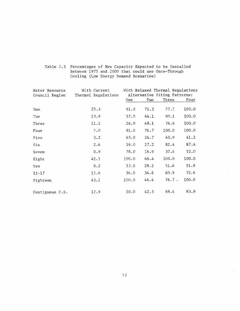
Percentages of New Capacity Expected to be InstalledBetween 1975 and 2000 that could use Once-ThroughCooling (Low Energy Demand Scenarios)

Water ResourceCouncil Region

With CurrentThermal Regulations

With Relaxed Thermal RegulationsAlternative Siting Patterns:

One Two Three Four

91.0 71.3

57.0

26.0

81.0

63.0

59.0

78.0

100.0

53.0

36.0

100.0

44.1

48.1

76.7

24.7

27.2

16.9

66.4

28.2

34.6

46.4

77.7 100.0

90.1

76.6

100.0

40.9

82.4

37.4

100.0

51.6

60.9

76.7

100.0

100.0

100.0

41.2

87.4

52.0

100.0

51.8

72.6

100.0

Contiguous U.S. 12.9 50.0 42.3

1 8

Table 2.3

One

Two

Three

Four

Five

Six

Seven

Eight

Ten

11-17

Eighteen

25.3

13.9

11.2

7.0

3.2

2.6

0.9

42.5

8.2

15.6

43.1

69.4 83.9

To estimate the percentage of new plants which might use

once-through cooling under more lenient regulations than are currently in

effect, we postulate a number of alternative siting and cooling system

selection patterns which reflect this leniency, using the siting patterns

originally indicated in the FERC model as our guides. The favorable feat-

ure of the FERC siting patterns is that they account for many of the siting

criteria utilities normally consider when locating new plants. These

criteria include site proximity to load demand and fuel source, population

density in the neighborhood of the site, and location with respect to the

existing and anticipated system grid. In practice, the cooling system

options available at a ite (e.g. the possibility of accomodating once-

through cooling) also serve as criteria for plant location. However, since

the FERC siting patterns reflect anticipated restrictions of the use of

once-through cooling for new plants, these patterns place less emphasis

on the possibility of using once-through cooling at any potential site

than they would were these restriction lifted.

In speculating how once-through cooling might be used under relaxed

thermal controls, we attempt to correct the earlier bias against this mode

of cooling found in the FERC projections by placing a greater emphasis on

using once-through cooling systems in our alternative siting patterns.

For this purpose, we consider four alternative patterns: one that

applies engineering considerations to determine whether once-through

cooling may be located on particular bodies of water, and three that apply

relaxed themal standard criteria for using once-through cooling.

Alternative Pattern 1 (Extension of Historical Patterns)

Here, we locate new power plants in every aggregated sub area in WRC

19

Regions 1-12, 17 and 18 on major bodies of water, following the same

distributions by water source that were observed before 1973. In this

manner the siting patterns ound in these sub areas before 1975 are repl-

icated for the years 1975-2000. Historically, open-cycle cooling has been

of little consequence in WRC Regions 13-16, and, consequently, we do not

assess in detail the once-through cooling potential in these four regions.

In addition, prior to 1973, once-through cooling was installed at rela-

tively few plants in regions 11, 12 and 17. Therefore, for this siting

pattern we lump our results for regions 11-17 in a single catagory. For

our high energy demand scenario, we use the FERC projections by ASA to

estimate how many megawatts of new fossil and new nuclear capacity will

be installed in every ASA between 1975 and 2000. The projections for

new capacity additions by ASA are scaled down in the low energy demand

scenario to account for the overall lower rates of capacity expression

incorporated in this scenario. In locating new capacity additions to

resemble pre-1975 patterns, we assume that new fossil plant sizes will

not exceed 800 MW and that new nuclear plant sizes will not exceed 1200

MW. We make the assumption that capacity located on lakes and oceans

will use once-through cooling. On river sites, the feasibility of once-

through cooling is based on historical relationships involving the ratio

of average annual river flow to the size of the station. Based on an

analysis of plants built before 1973, it was found that a ratio of

10 mgd/MWe separated plants using closed cycle from plants using open cycle

cooling. Thus in this hypothetical plant siting scenario an average annual

river flow of at least 10 mgd/MWe served as the minimum acceptable flow in

order to use once-through cooling on any river. In our opinion this ratio

20

represents a conservative estimate of the flow necessary for the use of

once-through cooling based on engineering and reliability considerations.

Because this criterion reflects engineering rather than environmental

considerations, the cumulative thermal effects among new and existing

plants are not considered.

Tables 2.2 and 2.3 indicate the percentage, by Water Resource

Council Region, of new capacity which could utilize once-through cooling

under this pattern. Nationally, the percentages are 54% and 50% for the

high and low energy demand scenarios respectively. Further details of

our analysis are presented in Appendix A-1.

Alternative Pattern 2 (Maximize Once-Through Cooling using FERC Siting

under Relaxed Regulations)

Unlike Pattern 1 where we locate new plants according to historic patterns,

we retain all the new sites that are identified in the FERC projections

as well as maintain the same projected capacity at each site. More-

over, the criteria for using once-through cooling at every site is differ-

ent from the criteria used in Pattern 1, and is based on a maximum allow-

able temperature rise at the edge of a mixing zone. While this criteria

is more -restrictive in allowing once-through cooling at any one site

than the engineering criteria of 10 mgd/MWe used in Pattern 1, we feel

the allowable temperature rise considered here is more lenient than

current standards. The allowable temperature rise is approxiamately

5°F for lakes and for rivers at low flow, with the low flow in rivers

defined as the lowest monthly flow expected every twenty years. For

sites on estuaries and open coasts the amount of allowable once-through

cooling is determined by the relative openness of the sites and ranges

21

from a minimum of 1000 MW per site for enclosed estuarine sites to a maxi-

mum of 5000 MW per site for sites on the open coast. Further details are

included in Appendix Al.

Tables 2.2 and 2.3 indicate the percentage of plants by Water

Resource Council Region that could install once-through cooling under this

siting pattern for the high and low energy demand scenarios, respectively.

Nationally, these percentages are 35.6% and 42.3% for the high and low

energy scenarios, respectively. Comparing these percentages with the

percentages expected under current regulations, it is apparent that the

limitations on once-through cooling suggested by this pattern represent

a liberal relaxation over current standards. (Few states have water

quality standards allowing a temperature rise greater than 5F, while

almost all set lower allowable increases for lakes in general as well

as for streams that are classified as cold water fisheries; Peterson,

et al., 1973).

Alternative Pattern 3 (Maximize Once-Through Cooling by Aggregated

Sub-Area)

In Pattern 2 all we have done is to witch from using closed cycle cooling

at a designated FERC site to open cycle cooling provided the lenient ther-

mal standards are not violated in doing so. Nevertheless, because all the

original FERC sites are maintained, the siting patterns found in Pattern 2

reflect the same bias against using the potential for installing once-

through cooling as a siting criteria for new plants that was found in

the FERC siting pattern. We attempt to correct this bias by considering

in Pattern 3 modifications which reflect a greater potential for using

once-through cooling at new sites.

22

Here, as in Pattern 2, we use FERC sites and adopt the same 5°F

nominal temperature rise limitation. However we modify the old siting

pattern by relocating capacity within each ASA from sites which have

no remaining once-through cooling potential to sites with potential re-

maining. Thus, we relax the siting criteria implied in the original FERC

forecast to accomodate additional once-through cooling; the overall gen-

eration patterns implied in the FERC projections need hold only down to the

ASA level and not at every site indicated by FERC. The regional breakdown

of allowable once through cooling based on this pattern is included in

Tables 2.2 and 2.3. Nationally, the percentages are 54.0% and 69.4%

for the high and low energy demand scenarios respectively.

Alternative Pattern 4 (Maximize Once-Through Cooling by Water Resource

Council Region)

Here, as in Patterns 2 & 3, we use FERC sites and adopt the same 5°F

nominal temperature rise criteria for once-through cooling. However,

we modify the FERC patterns further still by relocating new capacity

within each WRC region from aggregated sub-areas having no remaining

once-through cooling to ASA's with poLential remaining. By allowing

this redistribution of capacity between ASA's we have greatly relaxed the

FERC siting criteria to accomodate once-through cooling by assuming the

non-cooling siting criteria implied in the FERC projection need be main-

tained only down to the broad regional level. The regional breakdown

of allowable once-through cooling based on this pattern is included in

Tables 2.2 and 2.3. Nationally, the percentages are 60.9% and 83.9%

for the high and low energy demand scenarios, respectively.

Summarizing the results of our analysis so far, for two energy

23

demand scenarios we have estimated the net number of megawatts in elec-

tric generating capacity which we feel will be required to install closed

cycle cooling systems to comply with current thermal regulations restrict-

ing further once-through cooling development. Our proceedure has been

to take a proposed future plant siting pattern which reflects a heavy bias

against the further use of once-through cooling and, in a sequential

manner, modify the pattern to reflect an ever increasing emphasis on the

potential for using once-through cooling as a siting criteria. Tables

2.2 and 2.3 provide estimates of the percentages, by Water Resource Council

Region, of new plants whcih could utilize once-through cooling for each of

the four alternative plant siting and cooling system selection patterns

which allow more liberalized use of once-through cooling. Nationally,

these percentages range from 35.6% to 60.9% for the high energy demand

scenario and from 42.3% to 83.9% for the low energy demand scenario.

These numbers are in sharp contrast to the 12.9% projected by the

electric utility industry given the current thermal regulations.

One could offer the criticism that our siting pattern modifications

are arbitrary in the sense that our plant relocations are constrained by

hydrologic boundaries (WRC Region and sub-area boundaries). In reality,

utilities are more likely to be constrained by service area and/or elec-

tric reliability council boundaries when relocating proposed plants.

While this criticism is well taken we can compare our estimates of new

capacity that would be able to use once-throuigh cooling were thermal

controls to be removed/relaxed with estimates from a survey made by

National Economic Research Associates (NERA). NERA conducted a survey

24

Table 2.4 NERA Survey Results Indicating CoolingSystem Use for New Proposed GeneratingCapacity to be Installed Between 1977-1990

Once-ThroughCooling

38,695

Man-Made LakesOpen Cycle Closed Cycle

7,171 48,810

Closed CycleCooling

186,292

100.0

Ref.: UWAG (1978)

TotalAdditions

280,968

13.8 2.6 17.4 66.3

25

for the tilitv Water Act Croup (UWAG) to determine the percentage of

new proposed capacity that will be required to use closed cycle to

comply with thermal control regulations.

The NERA survey identified four alternative cooling system config-

urations: once-through cooling on oceans and rivers, once-through cooling

on man made lakes, closed cycle cooling on man made lakes, and closed

cycle cooling not located on man-made lakes. Table 2.4 presents their

survey results indicating the number of megawatts proposed for commercial

operation between 1977 and 1990 that are tentatively planned to operate

with each of the four cooling systems.

Utilities proposing to operate plants with closed cycle cooling not

on lakes were asked to identify the reasons for their choice. Possible

reasons included engineering/economic factors, need to comply

with state water quality standards, need to comply with federal

water quality standards or any combinations among these three. The

NERA results indicated that 48.3% of the new capacity that will be

installed with closed cycle cooling, with the exception of closed cycle

cooling on man made lakes, will do so wholly to comply with state and

federal thermal regulations. While the NERA results do not indicate

what percentage of the new capacity planning to use closed-cycle cooling

on man made lakes will do so to comply with thermal regulations, it may

be reasonable to assume it is roughly equivalent to the percentage

indicated for the other closed cycle cooling category. Making this assump-

tion, the percentage of the new capacity proposed to be brought into

commercial operation between 1977 and 1990 that will use closed cycle

cooling wholly in response to thermal regulations is:

26

100 x .483 (186,292 + 48,810) 404280,968

The NERA results indicated that 85.6% of the new capacity that will

be installed with closed cycle cooling, with the exception of closed

cycle cooling on man made lakes, will do so for environmental and joint

engineering/economic/environmental resons. Again, it may be reasonable

to apply this same percentage to closed cycle cooling located on man-made

lakes. Making that assumption, the percentages of the new capacity

proposed to be brought into commercial operation between 1977 and 1990

that will use closed cycle cooling because of environmental and joint

engineering/economic/environmental factors is:

100 x .856 (186,292 + 48,810) 71.6%280,968

Table 2.5 compares our estimates of the percentage of new capacity

that will install closed cycle cooling for environmental reasons and

NERA's estimates for the same. For the high energy demand scenario we

estimate that between 22.7% and 48% f the new capacity planned to be

built between 1975 and 2000 will be required to comply with thermal

regulations while for the low energy demand scenario the range is between

29.5% and 71.1%. As noted our interpolation of the NERA survey results

suggests 40.5% of the new capacity planned to 1990 will use closed cycle

cooling (lake and non lake) to comply with thermal standards alone and

71.6% will use closed cycle cooling either wholly or partially in res-

ponse to thermal regulations.

Examining Table 2.5 we observe that our projections of the per-

27

Comparison Between NERA's Estimates ofthe Percentage of New Capacity that willInstall Closed Cycle Cooling for Environ-mental Reasons and this Study's Estimatesof the Same

This Study **Alternative Siting Patterns

One Two Three

41.1% lo 22.7% 41.1%

37.1% 29.4% 56.5%

Four

48.0% High Energy Demand

71.0% Low Energy Demand

Percentage installing closed cycle cooling wholly for environmental reasons

Percentage installing closed cycle cooling either wholly or partially forenvironmental reasons

**Percentage installing once-through cooling under each alternative sitingscenario minus the percentage expected to install once-through coolingunder the FERC forecast.

Ref: UWAG (1978)

28

Table 2.5

NERA

40.5%

centages of new capacity that will install closed cycle cooling solely to

comply with environmental regulations from siting pattern scenarios 1 and 3

do not differ greatly from the percentages indicated in the NERA study.

This suggests that while our siting pattern modifications may not reflect

precisely how these modifications would actually be realized, their results

are nevertheless comensurate with the independent NERA study.

The development of the four alternative generations patterns des-

cribing possible levels of future once-through cooling development under

relaxed thermal regulations offers us the opportunity to examine a range

of possible outcomes were current controls to be relaxed. In addition,

this range offers us a basis for comparison with similar results from

other studies. For our cost analysis presented later in this report

we chose one pattern out of our four to describe future once-through

cooling development under relaxed controls. We use Pattern 1 (Extra-

polation from Historic Trends) because the percentages given by this

patterns are representative of both the four patterns we have developed

and the NERA survey results presented earlier.

For our estimates of the costs of current thermal standards, to

be presented in chapter Four, we assume new fossil and new nuclear

capacity additions to the year 2000 will be linearly distributed over

time. Tables 2.6 and 2.7 indicate the number of megawatts of new capacity

that will be installed with closed cycle cooling for environmental

reasons, in five year intervals, under Alternative Pattern 1 for the high

and low energy demand scenarios, respectively.

29

a) 1- '11 0 0 0 o C C) c C 0

coOC 00 I 0 0 0 tO a

v~~~~~~~~~~~~- - 0

o 0 0 0 0 0 0 0 0 o o o o oI

r)~~~~~~~~~~~C (D 0 C) 0 0 0 0 0 0 0 0 C) ,-C 0 00 0 0 N D N0 H 0 N 0

0 -4 ~ v- ~ N ~ C N N1 C)CD 00NI 4-)

H.) I ao0 (D 0 0 0 00C 0 0 C)o~ C~00000',.000000 0 5:~ ,C-) 0~~~~~Fx~~~i N~~ 0 cc Cf N I O C C) N ) O( Cf H

Cr 44~z CNI CY O0 tn) c,., o-'_h1 oC~a 0000000000 0-C 00000000 0' 0 0 0 -.I1:~ 0 0 0 N '.0 N H -t N 0 00 Lr) 11 . . . ~~~~~~~~~~~ ~~ ~~ . .~~~0 -:0r . Oa z m ON 'IO m H 0N N 'IC r- C,,N N0 a) H H r-q H-- cC

H r H a) -i

~~~~~~~~~~~~~~~~~~~~~~~~~~~~~ C)~,(~ 0 0 0 0 0 0 0 0 00 0 -)H--. D..) N 0 0 0C 0 CL C \] C') N ) 0) 0q H 0 ~~~~~ H ~~~~~~~~~~~~0

0 C) C C ) C 0 .0 0 0 N H '0

4OlDC O~ C) 0 0 Cq ) CN 0 '-.) C 0 ,. 0

~.~~~~~ -4 ao)4.J~~ ~ E... 0 0H04 000 000 00) C0 00 0 0 0 C

'q co p O\ 0 -00 N N -q CN 0

Ca 0 0 ' 0 .,4JH 0a) r 0" .0 C ' 0 H C N ) CD 0 0 ) .

0 rI UCJ1

~aa)~000000300000 0 0

z tc4 5u cc 000 '.0000000 C:) 0'z N C cc C)~ N 0 C~ N LC) C)~ H ) '.

:a H .'N31 C) ct N 0 '0 c,-4 Nt H- C) HOC-

~~: 'w H H ''z z 0 0 0 0 0 0 0 0 0 O C) ~~~~~~~~~~~~~~~~~~~~~~~~~~~~~~~~~~4.)i

to 00 00 0 0 00'0 0000 0 C)coC/

O ~~ 00000000000I 0

p 0O 0 -~ 00 N ,0 CN H- -T N 0

coJ-- cc0 z " '0 C) ~ N ' C- H N N

c~~~~~~~~~w H H~~~~~~~~~~~~~~~ c

cc C C 000 0 .C000 0C)

Nl C -) C ) 0 "C 0 C) C)- N H '0 0C

odon Ha~~~~~~~~~~~~~~~~~~~a) ~ ~ ~ ~ ~ ~ ~ ~ ~ ~ ~ ~ ~ ~ ~ ~ ~ aa C0- 00 N . N H

cap-i ccZ ~~~~~~~~ 0" '.0 ~~~~~~ H C') N '.0 ~~~~~~~~~' H t N N-H- S H H) cc a

'.0 LC~~~~~~~~ 0 0 0 0 0 0 0 0 0 00'Ff 0 .J

30

.Jc Z r ~~- , NcCV 0 ' '

~~~~~~~~~~~~~~~~~~~~~~~~~~~~~oooCd N N r- N 0V)Fz 0 0 It 0 0 0 CD 0 C0 -It 00D00000000 0 0

00 0 N Lf~~ C~v) cc ~-O H cc C'-) N ~ C- a

0~~ 0 0 0 0 0 C) 0 0 0 CS ~0~~~( CD 0~~~ CD C

Nq 4-a

*HOLr 0000000C C) 0 0 C 0 043N O ) 0000 C0 Lf) 00 0 00 0

O0 all r4 Cm L) m' cc 0 L) 0 0 o' L() H- 0~~~~~~~~~rq C4 C4 -T 10 -It .TC4 rq I OU T-4 C

H N N -~~~~~~ ¼C) -1- N N~~~~~~~ H -H a 0-o 0

Qa) ~ ~~~~ C~~~ a' C~~~~~ ir~~~~L cc 0 0 a 04-~~~~~~~~~~~4 ~~ ~ ~ ~ ~ ~ ~ 4

.M-e ~0 0 0 00000000 0 )

H C)(1) coH N N O - N N H H ap r o

4-J i 0 r-I ~~~~N a4-0-H cl ~,~ 00000000000 0 ,-

u " (3 L -) C a' C') LC C 0 0 C) . H 0cor.)d U O ' C O O L) C C C ) 0-P~~~~ ~ ~ u O0 Er O0 C)

co-- 0 -H/-H C) C0 ) cc C) O C) N C) N H HH

0 0 ' . L f 0 0 0 c

4-JHC W z 4~ n wJQ -C.0HC r) I 4IJUto 0000000C0000 0 0

4i cc 0 0 0rI-, 0 0 0 0C O C'- ul( C') c 0 C) 0C00 Lt H 0 r4j H~4 ~ H N N -I '0 - 0' H~'000 000000 0C0 0 -

0 000 C) 0 0 C) C )-C') a c L-) cc 0 0 0 H 0 C 0 m m Ln w 0 00 0 m r-4 C)~~ ~~~~ , -4 ,-O, L ut cO o

wJ2- 0'. L O

Z ) 000000000000 04)Ic 00000 L0 Ln 00000 0 C U)

m 'r. m' u--) c'- cc 0 Lr)C ) 0 C\0 Lf'. H- 0'.

H ~~~~~~~~~~~~~~~~~~~~~~~~~~~~~~~coaL4H N N - '.0 . -4 N

0 0 0 0 0 0 0 0 0 0o O4-JO) 0 0 0 0 0 0 0 0 0 0 0 00 -- I 0 1

C 0

-H~~~ ccz N~~~~ L C'- cc '. cc C') 0 HCO4-

4-i ~~~~~~~~~~ a'. Lt)r () -H W -i a )

I-I o Lr) 0 0 0 0 0 0 0 0 0 0 0 0~~~~~~~~~~~~~~~~~~~~~~~~~~~~~~.~ ~ 00 0 t 0000 0

~~~~c-c r)00.L- *~~ H ooo N~~ H N N - o '.0 o N N H H o

a)~

0~~~H ~ ~ ~~ -H

0 ~~-4 ~~ ~~> X ~~ ~ I ~~ o .4I 0):-a

~ a)::0.H. H ¢) -HI. 0

31

III COMPARISONS OF COST AND RESOURCE CONSUMPTIONBETWEEN OPEN AND CLOSED CYCLE COOLING SYSTEMS:

INDIVIDUAL PLANT LEVEL

3.1 Introduction

This chapter presents the methodology we use to estimate the incre-

mental costs and resource commitments associated with the use of closed-

cycle cooling over once-through cooling. Costs are estimated by plant

type (fossil or nuclear) and by year (1975 to 2000) for every Water

Resource Council Region using the cooling system simulation codes

developed in the course of our earlier work (Najjar, 1978). The results

from these codes are expressed as unit incremental annual costs ($/MWe)

for five year periods up to the year 2000. In addition incremental fuel

consumption rates (BTU/MWe) and water consumption rates (acre-ft/MWe)

are computed. The product of these unit costs and rates times the

amount of new capacity installed between 1975 and 2000 that will be

required by water quality regulations to use closed-cycle cooling repre-

sents the annual cost and resource commitments implied by current thermal

controls to the year 2000.

The first section of this chapter gives a brief description of the

general plant/cooling system performance simulation algorithms we use

and some arguments for using the approach we do. Greater detail is

presented in our earlier work (Najjar, et al., 1978). The next two

sections describe the criteria with which we select the economic and

meteorologic/hydrologic parameters incorporated in our simulation codes.

The final section presents the results from these simulation runs.

32

3.2 Simulation Algorithm

We select mechanical draft freshwater evaporative towers as the

representative closed cycle alternative to once-through cooling with

a surface discharge. Two other closed cycle systems, cooling ponds and

natural draft towers, are often competitive with mechanical draft towers;

however, installation and generating costs for these two are more site

specific than are the costs for mechanical draft towers. Given the

infeasibility of analyzing all potential sites in all regions we believe

it is reasonable to consider only mechanical draft towers.

Two representative plant types are chosen in our simulations:

a fossil unit facing an 800 MW base-load demand and a nuclear unit facing

a 1200 MW base-load demand. Capacity factors for each plant are 0.75.

In each region, cost comparisons between closed-cycle and open-cycle

cooling for the two plants are made by comparing optimal configurations

for each cooling system type. The optimal configuration is determined

by varying the size of the power plant and the cooling system to find

that configuration with the lowest combination of capital and operating

costs. For once-through systems we vary the flow rate through the

condenser; for closed cycle we vary the size of the towers. In general,

larger system sizes have higher capital costs, but are more consistent

in maintaining efficient plant operating conditions, thereby leading to

lower penalty costs. An optimum can usually be found at some intermediate

size. The optimal configuration for any cooling system will depend on

the specific plant operation conditions, the meteorology and/or hydrology

at the plant site and a number of economic factors (Najjar, 1978; Sebald,

33

1976; Croley, et al., 1975; United Engineers, 1974). Plant operating

conditions include plant capacity, specified constraints on the turbines'

operation (e.g. back pressure limitations) and the operating lifetime of

the unit. The relevant economic factors include current and anticipated

future prices for fuel, prices for replacement energy and cooling system

make-up water, plant and equipment costs and the capital amortization

factor.

Specific equipment costs for once-through systems include expendi-

tures for intake and discharge structures, for the condenser and for

pumphouse and electrical equipment. For evaporative towers, equipment

costs include expenditures for tower structures and foundations, for the

condenser and for pumphouse and electrical equipment.

The base year (1977) capital costs for once-through cooling systems

operating with surface intake and discharge canal structures are from

Najjar (1978) and are expressed by the following equations:

Fossil unit:

CCAP = 1.537 x F0.34 8 150 < F < 400

Nuclear unit:

CCAP = 0.632 x F'525 400 < F < 1000

where:

CCAP = cooling system capital cost ($ millions)

F = condenser flow rate (1000 gpm)

The base year capital costs for mechanical draft towers also come

from Najjar (1978) and are expressed by the following equations:

34

Fossil unit:

CCAP = 5.41 + 1.68 x TL 4 , TL 8

Nuclear unit:

CCAP = 7.08 + 1.75 x TL 8 TL 13

where:

TL = tower length (100 ft)

The equations for capital cost account for all component costs with the

exception of replacement capacity capital costs. (See Tables 3.3 and

3.4)

Our capital cost estimates for open-cycle and tower cooling systems

incorporate a number of simplifications which would not appear in actual

practice. In practice a number of cooling system components are designed

and integrated into the complete cooling system on the basis of site

specific sub-optimization studies. Additionally, in practice mechanical

draft tower capital costs are determined by a number of site specific

design performance parameters (Crowley, 1975; Najjar, 1978; Dickey

and Cates, 1973). Our capital cost equations for both open-cycle and

tower cooling systems are based on a single set of sub-optimization

studies and design performance parameters that were applicable to a mid-

western (Illinois) site examined in an earlier work (Najjar, et al., 1978).

The plant operating lifetime enters in the determination of costs

by setting the number of years over which plant and equipment are amor-

tized. Furthermore, given the expectation that real prices for fuel and

other inputs will change with time, the plant lifetime and the initial

year of operation, together, set the range of input prices within which

35

a plant will operate.

Our simulation codes evaluate system costs as the sum of capital,

operating, and penalty costs, using a fixed demand, scalable plant

concept. (See Fryer; 1976.) Transmission costs are not included. Open-

cycle cooling performance is governed by ambient water temperatures while

evaporative tower performance is governed by wet-bulb temperatures.

For each site a discrete annual frequency distribution is compiled for

both ambient water temperature and wet bulb temperature based on their

historical probability of occurrence. A plant must meet a constant

electrical demand through a combination of its power output plus addition-

al energy purchases, when necessary. For any plant/cooling system

combination the model records expenditures for fuel consumed directly by

the plant plus expenditures for outside energy purchases (penalty costs)

that are necessary to meet this demand during each environmental condition.

The sum of every year's operating costs discounted to the initial year

of operation is then added to the capital cost (plant + cooling system +

replacement capacity required during the worst environmental condition

expected in a year) to give the total cost of owning and operating that

particular plant/cooling system configuration.

Our simulation codes include a scaling sub-optimization routine

which, for a fixed cooling system size, seeks the least expensive

combination of base-load steam plant capacity and combustion turbine

capacity necessary to meet a constant electrical demand. Since base

load steam capacity is more expensive to install but less expensive to

operate than combustion turbine capacity, there is an optimal combination

of these two capacities which will supply the fixed demand for a fixed

36

cooling system size.

In summary, then, our simulation codes search for both the once

through cooling system and the tower cooling system with the minimum

present valued cost of operation for a representative plant in any region

by solving the following equation:

Min TC Tgj ,T,g

= PCAPTg * SF T + CCAP + ECAPT9~,T,g ks

N+T M

+ {i=T k=l

(FCONJ k g FCi g + ECON~ ,g F~, +g

iEC) * Pk, ' CAPFAC + MC~ T g}

. (l+r)- (i-T+l)

subject to the constraints

ECON + FCON EFF DEMAND for all g,j,k,gNkZ'g + k,Z,g k,g g-

ECONk g > 0

FCON,,g < MAXCONg

for all j,k,t

for all g,j,k,k

plus specific turbine and cooling system operation constraints where:

TC3 -QC ,T, g= present valued cost of owning and operating

a plant of fuel type g brought on line in year

T, in region , and installed with cooling

37

system size j ($)

PCAP ,Tg = Capital cost ($1977) for a baseload plant of

fuel type g brought on line in year T in region

M ($)

SF jTg = Optimized plant scaling factor for a baseload

plant of type g, brought on line in year T

in region and installed with cooling system

size

CCAP Tg = Capital cost ($1977) for a cooling system of2,T, g

size j, installed with plant type g in year

T in region ($)

ECAPJTg = Capital ($1977) cost for replacement capacity

necessary for a baseload plant of type g

installed with a cooling system of size j in

year T in region ,. ($)

T = Initial year of operation

N = Plant/cooling system lifetime

M = Number of meteorologic or hydrologic conditions

simulated in a year

FCON ,,g = Fuel consumption from plant g operating with

a cooling system of size j during environmental

condition k in region (BTU/hr)

FC i = Fuel cost ($1977) for plant type g in year iZ,g

in region 9, ($/BTU)

ECONJg = Replacement energy consumption for plant type

g operating with a cooling system of size j

38

during environmental condition k in region

I (MWe/hr)

EC = Replacement energy cost in year i in region

2 ($/MWe)

Pk, = Expected duration of environmental condition

k in an average year in region (hours)

MC] = Annual miscellaneous costs for plant type g,2,T,g

cooling system size j, installed in year T

in region (/year)

CAPFAC = Annual Capacity Factor

r = Constant dollar discount rate

EFFkg = Thermal efficiency of steam plant g operating

with cooling system j during environmental

condition k ( 33% for nuclear units; 40%

for fossil units)

DEMAND = Electrical demand on plant type g (MW)g

MAXCON = Maximum sustainable fuel consumption for steamg

plant g (BTU/hr)

The above formulation expresses the present valued cost of operation

($) of a particular plant/cooling system configuration. From this it is

possible to compute the annual cost of operation ($/year) by assigning

an annual fixed charge rate to amortize the capital costs. Thus the

cost in any year of operating a plant installed with the optimal cooling

*system configuration j built in year T in region 2 is thus:

39

i *AC = {PCAP SF + CCAPj + ECAPj } FCR +,T,g Z,T,g kT,g ,Tg

M * + (FCON *FC + ECON ECI)

k=1 k,g Rig k9,g 9

Pk, CAPFAC + MC ,Tg

where:

AC = Annual cost in year i ($)9.

FCR = Fixed charge rate (annualization factor)

Once the optimal cooling system has been identified the annual

fuel and water consumption can be computed. Fuel consumption comes from.* ~~*

the two terms FCON and ECON in the previous equation. Mechanicalkk',g k,Z,g

draft tower water consumption is a function of the ambient dry bulb

and wet bulb temperatures, fill geometry and turbine operating charac-

teristics. Figure 3.1 illustrates the functional relationship between

evaporation and the ambient dry bulb/wet bulb temperatures for a 1200 MWe

BWR nuclear unit operating with a 1200 foot mechanical draft tower,

and for an 800 MWe coal unit operating with an 500 foot mechanical

draft tower. Joint dry bulb/wet bulb temperature frequency distributions

for specific sites of interest were not readily available and so for the

report our water consumption rates are based on an average evaporation

rate at every wet bulb temperature. We do not calculate water consump-

tion from once through cooling directly, but assume the annual water

consumption from an optimal once-through system is 71% of the annual

consumption from its tower counterpart. This percentage which is from

40

Figure 3.1 Evaporation from Representative Wet Towers as aFunction of Wet-Bulb Temperature (TWB) and Dry-Bulb Temperature (TDB)

Curve Dry Bulb Temperature

1200 MW Nuclear Plant

00Fossi Plant

800 MW Fossil Plant

10 20 30

Wet Bulb

40 50 60

Temperature (TWB) °F

41

A TWB15

14

13

12

11

10

9

8

7

6

5

&

x

,,MI0

U)

.

4

3

2

1

70 80

I

I I I I I I I I

our site specific study (Najjar, 1978) is very similar to the average

value of 69% cited by Hendrickson (1978).

3.3 Site Selection by Region

Separate hydrologic/meteorologic parameters are used for each

Water Resource Council Region. Because environmental conditions can

exhibit considerable variation within regions, particularly in those

that cover areas of hundreds of thousands of square miles, it is necessary

to develop criteria with which to select a "representative" site for

each region.

From our scenarios describing once-through cooling potential

presented in Chapter 2, we select for each region the aggregated sub area

(ASA) which would have the greatest new once-through cooling capacity

without thermal regulations. We then examine the historical pattern

of plant location within that ASA to locate our "representative" site.

At each site synthetic monthly wet bulb temperature distributions

are generated from monthly mean and monthly twelve hour continuous

exceedence temperatures. (U.S. Dept. of Commerce, 1977). We assume

monthly distributions are normal and use the twelve hour continuous ex-

ceedence temperature in each month as an approximation to the temperature

exceeded for twelve hours in total for that month. There is, of course,

an error in this approximation as the temperature which is exceeded for

no more than twelve continuous hours in a month is likely to be exceeded

for more than twelve hours total. Therefore while the temperature

exceeded a total of twelve hours in a month represents a 1.66% frequency

of exceedence on a normal istribution we introduce a small correction

42

term and assume the twelve-hour continuously exceeded temperature repre-

sents a 2% frequency of exceedence on a normal distribution. The twelve

synthetic monthly temperature distributions at a site are aggregated into

the annual wet/bulb temperature distributions we use in our simulation

models.

3.4 Economic Parameters

Prices for fuel and replacement energy exhibit both inter-regional

and intra-regional variation. Intra-regional price variation is due in

part to the fact that the boundaries which define a particular Water

Resource Council region are not the same as those that influence input

prices. Water resource region boundaries are set by hydrologic conditions:

major river basins, coastal areas and, in the case of the Great Lakes

Region, the location of large lakes. Fuel prices, on the other hand,

are influenced by location to major fuel reserves, by state boundaries

and, in many instances, by the boundaries of utility service areas.

Inter-regional price variations are generally larger than intra-

regional variations, although this depends on the commodity considered.

Coal prices show the greatest inter-regional variation with as much as

a two fold difference in the average price among regions. Inter-regional

variations in prices for oil and natural gas are moderate, while

variation in nuclear fuel prices is generally quite small.

We specify separate fossil fuel prices for each region and assume

nuclear fuel prices are uniform for all regions. (See Table 3.3.) This

approach is similar to one adopted by EPRI/SRI(1977). The relative

fossil fuel price variation among regions is consistent with the variation

43

observed for the year 1975.(U.S. Dept. of Energy, January 1978; National

Coal Association, 1976; Edison Electric Institute Yearbook, 1976).

The projected future price escalation factors we use in our

performance simulations come from the published literature. There is

considerable variation found among projections (Table 3.1). Differing

assumptions among projections regarding future demand for electricity

(and energy), equipment and fuel supplies and government policies all

contribute to the observed variation.

Although we expect price escalation rates will differ from region

to region, we do not have sufficient information with which to specify

separate rates for each region. Thus we assume escalation rates will

apply uniformly over the entire United States. From the range of escala-

tion rates found in Table 3-1 we consider a high price scenario and a

low price scenario. The escalation rates for plant and equipment costs

and for fuel and replacement energy prices associated with these two

scenarios are presented in Table 3.2.

All prices used in our study are in 1977 dollars. The last year

for which we have detailed fuel and replacement energy costs by region

is 1975 and the last year for which we have U.S. average costs for fuel

and replacement energy is 1977. Therefore, the 1980, base year prices

for fuel and replacement energy in each region are calculated as

follows: 19751980 = +c 3 FC 975 -1977F~~~~~~C-1975

FC 1 = (1 + FCE) * _ FCZ,g FC

E- 19 7 5g1980 3 977EC (Il+ECE) 97 EC

C1975

44

where:

FCE = Fuel cost escalation rate for a particular price

scenario

ECE = Replacement energy escalation rate for a particular

price scenario

FCi = Average U.S. fuel price in year i for steam plantg

type "g"t ($/BTU)

EC = Average U.S. replacement energy price in year i

($/MWe)

Tables 3.3 and 3.4 present the 1980 base year resource costs, by region,

we use in our simulation models for the high and low price scenarios,

respectively. Resource costs for any subsequent year are calculated by

using the appropriate escalation factor for that resource. Because our

subsequent analyses will treat WRC regions 11-17 as one group, we do not

feel it is necessary to specify separate cost estimates for each region

in this group. The group average is a sum of weighted estimates for

each region, the weights reflecting the proportion of the total new capL

acity for that group to be installed in each separate region.

While use of once-through cooling and the use of wet towers both

consume water trough evaporation, we do not incorporate water consumption

expenditures in our cost simulation models. The difficulty in setting

a price for water consumption is that water markets for electric utilities

are usually undetermined in areas where once-through cooling has historic-

ally been the dominant mode of cooling. Because the ability to use once-

through cooling presupposes a large water supply, we expect that a water

45

r.. N oN,qH r- C,) <

z CN bl1 x N

-4 C' i

cc H rb cc

H cj H

-: t r- r-

Z ( J H:

o' 0 0 I'D

C· - C9 N

* l-o N,-~ C C ~ .c:

Z2 -; (NJ (N

· * . *- c

r-.a- -C) ,

' "

~~~~tovO'N S1 C

C) C5,- HD CC P:H I- ,C)6

rX C: r- b

46

Lr) C

00 o

r-. I

uct~D r-.. oCe4

oh o,-.to

Lr) 000 C0

i,--I.H0

C)Ce

u) o

C,--I oI

.X

0co

4..IuC:)C)

04-)

cf'

0

coUC/)lC.)

4-O

rd0cc

H

CJC)

0

4cC

ruE4

CE)

coo

o.~ 1e

0u . ) CD

r- 0,, C)

1--i4 ',t

-tC),-4,4)

0H- 4C)

H

P::I-.E

Cl)

'.I0

co

4U0a)

-HC).-4

C)U)4-ico0.H

4-)iccuCe

-x

Table 3.2 Real Dollar Price Escalation Factors Used in this Study

Coal

Gas

Oil

Uranium

Plant(Capital Cost)

Cooling System(Capital Cost)

High PriceScenario

.5%

4.0%

2.0%

2.0%

1.5%

0%

Low PriceScenario

0%

2.0%

1.5%

.4%

1.5%

0%

47

a) Qa) (P

uH Ia) a

o o44

C o

:E T~~~~~~~~~~~H

O~~~~~~~~~~~~~~~~~~~- 4-4or · -4

( .u

r-. O ,.o o-, o H- tWV)- N Nc CTh C') N CN N * H-*

P 00a)H~~~~~~~~~~ ~ -- ~0 4-oP: G~~~~~~~~~~~~~~~~~~~~~~~~~~~~~~~~~~~~~~~~~~~~~~~~~~~) -

c O

~- o ooUW H 4, 0oX X : W

4J~~~~~~~~~~~~~~~~~~~~~~~~~~~~~~~~~~~~~~~~~- ~4a, c/} -H ~ H H ~ H C H H:DFrr CZ14 C: Cl~ ~ ' C '- C' C' Cl Cl c'- C CZHC (a)

U 4

z ~~~~~~~~~~~~UH;* * * .. . .. ... U CHH 0 Co4-i~~~~~~~~~~~~~~~~~

a) U> o HC)~~~4-4 .-', a)'~~~~~~~~~~~~~~~~~~0 -~~ C'- 0 Co~~~~~~0 CN '-Cl H- H- H -It rn -1~~~~~ CO C)~~~~~ c~ r C, C-I C4 Lr 'rH~ . C .4 .~ C-1 C U) l

H

_3:C) 0I

0 Z H

4 - C4d a) -H -0 Z z C;)P: H CN Cl

cr r4It ri3-4

Cd UH 44 H ' ~U) a) -H -H 4CC > U) U) ,AV

a)f 44 U) U ) $A )Z a) a) U) U )C d ., i C -H -H -H

M U.)4-,3 a) 4 44 C) -H Cd :32B U )

O Cr H U A J

- ,C '0 C- C ! C)7*c.c., * r H

< wO ~~~~~~rs t

0

Cd OH~dJ2 *

4 O U)3-4.4 4i U

0U

.,.4 fg t4o~-OP 0H

*r- Ho-C,) C'~G '4-4

a -P

U) O0

ccOWC4- U)

a)0 w-o*H a) - 4 H 1r! H 0 U

H3 U)

Cr CO W Q-H Hr

· U o4 3oU)4 ~ o

-- O . Co ~ .- CV 0 W F-xD ) *H I a) Hr"C r ~ u P0 W W4Z4 e

-HO =C) U )Fx U01-)C) ) '^ H a)C *t do ) H ;i> t W O Ua

.*-...' -d~44Q Lr) -HOW :a3) CO tO0 H1 4 4

C) =H) Oo - H-

- Cd C C H (-H * H u W-H~d ~44'-.En u4444H g CH CO U )

C)CD)j U)P OCOco r a) 0 o) - C0H D44 X H C) to oo C) .

co TQ 4 rfi oj

:: 00 Z C)$ +

48

oC.rq

P

o-H44C)c)

0

-]

4WC;H

. I

Cda)C).-H~4

-

U)4.~j)0u

4-4CD

(D;

0CL

0u

0

4-)C)a)oc4(D4

mCl

a1)7_

.

0) -C

0

o~~~ 22s--. -, ~ o - ~ ~ o o0 LC r-. o o o.-~

r- r-4r- W ^

COC) ~Pc4D~ ~

4J 0 0 0 0 0 0 0 0 0 0 0~4-)X 4 4 4 4 4 4 4 4 J 4 44~~~~~e c~ ce (n e~x ce) cv~l cAnv~ sn'

r. Z

*r-

0/>_j o-

4-4LH,u-I0C)

-H I4-

U

r4 r-, 4-)

0 a) 4-i

a) 'H 4-

z Z C

* C. '"OQ A,

U)CZu)

-H vI co

U) a) *H *,i 1-c > co U W

· 4 ,. M ~4

.4 . , .u) X --I 'H *H1a) 1- U) U) X-> a) a) U UX Z a) O H *Hl Hz *H1 U) z 2 4) a) 1-4 1- 04 0 0 a a Ua) 'H U v U)O

* . ) . 0 * H0 0 H r· ~ L~ '.0 r-. 00 0,-~ ~:~ o .,

0

.0

.a) Ul

0) I:: o u44

o w Ul o

0 0 · U 0{t r-t c 04-jrU)

~J .~ ~, ~~~~~0 0

P 00 0

4 H 0 -i4-IJt 4Cd ~ c0

*,1 g X 0 0 C)0 )I H *,)-) c ) 10 04 U 5u4

M~ 0 .~ 0--a) 4- t4- Q)4 a) cs 0aU

C: 4 0 OC)4-)

~~~~ H~~~~~ ~x Q 0 *^ O)

4- ) 4-J

-H 04i 0

0 ~-0U v1 0

r

0 vI Oa'. U) X s a),

0o 0 to

H PC) O- *,1 0

1 4> ~ ~~~~~~~~~ 4 9

a) 5

U H

O or.~~b

) d

I) rI U )O- CO 4-)

00 r)- rI~1- ) ab a)0a

co-4-v- U) UUC0i UQ U ME M

r0) '1 )Z0x4P0 d K.Pr 41 *,

49

o

o

ooo

C.o

.-

a)4-iC)a)

0

a1)-oHc

o.a

price set equal to zero at all inland sites is a reasonable approximation

for our simulations. The exception to this will occur at coastal sites

where nearby freshwater supplies may not be large enough to accomodate

the consumptive requirements of freshwater evaporative towers (e.g. along

the coast of Southern California)

It is not feasible for us to examine every specific case where local

water supplies would be noticeably affected by the additional water

demands from closed cycle cooling systems. We offer, instead, projections

on the future water consumption as a consequence of thermal regulation,

by region, with additional comments regarding locations where we believe

the problems of water supply could become critical.

3.5 Simulation Results

Tables 3.5 and 3.6 present our estimates of the unit incremental

annual operating costs ($/MWe/year) of closed cycle cooling by region

for the high price escalation and the low price escalation scenarios,

respectively. These results, which are presented by plant type (fossil

and nuclear) apply for representative units that will begin commercial

operation in five-year intervals, beginning in 1980, and indicate the

annual cost of operating any unit type in select years subsequent to

its initial year of operation.

It is observed that the incremental costs applicable to representa-

tive fossil units in Region One and Eighteen are substantially greater

than the costs expected for fossil units in all other regions. This is

due to the fact that we assume new fossil units in Regions One and

Eighteen will continue to follow historical fuel consumption patterns

50

and hence use oil rather than coal as the fuel source. This assumption

runs counter to national energy policy objectives, which call for a

substitution of coal for oil at new fossil units. Thus, if compliance

with energy policy objectives requires the new fossil units planned for

Regions One and Eighteen to use coal, it will be necessary to revise

(downward) our cost estimates for these two regions.

Tables 3.7 and 3.8 present our estimates of the lifetime evaluated

present valued incremental costs, by WRC region, for representative

fossil and nuclear fueled plants under the high and low price escalation

scenarios respectively. These costs apply to units that will begin

commercial operation in five year increments, beginning in 1980, and

are present valued to the initial date of operation.

Tables 3.9 and 3.10 present our estimates of the relative incremen-

tal annual resource costs, by region, associated with the operation of

closed cycle cooling systems for reprentative fossil and nuclear steam

electric plants, respectively.

51

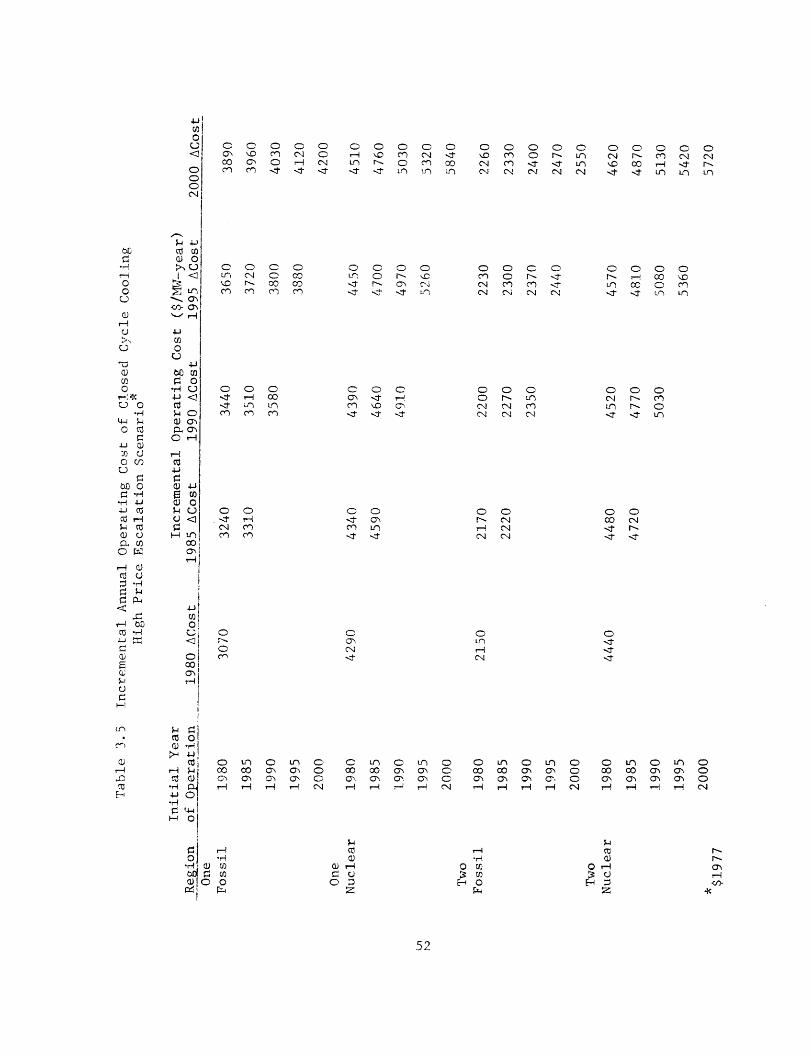
0000 0 00CC0 00 00 0 00 00 00 0O O O O C O O N O O O C) Oh C) N-) C C O O CNC O", H N q o o N -, o C 'N - .u c, . -o h-m m - - < J -. 1 Lr) e L) c N N c N -t -t U* Lf) Lr(

C C C o

0 0 C 00

"C~ L/'~ cc H C oo

O CO CO

00 -I0-< H oN Cn C

e"1

CO

-Oc'n

10 0 CO O O

-T -Z" -It -

C C)

O Ocn L)-It -.1

C.'C"].t

0 0D 0O O O o

('N ci C-,, o

C N CN CN N

) Oh- CN4o-4N C

04

oLI)

Oq

O O O O

u r 00 C

O OD O -sT -:T f Ln

C CO OC h- CnLn r- 0-: -I Ln

O O00 31't r-

OCo N

-zi-

O ) O U O C u1 O U) O00o Co C" o o Co 00o 0' O' 0G) 0, 0 0. 0 C 0.' . 0. CH H H H N H H H N

IH

. )U)

a) P P

CO

Q 3~o ~CJ~z

O tn 0 Ln O O L 0 0C CoO.'0 0 C C Cc' 0. 000' 0.'0 . 0. 0 0.'0 .(X) 0.' 0H H H H, o H H H H N

E-4O g:O

C4coa)

O HV

z

h-h-

a.'

-i

52

, O

CC

CC<c

o

oo0'1C)a)

HC)U)

o

0~

*<

oJo O

C.HWuS

H C)

-c U

O

C)

U)

H 0

C')

o

4~JHF Qo

C

0

OH~H

4i

w O

CoQ)a'

4JU1)0

C3

Co0H0

Hz 0CO)

40

.H

0!-H

!

!

o o 00 0 0 0 0 0 00000 c 000 0 oo r N o ID r- O i) N Co r- D ' \D n 0 - sD ooH C C Cn Cn H cv \O cc N Ln b 00 0o, N O N i) cN N C N N -T -t t L- Ns N N C C I Lr) Ln in

0 c 0c cn cc

H H N Nscn C N C

0 00 -It -, ccO H HN N N

O 0in OO HN Ns

0C0N

0 0 c 0ON 1 n 0

r1 cn in cN'l -~J -I -It

Io r- oC ci L)

00 H NO NCI-I -I'

0N-

c-n

\o I n nI) ' -N N N N

i 0oLr) \1 r-N N Ns

0

L-) Lr)N Ns

N--INl

0 0 0 0o L nN Ho N in

In Oh -CD 0 H)

-It -It in

0 O

10 in~o ccIT -Id

\0'-Iino

0 in 0 in 0 0 in 0 in 0 0 in 0 in 0 0 in 0 in 0oo 00 m O GO 00 o m 0 cc c o a 0 cc cc o O 0, m o m 0 (ON 0 0 0 C" ON aN C' 0 C a Co C' 0N

H H H H Ns H H H H N H H H H N H H H H CN

a) Ha1) -H-HO

p U)IC c

Cda)

I4 H

Eq z7

p- -H-

0 UrZ4

p a)

O U

z

53

4~i

c0C-4

00

a)HUa)

0

0 oHC-) 0 0

4 -HP: u

c -HOH

CdH Uk

~a) t

U)

r404-nQ)

,0Cd

Hr

4-ici)0

tn u

i Lr4-3co0

to

a) oN

criCd.1-3

0)~Oi

4-3a,)0

C)0all

p 0C 0a) 'H-

CdWcor'H p.

*H{

O

.0a)

0 0 0 0 0 0 0 00 0 0 0 0 0 0 0 0 0 0- N H ", 0 C ~ 0 Lr U CN 0', C N H. Cn . Ui. t L.. n>)0 0 ~C' Co 1 -.I- mc N -I in) 'I - COO C0 c ' 0)H N N N N -1 - in) in) i) NN N N N" -zf in) uin in) i

w ,^

, < Cl O O O,

~~ Lr -- -! c'q 0q~( N oOkC s3- 0m C O

-W

0U

-H C)4Jiw O<

CO$4 0

O H

4--

wJa) ui

E OQ0UwH4)

4-J

0

LOC0>al

C C) C,O r- -IC'~ O C

c C)

00 0i_bO 0">

o 0 cL 0 0 LnUL)o c C

-t -- Ilr) L)

O O C

L r- 0

00,- -- I

0H--

O O O

Cf) C) O

O ,- OO HO0 H- (DI

CN -11 -1CN N C

H Cr- Oan

_qcnN N

0IH..1

O O Or- C1 oh 00~- u' C1 V)- N) X Un

O O C)H s0 tt

rsO

O 00-t Lr0 0

'1'4HNt

0 in 0 in 0 0 in 0 it 0 0 In 0 In 0 0 In 0 i 000 00 a> Cl> 0 00 coc> 0> 0 0 00 0>0 cc o oo oO 0>0) o0>0>0>0> 0 >0>0>0>0 0> 0 o 0 0 0> a0 > 0>0H H H H No H r H H N H H H H CN H H H H N

11 .-

-H- Cl)~bnr o?~ i

.4CI

Wa)

*H C)

z

.H-4

X Cnri~ COcnq o

C4

V):C)

cezZ

0>

VI)--IC

54

0u0

CN

rjO0

00C)

0)

c~oC)C)0

<~H

J .HCi- -,,

C

WcJJ

C;

~C,-n

Vd

0

Cr)

-i

Ct'

a)

C0

H $-

c 0(1 ,4 14-O-Ha

04-40

C 04

0

Sw4 4- I

, --

Wu

ChqI

I

0 0 00 0 0 0 0 C 0 00 0 0 0 00 0 0 0 o r- n N '1 H 0 if' £0 N 0 .0 0 o H - I -pH H N -< Lfl 0 N L WO o N N m - u V) 0 0 r-N N N N N I ; L L L C N N N N -It -<t u) Lu) L

0

oH CN C"

C N N C

%D oM -'o4 CIA HoH NNS N N

000 HN Nq

CsN0N1

o 0 o0cro Ln O (01-Itl r- N1 -It

C C" C

-It 10 H--~J --:I I')

00Oco CY

CO

CY)C" m

0 0 0

O H C CH N N C

O H-- r-o H HH N1 C

0 0If) r

H N

00

o o o oH -I C r-If' r- ONc-I -I Ln Ln

Ln 00 CY)-I' '10 O-.1' -I' -It

0 C

C") \.0-I' -I'

0I

0 V) 0 in 0 0 n 0 I') 0 0' 1' 0 in 0 0 in 0 in 00000 C C 0 0 o Nc 0 0000 o CTa 0 0000 a C 0C C- C O 0 C C C' 0 C 0') 0 o 0 C-a ON O 0' 0H H H H N H H H H c H H H H N H H H H C

-H

C/ mUW O

PX

C)

z

z HY 'H

'H cJ,w *

PLIU

Y tH

'H U

z

r-

0'\

')>9

55

4I-J

0

0

00NCT

*H

0

4 HU)

0EnHQ49

CZ0coco*H

u) co ri

~4*4i4

HU

r4

$HC-)

H

coW

<

0Q4iJ

<

OC)'H Q

0)

<

OHQ) JJc

0*H

0OD

00000

0

it')

a')r-oH

oeP o

w Ya') 'H-

H -i

'H P.

- O.H

O

0'H.

0 0 00 0 0 0 00 0 0 0 O O C O 0 0 0 Ln CN I CIA H It O Q0 U C I'D C ) < L C rH Ln £Or- m O 1 N ul, CoO *q cc H H CN Cn n cc C N n c0

H CN Ci C1 -1 Jt Ln U L N N N N -d- L; Lf) LO

N C N 0r- r C -H H Ns No

C 1- C!

0 rs or- r- H H NS

0 0H0 L'IC r-

C c 0 0z n 70 *.

-4 r- c) -zOzr - L L

c-4 r 'Ot Co C)

-ci- -ci. -ct

0 0.0 N

-It -:-

0)NI

O Q 0 O0 h- Le, CI-H H N c5'N N N N

CD O Occ LI) le

O r-- C94N N C9

0 0

0 c

0

CN

0 LO 0 c)O LIN -cal-Ln r c9~ '-I- lt ULO L-

O C) OCcn C', 'I

-I -,I L)

O C00 c

cc c-c- -cIT

CCO)-ci

0 0 Ln0 00 0 0 U0) LI 0 0 0 0 01 L0 0 U0) 00 c C C 0 c c C) C) 0 c c C ( 0 cO 0 C) C 0C)) C C)o 0o CO C O, O 0 c) C C 0 ) C C) C 0H4 H- H H ~ N, H4 H H- H- N H- H- H-- H- NI H4 H- H- H N

i-4H0 cr

a)

a3)u

z

-HI CD

H rO

H a)I H

z

56

II

CCcN

0C)- 4'H

-)

'-4

OHC

Ht SU

C) C

~ o

OH

4 <

)ccrf r:S

4i

0U

4-J

m cUt0 c

OHH

pcia1 C,C

4!Jrc

(10O uUC-

0

4-

1-0

a1)H4

H0

a) 'H

-4 4.4.J'H

co G

O rlr-

h-C)-Hx

U)I

Ii

iI

,901 U CG r-4 C

W; I FT;

0 0 0 0 0 00 000H N- It 0 0 m w Lfn -I 00 H ~ cH. r N- O N IL O-,t -I ~" - .,i -I ,-If Ln Lrn Lrn

00OD00 O

on m m m

o CO CO 0r.- O0 10 'Y CY) cn o

0 00

0 0

00CY u) xm cnC C)

001

0 LU) 0 Lr) 000 00 o' o-C 0

CH H rh 0" CH

a)a) H

4-) -H

-H 04 rX1

oo It o onC) C) C O0 ' l c -d

O 00Cq O0 L

0 C) H

L 00

00

CLf)Ur)-d'-

C) ir) 0 L() 0CO O CO ' 0o o oo o O

u- -

H V*,1:~~~~~~~~~~~~~~~~~~-

57

4-Jw0

C

CNooo

o00ooa)

H

cD

o

-,

0o -)

o 4 rJ

oUoU

-oH

k41

o

r.0Cu)

)¢ -)

C-)C

a)

EH

c- o0(D O

OC--1<

4.J

OU,

co0 O

O'll- Q

--t

4-)OH c

H59CJ

F-4 Lr)

co<

aD

OO,.H0

0

0a) -H

*H -4-JO

HO

0-H-a)

000 00 0 0 o C C0 0 o 0 0 00 0 0 0 N O 1,0 LI) m - 'I n C ) Lrl N Oi a - 'a q r- < . r I x 0o ( L' 0 n-1 -. Z c N m -: N Ll h- 0 m' I -1 -1t -: L(, Lf c N N3 N IN -< -zt -T UL) L

O 0 0

'I 0 0-l

r N0 O Ooo- 0 Lr)r,) cn -,I

Co CD

0

0C)

0 L CN c

cn Ln cO r--I -I -Zl U)

c0 0) 0o-:'I -.r1 -t

N) LC

o CoC4 1e-1-, -:1-

crl

r- 0 V) o- o0 O.

_q N CN cN N N C

0 0,1-i0o-- o1 C4IQ N CNN N N

C N

N c

N

0 0 0 0L.' -I 'IC Lr)

Ln - 0~- -11 -11- Ur)

O 0 O--J- O. Lf)Nl -t r-N1J --:t -,

CD On 0

-:I- -It

0N1NT

0 Lu 0 V) 0 0 Ln 0 Lfn 0000 C O 0 00 O O 0

C o Cr : C, 0 0 a% C0 0- H - i-H r-4 .. N

"IH0) 0

C)C) -H

z

0 0 L 0 0 LIn 0 L 000 00 CSN a 0 0 C Ch o 0CO aN O7 M 0 aN a-n (ON a0{ 0- l- - CN -4 q rq cN

i-H.-H

O U)U)

HO0

01)O rH-

F- : irH,-I>

58

4-JU)

a0

0N

c U)

I <

'S r)o0,

u0n cr"

J-JU)Cau-

00U)4-)0 0

a) Cl

0r

4

J 4)~U)a-4o9 0v4 a

- L(C00am

4i)

000

C

.)

.

U) 3CC

0Uu

Id )

4-J

.)

C-)

Vl

In

a-H

�

ta r, U61 OO=A 1 P--

0 0 O 0 0 0 0 0 0 0 0 0 0 0 0 0 0 0 0

il 0 n o n 0 c -It r- un <- t <-. oo n o00 -

0 H r- N O cN <'t \ 0 <tn L \1 - O 0 n '.,0 O~ N in

N C N N N en - <t < < N N N N " < <t n in

0 0 0 0<t CO en C0 0 H HCN N C N

C) ) C O-0 HC N C

0OC

OhO

Ola"

0 0 0 C

CO 0 N0 '0CS H <t ,Cen -It <tj -It

r- C O Og oo <

00

CC0 -0"~en

0 0 C 00000r-~ in -It -It<t Ln "a

N N N N

't U) \,

0 0

N C

0L)

ItN1

000 0r,_ N 0' 0'-e O O H

000|D Ho C Oen) \ 00 <t <t <u-1 I -Itc ~ 0 0

i 0

0r CDLnO

-ItMen

0 U 0 U 0CO O 0 O 00- a o a 0

H H H H C

a) 1H

U)

H O,a(

0 in 0 in 0 0 i 0 n 0 0 in 0 in 000 o o 0 00 00 o o 00 0 0 0 o O 0 O o' o

. o\ 0 o c om o C ) o o. o- o 0

H _ H NS H H H H CN H H H N

1-4

Q) H HV 'H

0O0U)0 0

-4

00

z

59

-JU)co0

o0CP0CD

00

C)

u)0

H-40

0.r-I

a4-0

( .W

¢ d.-H.-I

c

0(n$4

C.)

W0

co UQ0~0I<C)

I0,

0

CDH

0<ccu 4-

rCCCl

C

0

c CC) or

4..

~0

a1)-i

Ho

CcC

4i C

SZ 4

1

0 0 0 0 0 C 0 0 0 0 C 0 0 C C C C 0 r- c) 0 00 vT O Lr 0 t C - r '- D 0 o 0 Ln - Ln0 C C C ,1 Cl - r- m Hd CN Cn t-t 'D \D o H ' I-tH H N N CN C < < L f U) N14 C4 Nl NT cq t t LI L Lf

0 0 0',. t, CO r-oo C C CO C h-

C) 0 C ,,o N Nhoo oh 0%1

C CCC C40 l

oo oh

0LI)00H Hq

0 0 CC ') D -- CCN -- rl- C

-t -:J- -~t Lr

C o C)

C! -1- -

CCD0 N -O

CDC4,4

-d'n

0 0 C

-Z' H- Cx*H Ns N N NS Ns

C) O O-I 1-- C-,

C Cs C9

CS CK

O C

C'

CN

0 CN - 1- .

1o 0 - -Z -I I L(1 Lfl

0 C CrH 0 C)'C oO H-. L)

C CC L()Q0 ccIt -I

C

Lr)-d-

0 Ln C U 0 0 C D C 0 0 UL 0 LI 0 C LU 0 U 0co0 cc - Coo oc o o Ca 0ao O C C> O c0 C° 0 C)a' a> C> a C C> m c C> C o C> C> C> C m m C> m CH H r H CI H r 1 H N9 H4 H H H C i H H H N1

H,-) rH

-,1q> rb0 r! U)

OD 44 rPe, i 0

~4

rH C)rz4 ::>

X ce

Hr CCC 0

da)

Hr C)

z

r-C>

-4

60

4J

0

<]

0 0l0icq

WI4,,>0

C0

r )U

&o

0i-x©

. 00

4- HC)m0

.4H

< o)

GJ o4-J

(JV4CC)C)i

~4Jt a)

0C)

4-im

4-i <M G)

C) a4 H)

O -~

4J

a) 4-

EJ CCU<

cc

4J

C,<3C0Coo,

4.-CC)

C)

CCo

H~

C0) *-

H 59~>- 4-).c, C)

4J O.H

O-4

©

0 0 0 0 0 0 0 0 0 0 0 0 0 0 0 0 0 0 0 0m 0 CO .0 UL) Ln 0 r- . MO u) H r- m 0 D O O' -1t N H0 H H Ns m m sC MO , -, COO O 0 H C ) Lf CO H --N c N CN N - - Z Lfl L rH H H " N - - - LCn Ln

0 C 0 c) 0 r- .00 H H NC ! CD! C

N OC' O000N C9 r-

O ON ON0 0N 0N

000NC)

N

00 0C0 0 0

cO O COH-It (ON1.- Ln

00

C 0O

-It- -- -Z

0

N Nm lI tZ0

00 00 0 0 0 0oo oo O' 0D

CZil l1 \1 n -

0 0 0N N- el)00 00 C7

CO COH H'H0 00 O

,-- ,--t

CC0OH-

0 0 0 0uM oon 00e00 Or~ O C Hu'0 C,-H

0000 1- C-zi -It --

0 0

cm Lr)-zt It

CCN

0 L(n 0 L(' 0 0 Lf' 0 L- 0 0 Lu 0 l 0Co COO o' 0) CO CO O' 0 O O o C Oo 00 o o' 0 00 O O 0 00 00 CS O 0H~o H 0H H N 0 H H oH N H' o o o'\ 0 o o l '~ ". o'. 0 ' o I Co

> U)

0) Ocn

Cia)

U) d

Z

U 'H

*H Cl)CL

0 Lu 0 Lf 0CO C O' 0 0

00 'Cr o 0

H H H H C

Ol -.- I ( I-HZ -K

61

4-Jco0Q

000CNCDc~

O

toO

l-0

u 0

,H

L) O OU

4-ri o0

cH0, r4

4 4-Ja -H

H /

4 oH

E4Jv

d4J

: oC)I <3U)

0Q

4IJ

-4 0

OH

Hp C)

a) u7

H Ofw -V -100

0o

4.)co

00000O'

41

0

U

CD

,0

-4

c 0d1) --I

.,--HH O-4.,--I I-J 0

HO

0

.r,4-OC:i

0 0 0 C 0 0 0 0 0 0 00 0 0 0 0 0r- -r N C 0 Cn 0-\ I) - IC Lr) - Cn C In L 0 r- .,.o r- cc C 0 n Ur) oo -I 0 i- N Cn < ' C i- -1- I- H i- N 4 I-N LrI ' N Il Nc N N -sr - -: LtL Ln

C o Cr- .- cc o

C o CH

' N-- r- 00r--,,

0'C

i-HI

0 C 0 00 1100 CN oo -< -zIno CO iH

It -- L )

O CD CD0- N- C,

cn In 0-zt - ,--

0 'Ccn L,

' 0 D 0It.j C,) cnq c'0 i-H N cn0 N C C

-, cn C'4

0000l N0 iH N>NM N N

C Nc C"N~ N-

00

-.

0 0 0 C,: o o' Cn LfY.0 iH

0 0 O'n 00 L11 Lr) 00- u -o-

0 OC r-cn L't -t

0i-

--

n ~~~ %1 0C)1 Cd a)I Y

o .H0

' O- -i E

In 0 0 0 0 o I o0 0 0) o0 I 0 n 0 U) 0co G c0 0 c c C" C" 0 00 cc c a On 0 Wo oo O\ 0'I 0

) on 0 ov Co ol C 0 ov c. c o O 0 c o 7 a 0I-- i-- i-~ cN -H r - -r (lN i-- i-H i-H i-H N -H i- 1 i 1- i-- N

i-- -HqCt-

--? 0i-HO

r- co

I i, C)liH

z

62

r-N-

0E

{t-

4-J

0

<E000

0.0

C

-H0

4-g0

t.U)

0

-iC0

rJ O *H

O--C

-H

'J

jU

(t 0)o

4-1

0

0C UX _:urhrn-H u

-4 C

C) O')

0r-

-4I

- io0h U)oo) a4

4-j

0u

o0

o'00crc-iH

s..0

c O

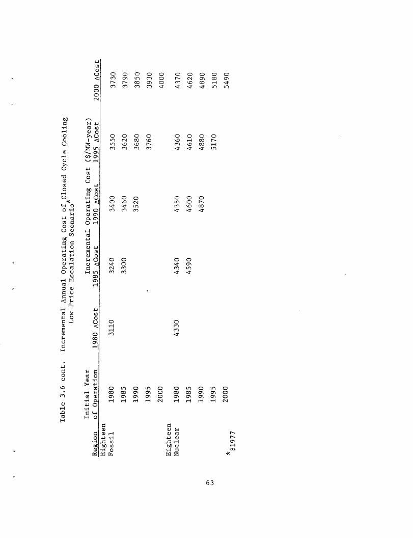
0 0 0 0 0 0 0 0 0 0m O L M 0 r- N ON o Or- N oo oC 0 1O 0o H -Im m m m -I -1 -I -I u Ln

0 0 0 Lf N 0 ~1L O O r-CY) cn C') C?)

0000 0 o0 \.D C 4

CO) C C

0 0It 0N1 C?)

C?) C?)

0

C?)

0 f- 0 L) 000 00 o O 0o O oC 0 0H H H H C

0 0 0

? ~D 00 H< L?) U

~C) 00

1? O --It- -- -Zr L0 C 0

00

ohM? L?)-I - -

0cqC?)N1

0 u' 0 u 000 00 O~ 0 0O O o cO 0H4 H- H- H1 N

a *H00 CJ

-H :ts- Z

r-

/-

-K

63

4

C

CCC,

io0

au0

Uo0

HC)

4-Ji0COO U1ow

C )

OH 0

4-J -H

COUa)0

-

4CZ

4 V

0C-,ce)4>0

a)H-o

EH

cCO

0

1)a

4-J

r4 C.4LJ

0)0

c

>44-C

Hc

0)rcC

Hi

HO

rC

a1)a) H4.. -H-

,C 04 r

Table 3.7 Incremental Present Valued Cost of Closed Cycle CoolingHigh Price Escalation Scenario

Initial Year of Operation ($/MW)

Region PlantType 1980 1985 1990 1995 2000

One Fossil 80,400 86,900 93,900 101,900 110,200

One Nuclear 106,100 111,900 118,200 125,000 132,300

Two Fossil 46,000 47,600 50,000 52,300 54,700

Two Nuclear 109,400 115,200 121,300 128,000 135,200

Three Fossil 37,800 39,300 40,900 42,700 44,500

Three Nuclear 98,000 103,200 108,800 114,900 121,400

Four Fossil 52,800 55,200 57,700 60,500 63,200

Four Nuclear 112,500 118,400 124,700 131,600 139,100

Five Fossil 41,400 43,300 45,300 47,500 49,700

Five Nuclear 109,100 114,800 120,900 127,600 134,800

Six Fossil 42,900 47,900 50,000 52,100 54,400

Six Nuclear 113,900 120,000 126,400 133,500 141,200

Seven Fossil 45,900 47,900 50,200 52,500 54,900

Seven Nuclear 107,100 113,100 119,100 125,800 132,900

Eight Fossil 47,400 54,400 57,000 59,800 62,900

Eight Nuclear 107,300 113,200 119,500 126,400 133,700

Ten Fossil 37,000 38,900 44,400 46,700 49,100

Ten Nuclear 106,700 112,600 119,000 125,600 132,800

Eleven- Fossil 46,400 48,400 50,600 52,900 55,400

Seventeen Nuclear 107,100 113,100 119,100 125,800 132,900

Eighteen Fossil 81,500 87,400 95,100 103,000 111,500

Eighteen Nuclear 112,100 118,000 124,300 131,100 138,500

Evaluated in 1977 dollars at the year of initial operation assuming a40 year lifetime and an inflation free discount rate of 4%.

64

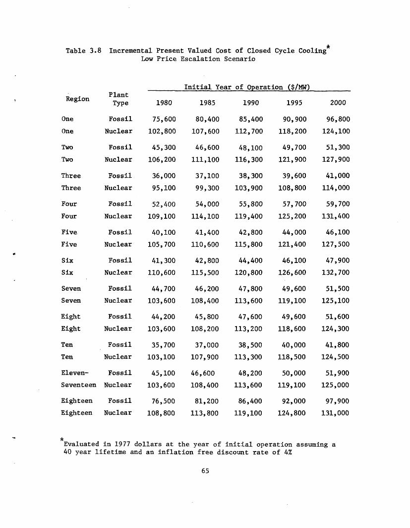
Table 3.8 Incremental Present Valued Cost of Closed Cycle CoolingLow Price Escalation Scenario

Initial Year of Operation ($/MW)Rego PlantRegion Type 1980 1985 1990 1995 2000

One Fossil 75,600 80,400 85,400 90,900 96,800

One Nuclear 102,800 107,600 112,700 118,200 124,100

Two Fossil 45,300 46,600 48,100 49,700 51,300

Two Nuclear 106,200 111,100 116,300 121,900 127,900

Three Fossil 36,000 37,100 38,300 39,600 41,000

Three Nuclear 95,100 99,300 103,900 108,800 114,000

Four Fossil 52,400 54,000 55,800 57,700 59,700

Four Nuclear 109,100 114,100 119,400 125,200 131,400

Five Fossil 40,100 41,400 42,800 44,000 46,100

Five Nuclear 105,700 110,600 115,800 121,400 127,500

Six Fossil 41,300 42,800 44,400 46,100 47,900

Six Nuclear 110,600 115,500 120,800 126,600 132,700

Seven Fossil 44,700 46,200 47,800 49,600 51,500

Seven Nuclear 103,600 108,400 113,600 119,100 125,100

Eight Fossil 44,200 45,800 47,600 49,600 51,600

Eight Nuclear 103,600 108,200 113,200 118,600 124,300

Ten Fossil 35,700 37,000 38,500 40,000 41,800

Ten Nuclear 103,100 107,900 113,300 118,500 124,500

Eleven- Fossil 45,100 46,600 48,200 50,000 51,900

Seventeen Nuclear 103,600 108,400 113,600 119,100 125,000

Eighteen Fossil 76,500 81,200 86,400 92,000 97,900

Eighteen Nuclear 108,800 113,800 119,100 124,800 131,000

Evaluated in 1977 dollars at the year of initial operation assuming a40 year lifetime and an inflation free discount rate of 4%

65

Table 3.9 Relative Incremental Annual Resource Costs Associatedwith Closed Cycle Cooling for Fossil Plants

Annual Cost% over O-T

1.7%

1.5%

1.5%

2.0%

1.7%

2.2%

1.9%

1.7%

1.8%

1.8%

1.6%

Annual EnergyLoss

(106 BTU/MWe)

720

520

% overO-T

1.3%

1.0%

410

690

520

650

550

540

620

550

680

Annual WaterLoss

(acre-feet/MWe)

3.2

3.3

3.6

1.3%

1.0%

1.2%

1.0%

1.0%

1.2%

1.0%

1.2%

3.2

3.3

3.4

3.2

3.6

3.2

3.2

3.4

tAssumes evaporation from once-throughmechanical draft evaporative towers.

cooling systems is 71% that of

66

Region

One

Two

Three

Four

Five

Six

Seven

Eight

Ten

11-17

Eighteen

% overO-T t

43%

43%

43%

43%

43%

43%

43%

43%

43%

43%

43%

Table 3.10 Relative Incremental Annual Resource Costs Associatedwith Closed Cycle Cooling for Nuclear Plants

AnnualCost

% over O-T

3.8%

3.9%

3.5%

4.0%

3.9%

4.1%

3.8%

3.8%

3.8%

3.8%

4.0%

Annual EnergyLoss

(106BTU/MWe)

1080

930

960

970

900

1100

1130

1170

1130

1130

940

% over Annual WaterO-T Loss

(acre-feet/MWe)

1.6% 4.7

1.4% 4.8

1.4% 5.3

1.4% 4.7

1.3% 4.8

1.6% 5.0

1.7% 4.7

1.7% 5.2

1.7% 4.7

1.7% 4.7

1.4% 5.0

Assumes evaporation from once-throughmechanical draft evaporative towers.

cooling systems is 70% that of

67

WRCRegion

One

Two

Three

Four

Five

Six

Seven

Eight

Ten

11-12

Eighteen

% overO-T t

43%

43%

43%

43%

43%

43%

43%

43%

43%

43%

43%

IV COMPARISON OF COSTS AND RESOURCE CONSUMPTION BETWEENOPEN AND CLOSED CYCLE COOLING SYSTEMS:

REGIONAL AND NATIONAL LEVEL

4.1 Introduction

With the assumption that without thermal controls new plants could

locate on water bodies in the patterns described by Alternative Siting

Pattern #1 (Chapter 2), our cost estimates display greater sensitivity to

our energy demand forecasts than to our price escalation forecasts. The

number of megawatts of new capacity which we estimate will be affected

by thermal standards under the high energy demand scenario is roughly

60% higher than the capacity similarly affected under the low energy

demand scenario. (Tables 2.3 and 2.4, Chapter II). In contrast,

the estimated unit incremental year 2000 annual operating costs under

the high price escalation scenario are only 6% higher then the correspon-

ding costs under the low price escalation scenario. This greater sensi-

tivity to demand forecasts is in part due to the method with which new

plants are located on water bodies with the siting pattern #1. If we were

to use any of the alternative potential siting patterns described in

Chapter Two we would continue to find that overall costs are more sensitive

to electric demand projections than to price escalation projection although

the relative difference in costs between the low and the high energy demand

projections would be reduced to approximately 14% - 23%. Because our

cost estimates will show a greater sensitivity to demand projections than

to price projections, we will henceforth consider only one price escala-

tion scenario - the high one - for future discussion.

63

4.2 Comparison of Cost and Resource Consumption

Tables 4.1 and 4.2 present our estimates of the overall annual

costs, by region, of complying with current thermal regulations in select

years between 1980 and 2000, for the high and low energy demand scenarios

respectively. The annual cost in any year is the product of the unit

incremental closed cycle cooling costs summarized in Tables 3.6 through

3.10 and the number of megawatts we expect will operate with closed

cycle cooling for environmental purposes by that year (Tables 2.6 & 2.7)

While Tables 4.1 and 4.2 present our estimates of incremental

annual costs of thermal pollution control for select years, we can fit

a function through these points to derive estimated annual costs in

any year. For the national incremental annual costs we found the

following functions fit well:

NACi - 1974)120 ($106) (high energy demand)

NAC = 2.8 (i - 1974)1 20 ($106) (owhigh energy demand)NAC = 32.9 (i - 1974) 1 2($106) (low energy demand)

where

NAC = national incremental annual cost in year i ($)

We can determine the cumulative annual costs of thermal controls

from 1975 to 2000 by summing the values of NAC for the years i between

1975 and 2000. The cumulative national incremental costs can be expec-

ted to be in the range of $20.4 billion (for the low energy demand

scenario) and $32.8 billion (for the high energy demand scenario). These

values are expressed in 1977 dollars.

Tables 4.3 presents our estimates of the additional annual fuel

69

Table 4.1 Expected Annual Cost of Current Thermal Regulationsby Region (High Energy Demand)t

Water ResourceCouncil Region

1980

One

Two

Three

Four

Five

Six

Seven

Eight

Ten

11-17

Eighteen

National

23.4

49.4

33.0

77.8

67.5

16.6

67.4

32.6

20.9

54.4

13.7

456.7

1985

49.1

102.0

68.0

161.0

139.5

34.8

139.9

68.2

43.3

112.9

28.6

947.5

Year

1990

77.57-, .

158.6

105.9

250.2

216.7

54.2

219.4

106.7

68.1

177.5

45.0

1479.8

1995

108.4

219.2

146.6

345.5

299.1

74.9

306.8

148.0

95.4

248.9

62.9

2055.7

t x 10 $1977; High price escalation scenario

70

2000

143.3

284.2

190.9

447.7

387.5

97.3

399.5

193.5

124.6

324.6

82.4

2675.5

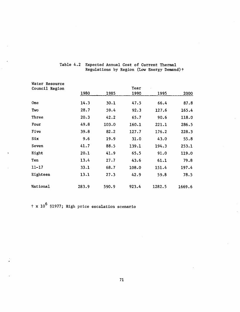
Table 4.2 Expected Annual Cost of Current ThermalRegulations by Region (Low Energy Demand)t

Water ResourceCouncil Region

1980

14.3

28.7

20.3

49.8

39.8

9.6

41.7

20.1

13.4

33.1

13.1

Eight

Ten

11-17

Eighteen

National 283.9

1985

30.1

59.4

42.2

103.0

82.2

19.9

88.5

41.9

27.7

68.7

27.3

590.9

Year

1990

47.5

92.3

65.7

160.1

127.7

31.0

139.1

65.5

43.6

108.0

42.9

923.4

1995

66.4

127.6

90.6

221.1

176.2

43.0

194.3

91.0

61.1

151.4

59.8

1282.5

t x 106 $1977; High price escalation scenario

71

One

Two

Three

Four

Five

Six

Seven

2000

87.8

165.4

118.0

286.5

228.3

55.8

253.1

119.0

79.8

197.4

78.5

1669.6

consumption in the year 2000 as a consequence of thermal pollution controls

for our high and low energy demand scenarios. Assuming a linear distribu-

tion of new capacity additions between the years 1975 and 2000, we esti-

mate the cumulative energy loss in this twenty-five year interval can

range from 0.73 Billion barrels oil equivalent for the low energy demand

scenario to 1.16 Billion Barrels oil equivalent for the high energy

demand scenario.1

Our estimates of the additional freshwater consumption due to

environmental controls are sensitive to the way in which we evaluate the

freshwater loss from closed cycle plants that would otherwise operate

with once-through cooling at coastal sites without controls. Such plants

may either install saltwater towers-in which case no additional freshwater

consumption occurs-or install freshwater towers-in which case the addi-

tional freshwater consumption is equal to the total water evaporation

from towers. Table 4.4 presents our estimates regarding the additional

fresh water consumption in the year 2000 for the low and the high energy

demand scenarios, respectively, assuming that all closed-cycle cooling

is with freshwater evaporative towers. Table 4.5 presents similar

estimates for the low and the high energy demand scenarios assuming that

all closed cycle cooling on coastal sites is with saltwater evaporative

towers. If all closed cycle cooling is with freshwater towers we expect

the additional freshwater consumption in the year 2000 will range from

2,320,000 acre feet to 3,420,000 acre feet for the low and the high energy

demand scenarios, respectively. With closed cycle cooling on coastal

Assumes one barrel of oil represents 6 x 10 BTU.

72

Table 4.3 Incremental Fuel Consumption in the Year 2000Due to Thermal Controls

6 High Energy Demand 1Region (10 Barrels oil equivalent)

One 4.8

Two

Three

Four

Five

Six

Seven

Eight

Ten

11-17

Eighteen

Total US

8.9

6.4

14.9

12.7

3.4

14.9

7.5

5.3

11.9

2.4

93.1

1,160.0Total US1975-2000

6 Low Energy Demand 1(10 Barrels oil equivalent)

3.0

5.2

4.0

9.6

7.5

2.0

9.4

4.6

3.4

7.3

2.3

58.3

730.0

Assuming 6 x 10 BTU/Barrel of oil

73

Table 4.4 Incremental Freshwater Consumption in the Year 2000without the Installation of Salt-Water Towers at

Coastal Sites

High Energy Demand(10 acre-feet/year)

L w Energy Demand(10 acre-feet/year)

290

760

250

420

420

90

410

210

140

480

250

180

430

140

270

250

50

250

130

90

290

240

2,3203,420

74

Region

One

Two

Three

Four

Five

Six

Seven

Eight

Ten

11-17

Eighteen

Total US

Table 4.5 Incremental Freshwater Consumption in the Year 2000with the Installation of Salt-Water Towers at

Coastal Sites

High Energy Demand(10 acre-feet/year)

50

60

230

420

420

90

410

210

140

220

0

Low Energy Demand(103 acre-feet/year)

30

30

140

270

250

50

250

130

90

130

0

1,3702,250

75

Region

One

Two

Three

Four

Five

Six

Seven

Eight

Ten

11-17

Eighteen

Total US

sites using saltwater evaporative towers, we expect the additional fresh-

water consumption in the year 2000 will range from 1,370,000 acre-feet

to 2,250,000 acre-feet for the low and the high energy demand scenarios,

respectively.

4.3 Discussion of Total Costs

Dllar Costs

Our estimates for the incremental dollar costs of complying with

current thermal regulations may be put in perspective by comparing these

values with several other measurements for the steam electric industry:

total cost of operation, potential revenues and potential profits, and

costs for other environmental controls. We estimate that under our high

price escalation scenario the sum of annualized capital costs, fuel costs

and replacement energy costs between 1975 and 2000 for all new capacity will

range from $1640 billion to $2620 billion (in $1977) for the low and

the high energy demand scenarios, respectively.1 Therefore, the corres-

ponding dollar costs of thermal controls, $20.4 billion and $32.8 billion

for the low and the high energy demand scenarios respectively, represent

approximately 1.3% of the expected costs of operating new capacity.

In 1977 the average unit revenue per Kwh for investor owned

electric utilities (which represented 76% of the commercial electric out-

put in 1977) in $1977, was roughly $.034/Kwh (Edison Electric Institute,

We assume roughly 54% of the new electric capacity planned for the years1975 to 2000 could be installed with once-through cooling without thermalcontrols (Chapter II, Alternative Siting Patterns #1). We assume newcapacity additions will be constant each year, with new additions tothe year 2000 equal to 937,000 MWe under the low energy demand scenarioand 1,504,000 MWe under the high energy demand scenario.

76

1978). Under our high price escalation scenario the average cost of

generating electricity will escalate (in real dollars) by roughly .8% per

year. If unit revenues escalate at the same rate, then we estimate the

cumulative revenues accruing to all new capacity between 1975 and 2000

($1977) will be between $3090 billion and $4950 billion for the low and

the high energy demand scenarios, respectively. Therefore the corres-

ponding dollar costs of thermal controls will represent approximately

0.7% of the expected revenues accruing to all new electric capacity.

For the years 1970 to 1977 the net income (revenues minus the sum

of operating costs, debt charges and taxes) per Kwh for investor owned

utilities remained at an almost constant $0.0045/Kwh in 1977 dollars

(Edison Electric Institute, 1978) (This consistency is partially explained

by the fact that profit levels for the industry are regulated by govern-

ment agencies.) Assuming this constant dollar return is maintained from

1975 to 2000, the cumulative net income accruing to new generating

capatiy for that period will be between $351 billion and $561 billion for

the low and the high energy demand scenarios, respectively ($1977).

Therefore the costs of thermal controls will represent roughly 5.8% of

the net income accruing to new generation capacity.

Finally, we offer a very rough comparison between the expected

costs of thermal pollution controls and the costs of flue-gas desulferiza-

tion controls for coal-fired plants. Jahnig and Shaw (1978) estimate that

flue gas desulferization increases coal plant operating costs by $0.0059/

Kwh. These investigators also suggest that 37% of all new coal fired

plants built between 1978 and 1986 will require flue gas desulferization

to meet air quality standards. For our rough comparison we will assume

77

1) that desulferization costs, in real dollars, remain constant at 5.9

mills/Kwh for the interval 1975 - 2000, and 2) that 37% of all new coal

fired plants built between 1975 and 2000 will require desulferization.

Our high energy demand scenario suggests roughtly 200,000 MW of coal

fired capacity will be built between 1975 and 2000. Assuming that this

new capacity is distributed linearly over time and that it operates at

a 75% capacity factor, the total estimated cost of meeting clean air

standards between the years 1975 and 2000 is:

½(25 years * 200,000 MW * 8760 hr/yr * .75 * 5.9 $/MWH) = $100 Billion

Thus, the estimated costs attributed to these air quality standards is

roughly 3 times the estimated cost of current thermal pollution regula-

tions ($32.8 billion for the high energy demand scenario). It should be

noted that in the event we have underestimated the actual percentage of

new generating capacity going to fossil fired plants, our thermal pollu-

tion control cost estimates will be too high and our air pollution control

cost estimates will be too low.

Fuel Consumption

The magnitude of the energy losses induced by closed cycle cooling

may be perceived by comparing these losses with projected energy commit-

ments elsewhere in the economy. We estimate the annual energy loss

from thermal controls for the high energy demand scenario will be roughly

5.5 x 1014 BTU/year in the year 2000. In contrast, under the high demand

scenario, the projected national energy consumption in the year 2000 will

be 163 x 1015 BTU/year and the projected electric utility fuel consumption

7 nU

will be roughly 91 x 1015 BTU/year (WRC, Appendix H, 1977). Thus, energy

losses due by thermal controls will represent approximately .3% of the

nation's energy consumption and .6% of the electric utility's energy

consumption.

Another useful comparison can be made with respect to the amount

of energy that could be saved if greater efficiencies in the steam cycle

energy conversion process were realized through new technologies.

ERDA (1975) estimated a maximum likely savings of 2.5 x 1015 BTU/year

would be realized by the year 2000, under a 160 quad energy consumption

scenario, if new technologies such as superconducting generators and

Brayton gas turbines, could be made economically feasible. At .55 x 1015

BTU/year, the energy loss due to thermal controls under the high energy

demand scenario represents approximately 22% of the energy that could be

saved if moderate emphasis were placed on improving the electric conver-

sion process of steam electric power plants.

Water Consumption

To place our estimates of incremental water consumption due to

thermal controls in perspective, we compare these estimates with a) the

expected growth between 1975 and 2000 in non-agricultural water demands

for each WRC region and b) the total non-agricultural water demand projec-

ted for each region in the year 2000. While agricultural water use is

often the dominant use in every region, agricultural water demands are

spread over large land areas and may not disrupt local supplies to the

extent non-agricultural uses do. Thus, agricultural water use is not

compared here. For regions where recovereable water may be in short

79

supply the first comparison (i.e. with growth in water demand) provides

some idea of the extent to which water demands due to thermal controls

will compete with all other new users while the latter comparison (i.e.

with total demand) suggests the extent to which thermal control induced

water demands will compete will all non-agricultural uers. These

comparisons are presented in Table 4.6. In addition this table indicates

how large these induced demands are relative to the single largest

growth in demand from any sector, excluding the agricultural sector and

the steam electric utility industry.

The figures in Table 4.6 refer to the high energy demand scenario

because both the projections for new regional freshwater demand and the

high energy demand scenario itself were developed simultaneously by

the U.S. Water Resources Council for its Second National Water Resources

Assessment (1978). Consequently, because these water use projections

may imply a higher level of future economic activity then is anticipated

with the low energy demand scenario, we feel it would be misleading to

compare the thermal control induced water demands under the low energy

demand scenario with the projections for new regional water demand

found in the WRC assessment.

From Table 4.6, we conclude that thermal control induced fresh

water demands will represent a substantial fraction of the new fresh

water demand in a number of regions (e.g. WRC Regions One, Two, Seven

and Eighteen), and in some regions will approach or exceed the level of

new demand from the largest non agricultural/electric utility sector

(e.g. Regions One, Two, Four, Seven, Ten, and Eighteen).

One final examination of the impact of thermal controls on water

0

N" r% Hb" N O K .N b.v-q H-- ~- -,t N, Cm N H4

H- Hr-

o

NQ b°' 'b- b°N N N N 0 0 N -: 0 N 'C Ln r-h- O\ H 'I T C CY) N H

H- H-

b,' b°' 'b,' N° b' Mo Nr-4 N t 0) O 00 00

H-

4-i

Cd

.H,--C)0

C)0)

U)CD1O0OP)

O~ 00 0

bN K NO 'b- 't`2 b° O N °00 M Ln OC Lf 0 00 L') b

--H H -- CN -4H H-4

0

-

4i

00

a1)H

Cl)

Cd a)

4-J

e~

O )o )Nq 4-i

Ol wSCd Fx

0

r- 0H O

o o.04-r- CD 0a)O a) ) 4

0 ,n oce ~ 00) co .

co r4-i a) CJ r- D 0U co a) QCO -H~~ ~~~'2 ~~~~~ 0 4-i Cl) 4-4-' C C

c- U i 4 40 a) 4

Oi 14- C^J4 0) "

1-4 r-A r-i r-i CIA ~ ~04i r.-1 ~LC) 4- ) fL00U

5-40 H- *H

4-i to C~4-lCd 0)

4-4o< sib 1 i 1 31 1 I C~ H U FpI

coH 0 r-5

4- co 4-4 *~

0~~~0t0 U ) S

H 4-4 0 0 >-~ ~ ~~v1 > HH a)

0 -H *H 0) *H 0) H -H 3 4O E; [H F.~14 P U000 cw H H 4 w to0 H 4

81

Q0>CZCD (a) ,E-4

00 00Ep- p- 0 --Cd O N

C44) 1rU L)

0 00 C, H

Hz

0

o0co0o CO

:3H00

~0HCl)

S-i

W C

0 Cd

Q 0I - H

0 wt) s-Pi 0)bHa)H5-PH 0

4- *,1 =

- id_4-J r-)00(1i.j04

co Cd

a) C3n O0

z a) O -'P> N EP

44 -H I B0 4-i Lr) 00

O L

0U)

0o0P4p Sco o d4w 1-

>O O

0

0) 0 'oo44 -,-I 0 4-i Lf)

o u) '

~o0

oC0

a)

use is to compare these induced water demands with the expected increase

in freshwater imports for select areas. One suspects that if a region

plans to increase its water imports it does so because projected water

demands are expected to exceed available supplies. It is in those

regions where additional water losses due to thermal controls will have

the greatest impact. While there are likely to be a number of regions

where future imports of water will be necessary to meet anticipated

demands, there are three subareas where plans for additional imports

have been approved (WRC subareas 103, 1805 and 1806). Table 4.7 compares

the quantities of additional planned imports with projected incremental

water consumption due to thermal controls for these subareas, In subarea

103 (Boston-Providence metroDolitan areas) either imports will have to

double over planned amounts if current thermal controls are maintained

(or if salt water cooling towers are infeasible) or new plants will be

required to locate farther from their primary points of demand. Subareas

1805 and 1806 are located wholly within the state of California where

current water policies effectively prohibit the use of inland freshwater

for power plant cooling (Hendrickson, 1978). Therefore, if current

thermal controls are maintained then it is uite likely that new plants

will either have to install salt/brackish water towers, pay additional

charges to treat municipal waste water for cooling purposes, or seek

sites outside the state.

82

OCS

,-i

,-.I

0 O

Oo 0oCY) OH-

O O Oo o'0.D LU) f 4N

Cn Lr) £

O O O

-0 O

83

(a) 4J

o-40H. .

a)4.J

CZ

"O oaJ

;-OC.) C14d 0

I-4 C)4J Lfn

H- CZ r-O a

.IJ i

0~0

a) )O Si O

OC) q

O G] G4i

O ) NU{ f N*H C) r-l

co 'H 0c~.~O

cU

r-.

ro

U)

O

U Uc4

HIc a)

a)-C)

CZ

c cu

a)aCo4i

a).1-4

)gI--CZ,En~

O4(~

-tIm

~4

00

H

-I

r44Ja4coJCl)

0

4JCO0

a)..

,4

0C)a)O

atC/)M

CO

H

"icn.

:J.I

a4MJ

V SUMMARY AND CONCLUSIONS

5.1 Introduction

The objectives of this chapter are two-fold: first, we shall

present a summary of our results estimating the dollar and resource costs

of complying with current thermal regulations; second, we shall set forth

a number of suggestions and caveats which we feel will aid decision makers

in drawing policy conclusions from this study.

5.2 Fuel Consumption as a Consequence of Controls

From the point of view of national energy conservation, it does

not appear than an overall relaxation of current thermal standards will save

appreciable amounts of energy. We expect that thermal controls will increase

overall U.S. energy consumption by 0.3% and increase overall energy consump-

tion from new steam electric power plants by 0.6% by the year 2000. However,

the crucial factor in terms of additional energy consumption due to thermal

controls may not be the additional average annual energy loss, but may,

instead, be the incremental peak energy loss suffered during the summer

months. The concern here is that with closed cycle cooling systems incurring

peak losses of between 2-5% plant capacity, a utility system having very low

reserve capacity margins and having historically relied on once-through

cooling for the majority of its cooling needs could suffer from a weakened

reliability of system operations during the summer months. Under such

circumstances, the utility would, in all likelihood, be forced to pay a

higher price for replacement energy than was assumed in this study. Thus,

while it does not ppear the current thermal regulations will appreciably

increase national energy consumption, we do recommend that these regulations

84

offer some flexibility in compliance for those utility systems that can

demonstrate system reliability will be seriously impaired by too rapid a

switch from open to closed cycle cooling.

5.3 Dollar Costs of Thermal Controls

For the combination of energy demand, price escalation and new

plant siting patterns we have examined, it appears that the costs of thermal

controls are a small percentage of potential "at site" operating costs and

utility revenues. It was shown earlier in Tables 3.9 and 3.10, in Chapter

3, that incremental closed cycle cooling system costs are approximately 2%

and 4% of the "at site" operating costs for fossil and nuclear plants,

respectively. Because "at site" operating costs make up only a fraction of

the total electricity costs borne by consumers, we conclude that current

thermal controls will increase the cost of electricity to consumers by no

more than 2-4% in those areas that have historically had a high percentage

of plants cooled by once-through cooling. Those WRC Regions falling into

this category are likely to be regions One, Four, Five, Seven, Eight and

Eighteen. Consumers can expect thermal control induced rate increases

substantially less than 2-4% over current levels in regions Two, Three,

Six, Ten, Eleven, Twelve and Seventeen, where the potential for continued

once-through cooling development would remain small in the absence of ther-

mal controls.

Thermal control costs could threaten the profitability of certain

utilities if rate setting agencies refuse to allow thermal control costs to

be passed on to consumers. Without rate increases, utilities that would be

35

able to install once-through cooling at all new plants in the absence of

thermal controls would lose between 14-18% of their after-tax profits as a

consequence of the current thermal regulations. Of course, the smaller the

potential for installing once-through cooling at new plants in the absence of

thermal controls, the smaller the loss on after-tax profits.

Because we do not incorporate a price for water consumed in our

models, it is possible that we have underestimated the costs for closed cycle

cooling in areas where freshwater is in short supply. Of course, at inland

sites, the ability to install once-through cooling presupposes a large

freshwater supply. However, there do exist sites along some coasts where

ocean once-through cooling could be installed in the absence of thermal

controls even though local freshwater supplies are insufficient for inland

freshwater once-through cooling. At these locations, the available freshwater

supply may be so scarce that such water does have a price (equal to at least

the cost of delivery) and it is possible this price may be too high to be

ignored.

5.4 Water Consumption as a Consequence of Controls

Nationally, the additional water consumption due to thermal

controls will account for between 10% and 14% of the projected growth in

non-agricultural water use between 1975 and 2000 (WRC, Part III, 1978). In

comparison, overall consumption from the steam electric power industry will

represent the leading sector in new demands for water, accounting for

roughly 42% of the growth in non-agricultural water consumption. Induced

consumption due to thermal controls is approximately one-third of the growth

36

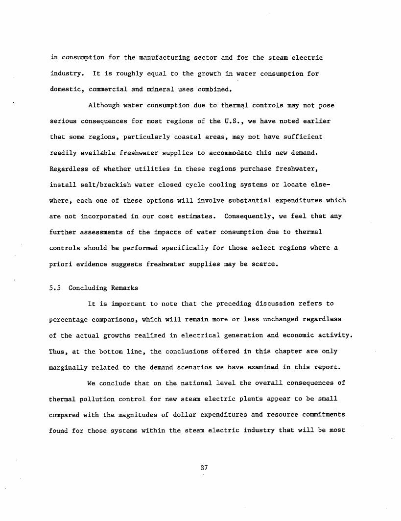
in consumption for the manufacturing sector and for the steam electric

industry. It is roughly equal to the growth in water consumption for

domestic, commercial and mineral uses combined.

Although water consumption due to thermal controls may not pose

serious consequences for most regions of the U.S., we have noted earlier

that some regions, particularly coastal areas, may not have sufficient

readily available freshwater supplies to accommodate this new demand.

Regardless of whether utilities in these regions purchase freshwater,

install salt/brackish water closed cycle cooling systems or locate else-

where, each one of these options will involve substantial expenditures which

are not incorporated in our cost estimates. Consequently, we feel that any

further assessments of the impacts of water consumption due to thermal

controls should be performed specifically for those select regions where a

priori evidence suggests freshwater supplies may be scarce.

5.5 Concluding Remarks

It is important to note that the preceding discussion refers to

percentage comparisons, which will remain more or less unchanged regardless

of the actual growths realized in electrical generation and economic activity.

Thus, at the bottom line, the conclusions offered in this chapter are only

marginally related to the demand scenarios we have examined in this report.

We conclude that on the national level the overall consequences of

thermal pollution control for new steam electric plants appear to be small

compared with the magnitudes of dollar expenditures and resource commitments

found for those systems within the steam electric industry that will be most

87

heavily affected by current thermal regulations. However, this assessment

should not be interpreted as a justification for current levels of thermal

controls. Whether the current level of thermal controls can be justified

depends on both the magnitude of the improvement of overall environmental

quality realized as a consequence of current standards and the relative value

with which society measures an improvement in environmental quality versus

an increase in resource commitments.

While we have not examined the potential environmental improvements

that can be realized under existing thermal regulations, we can postulate

how new once-through cooling development could be distributed among water

bodies, classified according to size, without controls. Figure 5.1 illus-

trates the distribution, by water body type, of the new capacity we feel

could install once-through cooling in the absence of thermal controls, over

and above the once-through development that has been projected under current

controls for the contiguous United States under the high energy demand

scenario. Table 5.1 presents this information by Water Resource Council

Region. To the extent that large water bodies are able to assimilate a

given heat input with a lower resultant temperature rise above ambient

than small water bodies, Table 5.1 indicates the regions where some relaxa-

tion in current standards may be acceptable. At the very least, these dis-

tributions may aid regional and state environmental agencies in determining

for what types of water bodies (e.g., lake, ocean, large river, etc.)

further research on the effects o heat stress on aquatic ecosystems would

be most pertinent.

33

We do not see a need for continuing studies to assess the costs

and resource commitments of thermal control at the national level. In

addition, we doubt there are substantial gains to be found in continuing

cost-assessment studies of this sort at the regional level for most regions.

We recognize that many regional factors have been ignored or understated in

this study, but we feel that in order to justify a further study to reassess

the costs in any region, evidence should be presented indicating that these

factors in fact represent greater costs than those we have presented here.

The consequences of induced water consumption may be worth examining, although,

as we have noted earlier, substantial consequences are likely to be found

only along coastal regions where a shift from coastal once-through cooling

to closed-cycle cooling may lead to either massive increases in freshwater

consumption or to additional costs not accounted for in this study. In the

same vein, the consequences of lower operational reliability during summer

months as well as the impact of reduced rates of return on investment could

justify further investigations, not at the regional level, but for those

individual utility systems that will appear to be most adversely affected

by the current thermal regulations.

89

~H o o o o o 00o ' N00

D~4 (i%~1 w 01) suOIT ppV ATodeD m-a-N

0O

-4H 4Jr-0b4

bo C

o N0 co

HvO Ce

U N.

rl~ ¢

O 4 ,

0 4-J

04I

0

¢>O )

'H ~4

4.J (U 'id'4-;

>0o 0 U.,-I V) Pr'H CV 4~

0-

P'

0Z 44

q4

-n >

P;

o c

0 OG

0g 0o i-i

o NO Ce

·, 4J

o

0

0O cO^ NC ,

C

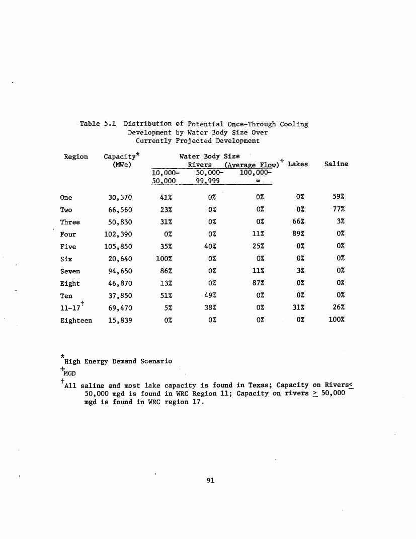
Table 5.1 Distribution of Potential Once-Through CoolingDevelopment by Water Body Size Over

Currently Projected Development

Region Capacity*(MWe)

One

Two

Three

Four

Five

Six

Seven

Eight

Ten

11-17±

Eighteen

30,370

66,560

50,830

102,390

105,850

20,640

94,650

46,870

37,850

69,470

15,839

Water Body SizeRivers (Average Flow)

10,000- 50,000- 100,000-50,000 99,999

41%

23%

31%

0%

35%

100%

86%

13%

51%

5%

0%

*High Energy Demand Scenario

MCD+

0%

0%

0%

0%

40%

0%

0%

0%

49%

38%

0%

0%

0%

0%

11%

25%

0%

11%

87%

0%

0%

0%

Lakes

0%

0%

66%

89%

0%

0%

3%

0%

0%

31%

0%

Saline

59%

77%

3%

0%

0%

0%

0%

0%

0%

26%

100%

All saline and most lake capacity is found in Texas; Capacity on Rivers<50,000 mgd is found in WRC Region 11; Capacity on rivers > 50,000mgd is found in WRC region 17.

91

I

References

Chapman, D., Mount, T. and Tyrrell, T. "Electricity Growth: Implicationsfor Research and Development." Testimony before the Committee on Sciencefor Astronautics, U.S. House of Representatives, June 16, 1972.

Croley, T.E., Patel, U.C., and Cheng, MS., Iowa Institute of HydraulicResearch, University of Iowa, "The Water and Total Optimizations ofWet and Dry-Wet Cooling Towers for Electric Power Plants," I.I.H.R.Report No. 163, January, 1975.

Dickey, W.B. and Cates, R.E., "Managing Waste Heat with the Water CoolingTower," Marley Company, Mission, Kansas, 1973.

Dupree, W. and West, R. "United States Energy Growth Through 2000," U.S.Dept. of Interior, Washington, D.C. Dec. 1972.

Edison Electric Institute Yearbook for 1975, EEI, New York, 1976.

Edison Electric Yearbook for 1977, EEI, New York, 1978.

Electric Power Research Institute (EPRI) "Fuel and Energy Price Forecasts,"

Febuary, 1977.

Electric Power Research Institute, "Regional Reference Energy Systems,"Topical Report A-462 by Brookhaven National Laboratory, June, 1977.

Electric Power Research Institute, "Demand 77, the EPRI Annual EnergyForecasts and Consumption Model," Special Report EA-621-SR, (Preview inEPRI Journal, December, 1977)

Energy Research and Development Administration, "A National Plan for EnergyResearch Development and Demonstration: Creating Energy Choices forthe Future," ERDA-48, Washington, D.C., June, 1975.

Energy Research and Development Adminitration (ERDA), "Energy Modelling andForecasting Program at ERDA," Washington, D.C., June, 1976.

Environmental Protection Agency (EPA) Quality Criteria for Water, WashingtonD.C. July, 1976.

Federal Energy Regulatory Commission (Data sets obtained thru PersonalCommunication) 1977.

Federal Power Commission, "Proposed Generating Capacity Additions, 1977-1986,"September, 1977.

"Federal Water Pollution Control Act Amendments of 1972," (FWPCAA) PublicLaw 92-500, 86 Stat. 816 et seq.,33 U.S.C. 1151 et seq., October, 1972.

Fryer, B.C., "A Review and Assessment of Engineering Economic Studies of DryCooled Electrical Generating Plants," BNWL-1976, Battelle, Pacific NorthwestLaboratories, Richland, Washington, March, 1976.

92

Hendrickson, P.L., "An Overview of Issues Affecting the Demand for Dry andWet-Dry Cooling for Thermal Power Plants," Prepared for the U.S. Depart-ment of Energy under Contract No. EY-76-C-06-1870, Battelle, PacificNorthwest Laboratory, September, 1978.

Hudson, E.A. and Jorgenson, D.W., "U.S. Energy Policy and Economic Growth,1975-2000," Bell Journal of Economics and Management Science,Autumn, 1977.

Jahnig, E.C. and Shaw, H. "A Comparitive Assessment of Flue Gas TreatmentProcesses," Exxon/GRU.3DJAO.77 April, 1978.

Meier, P.M., McCoy, T.H., Rahman, J., "Issues in the Future Supply ofElectricity to the Northeast," Brookhaven National Laboratory, June, 1976.

National Coal Association Steam Electric Plant Factors for 1975, Washington,D.C., 1976.

Peterson, D.E., Bailey, G.F., Engstrom, S.L. Schrotke, P.M., "Thermal Effectsof Projected Power Growth: The National Outlook," Hanford EngineeringDevelopment Laboratory, Richland, Washington, July, 1973.

Sebald, J.F., "Site and Design Temperature Related Economics of NuclearPower Plants with Evaporative and Non Evaporative Cooling Tower Systems,"Gilbert Associates, Report to ERDA No. 100-2392-1, January, 1976.

Spencer, D. and Gildersleeve, ., "Market Potential for New Coal Technologies,"EPRI Journal, May, 1978.

Teknekron, "Water Pollution Abatement Technology: Capabilities and Costs,"Vol. II, prepared for the National Commission on Water Quality, March, 1976.

United Engineers and Constructors, Inc., "Heat Sink Design and Cost Studyfor Fossil and Nuclear Power Plants," prepared for the U.S. AtomicEnergy Commission under Contract No. AT(11-1)-2226, Issued as WASH-1360,July, 1974.

U.S. Department of Commerce, "Climatic Atlas of the United States," Environ-mental Science Services Administration, Environmental Data Service, 1977.

U.S. Department of Energy, "Energy Data Report; Cost and Quality of Fuelsfor Electric Utility Plants," (for March, 1978), August, 1978.

U.S. Water Resources Council, "The Nation's Water Resources; The SecondNational Water Assessment," (Preliminary), Part V (Regional AssessmentSummaries), April, 1978.

U.S. Water Resources Council, "The Nation's Water Resources; The SecondNational Water Assessment," (Preliminary), Vol. A-Z (Water Supply andUse Data), April, 1978.

93

U.S. Water Resources Council, Energy and Related Water Requirements,Appendix H, April, 1977.

Utility Water Act Group (UWAG), "Comments on EPA's Proposed §304 Guidelinesand §306 Standards of Performance for Stream Electric Power Plants,"Vol. I Section II, June, 1974.

Utility Water Act Group (UWAG), "Thermal Control Cost Factors - Status ofPresent and Planned Water Intake and Discharge Systems for the ElectricUtility Industry: The Results of a Survey," Submitted to the UnitedStates Environmental Projection Agency, June, 1978.

94

Appendix A

Discussion of Alternative Siting Patterns

A.1 Introduction

This appendix will describe the development of the alternative

future plant siting patterns outlined in Chapter Two. The reader will

recall these siting patterns are used to estimate what proportions of

the new capacity to be installed between 1975 and the year 2000 could

use once-through cooling were thermal controls relaxed or removed.

The purpose behind developing a number of such siting patterns is to

explore the possible ways new electric generating stations could be

located on large bodies of water for the purpose of using once-through

cooling while at the same time preserving many of the other siting

characteristics utility planners consider when selecting a site from a

number of potential power plant sites.

Two methodologies are presented here: The first one is based on

an extrapolation of historic siting patterns, and is used in the develop-

ment of siting pattern number one. The second methodology is based on

the use of once-through cooling with a lenient thermal standard, and is

used in the development of siting patterns two through four.

A.2 Methodology Number One: Extrapolation of Historic Patterns

This siting pattern suggests where new steam electric power plants

could locate with respect to the plant water source based on siting

pattern trends observed before current thermal regulations were in effect.

The premise behind this pattern is that in the absence of thermal controls

new power plants could be sited on major bodies of water in the same

95

patterns that were observed prior to the promulgation of the current

thermal standards.

The analysis is performed by regional sub area, the smallest level

of detail for which we have accurate historic siting pattern data. By

examining patterns at the smallest level possible, we are able to capture

details of regional growth and regional cooling use patterns which would

otherwise be overlooked were the analysis performed for more aggregated

areas. For example, in 1975, the electric generating capacities in

subareas 307 and 308 made up, respectively, 11.3% and 11.2% of the

total capacity within Water Resource Council Region Three. By the

year 2000, however, the Federal Energy Regulatory Commission projects

that the share within subarea 307 will almost double to 20.7% while the

share within subarea 308 will fall to 2.2%. Furthermore, there are

fewer rivers that have historically supported once through cooling

in subarea 307 than in 308. With the disaggregated analysis we are

able to determine that the difference in growth rates between these two

subareas will lead to an overall reduction in the use of once-through

cooling for these two combined subareas, a result which would not be

found were we to lump these two subareas together. Thus the disaggregated

analysis allows us to examine changes in cooling system use which are

due wholly to differential growth rates among subareas having different

capacities to support once-through cooling.

This analysis proceeds along three lines: 1) forecasting the

number of megawatts of new capacity that will be installed in every

subarea for the two energy demand scenarios considered in this study;

2) assigning new capacity to major bodies of water; and 3) estimating the

96

minimum streamflow which will, from an engineering view of flow conditions

and reliability, support once-through cooling.

For the first task, we turn to the Federal Energy Regulatory

Commissions's (FERC) energy forecast which projects new capacity additions

by subarea for our high energy demand scenario. While the ERDA (low

energy demand scenario) projection does not break down new capacity additions

by subarea, we reduce every FERC subarea estimate proportionally until

the sum of the new additions for all the subareas in the contiguous

United States is equal to ERDA's national estimate.

The second task - assigning new capacity to major bodies of water -

consists of three steps. We first identify in every subarea the indivi-

dual rivers, lakes, and, if applicable, coastal sites on which generating

stations were located prior to 1973. We then determine what percentages

of the pre-1973 capacity in every subarea had been installed on each

water source. Finally, we use these percentages to assign to each water

source the projected capacity additions for each sub area. We assume

generating unit sizes will average 800 MWe for fossil plants and 1200

MWe for nuclear plants. The smallest unit size assigned to a water

source is 100 MWe and 500 MWe for fossil and nuclear plants, respectively.

Thus if the total amount of fossil or nuclear capacity to be assigned

to a water source is less than the respective minimum unit size, this

capacity is divided among the remaining water sources in that subarea.

The third task -- estimating the minimum streamflow which can

support once-through cooling -- compares the average annual flows

observed past units operating with once-through cooling with the flows

past units using closed cycle cooling prior to 1973. In its survey of

97

the steam electric power industry, National Economic Research Associates

(NERA) found that only 20% of the units operating with closed cycle cooling

before 1973 did so to comply with water quality standards (UWAG, 1978).

Therefore, we can assume that most plants that installed closed cycle

cooling prior to 1973 did so because the flow conditions past the plant

could not support once-through cooling with a sufficient reliability of

operation. We pproach the comparisons from two perspectives, both of

which give us similar results.

Our first approach is to analyze the ratio of the average annual

river flow versus installed capacity for plants operating with closed

and open cycle cooling. Figure A.1 illustrates the separation between

closed cycle and open cycle cooling systems as a function of the average

flow past known plants in operation before 1973. It is observed that

only one plant operated with closed cycle cooling when the flow at the

plant exceeded 10 MGD/MWe. On the other hand, fifteen of the ninety

six open cycle cooled plants were able to install once-through cooling

on rivers where flows were less than 5 MGD/MWe. Using this approach,

then, we do not think it is unreasonable to set the minimum annual

average streamflow to power ratio at which once-through cooling can be

supported at 10 MGD/MWe.

Our second approach is to analyze the ratio of the annual river

flow versus the design condenser flow. Figure A.2 illustrates the

separation between closed cycle and open cycle cooling systems as a

function of the river flow vs. design condenser flow. It is observed

that only four plants operated with closed cycle cooling when the river

flow was greater than 10 times the design condenser flow. Thirteen of

98

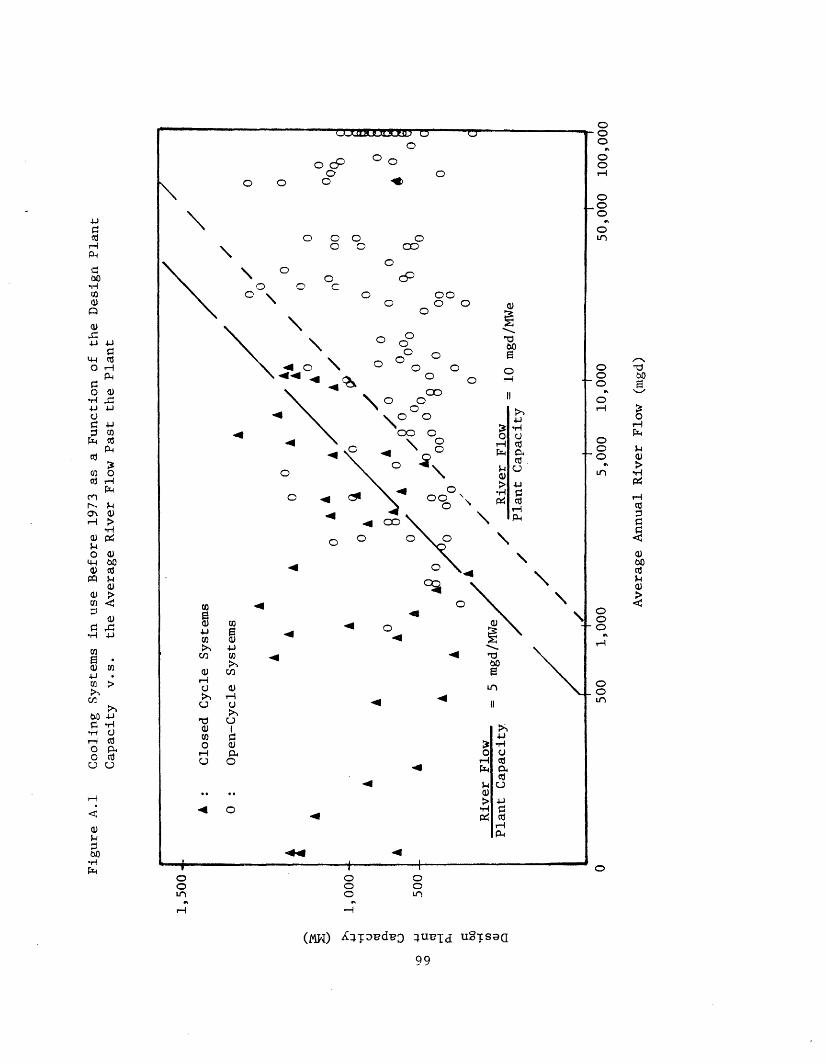
0

o cp O

O C O0 00

0 0 O

0 00 00) 0 0

0

O\

0

0

0O C

0 000 0 0

0

0 00

14 0 \ O 04 \ 0 00 0

\ 0' \ \0 o

\ \ooo4 0 o 0

\ 04 0~~40 4 0CD 0 \0

0 .4 00 \0

400%. o o0 0 0

4 0

-4 -4 0O

0

(0

Lr)

:30

H-

.4I4 40L I

0o0o

I0o

(MN) lToedv3 uiuUJ uTsaG

99

0)

0O-4

II

0-

00

ooH

_0o- o

0o-o

Ct( ,-c~o o bO0-(D

0.0 - r)CH wcoH

0)

0)toWcospQ0

-4O

H

0-o0OV)

r--4

-H

(0

4J 0)

0)

d -,.I .4.) .),..O H

P4o 0)r4-Ci

4-i 6U CoJ4.)

:3

eV.)

rr4

b)

C--to 4

0

Col

0 Uo

U4 U

0)

Xr4

:30

.H

0)

4-i.HUc.)

cdu

4.i

,

r.

Co

C.)CU0

,4-i

0)-)q

,C

0H-Q

CO

4i04.1Co

03)C-)

C,

a)040

4 0

4-i

C.)

4-i

H

0HL'-4

c_;,

{ {

O 00 0

O O OC) 00

O~~ O

000 0 00 00 0 0-400

0 0 0 00 0 0

,0

-4

C

0

0 O0

00 00

0

00 ooO0

O00000\RO )\O

0 40lC) -4

D 0< \4

0

0

0

0

'0

0

-4 C

00 0 .,)\^ O <<\~-

0\-4

C>0 C0'o

-4

o00

-4

o0'

(s;o) MoIa lOsupuoD U2TS~a

0

4

Iorr)ii0

U)

)r0,

C-

CIO.HQ)

4)OU

;4

c

o

-4

9C

o ;>

; Er5

4~'-- o

.,o) C)

,:94-JUC00

.,¥H0N

0

C

o

0-k-0

0-o

O0

0

0 -

00

o C)

r4)

.H

!-4c:

0

C-O C~

,-,OH

Q0

0

3 0O PW

14 fH03)

p U)

H 'd> a)

0U

\h u

i(I

-4

4-ioa):+

H

U)

CCaL

co0

U

C1)4-i

U)

a)ri

r.03

-4

000

Ij-7

o

0

.4

0ll�

ON 0

I00

the ninety-six open cycle cooled plants, on the other hand, were able to

install once-through cooling when the average annual riverflow was as low

as 5 times the design condenser flow. Using this approach, then, a minimum

annual average streamflow to design condenser flow ratio of 10 appears to

be a reasonable criteria for the use of once-through cooling.

Najjar (1978) found that for a wide range of economic parameters,

the optimal condenser flow rate for a nuclear plant is approximately

0.8 MGD/MWe and for a fossil plant, 0.7 MGD/MWe. We can now compare

the results of our two approaches towards finding the minimum streamflow

which will support once-through cooling: The criteria developed with

the second approach - an annual average streamflow at least ten times

the design condenser flow - translates into a streamflow vs. capacity ratio

of 8 MGD/MWe and 7 MGD/MWe for nuclear and fossil plants respectively.

We notice these ratios are very close to the streamflow vs. capacity

ratio of 10 which is found with the first approach. We conclude that

both approaches give answers that are reasonably close to each other.

The criteria of 10 MGD/MWe is the slightly more conservative of the two

criteria and is the one used in this study.

One criticism of the two approaches described above is that the

real criteria for the use of once-through cooling should be defined with

respect to flow conditions during low flow events (eg., the seven day -

ten year low flow) rather than during average flow events. A low flow

criteria is certainly the more accurate measure of the reliability with

which the river will provide condenser flows. Furthermore there are no

consistent functional relationships between average annual flow and say,

101

seven day - ten year low flow that can be uniformly applied for the

contiguous United States. For example, taking 7Q10 low flow data from

Technekron (1976) and average annual flow data from the Federal Energy

Regulatory Commission generating capacity forecasts (FERC, 1975) we

find that the ratio of low flow to average flow in all rivers is roughly

0.11 in Water Resource Council Regions One and Two, while this same ratio

is roughly 0.22 in Water Resource Council Regions Six and Seven.

Differences in climate, natural hydrology, and streamflow regulation

from on-stream reservoirs all contribute to the variation observed in

the ratio of low flow to average flow among regions. Therefore, it

appears that the average annual flow in a stream is not the best measure

of the stream's capacity to support once-through cooling.

While we would prefer to use the seven day - ten year low flow in

the development of our criteria for the use of once-through cooling on

rivers, these measurements are not readily available with good accuracy

on most streams where once-through cooling is found. Thus while the

average annual flow is an imperfect measurement the fact that it is

readily available plus the fact that our two approaches show a fairly

clear and consistent separation between closed cycle and open cycle

cooling based on this flow persuades us to use the average flow in our

criteria for the use of once-through cooling.

A.3 Methodology Number Two: Maximize Once-Through Cooling Within LimitsImposed by Lenient Thermal Regulations

This methodology, which is used in siting patterns 2,3, and 4,

allows once-through cooling at new plants provided lenient thermal

regulations will be met. The basic methodology is to determine how

102

many megawatts of new electric generating capacity cculd be installed

with once-through cooling cn major bodies of water subject to a somewhat

lenient thermal regulation limiting the waste heat induced temperature

rise to less than 5F. For rivers, this hypothetical standard must be

met during the low monthly flow expected every twenty years.

To llustrate how this standard of performance represents a

"lenient" thermal control it is necessary to compare it with existing

standards. The thermal standards for most states will allow thermal

discharges which will increase the water temperature above its natural

level by no more than 3 - 5F at the edge of a mixing zone. Typically,

the mixing zone in rivers may not involve more than of the flow or

cross-sectional area of the stream. In addition, states typically

have more stringent standards for waters classified as cold water

fisheries (e.g. trout streams); there the maximum temperature rise

is from 0° to 1°F. Furthermore, most states set a maximum absolute

temperature (Tmax) for bodies of water. For warm water fisheries this

Tmax ranges from 83° to 93°F and for cold water fisheries the Tmax

ranges from 65° to 68°F (depending on the latitude at which the body

of water is located). Finally, most states limit the temperature rise

in lakes and reservoirs to 3°F in the epilimnion and in marine and

estuarine environments to 4F, with the further restriction that during

reproductive seasons the temperature rise may not exceed 1.5°F.

We can now see how our hypothetical thermal standard serves as

a rather lenient restriction on once-through cooling. First, our allo-

wable temperature rise is equal to the highest currently found in almost

all states, and applies to both warm and cold water fisheries. Second,

103

our mixing zone extends across the entire river and not just across

one-quarter of the cross-section. That is, while the temperature in the

remaining 3/4 of the stream would be less than 5F if our mixing zone

were to follow the conventional standards,our standards allow the

temperature in the full section of the stream below the discharge to be

raised by 5F. Finally, we do not impose a constraint on the maximum

temperature allowed in the river. That is,under the current standards the

natural river temperature during summer months may be equal to or

greater than the Tmax limit during low flows; during these periods

plants are not allowed to make additional thermal discharges into that

river. Our regulation, however, imposes no such restriction.

Our methodology proceeds as follows: taking a standard plant

size of 500 MW we determine how many B.T.U.'s of the incoming energy to

the plant boiler will be rejected as waste heat to a water source, For

a fossil plant operating with a 38% turbine conversion effeciency and a

15% "loss" between the boiler and the turbine due to stack and in-plant

losses the ratio of waste heat to final electric output is:

waste heat 6 BTU '-.38-.15 6 BTU1. MW = 3413 x 10 2 - 38 4- x 10 M

For a nuclear plant operating with a 32% turbine efficiency and 5%

in-plant losses, this ratio is:

2.waste heat = 3.413 x 106 BTU (-. 32- 05= 6719 x 106 BTUMW .32 MWH

On the average then the ratio of waste heat to final electric output is

approximately:

104

3. (6.719 + 4.221) x 106 = 5.47 x 106 BTUMWH MWH

The temperature of the river just downstream of the plant, assuming

the waste heat is completely mixed, is:

6 BTU °F-Ft35.47 x 10 x 500 M 12170 sec

4. AT MixED 12170 62.4- lb BTU_ 3 s QecWlow Ft3

62.4 lb BTU x Q Ft x 3600 eFt lb-OF low sec Hr sec

where Qlow = the low monthly flow for the segment of a

particular ASA.

river within a

The residual temperature rise is defined as the

the 5F standard and the mixed temperature:

difference between

5. ATRES = 5 - ATMIXED

The distance downstream required to dissipate the excess heat is

proportional to the ratio ATRES/5°, i.e.,

ATRES K W x6. 50 = K )5 pC.Qlow

where K = surface heat transfer coefficient (BTU/Ft3-°F-sec)

W = average river width (Ft)

x = the distance required to bring the water temperature from the

initial 5F just downstream of the reference plant to AT RES(Ft)

pc = 62.4 BTUJ/Ft3 oF

Solving for x:

105

In ATR ] ' Qlow ' 0c7. RES

. X= K*W

Thus, Eq. (7) solves for the minimum spacing between 500 MW plants

operating with once-through cooling such that the 5F temperature rise

standard is not violated on a river having a width W and a low flow Qlow'

The total once-through cooling capacity of the river within an aggregated

sub-area is:

8. -T Capacity = (L/x) 500 MW

where L = the length of the river within the ASA (Ft)

At lake sites the maximum once-through capacity is determined by

calculating the number of acres of lake surface area per MW necessary

to remain within the 5F temperature rise limitation. Assuming the plant

efficiencies presented earlier, a 5F temperature rise, and a representative

surface heat transfer coefficient of K/pc = 2x10 5 Ft/sec, the surface area

required is:

lb BTU 2 -5 Ft BTU

Ft39. 62.4 -lb x 1 lBTF x5°F x AREA Ft · 2xlO = 1520Ft 3 16_OF xsec MW-sec

or

210. AREA 243,600 Ft /MW 5.6 Acres/MW

The size of every major lake listed in the FERC plant listings can be

found from U.S.G.S. guides and atlases, and thus the maximum once-

through cooling capacity for each lake may be determined. We limit the

number of megawatts using once-through cooling at any site to 5000 1W

unless the FERC listing indicates a utility has plans to install a larger

106

capacity at a particular lake site.

For saline sites the number of megawatts that may be installed

with once-through cooling is determined by the geometry of the local

coastline. Coastal sites for which discharges are made directly into

the open area are allowed 5000 MW per site. Partially closed and small

bays are allowed 3000 MW per site, and estuaries and almost completely

enclosed bays are allowed 1000 MW of once-through cooled capacity per

site. Saline sites are examined with the aid of maps to determine

coastline configuration.

To summarize so far, our preceeding methodology allows us to deter-

mine, for every river segment, lake and (if applicable) coastal site

in every aggregated subarea, the number of megawatts of new capacity

cooled with once-through cooling that can be installed under the hypo-

thetical thermal regulation.

In siting pattern #2 we do not relocate any capacity, but simply

switch as many plants as possible from closed cycle cooling to open

cycle cooling on every river segment, lake, and coastal region with the

limits established earlier. [eg. Eqs. 8 & 10.] However, even after

this has been accomplished some river segments, lakes, or coastal regions

in an ASA may have once-through cooling capacity remaining, while others

within the ASA may yet have capacity that will be required to install

closed-cycle cooling. In siting pattern #3, then, we allow capacity to

be transferred within every ASA in order to maximize the number of

megawatts operating with open-cycle cooling. After this modification some

ASA's still have unused once-through cooling potential, and so in siting

pattern #4 we allow capacity to be transferred between ASA's (but always

107

within the larger WRC region itself) in order to maximize the use of once-

through cooling by new plants.

108

Appendix B

Discussion of Economic Parameters

B.1 Introduction

This appendix presents the development of a number of economic

parameters used in Chapter 3 of this report. Fuel prices, expected

fuel price escalation rates, replacement energy prices and expected

replacement energy escalation rates are all found in the literature we

have referenced earlier, and are therefore not discussed here. However,

there are three parameters that are not readily available per se, but

can be derived from existing information: the average utility industry

inflation free discount rate; the average utility industry inflation

free fixed charge rate; and the inflation free plant cost escalation

rate.

In this appendix we will outline both the arguments for using the

approaches that we do and the procedures themselves. It is our intention

that this section will serve as a guide to other investigators in this

field.

B.2 The Derivation of the Real Discount Rate

Our estimate of the average utility industry inflation free discount

rate is pegged to the nominal (market) rates of return historically

offered on utility bonds. The argument here is that investors will

demand a nominal rate of return from their bonds which will cover both

the real rate of return desired plus the inflation rate expected during

the life of the bond.

109

That is:

1. 1 + rN = (1 + DR) (1 + I) = 1 + DR+ + I + DR Ie e e

where: rN = Nominal rate of return

DR = Real dollar rate of return

Ie= Annual inflation rate expected over the lifetimee

of the bond

For I, DR < .1, then:

2. I DR << I + DRe e

Therefore, as a first approximation we can re-write Eq. (1):

3. r N z DR+ IN e

Because future expectations are strongly influenced by past

behavior, we expect that the inflation rate investors anticipate for the

life of a bond is in some measure dependent on both the current inflation

rate and recent trends in the inflation rate. We propose the hypothesis

that the anticipated inflation rate is equal to the equivalent inflation

rate over the previous "N" years. That is:

i j-1 J-2 j~~~~l-N I~/N4. I i {[(1 + i)-(l + i).(l + i 2 ) l (1 + i+ )] -1}e

where: I = Inflation rate expected during the life of bonde issued in year j

4

i = Inflation rate in year j

N = Number of preceeding years over which the average

is taken

110

Examining the seventeen year period from 1960 - 1976 we may compare

the gas and electric utility bond rates in any year with the average

inflation over the N-years preceeding that year [Edison Electric

Yearbook, 1977]. The following regressions are found:

25. rN= 0.0451 + .53 I ; R = .69; N = 1rNe

6. rN = 0.0418 + .63 I; R = .88; N = 2

27. rN = 0.0398 + .71 I ; R = .93; N = 3

e

28. rN = 0.0399 + .76 I ; R = .93; N = 4

e

If an underlying hypothesis is correct then, from Eq. (3), we

would expect the coefficient for the variable I in Eqs. (5) - (8) toe

equal 1.0. While this condition is not met, thereby weakening the argument

of our hypothesis somewhat, we observe that for Eqs. (7) and (8) the

observed coefficients are not too far off from the expected value. There-

fore, while our hypothesis may have some weak points it nevertheless

offers a reasonable explanation of the true behavior affecting utility

bond rates. Furthermore, we observed that the y-intercept in Eqs. (5) - (8)

tends towards a value of 0.04. As the y-intercept in our regression

equations corresponds to the real discount rate, DR, in Eq. (3),

we conclude that the inflation free rate of return for the steam electric

power industry is approximately 4.0%.

B.3 The Derivation of the Inflation Free Fixed Charge Rate

We wish to remove the inflation component incorporated in the

conventional utility industry fixed charge rate from that latter parameter.

To do this we propose the argument that the real dollar fixed charge rate

should offer the same present valued gross return on capital when dollar

111

flows are discounted by the inflation free interest rate as they would

when the nominal fixed charge rate is used and dollar flows are discounted

by the nominal interest rate. This argument says:

M M

9. FCR r .CAPITAL = Y

j=1 (i+DR)j j=l

where: FCRr = Real

CAPITAL = Init

FCRN = Nomi

M = Plan

DR = Real

r = Nomi

FCRN CAPITALFCl+rN)J(l+rN) '

dollar fixed charge rate

ial capital cost

nal fixed charge rate

t lifetime

dollar discount rate

nal discount rate

Rearranging and expanding the terms in Eq. (9) gives:

N [(l+r ) -1110. FCRr [(l+DR) -1] = FCRN [(+rN) -1

DR(1+)R)M rN(l+rN)M

The average interest rate on utility bonds during the seven-year

period from 1970-1976 was approximately 8.6% [Edison Electric Institute,

1977]. Taking the real discount rate, DR, equal to 4% and the plant life-

time equal to 40 years, we obtain:

rN11. 19.79*FCR = 11.17.FCR

Typical nominal fixed charge rates for the steam electric utility

industry are in the range .17 - .19. Therefore, the inflation free fixed

charge rate is approximately 0.11.

112

B.4 The Determination of the Real Dollar Plant Cost Escalation Rate

Figure B.1 illustrates the recent behavior of plant escalation rates

for six broad geographical regions comprising the contiguous U.S.

[Edison Electric Institute, 1977]. This figure also shows recent movements

in the inflation rate. We observe there is some linkage between the

nominal plant cost escalation rates in these six regions and the overall

inflation rate, where the former almost always exceeds the latter. It

appears that the sharp rise in plant costs observed in 1974 is an

anomaly with respect to the rest of the record, and will be ignored in our

subsequent analysis. Two phenomena are found: 1) on the average, the

real dollar plant cost inflation rate was roughly 1.5% from 1969 - 1975;

2) no region has a history of plant cost escalation rates noticeably

different from the average. This almost negligible variation in the long-

term escalation rates among regions leads us to conclude that all regions

will share the same 1.5% real dollar plant escalation rate.

113

Regional Plant Cost Escalation Rates Over Time

- - : North Atlantic

- - : South Atlantic

- : North Central

----- : South Central

---- : Plateau

-... : Pacific

: Inflation Rate

114

26% _

24% _

22% -

wgo:4

o 12%

Cd

U

4 10%

8%

6%

4A

0

1969 1970 1971 1972 1973 1974 1975YEAR

Figure B. 1

.1

Work reported in this document was sponsored by the Department of Energyunder contract No E76-S-02-4114,AO01, This report was prepared as anaccount of work sponsored by the United States Government. Neither theUnited States nor the United States Department of Energy, nor any of theiremployees, makes any warranty, express or implied, or assumes any legalliability or responsibility for the accuracy, completeness, or usefulnessof any information, apparatus, product or process disclosed or representsthat its use would not infringe privately owned rights.