Economic impacts of long-term climate change on rice production and

farmers’ income: Evidence from computable general equilibrium

analysis

Yoji KUNIMITSU 1

Rural Development Planning Division, National Institute for Rural Engineering of NARO

(2-1-6, Kannondai, Tsukuba, Ibaraki, 305-8609, Japan)

Abstract

Future climate change will affect rice production, but whether these changes will be beneficial

or detrimental is unclear. The present study evaluates the effect of climate change on Japanese

rice production, farmers’ income, and regional economies by using the recursive-dynamic

regional computable general equilibrium (CGE) model. This model is associated with

crop-growth models, hydrological models, and global climate models. The simulation results

demonstrate that future climate change will increase Japanese rice production for the country as

a whole, but that the price of rice will decrease. As a result, the income of farmers in the rice

sector will decrease, despite the increase in production. Furthermore, climate change will not

benefit the northern and eastern parts of Japan, such as Hokkaido, Tohoku, and Kanto (including

Niigata Prefecture), where climate change will cause an increase in the total factor productivity

of rice. However, the western region will benefit, despite the decrease in production, and

consumer surplus in most regions will increase. As such, the impacts of climate change are

complicated and differ by region. To consider policy countermeasures against climate change,

the CGE model can provide useful information.

Discipline: Agricultural Economics

Additional key words: crop-growth model, global climate model, hydrological model,

recursive-dynamic regional CGE model, total factor productivity (TFP)

Corresponding author: ykuni@affrc.go.jp

Received

Running title: Climate change on rice production and farmers’ income

Introduction

Agriculture is highly dependent on climate conditions, such as temperature, solar

radiation, and precipitation, so future climate change will affect food production and may make

food supplies vulnerable. Stern (2006) predicted that agriculture in countries at higher

latitudes would likely benefit from a moderate level of warming (2–3° C), but that even a small

amount of climate change in tropical regions would cause yields to decline. Japan is located at

a relatively high latitude, so it is possible that Japanese rice production may benefit from future

climate change. However, an increase in yield does not necessarily mean an economic benefit.

To measure the economic effects of climate change, we need to evaluate changes in price and

quantity with considering market conditions. In this sense, a comprehensive evaluation of the

impact of climate change on the rice sector in Japan is important, both for making policy

decisions and from an academic interest point of view (Watanabe and Kume, 2009).

Changes in crop yields can be measured by field experiments and by using the objective

results of the crop-growth model based on biology. However, evaluating changes in the

quantity and price of agricultural products requires an economic model. Partial equilibrium

models can measure such changes, but they assume that agricultural markets do not affect the

rest of the economy (i.e., they are treated as exogenous). The computable general equilibrium

(CGE) model can depict inter-market relations and trade flows for the economy as a whole,

including the circular flow of income and expenditure. Therefore, they are better suited to

analyzing global effects on agricultural markets, as is the case with climate change (Palatnik and

Roson, 2011). Many previous studies have used the CGE model to analyze the effects of

climate change in Europe, the USA, and developing countries, as shown in the next section.

However, few CGE studies have evaluated the impact of climate change on the Japanese rice

sector.

The present study uses the CGE model to comprehensively evaluate the influence of

future climate change on Japan’s rice sector and regional economies. The features of this study

are as follows: (i) the recursive-dynamic regional CGE model is used to capture regional

differences in climate change; (ii) direct effects of climate conditions on rice productivity are

estimated using the crop-growth model and the hydrological model, in addition to the global

climate model (GCM), Model for Interdisciplinary Research on Climate (MIROC); (iii)

farmland is introduced into the model to consider restrictions on natural resources; and (iv) the

rice sector is separated from the agricultural sector, which is usually one aggregated sector in

the Japanese inter-regional input-output table, to enable us to specifically study the effects on

the rice sector.

Section 2 of the paper provides an overview of previous studies that have examined the

economic effects of climate change on agriculture. Section 3 explains the structure of the CGE

model, the data, and the simulation method used to measure the influences of climate change.

Section 4 presents the results of the simulation based on the CGE model. Finally, Section 5

concludes the paper, and discusses the possible policy implications resulting from the analysis.

Literature review and scientific question

Furuya and Koyama (2005) analyzed the influences of climate change using the global

econometric model. The rice yield function was estimated by considering temperature and

precipitation during the rice maturation period. Their results showed that a rise in future

temperatures, as a result of global warming, would increase rice production in most Asian

countries, including Japan. Their model assumed a linear influence of climate factors on

production levels, but the biology-based crop model has shown that climate factors affected rice

production in a non-linear way (Yokozawa, 2009; Iizumi, 2009). In other words, effects of

climate condition change from being positive to negative at a threshold value depending on

plant growth. Including such non-linear effects is important for useful long-term predictions.

Kunimitsu et al. (2013) estimated regression functions of total factor productivity for

Japanese rice production, including several causative factors such as socio-economic factors and

climate conditions. In their model, the potential impact of climate factors is shown by the

elasticity values of rice total factor productivity (TFP). Their results show that (i) the potential

impact of temperature and solar radiation via crop yield was high next to the economies of scale

represented by farm management scale per farm organization, and that (ii) climate factors in

addition to socio-economic factors cause regional gaps in rice TFP to increase over time.

Considering these features, we attempt to show how future climate change would influence

Japanese rice production and price by analyzing the rice market.

The CGE model has used market information to analyze agricultural production and trade

liberalization, as well as to run policy simulations. Saito (2002) analyzed the effects of a

farmland consolidation project on agricultural production. Kunimitsu (2009) measured the

economic effects of irrigation and drainage facilities on Japanese agriculture. The CGE

models used in these studies were static models. Bann (2007) and Masui (2005) used the

dynamic CGE model, but they did not use precise agricultural sectors and farmland as factors of

production in the model. In order to evaluate long-term climate change, the dynamic feature

needs to be installed in the CGE model.

With regards to CGE analyses of climate change, Lee (2009) quantitatively analyzed the

impact of climate change on global food prices and quantities by using a multi-sector CGE

model. Similar to Stern (2006), his analysis showed that climate change benefited the crop

yield of developed countries. Calzadilla (2011) also used a CGE model to analyze the effects

of climate change on agriculture in view of water use. In particular, they focused on climate

change and trade liberalization, and analyzed global agricultural production. Their results

showed that, although future climate changes will cause global agricultural production to

decrease as a result of water use, Japan and some countries may be able to increase production.

Trade liberalization reduced the negative impact of climate change on the welfare level. In

addition, it tended to reduce the use of water use in water scarce regions and increase the use of

water use in water abundant regions, all without using water market mechanisms. However, in

most previous analyses, the world economy was classified into a few regions, with Japan

merged with OECD countries such as the USA, Western Europe, and Australia. These broad

classifications make it very difficult to determine how the changes impact Japanese agriculture.

Therefore, a detailed multi-regional CGE model is needed to accurately and effectively analyze

rice production in Japan.

As shown in the above previous studies, CGE models have great potential as a way to

evaluate the effect of future climate change on agriculture by considering price and quantity in

the market. Since previous CGE analyses have rarely been applied to the issue of climate

change and the Japanese rice market, it will be interesting to evaluate whether future climate

change is beneficial or detrimental to Japanese rice production.

Method

1. Structure of the recursive-dynamic regional CGE model

The model used here is the recursive-dynamic CGE model, with multiple regions. The

structure of our model is based on the work of Bann (2007), which uses GAMS (GAMS

Development Corporation) and MPSGE (a modeling tool using the mixed complementary

problem), as developed by Rutherford (1999). The GAMS code of the model is shown in the

APPENDIX. The major modification points of this model are as follows.

The cost functions derived from the production functions are defined as nested-type CES

(constant elasticity of substitution) forms. Figure 1 shows the structure of the cost function.

The parameter (s) represents the substitution elasticities, and the values are set to the same as

those used by Bann (2007). The elasticity of substitution of farmland to other input factors,

which was not used in Bann (2007), is assumed to be 0.1 for agriculture. Egaitsu (1985)

concluded that the substitutability of farmland for other input factors was low, but the

substitutability between capital and labor was high, according to empirical evidence on Japanese

rice production from several studies. Based on these findings, we assumed that farmland is a

semi-fixed input for agricultural production and cannot really be substituted by other factors.

TFPr,t and TFP0 in the production functions refer to the total factor productivity in year t

and the substantial level (TFP0 = 1 in this study), respectively. With respect to climate change,

TFP varies per year, and this factor is defined in previous studies as follows (Kunimitsu, 2013):

54321

,,,,0, tr

DRtrtrttrtr CFICQICHIKKMATFP r

(1)

Here, MA is the management area per farmer, representing economies of scale, and KK is

knowledge capital stocks accumulated through research and development (R&D) investments.

CHI, CQI, and CFI are the crop-yield index, crop-quality index, and flood index, respectively.

The β’s represent the coefficients estimated from the panel data regression analysis, with β0 = –

2.7014, β1 = 0.3285, β2 = 0.0590, β3 = 0.1824, β4 = 0.0863, and β5 = –0.0277. DR is a dummy

variable, taking the value 1 for Hokkaido, and 0 otherwise. As explained in Kunimitsu et al.

(2013), CHI, CQI, and CFI are also defined by the crop-growth model, crop-quality model, and

hydrological model with using climate conditions, such as temperature, solar radiation, and

precipitation.

< Fig. 1 >

Consumption is defined by the CES function with a substitution elasticity of 0.5 (see

Figure 2). The elasticity values of substitution in the consumption, import, and export

functions are set to be the same as those used by Bann (2007), which were based on the GTAP

database. The government consumption and government investment (Figs. 3) are Leontief

type fixed share function.

< Fig. 2, Fig. 3 >

To form the recursive dynamic path, the capital stock equation is defined by annual

investment (I) and disposable rate (δ= 0.04), as follows.

trtrtr IKK ,1,, )1( δ (2)

In this model, K shows capital supply and is defined for every year from I, which is

endogenously defined by the CGE model.

2. Data and simulation method

To calibrate the parameters of the model, the social accounting matrix (SAM) was

estimated on the basis of Japan’s 2005 inter-regional input-output table. To analyze rice

production more precisely, the rice sector was separated from the aggregated agriculture,

forestry, and fishery sectors in the IO table, based on regional tables (404 × 350 sectors). Then,

the sectors were reassembled into 14 sectors: rice; other agriculture, forestry, and fishery;

mining and fuel; food processing; chemical products; general machinery; electric equipment and

machinery; other manufacturing; construction; electricity and gas; wholesale and retail sales;

financial services; and other services. Regions were also reassembled into eight regions:

Hokkaido; Tohoku; Kanto, including Niigata Prefecture; Chubu; Kinki; Chugoku; Shikoku; and

Kyushu, including Okinawa.

The factor input value of farmland, which was not shown in the Japanese I/O Table, was

estimated using farmland cultivation areas (Farmland statistics, Ministry of Agriculture, Forestry,

and Fishery, and every year) and multiplying the areas by farmland rents. Then, the farmland

factor input value was subtracted from the operation surplus in the original IO table. The value

of capital input was then composed of the rest of operation surplus and the depreciation value of

capital.

To simulate the macroeconomic impacts of climate change, we considered the following

cases.

CASE 0: This case represents a situation of business as usual (BAU), and is used as a base line.

In this case, farmland supply and labor supply in each region were fixed at the present levels

shown in the SAM data. The technological growth rate of the Japanese economy was assumed

to be 0 so as to show only the effects of climate change. The TFP of rice production was also

set to 1, showing no progress in technology and no change in climate conditions.

CASE 1: This case represents future climate change that only affects rice production. The

exogenous variables other than TFP were set to the same values as in CASE 0. Future rice

TFP levels were calculated using Eq. (1), as shown in Figure 4. These TFPs include the

influence of both socio-economic factors (MA and KK) and climate factors (CHI, CQI, and CFI).

To simulate the pure effect of the climate factors, the TFP in each region was divided by TFP′ =

f (MA, KK), which shows TFP changes resulting only from socio-economic factors, with the

same estimated coefficients as Eq. (1) (see Figure 5). Changes in climate factors were

predicted using the crop-growth model, crop-quality model, and hydrological model, along with

the projection results of MIROC, high-resolution version 3.0 (K-1 Model Developers, 2004).

The greenhouse gas emission scenario was A1B which shows balanced growth with rapid

economic growth, low population growth, and the rapid introduction of more efficient

technology in the Special Report on Emission Scenario (SRES) (Nakicenovic and Swart, 2000).

< Fig. 4, Fig. 5>

Results

To ensure the stability of the simulation results, a sensitivity analysis was conducted by

changing the substitution elasticities of demand and inter-regional material demand as

intermediate inputs. The degree of impact changed, but the directions of the changes were the

same for all variables. Therefore, the results presented below are reasonably stable and

common, as long as there is no change to the economic structure.

1. Rice production

Figure 6 shows chronological changes in rice production, estimated using the CGE model

with TFP changes. Although the exogenous variables were set as the status quo, rice

production in CASE 0 increased as a result of an increase in capital stocks, which were

endogenously accumulated by annual investment. Hence, the difference between CASE 1 and

CASE 0 shows only the effects of changes in climate factors.

In accordance with the TFP changes shown in Figure 5, climate change increased rice

production in the north and eastern regions, such as Hokkaido, Tohoku, and Kanto (including

Niigata Prefecture). However, rice production decreased in the western regions, such as Kinki,

Chugoku, Shikoku, and Kyushu. Annual production fluctuated under climate change, but the

average growth rates in Tohoku and Kanto were higher than other regions, so the scale of

vertical axis in these regions was double that of the other regions. In these two regions, rice

production amount was relatively large, so there were some capacities for the economies to

allocate production resources to other sectors. In contrast, the growth rates of rice production

in Kinki and Shikoku were low, because rice production in these two regions was small in

comparison to other agricultural sectors and other industries.

Even in the north and eastern regions, production levels fell below the CASE 0 level in

some years, with the exception of Hokkaido. Rice production in Hokkaido benefitted in all

years, even under bad climate conditions. The western regions experienced worse production

than CASE 0 in many years, but the difference between CASE 1 and CASE 0 fluctuated over

time. This degree of fluctuation degree increased after 2050. Until then, climate conditions

tended to increase the crop yield, but decrease crop quality. However, from the 2050s onwards,

when temperatures were frequently beyond the threshold level, climate conditions decreased

both crop yield and crop quality, showing agglomeration effects. Tohoku, Kanto, and Kyushu

showed wider fluctuations in production, because their rice production amounts were larger than

other regions. In the western regions, the decreases in crop yield and crop quality became

serious during the latter period of the simulation, largely because of negative agglomeration

effects of temperature to rice TFP via rice yield and quality.

Table 1 shows the sum of the annual production figures from 2005 to 2100. The

northern and eastern regions show positive production amounts, and can increase their total

production beyond that of CASE 0. The increase in production accelerated in these regions in

the latter period of the simulation. On the other hand, climate change had a negative effect on

the western regions, and these effects became stronger in the latter part of the simulation period

because of above-mentioned agglomeration effects of temperature. From these results, it is

clear that the effects of climate change on rice production differ according to location.

Figure 7 shows price changes in the rice sector resulting only from climate change. In

contrast to production quantity, the price of rice decreased in the northern and eastern regions,

but increased in the western region. Since rice consumption does not really increase, even

after a decrease in price, the price dropped in those regions where production increased, but rose

in those regions where production decreased. This is because price elasticity of rice demand is

low, which is common in food, and an imbalance in supply and demand is reflected in a sharp

change in price. Such situations may be similar in other agricultural sectors, but no climate

simulations were conducted for any other sectors.

< Fig.6, Fig.7, Table 1 >

2. Prices of input factors and farmers’ income

Table 2 shows factor price changes in the rice sector. The directions of the changes in

factor prices were the same as those of the rice prices in all regions. That is, the northern and

eastern regions, where the rice price decreased, experienced a decrease in factor prices, and the

western regions experienced an increase in factor prices. Changes in farmland rental rates

were larger than other factors, because we assumed that substitution elasticity of farmland to

other factors was low. In addition, farmland is immobile, and used only for agriculture, so rice

price changes in production within the region directly affect farmland rental values.

Table 3 shows sum of the rice farmers’ income (deflated by consumer price index), as

affected by rental rate, wage, and capital service price. The same trends were evident in both

agricultural farmers’ income including other agricultural sectors, and rice farmers’ income

excluding capital depreciation value. However, these results were omitted here because of a

limit in space.

Farmers’ income decreased in the northern and eastern regions, where rice production

increased after the climate change, but farmers’ income in the western regions (decreased rice

production) increased. This happened as a result of rice price changes, which changed in the

opposite direction to the changes in rice production. In other words, the degree of price

changes was larger than the degree of production changes.

Farmers’ income across the whole country decreased as a result of the climate change.

This negative impact on overall income also became more serious in the latter period of the

simulation. Therefore, overall, climate change does not benefit farmers.

< Table 2, Table 3 >

3. Gross regional production and social welfare

Table 4 shows the sum of gross regional production (GRP) during the simulation periods.

In contrast to farmers’ income changes, changes in GRP were positive in Kanto and Chubu.

Kanto and Chubu have sizeable manufacturing industries, so the demand for manufacturing and

service goods, which could increase by a shift of production factors from rice sector after the

increase in rice TFP, became concentrated in these regions. Overall, the total GRP for the

country increased after the climate change. However, Chugoku and Shikoku experienced

minor losses in GRP after the climate change, because the manufacturing sector is relatively

weak in these regions.

Table 5 shows the sum of the equivalent valuation (EV) corresponding to the consumer

surplus and the social welfare level. The EV in most regions increased after the climate

change, and even Chugoku and Shikoku, where the GRP effects were negative, experienced an

increase in welfare. The difference between EV and GRP is mostly reflected in income effects,

so the negative income effects overwhelmed the substitution effects caused by the climate

change in these regions. The EV in Hokkaido and Tohoku became negative, but such negative

effect was much smaller than negative effect in income. Therefore, social welfare levels of

non-farmers increased in these regions, although it could not overcome farmers' income loss.

Overall, the EV change for the country as a whole was positive; therefore, climate change

benefits Japanese consumers.

< Table 4, Table 5 >

Discussion and conclusion

This study used the CGE model to comprehensively evaluate the influence of future

climate change on Japan’s rice sector and regional economies. We built the recursive-dynamic

CGE model using multiple regions associated with the crop-growth model, crop-quality model,

and hydrological model. This CGE model was used to simulate the future impact of climate

change. Based on our simulation results, there are several policy implications.

First, future climate change increases rice production for the country as a whole, but

causes rice prices to decrease. As a result of these reverse effects, farmers’ income in the rice

sector decreases, despite the increase in production amount. This happens because of the

inelastic demand for rice, which does not increase very much, even after a decrease in price.

In the northern and eastern parts of Japan, such as Hokkaido, Tohoku, and Kanto (including

Niigata Prefecture), rice production increased after the climate change, but rice prices and

farmers’ income decreased. In contrast, the western regions experienced an increase in price

and income after the climate change, despite the decrease in production. Therefore, climate

change benefits regions where the total factor productivity for rice decreases in extremely high

temperatures. These effects are somewhat counterintuitive, as they show that farmers’ income

cannot be improved in the area where climate change primarily increases rice TFP. In the real

data, such effects of climate change may be too small to observe, because the Japanese rice

sector is small when compared to other industries. Of course, such effects are highly

dependent on the parameter values, such as substitution elasticities, in the CGE model.

Therefore, it is important to use an economic model for policymaking and to quantify the

parameters using econometric methods and precise data.

Second, the GRP and social welfare level measured by the EV change may improve after

based on the most recent published I/O table, so using more recent data is necessary. It is

hoped that new I/O data will soon be available. Third, because of computational ability and

the model structure, the CGE model used here has 14 sectors and 8 regions. Improving the

model structure to handle more precise sectors and regions is important. In addition, other

possible future tasks are to analyze the effects of climate change on other agricultural sectors,

forestry, and fishery, to measure the effects by considering trade liberalization, and to evaluate

policy instruments against future climate change.

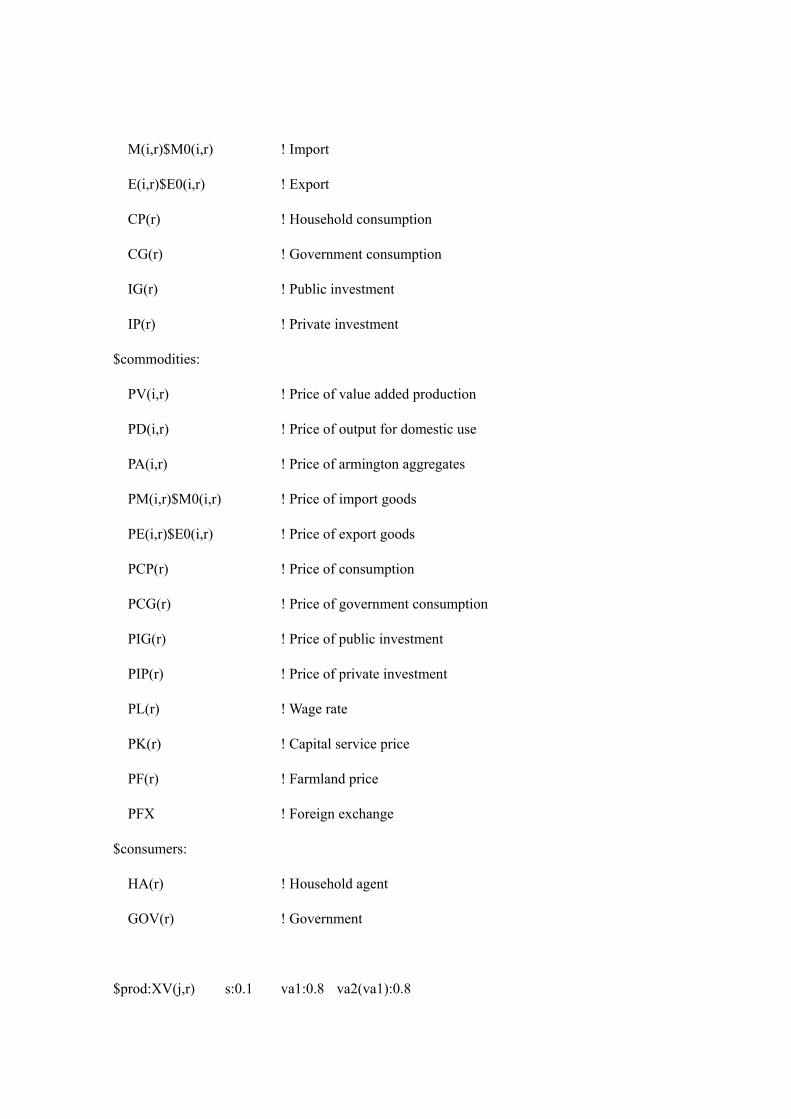
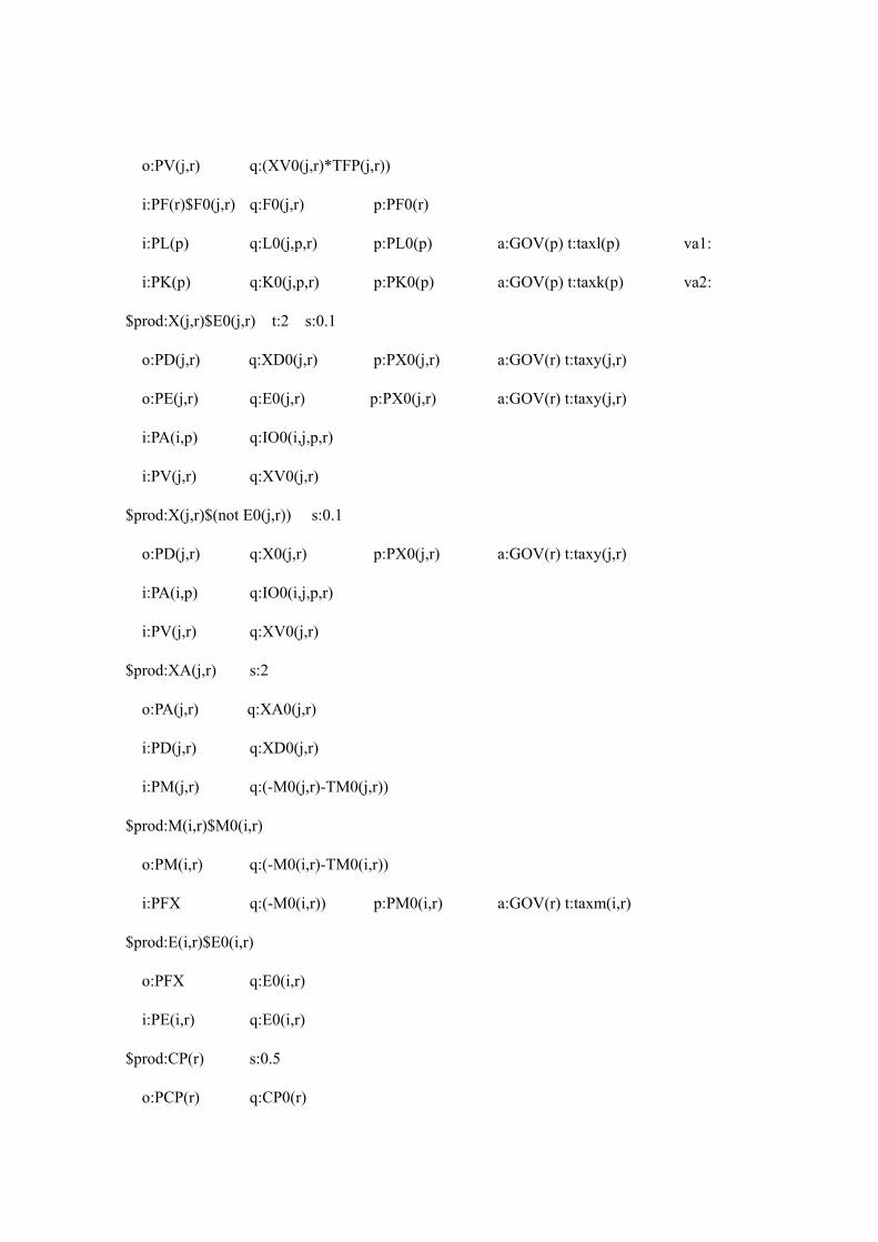
Appendix

The CGE model used here were composed by using GAMS with MPSGE solver. The

syntax of MPSGE is shown in Rutherford (1999). In equations, suffixes of i and j show sector

classification, suffixes of p and r show regions. Variables used in the model are explained in

Table A-1.

*===========================================================

* MPSGE model

*===========================================================

$ontext

$model:MRM_jpn

$sectors:

X(i,r) ! Production

XV(i,r) ! Value added production

XA(i,r) ! Armington aggregate

M(i,r)$M0(i,r) ! Import

E(i,r)$E0(i,r) ! Export

CP(r) ! Household consumption

CG(r) ! Government consumption

IG(r) ! Public investment

IP(r) ! Private investment

$commodities:

PV(i,r) ! Price of value added production

PD(i,r) ! Price of output for domestic use

PA(i,r) ! Price of armington aggregates

PM(i,r)$M0(i,r) ! Price of import goods

PE(i,r)$E0(i,r) ! Price of export goods

PCP(r) ! Price of consumption

PCG(r) ! Price of government consumption

PIG(r) ! Price of public investment

PIP(r) ! Price of private investment

PL(r) ! Wage rate

PK(r) ! Capital service price

PF(r) ! Farmland price

PFX ! Foreign exchange

$consumers:

HA(r) ! Household agent

GOV(r) ! Government

$prod:XV(j,r) s:0.1 va1:0.8 va2(va1):0.8

o:PV(j,r) q:(XV0(j,r)*TFP(j,r))

i:PF(r)$F0(j,r) q:F0(j,r) p:PF0(r)

i:PL(p) q:L0(j,p,r) p:PL0(p) a:GOV(p) t:taxl(p) va1:

i:PK(p) q:K0(j,p,r) p:PK0(p) a:GOV(p) t:taxk(p) va2:

$prod:X(j,r)$E0(j,r) t:2 s:0.1

o:PD(j,r) q:XD0(j,r) p:PX0(j,r) a:GOV(r) t:taxy(j,r)

o:PE(j,r) q:E0(j,r) p:PX0(j,r) a:GOV(r) t:taxy(j,r)

i:PA(i,p) q:IO0(i,j,p,r)

i:PV(j,r) q:XV0(j,r)

$prod:X(j,r)$(not E0(j,r)) s:0.1

o:PD(j,r) q:X0(j,r) p:PX0(j,r) a:GOV(r) t:taxy(j,r)

i:PA(i,p) q:IO0(i,j,p,r)

i:PV(j,r) q:XV0(j,r)

$prod:XA(j,r) s:2

o:PA(j,r) q:XA0(j,r)

i:PD(j,r) q:XD0(j,r)

i:PM(j,r) q:(-M0(j,r)-TM0(j,r))

$prod:M(i,r)$M0(i,r)

o:PM(i,r) q:(-M0(i,r)-TM0(i,r))

i:PFX q:(-M0(i,r)) p:PM0(i,r) a:GOV(r) t:taxm(i,r)

$prod:E(i,r)$E0(i,r)

o:PFX q:E0(i,r)

i:PE(i,r) q:E0(i,r)

$prod:CP(r) s:0.5

o:PCP(r) q:CP0(r)

i:PA(i,p) q:CPS0(i,p,r)

$prod:CG(r) s:0

o:PCG(r) q:CG0(r)

i:PA(i,p) q:CGS0(i,p,r)

$prod:IG(r) s:0

o:PIG(r) q:IG0(r)

i:PA(i,p) q:IGS0(i,p,r)

$prod:IP(r) s:0.5

o:PIP(r) q:IP0(r)

i:PA(i,p) q:IPS0(i,p,r)

$demand:HA(r)

d:PCP(r) q:CP0(r)

d:PIP(r) q:IP0(r)

e:PL(r) q:LS0(r)

e:PK(r) q:(KS(r)*rk(r))

e:PF(r) q:FS0(r)

e:PCG(r) q:SG0(r)

e:PFX q:(-SF0(r))

e:PCP(rnum) q:(-TRF0(r))

$demand:GOV(r)

d:PCG(r) q:CG0(r)

d:PIG(r) q:IG0(r)

e:PCG(r) q:(-SG0(r))

$offtext

$sysinclude mpsgeset MRM_jpn

< Insert Table A-1 >

Acknowledgement

This study was supported by the research project "Economic evaluation of global warming"

(Japanese Ministry of Agriculture, Forestry and Fishery, project reader Dr. Jyun Furuya) and by

JSPS KAKENHI Grant Number (24330073), project reader (Dr. Suminori Tokunaga). The

authors sincerely express their gratitude for this support.

References

1. Bann, K. (2007) Multi-regional Dynamic Computable General Equilibrium Model of

Japanese Economies: Forward Looking Multi-regional Analysis, RIETI Discussion Paper

Series, 07-J-043.

2. Calzadilla, A., Rehdanz, K. and Tol, R. S. J. (2011) Trade Liberalization and Climate Change:

A Computable General Equilibrium Analysis of the Impacts on Global Agriculture, Water, 3,

526-550.

3. Egaitsu, N. (1985) ed. An Economic Analysis on Japanese Agriculture: Habit Formation,

Technological Progress and Information, Taimeido press, Tokyo.

4. Furuya J, Koyama O (2005) Impacts of Climatic Change on World Agricultural Product

Markets: Estimation of Macro Yield Function. Japan Agricultural Research Quarterly 39(2):

121-134.

5. Iizumi T, Yokozawa M, Nishimori M (2009) Parameter estimation and uncertainty analysis of

a large-scale crop model for paddy rice: Application of a Bayesian approach. Agricultural

and Forest Meteorology 149: 333-348.

6. K-1 model developers (2004) K-1 coupled model (MIROC) description. K-1 technical report

1. Hasumi H, Emori S. (eds) K-1 Technical Report 1, Center For Climate System Research,

Univ. of Tokyo, Kashiwa, Japan: 1-34.

7. Kunimitsu (2009) Macro Economic Effects on Preservation of Irrigation and Drainage

Facilities: Application of Computable General Equilibrium Model, J. of Rural Econ.

Special Issue 2009, 59-66.

8. Kunimitsu Y, Iizumi T, Yokozawa M (2013) Is long-term climate change beneficial or

harmful for rice total factor productivity in Japan: Evidence from a panel data analysis.

Paddy and Water Environment: DOI 10.1007/s10333-013-0368-0.

9. Lee, H. (2009) The impact of climate change on global food supply and demand, food prices,

and land use, Paddy and Water Environment, 7, 321-331.

10. Masui, T. (2005) Policy evaluation under environmental constraints using a computable

general equilibrium model, European Journal of Operational Research, 166(3), 843-855.

11. Nakicenovic N, Swart R (2000) Special report on emissions scenarios: a special report of

working group III of the intergovernmental panel on climate change. Cambridge University

Press, Cambridge: 612.

12. Palatnik, R. R. and Roson, R. (2012) Climate change and agriculture in computable general

equilibrium models: alternative modeling strategies and data needs, Climate Change, 112,

1085-1100.

13. Rutherford, T. (1999) Applied General Equilibrium Modeling with MPSGE as a GAMS

Subsystem: An Overview of the Modeling Framework and Syntax, Computational

Economics, 14, 1-46

14. Saito, K. (2002) Public Investment and the Economy-Wide Effects: An Evaluation of

Agricultural Land Consolidation in Japan, Proceedings on International Conference of

Policy Modeling, 2002.

15. Stern N (ed) (2006) The economies of climate change: the stern review, H.M. Treasury, UK.

16. Yokozawa M, Iizumi T, Okada M (2009) Large scale Projection of Climate Change Impacts

on Variability in Rice Yield in Japan. Globe Environment 14(2): 199-206.

17. Watanave T, Kume T (2009) A general adaptation strategy for climate change impacts on

paddy cultivation: special reference to the Japanese context, Paddy and Water Environment,

7 (4), 313-320.