Embed Size (px)
Citation preview
Chapter 6
Economic Growth: from Malthus to Solow

Copyright © 2005 Pearson Addison-Wesley. All rights reserved. 6-2
Two Primary Phenomena that Macroeconomists study are:
•Economic Growth
•Business Cycle
Copyright © 2005 Pearson Addison-Wesley. All rights reserved. 6-3
Economic Growth is Important!
• If business cycles could be completely eliminated, the worst events we would able to avoid would be deviation from the trend of GDP by 5%.
• If changes in economic policy could cause the growth rate of real GDP to increase by 1% per year to 100 years, the GDP would be 2.7 times higher than it would otherwise have been.
Copyright © 2005 Pearson Addison-Wesley. All rights reserved. 6-4
Economic Growth Facts
• Pre-1800 (Industrial Revolution): constant per capita income across time and space, no improvement in standards of living.
• Post-1800: Sustained Growth in the Rich Countries. In the US, average growth rate of GDP per capita has been about 2% since 1869.
Copyright © 2005 Pearson Addison-Wesley. All rights reserved. 6-5
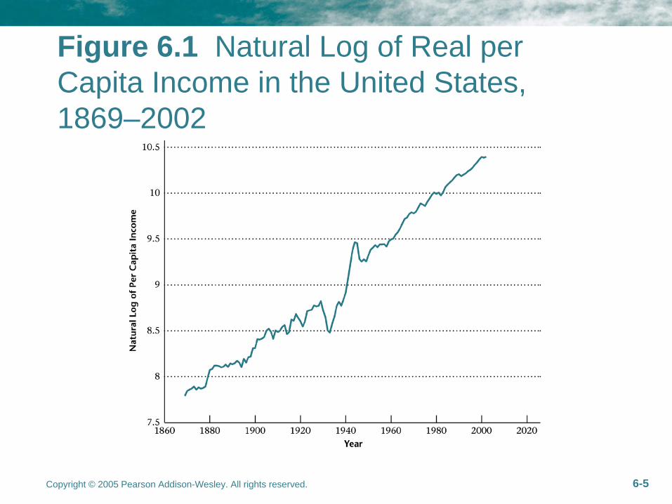
Figure 6.1 Natural Log of Real per Capita Income in the United States, 1869–2002
Copyright © 2005 Pearson Addison-Wesley. All rights reserved. 6-6
Economic Growth Facts Con’d
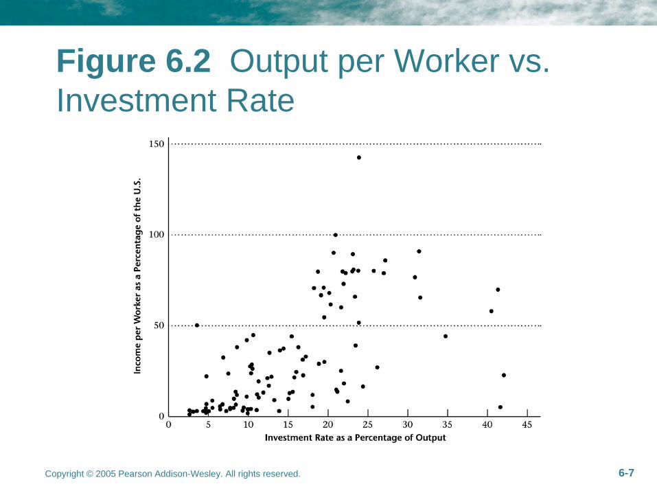
• High Investment High Standard of Living
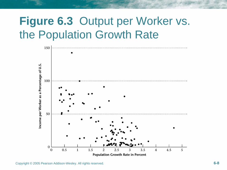
• High Population Growth Low Standard of Living
• Divergence of per capita Incomes: 1800–1950.
Copyright © 2005 Pearson Addison-Wesley. All rights reserved. 6-7
Figure 6.2 Output per Worker vs. Investment Rate
Copyright © 2005 Pearson Addison-Wesley. All rights reserved. 6-8
Figure 6.3 Output per Worker vs. the Population Growth Rate
Copyright © 2005 Pearson Addison-Wesley. All rights reserved. 6-9
Economic Growth Facts Con’d
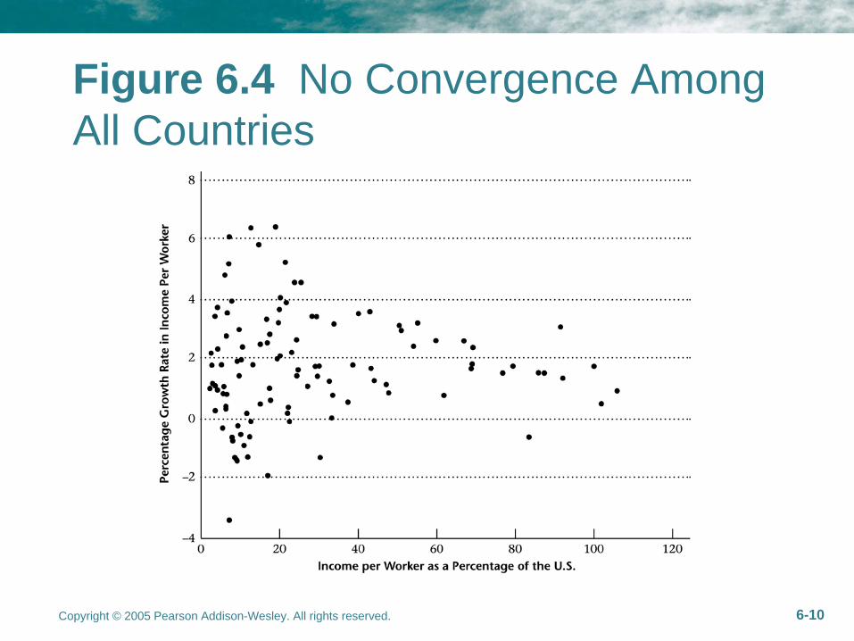
• No conditional Convergence amongst all Countries
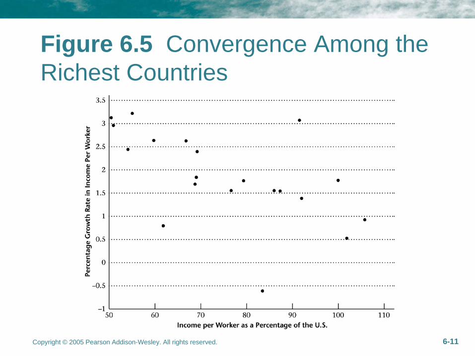
• (Weakly) Conditional Convergence amongst the Rich Countries
• No Conditional Convergence amongst the Poorest Countries
Copyright © 2005 Pearson Addison-Wesley. All rights reserved. 6-10
Figure 6.4 No Convergence Among All Countries
Copyright © 2005 Pearson Addison-Wesley. All rights reserved. 6-11
Figure 6.5 Convergence Among the Richest Countries

Copyright © 2005 Pearson Addison-Wesley. All rights reserved. 6-12
Figure 6.6 No Convergence Among the Poorest Countries

Copyright © 2005 Pearson Addison-Wesley. All rights reserved. 6-13
The Malthusian Model
• Idea was provided by Thomas Malthus in his highly influential book An Essay on the Principle of Population in 1798.
• He argued technological change improvement in standard living
population growth
reduce the average person to the subsistence level again
Copyright © 2005 Pearson Addison-Wesley. All rights reserved. 6-14
• In the long run there would be no increase in the standard of living unless there were some limits on population growth.
• It is a pessimistic theory!
Copyright © 2005 Pearson Addison-Wesley. All rights reserved. 6-15
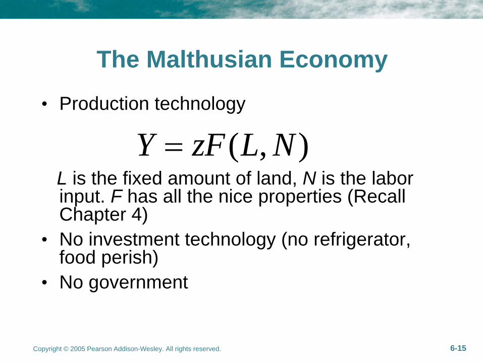
The Malthusian Economy
• Production technology
L is the fixed amount of land, N is the labor input. F has all the nice properties (Recall Chapter 4)
• No investment technology (no refrigerator, food perish)
• No government
( , )Y zF L N
Copyright © 2005 Pearson Addison-Wesley. All rights reserved. 6-16
• No leisure in the utility function.
• We normalize the labor endowment of each person to be 1, so N is both the population size and the labor input
( )U C C
Copyright © 2005 Pearson Addison-Wesley. All rights reserved. 6-17
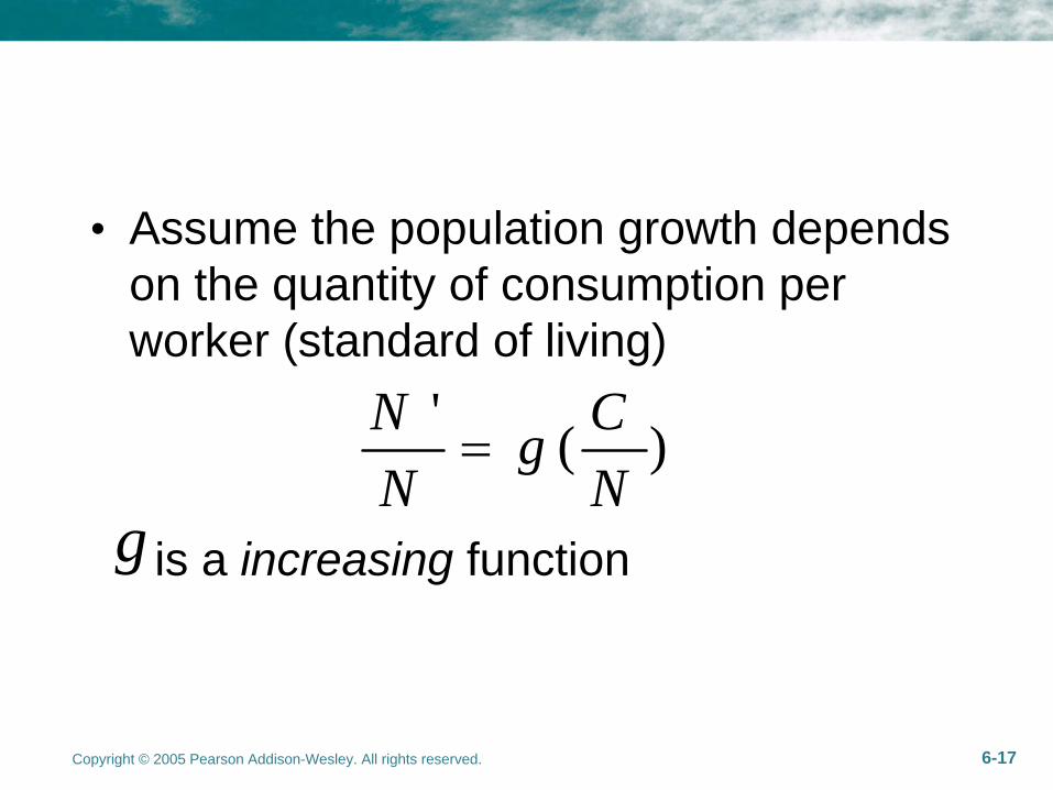
• Assume the population growth depends on the quantity of consumption per worker (standard of living)
is a increasing function
' ( )N CgN N
g

Copyright © 2005 Pearson Addison-Wesley. All rights reserved. 6-18
Figure 6.7 Population Growth Depends on Consumption per Worker in the Malthusian Model
Copyright © 2005 Pearson Addison-Wesley. All rights reserved. 6-19
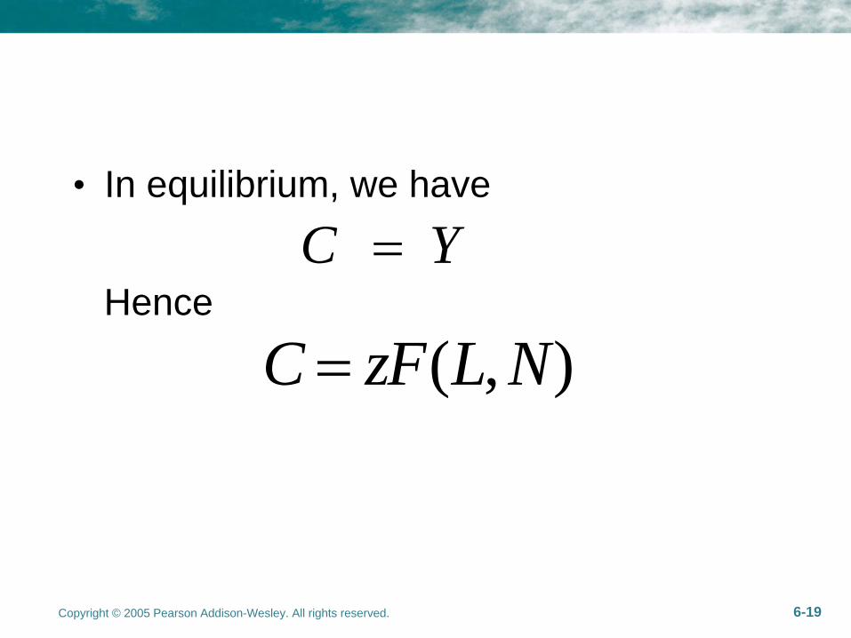
• In equilibrium, we have
HenceC Y
( , )C zF L N
Copyright © 2005 Pearson Addison-Wesley. All rights reserved. 6-20
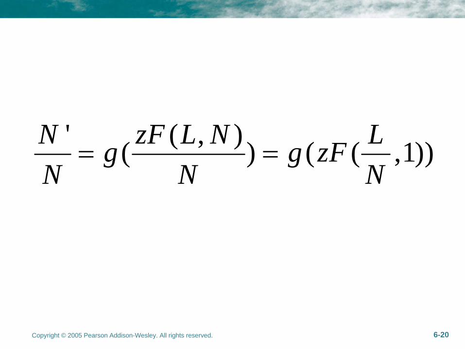
' ( , )( ) ( ( ,1))N zF L N Lg g zFN N N
Copyright © 2005 Pearson Addison-Wesley. All rights reserved. 6-21
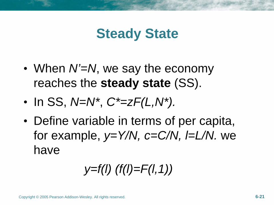
Steady State
• When N’=N, we say the economy reaches the steady state (SS).
• In SS, N=N*, C*=zF(L,N*).• Define variable in terms of per capita,
for example, y=Y/N, c=C/N, l=L/N. we have
y=f(l) (f(l)=F(l,1))
Copyright © 2005 Pearson Addison-Wesley. All rights reserved. 6-22
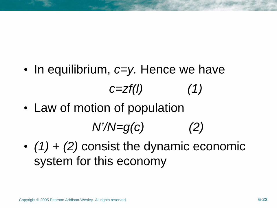
• In equilibrium, c=y. Hence we havec=zf(l) (1)
• Law of motion of populationN’/N=g(c) (2)
• (1) + (2) consist the dynamic economic system for this economy
Copyright © 2005 Pearson Addison-Wesley. All rights reserved. 6-23
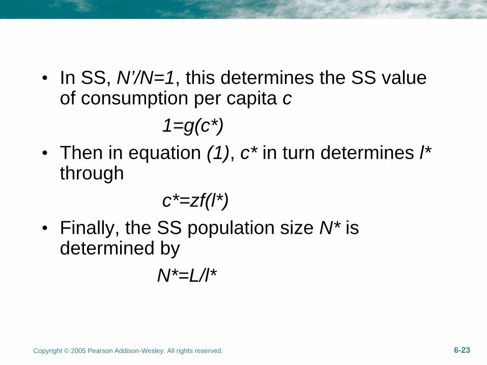
• In SS, N’/N=1, this determines the SS value of consumption per capita c
1=g(c*)• Then in equation (1), c* in turn determines l*
through c*=zf(l*)
• Finally, the SS population size N* is determined by
N*=L/l*

Copyright © 2005 Pearson Addison-Wesley. All rights reserved. 6-24
Figure 6.8 Determination of the Population in the Steady State

Copyright © 2005 Pearson Addison-Wesley. All rights reserved. 6-25
Figure 6.9 The Per-Worker Production Function
Copyright © 2005 Pearson Addison-Wesley. All rights reserved. 6-26
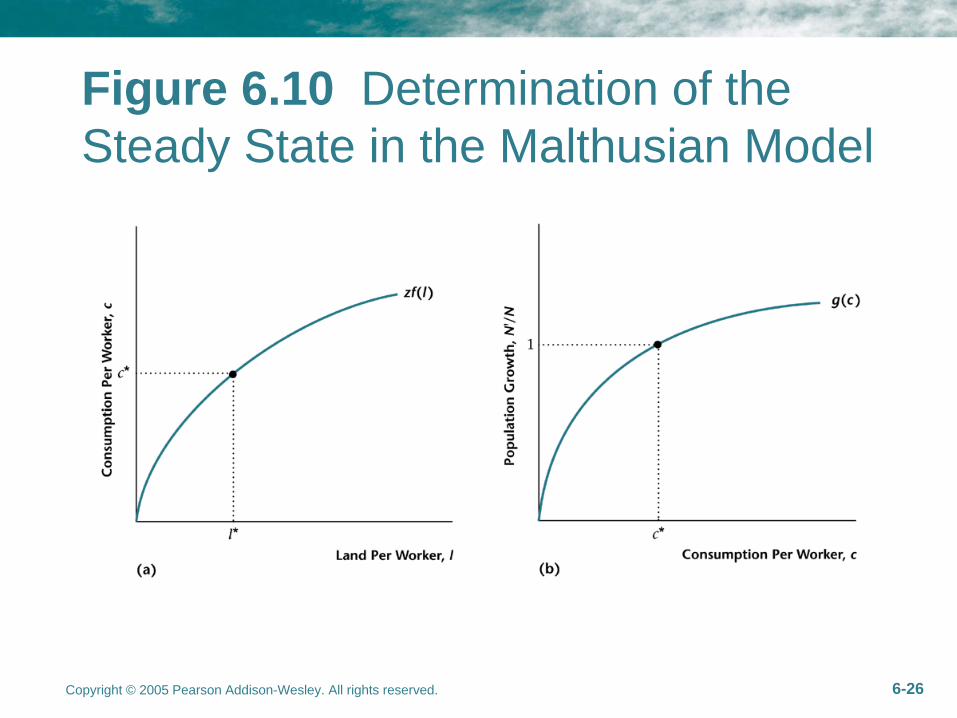
Figure 6.10 Determination of the Steady State in the Malthusian Model
Copyright © 2005 Pearson Addison-Wesley. All rights reserved. 6-27
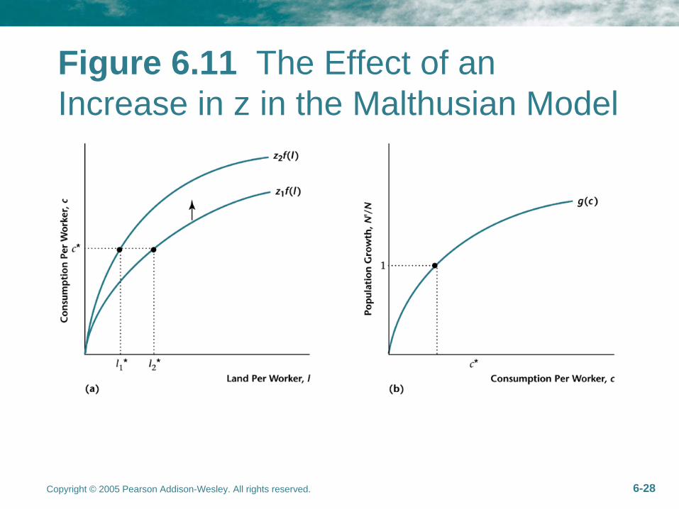
The Effect of TFP on the SS
• Do not improve the standard of living c* in the long run ( c* is determined by 1=g(c*) )
• Only increases the population (l*, N*)
Copyright © 2005 Pearson Addison-Wesley. All rights reserved. 6-28
Figure 6.11 The Effect of an Increase in z in the Malthusian Model
Copyright © 2005 Pearson Addison-Wesley. All rights reserved. 6-29
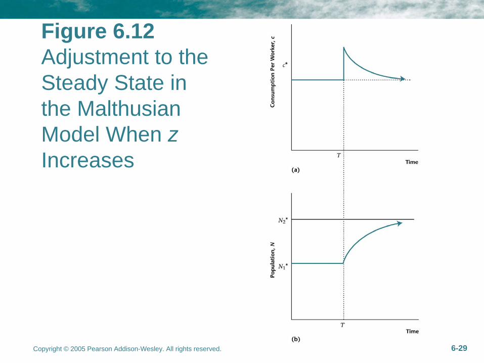
Figure 6.12 Adjustment to the Steady State in the Malthusian Model When z Increases
Copyright © 2005 Pearson Addison-Wesley. All rights reserved. 6-30
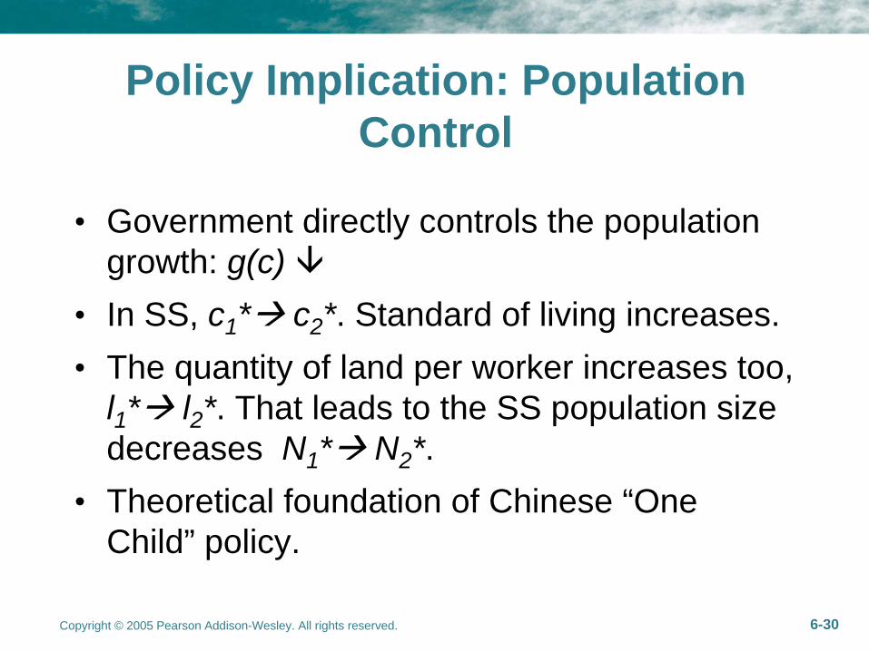
Policy Implication: Population Control
• Government directly controls the population growth: g(c)
• In SS, c1 * c2 *. Standard of living increases.• The quantity of land per worker increases too,
l1 * l2 *. That leads to the SS population size decreases N1 * N2 *.
• Theoretical foundation of Chinese “One Child” policy.

Copyright © 2005 Pearson Addison-Wesley. All rights reserved. 6-31
Figure 6.13 Population Control in the Malthusian Model
Copyright © 2005 Pearson Addison-Wesley. All rights reserved. 6-32
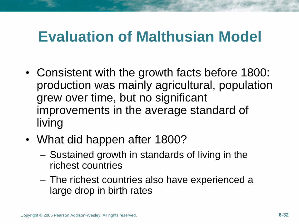
Evaluation of Malthusian Model
• Consistent with the growth facts before 1800: production was mainly agricultural, population grew over time, but no significant improvements in the average standard of living
• What did happen after 1800?– Sustained growth in standards of living in the
richest countries– The richest countries also have experienced a
large drop in birth rates
Copyright © 2005 Pearson Addison-Wesley. All rights reserved. 6-33
• Malthus was wrong on these two dimensions– He did not allow for the effect of increases in K on
production. Capital can produce itself.– He did not account for all of the effects of
economic forces on population growth. As economy develops, the opportunity cost of raising a large family becomes large. Fertility rate decreases.
• We need a GROWTH theory!
Copyright © 2005 Pearson Addison-Wesley. All rights reserved. 6-34
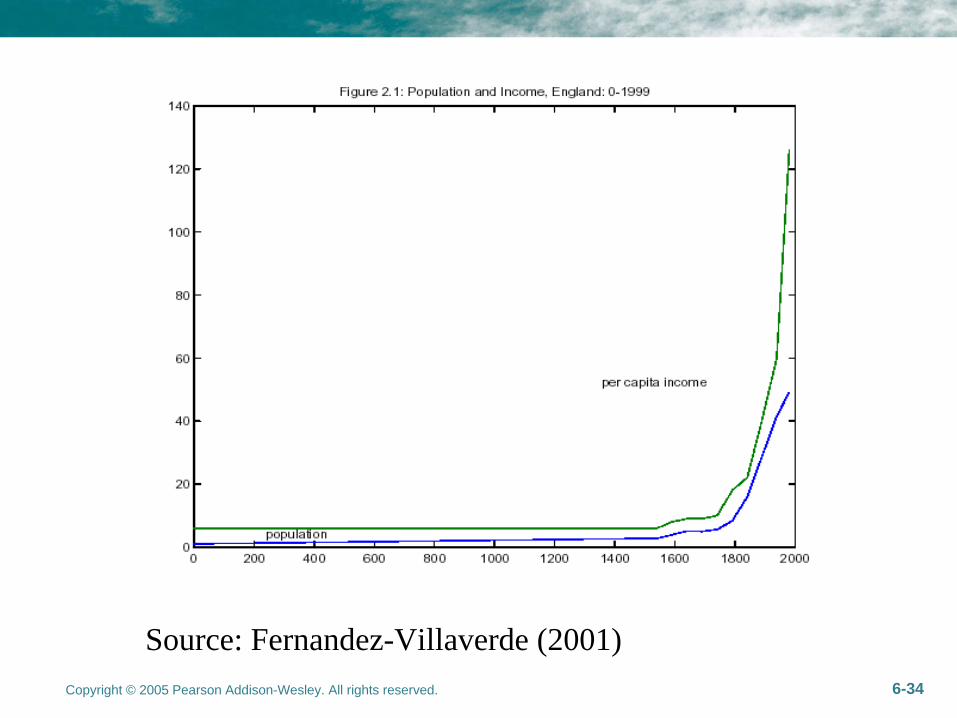
Source: Fernandez-Villaverde (2001)
Copyright © 2005 Pearson Addison-Wesley. All rights reserved. 6-35
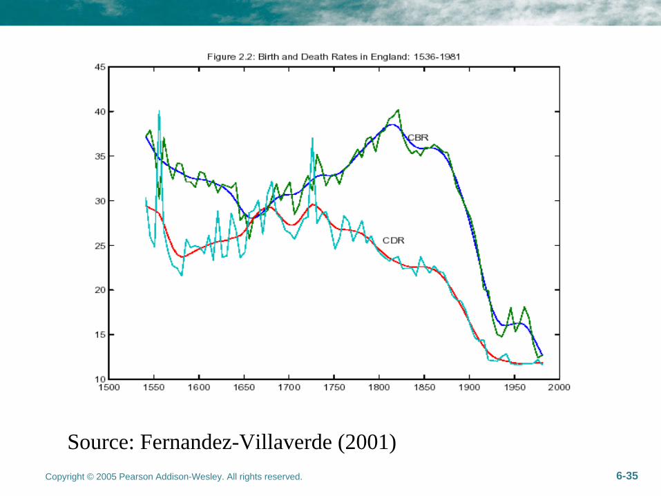
Source: Fernandez-Villaverde (2001)
Copyright © 2005 Pearson Addison-Wesley. All rights reserved. 6-36
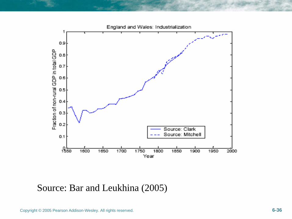
Source: Bar and Leukhina (2005)
Copyright © 2005 Pearson Addison-Wesley. All rights reserved. 6-37
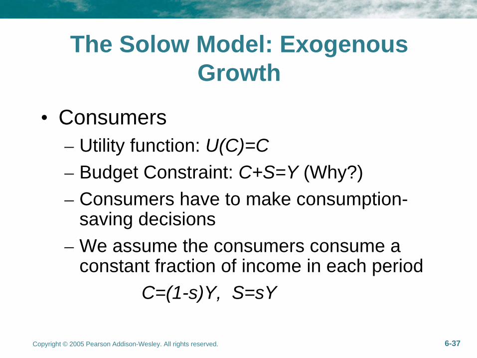
The Solow Model: Exogenous Growth
• Consumers– Utility function: U(C)=C– Budget Constraint: C+S=Y (Why?)– Consumers have to make consumption-
saving decisions– We assume the consumers consume a
constant fraction of income in each periodC=(1-s)Y, S=sY
Copyright © 2005 Pearson Addison-Wesley. All rights reserved. 6-38
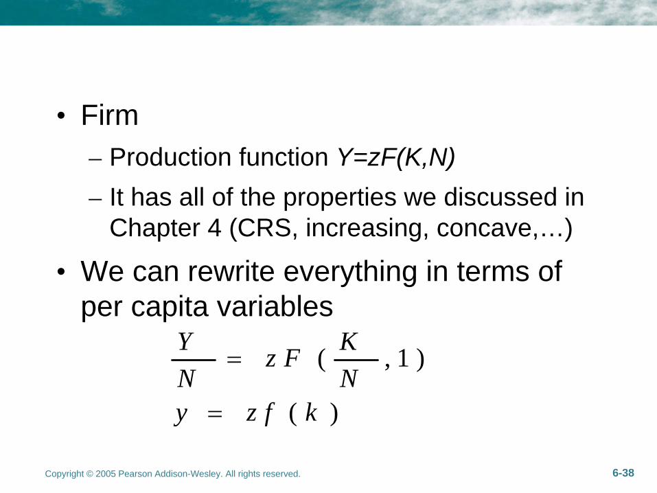
• Firm– Production function Y=zF(K,N)– It has all of the properties we discussed in
Chapter 4 (CRS, increasing, concave,…)
• We can rewrite everything in terms of per capita variables
( , 1 )
( )
Y Kz FN Ny z f k
Copyright © 2005 Pearson Addison-Wesley. All rights reserved. 6-39
• The capital stock evolves according toK’=(1-d)K+I
I is the investment. 0<d<1 is the depreciation rate.
Copyright © 2005 Pearson Addison-Wesley. All rights reserved. 6-40
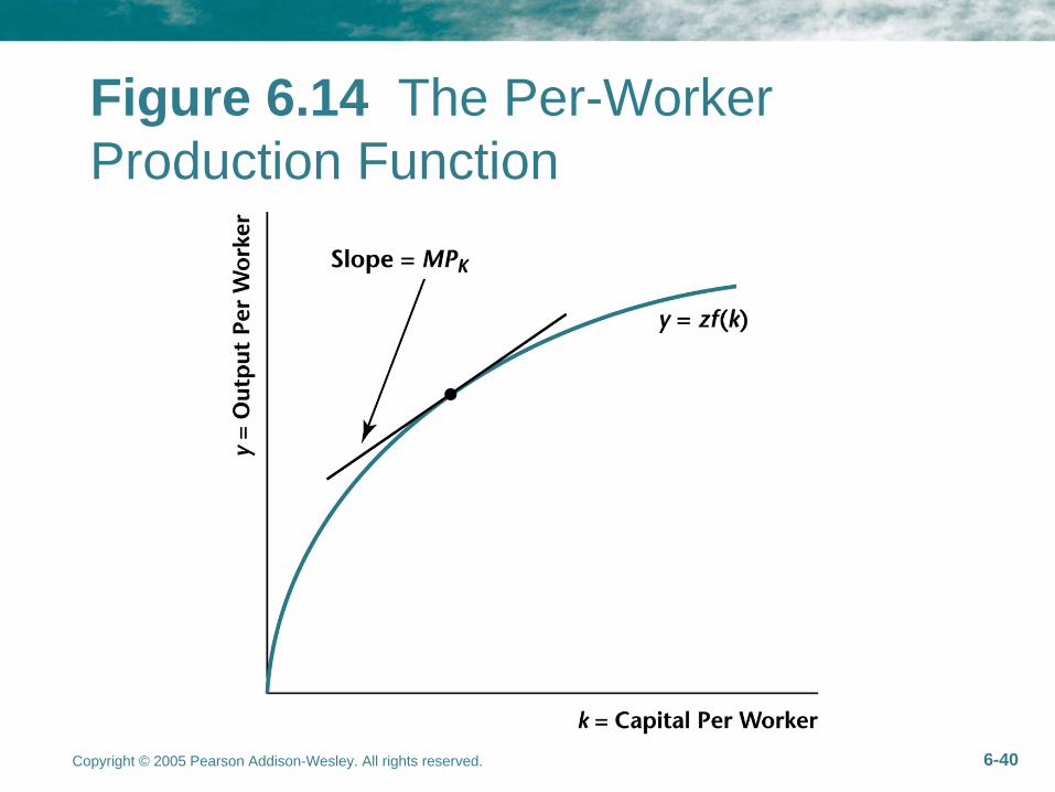
Figure 6.14 The Per-Worker Production Function
Copyright © 2005 Pearson Addison-Wesley. All rights reserved. 6-41
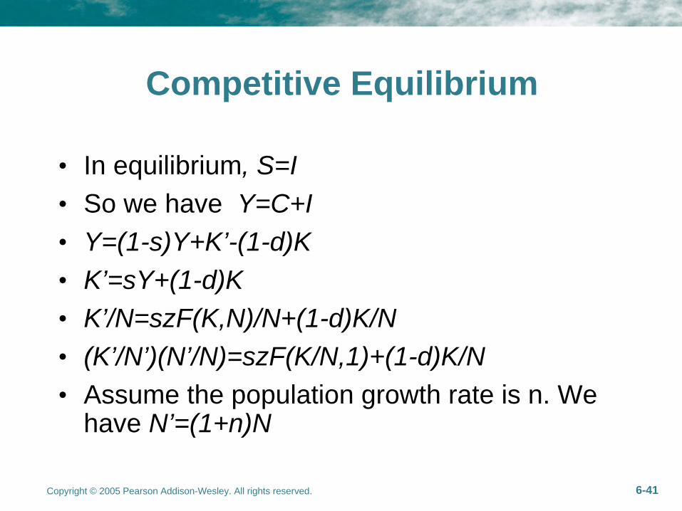
Competitive Equilibrium
• In equilibrium, S=I• So we have Y=C+I• Y=(1-s)Y+K’-(1-d)K• K’=sY+(1-d)K• K’/N=szF(K,N)/N+(1-d)K/N• (K’/N’)(N’/N)=szF(K/N,1)+(1-d)K/N• Assume the population growth rate is n. We
have N’=(1+n)N
Copyright © 2005 Pearson Addison-Wesley. All rights reserved. 6-42
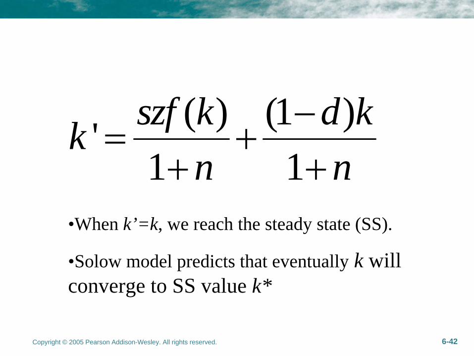
( ) (1 )'1 1szf k d kk
n n
•When k’=k, we reach the steady state (SS).
•Solow model predicts that eventually k will converge to SS value k*
Copyright © 2005 Pearson Addison-Wesley. All rights reserved. 6-43
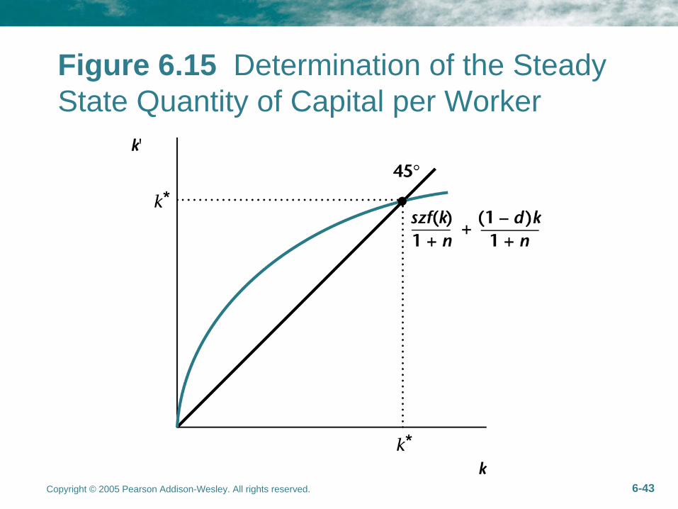
Figure 6.15 Determination of the Steady State Quantity of Capital per Worker
Copyright © 2005 Pearson Addison-Wesley. All rights reserved. 6-44
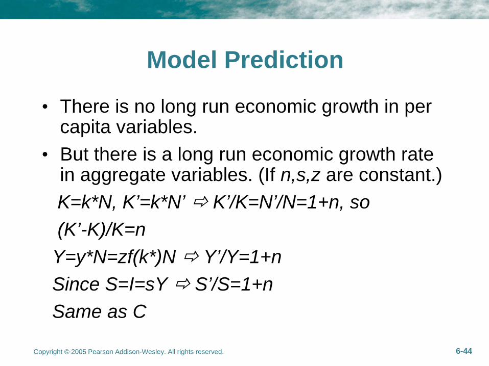
Model Prediction
• There is no long run economic growth in per capita variables.
• But there is a long run economic growth rate in aggregate variables. (If n,s,z are constant.)K=k*N, K’=k*N’ K’/K=N’/N=1+n, so (K’-K)/K=nY=y*N=zf(k*)N Y’/Y=1+nSince S=I=sY S’/S=1+nSame as C
Copyright © 2005 Pearson Addison-Wesley. All rights reserved. 6-45
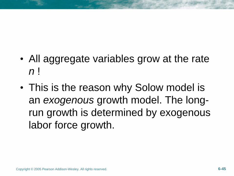
• All aggregate variables grow at the rate n !
• This is the reason why Solow model is an exogenous growth model. The long- run growth is determined by exogenous labor force growth.
Copyright © 2005 Pearson Addison-Wesley. All rights reserved. 6-46
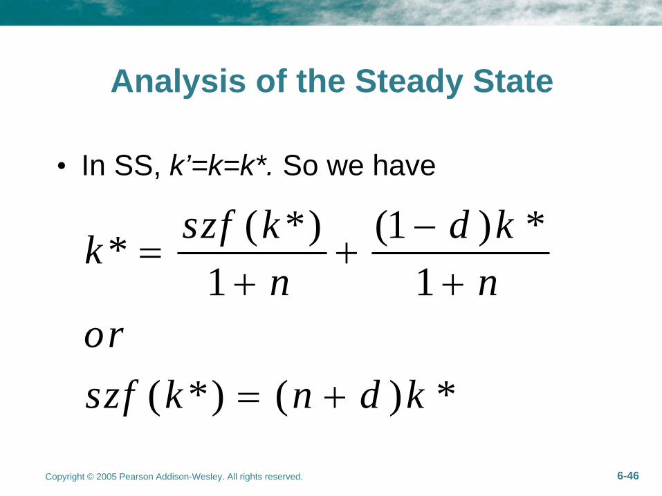
Analysis of the Steady State
• In SS, k’=k=k*. So we have
( *) (1 ) **1 1
( *) ( ) *
szf k d kkn n
orszf k n d k
Copyright © 2005 Pearson Addison-Wesley. All rights reserved. 6-47
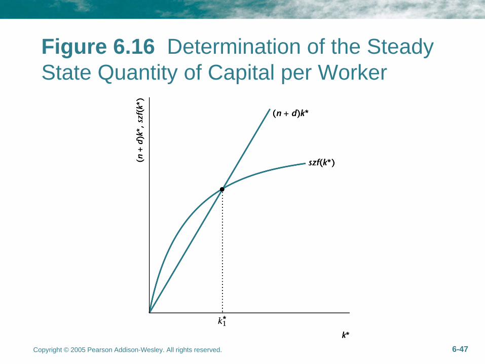
Figure 6.16 Determination of the Steady State Quantity of Capital per Worker
Copyright © 2005 Pearson Addison-Wesley. All rights reserved. 6-48
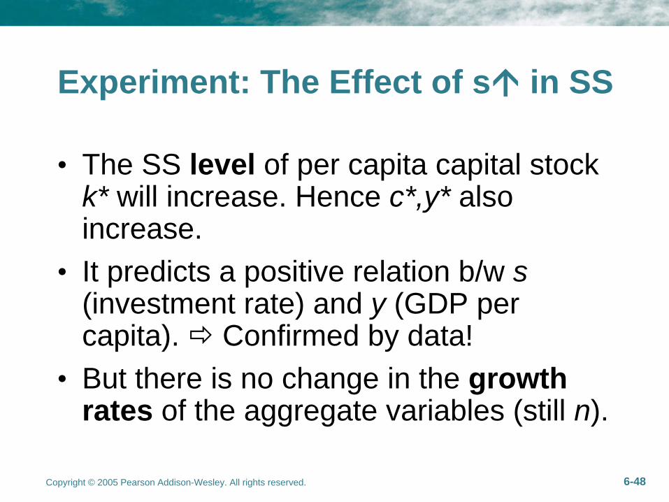
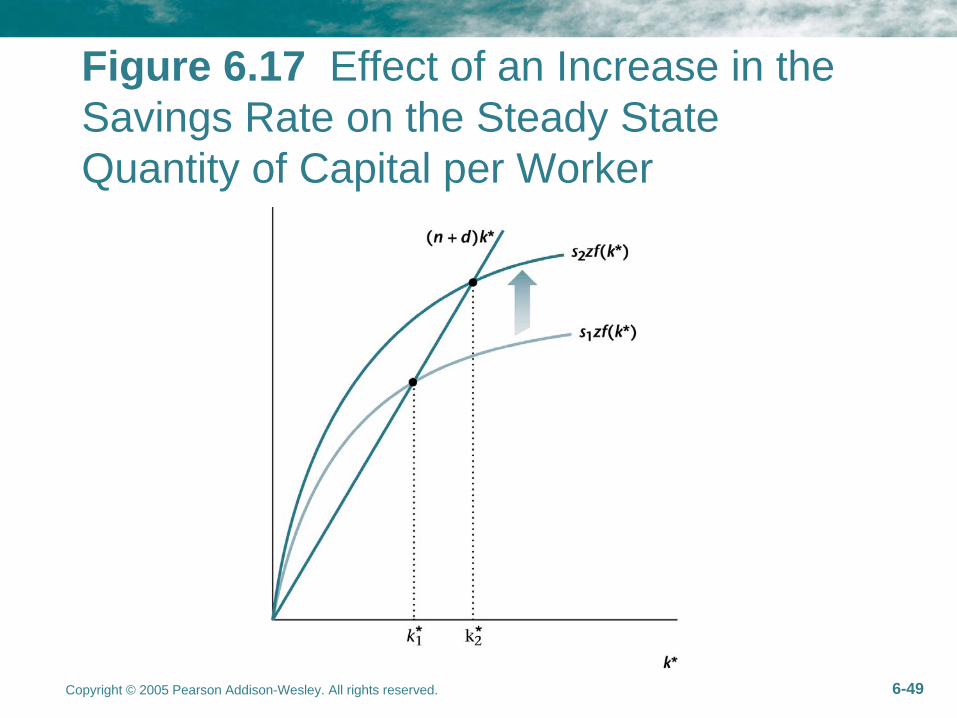
Experiment: The Effect of s in SS
• The SS level of per capita capital stock k* will increase. Hence c*,y* also increase.
• It predicts a positive relation b/w s (investment rate) and y (GDP per capita).
Confirmed by data!
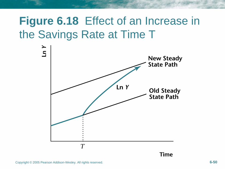
• But there is no change in the growth rates of the aggregate variables (still n).
Copyright © 2005 Pearson Addison-Wesley. All rights reserved. 6-49
Figure 6.17 Effect of an Increase in the Savings Rate on the Steady State Quantity of Capital per Worker
Copyright © 2005 Pearson Addison-Wesley. All rights reserved. 6-50
Figure 6.18 Effect of an Increase in the Savings Rate at Time T
Copyright © 2005 Pearson Addison-Wesley. All rights reserved. 6-51
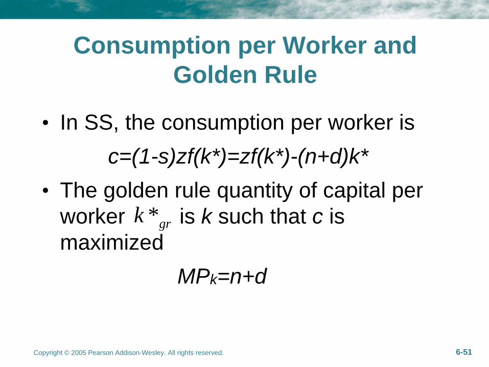
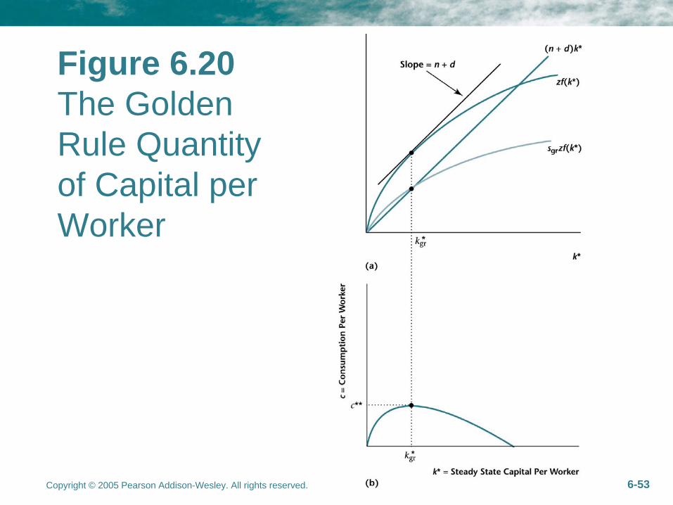
Consumption per Worker and Golden Rule
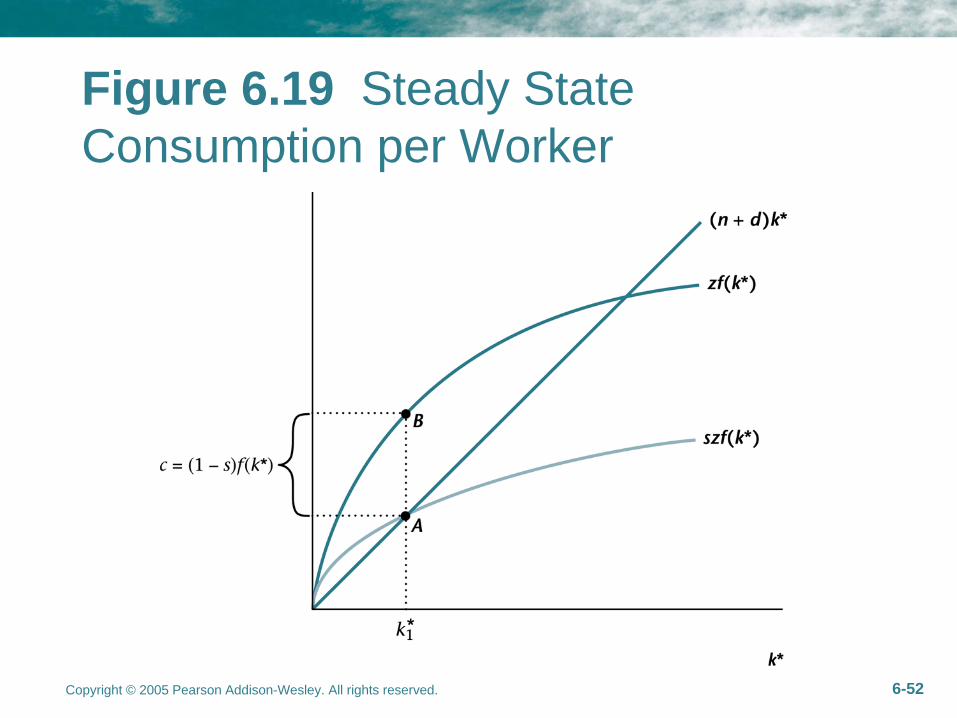
• In SS, the consumption per worker is c=(1-s)zf(k*)=zf(k*)-(n+d)k*
• The golden rule quantity of capital per worker is k such that c is maximized
MPk=n+d
*grk
Copyright © 2005 Pearson Addison-Wesley. All rights reserved. 6-52
Figure 6.19 Steady State Consumption per Worker
Copyright © 2005 Pearson Addison-Wesley. All rights reserved. 6-53
Figure 6.20 The Golden Rule Quantity of Capital per Worker
Copyright © 2005 Pearson Addison-Wesley. All rights reserved. 6-54
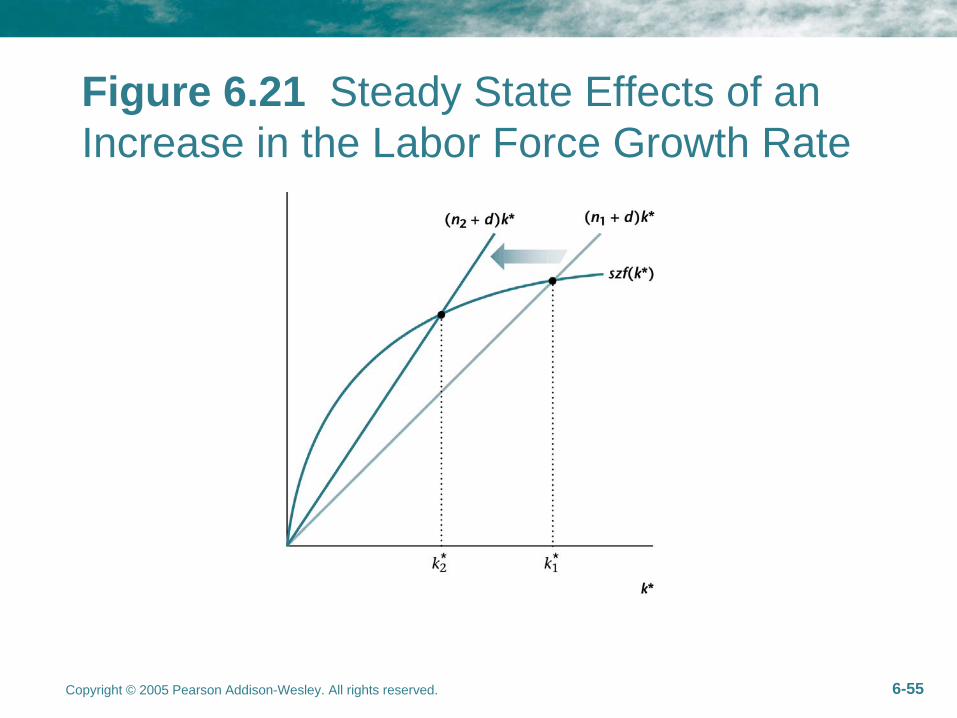
Experiment: The Effect of n in SS
• The SS quantity of capital per worker (k*) decreases.
• y* and c* also decrease. Hence n (population growth rate) is negatively correlated with y.
Confirmed by data
• But the aggregate variables Y, K, C all grow at higher rate
Copyright © 2005 Pearson Addison-Wesley. All rights reserved. 6-55
Figure 6.21 Steady State Effects of an Increase in the Labor Force Growth Rate
Copyright © 2005 Pearson Addison-Wesley. All rights reserved. 6-56
The prediction of Solow Model
• Solow model predicts saving rate (investment rate) y, and n
y• It is consistent with the data (recall it)
Copyright © 2005 Pearson Addison-Wesley. All rights reserved. 6-57
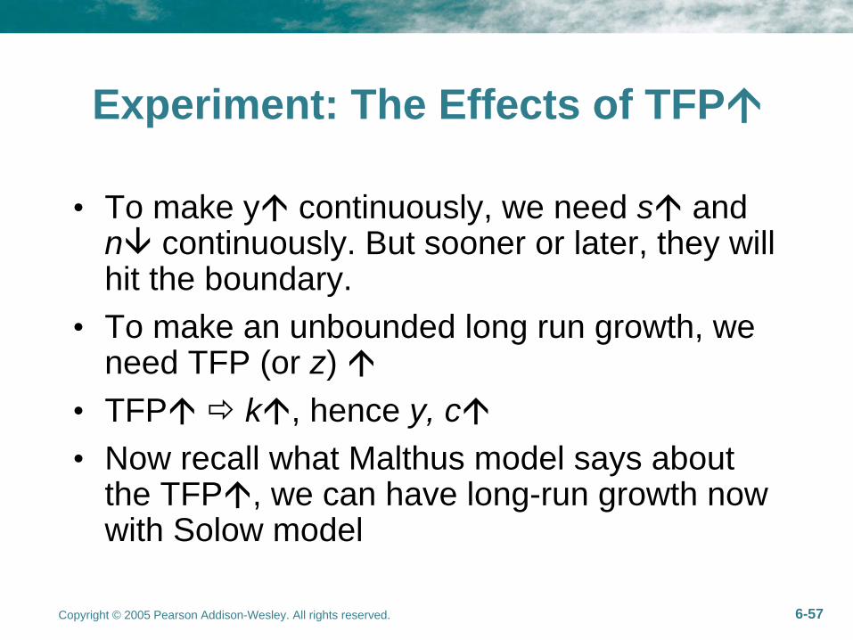
Experiment: The Effects of TFP
• To make y
continuously, we need s
and n
continuously. But sooner or later, they will
hit the boundary.• To make an unbounded long run growth, we
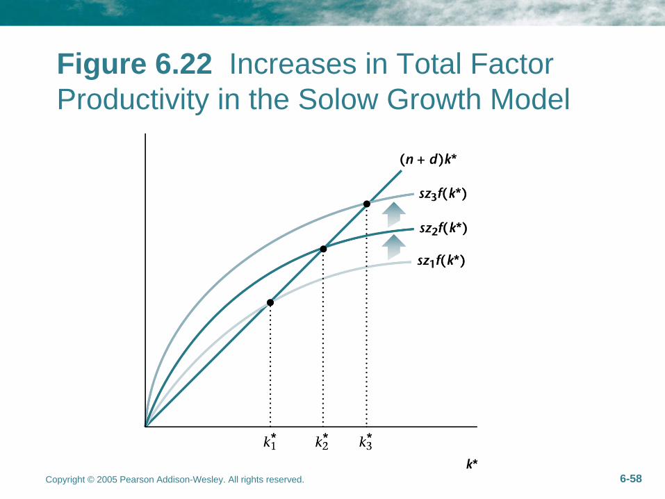
need TFP (or z) • TFP k, hence y, c• Now recall what Malthus model says about
the TFP, we can have long-run growth now with Solow model
Copyright © 2005 Pearson Addison-Wesley. All rights reserved. 6-58
Figure 6.22 Increases in Total Factor Productivity in the Solow Growth Model
Copyright © 2005 Pearson Addison-Wesley. All rights reserved. 6-59
Growth Accounting
• Typically, growing economies are experiencing growth in factors of production and in TFP.
• A natural question is can we measure how much of the growth in Y is accounted for by growth in each of the inputs to production and by increases in TFP.
Copyright © 2005 Pearson Addison-Wesley. All rights reserved. 6-60
• We call this exercise is Growth Accounting.
• Start from aggregate production function
• Profit maximization implies
1( )Y zK N
1
(1 ) ( )
(1 ) ( ) (1 )NMP zK N w
wN zK N Y
Copyright © 2005 Pearson Addison-Wesley. All rights reserved. 6-61
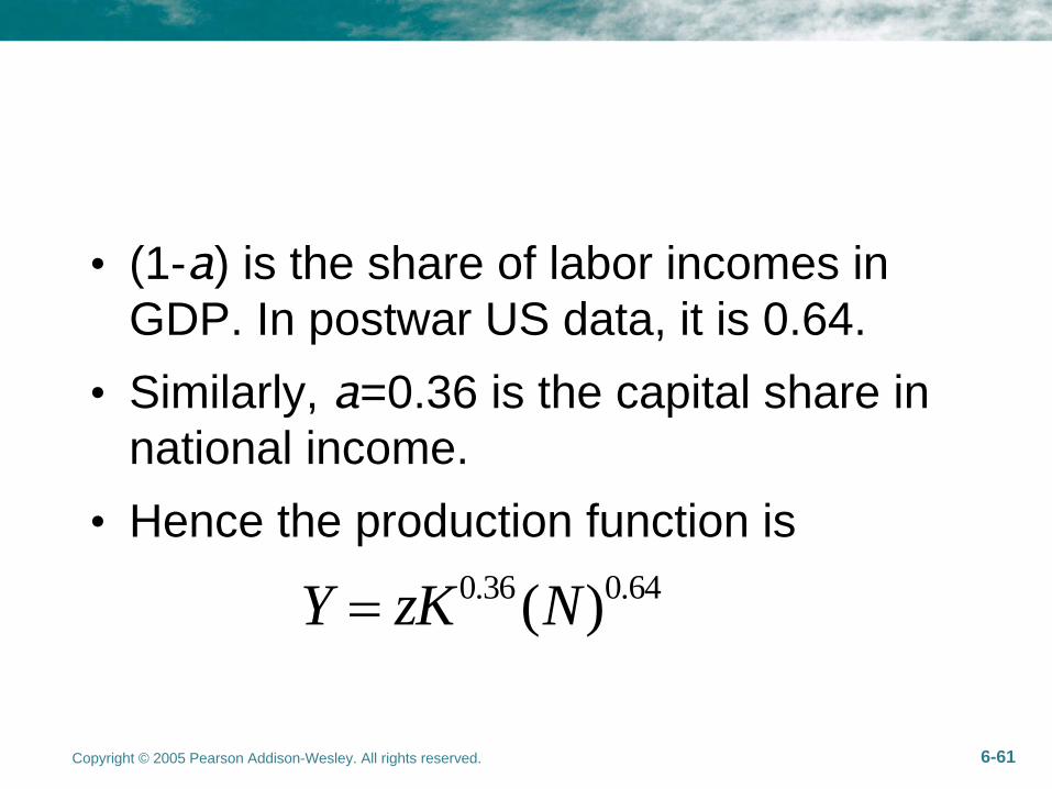
• (1-a) is the share of labor incomes in GDP. In postwar US data, it is 0.64.
• Similarly, a=0.36 is the capital share in national income.
• Hence the production function is0.36 0.64( )Y zK N
Copyright © 2005 Pearson Addison-Wesley. All rights reserved. 6-62
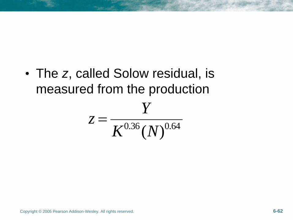
• The z, called Solow residual, is measured from the production
0.36 0.64( )Yz
K N
Copyright © 2005 Pearson Addison-Wesley. All rights reserved. 6-63
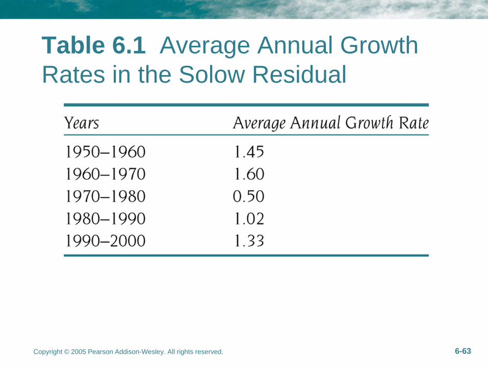
Table 6.1 Average Annual Growth Rates in the Solow Residual
Copyright © 2005 Pearson Addison-Wesley. All rights reserved. 6-64
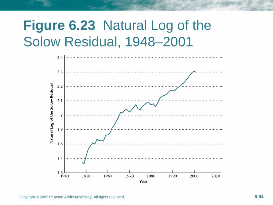
Figure 6.23 Natural Log of the Solow Residual, 1948–2001
Copyright © 2005 Pearson Addison-Wesley. All rights reserved. 6-65
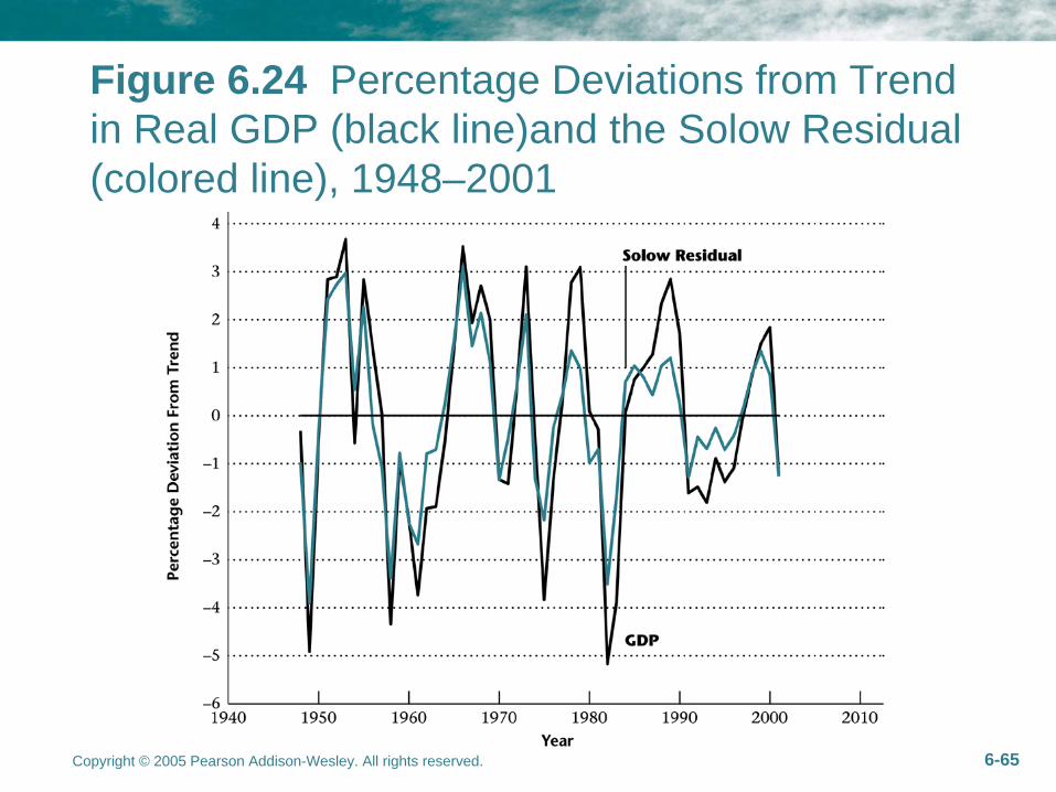
Figure 6.24 Percentage Deviations from Trend in Real GDP (black line)and the Solow Residual (colored line), 1948–2001
Copyright © 2005 Pearson Addison-Wesley. All rights reserved. 6-66
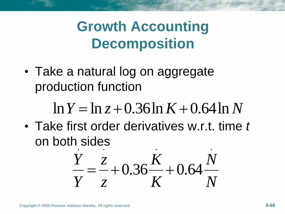
Growth Accounting Decomposition
• Take a natural log on aggregate production function
• Take first order derivatives w.r.t. time t on both sides
ln ln 0.36ln 0.64lnY z K N
. . . .
0.36 0.64Y z K NY z K N
Copyright © 2005 Pearson Addison-Wesley. All rights reserved. 6-67
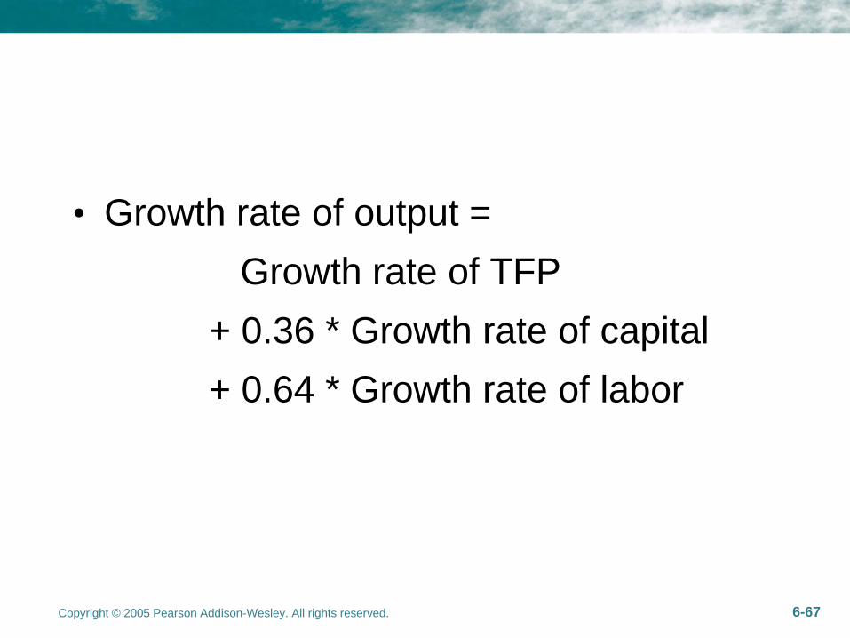
• Growth rate of output = Growth rate of TFP
+ 0.36 * Growth rate of capital+ 0.64 * Growth rate of labor
Copyright © 2005 Pearson Addison-Wesley. All rights reserved. 6-68
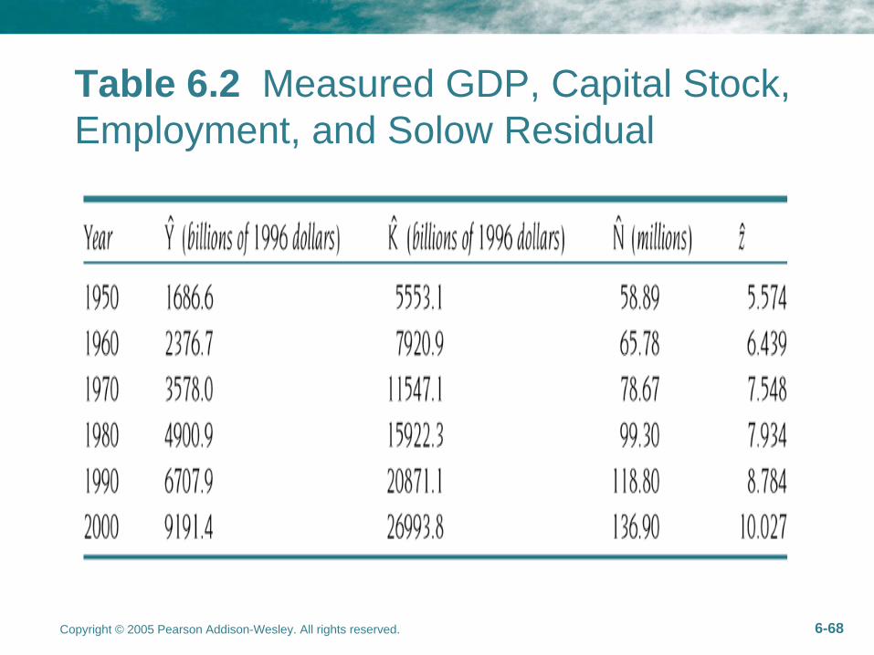
Table 6.2 Measured GDP, Capital Stock, Employment, and Solow Residual
Copyright © 2005 Pearson Addison-Wesley. All rights reserved. 6-69
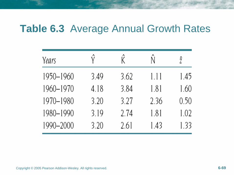
Table 6.3 Average Annual Growth Rates
Copyright © 2005 Pearson Addison-Wesley. All rights reserved. 6-70
An Example: East Asian Miracles
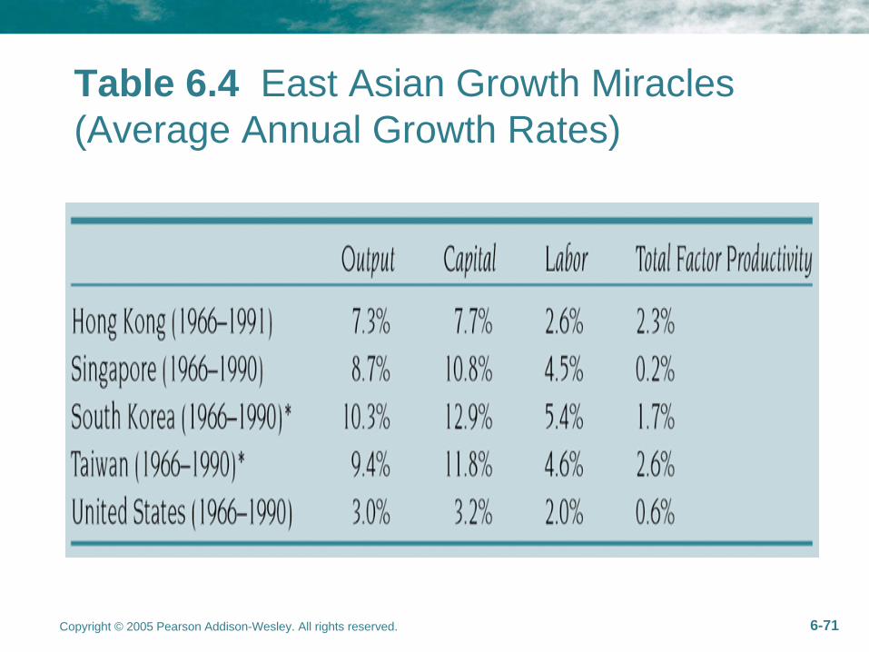
• Alwyn Young did a growth accounting exercise for “Four Little Dragons’’
• Found high rates of GDP growth in these countries were mainly due to high growth rates in factor inputs.
• Implication: East Asian Miracle is probably not sustainable over a longer period. (Japan recession in 1990s, South Korea Financial Crisis…)
Copyright © 2005 Pearson Addison-Wesley. All rights reserved. 6-71
Table 6.4 East Asian Growth Miracles (Average Annual Growth Rates)


![Robbins mgmt11 ppt06[1]](https://img.pdfslide.us/doc/110x75/54bd58c24a7959bc6d8b4573/robbins-mgmt11-ppt061.jpg)
![Rights Malthus[1]](https://img.pdfslide.us/doc/110x75/577dacfb1a28ab223f8e9e32/rights-malthus1.jpg)