The Dynamics of inflation and unemployment

Chapter 9Economic Dynamics

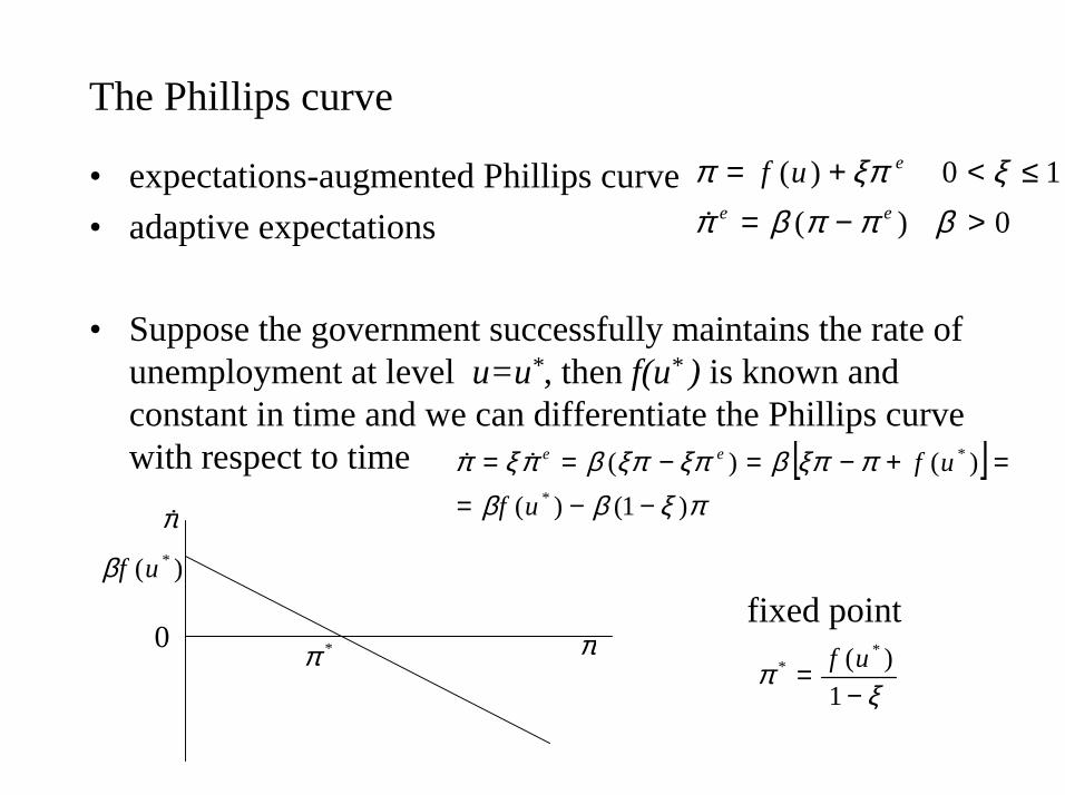
The Phillips curve

• expectations-augmented Phillips curve• adaptive expectations

• Suppose the government successfully maintains the rate of unemployment at level u=u*, then f(u* ) is known and constant in time and we can differentiate the Phillips curve with respect to time

fixed point

0 )(10 )(

>−=≤<+=

βππβπξξππ

ee

euf�

[ ]πξββ

πξπβξπξπβπξπ)1()(

)()(*

*

−−=

=+−=−==

ufufee

��

0

)( *ufβ

π�

π*πξ

π−

=1

)( ** uf

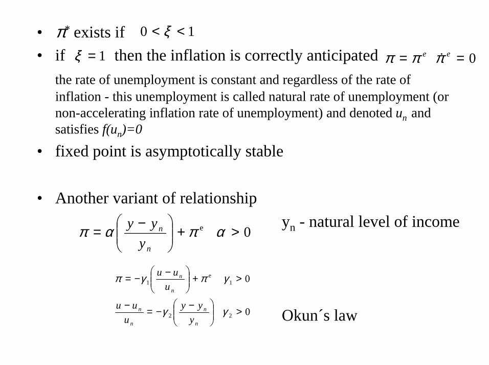
• π* exists if• if then the inflation is correctly anticipated

the rate of unemployment is constant and regardless of the rate of inflation - this unemployment is called natural rate of unemployment (or non-accelerating inflation rate of unemployment) and denoted un and satisfies f(un)=0

• fixed point is asymptotically stable

• Another variant of relationshipyn - natural level of income

Okun´s law

10 << ξ

1=ξ 0 == ee πππ �

0 e >+

−= απαπn

n

yyy

0

0

22

1e

1

>

−−=−

>+

−−=

γγ

γπγπ

n

n

n

n

n

n

yyy

uuu

uuu

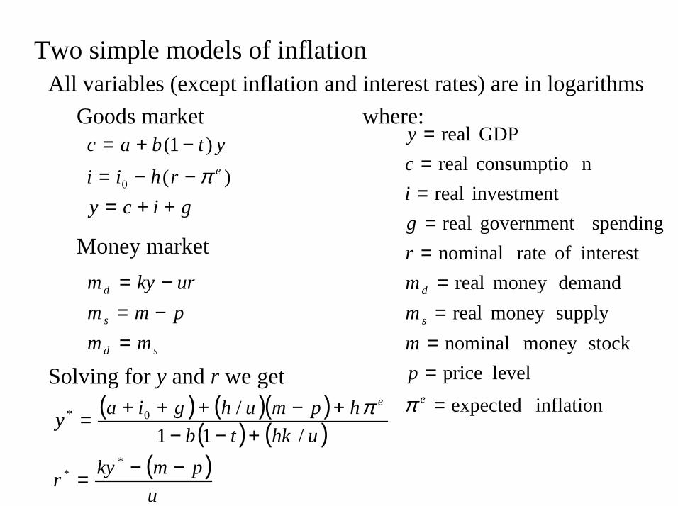
Two simple models of inflationAll variables (except inflation and interest rates) are in logarithms

Goods market where:

Money market

Solving for y and r we get

gicyrhii

ytbace

++=−−=−+=

)()1(

0 π

sd

s

d

mmpmmurkym

=−=−=

inflation expectedlevel price

stockmoney nominalsupplymoney realdemandmoney real

interest of rate nominalspending government real

investment realnconsumptio real

GDP real

=

====

==

===

e

s

d

pmmmrgicy

π( ) ( )( )( ) ( )

( )u

pmkyr

uhktbhpmuhgiay

e

−−=

+−−+−+++=

**

0*

/11/ π

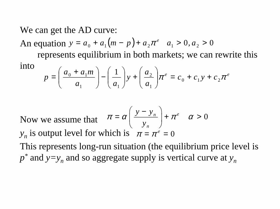
We can get the AD curve:An equation

represents equilibrium in both markets; we can rewrite this into

Now we assume thatyn is output level for which isThis represents long-run situation (the equilibrium price level is p* and y=yn and so aggregate supply is vertical curve at yn

( ) 0,0 21210 >>+−+= aaapmaay eπ

ee cyccaay

aamaap ππ 210

1

2

11

10 1 ++=

+

−

+=

0en

n

y yy

π α π α −= + >

0== eππ

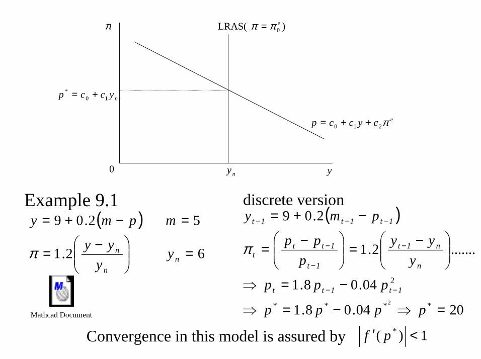
ecyccp π210 ++=

)LRAS( 0eππ =

nyccp 10* +=

0 ny y

π

Example 9.1( )

6 2.1

5 2.09

=

−=

=−+=

nn

n yy

yy

mpmy

π

( )

2004.08.1

04.08.1

.......2.1

2.09

****

2

2

=⇒−=⇒

−=⇒

−=

−=

−+=

−−

−

−

−

−−−

pppp

ppp

yyy

ppp

pmy

1t1tt

n

n1t

1t

1ttt

1t1t1t

π

discrete version

Convergence in this model is assured by 1)( * <′ pfMathcad Document

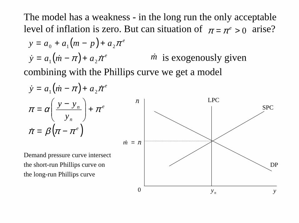
The model has a weakness - in the long run the only acceptable level of inflation is zero. But can situation of arise?

is exogenously givencombining with the Phillips curve we get a model

Demand pressure curve intersect the short-run Phillips curve on the long-run Phillips curve

0>= eππ( ) eapmaay π210 +−+=

( ) eamay ππ ��� 21 +−= m�

( )

( )e

e

n

n

e

yyy

amay

ππβπ

παπ

ππ

−=

+

−=

+−=

�

��� 21

DP

LPC

π=m�

0 ny y

πSPC

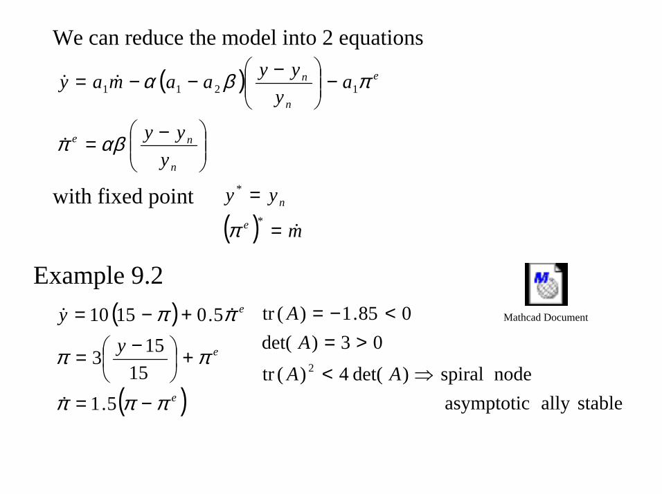
We can reduce the model into 2 equations

with fixed point

( )

−=

−

−−−=

n

ne

e

n

n

yyy

ay

yyaamay

αβπ

πβα

�

�� 1211

( ) m

yye

n

�=

=*

*

π

Example 9.2( )

( )e

e

e

yy

πππ

ππ

ππ

−=

+

−=

+−=

5.115

153

5.01510

�

��

stableally asymptotic node spiral)det(4)(tr

03)det(085.1)(tr

2⇒<

>=<−=

AAA

A Mathcad Document

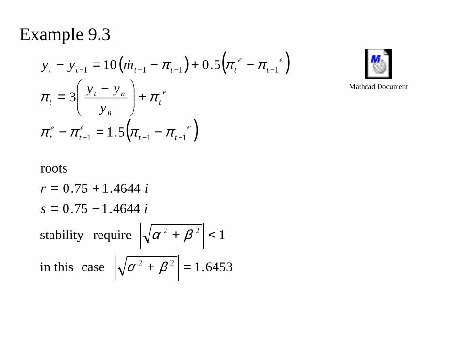
Example 9.3( ) ( )

( )ett

et

et

et

n

ntt

et

ettttt

yyy

myy

111

1111

5.1

3

5.010

−−−

−−−−

−=−

+

−=

−+−=−

ππππ

ππ

πππ�

6453.1 case in this

1 requirestability

4644.175.04644.175.0

roots

22

22

=+

<+

−=+=

βα

βα

isir

Mathcad Document

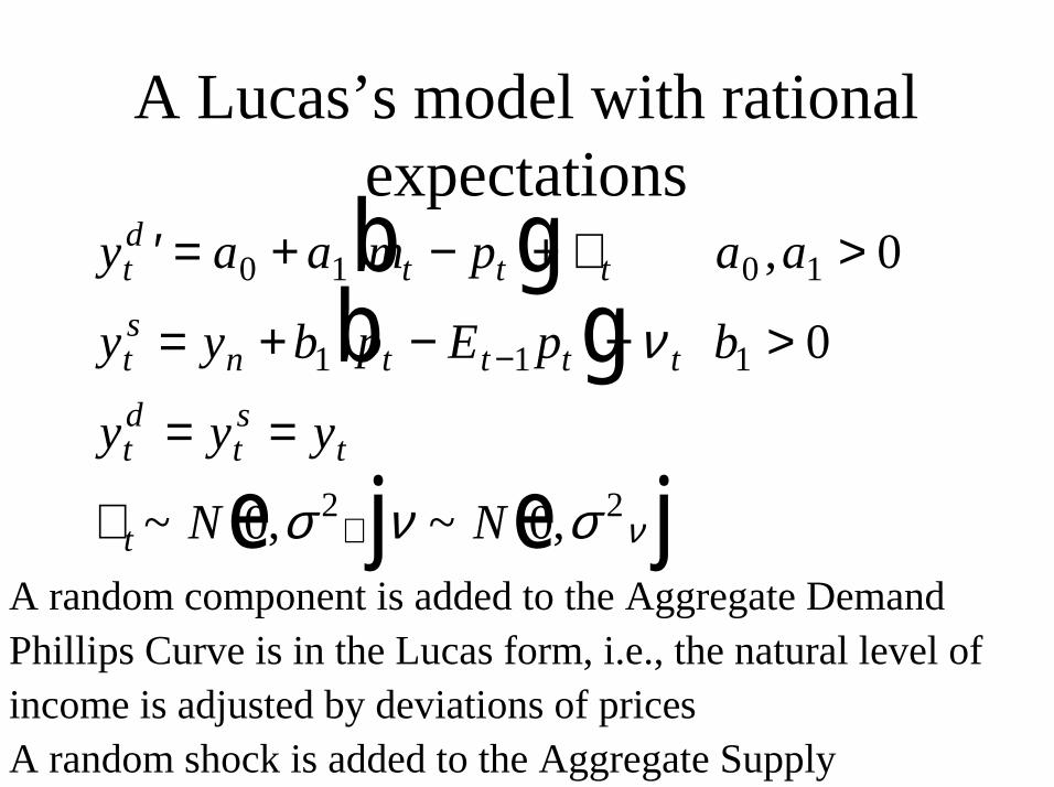
A Lucas’s model with rational expectations

A random component is added to the Aggregate DemandPhillips Curve is in the Lucas form, i.e., the natural level ofincome is adjusted by deviations of pricesA random shock is added to the Aggregate Supply

y a a m p a a

y y b p E p b

y y y

N N

td

t t t

ts

n t t t t

td

ts

t

t

′ = + − + ∈ >

= + − + >

= =

∈

−

∈

0 1 0 1

1 1 1

2 2

0

0

0 0

b gb g

e j e j

,

~ , ~ ,

ν

σ ν σ ν

Mathcad Document

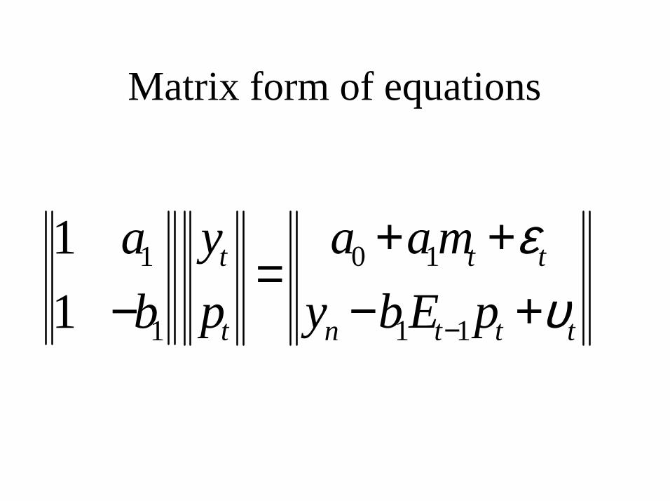
Matrix form of equations

0 11

1 11

11

t t t

t n t t t

y a a map y bE pb

ευ−

+ +=

− +−

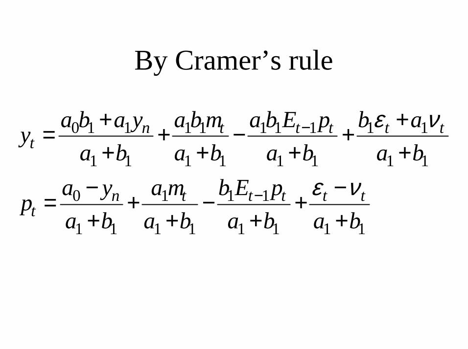
By Cramer’s rule

y a b a ya b

a b ma b

a b E pa b

b aa b

p a ya b

a ma b

b E pa b a b

tn t t t t t

tn t t t t t

=++

++

−+

+++

=−+

++

−+

+−+

−

−

0 1 1

1 1

1 1

1 1

1 1 1

1 1

1 1

1 1

0

1 1

1

1 1

1 1

1 1 1 1

ε ν

ε ν

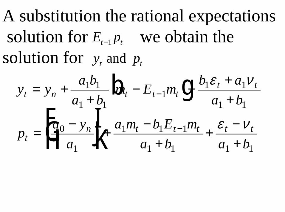
A substitution the rational expectationssolution for we obtain the

solution for

y y a ba b

m E m b aa b

p a ya

a m b E ma b a b

t n t t tt t

tn t t t t t

= ++

− +++

=−F

HGIKJ +

−+

+−+

−

−

1 1

1 11

1 1

1 1

0

1

1 1 1

1 1 1 1

b g ε ν

ε ν

1t tE p−

and t ty p

Mathcad Document

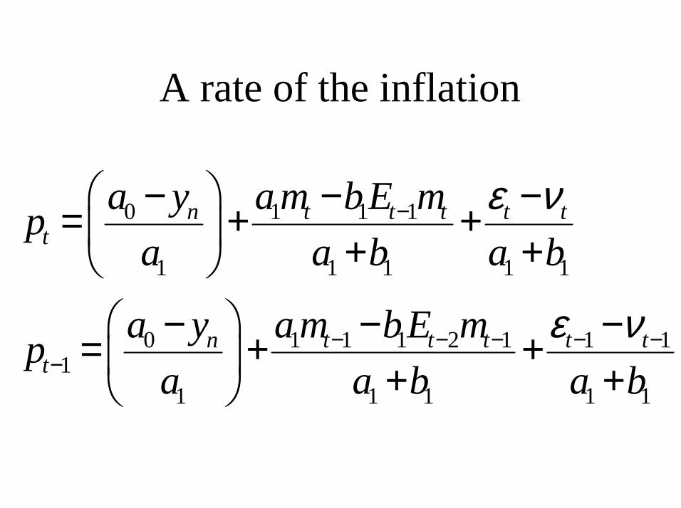
A rate of the inflation

0 1 1 1

1 1 1 1 1

0 1 1 1 2 1 1 11

1 1 1 1 1

n t t t t tt

n t t t t tt

a y a m bE mpa a b a b

a y a m bE mpa a b a b

ε ν

ε ν

−

− − − − −−

− − −= + + + +

− − −= + + + +

Mathcad Document

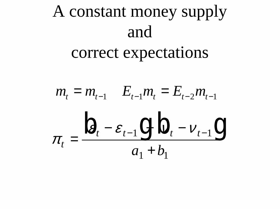
A constant money supplyand

correct expectations

πε ε ν ν

tt t t t

a b=

− − −+

− −1 1

1 1

b g b g1 1 2 1t t t t t tm m E m E m− − − −= =

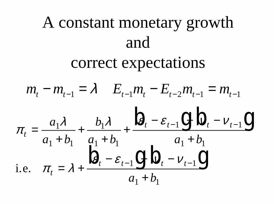
A constant monetary growthand

correct expectations

π λ λ ε ε ν ν

π λε ε ν ν

tt t t t

tt t t t

aa b

ba b a b

a b

=+

++

+− − −

+

= +− − −

+

− −

− −

1

1 1

1

1 1

1 1

1 1

1 1

1 1

b g b g

b g b gi.e.

1 1 2 1 1t t t t t t tm m E m E m mλ− − − − −− = − =

Mathcad Document

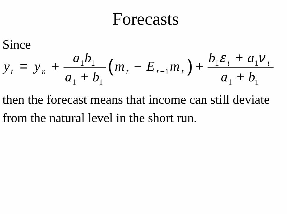
ForecastsSince

then the forecast means that income can still deviate from the natural level in the short run.

( ) 1 11 11

1 1 1 1

t tt n t t t

b aa by y m E ma b a b

ε ν−

+= + − ++ +

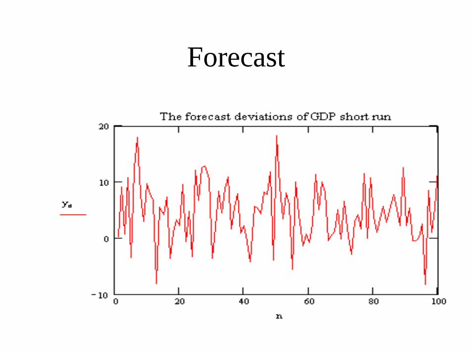
Forecast

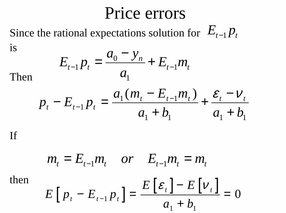
Price errorsSince the rational expectations solution foris

Then

If

then

1t tE p−

01 1

1

nt t t t

a yE p E ma− −−= +

1 11

1 1 1 1

( )t t t t tt t t

a m E mp E pa b a b

ε ν−−

− −− = ++ +

1 1t t t t t tm E m or E m m− −= =

[ ] [ ] [ ]1

1 1

0t tt t t

E EE p E p

a bε ν

−

−− = =

+

Mathcad Document

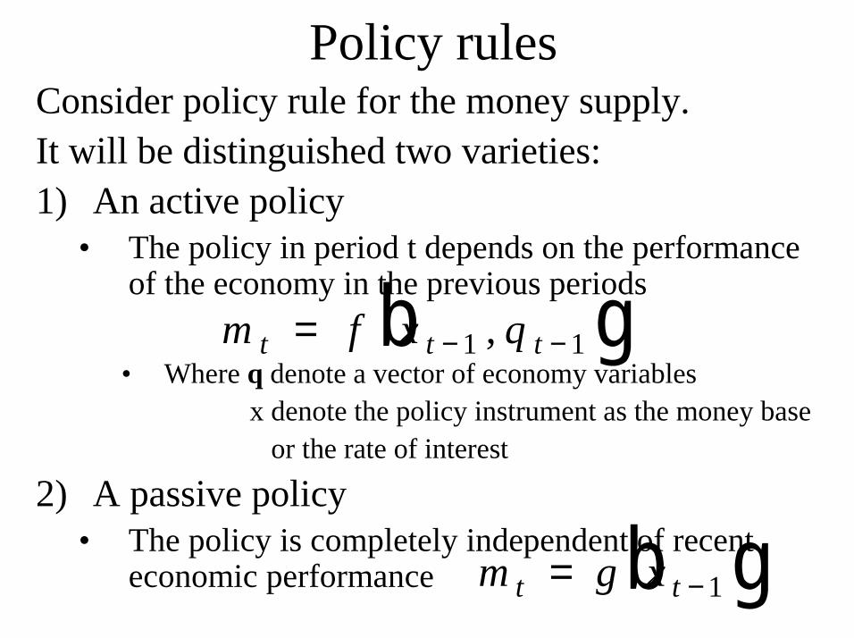
Policy rulesConsider policy rule for the money supply.It will be distinguished two varieties:1) An active policy

• The policy in period t depends on the performance of the economy in the previous periods

• Where q denote a vector of economy variablesx denote the policy instrument as the money base

or the rate of interest

2) A passive policy• The policy is completely independent of recent

economic performance

m f x qt t t= − −1 1,b g

m g xt t= −1b g

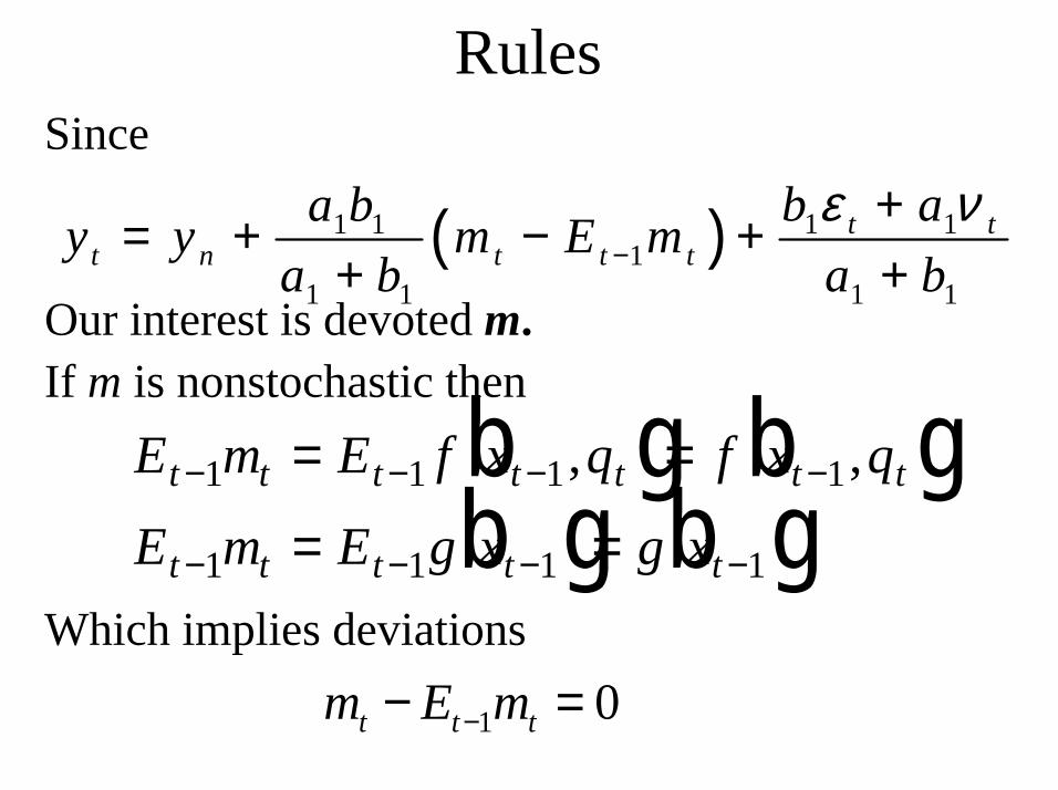
RulesSince

Our interest is devoted m.If m is nonstochastic then

Which implies deviations

E m E f x q f x q

E m E g x g xt t t t t t t

t t t t t

− − − −

− − − −

= =

= =1 1 1 1

1 1 1 1

, ,b g b gb g b g

( ) 1 11 11

1 1 1 1

t tt n t t t

b aa by y m E ma b a b

ε ν−

+= + − ++ +

1 0t t tm E m−− =

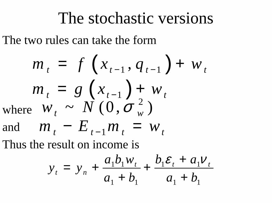
The stochastic versionsThe two rules can take the form

whereand Thus the result on income is

( )1 1,t t t tm f x q w− −= +

( )1t t tm g x w−= +2~ (0 , )t ww N σ

1t t t tm E m w−− =

1 1 1 1

1 1 1 1

t t tt n

a b w b ay ya b a b

ε ν+= + ++ +

Money, Growth, and Inflation

The motivation is to establish that along theequilibrium growth path, the expected rate of inflation equals the rate of monetary expansion minus the warranted rate of growth

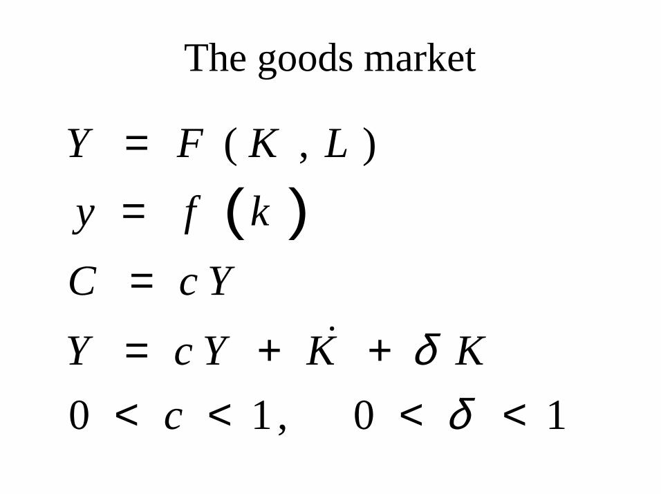
The goods market

( )( , )

0 1 , 0 1

Y F K Ly f kC c YY c Y K K

cδ

δ

==== + +< < < <

�

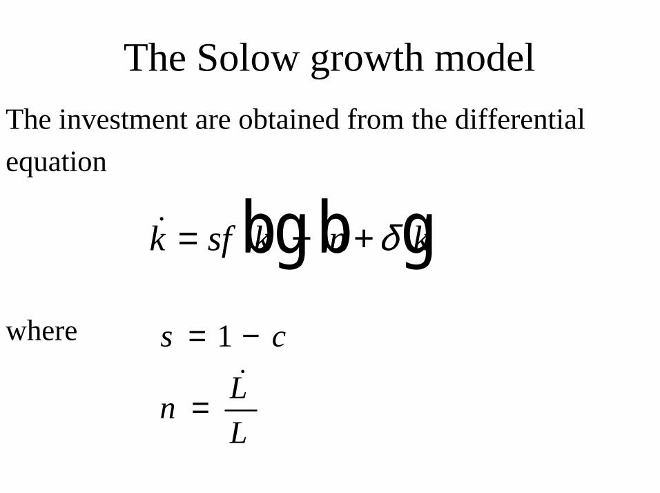
The Solow growth modelThe investment are obtained from the differentialequation

where

�k sf k n k= − +b g b gδ

1s cLnL

= −

=�

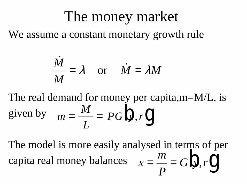
The money marketWe assume a constant monetary growth rule

The real demand for money per capita,m=M/L, isgiven by

The model is more easily analysed in terms of percapita real money balances

��

MM

M M= =λ λor

m ML

PG y r= = ,b g

x mP

G y r= = ,b g

The money market is assumed to be always in equilibrium,i.e.,Thus we can derive the implicit function

r H y x= ,

x mP

G y r= = ,b g

Two assetsIn this model exist only two assets1. Money2. Physical capitalThe real rate of interest is the nominal rate,r,minus the rate of inflation,p.In equilibrium this will be equated with themarginal product of capital adjusted for the rate ofdepreciation

r f k r f k− = ′ − = ′ − +π δ δ πb g b gor

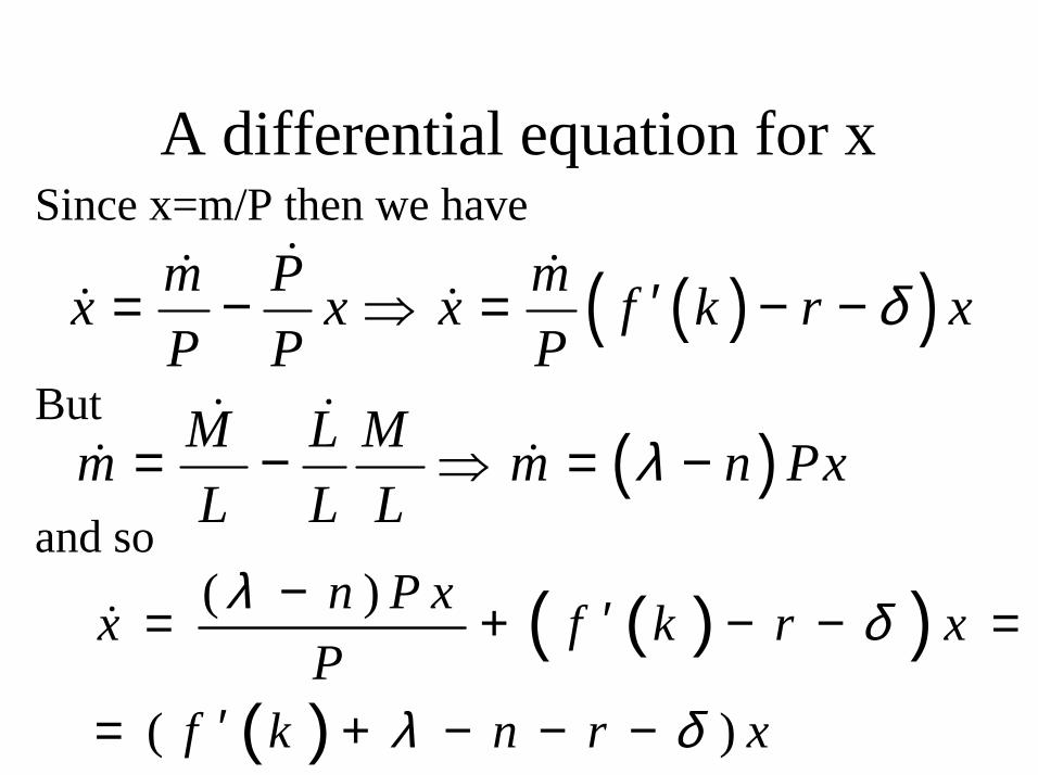
A differential equation for xSince x=m/P then we have

But

and so

( )( )m P mx x x f k r xP P P

δ′= − ⇒ = − −�� �

� �

( )M L Mm m n PxL L L

λ= − ⇒ = −� �

� �

( )( )( )

( )

( )

n P xx f k r xP

f k n r x

λ δ

λ δ

− ′= + − − =

′= + − − −

�

That is

� ,x f k n H f k x x= ′ + − − −b g b gc he jλ δ

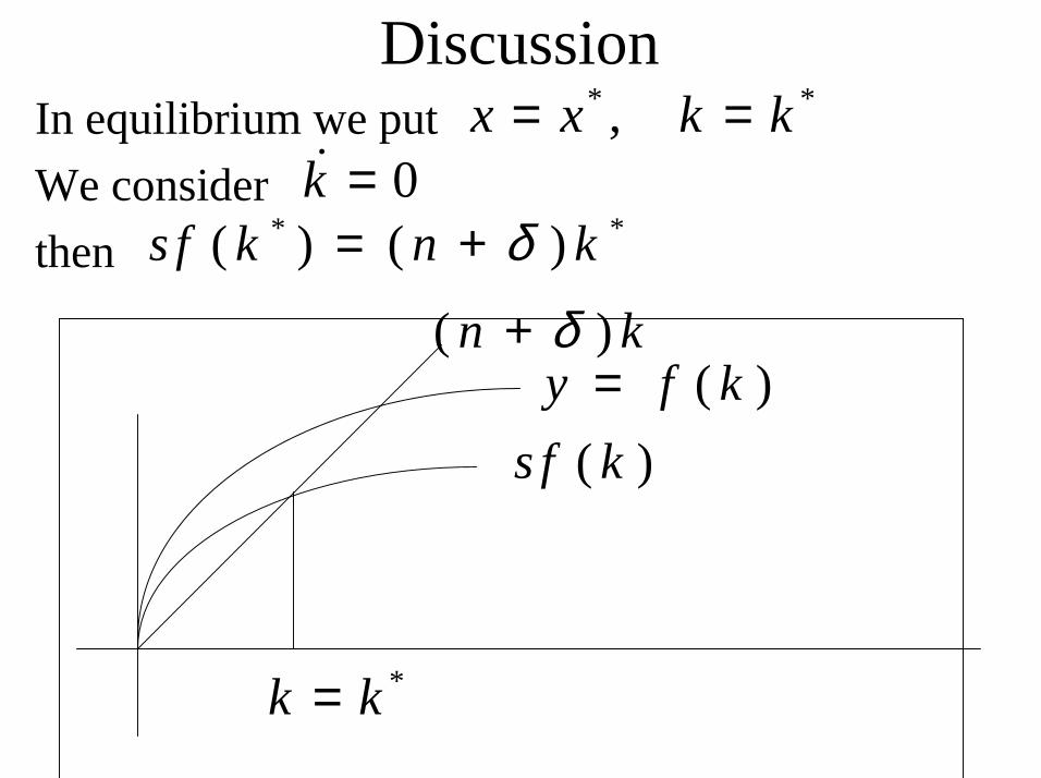
DiscussionIn equilibrium we putWe considerthen

* *,x x k k= =0k =�

* *( ) ( )s f k n kδ= +

*k k=

( )n kδ+( )y f k=

( )s f k

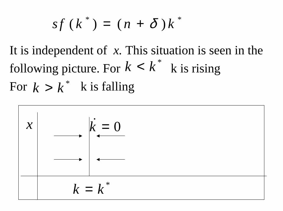
It is independent of x. This situation is seen in the following picture. For k is risingFor k is falling

* *( ) ( )s f k n kδ= +

*k k=

0k =�x

*k k<*k k>

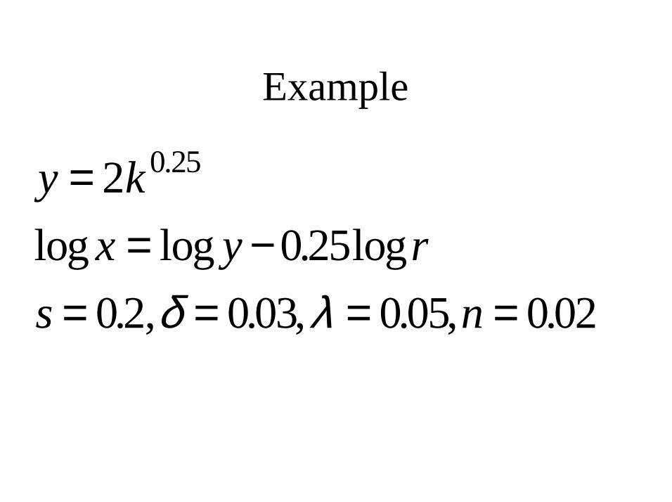
Example

y kx y r

s n

== −

= = = =

2025

02 003 005 002

0 25.

log log . log. , . , . , .δ λ

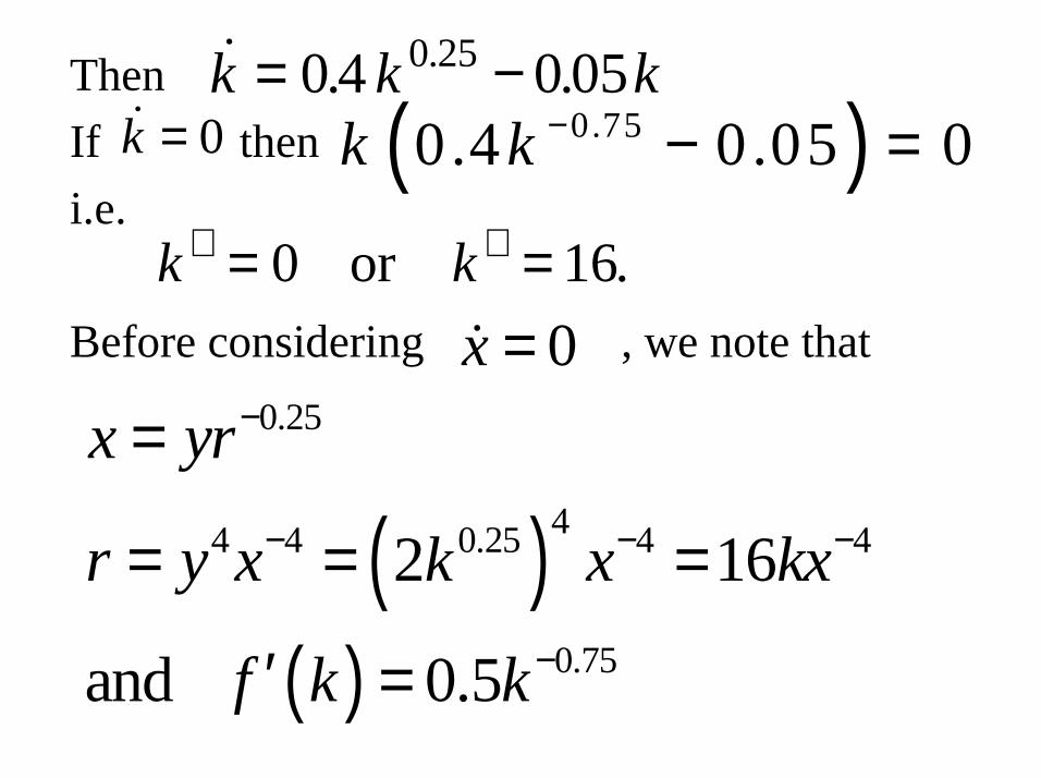
ThenIf theni.e.

Before considering , we note that

� . ..k k k= −0 4 0 050 25

�k = 0 ( )0.750.4 0.05 0k k − − =

k k∗ ∗= =0 16or .0x =�

( )( )

0.25

44 4 0.25 4 4

0.75

2 16

and 0.5

x yr

r y x k x kx

f k k

−

− − −

−

=

= = =

′ =

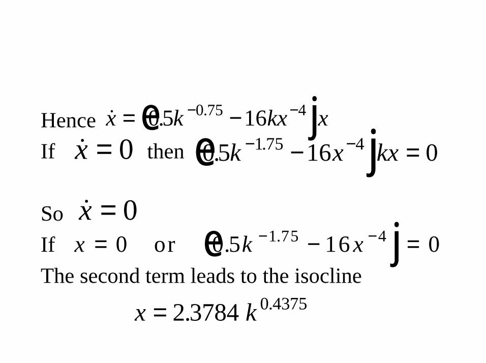
HenceIf then

SoIfThe second term leads to the isocline

� . .x k kx x= −− −05 160 75 4e j�x = 0 0 5 16 01 75 4. .k x kx− −− =e j�x = 0

x k x= − =− −0 0 5 16 01 75 4or . .e j

x k= 2 3784 0 4375. .

Mathcad Document

Unemployment and job turnoverThere is full employment in the sense that the number of jobs is matched by the number ofhouseholds seeking employment. At any instant of time a fraction s of individualsbecome unemployed and search over firms to find a suitable job.Let f denote the probability of finding a job. At any moment of time, if u is the fraction of theparticipating labor force unemployedthen

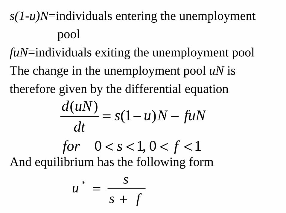
s(1-u)N=individuals entering the unemployment pool

fuN=individuals exiting the unemployment poolThe change in the unemployment pool uN is therefore given by the differential equation

And equilibrium has the following form

d uNdt

s u N fuN

for s f

( ) ( )

,

= - -

< < < <

1

0 1 0 1

u ss f

*=

+

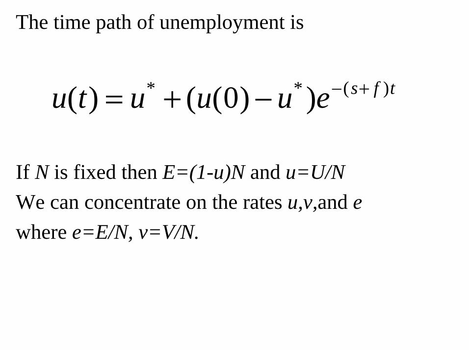
The time path of unemployment is

If N is fixed then E=(1-u)N and u=U/N We can concentrate on the rates u,v,and ewhere e=E/N, v=V/N.

u t u u u e s f t( ) ( ( ) )* * ( )= + -

- +0

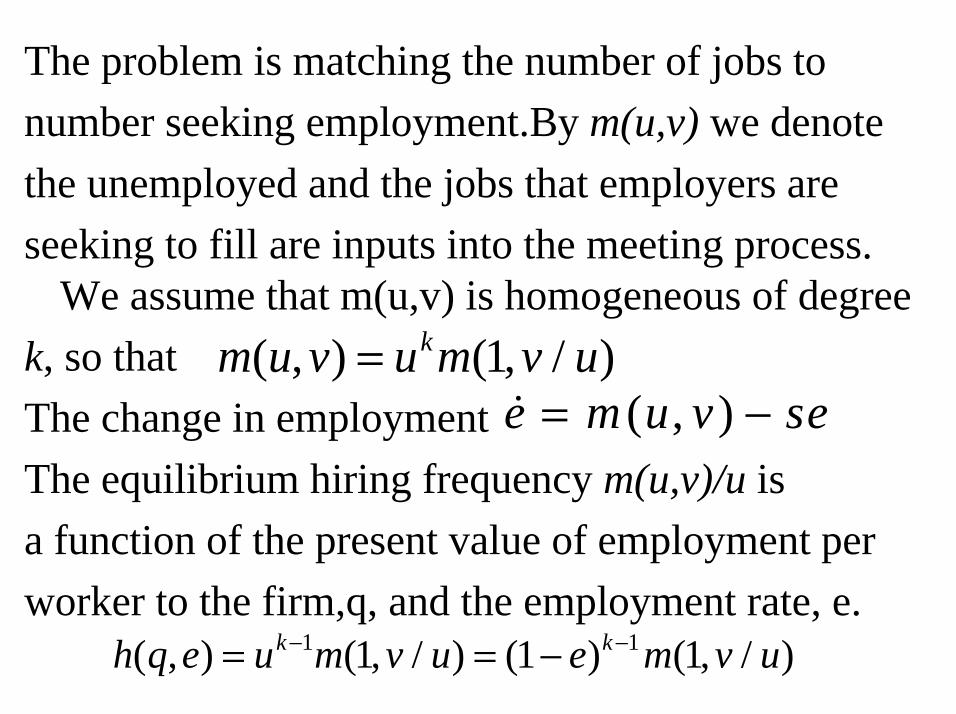
The problem is matching the number of jobs to number seeking employment.By m(u,v) we denote the unemployed and the jobs that employers are seeking to fill are inputs into the meeting process.

We assume that m(u,v) is homogeneous of degreek, so thatThe change in employmentThe equilibrium hiring frequency m(u,v)/u is a function of the present value of employment perworker to the firm,q, and the employment rate, e.

m u v u m v uk( , ) ( , / )= 1� ( , )e m u v se= -

h q e u m v u e m v uk k( , ) ( , / ) ( ) ( , / )= = -- -1 11 1 1

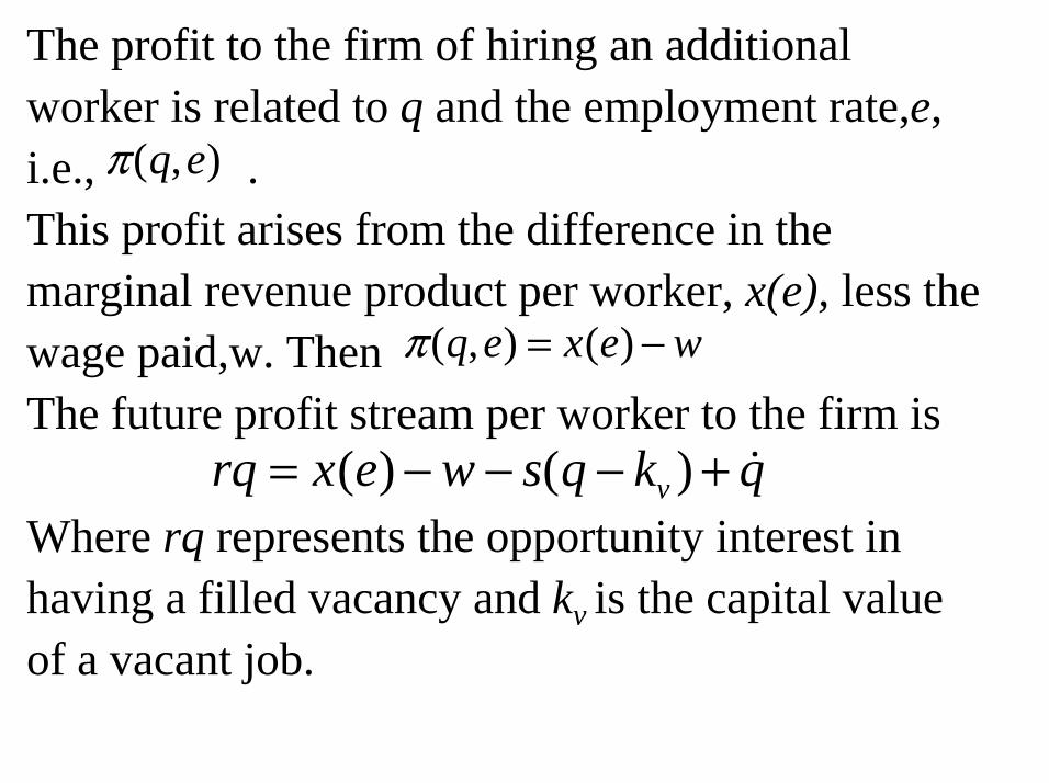
The profit to the firm of hiring an additionalworker is related to q and the employment rate,e, i.e., .This profit arises from the difference in themarginal revenue product per worker, x(e), less thewage paid,w. ThenThe future profit stream per worker to the firm is

Where rq represents the opportunity interest inhaving a filled vacancy and kv is the capital value of a vacant job.

p ( , )q e

p ( , ) ( )q e x e w= -

rq x e w s q k qv= - - - +( ) ( ) �

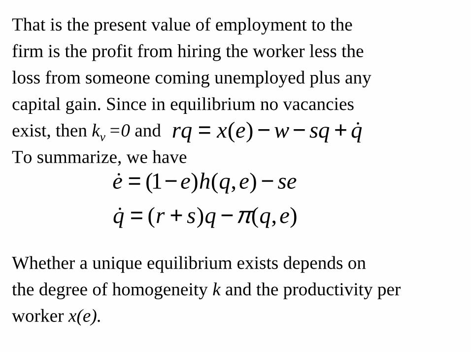
That is the present value of employment to the firm is the profit from hiring the worker less the loss from someone coming unemployed plus anycapital gain. Since in equilibrium no vacancies exist, then kv =0 andTo summarize, we have

Whether a unique equilibrium exists depends onthe degree of homogeneity k and the productivity per worker x(e).

( )rq x e w sq q= − − + �

(1 ) ( , )( ) ( , )

e e h q e seq r s q q eπ

= − −= + −

�

�

Wage determination models and the profit function

The profit function isWhere b is the value of leisure forgone whenemployed.If denotes the expected present value of a worker’s

income when employed and the expected presentvalue of a worker’s future income when unemployed,then in equilibrium

( , ) ( )q e x e bπ = −

ye

yu

λ y y be u− =b g

Furthermore

ry w s y y y

ry bm u v

vy y y

e u e e

u e u u

= + − +

= +LNM

OQP − +

b gb g b g

�

,�

The first states that the opportunity interest fromholding a job must equal the wage received plus

the income he receives when unemployed, which hefaces with probability s, plus any capital gain. The second equation states that the opportunity interest on being unemployed must equal the return from not working plus the income he receives when employed, which he faces with an average match of

, plus any capital gain.m u v u, /b g

In equilibrium and

Hence

�ye = 0

ry w sb

ry bm u v

ub

e

u

= −

= +LNM

OQPFHG

IKJ

λ

λ,b g

r y y w b sb m u vu

b

rb w b sb m u vu

b

e u− = − − −LNM

OQPFHG

IKJ

FHG

IKJ = − − −

LNM

OQPFHG

IKJ

b g b g

b gλ λ

λ λ λ

,

,

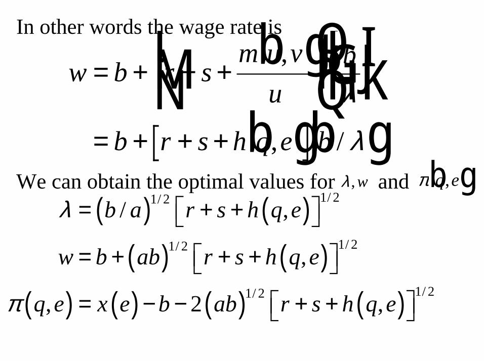
In other words the wage rate is

We can obtain the optimal values for and

w b r sm u v

ub

b r s h q e b

= + + +LNM

OQPFHG

IKJ

= + + +

,

, /

b g

b g b gλ

λλ ,w π q e,b g

( ) ( )( ) ( )

( ) ( ) ( ) ( )

1/ 21/ 2

1/ 21/ 2

1/ 21/ 2

/ ,

,

, 2 ,

b a r s h q e

w b ab r s h q e

q e x e b ab r s h q e

λ

π

= + +

= + + +

= − − + +

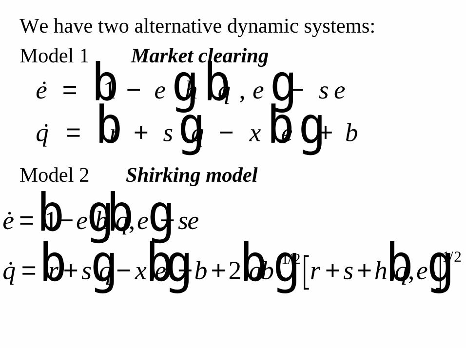
We have two alternative dynamic systems:Model 1 Market clearing

Model 2 Shirking model

� ,�

e e h q e s eq r s q x e b

= − −

= + − +

1b g b gb g b g

� ,

� ,/ /

e e h q e se

q r s q x e b ab r s h q e

= − −

= + − + + + +

1

2 1 2 1 2

b g b gb g b g b g b g

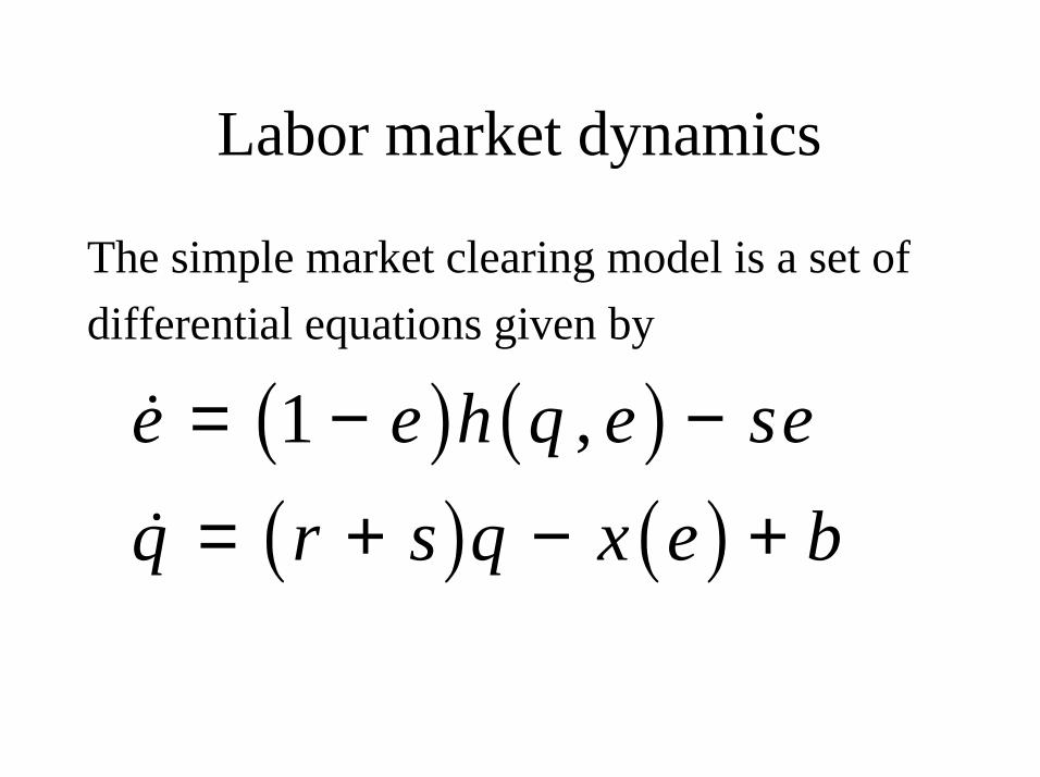
Labor market dynamics

The simple market clearing model is a set of differential equations given by

� ,�

e e h q e seq r s q x e b

= − −

= + − +

1