Embed Size (px)
Citation preview

Economic Computation and Economic Cybernetics Studies and Research, Issue 1/2017, Vol. 51
_______________________________________________________________________________
169
Associate Professor Zheng-Xin Wang, PhD
E-mail: [email protected]
Zhejiang University of Finance & Economics
A WEIGHTED NON-LINEAR GREY BERNOULLI MODEL FOR
FORECASTINGNON-LINEAR ECONOMICTIME SERIES WITH
SMALL DATA SETS
Abstract. To accurately forecast non-linear economic time series with
small data sets, the weighted non-linear grey Bernoulli model (WNGBM) is built in
this paper. Through the optimization of the power index and weights for
accumulative generation, WNGBM can more actively adapt to non-linear
fluctuations in the raw data than NGBM. A typical case of topological rolling
prediction verifies that the WNGBM exhibits better non-linear prediction
capabilities than other grey models. Furthermore, the forecasting performance of
WNGBM is compared with that of Holt-Winters, Support Vector Regression (SVR),
and BP Neural Network (BPNN) based on the Shanghai Stock Exchange(SSE)
Composite Indices. Results indicate that WNGBM shows the best ability to fit non-
linear data from small sample sizes, while it has a slightly higher error in the
prediction of out-of-sample data for the SSE Composite Index than that of BPNN.
The extreme values mean that the prediction curve of the Holt-Winters method
generally deviates from the actual data, which leads to a greater prediction error.
Keywords: grey systems theory; time series prediction; non-linear grey
Bernoulli model; small data sets; stock exchange composite index.
JEL Classification: C63
1. Introduction
Compared to classical statistical prediction methods, the grey forecasting
(Deng, 2002) is a novel prediction method based on grey theory. The advantage of
this method is that it is efficient in modeling and forecasting raw sequences with
sparse data (at least four sample points are required). In grey theory (Deng, 2002;
Liu & Lin, 2006), most real-life systems are regarded as “generalized energy
systems”, these include: agricultural systems, industrial systems, ecosystems, etc.
Any non-negative smooth discrete sequence produced by these systems can be
converted into a sequence based upon the grey exponent law through the
application of an accumulative generation operator (AGO). Then, a grey
differential equation is constructed to describe this exponent law and used to

Zheng-Xin Wang
______________________________________________________________
170
forecast the sequence produced by AGO. Finally, the final forecast values can be
derived by reducing the forecast results through inverse accumulative generation
operators (IAGO).
The most widely used grey forecasting model GM (1,1) – a first-order one-
variable grey differential equation – is proposed based on the aforementioned
principle (Deng, 2002). Its modeling principle does not depend on distribution
information from the raw data, but on the application of a first order accumulative
generation operator (1-AGO), so as to make the generated sequence display the
approximate exponential growth tendency. Based on this, a first-order grey
differential equation is constructed and solved. The forecast values are then derived
from the first order inverse accumulative generation operator (1-IAGO). Due to
GM (1,1) can be constructed without a large sample, and it is easy to be built and
calculated, GM (1,1) and its improved variant models, have been widely used (Li
et al, 2003; Wang & Hsu, 2008; Wang et al., 2014).
The non-linear grey Bernoulli model (NGBM) is a type of grey forecasting
model based on Bernoulli equation (Chen, 2008). Because its form and forecasting
function are non-linear, it can effectively forecast time sequence data exhibiting
non-linear fluctuations, while traditional GM (1,1) models cannot. Similar to
traditional grey models, the prediction precision was improved by the particle
swarm optimization algorithm (Zhou et al., 2009), Nash equilibrium based
optimization method (Chen et al., 2010).Though NGBM is better than traditional
grey models at forecasting non-linear economic time series, for wildly fluctuating
raw data, its prediction precision is not currently high as will be later demonstrated
in the study of test-cases.
In fact, the data at different time points play different roles in the output
forecast, which should be taken into consideration especially for the modeling of
raw data with obvious fluctuations as this can provide an effective description, and
record, of such random variations.
This study applies different weights to data at different time points in the
process of the accumulative generation operator on the raw data, thereby enhancing
the flexibility of NGBM and its ability to fit a fluctuating economic time series.
The improved NGBM is named as a weighted non-linear grey Bernoulli model
(WNGBM). Moreover, traditional forecasting methods such as Holt-Winters (Xu,
2005) and intelligent forecasting algorithms such as SVR (Li et al., 2013;
Suganyadevi&Babulal, 2014) and ANN (Ren et al., 2014) can also be applied to
forecast non-linear economic time series with small data sets. This work will
attempt to compare those methods with the proposed WNGBM (Wang et al.,
2016).
The rest of the paper is structured as follows: Section 2 presents the
construction process of WNGBM. Section 3 proves the advantage of the WNGBM
over the NGBM and explains the reasons by a classical case. Section 4compares
the forecasting performance of WNGBM, Holt-Winters, SVR, and BPNN using
A Weighted Non-linear Grey Bernoulli Model for Forecasting Non-linear
Economic Time Series with Small Data Sets
171
the non-linear time series of SSE Composite Index. Finally, the paper concludes
with some comments in Section 5.
2. Methodology
For the prediction of the non-linear time series with small sample sets, an
NGBM’s performance is better than that of traditional grey forecasting models, but
it still cannot adapt to volatile non-linear time series. In this section, the main
methodology for building a WNGBM (Wang et al., 2016) is presented.
2.1 The constrained first order weighted generation operators
In grey forecasting theory, accumulative generation operator, and its
inverse, are two basic operators applied to mine the raw data and reduce (simplify)
the original appearance of the data. To reflect the importance of data at different
time points, the weighted accumulative generation operator and its inverse are now
introduced.
Definition 1. Assume that (0)X is a sequence of raw data and D a sequence
operator satisfying:
(0) (0) (0) (0)(1), (2), , ( )X x x x m , (1)
(1), (2), , ( )m , (2)
and
(0) (0) (0) (0)(1) , (2) , , ( )X D x d x d x m d , (3)
where (0) (0)
1
( ) ( ) ( )k
i
x k d i x i
, 1,2, ,k m , 1
( )m
j
j m
, 0 ( )j m , for
1,2, ,k m . Then the sequence operator D is a constrained first-order weighted
accumulative generation operator of (0)X , denoted 1-CWAGO.
Assuming the total weight is a constraint on m, the data are endowed with
time-variant weights in 1-CWAGO. This indicates that the data at different times
can play different roles in the forecasting process. Since, according to the
accumulating generation operator described by Liu & Lin (2006), the weight
values obtained by (1-AGO) are 1, it is unable to distinguish the importance of data
at different times. This shows the difference between 1-CWAGO and 1-AGO.
Definition 2. Assume that (0)X is a sequence of raw data and D is a
sequence operator such that:
(0) (0) (0) (0)(1), (2), , ( )X x x x m , (4)
(1), (2), , ( )m , (5)
and
(0) (0) (0) (0)(1) , (2) , , ( )X D x d x d x m d , (6)

Zheng-Xin Wang
______________________________________________________________
172
where (0) (0)(1) (1) (1)x d x , (0) (0) (0)( ) ( ) ( 1) ( )x k d x k x k k , 1
( )m
j
j m
,
0 ( )j m , for 1,2, ,k m . Then D is a constrained weighted first-order inverse
accumulative generation operator of (0)X , denoted 1-CWIAGO.
1-CWIAGO is an inverse operator corresponding to 1-CWAGO. 1-
CWAGO sequences which are forecasted by the grey model constructed by the
sequences generated by 1-CWAGO are not the actual sequence. Therefore, the
function of 1-CWIAGO is to convert the direct output results of the grey model
into the forecast values of actual data by reduction. Compared with 1-AGO, as
described by Liu & Lin (2006), 1-CWIAGO is able to perform more accurate
reduction based on the weights of the data at different times. It is noted that 1-AGO
is a special case of 1-CWIAGO: in the case of ( ) 1, 1,2, ,k k m , 1-CWIAGO
degrades to 1-AGO.
2.2 Weighted non-linear grey Bernoulli model (WNGBM)
Based on the 1-CWAGO and 1-CWIAGO, the traditional non-linear grey
Bernoulli model proposed by Chen (2008) can be extended to a weighted non-
linear grey Bernoulli model (WNGBM). The modeling process is summarized as
follows.
Step1: assuming the original series of raw data contains m entries:
(0) (0) (0) (0)(1), (2), , ( )X x x x m , (7)
where x(0) (k) represents the behavior of the data at time k for k =1,2, ,m .
Step 2: construct (1)X by applying a one-time weighted accumulative
generation operator (1-CWAGO) to (0)X :
(1) (1) (1) (1)(1), (2), , ( )X x x x m , (8)
where (1) (0)
1
( ) ( ) ( )k
i
x k i x i
, 1,2, ,k m .
The stepwise ratio of 1-AGO sequence (1)X is given by:
1 0 1
1
1 1
11
1 1
x k x k x kk k
x k x k
(9)
where
1
11
1
k
i
x kk
x i
; 2,3, ,k m .
According to the properties of a non-negative smooth sequence (Liu & Lin,
2006), we obtain:
A Weighted Non-linear Grey Bernoulli Model for Forecasting Non-linear
Economic Time Series with Small Data Sets
173
1
1
1[1,1.5)
1
x kk
x k
(10)
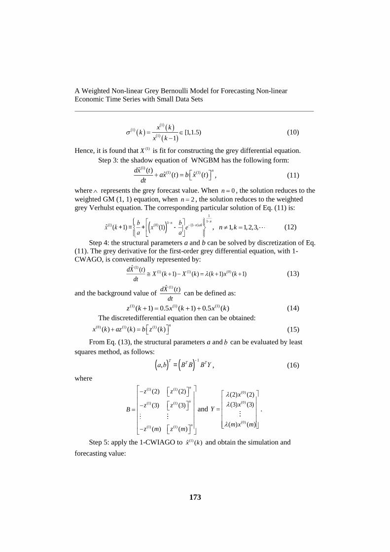
Hence, it is found that (1)X is fit for constructing the grey differential equation.
Step 3: the shadow equation of WNGBM has the following form: (1)
(1) (1)ˆ ( )ˆ ˆ( ) ( )
ndx tax t b x t
dt , (11)
where represents the grey forecast value. When 0n , the solution reduces to the
weighted GM (1, 1) equation, when 2n , the solution reduces to the weighted
grey Verhulst equation. The corresponding particular solution of Eq. (11) is:
x̂(1)(k +1) =b
a+ x(0)(1)( )
1-n
-b
a
é
ëê
ù
ûúe
-(1-n)akìíï
îï
üýï
þï
1
1-n
, 1, 1,2,3,n k (12)
Step 4: the structural parameters a and b can be solved by discretization of Eq.
(11). The grey derivative for the first-order grey differential equation, with 1-
CWAGO, is conventionally represented by: (1)
(1) (1) (0)ˆ ( )
( 1) ( ) ( 1) ( 1)dX t
X k X k k x kdt
(13)
and the background value of (1)ˆ ( )dX t
dt can be defined as:
(1) (1) (1)( 1) 0.5 ( 1) 0.5 ( )z k x k x k (14)
The discretedifferential equation then can be obtained: (0) (1) (1)( ) ( ) ( )
n
x k az k b z k (15)
From Eq. (13), the structural parameters a and b can be evaluated by least
squares method, as follows:
a,b( )T
= BTB( )-1
BTY , (16)
where
(1) (1)
(1) (1)
(1) (1)
(2) (2)
(3) (3)
( ) ( )
n
n
n
z z
z zB
z m z m
and
(0)
(0)
(0)
(2) (2)
(3) (3)
( ) ( )
x
xY
m x m
.
Step 5: apply the 1-CWIAGO to (1)ˆ ( )x k and obtain the simulation and
forecasting value:

Zheng-Xin Wang
______________________________________________________________
174
(0) (1) (1)ˆ ˆ ˆ( 1) ( 1) ( ) ( 1)x k x k x k k for 1,2,3,k . (17)
Based on this description, the grey predictor composed of 1-CWAGO, 1-
CWIAGO, and WNGBM can be constructed by: (0) (0)ˆ ( 1) CWIAGO NGBM CWAGO ( )x k x k (18)
Step 6: analyze the modeling error using both the relative and average
relative errors. For the forecast from models derived from datasets with more than
four samples, users are to apply topological rolling error analysis to test the
forecasting errors. The specific process and NGBM modelling procedure are
identical to the last step of the design process.
Step 6: the residual error test is adopted to compare the actual value with
that forecast. The residual error at k and average residual error of the grey
forecasting are usually defined as:
Relative error(0) (0)
(0)
ˆ ( ) ( )( ) 100%
( )
x k x kk
x k
, 2,3,4,k m , (19)
and
Average relative error2
1( ) ( )
1
m
k
avg km
, 2,3,4,k m . (20)
If the number of raw data points m is greater than 4, a WNGBM
topological rolling model can be constructed. Then topological rolling error
analysis is applied to test the one-step prediction error of other data apart from that
in the sample.
Firstly, a WNGBM is constructed on the basis of the first four entries in
the dataset (0) (0) (0) (0) (0)(1), (2), (3), (4)X x x x x , and the value of the next point
(0)ˆ (5)x is forecast. Then, WNGBM is built using the first five entries in the dataset
(0) (0) (0) (0) (0) (0)(1), (2), (3), (4), (5)X x x x x x to predict the value of the sixth point
(0)ˆ (6)x . This procedure is repeated until the end of the sequence. The topological
rolling error is defined as: (0) (0)
(0)
ˆ ( 1) ( 1)( , 1) 100%
( 1)
x k x ktp k
x k
, 4,5, , 1k m . (21)
The average topological rolling error is: 1
4
1( , ) ( , 1)
4
m
k
tp avg tp km
. (22)
2.3 Parameter optimization based on Nash equilibrium
The traditional NGBM model has only one unknown parameter, namely its
power index n which can be easily optimized by computer program. In the

A Weighted Non-linear Grey Bernoulli Model for Forecasting Non-linear
Economic Time Series with Small Data Sets
175
WNGBM model (Wang et al., 2016),m weights ( ), 1, 2, ,i i m are unknown,
apart from power index.
Supposing the initial condition value of the power index is 0n and the
initial condition of the weights is ( ) 1, 1,2, ,i i m : the optimization model is
built from the viewpoint of Nash equilibrium (Chen, 2010)to minimize the
forecasting error. Under the condition of giving the raw data sequence (0)X , the
minimization of average relative error is the objective of the optimization as stated
in Eq. (23).
(0)
, ( )2
1Min , ( ) | Min ( )
1
m
n kk
n k X km
(23)
where the power index n is a real number (n ≠ 1), and 1
( ) (0, ), ( )m
k
k m k m
.
Based on Eq. (23) and assisted by the operations research software,
LINGO, the optimal Nash solution *
Nn and * ( )N k for 1,2, ,k m can be reached.
The optimization process is as follows:
* (0)
0 ( ) 0
* (0) *
1 0( )
** (0)
( )
* (0) *
1 ( )
* (0
( )
Arg Min | , ( ) 1, 1,2, , ,
( ) Arg Min ( ) | , , 1, 2, , ,
Arg Min | , ( ) , 1, 2, , ,
( ) Arg Min ( ) | , , 1, 2, , ,
Arg Min |
n
k
i n i
i ik
N n
n n X k k m
k k X n n k m
n n X k k m
k k X n n k m
n n X
*)
* (0) *
( )
, ( ) , 1, 2, , ,
( ) Arg Min ( ) | , , 1, 2, , .
N
N Nk
k k m
k k X n n k m
(24)
In Eq. (24), the process for solving *
Nn and * ( )N k can be described as a
numerical application of the generalized Nash equilibrium algorithm. The
generalized Nash equilibrium problem refers to a non-cooperative game. Its
strategy sets and loss functions for each competitor are obtained by relying on
other competitors. Based on Eq. (24), the power index n and weight ( )k are
regarded as two competitors. The loss function (referring to the optimized
objective function) is (0), ( ) |n k X . The generalized Nash equilibrium algorithm
has been proved to be globally convergent. Thus, the algorithm described by Eq.
(24) exhibits global convergence. Salient inequalities are proved as follows:

Zheng-Xin Wang
______________________________________________________________
176
** (0)
** (0)
1
** (0)
1
** (0)
** (0)
0 1
* (0)
0 0
, ( ) |
, ( ) |
, ( ) |
, ( ) |
, ( ) |
, ( ) |
N N
N N
i i
i i
n k X
n k X
n k X
n k X
n k X
n k X
(25)
The further modeling process for future weights * *ˆ ˆ( 1), ( 2),N Nm m can be
abbreviated to: * *ˆ ( 1) IAGO NGBM AGO ( )N Nk k
. (26)
3. Validation of the weighted non-linear grey Bernoulli model –a case
of Chinese recruits to higher education
The example to validate the effectiveness of NGBM is based on a study by
Deng & Guo (1996) of the numbers of students recruited into higher education in
certain provinces in China from 1984 to 1990. Due to the effect of many uncertain
factors affecting higher education institution admissions in China, the data during
the time period present all the hallmarks of non-linearity. The original data are {0,
2.413, 6.159, 3.671, 3.582, 4.853, 3.821, 3.163} (× 10,000 recruits). Topological
analysis was performed on these data: during the time period, five topological sub-
sequences were used to build the topological rolling grey model (0)ˆ (1: 4)x , (0)ˆ (1: 5)x , (0)ˆ (1: 6)x , (0)ˆ (1: 7)x , (0)ˆ (1: 8)x . The forecast results of traditional grey models and
NGBM on five sub-sequences showed that the prediction precision of NGBM was
significantly better than that of traditional models(Chen, 2008). Even so, the
average errors of NGBM were still greater than 10%, at: 12.79%, 11.96%, 20.05%,
16.90%, and 14.93%.
3.1The forecast results of NGBM and WNGBM
This case study was re-analyzed by NGBM and WNGBM and Table 1 lists
the grey modeling results with relative, and average relative, errors of five sub-
sequences using NGBM and WNGBM, respectively. Table 1 and Table 2 indicate
that the average relative errors of WNGBM forecast on five sub-sequences are all
below 5%, while those of NGBM are greater than 10%. It can be seen that

A Weighted Non-linear Grey Bernoulli Model for Forecasting Non-linear
Economic Time Series with Small Data Sets
177
WNGBM greatly decreases the average forecasting errors of NGBM through
additionally optimizing the weights of accumulating generation.
Table 1.Forecast comparison: NGBM and WNGBM applied to the five
topological sub-sequences
ˆ (0)x (1: 4) k=1 k=2 k=3 k=4
NGBM ε(k)%
WNGBM *
Nλ (k)
ε(k)%
0
0
0
1.602
0
2.425
0.00
2.413
1.171
0.00
4.914
20.19
6.159
0.459
0.00
4.336
-18.17
3.671
0.769
0.00
ˆ (0)x (1: 5) k=1 k=2 k=3 k=4 k=5
NGBM ε(k)%
WNGBM *
Nλ (k)
ε(k)%
0
0
0
0.779
0
2.441
0.00
2.413
0.583
0.00
4.813
-21.84
5.038
0.758
-18.21
4.554
24.28
3.671
1.376
-0.01
3.519
-1.72
3.582
1.504
-0.01
(0)ˆ (1: 6)x k=1 k=2 k=3 k=4 k=5 k=6
NGBM ε(k)%
WNGBM *
Nλ (k)
ε(k)%
0
0
0
0.975
0
2.445
0.00
2.413
1.341
0.00
4.313
-30.06
5.679
0.707
-7.49
4.694
28.05
3.671
1.115
0.00
4.495
25.63
3.582
1.107
0.00
4.053
-16.53
4.877
0.756
2.42
ˆ (0)x (1: 7) k=1 k=2 k=3 k=4 k=5 k=6 k=7
NGBM ε(k)%
WNGBM *
Nλ (k)
ε(k)%
0
0
0
1.274
0
2.413
0.00
2.413
0.511
0.00
4.237
-31.21
6.159
0.450
0.00
4.675
27.36
3.254
1.157
-11.37
4.563
27.38
3.582
1.240
0.00
4.202
-13.41
4.853
1.010
-0.01
3.743
-2.04
3.821
1.358
0.00
ˆ (0)x (1: 8)
k=1 k=2 k=3 k=4 k=5 k=6 k=7 k=8
NGBM ε(k)%
WNGBM *
Nλ (k)
ε(k)%
0
0
0
1.747
0
2.413
0.00
2.415
1.024
0.07
4.240
31.16
6.132
0.522
-0.44
4.677
27.40
3.394
1.011
-7.56
4.562
27.35
3.600
0.978
0.51
4.199
13.49
4.885
0.724
0.66
3.737
2.20
3.852
0.912
0.81
3.256
2.93
3.193
1.083
0.96

Zheng-Xin Wang
______________________________________________________________
178
N.B The calculation results listed above have been handled in accordance with
mathematical rounding rules, so the sum of the optimal weights for analysis by
WNGBM does not precisely equal m , 4,5, ,8m .
Table 2. The average relative errors of NGBM and WNGBM
Topological
sub-
sequences
ˆ (0)x (1: 4) ˆ (0)
x (1: 5) ˆ (0)x (1: 6) ˆ (0)
x (1: 7) ˆ (0)x (1: 8)
NGBM 12.79% 11.96% 20.05% 16.90% 14.93%
WNGBM 0.00% 4.56% 1.98% 1.90% 1.57%
3.2 Explanation of the forecast results
To analyze the reasons why 1-CWAGO improves the modeling precision
of NGBM, topological sequence (0)ˆ (1: 6)x was used as an example to illustrate this.
As shown in Figure1, the curve shapes of the 1-AGO sequence (1) (1: 6)x of the raw
data, the 1-AGO sequence forecasted by NGBM, and the 1-CWAGO sequence (1)ˆ (1: 6)x predicted by WNGBM are in good agreement. However; after the
corresponding reduction of 1-IAGO and 1-CWIAGO, the differences between the
final prediction sequences (0)ˆ (1: 6)x of NGBM and WNGBM become obvious. The
curve shape of the final prediction sequence (see Figure2) of WNGBM (0)ˆ (1: 6)x
and that of the raw data (0) (1: 6)x are very close, while NGBM cannot effectively
track the non-linear fluctuations in the raw data. From the modelling procedures of
both NGBM and WNGBM it is found that the only step that makes (1)ˆ (1: 6)x
change to (0)ˆ (1: 6)x is inverse transformation. Therefore, the reason for this
phenomenon is believed to be enshrined in the fact that the accumulative
generation and its inverse transform of WNGBM at different times use different
optimal weights, while that of NGBM take the same optimal weights throughout
(as shown in Figure3).

A Weighted Non-linear Grey Bernoulli Model for Forecasting Non-linear
Economic Time Series with Small Data Sets
179
Figure 1.1-AGO predictions by: actual value, NGBM, and 1-CWAGO
prediction by WNGBM
Figure 2.Final forecast curves: actual value, NGBM, and WNGBM
0
5
10
15
20
25
0 1 2 3 4 5 6 7
Actual value NGBM WNGBM
0
1
2
3
4
5
6
7
0 1 2 3 4 5 6 7
Actual value NGBM WNGBM

Zheng-Xin Wang
______________________________________________________________
180
Figure 3.The weights curve of NGBM and WNGBM
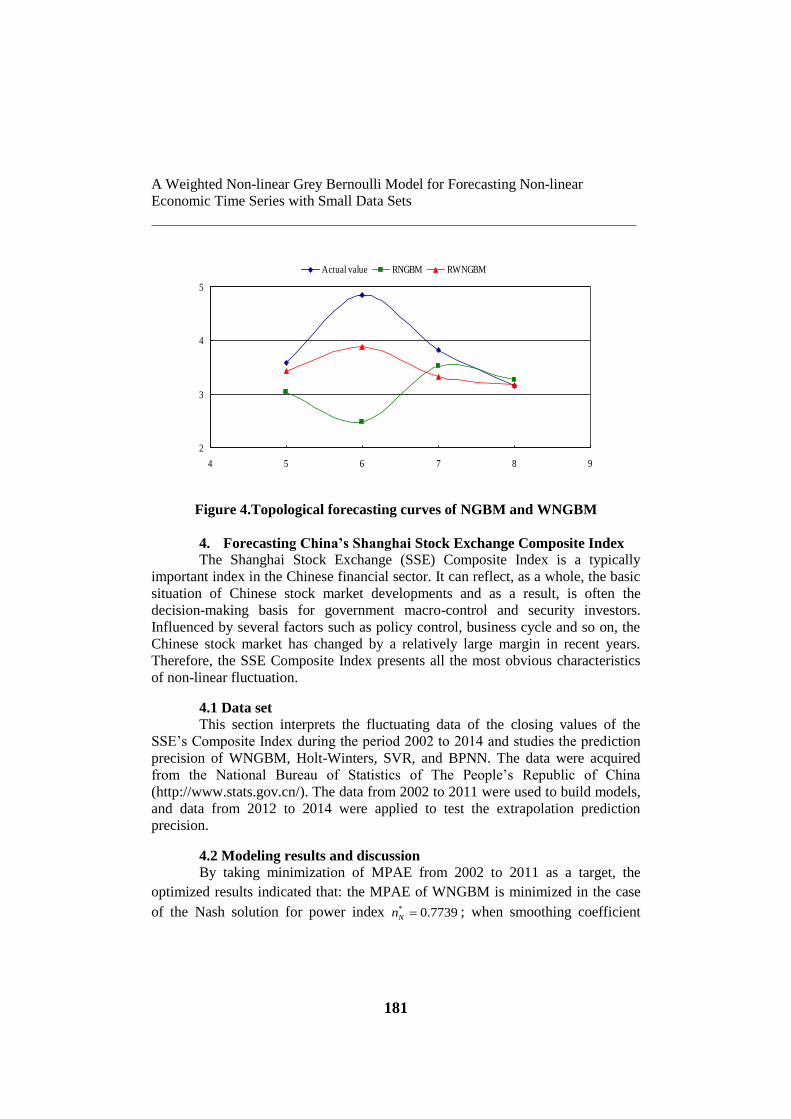
Topological error analysis can test the one-step prediction ability of grey
models on other data. The results of topological error analysis using NGBM and
WNGBM are given in Table 3: the average topological rolling errors of NGBM
and WNGBM are 18.8% and 9.35% respectively. From the topological prediction
curve (see Figure4) of NGBM and WNGBM on (0) ( ), 5,6,7,8x k k , it become
evident that the forecast results by WNGBM are closer to the actual values than
those by NGBM. This proves that the one-step extrapolation prediction precision
of other data is also better than that of NGBM.
Table 3.Topological error analysis using NGBM and WNGBM
k=5 k=6 k=7 k=8 δ(tp,avg)%
Topological sub-
sequence (0) (1: 4)x
(0) (1:5)x (0) (1: 6)x
(0) (1: 7)x
Actual value
NGBM
δ(tp,k)%
3.582
3.038
-15.18
4.853
2.483
-48.83
3.821
3.520
-7.87
3.163
3.264
3.18
18.77
WNGBM
ˆ *
Nλ (k)
δ(tp,k)%
3.434
0.822
-4.13
3.886
1.335
-19.93
3.330
1.054
-12.85
3.178
1.685
0.47
9.35
0.6
0.8
1
1.2
1.4
0 1 2 3 4 5 6 7
NGBM WNGBM
A Weighted Non-linear Grey Bernoulli Model for Forecasting Non-linear
Economic Time Series with Small Data Sets
181
Figure 4.Topological forecasting curves of NGBM and WNGBM
4. Forecasting China’s Shanghai Stock Exchange Composite Index
The Shanghai Stock Exchange (SSE) Composite Index is a typically
important index in the Chinese financial sector. It can reflect, as a whole, the basic
situation of Chinese stock market developments and as a result, is often the
decision-making basis for government macro-control and security investors.
Influenced by several factors such as policy control, business cycle and so on, the
Chinese stock market has changed by a relatively large margin in recent years.
Therefore, the SSE Composite Index presents all the most obvious characteristics
of non-linear fluctuation.
4.1 Data set
This section interprets the fluctuating data of the closing values of the
SSE’s Composite Index during the period 2002 to 2014 and studies the prediction
precision of WNGBM, Holt-Winters, SVR, and BPNN. The data were acquired
from the National Bureau of Statistics of The People’s Republic of China
(http://www.stats.gov.cn/). The data from 2002 to 2011 were used to build models,
and data from 2012 to 2014 were applied to test the extrapolation prediction
precision.
4.2 Modeling results and discussion
By taking minimization of MPAE from 2002 to 2011 as a target, the
optimized results indicated that: the MPAE of WNGBM is minimized in the case
of the Nash solution for power index * 0.7739Nn ; when smoothing coefficient
2
3
4
5
4 5 6 7 8 9
Actual value RNGBM RWNGBM

Zheng-Xin Wang
______________________________________________________________
182
0.17, 1 , the MPAE of Holt-Winters is minimized; using SVR to conduct
standardization of the data over the range [0, 1], the optimum regression
parameters c and are obtained by using an ε-SVR model and a radial basis
function kernel based on the cross-validation method; while BPNN applies a single
hidden layer with five nodes. Its nodal transfer function and training function use
tansig and trainlm respectively. The parameters are set as follows: the training time
is 100; the training target MAPE is 0.00001, and the learning rate is 0.1. The
dimensions of phase space using SVR and BPNN are 3, 4, and 5. The MAPE and
RMSE are used to measure the in-sample (2002 - 2011) and out-of-sample (2012 -
2014) performance of WNGBM, Holt-Winters, SVR, and BPNN: the results are
presented in Table 4 in which m denotes the dimension of the particular phase
space.
Table 4 Comparison of errors: Shanghai Stock Exchange composite index
data with WNGBM using Holt-Winters, SVR, and BPNN.
WNGB
M
Holt-
Winte
rs
SVR BPNN
m=3 m=4 m=5 m=3 m=4 m=5
MAPE
(%, 2002-
2011)
0.07 56.69 29.68 6.91 11.5
4 54.58 17.55 89.61
RMSE(20
02-2011) 4.09
1341.9
2
1261.
95
741.
32
863.
61
1582.
07
1338.
77
2905.
50
MAPE
(%, 2012-
2014)
8.37 24.56 16.65 23.7
7
21.6
4 6.32 10.31 9.54
RMSE(20
12-2014) 215.99 622.35
410.4
4
545.
74
502.
70
197.8
3
296.0
9
293.9
9
As shown by the in-sample forecast error in Table 4, the error when
forecasting the Shanghai Stock Exchange Composite Index between 2002 and
2011 using WNGM is smaller than in the other three methods. The MAPE and
RMSE are 0.07% and 4.09 respectively. The MAPE and RMSE using Holt-
Winters are significantly larger at 56.69% and 1341.92, respectively. This shows
that the Holt-Winters method fails to deal with the non-linear fluctuations of the
Shanghai Stock Exchange Composite Index. When the dimensions of the phase
space are 3, 4, and 5, the MAPEs of SVR are 29.68%, 6.91%, and 11.54%. Actual
values and the forecast curve are shown in Figure5. As shown, the SVR is the most
suitable for predicting the Shanghai Stock Exchange Composite Index when the
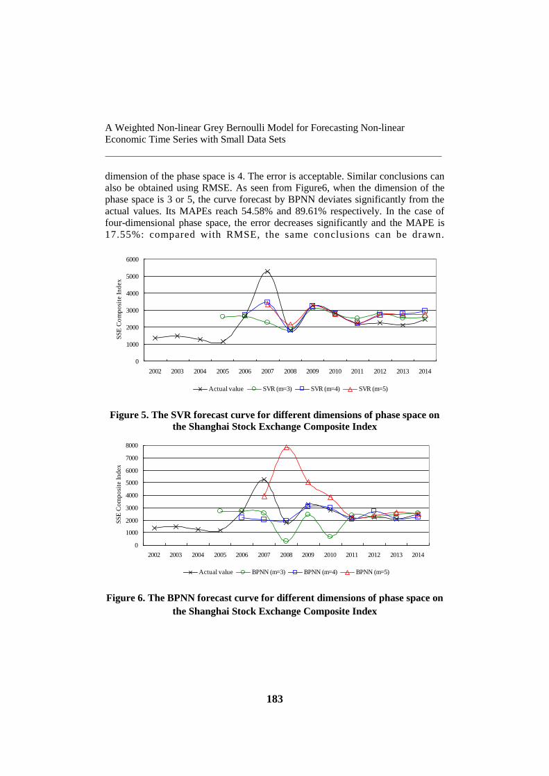
A Weighted Non-linear Grey Bernoulli Model for Forecasting Non-linear
Economic Time Series with Small Data Sets
183
dimension of the phase space is 4. The error is acceptable. Similar conclusions can
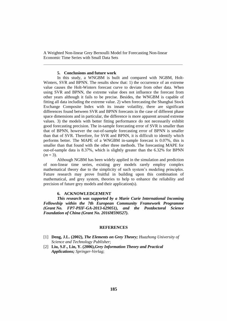
also be obtained using RMSE. As seen from Figure6, when the dimension of the
phase space is 3 or 5, the curve forecast by BPNN deviates significantly from the
actual values. Its MAPEs reach 54.58% and 89.61% respectively. In the case of
four-dimensional phase space, the error decreases significantly and the MAPE is
17.55%: compared with RMSE, the same conclusions can be drawn.
Figure 5. The SVR forecast curve for different dimensions of phase space on
the Shanghai Stock Exchange Composite Index
Figure 6. The BPNN forecast curve for different dimensions of phase space on
the Shanghai Stock Exchange Composite Index
0
1000
2000
3000
4000
5000
6000
2002 2003 2004 2005 2006 2007 2008 2009 2010 2011 2012 2013 2014
SS
E C
om
po
site
In
dex
Actual value SVR (m=3) SVR (m=4) SVR (m=5)
0
1000
2000
3000
4000
5000
6000
7000
8000
2002 2003 2004 2005 2006 2007 2008 2009 2010 2011 2012 2013 2014
SS
E C
om
po
site
In
dex
Actual value BPNN (m=3) BPNN (m=4) BPNN (m=5)

Zheng-Xin Wang
______________________________________________________________
184
According to the comparison of forecasting error for out-of-samples, the
MAPE and RMSE of WNGBM are 8.37% and 215.99; the MAPE and RMSE of
BPNN are 6.32% and 197.83 in the case of a three-dimensional phase space: these
are smaller than those of NGBM. However the in-sample forecasting errors of
BPNN reach 54.58% and 1582.07 for three-dimensional phase space 3. So, the
WNGBM exhibits better robustness than BPNN. It is difficult to judge whether or
not SVR is superior to BPNN, or vice versa. This is because although the in-
sample forecasting error of SVR is smaller than that of BPNN, the forecasting
MAPE for out-of-sample data exceeds 15%, which is higher than that of BPNN.
Compared with the other three methods, the forecasting error of Holt-Winters is
the greatest: its MAPE and RMSE are 24.56% and 622.35. Although there are
slight differences among the four methods with regard to the forecasting precision
for the Shanghai Stock Exchange Composite Index data from 2012 to 2014, the
forecasting curve and actual values exhibit similar trends.
To demonstrate the aforementioned results further, Figure7 shows the
forecast curve and the actual values for: WNGBM, Holt-Winters, SVR (m = 4) and
BPNN (m = 4). The Shanghai Stock Exchange Composite Index reached 2675 in
2006, increased to 5262 in 2007, and decreased to 1821 in 2008, which indicated a
nadir. To fit the extreme value in 2007, the whole curve had to be shifted upwards
when Holt-Winters was used to smooth the raw data. This led to a higher
forecasting error. Meanwhile, SVR and BPNN failed to forecast the extreme value
accurately, which influenced the MPAE and RMSPE to a certain extent. However
the forecast results for the data from other years using SVR and BPNN are not
influenced in that fashion. Figure7 shows that WNGBM is able to identify the
fluctuation in 2007 and provide a good fit to data in other years.
Figure 7. Forecast Shanghai Stock Exchange Composite Index curves using
the four methods
0
1000
2000
3000
4000
5000
6000
2002 2003 2004 2005 2006 2007 2008 2009 2010 2011 2012 2013 2014
SS
E C
om
po
site
In
dex
Actual value WNGBM HOLT-WINTERS SVR (m=4) BPNN (m=4)
A Weighted Non-linear Grey Bernoulli Model for Forecasting Non-linear
Economic Time Series with Small Data Sets
185
5. Conclusions and future work
In this study, a WNGBM is built and compared with NGBM, Holt-
Winters, SVR and BPNN. The results show that: 1) the occurrence of an extreme
value causes the Holt-Winters forecast curve to deviate from other data. When
using SVR and BPNN, the extreme value does not influence the forecast from
other years although it fails to be precise. Besides, the WNGBM is capable of
fitting all data including the extreme value. 2) when forecasting the Shanghai Stock
Exchange Composite Index with its innate volatility, there are significant
differences found between SVR and BPNN forecasts in the case of different phase
space dimensions and in particular, the difference is more apparent around extreme
values. 3) the models with better fitting performance do not necessarily exhibit
good forecasting precision. The in-sample forecasting error of SVR is smaller than
that of BPNN, however the out-of-sample forecasting error of BPNN is smaller
than that of SVR. Therefore, for SVR and BPNN, it is difficult to identify which
performs better. The MAPE of a WNGBM in-sample forecast is 0.07%, this is
smaller than that found with the other three methods. The forecasting MAPE for
out-of-sample data is 8.37%, which is slightly greater than the 6.32% for BPNN
(m = 3).
Although NGBM has been widely applied in the simulation and prediction
of non-linear time series, existing grey models rarely employ complex
mathematical theory due to the simplicity of such system’s modeling principles.
Future research may prove fruitful in building upon this combination of
mathematical, and grey system, theories to help to enhance the reliability and
precision of future grey models and their application(s).
6. ACKNOWLEDGEMENT
This research was supported by a Marie Curie International Incoming
Fellowship within the 7th European Community Framework Programme
(Grant No. FP7-PIIF-GA-2013-629051), and the Postdoctoral Science
Foundation of China (Grant No. 2016M590527).
REFERENCES
[1] Deng, J.L. (2002), The Elements on Grey Theory; Huazhong University of
Science and Technology Publisher;
[2] Liu, S.F., Lin, Y. (2006),Grey Information Theory and Practical
Applications; Springer-Verlag;
Zheng-Xin Wang
______________________________________________________________
186
[3] Akay D., Atak M. (2007),Grey Prediction with Rolling Mechanism for
Electricity Demand Forecasting of Turkey; Energy,volume 32, pp. 1670-
1675;
[4] Wang, C.H., Hsu, L.C. (2008),Using Genetic Algorithms Grey Theory to
Forecast High Technology Industrial Output; Applied Mathematics and
Computation, volume195, pp. 256-263;
[5] Lin, C.S., Liou, F.M., Huang, C.P. (2011),Grey Forecasting Model for
CO2Emissions: A Taiwan Study; Applied Energy,volume88, pp. 3816-3820;
[6] Wang, Y.H., Tang, J.R., Li, X.Z. (2014),Energy Savings Effect
Measurement of Energy Policies from 1999 to 2004 in Jiangsu Province;
Economic Computation and Economic Cybernetics Studies and Research,
volume48, pp. 271-286;
[7] Chen, C.I. (2008), Application of the Novel Nonlinear Grey Bernoulli
Model for Forecasting Unemployment Rate; Chaos, Solitons and
Fractals,volume37, pp. 278-287;
[8] Zhou, J.Z., Fang, R.C., Li, Y.H. (2009),Parameter Optimization of
Nonlinear Grey Bernoulli Model Using Particle Swarm
Optimization;Applied Mathematics and Computation,volume207, pp. 292-299;
[9] Chen, C.I., Hsin, P.H., Wu, C.S. (2010), Forecasting Taiwan's Major Stock
Indices by the Nash Nonlinear Grey Bernoulli Model; Expert Systems with
Applications, volume37, pp. 7557-7562;
[10] Wang, Z.X., Zhu, H.T., Ye, D.J. (2016),Increasing Prediction Precision of
NGBM(1,1) Based on 1-WAGO and 1-WIAGO Techniques; Journal of Grey
System,volume28, pp. 107-120;
[11] Xu,G.X. (2005),Statistical Forecasting and Decision-making; Shanghai
University of Finance and Economics Press;
[12] Li, H., Hong, L.Y.,He, J.X.,Xu, X.G., Sun, J. (2013), Small Sample-
oriented Case-based Kernel Predictive Modelling and its Economic
Forecasting Applications under n-splits-k-times Hold-out Assessment;
Economic Modelling, volume33, pp. 747-61;
[13] Suganyadevi, M.V.,Babulal, C.K. (2014), Support Vector Regression Model
for the Prediction of Loadability Margin of a Power System; Applied Soft
Computing, volume24, pp. 304-315;
[14] Ren, C.,An, N., Wang, J.Z. (2014),Optimal Parameter Selection for BP
Neural Network Based on Particle Swarm Optimization: A Case Study of
Wind Speed Forecasting; Knowledge-Based Systems, volume56, pp. 226-239;
[15] Deng, J.L.,Guo, H. (1996),Grey Prediction: Theory and Applications;
CHWA Publisher.