Embed Size (px)
Citation preview


Economic Bulletin May 2017
Lisbon, 2017 • www.bportugal.pt

Economic Bulletin | May 2017 • Banco de Portugal Av. Almirante Reis, 71 | 1150-012 Lisboa • www.bportugal.pt • Edition
Economics and Research Department • Design and printing Communication Directorate | Image and Graphic Design Unit •
Print run 25 • ISSN 0872-9794 (print) • ISSN 2182-0368 (online) • Legal Deposit no. 241772/06

Index
I The Portuguese economy in 2016 | 5
1. Overview | 7
Box 1 | Assessment of projections for 2016 | 10
2. International environment | 13
3. Monetary and financial conditions | 21
3.1. Euro area | 21
Box 3.1.1 | The impact of the Corporate Sector Purchase Programme | 24
Box 3.1.2 | Dispersion of interest rates in the euro area money market | 27
3.2. Portugal | 30
Box 3.2.1 | Market dynamics and the deleveraging of Portuguese firms | 39
4. Fiscal policy and situation | 43
Box 4.1 | Structural developments in tax revenue in 2016 | 50
Box 4.2 | Analysis of deviations in budget execution in 2016 | 52
5. Supply | 54
Box 5.1 | Capital per worker and productivity | 59
6. Demand | 62
Box 6.1 | Developments in unit values of Portuguese exports of goods | 71
7. Prices | 75
8. Balance of payments | 80
Box 8.1 | Direct investment flows into the Portuguese economy | 86
II Special issue | 91
Distribution mechanisms of monetary policy in the Portuguese economy | 93


IThe Portuguese economy in 2016
1. Overview
2. International environment
3. Monetary and financial conditions
4. Fiscal policy and situation
5. Supply
6. Demand
7. Prices
8. Balance of payments


7The Portuguese economy in 2016
1. OverviewIn 2016 output growth in the Portuguese econ-omy stood at 1.4 per cent, which compares with 1.6 per cent in the previous year. Albeit mod-erate, these GDP developments had a marked intra-annual profile, accelerating strongly in the second half of the year, signalling that the recov-ery process of the economy is expected to con-tinue. In 2016 Portuguese output growth stood 0.3 percentage points below that observed in the euro area, and its level is still 4 per cent below that registered in 2008, the year that marked the outbreak of the latest international economic and financial crisis.
In terms of the fundamental macroeconomic bal-ances, there was a slight increase in the current and capital account surplus (0.5 p.p.) and a signifi-cant decline in the total general government defi-cit (2.3 p.p.), against a background of stabilisation of the structural balance and decline in the struc-tural primary balance (0.3 p.p.). The improvement in these balances is a prerequisite to ensure macroeconomic stability and the credibility of the Portuguese economy among international inves-tors, and should therefore be a guideline for eco-nomic policy decisions adopted at the national level. In effect, the high indebtedness levels pre-vailing in the different institutional sectors make the Portuguese economy particularly vulnerable to any developments implying an increase in the interest rates applied to external financing.
The deleveraging process of the Portuguese economy continued in 2016, reflecting a decline in households’ and corporations’ indebtedness ratios, which nonetheless continued to be very high. Public debt ratio, in turn, virtually stabilised in net terms, in parallel with a reduction of exter-nal indebtedness in the total economy. In this context, there was an improvement in the inter-national investment position of 7 percentage points (p.p.) of GDP, which nonetheless stands at a negative level of 105 per cent of the product.
In the case of non-financial corporations, the con-tribution to the decline in debt due to the exit
of firms has been important, especially for small
firms and for those with activity in the construc-
tion sector (Box 3.2.1. ‘Market dynamics and the
deleveraging of Portuguese firms‛). Although the
exit of firms is part of a natural process of restruc-
turing and reallocation of productive factors in
the economy, the potential non-recovery of debts
raises difficulties to credit institutions, especially in
terms of profitability and impact on own funds.
The continued reduction of the indebtedness
levels of the Portuguese economy requires the
creation of favourable conditions to economic
growth, against a background of social cohe-
sion and sustained improvement of citizens’
living conditions. Investment is one of the key
variables for Portuguese economic growth. In
2016 this variable declined in volume by 0.8 per
cent, after an increase of 4.7 per cent in 2015,
although with an intra-annual recovery profile
and an acceleration in the business compo-
nent. However, investment developments, are
insufficient, not only because the fall during the
crisis period was very sharp, but also because
capital per employee in the Portuguese econ-
omy is still at low levels, when compared with
the euro area average (Box 5.1 ‘Capital per
worker and productivity‛). The low capital levels
contribute to the under-performance of labour
productivity in the Portuguese economy, which
declined again in 2016.
The resident population and the labour force con-
tinued to decline in 2016. These declines main-
tain the trend observed since 2011, although
slightly less marked than in previous years. In
2016 resident population in the 25-34 age group
declined by 2.5 per cent, while the labour force
declined by 2.7 per cent. The sharp demographic
trends in the Portuguese economy are not easily
revertible and are aggravated by migration phe-
nomena. Although the ageing of the population
is evident in several European countries, this situ-
ation is an important constraint to Portuguese
economic growth and puts greater pressure on

BANCO DE PORTUGAL • Economic Bulletin • May 20178
the dynamics of public expenditure with pensions
and health.
In 2016 labour market developments were char-
acterised by an increase in employment, exceed-
ing that of Gross Value Added and maintaining
the recovery profile observed since the second
quarter of 2013. Moreover, although remain-
ing at very high levels, the unemployment rate
declined by 1.3 p. p., in a context of stronger
wage dynamics than in past years. This may have
contributed to the slight increase in the inflation
rate in the course of 2016, via an increase in unit
labour costs. The inflation rate in Portugal, meas-
ured by the change in the Harmonised Index of
Consumer Prices, stood at 0.6 per cent in 2016,
with zero price growth in goods and 1.5 per cent
price growth in services.
The fall in investment contributed to less robust
growth of domestic demand than that observed
in 2015. Also, private consumption increased
slightly less than in the previous year, as a result
of less buoyant consumption of non-food cur-
rent goods and durable goods. In turn, public
consumption, determined by the dynamics of
compensation of employees and consumption
of goods and services in the general government,
increased slightly less in 2016 than in 2015.
Developments in investment and consumption
took place in a context of gradual improvement
of the financing conditions of private economic
agents, in line with the maintenance of an expan-
sionary stance of the monetary policy in the euro
area. This improvement, visible in the course
of 2016, was reflected in a decline of the inter-
est rate spread between Portugal and the euro
area, for both corporations and households. New
loans to households reinforced the growth trend
observed in early 2016, especially in consump-
tion. Notwithstanding the increase in new credit,
the households’ deleveraging process continued.
The annual rate of change of total credit to
corporations was also positive at the end of
the second half of 2016. Relevant, however,
was the important contribution of credit from
non-resident entities, almost exclusively focus-
ing on the issue of debt securities. Therefore,
it was possible to offset the new decline of the
stock of bank loans granted by resident banks,
which indicates an alternative means to finance
investment projects.
The less buoyant economic activity in 2016 also
reflected the deceleration in exports of goods
and services, against a background of lower
growth of the external demand directed towards
the Portuguese economy. The deceleration in
exports of goods and services in 2016 reflected
a lower growth of exports of non-tourism ser-
vices and chiefly the fall in exports of energy.
Excluding this category, growth of exports of
goods was 1.8 percentage points higher than in
2015. In turn, the buoyancy of exports of tour-
ism services continued to be high, in tandem
with the significant increase in nights spent by
non-residents in Portuguese hotels.
The performance of Portuguese exports in 2016
translated into a new gain in market share, which
underlines the competitive capacity of Portu-
guese firms in international markets. The stance
of the Portuguese economy, gradually turning
towards the production of goods and services
tradable abroad is a very positive feature of the
adjustment in the productive structure, which
was started before the latest international eco-
nomic and financial crisis. Only by strengthening
its export capacity may the Portuguese econo-
my accommodate growth of imports resulting
from a desirable strengthening of the invest-
ment rate and an increase in consumption lev-
els. The re-emergence of current account defi-
cits, even if financed via foreign investment, may
be perceived as a return to imbalances, which
will tend to adversely affect refinancing condi-
tions of existing debt. The relevance of exports
performance for developments in the Portu-
guese economy and the prevailing high indebt-
edness levels highlight the importance of devel-
opments in the international economy.
In 2016 world economic activity decelerated,
reaching the lowest growth since the latest

9The Portuguese economy in 2016
international economic and financial crisis. In
turn, growth in the euro area was slightly lower
than in 2015, with an increase in output more
based on domestic demand than in the past. In
2016 financial market developments were con-
ditioned by the UK referendum in June and the
US presidential election in November, with vola-
tility peaks and an increase in uncertainty follow-
ing both events. Stock market indices, however,
registered gains, chiefly in the second half of the
year and in the banking sector, partly reflecting
the strong liquidity creation via non-standard
monetary policies.
In a context of low economic growth, the exist-
ence of high volatility and strong valuations in
financial markets may lead to disturbances in
the international economy, which will tend to be
amplified in most indebted economies. In addi-
tion, the rise in inflation in the euro area from
mid-year onwards, triggered by energy prices, as
well as the increase in the federal funds rate tar-
get contribute to maintain concerns regarding
the development of the interest rate at which
the Portuguese economy is financed.
The Portuguese economy has shown a remark-
able macroeconomic adjustment capacity and
a sectoral restructuring based on the interna-
tionalisation of Portuguese firms. Continuing
economic growth and increasing citizens’ well-
being require the strengthening of firms’ pro-
ductive investment and the availability of skilled
human resources, in a context of financial sta-
bility and legal and fiscal certainty. In this con-
text, the obstacles created by the low savings
rates in the Portuguese economy and the unfa-
vourable demographic developments, as well
as cyclical difficulties associated with the high
indebtedness levels and the elevated uncer-
tainty in the international framework, require
a consistent and forward-looking approach to
economic policies.
The discussion on the deepening of European
integration, which has always been a catalyst for
reforms in the Portuguese economy, allowing for
gains through intensified capital flows and trade
in goods and services, shall be complementary
to internal debate on strengthening growth con-
ditions. The future of the Portuguese economy
depends heavily on its external partners, either
as destination of exports and source of produc-
tive investment, or within the scope of the ongo-
ing financial integration process. This stresses
the need to increase national agents’ standards
regarding the improvement of the country’s com-
petitiveness. Only in this vein shall it be possible to
resume convergence towards European Union’s
average levels of well-being.

10 BANCO DE PORTUGAL • Economic Bulletin • May 2017
Box 1 | Assessment of projections for 2016
This box analyses the gap between Banco de Portugal’s projection for GDP in 2016 and the actual figures, trying to identify the main factors explaining that gap. The analysis is based on the projec-tion published in March 2016, which contains for the first time comprehensive information for 2015.1
The above-mentioned projections for the Portuguese economy are based on Banco de Portugal’s quarterly econometric model (‘M’ Model). In addition to this main model, other satellite models are considered, such as the MIMO model for inflation projection, and bridge models of short-term activity developments.2 Forecasts depend on a range of assumptions regarding the external environment and a set of rules for the incorporation of fiscal variables. In the first case, as usually mentioned in the projection articles of the Economic Bulletin, assumptions correspond to those of the Eurosystem’s projection exercises. Fiscal variables follow the rule used within the scope of these exercises, i.e., incorporating the policy measures that have already been approved (or that are highly likely to be approved) and that have been specified in detail. As mentioned in the note published in March 2016, the projection incorporates most measures included in the State Budget for 2016, which are sufficiently detailed.
Projection errors are the result not only of the fact that assumptions incorporated in the forecast exercise have not materialised, but also of factors related to the model and judgement elements incorporated in the projection.
Comparing the annual growth rate of real GDP in 2016 published in the Quarterly National Accounts by Institutional Sector of 24 March with the projection published by Banco de Portugal in early 2016, it may be concluded that the projection error was -0.1 p.p., i.e., Banco de Portugal projected GDP growth at 1.5 per cent, while actual GDP growth was 1.4 per cent.
Based on elasticities implied in the ‘M’ model, it is possible to analyse the contributions to projec-tion errors made by changes in assumptions, in particular financial conditions, foreign exchange rates, and the international scenario (external demand, oil prices and external prices). In this context, Table 1 presents the revisions of the external environment assumptions – defined as the difference between the actual value and the value underlying the March exercise – and their impact on the annual GDP growth rate in 2016.
Table 1 • Revisions on the external environment and its impact on the real annual growth rate of GDP in 2016 | Revision on the annual growth rate in p.p., except interest rate, compared to the projection of March 2016
Revisions on the external environment
Impact on GDP
Interest rate 0.0 0.0
Euro effective exchange rate -0.3 0.0
Competitors' prices in national currency -1.0 0.0
Oil prices in euros 18.2 -0.1
External demand -1.9 -0.4
Impact of revisions on the external environment -0.5
Source: Banco de Portugal.
Note: A ‘-‛ sign in the effective euro exchange rate corresponds to a higher depreciation or a lower euro appreciation than expected in March.

The Portuguese economy in 2016 11
Expectations in early 2016 pointed to a more favourable international scenario than that subse-
quently observed. In particular, external demand for Portuguese goods and services was antici-
pated to have an annual average growth of 3.9 per cent, i.e., 1.9 p.p. above that actually registered
in 2016. This significant downward revision of external demand was due to both intra-euro area
countries and third countries (Section 2: ‘International environment’) and implied a downward
revision of the GDP growth rate projected at 0.4 p.p. for 2016. In addition, the technical assump-
tion for developments in the effective exchange rate of the euro, which assumes the maintenan-
ce, over the projection horizon, of the average levels observed in the two weeks prior to the cut-
-off date, was revised slightly downwards, implying an appreciation of the euro slightly below that
expected in March 2016. This was reflected in a slight improvement in the price competitiveness
of the Portuguese economy against the main competitors located outside the euro area. There
was also a slight decline in competitors’ prices in external markets, with a negative impact on the
price competitiveness of Portuguese exports. The impact on the GDP projection of the revision of
exchange rates and external prices is negligible.
The deterioration of the international scenario in the course of 2016 was offset by a more favour-
able than anticipated behaviour of the export market share in 2016. The very significant gains of
the Portuguese export market share were registered in both goods and services, particularly in
the second half of the year (Section 6: ‘Demand’). Therefore, contrary to any conclusion that might
be withdrawn from the broadly downward revision of the international environment assump-
tions, exports of goods and services were higher than projected in the March exercise.
As regards monetary and financial conditions, the technical assumption for the 3-month Euribor
rate remained virtually unchanged from March projection (Section 3.1: ‘Monetary and financial
conditions in the euro area’). The increase in oil prices in the course of 2016 was higher than that
expected and implied an upward revision from the assumption considered in the March exercise,
with a negative impact of approximately 0.1 p.p. on the GDP growth rate. Therefore, taking into
account the multipliers implied in the ‘M’ model, revisions of the external environment led to a
significant downward revision of GDP by around 0.5 p.p.
Table 2 presents the projection errors in GDP and its components, as well as the respective gross
and net contributions of the imported content. Analysing the components net of imports, it may
be concluded that the projection error of -0.1 p.p. in GDP was due to the overestimation of the
public finance variables, in particular to the lower growth of public consumption and to the stron-
ger fall of public investment (Box 4.2: ‘Analysis of deviations of budget execution in 2016‛). These
effects were partly offset by the underestimation of exports, largely reflecting the already mentio-
ned unanticipated gains in market share. In spite of an underestimation of private consumption
of 0.3 p.p. in gross terms, the contribution of this component net of the imported content for the
GDP error was virtually zero, given that the projection error of this variable largely reflected car
purchases.
Moreover, the annual average growth rate of GDP and its components in 2016 implied a sharp
intra-annual profile from the first to the second half of the year. The first half of the year was
characterised by low growth, with quarter-on-quarter rates of change of 0.2 per cent, whereas in
the second half there was an acceleration in economic activity, with quarter on quarter rates of
change of 0.9 and 0.7 per cent in the third and fourth quarters respectively.
The projection published in March 2016 did not anticipate these intra-annual GDP dynamics,
and projected a smoother profile, with a slight acceleration in the second half of the year. In this

12 BANCO DE PORTUGAL • Economic Bulletin • May 2017
context, there was an overestimation of GDP and its main components in the first half of the year
and an underestimation in the following half year.
Table 2 • Projection error in real GDP growth rate and in major components in 2016 | Observed– projected in March 2016
Weights 2015 in % GDP
Projection errorGross contributions
to GDP growthNet contributions
to GDP growth
GDP 100.0 -0.1 -0.1 -0.1Private consumption 65.6 0.5 0.3 0.0Public consumption 18.2 -0.6 -0.1 -0.1Investment 15.5 -1.0 -0.2 -0.2Exports 40.6 2.2 0.9 0.3Imports 39.8 2.3 -0.9
Source: Banco de Portugal.
Note: The demand aggregates net of imports are obtained by subtracting an estimate of the imports needed to meet each component. The calculation of import contents was based on data for 2005. For more information, see the Box entitled ‘The role of domestic demand and exports in economic activity developments in Portugal’, in the June 2014 issue of the Economic Bulletin.

13The Portuguese economy in 2016
2. International environment
World economic activity and trade decelerated further in 2016, dropping to the lowest level since the last international economic and financial crisis
In 2016 world economy decelerated, record-
ing the lowest growth since the last international
economic and financial crisis (Table 2.1 and
Chart 2.1). This slow recovery from the crisis
has been different across regions. In 2016 as a
whole, contrary to the previous year, advanced
economies slowed down and emerging market
and developing economies decelerated slightly.
After recovering from its major collapse, world
trade growth has been weakening since 2012.
Taking the pre-crisis period as reference (2002-07), international trade recorded an average growth much higher than global activity (around 8 and 5 per cent respectively), while world trade and GDP grew by around 3 per cent, on average, from 2012 to 2016, i.e. a decline in world trade elastic-ity of around 0.7 p.p. (Chart 2.2). This decrease in world trade elasticity is expected to be associated, inter alia, to slower developments in global value chains and a geographical change in trade ben-efiting emerging market economies, which have shown a slower response of trade to changes in output.
In 2016 developments in financial markets were affected by the referendum in the United King-dom in June and the presidential election in the United States in November, which were followed by volatility peaks and increased uncertainty.
Table 2.1 • Gross Domestic Product – Real year-on-year rate of change | Percentage
2002-07 2013 2014 2015 2016
World 4.8 3.4 3.5 3.4 3.1
Advanced economies 2.6 1.3 2.0 2.1 1.7
USA 2.7 1.7 2.4 2.6 1.6
Japan 1.4 2.0 0.2 1.2 1.0
Euro area 2.0 -0.2 1.2 1.9 1.7
Germany 1.4 0.6 1.6 1.5 1.8
France 1.8 0.6 0.7 1.2 1.1
Italy 1.1 -1.7 0.2 0.7 1.0
Spain 3.5 -1.7 1.4 3.2 3.2
United Kingdom 2.7 1.9 3.1 2.2 1.8
Emerging and developing economies 7.2 5.1 4.7 4.2 4.1
Emerging and developing Europe 5.9 4.9 3.9 4.7 3.0
Commonwealth of Independent States 7.6 2.1 1.1 -2.2 0.3
Russia 7.1 1.3 0.7 -2.8 -0.2
Emergind and developing Asia 9.0 6.9 6.8 6.7 6.4
China 11.2 7.8 7.3 6.9 6.7
Latin America and the Caribbean 4.1 2.9 1.2 0.1 -1.0
Brazil 3.9 3.0 0.5 -3.8 -3.6
Sources: Eurostat, IMF and Thomson Reuters.

BANCO DE PORTUGAL • Economic Bulletin • May 201714
In June, the result of the referendum raised con-
cerns about the UK’s economic outlook, and, in
November, the result of the US elections sig-
nalled shifting expectations regarding the new
administration’s policies. In the first half of the
year, long-term interest rates followed a down-
ward trend in the United States, the United King-
dom and Germany, amid doubts about growth
in global economic activity, the situation in the
euro area financial sector and continued (or
strengthening) accommodative monetary poli-
cies by major central banks (Chart 2.3). In con-
trast, long-term interest rates began increasing
from July onwards, reflecting reduced concerns about the world economy outlook, the percep-tion that monetary authorities might be less reactive to the first signs of an inflation hike, and the anticipation of a more expansionary fis-cal policy and an increase in investment in infra-structures after the US elections.
At the start of the year, equity indices record-ed losses, given the more negative outlook for the world economy, particularly in China, which were followed by a recovery, amid rising oil pric-es. After reaching a trough of 28 USD/barrel in January, oil prices increased gradually, before
Chart 2.1 • Gross Domestic
Product - annual growth between
2010 and 2016| Percentage
-2.0
0.0
2.0
4.0
6.0
8.0
10.0
12.0
World Advancedeconomies
Euro area US Emerging economies China
Pre-crisis growth (2002-2007)
Sources: Eurostat, IMF and Thomson Reuters.
Chart 2.2 • Growth of world
GDP and trade volumes
| Percentage and percentage points
0.6
1.1
1.6
2.1
2.6
-11.0
-5.0
1.0
7.0
13.0
1980 1984 1988 1992 1996 2000 2004 2008 2012 2016
Perc
enta
ge p
oint
s
Perc
enta
ge
GDP growth Trade growthPre-crisis GDP average growth Pre-crisis trade average growthTrade elasticity (rhs)
Sources: IMF and Banco de Portugal calculations.
Note: Trade elasticity is calculated over 5-year periods. Pre-crisis period: 2002-2007.

15The Portuguese economy in 2016
stabilising at around 50 USD/ barrel at the end
of the summer. At the end of the year, the stock
market in the United States reached historical
highs due to the anticipation of expansionary
policies, which influenced the various sectors,
in particular banks (Chart 2.4).
Advanced economies grew less strongly, while emerging economies accelerated slightly, despite differences across countries
Advanced economies grew by 1.7 per cent in 2016, compared with 2.1 per cent in 2015, improving in the second half of the year. For most economies, domestic demand and, in par-ticular, private consumption continued to be the drivers of growth. Investment, as measured by gross fixed capital formation (GFCF), continued to grow moderately and accelerated in the sec-ond half of 2016, making a marginal contribu-tion to GDP.
In the United States, economic activity slowed down in 2016, with GDP growing by 1.6 per cent, i.e. 1 p.p. less than in the previous year. The US
-1
0
1
2
3
4
5
6
Jan. 11 Jan. 12 Jan. 13 Jan. 14 Jan. 15 Jan. 16
Euro area US UK Japan
Chart 2.3 • 10-year sovereign debt rates| Percentage
Sources: Thomson Reuters and ECB.
25
50
75
100
125
150
175
200
Jan. 11 Jan. 12 Jan. 13 Jan. 14 Jan. 15 Jan. 16
Eurostoxx S&P500 FootsieBanks: euro area Banks: US Banks: UK
Chart 2.4 • Major stock markets indexes, total and banks| Index Jan. 2014=100
Source: Thomson Reuters.

BANCO DE PORTUGAL • Economic Bulletin • May 201716
economy recorded weak growth during the first
half of the year, largely due to developments in
private business investment, recovering in the
second half of the year owing to private con-
sumption. At the same time, labour market con-
ditions remained favourable, with the unem-
ployment rate remaining below 5 per cent, for
the first time since 2007. Inflation increased, in
particular from the middle of the year onwards,
due to an increase in commodity prices, but
continued below the Federal Reserve’s target.
In terms of the average annual rate of change,
inflation reached 1.3 per cent (0.1 per cent in
2015), while inflation excluding food and energy
remained slightly above 2 per cent. Against this
background, in December 2016, the Federal
Reserve decided to increase the target for the
federal funds interest rate to a 0.50-0.75 per
cent range.
The United Kingdom grew above the forecasts
released after the June referendum, which result-
ed in the United Kingdom leaving the European
Union. Economic activity grew by 1.8 per cent in
2016, i.e. 0.4 p.p. less than in 2015, supported by
private consumption, which, contrary to expec-
tations, did not show signs of slowing down.
However, in the next few years, real house-
hold income may decelerate, negatively affect-
ing private consumption, amid moderating wage
growth and higher import prices associated
with the depreciation of the pound sterling. The
year-on-year rate of change in the Harmonised
Index of Consumer Prices (HICP) remained below
2 per cent, but increased over the year, reaching
1.6 per cent (0.2 per cent in December 2015), as
a result of the depreciation of the pound ster-
ling, which was more pronounced immediately
after the referendum’s unexpected result. In this
context, in August, the Bank of England adopt-
ed a package of measures to support the econ-
omy, which included a cut in the Bank Rate, an
increase in the stock of purchased UK govern-
ment bonds, a programme to purchase non-
financial investment-grade corporate bonds and
a Term Funding Scheme for eligible institutions
to reinforce the pass-through of monetary policy
to the real economy.
Japan gradually recovered throughout 2016,
owing to domestic demand and supported by
accommodative monetary and fiscal policies
and favourable financial conditions. The Japa-
nese GDP grew by 1.0 per cent, compared with
1.2 per cent in 2015. In 2016, the Bank of Japan
made two changes to its Quantitative and Quali-
tative Monetary Easing programme, by intro-
ducing a negative interest rate to banks’ cur-
rent accounts in January, and by conditioning
the purchase of Japanese government bonds, in
September, so that 10-year interest rates would
remain close to zero. In addition, the Bank com-
mitted itself to expanding the monetary base
until the observed inflation rate exceeds the tar-
get (inflation-overshooting commitment).
The situation of emerging market and develop-
ing economies continued to be quite mixed. In
China, economic activity remained robust in
2016, with GDP growing by 6.7 per cent year-
on-year (6.9 per cent in 2015), benefiting from
the economic policy stimulus. Nevertheless, eco-
nomic activity was weaker than expected in a
number of Latin American countries, which have
been in a recession since 2015, specifically Bra-
zil. In Russia, economic growth was slightly better
than expected, partly owing to developments
in oil prices.
Euro area economic activity continued to recover gradually, with a greater support from domestic demand than in the past
Euro area GDP grew at a relatively stable rate
throughout the year. Growth of 1.7 per cent
reflected a positive contribution from domes-
tic demand and a negative contribution from
net exports. Above all, this pattern was driven
by consumption, associated with favourable
developments in households’ real disposable

17The Portuguese economy in 2016
income, amid growing employment and declin-
ing oil prices. The recovery in activity in the cur-
rent economic cycle has a greater support from
domestic demand than in the previous cycle,
with services playing a greater role (Chart 2.5).
The recovery seen after 2013 is also more broad-
ly-based across countries, with particularly posi-
tive developments in Spain (3.2 per cent growth)
(Chart 2.6). GDP grew by 1.8 per cent in Germa-
ny and slightly above 1 per cent in France. In
turn, GDP growth stood at 1.0 per cent in Italy,
standing considerably below pre-crisis levels.
Unemployment continued to decline in the euro area, with some cross-country differences. The larger economies experienced declines, with the exception of Italy. In parallel, employment continued to grow moderately, above the lev-els observed in 2015.
External demand for Portuguese goods and services decelerated
External demand for Portuguese goods and
services decelerated in 2016, growing by 2 per
Chart 2.5 • Euro area two latest economic recoveries – contributions by sector | Index 2009 Q2=100
Contributions to GDP Contributions to GVA
98
100
102
104
106
108
110
2009 Q2 2010 Q4 2012 Q2 2013 Q4 2015 Q2 2016 Q4
Domestic demandNet ExportsGDP cumulated growth since 2009 Q2
98
100
102
104
106
108
110
2009 Q2 2011 Q2 2013 Q2 2015 Q2IndustryServicesConstructionGross value added cumulated growth since 2009Q2
98
100
102
104
106
108
110
2009 Q2 2010 Q4 2012 Q2 2013 Q4 2015 Q2 2016 Q4
Domestic demandNet ExportsGDP cumulated growth since 2009 Q2
98
100
102
104
106
108
110
2009 Q2 2011 Q2 2013 Q2 2015 Q2IndustryServicesConstructionGross value added cumulated growth since 2009Q2
Sources: Eurostat, CEPR and Banco de Portugal calculations.
Note: Two latest economic recoveries - since the 2009 Q2 and 2013 Q1 troughs, according to the CEPR Dating Commitee.
90
95
100
105
110
115
120
2009 Q2 2010 Q4 2012 Q2 2013 Q4 2015 Q2 2016 Q4
Euro area Germany France Italy Spain
Chart 2.6 • GDP evolution since trough| Index 2009 Q2=100
Sources: Eurostat, CEPR and Banco de Portugal calculations.

BANCO DE PORTUGAL • Economic Bulletin • May 201718
cent year-on-year, after around 4 per cent in 2015 (Table 2.2). These developments result-ed from lower growth in demand from euro area trade partners (3.5 per cent, compared with 5.6 per cent in 2015), and a contraction in external demand from economies outside the euro area (-0.4 per cent, after 1.1 per cent in 2015). When external demand from Angola is taken into account, the effect is even more pronouced.3 External demand for goods and services is expected to have grown by 1.3 per cent in 2016, compared with 2.6 and 5.4 per cent in 2015 and 2014 respectively.
Increase in euro area inflation from the middle of the year
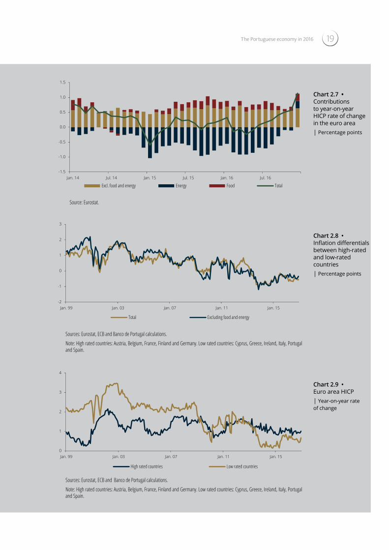
In 2016 developments in HICP inflation mostly
reflected the path of energy prices (Chart 2.7).
This influence translated into a low or nega-
tive inflation in the first months of the year and
subsequent increases, which were heightened
by the base effect of the falls observed in 2015
and related to an increase in energy prices.
Table 2.2 • External demand of goods and services – Real year-on-year rate of change | Percentage
Weights(b) 2013 2014 2015 2016
External demand (ECB)(a) 100.0 1.9 5.0 3.9 2.0
Intra euro area external demand 66.3 0.9 5.2 5.6 3.5
of which:
Spain 27.1 -0.5 6.5 5.6 3.3
Germany 13.7 3.2 4.0 5.0 3.6
France 12.5 2.2 4.8 6.4 3.6
Italy 3.9 -2.3 3.1 6.7 3.1
Extra euro area external demand 33.7 3.7 4.6 1.1 -0.4
of which:
United Kingdom 5.6 3.4 2.5 5.5 2.8
USA 3.5 1.1 4.4 4.6 1.1
Memo:
Goods and services imports from Angola (c) 9.0 11.4 -21.8 -27.8
Adjusted external demand (d) 2.3 5.4 2.6 1.3
Comércio mundial de bens e serviços (FMI) 3.7 3.7 2.7 2.2
Importações mundiais de mercadorias (CPB) 2.0 2.6 1.9 1.2
Sources: ECB, CPB, IMF, Thomson Reuters and Banco de Portugal calculations.
Notes: (a) External demand is computed as weighted average of the imports volume of Portugal's main trading partners. Each country/region is weighted by its share in Portuguese export. (b) Shares computed using 2012-2014 data. (c) The weight refers to the weight of nominal goods and services exports to Angola on portuguese exports. (d) External demand indicator adjusted for the importance of the foreign trade with Angola. Corresponds to the weighted average (by the exports weight) between the external demand indicator calculated by the ECB and the volume of the goods and services imports of the Angolan economy. The IMF forecasts (Word Economic Outlook) for the growth of the volume of imports of Angola in 2016 are used.
The year-on-year rate of change in HICP exclud-
ing energy and food remained stable at relatively
low levels, ranging between 0.7 and 1.0 per cent
throughout the year (Chart 2.7). Since mid-2016,
the increase in euro area inflation was boost-
ed by energy prices and broadly-based across
countries. As in the past, differentials between
groups of countries reflected divergences in
inflation excluding energy and food (Charts 2.8
and 2.9). At the end of the year, the year-on-year
rate of change in HICP excluding energy and
food stood at 1.4 per cent in Germany, 0.9 and
19The Portuguese economy in 2016
-1.5
-1.0
-0.5
0.0
0.5
1.0
1.5
Jan. 14 Jul. 14 Jan. 15 Jul. 15 Jan. 16 Jul. 16
Excl. food and energy Energy Food Total
Chart 2.7 • Contributions to year-on-year HICP rate of change in the euro area| Percentage points
Source: Eurostat.
0
1
2
3
4
Jan. 99 Jan. 03 Jan. 07 Jan. 11 Jan. 15
High rated countries Low rated countries
Chart 2.9 • Euro area HICP| Year-on-year rate of change
Sources: Eurostat, ECB and Banco de Portugal calculations.
Note: High rated countries: Austria, Belgium, France, Finland and Germany. Low rated countries: Cyprus, Greece, Ireland, Italy, Portugal and Spain.
-2
-1
0
1
2
3
Jan. 99 Jan. 03 Jan. 07 Jan. 11 Jan. 15
Total Excluding food and energy
Chart 2.8 • Inflation differentials between high-rated and low-rated countries| Percentage points
Sources: Eurostat, ECB and Banco de Portugal calculations.
Note: High rated countries: Austria, Belgium, France, Finland and Germany. Low rated countries: Cyprus, Greece, Ireland, Italy, Portugal and Spain.

BANCO DE PORTUGAL • Economic Bulletin • May 201720
Chart 2.10 • Euro area inflation
expectations and oil prices
| Percentage and USD dolars per barrel
25
50
75
100
125
150
175
0.0
0.5
1.0
1.5
2.0
2.5
3.0
Jan. 06 Jan. 08 Jan. 10 Jan. 12 Jan. 14 Jan. 16
US
dolla
rs
Perc
enta
ge
1-y, 1-y ahead 5-y, 5-y ahead Oil price (rhs)
Sources: Thomson Reuters and Banco de Portugal calculations.
Note: Expectations implicit in inflation swaps. Vertical line indicates the APP anouncement.
0.7 per cent in Spain and Italy respectively, and 0.4 per cent in France.
Since 2013, the inflation differential between high rated countries and lower rated coun-tries has been negative, in contrast to the pre-crisis period. This reflects lower growth in pric-es in the services component in lower-rated countries, associated with wage adjustments. Since the second half of 2015, the differential has decreased, reflecting continued low growth
in services prices in high rated countries and a
slight acceleration in lower rated countries. Long-
term inflation expectations increased from Sep-
tember onwards, standing above the levels seen
at the start of 2015, but below historical aver-
ages. Long-term inflation expectations seem to
have become rather more sensitive to changes
in short-term expectations and oil prices both in
the euro area and in the United States and the
United Kingdom (Chart 2.10).

21The Portuguese economy in 2016
3. Monetary and financial conditions3.1. Euro area
The Eurosystem maintained an accommodative monetary policy in 2016
2016 saw the adoption of non-standard mon-
etary policy measures on the part of the ECB in
March and December. At the start of the year,
economic and financial conditions deteriorated
and downside risks to inflation increased, lead-
ing the Governing Council to reduce the rates
on the main refinancing operations, the deposit
facility, and the marginal lending facility to 0 per
cent, -0.4 per cent and 0.25 per cent respectively,
and to adopt a number of other measures. This
package included expanding the monthly pur-
chases under the Expanded Asset Purchase
Program (APP) from €60 billion to €80 billion,
and extending it until March 2017, and expand-
ing the purchase programme to debt securities
issued by non-bank corporations established in
the euro area (Box 3.1.1: ‘The impact of the Cor-
porate Sector Purchase Programme‛). The ECB
also announced a new series of targeted long-
er-term refinancing operations (TLTRO II), to
support lending to the economy. These opera-
tions are different from previous TLTROs most-
ly because the bank will pay a rate equal to the
deposit facility rate if it grants loans above a spe-
cific limit. At the end of the year, the Governing
Council considered there was a need for further
substantial monetary stimulus to the economy in
order to ensure a sustained adjustment in the
path of inflation towards the inflation aim. The
Governing Council therefore decided to extend
the APP until December 2017, but to reduce the
purchases from €80 billion to €60 billion.
Monetary and financial conditions in the euro area continued to evolve favourably
Euro area financial markets were influenced by
the accommodative monetary policy stance. The
downward path in euro area government bond
yields reflected the effect of the APP purchases
and other monetary policy measures taken by
the ECB. Overall effects were also relevant, in
particular an increase in uncertainty about the
outlook for global growth at the start of the year
and the result of the UK referendum in June.
From the summer onwards, a decline in con-
cerns about developments in the global econ-
omy and the incorporation of an inflation risk
premium led to a partial reversal in the decline
seen in interest rates.
Euro area equity indices improved slightly through-
out the year, although the intra-annual pattern
showed marked movements, consistent with
the previously mentioned factors. Equity prices in
the European financial sector fell by around 8 per
cent in 2016, amid prospects of lower yields in the
future and the negative impact of non-performing
loans on bank profitability.
In foreign exchange markets, the euro appreci-
ated slightly, in effective terms, in the course of
the year, reflecting in particular the result of the
UK referendum, the world economic outlook
and monetary policy differences across juris-
dictions. The effective appreciation of around
2 per cent was the result of an appreciation of
17 per cent against the pound sterling and
4 per cent against the Chinese renminbi, and a
depreciation of 3 per cent against the US dollar
and 6 per cent against the Japanese yen. Money
market interest rates continued to decline, but,
since the summer of 2016, the differential has
been widening between the EONIA and deposit
facility rates vis-à-vis the secured money mar-
ket rates and rates on government debt, which
might indicate a less effective transmission of
monetary policy decisions (Box 3.1.2: ‘Disper-
sion of interest rates in the euro area money
market‛).

BANCO DE PORTUGAL • Economic Bulletin • May 201722
Firms’ financing costs continued to decline in
2016. In particular, the negative deposit facil-
ity rate and the new TLTRO II announced in
March are expected to have helped reduce the
interest rates on bank loans to firms. In addition,
the introduction of a purchase programme for
investment-grade bonds issued by corporations
established in the euro area might also partly
explain the decline in the respective interest
rates, which have stood at levels similar to those of
highly-rated banks’ bonds since June (Chart 3.1).
Against this background, the net issuance of euro-
denominated bonds increased considerably from
the second quarter of 2016 onwards (Chart 3.2).
The cost of bank loans to firms decreased by
around 30 b.p. throughout the year, slightly
below the decline seen in loans to households
for house purchase, standing at around 1.8 per
cent in both cases. In addition, the differential
between the cost of loans to firms in lower rated
and high rated countries returned to the levels
observed at the start of 2011.
Chart 3.1 • NFC's financing
costs | Percentage
0
1
2
3
4
5
6
Jan. 11 Jan. 12 Jan. 13 Jan. 14 Jan. 15 Jan. 16
High rated NFCs bonds NFC loans over 1 millionNFC loans below 1 million High rated Banks' bonds
Sources: ECB, Bank of America Merrill Lynch, Blooomberg and Banco de Portugal calculations.
Note: Vertical line indicates the announcement of CSPP and TLTRO II.
Chart 3.2 • External financing
of NFC in the euro area| Billion euros
0
5
10
15
125
175
225
275
Jan. 11 Jan. 12 Jan. 13 Jan. 14 Jan. 15 Jan. 16
Bank loans (new operations) Net issues of bonds in euros (rhs)
Source: ECB.
Note: 12-month moving average.

23The Portuguese economy in 2016
Bank lending to firms grew considerably in the
first half of the year both for high rated countries
and lower rated countries (Chart 3.3). In annu-
al average terms, loan growth stood at 2.3 per
cent in December 2016, compared with 0.5 per
cent in December 2015, accelerating 1.4 p.p. up
to June. Loans to households recovered more
slowly, particularly in high rated countries, from
1.4 to 2.0 per cent during the same period. The
improvement in financial and monetary condi-
tions is in line with the results of the euro area
Bank Lending Survey, which have indicated an
improvement in lending conditions for firms and
households in 2016. Banks have also reported
an increase in demand for loans to both firms
and households, which was broadly-based across
all loan categories. Banks have used the liquidity
obtained from the APP for granting loans, for refi-
nancing purposes and, to a lesser extent, for pur-
chasing assets. As regards the negative deposit
facility rate, banks have indicated a positive impact
on lending volumes, but a negative impact on net
interest income and loan margins.
-9.0
-6.0
-3.0
0.0
3.0
6.0
Jan. 11 Jan. 12 Jan. 13 Jan. 14 Jan. 15 Jan. 16
High rated countries Low rated countries Euro area
Chart 3.3 • Anual rate of change of bank loans in the euro area| Percentage
Source: ECB.
Note: Loans adjusted for sales and securitization. Full lines represent firms and dashed lines represent families.
24 BANCO DE PORTUGAL • Economic Bulletin • May 2017
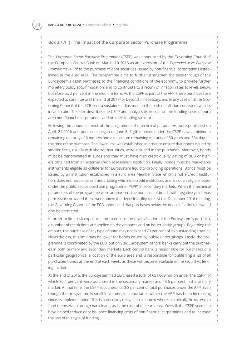
Box 3.1.1 | The impact of the Corporate Sector Purchase Programme
The Corporate Sector Purchase Programme (CSPP) was announced by the Governing Council of the European Central Bank on March, 10 2016 as an extension of the Expanded Asset Purchase Programme (APP)4 to the purchase of debt securities issued by non-financial corporations estab-lished in the euro area. The programme aims to further strengthen the pass-through of the Eurosystem’s asset purchases to the financing conditions of the economy, to provide further monetary policy accommodation, and to contribute to a return of inflation rates to levels below, but close to, 2 per cent in the medium term. As the CSPP is part of the APP, these purchases are expected to continue until the end of 20175 or beyond, if necessary, and in any case until the Gov-erning Council of the ECB sees a sustained adjustment in the path of inflation consistent with its inflation aim. This box describes the CSPP and analyses its impact on the funding costs of euro area non-financial corporations and on their funding structure.
Following the announcement of the programme, the technical parameters were published on April, 21 2016 and purchases began on June 8. Eligible bonds under the CSPP have a minimum remaining maturity of 6 months and a maximum remaining maturity of 30 years and 364 days at the time of the purchase. The lower limit was established in order to ensure that bonds issued by smaller firms, usually with shorter maturities, were included in the purchases. Moreover, bonds must be denominated in euros and they must have high credit quality (rating of BBB or high-er), obtained from an external credit assessment institution. Finally, bonds must be marketable instruments eligible as collateral for Eurosystem liquidity-providing operations. Bonds must be issued by an institution established in a euro area Member State which is not a credit institu-tion, does not have a parent undertaking which is a credit institution, and is not an eligible issuer under the public sector purchase programme (PSPP) in secondary markets. When the technical parameters of the programme were announced, the purchase of bonds with negative yields was permissible provided these were above the deposit facility rate. At the December 2016 meeting, the Governing Council of the ECB announced that purchases below the deposit facility rate would also be permitted.
In order to limit risk exposure and to ensure the diversification of the Eurosystem’s portfolio, a number of restrictions are applied on the amounts and on issuer entity’ groups. Regarding the amount, the purchase of any type of bond may not exceed 70 per cent of its outstanding amount. Nevertheless, this limit may be lower for bonds issued by public undertakings. Lastly, the pro-gramme is coordinated by the ECB, but only six Eurosystem central banks carry out the purchas-es in both primary and secondary markets. Each central bank is responsible for purchases of a particular geographical allocation of the euro area and is responsible for publishing a list of all purchased bonds at the end of each week, as these will become available in the securities lend-ing market.
At the end of 2016, the Eurosystem had purchased a total of €51,069 million under the CSPP, of which 86.4 per cent were purchased in the secondary market and 13.6 per cent in the primary market. At that time, the CSPP accounted for 3.3 per cent of total purchases under the APP. Even though the programme is small in volume, its importance within the APP has been increasing since its implementation. This is particularly relevant in a context where, historically, firms tend to fund themselves through bank loans, as is the case of the euro area. Overall, the CSPP seems to have helped reduce debt issuance financing costs of non-financial corporations and to increase the use of this type of funding.

The Portuguese economy in 2016 25
A preliminary assessment shows that apparently the programme had some impact on corporate bond yields and on the yields of bonds issued by other sectors. Economic literature assessing the APP has identified the impact of its announcement as the most significant event. The same seems to apply to the CSPP. The first vertical line in Chart 1 marks the date of the CSPP announcement and it is clear that, at that moment, bond yields dropped considerably for both non-financial cor-porations and banks. In the case of non-financial corporations, this downward trend continued, being only interrupted by some volatility in May and June, as a consequence of the outcome of the UK referendum on leaving the European Union. Following the start of the programme (second vertical line in Chart 1), developments in yields resumed the downward trend. Simultaneously, interest rates on long-term government bonds remained fairly constant, contributing to the per-ception that the implementation of the programme has helped reduce bond yields. High-yield bonds and yields on bonds issued by financial corporations also declined immediately after the announcement of the programme, particularly in peripheral countries (Table 1).
Table 1 • Change in yields following the CSPP announcement | Basis points
Investment-grade bonds High yield bonds issued by non-financial corporationsNon-financial corporations Banks
Euro Area -14 -8 -58
Germany -14 -4 -56
France -13 -8 -72
Italy -19 -17 -63
Spain -19 -16 -73
Portugal -65 - -64
Sources: Bloomberg, Bank of America Merril Lynch and Banco de Portugal calculations
Notes: Event study: change in yields within a 3-day window following the CSPP announcement on 10 March 2016.
Chart 1 • Euro area bond yields
0
50
100
150
200
250
300
350
400
-1
0
1
2
3
4
5
Jan. 12 Jan. 13 Jan. 14 Jan. 15 Jan. 16
Basi
s po
ints
Perc
enta
ge
Asset swap spread (rhs) Non-financial corporations Banks
Sources: Bloomberg, Bank of America Merril Lynch and Banco de Portugal calculations.
Note: Effective yields on euro-denominated investment-grade bonds. Asset swap spread: difference between the bond yield and a low-risk swap rate of the same maturity. Vertical lines: CSPP announcement; start of the program.

26 BANCO DE PORTUGAL • Economic Bulletin • May 2017
The programme must also be assessed in terms of volume. Financing of non-financial corpora-
tions through debt issuance has been increasing since the first quarter of 2016. In addition,
after a slow down that began in 2013, the average gross issuance of bonds between June and
December recovered in 2016 despite remaining at levels below those of previous years (Chart 2).
This period is particularly interesting as it compares the issuance during the months when the
programme was already being carried out with the same period in previous years. This suggests
that the CSPP may have led firms to be more likely to prefer funding via debt securities.
Although other factors may have influenced the financing costs of non-financial corporations
and were possibly taken into consideration when choosing between debt issuance and bank
loans, the developments described above seem to indicate that the CSPP has had the intended
effect on the financing conditions of the economy. On the one hand, the financing costs of debt
issuance have declined and remain low by historical standards. On the other hand, since the start
of the programme, activity in this market seems to have gained some momentum.
Chart 2 • Gross issuance of debt securities by euro area non-financial corporations| Millions of euros
0
20,000
40,000
60,000
80,000
100,000
Jan.10 Jan.11 Jan.12 Jan.13 Jan.14 Jan.15 Jan.16
Gross issuance June to December average
Sources: Thomson Reuters and Bloomberg.

The Portuguese economy in 2016 27
Box 3.1.2 | Dispersion of interest rates in the euro area money market
In a money market operating perfectly, interest rates on all financial instruments should fully reflect the central bank’s reference rate – perceived as a risk-free interest rate – plus premia associated, inter alia, with credit and liquidity risk. Money market interest rates should therefore stand at a level close to the central bank reference rate and, ceteris paribus, any change in this rate resulting from monetary policy decisions should mostly pass through to negotiated rates for granting and obtaining short-term funding.
At present, in the euro area, the deposit facility rate, which stands at -0.4 per cent since March 2016, would be expected to represent the effective lower bound of money market interest rates, and assets perceived to be safe and liquid would be expected to provide a yield close to this benchmark. However, since the start of 2015, the downward trend seen in the interest rates of short-term secured instruments and sovereign bonds with a high credit quality has been more marked than the declines in the deposit facility rate and the EONIA (Chart 1). This spread widened from the summer of 2016 onwards, contributing to greater dispersion around the ECB’s mon-etary policy interest rate, which should provide an anchor for euro area money market interest rates, under normal circumstances.
High dispersion of interest rates in the money market may indicate market segmentation, which, as a result of the lower importance given to the central bank’s rate, translates into difficulties in the mon-etary policy transmission. Against this backdrop, it is crucial to analyse the reasons behind the evi-dence illustrated in Chart 1.
First, the downward trend in interest rates on short-term instruments with a high credit qual-ity may reflect anticipation by financial market participants of further cuts in the ECB’s policy rates. Nonetheless, since the summer of 2016, agents’ expectations about further reductions in
Chart 1 • Evolution of representative euro area money market rates since 2015 | Percentage
-5
-4
-3
-2
-1
0
1
-1.25
-1.00
-0.75
-0.50
-0.25
0.00
0.25
Jan. 2015 Apr. 2015 Jul. 2015 Oct. 2015 Jan. 2016 Apr. 2016 Jul. 2016 Oct. 2016 Jan. 2017
Deposit facility rateEONIAGermany 3-month sovereign debt rateEuro area 3-month GC Polling rateGermany 3-month repo rate (rhs)
Sources: Thomson Reuters and Bloomberg.
28 BANCO DE PORTUGAL • Economic Bulletin • May 2017
the deposit facility rate were rather contained and consequently insufficient to explain the move-ment verified in some short-term interest rates in the euro area market.
Furthermore, the increase in the dispersion of euro area money market interest rates occurred at the time of the referendum on whether the UK should remain in the European Union. Once the results were known, behaviours typical of a decline in risk appetite were observed, such as a search for safe and liquid assets (safe havens), which exerted downward pressure on their inter-est rates. However, most of these movements were reversed the following weeks, which was not the case with euro area money market interest rates.
In addition, the misalignment of short-term interest rates and the ECB’s deposit facility rate may signal the existence of arbitrage opportunities that agents are not exploiting. In effect, to carry out a direct arbitrage operation on the basis of the current levels of short-term interest rates in the euro area, at least two conditions must apply: (i) accessing to the deposit facility rate6 and (ii) hold-ing securities with yields lower than the deposit facility rate. This fact leads to two considerations.
On the one hand, the persistence of potential arbitrage opportunities may indicate that monetary financial institutions (hereinafter called banks) in the euro area, which have access to the ECB’s deposit facility rate, face constraints in their capability to explore the apparent opportunities for profit persisting in the euro area money market. For example, the need to hold securities which may be used as collateral may justify why arbitrage operations are not conducted. Similarly, the fact that banks face non-negligible costs in adjusting their balance sheets may discourage chang-es to the composition of their portfolios.
On the other hand, the importance of non-bank institutions in the euro area has increased over the past few years. Likewise, a significant share of Eurosystem purchases under the expanded asset purchase programme (APP) comes from the non-bank sector and non-resident investors. Taking into account that, in the euro area, only banks may make deposits (without risk) with the ECB and assuming agents who do not belong to the banking sector may be unwilling to keep large amounts deposited (among other reasons, large amounts are not covered by a deposit insurance), these investors will tend to look for safe alternatives for their funds. In this context, an investment possibility would be to purchase instruments with high credit quality, which exerts downward pressure on their yields and may help explain the dispersion of interest rates in the euro area money market.
In parallel, in the recent past, there has been an increasing scarcity of short-term securities with low credit risk and high liquidity, which adds to the downward pressure on the level of their inter-est rates. This trend may be justified by at least three factors: (i) agents’ concerns arising from the considerable uncertainty patterns at international level; (ii) lesser availability of securities owing to the implementation of non-standard monetary policy measures on the part of the Eurosystem, namely the APP; and (iii) growing demand for liquid and safe securities, driven by regulatory requirements.
The scarcity of short-term securities is more visible in instruments associated with jurisdictions which are perceived as having a high credit quality. Specifically, in the past few years, German sovereign bonds have strengthened their status as a safe haven, are considered special,7 and therefore strongly sought after by financial market participants.
In addition to these arguments, the dispersion of short-term interest rates in the euro area may also reflect regulatory issues. In particular, the Basel III requirements may be affecting the smooth functioning of the money market. Admittedly, in the current regulatory framework, banks must

The Portuguese economy in 2016 29
comply with a set of requirements which have an impact on liquidity deposited with the central bank. These guidelines tend to influence money market activity as a whole, thereby influenc-ing short-term interest rates, and ultimately monetary policy transmission. Moreover, a stricter regulatory framework also leads to higher balance sheet adjustment costs.8 Consequently, the reversal of positions taken during times of lower risk appetite is harder than in the past and, in this sense, the correction of certain atypical phenomena, such as those resulting for the UK ref-erendum, tends to be more gradual.
To sum up, greater dispersion of interest rates in the euro area money market may be the result of a set of conditions interacting with each other, such as (i) greater uncertainty in global financial markets privileging low-risk assets; (ii) lower interbank activity on the part of euro area banks, which, in a demanding regulatory framework, do not take advantage of potential arbitrage oppor-tunities and face higher costs in adjusting their portfolios, which, in turn, may lead to temporary shocks having a more prolonged effect in time; (iii) growing importance of non-bank institutions which do not have access to the deposit facility rate and seek to allocate their resources to assets with a high credit quality; and (iv) increasingly lower availability of short-term securities perceived as safe havens. Although all of these factors may contribute to downward pressure on short-term interest rates, additional analysis is needed to assess their relative importance.
In this vein, it is relevant to continue to tackle the scarcity of liquid and safe securities, which might be accomplished, for example, through the Security Lending Scheme by Eurosystem cen-tral banks. Similarly to the initiative for reverse repurchase agreement operations, proposed by the US Federal Reserve, broadening the base for counterparties with access to the deposit facility rate might, in a context of ample liquidity, strengthen the role of the ECB’s policy interest rate. Hence, from the perspective of the stance and transmission of monetary policy and aspects related to financial stability, it is crucial to ensure the smooth functioning of the euro area money market, by avoiding distortions in price formation.

BANCO DE PORTUGAL • Economic Bulletin • May 201730
3.2. Portugal
Monetary and financial conditions continued to improve throughout 2016
Monetary and financial conditions in the non-financial private sector improved in 2016, helped by the impact of the non-standard monetary policy measures adopted by the ECB (Section 3.1: ‘Monetary and financial conditions in the euro area‛). In the course of 2016, the differential between interest rates in Portugal and the euro area decreased both for firms and households. The current differentials are comparable to those seen in the period before 2009 (Chart 3.4).
Interest rates on new loans to households remained on a downward trend
Interest rates on new loans to households for house purchase and consumption remained on the downward path observed since 2012 (Chart 3.5). In addition, December 2016 figures for these segments correspond to minimum lev-els in the series (which started in 2003). These developments are associated with the negative
levels seen in interbank reference rates, which continued to decline throughout 2016.
New loans to households reinforced the growth trend seen at the start of 2016, particularly in consumer credit
The growth rate of new bank loans to house-holds increased in the second half of 2016. Monthly volumes of new loans for house pur-chase continued to increase, despite remain-ing at levels far from those seen in the peri-od before the financial crisis (Chart 3.6). The share of loans with an initial rate fixation over 1 year continued to grow, accounting for more than 40 per cent of new loans granted in this segment at the end of 2016. This trend occurs amid very low interest rates – with the accom-modative conditions expected to continue for an extended period – and the existence of long-er-term financing instruments for banks.
The recovery in new loans for consumption con-tinued both in personal loans and loans for car purchase, with loans for the purchase of used cars gaining importance in this segment (Chart 3.7).
On the basis of the results of the Bank Lending Survey throughout 2016, the recovery in loans
Chart 3.4 • Interest rate differencials
between Portugal and the average of
the euro area | In percentage
-2.0
-1.0
0.0
1.0
2.0
3.0
4.0
5.0
Dec. 07 Jun. 08 Dec. 08 Jun. 09 Dec. 09 Jun. 10 Dec. 10 Jun. 11 Dec. 11 Jun. 12 Dec. 12 Jun. 13 Dec. 13 Jun. 14 Dec. 14 Jun. 15 Dec. 15 Jun. 16 Dec. 16
Differencial (Housing) Differencial (Consumption) Differencial (non financial corporations)
Sources: Consesus Economics, Thomson Reuters and Banco de Portugal.

31The Portuguese economy in 2016
to households for house purchase and con-sumption was in line with a sustained increase in demand, supported, in particular, by improve-ments in housing market prospects and the gen-eral level of interest rates. According to the sur-vey, although credit standards are relatively sta-ble, competitive pressure between banks and improvements in housing market prospects con-tributed to an easing of credit standards for loans to households. In addition, several banks reported a positive effect of TLTROs on an increase in loans to households across segments.
Household deleveraging continued, particularly in the housing segment
At the end of 2016, households’ total indebted-ness stood at 75.4 per cent of GDP, compared with 79.4 per cent one year earlier, continuing the deleveraging process that started in mid-2011. The annual rate of change in loan stocks for house purchase increased slightly, but never-theless remained at negative levels. In consumer credit, the upward trend continued, with a rate
0.0
2.0
4.0
6.0
8.0
10.0
12.0
14.0
Dec. 07 Dec. 08 Dec. 09 Dec. 10 Dec. 11 Dec. 12 Dec. 13 Dec. 14 Dec. 15 Dec. 16
EAPR – housing Spread – housing EAPR – consumption Spread – consumption
Chart 3.5 • Interest rates on new loans granted by resident banks to households | Percentage and percentage points
Sources: Thomson Reuters and Banco de Portugal.
Notes: Average interest rates are based on new loans by initial fixation period and weighted by new loan amounts in each period. In the case of loans for consumption, the 6-month Euribor, the 1-year Euribor and the 5 year swap rate were considered as reference interest rates for loans with initial fixation period of less than 1 year, 1 to 5 years and more than 5 years, respectively. In the case of housing, the reference interest rate is the 6-month Euribor.
0
500
1,000
1,500
2,000
2,500
Dec. 07 Dec. 08 Dec. 09 Dec. 10 Dec. 11 Dec. 12 Dec. 13 Dec. 14 Dec. 15 Dec. 16
Housing (<1 year) Housing (>=1 year) Consumption
Chart 3.6 • New loans granted by resident banks to households| 3-month moving average, EUR millions
Source: Banco de Portugal.
Note: In the case of housing, new loan amounts are disaggregated by interest rate fixation period.

BANCO DE PORTUGAL • Economic Bulletin • May 201732
of change of 5.7 per cent at the end of 2016. In loans for other purposes, the loan stock contin-ued to decline at a rate of around 2.5 per cent for the year as a whole (Chart 3.8).
Interest rates on new loans to firms reached new lows at the end of 2016
Interest rates on new loans to firms remained on a downward trend in 2016, reaching a new his-torical low of 2.8 per cent in December (Chart 3.9).
Nevertheless, the differential against the EURI-BOR stabilised over the course of the year. To-gether, these factors show the considerable im-pact of the ECB’s monetary policy on the reduction in bank interest rates.
The distribution of interest rates on new loans shows a gradual increase in risk differentiation
On the basis of estimates on the probability of default for Portuguese non-financial corporations
Chart 3.7 • New loans to
households for consumption by
credit category | 3-month moving
average, EUR millions
0
125
250
375
500
Dec. 09 Dec. 10 Dec. 11 Dec. 12 Dec. 13 Dec. 14 Dec. 15 Dec. 16
Personal credit Car loans – new Car loans – second hand
Source: Banco de Portugal.
Notes: New loan amounts for consumption granted by financial institutions. The analysis excludes credit cards, current accounts, and overdraft facilities.
Chart 3.8 • Loans granted
by resident banks to households | Annual rate
of change, percentage
-15.0
-10.0
-5.0
0.0
5.0
10.0
15.0
Dec. 2007 Dec. 2008 Dec. 2009 Dec. 2010 Dec. 2011 Dec. 2012 Dec. 2013 Dec. 2014 Dec. 2015 Dec. 2016
Total Consumption Housing Other purposes
Source: Banco de Portugal.
Notes: Annual rates of change are based on the relation between end-of-month outstanding amounts (adjusted for securitisation opera-tions) and monthly transactions. Monthly transactions correspond to the difference in the end-of-month outstanding amounts adjusted for reclassifications, write-offs/write-downs, exchange rate and price revaluations, and any other variations that do not correspond to financial transactions. Whenever relevant, figures are additionally adjusted for sales of credit portfolios.

33The Portuguese economy in 2016
in 2016, the distribution of interest rates on new loans to lower-risk firms continued to move to lower levels, particularly through the reduction in the volume of loans with high interest rates for the low risk profile of this class (Chart 3.10).9 Panel b) in Chart 3.10 shows that interest rates on new loans to risky firms continue to show a considera-ble dispersion. Nevertheless, a comparison of the distribution of interest rates in the last quarter of 2016 with those of the same period in 2015 in the segment for risky firms shows a greater concen-tration of new loans with interest rates close to
the average. This analysis may suggest the market is close to stabilising, with no further reductions expected in interest rates.
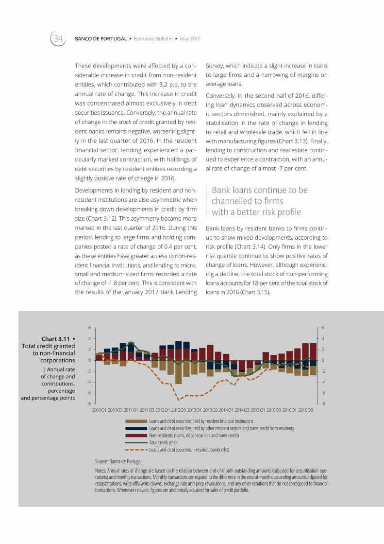
The annual rate of change in total credit to firms recorded positive levels in the second half of 2016
The annual rate of change in total credit to non-financial corporations recorded a positive level of 0.5 per cent at the end of 2016 (Chart 3.11).10
-2.0
0.0
2.0
4.0
6.0
8.0
Dec. 07 Dec. 08 Dec. 09 Dec. 10 Dec. 11 Dec. 12 Dec. 13 Dec. 14 Dec. 15 Dec. 16
Average interest rate Euribor (3-month) Differencial
Chart 3.9 • Interest rates on new loans granted by resident banks to households| Percentage and percentage points
Sources: Consesus Economics, Thomson Reuters and Banco de Portugal.
Notes: Average interest rates are based on new loans by initial fixation period, weighted by new loan amounts in each period.
Chart 3.10 • Density distribution of interest rates on new loans granted by banks to private corporations by credit risk profile
Panel a) – low risk Panel b) – high risk
0.0
0.2
0.4
0.6
0 1 3 5 6 8 9 11 12 14
Den
sity
Interest rate
2014 Q4 2015 Q4 2016 Q4
0.0
0.2
0.4
0.6
0 1 3 5 6 8 9 11 12 14
Den
sity
Interest rate
2014 Q4 2015 Q4 2016 Q4
Source: Banco de Portugal.
Note: Interest rates weighted by loan amounts. The sample includes pro-profit corporations. High (low) risk firms lie in the first (last) two deciles of the credit risk distribution. Credit risk is measured by the Z-score estimated according to Antunes, Gonçalves and Prego, ‘Firm default probabilities revisited‛, Banco de Portugal Economic Studies, Vol. 2, No 2, April 2016.
BANCO DE PORTUGAL • Economic Bulletin • May 201734
These developments were affected by a con-siderable increase in credit from non-resident entities, which contributed with 3.2 p.p. to the annual rate of change. This increase in credit was concentrated almost exclusively in debt securities issuance. Conversely, the annual rate of change in the stock of credit granted by resi-dent banks remains negative, worsening slight-ly in the last quarter of 2016. In the resident financial sector, lending experienced a par-ticularly marked contraction, with holdings of debt securities by resident entities recording a slightly positive rate of change in 2016.
Developments in lending by resident and non-resident institutions are also asymmetric when breaking down developments in credit by firm size (Chart 3.12). This asymmetry became more marked in the last quarter of 2016. During this period, lending to large firms and holding com-panies posted a rate of change of 0.4 per cent, as these entities have greater access to non-res-ident financial institutions, and lending to micro, small and medium-sized firms recorded a rate of change of -1.8 per cent. This is consistent with the results of the January 2017 Bank Lending
Survey, which indicate a slight increase in loans to large firms and a narrowing of margins on average loans.
Conversely, in the second half of 2016, differ-ing loan dynamics observed across econom-ic sectors diminished, mainly explained by a stabilisation in the rate of change in lending to retail and wholesale trade, which fell in line with manufacturing figures (Chart 3.13). Finally, lending to construction and real estate contin-ued to experience a contraction, with an annu-al rate of change of almost -7 per cent.
Bank loans continue to be channelled to firms with a better risk profile
Bank loans by resident banks to firms contin-ue to show mixed developments, according to risk profile (Chart 3.14). Only firms in the lower risk quartile continue to show positive rates of change of loans. However, although experienc-ing a decline, the total stock of non-performing loans accounts for 18 per cent of the total stock of loans in 2016 (Chart 3.15).
Chart 3.11 • Total credit granted
to non-financial corporations| Annual rate
of change and contributions,
percentage and percentage points
-8
-6
-4
-2
0
2
4
6
-8
-6
-4
-2
0
2
4
6
2010 Q1 2010 Q3 2011 Q1 2011 Q3 2012 Q1 2012 Q3 2013 Q1 2013 Q3 2014 Q1 2014 Q3 2015 Q1 2015 Q3 2016 Q1 2016 Q3
Loans and debt securities held by resident financial institutionsLoans and debt securities held by other resident sectors and trade credit from residentsNon-residents (loans, debt securities and trade credit)Total credit (rhs)Loans and debt securities – resident banks (rhs)
Source: Banco de Portugal.
Notes: Annual rates of change are based on the relation between end-of-month outstanding amounts (adjusted for securitisation ope-rations) and monthly transactions. Monthly transactions correspond to the difference in the end-of-month outstanding amounts adjusted for reclassifications, write-offs/write-downs, exchange rate and price revaluations, and any other variations that do not correspond to financial transactions. Whenever relevant, figures are additionally adjusted for sales of credit portfolio.
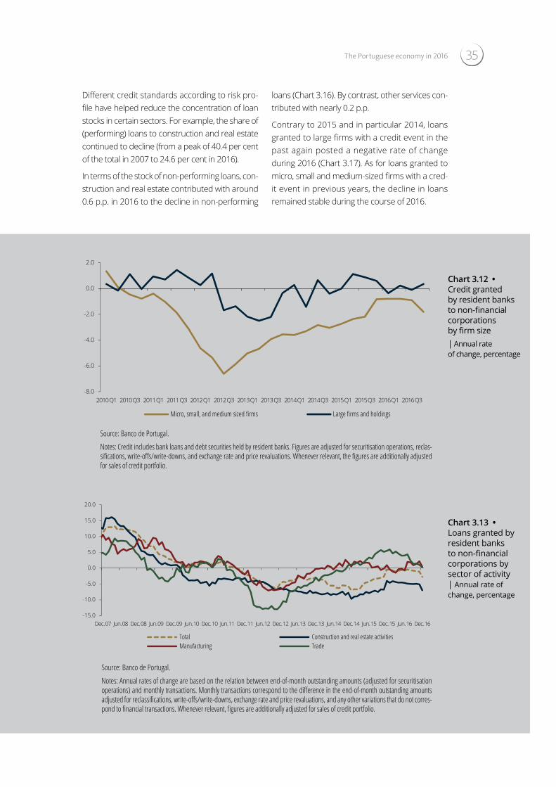
35The Portuguese economy in 2016
Different credit standards according to risk pro-file have helped reduce the concentration of loan stocks in certain sectors. For example, the share of (performing) loans to construction and real estate continued to decline (from a peak of 40.4 per cent of the total in 2007 to 24.6 per cent in 2016).
In terms of the stock of non-performing loans, con-struction and real estate contributed with around 0.6 p.p. in 2016 to the decline in non-performing
loans (Chart 3.16). By contrast, other services con-tributed with nearly 0.2 p.p.
Contrary to 2015 and in particular 2014, loans granted to large firms with a credit event in the past again posted a negative rate of change during 2016 (Chart 3.17). As for loans granted to micro, small and medium-sized firms with a cred-it event in previous years, the decline in loans remained stable during the course of 2016.
-8.0
-6.0
-4.0
-2.0
0.0
2.0
2010 Q1 2010 Q3 2011 Q1 2011 Q3 2012 Q1 2012 Q3 2013 Q1 2013 Q3 2014 Q1 2014 Q3 2015 Q1 2015 Q3 2016 Q1 2016 Q3
Micro, small, and medium sized firms Large firms and holdings
Chart 3.12 • Credit granted by resident banks to non-financial corporations by firm size| Annual rate of change, percentage
Source: Banco de Portugal.
Notes: Credit includes bank loans and debt securities held by resident banks. Figures are adjusted for securitisation operations, reclas-sifications, write-offs/write-downs, and exchange rate and price revaluations. Whenever relevant, the figures are additionally adjusted for sales of credit portfolio.
-15.0
-10.0
-5.0
0.0
5.0
10.0
15.0
20.0
Dec. 07 Jun. 08 Dec. 08 Jun. 09 Dec. 09 Jun. 10 Dec. 10 Jun. 11 Dec. 11 Jun. 12 Dec. 12 Jun. 13 Dec. 13 Jun. 14 Dec. 14 Jun. 15 Dec. 15 Jun. 16 Dec. 16
Total Construction and real estate activitiesManufacturing Trade
Chart 3.13 • Loans granted by resident banks to non-financial corporations by sector of activity | Annual rate of change, percentage
Source: Banco de Portugal.
Notes: Annual rates of change are based on the relation between end-of-month outstanding amounts (adjusted for securitisation operations) and monthly transactions. Monthly transactions correspond to the difference in the end-of-month outstanding amounts adjusted for reclassifications, write-offs/write-downs, exchange rate and price revaluations, and any other variations that do not corres-pond to financial transactions. Whenever relevant, figures are additionally adjusted for sales of credit portfolio.
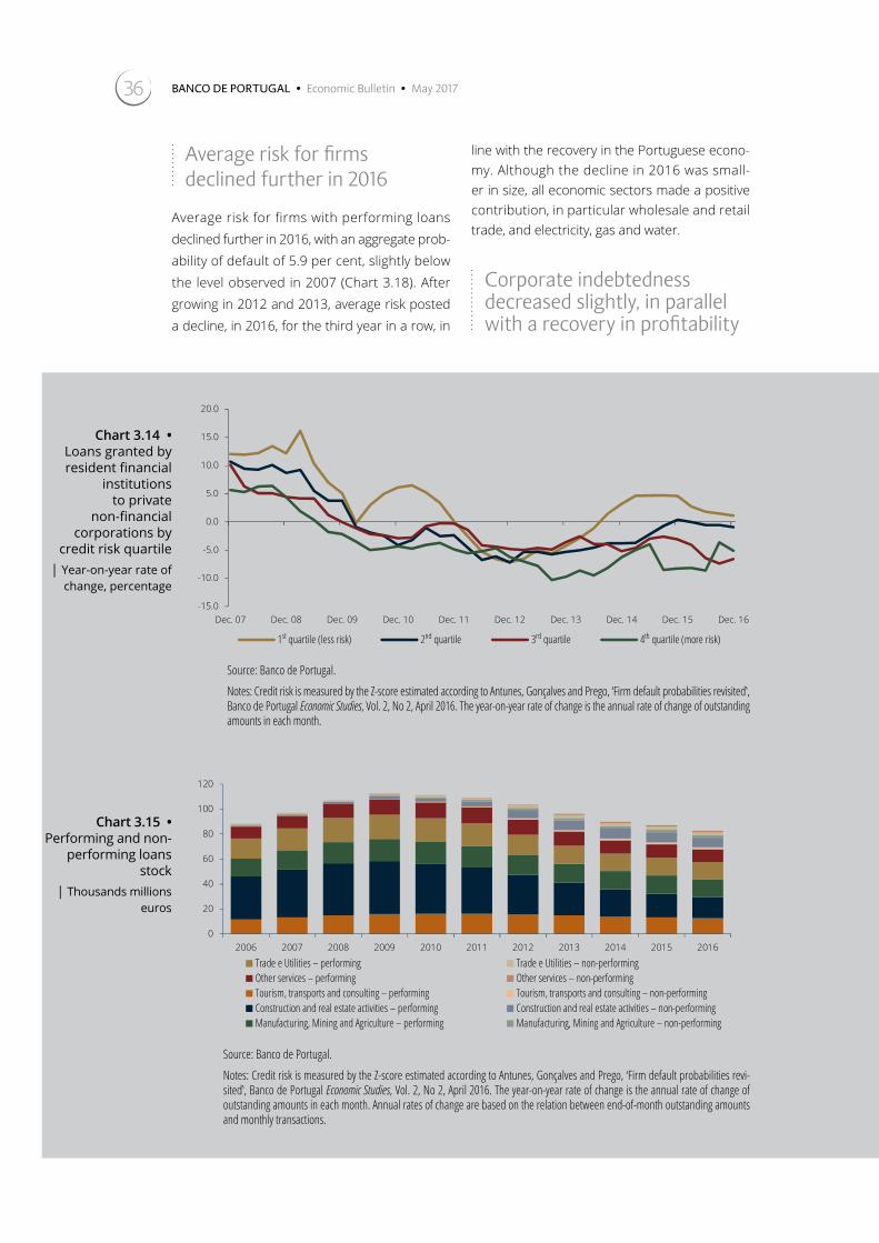
BANCO DE PORTUGAL • Economic Bulletin • May 201736
Average risk for firms declined further in 2016
Average risk for firms with performing loans declined further in 2016, with an aggregate prob-ability of default of 5.9 per cent, slightly below the level observed in 2007 (Chart 3.18). After growing in 2012 and 2013, average risk posted a decline, in 2016, for the third year in a row, in
line with the recovery in the Portuguese econo-my. Although the decline in 2016 was small-er in size, all economic sectors made a positive contribution, in particular wholesale and retail trade, and electricity, gas and water.
Corporate indebtedness decreased slightly, in parallel with a recovery in profitability
Chart 3.14 • Loans granted by resident financial
institutions to private
non-financial corporations by
credit risk quartile | Year-on-year rate of
change, percentage -15.0
-10.0
-5.0
0.0
5.0
10.0
15.0
20.0
Dec. 07 Dec. 08 Dec. 09 Dec. 10 Dec. 11 Dec. 12 Dec. 13 Dec. 14 Dec. 15 Dec. 16
1st quartile (less risk) 2nd quartile 3rd quartile 4th quartile (more risk)
Source: Banco de Portugal.
Notes: Credit risk is measured by the Z-score estimated according to Antunes, Gonçalves and Prego, ‘Firm default probabilities revisited‛, Banco de Portugal Economic Studies, Vol. 2, No 2, April 2016. The year-on-year rate of change is the annual rate of change of outstanding amounts in each month.
Chart 3.15 • Performing and non-
performing loans stock
| Thousands millions euros
0
20
40
60
80
100
120
2006 2007 2008 2009 2010 2011 2012 2013 2014 2015 2016
020406080100120
2006 2007 2008 2009 2010 2011 2012 2013 2014 2015 2016
Trade e Utilities – performing Trade e Utilities – non-performingOther services – performing Other services – non-performingTourism, transports and consulting – performing Tourism, transports and consulting – non-performingConstruction and real estate activities – performing Construction and real estate activities – non-performingManufacturing, Mining and Agriculture – performing Manufacturing, Mining and Agriculture – non-performing
Source: Banco de Portugal.
Notes: Credit risk is measured by the Z-score estimated according to Antunes, Gonçalves and Prego, ‘Firm default probabilities revi-sited‛, Banco de Portugal Economic Studies, Vol. 2, No 2, April 2016. The year-on-year rate of change is the annual rate of change of outstanding amounts in each month. Annual rates of change are based on the relation between end-of-month outstanding amounts and monthly transactions.

37The Portuguese economy in 2016
The deleveraging process of non-financial cor-
porations continued in 2016, with the level of
indebtedness standing at 105.5 per cent of GDP
at the end of the year, compared with 109.6 per
cent in the previous year.11 Although internation-
al comparisons of indebtedness ratios face sta-
tistical challenges, Portuguese firms have delev-
eraged more strongly than their euro area coun-
terparts.
Statistics on non-financial corporations in the
Central Balance Sheet Database, for 2015 as a
whole, confirm that their indebtedness ratio con-
tinued to improve (Chart 3.19). With the excep-
tion of services and accommodation, this decline
was broadly-based across economic sectors
and is partly explained by firms exiting the
market (Box 3.2.1: ‘Market dynamics and the
deleveraging of Portuguese firms‛). In parallel,
-1
0
1
2
3
4
2007 2008 2009 2010 2011 2012 2013 2014 2015 2016
Tourism, transports and consulting Construction and real estate activities Manufacturing, Mining and AgricultureOther services Trade e Utilities
Chart 3.16 • Non-performing loans evolution by industry sector|Percentage points annual contributions
Source: Banco de Portugal.
Notes: Credit risk is measured by the Z-score estimated according to Antunes, Gonçalves and Prego, ‘Firm default probabilities revisited‛, Ban-co de Portugal Economic Studies, Vol. 2, No 2, April 2016. The year-on-year rate of change is the annual rate of change of outstanding amounts in each month. Annual rates of change are based on the relation between end-of-month outstanding amounts and monthly transactions.
-30
-20
-10
0
10
20
30
Sep. 07 Sep. 08 Sep. 09 Sep. 10 Sep. 11 Sep. 12 Sep. 13 Sep. 14 Sep. 15 Sep. 16
Micro and SMEs Large firms
Chart 3.17 • Credit to firms with a past default event| Percentage points
Source: Banco de Portugal.
Note: This analysis includes the evolution of banking loans to firms that registered a credit default event during the period of 2006 to 2016.
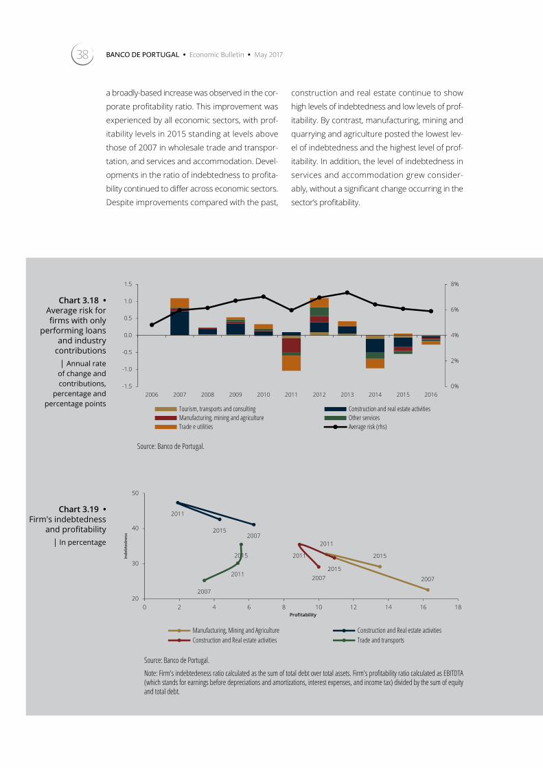
BANCO DE PORTUGAL • Economic Bulletin • May 201738
Chart 3.18 • Average risk for firms with only
performing loans and industry
contributions | Annual rate of change and contributions,
percentage and percentage points
0%
2%
4%
6%
8%
-1.5
-1.0
-0.5
0.0
0.5
1.0
1.5
2006 2007 2008 2009 2010 2011 2012 2013 2014 2015 2016
Tourism, transports and consulting Construction and real estate activitiesManufacturing, mining and agriculture Other servicesTrade e utilities Average risk (rhs)
Source: Banco de Portugal.
Chart 3.19 • Firm's indebtedness
and profitability| In percentage
2007
2011
2015
2007
2011
2015
2007
2011
2015
2007
2011
2015
20
30
40
50
0 2 4 6 8 10 12 14 16 18
Inde
bted
ness
Profitability
Manufacturing, Mining and Agriculture Construction and Real estate activitiesConstruction and Real estate activities Trade and transports
Source: Banco de Portugal.
Note: Firm's indebtedeness ratio calculated as the sum of total debt over total assets. Firm's profitability ratio calculated as EBITDTA (which stands for earnings before depreciations and amortizations, interest expenses, and income tax) divided by the sum of equity and total debt.
a broadly-based increase was observed in the cor-
porate profitability ratio. This improvement was
experienced by all economic sectors, with prof-
itability levels in 2015 standing at levels above
those of 2007 in wholesale trade and transpor-
tation, and services and accommodation. Devel-
opments in the ratio of indebtedness to profita-
bility continued to differ across economic sectors.
Despite improvements compared with the past,
construction and real estate continue to show
high levels of indebtedness and low levels of prof-
itability. By contrast, manufacturing, mining and
quarrying and agriculture posted the lowest lev-
el of indebtedness and the highest level of prof-
itability. In addition, the level of indebtedness in
services and accommodation grew consider-
ably, without a significant change occurring in the
sector’s profitability.

The Portuguese economy in 2016 39
Box 3.2.1 | Market dynamics and the deleveraging of Portuguese firms
The economic and financial crisis of 2008 highlighted the negative effects of the excessive in-debtedness of Portuguese firms on financial stability and economic growth. The Economic and Financial Assistance Programme identified the private sector deleveraging, including the financial system, as an important factor for the adjustment of the Portuguese economy. In this context, the indebtedness of Portuguese non-financial corporations as a proportion of total assets, is esti-mated to have declined by approximately 4 p.p. to 49 per cent in the period between 2012 and 2015, accounting for 118 per cent of GDP by the end of this period.12
Simultaneously to the deleveraging process observed in the past few years in the private sector, the number of firms ceasing their activity increased.13 Therefore, it is important to understand to what extent market dynamics contributed to explain the deleveraging process of Portuguese firms.
The firm balance sheet information reported in the survey Simplified Corporate Information (In-formação Empresarial Simplificada – IES) was considered in the analysis.14 This dataset allows the iden-tification of firms exiting and entering the market in the period between 2010 and 2015. A firm exit in year t is defined by its absence from the IES in that year, provided that this absence does not constitute a reporting gap.15 The entry of firms in the market is identified by the first year reporting to the IES. Chart 1 shows the number of new firms and firms that have ceased their activity in the period between 2010 and 2015.
In the analysis, debt includes the funding obtained (loans and debt securities) by the firm and reported in the IES. According to this information, the total debt of non-financial corporations declined by around 3.4 percent in 2014 and 6.0 percent in 2015 (Chart 2).
Chart 3 depicts the contributions to the change in the debt of non-financial corporations, consider-ing the set of new firms, the set of firms that have ceased their activity, and the set of firms that remained active in the period between 2011 and 2015. The contribution of the set of new firms to the aggregate change in debt is small, in contrast to the substantial contribution of firms that have
Chart 1 • Entry and exit of firms
0
2,000
4,000
6,000
8,000
10,000
12,000
14,000
16,000
18,000
20,000
2011 2012 2013 2014 2015
Entrants (1ˢᵗ report in t) Exits in t (do not report in t)
Source: Banco de Portugal.
Note: The sample includes private non-financial corporations of all economic activity sectors except insurance and financial activities.
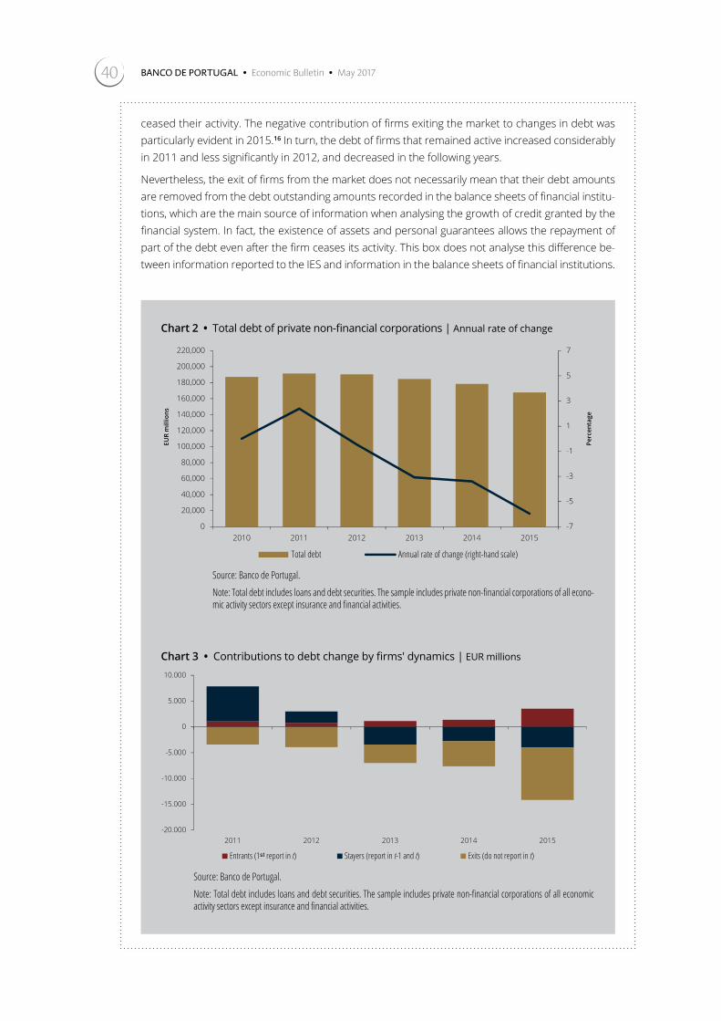
40 BANCO DE PORTUGAL • Economic Bulletin • May 2017
ceased their activity. The negative contribution of firms exiting the market to changes in debt was particularly evident in 2015.16 In turn, the debt of firms that remained active increased considerably in 2011 and less significantly in 2012, and decreased in the following years.
Nevertheless, the exit of firms from the market does not necessarily mean that their debt amounts are removed from the debt outstanding amounts recorded in the balance sheets of financial institu-tions, which are the main source of information when analysing the growth of credit granted by the financial system. In fact, the existence of assets and personal guarantees allows the repayment of part of the debt even after the firm ceases its activity. This box does not analyse this difference be-tween information reported to the IES and information in the balance sheets of financial institutions.
Chart 2 • Total debt of private non-financial corporations | Annual rate of change
-7
-5
-3
-1
1
3
5
7
0
20,000
40,000
60,000
80,000
100,000
120,000
140,000
160,000
180,000
200,000
220,000
2010 2011 2012 2013 2014 2015
Perc
enta
ge
EUR
mill
ions
Total debt Annual rate of change (right-hand scale)
Source: Banco de Portugal.
Note: Total debt includes loans and debt securities. The sample includes private non-financial corporations of all econo-mic activity sectors except insurance and financial activities.
Chart 3 • Contributions to debt change by firms' dynamics | EUR millions
-20.000
-15.000
-10.000
-5.000
0
5.000
10.000
2011 2012 2013 2014 2015
Entrants (1ˢᵗ report in t) Stayers (report in t-1 and t) Exits (do not report in t)
Source: Banco de Portugal.
Note: Total debt includes loans and debt securities. The sample includes private non-financial corporations of all economic activity sectors except insurance and financial activities.

The Portuguese economy in 2016 41
Chart 4 shows the contributions to changes in debt by firm size. The debt reduction resulting from the exit of firms is concentrated in smaller-sized firms. Large firms that remained in the market in 2014 and 2015 also registered a reduction in debt.
The decomposition of the contributions to changes in debt by sector of economic activity shows that the exit of firms in the construction sector had a substantial impact on debt reduction, especially in the last year (Chart 5). Firms in the trade sector that remained in the market in 2012 and 2013 significantly reduced their debt. The debt reduction resulting from the exit of firms in this sector of economic activ-ity is particularly relevant in 2015. In the manufacturing sector, it is particularly relevant the debt reduc-tion of firms that remained in the market in 2014 and firms that ceased their activity in 2015.
Chart 4 • Contributions to debt change by firms' dynamics | By firm size, EUR millions
SME Large corporations
-12.000-10.000-8.000-6.000-4.000-2.000
02.0004.0006.000
2011 2012 2013 2014 2015
Entrants (1ˢᵗ report in t) Stayers (report in t-1 and t) Exits (do not report in t)
-5.000-4.000-3.000-2.000-1.000
01.0002.0003.0004.0005.000
2011 2012 2013 2014 2015
Entrants (1ˢᵗ report in t) Stayers (report in t-1 and t) Exits (do not report in t)
Source: Banco de Portugal.
Note: Total debt includes loans and debt securities. The sample includes private non-financial corporations of all economic activity sectors except insurance and financial activities.
Chart 5 • Contributions to debt change by firms' dynamics | By sector of economic activity, EUR millions
Construction Trade
-6.000-5.000-4.000-3.000-2.000-1.000
01.0002.000
2011 2012 2013 2014 2015
Entrants (1ˢᵗ report in t) Stayers (report in t-1 and t) Exits (do not report in t)
-6.000-5.000-4.000-3.000-2.000-1.000
01.0002.000
2011 2012 2013 2014 2015
Entrants (1ˢᵗ report in t) Stayers (report in t-1 and t) Exits (do not report in t)
Manufacturing
-6.000-5.000-4.000-3.000-2.000-1.000
01.0002.000
2011 2012 2013 2014 2015
Entrants (1ˢᵗ report in t) Stayers (report in t-1 and t) Exits (do not report in t)
Source: Banco de Portugal.
Note: Total debt includes loans and debt securities. The sample includes private non-financial corporations of all economic activity sectors except insurance and financial activities.

42 BANCO DE PORTUGAL • Economic Bulletin • May 2017
In this context of corporate deleveraging, it is important to know to what extent the market dynamics
contributed to corporate indebtedness and profitability. The empirical analysis presented below de-
composes changes in indebtedness and profitability of Portuguese firms in the period between 2010
and 2015, according to market dynamics and firm age. In the analysis, firms are classified according
to their age: young firms are those that have been in the market for two years or less, vintage firms
are those with more than two years and less than five, and established firms are those aged more
than five years. Then, the following equation was estimated:
and 2015, according to market dynamics and firm age. In the analysis, firms are classified according to their age: young firms are those that have been in the market for two years or less, vintage firms are those with more than two years and less than five, and established firms are those aged more than five years. Then, the following equation was estimated:
��� � �� � �� � �� � �� � �������� � ����������� � ��������� � ����������� � ���where ��� assumes two indicators: indebtedness (ratio of total debt to assets) and profitability (ratio of EBIT17 to assets) of firm i in year t. The variables Exit and Entrant are binary variables equal to one for firms exiting and entering the market, respectively. The variables Young and Vintage are also binary variables equal to one for firms less than two years old and firms with two to five years, respectively. Finally, the terms �� , ��, and �� denote a set of firm, time, and sector of economic activity fixed effects, respectively. Firm and sector fixed effects account for their specific (observed and unobserved) characteristics, provided they remain constant over time. In turn, time effects attempt to capture the cyclical position of the economy. In this case, the comparison group are the established firms that remained in activity. In order to avoid extreme values, observations above the 99th percentile and below the 1st percentile were not considered. The analysis was performed using the fixed-effects estimator for panel data.
The results of the estimation are reported in Table 1. According to the estimates, firms exiting the market are the most indebted and the least profitable. In turn, firms that have recently entered the market are less indebted and less profitable than older incumbent firms. In particular, firms exiting the market are approximately 33.9 p.p. more indebted and 4.93 p.p. less profitable than older incumbent firms, on average. This selection dynamics suggests that the improvement in the aggregate financial position of Portuguese firms is partly due to the fact that the most indebted and less profitable firms have exited the market.
12. See Box “Developments in corporate indebtedness in Portugal and the euro area”, Economic Bulletin, May 2016, Banco de Portugal. The analysis considers data from the national financial accounts and the measure of indebtedness considered is the ratio of debt (loans and debt securities) to total assets. 13. Félix, S. (2017) “Firm creation and survival in Portugal”, Banco de Portugal Economic Studies, Banco de Portugal. 14. The survey IES includes economic, financial, and accounting information of virtually all the Portuguese non-financial corporations and is available for the period between 2005 and 2015. Nevertheless, changes in the accounting standards system in 2010 have led to a loss of data comparability. 15. A reporting gap is observed when the firm reports to the IES in year t-1 and year t+1, but is absent in year t. 16. Some of the absences that are considered exits from the market in 2015 may constitute reporting gaps. This can only be verified when the IES for 2016 becomes available. However, only about 0.2 per cent of the observations are reporting gaps in the period under analysis. 17. EBIT stands for Earnings Before Interest and Taxes.
Chart3.2.1EntryandexitoffirmsEntrants(1styearint)Exitsint(absentint)Source:BancodePortugal.Note:Thesampleincludesprivatenon‐financialcorporationsofalleconomicactivitysectorsexceptinsuranceandfinancialactivities.Chart3.2.2Totaldebtofprivatenon‐financialcorporations|Year‐on‐yearrateofchangeTotaldebtYear‐on‐yearrateofchange(right‐handscale)Source:BancodePortugal.Note:Totaldebtincludesloansanddebtsecurities.Thesampleincludesprivatenon‐financialcorporationsofalleconomicactivitysectorsexceptinsuranceandfinancialactivities.Chart3.2.3Contributionstodebtchangebyfirms'dynamics|EURmillionsEntrants(1styearint)Stayers(reportint‐1andt)Exitsint(absentint)Source:BancodePortugal.
where
65
Neste contexto de desalavancagem das empresas, importa aprofundar de que forma
a dinâmica de mercado contribuiu para o endividamento e rendibilidade das empresas.
A análise empírica abaixo decompõe a evolução do endividamento e da rendibilidade
das empresas portuguesas no período compreendido entre 2010 e 2015, de acordo
com a dinâmica de mercado e idade. A análise categoriza as empresas de acordo
com a idade: empresas novas são as que têm dois ou menos anos no mercado,
empresas vintage são as que têm mais de dois anos e menos de cinco, e empresas
estabelecidas são as que têm mais de cinco anos. De seguida, estimou-se a seguinte
equação:
em que assume dois indicadores: endividamento (rácio da dívida total no ativo) e
rendibilidade (rácio do EBIT17 no ativo) da empresa i no ano t. As variáveis Saída e
Entrada são binárias e iguais a um para empresas que saem e entram no mercado,
respetivamente. As variáveis Nova e Vintage são também binárias e assumem o valor
de um no caso de empresas novas e com idades entre dois e cinco anos,
respetivamente. Finalmente, os termos , e denotam um conjunto de efeitos da
empresa, tempo e setor, respetivamente. Os efeitos da empresa e do setor permitem
controlar para as respetivas características específicas (observadas e não
observadas), desde que sejam constantes ao longo do tempo. Por sua vez, os efeitos
temporais têm em consideração a posição cíclica da economia. Note-se que neste
caso o grupo de comparação são as empresas estabelecidas que permaneceram no
mercado. Para evitar a presença de valores extremos, não se consideraram
17 EBIT é o acrónimo para earnings before interest and taxes.
assumes two indicators: indebtedness (ratio of total debt to assets) and profitability
(ratio of EBIT17 to assets) of firm
65
Neste contexto de desalavancagem das empresas, importa aprofundar de que forma
a dinâmica de mercado contribuiu para o endividamento e rendibilidade das empresas.
A análise empírica abaixo decompõe a evolução do endividamento e da rendibilidade
das empresas portuguesas no período compreendido entre 2010 e 2015, de acordo
com a dinâmica de mercado e idade. A análise categoriza as empresas de acordo
com a idade: empresas novas são as que têm dois ou menos anos no mercado,
empresas vintage são as que têm mais de dois anos e menos de cinco, e empresas
estabelecidas são as que têm mais de cinco anos. De seguida, estimou-se a seguinte
equação:
em que assume dois indicadores: endividamento (rácio da dívida total no ativo) e
rendibilidade (rácio do EBIT17 no ativo) da empresa i no ano t. As variáveis Saída e
Entrada são binárias e iguais a um para empresas que saem e entram no mercado,
respetivamente. As variáveis Nova e Vintage são também binárias e assumem o valor
de um no caso de empresas novas e com idades entre dois e cinco anos,
respetivamente. Finalmente, os termos , e denotam um conjunto de efeitos da
empresa, tempo e setor, respetivamente. Os efeitos da empresa e do setor permitem
controlar para as respetivas características específicas (observadas e não
observadas), desde que sejam constantes ao longo do tempo. Por sua vez, os efeitos
temporais têm em consideração a posição cíclica da economia. Note-se que neste
caso o grupo de comparação são as empresas estabelecidas que permaneceram no
mercado. Para evitar a presença de valores extremos, não se consideraram
17 EBIT é o acrónimo para earnings before interest and taxes.
in year
65
Neste contexto de desalavancagem das empresas, importa aprofundar de que forma
a dinâmica de mercado contribuiu para o endividamento e rendibilidade das empresas.
A análise empírica abaixo decompõe a evolução do endividamento e da rendibilidade
das empresas portuguesas no período compreendido entre 2010 e 2015, de acordo
com a dinâmica de mercado e idade. A análise categoriza as empresas de acordo
com a idade: empresas novas são as que têm dois ou menos anos no mercado,
empresas vintage são as que têm mais de dois anos e menos de cinco, e empresas
estabelecidas são as que têm mais de cinco anos. De seguida, estimou-se a seguinte
equação:
em que assume dois indicadores: endividamento (rácio da dívida total no ativo) e
rendibilidade (rácio do EBIT17 no ativo) da empresa i no ano t. As variáveis Saída e
Entrada são binárias e iguais a um para empresas que saem e entram no mercado,
respetivamente. As variáveis Nova e Vintage são também binárias e assumem o valor
de um no caso de empresas novas e com idades entre dois e cinco anos,
respetivamente. Finalmente, os termos , e denotam um conjunto de efeitos da
empresa, tempo e setor, respetivamente. Os efeitos da empresa e do setor permitem
controlar para as respetivas características específicas (observadas e não
observadas), desde que sejam constantes ao longo do tempo. Por sua vez, os efeitos
temporais têm em consideração a posição cíclica da economia. Note-se que neste
caso o grupo de comparação são as empresas estabelecidas que permaneceram no
mercado. Para evitar a presença de valores extremos, não se consideraram
17 EBIT é o acrónimo para earnings before interest and taxes.
. The variables Exit and Entry are binary and equal to
one for firms exiting and entering the market respectively.The variables Exit and Entrant are binary
variables equal to one for firms exiting and entering the market, respectively. The variables Young
and Vintage are also binary variables equal to one for firms less than two years old and firms with
two to five years, respectively. Finally, the terms
65
Neste contexto de desalavancagem das empresas, importa aprofundar de que forma
a dinâmica de mercado contribuiu para o endividamento e rendibilidade das empresas.
A análise empírica abaixo decompõe a evolução do endividamento e da rendibilidade
das empresas portuguesas no período compreendido entre 2010 e 2015, de acordo
com a dinâmica de mercado e idade. A análise categoriza as empresas de acordo
com a idade: empresas novas são as que têm dois ou menos anos no mercado,
empresas vintage são as que têm mais de dois anos e menos de cinco, e empresas
estabelecidas são as que têm mais de cinco anos. De seguida, estimou-se a seguinte
equação:
em que assume dois indicadores: endividamento (rácio da dívida total no ativo) e
rendibilidade (rácio do EBIT17 no ativo) da empresa i no ano t. As variáveis Saída e
Entrada são binárias e iguais a um para empresas que saem e entram no mercado,
respetivamente. As variáveis Nova e Vintage são também binárias e assumem o valor
de um no caso de empresas novas e com idades entre dois e cinco anos,
respetivamente. Finalmente, os termos , e denotam um conjunto de efeitos da
empresa, tempo e setor, respetivamente. Os efeitos da empresa e do setor permitem
controlar para as respetivas características específicas (observadas e não
observadas), desde que sejam constantes ao longo do tempo. Por sua vez, os efeitos
temporais têm em consideração a posição cíclica da economia. Note-se que neste
caso o grupo de comparação são as empresas estabelecidas que permaneceram no
mercado. Para evitar a presença de valores extremos, não se consideraram
17 EBIT é o acrónimo para earnings before interest and taxes.
,
65
Neste contexto de desalavancagem das empresas, importa aprofundar de que forma
a dinâmica de mercado contribuiu para o endividamento e rendibilidade das empresas.
A análise empírica abaixo decompõe a evolução do endividamento e da rendibilidade
das empresas portuguesas no período compreendido entre 2010 e 2015, de acordo
com a dinâmica de mercado e idade. A análise categoriza as empresas de acordo
com a idade: empresas novas são as que têm dois ou menos anos no mercado,
empresas vintage são as que têm mais de dois anos e menos de cinco, e empresas
estabelecidas são as que têm mais de cinco anos. De seguida, estimou-se a seguinte
equação:
em que assume dois indicadores: endividamento (rácio da dívida total no ativo) e
rendibilidade (rácio do EBIT17 no ativo) da empresa i no ano t. As variáveis Saída e
Entrada são binárias e iguais a um para empresas que saem e entram no mercado,
respetivamente. As variáveis Nova e Vintage são também binárias e assumem o valor
de um no caso de empresas novas e com idades entre dois e cinco anos,
respetivamente. Finalmente, os termos , e denotam um conjunto de efeitos da
empresa, tempo e setor, respetivamente. Os efeitos da empresa e do setor permitem
controlar para as respetivas características específicas (observadas e não
observadas), desde que sejam constantes ao longo do tempo. Por sua vez, os efeitos
temporais têm em consideração a posição cíclica da economia. Note-se que neste
caso o grupo de comparação são as empresas estabelecidas que permaneceram no
mercado. Para evitar a presença de valores extremos, não se consideraram
17 EBIT é o acrónimo para earnings before interest and taxes.
and
65
Neste contexto de desalavancagem das empresas, importa aprofundar de que forma
a dinâmica de mercado contribuiu para o endividamento e rendibilidade das empresas.
A análise empírica abaixo decompõe a evolução do endividamento e da rendibilidade
das empresas portuguesas no período compreendido entre 2010 e 2015, de acordo
com a dinâmica de mercado e idade. A análise categoriza as empresas de acordo
com a idade: empresas novas são as que têm dois ou menos anos no mercado,
empresas vintage são as que têm mais de dois anos e menos de cinco, e empresas
estabelecidas são as que têm mais de cinco anos. De seguida, estimou-se a seguinte
equação:
em que assume dois indicadores: endividamento (rácio da dívida total no ativo) e
rendibilidade (rácio do EBIT17 no ativo) da empresa i no ano t. As variáveis Saída e
Entrada são binárias e iguais a um para empresas que saem e entram no mercado,
respetivamente. As variáveis Nova e Vintage são também binárias e assumem o valor
de um no caso de empresas novas e com idades entre dois e cinco anos,
respetivamente. Finalmente, os termos , e denotam um conjunto de efeitos da
empresa, tempo e setor, respetivamente. Os efeitos da empresa e do setor permitem
controlar para as respetivas características específicas (observadas e não
observadas), desde que sejam constantes ao longo do tempo. Por sua vez, os efeitos
temporais têm em consideração a posição cíclica da economia. Note-se que neste
caso o grupo de comparação são as empresas estabelecidas que permaneceram no
mercado. Para evitar a presença de valores extremos, não se consideraram
17 EBIT é o acrónimo para earnings before interest and taxes.
denote a set of firm, time, and sector
of economic activity fixed effects, respectively. Firm and sector fixed effects account for their spe-
cific (observed and unobserved) characteristics, provided they remain constant over time. In turn,
time effects attempt to capture the cyclical position of the economy. In this case, the comparison
group are the established firms that remained in activity. In order to avoid extreme values, obser-
vations above the 99th percentile and below the 1st percentile were not considered. The analysis
was performed using the fixed-effects estimator for panel data.
The results of the estimation are reported in Table 1. According to the estimates, firms exiting the
market are the most indebted and the least profitable. In turn, firms that have recently entered
the market are less indebted and less profitable than older incumbent firms. In particular, firms
exiting the market are approximately 33.9 p.p. more indebted and 4.93 p.p. less profitable than
older incumbent firms, on average. This selection dynamics suggests that the improvement in the
aggregate financial position of Portuguese firms is partly due to the fact that the most indebted
and less profitable firms have exited the market.
Table 1 • Fixed effects estimates
Indebtedness Profitability
Entrant -0.0332*** -0.0413***
(0.0031) (0.0018)
Exit 0.3386*** -0.0493***
(0.0047) (0.0024)
Young -0.0603*** -0.0543***
(0.0037) (0.0026)
Vintage -0.0223*** -0.0067***
(0.0025) (0.0016)
Observations 2,001,156 1,063,059
Note: *, **, *** denote statistical significance at 1, 5, and 10 percent, respectively. Both specifications include firm, sector of economic activity, and time fixed effects. Robust standard errors clustered at firm level in parentheses.

43The Portuguese economy in 2016
4. Fiscal policy and situation
The general government deficit declined significantly, against a background of a stabilisation in the structural balance and a reduction in the primary structural balance
In 2016, the general government deficit stood at 2.0 per cent of GDP, which is a historically low level (Table 4.1). This figure stands below the official target included in the State Budget for 2016 (2.2 per cent of GDP), the revised estimate included in the State Budget for 2017 (2.4 per cent of GDP), and the limit laid down by the European Union Council in August 2016 (2.5 per cent of GDP).
The deficit improved by 2.3 p.p. vis-à-vis the pre-vious year, chiefly as a result of the change in
the impact of temporary measures (Chart 4.1). In 2015 the general government balance was negatively affected by the resolution of BANIF (-1.4 per cent of GDP). In 2016 the effect of temporary measures corresponds to revenue obtained from full payments made within the scope of a special programme for the settle-ment of overdue tax and social contributions (Programa Especial de Redução do Endivida-mento ao Estado – PERES) and the refund by the European Financial Stability Facility (EFSF) of amounts previously paid by Portugal under the Economic and Financial Assistance Pro-gramme.18 Overall, these effects contributed to increase the fiscal balance in 2016 by 0.4 per cent of GDP. Therefore, the decline in the fis-cal deficit adjusted for temporary measures stood at 0.5 p.p. of GDP, 0.3 p.p. of which refer to a drop in interest expenditure.
Table 4.1 • Main fiscal indicators | In percentage of GDP
2010 2011 2012 2013 2014 2015 2016Change
2016-2015 (a)
Overall balance (1) -11.2 -7.4 -5.7 -4.8 -7.2 -4.4 -2.0 2.3
Temporary measures and special factors (a) (2)
-2.8 -0.2 0.0 0.3 -3.6 -1.4 0.4 1.8
Overall balance excluding temporary measures and special factors (3 = 1-2) -8.4 -7.2 -5.6 -5.2 -3.6 -3.0 -2.4 0.5
Cyclical component (4) 1.5 0.6 -1.7 -2.3 -1.4 -0.6 -0.1 0.5
Structural balance(b) (5 = 3 - 4) -9.9 -7.9 -3.9 -2.9 -2.2 -2.4 -2.3 0.0
Interest expenditure (6) 2.9 4.3 4.9 4.9 4.9 4.6 4.2 -0.3
Structural primary balance (7=5+6) -7.0 -3.5 1.0 2.0 2.7 2.2 1.9 -0.3
Structural revenue (percentage of trend GDP) (b)
39.9 42.0 43.1 44.9 44.9 44.1 42.5 -1.6
Structural primary expenditure (percentage of trend GDP) (b) 47.1 45.6 42.2 43.0 42.3 42.0 40.6 -1.3
Public debt 96.2 111.4 126.2 129.0 130.6 129.0 130.4 1.4
Change in public debt (in p.p.) 12.6 15.2 14.8 2.8 1.6 -1.6 1.4 –
(-) Primary balance 8.2 3.1 0.8 0.0 2.3 -0.2 -2.2 –
Differential between the effects of interest and of GDP growth
0.8 6.4 10.0 3.5 2.8 -0.1 0.5 –
Deficit-debt adjustments 3.5 5.8 4.0 -0.6 -3.5 -1.3 3.1 –
Sources: INE and Banco de Portugal.
Notes: (a) Special factors are operations with an one-off effect on the general government deficit which cannot be treated as temporary measures according to the definition adopted in the Eurosystem. (b) Structural figures are adjusted for the impacts of the cycle, temporary measures and special factors. The cyclical component and temporary measures are computed by Banco de Portugal according to the methodologies adopted in the Eurosystem.

BANCO DE PORTUGAL • Economic Bulletin • May 201744
According to the cyclical adjustment methodol-ogy adopted in the Eurosystem, economic activ-ity gave a positive contribution to fiscal develop-ments, accounting for 0.5 p.p. of the deficit improvement. Therefore, the structural balance is estimated to have stabilised in 2016.19 As regards the structural primary balance, which excludes the impact of interest expenditure, it is estimated to have declined for the second year in a row (by 0.3 p.p. of trend GDP).
The decline in the structural primary balance in 2016 reflects a drop in structural revenue by 1.6 p.p. of trend GDP, which more than offset the 1.3 p.p. contraction recorded by structural primary expenditure (Chart 4.2). In particular, in structural
terms, both the tax and contributory burden and the non-tax revenue declined as a ratio to trend GDP (by -0.9 p.p. and -0.7 p.p. respectively).
The drop in structural revenue largely stemmed from tax revenue developments
In actual terms, tax and contributory reve-nue rose by 2.2 per cent in 2016, reflecting an increase in revenue from taxes on production and imports and social contributions. Econom-ic activity is estimated to have given a positive contribution to these developments. They also reflect revenue collected within the scope of
Chart 4.2 • Structural revenue
and primary expenditure
developments| In percentage of
trend GDP
30
35
40
45
50
1995 1997 1999 2001 2003 2005 2007 2009 2011 2013 2015
Structural revenue Structural primary expenditure
Sources: INE and Banco de Portugal.
Chart 4.1 • Breakdown of
the change in the general government
balance| In percentage points
of trend GDP
-6.0
-4.0
-2.0
0.0
2.0
4.0
6.0
2011 2012 2013 2014 2015 2016
Structural primary expenditure ( - ) Interest expenditure ( - ) Cyclical componentTemporary measures Structural revenue Overall balance (p.p. of GDP)Structural balance (p.p. of GDP)
Sources: INE and Banco de Portugal.

45The Portuguese economy in 2016
PERES, part of which, as previously mentioned, has a temporary nature. The structural tax and contributory burden, which is adjusted for the impact of the cycle and temporary measures, stabilised in 2016, implying a decline by 0.9 p.p. of trend GDP (Chart 4.3). These developments are chiefly explained by a drop in revenue from the taxes on income and wealth (-0.8 p.p.), reflecting the impact of policy measures imple-mented not only in 2016, but also in previous years (Box 4.1: ‘Structural developments of tax revenue in 2016’).
In 2016 non-tax revenue declined by 6.3 per cent, resulting from a drop in other current rev-enue (including sales of goods and services) and capital revenue. The 3.7 per cent decline in oth-er current revenue reflects decreases in most of its items, particularly as regards interest and dividends. Capital revenue, in turn, declined by 27.9 per cent in actual terms. This occurred in spite of the refund of the margins previous-ly paid to the EFSF, which, as previously men-tioned, has a temporary impact. Therefore, the change in capital revenue adjusted for tempo-rary measures would be more negative in 2016, at -51.0 per cent, as a result of the significant fall in capital transfers from the European Union matched by expenditure in the same year.
The decrease in general government expenditure chiefly reflected a decline in investment
The structural decline in primary expenditure was chiefly driven by a decrease in capital expendi-ture. Adjusting for the effect of temporary meas-ures with an impact on 2015, the decline in capital expenditure was 0.9 p.p. of trend GDP.20 These developments were largely due to the decline in public investment (Chart 4.4). In 2016, in par-ticular, public investment declined by 30.9 per cent in nominal terms, which partly mirrored a base effect resulting from the recording of real estate acquisitions by Oitante in 2015, within the scope of the resolution of BANIF, and the record-ing of military material deliveries in 2016.21 The change in public investment adjusted for these factors stands at -24.8 per cent. This decline may have partly reflected a decrease in funds received from the European Union and it was particularly relevant in the Autonomous Services and Funds subsector. Turning to other capital expenditure adjusted for the impact of temporary measures, there was also a decline as a ratio to trend GDP (0.3 p.p.), reflecting several of base effects that contributed to a one-off growth of this expendi-ture item in 2015.22
-2.0
-1.0
0.0
1.0
2.0
3.0
2012 2013 2014 2015 2016
Taxes on households' income Taxes on firms' incomeVAT Other taxes on production and importsSocial contributions Other revenue (a)
Chart 4.3 • Breakdown of the change in structural revenue | In percentage points of trend GDP
Sources: INE and Banco de Portugal.
Note: (a) Other revenue encompasses ‘other current‛ revenue, including sales, and ‘capital revenue‛.
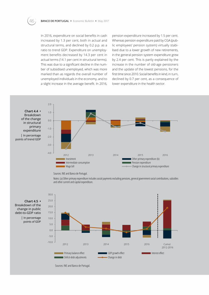
BANCO DE PORTUGAL • Economic Bulletin • May 201746
In 2016, expenditure on social benefits in cash increased by 1.3 per cent, both in actual and structural terms, and declined by 0.2 p.p. as a ratio to trend GDP. Expenditure on unemploy-ment benefits decreased by 14.3 per cent in actual terms (14.1 per cent in structural terms). This was due to a significant decline in the num-ber of subsidised unemployed, which was more marked than as regards the overall number of unemployed individuals in the economy, and to a slight increase in the average benefit. In 2016,
pension expenditure increased by 1.5 per cent. Whereas pension expenditure paid by CGA (pub-lic employees’ pension system) virtually stabi-lised due to a lower growth of new retirements, in the general pension system expenditure grew by 2.4 per cent. This is partly explained by the increase in the number of old-age pensioners and the update of the lowest pensions, for the first time since 2010. Social benefits in kind, in turn, declined by 0.7 per cent, as a consequence of lower expenditure in the health sector.
Chart 4.4 • Breakdown
of the change in structural
primary expenditure
| In percentage points of trend GDP
-4.0
-3.0
-2.0
-1.0
0.0
1.0
2.0
2012 2013 2014 2015 2016
Investment Other primary expenditure (b)Intermediate consumption Pension expenditureWage bill Change in structural primary expenditure
Sources: INE and Banco de Portugal.
Notes: (a) Other primary expenditure includes social payments excluding pensions, general government social contributions, subsidies and other current and capital expenditure.
Chart 4.5 • Breakdown of the
change in public debt-to-GDP ratio
| In percentage points of GDP
-10.0
-5.0
0.0
5.0
10.0
15.0
20.0
25.0
30.0
2012 2013 2014 2015 2016 Cumul: 2012-2016
Primary balance effect GDP growth effect Interest effectDeficit-debt adjustments Change in debt
Sources: INE and Banco de Portugal.

47The Portuguese economy in 2016
In 2016 compensation of employees and inter-mediate consumption remained unchanged as a ratio to trend GDP. Compensation of employ-ees increased by 2.8 per cent, after two years of decline. This is explained by the growth in wages and salaries, as a result of the full reinstatement of the wage cuts in force since 2011 and, to a lesser extent, of developments in the number of general government employees.23 Indeed, in 2016, against a backdrop of a decrease in the number of weekly hours worked in gener-al government, from 40 to 35, the number of employees recorded, for the first time since 2011, a positive quarterly average change. In the case of intermediate consumption, the 2.9 per cent increase was strongly influenced by the rise in expenditure related to public-pri-vate partnerships in the road sector, which was again significant. Excluding these outlays, this expenditure item decelerated.
The public debt ratio increased, reflecting a significant accumulation of deposits
At the end of 2016, the general government debt stood at 130.4 per cent of GDP, 1.4 p.p. above the figure recorded at the end of the previous year. In a context where the primary balance contributed to reduce the debt ratio (by -2.2 p.p. of GDP), the change was chiefly explained by deficit-debt adjustments (3.1 p.p. of GDP). The fact that the implicit interest rate on debt exceeded the nominal GDP growth rate has also contributed to increase the ratio (by 0.5 p.p. of GDP) (Chart 4.5).
As regards deficit-debt adjustments, the fig-ure recorded in 2016 is mostly explained by the increase in deposits held by the general govern-ment by an amount equivalent to 2.4 p.p. of GDP. This deposit accumulation was likely related to the need to finance the capital injection by the State in Caixa Geral de Depósitos, which occurred at the beginning of 2017. Therefore, in 2016 the debt ratio net of general government deposits declined from 118.9 to 118.1 per cent of GDP.
Similarly to developments in 2015, part of the loan granted by the IMF under the Economic and Financial Assistance Programme was repaid
in advance in 2016 (2.4 per cent of GDP). This repayment contributed to reduce the share of debt held by non-residents, from 66.5 per cent at the end of 2015 to 58.2 per cent at the end of 2016 (Chart 4.6). This effect was reinforced by the increased importance of Banco de Portugal as a holder of Portuguese public debt, reflecting the widening of the Eurosystem’s asset purchase programme to include sovereign bonds.24 More specifically, between 2014 and 2016 the per-centage of public debt held by the Central Bank increased from 0.7 to 8.8 per cent, implying an increase in the Central Bank’s exposure to sover-eign risk. This occurred against the decline in the share of non-residents and, to a lesser extent, of other MFIs as debt holders.
In the course of 2016, the Portuguese State par-ticipated regularly in sovereign debt markets. Against a backdrop of a widening in the differ-ential between the cost of financing 10-year Por-tuguese and German debt, the allotment rates of long-term securities were higher than those recorded in 2015 (Chart 4.7). In 2016, in par-ticular, the average rate on 10-year Treasury Bond auctions stood at 3.1 per cent, up from 2.3 in the previous year. As regards short-term issues, the average interest rate on Treasury Bill auctions declined slightly from 0.04 to 0.02 per cent.
General government debt servicing expendi-ture declined from 4.6 to 4.2 per cent of GDP in the year under review, which is underpinned by a reduction in the implicit interest rate from 3.6 per cent in 2015 to 3.3 per cent in 2016.25
These developments stem, on the one hand, from a decline in the interest burden associat-ed with loans under the Economic and Financial Assistance Programme and, on the other hand, from the repayment of Treasury Bonds with high-er rates than those of the new issues.
The euro area structural primary balance declined for the second year in a row
According to the European Commission Winter forecasts, published in February 2017, the struc-tural primary balance in the euro area declined

BANCO DE PORTUGAL • Economic Bulletin • May 201748
Chart 4.7 • 10 year government
bond yields| Percentage
-5.0
0.0
5.0
10.0
15.0
20.0
Jan.
07
May
07
Sep.
07
Jan.
08
May
08
Sep.
08
Jan.
09
May
09
Sep.
09
Jan.
10
May
10
Sep.
10
Jan.
11
May
11
Sep.
11
Jan.
12
May
12
Sep.
12
Jan.
13
May
13
Sep.
13
Jan.
14
May
14
Sep.
14
Jan.
15
May
15
Sep.
15
Jan.
16
May
16
Sep.
16
Portugal Germany Spain Italy
Source: Thomson Reuters.
Chart 4.6 • Breakdown
of public debt by holder
| Percentage
0
10
20
30
40
50
60
70
80
90
100
2011 2012 2013 2014 2015 2016
Non-residents Central Bank Other monetary financial institutions Other financial institutions Other residents
Source: Banco de Portugal.
Chart 4.8 • Fiscal policy and
cyclical position in the euro area in
2016 | In percentage
points of potential GDP
PT 12
PT 13
PT 14
PT 15
PT 16
EA 12
EA 13 EA 14
EA 15EA 16
-2
-1
0
1
2
3
4
5
6
-3.5 -3 -2.5 -2 -1.5 -1 -0.5 0 0.5 1 1.5 2
isca
l sta
nce
(cha
nge
in th
e st
ruct
ural
pri
mar
y ba
lanc
e)
Cyclical position (change in the output gap)
Pro-cyclical tightening of fiscal policy
Counter-cyclical loosening of fiscal policyPro-cyclical loosening of fiscal policy
Counter-cyclical tightening of fiscal policy
Source: European Commission (Winter 2017 Forecasts).
Note: The cyclical position of the economy is assessed by the change in the output gap, which broadly corresponds to the difference between actual GDP and potential GDP growth rates.
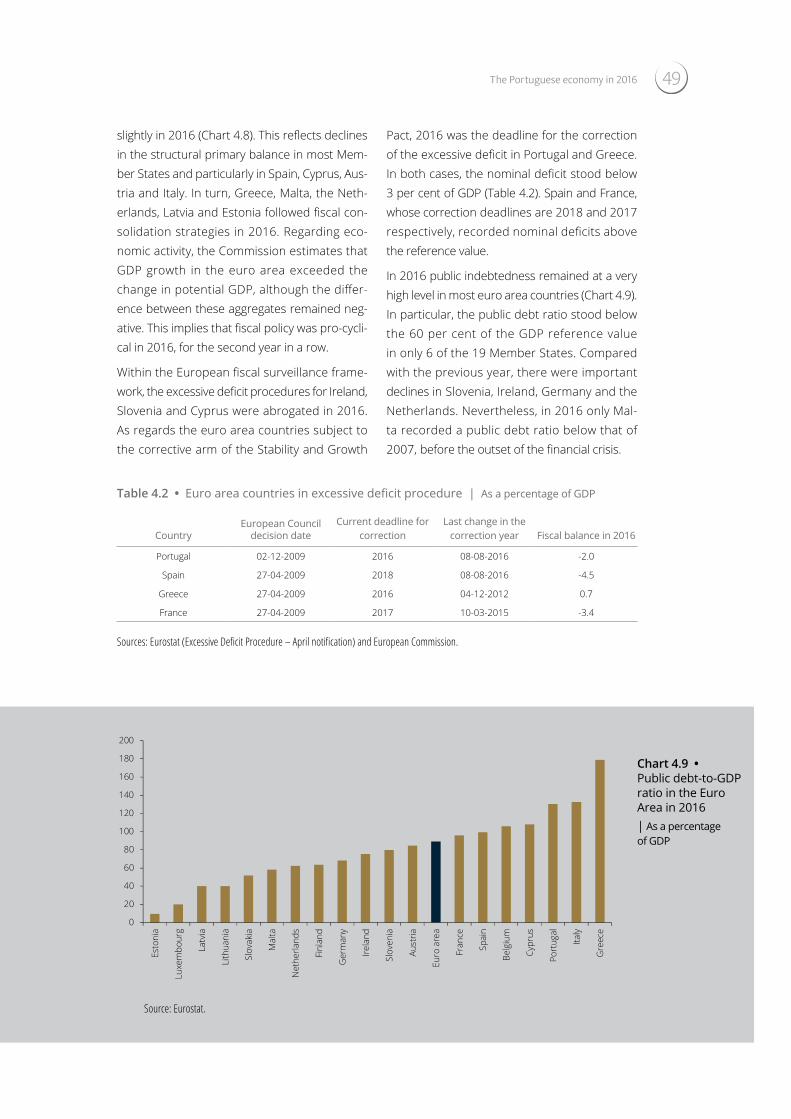
49The Portuguese economy in 2016
slightly in 2016 (Chart 4.8). This reflects declines in the structural primary balance in most Mem-ber States and particularly in Spain, Cyprus, Aus-tria and Italy. In turn, Greece, Malta, the Neth-erlands, Latvia and Estonia followed fiscal con-solidation strategies in 2016. Regarding eco-nomic activity, the Commission estimates that GDP growth in the euro area exceeded the change in potential GDP, although the differ-ence between these aggregates remained neg-ative. This implies that fiscal policy was pro-cycli-cal in 2016, for the second year in a row.
Within the European fiscal surveillance frame-work, the excessive deficit procedures for Ireland, Slovenia and Cyprus were abrogated in 2016. As regards the euro area countries subject to the corrective arm of the Stability and Growth
Pact, 2016 was the deadline for the correction of the excessive deficit in Portugal and Greece. In both cases, the nominal deficit stood below 3 per cent of GDP (Table 4.2). Spain and France, whose correction deadlines are 2018 and 2017 respectively, recorded nominal deficits above the reference value.
In 2016 public indebtedness remained at a very high level in most euro area countries (Chart 4.9). In particular, the public debt ratio stood below the 60 per cent of the GDP reference value in only 6 of the 19 Member States. Compared with the previous year, there were important declines in Slovenia, Ireland, Germany and the Netherlands. Nevertheless, in 2016 only Mal-ta recorded a public debt ratio below that of 2007, before the outset of the financial crisis.
Table 4.2 • Euro area countries in excessive deficit procedure | As a percentage of GDP
CountryEuropean Council
decision dateCurrent deadline for
correctionLast change in the
correction year Fiscal balance in 2016
Portugal 02-12-2009 2016 08-08-2016 -2.0
Spain 27-04-2009 2018 08-08-2016 -4.5
Greece 27-04-2009 2016 04-12-2012 0.7
France 27-04-2009 2017 10-03-2015 -3.4
Sources: Eurostat (Excessive Deficit Procedure – April notification) and European Commission.
0
20
40
60
80
100
120
140
160
180
200
Esto
nia
Luxe
mbo
urg
Latv
ia
Lith
uani
a
Slov
akia
Mal
ta
Net
herla
nds
Finl
and
Ger
man
y
Irela
nd
Slov
enia
Aust
ria
Euro
are
a
Fran
ce
Spai
n
Belg
ium
Cypr
us
Port
ugal
Italy
Gre
ece
Chart 4.9 • Public debt-to-GDP ratio in the Euro Area in 2016| As a percentage of GDP
Source: Eurostat.

50 BANCO DE PORTUGAL • Economic Bulletin • May 2017
Box 4.1 | Structural developments in tax revenue in 201626
In 2016 the ratio of structural revenue from taxes and social contributions to trend GDP declined by 0.9 p.p. vis-à-vis the previous year. This stemmed from a decline in taxes on income and wealth and, to a smaller extent, in taxes on production and imports (Chart 1). In the year under review, structural revenue from social contributions as a ratio to trend GDP remained unchanged. Note that the decline in structural tax revenue occurred notwithstanding the positive contribution of the permanent component of receipts obtained within the scope of PERES (0.05 p.p. of GDP).
In 2016 structural revenue from taxes on income and wealth declined by 0.8 p.p. of trend GDP, driven by the effect of legislative changes. In particular, revenue from taxes on households declined by 0.6 p.p. in structural terms, largely reflecting the elimination of the Personal Income Tax surcharge introduced in 2013 and the effect of the reform of this tax in 2015 (which impacted 2016 outturn via an increase in net refunds). The impact of the Personal Income Tax reform exceeded the initial estimates, which negatively affects the residual component. This component also reflects the decline in receipts from final withholding taxes on capital revenue resulting from the decrease in interest rates on financial investments. As regards the structural revenue from taxes on corporate income, there was a decline by 0.2 p.p. of trend GDP, reflecting measures approved in previous years. Indeed, the collection of the Corporate Income Tax was negatively affected by the decline in the statutory tax rate from 23 to 21 per cent (within the scope of the reform initiated in 2014), as well as by the change, in 2015, in the regime applicable to investment funds, which brought forward to that year revenue that would have been collected in 2016. These effects more than offset the overall positive impact of the change in the asset assessment regime included in the State Budget for 2016 and the permanent part of the Corporate Income Tax rev-enue collected under PERES (Chart 2).
Chart 1 • Breakdown of the overall change in structural fiscal burden | In percentage points of trend GDP
-2.0-1.5-1.0-0.50.00.51.01.52.02.53.03.5
2012 2013 2014 2015 2016
Legislation changesDecoupling between the macro base and GDP (in nominal trend terms)Impact of the tax elasticity (in structural terms)ResidualChange in structural tax burden
Sources: INE and Banco de Portugal.

The Portuguese economy in 2016 51
In structural terms, the ratio of revenue from taxes on production and imports to trend GDP declined by 0.1 p.p. in 2016. This was chiefly due to the fall in VAT structural revenue (-0.2 p.p.), which more than offset the increase in the collection of other indirect taxes (0.1 p.p.). In the case of VAT revenue, special reference should be made to the negative effect associated with the cut in the rate applicable to some restaurant services. The residual component of this tax is nega-tive, reflecting the unusually high growth of refunds in the first months of 2016. However, this may have been partly offset by the possible overestimation of the effect of the above mentioned VAT rate cut. As regards the other indirect taxes, the structural increase in the ratio of revenue to trend GDP was largely due to several legislative changes included in the State Budget for 2016 (yielding an overall impact of 0.3 p.p. of trend GDP). Due to the magnitude of their estimated impacts, reference should be made to the contributions of the rises in taxes on oil products and on tobacco (0.2 p.p. and 0.1 p.p. of trend GDP respectively). A negative residual (-0.2 p.p.) possibly indicates the overestimation of these effects.27
Finally, the ratio of structural revenue from social contributions to trend GDP remained virtually unchanged in 2016, reflecting two symmetrical effects. On the one hand, the fact that the private sector trend wage bill grew less than nominal GDP should have given a negative contribution to structural revenue from social contributions. On the other hand, similarly to previous years, the residual component net of the effect of social contributions related to the civil servants regime was positive.28 This result may suggest gains from increased efficiency in the collection of contributions.
Chart 2 • Breakdown of the change in structural taxes and social contributions in 2016 | In percentage points of trend GDP
-0.8
-0.6
-0.4
-0.2
0.0
0.2
0.4
Taxes on households'income
Taxes on firms' income VAT Other taxes onproduction and
imports
Social contributions
Legislation changesDecoupling between the macro base and GDP (in nominal trend terms)Impact of the tax elasticity (in structural terms)ResidualTotal
Sources: INE and Banco de Portugal.

52 BANCO DE PORTUGAL • Economic Bulletin • May 2017
Box 4.2 | Analysis of deviations in budget execution in 2016
In 2016 the general government deficit stood below the first official estimate for the year, pre-sented in the State Budget for 2016, and the revised estimate included in the State Budget for 2017. However, in the course of the year, different fiscal projections released by international institutions suggested that the official target would be missed. Against this background, an analy-sis of the fiscal deviations gains particular relevance, allowing not only for a better understanding of the 2016 outcome, but also for the identification of some risks in budget execution in the cur-rent year.
The State Budget for 2016 was published in early February and entered into force only in April. The estimate for the deficit in the National Accounts included in this document was thus based on information for 2015 with a lower than usual degree of uncertainty and appears to have benefitted from some information on revenue developments at the beginning of the year. The differential between budget outturn and this estimate turned out to be very small (0.2 per cent of GDP), but is underpinned by a significant negative deviation in total expenditure that is almost fully offset by a similar and also negative differential on the revenue side (Chart 1).
Indeed, total general government revenue outturn fell significantly short of the amount envisaged when the State Budget for 2016 was prepared, reflecting, in particular, an overestimation of the collection of non-tax current revenue (including sales) and capital revenue. Growth of tax collec-tion was also lower than expected, particularly as regards taxes on production and imports. In the latter case the deviation may reflect some overestimation of the impact of indirect taxation hikes included in the State Budget for 2016. Note that the decrease in tax revenue occurred in spite of the fact that developments in economic activity and, in particular, in private consumption were close to the projection included the State Budget for 2016. In addition, the deviation might have been more expressive if the PERES had not been implemented.
Chart 1 • Budget execution in 2016 in national accounts: deviations vis-à-vis the State Budget for 2016 | In million euro
-2,500 -2,000 -1,500 -1,000 -500 0 500 1,000
Total revenueTaxes on income and wealth
Taxes on production and importsSocial contributions
Other current revenueCapital revenue
Total expenditureSocial payments
Compensation of employeesIntermediate consumption
InterestSubsidies
Other current expenditureInvestment
Other capital expenditure
Overall balance
Sources: INE and Ministry of Finance.

The Portuguese economy in 2016 53
Total expenditure outturn stood also substantially below budgeted. A determining factor contrib-uting to this result was the fact that the State Budget for 2016 stipulated a very significant amount of expenditure in the form of provisions, reserves and spending appropriations. This raises signif-icantly the scope for discretion in the implementation of the budget and, given the limited nature of information available, hinders the monitoring of budget execution in the course of the year. For further details on the utilisation of budget control instruments in 2016, see Box 3 of the report ‘Analysis of the General Government Account 2016’, published by the Portuguese Fiscal Council.
Both intermediate consumption expenditure and other current expenditure posted in 2016 much lower figures than those considered in the State Budget for 2016. Due to its magnitude, reference should also be made to the negative deviation in public investment, which was likely be affected by the limited execution of revenue from structural funds received from the European Union. Finally, similarly to previous years, expenditure on debt servicing stood below forecasts.In fact, although the budget pointed to the near stabilisation of this expenditure item in 2016, it actually declined vis-à-vis the previous year.

BANCO DE PORTUGAL • Economic Bulletin • May 201754
5. Supply
Moderate growth of economic activity in 2016
As in the past few years, in 2016 Portuguese GDP per capita continued the convergence towards the average EU level and currently stands at around 71 per cent, still lower than observed at the onset of the international economic and financial crisis (Chart 5.1).
In 2016 gross value added (GVA) at basic prices increased by 0.8 per cent year-on-year, following 1.2 per cent growth in 2015. This increase consol-idated the moderate recovery path started at the end of 2013, with overall developments consist-ent with the coincident indicator for activity and the economic sentiment indicator (Chart 5.2). This notwithstanding, there was a deceleration vis-à-vis the previous year and, in this context, the GVA level was still around 3 per cent lower than the value recorded in 2008.
GVA in the services sector rose by 1.1 per cent year-on-year in 2016, as in the previous year. Growth in this sector continued on the recovery
path observed since early 2014. This increase mainly reflected 3.4 per cent activity growth in the subsectors trade and repair of motor vehicles and accommodation and food services (Chart 5.3). The dynamics observed in these sectors was associated with very favourable developments in tourism exports (9.7 per cent in real terms, fol-lowing an 8.9 per cent increase in 2015) and the dynamics of domestic demand. The services con-fidence indicator maintained a positive stance in 2016 (Chart 5.4).
There was a 0.7 per cent year-on-year increase in industrial activity, in contrast to a 2.0 per cent rise in 2015. However, this was not accompa-nied by an increase in industrial confidence over the year.
In 2016 activity in the construction sector de-clined by 1.8 per cent, after a virtual stabilisa-tion in 2015. In annual average terms, activity in this sector remained on a downward trend. This trend reflected this sector’s structural adjust-ment to a lower level of activity, following high investment in construction in previous decades.
Chart 5.1 • GDP per capita at current prices, PPP adjusted, Portugal as a percentage of the European Union (EU15)
Chart 5.2 • GVA, Coincident indicator of activity and economic sentiment indicator
6667686970717273747576
1999
2000
2001
2002
2003
2004
2005
2006
2007
2008
2009
2010
2011
2012
2013
2014
2015
2016
60
80
100
120
-5
-3
-1
1
3
2008 2009 2010 2011 2012 2013 2014 2015 2016
Inde
x 19
90-2
013
= 10
0
Year
-on-
year
rate
of c
hang
e,in
per
cen
t
Real GVACoincident indicator of activityEconomic sentiment indicator (r.h.s.)
Source: European Comission (Ameco).
Note: EU15 refers to the initial 15 members of the European Union.
Sources: European Comission, INE and Banco de Portugal.

55The Portuguese economy in 2016
GVA in construction at the end of 2016 account-ed for little over half of the value recorded in 2008.
Downward trend of the total population and labour force
In 2016 the resident population and the labour force continued to decline, by 0.3 per cent (Ta-ble 5.1). These developments continued to fol-low the downward trend observed since 2011, although slightly less markedly. Since 2008 the resident population and the labour force have decreased by approximately 250 and 350 thou-sand individuals respectively. Resident popula-tion in the 25-34 age group declined by 2.5 per cent in 2016, while the labour force fell by 2.7 per cent. These falls are quite relevant, but less sharp than those seen in the past few years. In cumulative terms, since 2008 the popula-tion and the labour force in this age group have
declined by 377 and 345 thousand individuals respectively (Chart 5.5).
The demographic trends in the Portuguese economy cannot be easily reversed, and emi-gration phenomena tend to compound them. This is a significant drag on Portuguese eco-nomic growth, given that the labour factor is an input for production, and the population dynamics itself stimulates activity in various sectors. In addition, a more aged society puts pressure on the sustainability of social security schemes.
Improvement in labour market conditions
Labour market developments in 2016 continued to be characterised by a rise in employment and a decline in the unemployment rate, maintaining the improvement seen from the second quarter of 2013 onwards, in a context of more marked wage dynamics.
Table 5.1 • Labour market indicators | Year-on-year rate of change, in per cent, unless otherwise stated
Thousands of individuals in 2016
Years Semesters
2014 2015 2016 S2 2015 S1 2016 S2 2016
Population 10 306 -0,6 -0,5 -0,3 -0,5 -0,3 -0,3
Population 25-34 years 1180 -3,6 -2,8 -2,5 -2,7 -2,7 -2,3
Labour force 5178 -1,1 -0,6 -0,3 -0,5 -0,7 0,1
Labour force 25-34 years 1055 -3,8 -3,1 -2,7 -3,1 -2,9 -2,4
Participation rate 15-64 years (in % of the population) 73,2 73,4 73,7 73,5 73,4 74,0
Total employment 4605 1,6 1,1 1,2 0,9 0,6 1,8
Employees 3787 4,4 2,8 2,1 1,9 1,7 2,4
Self-employment 789 -8,2 -5,7 -3,2 -3,6 -5,0 -1,3
Total unemployment 573 -15,1 -11,0 -11,4 -9,7 -10,0 -12,8
Unemployment rate (in % of the labour force) 13,9 12,4 11,1 12,1 11,6 10,5
Unemployment rate 25-34 years (in % of the labour force) 15,5 13,1 12,5 12,5 13,4 11,6
Long-term unemployment (in % of total unemployment) 65,5 63,5 62,1 62,7 61,5 62,7
Discouraged inactives (in % of the labour force) 5,2 5,0 4,6 5,2 4,5 4,7
Source: INE.
Notes: Long-term unemployment includes the unemployed individuals that have been actively seeking employment for 12 months or more. The discouraged inactives include the inactive individuals who were available for work but had not looked for a job during the period.

BANCO DE PORTUGAL • Economic Bulletin • May 201756
According to data released by the Ministry of Labour, Solidarity, and Social Security, average wages declared to Social Security in 2016 grew by 1.6 per cent compared to the same period a year earlier, which reflects a 1.0 p.p. accelera-tion from the previous year. This greater wage dynamics should partly reflect the increase in the national minimum wage. The wage dynam-ics plays a particularly important role in a con-text where collective bargaining instruments, particularly of a sectoral nature, are still a few, although there has been a slight increase from the minimum level recorded in 2012. In Portugal the wages of around 90 per cent of employees are defined within the scope of these instru-ments. This greater wage dynamics seems to have also influenced the trend of the inflation rate in 2016 (Section 7: ‘Prices’).
The unemployment rate declined, but remained at very high levels
According to Statistics Portugal’s Labour Force Survey, in 2016 the total number of unem-ployed declined by 11.4 per cent year-on-year, after a 11.0 per cent fall in 2015 (Table 5.1). The unemployment rate was 11.1 per cent (12.4 per
cent in 2015), maintaining the downward trend started in 2013 and standing close to the level observed in 2010. In 2016 the decline in the total number of unemployed year-on-year was particularly marked in the 35-44 age group. The share of unemployed receiving unemployment benefits amounted to 25.5 per cent in 2016, against 28.5 per cent in 2015 (Chart 5.6).
In addition, the number of discouraged work-ers, i.e. individuals not actively seeking a job but who are available for work, accounted for around 4.6 per cent of the labour force in 2016, slightly below the value recorded in 2015 (5.0 per cent). The measure of the unemployment rate that also includes discouraged workers contin-ued to evolve in parallel with that of the official unemployment rate, after having grown more rapidly than the latter up to 2013 (Chart 5.7). Nevertheless, this group is formed by around 238 thousand discouraged workers.
One of the most negative aspects of Portuguese labour market developments in the past few years was the very high level of long-term unem-ployment, which tends to cause a sharp depreci-ation of human capital, having an adverse impact on the economy’s potential growth. In 2016 the number of unemployed seeking a job for more than 12 months fell by 13.4 per cent (13.7 per
Chart 5.3 • GVA by main sectors of activity | Index 2008 Q1 =100
Chart 5.4 • Confidence indicators | Balances (quarterly mean)
50
60
70
80
90
100
110
120
2008 2009 2010 2011 2012 2013 2014 2015 2016
Total GVA Agriculture, forestry, and fishingServices ManufacturingConstruction
-80-70-60-50-40-30-20-100
1020
2008 2009 2010 2011 2012 2013 2014 2015 2016
Manufacturing confidence indicatorConstruction confidence indicatorServices confidence indicator
Source: INE. Source: European Comission.
Note: Seasonally adjusted figures.

57The Portuguese economy in 2016
cent fall in 2015). Nevertheless, the weight of these individuals in total unemployment has remained at a very high level (62.1 per cent, cor-responding to a total of approximately 356 thou-sand individuals). In turn, very long-term unem-ployment, covering those seeking a job for more than 24 months, accounted for almost half of the group of unemployed (47.5 per cent in 2016 on average).29 In the same vein, in 2016 the num-ber of unemployed seeking a job for less than 12 months fell by 7.8 per cent (5.7 per cent
decline in 2015). The share of these short-term unemployed in the labour force already stands at levels close to those observed prior to the international financial crisis (Chart 5.8).
Employment recorded a positive trend, although remaining at historically low levels
Chart 5.5 • Population, labour force, and employment – Total and age group (25-34 years) | Index 2008 =100
Chart 5.6 • Number of unemployed receiving unemployment benefits and coverage rate
70
75
80
85
90
95
100
105
2008 2009 2010 2011 2012 2013 2014 2015 2016
Population Labour forceEmployment Population (25-34 years)Labour force (25-34 years) Employment (25-34 years)
0
50
100
150
200
250
300
350
051015202530354045
2008 2009 2010 2011 2012 2013 2014 2015 2016
Num
ber o
f une
mpl
oyed
(Tho
usan
ds)
Une
mpl
oyed
rece
ivin
g un
empl
oym
ent
bene
fits
(as
a pe
rcen
tage
of t
otal
un
empl
oym
ent)
Coverage rate of unemployment benefitsNumber of unemployed receiving unemployment benefits (r.h.s.)
Source: INE (Labour Force Survey). Source: INE (Labour Force Survey).
2
2.5
3
3.5
4
4.5
5
10
12
14
16
18
20
22
2011 2012 2013 2014 2015 2016
Official rate Including discouraged workers Difference (r.h.s.)
Chart 5.7 • Official unemployment rate and unemployment rate including discouraged workers| Percentage
Source: INE (Labour Force Survey).

BANCO DE PORTUGAL • Economic Bulletin • May 201758
According to the Labour Force Survey, total employment increased by 1.2 per cent in 2016, after a 1.1 per cent increase in 2015. This reflects a higher number of employees (2.1 per cent more), given that self-employment fell markedly (3.2 per cent). In sectoral terms, the main con-tribution to the year-on-year rate of change in employment was recorded in tradable servic-es, which include tourism-related activities.30 In spite of the upward trend, employment remained at historically low levels, in the wake of an unprecedented fall observed between the end of 2008 and early 2013, which according to quarterly national accounts corresponded to around 650 thousand individuals. Approximate-ly 290 thousand jobs seem to have been recov-ered by the end of 2016. With respect to general government employment, according to informa-tion from the Directorate-General for Adminis-tration and Public Employment, the number of employees appears to have increased in 2016, as in 2015, which confirms the interruption of the downward trend observed in previous years.
Reduction in apparent labour productivity
The current recovery phase of the Portuguese economy brings together moderate activity growth and relatively stronger employment growth. In this context, apparent labour productivity based on the quarterly national accounts of Statistics Por-tugal declined in 2016, in the context of lower and atypical dynamics compared to prior phas-es of economic recovery.31 However, from 2011 to 2013 apparent labour productivity growth was strong, also in contrast to prior recessive phases of the cycle (Chart 5.9). The explana-tions for the reduction in productivity are com-plex and may relate to changes in the produc-tive structure, in a context where the levels of capital per worker remained low, after several years of low investment levels (Box 5.1: ‘Capital per worker and productivity’).
Chart 5.8 • Unemployment rate by duration of unemployment | Months
Chart 5.9 • Apparent labour productivity in the last three crisis and recoveries | Biannual figures; Minimum level of activity = semester t=100
02468
101214161820
2008 2009 2010 2011 2012 2013 2014 2015 2016
Unemployment rateShort-term unemployment (less than 12 months)Long-term unemployment (12 months or more)
94
96
98
100
102
104
106
108
t-4 t-3 t-2 t-1 t t+1 t+2 t+3 t+4 t+5 t+6 t+7
1993S1 2003S1 2013S1
Source: INE (Labour Force Survey). Sources: INE and Banco de Portugal.
Note: Labour productivity was computed dividing GVA (volume chain-linked data, millions of euro) by total (full-time equivalent) employment, except for the crisis in 1992, in which GDP was considered instead.

The Portuguese economy in 2016 59
Box 5.1 | Capital per worker and productivity
The low growth of apparent labour productivity in the Portuguese economy in the past few dec-
ades causes concern as it limits the ability to sustain higher levels of consumption without caus-
ing external imbalances. A significant catching-up of output per worker to the euro area average
is a particularly important challenge, in a context where there are still weaknesses in the Portu-
guese economy.
Developments in the level of output per worker relate to various structural issues whose interac-
tion is complex. In its simpler version, the economic growth theory points to the accumulation of
inputs and the evolution of the technological framework as determinants of output growth. In this
context, the level of output per worker depends on technology and increases with the level of the
available capital stock for each worker, with lower variations expected for higher capital intensi-
ties. Economic literature has addressed this issue, identifying more elaborate formulations that
include, for example, the quality of inputs and more flexible assumptions on their substitutabil-
ity. In addition, from an empirical viewpoint, the literature has shown weaknesses in the statistical
information needed for this analysis, for example as regards capital stock measurement.32 The
existing estimates for the capital stock level in economies typically result from the accumulation
of annual investment flows, less an annual depreciation rate resulting from assumptions on the
lifetime of the different capital goods.
This box presents some statistical information to place the Portuguese economy in the context
of the euro area in the 1995-2016 period in terms of the capital-labour ratio and how it relates to
productivity, measured as the level of output per worker.
Panel (a) of Chart 1 shows the cumulative trend of the capital-labour ratio since 1999 in Portu-
gal, jointly with the cumulative trend of each component. The demographic contraction trends
experienced by the Portuguese economy, and especially the sharp cyclical developments stem-
ming from the macroeconomic imbalances’ adjustment process, led to a strong reduction in
Chart 1 • Net capital stock per worker (2010 prices)
a) Portugal b) Euro area countries
80
90
100
110
120
130
140
150
1999
2000
2001
2002
2003
2004
2005
2006
2007
2008
2009
2010
2011
2012
2013
2014
2015
2016
Inde
x 19
99=1
00
Capital stock EmploymentCapital per worker
0
50
100
150
200
250
300
LV LT SK SI MT EE PT CY DE GR IT BE ES FI IE LU FR AU NL
2016 1999
Thou
sand
eur
os
Source: Ameco – European Commission.
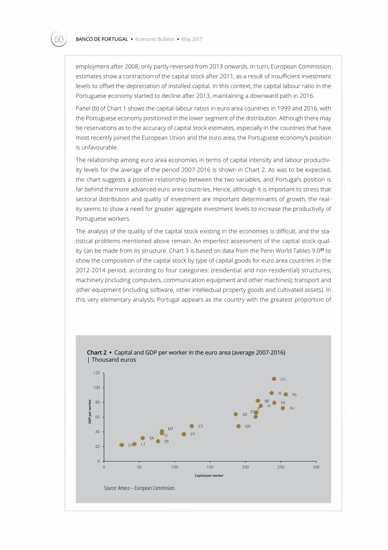
60 BANCO DE PORTUGAL • Economic Bulletin • May 2017
employment after 2008, only partly reversed from 2013 onwards. In turn, European Commission
estimates show a contraction of the capital stock after 2011, as a result of insufficient investment
levels to offset the depreciation of installed capital. In this context, the capital-labour ratio in the
Portuguese economy started to decline after 2013, maintaining a downward path in 2016.
Panel (b) of Chart 1 shows the capital-labour ratios in euro area countries in 1999 and 2016, with
the Portuguese economy positioned in the lower segment of the distribution. Although there may
be reservations as to the accuracy of capital stock estimates, especially in the countries that have
most recently joined the European Union and the euro area, the Portuguese economy’s position
is unfavourable.
The relationship among euro area economies in terms of capital intensity and labour productiv-
ity levels for the average of the period 2007-2016 is shown in Chart 2. As was to be expected,
the chart suggests a positive relationship between the two variables, and Portugal’s position is
far behind the more advanced euro area countries. Hence, although it is important to stress that
sectoral distribution and quality of investment are important determinants of growth, the real-
ity seems to show a need for greater aggregate investment levels to increase the productivity of
Portuguese workers.
The analysis of the quality of the capital stock existing in the economies is difficult, and the sta-
tistical problems mentioned above remain. An imperfect assessment of the capital stock qual-
ity can be made from its structure. Chart 3 is based on data from the Penn World Tables 9.033 to
show the composition of the capital stock by type of capital goods for euro area countries in the
2012-2014 period, according to four categories: (residential and non-residential) structures;
machinery (including computers, communication equipment and other machines); transport and
other equipment (including software, other intellectual property goods and cultivated assets). In
this very elementary analysis, Portugal appears as the country with the greatest proportion of
Chart 2 • Capital and GDP per worker in the euro area (average 2007-2016) | Thousand euros
EE
BE
DE
IE
GR
ES
FRIT
CY
LV LT
LU
MT
NL
AU
PTSISK
FI
0
20
40
60
80
100
120
0 50 100 150 200 250 300
GD
P pe
r w
orke
r
Capital per worker
Source: Ameco – European Commission.

The Portuguese economy in 2016 61
structures in the capital stock, which necessarily implies a lower share of equipment in machines
and intangible goods. These latter categories tend to be associated with higher profitability rates,
and thus there seems to be room for improving the composition of the national capital stock.
Portuguese economic growth will benefit from higher levels of investment in the firms, sectors
and types of goods with higher profitability. This investment effort should be primarily based on
higher public and private saving rates, to avoid jeopardising the current balance in the external
accounts, which is a key element of the Portuguese economy’s adjustment process of the past
few years. However, creating favourable conditions for attracting foreign direct investment, espe-
cially targeted at creating new productive capacity, is also a way to increase the levels of capital
per worker without compromising macroeconomic stability. The structural conditions needed to
attract foreign direct investment are largely also needed for a correct allocation of investment
towards more productive purposes. Efficient market functioning, a level playing field, the reduc-
tion of the so-called framework costs, and the stability of the regulatory and tax environments are
all part of this set of conditions.
Chart 3 • Structure of capital stock per type of investment (average 2012-2014) | Percentage
50
55
60
65
70
75
80
85
90
95
100
MT SK IE BE EE AU LU SI FI DE NL IT ES CY LT FR LV GR PT
Structures Machinery Transport equipment Other
Source: Penn World Tables.

BANCO DE PORTUGAL • Economic Bulletin • May 201762
6. Demand
Moderate GDP growth based on the dynamics of domestic demand and especially of exports
In 2016 the Portuguese economic activity grew by 1.4 per cent in volume, following a 1.6 per cent growth in 2015 (Table 6.1). In 2016 as a whole GDP growth in Portugal was once again lower than in the euro area, the differential standing at -0.3 p.p. (Chart 6.1). GDP growth in 2016 showed a markedly intra-annual profile, accelerating to 1.9 per cent in the second half of the year, above the value observed on aver-age in the euro area in the same period (1.7 per cent).
Developments in Portuguese economic activity in the most recent period continued to be char-acterised by moderate growth, particularly tak-ing into account the seriousness and duration
of the prior recession. In this context, the GDP level at the end of 2016 was around 4 per cent lower than at the start of 2008. The recovery of economic activity takes place in the context of high indebtedness levels of public and private economic agents and the need to adjust their balance sheets.
The important demographic changes that oc-curred in Portugal in the past few years ren-der the analysis of per capita GDP develop-ments particularly relevant. In 2016 this varia-ble grew by 1.7 per cent (2.1 per cent in 2015), which exacerbated the gap vis-à-vis GDP de-velopments (Chart 6.2). As in 2014 and 2015, GDP growth was once again higher than that of GVA, which in 2016 grew by 0.8 per cent (Chart 6.3). The discrepancy between GDP growth and GVA growth related to the evolution of taxes less subsidies, which grew by 4.8 per cent in volume in 2016, compared to 5.1 per cent in 2015.
Table 6.1 • GDP and main components | Year-on-year change in percentage, unless otherwise stated
% of GDP in 2016
20162015 2016
2015 2016
H1 H2 Q1 Q2 Q3 Q4
GDP 100.0 1.6 1.4 1.0 1.9 1.0 0.9 1.7 2.0
Domestic demand 98.8 2.5 1.5 1.1 1.8 1.5 0.8 1.0 2.5
Private consumption 65.8 2.6 2.3 2.1 2.5 2.5 1.6 1.9 3.0
Public consumption 18.0 0.7 0.5 0.8 0.3 1.2 0.5 0.2 0.3
Investment 14.9 4.7 -0.8 -2.1 0.6 -2.1 -2.1 -1.8 3.0
GFCF 14.8 4.5 -0.1 -2.4 2.2 -2.5 -2.2 -0.1 4.5
Change in inventories (a) 0.0 -0.1 0.0 -0.2 0.1 0.0 -0.3 -0.2
Exports 40.3 6.1 4.4 2.8 6.0 3.7 1.9 5.6 6.4
Imports 39.1 8.2 4.4 3.1 5.6 4.8 1.5 3.9 7.3
Contribution of domestic demand net of imports (a) 1.1 0.5 0.4 0.6 0.4 0.4 0.4 0.9
Contribution of exports net of imports (a) 0.5 0.9 0.6 1.2 0.7 0.6 1.3 1.1
Memo item:
GDP – change over the previous period 0.5 1.3 0.2 0.2 0.9 0.7
Domestic demand (exc. change in inventories) 98.7 2.5 1.6 1.1 2.0 1.4 0.8 1.3 2.7
Sources: INE and Banco de Portugal calculations.
Note: (a) Contributions to the real growth of GDP in percentage points. The demand aggregates net of imports are obtained by subtracting an estimate of the imports needed to meet each component. The calculation of import content was based on data for 2005. For more information, see the Box entitled ‘The role of domestic demand and exports in economic activity developments in Portugal’, in the June 2014 issue of the Economic Bulletin.

63The Portuguese economy in 2016
The less buoyant economic activity in 2016 reflects less robust domestic demand growth, largely due to a fall in investment, in parallel with a deceleration in exports of goods and services, in line with lower domestic demand growth. In this context, the reduction of trade flows with Angola had an impact on the Por-tuguese economy, with a particularly negative influence on exports of goods.34 In turn, pri-vate consumption grew slightly less than in the previous year, which was accounted for by the less buoyant consumption of non-food current goods and durable goods. Public consumption, determined by the dynamics of compensation of employees and expenses on goods and ser-vices in general government, grew by 0.5 per cent in 2016, i.e. slightly less than in 2015. The deceleration in some demand components with a greater import content translated into lower import growth in 2016 as a whole.
Considering demand components less imports (deducting from each component an estimate of the imports needed to meet said demand), the contribution from domestic demand to GDP growth is estimated to have amounted to 0.5 p.p. in 2016 and the contribution from exports to have stood at 0.9 p.p.
Intra-annual acceleration path of economic activity, reflecting a recovery of both domestic demand and exports of goods and services in the second half of the year
In spite of the lower dynamics over the year as a whole, developments in economic activity in 2016 were characterised by a clearly upward intra-an-nual profile. Hence, following 1.0 per cent growth in the first half of 2016, GDP increased by 1.9 per cent in the second half. The recovery of both do-mestic demand and exports of goods and servic-es contributed to this evolution.
The more buoyant domestic demand in the second half of 2016 was particularly evident in the last quarter, when both private consump-tion and investment accelerated. In a context of rapid expansion of the consumption of dura-ble goods over the whole year, the consump-tion of current goods accelerated in the sec-ond half of the year. In turn, investment grew slightly in the second half, after a fall in the first half of the year. This development had a major contribution from the significant recovery in investment in machinery and equipment.
Chart 6.1 • GDP growth in Portugal and in the euro area | Year-on-year change in percentage
Chart 6.2 • GDP and GDP per capita in Portugal | 2011Q1=100
-6-5-4-3-2-101234
2000 2002 2004 2006 2008 2010 2012 2014 2016
Portugal Euro area
92
94
96
98
100
102
2011 2012 2013 2014 2015 2016
GDP GDP per capita
Sources: Eurostat, INE and Banco de Portugal calculations. Sources: INE and Banco de Portugal calculations.

BANCO DE PORTUGAL • Economic Bulletin • May 201764
Private consumption followed an intra-annual recovery path over the year, with emphasis on consumption of current goods which accelerated considerably in the last quarter
In 2016 private consumption grew by 2.3 per
cent, i.e. 0.3 p.p. less than in 2015. Despite the
lower dynamics, private consumption contin-
ued to grow more than GDP. The behaviour of
consumption over the whole year was chiefly
accounted for by a deceleration in consump-
tion of current goods and services, in particular
the non-food component, in a context where
consumption of durable goods grew once
again considerably, though less than in 2015
(Chart 6.4). In 2016 the consumption of current
goods and services grew by 1.6 per cent, after
1.8 per cent in 2015, while the consumption of
durable goods grew by 9.5 per cent (11.9 per
cent in 2015). In particular, passenger car sales
grew by 16.1 per cent (Chart 6.5).
Intra-annual developments in private consump-
tion showed an upward profile, as a result of par-
ticularly pronounced growth in the last quarter
of the year, based on an acceleration in the con-
sumption of current goods and services and the
maintenance of the high growth of durable goods,
particularly sharp in the last quarter of the year.
The more favourable developments in private
consumption in the second half of the year oc-
curred in an environment of sharp improvement
in consumer confidence, which remained at his-
torically high levels, and a higher household dis-
posable income. The improvement in the con-
sumer confidence indicator at the end of 2016
was particularly noticeable in the assessment of
unemployment expectations, which lowered con-
siderably.
In 2016 the savings rate stood at 4.4 per cent of
disposable income, i.e. 0.1 p.p. below the rate
recorded in 2015 (Chart 6.6), reflecting slightly
higher nominal growth of private consumption
than that of disposable income (3.4 and 3.2 per
cent respectively). The increase in household dis-
posable income benefited from an improvement
Chart 6.3 • Recent behavior of GDP and GVA in Portugal | 2011Q1=100
Chart 6.4 • Main contributions for the growth of private consumption in volume | Year-on-year change in percentage, and contributions in percentage points; quarterly values
92
94
96
98
100
2011 2012 2013 2014 2015 2016
GDP GVA
-8
-6
-4
-2
0
2
4
2011 2012 2013 2014 2015 2016
Durables (exc. vehicles)Durables (vehicles)Non-durablesPrivate consumption (growth in percentage)
Sources: INE and Banco de Portugal calculations. Sources: INE and Banco de Portugal calculations.
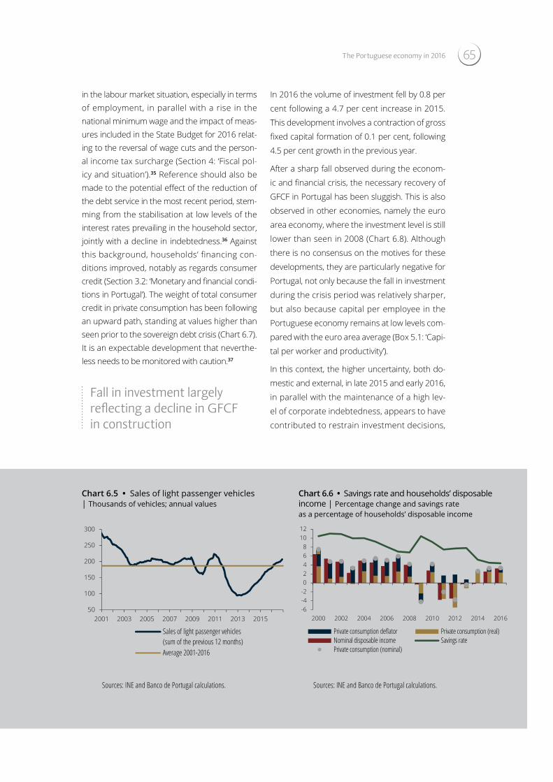
65The Portuguese economy in 2016
in the labour market situation, especially in terms of employment, in parallel with a rise in the national minimum wage and the impact of meas-ures included in the State Budget for 2016 relat-ing to the reversal of wage cuts and the person-al income tax surcharge (Section 4: ‘Fiscal pol-icy and situation’).35 Reference should also be made to the potential effect of the reduction of the debt service in the most recent period, stem-ming from the stabilisation at low levels of the interest rates prevailing in the household sector, jointly with a decline in indebtedness.36 Against this background, households’ financing con-ditions improved, notably as regards consumer credit (Section 3.2: ‘Monetary and financial condi-tions in Portugal’). The weight of total consumer credit in private consumption has been following an upward path, standing at values higher than seen prior to the sovereign debt crisis (Chart 6.7). It is an expectable development that neverthe-less needs to be monitored with caution.37
Fall in investment largely reflecting a decline in GFCF in construction
In 2016 the volume of investment fell by 0.8 per
cent following a 4.7 per cent increase in 2015.
This development involves a contraction of gross
fixed capital formation of 0.1 per cent, following
4.5 per cent growth in the previous year.
After a sharp fall observed during the econom-
ic and financial crisis, the necessary recovery of
GFCF in Portugal has been sluggish. This is also
observed in other economies, namely the euro
area economy, where the investment level is still
lower than seen in 2008 (Chart 6.8). Although
there is no consensus on the motives for these
developments, they are particularly negative for
Portugal, not only because the fall in investment
during the crisis period was relatively sharper,
but also because capital per employee in the
Portuguese economy remains at low levels com-
pared with the euro area average (Box 5.1: ‘Capi-
tal per worker and productivity’).
In this context, the higher uncertainty, both do-
mestic and external, in late 2015 and early 2016,
in parallel with the maintenance of a high lev-
el of corporate indebtedness, appears to have
contributed to restrain investment decisions,
Chart 6.5 • Sales of light passenger vehicles | Thousands of vehicles; annual values
Chart 6.6 • Savings rate and households’ disposable income | Percentage change and savings rate as a percentage of households’ disposable income
50
100
150
200
250
300
2001 2003 2005 2007 2009 2011 2013 2015
Sales of light passenger vehicles(sum of the previous 12 months)Average 2001-2016
-6-4-2024681012
2000 2002 2004 2006 2008 2010 2012 2014 2016
Private consumption deflator Private consumption (real)Nominal disposable income Savings ratePrivate consumption (nominal)
Sources: INE and Banco de Portugal calculations. Sources: INE and Banco de Portugal calculations.

BANCO DE PORTUGAL • Economic Bulletin • May 201766
namely in the first half of the year (Section 2: ‘In-
ternational environment’ and Section 3: ‘Mon-
etary and financial conditions’). However, in-
vestment recovered in the second half of 2016,
particularly in the last quarter, with gross capital
formation growing by 4.5 per cent year on year.
According to the Investment Survey released by
Statistics Portugal, in January 2017, 39.4 per cent
of firms claimed to have had their investment re-
strained in 2016. This was a historically low val-
ue that reflected a considerable fall vis-à-vis the
share computed in July 2016 (50.2 per cent).
In addition, although the deterioration of sales
prospects continued to be the main constraint
on investment, their weight decreased substan-
tially backed by factors such as self-financing ca-
pacity or the difficulty to obtain credit (Chart 6.9).
By institutional sector, the reduction in gross
fixed capital formation in 2016 as a whole
largely reflected a considerable decline in pub-
lic investment, which fell by 29.2 per cent in vol-
ume, after having increased by 16.4 per cent in
the previous year. Residential investment also
declined in 2016 (-1.9 per cent), with an impact
on activity in the construction sector (Section
5: ‘Supply’). The fall in residential investment in
the past few years, only interrupted in 2015,
is part of a stabilisation trend of the Portu-
guese housing stock, following a considerable
increase in the 1990s. This seems to have been
reinforced in the most recent period by a need
to reduce household indebtedness levels. By
contrast, corporate GFCF grew by 6.6 per cent
in volume in 2016, following a rate of change of
2.3 per cent in the previous year and showing
a markedly upward intra-annual profile.
The fall in GFCF in 2016 was largely accounted
for by the construction component. In the wake
of the declines observed since 2002, followed
by a significant recovery in 2015, this invest-
ment component, whose weight in total GFCF
was around 50 per cent, declined once again
sharply. This may partly reflect the effect of the
conclusion of a number of major public works
at the end of 2015. GFCF in construction recov-
ered slightly at the end of the year (Chart 6.10),
in line with the growth of cement sales to the
domestic market. In addition, the number and
amount of tenders for public works grew signifi-
cantly in the second half of 2016 (Chart 6.11).
After major falls at the end of 2015 and in
the first half of 2016, GFCF in machinery and
Chart 6.7 • Share of private consumption in new loans granted by banks to consumption | New operations in percentage
Chart 6.8 • Developments in GFCF in selected euro area countries | 2008Q1=100
0
1
2
3
4
5
6
7
8
2009 2010 2011 2012 2013 2014 2015 201660
70
80
90
100
110
2008 2009 2010 2011 2012 2013 2014 2015 2016
Euro area Germany FranceItaly Spain Portugal
Sources: INE and Banco de Portugal calculations. Sources: INE and Banco de Portugal calculations.
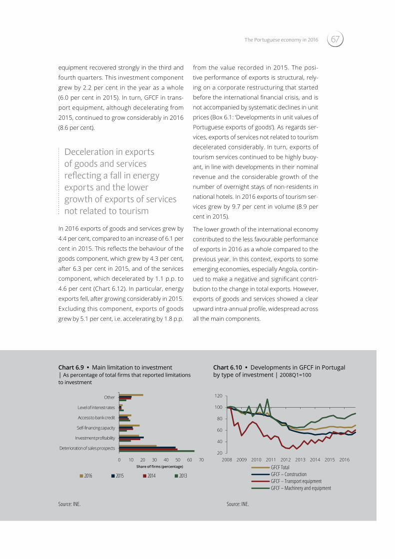
67The Portuguese economy in 2016
equipment recovered strongly in the third and
fourth quarters. This investment component
grew by 2.2 per cent in the year as a whole
(6.0 per cent in 2015). In turn, GFCF in trans-
port equipment, although decelerating from
2015, continued to grow considerably in 2016
(8.6 per cent).
Deceleration in exports of goods and services reflecting a fall in energy exports and the lower growth of exports of services not related to tourism
In 2016 exports of goods and services grew by
4.4 per cent, compared to an increase of 6.1 per
cent in 2015. This reflects the behaviour of the
goods component, which grew by 4.3 per cent,
after 6.3 per cent in 2015, and of the services
component, which decelerated by 1.1 p.p. to
4.6 per cent (Chart 6.12). In particular, energy
exports fell, after growing considerably in 2015.
Excluding this component, exports of goods
grew by 5.1 per cent, i.e. accelerating by 1.8 p.p.
from the value recorded in 2015. The posi-
tive performance of exports is structural, rely-
ing on a corporate restructuring that started
before the international financial crisis, and is
not accompanied by systematic declines in unit
prices (Box 6.1: ‘Developments in unit values of
Portuguese exports of goods’). As regards ser-
vices, exports of services not related to tourism
decelerated considerably. In turn, exports of
tourism services continued to be highly buoy-
ant, in line with developments in their nominal
revenue and the considerable growth of the
number of overnight stays of non-residents in
national hotels. In 2016 exports of tourism ser-
vices grew by 9.7 per cent in volume (8.9 per
cent in 2015).
The lower growth of the international economy
contributed to the less favourable performance
of exports in 2016 as a whole compared to the
previous year. In this context, exports to some
emerging economies, especially Angola, contin-
ued to make a negative and significant contri-
bution to the change in total exports. However,
exports of goods and services showed a clear
upward intra-annual profile, widespread across
all the main components.
Chart 6.9 • Main limitation to investment | As percentage of total firms that reported limitations to investment
Chart 6.10 • Developments in GFCF in Portugal by type of investment | 2008Q1=100
0 10 20 30 40 50 60 70
Deterioration of sales prospects
Investment profitability
Self-financing capacity
Access to bank credit
Level of interest rates
Other
Share of firms (percentage)
2016 2015 2014 2013
20
40
60
80
100
120
2008 2009 2010 2011 2012 2013 2014 2015 2016
GFCF TotalGFCF – ConstructionGFCF – Transport equipmentGFCF – Machinery and equipment
Source: INE. Source: INE.

BANCO DE PORTUGAL • Economic Bulletin • May 201768
The deflator of goods exports fell in 2016 (-3.4 per cent) though less markedly when excluding the fuels component (-2.4 per cent). Based on inter-national trade data, exports of goods grew by 1.0 per cent in nominal terms in 2016 (3.7 per cent in 2015). This was largely due to a fall in car exports, particularly to Germany, and a decline in exports of fuels and base metals. The reduc-tion in car exports reflected the temporary clo-sure of an important production unit in early 2016. By destination country, there was a sharp fall in exports of goods to non-EU markets, spe-cifically Angola and China, and to the Nether-lands. Angola’s contribution to the growth of nominal exports of goods in 2016 was -1.2 p.p., which corresponds to a drop of 28.4 per cent in the year as a whole. This adverse development faded away over the course of 2016 (Chart 6.13), contributing to the intra-annual acceleration profile of exports.38
The growth of the volume of exports of goods
and services in 2016 was higher than that of
the external demand indicator normally used
by Banco de Portugal, calculated on the basis
of the information used within the Eurosys-
tem, leading to a further gain in the export
share. However, this external demand indica-
tor does not consider the relative importance
of external trade with Angola. When taking into
account the actual weight of Angola and the
trend of its imports, external demand for Portu-
guese goods and services grew less in the most
recent period, which implied a slightly higher
gain in the share of exports than that obtained
with the indicator normally used (Chart 6.14).
Considering the main intra-EU trading part-
ners, exports of Portuguese goods and servic-
es to these destinations have been experiencing
overall higher nominal growth than that of total
Chart 6.11 • Number and amount of tenders for public work | Year-on-year change in percentage; half-yearly values
Chart 6.12 • Main contributions for the growth of goods and services exports in volume | Year-on-year change in percentage, and contributions in percentage points; quarterly values
-40
-20
0
20
40
60
H1 H2 H1 H2 H1 H2
2014 2015 2016
Call for tenders - number Call for tenders - value
-4
-2
0
2
4
6
8
10
2012 2013 2014 2015 2016
Other servicesTourismExports of energy goodsExports of goods (exc. energy)Exports of goods and services (year-on-year change, percentage)
Source: AECOPS. Sources: INE and Banco de Portugal calculations.

69The Portuguese economy in 2016
imports of goods and services from those coun-tries, understood as part of external demand for Portuguese goods and services (Chart 6.15). For example, in 2016 nominal exports of goods and services from Portugal to Spain grew by 5.8 per cent, while total Spanish imports grew by 1.6 per cent. Although expressed in nominal terms, this behaviour suggests that Portuguese exports per-formed well in the Spanish market.
The deceleration in imports of goods and services continued, linked to a fall in exports of energy and services not related to tourism
Imports of goods and services grew by 4.4 per cent in 2016 (8.2 per cent in 2015). This chief-ly reflected a fall in energy imports (-4.0 per
cent, after 15.0 per cent growth in 2015) and a less buoyant imports of services, which grew by 2.6 per cent in 2016, after a 6.7 per cent change in 2015 (Chart 6.16). Imports of goods excluding energy grew by 6.5 per cent, decel-erating slightly from the value observed in 2015 (7.1 per cent).
The deceleration in imports of goods in 2016 is consistent with the less buoyant behaviour of a number of demand components with a high import content, with a particular emphasis on a fall in exports of fuels and a significant decel-eration in GFCF in machinery and equipment.
Following the path observed since early 2013, the deflator of goods imports fell further in 2016 (-3.9 per cent). This reduction is less sig-nificant when excluding fuel exports, standing at -2.4 per cent. Based on international trade data, imports of goods recorded a 1.3 per cent
Chart 6.13 • Contributions from main trading markets for the nominal growth of goods exports excluding fuel | Year-on-year change in percentage, and contributions in percentage points; quarterly values
Chart 6.14 • Exports of goods and services and external demand | Year-on-year change in percentage
-6
-3
0
3
6
9
12
2012 2013 2014 2015 2016
ChinaAngolaExtra-EU exc. Angola and ChinaIntra-EUNominal exports exc. energy (growth in percentage)
-20
-15
-10
-5
0
5
10
15
2008 2010 2012 2014 2016
External demandPortuguese exportsExternal demand including Angola
Source: INE (International Trade) and Banco de Portugal calculations. Sources: INE, IMF, ECB and Banco de Portugal calculations.
Note: The indicator of external demand adjusted by the importance of foreign trade with Angola corresponds to the weighted average (weights based on ex-ports) between the indicator of external demand computed by the ECB and Angola’s total volume of imports of goods and services. These calculations use the IMF’s projections (Word Economic Outlook) for the growth in volume of Angola’s imports in 2016.

BANCO DE PORTUGAL • Economic Bulletin • May 201770
nominal growth in 2016. By product, in addi-
tion to a strong reduction in fuel purchases,
also imports of base metals dropped. Similar-
ly to exports, the lower dynamics of imports
of goods was particularly evident in non-EU
markets. In 2016 imports of goods from these
countries recorded a nominal reduction of
3.9 per cent, with imports originating in Angola dropping by 29.1 per cent.
In 2016 imports of goods and services grew more than the import-weighted overall demand, which led to an increase in import penetration, as in the three previous years.
Chart 6.15 • Exports of goods and services for the main EU trading partners in 2016 and total imports from these countries | Year-on-year change in percentage; nominal values
Chart 6.16 • Main contributions for the growth of goods and services imports in volume | Year-on-year change in percentage, and contributions in percentage points; quarterly values
Spain
France
Germany
UK
Netherlands
Italy
-8
-4
0
4
8
12
16
-8 -4 0 4 8 12 16
Gro
wth
of P
ortu
gues
e no
min
al
expo
rts o
f goo
ds a
nd s
ervi
ces
by
coun
try
of d
esti
nati
on; p
erce
ntag
e
Growth of total nominal imports of goods and services; percentage
-12
-8
-4
0
4
8
12
16
2012 2013 2014 2015 2016
Other servicesTourismImports of energy goodsImports of goods (exc. energy)Imports of goods and services (year-on-year change, percentage)
Sources: Eurostat, INE and Banco de Portugal calculations.
Note: The circles represent the locus of combinations between the growth of nominal imports of goods and services in each of the 6 countries conside-red (X-axis) and the growth of nominal exports of goods and services from Portugal to each of those countries (Y-axis). The size of the circles reflect the importance of each country in the Portuguese exporting structure.
Sources: INE and Banco de Portugal calculations.
45º

The Portuguese economy in 2016 71
Box 6.1 | Developments in unit values of Portuguese goods exports
This box complements the analysis of developments in Portuguese goods exports, focusing on
changes in their unit values from a predominantly microeconomic viewpoint.
The analysis presented here is based on unit values, which approximate the behaviour of exported
goods prices. Nevertheless, prices of internationally traded goods depend on a complex set of
factors, including the quality of products and the ability to exercise market power. All calcula-
tions are based on both Comext data and detailed reporting on international trade transactions
conducted by firms, within the scope of Intrastat and Extrastat surveys. In addition, consider-
ing the volatility associated with energy prices, their unit values were excluded from the analysis
based on corporate information.
Chart 1 presents the annual rate of change in the unit values of exported goods for the 2003-15
period. This growth rate has always been positive, except for 2003, 2009 and 2013-14. The most
exported goods over the whole period and, thus, contributing the most to the total rate of change
– namely ‘vehicles’ and ‘machinery, equipment and electrical components’ –, account on average
for 17 per cent of the total value of goods exports. The growth rates of these two categories of
the Standard International Trade Classification (SITC) show that their unit values have increased
after 2010, especially in the machinery and equipment component.
Analysing the growth of exports’ unit values is more meaningful if compared to developments
in a reference region. Hence, taking into account the existing institutional and economic envi-
ronment, the natural benchmark is the average rate of change in the unit values of goods
exported by the European Union (EU).39 The difference between the growth rates recorded in
Portugal and in the EU was centred around zero for the 2003-15 period, which seems to exclude
a scenario where Portuguese exporters sought to systematically compete on price (Chart 2).
Chart 1 • Unit-values growth rates of Portuguese goods exports (including energy goods) | Percentage
-12
-8
-4
0
4
8
2003 2004 2005 2006 2007 2008 2009 2010 2011 2012 2013 2014 2015
Total (incl. Energy goods)Road vehicles (including air-cushion vehicles)Electrical machinery, apparatus and appliances, n.e.s., and electrical parts thereof
Souce: Banco de Portugal calculations based on Comext dataset.

72 BANCO DE PORTUGAL • Economic Bulletin • May 2017
Among the products whose unit value growth rates surpassed those of the EU are, consistently,
‘articles of apparel and clothing accessories’, ‘crude animal and vegetable materials, n.e.s.’ and
‘organic chemicals’ (Chart 3). Finally, ‘footwear’ is the only category whose unit value growth rate
was always positive in the period under analysis, and in most years higher than the EU average
rate (Chart 4).
Corporate information offers an analysis of the relationship between the differences of unit val-
ues and firm characteristics, namely in terms of sector of activity and age. The share of goods
exporters by sector whose unit value growth rates are higher than the EU weighted average rate
Chart 3 • Unit-values growth rate of articles of apparel and clothing accessories | Percentage
-6
-4
-2
0
2
4
6
8
2002 2003 2004 2005 2006 2007 2008 2009 2010 2011 2012 2013 2014 2015
Portugal EU
Source: Banco de Portugal calculations based on Comext dataset.
Chart 2 • Differences in unit-values growth rates (Portugal vs EU) | Percentage points
-20
-15
-10
-5
0
5
10
15
20
2003 2004 2005 2006 2007 2008 2009 2010 2011 2012 2013 2014 2015
Source: Banco de Portugal calculations based on Comext dataset.
Note: The interval delimited by ‘+‛ signs represents the sample range after eliminating outliers – following Tukey (1977)'s method. The interval defined by the vertical line corresponds to the interquartile range and the circle to each distribution's median.

The Portuguese economy in 2016 73
is shown in Chart 5. In the period under review, on average, this share stood at 50 per cent both
for manufacturing and services firms. In 2011 and 2012 there was a decline in the proportion
of goods exports by service firms whose unit value rate was higher than the EU’s. However,
in the 2013-15 period as a whole, this percentage surpassed the previous, which may indicate
an increase in these firms’ competitiveness. Service firms that export goods may be international
trade wholesalers or may represent the commercial arm of corporate manufacturing groups.
As regards exporters’ age, there is volatility regarding prevalent changes in unit values above
the EU average. However, the share of exports associated with firms aged less than five years and
Chart 5 • Exports' share with positive difference in unit-values growth rate (Portugal vs EU) by sector of activity | Percentage
0
10
20
30
40
50
60
70
80
90
100
2003 2004 2005 2006 2007 2008 2009 2010 2011 2012 2013 2014 2015
Manufacture Services
Sources: Banco de Portugal calculations based on Intrastat, Extrastat surveys and Comext dataset.
Chart 4 • Footwear unit-values growth rate | Percentage
-1
0
1
2
3
4
5
6
2003 2004 2005 2006 2007 2008 2009 2010 2011 2012 2013 2014 2015
Portugal EU
Source: Banco de Portugal calculations based on Comext dataset.

74 BANCO DE PORTUGAL • Economic Bulletin • May 2017
between five and ten years whose growth rate in exported goods’ unit values was above that seen
in the EU on average is considerable, often surpassing that of firms aged more than ten years, as
was the case in the 2013-15 period (Chart 6).
Chart 6 • Exports' share with positive difference in unit-values growth rate (Portugal vs EU) by age cohort | Percentage
0
10
20
30
40
50
60
70
80
90
100
2003 2004 2005 2006 2007 2008 2009 2010 2011 2012 2013 2014 2015
age<=5 5<age<=10 age>10
Sources: Banco de Portugal calculations based on Intrastat, Extrastat surveys and Comext dataset.

75The Portuguese economy in 2016
7. Prices
Slight increase in the inflation rate, based on services and unprocessed food prices
In 2016 the inflation rate in Portugal as meas-ured by the rate of change in the Harmonised In-dex of Consumer Prices (HICP) was 0.6 per cent, compared to 0.5 per cent in 2015 (Table 7.1 and Chart 7.1). In the year as a whole, services and unprocessed food prices were more buoyant. By contrast, prices of industrial goods, in par-ticular energy, recorded a negative change.
An analysis of contributions from the different categories of goods to the inflation rate in 2016 (Chart 7.2) shows a positive contribution from the change in services prices (0.7 p.p.) and to a less-er extent in unprocessed food prices (0.2 p.p.). In turn, energy and non-energy industrial goods continued to make a negative contribution in 2016 (-0.1 and -0.2 p.p. respectively), while pro-cessed food made a virtually nil contribution.
In 2016 services prices grew by 1.5 per cent, accounting for a 0.1 p.p. rise from 2015. This was essentially due to accommodation services, which are part of the very dynamic Portuguese tourism sector. Reference should also be made,
although to a lesser extent, to the contribution of telephone and telefax services, financial ser-vices, and also restaurants and cafés. The rate of change in unprocessed food prices declined by 0.3 p.p. to 1.6 per cent in 2016, while the rate of change in processed food prices was only 0.3 per cent, i.e. 0.9 p.p. below the 2015 value.
Non-energy industrial goods maintained a nega-tive rate of change (-0.3 per cent), although less sharp than in the previous year (-0.7 per cent). In turn, energy prices remained on the down-ward trend started in November 2013, declin-ing by 1.8 per cent in 2016, after a 3.7 per cent fall in the previous year, in a context of recovery in oil prices throughout 2016.
Energy prices contributed to the rise in inflation, in a context of recovery in oil prices and an increase in the tax on oil products
The pattern of pre-tax fuel prices largely reflec-ted a decline in oil prices, and that of final prices was mainly influenced by a rise in the tax on oil prices in February 2016 (Charts 7.3 and 7.4).
Table 7.1 • HICP – Main components | As a percentage
Weights Year-on-year rate of change Annual rate of change2016 2014 2015 2016 16 Q1 16 Q2 16 Q3 16 Q4
Total 100.0 -0.2 0.5 0.6 0.4 0.5 0.7 0.8Total excluding energy 91.9 0.0 0.8 0.9 0.8 0.9 1.0 0.7Total excluding unprocessed food and energy 81.5 0.2 0.7 0.8 0.8 0.9 0.8 0.6
Goods 57.2 -1.1 -0.1 0.0 -0.2 -0.3 0.1 0.3Food 24.0 -0.7 1.5 0.8 0.4 0.6 1.5 0.8
Unprocessed food 10.4 -2.1 1.9 1.6 0.1 1.4 3.3 1.5Processed food 13.5 0.4 1.2 0.3 0.5 0.1 0.2 0.2
Industrial 33.3 -1.4 -1.3 -0.7 -0.7 -1.1 -0.8 -0.1Non-energy 25.2 -1.4 -0.7 -0.3 0.2 -0.2 -0.2 -0.8Energy 8.1 -1.5 -3.7 -1.8 -3.0 -3.6 -2.6 2.0
Services 42.8 1.1 1.4 1.5 1.4 1.7 1.5 1.6
Memo items:Contribution of administered prices (in p.p.) – 0.3 0.1 0.1 0.1 0.1 0.2 0.2Contribution of taxes (in p.p.) – 0.1 0.2 -0.1 0.2 0.3 -0.4 -0.4
Consumer Price Index (CPI) – -0.3 0.5 0.6 0.5 0.5 0.7 0.8
HICP – Euro area – 0.4 0.0 0.2 0.0 -0.1 0.3 0.7
Sources: Eurostat and Statistics Portugal.

BANCO DE PORTUGAL • Economic Bulletin • May 201776
This contrasts with developments in 2015, when profit margins and refining costs made a positive contribution.
Positive inflation differential between Portugal and the euro area continued
In 2016 the inflation rate in Portugal was high-er than the euro area’s, which stood at 0.2 per cent, maintaining the differential recorded in 2015 (Chart 7.5). Although the inflation rate in the euro area increased markedly in the second half of the year, only in November did it surpass inflation in Portugal. Energy industrial goods
accounted for most of the inflation differential between Portugal and the euro area in 2016 (Chart 7.6). In this component, the differential moved from 3.1 p.p. in 2015 to 3.3 p.p. in 2016. The services differential rose to 0.4 p.p. in 2016, after 0.2 p.p. in 2015. Conversely, non-energy industrial goods prices grew at a slower pace than in the euro area, as seen since early 2012.
Unit labour costs made the main contribution to the inflation rate
Chart 7.7 breaks down the year-on-year infla-tion rate into the contribution of the main HICP determinants based on Banco de Portugal’s
Chart 7.1 • Harmonized index of consumer prices
| In per cent
1.4
3.6
2.8
0.4
-0.20.5
0.6
-1.0
0.0
1.0
2.0
3.0
4.0
5.0
2010 2011 2012 2013 2014 2015 2016
YoY rate of change Annual average rate of change
Source: Statistics Portugal.
Chart 7.2 • Contributions to
the annual growth rate of the HICP
| In percentage points
-1.0
0.0
1.0
2.0
3.0
4.0
2010 2011 2012 2013 2014 2015 2016
Unprocessed food Processed foodEnergy Non-energy industrial goodsServices Total
Source: Statistics Portugal.

77The Portuguese economy in 2016
-2.0
-1.0
0.0
1.0
2.0
3.0
4.0
5.0
Jan. 10 Jul. 10 Jan. 11 Jul. 11 Jan. 12 Jul. 12 Jan. 13 Jul. 13 Jan. 14 Jul. 14 Jan. 15 Jul. 15 Jan. 16 Jul. 16
Differential Portugal Euro area
Chart 7.5 • HICP inflation in Portugal and in the euro area|Year-on-year rate of change in percentage and percentage points
Sources: Eurostat and Statistics Portugal.
Chart 7.3 • Contributions to the year-on-year rate of change of petrol prices | In percentage points
Chart 7.4 • Contributions to the year-on-year rate of change of diesel prices | In percentage points
-16.0
-8.0
0.0
8.0
16.0
2011 2012 2013 2014 2015 2016
Oil price Profit margins and refining costsTaxes Final price
-12.0
-6.0
0.0
6.0
12.0
18.0
24.0
2011 2012 2013 2014 2015 2016Oil price Profit margins and refining costsTaxes Final price
Sources: ECB and Directorate General for Energy and Geology. Sources: ECB and Directorate General for Energy and Geology.
-2.0
-1.5
-1.0
-0.5
0.0
0.5
1.0
1.5
2008 2009 2010 2011 2012 2013 2014 2015 2016 2016 Q1 2016 Q2 2016 Q3 2016 Q4
Unprocessed food Processed foodEnergy Non-energy industrial goodsServices Total
Chart 7.6 • Inflation differential between Portugal and the euro area | Contributions, in percentage points
Sources: Eurostat and Statistics Portugal.
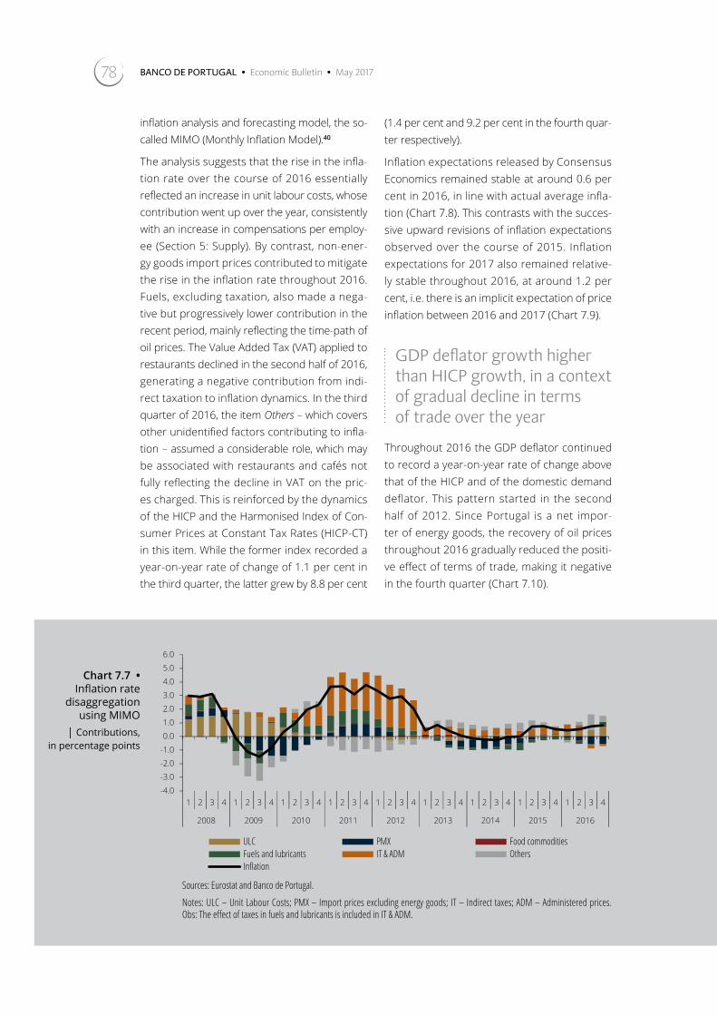
BANCO DE PORTUGAL • Economic Bulletin • May 201778
inflation analysis and forecasting model, the so-called MIMO (Monthly Inflation Model).40
The analysis suggests that the rise in the infla-tion rate over the course of 2016 essentially reflected an increase in unit labour costs, whose contribution went up over the year, consistently with an increase in compensations per employ-ee (Section 5: Supply). By contrast, non-ener-gy goods import prices contributed to mitigate the rise in the inflation rate throughout 2016. Fuels, excluding taxation, also made a nega-tive but progressively lower contribution in the recent period, mainly reflecting the time-path of oil prices. The Value Added Tax (VAT) applied to restaurants declined in the second half of 2016, generating a negative contribution from indi-rect taxation to inflation dynamics. In the third quarter of 2016, the item Others – which covers other unidentified factors contributing to infla-tion – assumed a considerable role, which may be associated with restaurants and cafés not fully reflecting the decline in VAT on the pric-es charged. This is reinforced by the dynamics of the HICP and the Harmonised Index of Con-sumer Prices at Constant Tax Rates (HICP-CT) in this item. While the former index recorded a year-on-year rate of change of 1.1 per cent in the third quarter, the latter grew by 8.8 per cent
(1.4 per cent and 9.2 per cent in the fourth quar-ter respectively).
Inflation expectations released by Consensus Economics remained stable at around 0.6 per cent in 2016, in line with actual average infla-tion (Chart 7.8). This contrasts with the succes-sive upward revisions of inflation expectations observed over the course of 2015. Inflation expectations for 2017 also remained relative-ly stable throughout 2016, at around 1.2 per cent, i.e. there is an implicit expectation of price inflation between 2016 and 2017 (Chart 7.9).
GDP deflator growth higher than HICP growth, in a context of gradual decline in terms of trade over the year
Throughout 2016 the GDP deflator continued to record a year-on-year rate of change above that of the HICP and of the domestic demand deflator. This pattern started in the second half of 2012. Since Portugal is a net impor-ter of energy goods, the recovery of oil prices throughout 2016 gradually reduced the positi-ve effect of terms of trade, making it negative in the fourth quarter (Chart 7.10).
Chart 7.7 • Inflation rate
disaggregation using MIMO
| Contributions, in percentage points
-4.0
-3.0
-2.0
-1.0
0.0
1.0
2.0
3.0
4.0
5.0
6.0
1 2 3 4 1 2 3 4 1 2 3 4 1 2 3 4 1 2 3 4 1 2 3 4 1 2 3 4 1 2 3 4 1 2 3 4
2008 2009 2010 2011 2012 2013 2014 2015 2016
ULC PMX Food commoditiesFuels and lubricants IT & ADM OthersInflation
Sources: Eurostat and Banco de Portugal.
Notes: ULC – Unit Labour Costs; PMX – Import prices excluding energy goods; IT – Indirect taxes; ADM – Administered prices. Obs: The effect of taxes in fuels and lubricants is included in IT & ADM.

79The Portuguese economy in 2016
-2.0
-1.0
0.0
1.0
2.0
3.0
4.0
5.0
2008 2009 2010 2011 2012 2013 2014 2015 2016
Current year forecast Next year forecast
Chart 7.9 • Inflation expectations for current and next year| In per cent
Source: Consensus Economics.
-2.0
-1.0
0.0
1.0
2.0
3.0
4.0
5.0
2008 2009 2010 2011 2012 2013 2014 2015 2016
Current year forecast Observed inflation (12-month average rate of change)
Chart 7.8 • Inflation expectations and observed inflation| In per cent
Sources: Consensus Economics and Statistics Portugal.
-4,0
-3,0
-2,0
-1,0
0,0
1,0
2,0
3,0
4,0
5,0
2010 Q1 2011 Q1 2012 Q1 2013 Q1 2014 Q1 2015 Q1 2016 Q1
Change in terms of trade GDP deflator Domestic demand deflator
Chart 7.10 • GDP deflator, domestic demand deflator and terms of trade | In per cent
Source: Statistics Portugal.

BANCO DE PORTUGAL • Economic Bulletin • May 201780
8. Balance of payments
In 2016 the net lending of the economy increased to 1.5 per cent of GDP, up from 0.3 per cent in 2015. This improvement reflected a sharper re-duction in investment than in savings, in a context of relative stabilisation of net capital transfers. In sectoral terms (Chart 8.1), households had a slight decline in net lending, due to the reduction in cap-ital transfers received. Current savings in this sec-tor, as a percentage of GDP, remained at a low-er level than investment, and both aggregates de-clined slightly in 2016. Non-financial corporations, in turn, moved from net borrowing in 2015 to net lending in 2016, as a result of the increase in cur-rent savings, which more than offset the slight in-crease in investment.
Increase in the current and capital account surplus, based on net exports of goods and services
In 2016 the current and capital account surplus increased to 1.7 per cent of GDP, up from 1.2 per cent in 2015 (Table 8.1). This increase in the bal-ance was the result of a reduction in the deficit of the goods and primary income accounts (both by 0.3 p.p. of GDP) and an increase in the surplus of the services account (by 0.2 p.p. of GDP), associ-ated with the performance of the tourism sector (Chart 8.2). In addition, the capital account surplus
declined to 0.9 p.p. of GDP, down from 1.2 p.p. in 2015, strengthening the trend observed in recent years, which are related to the decline in Europe-an fund transfers for investment purposes.
The buoyancy of the tourism sector continued to contribute decisively to the behaviour of the goods and services account
The goods account deficit declined by 0.3 p.p. for the second year in a row. This decline was a result of the more pronounced growth of goods’ exports (0.8 per cent) than imports (0.3 per cent).
The services account surplus increased again, to stand at 7.1 per cent of GDP in 2016. Exports of services grew by 4.4 per cent, decelerating from the previous year, when the rate of change had stood at 7.5 per cent. Growth in 2016 was chiefly due to the contribution of travel and tourism. This component continued to post very signifi-cant buoyancy, reflecting a 10.7 per cent change in 2016, up from 10.2 per cent in the previous year. The main contribution to the deceleration in exports of other services was made by the behaviour of services provided by corporations, which had a rate of change of -3.3 per cent, com-pared with 15.4 per cent growth in 2015.
Table 8.1 • Current and capital accounts | As a percentage of GDP
2013 2014 2015 2016
Current and capital accounts 3.2 1.5 1.2 1.7Current account 1.6 0.1 0.1 0.8
Goods and services account 1.9 1.1 1.8 2.2Goods -4.7 -5.5 -5.2 -4.9Services 6.6 6.6 6.9 7.1
of which:Travel and tourism 3.6 4.1 4.4 4.8
Primary income account -1.2 -2.0 -2.5 -2.2Secondary income account 0.9 0.9 0.8 0.8
of which:Emigrants / immigrants remittances 1.4 1.5 1.6 1.5
Capital account 1.6 1.4 1.2 0.9
Financial Account 3.3 1.6 1.2 1.7
Errors and omissions 0.1 0.1 0.0 0.0
Sources: INE and Banco de Portugal.

81The Portuguese economy in 2016
Imports of services had similar developments, with a change of 3.1 per cent, down from 5.8 per cent in 2015. The main contributions to growth in 2016 were travel and tourism, intellectual prop-erty rights not included elsewhere and other ser-vices.
The trade account balance in 2016 benefitted from a positive volume effect, contrary to devel-opments in the two previous years (Chart 8.3). The largest contribution, however, was made by the terms of trade effect, albeit less expressive than in the previous year. This was associated with the development of energy prices (Section 2: ‘International environment’ and Section 7: ‘Prices’).
Income paid abroad declined and the subsidies received from the European Union increased
The primary income account deficit decreased by 0.3 p.p. of GDP as a result of the 0.4 p.p. decline in income paid abroad and the maintenance of income received from non-resident entities. The decline in income paid abroad was mainly asso-ciated with the decrease in the stock of exter-nal liabilities by resident sectors, in particular the general government and other monetary finan-cial institutions (other MFI). The stabilisation of primary income received from abroad was the
-20
-15
-10
-5
0
5
10
2009 2010 2011 2012 2013 2014 2015 2016
Non-financial corporations Financial corporationsGeneral Government HouseholdsNet lending/net borrowing
Chart 8.1 • Net lending/net borrowing of the economy | As a percentage of GDP
Source: INE.
-10
-8
-6
-4
-2
0
2
4
6
8
10
2013 2014 2015 2016
Capital account Secondary income accountServices Primary income accountGoods Current and capital accounts
Chart 8.2 • Decomposition of current and capital account balance| As a percentage of GDP
Sources: INE and Banco de Portugal.
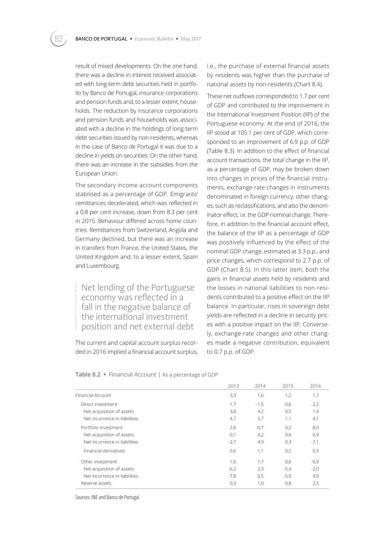
BANCO DE PORTUGAL • Economic Bulletin • May 201782
result of mixed developments. On the one hand, there was a decline in interest received associat-ed with long-term debt securities held in portfo-lio by Banco de Portugal, insurance corporations and pension funds and, to a lesser extent, house-holds. The reduction by insurance corporations and pension funds and households was associ-ated with a decline in the holdings of long-term debt securities issued by non-residents, whereas in the case of Banco de Portugal it was due to a decline in yields on securities. On the other hand, there was an increase in the subsidies from the European Union.
The secondary income account components stabilised as a percentage of GDP. Emigrants’ remittances decelerated, which was reflected in a 0.8 per cent increase, down from 8.3 per cent in 2015. Behaviour differed across home coun-tries. Remittances from Switzerland, Angola and Germany declined, but there was an increase in transfers from France, the United States, the United Kingdom and, to a lesser extent, Spain and Luxembourg.
Net lending of the Portuguese economy was reflected in a fall in the negative balance of the international investment position and net external debt
The current and capital account surplus recor-ded in 2016 implied a financial account surplus,
i.e., the purchase of external financial assets by residents was higher than the purchase of national assets by non-residents (Chart 8.4).
These net outflows corresponded to 1.7 per cent of GDP and contributed to the improvement in the International Investment Position (IIP) of the Portuguese economy. At the end of 2016, the IIP stood at 105.1 per cent of GDP, which corre-sponded to an improvement of 6.9 p.p. of GDP (Table 8.3). In addition to the effect of financial account transactions, the total change in the IIP, as a percentage of GDP, may be broken down into changes in prices of the financial instru-ments, exchange rate changes in instruments denominated in foreign currency, other chang-es, such as reclassifications, and also the denom-inator effect, i.e. the GDP nominal change. There-fore, in addition to the financial account effect, the balance of the IIP as a percentage of GDP was positively influenced by the effect of the nominal GDP change, estimated at 3.3 p.p., and price changes, which correspond to 2.7 p.p. of GDP (Chart 8.5). In this latter item, both the gains in financial assets held by residents and the losses in national liabilities to non-resi-dents contributed to a positive effect on the IIP balance. In particular, rises in sovereign debt yields are reflected in a decline in security pric-es with a positive impact on the IIP. Converse-ly, exchange-rate changes and other chang-es made a negative contribution, equivalent to 0.7 p.p. of GDP.
Table 8.2 • Financial Account | As a percentage of GDP
2013 2014 2015 2016
Financial Account 3,3 1,6 1,2 1,7
Direct investment -1,7 -1,5 -0,6 -2,2Net acquisition of assets 3,0 4,2 0,5 1,9Net incurrence in liabilities 4,7 5,7 1,1 4,1
Portfolio investment 2,6 -0,7 0,2 8,0Net acquisition of assets -0,1 4,2 0,6 0,9Net incurrence in liabilities -2,7 4,9 0,3 -7,1
Financial derivatives 0,6 1,1 0,2 0,3
Other investment 1,6 1,7 0,6 -6,9Net acquisition of assets -6,2 2,3 -5,4 -2,0Net incurrence in liabilities -7,8 0,5 -5,9 4,9
Reserve assets 0,3 1,0 0,8 2,5
Sources: INE and Banco de Portugal.

83The Portuguese economy in 2016
Banco de Portugal and non-financial corporations purchased foreign assets, whereas non-residents disinvested from public debt and other-MFI’s securities.
In 2016 Banco de Portugal was the main agent investing in external assets, especially via the
purchase of debt securities, either as reserve assets, or, in particular, as portfolio investment, and deposits with non-resident entities. This ini-tiative by Banco de Portugal corresponds to the participation in the implementation of Eurosys-tem’s monetary policy decisions. Notwithstand-ing these transactions, the IIP of Banco de Portu-gal remained virtually unchanged, also due to a significant increase in liabilities to non-residents,
-3,000
-2,000
-1,000
0
1,000
2,000
3,000
4,000
2013 2014 2015 2016
Volume effect Price effect Terms of trade effect Crossed effect Change in balance
Chart 8.3 • Decomposition of goods and services account| Million of euros
Sources: INE and Banco de Portugal.
Note: A positive change (negative) implies an increase (decrease) in the overall balance of the goods and services account. The change in the overall balance of goods and services account can be decomposed in four effects: – volume effect – effect of the change in quantities imported and exported; [Xt-1.vxt]-[Mt-1.vmt] – price effect – effect of the average price growth of external trade; [Xt-1.pt]-[Mt-1.pt] – terms of trade effect – effect of the relative change in exports and imports prices; [Xt-1.(pxt--pt)]-[Mt-1.( pmt-pt)] – crossed effect – effect of the interaction between the change in quantities and in prices of exports and imports; [Xt-1.vxt.pxt]-[Mt-1.vmt.pmt] The following notation applies: Xt-1 and Mt-1 are the exports and imports in year t-1 at current prices; vxt and vmt are the change rates in volume of exports and imports in t; pxt and pmt are the change rates of exports and imports prices in t; pt is the average change rate of the prices of external trade in year t ((pxt+pmt)/2).
-10.0
-5.0
0.0
5.0
10.0
15.0
2013 2014 2015 2016
Overall balance Net acquisition of assets Net incurrence of liabilities
Chart 8.4 • Net change in financial assets and liabilities and overall financial balance| As a percentage of GDP
Sources: INE and Banco de Portugal.

BANCO DE PORTUGAL • Economic Bulletin • May 201784
particularly in the form of liabilities to the Euro-system. Monetary gold valuation also contribut-ed to the increase in financial assets by 0.9 p.p. of GDP (Charts 8.6 and 8.7).
Non-financial corporations were also engaged in investments abroad, albeit to a lesser extent. These investments occurred mainly with corpo-rations with which they had established direct investment links and from which they had ob-tained funds (Box 8.1 ‘Direct investment flows into the Portuguese economy’). The balance of these cross transactions was reflected in a higher
increase in liabilities than in assets and in the de-terioration of the IIP balance of this sector.
Contrary to the increase in external assets by Banco de Portugal and non-financial corpora-tions, non-residents disinvested significantly from national public debt securities (Section 4: ‘Fiscal policy and situation’) and, to a lesser extent, from securities issued by other MFI.
In the case of the general government, and in addition to transactions in debt securities issued, reference should be made to the repayment of loans obtained under the European and Financial
Chart 8.5 • Change in
International investment
position| As a percentage
of GDP
112.0
105.1
1.7
2.7
3.3
0.7
100
102
104
106
108
110
112
IIP 2015 (symmetrical) Transactions Changes in prices Change in GDP Exchange rate and other adjustments
IIP 2016 (symmetrical)
Sources: INE and Banco de Portugal.
Chart 8.6 • Net acquisiton of assets (1) | As a percentage of GDP
Chart 8.7 • Net incurrence of liabilities(2) | As a percentage of GDP
-8
-6
-4
-2
0
2
4
6
8
Total CB OMFI GG NMFI NFPS
2015 2016
-8
-6
-4
-2
0
2
4
6
8
Total CB OMFI GG NMFI NFPS
2015 2016
Sources: INE and Banco de Portugal.
Note: (1) The net acquisiton of assets corresponds to buys less sells of foreign assets by residents. A plus sign represents a net outflow of funds from the por-tuguese economy.
Sources: INE and Banco de Portugal.
Note: (2) The net incurrance of liabilities corresponds to the increase less redemp-tions of national liabilities with non-resident entities. A plus sign corresponds to a net inflow of funds in the portuguese economy.

85The Portuguese economy in 2016
Assistance Programme. These transactions were an important contribution to the decline of 12.5 p.p. of GDP in the stock of external liabilities in this sector. This result also had the important contri-bution of both GDP and the devaluation of Treas-ury bonds, in a context of an increase in pub-lic debt yields.
As regards the liabilities of other MFI, in addition to the decline in liabilities in the form of debt securities, there was a decrease in deposits by non-residents. In the same vein, investments abroad in these type of securities by other-MFI
also declined. The volume of these transactions was more significant than the decline in liabili-ties, leading to a deterioration of the negative balance of the IIP in this sector by 1 p.p. of GDP.
Taking into account the significant transactions in debt securities issued by residents, net exter-nal debt, which is obtained by excluding capital instruments and financial derivatives from the IIP, declined by 7 p.p. of GDP, down from 101.5 per cent of GDP in 2015 to 94.4 per cent of GDP in 2016 (Chart 8.8).
Table 8.3 • International Investment Position | As a percentage of GDP
2013 2014 2015 2016
International Investment Position -116.3 -117.7 -112.0 -105.1
Direct investment -27.3 -31.1 -30.8 -32.0
Direct investment - Assets 42.1 42.7 42.6 43.5
Direct investment - Liabilities 69.4 73.9 73.4 75.5
Portfolio investment -10.2 -10.6 -9.2 0.8
Portfolio investment - Assets 64.8 68.8 66.7 65.9
Portfolio investment - Liabilities 75.0 79.3 76.0 65.1
Other investment -84.5 -84.3 -82.0 -86.6
Other investment - Assets 68.2 69.1 61.9 58.1
Other investment - Liabilities 152.7 153.4 143.9 144.7
Reserve assets and derivatives 5.7 8.3 10.0 12.8
Sources: INE and Banco de Portugal.
-140
-120
-100
-80
-60
-40
-20
0
2005 2006 2007 2008 2009 2010 2011 2012 2013 2014 2015 2016
Net External Debt (symmetrical) Net Capital Instruments International Investment Position
Chart 8.8 • International investment position, net external debt and position in capital instruments | As a percentage of GDP
Sources: INE and Banco de Portugal.

86 BANCO DE PORTUGAL • Economic Bulletin • May 2017
Box 8.1 | Direct investment flows into the Portuguese economy41
The current situation of the Portuguese economy is characterised by moderate economic growth, relatively weak investment rate and unfavourable developments in labour productivity, against a background of high indebtedness of the different institutional sectors. In this context, the accel-eration of economic activity and the increase in productivity require an investment effort that will be easier to implement if there is the possibility to attract external capital.
Foreign direct investment in Portugal reflects the Portuguese economy capacity to attract capital, also resulting in positive externalities, especially in terms of sharing technology and business knowl-edge. Therefore, it is important to analyse in more detail the nature and composition of these flows.
Balance of payments statistics on foreign direct investment in Portugal include financial transactions on assets and liabilities of resident corporations with their non-resident direct investors, as well as all financial transactions between resident and non-resident corporations, held (directly or indirectly) by the same non-resident entity.42 Diversified financial flows are thus recorded, comprising reinvested earnings, investment in real estate, debt instruments and other capital instruments.
Reinvested earnings correspond to corporations’ results that are retained, and reflect their alloca-tion to foreign holders of the respective capital. Their registration in the balance of payments is therefore made under investment income and in the financial account, corresponding to an increase in investment. Reinvested earnings are recorded in the period in which they are earned.
Investment in real estate corresponds to investment by non-residents in property and residences in the national territory, either for personal use or for rental.
Debt instruments cover funds lent by non-resident entities – in the form of loans or debt securi-ties – whereas capital instruments represent the property rights on the resident entity.
In an open economy as the Portuguese, foreign direct investment is an important source of finan-cial inflows. Compared with other European countries, Portugal is among the main recipients of direct investment as a percentage of GDP (Charts 1 and 2).
For many years, inflows into the Portuguese economy occurred mainly in the form of portfolio investment and other investment. In the 1996-2016 period, foreign direct investment, on aver-age, accounted for annual net inflows into the economy of 2.4 per cent of GDP. In most recent years, however, and in a context of declining external indebtedness, direct investment flows have been gaining relative importance in the Portuguese economy. In 2013 and 2015 they were in fact the main source of external financing (Chart 3).
Since 2008, this investment represented, on average, 2.1 per cent of GDP. It was higher in 2011 and 2012, when it reached 4.1 per cent of GDP, and in the last two years, when it stood, on aver-age, at 3.2 per cent of GDP.
Financing requirements of the Portuguese economy were partially met with recourse to privatisa-tions, which translated into the purchase of assets by non-residents. Therefore, in 2011 and 2012, the composition of foreign direct investment in Portugal primarily took the form of capital instruments, and was associated with the non-financial corporations sector (Charts 4 and 5).
After a decline in inflows in 2013 and 2014, financial transactions intensified again in the last two years. In terms of instrument, however, there was a decline in the amounts of investment in corpo-rations’ capital, against an increase in transactions in debt instruments. I.e., resident corporations that received foreign direct investment used that channel to obtain financing from the firms in the

The Portuguese economy in 2016 87
Chart 1 • Foreign Direct Investment – transactions – 2015 | As a percentage of GDP
-1
0
1
2
3
4
5
SK CR EE EL FI CZ DE DK ES IT UK SE AT FR LT RO LV PO PT IS BG SL BE
Source: Eurostat.
Chart 3 • Foreign direct investment and other inward funds in portuguese economy – transactions | As a percentage of GDP
-25
-20
-15
-10
-5
0
5
10
15
20
25
30
1996 1997 1998 1999 2000 2001 2002 2003 2004 2005 2006 2007 2008 2009 2010 2011 2012 2013 2014 2015 2016
FDI Portfolio investment Other investment
Sources: INE and Banco de Portugal.
Chart 2 • Direct investment – stocks – 2015 | As a percentage of GDP
BE
BG
CZ
DK
DE
EE
EL
ES
FR
CR
IT
LV
LT
AT
PORO
SL
SK
FI
SE
UK
IS
NO
PT
0
20
40
60
80
100
120
0 20 40 60 80 100 120
Inw
ard
flow
s,as
a p
erce
ntag
e of
GD
P
Outward flows, as a percentage of GDP
Source: Eurostat.
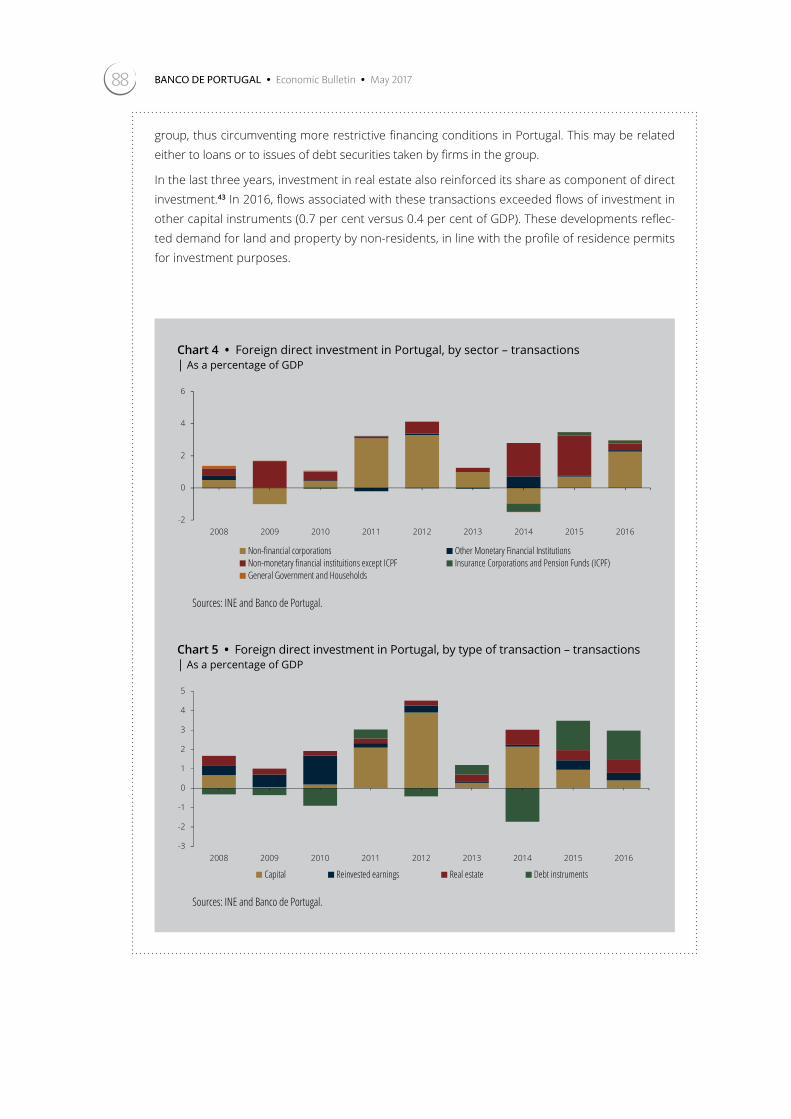
88 BANCO DE PORTUGAL • Economic Bulletin • May 2017
group, thus circumventing more restrictive financing conditions in Portugal. This may be related either to loans or to issues of debt securities taken by firms in the group.
In the last three years, investment in real estate also reinforced its share as component of direct investment.43 In 2016, flows associated with these transactions exceeded flows of investment in other capital instruments (0.7 per cent versus 0.4 per cent of GDP). These developments reflec-ted demand for land and property by non-residents, in line with the profile of residence permits for investment purposes.
Chart 5 • Foreign direct investment in Portugal, by type of transaction – transactions | As a percentage of GDP
-3
-2
-1
0
1
2
3
4
5
2008 2009 2010 2011 2012 2013 2014 2015 2016
Capital Reinvested earnings Real estate Debt instruments
Sources: INE and Banco de Portugal.
Chart 4 • Foreign direct investment in Portugal, by sector – transactions | As a percentage of GDP
-2
0
2
4
6
2008 2009 2010 2011 2012 2013 2014 2015 2016
Non-financial corporations Other Monetary Financial InstitutionsNon-monetary financial instituitions except ICPF Insurance Corporations and Pension Funds (ICPF)General Government and Households
Sources: INE and Banco de Portugal.

89The Portuguese economy in 2016
Notes
1. Available at https://www.bportugal.pt/sites/default/files/anexos/pdf-boletim/projecoes_mar_pt_0.pdf
2. For further details, see Félix et al. (2007) ‘MIMO – A Monthly Inflation Model’, winter 2007 issue of the Economic Bulletin of Banco de Portugal.
3. Angola is not included in the set of countries used under the Eurosystem’s procedure to calculate external demand for the goods and services of each individual country.
4. The APP is composed of four programmes: the Covered Bond Purchase Programme (CBPP), which is currently in its third programme; the Asset-backed Securities Purchase Programme (ABSPP), the Public Sector Purchase Programme (PSPP), and the CSPP. The first two programmes started in 2014 and the third programme in 2015.
5. In its December 2016 meeting, the Governing Council of the ECB announced its decision to extend the APP until the end of 2017. However, purchases were reduced from €80 billion to €60 billion from March onwards.
6. The Eurosystem’s architecture only allows monetary financial institutions to have access to the ECB’s deposit facility rate.
7. In this respect, see the speech by Yves Merch, ‘Ructions in the repo market – monetary easing or regulatory squeezing?‛, 26 January 2017.
8. This fact tends to be visible in the repo market, particularly on dates close to accounting reporting dates and for rates associated with jurisdictions perceived as safe. On the last business day of December 2016, a number of repo rates reached historical lows.
9. See Antunes, Homero and Prego (2016) ‘Firm default probabilities revisited‛, Banco de Portugal Economic Studies, Vol. 2, No. 2, Banco de Portugal.
10. Total credit to non-financial corporations includes loans by resident banks, loans by non-residents, debt securities issuance (held by residents and non-residents), trade credits (granted by residents and non-residents), household loans and Treasury loans (in the case of loans to public undertakings).
11. This definition of indebtedness includes the sum of bank loans, debt securities and trade credits.
12. See Box “Developments in corporate indebtedness in Portugal and the euro area”, Economic Bulletin, May 2016, Banco de Portugal. The analysis considers data from the national financial accounts and the measure of indebtedness considered is the ratio of debt (loans and debt securities) to total assets.
13. Félix, S. (2017) “Firm creation and survival in Portugal”, Banco de Portugal Economic Studies, Banco de Portugal.
14. The survey IES includes economic, financial, and accounting information of virtually all the Portuguese non-financial corporations and is available for the period between 2005 and 2015. Nevertheless, changes in the accounting standards system in 2010 have led to a loss of data comparability.
15. A reporting gap is observed when the firm reports to the IES in year t-1 and year t+1, but is absent in year t.
16. Some of the absences that are considered exits from the market in 2015 may constitute reporting gaps. This can only be verified when the IES for 2016 becomes available. However, only about 0.2 per cent of the observations are reporting gaps in the period under analysis.
17. EBIT stands for Earnings Before Interest and Taxes.
18. These factors meet the criteria for classification as temporary measures, as defined in the Eurosystem context, which does not necessarily coincide with the classification adopted by other institutions.
19. In August 2016, the EU Council recommended a stabilisation of the structural balance. Compliance with this recommendation shall be assessed on the basis of the cyclical adjustment methodology and the definition of temporary measures adopted by the European Commission.
20. The impact of the resolution of BANIF in 2015 is treated as a temporary measure, according to the definition adopted by the Eurosystem. This ope-ration had a significant impact on capital transfers, chiefly as a result of the capital increase by the State. To a lesser extent, it also affected the public investment aggregate via the recording of real estate acquisitions by Oitante, a special-purpose entity created in the context of the resolution process.
21. Military material delivered in 2016 relates to the sale of F-16 aircrafts to Romania, which negatively affects the general government investment ag-gregate. In spite of their one-off impact on the balance, these operations are not treated as temporary measures in the context of the definition adopted by the Eurosystem.
22. In 2015 a number of operations contributed to an increase in general government capital expenditure: the conversion into an equity increase of loans granted by Wolfpart to its holding Caixa Imobiliário; the recording of requests for budget increases by Instituto de Financiamento da Agricultura e Pescas (Agricultural and Fisheries Financing Institute); capital increases in public corporations that are not included in the general government.
23. In 2015 the general government wage cuts in force since 2011 started to be reversed, with 20 per cent of the cuts being reinstated. In 2016 the remainder was gradually reinstated in the course of the year, by 25 per cent each quarter.
24. In early 2015, the European Central Bank announced the widening of the asset purchase programmes then in force, to also include the purchase of bonds issued by euro area central governments, as well as by European organisations and institutions.
25. The implicit interest rate is computed as the ratio of interest expenditure to the simple average of the debt stock at the end of the current and the previous year.
26. The analysis in this box is based on the methodology developed in the context of the Eurosystem which allows the breakdown of structural revenue from taxes and social contributions into the following components: i) impact of legislative changes; ii) contribution of the discrepancy between the trend nominal change in the relevant macroeconomic base and GDP; iii) effect of the structural fiscal elasticity in structural terms and iv) residual component. The residual component corresponds to the part of the structural change that is not explained by the previous effects. For further details, see Kremer et al. (2006), A disag-gregated framework for the analysis of structural developments in public finances, Working paper ECB 579, and Braz, C. (2006), ‘The calculation of cyclically adjusted balances at Banco de Portugal: an update’, winter 2006 issue of the Economic Bulletin of Banco de Portugal.

BANCO DE PORTUGAL • Economic Bulletin • May 201790
27. In the case of the tax on oil products, the estimate for the impact of an increase in taxation reflects an ex post reassessment based on the final outturn for the year.
28. Total revenue from social contributions includes actual and imputed social contributions referring to civil servants, which are also recorded on the expenditure side, under compensation of employees.
29. See Box 5.2 of the October 2016 issue of the Economic Bulletin for a characterisation of very long-term unemployment in Portugal.
30. According to Eurostat's definition, tradable services include accommodation and food services, trade and repair, transportation and storage, and infor-mation and communication activities.
31. Apparent labour productivity was calculated dividing VAT (volume chain-linked series, € millions) by total employment (full-time equivalent), except in the 1992 recession, when it was calculated on the basis of GDP.
32. For a discussion, see for example F. Caselli (2005) ‘Accounting for Cross-Country Income Differences‛, Handbook of Economic Growth, volume 1, Chapter 9.
33. Information available at https://fred.stlouisfed.org/release?rid=285.
34. Taking into account the weight of trade with Angola in Portuguese nominal exports, it is possible to estimate the mechanical impact of the fall in exports to Angola on nominal GDP. Hence, in 2016 total exports to Angola (goods and services), excluding an estimate for import contents, appear to have made a contri-bution of around -0.6 p.p. to 3.0 per cent growth of nominal GDP (in 2015 the contribution was around -0.7 per cent for 3.7 per cent growth of nominal GDP).
35. In 2016, in particular, remuneration received by households grew by 3.6 per cent, after 2.4 per cent in 2015.
36. In 2016 the decline in interest expenses of households contributed 0.4 p.p. to the 3.2 per cent growth of nominal disposable income.
37. See the special issue ‘Recent developments in consumer lending: A macroprudential approach‛, Financial Stability Report, Banco de Portugal, November 2016.
38. Following 1.5 per cent year-on-year falls in the first two quarters of 2016, nominal exports of goods grew by 1.9 and 5.1 per cent respectively in the third and fourth quarters of 2016. This was also due to the stabilisation of exports of fuels in the second half of the year, after the break observed in the first half.
39. Information on the aggregation and calculation of rates of change in European export prices in Banco de Portugal, 2016, ‘Portuguese international traders: some facts about age, prices and markets‛, Economic Bulletin, October 2016, special issue.
40. For further details, see Félix et al. (2007) ‘MIMO – A Monthly Inflation Model ‛, Winter 2007 issue of the Economic Bulletin of Banco de Portugal.
41. This Box was based on information on Foreign Direct Investment in Portugal, according to the directional principle. I.e., all transactions with non--residents regarding resident direct investment firms are considered, irrespective of whether they are an asset or a liability of such corporations.
42. For further details on the statistical treatment of information on direct investment, see Banco de Portugal (2015), ‘Statistics of the balance of payments and the international investment position – Methodological notes’, Supplement to the Statistical Bulletin No. 2/2015.
43. For a more detailed analysis of real-estate investment, see Box 7.1 of the May 2016 issue of the Economic Bulletin.

IISpecial issue
Distribution mechanisms of monetary policy in the Portuguese economy


93Special issue
Distribution mechanisms of monetary policy in the Portuguese economy
1. IntroductionIn the wake of the global economic and financial
crisis, the link between the implementation of
monetary policy and developments in inequal-
ity has re-entered the public debate. This is set
against a background where inequality has once
again been considered inseparable from eco-
nomic policy. The perception that the reduction
in inequality seen throughout most of the last
century had been reversed, together with the
fact that advanced economies have failed to
return to the activity levels that would have been
reached if the trend before the crisis had con-
tinued, contributed to the greater importance
of issues related to the distribution of economic
resources.
It is well known that inequality is not, and should
not be, an objective pursued by central banks.
In the case of the euro area, the primary objec-
tive of the European Central Bank (ECB) is price
stability and, secondarily, support to the general
economic policies in the European Union. The
maintenance of price stability helps prevent the
arbitrary redistribution of income. In any case,
it is potentially important to understand the
link between the implementation of monetary
policy and inequality for two sets of reasons. On
the one hand, inequality levels prevailing in an
economy may affect monetary policy transmis-
sion to economic agents, thereby hampering its
expected results. On the other hand, monetary
policy may affect inequality levels prevailing in
the euro area and individual economies and,
as such, influence a considerable part of public
debate and the Eurosystem’s accountability.
The redistribution impact of monetary policy
has also been increasingly reviewed in econom-
ic literature (see e.g. Auclert, 2016, or Coibion et
al., 2016, and respective references). The use of
increased computing power to solve economic
models with heterogeneous agents, together with the dissemination of microeconomic data on an individual basis, has helped focus academic discussion on distribution issues. There is a new consensus in economic literature that monetary authorities must be aware of the redistribution effects of monetary policy, as well as the unob-served heterogeneity in the economy. This con-clusion stands even when the redistribution impact of monetary policy is relatively small over long periods, which are the most suitable when analysing structural developments in inequal-ity: over such time horizons, structural factors become more important, including inter alia the openness of economies, technological progress, institutional changes in the output and labour markets, the tax regime and the social protection network.
The purpose of this article is to look into some of the main monetary policy transmission chan-nels impacting on the distribution of monetary resources among households. Such channels are illustrated on the basis of microeconomic data on the Portuguese economy. However, the analysis will necessarily compare modestly with the title of this article. In fact, the impact of monetary policy on the Portuguese economy goes well beyond the channels analysed in this article. For instance, the reduction in the ECB’s intervention rates following the international financial crisis made a key contribution to reliev-ing the debt service of Portuguese households and to reduce liquidity constraints. This channel had a major impact on the Portuguese econo-my as a whole, but it will not be reviewed here. Studying the distribution effects of monetary policy would involve describing a counterfac-tual scenario that can only be created using a proper model.
The Special Issue is structured as follows. Section 2 looks into the methodology and the microdata

BANCO DE PORTUGAL • Economic Bulletin • May 201794
bases used in the analysis. Section 3 describes some of the main monetary policy redistribution channels, illustrating their potential impact based on microeconomic data on the Portuguese econ-omy. Section 4 includes an exercise that analyses the quantitative impact on the Portuguese econ-omy of the standard and non-standard mone-tary policy measures implemented over the past few years. Section 5 presents and discusses the main conclusions of this exercise.
2. Methodology and databasesIn this article, the household is the unit of analy-sis. By definition, this is the unit where inequal-ity resulting from its links with the market is of greater interest. Although in Portugal it is still not possible to track wealth trends for a repre-sentative sample of the population over time, results are now available from two rounds of the Household Finance and Consumption Survey, a Eurosystem initiative that Banco de Portugal and Statistics Portugal (Portuguese acronym: INE) have implemented domestically. The infor-mation gathered from these surveys will make it possible to start tracking the impact under review (see Banco de Portugal and Statistics Portugal, 2016, Costa and Farinha, 2012, and Costa, 2016).
In this article, household inequality is assessed on the basis of two concepts of wealth: wealth in broad sense and net wealth.
Wealth in broad sense assesses, at a given mo-ment in time, the range of decisions that house-holds may make in the course of their lifetime and, therefore, provides a good summary of the resulting well-being. This aggregate may be bro-ken down into two very different components, as illustrated by the following equation:
policy measures implemented over the past few years. Section 5 presents and discusses the main conclusions of this exercise.
2. Methodology and databases In this article, the household is the unit of analysis. By definition, this is the unit where inequality resulting from its links with the market is of greater interest. Although in Portugal it is still not possible to track wealth trends for a representative sample of the population over time, results are now available from two rounds of the Household Finance and Consumption Survey, a Eurosystem initiative that Banco de Portugal and Statistics Portugal (Portuguese acronym: INE) have implemented domestically. The information gathered from these surveys will make it possible to start tracking the impact under review (see Banco de Portugal and Statistics Portugal, 2016, Costa and Farinha, 2012, and Costa, 2016).
In this article, household inequality is assessed on the basis of two concepts of wealth: wealth in broad sense and net wealth.
Wealth in broad sense assesses, at a given moment in time, the range of decisions that households may make in the course of their lifetime and, therefore, provides a good summary of the resulting well-being. This aggregate may be broken down into two very different components, as illustrated by the following equation:
(1)
On the one hand, the net wealth (or non-human wealth) of each household when the period under review begins results from the difference between its assets and its liabilities. This net wealth, by construction, is predetermined and generates some return, including capital gains, over time. On the other hand, there is the so-called human wealth, i.e. the sum of current and future income resulting from household decisions as to how to spend time in the labour market.
Over the lifetime of each household, human wealth will depend on exogenous conditions – such as the labour market environment and structural changes – and idiosyncratic features of the household under review. Among household-specific features are the (accumulated or inherent) efficiency with which household members that participate in the labour market are able to turn their time into income, and the starting position in the labour market, which, together with age, partially determines future returns on that market. The transformation of initial conditions into returns in the labour market is anything but deterministic. As is well known, luck plays its part, which means that idiosyncratic shocks help determine, inter alia, which household members will be employed, the quality of the match between employees and workers (according to their skills) and developments in the sector of activity where a household member will work. Labour income results from the combination of these opportunities. This clearly shows that, in contrast to net wealth, human wealth depends on a great deal of unavailable information. At best, information is only available on probability distributions.
At a given moment in time, the sum of the expected value of labour income in the course of a lifetime, discounted back to that moment, determines the household’s human wealth. This aggregate includes pension income, given its close link to labour market participation. In practical terms, each household was assumed to have a wide horizon when making its decisions, as would be the case when using an infinite-horizon agent model. Assuming that labour income corresponds to a perpetuity, and taking into account a discount rate of 4%, this would imply that human wealth may be proxied by multiplying current labour income1 by 25. This proxy is used in the exercises below, although results are qualitatively robust to the use of different discount rates. Equation (1) can therefore be re-written as follows:
(1)
policy measures implemented over the past few years. Section 5 presents and discusses the main conclusions of this exercise.
2. Methodology and databases In this article, the household is the unit of analysis. By definition, this is the unit where inequality resulting from its links with the market is of greater interest. Although in Portugal it is still not possible to track wealth trends for a representative sample of the population over time, results are now available from two rounds of the Household Finance and Consumption Survey, a Eurosystem initiative that Banco de Portugal and Statistics Portugal (Portuguese acronym: INE) have implemented domestically. The information gathered from these surveys will make it possible to start tracking the impact under review (see Banco de Portugal and Statistics Portugal, 2016, Costa and Farinha, 2012, and Costa, 2016).
In this article, household inequality is assessed on the basis of two concepts of wealth: wealth in broad sense and net wealth.
Wealth in broad sense assesses, at a given moment in time, the range of decisions that households may make in the course of their lifetime and, therefore, provides a good summary of the resulting well-being. This aggregate may be broken down into two very different components, as illustrated by the following equation:
(1)
On the one hand, the net wealth (or non-human wealth) of each household when the period under review begins results from the difference between its assets and its liabilities. This net wealth, by construction, is predetermined and generates some return, including capital gains, over time. On the other hand, there is the so-called human wealth, i.e. the sum of current and future income resulting from household decisions as to how to spend time in the labour market.
Over the lifetime of each household, human wealth will depend on exogenous conditions – such as the labour market environment and structural changes – and idiosyncratic features of the household under review. Among household-specific features are the (accumulated or inherent) efficiency with which household members that participate in the labour market are able to turn their time into income, and the starting position in the labour market, which, together with age, partially determines future returns on that market. The transformation of initial conditions into returns in the labour market is anything but deterministic. As is well known, luck plays its part, which means that idiosyncratic shocks help determine, inter alia, which household members will be employed, the quality of the match between employees and workers (according to their skills) and developments in the sector of activity where a household member will work. Labour income results from the combination of these opportunities. This clearly shows that, in contrast to net wealth, human wealth depends on a great deal of unavailable information. At best, information is only available on probability distributions.
At a given moment in time, the sum of the expected value of labour income in the course of a lifetime, discounted back to that moment, determines the household’s human wealth. This aggregate includes pension income, given its close link to labour market participation. In practical terms, each household was assumed to have a wide horizon when making its decisions, as would be the case when using an infinite-horizon agent model. Assuming that labour income corresponds to a perpetuity, and taking into account a discount rate of 4%, this would imply that human wealth may be proxied by multiplying current labour income1 by 25. This proxy is used in the exercises below, although results are qualitatively robust to the use of different discount rates. Equation (1) can therefore be re-written as follows:
On the one hand, the net wealth (or non-human wealth) of each household when the period under review begins results from the difference
between its assets and its liabilities. This net wealth, by construction, is predetermined and generates some return, including capital gains, over time. On the other hand, there is the so-called human wealth, i.e. the sum of current and future income resulting from household decisions as to how to spend time in the labour market.
Over the lifetime of each household, human wealth will depend on exogenous conditions – such as the labour market environment and structural changes – and idiosyncratic features of the household under review. Among house-hold-specific features are the (accumulated or inherent) efficiency with which household mem-bers that participate in the labour market are able to turn their time into income, and the start-ing position in the labour market, which, togeth-er with age, partially determines future returns on that market. The transformation of initial conditions into returns in the labour market is anything but deterministic. As is well known, luck plays its part, which means that idiosyncratic shocks help determine, inter alia, which house-hold members will be employed, the quality of the match between employees and workers (according to their skills) and developments in the sector of activity where a household mem-ber will work. Labour income results from the combination of these opportunities. This clear-ly shows that, in contrast to net wealth, human wealth depends on a great deal of unavailable information. At best, information is only avail-able on probability distributions.
At a given moment in time, the sum of the expect-ed value of labour income in the course of a life-time, discounted back to that moment, deter-mines the household’s human wealth. This aggre-gate includes pension income, given its close link to labour market participation. In practical terms, each household was assumed to have a wide hori-zon when making its decisions, as would be the case when using an infinite-horizon agent mod-el. Assuming that labour income corresponds to
a perpetuity, and taking into account a discount

95Special issue
rate of 4%, this would imply that human wealth
may be proxied by multiplying current labour
income1 by 25. This proxy is used in the exercises
below, although results are qualitatively robust to
the use of different discount rates. Equation (1)
can therefore be re-written as follows:
(2)
Knowing the distribution of the sum of these two types of wealth among households representing a given population provides a good measure of inequality among that population. The way in which this distribution reacts to structural changes in the economy – including a persistent policy change – provides a measure of the distribution impact of that change.
To simplify the analysis, in this article households are broken down into wealth in broad sense and net wealth quintiles, assuming that the average of each quintile summarises the corresponding population group.2 The ratios used to gauge inequality are the ratio of the average population to the intermediate quintile (Average/Q3), the ratio of the highest quintile to the intermediate quintile (Q5/Q3) and the ratio of the highest quintile to the lowest quintile (Q5/Q1). The higher the ratios, the more unequal the distribution is. These ratios should be interpreted with caution. For instance, while the Average/Q3 ratio is not very sensitive to small changes in the distribution, the Q5/Q1 ratio reacts very strongly if Q1 figures are very low.3
Table 1 shows descriptive statistics on the level and distribution of wealth in broad sense and net wealth in the Portuguese economy, on the basis of the Household Finance and Consumption Survey for 2010 (to see a comparison between the outcome of the Household Finance and Consumption Survey for 2010 and that for 2013, see Costa, 2016). The various distribution quintiles for wealth in broad sense and net wealth comprise different households. Indeed, there is a relatively small overlap between households across distribution quintiles, as illustrated in Table 2. For instance, only 48 per cent of households in the lowest quintile of wealth in broad sense are also included in the lowest net wealth quintile. This different household composition in both measures of wealth distribution plays a key role when interpreting the results obtained in Section 3.4
Table 1 illustrates the high inequality levels in net wealth and wealth in broad sense in Portugal. In particular, the average value of net wealth in the first distribution quintile is close to zero. This explains the high inequality in net wealth as measured by the Q5/Q1 ratio. Turning to wealth in broad sense, its dispersion is much lower, given that human wealth’s dispersion is relatively low. Overall, the heterogeneity prevailing in the distribution of net wealth and wealth in broad sense suggests that the potential redistribution impact of monetary policy on the Portuguese economy cannot be ignored.
This article includes a number of stylised exercises discussing in what way monetary policy changes can be transmitted to household wealth. Monetary policy has distribution effects via several channels. The unexpected impact on price levels is one of the most studied channels in literature. This “Fisher channel” has been analysed in literature for a long time, starting with Fisher (1933). Briefly, an unexpected shock leading to an increase in the consumer price index has a redistribution effect by changing the real value of household exposures. An increase in prices redistributes resources from households with positive nominal wealth positions to households with negative nominal positions, which means that it generates a reduction in real wealth for creditors and an increase in real wealth for debtors, if assets held at the time of the policy shock are denominated in cash units.
Another redistribution channel attributable to monetary policy results from developments in nominal interest rates. Persistently increasing the average inflation rate, as well as the short-term nominal interest rate, results in a relatively larger increase in taxes for cash-holding households – with approximately zero nominal profitability – compared with households holding assets with positive returns. Given that relatively poorer agents hold a larger share of their wealth in cash, they are negatively affected by the aforementioned policy change compared with richer agents. This effect is described in Erosa and Ventura (2002) and Adão and Correia (2016).
Since the beginning of the euro area, the Portuguese economy has been characterised by a monetary regime where nominal interest rates and the inflation rate are low and not very volatile. Consequently, the redistribution
(2)
(2)
Knowing the distribution of the sum of these two types of wealth among households representing a given population provides a good measure of inequality among that population. The way in which this distribution reacts to structural changes in the economy – including a persistent policy change – provides a measure of the distribution impact of that change.
To simplify the analysis, in this article households are broken down into wealth in broad sense and net wealth quintiles, assuming that the average of each quintile summarises the corresponding population group.2 The ratios used to gauge inequality are the ratio of the average population to the intermediate quintile (Average/Q3), the ratio of the highest quintile to the intermediate quintile (Q5/Q3) and the ratio of the highest quintile to the lowest quintile (Q5/Q1). The higher the ratios, the more unequal the distribution is. These ratios should be interpreted with caution. For instance, while the Average/Q3 ratio is not very sensitive to small changes in the distribution, the Q5/Q1 ratio reacts very strongly if Q1 figures are very low.3
Table 1 shows descriptive statistics on the level and distribution of wealth in broad sense and net wealth in the Portuguese economy, on the basis of the Household Finance and Consumption Survey for 2010 (to see a comparison between the outcome of the Household Finance and Consumption Survey for 2010 and that for 2013, see Costa, 2016). The various distribution quintiles for wealth in broad sense and net wealth comprise different households. Indeed, there is a relatively small overlap between households across distribution quintiles, as illustrated in Table 2. For instance, only 48 per cent of households in the lowest quintile of wealth in broad sense are also included in the lowest net wealth quintile. This different household composition in both measures of wealth distribution plays a key role when interpreting the results obtained in Section 3.4
Table 1 illustrates the high inequality levels in net wealth and wealth in broad sense in Portugal. In particular, the average value of net wealth in the first distribution quintile is close to zero. This explains the high inequality in net wealth as measured by the Q5/Q1 ratio. Turning to wealth in broad sense, its dispersion is much lower, given that human wealth’s dispersion is relatively low. Overall, the heterogeneity prevailing in the distribution of net wealth and wealth in broad sense suggests that the potential redistribution impact of monetary policy on the Portuguese economy cannot be ignored.
This article includes a number of stylised exercises discussing in what way monetary policy changes can be transmitted to household wealth. Monetary policy has distribution effects via several channels. The unexpected impact on price levels is one of the most studied channels in literature. This “Fisher channel” has been analysed in literature for a long time, starting with Fisher (1933). Briefly, an unexpected shock leading to an increase in the consumer price index has a redistribution effect by changing the real value of household exposures. An increase in prices redistributes resources from households with positive nominal wealth positions to households with negative nominal positions, which means that it generates a reduction in real wealth for creditors and an increase in real wealth for debtors, if assets held at the time of the policy shock are denominated in cash units.
Another redistribution channel attributable to monetary policy results from developments in nominal interest rates. Persistently increasing the average inflation rate, as well as the short-term nominal interest rate, results in a relatively larger increase in taxes for cash-holding households – with approximately zero nominal profitability – compared with households holding assets with positive returns. Given that relatively poorer agents hold a larger share of their wealth in cash, they are negatively affected by the aforementioned policy change compared with richer agents. This effect is described in Erosa and Ventura (2002) and Adão and Correia (2016).
Since the beginning of the euro area, the Portuguese economy has been characterised by a monetary regime where nominal interest rates and the inflation rate are low and not very volatile. Consequently, the redistribution
(2)
Knowing the distribution of the sum of these two types of wealth among households representing a given population provides a good measure of inequality among that population. The way in which this distribution reacts to structural changes in the economy – including a persistent policy change – provides a measure of the distribution impact of that change.
To simplify the analysis, in this article households are broken down into wealth in broad sense and net wealth quintiles, assuming that the average of each quintile summarises the corresponding population group.2 The ratios used to gauge inequality are the ratio of the average population to the intermediate quintile (Average/Q3), the ratio of the highest quintile to the intermediate quintile (Q5/Q3) and the ratio of the highest quintile to the lowest quintile (Q5/Q1). The higher the ratios, the more unequal the distribution is. These ratios should be interpreted with caution. For instance, while the Average/Q3 ratio is not very sensitive to small changes in the distribution, the Q5/Q1 ratio reacts very strongly if Q1 figures are very low.3
Table 1 shows descriptive statistics on the level and distribution of wealth in broad sense and net wealth in the Portuguese economy, on the basis of the Household Finance and Consumption Survey for 2010 (to see a comparison between the outcome of the Household Finance and Consumption Survey for 2010 and that for 2013, see Costa, 2016). The various distribution quintiles for wealth in broad sense and net wealth comprise different households. Indeed, there is a relatively small overlap between households across distribution quintiles, as illustrated in Table 2. For instance, only 48 per cent of households in the lowest quintile of wealth in broad sense are also included in the lowest net wealth quintile. This different household composition in both measures of wealth distribution plays a key role when interpreting the results obtained in Section 3.4
Table 1 illustrates the high inequality levels in net wealth and wealth in broad sense in Portugal. In particular, the average value of net wealth in the first distribution quintile is close to zero. This explains the high inequality in net wealth as measured by the Q5/Q1 ratio. Turning to wealth in broad sense, its dispersion is much lower, given that human wealth’s dispersion is relatively low. Overall, the heterogeneity prevailing in the distribution of net wealth and wealth in broad sense suggests that the potential redistribution impact of monetary policy on the Portuguese economy cannot be ignored.
This article includes a number of stylised exercises discussing in what way monetary policy changes can be transmitted to household wealth. Monetary policy has distribution effects via several channels. The unexpected impact on price levels is one of the most studied channels in literature. This “Fisher channel” has been analysed in literature for a long time, starting with Fisher (1933). Briefly, an unexpected shock leading to an increase in the consumer price index has a redistribution effect by changing the real value of household exposures. An increase in prices redistributes resources from households with positive nominal wealth positions to households with negative nominal positions, which means that it generates a reduction in real wealth for creditors and an increase in real wealth for debtors, if assets held at the time of the policy shock are denominated in cash units.
Another redistribution channel attributable to monetary policy results from developments in nominal interest rates. Persistently increasing the average inflation rate, as well as the short-term nominal interest rate, results in a relatively larger increase in taxes for cash-holding households – with approximately zero nominal profitability – compared with households holding assets with positive returns. Given that relatively poorer agents hold a larger share of their wealth in cash, they are negatively affected by the aforementioned policy change compared with richer agents. This effect is described in Erosa and Ventura (2002) and Adão and Correia (2016).
Since the beginning of the euro area, the Portuguese economy has been characterised by a monetary regime where nominal interest rates and the inflation rate are low and not very volatile. Consequently, the redistribution
Knowing the distribution of the sum of these
two types of wealth among households rep-
resenting a given population provides a good
measure of inequality among that population.
The way in which this distribution reacts to
structural changes in the economy – including a
persistent policy change – provides a measure
of the distribution impact of that change.
To simplify the analysis, in this article households
are broken down into wealth in broad sense and
net wealth quintiles, assuming that the average
of each quintile summarises the correspond-
ing population group.2 The ratios used to gauge
inequality are the ratio of the average popula-
tion to the intermediate quintile (Average/Q3),
the ratio of the highest quintile to the intermedi-
ate quintile (Q5/Q3) and the ratio of the high-
est quintile to the lowest quintile (Q5/Q1). The
higher the ratios, the more unequal the distribu-
tion is. These ratios should be interpreted with
caution. For instance, while the Average/Q3 ratio
is not very sensitive to small changes in the dis-
tribution, the Q5/Q1 ratio reacts very strongly if
Q1 figures are very low.3
Table 1 shows descriptive statistics on the level
and distribution of wealth in broad sense and net
wealth in the Portuguese economy, on the basis
of the Household Finance and Consumption
Survey for 2010 (to see a comparison between
the outcome of the Household Finance and Con-
sumption Survey for 2010 and that for 2013, see Costa, 2016). The various distribution quintiles
for wealth in broad sense and net wealth com-prise different households. Indeed, there is a relatively small overlap between households across distribution quintiles, as illustrated in Table 2. For instance, only 48 per cent of house-holds in the lowest quintile of wealth in broad sense are also included in the lowest net wealth quintile. This different household composition in both measures of wealth distribution plays a key role when interpreting the results obtained in Section 3.4
Table 1 illustrates the high inequality levels in net wealth and wealth in broad sense in Portugal. In particular, the average value of net wealth in the first distribution quintile is close to zero. This explains the high inequality in net wealth as meas-ured by the Q5/Q1 ratio. Turning to wealth in broad sense, its dispersion is much lower, given that human wealth’s dispersion is relatively low. Overall, the heterogeneity prevailing in the distri-bution of net wealth and wealth in broad sense suggests that the potential redistribution impact of monetary policy on the Portuguese economy cannot be ignored.
This article includes a number of stylised exercis-es discussing in what way monetary policy chang-es can be transmitted to household wealth. Monetary policy has distribution effects via sev-eral channels. The unexpected impact on price levels is one of the most studied channels in lit-erature. This ‘Fisher channel‛ has been analysed in literature for a long time, starting with Fisher (1933). Briefly, an unexpected shock leading to an increase in the consumer price index has a redistribution effect by changing the real value of household exposures. An increase in prices redistributes resources from households with positive nominal wealth positions to households with negative nominal positions, which means that it generates a reduction in real wealth for creditors and an increase in real wealth for debt-ors, if assets held at the time of the policy shock are denominated in cash units.

BANCO DE PORTUGAL • Economic Bulletin • May 201796
Table 1 • Distribution of wealth in broad sense and net wealth in Portugal | Values in euros
Wealth in broad sense Net wealth
Q1 291,814 1,282
Q2 386,690 34,010
Q3 495,483 78,982
Q4 698,424 146,449
Q5 1,375.553 529,285
Total 649,441 157,933
Q5/Q3 2.8 6.7
Q5/Q1 4.7 412.8
Average/Q3 1.3 2.0
Note: Calculations based on HFCS 2010. Average values.
Table 2 • Distribution of the population by quintiles of wealth in broad sense and of net wealth | In percentage
Quintiles of wealth in broad sense Net wealth quintiles
<20 20-40 40-60 60-80 >=80 Total
<20 48 31 16 4 0 100
20-40 26 28 25 18 4 100
40-60 14 21 27 26 11 100
60-80 9 15 20 29 27 100
>=80 3 5 11 23 58 100
Total 100 100 100 100 100
Note: Calculations based on HFCS 2010. Average values.
Another redistribution channel attributable to
monetary policy results from developments in
nominal interest rates. Persistently increasing
the average inflation rate, as well as the short-
term nominal interest rate, results in a rela-
tively larger increase in taxes for cash-holding
households – with approximately zero nomi-
nal profitability – compared with households
holding assets with positive returns. Given that
relatively poorer agents hold a larger share of
their wealth in cash, they are negatively affected
by the aforementioned policy change compared
with richer agents. This effect is described in
Erosa and Ventura (2002) and Adão and Correia
(2016).
Since the beginning of the euro area, the Por-
tuguese economy has been characterised by a
monetary regime where nominal interest rates
and the inflation rate are low and not very volatile.
Consequently, the redistribution impact of mone-
tary policy via both channels described above has
probably been negligible in the recent past and,
therefore, is not analysed in this article. By con-
trast, the following section looks into the channels
that may have had a significant impact on the dis-
tribution of net wealth and human wealth among
Portuguese households in the recent past. These
channels result from the implementation of stand-
ard monetary policy measures – more specifically,
through changes in the ECB’s intervention rates –
as well as the adoption of non-standard monetary
policy measures, namely through the purchase of
assets by the Eurosystem.
On the one hand, as regards net wealth, the
article analyses the transmission channel via
asset prices and interest rates in various mar-
kets, i.e. the channel through which monetary
policy values (positively or negatively) household
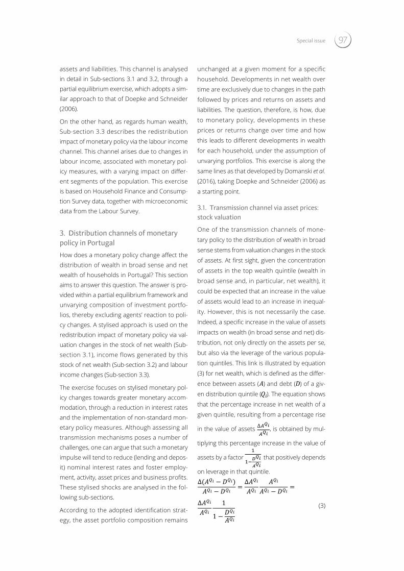
97Special issue
assets and liabilities. This channel is analysed in detail in Sub-sections 3.1 and 3.2, through a partial equilibrium exercise, which adopts a sim-ilar approach to that of Doepke and Schneider (2006).
On the other hand, as regards human wealth, Sub-section 3.3 describes the redistribution impact of monetary policy via the labour income channel. This channel arises due to changes in labour income, associated with monetary pol-icy measures, with a varying impact on differ-ent segments of the population. This exercise is based on Household Finance and Consump-tion Survey data, together with microeconomic data from the Labour Survey.
3. Distribution channels of monetary policy in PortugalHow does a monetary policy change affect the distribution of wealth in broad sense and net wealth of households in Portugal? This section aims to answer this question. The answer is pro-vided within a partial equilibrium framework and unvarying composition of investment portfo-lios, thereby excluding agents’ reaction to poli-cy changes. A stylised approach is used on the redistribution impact of monetary policy via val-uation changes in the stock of net wealth (Sub-section 3.1), income flows generated by this stock of net wealth (Sub-section 3.2) and labour income changes (Sub-section 3.3).
The exercise focuses on stylised monetary pol-icy changes towards greater monetary accom-modation, through a reduction in interest rates and the implementation of non-standard mon-etary policy measures. Although assessing all transmission mechanisms poses a number of challenges, one can argue that such a monetary impulse will tend to reduce (lending and depos-it) nominal interest rates and foster employ-ment, activity, asset prices and business profits. These stylised shocks are analysed in the fol-lowing sub-sections.
According to the adopted identification strat-egy, the asset portfolio composition remains
unchanged at a given moment for a specific
household. Developments in net wealth over
time are exclusively due to changes in the path
followed by prices and returns on assets and
liabilities. The question, therefore, is how, due
to monetary policy, developments in these
prices or returns change over time and how
this leads to different developments in wealth
for each household, under the assumption of
unvarying portfolios. This exercise is along the
same lines as that developed by Domanski et al.
(2016), taking Doepke and Schneider (2006) as
a starting point.
3.1. Transmission channel via asset prices: stock valuation
One of the transmission channels of mone-
tary policy to the distribution of wealth in broad
sense stems from valuation changes in the stock
of assets. At first sight, given the concentration
of assets in the top wealth quintile (wealth in
broad sense and, in particular, net wealth), it
could be expected that an increase in the value
of assets would lead to an increase in inequal-
ity. However, this is not necessarily the case.
Indeed, a specific increase in the value of assets
impacts on wealth (in broad sense and net) dis-
tribution, not only directly on the assets per se,
but also via the leverage of the various popula-
tion quintiles. This link is illustrated by equation
(3) for net wealth, which is defined as the differ-
ence between assets (
10
desta natureza tenderá a diminuir as taxas de juro nominais (ativas e passivas) e a
aumentar o emprego, a atividade, os preços dos ativos e os lucros das empresas. Estes
são os choques estilizados a analisar nas subseções seguintes.
A estratégia de identificação adotada mantém fixa a composição da carteira de ativos
num determinado momento para uma determinada família. A evolução do valor da
riqueza líquida ao longo do tempo é devida unicamente a alterações nas trajetórias de
preços e retornos dos ativos e responsabilidades. A questão será então como, devido à
política monetária, se altera a evolução ao longo do tempo destes preços ou retornos e
como daí decorre uma evolução diferente da riqueza de cada família, sob a hipótese de
carteiras invariantes. Trata‐se de um exercício na mesma linha do desenvolvido por
Domanski et al. (2016), partindo de Doepke e Schneider (2006).
3.1 Canal de transmissão pelos preços dos ativos: valorização do stock
Um dos canais de transmissão da política monetária à distribuição da riqueza em sentido
lato decorre de alterações na valorização do stock de ativos. À primeira vista, poderia
parecer que, dada a concentração dos ativos no último quintil da riqueza (em sentido
lato e, em particular, em termos líquidos), um aumento do valor dos ativos implicaria
um aumento da desigualdade. Esta conclusão não é, no entanto, correta. De facto, um
determinado aumento do valor dos ativos impacta a distribuição da riqueza (em sentido
lato e líquida) não só diretamente nos próprios ativos, mas também através do grau de
alavancagem dos diferentes quintis da população. Esta relação encontra‐se explicitada
na equação (3) para o caso da riqueza líquida, definida como a diferença entre os Ativos
(�) e as Dívidas (�) de um dado quintil da distribuição (��). A equação revela que o aumento percentual da riqueza líquida de um determinado quintil, decorrente de um
aumento percentual do valor dos ativos ����
��� , será igual ao produto entre esse aumento
percentual do valor dos ativos e um fator ���������
que depende positivamente do grau de
alavancagem desse quintil.
����� � ������� � ��� � ����
������
��� � ��� ��������
11 � ���
������
) and debt (
10
desta natureza tenderá a diminuir as taxas de juro nominais (ativas e passivas) e a
aumentar o emprego, a atividade, os preços dos ativos e os lucros das empresas. Estes
são os choques estilizados a analisar nas subseções seguintes.
A estratégia de identificação adotada mantém fixa a composição da carteira de ativos
num determinado momento para uma determinada família. A evolução do valor da
riqueza líquida ao longo do tempo é devida unicamente a alterações nas trajetórias de
preços e retornos dos ativos e responsabilidades. A questão será então como, devido à
política monetária, se altera a evolução ao longo do tempo destes preços ou retornos e
como daí decorre uma evolução diferente da riqueza de cada família, sob a hipótese de
carteiras invariantes. Trata‐se de um exercício na mesma linha do desenvolvido por
Domanski et al. (2016), partindo de Doepke e Schneider (2006).
3.1 Canal de transmissão pelos preços dos ativos: valorização do stock
Um dos canais de transmissão da política monetária à distribuição da riqueza em sentido
lato decorre de alterações na valorização do stock de ativos. À primeira vista, poderia
parecer que, dada a concentração dos ativos no último quintil da riqueza (em sentido
lato e, em particular, em termos líquidos), um aumento do valor dos ativos implicaria
um aumento da desigualdade. Esta conclusão não é, no entanto, correta. De facto, um
determinado aumento do valor dos ativos impacta a distribuição da riqueza (em sentido
lato e líquida) não só diretamente nos próprios ativos, mas também através do grau de
alavancagem dos diferentes quintis da população. Esta relação encontra‐se explicitada
na equação (3) para o caso da riqueza líquida, definida como a diferença entre os Ativos
(�) e as Dívidas (�) de um dado quintil da distribuição (��). A equação revela que o aumento percentual da riqueza líquida de um determinado quintil, decorrente de um
aumento percentual do valor dos ativos ����
��� , será igual ao produto entre esse aumento
percentual do valor dos ativos e um fator ���������
que depende positivamente do grau de
alavancagem desse quintil.
����� � ������� � ��� � ����
������
��� � ��� ��������
11 � ���
������
) of a giv-
en distribution quintile (
10
desta natureza tenderá a diminuir as taxas de juro nominais (ativas e passivas) e a
aumentar o emprego, a atividade, os preços dos ativos e os lucros das empresas. Estes
são os choques estilizados a analisar nas subseções seguintes.
A estratégia de identificação adotada mantém fixa a composição da carteira de ativos
num determinado momento para uma determinada família. A evolução do valor da
riqueza líquida ao longo do tempo é devida unicamente a alterações nas trajetórias de
preços e retornos dos ativos e responsabilidades. A questão será então como, devido à
política monetária, se altera a evolução ao longo do tempo destes preços ou retornos e
como daí decorre uma evolução diferente da riqueza de cada família, sob a hipótese de
carteiras invariantes. Trata‐se de um exercício na mesma linha do desenvolvido por
Domanski et al. (2016), partindo de Doepke e Schneider (2006).
3.1 Canal de transmissão pelos preços dos ativos: valorização do stock
Um dos canais de transmissão da política monetária à distribuição da riqueza em sentido
lato decorre de alterações na valorização do stock de ativos. À primeira vista, poderia
parecer que, dada a concentração dos ativos no último quintil da riqueza (em sentido
lato e, em particular, em termos líquidos), um aumento do valor dos ativos implicaria
um aumento da desigualdade. Esta conclusão não é, no entanto, correta. De facto, um
determinado aumento do valor dos ativos impacta a distribuição da riqueza (em sentido
lato e líquida) não só diretamente nos próprios ativos, mas também através do grau de
alavancagem dos diferentes quintis da população. Esta relação encontra‐se explicitada
na equação (3) para o caso da riqueza líquida, definida como a diferença entre os Ativos
(�) e as Dívidas (�) de um dado quintil da distribuição (��). A equação revela que o aumento percentual da riqueza líquida de um determinado quintil, decorrente de um
aumento percentual do valor dos ativos ����
��� , será igual ao produto entre esse aumento
percentual do valor dos ativos e um fator ���������
que depende positivamente do grau de
alavancagem desse quintil.
����� � ������� � ��� � ����
������
��� � ��� ��������
11 � ���
������
). The equation shows
that the percentage increase in net wealth of a
given quintile, resulting from a percentage rise
in the value of assets
10
desta natureza tenderá a diminuir as taxas de juro nominais (ativas e passivas) e a
aumentar o emprego, a atividade, os preços dos ativos e os lucros das empresas. Estes
são os choques estilizados a analisar nas subseções seguintes.
A estratégia de identificação adotada mantém fixa a composição da carteira de ativos
num determinado momento para uma determinada família. A evolução do valor da
riqueza líquida ao longo do tempo é devida unicamente a alterações nas trajetórias de
preços e retornos dos ativos e responsabilidades. A questão será então como, devido à
política monetária, se altera a evolução ao longo do tempo destes preços ou retornos e
como daí decorre uma evolução diferente da riqueza de cada família, sob a hipótese de
carteiras invariantes. Trata‐se de um exercício na mesma linha do desenvolvido por
Domanski et al. (2016), partindo de Doepke e Schneider (2006).
3.1 Canal de transmissão pelos preços dos ativos: valorização do stock
Um dos canais de transmissão da política monetária à distribuição da riqueza em sentido
lato decorre de alterações na valorização do stock de ativos. À primeira vista, poderia
parecer que, dada a concentração dos ativos no último quintil da riqueza (em sentido
lato e, em particular, em termos líquidos), um aumento do valor dos ativos implicaria
um aumento da desigualdade. Esta conclusão não é, no entanto, correta. De facto, um
determinado aumento do valor dos ativos impacta a distribuição da riqueza (em sentido
lato e líquida) não só diretamente nos próprios ativos, mas também através do grau de
alavancagem dos diferentes quintis da população. Esta relação encontra‐se explicitada
na equação (3) para o caso da riqueza líquida, definida como a diferença entre os Ativos
(�) e as Dívidas (�) de um dado quintil da distribuição (��). A equação revela que o aumento percentual da riqueza líquida de um determinado quintil, decorrente de um
aumento percentual do valor dos ativos ����
��� , será igual ao produto entre esse aumento
percentual do valor dos ativos e um fator ���������
que depende positivamente do grau de
alavancagem desse quintil.
����� � ������� � ��� � ����
������
��� � ��� ��������
11 � ���
������
, is obtained by mul-
tiplying this percentage increase in the value of
assets by a factor that positively depends
on leverage in that quintile.
10
desta natureza tenderá a diminuir as taxas de juro nominais (ativas e passivas) e a
aumentar o emprego, a atividade, os preços dos ativos e os lucros das empresas. Estes
são os choques estilizados a analisar nas subseções seguintes.
A estratégia de identificação adotada mantém fixa a composição da carteira de ativos
num determinado momento para uma determinada família. A evolução do valor da
riqueza líquida ao longo do tempo é devida unicamente a alterações nas trajetórias de
preços e retornos dos ativos e responsabilidades. A questão será então como, devido à
política monetária, se altera a evolução ao longo do tempo destes preços ou retornos e
como daí decorre uma evolução diferente da riqueza de cada família, sob a hipótese de
carteiras invariantes. Trata‐se de um exercício na mesma linha do desenvolvido por
Domanski et al. (2016), partindo de Doepke e Schneider (2006).
3.1 Canal de transmissão pelos preços dos ativos: valorização do stock
Um dos canais de transmissão da política monetária à distribuição da riqueza em sentido
lato decorre de alterações na valorização do stock de ativos. À primeira vista, poderia
parecer que, dada a concentração dos ativos no último quintil da riqueza (em sentido
lato e, em particular, em termos líquidos), um aumento do valor dos ativos implicaria
um aumento da desigualdade. Esta conclusão não é, no entanto, correta. De facto, um
determinado aumento do valor dos ativos impacta a distribuição da riqueza (em sentido
lato e líquida) não só diretamente nos próprios ativos, mas também através do grau de
alavancagem dos diferentes quintis da população. Esta relação encontra‐se explicitada
na equação (3) para o caso da riqueza líquida, definida como a diferença entre os Ativos
(�) e as Dívidas (�) de um dado quintil da distribuição (��). A equação revela que o aumento percentual da riqueza líquida de um determinado quintil, decorrente de um
aumento percentual do valor dos ativos ����
��� , será igual ao produto entre esse aumento
percentual do valor dos ativos e um fator ���������
que depende positivamente do grau de
alavancagem desse quintil.
����� � ������� � ��� � ����
������
��� � ��� ��������
11 � ���
������
(3)
10
desta natureza tenderá a diminuir as taxas de juro nominais (ativas e passivas) e a
aumentar o emprego, a atividade, os preços dos ativos e os lucros das empresas. Estes
são os choques estilizados a analisar nas subseções seguintes.
A estratégia de identificação adotada mantém fixa a composição da carteira de ativos
num determinado momento para uma determinada família. A evolução do valor da
riqueza líquida ao longo do tempo é devida unicamente a alterações nas trajetórias de
preços e retornos dos ativos e responsabilidades. A questão será então como, devido à
política monetária, se altera a evolução ao longo do tempo destes preços ou retornos e
como daí decorre uma evolução diferente da riqueza de cada família, sob a hipótese de
carteiras invariantes. Trata‐se de um exercício na mesma linha do desenvolvido por
Domanski et al. (2016), partindo de Doepke e Schneider (2006).
3.1 Canal de transmissão pelos preços dos ativos: valorização do stock
Um dos canais de transmissão da política monetária à distribuição da riqueza em sentido
lato decorre de alterações na valorização do stock de ativos. À primeira vista, poderia
parecer que, dada a concentração dos ativos no último quintil da riqueza (em sentido
lato e, em particular, em termos líquidos), um aumento do valor dos ativos implicaria
um aumento da desigualdade. Esta conclusão não é, no entanto, correta. De facto, um
determinado aumento do valor dos ativos impacta a distribuição da riqueza (em sentido
lato e líquida) não só diretamente nos próprios ativos, mas também através do grau de
alavancagem dos diferentes quintis da população. Esta relação encontra‐se explicitada
na equação (3) para o caso da riqueza líquida, definida como a diferença entre os Ativos
(�) e as Dívidas (�) de um dado quintil da distribuição (��). A equação revela que o aumento percentual da riqueza líquida de um determinado quintil, decorrente de um
aumento percentual do valor dos ativos ����
��� , será igual ao produto entre esse aumento
percentual do valor dos ativos e um fator ���������
que depende positivamente do grau de
alavancagem desse quintil.
����� � ������� � ��� � ����
������
��� � ��� ��������
11 � ���
������

BANCO DE PORTUGAL • Economic Bulletin • May 201798
In the case of wealth in broad sense, the impact
of changes in assets is illustrated by equation (4).
In this case, the wealth aggregate includes human
wealth,
a percentage rise in the value of assets ( ), is obtained by multiplying this percentage increase in the value
of assets by a factor ( ) that positively depends on leverage in that quintile.
( ) (3)
In the case of wealth in broad sense, the impact of changes in assets is illustrated by equation (4). In this case, the wealth aggregate includes human wealth, ( ), and, therefore, the impact of a percentage increase in assets is not only positively related to leverage in each quintile but also negatively related to the ratio of human wealth to total assets in each quintile:
( )
(4)
As such, to assess the distribution impact via this transmission channel, it is necessary to look into the link between the asset aggregate and the amount of liabilities held by each household typifying the distribution quintiles. This link is shown in Charts 1 and 2, for the distribution of wealth in broad sense and net wealth respectively. The slope of the lines for each quintile corresponds to leverage, measured by the debt-to-assets ratio. The charts show that the highest wealth quintiles (both net and in broad sense) have the lowest leverage.
In the case of net wealth, the Portuguese economy is characterised by a population where growing wealth corresponds to a decreasing indebtedness ratio. This is highly significant and implies that a similar percentage increase in the value of assets across net wealth distribution quintiles always improves the relative position of the lowest quintiles vis-à-vis the average quintile and the highest quintiles. This means that higher asset values increase relatively more the net wealth of poorer households, regardless of asset concentration. Similarly, in the case of a decrease in the value of assets, more leveraged households would post a larger decline in net wealth.
In the case of the distribution of wealth in broad sense across quintiles, the link between leverage and wealth is not so clearly monotonic (excluding the highest quintile). Therefore, in the case of a homogeneous increase in the value of assets, the final impact on inequality will result from the weighing of the relative share of human wealth in assets and leverage, as illustrated by equation (4). Chart 3 shows that the ratio of human wealth to assets (the term ( ) in equation (4)) is lower for the highest quintile of
wealth in broad sense than for the other quintiles, in contrast to the lower leverage in this quintile. Only an empirical simulation reveals which effect is predominant. Chart 4 shows this ratio for net wealth quintiles, but has no role in the analysis.
For that purpose, Table 3 (first column) presents a stylised simulation of the impact of changes in the value of assets for some interquintile ratios, in the case of both the wealth in broad sense and the net wealth distributions. Calculations were made on the basis of the Household Finance and Consumption Survey for 2010. The table confirms that a similar percentage increase in the value of assets across distribution quintiles fosters inequality in the distribution of wealth in broad sense and reduces inequality in net wealth distribution.
The table also breaks down the impact of the valuation of the various assets held by households. Assets are typically broken down into real assets and financial assets. Real assets chiefly include real estate and self-employment businesses5, and hold a large share in net wealth of households in Portugal and most euro area
, and, therefore, the impact of a per-
centage increase in assets is not only positively
related to leverage in each quintile but also nega-
tively related to the ratio of human wealth to total
assets in each quintile:
a percentage rise in the value of assets ( ), is obtained by multiplying this percentage increase in the value
of assets by a factor ( ) that positively depends on leverage in that quintile.
( ) (3)
In the case of wealth in broad sense, the impact of changes in assets is illustrated by equation (4). In this case, the wealth aggregate includes human wealth, ( ), and, therefore, the impact of a percentage increase in assets is not only positively related to leverage in each quintile but also negatively related to the ratio of human wealth to total assets in each quintile:
( )
(4)
As such, to assess the distribution impact via this transmission channel, it is necessary to look into the link between the asset aggregate and the amount of liabilities held by each household typifying the distribution quintiles. This link is shown in Charts 1 and 2, for the distribution of wealth in broad sense and net wealth respectively. The slope of the lines for each quintile corresponds to leverage, measured by the debt-to-assets ratio. The charts show that the highest wealth quintiles (both net and in broad sense) have the lowest leverage.
In the case of net wealth, the Portuguese economy is characterised by a population where growing wealth corresponds to a decreasing indebtedness ratio. This is highly significant and implies that a similar percentage increase in the value of assets across net wealth distribution quintiles always improves the relative position of the lowest quintiles vis-à-vis the average quintile and the highest quintiles. This means that higher asset values increase relatively more the net wealth of poorer households, regardless of asset concentration. Similarly, in the case of a decrease in the value of assets, more leveraged households would post a larger decline in net wealth.
In the case of the distribution of wealth in broad sense across quintiles, the link between leverage and wealth is not so clearly monotonic (excluding the highest quintile). Therefore, in the case of a homogeneous increase in the value of assets, the final impact on inequality will result from the weighing of the relative share of human wealth in assets and leverage, as illustrated by equation (4). Chart 3 shows that the ratio of human wealth to assets (the term ( ) in equation (4)) is lower for the highest quintile of
wealth in broad sense than for the other quintiles, in contrast to the lower leverage in this quintile. Only an empirical simulation reveals which effect is predominant. Chart 4 shows this ratio for net wealth quintiles, but has no role in the analysis.
For that purpose, Table 3 (first column) presents a stylised simulation of the impact of changes in the value of assets for some interquintile ratios, in the case of both the wealth in broad sense and the net wealth distributions. Calculations were made on the basis of the Household Finance and Consumption Survey for 2010. The table confirms that a similar percentage increase in the value of assets across distribution quintiles fosters inequality in the distribution of wealth in broad sense and reduces inequality in net wealth distribution.
The table also breaks down the impact of the valuation of the various assets held by households. Assets are typically broken down into real assets and financial assets. Real assets chiefly include real estate and self-employment businesses5, and hold a large share in net wealth of households in Portugal and most euro area
(4)
a percentage rise in the value of assets ( ), is obtained by multiplying this percentage increase in the value
of assets by a factor ( ) that positively depends on leverage in that quintile.
( ) (3)
In the case of wealth in broad sense, the impact of changes in assets is illustrated by equation (4). In this case, the wealth aggregate includes human wealth, ( ), and, therefore, the impact of a percentage increase in assets is not only positively related to leverage in each quintile but also negatively related to the ratio of human wealth to total assets in each quintile:
( )
(4)
As such, to assess the distribution impact via this transmission channel, it is necessary to look into the link between the asset aggregate and the amount of liabilities held by each household typifying the distribution quintiles. This link is shown in Charts 1 and 2, for the distribution of wealth in broad sense and net wealth respectively. The slope of the lines for each quintile corresponds to leverage, measured by the debt-to-assets ratio. The charts show that the highest wealth quintiles (both net and in broad sense) have the lowest leverage.
In the case of net wealth, the Portuguese economy is characterised by a population where growing wealth corresponds to a decreasing indebtedness ratio. This is highly significant and implies that a similar percentage increase in the value of assets across net wealth distribution quintiles always improves the relative position of the lowest quintiles vis-à-vis the average quintile and the highest quintiles. This means that higher asset values increase relatively more the net wealth of poorer households, regardless of asset concentration. Similarly, in the case of a decrease in the value of assets, more leveraged households would post a larger decline in net wealth.
In the case of the distribution of wealth in broad sense across quintiles, the link between leverage and wealth is not so clearly monotonic (excluding the highest quintile). Therefore, in the case of a homogeneous increase in the value of assets, the final impact on inequality will result from the weighing of the relative share of human wealth in assets and leverage, as illustrated by equation (4). Chart 3 shows that the ratio of human wealth to assets (the term ( ) in equation (4)) is lower for the highest quintile of
wealth in broad sense than for the other quintiles, in contrast to the lower leverage in this quintile. Only an empirical simulation reveals which effect is predominant. Chart 4 shows this ratio for net wealth quintiles, but has no role in the analysis.
For that purpose, Table 3 (first column) presents a stylised simulation of the impact of changes in the value of assets for some interquintile ratios, in the case of both the wealth in broad sense and the net wealth distributions. Calculations were made on the basis of the Household Finance and Consumption Survey for 2010. The table confirms that a similar percentage increase in the value of assets across distribution quintiles fosters inequality in the distribution of wealth in broad sense and reduces inequality in net wealth distribution.
The table also breaks down the impact of the valuation of the various assets held by households. Assets are typically broken down into real assets and financial assets. Real assets chiefly include real estate and self-employment businesses5, and hold a large share in net wealth of households in Portugal and most euro area
As such, to assess the distribution impact via
this transmission channel, it is necessary to look
into the link between the asset aggregate and
the amount of liabilities held by each household
typifying the distribution quintiles. This link is
shown in Charts 1 and 2, for the distribution of
wealth in broad sense and net wealth respec-
tively. The slope of the lines for each quintile
corresponds to leverage, measured by the debt-
to-assets ratio. The charts show that the highest
wealth quintiles (both net and in broad sense)
have the lowest leverage.
In the case of net wealth, the Portuguese econo-
my is characterised by a population where grow-
ing wealth corresponds to a decreasing indebt-
edness ratio. This is highly significant and implies
that a similar percentage increase in the value
of assets across net wealth distribution quintiles
always improves the relative position of the low-
est quintiles vis-à-vis the average quintile and the
highest quintiles. This means that higher asset
values increase relatively more the net wealth
of poorer households, regardless of asset con-
centration. Similarly, in the case of a decrease in
the value of assets, more leveraged households
would post a larger decline in net wealth.
In the case of the distribution of wealth in broad
sense across quintiles, the link between leverage
and wealth is not so clearly monotonic (exclud-
ing the highest quintile). Therefore, in the case of
a homogeneous increase in the value of assets,
the final impact on inequality will result from the
weighing of the relative share of human wealth
in assets and leverage, as illustrated by equation
(4). Chart 3 shows that the ratio of human wealth
to assets (the term
a percentage rise in the value of assets ( ), is obtained by multiplying this percentage increase in the value
of assets by a factor ( ) that positively depends on leverage in that quintile.
( ) (3)
In the case of wealth in broad sense, the impact of changes in assets is illustrated by equation (4). In this case, the wealth aggregate includes human wealth, ( ), and, therefore, the impact of a percentage increase in assets is not only positively related to leverage in each quintile but also negatively related to the ratio of human wealth to total assets in each quintile:
( )
(4)
As such, to assess the distribution impact via this transmission channel, it is necessary to look into the link between the asset aggregate and the amount of liabilities held by each household typifying the distribution quintiles. This link is shown in Charts 1 and 2, for the distribution of wealth in broad sense and net wealth respectively. The slope of the lines for each quintile corresponds to leverage, measured by the debt-to-assets ratio. The charts show that the highest wealth quintiles (both net and in broad sense) have the lowest leverage.
In the case of net wealth, the Portuguese economy is characterised by a population where growing wealth corresponds to a decreasing indebtedness ratio. This is highly significant and implies that a similar percentage increase in the value of assets across net wealth distribution quintiles always improves the relative position of the lowest quintiles vis-à-vis the average quintile and the highest quintiles. This means that higher asset values increase relatively more the net wealth of poorer households, regardless of asset concentration. Similarly, in the case of a decrease in the value of assets, more leveraged households would post a larger decline in net wealth.
In the case of the distribution of wealth in broad sense across quintiles, the link between leverage and wealth is not so clearly monotonic (excluding the highest quintile). Therefore, in the case of a homogeneous increase in the value of assets, the final impact on inequality will result from the weighing of the relative share of human wealth in assets and leverage, as illustrated by equation (4). Chart 3 shows that the ratio of human wealth to assets (the term ( ) in equation (4)) is lower for the highest quintile of
wealth in broad sense than for the other quintiles, in contrast to the lower leverage in this quintile. Only an empirical simulation reveals which effect is predominant. Chart 4 shows this ratio for net wealth quintiles, but has no role in the analysis.
For that purpose, Table 3 (first column) presents a stylised simulation of the impact of changes in the value of assets for some interquintile ratios, in the case of both the wealth in broad sense and the net wealth distributions. Calculations were made on the basis of the Household Finance and Consumption Survey for 2010. The table confirms that a similar percentage increase in the value of assets across distribution quintiles fosters inequality in the distribution of wealth in broad sense and reduces inequality in net wealth distribution.
The table also breaks down the impact of the valuation of the various assets held by households. Assets are typically broken down into real assets and financial assets. Real assets chiefly include real estate and self-employment businesses5, and hold a large share in net wealth of households in Portugal and most euro area
in equation (4)) is lower
for the highest quintile of wealth in broad sense
than for the other quintiles, in contrast to the
lower leverage in this quintile. Only an empirical
simulation reveals which effect is predominant.
Chart 1 • Relation between assets and liabilities, by quintiles of wealth in broad sense
Chart 2 • Relation between assets and liabilities, by net wealth quintiles
Note: Based on the Household Finance and Consumption Survey for 2010.
Note: Based on the Household Finance and Consumption Survey for 2010.

99Special issue
Chart 4 shows this ratio for net wealth quintiles, but has no role in the analysis.
For that purpose, Table 3 (first column) presents a stylised simulation of the impact of changes in the value of assets for some interquintile ratios, in the case of both the wealth in broad sense and the net wealth distributions. Calculations were
made on the basis of the Household Finance
and Consumption Survey for 2010. The table
confirms that a similar percentage increase in
the value of assets across distribution quintiles
fosters inequality in the distribution of wealth
in broad sense and reduces inequality in net
wealth distribution.
Table 3 • Impact of changes in the value of assets on the distributions of wealth in broad sense and net wealth | Percentage changes in initial ratios, excluding ratio values
Ratios based on quintiles of wealth in broad sense
Initial ratios
10% increase in real estate,
tradable assets and businesses
10% increase in real estate
10% increase in tradable assets
10% increase in the values of businesses
(1) (2) (3) (4)
Q5/Q3 3.6 0.305 -0.277 0.063 0.533
Q5/Q1 11.9 0.343 -0.292 0.060 0.589
Average/Q3 1.4 0.150 -0.157 0.034 0.279
Ratios based on net wealth quintiles
Initial ratios
10% increase in real estate,
tradable assets and businesses
10% increase in real estate
10% increase in tradable assets
10% increase in the values of businesses
(1) (2) (3) (4)
Q5/Q3 6.7 -1.411 -3.221 0.120 1.877
Q5/Q1 412.4 -48.701 -49.625 -0.015 1.686
Average/Q3 2.0 -0.761 -1.967 0.076 1.255
Note: Calculations based on HFCS 2010.
Chart 3 • Relation between human wealth and assets, by quintiles of wealth in broad sense
Chart 4 • Relation between human wealth and assets, by net wealth quintiles
Note: Calculations based on the Household Finance and Consump-tion Survey for 2010.
Note: Calculations based on the Household Finance and Consump-tion Survey for 2010.

BANCO DE PORTUGAL • Economic Bulletin • May 2017100
The table also breaks down the impact of the val-uation of the various assets held by households. Assets are typically broken down into real assets and financial assets. Real assets chiefly include real estate and self-employment businesses5, and hold a large share in net wealth of households in Portugal and most euro area countries. In turn, financial assets mainly comprise deposits and marketable securities, including shares, bonds and mutual fund investment units.
In the case of a percentage increase in a com-ponent of total household assets, e.g. housing, represented as
15
Por seu turno, os ativos financeiros são fundamentalmente compostos por depósitos e
títulos transacionáveis, que incluem ações, obrigações e unidades de participação em
fundos de investimento.
Para o caso de um aumento percentual de uma componente do ativo total das famílias,
por exemplo a habitação, designada por ���, a equação (3), relativa à distribuição da
riqueza líquida, seria reescrita como segue (e analogamente a equação (4) para o caso
da riqueza em sentido lato):
����� � ������� � ��� � ����
���������
������ � ��� �
�������
������
11 � ���
����������������������������������������������
Deste modo, um mesmo aumento percentual nos preços da habitação nos diferentes
quintis impactará a distribuição da riqueza líquida em função do aumento percentual
nos preços da habitação de cada quintil, do peso da habitação no total dos ativos de
cada quintil, e do respetivo grau de alavancagem.
As colunas 2, 3 e 4 do Quadro 3 caracterizam o efeito na riqueza de aumentos de 10%
nos preços da habitação, no valor dos ativos financeiros transacionáveis e no valor dos
negócios por conta própria. Esta análise é particularmente interessante dada a perceção
de que a política monetária — em particular a política monetária não convencional —
teve um impacto significativo sobre a valorização destes ativos.
Os resultados do exercício revelam que um aumento nos preços da habitação contribui
para diminuir a desigualdade da distribuição da riqueza, visto que este ativo tem uma
importância relativamente homogénea nos diferentes quintis de riqueza, mas menor no
caso do quintil mais elevado de riqueza (Gráficos 5 e 6). Por seu turno, um aumento no
valor das ações, obrigações e fundos de investimento contribui tipicamente para
aumentar a desigualdade, em linha com a elevada desigualdade na distribuição destes
ativos, muito concentrados e com um peso relativamente elevado no último quintil da
distribuição (Gráficos 7 e 8). A única exceção é o rácio Q5/Q1 na distribuição de riqueza
líquida, o que decorre do impacto da elevada alavancagem no primeiro quintil de
riqueza líquida, tal como atrás explicado (ver Gráfico 2). Analogamente, o contributo dos
, equation (3) on net wealth distribution would be re-written as follows (and analogously for equation (4) on wealth in broad sense):
15
Por seu turno, os ativos financeiros são fundamentalmente compostos por depósitos e
títulos transacionáveis, que incluem ações, obrigações e unidades de participação em
fundos de investimento.
Para o caso de um aumento percentual de uma componente do ativo total das famílias,
por exemplo a habitação, designada por ���, a equação (3), relativa à distribuição da
riqueza líquida, seria reescrita como segue (e analogamente a equação (4) para o caso
da riqueza em sentido lato):
����� � ������� � ��� � ����
���������
������ � ��� �
�������
������
11 � ���
����������������������������������������������
Deste modo, um mesmo aumento percentual nos preços da habitação nos diferentes
quintis impactará a distribuição da riqueza líquida em função do aumento percentual
nos preços da habitação de cada quintil, do peso da habitação no total dos ativos de
cada quintil, e do respetivo grau de alavancagem.
As colunas 2, 3 e 4 do Quadro 3 caracterizam o efeito na riqueza de aumentos de 10%
nos preços da habitação, no valor dos ativos financeiros transacionáveis e no valor dos
negócios por conta própria. Esta análise é particularmente interessante dada a perceção
de que a política monetária — em particular a política monetária não convencional —
teve um impacto significativo sobre a valorização destes ativos.
Os resultados do exercício revelam que um aumento nos preços da habitação contribui
para diminuir a desigualdade da distribuição da riqueza, visto que este ativo tem uma
importância relativamente homogénea nos diferentes quintis de riqueza, mas menor no
caso do quintil mais elevado de riqueza (Gráficos 5 e 6). Por seu turno, um aumento no
valor das ações, obrigações e fundos de investimento contribui tipicamente para
aumentar a desigualdade, em linha com a elevada desigualdade na distribuição destes
ativos, muito concentrados e com um peso relativamente elevado no último quintil da
distribuição (Gráficos 7 e 8). A única exceção é o rácio Q5/Q1 na distribuição de riqueza
líquida, o que decorre do impacto da elevada alavancagem no primeiro quintil de
riqueza líquida, tal como atrás explicado (ver Gráfico 2). Analogamente, o contributo dos
(5)
15
Por seu turno, os ativos financeiros são fundamentalmente compostos por depósitos e
títulos transacionáveis, que incluem ações, obrigações e unidades de participação em
fundos de investimento.
Para o caso de um aumento percentual de uma componente do ativo total das famílias,
por exemplo a habitação, designada por ���, a equação (3), relativa à distribuição da
riqueza líquida, seria reescrita como segue (e analogamente a equação (4) para o caso
da riqueza em sentido lato):
����� � ������� � ��� � ����
���������
������ � ��� �
�������
������
11 � ���
����������������������������������������������
Deste modo, um mesmo aumento percentual nos preços da habitação nos diferentes
quintis impactará a distribuição da riqueza líquida em função do aumento percentual
nos preços da habitação de cada quintil, do peso da habitação no total dos ativos de
cada quintil, e do respetivo grau de alavancagem.
As colunas 2, 3 e 4 do Quadro 3 caracterizam o efeito na riqueza de aumentos de 10%
nos preços da habitação, no valor dos ativos financeiros transacionáveis e no valor dos
negócios por conta própria. Esta análise é particularmente interessante dada a perceção
de que a política monetária — em particular a política monetária não convencional —
teve um impacto significativo sobre a valorização destes ativos.
Os resultados do exercício revelam que um aumento nos preços da habitação contribui
para diminuir a desigualdade da distribuição da riqueza, visto que este ativo tem uma
importância relativamente homogénea nos diferentes quintis de riqueza, mas menor no
caso do quintil mais elevado de riqueza (Gráficos 5 e 6). Por seu turno, um aumento no
valor das ações, obrigações e fundos de investimento contribui tipicamente para
aumentar a desigualdade, em linha com a elevada desigualdade na distribuição destes
ativos, muito concentrados e com um peso relativamente elevado no último quintil da
distribuição (Gráficos 7 e 8). A única exceção é o rácio Q5/Q1 na distribuição de riqueza
líquida, o que decorre do impacto da elevada alavancagem no primeiro quintil de
riqueza líquida, tal como atrás explicado (ver Gráfico 2). Analogamente, o contributo dos
As such, a similar percentage increase in housing prices across quintiles will impact on net wealth distribution according to the share of housing in total assets and leverage for each quintile.
Columns 2, 3 and 4 of Table 3 illustrate the effect on wealth of 10% increases in housing prices, on the value of marketable financial assets and on the value of self-employment businesses. This analysis is particularly useful given the perception that monetary policy – in particular, non-standard monetary policy – had a sizeable impact on the increase in value of these assets.
The exercise demonstrates that an increase in housing prices helps reduce inequality in wealth distribution, given that housing has a relatively homogenous importance across wealth quin-tiles, but lower in the case of the highest wealth quintile (Charts 5 and 6). In turn, an increase in the value of shares, bonds and mutual funds typically contributes to an increase in inequality, in line with the high inequality in the distribution of these assets, which are greatly concentrated and hold a relatively high share in the last distribution quintile (Charts 7 and 8). The sole exception is the Q5/Q1 ratio in net wealth distribution, stemming
from the impact of high leverage on the first net wealth quintile, as explained above (see Chart 2). Similarly, self-employment businesses also con-tribute, as expected, towards increased inequality in wealth distribution.
3.2. Transmission channel via return on net assets: income flows
A monetary policy change may lead to transfor-mations in the distribution of household wealth, not only due to changes in asset valuation (Sub-section 3.1), but also due to changes in income flows stemming from policy changes. This sub-section analyses the issue, once again by simu-lating stylised shocks applied to microeconomic data available in the Household Finance and Con-sumption Survey for 2010. More specifically, the stylised exercise consists in assessing the impact on the distribution of net wealth and wealth in broad sense of: (i) a 4 p.p. reduction in the inter-est rate on time deposits, (ii) a 4 p.p. increase in the return rate on self-employment businesses, and (iii) a 4 p.p. reduction in interest rates on con-sumer loans and housing loans.
This exercise is based on a number of assump-tions. First, it is once again assumed that no deci-sions have been made on wealth composition. It only varies due to changes in interest/return rates. Second, it takes into account a change in interest rates from 5% to 1% and a change in return on self-employment businesses from 1% to 5%, although results are relatively robust to other rate levels compatible with a similar 4 p.p. change. Third, it is assumed that, among depos-its, only time deposits bear interest. Fourth, the reduction in interest rates affects all time depos-its and housing loans, taking into account a resid-ual maturity of one year in deposits and the fact that housing loans typically have a floating rate. Fifth, it is assumed that the reduction in inter-est rates affects 40% of consumer loans, with a residual average maturity of 2.5 years. Finally, the exercise assumes that time deposits mature over this period and that interest is reinvested. Similarly, it is assumed that debt maturing over this period is refinanced, including interest.

101Special issue
Table 4 shows results for this exercise, simu-lating shocks that will tend to follow an expan-sionary monetary policy shock. Its main conclu-sions are as follows. First, on the asset side, a decrease in return on time deposits leads to an increase in net wealth inequality (column 1), reflecting the combination of greater leverage for poorer households and a relatively similar share of time deposits in total assets among the Q1, Q3 and Q5 net wealth distribution quin-tiles (Chart 10). In the case of wealth in broad sense, the decrease in return on deposits helps reduce inequality. In wealth in broad sense, both the dispersion in the share of deposits in total assets and the dispersion in leverage across household quintiles – in particular, the
Q1, Q3 and Q5 quintiles – is lower than in net wealth (Chart 9). Second, an increase in return on businesses leads to greater inequality, due to their greater share of the highest wealth (net and in broad sense) quintiles (column 2). Third, a decline in loan rates tends to reduce inequali-ty, given that leverage is relatively greater in the lowest wealth quintiles, particularly in the case of net wealth. This conclusion stands both for housing loans and consumer and other loans (columns 3 and 4). The smaller reduction in inequality in the case of wealth in broad sense is due to the lower dispersion in leverage as well as the fact that loans are more unevenly distributed across quintiles in this case.
Chart 5 • Relation between real estate and total assets, by quintiles of wealth in broad sense
Chart 6 • Relation between real estate and total assets, by net wealth quintiles
Note: Calculations based on the Household Finance and Consumption Survey for 2010.
Note: Calculations based on the Household Finance and Consumption Survey for 2010.
Chart 7 • Relation between tradable assets and total assets, by quintiles of wealth in broad sense
Chart 8 • Relation between tradable assets and total assets, by net wealth quintiles
Note: Calculations based on the Household Finance and Consumption Survey for 2010.
Note: Calculations based on the Household Finance and Consumption Survey for 2010.

BANCO DE PORTUGAL • Economic Bulletin • May 2017102
Table 4 • Impact of changes in income flows on the distributions of wealth in broad sense and net wealth | Percentage changes in initial ratios, excluding ratio values
Ratios based on quintiles of wealth in broad sense
Initial ratios
4 pp decrease in the interest
rate on deposits
4 pp increase in the rate of return
of businesses
4 pp decrease in the interest
rate on housing loans
4 pp decrease in the interest
rate on consumer loans
(1) (2) (3) (4)
Q5/Q3 3.6 -0.004 0.158 -0.004 -0.002
Q5/Q1 11.9 -0.006 0.175 -0.004 -0.003
Average/Q3 1.4 -0.001 0.083 -0.002 -0.001
Ratios based on net wealth quintiles
Initial ratios
4 pp decrease in the interest
rate on deposits
4 pp increase in the rate of return
of businesses
4 pp decrease in the interest
rate on housing loans
4 pp decrease in the interest
rate on consumer loans
(1) (2) (3) (4)
Q5/Q3 6.7 0.041 0.558 -0.042 -0.011
Q5/Q1 412.4 0.702 0.502 -2.242 -1.433
Average/Q3 2.0 0.027 0.373 -0.024 -0.005
Note: Calculations based on HFCS 2010.
3.3. Labour income channel: the redistribu-tion impact on human wealth
Monetary policy may also have redistribution effects due to the heterogeneous impact on labour remuneration developments. This het-erogeneity stems from the combination of two factors: on the one hand, cyclical labour market transitions are known to differ across demo-graphic groups; on the other hand, the distri-bution of the various demographic groups is uneven across wealth (net and in broad sense) quintiles. Several authors have documented that expansionary monetary policy dispropor-tionally reduces unemployment for young peo-ple and less qualified workers. If these popula-tion segments are predominant in the lowest wealth distribution quintiles, an expansionary monetary policy will tend to reduce inequality in the respective wealth distribution.
This section analyses the potential importance of this channel in the case of the Portuguese
economy, based on microeconomic data from the Labour Survey and the Household Finance and Consumption Survey. The exercise first shows that, comparing the 2011–13 recession with the recovery phase in 2013–16, a considera-ble heterogeneity emerges in transitions between employment and unemployment according to age and qualification. Afterwards, evidence is pre-sented on how individuals are unevenly distribut-ed across quintiles of wealth in broad sense and net wealth. Given the two time periods under review, in this stage, the exercise used data from the Household Finance and Consumption Survey for 2013, which provides a better picture of the 2011–16 period. Finally, the exercise looks into the redistribution impact of a 1% increase in net employment growth on the Portuguese economy.
Since the first quarter of 2011, there have been two distinct stages in the Portuguese econ-omy.6 Up to the second quarter of 2013, an unprecedented recession in recent times took hold. Afterwards, a sustained recovery began,

103Special issue
although more gradual compared with previous economic upturn periods. The two periods are used as a reference to illustrate heterogeneity in flows between states in the labour market in the Portuguese economy. More specifically, the anal-ysis focuses on the percentage change in the frequency of transitions between employment and unemployment, and vice-versa, by break-ing down the labour force into four demographic groups according to two predetermined charac-teristics of individuals: age and qualification.
Unsurprisingly, transitions from employment to unemployment are more frequent for younger and less qualified individuals. Moreover, transi-tions from unemployment to employment are
more frequent for younger and more qualified individuals. Comparing the two periods under review, i.e. 2011 Q2-2013 Q2 and 2013 Q3-2016 Q4, the frequency of flows between employ-ment and unemployment declined by approxi-mately 25% and the frequency between unem-ployment and employment increased by around 18%, both in terms of average quarterly transi-tions. According to microeconomic data from the Labour Survey, the decrease in flows to unem-ployment was relatively broad-based across age groups and relatively more concentrated in less qualified groups, while the increase in flows to employment was relatively higher in younger and less qualified groups (Charts 11 and 12).
Chart 9 • Relation between savings deposits and total assets, by quintiles of wealth in broad sense
Chart 10 • Relation between savings deposits and total assets, by net wealth quintiles
Note: Calculations based on the Household Finance and Consumption Survey for 2010.
Note: Calculations based on the Household Finance and Consumption Survey for 2010.
Chart 11 • Change in the frequency of transitions from unemployment to employment, between 2011 Q3-2013 Q2 and 2013 Q3-2016 Q4 | In percentage
Chart 12 • Change in the frequency of transitions from employment to unemployment, betwee 2011 Q3-2013 Q2 and 2013Q3-2016 Q4
-10.0-5.00.05.0
10.015.020.025.030.035.040.0
Total (working-age
persons)
Age < 45 and education
below secondary
Age < 45 and education equal to or
above secondary
Age >= 45 and <65 and
education below
secondary
Age >= 45 and <65 and
education equal to or
above secondary
-35.0
-30.0
-25.0
-20.0
-15.0
-10.0
-5.0
0.0
Total (working-age
persons)
Age < 45 and education
below secondary
Age < 45 and education equal to or
above secondary
Age >= 45 and <65 and
education below
secondary
Age >= 45 and <65 and
education equal to or
above secondary
Source: Labour Survey. Source: Labour Survey.

BANCO DE PORTUGAL • Economic Bulletin • May 2017104
Charts 13 and 14 confirm that this heteroge-
neity affects differently the various quintiles of
the distributions of wealth in broad sense and
net wealth. In terms of qualifications, the charts
show that the less qualified labour force is rela-
tively more concentrated in the lowest quintiles
of both distributions. However, in terms of age
groups, the two distributions differ. Indeed, in the
distribution of wealth in broad sense, the share of
individuals under 45 in total labour force is rela-
tively stable across distribution quintiles, while as
regards net wealth distribution the share of indi-
viduals under 45 is relatively higher in the low-
est distribution quintiles. Furthermore, the share
of individuals aged 65 or more in total popula-
tion is relatively higher in the lowest quintiles of
the distribution of wealth in broad sense, while
as regards net wealth distribution the opposite
applies, i.e. older age groups are more concen-
trated in the highest net wealth quintiles.
The combination of these data suggests that
policies contributing to a rise in employment will
tend to affect the distributions of wealth in broad
sense and net wealth differently. To quantify
these effects on the Portuguese economy, a styl-
ised exercise was conducted, by cross-checking
data from the Labour Survey and the Household
Finance and Consumption Survey for 2013.
The exercise assessed the distribution impact
of a net increase in employment of 1%, taking
into account the circumstances characteris-
ing the economic recovery seen since 2013.
Based on the Labour Survey, a 1 p.p. growth
in employment was broken down into the four
aforementioned age groups (for the working-
age population), similarly to that seen between
2011 Q2–2013 Q2 and 2013 Q3–2016 Q4. Next,
the assumption was that this growth occurred
regardless of the wealth distribution quintile of
the individuals. Under the assumption that, for
each demographic group in each wealth quintile,
job creation implies an increase in labour income
corresponding to remuneration per capita of
workers in that population segment, it is possi-
ble to estimate income changes in each segment
stemming from the 1% aggregate shock on net
employment. To take into account the possible
existence of unemployment benefits, as well as
the fact that income arising from a re-entry to
the labour market is typically below the average,
it was assumed that the increase in income for
an individual that finds a job is only 50% of the
Chart 13 • Population structure, by quintiles of wealth in broad sense
Chart 14 • Population structure, by net wealth quintiles
0.000.100.200.300.400.500.600.700.800.901.00
Quintile 1 Quintile 2 Quintile 3 Quintile 4 Quintile 5Age >= 65Age >= 45 and <65 and education equal to or above secondaryAge >= 45 and <65 and education below secondaryAge < 45 and education equal to or above secondaryAge < 45 and education below secondary
Note: Calculations based on the Household Finance and Consumption Survey for 2013.
Note: Calculations based on the Household Finance and Consumption Survey for 2013.

105Special issue
income per worker calculated for each popula-
tion segment. This factor affects the magnitude
but not the sign of the results.
Finally, it was assumed that the increase in labour
income fosters both wealth in broad sense and
net wealth. In the case of wealth in broad sense,
monetary policy is assumed to have no perma-
nent real effects and, therefore, labour income
increases only have an impact during the peri-
od under review.7 In the case of net wealth, it
was assumed that the increase in income is fully
invested in assets, with no changes to the com-
position of household portfolios. This choice is
not straightforward, but takes into account that
additional income expands the range of options
open to households at the end of the period.
Given the assumptions made, a 1% increase
in net employment helps reduce inequality in
net wealth and, to a lesser extent, inequality in
wealth in broad sense. In the case of net wealth,
the ratio of the top to the bottom quintile (Q5/
Q1) falls by 3.8% and the Q5/Q3 ratio by 0.1%.8
In the case of wealth in broad sense, percentage
decreases in these ratios are lower. The smaller
redistribution impact on wealth in broad sense
results, inter alia, from the fact that: (i) the bot-
tom net wealth distribution quintile is associated
with very low wealth, (ii) a relatively larger share
of population aged over 65 – assumed, in this
exercise, to not be working – is included in the
bottom quintiles of the distribution of wealth in
broad sense, and (iii) younger groups account
for a relatively significant share in the top quin-
tiles of the distribution of wealth in broad sense.
4. Stylised quantification of the distribution impact of monetary policy in Portugal after 2010The previous sections looked into the impact of
stylised changes in prices and other relevant fac-
tors on wealth inequality indicators. This section
aggregates these channels in their entirety as a
response to monetary policy changes. The start-
ing point for this exercise is a stylised change in
monetary policy that causes a continuous reduc-tion in the short-term nominal interest rate for a long period of time. This monetary impulse leads to changes in factors affecting wealth distribu-tion. The ultimate goal is to compare the relative importance of the various channels to wealth distribution changes, while keeping in mind the merely stylised nature of this exercise.
Although it can be challenging to pinpoint all mechanisms at play, models can be used in order to rationalise such effects. For instance, in a Neo-Keynesian model, an unexpected reduction in the nominal interest rate leads to a decrease in sav-ings – given that saving has become less appeal-ing – and the resulting immediate increase in consumption. This direct effect produces a tem-porary rise in economic activity leading to upward pressure on labour demand by firms. The result-ing increase in wages and employment is an indirect effect of monetary policy changes, via general equilibrium mechanisms in this type of economy. This indirect mechanism will positive-ly affect human wealth of households and, possi-bly, net wealth too, as a result of the investment of additional resources in various assets.
A further example is the effect of economic activi-ty on the profits of privately-owned firms. Indeed, if, during the monetary stimulus period, GDP grows more rapidly than without the stimulus, corporate profits will also be greater, thus free-ing up additional resources to the households that own these firms. The accumulated addi-tional resources correspond to an increase in non-human wealth at the end of the period under review.
To calculate realistic paths for the main aggre-gate variables associated with monetary stimu-lus that may help in the exercise, the PESSOA model was estimated for the Portuguese econo-my (see Almeida et al., 2013 and Júlio and Maria, 2017). This stylised simulation calculates the effect of additional monetary accommodation on any baseline scenario.
To make this exercise more illustrative of the Por-
tuguese experience in the recent past, monetary
BANCO DE PORTUGAL • Economic Bulletin • May 2017106
accommodation is analysed from the end of
2010 onwards, immediately after the Household
Finance and Consumption Survey for 2010, with
this stimulus being extended up to the end
of 2015.
During this period, euro area short-term nom-
inal interest rates fell markedly. From 2014
onwards, standard monetary policy was large-
ly exhausted given that ECB key interest rates,
particularly the deposit facility interest rate, were
close to their lower bound.9 Following the intro-
duction in 2015 of non-standard monetary pol-
icy measures based on the purchase of sover-
eign debt securities and other assets, inter-
est rates impacting on households and firms
kept on decreasing. When the nominal interest
rate is close to the lower bound, the concept of
the ‘shadow‛ interest rate becomes useful. In an
economy where no lower bound is applied to
interest rates and non-standard monetary pol-
icy measures have not been implemented, this
interest rate would have accommodative mon-
etary effects similar to those in an economy with
an interest rate set at the lower bound and non-
standard monetary policy measures in place.
The calculation of such shadow interest rates
(see, e.g. Wu and Xia, 2017, as well as the refer-
ences in that study) shows that they continued
to decrease up to late 2016. This exercise gaug-
es the impact of interest rate cuts in a bench-
mark case, e.g. a less aggressive reaction by the
ECB in terms of monetary accommodation.
Chart 15 illustrates possible developments in a
number of aggregate variables of importance to
the exercise. The nominal interest rate declined
throughout the five-year period and was nor-
malised to a 3 p.p. reduction from the initial val-
ue.10 This cannot be interpreted as an estimate
of total monetary accommodation in the course
of the period, but merely as a quantitative
benchmark allowing a comparison of the relative
importance of the various channels analysed in
this article. This accommodation is exogenous
to the Portuguese economy, as it is decided at
euro area level. The PESSOA model also takes into account changes in demand for Portuguese goods and services by euro area countries, given that they are also affected by reductions in the nominal interest rates.
A 3 p.p. monetary accommodation leads to a cumulative increase in GDP during the five-year period of approximately 5.2%, compared to a scenario where no additional accommodation is implemented. Employment increases by around 3.9% and disposable income by approximate-ly 8.4%. The chart also illustrates developments in EBITDA as a percentage of assets in private Portuguese firms. These developments result from the impact on this corporate profitability measure of the increase in economic activity and, in particular, the increase in GDP during the peri-od under review.11 The monetary stimulus leads to an increase in EBITDA, which, cumulatively over the period, results in a 1.9% increase in val-ue for firms, under the assumption of a reinvest-ment of earnings.12 These additional resources add, therefore, to initial non-human wealth.
Monetary policy also has an indirect impact on the prices of a number of assets. In particular, mac-roeconomic developments illustrated in Chart 15 lead to changes in housing prices, which, in turn, result in a 1.2% increase from the initial situation.13
Table 5 shows the outcome, in terms of the distributions of wealth in broad sense and net wealth, of the path followed by a number of vari-ables compared to a benchmark case where there is no monetary stimulus. The exercise employs the same methods and assumptions regarding the increase in value of stocks and flows as described in Section 3. Given that this is a five-year period, labour income increases are accumulated over the five years taking into account the gradual rise in employment. For the sake of simplicity, only the Q5/Q3 and Q5/Q1 ratios are presented.
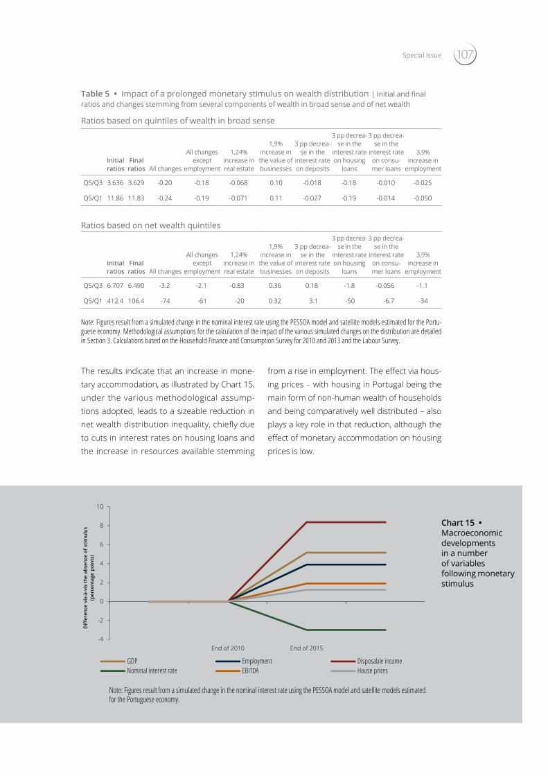
107Special issue
Table 5 • Impact of a prolonged monetary stimulus on wealth distribution | Initial and final ratios and changes stemming from several components of wealth in broad sense and of net wealth
Ratios based on quintiles of wealth in broad sense
Initial ratios
Final ratios All changes
All changes except
employment
1,24% increase in real estate
1,9% increase in the value of businesses
3 pp decrea-se in the
interest rate on deposits
3 pp decrea-se in the
interest rate on housing
loans
3 pp decrea-se in the
interest rate on consu-mer loans
3,9% increase in
employment
Q5/Q3 3.636 3.629 -0.20 -0.18 -0.068 0.10 -0.018 -0.18 -0.010 -0.025
Q5/Q1 11.86 11.83 -0.24 -0.19 -0.071 0.11 -0.027 -0.19 -0.014 -0.050
Ratios based on net wealth quintiles
Initial ratios
Final ratios All changes
All changes except
employment
1,24% increase in real estate
1,9% increase in the value of businesses
3 pp decrea-se in the
interest rate on deposits
3 pp decrea-se in the
interest rate on housing
loans
3 pp decrea-se in the
interest rate on consu-mer loans
3,9% increase in
employment
Q5/Q3 6.707 6.490 -3.2 -2.1 -0.83 0.36 0.18 -1.8 -0.056 -1.1
Q5/Q1 412.4 106.4 -74 -61 -20 0.32 3.1 -50 -6.7 -34
Note: Figures result from a simulated change in the nominal interest rate using the PESSOA model and satellite models estimated for the Portu-guese economy. Methodological assumptions for the calculation of the impact of the various simulated changes on the distribution are detailed in Section 3. Calculations based on the Household Finance and Consumption Survey for 2010 and 2013 and the Labour Survey.
The results indicate that an increase in mone-tary accommodation, as illustrated by Chart 15, under the various methodological assump-tions adopted, leads to a sizeable reduction in net wealth distribution inequality, chiefly due to cuts in interest rates on housing loans and the increase in resources available stemming
from a rise in employment. The effect via hous-ing prices – with housing in Portugal being the main form of non-human wealth of households and being comparatively well distributed – also plays a key role in that reduction, although the effect of monetary accommodation on housing prices is low.
-4
-2
0
2
4
6
8
10
End of 2010 End of 2015
Diff
eren
ce v
is-à
-vis
the
abse
nce
of s
timul
us
(per
cent
age
poin
ts)
GDP Employment Disposable incomeNominal interest rate EBITDA House prices
Chart 15 • Macroeconomic developments in a number of variables following monetary stimulus
Note: Figures result from a simulated change in the nominal interest rate using the PESSOA model and satellite models estimated for the Portuguese economy.
BANCO DE PORTUGAL • Economic Bulletin • May 2017108
In turn, improvements in corporate profitabi-
lity stemming from increased GDP growth con-
tribute to an increase in inequality, given that
households in the top two quintiles benefit the
most from this channel. However, households
in the bottom quintiles also benefit indirectly
from improvements in corporate profitability due
to a rise in employment, stemming from firms
distribution inequality.
Overall effects on wealth in broad sense are
lower than those in net wealth. Turning to the
impact of labour income, the underlying rea-
sons are analysed in Section 3 and include the
relatively larger share of population aged over
65 in the bottom quintiles of the distribution,
together with a higher share of younger and
more qualified individuals in the top quintiles.
As such, the boost given by monetary policy to
employment is broadly shared across popula-
tion groups.
The outcome of the exercise is broadly in line
with empirical and quantitative literature on the
impact of monetary policy on net wealth (see
Coibion et al., 2016, Deutsche Bundesbank, 2016
or Furceri et al., 2016). This study shows that, in
the case of Portugal and with certain caveats, the
outcome can also be applied to wealth in broad
sense, although in this case the impact is lower.
5. ConclusionsThis Special Issue looks into the distribution
effects of monetary policy using exercises based
on empirical data on the Portuguese econo-
my. First, wealth is characterised using House-
hold Finance and Consumption Survey data, as
well as Labour Survey microdata, and the various
channels affecting two types of wealth – wealth
in broad sense and net wealth – are analysed. It
is also demonstrated that households in quintiles
of wealth in broad sense are not necessarily those
of the corresponding net wealth quintiles. Exer-
cises conducted here assess in a stylised man-
ner the impact of increased monetary accom-
modation, which will tend to lead to increases
in asset prices, business profitability and net job creation, and declines in interest rates on depos-its and loans.
Distribution effects via an increase in asset pric-es depend on leverage and the asset portfolio composition for each population group. In the case of Portugal, it is shown that households in the top wealth quintiles are, on average, less lev-eraged than those in the bottom quintiles. This implies that increases in value of assets tend to benefit relatively more households in the bot-tom quintiles, which, in turn, tends to reduce net wealth inequality.
Leverage also decreases with quintiles of wealth in broad sense, but less so than in the case of net wealth. The ratio of human wealth to total assets also decreases in parallel with wealth quintiles. As a result, the distribution effect of increases in the value of assets leads to an increase in ine-quality in wealth in broad sense.
The data suggest that increases in housing prices will tend to reduce inequality in net wealth and wealth in broad sense. In the case of an increase in self-employment businesses and marketable financial assets, it will lead to greater distribution inequality.
Reductions in interest rates tend, in turn, to affect the accumulation of wealth via changes in income flows from financial investments and loan instal-ments. In the case of deposit rates, their reduc-tion leads to a decline in net wealth inequality. Turning to loans, they reduce inequality in the dis-tribution of both types of wealth.
Net job creation potentially resulting from mon-etary policy chiefly benefits younger and less qualified workers. This effect tends to reduce net wealth inequality and, to a lesser extent, inequal-ity of wealth in broad sense, due to differences in population quintile distribution for both types of wealth.
The factors that help reduce wealth distribution inequality are not separable from those that con-tribute to its increase. For instance, the rise in employment (which helps reduce inequality) is largely due to higher corporate profitability (which

109Special issue
contributes to an increase in inequality). There-
fore, it is necessary to analyse the total effect of
the various channels on wealth distribution.
The Special Issue also includes a stylised exercise
where, using various macroeconomic and statis-
tical models adapted to the Portuguese econo-
my, all channels are simultaneously simulated.
Results are similar to those described above,
although the relative magnitude of the various
channels can now be analysed more realisti-
cally. In the case of net wealth, the total effect
leads to a reduction in inequality. In the case of
wealth in broad sense, the more homogeneous
distribution of various wealth components by
population groups also leads to a reduction in
inequality, although lower.
As a whole, the results describe monetary policy
as an instrument influencing not only the gener-
al state of the economy, but also cyclical devel-
opments in inequality, through several chan-
nels. However, a number of important channels
in terms of the impact of monetary policy on the
economy as a whole are not included in the anal-
ysis. More detailed research into the distribution
impact of these mechanisms would, therefore,
be an interesting topic for future study.
ReferencesAdão, B. and I. H. Correia, 2016, ‘Changes in Infla-
tion Regimes‛, manuscript.
Almeida, V., G. Castro, R. M. Félix, P. Júlio and J. R.
Maria, 2013, ‘Inside PESSOA – A detailed descrip-
tion of the model‛, Working Paper No 16/2013, Ban-
co de Portugal.
Auclert, A., 2016, ‘Monetary Policy and the Redistri-
bution Channel‛, manuscript, Stanford University.
Banco de Portugal and Statistics Portugal, 2016,
‘Household Finance and Consumption Survey for
2013‛, Press Release, 26 October.
Coibion, O., Y. Gorodnichenko, L. Kueng, and J.
Silvia, 2016, ‘Innocent Bystanders? Monetary Policy
and Inequality in the U.S.‛, University of Texas-Austin,
manuscript.
Costa, S., 2016, ‘Financial situation of the house-
holds in Portugal: an analysis based on the HFCS
2013‛, Banco de Portugal Economic Studies, 2(4),
pp. 15–55, Banco de Portugal.
Costa, S. and L. Farinha, 2012, ‘Inquérito à situa-
ção financeira das famílias: metodologia e prin-
cipais resultados‛, Occasional Paper No 1-2012
of Banco de Portugal.
Deutsche Bundesbank, 2016, ‘Distributional effects
of monetary policy‛, Monthly Report, September.
Doepke, M. and M. Schneider, 2006, ‘Inflation and
the Redistribution of Wealth‛, Journal of Political
Economy, 114(6): 1069–97.
Domanski, D., M. Scatigna and A. Zabai, 2016,
‘Wealth Inequality and Monetary Policy‛, BIS Quar-
terly Review (March).
Erosa, A. and G. Ventura, 2002, ‘On Inflation as
a Regressive Consumption Tax‛, Journal of Mon-
etary Economics, 49(4): 761–795.
Fisher, I., 1933, ‘The Debt-Deflation Theory of Great
Depressions‛, Econometrica Vol. 1, No. 4: 337-357.
Furceri, D., P. Loungani and A. Zdzienicka, 2016,
‘The Effects of Monetary Policy Shocks on Inequal-
ity‛, IMF Working Paper WP/16/245.
Júlio, P and J. F. Maria, 2017, ‘Output in the Por-
tuguese post-2008 period: A general equilibrium
narrative‛, Banco de Portugal Economic Studies,
3(2), Banco de Portugal.
Wu, J. C. and F. D. Xia, 2017, ‘Time Varying Lower
Bound of Interest Rates in Europe‛, Working Paper.

BANCO DE PORTUGAL • Economic Bulletin • May 2017110
Notes1. The 25x multiplier factor applied to labour income estimates the current value of that flow over a long period of time. For instance, a constant income flow updated at a 3.5% nominal rate over 40 years has a current value of approximately 22 times the value of the flow. In practice, this factor does not influence the outcome in the case of reasonable values in the update rate and the remaining period for the flow. As such, a 25x multiplier factor was adopted.
2. The quintiles for a given set of elements characterised by an attribute are the five groups such that each comprises a fifth of the whole, grouped in ascen-ding order of the attribute. Therefore, the first wealth quintile for a population of households corresponds to the 20% least wealthy households, the second quintile corresponds to the 20% of households that come immediately after in terms of wealth, and so on.
3. If households in the intermediate quintile are very differently affected from those in the bottom quintile, the Q5/Q3 and Q5/Q1 ratios may follow different paths.
4. Furthermore, by definition, the first quintile of the distribution of wealth in broad sense largely coincides with the first income distribution quintile. Indeed, approximately 75% of households in the first income distribution quintile are also included in the first quintile of the distribution of wealth in broad sense. By contrast, only one-third of households in the first income distribution quintile is included in the first net wealth distribution quintile. Therefore, the analysis of redistribution effects on the first quintile of wealth in broad sense is a better proxy for the situation of poor households, as typically defined within the European Union (i.e. the lack of monetary income, measured in relative terms against average population income).
5. Self-employment businesses are those where a household member owns and actively participates as a worker/manager.
6. In the first quarter of 2011, the Labour Survey underwent major methodological changes.
7. That is, the increase in labour income is not multiplied by 25 in the estimate for wealth in broad sense developments at the end of the period.
8. In the Household Finance and Consumption Survey for 2013, the first net wealth quintile is negative. Calculations assume that the first quintile posts positive net wealth, such that the Q5/Q1 ratio is close to 412, similarly to the Household Finance and Consumption Survey for 2010 (see Table 1).
9. See the Special Issue entitled ‘Life below zero: monetary policy transmission under negative interest rates‛, December 2016 Economic Bulletin, Banco de Portugal.
10. The path followed by the nominal interest rate is due to the magnitude of the reduction in shadow interest rates between the end of 2010 and the end of 2015 as implied in Wu and Xia (2017), although other references would result in similar values.
11. The impact of an increase in GDP on EBITDA of private firms was gauged using a model where the dependent variable is EBITDA as a percentage of assets of Portuguese small and medium-sized firms, selected among the class of autoregressive models of order zero, one and two, estimated in terms of levels, quarterly differences and year-on-year differences, with up to two explanatory variables of a group that includes: (i) logarithmic values of current GDP, GDP at constant prices, HICP and employment; (ii) the interest rate on the stocks of loans to non-financial corporations and the unemployment rate. The specification was selected using the Akaike information criterion. The chosen model implies a 0.37 elasticity of quarterly changes in EBITDA as a percentage of corporate assets vis-à-vis the year-on-year GDP growth rate.
12. This assumption implies that income flows from self-employment businesses remain constant compared with the initial value.
13. This impact is estimated on the basis of an econometric model that links housing prices in Portugal with variables such as employment, the real interest rate and household disposable income.