Embed Size (px)
Citation preview

Economic Bulletin
Issue 2 / 2019
ECB Economic Bulletin, Issue 2 / 2019 – Contents 1
Contents
Economic and monetary developments 2
Overview 2
1 External environment 6
Financial developments 13 2
Economic activity 18 3
Prices and costs 23 4
Money and credit 29 5
6 Fiscal developments 36
Boxes 39
Characterising the current expansion across non-euro area advanced 1economies: where do we go from here? 39
Liquidity conditions and monetary policy operations in the period from 31 2October 2018 to 29 January 2019 44
Employment growth and GDP in the euro area 50 3
4 New features in the Harmonised Index of Consumer Prices: analytical groups, scanner data and web-scraping 53
5 A new method for the package holiday price index in Germany and its impact on HICP inflation rates 56
6 Interest rate-growth differential and government debt dynamics 60
7 The European Commission’s 2019 assessment of macroeconomic imbalances and progress on reforms 64
Article 69
1 Taking stock of the Eurosystem’s asset purchase programme after the end of net asset purchases 69
Statistics S1

ECB Economic Bulletin, Issue 2 / 2019 – Economic and monetary developments Overview
2
Economic and monetary developments
Overview
Based on a thorough assessment of the economic and inflation outlook, the Governing Council took a series of monetary policy decisions at its monetary policy meeting on 7 March. The weakening in economic data points to a sizeable moderation in the pace of the economic expansion that will extend into the current year, even though there are signs that some of the idiosyncratic domestic factors dampening growth are starting to fade. The persistence of uncertainties related to geopolitical factors, the threat of protectionism and vulnerabilities in emerging markets appears to be leaving marks on economic sentiment. Moreover, underlying inflation continues to be muted. The weaker economic momentum is slowing the adjustment of inflation towards the Governing Council’s aim. At the same time, supportive financing conditions, favourable labour market dynamics and rising wage growth continue to underpin the euro area expansion and gradually rising inflation pressures. Against this background, the Governing Council decided to adjust its forward guidance on the key ECB interest rates to indicate its expectation that they will “remain at their present levels at least through the end of 2019, and in any case for as long as necessary to ensure the continued sustained convergence of inflation to levels that are below, but close to, 2% over the medium term”, as well as to reiterate its forward guidance on reinvestments. Furthermore, the Governing Council decided to launch a new series of targeted longer-term refinancing operations (TLTRO-III) and to continue conducting all lending operations as fixed rate tender procedures with full allotment at least until the end of the reserve maintenance period starting in March 2021. These decisions were taken to ensure that inflation remains on a sustained path towards levels that are below, but close to, 2% over the medium term.
Economic and monetary assessment at the time of the Governing Council meeting of 7 March 2019
Global growth momentum continued to moderate in late 2018. Global growth is projected to decelerate in 2019, but to stabilise over the medium term. The slowdown has been more pronounced in the manufacturing sector, with global trade decelerating sharply as a result. Heightened global uncertainties relating to trade disputes, the financial stress in emerging market economies last summer and signs of weaker growth in China have contributed to the slowdown in global growth and trade. While those headwinds are expected to continue to weigh on the global economy this year, recent economic policy measures are expected to provide some support. Global trade is expected to weaken more significantly this year and to grow in line with activity in the medium term. Global inflationary pressures are expected to remain contained, while downside risks to global activity have been accumulating.
Long-term risk-free rates have declined since the Governing Council’s meeting in December 2018, in the context of a deterioration in the macroeconomic
ECB Economic Bulletin, Issue 2 / 2019 – Economic and monetary developments Overview
3
outlook and a perceived slowing of the pace of monetary tightening in the United States. The prices of euro area risk assets such as equities and corporate bonds have recovered amid improved risk sentiment, fuelled in part by greater optimism regarding global trade negotiations. In foreign exchange markets, the euro has broadly weakened in trade-weighted terms.
Euro area real GDP growth remained subdued in the fourth quarter of 2018 at 0.2% quarter on quarter. Incoming information suggests that growth will continue at moderate rates in the near term. Data releases have continued to be weak, in particular in the manufacturing sector, reflecting the slowdown in external demand compounded by some country and sector-specific factors. The impact of these factors is turning out to be somewhat longer-lasting, which suggests that the near-term growth outlook will be weaker than previously anticipated. Looking ahead, the effect of these adverse factors is expected to unwind. The euro area expansion will continue to be supported by favourable financing conditions, further employment gains and rising wages, and the ongoing – albeit somewhat slower – expansion in global activity.
This assessment is broadly reflected in the March 2019 ECB staff macroeconomic projections for the euro area. These projections foresee annual real GDP increasing by 1.1% in 2019, 1.6% in 2020 and 1.5% in 2021. Compared with the December 2018 Eurosystem staff macroeconomic projections, the outlook for real GDP growth has been revised down substantially in 2019 and slightly in 2020. The risks surrounding the euro area growth outlook are still tilted to the downside, on account of the persistence of uncertainties related to geopolitical factors, the threat of protectionism and vulnerabilities in emerging markets.
According to Eurostat’s flash estimate, euro area annual HICP inflation increased to 1.5% in February 2019, from 1.4% in January. On the basis of current futures prices for oil, headline inflation is likely to remain at around current levels before declining towards the end of year. Measures of underlying inflation have remained generally muted, but labour cost pressures have strengthened and broadened amid high levels of capacity utilisation and tightening labour markets. Looking ahead, underlying inflation is expected to increase gradually over the medium term, supported by the ECB’s monetary policy measures, the ongoing economic expansion and rising wage growth.
This assessment is also broadly reflected in the March 2019 ECB staff macroeconomic projections for the euro area, which foresee annual HICP inflation at 1.2% in 2019, 1.5% in 2020 and 1.6% in 2021. Compared with the December 2018 Eurosystem staff macroeconomic projections, the outlook for HICP inflation has been revised down across the projection horizon, reflecting in particular the more subdued near-term growth outlook. Annual HICP inflation excluding energy and food is expected to be 1.2% in 2019, 1.4% in 2020 and 1.6% in 2021.
Money growth and credit dynamics moderated in January 2019, but bank funding and lending conditions remained favourable. Broad money (M3) growth decreased to 3.8% in January 2019, from 4.1% in December 2018. M3 growth continues to be backed by bank credit creation, notwithstanding a recent moderation in credit dynamics. The annual growth rate of loans to non-financial corporations

ECB Economic Bulletin, Issue 2 / 2019 – Economic and monetary developments Overview
4
declined to 3.3% in January 2019, from 3.9% in December 2018, reflecting a base effect but also, in some countries, the typical lagged reaction to the slowdown in economic activity, while the annual growth rate of loans to households remained stable at 3.2%. Borrowing conditions for firms and households are still favourable, as the monetary policy measures put in place since June 2014 continue to support access to financing, in particular for small and medium-sized enterprises. The Governing Council’s decisions, in particular the new series of TLTROs, will help to ensure that bank lending conditions remain favourable going forward.
The aggregate fiscal stance for the euro area is assessed to have been broadly neutral in 2018, but is projected to be mildly expansionary from 2019 onwards. This is mainly the result of a loosening fiscal stance in a less favourable macroeconomic environment.
Monetary policy decisions
Based on the regular economic and monetary analyses, the Governing Council made the following decisions:
• First, the key ECB interest rates were kept unchanged. The Governing Council now expects the key ECB interest rates to remain at their present levels at least through the end of 2019, and in any case for as long as necessary to ensure the continued sustained convergence of inflation to levels that are below, but close to, 2% over the medium term.
• Second, the Governing Council intends to continue reinvesting, in full, the principal payments from maturing securities purchased under the asset purchase programme for an extended period of time past the date when it starts raising the key ECB interest rates, and in any case for as long as necessary to maintain favourable liquidity conditions and an ample degree of monetary accommodation.
• Third, the Governing Council decided to launch a new series of quarterly targeted longer-term refinancing operations (TLTRO-III), starting in September 2019 and ending in March 2021, each with a maturity of two years. These new operations will help to preserve favourable bank lending conditions and the smooth transmission of monetary policy. Under TLTRO-III, counterparties will be entitled to borrow up to 30% of the stock of eligible loans as at 28 February 2019 at a rate indexed to the interest rate on the main refinancing operations over the life of each operation. Like the outstanding TLTRO-II programme, TLTRO-III will feature built-in incentives for credit conditions to remain favourable. Further details on the precise terms of TLTRO-III will be communicated in due course.
• Fourth, the Governing Council decided to conduct the Eurosystem’s lending operations as fixed rate tender procedures with full allotment for as long as necessary, and at least until the end of the reserve maintenance period starting in March 2021.

ECB Economic Bulletin, Issue 2 / 2019 – Economic and monetary developments Overview
5
The Governing Council took these decisions to ensure that inflation remains on a sustained path towards levels that are below, but close to, 2% over the medium term. The decisions will support the further build-up of domestic price pressures and headline inflation developments over the medium term. In any event, the Governing Council stands ready to adjust all of its instruments, as appropriate, to ensure that inflation continues to move towards its aim in a sustained manner.

ECB Economic Bulletin, Issue 2 / 2019 – Economic and monetary developments External environment
6
1 External environment
Global growth momentum continued to moderate in late 2018, and surveys suggest that it has weakened further in early 2019. The slowdown has been more pronounced in the manufacturing sector, with global trade decelerating sharply as a result. Heightened global uncertainties relating to the trade dispute between the United States and China, the financial stress that was seen in emerging market economies last summer and, more recently, signs of weaker growth in China have all contributed to the slowdown in global growth and trade. While those headwinds are expected to continue to weigh on the global economy this year, recent economic policy measures are expected to provide some support. As a result, global growth is projected to decrease in 2019, but to stabilise over the medium term. Global trade is expected to weaken more significantly this year and to grow in line with activity in the medium term. Global inflationary pressures are expected to remain contained, while downside risks to global activity have been accumulating.
Global economic activity and trade
Global growth momentum moderated further in late 2018. Economic activity in advanced economies weakened in the fourth quarter of 2018, with growth slowing in both the United States and the United Kingdom. While growth in Japan strengthened in that quarter, this followed a contraction in the previous quarter on account of a series of natural disasters. Growth in emerging market economies (EMEs) also weakened in late 2018 – including in China.
Survey-based evidence suggests that growth has continued to weaken in early 2019. The global composite output Purchasing Managers’ Index (PMI) excluding the euro area has continued to decline, owing mainly to weakening global manufacturing activity. Service sector activity has also moderated recently, although its decline has been weaker and from a higher level (see Chart 1). Global manufacturing activity has slowed against the backdrop of maturing business cycles in key advanced economies. At the same time, the pace of this slowdown has been accentuated by heightened uncertainties weighing on the global economy, such as the lingering trade dispute between the United States and China, the financial stress that was seen in EMEs last summer and, more recently, signs of weaker growth in China. The slowdown in global manufacturing activity is also weighing on global trade.

ECB Economic Bulletin, Issue 2 / 2019 – Economic and monetary developments External environment
7
Chart 1 Global composite output PMI
(diffusion indices)
Sources: Markit and ECB calculations. Notes: The latest observations are for February 2019. “Long-term average” refers to the period from January 1999 to January 2019.
Financial conditions in advanced economies remain accommodative overall, while the picture for EMEs remains mixed. Market expectations of further interest rate increases in the United States have eased amid a further decline in Treasury yields, partly reflecting developments in term premia. In China, financial conditions have also eased as policymakers have adopted a looser monetary policy stance in response to indications of weakening activity. Following a sharp decline at the end of 2018 against the backdrop of renewed concerns about the global economy, global stock prices have rebounded since the turn of the year. However, global risk sentiment has not yet fully recovered, and volatility in financial markets remains elevated. In some of the EMEs that were hardest hit by the financial market turbulence last summer – including Argentina and Turkey – financial conditions remain relatively tight and are continuing to weigh on activity.
Global growth is projected to soften this year amid increasing headwinds. These include weaker global manufacturing activity and trade in an environment of high and rising political and policy uncertainty. The sizeable procyclical fiscal stimulus in the United States (which includes tax cuts and increased spending) is continuing to help drive US and global growth, but the partial federal government shutdown, which ended in late January, is expected to weigh on growth in the first quarter of 2019. In China, domestic demand is expected to weaken in the first half of this year, as the impact of recently implemented policies is likely to kick in with something of a lag.
Looking further ahead, global growth is projected to stabilise over the medium term. Three key forces look set to shape the global economy over the projection horizon. First, cyclical momentum is expected to slow in key advanced economies as capacity constraints become increasingly restrictive and policy support gradually diminishes amid positive output gaps and low unemployment rates. Second, China is expected to continue its orderly transition to a weaker growth path that is less dependent on investment and exports. And finally, growth is forecast to recover in
48
50
52
54
56
58
2012 2013 2014 2015 2016 2017 2018 2019
Global composite output excluding the euro areaGlobal composite output excluding the euro area – long-term averageGlobal manufacturing output excluding the euro areaGlobal services excluding the euro area
ECB Economic Bulletin, Issue 2 / 2019 – Economic and monetary developments External environment
8
several key EMEs which are currently going through, or have recently experienced, deep recessions. Overall, the pace of global expansion is expected to settle at rates below those seen prior to the 2007-08 financial crisis.
Turning to developments in individual countries, activity in the United States has remained relatively robust. The country’s strong labour market, favourable financial conditions and fiscal stimulus are continuing to support growth, outweighing the adverse impact of the trade dispute with China. The negative impact of the partial federal government shutdown is expected to be temporary. Annual headline consumer price inflation fell to 1.6% in January from 1.9% in the previous month, largely on account of falling energy prices, while consumer price inflation excluding food and energy remained unchanged at 2.2%.
In Japan, recovering domestic demand supported growth in late 2018. This recovery followed a sharp contraction in the third quarter on account of a series of natural disasters. Looking ahead, the country’s accommodative monetary policy stance, its strong labour market and its robust demand for investment (despite a weakening external environment) are all projected to support growth. In addition, fiscal measures are expected to smooth out the negative impact of the consumption tax increase that is scheduled for October of this year. The fact that wage growth remains modest (despite a very tight labour market) and inflation expectations are at low levels suggests that inflation will remain below the Bank of Japan’s 2% target over the medium term.
In the United Kingdom, heightened political uncertainty is continuing to weigh on growth. Even the short-term outlook is subject to considerable uncertainty as a result of the forthcoming votes on the EU withdrawal agreement in parliament. Over the medium term, growth is expected to remain below its pre-referendum trajectory.
In central and eastern European countries, growth is projected to moderate somewhat this year. Investment growth remains strong, supported by EU funds, and consumer spending also remains robust, underpinned by strong labour market performance. However, the slowdown in the euro area is weighing on the growth outlook for this region. Over the medium term, growth levels in these countries are expected to fall back towards potential.
Growth in China has lost some of its momentum in recent months. Moreover, monthly indicators suggest that this trend is likely to continue in early 2019. In order to shield the economy from a sharper slowdown, the Chinese authorities have announced a number of fiscal and monetary policy measures, which are expected to deliver a smooth deceleration in activity this year. Looking further ahead, progress with the implementation of structural reforms is projected to result in an orderly transition to a more moderate growth path that is less dependent on investment and exports.
Economic activity in large commodity-exporting countries is projected to gradually strengthen. The outlook for growth in Russia is shaped by developments in global oil markets, and past declines in oil prices are projected to weigh on activity this year. Looking further ahead, economic activity in Russia is expected to gradually strengthen, amid constraints imposed by international sanctions and uncertainty

ECB Economic Bulletin, Issue 2 / 2019 – Economic and monetary developments External environment
9
relating to the implementation of structural reforms and spending commitments announced last year. Growth in Brazil is also projected to strengthen, supported by accommodative financial conditions and declining political uncertainty.
In Turkey, economic activity contracted significantly in the third quarter of 2018 as a result of the legacy of last summer’s financial turmoil, high inflation and procyclical monetary and fiscal policies. Following a strong adjustment in late 2018, growth is projected to resume later this year and gradually rise thereafter.
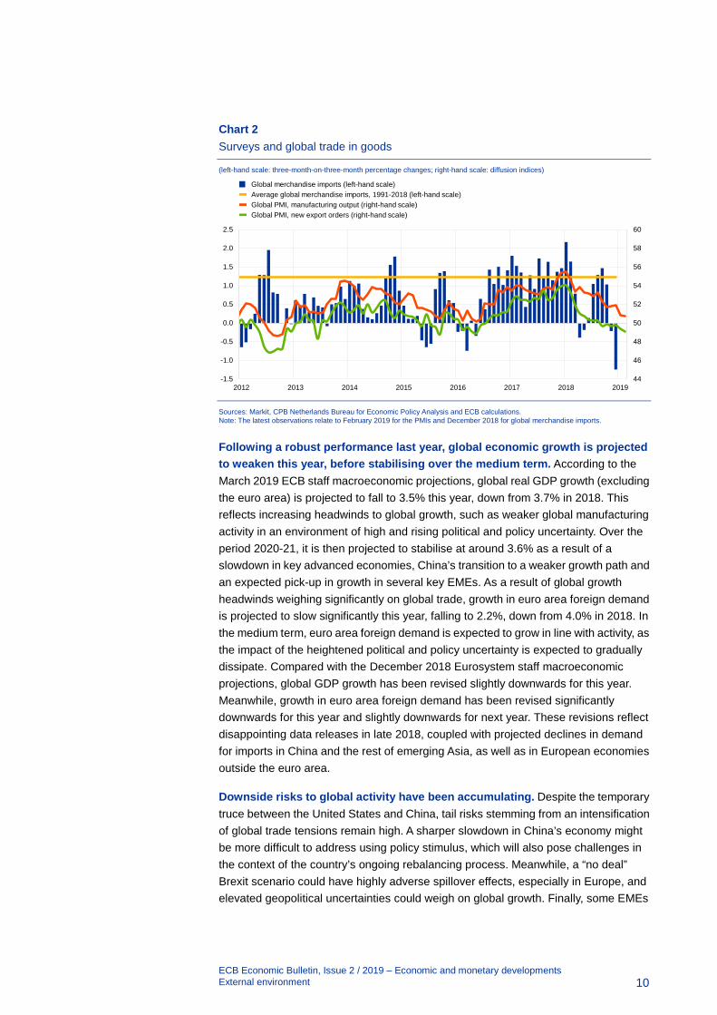
Global trade growth moderated last year amid significant volatility, with a strong performance being recorded in the first half of 2018, followed by a relatively sharp deceleration. That slowdown reflects weakening global manufacturing activity, heightened trade tensions and, more recently, a significant deterioration in trade in Asia – particularly in China. According to CPB data, the volume of global merchandise imports fell by 1.2% in December in three-month-on-three-month terms, signalling a further weakening of global trade momentum in the fourth quarter of 2018 (see Chart 2). Moreover, incoming data indicate that global trade growth has remained weak in the first quarter of 2019.
A temporary truce agreed between the United States and China in December 2018 put a further escalation of trade tensions on hold. Tariffs on USD 200 billion of Chinese exports to the United States had originally been set to rise from 10% to 25% as of 1 January 2019, but that increase was put on hold as a result of the agreed truce. While this sent a positive signal, there remains considerable uncertainty as to whether the ongoing trade negotiations will lead to a significant de-escalation of trade tensions. Meanwhile, President Trump has recently announced that the truce is to be extended, citing progress achieved in those trade negotiations, which means that the increase in tariff rates remains on hold. A formal trade agreement between the United States and China is currently expected to be signed in late March. Risks remain, however, as trade tensions could intensify again and the US administration could impose new tariffs on imports from other countries.
ECB Economic Bulletin, Issue 2 / 2019 – Economic and monetary developments External environment
10
Chart 2 Surveys and global trade in goods
(left-hand scale: three-month-on-three-month percentage changes; right-hand scale: diffusion indices)
Sources: Markit, CPB Netherlands Bureau for Economic Policy Analysis and ECB calculations. Note: The latest observations relate to February 2019 for the PMIs and December 2018 for global merchandise imports.
Following a robust performance last year, global economic growth is projected to weaken this year, before stabilising over the medium term. According to the March 2019 ECB staff macroeconomic projections, global real GDP growth (excluding the euro area) is projected to fall to 3.5% this year, down from 3.7% in 2018. This reflects increasing headwinds to global growth, such as weaker global manufacturing activity in an environment of high and rising political and policy uncertainty. Over the period 2020-21, it is then projected to stabilise at around 3.6% as a result of a slowdown in key advanced economies, China’s transition to a weaker growth path and an expected pick-up in growth in several key EMEs. As a result of global growth headwinds weighing significantly on global trade, growth in euro area foreign demand is projected to slow significantly this year, falling to 2.2%, down from 4.0% in 2018. In the medium term, euro area foreign demand is expected to grow in line with activity, as the impact of the heightened political and policy uncertainty is expected to gradually dissipate. Compared with the December 2018 Eurosystem staff macroeconomic projections, global GDP growth has been revised slightly downwards for this year. Meanwhile, growth in euro area foreign demand has been revised significantly downwards for this year and slightly downwards for next year. These revisions reflect disappointing data releases in late 2018, coupled with projected declines in demand for imports in China and the rest of emerging Asia, as well as in European economies outside the euro area.
Downside risks to global activity have been accumulating. Despite the temporary truce between the United States and China, tail risks stemming from an intensification of global trade tensions remain high. A sharper slowdown in China’s economy might be more difficult to address using policy stimulus, which will also pose challenges in the context of the country’s ongoing rebalancing process. Meanwhile, a “no deal” Brexit scenario could have highly adverse spillover effects, especially in Europe, and elevated geopolitical uncertainties could weigh on global growth. Finally, some EMEs
44
46
48
50
52
54
56
58
60
-1.5
-1.0
-0.5
0.0
0.5
1.0
1.5
2.0
2.5
2012 2013 2014 2015 2016 2017 2018 2019
Global merchandise imports (left-hand scale)Average global merchandise imports, 1991-2018 (left-hand scale)Global PMI, manufacturing output (right-hand scale)Global PMI, new export orders (right-hand scale)
ECB Economic Bulletin, Issue 2 / 2019 – Economic and monetary developments External environment
11
remain vulnerable to the reversal of capital flows, though the risk of significant numbers of EMEs suffering acute stress has recently subsided.
Global price developments
Oil prices have remained highly volatile. In the final quarter of 2018, oil prices declined amid assurances by Saudi Arabia and Russia that they would offset the effect on oil supply of the US sanctions against Iran. That downward pressure then intensified, with the US government granting temporary waivers for key importers of Iranian oil and US crude oil production standing at a high level amid renewed concerns about the global economy. Oil prices then recovered somewhat at the turn of the year as the OPEC+ agreement to cut production took effect, amid unexpectedly high levels of compliance by the various member countries. Looking ahead, oil prices are expected to remain broadly stable at this lower trajectory over the projection horizon. Consequently, the oil price assumptions underpinning the March 2019 ECB staff macroeconomic projections were around 8.6% lower for this year (and 8.2% and 8.0% lower for 2020 and 2021 respectively) relative to assumptions underpinning the December 2018 Eurosystem staff macroeconomic projections. Since the cut-off date for the March projections, however, the price of oil has increased further, standing slightly above USD 65 per barrel on 6 March.
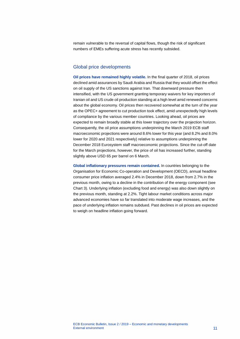
Global inflationary pressures remain contained. In countries belonging to the Organisation for Economic Co-operation and Development (OECD), annual headline consumer price inflation averaged 2.4% in December 2018, down from 2.7% in the previous month, owing to a decline in the contribution of the energy component (see Chart 3). Underlying inflation (excluding food and energy) was also down slightly on the previous month, standing at 2.2%. Tight labour market conditions across major advanced economies have so far translated into moderate wage increases, and the pace of underlying inflation remains subdued. Past declines in oil prices are expected to weigh on headline inflation going forward.
ECB Economic Bulletin, Issue 2 / 2019 – Economic and monetary developments External environment
12
Chart 3 OECD consumer price inflation
(year-on-year percentage changes; percentage point contributions)
Sources: OECD and ECB calculations. Note: The latest observations are for January 2019.
Looking ahead, global inflationary pressures are expected to remain contained. Growth in the export prices of the euro area’s competitors is expected to weaken sharply this year and remain steady over the medium term. This reflects a declining positive contribution from the oil price, which is projected to turn negative in the near term and will thus outweigh the upward pressures on underlying inflation stemming from diminishing spare capacity at the global level.
-1.5
-1.0
-0.5
0.0
0.5
1.0
1.5
2.0
2.5
3.0
3.5
2012 2013 2014 2015 2016 2017 2018 2019
Energy contributionFood contributionContribution of all items except food and energy Inflation excluding food and energyInflation including all items
ECB Economic Bulletin, Issue 2 / 2019 – Economic and monetary developments Financial developments
13
Financial developments 2
Since the Governing Council’s meeting in December 2018, global long-term risk-free rates have declined in the context of a deterioration in the macroeconomic outlook and a perceived slowing of the pace of monetary tightening in the United States. The prices of euro area risk assets, such as equities and corporate bonds, have recovered amid improved risk sentiment, fuelled in part by a greater sense of optimism regarding global trade negotiations. In foreign exchange markets, the euro has broadly weakened in trade-weighted terms.
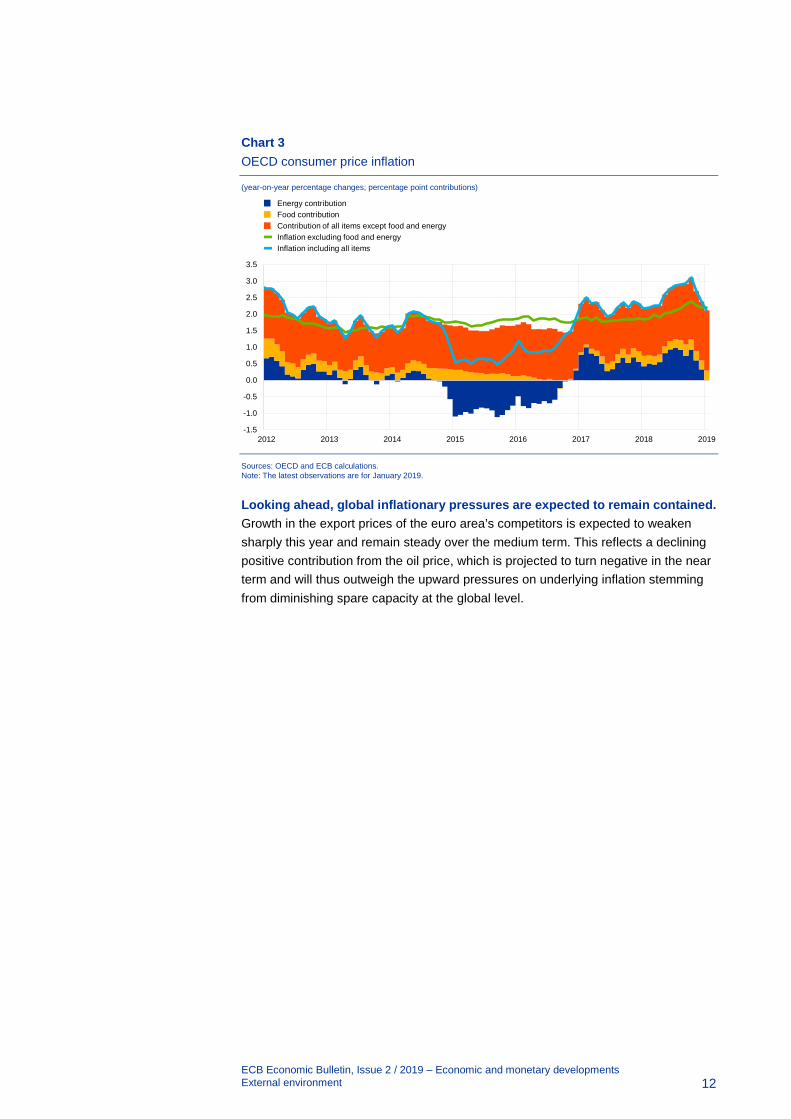
Long-term yields have declined in both the euro area and the United States. During the period under review (13 December 2018 to 6 March 2019), the euro area ten-year risk-free overnight index swap (OIS) rate fell to 0.48% (down 23 basis points) and the GDP-weighted euro area ten-year sovereign bond yield (see Chart 4) fell to 0.84% (down 23 basis points). In the United States, the ten-year sovereign bond yield fell by 22 basis points over that period to stand at 2.71%, while the equivalent yield in the United Kingdom fell 8 basis points to stand at 1.22%. Global long-term yields fell following communications from the Federal Reserve System which were interpreted by the markets as signalling a slower intended pace of monetary policy tightening. In addition to possible spillovers from the United States, euro area bond yields also reflected a deterioration in the macroeconomic outlook following a number of worse than expected macroeconomic data releases, as well as some reappraisal of the monetary policy outlook for the euro area as signalled by the short end of the yield curve.
Chart 4 Ten-year sovereign bond yields
(percentages per annum; daily data)
Sources: Thomson Reuters and ECB calculations. Notes: The vertical grey line denotes the start of the review period on 13 December 2018. The latest observations are for 6 March 2019.
Euro area sovereign bond spreads relative to the risk-free OIS rate remained broadly unchanged over the review period. Conditions in sovereign bond markets were largely stable throughout that period, with the exception of the Italian market,
-0.5
0.0
0.5
1.0
1.5
2.0
2.5
3.0
3.5
01/15 04/15 07/15 10/15 01/16 04/16 07/16 10/16 01/17 04/17 07/17 10/17 01/18 04/18 07/18 10/18 01/19
GDP-weighted euro area average United Kingdom United States Germany
ECB Economic Bulletin, Issue 2 / 2019 – Economic and monetary developments Financial developments
14
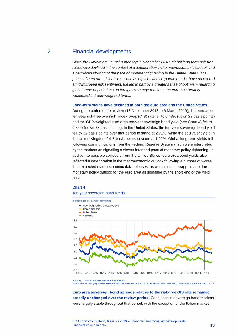
where the ten-year spread remained volatile (although it recovered to 2.11 percentage points at the end of the review period; see Chart 5). Consequently, the spread between the GDP-weighted average of euro area ten-year sovereign bond yields and the ten-year OIS rate remained stable over the review period, standing at 0.36 percentage points on 6 March.
Chart 5 Ten-year euro area sovereign bond spreads vis-à-vis the OIS rate
(percentage points per annum)
Sources: Thomson Reuters and ECB calculations. Notes: The spread is calculated by subtracting the ten-year OIS rate from the ten-year sovereign bond yield. The vertical grey line denotes the start of the review period on 13 December 2018. The latest observations are for 6 March 2019.
The euro overnight index average (EONIA) averaged -0.37% over the review period. Excess liquidity was broadly unchanged at around €1,890 billion. For further details of developments in liquidity conditions, see Box 2.
The EONIA forward curve shifted downwards somewhat over the review period. The curve is now below zero for all horizons prior to 2022, reflecting market expectations of a prolonged period of negative interest rates (see Chart 6).
-1.0
-0.5
0.0
0.5
1.0
1.5
2.0
2.5
3.0
3.5
4.0
01/16 04/16 07/16 10/16 01/17 04/17 07/17 10/17 01/18 04/18 07/18 10/18 01/19
GDP-weighted euro area average GermanyFranceItalySpainPortugal

ECB Economic Bulletin, Issue 2 / 2019 – Economic and monetary developments Financial developments
15
Chart 6 EONIA forward rates
(percentages per annum)
Sources: Thomson Reuters and ECB calculations.
Broad indices of euro area equity prices increased over the review period amid a general improvement in risk sentiment. The equity prices of euro area banks and non-financial corporations (NFCs) increased by around 7% over the period (with similar increases being observed in the United States), reversing a large percentage of the declines seen in the fourth quarter of 2018 (see Chart 7). That recovery in equity prices reflected a greater sense of optimism regarding the outlook for global trade and was underpinned by communications from the Federal Reserve System which were interpreted by the markets as signalling a slowdown in the intended pace of monetary policy tightening. At the same time, both short and longer-term corporate earnings expectations were revised downwards over the review period, reflecting a perceived deterioration in the macroeconomic outlook for the euro area.
Chart 7 Euro area and US equity price indices
(index: 1 January 2015 = 100)
Sources: Thomson Reuters and ECB calculations. Notes: The vertical grey line denotes the start of the review period on 13 December 2018. The latest observations are for 6 March 2019.
-0.5
0.0
0.5
1.0
1.5
2.0
2019 2020 2021 2022 2023 2024 2025 2026 2027
6 March 201913 December 2018
50
70
90
110
130
150
170
01/15 04/15 07/15 10/15 01/16 04/16 07/16 10/16 01/17 04/17 07/17 10/17 01/18 04/18 07/18 10/18 01/19
Euro area banks Euro area NFCs US banks US NFCs

ECB Economic Bulletin, Issue 2 / 2019 – Economic and monetary developments Financial developments
16
Euro area corporate bond spreads declined over the review period, largely reflecting an improvement in risk sentiment. Since December the spread between the yield on investment-grade NFC bonds and the risk-free rate has declined by around 14 basis points to stand at 78 basis points (see Chart 8). Yields on financial sector debt have also declined, resulting in the relevant spread falling by around 18 basis points. Despite these recent declines, both spreads remain above the levels observed a year ago.
Chart 8 Euro area corporate bond spreads
(basis points)
Sources: iBoxx indices and ECB calculations. Notes: The vertical grey line denotes the start of the review period on 13 December 2018. The latest observations are for 6 March 2019.
In foreign exchange markets, the euro broadly depreciated in trade-weighted terms over the review period (see Chart 9). Indeed, the nominal effective exchange rate of the euro, as measured against the currencies of 38 of the euro area’s most important trading partners, fell by 1.2% over that period. In bilateral terms, the euro weakened against most currencies. In particular, the euro depreciated slightly against the US dollar (by 0.6%) and weakened against most other major currencies, including the pound sterling (by 4.3%), the Japanese yen (by 2.1%) and the Chinese renminbi (by 3.1%). The euro also depreciated vis-à-vis the currencies of most emerging markets, while it appreciated against the currencies of most EU Member States outside the euro area.
0
20
40
60
80
100
120
140
160
01/15 04/15 07/15 10/15 01/16 04/16 07/16 10/16 01/17 04/17 07/17 10/17 01/18 04/18 07/18 10/18 01/19
Financial corporate bond spreadsNFC bond spreads

ECB Economic Bulletin, Issue 2 / 2019 – Economic and monetary developments Financial developments
17
Chart 9 Changes in the exchange rate of the euro vis-à-vis selected currencies
(percentage changes)
Source: ECB. Notes: “EER-38” is the nominal effective exchange rate of the euro against the currencies of 38 of the euro area’s most important trading partners. All changes have been calculated using the foreign exchange rates prevailing on 6 March 2019.
-10 -5 0 5 10 15 20 25 30 35
Croatian kunaIndian rupeeBrazilian realTaiwan dollarRomanian leuDanish krone
Hungarian forintIndonesian rupiahSouth Korean won
Turkish liraRussian roubleSwedish kronaCzech koruna
Polish zlotyJapanese yen
Swiss francPound sterling
US dollarChinese renminbi
EER-38
Since 13 December 2018Since 6 March 2018
ECB Economic Bulletin, Issue 2 / 2019 – Economic and monetary developments Economic activity
18
Economic activity 3
Euro area real GDP growth remained subdued in the fourth quarter of 2018 at 0.2% quarter on quarter, driven by a contraction in the industrial sector. Incoming data suggest that growth will continue at moderate rates in the near term. Looking ahead the expansion of the euro area economy is expected to continue, supported by favourable financing conditions, further employment gains and rising wages, as well as the ongoing, albeit somewhat slower, expansion in global activity. The March 2019 ECB staff macroeconomic projections for the euro area expect annual real GDP to increase by 1.1% in 2019, 1.6% in 2020 and 1.5% in 2021. Compared with the December 2018 Eurosystem staff macroeconomic projections, the outlook for real GDP growth has been revised downwards substantially for 2019 and slightly for 2020.
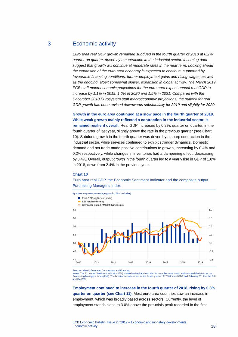
Growth in the euro area continued at a slow pace in the fourth quarter of 2018. While weak growth mainly reflected a contraction in the industrial sector, it remained resilient overall. Real GDP increased by 0.2%, quarter on quarter, in the fourth quarter of last year, slightly above the rate in the previous quarter (see Chart 10). Subdued growth in the fourth quarter was driven by a sharp contraction in the industrial sector, while services continued to exhibit stronger dynamics. Domestic demand and net trade made positive contributions to growth, increasing by 0.4% and 0.2% respectively, while changes in inventories had a dampening effect, decreasing by 0.4%. Overall, output growth in the fourth quarter led to a yearly rise in GDP of 1.8% in 2018, down from 2.4% in the previous year.
Chart 10 Euro area real GDP, the Economic Sentiment Indicator and the composite output Purchasing Managers' Index
(quarter-on-quarter percentage growth; diffusion index)
Sources: Markit, European Commission and Eurostat. Notes: The Economic Sentiment Indicator (ESI) is standardised and rescaled to have the same mean and standard deviation as the Purchasing Managers’ Index (PMI). The latest observations are for the fourth quarter of 2018 for real GDP and February 2019 for the ESI and the PMI.
Employment continued to increase in the fourth quarter of 2018, rising by 0.3% quarter on quarter (see Chart 11). Most euro area countries saw an increase in employment, which was broadly based across sectors. Currently, the level of employment stands close to 3.0% above the pre-crisis peak recorded in the first
-0.6
-0.3
0.0
0.3
0.6
0.9
1.2
44
47
50
53
56
59
62
2012 2013 2014 2015 2016 2017 2018 2019
Real GDP (right-hand scale)ESI (left-hand scale)Composite output PMI (left-hand scale)

ECB Economic Bulletin, Issue 2 / 2019 – Economic and monetary developments Economic activity
19
quarter of 2008. Taking into account the latest increase, there has been cumulative growth in employment in the euro area, with 10 million more persons in employment than at the time of the trough in the second quarter of 2013. Continued employment growth combined with a drop in GDP growth in 2018 has led to a moderation in productivity growth, following a modest pick-up in 2017. Empirically, adjustments in employment tend to lag behind declines in output. One reason is that longer-term employment contracts cannot be adjusted immediately when firms face a slowdown in demand.
Recent short-term labour market indicators continue to point to positive but moderating employment growth in the first quarter of 2019. The euro area unemployment rate stood at 7.8% in January 2019, unchanged from December 2018, and remains at its lowest level since October 2008. Survey indicators point to a further slowdown in employment growth in the first quarter of 2019.
Chart 11 Euro area employment, PMI assessment of employment and unemployment
(quarter-on-quarter percentage changes; diffusion index; percentages of the labour force)
Sources: Eurostat, Markit and ECB calculations. Notes: The Purchasing Managers' Index (PMI) is expressed as a deviation from 50 divided by 10. The latest observations are for the fourth quarter of 2018 for employment, February 2019 for the PMI and January 2019 for the unemployment rate.
Private consumption growth edged up in the fourth quarter of 2018 and is expected to regain further momentum in the quarters ahead, as temporary dampening effects wane in an environment of continued strengthening of households’ labour income. Private consumption increased by 0.2%, quarter on quarter, in the fourth quarter of 2018, following somewhat weaker growth in the third quarter. The weakness in household expenditure partly reflected temporary bottlenecks in the car sector, affecting the consumption of durable goods, and the negative effect of energy price increases on household purchasing power. The crude oil price (in euro) increased from the fourth quarter of 2017 to the third quarter of 2018, which negatively affected consumption growth, in particular of non-durable goods, i.e. food and energy. Subsequently, the oil price declined sharply (before recovering somewhat in the last two months). This should support consumption of non-durable goods in the near term. Furthermore, employment growth strengthened in the fourth quarter of 2018 in an environment of robust wage increases. This implies steady
7
8
9
10
11
12
13
-0.6
-0.4
-0.2
0.0
0.2
0.4
0.6
2012 2013 2014 2015 2016 2017 2018 2019
Employment (left-hand scale)PMI assessment of employment (left-hand scale)Unemployment rate (right-hand scale)
ECB Economic Bulletin, Issue 2 / 2019 – Economic and monetary developments Economic activity
20
growth in households’ real disposable income and supports consumer confidence and spending. In addition, while financing conditions remain very favourable, households’ net worth improved at a strong rate in the third quarter of 2018.
Latest indicators also suggest some strengthening of private consumption momentum in the course of the year ahead. Recent data on retail sales and car registrations indicate moderate but steady growth in consumer spending. The volume of retail sales increased by 1.4% in January 2019, following a drop in the previous month. As a result, sales stood at 1.5% above their average level in the fourth quarter of 2018. The indicator for new passenger car registrations posted its fourth consecutive increase in January 2019, rising by 4.8% on a monthly basis. This confirms previous expectations for a normalisation in car registrations, following the volatile developments triggered by the introduction of the new Worldwide Harmonised Light Vehicle Test Procedure (WLTP) on 1 September 2018. In addition, consumer confidence increased for a second consecutive month in February, halting the declining trend observed throughout most of 2018. The latest improvement reflects households’ more benign views regarding their past and future financial situation, as well as the expected general economic situation and unemployment. Consumer confidence remains above its historical average level and is consistent with ongoing steady growth in private consumption.
The ongoing recovery in housing markets is also expected to continue, albeit at a slower pace than in 2018. Housing investment increased by 0.6% in the fourth quarter of 2018, reflecting the ongoing recovery in many euro area countries and in the euro area as a whole. Although growth over 2018 was slower than the buoyant growth experienced in 2017, it remains at solid, healthy levels. In line with these developments, recent short-term indicators and survey results point to positive, but slowing momentum. Construction production in the buildings segment increased by 0.2%, quarter on quarter, in the fourth quarter of 2018, recovering from -0.8% in the third quarter. The European Commission’s construction confidence indicators for the past few months point to positive, albeit weakening, momentum in the fourth quarter of 2018 and early 2019. The Purchasing Managers’ Index (PMI) for housing activity averaged 52.0 in the last quarter of 2018, but decreased to 50.6 in January 2019. However, both the PMI indicators and the European Commission’s confidence indicators remain clearly above their long-run averages.
Business investment in the euro area appears to have lost some momentum in the second half of 2018, but fundamentals remain supportive. Available country data for some of the larger euro area countries point overall to a slowdown in business investment growth in the fourth quarter of 2018. The slowdown in business investment partly reflects heightened policy uncertainty and financial volatility in some euro area countries. Persistent concerns about global trade developments, the possibility of a no-deal Brexit and economic weaknesses in China also appear to have adversely affected business confidence. The assessment of export order books and production expectations in the capital goods sector continued to worsen in January and February 2019. However, fundamentals remain supportive of business investment. First, capacity utilisation remains well above its long-term average, and a large share of manufacturing firms report lack of equipment as a factor limiting production. Second,

ECB Economic Bulletin, Issue 2 / 2019 – Economic and monetary developments Economic activity
21
the ECB’s monetary policy measures continue to support favourable financing conditions and access to financing for euro area firms. Third, during the recent period of recovery, firms have also used profits to build up a sizeable liquidity overhang.
Euro area trade in goods continued to grow at a subdued pace at the end of 2018 and is expected to decline further in the near term. According to the latest release of data from the national accounts, in the last quarter of 2018 total euro area exports increased by 0.9%, while imports increased by 0.5% on a quarterly basis. Incoming data on the monthly trade in goods confirm a poor performance by total euro area trade in the fourth quarter, mostly driven by intra-euro area trade. In December 2018 nominal euro area exports contracted by 0.5%, month on month, with intra-euro area exports decreasing even more (by 0.9%). Nominal euro area imports saw a slight month-on-month increase of 0.4%. Temporary factors, such as the new regulations on vehicle emissions tests, have weighed on exports. However, a generalised decrease can be observed across all product categories. The United Kingdom, Turkey and China continue to drive the weakness in extra-euro area exports observed in the last few months of 2018. Looking ahead leading indicators point to a further reduction in extra-euro area exports in the coming months. In February 2019 the manufacturing PMI for new export orders outside of the euro area was at its lowest since November 2012 (46.4), and the European Commission’s assessment went more negative compared with January.
The latest survey results have continued to disappoint and suggest that euro area growth is moderating in the short term. The European Commission’s Economic Sentiment Indicator remained broadly unchanged in February, standing above its long-term average. So far in 2019 the average stands at 106.2, below the 108.9 average for the last quarter of 2018. Although the indicator declined for the industry and construction sectors, this was broadly offset by positive sentiment in services, the retail sector and households. The composite output PMI increased slightly in February, but the average for the first two months of the first quarter of 2019 stood below that for the previous quarter (51.4 compared with 52.3).
Despite the current slowdown, over the medium term the broad-based economic expansion is expected to regain traction and to continue over the period ahead. The ECB’s accommodative monetary policy continues to strengthen domestic demand. Ongoing growth in employment and wages should keep private consumption high. At the same time business investment is supported by healthy domestic demand, favourable financing conditions and improving balance sheets, and housing investment remains strong.
The March 2019 ECB staff macroeconomic projections for the euro area forecast annual real GDP to increase by 1.1% in 2019, 1.6% in 2020 and 1.5% in 2021 (see Chart 12). Compared with the December 2018 Eurosystem staff projections, the outlook for real GDP growth has been revised downwards substantially for 2019 and slightly for 2020. The risks surrounding the euro area outlook remain tilted to the downside.

ECB Economic Bulletin, Issue 2 / 2019 – Economic and monetary developments Economic activity
22
Chart 12 Euro area real GDP (including projections)
(quarter-on-quarter percentage changes)
Sources: Eurostat and the article entitled “March 2019 ECB staff macroeconomic projections for the euro area”, published on the ECB’s website on 7 March 2019. Notes: The ranges shown around the central projections are based on the differences between actual outcomes and previous projections carried out over a number of years. The width of the range is twice the average absolute value of these differences. The method used for calculating the ranges, involving a correction for exceptional events, is documented in the “New procedure for constructing Eurosystem and ECB staff projection ranges”, ECB, December 2009.
-0.5
0.0
0.5
1.0
2012 2013 2014 2015 2016 2017 2018 2019 2020 2021

ECB Economic Bulletin, Issue 2 / 2019 – Economic and monetary developments Prices and costs
23
Prices and costs 4
According to Eurostat’s flash estimate, euro area annual HICP inflation increased to 1.5% in February 2019, up from 1.4% in January. While measures of underlying inflation continued to move sideways, domestic cost pressures strengthened and broadened amid high levels of capacity utilisation and tightening labour markets. Looking ahead underlying inflation is expected to increase gradually over the medium term, supported by the ECB’s monetary policy measures, the ongoing economic expansion and rising wage growth. This assessment is also broadly reflected in the March 2019 ECB staff macroeconomic projections for the euro area, which foresee annual HICP inflation at 1.2% in 2019, 1.5% in 2020 and 1.6% in 2021 – revised downwards across the projection horizon, reflecting in particular the more subdued near-term growth outlook. Annual HICP inflation excluding energy and food is expected to be 1.2% in 2019, 1.4% in 2020 and 1.6% in 2021.
Headline inflation increased in February owing to stronger price increases in volatile categories. According to Eurostat’s flash estimate, euro area annual HICP inflation increased to 1.5% in February 2019, up from 1.4% in January (see Chart 13). This reflected higher inflation rates for the more volatile categories, energy and food, while HICP inflation excluding energy and food (HICPX) declined. The higher inflation rate for energy reflected upward base effects and a moderate increase in oil prices (in euro terms). When discussing HICP data since January 2019, one should note that two methodological changes have been introduced that imply revisions to the historical data (see Box 4 “New features in the Harmonised Index of Consumer Prices: analytical groups, scanner data and web-scraping” and Box 5 “A new method for the package holiday price index in Germany and its impact on HICP inflation rates”).
Chart 13 Contributions of components to euro area headline HICP inflation
(annual percentage changes; percentage point contributions)
Sources: Eurostat and ECB calculations. Notes: The latest observations are for February 2019 (flash estimates). Growth rates for 2015 are distorted upwards owing to a methodological change (see Box 5 in this issue of the ECB’s Economic Bulletin).
-1.5
-1.0
-0.5
0.0
0.5
1.0
1.5
2.0
2.5
3.0
3.5
2012 2013 2014 2015 2016 2017 2018 2019
HICPServicesNon-energy industrial goods FoodEnergy

ECB Economic Bulletin, Issue 2 / 2019 – Economic and monetary developments Prices and costs
24
Measures of underlying inflation continued their recent sideways movement after rising from earlier lows. HICP inflation excluding energy and food was 1.0% in February, down from 1.1% in January. It thus continued to hover around the 1% rate that it reached after rising from its low in mid-2016. The decrease in February reflected a decline in services inflation from 1.6% to 1.3%, while non-energy industrial goods inflation remained unchanged at 0.3%. Other measures of underlying inflation, including the Persistent and Common Component of Inflation indicator (PCCI) and the Supercore indicator,1 which are only available for the period to January, also pointed to a continuation of the broad sideways movement of recent months (see Chart 14). Nonetheless, each of the statistical and model-based measures remained higher than their respective lows in 2016. Looking ahead measures of underlying inflation are expected to increase gradually, driven by a further strengthening of wage growth and the pick-up observed in domestic producer price inflation.
Chart 14 Measures of underlying inflation
(annual percentage changes)
Sources: Eurostat and ECB calculations. Notes: The latest observations are for February 2019 (flash estimate) for HICP excluding energy and food and for January 2019 for all the other measures. The range of measures of underlying inflation consists of the following: HICP excluding energy; HICP excluding energy and unprocessed food; HICP excluding energy and food; HICP excluding energy, food, travel-related items and clothing; the 10% trimmed mean; the 30% trimmed mean; and the weighted median of the HICP. Growth rates for HICP excluding energy and food for 2015 are distorted upwards owing to a methodological change (see Box 5 in this issue of the ECB’s Economic Bulletin).
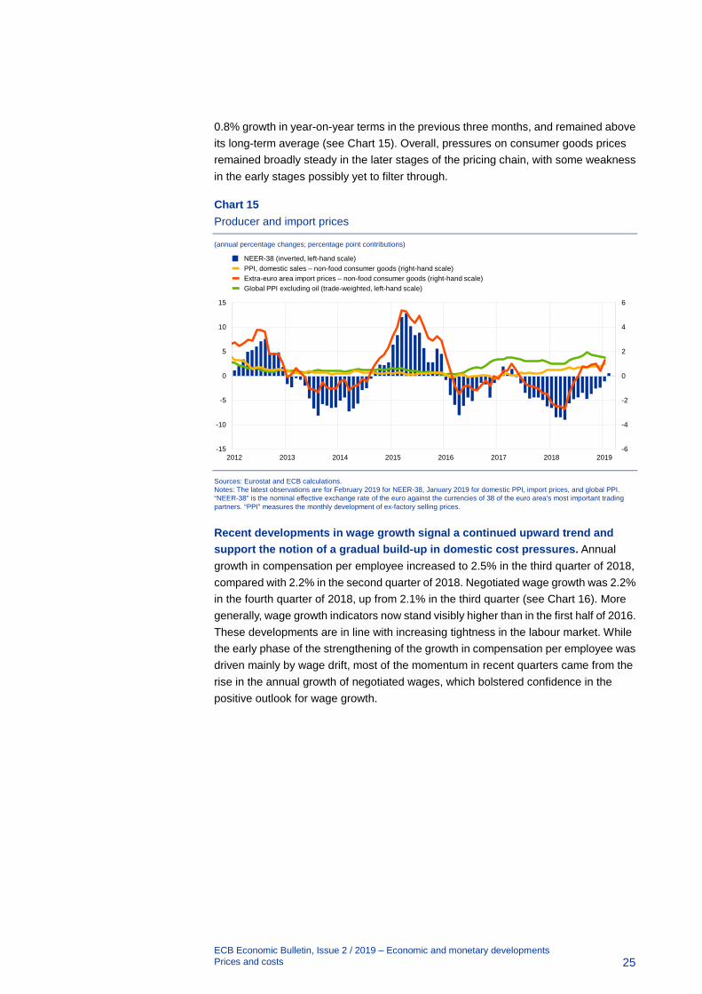
Price pressures for non-energy industrial goods increased at the later stages of the pricing chain, while signals at the earlier stages were mixed. At the very early stages, pipeline price pressures have rebounded, as the annual rate of change in oil prices and industrial raw material prices (in euro terms) increased markedly in February. Global non-energy producer price inflation, in contrast, declined slightly further in January. The previous weak price pressures in the early stages have had an impact on import price and producer price inflation for intermediate goods, with both continuing to decline since August last year. At the later stages, the year-on-year growth of import prices for non-food consumer goods increased to 1.3% in January from (a revised downwards) 0.4% in December. Also, domestic producer price inflation for these goods increased to 1.0% in January 2019, after recording a stable 1 For more information on these measures of underlying inflation, see Boxes 2 and 3 in the article
"Measures of underlying inflation for the euro area", Economic Bulletin, Issue 4, ECB, 2018.
0.0
0.5
1.0
1.5
2.0
2.5
3.0
2011 2012 2013 2014 2015 2016 2017 2018 2019
HICP excluding energy and foodHICP excluding energy, food, travel-related items and clothingSupercorePCCI
ECB Economic Bulletin, Issue 2 / 2019 – Economic and monetary developments Prices and costs
25
0.8% growth in year-on-year terms in the previous three months, and remained above its long-term average (see Chart 15). Overall, pressures on consumer goods prices remained broadly steady in the later stages of the pricing chain, with some weakness in the early stages possibly yet to filter through.
Chart 15 Producer and import prices
(annual percentage changes; percentage point contributions)
Sources: Eurostat and ECB calculations. Notes: The latest observations are for February 2019 for NEER-38, January 2019 for domestic PPI, import prices, and global PPI. “NEER-38” is the nominal effective exchange rate of the euro against the currencies of 38 of the euro area’s most important trading partners. “PPI” measures the monthly development of ex-factory selling prices.
Recent developments in wage growth signal a continued upward trend and support the notion of a gradual build-up in domestic cost pressures. Annual growth in compensation per employee increased to 2.5% in the third quarter of 2018, compared with 2.2% in the second quarter of 2018. Negotiated wage growth was 2.2% in the fourth quarter of 2018, up from 2.1% in the third quarter (see Chart 16). More generally, wage growth indicators now stand visibly higher than in the first half of 2016. These developments are in line with increasing tightness in the labour market. While the early phase of the strengthening of the growth in compensation per employee was driven mainly by wage drift, most of the momentum in recent quarters came from the rise in the annual growth of negotiated wages, which bolstered confidence in the positive outlook for wage growth.
-6
-4
-2
0
2
4
6
-15
-10
-5
0
5
10
15
2012 2013 2014 2015 2016 2017 2018 2019
NEER-38 (inverted, left-hand scale)PPI, domestic sales – non-food consumer goods (right-hand scale)Extra-euro area import prices – non-food consumer goods (right-hand scale)Global PPI excluding oil (trade-weighted, left-hand scale)

ECB Economic Bulletin, Issue 2 / 2019 – Economic and monetary developments Prices and costs
26
Chart 16 Contributions of components of compensation per employee
(annual percentage changes; percentage point contributions)
Sources: Eurostat and ECB calculations. Note: The latest observations are for the third quarter of 2018 for compensation per employee and the fourth quarter of 2018 for negotiated wage growth.
Market and survey-based measures of longer-term inflation expectations have fallen somewhat. The five-year inflation-linked swap rate five years ahead stood at 1.51% on 6 March 2019, 13 basis points lower than the level which prevailed in mid-December (see Chart 17). The forward profile of market-based measures of inflation expectations continues to point towards a prolonged period of low inflation with a gradual return to inflation levels below, but close to, 2%. The risk-neutral probability of negative average inflation over the next five years implied by inflation options markets is negligible, which suggests that markets currently consider the risk of deflation to be very low. According to the ECB Survey of Professional Forecasters for the first quarter of 2019, longer-term inflation expectations were 1.8%, slightly down from 1.9% compared with the previous survey.
-1.5
-1.0
-0.5
0.0
0.5
1.0
1.5
2.0
2.5
3.0
2012 2013 2014 2015 2016 2017 2018
Compensation per employee growth Negotiated wages Social security contributions Wage drift

ECB Economic Bulletin, Issue 2 / 2019 – Economic and monetary developments Prices and costs
27
Chart 17 Market-based measures of inflation expectations
(annual percentage changes)
Sources: Thomson Reuters and ECB calculations. Note: The latest observations are for 6 March 2019.
The March 2019 ECB staff macroeconomic projections expect underlying inflation to increase gradually over the projection horizon. On the basis of the information available at mid-February, these projections expect headline HICP inflation to average 1.2% in 2019, 1.5% in 2020 and 1.6% in 2021, compared with 1.6%, 1.7% and 1.8% respectively in the December 2018 Eurosystem staff macroeconomic projections (see Chart 18). This pattern reflects a sharp decline in HICP energy inflation in 2019, which is mainly accounted for by the strong drop in oil prices at the end of 2018 and downward base effects related to their prior increase in 2018. Looking ahead HICP energy prices are expected to grow at subdued rates consistent with the relatively flat oil price futures curve. HICP inflation excluding energy and food will be on a gradual upward path supported by the more gradual but continued economic recovery and the tightening labour market conditions, leading to higher domestic cost pressures. HICP inflation excluding energy and food is expected to rise from 1.2% in 2019 to 1.4% in 2020 and 1.6% in 2021, representing a downward revision of 0.2 percentage point in each year of the projection horizon.
0.0
0.5
1.0
1.5
2.0
2.5
3.0
2012 2013 2014 2015 2016 2017 2018 2019
One-year rate one year ahead One-year rate two years ahead One-year rate four years ahead One-year rate nine years ahead Five-year rate five years ahead

ECB Economic Bulletin, Issue 2 / 2019 – Economic and monetary developments Prices and costs
28
Chart 18 Euro area HICP inflation (including projections)
(annual percentage changes)
Sources: Eurostat and the article entitled “March 2019 ECB staff macroeconomic projections for the euro area”, published on the ECB’s website on 7 March 2019. Notes: The latest observations are for the fourth quarter of 2018 (actual data) and the fourth quarter of 2021 (projection). The ranges shown around the central projections are based on the differences between actual outcomes and previous projections carried out over a number of years. The width of the ranges is twice the average absolute value of these differences. The method used for calculating the ranges, involving a correction for exceptional events, is documented in the “New procedure for constructing Eurosystem and ECB staff projection ranges”, ECB, December 2009. The cut-off date for data included in the projections was 21 February 2019 and thus before the revision to historical data in the HICP on account of methodological changes.
-0.5
0.0
0.5
1.0
1.5
2.0
2.5
3.0
2012 2013 2014 2015 2016 2017 2018 2019 2020 2021
HICPProjection range

ECB Economic Bulletin, Issue 2 / 2019 – Economic and monetary developments Money and credit
29
Money and credit 5
Money growth and credit dynamics moderated in January 2019. Broad money growth has shown strong resilience in the face of the phasing-out of monthly net purchases under the asset purchase programme (APP). At the same time, bank funding and lending conditions remained favourable. Net issuance of debt securities by NFCs declined significantly in the fourth quarter of 2018, against the background of a continuing gradual deterioration in bond market conditions that started in late 2017.
Broad money growth moderated in January, with rates continuing to hover around the level observed since March 2018. The annual growth rate of M3 decreased to 3.8% in January 2019 from 4.1% in December 2018 (see Chart 19). This development shows the resilience of M3 growth in the face of the declining mechanical contribution of APP purchases. M3 growth has eased since late 2017, coinciding with the phasing-out of net asset purchases. This in turn implies that the APP had a smaller positive impact on M3 growth. The narrow money aggregate M1, which includes the most liquid components of M3, continued to make a large contribution to broad money growth, despite declining to 6.2% in January. Money growth continued to receive support from sustained economic expansion and the low opportunity cost of holding the most liquid instruments in an environment of very low interest rates.
Chart 19 M3, M1 and loans to the private sector
(annual percentage changes; adjusted for seasonal and calendar effects)
Source: ECB. Notes: Loans are adjusted for loan sales, securitisation and notional cash pooling. The latest observation is for January 2019.
Overnight deposits remained the main contributor to M3 growth. The annual growth rate of overnight deposits decreased to 6.4% in January, reflecting the moderation in the annual growth of overnight deposits held by NFCs, while the expansion of overnight deposits held by households remained stable. Moreover, steady growth in currency in circulation speaks against any large-scale substitution of cash for deposits in an environment of very low or negative interest rates for the euro area as a whole. Short-term deposits other than overnight deposits (i.e. M2 minus M1) continued to make a negative contribution to M3 growth, although the spread between the interest rates on short-term time deposits and overnight deposits has stabilised
-4
-2
0
2
4
6
8
10
12
2012 2013 2014 2015 2016 2017 2018 2019
M3M1Loans to the private sector

ECB Economic Bulletin, Issue 2 / 2019 – Economic and monetary developments Money and credit
30
since late 2017. Marketable instruments (i.e. M3 minus M2), which are currently growing at a slow pace given the low remuneration of these instruments, had a neutral overall impact on M3 growth.
Credit to the private sector remained the largest driver of broad money growth from a counterpart perspective (see Chart 20). In the context of the aforementioned phasing-out of monthly net purchases under the APP, the positive contribution to M3 growth from general government securities held by the Eurosystem decreased further (see the red parts of the bars in Chart 20). This has been largely offset by a moderate increase in the contribution from credit to the private sector since late 2017 (see the blue parts of the bars in Chart 20). While private credit remained the main source of money creation, the decline in the contribution of the APP has recently been replaced by external monetary flows (see the yellow parts of the bars in Chart 20) and credit to the general government (see the light green parts of the bars in Chart 20). The increasing contribution from net external assets in part reflects investors’ preferences for euro area assets in the context of a greater aversion to risk linked to higher uncertainty. Moreover, purchases of government securities by commercial banks have increasingly stabilised M3 in recent months. These developments mark an ongoing shift towards more self-sustained sources of money creation.
Chart 20 M3 and its counterparts
(annual percentage changes; contributions in percentage points; adjusted for seasonal and calendar effects)
Source: ECB. Notes: Credit to the private sector includes MFI loans to the private sector and MFI holdings of debt securities issued by the euro area private non-MFI sector. As such, it also covers purchases by the Eurosystem of non-MFI debt securities under the corporate sector purchase programme. The latest observation is for January 2019.
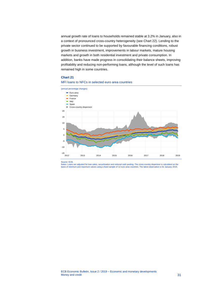
Credit dynamics moderated in January. The annual growth rate of MFI loans to the private sector (adjusted for loan sales, securitisation and notional cash pooling) declined to 3.0% in January from 3.4% in December (see Chart 19). This was owing to a strong decline in the annual growth rate of loans to NFCs to 3.3% in January from 3.9% in December. Loan growth for firms, which was accompanied by considerable heterogeneity across countries, matches historical patterns and can be explained by the slowdown in real GDP since early 2018 (see Chart 21). At the same time, the
-6
-4
-2
0
2
4
6
8
10
2013 2014 2015 2016 2017 2018 2019
M3Net external assetsGeneral government debt securities held by the EurosystemCredit to general government from MFIs excluding the EurosystemCredit to the private sectorInflows from longer-term financial liabilities and other counterparts
ECB Economic Bulletin, Issue 2 / 2019 – Economic and monetary developments Money and credit
31
annual growth rate of loans to households remained stable at 3.2% in January, also in a context of pronounced cross-country heterogeneity (see Chart 22). Lending to the private sector continued to be supported by favourable financing conditions, robust growth in business investment, improvements in labour markets, mature housing markets and growth in both residential investment and private consumption. In addition, banks have made progress in consolidating their balance sheets, improving profitability and reducing non-performing loans, although the level of such loans has remained high in some countries.
Chart 21 MFI loans to NFCs in selected euro area countries
(annual percentage changes)
Source: ECB. Notes: Loans are adjusted for loan sales, securitisation and notional cash pooling. The cross-country dispersion is calculated on the basis of minimum and maximum values using a fixed sample of 12 euro area countries. The latest observation is for January 2019.
-15
-10
-5
0
5
10
15
20
2012 2013 2014 2015 2016 2017 2018 2019
Euro areaGermanyFranceItalySpainCross-country dispersion

ECB Economic Bulletin, Issue 2 / 2019 – Economic and monetary developments Money and credit
32
Chart 22 MFI loans to households in selected euro area countries
(annual percentage changes)
Source: ECB. Notes: Loans are adjusted for loan sales and securitisation. The cross-country dispersion is calculated on the basis of minimum and maximum values using a fixed sample of 12 euro area countries. The latest observation is for January 2019.
Bank funding conditions remained favourable by historical standards. In January, the composite cost of debt financing for euro area banks remained stable, after having progressively increased since the beginning of 2018 (see Chart 23). This development reflected unchanged bank bond yields in the euro area as a whole. Heterogeneity across countries was considerable, given that political uncertainty was high and banks’ access to wholesale funding was uneven. At the same time, the costs of deposit funding remained unchanged. The repercussions of higher costs of funding through the issuance of debt securities on the overall composite cost of funding for banks have been rather limited owing to this type of funding’s limited importance in banks’ funding structures. Overall, therefore, bank funding conditions have remained favourable, reflecting the ECB’s accommodative monetary policy stance and the strengthening of banks’ balance sheets. Moreover, the new series of TLTROs will help to ensure that bank lending conditions remain favourable going forward.
-10
-5
0
5
10
2012 2013 2014 2015 2016 2017 2018 2019
Euro areaGermanyFranceItalySpainCross-country dispersion
ECB Economic Bulletin, Issue 2 / 2019 – Economic and monetary developments Money and credit
33
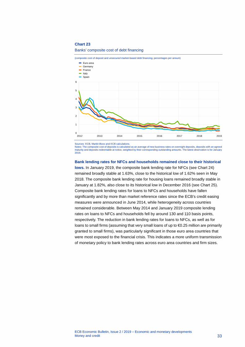
Chart 23 Banks’ composite cost of debt financing
(composite cost of deposit and unsecured market-based debt financing; percentages per annum)
Sources: ECB, Markit iBoxx and ECB calculations. Notes: The composite cost of deposits is calculated as an average of new business rates on overnight deposits, deposits with an agreed maturity and deposits redeemable at notice, weighted by their corresponding outstanding amounts. The latest observation is for January 2019.
Bank lending rates for NFCs and households remained close to their historical lows. In January 2019, the composite bank lending rate for NFCs (see Chart 24) remained broadly stable at 1.63%, close to the historical low of 1.62% seen in May 2018. The composite bank lending rate for housing loans remained broadly stable in January at 1.82%, also close to its historical low in December 2016 (see Chart 25). Composite bank lending rates for loans to NFCs and households have fallen significantly and by more than market reference rates since the ECB’s credit easing measures were announced in June 2014, while heterogeneity across countries remained considerable. Between May 2014 and January 2019 composite lending rates on loans to NFCs and households fell by around 130 and 110 basis points, respectively. The reduction in bank lending rates for loans to NFCs, as well as for loans to small firms (assuming that very small loans of up to €0.25 million are primarily granted to small firms), was particularly significant in those euro area countries that were most exposed to the financial crisis. This indicates a more uniform transmission of monetary policy to bank lending rates across euro area countries and firm sizes.
0
1
2
3
4
5
6
2012 2013 2014 2015 2016 2017 2018 2019
Euro areaGermanyFranceItalySpain

ECB Economic Bulletin, Issue 2 / 2019 – Economic and monetary developments Money and credit
34
Chart 24 Composite lending rates for NFCs
(percentages per annum; three-month moving averages)
Source: ECB. Notes: The indicator for the total cost of bank borrowing is calculated by aggregating short and long-term rates using a 24-month moving average of new business volumes. The cross-country standard deviation is calculated using a fixed sample of 12 euro area countries. The latest observation is for January 2019.
Chart 25 Composite lending rates for house purchase
(percentages per annum; three-month moving averages)
Source: ECB. Notes: The indicator for the total cost of bank borrowing is calculated by aggregating short and long-term rates using a 24-month moving average of new business volumes. The cross-country standard deviation is calculated using a fixed sample of 12 euro area countries. The latest observation is for January 2019.
The annual flow of total external financing to euro area NFCs is estimated to have stabilised in the fourth quarter of 2018. Bank lending growth was solid, supported by still-favourable credit standards and a further decline in the relative cost of bank lending. By contrast, net issuance of securities was negative over the quarter, reflecting the moderation of economic growth, lower values of mergers and
0.0
0.4
0.8
1.2
1.6
2.0
0
1
2
3
4
5
2012 2013 2014 2015 2016 2017 2018 2019
Euro areaGermanyFranceItalySpainCross-country standard deviation (right-hand scale)
0.0
0.2
0.4
0.6
0.8
1.0
0
1
2
3
4
5
2012 2013 2014 2015 2016 2017 2018 2019
Euro areaGermanyFranceItalySpainCross-country standard deviation (right-hand scale)

ECB Economic Bulletin, Issue 2 / 2019 – Economic and monetary developments Money and credit
35
acquisitions as well as increases in the cost of market-based financing and uncertainty, along with other factors. These developments are, however, becoming increasingly heterogeneous across countries.
In the fourth quarter of 2018 the net issuance of debt securities by NFCs was significantly negative amidst a continuing increase in the cost of debt issuance during that time. The weakness in net issuance activity in the last quarter of 2018 can be partly attributed to the seasonal pattern of the series, but from a more medium-term perspective the annual net issuance flows for December 2018 reached the lowest reading since May 2016 (see Chart 26), and remain in line with the declining trend that started at the beginning of 2017. Market data suggest that the net issuance of debt securities by investment-grade issuers increased in the first months of 2019, while it remained virtually zero in the high-yield segment. The net issuance of listed shares was basically zero in the fourth quarter of 2018.
Chart 26 Net issuance of debt securities and quoted shares by euro area NFCs
(annual flows in EUR billions)
Source: ECB. Notes: Monthly figures based on a 12-month rolling period. The latest observation is for December 2018.
In December 2018, the cost of financing for NFCs edged up further. In December the overall nominal cost of external financing for NFCs, comprising bank lending, debt issuance in the market and equity finance, stood at 4.8%, up from 4.7% in November. The current cost of external financing surpasses the historical low of August 2016 by 57 basis points but remains substantially lower than the level seen in mid-2014, when market expectations regarding the introduction of the public sector purchase programme began to emerge.
-25
0
25
50
75
100
125
12/11 06/12 12/12 06/13 12/13 06/14 12/14 06/15 12/15 06/16 12/16 06/17 12/17 06/18 12/18
Debt securitiesQuoted shares

ECB Economic Bulletin, Issue 2 / 2019 – Economic and monetary developments Fiscal developments
36
6 Fiscal developments
A mildly expansionary euro area fiscal stance and the operation of automatic stabilisers are providing support to economic activity. At the same time, countries where government debt is high need to continue rebuilding fiscal buffers. All countries should continue to increase efforts to achieve a more growth-friendly composition of public finances. Likewise, the transparent and consistent implementation of the European Union’s fiscal and economic governance framework over time and across countries remains essential to bolster the resilience of the euro area economy.
Following an improvement last year, the euro area general government budget deficit is projected to deteriorate in 2019 and remain broadly stable in the following two years.2 Based on data for 2018 that are still incomplete, the general government deficit ratio for the euro area is estimated to have stood at 0.5% of GDP, compared with 1.0% of GDP in 2017. The fall in 2018 was mainly the result of favourable cyclical conditions and declining interest payments. The improvement is likely to be reversed this year on account of a significantly lower cyclically adjusted primary balance. The higher deficit is also expected to persist over the next two years (see Chart 27).
The outlook for the euro area general government deficit for the next two years has deteriorated compared with the December 2018 Eurosystem staff macroeconomic projections. The higher deficit is partly the outcome of a lower primary balance reflecting policies that are more expansionary than previously expected in several of the largest euro area countries. It is also the result of a lower cyclical component given that the macroeconomic outlook has been revised downwards.
2 See the “March 2019 ECB staff macroeconomic projections for the euro area”, published on the ECB’s
website on 7 March 2019.

ECB Economic Bulletin, Issue 2 / 2019 – Economic and monetary developments Fiscal developments
37
Chart 27 Budget balance and its components
(percentage of GDP)
Sources: ECB and March 2019 ECB staff macroeconomic projections. Notes: The data refer to the aggregate general government sector of the euro area.
The aggregate fiscal stance for the euro area is assessed to have been broadly neutral in 2018 but is projected to be mildly expansionary from 2019 onwards.3 This profile is mainly driven by cuts to direct taxes and social security contributions in both Germany and France but it is also a result of relatively dynamic expenditure growth in several countries.
The decline in the euro area aggregate public debt-to-GDP ratio is projected to continue at a slower pace. According to the March 2019 ECB staff macroeconomic projections, the aggregate general government debt-to-GDP ratio in the euro area is expected to decline from 86.8% of GDP in 20174 to 81.1% of GDP in 2021. The projected reduction in government debt is supported by both the negative interest rate-growth rate differential5 and continued primary surpluses (see Chart 28), although deficit-debt adjustments are expected to offset some of these effects. Over the projection horizon, the debt ratio is projected to fall or increase only slowly in all euro area countries but will continue to far exceed the reference value of 60% of GDP in a number of countries. Compared with the December 2018 projections, the decline in the aggregate euro area debt-to-GDP ratio is expected to be more subdued over the whole horizon. This is mainly due to the increasing interest-growth differential in 2019 reflecting the downward revision of GDP growth, as well as lower primary balances.
3 The fiscal stance reflects the direction and size of the stimulus from fiscal policies to the economy,
beyond the automatic reaction of public finances to the business cycle. It is measured here as the change in the cyclically adjusted primary balance ratio net of government support to the financial sector. For more details on the concept of the euro area fiscal stance, see the article entitled “The euro area fiscal stance”, Economic Bulletin, Issue 4, ECB, 2016.
4 As the projections usually take the most recent data revisions into account, there might be discrepancies compared with the latest validated Eurostat data.
5 For more information, see the box entitled “Interest rate-growth differential and government debt dynamics” in this issue of the Economic Bulletin.
-2.5
-2.0
-1.5
-1.0
-0.5
0.0
0.5
1.0
1.5
2017 2018 2019 2020 2021
Cyclically adjusted primary balance (net of financial sector support)Cyclical component Interest payments Budget balance Financial sector support

ECB Economic Bulletin, Issue 2 / 2019 – Economic and monetary developments Fiscal developments
38
Chart 28 Drivers of change in public debt
(percentage points of GDP)
Sources: ECB and March 2019 ECB staff macroeconomic projections. Notes: The data refer to the aggregate general government sector of the euro area.
Countries need to continue their fiscal policies in full compliance with the Stability and Growth Pact. This may include allowing automatic stabilisers to operate where appropriate. At the same time, countries where government debt is high need to continue rebuilding fiscal buffers. All countries should continue to increase efforts to achieve a more growth-friendly composition of public finances.
-8
-7
-6
-5
-4
-3
-2
-1
0
1
2
2017 2018 2019 2020 2021 2018-21
Cumulative change
Primary balance (-)Deficit-debt adjustmentInterest-growth differentialConsolidated gross debt

ECB Economic Bulletin, Issue 2 / 2019 – Boxes Characterising the current expansion across non-euro area advanced economies: where do we go from here?
39
Boxes
Characterising the current expansion across non-euro 1area advanced economies: where do we go from here?
Prepared by Alina Bobasu, Mariarosaria Comunale, Ramon Gomez-Salvador and Lucia Quaglietti
This box looks at the current phase of the business cycle in major non-euro area advanced economies with a view to assessing the factors behind the transition to weaker growth.6 Although growth in non-euro area advanced economies has been slowing, signals of a severe slowdown or recession appear contained at the current juncture and our baseline scenario remains one of a modest economic deceleration.
From a historical perspective, the current expansion in non-euro area advanced economies has been relatively unusual in terms of both length and pace. Following the global financial crisis, the recovery in activity started in a context of very large output gaps. The global expansion has now entered its tenth year and is on track to become the longest on record. Seen in a historical perspective, it has also been comparatively shallow, with cumulated GDP growth of less than 20% since 2009, which is well below the levels seen in previous expansions (see Chart A). The sluggishness of the recovery might be consistent with the view that potential growth has fallen in the past decade.
Chart A Amplitude, duration and slope of expansions in non-euro area advanced economies
(left-hand scale: percentages and quarters; right-hand scale: percentages)
Source: ECB staff. Notes: Advanced economies’ cycles are obtained as a weighted average of the countries in the sample. See the first footnote in this box for country coverage. “Amplitude” refers to the percentage change in real GDP from trough to the next peak in an expansion; “duration” is defined as the number of quarters from trough to the next peak in an expansion; and “slope” is the ratio of amplitude to duration. 6 The analysis is based on the following non-euro area countries: United States (US), Japan (JP), United
Kingdom (UK), Canada (CA), Switzerland (CH), Sweden (SE), Denmark (DK), Norway (NO) and Australia (AU).
0.2
0.4
0.6
0.8
1.0
1.2
0
10
20
30
40
50
1970-74 1975-80 1980-81 1982-90 1991-2001 2002-08 2009-18
Amplitude (left-hand scale)Duration (left-hand scale, quarters)Slope (right-hand scale)

ECB Economic Bulletin, Issue 2 / 2019 – Boxes Characterising the current expansion across non-euro area advanced economies: where do we go from here?
40
A more in-depth analysis of the dynamics of the business cycle requires a more refined definition of its various phases. For the purpose of this box, we combine two approaches. First we detect recessions relying on the pure technical definition, i.e. a recession implies at least two quarters of decline in the level of real GDP, by adopting the Bry-Boschan algorithm.7 This is referred to in the literature as the “classical” approach to business cycle dating.8 Once the dates of recessions have been established, we use the cyclical component of GDP, obtained by de-trending real GDP levels using estimates of potential GDP growth, to distinguish different phases of cyclical expansions.9 We separate movements in the GDP cycle into four additional phases according to whether actual GDP is expanding faster or slower than potential, and whether the output gap is in positive or negative territory, imposing again a minimum of two consecutive quarters in defining each phase.10,11 Chart B presents an example of the five phases based on the aggregate of non-euro area advanced economies.
The second step allows us to provide a more refined characterisation of the different phases of expansions. Specifically, it allows us to take into account the implications stemming from a declining pace of potential growth. By combining recessions as identified in step 1 (red-shaded area in Chart B) with the additional cyclical phases detected in step 2 (light green, dark green, yellow and orange shaded areas) we separate “hard landings”, i.e. outright recessions, from “soft landings”, i.e. periods in which economic activity decelerates relative to potential, with the output gaps falling into negative territory at times, but without entering a recession.12
7 See Bry, G. and Boschan, C., “Cyclical Analysis of Time Series: Selected Procedures and Computer
Programs”, NBER Books, National Bureau of Economic Research, 1971. This method provides a good approximation and has been widely used in empirical studies of expansions and recessions. See, for example, for G7 and EU countries, Artis, M.J., Kontolemis, Z.G. and Osborn, D.R., “Business Cycles for G7 and European Countries”, The Journal of Business, Vol. 70, No 2, April 1997, pp. 249-279; and, for the United States, Stock, J.H. and Watson, M.W., “Estimating turning points using large data sets”, Journal of Econometrics, Vol. 178, Part 2, January 2014, pp. 368-381. The results are broadly comparable with the dating reported by the Centre for Economic Policy Research (CEPR) and the NBER for the euro area and the United States respectively, both of which use more comprehensive methods that include not only quarterly GDP but also key GDP components, employment and industrial activity, among other variables. Recessions are defined as two consecutive quarters of decline in the level of GDP.
8 See Burns, A.F. and Mitchell, W.C., “Measuring Business Cycles”, NBER Books, National Bureau of Economic Research, December 1946.
9 For a similar approach to business cycle dating, see the box entitled “The measurement and prediction of the euro area business cycle”, Monthly Bulletin, ECB, May 2011.
10 The analysis in this box and the ensuing dating of the phases of the business cycle are sensitive to the estimates of potential GDP. IMF and ECB estimates of potential growth are utilised. Annual data have been interpolated by cubic spline to obtain quarterly frequencies. Estimates of potential growth for the period before 1980 are obtained through simple de-trending techniques.
11 The OECD Composite Leading Indicators follow an alternative approach that focuses on anticipating turning points in economic activity.
12 As a result of the two-step approach, recession phases could follow any of the four expansionary phases, although in practice they mostly follow phase C and, to a lesser extent, phases B and D.

ECB Economic Bulletin, Issue 2 / 2019 – Boxes Characterising the current expansion across non-euro area advanced economies: where do we go from here?
41
Chart B Non-euro area advanced economies business cycle
(left-hand scale: index (in logs); right-hand scale: percentages)
Source: ECB staff. Notes: The chart shows a periodisation of five phases of the business cycle for advanced economies. In a first step we rely on the classical approach to business cycle dating in order to separate expansions from recessions, adopting the Bry-Boschan algorithm applied to real GDP levels (in logs). The second step separates movements in the cyclical component of real GDP into four phases. Phase A refers to periods in which the output gap is still negative but GDP is growing faster than potential. Phase B indicates the case in which the output gap is positive with GDP growing faster than potential. In phase C, a positive output gap is associated with GDP expanding slower than potential. Lastly, phase D characterises periods in which the output gap is negative and GDP is expanding slower than potential. The latest observation is for the fourth quarter of 2018.
This methodology suggests that in several key advanced economies the output gap is currently in positive territory, with activity still expanding faster than potential (see Chart C). Our estimates suggest that in the United States, Japan, Canada, Switzerland and Denmark output gaps are positive with activity still expanding at a faster pace than potential. Sweden, however, might have already transitioned into a phase in which activity is increasing at a pace below potential. By contrast, the recovery in the United Kingdom, Norway and Australia appears to have endured since the Great Recession, but some spare capacities still prevail in these economies.
-6
-4
-2
0
2
4
6
8
10
0.00
0.05
0.10
0.15
0.20
0.25
0.30
0.35
1999 2000 2001 2002 2003 2004 2005 2006 2007 2008 2009 2010 2011 2012 2013 2014 2015 2016 2017 2018
GDP level (left-hand scale)Output gap (right-hand scale)RecessionPhase APhase BPhase CPhase D

Chart C A periodisation of business cycles for selected advanced economies
(phases)
Source: ECB staff calculations. Notes: Recessions are detected using the Bry-Boschan algorithm applied to real GDP levels (in logs). Phase A refers to periods in which the output gap is still negative but GDP is growing faster than potential. Phase B indicates the case in which the output gap is positive with GDP growing faster than potential. In phase C, a positive output gap is associated with GDP expanding slower than potential. Lastly, phase D characterises periods in which the output gap is negative and GDP is expanding slower than potential. The latest observation is for the fourth quarter of 2018.
Past experience suggests that economies can operate above potential for quite some time, with economies more likely to experience a soft landing rather than outright recessions. Chart C indicates that in economies with positive output gaps GDP can grow above potential for about two to three years on average before the cycle turns. Moreover, in most cases, economies gradually slow down and experience a soft landing. Historical (unconditional) probabilities of transitioning between different phases of the business cycle suggest that, following a period in which the output gap is positive and growth is expanding at a pace above potential (phase B), about one-third of countries experience a recession, while two-thirds transition to a phase of more modest growth as activity decelerates below potential growth.
Our baseline scenario remains one of a modest economic deceleration in advanced economies. After peaking in 2017, GDP growth in advanced economies started to slow in the first half of 2018, and survey-based indicators point to a further moderation at the turn of the year. The slowdown in manufacturing activity appears to be particularly pronounced, probably accentuated by growing uncertainties weighing on global investment and activity. The latest update of the IMF World Economic Outlook suggests that overall growth in the advanced economies will gradually decline from 2.3% in 2018 to 2.0% in 2019 and further to 1.7% in 2020, which is broadly in line with the March 2019 ECB staff macroeconomic projections.13
Overall, although growth in non-euro area advanced economies has been slowing, signals of a severe slowdown or recession appear contained. This notwithstanding, downside risks abound and have increased lately. An exacerbation of
13 See “March 2019 ECB staff macroeconomic projections for the euro area”, published on the ECB’s
website on 7 March 2019.
USJPUKCACHSEDKNOAU
Recession
Phase D
Phase APhase BPhase C
1970
1972
1974
1976
1978
1980
1982
1984
1986
1988
1990
1992
1994
1996
1998
2000
2002
2004
2006
2008
2010
2012
2014
2016
2018

trade tensions, for example, or a “no deal” Brexit scenario would negatively affect prospects for advanced economies.

ECB Economic Bulletin, Issue 2 / 2019 – Boxes Liquidity conditions and monetary policy operations in the period from 31 October 2018 to 29 January 2019
44
Liquidity conditions and monetary policy operations in the 2period from 31 October 2018 to 29 January 2019
Prepared by Toshi Nakamura and Pamina Karl
This box describes the ECB’s monetary policy operations during the seventh and eighth reserve maintenance periods of 2018, which ran from 31 October 2018 to 18 December 2018 and from 19 December 2018 to 29 January 2019 respectively. Throughout this period the interest rates on the main refinancing operations (MROs), the marginal lending facility and the deposit facility remained unchanged at 0.00%, 0.25% and −0.40% respectively. In parallel, the Eurosystem continued to purchase public sector securities, covered bonds, asset-backed securities and corporate sector securities as part of its asset purchase programme (APP), with a target of €15 billion of net purchases on average per month until the end of December 2018. It then entered the reinvestment phase on 1 January 2019.
Liquidity needs
In the period under review, the average daily liquidity needs of the banking system, defined as the sum of net autonomous factors and reserve requirements, stood at €1,511.5 billion, an increase of €51.8 billion compared with the previous review period (i.e. the fifth and sixth maintenance periods of 2018). This rise in liquidity needs was largely the result of an increase in net autonomous factors, which grew on average by €51.4 billion to €1,384.5 billion during the review period, while minimum reserve requirements increased on average by €0.4 billion to €127.1 billion.
The growth in net autonomous factors was due to an increase in liquidity-absorbing factors and a decrease in liquidity-providing factors. Among liquidity-absorbing factors, banknotes in circulation and other autonomous factors rose on average by €16.8 billion to €1,210 billion and by €18.5 billion to €730.7 billion respectively, partly offset by a decline in government deposits of €23.3 billion to €236.1 billion. The most significant contribution to the growth in net autonomous factors came from a decrease in net assets denominated in euro, which declined on average by €46.7 billion to €153.5 billion. Eurosystem liabilities to non-euro area residents in euro increased on average by €50.5 billion, reflecting a more pronounced seasonal pattern at the year-end than at the quarter-end during the previous review period14 and thus contributing negatively to the (liquidity-providing) average net assets denominated in euro.
14 Eurosystem liabilities to non-euro area residents in euro mainly consist of euro-denominated deposits in
accounts held by non-euro area central banks with the Eurosystem. Quarter-ends, and to a lesser extent month-ends, are typically affected by increases in these deposits, as commercial banks are more reluctant to accept cash, either in the unsecured or secured market, ahead of balance sheet reporting dates. On 31 December 2018 liabilities to non-euro area residents denominated in euro increased to €459.3 billion, compared to an average of €315.3 billion during the seventh and eighth maintenance periods. This implied a more pronounced effect than that observed on 30 September 2018, when these liabilities increased to €301.7 billion, compared to an average of €264.7 billion in the fifth and sixth maintenance periods.
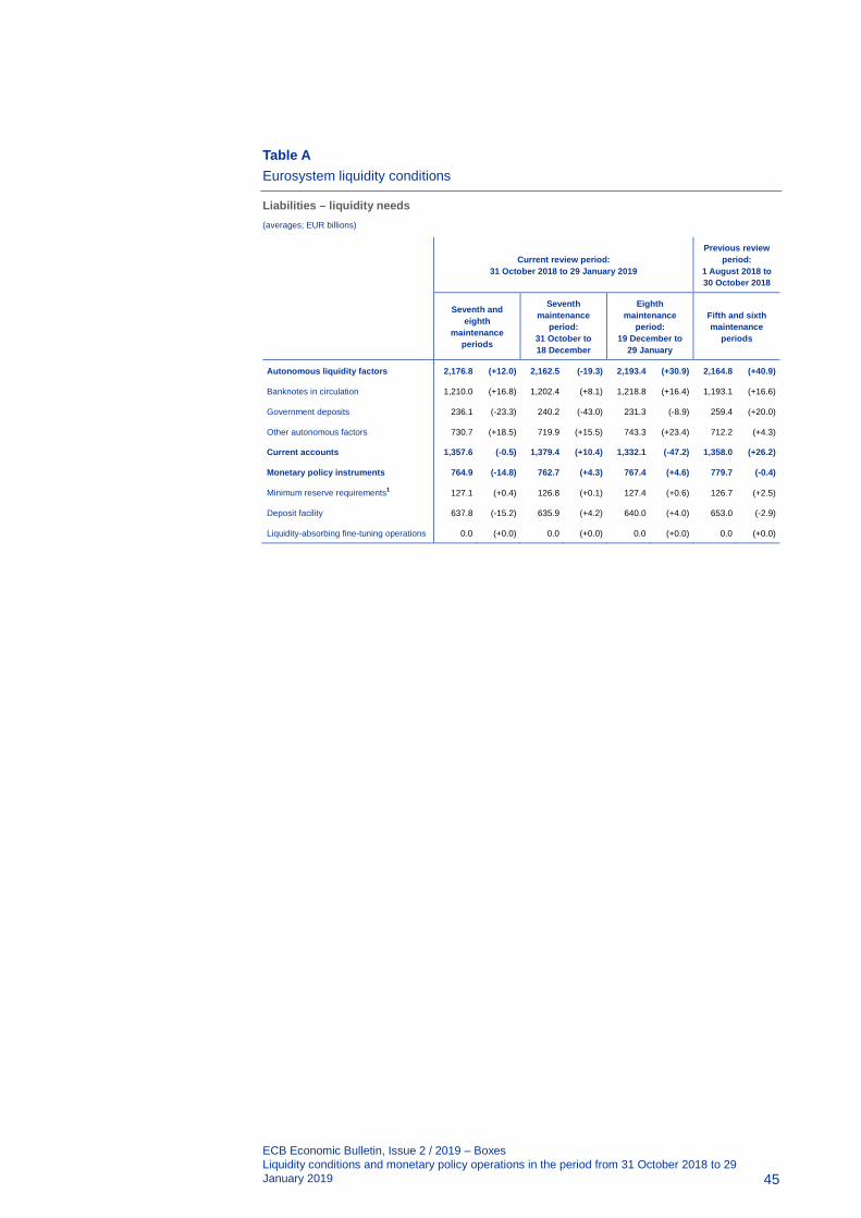
ECB Economic Bulletin, Issue 2 / 2019 – Boxes Liquidity conditions and monetary policy operations in the period from 31 October 2018 to 29 January 2019
45
Table A Eurosystem liquidity conditions
Liabilities – liquidity needs (averages; EUR billions)
Current review period: 31 October 2018 to 29 January 2019
Previous review period:
1 August 2018 to 30 October 2018
Seventh and eighth
maintenance periods
Seventh maintenance
period: 31 October to 18 December
Eighth maintenance
period: 19 December to
29 January
Fifth and sixth maintenance
periods
Autonomous liquidity factors 2,176.8 (+12.0) 2,162.5 (-19.3) 2,193.4 (+30.9) 2,164.8 (+40.9)
Banknotes in circulation 1,210.0 (+16.8) 1,202.4 (+8.1) 1,218.8 (+16.4) 1,193.1 (+16.6)
Government deposits 236.1 (-23.3) 240.2 (-43.0) 231.3 (-8.9) 259.4 (+20.0)
Other autonomous factors 730.7 (+18.5) 719.9 (+15.5) 743.3 (+23.4) 712.2 (+4.3)
Current accounts 1,357.6 (-0.5) 1,379.4 (+10.4) 1,332.1 (-47.2) 1,358.0 (+26.2)
Monetary policy instruments 764.9 (-14.8) 762.7 (+4.3) 767.4 (+4.6) 779.7 (-0.4)
Minimum reserve requirements1 127.1 (+0.4) 126.8 (+0.1) 127.4 (+0.6) 126.7 (+2.5)
Deposit facility 637.8 (-15.2) 635.9 (+4.2) 640.0 (+4.0) 653.0 (-2.9)
Liquidity-absorbing fine-tuning operations 0.0 (+0.0) 0.0 (+0.0) 0.0 (+0.0) 0.0 (+0.0)
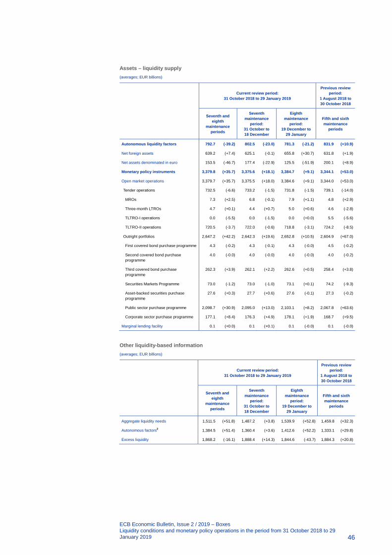
ECB Economic Bulletin, Issue 2 / 2019 – Boxes Liquidity conditions and monetary policy operations in the period from 31 October 2018 to 29 January 2019
46
Assets – liquidity supply (averages; EUR billions)
Current review period: 31 October 2018 to 29 January 2019
Previous review period:
1 August 2018 to 30 October 2018
Seventh and eighth
maintenance periods
Seventh maintenance
period: 31 October to 18 December
Eighth maintenance
period: 19 December to
29 January
Fifth and sixth maintenance
periods
Autonomous liquidity factors 792.7 (-39.2) 802.5 (-23.0) 781.3 (-21.2) 831.9 (+10.9)
Net foreign assets 639.2 (+7.4) 625.1 (-0.1) 655.8 (+30.7) 631.8 (+1.9)
Net assets denominated in euro 153.5 (-46.7) 177.4 (-22.9) 125.5 (-51.9) 200.1 (+8.9)
Monetary policy instruments 3,379.8 (+35.7) 3,375.6 (+18.1) 3,384.7 (+9.1) 3,344.1 (+53.0)
Open market operations 3,379.7 (+35.7) 3,375.5 (+18.0) 3,384.6 (+9.1) 3,344.0 (+53.0)
Tender operations 732.5 (-6.6) 733.2 (-1.5) 731.8 (-1.5) 739.1 (-14.0)
MROs 7.3 (+2.5) 6.8 (-0.1) 7.9 (+1.1) 4.8 (+2.9)
Three-month LTROs 4.7 (+0.1) 4.4 (+0.7) 5.0 (+0.6) 4.6 (-2.8)
TLTRO-I operations 0.0 (-5.5) 0.0 (-1.5) 0.0 (+0.0) 5.5 (-5.6)
TLTRO-II operations 720.5 (-3.7) 722.0 (-0.6) 718.8 (-3.1) 724.2 (-8.5)
Outright portfolios 2,647.2 (+42.2) 2,642.3 (+19.6) 2,652.8 (+10.5) 2,604.9 (+67.0)
First covered bond purchase programme 4.3 (-0.2) 4.3 (-0.1) 4.3 (-0.0) 4.5 (-0.2)
Second covered bond purchase programme
4.0 (-0.0) 4.0 (-0.0) 4.0 (-0.0) 4.0 (-0.2)
Third covered bond purchase programme
262.3 (+3.9) 262.1 (+2.2) 262.6 (+0.5) 258.4 (+3.8)
Securities Markets Programme 73.0 (-1.2) 73.0 (-1.0) 73.1 (+0.1) 74.2 (-9.3)
Asset-backed securities purchase programme
27.6 (+0.3) 27.7 (+0.6) 27.6 (-0.1) 27.3 (-0.2)
Public sector purchase programme 2,098.7 (+30.9) 2,095.0 (+13.0) 2,103.1 (+8.2) 2,067.8 (+63.6)
Corporate sector purchase programme 177.1 (+8.4) 176.3 (+4.9) 178.1 (+1.9) 168.7 (+9.5)
Marginal lending facility 0.1 (+0.0) 0.1 (+0.1) 0.1 (-0.0) 0.1 (-0.0)
Other liquidity-based information (averages; EUR billions)
Current review period: 31 October 2018 to 29 January 2019
Previous review period:
1 August 2018 to 30 October 2018
Seventh and eighth
maintenance periods
Seventh maintenance
period: 31 October to 18 December
Eighth maintenance
period: 19 December to
29 January
Fifth and sixth maintenance
periods
Aggregate liquidity needs 1,511.5 (+51.8) 1,487.2 (+3.8) 1,539.9 (+52.8) 1,459.8 (+32.3)
Autonomous factors2 1,384.5 (+51.4) 1,360.4 (+3.6) 1,412.6 (+52.2) 1,333.1 (+29.8)
Excess liquidity 1,868.2 (-16.1) 1,888.4 (+14.3) 1,844.6 (-43.7) 1,884.3 (+20.8)

ECB Economic Bulletin, Issue 2 / 2019 – Boxes Liquidity conditions and monetary policy operations in the period from 31 October 2018 to 29 January 2019
47
Interest rate developments (averages; percentages)
Current review period: 31 October 2018 to 29 January 2019
Previous review period:
1 August 2018 to 30 October 2018
Seventh and eighth
maintenance periods
Seventh maintenance
period: 31 October to 18 December
Eighth maintenance
period: 19 December to
29 January
Fifth and sixth maintenance
periods
MROs 0.00 (+0.00) 0.00 (+0.00) 0.00 (+0.00) 0.00 (+0.00)
Marginal lending facility 0.25 (+0.00) 0.25 (+0.00) 0.25 (+0.00) 0.25 (+0.00)
Deposit facility -0.40 (+0.00) -0.40 (+0.00) -0.40 (+0.00) -0.40 (+0.00)
EONIA -0.363 (-0.00) -0.360 (+0.01) -0.366 (-0.01) -0.362 (+0.00)
Source: ECB. Notes: All figures in the table are rounded to the nearest €0.1 billion. Figures in brackets denote the change from the previous review or maintenance period. 1) “Minimum reserve requirements” is a memo item that does not appear on the Eurosystem balance sheet and therefore should not be included in the calculation of total liabilities. 2) The overall value of autonomous factors also includes “items in course of settlement”.
Liquidity provided through monetary policy instruments
The average amount of liquidity provided through open market operations – including both tender operations and APP purchases – increased by €35.7 billion to €3,379.8 billion (see Chart A). This increase was fully attributable to net APP purchases, while demand for tender operations decreased slightly.
Chart A Evolution of open market operations and excess liquidity
(EUR billions)
Source: ECB.
The average amount of liquidity provided through tender operations declined slightly over the review period, by €6.6 billion to €732.5 billion. This decrease was entirely due to a lower average outstanding amount of targeted longer-term refinancing operations (TLTROs), which decreased by €9.2 billion. The average
0
500
1,000
1,500
2,000
2,500
3,000
3,500
07/14 01/15 07/15 01/16 07/16 01/17 07/17 01/18 07/18 01/19
Tender operationsOutright portfoliosExcess liquidity

ECB Economic Bulletin, Issue 2 / 2019 – Boxes Liquidity conditions and monetary policy operations in the period from 31 October 2018 to 29 January 2019
48
liquidity provided through MROs increased by €2.5 billion to €7.3 billion, which partially offset the decline in TLTROs.
Liquidity provided through the Eurosystem’s monetary policy portfolios increased by €42.2 billion to €2,647.2 billion on average, owing to net APP purchases, which continued into December 2018. However, the size of the increase shrank by €24.8 billion compared to the previous review period. Liquidity provided by the public sector purchase programme, the third covered bond purchase programme, the corporate sector purchase programme and the asset-backed securities purchase programme rose on average by €30.9 billion, €3.9 billion, €8.4 billion and €0.3 billion respectively. Redemptions of bonds held under the Securities Markets Programme and the previous two covered bond purchase programmes totalled €1.3 billion.
Excess liquidity
As a consequence of the developments detailed above, average excess liquidity decreased slightly compared with the previous review period, by €16.1 billion to €1,868.2 billion (see Chart A). This decrease reflects higher net autonomous factors, mainly in the eighth maintenance period, driven partly by year-end developments in liabilities to non-euro area residents in euro, which were only partially offset by the liquidity provided through the APP purchases, which slowed down towards the end of December, prior to entering the reinvestment phase on 1 January. Regarding the allocation of excess liquidity holdings between current accounts and the deposit facility, average current account holdings marginally declined by €0.5 billion to €1,357.6 billion, and average recourse to the deposit facility declined by €15.2 billion to €637.8 billion.
Interest rate developments
Overnight unsecured and secured money market rates remained close to the ECB deposit facility rate. In the unsecured market, the euro overnight index average (EONIA) averaged −0.363%, almost unchanged from the previous review period. The EONIA fluctuated between a low of −0.374% observed on 21 December and a high of −0.335% observed on 27 December. Regarding the secured market, the spread between the average overnight repo rates for the standard and the extended collateral baskets in the general collateral (GC) pooling market15 narrowed. Compared to the previous period, the average overnight repo rate for the standard collateral basket increased by 2 basis points to −0.417%, while for the extended collateral basket it declined by 2 basis points to −0.406%. The 2018 year-end decline in core repo rates was less pronounced than the 2017 year-end decline. This suggests that market participants have adopted more efficient collateral management practices. In addition,
15 The GC Pooling market allows repurchase agreements to be traded on the Eurex platform against
standardised baskets of collateral.

ECB Economic Bulletin, Issue 2 / 2019 – Boxes Liquidity conditions and monetary policy operations in the period from 31 October 2018 to 29 January 2019
49
the Eurosystem public sector purchase programme securities lending facility continued to support the smooth functioning of the repo market.
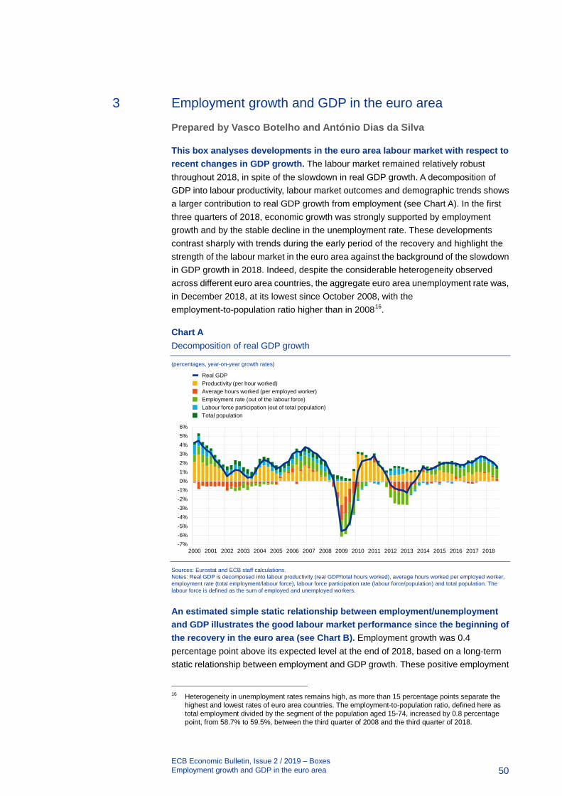
ECB Economic Bulletin, Issue 2 / 2019 – Boxes Employment growth and GDP in the euro area 50
Employment growth and GDP in the euro area 3
Prepared by Vasco Botelho and António Dias da Silva
This box analyses developments in the euro area labour market with respect to recent changes in GDP growth. The labour market remained relatively robust throughout 2018, in spite of the slowdown in real GDP growth. A decomposition of GDP into labour productivity, labour market outcomes and demographic trends shows a larger contribution to real GDP growth from employment (see Chart A). In the first three quarters of 2018, economic growth was strongly supported by employment growth and by the stable decline in the unemployment rate. These developments contrast sharply with trends during the early period of the recovery and highlight the strength of the labour market in the euro area against the background of the slowdown in GDP growth in 2018. Indeed, despite the considerable heterogeneity observed across different euro area countries, the aggregate euro area unemployment rate was, in December 2018, at its lowest since October 2008, with the employment-to-population ratio higher than in 200816.
Chart A Decomposition of real GDP growth
(percentages, year-on-year growth rates)
Sources: Eurostat and ECB staff calculations. Notes: Real GDP is decomposed into labour productivity (real GDP/total hours worked), average hours worked per employed worker, employment rate (total employment/labour force), labour force participation rate (labour force/population) and total population. The labour force is defined as the sum of employed and unemployed workers.
An estimated simple static relationship between employment/unemployment and GDP illustrates the good labour market performance since the beginning of the recovery in the euro area (see Chart B). Employment growth was 0.4 percentage point above its expected level at the end of 2018, based on a long-term static relationship between employment and GDP growth. These positive employment
16 Heterogeneity in unemployment rates remains high, as more than 15 percentage points separate the highest and lowest rates of euro area countries. The employment-to-population ratio, defined here as total employment divided by the segment of the population aged 15-74, increased by 0.8 percentage point, from 58.7% to 59.5%, between the third quarter of 2008 and the third quarter of 2018.
-7%-6%-5%-4%-3%-2%-1%0%1%2%3%4%5%6%
2000 2001 2002 2003 2004 2005 2006 2007 2008 2009 2010 2011 2012 2013 2014 2015 2016 2017 2018
Real GDPProductivity (per hour worked)Average hours worked (per employed worker)Employment rate (out of the labour force)Labour force participation (out of total population)Total population
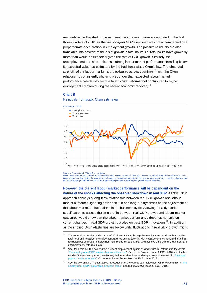
ECB Economic Bulletin, Issue 2 / 2019 – Boxes Employment growth and GDP in the euro area
51
residuals since the start of the recovery became even more accentuated in the last three quarters of 2018, as the year-on-year GDP slowdown was not accompanied by a proportionate deceleration in employment growth. The positive residuals are also translated into positive residuals of growth in total hours, i.e. total hours have grown by more than would be expected given the rate of GDP growth. Similarly, the unemployment rate also indicates a strong labour market performance, trending below its expected value, as estimated by the traditional static Okun’s law. The observed strength of the labour market is broad-based across countries17, with the Okun relationship consistently showing a stronger than expected labour market performance, which may be due to structural reforms that contributed to higher employment creation during the recent economic recovery18.
Chart B Residuals from static Okun estimates
(percentage points)
Sources: Eurostat and ECB staff calculations. Notes: Estimates based on data for the period between the first quarter of 1998 and the third quarter of 2018. Residuals from a static Okun relationship that relates the year-on-year changes in the unemployment rate, the year-on-year growth rate in total employment and the year-on-year growth rate in total hours to the contemporaneous year-on-year growth rate in real GDP.
However, the current labour market performance will be dependent on the nature of the shocks affecting the observed slowdown in real GDP. A static Okun approach conveys a long-term relationship between real GDP growth and labour market outcomes, ignoring both short-run and long-run dynamics on the adjustment of the labour market to fluctuations in the business cycle. Allowing for a dynamic specification to assess the time profile between real GDP growth and labour market outcomes would show that the labour market performance depends not only on current changes in real GDP growth but also on past GDP innovations19. In addition, as the implied Okun elasticities are below unity, fluctuations in real GDP growth might 17 The exceptions for the third quarter of 2018 are: Italy, with negative employment residuals but positive
total hour and negative unemployment rate residuals; Estonia, with negative employment and total hour residuals but positive unemployment rate residuals; and Malta, with positive employment, total hour and unemployment rate residuals.
18 See, for example, the box entitled “Recent employment dynamics and structural reforms” in the article “The employment-GDP relationship since the crisis”, Economic Bulletin, Issue 6, ECB, 2016, and the box entitled “Labour and product market regulation, worker flows and output responsiveness” in “Structural policies in the euro area”, Occasional Paper Series, No 210, ECB, June 2018.
19 See the box entitled “A quantitative investigation of the euro area employment-GDP relationship” in “The employment-GDP relationship since the crisis”, Economic Bulletin, Issue 6, ECB, 2016.
-2,5
-2,0
-1,5
-1,0
-0,5
0,0
0,5
1,0
1,5
2000 2001 2002 2003 2004 2005 2006 2007 2008 2009 2010 2011 2012 2013 2014 2015 2016 2017 2018
Unemployment rateTotal employmentTotal hours

ECB Economic Bulletin, Issue 2 / 2019 – Boxes Employment growth and GDP in the euro area
52
imply a somewhat protracted and mitigated response of total employment, the unemployment rate and total hours. Moreover, the current strong labour market performance and its subsequent path could also be affected by the specific nature of the shocks hitting the economy.
Overall, these results highlight the strong labour market dynamics since the beginning of the recovery and underline the recent robustness of the labour market in the face of the recent slowdown in real GDP in 2018. Indeed, while GDP growth decelerated by 0.7 percentage point during 2018, employment growth decelerated only by 0.2 percentage point, with the static Okun residuals becoming even more negative for unemployment and more positive for employment and total hours. However, the labour market is also characterised by a protracted response to changes in GDP, and that will be one of the various factors influencing how the labour market evolves in subsequent quarters.
ECB Economic Bulletin, Issue 2 / 2019 – Boxes New features in the Harmonised Index of Consumer Prices: analytical groups, scanner data and web-scraping 53
4 New features in the Harmonised Index of Consumer Prices: analytical groups, scanner data and web-scraping
Prepared by Martin Eiglsperger
Harmonised indices of consumer prices (HICPs) for food, industrial goods, services and energy are measures that the ECB uses for its more detailed analysis of inflation in the euro area. With the release of the HICPs for January 2019, these analytical groups - special aggregates - are based on a more exact allocation of products. As a result, the distinction between goods and services and between unprocessed and processed food is now more precise. This improvement has been achieved by deriving special aggregates from the HICP’s generic classification – the “European Classification of Individual Consumption according to Purpose” (ECOICOP) – which provides a more detailed level of breakdown than the product classification used thus far. Another recent enhancement is the extended use of supermarket scanner data. “Web-scraping” – an automated approach to collecting mass data from websites – is also being more broadly applied. Overall, these changes reflect better the actual consumer price developments in the economy, especially since they increase the coverage of sales prices.
The ECB monitors and analyses inflation using the HICP grouped into unprocessed food, processed food, industrial goods, services and energy. These special aggregates often exhibit distinct properties, such as the greater volatility of the HICPs for unprocessed food and for energy. Some measures of underlying inflation are derived by excluding some of these special aggregates.20 In general, special aggregates are used to better analyse and understand the drivers of inflation.
Statistical offices in the European Union have introduced a further level of detail into the HICP classification by consumption purpose. At its most detailed level, ECOICOP includes around 300 sub-categories, for example “Mobile telephone equipment” (formerly the most detailed level of breakdown grouped all telephone and telefax equipment in one category). “Repair of telephone or telefax equipment” has also been grouped as a separate category. Statistical offices are providing breakdowns of their national HICPs in accordance with ECOICOP for different time spans. While France and Lithuania have back-calculated the entire time series, Ireland and Finland have only published data from 2017 onwards.
Price indices for analytical groups based on the more detailed classification of products by consumption purpose have been introduced with the publication of the euro area HICP for January 2019. Eurostat, the statistical office of the European Union, has calculated these new special aggregates back to January 2017 for the euro area and the European Union as a whole, as well as for all individual EU Member States. The old HICP special aggregates have been replaced. Up to December 2016, data for HICP special aggregates remain based on the less detailed breakdown, implying a statistical break in the respective time series. Chart A illustrates how the more detailed level of product breakdown impacts on the HICPs for
20 See the article “Measures of underlying inflation for the euro area”, Economic Bulletin, Issue 4, ECB, 2018.

ECB Economic Bulletin, Issue 2 / 2019 – Boxes New features in the Harmonised Index of Consumer Prices: analytical groups, scanner data and web-scraping
54
unprocessed food and for industrial goods excluding energy. Apart from the split into unprocessed and processed food, the effects of the more detailed data on special aggregates are relatively minor. Nevertheless, this may have some implications for the forecasting and seasonal adjustment of HICP special aggregates.
Chart A More detailed classification on euro area HICPs for unprocessed food and for industrial goods excluding energy
(index: 2015 = 100)
Source: Eurostat.
Having HICPs for food, goods, services and energy derived from a more detailed classification of products by consumption purpose is an important improvement. It helps to better identify drivers of inflation, such as wage increases for services activities. Econometric modelling of inflation by analytical groups can also be expected to benefit from the more precise allocation.
With the publication of HICPs for January 2019, the use of web-scraped data has expanded further; supermarket scanner data are already used by several statistical offices. Traditionally, prices in bricks-and-mortar shops are collected by price observers, who focus on the prices of the most sold product variants and visit outlets at least once a month; for more volatile prices the visits are more frequent. While in many EU Member States price collection in shops is still central to HICP data sampling, many statistical offices have started or are intensifying the use of scanner and web-scraped data.
These new data collection methods provide considerably more price data, reflecting product variability, and they also cover a greater number of shopping days sampled within a month. In contrast to the standard survey-based price collection in bricks-and-mortar stores, index calculation using scanner data uses turnover by product bar codes (Global Trade Item Number, GTIN) or another identification code. Prices are derived by dividing the turnover of a certain product, identified by its item code, by the amount sold. Scanner data ensure that many more products are included over a longer time period. Prices derived from scanner data are closer to the average for the month, compared with point-in-time price collection.
100
101
102
103
104
105
106
107
108
109
110
01/17 05/17 09/17 01/18 05/18 09/18 01/19
a) Unprocessed food
Existing breakdownMore detailed breakdown
95
96
97
98
99
100
101
102
103
104
01/17 05/17 09/17 01/18 05/18 09/18 01/19
b) Industrial goods excluding energy

ECB Economic Bulletin, Issue 2 / 2019 – Boxes New features in the Harmonised Index of Consumer Prices: analytical groups, scanner data and web-scraping
55
New data collection methods require new statistical approaches. The significantly larger volume of data requires statistical offices to treat the data in an automated manner. The compilation of product-specific price indices from scanner data poses several challenges, in particular the treatment of discount prices and the greater purchase volumes triggered by discounts. Low turnover in post-discount periods implies that price indices, weighted by sales volumes, tend to be prone to a downward drift when established price index formulae are applied.21 In most cases, statistical offices that use scanner data currently compile drift-free indices by not incorporating index weights derived from concurrent turnover. Statistical researchers are currently developing methods to take account of turnover by means of expenditure weights while avoiding downward biases.22
Relaunched products may also cause compilation issues when scanner data are used. While maintaining their essential product features, relaunched products may change their item code and sell at a higher price. Compiling price indices at the level of item codes would not capture such price increases. It is therefore necessary to develop methods that identify relaunches also when item codes have changed.
A larger range of product variants, a greater frequency of recording and higher coverage of the reporting month are the three main ways scanner and web-scraped data affect the HICP. Scanner data typically refer to a period of two to three weeks of a month. HICP flash estimates may cover less than this. Therefore, the use of scanner data may occasionally lead to higher and/or more frequent revisions to flash estimates. Overall, the larger amount of data implies that monthly price indices are more affected by the price setting of supermarkets and internet retailers. For example, weekend days, as well as the shopping days before Easter and Christmas, are covered better using these new methods.
Scanner data better indicate sharp changes in prices related to discounts. Sales prices around Christmas may have an impact, in particular when scanner data are incorporated for the first time, since the HICP formula requires chain-linking over December. Generally, with the use of scanner data, sales prices are covered more comprehensively, both across time and across products, implying that scanner data-based price indices may be significantly more volatile.
21 See, for example, de Haan, J. and van der Grient, H., “Eliminating chain drift in price indexes based on
scanner data”, Journal of Econometrics, Vol. 161(1), pp. 36-46, March 2011. 22 See, for example, Chessa, A., Verburg, J. and Willenborg, L., “A Comparison of Price Index Methods for
Scanner Data”, presented at the 15th Meeting of the Ottawa Group, 10-12 May 2017, Eltville am Rhein, Germany.
ECB Economic Bulletin, Issue 2 / 2019 – Boxes A new method for the package holiday price index in Germany and its impact on HICP inflation rates
56
5 A new method for the package holiday price index in Germany and its impact on HICP inflation rates
Prepared by Martin Eiglsperger
Harmonised indices of consumer prices (HICPs) are regularly updated for changes in consumption weights and the items included, and on occasion also for methodological improvements. One such improvement is a change in the way the price index for package holidays is calculated in the HICP for Germany, which was implemented with the HICP release for January 2019. This has led to revisions of annual rates of change not only for Germany, but also for the euro area as a whole.
The German price index for package holidays now shows a more meaningful seasonal pattern. While the previous method used seasonal expenditure weights – i.e. different weights in the price index for package holidays taken at different times of the year – the new approach uses annual weights that are kept fixed over the entire year. This means that the price index for package holidays is no longer affected by the switch between seasonal weights at the beginning and end of seasons. However, the application of fixed weights implies that, during out-of-season periods, when prices for seasonal trips are not observable, the missing changes in prices have to be estimated. For instance, in summer it is necessary to include estimates for the changes in prices of trips normally taken in the winter, and in the winter it is necessary to use estimates for the changes in prices in the summer. The estimation is done by means of imputation, where changes in holiday prices in out-of-season periods are estimated on the basis of the price dynamics of other trips actually conducted in that season. Whereas the former approach treated winter and summer holidays separately, the new integrated sample also includes destinations to which trips are made over the entire calendar year. This establishes a relationship between price developments of seasonal trips.
The methodological change has led to a more pronounced seasonal profile for the package holiday price index for Germany and also for the euro area. Chart A shows that the index for the euro area has greater seasonal variation than before, with higher values in the summer months and lower values in the winter months. While the new index varies more between seasonal peaks and troughs, however, its profile is less erratic.

ECB Economic Bulletin, Issue 2 / 2019 – Boxes A new method for the package holiday price index in Germany and its impact on HICP inflation rates
57
Chart A Price index for package holidays for the euro area before and after the revision
(index: 2015 = 100)
Source: Eurostat.
The revised data have had a considerable impact on the annual rates of change of several aggregates of the euro area HICP for the first year for which the methodological change was incorporated; afterwards the impact is more moderate (see Chart B). Index numbers from 2015 onwards use data compiled according to the new method, while the index for 2014 and before is still based on the former treatment of package holidays. The annual rates of change for 2015 are calculated using index values that are based on differing methods, and are therefore distorted.23 As of 2016, annual growth rates are based entirely on the new method and are therefore undistorted. The impact on the annual growth rates for the period 2016 to 2018 is relatively moderate.
23 See Eurostat, “Improved calculation of HICP special aggregates and German package holidays
methodological change”, February 2019, p. 2.
60
70
80
90
100
110
120
130
140
01/12 07/12 01/13 07/13 01/14 07/14 01/15 07/15 01/16 07/16 01/17 07/17 01/18 07/18 01/19
BeforeAfter

ECB Economic Bulletin, Issue 2 / 2019 – Boxes A new method for the package holiday price index in Germany and its impact on HICP inflation rates
58
Chart B Impact of the methodological change for the German package holiday price index on euro area HICP aggregates
(annual inflation rates)
Source: Eurostat. Note: The annual growth rates in the HICP for services for the years 2017 and 2018 after the revision are also affected by the introduction of a more detailed product classification; see the box entitled “New features in the Harmonised Index of Consumer Prices: analytical groups, scanner data and web-scraping” in this issue of the Economic Bulletin.
Users must look through the distortions in annual growth rates, especially for 2015, when assessing past inflation developments. This is particularly the case, for instance, for euro area HICP inflation excluding food and energy as a measure of underlying inflation (see Chart C). The revision of the series distorts the picture of successive years of low underlying inflation. For analytical purposes, users can correct the series of annual percentage changes in different ways.24 A simple approach to obtaining annual inflation rates that do not comprise data based on different methods is to use annual rates of change up to December 2015 based on the index before the methodological change, and to use annual growth rates that are derived from the index calculated according to the new method from January 2016.25
24 Approaches to mitigating the impact of the distortions could be facilitated by the use of time series
analysis techniques such as seasonal adjustment. 25 However, this method cannot be used to derive an HICP time series. The HICP is a price index based on
a Laspeyres-type formula (See Eurostat, “Harmonised Index of Consumer Prices (HICP), Methodological Manual”, November 2018, p. 170.), meaning that annual expenditure weights are applied to component indices rather than their growth rates.
0.4
0.0
0.2
1.5
1.7
0.8 0.80.9
1.0 1.0
1.2 1.21.1
1.41.3
0.4
0.2 0.2
1.5
1.8
0.8
1.1
0.8
1.0 1.0
1.2
1.5
1.1
1.41.5
0.0
0.2
0.4
0.6
0.8
1.0
1.2
1.4
1.6
1.8
2.0
2014 2015 2016 2017 2018 2014 2015 2016 2017 2018 2014 2015 2016 2017 2018
Headline HICP HICP excluding food and energy HICP for services
BeforeAfter

ECB Economic Bulletin, Issue 2 / 2019 – Boxes A new method for the package holiday price index in Germany and its impact on HICP inflation rates
59
Chart C Euro area HICP inflation excluding food and energy before and after the revision
(annual rates of change)
Source: Eurostat.
0,0
0,2
0,4
0,6
0,8
1,0
1,2
1,4
1,6
01/14 07/14 01/15 07/15 01/16 07/16 01/17 07/17 01/18 07/18 01/19
BeforeAfter

ECB Economic Bulletin, Issue 2 / 2019 – Boxes Interest rate-growth differential and government debt dynamics
60
6 Interest rate-growth differential and government debt dynamics
Prepared by Cristina Checherita-Westphal
The difference between the average interest rate that governments pay on their debt and the nominal growth rate of the economy is a key variable for debt dynamics and sovereign sustainability analysis. The change in government debt between two years equals the interest paid on the stock of debt, the primary deficit (excess of expenditure, excluding interest payments, over revenue), and other factors (deficit-debt adjustments). For ratios to GDP, the change in debt is then mainly determined by the primary balance and the difference between the interest rate and the GDP growth rate. If the interest rate-growth differential (𝑖𝑖 − 𝑔𝑔) is strictly positive, a primary fiscal surplus is needed to stabilise or reduce the debt-to-GDP ratio. The higher the initial debt level, the higher the primary surplus will need to be. Conversely, a persistently negative 𝑖𝑖 − 𝑔𝑔 on government debt (𝑖𝑖 < 𝑔𝑔) would imply that debt ratios could be reduced even in the presence of primary budget deficits (lower than the debt effect induced by the differential).26
Recently, 𝑖𝑖 − 𝑔𝑔 has turned negative in most advanced economies, including euro area sovereigns. According to the European Commission’s Autumn 2018 forecast, all euro area countries except Italy had negative 𝑖𝑖 − 𝑔𝑔 in 2017. The differential is projected to increase in 12 euro area countries by 2020, but to remain in negative territory for all countries except Italy.
The debate on the role of fiscal policy with a persistently negative interest rate-growth differential has been revived by Olivier Blanchard in his 2019 AEA Presidential address.27 Using the US example, Blanchard makes the point that the costs of government debt may be smaller than generally assumed in the policy discussion. This is because the (US) safe interest rate (a proxy of marginal bond rates) is below the nominal GDP growth rate and this is more the historical norm rather than the exception. With a negative 𝑖𝑖 − 𝑔𝑔 differential, public debt may have no fiscal cost. It may still have welfare costs, but these may also be lower than typically assumed. An implication of this proposition would be that the US can sustain (roll-over) high(er) debts without significant costs. The author stresses, however, that the purpose of the lecture is not to argue for higher debt per se, but to allow for a richer discussion of debt policy and appropriate debt rules than is currently the case.
Theoretical models do not provide clear cut conclusions with respect to the sign and size of the interest rate-growth differential on government debt. In 26 ∆𝑏𝑏𝑡𝑡 = �𝑖𝑖𝑡𝑡−𝑔𝑔𝑡𝑡
1+𝑔𝑔𝑡𝑡� 𝑏𝑏𝑡𝑡−1 − 𝑝𝑝𝑏𝑏𝑡𝑡 + 𝑑𝑑𝑑𝑑𝑑𝑑𝑡𝑡 (𝑒𝑒𝑒𝑒. 1)
Equation 1 (the typical debt accumulation equation) provides a simple accounting framework to decompose the change in the government gross debt-to-GDP ratio (∆𝑏𝑏𝑡𝑡) into its key drivers, consisting of: (i) the “snowball effect”, i.e. the impact of the difference between the average nominal interest rate charged on government debt (𝑖𝑖𝑡𝑡) and the nominal GDP growth rate (𝑔𝑔𝑡𝑡) multiplied by the debt-to-GDP ratio in the previous period (𝑏𝑏𝑡𝑡−1); (ii) the primary budget balance (surplus) ratio (𝑝𝑝𝑏𝑏𝑡𝑡); and (iii) the deficit-debt adjustment as a share of GDP (𝑑𝑑𝑑𝑑𝑑𝑑𝑡𝑡) or the stock-flow adjustment, comprising factors that affect debt but are not included in the budget balance (such as acquisitions or sales of financial assets).
27 “Public Debt and Low Interest Rates”, 2019 AEA Presidential Address by Olivier Blanchard (Atlanta, 5 January 2019). The lecture was essentially a presentation of his recent academic work entitled “Public Debt and Low Interest Rates”.
ECB Economic Bulletin, Issue 2 / 2019 – Boxes Interest rate-growth differential and government debt dynamics
61
general, models are based on the assumption that the inter-temporal budget constraint holds, i.e. the present value of future primary surpluses should equal the current level of debt (no explosive debt paths). While standard growth theory implies a positive 𝑖𝑖 − 𝑔𝑔 for economies that operate at their steady state (along a balanced growth path), including for the safe rate, in overlapping-generation models with non-diversifiable uncertainty or models with rational bubbles, a negative 𝑖𝑖 − 𝑔𝑔 on government debt could co-exist with a dynamically efficient economy.28 Moreover, it must be recognised that such models analyse the “risk-free rate”, while accounting for sovereign credit risk or possibility of default would raise the cost of public debt.29
Empirically, the relevant interest rate-growth differential for public debt dynamics, as defined above, has been positive for advanced mature economies over longer periods. The value of 𝑖𝑖 − 𝑔𝑔 for mature economies over extended periods of time has hovered around one percentage point.30 Positive values are also typically observed for the largest euro area economies (see Chart A). On the other hand, negative 𝑖𝑖 − 𝑔𝑔 values are observed for advanced economies during periods of overheating or, more generally, for emerging economies. As documented in the empirical literature31, the main factors behind the “puzzle” of persistently negative differentials in emerging economies are financial repression, including during periods of hyperinflation, and to some extent also the income catch-up effect. Finally, the primary balance also plays an important role in debt dynamics. Even in the presence of negative 𝑖𝑖 − 𝑔𝑔, large enough primary deficits would prevent debt ratios from stabilising. In this respect, primary surpluses in most euro area countries have helped put debt ratios on a downward path.32
Moreover, while the interest rate has followed a clear downward trend since the 1980s, to a certain extent the GDP growth rate has done so as well. Since the 1980s in particular, real interest rates in advanced economies have declined and, in the wake of the global financial crisis, plummeted to exceptionally low levels. This development has often been associated with a decline in the estimated natural or neutral rate of interest, which in turn has been linked in many studies to a decline in potential output growth.33 There is therefore still a question about the trend in the 28 Blanchard, O. and Fischer, S., Lectures on Macroeconomics, The MIT Press, Cambridge, 1989, and
Blanchard (2019), op. cit. 29 For a summary of this literature, see D’Erasmo, P., Mendoza, E. and Zhang, J., “What is a Sustainable
Public Debt?”, Handbook of Macroeconomics, Vol. 2B, 2016, pp. 2557-2588. 30 See Escolano, J., “A Practical Guide to Public Debt Dynamics, Fiscal Sustainability, and Cyclical
Adjustment of Budgetary Aggregates”, IMF Technical Notes and Manuals, Washington DC, 2010. A seminal OECD paper on measures for public debt sustainability (Blanchard et al., 1990) concludes that even if the configuration of a negative differential being easily rejected based on theoretical or empirical grounds remains “a theoretical curiosum [,…] Still, there is general agreement that the condition of an excess in the interest rate over the growth rate probably holds, if not always, at least in the medium and long run.” (pp. 15). See Blanchard, O., Chouraqui, J.-C., Hagemann, R. and Sartor, N., “The Sustainability of Fiscal Policy: New Answers to an Old Question”, Economic Studies, No 15, OECD, Paris, 1990.
31 See, for instance: Escolano, J., Shabunina, A. and Woo, J., “The Puzzle of Persistently Negative Interest-Rate–Growth Differentials: Financial Repression or Income Catch-Up?”, Fiscal Studies, Vol. 38(2), 2017, pp. 179–217.
32 According to the Commission’s Autumn 2018 forecast, the euro area primary balance is projected to be in surplus (+1.2% of GDP) in 2018, as opposed to deficits in the US (-2.1% of GDP) and Japan (-1.5% of GDP). All euro area countries apart from France, Spain and Latvia are projected to have recorded a primary surplus in 2018.
33 See Brand, C., Bielecki, M. and Penalver, A., “The natural rate of interest: estimates, drivers, and challenges to monetary policy”, Occasional Paper Series, No 217, ECB, Frankfurt am Main, 2018.
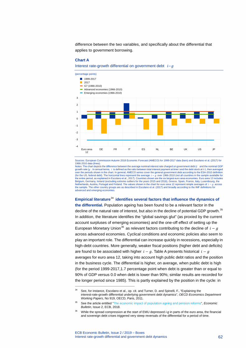
ECB Economic Bulletin, Issue 2 / 2019 – Boxes Interest rate-growth differential and government debt dynamics
62
difference between the two variables, and specifically about the differential that applies to government borrowing.
Chart A Interest rate-growth differential on government debt (𝑖𝑖−𝑔𝑔)
(percentage points)
Sources: European Commission Autumn 2018 Economic Forecast (AMECO) for 1999-2017 data (bars) and Escolano et al. (2017) for 1966-2010 data (lines). Notes: The chart depicts the difference between the average nominal interest rate charged on government debt (𝑖𝑖) and the nominal GDP growth rate (𝑔𝑔). In annual terms, 𝑖𝑖 is defined as the ratio between total interest payment at time t and the debt stock at t-1, then averaged over the periods shown in the chart. In general, AMECO series cover the general government debt according to the ESA-2010 definition (for the US, federal debt). The horizontal lines represent the average 𝑖𝑖 − 𝑔𝑔 over 1966-2010 (not all countries in the sample available for the entire period, as explained in Escolano et al., 2017). Countries shown are the six largest euro area economies. Euro area 12 includes Belgium, Germany, Ireland (excluding extreme outliers for the years 2015 and 2016), Greece, Spain, France, Italy, Luxembourg, the Netherlands, Austria, Portugal and Finland. The values shown in the chart for euro area 12 represent simple averages of 𝑖𝑖 − 𝑔𝑔 across the sample. The other country groups are as described in Escolano et al. (2017) and broadly according to the IMF definitions for advanced and emerging economies.
Empirical literature34 identifies several factors that influence the dynamics of the differential. Population ageing has been found to be a relevant factor in the decline of the natural rate of interest, but also in the decline of potential GDP growth.35 In addition, the literature identifies the “global savings glut” (as proxied by the current account surpluses of emerging economies) and the one-off effect of setting up the European Monetary Union36 as relevant factors contributing to the decline of 𝑖𝑖 − 𝑔𝑔 across advanced economies. Cyclical conditions and economic policies also seem to play an important role. The differential can increase quickly in recessions, especially in high-debt countries. More generally, weaker fiscal positions (higher debt and deficits) are found to be associated with higher 𝑖𝑖 − 𝑔𝑔. Table A presents historical 𝑖𝑖 − 𝑔𝑔 averages for euro area 12, taking into account high public debt ratios and the position in the business cycle. The differential is higher, on average, when public debt is high (for the period 1999-2017,1.7 percentage point when debt is greater than or equal to 90% of GDP versus 0.0 when debt is lower than 90%; similar results are recorded for the longer period since 1985). This is partly explained by the position in the cycle: in 34 See, for instance, Escolano et al., op. cit. and Turner, D. and Spinelli, F., “Explaining the
interest-rate-growth differential underlying government debt dynamics”, OECD Economics Department Working Papers, No 919, OECD, Paris, 2011.
35 See the article entitled “The economic impact of population ageing and pension reforms”, Economic Bulletin, Issue 2, ECB, 2018.
36 While the spread compression at the start of EMU depressed i-g in parts of the euro area, the financial and sovereign debt crises triggered very steep reversals of the differential for a period of time.
-4
-3
-2
-1
0
1
2
3
Euro area12
DE FR IT ES NL BE UK US JP
1999-20172017G7 (1966-2010)Advanced economies (1966-2010)Emerging economies (1966-2010)
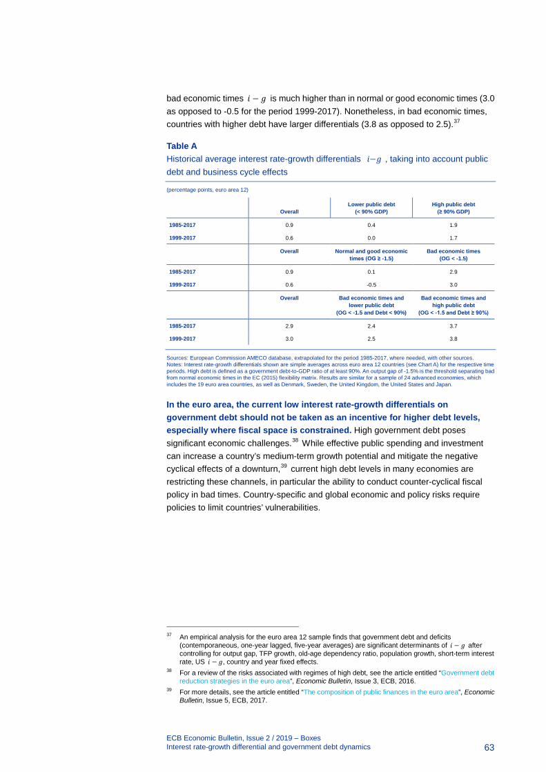
ECB Economic Bulletin, Issue 2 / 2019 – Boxes Interest rate-growth differential and government debt dynamics
63
bad economic times 𝑖𝑖 − 𝑔𝑔 is much higher than in normal or good economic times (3.0 as opposed to -0.5 for the period 1999-2017). Nonetheless, in bad economic times, countries with higher debt have larger differentials (3.8 as opposed to 2.5).37
Table A Historical average interest rate-growth differentials (𝑖𝑖−𝑔𝑔), taking into account public debt and business cycle effects
(percentage points, euro area 12)
Overall Lower public debt
(< 90% GDP) High public debt
(≥ 90% GDP)
1985-2017 0.9 0.4 1.9
1999-2017 0.6 0.0 1.7
Overall Normal and good economic times (OG ≥ -1.5)
Bad economic times (OG < -1.5)
1985-2017 0.9 0.1 2.9
1999-2017 0.6 -0.5 3.0
Overall Bad economic times and lower public debt
(OG < -1.5 and Debt < 90%)
Bad economic times and high public debt
(OG < -1.5 and Debt ≥ 90%)
1985-2017 2.9 2.4 3.7
1999-2017 3.0 2.5 3.8
Sources: European Commission AMECO database, extrapolated for the period 1985-2017, where needed, with other sources. Notes: Interest rate-growth differentials shown are simple averages across euro area 12 countries (see Chart A) for the respective time periods. High debt is defined as a government debt-to-GDP ratio of at least 90%. An output gap of -1.5% is the threshold separating bad from normal economic times in the EC (2015) flexibility matrix. Results are similar for a sample of 24 advanced economies, which includes the 19 euro area countries, as well as Denmark, Sweden, the United Kingdom, the United States and Japan.
In the euro area, the current low interest rate-growth differentials on government debt should not be taken as an incentive for higher debt levels, especially where fiscal space is constrained. High government debt poses significant economic challenges.38 While effective public spending and investment can increase a country’s medium-term growth potential and mitigate the negative cyclical effects of a downturn,39 current high debt levels in many economies are restricting these channels, in particular the ability to conduct counter-cyclical fiscal policy in bad times. Country-specific and global economic and policy risks require policies to limit countries’ vulnerabilities.
37 An empirical analysis for the euro area 12 sample finds that government debt and deficits
(contemporaneous, one-year lagged, five-year averages) are significant determinants of 𝑖𝑖 − 𝑔𝑔 after controlling for output gap, TFP growth, old-age dependency ratio, population growth, short-term interest rate, US 𝑖𝑖 − 𝑔𝑔, country and year fixed effects.
38 For a review of the risks associated with regimes of high debt, see the article entitled “Government debt reduction strategies in the euro area”, Economic Bulletin, Issue 3, ECB, 2016.
39 For more details, see the article entitled “The composition of public finances in the euro area”, Economic Bulletin, Issue 5, ECB, 2017.
7 The European Commission’s 2019 assessment of macroeconomic imbalances and progress on reforms
Prepared by Nick Ligthart
On 27 February 2019, the European Commission published its annual assessment of macroeconomic imbalances and the progress made with structural reforms based on the country-specific recommendations (CSRs) as adopted in July 2018. This assessment is a key part of the European Semester framework for coordinating economic and fiscal policies across the EU. Within this context, the macroeconomic imbalance procedure (MIP) provides a framework for assessing macroeconomic imbalances. It aims to prevent the emergence of harmful imbalances and to actively correct imbalances where they have already become excessive.40
Macroeconomic imbalances
According to the Commission, the number of countries experiencing imbalances has increased to 13 overall, from 11 in 2018 (see Table A). This year, three countries have been assessed as experiencing “excessive imbalances” – Italy, Cyprus and Greece. While Italy and Cyprus were also included in this category last year, Greece has been included in this exercise for the first time this year as it exited its financial assistance programme in summer 2018. Its major challenges are high public debt, a negative net international investment position, a very high share of non-performing loans, a still-high unemployment rate and low growth potential. Cyprus is still facing challenges related to high levels of both non-performing loans and external, private and government debt. For Italy, the Commission finds that fiscal sustainability risks, as well as broadly stalling reform progress and backtracking, are now overshadowing the progress made in previous years. In addition, the Commission recategorised two countries in this year’s assessment. Croatia was recategorised from “excessive imbalances” to “imbalances”, owing to a decrease of private, public and external sector debt, among other factors. Romania was also recategorised, from “no imbalances” to “imbalances”, due to factors including reduced competitiveness and a widening of current account imbalances.
40 To identify imbalances, the Commission uses a standardised scoreboard to select countries that require
an in-depth review. There are three possible outcomes from these in-depth reviews: “no imbalances”, “imbalances” or “excessive imbalances”. If the Commission identifies imbalances, the country concerned will receive policy recommendations meant to address them. When the imbalances are assessed as being so severe that they are found to be “excessive”, the Commission can take further action by recommending that the Council activates the excessive imbalance procedure (EIP).
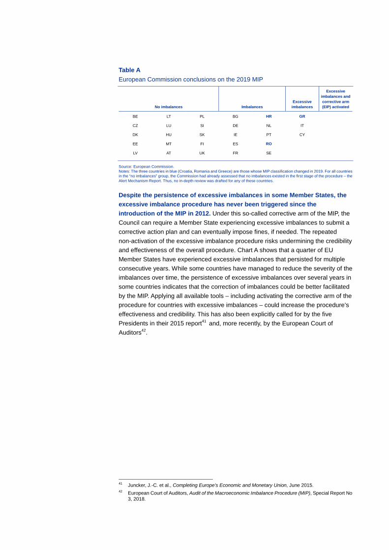
Table A European Commission conclusions on the 2019 MIP
No imbalances Imbalances Excessive
imbalances
Excessive imbalances and corrective arm (EIP) activated
BE LT PL BG HR GR
CZ LU SI DE NL IT
DK HU SK IE PT CY
EE MT FI ES RO
LV AT UK FR SE
Source: European Commission. Notes: The three countries in blue (Croatia, Romania and Greece) are those whose MIP classification changed in 2019. For all countries in the “no imbalances” group, the Commission had already assessed that no imbalances existed in the first stage of the procedure – the Alert Mechanism Report. Thus, no in-depth review was drafted for any of these countries.
Despite the persistence of excessive imbalances in some Member States, the excessive imbalance procedure has never been triggered since the introduction of the MIP in 2012. Under this so-called corrective arm of the MIP, the Council can require a Member State experiencing excessive imbalances to submit a corrective action plan and can eventually impose fines, if needed. The repeated non-activation of the excessive imbalance procedure risks undermining the credibility and effectiveness of the overall procedure. Chart A shows that a quarter of EU Member States have experienced excessive imbalances that persisted for multiple consecutive years. While some countries have managed to reduce the severity of the imbalances over time, the persistence of excessive imbalances over several years in some countries indicates that the correction of imbalances could be better facilitated by the MIP. Applying all available tools – including activating the corrective arm of the procedure for countries with excessive imbalances – could increase the procedure’s effectiveness and credibility. This has also been explicitly called for by the five Presidents in their 2015 report41 and, more recently, by the European Court of Auditors42.
41 Juncker, J.-C. et al., Completing Europe’s Economic and Monetary Union, June 2015. 42 European Court of Auditors, Audit of the Macroeconomic Imbalance Procedure (MIP), Special Report No
3, 2018.

Chart A EU Member States with excessive imbalances
Source: European Commission. Notes: The chart shows those countries assessed by the European Commission as experiencing “excessive imbalances” in the years indicated. A country subject to an economic adjustment programme enters the MIP automatically once the programme ends. In 2012 no country was assessed as having excessive imbalances.
Persistent macroeconomic imbalances – whether excessive or not – leave Member States vulnerable to adverse macroeconomic shocks and tend to increase the probability of recessions, which often carry high social and economic costs. While the EU has experienced economic growth for the past seven years, uncertainties related to geopolitical factors, the threat of protectionism and macroeconomic imbalances pose downside risks to economic activity. It is therefore important that countries undertake ambitious reform efforts to strengthen the resilience of their economies to adverse shocks.
Debt levels are still historically high in some Member States, for both government and private debt, which makes responding to a downturn or to negative shocks more difficult. Higher economic growth has helped to reduce debt-to-GDP ratios in recent years, but debt levels in several cases remain very high. Corporations have managed to reduce debt levels faster than households. At the same time, in a number of countries the high public and private indebtedness is reflected in large stocks of external debt, which highlights the need to ensure sufficient current account surpluses.
To support rebalancing and avoid new imbalances in cost competitiveness across the EU, accelerating growth in unit labour costs in some countries has to be carefully monitored. In particular, in countries with current account surpluses that the Commission finds are experiencing a lack of domestic demand and labour shortages, unit labour cost growth that is higher than the euro area average might facilitate rebalancing among euro area countries. At the same time, a relative deterioration of cost competitiveness in more vulnerable countries with relatively high unemployment should be monitored carefully so that a reversal of the positive adjustment achieved in recent years can be avoided.
GRHR HR HR HR HR
IT IT IT IT IT IT
ES
PT PT PT
BG BG BG
FR FR FR
SI
SI
CY CY
CY CY
2012 2013 2014 2015 2016 2017 2018 2019
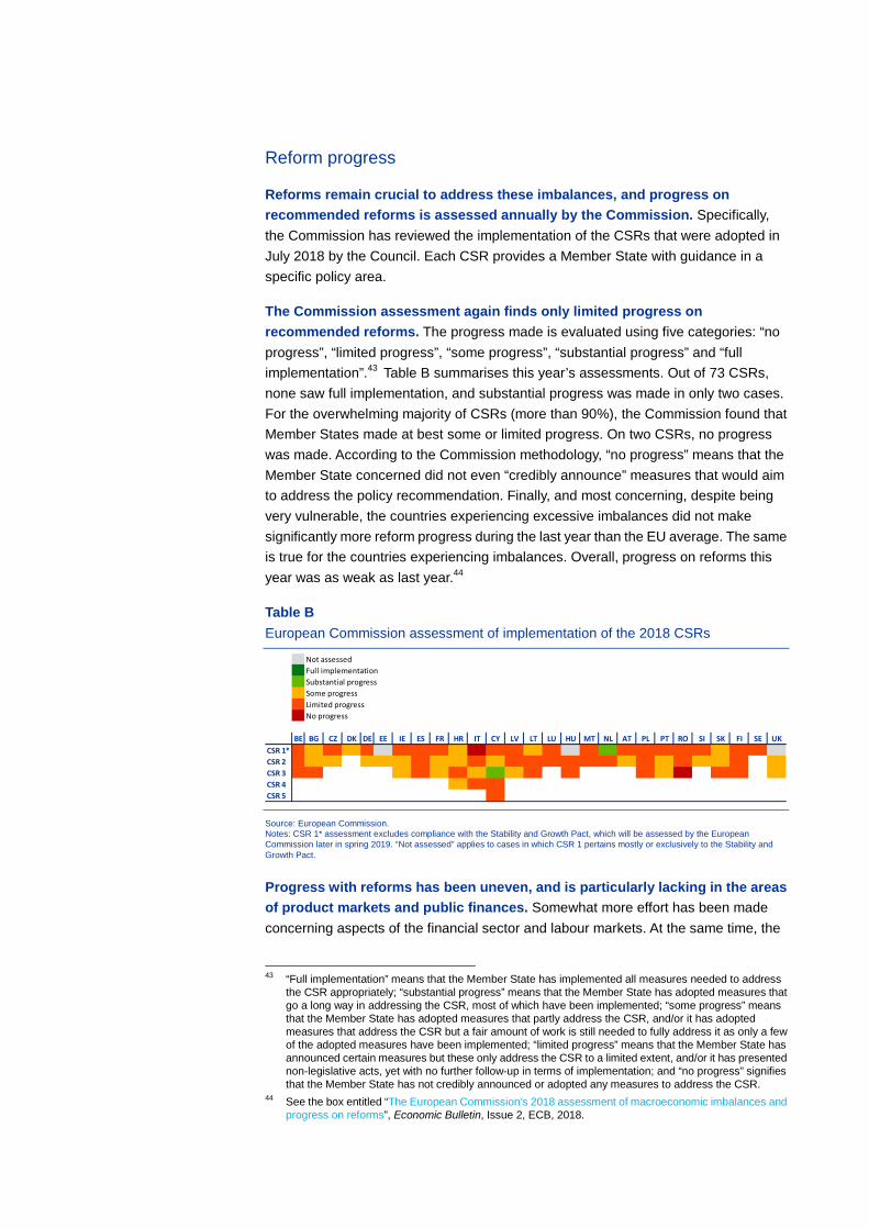
Reform progress
Reforms remain crucial to address these imbalances, and progress on recommended reforms is assessed annually by the Commission. Specifically, the Commission has reviewed the implementation of the CSRs that were adopted in July 2018 by the Council. Each CSR provides a Member State with guidance in a specific policy area.
The Commission assessment again finds only limited progress on recommended reforms. The progress made is evaluated using five categories: “no progress”, “limited progress”, “some progress”, “substantial progress” and “full implementation”.43 Table B summarises this year’s assessments. Out of 73 CSRs, none saw full implementation, and substantial progress was made in only two cases. For the overwhelming majority of CSRs (more than 90%), the Commission found that Member States made at best some or limited progress. On two CSRs, no progress was made. According to the Commission methodology, “no progress” means that the Member State concerned did not even “credibly announce” measures that would aim to address the policy recommendation. Finally, and most concerning, despite being very vulnerable, the countries experiencing excessive imbalances did not make significantly more reform progress during the last year than the EU average. The same is true for the countries experiencing imbalances. Overall, progress on reforms this year was as weak as last year.44
Table B European Commission assessment of implementation of the 2018 CSRs
Source: European Commission. Notes: CSR 1* assessment excludes compliance with the Stability and Growth Pact, which will be assessed by the European Commission later in spring 2019. “Not assessed” applies to cases in which CSR 1 pertains mostly or exclusively to the Stability and Growth Pact.
Progress with reforms has been uneven, and is particularly lacking in the areas of product markets and public finances. Somewhat more effort has been made concerning aspects of the financial sector and labour markets. At the same time, the
43 “Full implementation” means that the Member State has implemented all measures needed to address
the CSR appropriately; “substantial progress” means that the Member State has adopted measures that go a long way in addressing the CSR, most of which have been implemented; “some progress” means that the Member State has adopted measures that partly address the CSR, and/or it has adopted measures that address the CSR but a fair amount of work is still needed to fully address it as only a few of the adopted measures have been implemented; “limited progress” means that the Member State has announced certain measures but these only address the CSR to a limited extent, and/or it has presented non-legislative acts, yet with no further follow-up in terms of implementation; and “no progress” signifies that the Member State has not credibly announced or adopted any measures to address the CSR.
44 See the box entitled “The European Commission’s 2018 assessment of macroeconomic imbalances and progress on reforms”, Economic Bulletin, Issue 2, ECB, 2018.
Not assessedFull implementationSubstantial progressSome progressLimited progressNo progress
BE BG CZ DK DE EE IE ES FR HR IT CY LV LT LU HU MT NL AT PL PT RO SI SK FI SE UKCSR 1*CSR 2CSR 3CSR 4CSR 5
Commission even finds cases of backtracking on reforms, for instance regarding the long-term sustainability of public finances (including pensions).
Further reforms to improve the investment environment are essential to stimulate well-targeted investment that improves productivity, potential growth and resilience. The Commission finds that the highest barriers to investment are low quality of institutions and burdensome regulations. Creating an investment-friendly environment will help strengthen investment focused on productivity and growth – essential at this point in the business cycle. In turn, investment needs to be well targeted to be most effective. While investment in education, research, development and innovation is needed in most EU countries, it is important that it flows to those sectors where it would most increase productivity growth and competitiveness. To this end, the Commission has taken the positive step of adding a new annex to the country reports. The annex identifies country-specific investment needs and bottlenecks, and also aims to better align the use of EU funds with the European Semester’s analysis.

ECB Economic Bulletin, Issue 2 / 2019 – Article Taking stock of the Eurosystem’s asset purchase programme after the end of net asset purchases
69
Article
1 Taking stock of the Eurosystem’s asset purchase programme after the end of net asset purchases
Prepared by Felix Hammermann, Kieran Leonard, Stefano Nardelli and Julian von Landesberger
Following the Governing Council’s decision in December 2018 to end net asset purchases under the Eurosystem’s asset purchase programme (APP), this article reviews the implementation and effects of the asset purchases. The APP has proved to be an adaptable and effective instrument to ease monetary and financial conditions, foster economic recovery, counteract disinflationary pressures and anchor inflation expectations, thereby supporting a sustained adjustment in the path of inflation towards price stability. The APP has been part of a package of policy measures together with negative interest rates on the deposit facility, forward guidance and targeted longer-term refinancing operations (TLTROs), jointly creating synergies that have enhanced the effectiveness of each of the package’s individual components. From an implementation viewpoint, the Eurosystem ensured that asset purchases were conducted smoothly and flexibly by striving for market neutrality and mitigating unintended side effects for market functioning.
Whereas net asset purchases have come to an end, principal payments from maturing securities purchased under the APP will continue to be reinvested as this, together with enhanced forward guidance, provides the monetary accommodation that the Governing Council judges to be required for the continued sustained convergence of inflation to levels that are below, but close to, 2% over the medium term.
1 Introduction
The APP is part of a package of policy measures that was initiated in mid-2014 to support the monetary policy transmission mechanism and provide the amount of policy accommodation needed to ensure price stability. The room for further interest rate cuts had become very limited after monetary conditions were eased in the wake of the financial and sovereign debt crises by cutting key interest rates and deploying unprecedented measures to support monetary policy transmission. The APP, in combination with negative interest rates on the deposit facility, forward guidance and TLTROs, has helped the ECB meet its price stability objective. The APP comprises the third covered bond purchase programme (CBPP3, launched on 20 October 2014), the asset-backed securities purchase programme (ABSPP, launched on 21 November 2014), the public sector purchase programme (PSPP, launched on 9 March 2015) and the corporate sector purchase programme (CSPP, launched on 8 June 2016). APP net asset purchases were conducted until the end of December 2018, involving a total amount of €2.6 trillion. A snapshot of the APP portfolio in December 2018 shows the PSPP contributing the largest share,

ECB Economic Bulletin, Issue 2 / 2019 – Article Taking stock of the Eurosystem’s asset purchase programme after the end of net asset purchases
70
accounting for 82% of the total net purchases, followed by the CBPP3 (10%), the CSPP (7%) and the ABSPP (1%). The size of the APP portfolio is currently being kept stable by reinvesting principal payments from maturing securities.
2 The monetary policy rationale for launching the APP
Following a double-dip recession in the wake of the financial and sovereign debt crises, the euro area experienced a prolonged period of deleveraging, an atypically shallow recovery and persistently weak inflation. Bank lending conditions started to deteriorate and loan volumes (in particular those involving non-financial corporations) to contract at the end of 2011. Persistent weakness in the underlying growth momentum perpetuated capacity underutilisation, as also visible in high levels of unemployment. Inflation rates exhibited a protracted downward trend: in the core components, this was due to the general economic weakness, while declines in energy and food prices influenced the headline readings. Euro area inflation was generally projected to remain weak and fall over time, as reflected in successive downward adjustments in macroeconomic projections by most international organisations and the ECB (see Chart 1). Euro area annual HICP inflation fell to -0.2% in December 2014, and Eurosystem staff macroeconomic projections entailed further substantive downward revisions of inflation forecasts, from 1.1% to 0.7% in 2015 and from 1.4% to 1.3% in 2016.
Chart 1 Actual and projected HICP inflation with revisions
(percentages, year-on-year)
Sources: Eurosystem staff macroeconomic projections and ECB calculations. Notes: The grey lines in the chart refer to projected HICP inflation underpinning the (Broad) Macroeconomic Projection Exercise ((B)MPE) projection vintages in 2014 and 2018.
Persistently weak inflation in 2013-2014 contributed to a downtrend in inflation expectations and an increasing risk of those expectations becoming unmoored from the ECB’s price stability objective. Market-based measures of inflation expectations drifted to extraordinarily low levels. At the end of December 2014 the option-implied probability density function of euro area inflation indicated that markets
-1.0
-0.5
0.0
0.5
1.0
1.5
2.0
2.5
3.0
2011 2012 2013 2014 2015 2016 2017 2018 2019 2020 2021
HICP inflationDec 2018 BMPEDec 2014 BMPE

ECB Economic Bulletin, Issue 2 / 2019 – Article Taking stock of the Eurosystem’s asset purchase programme after the end of net asset purchases
71
assigned a probability of almost 50% to deflation and saw only a marginal probability of annual inflation reaching a level close to 2% or above (see Chart 9 below). These developments indicated risks that too prolonged a period of low inflation could become entrenched in inflation expectations, with adverse consequences for price stability.
To reverse the downtrend in inflation and forestall a disanchoring of inflation expectations, the APP was designed to expand and complement existing monetary policy measures. With the APP, announced in January 2015, the PSPP, an additional programme consisting of purchases of debt securities issued by public entities, was launched to complement the two ongoing asset purchase programmes, the CBPP3 and the ABSPP.
During the period 2015-2018 net asset purchases under the APP were the principal instrument of monetary policy and their size and duration were linked to achieving a sustained adjustment in the path of inflation towards price stability. In January 2015, following the APP announcement, net asset purchases were made the principal policy instrument and the Governing Council adopted a structured forward guidance. The first building block of this guidance pertained to the principal instrument itself and featured a combination of a time-dependent and state-dependent formulation. The time-dependent leg stated that the net asset purchases were intended to run at a certain monthly pace at least until a specific date (see Figure 1). The state-dependent leg established an explicit link to the price stability objective (“or beyond, if necessary, and in any case until the Governing Council sees a sustained adjustment in the path of inflation consistent with its inflation aim”). As shown in Figure 1, following the first announcement in January 2015 the Governing Council extended the programme through a series of recalibrations, in which the minimum horizon for the monthly purchases was pushed back sequentially and the pace of purchases was adjusted as necessary to advance progress towards the sustained adjustment. The second building block of the forward guidance pertained to the period over which the Governing Council expected that it would not be appropriate to raise the key ECB interest rates. In March 2016 the length of that period was linked to the end of the net asset purchases.
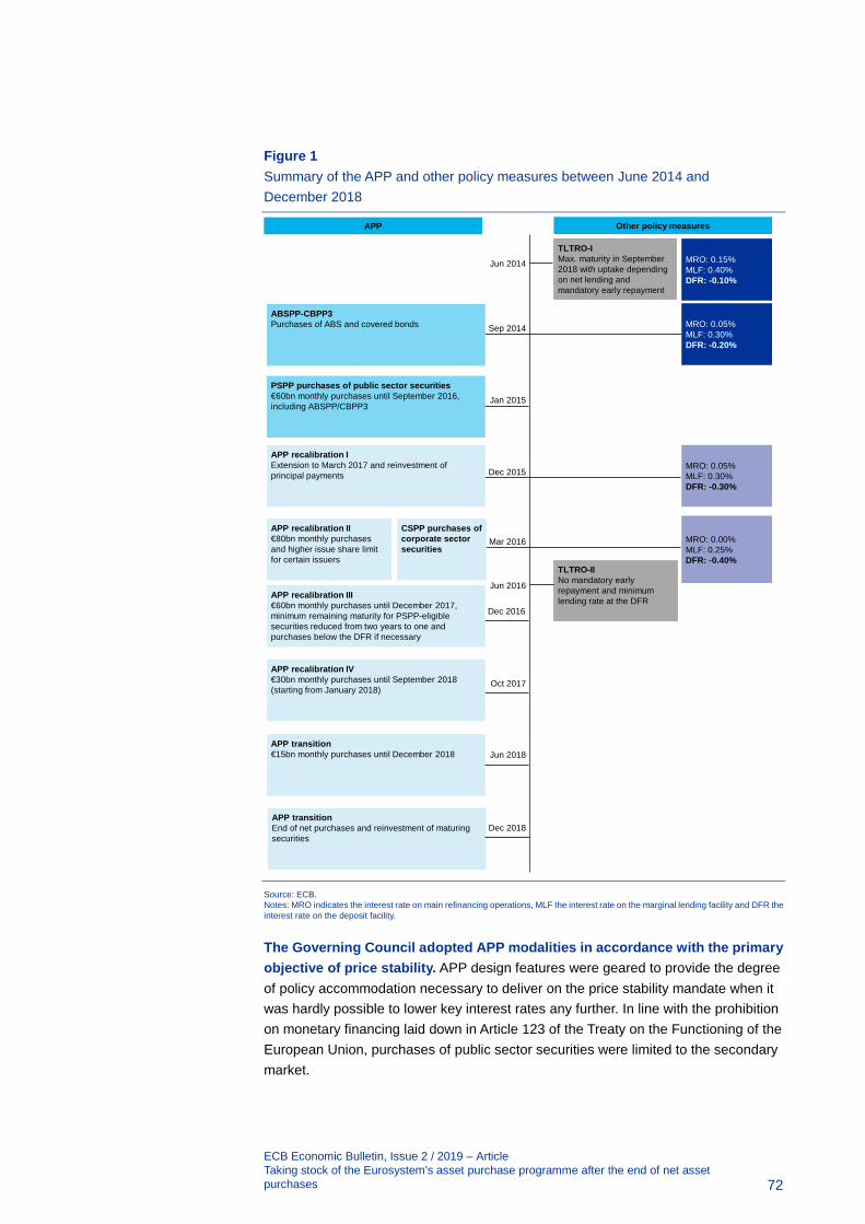
ECB Economic Bulletin, Issue 2 / 2019 – Article Taking stock of the Eurosystem’s asset purchase programme after the end of net asset purchases
72
Figure 1 Summary of the APP and other policy measures between June 2014 and December 2018
Source: ECB. Notes: MRO indicates the interest rate on main refinancing operations, MLF the interest rate on the marginal lending facility and DFR the interest rate on the deposit facility.
The Governing Council adopted APP modalities in accordance with the primary objective of price stability. APP design features were geared to provide the degree of policy accommodation necessary to deliver on the price stability mandate when it was hardly possible to lower key interest rates any further. In line with the prohibition on monetary financing laid down in Article 123 of the Treaty on the Functioning of the European Union, purchases of public sector securities were limited to the secondary market.
Sep 2014
Jan 2015
Dec 2015
Mar 2016
Oct 2017
Jun 2018
Dec 2016
Jun 2014
Dec 2018
ABSPP-CBPP3Purchases of ABS and covered bonds
PSPP purchases of public sector securities€60bn monthly purchases until September 2016, including ABSPP/CBPP3
APP recalibration IExtension to March 2017 and reinvestment of principal payments
CSPP purchases of corporate sector securities
APP recalibration II€80bn monthly purchases and higher issue share limit for certain issuers
APP recalibration IV€30bn monthly purchases until September 2018 (starting from January 2018)
APP recalibration III€60bn monthly purchases until December 2017, minimum remaining maturity for PSPP-eligible securities reduced from two years to one and purchases below the DFR if necessary
APP transition€15bn monthly purchases until December 2018
APP transitionEnd of net purchases and reinvestment of maturing securities
APP
MRO: 0.15%MLF: 0.40%DFR: -0.10%
MRO: 0.05%MLF: 0.30%DFR: -0.20%
MRO: 0.05%MLF: 0.30%DFR: -0.30%
MRO: 0.00%MLF: 0.25% DFR: -0.40%
TLTRO-IMax. maturity in September 2018 with uptake depending on net lending and mandatory early repayment
TLTRO-IINo mandatory early repayment and minimum lending rate at the DFR
Other policy measures
Jun 2016
ECB Economic Bulletin, Issue 2 / 2019 – Article Taking stock of the Eurosystem’s asset purchase programme after the end of net asset purchases
73
The APP was designed to take into account both market structures and the institutional set-up of the euro area. Purchases of public debt instruments were guided by the ECB capital key, which specifies the share of the ECB’s capital attributable to each of the national central banks. At the same time, private sector programmes were based on the market capitalisation of the eligible bonds included in the purchases.
3 Implementation issues
3.1 Market neutrality
When implementing the APP, the Eurosystem aimed to ensure market neutrality in order to minimise the impact on relative prices within the eligible universe and unintended side effects on market functioning. For instance, while aimed at affecting bond prices, the APP purchases were conducted with a view to preserving the price discovery mechanism and limiting distortions in market liquidity. Key features designed to ensure market neutrality in APP implementation are detailed below.
Clear and observable monthly APP targets were defined, with seasonal patterns in market liquidity also being taken into account. The average monthly APP target set ex ante by the Governing Council was decomposed internally into monthly purchase guidance per programme. The programme operating in the most liquid market, the PSPP, acted as a buffer to ensure the precise fulfilment of the overall monthly purchase target. In addition, the Eurosystem took into account seasonal patterns in fixed income market activity, such as the decline in market liquidity from mid-July to late August and in December. Purchase activity was front and back-loaded around these periods (see Chart 2). In all months, the purchase guidance was expressed in monthly totals, rather than strict daily volumes, providing flexibility in the day-to-day execution of purchases.

ECB Economic Bulletin, Issue 2 / 2019 – Article Taking stock of the Eurosystem’s asset purchase programme after the end of net asset purchases
74
Chart 2 Pace and composition of net APP purchases
(EUR billions)
Source: ECB. Note: The average monthly APP targets were first set by the ECB Governing Council at the beginning of the PSPP in March 2015.
Comprehensive ex ante communication on the operational parameters of the APP supported the price discovery mechanism. The parameters defined the operational scope of the APP through (i) stringent eligibility criteria aligned with the procedures in place for the Eurosystem collateral framework45 and using the expertise of Eurosystem collateral management experts, (ii) maturity restrictions,46 (iii) the exclusion of certain issuers,47 (iv) pricing frameworks to ensure that purchases were conducted taking into account available market prices, and (v) different limit systems.48
The Eurosystem took a rule-based approach to the composition of purchases with a view to maintaining adequate diversification across issuers and counterparties. APP purchases were broad-based across jurisdictions, maturity segments, issuers and types of eligible bond in terms of different coupon types or different collateral types, for instance. For the PSPP, the ECB’s capital key provided a straightforward, stable guideline for the composition of purchases across jurisdictions.
45 Assets were thus subject to a minimum credit quality requirement of step 3 on the Eurosystem’s
harmonised rating scale, which implied having at least one credit rating provided by an external credit assessment institution accepted under the Eurosystem credit assessment framework. Assets were also required to be euro-denominated and issued and settled within the euro area. For ABSs, the underlying debtors were required to be predominantly located within the euro area.
46 At the end of 2018, the minimum remaining maturity for the PSPP was one year and the maximum remaining maturity 30 years. The minimum remaining maturity for the CSPP was six months and the maximum remaining maturity 30 years. No maturity restrictions were defined for the CBPP3 or the ABSPP.
47 Securities issued by credit institutions were not eligible for the CSPP. Debt securities of bad banks were not eligible for the PSPP.
48 The issue share limit for the private sector purchase programmes was 70%, with lower limits for the CSPP in specific cases. The PSPP issue share limit was 33% of the issued amount outstanding, subject to case-by-case verification that it would not lead to the Eurosystem having a blocking majority for the purpose of collective action clauses (in which case it was set at 25%). The PSPP issuer limit was also 33%.
0
10
20
30
40
50
60
70
80
90O
ct
Dec Mar
Jun
Sep
Dec Mar
Jun
Sep
Dec Mar
Jun
Sep
Dec Mar
Jun
Sep
Dec
2014 2015 2016 2017 2018
PSPPCSPPCBPP3ABSPPAverage monthly APP target

ECB Economic Bulletin, Issue 2 / 2019 – Article Taking stock of the Eurosystem’s asset purchase programme after the end of net asset purchases
75
The Eurosystem geared its monthly purchase allocation to align a jurisdiction’s share in the stock of PSPP purchases as closely as possible with the respective share of the ECB capital key by the end of the net asset purchase phase. Chart 3 illustrates the deviation of the share of cumulative net purchases at the end of 2018 relative to the ECB capital key for each jurisdiction. For instance, the Eurosystem’s stock of German securities at the end of 2018 was 4.5% above the German share of the ECB capital key. This surplus equates to €22.3 billion.
Chart 3 Deviation in the share of net cumulative purchases relative to the ECB capital key at the end of 2018
(percent)
Source: ECB.
A relative share of the PSPP stock above the ECB capital key in a jurisdiction resulted mechanically from the need to offset downward deviations in other jurisdictions. These downward deviations arose for two reasons. First, Greek government bonds were ineligible for the PSPP over the entire net asset purchase phase. Second, limitations were experienced in the availability of bonds for purchase, which arose, for instance, as bonds were held by hold-to-maturity investors or because of the overall size of the eligible universe in some jurisdictions.
APP purchases were executed regularly, while some flexibility was maintained to adapt to prevailing market conditions (see Box 1). The Eurosystem aimed to maintain a continuous market presence throughout the day, thereby avoiding temporary market dominance. Depending on a central bank’s operational modalities, flexibility can relate inter alia to the selection of securities to purchase, the timing of operations and the overall purchase amount for the day. Moreover, spreading purchases flexibly across the different asset classes included in a programme also helped to preserve market neutrality. As an example of this flexibility, the share of regional government purchases as a proportion of total PSPP purchases fluctuated significantly in 2018 (see Chart 4).
-100
-80
-60
-40
-20
0
20
IT AT FR BE ES DE NL FI IE SI PT MT SK LU LT LV CY EE GR
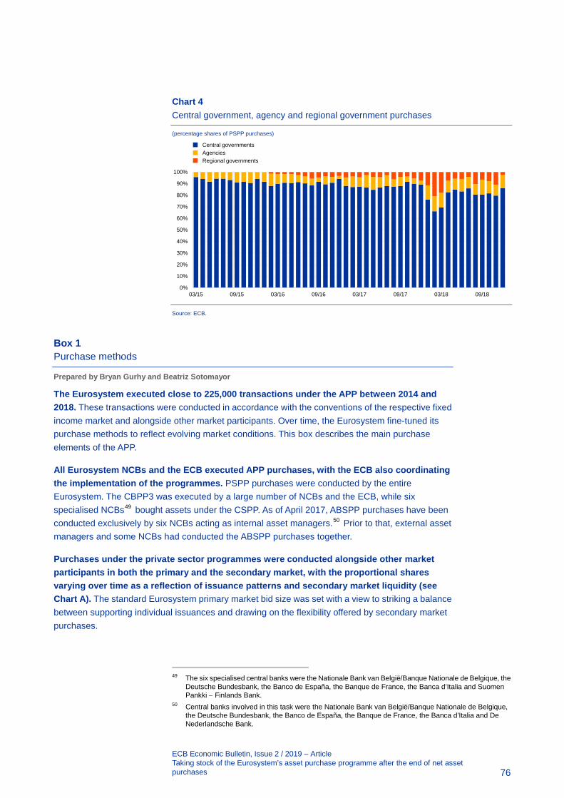
ECB Economic Bulletin, Issue 2 / 2019 – Article Taking stock of the Eurosystem’s asset purchase programme after the end of net asset purchases
76
Chart 4 Central government, agency and regional government purchases
(percentage shares of PSPP purchases)
Source: ECB.
Box 1 Purchase methods
Prepared by Bryan Gurhy and Beatriz Sotomayor
The Eurosystem executed close to 225,000 transactions under the APP between 2014 and 2018. These transactions were conducted in accordance with the conventions of the respective fixed income market and alongside other market participants. Over time, the Eurosystem fine-tuned its purchase methods to reflect evolving market conditions. This box describes the main purchase elements of the APP.
All Eurosystem NCBs and the ECB executed APP purchases, with the ECB also coordinating the implementation of the programmes. PSPP purchases were conducted by the entire Eurosystem. The CBPP3 was executed by a large number of NCBs and the ECB, while six specialised NCBs49 bought assets under the CSPP. As of April 2017, ABSPP purchases have been conducted exclusively by six NCBs acting as internal asset managers.50 Prior to that, external asset managers and some NCBs had conducted the ABSPP purchases together.
Purchases under the private sector programmes were conducted alongside other market participants in both the primary and the secondary market, with the proportional shares varying over time as a reflection of issuance patterns and secondary market liquidity (see Chart A). The standard Eurosystem primary market bid size was set with a view to striking a balance between supporting individual issuances and drawing on the flexibility offered by secondary market purchases.
49 The six specialised central banks were the Nationale Bank van België/Banque Nationale de Belgique, the
Deutsche Bundesbank, the Banco de España, the Banque de France, the Banca d’Italia and Suomen Pankki − Finlands Bank.
50 Central banks involved in this task were the Nationale Bank van België/Banque Nationale de Belgique, the Deutsche Bundesbank, the Banco de España, the Banque de France, the Banca d’Italia and De Nederlandsche Bank.
0%
10%
20%
30%
40%
50%
60%
70%
80%
90%
100%
03/15 09/15 03/16 09/16 03/17 09/17 03/18 09/18
Central governmentsAgenciesRegional governments

ECB Economic Bulletin, Issue 2 / 2019 – Article Taking stock of the Eurosystem’s asset purchase programme after the end of net asset purchases
77
Chart A Private programme purchases broken down by primary and secondary market
(EUR millions)
Source: ECB. Notes: Purchases approximated from change in holdings. Negative values for a subcategory indicate that redemptions were greater than gross purchases for that period.
The majority of APP purchases were executed by bilateral trades with counterparties. These trades were conducted via major electronic platforms and by voice. Bilateral trading entails responding flexibly to market participants’ offers, requesting prices from several counterparties for the same security and then trading at the best price. Bilateral trades are particularly well suited to the liquidity and heterogeneity of euro area bond markets as they can be tailored to market conditions in order to avoid market distortions. For instance, the PSPP purchased securities of 110 issuers,51 while other major central banks generally purchased only a single sovereign issuer when implementing their large-scale asset purchase programmes.
The Deutsche Bundesbank, the Banque de France, Lietuvos Bankas and De Nederlandsche Bank conducted regular auctions in specific market segments when implementing the PSPP. The decision to use auctions reflected the intention to achieve certain volumes while also taking account of transparency considerations. In the days before each auction, market participants were provided with a list of securities that each NCB was considering buying at prevailing market prices. This gave counterparties a well identified “liquidity window” every week to communicate their interest in selling specific securities while being guaranteed equal pricing. Some NCBs focussed their auctions on illiquid bonds, which were difficult to source bilaterally, while others used auctions for liquid bonds to foster price transparency for other market participants. The Eurosystem applied the same trading rules to align the purchase price in bilateral trading and reverse auctions with the prevailing market offer price.
Bid wanted in competition (BWIC) is a transaction method specific to the ABS market. BWICs are organised by dealers on behalf of investors to sell ABS holdings while ensuring best execution by inviting a large range of potential buyers. The ABSPP regularly participated in BWICs for both liquid and less liquid jurisdictions and across all ABS collateral types. The share of ABSPP purchases
51 In addition to the 17 central government issuers, the PSPP purchased securities of 43 PSPP-eligible
agencies and of 43 regional governments and six EU supranational institutions as well as one non-financial corporate.
-5,000
0
5,000
10,000
15,000
20,000
25,000
30,000
35,000
40,000
Q4 Q1 Q2 Q3 Q4 Q1 Q2 Q3 Q4 Q1 Q2 Q3 Q4 Q1 Q2 Q3 Q4
2014 2015 2016 2017 2018
CBPP3 PMCBPP3 SMCSPP PMCSPP SMABSPP PMABSPP SM

ECB Economic Bulletin, Issue 2 / 2019 – Article Taking stock of the Eurosystem’s asset purchase programme after the end of net asset purchases
78
executed through BWICs was relatively low, however, as the Eurosystem aimed to purchase at market prices without pushing prices to artificially high levels. The ECB set up a governance structure to assess all securities purchased and provide guidance on appropriate market pricing.
3.2 Fixed income market liquidity and its interaction with APP implementation
The APP purchases were executed in a way that aimed to safeguard the liquidity of euro area fixed income markets. Eurosystem staff regularly assessed bond market liquidity indicators. Taken together with market intelligence, these assessments indicate that the design of the APP has been successful in mitigating potential detrimental effects on market functioning and that the impact of the APP on market liquidity has been at most transitory.52
Daily purchase modalities, and in particular the day-to-day selection of securities to be purchased, were applied with a view to preserving market liquidity conditions. The Eurosystem actively incorporated the offers from a broad range of counterparties in the daily bond selection. In addition, significant efforts were undertaken to avoid buying securities that were scarce, as measured by such metrics as relative value indicators, pricing in the repo market and trading volumes.
The size of individual transactions was responsive to the observed offer sizes. For APP transactions, the average secondary market transaction ranged from €4 million in the CSPP to €14 million in the PSPP. These averages mask compositional heterogeneity, with transaction sizes increasing for more liquid securities and declining for illiquid bonds.
Using a broad set of counterparties facilitated the smooth implementation of purchases and fostered competition, with the Eurosystem trading with more than 350 counterparties. A very large majority of APP purchases involve counterparties located in a different country from the purchasing central bank, which also impacted the distribution of Target 2 balances across jurisdictions.53 Individual central banks expanded their set of counterparties in order to reach all relevant segments of the fixed income market. APP implementation thus avoided persistent effects in the micro-structure of bond market segments through the competitive use of counterparties. Against this background, the Eurosystem adopted a wide range of transparency tools to minimise the informational advantages for eligible counterparties. These initiatives helped to level the playing field among financial market participants while preserving the timely execution of operations (see Box 2).
52 See Jurskas et al., “Euro area sovereign bond market liquidity since the start of the PSPP”, Economic
Bulletin, Issue 2, ECB, 2018, pp. 41-44. 53 See Box 1 entitled “The ECB’s asset purchase programme and TARGET balances: monetary policy
implementation and beyond”, Economic Bulletin, Issue 3, ECB 2017, pp. 21-26 and Box 2 entitled “TARGET balances and the asset purchase programme”, Economic Bulletin, Issue 7, ECB, 2016, pp. 20-23.

ECB Economic Bulletin, Issue 2 / 2019 – Article Taking stock of the Eurosystem’s asset purchase programme after the end of net asset purchases
79
Box 2 Providing additional transparency on aggregate APP holdings
Prepared by Kieran Leonard and Beatriz Sotomayor
Transparency has played a central role in the APP by allowing market participants to better understand how the programmes are implemented. The regular disclosure of information on APP purchases and holdings on the ECB website was complemented by additional information on the CSPP in a box in the June 2017 issue of the Economic Bulletin.54 Similar data on the aggregate holdings of the CBPP3 and the ABSPP are presented below. In addition, the box provides a comparison of the weighted average maturity of PSPP net cumulative purchases with the relevant eligible universe.
CBPP3 purchases were broadly oriented towards a market capitalisation-based benchmark of eligible securities, with due consideration being given to market liquidity conditions. This allowed purchases to be conducted across a broad range of countries on an ongoing basis. The Eurosystem was responsive to the availability of individual bonds in day-to-day implementation.
Table A Country and rating distributions of CBPP3 holdings and benchmark at the end of 2018
Sources: ECB and ECB calculations. Notes: The benchmark is constructed using the universe of eligible securities pertaining at the end of 2018. The weights of certain covered bond classes have been adjusted lower to reflect their lack of availability and illiquidity. Only bonds with an asset rating are included in the data for the credit rating distribution. The ratings are first-best asset ratings. The distributions are by nominal value.
The market capitalisation approach evolved over time, with the benchmark weights attached to certain securities decreasing as some covered bond categories were found to be increasingly hard to purchase. For example, the launch of TLTRO-II increased the attractiveness of retaining covered bonds as collateral rather than placing them in the market. To account for this, the relative weight of retained covered bonds was reduced in the eligible CBPP3 benchmark.
To accommodate the dynamic nature of the CBPP3-eligible universe, with its variable issuance patterns and liquidity conditions across jurisdictions, the market capitalisation-based benchmark was updated regularly so as to guide future purchases. This evolutionary approach is the main explanation for the differences evident in Table A, where, for example, CBPP3 holdings in Spanish covered bonds are considerably higher than the current benchmark would imply. At the same time, the share of French covered bonds in the holdings has increased over time, guided by an increase in their benchmark weight. The deviations in the rating
54 See Box 2 entitled “The ECB’s corporate sector purchase programme: its implementation and impact”,
Economic Bulletin, Issue 4, ECB, 2017, pp. 40-45.
Country of risk distribution Credit rating distribution
Jurisdiction Holdings Benchmark Rating Holdings Benchmark
FR 26.2% 30.0% AAA 68.9% 76.5%
DE 22.0% 22.8% AA 28.1% 20.4%
ES 21.8% 15.1% A 2.7% 2.7%
IT 11.5% 9.0% BBB 0.3% 0.3%
NL 5.7% 8.3%
FI 3.7% 4.6%
AT 3.3% 4.4%
Other euro area 5.7% 5.9%

ECB Economic Bulletin, Issue 2 / 2019 – Article Taking stock of the Eurosystem’s asset purchase programme after the end of net asset purchases
80
distribution between CBPP3 holdings and the current benchmark also reflect the outcome of the evolutionary approach.
Turning to the ABSPP, the cumulative gross purchases have been added to the presentation of holdings to provide a more accurate illustration of implementation across the Eurosystem (see Table B). This additional information is needed to reflect the faster repayment of ABSs compared to other fixed income asset classes, with cumulative gross purchases of €51.6 billion set against holdings of only €27.5 billion at end-2018.
Table B Country, collateral and rating distribution of ABSPP holdings and universe at the end of 2018
Sources: ECB, Bloomberg, company publications. Notes: The universe is a theoretical measure of the purchasable senior tranche securities eligible as Eurosystem collateral outstanding at the end of 2018. Credit rating distribution based on second-best rating consistent with collateral eligibility. The distributions are by outstanding amount.
Gross ABSPP purchases were more broadly distributed across jurisdictions than the holdings at the end of 2018 would indicate, reflecting the prevalence of different asset types in each country. For example, auto ABSs dominate the German ABS market. These securities have a much lower weighted average life than residential mortgage backed securities (RMBS), which are more common in the Netherlands. Furthermore, the portfolio composition also reflected market capitalisation and market liquidity. Core markets with lower yielding securities generally had a higher number of actively offered securities, which has led to some over-representation of Dutch RMBS in the portfolio, for example. At the same time, non-core and higher yielding securities were largely held by hold-to-maturity investors and were not offered to the Eurosystem to the same extent. Moreover, there was a higher concentration in securities issued since the start of the ABSPP, given the ability of the ABSPP to make primary market purchases and hence purchase larger volumes in these issues. This resulted in a lower presence in jurisdictions with less issuance since October 2014, such as Spain and Portugal.
With regard to the PSPP, a comparison of the weighted average maturity (WAM) of cumulative net purchases with the WAM of the eligible universe shows that they were broadly in line with each other at the end of 2018 (see Table C). The dispersion of WAMs of the eligible universe across jurisdictions reflects the past issuance patterns of PSPP-eligible issuers. The WAM measure for cumulative net purchases includes the contribution of bonds which are no longer eligible owing to a maturity of less than one year and broadly reflects the availability of individual bonds for purchase
Country of risk distribution Credit rating distribution
Jurisdiction Gross purchases Holdings Universe Rating Holdings Universe
NL 41.4% 50.1% 38.1% AAA 87.0% 80.0%
IT 18.7% 13.5% 15.4% AA 12.1% 15.4%
DE 17.2% 12.7% 16.0% A 0.8% 4.4%
ES 8.2% 9.8% 10.8% BBB 0.1% 0.2%
FR 8.0% 6.9% 10.4% Collateral type distribution
IE 2.5% 3.7% 4.1% Collateral Holdings Universe
PT 2.3% 1.6% 3.3% Residential mortgages 71.5% 61.9%
FI 1.0% 1.0% 0.6% Auto loans 19.7% 20.3%
BE 0.7% 0.7% 1.3% Consumer loans 6.3% 8.4%
Leasing contracts 1.1% 6.2%
Credit card receivables 0.8% 1.3%
Loans granted to SME 0.6% 1.9%

ECB Economic Bulletin, Issue 2 / 2019 – Article Taking stock of the Eurosystem’s asset purchase programme after the end of net asset purchases 81
across time. Moreover, securities with short to medium-term maturities at the start of the PSPP were already extensively held by the Eurosystem as a result of the securities markets programme. These holdings limited the ability to purchase such bonds under the PSPP in certain jurisdictions. Therefore, the WAM measure for cumulative net purchases in these jurisdictions is higher than would have otherwise been the case.
Table C Weighted average maturities by jurisdiction for the PSPP at the end of 2018
(years)
Notes: The WAM measure for cumulative net purchases in jurisdictions which were purchased under the ECB’s securities markets programme (SMP) is higher than would have been the case if many short to medium-term maturity securities had not already been extensively purchased under the SMP.
3.3 Securities lending
APP securities lending facilities addressed challenging repo market conditions. Combined with the gradual expansion of PSPP holdings, increasing demand for high quality liquid assets in line with regulatory requirements contributed to challenging repo market conditions through 2016. The Eurosystem purchases reduced the effective availability of securities for market participants, which could have resulted in a shortage of bonds to be used as collateral55 and lower market liquidity, while possibly impairing the price discovery mechanism. The Eurosystem’s securities lending approach served to minimise such unintended consequences of the APP.56
The Eurosystem conducts securities lending activities, which continue in the reinvestment phase of the APP, in a decentralised manner on the basis of common principles. The Eurosystem acts as a backstop without curtailing normal repo market activity.57 The institutional set-up of the Eurosystem means that securities lending implementation is decentralised and various lending channels are used (e.g. bilateral lending or through custodians). As illustrated in the upper panel of Chart 5, the share of German government bonds trading “special” – that is trading at a premium to general collateral in the repo market – increased markedly in 2016. The Eurosystem responded by introducing a number of modifications to the securities lending facilities, such as the option to borrow bonds against cash collateral. This was introduced in December 2016, effectively increasing the supply of bonds available in
55 Government bonds are the main type of collateral used in the euro repo markets due to their safety and liquidity.
56 PSPP securities were made available for lending in April 2015, shortly after the start of the purchases. Lending of CSPP securities by Eurosystem NCBs is also mandatory, while lending of CBPP3 holdings is voluntary. However, holdings from each covered bond jurisdiction are made available for lending by at least one Eurosystem central bank. Lending of ABSPP holdings is possible in principle, but no requests have been received since the start of the programme.
57 To ensure this, the lending is conducted at a certain spread against general collateral (for lending against securities), and the cash collateral option (for PSPP only) is offered at a rate equal to the lower of the rate of the deposit facility minus 30 basis points and the prevailing market repo rate.
Jurisdiction BE DE EE IE GR ES FR IT CY LV LT LU MT NL AT PT SI SK FI EU Total
Cumulative net purchases 9.2 6.3 0.0 8.8 0.0 8.3 7.3 7.5 5.8 8.7 8.5 4.9 10.6 7.2 8.1 7.8 10.6 9.1 7.1 7.5 7.4
Eligible universe 10.1 7.2 0.0 8.8 0.0 8.2 7.9 7.7 5.1 9.8 9.1 5.7 9.9 8.2 8.1 7.2 10.2 8.9 7.6 8.2 7.9
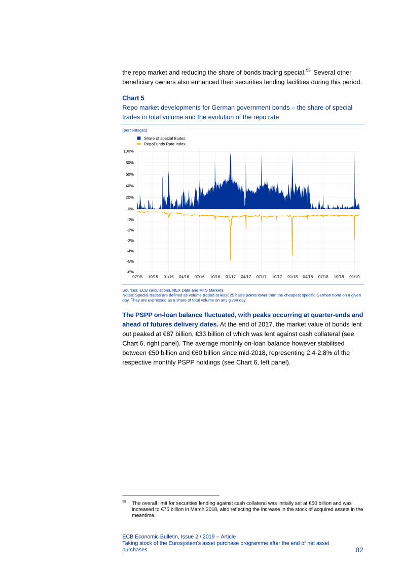
ECB Economic Bulletin, Issue 2 / 2019 – Article Taking stock of the Eurosystem’s asset purchase programme after the end of net asset purchases
82
the repo market and reducing the share of bonds trading special.58 Several other beneficiary owners also enhanced their securities lending facilities during this period.
Chart 5 Repo market developments for German government bonds – the share of special trades in total volume and the evolution of the repo rate
(percentages)
Sources: ECB calculations, NEX Data and MTS Markets. Notes: Special trades are defined as volume traded at least 25 basis points lower than the cheapest specific German bond on a given day. They are expressed as a share of total volume on any given day.
The PSPP on-loan balance fluctuated, with peaks occurring at quarter-ends and ahead of futures delivery dates. At the end of 2017, the market value of bonds lent out peaked at €87 billion, €33 billion of which was lent against cash collateral (see Chart 6, right panel). The average monthly on-loan balance however stabilised between €50 billion and €60 billion since mid-2018, representing 2.4-2.8% of the respective monthly PSPP holdings (see Chart 6, left panel).
58 The overall limit for securities lending against cash collateral was initially set at €50 billion and was
increased to €75 billion in March 2018, also reflecting the increase in the stock of acquired assets in the meantime.
-6%
-5%
-4%
-3%
-2%
-1%
0%
07/15 10/15 01/16 04/16 07/16 10/16 01/17 04/17 07/17 10/17 01/18 04/18 07/18 10/18 01/19
0%
20%
40%
60%
80%
100%
Share of special tradesRepoFunds Rate index

ECB Economic Bulletin, Issue 2 / 2019 – Article Taking stock of the Eurosystem’s asset purchase programme after the end of net asset purchases
83
Chart 6 PSPP on-loan balance divided into loans against securities collateral and cash collateral
(EUR billions)
Sources: ECB calculations. Notes: Amounts are in market value terms. Starting 15 December 2016, the Eurosystem introduced the option of also accepting cash as collateral in its PSPP securities lending facilities.
4 Transmission and impact on the macroeconomy
4.1 Main transmission channels
The APP has provided a substantial improvement in financing conditions via several transmission channels, and each individual policy measure, being part of a package of policy measures, has benefitted from reinforcing synergies. Evidence based on event studies shows that yields fell significantly across all financial market segments following the APP announcement.59 Over the course of APP implementation, declining bank lending rates and credit expansion helped to ease financing conditions, support a firming of the economic recovery and counter disinflationary forces. As documented by a large body of literature, the APP operates through three main channels: the signalling channel, the portfolio rebalancing channel and the direct pass-through channel.60 The package of policy measures of which the APP was part has created mutually reinforcing synergies across the individual measures.
59 See Dell’Ariccia, G., Rabanal, P. and Sandri, D., “Unconventional Monetary Policies in the Euro Area,
Japan, and the United Kingdom”, Journal of Economic Perspectives, Volume 32, Number 4, Fall 2018, pp. 147-172; Altavilla, C., Carboni, G. and Motto, R., “Asset purchase programmes and financial markets: lessons from the euro area”, Working Paper Series, No 1864, ECB, November 2015; De Santis, R., “Impact of the asset purchase programme on euro area government bond yields using market news”, Working Paper Series, No 1939, ECB, July 2016; and De Santis, R. and Holm-Hadulla, F., “Flow effects of central bank asset purchases on euro area sovereign bond yields: evidence from a natural experiment”, Working Paper Series, No 2052, ECB, May 2017.
60 For an overview of the channels and further analyses, please see the article entitled “The transmission of the ECB’s recent non-standard monetary policy measures”, Economic Bulletin, Issue 7, ECB, 2015, and the box entitled “Impact of the ECB’s non-standard measures on financing conditions: taking stock of recent evidence”, Economic Bulletin, Issue 2, ECB, 2017.
0
10
20
30
40
50
60
70
80
90
07/15 07/16 07/17 07/18
Loans against securities collateralLoans against cash collateral
11/17 02/18 05/18 08/18 11/180
10
20
30
40
50
60
70
80
90
Quarter-endsFutures deliveries

ECB Economic Bulletin, Issue 2 / 2019 – Article Taking stock of the Eurosystem’s asset purchase programme after the end of net asset purchases
84
Via the signalling channel, the APP has underscored the ECB’s intention to provide sufficient monetary stimulus for an extended period of time, thereby also contributing to anchor policy rate expectations. The APP has enhanced the signal that key policy rates would remain low for long. The signalling aspect of central banks’ large-scale asset purchases has always been found to be an important component of transmission for such policy programmes. This component was reinforced in March 2016, when the Governing Council’s communication of the expected future rate path was made conditional on the end of net asset purchases.
Via the portfolio rebalancing channel, the APP has compressed yields across a wide range of asset classes, with negative rates on reserves providing additional incentives to the rebalancing process. With the price of the purchased assets being bid up, their yields decrease. The lower yields induce investors to sell these securities, earning the associated capital gain. As sellers may not view holding the liquidity received as being a perfect substitute for the assets sold, they reinvest and rebalance their portfolios towards other assets, such as securities and loans (see also Box 4). This process is reinforced by the negative rates charged on reserves.61 Consequently, yields also decreased in other market segments not targeted by the central bank purchases, including a rebalancing in non-euro denominated debt and equity markets.62
Within the portfolio rebalancing channel, the extraction of duration risk has been a particularly relevant mechanism affecting the term premium component of medium and long-term yields (Box 3). Asset purchases decrease the duration risk borne by private investors, thus increasing their risk-bearing capacity and incentivising them to restore the desired overall risk profile of their portfolio by investing in different assets. Therefore, duration extraction affects the pricing of maturities and asset classes beyond securities purchased.
Via the direct pass-through channel, which comes into play for the ABSPP and the CBPP3 in particular, the APP has directly improved credit conditions for the private non-financial sector. At the same time, the CBPP3 and TLTROs have interacted to foster lending to small and medium-size enterprises (SMEs) as well.63 More generally, TLTROs have alleviated the funding costs for participant banks, thus mitigating possible negative effects on bank lending stemming from negative rates on reserves. Central bank purchases have raised the price of ABS and covered bonds, lowered the market interest rate paid by the originators and encouraged banks to create more loans with a view to repackaging them and selling them on. Through this mechanism, bond purchases have supported borrowing conditions in the private non-financial sector. Similarly, the CSPP has reduced funding costs for firms accessing financial markets directly and supported a switch from bank funding to
61 See Ryan, E. and Whelan, K., “Quantitative Easing and the Hot Potato Effect: Evidence from the Euro
Area Banks”, Research Technical Paper, Vol. 2019, No. 1, Central Bank of Ireland, 2019. 62 See “The international dimension of the ECB’s asset purchase programme”, speech by Benoît Cœuré,
Member of the Executive Board of the ECB, at the Foreign Exchange Contact Group meeting, Frankfurt am Main, 11 July 2017.
63 See the article entitled “MFI lending rates: pass-through in the time of non-standard monetary policy”, Economic Bulletin, Issue 1, ECB, 2017.

ECB Economic Bulletin, Issue 2 / 2019 – Article Taking stock of the Eurosystem’s asset purchase programme after the end of net asset purchases
85
market funding for large firms, thereby freeing up capacity on bank balance sheets to finance loans to SMEs.64
Box 3 The impact of the APP on the term structure of euro area bond yields – a model-based assessment
Prepared by Fabian Eser, Wolfgang Lemke and Andreea Liliana Vladu
The term premium component of yields reflects the aggregate duration risk borne by investors. Risk-free long-term bond yields have two components: average expectations of short-term interest rates over the life of the bond and a term premium. The latter comprises the current and future expected risk exposure of individual bonds (their bond-specific duration risk), as well as the compensation per unit of risk exposure. This compensation – the “price of risk” – depends in turn on the aggregate duration risk to be borne by the market.
Central bank asset purchases decrease the overall duration risk to be absorbed by private investors, thus reducing the price of risk and, in turn, the term premium. Importantly, the effect of asset purchases on the term premium depends on the entire path of the duration-weighted bond portfolio acquired. For a ten-year bond, lower aggregate duration risk in, say, five years decreases the required risk compensation in the future and hence also the term premium today.
The APP’s impact on the term premium can be estimated using an arbitrage-free term structure model.65 The drivers of bond rates are summarised by three factors, one of which reflects the “free float of duration risk” in the hands of those market participants who are deemed willing to rebalance their bond portfolio when bond prices change.66 The model links current and future changes in the free-float to changes in current term premia and can thereby explain how current and expected future APP volumes affect the yield curve.67
The compression in sovereign yields due to the APP-induced reduction in current and expected bond free float is estimated to stand at around 100 basis points for the ten-year maturity (Chart A, left panel). The chart illustrates the impact of the APP on term premia across the term structure at the time when the PSPP was announced and at the end of net asset purchases in December 2018. The term premium impact is larger for longer maturities.
Looking ahead, the substantial stock of acquired assets and the forthcoming reinvestments mean that a sizeable amount of duration risk will continue to be extracted, even after net
64 See the article entitled “The impact of the corporate sector purchase programme on corporate bond
markets and the financing of euro area non-financial corporations”, Economic Bulletin, Issue 3, ECB, 2018.
65 The model is described in more detail in Eser, F., Lemke, W., Nyholm, K., Radde, S. and Vladu, A., Tracing the impact of the ECB’s asset purchase programme on the yield curve, forthcoming as an ECB Working Paper in 2019. This has a similar framework to Li, C. and Wei, M., “Term Structure Modeling with Supply Factors and the Federal Reserve’s Large-Scale Asset purchase Programs”, International Journal of Central Banking, 9(1), 3-39, 2013, which is used by the Federal Reserve to estimate the yield impact of large-scale sovereign bond purchases.
66 Non-financial corporations, households, money market funds and monetary financial institutions (excluding the Eurosystem) are considered to be price-sensitive. By contrast, the Eurosystem − in terms of both monetary policy and non-monetary policy portfolios − non-euro area official sector holdings (in particular central bank foreign exchange reserves), intra-euro area government bond holdings and holdings by insurance companies and pension funds are considered to be price-insensitive.
67 The required free-float projections at each point in time are based on the APP parameters communicated by the Governing Council and on private-sector expectations as proxied by survey information.

ECB Economic Bulletin, Issue 2 / 2019 – Article Taking stock of the Eurosystem’s asset purchase programme after the end of net asset purchases
86
purchases have ceased (Chart A, right panel). The chart plots the evolution of the ten-year term premium compression, based on the projected free float as at the end of net asset purchases. The term premium impact gradually fades over time, which reflects the ageing of the portfolio − i.e. its gradual loss of duration as the securities held in the portfolio mature − as well as the run-down of the portfolio that market participants anticipate will eventually follow the end of the expected horizon of reinvestments.
Chart A Estimated impact of the APP on euro area sovereign yields
Source: Based on Eser, Lemke, Nyholm, Radde and Vladu (2019). Notes: The left panel shows by how much the term premium component of sovereign euro area yields with maturities of one year to ten years are estimated to be compressed due to the APP, at the time of the launch of the APP (Q1 2015), as well as at the end of the net purchase phase in December 2018. The right panel shows point estimates of the ten-year yield term premia compression over time. The confidence band reflects parameter uncertainty around these point estimates, constructed using bootstrap/Monte Carlo resampling techniques. Euro area yields are proxied by the GDP-weighted zero-coupon yields of the four largest euro area jurisdictions.
Quantifying the impact of the APP on the yield curve is subject to several layers of uncertainty. Accounting for parameter uncertainty in the model estimation suggests that the impact of the APP on ten-year term premia currently lies in a range of 70 to 130 basis points.68 Additional sources of uncertainty relate to model specification, the estimation window and the quantification of the free float measure.
The APP has eased financing conditions across asset classes. Liquidity injected by the APP has tied up short-term money market interest rates at levels close to the ECB’s deposit facility rate and, together with negative rates and forward guidance, anchored the expected path of money market rates in line with the intended policy stance. Chart 7 shows the estimated accumulated easing impact of the APP across asset classes – alongside that from other easing measures – relative to actual asset price changes recorded since 2014.69 The APP is estimated to have decreased sovereign yields and pushed down yields of bonds issued by non-financial corporations (NFCs), and to have contributed to an increase in share prices.
68 Chart 7 presents further evidence using additional methodological frameworks, together with the impact
of other measures taken since June 2014. 69 Box 3 presents further evidence on the impact of the APP.
-130-120-110-100-90-80-70-60-50-40-30-20-10
0
1 2 3 4 5 6 7 8 9 10
Bas
is p
oint
s
a) Term premia impact across maturities
Launch of the programme (Q1 2015)End of net purchases (Q4 2018)
Maturity of yields in years
-130-120-110-100-90-80-70-60-50-40-30-20-10
0
2018 2021 2024 2027 2030 2033
Bas
is p
oint
s
Point estimate5-95% confidence band
b) 10-year term premium impact over time
Years

ECB Economic Bulletin, Issue 2 / 2019 – Article Taking stock of the Eurosystem’s asset purchase programme after the end of net asset purchases
87
Chart 7 Impact of policy measures on financial prices and yields
Source: ECB calculations. Notes: The chart shows the impact of the June and September 2014 policy measures, the APP and cuts in the deposit facility rate (DFR) on financial prices and yields. The impact of the June and September 2014 policy measures is estimated on the basis of an event-study methodology which focuses on the announcement effects of these measures; see the ECB Economic Bulletin article entitled “The transmission of the ECB’s recent non-standard monetary policy measures” (Issue 7/2015). The impact of the cuts of the deposit facility rate (DFR) rests on the announcement effects of the September 2014 DFR cut, while the impact of the subsequent DFR cuts is difficult to disentangle from the simultaneous APP adjustments. Both effects are therefore shown jointly. APP encompasses the effects of the asset purchase measures adopted at the Governing Council meetings in January and December 2015, March and December 2016, and October 2017. The January 2015 APP impact is estimated on the basis of two event-study exercises considering a broad set of events that, starting from September 2014, have affected market expectations about the programme; see Altavilla, C., Carboni, G. and Motto, R., op. cit., and De Santis, R., op. cit. The quantification of the impact of the December 2015 policy package on asset prices rests on a broad-based assessment comprising event studies and model-based counterfactual exercises. The impact of the March 2016 and December 2016 policy packages is assessed using model-based counterfactual exercises. The impact of the October 2017 policy package is assessed using two models: a term structure modelling framework similar to the one used in Box 3, and an ISIN-by-ISIN regression framework akin to D’Amico, S. and King, T.B., “Flow and stock effects of large-scale treasury purchases: Evidence on the importance of local supply”, Journal of Financial Economics, Vol. 108, Issue 2, 2013, pp. 425-448.
Banks have played a crucial role in the transmission of net asset purchases to financing conditions. Bank-based financial intermediation remains very important, notwithstanding a trend towards market funding in the financing structure of euro area NFCs over the last decade. The APP, acting in conjunction with negative interest rates on the deposit facility and TLTROs, has incentivised banks to reinvest the proceeds from asset sales into loan creation (see Box 4).
As a result, bank lending rates have steadily declined and converged across euro area countries since mid-2014. Composite lending rates to NFCs currently stand close to record lows (see Chart 8, left panel). Model-based results indicate that the APP and DFR cuts have led to a reduction of around 50 basis points in bank lending rates to NFCs since June 2014 due to their impact on the yield curve.70 Previously large dispersions in borrowing costs across euro area countries have progressively narrowed to the point of being almost fully reabsorbed.
70 This estimate compares to an overall decline of 129 basis points in bank lending rates to NFCs between
June 2014 and October 2018. The estimation is based on lending rate pass-through mechanisms that operate via the relationship between government bond yields and bank funding costs, including: (i) standard pass-through mechanisms used for the projections, and (ii) pass-through models using granular bank balance sheet information. On (ii), see Altavilla, C., Canova, F. and Ciccarelli, M., “Mending the broken link: heterogeneous bank lending and monetary policy pass-through”, Journal of Monetary Economics, 2019, forthcoming. Additionally, the TLTROs provided further downward pressure on bank lending rates.
-250
-225
-200
-175
-150
-125
-100
-75
-50
-25
0
Euro area DE FR IT ES
10-year government yields
Bas
is p
oint
s
June and September 2014 policy measures APP+DFRChange 5 February 2019 - 4 June 2014
-100
-80
-60
-40
-20
0
NFC bondyield
0
5
10
15
20
25
Euro Stoxx
Perc
enta
ges

ECB Economic Bulletin, Issue 2 / 2019 – Article Taking stock of the Eurosystem’s asset purchase programme after the end of net asset purchases
88
Chart 8 Cost of borrowing for new NFC loans and MFI loans to NFCs
Source: ECB. Notes: The indicator for the total cost of borrowing is calculated by aggregating short and long-term rates using a 24-month moving average of new business volumes. Loans are adjusted for sales, securitisation and notional cash pooling. MFI stands for monetary financial institutions. The latest observations are for November 2018.
The APP is also found to have contributed significantly to the recovery in loan growth. NFC loan volumes started growing again with positive rates in mid-2015. Model-based simulations suggest that almost half of the annual growth in NFC loan volumes in the third quarter of 2018 (4.3%, see Chart 8, right panel) can be attributed to the effects of the APP.71 Box 4 provides further details on the bank-based transmission of the APP to lending.
Box 4 Impact of the APP on lending to enterprises
Prepared by Miguel Boucinha and Sarah Holton
All monetary policy measures taken since mid-2014 have helped to support lending conditions, which makes it difficult to separate out the impact of each individual measure. This identification problem can be addressed by using granular data. It is possible to identify the contribution of the APP to lending to enterprises by matching bank-level qualitative information from the Bank Lending Survey (BLS) with individual bank balance sheet characteristics and lending flows.
Granular data show that banks had diverse liquidity inflows associated with the APP.72 Asset purchases increase bank liquidity directly through sales of bonds by banks and indirectly through an
71 The figure reported corresponds to the average of alternative estimates: (i) DGSE simulations aimed at
capturing the impact of the APP based on Darracq Pariès, M. and Kühl, M., “The optimal conduct of central bank asset purchases,” Working Paper Series, No 1973, ECB, 2016; (ii) estimates of the impact of the APP based on a VAR with time-varying parameters and stochastic volatility based on a paper by Gambetti, L. and Musso, A., “The macroeconomic impact of the ECB’s expanded asset purchase programme (APP)”, Working Paper Series, No 2075, ECB, 2017; (iii) country estimates of the impact of unconventional monetary policy shocks based on the multi-country BVAR model from Altavilla, C., Giannone, D. and Lenza, M., “The financial and macroeconomic effects of the OMT announcements,” International Journal of Central Banking, Vol. 12(3), September 2016, pp. 29-57.
72 See also Altavilla, C., Canova, F. and Ciccarelli, M., op. cit.; Albertazzi, U., Becker, B. and Boucinha, M., “Portfolio rebalancing and the transmission of large-scale asset programmes: evidence from the euro area”, Working Paper Series, No 2125, ECB, 2018.
1.0
1.5
2.0
2.5
3.0
3.5
4.0
4.5
2013 2014 2015 2016 2017 2018
Perc
enta
ges
per a
nnum
Euro areaDEESFRIT
a) Cost of borrowing for new NFC loans
-20
-15
-10
-5
0
5
10
15
2013 2014 2015 2016 2017 2018
Ann
ual p
erce
ntag
e ch
ange
s
b) MFI loans to NFCs

ECB Economic Bulletin, Issue 2 / 2019 – Article Taking stock of the Eurosystem’s asset purchase programme after the end of net asset purchases
89
increase in deposits stemming from their customers’ bond sales. Linking the BLS with balance sheet data confirms that, on average, banks with higher holdings of sovereign bonds just before the APP was launched reported a stronger impact on liquidity from the programme (Chart A, left panel). On average, just over 20% of banks reported a positive impact on liquidity from the programme in net percentage terms, while for the banks with relatively high holdings of sovereign bonds at the end of 2014, the net percentage reporting a positive impact increases by 10 percentage points to over 30%. The banks that experienced an increase in liquidity owing to the APP could then adjust towards other assets, such as loans.
Banks with larger liquidity inflows associated with the APP are found to have recorded stronger loan growth to enterprises following the implementation of the programme. Using BLS data on liquidity inflows to identify banks that were more exposed to the policy, the right panel of Chart A indicates that this group of banks had higher cumulative loan growth than other banks following the introduction of the APP. While Chart A implies that the policy was effective, the trend may be driven by other confounding factors such as the macroeconomic environment, bank business models and the demand conditions faced by the banks that were more exposed to the policy. To make a causal statement regarding the impact of the programme on credit supply, it is necessary to control for these factors. Model-based analysis shows that, even after controlling for bank characteristics (both time-varying and fixed unobservable features), demand conditions and macroeconomic variation, the APP continues to be found a strong driver of higher credit supply for the banks that were more exposed to liquidity inflows associated with the APP.73
Chart A Impact of the APP on bank liquidity and lending
Sources: ECB and ECB calculations; Altavilla, Boucinha, Holton and Ongena (2018). Notes: The chart on the left hand side shows net percentages, i.e. the difference between the percentage of banks reporting a positive and a negative impact. Banks with high sovereign holdings are those that are in the 75th percentile in terms of their holdings of sovereign bonds relative to main assets in December 2014. Other banks are the remainder. The chart on the right shows the cumulative differences in quarterly growth rates between banks which on average reported that the APP impact on their liquidity position was more positive and other banks. The red line indicates the start of APP purchases in March 2015.
73 See Altavilla, C., Boucinha, M., Holton, S. and Ongena, S., “Credit supply and demand in unconventional
times”, Working Paper Series, No 2202, ECB, 2018.
0.0
0.1
0.2
0.3
0.4
High sovereign holding banks Other banks
a) Effect of APP on liquidity across banks
Net
per
cent
ages
Total
-5
0
5
10
15
06/12 06/13 06/14 06/15 06/16 06/17
b) Cumulative differences between banks affected by APP
Diff
eren
ces
in q
uart
erly
gro
wth
rate
s of
NFC
loan
s
APP

ECB Economic Bulletin, Issue 2 / 2019 – Article Taking stock of the Eurosystem’s asset purchase programme after the end of net asset purchases
90
4.2 Impact on the euro area economy and inflation, and progress towards a sustained adjustment in the path of inflation
The APP, in conjunction with the other monetary policy measures, has provided a substantial contribution to the economic recovery and the formation of inflation expectations. According to calculations by Eurosystem staff, the overall impact of the policy measures adopted since mid-2014 on the euro area inflation rate is estimated to be around 1.9 percentage points cumulatively between 2016 and 2020, with the strongest impact being felt in 2016 and 2017 (see Table 1). The impact on real GDP growth is of a similar size.
Table 1 Impact of non-standard policy measures on euro area inflation and real GDP growth
Inflation (percentage points) Real GDP growth (percentage points)
2016 2017 2018 2019 2020 cumulative (2016-2020) 2016 2017 2018 2019 2020
cumulative (2016-2020)
All measures taken since June 2014 0.85 0.49 0.22 0.21 0.16 1.9 0.79 0.48 0.31 0.2 0.08 1.9
Sources: Eurosystem staff calculations and NCB country-based models. Notes: The table reports the estimated impact of all policy measures adopted since mid-2014. The assessment takes as reference the December 2018 BMPE information set. The estimates are derived on the basis of various modelling frameworks, comprising the suite of models developed by staff of the ECB and NCBs, as well as the NCBs’ country-based models. Totals may not add up due to rounding.
In June 2018 the Governing Council signalled that it expected to end the net purchases by the end of the year, and in December 2018 the decision to terminate the net purchases was confirmed. The decisions taken by the Governing Council at different stages of the asset purchase programme to extend, expand, scale back and finally end net asset purchases have consistently been informed by its assessment of the progress made towards achieving a sustained adjustment in the path of inflation. Upon a review of the progress made, in June 2018 the Governing Council signalled its anticipation that, subject to incoming data confirming the Governing Council’s medium-term inflation outlook, net asset purchases would end in December 2018. The end of net asset purchases was indeed confirmed in December 2018.
The assessment that the progress was substantial was based on a comprehensive review that took into account, among other elements, Eurosystem staff macroeconomic projections, measures of price and wage pressure, and uncertainties surrounding the inflation outlook. The Governing Council’s positive assessment of the progress towards a sustained adjustment of inflation that was carried out in June and December 2018 was underpinned by the stronger anchoring of longer-term inflation expectations, the underlying strength of domestic demand and the continuing ample degree of monetary accommodation, which provided grounds for confidence that sustained convergence would continue and be maintained even after the end of net asset purchases.
Over the course of 2018, the medium-term projections for headline inflation had moved closer to 2% (see Chart 1). Furthermore, uncertainty surrounding the inflation outlook had receded significantly, with the risk of deflation virtually vanishing.

ECB Economic Bulletin, Issue 2 / 2019 – Article Taking stock of the Eurosystem’s asset purchase programme after the end of net asset purchases
91
Inflation expectations as measured using different sources had been gradually improving, and had moved to levels closer to the ECB’s inflation aim. The predictive distribution derived from model-based assessments, market-based measures of inflation compensation (see Chart 9), and survey-based measures of inflation expectations had shown that substantial progress had been achieved. Moreover, while measures of underlying inflation remained generally muted, labour cost pressures had continued to strengthen amid high levels of capacity utilisation and tightening labour markets, thereby providing additional supporting evidence that the return of headline inflation towards the ECB’s target was sustainable.
Chart 9 Option-implied probability density function of euro area inflation compensation over the next two years
(annual percentage changes, density)
Source: ECB. Notes: The chart shows the option-implied probability density function based on two-year zero-coupon inflation options. These risk-neutral probabilities may differ significantly from physical, or true, probabilities. They are estimated on the basis of call (“caplets”) and put options (“floorlets”) with different strike rates on the (three-month lagged) euro area HICPxT (ex tobacco) index, assuming Black-Scholes option pricing and implied volatilities that vary across strike rates (“volatility smile”).
Finally, the path of future inflation was judged to have become more resilient over time, making it less reliant on net asset purchases. Consistent with the propagation patterns that are characteristic for standard and non-standard policy interventions, the estimated profile of the impact of net additions to the APP portfolio had a tendency to diminish progressively over time. Based on this evidence, current and future inflation developments could be assessed to be less reliant on net asset purchases.
5 Outlook
The Governing Council’s decision in December 2018 to end net asset purchases was accompanied by the decision to continue reinvesting the principal payments from maturing securities purchased under the APP and to enhance its forward guidance on policy rates and reinvestment. In December 2018 the Governing Council completed the rotation from net asset purchases to policy rates as the new principal policy instrument. As regards the first building block of its
-2.0 -1.0 0.0 1.0 2.0 3.0 4.0
31 December 201431 December 2018
ECB Economic Bulletin, Issue 2 / 2019 – Article Taking stock of the Eurosystem’s asset purchase programme after the end of net asset purchases
92
forward guidance, and similarly to the structure adopted during the period of net asset purchases, the rate guidance provided by the Governing Council since December 2018 features a time-dependent leg (i.e. key ECB interest rates are expected to “remain at their present levels at least through the summer of 2019”) and a state-dependent leg linking the evolution of policy rates to the price stability objective (“and in any case for as long as necessary to ensure the continued sustained convergence of inflation to levels that are below, but close to, 2% over the medium term”). The second building block of the guidance links the reinvestment horizon directly to the principal policy instrument in a chained manner. Accordingly, the Governing Council currently states its intention to continue reinvesting, in full, the principal payments from maturing securities purchased under the APP for an extended period of time past the date when key ECB interest rates would be raised, and in any case for as long as necessary to maintain favourable liquidity conditions and an ample degree of monetary accommodation.
During the reinvestment phase, the Eurosystem will continue to adhere to the principle of market neutrality built around smooth and flexible implementation. To this end, the principal redemptions will be reinvested with a view to allow for a regular and balanced market presence. In 2019, APP redemptions will amount to EUR 203 billion, implying average monthly reinvestments of nearly EUR 17 billion. Limited temporary deviations in the overall size and composition of the APP may occur during the reinvestment phase for operational reasons. Any adjustment to the portfolio allocation across jurisdictions will be gradual and calibrated as appropriate to safeguard orderly market conditions.
Overall, the APP has helped the ECB fulfil its price stability mandate, making it an effective instrument in the central bank’s policy toolkit. Alongside other policy measures taken since mid-2014, the APP has proved to be an adaptable and effective monetary policy instrument, helping the ECB to carry out its mandate.

Statistics
S 1ECB Economic Bulletin, Issue 2 / 2019 - Statistics
Contents
1 External environment S 2
2 Financial developments S 3
3 Economic activity S 8
4 Prices and costs S 14
5 Money and credit S 18
6 Fiscal developments S 23
Further information
ECB statistics can be accessed from the Statistical Data Warehouse (SDW): http://sdw.ecb.europa.eu/
Data from the statistics section of the Economic Bulletin are available from the SDW: http://sdw.ecb.europa.eu/reports.do?node=1000004813
A comprehensive Statistics Bulletin can be found in the SDW: http://sdw.ecb.europa.eu/reports.do?node=1000004045
Methodological definitions can be found in the General Notes to the Statistics Bulletin: http://sdw.ecb.europa.eu/reports.do?node=10000023
Details on calculations can be found in the Technical Notes to the Statistics Bulletin: http://sdw.ecb.europa.eu/reports.do?node=10000022
Explanations of terms and abbreviations can be found in the ECB’s statistics glossary: http://www.ecb.europa.eu/home/glossary/html/glossa.en.html
Conventions used in the tables
- data do not exist/data are not applicable
. data are not yet available
... nil or negligible
(p) provisional
s.a. seasonally adjusted
n.s.a. non-seasonally adjusted

1 External environment
S 2ECB Economic Bulletin, Issue 2 / 2019 - Statistics
1.1 Main trading partners, GDP and CPI
GDP 1) CPI
(period-on-period percentage changes) (annual percentage changes)
G20 United United Japan China Memo item: OECD countries United United Japan China Memo item:States Kingdom euro area States Kingdom euro area 2)
Total excluding food (HICP) (HICP)and energy
1 2 3 4 5 6 7 8 9 10 11 12 13
2016 3.2 1.6 1.8 0.6 6.7 2.0 4.5 1.8 1.3 0.7 -0.1 2.0 0.22017 3.8 2.2 1.8 1.9 6.8 2.4 9.1 1.8 2.1 2.7 0.5 1.6 1.52018 . 3.0 1.4 0.7 6.6 . 10.4 2.1 2.4 2.5 1.0 2.1 1.8
2018 Q1 0.9 0.5 0.1 -0.2 1.5 0.4 2.2 1.9 2.2 2.7 1.3 2.2 1.3 Q2 1.0 1.0 0.4 0.6 1.7 0.4 2.6 2.0 2.7 2.4 0.7 1.8 1.7 Q3 0.8 0.8 0.6 -0.7 1.6 0.2 2.9 2.2 2.6 2.5 1.1 2.3 2.1 Q4 . 0.6 0.2 0.3 1.5 0.2 2.7 2.3 2.2 2.3 0.8 2.2 1.9
2018 Sep. - - - - - - 2.9 2.3 2.3 2.4 1.2 2.5 2.1 Oct. - - - - - - 3.1 2.3 2.5 2.4 1.4 2.5 2.3 Nov. - - - - - - 2.7 2.2 2.2 2.3 0.8 2.2 1.9 Dec. - - - - - - 2.4 2.2 1.9 2.1 0.3 1.9 1.5
2019 Jan. - - - - - - . . 1.6 1.8 0.2 1.7 1.4 Feb. 3) - - - - - - . . . . . . 1.5
Sources: Eurostat (col. 3, 6, 10, 13); BIS (col. 9, 11, 12); OECD (col. 1, 2, 4, 5, 7, 8).1) Quarterly data seasonally adjusted; annual data unadjusted.2) Data refer to the changing composition of the euro area.3) The figure for the euro area is an estimate based on provisional national data, as well as on early information on energy prices.
1.2 Main trading partners, Purchasing Managers’ Index and world trade
Purchasing Managers’ Surveys (diffusion indices; s.a.) Merchandise
imports 1) Composite Purchasing Managers’ Index Global Purchasing Managers’ Index 2)
Global 2) United United Japan China Memo item: Manufacturing Services New export Global Advanced EmergingStates Kingdom euro area orders economies market
economies
1 2 3 4 5 6 7 8 9 10 11 12
2016 51.6 52.4 53.4 50.5 51.4 53.3 51.7 52.0 50.1 1.2 1.4 1.02017 53.2 54.3 54.7 52.5 51.8 56.4 53.8 53.8 52.8 5.6 3.1 7.32018 53.4 55.0 53.3 52.1 52.3 54.6 53.1 53.8 50.9 4.1 2.9 4.9
2018 Q1 53.5 54.6 53.4 52.1 53.0 57.0 53.7 53.5 52.3 1.3 0.6 1.7 Q2 53.9 55.9 54.3 52.3 52.5 54.7 53.1 54.2 50.3 0.0 -0.8 0.4 Q3 53.1 54.8 53.9 51.5 52.1 54.3 52.6 53.2 49.8 2.0 0.8 2.7 Q4 53.1 54.7 51.4 52.3 51.5 52.3 52.0 53.5 49.9 -1.6 1.2 -3.3
2018 Sep. 52.4 53.9 54.1 50.7 52.1 54.1 52.2 52.5 49.5 2.0 0.8 2.7 Oct. 53.0 54.9 52.1 52.5 50.5 53.1 51.8 53.3 50.0 1.6 1.5 1.6 Nov. 53.3 54.7 50.8 52.4 51.9 52.7 52.0 53.8 49.8 0.2 1.3 -0.5 Dec. 53.1 54.4 51.4 52.0 52.2 51.1 52.1 53.4 50.0 -1.6 1.2 -3.3
2019 Jan. 52.4 54.4 50.3 50.9 50.9 51.0 50.9 53.0 49.6 . . . Feb. 52.8 55.5 51.5 50.7 50.7 51.9 51.0 53.4 49.6 . . .
Sources: Markit (col. 1-9); CPB Netherlands Bureau for Economic Policy Analysis and ECB calculations (col. 10-12).1) Global and advanced economies exclude the euro area. Annual and quarterly data are period-on-period percentages; monthly data are 3-month-on-3-month percentages. All data
are seasonally adjusted.2) Excluding the euro area.
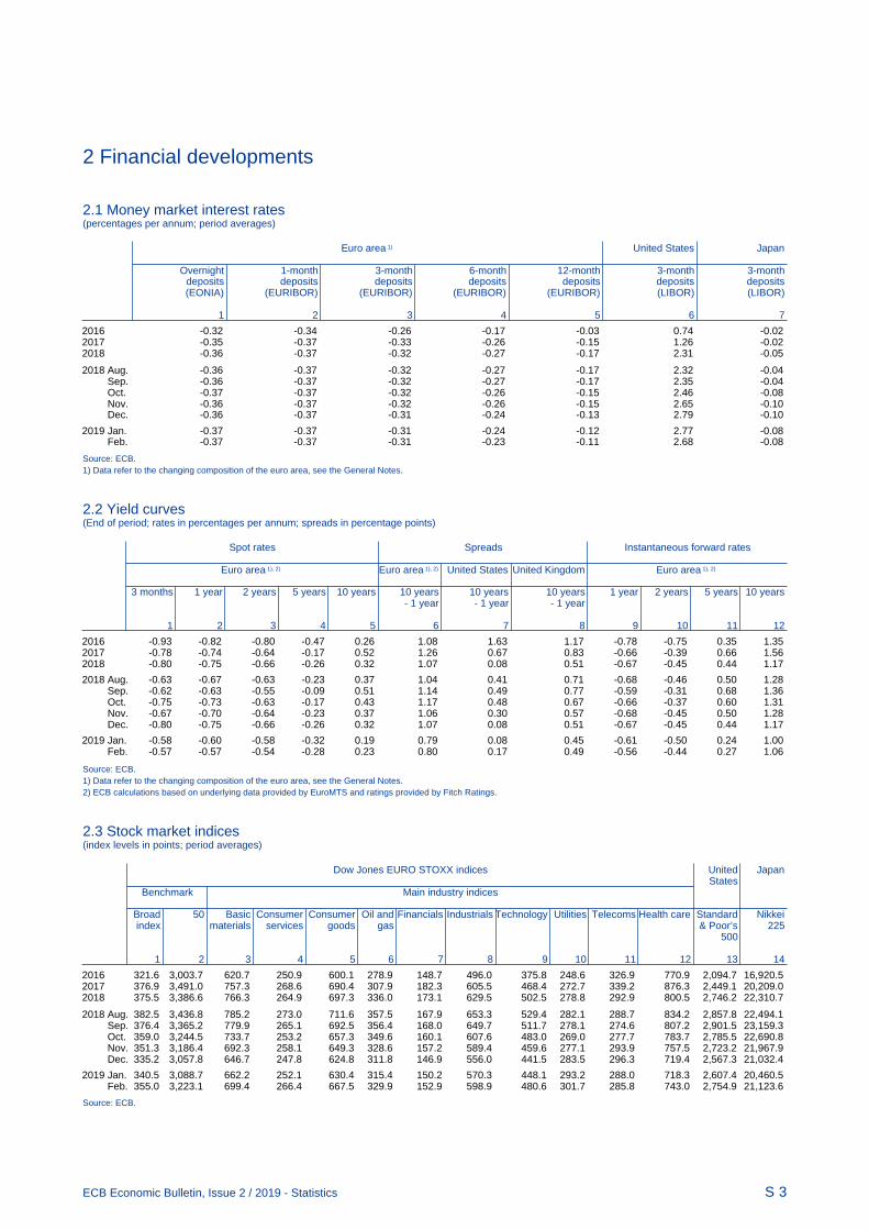
2 Financial developments
S 3ECB Economic Bulletin, Issue 2 / 2019 - Statistics
2.1 Money market interest rates(percentages per annum; period averages)
Euro area 1) United States Japan
Overnight 1-month 3-month 6-month 12-month 3-month 3-monthdeposits deposits deposits deposits deposits deposits deposits(EONIA) (EURIBOR) (EURIBOR) (EURIBOR) (EURIBOR) (LIBOR) (LIBOR)
1 2 3 4 5 6 7
2016 -0.32 -0.34 -0.26 -0.17 -0.03 0.74 -0.022017 -0.35 -0.37 -0.33 -0.26 -0.15 1.26 -0.022018 -0.36 -0.37 -0.32 -0.27 -0.17 2.31 -0.05
2018 Aug. -0.36 -0.37 -0.32 -0.27 -0.17 2.32 -0.04 Sep. -0.36 -0.37 -0.32 -0.27 -0.17 2.35 -0.04 Oct. -0.37 -0.37 -0.32 -0.26 -0.15 2.46 -0.08 Nov. -0.36 -0.37 -0.32 -0.26 -0.15 2.65 -0.10 Dec. -0.36 -0.37 -0.31 -0.24 -0.13 2.79 -0.10
2019 Jan. -0.37 -0.37 -0.31 -0.24 -0.12 2.77 -0.08 Feb. -0.37 -0.37 -0.31 -0.23 -0.11 2.68 -0.08
Source: ECB.1) Data refer to the changing composition of the euro area, see the General Notes.
2.2 Yield curves(End of period; rates in percentages per annum; spreads in percentage points)
Spot rates Spreads Instantaneous forward rates
Euro area 1), 2) Euro area 1), 2) United States United Kingdom Euro area 1), 2)
3 months 1 year 2 years 5 years 10 years 10 years 10 years 10 years 1 year 2 years 5 years 10 years- 1 year - 1 year - 1 year
1 2 3 4 5 6 7 8 9 10 11 12
2016 -0.93 -0.82 -0.80 -0.47 0.26 1.08 1.63 1.17 -0.78 -0.75 0.35 1.352017 -0.78 -0.74 -0.64 -0.17 0.52 1.26 0.67 0.83 -0.66 -0.39 0.66 1.562018 -0.80 -0.75 -0.66 -0.26 0.32 1.07 0.08 0.51 -0.67 -0.45 0.44 1.17
2018 Aug. -0.63 -0.67 -0.63 -0.23 0.37 1.04 0.41 0.71 -0.68 -0.46 0.50 1.28 Sep. -0.62 -0.63 -0.55 -0.09 0.51 1.14 0.49 0.77 -0.59 -0.31 0.68 1.36 Oct. -0.75 -0.73 -0.63 -0.17 0.43 1.17 0.48 0.67 -0.66 -0.37 0.60 1.31 Nov. -0.67 -0.70 -0.64 -0.23 0.37 1.06 0.30 0.57 -0.68 -0.45 0.50 1.28 Dec. -0.80 -0.75 -0.66 -0.26 0.32 1.07 0.08 0.51 -0.67 -0.45 0.44 1.17
2019 Jan. -0.58 -0.60 -0.58 -0.32 0.19 0.79 0.08 0.45 -0.61 -0.50 0.24 1.00 Feb. -0.57 -0.57 -0.54 -0.28 0.23 0.80 0.17 0.49 -0.56 -0.44 0.27 1.06
Source: ECB.1) Data refer to the changing composition of the euro area, see the General Notes.2) ECB calculations based on underlying data provided by EuroMTS and ratings provided by Fitch Ratings.
2.3 Stock market indices(index levels in points; period averages)
Dow Jones EURO STOXX indices United Japan
States Benchmark Main industry indices
Broad 50 Basic Consumer Consumer Oil and Financials Industrials Technology Utilities Telecoms Health care Standard Nikkeiindex materials services goods gas & Poor’s 225
500
1 2 3 4 5 6 7 8 9 10 11 12 13 14
2016 321.6 3,003.7 620.7 250.9 600.1 278.9 148.7 496.0 375.8 248.6 326.9 770.9 2,094.7 16,920.52017 376.9 3,491.0 757.3 268.6 690.4 307.9 182.3 605.5 468.4 272.7 339.2 876.3 2,449.1 20,209.02018 375.5 3,386.6 766.3 264.9 697.3 336.0 173.1 629.5 502.5 278.8 292.9 800.5 2,746.2 22,310.7
2018 Aug. 382.5 3,436.8 785.2 273.0 711.6 357.5 167.9 653.3 529.4 282.1 288.7 834.2 2,857.8 22,494.1 Sep. 376.4 3,365.2 779.9 265.1 692.5 356.4 168.0 649.7 511.7 278.1 274.6 807.2 2,901.5 23,159.3 Oct. 359.0 3,244.5 733.7 253.2 657.3 349.6 160.1 607.6 483.0 269.0 277.7 783.7 2,785.5 22,690.8 Nov. 351.3 3,186.4 692.3 258.1 649.3 328.6 157.2 589.4 459.6 277.1 293.9 757.5 2,723.2 21,967.9 Dec. 335.2 3,057.8 646.7 247.8 624.8 311.8 146.9 556.0 441.5 283.5 296.3 719.4 2,567.3 21,032.4
2019 Jan. 340.5 3,088.7 662.2 252.1 630.4 315.4 150.2 570.3 448.1 293.2 288.0 718.3 2,607.4 20,460.5 Feb. 355.0 3,223.1 699.4 266.4 667.5 329.9 152.9 598.9 480.6 301.7 285.8 743.0 2,754.9 21,123.6
Source: ECB.

2 Financial developments
S 4ECB Economic Bulletin, Issue 2 / 2019 - Statistics
2.4 MFI interest rates on loans to and deposits from households (new business) 1), 2) (Percentages per annum; period average, unless otherwise indicated)
Deposits Revolving Extended Loans for consumption Loans Loans for house purchase
loans credit to sole Over- Redeem- With and card By initial period APRC 3) proprietors By initial period APRC 3) Compositenight able an agreed overdrafts credit of rate fixation and of rate fixation cost-of-
at maturity of: unincor- borrowingnotice Floating Over porated Floating Over 1 Over 5 Over indicatorof up Up to Over rate and 1 partner- rate and and up and up 10to 3 2 2 up to year ships up to to 5 to 10 years
months years years 1 year 1 year years years
1 2 3 4 5 6 7 8 9 10 11 12 13 14 15 16
2018 Feb. 0.04 0.44 0.34 0.69 6.19 16.88 4.72 5.70 6.19 2.37 1.64 1.88 1.93 1.91 2.14 1.84 Mar. 0.04 0.45 0.35 0.67 6.14 16.89 4.71 5.57 6.05 2.34 1.63 1.85 1.95 1.91 2.15 1.84 Apr. 0.04 0.45 0.34 0.61 6.12 16.87 4.94 5.67 6.14 2.37 1.62 1.85 1.96 1.90 2.13 1.83 May 0.04 0.46 0.34 0.57 6.10 16.89 4.82 5.88 6.39 2.39 1.58 1.85 1.97 1.90 2.13 1.83 June 0.03 0.46 0.33 0.63 6.05 16.84 4.50 5.64 6.11 2.31 1.60 1.81 1.97 1.88 2.12 1.82 July 0.03 0.45 0.33 0.63 6.01 16.80 4.84 5.75 6.22 2.41 1.63 1.83 1.93 1.85 2.12 1.81 Aug. 0.03 0.45 0.30 0.63 6.02 16.78 5.42 5.88 6.41 2.39 1.63 1.82 1.92 1.85 2.12 1.81 Sep. 0.03 0.45 0.30 0.69 6.05 16.71 5.28 5.74 6.27 2.38 1.60 1.81 1.91 1.85 2.09 1.79 Oct. 0.03 0.45 0.29 0.73 5.98 16.73 5.04 5.71 6.23 2.46 1.60 1.80 1.91 1.86 2.09 1.80 Nov. 0.03 0.44 0.29 0.72 5.94 16.54 4.92 5.68 6.18 2.38 1.61 1.85 1.94 1.88 2.11 1.81 Dec. 0.03 0.43 0.30 0.77 5.87 16.55 4.91 5.47 5.98 2.30 1.61 1.80 1.91 1.84 2.10 1.80
2019 Jan. (p) 0.03 0.42 0.33 0.74 5.92 16.63 5.30 5.82 6.33 2.37 1.61 1.81 1.89 1.86 2.09 1.82
Source: ECB.1) Data refer to the changing composition of the euro area.2) Including non-profit institutions serving households.3) Annual percentage rate of charge (APRC).
2.5 MFI interest rates on loans to and deposits from non-financial corporations (new business) 1), 2) (Percentages per annum; period average, unless otherwise indicated)
Deposits Revolving Other loans by size and initial period of rate fixation Composite
loans and cost-of-Over- With an agreed overdrafts up to EUR 0.25 million over EUR 0.25 and up to 1 million over EUR 1 million borrowingnight maturity of: indicator
Floating Over Over Floating Over Over Floating Over OverUp to Over rate 3 months 1 year rate 3 months 1 year rate 3 months 1 year
2 years 2 years and up to and up to and up to and up to and up to and up to3 months 1 year 3 months 1 year 3 months 1 year
1 2 3 4 5 6 7 8 9 10 11 12 13 14
2018 Feb. 0.04 0.09 0.43 2.36 2.37 2.49 2.33 1.66 1.63 1.74 1.18 1.35 1.64 1.71 Mar. 0.04 0.08 0.40 2.33 2.41 2.53 2.34 1.67 1.61 1.70 1.26 1.39 1.66 1.73 Apr. 0.04 0.06 0.32 2.32 2.37 2.42 2.33 1.67 1.61 1.74 1.23 1.29 1.65 1.71 May 0.03 0.08 0.43 2.28 2.31 2.47 2.38 1.65 1.61 1.74 1.07 1.22 1.65 1.62 June 0.04 0.07 0.74 2.29 2.27 2.44 2.31 1.64 1.56 1.71 1.21 1.33 1.70 1.68 July 0.03 0.08 0.38 2.27 2.16 2.41 2.28 1.67 1.59 1.68 1.14 1.30 1.66 1.64 Aug. 0.03 0.08 0.60 2.25 2.21 2.42 2.35 1.66 1.63 1.74 1.10 1.27 1.69 1.64 Sep. 0.03 0.08 0.44 2.22 2.21 2.34 2.32 1.65 1.55 1.69 1.12 1.40 1.69 1.65 Oct. 0.03 0.08 0.52 2.22 2.14 2.42 2.34 1.65 1.60 1.70 1.23 1.10 1.66 1.64 Nov. 0.03 0.07 0.63 2.19 2.20 2.40 2.34 1.66 1.60 1.69 1.20 1.35 1.69 1.66 Dec. 0.03 0.07 0.53 2.18 2.21 2.28 2.26 1.61 1.59 1.69 1.21 1.39 1.59 1.64
2019 Jan. (p) 0.03 0.07 0.56 2.22 2.15 2.39 2.32 1.68 1.61 1.73 1.13 1.30 1.61 1.63
Source: ECB.1) Data refer to the changing composition of the euro area.2) In accordance with the ESA 2010, in December 2014 holding companies of non-financial groups were reclassified from the non-financial corporations sector to the financial
corporations sector.

2 Financial developments
S 5ECB Economic Bulletin, Issue 2 / 2019 - Statistics
2.6 Debt securities issued by euro area residents, by sector of the issuer and initial maturity(EUR billions; transactions during the month and end-of-period outstanding amounts; nominal values)
Short-term
Outstanding amounts Gross issues 1)
Total MFIs Non-MFI corporations General government Total MFIs Non-MFI corporations General government
(including (including Euro- Financial Non- Central Other Euro- Financial Non- Central Other
system) corporations financial govern- general system) corporations financial govern- generalother than FVCs corporations ment govern- other than FVCs corporations ment govern-
MFIs ment MFIs ment
1 2 3 4 5 6 7 8 9 10 11 12 13 14
2015 1,269 517 147 . 62 478 65 347 161 37 . 33 82 342016 1,241 518 136 . 59 466 62 349 161 45 . 31 79 332017 1,241 519 156 . 70 438 57 368 167 55 . 37 79 31
2018 July 1,313 526 178 . 96 453 60 436 191 77 . 48 79 42 Aug. 1,311 525 178 . 95 447 65 408 201 61 . 31 82 33 Sep. 1,295 531 179 . 89 444 52 378 164 73 . 42 72 28 Oct. 1,280 525 171 . 92 439 54 411 184 66 . 46 77 38 Nov. 1,270 518 166 . 89 445 52 353 154 57 . 36 74 31 Dec. 1,200 499 159 . 72 424 47 267 109 53 . 36 44 26
Long-term
2015 15,250 3,786 3,270 . 1,075 6,481 637 216 68 46 . 14 80 92016 15,380 3,695 3,234 . 1,126 6,684 641 220 62 54 . 18 78 82017 15,362 3,560 3,109 . 1,185 6,865 642 247 66 74 . 17 83 7
2018 July 15,555 3,570 3,158 . 1,203 7,003 621 220 54 55 . 16 87 8 Aug. 15,564 3,578 3,167 . 1,186 7,010 622 131 50 38 . 2 38 3 Sep. 15,683 3,616 3,183 . 1,206 7,055 623 254 79 60 . 29 82 4 Oct. 15,719 3,672 3,188 . 1,205 7,026 628 215 60 61 . 14 69 10 Nov. 15,802 3,697 3,215 . 1,208 7,054 629 223 67 70 . 8 72 7 Dec. 15,747 3,694 3,194 . 1,212 7,020 626 175 60 74 . 14 24 3
Source: ECB.1) For the purpose of comparison, annual data refer to the average monthly figure over the year.
2.7 Growth rates and outstanding amounts of debt securities and listed shares(EUR billions; percentage changes)
Oustanding amount
Debt securities Listed shares
Total MFIs Non-MFI corporations General government Total MFIs Financial Non-
(including corporations financialEurosystem) Financial Non- Central Other other than corporations
corporations financial government general MFIsother than FVCs corporations government
MFIs
1 2 3 4 5 6 7 8 9 10 11
2015 16,518.8 4,303.2 3,417.2 . 1,137.0 6,958.9 702.4 6,814.4 584.3 968.3 5,261.92016 16,621.2 4,213.3 3,369.3 . 1,185.3 7,149.9 703.5 7,089.5 537.6 1,080.2 5,471.62017 16,602.8 4,079.7 3,264.5 . 1,255.2 7,303.6 699.8 7,954.7 612.5 1,249.4 6,092.8
2018 July 16,867.9 4,095.9 3,335.9 . 1,299.3 7,455.8 681.0 8,168.5 576.1 1,293.6 6,298.8 Aug. 16,874.8 4,102.8 3,345.2 . 1,281.6 7,457.7 687.5 8,019.9 521.1 1,282.5 6,216.3 Sep. 16,978.4 4,147.2 3,361.8 . 1,295.4 7,499.3 674.8 7,955.7 543.5 1,293.9 6,118.4 Oct. 16,999.6 4,197.4 3,358.4 . 1,296.9 7,464.9 682.0 7,546.6 515.4 1,201.8 5,829.4 Nov. 17,072.6 4,214.6 3,381.3 . 1,296.7 7,499.0 681.0 7,475.0 512.1 1,179.2 5,783.6 Dec. 16,947.3 4,192.7 3,353.5 . 1,283.7 7,444.7 672.7 7,030.7 465.1 1,099.0 5,466.6
Growth rate
2015 0.2 -7.0 5.8 . 4.1 1.8 0.6 1.1 4.2 1.8 0.62016 0.3 -3.0 -1.2 . 6.5 2.2 -0.1 0.5 1.2 0.9 0.42017 1.3 -0.5 -0.2 . 6.1 2.2 0.5 1.1 6.1 2.8 0.3
2018 July 1.2 -0.8 0.6 . 5.0 2.4 -2.5 1.2 0.4 4.8 0.6 Aug. 1.4 -0.2 1.2 . 4.2 2.2 -2.6 1.2 0.5 4.7 0.5 Sep. 1.8 0.9 1.3 . 5.1 2.4 -3.7 1.1 0.5 3.9 0.5 Oct. 1.9 0.9 2.0 . 4.9 2.4 -3.1 1.0 0.5 3.1 0.6 Nov. 2.0 1.3 2.5 . 3.7 2.4 -3.6 0.9 0.4 2.9 0.5 Dec. 1.7 1.7 1.6 . 3.4 1.9 -4.3 0.8 -0.1 2.8 0.4
Source: ECB.

2 Financial developments
S 6ECB Economic Bulletin, Issue 2 / 2019 - Statistics
2.8 Effective exchange rates 1) (period averages; index: 1999 Q1=100)
EER-19 EER-38
Nominal Real CPI Real PPI Real GDP Real ULCM 2) Real ULCT Nominal Real CPIdeflator
1 2 3 4 5 6 7 8
2016 94.4 89.4 90.9 85.1 79.4 89.1 109.7 88.72017 96.6 91.3 92.0 86.0 78.8 89.9 112.0 89.92018 98.9 93.3 93.5 . . . 117.9 93.7
2018 Q1 99.6 93.9 94.4 88.2 80.1 91.8 117.0 93.3 Q2 98.4 92.9 93.2 87.3 78.8 90.6 117.0 93.2 Q3 99.2 93.5 93.5 87.8 79.5 91.4 119.2 94.6 Q4 98.5 92.8 93.0 . . . 118.4 93.6
2018 Sep. 99.5 93.7 93.7 - - - 120.4 95.4 Oct. 98.9 93.2 93.3 - - - 119.0 94.2 Nov. 98.3 92.7 92.8 - - - 117.9 93.4 Dec. 98.4 92.6 93.0 - - - 118.0 93.2
2019 Jan. 97.8 92.0 92.5 - - - 117.3 92.5 Feb. 97.4 91.5 92.2 - - - 116.6 91.8
Percentage change versus previous month
2019 Feb. -0.4 -0.5 -0.4 - - - -0.6 -0.8
Percentage change versus previous year
2019 Feb. -2.2 -2.4 -2.4 - - - -0.6 -1.8
Source: ECB.1) For a definition of the trading partner groups and other information see the General Notes to the Statistics Bulletin.2) ULCM-deflated series are available only for the EER-18 trading partner group.
2.9 Bilateral exchange rates(period averages; units of national currency per euro)
Chinese Croatian Czech Danish Hungarian Japanese Polish Pound Romanian Swedish Swiss USrenminbi kuna koruna krone forint yen zloty sterling leu krona franc Dollar
1 2 3 4 5 6 7 8 9 10 11 12
2016 7.352 7.533 27.034 7.445 311.438 120.197 4.363 0.819 4.4904 9.469 1.090 1.1072017 7.629 7.464 26.326 7.439 309.193 126.711 4.257 0.877 4.5688 9.635 1.112 1.1302018 7.808 7.418 25.647 7.453 318.890 130.396 4.261 0.885 4.6540 10.258 1.155 1.181
2018 Q1 7.815 7.438 25.402 7.447 311.027 133.166 4.179 0.883 4.6553 9.971 1.165 1.229 Q2 7.602 7.398 25.599 7.448 317.199 130.045 4.262 0.876 4.6532 10.330 1.174 1.191 Q3 7.915 7.417 25.718 7.455 324.107 129.606 4.303 0.892 4.6471 10.405 1.144 1.163 Q4 7.895 7.420 25.864 7.462 322.995 128.816 4.299 0.887 4.6605 10.320 1.137 1.141
2018 Sep. 7.993 7.429 25.614 7.458 324.818 130.535 4.301 0.893 4.6471 10.443 1.129 1.166 Oct. 7.948 7.425 25.819 7.460 323.843 129.617 4.305 0.883 4.6658 10.384 1.141 1.148 Nov. 7.888 7.428 25.935 7.461 322.330 128.789 4.302 0.881 4.6610 10.292 1.138 1.137 Dec. 7.840 7.404 25.835 7.465 322.738 127.878 4.290 0.898 4.6536 10.277 1.129 1.138
2019 Jan. 7.750 7.429 25.650 7.466 319.800 124.341 4.292 0.886 4.7062 10.269 1.130 1.142 Feb. 7.649 7.415 25.726 7.463 317.908 125.280 4.318 0.873 4.7486 10.499 1.137 1.135
Percentage change versus previous month
2019 Feb. -1.3 -0.2 0.3 0.0 -0.6 0.8 0.6 -1.5 0.9 2.2 0.6 -0.6
Percentage change versus previous year
2019 Feb. -2.0 -0.3 1.6 0.2 2.0 -6.0 3.7 -1.3 2.0 5.6 -1.5 -8.1
Source: ECB.

2 Financial developments
S 7ECB Economic Bulletin, Issue 2 / 2019 - Statistics
2.10 Euro area balance of payments, financial account(EUR billions, unless otherwise indicated; outstanding amounts at end of period; transactions during period)
Outstanding amounts (international investment position)
Total 1) Direct Portfolio Net Other investment Reserve Memo:
investment investment financial assets Grossderivatives external
Assets Liabilities Net Assets Liabilities Assets Liabilities Assets Liabilities debt
1 2 3 4 5 6 7 8 9 10 11 12
2017 Q4 24,840.3 25,526.8 -686.5 10,675.3 8,735.2 8,550.4 10,967.5 -55.7 5,000.6 5,824.1 669.7 13,890.4
2018 Q1 24,898.2 25,761.3 -863.1 10,643.9 8,825.8 8,532.1 10,933.7 -75.8 5,124.8 6,001.8 673.2 14,134.5 Q2 25,526.6 26,196.4 -669.8 10,828.6 8,922.0 8,743.6 11,010.0 -83.1 5,347.4 6,264.4 690.0 14,369.5 Q3 25,832.2 26,425.6 -593.5 10,939.9 9,011.5 8,883.2 11,099.3 -61.4 5,396.5 6,314.8 673.9 14,450.1
Outstanding amounts as a percentage of GDP
2018 Q3 224.8 230.0 -5.2 95.2 78.4 77.3 96.6 -0.5 47.0 55.0 5.9 125.8
Transactions
2018 Q1 440.6 319.3 121.3 62.7 -77.8 192.3 196.5 3.1 171.1 200.7 11.4 - Q2 167.7 105.1 62.6 -2.2 -29.7 -1.9 -41.4 38.0 127.3 176.2 6.6 - Q3 174.1 81.3 92.8 49.1 28.9 41.0 6.3 33.3 49.5 46.1 1.2 - Q4 -309.8 -428.1 118.2 -108.2 -219.7 -124.6 -123.0 17.9 -100.6 -85.3 5.7 -
2018 July 143.0 140.1 2.9 43.1 36.9 20.9 13.4 12.8 70.6 89.8 -4.4 - Aug. 31.6 1.5 30.1 -2.4 8.8 29.0 -42.3 14.1 -12.4 35.1 3.3 - Sep. -0.5 -60.4 59.9 8.4 -16.8 -8.8 35.2 6.4 -8.7 -78.7 2.2 - Oct. 91.7 74.3 17.4 68.3 -2.7 -30.8 -17.5 1.7 53.2 94.5 -0.7 - Nov. -101.6 -126.4 24.8 -105.9 -97.4 -45.3 -34.0 9.9 36.5 5.0 3.2 - Dec. -299.9 -376.0 76.0 -70.6 -119.7 -48.5 -71.5 6.3 -190.3 -184.8 3.2 -
12-month cumulated transactions
2018 Dec. 472.6 77.6 395.0 1.3 -298.3 106.8 38.3 92.4 247.3 337.6 24.8 -
12-month cumulated transactions as a percentage of GDP
2018 Dec. 4.1 0.7 3.4 0.0 -2.6 0.9 0.3 0.8 2.2 2.9 0.2 -
Source: ECB.1) Net financial derivatives are included in total assets.
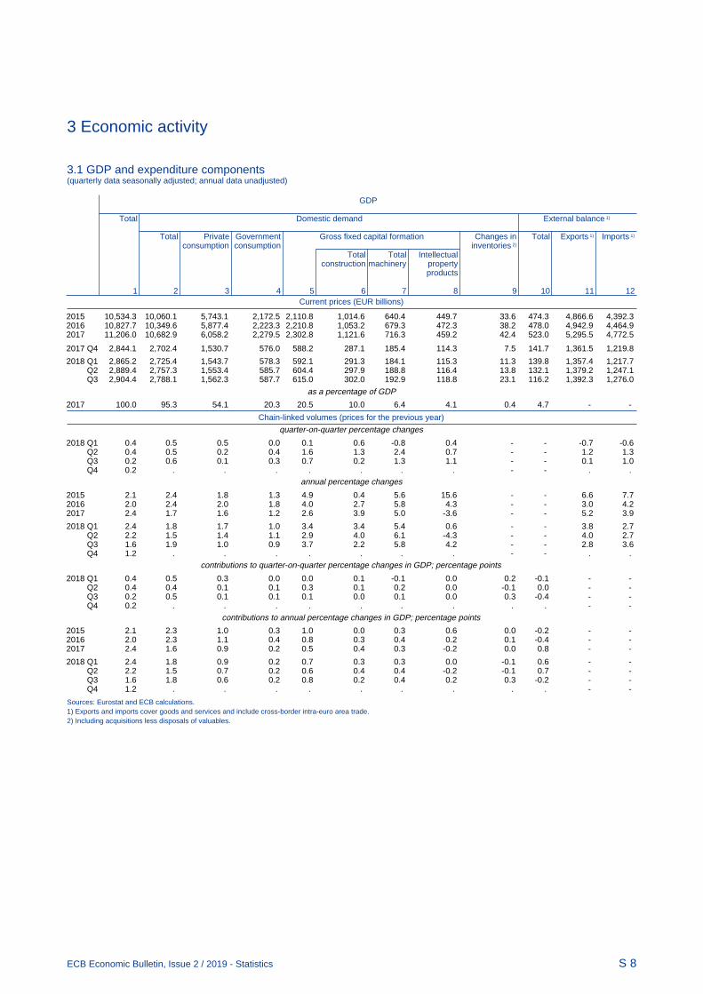
3 Economic activity
S 8ECB Economic Bulletin, Issue 2 / 2019 - Statistics
3.1 GDP and expenditure components(quarterly data seasonally adjusted; annual data unadjusted)
Current prices (EUR billions)
GDP
Total Domestic demand External balance 1)
Total Private Government Gross fixed capital formation Changes in Total Exports 1) Imports 1)
consumption consumption inventories 2)
Total Total Intellectualconstruction machinery property
products
1 2 3 4 5 6 7 8 9 10 11 12
2015 10,534.3 10,060.1 5,743.1 2,172.5 2,110.8 1,014.6 640.4 449.7 33.6 474.3 4,866.6 4,392.32016 10,827.7 10,349.6 5,877.4 2,223.3 2,210.8 1,053.2 679.3 472.3 38.2 478.0 4,942.9 4,464.92017 11,206.0 10,682.9 6,058.2 2,279.5 2,302.8 1,121.6 716.3 459.2 42.4 523.0 5,295.5 4,772.5
2017 Q4 2,844.1 2,702.4 1,530.7 576.0 588.2 287.1 185.4 114.3 7.5 141.7 1,361.5 1,219.8
2018 Q1 2,865.2 2,725.4 1,543.7 578.3 592.1 291.3 184.1 115.3 11.3 139.8 1,357.4 1,217.7 Q2 2,889.4 2,757.3 1,553.4 585.7 604.4 297.9 188.8 116.4 13.8 132.1 1,379.2 1,247.1 Q3 2,904.4 2,788.1 1,562.3 587.7 615.0 302.0 192.9 118.8 23.1 116.2 1,392.3 1,276.0
as a percentage of GDP
2017 100.0 95.3 54.1 20.3 20.5 10.0 6.4 4.1 0.4 4.7 - -
Chain-linked volumes (prices for the previous year)
quarter-on-quarter percentage changes
2018 Q1 0.4 0.5 0.5 0.0 0.1 0.6 -0.8 0.4 - - -0.7 -0.6 Q2 0.4 0.5 0.2 0.4 1.6 1.3 2.4 0.7 - - 1.2 1.3 Q3 0.2 0.6 0.1 0.3 0.7 0.2 1.3 1.1 - - 0.1 1.0 Q4 0.2 . . . . . . . - - . .
annual percentage changes
2015 2.1 2.4 1.8 1.3 4.9 0.4 5.6 15.6 - - 6.6 7.72016 2.0 2.4 2.0 1.8 4.0 2.7 5.8 4.3 - - 3.0 4.22017 2.4 1.7 1.6 1.2 2.6 3.9 5.0 -3.6 - - 5.2 3.9
2018 Q1 2.4 1.8 1.7 1.0 3.4 3.4 5.4 0.6 - - 3.8 2.7 Q2 2.2 1.5 1.4 1.1 2.9 4.0 6.1 -4.3 - - 4.0 2.7 Q3 1.6 1.9 1.0 0.9 3.7 2.2 5.8 4.2 - - 2.8 3.6 Q4 1.2 . . . . . . . - - . .
contributions to quarter-on-quarter percentage changes in GDP; percentage points
2018 Q1 0.4 0.5 0.3 0.0 0.0 0.1 -0.1 0.0 0.2 -0.1 - - Q2 0.4 0.4 0.1 0.1 0.3 0.1 0.2 0.0 -0.1 0.0 - - Q3 0.2 0.5 0.1 0.1 0.1 0.0 0.1 0.0 0.3 -0.4 - - Q4 0.2 . . . . . . . . . - -
contributions to annual percentage changes in GDP; percentage points
2015 2.1 2.3 1.0 0.3 1.0 0.0 0.3 0.6 0.0 -0.2 - - 2016 2.0 2.3 1.1 0.4 0.8 0.3 0.4 0.2 0.1 -0.4 - - 2017 2.4 1.6 0.9 0.2 0.5 0.4 0.3 -0.2 0.0 0.8 - -
2018 Q1 2.4 1.8 0.9 0.2 0.7 0.3 0.3 0.0 -0.1 0.6 - - Q2 2.2 1.5 0.7 0.2 0.6 0.4 0.4 -0.2 -0.1 0.7 - - Q3 1.6 1.8 0.6 0.2 0.8 0.2 0.4 0.2 0.3 -0.2 - - Q4 1.2 . . . . . . . . . - -
Sources: Eurostat and ECB calculations.1) Exports and imports cover goods and services and include cross-border intra-euro area trade.2) Including acquisitions less disposals of valuables.
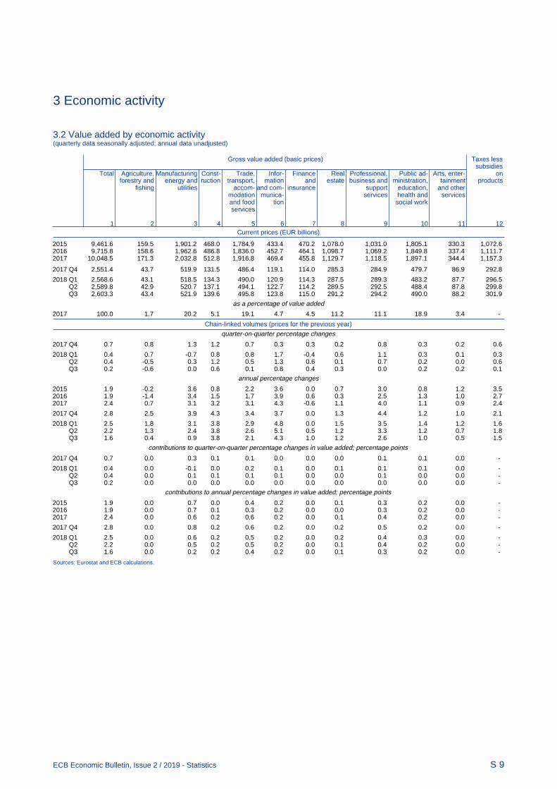
3 Economic activity
S 9ECB Economic Bulletin, Issue 2 / 2019 - Statistics
3.2 Value added by economic activity(quarterly data seasonally adjusted; annual data unadjusted)
Current prices (EUR billions)
Gross value added (basic prices) Taxes less
subsidiesTotal Agriculture, Manufacturing Const- Trade, Infor- Finance Real Professional, Public ad- Arts, enter- on
forestry and energy and ruction transport, mation and estate business and ministration, tainment productsfishing utilities accom- and com- insurance support education, and other
modation munica- services health and servicesand food tion social workservices
1 2 3 4 5 6 7 8 9 10 11 12
2015 9,461.6 159.5 1,901.2 468.0 1,784.9 433.4 470.2 1,078.0 1,031.0 1,805.1 330.3 1,072.62016 9,715.8 158.6 1,962.6 486.8 1,836.0 452.7 464.1 1,098.7 1,069.2 1,849.8 337.4 1,111.72017 10,048.5 171.3 2,032.8 512.8 1,916.8 469.4 455.8 1,129.7 1,118.5 1,897.1 344.4 1,157.3
2017 Q4 2,551.4 43.7 519.9 131.5 486.4 119.1 114.0 285.3 284.9 479.7 86.9 292.8
2018 Q1 2,568.6 43.1 518.5 134.3 490.0 120.9 114.3 287.5 289.3 483.2 87.7 296.5 Q2 2,589.8 42.9 520.7 137.1 494.1 122.7 114.2 289.5 292.5 488.4 87.8 299.8 Q3 2,603.3 43.4 521.9 139.6 495.8 123.8 115.0 291.2 294.2 490.0 88.2 301.9
as a percentage of value added
2017 100.0 1.7 20.2 5.1 19.1 4.7 4.5 11.2 11.1 18.9 3.4 -
Chain-linked volumes (prices for the previous year)
quarter-on-quarter percentage changes
2017 Q4 0.7 0.8 1.3 1.2 0.7 0.3 0.3 0.2 0.8 0.3 0.2 0.6
2018 Q1 0.4 0.7 -0.7 0.8 0.8 1.7 -0.4 0.6 1.1 0.3 0.1 0.3 Q2 0.4 -0.5 0.3 1.2 0.5 1.3 0.6 0.1 0.7 0.2 0.0 0.6 Q3 0.2 -0.6 0.0 0.6 0.1 0.8 0.4 0.3 0.0 0.2 0.2 0.1
annual percentage changes
2015 1.9 -0.2 3.6 0.8 2.2 3.6 0.0 0.7 3.0 0.8 1.2 3.52016 1.9 -1.4 3.4 1.5 1.7 3.9 0.6 0.3 2.5 1.3 1.0 2.72017 2.4 0.7 3.1 3.2 3.1 4.3 -0.6 1.1 4.0 1.1 0.9 2.4
2017 Q4 2.8 2.5 3.9 4.3 3.4 3.7 0.0 1.3 4.4 1.2 1.0 2.1
2018 Q1 2.5 1.8 3.1 3.8 2.9 4.8 0.0 1.5 3.5 1.4 1.2 1.6 Q2 2.2 1.3 2.4 3.8 2.6 5.1 0.5 1.2 3.3 1.2 0.7 1.8 Q3 1.6 0.4 0.9 3.8 2.1 4.3 1.0 1.2 2.6 1.0 0.5 1.5
contributions to quarter-on-quarter percentage changes in value added; percentage points
2017 Q4 0.7 0.0 0.3 0.1 0.1 0.0 0.0 0.0 0.1 0.1 0.0 -
2018 Q1 0.4 0.0 -0.1 0.0 0.2 0.1 0.0 0.1 0.1 0.1 0.0 - Q2 0.4 0.0 0.1 0.1 0.1 0.1 0.0 0.0 0.1 0.0 0.0 - Q3 0.2 0.0 0.0 0.0 0.0 0.0 0.0 0.0 0.0 0.0 0.0 -
contributions to annual percentage changes in value added; percentage points
2015 1.9 0.0 0.7 0.0 0.4 0.2 0.0 0.1 0.3 0.2 0.0 - 2016 1.9 0.0 0.7 0.1 0.3 0.2 0.0 0.0 0.3 0.2 0.0 - 2017 2.4 0.0 0.6 0.2 0.6 0.2 0.0 0.1 0.4 0.2 0.0 -
2017 Q4 2.8 0.0 0.8 0.2 0.6 0.2 0.0 0.2 0.5 0.2 0.0 -
2018 Q1 2.5 0.0 0.6 0.2 0.5 0.2 0.0 0.2 0.4 0.3 0.0 - Q2 2.2 0.0 0.5 0.2 0.5 0.2 0.0 0.1 0.4 0.2 0.0 - Q3 1.6 0.0 0.2 0.2 0.4 0.2 0.0 0.1 0.3 0.2 0.0 -
Sources: Eurostat and ECB calculations.
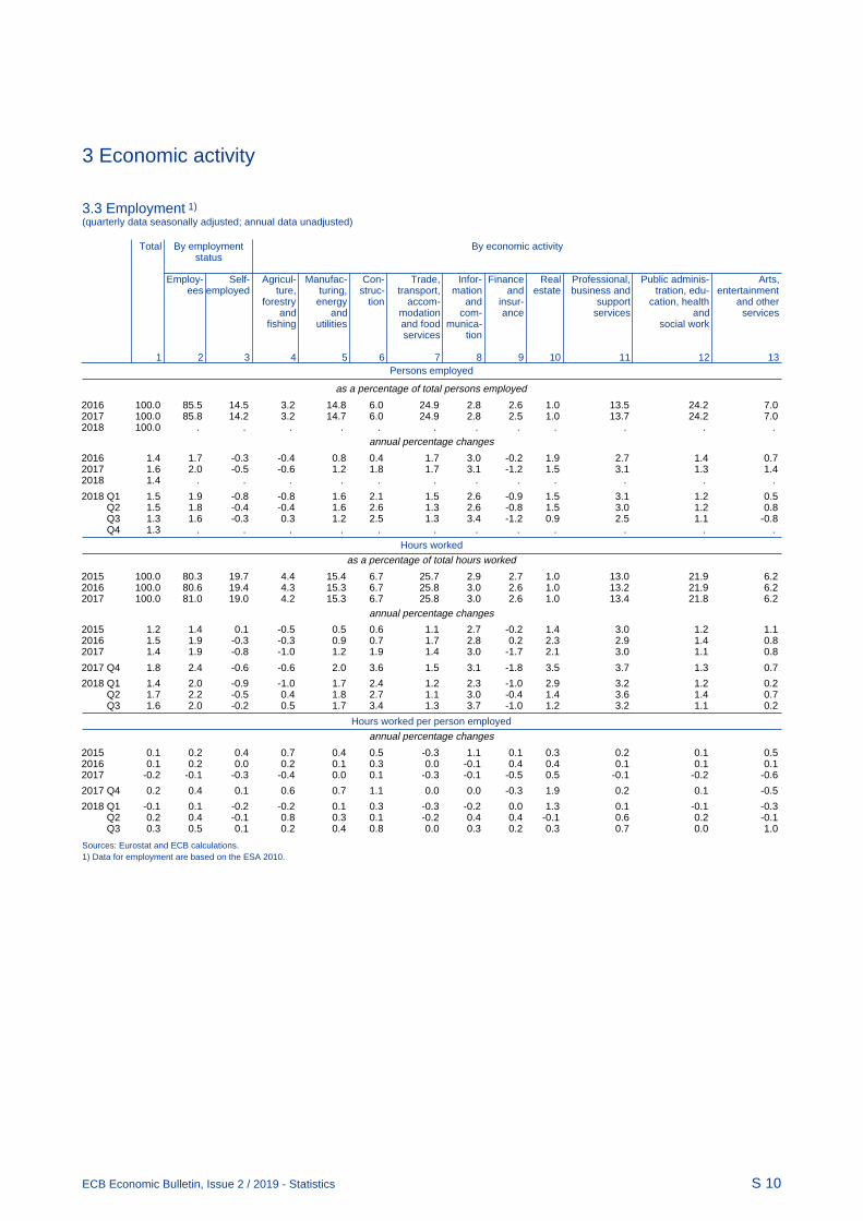
3 Economic activity
S 10ECB Economic Bulletin, Issue 2 / 2019 - Statistics
3.3 Employment 1)
(quarterly data seasonally adjusted; annual data unadjusted)
Persons employed
Total By employment By economic activity
status
Employ- Self- Agricul- Manufac- Con- Trade, Infor- Finance Real Professional, Public adminis- Arts,ees employed ture, turing, struc- transport, mation and estate business and tration, edu- entertainment
forestry energy tion accom- and insur- support cation, health and otherand and modation com- ance services and services
fishing utilities and food munica- social workservices tion
1 2 3 4 5 6 7 8 9 10 11 12 13
as a percentage of total persons employed
2016 100.0 85.5 14.5 3.2 14.8 6.0 24.9 2.8 2.6 1.0 13.5 24.2 7.02017 100.0 85.8 14.2 3.2 14.7 6.0 24.9 2.8 2.5 1.0 13.7 24.2 7.02018 100.0 . . . . . . . . . . . .
annual percentage changes
2016 1.4 1.7 -0.3 -0.4 0.8 0.4 1.7 3.0 -0.2 1.9 2.7 1.4 0.72017 1.6 2.0 -0.5 -0.6 1.2 1.8 1.7 3.1 -1.2 1.5 3.1 1.3 1.42018 1.4 . . . . . . . . . . . .
2018 Q1 1.5 1.9 -0.8 -0.8 1.6 2.1 1.5 2.6 -0.9 1.5 3.1 1.2 0.5 Q2 1.5 1.8 -0.4 -0.4 1.6 2.6 1.3 2.6 -0.8 1.5 3.0 1.2 0.8 Q3 1.3 1.6 -0.3 0.3 1.2 2.5 1.3 3.4 -1.2 0.9 2.5 1.1 -0.8 Q4 1.3 . . . . . . . . . . . .
Hours worked
as a percentage of total hours worked
2015 100.0 80.3 19.7 4.4 15.4 6.7 25.7 2.9 2.7 1.0 13.0 21.9 6.22016 100.0 80.6 19.4 4.3 15.3 6.7 25.8 3.0 2.6 1.0 13.2 21.9 6.22017 100.0 81.0 19.0 4.2 15.3 6.7 25.8 3.0 2.6 1.0 13.4 21.8 6.2
annual percentage changes
2015 1.2 1.4 0.1 -0.5 0.5 0.6 1.1 2.7 -0.2 1.4 3.0 1.2 1.12016 1.5 1.9 -0.3 -0.3 0.9 0.7 1.7 2.8 0.2 2.3 2.9 1.4 0.82017 1.4 1.9 -0.8 -1.0 1.2 1.9 1.4 3.0 -1.7 2.1 3.0 1.1 0.8
2017 Q4 1.8 2.4 -0.6 -0.6 2.0 3.6 1.5 3.1 -1.8 3.5 3.7 1.3 0.7
2018 Q1 1.4 2.0 -0.9 -1.0 1.7 2.4 1.2 2.3 -1.0 2.9 3.2 1.2 0.2 Q2 1.7 2.2 -0.5 0.4 1.8 2.7 1.1 3.0 -0.4 1.4 3.6 1.4 0.7 Q3 1.6 2.0 -0.2 0.5 1.7 3.4 1.3 3.7 -1.0 1.2 3.2 1.1 0.2
Hours worked per person employed
annual percentage changes
2015 0.1 0.2 0.4 0.7 0.4 0.5 -0.3 1.1 0.1 0.3 0.2 0.1 0.52016 0.1 0.2 0.0 0.2 0.1 0.3 0.0 -0.1 0.4 0.4 0.1 0.1 0.12017 -0.2 -0.1 -0.3 -0.4 0.0 0.1 -0.3 -0.1 -0.5 0.5 -0.1 -0.2 -0.6
2017 Q4 0.2 0.4 0.1 0.6 0.7 1.1 0.0 0.0 -0.3 1.9 0.2 0.1 -0.5
2018 Q1 -0.1 0.1 -0.2 -0.2 0.1 0.3 -0.3 -0.2 0.0 1.3 0.1 -0.1 -0.3 Q2 0.2 0.4 -0.1 0.8 0.3 0.1 -0.2 0.4 0.4 -0.1 0.6 0.2 -0.1 Q3 0.3 0.5 0.1 0.2 0.4 0.8 0.0 0.3 0.2 0.3 0.7 0.0 1.0
Sources: Eurostat and ECB calculations.1) Data for employment are based on the ESA 2010.

3 Economic activity
S 11ECB Economic Bulletin, Issue 2 / 2019 - Statistics
3.4 Labour force, unemployment and job vacancies(seasonally adjusted, unless otherwise indicated)
Labour Under- Unemployment Job
force, employ- vacancymillions 1) ment, Total Long-term By age By gender rate 2)
% of unemploy- labour Millions % of ment, Adult Youth Male Femaleforce 1) labour % of
force labour Millions % of Millions % of Millions % of Millions % of % of totalforce 1) labour labour labour labour posts
force force force force
1 2 3 4 5 6 7 8 9 10 11 12 13 14
% of total 100.0 81.7 18.3 52.2 47.8 in 2016
2016 162.028 4.3 16.254 10.0 5.0 13.291 9.0 2.963 20.9 8.482 9.7 7.772 10.4 1.72017 162.659 4.1 14.765 9.1 4.4 12.098 8.1 2.667 18.8 7.639 8.7 7.126 9.5 1.92018 . . 13.393 8.2 . 10.957 7.3 2.436 17.0 6.902 7.9 6.491 8.6 2.1
2018 Q1 162.591 4.0 13.941 8.5 4.2 11.436 7.7 2.505 17.6 7.193 8.2 6.748 8.9 2.1 Q2 163.180 3.9 13.495 8.3 3.9 11.061 7.4 2.433 17.0 6.954 7.9 6.541 8.7 2.1 Q3 163.709 3.6 13.156 8.1 3.6 10.750 7.2 2.407 16.8 6.800 7.7 6.356 8.4 2.1 Q4 . . 12.979 7.9 . 10.581 7.1 2.398 16.6 6.659 7.6 6.320 8.3 2.3
2018 Aug. - - 13.121 8.0 - 10.717 7.2 2.404 16.8 6.782 7.7 6.338 8.4 - Sep. - - 13.108 8.0 - 10.695 7.2 2.414 16.8 6.779 7.7 6.329 8.4 - Oct. - - 13.102 8.0 - 10.672 7.1 2.430 16.9 6.739 7.7 6.363 8.4 - Nov. - - 12.965 7.9 - 10.583 7.1 2.382 16.5 6.661 7.6 6.304 8.3 - Dec. - - 12.871 7.8 - 10.489 7.0 2.382 16.5 6.578 7.5 6.292 8.3 -
2019 Jan. - - 12.848 7.8 - 10.465 7.0 2.383 16.5 6.568 7.5 6.279 8.2 -
Sources: Eurostat and ECB calculations.1) Not seasonally adjusted.2) The job vacancy rate is equal to the number of job vacancies divided by the sum of the number of occupied posts and the number of job vacancies, expressed as a percentage.
3.5 Short-term business statistics
Industrial production Con- ECB indicator Retail sales New
struction on industrial passenger Total Main Industrial Groupings produc- new orders Total Food, Non-food Fuel car regis-
(excluding construction) tion beverages, trationstobacco
Manu- Inter- Capital Consumer Energyfacturing mediate goods goods
goods
1 2 3 4 5 6 7 8 9 10 11 12 13
% of total 100.0 88.7 32.1 34.5 21.8 11.6 100.0 100.0 100.0 40.4 52.5 7.1 100.0in 2015
annual percentage changes
2016 1.6 1.8 1.8 1.9 1.7 0.5 3.1 0.6 1.6 1.0 2.1 1.4 7.22017 3.0 3.2 3.4 3.9 1.5 1.1 3.0 7.9 2.3 1.4 3.3 0.9 5.72018 1.0 1.3 0.6 2.1 1.3 -1.5 2.2 2.5 1.5 1.3 1.8 0.6 0.8
2018 Q1 3.1 3.4 3.1 4.4 2.4 0.6 2.5 6.6 1.7 1.6 1.8 0.1 5.3 Q2 2.4 2.8 1.8 4.6 2.0 -1.9 2.7 3.8 1.7 1.2 2.3 0.8 3.2 Q3 0.7 0.9 -0.2 1.9 1.0 -1.2 2.2 1.5 1.2 1.0 1.4 -0.1 3.4 Q4 -1.9 -1.7 -2.3 -2.0 -0.3 -3.6 1.4 -1.7 1.5 1.3 1.7 1.4 -9.4
2018 Aug. 1.1 1.4 -0.2 1.8 3.1 -1.0 0.9 2.4 2.3 1.8 2.7 -0.3 30.9 Sep. 0.6 0.9 -0.4 2.2 0.6 -1.4 3.6 0.4 0.3 0.1 0.5 0.7 -21.2 Oct. 1.3 1.6 0.0 3.7 0.8 -2.6 0.8 -0.2 2.5 2.4 3.0 1.1 -11.8 Nov. -3.0 -2.9 -3.1 -4.4 0.4 -4.0 1.1 1.0 1.9 0.8 2.4 1.7 -8.9 Dec. -4.2 -4.0 -4.0 -5.5 -2.2 -4.2 0.7 -5.7 0.3 0.7 -0.1 1.4 -7.5
2019 Jan. . . . . . . . . 2.2 2.2 1.7 4.3 -2.5
month-on-month percentage changes (s.a.)
2018 Aug. 1.2 1.2 0.4 1.9 2.0 1.5 0.7 2.8 0.4 0.4 0.6 -0.5 21.9 Sep. -0.7 -0.4 -0.4 -0.5 -1.0 -2.0 2.0 -1.1 -0.4 -0.4 -0.6 0.8 -37.1 Oct. 0.1 0.1 0.1 0.4 -0.2 -1.0 -1.4 0.1 0.7 0.7 0.6 0.5 9.1 Nov. -1.7 -1.7 -1.2 -2.7 -0.5 0.2 0.3 2.2 0.8 -0.3 1.5 0.4 6.7 Dec. -0.9 -1.0 0.0 -1.5 -1.5 -0.4 -0.4 -4.3 -1.4 -0.1 -2.4 0.1 2.5
2019 Jan. . . . . . . . . 1.3 0.6 1.7 1.6 4.8
Sources: Eurostat, ECB calculations, ECB experimental statistics (col. 8) and European Automobile Manufacturers Association (col. 13).

3 Economic activity
S 12ECB Economic Bulletin, Issue 2 / 2019 - Statistics
3.6 Opinion surveys(seasonally adjusted)
European Commission Business and Consumer Surveys Purchasing Managers’ Surveys
(percentage balances, unless otherwise indicated) (diffusion indices)
Economic Manufacturing industry Consumer Construction Retail Service industries Purchasing Manu- Business Compositesentiment confidence confidence trade Managers’ facturing activity outputindicator Industrial Capacity indicator indicator confid- Services Capacity Index (PMI) output for
(long-term confidence utilisation ence confidence utilisation for manu- servicesaverage indicator (%) indicator indicator (%) facturing
= 100)
1 2 3 4 5 6 7 8 9 10 11 12
1999-15 99.2 -5.3 80.7 -12.3 -15.0 -8.7 7.2 - 51.2 52.5 53.0 52.8
2016 104.1 -1.8 81.7 -8.6 -16.4 0.6 11.3 88.9 52.5 53.6 53.1 53.32017 110.1 5.5 83.2 -6.0 -4.2 2.3 14.6 89.8 57.4 58.5 55.6 56.42018 111.2 6.6 83.8 -5.5 6.1 1.3 15.2 90.3 54.9 54.7 54.5 54.6
2018 Q1 113.2 8.9 84.1 -4.2 4.5 3.0 16.8 90.3 58.2 58.9 56.4 57.0 Q2 111.8 7.8 83.9 -5.2 5.5 0.5 15.1 90.4 55.6 55.1 54.5 54.7 Q3 110.9 5.9 83.7 -5.6 6.6 1.9 15.3 90.3 54.3 54.0 54.4 54.3 Q4 108.9 3.6 83.6 -6.9 7.9 -0.3 13.4 90.4 51.7 51.0 52.8 52.3
2018 Sep. 110.4 5.5 - -6.2 8.3 2.7 15.2 - 53.2 52.7 54.7 54.1 Oct. 109.7 4.2 83.6 -5.9 8.0 -0.5 14.0 90.1 52.0 51.3 53.7 53.1 Nov. 109.5 4.4 - -6.6 8.3 -0.2 14.0 - 51.8 50.7 53.4 52.7 Dec. 107.4 2.3 - -8.3 7.3 -0.1 12.2 - 51.4 51.0 51.2 51.1
2019 Jan. 106.3 0.6 83.6 -7.9 8.4 -2.1 11.0 90.7 50.5 50.5 51.2 51.0 Feb. 106.1 -0.4 - -7.4 6.4 -1.6 12.1 - 49.3 49.4 52.8 51.9
Sources: European Commission (Directorate-General for Economic and Financial Affairs) (col. 1-8) and Markit (col. 9-12).
3.7 Summary accounts for households and non-financial corporations(current prices, unless otherwise indicated; not seasonally adjusted)
Households Non-financial corporations
Saving Debt Real gross Financial Non-financial Net Hous- Profit Saving Debt Financial Non-financial Finan-ratio ratio disposable investment investment worth ing share 3) ratio ratio 4) investment investment cing
(gross) 1) income (gross) 2) wealth (net) (gross)
Percentage of Percentage of net Percent- gross disposable Annual percentage changes value added age of Annual percentage changes income (adjusted) GDP
1 2 3 4 5 6 7 8 9 10 11 12 13
2015 12.4 94.0 1.6 2.0 1.2 3.2 2.0 34.7 6.2 138.8 5.0 7.8 2.92016 12.3 94.2 1.8 2.0 6.2 3.4 2.8 35.2 7.7 139.0 4.9 6.2 2.92017 11.8 94.1 1.2 1.9 6.9 4.0 4.1 34.7 6.9 137.0 3.4 5.0 2.0
2017 Q4 11.8 94.1 1.5 1.9 6.4 4.0 4.1 34.7 6.9 137.0 3.4 1.4 2.0
2018 Q1 11.8 93.8 1.8 1.9 5.7 3.6 4.5 34.8 7.0 136.8 3.0 0.0 1.6 Q2 12.0 93.8 1.9 1.9 8.4 3.8 4.6 34.9 6.9 137.6 3.1 1.0 1.7 Q3 12.1 93.7 1.4 1.9 8.5 3.8 5.1 34.5 6.9 137.0 2.8 8.1 1.7
Sources: ECB and Eurostat.1) Based on four-quarter cumulated sums of both saving and gross disposable income (adjusted for the change in the net equity of households in pension fund reserves).2) Financial assets (net of financial liabilities) and non-financial assets. Non-financial assets consist mainly of housing wealth (residential structures and land). They also include
non-financial assets of unincorporated enterprises classified within the household sector.3) The profit share uses net entrepreneurial income, which is broadly equivalent to current profits in business accounting. 4) Based on the outstanding amount of loans, debt securities, trade credits and pension scheme liabilities.
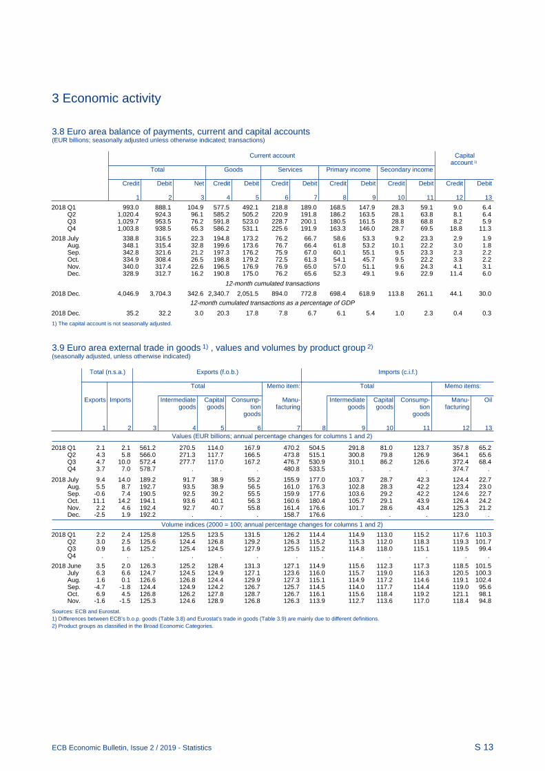
3 Economic activity
S 13ECB Economic Bulletin, Issue 2 / 2019 - Statistics
3.8 Euro area balance of payments, current and capital accounts(EUR billions; seasonally adjusted unless otherwise indicated; transactions)
Current account Capital
account 1) Total Goods Services Primary income Secondary income
Credit Debit Net Credit Debit Credit Debit Credit Debit Credit Debit Credit Debit
1 2 3 4 5 6 7 8 9 10 11 12 13
2018 Q1 993.0 888.1 104.9 577.5 492.1 218.8 189.0 168.5 147.9 28.3 59.1 9.0 6.4 Q2 1,020.4 924.3 96.1 585.2 505.2 220.9 191.8 186.2 163.5 28.1 63.8 8.1 6.4 Q3 1,029.7 953.5 76.2 591.8 523.0 228.7 200.1 180.5 161.5 28.8 68.8 8.2 5.9 Q4 1,003.8 938.5 65.3 586.2 531.1 225.6 191.9 163.3 146.0 28.7 69.5 18.8 11.3
2018 July 338.8 316.5 22.3 194.8 173.2 76.2 66.7 58.6 53.3 9.2 23.3 2.9 1.9 Aug. 348.1 315.4 32.8 199.6 173.6 76.7 66.4 61.8 53.2 10.1 22.2 3.0 1.8 Sep. 342.8 321.6 21.2 197.3 176.2 75.9 67.0 60.1 55.1 9.5 23.3 2.3 2.2 Oct. 334.9 308.4 26.5 198.8 179.2 72.5 61.3 54.1 45.7 9.5 22.2 3.3 2.2 Nov. 340.0 317.4 22.6 196.5 176.9 76.9 65.0 57.0 51.1 9.6 24.3 4.1 3.1 Dec. 328.9 312.7 16.2 190.8 175.0 76.2 65.6 52.3 49.1 9.6 22.9 11.4 6.0
12-month cumulated transactions
2018 Dec. 4,046.9 3,704.3 342.6 2,340.7 2,051.5 894.0 772.8 698.4 618.9 113.8 261.1 44.1 30.0
12-month cumulated transactions as a percentage of GDP
2018 Dec. 35.2 32.2 3.0 20.3 17.8 7.8 6.7 6.1 5.4 1.0 2.3 0.4 0.3
1) The capital account is not seasonally adjusted.
3.9 Euro area external trade in goods 1) , values and volumes by product group 2) (seasonally adjusted, unless otherwise indicated)
Values (EUR billions; annual percentage changes for columns 1 and 2)
Total (n.s.a.) Exports (f.o.b.) Imports (c.i.f.)
Total Memo item: Total Memo items:
Exports Imports Intermediate Capital Consump- Manu- Intermediate Capital Consump- Manu- Oilgoods goods tion facturing goods goods tion facturing
goods goods
1 2 3 4 5 6 7 8 9 10 11 12 13
2018 Q1 2.1 2.1 561.2 270.5 114.0 167.9 470.2 504.5 291.8 81.0 123.7 357.8 65.2 Q2 4.3 5.8 566.0 271.3 117.7 166.5 473.8 515.1 300.8 79.8 126.9 364.1 65.6 Q3 4.7 10.0 572.4 277.7 117.0 167.2 476.7 530.9 310.1 86.2 126.6 372.4 68.4 Q4 3.7 7.0 578.7 . . . 480.8 533.5 . . . 374.7 .
2018 July 9.4 14.0 189.2 91.7 38.9 55.2 155.9 177.0 103.7 28.7 42.3 124.4 22.7 Aug. 5.5 8.7 192.7 93.5 38.9 56.5 161.0 176.3 102.8 28.3 42.2 123.4 23.0 Sep. -0.6 7.4 190.5 92.5 39.2 55.5 159.9 177.6 103.6 29.2 42.2 124.6 22.7 Oct. 11.1 14.2 194.1 93.6 40.1 56.3 160.6 180.4 105.7 29.1 43.9 126.4 24.2 Nov. 2.2 4.6 192.4 92.7 40.7 55.8 161.4 176.6 101.7 28.6 43.4 125.3 21.2 Dec. -2.5 1.9 192.2 . . . 158.7 176.6 . . . 123.0 .
Volume indices (2000 = 100; annual percentage changes for columns 1 and 2)
2018 Q1 2.2 2.4 125.8 125.5 123.5 131.5 126.2 114.4 114.9 113.0 115.2 117.6 110.3 Q2 3.0 2.5 125.6 124.4 126.8 129.2 126.3 115.2 115.3 112.0 118.3 119.3 101.7 Q3 0.9 1.6 125.2 125.4 124.5 127.9 125.5 115.2 114.8 118.0 115.1 119.5 99.4 Q4 . . . . . . . . . . . . .
2018 June 3.5 2.0 126.3 125.2 128.4 131.3 127.1 114.9 115.6 112.3 117.3 118.5 101.5 July 6.3 6.6 124.7 124.5 124.9 127.1 123.6 116.0 115.7 119.0 116.3 120.5 100.3 Aug. 1.6 0.1 126.6 126.8 124.4 129.9 127.3 115.1 114.9 117.2 114.6 119.1 102.4 Sep. -4.7 -1.8 124.4 124.9 124.2 126.7 125.7 114.5 114.0 117.7 114.4 119.0 95.6 Oct. 6.9 4.5 126.8 126.2 127.8 128.7 126.7 116.1 115.6 118.4 119.2 121.1 98.1 Nov. -1.6 -1.5 125.3 124.6 128.9 126.8 126.3 113.9 112.7 113.6 117.0 118.4 94.8
Sources: ECB and Eurostat.1) Differences between ECB’s b.o.p. goods (Table 3.8) and Eurostat’s trade in goods (Table 3.9) are mainly due to different definitions.2) Product groups as classified in the Broad Economic Categories.

4 Prices and costs
S 14ECB Economic Bulletin, Issue 2 / 2019 - Statistics
4.1 Harmonised Index of Consumer Prices 1)
(annual percentage changes, unless otherwise indicated)
Total Total (s.a.; percentage change vis-à-vis previous period) 2)
Administered pricesIndex: Total Goods Services Total Processed Unpro- Non-energy Energy Services2015 food cessed industrial (n.s.a.) Total HICP Admini-
= 100 Total food goods excluding steredexcluding administered pricesfood and prices
energy
1 2 3 4 5 6 7 8 9 10 11 12 13
% of total 100.0 100.0 70.9 55.5 44.5 100.0 14.5 4.5 26.4 10.1 44.5 83.6 16.4in 2019
2016 100.2 0.2 0.8 -0.4 1.1 - - - - - - 0.2 0.32017 101.8 1.5 1.0 1.6 1.4 - - - - - - 1.6 1.22018 103.6 1.8 1.0 2.0 1.5 - - - - - - 1.7 2.1
2018 Q1 102.1 1.3 1.0 1.1 1.4 0.5 0.5 0.2 0.1 1.9 0.5 1.2 1.8 Q2 103.8 1.7 1.0 2.0 1.4 0.6 0.7 0.9 0.0 1.9 0.5 1.7 1.7 Q3 104.1 2.1 1.0 2.6 1.5 0.5 0.4 0.5 0.1 2.7 0.3 2.1 2.3 Q4 104.3 1.9 1.0 2.3 1.5 0.3 0.2 0.4 0.1 1.6 0.2 1.8 2.6
2018 Sep. 104.4 2.1 1.0 2.6 1.4 0.2 0.1 1.3 0.0 1.3 0.1 2.0 2.3 Oct. 104.7 2.3 1.2 2.7 1.7 0.2 0.1 -0.3 0.0 1.8 0.1 2.2 2.7 Nov. 104.1 1.9 0.9 2.4 1.4 0.0 0.1 -0.5 0.0 0.0 0.0 1.8 2.7 Dec. 104.1 1.5 0.9 1.7 1.3 -0.3 0.0 0.3 0.0 -3.3 0.0 1.3 2.5
2019 Jan. 103.0 1.4 1.1 1.2 1.6 0.0 0.3 0.1 0.0 -0.9 0.1 1.2 2.3 Feb. 3) 103.3 1.5 1.0 . 1.3 0.2 0.2 0.7 0.0 0.6 0.0 . .
Goods Services
Food (including alcoholic Industrial goods Housing Transport Communi- Recreation Miscel- beverages and tobacco) cation and laneous
personalTotal Processed Unpro- Total Non-energy Energy Rents care
food cessed industrialfood goods
14 15 16 17 18 19 20 21 22 23 24 25
% of total 19.0 14.5 4.5 36.5 26.4 10.1 11.0 6.5 7.2 2.6 15.3 8.4in 2019
2016 0.9 0.6 1.4 -1.1 0.4 -5.1 1.1 1.1 0.8 0.0 1.3 1.22017 1.8 1.5 2.4 1.5 0.3 4.9 1.3 1.2 2.1 -1.1 2.1 0.82018 2.2 2.1 2.3 1.9 0.3 6.4 1.2 1.2 1.5 -0.1 2.0 1.4
2018 Q1 1.7 2.2 0.2 0.8 0.3 2.2 1.3 1.3 1.7 -0.2 1.9 1.2 Q2 2.6 2.3 3.3 1.6 0.2 5.6 1.2 1.2 1.3 0.1 1.9 1.3 Q3 2.5 2.1 3.8 2.7 0.2 9.5 1.1 1.1 1.4 0.2 2.2 1.3 Q4 2.0 1.9 2.0 2.4 0.2 8.4 1.2 1.1 1.5 -0.3 1.9 1.7
2018 Sep. 2.6 2.1 4.3 2.6 0.2 9.6 1.1 1.1 1.3 0.0 2.0 1.3 Oct. 2.2 2.1 2.4 3.0 0.2 10.8 1.2 1.1 1.8 -0.2 2.5 1.7 Nov. 1.9 2.0 1.8 2.6 0.2 9.1 1.2 1.1 1.6 -0.5 1.5 1.7 Dec. 1.8 1.7 1.8 1.6 0.2 5.5 1.2 1.1 1.2 -0.3 1.6 1.7
2019 Jan. 1.8 1.8 1.8 0.9 0.3 2.7 1.2 1.1 1.6 -0.4 2.2 1.5 Feb. 3) 2.4 2.2 2.9 . 0.3 3.5 . . . . . .
Sources: Eurostat and ECB calculations.1) Data refer to the changing composition of the euro area.2) In May 2016 the ECB started publishing enhanced seasonally adjusted HICP series for the euro area, following a review of the seasonal adjustment approach as described
in Box 1, Economic Bulletin, Issue 3, ECB, 2016 (https://www.ecb.europa.eu/pub/pdf/ecbu/eb201603.en.pdf).3) Estimate based on provisional national data, as well as on early information on energy prices.

4 Prices and costs
S 15ECB Economic Bulletin, Issue 2 / 2019 - Statistics
4.2 Industry, construction and property prices(annual percentage changes, unless otherwise indicated)
Industrial producer prices excluding construction 1) Con- Residential Experimental
struction property indicator ofTotal Total Industry excluding construction and energy Energy 2) prices 3) commercial
(index: property2015 = 100) Manu- Total Intermediate Capital Consumer goods prices 3)
facturing goods goodsTotal Food, Non-
beverages foodand tobacco
1 2 3 4 5 6 7 8 9 10 11 12 13
% of total 100.0 100.0 77.3 72.1 28.9 20.7 22.5 16.5 5.9 27.9 in 2015
2016 97.9 -2.1 -1.4 -0.5 -1.6 0.5 0.0 0.0 0.0 -6.9 0.6 3.4 5.02017 100.8 3.0 3.0 2.1 3.2 0.9 1.9 2.8 0.2 5.7 2.2 3.7 5.12018 104.0 3.2 2.5 1.5 2.7 1.0 0.4 0.2 0.7 8.1 . . .
2018 Q1 102.4 1.7 1.6 1.5 2.4 0.9 0.8 1.0 0.5 2.0 2.4 4.3 4.7 Q2 103.1 2.8 2.6 1.4 2.5 1.0 0.3 0.1 0.6 6.7 2.4 4.2 4.2 Q3 104.9 4.3 3.2 1.5 3.1 1.1 0.1 -0.3 0.7 12.5 2.7 4.3 . Q4 105.7 4.0 2.3 1.4 2.5 1.1 0.3 -0.2 0.8 11.1 . . .
2018 Aug. 104.8 4.3 3.3 1.6 3.3 1.1 0.1 -0.3 0.7 12.4 - - - Sep. 105.4 4.6 3.0 1.5 2.9 1.1 0.0 -0.4 0.7 13.0 - - - Oct. 106.2 4.9 3.2 1.5 2.7 1.2 0.2 -0.3 0.8 14.6 - - - Nov. 105.9 4.0 2.3 1.5 2.6 1.2 0.2 -0.2 0.8 11.0 - - - Dec. 105.1 3.0 1.5 1.3 2.2 1.1 0.4 0.0 0.8 7.7 - - -
2019 Jan. 105.5 3.0 1.0 1.2 1.7 1.4 0.5 0.0 1.0 7.3 - - -
Sources: Eurostat, ECB calculations, and ECB calculations based on MSCI data and national sources (col. 13).1) Domestic sales only.2) Input prices for residential buildings.3) Experimental data based on non-harmonised sources (see https://www.ecb.europa.eu/stats/ecb_statistics/governance_and_quality_framework/html/experimental-data.en.html
for further details).
4.3 Commodity prices and GDP deflators(annual percentage changes, unless otherwise indicated)
GDP deflators Oil prices Non-energy commodity prices (EUR)
(EUR per Total Total Domestic demand Exports 1) Imports 1) barrel) Import-weighted 2) Use-weighted 2) (s.a.;
index: Total Private Govern- Gross Total Food Non-food Total Food Non-food2010 consump- ment fixed
= 100) tion consump- capitaltion formation
1 2 3 4 5 6 7 8 9 10 11 12 13 14 15
% of total 100.0 45.4 54.6 100.0 50.4 49.6
2016 106.9 0.8 0.5 0.4 0.5 0.7 -1.4 -2.5 39.9 -2.0 -1.4 -2.8 -3.1 -3.7 -2.32017 108.0 1.1 1.5 1.4 1.4 1.5 1.9 2.9 48.1 5.8 -3.5 16.6 6.7 -1.6 17.82018 . . . . . . . . 60.4 -0.9 -6.3 4.3 -0.2 -5.5 5.7
2018 Q1 108.9 1.4 1.5 1.2 1.5 1.8 0.4 0.4 54.6 -8.9 -14.6 -3.2 -7.6 -12.9 -1.4 Q2 109.4 1.4 1.8 1.5 2.0 1.9 1.0 2.0 62.6 2.1 -6.0 10.3 1.9 -6.3 11.7 Q3 109.8 1.4 2.1 1.8 1.9 2.5 2.2 3.9 64.8 2.0 -3.4 7.1 3.1 -2.2 8.8 Q4 . . . . . . . . 59.5 2.0 0.1 3.6 2.3 0.2 4.4
2018 Sep. - - - - - - - - 67.6 0.8 -3.0 4.2 2.3 -1.0 5.7 Oct. - - - - - - - - 70.1 2.6 -0.9 5.7 2.9 -0.4 6.4 Nov. - - - - - - - - 57.4 1.8 -0.9 4.1 1.7 -1.2 4.8 Dec. - - - - - - - - 49.8 1.5 2.0 1.1 2.2 2.4 2.1
2019 Jan. - - - - - - - - 51.9 1.3 4.0 -1.1 1.5 3.8 -0.7 Feb. - - - - - - - - 56.5 2.2 4.4 0.3 2.7 4.7 0.7
Sources: Eurostat, ECB calculations and Bloomberg (col. 9).1) Deflators for exports and imports refer to goods and services and include cross-border trade within the euro area.2) Import-weighted: weighted according to 2009-11 average import structure; use-weighted: weighted according to 2009-11 average domestic demand structure.
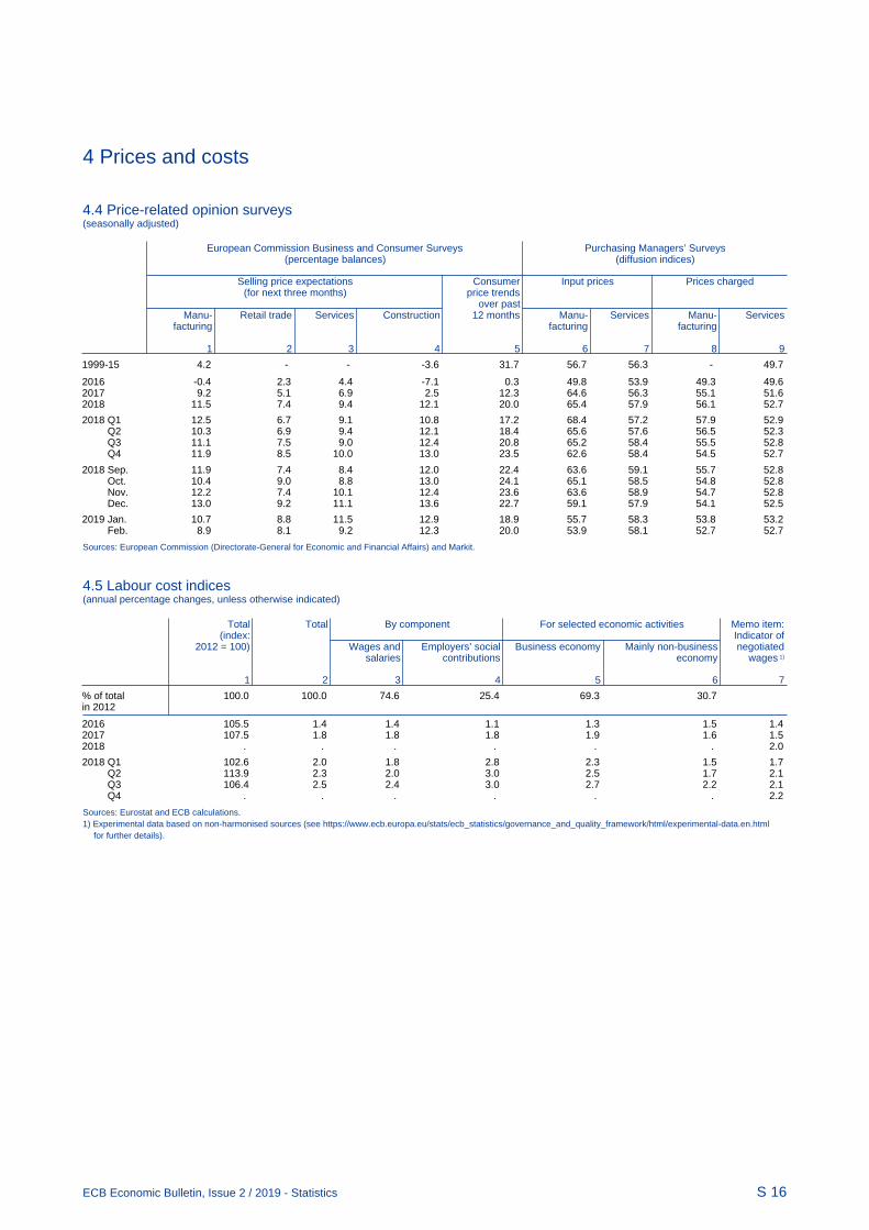
4 Prices and costs
S 16ECB Economic Bulletin, Issue 2 / 2019 - Statistics
4.4 Price-related opinion surveys(seasonally adjusted)
European Commission Business and Consumer Surveys Purchasing Managers’ Surveys
(percentage balances) (diffusion indices)
Selling price expectations Consumer Input prices Prices charged (for next three months) price trends
over pastManu- Retail trade Services Construction 12 months Manu- Services Manu- Services
facturing facturing facturing
1 2 3 4 5 6 7 8 9
1999-15 4.2 - - -3.6 31.7 56.7 56.3 - 49.7
2016 -0.4 2.3 4.4 -7.1 0.3 49.8 53.9 49.3 49.62017 9.2 5.1 6.9 2.5 12.3 64.6 56.3 55.1 51.62018 11.5 7.4 9.4 12.1 20.0 65.4 57.9 56.1 52.7
2018 Q1 12.5 6.7 9.1 10.8 17.2 68.4 57.2 57.9 52.9 Q2 10.3 6.9 9.4 12.1 18.4 65.6 57.6 56.5 52.3 Q3 11.1 7.5 9.0 12.4 20.8 65.2 58.4 55.5 52.8 Q4 11.9 8.5 10.0 13.0 23.5 62.6 58.4 54.5 52.7
2018 Sep. 11.9 7.4 8.4 12.0 22.4 63.6 59.1 55.7 52.8 Oct. 10.4 9.0 8.8 13.0 24.1 65.1 58.5 54.8 52.8 Nov. 12.2 7.4 10.1 12.4 23.6 63.6 58.9 54.7 52.8 Dec. 13.0 9.2 11.1 13.6 22.7 59.1 57.9 54.1 52.5
2019 Jan. 10.7 8.8 11.5 12.9 18.9 55.7 58.3 53.8 53.2 Feb. 8.9 8.1 9.2 12.3 20.0 53.9 58.1 52.7 52.7
Sources: European Commission (Directorate-General for Economic and Financial Affairs) and Markit.
4.5 Labour cost indices(annual percentage changes, unless otherwise indicated)
Total Total By component For selected economic activities Memo item:
(index: Indicator of2012 = 100) Wages and Employers’ social Business economy Mainly non-business negotiated
salaries contributions economy wages 1)
1 2 3 4 5 6 7
% of total 100.0 100.0 74.6 25.4 69.3 30.7 in 2012
2016 105.5 1.4 1.4 1.1 1.3 1.5 1.42017 107.5 1.8 1.8 1.8 1.9 1.6 1.52018 . . . . . . 2.0
2018 Q1 102.6 2.0 1.8 2.8 2.3 1.5 1.7 Q2 113.9 2.3 2.0 3.0 2.5 1.7 2.1 Q3 106.4 2.5 2.4 3.0 2.7 2.2 2.1 Q4 . . . . . . 2.2
Sources: Eurostat and ECB calculations.1) Experimental data based on non-harmonised sources (see https://www.ecb.europa.eu/stats/ecb_statistics/governance_and_quality_framework/html/experimental-data.en.html
for further details).

4 Prices and costs
S 17ECB Economic Bulletin, Issue 2 / 2019 - Statistics
4.6 Unit labour costs, compensation per labour input and labour productivity(annual percentage changes, unless otherwise indicated; quarterly data seasonally adjusted; annual data unadjusted)
Unit labour costs
Total Total By economic activity
(index:2010 Agriculture, Manu- Con- Trade, Information Finance Real Professional, Public ad- Arts, enter-
=100) forestry facturing, struction transport, and commu- and estate business and ministration, tainmentand fishing energy and accom- nication insurance support education, and other
utilities modation and services health and servicesfood services social work
1 2 3 4 5 6 7 8 9 10 11 12
2015 104.6 0.4 0.4 -1.4 0.6 0.4 0.7 0.5 2.4 1.3 1.4 1.12016 105.3 0.6 1.3 -1.3 0.6 1.3 -0.7 1.4 3.8 0.6 1.4 1.52017 106.1 0.8 0.3 -0.4 -0.1 0.3 0.8 -0.5 4.4 2.2 1.6 1.8
2017 Q4 106.4 0.8 -1.3 -0.6 -0.1 -0.1 1.7 -1.4 4.4 2.3 1.7 1.7
2018 Q1 107.0 1.1 0.4 0.0 -0.5 0.6 0.6 0.8 3.3 2.2 1.7 1.6 Q2 107.6 1.6 1.0 1.3 0.3 0.9 0.4 0.6 3.1 2.5 2.2 2.5 Q3 108.4 2.2 1.9 2.6 1.1 1.7 1.4 0.2 3.6 3.0 2.4 2.6
Compensation per employee
2015 108.0 1.4 1.3 2.0 1.2 1.3 2.7 0.8 2.0 1.6 1.1 1.82016 109.3 1.2 0.2 1.3 1.8 1.3 0.2 2.2 2.2 0.4 1.3 1.72017 111.1 1.6 1.6 1.5 1.2 1.6 1.9 0.0 4.0 3.1 1.5 1.3
2017 Q4 112.1 1.9 2.4 1.9 1.6 1.8 2.4 0.1 4.1 3.3 1.6 1.6
2018 Q1 112.6 1.9 3.0 1.6 1.2 2.0 2.8 1.7 3.3 2.5 1.9 2.2 Q2 113.3 2.2 2.6 2.1 1.5 2.2 2.9 1.9 2.8 2.8 2.3 2.4 Q3 114.1 2.5 1.9 2.3 2.4 2.4 2.4 2.4 3.9 3.0 2.3 4.0
Labour productivity per person employed
2016 103.9 0.6 -1.0 2.6 1.1 0.0 0.9 0.7 -1.5 -0.2 -0.1 0.32017 104.7 0.8 1.3 1.9 1.3 1.4 1.1 0.6 -0.4 0.8 -0.2 -0.52018 . . . . . . . . . . . .
2018 Q1 105.3 0.9 2.7 1.5 1.7 1.4 2.2 0.9 0.0 0.3 0.2 0.7 Q2 105.3 0.6 1.6 0.8 1.2 1.3 2.4 1.3 -0.3 0.3 0.0 -0.1 Q3 105.3 0.3 0.0 -0.3 1.3 0.7 0.9 2.2 0.3 0.1 -0.1 1.3 Q4 105.2 -0.1 . . . . . . . . . .
Compensation per hour worked
2015 109.7 1.2 1.4 1.6 0.7 1.3 1.5 0.7 1.4 1.1 1.2 1.52016 110.8 1.0 -0.4 1.2 1.7 0.9 0.2 1.8 1.9 0.0 1.3 1.52017 112.6 1.7 1.3 1.5 1.0 1.9 1.8 0.5 3.3 2.8 1.6 1.7
2017 Q4 113.2 1.5 1.6 1.1 0.6 1.6 2.1 0.3 2.1 2.7 1.4 1.8
2018 Q1 113.8 1.8 2.9 1.4 0.3 2.2 2.9 1.8 2.0 2.2 1.9 2.0 Q2 114.3 1.9 1.1 1.8 0.9 2.1 2.2 1.5 2.3 2.1 2.0 1.9 Q3 114.8 2.0 1.9 1.7 1.5 2.2 2.1 2.2 2.7 2.3 2.2 2.2
Hourly labour productivity
2015 105.2 0.9 0.2 3.1 0.2 1.1 0.9 0.2 -0.7 0.0 -0.4 0.12016 105.7 0.5 -1.2 2.5 0.8 0.0 1.0 0.3 -2.0 -0.4 -0.2 0.22017 106.8 1.0 1.7 1.9 1.3 1.7 1.2 1.1 -0.9 0.9 0.0 0.1
2017 Q4 107.1 0.9 3.1 1.9 0.7 1.9 0.7 1.8 -2.1 0.7 -0.2 0.4
2018 Q1 107.2 0.9 2.8 1.4 1.3 1.7 2.4 1.0 -1.4 0.2 0.3 1.0 Q2 107.0 0.4 0.9 0.5 1.0 1.5 2.0 0.9 -0.2 -0.3 -0.2 0.0 Q3 106.7 0.0 -0.1 -0.7 0.4 0.8 0.6 2.0 0.0 -0.6 -0.2 0.3
Sources: Eurostat and ECB calculations.
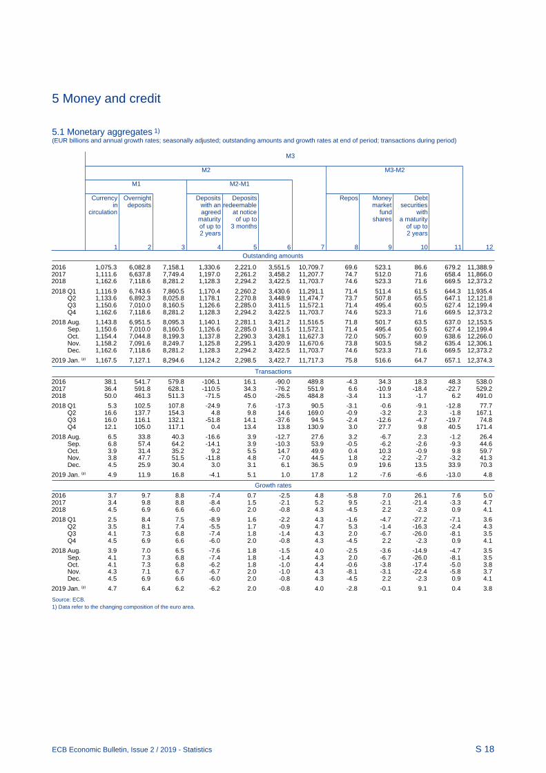
5 Money and credit
S 18ECB Economic Bulletin, Issue 2 / 2019 - Statistics
5.1 Monetary aggregates 1) (EUR billions and annual growth rates; seasonally adjusted; outstanding amounts and growth rates at end of period; transactions during period)
Outstanding amounts
M3
M2 M3-M2
M1 M2-M1
Currency Overnight Deposits Deposits Repos Money Debtin deposits with an redeemable market securities
circulation agreed at notice fund withmaturity of up to shares a maturityof up to 3 months of up to2 years 2 years
1 2 3 4 5 6 7 8 9 10 11 12
2016 1,075.3 6,082.8 7,158.1 1,330.6 2,221.0 3,551.5 10,709.7 69.6 523.1 86.6 679.2 11,388.92017 1,111.6 6,637.8 7,749.4 1,197.0 2,261.2 3,458.2 11,207.7 74.7 512.0 71.6 658.4 11,866.02018 1,162.6 7,118.6 8,281.2 1,128.3 2,294.2 3,422.5 11,703.7 74.6 523.3 71.6 669.5 12,373.2
2018 Q1 1,116.9 6,743.6 7,860.5 1,170.4 2,260.2 3,430.6 11,291.1 71.4 511.4 61.5 644.3 11,935.4 Q2 1,133.6 6,892.3 8,025.8 1,178.1 2,270.8 3,448.9 11,474.7 73.7 507.8 65.5 647.1 12,121.8 Q3 1,150.6 7,010.0 8,160.5 1,126.6 2,285.0 3,411.5 11,572.1 71.4 495.4 60.5 627.4 12,199.4 Q4 1,162.6 7,118.6 8,281.2 1,128.3 2,294.2 3,422.5 11,703.7 74.6 523.3 71.6 669.5 12,373.2
2018 Aug. 1,143.8 6,951.5 8,095.3 1,140.1 2,281.1 3,421.2 11,516.5 71.8 501.7 63.5 637.0 12,153.5 Sep. 1,150.6 7,010.0 8,160.5 1,126.6 2,285.0 3,411.5 11,572.1 71.4 495.4 60.5 627.4 12,199.4 Oct. 1,154.4 7,044.8 8,199.3 1,137.8 2,290.3 3,428.1 11,627.3 72.0 505.7 60.9 638.6 12,266.0 Nov. 1,158.2 7,091.6 8,249.7 1,125.8 2,295.1 3,420.9 11,670.6 73.8 503.5 58.2 635.4 12,306.1 Dec. 1,162.6 7,118.6 8,281.2 1,128.3 2,294.2 3,422.5 11,703.7 74.6 523.3 71.6 669.5 12,373.2
2019 Jan. (p) 1,167.5 7,127.1 8,294.6 1,124.2 2,298.5 3,422.7 11,717.3 75.8 516.6 64.7 657.1 12,374.3
Transactions
2016 38.1 541.7 579.8 -106.1 16.1 -90.0 489.8 -4.3 34.3 18.3 48.3 538.02017 36.4 591.8 628.1 -110.5 34.3 -76.2 551.9 6.6 -10.9 -18.4 -22.7 529.22018 50.0 461.3 511.3 -71.5 45.0 -26.5 484.8 -3.4 11.3 -1.7 6.2 491.0
2018 Q1 5.3 102.5 107.8 -24.9 7.6 -17.3 90.5 -3.1 -0.6 -9.1 -12.8 77.7 Q2 16.6 137.7 154.3 4.8 9.8 14.6 169.0 -0.9 -3.2 2.3 -1.8 167.1 Q3 16.0 116.1 132.1 -51.8 14.1 -37.6 94.5 -2.4 -12.6 -4.7 -19.7 74.8 Q4 12.1 105.0 117.1 0.4 13.4 13.8 130.9 3.0 27.7 9.8 40.5 171.4
2018 Aug. 6.5 33.8 40.3 -16.6 3.9 -12.7 27.6 3.2 -6.7 2.3 -1.2 26.4 Sep. 6.8 57.4 64.2 -14.1 3.9 -10.3 53.9 -0.5 -6.2 -2.6 -9.3 44.6 Oct. 3.9 31.4 35.2 9.2 5.5 14.7 49.9 0.4 10.3 -0.9 9.8 59.7 Nov. 3.8 47.7 51.5 -11.8 4.8 -7.0 44.5 1.8 -2.2 -2.7 -3.2 41.3 Dec. 4.5 25.9 30.4 3.0 3.1 6.1 36.5 0.9 19.6 13.5 33.9 70.3
2019 Jan. (p) 4.9 11.9 16.8 -4.1 5.1 1.0 17.8 1.2 -7.6 -6.6 -13.0 4.8
Growth rates
2016 3.7 9.7 8.8 -7.4 0.7 -2.5 4.8 -5.8 7.0 26.1 7.6 5.02017 3.4 9.8 8.8 -8.4 1.5 -2.1 5.2 9.5 -2.1 -21.4 -3.3 4.72018 4.5 6.9 6.6 -6.0 2.0 -0.8 4.3 -4.5 2.2 -2.3 0.9 4.1
2018 Q1 2.5 8.4 7.5 -8.9 1.6 -2.2 4.3 -1.6 -4.7 -27.2 -7.1 3.6 Q2 3.5 8.1 7.4 -5.5 1.7 -0.9 4.7 5.3 -1.4 -16.3 -2.4 4.3 Q3 4.1 7.3 6.8 -7.4 1.8 -1.4 4.3 2.0 -6.7 -26.0 -8.1 3.5 Q4 4.5 6.9 6.6 -6.0 2.0 -0.8 4.3 -4.5 2.2 -2.3 0.9 4.1
2018 Aug. 3.9 7.0 6.5 -7.6 1.8 -1.5 4.0 -2.5 -3.6 -14.9 -4.7 3.5 Sep. 4.1 7.3 6.8 -7.4 1.8 -1.4 4.3 2.0 -6.7 -26.0 -8.1 3.5 Oct. 4.1 7.3 6.8 -6.2 1.8 -1.0 4.4 -0.6 -3.8 -17.4 -5.0 3.8 Nov. 4.3 7.1 6.7 -6.7 2.0 -1.0 4.3 -8.1 -3.1 -22.4 -5.8 3.7 Dec. 4.5 6.9 6.6 -6.0 2.0 -0.8 4.3 -4.5 2.2 -2.3 0.9 4.1
2019 Jan. (p) 4.7 6.4 6.2 -6.2 2.0 -0.8 4.0 -2.8 -0.1 9.1 0.4 3.8
Source: ECB.1) Data refer to the changing composition of the euro area.
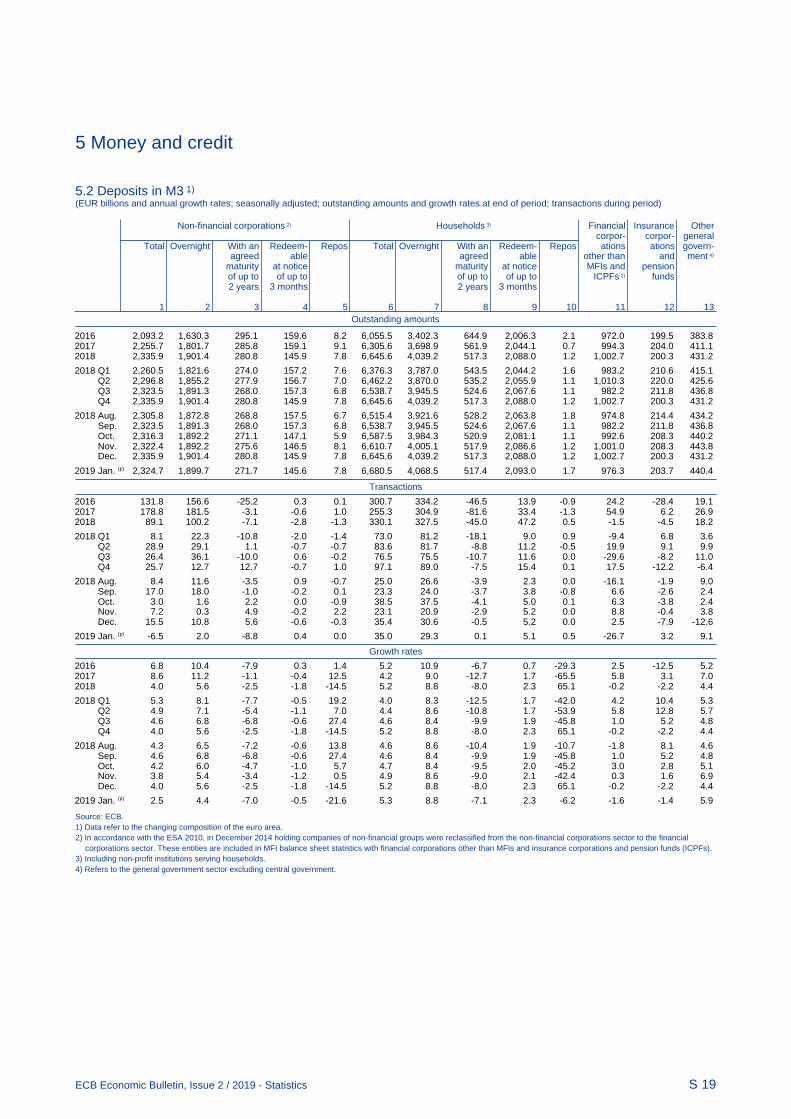
5 Money and credit
S 19ECB Economic Bulletin, Issue 2 / 2019 - Statistics
5.2 Deposits in M3 1) (EUR billions and annual growth rates; seasonally adjusted; outstanding amounts and growth rates at end of period; transactions during period)
Outstanding amounts
Non-financial corporations 2) Households 3) Financial Insurance Other
corpor- corpor- generalTotal Overnight With an Redeem- Repos Total Overnight With an Redeem- Repos ations ations govern-
agreed able agreed able other than and ment 4)
maturity at notice maturity at notice MFIs and pensionof up to of up to of up to of up to ICPFs 2) funds2 years 3 months 2 years 3 months
1 2 3 4 5 6 7 8 9 10 11 12 13
2016 2,093.2 1,630.3 295.1 159.6 8.2 6,055.5 3,402.3 644.9 2,006.3 2.1 972.0 199.5 383.82017 2,255.7 1,801.7 285.8 159.1 9.1 6,305.6 3,698.9 561.9 2,044.1 0.7 994.3 204.0 411.12018 2,335.9 1,901.4 280.8 145.9 7.8 6,645.6 4,039.2 517.3 2,088.0 1.2 1,002.7 200.3 431.2
2018 Q1 2,260.5 1,821.6 274.0 157.2 7.6 6,376.3 3,787.0 543.5 2,044.2 1.6 983.2 210.6 415.1 Q2 2,296.8 1,855.2 277.9 156.7 7.0 6,462.2 3,870.0 535.2 2,055.9 1.1 1,010.3 220.0 425.6 Q3 2,323.5 1,891.3 268.0 157.3 6.8 6,538.7 3,945.5 524.6 2,067.6 1.1 982.2 211.8 436.8 Q4 2,335.9 1,901.4 280.8 145.9 7.8 6,645.6 4,039.2 517.3 2,088.0 1.2 1,002.7 200.3 431.2
2018 Aug. 2,305.8 1,872.8 268.8 157.5 6.7 6,515.4 3,921.6 528.2 2,063.8 1.8 974.8 214.4 434.2 Sep. 2,323.5 1,891.3 268.0 157.3 6.8 6,538.7 3,945.5 524.6 2,067.6 1.1 982.2 211.8 436.8 Oct. 2,316.3 1,892.2 271.1 147.1 5.9 6,587.5 3,984.3 520.9 2,081.1 1.1 992.6 208.3 440.2 Nov. 2,322.4 1,892.2 275.6 146.5 8.1 6,610.7 4,005.1 517.9 2,086.6 1.2 1,001.0 208.3 443.8 Dec. 2,335.9 1,901.4 280.8 145.9 7.8 6,645.6 4,039.2 517.3 2,088.0 1.2 1,002.7 200.3 431.2
2019 Jan. (p) 2,324.7 1,899.7 271.7 145.6 7.8 6,680.5 4,068.5 517.4 2,093.0 1.7 976.3 203.7 440.4
Transactions
2016 131.8 156.6 -25.2 0.3 0.1 300.7 334.2 -46.5 13.9 -0.9 24.2 -28.4 19.12017 178.8 181.5 -3.1 -0.6 1.0 255.3 304.9 -81.6 33.4 -1.3 54.9 6.2 26.92018 89.1 100.2 -7.1 -2.8 -1.3 330.1 327.5 -45.0 47.2 0.5 -1.5 -4.5 18.2
2018 Q1 8.1 22.3 -10.8 -2.0 -1.4 73.0 81.2 -18.1 9.0 0.9 -9.4 6.8 3.6 Q2 28.9 29.1 1.1 -0.7 -0.7 83.6 81.7 -8.8 11.2 -0.5 19.9 9.1 9.9 Q3 26.4 36.1 -10.0 0.6 -0.2 76.5 75.5 -10.7 11.6 0.0 -29.6 -8.2 11.0 Q4 25.7 12.7 12.7 -0.7 1.0 97.1 89.0 -7.5 15.4 0.1 17.5 -12.2 -6.4
2018 Aug. 8.4 11.6 -3.5 0.9 -0.7 25.0 26.6 -3.9 2.3 0.0 -16.1 -1.9 9.0 Sep. 17.0 18.0 -1.0 -0.2 0.1 23.3 24.0 -3.7 3.8 -0.8 6.6 -2.6 2.4 Oct. 3.0 1.6 2.2 0.0 -0.9 38.5 37.5 -4.1 5.0 0.1 6.3 -3.8 2.4 Nov. 7.2 0.3 4.9 -0.2 2.2 23.1 20.9 -2.9 5.2 0.0 8.8 -0.4 3.8 Dec. 15.5 10.8 5.6 -0.6 -0.3 35.4 30.6 -0.5 5.2 0.0 2.5 -7.9 -12.6
2019 Jan. (p) -6.5 2.0 -8.8 0.4 0.0 35.0 29.3 0.1 5.1 0.5 -26.7 3.2 9.1
Growth rates
2016 6.8 10.4 -7.9 0.3 1.4 5.2 10.9 -6.7 0.7 -29.3 2.5 -12.5 5.22017 8.6 11.2 -1.1 -0.4 12.5 4.2 9.0 -12.7 1.7 -65.5 5.8 3.1 7.02018 4.0 5.6 -2.5 -1.8 -14.5 5.2 8.8 -8.0 2.3 65.1 -0.2 -2.2 4.4
2018 Q1 5.3 8.1 -7.7 -0.5 19.2 4.0 8.3 -12.5 1.7 -42.0 4.2 10.4 5.3 Q2 4.9 7.1 -5.4 -1.1 7.0 4.4 8.6 -10.8 1.7 -53.9 5.8 12.8 5.7 Q3 4.6 6.8 -6.8 -0.6 27.4 4.6 8.4 -9.9 1.9 -45.8 1.0 5.2 4.8 Q4 4.0 5.6 -2.5 -1.8 -14.5 5.2 8.8 -8.0 2.3 65.1 -0.2 -2.2 4.4
2018 Aug. 4.3 6.5 -7.2 -0.6 13.8 4.6 8.6 -10.4 1.9 -10.7 -1.8 8.1 4.6 Sep. 4.6 6.8 -6.8 -0.6 27.4 4.6 8.4 -9.9 1.9 -45.8 1.0 5.2 4.8 Oct. 4.2 6.0 -4.7 -1.0 5.7 4.7 8.4 -9.5 2.0 -45.2 3.0 2.8 5.1 Nov. 3.8 5.4 -3.4 -1.2 0.5 4.9 8.6 -9.0 2.1 -42.4 0.3 1.6 6.9 Dec. 4.0 5.6 -2.5 -1.8 -14.5 5.2 8.8 -8.0 2.3 65.1 -0.2 -2.2 4.4
2019 Jan. (p) 2.5 4.4 -7.0 -0.5 -21.6 5.3 8.8 -7.1 2.3 -6.2 -1.6 -1.4 5.9
Source: ECB.1) Data refer to the changing composition of the euro area.2) In accordance with the ESA 2010, in December 2014 holding companies of non-financial groups were reclassified from the non-financial corporations sector to the financial
corporations sector. These entities are included in MFI balance sheet statistics with financial corporations other than MFIs and insurance corporations and pension funds (ICPFs).3) Including non-profit institutions serving households.4) Refers to the general government sector excluding central government.

5 Money and credit
S 20ECB Economic Bulletin, Issue 2 / 2019 - Statistics
5.3 Credit to euro area residents 1) (EUR billions and annual growth rates; seasonally adjusted; outstanding amounts and growth rates at end of period; transactions during period)
Outstanding amounts
Credit to general government Credit to other euro area residents
Total Loans Debt Total Loans Debt Equity and
securities securities non-money Total To non- To house- To financial To insurance market fund
financial holds 4) corporations corporations investmentAdjusted corpor- other than and pension fund shares
loans 2) ations 3) MFIs and fundsICPFs 3)
1 2 3 4 5 6 7 8 9 10 11 12
2016 4,389.3 1,084.0 3,292.1 12,881.4 10,711.1 10,982.1 4,311.4 5,449.3 836.7 113.5 1,387.4 782.92017 4,625.9 1,033.3 3,578.7 13,116.4 10,874.1 11,171.2 4,326.5 5,598.8 839.2 109.6 1,442.4 799.82018 4,686.9 1,007.4 3,668.1 13,418.6 11,127.4 11,481.7 4,409.2 5,741.5 848.8 127.9 1,520.1 771.0
2018 Q1 4,605.0 1,023.1 3,568.0 13,195.9 10,941.2 11,233.7 4,343.8 5,633.0 851.7 112.8 1,467.4 787.4 Q2 4,602.9 1,017.7 3,571.0 13,276.2 10,990.8 11,328.3 4,358.1 5,659.7 853.2 119.8 1,496.6 788.7 Q3 4,627.4 1,003.5 3,609.9 13,363.0 11,064.5 11,398.1 4,396.8 5,701.3 841.9 124.4 1,513.8 784.8 Q4 4,686.9 1,007.4 3,668.1 13,418.6 11,127.4 11,481.7 4,409.2 5,741.5 848.8 127.9 1,520.1 771.0
2018 Aug. 4,612.1 1,004.0 3,593.9 13,352.8 11,054.9 11,383.1 4,394.3 5,693.2 847.2 120.2 1,515.3 782.6 Sep. 4,627.4 1,003.5 3,609.9 13,363.0 11,064.5 11,398.1 4,396.8 5,701.3 841.9 124.4 1,513.8 784.8 Oct. 4,612.0 1,000.6 3,597.4 13,394.2 11,090.4 11,423.6 4,404.2 5,716.2 849.3 120.8 1,524.7 779.1 Nov. 4,612.6 1,003.4 3,594.3 13,411.9 11,112.4 11,446.1 4,421.2 5,731.8 838.7 120.7 1,516.8 782.8 Dec. 4,686.9 1,007.4 3,668.1 13,418.6 11,127.4 11,481.7 4,409.2 5,741.5 848.8 127.9 1,520.1 771.0
2019 Jan. (p) 4,685.7 1,006.7 3,667.6 13,453.2 11,157.5 11,499.9 4,409.3 5,758.5 862.1 127.7 1,523.5 772.2
Transactions
2016 485.9 -34.5 520.3 319.7 235.8 259.9 82.5 121.1 43.2 -11.0 80.3 3.62017 289.7 -43.3 332.3 361.8 273.9 314.8 82.8 173.6 21.1 -3.5 64.3 23.62018 92.1 -28.5 120.7 373.0 304.8 373.4 122.4 167.3 -3.1 18.1 89.5 -21.2
2018 Q1 -31.0 -10.1 -20.8 115.7 98.1 94.4 41.3 40.1 13.6 3.2 27.5 -9.9 Q2 34.7 -6.0 40.3 85.6 55.5 103.7 17.1 34.9 -3.4 6.9 29.7 0.4 Q3 48.0 -16.2 64.5 105.2 90.9 87.1 48.6 49.8 -12.1 4.5 18.6 -4.2 Q4 40.5 3.8 36.7 66.5 60.3 88.2 15.4 42.6 -1.2 3.4 13.7 -7.5
2018 Aug. 14.4 -6.6 21.1 29.9 31.1 30.5 13.6 18.0 -0.2 -0.2 4.3 -5.5 Sep. 6.7 -3.7 10.7 23.8 22.5 28.6 9.3 14.9 -6.0 4.2 -0.9 2.3 Oct. -9.5 -3.3 -6.3 33.3 22.0 20.7 5.6 15.5 4.7 -3.7 12.6 -1.3 Nov. -7.9 2.8 -11.7 26.6 29.9 32.1 22.6 18.4 -11.0 0.0 -6.4 3.2 Dec. 57.9 4.2 54.7 6.6 8.4 35.5 -12.7 8.7 5.1 7.2 7.6 -9.3
2019 Jan. (p) -10.9 -0.8 -10.1 33.0 34.5 20.8 3.0 18.2 13.6 -0.2 0.3 -1.8
Growth rates
2016 12.4 -3.1 18.7 2.5 2.3 2.4 1.9 2.3 5.5 -8.9 6.1 0.52017 6.6 -4.0 10.2 2.8 2.6 2.9 1.9 3.2 2.5 -3.1 4.6 3.02018 2.0 -2.8 3.4 2.9 2.8 3.4 2.8 3.0 -0.4 16.5 6.2 -2.7
2018 Q1 3.9 -4.0 6.5 2.6 2.6 3.0 2.3 3.0 2.0 -0.3 3.9 -0.1 Q2 4.0 -3.9 6.5 2.8 2.9 3.5 2.6 3.0 3.0 6.9 4.8 -1.4 Q3 3.1 -4.4 5.3 3.0 3.0 3.4 3.2 3.1 -0.4 11.7 5.9 -1.1 Q4 2.0 -2.8 3.4 2.9 2.8 3.4 2.8 3.0 -0.4 16.5 6.2 -2.7
2018 Aug. 3.3 -4.5 5.6 3.0 3.0 3.4 3.1 3.2 0.8 4.7 6.1 -1.8 Sep. 3.1 -4.4 5.3 3.0 3.0 3.4 3.2 3.1 -0.4 11.7 5.9 -1.1 Oct. 2.7 -4.3 4.8 3.0 2.8 3.3 2.8 3.2 -0.5 7.4 7.2 -1.5 Nov. 2.1 -3.9 3.8 2.9 2.8 3.2 3.0 3.2 -1.8 5.2 6.6 -1.8 Dec. 2.0 -2.8 3.4 2.9 2.8 3.4 2.8 3.0 -0.4 16.5 6.2 -2.7
2019 Jan. (p) 2.4 -2.8 3.9 2.5 2.5 3.0 2.2 3.2 -1.6 13.0 5.3 -2.7
Source: ECB.1) Data refer to the changing composition of the euro area.2) Adjusted for loan sales and securitisation (resulting in derecognition from the MFI statistical balance sheet) as well as for positions arising from notional cash pooling services
provided by MFIs.3) In accordance with the ESA 2010, in December 2014 holding companies of non-financial groups were reclassified from the non-financial corporations sector to the financial
corporations sector. These entities are included in MFI balance sheet statistics with financial corporations other than MFIs and insurance corporations and pension funds (ICPFs).4) Including non-profit institutions serving households.

5 Money and credit
S 21ECB Economic Bulletin, Issue 2 / 2019 - Statistics
5.4 MFI loans to euro area non-financial corporations and households 1) (EUR billions and annual growth rates; seasonally adjusted; outstanding amounts and growth rates at end of period; transactions during period)
Outstanding amounts
Non-financial corporations 2) Households 3)
Total Up to 1 year Over 1 Over 5 years Total Loans for Loans for Other loans
and up to consumption houseAdjusted 5 years Adjusted purchase
loans 4) loans 4)
1 2 3 4 5 6 7 8 9 10
2016 4,311.4 4,309.1 1,013.3 795.7 2,502.4 5,449.3 5,728.7 615.9 4,084.1 749.32017 4,326.5 4,364.8 987.7 820.4 2,518.4 5,598.8 5,865.5 654.0 4,217.0 727.92018 4,409.2 4,491.1 995.7 844.6 2,568.9 5,741.5 6,023.4 683.7 4,353.9 703.9
2018 Q1 4,343.8 4,381.2 997.8 820.8 2,525.2 5,633.0 5,904.5 663.3 4,243.8 725.9 Q2 4,358.1 4,425.0 986.0 828.3 2,543.8 5,659.7 5,940.5 669.8 4,273.2 716.6 Q3 4,396.8 4,464.3 1,000.1 836.2 2,560.5 5,701.3 5,978.6 678.3 4,311.6 711.4 Q4 4,409.2 4,491.1 995.7 844.6 2,568.9 5,741.5 6,023.4 683.7 4,353.9 703.9
2018 Aug. 4,394.3 4,453.8 1,001.3 835.0 2,558.0 5,693.2 5,972.2 677.3 4,300.9 715.0 Sep. 4,396.8 4,464.3 1,000.1 836.2 2,560.5 5,701.3 5,978.6 678.3 4,311.6 711.4 Oct. 4,404.2 4,469.7 985.0 844.1 2,575.0 5,716.2 5,996.5 681.7 4,324.0 710.4 Nov. 4,421.2 4,486.5 989.2 850.9 2,581.0 5,731.8 6,010.7 685.6 4,336.4 709.8 Dec. 4,409.2 4,491.1 995.7 844.6 2,568.9 5,741.5 6,023.4 683.7 4,353.9 703.9
2019 Jan. (p) 4,409.3 4,489.3 980.1 846.7 2,582.5 5,758.5 6,037.0 687.5 4,367.5 703.5
Transactions
2016 82.5 100.4 -14.7 43.2 54.0 121.1 113.8 24.1 105.4 -8.42017 82.8 131.8 -0.3 38.0 45.0 173.6 165.5 45.1 134.3 -5.82018 122.4 170.3 19.0 33.1 70.3 167.3 188.8 40.1 136.5 -9.2
2018 Q1 41.3 39.0 17.6 6.1 17.6 40.1 45.5 11.3 27.7 1.1 Q2 17.1 48.2 -12.2 10.3 19.0 34.9 44.3 10.5 29.0 -4.6 Q3 48.6 47.8 16.4 9.5 22.6 49.8 47.7 10.3 40.4 -0.9 Q4 15.4 35.4 -2.9 7.2 11.1 42.6 51.3 8.1 39.4 -4.9
2018 Aug. 13.6 12.5 3.8 1.7 8.1 18.0 17.2 4.0 14.0 0.0 Sep. 9.3 17.1 -0.1 2.3 7.0 14.9 14.0 1.9 13.2 -0.2 Oct. 5.6 3.3 -16.9 8.0 14.5 15.5 19.1 3.7 12.1 -0.3 Nov. 22.6 22.7 5.7 8.3 8.6 18.4 18.2 4.2 14.1 0.0 Dec. -12.7 9.4 8.3 -9.1 -11.9 8.7 13.9 0.2 13.1 -4.6
2019 Jan. (p) 3.0 -0.8 -13.6 2.3 14.2 18.2 15.1 4.1 14.1 0.0
Growth rates
2016 1.9 2.4 -1.4 5.7 2.2 2.3 2.0 4.1 2.7 -1.12017 1.9 3.1 0.0 4.8 1.8 3.2 2.9 7.3 3.3 -0.82018 2.8 3.9 1.9 4.1 2.8 3.0 3.2 6.2 3.2 -1.3
2018 Q1 2.3 3.3 2.6 4.6 1.5 3.0 2.9 7.2 3.0 -0.4 Q2 2.6 4.1 1.4 5.5 2.2 3.0 3.0 7.2 3.1 -1.1 Q3 3.2 4.3 3.3 4.5 2.8 3.1 3.1 6.9 3.2 -0.8 Q4 2.8 3.9 1.9 4.1 2.8 3.0 3.2 6.2 3.2 -1.3
2018 Aug. 3.1 4.1 3.1 5.3 2.5 3.2 3.1 7.2 3.2 -0.8 Sep. 3.2 4.3 3.3 4.5 2.8 3.1 3.1 6.9 3.2 -0.8 Oct. 2.8 3.9 0.7 5.0 3.0 3.2 3.2 7.1 3.3 -0.7 Nov. 3.0 4.0 1.3 5.2 3.0 3.2 3.3 6.7 3.3 -0.8 Dec. 2.8 3.9 1.9 4.1 2.8 3.0 3.2 6.2 3.2 -1.3
2019 Jan. (p) 2.2 3.3 -0.4 3.5 2.8 3.2 3.2 6.1 3.5 -1.3
Source: ECB.1) Data refer to the changing composition of the euro area.2) In accordance with the ESA 2010, in December 2014 holding companies of non-financial groups were reclassified from the non-financial corporations sector to the financial
corporations sector. These entities are included in MFI balance sheet statistics with financial corporations other than MFIs and insurance corporations and pension funds (ICPFs).3) Including non-profit institutions serving households.4) Adjusted for loan sales and securitisation (resulting in derecognition from the MFI statistical balance sheet) as well as for positions arising from notional cash pooling services
provided by MFIs.

5 Money and credit
S 22ECB Economic Bulletin, Issue 2 / 2019 - Statistics
5.5 Counterparts to M3 other than credit to euro area residents 1) (EUR billions and annual growth rates; seasonally adjusted; outstanding amounts and growth rates at end of period; transactions during period)
Outstanding amounts
MFI liabilities MFI assets
Central Longer-term financial liabilities vis-à-vis other euro area residents Net external Other
government assets holdings 2) Total Deposits Deposits Debt Capital Total
with an redeemable securities and reservesagreed at notice with a Repos Reverse
maturity of over maturity with central repos toof over 3 months of over counter- central2 years 2 years parties 3) counter-
parties 3)
1 2 3 4 5 6 7 8 9 10
2016 307.7 6,955.9 2,089.5 70.9 2,145.9 2,649.6 1,124.8 257.0 205.9 121.62017 343.4 6,768.4 1,968.3 59.7 2,014.1 2,726.2 935.6 300.1 143.5 92.52018 378.7 6,816.6 1,941.4 56.0 2,096.0 2,723.3 1,026.7 436.2 187.0 194.9
2018 Q1 340.8 6,744.7 1,952.7 59.4 2,014.7 2,717.9 903.8 316.2 135.9 86.2 Q2 330.4 6,708.6 1,950.7 58.4 2,025.6 2,673.9 858.9 422.8 174.1 183.8 Q3 403.3 6,693.6 1,934.8 56.9 2,048.5 2,653.5 881.2 424.7 177.3 183.0 Q4 378.7 6,816.6 1,941.4 56.0 2,096.0 2,723.3 1,026.7 436.2 187.0 194.9
2018 Aug. 391.6 6,676.1 1,942.9 57.3 2,016.1 2,659.9 845.8 410.5 181.4 189.0 Sep. 403.3 6,693.6 1,934.8 56.9 2,048.5 2,653.5 881.2 424.7 177.3 183.0 Oct. 398.1 6,795.5 1,936.3 56.6 2,104.4 2,698.2 993.4 460.0 167.1 174.3 Nov. 390.3 6,782.9 1,929.9 55.8 2,098.7 2,698.5 1,036.3 418.5 196.1 204.4 Dec. 378.7 6,816.6 1,941.4 56.0 2,096.0 2,723.3 1,026.7 436.2 187.0 194.9
2019 Jan. (p) 377.2 6,859.1 1,939.8 55.6 2,112.5 2,751.2 1,066.7 405.1 199.2 208.4
Transactions
2016 22.0 -122.9 -71.3 -8.6 -118.7 75.7 -278.3 -90.2 12.8 -12.02017 39.2 -74.9 -83.7 -6.6 -72.0 87.4 -92.3 -65.6 -60.9 -27.62018 39.0 47.1 -38.6 -4.9 16.9 73.7 70.1 41.8 21.8 24.2
2018 Q1 -2.7 8.0 -17.1 -1.4 9.3 17.2 53.2 -55.0 -7.6 -6.3 Q2 -10.4 -10.0 -4.8 -1.1 -15.0 11.0 -62.2 88.6 16.4 19.4 Q3 76.3 29.8 -16.2 -1.5 19.2 28.4 38.8 -11.2 3.2 -0.8 Q4 -24.1 19.3 -0.4 -0.9 3.4 17.2 40.2 19.4 9.7 11.9
2018 Aug. 36.8 -6.6 -9.1 -0.4 -5.8 8.6 -6.7 18.9 -2.6 -3.5 Sep. 15.3 28.0 -8.4 -0.5 28.1 8.8 46.2 11.1 -4.1 -6.0 Oct. -5.5 14.2 0.0 -0.2 4.5 10.0 19.6 25.1 -10.2 -8.7 Nov. -7.9 -6.6 -6.1 -0.9 -2.3 2.7 45.1 -37.0 29.0 30.0 Dec. -10.8 11.6 5.7 0.2 1.3 4.5 -24.5 31.2 -9.1 -9.5
2019 Jan. (p) -1.5 15.4 -5.8 -0.4 16.5 5.1 24.6 -27.9 12.2 13.6
Growth rates
2016 7.8 -1.7 -3.4 -10.9 -5.3 2.9 - - 6.3 -9.02017 12.6 -1.1 -4.0 -9.7 -3.4 3.3 - - -29.7 -22.72018 11.3 0.7 -2.0 -8.1 0.8 2.8 - - 11.0 2.2
2018 Q1 11.9 -0.6 -4.1 -9.8 -1.5 3.2 - - -25.6 -22.2 Q2 6.6 -0.9 -3.2 -10.8 -2.5 2.4 - - -3.6 -18.0 Q3 14.4 0.0 -2.8 -9.3 0.0 2.3 - - 7.7 4.9 Q4 11.3 0.7 -2.0 -8.1 0.8 2.8 - - 11.0 2.2
2018 Aug. 16.3 -0.7 -2.7 -9.9 -2.6 2.5 - - 24.6 34.2 Sep. 14.4 0.0 -2.8 -9.3 0.0 2.3 - - 7.7 4.9 Oct. 18.1 0.6 -1.8 -8.7 0.6 2.5 - - -9.9 -22.0 Nov. 24.7 0.5 -2.2 -9.1 0.8 2.5 - - -0.1 -24.6 Dec. 11.3 0.7 -2.0 -8.1 0.8 2.8 - - 11.0 2.2
2019 Jan. (p) 18.9 0.8 -1.9 -7.7 0.8 2.9 - - 28.2 22.7
Source: ECB.1) Data refer to the changing composition of the euro area.2) Comprises central government holdings of deposits with the MFI sector and of securities issued by the MFI sector.3) Not adjusted for seasonal effects.

6 Fiscal developments
S 23ECB Economic Bulletin, Issue 2 / 2019 - Statistics
6.1 Deficit/surplus(as a percentage of GDP; flows during one-year period)
Deficit (-)/surplus (+) Memo item:
PrimaryTotal Central State Local Social deficit (-)/
government government government security surplus (+)funds
1 2 3 4 5 6
2014 -2.5 -2.1 -0.2 0.0 -0.1 0.12015 -2.0 -1.9 -0.2 0.1 -0.1 0.32016 -1.6 -1.7 -0.1 0.2 0.0 0.62017 -1.0 -1.3 0.0 0.2 0.1 1.0
2017 Q4 -1.0 . . . . 1.0
2018 Q1 -0.8 . . . . 1.2 Q2 -0.5 . . . . 1.4 Q3 -0.4 . . . . 1.5
Sources: ECB for annual data; Eurostat for quarterly data.
6.2 Revenue and expenditure(as a percentage of GDP; flows during one-year period)
Revenue Expenditure
Total Current revenue Capital Total Current expenditure Capital
revenue expenditureDirect Indirect Net social Compen- Intermediate Interest Socialtaxes taxes contributions sation of consumption benefits
employees
1 2 3 4 5 6 7 8 9 10 11 12 13
2014 46.7 46.2 12.5 13.1 15.4 0.5 49.1 45.2 10.2 5.3 2.6 23.0 3.92015 46.2 45.7 12.5 13.0 15.2 0.5 48.3 44.4 10.0 5.2 2.3 22.7 3.92016 46.0 45.5 12.6 12.9 15.2 0.5 47.5 44.0 9.9 5.2 2.1 22.7 3.62017 46.1 45.7 12.8 12.9 15.2 0.4 47.0 43.3 9.8 5.1 2.0 22.5 3.8
2017 Q4 46.1 45.7 12.8 12.9 15.2 0.4 47.0 43.3 9.8 5.1 2.0 22.5 3.8
2018 Q1 46.1 45.7 12.9 12.9 15.2 0.4 46.9 43.1 9.8 5.1 1.9 22.4 3.7 Q2 46.1 45.7 12.9 12.9 15.2 0.4 46.6 43.0 9.8 5.1 1.9 22.3 3.7 Q3 46.2 45.8 12.9 12.9 15.2 0.4 46.6 43.0 9.8 5.1 1.9 22.3 3.6
Sources: ECB for annual data; Eurostat for quarterly data.
6.3 Government debt-to-GDP ratio(as a percentage of GDP; outstanding amounts at end of period)
Total Financial instrument Holder Original maturity Residual maturity Currency
Currency Loans Debt Resident creditors Non-resident Up to Over Up to Over 1 Over Euro or Other
and securities creditors 1 year 1 year 1 year and up to 5 years participating curren-deposits MFIs 5 years currencies cies
1 2 3 4 5 6 7 8 9 10 11 12 13 14
2014 91.8 2.7 17.1 71.9 43.9 25.8 47.9 9.8 82.0 18.8 31.8 41.1 89.7 2.12015 89.9 2.8 16.2 70.9 44.1 27.3 45.7 9.1 80.8 17.5 31.2 41.2 87.8 2.12016 89.1 2.7 15.4 71.0 46.6 30.5 42.5 8.8 80.3 17.1 29.9 42.1 87.0 2.12017 86.8 2.6 14.2 70.0 47.3 31.9 39.5 8.0 78.8 15.9 28.8 42.2 85.0 1.8
2017 Q4 86.8 2.6 14.2 70.0 . . . . . . . . . .
2018 Q1 86.9 2.6 14.0 70.3 . . . . . . . . . . Q2 86.3 2.6 13.7 70.0 . . . . . . . . . . Q3 86.1 2.6 13.5 70.0 . . . . . . . . . .
Sources: ECB for annual data; Eurostat for quarterly data.

6 Fiscal developments
S 24ECB Economic Bulletin, Issue 2 / 2019 - Statistics
6.4 Annual change in the government debt-to-GDP ratio and underlying factors 1) (as a percentage of GDP; flows during one-year period)
Change in Primary Deficit-debt adjustment Interest- Memo item:
debt-to- deficit (+)/ growth BorrowingGDP ratio 2) surplus (-) Total Transactions in main financial assets Revaluation Other differential requirement
effectsTotal Currency Loans Debt Equity and and other
and securities investment changes indeposits fund shares volume
1 2 3 4 5 6 7 8 9 10 11 12
2014 0.2 -0.1 -0.2 -0.4 0.2 -0.4 -0.3 0.0 0.1 0.2 0.5 2.32015 -1.9 -0.3 -0.8 -0.5 0.2 -0.3 -0.3 -0.1 0.0 -0.4 -0.8 1.22016 -0.8 -0.6 0.1 0.2 0.3 -0.1 0.0 0.1 0.0 -0.1 -0.3 1.62017 -2.2 -1.0 -0.2 0.3 0.5 0.0 -0.2 0.1 -0.1 -0.3 -1.0 0.9
2017 Q4 -2.2 -1.0 -0.2 0.4 0.5 0.0 -0.2 0.1 -0.1 -0.4 -1.0 0.9
2018 Q1 -2.4 -1.2 -0.1 0.5 0.5 0.0 -0.1 0.1 -0.1 -0.4 -1.1 0.8 Q2 -2.9 -1.4 -0.2 0.3 0.2 -0.1 -0.1 0.2 -0.1 -0.3 -1.3 0.5 Q3 -2.1 -1.5 0.5 0.8 0.6 0.0 0.0 0.2 -0.1 -0.2 -1.1 1.0
Sources: ECB for annual data; Eurostat for quarterly data.1) Intergovernmental lending in the context of the financial crisis is consolidated except in quarterly data on the deficit-debt adjustment.2) Calculated as the difference between the government debt-to-GDP ratios at the end of the reference period and a year earlier.
6.5 Government debt securities 1) (debt service as a percentage of GDP; flows during debt service period; average nominal yields in percentages per annum)
Debt service due within 1 year 2) Average Average nominal yields 4)
residual Total Principal Interest maturity Outstanding amounts Transactions
in years 3) Maturities Maturities Total Floating Zero Fixed rate Issuance Redemptionof up to 3 of up to 3 rate coupon
months months Maturitiesof up to 1
year
1 2 3 4 5 6 7 8 9 10 11 12 13
2016 14.1 12.4 4.6 1.7 0.4 6.9 2.6 1.2 -0.1 3.0 2.9 0.2 1.22017 12.9 11.2 4.2 1.7 0.4 7.1 2.4 1.1 -0.2 2.8 2.3 0.3 1.12018 13.0 11.4 3.9 1.5 0.4 7.3 2.3 1.1 -0.1 2.7 2.5 0.4 0.9
2017 Q4 12.9 11.2 4.2 1.7 0.4 7.1 2.4 1.1 -0.2 2.8 2.3 0.3 1.1
2018 Q1 12.9 11.3 4.2 1.6 0.4 7.2 2.4 1.1 -0.2 2.8 2.5 0.4 1.1 Q2 12.8 11.2 3.6 1.6 0.4 7.3 2.4 1.1 -0.2 2.8 2.5 0.4 0.9 Q3 13.1 11.5 3.8 1.6 0.4 7.3 2.3 1.1 -0.1 2.7 2.6 0.4 0.9
2018 Aug. 12.8 11.2 3.8 1.6 0.4 7.2 2.3 1.1 -0.2 2.7 2.5 0.4 1.0 Sep. 13.1 11.5 3.8 1.6 0.4 7.3 2.3 1.1 -0.1 2.7 2.6 0.4 0.9 Oct. 13.3 11.8 3.6 1.6 0.4 7.3 2.3 1.1 -0.1 2.7 2.5 0.4 1.0 Nov. 13.4 11.9 3.7 1.6 0.4 7.3 2.3 1.1 -0.1 2.7 2.5 0.5 1.0 Dec. 13.0 11.4 3.9 1.5 0.4 7.3 2.3 1.1 -0.1 2.7 2.5 0.4 0.9
2019 Jan. 13.3 11.7 4.1 1.5 0.4 7.3 2.3 1.1 -0.1 2.7 2.5 0.4 0.9
Source: ECB.1) At face value and not consolidated within the general government sector.2) Excludes future payments on debt securities not yet outstanding and early redemptions.3) Residual maturity at the end of the period.4) Outstanding amounts at the end of the period; transactions as 12-month average.

6 Fiscal developments
S 25ECB Economic Bulletin, Issue 2 / 2019 - Statistics
6.6 Fiscal developments in euro area countries(as a percentage of GDP; flows during one-year period and outstanding amounts at end of period)
Government deficit (-)/surplus (+)
Belgium Germany Estonia Ireland Greece Spain France Italy Cyprus
1 2 3 4 5 6 7 8 9
2014 -3.1 0.6 0.7 -3.6 -3.6 -6.0 -3.9 -3.0 -9.02015 -2.5 0.8 0.1 -1.9 -5.6 -5.3 -3.6 -2.6 -1.32016 -2.4 0.9 -0.3 -0.5 0.5 -4.5 -3.5 -2.5 0.32017 -0.9 1.0 -0.4 -0.2 0.8 -3.1 -2.7 -2.4 1.8
2017 Q4 -0.9 1.0 -0.4 -0.2 0.8 -3.1 -2.7 -2.4 1.8
2018 Q1 -0.9 1.3 -0.6 -0.3 1.1 -2.9 -2.7 -2.2 2.5 Q2 -0.3 1.9 -0.2 -0.3 0.9 -2.7 -2.8 -1.9 3.0 Q3 -0.1 1.9 0.0 -0.1 0.8 -2.7 -2.7 -1.8 -4.0
Government debt
2014 107.6 74.5 10.5 104.1 178.9 100.4 94.9 131.8 108.02015 106.5 70.8 9.9 76.8 175.9 99.3 95.6 131.6 108.02016 106.1 67.9 9.2 73.4 178.5 99.0 98.2 131.4 105.52017 103.4 63.9 8.7 68.4 176.1 98.1 98.5 131.2 96.1
2017 Q4 103.4 63.9 8.7 68.4 176.1 98.1 98.5 131.2 96.1
2018 Q1 106.4 62.7 8.5 69.3 177.9 98.7 99.4 132.8 93.4 Q2 105.9 61.5 8.3 69.2 177.4 98.1 99.1 133.1 104.0 Q3 105.4 61.0 8.0 68.8 182.2 98.3 99.5 133.0 110.9
Government deficit (-)/surplus (+)
Latvia Lithuania Luxembourg Malta Netherlands Austria Portugal Slovenia Slovakia Finland
10 11 12 13 14 15 16 17 18 19
2014 -1.5 -0.6 1.3 -1.7 -2.2 -2.7 -7.2 -5.5 -2.7 -3.22015 -1.4 -0.3 1.3 -1.0 -2.0 -1.0 -4.4 -2.8 -2.6 -2.82016 0.1 0.3 1.6 0.9 0.0 -1.6 -2.0 -1.9 -2.2 -1.72017 -0.6 0.5 1.4 3.5 1.2 -0.8 -3.0 0.1 -0.8 -0.7
2017 Q4 -0.6 0.5 1.4 3.5 1.2 -0.8 -3.0 0.1 -0.8 -0.7
2018 Q1 0.0 0.4 1.4 3.1 1.6 -0.6 -0.7 0.5 -0.7 -0.7 Q2 0.3 0.7 1.5 3.9 1.9 0.2 -1.0 0.6 -0.7 -0.9 Q3 0.0 0.6 1.9 3.6 2.1 0.1 0.0 0.7 -0.7 -0.8
Government debt
2014 40.9 40.5 22.7 63.7 67.9 84.0 130.6 80.4 53.5 60.22015 36.8 42.6 22.2 58.6 64.6 84.8 128.8 82.6 52.2 63.62016 40.3 39.9 20.7 56.3 61.9 83.0 129.2 78.7 51.8 63.02017 40.0 39.4 23.0 50.9 57.0 78.3 124.8 74.1 50.9 61.3
2017 Q4 40.0 39.4 23.0 50.2 57.0 78.3 124.8 74.1 50.9 61.3
2018 Q1 35.5 36.0 22.2 49.8 55.1 77.2 125.4 75.5 50.9 59.9 Q2 36.9 35.0 22.0 49.0 54.0 76.5 125.0 72.7 51.9 59.6 Q3 37.1 35.0 21.7 45.9 52.9 75.6 125.0 71.0 51.5 58.8
Source: Eurostat.

© European Central Bank, 2019
Postal address 60640 Frankfurt am Main, Germany Telephone +49 69 1344 0 Website www.ecb.europa.eu
All rights reserved. Reproduction for educational and non-commercial purposes is permitted provided that the source is acknowledged.
This Bulletin was produced under the responsibility of the Executive Board of the ECB. Translations are prepared and published by the national central banks.
The cut-off date for the statistics included in this issue was 6 March 2019.
For specific terminology please refer to the ECB glossary (available in English only).
PDF ISSN 2363-3417, QB-BP-19-002-EN-N HTML ISSN 2363-3417, doi:10.2866/662337, QB-BP-19-002-EN-Q