Embed Size (px)
Citation preview

Louisiana State UniversityLSU Digital Commons
LSU Master's Theses Graduate School
2012
Economic assessment of rapid land-buildingtechnologies for coastal restorationHua WangLouisiana State University and Agricultural and Mechanical College, [email protected]
Follow this and additional works at: https://digitalcommons.lsu.edu/gradschool_theses
Part of the Agricultural Economics Commons
This Thesis is brought to you for free and open access by the Graduate School at LSU Digital Commons. It has been accepted for inclusion in LSUMaster's Theses by an authorized graduate school editor of LSU Digital Commons. For more information, please contact [email protected].
Recommended CitationWang, Hua, "Economic assessment of rapid land-building technologies for coastal restoration" (2012). LSU Master's Theses. 3669.https://digitalcommons.lsu.edu/gradschool_theses/3669

ECONOMIC ASSESSMENT OF RAPID LAND-BUILDING
TECHNOLOGIES FOR COASTAL RESTORATION
A Thesis
Submitted to the Graduate Faculty of the Louisiana State University and
Agricultural and Mechanical College in partial fulfillment of the
requirements for the degree of Master of Science
in
The Department of Agricultural Economics and Agribusiness
by Hua Wang
B.S., Xiangtan University, China, 2002 May 2012
ACKNOWLEDGMENTS
I would like to thank my major professor, Dr. Rex H. Caffey, for the guidance, patience,
understanding, and encouragement throughout the completion of the work. Without whose help
and support, this thesis would not have been possible.
I would also like to thank my committee of Dr. Margaret Reams, Dr. Richard
Kazmierczak and Dr. John Westra for their time and guidance. Special thanks to my ad hoc
committee member of Dr. Daniel Petrolia for his patience and selfless support that was
instrumental to my success. I would also like to thank my ad hoc committee member of Dr.
Matthew Freeman for his support. Special thanks to Mr. Brad Miller and Mr. Ran Boustany for
their generous help, counsel and understanding during the project. I would also like to thank Ms.
Huizhen Niu for GIS technical support. Thanks to Dr. Gail Cramer for his encouragement and
support. I would also like to thank all my colleagues and friends here who made my stay at LSU
an enjoyable and a memorable one.
My most sincere gratitude goes to my wife Miao for her constant encouragement, love
and support and my beloved sons Gavin and Gabriel, who have been my greatest strength and
support.
ii

TABLE OF CONTENTS
ACKNOWLEDGMENTS .............................................................................................................. ii
LIST OF TABLES ......................................................................................................................... vi
LIST OF FIGURES ....................................................................................................................... ix
ABSTRACT ................................................................................................................................... xi
CHAPTER 1. INTRODUCTION ................................................................................................... 1 1.1 General Background ............................................................................................................. 1 1.2 Methods for Restoration ....................................................................................................... 2 1.3 Efficiency in Restoration ...................................................................................................... 3 1.4 Shifting the Focus ................................................................................................................. 7 1.5 Problem Statement ................................................................................................................ 8 1.6 Objectives ............................................................................................................................. 9 1.7 Data and Methods ................................................................................................................. 9 1.8 Rationale ............................................................................................................................. 12
CHAPTER 2. DESCRIPTIVE DATA .......................................................................................... 14 2.1 Introduction ......................................................................................................................... 14
2.1.1 CWPPRA Project Data ................................................................................................ 15 2.2 Data for Analysis ................................................................................................................ 20
2.2.1 Project Data: Marsh Creation ....................................................................................... 20 2.2.2 Project Data: Barrier Island ......................................................................................... 21 2.2.3 Project Data: Freshwater Diversion ............................................................................. 28
2.3 Summary ............................................................................................................................. 30
CHAPTER 3. GENERIC BENEFIT MODELS ........................................................................... 33 3.1 Introduction ......................................................................................................................... 33 3.2 Generic Benefit Model: Marsh Creation ............................................................................. 33 3.3 Generic Benefit Model: Barrier Island ............................................................................... 35 3.4 Generic Benefit Model: Freshwater Diversion ................................................................... 41 3.5 Other Freshwater Diversion Benefit Models ...................................................................... 47
3.5.1 Crevasse Model ............................................................................................................ 47 3.5.2 N-SED Model .............................................................................................................. 52 3.5.3 Extant Flood Control Structures .................................................................................. 54
3.6 Summary ............................................................................................................................. 55
CHAPTER 4. GENERIC COST MODELS ................................................................................. 57 4.1 Introduction ......................................................................................................................... 57 4.2 Potential Variables .............................................................................................................. 58
4.2.1 Dependent Variables (Cost Models) ............................................................................ 59 4.2.2 Dependent Variables (Materials Models) .................................................................... 59 4.2.3 Independent Variables (Cost Models) ......................................................................... 59
iii

4.2.4 Independent Variables (Materials Models) .................................................................. 61 4.3 Generic Cost Models: Marsh Creation ............................................................................... 62
4.3.1 Historic Drivers of MC Cost ........................................................................................ 62 4.3.2 Present Drivers of MC Cost ......................................................................................... 65
4.4 Generic Cost Models: Barrier Islands ................................................................................. 68 4.4.1 Historic Cost Models for BI Project ............................................................................ 68 4.4.2 Present Cost Models for BI Project ............................................................................. 70
4.5 Generic Cost Models: Freshwater Diversions .................................................................... 73 4.5.1 Historic and Present Drivers of FWD Cost.................................................................. 73
4.6 Summary ............................................................................................................................. 76
CHAPTER 5. BENEFIT-COST ANALYSIS............................................................................... 79 5.1 Introduction ......................................................................................................................... 79 5.2 The Mechanism of NPV ..................................................................................................... 79 5.3 Region-Specific Landscape Changes .................................................................................. 81 5.4 Time Lag ............................................................................................................................. 83 5.5 Discount Rate ...................................................................................................................... 84 5.6 Integrated NPV Models ...................................................................................................... 86
5.6.1 NPV Model: Marsh Creation ....................................................................................... 86 5.6.2 NPV Model: Barrier Islands ........................................................................................ 90 5.6.3 NPV Model: Freshwater Diversions ............................................................................ 93
5.7 Summary ............................................................................................................................. 96
CHAPTER 6. BREAK-EVEN SIMULATIONS .......................................................................... 97 6.1 Introduction ......................................................................................................................... 97 6.2 Valuing Coastal Wetlands ................................................................................................... 97
6.2.1 Non-Market Based Methods ........................................................................................ 98 6.2.2 Non-Monetary Based Methods .................................................................................... 99
6.3 Coastal Wetland Values ...................................................................................................... 99 6.4 Simulations ....................................................................................................................... 100
6.4.1 Break-Even Simulations ............................................................................................ 100 6.4.2 The Profile of NPV Models ....................................................................................... 103 6.4.3 Baseline Simulations .................................................................................................. 105 6.4.4 Simulations under Different Assumptions ................................................................. 107
6.5 Summary ........................................................................................................................... 128
CHAPTER 7 INCORPORATING UNCERTAINTY ................................................................ 130 7.1 Introduction ....................................................................................................................... 130 7.2 Risk and Uncertainty......................................................................................................... 130 7.3 Hurricane Risk .................................................................................................................. 131
7.3.1 NPV Models with Hurricane Risk ............................................................................. 132 7.3.1.1 Hurricane Risk 1 Scenario .................................................................................. 134 7.3.1.2 Hurricane Risk 2 Scenario .................................................................................. 135
7.3.2 Depicting Hurricane Risk Impacts on Wetland Restoration Projects ........................ 136 7.4 Refining Risk Assumptions .............................................................................................. 137
7.4.1 Scaling Hurricane Impacts ......................................................................................... 139
iv

7.4.2 Adjusting for Political Risk ....................................................................................... 141 7.5 Summary ........................................................................................................................... 148
CHAPTER 8 CASE STUDIES ................................................................................................... 151 8.1 Introduction ....................................................................................................................... 151 8.2 Assumptions of Case Studies ............................................................................................ 151 8.3 Depicting Acreage Effects ................................................................................................ 157 8.4 Comparison of Case Studies ............................................................................................. 158 8.5 Summary ........................................................................................................................... 163
CHAPTER 9. SUMMARY and CONCLUSIONS ..................................................................... 165 9.1 Summary and Conclusions ............................................................................................... 165 9.2 Limitations and Refinements ............................................................................................ 170 9.3 Policy Recommendations ................................................................................................. 173
REFERENCES ........................................................................................................................... 175
APPENDIX A: CORRELATION ANALYSIS FOR MC PROJECT BASED ON HISTORIC DATA ................................................................................................................ 182
APPENDIX B: CORRELATION ANALYSIS AND NORMALITY TEST FOR MC PROJECT
ON PHYSICAL MATERIAL MODEL ............................................................ 183 APPENDIX C: CORRELATION ANALYSIS FOR BI PROJECT BASED ON HISTORIC
DATA ................................................................................................................ 188 APPENDIX D: CORRELATION ANALYSIS AND NORMALITY TEST FOR BI PROJECT
ON PHYSICAL MATERIAL MODEL ............................................................ 189 APPENDIX E: CORRELATION ANALYSIS AND NORMALITY TEST FOR FWD
PROJECT ON TOTAL COST MODEL ........................................................... 194 APPENDIX F: NPV MODEL ASSUMPTIONS FOR MC, BI, AND FWD PROJECTS ......... 199 VITA ........................................................................................................................................... 201
v

LIST OF TABLES
Table 2.1 Louisiana Coastal Restoration Programs and Projects 1991-2009 ............................. 15
Table 2.2 Average Cost for CWPPRA Authorized Projects (n=124) ......................................... 16
Table 2.3 Authorized MC Projects and Attributes, CWPPRA 1991-2009 (n=23) ..................... 22
Table 2.4 Projected MC Projects and Attributes, 1998-2004 (n=46) ......................................... 23
Table 2.5 Barrier Island Projects and Attributes, CWPPRA 1991-2009 (n=13) ........................ 25
Table 2.6 Projected BI Projects and Attributes, 1991-2001 (n=39) ........................................... 26
Table 2.7 Freshwater Diversion Projects and Attributes, CWPPRA 1991-2009 (n=15)............ 29
Table 2.8 WRDA Freshwater Diversion Projects (n=9) ............................................................. 31
Table 3.1 N-SED1 Land Building Model ................................................................................... 53
Table 4.1 Variable Descriptions and Expected Signs ................................................................. 62
Table 4.2 Parameter Estimate 1: March Creation Costs - $/NAM .............................................. 63
Table 4.3 Parameter Estimate 2: Marsh Creation Costs - $/NAM ............................................... 64
Table 4.4 Parameter Estimate 3: Marsh Creation Construction Costs - CCM............................. 66
Table 4.5 Parameter Estimate 4: Marsh Materials Model - CYDM ............................................ 67
Table 4.6 Pearson Correlation Coefficients 1: MC - CYDM ...................................................... 68
Table 4.7 Parameter Estimate 5: Barrier Island Costs - $/NAB .................................................. 70
Table 4.8 Parameter Estimate 6: Barrier Island Construction Costs - CCB ................................ 71
Table 4.9 Parameter Estimate 7: Barrier Island Materials Model - CYDB ................................. 72
Table 4.10 Pearson Correlation Coefficients 2: BI - CYDB ......................................................... 73
Table 4.11 Parameter Estimate 8: Fresh Water Diversion Costs - $/NAF .................................... 74
Table 4.12 Parameter Estimate 9: Freshwater Diversion Fully Funded Costs - TCF ................... 75
Table 5.1 Existing and Projected Habitat Types in Each Coast 2050 Region ............................ 82
vi

Table 5.2 Average Project Design and Construction Period under CWPPRA Program (n=105) ........................................................................................................................ 84
Table 6.1 Non-Market Values for Coastal Wetlands ................................................................ 101
Table 6.2 NPV Model ............................................................................................................... 104
Table 6.3 User-Specified Value in Baseline simulation NPV Model ....................................... 108
Table 6.4 Effects of Time on BEV for RLB and FWD Projects .............................................. 110
Table 6.5 Effects of Scale (Acreage) on BEV for RLB and FWD Projects ............................. 112
Table 6.6 Effects of Discount Rate on BEV for RLB and FWD Projects ................................ 114
Table 6.7 Effects of Mobilization/Demobilization Costs on BEV for RLB and FWD Projects ...................................................................................................................... 116
Table 6.8 Effects of Distance on BEV for RLB and FWD Projects ......................................... 118
Table 6.9 Effects of Access Dredging on BEV for RLB and FWD Projects ........................... 120
Table 6.10 Effects of Land Loss Rate on BEV for RLB and FWD Projects .............................. 122
Table 6.11 Effects of Long-Shore Sedimentation on BEV for RLB and FWD Projects ............ 124
Table 6.12 Effects of Lag Time on BEV for RLB and FWD Projects ....................................... 126
Table 6.13 Effects of Time on BEV for FWD Projects .............................................................. 127
Table 7.1 Probabilities of Hurricane Landfall in Five Coastal States ....................................... 133
Table 7.2 Probabilities of Hurricane Landfall at Coastal Parishes in Louisiana ...................... 133
Table 7.3 Percent Acreage Loss fixed with a Major Hurricane (Risk1) ................................... 134
Table 7.4 Percent Acreage Loss Varies with a Major Hurricane (Risk2) ................................ 135
Table 7.5 Caernarvon Freshwater Diversion Project Land Change Pre and Post Hurricane Katrina....................................................................................................................... 141
Table 7.6 Holly Beach Sand Management Project Land Change Pre and Post Hurricane Rita 141
Table 7.7 Caernarvon Freshwater Diversion Annual Flow Rate (2001-2010) ......................... 146
Table 7.8 Davis Pond Freshwater Diversion Annual Flow Rate (2003-2010) ......................... 147
vii

Table 8.1 Upper and Lower Estuary Case Study Scenarios - Qualitative Descriptions ........... 154
Table 8.2 Case Study Parameters - Upper Estuary Scenarios .................................................. 155
Table 8.3 Case Study Parameters - Lower Estuary Scenarios .................................................. 156
Table 8.4 Cost and Benefit Output for Upper Estuary Scenarios ............................................. 162
Table 8.5 Cost and Benefit Output for Lower Estuary Scenarios ............................................. 162
viii

LIST OF FIGURES
Figure 2.1 Average costs of net acre for CWPPRA projects by type, 1991-2009 (n=124) ........ 18
Figure 2.2 Geographic locations of four selected restoration methods in Louisiana (CWPPRA project data 1991-2009) ............................................................................................. 19
Figure 2.3 Selection of land-building restoration projects by period (CWPPRA project data,
n=51) ......................................................................................................................... 20 Figure 3.1 Six net acre trajectories by marsh creation technology under CWPPRA (n=6) ........ 36
Figure 3.2 Marsh creation projects trajectories without and with engineering design consideration for the trend of net acres under CWPPRA (n=6) ................................ 37
Figure 3.3 Marsh creation projects percent completion curves without and with engineering
design consideration .................................................................................................. 38 Figure 3.4 Estimated sediment requirements for marsh creation technology under CWPPRA
(n=8) .......................................................................................................................... 39 Figure 3.5 Six net acre trajectories by barrier island technology under CWPPRA (n=6) .......... 42
Figure 3.6 Barrier island projects trajectories without and with engineering design consideration for the trend of net acres under CWPPRA (n=6) ...................................................... 43
Figure 3.7 Barrier island projects percent completion curves without and with engineering
design consideration .................................................................................................. 44 Figure 3.8 Estimated sediments rate by barrier island projects technology under CWPPRA
(n=8) .......................................................................................................................... 45 Figure 3.9 Six net acre trajectories by freshwater diversion technology under CWPPRA (n=6) 48
Figure 310 Freshwater diversion projects trajectories and regression line for the trend of net acres under CWPPRA (n=6) ............................................................................................... 49
Figure 3.11 Fresh water diversion projects percentage of net acre accrued curve without and with
engineering design consideration .............................................................................. 50 Figure 3.12 Water flow rate by freshwater diversion technology under CWPPRA (n=7) ........... 51
Figure 6.1 Total fully funded costs for RLB and FWD projects .............................................. 109
Figure 6.2 Required break-even ESV for RLB and FWD projects .......................................... 109
ix
Figure 6.3 Effects of time on BEV for RLB and FWD projects ............................................... 111
Figure 6.5 Effects of discount rate on BEV for RLB and FWD projects ................................. 114
Figure 6.6 Effects of mobilization/demobilization costs on BEV for RLB and FWD projects 116
Figure 6.7 Effects of distance on BEV for RLB and FWD projects ......................................... 118
Figure 6.8 Effects of access dredging on BEV for RLB and FWD projects ............................ 120
Figure 6.9 Effects of land loss rate on BEV for RLB and FWD projects ................................. 122
Figure 6.10 Effects of Lang-shore sediment transport rate on BEV for RLB and FWD projects .................................................................................................................... 124
Figure 6.11 Effects of lag time on BEV for RLB and FWD projects ......................................... 126
Figure 6.12 Effects of lag time on BEV for FWD projects ........................................................ 127
Figure 7.1 Effects of erosion and risk on net acres for RLB and FWD projects ...................... 138
Figure 7.2 Classified Image of Caernarvon Freshwater Diversion Project Pre-Post Hurricane Katrina ..................................................................................................................... 142
Figure 7.3 Landsat Image of Holly Beach Sand Management Project Pre-Post Hurricane
Rita .......................................................................................................................... 143 Figure 7.4 Yearly Mean Discharge at Caernarvon Freshwater Diversion ................................ 146
Figure 7.5 Yearly Mean Discharge at Davis Pond Freshwater Diversion ................................ 147
Figure 7.6 Effects of erosion and risk on net acres for FWD project ....................................... 149
Figure 8.1 Case studies project at upper and lower estuary locations ...................................... 152
Figure 8.2 Effects of scale, and risk on net acres for RLB and FWD projects at upper estuary location .................................................................................................................... 159
Figure 8.3 Effects of scale, and risk on net acres for RLB and FWD projects at lower estuary
location .................................................................................................................... 160
x

ABSTRACT
In the wake of recent hurricanes, coastal managers in Louisiana have begun integrating
infrastructure protection and habitat restoration. Concurrent with this change, emphasis has been
placed on marsh creation (MC) techniques that rely on mechanical dredges and sediment
conveyance pipelines to rapidly build new land. The costs and benefits of this approach are
increasingly compared to more natural and slower methods using fresh water diversions (FWD),
yet such comparisons are not typically inclusive of time and risk considerations.
Data for more than 300 coastal wetland restoration projects were evaluated for the
statistical development of generic acreage trajectories and restoration cost models. These models
were incorporated into a benefit-cost construct and sensitivity analyses were conducted to
examine the relative importance of specific project attributes related to time, distance, project
scale, discount rate, and site-specific land loss rates. Benefit uncertainty was addressed through
incorporation of climatological and political risk within an expected valuation framework. Case
studies were examined for MC and FWD projects under hypothetical acreage targets and
locations.
As expected, project period and scale were found to be inversely correlated with unit cost
($/acre). Likewise, discount rate, distance from source material to project site, and specific sub-
costs associated with dredge mobilization were positively related to unit cost. The degree of
these effects, however, differed greatly between the two generic models. The most pronounced
finding is that the relatively slow rate of restoration from FWD projects negatively affects project
feasibility. Furthermore, the incorporation of project-specific types of risk (hurricane impacts
and social constraints) was found to compound the problems associated with slower performing
projects.
xi

xii
Perhaps most importantly, simulations for both FWD and MC projects indicated that
required break-even annual benefits were considerably larger than actual benefits reported as
accounting from similar projects in the non-market ecosystem valuation literature. This finding
suggests the need for a reevaluation of current spending to ensure the most cost-effective
combination of attributes in project selection. The decision framework provided here allows
restoration managers to increase efficiency in the allocation of limited funding for coastal
restoration.
CHAPTER 1. INTRODUCTION
1.1 General Background
Louisiana’s coastal wetlands are of tremendous economic, ecological, cultural and
recreational value to residents of the state. Moreover, the coastal wetlands of south Louisiana are
one of the most important, productive ecosystems in the United States. In 2006, over 2 million
residents -more than 47% of the state’s population according to U.S. Census estimates- lived in
Louisiana’s coastal parishes (U.S. Census Bureau, 2007). The coastal zone covers approximately
14,913 square miles, of which 6,737 square miles is water and 8,176 square miles land (LOSCO,
2005).
Louisiana has lost more than 2,100 square miles of coastal wetlands since the 1930’s
partly due to natural forces, such as sea level rise, subsidence, erosion, saltwater intrusion,
tropical storm and hurricane impacts, but also due to human activities such as dredged canals,
man-made levees and development (Barras et al., 2003; Dunbar et al., 1992; LaCPRA 2007). In
addition, there are other factors including upstream dams and soil conservation practices which
have modified the movement of freshwater, suspended sediment, and made the coastal
ecosystem more susceptible to saltwater intrusion (Caffey et al., 2003). Human disturbance has
had a massive impact on the balance of wetland growth and decline. In the past 100 years,
Louisiana has lost 20% of its wetlands, representing an acceleration of 10 times the natural rate
(CPRA 2000). Within the last 50 years, land loss rates have exceeded 40 square miles per year,
and in the 1990’s the rate has been estimated to be between 25 and 35 square miles each year.
Thus, the rate of coastal land loss in Louisiana has reached where it represents 80% of the coastal
wetland loss in the entire continental United States. Louisiana will lose an additional 800,000
acres of wetland by the year 2040 without significant action (Desmond, 2005). To find solutions
1

to the coastal land loss problem, many measures have been evaluated, including controlled and
uncontrolled sediment diversions, placement of dredged material, fresh water diversions, and
regulation of wetland alteration.
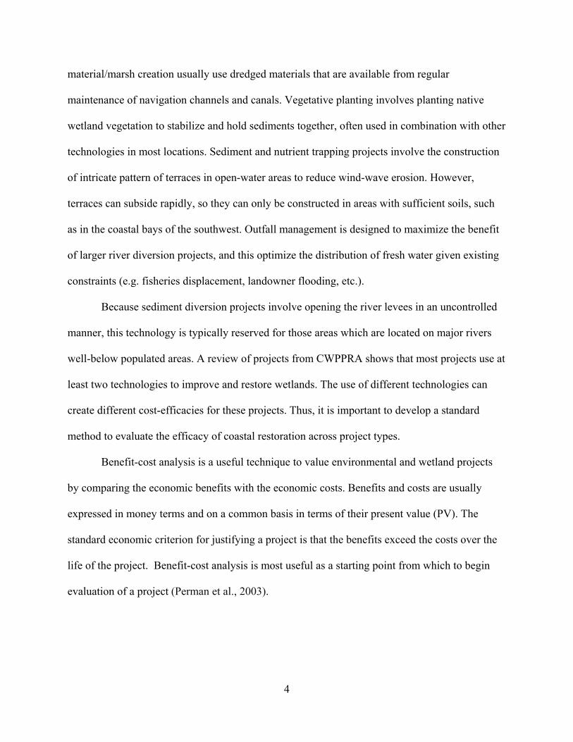
1.2 Methods for Restoration
The Coastal Wetlands Planning, Protection and Restoration Act (CWPPRA) projects
primarily focus on restoration and protection of fragile wetlands. Restoration projects are
grouped as vegetative, structural and hydrologic projects. Vegetative projects use appropriate
plants to trap sediment in vulnerable areas. To create new wetlands or protect existing wetlands,
structural projects use materials, including dredged material or rocks, for shoreline protection
and barrier island restoration. Hydrologic projects restore more natural flow and salinity patterns
and include freshwater/sediment diversion, sediment and nutrient trapping, outfall management,
marsh management, and hydrological restoration. According to the description of project types
from the Office of Coastal Protection and Restoration (OCPR), a brief introduction of each
technique is given below.
Dredged material/marsh creation (MC) projects use dredged sediments from regular
maintenance of navigation channels and access canals, or use sediments dredged specifically to
create new marsh. Barrier island (BI) projects integrate different techniques to protect and restore
Louisiana’s barrier island chain, such as the placement of dredged material to increase the height
and width of the coastal islands, and use vegetative planting and sand-trapping fences to hold
sediments together and stabilize sand dunes on barrier island beaches. Shoreline protection (SP)
projects use various techniques to decrease shoreline erosion, such as rock berms, segmented
breakwaters, and wave-dampening fences. Freshwater diversion (FWD) projects are usually
2

located along major rivers and use gates or siphons to control the volume of water into coastal
marshes.
Vegetative planting (VI) projects are often used in combination with shoreline protection,
barrier island restoration, sediment trapping, and marsh creation techniques. This type of
restoration uses the planting native wetland plants to stabilize and hold sediments together to
establish new wetland.
Hydrologic restoration (HR) projects address wetland damaging problems associated
with human-induced hydrological changes. These projects use locks or gates on major navigation
channels, the blocking of dredged canals, or the cutting of gaps in levee banks. Sediment &
nutrient trapping (SNT) projects use the construction of complex patters of earthen terraces to
slow water flow and help the buildup of sediments in open areas of water.
Marsh management (MM) projects involve controlling water level and salinity in order to
improve vegetation and wildlife habitat in an impounded marsh area. Outfall management (OM)
projects use a variety of techniques to regulate the flow of freshwater diversion to ensure that
water and sediment reach needed areas and maximize the benefit of projects. These projects
utilize water structures and management regimes to assist in optimizing the distribution of fresh
water to nourish coastal wetlands. Sediment diversion projects involve cutting gaps into river
levees in an uncontrolled manner, allowing sediment-loaded water to flow into shallow open
water areas and imitate natural land-building processes to create new marsh.
1.3 Efficiency in Restoration
Selection of the appropriate technology is important for making efficient decisions
concerning wetland restoration. Technology selection is partly determined by the location of the
wetland to be restored. Freshwater diversions must be located along major rivers. Dredged
3
material/marsh creation usually use dredged materials that are available from regular
maintenance of navigation channels and canals. Vegetative planting involves planting native
wetland vegetation to stabilize and hold sediments together, often used in combination with other
technologies in most locations. Sediment and nutrient trapping projects involve the construction
of intricate pattern of terraces in open-water areas to reduce wind-wave erosion. However,
terraces can subside rapidly, so they can only be constructed in areas with sufficient soils, such
as in the coastal bays of the southwest. Outfall management is designed to maximize the benefit
of larger river diversion projects, and this optimize the distribution of fresh water given existing
constraints (e.g. fisheries displacement, landowner flooding, etc.).
Because sediment diversion projects involve opening the river levees in an uncontrolled
manner, this technology is typically reserved for those areas which are located on major rivers
well-below populated areas. A review of projects from CWPPRA shows that most projects use at
least two technologies to improve and restore wetlands. The use of different technologies can
create different cost-efficacies for these projects. Thus, it is important to develop a standard
method to evaluate the efficacy of coastal restoration across project types.
Benefit-cost analysis is a useful technique to value environmental and wetland projects
by comparing the economic benefits with the economic costs. Benefits and costs are usually
expressed in money terms and on a common basis in terms of their present value (PV). The
standard economic criterion for justifying a project is that the benefits exceed the costs over the
life of the project. Benefit-cost analysis is most useful as a starting point from which to begin
evaluation of a project (Perman et al., 2003).
4
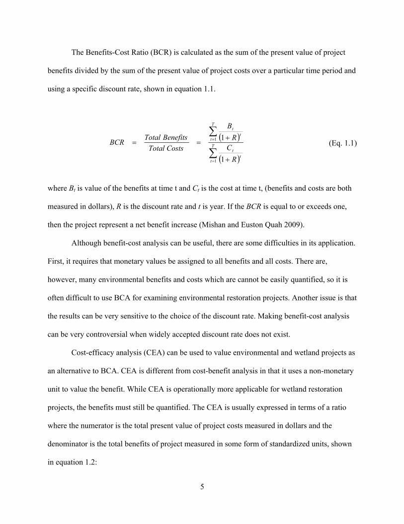
The Benefits-Cost Ratio (BCR) is calculated as the sum of the present value of project
benefits divided by the sum of the present value of project costs over a particular time period and
using a specific discount rate, shown in equation 1.1.
( )
( )∑
∑
=
=
+
+== T
tt
t
T
tt
t
RC
RB
CostsTotalBenefitsTotalBCR
1
1
1
1 (Eq. 1.1)
where Bt is value of the benefits at time t and Ct is the cost at time t, (benefits and costs are both
measured in dollars), R is the discount rate and t is year. If the BCR is equal to or exceeds one,
then the project represent a net benefit increase (Mishan and Euston Quah 2009).
Although benefit-cost analysis can be useful, there are some difficulties in its application.
First, it requires that monetary values be assigned to all benefits and all costs. There are,
however, many environmental benefits and costs which are cannot be easily quantified, so it is
often difficult to use BCA for examining environmental restoration projects. Another issue is that
the results can be very sensitive to the choice of the discount rate. Making benefit-cost analysis
can be very controversial when widely accepted discount rate does not exist.
Cost-efficacy analysis (CEA) can be used to value environmental and wetland projects as
an alternative to BCA. CEA is different from cost-benefit analysis in that it uses a non-monetary
unit to value the benefit. While CEA is operationally more applicable for wetland restoration
projects, the benefits must still be quantified. The CEA is usually expressed in terms of a ratio
where the numerator is the total present value of project costs measured in dollars and the
denominator is the total benefits of project measured in some form of standardized units, shown
in equation 1.2:
5

( )BenefitsTotal
RC
BenefitsTotalCostsTotalCE
T
tt
t∑= +
== 1 1 (Eq. 1.2)
where CE is cost effectiveness. Total costs can be derived from existing cost data by adding the
appropriately discounted total capital and operating/maintenance costs (Mishan and Euston Quah
2009).
In order to better employ CEA, wetland benefits must be clearly categorized and
standardized; however, it is usually hard to measure them since there are numerous ways to
measure the value of wetlands. Economists would employ any number of market and non-market
valuation techniques, yet most wetland assessment procedures have been developed by
biophysical scientists. The technique developed specifically for CWPPRA is known as the
Wetland Value Assessment or “WVA Method’ (Bartoldus 1999a).
The Wetland Value Assessment (WVA) technique utilizes a community ecology
approach to determine wetland benefits of proposed projects, where the benefits expressed in
Average Annual Habitat Units (AAHUs). The WVA can be used to measure restoration benefits
on several habitat types along the Louisiana coast. Community models include fresh marsh,
intermediate marsh, brackish marsh, saline marsh, fresh swamp, barrier islands, and barrier
headlands. Each model employs a number of specifically weighted variables of habitat quantity
and quality and these variables are used to develop model scores using a Habitat Suitability
Index (HSI). The net benefits of a proposed project are determined by predicting future habitat
conditions under two scenarios– future without project and future with project, with benefits
expressed as Habitat Units (HU) over the life of the project. These are then annualized to
produce Average Annual Habitat Units. The results of the WVA can be combined with cost data
to determine the effectiveness of proposed project in terms of average annual cost per AAHU.
6
Aust (2006) indicated that WVA is the current method for evaluating the benefits of
CWPPRA projects because it can standardize project comparisons and allow for prioritization by
cost-efficiency and facilitate selection of projects. However, the research also found that in recent
years the program appeared to be favoring projects that were less efficient on an AAHU basis. A
preference for rapid land-building projects - those relying primarily on the mechanical recovery and
placement of sediments - had become a significant driver of project selection during the 1999-2004
program period, despite the fact that such projects are relatively inefficient on a $/AAHU basis.
1.4 Shifting the Focus
Hurricanes Katrina and Rita hit the southeastern and southwestern part of Louisiana on
August 29 and September 23, 2005, respectively. They were unparalleled in recent history and
resulted in massive property damage and human fatalities. Katrina caused $81 billion and Rita
caused $11.3 billion in total estimated property damage (National Hurricane Center, 2007). At
least 1,800 people lost their lives in the storms and their aftermath. Over 80% of New Orleans
was under water by the time Katrina passed, and over 700,000 homes were destroyed along the
Louisiana, Mississippi, and Alabama coasts. Katrina and Rita also had a profound impact on the
environment. The storm surge caused substantial beach erosion, in some cases completely
submerging coastal areas. The US Geological Survey has estimated that 217 square miles of land
were transformed to water by Katrina and Rita (LaCPRA 2007), an amount that represents 42
percent of what was predicted to occur over a 50-year period from 2000 to 2050 before
Hurricanes Katrina and Rita (USGS, 2006).
In the wake of Hurricanes Katrina and Rita, state and federal agencies began seeking
ways to integrate the previously separate objectives of hurricane protection and coastal
restoration (Petrolia and Kim 2010, Petrolia et al., 2011). Moreover, Hurricanes Katrina and Rita
7
changed the policy focus from slow-moving wetland restorations focused on ecological services
toward more immediate, human-focused issues such as hurricane protection. Additionally, state
managers have realized that coastal land loss occurs at a much greater rate than was originally
estimated prior to the storms when environmental benefits (AAHU) were the primary focus
(Petrolia et al., 2009). Because time has become more critical, many citizens and scientists have
begun supporting quantity over quality in order to keep the remaining wetlands in place. Thus,
policy emphasis has begun to shift increasingly towards the integration of coastal protection with
coastal restoration. This integration introduces a new benefits construct – which in many cases is
simply to build land as rapidly as possible. The term “rapid land-building”(RLB) as used here
refers to those technologies with the potential for creating or restoring substantial amounts of
wetland acreage within a very short time frame compared to other methods. Examples of RLB
include pumping sediments, pipeline sediment conveyance, and beneficial issue of dredge spoil.
1.5 Problem Statement
Louisiana coastal communities have shifted their focus to preserving remaining coastal
wetlands and are paying more attention to rapid wetland restoration projects after the losses of
Hurricanes Katrina and Rita (Petrolia et al., 2011). Previous economic analyses have focused on
the qualitative benefits (i.e. $/AAHU) of coastal restoration spending. However, a new benefit
construct, which in many cases is simply to build land as rapidly as possible (i.e. $/acre), is now
emerging. For wetland restoration, freshwater diversions (FWD) and rapid land building
technologies are the two main restoration options. Freshwater diversions mimic nature’s way to
build new land. Also, this technology results in high quality and sustainable land and is an
excellent option for protecting existing marshes. Although this technique helps protect and
sustain existing wetlands, it could take decades or centuries for new lands to be built up. In
8
contrast, RLB technologies can build land quickly and gain earlier benefits which may mean less
project risk over time. When time and risk are accounted for, rapid land building projects may be
more cost-effective than freshwater diversions.
It is still unclear, however, if the benefits of the more natural, freshwater diversion
method outweigh the risks of waiting for the land to be restored. Also, it is not clear if the risk
reduction by moving benefits up in time outweigh the higher costs and loss of natural wetland
functions. Furthermore, available sediments and project distance are two of several variables that
must be considered when comparing the two technologies. Only a comprehensive economic
assessments of these technologies can provide the information to remove these uncertainties
from the decision making process of coastal restoration managers.
1.6 Objectives
The main objective of this study is to develop a comparative economic assessment of
rapid land-building (RLB) technologies and freshwater diversions (FWD) (existing and
proposed) for coastal restoration. The specific objectives include:
1. Develop generic models of coastal restoration project trajectories
and cost by technology;
2. Conduct sensitivity analyses with varying values for coastal wetlands,
discount rates and risk; and
3. Perform case-studies to illustrate tradeoffs between coastal restoration
technologies.
1.7 Data and Methods
Benefit trajectory and cost data for objective 1 were collected from coastal restoration
project cost estimates from surveys, bids, and actual project expenditures. The main source of
9
data came from actual coastal restoration projects constructed and proposed under CWPPRA.
Additional cost data were obtained from project proposals and bids submitted to the Louisiana
Department of Natural Resources (LaDNR) and Louisiana Office of Coastal Protection and
Restoration (OCPR) under the Water Resources Development Act (WRDA), the Coastal Impact
Assistance Program (CIAP), and the Louisiana Coastal Area (LCA) Restoration Program. To a
lesser extent, direct communications with coastal engineering firms were used to provide
additional costs and benefits data. Data were aggregated into like categories and multiple
regression analysis employed to develop generic models of costs and benefits by technology.
Cost for delivery of physical quantities of wetland restoration material (i.e. $/acre) were
estimated as a function of several variables, including mobilization/demobilization costs,
distance, dredging quantity, containment, shaping, and vegetation. Generic cost models were
constructed for FWD and RLB projects.
Benefit data for objective 2 were obtained from two sources; market prices for coastal
wetland acreage and non-market, ecological service values ($/acre) from existing literature. The
wetland valuation literature employs a wide range of non-market techniques to place dollar
estimates on coastal wetland functions and values (e.g. habitat, water quality, storm surge
reduction). A compilation of these estimates were used to quantity annual service values. Using
a benefits-transfer approach, these estimates were used to inform simulations where benefits
need to be expressed in dollar terms. Cost and benefit estimates were incorporated into a NPV
framework, with varying levels of risk (i.e. storm landfall probabilities, project scales, and
technology efficacy data) and variable discount rates. Gamma discounting has been shown to be
better than static (constant) discount rates, which can underestimate the value of ecosystem
restoration that takes many years to deliver (Weitzman, 1994-2001).
10
The basic model uses a net present value (NPV) approach that incorporates hurricane risk
(Klotzbach and Gray, 2009), scale of the restoration project (CWPPRA 1992-2008), and varying
assumptions on technology efficacy for FWD and RLB projects. The net present value is the
current value of all project net benefits at a particular discount rate. Net benefits are simply the
sum of benefits minus costs. The basic formula for NPV is given by equation 1.3:
( ) ( ) ( )∑∑∑=== +
−+
=+
−=
T
tt
tT
tt
tT
tttt
RC
RB
RCB
NPV111 111
(Eq. 1.3)
where Bt is the sum of benefit at time t, Ct is the sum of cost at time t, R is the discount rate and t
is the year. If the NPV is greater than zero, then the project might be a good candidate for
implementation (Perman et al., 2003). Given that projects costs usually known and can be
generically modeled, the benefit-value per acre can be solved with a positive NPV. Petrolia et al.
(2009) developed simulations of hurricane risk-adjusted NPV for CWPPRA projects and
compared the results of similar time and risk assumptions with FWD and RLB projects over 20-
50 years periods. These simulations provide the basis for an expanded model, where risk was
more fully quantified based on existing literature.
Once the model framework was in place, simulations (Objective 3) were conducted based
on actual proposed restoration scenarios in coastal Louisiana. Such simulations can be used to
inform policy decisions. One example of such an application is the Third Delta Conveyance
Channel Feasibility alternatives developed in 2005 (CH2M-Hill 2006). That analysis compared
the cost/acre of a large-scale FWD project against the cost/acre for three RLB project alternatives.
This case-study approach was successful in informing public policy about the relative
disadvantages of large scale FWD. Expansion of these types of comparisons in a risk-adjusted
11
framework provides addition information for future spending of coastal restoration dollars. The
core issue between FWD and RLB projects is: will the risk reduction gained by moving benefits
up in time with RLB marsh creation projects outweigh the higher costs of land built by slower,
FWD marsh creation projects?
1.8 Rationale
Given the increasing debate whether RLB or FWD project are more appropriate,
additional economic research is needed. RLB projects are often dismissed for being too
expensive and less sustainable than other types of coastal restoration methods. On the other hand,
FWD projects are often dismissed as being too slow and ineffectual for short term needs. This
debate comes at a time when coastal restoration costs are increasing dramatically. The CWPPRA
program has allocated more than $1.5 billion for projects constructed and operation since in
1990. In 1998, the COAST 2050 report estimated that an additional $14 billion was needed to
address Louisiana’s land loss problem. In 2002, the LCA Plan requested that $14 billion, but
only $1.9 billion was authorized in 2004 through the WRDA. Furthermore, attempts to get
federal royalties from petroleum activities off the state’s outer continental shelf (OCS) were
unsuccessful until 2005, when a one-time payment of $540 million was allocated to Louisiana
under the CIAP. In 2007, the Gulf of Mexico Energy Security Act (GOMESA) approved more
OCS revenue, and it is now projected that the state will receive $210 million annually through
2017 and $650 million after 2017. Despite these increases, the CPRA recently estimated that
$100 billion would be needed to fully integrate coastal restoration and protection (Graves 2009).
Given current sources of projected funding, that means that Louisiana will have only 13% of the
funds needed to accomplish its coastal wetland restoration goals.
12
Based on that information, it is important that large-scale spending needs be allocated to
obtain the greatest benefits for the limited funding available. Thus, more information is needed to
guide program planning and to assess different wetland restoration techniques on an economic
basis.
This thesis research will establish generic cost and benefit functions for RLB and FWD
projects as a function of variables such as technology, distance, sediment source, depreciation,
risk and time for rapid land-building and freshwater diversion projects. Based on this
information, and an examination of project-specific constraints, information will be generated in
the total economic and environmental costs and benefits of competing project alternatives.
Incorporation of time and uncertainty consideration will help to better understand the feasibility
of rapid land-building projects compared to more traditional methods, such as freshwater
diversion projects. Results from this research will be helpful to costal restoration programs, such
as CWPPRA, CIAP, LCA, WRDA, CPRA, and GOMESA.
13

CHAPTER 2. DESCRIPTIVE DATA
2.1 Introduction
In order to develop a comprehensive economic comparison of rapid land-building (RLB)
technologies and freshwater diversions (FWD) (existing and proposed) for coastal restoration, it
is necessary to understand the general costs and benefits of these projects. As mentioned in
Chapter 1, there are three potential sources of information for project costs and benefits: 1)
authorized coastal restoration projects, 2) bids for coastal restoration projects; and 3) surveys.
Given the sensitivity of this information, it is unlikely that surveys of project contractors would
yield reliable information. For this reason, the focus here will be on authorized project data and
pending projected data (e.g. bid data).1 Thus, wetland restoration project data for this portion of
the study are collected from numerous sources, including data on authorized and bidded projects
from the Office of Coastal Protection and Restoration (OCPR), CWPPRA priority project list
appendices for years 1991-2009, and CWPPRA ecological review reports and project fact sheets.
Between 1991 and 2009, a total of 341 restoration projects were authorized under
programs such as CWPPRA, Coastal Impact Assistance Program (CIAP), Federal Emergency
Management Agency (FEMA), Hurricane Storm Damage Risk Reduction System (HSDRRS),
Louisiana Coastal Area (LCA), the State of Louisiana (STATE), and Water Resources
Development Act (WRDA). Table 2.1 lists the number of the projects under these programs. A
majority of the projects (52%) are sponsored by the CWPPRA program, which to date has
initiated 178 coastal wetlands restoration projects. State projects, at 23%, are the second most
frequent project type, and are usually low cost vegetative planting projects. The remaining
1 Bids are competitive offers from commercial contractors for wetland restoration projects. In all cases, projects bids are in response to state and federal solicitations that include detailed project expectations. If accepted, bids are legally binding.
14

15
projects are sponsored by the CIAP program (77%), WRDA (4.5%), FEMA (4.5%), LCA (4%),
HSDRRS (2%) and other programs (3%).
Table 2.1 Louisiana Coastal Restoration Programs and Projects 1991-2009 Programs Project Number (n=341) Percentage (%) CWPPRA 178 52% STATE 75 23% CIAP 26 8% WRDA 16 5% FEMA 16 5% LCA 14 4% OTHERS 10 3% HSDRRS 6 2%
2.1.1 CWPPRA Project Data
Since the majority of projects are funded by CWPPRA, this program provides the most
readily available data. This study will focus primarily on coastal restoration projects authorized
and proposed under the CWPPRA program from 1991 to 2009, with project data from additional
restoration programs included as appropriate. Specific project details are collected from
aggregated and individual CWPPRA project reports. Of the 178 initiated projects under
CWPPRA, 124 projects are authorized, 29 projects have been de-authorized, 4 projects have
been transferred and 21 are considered demonstration projects. Table 2.2 shows the average cost
per unit for the following measures of restoration: AAHU, enhancement acres, acres protected,
and total net acre.2 Average costs are reported for the 124 authorized projects initiated by
CWPPRA. All cost-effectiveness measures are adjusted by the civil works construction cost
index (CWCCIS) and expressed in terms of 2009 dollars (USACE 2010). Projects are organized
2 Enhancement acres represent the acres of rehabilitation or reestablishment from a degraded wetland area or the acres of modification from an existing wetland area as a result of a wetland restoration project. Acres protected represent the acres of emergent marsh protected from loss as a result of a wetland restoration project.
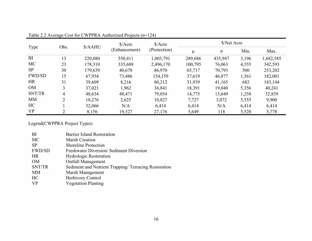
Table 2.2 Average Cost for CWPPRA Authorized Projects (n=124) $/Net Acre
Type Obs. $/AAHU $/Acre (Enhancement)
$/Acre (Protection) µ σ Min. Max.
BI 13 220,080 550,411 1,003,791 289,686 435,947 3,196 1,682,585 MC 23 178,310 335,688 2,496,170 100,795 76,063 4,555 342,593 SP 30 179,639 40,670 86,970 65,717 70,793 500 253,202 FWD/SD 15 67,934 73,486 154,159 37,619 46,877 1,561 182,001 HR 31 39,609 8,216 80,212 31,939 41,165 682 183,144 OM 3 37,021 1,962 36,841 18,391 19,040 5,356 40,241 SNT/TR 4 48,634 48,471 79,054 14,775 13,649 1,258 32,839 MM 2 18,276 2,625 10,827 7,727 3,072 5,555 9,900 HC 1 32,066 N/A 6,414 6,414 N/A 6,414 6,414 VP 2 8,156 19,527 27,176 5,649 118 5,520 5,778 Legend(CWPPRA Project Types)
BI Barrier Island Restoration MC Marsh Creation SP Shoreline Protection FWD/SD Freshwater Diversion/ Sediment Diversion HR Hydrologic Restoration OM Outfall Management SNT/TR Sediment and Nutrient Trapping/ Terracing Restoration MM Marsh Management HC Herbivory Control VP Vegetation Planting
16

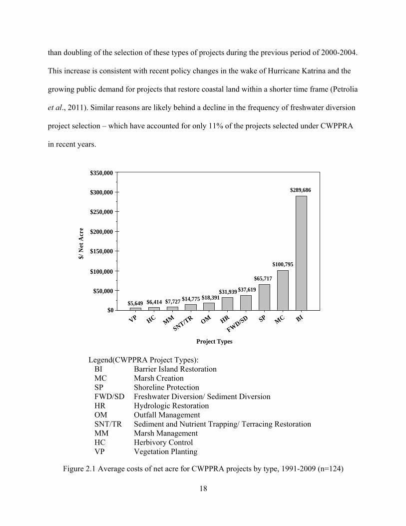
by dominant type of technology used in the restoration.3 The average cost per net acre for all
projects ranges from a low of $5,649/acre to a high of $289,686/acre. This large range is due to
vast differences in project technology, location, and size. At the upper bound of this range are
barrier island (BI) restoration projects, with an average cost per net acre of $289,686 (Figure 2.1).
These projects are very expensive because of their remoteness (i.e. distance from shore), higher
transportation and labor costs, and their vulnerability to high-energy waves. In fact, barrier island
projects are currently 2.9 times the average cost of the next highest project type, marsh creation
(MC) ($100,795). Additional project types that have a high average cost include shoreline
protection (SP) ($65,717) and freshwater diversion projects (FWD) ($37,619). These four project
types account for more than 65 percent of all CWPPRA projects selected and more than 83
percent of the budgeted program spending from 1991-2009.
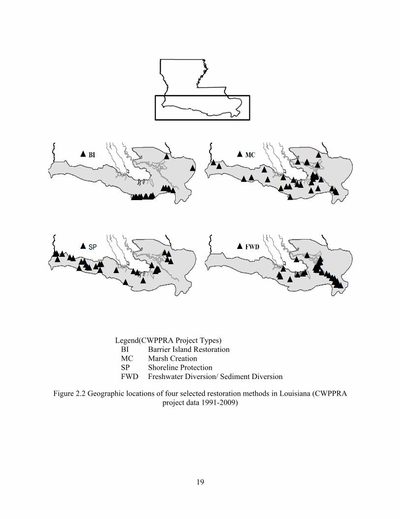
Figure 2.2 depicts the geographic location of these four project types. Note that two of
these types (MC and SP) are dispersed equally across the coast. The other two, however, are
restricted to being offshore (BI) or at the end of major rivers (FWD). Despite these location
differences, there are occasions when two or more of these methods are considered as restoration
alternatives for the same location. A common example of this option can be found at coastal
locations where both MC and FWD are possible. But, of these four methods, only three have the
potential for significant land-building. Shoreline protection projects are designed primarily for
maintaining and protecting existing shorelines. Figure 2.3 depicts the frequency of selection for
the three most expensive methods of land-building (MC, BI, and FWD) and shows an increasing
trend towards the use of MC projects. Approximately 61% of the projects authorized during the
2005 to 2009 time period under CWPPRA were marsh creation projects. This represents a more
3 While it is typical for some projects to utilize more than one restoration method, the categorization here is by the dominant type of technology.
17
than doubling of the selection of these types of projects during the previous period of 2000-2004.
This increase is consistent with recent policy changes in the wake of Hurricane Katrina and the
growing public demand for projects that restore coastal land within a shorter time frame (Petrolia
et al., 2011). Similar reasons are likely behind a decline in the frequency of freshwater diversion
project selection – which have accounted for only 11% of the projects selected under CWPPRA
in recent years.
Project Types
VP HCMM
SNT/TR OM HR
FWD/SD SP MC BI
$/ N
et A
cre
$5,649
$31,939
$289,686
$37,619
$65,717
$100,795
$18,391$7,727 $14,775$6,414
$350,000
$300,000
$250,000
$200,000
$150,000
$100,000
$50,000
$0
Legend(CWPPRA Project Types): BI Barrier Island Restoration MC Marsh Creation SP Shoreline Protection FWD/SD Freshwater Diversion/ Sediment Diversion HR Hydrologic Restoration OM Outfall Management SNT/TR Sediment and Nutrient Trapping/ Terracing Restoration MM Marsh Management HC Herbivory Control VP Vegetation Planting
Figure 2.1 Average costs of net acre for CWPPRA projects by type, 1991-2009 (n=124)
18
Legend(CWPPRA Project Types) BI Barrier Island Restoration MC Marsh Creation SP Shoreline Protection FWD Freshwater Diversion/ Sediment Diversion
Figure 2.2 Geographic locations of four selected restoration methods in Louisiana (CWPPRA project data 1991-2009)
19

Time Period
1991-1995 1996-2000 2001-2004 2005-2009
Perc
ent o
f Pro
ject
s
0
10
20
30
40
50
60
70
MC BI FWD
Legend(CWPPRA Project Types) BI Barrier Island Restoration MC Marsh Creation FWD Freshwater Diversion/ Sediment Diversion
Figure 2.3 Selection of land-building restoration projects by period (CWPPRA project data, n=51)
2.2 Data for Analysis
In order to develop a comprehensive comparison of the costs and benefits of RLB and
FWD projects, it is necessary to identify all available data for these types of projects.4 The
following sections provide a listing of this data for authorized and proposed projects.
2.2.1 Project Data: Marsh Creation
Tables 2.3 and 2.4 depict the cost of MC projects from CWPPRA and Bid data. The
costs per net acre are reported for 23 authorized MC projects. An additional 46 bids for MC
4 From this point forward, the reference to rapid land building projects (RLB) will be limited to two methods: marsh creation (MC) and barrier island (BI).
20

21
projects are also available. As legally-binding offers, these bids include much of the same
detailed information on costs and benefits. Bids were collected from the Louisiana Office of
Coastal Protection and Restoration (OCPR) for projects authorized between 1998 and 2004 and
adjusted by the CWCCIS in terms of 2009 dollars. Table 2.4 shows the bids for marsh creation
projects under CWPPRA and STATE programs. Each project contains up to five bids by the
same or different construction companies. Data are presented by project for the following:
Priority Project List (PPL), Bid, Total Bid Cost (TBC), and total millions Cubic Yards of
Sediment (CYD) estimated.5
2.2.2 Project Data: Barrier Island
Table 2.5 describes the authorized BI projects and their attributes under CWPPRA
between 1991 and 2009. Data are presented by project for the following: project priority list
(PPL), fully funded cost (FFC), net acres, total AAHUs, dollar per net acre, dollar per AAHU,
and total cubic yards of sediment required. The fully funded costs of each project were adjusted
by the civil works construction cost index (CWCCIS) and expressed in terms of 2009 dollars
(USACE 2010). The costs per net acre are reported for 13 authorized BI projects.
An additional 39 bids for BI projects were also available. Bids were collected from the
Louisiana Office of Coastal Protection and Restoration (OCPR) for projects authorized between
1991 and 2001 and adjusted by the CWCCIS in terms of 2009 dollars. Table 2.6 shows these
bids for BI island projects authorized under the CWPPRA program. Each project contains up to
seven bids by the same or different wetland restoration contractors.
5 Total Bid Cost (TBC) is only the costs associated with project construction. This estimate differs from the Fully Funded Costs (FFC) which includes planning, design, operation, monitoring and maintenance in addition to construction.

Table 2.3 Authorized MC Projects and Attributes, CWPPRA 1991-2009 (n=23)6
Number Project Name PPL FFC($) Net Acres
$/Net Acre AAHU $/AAHU Total
cyds ME-31 Freshwater Bayou Marsh Creation 19 25,523,755 279 91,483 108 236,331 640,000 PO-75 Labranche East Marsh Creation 19 32,323,291 715 45,207 339 95,349 N/A TE-72 Lost Lake Marsh Creation 19 22,943,866 749 30,633 281 81,651 N/A BA-68 Grand Liard Marsh Restoration 18 30,797,529 286 107,684 158 194,921 3,900,000 BA-47 West Pointe a la Hache Marsh Creation 17 16,842,940 203 82,970 126 133,674 N/A BA-48 Bayou Dupont Marsh and Ridge Creation 17 22,573,372 187 120,713 121 186,557 N/A PO-34 Alligator Bend Marsh Restoration 16 32,736,490 127 257,768 56 584,580 2,988,700 TE-51 Madison Bay Marsh Creation and Terracing 16 35,432,419 372 95,248 242 146,415 N/A TE-52 West Belle Pass Barrier Restoration 16 46,271,351 305 151,709 203 227,938 2,774,000 BA-42 Lake Hermitage Marsh Creation 15 43,957,905 447 98,340 211 208,331 5,526,440 MR-15 Venice Ponds Marsh Creation and Crevasses 15 10,391,951 511 20,336 153 67,921 1,666,800 TV-21 East Marsh Island Marsh Creation 14 28,333,932 169 134,284 106 267,301 2,382,974 PO-33 Goose Point/Pointe Platte Marsh Creation 13 21,049,245 436 48,278 297 70,873 3,977,270 BA-39 Bayou Dupont Sediment Delivery System 12 37,120,258 326 113,866 159 233,461 5,200,000 BA-36 Dredging on the Barataria Basin Landbridge 11 22,118,619 242 91,399 135 163,842 6,845,696 BA-37 Little Lake Shoreline Protection 11 41,106,558 713 57,653 349 117,929 4,828,865 TE-46 West Lake Boudreaux Restoration 11 27,344,085 277 98,715 129 211,970 1,255,980 TE-48 Raccoon Island Marsh Creation 11 24,324,092 71 342,593 64 380,064 1,036,728 TE-44 North Lake Mechant Landbridge Restoration 10 55,128,127 604 91,272 367 150,213 4,000,000 TV-19 Weeks Bay Marsh Creation 9 43,415,799 278 156,172 N/A N/A N/A CS-28 Sabine Refuge Marsh Creation 8 44,592,375 993 44,907 386 115,524 4,666,200 BA-19 Barataria Bay Waterway Restoration 1 2,027,007 445 4,555 151 13,424 1,740,000 PO-17 Bayou LaBranche Wetland Creation 1 6,598,171 203 32,503 191 34,545 2,851,133
6 Authorized MC projects and their attributes under CWPPRA (1991 and 2009) are presented by project for the following: Priority Project List (PPL), Fully Funded Cost (FFC), Net Acre, Dollar per Net Acre ($/Net Acre), Average Annual Habitat Unit (AAHU), Dollar per AAHU ($/AAHU), and total Cubic Yards of Sediment (CYD) required. The fully funded costs of each project are adjusted by the civil works construction cost index (CWCCIS) and expressed in terms of 2009 dollars (USACE 2010).
22

Table 2.4 Projected MC Projects and Attributes, 1998-2004 (n=46)
Number Project Name PPL Bid TBC($) Total MM cyds
TV-21 East Marsh Island Marsh Creation Project 14 3 26,991,137 2.82 TV-21 East Marsh Island Marsh Creation Project 14 2 19,640,463 2.82 TV-21 East Marsh Island Marsh Creation Project 14 1 16,199,401 2.82 PO-33 Goose Point/Pointe Platte Marsh Creation 13 4 21,887,914 3.01 PO-33 Goose Point/Pointe Platte Marsh Creation 13 3 18,240,170 3.01 PO-33 Goose Point/Pointe Platte Marsh Creation 13 2 17,661,557 3.01 PO-33 Goose Point/Pointe Platte Marsh Creation 13 1 16,649,047 3.01 BA-39 Mississippi River Sediment Delivery System - Bayou Dupont 12 2 31,605,120 2.34 BA-39 Mississippi River Sediment Delivery System - Bayou Dupont 12 1 28,148,184 2.34 BA-36 Dedicated Dredging on the Barataria Basin Landbridge 11 3 46,035,945 6.50 BA-36 Dedicated Dredging on the Barataria Basin Landbridge 11 2 37,235,600 6.50 BA-36 Dedicated Dredging on the Barataria Basin Landbridge 11 1 36,990,153 6.50 TE-44 North Lake Mechant Landbridge Restoration 10 4 61,442,194 4.97 TE-44 North Lake Mechant Landbridge Restoration 10 3 55,776,722 4.97 TE-44 North Lake Mechant Landbridge Restoration 10 2 45,833,353 4.97 TE-44 North Lake Mechant Landbridge Restoration 10 1 43,654,494 4.97 CS-28-2 & 3 Sabine Refuge Marsh Creation, Cycles 2 & 3 8 3 34,278,786 4.04 CS-28-2 & 3 Sabine Refuge Marsh Creation, Cycles 2 & 3 8 2 26,191,271 4.04 CS-28-2 & 3 Sabine Refuge Marsh Creation, Cycles 2 & 3 8 1 20,824,592 4.04 CS-28-3 Sabine Refuge Marsh Creation, Cycle 3 8 1 22,203,378 5.33 CS-28-1 Sabine Refuge Marsh Creation, Cycle 1 8 1 11,342,798 2.52 4351-BRM Brown Marsh Small Dredge Demo Project N/A 5 769,604 0.07 4351-BRM Brown Marsh Small Dredge Demo Project N/A 4 748,081 0.07 4351-BRM Brown Marsh Small Dredge Demo Project N/A 3 564,945 0.07 4351-BRM Brown Marsh Small Dredge Demo Project N/A 2 420,742 0.07 4351-BRM Brown Marsh Small Dredge Demo Project N/A 1 0.07 353,013
23

24
Table 2.4 continued LA-01b Dedicated Dredging Program-Bayou Dupont N/A 5 1,812,541 0.41 LA-01b Dedicated Dredging Program-Bayou Dupont N/A 4 1,844,674 0.41 LA-01b Dedicated Dredging Program-Bayou Dupont N/A 3 1,725,979 0.41 LA-01b Dedicated Dredging Program-Bayou Dupont N/A 2 1,428,090 0.41 LA-01b Dedicated Dredging Program-Bayou Dupont N/A 1 1,441,006 0.41 LA-01c Dedicated Dredge Program - Pass A Loutre N/A 3 3,273,113 0.39 LA-01c Dedicated Dredge Program - Pass A Loutre N/A 2 1,821,474 0.39 LA-01c Dedicated Dredge Program - Pass A Loutre N/A 1 1,926,253 0.39 LA-01d Dedicated Dredging-Terrebonne Parish School Board N/A 3 3,390,167 0.30 LA-01d Dedicated Dredging-Terrebonne Parish School Board N/A 2 2,296,069 0.30 LA-01d Dedicated Dredging-Terrebonne Parish School Board N/A 1 1,593,580 0.30 LA-01e Dedicated Dredging-Grand Bayou Blue N/A 5 3,824,896 0.30 LA-01e Dedicated Dredging-Grand Bayou Blue N/A 4 3,285,078 0.30 LA-01e Dedicated Dredging-Grand Bayou Blue N/A 3 3,264,121 0.30 LA-01e Dedicated Dredging-Grand Bayou Blue N/A 2 2,999,070 0.30 LA-01e Dedicated Dredging-Grand Bayou Blue N/A 1 2,648,174 0.30 LA-01f Dedicated Dredging-Point Au Fer N/A 4 6,531,028 0.30 LA-01f Dedicated Dredging-Point Au Fer N/A 3 5,333,542 0.30 LA-01f Dedicated Dredging-Point Au Fer N/A 2 4,773,636 0.30 LA-01f Dedicated Dredging-Point Au Fer N/A 1 3,570,233 0.30 Legend(CWPPRA Project Types)
PPL Priority Project List TBC Total Bid Cost CYD Cubic Yards of Sediment

Table 2.5 Barrier Island Projects and Attributes, CWPPRA 1991-2009 (n=13)
Number Project Name PPL FFC($) Net acres $/net acre AAHU $/AAHU Total
cyds
BA-76 Cheniere Ronquille Barrier Island Restoration 19 43,828,285 234 187,300 190 230,675 3,000,000
BA-40 Riverine Sand Mining/Scofield Island Restoration 14 54,814,331 234 234,249 229 239,364 2,415,620
TE-50 Whiskey Island Backbarrier Marsh Creation 13 40,345,509 272 148,329 292 138,170 2,026,000BA-35 Pass Chaland to Grand Bayou Restoration 11 61,354,800 263 233,288 208 294,975 2,561,767BA-38 Barataria Barrier Island Complex Project 11 107,657,656 334 322,328 287 375,114 4,010,000TE-47 Ship Shoal: Whiskey West Flank Restoration 11 86,214,651 195 442,126 269 320,501 4,000,000TE-37 New Cut Dune and Marsh Restoration 9 19,026,123 102 186,531 43 442,468 844,540 TE-40 Timbalier Island Dune and Marsh Creation 9 25,290,391 273 92,639 124 203,955 3,600,000TE-30 East Timbalier Island Restoration II 4 12,158,165 215 56,550 140 86,844 1,677,815TE-25 East Timbalier Island Restoration I 3 6,113,799 1,913 3,196 319 19,166 949,300 TE-27 Whiskey Island Restoration 3 11,677,372 1,239 9,425 549 21,270 2,500,000TE-24 Isles Dernieres Restoration Trinity Island 2 18,242,876 109 167,366 120 152,024 3,371,616TE-20 Isles Dernieres Restoration East Island 1 15,143,267 9 1,682,585 45 336,517 3,935,000
25
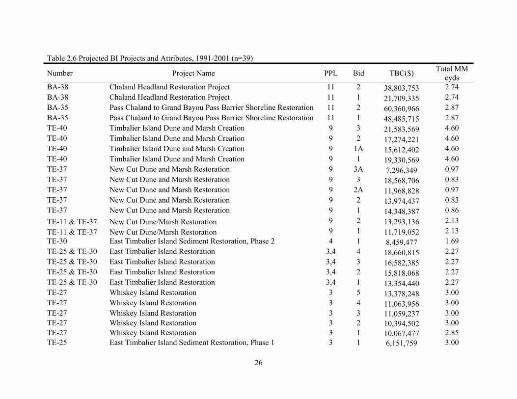
Table 2.6 Projected BI Projects and Attributes, 1991-2001 (n=39)
Number Project Name PPL Bid TBC($) Total MM cyds
BA-38 Chaland Headland Restoration Project 11 2 38,803,753 2.74 BA-38 Chaland Headland Restoration Project 11 1 21,709,335 2.74 BA-35 Pass Chaland to Grand Bayou Pass Barrier Shoreline Restoration 11 2 60,360,966 2.87 BA-35 Pass Chaland to Grand Bayou Pass Barrier Shoreline Restoration 11 1 48,485,715 2.87 TE-40 Timbalier Island Dune and Marsh Creation 9 3 21,583,569 4.60 TE-40 Timbalier Island Dune and Marsh Creation 9 2 17,274,221 4.60 TE-40 Timbalier Island Dune and Marsh Creation 9 1A 15,612,402 4.60 TE-40 Timbalier Island Dune and Marsh Creation 9 1 19,330,569 4.60 TE-37 New Cut Dune and Marsh Restoration 9 3A 7,296,349 0.97 TE-37 New Cut Dune and Marsh Restoration 9 3 18,568,706 0.83 TE-37 New Cut Dune and Marsh Restoration 9 2A 11,968,828 0.97 TE-37 New Cut Dune and Marsh Restoration 9 2 13,974,437 0.83 TE-37 New Cut Dune and Marsh Restoration 9 1 14,348,387 0.86 TE-11 & TE-37 New Cut Dune/Marsh Restoration 9 2 13,293,136 2.13 TE-11 & TE-37 New Cut Dune/Marsh Restoration 9 1 11,719,052 2.13 TE-30 East Timbalier Island Sediment Restoration, Phase 2 4 1 8,459,477 1.69 TE-25 & TE-30 East Timbalier Island Restoration 3,4 4 18,660,815 2.27 TE-25 & TE-30 East Timbalier Island Restoration 3,4 3 16,582,385 2.27 TE-25 & TE-30 East Timbalier Island Restoration 3,4 2 15,818,068 2.27 TE-25 & TE-30 East Timbalier Island Restoration 3,4 1 13,354,440 2.27 TE-27 Whiskey Island Restoration 3 5 13,378,248 3.00 TE-27 Whiskey Island Restoration 3 4 11,063,956 3.00 TE-27 Whiskey Island Restoration 3 3 11,059,237 3.00 TE-27 Whiskey Island Restoration 3 2 10,394,502 3.00 TE-27 Whiskey Island Restoration 3 1 10,067,477 2.85 TE-25 East Timbalier Island Sediment Restoration, Phase 1 3 1 3.00 6,151,759
26

27
Table 2.6 continued TE-20 & TE-24 Isles Dernieres Restoration (Phase 1-Trinity Island) 1,2 4 19,025,122 4.85 TE-20 & TE-24 Isles Dernieres Restoration (Phase 1-Trinity Island) 1,2 3 18,539,547 4.85 TE-20 & TE-24 Isles Dernieres Restoration (Phase 1-Trinity Island) 1,2 2A 1,691,258 4.85 TE-20 & TE-24 Isles Dernieres Restoration (Phase 1-Trinity Island) 1,2 2 16,224,982 4.85 TE-20 & TE-24 Isles Dernieres Restoration (Phase 1-Trinity Island) 1,2 1A 18,238,179 4.85 TE-20 & TE-24 Isles Dernieres Restoration (Phase 1-Trinity Island) 1,2 1 16,545,100 4.85 TE-20 & TE-24 Isles Dernieres Restoration (Phase 0-East Island) 1,2 4A 15,898,514 3.60 TE-20 & TE-24 Isles Dernieres Restoration (Phase 0-East Island) 1,2 4 15,898,514 3.60 TE-20 & TE-24 Isles Dernieres Restoration (Phase 0-East Island) 1,2 3 13,456,045 3.60 TE-20 & TE-24 Isles Dernieres Restoration (Phase 0-East Island) 1,2 2A 14,614,119 3.60 TE-20 & TE-24 Isles Dernieres Restoration (Phase 0-East Island) 1,2 2 11,981,806 3.60 TE-20 & TE-24 Isles Dernieres Restoration (Phase 0-East Island) 1,2 1A 10,924,476 3.60 TE-20 & TE-24 Isles Dernieres Restoration (Phase 0-East Island) 1,2 1 11,660,966 3.60 Legend(CWPPRA Project Types)
PPL Priority Project List TBC Total Bid Cost CYD Cubic Yards of Sediment

2.2.3 Project Data: Freshwater Diversion
Table 2.7 shows the authorized FWD projects and their attributes under CWPPRA
between 1991 and 2009. The fully funded costs of each project are adjusted by the civil works
construction cost index (CWCCIS) and expressed in terms of 2009 dollars (USACE 2010). The
costs per net acre are reported for the 15 FWD projects authorized by CWPPRA since 1991.
Compared to MC projects which have recently dominated project selection under CWPPRA (61%
of all projects authorized since 2005), FWD projects have comprised less than 15% of selected
projects in the last 5 years.
At the time of this study, no bid data were available from CWPPRA for FWD projects.
While CWPPRA provides funding for the majority of restoration projects in coastal Louisiana,
some of the larger scale FWD projects are beyond the scope of CWPPRA budget constraints.
Additional funding for FWD projects began in 1998 when the state of Louisiana and federal
partners sponsored the Coast 2050 visioning process. Recognizing a more aggressive effort was
needed, 77 ecosystem restoration strategies were identified at an estimated cost of $14 billion
(Louisiana Coastal Wetland Conservation and Restoration Task Force and the Wetlands
Conservation and Restoration Authority 1998). In 2001, funding for FWD projects identified in
the Coast 2050 plan was sought via the Louisiana Coastal Area (LCA) Louisiana-Ecosystem
Restoration Study (LCA 2004). The LCA program would help Louisiana to design and build the
large-scale FWD projects needed to protect and restore coastal resources. Such projects are
typically funded through the Water Resources Development Act (WRDA), the congressional
legislation that authorizes the U.S. Army Corps of Engineers (Corps) to deal with various aspects
of water resources, including flood control, navigation, ecosystem restoration and stream bank
erosion prevention projects. The first WRDA was passed in 1974, and subsequent versions of the
28

Table 2.7 Freshwater Diversion Projects and Attributes, CWPPRA 1991-2009 (n=15)7
Number Project Name PPL FFC($) Net Acres
$/Net Acre AAHU $/AAHU Avg.
cfs BS-18 Bertrandville Siphon 18 22,151,631 1,613 13,733 965 22,955 2,000 CS-49 Cameron-Creole Freshwater Introduction 18 12,545,415 473 26,523 524 23,942 N/A BS-15 Bohemia Mississippi River Reintroduction 17 7,226,847 637 11,345 989 7,307 10,000 BS-12 White Ditch Diversion Restoration 14 18,267,729 189 96,655 107 170,726 500 MR-14 Spanish Pass Diversion 13 17,488,762 433 40,390 79 221,377 7,000 TE-49 Avoca Island Diversion and Land Building 12 26,026,210 143 182,001 132 197,168 1,000 PO-29 River Reintroduction into Maurepas Swamp 11 231,730,462 5,438 42,613 8,486 27,307 1,500
BS-10 Delta Building Diversion North of Fort St. Phillip 10 9,396,627 501 18,756 157 59,851 2,500
BA-34 Mississippi River Reintroduction Into Northwest Barataria 10 20,899,000 941 22,209 781 26,759 800
MR-13 Benneys Bay Diversion 10 42,848,824 5,706 7,509 1,426 30,048 50,000
TE-39 South Lake de Cade Freshwater Introduction 9 7,552,982 202 37,391 60 125,883 N/A
TE-32a North Lake Boudreaux Basin Freshwater Introduction and Hydrologic Management 6 31,138,632 603 51,640 422 73,788 3,750
MR-09 Delta Wide Crevasses 6 7,192,332 2,386 3,014 927 7,759 N/A MR-06 Channel Armor Gap Crevasse 3 1,460,758 936 1,561 234 6,243 2,500 MR-03 West Bay Sediment Diversion 1 87,902,656 9,831 8,941 4,912 17,895 19,188
7 Data are presented by project for the following: Priority Project List (PPL), Fully Funded Cost (FFC), Net Acre, Dollar per Net Acre ($/Net Acre), Average Annual Habitat Unit (AAHU), Dollar per AAHU ($/AAHU), and Average Water Flow Rate which is measured by cubic feet per second (CFS).
29

Act was authorized in 1976, 1986, 1988, 1990, 1992, 1996, 1999, 2000, and 2007. Title VII of
WRDA 2007 focuses on addressing hurricane damage, storm protection and ecosystem
restoration projects outlined in the LCA report of 2004. The entire ACT authorizes $23 billion in
projects nationwide, with $1 billion for wetland restoration projects in Louisiana (Heikkila et al.,
2008).
Prior to 1974, the U.S. Congress authorized the Corps’ flood control and navigation
projects primarily under the Flood Control Act (FCA), enacted by Congress in response to costly
floods. Large-scale FWD projects authorized under this Act include Caernarvon and Davis Pond
authorized in 1965. These structures were subsequently modified by the WRDAs of 1974, 1986
and 1996. The WRDA 2007 would re-authorize/modify the operation of the Davis Pond and
Caernarvon Freshwater and set the average flow rate of each of these two structures at 5000 cfs.
The current rates of each of these two freshwater diversion projects are less than 2000 cfs. An
additional six freshwater diversion projects are proposed, including a medium scale diversions at
White’s Ditch and Myrtle Grove (35,000 cfs) and small-scale diversions at Convent/Blind River
(1,500 cfs), Bayou Lafourche, Amite River, and Hope Canal (2,000 cfs) (LCA 2004). As shown
in Table 2.8, the larger scale diversion projects (including all LCA projects) have been
authorized under the FCA/WRDA program.
2.3 Summary
A review of coastal restoration project data for Louisiana identified 341 projects under 7
major programs. Of these programs, the largest contributor of projects and detailed project
information is the CWPPRA program. An evaluation of 124 CWPPRA projects constructed
from 1991-2009 shows that the most expensive three options for land-building are MC, BI, and
FWD projects. Detailed information for these three projects types is limited and highly variable.
30
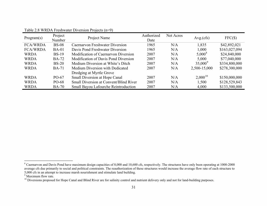
Table 2.8 WRDA Freshwater Diversion Projects (n=9)
Program(s) Project Number Project Name Authorized
Date Net Acres Avg.(cfs) FFC($)
FCA/WRDA BS-08 Caernarvon Freshwater Diversion 1965 N/A 1,835 $42,892,021 FCA/WRDA BA-01 Davis Pond Freshwater Diversion 1965 N/A 1,000 $163,027,094 WRDA BS-19 Modification of Caernarvon Diversion 2007 N/A 5,0008 $24,840,000 WRDA BA-72 Modification of Davis Pond Diversion 2007 N/A 5,000 $77,040,000 WRDA BS-20 Medium Diversion at White’s Ditch 2007 N/A 35,0009 $334,800,000 WRDA BA-71 Medium Diversion with Dedicated
Dredging at Myrtle Grove 2007 N/A 2,500-15,000 $278,300,000
WRDA PO-67 Small Diversion at Hope Canal 2007 N/A 2,00010 $150,000,000 WRDA PO-68 Small Diversion at Convent/Blind River 2007 N/A 1,500 $128,529,843 WRDA BA-70 Small Bayou Lafourche Reintroduction 2007 N/A 4,000 $133,500,000
8 Caernarvon and Davis Pond have maximum design capacities of 8,000 and 10,600 cfs, respectively. The structures have only been operating at 1000-2000 average cfs due primarily to social and political constraints. The reauthorization of these structures would increase the average flow rate of each structure to 5,000 cfs in an attempt to increase marsh nourishment and stimulate land building. 9 Maximum flow rate. 10 Diversions proposed for Hope Canal and Blind River are for salinity control and nutrient delivery only and not for land-building purposes.
31

Additionally, some values are absent due to incomplete reporting and some may
subsequently change over time due to social, political, and financial constraints or as new
information becomes available.
From the CWPPRA program data are available for 23 MC projects, 13 BI projects, and
15 FWD projects. An additional 85 project bids for CWPPRA and State projects are also
available, but these bids are limited only to RLB projects. Given the large-scale and high costs of
FWD projects, data must be collected from other programs. The LCA and WRDA initiatives
contain 9 additional FWD projects for which costs and benefits have been estimated. Despite
these limitations, these projects represent the best available historic data for informing future
investments in coastal restoration. To date, this baseline information has provided the basis for
more than $1 billion in coastal restoration spending in Louisiana alone. The challenge is to
determine if the data can be used to develop representative models of how the benefits and costs
of these projects accrue.
32

CHAPTER 3. GENERIC BENEFIT MODELS
3.1 Introduction
In order to develop a comprehensive economic comparison of RLB technologies and
FWD (existing and proposed) for coastal restoration, it is necessary to estimate and build generic
models that describe the way that these projects restore land over time. The rate and shape of
land gain, referred to as the restoration trajectory, is needed so that the elements of costs,
benefits, time and risk can be used in the economic analysis. Data for authorized CWPPRA
projects (n=51) described in Chapter 2 provide the basis for the development of generic benefit
models. Restoration trajectories in the following section are developed by using information
generated by the technical review within the CWPPRA committee.11 Under the program, net
acres are predicted for each project under two scenarios - future with-project and future without-
project. These predictions can be made on a yearly basis, but are more commonly provided at
only a few intervals during the 20-year project life.
3.2 Generic Benefit Model: Marsh Creation
Data for MC benefits were obtained from technical review documents for 23 projects
(Table 2.3). After examining inter-period acreage projections for these projects, the six most
representative MC projects were chosen for development of the generic benefits model. 12
Figure 3.1 depicts restoration trajectories for the six typical MC projects. As evident from these
curves, expected marsh creation usually follow a sigmoid trajectory in which net acres are static
or decreasing in year 1, followed by a rapid accrual of acreage in years 2-5. Most of the land
gained in the first 5 years is due to rapid placement of sediment from either a dredge or dredge 11 Technical review includes WVA assessments, project appendices, and ecological reviews. 12 Only a portion of the MC projects had inter-period acreage projection data available. After removal of outliers, six MC projects were chosen for development of the generic model.
33
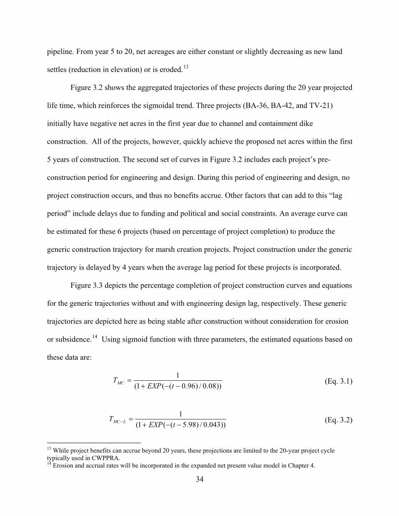
pipeline. From year 5 to 20, net acreages are either constant or slightly decreasing as new land
settles (reduction in elevation) or is eroded.13
Figure 3.2 shows the aggregated trajectories of these projects during the 20 year projected
life time, which reinforces the sigmoidal trend. Three projects (BA-36, BA-42, and TV-21)
initially have negative net acres in the first year due to channel and containment dike
construction. All of the projects, however, quickly achieve the proposed net acres within the first
5 years of construction. The second set of curves in Figure 3.2 includes each project’s pre-
construction period for engineering and design. During this period of engineering and design, no
project construction occurs, and thus no benefits accrue. Other factors that can add to this “lag
period” include delays due to funding and political and social constraints. An average curve can
be estimated for these 6 projects (based on percentage of project completion) to produce the
generic construction trajectory for marsh creation projects. Project construction under the generic
trajectory is delayed by 4 years when the average lag period for these projects is incorporated.
Figure 3.3 depicts the percentage completion of project construction curves and equations
for the generic trajectories without and with engineering design lag, respectively. These generic
trajectories are depicted here as being stable after construction without consideration for erosion
or subsidence.14 Using sigmoid function with three parameters, the estimated equations based on
these data are:
))08.0/)96.0((1(1−−+
=tEXP
TMC (Eq. 3.1)
))043.0/)98.5((1(1−−+
=− tEXPT LMC (Eq. 3.2)
13 While project benefits can accrue beyond 20 years, these projections are limited to the 20-year project cycle typically used in CWPPRA. 14 Erosion and accrual rates will be incorporated in the expanded net present value model in Chapter 4.
34
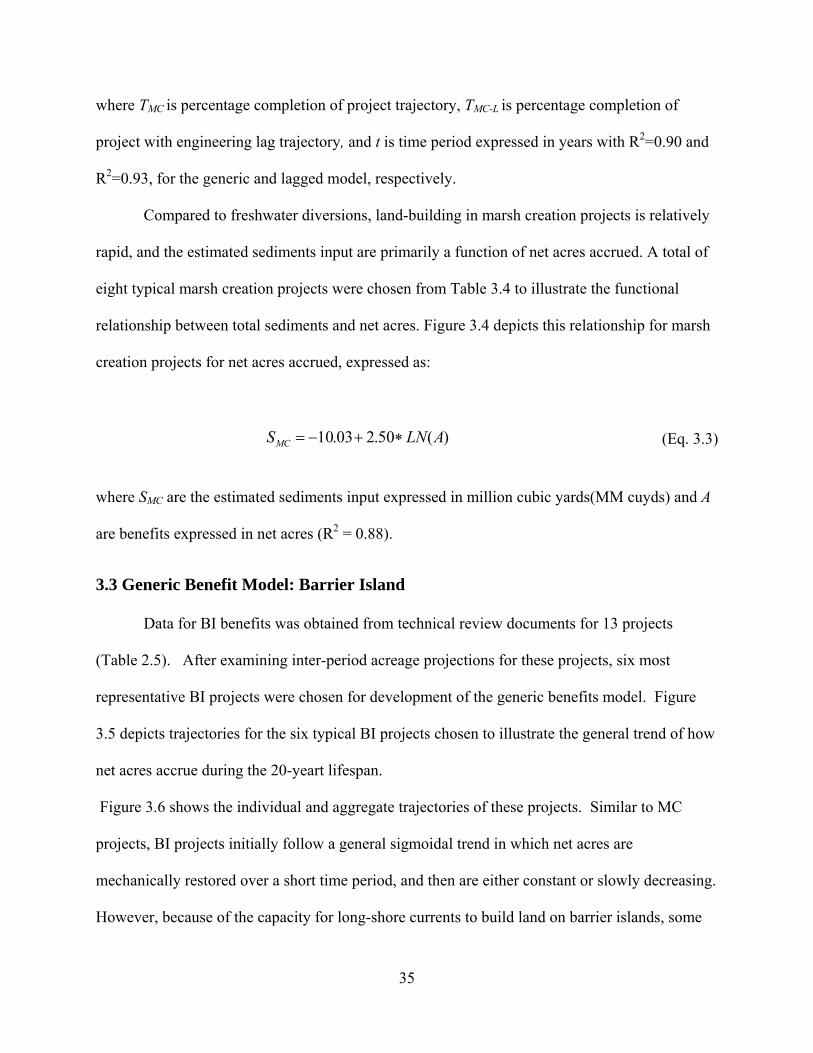
where TMC is percentage completion of project trajectory, TMC-L is percentage completion of
project with engineering lag trajectory, and t is time period expressed in years with R2=0.90 and
R2=0.93, for the generic and lagged model, respectively.
Compared to freshwater diversions, land-building in marsh creation projects is relatively
rapid, and the estimated sediments input are primarily a function of net acres accrued. A total of
eight typical marsh creation projects were chosen from Table 3.4 to illustrate the functional
relationship between total sediments and net acres. Figure 3.4 depicts this relationship for marsh
creation projects for net acres accrued, expressed as:
)(50.203.10 ALNSMC ∗+−= (Eq. 3.3)
where SMC are the estimated sediments input expressed in million cubic yards(MM cuyds) and A
are benefits expressed in net acres (R2 = 0.88).
3.3 Generic Benefit Model: Barrier Island
Data for BI benefits was obtained from technical review documents for 13 projects
(Table 2.5). After examining inter-period acreage projections for these projects, six most
representative BI projects were chosen for development of the generic benefits model. Figure
3.5 depicts trajectories for the six typical BI projects chosen to illustrate the general trend of how
net acres accrue during the 20-yeart lifespan.
Figure 3.6 shows the individual and aggregate trajectories of these projects. Similar to MC
projects, BI projects initially follow a general sigmoidal trend in which net acres are
mechanically restored over a short time period, and then are either constant or slowly decreasing.
However, because of the capacity for long-shore currents to build land on barrier islands, some
35

BA-42 (5.5 MM cyds)
Year
0 2 4 6 8 10 12 14 16 18 20
Net
Acr
es
-200
0
200
400
600
PO-33 (4 MM cyds)
Net
Acr
es
-200
0
200
400
600
BA-36 (6.8 MM cyds)
Year
0 2 4 6 8 10 12 14 16 18 20
TE-46 (1.3 MM cyds)N
et A
cres
-200
0
200
400
600
BA-39 (5.2 MM cyds)
TV-21 (2.4 MM cyds)
Figure 3.1 Six net acre trajectories by marsh creation technology under CWPPRA (n=6)
36
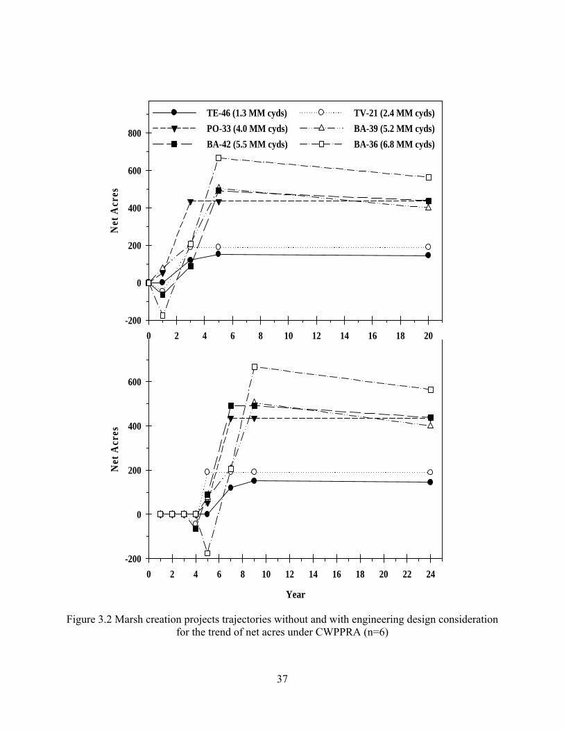
Year
0 2 4 6 8 10 12 14 16 18 20 22 24
Net
Acr
es
-200
0
200
400
600
0 2 4 6 8 10 12 14 16 18 20
Net
Acr
es
-200
0
200
400
600
800
TE-46 (1.3 MM cyds) TV-21 (2.4 MM cyds)PO-33 (4.0 MM cyds) BA-39 (5.2 MM cyds)BA-42 (5.5 MM cyds) BA-36 (6.8 MM cyds)
Figure 3.2 Marsh creation projects trajectories without and with engineering design consideration for the trend of net acres under CWPPRA (n=6)
37

CMC-L= 100/(1+EXP(-(t-5.98)/0.043))R2=0.93
Year
4 5 6 7
Perc
enta
ge o
f Con
stru
ctio
n w
ith L
ag
8
0
20
40
60
80
100
0 2 64 8
CMC= 100/(1+EXP(-(t-0.96)/0.08))R2=0.90
Perc
enta
ge o
f Con
stru
ctio
n
0
20
40
60
80
100
Figure 3.3 Marsh creation projects percent completion curves without and with engineering design consideration
38

SMC = -10.03+2.50*LN(A)R2=0.88
Net Acres
0 200 400 600
CuY
ds(M
M)
0.0
2.0
4.0
6.0
8.0
Figure 3.4 Estimated sediment requirements for marsh creation technology under CWPPRA (n=8)
39

of the CWPPRA models have restoration trajectories that predict gradual increases in land
beyond initial construction – usually after year 10. Modeling this trajectory is difficult because of
the dynamics of these systems, and also because of the extreme variability between projects. The
second set of curves in Figure 3.6 includes each project’s pre-construction period for engineering
and design. During the engineering and design stages, similar to marsh creation projects, no net
acres accrue. Meanwhile, funding and social constraints can be added to this stage to delay the
net acres accumulated.
Based on percentage of project completion, a global curve was estimated for these 6
projects to illustrate the generic construction trajectory for barrier island projects. Similar to
marsh creation project, project construction is delayed by an average of 4 years when the average
lag period for these projects is incorporated into the generic trajectory. Figure 3.7 depicts the
percentage completion of project construction curves and equations for this generic trajectory
without and with engineering design lag. As with marsh creation projects, the generic trajectories
depicted here are held stable after construction without consideration for long-shore sediment
transportation, erosion or subsidence. The equations for these generic curves are:
))0654.0/)89.0((1(1−−+
=tEXP
TBI (Eq. 3.4)
))0654.0/)89.4((1(1−−+
=− tEXPT LBI (Eq. 3.5)
40
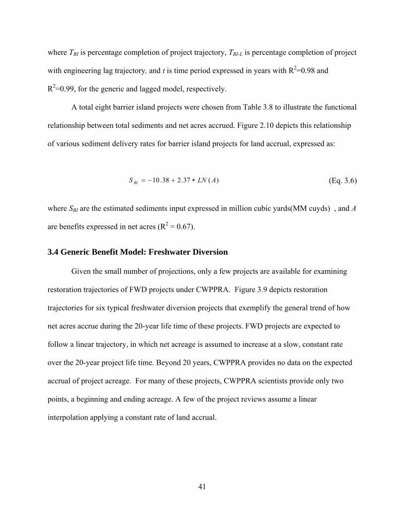
where TBI is percentage completion of project trajectory, TBI-L is percentage completion of project
with engineering lag trajectory, and t is time period expressed in years with R2=0.98 and
R2=0.99, for the generic and lagged model, respectively.
A total eight barrier island projects were chosen from Table 3.8 to illustrate the functional
relationship between total sediments and net acres accrued. Figure 2.10 depicts this relationship
of various sediment delivery rates for barrier island projects for land accrual, expressed as:
(Eq. 3.6))(37.238.10 ALNS BI ∗+−=
where SBI are the estimated sediments input expressed in million cubic yards(MM cuyds) , and A
are benefits expressed in net acres (R2 = 0.67).
3.4 Generic Benefit Model: Freshwater Diversion
Given the small number of projections, only a few projects are available for examining
restoration trajectories of FWD projects under CWPPRA. Figure 3.9 depicts restoration
trajectories for six typical freshwater diversion projects that exemplify the general trend of how
net acres accrue during the 20-year life time of these projects. FWD projects are expected to
follow a linear trajectory, in which net acreage is assumed to increase at a slow, constant rate
over the 20-year project life time. Beyond 20 years, CWPPRA provides no data on the expected
accrual of project acreage. For many of these projects, CWPPRA scientists provide only two
points, a beginning and ending acreage. A few of the project reviews assume a linear
interpolation applying a constant rate of land accrual.
41

TE-47 (4.0 MM cyds)
Year
0 2 4 6 8 10 12 14 16 18 20
Net
Acr
es
-200
0
200
400
600
BA-40 (2.4 MM cyds)
Net
Acr
es
-200
0
200
400
600
TE-30 (1.7 MM cyds)N
et A
cres
-200
0
200
400
600
TE-50 (2.0 MM cyds)
BA-35 (2.6 MM cyds)
BA-38 (4.0 MM cyds)
Year
0 2 4 6 8 10 12 14 16 18 20
Figure 3.5 Six net acre trajectories by barrier island technology under CWPPRA (n=6)
42

Year
0 2 4 6 8 10 12 14 16 18 20 22 24
Net
Acr
es
0
150
300
450
0 2 4 6 8 10 12 14 16 18 20
Net
Acr
es
0
150
300
450
600 TE-30 (1.7 MM cyds) TE-50 (2.0 MM cyds)
BA-40 (2.4 MM cyds) BA-35 (2.6 MM cyds)TE-47 (4.0 MM cyds) BA-38 (4.0 MM cyds)
Figure 3.6 Barrier island projects trajectories without and with engineering design consideration for the trend of net acres under CWPPRA (n=6)
43

TBI= 1/(1+EXP(-(t-0.89)/0.0654))R2=0.98
Perc
enta
ge o
f Con
stru
ctio
n
0
20
40
60
80
100
TBI-L= 1/(1+EXP(-(t-4.89)/0.0654))R2=0.99
Years
0 2 4 6 8
Perc
enta
ge o
f Con
stru
ctio
n w
ith L
ag
10
0
20
40
60
80
100
Figure 3.7 Barrier island projects percent completion curves without and with engineering design consideration
44
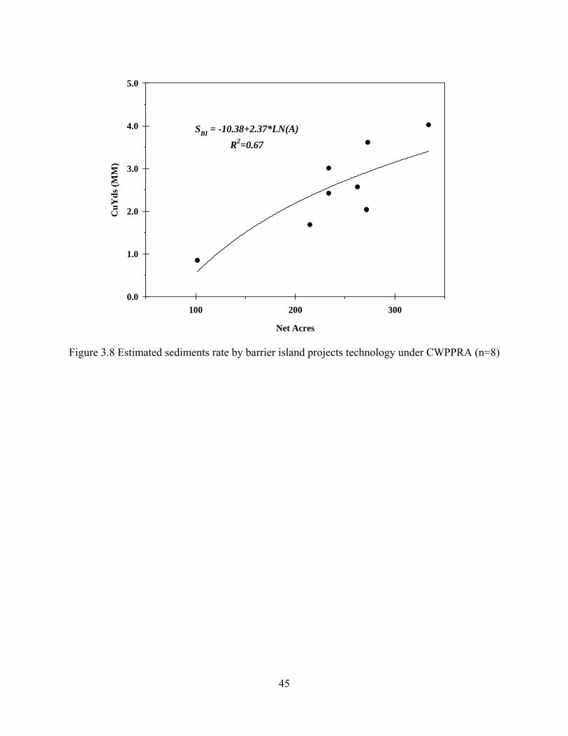
SBI = -10.38+2.37*LN(A)R2=0.67
Net Acres
100 200 300
CuY
ds (M
M)
0.0
1.0
2.0
3.0
4.0
5.0
Figure 3.8 Estimated sediments rate by barrier island projects technology under CWPPRA (n=8)
45

Figure 3.10 shows the aggregated trajectories for six typical freshwater diversion projects
which follow a gradually land increase after the completion of project structure.15 The second
set of curves in Figure 3.10 shows these trajectories under engineering and design consideration.
Similar to marsh creation and barrier island projects, no benefits accrue during this lag stage.
Project construction under the generic trajectory is delayed by an average of 7 years when the
average lag period for these projects is incorporated.16 Figure 3.11 depicts the generic
trajectories and equations for these FWD projects. It is important to note that the generic
trajectory here is cumulative percentage of net acre accrual. Given that these projects take an
average of 2 years to construct, the actual lag period is 9 years before any acreage begins to
accrue. The graphics depicted in Figure 3.11 represent this trajectory without and with
engineering design lag, respectively. With erosion and natural land accrual rates held constant,
these generic trajectories depict a gradual and stable rate of benefit increase after construction.
The constant land accrual rate is depicted by the simple regression lines, and the equations for
these generic curves are given by:
tTFWD ∗+−= 0501.00029.0 (Eq. 3.7)
tT LFWD ∗+−=− 0375.01394.0 (Eq. 3.8)
15 It should be noted that completion of project construction here does not immediately produce acreage benefits as with RLB projects. In this situation, construction refers to completion of the project structure (i.e. siphons, gates, culverts, etc.) 16 Freshwater diversions projects have historically had a longer average lag period because social constraints tend to be greater for these projects (e.g. land rights acquisition, fisheries implications, salinity changes, etc.). The lag period of the CWPPRA-funded freshwater diversion projects listed in Table 2.5 ranges from 1 to 13 years.
46
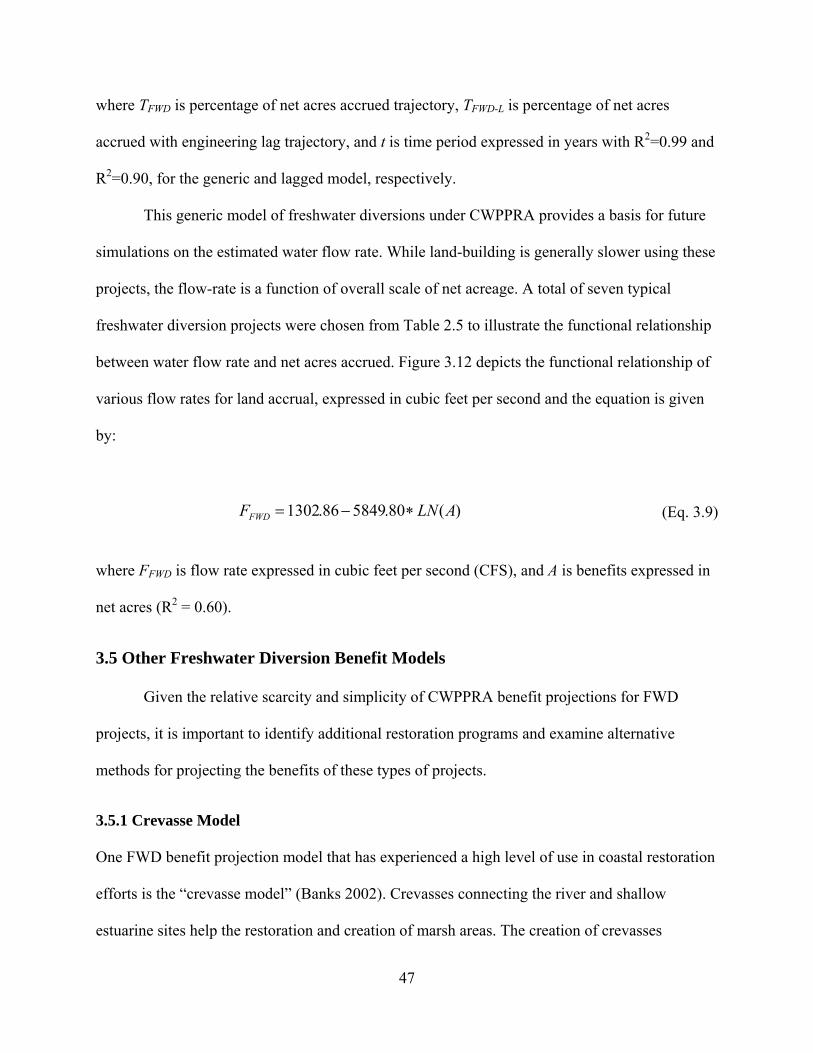
where TFWD is percentage of net acres accrued trajectory, TFWD-L is percentage of net acres
accrued with engineering lag trajectory, and t is time period expressed in years with R2=0.99 and
R2=0.90, for the generic and lagged model, respectively.
This generic model of freshwater diversions under CWPPRA provides a basis for future
simulations on the estimated water flow rate. While land-building is generally slower using these
projects, the flow-rate is a function of overall scale of net acreage. A total of seven typical
freshwater diversion projects were chosen from Table 2.5 to illustrate the functional relationship
between water flow rate and net acres accrued. Figure 3.12 depicts the functional relationship of
various flow rates for land accrual, expressed in cubic feet per second and the equation is given
by:
)(80.584986.1302 ALNFFWD ∗−= (Eq. 3.9)
where FFWD is flow rate expressed in cubic feet per second (CFS), and A is benefits expressed in
net acres (R2 = 0.60).
3.5 Other Freshwater Diversion Benefit Models
Given the relative scarcity and simplicity of CWPPRA benefit projections for FWD
projects, it is important to identify additional restoration programs and examine alternative
methods for projecting the benefits of these types of projects.
3.5.1 Crevasse Model
One FWD benefit projection model that has experienced a high level of use in coastal restoration
efforts is the “crevasse model” (Banks 2002). Crevasses connecting the river and shallow
estuarine sites help the restoration and creation of marsh areas. The creation of crevasses
47

MR-06 (2500 cfs)
Year
0 2 4 6 8 10 12 14 16 18 20
Net
Acr
es
0
200
400
600
800
1000
MR-14 (1350 cfs)
Net
Acr
es
0
200
400
600
800
1000
BS-12 (500 cfs)
Net
Acr
es
0
200
400
600
800
1000
TE-32a (3750 cfs)
Year
0 2 4 6 8 10 12 14 16 18 20
BS-10 (2500 cfs)
TE-49 (1000 cfs)
Figure 3.9 Six net acre trajectories by freshwater diversion technology under CWPPRA (n=6)
48
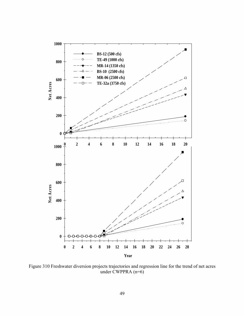
Year
0 2 4 6 8 10 12 14 16 18 20 22 24 26 28
Net
Acr
es
0
200
400
600
800
1000 0 2 4 6 8 10 12 14 16 18 20
Net
Acr
es
0
200
400
600
800
1000
BS-12 (500 cfs)TE-49 (1000 cfs)MR-14 (1350 cfs)BS-10 (2500 cfs)MR-06 (2500 cfs)TE-32a (3750 cfs)
Figure 310 Freshwater diversion projects trajectories and regression line for the trend of net acres under CWPPRA (n=6)
49

TFWD= -0.0029+0.0501*tR2=0.99
Perc
enta
ge o
f Net
Acr
es A
ccru
ed
0
20
40
60
80
100
TFWD-L= -0.1394+0.0375*tR2=0.90
Years
0 2 4 6 8 10 12 14 16 18 20 22 24 26 28
Perc
enta
ge o
f Net
Acr
e A
ccru
ed w
ith L
ag
0
20
40
60
80
100
Figure 3.11 Fresh water diversion projects percentage of net acre accrued curve without and with engineering design consideration
50
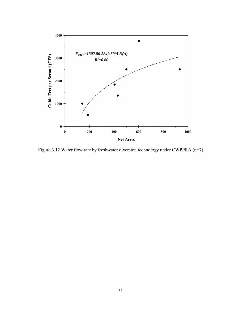
FFWD=1302.86-5849.80*LN(A)R2=0.60
Net Acres
0 200 400 600 800 1000
Cub
ic F
eet p
er S
econ
d (C
FS)
0
1000
2000
3000
4000
Figure 3.12 Water flow rate by freshwater diversion technology under CWPPRA (n=7)
51

not only helps to rebuild the desired site but also helps to mimic natural paths in a river with
modified hydrology. According to Banks (2002), “the most successful crevasse is one that
discharges from a large pass into a large, open-ended receiving basin that allows water to flow
efficiently through the system.” To predict the growth rate of land building, the author employed
a multiple linear regression analysis to explore the relationship between the selected parameters
and growth rate. The model is given by:
RACCSACAPWPOG ∗+∗+∗−∗+∗−= 004.0039.0324.0002.0299.1097.3 (Eq. 3.10)
where: G refers to the growth rate of land building. PO stands for parent order, which is a
descriptive variable used to denote the source and scale of the incoming water source. Where the
Mississippi and Atchafalaya Rivers are examples of a primary (PO=1), and distributaries are
numbered 2, 3, and 4 based on size and scale. PW is parent channel width, CA is crevasse age,
CCSA is crevasse cross-sectional area, and RA is receiving area (Banks 2002).
3.5.2 N-SED Model
Unlike the project described above, most large-scale FWD projects use controlled structures17
and thus can’t be modeled as a natural flow crevasse. For these projects, an alternative model
has been developed. Boustany (2007) developed a model for FWD projects that incorporates a
“mass balance”18 approach to estimate project benefits. Under the N-SED1 model (i.e. short for
Nutrient-Sediment model #1), land building is a function of flow rate, nutrients and sediments.
Within these three module components there are 21 sub-variables and sub-functions that govern
the way that benefits (net acres) accrue under a given combination of assumptions. Given the
17 Controlled structures are those diversions that use a valve or a gate to control the flow of water. 18 The “mass balance” approach here refers to a numerical method of projecting the output of net land as a function of specific inputs of associated with freshwater, nutrients, and sediments into a specific project area.
52
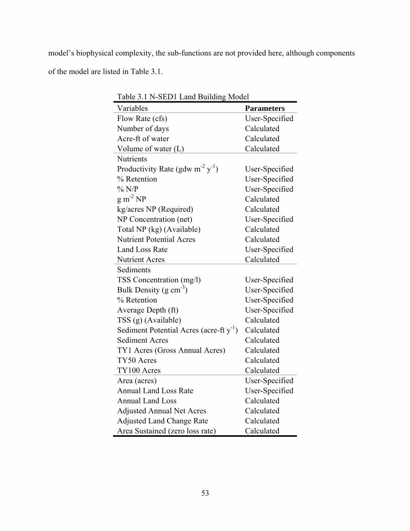
model’s biophysical complexity, the sub-functions are not provided here, although components
of the model are listed in Table 3.1.
Table 3.1 N-SED1 Land Building Model Parameters Variables
Flow Rate (cfs) User-Specified Number of days Calculated Acre-ft of water Calculated Volume of water (L) Calculated Nutrients Productivity Rate (gdw m-2 y-1) User-Specified % Retention User-Specified % N/P User-Specified g m-2 NP Calculated kg/acres NP (Required) Calculated NP Concentration (net) User-Specified Total NP (kg) (Available) Calculated Nutrient Potential Acres Calculated Land Loss Rate User-Specified Nutrient Acres Calculated Sediments TSS Concentration (mg/l) User-Specified Bulk Density (g cm-3) User-Specified % Retention User-Specified Average Depth (ft) User-Specified TSS (g) (Available) Calculated Sediment Potential Acres (acre-ft y-1) Calculated Sediment Acres Calculated TY1 Acres (Gross Annual Acres) Calculated TY50 Acres Calculated TY100 Acres Calculated Area (acres) User-Specified Annual Land Loss Rate User-Specified Annual Land Loss Calculated Adjusted Annual Net Acres Calculated Adjusted Land Change Rate Calculated Area Sustained (zero loss rate) Calculated
53
According to Boustany (2010), the flow rate is specified and based on particular
combinations of descriptors, including project goal, location, and scale. The number of days at a
particular flow rate is used to determine the volume of source water. Nutrient benefits are based
on total nitrogen and phosphorus concentration in the source water, nutrients required for plants
based upon annual growth rates, and the percentage of nutrients retained in the system. Sediment
benefits are based upon total amount of suspended solids in the source water, bulk density of
marsh in the project area, average depth, and retention of these materials introduced. Nutrient
benefits and sediment benefits are combined together and used to adjust the overall land loss rate.
3.5.3 Extant Flood Control Structures
Finally, benefits of FWD projects can also be projected by using existing flood control
projects (FCP) such as the Bonnet Carre Spillway on Lake Pontchartrain and the Morganza
Spillway in east central Louisiana. The largest existing FCP is the Old River Control Structure,
commissioned in 1954. This structure has received 30 percent of the Mississippi River’s annual
average flow rate (495,000 cfs) since the project was completed in 1963 (CWPPRA 2000).
Sedimentation rates in the Atchafalaya Basin and the deltas forming at Wax Lake and
Atchafalaya Bay provide evidence of the power of a large scale diversion to build new land.
According to CWPPRA, the lower Atchafalaya Delta and Wax Lake delta currently have a total
of 16,000 acres of subaerial land.19 Given the land building that is occurring from sediments and
nutrients via the Atchafalaya River, the region is expected to have an additional 67,000 acres in
the year 2050, a growth rate of 1,275 acres per year. This rate is for net acreage of coastal land,
and does not reflect the submarine infilling of sediments into deeper water bodies.
19 The term subaerial is mainly used in geology to describe structures that existing, occurring, or formed in the open air or on the earth’s surface, not under water or underground.
54

3.6 Summary
Developing generic benefit models of coastal restoration projects is constrained by two
major factors: 1) there are relatively few programs that sponsor such projects from which
benefits can be estimated in a standardized way; and 2) variation within comparable project types
is often very large. An evaluation of 124 CWPPRA projects provided data for 23 marsh creation
projects, 13 barrier island projects, and 15 freshwater diversion projects. While apparently the
least expensive of these three methods, FWD projects require a relatively long time to restore or
create new land. The constant, linear accrual rate of FWD projects is in stark contrast to the
rapid, mechanical construction of net acres achieved under marsh creation and barrier island
projects – which by comparison, are three to eight times more expensive to construct,
respectively. This wide range of physical scales produces difficulties in the production of
generic restoration trajectories. Alternative models for estimating FWD benefits have recently
become available for large-scale, WRDA sponsored projects. The crevasse model is one
example; however, the N-SED1 model has been used more for the technical review of FWD
projects. In addition to the generic benefits models derived here, the crevasse and N-SED1 model
can also be used in the cost-benefit simulations.
The fit of generic restoration trajectories is general given the limited data. These three
project types represent the extreme ends of the restoration natural-to-artificial continuum from
less expensive to more expensive, from slow to rapid. From the standpoint of time, the MC
technology is almost four times faster than FWD technology. From the viewpoint of cost, the
average cost per net acre for MC technology ($100,795) is 2.68 times higher than that of
freshwater diversion technology ($37,619). While descriptive statistics on project costs were
identified in Chapter 2, specific drivers of these costs have not been estimated. Similar to benefit
55

trajectories, generic cost models by technology are needed for benefit-cost simulations. Such
models would reflect the cost of establishing physical quantities of wetland restoration ($/net
acre) as a function of location, time and scale variables (e.g. dredging quantity and volume of
flow).
56

CHAPTER 4. GENERIC COST MODELS
4.1 Introduction
In Chapter 3, projects authorized under CWPPRA were used to develop generic
trajectories of coastal restoration benefits. Additional projects authorized under WRDA were
also considered, along with alternative benefit projection models. This chapter is concerned with
understanding the costs associated with those trajectories. Specifically, how have costs for
marsh creation (MC), barrier island (BI), and freshwater diversion (FWD) projects been
calculated in the past, and how are those costs determined today. The relevant questions are:
What have been the historic drivers of project costs? What are the present drivers of project cost?
How can these drivers be used to build generic cost models for these three methods?
To better examine the effectiveness of RLB and FWD restoration projects, some generic
understanding of project costs is necessary. Aust (2006) developed cost models of CWPPRA
projects on a dollar per AAHU basis. Comparison assessments developed using CWPPRA data
on a dollar per net acre basis will provide information on the differences between quality
(AAHU) and quantity (net acres) as drivers of project efficiency. Additionally, bid data from
recent and pending projects can be used to estimate the major cost components of construction.
Bids are legal contracts, which contain detailed project information. Indeed, all authorized
wetland restoration projects funded by state or federal agencies have been based on contract bids.
All generic cost models are developed by building on the descriptive data for project costs
outlined in Chapter 2 (Tables 2.1 - 2.8).
Generic cost functions for each project type were developed using regression analysis.
Potential drivers of costs were selected as independent variables and obtained from the following
sources: past and current cost projections, project bids, and project alternatives; project
57

operation, maintenance, and monitoring reports; fact sheets, monitoring plans, completion
reports, ecological reviews, PPL appendices, and personal communication with CWPPRA
project managers (CWPPRA 2010; Browning 2010).
Regression models were constructed to determine the relationship between dependent and
independent variables by fitting a linear equation to observed data. The basic regression model is
given by:
nn XXXY ββββ +⋅⋅⋅+++= 221`10 (Eq. 4.1)
where Y is the dependent variable, X is a series of independent variables. The parameter β0 is the
intercept and parameters β1, β2 … βn are the regression coefficients (Abraham and Ledolter
2005). The following sections use multiple regression techniques to estimate the cost models for
MC, BI, and FWD projects.
4.2 Potential Variables
The following section defines the dependent and independent variables for regression
models to determine past and present drivers of project costs and project materials. Separate
models are estimated for each of the three wetland restoration types being investigated (MC, BI
and FWD), and in some cases, specific variables are used as dependent or independent variables,
depending on the modeling objective. All variables were identified through consultation with
coastal scientists and restoration project managers. A list of the dependent and independent
variables utilized is provided below and in Table 4.1.
58

4.2.1 Dependent Variables (Cost Models)
• Dollars per Net Acre ($/Net Acre): For CWPPRA authorized projects, dollars per net acre is used to measure program efficiency. This measure divides the fully funded costs of a project by the total net acres (NA) created, restored, and enhanced during the 20 years project life.
• Construction Cost (CCM and CCB): For authorized and bidded CWPPRA projects, the total construction costs (CC) refers to the total costs for completing the built portion of the restoration project. For MC and BI projects, this includes all project-specific structures. CC is limited to construction of the project structure only. On average, CC comprises approximately 85% of total costs for CWPPRA projects (M=marsh creation, B=barrier island).
• Total Cost (FWD) (TCF): This is the total cost estimate for completion of all tasks associated with construction of a freshwater diversion project. It is generally compose of three types of costs; engineering and design, construction costs, and operation and monitoring (F=freshwater diversion). 20
4.2.2 Dependent Variables (Materials Models)
• Dredged Material (Cubic Yards of Sediment CYDM and CYDB): In this research, the physical materials were considered dependent variables associate with acreage created, project elevation and depth for MC and BI projects.
• Average Flow rate (AFRF): Similar to RLB project, the physical materials, cubic feet per second (CFS) or average flow rate (AFRF), was considered as a dependent variable associated with acreage accrued, project boundary area for FWD projects.
4.2.3 Independent Variables (Cost Models)
• Priority Project List (PPL): The PPL is a term developed by CWPPRA that describes the annually produced list of high priority restoration projects. Since the CWPPRA program was enacted in 1990, there have been 19 PPLs. This list, referred to as the “Priority Project List” or “PPL”, includes only those projects that have been authorized for funding in a given year. For example, PPL 1 means the project was approved in 1991 and PPL 2 means this project was approved in 1992. Over time, project costs have increased dramatically. Previous research has shown that a positive relationship exists between costs and time (PPL). Aust (2006) theorized that this might occur if the easy projects were completed in earlier years, with an increasing number of large and complex projects appearing in recent years. Program managers have also pointed out that apparent
20 The total costs (TC) refers to the fully funded cost (FFC) of a RLB or FWD project in this research. The typical planning horizon for CWPPRA projects is 20 years.
59

increases in cost over time may be driven by more comprehensive cost accounting (Roy 2005).
• Project Boundary Area (PBA): PBA refers to the total benefited area (includes acres
enhanced) determined by the CWPPRA Environmental Work Group during the Wetland Value Assessment (WVA) process. The relationship between project boundary and costs is unknown.
• Average Annual Habitat Units (AAHU): AAHU as determined by the CWPPRA Environmental Work Group, represent a numerical integration of variables focused on habitat quality within a given area at a given point in time. AAHU represent the average number of habitat units within any given year over the project life for a given area. Aust (2006) found that project costs per unit generally decrease with AAHU increase, this indict potential economies of scale.
• Dredged Material (CYD): For RLB project, dredged material measured in cubic yards
(CYD), comprises a substantial portion of total construction costs. The expected relationship between costs and sediments is positive. The more sediment needed, the higher the costs are expected to be.
• Distance (DIST): For RLB project, DIST is the distance in miles from sediment borrows
site(s) to the marsh creation site(s). Data for this variable were collected from project fact sheets, scaled project maps, or from project managers. In general, the longer the distance, the higher the costs (i.e. positive relationship between cost and distance).
• Mobilization (MOB): Overhead expenditures include a wide range of costs, for RLB
projects one of the largest overhead costs is the transporting of large-scale dredge equipment to and from the project site. Mobilization and demobilization costs (MOB) include the installation and removal of all on-site support facilities needed for the project. So, this variable is expected to have a positive relationship with costs.
• Dredge Size (DS): Most RLB projects use bucket dredge or a cutter-head dredge. For projects that pump dredged sediment from remote borrow sites, the dredge size diameter and initial pipeline diameter ranges from 24 inches to 36 inches. The expected relationship between dredge size (DS) and costs is unknown and depends on the operational efficiency of the particular dredge being used.
• Payment Type (PYT): For RLB project, contractors usually receive payment in one of two ways – they are either paid by the cut or by the fill. If they are paid by cut, the compensation is based on the amount of sediments removed from the borrow site. If they are paid by fill, the compensation is based on the average filling elevation of the target project site. In this case, PYT is a binary variable. In general, payment by fill is the most costly for contractors because of sediment settlement and sediment losses from the project area.
60

• Pumps (BP): For RLB project, booster pumps (BP) can help transport sediments needed for land building restoration. The number of booster pumps needed depends on the distance from sediment borrow site to marsh creation site. Usually every 5 miles one booster pump is needed to assistant in the movement of sediment slurry through the pipeline. The expected relationship is positive between the costs and the number of booster pump.
• Average Flow rate (AFR): For FWD project, water flow rate is usually measured in cubic feet per second (CFS). Water flow rate can be measured regularly or measured over time in different seasons. Because these rates vary, an average annual flow rate is used to quantify this parameter. The higher the average annual flow rate, the more sediment and nutrition input provided. Average flow rate is expected have positive relationship with project costs.
• Diversion Control (CON): For FWD project, control of flow rate is accomplished by gates, culverts, siphons, constructed channels, weirs, and natural crevasses. There are basically two ways to manage these projects - one is the manual control of water discharge over a certain time horizon, and the other involves uncontrolled discharges which allow the water to flow naturally to nourish the target area. In generally, controlled freshwater diversion projects have higher costs compared to uncontrolled FWD projects (which, in general, have lower operation and monitoring cost).
• Containment Dikes (CD): For RLB project, containment dikes or small levees are often constructed to maintain sediment slurry. The expected effect on cost is positive.
• Access Dredging (AD): For RLB and FWD project, access dredging is often required to get heavy equipment on location or to provide a conduit for the distribution of sediment and nutrients. The expected effect on cost is positive.
4.2.4 Independent Variables (Materials Models)
• Net Acres (NA): This measure is total net acres for a project. It includes acres of emergent marsh protected, created, and restored. The relationship between net acres and costs is expected to be positive.
• Average Elevation (AVE): For RLB project, elevation is the project site elevation above
sea level, using the standard North American Vertical Datum 1988 (NAVD88). Although different elevation targets can be reported within each project, a summary or average elevation estimate is provided for most projects.
• Average Depth (AEP): For RLB projects, depth is the project site depth below sea level,
using the standard North American Vertical Datum 1988 (NAVD88). Although different depths can be reported within the initial boundary for each project, a summary or average depth is provided by consultation with CWPPRA project engineers. The relationship between average depth and costs is expected to be positive.
61

• Target Thickness (THK) For RLB project, target thickness is the difference between average elevation and average depth. Although thickness measures may vary across a project boundary, the target thickness is a summary or average for the entire project estimated by CWPPRA project engineers. The relationship between thickness and costs is expected to be positive. In combination with target acreage, this variable is expected to be a significant driver of the quantity of sediments (CYD) required for a RLB project.
Table 4.1 Variable Descriptions and Expected Signs Variable Abbreviation Variable Description Dependent Variables $/Net Acre Dollars per Net Acre CCM and CCB Total Construction Costs for MC and BI Projects TCF Total Costs for FWD projects CYDM and CYDB Dredged Material for MC and BI Projects AFRF Average Flow rate for FWD projects Independent Variables Expected
Sign PPL Project Priority List (Year) + PBA Project Boundary Area unknown AAHU Average Annual Habitat Units - CYD Cubic Yard of Sediments + DIST Average Sediment Transport Distance + MOB Mobilization and demobilization + DS Dredge Size (diameter in inches) unknown PYT Payment Type (Cut=0, Fill=1) - BP Number of Booster Pumps + AFR Average Annual Water Flow Rate (CFS) + CON Diversion Control (Natural Flow=0, Manual
Control=1) +
CD Containment Dikes + AD Access Dredging + NA Net Acres + AVE Average Project Elevation + ADP Average Depth + THK Target Thickness +
4.3 Generic Cost Models: Marsh Creation
4.3.1 Historic Drivers of MC Cost
A total of 23 authorized MC projects from CWPPRA (1990-2009) were examined for
development of a generic cost model. Twelve of these projects have been completed and 11 are
62

under construction or in the engineering or design stages. Nine variables were selected to
construct a conceptual cost relationship:
),,,,,,,,(/$ AAHUBPPYTDSMOBDISTPBACYDPPLfNAM = (Eq. 4.2)
where $/NAM is the cost for an MC project expressed in dollars per net acre and PPL, CYD,
PBA, DIST, MOB, DS, PYT, BP, and AAHU are independent variables (Table 4.1). The
assumption is that MC project costs have a linear relationship with these independent variables.
Due to data gaps, 12 of the 23 MC projects contained data for all nine independent
variables. Data for the model were imported and analyzed into statistical programs SigmaPlot
11.0 and SAS 9.1. The resulting analysis is contained in Table 4.2.
Table 4.2 Parameter Estimate 1: March Creation Costs - $/NAM N=12 R-square = 0.98
Variable ParameterEstimate
StandardError t Value Pr > |t|
Variance Inflation21
Intercept -131942 61460 -2.15 0.16 0
PPL -11148 3600.35 -3.10 0.09 20.98
CYD -3426.67 2859.56 -1.20 0.35 3.46
PBA 9.04 1.86 4.86 0.04 3.16
DIST 3958.57 3237.73 1.22 0.35 6.10
MOB 0.02 0.01 1.42 0.29 27.09
DS 14076 3470.14 4.06 0.06 13.60
PYT 20041 8928.53 2.24 0.15 2.60
BP -65002 18580 -3.50 0.07 12.32
AAHU -172.50 48.40 -3.56 0.07 3.32
21 Variance inflation factors are a measure of the multicollinearity in a regression design matrix. A VIF value is greater than 10 is an indication of potential multicollinearity problems.
63
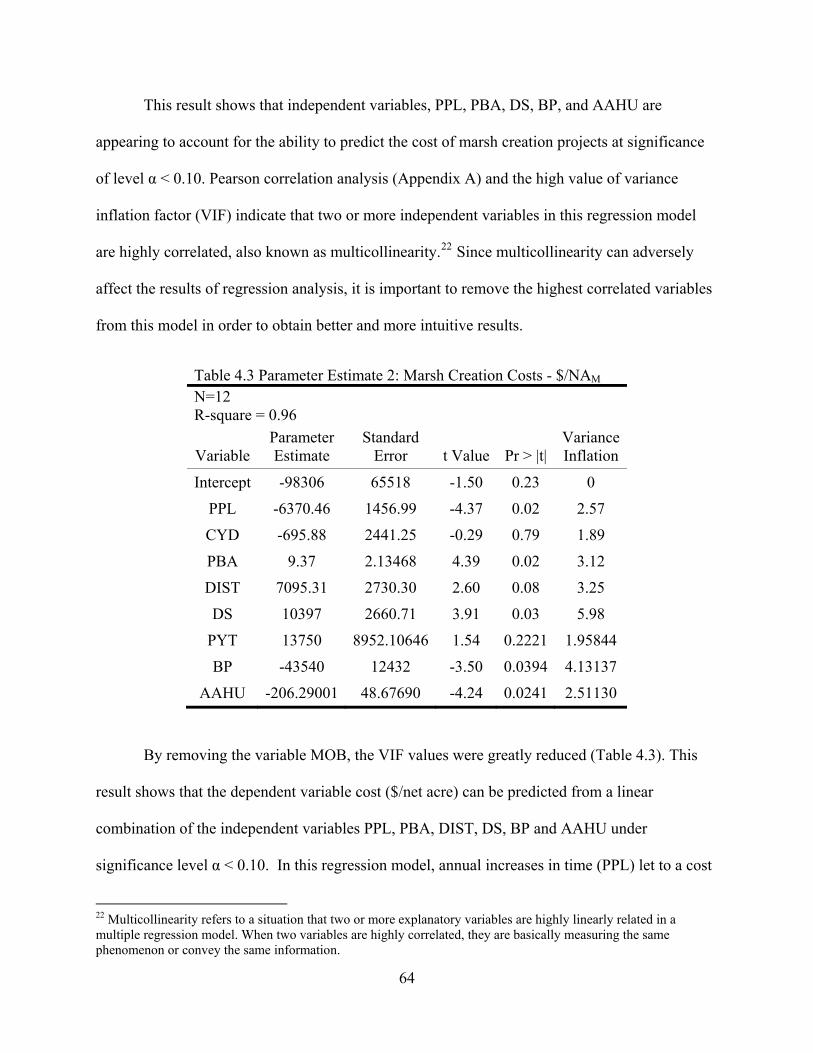
This result shows that independent variables, PPL, PBA, DS, BP, and AAHU are
appearing to account for the ability to predict the cost of marsh creation projects at significance
of level α < 0.10. Pearson correlation analysis (Appendix A) and the high value of variance
inflation factor (VIF) indicate that two or more independent variables in this regression model
are highly correlated, also known as multicollinearity.22 Since multicollinearity can adversely
affect the results of regression analysis, it is important to remove the highest correlated variables
from this model in order to obtain better and more intuitive results.
Table 4.3 Parameter Estimate 2: Marsh Creation Costs - $/NAM N=12 R-square = 0.96
Variable ParameterEstimate
Standard Error t Value Pr > |t|
Variance Inflation
Intercept -98306 65518 -1.50 0.23 0
PPL -6370.46 1456.99 -4.37 0.02 2.57
CYD -695.88 2441.25 -0.29 0.79 1.89
PBA 9.37 2.13468 4.39 0.02 3.12
DIST 7095.31 2730.30 2.60 0.08 3.25
DS 10397 2660.71 3.91 0.03 5.98
PYT 13750 8952.10646 1.54 0.2221 1.95844
BP -43540 12432 -3.50 0.0394 4.13137
AAHU -206.29001 48.67690 -4.24 0.0241 2.51130
By removing the variable MOB, the VIF values were greatly reduced (Table 4.3). This
result shows that the dependent variable cost ($/net acre) can be predicted from a linear
combination of the independent variables PPL, PBA, DIST, DS, BP and AAHU under
significance level α < 0.10. In this regression model, annual increases in time (PPL) let to a cost
22 Multicollinearity refers to a situation that two or more explanatory variables are highly linearly related in a multiple regression model. When two variables are highly correlated, they are basically measuring the same phenomenon or convey the same information.
64
decrease of $6,370.46/net acre for marsh creation (with PBA, DIST, DS, BP and AAHU held
constant). This finding is the opposite of what Aust (2006) found for the effects of time on the
cost for all project types combines.23 A unit increase in the number of booster pumps (BP)
results in decreased costs of $43,540/net acre. This result also is the opposite of what was
expected. Even more confounding is that the variable CYD, expected to be highly important,
does not emerge as a significant driver. This result is likely due to the limited number of useable
observations and the huge cost variations between and within MC projects authorized under
CWPPRA during the past 20 years.
4.3.2 Present Drivers of MC Cost
An alternative cost model can be constructed using more current data (2000-2009) from
project bids in which total construction costs (CC) is the dependent variable. A total of 34 MC
project bids were examined to develop an alternative generic cost model for MC projects. Due to
data limitations, this more simplified, bid-based model is conceptualized with five variables that
account for 93 percent of average construction costs. The conceptual cost relationship is given
by:
),,,( ADDISTMOBCYDfCCM = (Eq. 4.3)
where CCM is the total construction costs for a MC project expressed in dollars based on bidded
project data and CYD, MOB, DIST, and AD are independent variables (Table 4.1). The
assumption is that the CC of MC project has a linear relationship with CYD, MOB, DIST, and AD
23 Aust (2006) did not develop cost models for specific project types; rather the analysis was for all project types combined.
65

variables. Data for the MC construction costs model were imported and analyzed in statistical
programs SigmaPlot 11.0 and SAS 9.1. The resulting analysis is contained in Table 4.4.
Table 4.4 Parameter Estimate 3: Marsh Creation Construction Costs - CCM N=34 R-square = 0.94
Variable Parameter Estimate
Standard Error t Value Pr > |t|
Variance Inflation
Intercept -1507336 1676901 -0.90 0.3761 0 CYD 2486867 688322 3.61 0.0011 3.15583 MOB 2.73887 0.90917 3.01 0.0053 3.69121 DIST 2379910 1084981 2.19 0.0364 2.59813 AD 15.10992 2.73958 5.52 <.0001 3.28683
From the statistical analysis results, variables, CYD, MOB, DIST and AD were
significant drivers of the costs for MC projects (α=0.10 R2=0.93). Based on the statistical
analyses, the linear regression model for future MC projects bids is given by:
ADDISTMOBCYDCCM ∗+∗+∗+∗+−= 11.15237991074.224868671507336 (Eq. 4.4)
In this regression model, the CCM increase $2,486,867 when the average dredged
material increases one million cubic yard (with MOB, DIST, and AD held constant). The
construction costs increase $2.74 when the MOB increase one dollar (with CYD, DIST, and AD
held constant). The construction costs increase $2,379,910 when the distance from the sediment
borrow site to marsh creation site increases one mile (with CYD, MOB, and AD held constant).
The construction costs increase $15.11 when the AD cost increase one dollar (with CYD, MOB,
and DIST held constant).
66

In addition to the CCM model, it is helpful to develop a physical materials model in order
to account for additional factors that influence the total quantity of sediments needed to build an
MC project. While Figure 3.4 describes this as a simple function of acreage, additional variables
can be used to refine the relationship. A conceptual model is that the CYD of MC project is a
function of NA, AVE, DEP, and THK. Due to the data limitations, there are only a few DEP and
THK data available. The conceptual model for the sediment required in a MC project was
simplified and is given by:
),( AVENAfCYDM = (Eq. 4.5)
where CYDM is the total sediments required for an MC project expressed in millions of cubic
yards and NA and AVE are independent variables (Table 4.1). The assumption is that the CYD of
MC project has a linear relationship with NA and AVE variables. The MC sediments model were
imported and analyzed in SigmaPlot 11.0 and SAS 9.1. The resulting analysis is contained in
Table 4.5.
Table 4.5 Parameter Estimate 4: Marsh Materials Model - CYDM N=16 R-square = 0.59
Parameter Estimate
Standard Error t Value Pr > |t|
Variance Inflation
Intercept 4.50205 1.94679 2.31 0.0378 0 NA 0.00544 0.00188 2.90 0.0123 1.09499
AVE -1.30727 0.59703 -2.19 0.0474 1.09499
Results indicate that NA and AVE were significant drivers of the sediments required for
MC projects (α=0.10 R2=0.59). Results from Pearson correlation coefficients analysis indicated
67
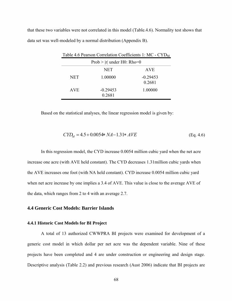
that these two variables were not correlated in this model (Table.4.6). Normality test shows that
data set was well-modeled by a normal distribution (Appendix B).
Table 4.6 Pearson Correlation Coefficients 1: MC - CYDM Prob > |r| under H0: Rho=0
NET AVE
NET 1.00000
-0.29453 0.2681
AVE -0.29453 0.2681
1.00000
Based on the statistical analyses, the linear regression model is given by:
AVENACYDM ∗−∗+= 31.10054.05.4 (Eq. 4.6)
In this regression model, the CYD increase 0.0054 million cubic yard when the net acre
increase one acre (with AVE held constant). The CYD decreases 1.31million cubic yards when
the AVE increases one foot (with NA held constant). CYD increase 0.0054 million cubic yard
when net acre increase by one implies a 3.4 of AVE. This value is close to the average AVE of
the data, which ranges from 2 to 4 with an average 2.7.
4.4 Generic Cost Models: Barrier Islands
4.4.1 Historic Cost Models for BI Project
A total of 13 authorized CWWPRA BI projects were examined for development of a
generic cost model in which dollar per net acre was the dependent variable. Nine of these
projects have been completed and 4 are under construction or engineering and design stage.
Descriptive analysis (Table 2.2) and previous research (Aust 2006) indicate that BI projects are
68

relatively high cost projects compared to MC projects. The higher costs for barrier island
projects are likely due to remoteness and their location in high energy, offshore environments.
Likewise, in this model, dollars per net acre is expected to be a function of year approved,
quantity of dredged material, project area, elevation, distance, overhead costs, payment type, and
average annual habitat units. Dredge size and number of booster pumps were not included in this
model due to insufficient data.
Given these description and expectation, BI project costs could be determined by 7
different variables. The conceptual cost relationship for BI projects is given by:
),,,,,,(/$ AAHUPYTMOBDISTPBACYDPPLfNAB = (Eq. 4.7)
where $/NAB is the costs for a BI project expressed in dollars per net acre based on fully funded
cost for authorized BI projects and PPL, CYD, PBA, DIST, MOB, PYT, and AAHU are
independent variables (Table 4.1). The assumption is that project costs have a linear relationship
with these independent variables.
Similar to MC cost model analysis, Pearson correlation analysis (Appendix C) and the
high value of VIF indicate that model runs for BI projects produced problems with
multicollinearity. A recombination of the variables (removal of PYT) yielded 11 authorized BI
projects that contained data for the remaining 6 independent variables. Data for the model were
imported and analyzed in SigmaPlot 11.0 and SAS 9.1. The resulting analysis is presented in
Table 4.7.
As indicated in the initial model runs with MC projects, the results with authorized BI
project data were confounding. Specifically, the materials variable (CYD) was found to be
insignificant. This result is once again likely due to the limited number of useable observations
69
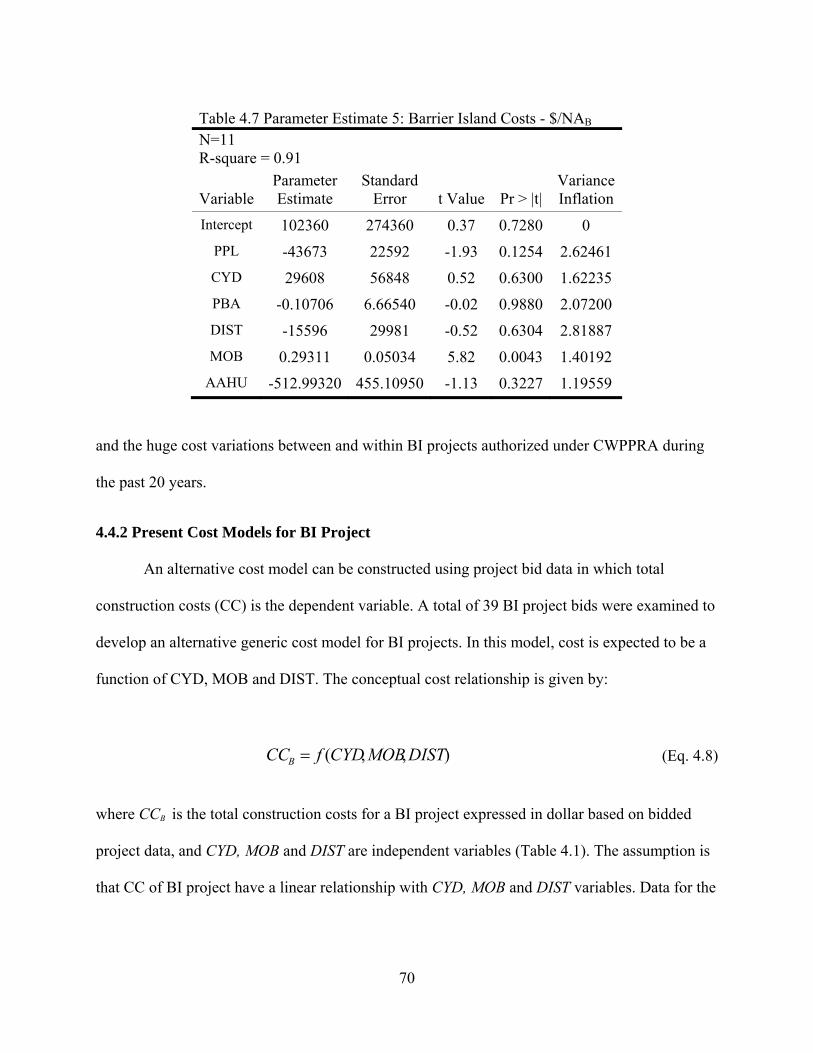
Table 4.7 Parameter Estimate 5: Barrier Island Costs - $/NAB N=11 R-square = 0.91
Variable ParameterEstimate
Standard Error t Value Pr > |t|
Variance Inflation
Intercept 102360 274360 0.37 0.7280 0 PPL -43673 22592 -1.93 0.1254 2.62461 CYD 29608 56848 0.52 0.6300 1.62235 PBA -0.10706 6.66540 -0.02 0.9880 2.07200 DIST -15596 29981 -0.52 0.6304 2.81887 MOB 0.29311 0.05034 5.82 0.0043 1.40192
AAHU -512.99320 455.10950 -1.13 0.3227 1.19559
and the huge cost variations between and within BI projects authorized under CWPPRA during
the past 20 years.
4.4.2 Present Cost Models for BI Project
An alternative cost model can be constructed using project bid data in which total
construction costs (CC) is the dependent variable. A total of 39 BI project bids were examined to
develop an alternative generic cost model for BI projects. In this model, cost is expected to be a
function of CYD, MOB and DIST. The conceptual cost relationship is given by:
),,( DISTMOBCYDfCCB = (Eq. 4.8)
where CCB is the total construction costs for a BI project expressed in dollar based on bidded
project data, and CYD, MOB and DIST are independent variables (Table 4.1). The assumption is
that CC of BI project have a linear relationship with CYD, MOB and DIST variables. Data for the
70

BI construction costs model was imported and analyzed in SigmaPlot 11.0 and SAS 9.1. The
resulting analysis is contained in Table 4.8.
Table 4.8 Parameter Estimate 6: Barrier Island Construction Costs - CCB N=39 R-square = 0.71
Parameter Estimate
Standard Error t Value Pr > |t|
Variance Inflation
Intercept -10100291 4428163 -2.28 0.0288 0 CYD 3910489 1002575 3.90 0.0004 1.71326 MOB 4.18020 0.63399 6.59 <.0001 1.33729 DIST 1349345 463073 2.91 0.0062 2.11973
This model shows that independent variables, CYD, MOB, and DIST, were significant
predictors of total construction cost at ten percent significance level (α=0.10 R2=0.72). Based on
these results, the construction cost model for future BI projects is given by:
DISTMOBCYDCCB ∗+∗+∗+−= 134934518.4391048910100291 (Eq. 4.9)
In this regression model, the CCB increase $3,910,489 when the average dredged material
increases one million cubic yards (with MOB and DIST held constant), the construction costs
increase $4.18 when the MOB increase one dollar (with CYD and DIST held constant), and the
construction costs increase $1,349,345 when the distance from sediments borrow site to project
fill site increase one mile (with CYD and MOB held constant).
In addition to the CCB model, it is helpful to develop a physical materials model in order
to account for additional factors that influence the total quantity of sediments needed to build a
BI project. While Figure 3.8 describes this a simple function of acreage, additional variables can
be used to refine the relationship. A conceptual model is that the CYD of BI project is a function
71

of NA, AVE, DEP, and THK. Likewise, due to the data limitations, there are only a few DEP and
THK data available. The conceptual model for the sediment required in a BI project was
simplified and is given by:
),( AVENAfCYDB = (Eq. 4.10)
where CYDB is the total sediments required for a BI project expressed in million cubic yard. NA
and AVE are independent variables (Table 4.1). The assumption is that the CYD of BI project has
a linear relationship with NA, AVE, DEP, and THK variables. Data for the BI sediments model
were imported and analyzed in SigmaPlot 11.0 and SAS 9.1. The resulting analysis is contained
in Table 4.9.
Table 4.9 Parameter Estimate 7: Barrier Island Materials Model - CYDB N=6 R-square = 0.79
Parameter Estimate
Standard Error t Value Pr > |t|
Variance Inflation
Intercept 0.00167 1.93911 0.00 0.9994 0 NA 0.01267 0.00422 3.00 0.0576 1.12719
AVE -0.27226 0.56727 -0.48 0.6641 1.12719
From the statistical results, variables, NA was found to be a significant drivers of the
sediments required for MC projects (α=0.10 R2=0.79). The variable AVE did not significantly
add to the ability of the equation to predict the sediments required. Results from Pearson
correlation coefficients analysis indicated that these two variables were not correlated in this
model (Table.4.10). Normality test shows that data set was well-modeled by a normal
distribution (Appendix D).
72

Table 4.10 Pearson Correlation Coefficients 2: BI - CYDB Prob > |r| under H0: Rho=0
NET AVE
NET 1.00000
-0.33591 0.5151
AVE -0.33591 0.5151
1.00000
Based on the statistical analyses, the linear regression model is given by:
NACYDB ∗= 01267.0 (Eq. 4.11)
In this regression model, the CYD increase 0.01267 million cubic yard when the net acre
increase one acre.
4.5 Generic Cost Models: Freshwater Diversions
4.5.1 Historic and Present Drivers of FWD Cost
A total of 15 FWD projects were examined for development of a generic cost model in
which dollar per net acre was the dependent variable. Water diversion and sediment diversion
restoration projects were combined in the dataset. Three of these projects have been completed
and 12 are under construction or in the engineering and design stage. In this model, dollars per
net acre is expected to be a function of year approved, water flow rate, project boundary area,
diversion types (controlled or uncontrolled), and average annual habitat units. Thus, the
hypothesized cost relationship is given by:
),,,,(/$ AAHUCONPBAAFRPPLfNAF = (Eq. 4.12)
73

where $/NAF is the costs for a FWD project expressed in dollar per net acre and PPL, AFR, PBA,
CON, and AAHU are independent variables. The assumption is that project costs have a linear
relationship with these independent variables.
Thirteen of the 15 FWD projects contained data for all 5 independent variables. Data for
the model were imported and analyzed in SigmaPlot 11.0 and SAS 9.1. The resulting analysis is
contained in Table 4.11.
Table 4.11 Parameter Estimate 8: Fresh Water Diversion Costs - $/NAF N=13 R-square = 0.17
Variable Parameter Estimate
Standard Error t Value Pr > |t|
Variance Inflation
Intercept 46812 48752 0.96 0.3689 0
PPL 129.98567 4525.43148 0.03 0.9779 1.99078
AFR -0.99443 1.49943 -0.66 0.5284 1.47973
PBA 2.35955 3.79495 0.62 0.5538 5.01669
CON -30008 46949 -0.64 0.5431 1.93906
AAHU -11.15195 15.18187 -0.73 0.4865 4.80145
From the statistical analysis results, none of the independent variables were found to be
significant drivers of the costs for FWD projects (α=0.10). Similar to MC and BI projects, this
result could be due to the sparse amount of observations available (n=13), or the long period of
time between projects included in the model (20 years). Moreover, as seen with the MC and BI
projects, the huge variation in project costs over time makes it extremely difficult to develop a
representative cost model for FWD projects on dollar per unit cost basis.
Because there are currently no formal bid data available for FWD projects under
CWPPRA, an alternative cost model for FWD projects was developed using fully funded cost
(FFC) estimates as the dependent variable. Unlike RLB projects, restoration project materials
74

(sediments and nutrients) for FWD projects are not delivered by dredge or pipeline conveyance,
but instead are delivered via river water. Thus, the size and capacity of a FWD – as expressed by
average annual flow rate (AFR) - could have some influence on total project costs. Moreover,
another variable that could influence a project’s fully funded cost include is whether or not the
structure is controlled by gates or valves or is free flowing/uncontrolled (CON). Eight authorized
CWPPRA FWD projects were used to develop a generic cost model for FWD projects. In this
model, costs are expected to be a function of AFR and CON. Project costs could be determined
by these two variables alone, with a conceptual relationship given by:
),( CONAFRfTCF = (Eq. 4.13)
where TCF is the total cost for a FWD project expressed in dollar based on authorized project
data and AFR and CON are independent variables. The assumption is that project costs have a
linear relationship with these two independent variables. Results from Pearson correlation
coefficients analysis and normality test indicated that these two variables were not correlated in
this model and the data set was well-modeled by a normal distribution (Appendix E). Data for
the model were imported and analyzed in SigmaPlot 11.0 and SAS 9.1. The resulting analysis is
contained in Table 4.12.
Table 4.12 Parameter Estimate 9: Freshwater Diversion Fully Funded Costs - TCF
N=8 R-square = 0.86
Variable Parameter Estimate
Standard Error t Value Pr > |t|
Variance Inflation
Intercept 6024854 2825933 2.13 0.0862 0
CFS 521.52627 126.43960 4.12 0.0091 1.05815
CON 10894218 3984605 2.73 0.0411 1.05815
75

This model shows that independent variables, CFS and CON, were significantly related
to FFC at the ten percent significance level (α=0.10 R2=0.86). Based on the statistical analyses,
the linear regression model for FWD projects is given by:
CONCFSTCF ∗+∗+= 1089421853.5216024854 (Eq. 4.14)
In this regression model, CON is equal to one if the diversion uses manual control and
CON is equal to zero if the diversion use natural flow. The costs increase $521.53 when the
average water flow rate increases one cubic foot per second. There is $10,894,218 more cost for
manual control projects comparing to natural flow diversion structure during the project life
time. In addition to the TCF cost model, it is helpful to develop a physical materials model in
order to account for additional factors that influence the average flow rate (CFS) needed for a
particular FWD project. Figure 3.12 describes this simple function,
)(*80.584986.1302 NALNCFSF −= (Eq. 4.15)
where the flow rate of a diversion is related to targeted net acreage (NA) (R2=.60). As with RLB
projects, additional variables can be incorporated to refine the materials function, but those
variables are not readily available from CWWPRA program data. Some of these project-specific
variables can be incorporated through the use of external models, such as N-SED (Table 3.1) for
case studies where specific project conditions are known.
4.6 Summary
Generic cost models of coastal restoration projects are very difficult to construct based on
the authorized projects data alone. If analysis is constrained to authorized projects, there are only
76

12 MC projects, 11 BI projects, and 12 FWD projects in which sufficient data exists for multiple
independent variables. Moreover, regression analyses of authorized project data often yielded
counterintuitive results, with obvious problems in the hypothesized significance and sign of
primary variables. These problems may be due to the large amount of changes that have
occurred in the cost and benefit estimation process over the last 20 years of coastal restoration
under CWPPRA. Recall that Aust (2006) focused on the cost-efficacy of habitat restoration
($/AAHU), while this analysis focuses on the efficiency of land building. Prior to 2005, the
AAHU benefit model of CWPPRA was rapidly evolving, but land building did not become a
major policy objective until after the hurricanes of 2005. Because project benefits have
constantly evolved, it is often difficult to observe a significant relationship with spending.
Through the use of project bid data, generic cost models can be more easily constructed
for MC and BI projects. As legally-binding offers, these bids include much of the same detailed
information on costs and benefits. Using total construction costs (TCC) as the dependent
variable, and analyzing a total of 85 RLB project bids, simplified, but representative, cost models
were developed for MC and BI projects. In addition, the development of refined materials
models for each of these RLB methods provides the flexibility to vary project conditions in
future cost-benefit simulations.
While no current bid data from CWPPRA were available for FWD projects, a suitable
model for estimating FFC was derived as a function of three variables. Additional refinement of
flow rate requirements (CFS) can be obtained from exogenous variables generated by extant
models of FWD benefits (e.g. N-SED model).
Based on the generic benefit and cost models for MC, BI, and FWD projects developed
in Chapters 3 and 4, a conceptual benefit-cost model can be established to conduct the economic
77

comparison of RLB and FWD technologies. As discussed in Chapter 1, the basic conceptual
model will be net present value. Thus, the results derived from this research can be used to focus
on generic simulations or case studies of actual or proposed restoration project alternatives.
Before simulations and case studies can be conducted, synthesis of the basic NPV model is
needed.
78

CHAPTER 5. BENEFIT-COST ANALYSIS
5.1 Introduction
As discussed in Chapter 1, benefit-cost analysis (BCA) is a common and useful means to
examine environmental and wetland projects. BCA provides economic insight and involves
comparison of the long-term economic benefits and costs. This technique can help decision
makers to evaluate project alternatives that offer the greatest benefits to the community by
comparing the economic benefits with economic costs. Several variations on the basic benefit-
cost analysis can be used to compare the benefits and costs of a proposal project, which include
benefit cost ratio (BCR), internal rate of return (IRR), and net present value (NPV) (Hanley and
Spash, 1993).
The BCR is the ratio of discounted benefits divided by the discounted costs:
( )
( )∑=
=
+
+= T
tt
t
tt
RC
RBCR
0
0
1
1∑T
tB
(Eq. 5.1)
where Bt is the benefit in time t and Ct is the cost in time t (benefits and costs are both measured
in dollars). R is the discount rate. If the BCR is equal to or exceeds one, then the project is
expected to yield a net welfare gain, and thus a good candidate for acceptance.
5.2 The Mechanism of NPV
Net present value (NPV) is the value of all projected net benefits in today’s dollar terms.
Projected net benefits are simply the sum of benefits minus costs in each time period under a
79
specific discount rate. In Chapter 1, Equation 1.3 shows the basic mechanics of NPV. The
equation is given by:
( ) ( ) ( )∑∑∑=== +
−+
=+
−=
T
tt
tT
tt
tT
tttt
RC
RB
RCB
NPV000 111
(Eq. 5.2)
where Bt is the sum of benefit in time t, Ct is the sum of cost in time t, R is the discount rate and t
is the year.
The NPV approach calculates the present value of a series of different future costs and
benefits. In the NPV function, costs and benefits of a project need to be identified with the same
units and appropriate discount rates should be taken into account. Then the NPV can be
calculated to make comparison between or among alternatives. If the NPV is greater than zero,
then the project is generally considered to be a good candidate for implementation (Perman et al.,
2003). If there are two potential projects, the one with higher NPV would typically be chosen.
The major factors affecting present value are the time and the discount (interest) rate. The change
in the discount (interest) rate would have a significant effect on net present value analysis.
Generic cost models for marsh creation (MC), barrier island (BI), and freshwater
diversion (FWD) projects have been developed in Chapter 4 and all project cost expressed in
dollar basis. To apply NPV models for wetland restoration alternatives, the costs and benefits of
a project must have the same units. Therefore, full utilization of NPV required that benefits, in
addition to cost, be expressed in common units. To be consistent with actual policy decisions,
this research uses dollars as the basic unit.
As described in Chapters 1 and 2, the CWPPRA program standardized benefits into
common units known as annual average habitat units (AAHU). Aust (2006) examined the cost
efficacy of different projects on a $/AAHU basis. Instead of a quality-of-benefit examination,
80

this research standardizes output on a quantity-of-benefit basis, such as net acres. Likewise, in
Chapter 3 generic benefit trajectories for marsh creation (MC), barrier island (BI), and
freshwater diversion (FWD) projects have been developed and the benefits are expressed on a
net acre (quantity) basis. Additional refinements include incorporating land loss and land
accretion rates, incorporating method-specific time lags, and selecting appropriate discount rates.
The following sections discuss these challenges in regards to their impact on the NPV model for
evaluating wetland restoration projects.
5.3 Region-Specific Landscape Changes
In Chapter 3, wetland restoration benefit trajectories are developed. For rapid land-
building projects (MC and BI), all desired net acres are obtained during project construction. For
freshwater diversions, net acres accrue slowly after the project structure is completed. During or
beyond project life time, land loss or erosion is a constant force. As introduced in Chapter 1,
there are many forms of natural and human disturbance that contribute to coastal land loss.
Land loss rates have been determined and projected for each of the four Coast 2050
planning regions for the 1990-2050 period (LaDNR 1998). Table 5.1 describes the land loss
rates for different habitat types in these regions. On a habitat scale, the projected average annual
loss rates range from a low of 0.03% to a high of 0.70% for all regions. For the entire Louisiana
coast, the projected average annual loss rates for Regions 1, 2, 3, and 4 are 0.30%, 0.32%,
0.28%, and 0.22%, respectively, for the period 1990 to 2050. Differences in land loss rates
among these individual regions are caused by subsidence, sea level rise, storm induced erosion,
channelization and dredging of waterways (LaDNR 1998). These average annual land loss rates
provide a habitat-specific and regional-specific way to introduce erosion into the NPV model. In
some cases, accretion rates might exceed erosion; however, the average accretion rates of 0.7 to
81

Table 5.1 Existing and Projected Habitat Types in Each Coast 2050 Region
Fresh marsh
acres
Saline marsh acres
Intermediate marsh acres
Brackish marsh acres
Total marsh acres
Region 1 Acreage in 1990 34,700 27,700 110,900 79,700 253,000 Projected acreage in 2050 30,100 16,000 99,900 61,400 204,000 Net acres lost by 2050* 4,600 11,700 11,000 18,300 45,600 Percent 1990 marsh lost 13% 42% 10% 23% 18% Average Annual Loss Rate (1990-2050) 0.22% 0.70% 0.17% 0.38% 0.30% Region 2 Acreage in 1990 220,100 73,000 214,500 151,100 658,700 Projected acreage in 2050 194,250 61,900 174,900 102,100 533,150 Net acres lost by 2050* 25,850 11,100 39,600 49,000 125,550 Percent 1990 marsh lost 12% 15% 18% 32% 19% Average Annual Loss Rate (1990-2050) 0.20% 0.25% 0.30% 0.53% 0.32% Region 3 Acreage in 1990 298,300 92,700 240,700 140,200 771,900 Projected acreage in 2050 292,330 69,100 184,800 94,900 641,130 Net acres lost by 2050* 5,970 23,600 55,900 45,300 130,770 Percent 1990 marsh lost 2% 25% 23% 32% 17% Average Annual Loss Rate (1990-2050) 0.03% 0.42% 0.38% 0.53% 0.28% Region 4 Acreage in 1990 354,600 171,700 198,600 33,200 758,100 Projected acreage in 2050 317,070 151,070 160,200 32,250 660,590 Net acres lost by 2050* 37,530 20,630 38,400 950 97,510 Percent 1990 marsh lost 11% 12% 19% 3% 13% Average Annual Loss Rate (1990-2050) 0.18% 0.20% 0.32% 0.05% 0.22% *includes acres preserved by Breaux Act Priority Lists 1-6 and Caernarvon and Davis Pond Diversions. Source from Coast 2050: Toward a Sustainable Coastal Louisiana
0.8 cm/yr across the Louisiana coastal region are not sufficient to keep up with current sea level
rise rate, which measured to be 1.0 cm/yr in most regions (DeLaune et al. 1992). For BI projects,
land accretion from long shore sediment transport is an important factor in shoreline change.
82

Longshore sediment is mainly driven by waves that arrive at the shoreline at an angle. Longshore
sediment transport direction and rate is a function of the angle of wave approach, wave strength
and the time between consecutive waves (Hart et al., 2008). The sediments that accumulate
through this natural force can result in net acreage gains for barrier islands. There are many
investigations about the shoreline rate change along the Louisiana coast, especially on
Chandeleur Island. Williams et al. (1992) provided the most comprehensive analysis of gulf and
bayside shoreline change (1853 to 1989). The shoreline rate change varies greatly from south to
the north of Chandeleur Island. McBride et al (1993) found that the average rate of gulf shoreline
change for the entire island is -6.5 m/yr for the 134 years record, while the bayside change rate is
2.9 m/yr during the same period. On average, the accretion rate is around 0.8% for barrier islands
in Louisiana. Choosing an appropriate accretion rate; however, requires consideration of region-
specific land loss and accretion rates in combination. The interaction of erosion and accretion
forces will affect the net acreage accrual rate for BI projects. If the land loss rate is less than the
accretion rate, net acreage is increasing. If the land loss rate is equal to the accretion rate, the net
acreage is constant. If the land loss rate is greater the accretion rate, net acreage is declining.
5.4 Time Lag
The amount of time required between project authorization and final structure completion
is referred to as the construction time lag. During this period, engineering and design (E&D)
studies are carried out and social constraints are addressed, but there are no benefits accruing. As
detailed in Chapter 3, MC and BI projects authorized under CWPPRA have taken an average
E&D period of 4 years, with a range from a low of 1 year to a high of 12 years. However, the
time lag for FWD projects averages 7 years, and ranges from a low of less than 1 year to a high
83
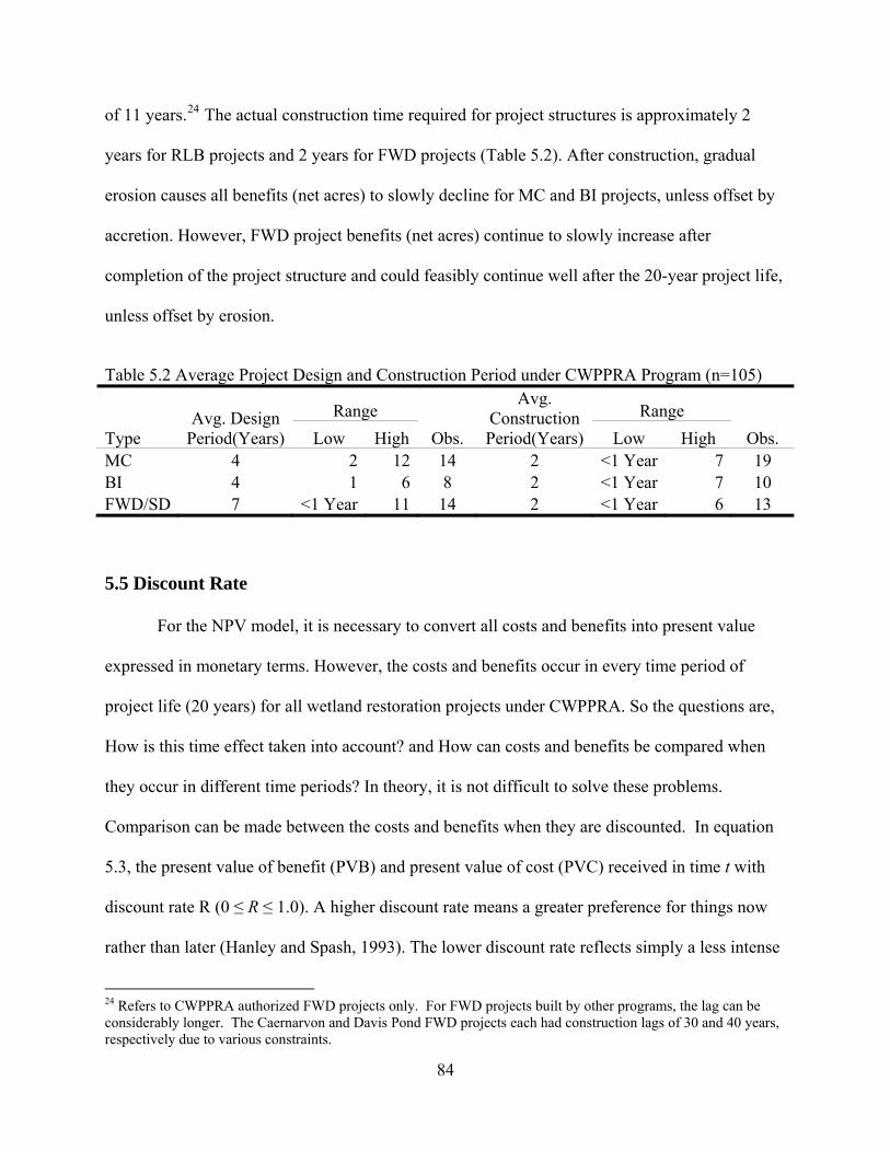
of 11 years.24 The actual construction time required for project structures is approximately 2
years for RLB projects and 2 years for FWD projects (Table 5.2). After construction, gradual
erosion causes all benefits (net acres) to slowly decline for MC and BI projects, unless offset by
accretion. However, FWD project benefits (net acres) continue to slowly increase after
completion of the project structure and could feasibly continue well after the 20-year project life,
unless offset by erosion.
Table 5.2 Average Project Design and Construction Period under CWPPRA Program (n=105)
Type Avg. Design
Period(Years) Range
Avg. Construction Period(Years)
Range Obs. Obs. Low High Low High
MC 4 2 12 14 2 <1 Year 7 19 BI 4 1 6 8 2 <1 Year 7 10 FWD/SD 7 <1 Year 11 14 2 <1 Year 6
13
5.5 Discount Rate
For the NPV model, it is necessary to convert all costs and benefits into present value
expressed in monetary terms. However, the costs and benefits occur in every time period of
project life (20 years) for all wetland restoration projects under CWPPRA. So the questions are,
How is this time effect taken into account? and How can costs and benefits be compared when
they occur in different time periods? In theory, it is not difficult to solve these problems.
Comparison can be made between the costs and benefits when they are discounted. In equation
5.3, the present value of benefit (PVB) and present value of cost (PVC) received in time t with
discount rate R (0 ≤ R ≤ 1.0). A higher discount rate means a greater preference for things now
rather than later (Hanley and Spash, 1993). The lower discount rate reflects simply a less intense
24 Refers to CWPPRA authorized FWD projects only. For FWD projects built by other programs, the lag can be considerably longer. The Caernarvon and Davis Pond FWD projects each had construction lags of 30 and 40 years, respectively due to various constraints.
84

preference for the present and does and does not reflect a preference for the future over the
present (Uyar 1993).The rationale is simple. For example, one dollar invested now at an interest
rate of 10% in ten years will have grown to $1*(1+10%)10, which is $2.59. This means that $2.59
in ten years is worth the same as $1 now.
Although discounting is the most appropriate method for accumulating costs and benefits
over time, it is sometimes politically difficult to identify a consensus discount rate when
assessing a project with a long time horizon. If using common discount rates between 4% and
10%, the costs or benefits in a very long time horizon often have little impact on NPV (Holland
et al., 2010). At a discount rate of 10%, one dollar to be received in 100 years is worth less than
one cent. At discount rates 0%, one dollar benefit to be received in 100 years is worth exactly
one dollar.
It has been long debated how to select the correct discount rate for an environmental
projects when applying BCA analysis. In fact, there is no agreement on a single discount rate
used by environmental economists. Using zero discount rate means that benefits today are the
same with benefits received in the future from now. Conversely, a 100% high discount rate
means all future actions are meaningless. Most economists agree that positive discount rates
should be used when using BCA methods to evaluate environmental projects. The reasons for
applying a positive discount rate are: positive rates of inflation diminish the purchasing power of
dollars over time, dollars can be invested today, earning a positive rate of return, future benefits
might not ever be realized because of the existence of uncertainty, and humans are generally
impatient and prefer instant gratification rather than waiting for long-term benefits (NOAA
2000). However, some non-economists would argue that negative discount rate, or at least zero
discount rate should be used in BCA models. The assumption that there will always be growth in
85
the long term, a basis for positive discount rates, doesn’t necessarily always hold. It is entirely
possible that the human race could overexploit and exhaust the natural resources necessary for
growth. The economy could start at some point to decay or be precipitated to a crash all at once
because of some disaster or a war. When global recession and decline occur, a negative or zero
discount rate should be taken into account (Environmental Economics 2005). Weitzman (2001)
conducted a survey to determine discount rate from the opinions of 2,160 economists. He points
out that even if every individual believes in a constant discount rate, the wide spread opinion on
discount rates means that a declining rate should be used in any benefit-cost analysis for long-
term environmental projects. For these reasons, this research will use a variety of discount rates
and evaluate their impact on NPV results using sensitivity analysis. Another way is to use a time-
declining rate of discount, which might begin at 4%-10% value and decline slowly over time
(Holland et al., 2010, Weitzman 2001).
5.6 Integrated NPV Models
As stated in Chapter 1, the main objective of this study is to develop a comprehensive
economic assessment of rapid land-building (RLB) technologies and freshwater diversions
(FWD) (existing and proposed) for coastal restoration. The benefits trajectories and associated
costs functions defined in Chapters 2, 3 and 4 can be integrated into a basic NPV analysis (Eq.
5.2) for these various restoration methods over a given time period. In the following sections,
three general models for NPV are constructed by integrating previously described benefit and
costs variables and functions for MC, BI, and FWD projects.
5.6.1 NPV Model: Marsh Creation
From equation 5.2, we define benefits in period t for MC projects by the function:
86

( ) ( )( ) ( ) )(1
08.096.0
1
1m
lagt
mt ESVE
lagtEXP
NAMCB m ∗−∗
⎥⎥⎥⎥
⎦
⎤
⎢⎢⎢⎢
⎣
⎡
⎟⎠
⎞⎜⎝
⎛ −−−+
∗= − (Eq. 5.3)
where t is the number of years (ranging from 1 to 20 for CWPPRA projects). Bt (MC) is the total
annual benefits (in $) of a MC project in year t. NA is a user specified variable referring to the
desired net acreage gain from the project over a given time period. The bracketed expression [Eq
3.1] is the percentage of project construction for a MC project completed in year t. The time lagm
is the engineering and design (E&D) phase for MC projects, which is also a user specified
variable in this model. The capital letter E stands for a geographically-specific land loss rate
obtained from Table 5.2, such that (1-E)t-lagm is the proportion of land remaining at time t.
The acronym ESVM stands for the annual non-market, ecosystem values for each acre
restored. By isolating this value, we can solve for the break-even level of ESVM that would be
needed for a BCR of 1.0, or greater:
( )
( )( ) ( ) mlagt
m
tM
Elagt
EXPNA
MCBESV
−−∗
⎥⎥⎥⎥
⎦
⎤
⎢⎢⎢⎢
⎣
⎡
⎟⎠
⎞⎜⎝
⎛ −−−+
∗
=
1
08.096.0
1
1
(Eq. 5.4)
To obtain the PVB, a discount rate is introduced into the model and the equation is given
by:
( ) ( )( )∑
= +∗=
20
1 11
ttt R
MCBMCPVB (Eq. 5.5)
87

where the t stands for a given year from 1 to 20. PVB(MC) is the total discounted benefits (in $)
of a marsh creation project during the project life R is the discount rate.
The associated costs of engineering and design Ct (EDM) and operation and maintenance
Ct (OMM) typically account for 10% and 5%, respectively of total project costs under CWPPRA.
Although specific data for these two costs is unavailable, they can be derived algebraically as a
function of construction costs Ct (CCM), which accounts on average for 85% of CWPPRA costs
for MC projects. In turn construction costs are estimated from regression analysis of cost
factors for MC projects under CWPPRA (see Chapter 4 Eq.4.4). In this model, CYD is an
independent variable representing the number of cubic yards of sediment (in millions), and MOB,
DIST, and AD are user specified variables representing mobilization and demobilization costs ($),
average sediment transport distance in miles, and access dredging/channel costs ($), respectively.
The corresponding cost in period t for MC projects is given by the function:
( ) ( )( ) ( )( ) ( )MtMMtMMtt CCCCCOMCCCEDCMCTC ++= (Eq. 5.6)
where:
( ) ( )MtMt CCCEDC ∗= 12.0 (Eq. 5.6.1)
( ) ( )CCMCtOMC Mt ∗= 06.0 (Eq. 5.6.2)
( ) ADDISTMOBCYDCCC Mt ∗+∗+∗+∗+−= 11.15237991074.224868671507336 (Eq. 5.6.3)
By substituting Eq.5.6.1, Eq.5.6.2 and Eq.5.6.3 into Eq.5.6, the following model is
obtained:
88
( ) ( ) ( ) ( )MtMtMtt CCCCCCCCCMCTC ∗+∗+= 06.012.0 (Eq. 5.7)
( ) ( 06.012.01 )++∗= Mt CCC
( )Mt CCC∗= 18.1
where TCt (MC) is the total annual costs of a MC project in year t, Ct (EDM) is the engineering
and design costs of a MC project in year t, Ct (OMM) is the operation and maintenance costs of a
MC project in year t, Ct (CCM) is the construction costs of a MC project in year t.
The sub equation (5.6.3.1) for CYD is derived from representative MC projects described
in Chapter 4 (see Eq.4.5) and rewritten here as:
AVENACYDM ∗−∗+= 31.10054.05.4 (Eq. 5.6.3.1)
where the MCYD is a function of NA (net acreage desired) and the AVE (average project
elevation) and the NA and AVE are user specified variables.
Combining Eq.5.7 with Eq. 5.6.3 yields:
( ) ( Mtt CCCMCTC ∗= 18.1 ) (Eq. 5.8)[ ]ADDISTMOBCYD ∗+∗+∗+∗+−∗= 11.15237991074.22486867150733618.1
Therefore, the PVC function for MC projects can be expressed as:
( ) ( ) ( )( ) ( )( )( )tt
MtMMtMMt RCCCCCOMCCCEDCMCPVC
+∗++= ∑
= 11)(
20
1
(Eq. 5.9)
89

where t stands for the number of year of a project and range from 1 to 20. PVC(MC) is the total
discounted costs (in $) of a MC project during the project life. Ct(MC) is the total annual costs of
a MC project in year t. R is the discount rate.
5.6.2 NPV Model: Barrier Islands
Benefits in period t for BI project are given by the function:
( ) ( )( ) ( ) ESVAlagt
EXPNABIB blagt
bt ∗+∗
⎥⎥⎥⎥
⎦
⎤
⎢⎢⎢⎢
⎣
⎡
⎟⎠⎞
⎜⎝⎛ −−−
+∗= −1
0654.089.0
1
1 (Eq. 5.10)
where the t stands for the number of years (ranging from 1 to 20 for CWPPRA projects). Bt (BI)
is the total annual benefits (in $) of a BI project in year t. NA is a user specified variable referring
to the desired net acreage gain from the project over a given time period. The bracketed
expression [Eq 3.4] is the percentage of project construction for a BI project completed in year t.
The time lagb is the engineering and design (E&D) phase for BI projects, which is also a user
specified variable in this model. The capital A is a derived variable referring to net accretion rate
for BI projects in coastal Louisiana.
The sub function for net accretion rate (A) is given by:
(Eq. 5.10.1)ELA −=
where the capital L is a user specified variable and stands for long shore sediment transport rate
in coastal Louisiana. The capital letter E stands for a location-specific land loss rate obtained
from Table 5.2.
90

The acronym ESVb stands for the annual non-market, ecosystem values for each acre
restored. By isolating this value, we can solve for the break-even level of ESVb that would be
needed for a BCR of 1.0, or greater:
( )
( )( ) ( ) blagt
b
tB
Alagt
EXPNA
BIBESV
−+∗
⎥⎥⎥⎥
⎦
⎤
⎢⎢⎢⎢
⎣
⎡
⎟⎠⎞
⎜⎝⎛ −−−
+∗
=
1
0654.089.0
1
1
(Eq. 5.11)
To obtain the PVB, a discount rate is introduced into the model and the equation is given
by:
( ) ( )( )∑
= +∗=
20
1 11
ttt R
BIBBIPVB (Eq. 5.12)
where the t stands for a given year from 1 to 20. PVB(BI) is the total discounted benefits (in $) of
a barrier island project during the project life and R is the discount rate.
The associated costs of engineering and design Ct (EDB) and operation and maintenance
Ct (OMB) typically account for 10% and 5%, respectively of total project costs under CWPPRA.
Although specific data for these two costs is unavailable, they can be derived algebraically as a
function of construction costs Ct (CCB), which accounts on average for 85% of CWPPRA costs
for BI projects. In turn construction costs are estimated from regression analysis of cost factors
for BI projects under CWPPRA (see Chapter 4 Eq.4.9). In this model, CYD is an independent
variable representing the number of cubic yards of sediment (in millions). MOB and DIST are
user specified variables representing mobilization and demobilization costs ($) and average
91
sediment transport distance in miles, respectively. The corresponding cost in period t for BI
projects is given by the function:
( ) ( )( ) ( )( ) ( )BtBBtBBtt CCCCCOMCCCEDCBITC ++= (Eq. 5.13)
Where
( ) ( )BtBt CCCEDC ∗= 12.0 (Eq. 5.13.1)
( ) ( )BtBt CCCOMC ∗= 06.0 (Eq. 5.13.2)
( ) DISTMOBCYDCCC Bt ∗+∗+∗+−= 13493418.4391048910100291 (Eq. 5.13.3)
By substituting Eq.5.12.1, Eq.5.12.2 and Eq.5.12.3 into Eq.5.12, the following model is obtained:
( ) ( ) ( ) ( )BtBtBtt CCCCCCCCCBITC ∗+∗+= 06.012.0 (Eq. 5.14)
( ) [ ]6.012.01 ++∗= Bt CCC
( )Bt CCC∗= 18.1
Combining 5.14 with 5.13.3 yields:
( ) ( Btt CCCBITC ∗= 18.1 ) (Eq. 5.15)
[ ]DISTMOBCYD ∗+∗+∗+−∗= 134934518.439104891010029118.1
where TCt (BC) is the total annual costs of a BC project in year t, Ct (EDB) is the engineering and
design costs of a BI project in year t, Ct (OMB) is the operation and maintenance costs of a BI
project in year t, Ct (CCB) is the construction costs of a BI project in year t.
92
The sub equation (5.12.3.1) for CYD is derived from representative BI projects described
in Chapter 4 (see Eq.4.11) and rewritten here as:
NACYDB ∗= 01627.0 (Eq. 5.13.3.1)
where the BCYD is a function of NA (net acreage desired) and the NA is a user specified variable.
Therefore, the PVC function for BI projects can be expressed as:
( ) ( ) ( )(( )
) tt
BtBtBt RCCCOMCEDCBIPVC
+∗++= ∑
= 11)(
20
1
(Eq. 5.16)
where t stands for the number of year of a project and range from 1 to 20. PVC(BI) is the total
discounted costs (in $) of a BI project during the project life. Ct(BI) is the total annual costs of a
BI project in year t. R is the discount rate.
5.6.3 NPV Model: Freshwater Diversions
The benefits function of the basic NPV model for FWD projects is given by:
( ) ( )[ ] ( ) ESVElagtNAFWDB flagtft ∗−∗−∗+−∗= −10501.00029.0 (Eq. 5.17)
where the t stands for the number of years (ranging from 1 to 20 for CWPPRA projects). Bt
(FWD) is the total annual benefits (in $) of a FWD project in year t. NA is a user specified
variable referring to the desired net acreage gain from the project over a given time period.
Unlike MC and BI projects, the bracketed expression [Eq 3.7] is the percentage of net acres
93

accrued for a FWD project in year t. The time lagf is the engineering and design (E&D) phase for
FWD projects, which is also a user specified variable in this model.
The acronym ESVf stands for the annual non-market, ecosystem values for each acre
restored. By isolating this value, we can solve for the break-even level of ESVf that would be
needed for a BCR of 1.0, or greater:
( )( )[ ] ( ) flagt
f
tF ElagtNA
FWDBESV −−∗−∗+−∗
=10501.00029.0
(Eq. 5.18)
To obtain the PVB, a discount rate is introduced into the model and the equation is given
by:
( ) ( )( )∑
= +∗=
20
1 11
ttt R
FWDBFWDPB (Eq. 5.19)
where the t stands for a given year from 1 to 20. PVB(FWD) is the total discounted benefits (in $)
of a freshwater diversion project during the project life and D(t) is the discount factor in year t
and R is the discount rate.
The associated costs of engineering and design Ct (EDF), construction costs Ct (CCF), and
operation and maintenance Ct (OMF) typically account for 10%, 85%, and 5%, respectively of
total project costs under CWPPRA. These three cost categories can be derived algebraically as a
function of CWPPRA costs for FWD projects. The corresponding cost function of the basic NPV
model for FWD projects is given by:
( ) ( ) ( ) ( )FtFtFtt OMCCCCEDCFWDTC ++= (Eq. 5.20)
94

where TCt (FWD) is the total annual costs of a FWD project in year t, Ct (EDF) is the engineering
and design costs of a FWD project in year t, Ct (CCF) is the construction costs of a FWD project
in year t, Ct (OMF) is the operation and maintenance costs of a FWD project in year t. The sub
functions for individual cost categories are given by:
( ) ( )FWDCEDC tFt ∗= 10.0 (Eq. 5.20.1)
( ) ( )FWDCCCC tFt ∗= 85.0 (Eq. 5.20.2)
( ) ( )FWDCOMC tFt ∗= 05.0 (Eq. 5.20.3)
The total costs for a FWD project are estimated from regression analysis using CWPPRA
data (see Chapter 4 Eq.4.14) and given by:
( ) CONAFRFWDCt ∗+∗+= 1089421853.5216024854 (Eq. 5.21)
where AFR and CON are derived variables and stand for average annual water flow rate (cubic
feet per second, cfs), diversion types (controlled=0 and uncontrolled=1) respectively. The sub
equation (5.20.4.1) for AFR is derived from representative FWD projects described in Chapter 4
(see Eq.4.15) and rewritten here as:
)(80.584986.1302 NALNAFRF ∗−= (Eq. 5.21.1)
where the AFRF is a function of NA (net acreage desired) and the NA is a user specified variable.
95

Therefore, the PVC function for FWD projects can be expressed as:
( ) ( ) ( )(( )
) tt
FtFtFt ROMCCCEDCFWDPC
+∗++= ∑
= 11)(
20
1
(Eq. 5.22)
where t stands for the number of year of a project and range from 1 to 20. PVC(FWD) is the total
discounted costs (in $) of a FWD project during the project life. Ct(FWD) is the total annual
costs of a FWD project in year t. D(t) is the discount factor and R is the discount rate.
5.7 Summary
A NPV model for comparing coastal restoration projects has been developed using
representative benefit trajectories and generic cost models. Additional refinements have been
incorporated to capture geographically-specific land loss and land accretion rates, method-
specific time lags, and accounting for the time value of benefits and costs over many years. All
these factors have an effect on the output of BCA calculations.
This basic model framework provides a template for the economic assessment of three
coastal wetland restoration methods, MC, BI, and FWD projects. Once all simulation or case
study variables have been set, the model can readily conduct comparisons of project alternatives.
As currently expressed, the model can be used to derive the level of annual level of break-even
ESV benefits that must be obtained for project costs to be covered. These dollar-based estimates
can be compared to existing ecosystem values from the literature in order to assess the feasibility
of a given simulation or case study example.
96
CHAPTER 6. BREAK-EVEN SIMULATIONS
6.1 Introduction
In Chapter 5, net present value (NPV) models have been integrated for rapid land-
building (RLB) and freshwater diversion (FWD) projects to develop a process for comparing the
economic outcomes of wetland restoration alternatives. It is difficult, however, to place a value
on the functional benefits of a restored coastal wetland. Such benefits are typically not traded in
markets. The challenge here is to determine how these wetland values should be taken into
account and how to express quantity-based benefits (net acres) in monetary terms (dollars). This
chapter provides a brief summary of non-market valuation methods and develops a series of
simulated required break-even ecosystem values (ESV) for RLB and FWD projects under
different assumptions.
6.2 Valuing Coastal Wetlands
Wetlands provide not only food and habitat for fish and wildlife but also a number of
economic services and goods to humans. The economic services of wetlands are derived from
their ecological and physical functions. These services include flood control, water quality
maintenance, soil erosion prevention, and recreation opportunities (EPA 2006). More
specifically, coastal wetlands provide estuarine habitat and protection of human infrastructure
from storm and tidal surge. These provisions are tremendously valuable to all coastal
communities. However, measuring the value of these coastal wetland functions is not always
easy. In theory, benefits from wetlands would be measured either through market-based methods
or non-monetary, numerically-based methods. In practice, there is a wide array of market and
97

non-market methods, which have been used to assess the different values of wetlands. The
following section will provide a brief overview of these methods.
6.2.1 Non-Market Based Methods
Ecosystem services are not usually captured directly by per acre market prices for coastal
wetlands. Non market valuation techniques are required to measure these service benefits for
coastal restoration projects. Because there is lack of a clearly defined market, these methods
typically rely on surveys and secondary data to acquire the direct and indirect information
needed to value these environmental benefits. A brief look at non-market based methods (below)
includes the hedonic method, travel cost method, contingent valuation, energy analysis, and
benefits transfer.
• Hedonic Method (HM): The hedonic price method is technique that determines coastal resource value as a function of environmental quality. It can be used to estimate the impact of certain amenities (e.g. wildlife, recreation, aesthetics) or inconveniences (e.g. water, air, or noise pollution), on the price of a house or other property. By comparing the market value of two properties, the implicit price of that characteristic can be obtained by estimating people's willingness to pay for environmental quality (Lipton 1995).
• Travel Cost Method (TC): The travel cost method is used to determine the recreation
value of a coastal resource by the expenditures of visitors. This method quantifies the total value of a wetland site by calculating the trip-related market-based expenditures; including food, hotel, transportation costs, entrance fees, and opportunity cost of travel time (White 1998).
• Contingent Valuation (CV): This is a purely non-market-based technique that measures
the value people place on non-market goods or services by asking them questions directly. The examiners set up a hypothetical scenario market and query a random population to estimate how much people would be willing to pay for the improvement or how much compensation people would be willing to accept for the decline in environmental quality. Contingent valuation methods are a useful when no market-based alternative exists for valuing ecosystem services. Based on survey responses, examiners estimate the mean and median willingness to pay for an environmental improvement or willingness to accept compensation for a decline in environmental quality (Carson et al., 2001).
98

6.2.2 Non-Monetary Based Methods
• Energy Analysis (EA): This approach looks at the relationships within natural systems that lead to the production (supply) of natural services, rather than human demand for natural system products (Costanza and Farber 1984). It uses the total amount of energy captured by natural ecosystems in primary production as an estimate of their potential to produce economically useful products such as fish and wildlife. The critical link in using energy analysis for nonmarket valuation is the relationship between the energy embodied in the system and its economic value, and this relationship is controversial (Costanza 1980 and 1984, Daly 1981, Huettner 1982). Even with this uncertainty, energy analysis is frequently used by ecologists to estimate the economic value of natural systems.
• Benefits Transfer (BT): The benefit transfer method is used to estimate economic values
for ecosystem services by transferring available economic information from one place and time to make inferences about the economic value of environmental goods and services at another place and time (Wilson and Hoen, 2006). Thus, the basic goal of benefit transfer is to estimate benefits for one context by adapting an estimate of benefits from some other context. Benefit transfer is often used when it is too expensive and/or there is too little time available to conduct an original valuation study and it can only be as accurate as the initial study.
• Meta-Analysis (MA): Meta-analysis use formal and informal statistical methods
collecting information to combine the results of several studies that address related research purposes. Glass (1976) first used the term meta-analyses to refer to the statistical analysis of a large collection of analysis results for the purpose of integrating the findings. Cooper and Hedges (1994) describe meta-analysis as a set of methods to synthesize empirical research. The main advantage of meta-analysis is providing a rigorous statistical synthesis of literature that cannot be achieved by using qualitative analysis (Woodward and Wui 2001).
6.3 Coastal Wetland Values
Understanding the annual economic contributions of ecosystem services from coastal
wetlands can provide useful information for NPV analyses. Although there are many ecosystem
services existing in coastal wetlands; reduction of storm surge, habitat provision, and water
quality improvement are the three most often studied. These services are considered to be
primary nonmarket value drivers of coastal restoration project benefits. Conducting a nonmarket
valuation study for each project-specific NPV simulation would be beyond the scope of this
study. Instead, this research compares derived ESV benefit estimates to existing research on the
99

100
non-market value of coastal wetlands for storm surge attenuation and habitat and water quality
provision.
There is limited literature on coastal wetland valuation of ecosystem services and the
range of these estimates is very large. Costanza (2008) provides the most recent estimates for
storm protection value. He estimated the value of coastal wetlands for storm surge attenuation
ranging from $101/acre/year to $20,648/acre/year in 2007 dollars, with a mean of
$3,336/acre/year and median of $1,308/acre/year. By using meta-analysis approach,
Kazmierczak (2001) provided mean, median, lower and upper bound estimates of the value of
wetlands for habitat/species protection, hunting and fishing, and water quality. These estimates,
expressed in year 2000 dollars, ranged from a low of $1.05/acre/year for outdoor recreation to a
high of $5,673.80 water quality provision. Farber (1996) provided per acre values of wetlands
for fisheries production in coastal Louisiana. He estimated values ranging from $36.93 per acre
to $51.52 per acre in 1990 dollars. Woodward and Wui (2001) estimated additional values for
these services and for other services including bird watching, flood absorption, and recreational
hunting and fishing. Table 6.1 lists coastal wetland valuation studies with examples to illustrate a
range of estimation methods and non-market service values.
6.4 Simulations
6.4.1 Break-Even Simulations
The generic benefit and cost models were incorporated into a net present valuation
construct (Eq.1.3) and given by developed within Microsoft Excel 2010. From this construct, a
“ecosystem services break-even analysis” can be conducted by setting the B:C ratio (Eq.1.1)
equal to 1.0 and solving for the average annual value per acre that equates project benefits and
costs over the period.
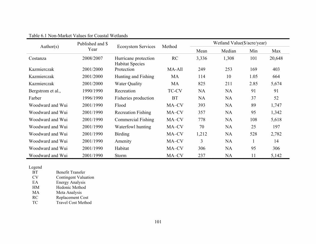
Table 6.1 Non-Market Values for Coastal Wetlands
Published and $ Year Author(s) Ecosystem Services Method
Wetland Value($/acre/year)
Mean Median Min Max Costanza 2008/2007 Hurricane protection RC 3,336 1,308 101 20,648
Kazmierczak 2001/2000 Habitat Species Protection MA-All 249 253 169 403
Kazmierczak 2001/2000 Hunting and Fishing MA 114 10 1.05 664 Kazmierczak 2001/2000 Water Quality MA 825 211 2.85 5,674 Bergstrom et al., 1990/1990 Recreation TC-CV NA NA 91 91 Farber 1996/1990 Fisheries production BT NA NA 37 52 Woodward and Wui 2001/1990 Flood MA–CV 393 NA 89 1,747 Woodward and Wui 2001/1990 Recreation Fishing MA–CV 357 NA 95 1,342 Woodward and Wui 2001/1990 Commercial Fishing MA–CV 778 NA 108 5,618 Woodward and Wui 2001/1990 Waterfowl hunting MA–CV 70 NA 25 197 Woodward and Wui 2001/1990 Birding MA–CV 1,212 NA 528 2,782 Woodward and Wui 2001/1990 Amenity MA–CV 3 NA 1 14 Woodward and Wui 2001/1990 Habitat MA–CV 306 NA 95 306 Woodward and Wui 2001/1990 Storm MA–CV 237 NA 11 5,142 Legend
BT Benefit Transfer CV Contingent Valuation EA Energy Analysis HM Hedonic Method MA Meta Analysis RC Replacement Cost TC Travel Cost Method
101

( )
( )
0.1
1
1
1
1 =
+
+==
∑
∑
=
=T
tt
t
T
tt
t
RC
RB
CostsTotalBenefitsTotalBCR (Eq. 6.1)
The cost and benefit function for MC projects have already been expressed in equation
5.8 and equation 5.5. By rewriting equation 5.8 and equation 5.5 and solving for the break-even
ESV yields:
( )
( )( ) ( )
∑=
−−∗
⎥⎥⎥⎥
⎦
⎤
⎢⎢⎢⎢
⎣
⎡
⎟⎠⎞
⎜⎝⎛ −−−
+∗
=T
t
lagt
m
M
mElagtEXP
TA
MCTCESV1
1
08.096.01
1
(Eq. 6.2)
Also, the cost and benefit function for BI projects have already been expressed in
equation 5.15 and equation 5.21. By rewriting equation 5.15 and equation 5.12 and solving for
the break-even ESV yields:
( )
( )( ) ( )
∑=
−−∗
⎥⎥⎥⎥
⎦
⎤
⎢⎢⎢⎢
⎣
⎡
⎟⎠⎞
⎜⎝⎛ −−−
+∗
=T
t
lagt
b
B
bElagt
EXPTA
BITCESV1
1
08.096.0
1
1
(Eq. 6.3)
Likewise, the associated cost and benefit function in period T for FWD projects have
already been expressed in equation 5.21 and equation 5.19. By rewriting equation 5.21 and
equation 5.19 and solving for the break-even ESV yields:
102

( )( )[ ( )]∑
=−−∗−∗+−∗
=T
tlagt
fF fElagtTA
FWDTCESV1 10501.00029.0
(Eq. 6.4)
6.4.2 The Profile of NPV Models
This section takes up NPV simulations under different assumptions for two RLB models
and 2 FWD models. As shown in Table 6.2, a total of 47 components, which include 22 user-
specified parameters and 25 derived parameters, were introduced into the mathematical NPV
model developed in Chapter 5 using MS Excel software. For each control parameter, ranges were
obtained from project data and related literature. Ranges were set up from a low to high with a
mean value for user-specified variables. Derived parameters were produced from regression
models and mathematical results after the user-specified parameter were inputted to the models.
For a view of the four spreadsheet models, see Appendix F.
To calculate the required break-even ecosystem services value (ESV) for RLB and FWD
projects, non-market values of wetland are needed. As mentioned before, due to the limited
literature on coastal wetland valuation of ecosystem services and the scope of this research, this
study used three non-market values (storm surge attenuation and habitat and water quality
provision) from the existing literature as “starting values.” By initially incorporating these starter
values into the NPV model in MS Excel and setting the cost-benefit ratio equal to one, the
required break-even ESV (annual $/year) can be calculated through the MS-Excel analytical tool
“SOLVER”. For the following simulations, no market values for coastal wetlands are
incorporated. The assessments focus only on the annual ESV benefits that would be required to
generate a positive cost-benefit result.
103
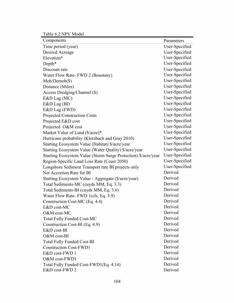
Table 6.2 NPV Model Components Parameters Time period (year) User-SpecifiedDesired Acreage User-SpecifiedElevation* User-SpecifiedDepth* User-SpecifiedDiscount rate User-SpecifiedWater Flow Rate- FWD 2 (Boustany) User-SpecifiedMob/Demob($) User-SpecifiedDistance (Miles) User-SpecifiedAccess Dredging/Channel ($) User-SpecifiedE&D Lag (MC) User-SpecifiedE&D Lag (BI) User-SpecifiedE&D Lag (FWD) User-SpecifiedProjected Construction Costs User-SpecifiedProjected E&D cost User-SpecifiedProjected O&M cost User-SpecifiedMarket Value of Land ($/acre)* User-SpecifiedHurricane probability (Klotzbach and Gray 2010) User-SpecifiedStarting Ecosystem Value (Habitat) $/acre/year User-SpecifiedStarting Ecosystem Value (Water Quality) $/acre/year User-SpecifiedStarting Ecosystem Value (Storm Surge Protection) $/acre/year User-SpecifiedRegion-Specific Land Loss Rate (Coast 2050) User-SpecifiedLongshore Sediment Transport rate BI projects only User-SpecifiedNet Accretion Rate for BI Derived Starting Ecosystem Value - Aggregate ($/acre/year) Derived Total Sediments-MC (cuyds MM, Eq. 3.3) Derived Total Sediments-BI (cuyds MM, Eq. 3.6) Derived Water Flow Rate- FWD 1(cfs, Eq. 3.9) Derived Construction Cost-MC (Eq. 4.4) Derived E&D cost-MC Derived O&M cost-MC Derived Total Fully Funded Cost-MC Derived Construction Cost-BI (Eq. 4.9) Derived E&D cost-BI Derived O&M cost-BI Derived Total Fully Funded Cost-BI Derived Construction Cost-FWD1 Derived E&D cost-FWD 1 Derived O&M cost-FWD1 Derived Total Fully Funded Cost-FWD1(Eq. 4.14) Derived E&D cost-FWD 2 Derived
104
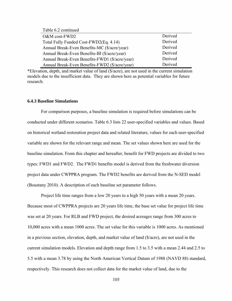
Table 6.2 continued O&M cost-FWD2 Derived Total Fully Funded Cost-FWD2(Eq. 4.14) Derived Annual Break-Even Benefits-MC ($/acre/year) Derived Annual Break-Even Benefits-BI ($/acre/year) Derived
Derived Annual Break-Even Benefits-FWD1 ($/acre/year) Derived Annual Break-Even Benefits-FWD2 ($/acre/year)
*Elevation, depth, and market value of land ($/acre), are not used in the current simulation models due to the insufficient data. They are shown here as potential variables for future research.
6.4.3 Baseline Simulations
For comparison purposes, a baseline simulation is required before simulations can be
conducted under different scenarios. Table 6.3 lists 22 user-specified variables and values. Based
on historical wetland restoration project data and related literature, values for each user-specified
variable are shown for the relevant range and mean. The set values shown here are used for the
baseline simulation. From this chapter and hereafter, benefit for FWD projects are divided to two
types: FWD1 and FWD2. The FWD1 benefits model is derived from the freshwater diversion
project data under CWPPRA program. The FWD2 benefits are derived from the N-SED model
(Boustany 2010). A description of each baseline set parameter follows.
Project life time ranges from a low 20 years to a high 50 years with a mean 20 years.
Because most of CWPPRA projects are 20 years life time, the base set value for project life time
was set at 20 years. For RLB and FWD project, the desired acreages range from 300 acres to
10,000 acres with a mean 1000 acres. The set value for this variable is 1000 acres. As mentioned
in a previous section, elevation, depth, and market value of land ($/acre), are not used in the
current simulation models. Elevation and depth range from 1.5 to 3.5 with a mean 2.44 and 2.5 to
5.5 with a mean 3.78 by using the North American Vertical Datum of 1988 (NAVD 88) standard,
respectively. This research does not collect data for the market value of land, due to the
105

insignificance of this value in the scope of costal restoration cost-benefit analyses. Discount rates
were set to range from 0 to 0.15 with a mean 0.04 (Holland et al., 2010, Weitzman 2001). Water
flow rate for FWD2 was set up to 1,029 cubic feet per second based on the desired acreage (1000
acre) and input from N-SED model. Mobilization and demobilization (MOB) costs range from a
low $110,000 to high $4,000,000, the mean value $1,000,000 is used as the set value in the
baseline simulation for RLB projects. Sediment delivery distance ranges from a low 1 mile to a
high 50 miles (projected) with a mean 4 miles for RLB projects. For MC projects, access
dredging (AD) costs range from 0 to $2,000,000 with the mean $600,000. The average engineer
and design period are 4 and 7 years for RLB and FWD projects, respectively. Projected
construction costs (CC), E&D costs, and O&M costs were set up to 85%, 15%, and 5% based on
the CWPPRA project data, respectively. Hurricane probabilities are not incorporated in the
baseline simulation and will be discussed in the following chapter. The average starting
ecosystem value (habitat, water quality, and storm surge protection) were set at $249/ acre/year,
$825/ acre/year, and $3,336/ acre/year (Costanza 2008, Kazmierczak 2001). The region-specific
land loss rate ranges from 0.03% to 0.7% per year (see Table 5.1 for fresh, intermediate, brackish,
and saline marshes). A set value of 0.35% per year is used in the base simulation because it is
more indicative of the loss rates in brackish and saline marshes. Long-shore sediment transport
rate ranged from 0 to 1% per year and was set at zero for BI projects in the baseline simulation.
These set values were used for developing the baseline scenario.
Figure 6.1 shows that the highest fully funded project cost (FFC) for the base simulation
is the marsh creation project model. At $44,000,000, this method is 1.3 times the FFC of the
next highest project type, barrier islands ($33,000,000). Freshwater diversion projects also have
a high average FFC, including FWD1 at $26,000,000 and FWD2 projects at $17,000,000. While
106

107
these FFC estimates are based on a 1000 acre simulation, the freshwater diversion projects do not
achieve this level of acreage within the set time period of 20 years. Thus, the cost comparison
changes when the actual per unit cost of restored acreage is considered. Figure 6.2 depicts the
baseline simulation result of the break-even ESV that would be required for benefits to equal
cost in each of these of the four project models. Note that freshwater diversion projects (FWD1
and FWD2) have the highest and the next highest projected costs, with required break-even ESV
values at $8,291/acre/year and $5,449/acre/year, respectively. While more expensive on a FFC
basis, the other two models (MC and BI) are more cost efficient, with required break-even ESV
are at $4,010/acre/year and $2,907/acre/year, respectively.
6.4.4 Simulations under Different Assumptions
Ten different simulations were developed in which a single, user-specified parameter is
allowed to vary across its known range, and all other parameters are held constant at the baseline
set level described in section 6.4.2. In each simulation the effect of these parameter variations
are incorporated into the specified NPV model to determine the required break-even ESV
($/acre/year) for each of the four model types.
• Scenario 1: Changes in Project Life-Span
Project life time is allowed to range from 5 years to 50 years at a 5 year interval, with all
other set parameters held constant at the baseline level described in section 6.4.2. Table 6.4
provides results of this simulation and required break-even ESVs at each interval for all four
project types. The percentages at the bottom of the table (% Change) depict the overall change in
the starting and ending ESVs across the simulated range. For all project types, benefits are
increasing over time at various rates according to the benefit and cost models established in
Chapters 3 and 4. These simulations currently assume no natural disaster or human disruption.

Table 6.3 User-Specified Value in Baseline simulation NPV Model Range User-Specified Set Value Low High Mean
Time period (year) 20 20 50 20Desired Acreage 1,000 300 10,000 1000Elevation 2 1.5 3.5 2.44Depth 4 2.5 5.5 3.78Discount rate 0.04 0 0.15 0.04Water Flow Rate- FWD 2 (Boustany 2010) 1,029 1,029Mob/Demob($) $1,000,000 $110,000 $4,000,000 $1,000,000Distance (Miles) 4.00 1 50 4Access Dredging/Channel ($) $600,000 $0 $2,000,000 $600,000E&D Lag (MC) 4 2 7 4E&D Lag (BI) 4 1 6 4E&D Lag (FWD) 7 1 30 7Projected Construction Costs 85% 50% 90% 85%Projected E&D cost 15% 5% 30% 15%Projected O&M cost 5% 1% 20% 5%Market Value of Land ($/acre) $0 Hurricane probability (Klotzbach and Gray 2010) 23% 0% 100% 23%Starting Ecosystem Value (Habitat) $/acre/year $249 $169 $403 $249Starting Ecosystem Value (Water Quality) $/acre/year $825 $3 $5,674 $825Starting Ecosystem Value (Storm Surge Protection) $/acre/year $3,336 $101 $20,648 $3,336Region-Specific Land Loss Rate (Coast 2050) 0.30% 0.03% 0.7% 0.33%Longshore Sediment Transport rate BI projects only 0 0 0.01 0.008
108

0 10 20 30 40 5
MC
BI
FWD1
FWD2
Total Fully Funded Costs (MM $)
Proj
ect T
ypes
0
Figure 6.1 Total fully funded costs for RLB and FWD projects
0 2,000 4,000 6,000 8,000 10,000
MC
BI
FWD1
FWD2
Req. Break-Even ESV ($/acre/year)
Proj
ect T
ypes
Figure 6.2 Required break-even ESV for RLB and FWD projects
109
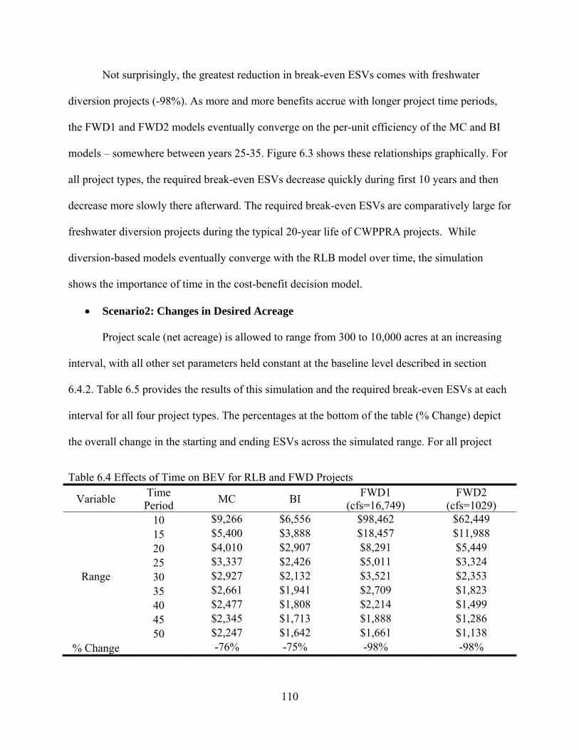
Not surprisingly, the greatest reduction in break-even ESVs comes with freshwater
diversion projects (-98%). As more and more benefits accrue with longer project time periods,
the FWD1 and FWD2 models eventually converge on the per-unit efficiency of the MC and BI
models – somewhere between years 25-35. Figure 6.3 shows these relationships graphically. For
all project types, the required break-even ESVs decrease quickly during first 10 years and then
decrease more slowly there afterward. The required break-even ESVs are comparatively large for
freshwater diversion projects during the typical 20-year life of CWPPRA projects. While
diversion-based models eventually converge with the RLB model over time, the simulation
shows the importance of time in the cost-benefit decision model.
• Scenario2: Changes in Desired Acreage
Project scale (net acreage) is allowed to range from 300 to 10,000 acres at an increasing
interval, with all other set parameters held constant at the baseline level described in section
6.4.2. Table 6.5 provides the results of this simulation and the required break-even ESVs at each
interval for all four project types. The percentages at the bottom of the table (% Change) depict
the overall change in the starting and ending ESVs across the simulated range. For all project
Table 6.4 Effects of Time on BEV for RLB and FWD Projects
Variable Time MC BI FWD1 (cfs=16,749)
FWD2 (cfs=1029) Period
Range
10 $9,266 $6,556 $98,462 $62,449 15 $5,400 $3,888 $18,457 $11,988 20 $4,010 $2,907 $8,291 $5,449 25 $3,337 $2,426 $5,011 $3,324 30 $2,927 $2,132 $3,521 $2,353 35 $2,661 $1,941 $2,709 $1,823 40 $2,477 $1,808 $2,214 $1,499 45 $2,345 $1,713 $1,888 $1,286 50 $2,247 $1,642 $1,661 $1,138
-76% -75% -98% -98% % Change
110
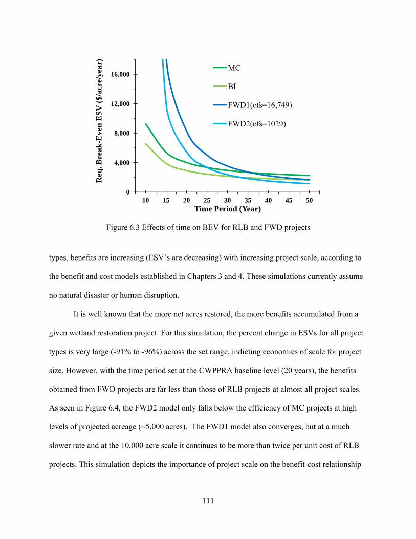
Figure 6.3 Effects of time on BEV for RLB and FWD projects
types, benefits are increasing (ESV’s are decreasing) with increasing project scale, according to
the benefit and cost models established in Chapters 3 and 4. These simulations currently assume
no natural disaster or human disruption.
It is well known that the more net acres restored, the more benefits accumulated from a
given wetland restoration project. For this simulation, the percent change in ESVs for all project
types is very large (-91% to -96%) across the set range, indicting economies of scale for project
size. However, with the time period set at the CWPPRA baseline level (20 years), the benefits
obtained from FWD projects are far less than those of RLB projects at almost all project scales.
As seen in Figure 6.4, the FWD2 model only falls below the efficiency of MC projects at high
levels of projected acreage (~5,000 acres). The FWD1 model also converges, but at a much
slower rate and at the 10,000 acre scale it continues to be more than twice per unit cost of RLB
projects. This simulation depicts the importance of project scale on the benefit-cost relationship
0
4,000
8,000
12,000
16,000
10 15 20 25 30 35 40 45 50
Req
. Bre
ak-E
ven
ESV
($/a
cre/
year
)
Time Period (Year)
MC
BI
FWD1(cfs=16,749)
FWD2(cfs=1029)
111

Table 6.5 Effects of Scale (Acreage) on BEV for RLB and FWD Projects Desired Acreage MC BI FWD1
(cfs=1,296~46,303) FWD2
(cfs=925~2,064) Variable
Range
300 $10,722 $5,577 $18,955 $15,071 500 $7,107 $4,393 $13,583 $10,901 800 $4,829 $3,347 $9,760 $6,811
1,000 $4,010 $2,906 $8,291 $5,449 1,500 $2,852 $2,215 $6,112 $3,640 2,000 $2,234 $1,808 $4,895 $2,734 3,000 $1,578 $1,344 $3,556 $1,829 4,000 $1,231 $1,082 $2,822 $1,377 5,000 $1,014 $911 $2,355 $1,105 10,000 $553 $527 $1,327 $562
-95% -91% -93% -96% % Change
0
4,000
8,000
12,000
16,000
20,000
Req
. Bre
ak-E
ven
ESV
($/a
cre/
year
)
Desired Acreage
MC (MM cyds=4.26~12.97)BI (MM cyds=3.15~11.46)FWD1(cfs=1,296~46,303)FWD2 (cfs=925~2,064)
Figure 6.4 Effects of scale on BEV for RLB and FWD projects
112

of coastal restoration projects in Louisiana. Generally speaking, as project scales increases,
differences in methodological efficiency decrease, especially for projects of 5000 acres or
greater.
• Scenario3: Changes in Discount Rate
Discount rate (%) is allowed to range from 0 to 15% at an increasing interval, with all
other set parameters held constant at the baseline level described in section 6.4.2. Table 6.6
provides the results of this simulation and the required break-even ESVs at each interval for all
four project types. The percentages at the bottom of the table (% Change) depict the overall
change in the starting and ending ESVs across the simulated range. For all project types, the
required break-even ESVs are increasing with increasing discount rates, according to the benefit
and cost models established in Chapters 3 and 4. These simulations currently assume no natural
disaster or human disruption.
Table 6.6 depicts the required break-even ESV increase for both of RLB and FWD
projects with an increasing discount rate. For this simulation, the percent change in ESVs for all
project types is very large (138% to 185%) across the set range, indicting the substantial effect of
discounting on project cost and benefits. The required break-even ESVs at the highest discount
rate (15%) are more than two times higher than the required break-even ESVs with no discount
rate applied (0%). Figure 6.5 shows these effects graphically, with a divergence in model
efficiencies for increasing discount rates. As evident from these curves, a higher discount rate
usually means a higher time costs, thus the application of any type of project benefit discounting
will compound the problems associated with slower restoration methods. To a very large degree,
the selection of an appropriate discount rate will have a major impact on the cost-benefit decision
analysis for coastal restoration.
113

Table 6.6 Effects of Discount Rate on BEV for RLB and FWD Projects
Variable Discount MC BI FWD1 (cfs=16,749)
FWD2 (cfs=1029) Rate
Range
0% $3,047 $2,203 $6,121 $4,030 1% $3,274 $2,369 $6,615 $4,353 2% $3,511 $2,542 $7,140 $4,697 3% $3,756 $2,721 $7,699 $5,062 4% $4,010 $2,906 $8,291 $5,449 5% $4,273 $3,098 $8,919 $5,859 6% $4,543 $3,295 $9,583 $6,293 8% $5,105 $3,704 $11,027 $7,235 10% $5,694 $4,133 $12,635 $8,282 15% $7,266 $5,272 $17,448 $11,410
% Change 138% 139% 185% 183%
Figure 6.5 Effects of discount rate on BEV for RLB and FWD projects
0
4,000
8,000
12,000
16,000
20,000
0% 1% 2% 3% 4% 5% 6% 8% 10% 15%
Req
. Bre
ak-E
ven
ESV
($/a
cre/
year
)
Discount Rate
MCBIFWD1(cfs=16,749)FWD2(cfs=1029)
114

• Scenario 4: Changes in Mobilization and Demobilization Costs
Mobilization and demobilization costs are allowed to range from $110,000 to $4,000,000 at
an increasing interval, with all other set parameters held constant at the baseline level described
in section 6.4.2. Table 6.7 provides results of this simulation and required break-even ESVs at
each interval for all four project types. The percentages at the bottom of the table (% Change)
depict the overall change in the starting and ending ESVs across the simulated range. The
percentages are zero for both FWD1 and FWD2 models because there are no MOB costs
reported on budgets for FWD projects. For RLB project types, ESV break-even costs are
increasing with increases in MOB costs according to the benefit and cost models established in
Chapters 3 and 4. These simulations currently assume no natural disaster or human disruption.
For this simulation, the percent change in ESVs caused by increases in MOB across the
known range result in 30% and 68% increases in break-even costs of MC and BI projects,
respectively. The effect of MOB is most pronounced with BI projects, where the required break-
even ESV at the highest MOB costs ($4,000,000) is almost two times higher than at the lowest
MOB cost ($110,000) for BI project. Figure 6.6 shows these effects graphically. The required
break-even ESVs are constant for FWD projects and are increasing, and slightly converging for
the RLB projects. This simulation indicates that as a single project cost variable, MOB has a
substantial effect on RLB project costs, but it is more sensitive for BI projects due to their
relatively lower starting value.
• Scenario 5: Changes in Distance
Distances are allowed to range from 1 to 50 miles at an increasing interval, with all other
set parameters held constant at the baseline level described in section 6.4.2. Table 6.8 provides
results of this simulation and required break-even ESVs at each interval for all four project types.
115

Table 6.7 Effects of Mobilization/Demobilization Costs on BEV for RLB and FWD Projects
Variable MC BI FWD1 (cfs=16,749)
FWD2 (cfs=1029) Mob
Range
$110,000 $3,752 $2,516 $8,291 $5,449 $300,000 $3,807 $2,600 $8,291 $5,449 $600,000 $3,894 $2,731 $8,291 $5,449 $800,000 $3,952 $2,819 $8,291 $5,449
$1,000,000 $4,010 $2,906 $8,291 $5,449 $1,500,000 $4,156 $3,126 $8,291 $5,449 $2,000,000 $4,301 $3,345 $8,291 $5,449 $2,500,000 $4,447 $3,564 $8,291 $5,449 $3,000,000 $4,592 $3,784 $8,291 $5,449 $4,000,000 $4,883 $4,222 $8,291 $5,449
% Change 30% 68% 0% 0%
Figure 6.6 Effects of mobilization/demobilization costs on BEV for RLB and FWD projects
0
2,000
4,000
6,000
8,000
10,000
0.11 0.30 0.60 0.80 1.00 1.50 2.00 2.50 3.00 4.00
Req
. Bre
ak-E
ven
ESV
($/a
cre/
year
)
Mob/ Demob Costs (MM $)
MC BIFWD1(cfs=16,749) FWD2(cfs=1029)
116

The percentages at the bottom of the table (% Change) depict the overall change in the starting
and ending ESVs across the simulated range. These percentages are zero for both FWD1 and
FWD2 models because sediments delivery distances do not affect FWD projects. For RLB
project types, ESV break-even costs are increasing with increases in distance according to the
benefit and cost models established in Chapters 3 and 4. These simulations currently assume no
natural disaster or human disruption.
Table 6.8 depicts the required break-even ESV for RLB projects at increasing distances.
For this simulation, the percent increase in ESVs for RLB project types is very large (280%-
381%) across the set range, indicting the substantial effect of distance on project cost and
benefits. The required break-even ESVs at the longest distance (50 miles) are more than three
times higher than the required break-even ESVs at the nearest distance (1 mile) for RLB projects.
Figure 6.7 shows these effects graphically. The required break-even ESVs remain constant for
FWD projects and with a divergence in model efficiencies for increasing distance for RLB
projects. For RLB project types, the required break-even ESVs increase slowly from 1 to 10
miles and then increase more quickly there afterward. To a large degree, the proximity of the
sediment borrow site has a major impact on the cost-benefit decision analysis for RLB projects,
with costs per unit increasing rapidly beyond 10 miles.
• Scenario 6: Changes in Access Dredging Costs
Access dredging costs are allowed to range from $0 to $2,000,000 at an increasing
interval, with all other set parameters held constant at the baseline level described in section
6.4.2. Table 6.9 provides results of this simulation and required break-even ESVs at each interval
for all four project types. The percentages at the bottom of the table (% Change) depict the
overall change in the starting and ending ESVs across the simulated range. The percentages are
117

Table 6.8 Effects of Distance on BEV for RLB and FWD Projects
Variable Distance MC BI FWD1 (cfs=16,749)
FWD2 (cfs=1029) (Miles)
Range
1 $3,252 $2,482 $8,291 $5,449 2 $3,505 $2,623 $8,291 $5,449 3 $3,758 $2,765 $8,291 $5,449 4 $4,010 $2,906 $8,291 $5,449 6 $4,516 $3,190 $8,291 $5,449 8 $5,021 $3,473 $8,291 $5,449 10 $5,527 $3,756 $8,291 $5,449 20 $8,054 $5,172 $8,291 $5,449 30 $10,581 $6,587 $8,291 $5,449 50 $15,635 $9,419 $8,291 $5,449
% Change 381% 280% 0% 0%
0
4,000
8,000
12,000
16,000
20,000
1 2 3 4 6 8 10 20 30 50
Req
. Bre
ak-E
ven
ESV
($/a
cre/
year
)
Distance (Miles)
MCBIFWD1(cfs=16,749)FWD2(cfs=1029)
Figure 6.7 Effects of distance on BEV for RLB and FWD projects
118

zero for BI, FWD1 and FWD2 models because AD costs are not usually reported in cost
estimates in these models. For MC project types, the required break-even ESV is increasing with
increases in AD costs, according to the benefit and cost models established in Chapters 3 and 4.
These simulations currently assume no natural disaster or human disruption.
For this simulation, the percent change in required ESVs for MC project types is very
large (105%) across the set range. The required break-even ESV at the highest AD costs
($2,000,000) is more than two times higher than the required break-even ESV with no AD costs
applied ($0) for MC project. Figure 6.8 shows these effects graphically, the required break-even
ESVs remain constant for BI and FWD projects and increase quickly for MC projects. This
simulation indicates the significant relationship of AD costs in the MC cost model.
• Scenario 7: Changes in Land Loss Rate
Land loss rate (%) is allowed to range from 0.03% to 0.7% per year at an increasing
interval, with all other set parameters held constant at the baseline level described in section
6.4.2. Table 6.10 provides the results of this simulation and the required break-even ESVs at
each interval for all four project types. The percentages at the bottom of the table (% Change)
depict the overall change in the starting and ending ESVs across the simulated range. For all
project types, the required break-even ESVs are increasing with increasing land loss rates,
according to the benefit and cost models established in Chapters 3 and 4.
Table 6.10 depicts the required break-even ESV increase for both of RLB and FWD
projects with an increasing land loss rate. For this simulation, the percent increase in ESVs for all
project types is small (5%-6%) across the set range, indicting the relatively weak effect of land
loss on project cost and benefits.
119
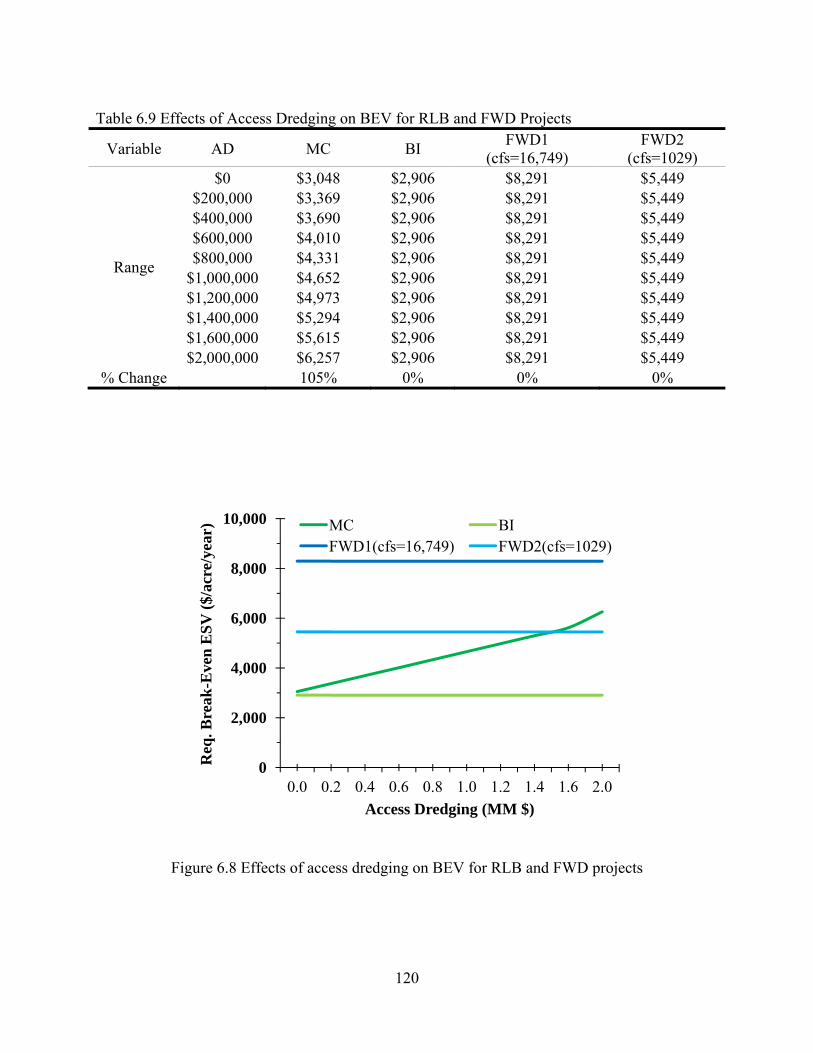
Table 6.9 Effects of Access Dredging on BEV for RLB and FWD Projects
Variable MC BI FWD1 (cfs=16,749)
FWD2 (cfs=1029) AD
Range
$0 $3,048 $2,906 $8,291 $5,449 $200,000 $3,369 $2,906 $8,291 $5,449 $400,000 $3,690 $2,906 $8,291 $5,449 $600,000 $4,010 $2,906 $8,291 $5,449 $800,000 $4,331 $2,906 $8,291 $5,449
$1,000,000 $4,652 $2,906 $8,291 $5,449 $1,200,000 $4,973 $2,906 $8,291 $5,449 $1,400,000 $5,294 $2,906 $8,291 $5,449 $1,600,000 $5,615 $2,906 $8,291 $5,449 $2,000,000 $6,257 $2,906 $8,291 $5,449
% Change 105% 0% 0% 0%
0
2,000
4,000
6,000
8,000
10,000
0.0 0.2 0.4 0.6 0.8 1.0 1.2 1.4 1.6 2.0
Req
. Bre
ak-E
ven
ESV
($/a
cre/
year
)
Access Dredging (MM $)
MC BIFWD1(cfs=16,749) FWD2(cfs=1029)
Figure 6.8 Effects of access dredging on BEV for RLB and FWD projects
120
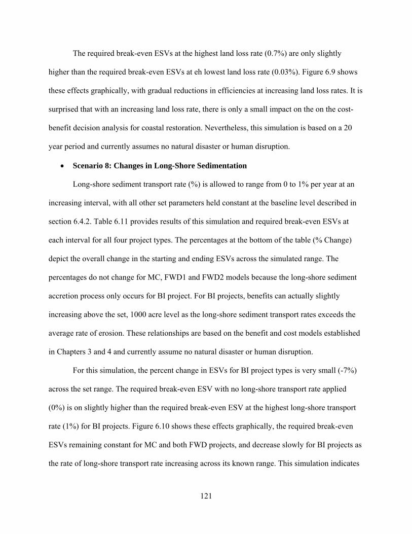
The required break-even ESVs at the highest land loss rate (0.7%) are only slightly
higher than the required break-even ESVs at eh lowest land loss rate (0.03%). Figure 6.9 shows
these effects graphically, with gradual reductions in efficiencies at increasing land loss rates. It is
surprised that with an increasing land loss rate, there is only a small impact on the on the cost-
benefit decision analysis for coastal restoration. Nevertheless, this simulation is based on a 20
year period and currently assumes no natural disaster or human disruption.
• Scenario 8: Changes in Long-Shore Sedimentation
Long-shore sediment transport rate (%) is allowed to range from 0 to 1% per year at an
increasing interval, with all other set parameters held constant at the baseline level described in
section 6.4.2. Table 6.11 provides results of this simulation and required break-even ESVs at
each interval for all four project types. The percentages at the bottom of the table (% Change)
depict the overall change in the starting and ending ESVs across the simulated range. The
percentages do not change for MC, FWD1 and FWD2 models because the long-shore sediment
accretion process only occurs for BI project. For BI projects, benefits can actually slightly
increasing above the set, 1000 acre level as the long-shore sediment transport rates exceeds the
average rate of erosion. These relationships are based on the benefit and cost models established
in Chapters 3 and 4 and currently assume no natural disaster or human disruption.
For this simulation, the percent change in ESVs for BI project types is very small (-7%)
across the set range. The required break-even ESV with no long-shore transport rate applied
(0%) is on slightly higher than the required break-even ESV at the highest long-shore transport
rate (1%) for BI projects. Figure 6.10 shows these effects graphically, the required break-even
ESVs remaining constant for MC and both FWD projects, and decrease slowly for BI projects as
the rate of long-shore transport rate increasing across its known range. This simulation indicates
121
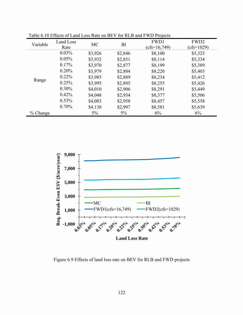
Table 6.10 Effects of Land Loss Rate on BEV for RLB and FWD Projects
Variable Land Loss MC BI FWD1 (cfs=16,749)
FWD2 (cfs=1029) Rate
Range
0.03% $3,926 $2,846 $8,100 $5,325 0.05% $3,932 $2,851 $8,114 $5,334 0.17% $3,970 $2,877 $8,199 $5,389 0.20% $3,979 $2,884 $8,220 $5,403 0.22% $3,985 $2,889 $8,234 $5,412 0.25% $3,995 $2,895 $8,255 $5,426 0.30% $4,010 $2,906 $8,291 $5,449 0.42% $4,048 $2,934 $8,377 $5,506 0.53% $4,083 $2,958 $8,457 $5,558 0.70% $4,138 $2,997 $8,581 $5,639
% Change 5% 5% 6% 6%
Figure 6.9 Effects of land loss rate on BEV for RLB and FWD projects
-1,000
1,000
3,000
5,000
7,000
9,000
Req
. Bre
ak-E
ven
ESV
($/a
cre/
year
)
Land Loss Rate
MC BIFWD1(cfs=16,749) FWD2(cfs=1029)
122
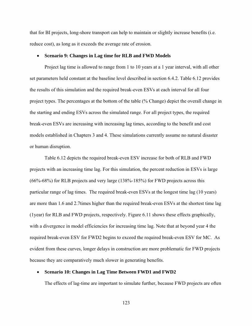
that for BI projects, long-shore transport can help to maintain or slightly increase benefits (i.e.
reduce cost), as long as it exceeds the average rate of erosion.
• Scenario 9: Changes in Lag time for RLB and FWD Models
Project lag time is allowed to range from 1 to 10 years at a 1 year interval, with all other
set parameters held constant at the baseline level described in section 6.4.2. Table 6.12 provides
the results of this simulation and the required break-even ESVs at each interval for all four
project types. The percentages at the bottom of the table (% Change) depict the overall change in
the starting and ending ESVs across the simulated range. For all project types, the required
break-even ESVs are increasing with increasing lag times, according to the benefit and cost
models established in Chapters 3 and 4. These simulations currently assume no natural disaster
or human disruption.
Table 6.12 depicts the required break-even ESV increase for both of RLB and FWD
projects with an increasing time lag. For this simulation, the percent reduction in ESVs is large
(66%-68%) for RLB projects and very large (138%-185%) for FWD projects across this
particular range of lag times. The required break-even ESVs at the longest time lag (10 years)
are more than 1.6 and 2.7times higher than the required break-even ESVs at the shortest time lag
(1year) for RLB and FWD projects, respectively. Figure 6.11 shows these effects graphically,
with a divergence in model efficiencies for increasing time lag. Note that at beyond year 4 the
required break-even ESV for FWD2 begins to exceed the required break-even ESV for MC. As
evident from these curves, longer delays in construction are more problematic for FWD projects
because they are comparatively much slower in generating benefits.
• Scenario 10: Changes in Lag Time Between FWD1 and FWD2
The effects of lag-time are important to simulate further, because FWD projects are often
123

Table 6.11 Effects of Long-Shore Sedimentation on BEV for RLB and FWD Projects
Variable Long-Shore MC BI FWD1 (cfs=16,749)
FWD2 (cfs=1029) Trans Rate
Range
0% $4,010 $2,906 $8,291 $5,449 0.2% $4,010 $2,862 $8,291 $5,449 0.3% $4,010 $2,840 $8,291 $5,449 0.4% $4,010 $2,862 $8,291 $5,449 0.5% $4,010 $2,884 $8,291 $5,449 0.6% $4,010 $2,774 $8,291 $5,449 0.7% $4,010 $2,753 $8,291 $5,449 0.8% $4,010 $2,731 $8,291 $5,449 0.9% $4,010 $2,710 $8,291 $5,449 1.0% $4,010 $2,689 $8,291 $5,449
% Change 0% -7% 0% 0%
Figure 6.10 Effects of Lang-shore sediment transport rate on BEV for RLB and FWD projects
0
2,000
4,000
6,000
8,000
10,000
Req
. Bre
ak-E
ven
ESV
($/a
cre/
year
)
Long-Shore Trans Rate
MC BIFWD1(cfs=16,749) FWD2(cfs=1029)
124

very controversial and can be delayed for many years due to public concerns over flooding and
changes in salinity (see section 5.4). Outside of CWPPRA, the time lag time for FWD has been
as high as 30 to 40 years between authorization and construction for projects like Caernarvon
and Davis Pond. In this simulation, project lag is allowed to vary for FWD projects only and
ranged from 1 to 20 years at a set interval, with other set parameters held constant at the baseline
level described in section 6.4.2. Table 6.13 provides the results of this simulation and the
required break-even ESVs at each interval for FWD project types. The percentages at the bottom
of the table (% Change) depict the overall change in the starting and ending ESVs across the
simulated range. For FWD project types, the required break-even ESVs increases dramatically
over the set range, according to the benefit and cost models established in Chapters 3 and 4.
Table 6.13 depicts the required break-even ESV increase for both of FWD1 and FWD2
projects with an increasing time lag. For this simulation, the percent reduction in ESVs for RLB
is huge (7139%-7737%) for FWD projects across the set range, indicting the tremendously high
degree of influence that time lag has on both project cost and benefits. The required break-even
ESVs at the longest time lag (20 years) are more than 70 times higher than the required break-
even ESVs at the shortest time lag (1year) FWD projects. Figure 6.12 shows these effects
graphically, with sharp increases beyond 10 years. For example, in a 20 year lag, no benefits
have accrued, yet planning and engineering expenditures (overhead) have already been made -
usually within the in the first few years. In this scenario, break-even ESVs tends to infinity with
ever-increasing time lags and at a minimum would far exceed the ranges reported for ESVs in
the non-market valuation literature.
125
Table 6.12 Effects of Lag Time on BEV for RLB and FWD Projects
Variable MC BI FWD1 (cfs=16,749)
FWD2 (cfs=1029) Time Lag
Range
1 $3,521 $2,558 $4,537 $3,014 2 $3,665 $2,660 $4,930 $3,270 3 $3,827 $2,776 $5,389 $3,568 4 $4,010 $2,906 $5,929 $3,919 5 $4,219 $3,055 $6,762 $4,336 6 $4,459 $3,225 $7,522 $4,838 7 $4,738 $3,423 $8,291 $5,449 8 $5,065 $3,654 $9,462 $6,206 9 $5,454 $3,928 $10,940 $7,160 10 $5,925 $4,258 $12,844 $8,387
% Change 68% 66% 183% 178%
Figure 6.11 Effects of lag time on BEV for RLB and FWD projects
0
4,000
8,000
12,000
16,000
1 2 3 4 5 6 7 8 9 10
Req
. Bre
ak-E
ven
ESV
($/a
cre/
year
)
Lag Time (Year)
MCBIFWD1(cfs=16,749)FWD2(cfs=1029)
126

Table 6.13 Effects of Time on BEV for FWD Projects
Variable Time Lag MC BI FWD1 (cfs=16,749)
FWD2 (cfs=1029) (FWD 1~20)
Range
1 $4,010 $2,906 $4,537 $3,014 3 $4,010 $2,906 $5,389 $3,568 5 $4,010 $2,906 $6,762 $4,336 7 $4,010 $2,906 $8,291 $5,449 9 $4,010 $2,906 $10,940 $7,160
10 $4,010 $2,906 $12,844 $8,387 13 $4,010 $2,906 $23,662 $15,322 16 $4,010 $2,906 $62,437 $39,894 19 $4,010 $2,906 $355,548 $218,187 20 $4,010 $2,906 $355,548 $218,187
% Change 0% 0% 7737% 7139%
0
10,000
20,000
30,000
40,000
50,000
1 3 5 7 9 10 13 16 19
Req
. Bre
ak-E
ven
ESV
($/a
cre/
year
)
Lag Time (FWD 1~20 Year)
MCBIFWD1(cfs=16,749)FWD2(cfs=1029)
Figure 6.12 Effects of lag time on BEV for FWD projects
127
6.5 Summary
In this chapter, methods and estimates for the non-market, ecosystem service values
(ESV) of wetlands have been discussed and identified. Starting values for estimates were
incorporated into a mathematical NPV model along with 22 other user-specified set values to
develop baseline cost-benefit simulations for two RLB models (MC and BI) and two freshwater
diversion models (FWD1 and FWD2. Simulations against this baseline were conducted by
allowing a single, user-specified parameter to vary across its known range and generating the
required break-even ESV ($/acre/year) for each simulation. In the vast majority of these
simulations, the required ESV is considerably higher than the range of values reported in the
non-market valuation literature.
As found in chapters 3, 4, and 5, project life time, scale, discount rate, and time lag have
a major impact on the cost-benefit decision analysis for coastal restoration. The MOB costs were
founded more sensitive for BI projects than MC projects. For a RLB project, the distance
between sediments borrow site and project site will have a major impact on the cost-benefit
decision analysis. The cost of AD is not an important fact for BI and FWD projects, but it is
significant on MC projects cost and benefits analysis. The long-shore transport rate has a very
small effect on BI projects cost and benefits only. Finally, time lag was found to have a very
import impact on the cost-benefit decision analysis for all models, especially FWD projects.
Surprisingly, the rate of land loss had only a small impact the cost-benefit relationship for
RLB and FWD projects. This indicates that average land loss rates are usually too small to affect
the costs and benefits of a wetland restoration project; however, these simulations assume no
natural disaster or human disruption. Therefore, uncertainty should be considered and the
probabilities of hurricane occurrence should be incorporated into the NPV models. Once the
128
probabilities of hurricane landfall have been identified and incorporated into these models, a
more reliable result will be obtained from these simulations. The following chapter will
introduce and explore this uncertainty.
129

CHAPTER 7 INCORPORATING UNCERTAINTY
7.1 Introduction
So far in this study, net present value (NPV) analysis has primarily focused on conditions
in which the user-controlled set values affecting the simulated outcomes have been assumed to
be known with certainty. In most cases, however, comparisons of wetland restoration
alternatives using the NPV method are developed with a consideration of uncertainty. This can
be accomplished through a variety of climatological, political, and ecological factors that
influence project costs and benefits.
7.2 Risk and Uncertainty
While the terms “risk” and “uncertainty” are often used interchangeably, the terms have
many different definitions and applications and there is no single consistent method for their
incorporation into decision-making. Knight (1921) introduced the definitional difference between risk
and uncertainty by pointing out that risk has an unknown outcome, but the likelihood distribution
of that outcome can be calculated. In contrast, “uncertainty” refers to the case in which the
likelihood distribution of an outcome cannot be expressed in terms of mathematical probability.
Hubbard (2007, 2009) defines risk as a state of uncertainty where some possible outcomes have
an undesired effect or significant loss. And Jones (2006) defines risk as the probable frequency and
magnitude of future loss. In economic terms, this can refer to a decline in income due to losses
resulting from a natural hazard.
Many uncertainties are faced when deciding to fund a restoration project. In regards to
hurricanes, managers need information on the frequency and impact of these storms on coastal
restoration projects. Specific questions include: What is the statistical probability of a major
130

hurricane making landfall in the project area?; How would such a storm affect the benefits and
costs of the project?; and, How can this risk and impact be incorporated into the NPV analysis of
the project? Political constraints might delay a wetland restoration project, cut the project budget,
or constrain its operation. Ecological factors might also impose risk by constraining optimal
plant growth or through changes in water quality. Without incorporating these risks, comparisons
based on NPV methods might provide misleading results. This section primarily explores
hurricane risk, how to incorporate that risk into the NPV method, and the impacts of hurricanes
on a given project type and location. This information is used to revisit the estimates of required
break-even ecosystem services value (ESV) for RLB and FWD projects under the situation of
hurricane landfall. Meanwhile, political and ecological risks are discussed.
7.3 Hurricane Risk
From a climatological perspective, risk can be expressed as the likelihood of hurricane
landfall, which would alter the benefits and costs of a wetland restoration project. The
probability of a hurricane in any given year would range from 0 to 1 (0% to 100%) during the
project life period. For the purpose of NPV analysis, however, probabilities are rarely based
strictly on historical information. The adjusted currently available information is taken into
account and referred to as subjective probabilities of hurricane landfall. Once the probabilities of
hurricane landfall have been characterized and quantified, this information may be introduced
into NPV analysis. Klotzbach and Gray (2011) report that the annual probabilities of major storm
(i.e. Category 3 or greater) making landfall in Louisiana are 12% and 20% for climatological and
current-year probabilities, respectively. In their research, these storms are defined in two
categories: hurricanes (75mph ≤ winds <115) and intense hurricane (major hurricane winds ≥115
mph). To simplify the analysis of major hurricane landfall risk, this study adopts the current-year
131

probability and assumes that this probability is the same each year during the project life time.
Meanwhile, this research assumes that there are two different situations that will be denoted as
Risk1 and Risk2. Risk1 refers to a hurricane impact (percent acreage loss) for the project that is
static or averaged over the life of the project. Risk2 refer to a percent acreage loss that varies
annually according to the degree of project completion.
Table 7.1 depicts the probabilities of hurricane landfall in five coastal states: Texas,
Louisiana, Mississippi, Alabama, and Florida. The annual probability of hurricane landfall
ranges from a low of 11% to a high 51% and a low of 18% to a high 72% for climatological and
current-year probability, respectively. The annual probability of from a major hurricane ranges
from a low of 3% to a high 21% and a low of 5% to a high 35% for climatological and current-
year probability, respectively. Table 7.2 depicts the probabilities of hurricane landfall for 18
coastal parishes in Louisiana. The range of probability of 1 or more hurricanes making landfall in
the parish are from a low 1% to a high 10% and the range of probability of 1 or more major
hurricanes making landfall in the parish are from a low 1% to a high 5%.
7.3.1 NPV Models with Hurricane Risk
The basic framework for incorporating risk to be used in this study will be Expected
Value (EV) analysis. This process involves identifying the probability of specific outcomes and
incorporating that probability into the NPV process. Holland (2010) describes this incorporation
as:
[ ] ( )∑=
∗−=T
tttt PCBNBE
1 (Eq. 7.1)
( ) ( ) ttt PCBPCBPCB −++−+−= K222111 )(
132
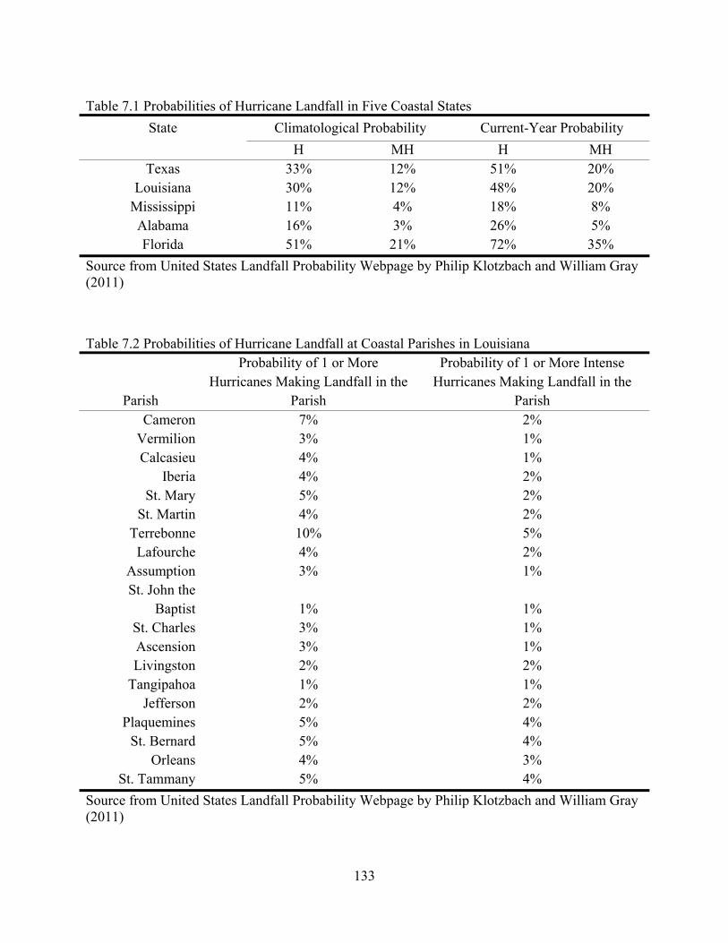
Table 7.1 Probabilities of Hurricane Landfall in Five Coastal States State Climatological Probability Current-Year Probability
H MH H MH Texas 33% 12% 51% 20%
Louisiana 30% 12% 48% 20% Mississippi 11% 4% 18% 8% Alabama 16% 3% 26% 5% Florida 51% 21% 72% 35%
Source from United States Landfall Probability Webpage by Philip Klotzbach and William Gray (2011)
Table 7.2 Probabilities of Hurricane Landfall at Coastal Parishes in Louisiana Probability of 1 or More
Hurricanes Making Landfall in the Parish
Probability of 1 or More Intense Hurricanes Making Landfall in the
Parish Parish Cameron 7% 2%
Vermilion 3% 1% Calcasieu 4% 1%
Iberia 4% 2% St. Mary 5% 2%
St. Martin 4% 2% Terrebonne 10% 5% Lafourche 4% 2%
Assumption 3% 1% St. John the
Baptist 1% 1% St. Charles 3% 1% Ascension 3% 1% Livingston 2% 2%
Tangipahoa 1% 1% Jefferson 2% 2%
Plaquemines 5% 4% St. Bernard 5% 4%
Orleans 4% 3% St. Tammany 5% 4%
Source from United States Landfall Probability Webpage by Philip Klotzbach and William Gray (2011)
133
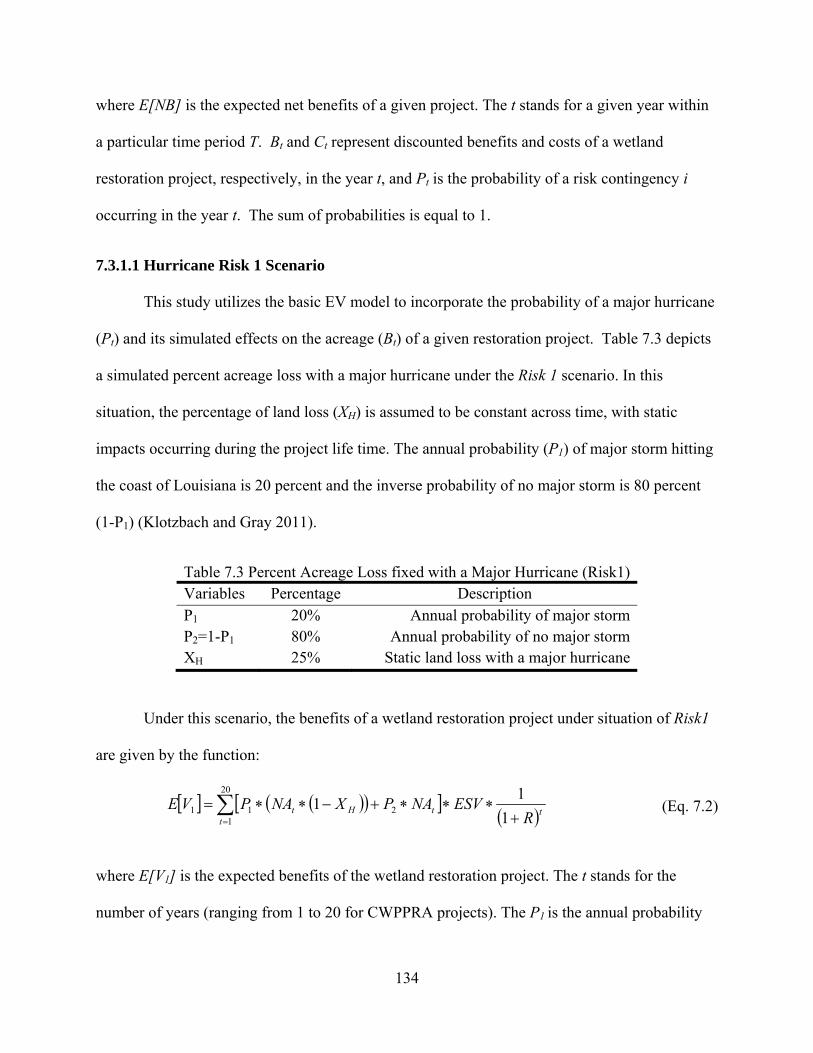
where E[NB] is the expected net benefits of a given project. The t stands for a given year within
a particular time period T. Bt and Ct represent discounted benefits and costs of a wetland
restoration project, respectively, in the year t, and Pt is the probability of a risk contingency i
occurring in the year t. The sum of probabilities is equal to 1.
7.3.1.1 Hurricane Risk 1 Scenario
This study utilizes the basic EV model to incorporate the probability of a major hurricane
(Pt) and its simulated effects on the acreage (Bt) of a given restoration project. Table 7.3 depicts
a simulated percent acreage loss with a major hurricane under the Risk 1 scenario. In this
situation, the percentage of land loss (XH) is assumed to be constant across time, with static
impacts occurring during the project life time. The annual probability (P1) of major storm hitting
the coast of Louisiana is 20 percent and the inverse probability of no major storm is 80 percent
(1-P1) (Klotzbach and Gray 2011).
Table 7.3 Percent Acreage Loss fixed with a Major Hurricane (Risk1) Variables Percentage Description P1 20% Annual probability of major storm P2=1-P1 80% Annual probability of no major storm XH 25% Static land loss with a major hurricane
Under this scenario, the benefits of a wetland restoration project under situation of Risk1
are given by the function:
[ ] ( )( )[ ]( )tt
tHt RESVNAPXNAPVE
+∗∗∗+−∗∗= ∑
= 111
20
1211 (Eq. 7.2)
where E[V1] is the expected benefits of the wetland restoration project. The t stands for the
number of years (ranging from 1 to 20 for CWPPRA projects). The P1 is the annual probability
134

of major storm and P2 = (1-P1), which stands for the annual probability of no major storm. NAt is
a user specified variable referring to the desired net acreage gain from the project in year t. XH
stands for the percent acreage loss expected with a major hurricane. The acronym ESV stands for
the annual non-market, ecosystem values for each acre restored. R is the discount rate.
7.3.1.2 Hurricane Risk 2 Scenario
Table 7.4 depicts the simulated percent acreage loss with a major hurricane under the
Risk 2 scenario. In this situation, XH is allowed to vary per year as a function of the percent
completion of a given wetland restoration project. The annual probability of a major storm
(coast-wide) is set at 20 percent and the annual probability of no major storm is 80 percent
(Klotzbach and Gray 2011). To capture an element of resiliency/vulnerability, a sliding scale is
introduced in which the simulated percent acreage loss is higher/lower for projects that are
less/more completed. For example, an 80% reduction in acreage might occur from an major
hurricane if the given project’s percent completion was less than or equal to 20% in time period
t; The percent acreage loss is set at 60% for a major hurricane if completion is less than 40% in
time period t. The percent acreage loss is set at 40% if project is less than or equal to 60%
complete in time period t. And finally, the percent acreage loss is set at 20% if project is than or
equal to 80% complete in time period t.
Table 7.4 Percent Acreage Loss Varies with a Major Hurricane (Risk2) Variables Percentage Description P1 20% Annual probability of major storm P2=1-P1 80% Annual probability of no major storm Simulated Impacts XH1 80% If project completion≤20% XH2 60% If project completion≤40% XH3 40% If project completion≤60% XH4 20% If project completion≤80%
135

Benefits for wetland restoration project under situation of Risk2 scenario are given by the
function:
[ ] ( )( )[ ]( )tt
tHNt RESVNAPXNAPVE
+∗∗∗+−∗∗= ∑
= 111
20
1212 (Eq. 7.3)
where E[V2] is the expected benefits of the wetland restoration project. The t stands for the
number of years (ranging from 1 to 20 for CWPPRA projects). The P1 is the annual probability
of major storm and P2 = (1-P1), which stands for the annual probability of no major storm. NAt is
a user specified variable referring to the desired net acreage gain from the project in year t. XHN
(N=1, 2, 3, 4) stands for the percent acreage loss with a major hurricane and varies per year as a
function of percent completion of a given wetland restoration project. The acronym ESV stands
for the annual non-market, ecosystem values for each acre restored. R is the discount rate.
7.3.2 Depicting Hurricane Risk Impacts on Wetland Restoration Projects
After examining and incorporating hurricane risk for these projects, benefits were re-
calculated based on NPV models. Figure 7.3 depicts effects of erosion and simulated hurricane
risk on net acres for RLB and FWD projects. As described in Chapter 3, with an average four
year delay of project construction, MC projects follow a sigmoid trajectory. Net acres are static
in year 4, followed by a rapid accrual of acreage in years 4-6, with most of the land gain
occurring in years 5 and 6. From year 6 to year 20, net acreage is either constant or slightly
decreasing (because of erosion) given a no hurricane scenario. Under hurricane scenarios of Risk
1 (constant impacts) and Risk 2 (scaled impacts), MC projects would still follow a sigmoid
trajectory but with reduced levels of benefits. Projected benefits (net acres) would be the least
under the Risk 1 scenario because of the constant (equal) probability of land loss across the
project life time. Conversely, the benefits under the Risk 2 scenario would be slightly higher
136

137
because of the varying probability of land loss due to the scaled impact related to project
completion. Likewise, with an average four years delay of project construction, BI projects
initially follow a similar sigmoidal trend. Net acres are mechanically restored over a short time
period, and then are either constant or slowly decreasing under in the absence of hurricanes.
Under hurricane Risk 1and Risk 2 scenarios, BI projects follow the same general sigmoid trends
as the MC projects and benefits (net acre) are the lowest under Risk 1 scenario.
Figure 7.1 also depicts the effects of erosion and simulated hurricane risk on net acre
accrual for FWD 1 and FWD2 projects. As described in Chapter 3, the average FWD project has
an average seven year lag prior to construction and benefits follow a linear trajectory. Net
acreages increase at a slow, constant rate over a 20-year time span in a no hurricane scenario.
Unlike with MC and BI projects, hurricane-based acreage reductions for FWD projects are
assumed to be greater in the Risk 2 scenario because of the slow rate of benefit accrual with
FWD projects. This effect is partially evident in the documented impacts to the Caernarvon
freshwater diversion project, which was heavily impacted by Hurricane Katrina in 2005. The
effects of Katrina on Caernarvon have greatly expanded the range of thinking about coastal
restoration options under hurricane risk (Zinn 2007).
7.4 Refining Risk Assumptions
While the landfall probabilities of a major hurricane are easily extracted from
climatological studies, the degree of impact from these storms on a coastal restoration project is
less predictable. At a minimum, the impact is expected to be a function of scale, location, and
project type. How big a project is, its proximity to the coast, and whether it is a FWD or RLB
project are all factors that have an influence on hurricane vulnerability. Additionally, other forms
of risk to coastal restoration projects exist – such social and mechanical constraints.
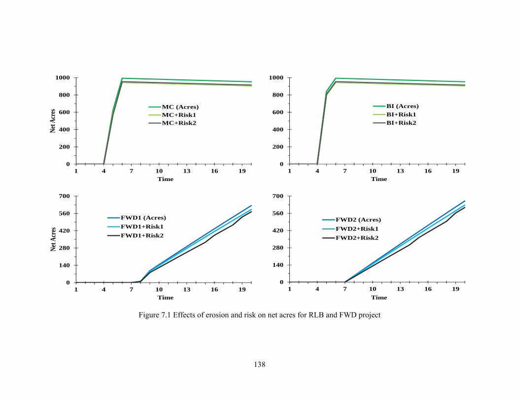
0
200
400
600
800
1000
1 4 7 10 13 16 19
Net A
cres
Time
MC (Acres)MC+Risk1MC+Risk2
0
200
400
600
800
1000
1 4 7 10 13 16 19Time
BI (Acres)BI+Risk1BI+Risk2
0
140
280
420
560
700
1 4 7 10 13 16 19
Net A
cres
Time
FWD1 (Acres)FWD1+Risk1FWD1+Risk2
0
140
280
420
560
700
1 4 7 10 13 16 19Time
FWD2 (Acres)FWD2+Risk1FWD2+Risk2
Figure 7.1 Effects of erosion and risk on net acres for RLB and FWD project
138

7.4.1 Scaling Hurricane Impacts
On August 29, 2005 Hurricane Katrina struck the northern Gulf Coast as a category 4
storm with 140 mph winds and caused adverse effects on the wetlands being created at the
Caernarvon Freshwater Diversion restoration project. Salinities and water levels were
dramatically impacted by the storm with devastating effects on the marshes in Breton Sound.
Just three weeks later, on September 24, 2005 Hurricane Rita made landfall near Sabine Pass at
the Louisiana-Texas border as a category 3 storm with 120-140 mph winds. The storm impacted
the Holly Beach Sand Management Project, a RLB project completed in 2002.
These two projects can be used to demonstrate a process through which the impacts of
hurricanes to restoration projects can be further refined. In order to scale the effect of hurricane
impacts on these two typical projects, a land change analysis was undertaken through the use of
Geographic Information Systems (GIS) lab of the Department of Agricultural Economics at
Louisiana State University. The degree of acreage effect at Caernarvon and Holly Beach can be
estimated using pre- and post-storm imagery. Project specific impacts (i.e. adjusting XH under the
Risk2 scenario) were refined for these two storms and two projects using Earth Resource Data
Analysis System (ERDAS) software (version 10.1). Digital Orthoimagery Quarter Quadrangles
(DOQQ) images from pre- and post-landfall of Hurricanes Katrina and Rita acquired from the
U.S.Geological Survey (USGS).
Table 7.5 depicts that the calculated project area of the Caernarvon Freshwater Diversion
outfall area in Breton Sound, comprising approximately 690,759 acres, of which 443,340 acres
are classified as water and 247,419 acres were classified as land in 2005 before Hurricane
Katrina. The water area increased to 481,893 acres and the land area decreased to 208,866 acres
in 2006 after Hurricane Katrina. An approximately 38,553 acres of coastal land was converted to
139
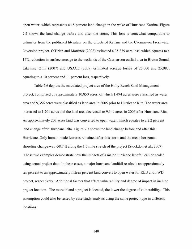
open water, which represents a 15 percent land change in the wake of Hurricane Katrina. Figure
7.2 shows the land change before and after the storm. This loss is somewhat comparable to
estimates from the published literature on the effects of Katrina and the Caernarvon Freshwater
Diversion project. O’Brien and Matrinez (2008) estimated a 35,839 acre loss, which equates to a
14% reduction in surface acreage to the wetlands of the Caernarvon outfall area in Breton Sound.
Likewise, Zinn (2007) and USACE (2007) estimated acreage losses of 25,000 and 25,983,
equating to a 10 percent and 11 percent loss, respectively.
Table 7.6 depicts the calculated project area of the Holly Beach Sand Management
project, comprised of approximately 10,850 acres, of which 1,494 acres were classified as water
area and 9,356 acres were classified as land area in 2005 prior to Hurricane Rita. The water area
increased to 1,701 acres and the land area decreased to 9,149 acres in 2006 after Hurricane Rita.
An approximately 207 acres land was converted to open water, which equates to a 2.2 percent
land change after Hurricane Rita. Figure 7.3 shows the land change before and after this
Hurricane. Only human-made features remained after this storm and the mean horizontal
shoreline change was -58.7 ft along the 1.5 mile stretch of the project (Stockdon et al., 2007).
These two examples demonstrate how the impacts of a major hurricane landfall can be scaled
using actual project data. In these cases, a major hurricane landfall results is an approximately
ten percent to an approximately fifteen percent land convert to open water for RLB and FWD
project, respectively. Additional factors that affect vulnerability and degree of impact in include
project location. The more inland a project is located, the lower the degree of vulnerability. This
assumption could also be tested by case study analysis using the same project type in different
locations.
140

Table 7.5 Caernarvon Freshwater Diversion Project Land Change Pre and Post Hurricane Katrina 2005 (March-April) 2006 (June) Total Area (acre) 690,759 690,759 Water Acreage 443,340 481,893 Land Acreage 247,419 208,866 Land Loss after Hurricane Katrina (acre) 38,553 Percentage of Land Loss 15%
Table 7.6 Holly Beach Sand Management Project Land Change Pre and Post Hurricane Rita 2005 (April) 2006 (June) Total Area (acre) 10,850 10,850 Water Acreage 1,494 1,701 Land Acreage 9,356 9,149 Land Loss after Hurricane Rita (acre) 207 Percentage of Land Loss 2.2%
7.4.2 Adjusting for Political Risk
From a social perspective, risk can also be expressed as the likelihood of political
constraints, which would alter the benefits and costs of a wetland restoration project. The
probability of political constraints is not typically calculated, as with hurricane frequencies, and
it must be estimated based using case-specific historical information. As discussed in Chapters 2
and 3, project construction is, on average, delayed by four years and seven years for RLB and
FWD projects, respectively. Some of this lag is due to political and social constraints. These lag
effects were incorporated and simulated into the NPV model in chapters 5 and 6. For FWD
projects, however, project operation can also be fraught with social constraints. The following
two cases illustrate particular constraints associated with FWD projects.
141

2005
2006
Figure 7.2 Classified Image of Caernarvon Freshwater Diversion Project Pre-Post Hurricane Katrina
142

2005
2006
Figure 7.3 Landsat Image of Holly Beach Sand Management Project Pre-Post Hurricane Rita
143

The Caernarvon Freshwater Diversion Project was authorized by the U.S. Congress under
the Flood Control Act of 1965 and the Water Resources Development Act of 1974, 1986, and
1996. The project was constructed between 1988 and 1991 and began operations in August 1991.
From initial project authorization to construction, this project had a lag of 26 years. The structure
is designed to divert up to 8,000 cubic feet per second (cfs) of freshwater from the Mississippi
river into the marshes and bays of the Breton Sound estuary. Since opening, flow rates for the
Caernarvon project have been curtailed by a number of constraints related primarily to short-
term fisheries impacts (Caffey and Schexnayder 2003). Soon after opening 1991, oyster
fishermen argued that this diversion project damaged many of the oyster beds and filed law suit
against the state. This law suit led to $2.3 billion in judgments that threatened the ability to
conduct future wetland restoration projects in Louisiana. To deal with these problems and
combat the high rate of coastal wetlands loss in Louisiana, the 2003 Louisiana legislature passed
three constitutional amendments through referendum, which were intended to remove these
constraints and increase the state’s capacity for coastal wetland restoration. These amendments
limited the state’s liability to compensate property damage caused by coastal restoration projects.
The value of operational losses was limited to the fair market value of affected property (Caffey
and Schexnayder 2003). In addition to the oyster industry, a number of other stakeholders have
requested reduced flow rates for the Caernarvon structure. Shrimp fishermen, crab harvesters,
land owners, recreational fishermen and hunters, and navigation interests have all served on the
interagency advisory committees that controls the structures flow rate.
Due to all of these constraints, the 14 year (1991-2005) average operational discharge for
the project has been relatively low. Although the structure has been opened to 6,500 cfs for short
term periods during a “pulsing” study conducted by Louisiana State University, the long-term
144
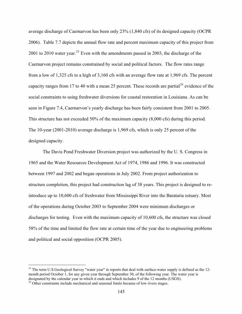
average discharge of Caernarvon has been only 23% (1,840 cfs) of its designed capacity (OCPR
2006). Table 7.7 depicts the annual flow rate and percent maximum capacity of this project from
2001 to 2010 water year.25 Even with the amendments passed in 2003, the discharge of the
Caernarvon project remains constrained by social and political factors. The flow rates range
from a low of 1,325 cfs to a high of 3,160 cfs with an average flow rate at 1,969 cfs. The percent
capacity ranges from 17 to 40 with a mean 25 percent. These records are partial26 evidence of the
social constraints to using freshwater diversions for coastal restoration in Louisiana. As can be
seen in Figure 7.4, Caernarvon’s yearly discharge has been fairly consistent from 2001 to 2005.
This structure has not exceeded 50% of the maximum capacity (8,000 cfs) during this period.
The 10-year (2001-2010) average discharge is 1,969 cfs, which is only 25 percent of the
designed capacity.
The Davis Pond Freshwater Diversion project was authorized by the U. S. Congress in
1965 and the Water Resources Development Act of 1974, 1986 and 1996. It was constructed
between 1997 and 2002 and began operations in July 2002. From project authorization to
structure completion, this project had construction lag of 38 years. This project is designed to re-
introduce up to 10,600 cfs of freshwater from Mississippi River into the Barataria estuary. Most
of the operations during October 2003 to September 2004 were minimum discharges or
discharges for testing. Even with the maximum capacity of 10,600 cfs, the structure was closed
58% of the time and limited the flow rate at certain time of the year due to engineering problems
and political and social opposition (OCPR 2005).
25 The term U.S.Geological Survey "water year" in reports that deal with surface-water supply is defined as the 12-month period October 1, for any given year through September 30, of the following year. The water year is designated by the calendar year in which it ends and which includes 9 of the 12 months (USGS). 26 Other constraints include mechanical and seasonal limits because of low rivers stages.
145

Table 7.7 Caernarvon Freshwater Diversion Annual Flow Rate (2001-2010) Water Year Annual Flow Rate (cfs) Percentage of Max Capacity (8,000 cfs)
2001 1,511 19% 2002 1,471 18% 2003 1,325 17% 2004 1,467 18% 2005 1,594 20% 2006 1,967 25% 2007 2,935 37% 2008 2,709 34% 2009 1,554 19% 2010 3,160 40%
Average 1,969 25% Source: the U.S.Geological Survey (USGS). National Water Information System: Web Interface
.
Figure 7.4 Yearly Mean Discharge at Caernarvon Freshwater Diversion
Table 7.8 depicts the annual flow rate and percent maximum capacity of Davis Pond
project from 2003 to 2010 water year. Likewise, even with the 2003 constitutional amendments,
the discharge rate of this project has also constrained by social and political factors. The flow
rates range from a low of 683 cfs to a high of 3,873 cfs with an average flow rate at 2,143 cfs.
146

The percent capacity ranges from 6 to 36 with a mean 22 percent. As can be seen in Figure 7.4,
Davis Pond yearly discharge were relative lower in the year 2003, 2004 and 2005 after operation
and has not exceeded 10% of the maximum capacity. Davis Pond discharge for the 8- year
(2003-2010) time period averaged 2,143 cfs, which is only 22 percent of the maximum capacity.
These records and graph are also partially indicative of the social constraints to freshwater
diversion projects in coastal Louisiana.
Table 7.8 Davis Pond Freshwater Diversion Annual Flow Rate (2003-2010) Water Year Annual Flow Rate (cfs) Percentage of Max Capacity (10,600 cfs)
2003 833 8% 2004 683 6% 2005 821 8% 2006 3,101 29% 2007 2,207 21% 2008 3,551 34% 2009 3,802 36% 2010 3,873 36%
Average 2,143 22% Source: U.S.Geological Survey (USGS). National Water Information System: Web Interface
Figure 7.5 Yearly Mean Discharge at Davis Pond Freshwater Diversion
147

Unlike the expected valuation construct used for hurricane scenarios (Risk 1 and Risk 2),
the incorporation of social constraints to FWD operations is represented here through a simple
numerical factor. Drawing from the benefit model of FWD-based wetland restoration (Eq. 5.17),
the factor is applied as:
( ) ( )[ ] ( )( )( )tS
tf
lagtft R
XESVElagtNAFWDB f
+∗∗−∗−∗+−∗=∑
=
−
11*1051.00029.0
20
1
(Eq. 7.4)
where the XS is a user-defined social constraints for FWD operation ranging from 0 to 100
percent.
Figure 7.6 depicts the simulated effects of political risk on net acre accrual for FWD 1
and FWD2 projects. Using a simulated social constraint to operations “Risk 3” scenario, the
average FWD project has an average seven year lag prior to construction, social constraint (Xs)
is set to 23 percent of the designed capacity of the structure, and benefits still follow a linear
trajectory but with much higher reduced levels of benefits. Net acreages increase at a slower,
constant rate over the 20-year life time.
7.5 Summary
Although risk assumptions are often hidden in economic comparisons, all coastal wetland
restoration projects face direct and indirect sources of uncertainty and risk as to the benefits they
provide. In this chapter, risk are discussed and incorporated into the NPV process. Hurricane
risk was considered in two different situations - static and dynamic. Under static hurricane risk
(XH, Risk1), the percentage of hurricane-driven land loss was assumed to occur at a constant rate
across project life time. Under the dynamic hurricane risk scenario (XH, Risk2); however, the
percentage of hurricane-driven land loss varied each time interval as a function of scale (i.e.
148

0
140
280
420
560
700
1 4 7 10 13 16 19
Net
Acr
es
Time
FWD1 (Acres)FWD1+Risk1FWD1+Risk2FWD1+Risk3
0
140
280
420
560
700
1 4 7 10 13 16 19
Net
Acr
es
Time
FWD2 (Acres)FWD2+Risk1FWD2+Risk2FWD2+Risk3
Figure 7.6 Effects of erosion and risk on net acres for FWD project
percent completion of the project). Hurricane risks were found to have the greatest impact on
FWD projects due to their relatively slow rate of restoration. A method is described through
which pre- and post-storm imagery can be used to determine actual project impacts and to adjust
149
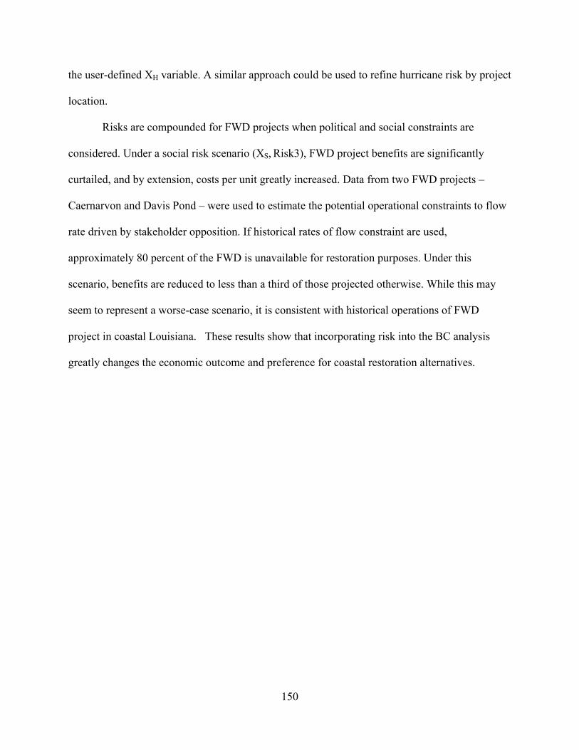
the user-defined XH variable. A similar approach could be used to refine hurricane risk by project
location.
Risks are compounded for FWD projects when political and social constraints are
considered. Under a social risk scenario (XS, Risk3), FWD project benefits are significantly
curtailed, and by extension, costs per unit greatly increased. Data from two FWD projects –
Caernarvon and Davis Pond – were used to estimate the potential operational constraints to flow
rate driven by stakeholder opposition. If historical rates of flow constraint are used,
approximately 80 percent of the FWD is unavailable for restoration purposes. Under this
scenario, benefits are reduced to less than a third of those projected otherwise. While this may
seem to represent a worse-case scenario, it is consistent with historical operations of FWD
project in coastal Louisiana. These results show that incorporating risk into the BC analysis
greatly changes the economic outcome and preference for coastal restoration alternatives.
150
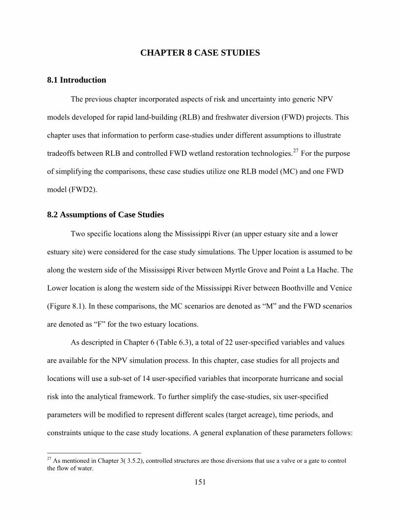
CHAPTER 8 CASE STUDIES
8.1 Introduction
The previous chapter incorporated aspects of risk and uncertainty into generic NPV
models developed for rapid land-building (RLB) and freshwater diversion (FWD) projects. This
chapter uses that information to perform case-studies under different assumptions to illustrate
tradeoffs between RLB and controlled FWD wetland restoration technologies.27 For the purpose
of simplifying the comparisons, these case studies utilize one RLB model (MC) and one FWD
model (FWD2).
8.2 Assumptions of Case Studies
Two specific locations along the Mississippi River (an upper estuary site and a lower
estuary site) were considered for the case study simulations. The Upper location is assumed to be
along the western side of the Mississippi River between Myrtle Grove and Point a La Hache. The
Lower location is along the western side of the Mississippi River between Boothville and Venice
(Figure 8.1). In these comparisons, the MC scenarios are denoted as “M” and the FWD scenarios
are denoted as “F” for the two estuary locations.
As descripted in Chapter 6 (Table 6.3), a total of 22 user-specified variables and values
are available for the NPV simulation process. In this chapter, case studies for all projects and
locations will use a sub-set of 14 user-specified variables that incorporate hurricane and social
risk into the analytical framework. To further simplify the case-studies, six user-specified
parameters will be modified to represent different scales (target acreage), time periods, and
constraints unique to the case study locations. A general explanation of these parameters follows:
27 As mentioned in Chapter 3( 3.5.2), controlled structures are those diversions that use a valve or a gate to control the flow of water.
151
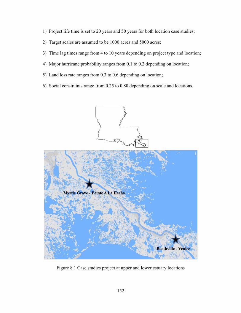
1) Project life time is set to 20 years and 50 years for both location case studies; 2) Target scales are assumed to be 1000 acres and 5000 acres; 3) Time lag times range from 4 to 10 years depending on project type and location; 4) Major hurricane probability ranges from 0.1 to 0.2 depending on location; 5) Land loss rate ranges from 0.3 to 0.6 depending on location; 6) Social constraints range from 0.25 to 0.80 depending on scale and locations.
Figure 8.1 Case studies project at upper and lower estuary locations
152

A qualitative description of the 16 case scenarios is provided in Table 8.1. Table 8.2
depicts 14 parameters for the eight scenarios at the upper estuary location with 6 variables
adjusted to reflect project-specific conditions. The Upper M-1and Upper F-1 scenarios estimate
the total benefits and costs based on a target of 1000 acres and a 20-year project life time. The
Upper M-2 and Upper F-2 scenarios are for 1000 acres and a 50-year project life time. The
Upper M-3 and Upper F-3 scenarios determine the total benefits and costs based on a 5000 acre
target and a 20-year project life time. The Upper M-4 and Upper F-4 scenarios are based on the
same target and a 50-year project life time. For these four Upper estuary scenarios, lag times are
assumed to be 4 years for MC project and 10 years for FWD projects, probability of hurricane
land fall is set to 10 percent, regional-specified land loss rate is assumed to be 0.3 percent per
year, and capacity is set to 40 percent for small scale FWD project and 25 percent for large scale
project, respectively. Finally, four different water flow rates were derived from the N-SED1
model (Boustany 2007) for the upper basin scenarios, including 1,029 cubic feet per second (cfs),
963 cfs, 1489 cfs, and 1161 cfs based on the desired acreage and project life time.
Table 8.3 depicts 14 parameters for the eight scenarios at the Lower estuary location with
6 variables adjusted to reflect project-specific conditions. The Lower M-1and Lower F-1
scenario estimate the total benefits and costs for two wetland restoration project types (MC and
FWD2) based on 1000 target acres during a 20-year project life time. The Lower B-2and Lower
F-2 scenarios are based on a 50-year project life time. The Lower M-3and Lower F-3 scenarios
determine the total benefits and costs based on a 5000 target acre during a 20-year project life
time. The Lower M-4and Lower F-4 scenarios are based on a 50-year project life time. For these
four lower estuary scenarios, lag times are assumed to be 4 years for MC project and 7 years for
FWD project, probability of hurricane land fall is set to 20 percent, regional-specified land loss
153

154
Table 8.1 Upper and Lower Estuary Case Study Scenarios - Qualitative Descriptions
Scenario Description
Upper M-1 Upper estuary MC project, 20 years, 1000 acre target, low/no public opposition, lower hurricane risk, lower erosion, shorter lag time
Upper M-2 Upper estuary MC project, 50 years, 1000 acre target, low/no public opposition, lower hurricane risk, lower erosion, shorter lag time
Upper M-3 Upper estuary MC project, 20 years, 5000 acre target, low/no public opposition, lower hurricane risk, lower erosion, shorter lag time
Upper M-4 Upper estuary MC project, 50 years, 5000 acre target, low/no public opposition, lower hurricane risk, lower erosion, shorter lag time
Upper F-1 Upper estuary MC project, 20 years, 1000 acre target, medium/high public opposition, lower hurricane risk, lower erosion, longer lag time
Upper F-2 Upper estuary MC project, 50 years, 1000 acre target, medium/high public opposition, lower hurricane risk, erosion, longer lag time
Upper F-3 Upper estuary MC project, 20 years, 5000 acre target, high public opposition, lower hurricane risk, lower erosion, longer lag time
Upper F-4 Upper estuary MC project, 50 years, 5000 acre target, high public opposition, lower hurricane risk, lower erosion, longer lag time
Lower M-1 Lower estuary MC project, 20 years, 1000 acre target, low/no public opposition, higher hurricane risk, higher erosion, shorter lag time
Lower M-2 Lower estuary MC project, 50 years, 1000 acre target, low/no public opposition, higher hurricane risk, higher erosion, shorter lag time
Lower M-3 Lower estuary MC project, 20 years, 5000 acre target, low/no public opposition, higher hurricane risk, higher erosion, shorter lag time
Lower M-4 Lower estuary MC project, 50 years, 5000 acre target, low/no public opposition, higher hurricane risk, higher erosion, shorter lag time
Lower F-1 Lower estuary MC project, 20 years, 1000 acre target, medium public opposition, higher hurricane risk, higher erosion, longer lag time
Lower F-2 Lower estuary MC project, 50 years, 1000 acre target, medium public opposition, higher hurricane risk, higher erosion, longer lag time
Lower F-3 Lower estuary MC project, 20 years, 5000 acre target, medium/high public opposition, higher hurricane risk, higher erosion, longer lag time
Lower F-4 Lower estuary MC project, 50 years, 5000 acre target, medium/high public opposition, higher hurricane risk, higher erosion, longer lag time

Table 8.2 Case Study Parameters - Upper Estuary Scenarios
User-Specified
Set Values for MC and FWD2 Case Studies Range Upper M-1 Upper F-1 1000ac/20y
Upper M-2 Upper F-2 1000ac/50y
Upper M-3 Upper F-3 5000ac/20y
Upper M-4 Upper F-4 5000ac/50y
Low High Mean
Time period (year) 20 50 20 50 20 50 20 Desired Acreage 1,000 1,000 5,000 5,000 300 10,000 1000 Discount rate 0.04 0.04 0.04 0.04 0 0.15 0.04 Water Flow Rate- FWD 2 (Boustany 2010) 1,029 963 1,489 1161 0 35,000 1,029 Mob/Demob($) $1,000,000 $1,000,000 $1,000,000 $1,000,000 $110,000 $4,000,000 $1,000,000Distance (Miles) 4.00 4.00 4.00 4.00 1 50 4 Access Dredging/Channel ($) $600,000 $600,000 $600,000 $600,000 $0 $2,000,000 $600,000 E&D Lag (MC) 4 4 4 4 2 7 4 E&D Lag (FWD) 10 10 10 10 1 30 7 Projected Construction Costs 85% 85% 85% 85% 50% 90% 85% Projected E&D cost 15% 15% 15% 15% 5% 30% 15% Projected O&M cost 5% 5% 5% 5% 1% 20% 5% Hurricane probability
10% 10% 10% 10% 0% 100% 20% (Klotzbach and Gray 2010) Region-Specific Land Loss Rate (Coast 2050) 0.3% 0.3% 0.3% 0.3% 0.03% 0.7% 0.33% Social Constraint to Diversion Operations (% of capacity) 40% 40% 25% 25% 0 100% 23%
155
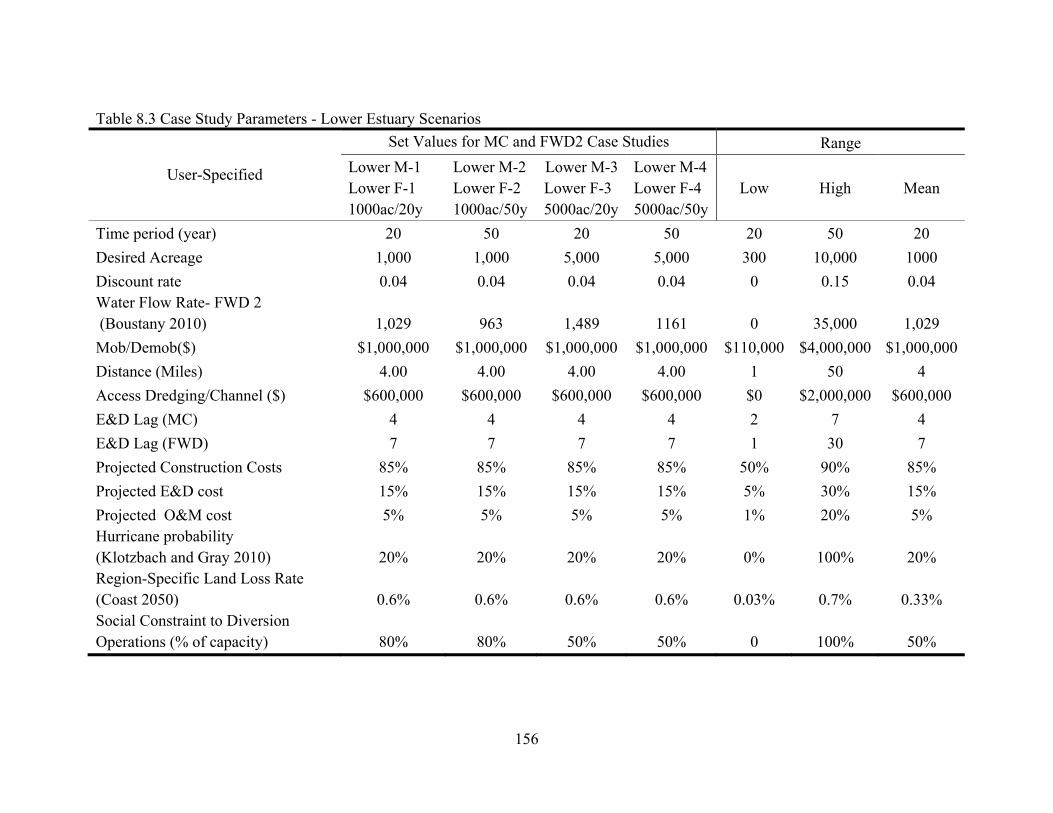
156
Table 8.3 Case Study Parameters - Lower Estuary Scenarios
User-Specified
Set Values for MC and FWD2 Case Studies Range Lower M-1 Lower F-1 1000ac/20y
Lower M-2 Lower F-2 1000ac/50y
Lower M-3 Lower F-3 5000ac/20y
Lower M-4 Lower F-4 5000ac/50y
Low High Mean
Time period (year) 20 50 20 50 20 50 20 Desired Acreage 1,000 1,000 5,000 5,000 300 10,000 1000 Discount rate 0.04 0.04 0.04 0.04 0 0.15 0.04 Water Flow Rate- FWD 2 (Boustany 2010) 1,029 963 1,489 1161 0 35,000 1,029 Mob/Demob($) $1,000,000 $1,000,000 $1,000,000 $1,000,000 $110,000 $4,000,000 $1,000,000Distance (Miles) 4.00 4.00 4.00 4.00 1 50 4 Access Dredging/Channel ($) $600,000 $600,000 $600,000 $600,000 $0 $2,000,000 $600,000 E&D Lag (MC) 4 4 4 4 2 7 4 E&D Lag (FWD) 7 7 7 7 1 30 7 Projected Construction Costs 85% 85% 85% 85% 50% 90% 85% Projected E&D cost 15% 15% 15% 15% 5% 30% 15% Projected O&M cost 5% 5% 5% 5% 1% 20% 5% Hurricane probability (Klotzbach and Gray 2010) 20% 20% 20% 20% 0% 100% 20% Region-Specific Land Loss Rate (Coast 2050) 0.6% 0.6% 0.6% 0.6% 0.03% 0.7% 0.33% Social Constraint to Diversion Operations (% of capacity) 80% 80% 50% 50% 0 100% 50%

rate is assumed to be 0.6 percent per year, and the percent of capacity are set to 80 for small scale
FWD project and 50 percent for large scale project, respectively. Finally, four different water
flow rates were derived from the N-SED1 model (Boustany 2007) for the lower basin scenarios,
including 1,029 cubic feet per second (cfs), 963 cfs, 1489 cfs, and 1161 cfs based on the desired
acreage and project life time.
8.3 Depicting Acreage Effects
Figure 8.2 depicts the effects of scale, lag time, land loss rate, and risk on net acres for
MC and FWD projects at Upper Estuary location under the assumptions for a target of 1000 and
5000 acres during a 20 and 50 year project life time. As evident in the graphics, the net acres
from the MC project are far greater than the gained net acres from FWD project during the first
several decades. As described in Chapter 3 and Chapter 7, net acreage follows a sigmoid
trajectory for MC projects. With the four year lag time, acreage is not realized until year 4, and
then most of the land is gained in years 4-6. After year 6, the land gradually decreases because of
erosion and hurricane risk. In comparison, because of the 10 year lag time for FWD project in
the upper estuary, net acres are zero until year 10, and then increase very slowly over the project
life time following a linear trajectory. However, due to public opposition - which is greater in the
upper estuary and also higher for large scale projects – the assumed flow rates of the FWD
projects are constrained to 25 to 40 percent of their designed capacity. Because of this constraint,
the trajectories for diversion projects (F1, F2, F3, and F4) produce less than 20% of the target
acreage.
Figure 8.3 depicts the effects of location, scale, lag time, land loss rate, and risk on net
acres for MC and FWD projects at Lower Estuary location with the same assumption: a target
1000 and 5000 acres and a 20 and 50 year project life time. The benefits also follow a sigmoid
157

158
trajectory for MC project, with net acres at zero until 4, and then rapidly gained in years 4-6.
After year 6, net acreage for MC projects is slightly decreasing (because of erosion and hurricane
risk). For the FWD projects, net acreage is zero until year 7, and then increase at a slow, constant
rate over project time period following a linear trajectory. In these simulations, the net acreage
appears to converge on the MC projects beyond 50 years. These results demonstrate the potential
for FWD projects in the absence of social constraints – where lower levels of public opposition
and shorter time lags allow for higher flow rates.
8.4 Comparison of Case Studies
Sixteen case studies were conducted in which six user-specified parameters were
modified to represent different scenarios at Upper and Lower estuary locations for MC and FWD
projects. In each scenario, these modified parameters were incorporated into the specified NPV
model to determine the net acres, total NPV benefits ($), total NPV costs ($), B-C ratio, and cost
per unit ($/acre).
Table 8.4 and Table 8.5 provide the economic results of NPV simulations for the Upper
and Lower estuary locations, respectively. In each table, five types of estimate are provided MC
and FWD projects of 1000 and 5000 acre target scales and 20 and 50 year time periods. The
additional parameters for these case simulations were previously described in Tables 8.2 and 8.3.
• Acreage
In all case simulations, the MC project acreage exceeds the acreage for FWD projects;
however, for 50-year periods in the lower basin, the FWD project acreage is very close to
converging on acreage of the MC projects. For both project types, neither achieves the target
acreage during the specified time period. In the case of MC projects, three factors constrain the
project’s ability to reach the target benefit: lag time, erosion, and hurricane effects (XHN).
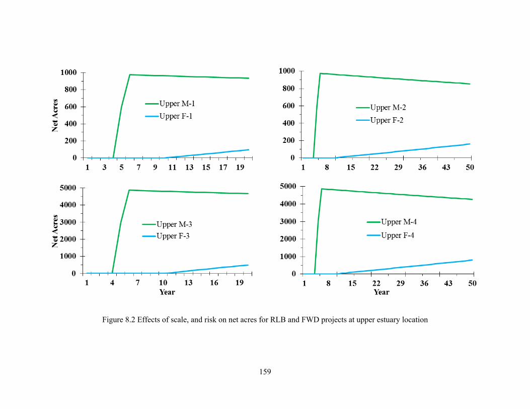
Figure 8.2 Effects of scale, and risk on net acres for RLB and FWD projects at upper estuary location
159

160
Figure 8.3 Effects of scale, and risk on net acres for RLB and FWD projects at lower estuary location

Because of these constraints MC projects achieve only 85 and 93 percent of the target
acreage in the upper estuary; and only 87 and 73 percent of the target acreage in the lower
estuary. In the case of FWD projects, four factors constrain the project’s ability to reach the
target benefit: lag time, erosion, hurricane effects (XHN) , and social constraints (XS). Because of
these constraints FWD project benefits range from 12 to 32 percent of the target acreage in the
upper estuary; and 30 to 87 percent of the target acreage in the lower estuary.
• Costs
One of the often cited arguments against RLB projects is their apparent high costs. In
Tables 8.4 and 8.5 this argument can be seen. The costs for MC projects at similar scales, time
periods, and locations ranges from 2.8 to nearly 4 times higher than the comparable costs of
FWD projects designed for the same target acreage. While FWD projects do produce the lowest
per unit cost for 50-year projects in the lower estuary, those simulations involved very low public
opposition (i.e. flow constraints). For FWD projects to operate at higher capacity in the upper,
populated basin; additional cost would likely be incurred – such as compensation for fisheries
displacement and fair market value expropriation of private property. Pre-emptive compensation
to diversion-affected parties would need to be estimated and added to the operational cost model
for diversions. The estimation of such costs; however, are beyond the scope of this study.
• Benefits
Conversely, and as seen in the acreage data, the MC project benefits greatly exceed the
performance of the FWD projects under the same scale, time, and location assumptions of these
case studies. Given that benefits are assigned on an annual basis using three non-market,
ecosystem valuation estimates (Table 6.2), the net benefits in dollars for MC projects ranges
from 4 to 27 times higher than the comparable benefits of FWD projects designed for the same
161

Table 8.4 Cost and Benefit Output for Upper Estuary Scenarios
MC FWD
Upper M-1 1000ac/20y
Upper M-2 1000ac/50y
Upper M-3 5000ac/20y
Upper A-4 5000ac/50y
Upper F-1 1000ac/20y
Upper F-2 1000ac/50y
Upper F-3 5000ac/20y
Upper F-4 5000ac/50y
Net Acres 934 853 4670 4267 193 321 602 1003
NPV Costs ($) 37,798,400 37,423,575 47,801,529 47,327,509 12,035,230 11,830,916 12,082,695 11,900,929
NPV Benefits ($) 40,687,958 71,993,875 203,439,791 359,969,373 2,399,596 7,323,328 7,496,977 22,880,297
B-C Ratio 1.08 1.92 4.26 7.61 0.2 0.62 0.62 1.92
$/acre 40,469 43,873 10,236 11,092 62,359 36,856 20,071 11,865
Table 8.5 Cost and Benefit Output for Lower Estuary Scenarios
MC FWD
Lower M-1 1000ac/20y
Lower M-2 1000ac/50y
Lower M-3 5000ac/20y
Lower M-4 5000ac/50y
Lower F-1 1000ac/20y
Lower F-2 1000ac/50y
Lower F-3 5000ac/20y
Lower F-4 5000ac/50y
Net Acres 872 728 4359 3639 508 671 1520 2098
NPV Costs ($) 37,798,400 37,423,575 47,801,529 47,327,509 13,366,465 13,151,140 13,419,179 13,229,091
NPV Benefits ($) 38,885,396 67,044,229 194,426,982 335,221,144 8,161,172 16,722,894 24,271,476 52,247,394
B-C Ratio 1.03 1.79 4.07 7.08 0.61 1.27 1.81 3.95
$/acre 43,347 51,406 10,966 13,006 26,312 19,599 8,828 6,306
162

target acreages.
• B-C Ratio and Unit Costs
All B-C ratios are greater than 1.0 for the 8 MC case study projects, and exceed 1.0 in
four of the 8 FWD case scenarios. The overall B-C ratio for MC projects ranges from a low of
1.03 to a high of 7.61. For FWD projects, B-C ratios range from 0.2 to 3.95. The least expensive
(most efficient) projects in these case study comparisons are the large scale FWD projects in the
lower estuary. These projects achieve a unit cost of $8,828 and $6,306 per acre for 20 year and
50 year trajectories, respectively. This finding is consistent with the recommendations of coastal
restoration planners and diversion advocates who tend to dismiss RLB projects as overly
expensive and unsustainable and who promote the use of large scale FWD projects on a long-
term basis as the only sustainable solution for addressing Louisiana’s coastal land loss crisis
(Reed 2009). In reality, there are very few locations where such projects can be implemented
without major opposition from fishermen, land owners, and other interests. Primarily because of
social constraints, the use of FWD projects in the middle to upper estuary is much more
problematic and less efficient. The unit cost of FWD projects in the upper estuary ranges from
$11,865 to $62,359 – and in each of the four comparable scenarios, the MC projects have a lower
cost per unit acre –ranging from $10,236 to $40,449.
8.5 Summary
This chapter incorporates all of the benefit and cost model calculations developed in
Chapters 1-7 to perform preliminary case studies for MC and FWD projects in two hypothesized
locations of coastal Louisiana. A total of 16 case studies scenarios were developed for upper and
lower estuary locations based on varying target scales, time periods, lag times, erosion rates,
hurricane risks, and social constraints. These case studies provide an example of how the time
163
and risk-adjusted NPV models can provide useful information to decision-maker about the
choice of restoration projects.
Two FWD projects were found to achieve the lowest unit cost per acre (highest
efficiency), but only for lower estuary locations where public opposition is assumed to be much
lower. For a large-scale FWD projects to be constructed and operated at full capacity in the
middle to upper estuary, social costs would dramatically increase. This study addresses those
cost through a mathematical constraint to diversion flow rate (XS) – which is enumerated in a
manner consistent with the public operation of these structures.
Given the limited number of locations where a large FWD can be located with minimum
social opposition, and considering the tremendous rate of coastal land loss in Louisiana, there
would appear to be a preference for those projects that build land rapidly and cost-efficiency at
upper and middle estuary locations. Results indicate that even with a much higher total NPV
costs, MC projects are more cost effective in the majority of the simulations.
An alternative simulation would include calculating the costs of pre-emptive
compensation to diversion-affected parties and then adding those costs into the estimated cost
model for diversions. While such compensation costs are beyond the scope of this study, these
costs must be addressed formally by coastal restoration managers and planners if large-scale
FWD projects are to be used in the middle to upper estuary.
164
CHAPTER 9. SUMMARY and CONCLUSIONS
9.1 Summary and Conclusions
Using natural or artificial ways of building wetlands to combat coastal land loss has long
been debated in coastal Louisiana. In the wake of Hurricanes Katrina and Rita, the Louisiana
Coastal Protection and Restoration Authority was (CPRA) was established in an attempt to
integrate programs for habitat restoration and infrastructure protection. As a result, wetland
restoration has begun shifting from ecosystem-focused to more human-focused issues. Coastal
communities have expressed strong interest in the rapid land-building (RLB) techniques that rely
on mechanical dredges and sediment conveyance pipelines to build new land, even though these
projects have apparent high costs.
The costs and benefits of RLB methods are increasingly compared to the more traditional
methods of fresh water and sediment diversions (FWD). Selecting an appropriate technology is
very important to make wetland restoration more efficient. Previous economic analyses have
focused on the qualitative benefits (dollars per habitat unit) of coastal restoration spending. This
study focused on quantitative benefits (net acres) associated with project contributions and
incorporated time and risk factors into benefit-cost (BC) models for RLB and FWD wetland
restoration project types in Louisiana.
The overall objective was to develop a comprehensive economic assessment, and
comparison of RLB and FWD for coastal restoration. The specific objectives were: (1) to
estimate generic models of coastal restoration project trajectories and cost by technology; (2) to
conduct sensitivity analyses with varying values of variables, and; (3) to perform case-studies to
illustrate tradeoffs between/within coastal restoration technologies.
165
Data from a total of 341 projects were collected from numerous sources including 124
projects authorized by the Coastal Wetland Planning Protection and Restoration Act (CWPPRA).
A total of 23 marsh creation (MC) projects, 13 barrier island (BI) projects, and 15 FWD projects
were authorized by CWPPRA projects and available for use in the BC analyses. To supplement
the available data, 85 RLB project bids and 9 additional FWD projects estimates were obtained
from the Louisiana Coastal Areas (LCA) Ecosystem Restoration Program and the Water
Resources Development Act (WRDA). Initial comparisons indicated that the most expensive,
and most frequently used coastal land-building technologies are MC, BI, and FWD. Together,
these three project types have accounted for more than 78% of CWPPRA projects authorized
since 2005.
Generic benefit trajectories and cost models were constructed through the consideration
of authorized project data and formal bids for MC projects (n=69), BI projects (n=52), and FWD
projects (n=25). Using multiple regression analysis, benefit trajectories were constructed by
examining the percent completion of target acreage goal by year. For RLB projects, these
trajectories were sigmoidal in shape and for FWD projects these trajectories were constant and
upward sloping. Because of the relatively small amount of FWD benefit data, an exogenous
benefit model was incorporated (FWD2) into the analyses. The NSED1 model is a nutrient and
sediment-based mass-balance model developed by the Natural Resources Conservation Service
(NRCS) and refined by the US Army Corps of Engineers (USACE) to examine the accretion
potential of FWD projects.
For the comparative costs models, numerous independent variables were found to be
significant drivers of the costs for MC projects (α=.10). Cubic yards of sediment (CYD),
mobilization and demobilization costs (MOB), distance (DIST) and access dredging (AD) were
166
positively correlated with the cost RLB projects. Likewise, the variables, cubic feet per second
(CFS) and diversion control (CON), were found to be significant and positive predictors of the
costs of FWD projects.
These benefit and cost models were incorporated into a net present valuation (NPV)
framework and sensitivity analyses were conducted to examine the relative importance of
specific attributes related to time, distance, project scale, discount rate, and site-specific land loss
rates. Data for 22 project-specific attributes were used to develop baseline BC simulations for
two RLB project types (MC and BI) and two freshwater diversion models (FWD1 and FWD2).
Simulations against the baseline were conducted by allowing a single, user-specified parameter
to vary across its known range and solving for the break-even cost ($/acre/year) in which the BC
ratio was equal to 1.0.
As expected, project life time, scale, discount rate, and time lag have a major impact on
the cost-benefit decision analysis for coastal restoration. Increases in project life time and project
scale serve to decrease per unit costs where increases in discount rate and time lag were found to
increase per unit cost. Additional factors, such as the mobilization of dredging equipment costs
were found to be more sensitive for BI projects than MC projects. Dredging access costs and the
distance between sediment borrow site and project site also had a major impact on the costs of
RLB projects. The rate of long-shore sediment transport had a very small effect on BI projects
cost and benefits only. Under the assumption with no hurricane and human disruption, the rate of
land loss was found to have only a small impact the cost-benefit relationship for RLB and FWD
projects.
Hurricane risks were examined using landfall probabilities unique to the Louisiana cost
and modeled under an expected valuation framework. The scaling of hurricane impacts was
167
demonstrated under two scenarios, constant and dynamic. Under static hurricane risk (XH,
Risk1), the percentage of hurricane-driven land loss was assumed to occur at a constant rate
across project life time. Under the dynamic hurricane risk scenario (XH, Risk2); however, the
percentage of hurricane-driven land loss varied each time interval as a function of scale (i.e.
percent completion of the project). Hurricane risks were found to have the greatest impact on
FWD projects due to their relatively slow rate of restoration. A method is described through
which pre- and post-storm imagery could be used to determine actual project impacts and to
adjust the user-defined XH variable. A similar approach could be used to refine hurricane risk by
project location. When political and social constraints (XS, Risk3) are considered; however, the
benefits were significantly curtailed. Per unit costs were dramatically increased due to their
relatively slow rate of restoration, and the incorporation of social risk into the BC analysis
greatly changed the economic outcome and potential preference for coastal restoration
alternatives.
Case studies for MC and FWD projects were conducted in two hypothesized locations of
coastal Louisiana. A total of 16 case studies scenarios were developed for upper and lower
estuary locations based on varying target scales, time periods, lag times, erosion rates, hurricane
risks, and social constraints. Two FWD projects were found to achieve the lowest unit cost per
acre (highest efficiency), but only for lower estuary locations where public opposition is assumed
to be much lower. For any large-scale FWD projects to be constructed and operated at full
capacity in the middle to upper estuary, social costs would increase. This study addresses those
cost through a mathematical constraint to diversion flow rate (XS) – which is enumerated in a
manner consistent with the public operation of these structures. These case studies provide an
example of how the time and risk-adjusted NPV models can provide useful information to
168

decision-maker about the choice of restoration projects. Future simulations might also benefit
from the use of declining (Gamma) discount rates applications that vary according to time and
project scale.
The results from this research showed that while RLB projects are often characterized as
being cost-prohibitive, when time and risk are considered these projects are much more
competitive in comparison to more natural methods. Delays in construction (time lag) and the
relatively slow rate of restoration proved to be major, negative factors on the feasibility of the
FWD projects. Furthermore, the incorporation of project-specific types of risk was found to
compound the problems associated with the slower performing, FWD projects. Perhaps more
importantly, results indicated that the break-even annual costs in the vast majority of simulations
were considerably higher than the range of annual benefits reported in the non-market,
ecosystem valuation literature. This finding suggests the need for additional scrutiny to ensure
the most feasible combination of project attributes. The generic cost and benefit functions
established in this analysis provide a decision framework for the CPRA to utilize in the
economic assessment of competing technologies for coastal wetland restoration. Results indicate
that even with a much higher total NPV costs, MC projects are more cost effective in the
majority of the simulations. Given the limited number of locations where a large FWD can be
located with minimum social opposition, and considering the tremendous rate of coastal land loss
in Louisiana, there would appear to be a preference for those projects that build land rapidly and
cost-efficiency at upper and middle estuary locations. Simulations in this portion of the study
showed that MC projects and FWD project are more comparable because BI projects are limited
in where it can only be constructed on coastal islands.
169

9.2 Limitations and Refinements
• Data Availability and Frontier Analysis
Although every effort was made to obtain all available program data and variables for the
models developed in this study, there was only a small amount of project data available be used
to construct the cost and benefits models. Meanwhile, there is large degree of data variation
within comparable project types and the lacking data for variables could be very important to the
simulation model (e.g. estimating depth, elevation, and thickness). These data limitations;
however, are not unique to this study. In reality, these are the only cost and benefit data
available to the state for guiding the analysis and future allocation of potential billions in
restoration spending. More benefit and cost data should be collected on current and proposed
coastal wetland restoration projects. As additional projects come on-line (constructed) and
additional bids are generated, these costs and benefit models should be refined. For RLB
projects, attempts to model project thickness as a function of average depth of receiving area and
elevation proved problematic. Moreover, attempts to model the effects of RLB payment type (on
the cut versus on the fill) were plagued by insufficient data. Thus, a more detailed tracking of
these measurements is needed for RLB projects. Meanwhile, an alternative analysis-frontier
analysis, which estimates maxima or minima of a dependent variable given explanatory
variables, could be used to determine the cost models.
• Static Discount Rate and Gamma/Dynamic Discounting
This research used the static discount rate in which the discount rate keep constant during
the project life time. By comparison, dynamic discounting (a time-declining rate of discount)
could be considered incorporating into NPV analysis. The time-declining discount rate is known
170

as Gamma discount rate, which gave a declining discount rate schedule as a simple function of
time (Weitzman 2010).
• Sea Level Rise/Subsidence and Erosion Constant or Risk Function
At many coastal sites, global sea level rise and/or subsidence are the main factors
responsible for land loss. Douglas (1997) estimated that each year global sea level rises about 1.8
mm as a result of a worldwide increase in water volume. This value, however, is substantially
less than the total rise in relative sea level recorded at many tide gauges (Emery and Aubrey,
1991). Scientists have concluded that the remaining amount of relative sea-level rise is caused by
land subsidence. The relative sea level rise and/or subsidence accelerate coastal erosion (Morton
2003). This research used a constant annual land loss rate from the Coast2050 report. A dynamic
land loss rate or risk function associated with sea level rise and/or subsidence could be
considered and incorporate into NPV models.
• Scale Limitations and Consideration of Massive-Scale Projects
Case studies assumed two project scale scenarios: 1000 and 5000 target acreages.
Massive-scale project simulations would be considered. An alternative, more comprehensive cost
simulation for FWD would involve calculating the costs of pre-emptive compensation to
diversion-affected parties and then adding those costs into the estimated cost model for
diversions. While such compensation costs are beyond the scope of this study, these costs should
be formally assessed by coastal restoration managers and planners in cases where large-scale
FWD projects are being considered in the middle to upper regions of the estuary.
Independent Modeling and Integrated Benefit-Cost Analysis (BCA)
All comparison of freshwater diversion and rapid land-building are independent. The
generic benefit and cost model based on independent project type. For FWD projects, the cost
171

model utilized is simply a function of estimated average flow rate and the type of diversion
(controlled or uncontrolled). The two benefit models used for diversions (FWD1 and FWD2)
were vastly different in their estimated flow rates required for simulations of target acreage –
with the required flow to meet target acreage for the former being as much as sixteen times the
latter. Thus, while the FWD1 benefit model estimated in this study might prove too conservative,
the FWD2 model - which was used for the case study simulations - could prove too liberal in the
estimation of project benefits. This wide difference in benefit trajectories illustrates some of the
scientific uncertainly associated with the efficacy of freshwater diversions. Addition analyses
will be required to examine the case studies with some hybrid combination of the two benefit
trajectories and their associated costs.
In reality, a more integrated wetland restoration scenario could involve the combination
of a RLB project sustained by a FWD. This scenario is increasingly promoted as a compromise
for the use of these approaches in restoring coastal Louisiana. The models developed in this
study could easily be used for such a simulation.
• Benefits Transfer and Site-Specific/Project-Specific Development of ESV Estimates
Limited literature on coastal wetland valuation of ecosystem services and the wide range
of these estimates is also problematic. This research used three primary non market values (e.g.
storm surge attenuation, habitat protection, and water quality provision) from the existing
literature as “starting values” to quantify the break-even simulations. Ecosystem values
incorporated into this study via benefit-transfer, which might not always appropriate. Additional
recently site-specific and project-specific estimates are required to refine the ecosystem services
value.
172

• Lack of Market Values and Addition of Annualized Market Values
The market value of an acre wetland could be ranged from a few hundred dollars to a few
million dollars per acre in different coastal areas. It can be measured through direct, observable
market behavior to place monetary values on wetland. Additional annualized market value data
are required to further refine the cost models and could be added into these cost functions using a
high and a low value in the simulations to show the difference.
• Scaling Risks and Impacts and Additional GIS Case Studies
Finally, the degree of impact from a major hurricane land fall on a coastal restoration
project can be measured using GIS analysis; however, the number of direct hits from major
hurricanes is limited. This study demonstrated a dynamic impact scenario in which scale (size
and percent completion) and project type can be used to adjust the risk from future storms. The
impacts of social constraints, by comparison, are much more difficult to model. Increased time
lag and operational flow constraints are common for FWD projects in coastal Louisiana. This
study uses a very simple approach to constrain FWD benefits based on case-specific historical
information.
9.3 Policy Recommendations
While project selection processes have traditionally relied on limited interval or end-of-
stage cost comparisons, economic modeling based on a dynamic trajectory allows for more
comprehensive accounting of a project’s ecosystem services over time. Through this approach,
decision-makers can examine highly detailed economic trade-offs between project type, scale,
time, distance, risk, and location. The model developed by this study provides a novel construct
for examining the efficiency of competing projects, and it could substantially improve the return
173
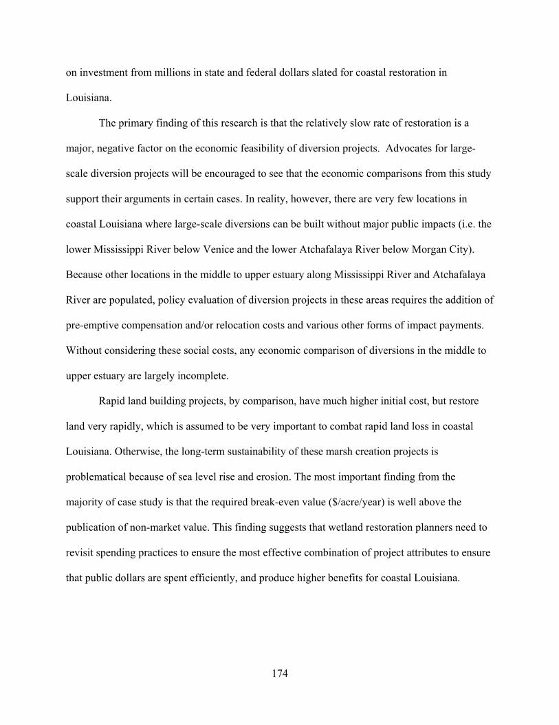
on investment from millions in state and federal dollars slated for coastal restoration in
Louisiana.
The primary finding of this research is that the relatively slow rate of restoration is a
major, negative factor on the economic feasibility of diversion projects. Advocates for large-
scale diversion projects will be encouraged to see that the economic comparisons from this study
support their arguments in certain cases. In reality, however, there are very few locations in
coastal Louisiana where large-scale diversions can be built without major public impacts (i.e. the
lower Mississippi River below Venice and the lower Atchafalaya River below Morgan City).
Because other locations in the middle to upper estuary along Mississippi River and Atchafalaya
River are populated, policy evaluation of diversion projects in these areas requires the addition of
pre-emptive compensation and/or relocation costs and various other forms of impact payments.
Without considering these social costs, any economic comparison of diversions in the middle to
upper estuary are largely incomplete.
Rapid land building projects, by comparison, have much higher initial cost, but restore
land very rapidly, which is assumed to be very important to combat rapid land loss in coastal
Louisiana. Otherwise, the long-term sustainability of these marsh creation projects is
problematical because of sea level rise and erosion. The most important finding from the
majority of case study is that the required break-even value ($/acre/year) is well above the
publication of non-market value. This finding suggests that wetland restoration planners need to
revisit spending practices to ensure the most effective combination of project attributes to ensure
that public dollars are spent efficiently, and produce higher benefits for coastal Louisiana.
174

REFERENCES
Abraham, B. and J. Ledolter (2005). Introduction to Regression Modeling. 1st ed. Duxbury Press, pp: 15-16.
Anderson R. and M. Rockel (1991). Economic valuation of wetlands. Discussion Paper No. 065.
American Petroleum Institute, Washington, DC. Aust, C. (2006). Cost-efficacy of Wetland preservation and Restoration in Coastal. Master thesis.
Louisiana State University. Banks, D.P. (2002). Ecological Review-Delta Management at Fort St. Phillip CWPPRA Priority
Project List 10 State No. BS-11. Restoration Technology Section Coastal Restoration Division Louisiana Department of Natural Resources.
Barras, J.A., S. Beville, D. Britsch, S. Hartley, S. Hawes, J. Johnston, P. Kemp, Q. Kinler, A.
Martucci, J. Porthouse, D. Reed, K. Roy, S. Sapkota, and J. Suhayda (2003). Historical and projected coastal Louisiana land changes: 1978-2050: USGS Open File Report 03-334.
Bartoldus, C.C. (1999). A Comprehensive Review of Wetland Assessment Procedures: A Guide
for Wetland Practitioners. Environmental Concern Inc., St. Michaels, MD. pp:196. Browning, G. (2010). Cash Flow Estimates by PPL with Future Funding Requirements. Coastal
Wetland Planning Protection and Restoration Act, Planning and Evaluation Committee Report, June 2010.
Boustany, R. (2010). Estimating the Benefits of Freshwater Introduction into Coastal Wetland
Ecosystems in Louisiana: Nutrient and Sediment Analyses. Ecological Restoration, 28(2):160-174.
Caffey, R. H. and M. Schexnayder (2002). Fisheries Implications of Freshwater Reintroductions,
Interpretive Topic Series on Coastal Wetland Restoration in Louisiana, Coastal Wetland Planning, Protection, and Restoration Act (eds.), National Sea Grant Library No. LSU-G-02-003, pp: 8.
Caffey, R.H., K. Savoie, and M. Shirley (2003). Stewardship Incentives for Louisiana’s Coastal
Landowners, Interpretive Topic Series on Coastal Wetland Restoration in Louisiana, Coastal Wetlands Planning, Preservation and Restoration Act. National Sea Grant Library.
Carson, R.T., N.E. Flores, and N.F. Meade (2001). Contingent Valuation: Controversies and
Evidence. Environmental and Resource Economics, 19:173-210.
175
CH2M Hill (2006). Phase 2 Reconnaissance-level Evaluation of the Third Delta Conveyance Channel Project, Prepared by CH2M HILL in association with Mussetter Engineering, Inc. for the Louisiana Department of Natural Resources, October 2006.
CPRA (Coastal Protection and Restoration Authority) (2000). What’s causing the crisis?
Retrieved from http://coastal.louisiana.gov/index.cfm?md=pagebuilder&tmp=home&pid=118 (Accessed on Sept. 18, 2009).
CWPPRA (Coastal Wetland Planning, Protection and Restoration Act) (2000). Mississippi River
Sediment, Nutrient, & Freshwater Redistribution Study, Draft report & Environmental Resources Document July 2000. Retrieved from http://www.clear.lsu.edu/pdfs/clear_report_20081022112825.pdf (Accessed on Jun. 23, 2010).
CWPPRA (Coastal Wetland Planning, Protection and Restoration Act) (2010). The Atchafalaya
Basin: Existing Conditions and Problems. Retrieved from http://lacoast.gov/newsAbout/Basin data/at/default.aspx (Accessed on Sept. 30, 2010).
CWPPRA (Coastal Wetland Planning Protection and Restoration Act) (2010). Planning and
Evaluation. Retrieved from http://lacoast.gov/new/Projects/List.apx (Accessed on Aug. 25, 2010).
Cooper, H. and L.V. Hedges (1994). Research Synthesis as A Scientific Enterprise, in H. Cooper
and L. V. Hedges, eds. The Handbook of Research Synthesis. New York: Russell Sage Foundation, pp: 3–14.
Costanza, R. (1980). Embodied Energy and Economic Valuation. Science, 225:890-897. Costanza, R. (1984). Natural Resource Valuation and Management: Toward an Ecological
Economics. pp:7-18 in A. M. Jansson (ed.), Integration of economy and ecology: an outlook for the eighties. University of Stockholm Press, Stockholm, Sweden.
Costanza, R. and S.C. Farber (1984). Theories and Methods of Valuation of Natural Systems: A
Comparison of Willingness- to-Pay and Energy Analysis Based Approaches. Man, Environment, Space and Time, 4:1-38.
Costanza, R. and R. A. Herendeen (1984). Embodied Energy and Economic Value in the United
States economy: 1963, 1967, and 1972. Resources and Energy, 6:129-163. Costanza, R. and C. Neill (1984). Energy Intensities, Interdependence, and Value in Ecological
Systems: A Linear Programming Approach. Journal of Theoretical Biology, 106:41- 57. Costanza, R., O. Perez-Maqueo, L.M. Martinez, P. Sutton, S.J. Anderson, and K. Mulder (2008).
The Value of Coastal Wetlands for Hurricane Protection. Ambio, 37(4): 241-248.
176
LaDNR (Louisiana Department of Natural Resources) (1998). Coast 2050: Toward a Sustainable Coastal Louisiana. http://www.coast2050.gov/products/docs/orig/2050report.pdf.
Daly, H.E. (1981). Postscript: Unresolved Problems and Issues for Further Research. pp: 165-
186 in H. E. Daly and A.F. Umana (eds.), Energy, Economics and the Environment: Conflicting Views of an Essential Interrelationship. Westview, Boulder, Colorado.
DeLaune, R. D., W. H. Patrick, Jr., and C. J. Smith (1992). Marsh Aggradation and Sediment
Distribution Along Rapidly Submerging Louisiana Gulf Coast. Environmental Geology Science, 20(1): 57-64.
Desmond, J.M. (2005). The Dying Louisiana Wetlands. Janus Head, 8(2):485-492. Dunbar, J.B., L. Britsch, and E. Kemp (1992). Land loss rates: Louisiana Coastal Plain.
Technical Report GL-92-3, U.S. Army Engineer Waterways Experiment Station, Vicksburg, MS.
Environmental Economics (2005). Economists on Environmental and Natural Resources News,
Opinion, Analysis. Discount rates for benefit-cost Retrieved from http://www.env-econ.net/2005/08/discount_rates_.html (Accessed on Apr. 12, 2011).
EPA (United States Environmental Protection Agency) (2006). Economic Benefits of Wetlands.
Retrieved from http://www.epa.gov/owow/wetlands/pdf/EconomicBenefits.pdf (Accessed on Oct. 27, 2010).
Glass, G. V. (1976). Primary, Secondary, and Meta-Analysis. Educational Researcher, 5:3–8. Graves, G. (2009). Navigating the Environment - Managing Risks and Sustaining Benefits,
Coastal Systems: Navigation, Flood, Ecosystems and protecting Louisiana’s coast, PIANC Conference, October 28, 2009. Retrieved from www.pianc.iwr.usace.army.mil/docs/NTE2009Conf/16-Graves_PIANC_10-28-09.v2.pdf (Accessed on Oct. 14, 2009).
Hanley, N. and C.L. Spash (1993). Cost-Benefit Analysis and the Environment. Edward Elgar
Publishing, Inc. pp:16-20. Hart, D.E., I, Marsden. and M. Francis (2008). In Winterbourne, M. Natural history of
Canterbury. 3rd ed. Canterbury University Press, pp: 653–684. Heimlich R.E., K.D.Weibe, R. Claassen, D. Gadsy, and R.M. House (1998). Wetlands and
Agriculture: Private Interests and Public Benefits. Resource Economics Division, E.R.S., USDA, Agricultural Economic Report 765.10.
Heikkila T., K. Appleby, M. Bahamdoun, S. Caputo, D. Coyle, M. DeSalle, R. McCadney,
J.McHugh, S. Shuford, E. Tang, A. Varga, and B. Williams (2008).
177

The Water Resources Development Act Title VII Louisiana Coastal Area Final Report. Retrieved from http://www.columbia.edu/cu/mpaenvironment/pages/projects/summer2008/TitleVIIfinal.pdf (Accessed on Jun. 18, 2010).
Howard N.A. (2002). Environmental Value: A Business View of Environmental Costs and
Opportunities. Environmental Quality Management, pp: 75-81. Holland D.S., J.N. Sanchirico, R.J. Johnston and D. Joglekar (2010). Economic Analysis for
Ecosystem-Based Management. RFF Press, pp: 29-30. Huetmer, D.A. (1982). Economic Values and Embodied Energy. Science, 216:1141 - 1143. Hubbard, D.W. (2007). How to Measure Anything: Finding the Value of Intangibles in Business. John
Wiley & Sons, Inc. Hubbard, D.W. (2009). The Failure of Risk Management: Why It's Broken and How to Fix It.
John Wiley & Sons, Inc. pp: 21-24. Jones, J. (2006). An Introduction to Factor Analysis of Information Risk (FAIR). Risk
Management Insight LLC. Kazmierczak, Jr., Richard F. (2001)a. "Economic Linkages Between Coastal Wetlands and
Water Quality: A Review of Value Estimates Reported in the Published Literature." Staff Paper 2001-02, Department of Agricultural Economics and Agribusiness, Louisiana State University, Baton Rouge, May 2001.
Kazmierczak, Jr., Richard F. (2001)b. "Economic Linkages Between Coastal Wetlands and
Habitat/Species Protection: A Review of Value Estimates Reported in the Published Literature." Staff Paper 2001-04, Department of Agricultural Economics and Agribusiness, Louisiana State University, Baton Rouge, May 2001.
Kazmierczak, Jr., Richard F. (2001)c. "Economic Linkages Between Coastal Wetlands and
Hunting and Fishing: A Review of Value Estimates Reported in the Published Literature." Staff Paper 2001-03, Department of Agricultural Economics and Agribusiness, Louisiana State University, Baton Rouge, May 2001.
Klotzbach and Gray (2009). United States Landfalling Hurricane Probability Project. Retrieved
from http://www.e-transit.org/hurricane/welcome.html (Accessed on Oct. 28, 2009). Klotzbach, P.J. and W.M. Gray (2011). Forecast of Atlantic Seasonal Hurricane Activity and
Landfall Strike Probability for 2011. Retrieved from http://hurricane.atmos.colostate.edu/forecasts/2011/aug2011/aug2011.pdf (Accessed on Aug. 8, 2011).
Knight, F.H. (1921). Risk, Uncertainty and Profit. Boston and New York: Houghton Mifflin. pp:
19.
178

LaCPRA (Louisiana Coastal Protection and Restoration Authority) (2007). Louisiana's
Comprehensive Master Plan for a Sustainable Coast, Executive Summary. Retrieved from http://dnr.louisiana.gov/crm/ocpr.asp (Accessed on Sept. 7, 2009).
LCA (Louisiana Coastal Area) (2004). Ecosystem Restoration Study, November 2004 Final.
Retrieved from http://www.lca.gov/Library/ProductList.aspx?ProdType=0&folder=1125 (Accessed on Jul. 8, 2010).
Lipton, D.W., K. Wellman, and I.C. Sheifer (1995). Economic Valuation of Natural Resources:
A Handbook for Coastal Resource Policymakers. National Oceanic and Atmospheric Adminstration (NOAA), USA.
LOSCO (Louisiana Oil Spill Coordinator's Office) (2005). Land and Water Interface for
Louisiana from 2002 Landsat Thematic Mapper Satellite Imagery. Geographic NAD83, LOSCO (2005).
McBride, R.A., M.W. Hiland, S. Penland, K.A. Westphal, S.J. Williams. (1993). Long-term
Shoreline Change of the Chandeleur Island Barrier System, Louisiana: 1855 to 1989. Coastlines of the Gulf of Mexico, Proceedings of 8th Symposium on Coastal and Ocean Management. American Society of Civil Engineers. pp: 234–248.
Miller, B. (2010). Personal Communication, Project Manager, Coastal Wetland Planning
Protection and Restoration Act, Office of Coastal Restoration and Protection, Louisiana Department of Natural Resources, June 2010.
Moore, R., D. Petrolia, and T. Kim (2010). Preferences for Timing of Wetland Loss Prevention
in Louisiana. Abstracted in, Challenges of Natural Resource Economics and Policy: the Third National Forum on Socioeconomic Research in Coastal Systems, pp: 47.
National Hurricane Center (2007). November 2005 Atlantic Tropical Weather Summary.
National Oceanic and Atmospheric Administration. Retrieved from http://www.nhc.noaa.gov/archive/2005/tws/MIATWSAT_nov_final.shtml (Accessed on Nov. 6, 2009).
NOAA (National Oceanic and Atmospheric Administration) (2005). Restoration Economics:
Discounting and Time Preference. Retrieved from http://www.csc.noaa.gov/coastal/economics/discounting.htm (Accessed on Feb. 22, 2011).
OCPR (Office of Coastal Protection and Restoration) (2005). Davis Pond Freshwater Diversion
Project Annual Report 2004-2005. Retrieved from http://sonris.com/direct.asp (Accessed on Aug. 25, 2011).
OCPR (Office of Coastal Protection and Restoration) (2006). Caernarvon Freshwater Diversion
Project Annual Report 2005. Retrieved
179

from http://www.ocpr.louisiana.gov/crm/coastres/project.asp?id=BS-08 (Accessed on Aug. 25, 2011).
O’Brien S. and L. Martinez (2008). Potential Impacts of Freshwater Diversions from the
Mississippi Rive. University of New Orleans - Pontchartrain Institute for Environmental Sciences.
Petrolia, D.R., T.G. Kim, R.G. Moore, and R.H. Caffey (2009). A Cost Analysis of Rapid Land-
Building Technologies for Coastal Restoration in Louisiana. the Southern Agricultural Economics Association Annual Meeting, Atlanta, Georgia.
Petrolia, D.R. and T.G. Kim (2010). Preventing Land Loss in Coastal Louisiana: Estimates of
WTP and WTA. Journal of Environmental Management, 92(2011) 859-865. Petrolia D.R, R.G Moore, and T.G Kim (2011). Preferences for Timing of Wetland Loss
Prevention in Louisiana. Wetlands. Perman, R., Y. Ma, J. McGilvray, and M. Common (2003). Natural Resource and Environmental
Economics. 3rd ed. Gosport. Ashford Colour Press Ltd, pp: 373-378. Reed, D.J. (2009). A New Approach to River Management: Action for A Sustainable Coastal
Landscape. Journal of Contemporary Water Research & Education, 141: 35-38. Roy, K. (2005). Personal Communication. CWPPRA Senior Field Biologist, U.S. Fish and
Wildlife Service, 646 Cajundome Blvd, Suite 400, Lafayette, LA 70506. Stockdon H. F., L, A. Fauver, A. H. Sallenger, and C. W. Wright (2005). Impacts of Hurricane
Rita on the Beaches of Western Louisiana. Science and Storms: The USGS Response to Hurricanes of 2005. pp: 119-123. Retrieved from http://pubs.usgs.gov/circ/1306/pdf/c1306_ch5_d.pdf (Accessed on Aug. 10, 2011).
USACE (U.S. Army Corps of Engineers) (2000). Engineering and Design-Civil Works
Construction Cost Index System (CWCCIS). Retrieved from http://140.194.76.129/publications/eng-manuals/em1110-2-1304/entire.pdf (Accessed on May 15, 2010).
USACE (U. S. Army Corps of Engineers) (2005). Freshwater Diversion. New Orleans District.
Retrieved from http://www.mvn.usace.army.mil/pao/bro/FreshwaterDiversion.pdf (Accessed on Sep. 20, 2011).
USGS (U.S. Geological Survey) (2006). USGS Reports Latest Land Change Estimates for
Louisiana Coast. Retrieved from http://landsat.gsfc.nasa.gov/pdf_archive/sci_0006.pdf (Accessed on Sept. 2, 2009).
U.S. Census Bureau (2007). Annual Estimates of the Population for Counties: April 1, 2000 to
July 1, 2006. (Coastal parish population total was calculated based on the sum of the
180

populations of the 20 coastal parishes: Ascension, Assumption, Calcasieu, Cameron, Iberia, Jefferson, Lafourche, Livingston, Orleans, Plaquemines, St. Bernard, St. Charles, St. James, St. John the Baptist, St. Martin, St. Mary, St. Tammany, Tangipahoa, Terrebonne, and Vermilion.) Retrieved from http://www.census.gov/popest/counties/tables/CO-EST2006-01-22.xls (Accessed on Sept. 2, 2009).
Uyar, B., (1993). The Discount Rate and Intergenerational Equity. Atlantic Economic Society,
v(21): 89(1). Weitzman, M. (1994). On the “Environmental” Discount Rate. Journal of Environmental
Economics and Management, 26:200-209. Weitzman, M. (1998). Why the Far-Distant Future Should be Discounted at Its Lowest Possible
Rate. Journal of Environmental Economics and Management, 36:201-208. Weitzman, M. (2001). Gamma Discounting. American Economic Review, 91(1): 261-271. Weitzman, M. (2010). Risk-adjusted Gamma Discounting. Journal of Environmental Economics
and Management, 60(1):1-13. White, A.T. and A. Cruz-Trinidad (1998). The Values of Philippine Coastal Resources: Why
Protection and Management are Critical. Coastal Resource Management Project, Cebu City, Philippines.
Wilson, M. and J.P. Hoehn (2006). Valuing Environmental Goods and Services Using Benefit
Transfer: The State-Of-The Art and Science. Ecological Economics, 60:335–342. Williams, S.J., S. Penland, Jr. Sallenger, A.H. (Eds.). (1992). Louisiana Barrier Island Erosion
Study-Atlas of Shoreline Changes From 1853 to 1989. U.S. Geological SurveyMiscellaneous Investigation Series, vol. I-2150-A, pp: 103.
Woodward, R.T. and Y.S. Wui (2001). The Economic Value of Wetland Services: A Meta-
Analysis. Ecological Economics, 37:257–270. Zinn, A.J. (2007). Congressional Research Service Reports for Congress: Coastal Louisisana
Ecosystem Restoration after Hurricane Katrina and Rita.. Retrieved from http://www.cnie.org/NLE/CRSreports/07Nov/RS22276.pdf (Accessed on Aug. 12, 2011).
Mishan, E. J. and Euston Quah (2009). Cost Benefit Analysis 5th Edition. T & F Books UK. pp:
1–10. Perman, R., Y. Ma, J. McGilvray, and M. Common (2003). Natural Resource and Environmental
Economics. 3rd ed. Gosport. Ashford Colour Press Ltd, pp: 373-378.
181

APPENDIX A: CORRELATION ANALYSIS FOR MC PROJECT BASED ON HISTORIC DATA
The CORR Procedure
Pearson Correlation Coefficients, N = 12 Prob > |r| under H0: Rho=0
PPL CYD PBA DIST MOB DS PYT BP AAHU
PPL 1.00000
-0.37325 0.2321
-0.01867 0.9541
0.412030.1832
0.812450.0013
0.414200.1807
-0.106500.7418
0.24185 0.4489
-0.088150.7853
CYD -0.37325 0.2321
1.00000
-0.18345 0.5682
-0.314540.3194
-0.355250.2571
0.131590.6835
0.273520.3897
-0.05518 0.8648
0.210620.5111
PBA -0.01867 0.9541
-0.18345 0.5682
1.00000
-0.377230.2267
-0.061050.8505
-0.645340.0234
-0.285750.3679
-0.37797 0.2257
0.580270.0479
DIST 0.41203 0.1832
-0.31454 0.3194
-0.37723 0.2267
1.00000 0.738360.0061
0.368760.2382
0.330990.2933
0.56758 0.0542
-0.582450.0469
MOB 0.81245 0.0013
-0.35525 0.2571
-0.06105 0.8505
0.738360.0061
1.00000 0.351230.2629
0.088140.7853
0.52181 0.0818
-0.317100.3152
DS 0.41420 0.1807
0.13159 0.6835
-0.64534 0.0234
0.368760.2382
0.351230.2629
1.00000 0.191270.5515
0.68584 0.0138
-0.396540.2019
PYT -0.10650 0.7418
0.27352 0.3897
-0.28575 0.3679
0.330990.2933
0.088140.7853
0.191270.5515
1.00000 0.47809 0.1159
-0.043220.8939
BP 0.24185 0.4489
-0.05518 0.8648
-0.37797 0.2257
0.567580.0542
0.521810.0818
0.685840.0138
0.478090.1159
1.00000
-0.318960.3123
AAHU -0.08815 0.7853
0.21062 0.5111
0.58027 0.0479
-0.582450.0469
-0.317100.3152
-0.396540.2019
-0.043220.8939
-0.31896 0.3123
1.00000
182
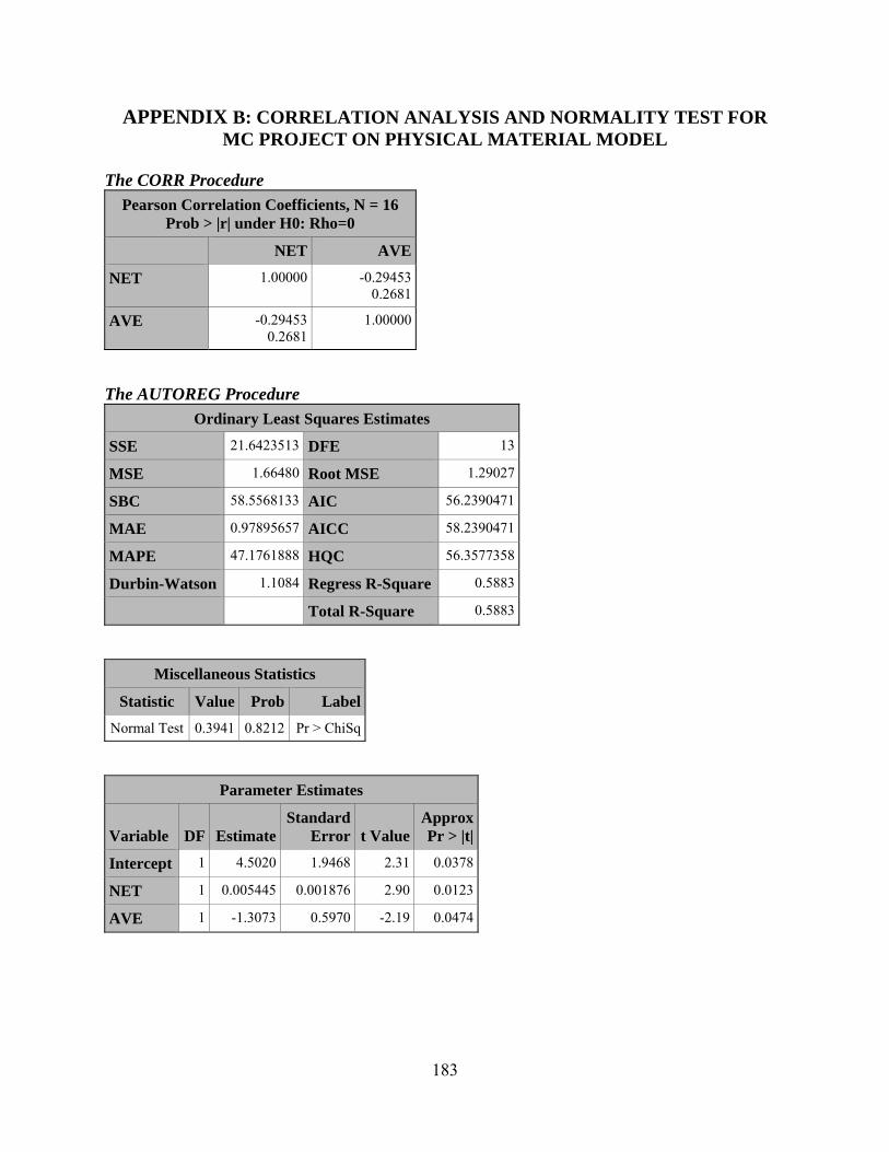
APPENDIX B: CORRELATION ANALYSIS AND NORMALITY TEST FOR MC PROJECT ON PHYSICAL MATERIAL MODEL
The CORR Procedure
Pearson Correlation Coefficients, N = 16 Prob > |r| under H0: Rho=0
NET AVE
NET 1.00000
-0.294530.2681
AVE -0.29453 0.2681
1.00000
The AUTOREG Procedure
Ordinary Least Squares Estimates
SSE 21.6423513 DFE 13
MSE 1.66480 Root MSE 1.29027
SBC 58.5568133 AIC 56.2390471
MAE 0.97895657 AICC 58.2390471
MAPE 47.1761888 HQC 56.3577358
Durbin-Watson Regress R-Square1.1084 0.5883
Total R-Square 0.5883
Miscellaneous Statistics
Statistic Value Prob LabelNormal Test 0.3941 0.8212 Pr > ChiSq
Parameter Estimates
Variable DF Estimate Standard
Error t ValueApproxPr > |t|
Intercept 1 4.5020 1.9468 2.31 0.0378
NET 1 0.005445 0.001876 2.90 0.0123
AVE 1 -1.3073 0.5970 -2.19 0.0474
183

The REG Procedure
Analysis of Variance
Source DF Sum of
Squares Mean
Square F Value Pr > F
Model 2 30.92424 15.46212 9.29 0.0031
Error 13 21.64235 1.66480
Corrected Total 15 52.56659 Root MSE 1.29027 R-Square 0.5883
Dependent Mean Adj R-Sq3.00563 0.5249
Coeff Var 42.92850
184

Parameter Estimates
DF Parameter
Estimate Standard
Error t Value Pr > |t| ToleranceVariance Inflation Variable
1 4.50205 1.94679 2.31 0.0378 . 0 Intercept 1 0.00544 0.00188 2.90 0.0123 0.91325 1.09499 NET
AVE 1 -1.30727 0.59703 -2.19 0.0474 0.91325 1.09499
185
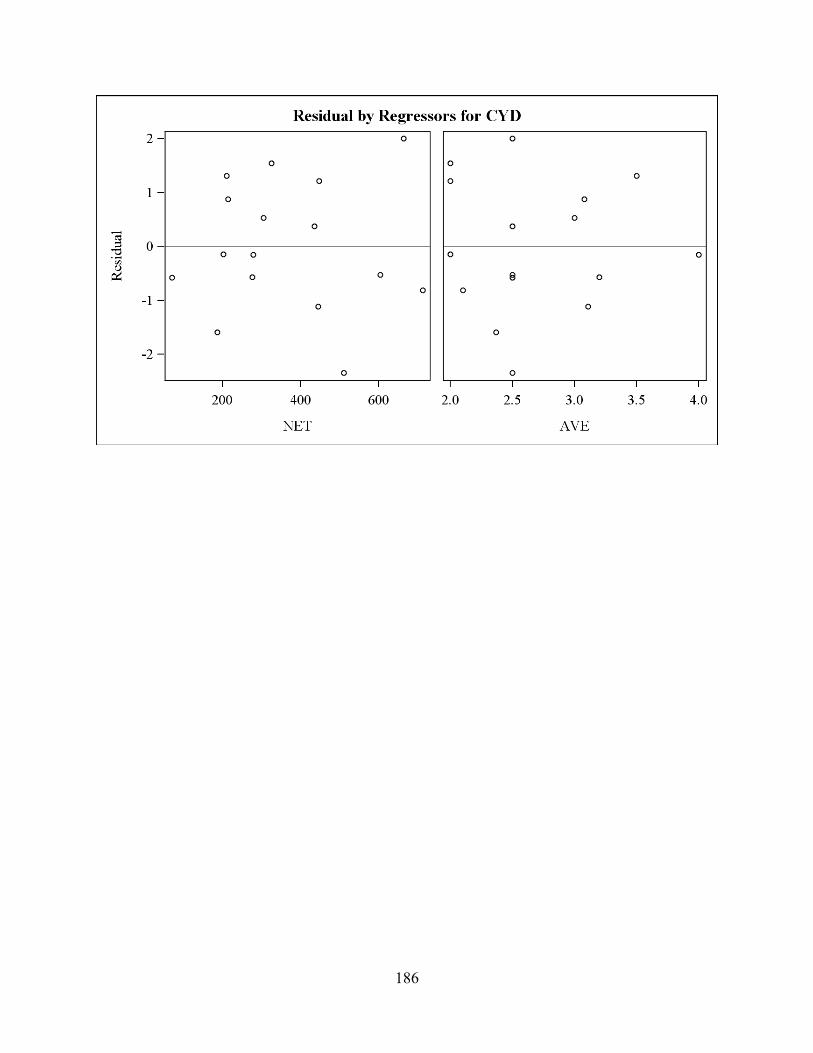
186

The UNIVARIATE Procedure
Tests for Normality
Test Statistic p Value
Shapiro-Wilk W 0.979635 Pr < W 0.9606
Kolmogorov-Smirnov D 0.109824 Pr > D >0.1500
Cramer-von Mises W-Sq 0.028258 Pr > W-Sq >0.2500
Anderson-Darling A-Sq Pr > A-Sq 0.173898 >0.2500
Stem Leaf # Boxplot 2 0 1 | 1 5 1 | 1 23 2 +-----+ 0 59 2 | | 0 4 1 | + | -0 21 2 *-----* -0 8665 4 +-----+ -1 1 1 | -1 6 1 | -2 3 1 | ----+----+----+----+ Normal Probability Plot 2.25+ +*++ | *+++ | *+*++ 0.75+ *+*++ | ++*++ | +++* * -0.75+ *+*+* * | ++*+ | +++*
-2.25+ ++*+ +----+----+----+----+----+----+----+----+----+----+
-2 -1 0 +1 +2
187

APPENDIX C: CORRELATION ANALYSIS FOR BI PROJECT BASED ON HISTORIC DATA
The CORR Procedure
Pearson Correlation Coefficients, N = 11 Prob > |r| under H0: Rho=0
PPL CYD PBA DIST MOB PYT AAHU 1.00000
0.00396
0.9908 -0.36714
0.2667 0.76533
0.00610.25371
0.45160.86949
0.00050.05846
0.8644PPL
0.00396 0.9908
1.00000
-0.54582 0.0824
-0.028750.9331
0.256710.4461
-0.128130.7073
-0.090840.7905
CYD
-0.36714 0.2667
-0.54582 0.0824
1.00000
-0.372390.2594
-0.411600.2085
-0.367340.2664
0.275760.4118
PBA
0.76533 0.0061
-0.02875 0.9331
-0.37239 0.2594
1.00000 0.391840.2333
0.867570.0005
-0.074320.8281
DIST
0.25371 0.4516
0.25671 0.4461
-0.41160 0.2085
0.391840.2333
1.00000 0.448880.1661
-0.267690.4261
MOB
0.86949 0.0005
-0.12813 0.7073
-0.36734 0.2664
0.867570.0005
0.448880.1661
1.00000 0.012860.9701
PYT
AAHU 0.05846 0.8644
-0.09084 0.7905
0.27576 0.4118
-0.074320.8281
-0.267690.4261
0.012860.9701
1.00000
188

APPENDIX D: CORRELATION ANALYSIS AND NORMALITY TEST FOR BI PROJECT ON PHYSICAL MATERIAL MODEL
The CORR Procedure
Pearson Correlation Coefficients, N = 6 Prob > |r| under H0: Rho=0
NET AVE
NET 1.00000
-0.335910.5151
AVE -0.33591 0.5151
1.00000
The AUTOREG Procedure
Ordinary Least Squares Estimates
SSE 1.47491092 DFE 3
MSE 0.49164 Root MSE 0.70117
SBC 13.9835696 AIC 14.6082912
MAE 0.45127644 AICC 26.6082912
MAPE 23.5066878 HQC 12.1074797
Durbin-Watson Regress R-Square1.0212 0.7931
Total R-Square 0.7931
Miscellaneous Statistics
Statistic Value Prob LabelNormal Test 0.7389 0.6911 Pr > ChiSq
Parameter Estimates
Variable DF Estimate Standard
Error t ValueApproxPr > |t|
Intercept 1 0.001671 1.9391 0.00 0.9994
NET 1 0.0127 0.004222 3.00 0.0576
AVE 1 -0.2723 0.5673 -0.48 0.6641
189
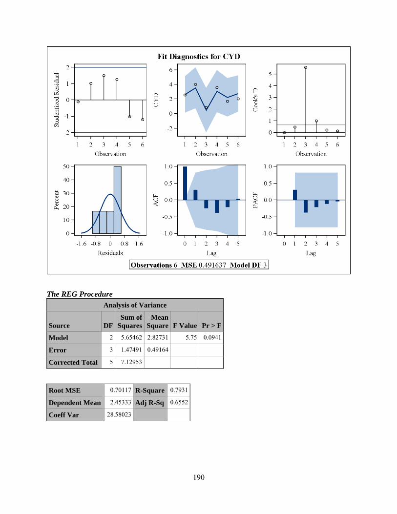
The REG Procedure
Analysis of Variance
Source DF Sum of
Squares Mean
Square F Value Pr > F
Model 2 5.65462 2.82731 5.75 0.0941
Error 3 1.47491 0.49164
Corrected Total 5 7.12953 Root MSE 0.70117 R-Square 0.7931
Dependent Mean Adj R-Sq2.45333 0.6552
Coeff Var 28.58023
190
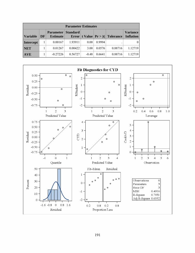
Parameter Estimates
DF Parameter
Estimate Standard
Error t Value Pr > |t| ToleranceVariance Inflation Variable
1 0.00167 1.93911 0.00 0.9994 . 0 Intercept 1 0.01267 0.00422 3.00 0.0576 0.88716 1.12719 NET
AVE 1 -0.27226 0.56727 -0.48 0.6641 0.88716 1.12719
191

192

The UNIVARIATE Procedure Tests for Normality
Test Statistic p Value
Shapiro-Wilk W 0.870656 Pr < W 0.2288
Kolmogorov-Smirnov D 0.247887 Pr > D >0.1500
Cramer-von Mises W-Sq 0.061706 Pr > W-Sq >0.2500
Anderson-Darling A-Sq Pr > A-Sq 0.388237 >0.2500
Stem Leaf # Boxplot 4 72 2 +-----+ 2 6 1 | | 0 *--+--* -0 7 1 | | -2 | | -4 5 1 +-----+ -6 4 1 | ----+----+----+----+ Multiply Stem.Leaf by 10**-1 Normal Probability Plot 0.5+ * ++++ * | * ++++ | ++++ -0.1+ +*+ | ++++ | ++++ * -0.7+ +*+ +----+----+----+----+----+----+----+----+----+----+ -2 -1 0 +1 +2
193

APPENDIX E: CORRELATION ANALYSIS AND NORMALITY TEST FOR FWD PROJECT ON TOTAL COST MODEL
The CORR Procedure
Pearson Correlation Coefficients, N = 8 Prob > |r| under H0: Rho=0
CFS CON
CFS 1.00000
0.234420.5763
CON 0.23442 0.5763
1.00000
The AUTOREG Procedure
Ordinary Least Squares Estimates
SSE 1.50046E14 DFE 5
MSE 3.00092E13 Root MSE 5478063
SBC 273.441507 AIC 273.203182
MAE 3632945.48 AICC 279.203182
MAPE 72.8956964 HQC 271.595778
Durbin-Watson Regress R-Square2.9631 0.8630
Total R-Square 0.8630
Miscellaneous Statistics
Statistic Value Prob LabelNormal Test 0.3979 0.8196 Pr > ChiSq
Parameter Estimates
Variable DF Estimate Standard
Error t ValueApproxPr > |t|
Intercept 1 6024854 2825933 2.13 0.0862
CFS 1 521.5263 126.4396 4.12 0.0091
CON 1 10894218 3984605 2.73 0.0411
194

The REG Procedure
Analysis of Variance
Source DF Sum of
Squares Mean
Square F Value Pr > F
Model 2 9.454999E14 4.7275E14 15.75 0.0069
Error 5 1.500459E14 3.000918E13
Corrected Total 7 1.095546E15 Root MSE 5478063 R-Square 0.8630
Dependent Mean Adj R-Sq16266745 0.8083
Coeff Var 33.67645
195

Parameter Estimates
DF Parameter
Estimate Standard
Error t Value Pr > |t| ToleranceVariance Inflation Variable
1 6024854 2825933 2.13 0.0862 . 0 Intercept 1 521.52627 126.43960 4.12 0.0091 0.94505 1.05815 CFS
CON 1 10894218 3984605 2.73 0.0411 0.94505 1.05815
196

197

The UNIVARIATE Procedure Tests for Normality
Test Statistic p Value
Shapiro-Wilk W 0.953967 Pr < W 0.7511
Kolmogorov-Smirnov D 0.181983 Pr > D >0.1500
Cramer-von Mises W-Sq 0.031812 Pr > W-Sq >0.2500
Anderson-Darling A-Sq Pr > A-Sq 0.222577 >0.2500
Stem Leaf # Boxplot 6 8 1 | 4 | 2 16 2 +-----+ 0 1 1 *--+--* -0 1 1 | | -2 | | -4 950 3 +-----+ ----+----+----+----+ Multiply Stem.Leaf by 10**+6 Normal Probability Plot 7000000+ +*+++ | ++++ | *+++* 1000000+ ++*++ | ++*+ | ++++ -5000000+ * +++* * +----+----+----+----+----+----+----+----+----+----+ -2 -1 0 +1 +2
198

APPENDIX F: NPV MODEL ASSUMPTIONS FOR MC, BI, AND FWD PROJECTS
Land Building Cost and Benefit Assumptions (MC, BI, and FWD)
User Specified Range
Derived Low High Mean
Time period (yrs) 20 20 50 20 Desired Acreage 1,000 300 10,000 1000 Elevation 2 1.5 3.5 2.44 Depth 4 2.5 5.5 3.78 Discount rate 0.04 0 0.15 0.04 Water Flow Rate- FWD 2 (Boustany) 1,029 1000 Mob/Demob($) $1,000,000 $110,000 $4,000,000 $1,000,000 Distance (Miles) 4.00 1 50 4 Access Dredging/Channel ($) $600,000 $0 $2,000,000 $600,000 E&D Lag (MC) 4 2 7 4 E&D Lag (BI) 4 1 6 4 E&D Lag (FWD) 7 1 30 7 Projected Construction Costs 85% 50% 90% 85% Projected E&D cost 10% 5% 30% 15% Projected O&M cost 5% 1% 20% 5% Market Value of Land ($/acre) $0 Hurricane probability (Klotzbach and Gray 2010) 20% 15% 30% 20% Starting Ecosystem Value (Habitat) $/acre/year $249 $169 $403 $249 Starting Ecosystem Value (Water Quality) $/acre/year $825 $3 $5,674 $825 Starting Ecosystem Value (Storm Surge Protection) $/acre/year $3,336 $101 $20,648 $3,336 Region-Specific Land Loss Rate (Coast 2050) 0.003 0.0003 0.007 0.003 Longshore Sediment Transport rate BI projects only 0 0 0.01 0.008 Net Accretion Rate for BI -0.003 -0.0003 0.003 0.005 Starting Ecosystem Value - Aggregate ($/acre/year) $4,410 $273 $26,725 $4,410 Total Sediments-MC (cuyds MM, Eq. 3.3) 7.22 Total Sediments-BI (cuyds MM, Eq. 3.6) 6.00 Water Flow Rate- FWD 1(cfs, Eq. 3.9) 16,749 Construction Cost-MC (Eq. 4.4) $37,767,448 E&D cost-MC $4,443,229 O&M cost-MC $2,221,615 Total Fully Funded Cost-MC $44,432,291 Construction Cost-BI (Eq. 4.9) $27,703,380 E&D cost-BI $3,259,221 O&M cost-BI $1,629,611 Total Fully Funded Cost-BI $32,592,212
199
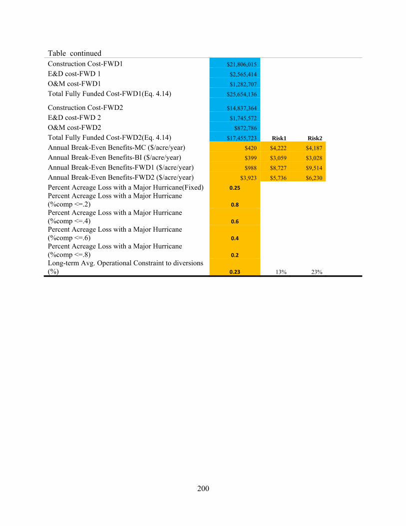
Table continued Construction Cost-FWD1 $21,806,015 E&D cost-FWD 1 $2,565,414 O&M cost-FWD1 $1,282,707 Total Fully Funded Cost-FWD1(Eq. 4.14) $25,654,136
Construction Cost-FWD2 $14,837,364 E&D cost-FWD 2 $1,745,572 O&M cost-FWD2 $872,786 Total Fully Funded Cost-FWD2(Eq. 4.14) $17,455,723 Risk1 Risk2 Annual Break-Even Benefits-MC ($/acre/year) $420 $4,222 $4,187 Annual Break-Even Benefits-BI ($/acre/year) $399 $3,059 $3,028 Annual Break-Even Benefits-FWD1 ($/acre/year) $988 $8,727 $9,514 Annual Break-Even Benefits-FWD2 ($/acre/year) $3,923 $5,736 $6,230 Percent Acreage Loss with a Major Hurricane(Fixed) 0.25 Percent Acreage Loss with a Major Hurricane (%comp <=.2) 0.8 Percent Acreage Loss with a Major Hurricane (%comp <=.4) 0.6 Percent Acreage Loss with a Major Hurricane (%comp <=.6) 0.4 Percent Acreage Loss with a Major Hurricane (%comp <=.8) 0.2 Long-term Avg. Operational Constraint to diversions (%) 0.23 13% 23%
200
201
VITA
Hua Wang graduated from Xiangtan University in Hunan Province, China, in May 2002,
where he received the title of Bachelor in Business Management. After the completion of this
degree, he worked five years and came to Louisiana State University to pursue his master degree
studying at the Department of Agricultural Economics in 2009 Spring. He is expecting to get the
degree of Master of Science in Spring, 2012.