1Risk Aversion

This chapter looks at a basic concept behind modeling individual preferences in theface of risk. As with any social science, we of course are fallible and susceptibleto second-guessing in our theories. It is nearly impossible to model many naturalhuman tendencies such as “playing a hunch” or “being superstitious.” However, wecan develop a systematic way to view choices made under uncertainty. Hopefully, ourmodels can capture the basic human tendencies enough to be useful in understandingmarket behavior towards risk. In other words, even if we are not correct in predictingbehavior under risk for every individual in every circumstance, we can still makegeneral claims about such behavior and can still make market predictions, whichafter all are based on the “marginal consumer.”

To use (vaguely) mathematical language, the understanding of this chapter is anecessary but not sufficient condition to go further into the analysis. Because of theimportance of risk aversion in decision making under uncertainty, it is worthwhileto first take an “historical” perspective about its development and to indicate howeconomists and decision scientists progressively have elaborated upon the tools andconcepts we now use to analyze risky choices. In addition, this “history” has somesurprising aspects that are interesting in themselves. To this end, our first section inthis chapter broadly covers these retrospective topics. Subsequent sections are more“modern” and they represent an intuitive introduction to the central contribution toour field, that of Pratt (1964).

1.1 An Historical Perspective on Risk Aversion

As it is now widely acknowledged, an important breakthrough in the analysis ofdecisions under risk was achieved when Daniel Bernoulli, a distinguished Swissmathematician, wrote in St Petersburg in 1738 a paper in Latin entitled: “Specimentheoriae novae de mensura sortis,” or “Exposition of a new theory on the mea-surement of risk.” Bernoulli’s paper, translated into English in Bernoulli (1954), isessentially nontechnical. Its main purpose is to show that two people facing the samelottery may value it differently because of a difference in their psychology. This ideawas quite novel at the time, since famous scientists before Bernoulli (among them

Economic & Financial Decisions under Risk (Chapters 1&2)Eeckhoudt, Gollier & Schlesinger (Princeton Univ Press 2005)

4 1. Risk Aversion

Pascal and Fermat) had argued that the value of a lottery should be equal to itsmathematical expectation and hence identical for all people, independent of theirrisk attitude.

In order to justify his ideas, Bernoulli uses three examples. One of them, the“St Petersburg paradox” is quite famous and it is still debated today in scientificcircles. It is described in most recent texts of finance and microeconomics and forthis reason we do not discuss it in detail here. Peter tosses a fair coin repetitivelyuntil the coin lands head for the first time. Peter agrees to give to Paul 1 ducat if headappears on the first toss, 2 ducats if head appears only on the second toss, 4 ducatsif head appears for the first time on the third toss, and so on, in order to double thereward to Paul for each additional toss necessary to see the head for the first time.The question raised by Bernoulli is how much Paul would be ready to pay to Peterto accept to play this game.

Unfortunately, the celebrity of the paradox has overshadowed the other two exam-ples given by Bernoulli that show that, most of the time, the value of a lottery is notequal to its mathematical expectation. One of these two examples, which presentsthe case of an individual named “Sempronius,” wonderfully anticipates the centralcontributions that would be made to risk theory about 230 years later by Arrow, Prattand others.

Let us quote Bernoulli:1

Sempronius owns goods at home worth a total of 4000 ducats andin addition possesses 8000 ducats worth of commodities in foreigncountries from where they can only be transported by sea. However,our daily experience teaches us that of [two] ships one perishes.

In modern-day language, we would say that Sempronius faces a risk on his wealth.This wealth may represented by a lottery x, which takes on a value of 4000 ducatswith probability 1

2 (if his ship is sunk), or 12 000 ducats with probability 12 . We will

denote such a lottery x as being distributed as (4000, 12 ; 12 000, 1

2 ). Its mathematicalexpectation is given by:

Ex ≡ 12 4000 + 1

2 12 000 = 8000 ducats.

Now Sempronius has an ingenious idea. Instead of “trusting all his 8000 ducatsof goods to one ship,” he now “trusts equal portions of these commodities to twoships.” Assuming that the ships follow independent but equally dangerous routes,Sempronius now faces a more diversified lottery y distributed as

(4000, 14 ; 8000, 1

2 ; 12 000, 14 ).

1We altered Bernoulli’s probabilities to simplify the computations. In particular, Bernoulli’s originalexample had one ship in ten perish.

1.1. An Historical Perspective on Risk Aversion 5

Indeed, if both ships perish, he would end up with his sure wealth of 4000 ducats.Because the two risks are independent, the probability of these joint events equalsthe product of the individual events, i.e. ( 1

2 )2 = 14 . Similarly, both ships will succeed

with probability 14 , in which case his final wealth amounts to 12 000 ducats. Finally,

there is the possibility that only one ship succeeds in downloading the commoditiessafely, in which case only half of the profit is obtained. The final wealth of Sem-pronius would then just amount to 8000 ducats. The probability of this event is 1

2because it is the complement of the other two events which have each a probabilityof 1

4 .Since common wisdom suggests that diversification is a good idea, we would

expect that the value attached to y exceeds that attributed to x. However, if wecompute the expected profit, we obtain that

Ey = 14 4000 + 1

2 8000 + 14 12 000 = 8000 ducats,

the same value as for Ex! If Sempronius would measure his well-being ex ante byhis expected future wealth, he should be indifferent about whether to diversify ornot. In Bernoulli’s example, we obtain the same expected future wealth for bothlotteries, even though most people would find y more attractive than x. Hence,according to Bernoulli and to modern risk theory, the mathematical expectation of alottery is not an adequate measure of its value. Bernoulli suggests a way to expressthe fact that most people prefer y to x: a lottery should be valued according tothe “expected utility” that it provides. Instead of computing the expectation of themonetary outcomes, we should use the expectation of the utility of the wealth. Noticethat most human beings do not extract utility from wealth. Rather, they extract utilityfrom consuming goods that can be purchased with this wealth. The main insight ofBernoulli is to suggest that there is a nonlinear relationship between wealth and theutility of consuming this wealth.

What ultimately matters for the decision maker ex post is how much satisfactionhe or she can achieve with the monetary outcome, rather than the monetary outcomeitself. Of course, there must be a relationship between the monetary outcome andthe degree of satisfaction. This relationship is characterized by a utility function u,which for every wealth level x tells us the level of “satisfaction” or “utility” u(x)

attained by the agent with this wealth. Of course, this level of satisfaction derivesfrom the goods and services that the decision maker can purchase with a wealth levelx. While the outcomes themselves are “objective,” their utility is “subjective” andspecific to each decision maker, depending upon his or her tastes and preferences.Although the function u transforms the objective result x into a perception u(x) bythe individual, this transformation is assumed to exhibit some basic properties ofrational behavior. For example, a higher level of x (more wealth) should induce ahigher level of utility: the function should be increasing in x. Even for someone

6 1. Risk Aversion

who is very altruistic, a higher x will allow them to be more philanthropic. Readersfamiliar with indirect utility functions from microeconomics (essentially utility overbudget sets, rather than over bundles of goods and services) can think of u(x) asessentially an indirect utility of wealth, where we assume that prices for goods andservices are fixed. In other words, we may think of u(x) as the highest achievablelevel of utility from bundles of goods that are affordable when our income is x.

Bernoulli argues that if the utility u is not only increasing but also concave inthe outcome x, then the lottery y will have a higher value than the lottery x, inaccordance with intuition. A twice-differentiable function u is concave if and onlyif its second derivative is negative, i.e. if the marginal utility u′(x) is decreasing in x.2

In order to illustrate this point, let us consider a specific example of a utility function,such as u(x) = √

x, which is an increasing and concave function of x. Using thesepreferences in Sempronius’s problem, we can determine the expectation of u(x):

Eu(x) = 12

√4000 + 1

2

√12 000 = 86.4

Eu(y) = 14

√4000 + 1

2

√8000 + 1

4

√12 000 = 87.9.

Because lottery y generates a larger expected utility than lottery x, the former ispreferred by Sempronius. The reader can try using concave utility functions otherthan the square-root function to obtain the same type of result. In the next section,we formalize this result.

Notice that the concavity of the relationship between wealth x and satisfac-tion/utility u is quite a natural assumption. It simply implies that the marginal utilityof wealth is decreasing with wealth: one values a one-ducat increase in wealthmore when one is poorer than when one is richer. Observe that, in Bernoulli’sexample, diversification generates a mean-preserving transfer of wealth from theextreme events to the mean. Transferring some probability weight from x = 4000to x = 8000 increases expected utility. Each probability unit transferred yields anincrease in expected utility equaling u(8000) − u(4000). On the contrary, trans-ferring some probability weight from x = 12 000 to x = 8000 reduces expectedutility. Each probability unit transferred yields a reduction in expected utility equal-ing u(12 000) − u(8000). But the concavity of u implies that

u(8000) − u(4000) > u(12 000) − u(8000), (1.1)

i.e. that the positive effect of these combined transfers must dominate the negativeeffect. This is why all investors with a concave utility would support Sempronius’sstrategy to diversify risks.

2For simplicity, we maintain the assumption that u is twice differentiable throughout the book.However, a function need not be differentiable to be concave. More generally, a function u is concave ifand only if λu(a) + (1 − λ)u(b) is smaller than u(λa + (1 − λ)b) for all (a, b) in the domain of u andall scalars λ in [0, 1]. A function must, however, be continuous to be concave.

1.2. Definition and Characterization of Risk Aversion 7

utili

ty

12 00080004000

a

c d

f e

wealth

Figure 1.1. Measuring the expecting utility of final wealth (4000, 12 ; 12000, 1

2 ).

1.2 Definition and Characterization of Risk Aversion

We assume that the decision maker lives for only one period, which implies that heimmediately uses all his final wealth to purchase and to consume goods and services.Later in this book, we will disentangle wealth and consumption by allowing the agentto live for more than one period. Final wealth comes from initial wealth w plus theoutcome of any risk borne during the period.

Definition 1.1. An agent is risk-averse if, at any wealth level w, he or she dislikesevery lottery with an expected payoff of zero: ∀w, ∀z with Ez = 0, Eu(w + z) �u(w).

Observe that any lottery z with a non-zero expected payoff can be decomposedinto its expected payoff Ez and a zero-mean lottery z−Ez. Thus, from our definition,a risk-averse agent always prefers receiving the expected outcome of a lottery withcertainty, rather than the lottery itself. For an expected-utility maximizer with autility function u, this implies that, for any lottery z and for any initial wealth w,

Eu(w + z) � u(w + Ez). (1.2)

If we consider the simple example from Sempronius’s problem, with only one shipthe initial wealth w equals 4000, and the profit z takes the value 8000 or 0 with equalprobabilities. Because our intuition is that Sempronius must be risk averse, it mustfollow that

12u(12 000) + 1

2u(4000) � u(8000). (1.3)

If Sempronius could find an insurance company that would offer full insurance atan actuarially fair price of Ez = 4000 ducats, Sempronius would be better off by

8 1. Risk Aversion

purchasing the insurance policy. We can check whether inequality (1.3) is verifiedin Figure 1.1. The right-hand side of the inequality is represented by point ‘f’ onthe utility curve u. The left-hand side of the inequality is represented by the middlepoint on the arc ‘ae’, i.e. by point ‘c’. This can immediately be checked by observingthat the two triangles ‘abc’and ‘cde’are equivalent, since they have the same baseand the same angles. We observe that ‘f’ is above ‘c’: ex ante, the welfare derivedfrom lottery z is smaller than the welfare obtained if one were to receive its expectedpayoff Ez with certainty. In short, Sempronius is risk-averse. From this figure, wesee that this is true whenever the utility function is concave. The intuition of theresult is very simple: if marginal utility is decreasing, then the potential loss of4000 reduces utility more than the increase in utility generated by the potential gainof 4000. Seen ex ante, the expected utility is reduced by these equally weightedpotential outcomes.

It is noteworthy that Equations (1.1) and (1.3) are exactly the same. The prefer-ence for diversification is intrinsically equivalent to risk aversion, at least under theBernoullian expected-utility model.

Using exactly the opposite argument, it can easily be shown that, if u is convex,the inequality in (1.2) will be reversed. Therefore, the decision maker prefers thelottery to its mathematical expectation and he reveals in this way his inclination fortaking risk. Such individual behavior will be referred to as risk loving. Finally, if u

is linear, then the welfare Eu is linear in the expected payoff of lotteries. Indeed, ifu(x) = a + bx for all x, then we have

Eu(w + z) = E[a + b(w + z)] = a + b(w + Ez) = u(w + Ez),

which implies that the decision maker ranks lotteries according to their expectedoutcome. The behavior of this individual is called risk-neutral.

In the next proposition, we formally prove that inequality (1.2) holds for anylottery z and any initial wealth w if and only if u is concave.

Proposition 1.2. A decision maker with utility function u is risk-averse, i.e. inequal-ity (1.2) holds for all w and z, if and only if u is concave.

Proof. The proof of sufficiency is based on a second-order Taylor expansion ofu(w + z) around w + Ez. For any z, this yields

u(w + z) = u(w + Ez) + (z − Ez)u′(w + Ez) + 12 (z − Ez)2u′′(ξ(z))

for some ξ(z) in between z and Ez. Because this must be true for all z, it followsthat the expectation of u(w + z) is equal to

Eu(w + z) = u(w + Ez) + u′(w + Ez)E(z − Ez) + 12E[(z − Ez)2u′′(ξ(z))].

1.3. Risk Premium and Certainty Equivalent 9

Observe now that the second term of the right-hand side above is zero, since E(z −Ez) = Ez − Ez = 0. In addition, if u′′ is uniformly negative, then the third termtakes the expectation of a random variable (z−Ez)2u′′(ξ(z)) that is always negative,as it is the product of a squared scalar and negative u′′. Hence, the sum of these threeterms is less than u(w + Ez). This proves sufficiency.

Necessity is proven by contradiction. Suppose that u is not concave. Then, theremust exist some w and some δ > 0 for which u′′(x) is positive in the interval[w − δ, w + δ]. Now take a small zero-mean risk ε such that the support of finalwealth w+ε is entirely contained in (w−δ, w+δ). Using the same Taylor expansionas above yields

Eu(w + ε) = u(w) + 12E[ε2u′′(ξ(ε))].

Because ξ(ε) has a support that is contained in [w − δ, w + δ] where u is locallyconvex, u′′(ξ(ε)) is positive for all realizations of ε. Consequently, it follows thatE[ε2u′′(ξ(ε))] is positive, and Eu(w + ε) is larger than u(w). Thus, accepting thezero-mean lottery ε raises welfare and the decision maker is not risk-averse. This isa contradiction.

The above proposition is in fact nothing more than a rewriting of the famousJensen inequality. Consider any real-valued function φ. Jensen’s inequality statesthat Eφ(y) is smaller than φ(Ey) for any random variable y if and only if φ isa concave function. It builds a bridge between two alternative definitions of theconcavity of u: the negativity of u′′ and the property that any arc linking two pointson curve u must lie below this curve. Figure 1.1 illustrates this point. It is intuitivethat decreasing marginal utility (u′′ < 0) means risk aversion. In a certain world,decreasing marginal utility means that an increase in wealth by 100 dollars hasa positive effect on utility that is smaller than the effect of a reduction in wealthby 100 dollars. Then, in an uncertain world, introducing the risk to gain or to lose100 dollars with equal probability will have a negative net impact on expected utility.In expectation, the benefit of the prospect of gaining 100 dollars is overweighted bythe cost of the prospect of losing 100 dollars with the same probability. Over the lasttwo decades, many prominent researchers in the field have challenged the idea thatrisk aversion comes only from decreasing marginal utility. Some even challengedthe idea itself, that there should be any link between the two.3

1.3 Risk Premium and Certainty Equivalent

A risk-averse agent is an agent who dislikes zero-mean risks. The qualifier “zero-mean” is very important. A risk-averse agent may like risky lotteries if the expected

3This question will be discussed in the last chapter of this book. Yaari (1987) provides a model thatis dual to expected utility, where agents may be risk-averse in spite of the fact that their utility is linearin wealth.

10 1. Risk Aversion

payoffs that they yield are large enough. Risk-averse investors may want to purchaserisky assets if their expected returns exceed the risk-free rate. Risk-averse agentsmay dislike purchasing insurance if it is too costly to acquire. In order to determinethe optimal trade-off between the expected gain and the degree of risk, it is usefulto quantify the effect of risk on welfare. This is particularly useful when the agentsubrogates the risky decision to others, as is the case when we consider public safetypolicy or portfolio management by pension funds, for example. It is important toquantify the degree of risk aversion in order to help people to know themselvesbetter, and to help them to make better decisions in the face of uncertainty. Mostof this book is about precisely this problem. Clearly, people have different attitudestowards risks. Some are ready to spend more money than others to get rid of aspecific risk. One way to measure the degree of risk aversion of an agent is to askher how much she is ready to pay to get rid of a zero-mean risk z. The answer to thisquestion will be referred to as the risk premium Π associated with that risk. For anagent with utility function u and initial wealth w, the risk premium must satisfy thefollowing condition:

Eu(w + z) = u(w − Π). (1.4)

The agent ends up with the same welfare either by accepting the risk or by paying therisk premium Π . When risk z has an expectation that differs from zero, we usuallyuse the concept of the certainty equivalent. The certainty equivalent e of risk z is thesure increase in wealth that has the same effect on welfare as having to bear risk z,i.e.

Eu(w + z) = u(w + e). (1.5)

When z has a zero mean, comparing (1.4) and (1.5) implies that the certainty equiv-alent e of z is equal to minus its its risk premium Π .

A direct consequence of Proposition 1.2 is that the risk premium Π is nonnegativewhen u is concave, i.e. when she is risk-averse. In Figure 1.2, we measure Π forthe risk (−4000, 1

2 ; 4000, 12 ) for initial wealth w = 8000. Notice first that the risk

premium is zero when u is linear, and it is nonpositive when u is convex.One very convenient property of the risk premium is that it is measured in the

same units as wealth, e.g. we can measure Sempronius’s risk premium in ducats.Although the measure of satisfaction or utility is hard to compare between dif-ferent individuals—what would it mean to say Sempronius was “happier” thanAlexander?—the risk premium is not. We can easily determine whether Sempro-nius or Alexander is more affected by risk z by comparing their two risk premia.

The risk premium is a complex function of the distribution of z, of initial wealthw and of the utility function u. We can estimate the amount that the agent is readyto pay for the elimination of this zero-mean risk by considering small risks. Assume

1.3. Risk Premium and Certainty Equivalent 11

utili

ty

12 00080004000 8000 −

Π

wealthΠ

Figure 1.2. Measuring the risk premium P of risk (−4000, 12 ; 4000, 1

2 )

when initial wealth is w = 8000.

that Ez = 0. Using a second-order and a first-order Taylor approximation for theleft-hand side and the right-hand side of equation (1.4), respectively, we obtain that

u(w − Π) � u(w) − Πu′(w)

and

Eu(w + z) � E[u(w) + zu′(w) + 12 z2u′′(z)]

= u(w) + u′(w)Ez + 12u′′(w)Ez2

= u(w) + 12σ 2u′′(w),

where Ez = 0 and σ 2 = Ez2 is the variance of the outcome of the lottery. Replacingthese two approximations in equation (1.4) yields

Π � 12σ 2A(w), (1.6)

where the function A is defined as

A(w) = −u′′(w)

u′(w). (1.7)

Under risk aversion, function A is positive. It would be zero or negative respectivelyfor a risk-neutral or risk-loving agent. A(·) is hereafter referred to as the degreeof absolute risk aversion of the agent. From (1.6), we see that the risk premiumassociated with risk ε for an agent with wealth w is approximately equal to one-halfthe product of the variance of z and the degree of absolute risk aversion of the agentevaluated at w. Equation (1.6) is known as the Arrow–Pratt approximation, as it wasdeveloped independently by Arrow (1963) and Pratt (1964).

12 1. Risk Aversion

The cost of risk, as measured by the risk premium, is approximately proportionalto the variance of its payoffs. Thus, the variance might appear to be a good measureof the degree of riskiness of a lottery. This observation induced many authors to usea mean–variance decision criterion for modeling behavior under risk. In a mean–variance model, we assume that individual risk attitudes depend only upon the meanand the variance of the underlying risks. However, the validity of these models isdependent on the degree of accuracy of the approximation in (1.6), which can beconsidered accurate only when the risk is small or in very special cases. In suchcases, the mean–variance approach for decisions under risk, which has historicallyplayed a very important role in the development of the theory of finance, can beseen as a special case of the expected-utility theory. In most cases however, the riskpremium associated with any (large) risk will also depend upon the other momentsof the distribution of the risk, not just its mean and variance. For example, it seemsintuitive that whether or not x is symmetrically distributed about its mean mattersfor determining the risk premium. The degree of skewness (i.e. third moment) mightvery well affect the desirability of a risk. Hence, two risks with the same mean andvariance, but one with a distribution that is skewed to the right and the other witha distribution that is skewed to the left, should not be expected to necessarily havethe same risk premium. A similar argument can be made about the kurtosis (fourthmoment), which is linked to the probability mass in the tails of the distribution.

At this stage, it is worth noting that, at least for small risks, the risk premiumincreases with the size of the risk proportionately to the square of this size. To seethis, let us assume that z = kε, with Eε = 0. Parameter k can be interpreted as thesize of the risk. When k tends to zero, the risk becomes very small. Of course, therisk premium is a function of the size of the risk. We may expect that this functionΠ(k) is increasing in k. We are interested in describing the functional form linkingthe risk premium Π to the size k of the risk. Because the variance of z equals k2

times the variance of ε,4 we obtain that

Π(k) � 12k2σ 2

ε A(w),

i.e. the risk premium is approximately proportional to the square of the size ofthe risk. From this observation, we can observe directly that, not only does Π(k)

approach zero as k approaches zero, but also Π ′(0) = 0. This is an importantproperty of expected-utility theory. At the margin, accepting a small zero-meanrisk has no effect on the welfare of risk-averse agents! We say that risk aversion is a

4The general formula is

var(ax + by) = a2 var(x) + b2 var(y) + 2ab cov(x, y).

1.4. Degree of Risk Aversion 13

second-order phenomenon.5 “In the small,” we—the expected-utility maximizers—are all risk neutral.

Proposition 1.3. If the utility function is differentiable, the risk premium tends tozero as the square of the size of the risk.

Proof. In the following, we prove formally that Π ′(0) = 0, as suggested by theArrow–Pratt approximation in our comments above. The relationship between Π andk can be obtained by fully differentiating the equation Eu(w + kε) = u(w −Π(k))

with respect to k. This yields

Π ′(k) = −Eεu′(w + kε)

u′(w − Π(k)). (1.8)

We directly infer that Π ′(0) = 0, since by assumption Eε = 0.

1.4 Degree of Risk Aversion

Let us consider the following simple decision problem. An agent is offered a take-it-or-leave-it offer to accept lottery z with mean µ and variance σ 2. Of course, theoptimal decision is to accept the lottery if

Eu(w + z) � u(w), (1.9)

or, equivalently, if the certainty equivalent e of z is positive. In the following, weexamine how this decision is affected by a change in the utility function.

Notice at this stage that an increasing linear transformation of u has no effect on thedecision maker’s choice, and on certainty equivalents. Indeed, consider a functionv(·) such that v(x) = a + bu(x) for all x, for some pair of scalars a and b, whereb > 0. Then, obviously Ev(w + z) � v(w) yields exactly the same restrictions onthe distribution of z as condition (1.9). The same analysis can be done on equation(1.5) defining certainty equivalents. The neutrality of certainty equivalents to lineartransformations of the utility function can be verified in the case of small risks byusing the Arrow–Pratt approximation. If v ≡ a + bu, it is obvious that

A(x) = −v′′(x)

v′(x)= −bu′′(x)

bu′(x)= −u′′(x)

u′(x)

for all x. Thus, by (1.6), risk premia for small risks are not affected by the lineartransformation. Because the certainty equivalent equals the mean payoff of the riskminus the risk premium, the same neutrality property holds for certainty equivalents.

5This property in general models, not restricted to expected utility, is called “second-order riskaversion.”Within the expected-utility model, this property relies on the assumption that the utility functionis differentiable.

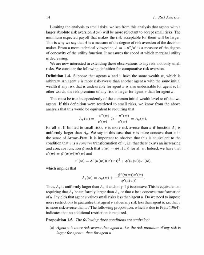
14 1. Risk Aversion

Limiting the analysis to small risks, we see from this analysis that agents with alarger absolute risk aversion A(w) will be more reluctant to accept small risks. Theminimum expected payoff that makes the risk acceptable for them will be larger.This is why we say that A is a measure of the degree of risk aversion of the decisionmaker. From a more technical viewpoint, A = −u′′/u′ is a measure of the degreeof concavity of the utility function. It measures the speed at which marginal utilityis decreasing.

We are now interested in extending these observations to any risk, not only smallrisks. We consider the following definition for comparative risk aversion.

Definition 1.4. Suppose that agents u and v have the same wealth w, which isarbitrary. An agent v is more risk-averse than another agent u with the same initialwealth if any risk that is undesirable for agent u is also undesirable for agent v. Inother words, the risk premium of any risk is larger for agent v than for agent u.

This must be true independently of the common initial wealth level w of the twoagents. If this definition were restricted to small risks, we know from the aboveanalysis that this would be equivalent to requiring that

Av(w) = −v′′(w)

v′(w)� −u′′(w)

u′(w)= Au(w),

for all w. If limited to small risks, v is more risk-averse than u if function Av isuniformly larger than Au. We say in this case that v is more concave than u inthe sense of Arrow–Pratt. It is important to observe that this is equivalent to thecondition that v is a concave transformation of u, i.e. that there exists an increasingand concave function φ such that v(w) = φ(u(w)) for all w. Indeed, we have thatv′(w) = φ′(u(w))u′(w) and

v′′(w) = φ′′(u(w))(u′(w))2 + φ′(u(w))u′′(w),

which implies that

Av(w) = Au(w) + −φ′′(u(w))u′(w)

φ′(u(w)).

Thus, Av is uniformly larger than Au if and only if φ is concave. This is equivalent torequiring that Av be uniformly larger than Au or that v be a concave transformationof u. It yields that agent v values small risks less than agent u. Do we need to imposemore restrictions to guarantee that agent v values any risk less than agent u, i.e. that vis more risk-averse than u? The following proposition, which is due to Pratt (1964),indicates that no additional restriction is required.

Proposition 1.5. The following three conditions are equivalent.

(a) Agent v is more risk-averse than agent u, i.e. the risk premium of any risk islarger for agent v than for agent u.

1.4. Degree of Risk Aversion 15

(b) For all w, Av(w) � Au(w).

(c) Function v is a concave transformation of function u : ∃φ(·) with φ′ > 0 andφ′′ � 0 such that v(w) = φ(u(w)) for all w.

Proof. We have already shown that (b) and (c) are equivalent. That (a) implies (b)follows directly from the Arrow–Pratt approximation. We now prove that (c) implies(a). Consider any lottery z. Let Πu and Πv denote the risk premium for zero-meanlottery z of agent u and agent v, respectively. By definition, we have that

v(w − Πv) = Ev(w + z) = Eφ(u(w + z)).

Define random variable y as y = u(w + z). Because φ is concave, Eφ(y) is smallerthan φ(Ey) by Jensen’s inequality. It thus follows that

v(w − Πv) � φ(Eu(w + z)) = φ(u(w − Πu)) = v(w − Πu).

Because v is increasing, this implies that Πv is larger than Πu.

In the case of small risks, the only thing that we need to know to determine whethera risk is desirable is the degree of concavity of u locally at the current wealth levelw. For larger risks, the proposition above shows that we need to know much more totake a decision. Namely, we need to know the degree of concavity of u at all wealthlevels. The degree of concavity must be increased at all wealth levels to guaranteethat a change in u makes the decision maker more reluctant to accept risks. If v

is locally more concave at some wealth levels and is less concave at other wealthlevels, the comparative analysis is intrinsically ambiguous.

To illustrate the proposition, let us go back to the example of Sempronius’s singleship yielding outcome z = (0, 1

2 ; 8000, 12 ), with a initial wealth w0 = 4000 ducats.

If Sempronius’s utility function is u(w) = √w, his certainty equivalent of z equals

eu = 3464.1, since

12

√4000 + 1

2

√12 000 = 86.395 = √

7464.1

Alternatively, suppose that Sempronius’s utility function is v(w) = ln(w), which isalso increasing and concave. It is easy to check that v is more concave than u in thesense of Arrow–Pratt. Indeed, these functions yield

Av(w) = 1

w� 1

2w= Au(w)

for all w. From the above proposition, this change in utility should reduce thecertainty equivalent of any risk. In the case of w0 = 4000 and z ∼ (0, 1

2 ; 8000, 12 ),

the certainty equivalent of z under v equals ev = 2928.5, since

12 ln(4000) + 1

2 ln(12 000) = 8.8434 = ln(6928.5).

16 1. Risk Aversion

Thus, ev is smaller than eu. Notice that the risk premium Πv = 1071.5 under v

is approximately twice the risk premium Πu = 535.9. This was predicted by theArrow–Pratt approximation, since Av is equal to 2Au.

1.5 Decreasing Absolute Risk Aversion and Prudence

We have seen that risk aversion is driven by the fact that one’s marginal utilityis decreasing with wealth. In this section, we examine another question related toincreasing wealth. Namely, we are interested in determining how the risk premiumfor a given zero-mean risk z is affected by a change in initial wealth w. Arrowargued that intuition implies that wealthier people are generally less willing to payfor the elimination of fixed risk. A lottery to gain or lose 100 with equal probabilityis potentially life-threatening for an agent with initial wealth w = 101, whereas itis essentially trivial for an agent with wealth w = 1 000 000. The former should beready to pay more than the latter for the elimination of risk. We can check that thisproperty holds for the square-root utility function, with Π = 43.4 when w = 101and Π = 0.0025 when w = 1 000 000. If wealth is measured in euros, the individualwould be willing to pay over 43 euros to avoid the risk when wealth is w = 101,whereas the same individual would not even pay one euro cent to get rid of this riskwhen wealth is one million euros! In the following, we characterize the set of utilityfunctions that have this property.

The risk premium Π = π(w) as a function of initial wealth w can be evaluatedby solving

Eu(w + z) = u(w − π(w)) (1.10)

for all w. Fully differentiating (1.10) with respect to w yields

Eu′(w + z) = (1 − π ′(w))u′(w − π),

or, equivalently,

π ′(w) = u′(w − π) − Eu′(w + z)

u′(w − π). (1.11)

Thus, the risk premium is decreasing with wealth if and only if

Ev(w + z) � v(w − π(w)), (1.12)

where function v ≡ −u′ is defined as minus the derivative of function u. Becausethe function v is increasing, we can also interpret it as another utility function.Condition (1.12) then just states that the risk premium of agent v is larger thanthe risk premium π of agent u. From Proposition 1.5, this is true if and only if v

is more concave than u in the sense of Arrow–Pratt, that is, if −u′ is a concavetransformation of u. For this utility v, the measure of absolute risk aversion isAv = A−u′ = −u′′′/u′′. This measure has several uses, which will be made clearer

1.6. Relative Risk Aversion 17

later in this book. For this reason, without justifying the terminology at this stage,we will define P(w) = −u′′′(w)/u′′(w) as the degree of absolute prudence of theagent with utility u. It follows from (1.12) that −u′ is more concave than u if andonly if

P(w) � A(w)

for all w. We conclude that condition P � A uniformly is necessary and sufficientto guarantee that an increase in wealth reduces risk premia. Because

A′(w) = A(w)[A(w) − P(w)],condition P � A is equivalent to the condition A′ � 0. We obtain the followingproposition.

Proposition 1.6. The risk premium associated to any risk z is decreasing in wealthif and only if absolute risk aversion is decreasing; or equivalently if and only ifprudence is uniformly larger than absolute risk aversion.

Observe that the utility function u(w) = √w satisfies this condition. Indeed,

we have Au(w) = 12w−1, which is decreasing. This can alternatively checked by

observing that v(w) = − 12w−1/2 and Av(w) = Pu(w) = 1.5w−1, which is uni-

formly larger than Au(w). Notice that Decreasing Absolute Risk Aversion (DARA)requires that the third derivative of the utility function be positive. Otherwise, pru-dence would be negative, which would imply that P < A: a condition that impliesthat absolute risk aversion would be increasing in wealth. Thus, DARA, a veryintuitive condition, requires the necessary (but not sufficient) condition that u′′′ bepositive, or that marginal utility be convex.

1.6 Relative Risk Aversion

Absolute risk aversion is the rate of decay for marginal utility. More particularly,absolute risk aversion measures the rate at which marginal utility decreases whenwealth is increased by one euro.6 If the monetary unit were the dollar, absolute riskaversion would be a different number. In other words, the index of absolute riskaversion is not unit free, as it is measured per euro (per dollar, or per yen).

Economists often prefer unit-free measurements of sensitivity. To this end, definethe index of relative risk aversion R as the rate at which marginal utility decreases

6In general, the growth rate for a function f (x) is defined as

df (x)

dx· 1

f (x).

Since marginal utility u′(x) declines in wealth, its growth rate is negative. The absolute value of thisnegative growth rate, which is the measure of absolute risk aversion, is called the decay rate.

18 1. Risk Aversion

when wealth is increased by one percent. In terms of standard economic theory, thismeasure is simply the wealth-elasticity of marginal utility. It can be computed as

R(w) = −du′(w)/u′(w)

dw/w= −wu′′(w)

u′(w)= wA(w). (1.13)

Note that the measure of relative risk aversion is simply the product of wealth andabsolute risk aversion.

The (absolute) risk premium and the index of absolute risk aversion are linkedby the Arrow–Pratt approximation and by Propositions 1.5 and 1.6. We can developanalogous kinds of results for relative risk aversion. Suppose that your initial wealthw is invested in a portfolio whose return z over the period is uncertain. Let us assumethat Ez = 0. Which share of your initial wealth are you ready to pay to get rid ofthis proportional risk? The solution to this problem is referred to as the relativerisk premium Π . This measure also is a unit-free measure, unlike the absolute riskpremium, which is measured in euros. It is defined implicitly via the followingequation:

Eu(w(1 + z)) = u(w(1 − Π)). (1.14)

Obviously, the relative risk premium and the absolute risk premium are equal ifwe normalize initial wealth to unity. More generally, the relative risk premium forproportional risk z equals the absolute risk premium for absolute risk wz, divided byinitial wealth w: Π(z) = Π(wz)/w. From this observation, we obtain the fact that,if agent v is more risk-averse than agent u with the same initial wealth, then agent v

will be ready to pay a larger share of his wealth than agent u to insure against a givenproportional risk z. Moreover, if σ 2 denotes the variance of z, then the variance ofwz equals w2σ 2. Using the Arrow–Pratt approximation thus yields

Π(z) = Π(wz)

w�

12w2σ 2A(w)

w= 1

2σ 2R(w). (1.15)

The relative risk premium is approximately equal to half of the variance of the pro-portional risk times the index of relative risk aversion. This can be used to establisha range for acceptable degrees of risk aversion. Suppose that one’s wealth is subjectto a risk of a gain or loss of 20% with equal probability. What is the range that onewould find reasonable for the share of wealth Π that one would be ready to pay toget rid of this zero-mean risk? From our various experiments in class, we found thatmost people would be ready to pay between 2% and 8% of their wealth. Becauserisk z in this experiment has a variance of 0.5(0.2)2 + 0.5(−0.2)2 = 0.04, usingapproximation (1.15) yields a range for relative risk aversion between 1 and 4. Thisinformation will be useful later in this book.

There is no definitive argument for or against decreasing relative risk aversion.Arrow originally conjectured that relative risk aversion is likely to be constant, or

1.7. Some Classical Utility Functions 19

perhaps increasing, although he stated that the intuition was not as clear as wasthe intuition for decreasing absolute risk aversion. Since then, numerous empiricalstudies have offered conflicting results. We might also try to examine this questionby introspection. If your wealth would increase, would you want to devote a largeror a smaller share of your wealth to get rid of a given zero-mean proportional risk?For example, what would you pay to avoid the risk of gaining or losing 20% ofyour wealth, each with an equal probability? If the share is decreasing with wealth,you have decreasing relative risk aversion. There are two contradictory effects herethat need to be considered. On the one hand, under the intuitive DARA assumption,becoming wealthier also means becoming less risk-averse.This effect tends to reduceΠ . But, on the other hand, becoming wealthier also means facing a larger absoluterisk wz. This effect tends to raise Π . There is no clear intuition as to whether the firsteffect or the second effect will dominate. For example, many of the classic models inmacroeconomics are based on relative risk aversion being constant over all wealthlevels, which is implicitly assuming that our two effects exactly cancel each otherout. Of course, there also is no a priori reason to believe that the dominant effect willnot change over various wealth levels. For instance, some recent empirical evidenceindicates a possible “U-shape” for relative risk aversion, with R decreasing at lowwealth levels, then leveling off somewhat before increasing at higher wealth levels.

1.7 Some Classical Utility Functions

As already noted above, expected-utility (EU) theory has many proponents andmany detractors. In Chapter 13, we examine some generalizations of the EU crite-rion that satisfy those who find expected utility too restrictive. But researchers inboth economics and finance have long considered—and most of them still do—EUtheory as an acceptable paradigm for decision making under uncertainty. Indeed,EU theory has a long and prominent place in the development of decision makingunder uncertainty. Even detractors of the theory use EU as a standard by which tocompare alternative theories. Moreover, many of the models in which EU theoryhas been applied can be modified, often yielding better results.

Whereas the current trend is to generalize the EU model, researchers often restrictEU criterion by considering a specific subset of utility functions. This is done toobtain tractable solutions to many problems. It is important to note the implicationsthat derive from the choice of a particular utility function. Some results in theliterature may be robust enough to apply for all risk-averse preferences, while othersmight be restricted to applying only for a narrow class of preferences. In this section,we examine several particular types of utility functions that are often encounteredin the economics and the finance literature. Remember that utility is unique only upto a linear transformation.

20 1. Risk Aversion

Historically, much of the theory of finance was developed during the 1960s byconsidering the subset of utility functions that are quadratic of the form

u(w) = aw − 12w2, for w � a.

Note that the domain of wealth on which u is defined comes from the necessaryrequirement that u be nondecreasing, which is true only if w is smaller than a.This set of functions is useful because the EU generated by any distribution of finalwealth is a function of only the first two moments of this distribution:

Eu(w) = aEw − 12Ew2.

Therefore, in this case, the EU theory simplifies to a mean–variance approach todecision making under uncertainty. However, as already discussed, it is very hard tobelieve that preferences among different lotteries be determined only by the meanand variance of these lotteries.

Above wealth level a, marginal utility becomes negative. Since quadratic utilityis decreasing in wealth for w > a, many people might feel this is not appropriate asa utility function. However, it is important to remember that we are trying to modelhuman behavior with mathematical models. For example, if the quadratic utilityfunction models your behavior quite well with a = 100 million euros, is it reallya problem that this function declines for higher wealth levels? The point is that thequadratic utility might work well for more realistic wealth levels, and if it does, weshould not be overly concerned about its properties at unrealistically high wealthlevels. However, the quadratic utility function has another property that is moreproblematic. Namely, the quadratic utility functions exhibit increasing absolute riskaversion:

A(w) = 1

a − w⇒ A′(w) = 1

(a − w)2 > 0.

For this reason, quadratic utility functions are not as in fashion anymore.A second set of classical utility functions is the set of so-called constant-absolute-

risk-aversion (CARA) utility functions, which are exponential functions character-ized by

u(w) = −exp(−aw)

a,

where a is some positive scalar. The domain of these functions is the real line. Thedistinguishing feature of these utility functions is that they exhibit constant absoluterisk aversion, with A(w) = a for all w. It can be shown that the Arrow–Prattapproximation is exact when u is exponential and w is normally distributed with

1.7. Some Classical Utility Functions 21

mean µ and variance σ 2. Indeed, we can take expectations to see that

Eu(w)

= −1

σa√

2π

∫exp(−aw) exp

(− (w − µ)2

2σ 2

)dw

= −1

aexp(−a(µ − 1

2aσ 2))

[1

σ√

2π

∫exp

(− (w − (µ − 1

2aσ 2))2

2σ 2

)dw

]

= −1

aexp(−a(µ − 1

2aσ 2)) = u(µ − 12aσ 2). (1.16)

The third equality comes from the fact that the bracketed term is the integral of thedensity of the normal distribution N(µ − 1

2aσ 2, σ ), which must be equal to unity.Thus, the risk premium is indeed equal to 1

2σ 2A(w). In this very specific case, weobtain that the Arrow–Pratt approximation is exact. The fact that risk aversion isconstant is often useful in analyzing choices among several alternatives. As we willsee later, this assumption eliminates the income effect when dealing with decisionsto be made about a risk whose size is invariant to changes in wealth. However, thisis often also the main criticism of the CARA utility, since absolute risk aversion isconstant rather than decreasing.

Finally, one set of preferences that has been by far the most used in the literature isthe set of power utility functions. Researchers in finance and in macroeconomics areso accustomed to this restriction that many of them do not even mention it anymorewhen they present their results. Suppose that

u(w) = w1−γ

1 − γfor w > 0.

The scalar γ is chosen so that γ > 0, γ �= 1. It is easy to show that γ equals thedegree of relative risk aversion, since A(w) = γ /w and R(w) = γ for all w. Thus,this set exhibits decreasing absolute risk aversion and constant relative risk aversion,which are two reasonable assumptions. For this reason, these utility functions arecalled the constant-relative-risk-aversion (CRRA) class of preferences. Notice thatour definition does not allow for γ = 1. However, it is straightforward to show thatfunction u(w) = ln(w) satisfies the property that R(w) = 1 for all w. Thus, the setof all CRRA utility functions is completely defined by7

u(w) =

⎧⎪⎨⎪⎩

w1−γ

1 − γfor γ � 0, γ �= 1,

ln(w) for γ = 1.

(1.17)

7We can also show that u(w) = ln(w) as a limiting case of the power utility function. To this end,rewrite the power utility function, using a linear transformation, as

u(w) = 1

1 − γ(w1−γ − 1).

22 1. Risk Aversion

As we will see later in this book, this class of utility functions eliminates anyincome effects when making decisions about risks whose size is proportional toone’s level of wealth. For example, the relative risk premium Π defined by equation(1.14) is independent of wealth w in this case. The assumption that relative riskaversion is constant enormously simplifies many of the problems often encounteredin macroeconomics and finance.

1.8 Bibliographical References, Extensions and Exercises

The contribution by Pratt (1964) basically opened and closed the field covered in thischapter. It is, however, fair to mention that the measure of absolute risk aversion hasbeen discovered independently by Arrow (1963) and de Finetti (1952). The paper byde Finetti was written in Italian and even today is not given the attention it deserves.The paper by Pratt is by far the most advanced in defining the notions of an increasein risk aversion and of decreasing absolute risk aversion. The orders of risk aversionare introduced by Segal and Spivak (1990).

Ross (1981) challenged the idea that A = −u′′/u′ is a good measure of the degreeof risk aversion of an agent. Kihlstrom, Romer and Williams (1981) and Nachman(1982) showed that if initial wealth is uncertain, it is not true that an agent v, who ismore risk-averse than another agent u in the sense of Arrow–Pratt, will be ready topay more to get rid of another risk. Ross (1981) characterized the conditions on u

and v that imply that Πv � Πu even when initial wealth is uncertain and potentiallycorrelated with the risk under scrutiny. These conditions are of course stronger thanAv � Au.

There is much contradictory empirical evidence on the shape of relative risk aver-sion as a function of wealth. Many authors have empirically estimated R, assumingthat we have CRRA. Fewer authors have examined whether R might be increas-ing or decreasing in wealth. A good summary of many of these results appears inAit-Sahalia and Lo (2000).

Chapter Bibliography

Ait-Sahalia,Y. andA.W. Lo. 2000. Nonparametric risk management and implied risk aversion.Journal of Econometrics 94:9–51.

Arrow, K. J. 1963. Liquidity preference. Lecture VI in Lecture Notes for Economics 285, TheEconomics of Uncertainty, pp. 33-53, undated, Stanford University.

———. 1965. Yrjo Jahnsson lecture notes, Helsinki. (Reprinted in Arrow 1971).———. 1971. Essays in the theory of risk bearing. Chicago: Markham Publishing Co.

Taking the limit as γ → 1 and applying L’Hopital’s rule, we obtain

limγ → 1

u(w) = limγ → 1

−(w1−γ ) ln(w)

−1= ln(w).

1.8. Bibliographical References, Extensions and Exercises 23

Bernoulli, D. 1954. Exposition of a new theory on the measurement of risk. (English Transl.by Louise Sommer.) Econometrica 22: 23–36.

Bernstein, P. L. 1998. Against the Gods. Wiley.de Finetti, B. 1952. Sulla preferibilita. Giornale Degli Economisti E Annali Di Economia

11:685–709.Kihlstrom, R., D. Romer, and S. Williams. 1981. Risk aversion with random initial wealth.

Econometrica 49:911–920.Nachman, D. C. 1982. Preservation of ‘more risk averse’ under expectations. Journal of

Economic Theory 28:361–368.Pratt, J. 1964. Risk aversion in the small and in the large. Econometrica 32:122–136.Ross, S. A. 1981. Some stronger measures of risk aversion in the small and in the large with

applications. Econometrica 3:621–638.Segal, U. and A. Spivak. 1990. First order versus second order risk aversion. Journal of

Economic Theory 51:111–125.Yaari, M. E. 1987. The dual theory of choice under risk. Econometrica 55:95–115.

24 1. Risk Aversion

Exercises

(1.1) An individual has the following utility function:

u(w) = w1/2.

Her initial wealth is 10 and she faces the lottery X : (−6, 12 ; +6, 1

2 ).

(a) Compute the exact value of the certainty equivalent and of the riskpremium.

(b) Apply Pratt’s formula to obtain an approximation of the risk premium.

(c) Show that with such a utility function absolute risk aversion is decreasingin wealth while relative risk aversion is constant.

(d) If the utility function becomes

v(w) = w1/4,

answer again part (a). Are you surprised by the changes in the certaintyequivalent and in the risk premium? Relate this change to the notionof ‘more risk averse’ (i.e. express v(w) as a concave transformation ofu(w)).

(e) If the risk becomes Y : (−3, 12 ; +3, 1

2 ), compute the new risk premiumas approximated by Pratt’s formula. Why is the approximated risk pre-mium four times smaller than the risk premium for X?

(1.2) As in the previous exercise, consider an initial wealth of 10 and the lottery X.Assume now that the utility is:

u ={

w for w � 10,

12w + 5 for w � 10.

(1.18)

(a) Draw the utility function. Is it globally concave?

(b) Compute the certainty equivalent and the risk premium attached to X.

(c) Can you apply the Arrow–Pratt approximation? Why?

(d) Consider now the lottery Y defined in exercise 1.1. Compute the riskpremium attached to Y . Is it smaller than for X? Why?

(e) Answer (b) and (d) above if the individual has an initial wealth of 20.How do the risk premia for X and Y compare?

1.8. Bibliographical References, Extensions and Exercises 25

(1.3) Let u = w2 for w � 0.

(a) Compute the exact risk premium if initial wealth is 4 and if a decisionmaker faces the lottery (−2, 1

2 ; +2, 12 ). Explain why the risk premium

is negative.

(b) If the utility function becomes v = w4, what happens to the risk pre-mium? Show that v is a convex transformation of u.

(1.4) Let u = ln w.

(a) Does this utility function exhibit the DARA property?

(b) Compute −u′′′/u′′ and compare it with −u′′/u′.(e) Prove that −u′(w) is a concave transformation of u(w) (hint: use Pratt’s

theorem).

(1.5) Consider the family of exponential utility functions

u = 1 − exp(−aw)

a.

(a) Show that a is the degree of absolute risk aversion.

(b) Show that u becomes linear in w when a tends to zero (hint: useL’Hopital’s rule).

(c) Consider lottery x with positive and negative payoffs. Determine thevalue of Eu(x) when a tends to infinity.

2The Measures of Risk

In Chapter 1, we defined the concept of risk aversion by considering the effect ofthe introduction of a zero-mean risk on welfare. That is, we assumed that the initialenvironment of the consumer was risk free. Our only conclusion from risk aversionwas that the individual preferred no risk to a zero-mean risk. But what about choicesamong different zero-mean risks? For example, recall from the previous chapter thatwe might interpret Sempronius’s situation as facing the risk (−4000, 1

2 ; 4000, 12 )

with initial wealth w = 8000. The alternative, using two separate ships, can bethought of as facing the risk (−4000, 1

4 ; 0, 12 ; +4000, 1

4 ) from the same initialwealth. We argued that the second alternative seemed more valuable, in some sense.In this chapter, we will examine this question more closely and consider the com-parison of such competing risks.

If one could know the utility function of the agent, ranking lotteries would be easy.For example, let us compare two different wealth prospects (i.e. two distributions offinal wealth) w1 and w2. The first is preferred to the second by an agent with utilityfunction u if Eu(w1) � Eu(w2). This preference order, which is specific to a singleutility function u, is complete in the sense that, for any pair (w1, w2), w1 is preferredto w2, or w2 is preferred to w1, or we are indifferent to both wealth prospects. Inthis chapter, we consider several relatively weak restrictions on preferences; forexample, that “agents are risk-averse” or that “agents are prudent.” We want tofind restrictions on the change in risk from w1 to w2 that are unanimously dislikedby the group of agents under scrutiny. In that case, we say that w1 dominates w2

for this class of utility functions. As soon as the class is not limited to a singleutility function, these preference orders are incomplete in the sense that it is nottrue that, for any pair of lotteries, one must necessarily dominate the other. Somepeople in the group may prefer the first, whereas other members in the group mayprefer the second. Imposing unanimity in the group is a very strong constraint onthe change in risk. Considering a larger group makes the constraint of unanimitystronger. On the other hand, if among our group we do find unanimity that w1

dominates w2, it allows us to choose w1 over w2 when these are our only twooptions.

28 2. The Measures of Risk

The theory of stochastic dominance looks at certain statistical properties of thedistributions of w1 and w2, which allow us to infer unanimous agreement for certainclasses of preferences. This is important not only for our understanding of individualbehavior, but also for decision making designed to benefit a group, such as a corporatemanager making decisions on behalf of the company’s shareholders. In this book,we will consider basically three stochastic orders. In Section 2.1, we first considerthe most natural set of utility functions from what we have seen in Chapter 1. Weconsider in that section the set of all risk-averse agents. It generates the conceptof an increase in risk that was first examined by Rothschild and Stiglitz (1970). InSection 2.2, we focus on the set of prudent agents, which yields the concept of anincrease in downside risk introduced by Menezes, Geiss and Tressler (1980). Finally,in Section 2.3, we assume only that agents have an increasing utility function. Thecorresponding stochastic order is called “first-order stochastic dominance.”

2.1 Increases in Risk

In this section, we characterize the changes in risk that make all risk-averse agentsworse off. We focus the analysis on changes in risk which preserve the expectedoutcome, i.e. mean-preserving changes in risk. These changes are called “increasesin risk.” There are at least three equivalent ways to define them.

2.1.1 Adding Noise

Consider the binary lottery faced by Sempronius using a single ship. This maybe written as w1 ∼ (4000, 1

2 ; 12 000, 12 ). In the low wealth state, the ship is lost,

whereas in the high wealth state, the ship succeeds in bringing the spices safely tothe harbor. Let us assume that the ship contains 8000 pounds of spices, which willbe sold at a unit price of one ducat. This environment generates a distribution w1

for Sempronius’s final wealth.Suppose alternatively that the price at which the spices will be sold at the harbor is

unknown at the time that the ship leaves the East Indies. More precisely, let us sup-pose that the unit price will be either 0.5 ducats or 1.5 ducats with equal probabilities.In this alternative environment, the final wealth is still 4000 in the case of the shipbeing sunk. But, conditional on the ship’s arriving safely in Europe, Sempronius’sfinal wealth will be either 8000 or 16 000 with equal probabilities, or 12 000 + ε,with ε ∼ (−4000, 1

2 , 4000, 12 ). Because Eε = 0, the price uncertainty adds a zero-

mean noise to Sempronius’s final wealth, conditional upon the no-loss state. Ex ante,the agent faces an uncertain wealth distributed as w2 ∼ (4000, 1

2 ; 12 000 + ε, 12 ).

This situation describes what is called a compound lottery, i.e. a lottery for whichsome of the outcomes are themselves lotteries.

Intuition suggests that Sempronius should dislike this additional uncertainty. Thereader can check that this is indeed the case. For example, if Sempronius’s utility

2.1. Increases in Risk 29

12 0004000 4000 8000

prob

abili

ty

16 000 wealth wealth

(a) (b)12

12

14

Figure 2.1. Transfer of probability mass to describe an increase in risk.

function is a square root, we have that

Eu(w1) = 12

√4000 + 1

2

√12 000 = 86.395,

whereas

Eu(w2) = 12

√4000 + 1

2

[12

√8000 + 1

2

√16 000

]= 85.606 < 86.395.

The same qualitative result would hold if Sempronius would have another concaveutility function. In fact, adding a zero-mean noise conditional upon some specificstate always reduces the EU of risk-averse agents, as we now show.

To keep the presentation relatively simple, suppose that w1 can take n differentpossible values ω1, ω2, . . . , ωn. Let ps denote the probability that w1 takes valueωs . Suppose that the alternative wealth distribution w2 be obtained by compoundingw1 with zero-mean noises εs for the different outcomes ωs of w1. This means thateach outcome ωs of w1 is replaced by ωs + εs with Eεs = 0:

w2 = w1 + ε with E[ε | w1 = ωs] = E[εs] = 0.

The price uncertainty presented above is an example of this technique of addingnoises to each possible outcome of the initial distribution of wealth.

With this notation, it is easy to show that any such alternative lottery w2 makesall risk-averse agents worse off. Because Eεs is zero, risk aversion implies thatEu(ωs + εs ) � u(ωs). It follows that

Eu(w2) =n∑

s=1

psEu(ωs + εs ) �n∑

s=1

psu(ωs) = Eu(w1).

All risk-averse agents dislike adding zero-mean noises to the possible outcomes oftheir wealth.

2.1.2 Mean-Preserving Spreads in Probability

The existence of price uncertainty in the situation faced by Sempronius can alterna-tively be seen as transferring probability masses. In Figure 2.1(a), we represent theprobability distribution in the absence of price uncertainty. Figure 2.1(b) describes

30 2. The Measures of Risk

the probability distribution when the price uncertainty is taken into account. We seethat adding noise ε ∼ (−4000, 1

2 , 4000, 12 ) is equivalent to transfering half of the

12 -probability mass at 12 000 to 8000, and the remaining of the probability massat 12 000 to 16 000. By doing this, we do not modify the center of gravity of theprobability distribution, i.e. we preserve the mean. In short, we construct what iscalled a “mean-preserving spread” of the probability distribution.

Let fi(w) denote the probability mass of wi at w. In the case of a continuousdistribution, fi(·) is the probability density of wi . The following definition formal-izes the concept of a mean-preserving spread, which is an operation consisting ofthe partial removal of probability mass from some interval I in order to transfer itoutside this interval.

Definition 2.1. w2 is a mean-preserving spread (MPS) of w1 if

1. Ew2 = Ew1, and

2. there exists an interval I such that f2(w) � f1(w) for all w in I , and f2(w) �f1(w) for all w outside I .

Adding noise or constructing a sequence of MPS’s are obviously two equivalentways to increase risk. In some circumstances, it is easier to use one representationthan the other. For example, let us compare distribution w1 ∼ (4000, 1

2 ; 12 000, 12 )

to distribution w2 ∼ (2000, 12 ; 14 000, 1

2 ). Obviously, the two distributions have thesame mean, and the second is obtained by transferring some probability mass frominterval I = [4000, 12 000] outside I . Thus, w2 is an increase in risk of w1. It mustbe the case that w2 is obtained from w1 by adding some noise ε1 to outcome 4000and another noise ε2 to outcome 12 000 of w1. The reader may easily verify thatindeed defining

ε1 ∼ (−2000, 56 ; 10 000, 1

6 ) and ε2 ∼ (2000, 56 ; −10 000, 1

6 )

does the job.It is often useful to translate the definition of a mean-preserving spread into a

condition on the cumulative distribution functions of w1 and w2. Let Fi(w) denotethe probability that wi be no greater than w. That is, define

Fi(w) =∑

s|ωs�w

fi(s)

in the discrete case, and

Fi(w) =∫ w

fi(s) ds

in the continuous case. In the latter case, the density function fi is simply thederivative of Fi . To keep the level of technicality at a minimum, let us assume that

2.1. Increases in Risk 31

dens

ity

cum

ulat

ive

prob

abili

ty

wealth wealthI I

f1 F1F2f2

Figure 2.2. Example of a mean-preserving spread for a continuous distribution.

all possible final wealth levels are in the interval (a, b]. Suppose that w2 is an MPSof w1. Integrating by parts, preservation of the mean implies that∫ b

a

[F2(s) − F1(s)] ds = −∫ b

a

s[f2(s) − f1(s)] ds = Ew2 − Ew1 = 0.

The fact that the expectation is preserved means that the area between F1 and F2

(counted as positive when F2 is above F1 and counted as negative otherwise) mustsum up to zero. Also, by definition of an MPS, the derivative of F2 is smaller (resp.larger) than the derivative of F1 within the interval I (resp. outside I ). Thus, F2

must be larger than F1 to the left of some threshold w and F2 must be smaller thanF1 to its right. We illustrate this property in Figure 2.2 in the continuous case, andin Figure 2.3 in the discrete case considered in the previous paragraph.

This so-called “single-crossing” property of MPS implies in particular that

S(w) =∫ w

a

[F2(s) − F1(s)] ds � 0 (2.1)

for all w, with an equality when w equals b. This integral condition is examined inmore detail in the next section.

2.1.3 The Integral Condition and Risk-Averse Preferences

We now examine the problem of characterizing changes in risk that reduce the EUof all risk-averse agents. By integrating by parts, we obtain

Eu(wi) =∫ b

a

u(ω)fi(ω) dω = u(ω)Fi(ω)|ω=bω=a −

∫ b

a

u′(ω)Fi(ω) dω,

or, equivalently, that

Eu(wi) = u(b) −∫ b

a

u′(ω)Fi(ω) dω.

It follows that

Eu(w2) − Eu(w1) =∫ b

a

u′(ω)[F1(ω) − F2(ω)] dω. (2.2)

32 2. The Measures of Risk

1/2

3/4

1

without price riskwith price risk

cum

ulat

ive

prob

abili

ty

4000 8000 12 000 16 000wealth

Figure 2.3. Cumulative distribution functions of Sempronius’s final wealthwith one ship, and with or without price uncertainty.

The difference in EU in transforming w1 into w2 is equal to the areas between F1

and F2 (“+” if F1 is above F2, and “−” otherwise) weighted by the marginal valueof wealth. Integrating by parts once again yields

Eu(w2) − Eu(w1) = −u′(ω)S(ω)|ω=bω=a +

∫ b

a

u′′(ω)S(ω) dω,

where function S is defined by equation (2.1) and is such that S′(w) = F2(w) −F1(w). Because we focused the analysis on changes in risk that preserve the mean,we have that S(a) = S(b) = 0. The above equation thus simplifies to

Eu(w2) − Eu(w1) =∫ b

a

u′′(ω)S(ω) dω. (2.3)

Equation (2.3) implies that all risk-averse agents dislike mean-preserving increasesin risk, that is changes in risk for which the condition S(w) � 0 is satisfied for all w.This condition would indeed imply that the integrand in (2.3) is uniformly negative.Its integral in [a, b] should therefore be negative. The condition that S(w) � 0 for allw is also necessary to guarantee that every risk averter would unanimously preferw1 over w2. Indeed, suppose by contradiction that S is positive in some intervalJ ⊆ [a, b]. Let us consider the concave utility function u that is linear outside J ,and which is strictly concave in J . Then, from equation (2.3), agent u increases herEU by transforming w1 into w2. The integrand u′′S is zero for w outside J and ispositive for w in J .

2.1. Increases in Risk 33

To sum up, the condition that S(w) = ∫ w(F2(s) − F1(s)) ds be nonnegative is

both a necessary and a sufficient condition for mean-preserving changes in risk toreduce the EU of all risk-averse agents. It was examined by Rothschild and Stiglitz(1970). Notice from equation (2.2) that the condition S(w) � 0 implies that agentswith the concave utility functions uw(x) = min(x, w) ∀w ∈ [a, b] all prefer risk w1

to risk w2. We hope that this observation makes this integral condition less artificial.There is a clear link between the integral condition S � 0 and the notion of a

mean-preserving spread. It has been partly derived at the end of the previous section,where we have shown that a mean-preserving spread implies that S is nonnegative.Rothschild and Stiglitz (1970) have shown that the integral condition is equivalentto a sequence of mean-preserving spreads. In fact, they have proved the followingproposition, showing how several interpretations of a mean-preserving increase inrisk are all the same.

Proposition 2.2. Consider two random variables w1 and w2 with the same mean.The following four conditions are equivalent.

(a) All risk-averse agents prefer w1 to w2: Eu(w2) � Eu(w1) for all concavefunctions u.

(b) w2 is obtained from w1 by adding zero-mean noise terms to the possibleoutcomes of w1:

w2d= w1 + ε,

with E[ε | w1 = ω] = 0 for all ω, where “d=” means “equal in distribution.”

(c) w2 is obtained from w1 by a sequence of mean-preserving spreads.

(d) S(w) ≡ ∫ w(F2(w) − F1(w)) dw � 0 for all w.

Any one of these four equivalent conditions may define what we call an increase inrisk from w1 to w2. Correspondingly, a change from w2 to w1 is labeled a reductionin risk.

2.1.4 Preference for Diversification

In Chapter 1, we have shown that Sempronius prefers to transfer the spices from thecolonies by two ships rather than by only one. By doing so, he diversifies the risk.Let us now formalize this example by defining the random variable xi which takesvalue 0 if ship i is sunk (probability 1

2 ), and which takes value 1 otherwise. In short,xi is distributed as (0, 1

2 ; 1, 12 ). By assumption, the risks faced by the two ships are

independent. If Sempronius puts his 8000 pounds of spice in ship 1, his final wealthwould equal

w2 = w + 8000x1.

34 2. The Measures of Risk

1/21/4

1/4

0

1

0 0

01

1/2

1/2 1/2

−1/2

+1/2

1/2

1/2

x1 y ε= +~ ~ ~

Figure 2.4. Diversification and reduction of risk.

We assume here that the price of spice is risk free and normalized to unity. If hesplits the goods in two equal parts to be brought to London in ships 1 and 2, his finalwealth equals

w1 = w + 8000

(x1 + x2

2

)= w + 8000y,

where y = 12 (x1 + x2) can be interpreted as the rate of success. The rate of success is

distributed as (0, 14 ; 1

2 , 12 ; 1, 1

4 ). It is easy to check that x1 can be obtained from y byadding the noise ε ∼ (− 1

2 , 12 ; + 1

2 , 12 ) conditional upon y = 1

2 , as seen in Figure 2.4.It then follows from Proposition 2.2 that, independent of the utility function ofSempronius, he must prefer two ships to one ship as soon as this function is concave.Diversifying the transfer of spice to two ships is a way to diversify the risk facedby Sempronius. Not “putting all the eggs in one basket” is a rational behavior forrisk-averse agents.

More generally, one can verify that, if x1 and x2 are two independent and iden-tically distributed (i.i.d.) random variables, then y = 1

2 (x1 + x2) is a reduction ofrisk with respect to x1. We have that

x1 = y + ε with ε = x1 − x2

2and

E[ε | y = y] = E

[x1 − x2

2

∣∣∣∣ x1 + x2

2= y

]

= E

[x1

∣∣∣∣ x1 − x2

2

]− E

[x2

∣∣∣∣ x1 − x2

2

],

which must be equal to zero by symmetry. Thus, x1 is riskier than y. In other words,diversification is a risk-reduction device in the sense of Rothschild and Stiglitz. Allrisk-averse agents should diversify their risks when possible. This guideline doesnot rely on any preference restrictions other than risk aversion.

2.1. Increases in Risk 35

2.1.5 And the Variance?

The risk premium is the amount of money that the agent is ready to pay to elim-inate the (zero-mean) risk. Facing the risk wi or receiving its certainty equivalentEwi − Πi generates the same EU. Consider two risky wealth prospects w1 andw2 with equal means. It is clear that w1 is preferred to w2 if and only if Π2 islarger than Π1. Proposition 2.2 states the conditions on w1 and w2 that guaranteethat Π2 is larger than Π1. Notice that, for small risks, we can use the Arrow–Prattapproximation

Πi � 12σ 2

i A

to claim that w1 is preferred to w2 if and only if the variance of w2 is larger than thevariance of w1 : σ 2

2 � σ 21 . Should not it also be the case that this holds for larger

risks as well? That is to say, could we not add another equivalent statement (e) toProposition 2.2 that would be written as follows:

(e) the variance of w2 is larger than the variance of w1?

The answer is definitely no! In general, statistical moments of orders higher than 2will matter when comparing two random variables. By limiting the development ofTaylor of the utility function to the second order, theArrow–Pratt approximation is ofno value for larger risks. The only exception is when the utility function is quadratic.A correct statement would then be that all risk-averse agents with a quadratic utilityfunction prefer w1 to w2 if and only if the variance of the second is larger than thevariance of the first.1

However, it is easy to check that an increase in variance is a necessary, but notsufficient, condition for an increase in risk. Indeed, it is a necessary condition forthose agents with a quadratic concave utility function to dislike this change in risk.Thus, it is a necessary for all agents with a concave function to dislike it.

It is noteworthy that the necessary condition for an increase in the variance canbe can be written as

σ 22 − σ 2

1 =∫ b

a

w2(f2(w) − f1(w)) dw

= 2∫ b

a

S(w) dw � 0.

This equation is a direct consequence of equation (2.3) applied for u(w) = w2. Wesee that the increase in variance just means that the integral of function S must benonnegative. The Rothschild–Stiglitz increase in risk is a much stronger requirementthat S be uniformly nonnegative.

1Another strategy is to limit the set of random variables to those that can be parametrized by theirmean and variance only, as the set of normal distributions.

36 2. The Measures of Risk

4000

16 000

8000

12 000

8000

01/2

1/2

1/4

1/4

1/4

1/4

w2 w3~~

Figure 2.5. Increase in downside risk.

2.2 Aversion to Downside Risk

In this short section, we explore another set of changes in risk which are referred to asincreases in downside risk. These changes have the property that they preserve boththe mean and the variance of final wealth. To illustrate, consider again the distribu-tion of final wealth w2 ∼ (4000, 1

2 ; 12 000 + ε, 12 ), with ε ∼ (−4000, 1

2 , 4000, 12 ).

Sempronius faces the price risk ε in addition to the risk of losing his single ship.Observe that this is a situation where the additional zero-mean risk ε is borne onlyin the good state, i.e. when the ship arrives safely at the harbor of London. Consideran alternative situation where this zero-mean risk would be borne in the bad state. Itwould thus yield a final wealth distributed as w3 ∼ (4000 + ε, 1

2 ; 12 000, 12 ). Which

of these two distributions of final wealth do you think Sempronius would prefer?To assist you in your choice, we represent these two distribution in Figure 2.5.

Observe that the means are the same: Ew2 = Ew3 = 8000. The variance isalso unchanged by the change in distribution: σ 2

2 = σ 23 = 24 × 106. In fact, the

reader can check that function S alternates in sign in the interval of final wealth levels[0, 16 000]. Thus, this cannot be an increase in risk. Hence, by Proposition 2.2, somerisk-averse agents will like this change, whereas others will dislike it. However,experiments have shown that most people in the real world prefer w2 to w3. Thatis to say, they prefer to bear a zero-mean risk in the wealthier state. In other words,they dislike transferring a zero-mean risk from a richer to a poorer state. In this case,we say that they are averse to downside risk.

We are interested in determining a condition on the utility function that guaranteesthat an agent is averse to downside risk. Suppose that the agent is initially facinga risk that is characterized by w ∼ (z1, 1/n; z2, 1/n; . . . ; zn, 1/n). We assume forsimplicity that these n states have the same probability of occurrence. Consider anadditional risk ε with a zero mean. The EU of final wealth depends upon the state i

to which this additional risk is imposed. We denote

V i = 1

nEu(zi + ε) +

∑j �=i

1

nu(zj )

2.3. First-Degree Stochastic Dominance 37

for the EU when ε is borne in state i. Observe that

n(V i − Vj ) = [Eu(zi + ε) − u(zi)] − [Eu(zj + ε) − u(zj )]=

∫ zi

zj

[Eu′(ω + ε) − u′(ω)] dω.

Although intuition suggests the empirical observation that V i > Vj when zi > zj ,we see from the above equation that this is true if and only if

Eu′(ω + ε) � u′(ω)

for all ω. Because ε is constrained only to have a zero mean, this condition issatisfied if and only if u′(·) is itself convex, i.e. if the agent is prudent. This is adirect application of Jensen’s inequality. We thus obtain the following result.

Proposition 2.3. An agent dislikes any increase in downside risk if and only if heis prudent.

Prudence and aversion to downside risk are two equivalent concepts.

2.3 First-Degree Stochastic Dominance

Up to now, we have focused the analysis to changes in risk that preserve the mean.This is a strong requirement. For example, two portfolios with different proportionsinvested in stocks typically have different expected returns. Or, purchasing moreinsurance typically induces a reduction in expected wealth, since the insurancepremium likely contains a loading. More generally, most decision making underuncertainty yields a trade-off between risk and (expected) return. In this section, weexplore an important stochastic order named “First-degree Stochastic Dominance”(FSD), in which changes in mean are required.

There is often a discrepancy in the common use of the wording of “an increasein risk” between economists and the rest of the world. In common language, oneoften says that the risk is increased when the probability of an accident is increased.However, taken to the extreme this would imply that someone who always has anaccident with the highest possible loss is the most “risky,” whereas in a technicalsense, there is no risk at all involved here: the lowest wealth value is realized withcertainty! Of course, if the probability of an accident is increased, the expected finalwealth of the risk bearer is reduced, which implies that this change in risk cannot bean increase in risk in the sense of Rothschild and Stiglitz. Economists say that therisk undergoes a dominated shift in the sense of FSD. More generally, any changein risk that is generated by a transfer of probability mass from high wealth statesto low wealth states is said to be FSD-deteriorating. Such transfers of probabilityobviously raise F(w), the probability that final wealth be no greater than than w,for all w.

38 2. The Measures of Risk

Definition 2.4. w2 is dominated by w1 in the sense of the first-degree stochasticdominance order if F2(w) � F1(w) for all w.

It is obvious that all consumers in the real world dislike FSD-dominated shifts inthe distribution of final wealth. Rewriting condition (2.2) as

Eu(w2) − Eu(w1) = −∫ b

a

u′(ω)[F2(ω) − F1(ω)] dω, (2.4)

we see that Eu(w2) is smaller than Eu(w1) if w2 is dominated by w1 in the senseof FSD and if u′ is positive. These two conditions indeed imply that the integrandof the above equation is always positive. Suppose that the only restriction that weimpose on the utility function is that it be nondecreasing: more wealth is preferredto less. This means that we allow for both risk aversion and risk-loving behavior.Then, equation (2.4) tells us that F2 − F1 nonnegative is a necessary and sufficientcondition for Eu(w2) to be smaller than Eu(w1). To prove this suppose by contra-diction that F2 − F1 is negative in the neighborhood of some ω0. Then, consider thenondecreasing utility function that is flat everywhere except in this neighborhoodof ω0. For this specific utility function, the integrand of (2.4) is zero everywhereexcept in the neighborhood of ω0, where it is negative. Thus, the integral is nega-tive, and this agent prefers w2 to w1, a contradiction. We have thus just proven theequivalence of (a) and (b) in the following proposition. The equivalence of (c) hasbeen shown by several authors.

Proposition 2.5. The following conditions are equivalent.

(a) All agents with a nondecreasing utility function prefer w1 to w2 : Eu(w2) �Eu(w1) for all nondecreasing functions u.

(b) w2 is dominated by w1 in the sense of FSD: w2 is obtained from w1 bya transfer of probability mass from the high wealth states to lower wealthstates, or F2(ω) � F1(ω) for all ω.

(c) w1 is obtained from w2 by adding nonnegative noise terms to the possibleoutcomes of w2 : w1

d= w2 + ε, where ε � 0 with probability one.

Without surprise, this type of change in risk, where the probability of lower wealthstates is increased, is disliked by a very wide set of agents.

Of course, we can combine various changes in risk. For example, combining anyFSD-dominated shift in distribution with any increase in risk yields what is calleda (SSD) shift in distribution. Obviously, SSD shifts are disliked by the set of agentswith a nondecreasing and concave utility function. Combining any SSD shift withany increase in downside risk yields a Third-degree Stochastically Dominated (TSD)shift in distribution. They are disliked by all prudent agents with a nondecreasingand concave utility function.

2.4. Bibliographical References, Extensions and Exercises 39

Of these three stochastic dominance orders, FSD is the most demanding one. Formany applications however, it is considered to be too broad to yield unambiguouscomparative static results. In the principal–agent literature, for example, one usuallyuses the more restrictive concept of the Monotone Likelihood Ratio (MLR) order.Wesay that w2 is dominated by w1 in the sense of MLR if f2(ω)/f1(ω) is nonincreasingin ω. One can check that MLR is a special case of FSD.

2.4 Bibliographical References, Extensions and Exercises

The origin of the concepts developed in the literature on stochastic dominance can befound in an old book by famous mathematicians Hardy, Littlewood and Polya (1934).Its revival in the late 1960s is due to Hadar and Russell (1969) and Hanoch and Levy(1969) for the concepts of first-degree and second-degree stochastic dominance,while Rothschild and Stiglitz (1970) discussed mean-preserving increases in risk,a special case of SSD. Whitmore (1971) and Menezes, Geiss and Tressler (1980)were interested in third-degree stochastic dominance. The proof that diversificationis liked by all risk-averse agents can be found in Samuelson (1967) and Rothschildand Stiglitz (1971).

Chapter Bibliography

Geiss, C., C. Menezes, and J. Tressler. 1980. Increasing downside risk. American EconomicReview 70(5):921–931.

Hadar, J. and W. R. Russell. 1969. Rules for ordering uncertain prospects. American EconomicReview 59:25–34.

Hanoch, G. and H. Levy. 1969. Efficiency analysis of choices involving risk. Review ofEconomic Studies 36:335–346.

Hardy, G. H., J. E. Littlewood and G. Polya. 1934. Inequalities. (Reprinted in 1997 byCambridge University Press.)

Rothschild, M. and J. Stiglitz. 1970. Increasing risk. I. A definition. Journal of EconomicTheory 2:225–243.

———. 1971. Increasing risk. II. Its economic consequences. Journal of Economic Theory3:66–84.

Samuelson, P. A. 1967. General proof that diversification pays. Journal of Financial andQuantitative Analysis. 2(2):1–13.

Whitmore, G. A. 1970. Third-degree stochastic dominance. American Economic Review60:457–459.

40 2. The Measures of Risk

Exercises

(2.1) Consider the following two random variables: X has a (continuous) uni-form density on [−1, +1], while Y is a discrete random variable definedby (−1, 1

2 ; +1, 12 ).

(a) Do X and Y have the same mean?

(b) Compute their variances.

(c) Draw their cumulative distributions.

(d) Which random variable is riskier? Apply the ‘integral condition’ andalso ask yourself which random variable has more weight in the center.

(e) Find the distributions of the ‘white noise’ that must be added to the lessrisky lottery to obtain the riskier one.

(2.2) Let X be a binomial random variable with n = 2 and p = 12 , while Y is also

binomial but with n = 3 and p = 13 .

(a) Draw their cumulative distribution functions. Is Y riskier than X in thesense of Rothschild and Stiglitz?

(b) Compute σ 2 for X and Y . (You should of course obtain that σ 2Y

exceeds

σ 2X

.)

(2.3) Besides a certain wealth of 100, Ms. A owns one house, the value of whichis 80. The probability of full loss (due to fire) for this house is equal to 0.10for a given time period and Ms. A has no access to an insurance market. Inthe absence of fire, the value of the house remains equal to its initial value.Mr. B has the same initial wealth but owns two houses valued at 40 for each.The probability of full loss for each house is 0.10 and the fires are assumedto be independent random variables (e.g. because one house is in Toulouse(France) and the other one in Mons (Belgium)).

(a) Draw the cumulative distribution functions of final wealth for Ms. A andMr. B and compute the expected final wealth for each of them.

(b) Show that Ms. A has a riskier portfolio of houses.

(c) Select three (or more) concave utility functions and compute the ex-pected utility for Ms. A and Mr. B. If you do not make mistakes, thenthe expected utility of Mr. B must be systematically higher than that ofMs. A for each utility curve you have selected.

2.4. Bibliographical References, Extensions and Exercises 41

(2.4) Consider lottery X distributed as (−10, 13 ; 0, 1

3 ; +10, 13 ) and a ‘white noise’ ε

distributed as (−5, 12 ; +5, 1

2 ). First generate lottery Y by attaching the whitenoise to the worst outcome of X (i.e. −10) and then generate lottery Z byattaching the white noise instead to the best outcome of X (i.e. +10).

(a) Compute E(Y ), E(Z), var(Y ), var(Z).

(b) Draw the cumulative distributions of Y and Z. Can you say that one isriskier than the other? Why or why not?

(c) If a decision maker has a quadratic utility such as u(w) = w − 0.01w2,compute E[u(Y )] and E[u(Z)]. Are you surprised by the fact thatE[u(Y )] = E[u(Z)]?

(d) Choose a utility function such that u′′′ > 0 and then show that

E[u(Y )] < E[u(Z)].(2.5) A corporation must decide between two mutually exclusive projects. Both

projects require an initial outlay of 100 million euro, and they generate cashflows that are independent of the growth of the economy. Project A has anequal probability of four gross payoffs: 80 million euro, 100 million euro,120 million euro or 140 million euro. Project B has a 50:50 chance of payingeither 90 million euro or 130 million euro. Assuming that shareholders are allrisk averse, show that they unanimously prefer Project B to Project A.