2&3-1

Introduction to Econometrics The statistical analysis of economic (and related) data

2&3-2

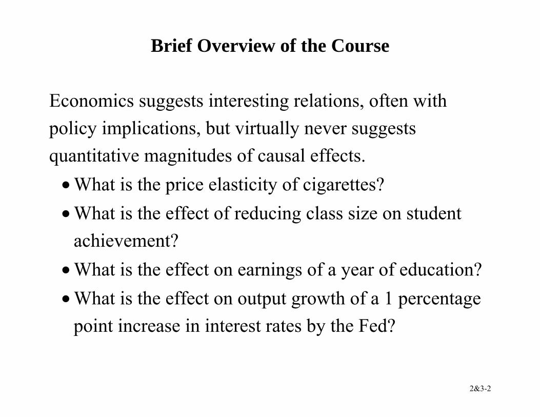
Brief Overview of the Course Economics suggests interesting relations, often with policy implications, but virtually never suggests quantitative magnitudes of causal effects.

• What is the price elasticity of cigarettes? • What is the effect of reducing class size on student

achievement? • What is the effect on earnings of a year of education? • What is the effect on output growth of a 1 percentage

point increase in interest rates by the Fed?

2&3-3

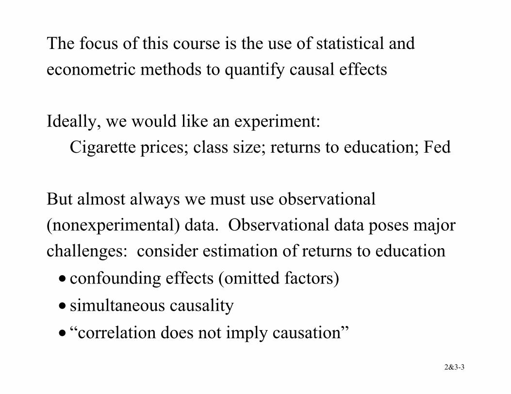
The focus of this course is the use of statistical and econometric methods to quantify causal effects Ideally, we would like an experiment:

Cigarette prices; class size; returns to education; Fed But almost always we must use observational (nonexperimental) data. Observational data poses major challenges: consider estimation of returns to education

• confounding effects (omitted factors) • simultaneous causality • “correlation does not imply causation”

2&3-4

In this course you will: • Learn methods for estimating causal effects using

observational data; • Learn some tools that can be used for other purposes,

for example forecasting using time series data; • Focus on applications – theory is used only as needed

to understand the “why”s of the methods; • Learn to produce (you do the analysis) and consume

(evaluate the work of others) econometric applications; and

• Practice “producing” in your problem sets.

2&3-5

Review of Probability and Statistics (SW Chapters 2,3)

Empirical problem: Class size and educational output

• Policy question: What is the effect of reducing class size by one student per class? by 8 students/class?

• What is the right output measure (“dependent variable”)?

parent satisfaction student personal development future adult welfare and/or earnings performance on standardized tests

2&3-6

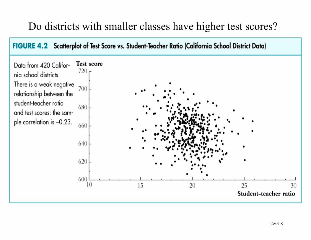
What do data say about the class size/test score relation?

The California Test Score Data Set All K-6 and K-8 California school districts (n = 420) Variables:

5th grade test scores (Stanford-9 achievement test, combined math and reading), district average Student-teacher ratio (STR) = no. of students in the district divided by no. full-time equivalent teachers

2&3-7

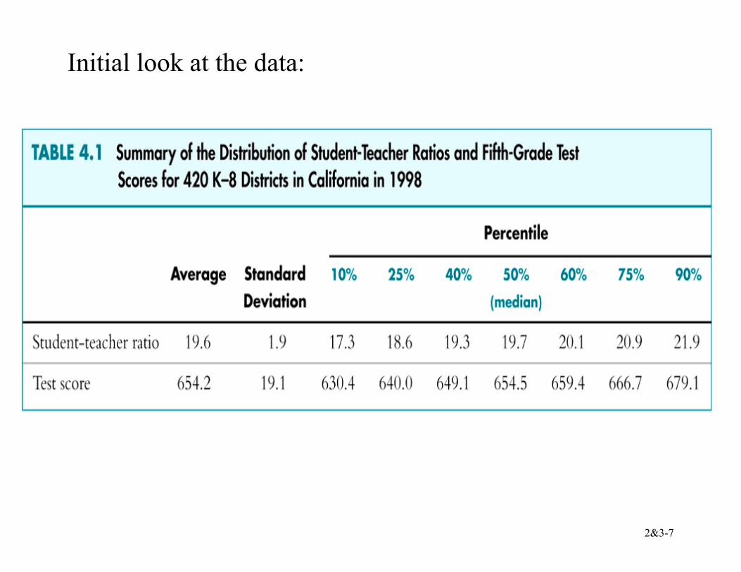
Initial look at the data:

2&3-8

Do districts with smaller classes have higher test scores?

2&3-9

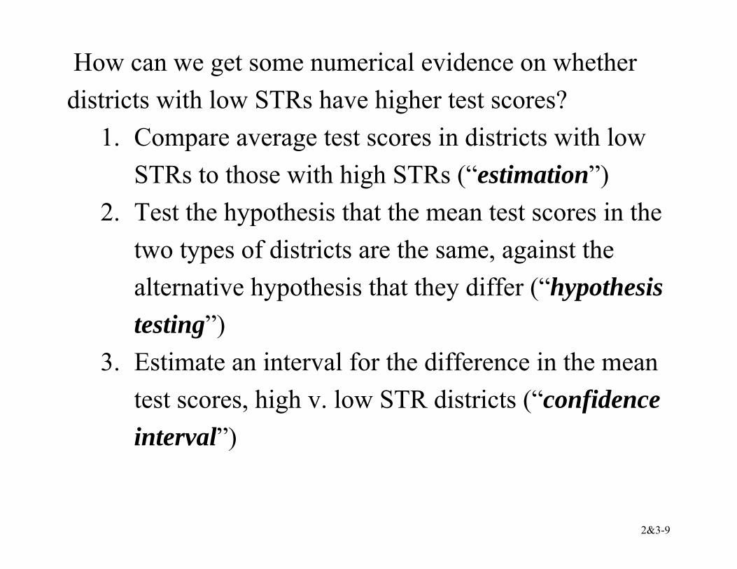
How can we get some numerical evidence on whether districts with low STRs have higher test scores?

1. Compare average test scores in districts with low STRs to those with high STRs (“estimation”)

2. Test the hypothesis that the mean test scores in the two types of districts are the same, against the alternative hypothesis that they differ (“hypothesis testing”)

3. Estimate an interval for the difference in the mean test scores, high v. low STR districts (“confidence interval”)

2&3-10

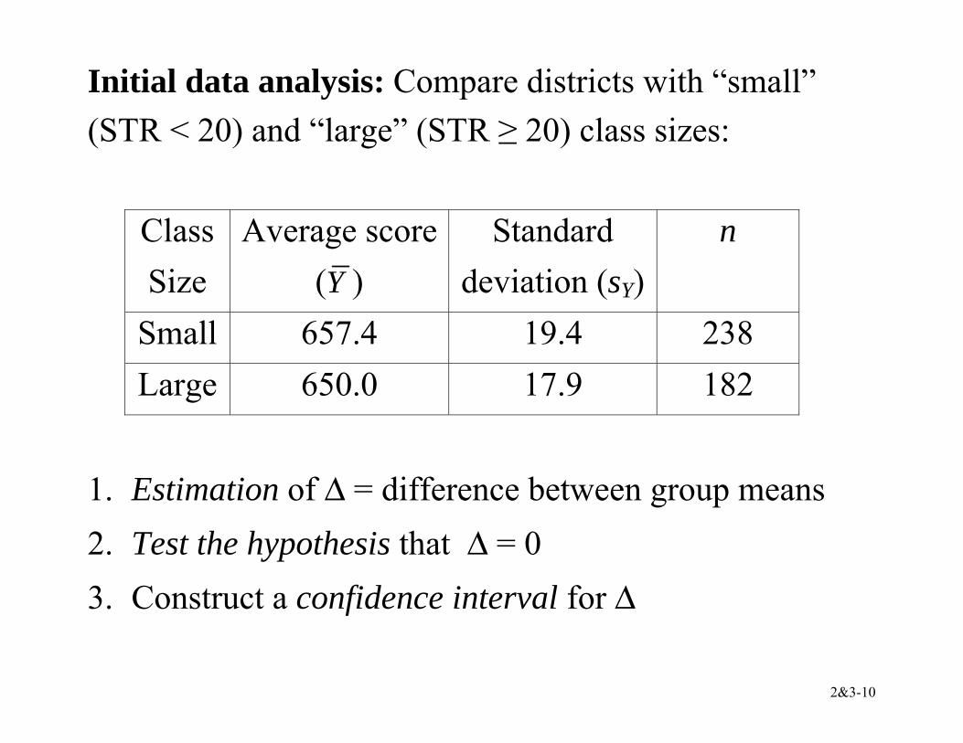
Initial data analysis: Compare districts with “small” (STR < 20) and “large” (STR ≥ 20) class sizes:

Class Size

Average score (Y )

Standard deviation (sY)

n

Small 657.4 19.4 238 Large 650.0 17.9 182

1. Estimation of ∆ = difference between group means 2. Test the hypothesis that ∆ = 0 3. Construct a confidence interval for ∆

2&3-11

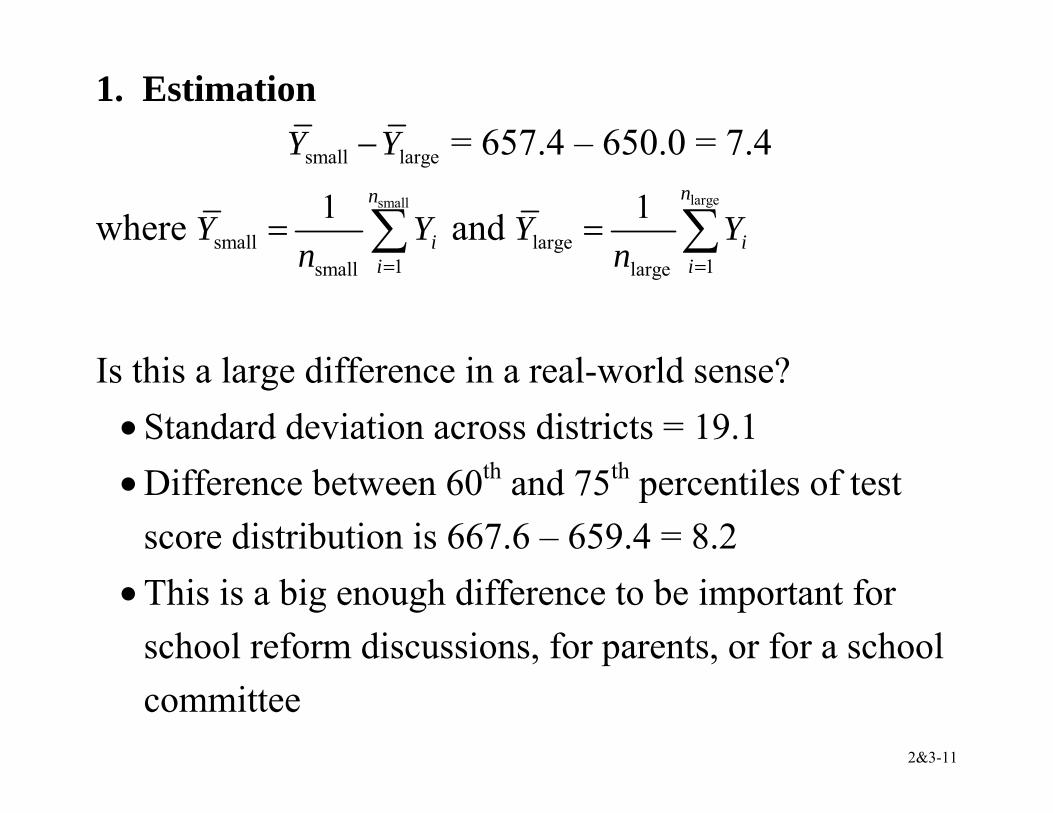
1. Estimation

small largeY Y− = 657.4 – 650.0 = 7.4

where small

small1small

1 n

ii

Y Yn =

= ∑ and large

large1large

1 n

ii

Y Yn =

= ∑

Is this a large difference in a real-world sense?

• Standard deviation across districts = 19.1 • Difference between 60th and 75th percentiles of test

score distribution is 667.6 – 659.4 = 8.2 • This is a big enough difference to be important for

school reform discussions, for parents, or for a school committee

2&3-12

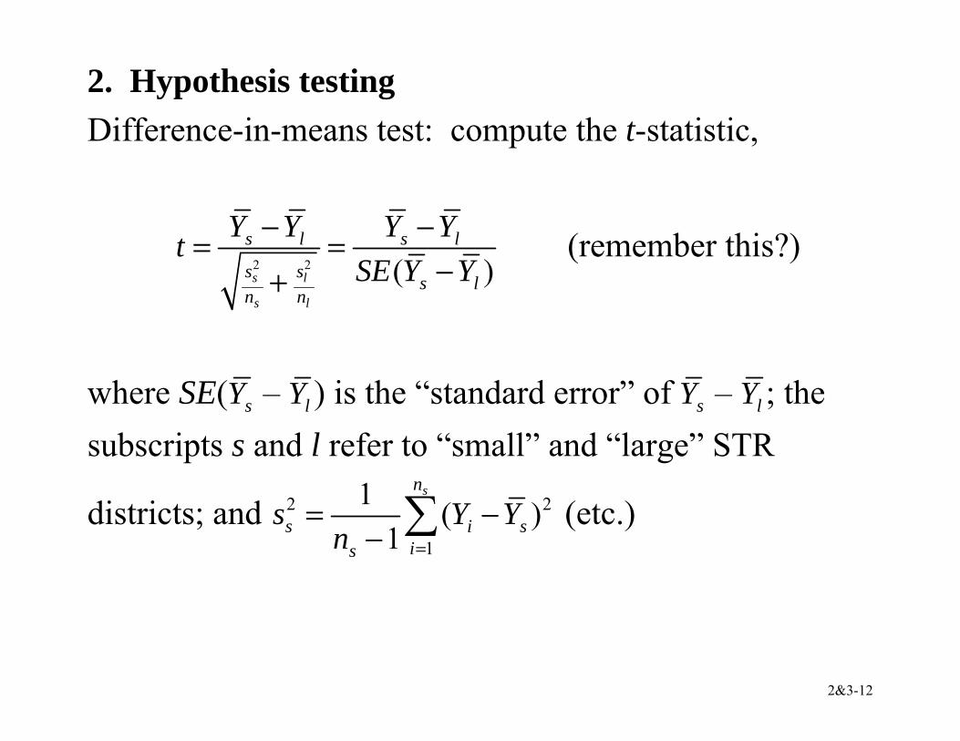
2. Hypothesis testing Difference-in-means test: compute the t-statistic,

2 2 ( )s l

s l

s l s l

s s s ln n

Y Y Y YtSE Y Y

− −= =−+

(remember this?)

where SE( sY – lY ) is the “standard error” of sY – lY ; the subscripts s and l refer to “small” and “large” STR

districts; and 2 2

1

1 ( )1

sn

s i sis

s Y Yn =

= −− ∑ (etc.)

2&3-13

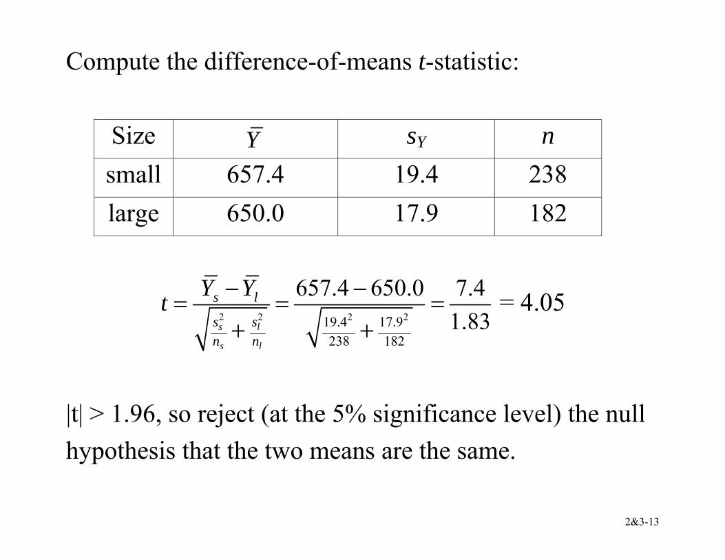
Compute the difference-of-means t-statistic:

Size Y sY n small 657.4 19.4 238 large 650.0 17.9 182

2 2 2 219.4 17.9238 182

657.4 650.0 7.41.83s l

s l

s l

s sn n

Y Yt − −= = =+ +

= 4.05

|t| > 1.96, so reject (at the 5% significance level) the null hypothesis that the two means are the same.

2&3-14

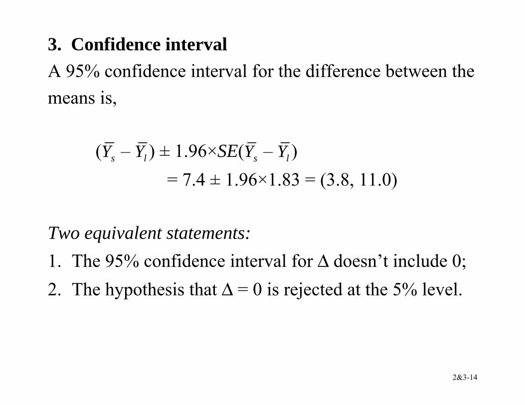
3. Confidence interval A 95% confidence interval for the difference between the means is,

( sY – lY ) ± 1.96×SE( sY – lY ) = 7.4 ± 1.96×1.83 = (3.8, 11.0) Two equivalent statements: 1. The 95% confidence interval for ∆ doesn’t include 0; 2. The hypothesis that ∆ = 0 is rejected at the 5% level.

2&3-15

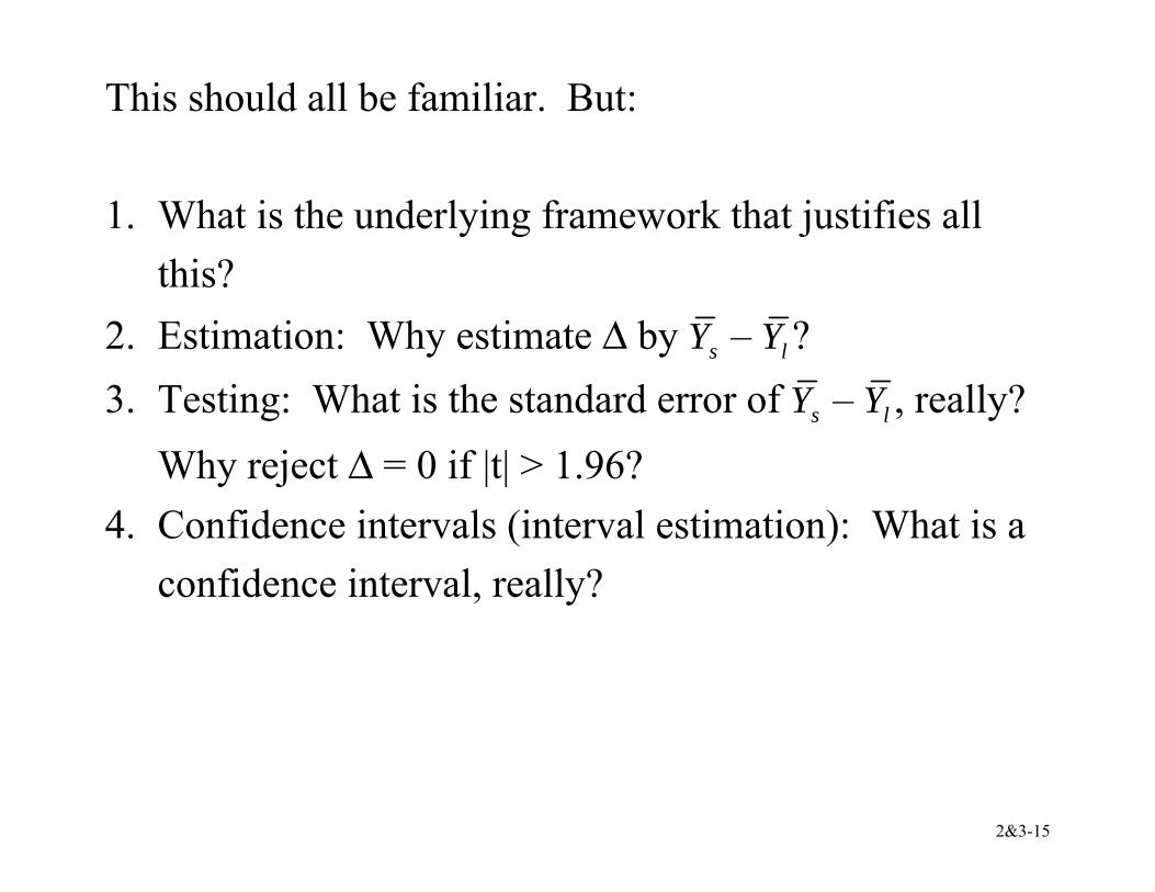
This should all be familiar. But: 1. What is the underlying framework that justifies all

this? 2. Estimation: Why estimate ∆ by sY – lY ? 3. Testing: What is the standard error of sY – lY , really?

Why reject ∆ = 0 if |t| > 1.96? 4. Confidence intervals (interval estimation): What is a

confidence interval, really?

2&3-16

1. The probability framework for statistical inference 2. Estimation 3. Testing 4. Confidence Intervals Population

• The group or collection of entities of interest • Here, “all possible” school districts • “All possible” means “all possible” circumstances that

lead to specific values of STR, test scores • We will think of populations as infinitely large; the

task is to make inferences from a sample from a large population

2&3-17

Random variable Y • Numerical summary of a random outcome • Here, the numerical value of district average test

scores (or district STR), once we choose a year/district to sample.

Population distribution of Y

• The probabilities of different values of Y that occur in the population, for ex. Pr[Y = 650] (when Y is discrete)

• or: The probabilities of sets of these values, for ex. Pr[Y > 650] (when Y is continuous).

2&3-18

“Moments” of the population distribution mean = expected value

= E(Y) = µY = long-run average value of Y over repeated

realizations of Y variance = E(Y – µY)2

= 2Yσ

= measure of the squared spread of the distribution

standard deviation = variance = σY

2&3-19

Conditional distributions • The distribution of Y, given value(s) of some other

random variable, X • Ex: the distribution of test scores, given that STR < 20

Moments of conditional distributions • conditional mean = mean of conditional distribution

= E(Y|X = x) (important notation) • conditional variance = variance of conditional

distribution • Example: E(Test scores|STR < 20), the mean of test

scores for districts with small class sizes

2&3-20

The difference in means is the difference between the means of two conditional distributions: ∆ = E(Test scores|STR < 20) – E(Test scores|STR ≥ 20) Other examples of conditional means:

• Wages of all female workers (Y = wages, X = gender) • One-year mortality rate of those given an

experimental treatment (Y = live/die; X = treated/not treated)

The conditional mean is a new term for the familiar idea of the group mean

2&3-21

Inference about means, conditional means, and differences in conditional means We would like to know ∆ (test score gap; gender wage gap; effect of experimental treatment), but we don’t know it. Therefore we must collect and use data that permits making statistical inferences about ∆.

• Experimental data • Observational data

2&3-22

Simple random sampling • Choose an individual (district, entity) at random from

the population Randomness and data

• Prior to sample selection, the value of Y is random because the individual selected is random

• Once the individual is selected and the value of Y is observed, then Y is just a number – not random

• The data set is (Y1, Y2,…, Yn), where Yi = value of Y for the ith individual (district, entity) sampled

2&3-23

Implications of simple random sampling Because individuals #1 and #2 are selected at random, the value of Y1 has no information content for Y2. Thus:

• Y1, Y2 are independently distributed • Y1 and Y2 come from the same distribution, that is, Y1,

Y2 are identically distributed • That is, a consequence of simple random sampling is

that Y1 and Y2 are independently and identically distributed (i.i.d.).

• More generally, under simple random sampling, {Yi}, i = 1,…, n, are i.i.d

2&3-24

1. The probability framework for statistical inference 2. Estimation 3. Testing 4. Confidence Intervals

Y is the natural estimator of the mean. But:

• What are the properties of this estimator? • Why should we use Y rather than some other

estimator? Y1 (the first observation) maybe unequal weights – not simple average median(Y1,…, Yn)

2&3-25

To answer these questions we need to characterize the sampling distribution of Y

• The individuals in the sample are drawn at random. • Thus the values of (Y1,…, Yn) are random • Thus functions of (Y1,…, Yn), such as Y , are random:

had a different sample been drawn, they would have taken on a different value

• The distribution of Y over different possible samples of size n is called the sampling distribution of Y .

• The mean and variance of Y are the mean and variance of its sampling distribution, E(Y ) and var(Y ).

• To compute var(Y ), we need the covariance

2&3-26

The covariance between r.v.’s X and Z is, cov(X,Z) = E[(X – µX)(Z – µZ)] = σXZ

• The covariance is a measure of the linear association

between X and Z; its units are units of X × units of Z • cov(X,Z) > (<) 0: X and Z positive (negative) relation

between X and Z • If X and Z are independently distributed, then cov(X,Z)

= 0 (but not vice versa!!) • The covariance of a r.v. with itself is its variance:

cov(X,X) = E[(X – µX)(X – µX)] = E[(X – µX)2] = 2Xσ

2&3-27

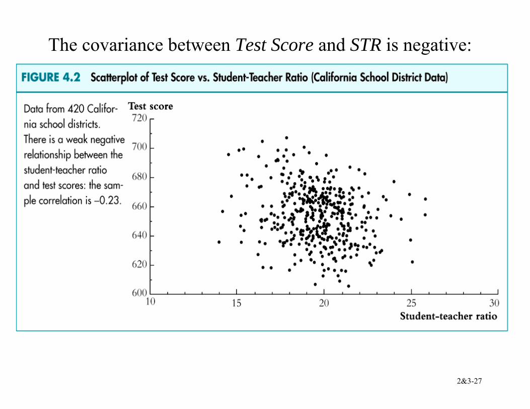
The covariance between Test Score and STR is negative:

2&3-28

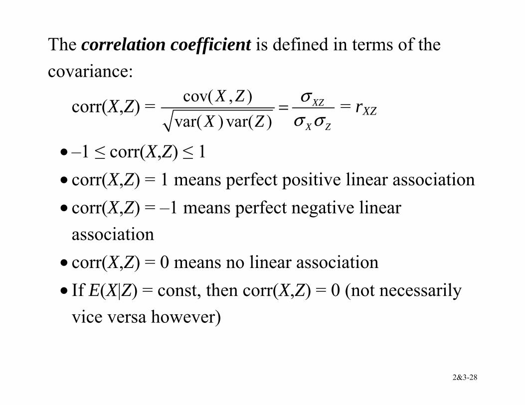
The correlation coefficient is defined in terms of the covariance:

corr(X,Z) = cov( , )var( ) var( )

XZ

X Z

X ZX Z

σσ σ

= = rXZ

• –1 ≤ corr(X,Z) ≤ 1 • corr(X,Z) = 1 means perfect positive linear association • corr(X,Z) = –1 means perfect negative linear

association • corr(X,Z) = 0 means no linear association • If E(X|Z) = const, then corr(X,Z) = 0 (not necessarily

vice versa however)

2&3-29

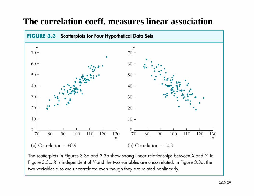
The correlation coeff. measures linear association

2&3-30

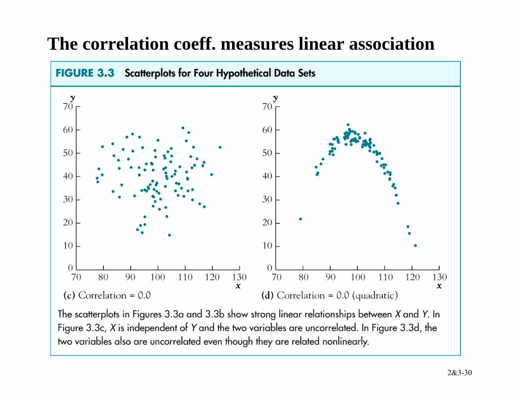
The correlation coeff. measures linear association

2&3-31

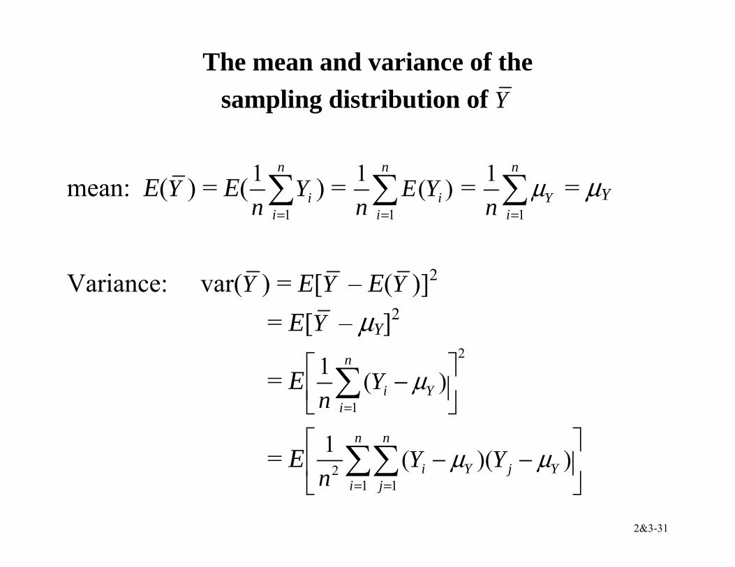
The mean and variance of the sampling distribution of Y

mean: E(Y ) = E(1

1 n

ii

Yn =∑ ) =

1

1 ( )n

ii

E Yn =∑ =

1

1 n

Yin

µ=∑ = µY

Variance: var(Y ) = E[Y – E(Y )]2

= E[Y – µY]2

= E2

1

1 ( )n

i Yi

Yn

µ=

⎡ ⎤−⎢ ⎥⎣ ⎦∑

= E 21 1

1 ( )( )n n

i Y j Yi j

Y Yn

µ µ= =

⎡ ⎤− −⎢ ⎥

⎣ ⎦∑∑

2&3-32

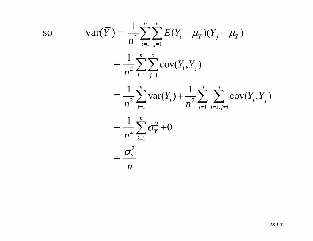
so var(Y ) = 21 1

1 ( )( )n n

i Y j Yi j

E Y Yn

µ µ= =

− −∑∑

= 21 1

1 cov( , )n n

i ji j

Y Yn = =∑∑

= 2 21 1 1,

1 1var( ) cov( , )n n n

i i ji i j j i

Y Y Yn n= = = ≠

+∑ ∑ ∑

= 22

1

1 0n

Yin

σ=

+∑

= 2Y

nσ

2&3-33

Summary: E(Y ) = µY and var(Y ) = 2Y

nσ .

Implications:

• Y is an unbiased estimator of µY (that is, E(Y ) = µY) • var(Y ) is inversely proportional to n • spread of sampling distribution is proportional to

1/ n • in this sense, the sampling uncertainty arising from

using Y to make inferences about µY is proportional to 1/ n

2&3-34

What about the entire sampling distribution of Y , not just the mean and variance?

In general, the exact sampling distribution of Y is very complicated and depends on the population distribution of Y.

Example: Suppose Y takes on 0 or 1 (a Bernoulli random variable) with the probability distribution,

Pr[Y = 0] = .22, Pr(Y =1) = .78

Then E(Y) = .78 and 2Yσ = .78× (1–.78) = 0.1716

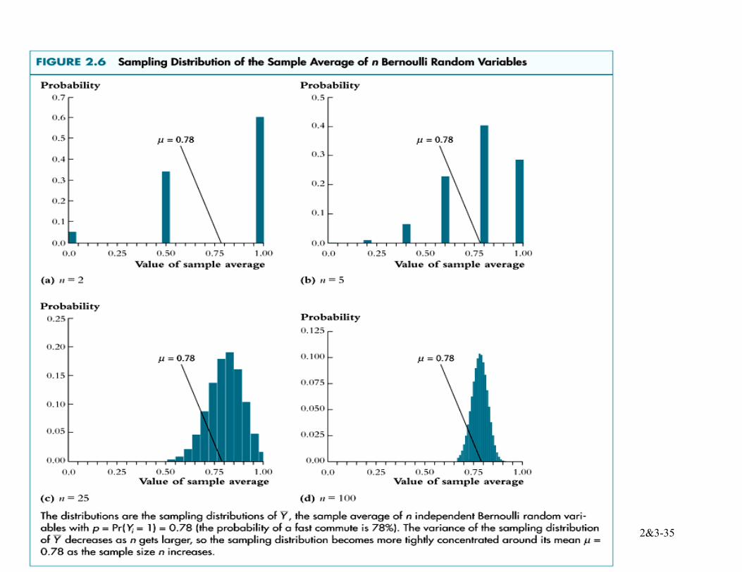
2&3-35

2&3-36

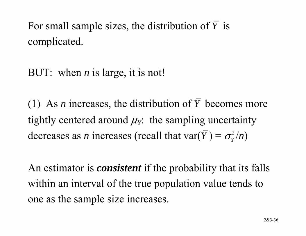
For small sample sizes, the distribution of Y is complicated. BUT: when n is large, it is not! (1) As n increases, the distribution of Y becomes more tightly centered around µY: the sampling uncertainty decreases as n increases (recall that var(Y ) = 2

Yσ /n) An estimator is consistent if the probability that its falls within an interval of the true population value tends to one as the sample size increases.

2&3-37

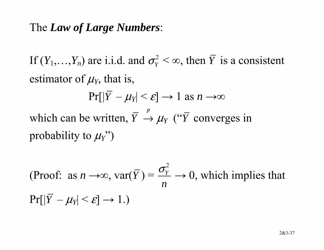
The Law of Large Numbers: If (Y1,…,Yn) are i.i.d. and 2

Yσ < ∞, then Y is a consistent estimator of µY, that is,

Pr[|Y – µY| < ε] → 1 as n →∞

which can be written, Y p

→ µY (“Y converges in probability to µY”)

(Proof: as n →∞, var(Y ) = 2Y

nσ → 0, which implies that

Pr[|Y – µY| < ε] → 1.)

2&3-38

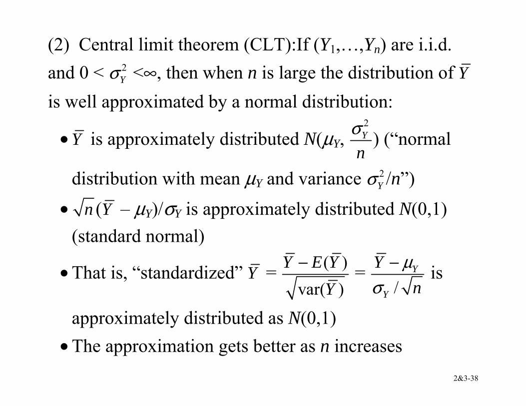
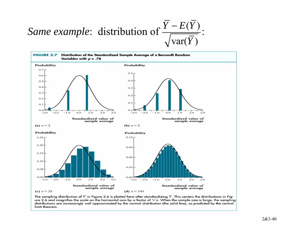
(2) Central limit theorem (CLT):If (Y1,…,Yn) are i.i.d. and 0 < 2

Yσ <∞, then when n is large the distribution of Y is well approximated by a normal distribution:

• Y is approximately distributed N(µY, 2Y

nσ ) (“normal

distribution with mean µY and variance 2Yσ /n”)

• n (Y – µY)/σY is approximately distributed N(0,1) (standard normal)

• That is, “standardized” Y = ( )var( )

Y E YY

− = /

Y

Y

Yn

µσ

− is

approximately distributed as N(0,1) • The approximation gets better as n increases

2&3-39

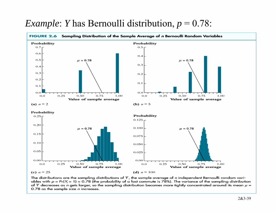
Example: Y has Bernoulli distribution, p = 0.78:

2&3-40

Same example: distribution of ( )var( )

Y E YY

− :

2&3-41

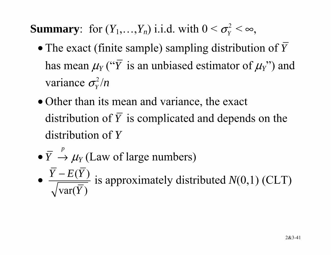
Summary: for (Y1,…,Yn) i.i.d. with 0 < 2Yσ < ∞,

• The exact (finite sample) sampling distribution of Y has mean µY (“Y is an unbiased estimator of µY”) and variance 2

Yσ /n • Other than its mean and variance, the exact

distribution of Y is complicated and depends on the distribution of Y

• Y p

→ µY (Law of large numbers)

• ( )var( )

Y E YY

− is approximately distributed N(0,1) (CLT)

2&3-42

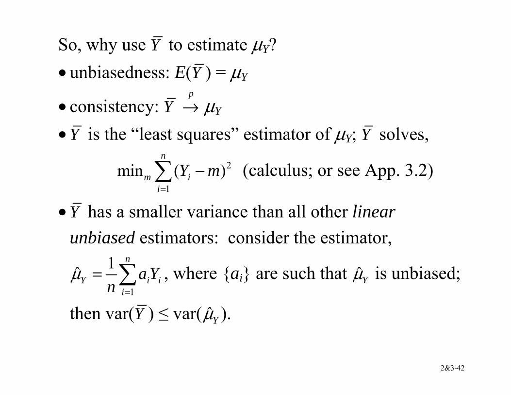
So, why use Y to estimate µY? • unbiasedness: E(Y ) = µY

• consistency: Y p

→ µY • Y is the “least squares” estimator of µY; Y solves,

2

1

min ( )n

m ii

Y m=

−∑ (calculus; or see App. 3.2)

• Y has a smaller variance than all other linear unbiased estimators: consider the estimator,

1

1ˆn

Y i ii

a Yn

µ=

= ∑ , where {ai} are such that ˆYµ is unbiased;

then var(Y ) ≤ var( ˆYµ ).

2&3-43

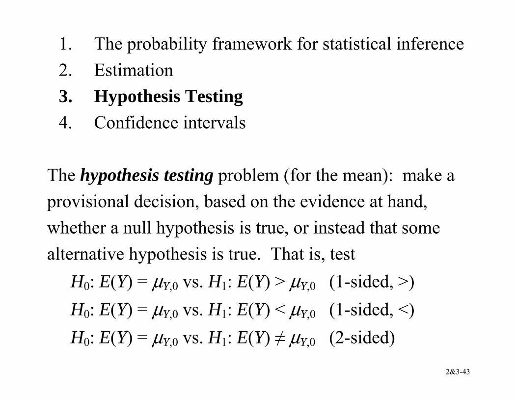
1. The probability framework for statistical inference 2. Estimation 3. Hypothesis Testing 4. Confidence intervals

The hypothesis testing problem (for the mean): make a provisional decision, based on the evidence at hand, whether a null hypothesis is true, or instead that some alternative hypothesis is true. That is, test

H0: E(Y) = µY,0 vs. H1: E(Y) > µY,0 (1-sided, >) H0: E(Y) = µY,0 vs. H1: E(Y) < µY,0 (1-sided, <) H0: E(Y) = µY,0 vs. H1: E(Y) ≠ µY,0 (2-sided)

2&3-44

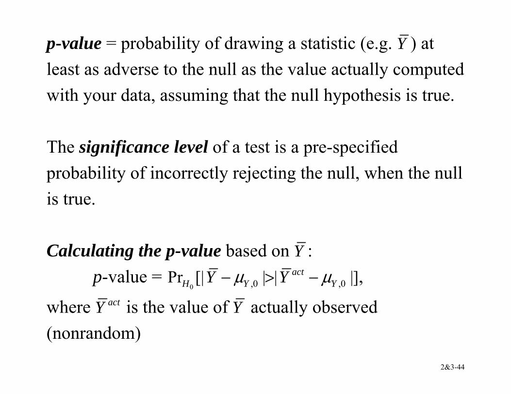
p-value = probability of drawing a statistic (e.g. Y ) at least as adverse to the null as the value actually computed with your data, assuming that the null hypothesis is true. The significance level of a test is a pre-specified probability of incorrectly rejecting the null, when the null is true. Calculating the p-value based on Y :

p-value = 0 ,0 ,0Pr [| | | |]act

H Y YY Yµ µ− > − ,

where actY is the value of Y actually observed (nonrandom)

2&3-45

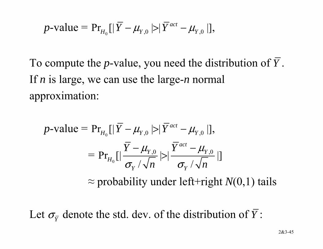
p-value = 0 ,0 ,0Pr [| | | |]act

H Y YY Yµ µ− > − ,

To compute the p-value, you need the distribution of Y . If n is large, we can use the large-n normal approximation:

p-value = 0 ,0 ,0Pr [| | | |]act

H Y YY Yµ µ− > − ,

= 0

,0 ,0Pr [| | | |]/ /

actY Y

HY Y

Y Yn n

µ µσ σ

− −>

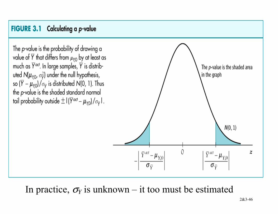
≈ probability under left+right N(0,1) tails Let Yσ denote the std. dev. of the distribution of Y :

2&3-46

In practice, σY is unknown – it too must be estimated

2&3-47

Estimator of the variance of Y:

2Ys = 2

1

1 ( )1

n

ii

Y Yn =

−− ∑

Fact:

If (Y1,…,Yn) are i.i.d. and E(Y4) < ∞, then 2Ys

p→ 2

Yσ Why does the law of large numbers apply? because 2

Ys is a sample average; see Appendix 3.3 Technical note: we assume E(Y4) < ∞ because here the average is not of Yi, but of its square; see App. 3.3

2&3-48

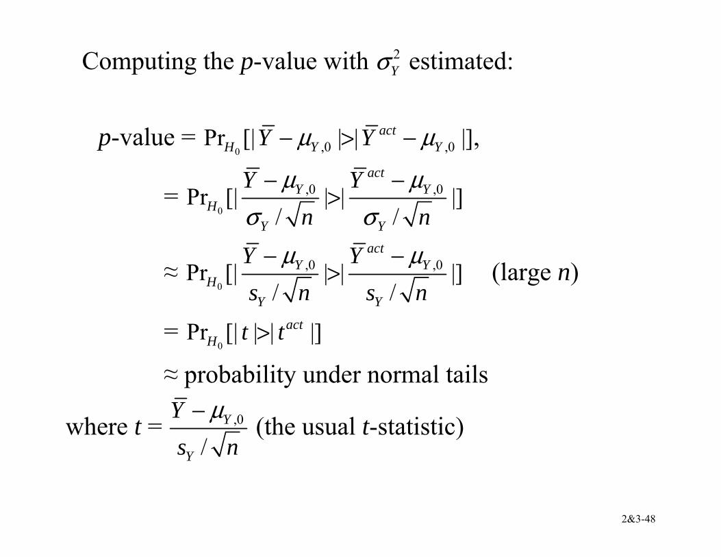
Computing the p-value with 2Yσ estimated:

p-value =

0 ,0 ,0Pr [| | | |]actH Y YY Yµ µ− > − ,

= 0

,0 ,0Pr [| | | |]/ /

actY Y

HY Y

Y Yn n

µ µσ σ

− −>

≈ 0

,0 ,0Pr [| | | |]/ /

actY Y

HY Y

Y Ys n s n

µ µ− −> (large n)

= 0

Pr [| | | |]actH t t>

≈ probability under normal tails

where t = ,0

/Y

Y

Ys n

µ− (the usual t-statistic)

2&3-49

The p-value and the significance level With a prespecified significance level (e.g. 5%):

• reject if |t| > 1.96 • equivalently: reject if p < 0.05. • The p-value is sometimes called the marginal

significance level.

2&3-50

The Student t-distribution If Y is distributed N(µY, 2

Yσ ), then the t-statistic has the Student t-distribution (tabulated in back of all stats books)

Some comments: • For n > 30, the t-distribution and N(0,1) are very close • The assumption that Y is distributed N(µY, 2

Yσ ) is rarely plausible in practice (income? number of children?)

• The t-distribution is an historical artifact from days when sample sizes were very small

• In this class, we won’t use the t distribution – we rely solely on the large-n approximation given by the CLT

2&3-51

1. The probability framework for statistical inference 2. Estimation 3. Testing 4. Confidence intervals A 95% confidence interval for µY is an interval that contains the true value of µY in 95% of repeated samples. (What is random here? the confidence interval – it will differ from one sample to the next; the population parameter, µY, is not random, we just don’t know it.)

2&3-52

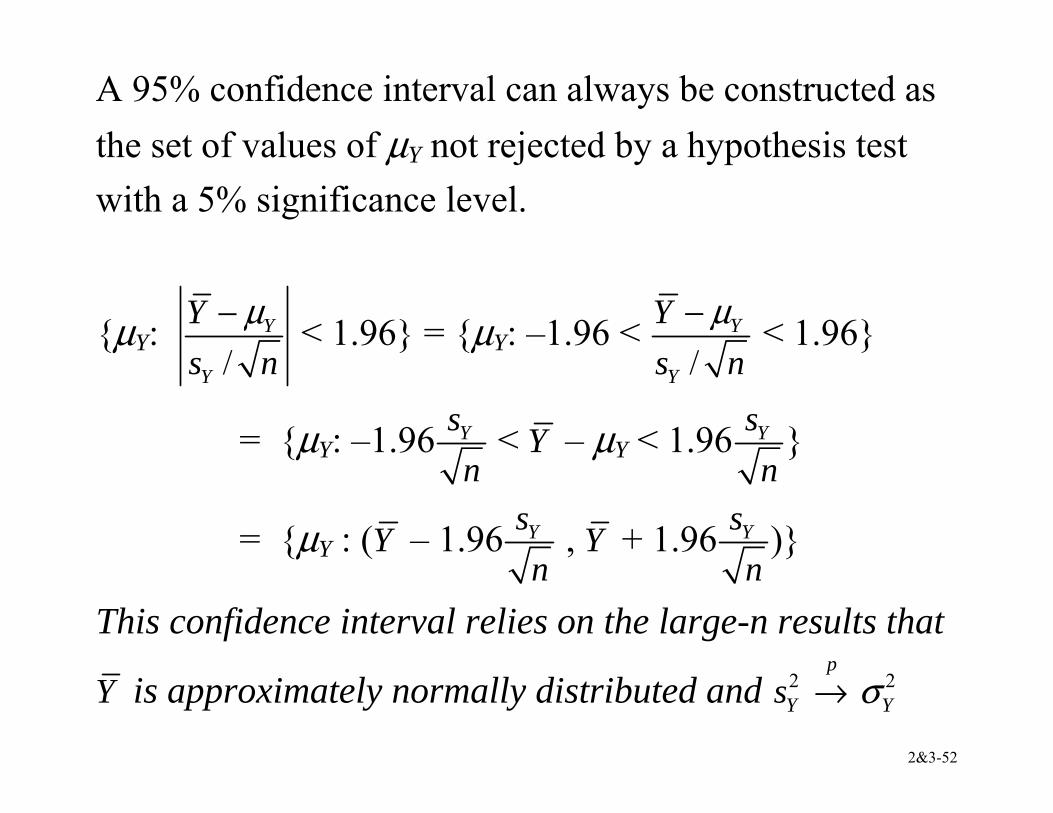
A 95% confidence interval can always be constructed as the set of values of µY not rejected by a hypothesis test with a 5% significance level.

{µY: /

Y

Y

Ys n

µ− < 1.96} = {µY: –1.96 < /

Y

Y

Ys n

µ− < 1.96}

= {µY: –1.96 Ysn

< Y – µY < 1.96 Ysn

}

= {µY : (Y – 1.96 Ysn

, Y + 1.96 Ysn

)}

This confidence interval relies on the large-n results that

Y is approximately normally distributed and 2Ys

p→ 2

Yσ

2&3-53

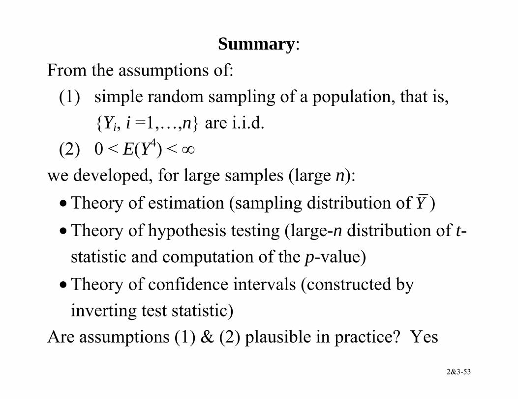
Summary: From the assumptions of:

(1) simple random sampling of a population, that is, {Yi, i =1,…,n} are i.i.d.

(2) 0 < E(Y4) < ∞ we developed, for large samples (large n):

• Theory of estimation (sampling distribution of Y ) • Theory of hypothesis testing (large-n distribution of t-

statistic and computation of the p-value) • Theory of confidence intervals (constructed by

inverting test statistic) Are assumptions (1) & (2) plausible in practice? Yes

2&3-54

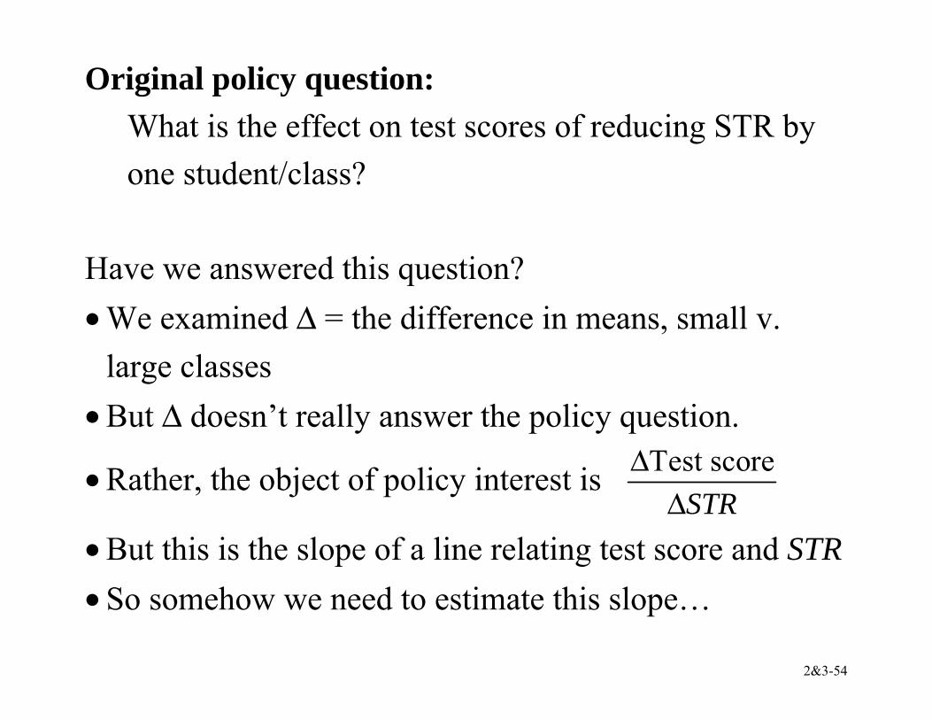
Original policy question: What is the effect on test scores of reducing STR by one student/class?

Have we answered this question? • We examined ∆ = the difference in means, small v.

large classes • But ∆ doesn’t really answer the policy question.

• Rather, the object of policy interest is Test scoreSTR

∆∆

• But this is the slope of a line relating test score and STR • So somehow we need to estimate this slope…